possible role of wetlands, permafrost, and methane hydrates in the

POSSIBLE ROLE OF WETLANDS, PERMAFROST,AND METHANE HYDRATES IN THE METHANECYCLE UNDER FUTURE CLIMATE CHANGE:A REVIEW

Fiona M. O’Connor,1 O. Boucher,1 N. Gedney,2 C. D. Jones,1 G. A. Folberth,1 R. Coppell,3

P. Friedlingstein,4 W. J. Collins,1 J. Chappellaz,5 J. Ridley,1 and C. E. Johnson1

Received 11 January 2010; revised 27 May 2010; accepted 22 June 2010; published 23 December 2010.

[1] We have reviewed the available scientific literature onhow natural sources and the atmospheric fate of methanemay be affected by future climate change. We discusshow processes governing methane wetland emissions, per-mafrost thawing, and destabilization of marine hydratesmay affect the climate system. It is likely that methane wet-land emissions will increase over the next century. Uncertain-ties arise from the temperature dependence of emissions andchanges in the geographical distribution of wetland areas.Another major concern is the possible degradation or thawof terrestrial permafrost due to climate change. The amountof carbon stored in permafrost, the rate at which it will thaw,and the ratio of methane to carbon dioxide emissions upondecomposition form the main uncertainties. Large amountsof methane are also stored in marine hydrates, and they could

be responsible for large emissions in the future. The timescales for destabilization of marine hydrates are not wellunderstood and are likely to be very long for hydrates foundin deep sediments but much shorter for hydrates below shal-low waters, such as in the Arctic Ocean. Uncertainties aredominated by the sizes and locations of the methane hydrateinventories, the time scales associated with heat penetrationin the ocean and sediments, and the fate of methane releasedin the seawater. Overall, uncertainties are large, and it is dif-ficult to be conclusive about the time scales and magnitudesof methane feedbacks, but significant increases in methaneemissions are likely, and catastrophic emissions cannot beruled out. We also identify gaps in our scientific knowledgeand make recommendations for future research and develop-ment in the context of Earth system modeling.

Citation: O’Connor, F. M., et al. (2010), Possible role of wetlands, permafrost, and methane hydrates in the methane cycleunder future climate change: A review, Rev. Geophys., 48, RG4005, doi:10.1029/2010RG000326.

1. INTRODUCTION TO THE METHANE CYCLE

[2] Methane (CH4) is an important greenhouse gas. Itsatmospheric concentration in dry air mole fractions (nmolmol−1, abbreviated ppb) has increased from 380 ppb at theLast Glacial Maximum (LGM) [Monnin et al., 2001] to715 ppb in 1750 [Etheridge et al., 1998] and 1787 ppb in2008 [Dlugokencky et al., 2009]. It fluctuated between320 and 780 ppb (Antarctic concentration) over the last800,000 years [Loulergue et al., 2008]. Ice core methane

records also reveal abrupt changes concomitant with theabrupt warmings of the last glacial period recorded inGreenland [Chappellaz et al., 1993a], with a responsereaching 16 ppb per °C of Greenland warming [Huber et al.,2006] and increases of up to 200 ppb within a century [Wolffet al., 2010]. The radiative efficiency of CH4 is 1 order ofmagnitude larger than that of carbon dioxide (3.7 × 10−4

versus 1.548 × 10−5 W m−2 ppb−1 [Ramaswamy et al., 2001]).This is why CH4 is the second most important anthropo-genic greenhouse gas with a radiative forcing of over0.48 W m−2 in 2008 relative to preindustrial times (to becompared to 1.74 W m−2 for carbon dioxide (CO2) based ona global mean concentration of 385 ppm for 2008 fromPieter Tans, Earth System Research Laboratory, NOAA,http://www.esrl.noaa.gov/gmd/ccgg/trends). The global meanatmospheric abundance of CH4 is determined by the interplaybetween emissions and sinks. CH4 emissions are very diverse,covering a wide range of natural (wetlands, termites, oceans,

1Met Office Hadley Centre, Exeter, UK.2Joint Centre for Hydrometeorological Research, Met Office

Hadley Centre, Crowmarsh Gifford, UK.3School of Geography, University of Leeds, Leeds, UK.4College of Engineering, Mathematics and Physical Sciences,

University of Exeter, Exeter, UK.5Laboratoire de Glaciologie et Geophysique de l’Environnement,

CNRS–University of Grenoble, Saint Martin d’Hères, France.

Published in 2010 by the American Geophysical Union. Reviews of Geophysics, 48, RG4005 / 20101 of 33

Paper number 2010RG000326RG4005

marine hydrates, geological sources, wild animals, andwildfires) and anthropogenic (energy, mining, landfills andwaste treatment, ruminants, rice agriculture, and biomassburning) sources [Denman et al., 2007, Table 7.6]. It iswidely accepted that reductions in anthropogenic CH4

emissions should play a role in a multigas strategy to miti-gate climate change because reductions have a relativelylarge radiative payoff and can be economically beneficial(e.g., capturing CH4 from underground coal mines andmarketing it). However, it is feared that the natural sourcesof CH4 may increase significantly in a warmer climate,through feedback loops that are not included in currentclimate models. The objective of this paper is to review thescientific literature in order to assess the importance andlevel of understanding of these potential feedback loops andto make some recommendations for future research.[3] A prerequisite to the understanding of CH4 feedbacks

is a quantitative understanding of the CH4 sources and sinksin the present‐day climate. Estimates for individual sourcescan be obtained using “bottom‐up” estimates, which involvea variety of techniques from field studies [e.g., Khalil et al.,1998;Mastepanov et al., 2008] and economic analyses [e.g.,van Aardenne et al., 2001; Olivier et al., 2005] to process‐based modeling [e.g., Walter et al., 2001a], or inversionmodeling, the so‐called “top‐down” approach [e.g.,Houweling et al., 1999; Wang et al., 2004; Bergamaschi etal., 2005]. In addition, 13C/12C isotopic ratios help constrainemissions sectorally [e.g., Mikaloff Fletcher et al., 2004a]and geographically [e.g., Mikaloff Fletcher et al., 2004b].[4] The best estimates for individual source strengths are

given by Denman et al. [2007] and, in turn, originate from anumber of studies [e.g., Houweling et al., 2000; Wuebblesand Hayhoe, 2002; Olivier et al., 2005; Chen and Prinn,2006]. Wetland emissions of CH4 are the largest singlesource. The estimated flux from Denman et al. [2007] to theatmosphere is given as 100–230 Tg yr−1. These uncertaintybounds indicate the remaining large level of uncertainty intheir source strength. To balance sources, atmosphericCH4 is removed by oxidation with the hydroxyl (OH) rad-ical in the troposphere, biological oxidation in drier soil[Born et al., 1990; Ridgwell et al., 1999], reaction withchlorine and/or oxygen (O(1D)) atoms in the stratosphere,and oxidation with chlorine atoms in the marine boundarylayer [Platt et al., 2004; Allan et al., 2005]. Of these, oxi-dation with tropospheric OH is by far the most importantand is responsible for removing 85%–90% of atmosphericCH4. The abundance of OH and, consequently, the CH4

lifetime depend on local concentrations of CH4 itself,nitrogen oxides (NOx), carbon monoxide (CO), and non-methane volatile organic compounds (NMVOCs). For anoverview of OH chemistry and its stability, the reader isreferred to Lelieveld et al. [2002, 2004].[5] Although there is uncertainty in individual source and

sink estimates, the total global source of CH4 is relativelywell constrained to within ±15% [Prather et al., 2001] andlargely reflects the uncertainty in the overall sink strength of±15% [Denman et al., 2007]. By knowing the atmosphericconcentration and the loss rate, the global source is esti-

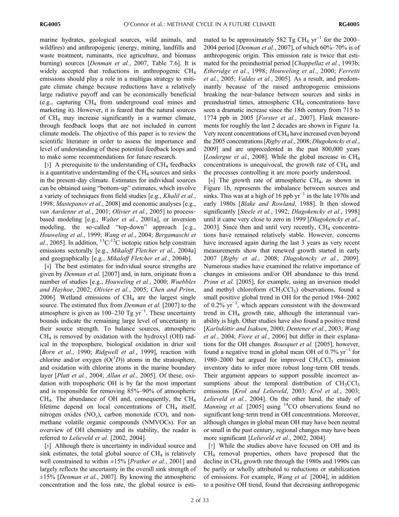
mated to be approximately 582 Tg CH4 yr−1 for the 2000–

2004 period [Denman et al., 2007], of which 60%–70% is ofanthropogenic origin. This emission rate is twice that esti-mated for the preindustrial period [Chappellaz et al., 1993b;Etheridge et al., 1998; Houweling et al., 2000; Ferrettiet al., 2005; Valdes et al., 2005]. As a result, and predom-inantly because of the raised anthropogenic emissionsbreaking the near‐balance between sources and sinks inpreindustrial times, atmospheric CH4 concentrations haveseen a dramatic increase since the 18th century from 715 to1774 ppb in 2005 [Forster et al., 2007]. Flask measure-ments for roughly the last 2 decades are shown in Figure 1a.Very recent concentrations of CH4 have increased even beyondthe 2005 concentrations [Rigby et al., 2008;Dlugokencky et al.,2009] and are unprecedented in the past 800,000 years[Loulergue et al., 2008]. While the global increase in CH4

concentrations is unequivocal, the growth rate of CH4 andthe processes controlling it are more poorly understood.[6] The growth rate of atmospheric CH4, as shown in

Figure 1b, represents the imbalance between sources andsinks. This was at a high of 16 ppb yr−1 in the late 1970s andearly 1980s [Blake and Rowland, 1988]. It then slowedsignificantly [Steele et al., 1992; Dlugokencky et al., 1998]until it came very close to zero in 1999 [Dlugokencky et al.,2003]. Since then and until very recently, CH4 concentra-tions have remained relatively stable. However, concernshave increased again during the last 3 years as very recentmeasurements show that renewed growth started in early2007 [Rigby et al., 2008; Dlugokencky et al., 2009].Numerous studies have examined the relative importance ofchanges in emissions and/or OH abundance to this trend.Prinn et al. [2005], for example, using an inversion modeland methyl chloroform (CH3CCl3) observations, found asmall positive global trend in OH for the period 1984–2002of 0.2% yr−1, which appears consistent with the downwardtrend in CH4 growth rate, although the interannual vari-ability is high. Other studies have also found a positive trend[Karlsdóttir and Isaksen, 2000; Dentener et al., 2003; Wanget al., 2004; Fiore et al., 2006] but differ in their explana-tions for the OH changes. Bousquet et al. [2005], however,found a negative trend in global mean OH of 0.7% yr−1 for1980–2000 but argued for improved CH3CCl3 emissioninventory data to infer more robust long‐term OH trends.Their argument appears to support possible incorrect as-sumptions about the temporal distribution of CH3CCl3emissions [Krol and Lelieveld, 2003; Krol et al., 2003;Lelieveld et al., 2004]. On the other hand, the study ofManning et al. [2005] using 14CO observations found nosignificant long‐term trend in OH concentrations. Moreover,although changes in global mean OH may have been neutralor small in the past century, regional changes may have beenmore significant [Lelieveld et al., 2002, 2004].[7] While the studies above have focused on OH and its

CH4 removal properties, others have proposed that thedecline in CH4 growth rate through the 1980s and 1990s canbe partly or wholly attributed to reductions or stabilizationof emissions. For example, Wang et al. [2004], in additionto a positive OH trend, found that decreasing anthropogenic

O’Connor et al.: METHANE CYCLE IN A FUTURE CLIMATE RG4005RG4005

2 of 33

emissions (ruminants, gas leakage, and coal mining) fromEastern Europe and the former Soviet Union (FSU) con-tributed to the declining growth rate between 1988 and 1997.This reduction is supported by other studies [Dlugokenckyet al., 2003; Bousquet et al., 2006; Chen and Prinn, 2006],although there may also be a contribution from wetlands[Walter et al., 2001b; Bousquet et al., 2006]. Furthermore,Cunnold et al. [2002] inferred from atmospheric CH4

measurements that net annual emissions from 1985 to 1997were fairly constant, which is consistent with Dlugokenckyet al. [1998]. While emissions from Eastern Europe andthe FSU may have decreased in the late 1980s and early1990s, global anthropogenic emissions increased during theentire 1970–1992 period, were fairly constant between 1993and 2000, and have increased since 2000, according to theEmissions Database for Global Atmospheric Research(EDGAR4) database (http://edgar.jrc.ec.europa.eu). Since1999, the increase in global anthropogenic emissions mayhave been masked by a coincident decrease in wetlandemissions driven by extended droughts [Bousquet et al.,2006]. Bousquet et al. [2006] suggested that atmosphericCH4 may increase further if wetland emissions return totheir 1990s level. Indeed, the very recent reversal to apositive CH4 growth rate has been attributed by Rigby et al.[2008] to increasing emissions globally or in the NorthernHemisphere alone, depending on the assumption regardingOH concentrations. Dlugokencky et al. [2009], morerecently, indicated that the increase in 2007 was due toincreased emissions from northern wetlands caused byanomalously high temperatures with a small contributionfrom the tropics. A further increase in atmospheric CH4 wasevident in 2008, particularly in the tropics, and was attrib-uted to increased emissions from tropical wetlands associ-ated with positive anomalies in precipitation over Indonesia

and the eastern Amazon typical of La Niña events[Dlugokencky et al., 2009]. Using satellite observations, aninversion model, and a simple CH4 wetland emissionsmodel, Bloom et al. [2010] estimated a 7% rise in wetlandemissions over the 2003–2007 period as a result of midlati-tude and high‐latitude warming.[8] From Figure 1b, there is significant variation in the

atmospheric CH4 growth rate between years. This variationsuggests a strong interannual variation in sources and/orsinks, but the main causes remain uncertain. For example,the anomalously low growth rate in 1992 following theMount Pinatubo eruption has been attributed to aerosol‐induced stratospheric ozone depletion and anomalously highOH concentrations [Bekki et al., 1994;Wang et al., 2004]. Amore recent study by Telford et al. [2010] suggests that thelow growth rate and enhanced OH could be attributed toreduced biogenic volatile organic compound (BVOC)emissions following the Mount Pinatubo eruption. On theother hand, other studies suggest that the anomaly was due tolower emissions from northern fossil fuel sources [Bousquetet al., 2006] and biomass burning [Lowe et al., 1997], withsome contribution from lower wetland emissions [Wanget al., 2004]. The enhanced growth rate in the 1997–1998El Niño year has been attributed to changes in emissionsfrom wetlands [Dlugokencky et al., 2001; Mikaloff Fletcheret al., 2004a; Chen and Prinn, 2006; Morimoto et al.,2006], biomass burning [Langenfelds et al., 2002; Morimotoet al., 2006], and wildfires [Prinn et al., 2005; Bousquetet al., 2006]. An assessment of emissions for the period1997–2004 clearly supports anomalous burning during the1997–1998 El Niño year [van der Werf et al., 2006], and theenhancement in CH4 emissions alone accounts for approxi-mately two thirds of the CH4 growth rate anomaly. In addi-tion to OH and emission changes, the CH4 growth rate

Figure 1. Time series of (a) globally averaged atmospheric CH4 concentrations in ppb and (b) instan-taneous CH4 growth rate for globally averaged CH4 in ppb yr−1 for the period 1983–2008 derived fromobservations from NOAA’s global surface air sampling network. Adapted from Dlugokencky et al.[2009].


3 of 33

appears to be influenced by interannual variability in mete-orology [Warwick et al., 2002].[9] Despite the individual source strength uncertainties

and the lack of understanding of the atmospheric CH4 growthrate, it is still widely accepted that reductions in anthropo-genic CH4 emissions should play a role in a multigas strategyto mitigate climate change. However, as the climate warms,natural sources of CH4 may increase through feedback loopsthat are currently not represented in climate models. Insections 2–4, we examine the importance and level ofunderstanding of potential feedback loops involving wet-lands, permafrost, and marine hydrates, respectively.

2. WETLANDS

2.1. Methane Emissions From Wetlands[10] Wetlands are the dominant natural source of CH4

over the globe and emit between 100 and 231 Tg CH4 yr−1

globally [Denman et al., 2007] out of a total of about582 TgCH4 yr

−1 during the 2000–2004 period. This represents∼17%–40% of the global present‐day atmospheric CH4

budget, which is dominated by anthropogenic sources. Aswell as uncertainty in the global mean contribution of wetlandCH4 emissions to the overall budget, there is considerableuncertainty over its geographical distribution.[11] Methane is produced by the anaerobic respiration of

methanogenic microbes. This occurs in saturated anoxic soilbelow the water table [Arneth et al., 2010]. The rate of CH4

production is dependent on soil temperature, the amount andquality of substrate available from vegetation primary pro-duction and organicmatter decomposition [Christensen et al.,2003], and soil pH [Garcia et al., 2000]. The CH4 is trans-ported out of the saturated zone either through diffusion,ebullition, or vegetation‐mediated transfer in vascular plants.Ebullition is the formation and release of bubbles into theunsaturated soil pore space (or atmosphere if the water table isabove the surface). Vegetation‐mediated transport can alsooccur from the saturated zone through the roots of manyspecies of wetland plants, thereby bypassing the unsaturatedoxic soil above the water table.[12] In non‐vegetation‐mediated transport, CH4 is oxidized

in the oxic (unsaturated) region of the soil. Hence, the posi-tion of the water table defines the sizes of both the productionand consumption zones. As the oxic region of the soil ishighly efficient at oxidizing CH4, significant amounts of CH4

are generally only released from the soil into the atmospherewhen the water table is relatively high [Roulet et al., 1992].[13] The rates of CH4 production and oxidation are both

strongly temperature dependent. Both the production andoxidation rates are often described by a Q10 factor, whereQ10 is the factor by which a reaction rate increases with a 10Kincrease in temperature. This observation‐based value is anapproximation to the Arrhenius equation, which describesthe temperature dependence of a single biological process.Moreover, estimating Q10 from observed CH4 emissionsusually combines a number of processes (e.g., substrateproduction, CH4 production, and oxidation) and can thus

generally be regarded as a semiempirical fitting parameter forsimple models which lump these processes together. Q10‐derived values from observational studies give a range of1.7–16 for CH4 emissions [Walter and Heimann, 2000].However, much of this discrepancy is probably due to thedifficulty in eliminating other environmental factors suchas soil moisture variation [Khalil et al., 1998].[14] The amount of CH4 emitted anaerobically from

wetlands has been shown to be predominantly dependent onwater table position, temperature, and the availability ofcarbonaceous substrate [Christensen et al., 2003; Mooreet al., 1998]. However, the sensitivity of the emissions tothese factors is still highly uncertain [Walter and Heimann,2000]. The cause of the interannual variability in wetlandCH4 emissions is also uncertain, with various studies show-ing differing temperature and hydrological sensitivities[Dlugokencky et al., 2001; Gedney et al., 2004; Bloom et al.,2010; Ringeval et al., 2010].[15] Aerated soils can also take up atmospheric CH4

through oxidation by methanotrophic bacteria. Figure 2shows modeled net CH4 fluxes to the atmosphere for thepan‐Arctic region during the 1990s from Zhuang et al.[2004]. Although there are extensive areas with net uptakeof CH4 from the atmosphere, this component is relativelysmall compared to the tropospheric OH sink.[16] Estimates of present‐day global wetland CH4 emis-

sions are usually derived from process‐based models(bottom‐up approach [e.g., Cao et al., 1996; Walter et al.,2001a]) or global inverse models (top‐down approach [e.g.,Hein et al., 1997; Bousquet et al., 2006]). Process‐basedmodels tend to be calibrated at individual wetland sites andthen applied across the globe. Some of these process‐basedmodels do not include all the different CH4 transport path-ways from the soil to the atmosphere. Some schemesincorporate substrate availability through modeling themultiple soil carbon pools [e.g., Cao et al., 1996], whereasothers use net primary productivity as a surrogate [e.g.,Christensen and Cox, 1995; Walter et al., 2001a]. Mostwetland CH4 emission models tend to use relatively simplehydrology models with the grid box mean water table depthestimated from a simple function of soil moisture [e.g., Caoet al., 1996].[17] Regardless of the complexity of the process‐based

models, they are not globally constrained. This probablyexplains the large range in emissions estimates producedusing this approach: e.g., 92 Tg CH4 yr

−1 with ∼64% fromtropical wetlands [Cao et al., 1998] to 260 Tg CH4 yr

−1 with∼75% from tropical wetlands [Walter et al., 2001a].[18] Inverse models use a chemical transport model to

estimate the most likely distribution of CH4 wetland emis-sions given the observed atmospheric chemistry and mete-orology and estimates of anthropogenic CH4 emissions.These studies tend to rely on relatively simple models ofCH4 emissions from wetlands [e.g., Hein et al., 1997]. Morerecent inversion studies have used isotopic CH4 data inorder to constrain the model further by attempting to dis-tinguish between biogenic and anthropogenic CH4 sources.


4 of 33

However, there is still considerable spread in global esti-mates from inversion models with a range of 145–231 TgCH4 yr

−1 [Denman et al., 2007]. Much of this spread is dueto a lack of observations [Chen and Prinn, 2006]. A prioriestimates of fluxes also play a significant role in determiningthe results of the inversion [Hein et al., 1997]. Anothercause of uncertainty is in OH, the global total of which iscurrently assumed to be known to within 10%. Some of theemissions spread may also be explained by the difficulty indifferentiating between rice and natural wetland emissionsdue to their close proximity in Southeast Asia. Indeed, Chenand Prinn [2006] merge their estimates of wetland and riceemissions over Southeast Asia as they state it would bedifficult to separate them in an inversion model.[19] Satellite estimates of total column CH4 from the

Scanning Imaging Absorption Spectrometer for AtmosphericChartography (SCIAMACHY) instrument have recentlybecome available and have been used in inversion studies[e.g., Frankenberg et al., 2005; Bergamaschi et al., 2009].

Most inversion studies (regardless of whether they useSCIAMACHY data or not) produce a higher proportion oftropical emissions than the bottom‐up studies: the percen-tages of emissions from tropical wetlands from a number ofinversion studies are 81%, 85%, 88%, and 76% forHein et al.[1997], Wang et al. [2004], Mikaloff Fletcher et al. [2004a],and Chen and Prinn [2006], respectively. The bottom‐upapproaches have typically given more emphasis to the highlatitudes where the majority of the wetlands occur (see above)and where most of the field experiment data are available[Walter et al., 2001a].

2.2. Response of Methane Wetland Emissionsto Changing Climate[20] Historical studies also have the potential to constrain

wetland CH4 models; however, this constraint is not verystrong. LGM and preindustrial atmospheric CH4 concen-trations are highly correlated with rapid variations in the

Figure 2. Simulated net CH4 fluxes (emissions and consumption) in the pan‐Arctic region for the 1990s.Positive values indicate net emissions to the atmosphere, and negative values indicate net uptake from theatmosphere. Reproduced from Zhuang et al. [2004].


5 of 33

polar temperature records [Chappellaz et al., 1993a]. Meth-ane concentrations have varied between 350 and 700 ppbover this period. This suggests that there might be a strongfeedback between temperature and wetland CH4 emissions.Precise measurements of the interpolar difference of the CH4

mixing ratio during the Holocene and back to the LGM haveprovided constraints on the latitudinal distribution of thesource‐sink changes through time [Chappellaz et al., 1997;Brook et al., 1999; Dällenbach et al., 2000]. These studiessuggest that tropical wetlands played a key role in drivingglacial‐interglacial and Holocene CH4 changes but thatabrupt CH4 increases accompanying the rapid Dansgaard‐Oeschger warmings mostly involved boreal wetland switchon/off. Recent isotopic (13C/12C and D/H) mass balance ofthe CH4 budget between the LGM and the Holocene sug-gests that wetland changes (both in the tropics and at boreallatitudes) should have been key players to explain the CH4

doubling between glacial and interglacial conditions [Fischeret al., 2008]. Wetland extent and climate were consider-ably different during the LGM and are not well known[Chappellaz et al., 1993b; Kaplan, 2002]. Moreover, theatmospheric oxidizing capacity may have been influencedby other factors such as emissions of BVOCs (see alsosection 5.4).[21] In the more recent past, increasing soil temperatures

and draining land for agriculture [Chappellaz et al., 1993b;Houweling et al., 2000] are likely to have had opposingeffects on emissions. Zhuang et al. [2004] estimate thatemissions have increased by an average of 0.8 Tg CH4 yr

−1

over the 20th century across the pan‐Arctic region.Houweling et al. [2000] suggest that wetland emissionswould have decreased by roughly 10% since the beginningof industrialization.[22] The overall change of wetland CH4 emissions in

response to future climate is mainly dependent on thecombined effect of geographical changes in temperature andprecipitation. The largest warming is projected over the highlatitudes [Meehl et al., 2007]. Christensen and Cox [1995]hypothesized that enhanced anaerobic decomposition ofsoil carbon and the associated increase in CH4 productioncould provide a significant positive feedback on theanthropogenic greenhouse effect. However, the height of thewater table is strongly dependent on the extent of permafrostin the soil. Observations suggest that permafrost thawinghas already been seen over large areas in the Arctic and sub‐Arctic [Stokstad, 2004]. This is discussed in more detail insection 3.3.[23] As well as changes in climate, changes in sulfate

deposition may also have a considerable impact on wetlandemissions. Sulfur‐reducing bacteria have a higher affinityfor hydrogen and acetate (both of which are involved inmethanogenesis). As a consequence, acid deposition may besuppressing CH4 emissions from peatlands by ∼15% in thepresent day [Gauci et al., 2004]. Acid deposition is likely todecrease in the future because of air quality control policies,thus unmasking the suppression in CH4 emissions that mayhave occurred in the recent past.

[24] The supply of substrate for CH4 production is alsolikely to change under climate change. In a dynamic globalvegetation model comparison, the global vegetation pro-ductivity is predicted to decrease, and soil carbon decom-position is predicted to increase [Sitch et al., 2008]. Theregional response is complex, however, with the extratropicspredicting an increase in vegetation productivity.[25] Cao et al. [1998] applied idealized changes to the

climate in a process‐based ecosystem model of naturalwetlands and rice paddies. A uniform increase in tempera-ture of 2°C and a 10% rise in precipitation resulted in apredicted increase in CH4 emissions of 19%. Temperatureincreases above 4°C, however, resulted in a reduced fluxdue to soil moisture depletion.[26] Gedney et al. [2004] used a simple CH4 emissions

model coupled to a version of the Met Office SurfaceExchange Scheme [Gedney and Cox, 2003] to estimate theresponse of wetland emissions to future climate. The modelhad a temperature‐dependent Q10 which was equivalent tothe Arrhenius equation, and the substrate availability isproportional to the soil carbon content. The model incor-porated a prognostic water table depth and soil freezing andthawing. Hence, it could respond to both hydrological andthermodynamic changes caused by climate change. TheCH4 model parameters (Q10 and a global rate factor con-stant) were first constrained using the observed interannualvariability in global atmospheric CH4 concentrations. Thebest estimate of Q10 was found to be ∼3.7 at 0°C (equivalentto 3.3 at 25°C) and total wetland and rice CH4 emissions of300 Tg CH4 yr

−1. Gedney et al. [2004] predicted an increaseof between 75% and 100% in wetland emissions over the21st century under the IS92A scenario. This is equivalent toa ∼25%–35% change in global wetland emissions perdegree of global temperature change and amounts to a 4%–5% increase in the total predicted warming by 2100. Thedominant driving force in the model was found to be theincrease in temperature, rather than changes in water table.The absolute increases in wetland emissions were largestover the tropics.[27] Shindell et al. [2004] used the Goddard Institute for

Space Studies climate model to predict the change in CH4

emissions due to climate change with both the emission rateand the geographic distribution of wetlands responding toclimate. They simulated an increase in wetland CH4 emis-sions from 156 to 277 Tg yr−1 for a doubling of atmosphericCO2 with the bulk of the increase due to enhanced emissionsfrom existing tropical wetlands. In most wetland regions, theincreases were driven both by warmer temperatures and byenhanced precipitation.[28] Eliseev et al. [2008] predicted future changes of

wetland CH4 emissions for three scenarios (A2, A1B, andB2) from the Intergovernmental Panel on Climate Change(IPCC)’s Special Report on Emissions Scenarios (SRES)[Nakićenović et al., 2000] using the Institute of AppliedPhysics, Russian Academy of Sciences (IAP RAS), climatemodel of intermediate complexity. Wetland areas were fixedin time and prescribed from observations. Eliseev et al.[2008] also assumed that all wetland ecosystem soils were


6 of 33

completely water saturated. The wetland CH4model assumeda Q10 temperature dependence of 2 with no account taken ofsubstrate availability. Methane was incorporated into theatmosphere using a simple well‐mixed approximation anddecay time. The absolute increases in wetland emissionswere largest over the high latitudes mainly because of thegreater climatic change there. The global CH4 wetlandemissions between preindustrial times and 2100 were pre-dicted to change from 130–140 to 170–200 Tg CH4 yr−1

depending on the scenario used. This is approximatelyequal to 20–25 Tg CH4 yr−1 per degree of global temper-ature change or 10%–15% change in global wetland emis-sions per degree of global temperature change. This resultsin approximately an additional 1%–2% additional warmingbetween the preindustrial period and 2100 for the scenariosconsidered (A2, A1B, and B2).[29] Volodin [2008] also used the IAP RAS climate model

but with a more complex wetland model where the CH4

diffusion and ebullition as well as CH4 oxidation in the soilwere explicitly modeled. The CH4 production was based onnet primary productivity rather than soil organic matter. TheQ10 value for CH4 production was also much higher (Q10 =6). The geographical distribution of wetland area was fixed,but the water table was modeled. The absolute increases inwetland emissions were largest over the tropics. Volodin[2008] predicted an increase from preindustrial times to2100 for the A1B scenario run of 240–340 Tg CH4 yr−1.This is equal to approximately a 12% change in globalwetland emissions per degree of global temperature changedue to both temperature and precipitation increases. Giventhe relatively high Q10 value that was used, it is not sur-prising that Volodin predicts a much larger additionalwarming (8%) due to interactive wetland CH4 than Eliseevet al. [2008]. Volodin also used a slightly different equa-tion to calculate the CH4 concentration in the atmosphere,which may also partly explain this.[30] The interactive wetland and atmospheric chemistry

studies which predict the impact of changes in climate onCH4 and its subsequent climate feedback [Gedney et al.,2004; Eliseev et al., 2008; Volodin, 2008] predict very dif-ferent present‐day values and changes in future wetlandemissions. The range of additional warming from wetlandCH4 emissions from preindustrial times to 2100 is predictedto be between ∼1% and 8% for the SRES A2, A1B, and B2scenarios [Eliseev et al., 2008; Volodin, 2008]. The Gedneyet al. [2004] simulation, which started from 1990 and usedthe IS92a scenario, predicted a 4%–5% increase in warmingbetween 1990 and 2100. The enhanced wetland emissionsgiven by Shindell et al. [2004] and Volodin [2008] were dueto both temperature and precipitation increases, whereasthose given by Gedney et al. [2004] were dominated bytemperature alone (Eliseev et al. [2008] fix the water contentin their wetlands so their emissions increases must be due totemperature changes alone).[31] All these interactive climate studies [Gedney et al.,

2004; Eliseev et al., 2008; Volodin, 2008] predict present‐day global wetland emissions that are within the range of (orvery close to) current estimates [Denman et al., 2007]. In the

Eliseev et al. [2008] study, the modeled atmosphericCH4 concentrations agree well with observations betweenapproximately 1960 and 2000 but are approximately 100–150 ppb too high between 1860 and 1960. In the Volodin[2008] study, the atmospheric CH4 concentration was toolow (∼50–100 ppb) from preindustrial times to 1990. Afterthis, the model simulation improved until 2000, where themodel agrees well with the observations. Given the overalluncertainties in the historical CH4 budget, none of thesestudies can be obviously eliminated through their compari-son against observations.

2.3. Challenges and Prospects[32] There has been success in isolating the main controls

of CH4 emissions from wetlands, namely, water table depth,soil temperature, and substrate availability and quality[Roulet et al., 1992; Khalil et al., 1998; Christensen et al.,2003]. However, the fundamental processes governingthese and how they respond to changes in climate need to bemodeled to an adequate level of complexity. In order tosuccessfully model wetland CH4 emissions, the wetlandhydrology and thermodynamics must first be adequatelyparameterized.[33] Water table depth and inundation extent are strongly

controlled by soil hydraulic properties, local topography,permafrost, and the active layer depth, in addition to climate.Presently, most models prescribe the inundated regions ofthe world from observations and use a simple hydrologymodel to estimate the height of the water table.[34] The current global geographical distribution of wet-

lands is uncertain, however. There are a number of data setsavailable [e.g., Matthews and Fung, 1987; Aselmann andCrutzen, 1989; Prigent et al., 2007]. Most of the earlydata sets were based on regional charts and have differinglevels of coverage. Prigent et al. [2007] used a multisatelliteapproach to indentify regions of surface inundation. Thistechnique may underestimate small inundated areas espe-cially under dense vegetation coverage. Also, it will fail tofind noninundated wetlands by definition as here the watertable is beneath the surface. However, unlike the map‐baseddata sets, this approach produces monthly data which arehelpful in the validation of modeled wetland hydrology.[35] Some large‐scale simple wetland models have been

developed which combine subgrid‐scale topographic sta-tistical information and soil water content to predict thefractional inundation extent [e.g., Gedney and Cox, 2003;Decharme et al., 2008]. The Gedney and Cox [2003] modelallowed for a saturated zone and water table to develop inthe soil. This is dependent not only on climate but also ontopography as the flatter the region, the slower the lateralwater flow out of the soil column. The Decharme et al.[2008] model included a prognostic reservoir which fillswhen the river height exceeds a threshold. More sophisti-cated schemes are available which use spatially explicitsubgrid‐scale elevation data to model flow and inundationwithin the grid box [e.g., Dadson et al., 2010]. To date,these schemes have not been run in full Earth system models(ESMs).


7 of 33

[36] Soil properties also impact the water table heightsignificantly. The hydraulic properties of organic soils typ-ically found in wetland areas are typified by high hydraulicconductivity near the soil surface which rapidly reduceswith depth. These properties have not been incorporated intomost climate models, although some land surface schemesdo include them [e.g., Letts et al., 2000].[37] The ability to model permafrost extent and the evo-

lution of the active layer is discussed in detail in section 3and is important in determining the water table depth. Theexact nature of how permafrost thawing impacts water tableheight is likely to be highly significant but is still unclear ascontrasting responses have been observed over the borealregions [Jorgenson et al., 2001; Turetsky et al., 2002;Christensen et al., 2004; Stokstad, 2004]. Depending on theconditions, thawing may lead to enhanced soil drainage andtherefore a lowering of the water table or landscape collapseleading to impeded drainage and a raised water table. Morestudies are therefore needed to clarify the relationshipbetween permafrost thawing and change in the water tableheight.[38] Another key driver of wetland CH4 emissions is tem-

perature. Temperature not only affects the rate of produc-tion of CH4 emissions directly but also affects the quantityof substrate available through plant matter production andorganic decomposition. However, there is considerableuncertainty in the response of plant productivity and soildecomposition to changes in climate [Sitch et al., 2008].[39] Assuming the driving variables are adequately

modeled, the level of detail that is required to model CH4

emissions at the large scale is still unclear. In order to fullyconstrain detailed process‐based CH4 emission models andisolate production, transport pathways, and oxidation,detailed field data are required. However, the number of fieldexperiments that have been carried out in order to validatethese models is limited, especially over the tropics [Walteret al., 2001a]. Many wetland ecosystems have not beenstudied in sufficient detail to derive reliable parameteriza-tions. Simpler models are easier to constrain as they tend tolump processes together, e.g., resulting in an overall modeltemperature dependence [e.g., Gedney et al., 2004; Ringevalet al., 2010]. However, they may lack processes which turnout to be important. All of these models would benefit fromthe availability of more field data, especially over the tropics.[40] Given the general lack of calibration data, it is not

surprising that there are widely differing results from thelimited number of future climate change studies so far car-ried out. Some of this is likely to be partly due to differingtemperature dependencies for CH4 production. This uncer-tainty is likely to decrease as wetland models become betterconstrained.[41] Inverse modeling provides a helpful tool in reducing

the uncertainty in large‐scale emissions. Using historicalstudies to constrain wetland CH4 models is hampered bylimited CH4 measurements and more limited knowledge ofwetland extent and climate. Preindustrial studies have theadvantage that anthropogenic sources are small, althoughtheir exact estimates are based on crude assumptions

[Houweling et al., 2000]. Also, it is not clear how wetlandarea changed because of drainage and cultivation betweenpreindustrial times and the present day. Houweling et al.[2000] suggest that better isotopic measurements from icecores would constrain preindustrial wetland emission esti-mates further.[42] Modeling the trends in the recent historical CH4

budget and its interannual and seasonal variability is likelyto be effective in constraining wetland emissions and theirsensitivities to temperature and hydrological changes. Thedata required to constrain the system are better known overthis time period. However, even over this time period, lackof observations, uncertainties in transport models, anthro-pogenic emissions, and the OH concentration distributionlimit this technique.[43] In the future, the use of total column CH4 estimates

from satellite data [e.g., Frankenberg et al., 2005] and betteremissions inventories should help to constrain wetland CH4

models further. The use of CH4 isotopes may also help inisolating different emission processes [e.g.,Mikaloff Fletcheret al., 2004a]. Use of more complex wetland models ininversion studies may also help to provide better a prioridata in top‐down studies. Satellite‐derived estimates ofmonthly wetland area [e.g., Prigent et al., 2007] could alsobe incorporated into inverse studies.

3. TERRESTRIAL PERMAFROST

3.1. Definition and Description of Permafrost[44] Permafrost is defined as perennial sub‐0°C ground

and covers approximately 20% of the terrestrial surface ofthe world [Davis, 2001], storing large quantities of carbon[Schuur et al., 2008]. Permafrost is up to 50 m deep in the“discontinuous” zone where a patchwork of permafrost andnonpermafrost occurs and 350–650 m deep in the “contin-uous” zone [Schuur et al., 2008]. Permafrost has a lowervertical limit owing to the Earth’s geothermal gradientcausing temperature to increase toward the Earth’s core, at arate of approximately 1°C per 30–60 m [Lachenbruch,1968]. Permafrost in the discontinuous zone is especiallyvulnerable to environmental change as it typically comprisesthinner soils and is already close to its thawing point. Per-mafrost also exists in the marine environment as subseapermafrost and is discussed in the context of CH4 hydrates insection 4.4.2.[45] The layer of ground above permafrost which is

subject to spring/summer thawing and winter refreezing istermed the active layer (Figure 3). This influences hydrol-ogy, plant rooting, and organic carbon storage and decom-position [Schuur et al., 2008]. In winter, the active layer issandwiched between freezing air above and subzero per-mafrost below and loses heat both upward and downward,leading to progressive freezing. During such freezing alongtwo fronts above and below (the “zero curtain effect”) withliquid water migration prevented by the two fronts, the latentheat of fusion holds the temperature at the freezing pointuntil the freeze or thaw is complete and raises hydraulic


8 of 33

pressure [Putkonen, 2008; Williams and Smith, 1989].Freeze‐thaw cycles are now also thought to contribute to theseasonal cycle of emissions of CH4 [Mastepanov et al.,2008], but the mechanisms remain uncertain.[46] Carbon stored in permafrost can be conceptually split

into two categories: largely organic‐rich carbon in frozenpeatlands and carbon in mineral soils within the permafrost.Peatlands develop as highly organic soils because of reduceddecomposition in saturated anoxic conditions. The physicalaccumulation of organic soil in peatland means that layers ofcarbon formerly in the active layer become increasingly deepand can hence become permanently frozen as permafrost.Where permafrost exists, basal decomposition may be halted,creating deeper peat structures incorporating ice [French,2007]. Kuhry and Turonen [2006] identify early inceptionof peatlands following the last glacial in boreal areas overpermafrost. Because this carbon has been deposited near thesurface by biological activity, the surface tends to have highcarbon density, but physical disturbance from cryoturbation(see below) can lead to significant carbon density at depth too.[47] Lower carbon content mineral soils can also become

buried in time because of deposition of wind‐borne dust andsilt (termed “loess”). Such deposits also result in carbonoriginally at the surface becoming increasingly deep andhence subject to permafrost freezing. Yedoma is relictgrassland, incorporating root, plant, and animal matterburied deep under wind‐borne or fluvial sediments. Suchdeep deposits of organic‐rich material buried during thePleistocene have survived for thousands of years in areas of

Alaska and Siberia by being preserved in permafrost [Zimovet al., 2006b]. Despite its lower organic carbon fraction,loess has more labile carbon because it has seen very littledecomposition before freezing, whereas permafrost derivedfrom bottom peat is entraining organic matter that hasalready been decomposing for hundreds or thousands ofyears so it is less labile, even if it is of higher carbon con-tent. Additional deep carbon accumulations in permafrosthave been identified in subpeat organic soils from cryo-turbation or lake bed accumulation [Walter et al., 2007].[48] Cryoturbation, or cryogenic mixing, of subsurface

sediments from mechanical freezing processes leads todistribution of relatively high organic content in deepermineral layers throughout permafrost regions with surfacevegetation [Goryachkin et al., 2004; Schuur et al., 2008].Local topography is also important, and north facing slopesin Arctic Canada have been found to exhibit permafrost,organic soil development, and inhibited drainage, whereaslocal south facing slopes did not [Carey and Woo, 1999].The balance of mechanisms which have formed the per-mafrost (climate and/or ecosystem driven) will affect itsstability and vulnerability to future climate change [Shurand Jorgenson, 2007].

3.2. Distribution and Inventories[49] The carbon content in frozen deep peatlands ranges

from 20% to 60% and is <20% in frozen organic soil (peator loess) mixed with mineral soil [Schuur et al., 2008]. Thelatter includes yedoma with its higher carbon lability. Butthe heterogeneous nature of permafrost regions has madeupscaling local measurements to regional totals difficult andhas led to uncertainties in estimates of carbon stored in peatand permafrost [Hugelius and Kuhry, 2009].[50] Schuur et al. [2008] calculate a total northern cir-

cumpolar carbon pool in permafrost areas of 1672 Gt C,split into 277 Gt C in frozen peatlands, 407 Gt C in Siberianyedoma, 747 Gt C in nonrelict organic/mineral soils, and241 Gt C in deep alluvial sediments in major river deltas.This includes nonfrozen surface soil carbon overlying per-mafrost. Zimov et al. [2006a] estimate 450 Gt C in Siberianyedoma deposits, and Zimov et al. [2006b] estimate about400 Gt C in nonyedoma, nonpeat permafrost.[51] Increasing availability of new measurements and data

sets has led to the recently updated Northern CircumpolarSoil Carbon Database estimates [Tarnocai et al., 2009].Tarnocai et al. [2009] break down the estimates of Schuuret al. [2008] by regions, permafrost extent, depth, and soiltypes. Of the 18.8 × 103 km2 surveyed, 10.1 × 103 km2 wascontinuous permafrost with about 70% of this in Eurasia andthe rest in North America. As in the work by Schuur et al.[2008], Tarnocai et al. [2009] estimate 1672 Gt C in total,with 1024 Gt C in the top 3 m of nonyedoma, nonalluvialcarbon soil. This estimate is further broken down into496 (191) Gt C estimated in the top 1 m (30 cm) depth ofsoil. The continuous permafrost region accounts for 60% ofthis mass of carbon, and they estimate that 30% of it is inpeat soils (see Figure 4).

Figure 3. An illustration of the range in temperatures expe-rienced at different depths in the ground during the year. Theactive layer above thaws each summer and freezes each win-ter, while the permafrost layer below remains below 0°C.Reproduced with the permission of Natural ResourcesCanada 2010, courtesy of the Geological Survey of Canada(http://cgc.rncan.gc.ca/permafrost/whatis_e.php).


9 of 33

Figure 4. (a) Distribution of permafrost and (b) soil organic carbon content within the top 1 m in northernhigh latitudes. Reproduced from Tarnocai et al. [2009].


10 of 33

3.3. Observed Changes and Processes GoverningPermafrost Thawing[52] A major concern is the fate of permafrost that is

currently near the surface and could face degradation orthaw due to climate change within the coming decades.Thawing of these high‐latitude permafrost regions mayresult in a large source of carbon to the atmosphere[Goulden et al., 1998]. Recent observations suggest thatsuch thawing is beginning to take place [Jorgenson et al.,2006] and that the active layer is increasing in depth[Oelke et al., 2004], although local conditions will influencethe permafrost response to changes in air temperature [Smithet al., 2005]. A warmer climate and changes to soil drainagebecause of permafrost thawing may have a large impact onthe carbon stored in high‐latitude peatlands. Drying out ofpeatland areas has been shown to increase respiration[Bubier et al., 2003; Lafleur et al., 2003] and thereforerelease CO2 and may become a significant contribution tothe climate–carbon cycle feedback [Schimel et al., 1994].Permafrost thawing will not only increase amounts of activecarbon available for decomposition and release to theatmosphere but also alter the soil’s physical structure andhydrological properties, leading to changes in the extent ofwetlands and lakes, which could increase CH4 emissionssignificantly [Zhuang et al., 2009].[53] High latitudes are currently a sink of CO2 but a

source of CH4 [Sitch et al., 2007a]. Future climate changecould reverse the current carbon sink and significantly alterthe production of CH4. This is driven primarily by a warmer,wetter climate and a longer thawing season, but themechanisms by which climate change affects the carbonbalance and CH4 emissions are complex, involving changesin both phase and amount of soil moisture governed by thephysical impacts on permafrost and feedbacks with surfacevegetation cover [Hinzman et al., 2005; Shur and Jorgenson,2007]. The impacts of permafrost thawing therefore have tobe viewed in the context of a vegetation and terrestrial carboncycle response to regional climate change as well.[54] The slow nature of soil accumulation, either by organic

peat accumulation or by windblown deposition, means thatgrowth of present‐day carbon in permafrost has occurredover many thousands of years. Some ice wedges in NorthAmerican permafrost have been dated back to 700,000 yearsbefore present [Froese et al., 2008]. This implies that at leastsome permafrost has survived several glacial‐interglacialcycles, including prolonged periods warmer than today.However, Jorgenson et al. [2001] identify significantregions of permafrost degradation in Alaska that has occurredsince 1700, indicating sensitivity to periods of relativelywarm climate.[55] Processes governing vulnerability of permafrost

carbon can be split into gradual changes such as active layerdeepening and talik formation and sudden changes such asthermokarst or fire. These gradual and sudden changes willeach be discussed in turn.[56] Active layer deepening is a simple gradual thawing of

successively deeper and deeper levels due to warmer tem-

peratures (enhanced thawing in summer and reducedrefreezing in winter) and longer above‐freezing seasons.Soil moisture may increase from simple thawing, withmoisture retention capacity further increasing with soilorganic content as vegetation increases. An increase in soilmoisture leads to a higher heat capacity of the soil, whichmakes it slower to refreeze. It also leads to higher thermalconductivity, increasing thermal coupling with the atmo-sphere, which counteracts the higher heat capacity. Thisleads to increased summer thawing that may not be balancedby winter refreezing. Increased snow cover in autumn (aspredicted by some climate models) leads to increasedinsulation and hence reduced refreezing. This mechanismrather than air temperature has been identified as the mostlikely cause of recent observed increases in Arctic soiltemperature. Schuur et al. [2008] contend that processes thatthaw carbon from a perennially frozen state operate an orderof magnitude quicker than direct temperature sensitivity ofcarbon release and are thus more important processes.Active layer deepening is the clearest such mechanism ofcarbon release by thawing. A further feedback occurs in thatdecomposition of soil organic matter releases heat energyand can further warm the soil. If this occurs at sufficientdepth that the soil is well insulated from the atmosphere,then the warming can become self‐sustaining as it leads tofurther decomposition [Khvorostyanov et al., 2008a].[57] In dryland or upland areas, a longer growing season

may induce further warming through a lower surface albedobecause of increased shrub abundance or taiga‐tundrafeedback [Sturm et al., 2001]. Increased shrubs may alsopromote summer desiccation and wildfires. In wetland areas,however, mosses retain moisture well, and increased pro-ductivity can lead to increased soil organic content withgreater moisture retention properties, feeding back into thethermal processes outlined above. The impact of overlyingvegetation on soil moisture will influence whether decom-position proceeds aerobically (producing CO2) or anaero-bically (producing CH4), but this influence may varyregionally in sign.[58] Sudden changes to the landscape can occur because

of the effects of thermokarst and fires. Thermokarst is thephysical collapse of the ground surface due to thawing ofthe underlying permafrost. This occurs when the active layerincreases because of a change in the thermal equilibrium andleads to heterogeneous subsidence features and lowland lakeformation [Schuur et al., 2008] and possibly also thedestruction of overlying forest [Osterkamp et al., 2000;Hinzman et al., 2005]. This is dependent on ice distributionand thaw, in turn dependent on soil properties, geomor-phology, and topography [Shur and Jorgenson, 2007]. Highice content is necessary for thermokarst to occur, with highthermal coupling to the atmosphere and low heat capacity ofthe permafrost‐affected ground. This favors soils and sedi-ments in discontinuous permafrost and disfavors rockyareas, mountainous areas, and continuous permafrost areas[French, 2007]. Thawing can lead to both increased lakes ifthermokarst collapses fill with water [Jorgenson et al.,2001] or decreased lakes if frozen soil forms the bottom


11 of 33

of a lake, allowing it to drain [Yoshikawa and Hinzman,2003]. Which of these happens upon thawing depends onlocation, extent, and ice content of the permafrost.[59] Wildfires have a sudden and marked impact on the

landscape. In addition to the impact on standing biomass,fire can consume the surface cover of dead litter whichprovided insulation to the soil prior to the fire. It can alsoreduce the albedo. Both the decrease in insulation of the soiland the subsequent warming due to reduced albedo can leadto an increase in active layer depth [Liljedahl et al., 2007].North American boreal fires have been observed to increaseover the second half of the 20th century in both burned areaand extreme fire frequency [Kasischke and Turetsky, 2006].This increase has been attributed to anthropogenic climatechange [Gillett et al., 2004] and is also likely to be the casein Siberia, where Soja et al. [2007] report a recent increasein extreme fire seasons and a long‐term upward trend inreported area burned. Changes in future fire regimes in borealecosystems will be determined by interactions between cli-mate, soil moisture, and vegetation cover and composition,with longer projected fire seasons and increased seasonalseverity [Stocks et al., 1998] both leading to likely increasesin carbon released because of fires.[60] Taliks generally refer to horizontal permanently

unfrozen layers between the seasonally frozen active layerabove and frozen permafrost below. They are common inmarginal permafrost areas but uncommon in continuouspermafrost zones [French, 2007]. As the active layer deepensand can no longer fully refreeze during winter, talik formationcan occur as progressively thicker layers of ground are leftpermanently unfrozen year round. Taliks can influence sub-surface runoff and drainage [Yoshikawa and Hinzman, 2003]and provide year‐roundmoisture for soil respiration, meaningthat CO2 and CH4 production from decomposition can pro-ceed throughout the winter months.[61] The most important determinant of whether release of

frozen carbon happens as CO2 or CH4 is whether decom-position proceeds aerobically or anaerobically, which gen-erally depends on whether the thawing permafrost is watersaturated or not. This, in turn, depends on the subsurface soilstructure and whether thawing has allowed increaseddrainage. In anaerobic conditions, a greater proportion ofsoil organic carbon decomposition is released as CH4,although not all of it necessarily reaches the atmosphere.Diffusion of oxygen in and CH4 out of the soil both occurthrough the soil profile and also through plant tissue. IfCH4 percolates through enough depth of soil with sufficientoxygen levels, it can be oxidized to CO2 before reaching theatmosphere. If CH4 is produced in sufficiently high con-centrations, then it can form bubbles and be released to theatmosphere through ebullition.

3.4. Permafrost Modeling and Future Projections[62] Existing approaches for modeling permafrost use

different models which give emphasis to different aspectsfrom small to large scales and short to long time scales andwhich focus on physical or biogeochemical processes.Lawrence and Slater [2005] performed a future simulation

of the fate of Arctic permafrost. They find a 90% reductionin permafrost extent by 2100 for the SRES A2 scenario. Asthe model did not simulate carbon dynamics, there are noassociated estimates of CH4 or CO2 release, but Lawrenceet al. [2008b] did consider an additional feedback of localwarming amplified by sea ice melt and subsequent albedoreduction. Burn and Nelson [2006] and Delisle [2007] claimthat the Lawrence and Slater [2005] figure is an overestimateowing to limited simulation of deep soil thermal fluxes.Lawrence and Slater [2006] respond by acknowledging thatdeep permafrost below 3.5 m is not modeled and citingadditional mechanisms that might increase the impact ofpermafrost thaw (carbon efflux from thawed soil, vegetationcover response, and wildfires). This simulation thereforehighlights the potential for significant near‐surface perma-frost thaw, while showing deficiencies in permafrost repre-sentation in a general purpose land surface scheme.[63] Citing model scenarios and risk assessments, Schuur

et al. [2008] give a range of 50–100 Gt C release fromthawing permafrost by 2100. Consideration of self‐sustainingbiological warming from organic matter decompositionsuggests that the higher figure is more likely [Khvorostyanovet al., 2008b]. Tarnocai and Stolbovoy [2006] give a similarvolumetric estimate for permafrost peatland carbon releasefrom Canada of 48 Gt C for the 21st century consistent withlower lability of the peat carbon store.[64] Zimov et al. [2006b] estimate that where thawing,

yedoma could release all of its carbon content within a fewdecades. Dutta et al. [2006] calculate that 40 Gt C could bereleased this way over 4 decades if 10% of the Siberianyedoma thaws. This is dependent on the high lability ofcarbon in yedoma and decomposition leading to bacterialrespiratory warming accelerating the thawing process. Itfurther assumes a rate of thaw at the high order of magnitudesimulated by Lawrence and Slater [2005], which has beenquestioned as being too high.[65] Khvorostyanov et al. [2008a] developed a permafrost

model specifically for the yedoma region, in eastern Siberia.Driving the model with an idealized linear warming trend,ranging from 3°C to 8°C per century, the authors found arelease of 75% of the 500 Gt C initial stock of frozen carbonwithin the next 3–4 centuries. The average release rate wasestimated to be about 2.8 Gt C yr−1; this is about one third ofthe current rate of CO2 emission from fossil fuel burning[Khvorostyanov et al., 2008c]. However, no fluxes ofCH4 were reported in that study. In a separate study,Khvorostyanov et al. [2008b] used the SRES A2 warmingscenario from the Institut Pierre‐Simon Laplace climatemodel over the 21st century, followed by stabilization toforce the same model but for a single location, in theYedoma Ice Complex (59.3°N, 101.5°E). The amount ofcarbon released between 2100 and 2200 in the form of CO2

was about 236 kg C m−2 or 92%, and 20 kg C m−2 or 8%was released in the form of CH4. In this case, anaerobicformation of CH4 is caused not by water saturation but bylack of oxygen diffusing to the deep levels where decom-position is occurring. No regional total estimate was re-ported as this was a site level study, but if this were to


12 of 33

happen over an area of yedoma of 1 million km2 [Zimovet al., 2006b], it would equate to 236 Gt C released over a100 year period.[66] Ise et al. [2008] have coupled a one‐dimensional

cohort model with thermal and hydrological feedbacks, butnot plant growth, under warming/thawing and drying con-ditions. They found that feedbacks between organic carboncontent and soil thermal and hydrological properties couldaccelerate loss of peat, with particular sensitivity to extendeddry periods in climate. In their simulations there is an initialpulse of CH4 release in response to warming, but the majorityof the carbon is later released as CO2 as the soil column driesand decomposition can proceed aerobically.[67] Wania et al. [2009a] tried to address both physical

and biogeochemical model aspects by extending the Lund,Potsdam, and Jena vegetation model to include eight organicsoil layers in the top 2 m and extend down to 10 m depthwith an explicit treatment of peat and nonpeat hydrologyand the influence of carbon content on soil properties. Thesechanges allowed the model to better simulate soil tempera-ture and permafrost extent and also improved the carbonbalance in frozen ecosystems [Wania et al., 2009b]. Whenused to examine the impact of future climate change [Wania,2007], this model simulated large losses (>60%) of perma-frost in the region 45°N–60°N, even under the B1 emissionsscenario. Significant losses also occurred in the region60°N–75°N, but north of 75°N, despite rapid soil warming,soil temperatures remained sufficiently below freezing thatno loss of permafrost occurred.

3.5. Challenges and Prospects for Modelingin Global ESMs[68] Current climate carbon cycle models tend to treat soil

organic content in mineral soils but not in organic soils.Organic soils have much higher content of organic matter,so the carbon itself affects their physical properties, unlikein mineral soils where the physical properties tend to bedetermined by the mineral soil itself with soil organic matterlargely responding to, but not affecting, the environmentalconditions. Feedbacks between hydrological and thermalconductivity and soil organic matter content can accelerateboth peat accumulation and loss [Ise et al., 2008]. It ispossible that the nature of the temperature response ofheterotrophic respiration changes across the freeze‐thawboundary [Michaelson and Ping, 2003; Zhuang et al., 2003].[69] Similarly, land surface schemes can typically treat

freezing and thawing of soil moisture but only up to alimited depth, for example, 3 m in the Hadley Centre climatemodels and the Joint UK Land Environment Simulator landsurface model [Essery et al., 2003]. But such shallow layersare unable to properly represent the temperature cycles andevolution of deeper soils and typically overestimate vari-ability and rate of change [Lawrence et al., 2008a]. Alexeevet al. [2007] describe how at least 30 m depth of soil isrequired in the Community Land Model in order to capturepermafrost dynamics. They also suggest that a thick per-mafrost slab below the explicitly resolved layers may be acomputationally efficient solution without the need for

explicit soil physics below this. Riseborough et al. [2008]review recent numerical deep permafrost models at regionaland global spatial scales. The National Snow and Ice DataCenter model; the Main Geophysical Observatory (St. Pe-tersburg) model; the Northern Ecosystem Soil Temperaturemodel; and University of Alaska Fairbanks–GeophysicalInstitute Permafrost Lab model, version 2 (UAF‐GIPL v2),are uncoupled spatial permafrost models. These modelsadopt observed soil and snow properties and extent. UAF‐GIPL v2 [Marchenko et al., 2008] uses enthalpy to solve forvertical heat conservation, which gives implicit consider-ation of phase change dynamics in deeper soils or rocks.These models have been used to predict permafrost extentand active layer thickness at regional scales, driven by cli-mate projections from a general circulation model.[70] Deeper thermal physics can be addressed by includ-

ing more layers within existing mineral soil models. Deeperorganic soil development requires an explicit model. Thepeat decomposition model (PDM) of Frolking et al. [2001]represents and tracks individual cohorts of peat depositedover tens to thousands of years on an annual time scale andis used in the Peatland Carbon Simulator system [Frolkinget al., 2002] to explicitly simulate the carbon balance ofnorthern peatlands in a way which may be coupled to large‐scale land surface models and climate models. PDMexplicitly includes belowground litter input from roots andthe productivity of both vascular and nonvascular plants.[71] An issue for large‐scale modeling of permafrost

response is the high level of spatial heterogeneity. Dynamicpermafrost landforms such as peat palsas and plateaus,vertical ice wedge formation, and characteristic polygonpatterns from frozen ground contraction exist on the meterscale. Subsurface hydrology may also be further compli-cated by networks of heterogeneous holes or “pipes”[Holden et al., 2009; Holden, 2005; Carey and Woo, 2000].These issues cannot be explicitly represented in large‐scaleland surface models and so need to be parameterized. Forexample, cryoturbation processes from ice wedge freeze‐thaw cycles can be represented as a simple diffusion ofcarbon content through model vertical levels, or thermokarstprocesses could be represented by changing surface rough-ness or topographical parameters. There is often no con-sensus between authors over their detailed interpretations ofthe geomorphological processes [e.g., Davis, 2001; French,2007]. Models of these dynamic high‐latitude geomorphol-ogies tend to characterize individual features [e.g., Nixon,1983], as a by‐product of civil engineering models. Detailedfine‐scale models and observations are required to enable this.[72] Peatland and permafrost models are beginning to

be incorporated into land surface and vegetation modelsbut, to date, have not been run in coupled climate models.The complex interactions between climate, soil moisture,snow cover, ecosystems, fire, and permafrost provide asignificant challenge; it is hard to study any of theseaspects in isolation without a sound understanding of allof them. A key question is how permafrost thawing willhave an impact on the water table depth as this is key to


13 of 33

determining CH4 emissions. This remains a clear gap inEarth system modeling.

4. OCEANIC METHANE HYDRATES

4.1. Definition of Methane Hydrates and the GasHydrate Stability Zone[73] Clathrates are a class of crystalline compounds which

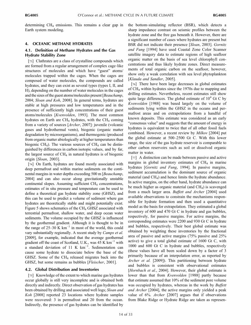
are formed from a regular arrangement of complex cage‐likestructures of molecules and which have “guest” atoms/molecules trapped within the cages. When the cages arecomposed of water molecules, the compounds are calledhydrates, and they can exist as several types (types I, II, andH), depending on the number of water molecules in the cagesand the sizes of the guest atoms/molecules present [Beauchamp,2004; Sloan and Koh, 2008]. In general terms, hydrates arestable at high pressures and low temperatures and in thepresence of sufficiently high concentrations of their guestatoms/molecules [Kvenvolden, 1993]. The most commonhydrates on Earth are CH4 hydrates, with the CH4 comingfrom a variety of sources [Archer, 2007]: juvenile (volcanicgases and hydrothermal vents), biogenic (organic matterdegradation by microorganisms), and thermogenic (producedfrom organic matter abiologically at higher temperatures thanbiogenic CH4). The various sources of CH4 can be distin-guished by differences in carbon isotopic values, and by far,the largest source of CH4 in natural hydrates is of biogenicorigin [Sloan, 2003].[74] On Earth, hydrates are found mostly associated with

deep permafrost and within marine sediments on the conti-nental margins in water depths exceeding 500 m [Beauchamp,2004] and can also occur along gravitationally unstablecontinental slopes. Assuming sufficient CH4 concentrations,estimates of in situ pressure and temperature can be used todefine a theoretical gas hydrate stability zone (GHSZ), andthis can be used to predict a volume of sediment where gashydrates are theoretically stable and might potentially exist.Figure 5 shows schematics of the CH4 GHSZ associated withterrestrial permafrost, shallow water, and deep ocean watersediments. The volume occupied by the GHSZ is influencedby the geothermal gradient. Although it is thought to be inthe range of 25–30 K km−1 in most of the world, this couldvary substantially regionally. A recent study by Camps et al.[2009], for example, indicated that the average geothermalgradient off the coast of Scotland, U.K., was 45 K km−1 witha standard deviation of 11 K km−1. Sedimentation cancause some hydrate to dissociate below the base of theGHSZ. Some of the CH4 released migrates back into theGHSZ, but some remains as bubbles [Fleischer, 2001].

4.2. Global Distribution and Inventories[75] Knowledge of the extent to which marine gas hydrates

occur globally is still very incomplete and is obtained bothdirectly and indirectly. Direct observation of gas hydrates hasbeen obtained by drilling and associated well logs; Sloan andKoh [2008] reported 23 locations where hydrate sampleswere recovered: 3 in permafrost and 20 from the ocean.Indirectly, the presence of gas hydrates can be identified by

the bottom‐simulating reflector (BSR), which detects asharp impedance contrast on seismic profiles between thehydrate zone and the free gas beneath it. However, there area significant number of cases where hydrates are present butBSR did not indicate their presence [Sloan, 2003]. Gornitzand Fung [1994] have used Coastal Zone Color Scannersatellite imagery data to estimate regions of high seafloororganic matter on the basis of sea level chlorophyll con-centrations and thus likely hydrate zones. Direct measure-ments of total organic carbon on the seafloor, however,show only a weak correlation with sea level phytoplankton[Klauda and Sandler, 2005].[76] There have been large decreases in global estimates

of CH4 within hydrates since the 1970s due to mapping anddrilling estimates. Nevertheless, recent estimates still showquite large differences. The global estimate of 104 Gt C byKvenvolden [1988] was based largely on the volume ofsediments lying within the GHSZ in the oceans and per-mafrost areas and on extrapolations from a handful ofknown deposits. This estimate was considered as an early“consensus value” and suggests that the amount of energy inhydrates is equivalent to twice that of all other fossil fuelscombined. However, a recent review by Milkov [2004] putthe global estimate at 500–2500 Gt C. With this lowerrange, the size of the gas hydrate reservoir is comparable toother carbon reservoirs such as soil or dissolved organicmatter in water.[77] A distinction can be made between passive and active

margins in global inventory estimates of CH4 in marinehydrates [Gornitz and Fung, 1994]. In passive margins,sediment accumulation is the dominant source of organicmaterial (and CH4) and hence limits the hydrate abundance.In active margins, on the other hand, hydrate abundance canbe much higher as organic material (and CH4) is scavengedfrom a much larger area. Buffett and Archer [2004] usedavailable observations to constrain the mechanisms respon-sible for hydrate formation and then used a quantitativemodel as the basis for extrapolation. They estimated a globalinventory of 600 and 470 Gt C in hydrate and gas bubbles,respectively, for passive margins. For active margins, thecorresponding estimates were 2200 and 930 Gt C in hydrateand bubbles, respectively. Their best global estimate wasobtained by weighting these inventories by the fractionalarea of passive and active margins (75% passive and 25%active) to give a total global estimate of 1600 Gt C, with1000 and 600 Gt C in hydrate and bubbles, respectively(these values have all been scaled down by a factor of 3primarily because of an interpolation error, as reported byArcher et al. [2009]). This partitioning between hydrateand bubbles is consistent with observational estimates[Hornbach et al., 2004]. However, their global estimate islower than that from Kvenvolden [1988] partly becausethat estimate assumed that 10% of the sediment pore volumewas occupied by hydrates, whereas in the work by Buffettand Archer [2004], the active margins only yielded a peakvalue of 6%. Archer [2007] argues that if observationsfrom Blake Ridge or Hydrate Ridge are taken as represen-


14 of 33

tative of global hydrates, then the 10% volume fraction usedby Kvenvolden [1988] was too high.[78] As shown above, the amount of hydrate filling the

pore volume presents a large uncertainty in global estimates.As a result, the recent study of Klauda and Sandler [2005]included a mass transfer model to estimate the pore volumeoccupied by hydrates. Their global estimate of 56 × 103 Gt Cis larger than that of Kvenvolden [1988] and much higherthan those of Milkov [2004] and Buffett and Archer [2004].Archer [2007] suggested that the difference with Buffett andArcher [2004] could be attributed to differences in thesediment accumulation rate and carbon conversion effi-ciencies, with the Klauda and Sandler [2005] study using an

accumulation rate of sediment which was far too high for thedeep ocean. However, they argue that their estimate is largebecause they include inland seas and hydrates at greaterocean depths as well as continental margins. When con-sidering seafloor depths of less than 3000 m, they get anestimate of 20 × 103 Gt C, which is comparable with theconsensus value of Kvenvolden [1988]. However, it is stillmuch higher than the estimate of Milkov [2004], but thatstudy assumed that only 20% of the continental marginscontained suitable conditions for hydrate growth and used alower pore volume fraction than was calculated by Klaudaand Sandler [2005].

Figure 5. Illustration of the gas hydrate stability zone (a) associated with terrestrial permafrost, (b) inshallow offshore regions, and (c) in the deep ocean, adapted from Kvenvolden and Lorenson [2001].


15 of 33

[79] In the model study by Buffett and Archer [2004], thedownward flux of organic matter (carbon rain) in the watercolumn was prescribed as a function of water depth, i.e.,maximum fluxes in shallow water with lower fluxes in deepwater. However, they found that the rate at which organiccarbon is buried in the ocean sediment is sensitive to theoxygen concentration in the overlying water. A decrease inoxygen concentration of 40 mM in the deep ocean canincrease the CH4 inventory by a factor of 2 and vice versa.They also found that an increase in carbon rain by 50%(using two different assumptions) resulted in the global CH4

inventory increasing by a factor of 2, with the partitioning ofthe additional CH4 between clathrate and bubbles dependenton the assumption. This suggests that oxygen and the rate ofcarbon rain, as well as temperature, may be important forassessing the size of past and present‐day hydrate inventories.[80] The more recent review by Archer [2007] with a

revision from Archer et al. [2009] suggests that a realisticconsensus on the global estimate of the CH4 stored inmarine hydrates is in the range of 170–1000 Gt C, with theinclusion of bubble CH4 adding a similar amount. Both theareal coverage of CH4 hydrate sediment and the averagehydrate volume fraction contribute a factor of 3 to theuncertainty in the global estimate, thereby resulting in afactor of 10 in the overall uncertainty. This could be reducedby further CH4 hydrate sampling and by improving thetechniques used for estimating the CH4 concentration.[81] As mentioned above, there are also stores of CH4 in

polar regions, held in terrestrial hydrates under ice sheetsand within permafrost soils. Although the amount of CH4

held in such hydrates is lower than in marine hydrates andlargely uncertain, it could still be quite large [Harvey andHuang, 1995, and references therein]. They are also vul-nerable to climate change particularly given future expectedtemperature changes in high latitudes [Meehl et al., 2007].For a full discussion on terrestrial hydrates, the mechanismsinvolved in their destabilization, and their potential torelease CH4 to the atmosphere with anthropogenic warming,the reader is referred to Brook et al. [2008].

4.3. Methane Hydrates and Past Climate Change[82] Hydrates are very sensitive to changes in temperature

and pressure [Dickens and Quinby‐Hunt, 1994; Brewer et al.,1997]. As a result, they have been implicated in past climatechange [e.g., Dickens et al., 1995; Kennett et al., 2000].[83] The Paleocene‐Eocene thermal maximum (PETM),

for example, occurred 55 Myr ago and was characterized bya period of intense global warming and a rapid decrease (upto −3‰) in the global mean carbon d13C isotopic ratio[Kennett and Stott, 1991; Koch et al., 1992; Katz et al.,1999; Bains et al., 1999; Dickens, 1999]. Deep oceanwarming of about 4°C–6°C has been inferred in many cores,with an ocean surface warming of 4°C–8°C [Katz et al.,1999]. The intense warming could have been driven by amassive CH4 release from hydrates along the continentalmargins [Dickens et al., 1995], the so‐called “methaneburp” hypothesis, in which the release involved 1500–2000 Gt C over a few thousand years [Norris and Röhl,

1999]. If Paleocene and present‐day margins are consid-ered as similar, then the global volume of the PaleoceneGHSZ was approximately 43% of the present‐day GHSZ(because of warmer water temperatures) and halved duringthe PETM [Dickens, 2001]. With the present‐day globalestimate of CH4 within gas hydrates of 500–2500 Gt C byMilkov [2004], for example, this would imply that there wasan insufficient release of CH4 to account for the observedd13C excursion at the PETM [Milkov et al., 2003].[84] Quaternary climate change refers to brief atmospheric

warming events, and there is evidence of correspondinglarge oscillations in atmospheric CH4 from polar ice coreson orbital, millennial, and decadal time scales [Lorius et al.,1990; Chappellaz et al., 1990; Loulergue et al., 2008].Kennett et al. [2000] suggest, from the observation of carbonisotopic anomalies in benthic and planktic foraminifera, thatthermal dissociation of CH4 hydrates repeatedly dischargedlarge quantities of CH4 from marine sediments into the atmo-sphere, the so‐called “clathrate gun hypothesis” [Kennett et al.,2002]. Dissociation has also been attributed to sea level falls[Paull et al., 1991]. However, an alternative hypothesis isthat the increases in atmospheric CH4 could be attributed toenhanced methanogenesis (section 2.1) in tropical wetlandsreceiving greater precipitation during intense monsoonactivity and the effect of temperature [Chappellaz et al.,1990]. Indeed, D/H isotopic ratios from ice cores mea-sured over the rapid CH4 increases of the last deglaciationand during a single Dansgaard‐Oeschger warm event of thelast glacial period suggest that marine hydrates were stableduring these abrupt warming episodes [Sowers, 2006].

4.4. Methane Hydrate Sensitivity and ProcessesGoverning Release of Methane to the Atmosphere[85] There is still some debate on the extent to which the

decomposition of hydrates is responsible for past variationsin atmospheric CH4 concentrations. Nevertheless, there isconcern that future global warming may lead to hydrateinstability and an enhanced CH4 flux to the atmosphere,thereby imposing a strong positive feedback that wouldamplify anthropogenic warming [Harvey and Huang, 1995;Prather et al., 2001].[86] As atmospheric temperatures increase because of

increasing greenhouse gases, higher temperatures willpropagate into the deep ocean/seafloor, and the inventory ofhydrate is expected to decrease. The time scale for changingthe temperature of the ocean increases with depth, but thereare significant regional variations in this time scale. Inparticular, the Arctic is expected to warm more strongly thanthe global mean. Dickens [2001] calculated that the volumeof the GHSZ associated with marine hydrates halved duringthe PETM with a temperature increase of 5°C. On the otherhand, Buffett and Archer [2004] used their mechanisticmodel to predict the sensitivity of the steady state CH4

marine hydrate inventory. They found that an increase intemperature reduced the steady state global inventorybecause of a reduction in the GHSZ and an increase in thediffusive loss of CH4 from the sediments toward the seafloor.For an ocean temperature increase of 3°C, their inventory of


16 of 33

CH4 reduced to approximately 15% of the present‐dayinventory. Unfortunately, their calculated change is a steadystate solution and does not reveal the time scale overwhich the transition could occur.[87] The build up to a steady state hydrate inventory took

several million years [Davie and Buffett, 2001]; its desta-bilization due to warming may be relatively rapid [Dickens,2003]. However, this may still be slow compared to the timescale of anthropogenic global warming. Archer [2007]suggests that most hydrates are well insulated from theEarth’s surface so that their decomposition will take placeon time scales of millennia or longer. The heat conduction ina solid, such as ocean sediments, is proportional to thermalconductivity which has values of 0.65–1.2 W m−1 K−1

[Newson and Brunning, 2004; Sclater et al., 1969; Moqsudet al., 2008]. The response of such sediments to a transientthermal forcing can only be determined numerically andrequires knowledge of the material density and heat capacity.Using typical values for ocean sediments, it takes about2000 years for a 2°C positive anomaly to raise the temper-ature at 100 m depth by 1°C. In addition, hydrate decom-position is an endothermic process and thus decreasesambient temperature, which slows down heat propagation inthe medium even more.[88] Because of the sensitivity of the GHSZ to tempera-

ture and pressure, several studies have investigated theeffect of changes to sea level and seafloor temperature onthe CH4 hydrate reservoir [Xu et al., 2001; Katz et al., 2001;Dickens, 2003]. However, these studies used idealizedtemperature and pressure changes over a single ocean sed-iment column, thereby neglecting regional variability. Onthe other hand, Fyke and Weaver [2006] used a global cli-mate model in combination with a simple time‐dependentGHSZ model to estimate potential spatial and temporalchanges to the GHSZ volume in response to a range of climatemodel experiments. They found that along the continentalmargins, warming was significantly greater than the globalaverage warming. Over half of the associated GHSZ lossoccurred within the first 5000 years after initiation of theatmospheric CO2 increase, with the initial significant lossoccurring within 200 years. This initial loss principallyoccurred in shallow water in midlatitude to high‐latituderegions associated with sea ice loss. They also noted thesensitivity of the GHSZ volume decrease to thermal dif-fusivity of the seafloor.[89] As can be seen from Figures 5b and 5c, shallow water

hydrates destabilize from the top and bottom parts of theirstability zone, whereas deep ocean hydrates only destabilizefrom the bottom part of their stability zone, which is typi-cally hundreds of meters below the seabed. Only when asustained increase in seafloor temperature has propagatedthrough the sediment column to the bottom of the GHSZwill it cause the deepest, most marginal hydrate to start tobreak down.[90] Detailed models of CH4 hydrate destabilization have

been developed (e.g., TOUGH+HYDRATE) initially withthe aim to understand the risk of hydrate destabilizationrelated to offshore oil drilling. These models resolve how a

temperature and pressure perturbation propagates down-ward, including the effect of fluid motion within the sedi-ment column, and how destabilized CH4 can move upward.Although these models have been tested and used locally,there is no assessment yet of the time scale associated withCH4 hydrate destabilization at the global scale.[91] A recent study by Lamarque [2008] used the IPCC’s

fourth assessment report (AR4) 1%‐CO2 increase per yearsimulations to quantify the potential for CH4 hydratedestabilization with a doubling of CO2. He found the largesttemperature increases occurred mostly in the NorthernHemisphere, particularly north of 50°N. Using these tem-perature changes and on the assumption that the existence ofhydrates is only dependent on depth (pressure) and tem-perature, he calculated a model mean release of CH4 at thebottom of the ocean of 560–2140 Tg CH4 yr

−1 as an upperbound. This flux was reduced to 5–21 Tg CH4 yr−1 torepresent a flux reaching the atmosphere by applying anobserved leakage rate of 1% from a large seepage zone[Mau et al., 2007]. The uncertainties on the fraction of CH4

emitted at the sea bottom reaching the atmosphere are dis-cussed in section 4.4.3. Although the intermodel standarddeviation was approximately 30%, these estimates remainhighly uncertain. No consideration was given to the globaloccurrence and/or depth of CH4 hydrates or the time scaleassociated with the propagation of a temperature anomaly atthe seafloor into the sediment.[92] Acoustic observations above the seabed west of

Spitzbergen have recently revealed more than 250 plumes ofCH4 bubbles in the water column above the GHSZ, coin-ciding with a recent warming of bottom waters by about1°C over the last 30 years [Westbrook et al., 2009]. Part ofthe escaping gas could correspond to free gas usuallytrapped below the GHSZ and migrating upward along theGHSZ lower boundary until it reaches the intersectionbetween the sediment‐water interface and the GHSZ. Theseobservations suggest a close connection between bottomwater warming and methane hydrate degassing under pres-ent conditions. More recently, Reagan and Moridis [2009]used TOUGH+HYDRATE to run a two‐dimensional sim-ulation of the conditions representative of the west Spits-bergen margin; their model results were remarkablyconsistent with Westbrook et al.’s [2009] observations andindicated that the observed CH4 plumes could have origi-nated from temperature‐driven dissociation of hydrates.4.4.1. Role of Pockmarks and Landslides[93] As well as deep ocean temperature change, CH4 could

be released from hydrates through pockmarks [Archer,2007]. These are holes in the sediment surface resultingfrom brutal escape of gas to the ocean. They range in sizefrom meters to kilometers, with one on the crest of BlakeRidge being 700 km2 in size [Kvenvolden, 1999]. Theamount of CH4 released through pockmarks is small com-pared to the atmospheric CH4 burden. If the Blake Ridgepockmark is the result of a large venting of gas in a singleevent, for example, it could only have released about 1 Gt Cas CH4 [Archer, 2007].


17 of 33

[94] Submarine landslides are an integral part of the oceansedimentary system [Hampton et al., 1996] and are com-monplace in river deltas. There have been regular landslidesoff the coast of Norway and in the Mediterranean Sea[Rothwell et al., 2000], with the potential for landslides offthe east coast of the United States [Dugan and Flemings,2000]. A drop in sea level or warming may triggerhydrate destabilization, leading to landslides [Kvenvolden,1999; Driscoll et al., 2000; Vogt and Jung, 2002]. Suchlandslides individually could release up to 5 Gt C as CH4

[Archer, 2007]. A well‐documented example is the largeStoregga slide off Norway, which occurred in two stepssince 50,000 years before present and could have releasedeven more CH4 [Nisbet, 1992]. However, it is not known iffuture warming is sufficient to cause failure of continentalslopes on a global scale, but isotopic evidence of rapidcarbon release in the past is suggestive [Buffett and Archer,2004].[95] There have been other observations of CH4 bubbling

through the seafloor. For instance, Are [2001] reports thatrelease of gas bubbles was observed by Ivanov in the deltaof the Yana River (Laptev Sea) as early as the 1960s. Paullet al. [2007] also recently documented methane‐rich gasbubbles in the Beaufort Sea shelf. These gas bubbles orig-inate from what they call “pingo‐like features” on theBeaufort Sea shelf. Pingos are mounds of earth in thepermafrost environment of the Arctic, sub‐Arctic, andAntarctica that can reach up to 70 m in height and up to2 km in diameter. Paull et al. [2007] hypothesized thatgrowing submarine pingos result from gas pressure associ-ated with gas hydrate decomposition. Shakhova et al. [2005]observed very large CH4 supersaturation of bottom waterson the Siberian shelf, in areas where CH4 hydrates areubiquitous in sediments, thus suggesting a significant con-tribution of hydrate decomposition to the current CH4 bal-ance of waters on this continental shelf. More recently, theyhave also reported on CH4 gas venting into the atmosphere[Shakhova et al., 2010].[96] Emissions from pockmarks, landslides, and pingos

contribute to the CH4 budget and may constitute the conduitfor increased emissions in the future. However, there is noevidence that such emissions have yet increased because ofglobal warming.4.4.2. Particular Case of the Arctic Ocean[97] Both models and geophysical data support the exis-

tence of subsea permafrost in large areas of the Arcticshelves down to a water depth of about 100 m [Racholdet al., 2007]. Subsea permafrost is the result of exposure ofthe seabed to cold temperatures during the LGM when sealevel was much lower. Subsea permafrost is still poorlyunderstood, mainly because of the lack of direct observa-tions. However, it is known to be associated with gashydrates, which can be stored below the subsea permafrost,and the stability of these hydrates is sustained by the exis-tence of permafrost. It is unclear whether some CH4

hydrates can also be stored within the permafrost layer and,if so, how big this reservoir is.

[98] Since the hydrates are often several hundred metersunder the sediments, it is likely that the heat diffusingthrough the sediments over the last 10,000 years (since thelast deglaciation) is now just reaching them. For instance,Paull et al. [2007] offer a scenario where these thermalchanges are caused by the continued warming associatedwith Holocene sea level rise and do not mention anthropo-genic warming at all in their study. Both Weitemeyer andBuffett [2006] and Wadham et al. [2008] propose a mech-anism by which CH4 hydrate accumulates below continentalice sheets during ice ages. The source of CH4 is microbialdecomposition of organic material below the ice sheet.Deglaciation then releases the CH4 from hydrates into theatmosphere. Wadham et al. [2008] estimate the size of thesubglacial reservoir of organic carbon and the amount that isavailable for microbial conversion. They conclude that theCH4 release (63 Gt C during a deglaciation) would have tobe episodic to have a significant impact on atmospheric CH4

concentrations. However, Wadham et al. [2008] include afairly shallow depth of ocean sediments in their estimatesand do not examine the fraction of the CH4 reservoir thatmay respond on a longer time scale during a deglaciation.[99] Anthropogenic warming is adding to the warming

experienced in the Arctic since the LGM. Seawater tem-perature increases in response to increased atmospherictemperature, lack of insulation by disappearing sea ice, andwarmer Atlantic water inflow. The Arctic Ocean tempera-tures at the seabed in a historical integration [Stott et al.,2006] of the Hadley Centre Global Environment Model,version 1 [Johns et al., 2006], have really only increasedsince preindustrial times in the last 25 years. The waters ofthe Barents and Kara seas (and to a lesser extent the LaptevSea) have warmed by about 2.5 K. The pattern of warmingand salinity is entirely consistent with the cause beingincreased inflow of warm saline Atlantic waters. Elsewherein the Arctic, the bottom temperatures have risen by about0.1–0.2 K (up to 1 K in the West Spitzbergen Current), andthis appears to be due to changes in buoyancy (with agradual freshening of deeper water) resulting in slightlyconvective deeper mixing (although not to the seabed).Diffusion of heat would take the warming the rest of theway. The relative contributions of the Holocene warmingand the recent anthropogenic warming to the diffusion ofheat into the subsea permafrost and deep marine sedimentsat the origin of the CH4 emissions discussed previously arenot known.[100] We analyze here simulations from the AR4 multi-

model ensemble [Meehl et al., 2007] which were forcedwith the SRES A1B emissions scenario [Nakićenović et al.,2000]. In the ensemble mean, the warming at the ocean bed,as defined by the physical temperature of each model’slowest ocean level, is greatest in the region of the westernBarents Sea. We select this region (20°E–30°E, 73°N–76°N)from each of the AR4 models to obtain a spread in modelocean floor temperatures and depths across the AR4ensemble for 1860 and 2100. Figure 6 shows these modeledtemperature profiles in relation to the hydrate stability curve.This stability curve is obtained from a corrected version of


18 of 33

equation 1 from Dickens and Quinby‐Hunt [1994] so that itis consistent with their Figure 1. All of the models exceptone show some hydrate stability in the western Barents Seain 1860 but a reduction and/or disappearance of the stabilityzone by 2100 using the SRES A1B emissions scenario.Again, these are equilibrium results, and the dynamics of thesediment warming has yet to be modeled.4.4.3. Fate of Methane Emitted at the Seafloor[101] A less explored issue is the fate of CH4 emitted at

the seafloor. CH4 solubility in seawater is small (it is muchsmaller than that of CO2). For a given temperature‐pressureprofile, Zhang [2003] estimated that CH4 solubility increaseswith depth to about 0.1 wt % at 500 m below sea level, usingdata from Duan et al. [1992]; note that the data have beenupdated by Duan and Mao [2006]. At low depths (lowpressure), CH4 dissolves in water, and if the CH4 concen-tration exceeds the solubility, the excess CH4 would be inthe gas phase. However, there might not be enough nucle-ation sites within the seawater to actually turn the excessCH4 into bubbles. The ocean can therefore be supersaturatedwith respect to CH4 in some places. At larger depths (highpressure), CH4 hydrates are stable, and any excess CH4

would be found in the hydrate phase. In the sedimentcolumn, CH4 hydrate stability decreases with increasingdepth (because of increasing temperature), and CH4 solu-bility in pore water increases. The relatively high CH4 sol-ubility at large depth suggests that the ocean could storelarge amounts of CH4 emitted at the seafloor, but decreasingsolubility with decreasing pressure means that this CH4

would eventually turn into bubbles and outgas to theatmosphere when the water rises.[102] Zhang [2003] reviewed what could happen follow-

ing a release of CH4 at the seafloor. If CH4 is released asCH4 hydrate, since the density of CH4 hydrate is lower thanthat of seawater, whether released hydrate (e.g., from asubmarine landslide or faulting) rises through the watercolumn or not depends on how much sediment is mixedwith it. If sediment mixing is small, then CH4 hydrate wouldrise through the water column and experience dissolutionand dissociation during ascent. Zhang and Xu [2003] haveestimated that hydrate chunks larger than 100 mm in radiuswould be able to survive dissociation through a 530 msurface layer. This is consistent with observations by Breweret al. [2002], who revealed that hydrate pieces of 100 mmsize easily survived transit from the seafloor (780 m) to theocean surface. Paull et al. [2003] also report that marineslumping can release large pieces of solid gas hydrate thatwould float upward in the water column and reach the upperlayers of the ocean before decomposing.[103] If CH4 is released as bubbles, then the bubbles

would rise through the water and expand as the pressuredecreases. However, if the ocean is not saturated withrespect to CH4, then dissolution would also happen, andwhether the size of the bubble increases or not depends onthe competition between expansion and dissolution. Zhang[2003] reported that the critical radius for a bubble to sur-vive a 50 m rise is 0.9 mm. If the CH4 bubble is releasedinto deep water where hydrate is stable, then a hydrate shellwould form around the bubble, which slows down disso-lution. The hydrate shell will break and reform as the CH4

gas in the bubble expands during the rise of the bubble.Rehder et al. [2002] have observed the phenomenon ofhydrate skin formation on CH4 bubbles. They found that therise of CH4 and argon bubbles were similar above the CH4

hydrate stability zone (i.e., about 520 m depth). Below this,enhanced CH4 bubble lifetime was observed which theyattributed to the formation of a hydrate skin. McGinnis et al.[2006] modeled the size of CH4 bubbles rising through thewater column. They point out that even though the size of abubble reaching the surface can be larger than its initial size,it would only contain a fraction of the CH4 that was initiallyreleased because of the difference in pressure. For instance,in the Black Sea a bubble released as a 12 mm bubble at90 m depth would only contain 10% of the initial CH4, withthe other 90% mainly dissolving in the water close to theseafloor. McGinnis et al. [2006] conclude that significantCH4 release to the atmosphere is only possible from shallowwater depths (i.e., less than 100 m). Zhang [2003] also notesthat in the case of a major eruption bubbles would risecollectively as a bubbly water plume because bubbly waterhas a lower density than the surrounding seawater, whichcan lead to a rapid buoyant rise of the water plume. Thisprocess could considerably enhance the fraction of emittedCH4 that reaches the ocean surface.[104] If CH4 dissolution is important, then it is important

to determine what the fate of that dissolved CH4 is andwhether it can leak into the atmosphere when the ocean is

Figure 6. Illustration of the change in shallow water gashydrate stability zone in the western Barents Sea. The stabil-ity curve (shown in black) is calculated from a correctedversion of equation 1 from Dickens and Quinby‐Hunt[1994]; the correction was required to be consistent withtheir Figure 1. The vertical temperature profiles are from theIPCC AR4 multimodel ensemble along with an assumedgeothermal gradient of 0.02 K m−1 [Lachenbruch, 1968].The majority of models show some hydrate stability back in1860 (blue) but a reduction and/or disappearance of thestability zone by 2100 (red). The depth of the water appearsto be different because of the different horizontal resolutionof each model.


19 of 33

ventilated. There is evidence that CH4 is consumed in deepwater by microbial oxidation. This phenomenon couldexplain why marine sediments record numerous episodes ofCH4 hydrate decomposition during the Quaternary era,whereas ice core records suggest a minor contribution ofsuch degassing on the atmospheric CH4 budget. Scrantonand Brewer [1978] showed that dissolved CH4 concentra-tions rapidly decrease with depth in the North Atlantic andNorth Pacific oceans. However, they observed that CH4

consumption ceases within 100 years of isolation from theocean surface. Rehder et al. [1999] deduced a time scale forCH4 oxidation in the North Atlantic Deep Water of about50 years. This may have implications for the scenarios ofhydrate release under climate change. While some regionsof the ocean have low concentrations of CH4 because ofCH4 oxidation, other regions exhibit larger CH4 concentra-tions because of natural sources of CH4 at the seafloor. It istherefore important to determine the extent to which theocean is undersaturated, saturated, or supersaturated withrespect to CH4. For example, Ward et al. [1987] show avertical profile of CH4 in the western Cariaco Basin down to1200 m, which reveals an increase in CH4 concentration upto 12 mM at 1300 m. Ward et al. [1987] also estimated aCH4 oxidation rate of 0.4 nM d−1 below 600 m depth in thedeep anoxic layer. Mau et al. [2007] observed a CH4 plumeemitted at the seafloor from the Coal Oil Point on theCalifornian coast. They found that only 1% of the dissolvedCH4 released at the seafloor enters the atmosphere withintheir study area of 280 km2. The rest of the dissolved CH4

emitted from the Coal Oil Point may enter the atmospherefarther away from the source or be oxidized by microbes inshallow coastal water or farther away in deep water where ithas been mixed. Mau et al. [2007] argue that most of thedissolved CH4 seems to be transported and oxidized belowthe water surface.[105] In addition to bubble and hydrate dynamics and

physics, the sea surface microlayer is also important in boththe consumption and production of atmospheric trace gases[Conrad and Seiler, 1988]. There is evidence that generalmicrobial activity and metabolism at the air‐sea interfacecan regulate air‐sea gas exchange. In the tropical AtlanticOcean, Conrad and Seiler [1988] found a significant mis-match between the invasive and evasive exchange of tracegases (e.g., CH4 and CO) which they attributed to microbialgas consumption in the sea surface microlayer. Similarly,Frost [1999] found an invasion‐evasion mismatch of up to8% for CH4 in the coastal North Sea. Further work in alaboratory gas exchange tank with added methanotrophsconfirmed the potential for active bacterioneuston control oftrace gas exchange; air‐water CH4 exchange differed by upto 10% relative to both nitrous oxide (N2O) and an inerttracer (sulfur hexafluoride), consistent with active metaboliccontrol of CH4 exchange by the bacterioneuston [Upstill‐Goddard et al., 2003]. These studies collectively suggestthat the bacterioneuston is intimately involved in the cyclingof at least some climatically active trace gases, includingCH4, and that it is potentially both a small gas source and a

small gas sink dependent upon the prevailing microbial andbiogeochemical regimes.[106] In conclusion, the evidence for the importance of

CH4 emission by hydrates to the atmosphere is contradic-tory. On the one hand, observations and calculations showthat a significant fraction of the CH4 can reach the watersurface and the atmosphere if the CH4 is emitted in largequantities or as large bubbles, especially from shallow waterdepths. On the other hand, CH4 dissolution, mixing withdeeper water, and microbial CH4 oxidation could play animportant role to significantly decrease the flux of CH4 tothe atmosphere if the CH4 source is smaller, is more diffuse,happens through smaller bubbles, or takes place deeper inthe ocean. There are few measurements of the CH4 con-centration in the ocean and no global picture of the oceanicCH4 distribution. It seems important to investigate furtherthe fate of CH4 in the ocean for different source locations,emission rates, and bubble size.

4.5. Challenges and Prospects for Modelingin Global ESMs[107] A key challenge in CH4 hydrate research is improving

our knowledge of the characterization of CH4 hydrates witha particular focus on their global occurrence, physical andchemical properties, and total CH4 inventory. Further dataare also needed on the geothermal gradient and thermaldiffusivity in the sediment column. Direct observations ofgas hydrates have been obtained by drilling and associatedwell logs, but to date, there is still a relatively small numberof locations where hydrate samples have been recovered.The overall uncertainty in the CH4 inventory is still quitehigh because of uncertainties in both the hydrate areal extentand the average hydrate volume fraction. This uncertaintycould be reduced by further hydrate sampling and byimproving the techniques used for estimating the CH4

concentration.[108] As well as improving our knowledge on the occur-

rence, characteristics, and location of CH4 hydrates in theocean sediments by field and laboratory‐based studies, it isnecessary to develop process‐based models of hydrate‐bearing sediments. Complex biological models describingthe sedimentation and burial of biological material on thebed of shallow seas exist [e.g., Moll and Radach, 2003], butconsiderable development is required to translate these intomodels of clathrate formation. Some geological models alsoexist, but they are used largely in the oil and gas industriesrather than in the context of climate change. By simulatingthe processes of hydrate formation and dissociation, it willbe possible to use these models to examine how the GHSZwill change under different equilibrium conditions. A par-ticular focus should also be on how the ocean warming willpropagate through the sediment column, the time scaleassociated with it, and the transient rather than the steadystate response of the hydrates. Given the long time scalesassociated with the deep ocean, it is recommended that thesemodels be applied to shallow water hydrates in the ArcticOcean, where substantial warming has already been observedand modeled. A case study for these models could well be the


20 of 33

last interglacial period, 115,000–130,000 years before pres-ent. With about 50 W m−2 of additional insolation duringsummer months, the Arctic region experienced considerablewarming, with surface summer temperature 4°C–5°Cwarmer than today [CAPE‐Last Interglacial Project Members,2006]. Detailed records of atmospheric CH4 and its carbonand hydrogen isotopic ratios measured in polar ice corescould disentangle the possible contribution of hydrate de-gassing under such critical conditions.[109] Once destabilization occurs, the fate of the CH4

emitted from ocean sediments is also unclear. Process mod-eling of the ocean CH4 cycle will be required to understandthe various processes in the ocean (bacterial oxidation ofCH4, horizontal and vertical transport mechanisms formethane, and air‐sea flux of CH4). This work could beextended to examine the sensitivity to the location and rate ofCH4 emissions at the seafloor.

5. METHANE PHOTOCHEMICAL FEEDBACKSON CLIMATE

5.1. Methane Chemistry[110] As described in section 1, the principle destruction

pathway for CH4 is via oxidation by the OH radical. Therate of this reaction includes a temperature term with theconsequence that the loss of CH4 increases by approxi-mately 2.3% for every 1°C increase in temperature. Theprinciple source of OH is UV photolysis of ozone in thepresence of water vapor. The densities of OH are highestwhere the sources are highest, i.e., in regions of high watervapor density such as the tropical lower troposphere. Undera changed climate where both temperature and water vapordensity are expected to rise, the combined effect is toincrease the removal rate of CH4 [Johnson et al., 1999,2001]. A multimodel study by Stevenson et al. [2006] foundthat by 2030 climate change might be expected to reducethe CH4 lifetime by around 4% compared to the climate atthe year 2000. Future changes in emissions of CO, hydro-carbons, and NOx will affect the OH density and hence CH4

lifetime, with increases of CO and hydrocarbons decreasingOH and increases in NOx increasing OH.[111] The chemistry that determines the OH radical con-

centration in the atmosphere can be complex and involvesnumerous reactions between various species. Detailed dis-cussions are given, for instance, by Levy [1971], Rasmussenand Khalil [1984], Blake and Rowland [1988], Cicerone[1988], or Hough and Derwent [1990]. Essentially, though,OH is determined by the following reaction chain:

HO2ðRO2Þ þ NO ! OHþ NO2ðR1Þ

NO2 þ h� ! NOþ Oð3PÞðR2Þ

Oð3PÞ þ O2 þM ! O3 þMðR3Þ

O3 þ h� ! Oð1DÞ þ O2ðR4Þ

followed by

Oð1DÞ þ H2O ! 2OH

O3 þ HO2 ! OHþ 2O2ðR5Þ

O3 þ OH ! HO2 þ O2:ðR6Þ

Incidentally, reactions (R1)–(R3) lead to the formation of O3,and reactions (R4)–(R6) result in O3 destruction. Nitrogenoxides and hydrogen radicals are recycled through this cata-lytic reaction chain. Chain breaking occurs through the fol-lowing reactions:

NO2 þ OHþM ! HNO3 þMðR7Þ

HO2 þ HO2 þM ! H2O2 þMðR8Þ

OHþ HO2 ! H2Oþ O2;ðR9Þ

in which both NOx and OH are eventually lost from the cat-alytic cycle. The reaction of OH with CO, CH4, andNMVOCs produces peroxy radicals that feed into reaction(R1) and result in cycle closure:

OHþ CO ! ðO2;MÞ ! HO2 þMðR10Þ

OHþ CH4 ! ðO2;MÞ ! H2Oþ CH3O2:ðR11Þ

The net effect will depend on the balance between CO,NMVOC, and NOx emissions in any particular scenario.Stevenson et al. [2006] found changes in CH4 lifetime of0.0%, +1.4%, and +2.7% for three different emission sce-narios for 2030.

5.2. Methane Feedback on Itself[112] Because CH4 changes its own loss rate, a perturba-

tion to the CH4 distribution (such as an emission pulse) willnot decay with the tropospheric lifetime but will last longerbecause of the reduced OH density. For the troposphericchemistry models that contributed to the IPCC third assess-ment report [Prather et al., 2001], the average increase inlifetime was found to be a factor of 1.4. This means that foran atmospheric lifetime of 8.4 years (including dry deposi-tion and stratospheric loss), the perturbation lifetime of anemission pulse is 12 years. In the steady state response to astep emission change, the fractional change in the CH4

burden due to the fractional change (d) in the emissions israised to the power of 1.4 (i.e., CH4 → CH4 × (1 + d)1.4). Soa 1% increase in CH4 emissions would lead to an increase inthe CH4 burden of 1.4%.

5.3. Methane Direct and Indirect Effects[113] CH4 concentrations have increased from values of

around 715 ppb in preindustrial times to 1787 ppb in 2008[Dlugokencky et al., 2009]. This gives a CH4 radiativeforcing of over 0.48 W m−2. This change in CH4 is less thanthat expected because of the increase in CH4 emissions as


21 of 33

concurrent increases in NOx emissions have increased therate of removal. The impact of CH4 emissions alone sincepreindustrial times is 0.59 W m−2 [Shindell et al., 2005].[114] As well as a direct radiative forcing, CH4 emissions

can change the concentrations of other greenhouse gases.CH4 is a precursor of tropospheric ozone, under atmosphericconditions rich in NOx. Shindell et al. [2005] estimate thatCH4 emissions since the preindustrial era have contributedto a forcing by tropospheric ozone of 0.2 W m−2. Sitch et al.[2007b] suggest that the damage caused by ozone to vege-tation could be to double the effective direct radiativeforcing from an increase in tropospheric ozone alone bysuppressing the land carbon sink. This results in additionalanthropogenic CO2 emissions accumulating in the atmo-sphere and is therefore an indirect radiative forcing ofclimate.[115] The impact of CH4 changes on stratospheric water

vapor from 1880 to 2000 is estimated to be +0.07 ±0.05 W m−2 [Hansen et al., 2005]. Finally, the ultimatedegradation product from CH4 is CO2. The contributionfrom CH4 concentration changes to the CO2 forcing is0.016 W m−2 [Forster et al., 2007]. The latter two con-tributions need to be scaled up by 20% to attribute theforcing to CH4 emissions in the absence of concurrent NOx

emissions. Therefore, the total radiative forcing from pre-industrial times to the present day due to CH4 emissions(including the ozone damage effect) is 1.1 ± 0.2 W m−2, andthis estimate is even higher when the direct and indirecteffects of nitrate and sulfate aerosols are also considered.Shindell et al. [2009] find a decrease in aerosol formation inresponse to an increase in CH4 due to the chemical feed-back which leads to a net positive radiative forcing. Thisshould be compared to a present‐day radiative forcing of1.74 W m−2 from anthropogenic CO2 emissions.

5.4. Interplay of the Methane Cycle With VolatileOrganic Compounds[116] Oxidation by OH radicals represents the main

atmospheric sink not only for CH4 but also for many organiccompounds of natural and anthropogenic origin. Onceemitted into the atmosphere they compete for the availableOH radicals, thereby altering the oxidizing capacity of theatmosphere [Levy, 1971;Hauglustaine et al., 1998; Bey et al.,2001;Collins et al., 2002;Folberth et al., 2006]. Through thisinteraction, NMVOCs have a significant impact on thechemical lifetime of CH4 in the atmosphere.[117] Generally, it is expected that NMVOCs deplete

OH in an unpolluted environment, thereby increasing thechemical lifetime of CH4 [Granier et al., 2000; Lelieveldet al., 2002; von Kuhlmann et al., 2004]. As outlined insection 5.2, this perturbation to the CH4 lifetime will beamplified by the CH4 feedback on its own lifetime. How-ever, in a polluted environment where NMVOC emissionsare generally collocated with pronounced emissions of NOx,NMVOC oxidation leads to a buildup of ozone and, con-sequently, OH by the catalytic action of NOx. This widelyaccepted picture has recently been challenged by Lelieveld

et al. [2008], who indicate that oxidation of naturalNMVOCs, notably isoprene, might provide a mechanism forOH recycling even in a pristine, low‐NOx environment. Thisproposed mechanism could effectively limit the impact ofprimary NMVOCs on the CH4 lifetime. Thus, it could havesignificant implications for the future evolution of the CH4

atmospheric burden, but the mechanism of OH recyclingremains largely unclear.[118] Using a dynamic global vegetation model, Lathière

et al. [2005] have calculated that total BVOC emissionscould increase from 725 Tg C yr−1 at present‐day conditionsto 1250 Tg C yr−1 at the end of the 21st century in responseto climate change. This increase by 75% over the present‐day source implies a significant increase in the CH4 lifetimeand, consequently, its atmospheric concentration, addingfurther to a direct radiative forcing. The study by Lathièreet al. [2005] did not take into account the inhibiting effectof increasing CO2 concentrations on isoprene formation[Monson et al., 2007]. However, further studies by Arnethet al. [2007] and Heald et al. [2009] have found little orno impact on future isoprene emissions as a consequenceof the CO2 inhibition effect.[119] It has to be pointed out, though, that the predictions

of future NMVOC emissions from the biosphere areaffected by extremely large uncertainties related to both theecosystem adaptation and distribution in a changing climateas well as the actual emission magnitude itself. Effects thathave been outlined include a reduced stomatal exchange ratewith the atmosphere in response to elevated CO2 levels[Field et al., 1995], damage of plants due to exposure tosurface ozone [Sitch et al., 2007b], inhibition of isopreneemissions on an intercellular level by elevated ambient CO2

concentrations which could partially counteract the long‐term CO2 fertilization effects [Arneth et al., 2007; Healdet al., 2009], and reduced isoprene emissions as a conse-quence of drought [Pegoraro et al., 2004]. In addition, theseprocesses depend on and interact with each other and theclimate and atmospheric composition, implying a highlynonlinear response to future changes.[120] The overall impact of these processes on future

BVOC emissions is largely unknown at present, and most ofthe research is at a very early stage. Keeping in mind thevery large uncertainties around all processes that governBVOC emissions from the terrestrial biosphere, the mostlikely future scenario currently anticipated is one in whichemissions of BVOCs which dominate over anthropogenicNMVOCs in the present‐day atmosphere will increasesubstantially in response to a warmer climate and elevatedatmospheric CO2 levels [Sanderson et al., 2003; Lathièreet al., 2006; Monson et al., 2007] and, hence, will playa key role in the global CH4 budget.[121] The future evolution of atmospheric CH4 con-

centrations may also be understood by turning to the past.The study of past atmospheric CH4 fluctuations from icecores allows some of the vast uncertainties around themagnitude of the CH4‐NMVOC feedback in future climateto be constrained. CH4 concentrations measured in gas


22 of 33

bubbles that were preserved in the ice show that atmosphericconcentrations of CH4 have increased from about 380 ppb atthe LGM 21,000 years before present to roughly 715 ppbduring the preindustrial era [Chappellaz et al., 1993b, 1997;Brook et al., 2000]. This increase in the atmospheric CH4

concentration by more than 65%, which is similar to the onepredicted to occur over the 21st century, has been attributedto a substantial amount to the increase in BVOC emissionsfrom a more productive tropical forest and the developingboreal forests as a consequence of the shrinking of thecontinental ice sheets [Valdes et al., 2005; Kaplan et al.,2006; Harder et al., 2007].[122] Valdes et al. [2005] and Kaplan et al. [2006] have

calculated an increase of the CH4 lifetime by approximately1.3 years (19%) and 2.1 years (29%) from 7.1 and 7.3 yearsat LGM to 8.4 and 9.4 years, respectively, for the prein-dustrial Holocene (PIH) as a consequence of increasingBVOC emissions. In those studies, BVOC emissions werecalculated to increase by 100% and 57%. This increase inCH4 atmospheric lifetime would account for between 55%and 88% of the increase in the atmospheric CH4 concentra-tion from LGM to PIH [Valdes et al., 2005; Kaplan et al.,2006]. However, these model studies have large uncertaintiessince many effects cannot be taken into account at thecurrent stage of model development. Nevertheless, thesemodeling studies have found experimental support recently[Loulergue et al., 2008]. Because of its inherently nonlinearnature it is not possible to extrapolate the past feedbackdirectly into a future atmosphere quantitatively. Neverthe-less, it seems legitimate to assume that a similar feedbackprocess in the past will result in a feedback of the same signand possibly similar magnitude in the future. Furthermore,the available results at least allow us to speculate about howthe future increase in BVOC emissions will affect the evo-lution of the CH4 burden over the 21st century. It can behypothesized that a 75% increase in BVOC emissions ispossible over the 21st century [Lathière et al., 2005] withlittle impact from the CO2 inhibition effect [Arneth et al.,2007; Heald et al., 2009]. A similar increase in BVOCemissions from the LGM to the preindustrial period resultsin an increase of the CH4 lifetime by roughly 1–2 years[Valdes et al., 2005; Kaplan et al., 2006]. A simple reactionkinetic consideration implies a 2.3% or roughly 3 monthdecrease in CH4 chemical lifetime per °C increase in tem-perature at constant OH concentrations. The CH4 feedbackon its own lifetime extends this lifetime decrease to 3.2% oralmost 4 months per °C warming. A global warming of 2°C–4°C by 2100 [Meehl et al., 2007] results in a decrease in theCH4 chemical lifetime due to temperature and humiditychanges alone of between approximately 8 and 15 months.[123] Consequently, this very rough comparison would

indicate that the effect of a 75% increase in BVOC emis-sions on the CH4 lifetime and the chemical kinetic effect dueto expected global warming are of the same order of mag-nitude but of opposite sign, potentially cancelling eachother. However, very large uncertainties persist around thesefigures, and further model improvements are required to

assess the importance of nonlinear chemical feedbacks inthe Earth system.

6. CONCLUSIONS AND RECOMMENDATIONSFOR FUTURE RESEARCH

[124] We have made an assessment of the available sci-entific literature on CH4 feedbacks related to natural sourcesof CH4 from wetlands, permafrost, and ocean sediments. Insummary, the complex and nonlinear processes governingthe sources and atmospheric chemistry of CH4 cause afeedback loop between the climate, the terrestrial vegetationas the source of BVOCs, the oxidation capacity of theatmosphere, and the atmospheric CH4 burden. The feedbackloop can be described in simple terms as follows: rising CH4

emissions from wetlands, thawing permafrost, and destabi-lizing marine hydrates increase atmospheric CH4 con-centrations; this increase in CH4 concentration, amplified bythe effect of CH4 on its own chemical lifetime, results in agreater radiative forcing on climate and terrestrial ecosys-tems. The ecosystems, given our current understanding,respond to the warmer, more humid conditions by anincrease in BVOCs, which further augments the chemicallifetime of CH4. Finally, the resulting additional radiativeforcing could lead to more or faster thawing of permafrost,further destabilization of marine hydrates, and potentiallyeven larger wetland CH4 emissions. But this feedback loopcould break down because of increased drought conditionsresulting in a loss of global wetland area or a reduced BVOCemission efficiency in the terrestrial ecosystems under waterstress or be limited by the speed of permafrost thawing and/ordestabilization of marine hydrates. It is difficult, if notimpossible, to predict if and when this breakdown occurswithout simulating the entire feedback loop. Many of theprocesses involved are poorly understood or are only nowbeing uncovered. The next generation of ESMs will providethe required framework to analyze the numerous inter-dependencies that contribute to the global CH4 cycle.[125] Our main findings on future CH4 emissions are

summarized in Figure 7, which shows cumulative emissionsof CH4 as a function of the time scale of climate change.The diagram is semiquantitative and should be interpreted assuch. The light blue line corresponds to present‐day emis-sions of ∼600 Tg CH4 yr−1 and can be used to assess theimportance of the CH4 feedbacks on different time scales.Our review indicates an increase in wetland emissions of10%–35% per °C warming, which we roughly translatedinto a range of cumulative emissions until 2100 (red lines).There are no studies looking at longer time scales, butemissions would be expected to continue, although perma-frost thawing, changes in land use, and soil humidity allcontribute to increase the uncertainty range. The change inCH4 lifetime due to changing BVOC emissions is fairlyuncertain but can be translated into equivalent emissions aswas done with the pink lines in Figure 7; it is thought to be asmaller effect than that from wetland emissions, especially ifthere is a CO2 inhibition effect on BVOC emissions. Thechange in CH4 lifetime due to the increase in temperature


23 of 33

and humidity is expected to be of a similar magnitude butopposite sign (not shown in Figure 7). Thawing of theterrestrial permafrost will result in CO2 and CH4 emissionson time scales of a few decades to several centuries. Uncer-tainties in future emissions are dominated by the extent ofcarbon stores, the fractional area and volume of permafrostthawing, and the ratio of CH4 to CO2 emissions. We place arange in Figure 7 that reflects published estimates compiledin this review. We limit here the cumulative emissions ofCH4 from terrestrial permafrost to a fraction of the carbonstores, but emissions can carry on as permafrost regions aretransformed into wetlands with their own vegetationdynamics. Existing inventories on marine hydrates place anupper bound on cumulative CH4 emissions from this source;the blue dotted lines in Figure 7 show the range of 4 × 105

and 3 × 106 Tg CH4. Marine hydrates can only be fullydestabilized on time scales of millennia because of the largeinertia associated with the global oceanic circulation andheat propagation in sediments. It is difficult to put a lowerbound on atmospheric CH4 emissions from hydratesbecause of the possibility of large quantities of CH4 beingoxidized in oceanic water and the range of future climateprojections. Likewise, it is not possible to give an estimatefor emissions on shorter time scales. It is clear, however, thatthis is a very large reservoir of CH4 that could dominateother sources of CH4 even if emitted on long time scales.Methane has a lifetime of the order of 10 years so cumu-lative emissions, as presented in Figure 7, are only partiallyrelevant for climate change. While the enhanced emissionsfrom wetlands or the enhanced lifetime due to BVOCemissions would happen continuously, emissions from theterrestrial permafrost or marine hydrates could happen in anonlinear way as various thresholds are crossed.[126] A significant increase in CH4 emissions and atmo-

spheric concentrations due to climate change is therefore a

possible scenario for the next century. However, uncer-tainties are very large, and as discussed above, it is difficultto be very conclusive regarding the magnitude of CH4

feedbacks and their time scales. The following statementscan nevertheless be made:[127] 1. Natural emissions of CH4 are likely to increase in a

warmer climate; however, the magnitude and rate of changeof future emissions from natural sources are largely unknown.[128] 2. There are large amounts of carbon stored as

organic matter in permafrost or as CH4 hydrates in the oceansediments. However, it is not clear how quickly these carbonstores can be released and how much would survivemicrobial oxidation between the source and the atmosphere.The risk of a rapid increase in CH4 emissions is real butremains largely unquantified.[129] 3. Climate change will affect the CH4 lifetime. The

anticipated increases in temperature and water vapor con-centrations and emissions of BVOCs will have effects ofopposite signs on the CH4 lifetime. In any case, the potentialfor increased CH4 emissions is larger than the potential forincreased CH4 sinks.[130] We also identify a number of gaps in our knowledge:[131] 1. Our understanding of the present‐day distribution,

CH4 fluxes, and sensitivities associated with wetlands(including wetland spatial and seasonal distribution itself)needs to be improved, particularly in relation to tropicalwetlands. Therefore, there is a requirement that ESMs suc-cessfully represent the wetland hydrology, permafrost pro-cesses, and vegetation as well as the processes for CH4

formation (including substrate supply), transfer, oxidation,and emission. Only by improving our understanding ofthese processes will we be able to quantify the climatefeedback on wetland CH4 emissions with greater certainty.[132] 2. The carbon stores in boreal regions are not well

known, although some recent inventories of soil organicpools in permafrost regions constitute a good starting pointfor global‐scale modeling. It is of fundamental importanceto understand the horizontal and vertical distributions ofthe carbon stored as organic matter in the land permafrostand CH4 hydrates in the ocean sediments. Land CH4

hydrates and subsea permafrost may also play a role. Betterinventories of carbon stores will benefit from moreobservations and better integration of existing observations,as well as modeling of paleoclimatic ecosystems and sedi-ment formation (notably by considering past warmer inter-glacials as a case study).[133] 3. It is timely to develop models of permafrost

dynamics. The modeling needs to focus on accuratelyrepresenting heat and water transfer within a deep soil layerwith potentially high content of organic matter. The sensi-tivity of permafrost thawing to global warming will need tobe investigated. It is also important to understand to whatextent permafrost thawing will result in changes in thewater table depth and wetland area in order to predict therelative strengths of CH4 and CO2 emissions associatedwith the decomposition of the organic matter present in thepermafrost.

Figure 7. . Summary diagram of the relative sizes and timescales associated with methane feedbacks. See text for a dis-cussion. Note that the diagram is semiquantitative. BVOCs,biogenic volatile organic compounds.


24 of 33

[134] 4. It is not just sufficient to know the location of CH4

hydrates in the ocean sediments and how the CH4 hydratestability zonewouldmove for different equilibrium conditions;we need to understand how and how quickly the oceanwarming will propagate through the sediment column. Furtherdata are needed on the geothermal gradient and thermal dif-fusivity in the sediment column. It is important that modelingfocuses on understanding the transient rather than steady stateresponse of marine hydrates to climate change. Some geo-logical models exist but have hardly been used in the context ofclimate change. Given the long time scales associated with thedeep ocean and that CH4 is not likely to enter the atmospherefrom the deep ocean, it is recommended that researchfocuses on ocean shelves with a particular emphasis on theArctic Ocean where substantial warming has been observedand modeled. A particular challenge in modeling hydrates inESMs will be the different time scales associated with hydrateformation, heat propagation, etc.[135] 5. The fate of CH4 emitted from ocean sediments is

unclear. Some simple modeling of the ocean CH4 cycleshould be initiated to understand the various processes atplay in the ocean (bacterial oxidation of CH4, horizontal andvertical transport mechanisms for methane, and air‐sea fluxof CH4). Sensitivity studies on the location and rate of CH4

emissions at the seafloor should be performed.[136] 6. The atmospheric response to a large emission rate

of CH4 is not well known. The sensitivity of the oxidizingcapacity of the atmosphere to large emissions of CH4 shouldbe investigated. This is in the context of changes in theoxidizing capacity of the atmosphere driven by expectedchanges in atmospheric temperature, water vapor, VOCemissions from the biosphere, and the CH4 feedback onitself. Earth system models will provide further insight intothe importance of the numerous feedbacks that are involved.[137] This research should be done collaboratively, pulling

together the relevant multidisciplinary expertise, and shouldbe quickly incorporated into scientific advice that is pro-vided to governments regarding safe levels of climatechange.

[138] ACKNOWLEDGMENTS. The Met Office HadleyCentre is funded by the Joint DECC and Defra Integrated ClimateProgramme, DECC/Defra (GA01101). R. Coppell is supported bya NERC scholarship, NE/F008341/1, supported by the Met OfficeHadley Centre as a CASE partner. J. Chappellaz was supported bythe French ANR project IMPACT‐BOREAL under the Vulnérabilité2006 program and also by the INSU‐QUEST British‐French projectDESIRE. We also wish to acknowledge Philip Cameron‐Smith,Michael Cunliffe, Chris Huntingford, Mike Lovell, Andy Ridgwell,and Chris Rochelle for useful discussions and comments.[139] The Editor for this paper was Mark Moldwin. He thanks

reviewer Rita Wania and two additional anonymous reviewers.

REFERENCES

Alexeev, V. A., D. J. Nicolsky, V. E. Romanovsky, and D. M.Lawrence (2007), An evaluation of deep soil configurations inthe CLM3 for improved representation of permafrost, Geophys.Res. Lett., 34, L09502, doi:10.1029/2007GL029536.

Allan, W., D. C. Lowe, A. J. Gomez, H. Struthers, and G. W.Brailsford (2005), Interannual variation of 13C in troposphericmethane: Implications for a possible atomic chlorine sink inthe marine boundary layer, J. Geophys. Res., 110, D11306,doi:10.1029/2004JD005650.

Archer, D. (2007), Methane hydrate stability and anthropogenicclimate change, Biogeosciences, 4, 521–544, doi:10.5194/bg-4-521-2007.

Archer, D., B. Buffett, and V. Brovkin (2009), Ocean methanehydrates as a slow tipping point in the global carbon cycle, Proc.Natl. Acad. Sci. U. S. A., 106(49), 20,596–20,601.

Are, F. E. (2001), The problem of the emission of deep‐buriedgases to the atmosphere, in Permafrost Response on EconomicDevelopment, Environmental Security and Natural Resources,edited by R. Paepe and V. Melnikov, pp. 497–509, KluwerAcad., Dordrecht, Netherlands.

Arneth, A., P. A. Miller, A. Scholze, T. Hickler, G. Schurges,B. Smith, and I. C. Prentice (2007), CO2 inhibition of globalterrestrial isoprene emissions: Potential implications for atmo-spheric chemistry, Geophys. Res. Lett., 34, L18813, doi:10.1029/2007GL030615.

Arneth, A., et al. (2010), From biota to chemistry and climate:Towards a comprehensive description of trace gas exchangebetween the biosphere and atmosphere, Biogeosciences, 7,121–149, doi:10.5194/bg-7-121-2010.

Aselmann, I., and P. J. Crutzen (1989), Global distribution ofnatural fresh‐water wetlands and rice paddies, their net pri-mary productivity, seasonality and possible methane emissions,J. Atmos. Chem., 8(4), 307–358.

Bains, S., R. M. Corfield, and R. D. Norris (1999), Mechanismsof climate warming at the end of the Paleocene, Science, 285,724–727, doi:10.1126/science.285.5428.724.

Beauchamp, B. (2004), Natural gas hydrates: Myths, facts andissues, C. R. Geosci., 336, 751–765, doi:10.1016/j.crte.2004.04.003.

Bekki, S., K. S. Law, and J. A. Pyle (1994), Effect of ozone deple-tion on atmospheric CH4 and CO concentrations, Nature, 371,595–597, doi:10.1038/371595a0.

Bergamaschi, P.,M. Krol, F. Dentener, A. Vermeulen, F.Meinhardt,R. Graul, M. Ramonet, W. Peters, and E. J. Dlugokencky(2005), Inverse modelling of national and European CH4 emis-sions using the atmospheric zoom model TM5, Atmos. Chem.Phys., 5, 2431–2460, doi:10.5194/acp-5-2431-2005.

Bergamaschi, P., et al. (2009), Inverse modeling of global andregional CH4 emissions using SCIAMACHY satellite retrievals,J. Geophys. Res., 114, D22301, doi:10.1029/2009JD012287.

Bey, I., D. J. Jacob, R. M. Yantosca, J. A. Logan, B. D. Field,A. M. Fiore, Q. B. Li, H. G. Y. Liu, L. J. Mickley, andM. G. Schultz (2001), Global modeling of tropospheric chemistrywith assimilated meteorology: Model description and evaluation,J. Geophys. Res., 106, 23,073–23,095, doi:10.1029/2001JD000807.

Blake, D. R., and F. S. Rowland (1988), Continuing worldwideincrease in tropospheric methane, 1978 to 1987, Science, 239,1129–1131, doi:10.1126/science.239.4844.1129.

Bloom, A. A., P. I. Palmer, A. Fraser, D. S. Reay, and C. Frankenberg(2010), Large‐scale controls of methanogenesis inferred frommethane and gravity spaceborne Data, Science, 327, 322–325,doi:10.1126/science.1175176.

Born, M., H. Dorr, and I. Levin (1990), Methane consumption inaerated soils of the temperate zone, Tellus, Ser. B, 42, 2–8.

Bousquet, P., D. A. Hauglustaine, P. Peylin, C. Carouge, andP. Ciais (2005), Two decades of OH variability as inferred byan inversion of atmospheric transport and chemistry of methylchloroform, Atmos. Chem. Phys., 5, 2635–2656, doi:10.5194/acp-5-2635-2005.

Bousquet, P., et al. (2006), Contribution of anthropogenic andnatural sources to atmospheric methane variability, Nature,443, 439–443, doi:10.1038/nature05132.


25 of 33

Brewer, P. G., F. M. Orr Jr., G. Friederich, K. A. Kvenvolden,D. L. Orange, J. McFarlane, and W. Kirkwood (1997), Deep‐ocean field test of methane hydrate formation from a remotelyoperated vehicle, Geology, 25, 407–410, doi:10.1130/0091-7613(1997)025<0407:DOFTOM>2.3.CO;2.

Brewer, P. G., C. Paull, E. T. Peltzer, W. Ussler, G. Rehder, andG. Friederich (2002), Measurements of the fate of gas hydratesduring transit through the ocean water column, Geophys. Res.Lett., 29(22), 2081, doi:10.1029/2002GL014727.

Brook, E. J., S. Harder, J. Severinghaus, and M. Bender (1999),Atmospheric methane and millennial‐scale climate change, inMechanisms of Global Climate Change at Millennial Time Scale,Geophys. Monogr. Ser., vol. 112, edited by P. U. Clark, R. S.Webb, and L. D. Keigwin, pp. 165–175, AGU, Washington,D. C.

Brook, E. J., S. Harder, J. Severinghaus, E. J. Steig, and C. M.Sucher (2000), On the origin and timing of rapid changes inatmospheric methane during the last glacial period, Global Bio-geochem. Cycles, 14, 559–572, doi:10.1029/1999GB001182.

Brook, E., D. Archer, E. Dlugokencky, S. Frolking, and D. Lawrence(2008), Potential for abrupt changes in atmospheric methane, inAbrupt Climate Change. A Report by the U.S. Climate ChangeScience Program and the Subcommittee on Global ChangeResearch, pp. 360–452, U.S. Geol. Surv., Reston, Va.

Bubier, J. L., G. Bhatia, T. R. Moore, N. T. Roulet, and P. M.Lafleur (2003), Spatial and temporal variability in growing sea-son net ecosystem carbon dioxide exchange at a large peatlandin Ontario, Canada, Ecosystems, 6, 353–367.

Buffett, B., and D. Archer (2004), Global inventory of methaneclathrate: Sensitivity to changes in the deep ocean, Earth Planet.Sci. Lett., 227, 185–199, doi:10.1016/j.epsl.2004.09.005.

Burn, C. R., and F. E. Nelson (2006), Comment on “A projectionof severe near‐surface permafrost degradation during the 21stcentury” by David M. Lawrence and Andrew G. Slater, Geophys.Res. Lett., 33, L21503. doi:10.1029/2006GL027077.

Camps, A. P., D. Long, C. A. Rochelle, and M. A. Lovell (2009),Mapping hydrate stability zones offshore Scotland, in Sediment‐Hosted Gas Hydrates: New Insights on Natural and SyntheticSystems, Geol. Soc. Spec. Publ., 319, 81–91, doi:10.1144/SP319.7.

Cao, M., S. Marshall, and K. Gregson (1996), Global carbonexchange and methane emissions from natural wetlands: Appli-cation of a process‐based model, J. Geophys. Res., 101(D9),14,399–14,414, doi:10.1029/96JD00219.

Cao, M., K. Gregson, and S. Marshall (1998), Global methaneemission from wetlands and its sensitivity to climate change,Atmos. Environ., 32, 3293–3299, doi:10.1016/S1352-2310(98)00105-8.

CAPE–Last Interglacial Project Members (2006), Last InterglacialArctic warmth confirms polar amplification of climate change,Quat. Sci. Rev., 25, 1383–1400, doi:10.1016/j.quascirev.2006.01.033.

Carey, S. K., and M. K. Woo (1999), Hydrology of two slopes insubarctic Yukon, Canada, Hydrol. Processes, 13, 2549–2562,doi:10.1002/(SICI)1099-1085(199911)13:16<2549::AID-HYP938>3.0.CO;2-H.

Carey, S. K., and M. K. Woo (2000), The role of soil pipes as aslope runoff mechanism, Subarctic Yukon, Canada, J. Hydrol.,233, 206–222, doi:10.1016/S0022-1694(00)00234-1.

Chappellaz, J., J. M. Barnola, D. Raynaud, Y. S. Korotkevich, andC. Lorius (1990), Ice‐core record of atmospheric methane overthe past 160,000 years, Nature, 345, 127–131, doi:10.1038/345127a0.

Chappellaz, J., T. Blunier, D. Raynaud, J.M. Barnola, J. Schwander,and B. Stauffer (1993a), Synchronous changes in atmosphericCH4 and Greenland climate between 40 and 8 Kyr BP, Nature,366, 443–445, doi:10.1038/366443a0.

Chappellaz, J. A., I. Y. Fung, and A. M. Thompson (1993b), Theatmospheric CH4 increase since the Last Glacial Maximum (1)Source estimates, Tellus, Ser. B, 45, 228–241.

Chappellaz, J. A., T. Blunier, S. Kints, A. Dallenbach, J.‐M. Barnola,J. Schwander, D. Raynaud, and B. Stauffer (1997), Changes inthe atmospheric CH4 gradient between Greenland and Antarcticaduring the Holocene, J. Geophys. Res., 102, 15,987–15,997,doi:10.1029/97JD01017.

Chen, Y.‐H., and R. G. Prinn (2006), Estimation of atmosphericmethane emissions between 1996 and 2001 using a three‐dimensional global chemical transport model, J. Geophys. Res.,111, D10307, doi:10.1029/2005JD006058.

Christensen, T. R., and P. Cox (1995), Response of methaneemission from arctic tundra to climatic change: Results from amodel simulation, Tellus, Ser. B, 47, 301–309, doi:10.1034/j.1600-0889.47.issue3.2.x.

Christensen, T. R., A. Ekberg, L. Ström,M.Mastepanov, N. Panikov,M. Öquist, B. H. Svensson, H. Nykänen, P. J. Martikainen, andH. Oskarsson (2003), Factors controlling large scale variations inmethane emissions from wetlands, Geophys. Res. Lett., 30(7),1414, doi:10.1029/2002GL016848.

Christensen, T. R., T. Johansson, H. J. Aakerman, M. Mastepanov,N. Malmer, T. Friborg, P. Crill, and B. H. Svensson (2004),Thawing sub‐arctic permafrost: Effects on vegetation and meth-ane emissions, Geophys. Res. Lett., 31, L04501, doi:10.1029/2003GL018680.

Cicerone, R. J. (1988), How has the atmospheric concentration ofCO changed?, in The Changing Atmosphere, edited by F. S.Rowland and I. S. A. Isaksen, pp. 44–61, John Wiley, New York.

Collins, W. J., R. G. Derwent, C. E. Johnson, and D. S. Stevenson(2002), The oxidation of organic compounds in the troposphereand their global warming potentials, Clim. Change, 52, 453–479,doi:10.1023/A:1014221225434.

Conrad, R., and W. Seiler (1988), Influence of the surface micro-layer on the flux of nonconservative trace gases (CO, H2, CH4,N2O) across the ocean‐atmosphere interface, J. Atmos. Chem.,6, 83–94, doi:10.1007/BF00048333.

Cunnold, D. M., et al. (2002), In situ measurements of atmosphericmethane at GAGE/AGAGE sites during 1985–2000 and result-ing source inferences, J. Geophys. Res., 107(D14), 4225,doi:10.1029/2001JD001226.

Dadson, S. J., I. Ashpole, P. Harris, H. N. Davies, D. B. Clark,E. Blyth, and C. M. Taylor (2010), Wetland inundation dynamicsin a model of land‐surface climate: Evaluation in the Nigerinland Delta region, J. Geophys. Res., doi:10.1029/2010JD014474,in press.

Dällenbach, A., T. Blunier, J. Flückiger, B. Stauffer, J. Chappellaz,and D. Raynaud (2000), Changes in the atmospheric CH4

gradient between Greenland and Antarctica during the last glacialand the transition to the Holocene, Geophys. Res. Lett., 27(7),1005–1008, doi:10.1029/1999GL010873.

Davie, M. K., and B. A. Buffett (2001), A numerical model for theformation of gas hydrate below the seafloor, J. Geophys. Res.,106(B1), 497–514, doi:10.1029/2000JB900363.

Davis, N. (2001), Permafrost: A Guide to Frozen Ground in Tran-sition, Univ. of Alaska Press, Fairbanks.

Decharme, B., H. Douville, C. Prigent, F. Papa, and F. Aires(2008), A new river flooding scheme for global climate applica-tions: Off‐line evaluation over South America, J. Geophys. Res.,113, D11110, doi:10.1029/2007JD009376.

Delisle, G. (2007), Near‐surface permafrost degradation: Howsevere during the 21st century?, Geophys. Res. Lett., 34,L09503, doi:10.1029/2007GL029323.

Denman, K., et al. (2007), Couplings between changes in the cli-mate system and biogeochemistry, in Climate Change 2007:The Physical Science Basis. Contribution of Working Group Ito the Fourth Assessment Report of the Intergovernmental Panelon Climate Change, edited by S. Solomon et al., pp. 499–587,Cambridge Univ. Press, Cambridge, U. K.

Dentener, F., W. Peters, M. Krol, M. van Weele, P. Bergamaschi,and J. Lelieveld (2003), Interannual variability and trend of CH4

lifetime as a measure for OH changes in the 1979–1993 time


26 of 33

period, J. Geophys. Res., 108(D15), 4442, doi:10.1029/2002JD002916.

Dickens, G. R. (1999), The blast in the past, Nature, 401, 752–755,doi:10.1038/44486.

Dickens, G. R. (2001), The potential volume of oceanic methanehydrates with variable external conditions, Org. Geochem., 32,1179–1193, doi:10.1016/S0146-6380(01)00086-9.

Dickens, G. R. (2003), Rethinking the global carbon cycle with alarge, dynamic and microbially mediated gas hydrate capacitor,Earth Planet. Sci. Lett., 213, 169–183, doi:10.1016/S0012-821X(03)00325-X.

Dickens, G. R., and M. S. Quinby‐Hunt (1994), Methane hydratestability in seawater, Geophys. Res. Lett., 21, 2115–2118,doi:10.1029/94GL01858.

Dickens, G. R., J. R. O’Neil, D. K. Rea, and R. M. Owen (1995),Dissociation of oceanic methane hydrate as a cause of the carbonisotope excursion at the end of the Paleocene, Paleoceanography,10, 965–971, doi:10.1029/95PA02087.

Dlugokencky, E. J., K. A. Masarie, P. M. Lang, and P. P. Tans(1998), Continuing decline in the growth rate of the atmosphericmethane burden, Nature, 393, 447–450, doi:10.1038/30934.

Dlugokencky, E. J., B. P. Walter, K. A. Masarie, P. M. Lang, andE. S. Kasischke (2001), Measurements of an anomalous globalmethane increase during 1998, Geophys. Res. Lett., 28(3),499–502, doi:10.1029/2000GL012119.

Dlugokencky, E. J., S. Houweling, L. Bruhwiler, K. A. Masarie,P. M. Lang, J. B. Miller, and P. P. Tans (2003), Atmosphericmethane levels off: Temporary pause or a new steady‐state?,Geophys. Res. Lett., 30(19), 1992, doi:10.1029/2003GL018126.

Dlugokencky, E. J., et al. (2009), Observational constraints onrecent increases in the atmospheric CH4 burden, Geophys. Res.Lett., 36, L18803, doi:10.1029/2009GL039780.

Driscoll, N. W., J. K. Weissel, and J. A. Goff (2000), Potential forlarge‐scale submarine slope failure and tsunami generation alongthe US mid‐Atlantic coast, Geology , 28(5), 407–410,doi:10.1130/0091-7613(2000)28<407:PFLSSF>2.0.CO;2.

Duan, Z., and S. Mao (2006), A thermodynamic model for calcu-lating methane solubility, density and gas phase composition ofmethane‐bearing aqueous fluids from 273 to 523 K and from1 to 2000 bar, Geochimica, 70, 3369–3386, doi:10.1016/j.gca.2006.03.018.

Duan, Z. H., N. Moller, and J. H. Weare (1992), Moleculardynamics simulation of PVT properties of geological fluidsand a equation of state of nonpolar and weakly polar gases upto 2000 K and 20,000 bar, Geochim. Cosmochim. Acta, 56,3839–3845, doi:10.1016/0016-7037(92)90175-I.

Dugan, B., and P. B. Flemings (2000), Overpressure and fluid flowin the New Jersey continental slope: Implications for slope failureand cold seeps, Science, 289, 288–291, doi:10.1126/science.289.5477.288.

Dutta, K., E. A. G. Schuur, J. C. Neff, and S. A. Zimov (2006),Potential carbon release from permafrost soils of northeasternSiberia, Global Change Biol., 12, 2336–2351, doi:10.1111/j.1365-2486.2006.01259.x.

Eliseev, A. V., I. I. Mokhov, M. M. Arzhanov, P. F. Demchenko,and S. N. Denisov (2008), Interaction of the methane cycle andprocesses in wetland ecosystems in a climate model of interme-diate complexity, Izv. Russ. Acad. Sci. Atmos. Oceanic Phys.,Engl. Transl., 44, 139–152, doi:10.1134/S0001433808020011.

Essery, R. L. H., M. J. Best, R. A. Betts, P. M. Cox, and C. M.Taylor (2003), Explicit representation of subgrid heterogeneityin a GCM land‐surface scheme, J. Hydrometeorol., 4(3), 530–543,doi:10.1175/1525-7541(2003)004<0530:EROSHI>2.0.CO;2.

Etheridge, D. M., L. P. Steele, R. J. Francey, and R. L. Langenfelds(1998), Atmospheric methane between 1000 A.D. and present:Evidence of anthropogenic emissions and climatic variability,J. Geophys. Res., 103(D13), 15,979–15,993, doi:10.1029/98JD00923.

Ferretti, D. F., et al. (2005), Unexpected changes to the global meth-ane budget over the past 2000 years, Science, 309, 1714–1717,doi:10.1126/science.1115193.

Field, C., R. Jackson, and H. Mooney (1995), Stomatal responsesto increased CO2: Implications from the plant to the global scale,Plant Cell Environ., 18, 1214–1225, doi:10.1111/j.1365-3040.1995.tb00630.x.

Fiore, A. M., L. W. Horowitz, E. J. Dlugokencky, and J. J. West(2006), Impact of meteorology and emissions on methane trend,1990–2004, Geophys. Res. Lett., 33, L12809, doi:10.1029/2006GL026199.

Fischer, H., et al. (2008), Changing boreal methane sources andconstant biomass burning during the last termination, Nature,452, 864–867, doi:10.1038/nature06825.

Fleischer, P. (2001), Distribution of free gas in marine sediments:A global overview, Geo Mar. Lett., 21, 103–122, doi:10.1007/s003670100072.

Folberth, G. A., D. A. Hauglustaine, J. Lathière, and F. Brocheton(2006), Interactive chemistry in the Laboratoire de MétéorologieDynamique general circulation model: Model description andimpact analysis of biogenic hydrocarbons on tropospheric chem-istry, Atmos. Chem. Phys., 6, 2273–2319, doi:10.5194/acp-6-2273-2006.

Forster, P., et al. (2007), Changes in atmospheric constituents andin radiative forcing, in Climate Change 2007: The PhysicalScience Basis. Contribution of Working Group I to the FourthAssessment Report of the Intergovernmental Panel on ClimateChange, edited by S. Solomon et al., pp. 129–234, CambridgeUniv. Press, Cambridge, U. K.

Frankenberg, C., J. F. Meirink, M. van Weele, U. Platt, andT. Wagner (2005), Assessing methane emission from globalspace‐borne observation, Science, 308, 1010–1014, doi:10.1126/science.1106644.

French, H. M. (2007), The Periglacial Environment, John Wiley,Chichester, U. K.

Froese, D. G., J. A. Westgate, A. V. Reyes, R. J. Enkin, andS. J. Preece (2008), Ancient permafrost and a future, warmerArctic, Science, 321, 1648, doi:10.1126/science.1157525.

Frolking, S., N. T. Roulet, T. R. Moore, P. J. H. Richard, M. Lavoie,and S. D. Muller (2001), Modeling northern peatland decompo-sition and peat accumulation, Ecosystems , 4, 479–498,doi:10.1007/s10021-001-0105-1.

Frolking, S., N. T. Roulet, T. R. Moore, P. M. Lafleur, J. L. Bubier,and P. M. Crill (2002), Modeling seasonal to annual carbonbalance of Mer Bleue Bog, Ontario, Canada, Global Biogeo-chem. Cycles, 16(3), 1030, doi:10.1029/2001GB001457.

Frost, T. (1999), Environmental control of air‐water gas exchange,Ph.D. thesis, Newcastle Univ., Newcastle upon Tyne, U. K.

Fyke, J. G., and A. J. Weaver (2006), The effect of potential futureclimate change on the marine methane hydrate stability zone,J. Clim., 19, 5903–5917, doi:10.1175/JCLI3894.1.

Garcia, J. L., B. K. C. Patel, and B. Ollivier (2000), Taxonomic,phylogenetic, and ecological diversity of methanogenic Archaea,Anaerobe, 6, 205–226, doi:10.1006/anae.2000.0345.

Gauci, V., E. Matthews, N. Dise, B. Walter, D. Koch, andG. Granberg (2004), Sulfur pollution suppression of the wetlandmethane source in the 20th and 21st centuries, Proc. Natl. Acad. Sci.U. S. A., 101(34), 12,583–12,587, doi:10.1073/pnas.0404412101.

Gedney, N., and P. M. Cox (2003), The sensitivity of global climatemodel simulations to the representation of soil moisture heteroge-neity, J. Hydrometeorol., 4, 1265–1275, doi:10.1175/1525-7541(2003)004<1265:TSOGCM>2.0.CO;2.

Gedney, N., P. M. Cox, and C. Huntingford (2004), Climate feed-back from wetland methane emissions, Geophys. Res. Lett., 31,L20503, doi:10.1029/2004GL020919.

Gillett, N. P., A. J. Weaver, F. W. Zwiers, and M. D. Flannigan(2004), Detecting the effect of climate change on Canadian forestf i res , Geophys. Res. Let t . , 31 , L18211, doi:10.1029/2004GL020876.


27 of 33

Gornitz, V., and I. Fung (1994), Potential distribution of methanehydrates in the worlds oceans, Global Biogeochem. Cycles, 8(3),335–347, doi:10.1029/94GB00766.

Goryachkin, S. V., H. P. Blume, L. Beyer, I. Campbell, G. Claridge,J. G. Bockheim, N. A. Karavaeva, V. Targulian, and C. Tarnocai(2004), Similarities and differences in Arctic and Antarctic soilzones, in Cryosols, Permafrost‐Affected Soils, edited by J. M.Kimble, pp. 49–70, Springer, Berlin.

Goulden, M. L., et al. (1998), Sensitivity of boreal forest carbonbalance to soil thaw, Science, 279, 214–217, doi:10.1126/science.279.5348.214.

Granier, C., G. Petron, J.‐F. Müller, and G. Brasseur (2000), Theimpact of natural and anthropogenic hydrocarbons on the tropo-spheric budget of carbon monoxide, Atmos. Environ., 34, 5255–5270, doi:10.1016/S1352-2310(00)00299-5.

Hampton, M. A., H. J. Lee, and J. Locat (1996), Submarine land-slides, Rev. Geophys., 34(1), 33–59, doi:10.1029/95RG03287.

Hansen, J., et al. (2005), Efficacy of climate forcings, J. Geophys.Res., 110, D18104, doi:10.1029/2005JD005776.

Harder, S. L., D. T. Shindell, G. A. Schmidt, and E. J. Brook(2007), A global climate model study of CH4 emissions duringthe Holocene and glacial‐interglacial transitions constrained byice core data, Global Biogeochem. Cycles, 21, GB1011,doi:10.1029/2005GB002680.

Harvey, L. D. D., and Z. Huang (1995), Evaluation of the potentialimpact of methane clathrate destabilization on future globalwarming, J. Geophys. Res., 100, 2905–2926, doi:10.1029/94JD02829.

Hauglustaine, D. A., G. P. Brasseur, S. Walters, P. J. Rasch, J.‐F.Muller, L. K. Emmons, and C. A. Carroll (1998), MOZART, aglobal chemical transport model for ozone and related chemicaltracers: 2. Model results and evaluation, J. Geophys. Res., 103,28,291–28,335, doi:10.1029/98JD02398.

Heald, C. L., M. J. Wilkinson, R. K. Monson, C. A. Alos, G. Wang,and A. Guenther (2009), Response of isoprene emission to ambi-ent CO2 changes and implications for global budgets, GlobalChange Bio l . , 15 , 1127–1140 , do i :10 .1111 / j . 1365-2486.2008.01802.x.

Hein, R., P. J. Crutzen, and M. Heimann (1997), An inverse mod-eling approach to investigate the global atmospheric methanecycle, Global Biogeochem. Cycles, 11, 43–76, doi:10.1029/96GB03043.

Hinzman, L. D., et al. (2005), Evidence and implications of recentclimate change in Northern Alaska and other Arctic regions,Clim. Change, 72, 251–298, doi:10.1007/s10584-005-5352-2.

Holden, J. (2005), Peatland hydrology and carbon cycling: Whysmall‐scale process matters, Philos. Trans. R. Soc. A, 363,2891–2913, doi:10.1098/rsta.2005.1671.

Holden, J., R. Smart, P. J. Chapman, A. J. Baird, and M. Billett(2009), The role of natural soil pipes in water and carbon transferin and from peatlands, in Northern Peatlands and CarbonCycling, Geophys. Monogr. Ser., vol. 184, edited by A. J. Bairdet al., pp. 251–264, AGU, Washington, DC.

Hornbach, M. J., D. M. Saffer, and W. S. Holbrook (2004), Criti-cally pressured free‐gas reservoirs below gas hydrate provinces,Nature, 427, 142–144, doi:10.1038/nature02172.

Hough, A. M., and R. G. Derwent (1990), Changes in the globalconcentration of tropospheric ozone due to human activities,Nature, 344, 645–648, doi:10.1038/344645a0.

Houweling, S., T. Kaminski, F. Dentener, J. Lelieveld, andM. Heimann (1999), Inverse modelling of methane sources andsinks using the adjoint of a global transport model, J. Geophys.Res., 104(D21), 26,137–26,160, doi:10.1029/1999JD900428.

Houweling, S., F. Dentener, and J. Lelieveld (2000), Simulation ofpreindustrial atmospheric methane to constrain the global sourcestrength of natural wetlands, J. Geophys. Res., 105(D13),17,243–17,255, doi:10.1029/2000JD900193.

Huber, C., M. Leuenberger, R. Spahni, J. Flückiger, J. Schwander,T. F. Stocjer, S. Johnsen, A. Landais, and J. Jouzel (2006), Iso-

tope calibrated Greenland temperature record over Marine Iso-tope Stage 3 and its relation to CH4, Earth Planet. Sci. Lett.,243, 504–519, doi:10.1016/j.epsl.2006.01.002.

Hugelius, G., and P. Kuhry (2009), Landscape partitioning andenvironmental gradient analyses of soil organic carbon in a per-mafrost environment, Global Biogeochem. Cycles, 23, GB3006,doi:10.1029/2008GB003419.

Ise, T., A. L. Dunn, S. C. Wofsy, and P. R. Moorcroft (2008), Highsensitivity of peat decomposition to climate change throughwater‐table feedback, Nat. Geosci., 1, 763–766, doi:10.1038/ngeo331.

Johns, T. C., et al. (2006), The new Hadley Centre climate modelHadGEM1: Evaluation of coupled simulations, J. Clim., 19,1327–1353, doi:10.1175/JCLI3712.1.

Johnson, C. E., W. J. Collins, D. S. Stevenson, and R. G. Derwent(1999), Relative roles of climate and emissions changes on futuretropospheric oxidant concentrations, J. Geophys. Res., 104(D15),18,631–18,645, doi:10.1029/1999JD900204.

Johnson, C. E., D. S. Stevenson, W. J. Collins, and R. G. Derwent(2001), Role of climate feedback on methane and ozone studiedwith a coupled Ocean‐Atmosphere‐Chemistry model, Geophys.Res. Lett., 28, 1723–1726, doi:10.1029/2000GL011996.

Jorgenson, M. T., C. H. Racine, J. C. Walters, and T. E. Osterkamp(2001), Permafrost degradation and ecological changes associ-ated with a warming climate in central Alaska, Clim. Change,48, 551–579, doi:10.1023/A:1005667424292.

Jorgenson, M. T., Y. L. Shur, and E. R. Pullman (2006), Abruptincrease in permafrost in Arctic Alaska, Geophys. Res. Lett.,33, L02503, doi:10.1029/2005GL024960.

Kaplan, J. O. (2002), Wetlands at the Last Glacial Maximum: Dis-tribution and methane emissions, Geophys. Res. Lett., 29(6),1079, doi:10.1029/2001GL013366.

Kaplan, J. O., G. Folberth, and D. A. Hauglustaine (2006), Role ofmethane and biogenic volatile organic compound sources in lateglacial and Holocene fluctuations of atmospheric methane con-centrations, Global Biogeochem. Cycles , 20 , GB2016,doi:10.1029/2005GB002590.

Karlsdóttir, S., and I. S. A. Isaksen (2000), Changing methane life-time: Possible cause for reduced growth, Geophys. Res. Lett., 27,93–96, doi:10.1029/1999GL010860.

Kasischke, E. S., and M. R. Turetsky (2006), Recent changes in thefire regime across the North American boreal region—Spatialand temporal patterns of burning across Canada and Alaska,Geophys. Res. Lett., 33, L09703, doi:10.1029/2006GL025677.

Katz, M. E., D. K. Pak, G. R. Dickens, and K. G. Miller (1999),The source and fate of massive carbon input during the latestPaleocene Thermal Maximum, Science, 286, 1531–1533,doi:10.1126/science.286.5444.1531.

Katz, M. E., B. S. Cramer, G. S. Mountain, S. Katz, and K. G.Miller (2001), Uncorking the bottle: What triggered the Paleocene/Eocene thermal maximum methane release?, Paleoceanography,16, 549–562, doi:10.1029/2000PA000615.

Kennett, J., and L. D. Stott (1991), Abrupt deep sea warming, paleo-ceanographic changes and benthic extinctions at the end of thePaleocene, Nature, 353, 225–229, doi:10.1038/353225a0.

Kennett, J. P., K. G. Cannariato, I. L. Hendy, and R. J. Behl(2000), Carbon isotopic evidence for methane hydrate instabilityduring Quaternary interstadials, Science, 288, 128–133,doi:10.1126/science.288.5463.128.

Kennett, J. P., K. G. Cannariato, I. L. Hendy, and R. J. Behl(2002), Methane Hydrates in Quaternary Climate Change: TheClathrate Gun Hypothesis, AGU, Washington, D. C.

Khalil, M., R. Rasmussen, M. Shearer, R. Dalluge, L. Ren, andC.‐L. Duan (1998), Factors affecting methane emissions from ricefields, J. Geophys. Res., 103(D19), 25,219–25,231, doi:10.1029/98JD01115.

Khvorostyanov, D., G. Krinner, P. Ciais, M. Heimann, and S. A.Zimov (2008a), Vulnerability of permafrost carbon to globalwarming. Part I: Model description and role of heat generated


28 of 33

by organic matter decomposition, Tellus, Ser. B, 60(2), 250–264,doi:10.1111/j.1600-0889.2007.00333.x.

Khvorostyanov, D., P. Ciais, G. Krinner, S. A. Zimov, C. Corradi,and G. Guggenberger (2008b), Vulnerability of permafrost car-bon to global warming. Part II. Sensitivity of permafrost carbonstock to global warming, Tellus, Ser. B, 60(2), 265–275,doi:10.1111/j.1600-0889.2007.00336.x.

Khvorostyanov, D., P. Ciais, G. Krinner, and S. A. Zimov (2008c),Vulnerability of East Siberia’s frozen carbon stores to futurewarming, Geophys. Res. Lett., 35, L10703, doi:10.1029/2008GL033639.

Klauda, J. B., and S. I. Sandler (2005), Global distribution of meth-ane hydrate in ocean sediment, Energy Fuels, 19, 459–470,doi:10.1021/ef049798o.

Koch, P. L., J. C. Zachos, and P. Gingerich (1992), Correlationbetween isotope record in marine and continental carbon reser-voirs near the Palaeocene/Eocene boundary, Nature, 358,319–322, doi:10.1038/358319a0.

Krol, M. C., and J. Lelieveld (2003), Can the variability in tropo-sphericOHbe deduced frommeasurements of 1,1,1‐trichloroethane(methyl chloroform)?, J. Geophys. Res., 108(D3), 4125,doi:10.1029/2002JD002423.

Krol, M. C., J. Lelieveld, D. E. Oram, G. A. Sturrock, S. A. Penkett,C. A. M. Brenninkmeijer, V. Gros, J. Williams, and H. A.Scheeren (2003), Continuing emissions of methyl chloroformfrom Europe, Nature, 421, 131–135, doi:10.1038/nature01311.

Kuhry, P., and J. Turonen (2006), The postglacial development ofboreal and subarctic peatlands, in Boreal Peatland Ecosystems,pp. 25–46, doi:10.1007/978-3-540-31913-9_3, Springer, Berlin.

Kvenvolden, K. A. (1988), Methane hydrate—A major reservoir ofcarbon in the shallow geosphere?, Chem. Geol., 71, 41–51,doi:10.1016/0009-2541(88)90104-0.

Kvenvolden, K. A. (1993), Gas hydrates—Geological perspectiveand global change, Rev. Geophys., 31(2), 173–187, doi:10.1029/93RG00268.

Kvenvolden, K. A. (1999), Potential effects of gas hydrate on humanwelfare, Proc. Natl. Acad. Sci. U. S. A., 96, 3420–3426,doi:10.1073/pnas.96.7.3420.

Kvenvolden, K. A., and T. D. Lorenson (2001), The global occur-rence of natural gas hydrates, in Natural Gas Hydrates: Occur-rence, Distribution, and Detection, Geophys. Monogr. Ser.,vol. 124, edited by C. K. Paull and W. P. Dillon, pp. 3–18,AGU, Washington, D. C.

Lachenbruch, A. H. (1968), Rapid estimation of the topographicdisturbance to superficial thermal gradients, Rev. Geophys., 6,365–400, doi:10.1029/RG006i003p00365.

Lafleur, P. M., N. T. Roulet, J. L. Bubier, S. Frolking, and T. R.Moore (2003), Interannual variability in the peatland‐atmospherecarbon dioxide exchange at an ombrotrophic bog, Global Bio-geochem. Cycles, 17(2), 1036, doi:10.1029/2002GB001983.

Lamarque, J.‐F. (2008), Estimating the potential for methane clath-rate instability in the 1%‐CO2 IPCC AR‐4 simulations, Geophys.Res. Lett., 35, L19806, doi:10.1029/2008GL035291.

Langenfelds, R. L., R. J. Francey, B. C. Pak, L. P. Steele, J. Lloyd,C. M. Trudinger, and C. E. Allison (2002), Interannual growthrate variations of atmospheric CO2 and its d13C, H2, CH4, andCO between 1992 and 1999 linked to biomass burning, GlobalBiogeochem. Cycles, 16(3), 1048, doi:10.1029/2001GB001466.

Lathière, J., D. A. Hauglustaine, N. deNoblet‐Ducoudré, G. Krinner,and G. A. Folberth (2005), Past and future changes in biogenicvolatile organic compound emissions simulated with a globaldynamic vegetation model, Geophys. Res. Lett., 32, L20818,doi:10.1029/2005GL024164.

Lathière, J., D. A. Hauglustaine, A. D. Friend, N. de Noblet‐Ducoudré, N. Viovy, and G. A. Folberth (2006), Impact of climatevariability and land use changes on global biogenic volatileorganic compound emissions, Atmos. Chem. Phys., 6, 2129–2146, doi:10.5194/acp-6-2129-2006.

Lawrence, D. M., and A. G. Slater (2005), A projection of severenear‐surface permafrost degradation during the 21st century,Geophys. Res. Lett., 32, L24401, doi:10.1029/2005GL025080.

Lawrence, D. M., and A. G. Slater (2006), Reply to comment byC. R. Burn and F. E. Nelson on “A projection of near surfacepermafrost degradation during the 21st century”, Geophys. Res.Lett., 33, L21504, doi:10.1029/2006GL027955.

Lawrence, D. M., A. G. Slater, V. E. Romanovsky, and D. J.Nicolsky (2008a), Sensitivity of a model projection of near‐surface permafrost degradation to soil column depth and represen-tation of soil organic matter, J. Geophys. Res., 113, F02011,doi:10.1029/2007JF000883.

Lawrence, D. M., A. G. Slater, R. A. Tomas, M. M. Holland, andC. Deser (2008b), Accelerated Arctic land warming and perma-frost degradation during rapid sea ice loss, Geophys. Res. Lett.,35, L11506, doi:10.1029/2008GL033985.

Lelieveld, J., W. Peters, F. J. Dentener, and M. C. Krol (2002),Stability of tropospheric hydroxyl chemistry, J. Geophys. Res.,107(D23), 4715, doi:10.1029/2002JD002272.

Lelieveld, J., F. J. Dentener, W. Peters, and M. C. Krol (2004), Onthe role of hydroxyl radicals in the self‐cleansing capacity of thetroposphere, Atmos. Chem. Phys., 4, 2337–2344, doi:10.5194/acp-4-2337-2004.

Lelieveld, J., et al. (2008), Atmospheric oxidation capacity sus-tained by a tropical forest, Nature, 452, 737–740, doi:10.1038/nature06870.

Letts, M. G., N. T. Roulet, N. T. Comer, M. R. Skarupa, and D. L.Verseghy (2000), Parametrization of peatland hydraulic proper-ties for the Canadian Land Surface Scheme, Atmos. Ocean, 38,141–160.

Levy, H., II (1971), Normal atmosphere: Large radical and formal-dehyde concentrations predicted, Science, 173, 141–143,doi:10.1126/science.173.3992.141.

Liljedahl, A., L. Hinzman, R. Busey, and K. Yoshikawa (2007),Physical short‐term changes after a tussock fire, Seward Penin-sula, Alaska, J. Geophys. Res., 112, F02S07, doi:10.1029/2006JF000554.

Lorius, C., J. Jouzel, D. Raynaud, J. Hansen, and H. Le Treut(1990), The ice‐core record: Climate sensitivity and future green-house warming, Nature, 347, 139–145, doi:10.1038/347139a0.

Loulergue, L., A. Schilt, R. Spahni, V. Masson‐Delmotte, T. Blunier,B. Lemieux, J.‐M. Barnola, D. Raynaud, T. F. Stocker, and J. E.Chappellaz (2008), Orbital and millennial‐scale features of atmo-spheric CH4 over the past 800,000 years, Nature, 453, 383–386,doi:10.1038/nature06950.

Lowe, D. C., M. R. Manning, G. W. Brailsford, and A. M. Bromley(1997), The 1991–1992 atmospheric methane anomaly: SouthernHemisphere 13C decrease and growth rate fluctuations, Geophys.Res. Lett., 24(8), 857–860, doi:10.1029/97GL00830.

Manning, M. R., D. C. Lowe, R. C. Moss, G. E. Bodeker, andW. Allan (2005), Short‐term variations in the oxidizing power ofthe atmosphere,Nature, 436, 1001–1004, doi:10.1038/nature03900.

Marchenko, S., V. E. Romanovsky, and G. Tipenko (2008),Numerical modeling of spatial permafrost dynamics in Alaska,in Ninth International Conference on Permafrost, edited byD. L. Kane and K. M. Hinkel, pp. 1125–1130, Inst. of North.Eng., Univ. of Alaska Fairbanks, Fairbanks.

Mastepanov, M., C. Sigsgaard, E. J. Dlugokencky, S. Houweling,L. Ström, M. P. Tamstorf, and T. R. Christensen (2008), Largetundra methane burst during onset of freezing, Nature, 456,628–630, doi:10.1038/nature07464.

Matthews, E., and I. Fung (1987), Methane emission from naturalwetlands: Global distribution, area, and environmental character-istics of sources, Global Biogeochem. Cycles, 1(1), 61–86,doi:10.1029/GB001i001p00061.

Mau, S., D. L. Valentine, J. F. Clark, J. Reed, R. Camilli, andL. Washburn (2007), Dissolved methane distributions and air‐seaflux in the plume of a massive seep field, Coal Oil Point, California,Geophys. Res. Lett., 34, L22603, doi:10.1029/2007GL031344.


29 of 33

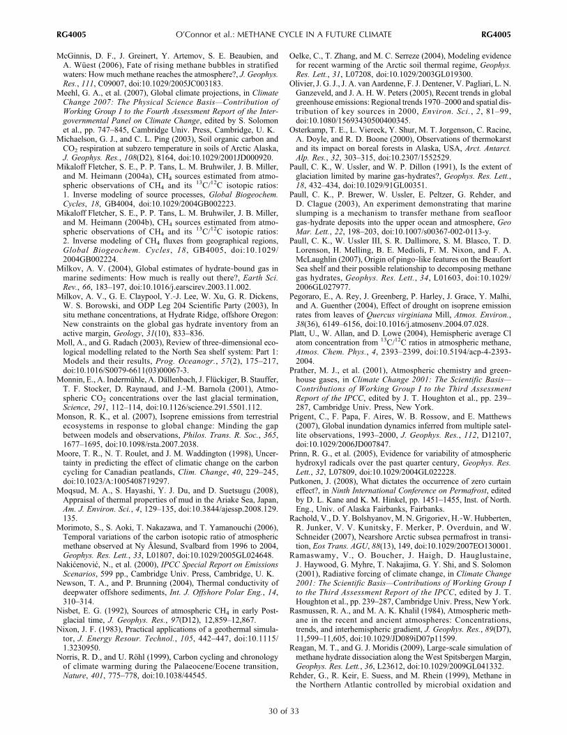
McGinnis, D. F., J. Greinert, Y. Artemov, S. E. Beaubien, andA. Wüest (2006), Fate of rising methane bubbles in stratifiedwaters: How much methane reaches the atmosphere?, J. Geophys.Res., 111, C09007, doi:10.1029/2005JC003183.

Meehl, G. A., et al. (2007), Global climate projections, in ClimateChange 2007: The Physical Science Basis—Contribution ofWorking Group I to the Fourth Assessment Report of the Inter-governmental Panel on Climate Change, edited by S. Solomonet al., pp. 747–845, Cambridge Univ. Press, Cambridge, U. K.

Michaelson, G. J., and C. L. Ping (2003), Soil organic carbon andCO2 respiration at subzero temperature in soils of Arctic Alaska,J. Geophys. Res., 108(D2), 8164, doi:10.1029/2001JD000920.

Mikaloff Fletcher, S. E., P. P. Tans, L. M. Bruhwiler, J. B. Miller,and M. Heimann (2004a), CH4 sources estimated from atmo-spheric observations of CH4 and its 13C/12C isotopic ratios:1. Inverse modeling of source processes, Global Biogeochem.Cycles, 18, GB4004, doi:10.1029/2004GB002223.

Mikaloff Fletcher, S. E., P. P. Tans, L. M. Bruhwiler, J. B. Miller,and M. Heimann (2004b), CH4 sources estimated from atmo-spheric observations of CH4 and its 13C/12C isotopic ratios:2. Inverse modeling of CH4 fluxes from geographical regions,Global Biogeochem. Cycles, 18, GB4005, doi:10.1029/2004GB002224.

Milkov, A. V. (2004), Global estimates of hydrate‐bound gas inmarine sediments: How much is really out there?, Earth Sci.Rev., 66, 183–197, doi:10.1016/j.earscirev.2003.11.002.

Milkov, A. V., G. E. Claypool, Y.‐J. Lee, W. Xu, G. R. Dickens,W. S. Borowski, and ODP Leg 204 Scientific Party (2003), Insitu methane concentrations, at Hydrate Ridge, offshore Oregon:New constraints on the global gas hydrate inventory from anactive margin, Geology, 31(10), 833–836.

Moll, A., and G. Radach (2003), Review of three‐dimensional eco-logical modelling related to the North Sea shelf system: Part 1:Models and their results, Prog. Oceanogr., 57(2), 175–217,doi:10.1016/S0079-6611(03)00067-3.

Monnin, E., A. Indermühle, A. Dällenbach, J. Flückiger, B. Stauffer,T. F. Stocker, D. Raynaud, and J.‐M. Barnola (2001), Atmo-spheric CO2 concentrations over the last glacial termination,Science, 291, 112–114, doi:10.1126/science.291.5501.112.

Monson, R. K., et al. (2007), Isoprene emissions from terrestrialecosystems in response to global change: Minding the gapbetween models and observations, Philos. Trans. R. Soc., 365,1677–1695, doi:10.1098/rsta.2007.2038.

Moore, T. R., N. T. Roulet, and J. M. Waddington (1998), Uncer-tainty in predicting the effect of climatic change on the carboncycling for Canadian peatlands, Clim. Change, 40, 229–245,doi:10.1023/A:1005408719297.

Moqsud, M. A., S. Hayashi, Y. J. Du, and D. Suetsugu (2008),Appraisal of thermal properties of mud in the Ariake Sea, Japan,Am. J. Environ. Sci., 4, 129–135, doi:10.3844/ajessp.2008.129.135.

Morimoto, S., S. Aoki, T. Nakazawa, and T. Yamanouchi (2006),Temporal variations of the carbon isotopic ratio of atmosphericmethane observed at Ny Ålesund, Svalbard from 1996 to 2004,Geophys. Res. Lett., 33, L01807, doi:10.1029/2005GL024648.

Nakićenović, N., et al. (2000), IPCC Special Report on EmissionsScenarios, 599 pp., Cambridge Univ. Press, Cambridge, U. K.

Newson, T. A., and P. Brunning (2004), Thermal conductivity ofdeepwater offshore sediments, Int. J. Offshore Polar Eng., 14,310–314.

Nisbet, E. G. (1992), Sources of atmospheric CH4 in early Post-glacial time, J. Geophys. Res., 97(D12), 12,859–12,867.

Nixon, J. F. (1983), Practical applications of a geothermal simula-tor, J. Energy Resour. Technol., 105, 442–447, doi:10.1115/1.3230950.

Norris, R. D., and U. Röhl (1999), Carbon cycling and chronologyof climate warming during the Palaeocene/Eocene transition,Nature, 401, 775–778, doi:10.1038/44545.

Oelke, C., T. Zhang, and M. C. Serreze (2004), Modeling evidencefor recent warming of the Arctic soil thermal regime, Geophys.Res. Lett., 31, L07208, doi:10.1029/2003GL019300.

Olivier, J. G. J., J. A. van Aardenne, F. J. Dentener, V. Pagliari, L. N.Ganzeveld, and J. A. H. W. Peters (2005), Recent trends in globalgreenhouse emissions: Regional trends 1970–2000 and spatial dis-tribution of key sources in 2000, Environ. Sci., 2, 81–99,doi:10.1080/15693430500400345.

Osterkamp, T. E., L. Viereck, Y. Shur, M. T. Jorgenson, C. Racine,A. Doyle, and R. D. Boone (2000), Observations of thermokarstand its impact on boreal forests in Alaska, USA, Arct. Antarct.Alp. Res., 32, 303–315, doi:10.2307/1552529.

Paull, C. K., W. Ussler, and W. P. Dillon (1991), Is the extent ofglaciation limited by marine gas‐hydrates?, Geophys. Res. Lett.,18, 432–434, doi:10.1029/91GL00351.

Paull, C. K., P. Brewer, W. Ussler, E. Peltzer, G. Rehder, andD. Clague (2003), An experiment demonstrating that marineslumping is a mechanism to transfer methane from seafloorgas‐hydrate deposits into the upper ocean and atmosphere, GeoMar. Lett., 22, 198–203, doi:10.1007/s00367-002-0113-y.

Paull, C. K., W. Ussler III, S. R. Dallimore, S. M. Blasco, T. D.Lorenson, H. Melling, B. E. Medioli, F. M. Nixon, and F. A.McLaughlin (2007), Origin of pingo‐like features on the BeaufortSea shelf and their possible relationship to decomposing methanegas hydrates, Geophys. Res. Lett., 34, L01603, doi:10.1029/2006GL027977.

Pegoraro, E., A. Rey, J. Greenberg, P. Harley, J. Grace, Y. Malhi,and A. Guenther (2004), Effect of drought on isoprene emissionrates from leaves of Quercus virginiana Mill, Atmos. Environ.,38(36), 6149–6156, doi:10.1016/j.atmosenv.2004.07.028.

Platt, U., W. Allan, and D. Lowe (2004), Hemispheric average Clatom concentration from 13C/12C ratios in atmospheric methane,Atmos. Chem. Phys., 4, 2393–2399, doi:10.5194/acp-4-2393-2004.

Prather, M. J., et al. (2001), Atmospheric chemistry and green-house gases, in Climate Change 2001: The Scientific Basis—Contributions of Working Group I to the Third AssessmentReport of the IPCC, edited by J. T. Houghton et al., pp. 239–287, Cambridge Univ. Press, New York.

Prigent, C., F. Papa, F. Aires, W. B. Rossow, and E. Matthews(2007), Global inundation dynamics inferred from multiple satel-lite observations, 1993–2000, J. Geophys. Res., 112, D12107,doi:10.1029/2006JD007847.

Prinn, R. G., et al. (2005), Evidence for variability of atmospherichydroxyl radicals over the past quarter century, Geophys. Res.Lett., 32, L07809, doi:10.1029/2004GL022228.

Putkonen, J. (2008), What dictates the occurrence of zero curtaineffect?, in Ninth International Conference on Permafrost, editedby D. L. Kane and K. M. Hinkel, pp. 1451–1455, Inst. of North.Eng., Univ. of Alaska Fairbanks, Fairbanks.

Rachold, V., D. Y. Bolshyanov, M. N. Grigoriev, H.‐W. Hubberten,R. Junker, V. V. Kunitsky, F. Merker, P. Overduin, and W.Schneider (2007), Nearshore Arctic subsea permafrost in transi-tion, Eos Trans. AGU, 88(13), 149, doi:10.1029/2007EO130001.

Ramaswamy, V., O. Boucher, J. Haigh, D. Hauglustaine,J. Haywood, G. Myhre, T. Nakajima, G. Y. Shi, and S. Solomon(2001), Radiative forcing of climate change, in Climate Change2001: The Scientific Basis—Contributions of Working Group Ito the Third Assessment Report of the IPCC, edited by J. T.Houghton et al., pp. 239–287, Cambridge Univ. Press, New York.

Rasmussen, R. A., and M. A. K. Khalil (1984), Atmospheric meth-ane in the recent and ancient atmospheres: Concentrations,trends, and interhemispheric gradient, J. Geophys. Res., 89(D7),11,599–11,605, doi:10.1029/JD089iD07p11599.

Reagan, M. T., and G. J. Moridis (2009), Large‐scale simulation ofmethane hydrate dissociation along the West Spitsbergen Margin,Geophys. Res. Lett., 36, L23612, doi:10.1029/2009GL041332.

Rehder, G., R. Keir, E. Suess, and M. Rhein (1999), Methane inthe Northern Atlantic controlled by microbial oxidation and


30 of 33

atmospheric history, Geophys. Res. Lett., 26, 587–590,doi:10.1029/1999GL900049.

Rehder, G., P. W. Brewer, E. T. Peltzer, and G. Friederich (2002),Enhanced lifetime of methane bubble streams within the deepocean, Geophys. Res. Lett., 29(15), 1731, doi:10.1029/2001GL013966.

Ridgwell, A. J., S. J. Marshall, and K. Gregson (1999), Consump-tion of atmospheric methane by soils: A process‐based model,Global Biogeochem. Cycles , 13 , 59–70, doi:10.1029/1998GB900004.

Rigby, M., et al. (2008), Renewed growth of atmospheric methane,Geophys. Res. Lett., 35, L22805, doi:10.1029/2008GL036037.

Ringeval, B., N. de Noblet‐Ducoudré, P. Ciais, P. Bousquet,C. Prigent, F. Papa, andW.B. Rossow (2010), An attempt to quan-tify the impact of changes in wetland extent on methane emissionson the seasonal and interannual time scales, Global Biogeochem.Cycles, 24, GB2003, doi:10.1029/2008GB003354.

Riseborough, D., N. Shiklomanov, B. Etzelmuller, S. Gruber, andS. Marchenko (2008), Recent advances in permafrost modelling,Permafrost Periglacial Processes, 19, 137–156, doi:10.1002/ppp.615.

Rothwell, R. G., M. S. Reeder, G. Anastasakis, D. A. V. Stow,J. Thomson, and G. Kahler (2000), Low sea‐level stand emplace-ment of megaturbidites in the western and eastern MediterraneanSea, Sediment. Geol., 135(1–4), 75–88.

Roulet, N., T. Moore, J. Bubier, and P. Lafleur (1992), Northernfens: Methane flux and climatic change, Tellus, Ser. B, 44,100–105.

Sanderson, M. G., C. D. Jones, W. J. Collins, C. E. Johnson, andR. G. Derwent (2003), Effect of climate change on isopreneemissions and surface ozone levels, Geophys. Res. Lett., 30(18),1936, doi:10.1029/2003GL017642.

Schimel, D. S., B. H. Braswell, E. A. Holland, R. McKeown, D. S.Ojima, T. H. Painter, W. J. Parton, and A. R. Townsend (1994),Climatic, edaphic, and biotic controls over storage and turnoverof carbon in soils, Global Biogeochem. Cycles, 8(3), 279–293,doi:10.1029/94GB00993.

Schuur, E. A. G., et al. (2008), Vulnerability of permafrost carbonto climate change: Implications for the global carbon cycle,Bioscience, 58, 701–714, doi:10.1641/B580807.

Sclater, J. G., C. E. Corry, and V. Vacquier (1969), In situmeasurement of the thermal conductivity of ocean‐floor sediments,J. Geophys. Res., 74(4), 1070–1081, doi:10.1029/JB074i004p01070.

Scranton, M. I., and P. G. Brewer (1978), Consumption of dis-solved methane in the deep ocean, Limnol. Oceanogr., 23(6),1207–1213, doi:10.4319/lo.1978.23.6.1207.

Shakhova, N., I. Semiletov, and G. Panteleev (2005), The distribu-tion of methane on the Siberian Arctic shelves: Implications forthe marine methane cycle, Geophys. Res. Lett., 32, L09601,doi:10.1029/2005GL022751.

Shakhova, N., I. Semiletov, A. Salyuk, V. Yusupov, D. Kosmach,and Ö. Gustafsson (2010), Extensive methane venting to theatmosphere from sediments of the East Siberian Arctic Shelf,Science, 327, 1246–1250, doi:10.1126/science.1182221.

Shindell, D. T., B. P. Walter, and G. Faluvegi (2004), Impacts ofclimate change on methane emissions from wetlands, Geophys.Res. Lett., 31, L21202, doi:10.1029/2004GL021009.

Shindell, D. T., G. Faluvegi, N. Bell, and G. A. Schmidt (2005),An emissions‐based view of climate forcing by methane and tro-pospheric ozone, Geophys. Res. Lett., 32, L04803, doi:10.1029/2004GL021900.

Shindell, D. T., G. Faluvegi, D. M. Koch, G. A. Schmidt, N. Unger,and S. E. Bauer (2009), Improved attribution of climate forcing toemissions, Science, 326, 716–718, doi:10.1126/science.1174760.

Shur, Y. L., and M. T. Jorgenson (2007), Patterns of permafrostformation and degradation in relation to climate and ecosystems,Permafrost Periglacial Processes, 18, 7–19, doi:10.1002/ppp.582.

Sitch, S., A. D. McGuire, J. Kimball, N. Gedney, J. Gamon,R. Engstrom, A. Wolf, Q. Zhuang, J. Clein, and K. McDonald(2007a), Assessing the carbon balance of circumpolar Arctic tun-dra using remote sensing and process modeling, Ecol. Appl., 17,213–234, doi:10.1890/1051-0761(2007)017[0213:ATCBOC]2.0.CO;2.

Sitch, S., P. M. Cox, W. J. Collins, and C. Huntingford (2007b),Indirect radiative forcing of climate change through ozone effectson the land‐carbon sink, Nature, 448, 791–794, doi:10.1038/nature06059.

Sitch, S., et al. (2008), Evaluation of the terrestrial carbon cycle,future plant geography and climate‐carbon cycle feedbacks usingfive Dynamic Global Vegetation Models (DGVMs), GlobalChange Biol., 14(9), 2015–2039, doi:10.1111/j.1365-2486.2008.01626.x.

Sloan, E. D. (2003), Fundamental principles and applications ofnatural gas hydrates, Nature, 426, 353–363, doi:10.1038/nature02135.

Sloan, E. D., and C. A. Koh (2008), Clathrate Hydates of NaturalGases, 3rd ed., CRC Press, Boca Raton, Fla.

Smith, S. L., M. M. Burgess, D. Riseborough, and F. M. Nixon(2005), Recent trends from Canadian permafrost thermal moni-toring network sites, Permafrost Periglacial Processes, 16(1),19–30, doi:10.1002/ppp.511.

Soja, A. J., N. M. Tchebakove, N. H. F. French, M. D. Flannigan,H. H. Shugart, B. J. Stocks, A. I. Sukhinin, E. I. Parfenova, F. S.Chapin III, and P. W. Stackhouse Jr. (2007), Climate‐inducedboreal forest change: Predictions versus current observations,Global Planet. Change, 56, 274–296, doi:10.1016/j.gloplacha.2006.07.028.

Sowers, T. (2006), Late quaternary atmospheric CH4 isotoperecord suggests marine clathrates are stable, Science, 311,838–840, doi:10.1126/science.1121235.

Steele, L. P., E. J. Dlugokencky, P. M. Lang, P. P. Tans, R. C.Martin, and K. A. Masarie (1992), Slowing down of the globalaccumulation of atmospheric methane during the 1980s, Nature,358, 313–316, doi:10.1038/358313a0.

Stevenson, D. S., et al. (2006), Multimodel ensemble simulationsof present‐day and near‐future tropospheric ozone, J. Geophys.Res., 111, D08301, doi:10.1029/2005JD006338.

Stocks, B. J., et al. (1998), Climate change and forest fire potentialin Russian and Canadian boreal forests, Clim. Change, 38, 1–13,doi:10.1023/A:1005306001055.

Stokstad, E. (2004), Defrosting the carbon freezer of the north,Science, 304, 1618–1620, doi:10.1126/science.304.5677.1618.

Stott, P. A., G. S. Jones, J. A. Lowe, P. Thorne, C. Durman, T. C.Johns, and J.‐C. Thelen (2006), Transient climate simulationswith the HadGEM1 climate model: Causes of past warmingand future climate change, J. Clim., 19(12), 2763–2782,doi:10.1175/JCLI3731.1.

Sturm, M., C. Racine, and K. Tape (2001), Increasing shrub abun-dance in the Arctic, Nature, 411, 546–547, doi:10.1038/35079180.

Tarnocai, C., and V. Stolbovoy (2006), Northern peatlands: Theircharacteristics, development and sensitivity to climate change, inPeatlands: Evolution and Records of Environmental and ClimateChanges, Dev. Earth Surface Processes, vol. 9, edited by I. P.Martini, A. Martinez Cortizas, and W. Chesworth, chap. 2,pp. 17–51, doi:10.1016/S0928-2025(06)09002-X, Elsevier,Amsterdam.

Tarnocai, C., J. G.Canadell, E.A. G. Schuur, P. Kuhry,G.Mazhitova,and S. Zimov (2009), Soil organic carbon pools in the northerncircumpolar permafrost region, Global Biogeochem. Cycles, 23,GB2023, doi:10.1029/2008GB003327.

Telford, P. J., et al. (2010), Effects of climate induced changes inisoprene emissions after the eruption of Mount Pinatubo, Atmos.Chem. Phys., 10, 7117–7125, doi:10.5194/acp-10-7117-2010.


31 of 33

Turetsky, M. R., R. K. Wieder, and D. H. Vitt (2002), Borealpeatland C fluxes under varying permafrost regimes, Soil Biol.Biochem., 34(7), 907–912, doi:10.1016/S0038-0717(02)00022-6.

Upstill‐Goddard, R. C., T. Frost, G. R. Henry, M. Franklin, J. C.Murrell and N. J. P. Owens (2003), Bacterioneuston control ofair‐water methane exchange determined with a laboratory gasexchange tank, Global Biogeochem. Cycles, 17(4), 1108,doi:10.1029/2003GB002043.

Valdes, P. J., D. J. Beerling, and C. E. Johnson (2005), The ice agemethane budget, Geophys. Res. Lett., 32, L02704, doi:10.1029/2004GL021004.

van Aardenne, J. A., F. J. Dentener, J. G. J. Olivier, C. G. M. KleinGoldewijk, and J. Lelieveld (2001), A 1° × 1° resolution data setof historical anthropogenic trace gas emissions for the period1890–1990, Global Biogeochem. Cycles, 15(4), 909–928,doi:10.1029/2000GB001265.

van der Werf, G. R., J. T. Randerson, L. Giglio, G. J. Collatz, P. S.Kasibhatla, and A. F. Arellano Jr. (2006), Interannual variabilityin global biomass burning emissions from 1997 to 2004, Atmos.Chem. Phys., 6, 3423–3441, doi:10.5194/acp-6-3423-2006.

Vogt, P. R., and W. Y. Jung (2002), Holocene mass wasting onupper non‐Polar continental slopes–due to post‐Glacial oceanwarming and hydrate dissociation?, Geophys. Res. Lett., 29(9),1341, doi:10.1029/2001GL013488.

Volodin, E. M. (2008), Methane cycle in the INM RAS climatemodel, Izv. Russ. Acad. Sci. Atmos. Oceanic Phys., Engl. Transl.,44, 153–159, doi:10.1134/S0001433808020023.

von Kuhlmann, R., M. G. Lawrence, U. Pöschl, and P. J. Crutzen(2004), Sensitivities in global scale modeling of isoprene, Atmos.Chem. Phys., 4, 1–17, doi:10.5194/acp-4-1-2004.

Wadham, J. L., M. Tranter, S. Tulaczyk, and M. Sharp (2008),Subglacial methanogenesis: A potential climatic amplifier?,Global Biogeochem. Cycles, 22, GB2021, doi:10.1029/2007GB002951.

Walter, B. P., and M. Heimann (2000), A process‐based, climate‐sensitive model to derive methane emissions from natural wet-lands: Application to five wetland sites, sensitivity to modelparameters, and climate, Global Biogeochem. Cycles, 14(3),745–765, doi:10.1029/1999GB001204.

Walter, B. P., M. Heimann, and E. Matthews (2001a), Modelingmodern methane emissions from natural wetlands: 1. Modeldescription and results, J. Geophys. Res., 106(D24), 34,189–34,206, doi:10.1029/2001JD900165.

Walter, B. P., M. Heimann, and E. Matthews (2001b), Modelingmodern methane emissions from natural wetlands: 2. Interannualvariations 1982–1993, J. Geophys. Res., 106(D24), 34,207–34,219, doi:10.1029/2001JD900164.

Walter, K. M., L. C. Smith, and F. S. Chapin (2007), Methane bub-bling from northern lakes: Present and future contributions to theglobal methane budget, Philos. Trans. R. Soc., 365, 1657–1676,doi:10.1098/rsta.2007.2036.

Wang, J. S., J. A. Logan, M. B. McElroy, B. N. Duncan, I. A.Megretskaia, and R. M. Yantosca (2004), A 3‐D model analysisof the slowdown and interannual variability in the methane growthrate from 1988 to 1997,Global Biogeochem. Cycles, 18, GB3011,doi:10.1029/2003GB002180.

Wania, R. (2007), Modelling northern peatlands land surface pro-cesses, vegetation dynamics and methane emissions, Ph.D. thesis,Univ. of Bristol, Bristol, U. K.

Wania, R., I. Ross, and I. C. Prentice (2009a), Integrating peatlandsand permafrost into a dynamic global vegetation model: 1. Eval-uation and sensitivity of physical land surface processes, GlobalBiogeochem. Cycles, 23, GB3014, doi:10.1029/2008GB003412.

Wania, R., I. Ross, and I. C. Prentice (2009b), Integrating peat-lands and permafrost into a dynamic global vegetation model:2. Evaluation and sensitivity of vegetation and carbon cycle pro-cesses, Global Biogeochem. Cycles, 23, GB3015, doi:10.1029/2008GB003413.

Ward, B. B., K. A. Kilpatrick, P. C. Novelli, and M. I. Scranton(1987), Methane oxidation and methane fluxes in the ocean sur-face layer and deep anoxic waters, Nature, 327, 226–229,doi:10.1038/327226a0.

Warwick, N. J., S. Bekki, K. S. Law, E. G. Nisbet, and J. A. Pyle(2002), The impact of meteorology on the interannual growthrate of atmospheric methane, Geophys. Res. Lett., 29(20),1947, doi:10.1029/2002GL015282.

Weitemeyer, K. A., and B. A. Buffett (2006), Accumulation andrelease of methane from clathrates below the Laurentide and Cor-dilleran ice sheets, Global Planet. Change, 53, 176–187,doi:10.1016/j.gloplacha.2006.03.014.

Westbrook, G. K., et al. (2009), Escape of methane gas from theseabed along the West Spitsbergen continental margin, Geophys.Res. Lett., 36, L15608, doi:10.1029/2009GL039191.

Williams, P. J., and M. W. Smith (1989), The Frozen Earth: Fun-damentals of Geocryology, doi:10.1017/CBO9780511564437,Cambridge Univ. Press, Cambridge, U. K.

Wolff, E. W., J. Chappellaz, T. Blunier, S. O. Rasmussen, andA. Svensson (2010), Millennial‐scale variability during the lastglacial: The ice core record, Quat. Sci. Rev., 29(21–22), 2828–2838, doi:10.1016/j.quascirev.2009.10.013.

Wuebbles, D. J., and K. Hayhoe (2002), Atmospheric methane andglobal change, Earth Sci. Rev., 57, 177–210, doi:10.1016/S0012-8252(01)00062-9.

Xu, W., R. P. Lowell, and E. T. Peltzer (2001), Effect of seafloortemperature and pressure variations on methane flux from a gashydrate layer: Comparison between current and late Paleoceneclimate conditions, J. Geophys. Res., 106, 26,413–26,423,doi:10.1029/2001JB000420.

Yoshikawa, K., and L. D. Hinzman (2003), Shrinking thermokarstponds and groundwater dynamics in discontinuous permafrostnear Council, Alaska, Permafrost Periglacial Processes, 14,151–160, doi:10.1002/ppp.451.

Zhang, Y. (2003), Methane escape from gas hydrate systems inmarine environment, and methane‐driven oceanic eruptions,Geophys. Res. Lett., 30(7), 1398, doi:10.1029/2002GL016658.

Zhang, Y., and Z. Xu (2003), Kinetics of convective crystal disso-lution and melting, with applications to methane hydrate dissolu-tion and dissociation to seawater, Earth Planet. Sci. Lett., 213,133–148, doi:10.1016/S0012-821X(03)00297-8.

Zhuang, Q., et al. (2003), Carbon cycling in extratropical terrestrialecosystems of the Northern Hemisphere during the 20th century:A modeling analysis of the influences of soil thermal dynamics,Tellus, Ser. B, 55, 751–776.

Zhuang, Q., J. M. Melillo, W. Kickighter, R. G. Prinn, A. D.McGuire, P. A. Steudler, B. S. Felzer, and S. Hu (2004), Meth-ane fluxes between terrestrial ecosystems and the atmosphere atnorthern high latitudes during the past century: A retrospectiveanalysis with a process‐based biogeochemistry model, GlobalBiogeochem. Cycles, 18, GB3010, doi:10.1029/2004GB002239.

Zhuang, Q., J. M. Melack, S. Zimov, K. M. Walter, C. L. Butenh-off, and M. A. K. Khalil (2009), Global methane emissions fromwetlands, rice paddies, and lakes, Eos Trans. AGU, 90(5), 37–38,doi:10.1029/2009EO050001.

Zimov, S. A., S. P. Davydov, G. M. Zimova, A. I. Davydova, E. A.G. Schuur, K. Dutta, and F. S. Chapin III (2006a), Permafrostcarbon: Stock and decomposability of a globally significant car-bon pool, Geophys. Res. Lett., 33, L20502, doi:10.1029/2006GL027484.

Zimov, S. A., E. A. G. Schuur, and F. S. Chapin (2006b), Perma-frost and the global carbon budget, Science, 312, 1612–1613,doi:10.1126/science.1128908.

O. Boucher, W. J. Collins, G. A. Folberth, C. E. Johnson, C. D. Jones,F. M. O’Connor, and J. Ridley, Met Office Hadley Centre, FitzRoyRoad, Exeter EX1 3PB, UK.


32 of 33

J. Chappellaz, Laboratoire de Glaciologie et Géophysique del’Environnement, CNRS–University of Grenoble, F‐38400 SaintMartin d’Hères, France.R. Coppell, School of Geography, University of Leeds, Leeds LS2 9JT,

UK.

P. Friedlingstein, College of Engineering, Mathematics and PhysicalSciences, University of Exeter, Harrison Building, North Park Road,Exeter EX4 4QF, UK.N. Gedney, Joint Centre for Hydrometeorological Research, Met

Office Hadley Centre, Maclean Building, Crowmarsh Gifford OX108BB, UK.


33 of 33

possible role of wetlands, permafrost, and methane hydrates in the

Documents