post-acquisition performance of acquiring firms in the ... · i post-acquisition performance of...

i

Post-acquisition performance of acquiring firms in

the short-term, during industrial merger waves: A

first-mover approach

Nuno Bernardo Faria

[email protected]

Dissertation

Master in Finance

Supervisors:

Miguel Sousa, Phd

Jorge Farinha, Phd

September 15th, 2017

mailto:[email protected]

ii

The Author

Nuno Bernardo Faria was born on 6th February 1991. After a brief experience in the

School of Engineering at University of Porto (FEUP), he attended the bachelor degree in

Economics in the School of Economics and Management at the same university (FEP). When

completed in 2014, he started to study in the Master in Finance lectured in the same institution.

Professionally, he did an internship in the audit department of EY and currently,

during the last one and a half years, he is been working as analyst for the Corporate Finance

department of KPMG.

iii

Acknowledgements

First I want to exalt all my gratitude to the Professors who have closely followed my

work, namely Miguel Sousa, PhD and Jorge Farinha, PhD, for all their support, dedication

and readiness to helping me taking this dissertation to a successful conclusion.

I also want to thank the help and support of all my colleagues, friends and family.

iv

Abstract

With no doubt the number of Mergers and Acquisitions (hereafter M&A) operations has been

increasing through the last years. These deals often occur in global waves identified usually

as an aggregate of specific industrial merger waves. The theoretical explanations and

empirical studies for these events are vast, from stock market misevaluation to economic,

technological or regulatory shocks. This study, supported by the neoclassical theory, leaves

aside the explanation and focuses on the short-term returns inside the different industrial

merger waves, comparing the gap between waves’ participants and non-participants returns,

and comparing the first and latter movers’ returns within those waves. The theory suggests a

timing advantage for the first movers inside an industrial merger wave, which somehow

proves the possible existence of a bandwagon effect. Our results were positive regarding

participants and non-participants returns, however, they showed a significant advantage for

the latter movers contradicting previous works and also failing to support the bandwagon

effect verification.

Keywords: Bandwagon; mergers and acquisitions; short-term returns; post-acquisition

performance; waves.

JEL-Codes: G34.

v

Abstract (Portuguese)

Sem dúvida alguma que o número de Fusões e Aquisições tem vindo a aumentar durante os

últimos anos. Estas operações ocorrem frequentemente através de “ondas” globais

normalmente identificadas como um conjunto de “ondas” de aquisições dentro de indústrias

específicas. São inúmeras as teorias explicativas e os estudos de casos práticos para este tipo

de eventos, variando desde avaliações incorrectas dentro do mercado bolsista a choques

económicos, tecnológicos ou regulatórios. Este estudo é maioritariamente suportado pela

teoria neoclássica e, deixando de lado todas as explicações teóricas, foca-se antes nos

retornos de curto prazo dentro das diferentes “ondas” industriais. Comparando não só as

diferenças nos retornos dos compradores que participam nessas “ondas” com aqueles que

ficam de fora, mas assim como os retornos dos primeiros participantes com os dos últimos.

A teoria sugere que existe uma vantagem para os primeiros participantes numa onda de

aquisições dentro de uma indústria específica, o que de certa forma comprova a existência de

um efeito bandwagon (efeito imitação). Por um lado, os nossos resultados foram claros no

que toca à comparação entre os retornos dos participantes com aqueles dos não-participantes,

mostrando uma patente vantagem para os primeiros. Contudo, e por outro lado, os resultados

referentes à comparação dos retornos dos primeiros participantes com os retornos dos

restantes mostraram uma vantagem estatisticamente significativa dos últimos, o que

contradiz trabalhos anteriores.

Palavras-chave: Bandwagon; fusões e aquisições; retornos de curto prazo; desempenho pós-

aquisição; “ondas”.

JEL-Code: G34.

vi

Index of Contents

1. Introduction ....................................................................................................................... 1

2. Literature review .............................................................................................................. 4

2.1. Mergers and Acquisitions (M&A) ........................................................................................ 4

2.2. Theory behind merger waves................................................................................................ 4

2.3. Bandwagon effect ................................................................................................................... 5

2.4. Value creation in M&A ......................................................................................................... 6

2.4.1. Short-term and long-term returns ..................................................................................... 7

2.4.2. Post-operating performance.............................................................................................. 8

2.5. Determinants of acquirers’ returns in the short term ........................................................ 9

3. Sample and Methodology ............................................................................................... 11

3.1. Hypotheses ............................................................................................................................ 11

3.1.1. Hypothesis I .................................................................................................................... 11

3.1.2 Hypothesis II ................................................................................................................... 13

3.2. Industrial wave identification ............................................................................................. 13

3.3. Short-term returns ............................................................................................................... 14

3.3.1. Measure of abnormal returns .......................................................................................... 15

3.4. Sample ................................................................................................................................... 20

4. Results .............................................................................................................................. 24

4.1. Hypothesis I .......................................................................................................................... 24

4.1.1. Descriptive and test statistics.......................................................................................... 24

4.1.2. Model and independent variables ................................................................................... 25

4.2. Hypothesis II ........................................................................................................................ 30

4.2.1. Scenario I ........................................................................................................................ 30

4.2.2. Scenario II ...................................................................................................................... 32

4.2.3. Scenario III ..................................................................................................................... 33

5. Conclusion ....................................................................................................................... 35

6. References ........................................................................................................................ 37

vii

Annex 1 ........................................................................................................................................ 42

Annex 2 ........................................................................................................................................ 43

Annex 3 ........................................................................................................................................ 44

Annex 4 ........................................................................................................................................ 45

Annex 5 ........................................................................................................................................ 46

viii

Index of Tables

Table 1. Variables definitions ............................................................................................... 12

Table 2. Main deal characteristics distributed by geographical area .................................... 23

Table 3. Summary of descriptive statistics ........................................................................... 25

Table 4. Descriptive statistics for all cash and other methods of payment bids ................... 26

Table 5. Descriptive statistics for industry related and industry diversified bids ................. 27

Table 6. Descriptive statistics for larger bidders and small bidders ..................................... 27

Table 7. Descriptive statistics for bidders from developed and developing countries ......... 28

Table 8. MM multiple regression of acquirers' CAR ........................................................... 30

Table 9. MM Multiple regression for Scenario I .................................................................. 31

Table 10. MM Multiple regression for scenario II ............................................................... 32

Table 11. MM Multiple regression for Scenario III ............................................................. 33

ix

Index of Figures

Figure 1. Timeline for an event study (Mackinlay,1997) ..................................................... 17

Figure 2. Geographic deal distribution by value and number ............................................... 22

Figure 3. Time horizon deal distribution by number and value............................................ 22

1

1. Introduction

The theme of merger waves, per se, is a topic that through several theoretical or

empirical studies was already much scrutinized in the finance history. The results seem to

point out that most of the time mergers occur in waves (Brealey and Myers, 2003) defined as

a set of specific industrial merger waves (Andrade and Stafford, 1999).

After the proven existence of these events it seemed logical that questions about

possible explanations would arise and the possible answers would consequently appear. From

works such as Gort (1969), and more recently Mitchell and Mulherin (1996) and Harford

(2005), neoclassical explanations were developed arguing that industry’s economic,

technological, or regulatory shocks associated with high liquidity were in the foundations of

industrial merger waves.

Conversely, Shleifer and Vishny (2003), and Rhodes-Kropf and Viswanathan (2004),

argue that merger waves result mainly from a managerial advantage due to stock market

overvaluation of their firms.

Considering the existence and the developing explanations for industrial merger

waves some space is still open to evaluate the performance of companies participating in

these waves, and furthermore comparing it with the performance of companies that chose to

stay out of these events.

Even with the considerable extant research analyzing the impact of M&A on value

creation for both acquirer and target companies, we still consider that the M&A literature

should be constantly updated with relevant and original improvements, in order to better

understand and improve companies’ decisions.

Despite the fact we present both the neoclassical and behavioral theory as

explanations for merger waves, this event study takes its support mostly from the industry’s

economic, technological (Mulherin and Boone, 200), financing innovations and regulatory

shocks (Mitchell and Mulherin, 1996), associated with sufficient capital liquidity to

accommodate the assets reallocation (Harford, 2005), as preeminent explanations for the

abovementioned phenomena.

Starting from the post-acquisition performance of acquiring firms in the short-term

and then narrowing it to a more specific subject, as it is the case of industrial merger waves

2

the expectations are that it would be possible to measure and somehow explain how the

market “inefficiencies” (whatever they are neoclassical or behavioural theory) are exploited

by managers according their different timing in entering the market.

When in an industrial merger wave some managers feel the pressure for entering the

market as a response to their rivals. However, what should be a rational and conscious

decision at times may be affected by copycat behavior characterized by following the

industry tendency signaled by managers with different information and opportunities. This

study purpose is to deepen into the bandwagon theory, (Pangarkar, 2000) a theory suggesting

that firms will tend to imitate their close rivals regardless of whether such imitation is value-

enhancing or not.

Regarding the first-mover advantage theory, other research has shown that the timing

of participation in the wave is a matter of relevant importance, since early movers outperform

later ones (Carow, et al., 2004; McNamara, et al., 2008).

The natural intuition seems to provide first movers with competitive advantages and

the later entrants with considerable disadvantages, however a specific firm must have certain

competences and skills to do so, because depending on their unique traits, some firms might

benefit from early entrance and others might benefit from following (Kerin, et al., 1992).

Not exactly in the same position as a firm developing a new product or entering a

new market, a first mover in an industrial merger wave is also endowed with the natural

assumptions of higher abnormal returns however, is along with a series of tests, that it is

expected to discover if that first mover advantage is real.

As the industrial merger waves, and consequently aggregate merger waves are

defined, another simple question automatically emerges. Independently of first or later

movers, is it advantageous to “surf” within a wave? It is hard to find empirical studies in this

field, nevertheless analysing returns between financial operations within and without waves

might be enlightening in which regards the managers’ concern about waves.

This last question will be briefly addressed as we try to reach some conclusions by

globally comparing short-term returns of companies caught within M&A waves with market

returns. Additionally, this work intends to answer to the following questions: 1) is timing

relevant in M&A? 2) Could the first companies reacting to market inefficiencies take

3

advantage over the subsequent ones? 3) Is it possible that some managers feel the pressure of

entering the market through M&A in response to their rivals regardless the operation creates

value or not? 4) Is it advantageous for a company to participate in a wave? 5) Could the

market inefficiencies exploited by firms “surfing” within a wave be observable in their short-

term returns? 6) What are the deal/firm characteristics that impact when a firm enters an

industry merger wave?

This study proceeds by using a sample of mergers and acquisitions from all the globe

between 2005 and 2014, and across a range of industries to test the timing of entry in

industrial merger waves within different geographies, economic development, means of

payment, among others. Fundamentally, our first major contribution is to investigate if the

early mover advantage (advantage from an acquisition that occurs in the beginning of an

industrial merger wave) is somehow reflected in the shareholder’s returns. And if it is, in our

second major contribution, we intend to test if those abnormal returns are still observable

after controlling for the transaction characteristics namely, the mean of payment used (cash

vs stock), economic growth (developed countries vs developing countries), size (large-cap

firms vs small-cap firms), geographical scope (cross-border vs domestic), and industry

relatedness (industry specialization vs industry diversification).

We are trying to prove that part of the later entrants only run for this kind of financial

operation as a response to their rivals, regardless of such reply creates value or not.

The following section briefly reviews the most relevant literature related to our study.

Chapter 3 presents the data and the methodology used to measure and compare the short-

term abnormal returns. Section 4 and 5 will respectively present the results and conclusions.

4

2. Literature review

In the first section, 2.1, we explain the definition and the differences between the

different types of M&As. In section 2.2 we present the theory behind merger waves and the

specific case of industrial merger waves. And we also discuss the results obtained by previous

studies. Sections 2.3 and 2.4 leave aside the global perspective of M&A and focus on two

main points of this study: the bandwagon effect, and the identification of industrial merger

waves. In section 2.5 we consider the different methodologies and results of value creation

studies in M&A, leaving for the section 2.6 the main conclusions regarding the more relevant

factors determining acquirers’ returns.

2.1. Mergers and Acquisitions (M&A)

According to Ross et al. (2013), an acquisition follows one of three different forms:

merger or consolidation, acquisition of stock or acquisition of assets.

In a merger, one firm absorbs the other, acquiring all its assets and liabilities. The

acquiring firm retains its name and identity while the acquired, from that moment, ceases to

exist. A consolidation is very similar to a merger; however, an entirely new firm is created

with the termination of both the acquiring and acquired firm.

2.2. Theory behind merger waves

The existence of merger waves is clearly documented (see, e.g., Brealey and Myers,

2003 and DePamphilis, 2010). The first wave began in the 19th century, in the 1890s to be

more precise, and ended in 1903. The second wave occurred from the 1910s through 1929,

closely following the end of the first wave, while the third took place between the 1950s and

1973. The fourth and fifth waves materialized in the periods from 1981 to 1989, and from

1993 to 2001, respectively.

Also well-known is the proven existence of clustering waves within industries (see,

e.g., Andrade, et al. (2001), and Mulherin and Boone (2000)) where they both play a

‘contractionary’ and ‘expansionary’ role in industry restructuring (Andrade and Stafford,

1999), invariably tied to two different explanatory concepts.

5

From the behavioural angle, Rhodes-Kropft and Viswanathan (2004) suggest that

potential market value deviations from fundamental value on both positive and negative sides

can rationally lead to a correlation between stock merger activity and market valuation; thus,

valuation fundamentally impacts mergers. In the same line of thought, the model of stock-

market-driven acquisitions plotted by Shleifer and Visnhy (2003) seems to be consistent with

the available empirical findings supporting the conclusion that firms with overvalued equity

might be able to make acquisitions, survive and grow while firms with undervalued, or

relatively less overvalued, equity become takeover target themselves.

As in the work of Gort (1969), the neoclassical explanations for merger waves are

based on economic disruptions that lead to industry reorganization. The results shown by

Mitchell and Mulherin (1996) support the argument that much of the takeover activity during

the 1980s was driven by broad fundamental factors such as technological, economic or

regulatory shocks. More recently Harford (2005), through several tests, reinforced that

industry shocks are the drivers for merger waves; however, whether the shocks lead to a wave

of mergers will depend on whether there is sufficient overall capital liquidity in the market.

2.3. Bandwagon effect

The first-mover advantages seemed, somehow, a belief that would automatically lead

to countless competitive gains but, as noted by Lieberman and Montgomery (1988, p. 52):

[F]or any given firm, the question of whether early or late entry is more

advantageous depends on the firm’s particular characteristics. If one firm has

unique R&D capabilities while the other has strong marketing skills, it is in

the interest of the first firm to pioneer and the second firm to enter at a later

date. Both may earn significant profits entering in this sequence, but neither

would gain if the (attempted) order of entry were reversed.

The first-mover problem would never exist if it were not due to imitators. As Keyfies

(1973) explains, people know that, in times of pressure or uncertainty as in the case of a

merger wave, their individual judgment is not trustworthy, and they tend to fall back on the

judgment of others whom they consider, perhaps, better informed. Thus, people tend to come

6

into compliance with the majority or the average.

Several models have been advanced for capturing the essence of such behaviour. One

of the terms that could better explain the manager’s attitude toward merger waves is mimetic

isomorphism, as suggested by DiMaggio and Powell (1983), which according to them results

from standard responses to uncertainty.

The probability model for mimetic isomorphism presented by Tseng and Chou (2010)

seems to point to an impact of institutional pressures on mimetic isomorphism in merger and

acquisitions activity. Isomorphism refers to the tendency for firms within the same

population, facing the same set of institutional pressures, to display the same behaviour

mainly because the social pressures common to all managers in the same industry cause firms

to exhibit similar structures and activities.

As in many other economic situations, mimetic behaviour is present in mergers.

Pangarkar (2000) identifies it as bandwagon effect and argues that firms will tend to imitate

their close rivals regardless of whether such imitation is value-enhancing or not.

It is assumed from the beginning that first movers would probably have advantages

over the ones. To develop this argument, some event studies will be realized so we can

compare the short-term returns between first and later movers.

In the results given by the theoretical model developed by McNamara, et al. (2008),

evidence was found that acquisition performance is higher for early movers but lower for

acquirers that participate at the height of an acquisition wave. However, findings also suggest

that both industry and acquirer characteristics affect the degree to which firms seize early-

mover advantages or fall prey to bandwagon pressures.

2.4. Value creation in M&A

Whether mergers add value or not is a question that has been raised for a long time.

In an M&A operation, value may be created, preserved or destroyed and, if we want to know

whether in practice mergers actually create value or not, we should be ready to examine

empirical evidence, as it is impossible to answer an empirical question in any other way.

Though there exist several different ways of measuring value creation, the great majority of

academics in the field tend to use event studies. These studies estimate abnormal returns on,

7

and around, the merger announcement date, comparing the actual returns with a market index

or control group of stocks.

2.4.1. Short-term and long-term returns

There are many perspectives we could use to determine takeover success. They could

vary from the perspectives of the target’s shareholders to those of any other stakeholders, e.g.

bondholders, managers, employees and consumers. In this specific case, though, we are

focusing on the bidder’s position, considering bidders as a company’s residual owners.

Several studies have already proved that abnormal returns are a good indicator of

acquisitions success (e.g., Healy, et al. (1992)) and, assuming the semi-strong form of

information efficiency by Fama (1970) where the current price reflects all the past and

present public information, short-term returns seem a plausible method to measure

acquisition performance.

To reach some conclusions about takeover profitability across the decade, it is

necessary to find a suitable measurement model. In a careful review of the vast academic

literature on the market for corporate control, Martynova and Renneboog (2008) presented a

list of the major studies of returns across the last five merger waves. Diverse preferences

regarding the benchmark return model and the event window from a number of different

authors can be observed; thereby, the most apt method to compare the post-acquisition

performance of acquiring firms is expected to be found.

The studies focusing on the bidding firm’s stockholder returns are immense but, on

average, abnormal returns realized by bidder shareholders at time of announcement are

statistically indistinguishable from zero; in other words, they are not statistically significant

(Andrade, et al. (2001)). In the first merger wave, Asquith (1983) and Eckbo (1983) report,

there were positive abnormal returns close to zero (0.2% and 0.1%, respectively). For the

second wave, Morck et al. (1990), Byrd and Hickman (1992), and Chang (1998) report

negative abnormal returns also close to zero (ranging from -1.2% to -0.7%). And for the third

wave, the findings of 17 different event studies are split almost evenly between positive and

negative abnormal returns (Martynova and Renneboog, 2008).

8

One explanation for such inconsistent results could be the different methodologies

used by the researchers. Noteworthy pioneering studies have included those of Fama et al.

(1969), using a methodology based on the Market Model (MM); Kummer and Hoffmeister

(1978), who used the Capital Asset Pricing Model (CAPM) as benchmark return model;

Asquish (1983), who introduced the Beta-Matched Control Portfolio (BMCP); and Dennis

and McConnell (1986), who used the Market-Adjusted Model (MAM) as a reference point,

in the short-term return of M&A. The abnormal return is the positive or negative difference

between the actual returns and the benchmark.

A benchmark should be used to rule out the impact of extraneous factors not related

to the operation or the share price. Considerably more methodological problems emerge

when long-term performance is evaluated, mainly because the company’s gains or losses

could be affected by several different factors in the long term and it is almost impossible to

completely isolate them.

Following the work of McWilliams and Siegel (1997), who argue that it is more

effective to use event studies than accounting studies, as stock prices are much less

manipulable by managers than accounting returns, we have established as our goal to develop

an event study about the short-term returns of acquiring firms. It is expected to compare the

timing of the financial operation, not the general returns. Our ambition is to conclude whether

there are significant return differences between the first movers and the later ones, and

between the industrial merger wave participants and the non–industrial merger wave

participants.

2.4.2. Post-operating performance

Apart from the abnormal returns measured by the short-term returns, other studies

examine the post-operating performance of acquiring firms, usually based on a comparison

between the accounting items or ratios preceding and following a takeover process. After the

deal, a positive variation on the company’s cash flows is expected, which usually implies an

increase in the firm’s value (Andrade et al., 2001). Such assessments include: return on equity

(ROE), return on assets (ROA), return on sales (ROS), sales growth, total assets growth,

9

leverage growth, employment growth, market share, cash flows, and others (Martynova et

al., 2008).

The main goal of this kind of study is to identify the sources of gains from M&A and

to determine whether the expected gains/losses seen in the share price movements at the

announcement are ever actually realized. Other studies compare the acquirer’s performance

with other companies in the same industry. If the creation of value of an acquisition, through

synergies or cost reduction, truly exists, the gains should eventually show up in the firm’s

financial statements, specifically in the cash flow and income statement.

A problem materializes in this specific approach. Sometimes operating performance

is affected, not merely by the takeover, but also by an array of other factors. Moreover, as

pointed by Martynova and Renneboog (2008), it seems that an industry adjustment trend is

necessary. Alternatively, one could compare the performance of merging companies with

their non-merging peers, grouped by similar size and market-to-book ratio, prior and after

the bid.

Martynova and Renneboog, 2008 accounted the combined operating gains of

takeovers and found out that, from 26 different studies, 14 reported a post-merger decline in

the operating returns of merged firms, 7 papers showed insignificant changes, and 5 provided

evidence of a significant increase. Hereafter, we could conclude that the findings in this

matter are not conclusive (Martynova et al., 2006). The inconclusive results can be partially

explained by the different choices within a group of peer companies, i.e. benchmarking.

2.5. Determinants of acquirers’ returns in the short term

Whether we focus on theoretical or empirical M&A literature, both bodies have

shown the existence of a variety of factors affecting the takeover announcement returns apart

from synergies. Some empirical authors have found evidence that changes in bidder and

target share prices in the short term, at the announcement date, could depend on the attributes

of the M&A deal and the characteristics of the acquiring and acquired firms (Martynova and

Renneboog, 2011).

In the same work, the authors defend the hypothesis that takeover returns could also

depend on the origin and the ownership structure of the bidding and target firm. The

10

following transaction attributes are likely to affect the acquirers’ and targets’ takeover

returns: 1) the geographical scope of the bid—cross-border M&As are likely to benefit from

imperfections in international capital, as compared with domestic M&As; 2) the form of the

bid and the attitude towards it—unlike friendly takeovers, tender offers are frequently

associated with lower takeover wealth effects for the bidder’s shareholders; 3) the legal status

of the target firm—takeover bids on privately held companies may lead to bidders’ returns

exceeding those obtained in the bids on public firms; 4) the industry relatedness of the bidding

and target firms—although diversifying acquisitions are expected to create operational and

financial synergies not seen in focus bids, the number of hitches created, such as rent-seeking

behaviour by divisional managers, bargaining problems within the firm or bureaucratic

rigidity, may outweigh the alleged synergies; 5) the type of acquisition—a partial acquisition

(of less than 100% of equity) is likely to lead to lower takeover returns to the target’s

shareholders than an acquisition in which a bidder obtains full control; 6) the means of

payments—all-cash takeovers are expected to generate higher returns to the bidder’s and

target’s shareholders than all-equity and mixed-offer; 7) deal transparency—whereas most

bidding companies fully disclose the means of payment and transaction value, some

companies conceal this information, and it is expected that the first type of deal will result in

higher returns to the bidder’s and target’s shareholders than the second kind, as they may

suspect that a non-transparent deal may lead to the expropriation of their rights either by the

bidder’s management or by a controlling shareholder; and 8) the timing of the takeover—

reports show that takeover returns to the bidder’s shareholders decline during and after

takeover wave peaks (Martynova and Renneboog, 2011).

11

3. Sample and Methodology

To reach some relevant conclusions at the end of this event study, it is a matter of

great importance to develop a complete and understandable database and methodology that

would allow all the tests to be accomplished (MacKinlay, 1997). Taking a period of 10 years,

from January 1, 2005 until December 31, 2014, different databases, such as Zephyr by

Bureau Van Dijk and Datastream Professional by Thomson Reuters, all the information

required to identify an industrial merger wave and to test our hypotheses has been gathered.

3.1. Hypotheses

This section introduces our research hypotheses and points out the impact of M&A

industrial waves on the market, as well as includes the comparison between first and latter

entrants.

3.1.1. Hypothesis I

The firms’ returns within an industrial merger wave are superior to those presented

by the market.

It seems natural that a rational CEO or Board of Directors would only perform an

acquisition when the possibility of value creation presents itself as likely.

However, as presented in the Section 2.4.1, despite countless event studies in this

matter there are no definitive answer regarding the positive or negative relation between

M&A activity and abnormal returns.

Regardless of our sample outcome, we cannot be sure that the results will only reflect

the synergies created by the specific deal, as other variables may impact such results.

Therefore, we have incorporated variables presented as relevant in previous works through

the following regression:

CARi(-t;+t) = α + ᵝ1 PAY + ᵝ2 IND + ᵝ3 EGROW + ᵝ4 SIZE + ɛi

12

Where,

(-t;+t) – Correspond to the days around the announcement day, which define an event

window. It may take the following values: (-10;+10); (-5;+5); (-3;+3); and (-1;+1).

In the presented model, the dependant variable regards the Cumulative Abnormal Returns

(CAR) of the acquirer companies, while the independent/explanatory variables are defined

in the Table 1:

Table 1. Variables definitions

We use the variable PAY to test the means of payment hypothesis, or in other words

if the acquirer tends to have better results (higher returns) in all-cash transaction or in other

type of offers. In the case of all-cash offers have better performance than different types of

acquisitions, this variable should show a positive sign. The variable IND is used to better

understand the effects of specializations versus diversification so, if same industry

acquisitions present better returns than the targeting of different industry firms the sign of the

variable shall be positive. EGROW variable pretends to differentiate the transactions made

by companies located in economies economically advanced (developed countries) from

acquisitions made by companies in other geographies (non-developed and developing

countries. If firms in developed economies take advantage over other firms the coefficient

associated with this variable should be positive. Finally, the SIZE variable compares the

returns of large acquirers with the returns of smaller ones. As some of the literature indicates,

Variable Description

CAR Cumulative Average Returns of Acquirers within the event window announced.

PAY

Zero-one dummy variable taking the value 1 if the bid is all cash and 0 otherwise

(shares or mixed).

IND

Zero-one dummy variable taking the value 1 if the bid is for a same industry

company and 0 otherwise.

EGROW

Zero-one dummy variable taking the value 1 if the bid is made by a company in a

developed country and 0 otherwise.

SIZE

Zero-one dummy variable taking the value 1 if the bid is made by a large company

(Market Capitalization over $5 Billion) and 0 otherwise.

13

for better results regarding small cap companies, the coefficient associated to this variable

should present a negative value.

3.1.2 Hypothesis II

The returns presented by firms first entering an industrial merger wave are superior

to those presented by the remaining companies.

The entrance timing may affect acquirer returns. McNamara, et al. (2008) found

evidence that first movers present better performance than the remaining ones.

Taking into account the multiple linear regressiondeveloped in the previous section, a

dummy variable was added to test the relevance of entering sooner in an industrial merger

wave. The following equation summarize our test statistic:

CARi(-t;+t) = α + ᵝ1 PAY + ᵝ2 IND + ᵝ3 EGROW + ᵝ4 SIZE + ᵝ5 ENTRYy + ɛi

where,

ENTRYy – is zero-one dummy variable taking he value 1 if the deal takes place earlier (yth

percentile on entrance order) on a M&A industrial wave and 0 otherwise;

y – may take the value of 50, 25, or 10 corresponding to Scenario I, Scenario II, and Scenario

III, respectively.

3.2. Industrial wave identification

The identification of a possible existing industrial mergers followed a complex

process: First, it was collected 1) all the acquisitions, mergers, institutional buy-outs,

MBIs/MBOs, management buy-ins, and management buy-outs label as completed by Bureau

Van Dijk’s Zephyr between January 1st, 2005 and December 31st 2014. Second, this data was

categorized by sector based on the different Standard Industrial Classification (SIC) codes,

and sector/industrial merger was only considered in the case a minimum of 1,000 deals, over

the 10-year period, in which the bidders have the same first two SIC algorithms.

14

For the identification of the industrial merger wave we have followed Mitchell and

Mulherin (1996), which established a merger wave as a period of 2 years or 24 months, and

Harford (2005), which simulated 1,000 different distributions of all the bids occurring over

a 120-month period by randomly assigning each occurrence to a month where the probability

of assignment is 1/120 for each month. Then, the highest 24-month concentration of activity

was calculated from each of the 1,000 draws. Finally, Harford compared the actual

concentration of activity from the potential wave to the empirical distribution of 1,000 peak

24-month concentrations: if the actual peak concentration exceeded the 95th percentile from

that empirical distribution, that period was coded a wave.

The level of maximum concentration for a 95th percentile reached by Harford (2005)

was 27%, so, every time different industries from 2005 to 2014 had an M&A bid

concentration of over 27% within any 24-month period, the interval was considered an

industrial merger wave.

3.3. Short-term returns

A huge range of stakeholders are usually affected by an operation of this importance,

from the target’s shareholder to bondholders, as well as managers, employees and consumers

of both target and bidder companies, but the primary goal here is to understand and measure

the effects linked to the bidder’s shareholders, being as they are the residual owners of the

‘new’ company.

Many types of event studies analysing short-term shareholders’ wealth effects have been

developed since 1970 (Martynova and Renneboog, 2008), and taking into consideration the

assumption of a semi-strong form of information efficiency by Fama (1970) where the

current price reflects all the past and present public information, the short-term returns seem

a plausible measure of the post-acquisition performance of the acquirer.

Every time an M&A deal happens, new information is brought to the market that

changes the investor’s expectations about the future performance of the company,

expectations consequently reflected in the share prices. For our purposes, only the impact

caused by the operation needs to be accounted for; thus, an expected return (benchmark) is

15

needed. Though the Fama-French three-factor model is the most common benchmark, the

CAPM, market model (MM) or market-adjusted model (MAM) can also be used.

Two commonly used event windows for these event studies are the three days

immediately preceding and following the merger announcement and the day itself (the seven-

day event window) and a longer one, beginning several days before the announcement and

ending at the close of the operation (Andrade, et al., 2001).

3.3.1. Measure of abnormal returns

As in any other event study, using financial market data allows for measuring the

impact of a specific event on the value of the firm (MacKinlay, 1997). Starting from this

assumption, and taking into consideration the acquiring shareholder’s cumulative abnormal

returns around the M&A’s announcement day, it is expected that the effects of that specific

event would be immediately reflected in the security prices (Fama, et al., 1969).

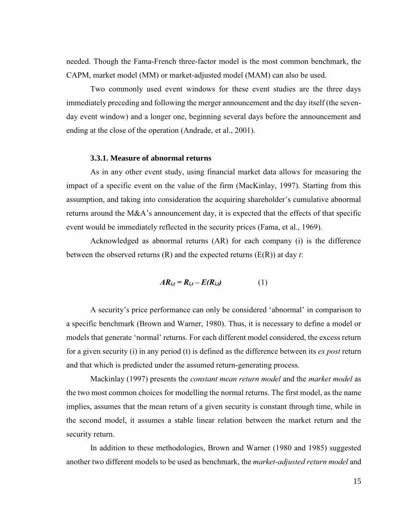
Acknowledged as abnormal returns (AR) for each company (i) is the difference

between the observed returns (R) and the expected returns (E(R)) at day t:

ARi,t = Ri,t – E(Ri,t) (1)

A security’s price performance can only be considered ‘abnormal’ in comparison to

a specific benchmark (Brown and Warner, 1980). Thus, it is necessary to define a model or

models that generate ‘normal’ returns. For each different model considered, the excess return

for a given security (i) in any period (t) is defined as the difference between its ex post return

and that which is predicted under the assumed return-generating process.

Mackinlay (1997) presents the constant mean return model and the market model as

the two most common choices for modelling the normal returns. The first model, as the name

implies, assumes that the mean return of a given security is constant through time, while in

the second model, it assumes a stable linear relation between the market return and the

security return.

In addition to these methodologies, Brown and Warner (1980 and 1985) suggested

another two different models to be used as benchmark, the market-adjusted return model and

16

the OLS market return model. Still following the work of Brown and Warner (1980), they

conclude that a simple methodology based on the market model is both well-specified and

relatively powerful under a wide variety of conditions, stating that in some cases even simpler

methods also perform well.

Using this information while complementing it with Martynova and Renneboog’s

(2008) summary of short-term return effects around M&A announcements, we have decided

to use both the market model (MM) and the market-adjusted model (MAM) as benchmarks,

these being the most used regarding the measure of abnormal returns during merger waves.

As explained before, the MM is a statistical model which relates the return of any

given security to the return of the market portfolio. For any security i the market model is

E(Ri,t) = αi + βi * Rm,t + εi,t (2)

assuming that:

E(Ri,t) = expected return of the share of acquiring firm i on day t;

αi = measure of average return of shares of acquiring firm i that it is not explained by the

market;

βi = measure of sensibility of the shares of acquiring firm i to market movements;

Rm,t = return of market index on day t; and

εi,t = stochastic error, Σεi,t = 0.

Our assumption, in this case, is the following: if the M&A operation was not

announced, the difference between actual return and expected return on day t would be zero.

However, in the situation of an M&A announcement deal, these returns should be different,

and the abnormal returns (AR) of company i on day t is obtained as follows:

εi,t = ARi,t = Ri,t – (αi + βi * Rm,t) (3)

Ri,t = actual return of the share of acquiring firm i on day t.

17

Figure 1. Timeline for an event study (Mackinlay,1997)

The abnormal return observations must be aggregated to draw an overall inference

for the event study (MacKinlay, 1997). The aggregation is made along two dimensions:

through time and across securities. In the first case we consider an aggregation of an

individual security through time. Here enters the concept of cumulative abnormal returns

(CAR); thus, the CAR of the acquiring firm i for a certain event window is the sum of all

abnormal performance from day one until the last day of the window:

CAR = ∑ 𝑨𝑹𝑻𝒕=𝟏 i,t (4)

Notwithstanding, tests with only one event observation are not likely to be useful, so

it is necessary to aggregate across the different securities. For this aggregation, and since the

securities and event dates were randomly selected, it is assumed that the abnormal returns

and the cumulative average abnormal returns will be independent. Considering N as the

number of companies, the cumulative average abnormal returns (CAAR) for acquiring firms

are calculated as:

C𝐀𝐀𝐑 = ∑ 𝑪𝑨𝑹𝒊𝑵

𝒊=𝟏

𝑵 (5)

To develop the framework where we are going to work, it is important to mark out

some notations to facilitate the measurements and analysis of abnormal returns. We define

day ‘0’ as the announcement day for a hypothetical M&A operation for a given company.

The announcement day will happen within the event window (period between T1 and T2),

which precedes the estimation window (the period from T0 to T1) and precedes the post-event

window (the period between T2 and T3).

18

Event windows change across different researchers, and consequently across the

different studies on post-acquisition performance in the short term. For example, the post-

event window will not be considered due to the lack of statistical relevance of long-term

abnormal returns as reported by Campa and Hernando (2004).

Brown and Warner (1985) set for each security the use of a maximum of 250 daily

return observations for the period around its respective event; however, as it is typical for the

estimation window and the event window not to overlap so that the parameters of the normal

return model are not affected by the returns around the event, it was decided to established a

period of 250 days (civil year) for the estimation window, from day -280 to day -30, and a

period of 60 days to the event window, between the day -30 and the day +30.

Despite the 60 days-period established as the event window, mainly due to the

problematic situation that could arise if both the normal returns and the abnormal returns

were to capture the event impact, we are expecting to test the abnormal returns only for

shorter periods. The 7-day event window (-3, +3) is the most commonly used but, in addition

to that, it is our intention to test the 3-, 11- and possibly the 21-day event window ([-1, +1];

[-5, +5]; [-10, +10] respectively), in order to diminish biases and better assess the impact of

M&A operations. This is shaky ground to trample as a too-small event window may exclude

information released before the announcement, while an extended window may mistakenly

include previous or future movements in the acquiring company’s stock price (Goergen and

Renneboog, 2004).

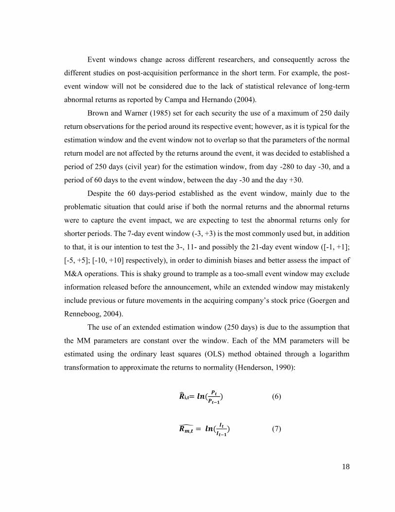
The use of an extended estimation window (250 days) is due to the assumption that

the MM parameters are constant over the window. Each of the MM parameters will be

estimated using the ordinary least squares (OLS) method obtained through a logarithm

transformation to approximate the returns to normality (Henderson, 1990):

�̂�i,t= 𝒍𝒏(𝑷𝒕

𝑷𝒕−𝟏) (6)

𝑹𝒎,�̂� = 𝒍𝒏(𝑰𝒕

𝑰𝒕−𝟏) (7)

19

where

Pt = market price of the share of acquiring firm i on day t;

Pt-1 = market price of the share of acquiring firm i on the day before day t;

It = index price on day t; and

It-1 = index price on the day before day t.

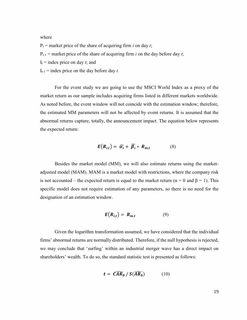
For the event study we are going to use the MSCI World Index as a proxy of the

market return as our sample includes acquiring firms listed in different markets worldwide.

As noted before, the event window will not coincide with the estimation window; therefore,

the estimated MM parameters will not be affected by event returns. It is assumed that the

abnormal returns capture, totally, the announcement impact. The equation below represents

the expected return:

𝑬(𝑹𝒊,𝒕) = 𝜶�̂� + 𝜷�̂� ∗ 𝑹𝒎,𝒕 (8)

Besides the market model (MM), we will also estimate returns using the market-

adjusted model (MAM). MAM is a market model with restrictions, where the company risk

is not accounted – the expected return is equal to the market return (α = 0 and β = 1). This

specific model does not require estimation of any parameters, so there is no need for the

designation of an estimation window.

𝑬(𝑹𝒊,𝒕) = 𝑹𝒎,𝒕 (9)

Given the logarithm transformation assumed, we have considered that the individual

firms’ abnormal returns are normally distributed. Therefore, if the null hypothesis is rejected,

we may conclude that ‘surfing’ within an industrial merger wave has a direct impact on

shareholders’ wealth. To do so, the standard statistic test is presented as follows:

𝒕 = 𝑪𝑨𝑹�̂� / 𝑺(𝑨𝑹�̂�) (10)

20

where,

𝐶𝐴𝑅0̂ = (1/N) ∑ 𝐴𝑅𝑖0𝑁𝑖=1 ; and

𝑆(𝐴𝑅0̂) is an estimate of standard deviation of the average abnormal returns σ(𝐴𝑅0̂).

However, considering the different event window lengths of our sample, we have

sought support from the work of Serra (2004) to test whether CAAR equals zero or not,

through the multi-week T-student test statistic presented below, subsequently adapted to a

sample comprising daily returns:

𝒕 = 𝑪𝑨𝑹�̂� / √𝑺𝟐(∑ 𝑨𝑹𝒍̂𝑳

𝒍=𝟏 ) (11)

where,

l denotes the weeks (days in the present event study) in the event window.

Assuming independence over time, we have:

𝑺𝟐(∑ 𝑨𝑹𝒍̂𝑳

𝒍=𝟏 ) = ∑ 𝑺𝟐(𝑨𝑹�̂�𝑳𝒍=𝟏 ) (12)

where,

𝑺𝟐(𝑨𝑹�̂�) = √∑ (𝑨𝑹𝒊𝒕− ∑ 𝑨𝑹𝒊𝒕𝒕

𝑻)𝟐𝑻

𝒕=𝟏

𝑻−𝒅 (13)

And the statistic is distributed as Student-t with T-d degrees of freedom. However,

the standard deviation presented (13) fails to account for autocorrelation in average abnormal

returns over the event window, usually leading to an underestimation of the multi-week

variance (Serra, 2004).

3.4. Sample

A total of 252,621 deals was obtained in the first sample extracted. When distributing

the data by industry and through the 120 months, we did not find enough concentration in

any of the 24-month periods across most of the 85 possible industries. Therefore, a change

21

in the methodology was required so it would be possible to identify industrial merger waves.

As a major methodology change, we dropped counting the number of deals for a

concentration measure, using instead the value of each transaction. We considered as an

industrial merger wave the 24-month period between January 1, 2005 and December 31,

2014, with maximum value concentration, provided that the period in question has a value

of deals larger than 27% of the total value of deals during the 10-year timeframe. For the

sample we had to restrict the number of deals, counting only transactions with known values,

reaching a total of 90,397 deals. A final total of 19 industrial merger waves was identified.

Then, the Datastream database was used to gather all deals included in the criteria

initially presented. The data are based on the sample adopted to identify the industrial M&A

waves plus some different criteria. Apart from the four conditions presented before, we will

consider only deals: (i) in which the value is disclosed; (ii) where the acquirer company is

listed on the announcement day; (iii) with value of at least 5% of the acquirer’s value, so as

to be considered relevant; (iv) where the acquirer becomes a majority shareholder of the

target company; and (v) that involve the acquisitions of at least 20% of total target’s shares.

Considering all the criteria mentioned, we were left with a total of 388 different deals.

Next, to every deal was attributed an entrance timing within the wave where it belongs.

For that we have used the first sample (gathered in Zephyr database) that includes all deals

occurred in one of the identified waves. In the end, the time of entrance in a wave (according

to the announcement date) was defined for the 388 deals.

From here, and with the help of Datastream database, we obtained the share price for

each of the 388 acquiring companies for the 10-year period along with the movements of

MSCI Index World over the same period.

Only acquiring companies with known share prices for the 280 days before the

announcement date were considered. At this stage 28 deals were dropped from the study.

Despite all these constraints, the sample still comprises acquirers from the most

diverse areas around the globe with a particularly strong representation in Europe and

Asia/Pacific. The geographical area distribution was considered in both value and number of

deals, as represented in Figure 2, respectively.

22

The sample obtained is concentrated mostly during the years 2006 and 2007,

exceeding 170 transactions and reaching almost 70 billion euros, 48% and 69% of the total

number and value of the deals, respectively. As expected, following the 2008 crisis there was

a decrease in M&A activity in both number and value, which seems to have been recovering

in the last years (Figure 3).

Figure 3. Time horizon deal distribution by number and value

19

86 85

21

7 6 8

24

4955

2

3831

93 1 1 1 4

10

2005 2006 2007 2008 2009 2010 2011 2012 2013 2014

Number (#)

Value ($ billions)

Figure 2. Geographic deal distribution by value and number

23

Table 2. Main deal characteristics distributed by geographical area

The Table 2 shows the deal distribution by means of payment, industry relatedness,

geographical scope, acquirer’s economic growth and acquirer’s size. The sample is

represented by 42% of all-cash and same-industry deals, while being completely dominated

by 100% cross-border deals. The developed countries present the larger part of the acquirer

companies (71%), signalling a specific financial availability from the strongest economies.

In terms of size, 272 deals (approximately 76% of the total sample) are comprised by

companies with a market capitalization below $1 billion.

Africa / Middle

EastAsia / Pacific Europe

Latin America

and Caribbean

United States

and CanadaTotal

Panel A: Means of Payment

All-Cash 6 70 63 4 7 150

All-Equity, Mixed, and others 13 80 95 11 11 210

Panel B: Industry Relatedness

Specialization (same industry) 6 61 65 9 11 152

Diversification (other industry) 13 89 93 6 7 208

Panel C: Geographical Scope

Cross-Border 19 150 158 15 18 360

Domestic 0 0 0 0 0 0

Panel D: Acquirer's Economic Growth

Developed Countries 7 72 157 0 18 254

Developing Countries 12 78 1 15 0 106

Panel E: Acquirer's Size

Large-Cap 1 33 47 5 2 88

Mid-Cap and Small-Cap 18 117 111 10 16 272

Source: Own calculations based on Zephyr, United Nations

Acquirer's Region

24

4. Results

This section, under Hypothesis I, presents the effects of M&A operation in acquirer

companies during industrial merger waves, comparing as abovementioned, the combined

firm share prices over the following event windows: [-10;10], [-5;5 ], [-3;3]; and [-1;1], using

both the MM and MAM. Apart from that, control variables such as: i) mean of payment, ii)

economic growth, iii) size; iv) industrial relatedness will be introduce in our analysis with

the purpose of strengthen the assumption that the participation in industrial merger waves is

the main explanation for the abnormal returns.

In the Hypothesis II we pretend to test, for the same event windows, if within

industrial merger waves there are advantages for the first movers. Using both the MM and

MAM approaches it will be compared the abnormal returns of the first i) half, ii) quarter, and

iii) tenth firms to “surf” within the wave against those of the remain companies.

Considering that the final sample of our work comprises 360 complete deals, which

have taken place during different 280-days periods (estimation window + event window +

post-event window) across the 10-year period under analysis. We had to develop an Ordinary

Least Square (OLS) regression for each of the cases in order to calculate the abnormal returns

for all the transactions.

4.1. Hypothesis I

The results presented in this section intend to explain the behaviour of our sample

when compared to the market performance.

4.1.1. Descriptive and test statistics

In the Table 3, the results shown by our sample confirm a positive relation between

participants in industrial merger waves and better short-term performance. Conversely to the

literature presented in the “Short-term and long-term returns” section, bidders’ returns are

statistically significant.

However, the differences between the means and the medians presented may indicate

the presence of relevant outliers amongst our sample.

25

[-10;+10] [-5;+5] [-3;+3] [-1;+1] [-10;+10] [-5;+5] [-3;+3] [-1;+1]

CAAR 0.0484*** 0.025*** 0.0168*** 0.0109*** 0.0653*** 0.0511*** 0.046*** 0.0305***

Median (CAR) 0.0066*** 0.0046*** 0.0029*** 0.0028*** 0.0315*** 0.0299*** 0.0246*** 0.0146***

Std. Deviation (CAR) 0.153 0.089 0.057 0.043 0.193 0.148 0.115 0.092

Positive CAR (#) 217 218 232 218 215 219 238 236

Observations 360 360 360 360 360 360 360 360

Source: Own calculations

t-statistic fo llows a t-student distribution. ***, **, * denotes for 1%, 5%, and 10% significance level for a two-tailed test.

Event window (days)

MM MAM

Table 3. Summary of descriptive statistics

However, to control for the possibility of considerable outliers we performed the non-

parametric Wilcoxon Signed Rank test, in order to understand if the samples’ median was

statistically distinguishable from zero. Therefore, considering our medians, the sample

presented positive abnormal returns for every event window with a 99% of confidence level.

These results appear to be more conclusive than the ones related in the previous works.

In previous waves Asquith (1983) and Eckbo (1983) reported positive returns close to zero

for the shareholders of acquiring firms, while Morck et al. (1990), Byrd and Hickman (1992)

and Chang (1998) reported negative abnormal returns also close to zero.

4.1.2. Model and independent variables

Besides the expected synergies, we have gathered some of the factors affecting

mergers’ returns, such as method of payment, industry relatedness, bidder size, and

economical environment. In this section we are trying to test the strength of the main

characteristics, and in which level they may affect acquirers’ performance.

4.1.2.1. Univariate analysis

In this section of our work we have developed a set of univariate analyses where we

have separated our sample in different sub-groups. Despite the statistically significance of

our results, the standard deviations presented and the differences between the means and

medians show us that there must be a relevant dispersion amongst the data gathered.

Therefore, in order to test the median statistical significance for every situation, a one

sample Wilcoxon Signed Rank test was performed.

26

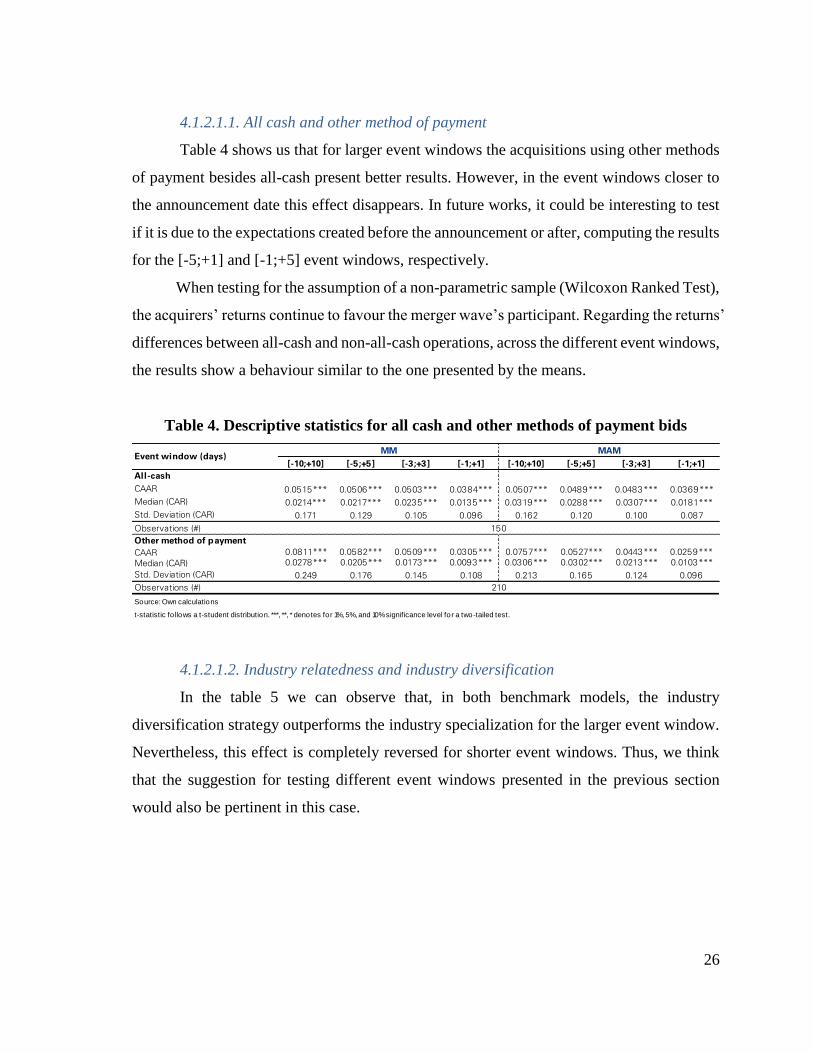
4.1.2.1.1. All cash and other method of payment

Table 4 shows us that for larger event windows the acquisitions using other methods

of payment besides all-cash present better results. However, in the event windows closer to

the announcement date this effect disappears. In future works, it could be interesting to test

if it is due to the expectations created before the announcement or after, computing the results

for the [-5;+1] and [-1;+5] event windows, respectively.

When testing for the assumption of a non-parametric sample (Wilcoxon Ranked Test),

the acquirers’ returns continue to favour the merger wave’s participant. Regarding the returns’

differences between all-cash and non-all-cash operations, across the different event windows,

the results show a behaviour similar to the one presented by the means.

Table 4. Descriptive statistics for all cash and other methods of payment bids

4.1.2.1.2. Industry relatedness and industry diversification

In the table 5 we can observe that, in both benchmark models, the industry

diversification strategy outperforms the industry specialization for the larger event window.

Nevertheless, this effect is completely reversed for shorter event windows. Thus, we think

that the suggestion for testing different event windows presented in the previous section

would also be pertinent in this case.

[-10;+10] [-5;+5] [-3;+3] [-1;+1] [-10;+10] [-5;+5] [-3;+3] [-1;+1]

All-cash

CAAR 0.0515*** 0.0506*** 0.0503*** 0.0384*** 0.0507*** 0.0489*** 0.0483*** 0.0369***

Median (CAR) 0.0214*** 0.0217*** 0.0235*** 0.0135*** 0.0319*** 0.0288*** 0.0307*** 0.0181***


Observations (#)

Other method of payment

CAAR 0.0811*** 0.0582*** 0.0509*** 0.0305*** 0.0757*** 0.0527*** 0.0443*** 0.0259***

Median (CAR) 0.0278*** 0.0205*** 0.0173*** 0.0093*** 0.0306*** 0.0302*** 0.0213*** 0.0103***


Observations (#)



Event window (days)

MM MAM

150

210

27

Table 5. Descriptive statistics for industry related and industry diversified bids

4.1.2.1.3. Large bidder and small bidder

In this section, we have tested the effect of the bidders’ market capitalization on the

returns around the announcement date. Considering the Table 6, it can be observed that

smaller bidders present better results than larger ones, for each one of the event windows

analysed.

Nonetheless, these consideration are more evident in larger event windows, as both

the CAAR and the median (CAR), of the larger bidders are losing statistical significance as

the time period increases

The results are consistent with Banz (1981) where he finds a negative correlation

between average returns and the market capitalization of the stocks.

Table 6. Descriptive statistics for larger bidders and small bidders

[-10;+10] [-5;+5] [-3;+3] [-1;+1] [-10;+10] [-5;+5] [-3;+3] [-1;+1]

Industry relatedness

CAAR 0.0616*** 0.0596*** 0.0526*** 0.0338*** 0.0536*** 0.0523*** 0.0456*** 0.0309***

Median (CAR) 0.0202*** 0.0207*** 0.0162*** 0.0098*** 0.0177*** 0.0274*** 0.0221*** 0.0183***


Observations (#)

Industry diversification

CAAR 0.0741*** 0.0517*** 0.0492*** 0.0338*** 0.0738*** 0.0502*** 0.0462*** 0.0302***

Median (CAR) 0.0276*** 0.0214*** 0.0189*** 0.107*** 0.0346*** 0.0329*** 0.0275*** 0.0128***


Observations (#)



Event window (days)

MM MAM

152

208

[-10;+10] [-5;+5] [-3;+3] [-1;+1] [-10;+10] [-5;+5] [-3;+3] [-1;+1]

Large bidder

CAAR 0.043** 0.0404** 0.0396*** 0.0228** 0.0568*** 0.0458*** 0.0419*** 0.0251**

Median (CAR) 0.0195* 0.0093* 0.0114*** 0.0059** 0.0316*** 0.0226*** 0.0159*** 0.0132***


Observations (#)

Small b idder

CAAR 0.0771*** 0.0597*** 0.0542*** 0.0374*** 0.068*** 0.0528*** 0.0473*** 0.0322***

Median (CAR) 0.0278*** 0.0232*** 0.0232*** 0.0112*** 0.0315*** 0.0318*** 0.025*** 0.0149***


Observations (#)



Event window (days)

MM MAM

88

272

28

4.1.2.1.4. Developed country and developing country

It is expected that the greater risk inherent to more volatile economies such as

developing countries should be compensated through a bigger premium. This rational is

strengthened by the results introduced by Table 7 where, acquirers’ returns from developing

countries exceed the returns presented by bidders headquartered in developed countries.

Table 7. Descriptive statistics for bidders from developed and developing countries

4.1.2.2. Model summary

The effect of all the explanatory variables was tested by running the multiple

regression developed under the Hypothesis I, for the event window [-3;+3]1 and using the

MM as benchmark.

The results presented in the Table 8 show that only the economic environment has

significant power to explain the acquirers’ CAR.

With a statistical significance level of 5%, it suggests that the level of development

of the acquirer’s country has a negative “statistically significant” effect on shareholders’

value. Saying that and considering our sample, bidders located in developing economies

perform better than the ones based on developed countries.

1 The regression has also been conducted for the other event windows. However, given the length of the larger

window (21 days), in which the results may be affected by other variables, and considering the similarity of

results or absence of statistical significance of the other windows, such results were not presented.

[-10;+10] [-5;+5] [-3;+3] [-1;+1] [-10;+10] [-5;+5] [-3;+3] [-1;+1]

Developed country

CAAR 0.0596*** 0.0464*** 0.0409*** 0.0294*** 0.0514*** 0.04*** 0.0353*** 0.0252***

Median (CAR) 0.0279*** 0.0199*** 0.0145*** 0.009*** 0.0309*** 0.0261*** 0.0191*** 0.0128***


Observations (#)

Developing country

CAAR 0.0907*** 0.0757*** 0.074*** 0.0444*** 0.0986*** 0.0778*** 0.0715*** 0.043***

Median (CAR) 0.0136** 0.0237*** 0.0253*** 0.0162*** 0.0319*** 0.037*** 0.0387*** 0.0198***


Observations (#)



166

Event window (days)

MM MAM

254

29

Nonetheless, the explanatory strength of the independent variables in the model is

low. As we may observe in the regression (7) only 1.6% of the acquirer’s CAR can be

explained by them.

The positive and statistical significant value of the constant reinforce our previous

results, therefore highlighting the advantages of “surfing” within an industrial merger wave.

There are no evidence regarding collinearity2 within our independent variables (see

Annex 4), nor even the variables’ coefficients changed the signal or significance level as new

variables were added to the single regressions.

Despite most of the coefficients presented were not statistical significant, the results

may, at some level, be compared with the literature reviewed. In our sample all-cash deals

negatively affect the acquirers’ CAR, conversely with the presented by Franks et al. (1991),

Leeth et al. (2000), and Martynova et al. (2011) where all-cash deals outperform the other

methods of payment.

Regarding industry relatedness, our results point out in the direction of previous

works. As in Morck et al. (1990), Leeth et al. (2000), and Martynova el al. (2011), when

compared to industry diversification, focused bids seem to positively affect acquirers’ returns.

2 The correlation matrix between explanatory variables is presented in Annex 4.

30

Variable

Event window (1) (2) (3) (4) (5) (6) (7)

PAY -0.001 -0.001 -0.002 -0.003

(0.014) (0.014) (0.014) (0.014)

IND 0.003 0.003 0.005 0.003

(0.014) (0.014) (0.014) (0.14)

SIZE -0.015 -0.015 -0.013

(0.016) (0.014) (0.16)

EGROW -0.033** -0.032**

(0.015) (0.15)

(Constant) 0.051*** 0.049*** 0.054*** 0.074*** 0.0490*** 0.053*** 0.076***

(0.009) (0.009) (0.008) (0.013) (0.011) (0.011) (0.016)

Observations 360 360 360 360 360 360 360

R-Squared 0.000 0.000 0.002 0.014 0.000 0.003 0.016

Adjusted R-Squared -0.003 -0.003 0.000 0.011 -0.005 -0.006 0.005

F-statistic 0.002 0.06 0.839 4.932 0.031 0.322 1.408

Prob(F-statistic) 0.969 0.806 0.36 0.027 0.97 0.809 0.231

Source: Own calculations.

Notes: Standard deviation presented under parenthisis. ***, **, * denotes for 1%, 5%, and 10% significance level. Regression (1) presents the effect of payment method in the bidders' CAR [ -3;+3].

Regression (2) presents the effect of industry relatedness in the bidders' CAR[-3;+3]. Regression (3) presents the effect of the firm's size in the bidders' CAR[-3;+3]. Regression (4) presents

the effect of acquirers' country of origin in the bidders' CAR[-3;+3]. Regression (5), (6) and (7) present other combinations of the previous variables.

MM

The table presents the effect of a set of variables on the acquirers' returns

Coefficient

Table 8. MM multiple regression of acquirers' CAR

4.2. Hypothesis II

Taking into account the multiple linear regression3 developed in the Section 3.1.2,

the following sections 4.2.1., 4.2.2., and 4.2.3. present the results of the comparison between

the first entrants returns and the returns of the remaining companies, for 3 different scenarios

(below detailed), and in 4 different event windows [-10;+10], [-5;+5], [-3;+3] and [-1;+1].

After adding the timing variables, and in line with the model presented in the previous

section, the constant presents a positive and statistical significant value, thus supporting the

advantages of participating in industrial merger wave.

4.2.1. Scenario I

The returns presented by firms entering in the first half of an industrial merger wave

are superior to those presented by the remaining companies.

The results for the first scenario are presented in the Table 9:

3 In this section, we are only presenting the results of the multiple regression using the MM as benchmark. The

results for the regression using the MAM are presented in the annexes.

31

Variable

Event window [-10;+10] [-5;+5] [-3;+3] [-1;+1]

PAY -0.034** -0.015 -0.010* -0.002

(0.016) (0.010) (0.006) (0.005)

IND -0.012 0.008 0.002 0.003

(0.016) (0.010) (0.006) (0.005)

SIZE -0.027 -0.008 -0.005 -0.002

(0.019) (0.011) (0.007) (0.005)

EGROW -0.03* -0.006 -0.005 0.003

(0.018) (0.010) (0.007) (0.005)

TIMING_50 -0.036** -0.021** -0.010* -0.009*

(0.016) (0.009) (0.006) (0.005)

(Constant) 0.111*** 0.043*** 0.03*** 0.013**

(0.019) (0.011) (0.007) (0.005)

Observations 360 360 360 360

R-Squared 0.042 0.026 0.020 0.013

Adjusted R-Squared 0.029 0.012 0.007 -0.001

F-statistic 3.120 1.900 1.473 0.926

Prob(F-statistic) 0.009 0.094 0.198 0.464


Notes: Standard deviations presented under parenthisis. ***, **, * denotes for 1%, 5%, and 10% significance level.

MM

The table presents the effect of the entry timing on the acquirers' returns

Coefficient

The results show that, for all the event windows, the coefficient associated to the

dependent variable related to the entry time is negative and statistically significant. These

results suggest that the value created by first 50% of firms “surfing” within an industrial

merger wave are different of the returns presented by the remaining companies. However,

surprisingly, the value created by the first movers is lower than the ones presented by the

latter movers.

We believe that the absence of a bandwagon effect, on one hand may be due to the

current semi-strong form of market efficiency. In this form of efficiency, the market reflects

all the publicly information (Fama, (1970)), however the first movers shall possess private

information regarding the industry’s specificities, which will only be reflected in the market

prices after the first deals are completed. Thus, at this moment, we cannot be sure that the

returns of latter entrants are entirely due to the merger synergies.

Table 9. MM Multiple regression for Scenario I

32

On the other hand, we presented a sample “divided” in two groups across the different

scenarios, (i) first entrants and (ii) all the remaining companies. Considering that the division

between first movers and latter movers is not completely clear, this method may implicate

that some of the first mover advantages are being reflected in the group of remaining firms.

To partially removed this effect, in future works we may only compare the industrial

merger tails, e.g. first 10% entering the market vs. last 10% entering the market.

4.2.2. Scenario II

The returns presented by firms entering in the first quarter of an industrial merger

wave are superior to those presented by the remaining companies.

The results for the second scenario are presented in the Table 10:

Table 10. MM Multiple regression for scenario II

Variable

Event window [-10;+10] [-5;+5] [-3;+3] [-1;+1]

PAY -0.036** -0.015 -0.01* -0.003

(0.016) (0.010) (0.006) (0.005)

IND -0.010 0.009 0.002 0.003

(0.016) (0.010) (0.006) (0.005)

SIZE -0.028 -0.008 -0.005 -0.002

(0.019) (0.011) (0.007) (0.005)

EGROW -0.032* -0.007 -0.006 0.003

(0.018) (0.010) (0.007) (0.005)

TIMING_25 -0.015 -0.014 -0.006 -0.004

(0.020) (0.012) (0.007) (0.006)

(Constant) 0.100*** 0.037*** 0.027*** 0.010*

(0.019) (0.011) (0.007) (0.005)


R-Squared 0.017 0.016 0.014 0.005


F-statistic 2.239 1.141 0.974 0.342

Prob(F-statistic) 0.050 0.338 0.433 0.887



MM


Coefficient

33

Our sample did not present the statistical power to assure that a difference between

the returns of the first 25% of firms “surfing” within an industrial merger wave and the

returns of the remaining firms exists. In this scenario we could not prove that the existence

of an advantageous or disadvantageous position for the first movers.

4.2.3. Scenario III

The returns presented by firms entering in the first tenth of an industrial merger wave

are superior to those presented by the remaining companies.

The results for the third scenario are presented in the Table 11:

There is no statistical significance between the difference of the returns presented by

the very first firms engaging in M&A deals and the remaining companies. Despite the small

Table 11. MM Multiple regression for Scenario III

Variable

Event window [-10;+10] [-5;+5] [-3;+3] [-1;+1]

PAY -0.036** -0.016 -0.011* -0.003

(0.016) (0.010) (0.006) (0.005)

IND -0.010 0.009 0.002 0.003

(0.016) (0.010) (0.006) (0.005)

SIZE -0.029 -0.008 -0.005 -0.002

(0.019) (0.011) (0.007) (0.005)

EGROW -0.032* -0.008 -0.006 0.003

(0.018) (0.010) (0.007) (0.005)

TIMING_10 -0.016 -0.006 -0.006 -0.006

(0.028) (0.016) (0.010) (0.008)

(Constant) 0.099*** 0.035*** 0.026*** 0.010*

(0.018) (0.011) (0.007) (0.005)


R-Squared 0.030 0.012 0.013 0.005

Adjusted R-Squared 0.016 -0.002 -0.001 -0.009

F-statistic 2.198 0.891 0.928 0.346

Prob(F-statistic) 0.054 0.487 0.463 0.885



MM


Coefficient

34

differences are not statistically significant, for all the event windows the ᵦ of the ENTRY

variable has a negative value, in accordance with both Scenario I and Scenario II.

35

5. Conclusion

The present study investigates and seeks to offer a further understanding of the

dynamics in the M&A sector, namely within industrial merger waves. Considering that those

merger waves occur due to economic disruption that leads to industry reorganization

(neoclassical approach) we have follow the work of several other authors to conclude if such

increase in M&A activity would have befallen in recent years.

From 2005 to 2014 we have concluded that there was not, in almost any period, such

a concentration in the number of mergers by industry4 that we could comprehend as a wave.

However, we found that there were intense peaks of M&A concentration, during some

periods, when measured by the value of each deal. Despite not all the deals’ values were

available, the approach used allowed us to identify 19 industrial merger waves during the 10-

year period, result in line with the existence of industrial merger waves.

Regarding the acquirers’ returns of the participants in industrial merger waves, the

results present positive and strong statistically significance across the different event

windows and different benchmark models. Fundamentally converging to the statistical

significance of the positive acquirer firm performance associated with prior works (Morck et

al. (1990), among others).

In what concerns the model tested, we have found that the control variables affect the

acquirer’s returns at a very low level. However, the results present statistical significance

related with economic environment of the acquirer’s country. Firms based on developing

countries positively affect the cumulative abnormal returns, when compared to firms

headquartered in developed economies. As there was no reliability behind the companies’

results (entry time vs control variables) some of the cases first selected for the comparison

during the wave progression were removed.

Finally, and surprisingly, the only statistically significant results revealed in the

hypothesis II of this study presented an increase in the returns as an acquisition’s wave

progress, contradicting the historical evidence presented by other authors, such as McNamara

et al. (2008).

4 Methodology used by Harford (2005)

36

Concerning future research recommendations, we believe that focusing in the most

important M&A markets such as USA, UK, or EU, instead of using a worldwide sample,

would be easier and more accurate to manage the control variables and better understand the

real impact of industrial merger waves in the acquirers’ returns.

Additionally, we believe that the economic, technological or regulatory shocks that,

according to the neoclassical theory, are the reason for the occurrence of industrial merger

waves, would probably impact the industry’s returns. These shocks, besides allowing for the

merger wave to happen, would probably signal a sector’s undervaluation.

Moreover, as the increase in value is not immediately reflected in the market prices,

the positive returns showed by latter acquirers may be due to the expected industry gains and

not from the acquisitions per se. This correlation between acquirer’s returns within industrial

merger should be accounted for.

37

6. References

Ahern, K. R., & Harford, J. (2014). The importance of industry links in merger waves. The

Journal of Finance, 69(2), 527-576.

Andrade, G., Mitchell, M. L., & Stafford, E. (2001). New evidence and perspectives on

mergers.

Andrade, G., & Stafford, E. (2004). Investigating the economic role of mergers. Journal of

Corporate Finance, 10(1), 1-36.

Asquith, P. (1983). Merger bids, uncertainty, and stockholder returns. Journal of financial

economics, 11(1), 51-83.

Asquith, P., Bruner, R. F., & Mullins, D. W. (1983). The gains to bidding firms from merger.

Journal of financial economics, 11(1), 121-139.

Banz, R. W. (1981). The Relationship between Return and Market Value of Common Stocks.

Journal of Financial Economics, 9, 3-18.

Brealey, R. A., & Myers, S. C. (2003). Principles of Corporate Finance, 7/e.

Brown, S. J., & Warner, J. B. (1980). Measuring security price performance. Journal of

financial economics, 8(3), 205-258.

Brown, S. J., & Warner, J. B. (1985). Using daily stock returns: The case of event studies.

Journal of financial economics, 14(1), 3-31.

Bruner, R. F. (2003). Does M&A Pay? (Chapter 3). Applied Mergers & Acquisitions.

Byrd, J. W., & Hickman, K. A. (1992). Do outside directors monitor managers?: Evidence

from tender offer bids. Journal of financial economics, 32(2), 195-221.

Carow, K., Heron, R., & Saxton, T. (2004). Do early birds get the returns? An empirical

investigation of early-mover advantages in acquisitions. Strategic management

journal(25), 563-585.

Campa, J. M., & Hernando, I. (2004). Shareholder value creation in European M&As.

European Financial Management, 10(1), 47-81.

Chang, S. (1998). Takeovers of privately held targets, methods of payment, and bidder

returns. Journal of Finance, 773-784.

Dennis, D. K., & McConnell, J. J. (1986). Corporate mergers and security returns. Journal

38

of financial economics, 16(2), 143-187.

DePamphilis, D. (2010). Mergers, Acquisitions, and Other Retructuring Activities.

DiMaggio, E. J., & Powell, W. W. (1983). The Iron Cage Revisited: Institutional

Isomorphism and Collective Rationality in Organizational Fields. American

Sociological Review, 48, 147-160.

Eckbo, B. E. (1983). Horizontal mergers, collusion, and stockholder wealth. Journal of

financial economics, 11(1), 241-273.

Fama, E. F. (1970). Efficient capital markets: A review of theory and empirical work*. The


Fama, E. F., Fisher, L., Jensen, M. C., & Roll, R. (1969). The adjustment of stock prices to

new information. International economic review, 10(1), 1-21.

Fiol, C. M., & O'Connor, E. J. (2003). Waking up! Mindfulness in the face of bandwagons.

Academy of management review, 28(1), 54-70.

Floegel, V., Gebken, T., & Johanning, L. (2005). The Dynamics within Merger Waves –

Evidence form Industry Merger Waves of the 1990s. European Business School,

Schloᵝ Reichartshausen, 65375 Oestrich-Winkel.

Franks, J., Harris, R., & Titman, S. (1991). The postmerger share-price performance of

acquiring firms. Journal of Financial economics, 29(1), 81-96.

Fuller, K., Netter, J., & Stegemoller, M. (2002). What do returns to acquiring firms tell us?

Evidence from firms that make many acquisitions. The Journal of Finance, 57(4),

1763-1793.

Goergen, M., & Renneboog, L. (2004). Shareholder wealth effects of European domestic and

cross-border takeover bids. European Financial Management, 10, 9-45.

Gort, M. (1969). An economic disturbance theory of mergers. The Quarterly Journal of

Economics, 624-642.

Haleblian, J. J., McNamara, G., Kolev, K., & Dykes, B. J. (2012). Exploring firm

characteristics that differentiate leaders from followers in industry merger waves: A

competitive dynamics perspective. Strategic Management Journal, 33, 1037-1052.

Harford, J. (2003). Efficient and Distortional Components to Industry Merger Waves. School

of Business Administration, University of Washington.

39

Harford, J. (2005). What drives merger waves? Journal of financial economics, 77(3), 529-

560.

Healy, P. M., Palepu, K. G., & Ruback, R. S. (1992). Does corporate performance improve

after mergers? Journal of financial economics, 31(2), 135-175.

Henderson Jr, G. V. (1990). Problems and solutions in conducting event studies. Journal of

Risk and Insurance, 282-306.

Jarrell, G. A., Brickley, J. A., & Netter, J. M. (1988). The market for corporate control: The

empirical evidence since 1980. The Journal of Economic Perspectives, 49-68.

Jensen, M. C., & Ruback, R. S. (1983). The market for corporate control: The scientific

evidence. Journal of financial economics, 11(1), 5-50.

Kerin, R. A., Varadarajan, P. R., & Peterson, R. A. (1992). First-mover advantage: A

synthesis, conceptual framework, and research propositions. The Journal of

Marketing, 33-52.

Keyfies, J. M. (1973). The Collected Writings of John Maynard Keynes XIV. London:

Macmillan.

Kummer, D. R., & Hoffmeister, J. R. (1978). Valuation consequences of cash tender offers.

The Journal of Finance, 33(2), 505-516.

Leeth, J. D., & Borg, J. R., (2000). The impact of takeovers on shareholder wealth during the

1920s merger wave. Journal of Financial and Quantitative Analysis, 35(2), 217-238.

Lieberman, M. B., & Montgomery, D. B. (1988). First-mover advantages. Strategic

management journal, 9(1), 41-58.

MacKinlay, A. C. (1997). Event studies in economics and finance. Journal of economic

literature, 13-39.

Martins, E. S. (2015). M&A in Portugal: an event study. (Master), Faculdade de Economia

da Universidade do Porto, Porto.

Martynova, M., Oosting, S., & Renneboog, L. (2006). The long-term operating performance

of European mergers and acquisitions. ECGI-Finance Working Paper(137).

Martynova, M., & Renneboog, L. (2008). A century of corporate takeovers: What have we

learned and where do we stand? Journal of Banking & Finance, 32(10), 2148-2177.

Martynova, M., & Renneboog, L. (2011). The performance of the European market for

40

corporate control: Evidence from the fifth takeover wave. European Financial

Management, 17(2), 208-259.

McNamara, G. M., Haleblian, J. J., & Dykes, B. J. (2008). The performance implications of

participating in an acquisition wave: Early mover advantages, bandwagon effects,

and the moderating influence of industry characteristics and acquirer tactics.

Academy of Management Journal, 51(1), 113-130.

McWilliams, A., & Siegel, D. (1997). Event studies in management research: Theoretical

and empirical issues. Academy of Management Journal, 40(3), 626-657.

Mitchell, M. L., & Mulherin, J. H. (1996). The impact of industry shocks on takeover and

restructuring activity. Journal of financial economics, 41(2), 193-229.

Moeller, S. B., & Schlingemann, F. P. (2005). Global diversification and bidder gains: A

comparison between cross-border and domestic acquisitions. Journal of Banking &

Finance, 29(3), 533-564.

Moeller, S. B., Schlingemann, F. P., & Stulz, R. M. (2005). Wealth destruction on a massive

scale? A study of acquiring‐firm returns in the recent merger wave. The Journal of

Finance, 60(2), 757-782.

Morck, R., Shleifer, A., Vishny, R. W., Shapiro, M., & Poterba, J. M. (1990). The stock

market and investment: is the market a sideshow? Brookings papers on economic

Activity, 157-215.

Mulherin, J. H., & Boone, A. L. (2000). Comparing acquisitions and divestitures. Journal of

Corporate Finance, 6(2), 117-139.

Pangarkar, N. (2000). What drives merger behavior of firms? Strategic momentum versus

bandwagons. International Journal of Organization Theory and Behavior, 3, 37-72.

Pangarkar, N., & Klein, S. (1998). Bandwagon pressures and interfirm alliances in the global

pharmaceutical industry. Journal of International Marketing, 54-73.

Ravenscraft, D. J., & Scherer, F. M. (1989). The profitability of mergers. International

journal of industrial organization, 7(1), 101-116.

Rhodes‐Kropf, M., & Viswanathan, S. (2004). Market valuation and merger waves. The


41

Ross, S. A., Westerfield, Randolph W., and Jaffe, Jeffrey. (2013). Corporate Finance, tenth

edition. New York: McGraw-Hill/Irwin.

Schenk, H. (1996). Bandwagon mergers, international competitiveness, and government

policy. Empirica, 23(3), 255-278.

Schlingemann, F. P. (2004). Financing decisions and bidder gains. Journal of Corporate

Finance, 10(5), 683-701.

Serra, A. P. (2004). Event study tests: a brief survey. Gestão. Org-Revista Electrónica de

Gestão Organizacional, 2(3), 248-255.

Shleifer, A., & Vishny, R. W. (2003). Stock market driven acquisitions. Journal of financial

economics, 70(3), 295-311.

Tseng, J.-J., & Chou, P.-H. (2011). Mimetic isomorphism and its effect on merger and

acquisition activities in Taiwanese financial industries. The Service Industries

Journal, 31(9), 1451-1469.

Yang, M., & Hyland, M. (2012). Similarity in cross-border mergers and acquisitions:

Imitation, uncertainty and experience among Chinese firms, 1985–2006. Journal of

International Management, 18(4), 352-365.

42

Annexes

Annex 1

MAM Multiple regression for Scenario I.

Variable

Event window [-10;+10] [-5;+5] [-3;+3] [-1;+1]

PAY -0.025 -0.004 0.003 0.011

(0.021) (0.016) (0.012) (0.010)

IND -0.023 0.000 -0.003 0.000

(0.021) (0.016) (0.012) (0.010)

SIZE -0.008 -0.005 -0.002 -0.005

(0.024) (0.016) (0.014) (0.011)

EGROW -0.045** -0.035** -0.034* -0.016

(0.022) (0.017) (0.013) (0.011)

TIMING_50 -0.043** -0.037** -0.02* -0.019*

(0.020) (0.016) (0.012) (0.010)

(Constant) 0.138*** 0.095*** 0.079*** 0.046***

(0.024) (0.019) (0.014) (0.012)


R-Squared 0.033 0.030 0.015 0.021

Adjusted R-Squared 0.019 0.016 0.114 0.007

F-statistic 2.379 2.157 2.097 1.542

Prob(F-statistic) 0.038 0.580 0.650 0.176



MAM


Coefficient

43

Annex 2

MAM Multiple regression for Scenario II.

Variable

Event window [-10;+10] [-5;+5] [-3;+3] [-1;+1]

PAY -0.027 -0.005 0.003 0.010

(0.021) (0.016) (0.012) (0.010)

IND -0.021 0.001 -0.002 0.000

(0.021) (0.016) (0.012) (0.010)

SIZE -0.008 -0.005 -0.003 -0.005

(0.024) (0.018) (0.014) (0.011)

EGROW -0.048** -0.037** -0.036*** -0.017

(0.022) (0.017) (0.013) (0.011)

TIMING_25 -0.013* -0.012 0.004 -0.006

(0.025) (0.020) (0.015) (0.012)

(Constant) 0.124*** 0.082*** 0.071*** 0.040***

(0.024) (0.018) (0.014) (0.011)


R-Squared 0.021 0.015 0.021 0.012


F-statistic 1.534 1.091 1.537 0.871

Prob(F-statistic) 0.178 0.365 0.178 0.501



MAM


Coefficient

44

Annex 3

MAM Multiple regression for Scenario III.

Variable

Event window [-10;+10] [-5;+5] [-3;+3] [-1;+1]

PAY -0.027 -0.006 0.003 0.010

(0.021) (0.016) (0.012) (0.010)

IND -0.021 0.001 -0.002 0.001

(0.021) (0.016) (0.012) (0.010)

SIZE -0.009 -0.006 -0.003 -0.006

(0.024) (0.018) (0.014) (0.011)

EGROW -0.048** -0.038** -0.036* -0.016

(0.022) (0.017) (0.013) (0.011)

TIMING_10 -0.02 -0.003 0.001 -0.02

(0.035) (0.027) (0.021) (0.017)

(Constant) 0.123*** 0.081*** 0.072*** 0.041***

(0.023) (0.018) (0.014) (0.011)


R-Squared 0.021 0.014 0.021 0.015

Adjusted R-Squared 0.007 0.000 0.007 0.002

F-statistic 1.540 1.020 1.525 1.113

Prob(F-statistic) 0.176 0.405 0.181 0.353



MAM


Coefficient

45

Annex 4

Correlation matrix between explanatory variables.

PAY IND SIZE EGROW

PAY 1.000 0.008 -0.087 -0.035

IND 0.008 1.000 0.103 -0.040

SIZE -0.087 0.103 1.000 0.055

EGROW -0.035 -0.040 0.055 1.000

46

SIC II Description No Value max concentration period value of max con. Per. %

10 Coal mining 2.035 441.374.476 jul-06 a jun-08 154.905.233 35%

13 Oil and gas extraction 2.969 1.130.087.183 mai-05 a abr-07 343.828.704 30%

15 Building construction-general contractors and operative

builders

1.313 164.515.894 jul-05 a jun-07 84.894.966 52%

16 Heavy construction other than builing construction-

contractors

1.187 137.152.680 jul-05 a jun-07 73.718.075 54%

20 Food and kindred products 2.647 602.898.869 mar-08 a fev-10 184.289.426 31%

27 Printing, publishing and allied industries 1.369 171.541.670 jan-05 a dez-06 78.933.900 46%

33 Primary metal industries 1.139 204.239.508 jun-05 a mai-07 126.326.227 62%

34 Fabricated metal products, except machinery and

transportation equipment

1.140 128.566.638 set-10 a ago-12 45.235.442 35%

36 Electronic and other electrical equipment and components,

except computer equipment

2.965 345.436.493 out-12 a set-14 141.780.523 41%

38 Measuring, analysing and controlling instruments,

photographic, medical and optical goods, w atches and

clocks

1.364 161.387.983 ago-05 a jul-07 59.425.666 37%

48 Communications 2.889 1.008.011.404 jan-05 a dez-06 380.943.170 38%

49 Electric, gas and sanitary services 2.014 568.584.371 jan-06 a dez-07 226.300.800 40%

50 Wholesale trade, durable goods 2.281 107.243.825 out-06 a set-08 33.225.109 31%

60 Depositary institutions 3.262 1.310.609.643 jun-05 a mai-07 622.167.315 47%

62 Security and commodity brokers, dealers, exchanges and

services

2.633 518.272.790 set-06 a ago-08 147.556.044 28%

65 Real estate 3.290 393.601.557 dez-05 a nov-07 159.493.615 41%

67 Holding and other investment off ices 17.870 2.302.651.945 set-05 a ago-07 928.117.597 40%

73 Business services 6.991 401.732.257 out-12 a set-14 120.631.291 30%

87 Engineering, accounting, research, management, and

related services

1.383 75.310.770 nov-06 a out-08 29.556.025 39%

Annex 5

Summary of the data gathered.

post-acquisition performance of acquiring firms in the ... · i post-acquisition performance of...

Documents