post-construction monitoring report - gi neighborhood
TRANSCRIPT

The City of New York Department of Environmental Protection
Office of Green Infrastructure Bureau of Sustainability
REPORT FOR POST-CONSTRUCTION MONITORING
GREEN INFRASTRUCTURE
NEIGHBORHOOD DEMONSTRATION AREAS
AUGUST 2014 UPDATED DECEMBER 2014

Post-Construction Monitoring Report for Green Infrastructure Neighborhood Areas
CONTENTS 1. INTRODUCTION .................................................................................................................................. 1
1.1. GREEN INFRASTRUCTURE PROGRAM OVERVIEW .......................................................... 1
1.2. REGULATORY CONTEXT ........................................................................................................ 1
1.3. INTRODUCTION TO NEIGHBORHOOD DEMONSTRATION AREAS ................................ 2
2. GREEN INFRASTRUCTURE SITING PROCEDURE AND CALCULATIONS............................... 3
2.1. DEMO TRIBUTARY DRAINAGE AREA (TDA) AND ROWB SUB-TRIBUTARY DRAINAGE AREA DELINEATION PROCEDURE ................................................................. 3
2.2. GREEN INFRASTRUCTURE SITING ....................................................................................... 4
2.3. ROWB SUB-TRIBUTARY DRAINAGE AREA ........................................................................ 4
2.4. RUNOFF COEFFICIENT CALCULATION ............................................................................... 5
2.5. ROWB VOLUME MANAGEMENT CALCULATION ............................................................. 8
3. NEIGHBORHOOD DEMONSTRATION AREAS ............................................................................ 11
3.1. DESCRIPTION OF DEMONSTRATION AREA 1 – HUTCHINSON RIVER ....................... 11
3.1.1. Land Use and Population .................................................................................................... 11
3.1.2. Impervious Surface Coverage ............................................................................................. 13
3.1.3. Subsurface Conditions ........................................................................................................ 13
3.1.4. Sewer and Hydraulic Connectivity ..................................................................................... 15
3.1.5. GI Practices within Demo Area 1 ....................................................................................... 15
3.2. DESCRIPTION OF DEMONSTRATION AREA 2 – 26TH WARD .......................................... 20
3.2.1. Land Uses and Population ................................................................................................... 20
3.2.2. Impervious Surface Coverage ............................................................................................. 21
3.2.3. Subsurface Conditions ........................................................................................................ 21
3.2.4. Sewer and Hydraulic Connectivity ..................................................................................... 23
3.2.5. GI Practices within Demo Area 2 ....................................................................................... 23
3.3. DESCRIPTION OF DEMONSTRATION AREA 3 – NEWTOWN CREEK ........................... 29
3.3.1. Land Use and Population .................................................................................................... 29
3.3.2. Impervious Surface Coverage ............................................................................................. 31
3.3.3. Subsurface Conditions ........................................................................................................ 31
3.3.4. Sewer and Hydraulic Connectivity ..................................................................................... 31
3.3.5. GI Practices within Demo Area 3 ....................................................................................... 35
i December 2014

Post-Construction Monitoring Report for Green Infrastructure Neighborhood Areas 4. PERFORMANCE EVALUATION METHODOLOGY ...................................................................... 42
4.1. DESCRIPTION OF SEWERSHED MONITORING PROGRAM ............................................ 42
4.1.1. Duration of Monitoring Activities ...................................................................................... 46
4.1.2. Monitoring Equipment ........................................................................................................ 46
4.1.1. Data Review and Quality Control Procedures .................................................................... 47
4.2. DESCRIPTION OF SITE-SCALE MONITORING PROGRAM .............................................. 48
4.3. PERFORMANCE EVALUATION ANALYSIS ....................................................................... 51
4.3.1. TDA Analyses ..................................................................................................................... 51
4.3.2. Site-Scale Analyses ............................................................................................................. 53
5. PRE- AND POST-GI MONITORING RESULTS AND DISCUSSION ............................................ 54
5.1. TDA MONITORING RESULTS AND DISCUSSION ............................................................. 54
5.1.1. Demonstration Area 1 – Hutchinson River ......................................................................... 54
5.1.2. Demonstration Area 2 – 26th Ward ..................................................................................... 57
5.1.3. Demonstration Area 3 – Newtown Creek ........................................................................... 61
5.2. SITE-SCALE MONITORING RESULTS AND DISCUSSION ............................................... 64
5.3. MONITORING RESULTS SUMMARY ................................................................................... 68
6. CONCLUSIONS .................................................................................................................................. 70
7. REFERENCES ..................................................................................................................................... 71
1. ON-SITE NEIGHBORHOOD DEMONSTRATION AREA PROJECTS ............................................ 1
2. ON-SITE GREEN INFRASTRUCTURE .............................................................................................. 4
2.1. BIORETENTION ......................................................................................................................... 4
2.2. PERVIOUS PAVEMENT ............................................................................................................ 4
2.3. SUBSURFACE STORMWATER CHAMBERS ......................................................................... 5
3. BASIS OF DESIGN FOR SETH LOW ................................................................................................. 5
3.1. SIZING CRITERIA ...................................................................................................................... 5
3.2. GEOTECHNICAL ANALYSIS ................................................................................................... 7
3.3. SUBSURFACE INFILTRATION DESIGN................................................................................. 8
4. BASIS OF DESIGN FOR HOPE GARDENS ..................................................................................... 10
4.1. INTRODUCTION ...................................................................................................................... 10
4.2. SIZING CRITERIA .................................................................................................................... 10
4.3. GEOTECHNICAL ANALYSIS ................................................................................................. 12
4.4. BIORETENTION DESIGN ........................................................................................................ 12
4.5. SUBSURFACE DETENTION DESIGN .................................................................................... 14
ii December 2014

Post-Construction Monitoring Report for Green Infrastructure Neighborhood Areas
APPENDIX A SOIL INVESTIGATION RESULTS
APPENDIX B ROWB CAPACITY CALCULATIONS
APPENDIX C ON-SITE GI DATA AND CALCULATIONS
iii December 2014

Post-Construction Monitoring Report for Green Infrastructure Neighborhood Areas
LIST OF FIGURES Figure 2-1: Schematic Showing Sub-Block Tributary Drainage Areas .................................................... 3 Figure 2-2: Schematic Showing a Demo CSO TDA Boundary (Yellow line) of a Typical Tributary
Drainage Area ........................................................................................................................ 4 Figure 2-3: Schematic of ROWB Sub-Tributary Drainage Area Delineation .......................................... 5 Figure 2-4: Example Storm Definition ..................................................................................................... 6 Figure 2-5: Example of Monitored Sewer Flows Before and After Dry Weather Adjustment ................ 7 Figure 2-6: Schematic of Managed Volume Capacity Elements of ROWB ............................................. 8 Figure 2-7: Expected ROWB Managed Volume Capacity Assuming a 0.5-In/Hr Permeability Rate ... 10 Figure 3-1: Location of Demo Area 1 - Hutchinson River ..................................................................... 12 Figure 3-2: Location of ROWBs and Geotechnical Investigations within Demo Area 1 ....................... 14 Figure 3-3: Box Plots of Measured Fines Content (left) and Permeability Rates (right) (25, 50 and
75th Percentiles) .................................................................................................................... 15 Figure 3-4: Overview of Sewer Configuration within Demo Area 1 ...................................................... 16 Figure 3-5: Calculated ROWB Volume Capacity and ROWB Tributary Drainage Area Runoff
Volume for 1-Inch Rainfall within Demo Area 1 ................................................................ 18 Figure 3-6: Portion of ROWB Sub-Tributary Drainage Areas Managed within Demo Area 1 .............. 19 Figure 3-7: Location of Demo Area 2 – 26th Ward ................................................................................ 20 Figure 3-8: Location of ROWBs and ROWBs Geotechnical Investigations within Demo Area 2 ........ 22 Figure 3-9: Box Plots of Measured Fines Content (left) and Permeability Rates (right) (25, 50 and
75th Percentiles) .................................................................................................................... 23 Figure 3-10: Overview of Sewer Configuration within Demo Area 2 ...................................................... 24 Figure 3-11: Calculated ROWB Managed Volume Capacity and ROWB Drainage Area Runoff
Volume for 1-Inch Rainfall within Demo Area 2 ................................................................ 26 Figure 3-12: Portion of ROWB Sub-Tributary Drainage Areas Managed within Demo Area 2 .............. 27 Figure 3-13: Location of On-site GI Controls in Demo Area 2 ................................................................ 28 Figure 3-14: Demo Area 2 Porous Concrete Panels and Inlet Grate at NYCHA’s Seth Low Houses ..... 29 Figure 3-15: Location of Demo Area 3 – Newtown Creek ....................................................................... 30 Figure 3-16: Location of ROWBs and ROWB Geotechnical Investigations within Demo Area 3 .......... 32 Figure 3-17: Box Plots of Measured Fines Content (left) and Permeability Rates (right) (25, 50 and
75th Percentiles) .................................................................................................................... 33 Figure 3-18: Overview of Sewer Configuration within Demo Area 3 ...................................................... 34 Figure 3-19: Calculated ROWB Managed Volume Capacity and ROWB Sub-Tributary Drainage
Area Runoff Volume for 1-Inch Rainfall within Demo Area 3 ........................................... 36 Figure 3-20: Portion of ROWB Sub-Tributary Drainage Areas Managed within Demo Area 3 .............. 38 Figure 3-21: Location of On-site GI Controls at Demo Area 3 ................................................................ 39 Figure 3-22: On-site Bioretention in Demo Area 3 Showing Curb Cuts and Plantings ........................... 40 Figure 3-23: Demo Area 3 Subsurface Detention System During and After Construction ...................... 41 Figure 4-1: Sewer Flow Monitoring Setup for Demo Area 1 ................................................................. 43 Figure 4-2: Sewer Flow Monitoring Setup for Demo Area 2 ................................................................. 44 Figure 4-3: Sewer Flow Monitoring Setup for Demo Area 3 ................................................................. 45
iv December 2014

Post-Construction Monitoring Report for Green Infrastructure Neighborhood Areas Figure 4-4: Duration of Pre and Post-GI Monitoring Activities ............................................................. 46 Figure 4-5: Area-Velocity Meter Measures Depth and the Average Velocity of Particles in the Flow
Stream .................................................................................................................................. 47 Figure 4-6: Tipping Bucket Rain Gauge with Continuous Wireless Transmission of Data ................... 48 Figure 4-7: Location of Monitored ROWBs within Demo Area 2 ......................................................... 49 Figure 4-8: Location of Monitored ROWBs within Demo Area 3 ......................................................... 50 Figure 4-9: ROWB Cross-section Schematic Showing Location of Water Level Loggers and Soil
Moisture Sensors .................................................................................................................. 51 Figure 5-1: Percentile Ranking of Storm Depths for Pre-GI and Post-GI Periods within Demo
Area 1 ................................................................................................................................... 55 Figure 5-2: Percentile Ranking of Peak Storm Intensities within Demo Area 1 .................................... 55 Figure 5-3: Pre-GI, Post-GI, and Expected Post-GI Volumetric Runoff Coefficients within Demo
Area 1 ................................................................................................................................... 56 Figure 5-4: Average Volumetric Runoff Coefficient Based on Storm Depth with 95% Confidence
Intervals Shown .................................................................................................................... 57 Figure 5-5: Percentile Ranking of Storm Depths for Pre-GI and Post-GI Periods within Demo Area
2 ............................................................................................................................................ 58 Figure 5-6: Percentile Ranking of Peak 5-min Storm Intensities within Demo Area 2 .......................... 59 Figure 5-7: Pre-GI, Post-GI, and Expected Post-GI Volumetric Runoff Coefficients within Demo
Area 2 ................................................................................................................................... 60 Figure 5-8: Average Volumetric Runoff Coefficient based on Storm Depth with 95% Confidence
Intervals Shown .................................................................................................................... 61 Figure 5-9: Percentile Ranking of Storm Depths for Pre-GI and Post-GI Periods at Demo Area 3 ....... 62 Figure 5-10: Percentile Ranking of Peak Storm Intensities at Demo Area 3 ............................................ 62 Figure 5-11: Pre-GI, Post-GI, and Expected Post-GI Volumetric Runoff Coefficients at Demo
Area 3 ................................................................................................................................... 63 Figure 5-12: Average Volumetric Runoff Coefficient Based on Storm Depth with 95% Confidence
Intervals Shown .................................................................................................................... 64 Figure 5-13: Portion of Monitored Storm Events Fully Managed by ROWBs ........................................ 65 Figure 5-14: Box Plots of Surface and Subsurface Storage Capacity Utilized within Demo Area 2
(25, 50 and 75th Percentiles) ................................................................................................. 66 Figure 5-15: Box Plots of Surface and Subsurface Storage Capacity Utilized within Demo Area 3 (25,
50 and 75th Percentiles) ........................................................................................................ 67 Figure 5-16: Box Plots of Monitored Surface Drawdown Rates for ROWBs within Demo Areas 2
and 3 (25, 50 and 75th Percentiles) ....................................................................................... 67
v December 2014

Post-Construction Monitoring Report for Green Infrastructure Neighborhood Areas
vi December 2014
LISTOFTABLES
Table 2-1: ROWB Storage Elements and Characteristics ....................................................................... 9 Table 3-1: Land Use Characteristics of Demo Area 1 ........................................................................... 12 Table 3-2: ROWB Sizes and Quantities Constructed within Demo Area 1 .......................................... 15 Table 3-3: Land Use Characteristics of Demo Area 2 ........................................................................... 21 Table 3-4: ROWB Sizes and Quantities Constructed ............................................................................ 25 Table 3-5: Land Use Characteristics of Demo Area 3 ........................................................................... 30 Table 3-6: ROWB Sizes and Quantities Implemented Within Demo Area 3 ........................................ 35 Table 5-1: Summary of Sewershed Monitoring Results ........................................................................ 68

Post-Construction Monitoring Report for Green Infrastructure Neighborhood Areas
LIST OF ACRONYMS
CSO Combined Sewer Overflow cfs Cubic feet per second Cv Volumetric Runoff Coefficient DEP New York City Department of Environmental Protection DEC New York State Department of Environmental Conservation ft Feet/foot GI Green Infrastructure HDPE High-density polyethylene in Inch LTCPs Long Term Control Plans MSL Mean Sea Level NYCHA New York City Housing Authority OGI Office of Green Infrastructure PVC Polyvinyl Chloride ROW Right-of-way ROWBs Right-of-way Bioswales SGSs Stormwater Greenstreets TDA Tributary Drainage Area USCS Unified Soil Classification System UST Underground Storage Tank WWTP Wastewater Treatment Plant
vii December 2014

Post-Construction Monitoring Report for Green Infrastructure Neighborhood Areas 1. INTRODUCTION
The New York City Department of Environmental Protection’s (DEP) Office of Green Infrastructure (OGI) identified three neighborhoods in priority combined sewer overflow (CSO) areas: Hutchinson River in the Bronx, Newtown Creek in Brooklyn and Jamaica Bay in Brooklyn, to test the effectiveness of green infrastructure (GI) systems on a multiple block scale. Construction of GI for the Jamaica Bay Neighborhood Demonstration Project was completed in December 2012 and construction of the Newtown Creek and Hutchinson River Neighborhood Demonstration Projects were completed in April 2013.
Prior to construction, DEP conducted sewer flow monitoring to document existing baseline conditions for runoff flow rates. DEP continued this monitoring following construction of GI in each of the GI Neighborhood Demonstration Areas (Demo Areas) to determine the changes in wet weather flows. This Post-construction Monitoring Report describes the comprehensive monitoring program and provides a summary of the analyses and results for each Demo Area. This report was developed in accordance with the specific milestones in DEP’s 2012 CSO Order on Consent (the Order) with the New York State Department of Environmental Conservation (DEC).
1.1. GREEN INFRASTRUCTURE PROGRAM OVERVIEW
DEP created OGI in January 2011 to develop a comprehensive program for the implementation of GI in priority CSO areas throughout the City. OGI is responsible for undertaking the work necessary to meet the Order’s GI-related milestones. DEP’s Green Infrastructure Program uses multiple strategies to meet the milestones of the Order. These strategies include phased area-wide construction of right-of-way bioswales (ROWBs), installation of GI practices on public properties and encouraging private on-site stormwater management practices with DEP’s Green Infrastructure Grant Program, NYC’s Green Roof Tax Abatement, and DEP’s Stormwater Performance Standard for new development and redevelopment. The collection of available GI practices includes ROWBs, stormwater greenstreets (SGSs), green and blue roofs, rain gardens and other bioretention practices, porous pavement, and subsurface retention/detention systems designed to manage stormwater runoff from impervious surfaces (roofs, sidewalks, roadways, and parking lots).
The adaptive management approach identified in the Order and being implemented by the OGI is critical to understand the benefits provided by DEP’s Green Infrastructure Program and the need for new approaches or technologies to ensure future milestones are met. As GI planning, geotechnical site review, design, and construction continues to progress in NYC, DEP is conducting ongoing assessments of different program strategies to update the understanding of GI planning, engineering and construction at multiple scales and long-term maintenance needs.
1.2. REGULATORY CONTEXT
New York City, like other long-established urban areas, is partially serviced by a combined sewer system where stormwater and wastewater are carried through a common single pipe. During wet weather, regulators in the combined sewer system are designed to send at least twice the average daily design dry weather flow to Wastewater Treatment Plants (WWTPs) and discharge the remaining combined flow to surrounding waterbodies through permitted CSO
1 December 2014

Post-Construction Monitoring Report for Green Infrastructure Neighborhood Areas outfalls. One essential component of the Order is the installation of public and private GI practices over the next 20 years to manage stormwater runoff before reaching the catch basins and discharging into the City’s combined sewer system. Through multiple GI initiatives the City must manage 1 inch of stormwater on 10% of the impervious area in the CSO tributary drainage areas (TDA) by 2030. The Order holds DEP accountable for siting, designing, and constructing GI practices to meet escalating performance targets and Order milestones. DEP must also perform periodic reviews so it can refine its approach, if needed, to incorporate information acquired from GI demonstration areas and other first phase projects.
1.3. INTRODUCTION TO NEIGHBORHOOD DEMONSTRATION AREAS
The Order requires DEP to characterize GI performance at multiple scales in three Demo Areas. These areas are located within Brooklyn and the Bronx and are all served by combined sewer systems. In consultation with DEC, OGI selected the Demo Areas in the Jamaica Bay-26th Ward, Newtown Creek and the Bronx River (later modified to Hutchinson River) watersheds, based in part upon the configuration of the local sewer systems and their suitability for monitoring purposes. GI installed within the Demo Areas consisted primarily of right-of-way (ROW) practices, such as ROWBs and SGSs. These practices were supplemented by larger ‘on-site’ GI practices situated on publicly-owned property, such as bioretention, porous surfaces, and subsurface retention/detention systems. Because all of these GI practices, in the ROW or on-site, manage stormwater runoff through infiltration, underlying soil conditions were an important aspect of siting and designing these GI practices. Subsurface conditions, along with other Demo Area characteristics and details of the GI implemented, are discussed in Section 3.
DEP selected Demo Area locations where the outflow from a defined combined sewer TDA discharges into a single pipe at a manhole, and is not subject to inflows or backflow from other adjacent sewer systems. This configuration ensures the impact of the single, critical variable – GI built in the period between pre-construction and post-construction monitoring – can be isolated for analysis. DEP began pre-construction flow monitoring of all three Demo Areas in late 2011 and early 2012 in order to have baseline data for assessing post-construction TDA flows. DEP began construction of GI in the Demo Areas in the summer of 2012 and completed construction in the spring of 2013. Concurrent monitoring of individual GI installations provided insight into site-specific functionality and performance, including storage volumes and actual infiltration rates.
The monitoring methodology is discussed in detail in Section 4 of this report, while analysis results and interpretation are discussed in Section 5. Collectively, this information will support the development of a CSO performance metrics report in 2016, as required by the Order. The 2016 report will advance the analyses presented herein and will provide detailed methods for calculating the CSO reduction benefits of GI based upon the scale and nature of implementation. Results of the Neighborhood Demonstration Area assessments will establish performance benchmarks to evaluate the ongoing implementation of DEP’s Green Infrastructure Program toward future milestones in the Order. These results will also provide realistic performance data for use in CSO models and related analyses that will aid in the development of the City-Wide Long Term Control Plan (LTCP).
2 December 2014

Post-Construction Monitoring Report for Green Infrastructure Neighborhood Areas 2. GREEN INFRASTRUCTURE SITING PROCEDURE AND CALCULATIONS
This section of the report provides an overview of the approach to critical calculations that were made during the analysis of the GI performance and are discussed throughout the remaining sections of this report.
2.1. DEMO TRIBUTARY DRAINAGE AREA (TDA) AND ROWB SUB-TRIBUTARY DRAINAGE AREA DELINEATION PROCEDURE
The Demo CSO TDA represents the entire Demo Area (impervious and pervious) that discharges to the combined sewers exiting each of the three Demo Areas, while the ROWB sub-tributary drainage areas represent the impervious sub-tributary area that drains to any individual ROWB. Demo CSO TDAs were developed using DEP Drainage Plan Criteria for the design of storm and combined sewers. The process involves a number of steps that delineate sub-block contributions to sewers in abutting streets.
• Block Drainage Analysis – Each block is first subdivided into sub-block TDAs. Each sub-block TDA discharges to a fronting street sewer. In the sample diagram provided in Figure 2-1, this typical block is divided into four sub-block TDAs. This analysis uses catch basin locations, topography and sewer slopes to aid in determining the directions of the runoff flow and the combined sewer that the runoff flow would enter.
Figure 2-1: Schematic Showing Sub-Block Tributary Drainage Areas
• Demo CSO Tributary Drainage Area –The Demo Areas were selected such that the combined sewer flow leaves the Demo Area through one manhole (see Figure 2-2) at the end of the Demo CSO TDA as described in Section 4.
3 December 2014

Post-Construction Monitoring Report for Green Infrastructure Neighborhood Areas
Figure 2-2: Schematic Showing a Demo CSO TDA Boundary (Yellow line) of a Typical Tributary Drainage Area
2.2. GREEN INFRASTRUCTURE SITING
ROWBs were sited once the Demo TDA boundary was defined and the individual blocks were divided into sub-block TDAs. This started with assessing the number of bioswales that would be needed to manage 1 inch of runoff from the impervious areas within each sub-block TDA based on the assumptions discussed in Section 2.5. It was assumed that 30% of the sub-block TDA is ROW impervious area. This was followed by conducting field inspections of each block to locate sites that would meet the City’s siting criteria regarding ROWB sizing and site constraints. The selected sites within each Demo Area where GI practices were installed are discussed further in Section 3.
2.3. ROWB SUB-TRIBUTARY DRAINAGE AREA
After ROWB locations were identified, a closer examination of ROWB sub-tributary drainage areas was conducted. For the purpose of analyses summarized in this report, ROWB sub-tributary drainage area (Figure 2-3) means the sidewalk area and half of the street upstream of each ROWB, plus a portion of the property areas located upstream of the ROWB. The portion of the property area draining toward the curb line and eventually to the ROWB is estimated at 10% of the street and sidewalk (ROW) area for consistency with OGI’s approach to developing managed areas being reported to the NYS DEC.
4 December 2014

Post-Construction Monitoring Report for Green Infrastructure Neighborhood Areas
Figure 2-3: Schematic of ROWB Sub-Tributary Drainage Area Delineation
2.4. RUNOFF COEFFICIENT CALCULATION
One of the primary metrics used for evaluating GI performance is the total proportion of stormwater leaving each Demo Area as runoff, referred to as the volumetric runoff coefficient (Cv). This conversion factor was calculated by comparing the total stormwater volume that fell on the Demo TDA against the actual volume measured leaving the Demo Area during the defined storm. Rainfall volume was based on 5 minute rain gauge data taken from recording gauges located within each Demo Area and the size of the Demo TDA.
The first step in the analysis was to define storm start and end times (durations). Storm events were defined based on the amount of time elapsed between rain gauge measurements, which were recorded for every 0.01 inch of rain. The beginning of a new storm event was defined whenever a rain gauge measurement was separated by more than 12 hours from a previous rainfall record (Figure 2-4). This duration was selected to be long enough for ROWBs to drain before analyzing a new storm. The end of a storm was defined based on a subsequent period of 1 hour without rainfall. Analysis of sewer flows covered the period from the start of a storm until 1 hour after the end of the storm in order to account for residual runoff draining to the monitoring location after rainfall had stopped.
5 December 2014

Post-Construction Monitoring Report for Green Infrastructure Neighborhood Areas
Figure 2-4: Example Storm Definition
The second step was to remove the base sanitary flow (dry weather flow) from the combined flow in order to isolate the flow attributable to stormwater. Because this dry weather flow varies normally and seasonally, monitored sewer flows used for storm analyses were adjusted to exclude approximated dry weather flows. The dry weather flow was assumed to be equivalent to the median sewer flow for each 5-minute interval over the course of a month. For example, the median sewer flow within a Demo Area for the 5-minute time interval ending at 1:20 AM throughout March was equal to 0.15 cubic feet per second (cfs). Therefore, all sewer flows at 1:20 AM for the month of March for that Demo Area were reduced by 0.15 cfs to remove the sanitary flow and isolate the runoff flow. This procedure was applied on a monthly basis to all sewer flow data used for storm analyses, both before and after GI implementation. Figure 2-5 provides an example of the total flow (raw flow) and the resulting runoff flow (adjusted flow) after removal of the sanitary component.
6 December 2014

Post-Construction Monitoring Report for Green Infrastructure Neighborhood Areas
Figure 2-5: Example of Monitored Sewer Flows Before and After Dry Weather Adjustment
The third step was to calculate the measured runoff volume for each storm event. This was done by integrating the 5-minute measured sewer flow data, with the dry weather adjustment, over the duration of the storm event. This resulted in a single measured storm volume for each event during the pre- and post-GI periods that was used to evaluate the performance of the GI.
This was followed by calculation of the volumetric runoff coefficient (Cv) for each storm event, which was the ratio of the single measured storm volume and the volume of rainfall that fell on the Demo TDA during the event. An example of that calculation is provided below.
Example of Cv Calculation Storm Depth= 0.85 inches Demo TDA = 1,050,000 ft² Rainfall Volume = 0.85 inches * (1 ft/12 in) * 1,050,000 ft² = 74,375 ft³ Measured Sewer Volume = 28,955 ft³ Cv = 28,955 ft³ / 74,375 ft³ = 39%
0
1
2
3
4
5
6
7
8
9
100
2
4
6
8
10
12
14
16
18
20
6/4 6/5 6/6 6/7 6/8 6/9 6/10
5-m
in S
torm
Inte
nsity
(in/
hr)
Sew
er F
low
(cfs
)
Raw Flow Adjusted Flow Storm Intensity
7 December 2014

Post-Construction Monitoring Report for Green Infrastructure Neighborhood Areas As shown in this example, 39% of the rain falling on the Demo TDA reached the combined sewer. The remainder (61%) was retained through mechanisms such as: infiltration, ponding, or evaporation, thereby never reaching the combined sewer.
2.5. ROWB VOLUME MANAGEMENT CALCULATION
GI within Demo Areas 1, 2 and 3 consisted mainly of ROWBs of various sizes and configurations. ROWBs were generally 5-feet wide by 20-feet long by about 5-feet deep. They consist of a surface ponding layer, an engineered soil layer, and a stone storage layer (Figure 2-6). The engineered soil layer served to pass water to the subsurface stone storage layer and as a storage area. The stone storage layer is used to transmit water to the native soils during runoff events and to store water for infiltration to native soils after storms end. Additional features added to selected ROWBs included chimneys, stone gabions and stone columns (Figure 2-6). Chimneys and stone gabions served to rapidly move runoff from the surface to the stone storage layer when the runoff rate exceeded the flow capacity of the engineered soil. Stone columns had a different purpose, which was to transmit runoff to deeper soils below the ROWB where measured soil permeability rates were higher than those observed at the bottom depth of the ROWBs.
Evaluations of GI performance considered the expected management capacity of individual ROWBs. The volume of stormwater that can be managed by an ROWB was estimated as the combination of storage volume within the ROWB (including on the surface, in the engineered soil, in the stone gabion and open-graded stone bed), the volume of water that infiltrates into the underlying soils directly from the bottom of the ROWBs or through the stone columns, and the volume of water that is removed from the ROWB via evapotranspiration (Figure 2-6).
Figure 2-6: Schematic of Managed Volume Capacity Elements of ROWB
Each of these elements is defined below and related characteristics are summarized (Table 2-1). Detailed calculations of the managed volume capacity for each element can be found in Appendix B.
8 December 2014
Post-Construction Monitoring Report for Green Infrastructure Neighborhood Areas
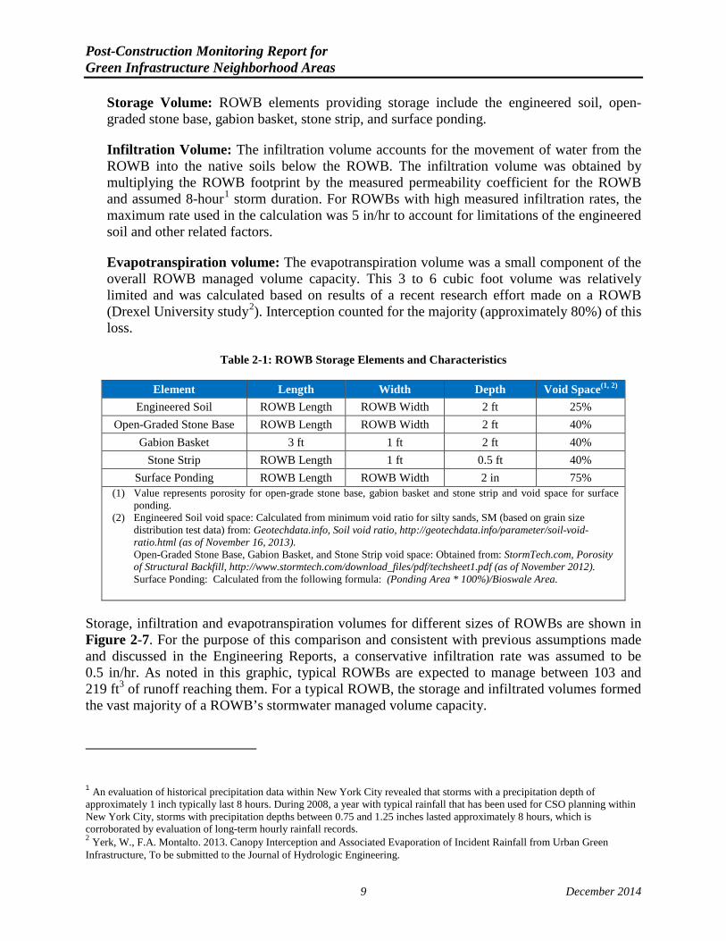
Storage Volume: ROWB elements providing storage include the engineered soil, open-graded stone base, gabion basket, stone strip, and surface ponding.
Infiltration Volume: The infiltration volume accounts for the movement of water from the ROWB into the native soils below the ROWB. The infiltration volume was obtained by multiplying the ROWB footprint by the measured permeability coefficient for the ROWB and assumed 8-hour1 storm duration. For ROWBs with high measured infiltration rates, the maximum rate used in the calculation was 5 in/hr to account for limitations of the engineered soil and other related factors.
Evapotranspiration volume: The evapotranspiration volume was a small component of the overall ROWB managed volume capacity. This 3 to 6 cubic foot volume was relatively limited and was calculated based on results of a recent research effort made on a ROWB (Drexel University study2). Interception counted for the majority (approximately 80%) of this loss.
Table 2-1: ROWB Storage Elements and Characteristics
Element Length Width Depth Void Space(1, 2)
Engineered Soil ROWB Length ROWB Width 2 ft 25% Open-Graded Stone Base ROWB Length ROWB Width 2 ft 40%
Gabion Basket 3 ft 1 ft 2 ft 40% Stone Strip ROWB Length 1 ft 0.5 ft 40%
Surface Ponding ROWB Length ROWB Width 2 in 75% (1) Value represents porosity for open-grade stone base, gabion basket and stone strip and void space for surface
ponding. (2) Engineered Soil void space: Calculated from minimum void ratio for silty sands, SM (based on grain size
distribution test data) from: Geotechdata.info, Soil void ratio, http://geotechdata.info/parameter/soil-void-ratio.html (as of November 16, 2013).
Open-Graded Stone Base, Gabion Basket, and Stone Strip void space: Obtained from: StormTech.com, Porosity of Structural Backfill, http://www.stormtech.com/download_files/pdf/techsheet1.pdf (as of November 2012).
Surface Ponding: Calculated from the following formula: (Ponding Area * 100%)/Bioswale Area.
Storage, infiltration and evapotranspiration volumes for different sizes of ROWBs are shown in Figure 2-7. For the purpose of this comparison and consistent with previous assumptions made and discussed in the Engineering Reports, a conservative infiltration rate was assumed to be 0.5 in/hr. As noted in this graphic, typical ROWBs are expected to manage between 103 and 219 ft3 of runoff reaching them. For a typical ROWB, the storage and infiltrated volumes formed the vast majority of a ROWB’s stormwater managed volume capacity.
1 An evaluation of historical precipitation data within New York City revealed that storms with a precipitation depth of approximately 1 inch typically last 8 hours. During 2008, a year with typical rainfall that has been used for CSO planning within New York City, storms with precipitation depths between 0.75 and 1.25 inches lasted approximately 8 hours, which is corroborated by evaluation of long-term hourly rainfall records. 2 Yerk, W., F.A. Montalto. 2013. Canopy Interception and Associated Evaporation of Incident Rainfall from Urban Green Infrastructure, To be submitted to the Journal of Hydrologic Engineering.
9 December 2014

Post-Construction Monitoring Report for Green Infrastructure Neighborhood Areas
10 December 2014
Cumulative managed capacity for all installed ROWBs in the Demo Areas are provided in Appendix B. The managed capacities provided in Appendix B for individual ROWBs are based on the specific dimensions, ROWB storage elements, and permeability characteristics of the native subsurface soils.
Figure 2-7: Expected ROWB Managed Volume Capacity Assuming a 0.5-In/Hr Permeability Rate
ROWB ROWB ROWB

Post-Construction Monitoring Report for Green Infrastructure Neighborhood Areas 3. NEIGHBORHOOD DEMONSTRATION AREAS
OGI selected three Demo Areas within priority CSO tributary areas of New York City to design, construct, and monitor the performance of GI practices at the site- and neighborhood-scales. The Demo Areas consist of multiple blocks within the Hutchinson River drainage area in the Bronx (Demo Area 1); within the Jamaica Bay drainage area in Brooklyn (Demo Area 2); and within the Newtown Creek drainage area in Brooklyn (Demo Area 3). The characteristics of each of these Demo Areas are described below including location, land uses and population, impervious surface coverage, subsurface features, sewer and hydraulic connectivity, and installed GI systems. Detailed engineering reports and designs previously submitted to DEC, in accordance with the Order, include additional information about the installed GI systems, basis of design, and flow metering setup.
DEP constructed various types of GI practices across the three Demo Areas. Only ROWBs were constructed in Demo Area 1; ROWBs and SGSs as well as different types of on-site practices were constructed in Demo Area 2; and ROWBs and on-site practices were constructed in Demo Area 3. The ROWBs were constructed within the ROW along the curb line within the sidewalk. The SGSs were constructed within the ROW along the curb line within the street. On-site practices consist of bioretention cells, porous pavement, and subsurface retention/detention. The on-site practices were constructed on New York City Housing Authority (NYCHA) properties; Seth Low Houses (Demo Area 2) and Hope Gardens Houses (Demo Area 3).
DEP certified completion of the Jamaica Bay Neighborhood Demonstration Project in Brooklyn in December 2012 (Demo Area 2). In spring 2013, DEP certified completion of the Newtown Creek Demonstration Project in Brooklyn (Demo Area 3) and the Hutchinson River Demonstration Project in the Bronx, (Demo Area 1), thereby achieving all three Order milestones on schedule. The following sections of the report summarize the characteristics of each of the three Demo Areas.
3.1. DESCRIPTION OF DEMONSTRATION AREA 1 – HUTCHINSON RIVER
The Hutchinson River Demonstration Area, Demo Area 1, is located in the northeastern portion of the Bronx, in the vicinity of NYCHA’s Edenwald Houses Complex (Figure 3-1). This 24.1-acre Demo Area generally abuts 1,800 feet of Schieffelin Avenue, between E. 225th Street and E. 229th Street, and ranges in width from 500 to 1,000 feet. Elevations within Demo Area 1 vary between 100 to 135 feet above mean sea level (MSL).
3.1.1. Land Use and Population
According to the 2010 census, Demo Area 1 has a population of 7,747 people and contains 2,721 housing units. The tax lots within Demo Area 1 were divided into individual land use characteristics as determined by the NYC Department of Planning. As shown in Table 3-1, much of the area can be characterized as multi-family high-rise, elevator buildings.
11 December 2014

Post-Construction Monitoring Report for Green Infrastructure Neighborhood Areas
Figure 3-1: Location of Demo Area 1 - Hutchinson River
Table 3-1: Land Use Characteristics of Demo Area 1
Land Use Acres % of Total Area One and Two Family Buildings 2.04 8% Multi-Family Walk-Up Buildings 0.39 2% Multi-Family Elevator Buildings 15.20 63% Mixed Residential and Commercial Buildings 0.15 1% Industrial and Manufacturing 0 0% Transportation and Utility 0 0% Public Facilities and Institutions 1.96 8% Parking Facilities 0 0% Vacant Land 0 0% Total Lot Area 19.74 82% Estimated Sidewalk/Street Area (Right-of-way) 4.38 18% Total Area Including Sidewalk and Street 24.12 100%
12 December 2014

Post-Construction Monitoring Report for Green Infrastructure Neighborhood Areas
3.1.2. Impervious Surface Coverage
The TDA of Demo Area 1 consists predominantly of impervious surfaces common throughout New York City, including streets, sidewalks, rooftops, playgrounds, driveways, and parking areas. As shown in Table 3-5, streets and sidewalks alone represent 18% of the total land area within Demo Area 1.
An analysis of multi-spectral infrared satellite imagery from April 2009 concluded that 81% of the TDA consists of impervious surfaces, with the remaining 19% pervious. However, not all of this measured impervious area is hydraulically connected to the combined sewer system and therefore does not contribute to CSOs. OGI considers about 30% of the TDA to be impervious ROW area. Of the three Demo Areas, Demo Area 1 has the lowest impervious coverage.
3.1.3. Subsurface Conditions
According to the New York City Reconnaissance Soil Survey, soils within Demo Area 1 generally belong to the Chatfield-Greenbelt complex (NYC Soil Survey Staff, 2005). This soil classification is described as areas of gneissic till and anthropogenic soils throughout bedrock controlled hills that have been cut and filled for development. Both the Chatfield and Greenbelt soil series are categorized by the Soil Survey as well-drained soils, meaning there is no evidence of long-term saturation near the surface, and consist of a mixture of silt, loam, and sand material (NYC Soil Survey Staff, 2005).
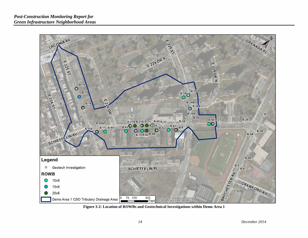
Limited geotechnical boring investigations and permeability tests were performed by Aquifer Drilling & Testing at selected ROWB locations throughout the Demo Area (Figure 3-2). Soil samples were collected at depths of 5 to 7 feet below the surface and 10 to 12 feet below the surface and analyzed to determine water content, Unified Soil Classification System (USCS) classification, organic content, and particle size distribution. In-situ permeability tests were performed at depths of 5 and 10 feet below the surface. Information on testing procedures and complete results of the subsurface investigations can be found in the “Soil Investigation Report, Right-of-Way Green Infrastructure within Hutchinson River Neighborhood Demonstration Area 1,” dated August 2012. A summary of soil and permeability measurements can be found in Appendix A. Only geotechnical results from constructed ROWBs are presented herein.
Like much of the Bronx, bedrock exists at shallow depths within and adjacent to Demo Area 1. The bedrock breaks the ground surface and is visible as rock outcrops at many locations. A number of planned ROWBs within and to the north of the current Demonstration Area boundary were rejected early in the planning process due to the existence of shallow bedrock. As a result, the Demo Area was reduced in size to exclude the area along Baychester Avenue.
Groundwater was not encountered within 12 feet of the surface at any of the boring locations within Demo Area 1. Soils within the area largely consisted of sand with some evidence of silt or clay at a few locations. Permeability rates were variable, with a median value of about 0.8 in/hr and were generally higher at the 5-foot depth than the 10-foot depth (Figure 3-3).
13 December 2014
Post-Construction Monitoring Report for Green Infrastructure Neighborhood Areas
Figure 3-2: Location of ROWBs and Geotechnical Investigations within Demo Area 1
14 December 2014

Post-Construction Monitoring Report for Green Infrastructure Neighborhood Areas
Figure 3-3: Box Plots of Measured Fines Content (left) and Permeability Rates (right)
(25, 50 and 75th Percentiles)
3.1.4. Sewer and Hydraulic Connectivity
Sewer flows within Demo Area 1 are conveyed in a predominantly northeasterly direction along Schieffelin Avenue (Figure 3-4). The TDA was developed as discussed in Section 2.1, supplemented with a manhole inspection to determine the direction of flow at the edge of the drainage area on East 229th Street. The tributary flow from the Demo Area discharges near the intersection of Schieffelin Avenue and E. 229th Street via a single 36-inch combined sewer, where flow monitoring equipment was installed. Details of the flow monitoring setup can be found within Section 4.1 of this report and the “Engineering Report, Right-of-Way Green Infrastructure within Hutchinson River Neighborhood Demonstration Area 1.” Combined sewer flow is regulated at HP-R15A, approximately 1.4 miles downstream, and during wet weather CSO may discharge to the Hutchinson River through nearby outfall HP-024.
3.1.5. GI Practices within Demo Area 1
A total of 22 ROWBs were constructed within Demo Area 1, ranging in size from 6 feet by 10 feet to 6 feet by 20 feet (Table 3-2). ROWB widths were increased from the standard 5 feet to 6 feet in this area to help accommodate transplanting of existing trees. ROWBs were generally distributed across the entire Demo Area, with the greatest concentration along Schieffelin Avenue. ROWBs were sited given local site-specific limitations; high bedrock, existing trees, and ongoing or planned construction activities were among the reasons why some locations did not include an ROWB (Figure 3-4).
Table 3-2: ROWB Sizes and Quantities Constructed within Demo Area 1
ROWB Size Quantity 6 ft x 10 ft 8 6 ft x 15 ft 4 6 ft x 20 ft 10
Total 22
1%
10%
100%
5' FinesContent
10' FinesContent
Fine
s Con
tent
(Sie
ve <
#20
0)
0.01
0.10
1.00
10.00
100.00
5' Permeability 10' Permeability
Perm
eabi
lity
(in/h
r)
15 December 2014

Post-Construction Monitoring Report for Green Infrastructure Neighborhood Areas
Figure 3-4: Overview of Sewer Configuration within Demo Area 1
16 December 2014

Post-Construction Monitoring Report for Green Infrastructure Neighborhood Areas For Demo Area 1, a 10-inch diameter solid open bottom HDPE pipe filled with stone and fitted with a perforated cap (stone column) was included in six ROWBs (B-9, B-9a, B-10, B-11, B-16 and B-17) to connect the surface ponding area, subsurface stone storage layer, and deeper subsurface soils. A total of 22 ROWBs/SGSs were constructed in Demo Area 1 and as such 27% contained this stone column connection that was installed to enhance flow to deeper and better infiltrating subsurface soils.
As discussed in Section 2, the volume of stormwater that can be managed by a ROWB was estimated as the combination of storage volume within the ROWB (including on the surface, in the engineered soil, and in the open-graded stone bed), the volume of water that infiltrates into the underlying soils, and the volume of water that is removed from the ROWB via evapotranspiration.
When accounting for site-specific permeability rates, the 22 ROWBs within Demo Area 1 were expected to have a collective runoff managed volume capacity of 4,900 ft³. This value is referred to herein as the unconstrained managed volume. Details of ROWB capacity calculations can be found within Appendix B. This capacity could effectively manage the stormwater generated from a 1-inch, 8-hour storm over 1.3 acres of impervious area if the area draining to these controls generated enough runoff to fully utilize the capacity.
Calculated capacities of individual ROWB and runoff volumes varied throughout the Demo Area based on ROWB size, location, and permeability and are presented in Figure 3-5 as solid green bars. Also shown in this figure are the calculated volumes of runoff from 1 inch of rainfall on the impervious surfaces upstream from each ROWB (solid blue bars). It should be noted that in five cases, ROWBs do not have an adequate TDA to allow for full use of their capacity for a 1-inch storm over their drainage area and were constrained. The remaining 17 ROWB drainage areas generate runoff from the 1-inch storm that fully utilizes the ROWBs capacity. Accounting for the fact that some ROWBs have a volume capacity larger than the runoff they will receive during a 1-inch, 8-hour storm, the actual managed area is slightly lower, but effectively remains the same at 1 inch of stormwater over 1.2 acres.
Also presented in Figure 3-5 are the calculated volumes of 1 inch of rainfall on 10% of the impervious area tributary to each ROWB (bars with blue dots). As noted in this figure, all ROWBs were constructed with adequate capacity to manage all the runoff from 10% of their respective tributary area for the 1-inch rainfall.
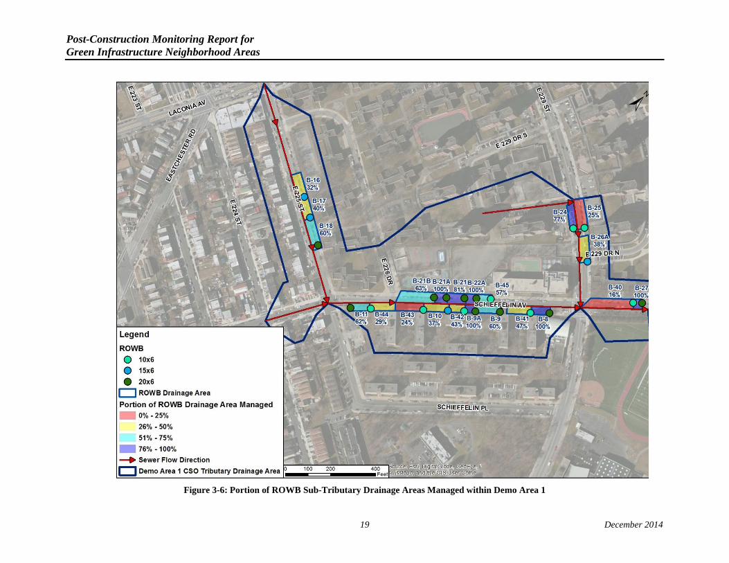
Figure 3-6 presents additional information in a more spatial format. This figure shows the amount of the 1-inch rainfall from the ROWB sub-tributary drainage area that would be expected to be managed by each ROWB constructed within Area 1. Depending on the size of the ROWB sub-tributary drainage area, the specific design features and the physical characteristics, ROWBs are expected to manage between 16 and 100% of the runoff from the 1-inch rainfall on their tributary area.
17 December 2014

Post-Construction Monitoring Report for Green Infrastructure Neighborhood Areas
Figure 3-5: Calculated ROWB Volume Capacity and ROWB Tributary Drainage Area Runoff Volume for 1-Inch Rainfall within Demo Area 1
1
10
100
1,000
10,000
B-16
B-17
B-18
B-11
B-44
B-43
B-10
B-42
B-9A B-
9
B-21
B
B-21
A
B-21
B-22
A
B-45
B-41 B-
8
B-24
B-25
B-26
A
B-40
B-27
Volu
me
(ft³)
ROWB Capacity
One-Inch Runoff Volume from 10% of Impervious Surface Tributary to ROWB
One-Inch Runoff Volume from Impervious Surface Tributary to ROWB
18 December 2014
Post-Construction Monitoring Report for Green Infrastructure Neighborhood Areas
Figure 3-6: Portion of ROWB Sub-Tributary Drainage Areas Managed within Demo Area 1
19 December 2014
Post-Construction Monitoring Report for Green Infrastructure Neighborhood Areas
3.2. DESCRIPTION OF DEMONSTRATION AREA 2 – 26TH WARD
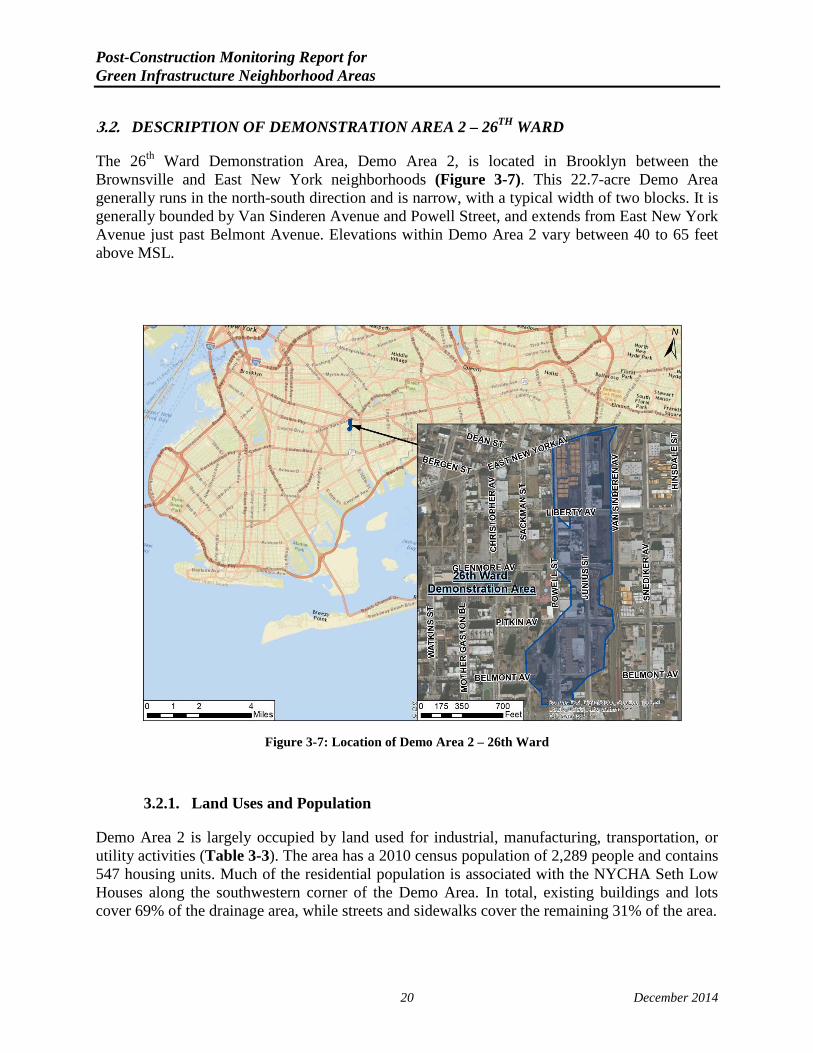
The 26th Ward Demonstration Area, Demo Area 2, is located in Brooklyn between the Brownsville and East New York neighborhoods (Figure 3-7). This 22.7-acre Demo Area generally runs in the north-south direction and is narrow, with a typical width of two blocks. It is generally bounded by Van Sinderen Avenue and Powell Street, and extends from East New York Avenue just past Belmont Avenue. Elevations within Demo Area 2 vary between 40 to 65 feet above MSL.
Figure 3-7: Location of Demo Area 2 – 26th Ward
3.2.1. Land Uses and Population
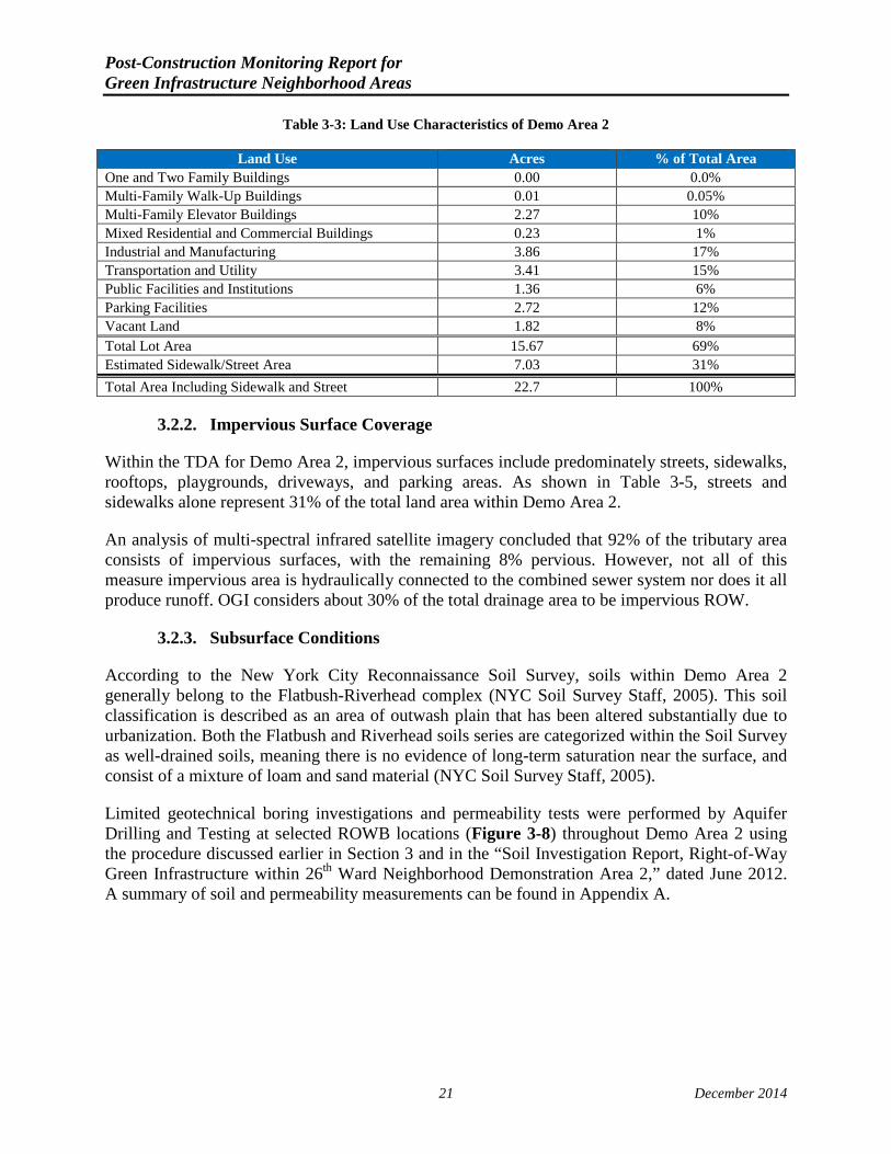
Demo Area 2 is largely occupied by land used for industrial, manufacturing, transportation, or utility activities (Table 3-3). The area has a 2010 census population of 2,289 people and contains 547 housing units. Much of the residential population is associated with the NYCHA Seth Low Houses along the southwestern corner of the Demo Area. In total, existing buildings and lots cover 69% of the drainage area, while streets and sidewalks cover the remaining 31% of the area.
20 December 2014
Post-Construction Monitoring Report for Green Infrastructure Neighborhood Areas
Table 3-3: Land Use Characteristics of Demo Area 2
Land Use Acres % of Total Area One and Two Family Buildings 0.00 0.0% Multi-Family Walk-Up Buildings 0.01 0.05% Multi-Family Elevator Buildings 2.27 10% Mixed Residential and Commercial Buildings 0.23 1% Industrial and Manufacturing 3.86 17% Transportation and Utility 3.41 15% Public Facilities and Institutions 1.36 6% Parking Facilities 2.72 12% Vacant Land 1.82 8% Total Lot Area 15.67 69% Estimated Sidewalk/Street Area 7.03 31% Total Area Including Sidewalk and Street 22.7 100%
3.2.2. Impervious Surface Coverage
Within the TDA for Demo Area 2, impervious surfaces include predominately streets, sidewalks, rooftops, playgrounds, driveways, and parking areas. As shown in Table 3-5, streets and sidewalks alone represent 31% of the total land area within Demo Area 2.
An analysis of multi-spectral infrared satellite imagery concluded that 92% of the tributary area consists of impervious surfaces, with the remaining 8% pervious. However, not all of this measure impervious area is hydraulically connected to the combined sewer system nor does it all produce runoff. OGI considers about 30% of the total drainage area to be impervious ROW.
3.2.3. Subsurface Conditions
According to the New York City Reconnaissance Soil Survey, soils within Demo Area 2 generally belong to the Flatbush-Riverhead complex (NYC Soil Survey Staff, 2005). This soil classification is described as an area of outwash plain that has been altered substantially due to urbanization. Both the Flatbush and Riverhead soils series are categorized within the Soil Survey as well-drained soils, meaning there is no evidence of long-term saturation near the surface, and consist of a mixture of loam and sand material (NYC Soil Survey Staff, 2005).
Limited geotechnical boring investigations and permeability tests were performed by Aquifer Drilling and Testing at selected ROWB locations (Figure 3-8) throughout Demo Area 2 using the procedure discussed earlier in Section 3 and in the “Soil Investigation Report, Right-of-Way Green Infrastructure within 26th Ward Neighborhood Demonstration Area 2,” dated June 2012. A summary of soil and permeability measurements can be found in Appendix A.
21 December 2014

Post-Construction Monitoring Report for Green Infrastructure Neighborhood Areas
Figure 3-8: Location of ROWBs and ROWBs Geotechnical Investigations within Demo Area 2
22 December 2014

Post-Construction Monitoring Report for Green Infrastructure Neighborhood Areas Neither groundwater nor bedrock was encountered within 12 feet of the surface at any of the boring locations within Demo Area 2. Soils were generally classified as sands and gravels. Measured permeability rates were highly variable, with a median of around 3 in/hr at 5 feet and 8 in/hr at 10 feet below the surface (Figure 3-9).
Figure 3-9: Box Plots of Measured Fines Content (left) and Permeability Rates (right) (25, 50 and 75th Percentiles)
3.2.4. Sewer and Hydraulic Connectivity
Sewer flows within Demo Area 2 are conveyed in a predominantly southerly direction. The sewer along Junius Street collects runoff from the street itself and adjacent side streets, while the Powell Street sewer follows a parallel path, with less side street drainage. Flow from the Demo Area 2 sewershed is consolidated in the vicinity of Belmont Avenue and Junius Street, where it leaves the area via a single 24-inch sewer, where flow monitoring equipment was installed (Figure 3-10). Details of the flow monitoring setup can be found within Section 4.1 and the “Engineering Report, Right-of-Way Green Infrastructure within 26th Ward Neighborhood Demonstration Area 2.” Combined sewer flow is regulated at 26W-R2 and discharges to the head end of Fresh Creek, a tributary to Jamaica Bay, through outfall 26W-003, near where Flatlands Avenue crosses the Fresh Creek.
3.2.5. GI Practices within Demo Area 2
GI within Demo Area 2 consists of ROWBs and SGSs distributed throughout the area, supplemented by on-site GI at NYCHA’s Seth Low Houses. In total, 29 ROWBs and two SGSs were installed within the Demo Area to manage ROW runoff (Table 3-4). ROWBs ranged in size from 5 feet by 15 feet to 5 feet by 20 feet, while the SGSs were approximately 5 feet by 25 feet.
1%
10%
100%
5' Fines Content 10' Fines Content
Fine
s Con
tent
(Sie
ve <
#20
0)
0.01
0.10
1.00
10.00
100.00
5' Permeability 10' PermeabilityPe
rmea
bilit
y (in
/hr)
23 December 2014

Post-Construction Monitoring Report for Green Infrastructure Neighborhood Areas
Figure 3-10: Overview of Sewer Configuration within Demo Area 2
24 December 2014

Post-Construction Monitoring Report for Green Infrastructure Neighborhood Areas
Table 3-4: ROWB Sizes and Quantities Constructed Within Demo Area 2
ROWB Size Quantity 5 ft x 15 ft 2 5 ft x 20 ft 27
5 ft x 25 ft (SGSs) 2 Total 31
For Area 2, a 10-inch diameter solid open bottom HDPE pipe filled with stone and fitted with a perforated cap (chimney) was included in six ROWBs (B-8, B-9*, B-15, B-25 and B-31) to connect between the surface ponding area and the subsurface stone storage layer. A total of 31 ROWBs/SGSs were constructed in Area 2 and as such 16% contained this chimney connection that was installed to enhance flow to subsurface stone storage layer.
The volume of stormwater that can be managed by a ROWB was estimated in accordance with procedures discussed in Section 2. For ROWBs with 5-foot widths, estimated typical runoff management capacities ranged from 119 ft³ to 217 ft³. When accounting for site-specific permeability rates, ROWBs within Demo Area 2 are expected to have a collective runoff managed volume capacity of 10,200 ft³. Details of ROWB capacity calculations for Demo Area 2 can be found within Appendix B.
Calculated management of ROWB drainage areas varied throughout the Demo Area based on ROWB size and permeability (Figure 3-11). Six ROWBs do not have an adequate drainage area upstream of them to allow for full use of their capacity. Twenty-five ROWBs have adequate drainage area upstream of them for full use of their capacity. If the size of the ROWB drainage area was not a limiting factor, these ROWBs could effectively manage the stormwater generated from a 1-inch, 8-hour storm on a 2.8-acre impervious area. Several ROWBs within Demo Area 2 were limited by the size of the ROWB drainage area rather than their capacity. Accounting for this limitation, ROWBs within Demo Area 2 should manage 2.5 acres. Many of the ROWB drainage areas within Demo Area 2 had adequate calculated capacity to manage at least 25% of runoff from individual ROWB drainage areas.
Also presented in Figure 3-11 are the calculated volumes of 1-inch rainfall on 10% of the impervious area tributary to each ROWB (bars with blue dots). These would be the volume that each ROWB would be expected to manage. As noted in this figure, all Area 2 ROWBs were constructed with adequate capacity to manage all the runoff from 10% of their respective tributary area.
Figure 3-12 presents additional information in a more spatial format. This figure shows the amount of the 1-inch rainfall from the upstream tributary area that would be expected to be managed by each ROWB constructed within Area 2. Depending on the upstream tributary area and the specific design features and physical characteristics, ROWBs are expected to manage between 12 and 100% of the runoff from the 1-inch rainfall on their tributary area.
25 December 2014

Post-Construction Monitoring Report for Green Infrastructure Neighborhood Areas
Figure 3-11: Calculated ROWB Managed Volume Capacity and ROWB Drainage Area Runoff Volume for 1-Inch Rainfall within Demo Area 2
1
10
100
1,000
10,000
B-29
B-30 B-
1B-
2B-
31B-
32B-
33 B-3
B-4
B-7
B-7* B-
8B-
8*B-
10B-
9*B-
11B-
12B-
13B-
22B-
27B-
24B-
25GS
-23
GS-2
6B-
28B-
15B-
17B-
19B-
20B-
18B-
16
Volu
me
(ft³)
ROWB Capacity
One-Inch Runoff Volume from 10% of Impervious Surface Tributary to ROWB
One-Inch Runoff Volume from Impervious Surface Tributary to ROWB
26 December 2014

Post-Construction Monitoring Report for Green Infrastructure Neighborhood Areas
Figure 3-12: Portion of ROWB Sub-Tributary Drainage Areas Managed within Demo Area 2
27 December 2014

Post-Construction Monitoring Report for Green Infrastructure Neighborhood Areas In addition to the ROWBs and SGSs located within the ROW to manage runoff, GI practices were also constructed at NYCHA’s Seth Low Houses (Figure 3-13). Completed in September 2013, a pair of permeable pavement systems with subsurface storage components was installed to manage runoff from paved pedestrian areas (Appendix C). These infiltration/storage elements were installed around yard inlets and consisted of a permeable surface (Figure 3-14) that allows runoff to infiltrate before reaching the inlet grate, along with a subsurface stone layer to support storage and infiltration. In addition, in one location within the housing complex, runoff was collected in a flow diversion structure and conveyed via a subsurface pipe to stormwater chambers with an infiltrating area below the porous pavement. The infiltration elements were sized to manage at least 1 inch of rainfall, the NYC DEP Green Infrastructure Plan goal. Unlike ROWBs, the on-site practices were sized based on their drainage area to manage the 1-inch volume. This would result in a managed drainage area of 18,940 ft² for the 1-inch rainfall. Inclusion of these on-site practices results in a calculated total managed volume capacity of 10,480ft3 and managed drainage area of 2.9 acres.
Figure 3-13: Location of On-site GI Controls in Demo Area 2
28 December 2014

Post-Construction Monitoring Report for Green Infrastructure Neighborhood Areas
Figure 3-14: Demo Area 2 Porous Concrete Panels and Inlet Grate at NYCHA’s Seth Low Houses
3.3. DESCRIPTION OF DEMONSTRATION AREA 3 – NEWTOWN CREEK
The Newtown Creek Demonstration Area, Demo Area 3, is located in the northeastern portion of Brooklyn, and is a tributary to Newtown Creek (Figure 3-15). This 19.3-acre Demo Area is generally located along Grove Street, between Wilson Avenue and Broadway, ranging in width from 250 to 500 feet.
3.3.1. Land Use and Population
Demo Area 3 has a 2010 census population of 3,443 people and contains 1,352 housing units. As shown in Table 3-5, the lot areas are comprised mostly of multi-family walk-up buildings and multi-family, high-rise elevator buildings. In total, buildings and lots cover 71% of the drainage area while streets and sidewalks cover the remaining 29%.
29 December 2014

Post-Construction Monitoring Report for Green Infrastructure Neighborhood Areas
Figure 3-15: Location of Demo Area 3 – Newtown Creek
Table 3-5: Land Use Characteristics of Demo Area 3
Land Use Acres % of Total Area One and Two Family Buildings 3.57 19% Multi-Family Walk-Up Buildings 3.89 20% Multi-Family Elevator Buildings 2.87 15% Mixed Residential and Commercial Buildings 0.61 3% Commercial and Office Buildings 0.13 1% Transportation and Utility 0.08 0% Public Facilities and Institutions 1.70 9% Open Space and Outdoor Recreation 0.09 0% Vacant Land 0.72 4% Total of Lot Area 13.67 71% Estimated Sidewalk/Street Area 5.63 29%
Total Area Including Sidewalk and Street 19.30 100%
30 December 2014

Post-Construction Monitoring Report for Green Infrastructure Neighborhood Areas
3.3.2. Impervious Surface Coverage
Within the TDA for Demo Area 3, impervious surfaces included predominately streets, sidewalks, rooftops, playgrounds, driveways, and parking areas. As shown in Table 3-5, streets and sidewalks alone represent 29% of the total land area within Demo Area 3.
An analysis of multi-spectral infrared satellite imagery concluded that 92% of the Demo Area consists of impervious surface, with the remaining 8% pervious. However, not all of this measure impervious area is hydraulically connected to the combined sewer system nor does it all produce runoff. OGI considers about 30% of the total drainage area to be ROW area. Elevations within Demo Area 3 ranged from approximately 35 to 55 feet above MSL.
3.3.3. Subsurface Conditions
According to the New York City Reconnaissance Soil Survey, soils within Demo Area 3 generally belong to the LaGuardia-Ebbets complex or are characterized as till substratum (NYC Soil Survey Staff, 2005). These soil classifications generally describe glacial till or anthropogenic soil mixtures, largely under impervious coverage. Both the LaGuardia and Ebbets soils series are categorized within the Soil Survey as well-drained soils, meaning there is no evidence of long-term saturation near the surface, and consist of a mixture of loam and sand material (NYC Soil Survey Staff, 2005).
Limited geotechnical boring investigations and permeability tests were performed by Aquifer Drilling and Testing at selected ROWB locations throughout Demo Area 3 using the procedure discussed earlier in Section 3 and in the “Soil Investigation Report, Right-of-Way Green Infrastructure within Newtown Creek Neighborhood Demonstration Area 3,” dated June 2012 (Figure 3-16). A summary of soil and permeability measurements can be found in Appendix A.
Neither groundwater nor bedrock were encountered within 12 feet of the surface at any of the boring locations within Demo Area 3. Soils were generally classified as sands. Measured permeability rates were highly variable, with a median of about 0.5 in/hr at 5 feet and about 2 in/hr at 10 feet (Figure 3-17).
3.3.4. Sewer and Hydraulic Connectivity
Sewer flows within Demo Area 3 are conveyed in a predominantly northerly direction along Grove Street (Figure 3-18). The TDA was developed as discussed in Section 2.1, supplemented with, a review of the Hope Gardens House yard drain drawings, a topographic survey of the Hope Gardens Houses properties and physical manhole surveys and dye testing. Flow from much of the tributary area leaves the Demo Area boundary near the intersection of Grove Street and Wilson Avenue through a single 18-inch sewer, where flow monitoring equipment was installed. Additionally, runoff originating within NYCHA’s Hope Gardens Houses leaves the Demo Area through a 12-inch NYCHA sewer, which was separately monitored. Combined sewer flow is regulated at NC-B1 and NC-B1A, and discharges to Newtown Creek through outfall NCB-015. Site connections along Menahan Street and Linden Street discharge into sewers outside the Demo Area; however, runoff from these streets between Bushwick Avenue and Evergreen Avenue reaches the monitoring location due to catch basin locations. The area south of Bushwick discharges into a large combined sewer that runs toward the west along Bushwick Avenue.
31 December 2014

Post-Construction Monitoring Report for Green Infrastructure Neighborhood Areas
Figure 3-16: Location of ROWBs and ROWB Geotechnical Investigations within Demo Area 3
32 December 2014

Post-Construction Monitoring Report for Green Infrastructure Neighborhood Areas
Figure 3-17: Box Plots of Measured Fines Content (left) and Permeability Rates (right)
(25, 50 and 75th Percentiles)
1%
10%
100%
5' Fines Content 10' Fines Content
Fine
s Con
tent
(Sie
ve <
#20
0)
0.01
0.10
1.00
10.00
100.00
5' Permeability 10' PermeabilityPe
rmea
bilit
y (in
/hr)
33 December 2014

Post-Construction Monitoring Report for Green Infrastructure Neighborhood Areas
Figure 3-18: Overview of Sewer Configuration within Demo Area 3
34 December 2014

Post-Construction Monitoring Report for Green Infrastructure Neighborhood Areas
35 December 2014
3.3.5. GI Practices within Demo Area 3
A total of 19 ROWBs (Table 3-6) were constructed within Demo Area 3, ranging in size from 5 by 10 feet to 5 by 20 feet. The ROWBs implemented in Demo Area 3 were constructed with stone gabions that provided additional storage and facilitated more rapid flow from the surface to the subsurface stone storage than the engineered soil. The ROWBs were supplemented by on-site GI at the NYCHA Hope Gardens Houses. Many of the ROWBs in Demo Area 3 are located within the upstream half of the tributary area, along and south of Evergreen Avenue.
Table 3-6: ROWB Sizes and Quantities
Implemented Within Demo Area 3
ROWB Size Quantity
5 ft x 10 ft 1
5 ft x 15 ft 6
5 ft x 20 ft 12
Total 19
For Area 3, all ROWBs had an open stone gabion 1-foot wide by 2-feet 3-inches long (15 ft by 5 ft ROWB) or 3-feet long (20 ft by 5 ft ROWB) filled with stone to connect between the surface ponding area and the subsurface stone storage layer. Some ROWBs (B-5, B-7, B-12) had a 10-inch diameter stone column that was connected to deep infiltrating soils to enhance infiltration. As such 100% of the 19 ROWBs in Area 3 contained a connection between the surface ponding area and the subsurface stone storage layer and 16% had a connection to deeper and better infiltrating subsurface soils.
The volume of stormwater that can be managed by a ROWB was estimated in accordance with procedures discussed in Section 2. As in Demo Area 2, estimated typical runoff management capacities for ROWBs with 5-foot widths ranged from 119 to 217 ft³. When accounting for site-specific permeability rates, ROWBs within Demo Area 3 are expected to have a collective runoff managed volume capacity of 3,400 ft³. Details of ROWB capacity calculations for Demo Area 3 can be found within Appendix B. If the size of the ROWB sub-tributary drainage area had not been a limiting factor, these ROWBs could effectively manage the runoff generated from a 1-inch storm on a 0.9-acre impervious area. Within Demo Area 3, three ROWBs had ROWB sub-tributary drainage areas (Figure 3-19) that were too large to have the 1-inch storm fully managed by the ROWB. As such, ROWBs within Demo Area 3 are still estimated to manage close to their full capacity at 0.9 acres. Only a few ROWBs within Demo Area 3 had the calculated capacity to manage the majority of runoff from their ROWB sub-tributary drainage area.
Also presented in Figure 3-19 are the calculated volumes of 1-inch rainfall on 10% of the impervious area tributary to each ROWB (bars with blue dots). As noted in this figure, all Demo Area 3 ROWBs were constructed with approximately enough capacity to manage all the runoff from 10% of their respective ROWB sub-tributary drainage area.

Post-Construction Monitoring Report for Green Infrastructure Neighborhood Areas
Figure 3-19: Calculated ROWB Managed Volume Capacity and ROWB Sub-Tributary Drainage Area Runoff Volume for 1-Inch
Rainfall within Demo Area 3
1
10
100
1,000
10,000
B-1
B-2
B-5
B-4
B-6
B-7
B-10
*
B-14
*
B-11 B-
9
B-8
B-12
B-13
B-15
B-16
B-17
B-18
B
B-18
B-20
Volu
me
(ft³)
ROWB Capacity
One-Inch Runoff Volume from 10% of Impervious Surface Tributary to ROWB
One-Inch Runoff Volume from Impervious Surface Tributary to ROWB
36 December 2014

Post-Construction Monitoring Report for Green Infrastructure Neighborhood Areas Figure 3-20 presents additional information in a more spatial format. This figure shows the amount of the 1-inch rainfall from the upstream tributary area that would be expected to be managed by each ROWB constructed within Demo Area 3. Depending on the size of the ROWB sub-tributary drainage area, the specific design features and physical characteristics, ROWBs are expected to manage between 7 and 100% of the runoff from 1 inch of rainfall on their ROWB sub-tributary drainage area.
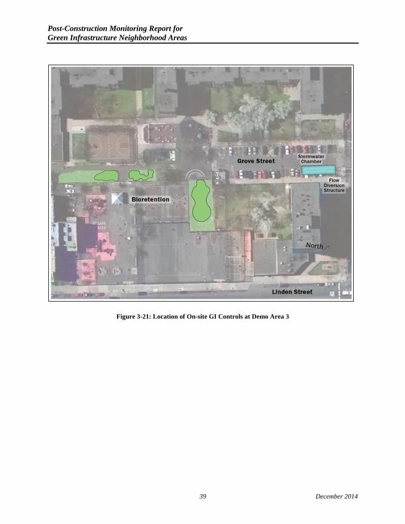
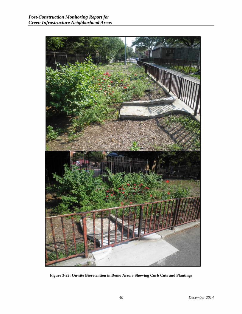
As with Demo Area 2, on-site GI practices were also constructed in Demo Area 3 on NYCHA property and completed in September 2013. In Demo Area 3, three GI bioretention areas and a subsurface retention system were installed to manage on-site runoff in the Hope Gardens Houses complex (Figure 3-21). The bioretention areas used curb cuts to capture runoff from pedestrian sidewalks (Figure 3-22). The subsurface retention system utilized stormwater chambers and stone installed under the parking lot at the northern end of the complex to manage runoff from the parking lot (Figure 3-23). These systems were sized to manage at least 1 inch of rainfall, the Green Infrastructure Plan requirement. In total, these on-site controls have a managed volume capacity for the 1-inch rainfall of 2,680 ft3 and were expected to manage a 1-inch storm for their tributary impervious area, which totaled 32,173 ft². Accounting for these on-site controls raises the total managed volume to 5,850 ft³ and total managed impervious area to 1.6 acres for Demo Area 3.
37 December 2014

Post-Construction Monitoring Report for Green Infrastructure Neighborhood Areas
Figure 3-20: Portion of ROWB Sub-Tributary Drainage Areas Managed within Demo Area 3
38 December 2014
Post-Construction Monitoring Report for Green Infrastructure Neighborhood Areas
Figure 3-21: Location of On-site GI Controls at Demo Area 3
39 December 2014
Post-Construction Monitoring Report for Green Infrastructure Neighborhood Areas
Figure 3-22: On-site Bioretention in Demo Area 3 Showing Curb Cuts and Plantings
40 December 2014

Post-Construction Monitoring Report for Green Infrastructure Neighborhood Areas
Figure 3-23: Demo Area 3 Subsurface Detention System During and After Construction
41 December 2014

Post-Construction Monitoring Report for Green Infrastructure Neighborhood Areas 4. PERFORMANCE EVALUATION METHODOLOGY
Green infrastructure performance within the Demo Areas was evaluated at both the TDA and site scales (individual ROWB monitoring). The general intent of these evaluations was to characterize the collective impact of multiple GI practices on sewer flows, validate this collective performance by examining the function of individual ROWBs, and support planning efforts for GI as a method of CSO control. The TDA- and site-scale monitoring methodologies are described in detail below, including information about monitoring durations, equipment, data review and QA/QC measures.
4.1. DESCRIPTION OF SEWERSHED MONITORING PROGRAM
Sewer flow monitoring was conducted in combined sewers within each Demo Area both before and after GI was implemented. As discussed previously, the Demo Areas were selected to have a well-defined total TDA with flow leaving each Demo Area via a single pipe or simplified sewer configuration with sewer pipe diameter of 36 inches or less. This configuration made it possible to develop a full-flow balance for the Demo Area with rainfall and sewer flow monitoring data. Sewer flow monitoring within Demo Area 1 was conducted within a single 36-inch pipe along Schieffelin Avenue (Figure 4-1). Demo Area 2 flow was monitored within a single 24-inch pipe near the intersection of Junius Street and Belmont Avenue (Figure 4-2). Three flow monitoring locations were utilized to evaluate pre-GI CSO flow leaving Demo Area 3. Four flow monitoring locations were utilized to evaluate sewer flows leaving Demo Area 3 post-GI (Figure 4-3). A flow meter was installed within an 18-inch pipe that flows north on Grove Street to Wilson Avenue to record flow originating south of NYCHA’s Hope Gardens Houses. Two additional flow meters were utilized to measure flow originating within the housing complex; one monitoring a 12-inch yard drain; the second monitoring the overflow from the subsurface chamber system implemented as part of the Demo Area program. A flow meter was also installed within an 18-inch pipe along Bushwick Avenue to record flow originating south of Bushwick Avenue that does not drain to the Wilson Avenue meter.
The flow monitoring data collection program was intended to provide high-quality flow data which could be used to determine total storm runoff volumes for periods prior to the construction of GI (pre-GI) and following the construction of GI (post-GI). The goal was to compile data on the volume and flow rate within the sewer for storm events before and after GI implementation to provide an assessment of the overall impact of GI within each Demo Area. In practice, the flow monitoring equipment was left in place through the construction period so as to fully maximize the number of storm events that would be captured and to assure that there were no differences in the pre-GI and post-GI data sets associated with the removal and re-installation of the flow monitoring sensors.
42 December 2014

Post-Construction Monitoring Report for Green Infrastructure Neighborhood Areas
Figure 4-1: Sewer Flow Monitoring Setup for Demo Area 1
43 December 2014

Post-Construction Monitoring Report for Green Infrastructure Neighborhood Areas
Figure 4-2: Sewer Flow Monitoring Setup for Demo Area 2
44 December 2014

Post-Construction Monitoring Report for Green Infrastructure Neighborhood Areas
Figure 4-3: Sewer Flow Monitoring Setup for Demo Area 3
45 December 2014

Post-Construction Monitoring Report for Green Infrastructure Neighborhood Areas
4.1.1. Duration of Monitoring Activities
Because of the way the ROWBs were constructed, pre-GI and post-GI periods varied. For Demo Areas 2 and 3, the GI construction contractor worked on all sites in parallel. For Demo Area 1, ROWBs were constructed in a more sequential manner to allow for tree transplanting. For the purposes of the analyses, pre-GI and post-GI periods were, therefore, defined based upon the duration and nature of construction activities (Figure 4-4). For Demo Areas 2 and 3, the pre-GI period was defined herein as extending up to the point where curb work was completed, the ROWBs were excavated and flow was first allowed to enter the ROWBs and percolate into native soils. The post-GI period began when the ROWB stone storage layer and engineered soil had been installed.
Unlike Demo Areas 2 and 3, ROWBs within Demo Area 1 were not constructed simultaneously, making it difficult to establish the exact pre- and post-GI periods for data analyses. The end of the pre-GI period for Area 1 was, therefore, defined as the date when curb cut construction began on the first ROWB and the post-GI period started with the completion of the last ROWB. For these reasons, the gap between the pre-GI and post-GI periods is longer for Demo Area 1 than Demo Areas 2 and 3. The pre-GI monitoring period for Demo Area 1 also began later than the other two Demo Areas. Flow meters had to be moved after installation for a more accurate definition of Demo Area 1 flow, as a portion of the Demo Area along Baychester Avenue was eliminated from the plans due to bedrock at or near the surface. In total, there are 18 months of monitoring data for Demo Area 1, 27 months of data for Demo Area 2, and 29 months of data for Demo Area 3.
Figure 4-4: Duration of Pre and Post-GI Monitoring Activities
As noted in Figure 4-4, on-site construction of GI practices lagged the ROWB construction. Construction of Demo Area 2 and Demo Area 3 on-site GI practices was completed at or beyond mid-way through the post-GI monitoring period. Because on-site GI construction was completed late during the post-construction monitoring period, little data were collected after on-site GI construction completion. Therefore, the expected area managed by these on-site controls was excluded from the analysis.
4.1.2. Monitoring Equipment
Sewer flows were determined using area-velocity meters, which operate by measuring the depth and velocity of water passing over the sensor in combination with pipe geometry (flow area) to establish the flow rate (Figure 4-5). These meters provided the most accurate measure of
46 December 2014

Post-Construction Monitoring Report for Green Infrastructure Neighborhood Areas average velocity in the size of pipes encountered for this monitoring program. Meters were installed either upstream or downstream of existing manholes at locations with steady flow and no evidence of short circuiting or hydraulic jumps based on visual inspections. Prior to deployment, depth (pressure) and velocity sensors were bench tested in a controlled laboratory environment to assure accuracy of measurement. Two identical meters were installed next to each other at each flow monitoring location in order to provide redundancy and support a high level of data recovery and accuracy. During installation, manual depth and velocity readings were made and compared to sensor readings and any necessary meter adjustments were made. Routine maintenance inspections were performed every two weeks during which visual inspection were made of the sensors, battery power was checked, and sensors were cleaned of debris. As part of each site visit, manual depth and velocity readings were taken and compared in real time to the sensor readings.
Figure 4-5: Area-Velocity Meter Measures Depth and the Average Velocity of Particles in the Flow Stream
Tipping bucket rain gauges were also installed within each Demo Area to record rainfall depths and intensities (Figure 4-6). These rain gauges operate by recording the date and time for every 0.01 inch of rain that has fallen on the gauge. These gauges were selected as they provide accurate measures of rainfall on a 5-minute basis. Sewer flow monitoring and rainfall data were reported throughout the pre-GI and post-GI monitoring periods at 5-minute intervals. Flow and rainfall data were analyzed to characterize individual storm events as well as aggregated storm events for the full pre-GI and post-GI periods.
4.1.1. Data Review and Quality Control Procedures
Data quality control efforts were conducted throughout the duration of flow monitoring. At least twice a week, data from the flow meters were downloaded via the telemetry system and evaluated to check for data anomalies and ensure data recorded by both parallel sensors were comparable. Bi-weekly site visits were conducted to perform routine logger and sensor maintenance and to check and adjust as necessary meter calibrations, as noted above. The flow meters were installed in a manner to limit interferences such as rags and other debris, and routine data checks and visits helped ensure sensor blockages were minimized. Rain gauges were visited on a monthly basis for data recovery and maintenance.
47 December 2014

Post-Construction Monitoring Report for Green Infrastructure Neighborhood Areas
Figure 4-6: Tipping Bucket Rain Gauge with Continuous Wireless Transmission of Data
4.2. DESCRIPTION OF SITE-SCALE MONITORING PROGRAM
Sewershed monitoring was supplemented by monitoring evaluations at individual ROWBs, within Demo Areas 2 and 3. Site-scale monitoring was not conducted in Demo Area 1, nor was it required by the Order. This site-scale monitoring was intended to provide insight into the function and performance of the ROWBs on an individual site basis and support the understanding of observed sewershed impacts. Five ROWBs were monitored within Demo Area 2 and six were monitored within Demo Area 3 (Figure 4-7, Figure 4-8).
Remote monitoring equipment installed at each monitored ROWB consisted of two pressure transducer water level loggers (also known as piezometers) and three soil moisture sensors (Figure 4-9). Water level loggers were installed to measure ponding at the soil surface and water stored within the stone storage layer and the engineered soil. Each of these loggers was installed within a 2-inch polyvinyl chloride (PVC) pipe that was perforated near its base to hydraulically connect the loggers with the location being measured. Water level loggers were intended to evaluate how much of the ROWB storage capacity was utilized under different storm events and support assessments of surface and subsurface drawdown rates.
Three soil moisture sensors were connected to a single data logger mounted at the surface. The soil moisture sensors were installed near the soil surface, near the bottom of the engineered soil layer and within the soil just below the open-graded stone base. Soil moisture sensors were intended to support assessments of how much pore space was utilized to store water and how long a ROWB retained water after a storm event.
Storm events were separated by 12 hours for the site-scale analyses using a method similar to the sewershed evaluations as described in Section 2. Although sewershed analyses extended 1 hour beyond the end of rainfall, ROWB monitoring analyses encompassed the period from the beginning of rainfall until the surface and subsurface drained, which could be longer than 1 hour.
48 December 2014

Post-Construction Monitoring Report for Green Infrastructure Neighborhood Areas
Figure 4-7: Location of Monitored ROWBs within Demo Area 2
49 December 2014

Post-Construction Monitoring Report for Green Infrastructure Neighborhood Areas
Figure 4-8: Location of Monitored ROWBs within Demo Area 3
50 December 2014

Post-Construction Monitoring Report for Green Infrastructure Neighborhood Areas
51 December 2014
Figure 4-9: ROWB Cross-section Schematic Showing Location of Water Level Loggers and Soil Moisture Sensors
4.3. PERFORMANCE EVALUATION ANALYSIS
4.3.1. TDA Analyses
Assessment of flow data in the combined sewers pre-GI and post-GI provides a direct measurement of the flow reduction resulting from the implemented GI practices. In addition to this direct measure, Demo Area monitoring efforts provided an opportunity to compare observed monitoring results against assumed or expected GI performance. The calculation of the expected GI performance draws upon the methodology described in Section 2 of this report and Appendix B.
In summary, the calculation of expected performance uses an estimate of the amount of stormwater runoff that can be managed within the GI practices due to the soil and stone void spaces, infiltration to the underlying soils during the rainfall event, surface ponding and evapotranspiration during the rainfall event. GI capacity is measured by volume. This expected capacity can be utilized by the GI feature if it is designed and functioning properly and if the rainfall event produces an adequate volume of runoff within the ROWB sub-tributary drainage area. If the storm event produces a runoff volume that is less than the expected capacity, then the GI feature can only absorb the runoff directed to it.
3-SIDED STEEL TREE PIT GUARD

Post-Construction Monitoring Report for Green Infrastructure Neighborhood Areas One of the primary metrics used for evaluating GI performance is the total proportion of rainfall leaving each Demo Area as sewer flow, referred to as the Cv. A storm with a lower Cv would indicate that more runoff was being retained within the Demo Area and kept out of the combined sewer system. This conversion factor was calculated by comparing the total rainfall volume that fell within the Demo Area or the total TDA against the cumulative flow volume measured leaving the Demo Area during the defined storm (Section 2).
The overall analysis to determine the reduction of flow in the sewers post-GI involved comparing volumetric runoff coefficients values for the pre-GI and post-GI periods directly, as a lower Cv value would reflect retention provided by GI. Comparisons of pre-GI and post-GI runoff coefficients over a range of storm sizes are provided in Section 5. For these sewer flow analyses, storm events with rainfall depths below 0.1 inches were excluded from the analysis. The volume of runoff produced by these low depth storms was small in relation to dry weather flow, making it difficult to conduct any meaningful analyses. Further, rainfall depths of 0.1 inches or less are generally retained by forming puddles or ponding on impervious surfaces or seeping into cracks, and do not produce runoff.
To support measurements of GI performance, the amount of runoff that would flow to each GI feature for a specified storm depth was estimated. The first step in calculating this runoff volume was to determine the calculated Cv. During this analysis it was determined that the Cv varied with storm rainfall depth. A power function was found to best represent the variation of Cv with storm rainfall depth. Multiplying the storm depth by the calculated Cv from the pre-GI period and by the ROWB sub-tributary drainage area produced the volume of runoff draining to each GI control. Subsequently, for each event, the amount of runoff retained by a GI control was calculated as the lesser of the runoff volume draining to that GI control and the expected capacity of that GI control. Example calculations of retained volume or design managed volume capacity for a 5 feet by 20 feet ROWB having a designed managed capacity of 183 ft3 are illustrated below for a ROWB with a sub-tributary drainage area of 5,000 ft2 and a 0.4-inch storm and for a ROWB with a drainage area of 8,000 ft2 and a 1.4-inch storm:
Example of Retained Volume Limited by Available Runoff Storm Depth = 0.4 inches ROWB Sub-Tributary Drainage Area = 5,000 ft² ROWB Capacity = 183 ft³ Pre-GI Cv = 48% (from regression analysis of pre-GI monitoring data) ROWB Tributary Runoff Volume = 0.4 inches * (1 ft/12 in) * 5,000 ft² * 48% = 80 ft³ 80 ft³ tributary <217 ft³ capacity; therefore, 80 ft³ retained Example of Retained Volume Limited by ROWB Capacity Storm Depth= 1.4 inches ROWB Sub-Tributary Drainage Area = 8,000 ft² ROWB Capacity = 183 ft³ Pre-GI Cv = 52% (from regression analysis of pre-GI monitoring data)
52 December 2014

Post-Construction Monitoring Report for Green Infrastructure Neighborhood Areas
ROWB Tributary Runoff Volume = 1.4 inches * (1/12) * 8,000 ft² * 52% = 485 ft³ 485 ft³ tributary > 183 ft³ capacity; therefore, 183 ft³ retained
For the first example, the storm depth of 0.4 inches produced less runoff (80 ft3) than the ROWB capacity. Therefore, only 80 ft3 (runoff volume) was considered as being managed for this event. For the second example, the storm depth of 1.4 inches produced more runoff (485 ft3) than the ROWB capacity. Therefore, only 183 ft3 (ROWB capacity) was considered as the managed volume.
These calculations were conducted for all ROWBs within each Demo Area using measured permeability rates and compiled to calculate the expected volume of runoff retained by all of the GI features within the Demo Area. Subtracting this retention volume from the pre-GI runoff volume, established through regression analysis, produced an expected Cv for each rainfall depth for the post-GI period. Generally, storm monitoring results with a higher Cv for a specified depth would suggest that GI did not perform as well as expected during that storm, while monitored storms with a lower Cv would reflect a better than expected performance. The analysis results are presented later in Section 5 of this report.
4.3.2. Site-Scale Analyses
At the ROWBs site scale, performance was assessed a number of ways. One assessment was to evaluate the surface ponding depths (ponding elevation) within the ROWB and to determine whether the depth of ponding (ponding elevation) exceeded the elevation of the ROWB outlet. When the surface ponding exceeded the elevation of the ROWB outlet, then water would be flowing out of the ROWB. To meet the GI Plan expectation of management of 1 inch of rainfall for the entire ROWB sub-tributary drainage area, the ROWB should not overflow for any storm event with less than 1 inch of rainfall.
The evaluation which determined if ROWB capacity was exceeded during a storm event involved determining if the depth recorded by the surface water level logger exceeded 0.3 feet, which represents the full surface ponding capacity.
In addition to evaluating the frequency of overflow, monitoring analyses also examined how much of the available surface and subsurface capacity were utilized during storm events. Depths recorded by the surface water level logger were compared to the 0.3-feet design depth. Depths recorded by the subsurface water logger were compared to the available 4-foot storage depth of engineered soil and open-graded stone.
Since some ROWB sub-tributary drainage areas generated more runoff for a 1-inch storm than the ROWB capacity, whether they met their target performance was further evaluated using a normalized storm. A normalized “effective” storm depth was calculated by multiplying the actual storm depth by the ratio of the individual ROWB drainage area to the 1-inch design drainage area. For example, a 5-foot by 20-foot ROWB has a managed capacity of 217 ft3, which would manage 1 inch of rainfall from a 2,600-ft² area. If the actual sub-tributary drainage area is 5,200 ft2, the effective storm depth would be reduced by 50% (2,600 ft2/5,200 ft2).
53 December 2014

Post-Construction Monitoring Report for Green Infrastructure Neighborhood Areas 5. PRE- AND POST-GI MONITORING RESULTS AND DISCUSSION
Following data collection, review and completion of QA/QC activities, monitoring data were analyzed to describe the performance of the GI systems at both the site and TDA scales. At the TDA scale, storm events and characteristics were analyzed and compared to volumetric runoff coefficients or the total amount of rainfall leaving each Demo Area as runoff through the combined sewer. At the site scale, monitoring data were analyzed to determine the storm events fully managed by the GI systems. Storm depths were normalized to properly assess ROWB performance against designs. Site-scale results also illustrate the portion of the subsurface and surface storage capacity utilized during actual storm events to better understand how these GI features influence runoff retention. These analyses are summarized below to describe actual performance compared to expected performance and to compare actual performance results to the 1-inch runoff management requirement of the Order.
5.1. TDA MONITORING RESULTS AND DISCUSSION
Results of the analyses of the sewer flow monitoring data are provided below for Demo Areas 1, 2 and 3, respectively. The following sections provide comparisons of pre-GI and post-GI volumetric runoff coefficients calculated based on total storm volumes. In addition, expected volumetric performance is assessed.
5.1.1. Demonstration Area 1 – Hutchinson River
Within Demo Area 1, there were 24 defined storms during the pre-GI period and 37 storms during the post-GI period. Storm depths were generally higher for the post-GI period, with a median depth of 0.22 inches before GI implementation and 0.32 inches after (Figure 5-1). As noted in this figure, the largest storm event monitored during the pre-GI period was about 1 inch, while there were five events larger than 1 inch during the post-GI monitoring period, with the largest being 3.8 inches. Peak storm intensities were generally lower during the post-GI period. The difference in the median peak intensities was 0.24 in/hr and the difference in the maximum peak intensity was 0.72 in/hr (Figure 5-2).
As discussed in Section 4, volumetric runoff coefficients were selected as the method of assessing pre- and post-GI performance. The expectation is that the post-GI runoff coefficient from the Demo Area would be less than the pre-GI runoff coefficient, since the GI would intercept a portion of the runoff. The volumetric runoff coefficients calculated for different rainfall events during the pre-GI period were found to vary widely (Figure 5-3, blue diamonds). The median Cv value of 33% suggests that under pre-GI conditions, most rainfall falling within the Demo Area boundary did not reach the sewer monitoring location. This low value is not unexpected since most storms (96%) had rainfall depths below 1 inch, where infiltration or depression storage from ponding and cracks in paved surfaces can have a greater relative impact on runoff volumes.
54 December 2014

Post-Construction Monitoring Report for Green Infrastructure Neighborhood Areas
Figure 5-1: Percentile Ranking of Storm Depths for Pre-GI and Post-GI Periods within Demo Area 1
Figure 5-2: Percentile Ranking of Peak Storm Intensities within Demo Area 1
Percent Less Than or Equal to Storm Depth
Percent Less Than or Equal to Peak 5-min Storm Intensity Percent Less Than or Equal to Peak 5-min Storm Intensity
Percent Less Than or Equal to Storm Depth
55 December 2014

Post-Construction Monitoring Report for Green Infrastructure Neighborhood Areas
Figure 5-3: Pre-GI, Post-GI, and Expected Post-GI Volumetric Runoff Coefficients within Demo Area 1
Post-GI runoff volume coefficients as shown in Figure 5-3 were also widely variable (green squares). This variability is likely attributed to differences in individual storm characteristics, including intensity and duration. Figure 5-3 also shows the pre-GI volumetric runoff coefficients (blue diamonds) and associated regression line (solid blue line). As seen in this graphic, the post-GI runoff coefficient (solid green line) is lower than the pre-GI runoff coefficient (solid blue line), clearly indicating an improvement and reduction in runoff from street surfaces during the post-GI period.
Figure 5-3 also provides the calculated expected volumetric runoff coefficient (dashed green line). As discussed in Section 4.3, this line is calculated by subtracting the expected reductions for various rain fall depths from the pre-GI volumetric runoff coefficient as measured by the solid blue regression line. In general, the post-GI monitoring results suggest better than expected performance for storms less than 1 inch since the solid green line (measured) is lower than the dashed green line (expected).
Regression analysis of runoff volume coefficients suggests that installed GI: (a) generally reduced runoff from pre-GI conditions, and (b) generally performed as anticipated within Demo Area 1, although performance during individual storms varied from what was expected.
56 December 2014

Post-Construction Monitoring Report for Green Infrastructure Neighborhood Areas A summary of the average pre-GI and post-GI volumetric runoff coefficients is provided in Figure 5-4 based solely on the calculated values. As noted, the overall pre-GI runoff volumetric runoff coefficients for all storms less than 1 inch is 35% while for the post-GI period this value is reduced to 28%. This represents a reduction of 20% ([35% – 28%] / 35%) in the runoff coefficient. A reduction is also observed (between pre-GI and post-GI) for all storms measured that were greater than 1 inch but, as expected, there is a smaller reduction in the volumetric runoff coefficient.
Figure 5-4: Average Volumetric Runoff Coefficient Based on Storm Depth with 95%
Confidence Intervals Shown
5.1.2. Demonstration Area 2 – 26th Ward
Within Demo Area 2, there were 29 defined storms during the pre-GI monitoring period and 48 storms during the post-GI period. The range of storm depths was generally similar when comparing the pre-GI and post-GI periods (Figure 5-5). The median pre-GI storm depth was 0.38 inches and the post-GI storm depth was 0.33 inches. For the less frequent larger events, pre-GI and post-GI 90th percentile events were almost exactly the same at 1 inch. Peak rainfall intensities were substantially higher for storms within the pre-GI period (Figure 5-6). For the
35%
53%
28%
47%
0%
10%
20%
30%
40%
50%
60%
70%
<1" >1"
Volu
met
ric R
unof
f Coe
ffic
ient
(Cv)
Storm Depth Range (in)
Pre-GI Post-GI
57 December 2014

Post-Construction Monitoring Report for Green Infrastructure Neighborhood Areas pre-GI period, the median peak intensity was 0.84 in/hr, while during the post-GI period it was lower at 0.48 in/hr. This difference is even more exaggerated for the less frequent higher intensity storms when the pre-GI period saw about a 2.5 in/hr 90th percentile intensity and the post-GI period exhibited only a 1.27 in/hr 90th percentile intensity. Consequently, it is possible that some differences in runoff response between the two evaluation periods may be due in part to underlying differences in storm characteristics.
Figure 5-5: Percentile Ranking of Storm Depths for Pre-GI and Post-GI Periods within Demo Area 2
Percent Less Than or Equal to Storm Depth
58 December 2014

Post-Construction Monitoring Report for Green Infrastructure Neighborhood Areas
Figure 5-6: Percentile Ranking of Peak 5-min Storm Intensities within Demo Area 2
Volumetric runoff coefficients were widely variable during the pre-GI period, particularly for storms with depths below 1 inch (Figure 5-7, blue diamonds). The median Cv for the pre-GI period was 45%. Although slightly higher than the Cv established for Demo Area 1, this finding also indicates that for many storms, a substantial portion of rainfall did not reach the sewer flow monitoring location before GI implementation.
Percent Less Than or Equal to Peak 5-min Storm Intensity
59 December 2014
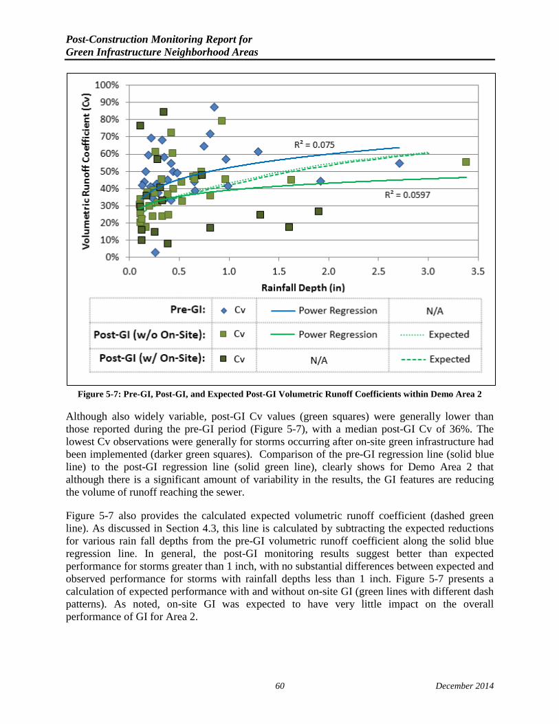
Post-Construction Monitoring Report for Green Infrastructure Neighborhood Areas
Figure 5-7: Pre-GI, Post-GI, and Expected Post-GI Volumetric Runoff Coefficients within Demo Area 2
Although also widely variable, post-GI Cv values (green squares) were generally lower than those reported during the pre-GI period (Figure 5-7), with a median post-GI Cv of 36%. The lowest Cv observations were generally for storms occurring after on-site green infrastructure had been implemented (darker green squares). Comparison of the pre-GI regression line (solid blue line) to the post-GI regression line (solid green line), clearly shows for Demo Area 2 that although there is a significant amount of variability in the results, the GI features are reducing the volume of runoff reaching the sewer.
Figure 5-7 also provides the calculated expected volumetric runoff coefficient (dashed green line). As discussed in Section 4.3, this line is calculated by subtracting the expected reductions for various rain fall depths from the pre-GI volumetric runoff coefficient along the solid blue regression line. In general, the post-GI monitoring results suggest better than expected performance for storms greater than 1 inch, with no substantial differences between expected and observed performance for storms with rainfall depths less than 1 inch. Figure 5-7 presents a calculation of expected performance with and without on-site GI (green lines with different dash patterns). As noted, on-site GI was expected to have very little impact on the overall performance of GI for Area 2.
60 December 2014

Post-Construction Monitoring Report for Green Infrastructure Neighborhood Areas Average volumetric runoff coefficients based on storm depth also demonstrate a reduction in runoff reaching the sewer for storms with depths below 1 inch (Figure 5-8). Overall analyses of Cv results suggest that a 21% ([48% - 38%] / 48%) reduction in runoff reaching the sewer was realized for storms with depths below 1 inch. A larger reduction in runoff volume was evident for storms larger than 1 inch; however, this result may be due in part to the limited number of storms meeting that criterion.
Figure 5-8: Average Volumetric Runoff Coefficient based on Storm Depth with 95%
Confidence Intervals Shown
5.1.3. Demonstration Area 3 – Newtown Creek
Within Demo Area 3, there were 49 storms during the pre-GI monitoring period and 26 storms during the post-GI period. Storm depths were generally similar between the two periods, although there were more large storms after GI implementation (Figure 5-9). The median pre-GI storm depth was about 0.39 inches and the post-GI storm depth was similar at about 0.31 inches. The 90th percentile pre-GI rainfall depth was about 1 inch, which is typical of the long term rainfall statistics for NYC. The 90th percentile storm depth during the post-GI period was higher at close to 1.7 inches. Conversely, peak storm intensities were observed to be higher than those in the pre-GI period (Figure 5-10). Although median peak intensities only differed by 0.12 in/hr, maximum intensities were 1.44 in/hr higher in the pre-GI period.
48% 53%
38% 34%
0%
10%
20%
30%
40%
50%
60%
70%
<1"
>1"
Volu
met
ric R
unof
f Coe
ffic
ient
(Cv)
Storm Depth Range (in)
Pre-GI Post-GI
61 December 2014
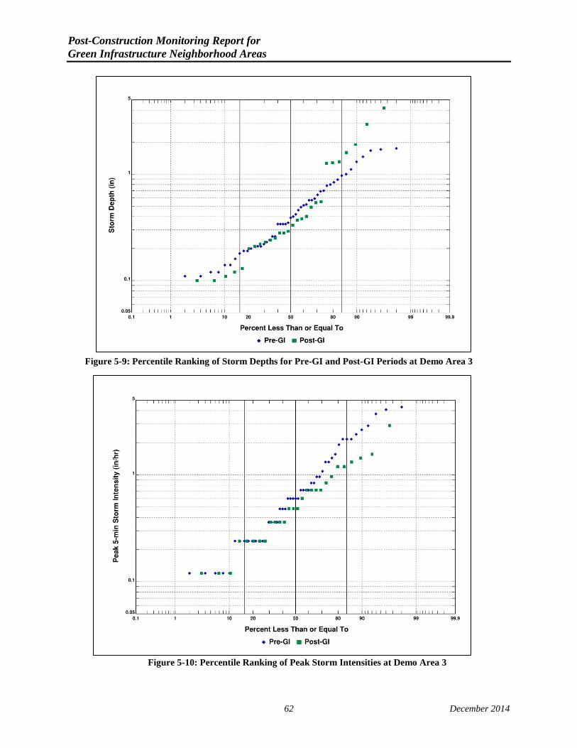
Post-Construction Monitoring Report for Green Infrastructure Neighborhood Areas
Figure 5-9: Percentile Ranking of Storm Depths for Pre-GI and Post-GI Periods at Demo Area 3
Figure 5-10: Percentile Ranking of Peak Storm Intensities at Demo Area 3
Percent Less Than or Equal to Storm Depth
Percent Less Than or Equal to Peak 5-min Storm Intensity
62 December 2014
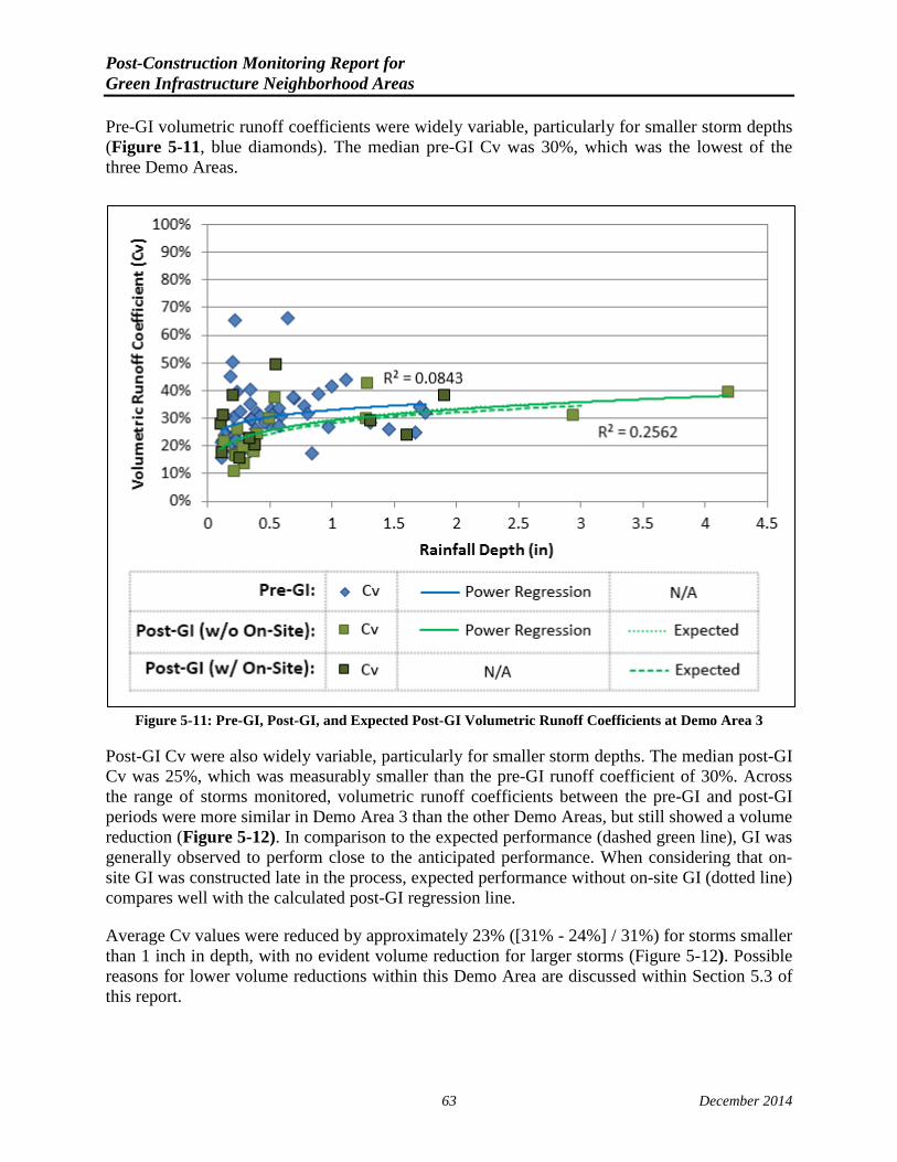
Post-Construction Monitoring Report for Green Infrastructure Neighborhood Areas Pre-GI volumetric runoff coefficients were widely variable, particularly for smaller storm depths (Figure 5-11, blue diamonds). The median pre-GI Cv was 30%, which was the lowest of the three Demo Areas.
Figure 5-11: Pre-GI, Post-GI, and Expected Post-GI Volumetric Runoff Coefficients at Demo Area 3
Post-GI Cv were also widely variable, particularly for smaller storm depths. The median post-GI Cv was 25%, which was measurably smaller than the pre-GI runoff coefficient of 30%. Across the range of storms monitored, volumetric runoff coefficients between the pre-GI and post-GI periods were more similar in Demo Area 3 than the other Demo Areas, but still showed a volume reduction (Figure 5-12). In comparison to the expected performance (dashed green line), GI was generally observed to perform close to the anticipated performance. When considering that on-site GI was constructed late in the process, expected performance without on-site GI (dotted line) compares well with the calculated post-GI regression line.
Average Cv values were reduced by approximately 23% ([31% - 24%] / 31%) for storms smaller than 1 inch in depth, with no evident volume reduction for larger storms (Figure 5-12). Possible reasons for lower volume reductions within this Demo Area are discussed within Section 5.3 of this report.
63 December 2014
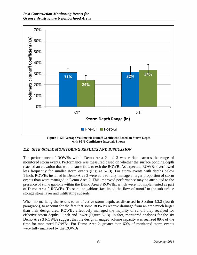
Post-Construction Monitoring Report for Green Infrastructure Neighborhood Areas
Figure 5-12: Average Volumetric Runoff Coefficient Based on Storm Depth
with 95% Confidence Intervals Shown
5.2. SITE-SCALE MONITORING RESULTS AND DISCUSSION
The performance of ROWBs within Demo Area 2 and 3 was variable across the range of monitored storm events. Performance was measured based on whether the surface ponding depth reached an elevation that would cause flow to exit the ROWB. As expected, ROWBs overflowed less frequently for smaller storm events (Figure 5-13). For storm events with depths below 1 inch, ROWBs installed in Demo Area 3 were able to fully manage a larger proportion of storm events than were managed in Demo Area 2. This improved performance may be attributed to the presence of stone gabions within the Demo Area 3 ROWBs, which were not implemented as part of Demo Area 2 ROWBs. These stone gabions facilitated the flow of runoff to the subsurface storage stone layer and infiltrating subsoils.
When normalizing the results to an effective storm depth, as discussed in Section 4.3.2 (fourth paragraph), to account for the fact that some ROWBs receive drainage from an area much larger than their design area, ROWBs effectively managed the majority of runoff they received for effective storm depths 1 inch and lower (Figure 5-13). In fact, monitored analyses for the six Demo Area 3 ROWBs suggest that the design managed volume capacity was realized 89% of the time for monitored ROWBs. For Demo Area 2, greater than 60% of monitored storm events were fully managed by the ROWBs.
31% 32%
24%
34%
0%
10%
20%
30%
40%
50%
60%
70%
<1" >1"
Volu
met
ric R
unof
f Coe
ffic
ient
(Cv)
Storm Depth Range (in)
Pre-GI Post-GI
64 December 2014

Post-Construction Monitoring Report for Green Infrastructure Neighborhood Areas
Figure 5-13: Portion of Monitored Storm Events Fully Managed by ROWBs
Within Demo Area 2, the surface storage capacity was utilized to a greater extent than the subsurface storage capacity, suggesting that surface infiltration was a limiting factor (Figure 5-14). The data indicated that for half of the monitored storms, only 10% of subsurface storage was utilized, while 90% of surface ponding storage was utilized. This finding is indicative of the fact that the engineered soil was limiting the ability for runoff to get to the subsurface storage and infiltration zones.
57% 70%
33% 26%
0%
10%
20%
30%
40%
50%
60%
70%
80%
90%
100%
Area 2Storms <= 1"
Area 3Storms <= 1"
Area 2Storms > 1"
Area 3Storms > 1"
Stor
ms F
ully
Man
aged
Actual Storm Depth Effective Storm Depth
64%
89%
28%
51%
65 December 2014

Post-Construction Monitoring Report for Green Infrastructure Neighborhood Areas
Figure 5-14: Box Plots of Surface and Subsurface Storage Capacity Utilized within Demo Area 2
(25, 50 and 75th Percentiles)
For the ROWBs monitored in Area 3, the results were different (Figure 5-15). Storms with depths below 1 inch utilized between 7% and 72% of the available subsurface storage capacity, with a median of 40%. Surface storage was found to be utilized between 10% and 100%, with a median of 41%. Subsurface storage capacity was utilized to a greater extent for larger storm events, suggesting that more water was able to reach the subsurface layer when surface storage capacity was frequently exceeded.
Within Demo Area 3, the surface storage capacity was filled less frequently than in Demo Area 2, while the subsurface storage was utilized to a greater extent (Figure 5-15). This result is likely indicative of the hydrologic benefit provided by the stone gabions. Although more runoff storage was realized in the subsurface layers, there were few instances where ROWBs appeared to be fully saturated.
The median monitored surface drawdown rate was approximately 1 in/hr for Demo Area 2 (Figure 5-16). Because Demo Area 2 ROWBs did not include stone gabions, this drawdown performance is likely indicative of the effective infiltration rate of the installed engineered soil. Within Demo Area 3, surface drawdown rates were substantially higher. These higher rates demonstrate the benefit of including a stone gabion to hydraulically connect surface storage with the open-graded stone base, while also indicating that the stone gabion did not have an unlimited hydraulic capacity.
0%
10%
20%
30%
40%
50%
60%
70%
80%
90%
100%
Surface StorageStorms <1"
SubsurfaceStorage
Storms <1"
Surface StorageStorms >1"
SubsurfaceStorage
Storms >1"
Capa
city
Util
ized
Durin
g St
orm
Eve
nt
Storms >1" Storms <1"
66 December 2014

Post-Construction Monitoring Report for Green Infrastructure Neighborhood Areas
Figure 5-15: Box Plots of Surface and Subsurface Storage Capacity Utilized within Demo Area 3 (25, 50 and 75th Percentiles)
Figure 5-16: Box Plots of Monitored Surface Drawdown Rates for ROWBs within Demo Areas 2 and 3 (25, 50 and 75th Percentiles)
0
1
2
3
4
5
6
7
8
Demo Area 2 Demo Area 3
Surf
ace
Draw
dow
n Ra
te (i
n/hr
)
0
1
2
3
4
5
6
7
8
Demo Area 2 Demo Area 3
Surf
ace
Draw
dow
n Ra
te (i
n/hr
)
0%
10%
20%
30%
40%
50%
60%
70%
80%
90%
100%
Surface StorageStorms <1"
SubsurfaceStorage
Storms <1"
Surface StorageStorms >1"
SubsurfaceStorage
Storms >1"
Capa
city
Util
ized
Durin
g St
orm
Eve
nt
Storms <1" Storms >1"
67 December 2014

Post-Construction Monitoring Report for Green Infrastructure Neighborhood Areas
68 December 2014
5.3. MONITORING RESULTS SUMMARY
Results of TDA- and site-scale monitoring within the Demo Areas indicate that GI has provided measurable stormwater management benefits. Specifically, GI practices have reduced the volume of runoff leaving all three of the Demo Areas. Because the volume of runoff generated during a storm event and the ability of GI to manage that runoff is impacted by numerous factors, volumetric runoff coefficients, used to evaluate collective GI performance, varied substantially. However, when examining the central tendencies of these results through regression analyses, GI appeared to reduce the volumetric runoff coefficient by absolute values of between 20 and 23% (Table 5-1). As expected, runoff retention performance was greater for storms with depths of 1 inch or less than storms with depths larger than 1 inch.
Table 5-1: Summary of Sewershed Monitoring Results
Demo Area 1 Demo Area 2 Demo Area 3
Sewershed Analyses
Total Tributary Drainage Area 24.1 ac 22.7 ac 19.3 ac
Impervious Cover* 81% 92% 92% Design Managed Area for 1-inch Rainfall
(% of Total Tributary Drainage Area) 1.2 ac (5.0%) 2.5 ac (11.0%)** 0.9 ac (4.7%)***
Design Managed Area for 1-inch Rainfall (% of Impervious Tributary Drainage Area)
1.2 ac (6.1%) 2.5 ac (12.0%)** 0.9 ac (5.1%)***
Measured Managed Area for 1-inch Rainfall (% of Total Tributary Drainage Area)
3.5 ac (14.5%) 3.9 ac (17.2%) 0.9 ac (4.6%)
Measured Managed Area for 1-inch Rainfall (% of Total Impervious Tributary
Drainage Area)* 3.5 ac (17.9%) 3.9 ac (18.7%) 0.9 ac (5.1%)
Cv Reduction for Storms Equaling 1-inch Rainfall
18% 25% 12%
Average Cv Reduction for 1-inch Rainfall or less
20% 21% 23%
Unconstrained Design Managed Volume for 1-inch Rainfall
4,900 ft3 10,200 ft3** 3,400 ft3***
Constrained Design Managed Volume for 1-inch Rainfall
4,400 ft3 8,900 ft3** 3,200 ft3***
Measured Managed Volume for 1-inch Rainfall
12,700 ft³ 14,300 ft³ 3,200 ft³
Did the GI Meet or Exceed Runoff Management Expectations (Yes or No)
Yes Yes Yes
Did GI Manage 1-inch Runoff Across 10% of Impervious Surfaces across Aggregate Area
from Demo Areas 1, 2 and 3 Yes (14.3%)
*Based on impervious coverage as measured by analysis of multi-spectral infrared satellite imagery. **Excludes on-site GI. Including on-site would increase managed area to 3.0 acres. ***Excludes on-site GI. Including on-site would increase managed area to 1.6 acres.
A clear result of the effect of adding the GI in each Demo Area was to lower the Cv from the drainage areas. Reductions in Cv values generally corresponded with the total managed area for each Demo Area established during GI planning and design for Demo Areas 1 and 2 and even

Post-Construction Monitoring Report for Green Infrastructure Neighborhood Areas exceed expected performance. Demo Area 3 results appeared to approximate the expected performance when only ROWBs are considered and is slightly lower than expectations when on-site GI is included. This difference may have been associated with the fact that on-site GI construction was completed approximately half-way through the post-construction monitoring period.
Reduced Demo Area 3 performance could also have been associated with the distribution of the storm events or the impacts of leaking hydrants. For example ROWBs B-18 and B-18* were observed, on March 2013 and multiple times after that occurrence, to be impacted by a leaking fire hydrant. ROWBs B-12 and B-13 (monitored at site scale) were found to be impacted by a fire hydrant opened repeatedly (almost daily for extended periods) during summer periods. In total, 21% of the Demo Area 3 ROWBs had their performance impacted by hydrant flow.
Site-scale analyses from a limited number of locations showed that ROWBs in Demo Area 2 managed about 64% of the target 1-inch event, while ROWBs in Demo Area 3 that were monitored managed 89% of the target 1-inch event. These results infer that incorporation of the stone gabion into the ROWBs, as was done in the Demo Area 3 ROWBs, improve performance of ROWBs. The improvement observed with the addition of the stone gabion effectively allows water to get from the surface ponding area to the subsurface storage and infiltration zones more rapidly. This was observed in the site-scale data through the evaluation of the use of the subsurface storage zone as well as through the examination of the effective surface drawdown rates. With the stone gabion, the data indicate that effective surface infiltration rates were approximately 6 in/hr for the Demo Area 3 ROWBs compared to about 1 in/hr for the Demo Area 2 ROWBs.
In Demo Area 1, performance could have been impacted somewhat by a change in the groundwater elevation between the time that geotechnical testing was performed and completion of construction, as water was observed within B-40 and B-27 during and after construction of the ROWBs. Possible reasons include surface flow infiltrating from a nearby vegetated area or groundwater slowly seeping from the high bedrock area in the vicinity and accumulating in the ROWBs. Since there is no site-scale monitoring for these ROWBs, it is difficult to determine the exact source (e.g. surface runoff vs groundwater) or assess how this water may have impacted the overall performance of those ROWBs.
69 December 2014

Post-Construction Monitoring Report for Green Infrastructure Neighborhood Areas 6. CONCLUSIONS
Based on the design, construction and testing work conducted within the Neighborhood Demonstration Areas, the following conclusions can be made.
• It was possible to find locations within the Demo Areas to install combinations of ROWBs and on-site GI that can be designed to manage areas that attain the NYC Green Infrastructure Plan goal management of 10% of the CSO impervious areas.
• Runoff coefficients for the storms that were monitored varied widely. However, the measured volumetric runoff coefficients tended to be low in comparison to the high level of impervious cover as measured by the infrared satellite technology. This difference can be attributed to the irregularity of the existing impervious surfaces and local stormwater retention in pavement depressions.
• The overall effect of installing GI practices was a reduction in the volumetric runoff coefficients for areas where practices were constructed.
• Performance of GI varied with individual locations and within larger areas but overall achieved the design goals.
• GI installed in the three Demonstration Areas met the goal of management of 1 inch of rainfall for impervious areas in the aggregate.
• Use of the stone gabions enhanced the performance of ROWBs.
• Median surface drawdown rates exceeding 5 in/hr were attained but there were large variations in the drawdown rates.
The analyses presented herein support the City’s adaptive management approach to GI implementation. With demonstrated performance at the ROWB-site scale and area-wide-TDA scale, GI is expected to serve as a valuable tool in managing stormwater runoff within combined sewer areas throughout New York City. It is anticipated that the realization of these benefits and improved understanding will continue to grow as New York City moves forward with GI implementation in accordance with the milestones of the Order.
70 December 2014

Post-Construction Monitoring Report for Green Infrastructure Neighborhood Areas 7. REFERENCES
New York City Soil Survey Staff. 2005.
New York City Department of Environmental Protection. June 2012. Soil Investigation Report, Right-of-Way Green Infrastructure within 26th Ward Neighborhood Demonstration Area 2.
New York City Department of Environmental Protection. August 2012. Soil Investigation Report, Right-of-Way Green Infrastructure within Hutchinson River Neighborhood Demonstration Area 1.
New York City Department of Environmental Protection. June 2012. Soil Investigation Report, Right-of-Way Green Infrastructure within Newtown Creek Neighborhood Demonstration Area 3.
New York State Department of Environmental Conservation. 2010. New York State Stormwater Design Manual.
71 December 2014

Post-Construction Monitoring Report for Green Infrastructure Neighborhood Areas
APPENDIX A
SOIL INVESTIGATION RESULTS

Post-Construction Monitoring Report for Green Infrastructure Neighborhood Areas
Area 1 – Soil Sampling Results
A-1 December 2014

Post-Construction Monitoring Report for Green Infrastructure Neighborhood Areas
Area 1 – Permeability Results
A-2 December 2014
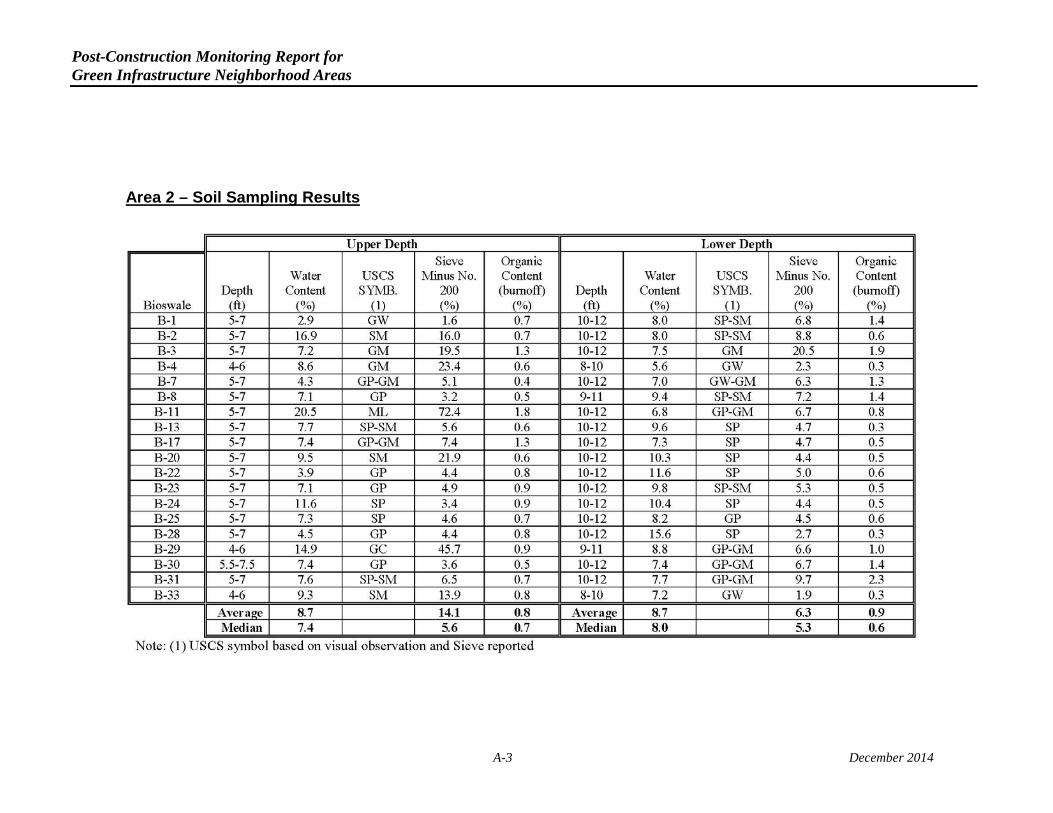
Post-Construction Monitoring Report for Green Infrastructure Neighborhood Areas
Area 2 – Soil Sampling Results
A-3 December 2014

Post-Construction Monitoring Report for Green Infrastructure Neighborhood Areas
Area 2 – Permeability Results
A-4 December 2014

Post-Construction Monitoring Report for Green Infrastructure Neighborhood Areas
Area 3 – Soil Sampling Results
A-5 December 2014

Post-Construction Monitoring Report for Green Infrastructure Neighborhood Areas
Area 3 – Permeability Results
A-6 December 2014

Post-Construction Monitoring Report for Green Infrastructure Neighborhood Areas
APPENDIX B
ROWB CAPACITY CALCULATIONS

Post-Construction Monitoring Report for Green Infrastructure Neighborhood Areas
B-1 December 2014

Post-Construction Monitoring Report for Green Infrastructure Neighborhood Areas
B-2 December 2014

Post-Construction Monitoring Report for Green Infrastructure Neighborhood Areas
B-3 December 2014

Post-Construction Monitoring Report for Green Infrastructure Neighborhood Areas
B-4 December 2014

Post-Construction Monitoring Report for Green Infrastructure Neighborhood Areas
B-5 December 2014

Post-Construction Monitoring Report for Green Infrastructure Neighborhood Areas
B-6 December 2014

Post-Construction Monitoring Report for Green Infrastructure Neighborhood Areas
APPENDIX C
ON-SITE GI DATA AND CALCULATIONS

Post-Construction Monitoring Report for Green Infrastructure Neighborhood Areas 1. ON-SITE NEIGHBORHOOD DEMONSTRATION AREA PROJECTS
In addition to the ROWBs constructed in the Demo Areas, DEP also identified a number of on-site opportunities within public properties where GI could be used to manage runoff through infiltration and detention practices. This Appendix summarizes information on the Demo Area 2 (26th Ward) and Demo Area 3 (Newtown Creek) areas where on-site GI opportunities were implemented; Seth Low Houses and Hope Gardens Houses.
The Seth Low Houses (Figure 1) are located within the southwestern portion of Demo Area 2. A portion of the Seth Low Houses properties is located within to the Demo Area 2 combined sewer system, while runoff from the western portion of the properties is directed in to another portion of the 26th Ward WWTP collection system.
The Hope Gardens Houses (Figure 2) are located at the northern most portion of Demo Area 3. Runoff from impervious surfaces directed runoff to yard drains within the properties that connect to a combined sewer running along the northern boundary of Demo Area 3.
C-1 December 2014

Post-Construction Monitoring Report for Green Infrastructure Neighborhood Areas
Figure 1: Demonstration Area 2 – Seth Low Houses
C-2 December 2014

Post-Construction Monitoring Report for Green Infrastructure Neighborhood Areas
Figure 2: Demonstration Area 3 – Newtown Creek Delineation
C-3 December 2014

Post-Construction Monitoring Report for Green Infrastructure Neighborhood Areas 2. ON-SITE GREEN INFRASTRUCTURE
A range of GI strategies were constructed at these two sites, which included bioretention, pervious pavement, and subsurface storage and infiltration. These strategies are described below.
2.1. BIORETENTION
The bioretention GI practice consists of bioinfiltration, and require specific engineering soil media (for filtering and plant growth), subsurface stone storage layers, a suitable planting plan, inlet pretreatment and energy dissipation, and outlet controls (Figure 3). The specified soil media generally is designed to contain 85-88% sand and 8-12% fines (with less than 5% clay). The organic matter content of the specified soil media is targeted as 3-6% by volume. Aged, well-aerated leaf compost (or an approved equivalent) is a common source used as an amendment to meet the organic matter content. The plant palette chosen for the bioinfiltration areas included a list of native species that tolerate the expected conditions of frequent wetting and drying cycles, maximizes evaporative losses and nutrient uptake, and beautifies the landscape. Pretreatment is provided to prevent excess fine sediment, trash, and debris from entering the bioinfiltration cells. Curb cuts were be used to convey water to the cells. A grouted, cobble energy dissipation flume was included to slow down the water, allow sediment and trash to fall out of solution, and provide diffuse flow of water through the surface area of the cell.
Figure 3: Conceptual Cross-section of Bioinfiltration Facility
Three bioretention systems were constructed at the Hope Gardens Houses.
2.2. PERVIOUS PAVEMENT
Pervious pavement is a GI control that manages stormwater runoff while providing a hard surface for pedestrian or vehicle traffic. There are several varieties of pervious pavement including porous asphalt, permeable interlocking concrete pavements, and porous concrete. In all applications the traffic surface is designed to maintain open and connected pore spaces that transmit flow to a subsurface stone layer, intended to provide structural support and storage for stormwater. During a storm event, water infiltrates through the surface of the pervious concrete into the stone layer, where it can be stored and infiltrate into the soil below. In the absence of an
C-4 December 2014

Post-Construction Monitoring Report for Green Infrastructure Neighborhood Areas underdrain, when the storage capacity of the pervious concrete is exceeded, stormwater would flow across the surface as it would if the surface was impervious. In areas where there is sufficient storage capacity and supporting infiltration rates, pervious pavements can be designed to manage not only direct rainfall, but also runoff from contributing upland areas.
In both locations at the Seth Low Houses, “infiltration skirts” were used for runoff management. These skirts consisted of porous surface materials retrofitted to surround the existing yard inlets. The GI system constructed at one location in the Seth Low Houses consisted of porous concrete panels with stormwater chambers underneath the porous surfaces to provide for additional storage of runoff. Excess runoff was routed to the sewer system via the existing yard inlets. At this location, infiltration trenches were constructed below the bottom of the stormwater chambers to reach soils that had better infiltrating capacity. At a second location, the porous surface media was a commercial product called Flexipave. Subsurface features at this location consisted of the stone storage layer without any stormwater chambers.
The subsurface infiltration facilities constructed at the Seth Low Houses were designed to provide stormwater detention while maximizing the potential for infiltration. Inflow was introduced directly through a pipe to the subsurface storm chambers, which conveyed runoff from an area a 100 feet from the practice areas. Overflow, if any, is conveyed to the existing NYCHA storm sewer by a perforated pipe or overflow pipe. Rain falling directly on to the porous surfaces flows through the surfaces to the stone storage layer below.
2.3. SUBSURFACE STORMWATER CHAMBERS
A parking area at Hope Gardens Houses was retrofitted with a subsurface storage stormwater chamber system. The existing yard inlets were replaced with catch basins with sumps that acted as pretreatment. The inflow was routed through a direct pipe connection to subsurface stormwater chambers. This system was then designed to overflow the excess runoff to the sewer system through a riser pipe. The subsurface stone and stormwater chamber storage system had an open bottom and was designed to infiltrate. Stone storage was provided around the stormwater chambers.
3. BASIS OF DESIGN FOR SETH LOW
The objective of the permeable pavement retrofits at Seth Low was to utilize permeable pavement “skirts” around existing yard inlet drains, infiltrating most runoff prior to reaching the drains. A combination of subsurface gravel beds and stormwater chambers was designed to retain and infiltrate the runoff generated from at least 1 inch of rainfall from the existing impervious surfaces within the individual tributary areas to the infiltration skirts. Any excess runoff will be conveyed to the existing drainage system.
3.1. SIZING CRITERIA
The design was based on infiltration practice sizing taken from the New York State Stormwater Design Manual (NYSDEC, 2010). The system resulting from this design was then checked to assure that the system would handle the targeted NYC Green Infrastructure required equivalent of 1 inch of rain.
C-5 December 2014

Post-Construction Monitoring Report for Green Infrastructure Neighborhood Areas Table 1 summarizes the Seth Low retrofit practices with respect to the runoff generated by the 1-inch rainfall event. For each practice, the impervious area within the tributary area is shown on the location maps. The available practice footprint are also shown.
Table 1: Summary of Contributing Impervious Area and BMP Size
Site Practice
Impervious Area In
Tributary (sf)
Practice Footprints
(sf)
Seth Low
Infiltration skirts (2 locations) 18,940 2,240
Due to the presence of an underground storage tank (UST) at the north end of the site, near location C, a flow diversion structure was used to divert the runoff associated with 1 inch of rainfall from the tributary area to location C shown in Figure 4 to the infiltration skirt area at location B.
Figure 4: Seth Low Houses Site Layout
Flow Diversion
Infiltration Skirts
B A
C
C-6 December 2014

Post-Construction Monitoring Report for Green Infrastructure Neighborhood Areas 3.2. GEOTECHNICAL ANALYSIS
Geotechnical borings from March 2012 at the site illustrate various rates of infiltration, as measured by the falling head permeability test, with depth (see Figure 5 and Table 2). The shallow infiltration test at location B was showed infiltration rates lower than the deeper test, thus in order to maximize infiltration, the system at location B was constructed include infiltration trenches at the bottom of the gravel bed, which will allow the systems to access the higher-infiltration capacity soils at the 10-foot depth without excessive excavation. The trench was lined with geotextile fabric and backfilled with gravel. The gravel bed and stormwater chamber system was constructed on top of the trenches. The test results at location A revealed adequate infiltration capacity at the shallower depth, and so this system will not include infiltration trenches.
Figure 5: Soil borings at Seth Low, March 2012
B
A
C-7 December 2014

Post-Construction Monitoring Report for Green Infrastructure Neighborhood Areas
Table 2: In-Situ Soil Permeability Test Results
Analysis Test 1 Test 2 Test 1 Test 2 Depth 5.0' 5.0' 10.0' 10.0'
Location Rate Rate Rate Rate A 26.7 in/hr 26.4 in/hr 2.9 in/hr 2.6 in/hr B 1.2 in/hr 1.0 in/hr 9.9 in/hr 12.3 in/hr C n/a n/a n/a n/a
3.3. SUBSURFACE INFILTRATION DESIGN
For each of the facilities, the standard criteria adopted for sizing the retention volume was the runoff volume generated by a 1-inch storm event within the tributary area as calculated by the NYS DEC Stormwater Manual approach. This volume was then checked against the 1-inch rainfall the target of the NYC Green Infrastructure Plan.
The stormwater volume associated with 1 inch of rain was calculated as follows:
V = (P)(Rv)(A)/12 Where: V = Runoff volume (in acre-feet) P = 1-inch Rv = 0.05 + 0.009(I), where I is percent impervious cover A = Drainage area (acres)
Only the stormwater volume from 1 inch of rain was considered for sizing the subsurface retention systems and infiltration skirts. Table 3 summarizes the drainage areas, target volumes, available practice footprints and resulting depths for each of the infiltration areas.
Table 3: Practice Area Stormwater Volume Calculation Summary
Area Drainage
Area (ft2)
Runoff Volume from 1" Rain Event
(ft3)
Practice Area (ft2)
Practice Depth (ft)
A 6,555 519 1,259 3.7 B 7,055 559 983 4.7 C
(flow diversion) 5,330 444 Stormwater chamber system
The targeted volume is retained in a combination of the gravel bed, stormwater chambers, and infiltration trenches. The stone utilized for the storage layers of these systems was conservatively assumed to have a porosity of 30% although in practice the void space may provide for higher storage and therefore management of a larger rainfall event.
The following narrative provides the methodology for sizing the subsurface storage volume.
C-8 December 2014

Post-Construction Monitoring Report for Green Infrastructure Neighborhood Areas Area A - Area ‘A’ has a permeable pavement (Flexipave) surface as the primary inlet, and a stone bed storage area. Storage was conservatively calculated below the 8-inch, perforated pipe underdrain, which is set at a depth of 12 inches below the surface for structural stability. Using an average-end-area method for determining the storage volume, the depth of storage was determined to be 3.67 feet:
Volume RequiredA = 519 ft3 Available Area at 1.67-ft depth (bottom of underdrain) = 1,037 ft2 Available Area at 3.67-ft depth (bottom of stone bed) = 798 ft2 Stone Storage Bed Volume = Average Area*Depth*Void Ratio = (1,037+798)/2*2.0*0.3 = 551 ft3 Total volume = 551 ft3 > Volume RequiredA
Area B - Area ‘B’ has a surface consisting of porous concrete panels as the primary inlet, 1:1 side slopes, and a combination stone storage bed and stormwater chamber storage area. The additional runoff routed from Area ‘C’ through a flow diversion structure required the use of the stormwater chambers, which have a higher unit storage volume per square foot than the stone storage bed. The area available for storage is controlled in Area ‘B’ by an existing Sycamore tree critical root zone, and sidewalk limits. Storage was only calculated below the 8-inch, perforated pipe underdrain, which is set at a depth of 12 inches below the surface for structural stability. Using an average-end-area method for determining the storage volume, the required depth of storage was determined to be 4.67 feet:
Volume RequiredB+C = 559 + 444 = 1,003 ft3 Available Area at 1.67-ft depth (bottom of underdrain) = 776 ft2 Available Area at 4.67-ft depth (bottom of stone storage bed) = 460 ft2 Volume available = Average Area * Depth = (776 + 460)/2*3.0 = 1,854 ft3 Stormwater chamber Volume = 75 ft3 * 6 Units = 450 ft3 Stone Storage Vol = (Vol Available–chamber Volume)*Void Ratio = (1,854 – 450)*0.3 = 421 ft3 Infil Trench Vol = Unit Area*Length*Void Ratio
= 3 Units*9 ft3/ft*17 ft * 0.3 voids = 138 ft3 Total storage volume = 450 + 421 + 138 =1,009 ft3 > Volume RequiredB+C
The total volume required was then checked against the Green Infrastructure Plan target of 1-inch rainfall managed.
Volume 1-inch = (6,555 ft2+7,055 ft2+5,330 ft2) *1-inch rainfall * 100% impervious Volume 1-inch = 1,578 ft3 Total available volume = 551 ft3 + 1,009 ft3 =1,560 ft3 ~ Volume 1-inch
C-9 December 2014

Post-Construction Monitoring Report for Green Infrastructure Neighborhood Areas As noted herein, the Seth Low permeable pavement system as designed provides adequate storage volume for the impervious area connected to it to provide for full containment of the 1-inch rainfall event.
The next step in the evaluation was to assess whether the system was capable of infiltrating the 1-inch volume of rainfall between rain events.
For Area A, the infiltration rate was taken as 2.6 in/hr. With a typical time between rainfall of 72 hours for NYC, the native soil should be able to infiltrate 15.6 feet (2.6 in/hr * 72 hours) of water, which is greater than the 1.1 feet of water (3.7 feet practice depth * 0.3 void space) in the stone storage layer easily between rainfall events.
For Area B, the infiltration rate was taken as 9.9 in/hr. With a typical time between rainfall of 72 hours for NYC, the native soil should be able to infiltrate >59.4 feet (9.9 in/hr * 72 hours) of water, which is greater than the 1.4 feet of water (4.7 feet practice depth * 0.3 void space) in the stone storage layer easily between rainfall events.
4. BASIS OF DESIGN FOR HOPE GARDENS
4.1. INTRODUCTION
The Hope Gardens site included three bioretention areas and one subsurface infiltration area to capture and treat stormwater from the impervious areas of the site, as shown in Figure 6. Each of the bioretention facilities employed sidewalk curb cuts to capture stormwater runoff from the surrounding impervious areas. Two of the bioretention areas run in a north-south direction parallel to the existing sidewalk in an existing grassed area (Bioretention 1 and 2). The third bioretention area runs east-west perpendicular to the existing sidewalk on an unused lot and involve the removal of impervious pavement (Bioretention 3). The subsurface detention facility was placed under the existing parking lot at the northern end of the site, and intercepts runoff from the existing stormwater inlets of the parking lot.
4.2. SIZING CRITERIA
The sizing criteria for impervious surface management for Hope Gardens targets the stormwater equivalent of 1 inch of rain. Table 4 describes each practice, the impervious area within the tributary area, as well as the available practice footprint. Sizing calculations are further discussed in the Bioretention Design and Subsurface Detention Design sections.
Table 4: Summary of Contributing Impervious Area and Practice Size
Site Practice Tributary
Impervious Area (sf)
Volume of Runoff from 1” Storm
(ft3)
Practice Footprint (sf)
Hope Gardens Subsurface detention 17,492 1,385 1,000
Bioretention 3 11,639 941 874 Bioretention 1 and 2 3,042 255 556
C-10 December 2014

Post-Construction Monitoring Report for Green Infrastructure Neighborhood Areas
Figure 6: Hope Gardens Drainage Areas and Facility Layout (Hatched Areas)
(Clockwise from top left to bottom, the photos show Bioretention 1 and 2, Bioretention 3, and the Subsurface Facility.)
C-11 December 2014

Post-Construction Monitoring Report for Green Infrastructure Neighborhood Areas 4.3. GEOTECHNICAL ANALYSIS
Four geotechnical soil borings were taken at Hope Gardens in March, 2012 (See Figure 7). The borings included infiltration testing at 5-foot depths for the bioretention areas, and both 5-foot and 10-foot depths for the subsurface detention facility. Soil boring results at HG-1 and HG-2, where the Bioretention 1 and 2 facilities are located, show that sufficient infiltration capacity, 0.5 in/hr and 1.25 in/hr respectively, is available in the native subsurface soils. The testing at HG-3, where the Bioretention 3 facility is located, resulted in poor infiltration capacity at 0.13 in/hr, indicating that the native subsoils are slow to infiltrate runoff and as such an underdrain was included. The results from the 5-foot infiltration test at HG-4, location of the subsurface detention facility, indicated very rapid infiltration rates at 15.9 in/hr. The deeper infiltration test at 10 feet was lower at only 0.12 in/hr. In this case, a surface overflow was included so the system could pass flow, in the event that infiltration had not yet emptied the system.
4.4. BIORETENTION DESIGN
For each of the bioretention facilities, the practice area was determined using the New York State Stormwater Design Manual (NYSDEC, 2010). Sizing is consistent with a filter bed with Manual specified bioretention parameters:
Af = (V)(df)/[(k)(hf+df)(tf)] Where: Af = Surface area of filter bed (ft2) V = Runoff volume (cf) df = Filter bed depth (ft) k = Coefficient of permeability of filter media (ft/day) hf = Average height of water above filter bed (ft) tf = Design filter bed drain time (days)
The filter bed depth, df, was taken as 2 feet for Bioretention 1, 2 and 3, the coefficient of permeability, k, was set to the Manual’s recommended value of 0.5 ft/day for bioretention, the average height of water above the filter bed, hf, was 0.25 feet, and the design filter bed drain time, tf, was the Manual’s recommended value of 2 days.
The runoff generated by a 1-inch storm event was calculated according to the Manual as follows:
V = (P)(Rv)(A)/12 Where: V = Runoff volume (in acre-feet) P = 1-inch Rv = 0.05 + 0.009(I), where I is percent impervious cover A = Drainage area (acres)
The drainage areas for each bioretention cell were estimated based on the site survey (1-foot contours) and from an on-site reconnaissance. Percent impervious was estimated based on the site survey, aerial maps, and an on-site reconnaissance. Drainage areas are shown in Figure 6.
C-12 December 2014

Post-Construction Monitoring Report for Green Infrastructure Neighborhood Areas
Figure 7: Hope Gardens Geotechnical Boring Locations
C-13 December 2014

Post-Construction Monitoring Report for Green Infrastructure Neighborhood Areas Practice footprints are shown in Table 4. Bioretention 1 and 2 are lumped together, as the design will allow any overflows of Bioretention 1 to flow into Bioretention 2. The bottom contour of each bioretention cell was sized to meet the calculated practice footprint, Af, as discussed above.
The engineered soil in the subsurface of the bioretention facilities needs to drain rapidly and support plant material, therefore the specified soil media contains: 85-88% sand, 8-12% silt, and less than 5% clay. The organic matter content of the specified soil media was specified at 3-6% by volume.
The planting palette for the bioretention areas was based on the plant lists for bioretention areas from the Office of Green Infrastructure and the New York City Parks Department, the plant palette for the Bronx River Houses bioretention areas, and New York native plants. The planting design focused on grouping plants to accentuate and respond to the contours of the bioretention facilities, while providing a vegetated backdrop that utilizes native grasses and other flowering herbaceous materials.
The design responds to shade of existing trees with areas of plants that prefer partial shade. Shorter flowering plants were planted closer to the sidewalk and public spaces, framed and backed by taller grasses and flowering plants. Herbaceous materials were chosen to provide seasonal visual appeal from spring to late summer and even into fall with the warm season grasses. Shrubs were used as accent points and to provide seasonal form and appeal in cold-weather months. Accent shrubs included red twig and silky dogwood, as well as spicebush and serviceberry. A new Pin Oak tree was specified in the upland plantings at the far end of Bioretention 3 to provide new canopy cover and increased infiltration and rainwater uptake.
4.5. SUBSURFACE DETENTION DESIGN
The final design approach employed was to size the system for a 1-inch rainfall event with direct connection overflow to the existing sewer manhole. To maximize storage volume while minimizing footprint area, stormwater chambers were used for treatment.
The direct runoff from the parking lot area was used as the basis to size the subsurface detention system. Drainage area of the parking lot is 17,492 ft2, all of which is impervious surface. The runoff volume associated with a 1-inch storm event was calculated according to the Manual as follows:
V = (P) (Rv)(A)/12 = 1-in*0.95*17,492 ft2 / 12 in/ft = 1,385 ft3
The stormwater chambers were sized according to the manufacturer guidance. Each chamber has an internal capacity of 115 cubic feet per chamber when the standard configuration is used (6 inch of stone above and below each chamber, with 9 inch spacing between chambers). In order to store the required volume, the system was designed with 15 chambers, in 3 rows of 5. However, during construction, subsurface utility interferences required reconfiguration of the system in to 2 rows of 7 chambers, totaling 14 stormwater chambers. A cleanout/observation well is added to the pretreatment chambers for access and maintenance.
Volume Storage = 115 ft3 * 14 = 1,610 ft3 > 1-in event
C-14 December 2014