post graduated master course tunnelling and tunnel …€¦ · rmi palmstrom 1995÷÷÷÷2000...
TRANSCRIPT
Post Graduated Master CourseTUNNELLING AND TUNNEL BORING MACHINES
With the support of
Lecturer : Dr. GIORDANO RUSSO Subject of the lesson : GEOMECHANICAL CLASSIFICATIONS
Company / Affiliation : GEODATA ENGINEERING
Endorced by
Academic year 2015-16
EXTRACT

Part Subject Slides n.
I General setting 12
II Earliest classification systems 35
III RMR & RME systems 34
IV Q & Qtbm systems 24
V Rock Mass Index (RMi) 21
VI Geological Strength Index (GSI) 22
VII RMR-Q-RMi comparison 13
VIII Excavation behaviour classification 42 (+5video)
Total 200 (+5video)
Outline of the lesson
EXTRACT

I - General setting (1 di 12)
The design methods of underground constructions can bebasically divided in [7]:
• “analytical ” methods → mainly based on stress/strainanalysis around the cavity (for example: numericalmethods);
• “observational ” methods → mainly based onbehaviour monitoring during excavation, as well as on thethe analysis of ground/support interation (for example, ingeneral terms the NATM);
• “empirical ” methods → mainly based on previousexperiences of tunneling (for example, thegeomechanical classifications)

I - General setting (2 di 12)
The geomechanical classifications developed andwidespread as a design empirical methods with the mainpurpose of [7]:
• subdividing the rock masses in geomechanical groups withsimilar behaviour;• providing a valid base to understand the mechanicalproperties of rock masses;• making the design easier, based on statistical analysis ofprecedent experiences;• assuring a common language between different types oftechnicians involved in the design.
I - General setting (3 di 12)
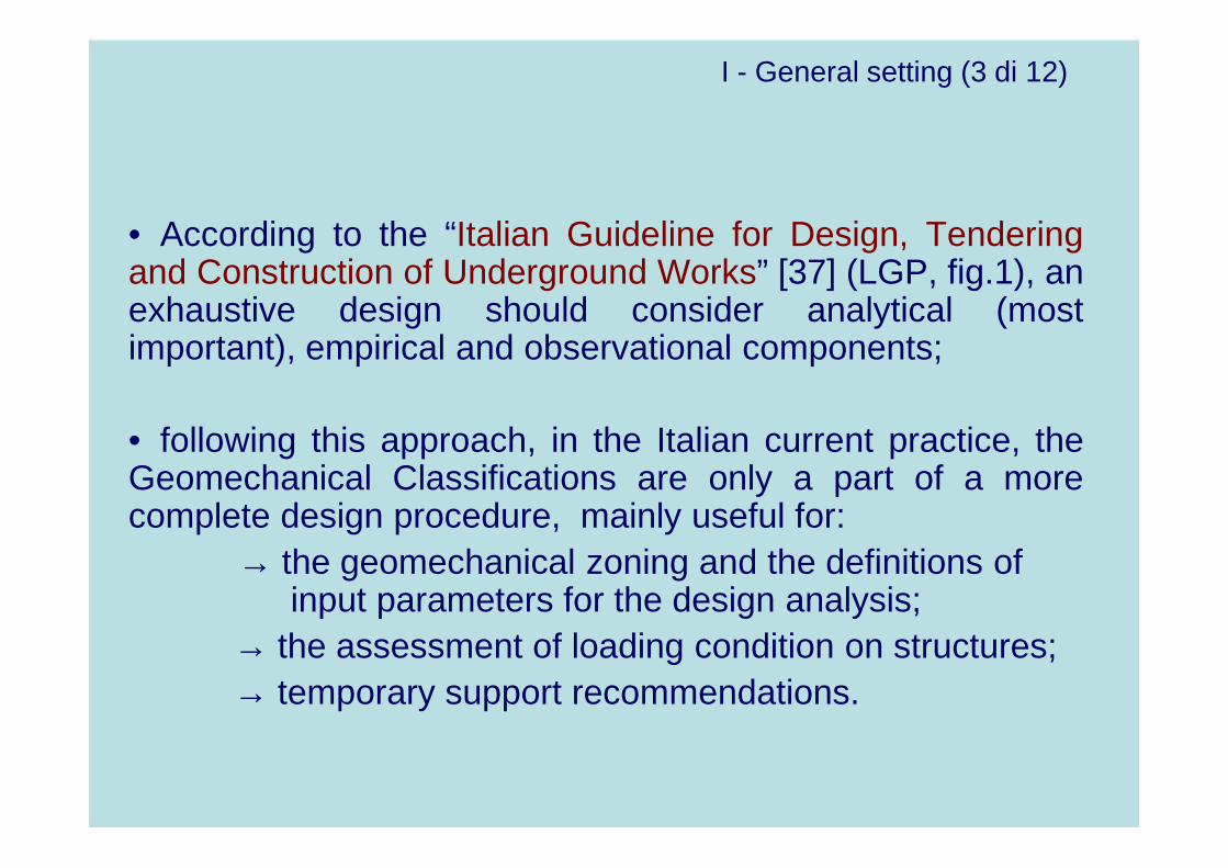
• According to the “Italian Guideline for Design, Tenderingand Construction of Underground Works” [37] (LGP, fig.1), anexhaustive design should consider analytical (mostimportant), empirical and observational components;
• following this approach, in the Italian current practice, theGeomechanical Classifications are only a part of a morecomplete design procedure, mainly useful for:
→ the geomechanical zoning and the definitions of input parameters for the design analysis;
→ the assessment of loading condition on structures;→ temporary support recommendations.

Fig.1
General setting (4 di 12)
Geological survey
Design of auxiliary work and tender documents
F
F1.1,...,F2.2 (9)F1,F2
General settingA
Main themes Key aspects Subjects (n o) Development
A1.1,...,A4.4 (10)A1,..., A4
B B1.1,...,B8.1 (19)B1,..., B8
Prediction of excavation behaviour
D
D1.1,..., ...D4.2 (7)D1,..., D4 D2.1,Assessment of the tunnel face
and contour behaviour
Geotechnical-geomechanical studies
CC1.1,..., ...C3.7 (13)C1,..., C4 C3.5,
Geomechanical classification of the rock masses
Design choices and calculations
EE1.1,..., ...E4.1 (12)E1,..., E4 E1.3, Definition of
section type
Monitoring during construction and operation
G
G1.1,...,G5.2 (16)G1,...,G5 Schematic structure of the ItalianGuideline for Design, Tendering andConstruction of Underground Works
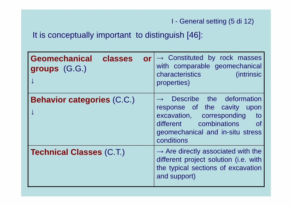
I - General setting (5 di 12)
Geomechanical classes orgroups (G.G.)↓
→ Constituted by rock masseswith comparable geomechanicalcharacteristics (intrinsicproperties)
Behavior categories (C.C.)↓
→ Describe the deformationresponse of the cavity uponexcavation, corresponding todifferent combinations ofgeomechanical and in-situ stressconditions
Technical Classes (C.T.) → Are directly associated with thedifferent project solution (i.e. withthe typical sections of excavationand support)
It is conceptually important to distinguish [46]:

I - General setting (6 di 12)
Main Classification Systems
Method Author Year G.G. C.C. C.T.
Rock loads (T) Terzaghi 1946 (combined system) indications
Stand-up time Lauffer 1958 ÷÷÷÷1988 √√√√ √√√√
RQD system Deere 1964 √√√√ √√√√
RSR system Wickham 1972 √√√√ √√√√
RMR system Bieniawski 1973 ÷÷÷÷1989 √√√√ √√√√
Lombardi Lombardi 1974 √√√√
(R-P) Rabcewicz-Pacher
1974 (combined system) indications
Q system Barton et al. 1974 ÷÷÷÷1999 √√√√ √√√√
Strength-size Franklin 1975 √√√√ √√√√
RMi Palmstrom 1995 ÷÷÷÷2000 √√√√ √√√√
GSI Hoek et al. 1995 ÷÷÷÷2000 √√√√
Adeco-RS Lunardi 1993 √√√√ indications
GD Classification Russo et al. 1998 ÷÷÷÷2007 √√√√ indications

I - General setting (7 di 12)
• As shown previously, (fig.2) the geomechanical classifications ofan underground project can be used as:
- a method of assessment of input geomechanicalparameters (equivalent-continuum model) aboutdesign analysis (→GEO) ;
- an empirical method of design (→PRO)
• Therefore, the choice of the most appropriate GeomechanicalClassification is also a function of the foreseen usage:
- in the first case (→GEO) “purequantitative” system are more advisable [for istance GSI(fabric index) and RMi ];
- in the second case (→PRO) traditional “quantitative”systems are more indicate (such as RMR, Q- System ,and even RMi).

I - General setting (8 di 12)
Fig.2 [46]
CLASSIFICAZIONI GEOMECCANICHE GEOMECHANICAL CLASSIFICATIONS
STRUMENTO PER LA CARATTERIZZAZIONE E ZONAZIONE GEOMECCANICA
“TOOL” FOR THE CHARACTERIZATION AND PROFILE SEGMENTATION INTO GEOMECHANICAL ZONES
"PURE": SI BASANO SOLO SULLA QUALITA' GEOMECCANICA DELLA
MASSA ROCCIOSA "PURE": BASED ONLY ON
GEOMECHANICAL QUALITY OF THE ROCK MASS
"IBRIDE": CONTENGONO
VALUTAZIONI PARAMETRICHE NON INTRINSECHE ALLA MASSA ROCCIOSA
"HYBRID": CONSIST OF EVALUATIONS OF PARAMETERS NON-
INTRINSIC TO THE ROCK MASS
CLASSIFICAZIONI GEOMECCANICHE GEOMECHANICAL CLASSIFICATIONS
METODO EMPIRICO DI PROGETTAZIONE
EMPIRICAL METHODS OF DESIGN
INDIRETTI: LE INDICAZIONI PROGETTUALI DERIVANO DA UNA
CARATTERIZZAZIONE QUALITATIVA E DA UNA CONSEGUENTE VALUTAZIONE DEI
CARICHI INDIRECT : PROJECT SUGGESTIONS
DERIVE FROM A QUALITATIVE EVALUATION AND AN ASSESSEMENT OF LOADS
DIRETTI: LE INDICAZIONI PROGETTUALI DERIVANO DIRETTAMENTE DA UNA
CARATTERIZZAZIONE QUALITATIVA DELLA MASSA ROCCIOSA
DIRECT: PROJECT SUGGESTIONS DERIVE FROM A QUALITATIVE EVALUATION OF THE
ROCK MASS
METODI QUALITATIVI QUALITATIVE METHODS
LE INDICAZIONI PROGETTUALI DERIVANO DA UNA CARATTERIZZAZIONE
QUANTITATIVA ED EVENTUALMENTE DALLA VALUTAZIONE DEI CARICHI
PROJECT SUGGESTIONS DERIVE FROM A QUANTITATIVE CHARACTERIZATION OF THE
ROCK MASS, AND EVENTUALLY FROM EVALUATION OF LOADING CONDITIONS
METODI QUANTITATIVI QUANTITATIVE METHODS
Tradizionali Traditional
RQD (1) Strength-size (2)
GSI (3) RMi (4)
Descrizioni quantitative Qualitative description AFTES (5) SIA 199 (6) ISRM (7)
Terzaghi (8)
RSR (9) Q-System (10) RMR
(11)
Rabcewicz Pacher
(12)
Rock loads (8)
Basati su un solo parametro
Based on one parameter only
Stand-up time (13) RQD (1)
Basati su diversi par. geomecc.
Based on various geomech. param.
RMR (11), RSR (9) Q-System (10)
Strength-size (2)
Raccomandazioni Recommendations
AFTES (5)
Note: (1) Deere, 1964; (2) Franklin, 1975; (3) Hoek, 1994 and Hoek et al., 1995; (4) Palmstrøm, 1996; (5) 1993; (6) 1975; (7) 1981; (8) Terzaghi, 1946; (9) Wickham,1972; (10) Barton et al., 1974, 1994; (11) Bieniawski, 1973, 1989; (12) 1974; (13) Lauffer, 1958, 1988.
Per la bibliografia si veda Russo (1994) - For bibliography refer to Russo (1994)

I - General setting (9 di 12)
T R-P RSR RMR Q RQD GSI RMi
Geomechanicalqualit y ↓
√√√√q- √√√√q- √√√√q+i √√√√q+i √√√√q+i √√√√q+p √√√√q+p √√√√q+p
Rock m ass param eters ↓
√√√√ √√√√ √√√√ √√√√
Evaluation of the loads ↓
√√√√ √√√√ √√√√ √√√√ (√√√√)
Ind icationsabout support
√√√√ √√√√ √√√√ √√√√ √√√√ (√√√√) √√√√
Note: q-/q+=with qualitative/quantitative assessment; p/i = “pure”/ibrid index;() proposed by other authors.

I - General setting (10 di 12)
Geomechanical Classifications limitations (1 of 3):
• As according to Guidelines (LGP), Geomechanicalclassifications cannot be the only means of design,particularly in more detailed phases and for permanentlining definition;
• often a problematic application to weak rocks(>>tendency of a geomechanical over evaluation ofcontinuous rock masses) and/or to structurally complexrock formations (>> difficult parameter definition) [44];
• as an empirical method, they are generally more reliablefor dimensioning radial stabilization measures infractured rock masses, where mainly gravitationalfailures occur;
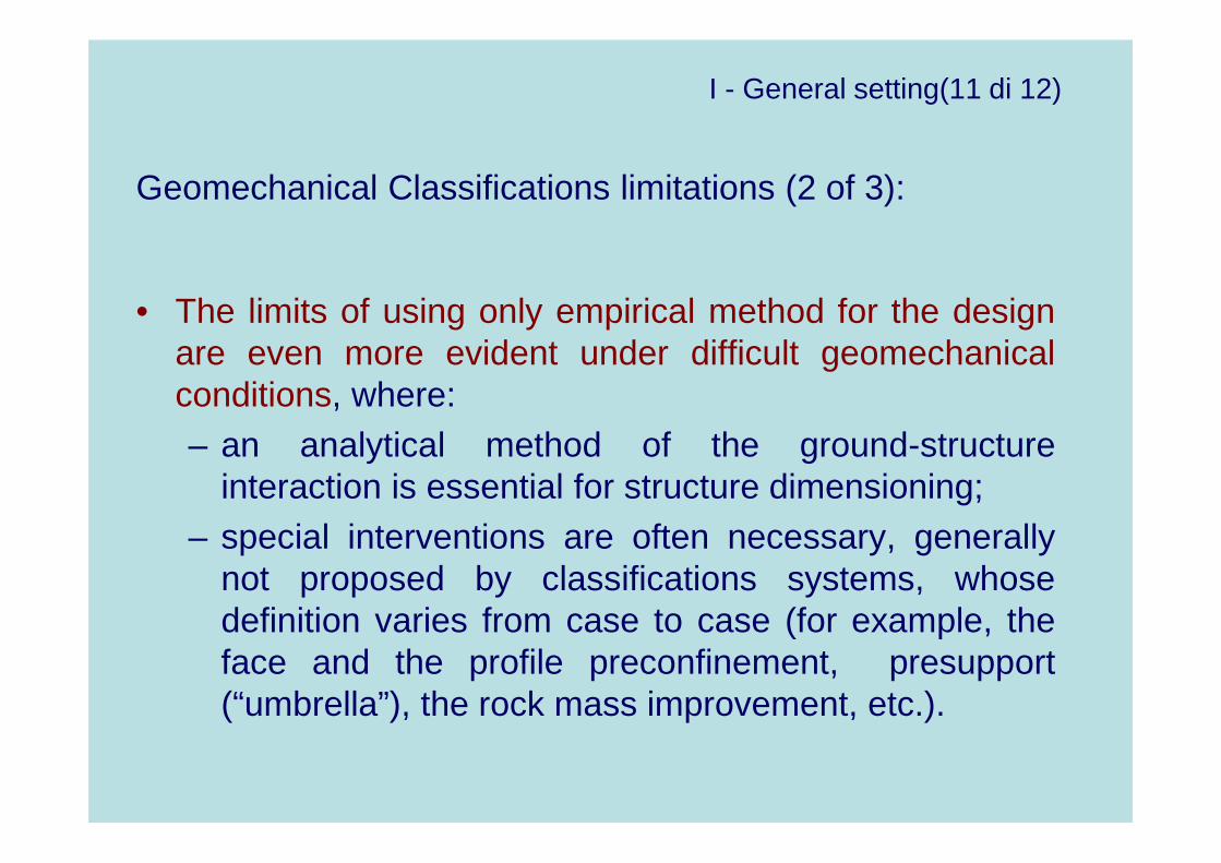
I - General setting(11 di 12)
• The limits of using only empirical method for the designare even more evident under difficult geomechanicalconditions, where:– an analytical method of the ground-structure
interaction is essential for structure dimensioning;– special interventions are often necessary, generally
not proposed by classifications systems, whosedefinition varies from case to case (for example, theface and the profile preconfinement, presupport(“umbrella”), the rock mass improvement, etc.).
Geomechanical Classifications limitations (2 of 3):

•Hoek & Brown (1980) “recommend classification systems forgeneral use in the preliminary design of undergroundexcavations”
•Bieniawski (1997) is of the opinion that “rock massclassifications on their own should only be used forpreliminary, planning purpose and not for final support”
•Stille & Palmstrom (2003) “strongly argued against using theexisting classification systems as the only indicator to definethe rock support or other engineering items”
Geomechanical Classifications limitations (3 of 3):
I - General setting(12 di 12)

II - Empirical methods (PRO) A
QUALITATIVE INDIRECT METHODS
Basic scheme:
Qualitative rock mass characterization →
→ Definitions of structure loads →
→ Support dimensioning

II - Rock Load Classification (PRO→A1)
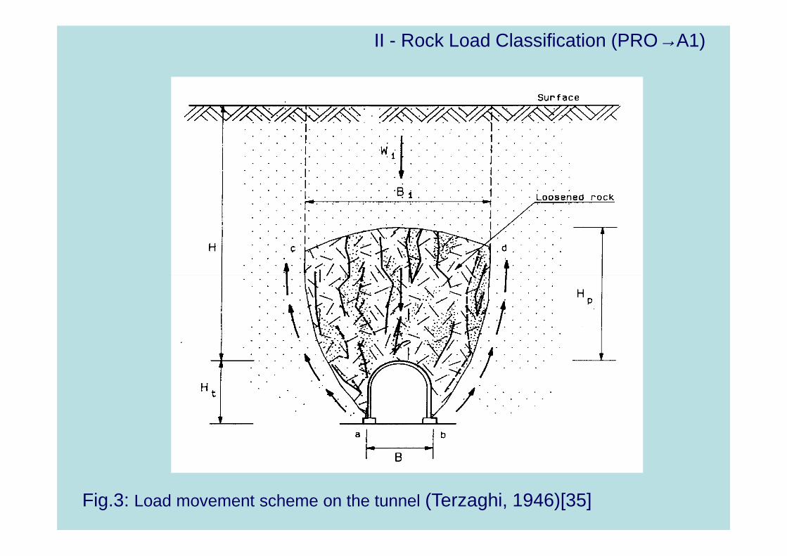
ROCK LOAD CLASSIFICATION (Terzaghi,1946)
Main features:
• Formulated for the assessment of rock loads fordimensioning a support composed by steel ribs;
• N. 9 rock mass classes are defined (fig.4), withcorrelated rock load conditions (function of the tunneldimensions), and indications about the expectedbehavior of the cavity are given;
• the rock load mobilization mechanism is showed in thefigg. 3 and 5;
• the modification proposed by Deere (1970) is presentedin fig.6
II - Rock Load Classification (PRO→A1)
Fig.3: Load movement scheme on the tunnel (Terzaghi, 1946)[35]

Fig.4 [7]


Fig.6 [7]

Esempio Terzaghi
K2
K1
K3
NORD
Tunnel Diameter D = 15m ( ≈≈≈≈49in.) in granite; H=100m; σσσσc = 50-100MPa; RQD = (80)-100% Discontinuity Spacing (2 systems + 1 random) = =0.6-2m ( ≈≈≈≈2-6.5in.)Prevalent System (K1) with dip direction against tunnel advance and dip= 80°, slightly weathered and rough. Dry.
→→→→Terzaghi:
• Massive rock, moderately jointed;
• Rock load H p=0÷÷÷÷0.25D (according Deere H p=0÷÷÷÷ 0.5D)
• Light support to prevent the falling of localized blocks

II - Empirical Methods (PRO) B
QUALITATIVE DIRECT METHODS
Basic scheme:
Rock mass qualitative characterization →
→ Support dimensioning/ Construction phases andprocedures

II - Rabcewicz-P. (PRO→ B1)
RABCEWICZ-PACHER CLA SSIFICATION (1974)Main features• Developed on the system base classification proposed
by Lauffer1 (1958) originating The New AustrianTunnelling Method (NATM)
• n.6 rock classes are considered (fig.7), a qualitativedescription of the characteristics and the behaviour isassociated to applicative procedures and supportdimensioning
• For the mechanized excavation with TBM specificadaptation and development have been arranged, asproposed by the Austrian Norm (ONORM) 2203 (fig.8),furthermore modified in fig.9.
Note: 1 The classified method proposed by Lauffer will be shown in the “ direct quantitative methods” section

Fig.7 [derived from13]
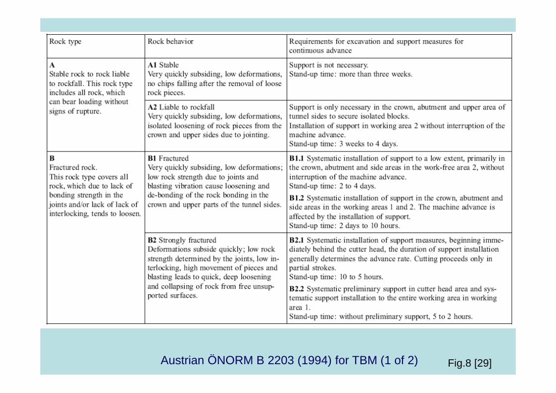
Fig.8 [29]Austrian ÖNORM B 2203 (1994) for TBM (1 of 2)

Austrian ÖNORM B 2203 (1994) for TBM
(2 of 2)
Fig.9 [29]

Esempio Rabcewicz-Pacher
K2
K1
K3
NORD
Tunnel Diameter D = 15m ( ≈≈≈≈49in.) in granite; H=100m; σσσσc = 50-100MPa; RQD = (80)-100% Discontinuity Spacing (2 systems + 1 random) = =0.6-2m (≈≈≈≈2-6.5in.)Prevalent System (K1) with dip direction against tunnel advance and dip= 80°, slightly weathered and rough. Dry.
→→→→ Rabcewicz- Pacher:
• Massive sound rock: Class I (stable);
• Full section excavation, stand-up time of several weeks in the tunnel crown
• Local bolts + mesh in the crown or shotcrete

II - Empirical Methods (PRO) C
QUANTITATIVE DIRECT METHODS
Basic scheme:
Quantitative characterization of rock masses →
→ eventual derivation of geomechanical propertiesand/or load conditions →
→ support dimensioning/ Construction phases andprocedures
There are methods based on a single parameter (such as“Stand-up time” by Lauffer and RQD by Deere) and methodsbased on the definition of more than one parameter (forexample RSR, RMR, Q, RMi)
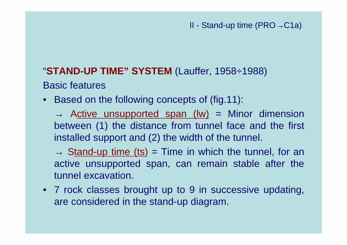
II - Stand-up time (PRO→C1a)
“STAND-UP TIME” SYSTEM (Lauffer, 1958÷1988)Basic features• Based on the following concepts of (fig.11):
→ Active unsupported span (lw) = Minor dimensionbetween (1) the distance from tunnel face and the firstinstalled support and (2) the width of the tunnel.→ Stand-up time (ts) = Time in which the tunnel, for anactive unsupported span, can remain stable after thetunnel excavation.
• 7 rock classes brought up to 9 in successive updating,are considered in the stand-up diagram.

Fig.11 [21]

II - Stand-up time (PRO→C1a)
Features introduced in the up-dating of 1988 (fig.12,13,14):
• The stand-up diagram was modified, introducing thefollowing expression:
tslw2 = 108.9-1.7z
where:z = stand-up coefficient associated to the rock mass characteristics,variable between 0 (superior limit class AA*) and 8 (limit betweenclasses G/H*)
z = (8.9 – logt s - 2logl w)/1.7
• new classes AA* e H*• parallel lines spaced 1.7logts, divide different stand-up
classes• to determine the active unsupported span, a corrective
factor “x” is introduced to consider the three-dimensionalface effect
• also the TBM characteristics are considered (fig.10)

II - RQD System (PRO→C1b / GEO→G1)
RQD SYSTEM (Deere, 1964 and following)Main features• Based on the parameter Rock Quality Designation
(RQD) defining 5 geomechanical classes (fig.15);• Associated with these 5 classes, quantitative indications
about necessary supports, are given, differing traditional and mechanized tunnelling with TBM (fig.16);
• As seen before (fig.6), Deere linked the index RQD toTerzaghi’s classification.

Fig.15 [8]

Limits of RQD as fracturing index Fig.16bis [41quater]
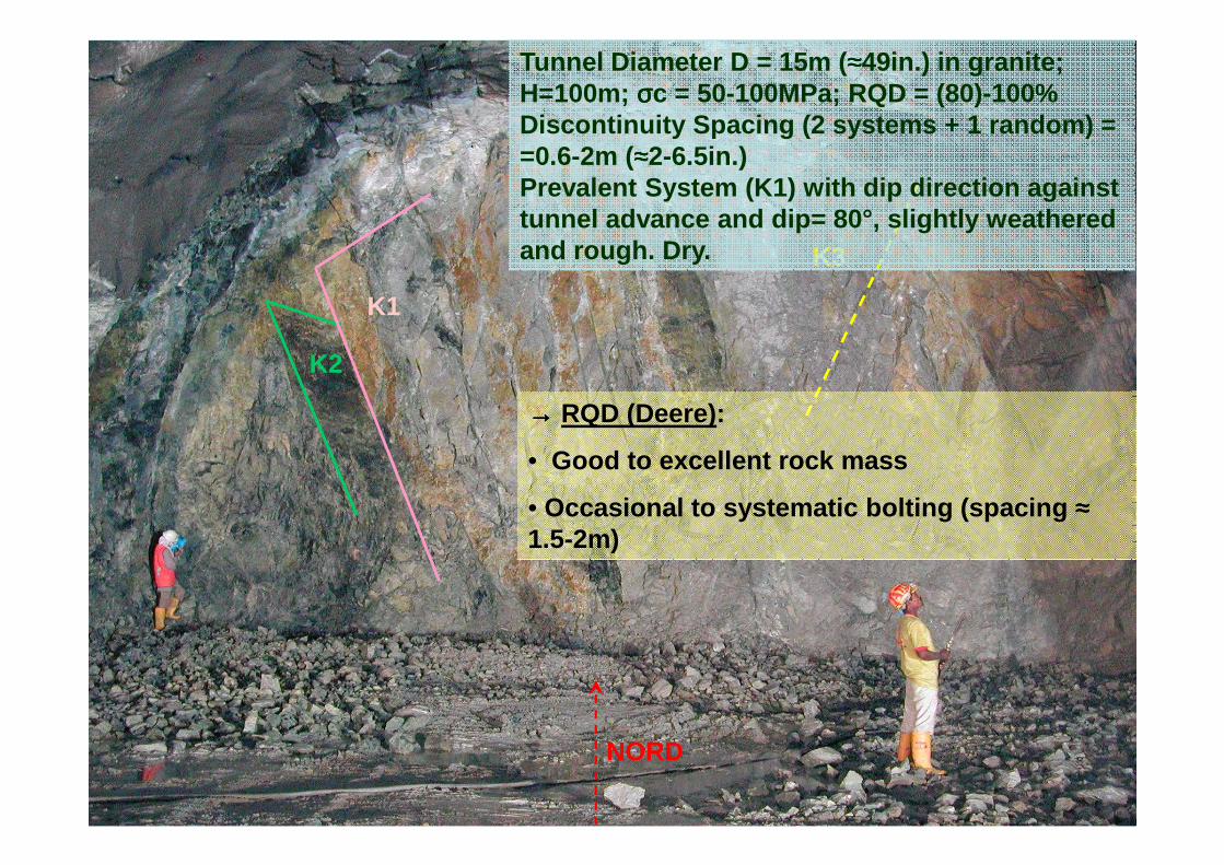
Esempio RQD (Deere)
K2
K1
K3
NORD
Tunnel Diameter D = 15m ( ≈≈≈≈49in.) in granite; H=100m; σσσσc = 50-100MPa; RQD = (80)-100% Discontinuity Spacing (2 systems + 1 random) = =0.6-2m (≈≈≈≈2-6.5in.)Prevalent System (K1) with dip direction against tunnel advance and dip= 80°, slightly weathered and rough. Dry.
→→→→ RQD (Deere):
• Good to excellent rock mass
• Occasional to systematic bolting (spacing ≈≈≈≈1.5-2m)

II - RSR Concept (PRO→C2a)
RSR Concept (Wickham, 1972)
Basic features:• Definition of a rock quality index RSR (Rock Structure
Rating) derived from the sum of three geological andconstructive parameters (fig.17)
RSR = A+B+CA = General area geologyB = Joint pattern, direction of driveC = ground water, joint condition.

Fig.17 [7]

II - RSR Concept (PRO→C2a)
• The method experimentally developed for defining a supportcomposed by steel arches, although there are suggesteddifferent correlations with other supports (bolts andshotcrete).
• To correlate the index RSR to the particular type of support,the "RIB RATIO“ (RR) was defined, so that differentsituations can be compared:RR = [theoretical spacing (Sd)/ real spacing (Sa)] * 100
• Each support with steel arches was related to a theoreticalspacing (Sd, fig.18) calculated using Terzaghi’s expressionto determine the loads in sandy grounds under water table.
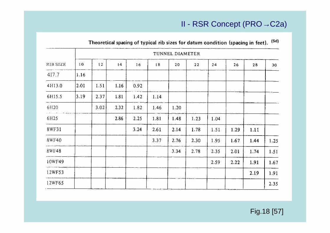
II - RSR Concept (PRO→C2a)
Fig.18 [57]
(Sd)

II - RSR Concept (PRO→C2a)
• Empirically, the following expressions were derived:(RR+ 70)(RSR+8)=6000Wr = (D/302)*RRWr = (D/302)*[(6000/(RSR+8))-70]S =24/Wr
t = 1+Wr/1.25 = D(65-RSR)/150whereWr = rock load (kips/ft2 = 4.882t/m2)D = tunnel diameter (ft) (1ft=0.304m)S = bolting spacing (ft) with elements of 25mmdiameter and design load 24000lb (≈11t)t = shotcrete thickness (ft)
• Using the above formulas, diagrams were derived for thedermination of necessary support fig. 19-20
• In case of use of TBM a correction of the value of RSR isapported, as shown in fig.21.

II - RSR Concept (PRO→C2a)
Fig.19 [13]
←Correlation between RSR, rock load and tunnel diameter
←Steel ribs dimensioning for a tunnel with 3.5m, 6.0m and 9.0m of diameter

II - RSR Concept (PRO→C2a)
Fig.20 [35 ]

Esempio RSR (Wickham)
K2
K1
K3
NORD
Tunnel Diameter D = 15m ( ≈≈≈≈49in.) in granite; H=100m; σσσσc = 50-100MPa; RQD = (80)-100% Discontinuity Spacing (2 systems + 1 random) = =0.6-2m (≈≈≈≈2-6.5in.)Prevalent System (K1) with dip direction against tunnel advance and dip= 80°, slightly weathered and rough. Dry.
→→→→ RSR (Wickham):
• Igneous rock of intermediate strength (Type 2);
• Geological structure: massive to slightly faulted (A = 20-27);
• B = 35 (Blocky to massive & Strike ⊥⊥⊥⊥axis, against dip)
• A+B = 55-62 →→→→ C = 22
• RSR = 77- 85; Wr ≈≈≈≈ 0.5t/m2 →→→→ systematic support not required

III - RMR System (PRO→C2b)
RMR SYSTEM (Bieniawski 1973, 1989)Main features:• Definition of a rock quality index RMR (Rock Mass
Rating) derived from the sum of six geological-geomechanical and constructive parameters (fig.22):
RMR=a+b+c+d+e+f
a intact rock compressive strength
b RQD
c Spacing of discontinuities
d Condition of discontinuities
e Ground water
f Adjustment for discontinuity orientation

Fig.22: General table forRMR ratings [8].
Note:• For a more detailed definitionof the ratings recent diagrams ofthe same Author are used(1989) Fig.23÷27;• when the characteristicconditions of the discontinuitiesresult mutually exclusive (forexample infilling and roughness)use A4 and not E.

III - RMR System (PRO→C2b)
Fig.23 [8]

III - RMR System (PRO→C2b)
Fig.24 [8]
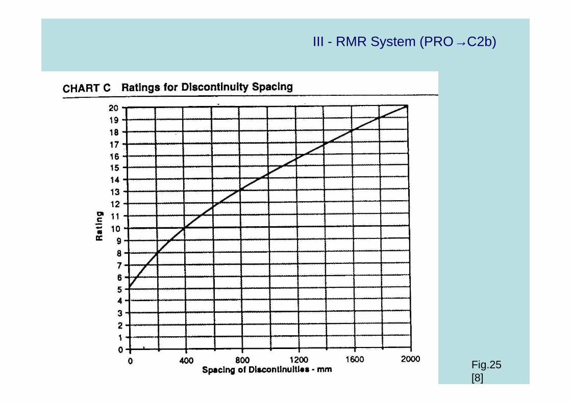
III - RMR System (PRO→C2b)
Fig.25 [8]

III - RMR System (PRO→C2b)
Figura 26 - Abacus for therating for the Bieniawskiclassification to determinespacing parameter, in arock presenting more thanone discontinuity set [inthe example A=0.2m,B=0.5m, C=1m from whichderives a rating of 7.
[8] modified after Laubsher(1981) and Brook andDharmaratne (1985).

III - RMR System (PRO→C2b)
Fig.27 [8]

III - RMR System (PRO→C2b)
Fig. 28: proposeddiagram for thedefinition of therating for the “f”parameter [45]

Fig. 28bis: recently some update was proposed [33b]
rating (Spacing+RQD) =39.94-6.157*landa^0.476 (G.Russo,2014)

III - RMR System (PRO→C2b)
• In function of the RMR values 5 technical classes aredefined from I (very good rock) to V (very poor rock).
• The sum of the first 5 parameters (except “f”) suppliesBMR (Basic Mass Rating), connected to the mainparameters of rock strength and deformability:
c = 5*BMR (kP a)ϕϕϕϕ = 5+BMR/2 (°)Ed = 2*BMR-100 (GPa, per BMR>50)Ed = 10(BMR-10)/40 (1)
Note: (1) The original version of Serafim e Pereira (1983) considered theindex of RMR. Other expressions, proposed for the determination of Hoekand Brown parameters, have been recently made with the GSI index andare regarded in a specific chapter.
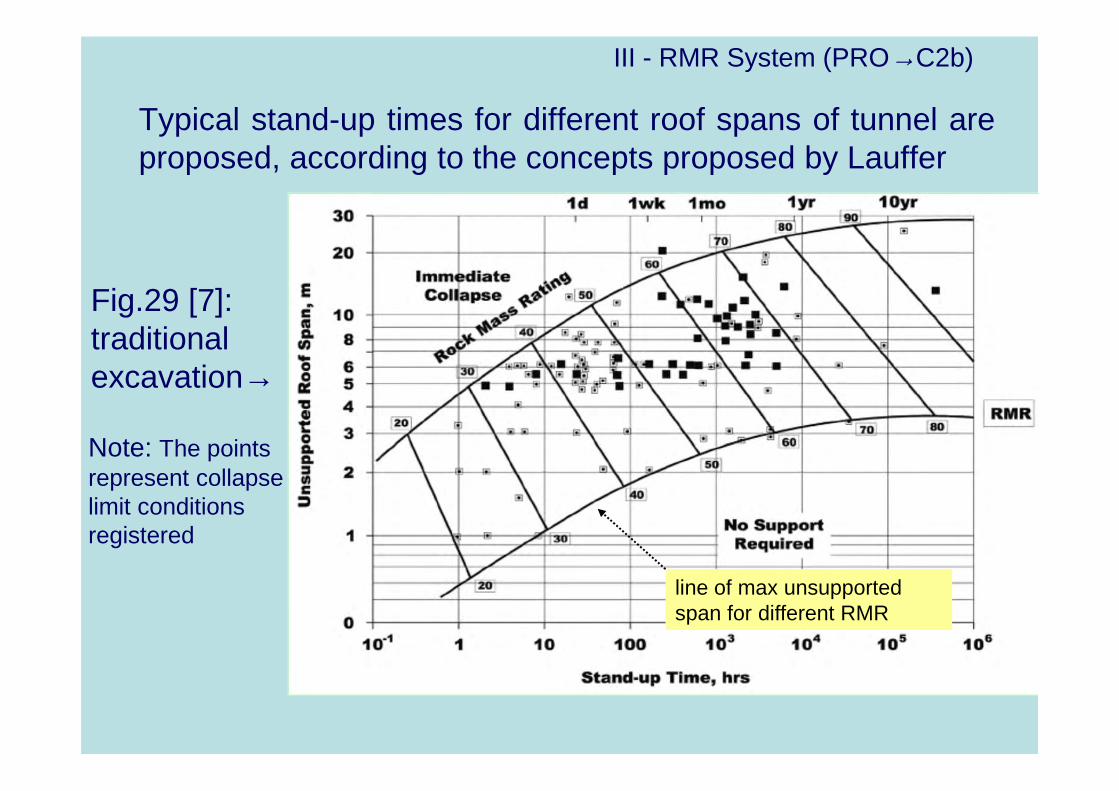
III - RMR System (PRO→C2b)
Typical stand-up times for different roof spans of tunnel areproposed, according to the concepts proposed by Lauffer
Fig.29 [7]: traditional excavation→
Note: The points represent collapse limit conditions registered
line of max unsupported span for different RMR

More properly, the following equation is proposed [10] in combination of the D&B chart: RMRTBM=0.8RMRD&B+20
Anyway this is not on the safe side for RMR<40 and the following is preferred
G. Russo, 2014

III - RMR System (PRO→C2b)
• The load (P) on the support and the active rockheight (ht) can be derived by the following equations(Unal, 1983,[7])
th*B**100
RMR-100P γγ == B*
100
RMR-100ht =
where
B= tunnel width (m)
γ = rock mass density (kg/m3)
In the previously cited update [33b]:

III - RMR System (PRO→C2b)
Associated to each class, quantitative indications about ways oftunnelling and which support is necessary are given (fig.31),with the hypothesis of:• “horse-shoe” shaped tunnel section• tunnel width 10m• vertical stress in situ less than 25MPa• tunnelling with a traditional drill & blast method

III - RMR System (PRO→C2b)
Fig.31 [7]
21

Esempio RMR (Bieniawski)
K2
K1
K3
NORD
Tunnel Diameter D = 15m ( ≈≈≈≈49in.) in granite; H=100m; σσσσc = 50-100MPa; RQD = (80)-100% Discontinuity Spacing (2 systems + 1 random) = =0.6-2m (≈≈≈≈2-6.5in.)Prevalent System (K1) with dip direction against tunnel advance and dip= 80°, slightly weathered and rough. Dry.
→→→→ RMR (Bieniawski):
• a = 7; b = 17-20; c = 15; d = 25; e = 15; f = - 5
• RMR = 74-77 (Class II: good rock)
• Full face: 1-1.5m advance; complete support 20m from the face
• Locally bolts in crown (3m long, spaced 2.5m with occasional wire mesh) and 50mm of shotcrete in crown where required
III - RMR System (PRO→C2b)
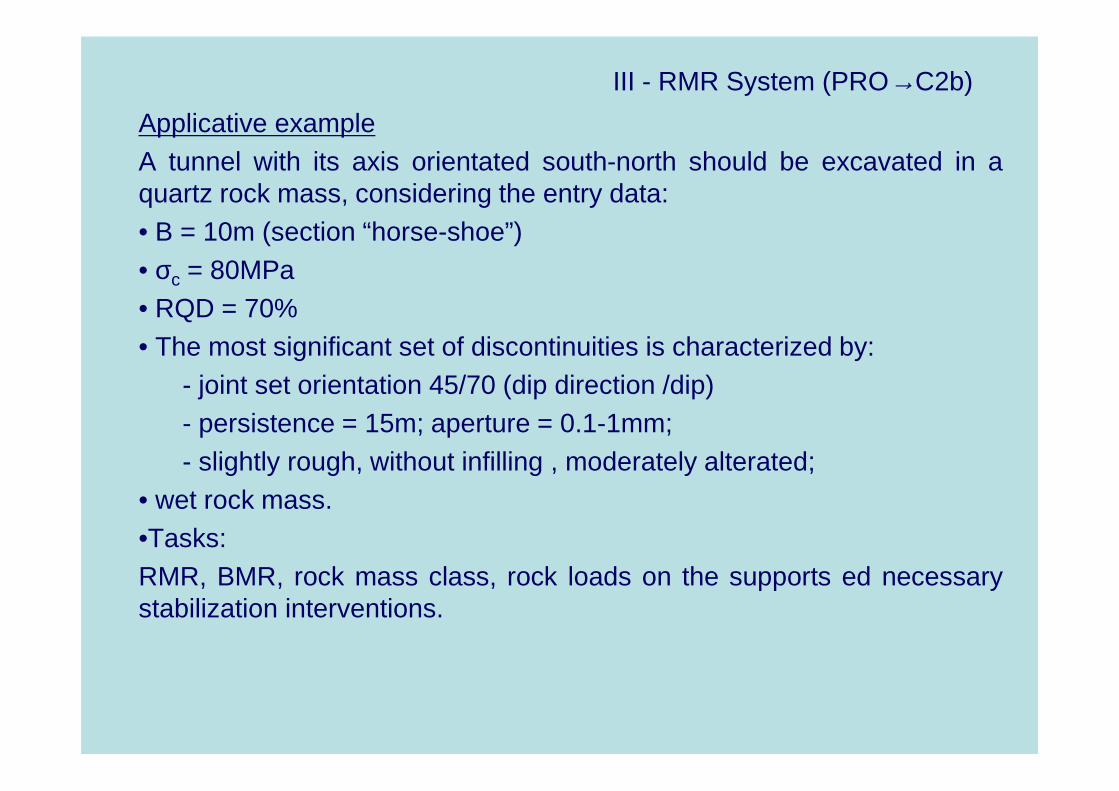
Applicative exampleA tunnel with its axis orientated south-north should be excavated in aquartz rock mass, considering the entry data:• B = 10m (section “horse-shoe”)• σc = 80MPa• RQD = 70%• The most significant set of discontinuities is characterized by:
- joint set orientation 45/70 (dip direction /dip)- persistence = 15m; aperture = 0.1-1mm;- slightly rough, without infilling , moderately alterated;
• wet rock mass.•Tasks:RMR, BMR, rock mass class, rock loads on the supports ed necessarystabilization interventions.

III - RMR System (PRO→C2b)
Parameter Reference Value Rating
a Fig. 23 σσσσc=80MPa 8
b+c Fig. 27 RQD=70% 21
d Fig. 22 1+4+3+6+3
e Fig. 22 wet 7
f Fig. 28 -6
RMR 47
Class III
BMR 53
ht = [(100-RMR)/100]*B 5.3m
Construction assessments (from fig.31):
• Top heading and bench: 1.5-3m advance in top heading;commence support after each blast and complete support 10mfrom the face;
• Support: Systematic bolts (4m long, spaced 1.5-2m in crownand walls, with wire welded mesh in crown) and shotcrete (50-100 /30mm in crown/sides).
Solution

III - RME method (2008)
The Rock Mass Excavability index is calculated on thebasis of the following parameters:
• Uniaxial compressive strength of intact rock• Drillability index• Rock mass discontinuities• Stand-up time• Groundwater inflow
Recently, the Rock Mass Excavability (RME) indexwas proposed by Bieniawski et al. [10bis] forestimating the performance of different types of TBM

III - RME method (2008)
Fig.31a: RME rating system

III - RME method (2008)
Fig.31b: detailed RME
rating system

III - RME method (2008)
Fig.31c: Stand-up time rating

III - RME method (2008)
The following approximate correlation is reported by Palmstrom [40]:DRI≈1000*σc
-0.6 (with σc in MPa)
[10ter]Fig.31d

III - RME method (2008)
Fig.31e: example RMEcalculation (Bieniawski et al. 07)

III - RME method (2008)
• Mainly on the basis of practical experience, the RME indexis correlated to the Average Advance Rate (ARA)
• In particular, one theoretical (t) and one real (r) ARA areconsidered, the latter taking into account some practicalcorrection factors.
• The following correlations have been derived:
TBM type n. σc>45MPa σc<45MPa
Open TBM 49 ARAt=0.839*RME-40.8(R=0.763)→ limitation: no data for RME<35
ARAt=0.324*RME-6.8(R=0.729)
Single Shield 62 ARAt=23*[1-242(45-RME)/17](R=?)
ARAt=10LnRME-13(R=0.784)→limitation: few data for RME<35
Double Shield(using grippers)
225 ARAt=0.422*RME-11.6(R=0.658)
ARAt=0.661*RME-20.4(R=0.867)→ limitation: only for RME>45
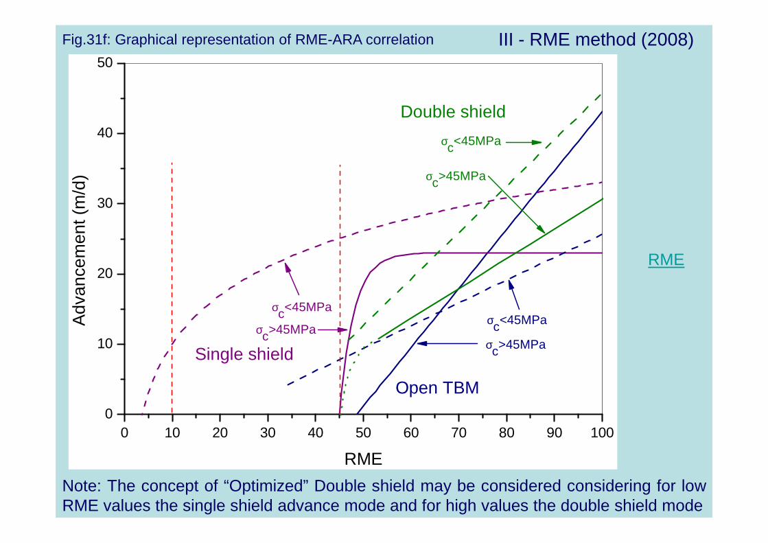
III - RME method (2008)
Note: The concept of “Optimized” Double shield may be considered considering for lowRME values the single shield advance mode and for high values the double shield mode
0 10 20 30 40 50 60 70 80 90 1000
10
20
30
40
50
σc>45MPa
σc<45MPa
σc>45MPa
σc<45MPa
σc>45MPa
Open TBM
Single shield
Adv
ance
men
t (m
/d)
RME
Double shield
σc<45MPa
RME
Fig.31f: Graphical representation of RME-ARA correlation

III - RME method (2008)
The real Average Advance rate is calculated according thefollowing equation:
ARAr= ARAt* FE*FA*FD
Where
FE= factor of crew efficiency = 0.7+FE1+FE2+FE3FA= factor of team adaption to the terrainFD= factor of tunnel diameter
Note: Remember correction in the text

III - RME method (2008)
FE= 0.7+FE1+FE2+FE3
Fig.31g: FE rating
III - RME method (2008)
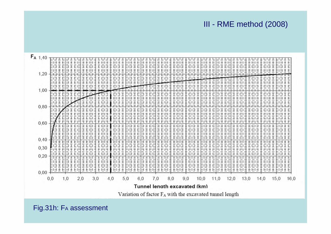
Fig.31h: FA assessment

III - RME method (2008)
Fig.31i: FD assessment

IV: Q-System (PRO→C2c)
Q-SYSTEM (Barton et al., 1974-1999)Main features:• Rock mass quality index Q (variable from 0.001 to
1000) obtained by the following equation:
QRQD
J
J
J
J
SRFn
r
a
w= * *
RQD Rock Quality Designation
Jn joint set number
Jr joint roughness number
Ja joint alteration number
Jw joint water reduction factor
SRF joint stress reduction factor

from Barton, 2006
Q is variable from 0.001 to 1000..
Fig.31 l

IV: Q-System (PRO→C2c)
RQD
Jn
→block size
→ inter-block shear strength
→ active stress
J
Jr
a
J
SRFw
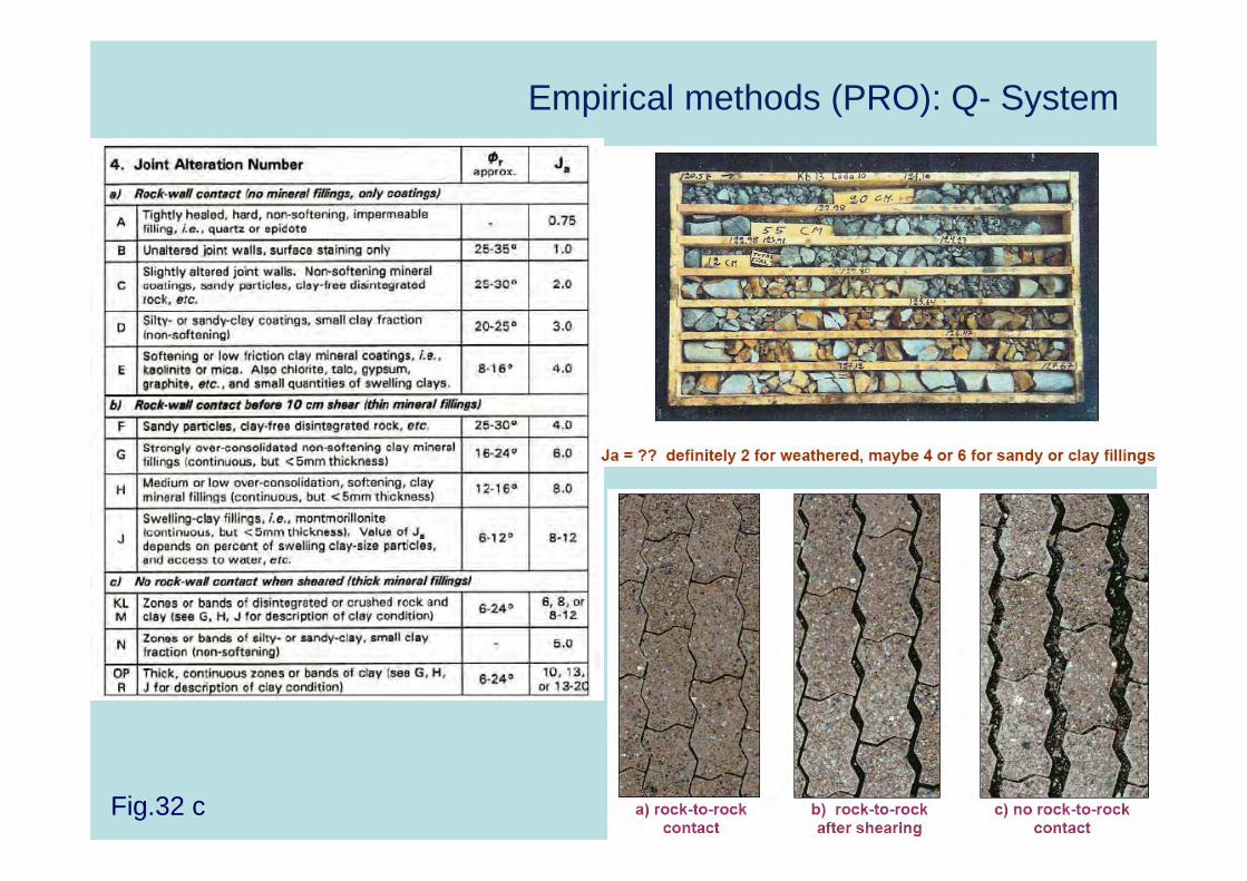
The table on fig. 32 gives the classification of individual parameters used toobtain the Tunnelling Quality Index Q for a rock mass.

Fig.32 [20] : Q-System rating assessment table (1of2)

Empirical methods (PRO): Q- System
Fig.32 a

Empirical methods (PRO): Q-System (Fig.32 b)
Fig.32 b
Empirical methods (PRO): Q- System
Fig.32 c

Empirical methods (PRO): Q- System
Fig.32 d
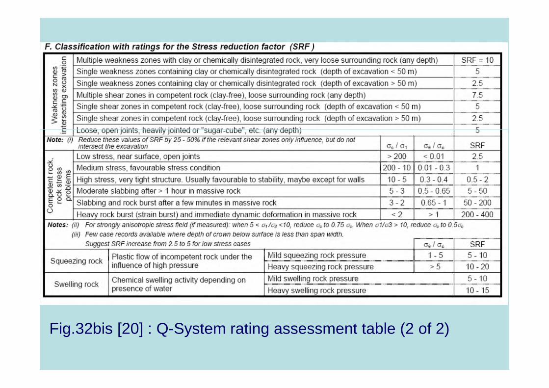
Fig.32bis [20] : Q-System rating assessment table (2 of 2)

IV: Q-System (PRO→C2c)
• 9 classes are distinguished : from a “very poor” rockmass (Q<0.01) to an “excellent” rock mass (Q>400)
• In relating the value of the index Q (fig.34) to the stabilityand support requirements of underground excavations,an additional parameter is defined, called “EquivalentDimension” of excavation, (De)
De = Excavation span, diameter or height (m)/ESRwhere ESR= Excavation Support Ratio, is related to thedegree of security which is demanded and has a similarmeaning to the reciprocate of the safety factor (fig.33)
• For the determination of a temporary support could beused Q(temp)=5Q and ESR(temp)=1.5ESR

IV: Q-System (PRO→C2c)
Fig. 33 [5b]

IV: Q-System (PRO→C2c)
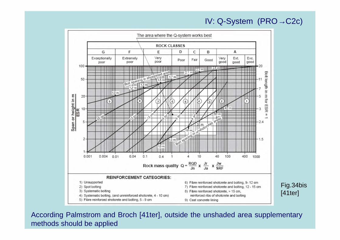
Fig.34 [20]
(50)
IV: Q-System (PRO→C2c)
According Palmstrom and Broch [41ter], outside the unshaded area supplementarymethods should be applied
Fig.34bis [41ter]

IV: Q-System (PRO→C2c)
Empirical correlations with geomechanical parameters (see also fig.35)
Max unsupported span (m) Dmax 2Q0.66
2ESR*Q0.4
Radial pressure acting on support (MPa) Pr ≈0.1Q-1/3
Rock mass deformability modulus (GPa) M ≈10Qc1/3
Longitudinal sismic waves velocity1 P (km/sec) Vp ≈3.5+logQc
Tunnel radial displacement (mm) ∆ ≈ D/Q
Lugeon Unit (U.L.) L ≈1/Qc
Note: Qc= Q*σc/100; σc= intact rock strength (MPa); D = excavationdimension; 1calculated with a refraction method with a maximum depth of25m.
Esempio Q (Barton)
K2
K1
K3
NORD
Tunnel Diameter D = 15m ( ≈≈≈≈49in.) in granite; H=100m; σσσσc = 50-100MPa; RQD = (80)-100% Discontinuity Spacing (2 systems + 1 random) = =0.6-2m (≈≈≈≈2-6.5in.)Prevalent System (K1) with dip direction against tunnel advance and dip= 80°, slightly weathered and rough. Dry.
→→→→ Q (Barton):
• RQD= 90; Jn=6; Jr = 1.5-2; Ja = 2; Jw = 1; SRF = 1
• Q = 11÷÷÷÷ 15 (Good rock mass)
• ESR = 1
• Sistematic Bolting (3-5m long, spaced 2-3m)

IV: Q-System (PRO→C2c)
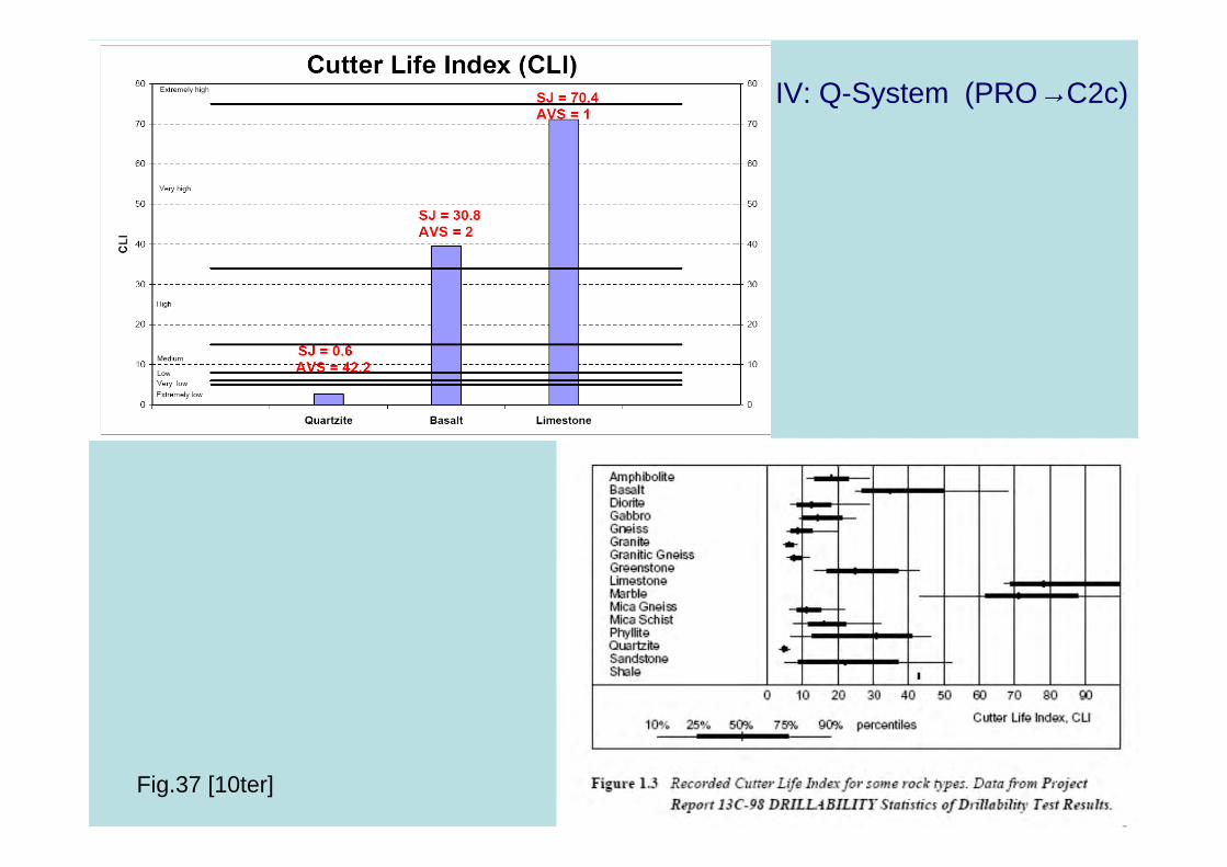
Proposed equation for TBM (figg. 36-37)
5
σ*
20
q*
CLI
20*
/20F
SIGMA*QQ
θ
910oTBM =
Qo = index calculated estimating RQD in the direction of the excavation and referring Jr/Ja to the joint set that mostly influences the tunnel excavation;
SIGMA = rock compressive strength (SIGMAcm=5 γγγγ*Qc1/3) or tensile strength (SIGMAtm=5 γγγγ*Qt1/3), in case ( σσσσc/Is50)>>25 and favorable orientation of the excavation;
Qt=Q*Is50/4 where Is50 is the Point Load Test Index; γγγγ= rock volume weight (g/cm3); F/20 = thrust per cutter (t), normalized against 20;
CLI = Cutter Life Index
q = quartz content (%)
σθσθσθσθ/5 = average bi-axial stresses along the tunnel face MPa, normalized against a value corresponding to 100m depth.

IV: Q-System (PRO→C2c)
Fig.36 [3]
IV: Q-System (PRO→C2c)
Fig.37 [10ter]

IV: Q-System (PRO→C2c)
QTBM is correlated to the TBM advancement parameters
Penetration rate PR (m/h) 5QTBM-0.2
Advance rate AR (m/h) U*PR
Utilisation factor U Tm
Decelaration gradient (negative) m (m/h2) (*)
(*) 0.050.100.150.20 )2n(*)20
q(*)CLI20(*)5
D(*mm 1≈
Q 0.001 0.01 0.1 1 10 100 1000
m1 ≈ -0.9 -0.7 -0.5 -0.22 -0.17 -0.19 -0.21
note: T=time in hours; n = porosity (%)
IV: Q-System (PRO→C2c)
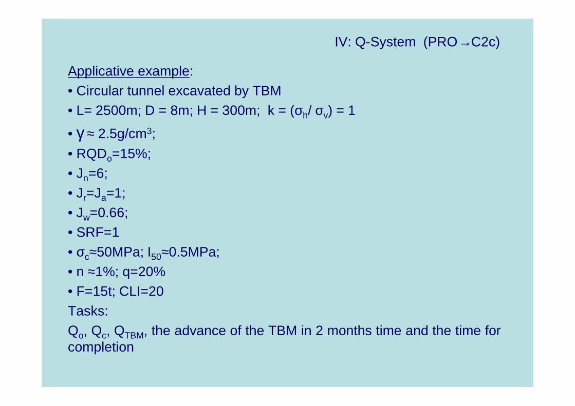
Applicative example:• Circular tunnel excavated by TBM• L= 2500m; D = 8m; H = 300m; k = (σh/ σv) = 1
• γ ≈ 2.5g/cm3;
• RQDo=15%;• Jn=6;• Jr=Ja=1;• Jw=0.66;• SRF=1• σc≈50MPa; I50≈0.5MPa;• n ≈1%; q=20%• F=15t; CLI=20Tasks:Qo, Qc, QTBM, the advance of the TBM in 2 months time and the time forcompletion

IV: Q-System (PRO→C2c)
Parameter Formula Value
Qo (15/6)*(1/1)*(0.66/1) 1.65
σσσσc/I50 50/0.5 100
σσσσθθθθ 2*γ*H = 2*0.025*300 15MPa
Qc Qo*σc /100 0.83
SIGMAcm 5 γ* Qc1/3 12MPa
Qt Qo*I50 /4 0.21
SIGMA tm 5 γ* Qt1/3 7.4MPa
QTBM 1.65*[7.4/(1510/209)]*(20/20)*(20/20)*(15/5) ≈≈≈≈ 33
Result (1 di 2)

IV: Q-System (PRO→C2c)
PR 5QTBM-0.2 = 5*33-0.2 2.5m/h
m1 (from table) -0.20
m -0.20*(8/5)0.20*(20/20)0.15*(20/20)0.10*(1/2)0.05 -0.21
T 2*30*24 1440h
U= Tm 1440-0.21 0.22
AR PR*U = 2.5*0.22 0.55m/h
L(2months) 0.55*1440 792m
T(end) (L/PR)[1/(1+m)] = (2500/2.5)[1/(1-0.21)] 6273h ≈ 9 months
Solution (2 di 2)
- TBM advancement in 2 months (L(2months))
- Completing time (T(end))

Fig.37bis [41ter]
Q_tbm limits: Advance rate for three TBM plotted against Qtbm (Sapigni et al. in 41ter)

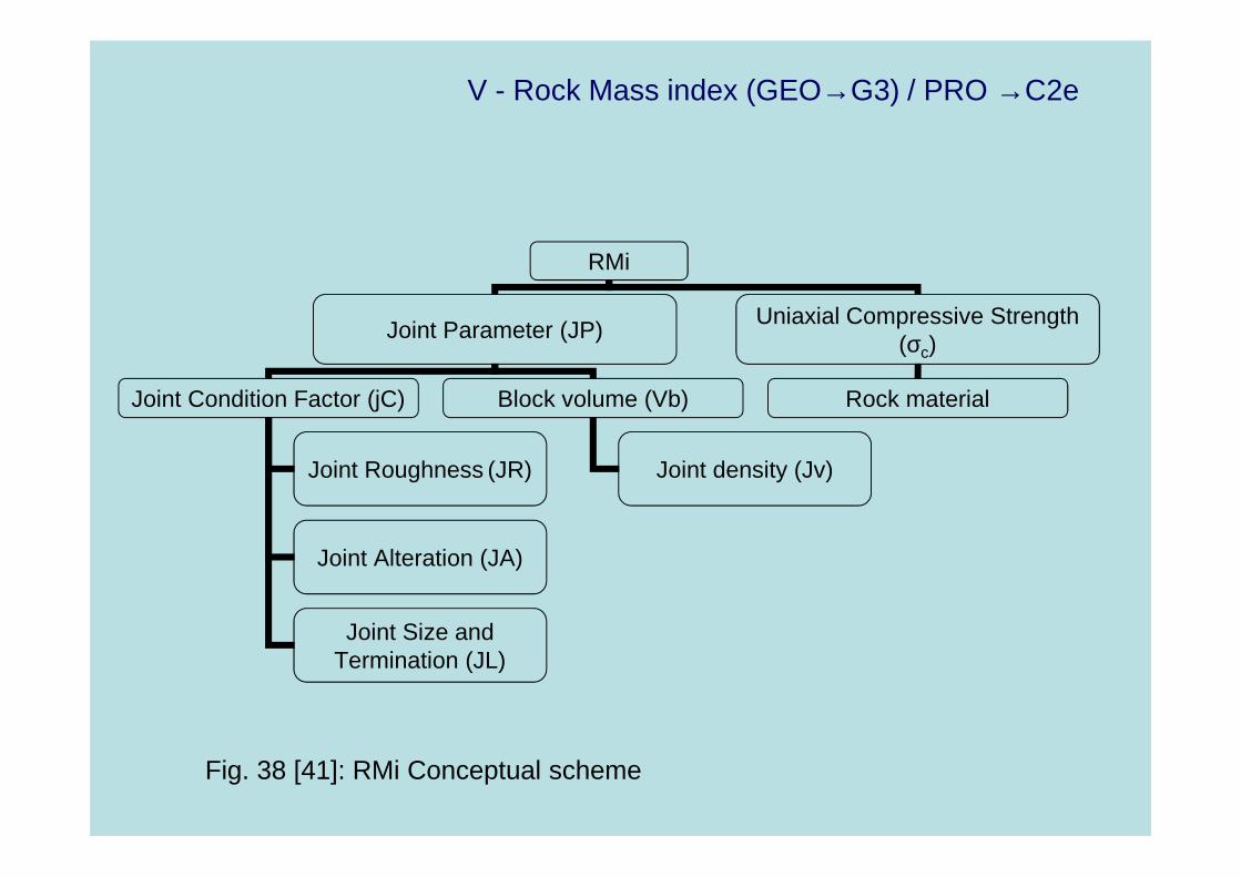
V - Rock Mass index (GEO→G3) / PRO →C2e
ROCK MASS index (RMi, Palmstrom, 1995 ÷÷÷÷2000)• The RMi index expresses the quality and the
geomechanical strength of rock mass (MPa) throughthe multiplication between the uniaxial intact rockcompressive strength (σc) and a corrective factor (JP)depending on the geostructural conditions (fig.38)
→for jointed rock masses (JP< fσ):
JP*σRMi c= Dc Vb*jC0.2*σ=
→ for massive rock masses (JP>fσ):
c0.2
cσc 0.5σ(0.05/Db)σf*σRMi ≈==
V - Rock Mass index (GEO→G3) / PRO →C2e
RMi
Joint Parameter (JP)Uniaxial Compressive Strength
(σc)
Joint Condition Factor (jC) Block volume (Vb)
Joint Roughness (JR)
Joint Alteration (JA)
Joint Size and Termination (JL)
Joint density (Jv)
Rock material
Fig. 38 [41]: RMi Conceptual scheme

V - Rock Mass index (GEO→G3) / PRO →C2e
• JP = Jointing Parameter, correlated to rock blocksize and to discontinuity properties. JP can vary from0 (very fractured rock) to 1 (intact rock).
DVb*jC*0.2JP=
• jC = Joint Condition factor = jL*(jR/jA)• jR = Joint roughness factor, similar to Jr of Q-System• jA = Joint alteration factor, similar to Ja of Q-System• jL = Joint size and continuity factor: reflects the discontinuity
persistence• The criterion for assigning the rating are shown in fig. 40.
0.20.37jCD −=
V - Rock Mass index (GEO→G3) / PRO →C2e
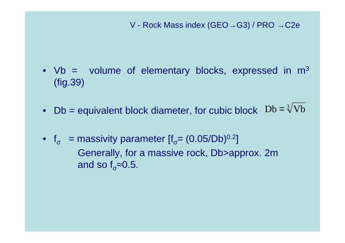
• Vb = volume of elementary blocks, expressed in m3
(fig.39)
• Db = equivalent block diameter, for cubic block
• fσ = massivity parameter [fσ= (0.05/Db)0.2]Generally, for a massive rock, Db>approx. 2mand so fσ≈0.5.
3 VbDb =

V - Rock Mass index (GEO→G3) / PRO →C2e
Fig. 39 [41bis]: Correlations between diameter and volume of the rock block, and other parameters of fracturing
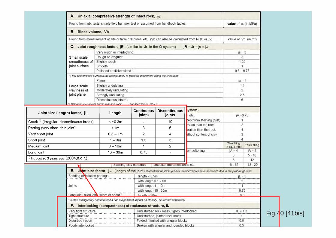
Fig.40 [41bis]
(2004,n.d.r.)

V - Rock Mass index (GEO→G3) / PRO →C2e
RMi [(-) (MPa)] DESCRIPTION (-) ROCK MASS (MPa)
<0.001 extremely low extremely week
0.001-0.01 very low very week
0.01-0.1 low week
0.1-1 moderate medium
1-10 high strong
10-100 very high very strong
>100 extremely high extremely strong

V - Rock Mass index (GEO→G3) / PRO →C2e
Geomechanical correlations
• s =JP2
• mb = mi*JP0.64 (undisturbed rock mass)• mb = mi*JP0.857 (disturbed rock mass)• Ed = 5.6RMi0.375
wheremi, mb, s = Hoek and Brown costants, (1980);
σc , σcm = intact strength, rock mass strengthEd = deformability modulus
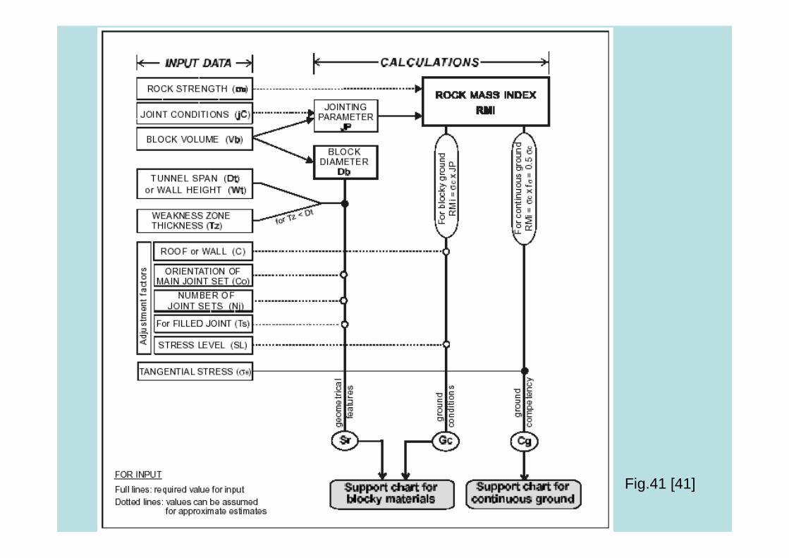
Fig.41 [41]
V - Rock Mass index (GEO→G3) / PRO →C2e
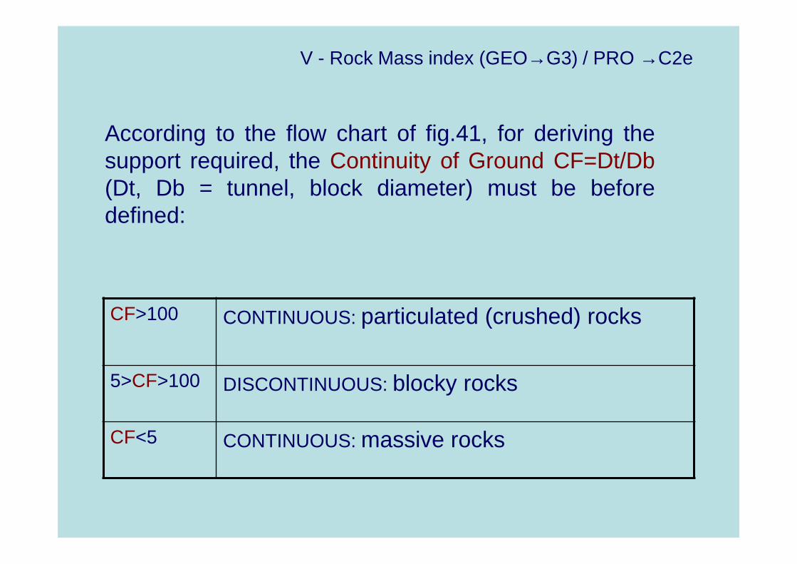
According to the flow chart of fig.41, for deriving thesupport required, the Continuity of Ground CF=Dt/Db(Dt, Db = tunnel, block diameter) must be beforedefined:
CF>100 CONTINUOUS: particulated (crushed) rocks
5>CF>100 DISCONTINUOUS: blocky rocks
CF<5 CONTINUOUS: massive rocks

V - Rock Mass index (GEO→G3) / PRO →C2e
Fig.42 [41]: Instability and rock mass behaviour
V - Rock Mass index (GEO→G3) / PRO →C2e
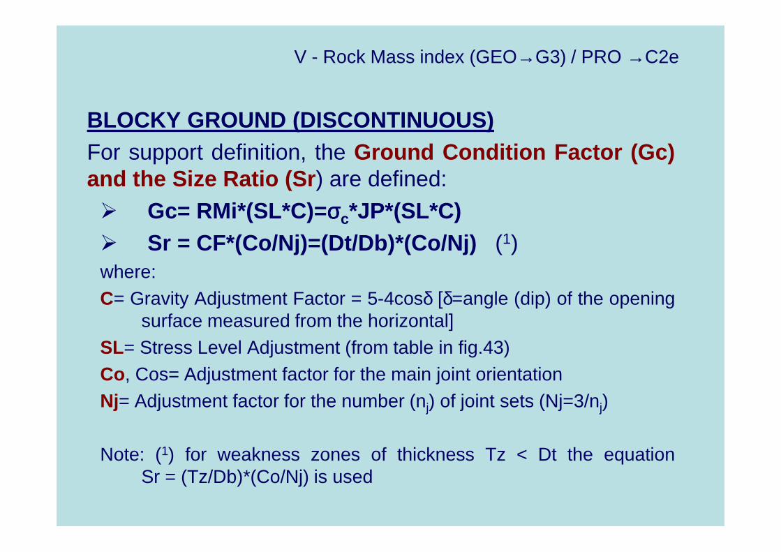
BLOCKY GROUND (DISCONTINUOUS)For support definition, the Ground Condition Factor (Gc)and the Size Ratio (Sr ) are defined:� Gc= RMi*(SL*C)=σσσσc*JP*(SL*C)� Sr = CF*(Co/Nj)=(Dt/Db)*(Co/Nj) (1)where:C= Gravity Adjustment Factor = 5-4cosδ [δ=angle (dip) of the opening
surface measured from the horizontal]SL= Stress Level Adjustment (from table in fig.43)Co, Cos= Adjustment factor for the main joint orientationNj= Adjustment factor for the number (nj) of joint sets (Nj=3/nj)
Note: (1) for weakness zones of thickness Tz < Dt the equationSr = (Tz/Db)*(Co/Nj) is used

V - Rock Mass index (GEO→G3) / PRO →C2e
Fig. 43 [41bis]:

Fig.44 [41]: Rock support chart for blocky groundV - Rock Mass index (GEO→G3) / PRO →C2e

V - Rock Mass index (GEO→G3) / PRO →C2e
Fig.44bis: Example of implementation by probabilistic approach
V - Rock Mass index (GEO→G3) / PRO →C2e
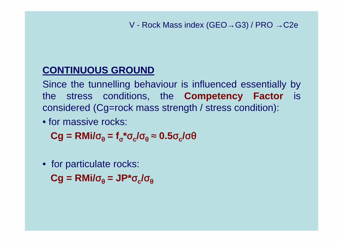
CONTINUOUS GROUNDSince the tunnelling behaviour is influenced essentially bythe stress conditions, the Competency Factor isconsidered (Cg=rock mass strength / stress condition):• for massive rocks:
Cg = RMi/σσσσθθθθ = fσσσσ*σσσσc/σσσσθθθθ ≈≈≈≈ 0.5σσσσc/σθσθσθσθ
• for particulate rocks:Cg = RMi/σσσσθθθθ = JP*σσσσc/σσσσθθθθ

V - Rock Mass index (GEO→G3) / PRO →C2e
Fig. 45 [41bis]: Chart for estimating support in continuous ground

V - Rock Mass index (GEO→G3) / PRO →C2e
Fig. 46 [41]: Recommended application of the support charts

Esempio RMi (Palmstrom)
K2
K1
K3
NORD
Tunnel Diameter D = 15m ( ≈≈≈≈49in.) in granite; H=100m; σσσσc = 50-100MPa; RQD = (80)-100% Discontinuity Spacing (2 systems + 1 random) = =0.6-2m (≈≈≈≈2-6.5in.)Prevalent System (K1) with dip direction against tunnel advance and dip= 80°, slightly weathered and rough. Dry.
→→→→ RMi (Palmtrom):
• σσσσc= 75MPa; jR=2-3; jA= 2; jL= 1, Vb= 0.5m 3;
• RMi= 11.6-14.3 (σσσσcm = 11.6-14.3MPa)
• Nj=1.2; Co= 1.5; SL=C=1; →→→→Gc= 12-14; Sr = 24
• Sistematic Bolts (3-4m long, 1.5-2m spaced) and 50-60mm of shotcrete

V- Table of Comparison
Bolts (L/spacing) m Shotcrete mm
Terzaghi (light localized support)
Rabcewicz-P. Localized + wire mesh (in alternative)
RSR-Concept (no systematic support)
RMR-System 3/2.5 + wire mesh 50 (eventual)
Q-System (3 ÷÷÷÷ 5)/(2 ÷÷÷÷ 3)
RMi (3 ÷÷÷÷ 4)/(1.5 ÷÷÷÷ 2) 50 ÷÷÷÷ 60

VI -Geological Strength Index (GEO→G2)
GEOLOGICAL STRENGTH INDEX (GSI, Hoek et al., 1995 ÷÷÷÷2000)• The GSI is introduced to better represent the rock mass structure, without totake into account other parameters such as intact strength, stress conditions,the orientation of discontinuity, the presence of water, etc.
• Initially, the Authors suggested to derive GSI:→a) from a modified RMR→b) from a modified Q-index
• In the following:→c) from graphs (qualitative assessment: Figg.47,48,49) [26,36]
• More recently, other Authors proposed:→d) from the same graph but with quantitative assessment
(Figg.50a,b) [11]→e) quantitative assessment by the same input parameters for the JP
estimation of RMi system (Figg. 51a,b,c,d,e) [49,50]
GRs
VI - Geological Strength Index (GEO→G2)
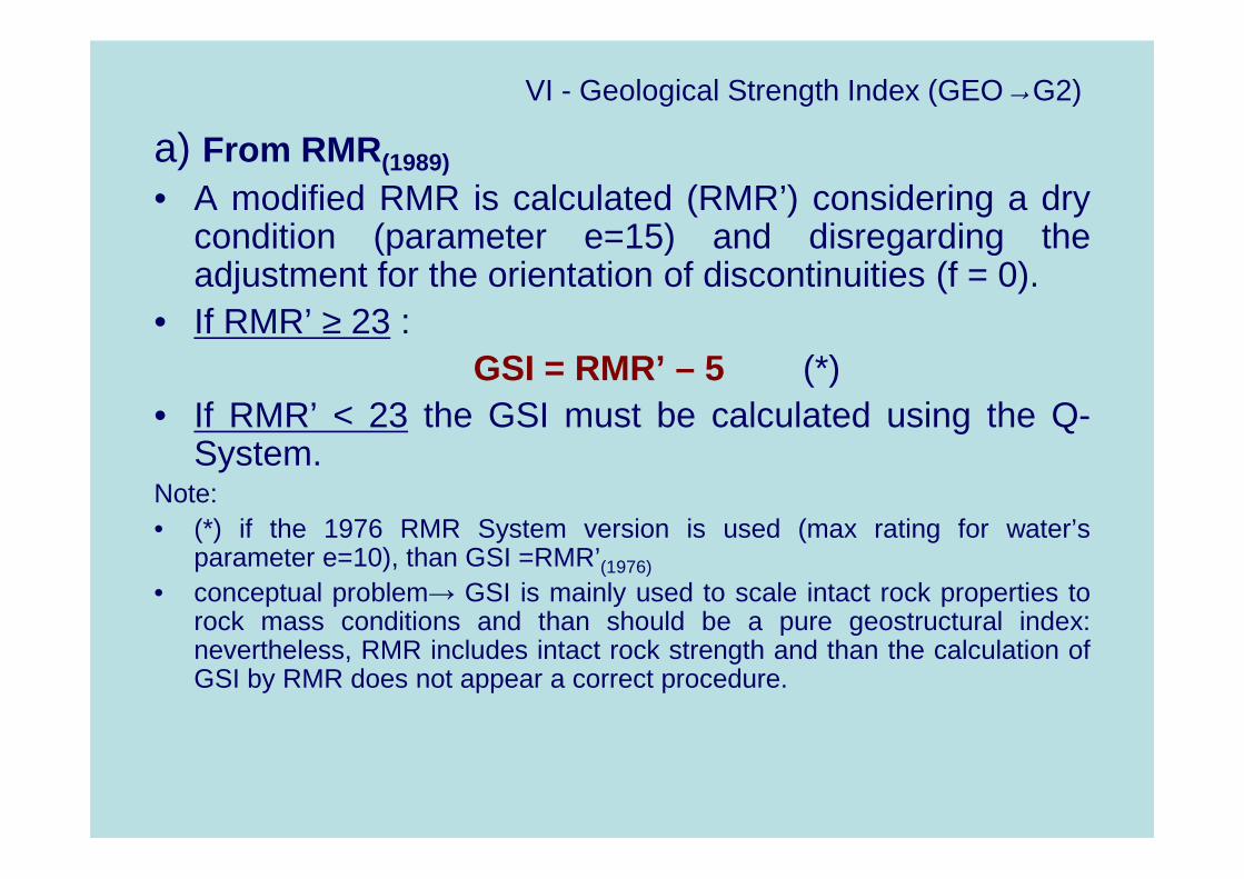
a) From RMR (1989)
• A modified RMR is calculated (RMR’) considering a drycondition (parameter e=15) and disregarding theadjustment for the orientation of discontinuities (f = 0).
• If RMR’ ≥ 23 :GSI = RMR’ – 5 (*)
• If RMR’ < 23 the GSI must be calculated using the Q-System.
Note:• (*) if the 1976 RMR System version is used (max rating for water’s
parameter e=10), than GSI =RMR’(1976)
• conceptual problem→ GSI is mainly used to scale intact rock properties torock mass conditions and than should be a pure geostructural index:nevertheless, RMR includes intact rock strength and than the calculation ofGSI by RMR does not appear a correct procedure.

VI - Geological Strength Index (GEO→G2)
b) From Q• Analogously, a modified Q is calculated (Q’), with
Jw/SRF = 1.Therefore:
GSI = 9lnQ’ + 44
• Use this expression even when RMR’<23.
c)
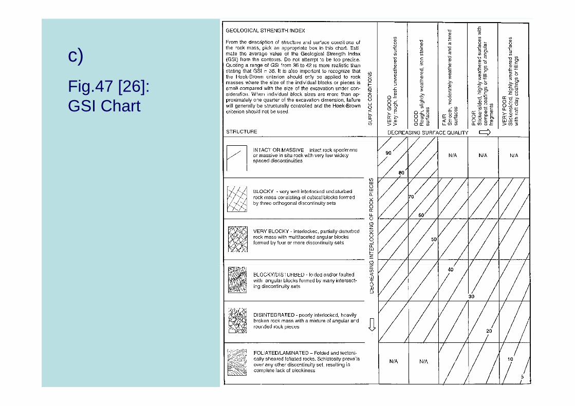
Fig.47 [26]: GSI Chart

VI - Geological Strength Index (GEO→G2)
c) Fig.48 [26]: GSI chart for heterogeneous rock masses
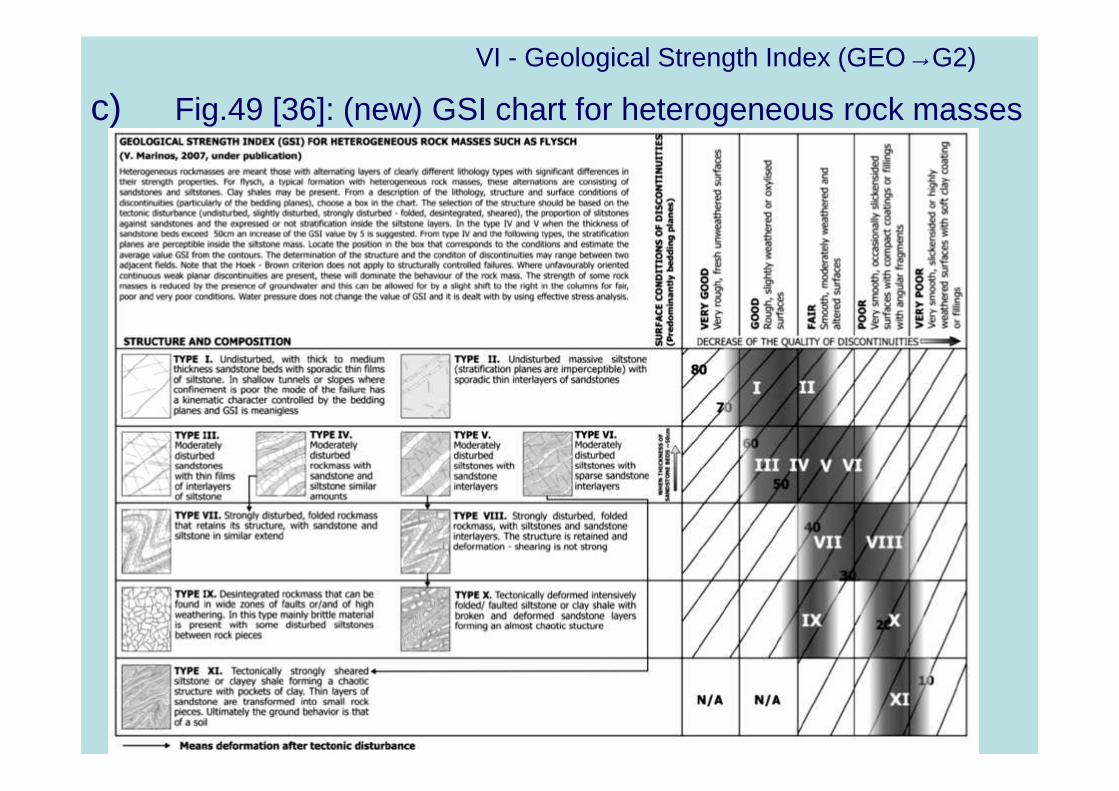
c) Fig.49 [36]: (new) GSI chart for heterogeneous rock masses
VI - Geological Strength Index (GEO→G2)

VI - Geological Strength Index (GEO→G2)
d)
Fig.50a [11]: Modified GSI graph proposed by Cai et al. (2004)
Quantitative assessment of input parameters

Geological Strength Index (GEO→G2)
d)Fig.50b [11]: Tables forevaluating the Joint ConditionFactor JC
JC = JW*JS/JA

VI - GSI (GEO→G2)
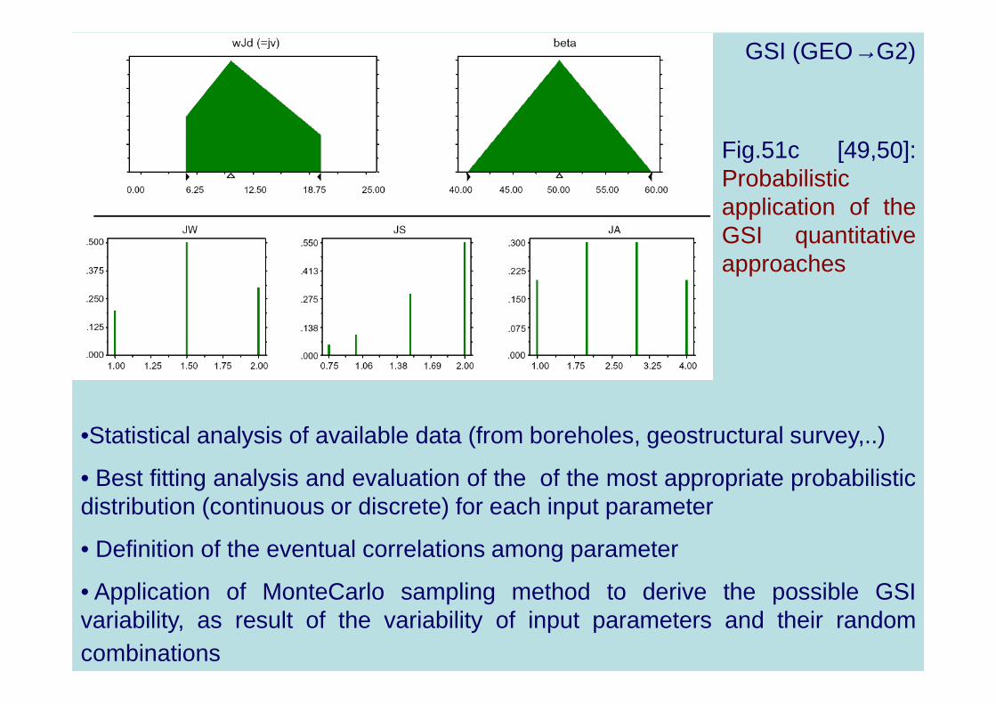
Fig.51a [49,50]: Integrated GSI-RMi system (GRs approach, 2007-2009) -Quantitative assessment of the same input parameters for estimating JP of RMi
jC TYPICAL CONDITIONS 1
24 Discontinuous cracks
12 Smal l, rough fessures
6 Undulating, rough short joint
3 Undulating, rough joint
1.75 Slightly undulating, rough joint
1 Smooth, planar joint
0.5 Weathered joint wall
0.2 Clay coated joint
0.1 Filled joint
1Palmstrom, 2000 (refer to the original RMitables for a more precise estimation of jC)
e)

VI - GSI (GEO→G2)
Fig.51b [50]: GRs approach, 2007: Relationship between GSI and JP
e)
GSI (GEO→G2)
•Statistical analysis of available data (from boreholes, geostructural survey,..)
• Best fitting analysis and evaluation of the of the most appropriate probabilisticdistribution (continuous or discrete) for each input parameter
• Definition of the eventual correlations among parameter
• Application of MonteCarlo sampling method to derive the possible GSIvariability, as result of the variability of input parameters and their randomcombinations
Fig.51c [49,50]:Probabilisticapplication of theGSI quantitativeapproaches

Fig.51d: Comparison between GRs ( ←←←←) and Cai et al. ( →→→→) methods
VI - GSI (GEO→G2)

VI - GSI (GEO→G2)
Fig.51e: differences between the Cai and GRs approaches [50]
Range for theexample

SMLP(LTF): graphitic schist GSI=25-40 Yacambù-Q.: graphitic phillite GSI≈35
Yacambù-Q.: graphitic phillite GSI≈25Peridotite GSI≈55
1.5m
Volcanic rock GSI≈30
Geostructural index: GSI
Some H&M GSI estimates (1of2)
Fig.51 f
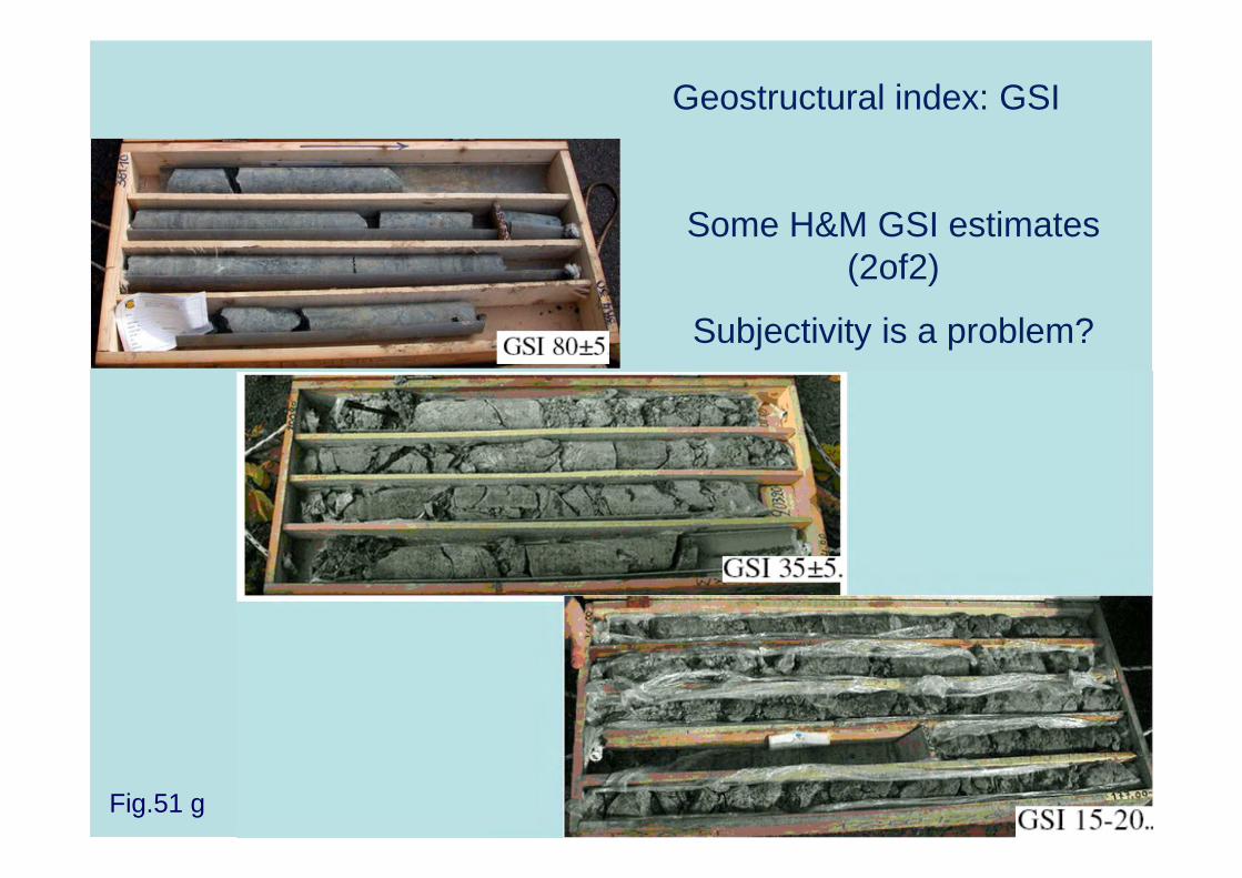
Some H&M GSI estimates(2of2)
Subjectivity is a problem?
Geostructural index: GSI
Fig.51 g
VI - Geological Strength Index (GEO→G2)
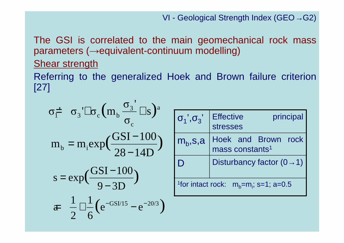
The GSI is correlated to the main geomechanical rock massparameters (→equivalent-continuum modelling)Shear strengthReferring to the generalized Hoek and Brown failure criterion[27]
a
c
3bc31 )( sσ
'σmσ'σ'σ ++=
)(14D28
100GSIexpmm ib −
−=
)(
)(
20/3GSI/15 ee6
1
2
1a
3D9
100GSIexps
−− −+=
−−=
σ1’,σ3’ Effective principalstresses
mb,s,a Hoek and Brown rockmass constants1
D Disturbancy factor (0→1)
1for intact rock: mb=mi; s=1; a=0.5

Residual Shear Strength
GSIr= GSI*e(-0.0134*GSI) [11b]
Fig. 52: relationship between the ratio GSIr/GSI and GSI [11b]Note: the dotted linear equation has been previously proposed in [46]
VI - GSI (GEO→G2)
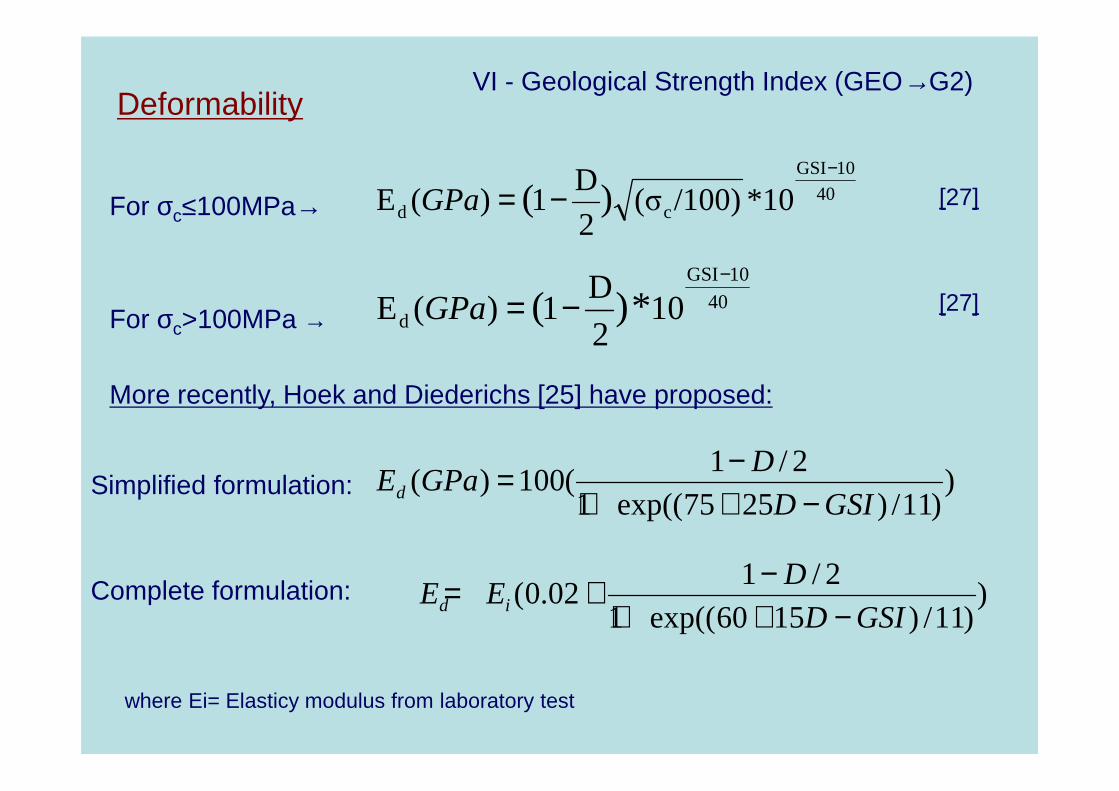
VI - Geological Strength Index (GEO→G2)Deformability
40
10GSI
cd 10*/100)(σ2
D1)(E )(
−
−=GPa
40
10GSI
d 102
D1)(E *)(
−
−=GPa
For σc≤100MPa→
For σc>100MPa →
More recently, Hoek and Diederichs [25] have proposed:
))11/)2575exp((1
2/1(100)(
GSID
DGPaEd −++
−=Simplified formulation:
))11/)1560exp((1
2/102.0(
GSID
DEE id −++
−+=Complete formulation:
where Ei= Elasticy modulus from laboratory test
[27]
[27]

0 10 20 30 40 50 60 70 80 90 1000.0
0.1
0.2
0.3
0.4
0.5
0.6
0.7
0.8
0.9
1.0
GSIres/GSI=exp(-0.0134*GSI)(Cai et al. 2007)
σcm
/σc=sa (Hoek et al., 2002)
s=exp((GSI-100)/9)a=(1/2)+(1/6)*((exp(-GSI/15)-exp(-20/3)))
Ed/E
i=[0.02+1/(1+exp((60-GSI)/11))]
(Hoek and Diederichs, 2005)
Geodata * Torino
(Ed/E
i) or
(σ cm
/σc)
or
(GS
I res/G
SI)
GSIFig.53: Equations based on GSI are used to derive the H&B rock massconstants (m,s,a) and the modulus of deformability (E d)
VI - GSI (GEO→G2)

GSI and RMR parameters affinity
[ref. 51 ter]Fig.53 a
Note that according the RMRupdate [33b] r2+r3 is assigned bythe number of disconinuities permeter

Esempio GSI (Hoek et al.)
K2
K1
K3
NORD
Tunnel Diameter D = 15m ( ≈≈≈≈49in.) in granite; H=100m; σσσσc = 50-100MPa; RQD = 80-100% Discontinuity Spacing (2 systems + 1 random) = =0.6-2m (≈≈≈≈2-6.5in.)Prevalent System (K1) with dip direction against tunnel advance and dip= 80°, slightly weathered and rough. Dry.
→→→→ GSI (Hoek et al.):
• by RMR: GSI = 74-77
• by Q: GSI = 66 - 68
• by Hoek graph: GSI ≈≈≈≈ 65-75
• by Cai approach: GSI ≈≈≈≈ 56-61 (Vb=0.5m3,Jc=1-1.5)
• by GRs approach: GSI ≈≈≈≈ 67-70 (Vb=0.5m3,jC=1-1.5)

Correlations between classification indexes
RMR = 9lnQ+44 Bieniawski 1976
RMR = 13.5logQ+43 Rutledge 1978
RMR ≈ 50+15log10Q Barton 1995
RSR = 13.3logQ+46.5 Rutledge 1978
RSR = 0.77RMR+12.4 Rutledge 1978
RMi = 10^[(RMR-40)/15] Palmstrom 1996
GSI = 9lnQ’+44 Hoek et al. 1995
GSI = 10lnQ’+32 (R2=0.73) Russo et al. 1998
GSI ≈ 153-165/[1+(JP/0.19)0.44] Russo 2007
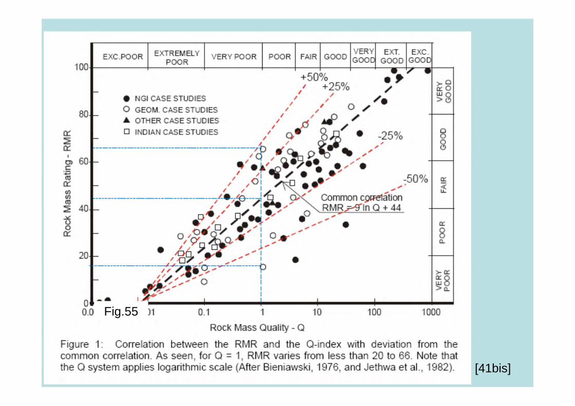
[41bis]
Fig.55

Fig.59: Some types of excavation behaviour (partly from Martin et al. 1999 and Hoek etal. 1995, as reported in [41quintum])
VIII – Introduction to Behaviour Classifications
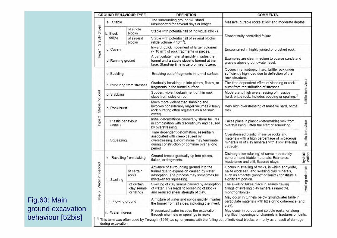
Fig.60: Main ground excavation behaviour [52bis]

VIII – Introduction to Behaviour Classifications
Fig.61: Main types of rock mass compositions [52bis]
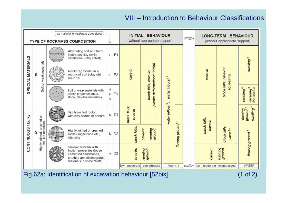
Fig.62a: Identification of excavation behaviour [52bis] (1 of 2)
VIII – Introduction to Behaviour Classifications

Fig.62b: Identification of excavation behaviour [52bis]
(2 of 2)

A quick overview on the Classification of the Behaviour ofthe excavation
It is possible to observe that there are methods based on
• stability of the cavity: for example the original Lauffer [30] systemdistinguished n.7 categories, from stable to very squeezing conditions
• stability of the tunnel face: for example Lunardi [34] proposed the Adeco RSapproach, based on three categories: A (stable face), B (stable face in the shortperiod) and C (unstable face)
• stability of both cavity and and tunnel face: for example, Lombardi [33]distinguished n.4 categories, taking into account all the possible combinations:from class I (face and cavity stable) to class IV (face and cavity unstable)
All these systems involve a qualitative assessment of the behaviour andtherefore they are often open to individual interpretations. In the following aquantitative classification system developed in Geodata [46,47,48], based ondeformation index of tunnel face, as well as of the cavity, is outlined.
VIII - Behaviour Classifications

Stress
Fracturing degree
Stable Caving
SqueezingRock Burst
Instablewedges
Fig. 63: General setting of behaviour of excavation by Geodata classification: Stress analysis + geo-structural conditions [47]

VIII - Behaviour Classifications
Fig.65: General scheme for the evaluation of the excavation behaviour [47,48]
Notes: δo=radial deformation at the face; Rp/Ro=plastic radius/radius of the cavity;σθ=max tangential stress; σcm=rock mass strength. The limits of shadow zones are justindicative

100 80 60 40 20 02.5
2.0
1.5
1.0
0.5
0.0INSTABLEWEDGES
SPALLING,ROCK BURST
STABLE
SQUEEZING
CAVING
δr at the face (%) Rp/Ro
RMR
δr a
t the
face
(%
)
10
8
6
4
2
0
Rp/R
o
Fig.67: General scheme for the evaluation of the excavation behaviour: example of aprobabilistic analysis for a relatively shallow tunnel in prevalent poor rock mass (ItalianNorth Apennines)
VIII - Behaviour Classifications

Plastic deformations/Squeezing
Extremely severe squeezing
Very severe squeezing
Severe squeezing
Hoek & Marinos, 2000 [ref.26]
Very severe squeezing
Severe squeezing
H&M classification based on δfinal
=δfin
GD classification based on δo and Rp/Ro
Extract of
GD classification
Fig.67b: Additional considerations: Squeezing
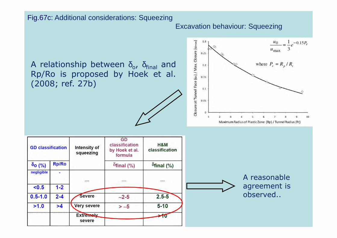
A relationship between δo, δfinal andRp/Ro is proposed by Hoek et al.(2008; ref. 27b)
Excavation behaviour: Squeezing
A reasonable agreement is observed..
Fig.67c: Additional considerations: Squeezing
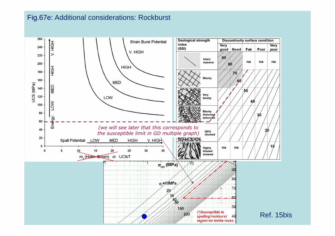
(we will see later that this corresponds to the susceptible limit in GD multiple graph)
Ref. 15bis
Fig.67e: Additional considerations: Rockburst

a→f=increasing levels of spall damage
[Ref. 15bis, 15ter]
It is observed that crack initiation threshold (CI) around a cavity occurs
when σmax ≈ 0.4 ( ±0.1) σc
Fig.67f: Additional considerations: Rockburst

I) Jc(1.75) + Vb(3dm3)= GSI (40)
II) GSI(40)+σc(25MPa)=σcm(0.8MPa)
III) σcm(0.8MPa) +H(500m)= IC(0.03)
IV) IC (0.03)+RMR(35)= severe squeezing
Fig. 68a: Simplified approach for a preliminary setting of excavation behaviour [51]

Fig. 68b: Simplified approach for a preliminary setting of excavation behaviour
[51ter]

Depending on type and intensity of the hazards, mitigation measures are selected
and support Section Types composed
IV – Design actionsFig.68 c [ reference 51ter]

Fig. 68d: Simplified approach for a preliminary setting of excavation behaviour [51ter]

Fig.70bis: A composite graph for brittle failures..
G. Russo (2013) based on Diederichs (2007,2010) and Hoek (2010), modified

Bibliography (2 di 5)
[15 bis] DIEDERICHS M, 2007." Mechanistic interpretationand practical application of damage and spalling predictioncriteria for deep tunneling”. The 2003 CanadianGeotechnical Colloquium
[15 ter] DIEDERICHS M, CARTER T., MARTIN D., 2010."Practical rock spall prediction in Tunnels” ITA World TunnelCongress Vancouver.
Bibliography (3 di 5)
HOEK E.
[27 bis] HOEK E., CARRANZA T.C, DIEDERICHS M.,CORKUM B. 2008."The 2008 Kersten lecture: Integration ofgeotechnical and structural design in tunnelling".Proceedings University of Minnesota 56th AnnualGeotechnical Engineering Conference.
[33b] LOWSON A.R & BIENIAWSKI Z.T.2013: "criticalassessment of rmr-based tunnel design practices: a practicalengineer’s approach"Proc. RETC 2013.Washington, DC:Society of Mining Engineers, p.180-198.

Bibliography (4 di 5)
G. Russo publications can be downloaded at
http://www.webalice.it/giordandue/
[41ter] PALMSTROM A. AND BROCH E., 2006. “Use andmisuse of rock mass classification systems with particularreference to the Q-system”. Tunnels and UndergroundSpace Technology, vol. 21, pp575-593
[41quater] PALMSTROM A., 2006. “Measurements of andcorrelations between block size and rock quality designation(RQD)”. Tunnels and Underground Space Technology, vol.20, pp362-367
[41quintum] PALMSTROM A. AND STILLE H., 2007.“Ground behaviour and rock engineering tools forunderground excavations)”. Tunnels and UndergroundSpace Technology, vol. 22, pp363-376
[52bis] STILLE H. AND PALMSTROM A., 2008. “Groundbehaviour and rock mass composition in undergroundexcavations)”. Tunnels and Underground Space Technology,vol. 23, pp46-64
[51 ter] RUSSO G. 2014."An update of the ."multiple graph"approach for the preliminary asssment of the excavationbehaviour in rock tunnelling, Tunnels and UndergroundSpace Technology, vol. 41

Bibliography (5 di 5)