post-newtonian approximation itsfoundationandapplications · post-newtonian approximation...
TRANSCRIPT
arX
iv:g
r-qc
/980
6108
v1 2
7 Ju
n 19
98
Progress of Theoretical Physics Supplement 1
Post-Newtonian Approximation
Its Foundation and Applications
Hideki Asada∗ and Toshifumi Futamase
∗ Yukawa Institute for Theoretical Physics, Kyoto University, Kyoto 606-01Astronomical Institute, Graduate School of Science, Tohoku University
Sendai 980-77, Japan
We discuss various aspects of the post-Newtonian approximation in general relativity.After presenting the foundation based on the Newtonian limit, we use the (3+1) formalism toformulate the post-Newtonian approximation for the perfect fluid. As an application we showthe method for constructing the equilibrium configuration of nonaxisymmetric uniformlyrotating fluid. We also discuss the gravitational waves including tail from post-Newtoniansystems.
§1. Introduction
The motion and associated emission of gravitational waves (GW) of self gravi-tating systems have been a main research interest in general relativity. The problemis complicated conceptually as well as mathematically because of the nonlinearityof Einstein’s equations. There is no hope in any foreseeable future to have exactsolutions describing motions of arbitrary shaped, massive bodies so that we have toadopt some sort of approximation scheme for solving Einstein’s equations to studysuch problems. In the past years many types of approximation schemes have beendeveloped depending on the nature of the system under consideration. Here weshall focus on a particular scheme called the post-Newtonian (PN) approximation.There are many systems in astrophysics where Newtonian gravity is dominant, butgeneral relativistic gravity plays also important roles in their evolution. For suchsystems it would be nice to have an approximation scheme which gives Newtoniandescription in the lowest order and general relativistic effects as higher order per-turbations. The post-Newtonian approximation is perfectly suited for this purpose.Historically Einstein computed first the post-Newtonian effects, the precession of theperihelion 36), but a systematic study of the post-Newtonian approximation was notmade until the series of papers by Chandrasekhar and associates 21), 22), 23), 24), 25).Now it is widely known that the post-Newtonian approximation is important in an-alyzing a number of relativistic problems, such as the equation of motion of binarypulsar 19), 40), 53), 31), solar-system tests of general relativity 97), 98), and gravitationalradiation reaction 25), 20).
Any approximation scheme nesseciates a small parameter(s) characterizing thenature of the system under consideration. Typical parameter which most of schemesadopt is the magnitude of the metric deviation away from a certain backgroundmetric. In particular if the background is Minkowski spacetime and there is no otherparameter, the scheme is sometimes called as the post-Minkowskian approximation
typeset using PTPTEX.sty <ver.0.8>
2 H. Asada and T. Futamase
in the sense that the constructed spacetime reduces to Minkowski spacetime in thelimit as the parameter tends to zero. This limit is called as the weak field limit.In the case of the post-Newtonian approximation the background spacetime is alsoMinkowski spacetime, but there is another small parameter, that is, the typicalvelocity of the system divided by the speed of light which we call ǫ henceforth.These two parameters (the deviation away from the flat metric and the velocity)have to have a certain relation in the following sense. As the gravitational fieldgets weaker, all velocities and forces characteristic of the material systems becomesmaller, in order to permit the weakening gravity to remain an important effect onthe system’s dynamics. For example in case of a binary system, the typical velocitywould be the orbital velocity v/c ∼ ǫ and the deviation from the flat metric wouldbe the Newtonian potential, say Φ. Then these are related by Φ/c2 ∼ v2/c2 ∼ ǫ2
which guarantees that the system is bounded by its own gravity.In the post-Newtonian approximation, the equations in general relativity take
the form of Newton’s equations in an appropriate limit as ǫ→ 0. Such a limit is calledas the Newtonian limit and it will be the bases of constructing the post-Newtonianapproximation. However the limit is not in any sense trivial since the limit may bethought of two limits tied together as just described. It is also worth noting thatthe Newtonian limit cannot be uniform everywhere for all time. For example anycompact binary systems, no matter how weak the gravity between components andslow its orbital motion, will eventually spiral together due to backreaction of theemission of gravitational waves. As the result the effects of its Newtonian gravitywill be swamped by those of its gravitational waves. This will mean that higherorder effect of the post-Newtonian approximation eventually dominates the lowestorder Newtonian dynamics and thus if the post-Newtonian approximation is notcarefully constructed, this effect can lead to many formal problems, such as divergentintegrals 35). It has been shown that such divergences may be avoided by carefullydefining Newtonian limit 44). Moreover, the use of such limit provides us a strongindication that the post-Newtonian hierarchy is an asymptotic approximation togeneral relativity 47). Therefore we shall first discuss in this paper the Newtonianlimit and how to construct the post-Newtonian hierarchy before attacking practicalproblems in later sections.
Before going into the details, we mention the reason for the growth of interestin the post-Newtonian approximation in recent years. Certainly the discovery ofthe binary neutron star system PSR 1913+16 was a strong reason to have renewedinterest in the post-Newtonian approximation since it is the first system in whichgeneral relativitistic gravity plays fundamental roles in its evolution 53). Particularlyindirect discovery of gravitational wave by the observation of the period shorteningled to many fruitful studies of the equation of motion with gravitational radiationemission in 1980’s 27), 82), 93). The effect of radiation reaction appears as the form ofthe potential force at the order of ǫ5 higher than Newtonian force in the equationof motion. There have been various attempts to show the validity of the so-calledquadrupole formula for the radiation reaction 2), 44), 54), 55), 56), 57), 58), 81), 94), 95).
At that time, however, no serious attempts had been made for the study ofhigher order effects in the equation of motion. The situation changed gradually in
Post-Newtonian Approximation 3
1990’s because of the increasing expectation of direct detection of gravitational wavesby Kilometer-size interferometric gravitational wave detectors, such as LIGO 1),VIRGO 18) and TAMA 61) now under construction. Coalescing binary neutron starsare the most promising candidate of sources of gravitational waves for such detec-tors. The reasons are that (1) we expect to detect the signal of coalescence of binaryneutron stars about several times per year 76), and (2) the waveform from coalescingbinaries can be predicted with a high accuracy compared with other sources 1), 91), 98).Informations carried by gravitational waves tell us not only various physical param-eters of neutron star 90), 91), but also the cosmological parameters 83), 66), 42), 96) if andonly if we can make a detailed comparison between the observed signal with theoret-ical prediction during the epoch of the so-called inspiraling phase where the orbitalseparation is much larger than the radius of component stars 26). This is the placewhere the post-Newtonian approximation may be applied to make a theoretical tem-plate for gravitational waves. The problem is that in order to make any meaningfulcomparison between theory and observation we need to know the detailed waveformsgenerated by the motion up to 4PN order which is of order ǫ8 higher than the Newto-nian order 88). This request from gravitational wave astronomy forces us to constructhigher order post-Newtonian approximation.
It should be mentioned that Blanchet and Damour have developed a system-atic scheme to calculate the waveform at higher order where the post-Minkowskianapproximation is used to construct the external field and the post-Newtonian ap-proximation is used to construct the field near the material source 9), 10), 11), 12), 13).Blanchet has obtained the waveform up to the 2.5 PN order which is of order ǫ5
higher than the lowest qudraupole wave 14), 7), 8) by using the equation of motion upto that order 28), 29), 30), 50), 60). We shall also study the waveform from different pointof view because of its importance. We obtain essentially the same results includingthe tail term with them.
There is another phase in the evolution of the binary neutron star which we canwithdraw useful informations from the observed signals of gravitational waves. Thatis the intermediate phase between the inspiralling phase and the event of merging.In the inspiralling phase the components are usually treated as point particles, whilethe extendedness becomes important in the intermediate phase and the merging.Full general relativistic hydrodynamic simulation is needed for the understanding ofthe merging. The material initial data for the simulation will be the density and thevelocity distribution of the fluid. The post-Newtonian approximation will be used toconstruct the data. Furthermore the post-Newtonian approximation is able to takeinto account of the tidal effect which is important for the orbital instability. Recently,Lai, Rasio and Shapiro 62), 63) have pointed out that such a tidal coupling of binaryneutron stars is very important for their evolution in the final merging phase becausethe tidal effect causes the instability of the circular motion even in the Newtoniangravity. Also important is the general relativistic gravity because in the intermediatephase, the orbital separation is about ten times as small as the Schwarzschild radiusof the system. Thus, we need not only a hydrodynamic treatment, but also generalrelativistic one in order to study the final stage of the evolution of binary neutronstars. Since the usual formulation of the post-Newtonian approximation is based on
4 H. Asada and T. Futamase
the particular gauge condition which is not so convenient for numerical purposes,we shall reformulate it by the (3+1) formalism often used in numerical approach ofgeneral relativity.
This paper is organized as follows. In section 2 we introduce the Newtonianlimit in general relativity and present how to construct the post-Newtonian hierar-chy. There we mention how to avoid divergent integrals which appears at higherorder in the previous treatments, and we also discuss how to incorporate strong in-ternal gravity in the post-Newtonian approximation. Next we reformulate the post-Newtonian approximation appropriate for numerical treatment in section 3. Therewe shall adopt the (3+1) formalism which is frequently used in numerical relativity.Based on the formalism developed in section 3, we present a formulation for con-structing numerically equilibrium solutions of uniformly rotating fluid in the 2PNapproximation in section 4. We shall also discuss the propagation of gravitationalwaves from slow motion systems in section 5.
§2. Foundation of the post-Newtonian approximation
Since the Newtonian limit is the basis of the post-Newtonian approximation, weshall first formulate the Newtonian limit. We shall follow the formulation by Futa-mase and Schutz 47). We will not mention other formulation of Newtonian limit byEhlers 38), 39), because it has not yet used to construct the post-Newtonian approxi-mation.
2.1. Newtonian limit along a regular asymptotic Newtonian sequence
The formulation is based on the observation that any asymptotic approximationof any theory need a sequence of solutions of the basic equations of the theory 87), 92).Namely, if we write the equations in abstract form as
E(g) = 0, (2.1)
for an unknown function g, one would like to have a one-parameter (or possiblymultiparameter) family of solutions,
E(g(λ)) = 0, (2.2)
where λ is some parameter. Asymptotic approximation then says that function f(λ)approximates g(λ) to order λp if |f(λ) − g(λ)|/λp → 0 as λ → 0. We choose thesequence of solutions with appropriate properties in such a way that the propertiesreflect the character of the system under consideration.
We shall formulate the post-Newtonian approximation according to the generalidea just described. As stated in the introduction, we would like to have an approx-imation which applies the systems whose motion is described almost by Newtoniantheory. Thus we need a sequence of solutions of Einstein’s equations parameterizedby ǫ (the typical velocity of the system divided by the speed of light) which has theNewtonian character as ǫ→ 0.
The Newtonian character is most conveniently described by the following scal-ing law. The Newtonian equations involve six variables, density (ρ), pressure (P ),
Post-Newtonian Approximation 5
gravitational potential (Φ), and velocity (vi, i = 1, 2, 3):
∇2Φ− 4πρ = 0, (2.3)
∂tρ+∇i(ρvi) = 0, (2.4)
ρ∂tvi + ρvj∇jv
i +∇iP + ρ∇iΦ = 0, (2.5)
supplemented by an equation of state. For simplicity we have considered perfectfluid. Here we have set G = 1.
It can be seen that the variables ρ(xi, t), P (xi, t), Φ(xi, t), vi(xj , t) obeying theabove equations satisfy the following scaling law.
ρ(xi, t) → ǫ2ρ(xi, ǫt),
P (xi, t) → ǫ4P (xi, ǫt),
vi(xk, t) → ǫvi(xk, ǫt),
Φ(xi, t) → ǫ2Φ(xi, ǫt). (2.6)
One can easily understand the meaning of this scaling by noticing that ǫ is themagnitude of typical velocity (divided by the speed of light). Then the magnitude ofthe gravitational potential will be of order ǫ2 because of the balance between gravityand centrifugal force. The scaling of the time variable expresses the fact that theweaker the gravity (ǫ→ 0) the longer the time scale.
Thus we wish to have a sequence of solutions of Einstein’s equations which hasthe above scaling as ǫ → 0. We shall also take the point of view that the sequenceof solutions is determined by the appropriate sequence of initial data. This has apractical advantage because there will be no solution of Einstein’s equations whichsatisfy the above scaling (2.6) even as ǫ → 0. This is because Einstein’s equationsare nonlinear in the field variables so it will not be possible to enforce the scalingeverywhere in spacetime. We shall therefore impose it only on the initial data forthe solution of the sequence.
Here we shall first make a general discussion on the formulation of the post-Newtonian approximation independent of any initial value formalism and then presentthe concrete treatment in the harmonic coordinate. The condition is used because ofits popularity and some advantages in the generalization to the systems with stronginternal gravity.
As the initial data for the matter we shall take the same data set in Newtoniancase, namely, the density ρ, the pressure P , and the coordinate velocity vi. In mostof the application, we usually assume a simple equation of state which relates thepressure to the density. The initial data for the gravitational field are gµν , ∂gµν/∂t.Since general relativity is overdetermined system, there will be constraint equationsamong the initial data for the field. We shall write the free data for the field as(Qij , Pij) whose explicit forms depend on the coordinate condition one assumes. Inany coordinate we shall assume these data for the field vanish since we are interestedin the evolution of an isolated system by its own gravitational interaction. It isexpected that these choice corresponds to the absence of radiation far away from the
6 H. Asada and T. Futamase
source. Thus we choose the following initial data which is indicated by Newtonianscaling:
ρ(t = 0, xi, ǫ) = ǫ2a(xi),
P (t = 0, xi, ǫ) = ǫ4b(xi),
vi(t = 0, xk, ǫ) = ǫci(xk),
Qij(t = 0, xi, ǫ) = 0,
Pij(t = 0, xi, ǫ) = 0, (2.7)
where the functions a, b , and ci are C∞ functions that have compact support con-tained entirely within a sphere of a finite radius.
Corresponding to the above data, we have a one-parameter set of spacetimeparameterized by ǫ. It may be helpful to visualize the set as a fiber bundle, withbase space R the real line (coordinate ǫ) and fiber R4 the spacetime (coordinatest, xi). The fiber ǫ = 0 is Minkowski spacetime since it is defined by zero data. Inthe following we shall assume that the solutions are sufficiently smooth functionsof ǫ for small ǫ 6= 0. We wish to take the limit ǫ → 0 along the sequence. Thelimit is, however, not unique and is defined by giving a smooth nowhere vanishingvector field on the fiber bundle which is nowhere tangent to each fiber 51), 87). Theintegral curves of the vector field give a correspondence between points in differentfibers, namely events in different spacetime with different values of ǫ. Rememberingthe Newtonian scaling of the time variable in the limit, we introduce the Newtoniandynamical time:
τ = ǫt, (2.8)
and define the integral curve as the curve on which τ and xi stay constant. In factif we take the limit ǫ → 0 along this curve, the orbital period of the binary systemwith ǫ = 0.01 is 10 times of that of the system with ǫ = 0.1 as expected from theNewtonian scaling. This is what we define as the Newtonian limit. Notice that thismap never reaches the fiber ǫ = 0 (Minkowski spacetime). There is no pure vacuumNewtonian limit as expected.
In the following we assume the existence of such a sequence of solutions con-structed by the initial data satisfying the above scaling with respect to ǫ. We shallcall such a sequence is a regular asymptotically Newtonian sequence. We have tomake further mathematical assumptions about the sequence to make explicit calcu-lations. We will not go into details of them partly because to prove the assumptionswe need a deep understanding of the existence and uniqueness properties of Cauchyproblem of Einstein’s equations with perfect fluids of compact support which are notavailable at present.
2.2. Post-Newtonian Hierarchy
We shall now define the Newtonian, post-Newtonian and higher approximationsof various quantities as the appropriate higher tangents of the corresponding quanti-ties to the above integral curve at ǫ = 0. For example the hierarchy of approximationsfor the spacetime metrics can be expressed as follows:
gµν(ǫ, τ, xi) = gµν(0, τ, x
i) + ǫ(LV gµν)(0, τ, xi)
Post-Newtonian Approximation 7
+1
2ǫ2(L2
V gµν)(0, τ, xi) + ..... +
ǫn
n!(LnV gµν)(0, τ, xi) +Rn+1, (2.9)
where LV is the Lie derivative with respect to the tangent vector of the curves definedabove, and the remainder term Rµνn+1 is
Rµνn+1 =ǫn+1
(n+ 1)!
∫ 1
0dℓ(1− ℓ)n+1(Ln+1
V gµν)(ℓǫ, τ, xi). (2.10)
Taylor’s theorem guarantees that the series is asymptotic expansion about ǫ = 0under certain assumptions mentioned above. It might be useful to point out thatthe above definition of the approximation scheme may be formulated purely geomet-rically in terms of jet bundle.
The above definition of the post-Newtonian hierarchy gives us asymptotic seriesin which each term in the series is manifestly finite. This is based on the ǫ depen-dence of the domain of dependence of the field point (τ, xk). The region is finite withfinite values of ǫ, and the diameter of the region increases as ǫ−1 as ǫ → 0. With-out this linkage of the region with the expansion parameter ǫ, the post-Newtonianapproximation leads to divergences in the higher orders. This is closely related withthe retarded expansion. Namely, it is assumed that the slow motion assumptionenabled one to Taylor expand the retarded integrals in retarded time such as
∫
drf(τ − ǫr, ...) =
∫
drf(τ, ...)− ǫ
∫
drrf(τ, ...),τ + .. (2.11)
and assign the second term to a higher order because of its explicit ǫ in front. Thisis incorrect because r → ǫ−1 as ǫ → 0 and thus ǫr is not uniformly small in theNewtonian limit. Only if the integrand falls off sufficiently fast, can retardation beignored. This happens in the lower-order PN terms. But at some higher order thereappear many terms which do not fall off sufficiently fast because of the nonlinearity ofEinstein’s equations. This is the reason that the formal PN approximation producesthe divergent integrals. It turns out that such divergence appears at 3PN orderindicating the breakdown of the PN approximation in the harmonic coordinate.This sort of divergence may be eliminated if we remember that the upper boundof integration does depend on ǫ as ǫ−1. Thus we would get something like ǫn ln ǫinstead of ǫn ln∞ in the usual approach. This shows that the asymptotic Newtoniansequence is not differentiable in ǫ at ǫ = 0, but there are no divergence in theexpansion and it has still an asymptotic approximation in ǫ that involves logarithms.
2.3. Explicit calculation in Harmonic coordinate
Here we shall use the above formalism to make explicit calculation in the har-monic coordinate. The reduced Einstein’s equation in the harmonic condition iswritten as
gαβ gµν,αβ = 16πΘµν − gµα,β gνβ,α, (2.12)
∂µ[gµν∂νx
α] = 0, (2.13)
wheregµν = (−g)1/2gµν , (2.14)
8 H. Asada and T. Futamase
Θαβ = (−g)(Tαβ + tαβLL), (2.15)
where tµνLL is the Landau-Lifshitz pseudotensor 64). In the following we shall choosean isentropic perfect fluid for Tαβ which is enough for most of applications.
Tαβ = (ρ+ ρΠ + P )uαuβ + Pgαβ , (2.16)
where ρ is the rest mass density, Π the internal energy, P the pressure, uµ the fourvelocity of the fluid with normalization;
gαβuαuβ = −1. (2.17)
The conservation of the energy and momentum is expressed as
∇βTαβ = 0. (2.18)
Defining the gravitational field variable as
hµν = ηµν − (−g)1/2gµν , (2.19)
where ηµν is the Minkowski metric, the reduced Einstein’s equation (2.12) and thegauge condition (2.13) take the following form;
(ηαβ − hαβ)hµν,αβ = −16πΘµν + hµα,βhνβ,α, (2.20)
hµν,ν = 0. (2.21)
Thus the characteristics is determined by the operator (ηαβ − hαβ)∂α∂β, and thusthe light cone deviates from that in the flat spacetime. We shall use this form ofthe reduced Einstein’s equations in the calculation of wave form far away from thesource because the deviation plays a fundamental role there. However in the studyof the gravitational field near the source it is not neccesary to consider the deviationof the light cone away from the flat one and thus it is convenient to use the followingform of the reduced Einstein’s equations 2).
ηµν hαβ,µν = −16πΛαβ , (2.22)
where
Λαβ = Θαβ + χαβµν,µν , (2.23)
χαβµν = (16π)−1(hαν hβµ − hαβ hµν). (2.24)
Equations (2.21) and (2.22) together imply the conservation law
Λαβ,β = 0. (2.25)
We shall take as our variables the set ρ, P, vi, hαβ, with the definition
vi = ui/u0. (2.26)
Post-Newtonian Approximation 9
The time component of 4-velocity u0 is determined from Eq.(2.17). To make a well-defined system of equations we must add the conservation law for number density nwhich is some function of the density ρ and pressure P :
∇α(nuα) = 0. (2.27)
Equations (2.25) and (2.27) imply that the flow is adiabatic. The role of the equationof state is played by the arbitrary function n(ρ, p).
Initial data for the above set of equations are hαβ , hαβ,0, ρ, P , and vi, but notall these data are independent because of the existence of constraint equations.Equations.(2.21) and (2.22) imply the four constraint equations among the initialdata for the field.
∆hα0 + 16πΛα0 − δij hα ,0i,j = 0, (2.28)
where ∆ is the Laplacian in the flat space. We shall choose hij and hij,0 as free
data and solve Eq.(2.28) for hα0(α = 0, .., 3) and Eq.(2.21) for hα0 ,0. Of coursethese constraints cannot be solved explicitly, since Λα0 contains hα0, but they canbe solved iteratively as explained below. As discussed above, we shall assume thatthe free data hij and hij,0 for the field vanish. One can show that such initial datasatisfy the O’Murchadha and York criterion for the absence of radiation far awayfrom the source 75).
In the actual calculation, it is convenient to use an expression with explicitdependence of ǫ. The harmonic condition allows us to have such expression in termsof the retarded integral.
hµν(ǫ, τ, xi) = 4
∫
C(ǫ,τ,xi)d3yΛµν(τ − ǫr, yi, ǫ)/r + hµνH (ǫ, τ, xi), (2.29)
where r = |yi − xi| and C(ǫ, τ, xi) is the past flat light cone of event (τ, xi) in thespacetime given by ǫ, truncated where it intersects with the initial hypersurfaceτ = 0. hµνH is the unique solution of the homogeneous equation
ηαβ hµν,αβ = 0. (2.30)
We shall henceforce ignore the homogeneous solution because they play no importantroles. Because of the ǫ dependence of the integral region, the domains of integrationare finite as long as ǫ 6= 0 and their diameter increases as ǫ−1 as ǫ→ 0.
Given the formal expression (2.29) in terms of initial data (2.7), we can takethe Lie derivative and evaluate these derivatives at ǫ = 0. The Lie derivative isnothing but partial derivative with respect to ǫ in the coordinate system for thefiber bundle given by (ǫ, τ, xi). Accordingly one should convert all the time indicesto τ indices. For example, T ττ = ǫ2T tt which is of order ǫ4 since T tt ∼ ρ is of orderǫ2. Similarly the other components of stress energy tensor T τi = ǫT ti and T ij are oforder ǫ4 as well. Thus we expect the first non-vanishing derivative in (2.29) will bethe forth-derivatives. In fact we find
(4)hττ (τ, xi) = 4
∫
R3
(2)ρ(τ, yi)
rd3y, (2.31)
10 H. Asada and T. Futamase
(4)hτi(τ, xi) = 4
∫
R3
(2)ρ(τ, yk)(1)v
i(τ, xk)
rd3y, (2.32)
(4)hij(τ, xk) = 4
∫
R3
(2)ρ(τ, yk)(1)v
i(τ, yk)(1)vj(τ, yk) + (4)t
ijLL(τ, y
k)
rd3y,
(2.33)
where we have adopted the notation
(n)f(τ, xi) =
1
n!limǫ→0
∂n
∂ǫnf(ǫ, τ, xi), (2.34)
and
(4)tijLL =
1
64π((4)h
ττ,i(4)h
ττ,j − 1
2δij (4)h
ττ,k(4)h
ττ,k). (2.35)
In the above calculation we have taken the point of view that hµν is a tensorfield, defined by giving its components in the assumed harmonic coordinate as thedifference between the tensor density
√−ggµν and ηµν .The conservation law (2.25) also has its first nonvanishing derivative at this
order, which are
(2)ρ(τ, xk),τ + ((2)ρ(τ, x
k)(1)vi(τ, xk)),i = 0, (2.36)
((2)ρ(1)vi),τ + ((2)ρ(1)v
i(1)v
j),j + (4)P,i − 1
4 (2)ρ(4)hττ,i = 0. (2.37)
Equations (2.31), (2.36), and (2.37) consist of Newtonian theory of gravity. Thus thelowest non-vanishing derivative with respect to ǫ is indeed Newtonian theory, andthe 1PN and 2PN equations emerge from sixth and eighth derivatives, respectively,in the conservation law (2.25). At the next derivative, the quadrupole radiationreaction term comes out.
2.4. Strong point particle limit
If we wish to apply the post-Newtonian approximation to the inspiraling phaseof binary neutron stars, the strong internal gravity must be taken into account. Theusual post-Newtonian approximation assumes explicitly the weakness of gravitationalfield everywhere including inside the material source. It is argued by appealingthe strong equivalence principle that the external gravitational field which governsthe orbital motion of the binary system is independent of internal structure of thecomponents up to tidal interaction. Thus it is expected that the results obtainedunder the assumption of weak gravity also apply for the case of neutron star binary.Experimental evidence for the strong equivalence principle is obtained only for thesystem with weak gravity 97), 98), but no experiment is available in case with stronginternal gravity at present.
In theoretical aspect, the theory of extended object in general relativity 34) is stillin preliminary stage for the application to realistic systems. Matched asymptoticexpansion technique has been used to treat the system with strong gravity in certainsituations 32), 33), 55), 56), 27). Another way to handle with strong internal gravity is by
Post-Newtonian Approximation 11
the use of Dirac’s delta function type source with a fixed mass 37). However, thismakes Einstein’s equations mathematically meaningless because of their nonlinearity.Physically, there is no such source in general relativity because of the existence ofblack holes. Before a body shrinks to a point, it forms a black hole whose size isfixed by its mass. For this reason, it has been claimed that no point particle existsin general relativity.
This conclusion is not correct, however. We can shrink the body keeping thecompactness (M/R), i.e., the strength of the internal field fixed. Namely we shouldscale the mass M just like the radius R. This can be fitted nicely into the concept ofregular asymptotic Newtonian sequence defined above because there the mass alsoscales along the sequence of solutions. In fact, if we take the masses of two stars as M,and the separation between two stars as L, then Φ ∼M/L. Thus the mass M scalesas ǫ2 if we fix the separation. In the above we have assumed that the density scalesas ǫ2 to guarantee this scaling for the mass understanding the size of the body fixed.Now we shrink the size as ǫ2 to keep the compactness of each component. Thenthe density should scale as ǫ−4. We shall call such a scheme as strong point particlelimit since the limit keeps the strength of internal gravity. The above considerationsuggests the following initial data to define a regular asymptotic Newtonian sequencewhich describes nearly Newtonian system with strong internal gravity 45). The initialdata are two uniformly rotating fluids with compact spatial support whose stress-energy tensor and size scales as ǫ−4 and ǫ2, respectively. We also assume that eachof these fluid configurations would be a stationary equilibrium solution of Einstein’sequation if other were absent. This is neccesary for the suppression of irrelevantinternal motions of each star. Any remaining motions are the tidal effects causedby the other body, which will be of order ǫ6 smaller than the internal self-force.This data allows us to use the Newtonian time τ = ǫt as a natural time coordinateeverywhere including inside the stars.
This choice of the data leads naturally to the introduction of the body zones BAand the body zone coordinates xkA defined by
BA = xk; |xk − ξkA| < ǫR, (2.38)
xkA = ǫ−2(xk − ξkA), (2.39)
where R is some constant, and ξkA(τ), A = I, II are the coordinates of the originof the two stars, where we have used letters with bar to distinguish the body-zonecoordinates from their counterparts. The scaling by ǫ−2 means that as the starshrinks with respect to the coordinate xk, it remains of fixed size in the body-zonecoordinate xk. The boundary of the body zone shrinks to a point with respect to xk,and expands to infinity with respect to xk as ǫ → 0. This makes a clean separationof the body zone from the exterior geometry generated by other star.
gµν = (gB)µν + (gC−B)µν , (2.40)
where (gB)µν is the contribution from the body zones, (gC−B)µν from elsewhere.Actual calculations are most easily performed in the harmonic coordinate. Take
two stationary solutions of Einstein’s equations for the perfect fluid T µνA (xi), gµνA (xi)
12 H. Asada and T. Futamase
as our initial data in the body zone. As explained above every component of thestress-energy tensor T µνA has the same ǫ−4 scaling in the inertia coordinates (t, xk)for a rapidly rotating star. In the body zone coordinates (τ, xk), these have thefollowing scalings:
T ττA = ǫ2T ttA ∼ ǫ−2, (2.41)
T τiA = ǫ−1T tiA ∼ ǫ−5, (2.42)
T ijA = ǫ−4T ijA ∼ ǫ−8. (2.43)
Transformed to the near zone coordinates (τ, xk), xk = ξiA+ ǫ2xk, they take the form
T ττN = T ττA , (2.44)
T τiN = ǫ2T τiA + viATττA , (2.45)
T ijN = ǫ4T ijA + 2ǫ2v(iAT
j)τA + viAv
jAT
ττA , (2.46)
where viA = dξiA/dτ is the velocity of the origin of the body A. If there were only onebody, these data would produce a stationary solution in the body zone, which moveswith uniform velocity viA in the near-zone coordinates. Now we know the ordering ofthe source, we can solve Eq.(2.29),iteratively as in the weak field case. The differenceis that we transform the integration variables to the body zone coordinates in theexpression of the fields whose contributions come from the body zone.
hµνB (ǫ; τ, xi) = 4ǫ6∑
A
∫
BA
d3yA|xA − ǫ2yA|−1Λµν(τ − ǫ|xA − ǫ2y|, yi, ǫ), (2.47)
where xiA = xi − ξiA. Expanding these expressions in terms of ǫ, we obtain
hττB (ǫ; τ, xi) = 4ǫ4∑
A
MA
|xA|+O(ǫ6), (2.48)
hτiB (ǫ; τ, xi) = 4ǫ3
∑
A
JA|xA|
+ 4ǫ4∑
A
MAviA
|xA|+O(ǫ5), (2.49)
hijB(ǫ; τ, xk) = 4ǫ2
∑
A
ZijA|xA|
+ 8ǫ3∑
A
v(iAJ
j)A
|xA|+ 4ǫ4
∑
A
MAviAv
jA
|xA|+O(ǫ5), (2.50)
where
MA = limǫ→0
ǫ2∫
BA
d3yΛττA (ǫ; τ, y), (2.51)
J iA = limǫ→0
ǫ3∫
BA
d3yΛτiA (ǫ; τ, y), (2.52)
ZijA = limǫ→0
ǫ4∫
BA
d3yΛijA(ǫ; τ, y). (2.53)
The MA defined above is the conserved ADM mass the body A would have if itwere isolated. Without loss of generality one can set the linear momentum J iA ofthe overall internal motion of each body to zero by choosing appropriate origin of
Post-Newtonian Approximation 13
the coordinates. If we did not assume the internal stationarity in the initial data,then ZijA would be finite and no approximation would be possible. However under
the condition of internal stationarity one can show that ZijA vanishes 45). Aboveexpressions for the body zone contribution are used to calculate the pseudotensor inthe near zone and then to evaluate the contribution hµνC−B outside the body zone.As the result we shall obtain the metric variables up to O(ǫ6).
hττ (τ, xi) = 4ǫ4∑
A
MA
|xA|+O(ǫ6), (2.54)
hτi(τ, xi) = 4ǫ4∑
A
MAviA
|xA|++2ǫ5
∑
A
xkA|xA|
MkiA +O(ǫ6), (2.55)
hij(τ, xk) = 4ǫ4∑
A
MAviAv
jA
|xA|− 2ǫ5I
(3)ijorb +O(ǫ6), (2.56)
where
M ijA = lim
ǫ→0ǫ42
∫
BA
d3yy[iΛj]τA (ǫ; τ, y), (2.57)
Iijorb =∑
A
ξiAξjAMAJ
iA. (2.58)
These are the angular momentum of the body A and the quadrupole moment forthe orbital motion, respectively. This kind of calculation is also performed at 2.5PNorder to get the standard quadrupole formula except that the mass in the definitionof the quadrupole moment is replaced with the ADM mass 45). The above methodhas been also applied for the calculation of spin precession and the same form of theequation in the case of weak gravity is obtained. Thus we can extend the strongequivalence principle for bodies with strong internal gravity to the generation ofgravitational waves and the spin precession. It is an open question if the strongpoint particle limit may be taken to lead a well defined equation of motion at higherpost-Newtonian orders.
§3. Post-Newtonian Approximation in the (3+1) Formalism
In the evolution of binary neutron stars, the orbital separation eventually be-comes comparable to the radius of the neutron star due to radiation reaction. Then,the point particle picture does not apply and each star of the binary begins to behaveas a hydrodynamic object because of tidal effect. As described in the introduction weneed not only a hydrodynamic treatment, but also general relativistic one in order tostudy the final stage of the evolution of binary neutron stars. Full general relativisticsimulation will be a direct way to answer such a question, but it is one of the hardestproblem in astrophysics. Although there is much progress in this direction 69), it willtake a long time until numerical relativistic calculations become reliable. One of themain reasons for this would be that we do not know the behavior of geometric vari-ables in the strong gravitational field around coalescing binary neutron stars. Owing
14 H. Asada and T. Futamase
to this, we do not know what sort of gauge condition is useful and how to give anappropriate general relativistic initial condition for coalescing binary neutron stars.
The other reason is a technical one: In the case of coalescing binary neutronstars, the wavelength is of order of λ ∼ πR3/2M−1/2, where R and M are the orbitalradius and the total mass of binary, respectively. Thus, in numerical simulations, weneed to cover a region L > λ ∝ R3/2 with numerical grids in order to attain goodaccuracy. This is in contrast with the case of Newtonian and/or PN simulations,in which we only need to cover a region λ > L > R. Since the circular orbit ofbinary neutron stars becomes unstable at R ≤ 10M owing to the tidal effects 62), 63)
and/or the strong general relativistic gravity 59), we must set an initial condition ofbinary at R ≥ 10M . For such a case the grid must cover a region L > λ ∼ 100M innumerical simulations to perform an accurate simulation. When we assume to covereach neutron star of its radius ∼ 5M with ∼ 30 homogeneous grids 72), 73), 74), 85), 86),we need to take grids of at least ∼ 5003, but it seems impossible to take such a largeamount of mesh points even for the present power of supercomputer. At present,we had better search other methods to prepare a precise initial condition for binaryneutron stars.
In the case of PN simulations, the situation is completely different because wedo not have to treat gravitational waves explicitly in numerical simulations, andas a result, only need to cover a region at most L ∼ 20 − 30M . In this case, itseems that ∼ 2003 grid numbers are enough. Furthermore, we can take into accountgeneral relativistic effects with a good accuracy: In the case of coalescing binaryneutron stars, the error will be at most ∼ M/R ∼ a few × 10% for the first PNapproximation, and ∼ (M/R)2 ∼ several % for 2PN approximation. Hence, if wecan take into account up through 2PN terms, we will be able to give a highly accurateinitial condition (the error ≤ several %).
For these reasons, we present in this section the 2.5PN hydrodynamic equationsincluding the 2.5PN radiation reaction potential in such a way that one can apply theformulation directly in numerical simulations. As for the PN hydrodynamic equation,Blanchet, Damour and Schafer 15) have already obtained the (1+2.5) PN equations.In their formulation, the source terms of all Poisson equations take nonvanishingvalues only on the matter, like in the Newtonian hydrodynamics. Although theirformulation is very useful for PN hydrodynamic simulations including the radiationreaction 72), 73), 74), 85), 86), 78), they did not take into account 2PN terms. In theirformulation, they also fixed the gauge conditions to the ADM gauge, but in numericalrelativity, it has not been known yet what sort of gauge condition is suitable forsimulation of the coalescing binary neutron stars and estimation of gravitationalwaves from them. First, we develop the formalism for the hydrodynamics using thePN approximation. In particular, we use the (3+1) formalism of general relativityso that we can adopt more general class of slice conditions 46), 4). Next, we presentmethods to obtain numerically terms at the 2PN order 4).
3.1. (3+1) Formalism for the post-Newtonian Approximation
According to the above discussion, we shall apply the (3+1) formalism to formu-late the PN approximation. In the (3+1) formalism 3), 92), 68), spacetime is foliated
Post-Newtonian Approximation 15
by a family of spacelike 3D hypersurfaces whose normal one-form is taken as
nµ = (−α, 0). (3.1)
Then the line element takes the following form
ds2 = −(α2 − βiβi)dt2 + 2βidtdx
i + γijdxidxj , (3.2)
where α, βi and γij are the lapse function, shift vector and metric on the 3D hyper-surface, respectively. Using the (3+1) formalism, the Einstein’s equation
Gµν = 8πTµν , (3.3)
is also split into the constraint equations and the evolution equations. The formersare the so-called Hamiltonian and momentum constraints which respectively become
trR−KijKij +K2 = 16πρH , (3.4)
DiKij −DjK = 8πJj , (3.5)
where Kij , K, trR and Di are the extrinsic curvature, the trace part of Kij , thescalar curvature of 3D hypersurface and the covariant derivative with respect of γij .ρH and Jj are defined as
ρH = Tµν nµnν , (3.6)
Jj = −Tµν nµγνj . (3.7)
The Evolution equations for the spatial metric and the extrinsic curvature are re-spectively
∂
∂tγij = −2αKij +Diβj +Djβi, (3.8)
∂
∂tKij = α(Rij +KKij − 2KilK
lj)−DiDjα+ (Djβ
m)Kmi + (Diβm)Kmj
+βmDmKij − 8πα
(
Sij +1
2γij(ρH − Sll)
)
, (3.9)
∂
∂tγ = 2γ(−αK +Diβ
i), (3.10)
∂
∂tK = α(trR+K2)−DiDiα+ βjDjK + 4πα(Sll − 3ρH), (3.11)
where Rij, γ and Sij are, respectively, the Ricci tensor with respect of γij , thedeterminant of γij and
Sij = Tklγkiγlj. (3.12)
Hereafter we use the conformal factor ψ = γ1/12 instead of γ for simplicity.To distinguish the wave part from the non-wave part (for example, Newtonian
potential) in the metric, we use γij = ψ−4γij instead of γij. Then det(γij) = 1 issatisfied. We also define Aij as
Aij ≡ ψ−4Aij ≡ ψ−4(
Kij −1
3γijK
)
. (3.13)
16 H. Asada and T. Futamase
We should note that in our notation, indices of Aij are raised and lowered by γij ,so that the relations, Aij = Aij and Aij = ψ4Aij , hold. Using these variables, theevolution equations (3.8)-(3.11) can be rewritten as follows;
∂
∂nγij = −2αAij + γil
∂βl
∂xj+ γjl
∂βl
∂xi− 2
3γij∂βl
∂xl, (3.14)
∂
∂nAij =
1
ψ4
[
α
(
Rij −1
3γijtrR
)
−(
DiDjα− 1
3γij∆α
)
− 2
ψ
(
ψ,iα,j + ψ,jα,i −2
3γij γ
klψ,kα,l
)]
+α(KAij − 2AilAlj) +
∂βm
∂xiAmj +
∂βm
∂xjAmi −
2
3
∂βm
∂xmAij
−8πα
ψ4
(
Sij −1
3γijS
ll
)
, (3.15)
∂
∂nψ =
ψ
6
(
−αK +∂βi
∂xi
)
, (3.16)
∂
∂nK = α
(
AijAij +
1
3K2)
− 1
ψ4∆α− 2
ψ5γklψ,kα,l + 4πα(Sii + ρH), (3.17)
where Di and ∆ are the covariant derivative and Laplacian with respect to γij and
∂
∂n=
∂
∂t− βi
∂
∂xi. (3.18)
The Hamiltonian constraint equation then takes the following form.
∆ψ =1
8trRψ − 2πρHψ
5 − ψ5
8
(
AijAij − 2
3K2)
, (3.19)
where trR is the scalar curvature with respect to γij. The momentum constraint isalso written as
Dj(ψ6Aji)−
2
3ψ6DiK = 8πψ6Ji. (3.20)
Now let us consider Rij in Eq.(3.15), which is one of the main source terms ofthe evolution equation for Aij . First we split Rij into two parts as
Rij = Rij +Rψij , (3.21)
where Rij is the Ricci tensor with respect to γij and Rψij is defined as
Rψij = − 2
ψDiDjψ − 2
ψγijD
kDkψ +6
ψ2(Diψ)(Djψ)−
2
ψ2γij(Dkψ)(D
kψ). (3.22)
Using det(γij) = 1, Rij is written as
Rij =1
2
[
−hij,kk + hjl,li + hil,lj + fkl,k(hlj,i + hli,j − hij,l)
+fkl(hkj,il + hki,jl − hij,kl)
]
− Γ lkjΓkli , (3.23)
Post-Newtonian Approximation 17
where ,i denotes ∂/∂xi, Γ kij is the Christoffel symbol, and we split γij and γij as
δij + hij and δij + f ij, by writing the flat metric as δij.
We shall consider only the linear order in hij and fij assuming |hij |, |fij| ≪ 1.(As a result, hij = −f ij + O(h2).) Such a treatment is justified because hij turnsout to be 2PN quantity in our choice of gauge condition (see below). Here, to clarifythe wave property of γij , we impose a kind of transverse gauge to hij as
hij,j = 0, (3.24)
which was first proposed by Nakamura in relation to numerical relativity 69). Here-after, we call this condition merely the transverse gauge. The equation (3.14) showsthat this condition is guaranteed if βi satisfies
− βk, j γij,k =
(
−2αAij + γilβl,j + γjlβ
l,i −
2
3γijβ
l,l
)
,j. (3.25)
Using the transverse gauge, Eq.(3.23) becomes
Rij = −1
2∆hij +O(h2), (3.26)
where ∆ is the Laplacian with respect to δij . Note that trR = O(h2) is guaranteed inthe transverse gauge because the traceless property of hij holds in the linear order.
We show the equations for the isentropic perfect fluid (2.16). The conservationlaw of mass density, (2.27), may be written as
∂ρ∗∂t
+∂(ρ∗v
i)
∂xi= 0, (3.27)
where ρ∗ is the conserved density defined as
ρ∗ = αψ6ρu0. (3.28)
The equation of motion and the energy equation are obtained from the conservationlaw (2.18) which takes the following forms.
∂Si∂t
+∂(Siv
j)
∂xj= −αψ6P,i − αα,iS
0 + Sjβj,i −
1
2S0SjSkγ
jk,i, (3.29)
and∂H
∂t+∂(Hvj)
∂xj= −P
(
∂(αψ6u0)
∂t+∂(αψ6u0vj)
∂xj
)
, (3.30)
where
Si = αψ6(ρ+ ρΠ + P )u0ui = ρ∗
(
1 +Π +P
ρ
)
ui(= ψ6Ji),
S0 = αψ6(ρ+ ρΠ + P )(u0)2(
=(ρH + P )ψ6
α
)
,
H = αψ6ρΠu0 = ρ∗Π,
vi ≡ ui
u0= −βi + γijSj
S0. (3.31)
Finally, we note that in the above equations, only βi appears, and βi does not, sothat, in the subsequent section, we only consider the PN expansion of βi, not of βi.
18 H. Asada and T. Futamase
3.2. Post-Newtonian approximation in the (3+1) formalism
Next, we consider the PN approximation of the above set of equations. Firstof all, we review the PN expansion of the variables. Each metric variable may beexpanded up to the relevant order as
ψ = 1 + (2)ψ + (4)ψ + (6)ψ + (7)ψ + . . . ,
α = 1 + (2)α+ (4)α+ (6)α+ (7)α+ . . . ,
= 1− U +
(
U2
2+X
)
+ (6)α+ (7)α+ . . . ,
βi = (3)βi + (5)β
i + (6)βi + (7)β
i + (8)βi + . . . ,
hij = (4)hij + (5)hij + . . . ,
Aij = (3)Aij + (5)Aij + (6)Aij + . . . ,
K = (3)K + (5)K + (6)K + . . . , (3.32)
where subscripts denote the PN order(ǫn) and U is the Newtonian potential satisfying
∆U = −4πρ. (3.33)
X depends on the slice condition, and in the standard PN gauge 21), we usually useΦ = −X/2, which satisfies
∆Φ = −4πρ
(
v2 + U +1
2Π +
3
2
P
ρ
)
. (3.34)
Note that the terms relevant to the radiation reaction appear in (7)ψ, (7)α, (8)βi and
(5)hij , and the quadrupole formula is derived from (7)α and (5)hij .The four velocity is expanded as
uτ = ǫ
[
1 + ǫ2(
1
2v2 + U
)
+ ǫ4(
3
8v4 +
5
2v2U +
1
2U2 + (3)β
ivi −X
)
+O(ǫ6)
]
,
uτ = −ǫ−1[
1 + ǫ2(
1
2v2 − U
)
+ ǫ4(
3
8v4 +
3
2v2U +
1
2U2 +X
)
+O(ǫ6)
]
,
ui = vi[
1 + ǫ2(
1
2v2 + U
)
+ ǫ4(
3
8v4 +
5
2v2U +
1
2U2 + (3)β
ivi −X
)]
+O(ǫ7),
ui = vi + ǫ3
(3)βi + vi
(
1
2v2 + 3U
)
+ ǫ5[
(5)βi + (3)β
i(
1
2v2 + 3U
)
+ (4)hijvj
+vi(
3
8v4 +
7
2v2U + 4U2 −X + 4(4)ψ + (3)β
jvj)]
+ ǫ6(
(6)βi + (5)hijv
j)
+O(ǫ7), (3.35)
where vi = O(ǫ) and v2 = vivi. From uµuµ = −1, we obtain the useful relation
(αuτ )2 = 1 + γijuiuj
= 1 + ǫ2v2 + ǫ4(
v4 + 4v2U + 2(3)βivi)
+O(ǫ6). (3.36)
Post-Newtonian Approximation 19
Thus ρH , Ji and Sij are respectively expanded as
ρH = ǫ2ρ
[
1 + ǫ2(
v2 +Π
)
+ ǫ4
v4 + v2(
4U +Π +P
ρ
)
+ 2(3)βivi]
+O(ǫ8),
Ji = ǫ3ρ
[
vi(
1 + ǫ2(
v2 + 3U +Π +P
ρ
))
+ ǫ3(3)βi]
+O(ǫ7),
Sij = ǫ4ρ
[(
vivj +P
ρδij
)
+ ǫ2(
v2 + 6U +Π +P
ρ
)
vivj + vi(3)βj + vj (3)β
i
+2UP
ρδij
]
+O(ǫ8),
S ll = ǫ4ρ
[
v2 +3P
ρ+ ǫ2
2(3)βivi + v2
(
v2 + 4U +Π +P
ρ
)]
+O(ǫ8). (3.37)
The conformal factor ψ (and α in the conformal slice) is determined by theHamiltonian constraint. In the PN approximation, the Laplacian with respect to γij
for the scalar is expanded as
∆ = ∆− (ǫ4(4)hij + ǫ5(5)hij)∂i∂j +O(ǫ6). (3.38)
At the lowest order, the Hamiltonian constraint becomes
∆(2)ψ = −2πρ. (3.39)
Thus, (2)α = −2(2)ψ = −U is satisfied in this paper. At the 2PN and 3PN orders,the Hamiltonian constraint equation becomes, respectively,
∆(4)ψ = −2πρ
(
v2 +Π +5
2U
)
, (3.40)
and
∆(6)ψ = −2πρ
v4 + v2(
Π +P
ρ+
13
2U
)
+ 2(3)βivi +
5
2ΠU +
5
2U2 + 5(4)ψ
+1
2 (4)hijU,ij −1
8
(
(3)Aij (3)Aij −2
3 (3)K2)
. (3.41)
The term relevant to the radiation reaction first appears in (7)ψ whose equationbecomes
∆(7)ψ =1
2 (5)hijU,ij. (3.42)
Hence, (7)α may be also relevant to the radiation reaction, depending on the slicecondition.
Let us now derive equations for βi. From Eq.(3.25), the relation between (3)Aijand (3)β
i becomes
− 2(3)Aij + (3)βi,j + (3)β
j , i− 2
3δij (3)β
l,l = 0. (3.43)
where we used the boundary condition that (3)Aij and (3)βi vanishes at the spatial
infinity. (3)Aij must also satisfy the momentum constraint. Since (3)Aij does not
20 H. Asada and T. Futamase
contain the transverse-traceless (TT) part and only contains the longitudinal part,it can be written as
(3)Aij = (3)Wi,j + (3)Wj,i −2
3δij (3)Wk,k , (3.44)
where (3)Wi is a vector on the 3D hypersurface and satisfies the momentum constraintat the first PN order as follows;
∆(3)Wi +1
3 (3)Wj,ji −2
3 (3)K,i = 8πρvi. (3.45)
From Eq.(3.43), the relation,
(3)βi = 2(3)Wi , (3.46)
holds and at the first PN order, Eq.(3.16) becomes
3U = −(3)K + (3)βl, l , (3.47)
where U denotes the derivative of U with respect to time. Thus Eq.(3.45) is rewrittenas
∆(3)βi = 16πρvi +
(
(3)K,i − U,i
)
. (3.48)
This is the equation for the vector potential at the first PN order.At the higher order, (n)β
i is also determined by the gauge condition, hij,j = 0.
The equation for (5)βi is obtained by using the momentum constraint and the 2PN
order of Eq.(3.16) as follows,
∆(5)βi = 16πρ
[
vi(
v2 + 2U +Π +P
ρ
)
+ (3)βi]
− 8U,j(3)Aij
+(5)K,i − U (3)K,i +1
3U,i(3)K − 2(4)ψ,i +
1
2(UU),i + ((3)β
lU,l),i .
(3.49)
The equation for (6)βi takes the purely geometrical form since the material contri-
bution Ji at the 1.5PN order vanishes.
∆(6)βi = (6)K,i . (3.50)
Then, let us consider the wave equation for hij. From Eqs.(3.14), (3.15), (3.21)and (3.26), the wave equation for hij is written as
hij =
(
1− α2
ψ4
)
∆hij +
(
∂2
∂n2− ∂2
∂t2
)
hij
+2α
ψ4
[
−2α
ψ
(
DiDj −1
3γij∆
)
ψ +6α
ψ2
(
DiψDjψ − 1
3γijDkψD
kψ
)
−(
DiDj −1
3γij∆
)
α− 2
ψ
(
DiψDjα+ DjψDiα− 2
3γijD
kψDkα
)]
+2α2(
KAij − 2AilAlj
)
+ 2α
(
βm, iAmj + βm,jAmi −2
3βm,mAij
)
−16πα2
ψ4
(
Sij −1
3γijS
ll
)
− ∂
∂n
(
βm,iγmj + βm,j γmi −2
3βm,mγij
)
+ 2∂α
∂nAij
≡ τij, (3.51)
Post-Newtonian Approximation 21
where is the flat spacetime wave operator defined as
= − ∂2
∂t2+∆. (3.52)
We should note that (4)τij has the TT property, i.e., (4)τij,j = 0 and (4)τii = 0. This
is a natural consequence of the transverse gauge, hij,j = 0 and hii = O(h2). Thus
(4)hij is determined from∆(4)hij = (4)τij. (3.53)
Since O(h2) turns out to be O(ǫ8), it is enough to consider only the linear order ofhij in the case when we perform the PN approximation up to the 3.5PN order. Wecan obtain (5)hij by evaluating
(5)hij(τ) =1
4π
∂
∂τ
∫
(4)τij(τ,y)d3y, (3.54)
and the quadrupole mode of gravitational waves in the wave zone is written as
hradij (τ,x) = − 1
4πlim
|x|→∞
∫
(4)τij(τ − ǫ|x− y|,y)|x− y| d3y. (3.55)
Later, we shall derive the quadrupole radiation-reaction metric in the near zone usingEq.(3.54).
Finally, we show the evolution equation for K. Since we adopt slice conditionswhich do not satisfy K = 0 (i.e. the maximal slice condition), the evolution equationfor K is necessary. The evolution equations appear at the 1PN, 2PN and 2.5PNorders which become respectively
∂
∂τ (3)K = 4πρ
(
2v2 +Π + 2U + 3P
ρ
)
−∆X, (3.56)
∂
∂τ (5)K = 4πρ
[
2v4 + v2(
6U + 2Π + 2P
ρ
)
−(
Π +3P
ρ
)
U − 4U2 + 4(4)ψ +X
+4(3)βivi]
+ (3)Aij (3)Aij +1
3 (3)K2 − (4)hijU,ij + (3)β
i(3)K,i
−3
2UU,kU,k − U,kX,k + 2U,k(4)ψ,k −∆(6)α+ 2U∆X, (3.57)
∂
∂τ (6)K = −∆(7)α− (5)hijU,ij. (3.58)
We note that for the PN equations of motion up to the 2.5PN order, we need
(2)α, (4)α, (6)α, (7)α, (2)ψ, (4)ψ, (3)βi, (5)β
i, (6)βi, (4)hij, (5)hij , (3)K, (5)K and (6)K.
Therefore, if we solve the above set of the equations, we can obtain the 2.5 PNequations of motion. Up to the 2.5PN order, the hydrodynamic equations become
∂Si∂τ
+∂(Siv
j)
∂xj= −
(
1 + 2U +5
4U2 + 6(4)ψ +X
)
P,i
+ρ∗
[
U,i
1 +Π +P
ρ+
3
2v2 − U +
5
8v4 + 4v2U
22 H. Asada and T. Futamase
+
(
3
2v2 − U
)(
Π +P
ρ
)
+ 3(3)βjvj
−X,i
(
1 +Π +P
ρ+v2
2
)
+ 2v2(4)ψ,i − (6)α,i − (7)α,i
+vj
(3)βj, i
(
1 +Π +P
ρ+v2
2+ 3U
)
+ (5)βj, i+ (6)β
j,i
+(3)βj(3)β
j,i +
1
2vjvk((4)hjk,i + (5)hjk,i)
]
+O(ǫ8), (3.59)
∂H
∂τ+∂(Hvj)
∂xj= −P
[
vj,j +∂
∂t
(
1
2v2 + 3U
)
+∂
∂xj
(
1
2v2 + 3U
)
vj
+O(ǫ5)
]
,
(3.60)
where we have omitted ǫn coefficients for the sake of simplicity, and used relations
αS0 = ρ∗
[
1 +Π +P
ρ+v2
2+v2
2
(
Π +P
ρ
)
+3
8v4 + 2v2U + (3)β
jvj)
]
+O(ǫ6),
Si = ρ∗
[
vi(
1 +Π +P
ρ+v2
2+ 3U
)
+ (3)βi]
+O(ǫ5). (3.61)
3.3. Strategy to obtain 2PN tensor potential
Although the 2PN tensor potential is formally solved as
(4)hij(τ,x) = − 1
4π
∫
(4)τij(τ,y)
|x− y| d3y, (3.62)
it is difficult to estimate this integral numerically since (4)τij → O(r−3) for r → ∞and the integral is taken all over the space. Thus it is desirable to replace thisequation by some tractable forms in numerical evaluation. We shall present twomethods to do so. One is to change Eq.(3.62) into the form in which the integrationis performed only over the matter distribution like as in the Newtonian potential.The other is to solve Eq.(3.62) as the boundary value problem 4).
Strategy1: Direct integration methodThe explicit form of (4)τij is
(4)τij = −2∂ij(X + 2(4)ψ) + U∂ijU − 3U,iU,j + δijU,kU,k − 16π
(
ρvivj − 1
3δijρv
2)
−(
(3)βi,j + (3)β
j,i −
2
3δij (3)β
k,k
)
, (3.63)
where
∂ij ≡∂2
∂xi∂xj− 1
3δij∆. (3.64)
Although (4)τij looks as if it depends on the slice condition, the independence isshown as follows. Eq.(3.48) is solved formally as
(3)βi = pi −
1
4π
(∫
(3)K
|x− y|d3y
)
,i, (3.65)
Post-Newtonian Approximation 23
where
pi = −4
∫
ρvi
|x− y|d3y − 1
2
(∫
ρ|x− y|d3y)
,i. (3.66)
From Eqs.(3.40) and (3.57), we obtain
(3)K = −∆(X + 2(4)ψ) + 4πρ
(
v2 + 3P
ρ− U
2
)
. (3.67)
Combining Eq.(3.65) with Eq.(3.67), the equation for (3)βi is written as
(3)βi = pi − (X + 2(4)ψ),i −
[∫
(
ρv2 + 3P − ρU/2
)
|x− y| d3y
]
,i. (3.68)
Using this relation, the source term, (4)τij, is split into five parts
(4)τij = (4)τ(S)ij + (4)τ
(U)ij + (4)τ
(C)ij + (4)τ
(ρ)ij + (4)τ
(V )ij , (3.69)
where we introduced the following notations.
(4)τ(S)ij = −16π
(
ρvivj − 1
3δijρv
2)
,
(4)τ(U)ij = UU,ij −
1
3δijU∆U − 3U,iU,j + δijU,kU,k,
(4)τ(C)ij = 4
∂
∂xj
∫
(ρvi)·
|x− y|d3y + 4
∂
∂xi
∫
(ρvj)·
|x− y|d3y − 8
3δij
∂
∂xk
∫
(ρvk)·
|x− y|d3y,
(4)τ(ρ)ij = ∂ij
∫
ρ|x− y|d3y,
(4)τ(V )ij = 2∂ij
∫
(
ρv2 + 3P − ρU/2
)
|x− y| d3y. (3.70)
Thus it becomes clear that (4)hij and (5)hij as well as (4)τij are expressed in termsof matter variables only and thus their forms do not depend on slicing conditions,though values of matter variables depend on gauge conditions.
Then, we define (4)h(S)ij = ∆−1
(4)τ(S)ij , (4)h
(U)ij = ∆−1
(4)τ(U)ij , (4)h
(C)ij = ∆−1
(4)τ(C)ij ,
(4)h(ρ)ij = ∆−1
(4)τ(ρ)ij and (4)h
(V )ij = ∆−1
(4)τ(V )ij , and consider each term separately.
First, since (4)τ(S)ij is a compact source, we immediately obtain
(4)h(S)ij = 4
∫
(
ρvivj − 13δijρv
2
)
|x− y| d3y. (3.71)
Second, we consider the following equation
∆G(x,y1,y2) =1
|x− y1||x− y2|. (3.72)
24 H. Asada and T. Futamase
It is possible to write (4)h(U)ij using integrals over the matter if this function, G, is
used. Eq.(3.72) has solutions 43), 71),
G(x,y1,y2) = ln(r1 + r2 ± r12), (3.73)
where
r1 = |x− y1|, r2 = |x− y2|, r12 = |y1 − y2|. (3.74)
Note that ln(r1 + r2 − r12) is not regular on the interval between y1 and y2, whileln(r1 + r2 + r12) is regular on the matter. Thus we use ln(r1 + r2 + r12) as a kernel.Using this kernel, UU,ij and U,iU,j are rewritten as
UU,ij =
[
∂2
∂xi∂xj
(∫
ρ(y1)
|x− y1|d3y1
)](∫
ρ(y2)
|x− y2|d3y2
)
=
∫
d3y1d3y2ρ(y1)ρ(y2)
∂2
∂yi1∂yj1
(
1
|x− y1||x− y2|
)
= ∆
∫
d3y1d3y2ρ(y1)ρ(y2)
∂2
∂yi1∂yj1
ln(r1 + r2 + r12),
U,iU,j =
(
∂
∂xi
∫
ρ(y1)
|x− y1|d3y1
)(
∂
∂xj
∫
ρ(y2)
|x− y2|d3y2
)
=
∫
d3y1d3y2ρ(y1)ρ(y2)
∂2
∂yi1∂yj2
(
1
|x− y1||x− y2|
)
= ∆
∫
d3y1d3y2ρ(y1)ρ(y2)
∂2
∂yi1∂yj2
ln(r1 + r2 + r12). (3.75)
Thus we can express (4)h(U)ij using the integral over the matter as
(4)h(U)ij =
∫
d3y1d3y2ρ(y1)ρ(y2)
[(
∂2
∂yi1∂yj1
− 1
3δij1
)
− 3
(
∂2
∂yi1∂yj2
− 1
3δij12
)]
× ln(r1 + r2 + r12), (3.76)
where we introduced
1 =∂2
∂yk1∂yk1
, 12 =∂2
∂yk1∂yk2
. (3.77)
Using relations ∆|x− y| = 2/|x− y| and ∆|x− y|3 = 12|x− y|, (4)h(C)ij , (4)h
(ρ)ij and
(4)h(V )ij are solved as
(4)h(C)ij = 2
∂
∂xi
∫
(ρvj)·|x− y|d3y + 2∂
∂xj
∫
(ρvi)·|x− y|d3y + 4
3δij
∫
ρ|x− y|d3y,(3.78)
(4)h(ρ)ij =
1
12
∂2
∂xi∂xj
∫
ρ|x− y|3d3y − 1
3δij
∫
ρ|x− y|d3y, (3.79)
Post-Newtonian Approximation 25
(4)h(V )ij =
∂2
∂xi∂xj
∫(
ρv2 + 3P − ρU
2
)
|x− y|d3y − 2
3δij
∫
(
ρv2 + 3P − ρU/2
)
|x− y| d3y.
(3.80)Thus we find that the 2PN tensor potentials can be expressed as the integrals onlyover the matter.
Strategy2: Partial use of boundary value approachAlthough the above expression for (4)hij is quite interesting and might play
an important role in some theoretical applications, it will take a very long timeto evaluate double integration numerically. Therefore, we propose another strategywhere Eq.(3.53) is solved as the boundary value problem. Here, we would like toemphasize that the boundary condition should be imposed at r(= |x|) ≫ |y1|, |y2|,but r does not have to be greater than λ, where λ is a typical wave length ofgravitational waves. We only need to impose r > R (a typical size of matter). Thismeans that we do not need a large amount of grid numbers compared with the caseof fully general relativistic simulations, in which we require r > λ≫ R.
First of all, we consider the equation
∆
(
(4)h(S)ij + (4)h
(U)ij
)
= (4)τ(S)ij + (4)τ
(U)ij . (3.81)
Since the source (4)τ(U)ij behaves as O(r−6) at r → ∞, this equation can be accurately
solved under the boundary condition at r > R as
(4)h(S)ij + (4)h
(U)ij =
2
r
(
Iij −1
3δij Ikk
)
+2
3r2
(
nkIijk −1
3δijn
kIllk + 2nk(Sikj + Sjki)−4
3δijn
kSlkl
)
+O(r−3), (3.82)
where
Iijk =
∫
ρxixjxkd3x,
Sijk =
∫
ρ(vixj − vjxi)xkd3x. (3.83)
Next, we consider the equations for (4)h(C)ij , (4)h
(ρ)ij and (4)h
(V )ij . Using the iden-
tity,ρ = −(ρvi)·,i = (ρvivj),ij +∆P − (ρU,i),i , (3.84)
we find the following relations;∫
ρ|x− y|d3y = −∫
d3yxi − yi
|x− y| (ρvi)·,
∫
ρ|x− y|3d3y = 3
∫
d3y
[
ρvivj(xi − yi)(xj − yj)
|x− y|
+
(
4P + ρv2 − ρU,i(xi − yi)
)
|x− y|]
. (3.85)
26 H. Asada and T. Futamase
Using Eqs.(3.85), (4)h(C)ij , (4)h
(ρ)ij and (4)h
(V )ij in Eqs.(3.78)-(3.80) can be written as
(4)h(C)ij = 2
∫
(ρvj)·xi − yi
|x− y|d3y + 2
∫
(ρvi)·xj − yj
|x− y| d3y − 4
3δij
∫
(ρvk)·xk − yk
|x− y| d3y,
(3.86)
(4)h(ρ)ij =
1
4
∂2
∂xi∂xj
∫
ρvkvl(xk − yk)(xl − yl)
|x− y| d3y +1
3δij
∫
(ρvk)·xk − yk
|x− y| d3y
+1
2
∂
∂xi
∫
P ′ (xj − yj)
|x− y| d3y +
∂
∂xj
∫
P ′ (xi − yi)
|x− y| d3y
−1
8
2
∫
ρU,j(x
i − yi) + U,i(xj − yj)
|x− y| d3y
+xk∂
∂xi
∫
ρU,k(x
j − yj)
|x− y| d3y + xk∂
∂xj
∫
ρU,k(x
i − yi)
|x− y| d3y
, (3.87)
and
(4)h(V )ij =
1
2
[
∂
∂xi
∫(
ρv2 + 3P − ρU
2
)
xj − yj
|x− y| d3y
+∂
∂xj
∫(
ρv2 + 3P − ρU
2
)
xi − yi
|x− y|d3y
]
−2
3δij
∫
(
ρv2 + 3P − ρU/2
)
|x− y| d3y, (3.88)
where P ′ = P + ρv2/4 + ρU,lyl/4. Furthermore they are rewritten in terms of the
potentials as follows.
(4)h(C)ij = 2(xi(3)P
j + xj (3)Pi −Qij) +
4
3δij
(
Qkk2
− xk(3)Pk)
,
(4)h(ρ)ij =
1
4
∂2
∂xi∂xj
(
V(ρv)kl xkxl − 2V
(ρv)k xk + V (ρv)
)
+1
3δij
(
xk(3)Pk −Qkk2
)
+1
2
∂
∂xi
(
V (P )xj − V(P )j
)
+∂
∂xj
(
V (P )xi − V(P )i
)
−1
8
2
(
xiV(ρU)j + xiV
(ρU)i − V
(ρU)ij − V
(ρU)ji
)
+xk∂
∂xi
(
xjV(ρU)k − V
(ρU)kj
)
+ xk∂
∂xj
(
xiV(ρU)k − V
(ρU)ki
)
,
(4)h(V )ij =
1
2
(
Q(I),j x
i +Q(I),i x
j −Q(I)i,j −Q
(I)j,i
)
+1
3Q(I)δij , (3.89)
Post-Newtonian Approximation 27
where the potentials are defined as
∆(3)Pi = −4πρvi,
∆Qij = −4π
(
xj(ρvi)· + xi(ρvj)·)
,
∆Q(I) = −4π
(
ρv2 + 3P − 1
2ρU
)
,
∆Q(I)i = −4π
(
ρv2 + 3P − 1
2ρU
)
xi,
∆V(ρv)ij = −4πρvivj ,
∆V(ρv)i = −4πρvivjxj,
∆V (ρv) = −4πρ(vjxj)2,
∆V (P ) = −4πP ′,
∆V(P )i = −4πP ′xi,
∆V(ρU)i = −4πρU,i,
∆V(ρU)ij = −4πρU,ix
j. (3.90)
It should be noted that these Poisson equations have compact sources.
In this strategy (4)h(S)ij and (4)h
(U)ij are solved as the boundary value problem,
while other parts are obtained by the same method as in Newtonian gravity.Strategy 3: Boundary Value approachInstead of the above procedure, we may solve the Poisson equation for (4)hij as
a whole carefully imposing the boundary condition for r ≫ R as
(4)hij =1
r
1
4I(2)ij +
3
4nk(
niI(2)kj + njI
(2)ki
)
−5
8ninjI
(2)kk +
3
8ninjnknlI
(2)kl +
1
8δijI
(2)kk − 5
8δijn
knlI(2)kl
+1
r2
[
− 5
12nkI
(2)ijk −
1
24(niI
(2)jkk + njI
(2)ikk) +
5
8nknl(niI
(2)jkl + njI
(2)ikl )
−7
8ninjnkI
(2)kll +
5
8ninjnknlnmI
(2)klm +
11
24δijn
kI(2)kll −
5
8δijn
knlnmI(2)klm
+
2
3nk(Sikj + Sjki)−
4
3(niSjkk + njSikk)
+2nknl(niSjkl + njSikl) + 2ninjnkSkll +2
3δijn
kSkll
]
+O(r−3).
(3.91)
It is verified that O(r−1) and O(r−2) parts satisfy the traceless and divergence-freeconditions respectively. It should be noted that (4)hij obtained in this way becomesmeaningless at the far zone because Eq.(3.53), from which (4)hij is derived, is validonly in the near zone.
28 H. Asada and T. Futamase
3.4. The Radiation Reaction due to Quadrupole Radiation
This topic has been already investigated by using some gauge conditions inprevious papers 25), 79), 15). However, if we use the combination of the conformal sliceand the transverse gauge, calculations are simplified.
3.4.1. conformal slice
In combination of the conformal slice 84) and the transverse gauge, Eq.(3.54)becomes 4)
(5)hij(τ) =1
4π
∂
∂τ
∫[
−16π
(
ρvivj − 1
3δijρv
2)
+
(
UU,ij −1
3δijU∆U − 3U,iU,j + δijU,kU,k
)]
d3y
+1
4π
∂
∂τ
∫(
(3)βi, j + (3)β
j,i −
2
3δij (3)β
k,k
)
d3y. (3.92)
From a straightforward calculation, we find 4) that the sum of the first and second
lines becomes −2 I−(3)ij and the third line becomes 6 I−(3)
ij /5, where I−(3)ij = d3 I−ij/dt
3
and
I−ij = Iij −1
3δijIkk. (3.93)
Thus, (5)hij in the near zone becomes
(5)hij = −4
5I−(3)ij . (3.94)
Since hij has the transverse and traceless property, it is likely that (5)hij remainsthe same for other slices. However it is not clear whether the TT property of hijis satisfied even after the PN expansion is taken in the near zone and, as a result,whether (5)hij is independent of slicing conditions or not. The fact that slicingconditions never affect (5)hij is understood on the ground that (4)τij does not dependon slices, as already shown in Eq.(3.69).
Then the Hamiltonian constraint at the 2.5PN order, Eq.(3.42), turns out to be
∆(7)ψ = −2
5I−(3)ij U,ij =
1
5I−(3)ij ∆χ,ij , (3.95)
where χ is the superpotential 21) defined as
χ = −∫
ρ|x− y|d3y, (3.96)
which satisfies the relation ∆χ = −2U . From this, we find (7)ψ takes the followingform,
(7)ψ = −1
5I−(3)ij
∫
ρ,i(xj − yj)
|x− y| d3y
=1
5I−(3)ij
(
−xjU,i +∫
ρ,iyj
|x− y|d3y
)
. (3.97)
Post-Newtonian Approximation 29
Therefore, the lapse function at the 2.5PN order, (7)α = −2(7)ψ, is derived from U
and Ur, where Ur satisfies 15)
∆Ur = −4π I−(3)ij ρ,ix
j . (3.98)
Since the right-hand side of Eq.(3.58) cancels out, (6)K disappears if the (6)K doesnot exist on the initial hypersurface, which seems reasonable under the condition thatthere are no initial gravitational waves. Also, (6)β
i vanishes according to Eq.(3.50).Hence, the quadrupole radiation reaction metric has the same form as that derivedin the case of the maximal slice 79), 15).
From Eq.(3.29), the PN equation of motion becomes
vi + vjvi, j = −P,iρ
+ U,i + F 1PNi + F 2PN
i + F 2.5PNi +O(ǫ8), (3.99)
where F 1PNi and F 2PN
i are, respectively, the 1PN and 2PN forces. Since the radi-ation reaction potentials, (5)hij and (7)α, are the same as those by Schafer (1985)and Blanchet, Damour and Schafer (1990) in which they use the ADM gauge, theradiation reaction force per unit mass, F 2.5PN
i ≡ F ri , is the same as their force and
F ri = −(
((5)hijvj)· + vkvj,k(5)hij + (7)α,i
)
=
[
4
5( I−(3)
ij vj)· +
4
5I−(3)ij v
kvj,k +2
5I−(3)kl
∂
∂xi
∫
ρ(t,y)(xk − yk)(xl − yl)
|x− y|3 d3y
]
.
(3.100)
Since the work done by the force (3.100) is given by
W ≡∫
ρF ri vid3x
=4
5
d
dτ
(
I−(3)ij
∫
ρvivjd3x
)
− 1
5I−(3)ij I−(3)ij , (3.101)
we obtain the so-called quadrupole formula of the energy loss by averaging Eq.(3.101)with respect to time as
⟨
dENdτ
⟩
= −1
5
⟨
I−(3)ij I−(3)ij
⟩
+O(ǫ6). (3.102)
3.4.2. Radiation reaction in other slice conditions
In this subsection, we do not specify the slice condition. In this case, the reactionforce takes the following form
F ri =4
5( I−(3)
ij vj)· +
4
5I−(3)ij v
kvj,k − (7)α,i − (6)βi + vj (6)β
j,i − vj (6)β
i,j. (3.103)
Here, (7)α corresponds to the slice condition. From Eq.(3.103), we obtain the workdone by the reaction force as
W ≡∫
ρF ri vid3x
30 H. Asada and T. Futamase
=
∫
d3xρvi[
4
5
(
I−(3)ij v
j)·
+4
5I−(3)ij v
j,lv
l
−(7)α,i − (6)βi + vj (6)β
j,i − vj (6)β
i,j
]
. (3.104)
Explicit calculations are done separately: For the first and second terms ofEq.(3.104), we obtain
4
5
∫
d3xρ
(
I−(3)ij v
j)·
vi =4
5
d
dt
[
I−(3)ij
∫
d3xρvivj]
− 1
5I−(3)ij I−(3)
ij
−2
5I−(3)ij
∫
d3xρ(x)vk∂
∂xk
∫
d3yρ(y)(xi − yi)(xj − yj)
|x− y|3
−2
5I−(3)ij
∫
d3xρvivj , (3.105)
and4
5
∫
d3xρ I−(3)ij v
j,lv
lvi =2
5I−(3)ij
∫
d3xρvivj. (3.106)
As for the fourth term in the integral of Eq.(3.104), we find the relation
(6)βi = −(7)α,i −
2
5I−(3)kl
∂
∂xi
∫
d3yρ(xk − yk)(xl − yl)
|x− y|3 , (3.107)
which is given by Eqs.(3.50), (3.58) and (3.94).Using Eqs.(3.104), (3.105), (3.106) and (3.107), we obtain
W =4
5
d
dτ
(
I−(3)ij
∫
ρvivjd3x
)
− 1
5I−(3)ij I−(3)ij . (3.108)
This expression for W does not depend on the slice condition. However, this nevermeans that the value of W is invariant under the change of the slice condition, sincethe meaning of the time derivative depends on the slice condition.
3.5. Conserved quantities
The conserved quantities are gauge-invariant so that, in general relativity, theyplay important roles to characterize various systems described in different gaugeconditions. From the practical point of view, these are also useful for checking thenumerical accuracy in simulations. Thus, we show several conserved quantities inthe 2PN approximation.
Conserved Mass And EnergyIn general relativity, we have the following conserved mass;
M∗ =
∫
ρ∗d3x. (3.109)
In the PN approximation, ρ∗ defined by Eq.(3.28) is expanded as 4)
ρ∗ = ρ
[
1 +
(
1
2v2 + 3U
)
+
(
3
8v4 +
7
2v2U +
15
4U2 + 6(4)ψ + (3)β
ivi)
+ (6)δ∗)
]
+O(ǫ7), (3.110)
Post-Newtonian Approximation 31
where (6)δ∗ denotes the 3PN contribution to ρ∗. This term (6)δ∗ will be calculatedlater.
Next, we consider the ADM mass which is conserved. Since the asymptoticbehavior of the conformal factor becomes
ψ = 1 +MADM
2r+O
(
1
r2
)
, (3.111)
the ADM mass in the PN approximation becomes
MADM = − 1
2π
∫
∆ψd3x
=
∫
d3xρ
[
1 +
(
v2 +Π +5
2U
)
+
(
v4 +13
2v2U + v2Π +
P
ρv2 +
5
2UΠ
+5
2U2 + 5(4)ψ + 2(3)β
ivi)
+1
16πρ
(
(3)Aij(3)Aij −2
3 (3)K2)
+(6)δADM +O(ǫ7)
]
, (3.112)
where (6)δADM denotes the 3PN contribution. This term (6)δADM will be calculatedlater.
Using these two conserved quantities, we can define the conserved energy asfollows;
E ≡MADM −M∗
=
∫
d3xρ
[(
1
2v2 +Π − 1
2U
)
+
(
5
8v4 + 3v2U + v2Π +
P
ρv2 +
5
2UΠ − 5
4U2 − (4)ψ + (3)β
ivi)
+1
16πρ
(
(3)Aij (3)Aij −2
3 (3)K2)
+
(
(6)δADM − (6)δ∗
)
+O(c−7)
]
≡ EN + E1PN + E2PN + · · · . (3.113)
We should note that the following equation holds
∫
(3)Aij (3)Aijd3x = −8π
∫
ρvi(3)βid3x+
∫(
2
3 (3)K2 + 2U (3)K
)
d3x, (3.114)
where we used Eqs.(3.47) and (3.48). Then, we obtain the Newtonian and the firstPN energies as
EN =
∫
ρ
(
1
2v2 +Π − 1
2U
)
d3x, (3.115)
and
E1PN =
∫
d3x
[
ρ
(
5
8v4 +
5
2v2U + v2Π +
P
ρv2 + 2UΠ − 5
2U2 +
1
2 (3)βivi)
+1
8πU (3)K
]
. (3.116)
32 H. Asada and T. Futamase
E1PN can be rewritten immediately in the following form used by Chandrasekhar 23);
E1PN =
∫
d3xρ
[
5
8v4 +
5
2v2U + v2
(
Π +P
ρ
)
+ 2UΠ − 5
2U2 − 1
2viqi
]
, (3.117)
where qi is the first PN shift vector in the standard PN gauge 23), which turns outto be (3)K = 0 in the (3+1) formalism and it satisfies
∆qi = −16πρvi + U,i. (3.118)
The total energy at the 2PN order E2PN is calculated from the 3PN quantities
(6)δ∗ and (6)δADM . In a straightforward manner, we obtain
(6)M∗ =
∫
ρ(6)δ∗d3x, (3.119)
where
(6)δ∗ =5
16v6 +
33
8v4U + v2
(
5(4)ψ +93
8U2 +
3
2 (3)βivi −X
)
+ 6(6)ψ + 15U (4)ψ
+5
2U3 + 7(3)β
iviU +1
2 (4)hijvivj +
1
2 (3)βi(3)β
i + (5)βivi. (3.120)
Next, we consider (6)δADM . The Hamiltonian constraint at O(ǫ8) becomes
∆(8)ψ − (4)hij (4)ψ,ij −1
2 (6)hijU,ij
= − 1
32(2(4)hkl,m(4)hkm,l + (4)hkl,m(4)hkl,m)− 2π(6)ρψ
−1
4
(
(3)Aij (5)Aij −2
3 (3)K(5)K
)
− 1
16U
(
(3)Aij(3)Aij −2
3 (3)K2)
, (3.121)
where we define (6)ρψ as
(6)ρψ = ρ
[
v6 + v4(
Π +P
ρ+
21
2U
)
+ v2
13
2U
(
Π +P
ρ
)
+ 9(4)ψ − 2X + 20U2
+Π
(
5(4)ψ +5
2U2)
+ 5(6)ψ + 10U (4)ψ +5
4U3 + (4)hijv
ivj
+2(3)βivi
2v2 +Π +P
ρ+
13
2U
+ 2(5)βivi + (3)β
i(3)β
i]
. (3.122)
Making use of the relations (4)hij,j = 0 and (6)hij,j = 0, we obtain
(6)MADM =
∫
d3x(6)ρψ +1
8π
∫
d3y
(
(3)Aij (5)Aij −2
3 (3)K(5)K
)
+1
32π
∫
d3yU
(
(3)Aij(3)Aij −2
3 (3)K2)
, (3.123)
where we assumed (6)hij → O(r−1) as r → ∞. Although this assumption mustbe verified by performing the 3PN expansions which have not been done here, it
Post-Newtonian Approximation 33
seems reasonable in the asymptotically flat spacetime. From (6)MADM and (6)M∗,we obtain the conserved energy at the 2PN order
E2PN = (6)MADM − (6)M∗
=
∫
d3xρ
[
11
16v6 + v4
(
Π +P
ρ+
47
8U
)
+v2
4(4)ψ −X + 6U
(
Π +P
ρ
)
+41
8U2 +
5
2 (3)βivi
+Π
(
5(4)ψ +5
4U2)
− 15
2U (4)ψ − 5
2U3
+1
2 (4)hijvivj + 2(3)β
ivi(
Π +P
ρ
)
+ 5U
+ (5)βivi +
1
2 (3)βi(3)β
i]
+1
8π
∫
d3y
(
(4)hijUU,ij + (3)Aij (5)Aij −2
3 (3)K(5)K
)
. (3.124)
Here we used Eq.(3.41) and the relation,∫
d3xρ(6)ψ = − 14π
∫
d3xU∆(6)ψ, in orderto eliminate (6)ψ.
Conserved linear momentumWhen we use the center of mass system as usual, the linear momentum of the
system should vanish. However, it may arise from numerical errors in numericalcalculations. Since it is useful to check the numerical accuracy, we mention thelinear momentum derived from
Pi =1
8πlimr→∞
∮(
Kijnj −Kni
)
dS
=1
8πlimr→∞
∮(
ψ4Aijnj − 2
3Kni
)
dS, (3.125)
where the surface integrals are taken over a sphere of constant r. Since the asymp-totic behavior of Aij is determined by
(3)Aij =1
2
(
(3)βi,j + (3)β
j,i −
2
3δij (3)β
l,l
)
+O(r−3), (3.126)
and
(5)Aij =1
2
(
(5)βi,j + (5)β
j,i −
2
3δij (5)β
l,l
)
+ (5)ATTij +O(r−3), (3.127)
the leading term of the shift vector is necessary. Using the asymptotic behaviorderived from Eq.(3.48)
(3)βi = −7
2
lir− 1
2
ninjljr
+O(r−2), (3.128)
we obtain∫(
(3)βi,j + (3)β
j,i −
2
3δij (3)β
l,l
)
njdS = 16πli, (3.129)
34 H. Asada and T. Futamase
where we defined li =∫
ρvid3x. Therefore the Newtonian linear momentum is
PNi =
∫
d3xρvi. (3.130)
Similarly the first PN linear momentum is obtained as
P1PNi =
∫
d3xρ
[
vi(
v2 +Π + 6U +P
ρ
)
+ (3)βi]
. (3.131)
We obtain P2PNi by the similar procedure as
P2PNi =
∫
d3xρvi[
2(3)βivi + 10(4)ψ +
(
6U + v2)(
Π +P
ρ
)
+67
4U2 + 10Uv2 + v4 −X
]
. (3.132)
§4. Formulation for Nonaxisymmetric Uniformly Rotating EquilibriumConfigurations
We now consider the construction of the spacetime involving a close binary neu-tron stars as an application of PN approximation. It is assumed that the binarystars are regarded as uniformly rotating equilibrium configurations. Here, we men-tion the importance of this investigation. To interpret the implication of the signal ofgravitational waves, we need to understand the theoretical mechanism of merging indetail. When the orbital separation of binary neutron stars is <∼ 10GM/c2, whereMis the total mass of binary neutron stars, they move approximately in circular orbitsbecause the timescale of the energy loss due to gravitational radiation is much longerthan the orbital period. However, when the orbital separation becomes 6−10GM/c2,the circular orbit cannot be maintained because of instabilities due to the GR grav-ity 59) or the tidal field 62), 63). As a result of such instabilities, the circular orbit ofbinary neutron stars changes into the plunging orbit to merge. Gravitational wavesemitted at this transition may present us important information about the structureof NS’s since the location where the instability occurs will depend sensitively on theequation of state (EOS) of NS 62), 63), 102). Thus, it is very important to investigatethe location of the innermost stable circular orbit (ISCO) of binary neutron stars.
In order to search the ISCO, we can take the following procedure: First, ne-glecting the evolution due to gravitational radiation, we construct equilibrium con-figurations. Next, we take into account the radiation reaction as a correction to theequilibrium configurations. The ISCO is the orbit, where the dynamical instabilityfor the equilibrium configurations occurs. Hence we shall present a formalism toobtain equilibrium configurations of uniformly rotating fluid in 2PN order as a firststep 5), though in reality due to the conservation of the circulation for gravitationalradiation reaction, tidally locked configuration such as uniformly rotating fluid is nota good approximation.
4.1. Formulation
We shall use in this section the maximal slice condition K ii = 0. As the spatial
gauge condition, we adopt the transverse gauge γij,j = 0 in order to remove the gauge
Post-Newtonian Approximation 35
modes from γij. In this case, up to the 2PN approximation, each metric variable isexpanded as 4)
ψ = 1 +1
c2U
2+
1
c4 (4)ψ +O(c−6), (4.1)
α = 1− 1
c2U +
1
c4
(
U2
2+X
)
+1
c6 (6)α+O(c−7), (4.2)
βi =1
c3 (3)βi +
1
c5 (5)βi +O(c−7), (4.3)
γij = δij +1
c4hij +O(c−5). (4.4)
In this section, we use 1/c instead of ǫ as the expansion parameter because of itsconvenience in numerical applications.
For simplicity, we assume that the matter obeys the polytropic equation of state(EOS);
P = (Γ − 1)ρΠ = KρΓ , (4.5)
where Γ and K are the polytropic exponent and polytropic constant, respectively.Up to the 2PN order, the four velocity is given by Eq.(3.35) 24), 4), 5). Since we needu0 up to 3PN order to obtain the 2PN equations of motion, we derive it here. UsingEq.(3.35), we can calculate (αu0)2 up to 3PN order as
(αu0)2 = 1 + ψ−4γijuiuj
= 1 +v2
c2+
1
c4
(
2(3)βjvj + 4Uv2 + v4
)
+1
c6
(3)βj(3)β
j + 8(3)βjvjU
+hijvivj + 2(5)β
ivi +
(
4(3)βjvj + 4(4)ψ +
15
2U2 − 2X
)
v2 + 8Uv4 + v6
+O(c−7), (4.6)
where we used γij = δij − c−4hij +O(c−5). Thus, we obtain u0 up to the 3PN orderas
u0 = 1 +1
c2
(
1
2v2 + U
)
+1
c4
(
3
8v4 +
5
2v2U +
1
2U2 + (3)β
ivi −X
)
+1
c6
−(6)α+1
2
(
(3)βj(3)β
j + hijvivj)
+ (5)βjvj + 5(3)β
jvjU − 2UX
+
(
3
2 (3)βjvj + 2(4)ψ + 6U2 − 3
2X
)
v2 +27
8Uv4 +
5
16v6
+O(c−7). (4.7)
Substituting PN expansions of metric and matter variables into the Einsteinequation, and using the polytropic EOS, we find that the metric variables obey thefollowing Poisson equations 4);
∆U = −4πρ, (4.8)
∆X = 4πρ
(
2v2 + 2U + (3Γ − 2)Π
)
, (4.9)
36 H. Asada and T. Futamase
∆(4)ψ = −2πρ
(
v2 +Π +5
2U
)
, (4.10)
∆(3)βi = 16πρvi − U,i, (4.11)
∆(5)βi = 16πρ
[
vi(
v2 + 2U + ΓΠ
)
+ (3)βi
]
− 4U,j
(
(3)βi,j + (3)β
j,i −
2
3δij (3)β
k,k
)
− 2(4)ψ,i +1
2(UU ),i + ((3)β
lU,l),i, (4.12)
∆hij =
(
UU,ij −1
3δijU∆U − 3U,iU,j + δijU,kU,k
)
− 16π
(
ρvivj − 1
3δijρv
2)
−(
(3)βi,j + (3)β
j,i −
2
3δij(3)β
k,k
)
− 2
(
(X + 2(4)ψ),ij −1
3δij∆(X + 2(4)ψ)
)
,
(4.13)
∆(6)α = 4πρ
[
2v4 + 2v2(
5U + ΓΠ
)
+ (3Γ − 2)ΠU + 4(4)ψ +X + 4(3)βivi]
− hijU,ij −3
2UU,lU,l + U,l(2(4)ψ −X),l
+1
2 (3)βi,j
(
(3)βi,j + (3)β
j,i −
2
3δij (3)β
k,k
)
. (4.14)
Here, we consider the uniformly rotating fluid around z-axis with the angularvelocity Ω, i.e.,
vi = ǫijkΩjxk = (−yΩ, xΩ, 0), (4.15)
where we choose Ωj = (0, 0, Ω) and ǫijk is the completely anti-symmetric unit tensor.In this case, the following relations hold;
(
∂
∂t+Ω
∂
∂ϕ
)
Q =
(
∂
∂t+Ω
∂
∂ϕ
)
Qi =
(
∂
∂t+Ω
∂
∂ϕ
)
Qij = 0, (4.16)
where Q, Qi and Qij are arbitrary scalars, vectors, and tensors, respectively. Then,the conservation law (2.18) can be integrated as 65)
∫
dP
ρc2 + ρΠ + P= lnu0 + C, (4.17)
where C is a constant. For the polytropic EOS, Eq.(4.17) becomes
ln
[
1 +ΓK
c2(Γ − 1)ρΓ−1
]
= lnu0 + C. (4.18)
Using Eq.(4.7), the 2PN approximation of Eq.(4.18) is written as
H − H2
2c2+H3
3c4=v2
2+ U +
1
c2
(
2Uv2 +v4
4−X + (3)β
ivi)
+1
c4
(
−(6)α+1
2 (3)βi(3)β
i + 4(3)βiviU − U3
6+ (3)β
iviv2 + 2(4)ψv2
Post-Newtonian Approximation 37
+15
4U2v2 + 2Uv4 +
1
6v6 − UX − v2X + (5)β
ivi +1
2hijv
ivj)
+C, (4.19)
where H = ΓKρΓ−1/(Γ − 1), v2 = R2Ω2 and R2 = x2 + y2. Note that Eq.(4.19)can be also obtained from the 2PN Euler equation like in the first PN case 22). Ifwe solve the coupled equations (4.8)-(4.14) and (4.19), we can obtain equilibriumconfigurations of the non-axisymmetric uniformly rotating body.
In the above Poisson equations for metric variables, the source terms in thePoisson equations for (3)β
i, (5)βi, and hij fall off slowly as r → ∞ because these
terms behave as O(r−3) at r → ∞. These Poisson equations do not take convenientforms when we try to solve them numerically as the boundary value problem. Hencein the following, we rewrite them into convenient forms.
As for hij, first of all, we split the equation into three parts as 4)
∆h(U)ij = U
(
U,ij −1
3δij∆U
)
− 3U,iU,j + δijU,kU,k ≡ −4πS(U)ij , (4.20)
∆h(S)ij = −16π
(
ρvivj − 1
3δijρv
2)
, (4.21)
∆h(G)ij = −
(
(3)βi,j + (3)β
j,i −
2
3δij (3)β
k,k
)
− 2
(
(X + 2(4)ψ),ij −1
3δij∆(X + 2(4)ψ)
)
. (4.22)
The equation for h(S)ij has a compact source, and also the source term of h
(U)ij behaves
as O(r−6) at r → ∞, so that Poisson equations for them are solved easily as the
boundary value problem. On the other hand, the source term of h(G)ij behaves as
O(r−3) at r → ∞, so that it seems troublesome to solve the equation as the boundary
value problem. In order to solve the equation for h(G)ij as the boundary value problem,
we had better rewrite the equation into useful forms. As shown by Asada, Shibataand Futamase 4), Eq.(4.22) is integrated to give
h(G)ij = 2
∂
∂xi
∫
(ρvj)·|x− y|d3y + 2∂
∂xj
∫
(ρvi)·|x− y|d3y + δij
∫
ρ|x− y|d3y
+1
12
∂2
∂xi∂xj
∫
ρ|x− y|3d3y + ∂2
∂xi∂xj
∫(
ρv2 + 3P − ρU
2
)
|x− y|d3y
−2
3δij
∫
(
ρv2 + 3P − ρU/2
)
|x− y| d3y. (4.23)
Using the relations
ρ = −(ρvj)·,j +O(c−2),
vi = 0,
vixi = 0, (4.24)
38 H. Asada and T. Futamase
Eq.(4.23) is rewritten as
h(G)ij =
7
4
(
xi(3)Pj + xj (3)Pi − Q(T )ij − Q
(T )ji
)
− δijxk(3)Pk
−1
8xk[
∂
∂xi
(
xj(3)Pk − Q(T )kj
)
+∂
∂xj
(
xi(3)Pk − Q(T )ki
)
]
+1
2
[
∂
∂xi
(
xjQ(I) −Q(I)j
)
+∂
∂xj
(
xiQ(I) −Q(I)i
)
]
− 2
3δijQ
(I), (4.25)
where
∆(3)Pi = −4πρvi, (4.26)
∆Q(T )ij = −4πρvixj , (4.27)
∆Q(I) = −4π
(
ρv2 + 3P − 1
2ρU
)
, (4.28)
∆Q(I)i = −4π
(
ρv2 + 3P − 1
2ρU
)
xi. (4.29)
Therefore, h(G)ij can be deduced from variables which satisfy the Poisson equations
with compact sources.The source terms in the Poisson equations (4.11) and (4.12) for (3)β
i and (5)βi
also fall off slowly. However, we can rewrite them as 4)
(3)βi = −4(3)Pi −
1
2
(
xiU − qi
)
, (4.30)
(5)βi = −4(5)Pi −
1
2
(
2xi(4)ψ − ηi
)
, (4.31)
where
∆qi = −4πρxi, (4.32)
∆(5)Pi = −4πρ
[
vi(
v2 + 2U + ΓΠ
)
+ (3)βi
]
+ U,j
(
(3)βi,j + (3)β
j,i −
2
3δij (3)β
k,k
)
−1
8(UU),i −
1
4((3)β
lU,l),i, (4.33)
∆ηi = −4πρ
(
v2 +Π +5
2U
)
xi. (4.34)
Thus (3)βi and (5)β
i can be obtained by solving the Poisson equations (4.32)-(4.34)
whose source terms fall off fast enough, O(r−5), for numerical calculation.For later convenience, using the relation (3)Pi = ǫizkqkΩ and Eq.(4.16), (3)β
i and
(5)βi may be written in the form with explicit Ω dependence as
(3)βi = Ω
[
−4ǫizkqk +1
2
(
xiU,ϕ − qi,ϕ
)]
≡ Ω(3)βi, (4.35)
(5)βi = Ω
[
−4(5)Pi +1
2
(
2xi(4)ψ,ϕ − ηi,ϕ
)]
, (4.36)
Post-Newtonian Approximation 39
where
∆(5)Pi = −4πρ
[
ǫizkxk(
v2 + 2U + ΓΠ
)
+ (3)βi
]
+ U,j
(
(3)βi,j + (3)β
j,i −
2
3δij(3)β
k,k
)
+1
8(UU,ϕ),i −
1
4((3)β
kU,k),i. (4.37)
4.2. Basic equations appropriate for numerical approach
Although equilibrium configurations can be formally obtained by solving Eq.(4.19)as well as metric potentials, U , X, (4)ψ, (6)α, (3)β
i, (5)βi and hij , they do not take
convenient forms for numerical calculation. Thus, we here change Eq.(4.19) intoforms appropriate to obtain numerically equilibrium configurations.
In numerical calculation, the standard method to obtain equilibrium configura-tions is as follows 52), 72);(1) We give a trial density configuration for ρ.(2) We solve the Poisson equations.(3) Using Eq.(4.19), we give a new density configuration.These procedures are repeated until a sufficient convergence is achieved. Here, at (3),we need to specify unknown constants, Ω and C. In standard numerical methods52), 72), these are calculated during iteration by fixing densities at two points; i.e.,if we put ρ1 at x1 and ρ2 at x2 into Eq.(4.19), we obtain two equations for Ω andC. Solving these two equations give us Ω and C. However, the procedure is notso simple in the PN case: Ω is included in the source of the Poisson equations for
the variables such as X, (4)ψ, (6)α, ηi, (5)Pi, h(S)ij , Q
(T )ij , Q(I) and Q
(I)i . Thus, if we
use Eq.(4.19) as it is, equations for Ω and C become implicit equations for Ω. Insuch a situation, the convergence to a solution is very slow. Therefore, we transformthose equations into other forms in which the potentials as well as Eq.(4.19) becomeexplicit polynomial equations in Ω.
First of all, we define q2, q2i, q4, qu, qe and qij which satisfy
∆q2 = −4πρR2, (4.38)
∆q2i = −4πρR2xi, (4.39)
∆q4 = −4πρR4, (4.40)
∆qu = −4πρU, (4.41)
∆qe = −4πρΠ, (4.42)
∆qij = −4πρxixj . (4.43)
Then, X, (4)ψ, Q(I), Q
(I)i , ηi, (5)Pi, Q
(T )ij , and h
(S)ij are written as
X = −2q2Ω2 − 2qu − (3Γ − 2)qe, (4.44)
(4)ψ =1
2
(
q2Ω2 + qe +
5
2qu
)
, (4.45)
Q(I) = q2Ω2 + 3(Γ − 1)qe −
1
2qu ≡ q2Ω
2 +Q(I)0 , (4.46)
Q(I)i = q2iΩ
2 +Q(I)0i , (4.47)
40 H. Asada and T. Futamase
ηi = q2iΩ2 + η0i, (4.48)
(5)Pi = ǫizkq2kΩ2 + (5)P0i, (4.49)
Q(T )ij = ǫizlqljΩ, (4.50)
h(S)ij = 4Ω2
(
ǫizkǫjzlqkl −1
3δijq2
)
, (4.51)
where Q(I)0i , η0i and (5)P0i satisfy
∆Q(I)0i = −4π
(
3P − 1
2ρU
)
xi = −4πρ
(
3(Γ − 1)Π − 1
2U
)
xi, (4.52)
∆η0i = −4πρ
(
Π +5
2U
)
xi, (4.53)
∆(5)P0i = −4πρ
[
ǫizkxk(
2U + ΓΠ
)
+ (3)βi
]
+ U,j
(
(3)βi,j + (3)β
j,i −
2
3δij (3)β
k,k
)
+1
8(UU,ϕ),i −
1
4((3)β
kU,k),i ≡ −4πS(P )i . (4.54)
Note that (5)βi and h
(G)ij are the cubic and quadratic equations in Ω, respectively, as
(5)βi = (5)β
i (A)Ω + (5)βi (B)Ω3, (4.55)
h(G)ij = h
(A)ij + h
(B)ij Ω2, (4.56)
where
(5)βi (A) = −4(5)P0i +
1
2
xi(
qe +5
2qu
)
,ϕ− η0i,ϕ
, (4.57)
(5)βi (B) = −4ǫizkq2k +
1
2
(
xiq2,ϕ − q2i,ϕ
)
, (4.58)
h(A)ij =
1
2
[
∂
∂xj
(
xiQ(I)0 −Q
(I)0i
)
+∂
∂xi
(
xjQ(I)0 −Q
(I)0j
)
− 4
3δijQ
(I)0
]
,
h(B)ij =
[
1
2
∂
∂xj
(
xiq2 − q2i
)
+∂
∂xi
(
xjq2 − q2j
)
− 4
3δijq2
−7
4
(
xiǫjzkqk,ϕ + xjǫizkqk,ϕ − ǫizkqkj,ϕ − ǫjzkqki,ϕ
)
+ δijxkǫkzlql
+1
8xk
∂
∂xi
(
xjǫkzlql,ϕ − ǫkzlqlj,ϕ
)
+∂
∂xj
(
xiǫkzlql,ϕ − ǫkzlqli,ϕ
)
]
. (4.59)
Finally, we write (6)α as
(6)α = (6)α0 + (6)α2Ω2 − 2q4Ω
4, (4.60)
where (6)α0 and (6)α2 satisfy
∆(6)α0 = 4πρ
[
(
3Γ − 2
)
ΠU −(
3Γ − 4
)
qe + 3qu
]
Post-Newtonian Approximation 41
−(
h(U)ij + h
(A)ij
)
U,ij −3
2UU,lU,l + U,l
∂
∂xl
(
9
2qu + (3Γ + 1)qe
)
≡ −4πS(α0), (4.61)
∆(6)α2 = 8πρR2(
5U + ΓΠ + 2(3)βϕ
)
−(
4ǫizkǫjzlqkl −4
3δijq2 + h
(B)ij
)
U,ij
+3q2,lU,l +1
2 (3)βi,j
(
(3)βi,j + (3)β
j,i −
2
3δij (3)β
k,k
)
≡ −4πS(α2). (4.62)
Using the above quantities, Eq.(4.19) is rewritten as
H − H2
2c2+H3
3c4= A+BΩ2 +DΩ4 +
R6
6c4Ω6 + C, (4.63)
where
A = U +1
c2
(
2qu + (3Γ − 2)qe
)
+1
c4
−(6)α0 −U3
6+ U
(
2qu + (3Γ − 2)qe
)
,
B =R2
2+
1
c2
(
2R2U + 2q2 + (3)βϕ
)
+1
c4
−(6)α2 +1
2 (3)βi(3)β
i + 4(3)βϕU
+(3Γ − 1)qeR2 +
9
2quR
2 +15
4U2R2 + 2q2U + (5)β
(A)ϕ +
1
2
(
h(U)ϕϕ + h(A)ϕϕ
)
,
D =R4
4c2+
1
c4
2q4 + (3)βϕR2 +
7
3q2R
2 + 2UR4 + (5)β(B)ϕ +
1
2
(
h(B)ϕϕ + 4R2qRR
)
.
(4.64)
Note that in the above, we use the following relations which hold for arbitrary vectorQi and symmetric tensor Qij ,
Qϕ = −yQx + xQy,
Qϕϕ = y2Qxx − 2xyQxy + x2Qyy,
R2QRR = x2Qxx + 2xyQxy + y2Qyy. (4.65)
We also note that source terms of Poisson equations for variables which appear inA, B and D do not depend on Ω explicitly. Thus, Eq.(4.63) takes the desired formfor numerical calculation.
In this formalism, we need to solve 29 Poisson equations for U , qx, qy, qz, (5)P0x,
(5)P0y, η0x, η0y, Q(I)0x , Q
(I)0y , Q
(I)0z , q2, q2x, q2y, q2z, qu, qe, h
(U)xx , h
(U)xy , h
(U)xz , h
(U)yy , h
(U)yz ,
qxx, qxy, qxz, qyz, (6)α0, (6)α2 and q4. In Table 1, we show the list of the Poissonequations to be solved. In Table 2, we also summarize what variables are needed
to calculate the metric variables U , X, (4)ψ, (6)α, (3)βi, (5)β
i, h(U)ij , h
(S)ij , h
(A)ij and
h(B)ij . Note that we do not need (5)P0z , η0z, and qzz because they do not appear in
any equation. Also, we do not have to solve the Poisson equations for h(U)zz and qyy
because they can be calculated from h(U)zz = −h(U)
xx − h(U)yy and qyy = q2 − qxx.
42 H. Asada and T. Futamase
In order to derive U , qi, q2, q2i, q4, qe and qij , we do not need any other potentialbecause only matter variables appear in the source terms of their Poisson equations.
On the other hand, for qu, Q(I)0i , η0i and h
(U)ij , we need the Newtonian potential U ,
and for (5)P0i, (6)α0 and (6)α2, we need the Newtonian as well as PN potentials.
Thus, U , qi, q2, q2i, q4, qe and qij must be solved first, and then qu, Q(I)0i , η0i, h
(U)ij ,
(5)P0i and (6)α2 should be solved. (6)α0 must be solved after we obtain qu becauseits Poisson equation involves qu in the source term. In Table 1 we also list potentialswhich are included in the source terms of the Poisson equations for other potentials.
The configuration which we are most interested in and would like to obtainis the equilibrium state for BNS’s of equal mass. Hence, we show the boundarycondition at r → ∞ for this problem. When we consider equilibrium configurationsfor BNS’s where the center of mass for each NS is on the x-axis, boundary conditionsfor potentials at r → ∞ become
U =1
r
∫
ρd3x+O(r−3), qx =nx
r2
∫
ρx2d3x+O(r−4),
q2 =1
r
∫
ρR2d3x+O(r−3), qy =ny
r2
∫
ρy2d3x+O(r−4),
qe =1
r
∫
ρΠd3x+O(r−3), qz =nz
r2
∫
ρz2d3x+O(r−4),
qu =1
r
∫
ρUd3x+O(r−3), q4 =1
r
∫
ρR4d3x+O(r−3), (4.66)
(5)P0x =nx
r2
∫
S(P )x xd3x+
ny
r2
∫
S(P )y yd3x+O(r−3),
(5)P0y =nx
r2
∫
S(P )y xd3x+
ny
r2
∫
S(P )y yd3x+O(r−3), (4.67)
η0x =nx
r2
∫
ρx2(
Π +5
2U
)
d3x+O(r−4),
η0y =ny
r2
∫
ρy2(
Π +5
2U
)
d3x+O(r−4), (4.68)
Q(I)0x =
nx
r2
∫
ρx2(
3(Γ − 1)Π − 1
2U
)
d3x+O(r−4), q2x =nx
r2
∫
ρR2x2d3x+O(r−4),
Q(I)0y =
ny
r2
∫
ρy2(
3(Γ − 1)Π − 1
2U
)
d3x+O(r−4), q2y =ny
r2
∫
ρR2y2d3x+O(r−4),
Q(I)0z =
ny
r2
∫
ρz2(
3(Γ − 1)Π − 1
2U
)
d3x+O(r−4), q2z =nz
r2
∫
ρR2z2d3x+O(r−4),
(4.69)
h(U)xx =
1
r
∫
S(U)xx d
3x+O(r−3), h(U)xy =
3nxny
r3
∫
S(U)xy xyd
3x+O(r−5),
Post-Newtonian Approximation 43
h(U)yy =
1
r
∫
S(U)yy d
3x+O(r−3), h(U)xz =
3nxnz
r3
∫
S(U)xz xzd
3x+O(r−5),
h(U)yz =
3nynz
r3
∫
S(U)yz yzd
3x+O(r−5), (4.70)
qxx =1
r
∫
ρx2d3x+O(r−3), qxy =3nxny
r3
∫
ρx2y2d3x+O(r−5),
qxz =3nxnz
r3
∫
ρx2z2d3x+O(r−5), qyz =3nynz
r3
∫
ρy2z2d3x+O(r−5), (4.71)
(6)α0 =1
r
∫
S(α0)d3x+O(r−3), (6)α2 =1
r
∫
S(α2)d3x+O(r−3), (4.72)
where ni = xi/r. We note that S(P )i → O(r−5), S
(U)ij → O(r−6), S(α0) → O(r−4)
and S(α2) → O(r−4) as r → ∞, so that all the above integrals are well defined.We would like to emphasize that from the 2PN order, the tensor part of the
3-metric, γij , cannot be neglected even if we ignore gravitational waves. Recently,Wilson and Mathews 100), Wilson, Mathews and Marronetti 101) presented numericalequilibrium configurations of binary neutron stars using a semi-relativistic approx-imation, in which they assume the spatially conformal flat metric as the spatial3-metric, i.e., γij = δij . Thus, in their method, a 2PN term, hij , was completelyneglected. However, it should be noted that this tensor potential plays an importantrole at the 2PN order: This is because they appear in the equations to determineequilibrium configurations as shown in previous sections and they also contribute tothe total energy and angular momentum of systems. This means that if we performedthe stability analysis ignoring the tensor potentials, we might reach an incorrect con-clusion. If we hope to obtain a general relativistic equilibrium configuration of binaryneutron stars with a better accuracy (say less than 1%), we should take into accountthe tensor part of the 3-metric.
In our formalism, we extract terms depending on the angular velocity Ω fromthe integrated Euler equation and Poisson equations for potentials, and rewrite theintegrated Euler equation as an explicit equation in Ω. This reduction will improvethe convergence in numerical iteration procedure. As a result, the number of Poissonequations we need to solve in each step of iteration reaches 29. However, source termsof the Poisson equations decrease rapidly enough, at worst O(r−4), in the region farfrom the source, so that we can solve accurately these equations as the boundaryvalue problem like in the case of the first PN calculations.
The formalism presented here will be useful to obtain equilibrium configurationsfor synchronized BNS’s or the Jacobi ellipsoid. In this context, Bonazzola, Friebenand Gourgoulhon (1996) obtained an approximate nonaxisymmetric neutron starby perturbing a stationary axisymmetric configuration. However, they do not solvethe exact 3D Einstein’s equation. Thus, it is interesting to examine their conclu-sion on the transition between equilibrium configurations, which are approximatelyellipsoids, by our PN methods.
44 H. Asada and T. Futamase
§5. Gravitational Waves from post-Newtonian sources
In the post-Minkowskian approximation, the background geometry is the Minkowskispacetime where linearized gravitational waves propagate 89), 11), 12). The correctionsto propagation of gravitational waves can be taken into account if one performs thepost-Minkowskian approximation up to higher orders. In fact, Blanchet and Damourobtained the tail term of gravitational waves as the integral over the past history ofthe source 12), 13). They introduced an unphysical complex parameter B, and usedthe analytic continuation as a mathematical device in order to evaluate the so-calledlog term in the tail contribution. The method is powerful, but it is not easy to seethe origin of the tail term. Will and Wiseman (1996) have also obtained the tailterm from the mass quadrupole moment, by improving the Epstein-Wagoner for-malism 41). Nakamura 70) and Schafer 80) have obtained the quadrupole energy lossformula including the contribution from the tail term by studying the wave propa-gation in the Coulomb type potential. This indicates clearly that the origin of thetail term is due to the Coulomb type potential generated by the mass of the source.In the following treatment we calculate the waveform from the slow motion sourceand show explicitly how the tail term originates from the difference between the flatlight cone and the true one which is due to the mass of the source GM/c2 as thelowest order correction.
5.1. Gravitational waves in Coulomb type potential
We wish to clarify that the main part of the tail term is due to the propagation ofgravitational waves on the light cone which deviates slightly from the flat light coneowing to the mass of the source. For this purpose, we shall work in the harmoniccoordinate since the deviation may be easily seen in the reduced Einstein’s equationin this coordinates.
(ηαβ − hαβ)hµν,αβ = −16πΘµν + hµα,βhνβ,α. (5.1)
Since we look for 1/r part of the solution, the spatial derivative is not relevant inthe differential operator so that it is more convenient for our purpose to transformEq.(5.1) into the following form
(− h00∂0∂0)hµν = −16πSµν , (5.2)
where we defined Sµν as
Sµν = Θµν − 1
16π(hµα,βh
νβ,α − 2h0ihµν,0i − hij hµν,ij). (5.3)
Substituting the lowest order expression for h00 derived in section 2, we finally obtainour basic equation to be solved.
[
−(
1 +4M
r
)
∂2
∂t2+∆
]
hµν = τµν , (5.4)
where the effective source τµν is defined as
τµν = Sµν − 1
16π
(
h00 − 4M
r
)
hµν,00. (5.5)
Post-Newtonian Approximation 45
At the lowest order, we obtain (4)τµν = (4)Θµν .The solution for (5.4) may be written down by using the retarded Green’s func-
tion in the following form.
hµν(x) =
∫
dx′G(+)M (x, x′)τµν(x′). (5.6)
The retarded Green’s function is defined as satisfying the equation;
MG(+)M (x, y) = δ4(x− y), (5.7)
with an appropriate boundary condition. We also defined the following symbol forthe differential operator appearing in our basic equation.
M =
[
−(
1 +4M
r
)
∂2
∂t2+∆
]
, (5.8)
where ∆ is the Laplacian in the flat space.The Green’s function G0 for M = 0 i.e. in the Minkowski spacetime is well
known. We shall present the detailed derivation of the Green function in appendixB, and present here the result
G(+)M (x, x′) =
∑
lm
eiσl∫
dωsgn(ω)
(
Ψ+ω lm(x)ΨS ω lm ∗(x′)θ(r − r′)
+ΨS ω lm(x)Ψ+ω lm ∗(x′)θ(r′ − r)
)
, (5.9)
where ∗ denotes the complex conjugate, sgn(ω) denotes a sign of ω and we definedΨ+ω lm(x) and ΨS ω lm(x) as
Ψ+ω lm(x) =
√
|ω|2πe−iωtρ−1u
(+)l (ρ; γ)Yl m,
ΨS ω lm(x) =
√
|ω|2πe−iωtρ−1Fl(ρ; γ)Yl m, (5.10)
where ρ = ωr and u(+)l is a spherical Coulomb function satisfying the outgoing wave
condition at null infinity, and Fℓ is also a spherical Coulomb function which is regularat the origin.
Since we study an asymptotic form of the waves, we use Eqs.(B.7) and (B.8) inappendix B to obtain the asymptotic form of the Green function as
G(+)M (x, x′) =
1
r
∑
lm
(−i)l2π
∫
dωcleiσle−iω(t−r−2M ln 2Mω−t′)(ωr′)lYlm(Ω)Y ∗
lm(Ω′)
+O(r−2) for r → ∞. (5.11)
In addition, for slow motion sources, we evaluate the asymptotic form of the Greenfunction up to O(Mω) as
G(+)M (x, x′) =
1
r
∑
lm
(−i)l2π(2l + 1)!!
∫
dω
1 + πMω + 2iMω
(
ln 2Mω −l∑
s=1
1
s+ C
)
46 H. Asada and T. Futamase
+O(M2ω2)
e−iω(t−r−t′)(ωr′)lYlm(Ω)Y ∗
lm(Ω′) +O(r−2)
=1
r
∑
lm
(−i)l2π(2l + 1)!!
∫
dω
[
1 + 2Mω
i
(
−l∑
s=1
1
s+ ln 2M
)
+π
2sgn(ω)
+i(ln |ω|+ C)
+O(M2ω2)
]
e−iω(t−r−t′)(ωr′)lYlm(Ω)Y ∗
lm(Ω′)
+O(r−2), (5.12)
where C is Euler’s number. In deriving the above expression we have used thefollowing expansion for cl and σl in Mω.
cl =1 + πMω +O(M2ω2)
(2l + 1)!!,
σl = 2Mω
(
C −l∑
s=1
1
s
)
+O(M2ω2). (5.13)
Now we apply the formula 49), 16)
ω
∫ 1
0dveiωv ln v + i
∫ ∞
1
dv
veiωv = −π
2sgn(ω)− i(ln |ω|+ C), (5.14)
to Eq.(5.12), then we obtain
G(+)M (x, x′) =
1
r
∑
lm
(−i)l2π(2l + 1)!!
×∫
dω
1− 2M
(
−l∑
s=1
1
s+ ln 2M
)
d
dt+ 2M
(∫ 1
0dveiωv ln v
)
d2
dt2
+2M
(∫ ∞
1
dv
veiωv
)
d
dt+O(M2ω2)
×e−iω(t−r−t′)(ωr′)lYlm(Ω)Y ∗lm(Ω
′) +O(r−2). (5.15)
It is worthwhile to point out that ln 2M in Eq.(5.15) can be removed by using thefreedom to time translation.
Here, we assume the no incoming radiation condition on the initial hypersurfaceso that we may take
limv→∞
e−iω(t−r−v−t′) ln v → 0. (5.16)
Thus we can make the following replacement∫ ∞
1
dv
veiωv → −iω
∫ ∞
1dveiωv ln v =
(∫ ∞
1dveiωv ln v
)
d
dt. (5.17)
Inserting Eq.(5.17) into Eq.(5.15), we finally obtain the desired expression for theretarded Green’s function
G(+)M (x, x′) =
1
r
∑
lm
(−i)l2π(2l + 1)!!
∫
dω
[
1 + 2M
( l∑
s=1
1
s− ln 2M
)
d
dt
Post-Newtonian Approximation 47
+2M
(∫ ∞
0dveiωv ln v
)
d2
dt2+O(M2ω2)
]
×e−iω(t−r−t′)(ωr′)lYlm(Ω)Y ∗lm(Ω
′) +O(r−2)
=1
rpart of
[
G0(x, x′) + 2M
d2
dt2
∑
lm
∫
dv
ln
(
v
2M
)
+l∑
s=1
1
s
Gl m0 (t− v,x, x′)
+O(M2)
]
+O(r−2), (5.18)
where we defined the spherical harmonic expansion coefficient of the flat Green’sfunction as follows.
Gl m0 (x, x′) = Yl m(Ω)
∫
dΩ′G0(x, x′)Yl m(Ω
′). (5.19)
As a result, we obtain the waveform generated by the linear part of the effectivesource which corresponds to (C1) by Blanchet 7).
hTTij =4
rPijpq
∞∑
l=2
1
l!
[
nL−2
MpqL−2(t− r) + 2Md2
dt2
∫
dv
ln
(
v
2M
)
+l−2∑
s=1
1
s
×MpqL−2(t− r − v)
− 2l
l + 1naL−2
ǫab(pSq)bL−2(t− r)
+2Md2
dt2
∫
dv
ln
(
v
2M
)
+l−1∑
s=1
1
s
ǫab(pSq)bL−2(t− r − v)
+O(M2)
]
+O(r−2), (5.20)
where Pijpq is the transverse and traceless projection tensor and parentheses denotesymmetrization. MpqL−2 and SpqL−2 are the mass and current multipole momentsgenerated by the full nonlinear effective source τµν . They take the same forms as inThorne (1980).
5.2. Comparison with the previous work
By using the post-Minkowskian approximation, Blanchet obtained the radiativemass moment and radiative current moment as 7)
U(l)L (u) =M
(l)L (u) + 2GM
∫ ∞
0dvM
(l+2)L (u− v)
ln
(
v
P
)
+ κl
+O(G2M2),
(5.21)
and
V(l)L (u) = S
(l)L (u) + 2GM
∫ ∞
0dvS
(l+2)L (u− v)
ln
(
v
P
)
+ κ′l
+O(G2M2),
(5.22)
48 H. Asada and T. Futamase
where their moments ML and SL do not contain the nonlinear contribution outsidethe matter, P is a constant with temporal dimension, and κl and κ
′l are defined as
κl =l−2∑
s=1
1
s+
2l2 + 5l + 4
l(l + 1)(l + 2), (5.23)
and
κ′l =l−1∑
s=1
1
s+
l − 1
l(l + 1). (5.24)
In black hole perturbation, the same tail corrections with multipole moments inducedby linear perturbations have been obtained 77). Compared with Eqs.(5.21)-(5.24),Eq.(5.20) shows that log term and
∑
1/s in the radiative moments (5.21) and (5.22)originate from propagation on the slightly curved light cone determined by Eq.(5.8).That is to say, log term is produced by propagation of gravitational waves in theCoulomb type potential in the external region. It is worthwhile to point out thefollowing fact: Only the log term has a hereditary property expressed as the integralover the past history of the source, since the constants κl and κ′l represent merelyinstantaneous parts after performing the integral under the assumption that thesource approaches static as the past infinity.
However, Eq.(5.20) does not apparently agree with Eqs.(5.21) and (5.22), be-cause the definition of the moments ML, SL and ML, SL are different. We shallshow the equivalence between our expression and that of Blanchet (1995), by calcu-lating the contribution from nonlinear terms likeM×ML orM×SL. It is noteworthythat the luminosity of gravitational waves obtained by the present approach agreesat the tail term i.e. O(c−3) with that by the post-Minkowskian approximation.
L =∞∑
l=2
(l + 1)(l + 2)
(l − 1)l
1
l!(2l + 1)!!<
(l+1)
UL(l+1)
UL >
+∞∑
l=2
4l(l + 2)
(l − 1)
1
(l + 1)!(2l + 1)!!<
(l+1)
VL(l+1)
VL > . (5.25)
5.3. Contributions from the nonlinear sources
In order to evaluate the waveform produced by the nonlinear sources in τµν , itis enough to use the flat Green’s function
G0(x, x′) = −i
∑
lm
∫
dωω
π
(
e−iωthl(ωr)Ylm(Ω)eiωt′
jl(ωr′)Y ∗
lm(Ω′)θ(r − r′)
+e−iωtjl(ωr)Ylm(Ω)eiωt′
hl(ωr′)Y ∗
lm(Ω′)θ(r′ − r)
)
.
(5.26)
Since the nonlinear sources have the form of either M ×ML or M ×SL, we haveto treat the following type of retarded integral
−1[
∂i(1
r)∂Q
(
F (t− r)
r
)]
= (−)q+1q∑
j=0
(q + j)!
2jj!(q − j)!
Post-Newtonian Approximation 49
×−1[(
niQ +q
2q + 1δi<aq nQ−1>
)
1
rj+3
(q−j)
F (t− r)
]
.
(5.27)
The evaluation can be made by using the formula which will be proved in appendixC.
−1[
nLrkF (t− r)
]
= −2l+1 limλ→0
( ∞∑
n=0
(l + n+ 1)!Γ (−k + l + 3 + 2n − λ)
n!(2l + 2n+ 2)!
)
× nLr
(k−3)
F (t− r) +O(r−2). (5.28)
Although some terms of nonlinear sources may produce disastrous divergence inEq.(5.28), we expect these divergent parts cancel out in total, which is explicitlydemonstrated in the appendix.
Using the above formula we find
−1[
∂i(1
r)∂Q
(
F (t− r)
r
)]
=(−)q
2(q + 1)
[
niQ − q + 1
2q + 1δi<a1 nQ−1>
]
1
r
(q)
F(t− r) +O(r−2), (5.29)
which is same with the expression (C2) obtained by Blanchet 7).Applying Eqs.(5.29) to the nonlinear source τµν , we can evaluate its contribution
to the waveform. Together with Eq.(5.20), we obtain the total waveform as
hTTij =4
rPijpq
∞∑
l=2
1
l!
[
nL−2
MpqL−2(t− r) + 2Md2
dt2
∫
dv
ln
(
v
2M
)
+ κl
×MpqL−2(t− r − v)
− 2l
l + 1naL−2
ǫab(pSq)bL−2(t− r)
+2Md2
dt2
∫
dv
ln
(
v
2M
)
+ κ′l
ǫab(pSq)bL−2(t− r − v)
+O(M2)
]
+O(r−2). (5.30)
In this section, we have derived the formula (5.30) for gravitational waves in-cluding tail by using the formula (5.20) and (5.29). We would like to emphasize twopoints on the derivation: First, in deriving Eq.(5.20), spherical Coulomb functionsare used, since we use the wave operator (5.8) which take account of the Coulomb-type potential M/r. As a consequence, ln(v/2M) appears naturally in Eq.(5.30).This is in contrast with Blanchet and Damour’s method, where an arbitrary con-stant with temporal dimension P appears in the form of ln(v/P ). Our derivationshows that the main part of the tail, which needs the past history of the sourceonly through ln v, is produced by propagation in the Coulomb-type potential. Ourmethod might make it easy to clarify conditions for wave formula including tail. Thisremains as a future work.

50 H. Asada and T. Futamase
The second point relates with physical application: At the starting point ofour derivation, the Fourier representation in frequency space has been used. Sucha representation seems to simplify the calculation of gravitational waveforms fromcompact binaries in the quasi-circular orbit, since such a system can be described bya characteristic frequency. Applications to physical systems will be also done in thefuture.
§6. Conclusion
We have discussed various aspects on the post-Newtonian approximation mainlybased on our own work. After presenting the basic structure of the PN approxima-tion in the framework of Newtonian limit along a regular asymptotic Newtoniansequence, we reformulated it in the appropriate form for numerical approach. Forthis purpose we have adopted the (3+1) formalism in general relativity. Althoughwe restricted ourselves within the transverse gauge in this paper, we can use anygauge condition and investigate its property relatively easily in the (3+1) formalism,compared with in the standard PN approximation performed so far 21), 22), 23), 24), 25).Using the developed formalism, we have written down the hydrodynamic equation upto 2.5PN order. For the sake of an actual numerical simulation, we consider carefullymethods to solve the various metric quantities, especially, the 2PN tensor potential
(4)hij . We found it possible to solve them by using the numerical methods familiarin Newtonian gravity. Thus, the formalism discussed in this paper will be useful innumerical applications. As an example of the application, we have presented theformalism for constructing the equilibrium configuration of nonaxisymmetric uni-formly rotating fluid. We have also discussed the propagation of gravitational wavesexplicitly taking into account of the deviation of the light cone from that of theflat spacetime and obtained essentially the same result with that of Blanchet andDamour for the waveform from post-Newtonian systems.
Acknowledgements We would like to thank Y. Kojima, T. Nakamura, K.Nakao, K. Oohaka, M. Sasaki, B. F. Schutz, M. Shibata and T. Tanaka for fruitfuldiscussion. Part of this work is based on the collaboration with M. Shibata. Thiswork is supported in part by the Japanese Grant-in-Aid for Science Research fundof Ministry of Education, Science and Culture No.09640332 (T.F.) and in part bySoryushi Shogakukai (H.A.).
References
[1] A. Abramovici et al. Science, 256 (1992), 325.[2] J. L. Anderson and T. C. Decanio, Gen. Rel. Grav. 6 (1975), 197.[3] R. Arnowitt, S. Deser and C. W. Misner, In An Introduction to Current Research, ed. L.
Witten, (Wiley, New York, 1962).[4] H. Asada, M. Shibata and T. Futamase, Prog. Theor. Phys. 96 (1996), 81.[5] H. Asada and M. Shibata, Phys. Rev. D54 (1996), 4944.[6] L. Blanchet, Phys. Rev. D47 (1993), 4392.[7] L. Blanchet, Phys. Rev. D51 (1995), 2559.[8] L. Blanchet, Phys. Rev. D54 (1996), 1417.
Post-Newtonian Approximation 51
[9] L. Blanchet and T. Damour, C. R. Acad. Sci. Paris, 298 (1984a), 431.[10] L. Blanchet and T. Damour, Phys. Lett, 104A (1984), 82.[11] L. Blanchet and T. Damour, Phil. Trans. R. Soc. London. A320 (1986), 379.[12] L. Blanchet and T. Damour, Phys. Rev. D37 (1988), 1410.[13] L. Blanchet and T. Damour, Phys. Rev. D46 (1992), 4304.[14] L. Blanchet, T. Damour, B. R. Iyer, C. M. Will and A. G. Wiseman, Phys. Rev. Lett.
74 (1995), 3515.[15] L. Blanchet, T. Damour and G. Schafer, Mon. Not. R. Astr. Soc. 242 (1990), 289.[16] L. Blanchet and G. Schafer, Class. Quant. Grav. 10 (1993), 2699.[17] S. Bonazzola, J. Frieben and E. Gourgoulhon, Astrophys. J. 460 (1996), 379.[18] C. Bradaschia et al., Nucl. Instrum. Method Phys. Res. Sect. A289 (1990), 518.[19] R. Blandford and S. A. Teukolsky, Astrophys. J. 205 (1969), 55.[20] W. L. Burke, J. Math. Phys. 12 (1971), 401.[21] S. Chandrasekhar, Astrophys. J. 142 (1965), 1488.[22] S. Chandrasekhar, Astrophys. J. 148 (1967), 621.[23] S. Chandrasekhar, Astrophys. J. 158 (1969a), 45.[24] S. Chandrasekhar and Y. Nutku, Astrophys. J. 158 (1969), 55.[25] S. Chandrasekhar and F. P. Esposito, Astrophys. J. 160 (1970), 153.[26] C. Cutler, T. A. Apostolatos, L. Bildsten, L. S. Finn, E. E. Flanagan, D. Kennefick,
D. M. Markovic, A. Ori, E. Poisson, G. J. Sussman, K. S. Thorne, Phys. Rev. Lett. 70(1993), 2984.
[27] T. Damour, In Gravitaional Radiation, ed. N. Deruelle and T. Piran (Les Heuches; North-Holland; 1982) p. 59.
[28] T. Damour and N. Deruelle, Phys. Lett. 87A (1981a), 81.[29] T. Damour and N. Deruelle, C. R. Acad. Sci. Paris 293 (1981b), 537.[30] T. Damour and N. Deruelle, C. R. Acad. Sci. Paris 293 (1981c), 877.[31] T. Damour and J. H. Taylor, Astrophys. J. 366 (1991), 501.[32] P. D. D’Eath, Phys. Rev. D11 (1975a), 1387.[33] P. D. D’Eath, Phys. Rev. D11 (1975b), 2183.[34] W. G. Dixon, In Isolated gravitating systems in general relativity, ed. J. Ehlers (North-
Hollan, Amsterdam, 1976), p. 156.[35] J. Ehlers, A. Rosenblum, J. N. Golberg and P. Havas, Astrophys. J. 208 (1976), L77.[36] A. Einstein, Preuss. Akad. Wiss. Berlin, 47 (1915), 831.[37] A. Einstein, L. Infeld and B. Hoffman, Ann. Math. 39 (1938), 65.[38] J. Ehlers, In Grunflagenprobleme der modernen Physik, ed J. Nitsch et. al. (Bibliographis-
ches, Mannheim, 1981).[39] J. Ehlers, Class. Quant. Grav. 14 (1997), A119.[40] R. Epstein, Astrophys. J. 216 (1977), 92.[41] R. Epstein and R. V. Wagoner, Astrophys. J. 197 (1975), 717.[42] L. S. Finn, Phys. Rev. D53, 2878 (1996).[43] V. Fock, The Theory of Space Time and Gravitation (Pergamon Press, Oxford, 1959).[44] T. Futamase, Phys. Rev. D28 (1983), 2373.[45] T. Futamase, Phys. Rev. D36 (1987), 321.[46] T. Futamase, In proceedings of Gtavitational Astronomy (in Japanese), ed. T. Nakamura,
(1992), p. 340.[47] T. Futamase and B. F. Schutz, Phys. Rev. D28, (1983) 2363.[48] T. Futamase and B. F. Schutz, Phys. Rev. D32 (1985), 2557.[49] I. S. Gradshteyn and I. M. Ryzhik, Table of Integrals, Series and Products (New York;
Academic 1980).[50] L. P. Grischuk and S. M. Kopejkin, Sov. Astron. Lett. 9 (1983), 230.[51] R. Geroch, Commun. Math. Phys. 13 (1969), 180.[52] I. Hachisu, Astrophys. J. Suppl. 62 (1986), 461.[53] R. A. Hulse and J. H. Taylor, Astrophys. J. Lett. 195 (1975), L51.[54] R. A. Isaacson, J. S. Welling and J. winicour, Phys. Rev. Lett. 53, (1984), 1870.[55] R. E. Kates, Phys. Rev. D22 (1980a), 1853.[56] R. E. Kates, Phys. Rev. D22 (1980b), 1871.[57] D. D. Kerlick, Gen. Rel. Grav. 12 (1980a), 467.[58] D. D. Kerlick, Gen. Rel. Grav. 12 (1980b), 521.
52 H. Asada and T. Futamase
[59] L. E. Kidder, C. M. Will and A. G. Wiseman, Phys. Rev. D47 (1993a), 3281.[60] S. M. Kopejkin, Sov. Astron. 29 (1985), 516.[61] K. Kuroda et. al., In proceedings of the international conference on gravitational waves:
Sources and Detections, ed. I. Ciufolini and F. Fidecard (World Scientific, 1997), p. 100.[62] D. Lai, F. Rasio and S. L. Shapiro, Astrophys. J. Suppl. 88 (1993), 205.[63] D. Lai, F. Rasio and S. L. Shapiro, Astrophys. J. 420 (1994), 811.[64] L. D. Landau and E. M. Lifshitz, The Classical Theory of Fields (Oxford: Pergamon
1962).[65] A. P. Lightman, W. H. Press, R. H. Price and S. A. Teukolsky, Problem Book in Relativity
and Gravitation (Princeton University Press, Princeton, NJ, 1975).[66] D. Markovic, Phys. Rev. D48 (1993), 4738.[67] A. Messiah, Mecanique Quantique, (Dunod, Paris; 1959).[68] T. Nakamura, K. Oohara and Y. Kojima, Prog. Theor. Phys. Suppl. 90 (1987).[69] T. Nakamura, In proceedings of the eighth Nishinomiya-Yukawa memorial symposium on
Relativistic Cosmology, ed. M. Sasaki (Universal Academy Press, Tokyo, 1994), p. 155.[70] T. Nakamura, talk at the fourth JGRG workshop held at Kyoto, (1994).[71] T. Ohta, H. Okamura, H. Kimura and K. Hiida, Prog. Theor. Phys. 51 (1974b), 1598.[72] K. Oohara and T. Nakamura, Prog. Theor. Phys. 83 (1990), 906.[73] K. Oohara and T. Nakamura, Prog. Theor. Phys. 86 (1991), 73.[74] K. Oohara and T. Nakamura, Prog. Theor. Phys. 88 (1992), 307.[75] N. O’Murchadha and J. W. York, Phys. Rev. D10 (1974), 2345.[76] E. S. Phinney, Astrophys. J. Lett. 380 (1991), 17.[77] E. Poisson and M. Sasaki, Phys. Rev. D51 (1995), 5753.[78] M. Ruffert, H-T. Janka and G. Schafer, Astron. and Astrophys. 311 (1996), 532.[79] G. Schafer, Ann. Phys. 161 (1985), 81.[80] G. Schafer, Astron. Nachr. 311 (1990), 213.[81] B. F. Schutz, Phys. Rev, D22 (1980), 249.[82] B. F. Schutz, T. In Relativistic Astrophysics and Cosmology, ed. X. Fustero and E. Verda-
guer (World Scientific; 1984) p. 35.[83] B. F. Schutz, Nature, 323 (1986), 210.[84] M. Shibata and T. Nakamura, Prog. Theor. Phys. 88 (1992), 317.[85] M. Shibata, T. Nakamura and K. Oohara, Prog. Theor. Phys. 88 (1992), 1079.[86] M. Shibata, T. Nakamura and K. Oohara, Prog. Theor. Phys. 89 (1993), 809.[87] J. M. Stewart and M. Walker, Proc. Roy. Soc. London A341 (1979), 49.[88] H. Tagoshi and T. Nakamura, Phys. Rev. D49 (1994a), 4016.[89] K. S. Thorne, Rev. Mod. Phys. 52 (1980), 285.[90] K. S. Thorne, In 300 Years of Gravitation, ed. S. Hawking and W. Israel (Cambridge;
1987) p. 330.[91] K. S. Thorne, In proceedings of the eighth Nishinomiya-Yukawa memorial symposium on
Relativistic Cosmology, ed. M. Sasaki (Universal Academy Press, Tokyo, 1994).[92] R. M. Wald, General relativity (The University of Chicago press, 1984).[93] M. Walker, In Relativistic Astrophysics and Cosmology, ed. X. Fustero and E. Verdaguer
(World Scientific; 1984) p. 99.[94] M. Walker and C. M. Will, Astrophys. J., Lett 242 (1980a), L129.[95] M. Walker and C. M. Will, Phys. Rev. Lett. 45 (1980b), 1741.[96] Y. Wang, A. Stebbins and E. L. Turner, Phys. Rev. Lett. 77 (1996), 2875.[97] C. M. Will, In 300 Years of Gravitation, ed. S. Hawking and W. Israel (Cambridge; 1987)
p. 80.[98] C. M. Will, In proceedings of the eighth Nishinomiya-Yukawa memorial symposium on
Relativistic Cosmology, ed. M. Sasaki (Universal Academy Press, Tokyo, 1994).[99] C. M. Will and A. G. Wiseman, Phys. Rev. D54 (1996), 4813.[100] J. R. Wilson and G. J. Mathews, Phys. Rev. Lett. 75 (1995), 4161.[101] J. R. Wilson, G. J. Mathews and P. Marronetti, Phys. Rev. D54 (1996), 1317.[102] X. Zhung, J. M. Centrella, and S. L. W. McMillan, Phys. Rev. D50 (1994), 6247.
Post-Newtonian Approximation 53
Appendix AConserved quantities for 2PN approximation of uniformly rotating fluid
The conserved quantities in the 2PN approximation will be useful to investigatethe stability property of equilibrium solutions obtained in numerical calculations.Since the definitions of the conserved quantities are given in section 3, we shallpresent only the results in this appendix.(1)Conserved mass 4);
M∗ ≡∫
ρ∗d3x, (A.1)
where
ρ∗ = ρ
[
1+1
c2
(
1
2v2 +3U
)
+1
c4
(
3
8v4 +
13
2v2U +
45
4U2 +3UΠ + (3)β
ivi)
+O(c−6)
]
.
(A.2)(2)ADM mass 3), 92), 4);
MADM = − 1
2π
∫
∆ψd3x ≡∫
ρADMd3x, (A.3)
where
ρADM = ρ
[
1 +1
c2
(
v2 +Π +5
2U
)
+1
c4
(
v4 + 9v2U + ΓΠv2 + 5UΠ +35
4U2 +
3
2 (3)βivi)
+O(c−6)
]
. (A.4)
(3)Total energy, which is calculated from MADM −M∗ in the third PN order 4);
E ≡∫
ρEd3x, (A.5)
where
ρE = ρ
[(
1
2v2 +Π − 1
2U
)
+1
c2
(
5
8v4 +
5
2v2U + Γv2Π + 2UΠ − 5
2U2 +
1
2 (3)βivi)
+1
c4
11
16v6 + v4
(
ΓΠ +47
8U
)
+ v2(
4(4)ψ + 6ΓΠU +41
8U2 +
5
2 (3)βivi −X
)
−5
2U3 + 2Γ (3)β
iviΠ + 5Π(4)ψ + 5U (3)βivi − 15
2U (4)ψ +
5
4U2Π
+1
2hijv
ivj +1
2 (3)βi(3)β
i
+U
16πρ
(
2hijU,ij + (3)βi,j
(
(3)βi,j + (3)β
j,i −
2
3δij (3)β
k,k
)
)
+O(c−6)
]
. (A.6)
It is noteworthy that terms including (5)βi cancel out in total.
54 H. Asada and T. Futamase
(4)Total linear and angular momenta: In the case K ii = 0, these are calculated from
(Wald 1984)
Pi =1
8πlimr→∞
∮
KijnjdS
=1
8π
∫
(ψ6K ji ),jd
3x
=
∫(
Ji +1
16πψ4γjk,iK
jk)
ψ6d3x, (A.7)
where Ji = (ρc2 + ρΠ + P )αu0ui. Up to the 2PN order, the second term in the lastline of Eq.(A.7) becomes
1
16π
∫
hjk,i(3)βj,kd
3x
=1
16π
∫
[
(
hjk,i(3)βj)
,k− hjk,ik(3)β
j
]
d3x
=1
16πlimr→∞
∮
hjk,i(3)βjnkdS = 0, (A.8)
where we use hjk → O(r−1) and (3)βj → O(r−2) at r → ∞, and the gauge condition
hjk,k = 0. Thus, in the 2PN approximation, Pi becomes
Pi ≡∫
pid3x, (A.9)
where
pi = ρ
[
vi +1
c2
vi(
v2 + ΓΠ + 6U
)
+ (3)βi
+1
c4
hijvj + (5)β
i
+(3)βi(
v2 + 6U + ΓΠ
)
+ vi(
2(3)βivi + 10(4)ψ + 6ΓΠU
+67
4U2 + ΓΠv2 + 10Uv2 + v4 −X
)
+O(c−5)
]
. (A.10)
The total angular momentum J becomes
J =
∫
pϕd3x, (A.11)
where pϕ = −ypx + xpy.
Appendix BConstruction of Green’s function
In this appendix we shall present a detailed derivation of Green’s function forM . The following procedure is similar to that by Thorne (1980) for the Minkowskibackground spacetime 89).
Post-Newtonian Approximation 55
The Green’s function satisfying Eq.(5.7) can be constructed by using the homo-geneous solutions for the equation
MΨ = 0. (B.1)
The homogeneous solution for Eq.(B.1) takes a form of
e−iωtfl(ρ)Ylm(θ, φ), (B.2)
where we definedρ = ωr. (B.3)
Then the radial function fl(ρ) ≡ ρfl(ρ) satisfies
(
d2
dρ2+ 1 +
4Mω
ρ− l(l + 1)
ρ2
)
fl(ρ) = 0, (B.4)
so that Eq.(B.2) is a solution for Eq.(B.1). Thus we can obtain homogeneous solu-
tions for Eq.(B.1) by choosing fl(ρ) as one of spherical Coulomb functions; u(±)l (ρ; γ),
Fl(ρ; γ) and Gl(ρ; γ) with γ = −2Mω. Here, we adopted the following definition ofthe spherical Coulomb function 67) as
Fl(ρ; γ) = cleiρρl+1F (l + 1 + iγ|2l + 2| − 2iρ),
u(±)l (ρ; γ) = ±2ie∓iσlcle
±iρρl+1W1(l + 1± iγ|2l + 2| ∓ 2iρ),
Gl(ρ; γ) =1
2(u
(+)l eiσl + u
(−)l e−iσl), (B.5)
where cl and σl are defined as
cl = 2le−πγ/2|Γ (l + 1 + iγ)|
(2l + 1)!,
σl = argΓ (l + 1 + iγ). (B.6)
Here, F and W1 are the confluent hypergeometric function and the Whittaker’sfunction respectively. These spherical Coulomb functions have asymptotic behavioras
Fl ∼ sin
(
ρ− γ ln 2ρ− 1
2lπ + σl
)
,
Gl ∼ cos
(
ρ− γ ln 2ρ− 1
2lπ + σl
)
,
u(±) ∼ exp
[
±i(
ρ− γ ln 2ρ− 1
2lπ
)]
for r → ∞, (B.7)
and
Fl ∼ clρl+1,
Gl ∼1
(2l + 1)clρ−l for r → 0. (B.8)
56 H. Asada and T. Futamase
In terms of spherical Coulomb functions introduced above, we can construct theGreen’s function in the standard way.
G(ǫ)M (x, x′) =
∑
lm
eiσl∫
dωsgn(ω)
(
Ψ ǫ ω lm(x)ΨS ω lm ∗(x′)θ(r − r′)
+ΨS ω lm(x)Ψ ǫ ω lm ∗(x′)θ(r′ − r)
)
, (B.9)
where ∗ denotes the complex conjugate, sgn(ω) denotes a sign of ω and we definedΨ ǫ ω lm(x) and ΨS ω lm(x) as
Ψ ǫω lm(x) =
√
|ω|2πe−iωtρ−1u
(+)l (ρ; γ)Yl m,
ΨS ω lm(x) =
√
|ω|2πe−iωtρ−1Fl(ρ; γ)Yl m. (B.10)
The retarded Green’s function is obtained for ǫ = +.
Appendix CDerivation of the formula (5.28)
We evaluate the asymptotic form of the retarded integral as
−1[
nLrkF (t− r)
]
=
∫
d4x′G0(x, x′)
[
n′Lr′kF (t′ − r′)
]
→ −i∫
dωωe−iωthl(ωr)FωnL
∫ r
0r′2dr′jl(ωr
′)eiωr
′
r′k
for large r, (C.1)
where we defined Fω as
Fω =1
2π
∫
dt eiωtF (t). (C.2)
Since the Bessel function is defined as
Jν(z) =∞∑
n=0
(−)n(z/2)ν+2n
n!Γ (ν + n+ 1), (C.3)
we obtain formally
∫ ∞
0dyJν(by)e
−ayyµ−1 =∞∑
n=0
(−)n(b/2)ν+2n
n!Γ (ν + n+ 1)
∫ ∞
0dye−ayyµ+ν+2n−1
=∞∑
n=0
(−)n(b/2)ν+2nΓ (µ+ ν + 2n)
n!aµ+ν+2nΓ (ν + n+ 1). (C.4)
Putting a = −i, b = 1, µ = −k + 5/2 − λ and ν = l + 1/2 in Eq.(C.4), we obtainwhere we introduced small λ ∈ C in order to avoid the pole of Γ (−k + l + 3 + 2n)
Post-Newtonian Approximation 57
for k ≥ l + 3. Thus we obtain
∫ r
0r′2dr′jl(ωr
′)eiωr
′
r′k+λ= ωk−3
(√
π
2
i−k+l+3
2l+1
2
∞∑
n=0
Γ (−k + l + 3 + 2n − λ)
22nn!Γ (l + n+ 32)
+O(r−1)
)
.
(C.5)
From Eqs.(C.1), (C.2) and (C.5), we obtain
−1[
nLrkF (t− r)
]
= − limλ→0
√π
2l+1
( ∞∑
n=0
Γ (−k + l + 3 + 2n− λ)
22nn!Γ (l + n+ 32 )
)
nLrk
(k−3)
F (t− r)
+O(r−2). (C.6)
This equation is valid for k ≥ 3. For 3 ≤ k ≤ l + 2, we obtain
−1[
nLrkF (t− r)
]
= −2k−3 (k − 3)!(l − k + 2)!
(l + k − 2)!
nLr
(k−3)
F (t− r) +O(r−2)
for 3 ≤ k ≤ l + 2, (C.7)
since√π
2l+1
( ∞∑
n=0
Γ (−k + l + 3 + 2n)
22nn!Γ (l + n+ 32 )
)
= 2k−3 (k − 3)!(l − k + 2)!
(l + k − 2)!for 3 ≤ k ≤ l + 2.
(C.8)This formula for 3 ≤ k ≤ l + 2 has been derived by Blanchet and Damour (1988).
Appendix DDerivation of (5.29)
From Eq.(5.27), we shall derive Eq.(5.29) in this appendix. First, for the firstterm in the right hand side of Eq.(5.27), we use Eq.(C.7) to obtain
(−)q+1q∑
j=0
(q + j)!
2jj!(q − j)!
−1[
niQ1
rj+3
(q−j)
F (t− r)
]
=(−)q
2(q + 1)
niQr
(q)
F(t− r) +O(r−2). (D.1)
Next, the second term in the right hand side of Eq.(5.27) is calculated as
(−)q+1 q
2q + 1
q−2∑
j=0
(q + j)!
2jj!(q − j)!
−1[
δi<aq nQ−1>1
rj+3
(q−j)
F (t− r)
]
= (−)qq − 1
2q + 1
δi<aq nQ−1>
r
(q)
F(t− r) +O(r−2), (D.2)
and
(−)q+1 q
2q + 1
q∑
j=q−1
(q + j)!
2jj!(q − j)!
−1[
δi<aq nQ−1>1
rj+3
(q−j)
F (t− r)
]
58 H. Asada and T. Futamase
= (−)qq(2q)!
(2q + 1)q!
δi<aq nQ−1>
r
(q)
F(t− r)
× limλ→0
[ ∞∑
n=1
(q + n)!
n!(2q + 2n)!
(
Γ (2n− λ) + Γ (2n− 1− λ)
)
+q!
(2q)!
(
Γ (−λ) + Γ (−1− λ)
)]
+O(r−2)
= (−)q+1 2q − 1
2(2q + 1)
δi<aq nQ−1>
r
(q)
F(t− r) +O(r−2). (D.3)
Here we used Eq.(5.28),
∞∑
n=1
(q + n)!
n!(2q + 2n)!
(
Γ (2n) + Γ (2n− 1)
)
=q!
2q(2q)!, (D.4)
and
limλ→0
(
Γ (−λ) + Γ (−1− λ)
)
= limλ→0
(−λ)Γ (−1− λ) = −1, (D.5)
which, in fact, means the cancellation of the poles.From Eqs.(5.27) and (D.1)-(D.3), we obtain
−1[
∂i(1
r)∂Q
(
F (t− r)
r
)]
=(−)q
2(q + 1)
[
niQ − q + 1
2q + 1δi<a1 nQ−1>
]
1
r
(q)
F(t− r) +O(r−2), (D.6)
which equals to (C2) obtained by Blanchet 7). As for Eq.(D.6), we used unphysicalbut small parameter λ in order to avoid the pole of the integrals. However, in thelimit λ → 0, we showed explicitly the cancellation of poles and obtained the finitevalues in total.
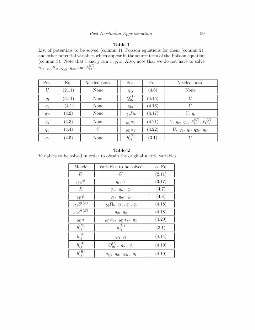
Post-Newtonian Approximation 59
Table 1List of potentials to be solved (column 1), Poisson equations for them (column 2),and other potential variables which appear in the source term of the Poisson equation(column 3). Note that i and j run x, y, z. Also, note that we do not have to solve
η0z, (5)P0z , qyy, qzz and h(U)zz .
Pot. Eq. Needed pots. Pot. Eq. Needed pots.
U (2.11) None qij (4.6) None
qi (3.14) None Q(I)0i (4.15) U
q2 (4.1) None η0i (4.16) U
q2i (4.2) None (5)P0i (4.17) U, qi
q4 (4.3) None (6)α0 (4.21) U, qe, qu, h(U)ij , Q
(I)0i
qu (4.4) U (6)α2 (4.22) U, q2, qi, q2i, qij
qe (4.5) None h(U)ij (3.1) U
Table 2Variables to be solved in order to obtain the original metric variables.
Metric Variables to be solved see Eq.
U U (2.11)
(3)βi qi, U (3.17)
X q2, qu, qe (4.7)
(4)ψ q2, qu, qe (4.8)
(5)βi (A)
(5)P0i, η0i, qu, qe (4.18)
(5)βi (B) q2i, q2 (4.18)
(6)α (6)α0, (6)α2, q4 (4.20)
h(U)ij h
(U)ij (3.1)
h(S)ij qij , q2 (4.14)
h(A)ij Q
(I)0i , qu, qe (4.19)
h(B)ij qij , q2, q2i, qi (4.19)