post-processing resolution enhancement of open skies
TRANSCRIPT

POST-PROCESSING RESOLUTION ENHANCEMENT OF OPEN SKIES PHOTOGRAPHIC IMAGERY
THESIS
Daniel E. Sperl, Captain, USAF
AFIT/GEO/ENG/00M-03
DEPARTMENT OF THE AIR FORCE AIR UNIVERSITY
AIR FORCE INSTITUTE OF TECHNOLOGY
Wright-Patterson Air Force Base, Ohio
APPROVED FOR PUBLIC RELEASE; DISTRIBUTION UNLIMITED.

The views expressed in this thesis/dissertation are those of the author and do not reflect
the official policy or position of the United States Air Force, Department of Defense, or
the U. S. Government

AFIT/GEO/ENG/00M-03
POST-PROCESSING RESOLUTIONENHANCEMENT OF OPEN SKIES PHOTOGRAPHIC IMAGERY
THESIS
Presented to the Faculty
Department of Electrical and Computer Engineering
Graduate School of Engineering and Management
of the Air Force Institute of Technology
Air University
Air Education and Training Command
In Partial Fulfillment of the Requirements for the
Degree of Master of Science in Electro-Optics
Daniel E. Sperl, B.S., M.B.A.
Captain, USAF
March 2000
Approved for public release; distribution unlimited

AFIT/GEO/ENG/00M-03
POST-PROCESSING RESOLUTION
ENHANCEMENT OF OPEN SKIES PHOTOGRAPHIC IMAGERY
Daniel E. Sperl, B.S., M.B.A. Captain, USAF
Approved:

ACKNOWLEDGMENTS
The writer wishes to express special thanks to my faculty advisors, Dr. Steve
Gustafson, Maj Eric Magee, and Dr. Mark Oxley, whose encouragement, helpful
counsel, and practical suggestions were crucial to the successful outcome of this thesis
project. Appreciation is also due to Capt Tom Fitzgerald and Dennis Grieshop for their
assistance with obtaining aerial photographs of Wright-Patterson AFB and to Capt Kelce
Wilson for his help with Matlab.
This statement would be incomplete without recognizing my wife Diana, who has
been so understanding during my graduate school career. She has been my scribe, my
proofreader, and my encouragement. I also must recognize my three children, Leland,
Sabrina, and Ryan. They have been my other source of inspiration.
Daniel E. Sperl
iv

TABLE OF CONTENTS
ACKNOWLEDGMENTS . . . . . . . . . . . . . . . . . . . . . . . . . . . . . . . . . . . . . . . . . . . . . . . . iv
LIST OF FIGURES . . . . . . . . . . . . . . . . . . . . . . . . . . . . . . . . . . . . . . . . . . . . . . . . . . . . . vi
LIST OF TABLES . . . . . . . . . . . . . . . . . . . . . . . . . . . . . . . . . . . . . . . . . . . . . . . . . . . . . viii
ABSTRACT . . . . . . . . . . . . . . . . . . . . . . . . . . . . . . . . . . . . . . . . . . . . . . . . . . . . . . . . . . . ix
I. INTRODUCTION . . . . . . . . . . . . . . . . . . . . . . . . . . . . . . . . . . . . . . . . . . . . . . . . . . . 1
II. BACKGROUND . . . . . . . . . . . . . . . . . . . . . . . . . . . . . . . . . . . . . . . . . . . . . . . . . . . 2 History . . . . . . . . . . . . . . . . . . . . . . . . . . . . . . . . . . . . . . . . . . . . . . . . . . . . . . . . . . . . 2 Data Collection and Aircraft Operations . . . . . . . . . . . . . . . . . . . . . . . . . . . . . . . . . 3 Imaging Test Objects . . . . . . . . . . . . . . . . . . . . . . . . . . . . . . . . . . . . . . . . . . . . . . . . 6
III. REVIEW OF RELEVANT LITERATURE AND RESEARCH . . . . . . . . . . . . . . 13Super-Resolution of Images: Algorithms, Principles, and Performance . . . . . . . . 13
IV. RESEARCH METHODOLOGY . . . . . . . . . . . . . . . . . . . . . . . . . . . . . . . . . . . . . . 15Enhancement Using Commercial Software . . . . . . . . . . . . . . . . . . . . . . . . . . . . . . 15Enhancement Using Model Fit . . . . . . . . . . . . . . . . . . . . . . . . . . . . . . . . . . . . . . . . 16
V. RESULTS . . . . . . . . . . . . . . . . . . . . . . . . . . . . . . . . . . . . . . . . . . . . . . . . . . . . . . . . 26Enhancement Using Commercial Product . . . . . . . . . . . . . . . . . . . . . . . . . . . . . . . 26Enhancement Using Model Fit . . . . . . . . . . . . . . . . . . . . . . . . . . . . . . . . . . . . . . . . 28
VI. CONCLUSIONS and RECOMMENDATIONS . . . . . . . . . . . . . . . . . . . . . . . . . . 50
APPENDIX A. Matlab Code . . . . . . . . . . . . . . . . . . . . . . . . . . . . . . . . . . . . . . . . . . . . . 52
APPENDIX B. List of Scanned Negatives . . . . . . . . . . . . . . . . . . . . . . . . . . . . . . . . . . . 80
BIBLIOGRAPHY . . . . . . . . . . . . . . . . . . . . . . . . . . . . . . . . . . . . . . . . . . . . . . . . . . . . . . 81
Vita . . . . . . . . . . . . . . . . . . . . . . . . . . . . . . . . . . . . . . . . . . . . . . . . . . . . . . . . . . . . . . . . . . 85
v

LIST OF FIGURES
Figure 1. US Optical Cameras . . . . . . . . . . . . . . . . . . . . . . . . . . . . . . . . . . . . . . . . . . . . . 3
Figure 2: Ground Resolution Distance . . . . . . . . . . . . . . . . . . . . . . . . . . . . . . . . . . . . . . . 4
Figure 3. US Open Skies OC-135 Aircraft [37] . . . . . . . . . . . . . . . . . . . . . . . . . . . . . . . . 5
Figure 4. 3-Bar Target . . . . . . . . . . . . . . . . . . . . . . . . . . . . . . . . . . . . . . . . . . . . . . . . . . . . 6
Figure 5. Airstar Emblem . . . . . . . . . . . . . . . . . . . . . . . . . . . . . . . . . . . . . . . . . . . . . . . . . 7
Figure 6. Aerial View of Area B, WPAFB . . . . . . . . . . . . . . . . . . . . . . . . . . . . . . . . . . . . 8
Figure 7. Extraction of 3-Bar Target from Area B Imagery . . . . . . . . . . . . . . . . . . . . . . . 9
Figure 8. Original Image of Group 9, 3-Bar Target, 2D & 3D Views . . . . . . . . . . . . . . 10
Figure 9. Original Image of Group 9, 3-Bar Target, 2D & 3D Views - Enlarged . . . . . 10
Figure 10. C-119 Cargo Plane . . . . . . . . . . . . . . . . . . . . . . . . . . . . . . . . . . . . . . . . . . . . . 11
Figure 11. B-1A Bomber . . . . . . . . . . . . . . . . . . . . . . . . . . . . . . . . . . . . . . . . . . . . . . . . . 11
Figure 12. Image of 2-Bar Target Degraded with German Filter . . . . . . . . . . . . . . . . . . 12
Figure 13: Bias/Variance Tradeoff . . . . . . . . . . . . . . . . . . . . . . . . . . . . . . . . . . . . . . . . . 17
Figure 14. Line Scan of an Image Row . . . . . . . . . . . . . . . . . . . . . . . . . . . . . . . . . . . . . . 20
Figure 15: Flowchart for 3-Bar and 2-Bar Target Model Fit . . . . . . . . . . . . . . . . . . . . . 21
Figure 16: Linescan Flowchart for 3-Bar and 2-Bar Target Model Fit . . . . . . . . . . . . . . 22
Figure 17. Line Plots of Bar Groups 13, 14, & 15 . . . . . . . . . . . . . . . . . . . . . . . . . . . . . 23
Figure 18: Flowchart for Airstar Model Fit . . . . . . . . . . . . . . . . . . . . . . . . . . . . . . . . . . 25
Figure 19. Enhancement by Commercial Software . . . . . . . . . . . . . . . . . . . . . . . . . . . . 26
Figure 20. Line Plots for Bar Groups 9, 11, &13 . . . . . . . . . . . . . . . . . . . . . . . . . . . . . . 27
Figure 21. Enhancement of a C-119 Cargo Plane . . . . . . . . . . . . . . . . . . . . . . . . . . . . . . 27
Figure 22. Original Image of Group 9, tar66a.tif, 2D & 3D Views . . . . . . . . . . . . . . . . 32
vi

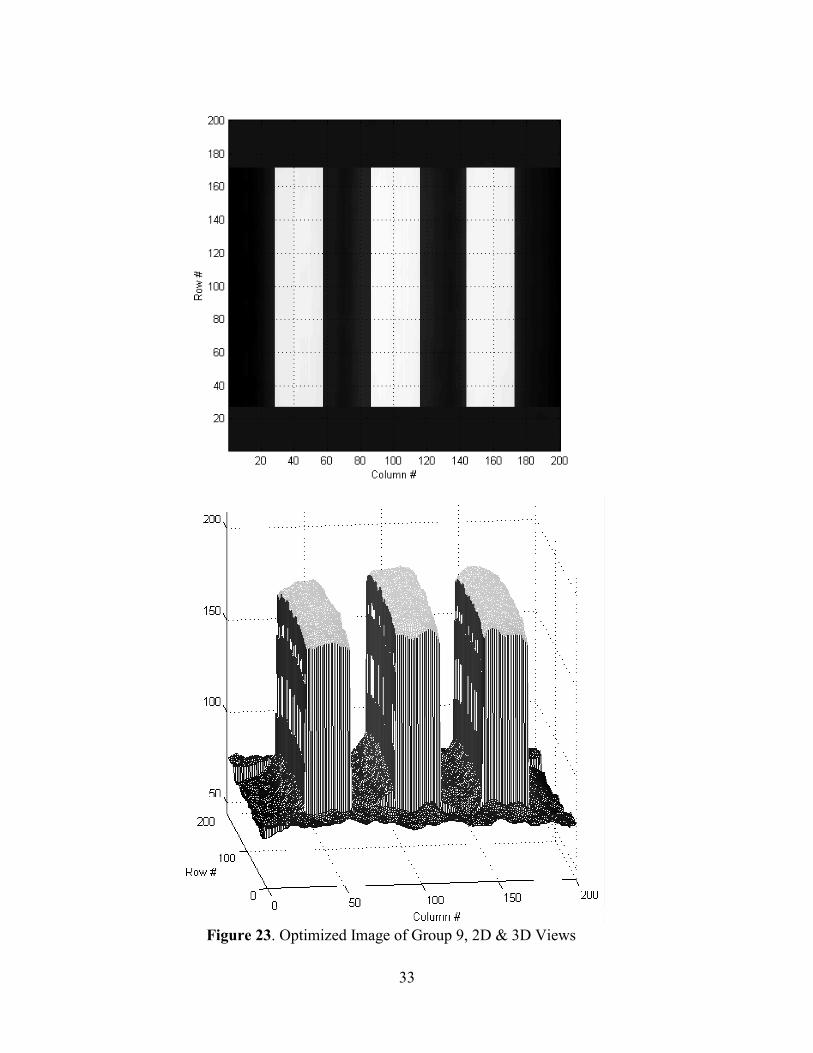
Figure 23. Optimized Image of Group 9, 2D & 3D Views . . . . . . . . . . . . . . . . . . . . . . . 33
Figure 24. Original & Optimized Images of Group 9 . . . . . . . . . . . . . . . . . . . . . . . . . . . 34
Figure 25. Original Image of Group 12, 5.7 micron scan, tar66a.tif, 2D & 3D Views . . 35
Figure 26. Optimized Image of Group 12, 2D & 3D Views . . . . . . . . . . . . . . . . . . . . . . 36
Figure 27. Original & Optimized Images of Group 12 . . . . . . . . . . . . . . . . . . . . . . . . . . 37
Figure 28. Original Image of Group 12, 4 micron scan, target66u.tif, 2D & 3D Views . 38
Figure 29. Optimized Image of Group 12, 2D & 3D Views . . . . . . . . . . . . . . . . . . . . . . 39
Figure 30. Original & Optimized Images of Group 12 . . . . . . . . . . . . . . . . . . . . . . . . . . 40
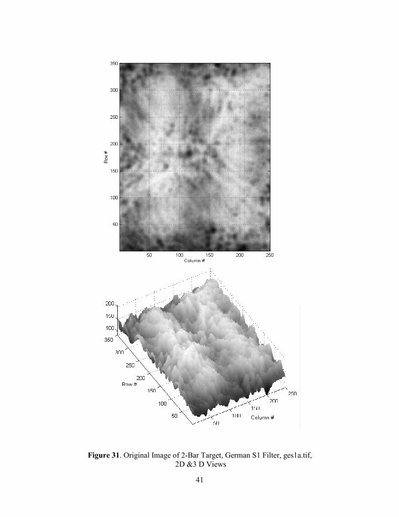
Figure 31. Original Image of 2-Bar Target, German S1 Filter, ges1a.tif,
2D &3 D Views . . . . . . . . . . . . . . . . . . . . . . . . . . . . . . . . . . . . . . . . . . . . . . 41
Figure 32. Optimized Image of 2-Bar Target, German S1 Filter, 2D & 3D Views . . . . 42
Figure 33. Original & Optimized Images of 2-Bar Target, German S1 Filter . . . . . . . . 43
Figure 34. Original Airstar, B-1A Bomber, plane55b.tif, 2D & 3D Views . . . . . . . . . . 44
Figure 35. Model Airstar, B-1A Bomber, 2D & 3D Views . . . . . . . . . . . . . . . . . . . . . . 45
Figure 36. Optimized Airstar, B-1A Bomber, 2D &3D Views . . . . . . . . . . . . . . . . . . . . 46
Figure 37. Original Airstar, C-119 Cargo Plane, plane55a.tif, 2D & 3D Views . . . . . . 47
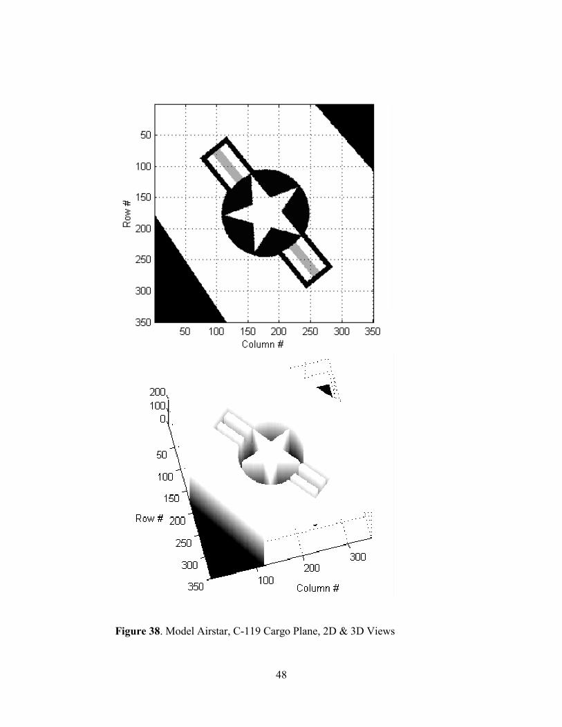
Figure 38. Model Airstar, C-119 Cargo Plane, 2D & 3D Views . . . . . . . . . . . . . . . . . . 48
Figure 39. Optimized Airstar, C-119 Cargo Plane, 2D & 3D Views . . . . . . . . . . . . . . . 49
vii

LIST OF TABLES
Table 1. Items Visible Based on the 30 Centimeter Ground Resolution Limit . . . . . . . . 2
Table 2. Generic Model Fit Procedure . . . . . . . . . . . . . . . . . . . . . . . . . . . . . . . . . . . . . . 19
Table 3. List of Matlab Code and Data Files . . . . . . . . . . . . . . . . . . . . . . . . . . . . . . . . . 52
viii

ABSTRACT
The Treaty on Opens Skies allows any signatory nation to fly a specifically
equipped reconnaissance aircraft anywhere over the territory of any other signatory
nation. For photographic images, this treaty allows for a maximum ground resolution of
30 cm. The National Air Intelligence Center (NAIC), which manages implementation of
the Open Skies Treaty for the US Air Force, wants to determine if post-processing of the
photographic images can improve spatial resolution beyond 30 cm, and if so, determine
the improvement achievable. Results presented in this thesis show that standard linear
filters (edge and sharpening) do not improve resolution significantly and that super-
resolution techniques are necessary. Most importantly, this thesis describes a prior-
knowledge model fitting technique that improves resolution beyond the 30 cm treaty
limit. The capabilities of this technique are demonstrated for a standard 3-Bar target, an
optically degraded 2-Bar target, and the USAF airstar emblem.
ix

Post-Processing Resolution
Enhancement of Open Skies Photographic Imagery
I. INTRODUCTION
The Treaty on Opens Skies is an international effort to promote goodwill and
openness. The treaty allows any signatory nation to fly a specifically equipped
reconnaissance aircraft anywhere over the territory of any other signatory nation [12:4].
For photographic images, the treaty allows for a maximum ground resolution of 30 cm.
Unfortunately, due to advances in technology, post-processing may increase this
maximum ground resolution. The goal of this research is to develop Matlab models that
demonstrate post-processing resolution enhancement of Open Skies photographic
imagery.
Chapter II provides background on Open Skies and the data set of aerial images
used for this research. Chapter III presents some relevant previous research, results, and
Chapter IV reviews super-resolution theory. Chapter V discusses results, and Chapter VI
presents conclusions and recommendations.
1

II. BACKGROUND
History
The United States, along with 26 other nations, signed the Treaty on Open Skies
(OS) on 24 March 1992 as part of an international effort to promote openness and trust
building; however, “The Treaty is not an arms control program [12:5].” Each country
allows overflights of their entire national territory, including territorial waters and islands
by other countries. The treaty enters into force (EIF) when twenty countries that include
Canada, Germany, Russia, Belarus, US, France, UK, Italy, Turkey, and Ukraine ratify it;
this has not happened yet [37]. Table 1 gives examples of items that are and are not
visible under the treaty resolution limit of 30 cm. The OS aircraft are equipped with an
approved suite of sensors.
Table 1. Items Visible Based on the 30 Centimeter Ground Resolution Limit [37] CAN CANNOT
Identify small aircraft by type (such as F-14s, F-15s, F-16s) when singly deployed. Read call letters and numbers on wings when 3 feet high. Detect uploaded weapons on aircraft wings. Identify an F-16 fighter from an F-16 trainer by canopy configuration. Detect presence of shipboard weapons and major electronics (guns, missiles, surface search radar). Detect the presence and pattern of mooring lines. Detect presence of life rails when raised. Accurately distinguish smaller vehicle types (for instance, pick-up trucks versus sedans).
Identify a specific model fighter (such as an F-16A versus F-16C) by small details such as dielectric patches on wings. Identify the pitot tube on a fighter aircraft.
Identify a specific weapon type.
Identify on the appropriate model fighter, wing flap actuator fairings and yaw vanes. Accurately identify by specific type shipboard weapons and major electronics.
Identify draft marks.
Identify mast configuration. Identify small ground support equipment by type, such as dollies, tow bars, and fire extinguisher carts.
2

Figure 1. US Optical Cameras
Data Collection and Aircraft Operations
The Treaty allows three types of sensors: optical, infrared, and Synthetic Aperture
Radar (SAR). Optical cameras (Figure 1) include one vertically mounted framing
camera, two obliquely mounted framing cameras, one panoramic camera, and one video
camera. Infrared sensors include a line scanner and a side-looking SAR. Currently, and
until EIF, the Treaty allows only optical sensors (cameras) [12:5]. The optical and SAR
sensors may be used during the first three years after EIF, but the infrared (IR) may not
be used until three years after EIF unless otherwise agreed. During an observation flight,
sensor operation is suspended if the aircraft altitude is below the minimum altitude, or if
the flight deviates more than 50 km from the planned flight path. Both parties receive
copies of the data, and any other treaty signatory may get a copy by written request and
3
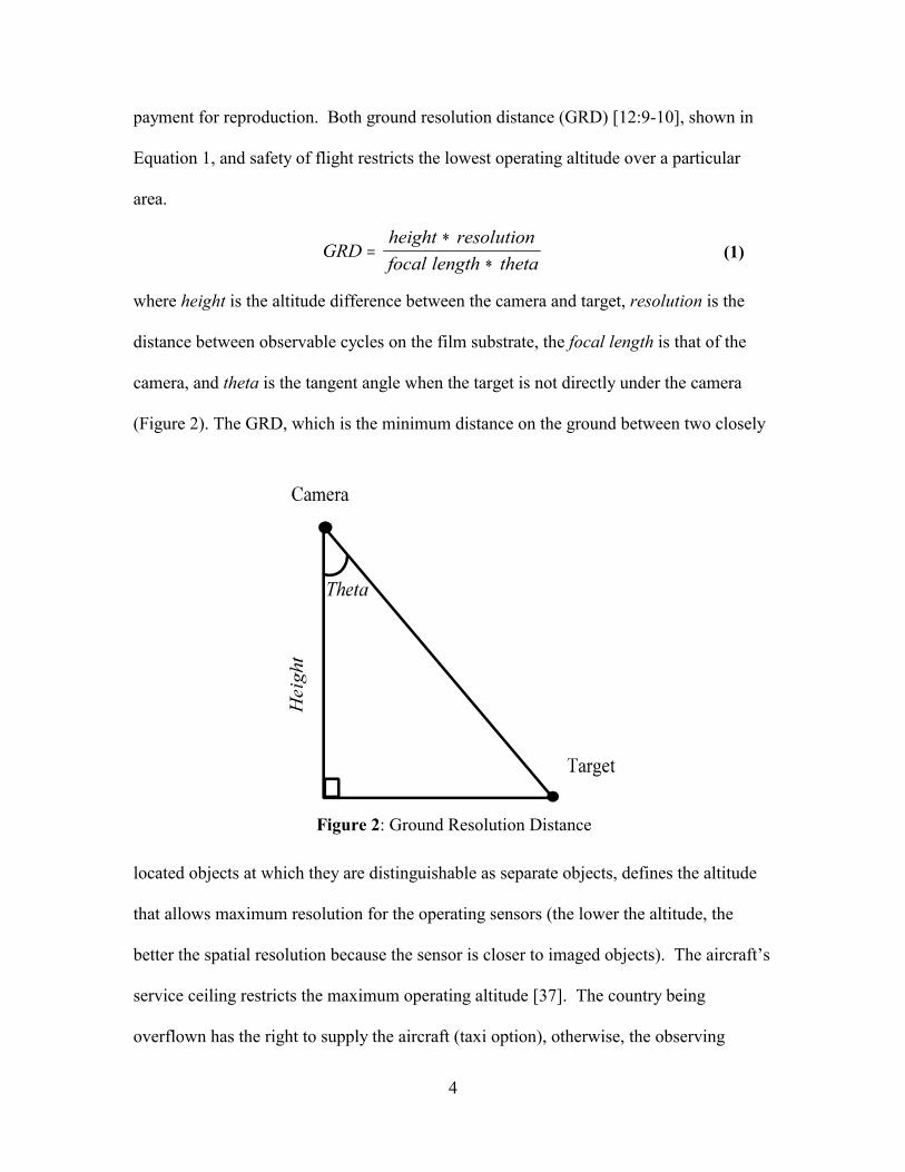
payment for reproduction. Both ground resolution distance (GRD) [12:9-10], shown in
Equation 1, and safety of flight restricts the lowest operating altitude over a particular
area.
GRD �height � resolution focal length � theta (1)
where height is the altitude difference between the camera and target, resolution is the
distance between observable cycles on the film substrate, the focal length is that of the
camera, and theta is the tangent angle when the target is not directly under the camera
(Figure 2). The GRD, which is the minimum distance on the ground between two closely
Figure 2: Ground Resolution Distance
located objects at which they are distinguishable as separate objects, defines the altitude
that allows maximum resolution for the operating sensors (the lower the altitude, the
better the spatial resolution because the sensor is closer to imaged objects). The aircraft’s
service ceiling restricts the maximum operating altitude [37]. The country being
overflown has the right to supply the aircraft (taxi option), otherwise, the observing
4

country may use its own aircraft. In either case, an inspection at the OS point of entry
ensures treaty conformance of aircraft and sensors. The United States uses OC-135B
aircraft as depicted in Figure 3.
Figure 3. US Open Skies OC-135 Aircraft [37]
5

Imaging Test Objects
The United States Air Force (USAF) uses a 3-Bar target (Figure 4) which includes
horizontal and vertical bar groups of various sizes and spacings. The two triangles show
which bar group meets the treaty spatial resolution limit of 30 cm, which means that
objects at least 30 cm apart on they can distinguish ground from each other [12:8-9].
Figure 4. 3-Bar Target
6

The airstar emblem (Figure 5) is a painted object on all US military aircraft; it
consists of a blue field with a white star and white and red stripes. This colored version
of the airstar emblem has been phased out and replaced with a grayscale version to
reduce visibility and increase survivability.
Figure 5. Airstar Emblem
For this research the data set is a series of aerial negatives from an altitude of
approximately 1,250 m provided by NAIC ( Appendix B). The images in these negatives
are of the 3-Bar target, the USAF Museum, and surrounding area in Area B at Wright-
Patterson AFB, Ohio, and a 2-Bar target located in Europe. These images were digitized
using a scanner with a pixel resolution of 5.7 microns. An example of one of these
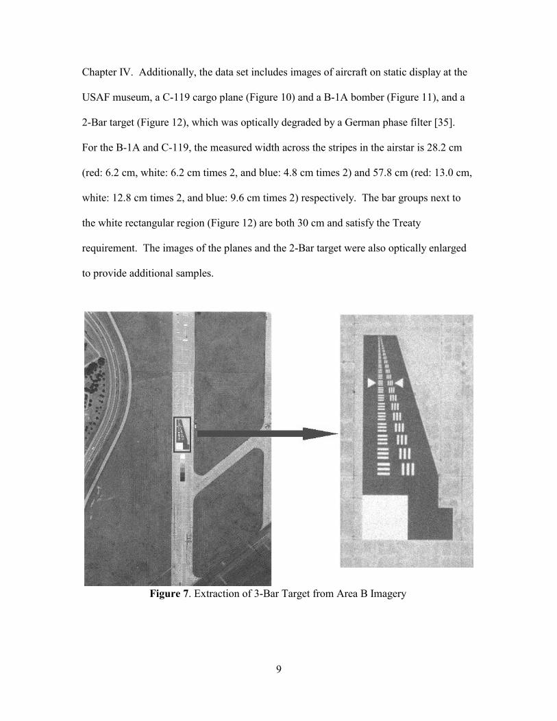
images (66target.tif) is given in Figure 6. Since multi-frame resolution was not the goal
of this thesis, frames were chosen (checkmarked in Appendix B) and the relevant regions
of interest were extracted. For example, an area that contained the 3-Bar target was
extracted from 66target.tif (Figure 7). The grain sizes on negatives are usually uniform
and submicron in size, but the grain size can be up to 4 microns [30]. Since the
7

resolution of the negatives is much finer than the scanner’s 5.7 micron resolution, the
negatives were optically enlarged and digitized to provide more samples. For example,
the group 9 bar group in the original negative yielded a 21 by 21 pixel matrix (Figure 8) ,
whereas the enlarged negative yielded a 200 by 200 pixel matrix (Figure 9). Enlarging
the negatives added some noise but did not affect the results, which are discussed in
Figure 6. Aerial View of Area B, WPAFB
8
Chapter IV. Additionally, the data set includes images of aircraft on static display at the
USAF museum, a C-119 cargo plane (Figure 10) and a B-1A bomber (Figure 11), and a
2-Bar target (Figure 12), which was optically degraded by a German phase filter [35].
For the B-1A and C-119, the measured width across the stripes in the airstar is 28.2 cm
(red: 6.2 cm, white: 6.2 cm times 2, and blue: 4.8 cm times 2) and 57.8 cm (red: 13.0 cm,
white: 12.8 cm times 2, and blue: 9.6 cm times 2) respectively. The bar groups next to
the white rectangular region (Figure 12) are both 30 cm and satisfy the Treaty
requirement. The images of the planes and the 2-Bar target were also optically enlarged
to provide additional samples.
Figure 7. Extraction of 3-Bar Target from Area B Imagery
9
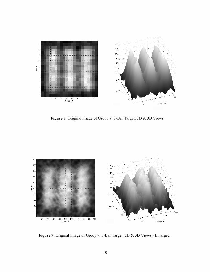
Figure 8. Original Image of Group 9, 3-Bar Target, 2D & 3D Views
Figure 9. Original Image of Group 9, 3-Bar Target, 2D & 3D Views - Enlarged
10
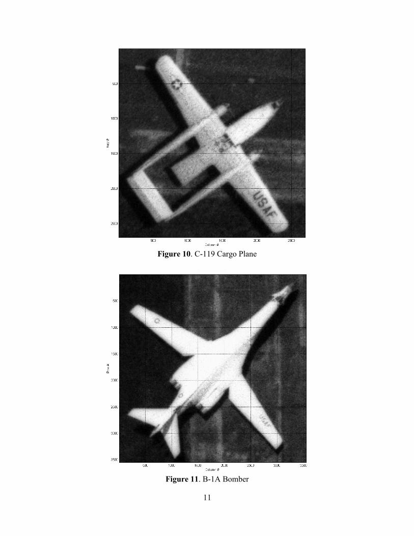
Figure 10. C-119 Cargo Plane
Figure 11. B-1A Bomber
11

Figure 12. Image of 2-Bar Target Degraded with German Filter
12

III. REVIEW OF RELEVANT LITERATURE AND RESEARCH
The review given here is based upon information available from libraries, the
Internet, and the National Air Intelligence Center.
Super-Resolution of Images: Algorithms, Principles, and Performance
Many technical documents relating to image enhancement [3, 4, 7, 10, 14, 15, 32,
38, 39], blind deconvolution [28, 29], and super-resolution [1, 9, 11, 17-22, 24-27, 34,
41-47] present methods for improving the resolution of multi-frame sequences.
Unfortunately, these documents do not apply to this research, because image registration
[1, 8, 19, 20, 23, 26, 25-27, 43, 45] is assumed, and the data set used in this research is
not registered. Image registration is an area of research beyond the scope of this thesis.
From these documents, only two are relevant to this research.
The first relevant article to this research is a paper on the super-resolution of images
by Hunt [22], which provides a good overview of super-resolution principles and
techniques. This paper discusses diffraction as the key motivation for performing super-
resolution, and it indicates that the use of prior information is one critical principle that
enables super-resolution:
• “The spatial frequencies that are captured by image formation below the diffraction limit contain some of the information necessary to reconstruct spatial frequencies above the diffraction limit;
• Using additional information about the object (e.g., compact, hence possessing an analytic Fourier transform) provides a means to use the information below the diffraction limit to reconstruct information above that limit [22:298-299].”
This paper also lists some features that affect the performance of super-resolution
13

algorithms:
• Object, size, shape, and location - “Usually the image of an object is adequate to make an estimate of the approximate size, shape, and location of the object. The size and shape characteristics of the object can be inferred from measured size and shape of the image and optical system PSF [22:301].”
• Bounds on object intensity - “The minimum intensity level of an object is zero, because negative light is meaningless in incoherent optical image formation[22:301].”
The other article that is relevant to this research is by Matson [33] and discusses
error reduction in images through use of perfect prior knowledge. The technique is based
on the notion that “part of an image may be known exactly, and this can be used as a
constraint to decrease noise levels in the image outside the region of perfectly known
data [33].” Matson’s algorithm requires multiple iterations between the spatial and
frequency domains until the noise is minimized outside the region of prior knowledge.
“The algorithm’s steps are: (1) in the image domain, replace the measured data with the
prior knowledge in the region where prior knowledge is available; (2) Fourier transform;
(3) if the real (imaginary) part of the measured Fourier data is less noisy than the
imaginary (real), replace the iterated real (imaginary) part of the Fourier data with the
measured data, but leave the imaginary (real) part unchanged; (4) inverse-Fourier-
transform; (5) go back to step (1) until the noise is minimized outside the region of prior
knowledge [33].”
The use of prior information, positive image intensity, object size, error reduction,
and shape relationships are the basis for the super-resolution techniques discussed in the
next chapter.
14

IV. RESEARCH METHODOLOGY
The Open Skies treaty requires a calibration flight to be flown over a 3-Bar target
before a signatory nation performs data gathering missions. Data from the calibration
flight is used to set the minimum altitude and GRD at which the data gathering missions
are flown. Due to weather constraints (i.e., clouds, storms, etc.), the National Air
Intelligence Center wants the capability to fly at lower altitudes while still maintaining
the 30 cm spatial resolution limit. Flying at lower altitudes increases spatial resolution.
Therefore, the optics used to record images must be degraded to the treaty requirement.
Since the optics are artificially degraded, it is also necessary to ensure that the increased
spatial resolution from flying at lower altitudes cannot be recovered (e.g., by post-
processing). This research demonstrates that the resolution of Open Skies photographic
imagery can be increased beyond the treaty limit of 30 cm if certain a priori knowledge
of the image exists. The methods reported here deal with a 3-Bar target (Figure 4) and an
airstar emblem (Figure 5).
Enhancement Using Commercial Software
Resolution enhancement was attempted using three commercially available
programs for editing photographs: Ulead PhotoImpact 4.2, Scion Image, and
Micrografx’s Picture Publisher. All three programs contain image enhancement
functions for sharpening, edge detection, and contrast adjustment.
15

Enhancement Using Model Fit
One classic approach to increasing the resolution of an image is to use the
Gerchberg algorithm [22], which requires multiple iterations and transformations
between the spatial and spatial frequency domains. Since enough prior information
exists about the 3-Bar target and the airstar emblem, employing a spatial domain model
fit algorithm is appropriate.
Resolution enhancement using the model fit method may be justified by extending
the rationale presented by Hunt [22] and Matson [33]. Suppose that a given gray level
digital image consists of an underlying model plus additive noise, but that no prior
knowledge is available about the model. Then the most unbiased (equivalent to
maximum entropy) choice for the underlying model is the image mean (i.e., the mean of
all pixel level values), and the standard deviation about this mean may be chosen as the
variance in the given data. Now suppose that prior knowledge about the model exists
(i.e., the model is a known object) and that the knowledge is perfect except for linear
transformations. Then the only unknowns are the relative translation, rotation, and scale
of the object and the linear scaling of the image intensity. Thus, six parameters may be
evaluated to fit the model to the image: horizontal and vertical placement, rotation angle
about the horizontal axis, size of the object, and minimum and maximum gray level
values. Some of these parameters may be fixed (e.g., the rotation angle is assumed zero).
The values of the six parameters that minimize the mean squared error (MSE) [5:11]
between the model and given data may be chosen to specify the fitted model where the
minimized quantity is:
16
� �
n m
� � ���Giveni j � Modeli j �
2 ��
MSE � i �1 j �1 (2)
nm
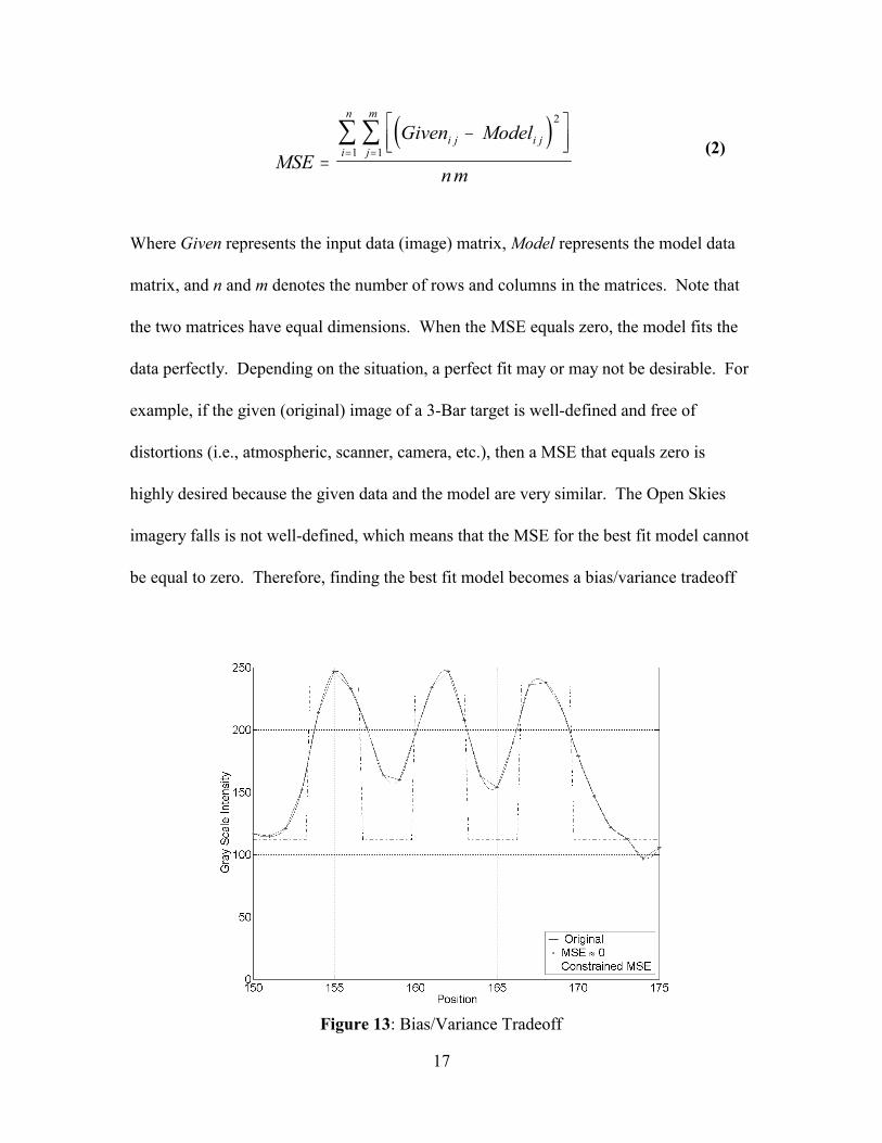
Where Given represents the input data (image) matrix, Model represents the model data
matrix, and n and m denotes the number of rows and columns in the matrices. Note that
the two matrices have equal dimensions. When the MSE equals zero, the model fits the
data perfectly. Depending on the situation, a perfect fit may or may not be desirable. For
example, if the given (original) image of a 3-Bar target is well-defined and free of
distortions (i.e., atmospheric, scanner, camera, etc.), then a MSE that equals zero is
highly desired because the given data and the model are very similar. The Open Skies
imagery falls is not well-defined, which means that the MSE for the best fit model cannot
be equal to zero. Therefore, finding the best fit model becomes a bias/variance tradeoff
Figure 13: Bias/Variance Tradeoff
17

�
(i.e., fit vs. smoothness of fit of the model to the given data) [5, 13] with the minimum
MSE contrained by prior knowledge (see Figure 13). The standard deviation about the
fitted model (i.e., MSE ) may then be chosen as a measure of the added noise, and this
standard deviation will generally be less than the standard deviation [5:34] about the
image mean ( Given ):
�Given Given
nm
i j j
m
i
n
� � ��
� ��
��
� � 2
1 1 � (3)
STD Given �
where
n m
� � �Giveni j � (4)Given �
i �1 j �1
nm
Therefore, the following expression may be chosen to specify a processed image that
incorporates the prior knowledge:
Newi j � Giveni j � � Modeli j � Giveni j � � � for 0 � � � 1 (5)
where New is the processed image, and � � MSE STD Given , is the ratio of
standard deviations for the given data about the fitted model to the given data (or image)
mean. This ratio is a scale factor that measures the extent to which available prior
knowledge reduces noise and enhances resolution. Note that Equation (5) is applied to
each pixel independently, and when necessary, the new data is re-scaled for gray level
18

values outside the 0-255 range. The model fit method matches a model (procedure in
Table 2, Matlab code in Appendix A) of the object to the given data in the spatial domain
only. Finally, for modeling purposes knowing the altitude and speed of the aircraft, or
the camera parameters (focal length, etc.) is not necessary; the only required information
is some prior knowledge about the imaged object.
The 3-Bar target has a height to width ratio of 5:1 and equal spacing within each
bar group ( i.e., the widths of the white bars and the black spacing between them are
equal, see Figure 4). The minimum contrast ratio (white/black) is 2:1, which means that
the minimum/maximum gray levels in the optimized image should be close to the
minimum/maximum gray levels in the original image. Each row of pixels across a bar
group has uniform gray intensity levels, and therefore the same model. By using this
prior knowledge, the model fit method can generate a model of each row or the whole bar
group. In addition, since the 3-Bar target consists of simple objects (rectangles),
generating the model is straight-forward because the algorithm adjusts only a few
variables. Adjusting five variables (bar width, horizontal and vertical bar placement,
Table 2. Generic Model Fit Procedure
1. Extract the region of interest from the given image.
2. Estimate initial parameter values (horizontal and vertical placement, the rotation angle about the horizontal axis, the size of the object, and the minimum and maximum gray level intensity).
3. Perform an exhaustive search to minimize the mean squared error between the given data and the model (using the initial estimates from Step 2).
4. Incorporate the prior knowledge into the given data using Equation 5.
19
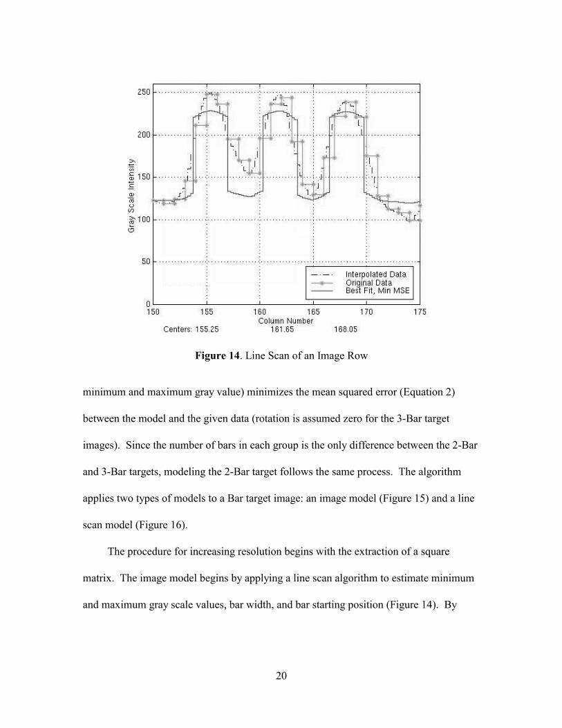
Figure 14. Line Scan of an Image Row
minimum and maximum gray value) minimizes the mean squared error (Equation 2)
between the model and the given data (rotation is assumed zero for the 3-Bar target
images). Since the number of bars in each group is the only difference between the 2-Bar
and 3-Bar targets, modeling the 2-Bar target follows the same process. The algorithm
applies two types of models to a Bar target image: an image model (Figure 15) and a line
scan model (Figure 16).
The procedure for increasing resolution begins with the extraction of a square
matrix. The image model begins by applying a line scan algorithm to estimate minimum
and maximum gray scale values, bar width, and bar starting position (Figure 14). By
20

Load Data
Perform linescan
Start
Shift Given Data
fmins('minmize',lam) lam = initial guesses for bar width & starting position
Make model using results from minimize
new MSE < MSE
Calculate new MSE
Yes
MSE = new MSE model = new model
bar width = new bar width start position = new start position
MSE_Count=MSE_Count + 1
No Incorporate
prior knowledge
end
While MSE_Count >0 & b1 < b2
No
Yes
b1 = bar width lower limit b2 = bar width upper limit
Estimate bar width, center of 1st bar (peak value of 1st bar), limit min/max gray scale to preserve contrast.
Save & display results
Figure 15: Flowchart for 3-Bar and 2-Bar Target Model Fit
21

Estimate initial values
Start
Perform iterative search using: min/max gray levels, b1, b2, & starting position
Make 1-D model
new MSE < MSE
Calculate new MSE
Yes
MSE = new MSE model = new model
bar width = new bar width start position = new start position
MSE_Count=MSE_Count + 1
No
Incorporate prior
knowledge
end
While MSE_Count >0 & b1 < b2
No
Yes
b1 = bar width lower limit b2 = bar width upper limit
Limit min/max gray scale values to preserve
image intensity Scan 3 rows to estimate bar width, center of 1st bar (peak value of 1st bar).
For noisy images, scan additional rows, & estimate center of 1st bar by setting a max gray threshold and finding the median position for intensities above the threshold.
Figure 16: Linescan Flowchart for 3-Bar and 2-Bar Target Model Fit
22

Figure 17. Line Plots of Bar Groups 13, 14, & 15
iterative search, models are generated from these estimates to minimize the MSE
between the model and the given data, with Equation 5 incorporating the prior knowledge
into the given data. Any of the adjustable parameters can be a source of possible fit
error, but measuring this error is impossible because an original perfect image does not
exist.
An optimized image could be generated for any of the smaller bar groups (13 and
up) using prior knowledge. However, the accuracy or confidence level of the model fit
method would be lower because the smaller bar groups do not show any distinguishable
bar separation (Figure 17). Therefore, the method was not used for bar groups that do not
show relative separation between bars.
Obviously, there are many more variables for complex objects such as airplanes or
23

buildings, and generating a model is much more difficult. For such objects, developing
the model for a small region of interest (ROI) limits the number of variables. For
example, instead of developing a model for a whole aircraft, or even an aircraft wing, the
ROI is limited to a part of the wing. For this research the ROI was limited to the area
surrounding the airstar emblem.
Modeling the airstar is much more difficult than the 3-Bar target because each row
of pixels is different and there are multiple gray levels that represent the red, white, and
blue colors. Although the airstar shape is more complex due to the stripes, circle, and the
star, it has known characteristics. The general procedure for modeling the airstar (Figure
18) is similar to modeling the bar target. Estimates are made for rotation, minimum and
maximum gray scale values, and placement. An iterative search is performed using these
estimates to minimize the MSE between the model and the given data, and Equation (5)
then incorporates the prior knowledge into the given data. As before, the adjustable
parameters can be a source of fit error, but the use of prior knowledge allows
development and application of a robust model while processing only in the spatial
domain.
24

Load Data
Estimate rotation from wing leading edge, min/max gray scale values
Start
Make model airstar. Adjust: scale, rotate, & placement
Set gray scale area outside wing surface = 0
Calculate MSE between Given & Model (MSE2) ratio = STD_MSE2/STD_Given
MSE1 < MSE MSE2 < MSE3
|rat - ratio|>=test_rat
Incorporate prior knowledge Calculate MSE between Given & Modified (MSE1)
rat = MSE1/MSE2
Yes
MSE = MSE1 MSE3 = MSE2
model airstar = new model airstar Optimized = Modified
MSE_Count=MSE_Count + 1
No
end
While MSE_Count >0 & rat<=ratio & b1>=0.08
No
Yes
b1 = scale factor lower limit
Save & display results
Note: Due to noise, the ratio of MSE1/MSE2 is necessary to limit the sized airstar in the model from being to small/large
Figure 18: Flowchart for Airstar Model Fit 25

V. RESULTS
Enhancement Using Commercial Product
At best, the three commercial products produced marginal results (Figure 19) using
the generic filters included in each product. Only two of the programs, Ulead’s
PhotoImpact and Scion Image, allowed for the creation and use of custom filters. The
generic filters generally enhanced image resolution, but also amplified image noise as
evidenced by speckling. Results also indicate that a darkening contrast adjustment had
Figure 19. Enhancement by Commercial Software 26
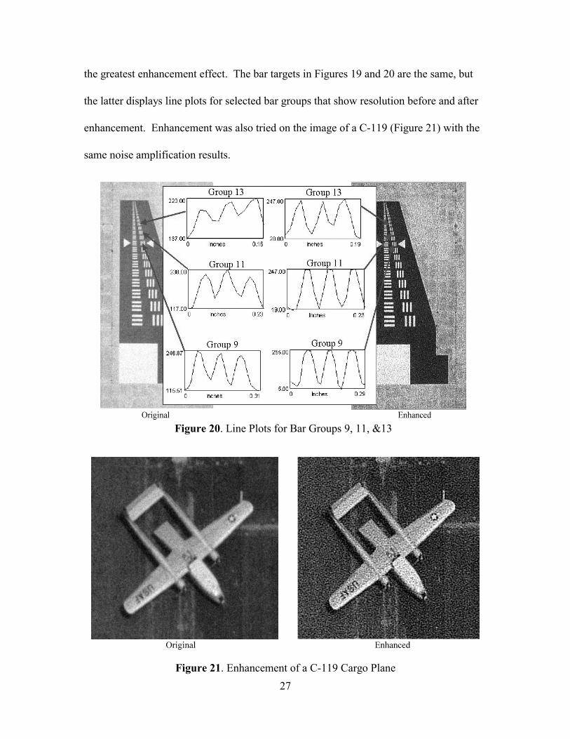
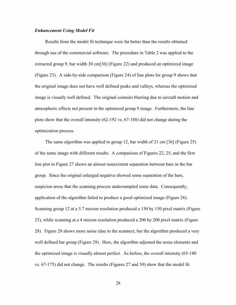
the greatest enhancement effect. The bar targets in Figures 19 and 20 are the same, but
the latter displays line plots for selected bar groups that show resolution before and after
enhancement. Enhancement was also tried on the image of a C-119 (Figure 21) with the
same noise amplification results.
Figure 20. Line Plots for Bar Groups 9, 11, &13
Figure 21. Enhancement of a C-119 Cargo Plane 27
Enhancement Using Model Fit
Results from the model fit technique were far better than the results obtained
through use of the commercial software. The procedure in Table 2 was applied to the
extracted group 9, bar width 30 cm[36] (Figure 22) and produced an optimized image
(Figure 23). A side-by-side comparison (Figure 24) of line plots for group 9 shows that
the original image does not have well defined peaks and valleys, whereas the optimized
image is visually well defined. The original contains blurring due to aircraft motion and
atmospheric effects not present in the optimized group 9 image. Furthermore, the line
plots show that the overall intensity (62-192 vs. 67-188) did not change during the
optimization process.
The same algorithm was applied to group 12, bar width of 21 cm [36] (Figure 25)
of the same image with different results. A comparison of Figures 22, 25, and the first
line plot in Figure 27 shows an almost nonexistent separation between bars in the bar
group. Since the original enlarged negative showed some separation of the bars,
suspicion arose that the scanning process undersampled some data. Consequently,
application of the algorithm failed to produce a good optimized image (Figure 26).
Scanning group 12 at a 5.7 micron resolution produced a 150 by 150 pixel matrix (Figure
25), while scanning at a 4 micron resolution produced a 200 by 200 pixel matrix (Figure
28). Figure 28 shows more noise (due to the scanner), but the algorithm produced a very
well defined bar group (Figure 29). Here, the algorithm adjusted the noise elements and
the optimized image is visually almost perfect. As before, the overall intensity (65-180
vs. 67-175) did not change. The results (Figures 27 and 30) show that the model fit
28

algorithm is highly dependent upon the number of available samples (i.e., scanning at 5.7
microns vs. 4 microns). In addition, the results indicate that sampling limits the amount
of increased resolution (i.e., the resolution of the film used to record the original image,
or the digital scanner used). For example, Figure 17 shows line plots of groups 13, 14,
and 15 that are unresolved. Prior knowledge insures that the object contains three bars,
but the film does not have the resolution to record three separate bars at an altitude that
satisfies the Treaty limit of 30 cm. Since the image satisfies the Treaty limit and the bar
group12 width is 21cm [36], post-processing increases the resolution by 9 cm, or a 30
percent increase.
Applying the model to the degraded image (Figure 31) introduced some new
challenges due to the added noise introduced by the German phase filter. The three-
dimensional plot in Figure 31 and the upper line plot in Figure 33 indicate that little or no
separation exists between the two bars. Modifying the model to handle two bars instead
of three was straight-forward, but handling the additional noise required a different
approach to finding the center of the first bar. For example, in the undegraded 3-Bar
target images (Figure 22) the bars have defined peaks and valleys, whereas the degraded
2-Bar target image (Figure 31) has much noise where the first bar should be. Therefore,
modifying the algorithm was necessary to find all values above a threshold in the first
130 positions of each row to estimate the starting bar width and bar position. In addition,
the algorithm used five rows instead of three to generate these estimates. Application of
the modified algorithm to the degraded 2-Bar target image (Figure 31) removed or
adjusted the added noise to produce an optimized image (Figure 32) for the 30 cm bar
29
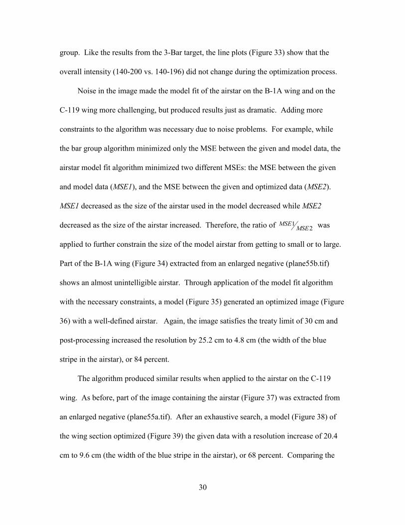
group. Like the results from the 3-Bar target, the line plots (Figure 33) show that the
overall intensity (140-200 vs. 140-196) did not change during the optimization process.
Noise in the image made the model fit of the airstar on the B-1A wing and on the
C-119 wing more challenging, but produced results just as dramatic. Adding more
constraints to the algorithm was necessary due to noise problems. For example, while
the bar group algorithm minimized only the MSE between the given and model data, the
airstar model fit algorithm minimized two different MSEs: the MSE between the given
and model data (MSE1), and the MSE between the given and optimized data (MSE2).
MSE1 decreased as the size of the airstar used in the model decreased while MSE2
decreased as the size of the airstar increased. Therefore, the ratio of MSEMSE
1 2 was
applied to further constrain the size of the model airstar from getting to small or to large.
Part of the B-1A wing (Figure 34) extracted from an enlarged negative (plane55b.tif)
shows an almost unintelligible airstar. Through application of the model fit algorithm
with the necessary constraints, a model (Figure 35) generated an optimized image (Figure
36) with a well-defined airstar. Again, the image satisfies the treaty limit of 30 cm and
post-processing increased the resolution by 25.2 cm to 4.8 cm (the width of the blue
stripe in the airstar), or 84 percent.
The algorithm produced similar results when applied to the airstar on the C-119
wing. As before, part of the image containing the airstar (Figure 37) was extracted from
an enlarged negative (plane55a.tif). After an exhaustive search, a model (Figure 38) of
the wing section optimized (Figure 39) the given data with a resolution increase of 20.4
cm to 9.6 cm (the width of the blue stripe in the airstar), or 68 percent. Comparing the
30

original images (Figures 34 and 37) shows more definition in the C-119 airstar than the
B-1A airstar. The five points of the star on the C-119 are identifiable, and a fairly
uniform rectangular region on each side faintly outlines the stripes of the star. None of
these features are clearly visible on the B-1A. The star on the B-1A is (for lack of a
better term) a blob in the middle of what should be a blue circular background, and the
stripes are not present. A comparison of the optimized images for the B-1A and C-119
with their respective original images indicates that the algorithm produced a better fit for
the C-119 than the B-1A. However, this is not so: A visual inspection of Figures 34 and
36 shows that the star is centered in the optimized image just as the blob is centered on
the original. Likewise, Figures 37 and 39 show that the star is centered in both the
original and optimized images. Therefore, the algorithm performed correctly when
minimizing the MSE.
31

Figure 22. Original Image of Group 9, tar66a.tif, 2D & 3D Views
32
33
Figure 23. Optimized Image of Group 9, 2D & 3D Views

Figure 24. Original & Optimized Images of Group 9
34

35
Figure 25. Original Image of Group 12, 5.7 micron scan, tar66a.tif, 2D & 3D Views

36
Figure 26. Optimized Image of Group 12, 2D & 3D Views
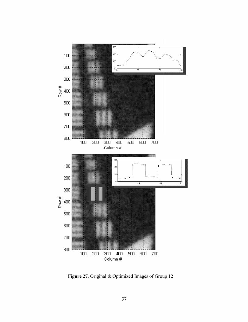
Figure 27. Original & Optimized Images of Group 12
37

38
Figure 28. Original Image of Group 12, 4 micron scan, target66u.tif, 2D & 3D Views

39
Figure 29. Optimized Image of Group 12, 2D & 3D Views

Figure 30. Original & Optimized Images of Group 12
40
41
Figure 31. Original Image of 2-Bar Target, German S1 Filter, ges1a.tif, 2D &3 D Views

42
Figure 32. Optimized Image of 2-Bar Target, German S1 Filter, 2D & 3D Views

43
Figure 33. Original & Optimized Images of 2-Bar Target, German S1 Filter
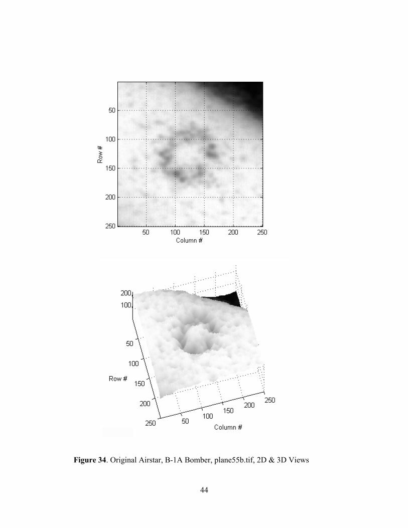
Figure 34. Original Airstar, B-1A Bomber, plane55b.tif, 2D & 3D Views
44

45
Figure 35. Model Airstar, B-1A Bomber, 2D & 3D Views
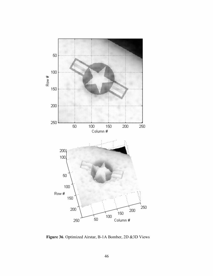
Figure 36. Optimized Airstar, B-1A Bomber, 2D &3D Views
46

Figure 37. Original Airstar, C-119 Cargo Plane, plane55a.tif, 2D & 3D Views
47
48
Figure 38. Model Airstar, C-119 Cargo Plane, 2D & 3D Views

Figure 39. Optimized Airstar, C-119 Cargo Plane, 2D & 3D Views
49

VI. CONCLUSIONS and RECOMMENDATIONS
The results clearly show that using prior information to develop a model fit super-
resolution algorithm can increase the resolution of any Open Skies aerial photographic
image (including optically degraded images) by processing only in the spatial domain.
This conclusion is evident from the sharp edges in the optimized images when compared
to the original images. Also, use of a model fit algorithm can produce results that are
almost perfect compared to the original or compared to the results achievable with
commercially available photograph editing software. Furthermore, this research shows
that increasing the resolution of OS photographs is dependent upon sampling: if the
original images were not optically enlarged, there would have been insufficient samples
for processing. For example, using the 5.7 micron scanner on group 9, the original
negative produced a 21 by 21 pixel matrix, while scanning the enlarged negative
produced a 200 by 200 pixel matrix. Scanning group 12 at 5.7 microns produced a 150
by 150 pixel matrix (Figure 25), while scanning at 4 microns produced a 200 by 200
pixel matrix (Figure 28). For group 12, the algorithm successfully optimized a 4 micron
scan, but failed when applied to the 5.7 micron scan. The algorithm also increased the
resolution of the airstar emblem present on the B-1A and the C-119 aircraft found outside
the USAF Museum by 84 and 68 percent respectively. In both cases the optimized
images show less noise (e.g., due to speckling) and more feature definition. In addition,
the results indicate that sampling limits the amount of increased resolution.
The robustness of the model fit method is tied to prior knowledge (i.e., the better
50

the prior knowledge, the better the results). In this application, prior knowledge allows
generation of specific models for specific images. When these models are applied to the
wrong object (i.e., 3-Bar target model applied to an airstar image), the algorithms fail and
the finished product may be nonsensical. For example, due to prior knowledge the 3-Bar
target model is coded to find the first bar in a 3-Bar target within the first third of the
image, while the 2-Bar target model finds the first bar within the first half of the image.
Since the first third in a 2-Bar target image should not contain a bar (or at best, should
contain only a portion of a bar), the 3-Bar target model fails when applied to a 2-Bar
target image. Likewise, the 2-Bar target model fails when applied to a 3-Bar target
image.
Follow-on research could easily extend this spatial domain prior knowledge model
fit method by incorporating wavelet-based noise reduction, the error reduction technique
developed by Matson [33], and developing additional models. Another area of research
could develop methods that limit the amount of increased resolution achievable using
prior knowledge.
51

APPENDIX A. Matlab Code
Table 3. List of Matlab Code and Data Files
Models Input Data Output Data
BarModel_3d.m group9_tar66a.mat group12_tar66a.mat group12_target66u.mat tar66a.mat target66u.mat
tar66a1_group9.mat tar66a1_group12.mat target66u_group12.mat
astar_model_plane55.m airstar.mat plane55a.mat plane55b.mat
astar_plane55b_B1.mat astar_plane55a_C119.mat
BarModel_GE_S1.m ges1.mat ges1_vbar.mat
Functions
makemodelc.m rect3.m scale_intensity.m line_MSE.m minmize.m minmize_2bar.m suptitle.m roundoff.m* makemodelc_2bar.m rect_2bar.m line_MSE_2bar.m fmins.m** shiftu.m* shiftl.m* shiftr.m* shiftd.m*
* Files are available at www.matlab.com ** Matlab built-in function
%--------------------------------------------------------------------------------------------------%--------------------------------------------------------------------------------------------------% program astar_model_plane55.m% By Dan Sperl% AFIT/GEO/ENG/00M-03%--------------------------------------------------------------------------------------------------% subroutines called% suptitle.m fmins.m roundoff.m% shiftd.m shiftu.m shiftl.m shiftr.m% scale_intensity.m%--------------------------------------------------------------------------------------------------% This program compares the airstar extracted from an image of a C-119 or a B-1A to a airstar model.% The program begins by estimating the degree of rotation in the original, then resizes the model% until it is smaller than the extracted section. Then the algorithm slides and rotates the model% until the MSE is minimized. Finally, the results are plotted.%--------------------------------------------------------------------------------------------------clear allclose allformat compact% Uncomment selection, either C-119 (default) or B-1A% Comment the othersplane='C-119';%plane='B-1A';
52

load airstar.mat if strcmp(plane,'C-119')
load plane55a.mat fig1_tit='C-119 Cargo Plane'; fig_tit='C-119 Airstar'; data_out=' astar_plane55a_C119'; test_rat=.1; rat=0.9; ratio=1.5; MSE=1E100; MSE3=4E100; qt=20;MSE_count=1; scale_test=0; count=20; count_y=5; angle=0; scale=0; adjust=0.04; b1=.2; b2=.4; a1=-2; a2=2;
else strcmp(plane,'B-1A') load plane55b.mat cargo=B1A; fig1_tit='B-1A Bomber'; fig_tit='B-1A Airstar'; data_out=' astar_plane55b_B1'; test_rat=0.16; rat=0.9; ratio=1.5; MSE=1E100; MSE3=4E100; qt=20;MSE_count=1; scale_test=0; count=20; count_y=3; angle=0; scale=0; adjust=0.03; b1=.1; b2=.15; a1=-1; a2=1;
end; % if%--------------------------------------------------------------------------------------------------airstar=airstar.*255;star_wing=double(star_wing);k=double(star_wing);p4=k;%--------------------------------------------------------------------------------------------------%determine spacing for x and y axis[yk,xt]=size(p4);%--------------------------------------------------------------------------------------------------% Determine degree of rotation[a,b]=size(k);angle=-atan((row2-row1)/(col2-col1));angle_deg=angle*180/pi%--------------------------------------------------------------------------------------------------% Begin main program'Performing Best Fit'
while ((MSE_count>0)&(b1>=.08)&(rat<=ratio)) x=linspace(b1,b2,count); y=linspace(a1,a2,3); MSE_count=0; for scale=length(x):-1:1
for angle=1:length(y) test_sc=x(scale) test_angle=(angle_deg+y(angle)) air=zeros(yk,xt)+max(max(airstar)); airstar_test=imresize(airstar,(test_sc)); [a,b]=size(airstar_test); ax=floor(yk/2-a/2); bx=floor(xt/2-b/2); if ((ax+a-1>yk)|(bx+b-1>xt)|ax<1|bx<1) % test size
'do nothing' %move on to next case else % test size
air(ax:ax+a-1,bx:bx+b-1)=airstar_test; airstar_rotate=shiftu(air,0,25,1);
53

airstar_rot=imrotate(airstar_rotate,test_angle,'crop'); [a,b]=find(airstar_rot==0); air=abs(airstar_rot); clear airstar_rotate airstar_test k=max(max(airstar)); for q=1:length(a)
if air(a(q),b(q))==0, air(a(q),b(q))=k; end; end; % for q p4=air; for s=1:9 % shifting procedure
for t=1:4:qt switch s case 1, if t==1 % 'No shift'
p4a=p4; end; case 2 %,['Shift ',num2str(t),' row(s) up']
p4a=shiftu(p4,0,t,1);
% if
case 3 %,['Shift ',num2str(t),' row(s) down'] p4a=shiftd(p4,0,t,1);
case 4 %,['Shift ',num2str(t),' colums(s) left'] p4a=shiftl(p4,0,t,1);
case 5 %,['Shift ',num2str(t),' columns(s) right'] p4a=shiftr(p4,0,t,1);
case 6 %,['Shift ',num2str(t),' row(s) up & column(s) left'] p5=shiftu(p4,0,t,1); p4a=shiftl(p5,0,t,1);
case 7 %,['Shift ',num2str(t),' row(s) up & column(s) right'] p5=shiftu(p4,0,t,1); p4a=shiftr(p5,0,t,1);
case 8 %,['Shift ',num2str(t),' row(s) down & column(s) left'] p5=shiftd(p4,0,t,1); p4a=shiftl(p5,0,t,1);
case 9 %,['Shift ',num2str(t),' row(s) down & column(s) right'] p5=shiftd(p4,0,t,1); p4a=shiftr(p5,0,t,1);
end; % case air1=p4a; %--------------------------------------------------------------------------------------% Redo the banding for trailing edge if strcmp(plane,'C-119')
rise=length(rowt1:rowt2);run=length(colt1:colt2);xcol=length(run:rise); %number or column adjustmentsshift=run/xcol;count=0; col=1;for q=rowt1:rowt2
count=count+1;col=col+1;if count>shift, col=col-1; count=shift-round(shift); end;air1(q,1:col)=0;
end; end; % if %--------------------------------------------------------------------------------------% Redo the banding for leading edge rise=length(row1:row2); run=length(col1:col2); count=0; col=col1; if strcmp(plane,'C-119')
xcol=length(run:rise); for q=1:length((row1):row2)
count=count+1; if count==xcol
54

air1(q,col:end)=0; col=col-1; count=0; else
col=col+1; air1(q,col:end)=0; end
end; % for else
xcol=rise/length(rise:run); for q=1:length((row1):row2)
count=count+1; if count>=xcol
air1(q,col:end)=0; col=col+2; count=count-xcol; else
col=col+1; air1(q,col:end)=0; end
end; % for end; % if C-119 [a1,a2]=size(star_wing); %--------------------------------------------------------------------------------------% Calculate MSE between given data and model MSE2=sum(sum((air1-star_wing).^2))/(a1*a2); qrms=sqrt(MSE2); model_diff=(air1-star_wing); %--------------------------------------------------------------------------------------% scale intensity of model_diff if greater than 255 or less than 0 model_diff=scale_intensity(model_diff); %--------------------------------------------------------------------------------------mean_given=(sum(sum(star_wing)))/(a1*a2); std_given=sqrt(sum(sum((star_wing-mean_given).^2))/(a1*a2)); ratio=(qrms/std_given); y_minz=(star_wing+ratio); %--------------------------------------------------------------------------------------% scale intensity of y_minz if greater than 255 or less than 0 y_minz=scale_intensity(y_minz); %--------------------------------------------------------------------------------------% Calculate MSE between given data and modified image MSE1=sum(sum((y_minz-star_wing).^2))/length(star_wing); rat=MSE1/MSE2; if (((MSE1<MSE)|(MSE2<MSE3))&(abs(rat-ratio))>=test_rat)
MSE=MSE1;MSE3=MSE2;ratio_test=rat;ratio;airstar_new=y_minz;airstar_model=air1;shift_angle=test_angle;scale_new=test_sc;qrms_min=sqrt(MSE1);MSE_count=MSE_count+1;
end; % if %-------------------------------------------------------------------------------
end; % test size end; % for t
end; % for s end; % for angle
end; % for scale if MSE_count>0
55

b1=scale_new-adjust; b2=scale_new+adjust; count=20;
end; % if end; % while %--------------------------------------------------------------------------------------------------% Save variables variables=' star_wing airstar_model airstar_new MSE MSE3 shift_angle scale_new ratio_test'; eval(strcat('save ',data_out,variables)) %--------------------------------------------------------------------------------------------------% Plotting routines %--------------------------------------------------------------------------------------------------eval(strcat('load ',data_out)) az=75; el=78; figure(11), set(gcf,'color',[1 1 1]) subplot(121) imagesc(star_wing),axis image, grid on; title('2D View'),ylabel('Row #'),xlabel('Column #') subplot(122) surf(star_wing'),axis image, grid on, view(az,el), shading interp; title('3D View'),ylabel('Row #'),xlabel('Column #') set(gcf,'PaperType','usletter'), set(gcf,'PaperOrientation','landscape'); set(gca,'ZTick',[0;100;200]) set(gcf,'PaperPosition',[ .25, .25, 10.5, 8]);
% left bottom width height colormap(gray(256)) suptitle(strcat(fig_tit,' - Original Image')); %--------------------------------------------------------------------------------------------------figure(12), set(gcf,'color',[1 1 1]) subplot(121) imagesc(airstar_model),axis image,grid on title('2D View'),ylabel('Row #'),xlabel('Column #') subplot(122) surf(airstar_model'),axis image, grid on, view(az,el),shading interp; title('3D View'),ylabel('Row #'),xlabel('Column #') set(gcf,'PaperType','usletter'), set(gcf,'PaperOrientation','landscape'); set(gca,'ZTick',[0;100;200]) set(gcf,'PaperPosition',[ .25, .25, 10.5, 8]);
% left bottom width height colormap(gray(256)) suptitle(strcat(fig_tit,' - Model')); %--------------------------------------------------------------------------------------------------az=75; el=78; figure(13), set(gcf,'color',[1 1 1]) subplot(121) imagesc(airstar_new),axis image, grid on; title('2D View'),ylabel('Row #'),xlabel('Column #') subplot(122) surf(airstar_new'),axis image, grid on, view(az,el),shading interp; title('3D View'),ylabel('Row #'),xlabel('Column #') set(gcf,'PaperType','usletter'), set(gcf,'PaperOrientation','landscape'); set(gca,'ZTick',[0;100;200]) set(gcf,'PaperPosition',[ .25, .25, 10.5, 8]);
% left bottom width height colormap(gray(256)) suptitle(strcat(fig_tit,' - Modified Image'));
56

%--------------------------------------------------------------------------------------------------%--------------------------------------------------------------------------------------------------% Program BarModel_3d.m% By Dan Sperl% AFIT/GEO/ENG/00M-03%--------------------------------------------------------------------------------------------------% subroutines called% makemodelc_2bar.m rect_2bar.m suptitle.m fmins.m% line_MSE_2bar.m roundoff.m shiftd.m scale_intensity.m% minmize_2bar.m shiftu.m shiftl.m shiftr.m%--------------------------------------------------------------------------------------------------% This program compares an extracted square matrix from the 3-Bar Target to a model.% The program begins by scanning three rows to get an average estimate of the bar width and the % the starting position. Using these estimates, the program calls subroutine 'makemodel.m'% to create a model. The program then tries to minimize the mean square error (MSE) by varing the% placement of the model by shifting the matrix (left, right, up, & down), width, starting% position, as well as adjusting the minimum and maximum gray levels in the given matrix..% The results are then plotted.%--------------------------------------------------------------------------------------------------clear allformat compact% Uncomment selection, either Group 9, tar66a.tif (default), Group 12, tar66a.tif, or Group 12, target66u.tif% Comment the otherstest_bar='Group 9, tar66a.tif';%test_bar='Group 12, tar66a.tif';%test_bar='Group 12, target66u.tif';if strcmp(test_bar,'Group 9, tar66a.tif')
fig_tit=' Group 9, tar66a.tif';data_in_1=' tar66a.mat';data_in_2=' grp9_tar66a.mat';data_out=' tar66a1_group9';av=1200; bv=2000; cv=1400; dv=2100;eval(strcat('load ',data_in_1))eval(strcat('load ',data_in_2))k=bar;b_width_est=[40];
elseif strcmp(test_bar,'Group 12, tar66a.tif') fig_tit=' Group 12, tar66a.tif'; data_in_1=' tar66a.mat'; data_in_2=' grp12_tar66a.mat'; data_out=' tar66a1_group12'; av=800; bv=2000; cv=1400; dv=2100; eval(strcat('load ',data_in_1)) eval(strcat('load ',data_in_2)) k=bar; b_width_est=[];
elseif strcmp(test_bar,'Group 12, target66u.tif') fig_tit=' Group 12, target66u.tif'; data_in_1=' target66u.mat'; data_in_2=' grp12_target66u.mat'; data_out=' target66u_group12'; av=1; bv=1300; cv=350; dv=1100; eval(strcat('load ',data_in_1)) eval(strcat('load ',data_in_2)) k=bar; b_width_est=[];
57
else 'do nothing'
end; % if %--------------------------------------------------------------------------------------------------% Declare global variables global max_gray_floor min_gray_ceil x yk xt yt min_gray max_gray p1 ab_max_p ab_min_p ...
scale_factor max_gray_floor min_gray_ceil p4 p4a y2 x0 b_width %--------------------------------------------------------------------------------------------------% setup initial conditions s1=a; % Start Row s2=c+a; % End Row x1=b; % Start Column x2=c+b; % End Column
p=double(k(s1:s2,x1:x2));p4=p; xx=x1:x2; beta=0.05;y_min1=[]; y_rms=[]; bf=[]; x0_rms=[]; y_min2=[];ab_max_p=max(max(p)); % maximum gray scale valueab_min_p=min(min(p)); % minimum gray scale value
%determine spacing for x and y axis[yk,xt]=size(p4);x=linspace(x1,x2,xt); %y axis spacingyt=linspace(s1,s2,xt); %x axis spacing%--------------------------------------------------------------------------------------------------% determine min and max gray levelsmax_gray_floor=round(ab_max_p-beta*ab_max_p); %determine floor and ceiling valuesmin_gray_ceil=round(ab_min_p+beta*1.5*ab_max_p); %for gray scale threshold%--------------------------------------------------------------------------------------------------% Perform the linescan of the three rows to obtain estimate% Pass variables row data'Performing Line Scan to Determine Estimate of Width and Starting Position'rows=[round(yk/3) round(yk/2) 2*round(yk/3)];p1=p4(rows,:); x0_est=[];for t=1:length(rows)
p1=p4(rows(t),:);[b_width,x0,MSE,qrms,y_min]=line_MSE(p1); % data to estimate bar width & starting positionb_width_est=cat(2,b_width_est,b_width);x0_est=cat(1,x0_est,x0);
end;% determine estimate for bar width & starting positionif (strcmp(test_bar,'Group 12, tar66a.tif')|strcmp(test_bar,'Group 12, target66u.tif'))
if mean(b_width_est(1:2))>mean(b_width_est(2:3)) b_width=mean(b_width_est(2:3)); x0=mean(x0_est(2:3,1));
elseif mean(b_width_est(2:3))>mean(b_width_est(1:2)) b_width=mean(b_width_est(1:2)); x0=mean(x0_est(1:2,1));
else b_width=mean(b_width_est); x0=mean(x0_est(:,1));
end; % inner if else
b_width=mean(b_width_est); x0=mean(x0(:,1));
end; % outer if
58

p1=p4(rows(2),:); %--------------------------------------------------------------------------------------------------% Begin main program 'Performing Best Fit' MSE=1E12; q=10; for s=1:9
for t=1:q switch s case 1, if t==1 % 'No shift'
p4a=p4; end; case 2 %,['Shift ',num2str(t),' row(s) up']
p4a=shiftu(p4,0,t,1); case 3 %,['Shift ',num2str(t),' row(s) down']
p4a=shiftd(p4,0,t,1); case 4 %,['Shift ',num2str(t),' colums(s) left']
p4a=shiftl(p4,0,t,1); case 5 %,['Shift ',num2str(t),' columns(s) right']
p4a=shiftr(p4,0,t,1); case 6 %,['Shift ',num2str(t),' row(s) up & column(s) left']
p5=shiftu(p4,0,t,1); p4a=shiftl(p5,0,t,1); case 7 %,['Shift ',num2str(t),' row(s) up & column(s) right']
p5=shiftu(p4,0,t,1); p4a=shiftr(p5,0,t,1); case 8 %,['Shift ',num2str(t),' row(s) down & column(s) left']
p5=shiftd(p4,0,t,1); p4a=shiftl(p5,0,t,1); case 9 %,['Shift ',num2str(t),' row(s) down & column(s) right']
p5=shiftd(p4,0,t,1); p4a=shiftr(p5,0,t,1); end; % case
count=11; b1=b_width-.5; b2=b_width+.5; MSE_count=1;
while (MSE_count>0&(b1<b2)) MSE_count=0; lam=[b_width, x0(1)]; MSE1=double(fmins('minimize',lam)); b_test=MSE1(1); x0=MSE1(2);
[y2,x0]=makemodelc(b_test,x0,p4a); MSE1=sum(sum((y2-p4).^2))/(xt*yk); if (MSE1<MSE)
MSE=MSE1y_min=y2; x0_min=x0;b_min=b_test;qrms_min=sqrt(MSE1);MSE_new=qrms_min+MSE;MSE_count=MSE_count+1;
end; %if
%Determine MSE
if MSE_count>0'MSE Lowered'; end; % if end; % while %--------------------------------------------------------------------------------------------% Collect variables bf=cat(2,bf,b_min); x0_rms=cat(1,x0_rms,x0_min); mean_given=sum(sum(p4))/(xt*yk);
59

std_given=sqrt(sum(sum((p4-mean_given).^2))/(xt*yk)); ratio=(y_min-p4).*(qrms_min/std_given); y_minz=p4+ratio;
end; %for t end; %for s
bf=roundoff(bf,4);x0_rms=roundoff(x0_rms,4);%--------------------------------------------------------------------------------------------------% Replace optimized section in Original matrixk_up=k;k_up(s1:s2,x1:x2)=y_minz;%--------------------------------------------------------------------------------------------------% Save variablesvar1=' y_min1 y_rms x0_rms bf p1 x xx y_min y_minz y_min2';var2=' ab_min_p ab_max_p s1 s2 qrms_min k_up p4 xt yk b_min';eval(strcat('save ',data_out,var1,var2))%--------------------------------------------------------------------------------------------------% Plotting routines%--------------------------------------------------------------------------------------------------eval(strcat('load ',data_in_1)) % Load data fileeval(strcat('load ',data_out)) % Load data file
if strcmp(test_bar,'Group 12, target66u.tif') k=target;
else k=bar;
end; % Display upsampled image az=-20; el=38; figure(12), set(gcf,'color',[1 1 1]) subplot(121) imagesc(p4),grid on,axis image,ylabel('Row #'),xlabel('Column #'); set(gca,'ydir','normal'); subplot(122) surf(p4),shading interp,view(az,el),axis image,ylabel('Row #'),xlabel('Column #'); colormap(bone),axis square set(gcf,'PaperType','usletter'), set(gcf,'PaperOrientation','landscape'); set(gcf,'PaperPosition',[ .25, .25, 10.5, 8]);
% left bottom width height suptitle(strcat(fig_tit,' - Original Image')); %--------------------------------------------------------------------------------------------------az=-7.5; el=14; y_minz1=y_minz; %scale intensity if greater than 255 or less than 0 if max(max(y_minz1))>255
y_minz1=y_minz1-(max(max(y_minz1))-255);end; if min(min(y_minz1))<0
[a,b]=find(y_minz1<0); for q=1:length(a), y_minz1(a(q),b(q))=0; end
end;z1=min(min(y_minz1))-20; if z1<0, z1=0; end;z2=max(max(y_minz1))+20; if z2>255, z2=255; end;figure(2), set(gcf,'color',[1 1 1])subplot(121)imagesc(y_minz1),grid on,axis image,ylabel('Row #'),xlabel('Column #');
60

set(gca,'ydir','normal')subplot(122)mesh(y_minz1),view(az,el),axis square,axis([0 yk 0 xt z1 z2]);ylabel('Row #'),xlabel('Column #')set(gcf,'PaperType','usletter'), set(gcf,'PaperOrientation','landscape');set(gcf,'PaperPosition',[ .25, .25, 10.5, 8]);
% left bottom width height colormap(bone) %colormap(copper) suptitle(strcat(fig_tit,' - Optmized Image')); %--------------------------------------------------------------------------------------------------figure(4), set(gcf,'color',[1 1 1]) subplot(121) imagesc(k(av:bv,cv:dv)),colormap(gray(256)),grid on,axis image,ylabel('Row #'),xlabel('Column #'); subplot(122) imagesc(k_up(av:bv,cv:dv)),colormap(gray(256)),grid on,axis image,ylabel('Row #'),xlabel('Column #'); set(gcf,'PaperType','usletter'), set(gcf,'PaperOrientation','landscape'); set(gcf,'PaperPosition',[ .25, .25, 10.5, 8]);
% left bottom width height suptitle(strcat(fig_tit,' - Original and Optmized Images'));
%--------------------------------------------------------------------------------------------------% Line plotsfigure(1), set(gcf,'color',[1 1 1])subplot(211)plot(p4(round(yk/2),:))subplot(212)plot(y_minz1(round(yk/2),:))
61

%--------------------------------------------------------------------------------------------------%--------------------------------------------------------------------------------------------------% Program BarModel_GE_S1.m% By Dan Sperl% AFIT/GEO/ENG/00M-03%--------------------------------------------------------------------------------------------------% subroutines called% makemodelc_2bar.m rect_2bar.m suptitle.m fmins.m% line_MSE_2bar.m roundoff.m shiftd.m scale_intensity.m% minmize_2bar.m shiftu.m shiftl.m shiftr.m%--------------------------------------------------------------------------------------------------% This program compares an extracted square matrix from the 2-Bar Target to a model.% The program begins by scanning five rows to get an average estimate of the bar width and the % the starting position. Using these estimates, the program calls subroutine 'makemodel.m'% to create a model. The program then tries to minimize the mean square error (MSE) by varing the% placement of the model by shifting the matrix (left, right, up, & down), width, starting% position, as well as adjusting the minimum and maximum gray levels in the given matrix..% The results are then plotted.%--------------------------------------------------------------------------------------------------clear allformat compactload ges1.mat % necessary data file%--------------------------------------------------------------------------------------------------% Declare global variablesglobal max_gray_floor min_gray_ceil x yk xt yt min_gray max_gray p1 ab_max_p ab_min_p ...
scale_factor max_gray_floor min_gray_ceil p4 p4a y2 x0 b_width%--------------------------------------------------------------------------------------------------% Setup initial conditions
k=bar;% Uncomment selection, either v_bar (default) or h_bar% Comment the otherstest_bar='v_bar';%test_bar='h_bar';if strcmp(test_bar,'v_bar')
fig1_tit='Vertical Bars'; fig_tit='German S1 Filter'; data_out=' ges1_vbar'; a=av; b=bv; c=cv; d=dv; p=double(v_bar);
else strcmp(test_bar,'h_bar') fig1_tit='Horizontal Bars'; fig_tit='German S1 Filter'; data_out=' ges1_hbar'; a=ah; b=bh; c=ch; d=dh; p=double(h_bar'); % transpose data to calculate
end; % if
s1=a; % Start Row s2=c+a; % End Row x1=b; % Start Column x2=d+b; % End Column p4=p; xx=x1:x2; beta=0.05;
y_min1=[]; y_rms=[]; bf=[]; x0_rms=[]; y_min2=[]; ab_max_p=max(max(p));
62

ab_min_p=min(min(p));
%determine spacing for x and y axis[yk,xt]=size(p);x2a=x1+xt;x=linspace(x1,x2,xt); %y axis spacings2a=s1+yk;yt=linspace(s1,s2,xt); %x axis spacing
%--------------------------------------------------------------------------------------------------%determine min and max gray levelsmax_gray_floor=round(ab_max_p-beta*ab_max_p); %determine floor and ceiling valuesmin_gray_ceil=round(ab_min_p+beta*1.5*ab_max_p); %for gray scale threshold
%--------------------------------------------------------------------------------------------------% Perform the linescan of the five rows to obtain estimate% Pass variables row data'Performing Line Scan to Determine Estimate of Width and Starting Position'rows=[round(yk/6) 2*round(yk/6) 3*round(yk/6) 4*round(yk/6) 5*round(yk/6)];p1=p(rows,:);x0_est=[];b_width_est=[];for t=1:length(rows)
strcat('row ',num2str(t))p1=p(rows(t),:);[b_width,x0,MSE,qrms,y_min]=line_MSE_2bar(p1);b_width_est=cat(2,b_width_est,b_width);x0_est=cat(1,x0_est,x0);
end;b_width=mean(b_width_est)x0=mean(x0_est(:,1))
%--------------------------------------------------------------------------------------------------% Begin main program'Performing Best Fit'MSE=1E12; q=10;for s=1:9
for t=1:q switch s
case 1, if t==1 'No shift' p4a=p4; end;
case 2, ['Shift ',num2str(t),' row(s) up'] p4a=shiftu(p4,0,t,1);
case 3, ['Shift ',num2str(t),' row(s) down'] p4a=shiftd(p4,0,t,1);
case 4, ['Shift ',num2str(t),' colums(s) left'] p4a=shiftl(p4,0,t,1);
case 5, ['Shift ',num2str(t),' columns(s) right'] p4a=shiftr(p4,0,t,1);
case 6, ['Shift ',num2str(t),' row(s) up & column(s) left'] p5=shiftu(p4,0,t,1); p4a=shiftl(p5,0,t,1);
case 7, ['Shift ',num2str(t),' row(s) up & column(s) right'] p5=shiftu(p4,0,t,1); p4a=shiftr(p5,0,t,1);
case 8, ['Shift ',num2str(t),' row(s) down & column(s) left'] p5=shiftd(p4,0,t,1); p4a=shiftl(p5,0,t,1);
case 9, ['Shift ',num2str(t),' row(s) down & column(s) right']
63

p5=shiftd(p4,0,t,1); p4a=shiftr(p5,0,t,1); end; % case
count=11; b1=b_width-.5; b2=b_width+.5; MSE_count=1;
while (MSE_count>0&(b1<b2)) MSE_count=0; lam=[b_width, x0(1)]; MSE1=double(fmins('minimize_2bar',lam)); b_test=MSE1(1); x0=MSE1(2);
[y2,x0]=makemodelc_2bar(b_test,x0,p4a); MSE1=sum(sum((y2-p4).^2))/(xt*yk); if (MSE1<MSE)
MSE=MSE1y_min=y2; x0_min=x0;b_min=b_test;qrms_min=sqrt(MSE1);MSE_new=qrms_min+MSE;MSE_count=MSE_count+1;end; %ifif MSE_count>0'MSE Lowered'; end; % if
end; %while%--------------------------------------------------------------------------------------------% Collect variablesbf=cat(2,bf,b_min); x0_rms=cat(1,x0_rms,x0_min);mean_given=sum(sum(p4))/(xt*yk);std_given=sqrt(sum(sum((p4-mean_given).^2))/(xt*yk));ratio=(y_min-p4).*(qrms_min/std_given);y_minz=p4+ratio;
end; %for t end; %for s
bf=roundoff(bf,4);x0_rms=roundoff(x0_rms,4);%--------------------------------------------------------------------------------------------------% Replace optimized section in Original matrixk_up=k;k_up(x1:x2,s1:s2)=y_minz;%--------------------------------------------------------------------------------------------------% Save variablesvar1=' y_min1 y_rms x0_rms bf p1 x xx y_min y_minz y_min2';var2=' ab_min_p ab_max_p s1 s2 qrms_min k_up p4 xt yk b_min';eval(strcat('save ',data_out,var1,var2))%--------------------------------------------------------------------------------------------------% Plotting routines%--------------------------------------------------------------------------------------------------eval(strcat('load ',data_out))load ges1.mat
k=bar;% Display upsampled image
64

az=-30; el=50;figure(12), set(gcf,'color',[1 1 1]),subplot(121)imagesc(p4),grid on,axis image,ylabel('Row #'),xlabel('Column #');set(gca,'ydir','normal')subplot(122)surf(p4),shading interp,view(az,el),axis image,ylabel('Row #'),xlabel('Column #');%colormap(copper)colormap(bone)set(gcf,'PaperType','usletter'), set(gcf,'PaperOrientation','landscape');set(gcf,'PaperPosition',[ .25, .25, 10.5, 8]);
% left bottom width height suptitle(strcat(fig_tit,' - Original Image')); %--------------------------------------------------------------------------------------------------az=-19; el=40; y_minz1=y_minz; % scale intensity if greater than 255 or less than 0 if max(max(y_minz1))>255
y_minz1=y_minz1-(max(max(y_minz1))-255);end;%(255-ab_max_p); end; if min(min(y_minz1))<0
[a,b]=find(y_minz1<0); for q=1:length(a), y_minz1(a(q),b(q))=0; end
end;z1=min(min(y_minz1))-20; if z1<0, z1=0; end;z2=max(max(y_minz1))+20; if z2>255, z2=255; end;figure(2), set(gcf,'color',[1 1 1])subplot(121)imagesc(y_minz1),grid on,axis image,ylabel('Row #'),xlabel('Column #');set(gca,'ydir','normal')subplot(122)mesh(y_minz1),view(az,el),axis square,axis([0 xt 0 yk z1 z2]);ylabel('Row #'),xlabel('Column #')%,set(gca,'ydir','rev')set(gcf,'PaperType','usletter'), set(gcf,'PaperOrientation','landscape');set(gcf,'PaperPosition',[ .25, .25, 10.5, 8]);
% left bottom width height %colormap(bone) colormap(copper) suptitle(strcat(fig_tit,' - Optmized Image')); %--------------------------------------------------------------------------------------------------figure(4), set(gcf,'color',[1 1 1]) a=2000; b=4300; c=1000; d=3100; subplot(121) imagesc(k(a:b,c:d)),colormap(gray(256)),grid on,axis image,ylabel('Row #'),xlabel('Column #'); subplot(122) imagesc(k_up(a:b,c:d)),colormap(gray(256)),grid on,axis image,ylabel('Row #'),xlabel('Column #'); set(gcf,'PaperType','usletter'), set(gcf,'PaperOrientation','landscape'); set(gcf,'PaperPosition',[ .25, .25, 10.5, 8]);
% left bottom width height suptitle(strcat(fig_tit,' - Original and Optmized Images')); %--------------------------------------------------------------------------------------------------% Line plots figure(1), set(gcf,'color',[1 1 1]) subplot(211),plot(p4(round(yk/2),:)) subplot(212),plot(y_minz1(round(yk/2),:))
65

%--------------------------------------------------------------------------------------------------%--------------------------------------------------------------------------------------------------function [B_MIN,X0_MIN,MSE,qrms_min,y_min]=line_MSE(P1)% Program line_MSE% by Dan Sperl% AFIT/GEO/ENG/00M-03%--------------------------------------------------------------------------------------------------global max_gray_floor min_gray_ceil x yk xt yt%--------------------------------------------------------------------------------------------------% Begin main program
PX=sort(P1);MSE=1E12; MSE2=0;count=5; b1=1; b2=60; MSE_count=1; b_min=b2;
% determine zzzz=1; aa=1; bb=1;max_gray=255; min_gray=0; % initialize gray levels for while loopwhile max_gray>max_gray_floor&min_gray<min_gray_ceil
max_gray=round(mean(PX(length(PX)-aa:length(PX)))); min_gray=round(mean(PX(1:bb))); zz=zz+1; aa=aa+1; bb=bb+1;
end;
kz=linspace(1,zz,count);y2x=zeros(count^4,length(x)); MSE1x=zeros(1,count^4); b_x=zeros(1,count^4); y_minx=[];qrms_x=zeros(1,count^4); min_gray_x=zeros(1,count^4);aa_count=1; bb_count=1; y_count=1; y1=[];max_gray_x=zeros(1,count^4);t1=find(P1==max(P1(1:round(yk/3)+2)));t2=x(t1(1)); % starting point for rectanglex1a=linspace(t2-1,t2+1,count);
while (MSE_count>0&(b1<b2)) %&(b_min<b2) z_count=1; MSE_count=0; %use 'for loops aa and bb' to minimize MSE for min_gray and max_gray for aa=1:length(kz) for bb=1:length(kz)
max_gray=round(mean(PX(length(PX)-aa:length(PX)))); min_gray=round(mean(PX(1:bb))); %detrmine min/max gray scale for each iteration
% find desired square wave that minimizes the MSE with P1 b=linspace(b1,b2,count); % set width dimensions for rectangle %use 'for loops y and z' to minimize MSE for rectangle width for y=1:length(x1a)
for z=1:length(b) z_count=z_count+1; [y2,x0]=rect3(x1a(y),b(z),x); % rectangle function y2xb=find(y2==1); y2(y2xb)=max_gray; % replace one values with max_gray values y2xa=find(y2==0); y2(y2xa)=min_gray; % replace zero values with min_gray values y2=y2+(P1-y2)/(sqrt(std(P1)));
MSE1=sum((y2-P1).^2)/length(y2);qrms=sqrt(MSE1); % calculate root mean square error
if ((MSE1<MSE)) MSE=MSE1;
66
y_min=y2; x0_min=x0;b_min=b(z)gray_min=min_gray;gray_max=max_gray;qrms_min=qrms;MSE_new=qrms+MSE;MSE_count=MSE_count+1;
end; % if end; % for z
end; % for y end; % for bb
end; % for aa mk=abs((b2-b1)/8); if MSE_count>0 'MSE Lowered'
b1=((b_min))-mk-0.2; % reduce rectangle testing widthb2=((b_min))+mk+0.2; % reduce rectangle testing widthif (b2-b1)<3, count=21; end;if (b2-b1)<=1.5, count=41; end;
end; % if end; % while B_MIN=b_min; X0_MIN=x0_min;
67

%--------------------------------------------------------------------------------------------------%--------------------------------------------------------------------------------------------------function [B_MIN,X0_MIN,MSE,qrms_min,y_min]=line_MSE_2bar(P1)% by Dan Sperl% AFIT/GEO/ENG/00M-03%--------------------------------------------------------------------------------------------------global max_gray_floor min_gray_ceil x yk xt yt%--------------------------------------------------------------------------------------------------% Begin main program
PX=sort(P1);MSE=1E12; MSE2=0;count=5; b1=1; b2=60; MSE_count=1; b_min=b2;
% determine zzzz=1; aa=1; bb=1;max_gray=255; min_gray=0; % initialize gray levels for while loopwhile max_gray>max_gray_floor&min_gray<min_gray_ceil
max_gray=round(mean(PX(length(PX)-aa:length(PX)))); min_gray=round(mean(PX(1:bb))); zz=zz+1; aa=aa+1; bb=bb+1;
end;
kz=linspace(1,zz,count);y2x=zeros(count^4,length(x)); MSE1x=zeros(1,count^4); b_x=zeros(1,count^4); y_minx=[];qrms_x=zeros(1,count^4); min_gray_x=zeros(1,count^4);aa_count=1; bb_count=1; y_count=1; y1=[];max_gray_x=zeros(1,count^4);t1=find(P1==max(P1(1:round(yk/3)+2)));t2=x(t1(1)); % starting point for rectanglex1a=linspace(t2-1,t2+1,count);
while (MSE_count>0&(b1<b2)) z_count=1; MSE_count=0; %use 'for loops aa and bb' to minimize MSE for min_gray and max_gray for aa=1:length(kz) for bb=1:length(kz)
max_gray=round(mean(PX(length(PX)-aa:length(PX)))); min_gray=round(mean(PX(1:bb))); % determine min/max gray scale for each iteration
% find desired square wave that minimizes the MSE with P1 b=linspace(b1,b2,count); % set width dimensions for rectangle %use 'for loops y and z' to minimize MSE for rectangle width for y=1:length(x1a)
for z=1:length(b) z_count=z_count+1; [y2,x0]=rect_2bar(x1a(y),b(z),x); % rectangle function y2xb=find(y2==1); y2(y2xb)=max_gray; % replace one values with max_gray values y2xa=find(y2==0); y2(y2xa)=min_gray; % replace zero values with min_gray values y2=y2+(P1-y2)/(sqrt(std(P1)));
MSE1=sum((y2-P1).^2)/length(y2);qrms=sqrt(MSE1); % calculate root mean square error
if ((MSE1<MSE)) MSE=MSE1; y_min=y2;
68

x0_min=x0;b_min=b(z)gray_min=min_gray;gray_max=max_gray;qrms_min=qrms;MSE_new=qrms+MSE;MSE_count=MSE_count+1;
end; % if end; % for z
end; % for y end; % for bb
end; % for aa mk=abs((b2-b1)/8); if MSE_count>0 'MSE Lowered'
b1=((b_min))-mk-0.2; % reduce rectangle testing widthb2=((b_min))+mk+0.2; % reduce rectangle testing widthif (b2-b1)<3, count=21; end;if (b2-b1)<=1.5, count=41; end;
end; % if end; % while B_MIN=b_min; X0_MIN=x0_min;
69

%--------------------------------------------------------------------------------------------------%--------------------------------------------------------------------------------------------------function [Y,X0]=makemodelc(B_ROWS,B_X0,Y_MIN1)% by Dan Sperl% AFIT/GEO/ENG/00M-03%---------------------------------------------------------------------------------------global x yk xt yt min_gray max_gray p1 ab_max_p ab_min_p scale_factor ...
max_gray_floor min_gray_ceil%----------------------------------------------------------------------------------------X=x; YK=yk; XT=xt; MIN_GRAY=ab_min_p; %min_gray;MAX_GRAY=ab_max_p; %max_gray;P1=p1;start_row=1; end_row=1;[QQ,RR]=size(Y_MIN1);
% Scan each to find beginning and ending row above thresholdfor t=1:QQ
PX=sort(Y_MIN1(t,:));aa=1; bb=1;max_gray=255; min_gray=0; % initialize gray levels for while loopwhile max_gray>max_gray_floor&min_gray<min_gray_ceil
max_gray=round(mean(PX(length(PX)-aa:length(PX)))); min_gray=round(mean(PX(1:bb))); aa=aa+1; bb=bb+1;
endend; %forstart_row;end_row;
% determine # of rows and average starting positionK1=round(YK/2-1); %use middle rowNUM_ROWS=round(B_ROWS*5);% calculate values for optimum square waveMIN_GRAY=round(min(Y_MIN1(K1,:)));MAX_GRAY=round(max(Y_MIN1(K1,:)));[Y2,X0]=rect3(B_X0,B_ROWS,X); % rectangle functionY2xb=find(Y2==1); Y2(Y2xb)=MAX_GRAY; % replace one values with max_gray valuesY2xa=find(Y2==0); Y2(Y2xa)=MIN_GRAY; % replace zero values with min_gray valuesY2=Y2+(P1-Y2)/(sqrt(std(P1)));Y_min2=zeros(YK,XT)+min(Y2)+10;
for t=round(K1-NUM_ROWS/2+1):round(K1+NUM_ROWS/2) Y_min2(t,:)=Y2;
end;
Y=Y_min2;
70

%--------------------------------------------------------------------------------------------------%--------------------------------------------------------------------------------------------------function [Y,X0]=makemodelc_2bar(B_ROWS,B_X0,Y_MIN1)% by Dan Sperl% AFIT/GEO/ENG/00M-03%---------------------------------------------------------------------------------------global x yk xt yt min_gray max_gray p1 ab_max_p ab_min_p scale_factor ...
max_gray_floor min_gray_ceil%----------------------------------------------------------------------------------------X=x; YK=yk; XT=xt; MIN_GRAY=ab_min_p; %min_gray;MAX_GRAY=ab_max_p; %max_gray;P1=p1;start_row=1; end_row=1;[QQ,RR]=size(Y_MIN1);
% Scan each to find beginning and ending row above thresholdfor t=1:QQ
PX=sort(Y_MIN1(t,:));aa=1; bb=1;max_gray=255; min_gray=0; % initialize gray levels for while loopwhile max_gray>max_gray_floor&min_gray<min_gray_ceil
max_gray=round(mean(PX(length(PX)-aa:length(PX)))); min_gray=round(mean(PX(1:bb))); aa=aa+1; bb=bb+1;
end;end; %forstart_row;end_row;
% determine # of rows and average starting positionK1=round(YK/2-1); %use middle rowNUM_ROWS=round(B_ROWS*5);% calculate values for optimum square waveMIN_GRAY=round(min(Y_MIN1(K1,:)));MAX_GRAY=round(max(Y_MIN1(K1,:)));[Y2,X0]=rect_2bar(B_X0,B_ROWS,X); %rectangle functionY2xb=find(Y2==1); Y2(Y2xb)=MAX_GRAY; % replace one values with max_gray valuesY2xa=find(Y2==0); Y2(Y2xa)=MIN_GRAY; % replace zero values with min_gray valuesY2=Y2+(P1-Y2)/(sqrt(std(P1)));Y_min2=zeros(YK,XT)+min(Y2)+10;
for t=round(K1-NUM_ROWS/2+1):round(K1+NUM_ROWS/2) %for t=start_row:end_row
Y_min2(t,:)=Y2; end;
Y=Y_min2;
71

%--------------------------------------------------------------------------------------------------%--------------------------------------------------------------------------------------------------function MSE1=minimize(lam)% By Dan Sperl% AFIT/GEO/ENG/00M-03% This function is called by the Matlab command ‘fmins’ to minimize the mean% squared error
global x yk xt yt min_gray max_gray p1 ab_max_p ab_min_p scale_factor ...max_gray_floor min_gray_ceil p4 p4a y2
b_width=lam(1);x0=lam(2);y2=makemodelc(b_width,x0(1),p4a);MSE1=sum(sum((y2-p4).^2))/(xt*yk); %Determine MSE
%--------------------------------------------------------------------------------------------------%--------------------------------------------------------------------------------------------------function MSE1=minimize_2bar(lam)% By Dan Sperl% AFIT/GEO/ENG/00M-03
global x yk xt yt min_gray max_gray p1 ab_max_p ab_min_p scale_factor ...max_gray_floor min_gray_ceil p4 p4a y2
b_width=lam(1);x0=lam(2);
y2=makemodela_2bar(b_width,x0(1),p4a);MSE1=sum(sum((y2-p4).^2))/length(y2); %Determine MSE
%--------------------------------------------------------------------------------------------------%--------------------------------------------------------------------------------------------------function [Y]=scale_intensity(X)% By Dan Sperl% AFIT/GEO/ENG/00M-03
% This function scales the intensity of an matrix to values between 0 and 255if min(min(X))<0
X=X+abs(min(min(X))); end; if max(max(X))>255
scale_X=max(max(X))/255; X=X/scale_X;
end;
72

%--------------------------------------------------------------------------------------------------%--------------------------------------------------------------------------------------------------function [YY,X0]=rect3(X1A,B,X)% By Dan Sperl% AFIT/GEO/ENG/00M-03
X0=[];for w=1:3% this for loop determines the placement of the 3 rectangles
X01=double(X1A+2*B*(w-1)); X0=cat(2,X0,X01);
end; % for w
% Optimum Rectangle Function Y2=zeros(1,length(X)); for t=1:length(X0)
q=(X-X0(t))/B; for r=1:length(q) if abs(q(r))>0.5
Y1(r)=0; else
Y1(r)=1; end; % if
end; % for r Y2=Y2+Y1; % sum the 3 iterations to get a vector with 3 rectangles
end; % for tYY=Y2;
%--------------------------------------------------------------------------------------------------%--------------------------------------------------------------------------------------------------function [YY,X0]=rect_2bar(X1A,B,X)% By Dan Sperl% AFIT/GEO/ENG/00M-03
X0=[];for w=1:2% this for loop determines the placement of the 3 rectangles
X01=round(double(X1A+3*B*(w-1)));X0=cat(2,X0,X01);
end; % for w%X0=x(X0);adj=.2;% Optimum Rectangle FunctionY2=zeros(1,length(X));for t=1:length(X0)
q=((X-X0(t))/B); q=roundoff(q,3); for r=1:length(q)
if abs(q(r))>0.5+adj Y1(r)=0;
else Y1(r)=1;
end; % if end; % for r Y2=Y2+Y1; % sum the 2 iterations to get a vector with 2 rectangles
end; %for t YY=Y2;
73
%--------------------------------------------------------------------------------------------------% This function was obtained from www.mathworks.com%--------------------------------------------------------------------------------------------------function hout=suptitle(str)%SUPTITLE Puts a title above all subplots. SUPTITLE('text') adds text to the top of the figure% above all subplots (a "super title"). Use this function after all subplot commands.% Drea Thomas 6/15/95 [email protected]% Warning: If the figure or axis units are non-default, this will break.% Parameters used to position the supertitle. Amount of the figure window devoted to subplots.
plotregion = .92;titleypos = .95; % Y position of title in normalized coordinatesfs = get(gcf,'defaultaxesfontsize')+4; % Fontsize for supertitlefudge=1; % Fudge factor to adjust y spacing between subplotshaold = gca;figunits = get(gcf,'units');
% Get the (approximate) difference between full height (plot + title + xlabel) and bounding rectangle.if (~strcmp(figunits,'pixels')),
set(gcf,'units','pixels'); pos = get(gcf,'position'); set(gcf,'units',figunits);
else, pos = get(gcf,'position');
end ff = (fs-4)*1.27*5/pos(4)*fudge;
% The 5 here reflects about 3 characters of height below % an axis and 2 above. 1.27 is pixels per point.
% Determine the bounding rectange for all the plots% h = findobj('Type','axes');% findobj is a 4.2 thing.. if you don't have 4.2 comment out% the next line and uncomment the following block.
h = findobj(gcf,'Type','axes'); % Change suggested by Stacy J. Hills
% If you don't have 4.2, use this code instead%ch = get(gcf,'children');%h=[];%for i=1:length(ch),% if strcmp(get(ch(i),'type'),'axes'),% h=[h,ch(i)];% end%end
max_y=0;min_y=1;
oldtitle =0;for i=1:length(h),
if (~strcmp(get(h(i),'Tag'),'suptitle')), pos=get(h(i),'pos'); if (pos(2) < min_y), min_y=pos(2)-ff/5*3;end; if (pos(4)+pos(2) > max_y), max_y=pos(4)+pos(2)+ff/5*2;end;
else,
74

oldtitle = h(i); end
end
if max_y > plotregion, scale = (plotregion-min_y)/(max_y-min_y); for i=1:length(h),
pos = get(h(i),'position');pos(2) = (pos(2)-min_y)*scale+min_y;pos(4) = pos(4)*scale-(1-scale)*ff/5*3;set(h(i),'position',pos);
end end
np = get(gcf,'nextplot'); set(gcf,'nextplot','add'); if (oldtitle),
delete(oldtitle); end ha=axes('pos',[0 1 1 1],'visible','off','Tag','suptitle'); ht=text(.5,titleypos-1,str);set(ht,'horizontalalignment','center','fontsize',fs); set(gcf,'nextplot',np); axes(haold); if nargout,
hout=ht; end
75

%--------------------------------------------------------------------------------------------------% This function was obtained from www.mathworks.com%--------------------------------------------------------------------------------------------------function y = shiftd(A,column,shift,type)
% PURPOSE: y = shiftd (A, column, shift) moves #column of matrix A downwards by #shift positions. % INPUT ARGUMENTS:% 'A' is the input matrix. ('A' can be a vector). 'column' is the number of the column to be shifted. If% column' is zero, then all columns in the matrix are shifted. 'shift' is the number of positions by which the% column is shifted down. 'type' is an optional argument. The shifted matrix-elements are discarded if% this argument is 0 or is omitted, then vacated spaces at the top are filled with zeroes. The shifted% matrix-elements are retained if 'type' is 1or any other non-zero value, then vacated spaces at the top are % filled with the shifted column-elements from the bottom (i.e. "wraparound").%[M,N] = size(A);if column > N | column < 0, error('Invalid Column'); endif shift < 0, error('Negative shift value - use "shiftu" instead'); endif shift > M, error('Shift value exceeds number of rows'); end
if column == 0 if nargin == 4 & type ~= 0
A = [A(M-shift+1:M,:); A(1:M-shift,:)]; else
A = [zeros(shift,N); A(1:M-shift,:)]; end
else if nargin == 4 & type ~= 0
A(:,column) = [A(M-shift+1:M,column); A(1:M-shift,column)]; else
A(:,column) = [zeros(shift,1); A(1:M-shift,column)]; end
end y = A; Y=X;
76

%--------------------------------------------------------------------------------------------------% This function was obtained from www.mathworks.com%--------------------------------------------------------------------------------------------------function y = shiftr(A,row,shift,type)
% PURPOSE:% y = shiftr (A, row, shift) moves #row of matrix A to the right by #shift positions. % INPUT ARGUMENTS:% 'A' is the input matrix. ('A' can be a vector). 'row' is the number of the row to be shifted. If 'row' is zero,% then all rows in the matrix are shifted. 'shift' is the number of positions by which the row is shifted% to the right. % 'type' is an optional argument. The shifted matrix-elements are discarded if this% argument is 0 or is omitted, then vacated spaces to the left are filled with zeroes. The shifted% matrix-elements are retained if 'type' is 1 or any other non-zero value, % then vacated spaces to the left are filled with the shifted row-elements from the right (i.e. "wraparound").%[M,N] = size(A);if row > M | row < 0, error('Invalid Row'); endif shift < 0, error('Negative shift value - use "shiftl" instead'); endif shift > N, error('Shift value exceeds number of columns'); end
if row == 0 if nargin == 4 & type ~= 0
A = [A(:,N-shift+1:N) A(:,1:N-shift)]; else
A = [zeros(M,shift) A(:,1:N-shift)]; end
else if nargin == 4 & type ~= 0
A(row,:) = [A(row,N-shift+1:N) A(row,1:N-shift)]; else
A(row,:) = [zeros(1,shift) A(row,1:N-shift)]; end
end y = A;
77

%--------------------------------------------------------------------------------------------------% This function was obtained from www.mathworks.com%--------------------------------------------------------------------------------------------------function y = shiftl(A,row,shift,type)
% PURPOSE:% y = shiftl (A, row, shift) moves #row of matrix A to the left by #shift positions.% INPUT ARGUMENTS: 'A' is the input matrix. ('A' can be a vector). 'row' is the number of the row to% be shifted. If 'row' is zero, then all rows in the matrix are shifted. 'shift' is the number of positions by% which the row is shifted to the right. 'type' is an optional argument. The shifted matrix-elements are % discarded if this argument is 0 or is omitted, then vacated spaces to the right are filled with zeros.% The shifted matrix-elements are retained if 'type' is 1 or any other non-zero value, then vacated spaces to% the right are filled with the shifted row-elements from the left (i.e. "wraparound").%[M,N] = size(A);if row > M | row < 0, error('Invalid Row'); endif shift < 0, error('Negative shift value - use "shiftr" instead'); endif shift > N, error('Shift value exceeds number of columns'); end
if row == 0 if nargin == 4 & type ~= 0
A = [A(:,1+shift:N) A(:,1:shift)]; else
A = [A(:,1+shift:N) zeros(M,shift)]; end
else if nargin == 4 & type ~= 0
A(row,:) = [A(row,1+shift:N) A(row,1:shift)]; else
A(row,:) = [A(row,1+shift:N) zeros(1,shift)]; end
end y = A;
78

%--------------------------------------------------------------------------------------------------% This function was obtained from www.mathworks.com%--------------------------------------------------------------------------------------------------function y = shiftu(A,column,shift,type)
% PURPOSE:% y = shiftu (A, column, shift) moves #column of matrix A upwards by #shift positions.% INPUT ARGUMENTS: 'A' is the input matrix. ('A' can be a vector). 'column' is the number of the% column to be shifted. If 'column' is zero, then all columns in the matrix are shifted. 'shift' is the number% of positions by which the column is shifted vertically. 'type' is an optional argument. The shifted% matrix-elements are discarded if this argument is 0 or is omitted, then vacated spaces on the bottom are % filled with zeroes. The shifted matrix-elements are retained if 'type' is 1 or any other non-zero value,% then vacated spaces on the bottom are filled with the shifted column-elements from the top (i.e.% "wraparound").%[M,N] = size(A);if column > N | column < 0, error('Invalid Column'); endif shift < 0, error('Negative shift value - use "shiftd" instead'); endif shift > M, error('Shift value exceeds number of rows'); endif column == 0
if nargin == 4 & type ~= 0 A = [A(1+shift:M,:); A(1:shift,:)];
else A = [A(1+shift:M,:); zeros(shift,N)];
end else
if nargin == 4 & type ~= 0 A(:,column) = [A(1+shift:M, column); A(1:shift, column)];
else A(:,column) = [A(1+shift:M, column); zeros(shift,1)];
end end y = A;
%--------------------------------------------------------------------------------------------------% This function was obtained from www.mathworks.com %--------------------------------------------------------------------------------------------------function y = roundoff(number,decimal_places)
% Rounds a number (vector) to a specified number of decimal places
decimals = 10.^decimal_places; y = fix(decimals*number + 0.5)./decimals;
79

APPENDIX B. List of Scanned Negatives
3-Bar Targets USAF Museum
55target.tif
56target.tif
57target.tif
58target.tif
59target.tif
60target.tif
61target.tif
62target.tif
63target.tif
64target.tif
65target.tif
66target.tif �
67target.tif
68target.tif
69target.tif
70target.tif
71target.tif
72target.tif
73target.tif
74target.tif
75target.tif
76target.tif
55aircraft.tif �
56aircraft.tif
56aircraft.tif
57aircraft.tif
58aircraft.tif
59aircraft.tif
60aircraft.tif
61aircraft.tif
62aircraft.tif
63aircraft.tif
64aircraft.tif
65aircraft.tif
Enlarged Negatives
tar66a.tif �
target66u.tif �
plane55a.tif �
plane55b.tif �
ges1a.tif � (7,283 feet)
80

BIBLIOGRAPHY
1. Alam, M. S., Bognar, J. G., Hardie, R. C., Yashuda, B. J. “High Resolution Infrared Image Reconstruction using Multiple, Randomly Shifted, Low Resolution, Aliased Frames.” Proceedings of SPIE Aerosense, Orlando FL, V3063, P102-112 (1997).
2. American Psychological Association. Publication Manual of the American Psychological Association (4th ed.). Washington, DC: Author (1994).
3. Banham, Mark R., & Katsaggelos, Aggelos, K. “Digital Image Restoration.” IEEE Signal Processing Magazine, March, P24-41 (1997).
4. Barnard, Kenneth J., White, Carl E., & Absi, Anthony E. “Two-Dimensional Restoration of Motion-Degraded CCD Imagery.” Applied Optics, V38, N10, P1942-1952 (1999).
5. Bishop, Christopher M. Neural Networks for Pattern Recognition. New York: Oxford University Press, Inc (1995).
6. Boyd, R.W. Nonlinear Optics. New York: Academic Press, Inc (1992).
7. Carrellas, P.T., & Fantone, S. D. “Lens Testing: the Measurement of MTF.” Photonics Spectra, September, P133-138 (1989).
8. Chen, Q., Defrise, M., & Deconinck, F. “Symmetric Phase-Only Matched Filtering of Fourier-Mellin Transforms for Image Registration and Recognition.” IEEE Transactions on Pattern Analysis and Machine Intelligence, V16, N12 (1994).
9. Condocia, Frank M., & Principe, Jose C. “Super-Resolution of Images Based on Local Correlations.” IEEE Transactions on Neural Networks, V10, N2, P372-380 (1999).
10. Crane, R. A Simplified Approach to Image Processing. New Jersey: Prentice-Hall (1997).
11. Elad, M., & Feuer, Arie. “Super Resolution of an Image Sequence.” IEEE Transactions on Image Processing, V8, N3, P387-395 (1999).
12. Gabriele, Mark David. The Treaty on Open Skies and Its Practical Implications for the United States. Ph.D. dissertation, Rand Graduate School, Santa Monica, California, 1998 (RGSD-143).
13. Gershenfield, Neil. The Nature of Mathematical Modeling. NewYork: Cambridge University Press, Inc (1999).
14. Gonzalez, R., & Woods, R. Digital Image Processing. New York:
81

Addison–Wesley Publishing (1993).
15. Goodman, J. W. Introduction to Fourier Optics. New York: McGraw-Hill (1996).
16. Hanselman, D., & Littlefield, Bruce. Mastering Matlab 5: A Comprehensive Tutorial and Reference. New Jersey: Prentice-Hall (1998).
17. Hardie, R. C., Cain, S., Barnard, K. J., Bognar, J. G., Armstrong, E. E., & Watson, E. A. “High-Resolution Image Reconstruction from a Sequence of Rotated and Translated Infrared Images.” Proceedings of SPIE Aerosense, Orlando FL, V3063, P113-124 (1997).
18. Hardie, Russell C., Tuinstra, Timothy R., Bognar, John G., Barnard, Kenneth J., & Armstrong, Ernest E. “High-Resolution Image Reconstruction from Digital Video with Global and Non-Global Scene Motion.” IEEE Transactions on Image Processing, V3063, P153-156 (1997).
19. Hardie, Russell C., Barnard, Kenneth J., Armstrong, Ernest E., Bognar, John G., & Watson, Edward A. “High-Resolution Image Reconstruction from a Sequence of Rotated and Translated Frames and its Application to an Infrared Imaging System.” Optical Engineering, V37, N1, P247-260 (1998).
20. Hardie, Russell C., Barnard, Kenneth J., & Armstrong, Ernest E. “Joint MAP Registration and High-Resolution Image Estimation Using a Sequence of Undersampled Images.” IEEE Transactions on Image Processing, V6, N12, P1621-1633 (1997).
21. Hunt, Bobby R., Overman, T. L., & Gough, Peter. “Image Reconstruction from Pairs of Fourier-transform Magnitude.” Optics Letters, V23, N14, P1123-1125 (1998).
22. Hunt, Bobby R. “Super-Resolution of Images: Algorithms, Principles, Performance.” International Journal of Imaging Systems and Technology, V6, P297-304 (1995).
23. Irani, M. & Peleg, S. “Improving Resolution by Image Registration.” CVGIP: Graphical Models and Image Processing, V53, N3, P231-239 (1991)..
24. Jacquemod, G., Odet, C., & Goutte, R. “Image Resolution Enhancement Using Subpixel Camera Displacement.” Elsevier Signal Processing, V26, P136-146 (1992).
25. Kaltenbacher, E. & Hardie, R. “High-Resolution Infrared Image Reconstruction Using Multiple, Low Resolution, Aliased Frames.” Proceedings of the IEEE NAECON Conference, V2, P702-709 (1996).
82

26. Kim, S. P., Bose, N. K., & Valenzuela, H. M. “Recursive Reconstruction of a High Resolution Image from Noisy Undersampled Multiframes.” IEEE Transactions on Acoustics, Speech, and Signal Processing, V38, N6, P1013-1027 (1990).
27. Kim, S. P. & Su, Wen-Yu. “Recursive High-Resolution Reconstruction of Blurred Multiframe Images.” IEEE Transactions on Image Processing, V2, N4, P534-539 (1993).
28. Kundur, Deepa, & Hatzinakos, Dimitrios. “A Novel Blind Deconvolution. Scheme for Image Restoration Using Recursive Filtering.” IEEE Transactions on Signal Processing Magazine, V46, N2, P375-390 (1998).
29. Kundur, Deepa, & Hatzinakos, Dimitrios. “Blind Image Deconvolution.” IEEE Signal Processing Magazine, May, P43-64 (1996).
30. Mango, Steve (personal communication) Kodak Corporation, Subject: Grain size of Kodak 3404 film (January 4, 2000).
31. Mathworks Inc. Matlab: Users Manual. (Release 11). Massachusetts: (1997).
32. Mathworks Inc. Matlab: Image Processing Toolbox. (Version 2). Natick, Massachusetts (1997).
33. Matson, Charles L. “Error Reduction in Images using High-Quality Prior Knowledge.” Optical Engineering, V336, N10, P3233-3236 (1994).
34. Miller, Casey, Hunt, Bobby R., Marcellin, Michael W., & Neifield, Mark A. “Image Restoration with the Viterbi Algorithm.” Journal of the Optical Society of America A, V17, N2, P265-275 (2000).
35. National Air Intelligence Center. German Open Skies Certification Document (Draft). TU-154 M Mission Equipment Sensors and Accessories (Trans.). Section 2.4, Wright-Patterson AFB, OH (1997).
36. National Air Intelligence Center: Open Skies Media Processing Facility. Target Baseline Report. Appendix A, para. 4.2.7. Wright-Patterson AFB, OH (1998).
37. Navy International Programs Office. Open Skies Treaty Web page: http://www.nawcwpns.navy.mil/~treaty/Open_Skies.html. Naval Air Warfare Center Weapons Division, China Lake, CA (1999).
38. Park, S. T., S and Schowengerdt, R., & Kaczynski, M. “Modulation-transfer-function analysis for sampled image systems.” Applied Optics, V23, N15, P2572-2582 (1984).
39. Pratt, W. K. Digital Image Processing. New York: John Wiley & Sons (1978).
83

40. Redfern, D., & Campbell, C. The Matlab 5 Handbook. New York: Springer -Verlag (1998).
41. Roggeman, Michael C., & Tyler, David C. “Model-Based Image Reconstruction by Means of a Constrained Least-Squares Solution.” Applied Optics, V36, N11, P2360-2369 (1997).
42. Sementilli, P. J., Hunt, Bobby R., & Nadar, M. S. “Analysis of the Limit to Super-resolution in Incoherent Imaging.” Journal of the Optical Society of America, V10, N11, P2265-2276 (1993).
43. Sheppard, David G., Hunt, Bobby R., & Marcellin, Michael W. “Iterative Multiframe Super-Resolution algorithms for Atmospheric-Turbulence Degraded Imagery.” Journal of the Optical Society of America A, V15, N, P978-992 (1998).
44. Stadtmiller, T. “Pixel Registration for Super Resolution Enhancement in Staring Infrared Imagers.” Master’s Thesis, University of Dayton (1996).
45. Tsai, R.Y., & Huang, T. S. “Multiframe Image Restoration and Registration.” Advances in Computer Vision and Image Processing, V1, P317-339 (1984).
46. Walsh, David O., & Nielsen-Delaney, Pamela A. “Direct Method for Super-Resolution.” Journal of the Optical Society of America A, V11, N2, P572-579 (1994).
47. Wang, Zhou, Yu, Yinglin, & Zhang, David. “Best Neighborhood Matching: An Information Loss Restoration Technique for Block-Based Image Coding Systems.” IEEE Transactions on Image Processing, V7, N7, P1056-1061 (1998).
84

Vita
Captain Daniel E. Sperl was born on 29 September 1965 in Homestead, Florida. He
graduated from Grace Baptist Academy in 1986. He entered undergraduate studies at
Florida International University in Miami, Florida, where he graduated with a Bachelor
of Science degree in Electrical Engineering. The USAF commissioned him through
Detachment 155, AFROTC, at the University of Miami, Florida.
His first assignment was at the Ballistic Missile Organization (BMO) in September
1991. In October 1994, BMO disbanded and became Detachment 10, Space and Missile
Systems Center. In August 1995, after acceptance into the AFIT Education with Industry
Program (EWI) at Long Beach, California, he worked at McDonnell Douglas (now
Boeing) on the C-17 Globemaster III program. Following Squadron Officer School at
Maxwell AFB, Alabama, he transferred to Edwards AFB, California, where he managed
flight tests. In August 1998, he entered the Electro-Optics program, School of
Engineering, Air Force Institute of Technology. Upon graduation, his follow on
assignment is the National Air Intelligence Center, Wright-Patterson AFB, Ohio.
Permanent Address: 1224 Winterhawk Drive St. Augustine, FL 32086
85


GENERAL INSTRUCTIONS FOR COMPLETING SF 298
The Report Documentation Page (RDP) is used in announcing and cataloging reports. It is important that this information be consistent with the rest of the report, particularly the cover and title page. Instructions for filling in each block of the form follow. It is important to stay within the lines to meet optical scanning requirements.
Block 1. Agency Use Only (Leave blank).
Block 2. Report Date. Full publication date including day, month, and year, if available (e.g. 1 Jan 88). Must cite at least the year.
Block 3. Type of Report and Dates Covered. State whether report is interim, final, etc. If applicable, enter inclusive report dates (e.g. 10 Jun 87 - 30 Jun 88).
Block 4. Title and Subtitle. A title is taken from the part of the report that provides the most meaningful and complete information. When a report is prepared in more than one volume, repeat the primary title, add volume number, and include subtitle for the specific volume. On classified documents enter the title classification in parentheses.
Block 5. Funding Numbers. To include contract and grant numbers; may include program element number(s), project number(s), task number(s), and work unit number(s). Use the following labels:
Block 12a. Distribution/Availability Statement. Denotes public availability or limitations. Cite any availability to the public. Enter additional limitations or special markings in all capitals (e.g. NOFORN, REL, ITAR).
C - Contract G - Grant PE - Program
Element
PR - Project TA - Task WU - Work Unit
Accession No.
Block 12b. Distribution Code.
Block 6. Author(s). Name(s) of person(s) responsible for writing the report, performing the research, or credited with the content of the report. If editor or compiler, this should follow the name(s).
Block 7. Performing Organization Name(s) and Address(es). Self-explanatory.
Block 8. Performing Organization Report Number. Enter the unique alphanumeric report number(s) assigned by the organization performing the report.
Block 9. Sponsoring/Monitoring Agency Name(s) and Address(es). Self-explanatory.
Block 10. Sponsoring/Monitoring Agency Report Number. (If known)
Block 11. Supplementary Notes. Enter information not included elsewhere such as: Prepared in cooperation with....; Trans. of....; To be published in.... When a report is revised, include a statement whether the new report supersedes or supplements the older report.
Block 13. Abstract. Include a brief (Maximum 200 words) factual summary of the most significant information contained in the report.
Block 14. Subject Terms. Keywords or phrases identifying major subjects in the report.
Block 15. Number of Pages. Enter the total number of pages.
Block 16. Price Code. Enter appropriate price code (NTIS only).
Blocks 17. - 19. Security Classifications. Self-explanatory. Enter U.S. Security Classification in accordance with U.S. Security Regulations (i.e., UNCLASSIFIED). If form contains classified information, stamp classification on the top and bottom of the page.
Block 20. Limitation of Abstract. This block must be completed to assign a limitation to the abstract. Enter either UL (unlimited) or SAR (same as report). An entry in this block is necessary if the abstract is to be limited. If blank, the abstract is assumed to be unlimited.
DOD -
DOE -NASA -NTIS -
See DoDD 5230.24, "Distribution Statements on Technical Documents." See authorities. See Handbook NHB 2200.2. Leave blank.
DOD -DOE -
NASA -NTIS -
Leave blank. Enter DOE distribution categories from the Standard Distribution for Unclassified Scientific and Technical Reports. Leave blank. Leave blank.
Standard Form 298 Back (Rev. 2-89)