"NVAL POSTGRADUATE SCHOOLMunterey, California

UTI FILEL op

DTICELECTEMAY 06 881W

D THESIS

ELECTRODYNAMIC DRIVER FOR THE

SPACE THERMOACOUSTIC REFRIGERATOR (STAR)

by

Michele Fitzpatrick

March 1988

Thesis Co-advisor: S. L. GarrettThesis Co-advisor: T. Hofler

Approved for public release; distribution is unlimited.

880 1

UNCLASSIFIEDbIATOF O THIS PAGE A

REPORT DOCUMENTATION PAGE"I. 111fTau TIORI Ib RESTRUTIVE MARKINGS

a. 7=7iCLASSICTO AU1RT 3. DISTRIBUTI 2N I AVAILABILITY OF REPORT

2b.DECASIFIATIN DONGRDIG SHEDLEApproved for public release;Zb.DECASSFICTIO/DWNGADIG SHEDLEdistribution is unlimited.

4. PERFORMING ORGANIZATION REPORT NUMBER(S) S. M0NITORIW~ ORGANIZATION REPORT NUMBER(S)

re NAME OF PERIFIZAM"RJ ORGANIZATION 1 6b. OFFICE SYMBOL 7a. NAM'F OF MONITORING ORGANIZATIONNaval Postgraduate School (if awlicable) Naval Postgraduate School

6lGx6c. ADDRESS (City, State, and ZIP Code) 7b. ADDRESS (City, State, and ZIP Code)Monterey, CA 93943-SOOLO Monterey, CA 93943-5000

So. NAME OF FUNDING i SPONSORING 8b. OFFICE SYMBOL 9. PROCUREMVENT INSTRUMENT IDENTIFICATION NUMBERORCANIZATION (tf IM-1.'.

Office o'F Naval Research Co~e 1112St. ADDRESS (City. Stot@, and ZIP Codell I ý. SOURCE OF FUNDING NUMBERS800 N. Quiney St. IPROGRAM IPRO~JECT ITASv I WORK UNITArlington, VA 22217 ELEMENT NO. NC. NO IACCESSION NO.

1I1. TITLE (Irachde S.-curity Clastfication)ELECTRODYNAMIC DRIVER FOR THE SPACE THERMOACOUSTIC REFRIGERATOR (STAR)

12. PERSONAL AUTHOR(S) Fitzpatrick, Michele

13a. TYP " >I''' 13b. TIME COVERED 14. DATE OF REPORT (Yar.Month, Day) I5. PAGP COUNTasterfs'Thesis FRowlan 8 7 TC Mar 8 1988 Marchý

1 6. SUPPLEMENTARY NOTATION

17. COSATI CODES IR SURIECT TERMS (Continue on reverse if norptvarv and idontify by block number)FIELD GROUP suB.G2t -tElectrodynamic loudspeaker,,

Thermoacoustic refrigeratorei:Z

19. ABSTRACT (Continue on reverie sf necessary and identify by block numb*W 1rie o~jec71Wv~ or-E STXRa project "s totest and space qualify a new continuous cycle cryogenic refrigeration system for cooling ofsensors and electronics, which is based upon the newly discovered thermoacoustic heat pramping.ffect. The new refrigerator has no sliding seals, a cycle frequency of about 300 Hz, anduses acoustic resonance t9 enhance the overall power densi'-y and efficiency. This thesis isconcerned specifically with the design and testing of the electrodynamic transducer which iresponsible for the electro'..acoustic power conversion. A computer model of the driver/resonator system is presented .along with the techniques for measurement of the electricaland mechanical parameters used~~siinput for the model.

A final driver design (inclii3.ng dimensional drawings) utilizing a modified JEL 2450Jneodymium-iron-boron compression~ driver and associated leakr~ght electrical feed-throughst,microphone, accelerometer, press re gage, pressure housing, and resonator interface isprovided., ,

0. ISTRIBUTION /AVAILABILITY OF ABSTRACT 21. 4SRCT SECURITY LASSIFICATION

WOS JNCLASS;FIED/UNLIMITED 03 SAME AS RPTý 0 DTIC USERS ucasf2e.~ NAME OF RESPONSIBLE INDIVIDUAL 22k , -- ode) I yMO,Steven Garrett 40O8-~646-25-40 61Gx

00 FORM 1473, 84 MAR 83 APR edition may be used until exhausted. SECURITY CLASSIFICATION OF THIS PAGEAll other editions are obsolete 0 us Goenmn Printins ofifce: sa6-G06.2

UNCLASSIFIED

Approved for public release; distribution is unlimited.

Electrodynanic Driver for theSpace Thersoacotatic Refrigerator (STAR)

by

Michele FitzpatrickLieutenant. United States Coast Guard

B.S., United States Coast Guard Academy, 1980

Submitted in partial fu]filiment of the

requirements for the degree of

MASTER OF SCIENCE IN PHYSICS

from the

NAVAL POSTGRADUATE SCHOOLMarch 1988

Author: , ,/7 Mhele Fitzpatrick

Appovd y:S. el~ rretti.ýThesis Co-Advisor

<." E.-Woehler, ChairmanDepartment of Physics

Gordon E. SchacherDean of Science and Engineering

ii

ABSTRACT

The objective of the STAR project is to test and space

qualify a new continuous cycle cryogenic refrigei'ation

system for cooling of sensors and electronics which is based

upon the newly discovered thermoacoustic heat pumping

effect. The new refrigerator has no sliding seals, a cycle

frequency of about 300 Hz, and uses acoustic resonance to

enhance the overall power density and efficiency. This

thesis is concerned specifically with the design and testing

of the electrodynamic transducer which is responsible for

the electro-acoustic power conversion. A computer model of

the driver/resonator system is presented along with the

techniques for measurement of the electrical and mechanical

parameters used as input for the model.

A final driver design (including dimensional dra~wings)

utilizing a modified JBL 2450J neodymium-iron-boron

compression driver and associated leak-tight electrical

feed-throughs, microphone, accelerometer, pressure gage.

pressure housing, and resonator interface is provided.

Accesion ForNTIS CRA&tDTIC TABUnannounced 0

By....aorl.. . ._. .

Dikt. ibution IAvawlabilhty Codes

iii , ----------:1 vai ancilor

Oi°,t • specialA.pIc a

TABLE OF CONTENTS

I. INTRODUCTION --------------------------------------- IA. BACKGROUND ------------------------------------- 1

1. History ------------------------------------ 12. Thermodynamics ----------------------------- 33. Overall Efficiency------------------------- 6

B. SPACE THERMOACOUSTIC REFRIGERATOR (STAR) ------ 111. Motivation ---------------------------------112. Get Away Special (GAS) Program -------------123. Shared Sub-systems from NASA G-313 ---------13

C. SCOPE ----------------------------------------- 16II. THEORY -------------------------------------------- 19

A. THERMOACOUSTIC THEORY------------------------- 19I. Qualitative Picture ------------------------192. Single Plate ------------------------------ 23

a. Heat Flow ----------------------------- 26b. Work Flow ----------------------------- 29c. Efficiency -----------------------------30

3. Short Stack ------------------------------- 314. Design Considerations ---------------------- 33

B. DRIVER REOUIREMENTS --------------------------- 34C. ELECTRODYNAMIC THEORY ------------------------- 36

1. Physics -----------------------------------362. Equivalent Circuit ------------------------ 393. Losses ------------------------------------ 42

D. COUPLED SYSTEM --------------------------------- 431. Computer Modei .----------------------------- 43

a. Input ---------------------------------44b. Output -------------------------------45

2. Assumed Typical Parameters ---------------- 46III, DRIVER PARAMETER MEASUREMENTS ----------------------54

A. INTRODUCTION ----------------------------------54B. IMPEDANCE ANALYZER ----------------------------- 55C. MECHANICAL PARAMETERS --------------------------56

1. Dynamic Mass Loading of Driver ------------ 572. Bellows Parameters -------------------------603. Combined System ----------------------------65

D. TRANSDUCTION COEFFICIENT (PL) ------------------67E. MICROPHONE CALIBRATION--------------------------69

•F.--ELECTROACCUSTIC EFFICIENCY-------------------- 71' ... COMPARISON TO COMPUTER MODEL ------------------ 731. Mechanical Resistance ---------------------- 752. Model Results ------------------------------79

H, DRIVER RESONANCE ALTERATION ------------------- 85IV. STAR DRIVER PARAMETERS ---------------------------- 90

A. INTRODUCTION ----------------------------------901. Interface with NASA GAS Cannister--------- 902. Maximizing Electroacoustic Efficiency ----- 91

iv

3. Driver Selection -- 91B. NIB PARAMETERS --------------------------------- 93

1. Moving Mass and Suspension Stiffress ------ q52. Transduction Coefficient (81) -------------973. Mechanical Resistance ---------------------103

C. MODELED EFFICIENCY --------------------------- 1101. Input Values for Pure Helium ------------- 1132. Input Values for Helium-Xenon -------------1143. Computer Model Results --------------------119

V. STAR DRIVER CONSTRUCTION -------------------------- 129A. INTRODUCTION --------------------------------- 129B. DESIGN CONSIDERATIONS -------------------------132

1. Electrical Feed-Throughs ----------------- 1322. Measurement Devices ----------------------- 139

VI. CONCLUSION AND RECOMMENDATIONS ------------------- 144APPENDIX A - Computer Model Calculation Program ------- 146APPENDIX B - Computer Model Graph Program ------------- 151APPENDIX C - STAR Driver Dimensional Drawings --------- 156APPENDIX D - STAR Driver List of Mate<* is ------------ 167REFERENCES --------------------------------------------168INITIAL DISTRIBUTION LIST ----------------------------- 171

V

LIST OF r&BLES

1l-1 Computer Model Input--Example Data ---------------47

111-1 Bellows Stiffness--Static Measurement Results----64

Z11-2 Static Measurement of Altec 290-16KTransduction Coefficient ------------------------- 69

111-3 Electroacoustic Efficiency Meaurýments ----------73

111-4 Computer Model Input--Altec 290-16K in Air ------- 80

111-5 Results of Altec 290-16K Driver ResonantFrequency Alteration -----------------------------88

IV-1 Static Loading of NIB Driver to DetermineSuspension Stiffness and TransductionCoefficient --------------------------------- 103

IV-2 Comparison Data for the Three Drivers -----------111.

IV-3 Computer Model Input--JBL NIB in HeliumPressurized to Ten Atmospheres atTemperature = 2SOK ------------------------------ 115

IV-4 CompLter Model Input--JBL NIB in Helium-Xenon Pressurized to Ten Atmospheres atTemperature = 250K ------------------------------ 118

IV-5 Computer Model Results for NIB Driver--Peak Electroacoustic Efficiency (%) ------------- 128

V-1 Helium Leak Detector Test Results on CopperWire-Epoxy Fixture------------------------------ 137

vi

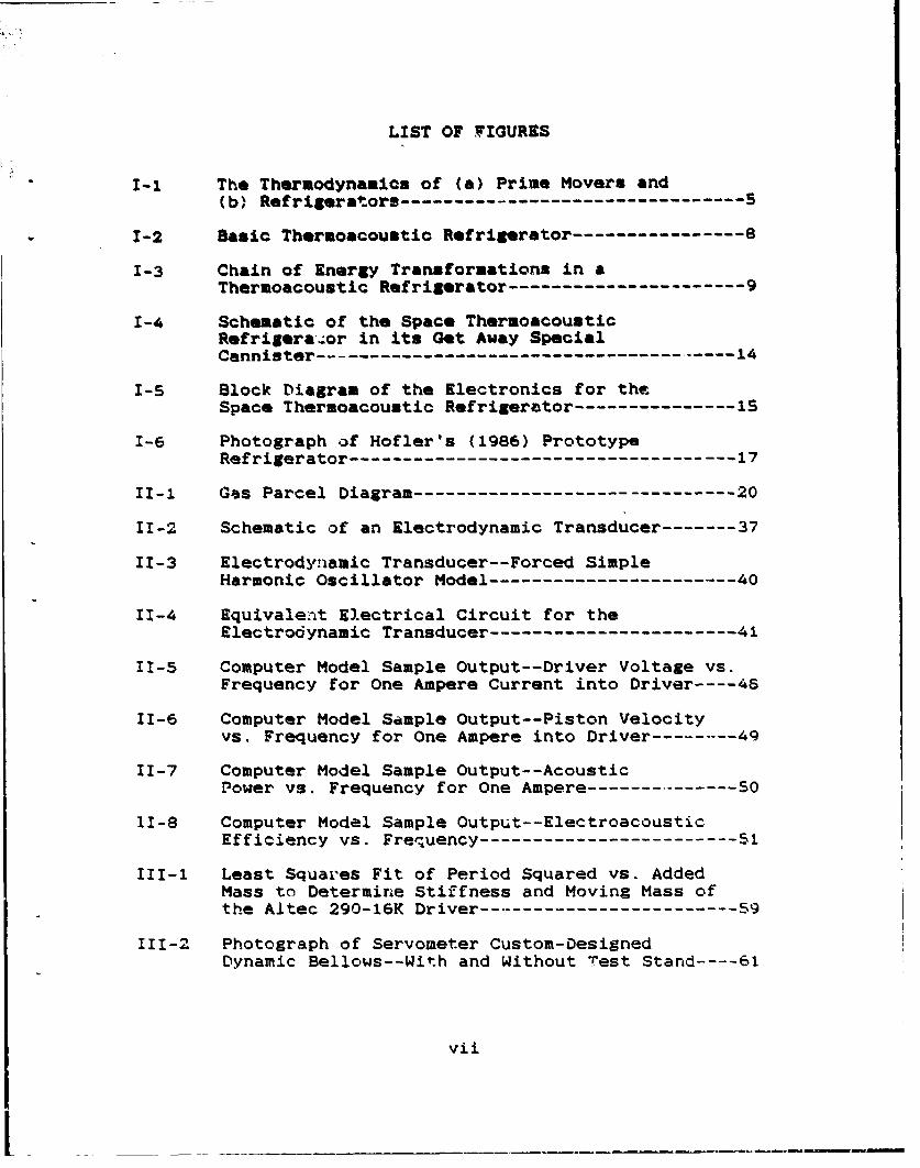
LIST OF FIGURES

1-_ The Thermodynamics of (a) Prime Movers and(b) Refrigerators -------------------------------- S

1-2 Basic Thermoacoustic Refrigerator ----------------8

1-3 Chain of Energy Transformations in aThermoacoustic Refrigerator ------------------- -9

1-4 Schematic of the Space ThermoacousticRefrigera.or in its Get Away SpecialCannister ---------------------------------------- 14

I-S Block Diagram of the Electronics for theSpace Thermoacoustic Refrigerator --------------- 15

1-6 Photograph of Hofler's (1986) Prototype

Refrigerator ------------------------------------ 17

II-1 Gas Parcel Diagram ------------------------------- 20

11-2 Schematic of an Electrodynamic Transducer ------- 37

11-3 Electrodynamic Transducer--Forced SimpleHarmonic Oscillator Model ----------------------- 40

11-4 Equivalent Electrical Circuit for theElectrodynamic Transducer ----------------------- 41

11-5 Computer Model Sample Output--Driver Voltage vs.Frequency for One Ampere Current into Driver ---48

11-6 Computer Model Sample Output--Piston Velocityvs. Frequency for One Ampere into Driver-------- 49

11-7 Computer Model Sample Output--AcousticPower vs. Frequency for One Ampere --------------- so

11-8 Computer Model Sample Output--ElectroacousticEfficiency vs. Frequency ------------------------ 51

III-1 Least Squares Fit of Period Squared vs. AddedMass to Determine Stiffness and Moving Mass ofthe Altec 290-16K Driver------------------------- 59

111-2 Photograph of Servometer Custom-DesignedDynamic Bellows--With and Without Test Stand----61

vii

111-3 Photograph of Linear Variable DifferentialTransformer (LVDT) in its Calibration Stand-----62

111-4 Calibration Data for LVDT Voltage Output vs.Displacemnt ----- ..-a----a----a----------------- 63

XI-S Least Squares Fit of Period Squared vs. AddedMass for Dynamio Loading of Bellows -------------63

111-6 Least Square* Fit of Period Squared vs. AddedMass for Combined Driver-Reducer-BellowsSystem-a -.-.-- ------------------------------.-------

111-7 Driver Displacement vs. Voice Coil Current asMeasured with LVOT/Lock-in Analyzer -- .---------- 66

I1I-8 Photograph of Altec 290-16K Driver Assemblywith Resonator Tube and Endevco Microphone ------ 74

111-9 Altec 290-16K Modified Impedance Magnitude vs.Frequency ------------------------------------ 77

111-10 Altec 290-16K Modified Impedance Phase Anglevs. Frequency--Full Frequency Range ------------- 78

III-11 Least Squares Fit of Altec 290-16K ModifiedImpedance Phase Angle as a Function ofFrequency Near Resonance ------------------------ 78

111-12 Computer Model Output for Altec 290-16K--Driver Voltage vs. Frequency for One Amp -------- 81

111-13 Computer Model Output for Altec 290-16K--Piston Velocity vs. Frequency for One Amp -------82

111-14 Computer Model Output for Altec 290-16K--Acoustic Power vs. Frequency for One Amp -------- 83

111-15 Computer Model Output for Altec 290-16K--

Electroacoustic Efficiency vs. Frequency -------- 84

IV-1 Schematic Drawing of JBL 2445J Driver ----------- 92

IV-2 Photographs of JBL Neodymium-Iron-BoronDriver ------------------------------------------- 94

IV-3 Least Squares Fit of Period Squared vs.Added Mass for NIB Driver in Air ---------------- 96

IV-4 Least Squares Fit of Period Squared vs.Added Mass for NIB Driver in Vacuum -------------- 96

viii

-V-S MTI-1000 Photonic Sensor with NIB Driver -------- 99

IV-6 Calibration Data for Photonic SensorVoltage Output vs. Displacement ----------------101

IV-7 Least Squares Fit of DC Current ThroughVoice Coil vs. Photonic Voltage Output --------- 101

IY-8 NIB Impedncoe Magnitude vs. Frequency ---------- 104

IV-9 NIB Impedance Phase Angle as a Function ofFrequency--Full Frequency Range ---------------- 106

IV-10 NIB Impedanca Phase Angle as a Function ofFrequency--Linear Segmsent Near Resonance ------- 106

IV-11 Sample of Free Decay Output from Nicolet310 Storage Oscilloscope ----------------------- 108

IV-12 Semi-log Plot of Amplitude vs. Period Numberfor NIB Free Decay in Air ---------------------- 109

IV-13 Semi-log Plot of Amplitude vs. Period Numberfor NIB Free Decay in Vacuum ------------------- 109

IV-14 Photographic Comparison of the Three Drivers-- Altec 290-16K, J8L 2U43J, and JBL NIB -------- 112

IV-1S Photograph of JBL NIE Driver with (a) Reducerand (b) Bellows -------------------------------- 116

IV-16 Computer Model Output for NIB with Helium(Bl a 15, Q - 20)--Driver Voltage vs.Frequency for One Amp -------------------------- 120

IV-17 Computer Model Output for NIB with helium(B1 - 15, Q a 20)--Piston Velocity vs.Frequency for One Amp ---------------------------121

IV-18 Computer Model Output for NIB with Helium(BI 1 15, Q = 20)--Acoustic Power vs.Frequency for One Amp -------------------------- 122

IV-19 Coneuter Model Output for NIB with Helium(Bl = 15, 0 = 20)--ElectroacousticEfficiency vs. Frequency ----------------------- 123

IV-20 Computer Model Output for NIB with Helium-Xenon (B1 = 15, 0 = 20)--Driver Voltage vs.Frequency for One Amp ---------------------------124

ix

IV-21 Computer Model Output for NIB with Helium-Xenon (B1 a IS, 0 a 20)--Platon Velocityvs. Frequency for One Amp ----.----------------- 125

IV-22 Comput-r Model Output for NIB with Helium-Xenon (S1 a 15, 0 a 20)--Acoustic Powervs. Frequency for One Amp -----------.----------- 126

IV-23 Computer Model Output for NIB with Helium-Xenon (BI n 15, Q a 20)--glectroacousticEfficiency vs. Frequency ----------------------- 127

V-1 Cross-sectional Schematic of the STAR DriverHousing ---------------------------------------- 130

V-2 Cross-sectional Schematic of the Helium LeokDetector Test Fixture -------------------------- 1Z1

V-3 Photograph of the Helium Leak Detector TestFixture ---------------------------------------- 135

V-4 Driver Housing Feed-through Plug for theElectrical Leads --------------------------------138

V-S Example of Wire Lead Connectors for Feed-Through Plug: (a) Single Wire and(b) Co-axial Cable ----------------------------- 140

V-6 DC Pressure Transducer and Driver HousingPlug Fitting --------------- \ ------------------ 142

C-1 NIB Driver with all Housing Parts andTest Lid ----------------------------------------156

C-2 Driver Housing--Resonator View -----------------1S7

C-3 Driver Housing--Side View AA ------------------- 158

C-4 Feed-Through for Electrical Leads -------------- 159

C-S Driver Housing--Side View BB -------------------160

C-6 DC Pzassure Transducer and Feed-Through Plug---161

C-1 Driver Housing Lid View ------------------------ 162

C-8 Aluminum Pusher Plate -------------------------- 163

C-9 Pressure Lid ------------------------------------ 164

C-10 Pressure and Helium Leak Test Lid -------------- 165

C-11 Reducer Cone ----------------------------------- 166

x

ACKNOWLEDGEMENT

The author would like to thank Mr. Fancher M. Murray,

P. R., a R~esearch F*1low JBL Incorporated, fcx his

cooperation in providing the modified Harmon-JBL!.cma

neodymium-iron-boron electrodynamic driver for use in the

Space Theraoacoustic Refrigerator (STAR). The author would

also like to thank her thesis advisors for their assistance,

interesting discussions, and inspiration.

xi

I. INTRODUCTION

A. BACKGROUND

1. History

Thermoacoustics can generally be described as the

study of the interaction between heat and sound. Scientific

interest in this interaction is not new. Lord Rayleigh (1878

and 1945) discussed various qualitative examples of the

production of sound by heat. In one of these examples he

describes investigations by Sondhauss (1850) of an effect

observed by glassblowers: heating a bulb of glass at the

end of a hollow rod occasionally led to the generation of

sound. Faraday (1818) demonstrated that this effect occurred

with gases other than air. Sondhauss proved that the vibra-

tion of the glass itself did not generate the sound, but he

offered no explanation as to what did. In his description of

Sonhauss' work, Rayleigh stressed the importance of the

phase difference between temperature and particle motion.

Rijke (1859) built an open tube with a wire mesh inside.

When the mesh was heated, the tube produced a sound of

impressive intensity. The functioning of this oscillator is

slightly different since it requires steady gas flow for its

operation. A similar sound production effect was observed by

Taconis, et al. (1949) in hollow tubes immersed in liquid

helium (4.2'K)" The Taconis oscillations were addressed

1

quantitatively by YaziAki, et al. (1980). The work described

above deals primarily with prime movers--devices that con-

vert a temperature gradient to sound energy. We call this

the classical era of thermoacoustics.

Interest in thermoacoustics was renewed when the

idea of the use of acoustical devices as refrigerators

appeared. Gifford and Longsworth (1966) described the pump-

ing of heat along a surface caused by a periodic change in

the pressure of the adjoining gas. Such a change can be

produced by the oscillations of a so-and wave. In their

experiments Merkli and Thomann (1974) explored the heating

and cooling effects on the wall of a gas-filled resonant

tube. They found that heat was transported from a region

near the velocity antinode (or maximum value) of the sound's

standing wave to regions near the adjacent pressure anti-

nodes. Thermoacoustic prime movers have also received recent

attention. Kempton (1976) investigated the excess noise of

aeroengines above that predicted by theory. He determined

that the sound was produced by unsteady heat transfer. Each

of these latter three groups of exprimenters used some

theory for comparison, but it was mostly qualitative. None

provided the complete quantitative theory that would explain

their experimental observations.

The theoretical breakthrough in thermoacoustics

field was made by Nicklaus Rott (1969, 1974, 1975, and

1980). His theory combined basic principles from physics,

2

thermodynamics, and acoustics to quantitatively describe the

effects found in both types of thermoacoustic devices: prime

movers and heat pumps. Prime movers use a temperature g:.a-

dient to create sound, as in the effects discussed by Sond-

hauss, Rayleigh, Taconis, and Kempton. Heat pumps, or refri-

gerators, use the oscillating pressure of a sound wave to

produce a temperature difference, as described by Gifford

and Longsworth ana Merkli and Thomann. Rott described the

effect found by Merkli and Thomann as thermoacoustic stream-

ing. It is this effect that makes thermoacoustic refrigera-

tion possible.

Inspired by Ceperley's (1979) traveling wave Ster-

ling Cycle heat engine and Rott's quantitative theory, the

team of Wheatley, Hoaler, Swift, Migliori, and Garrett

(1982, 1983a, 1983b, 1985, and 1986) developed a series of

thermoacoustic experiments at Los Alamos National Laboratory

in New Mexico. They investigated the basic thermoacous'ic

effects in both prime movers and refrigerators and compared

their experimental results to Rott's theory.

2. Thermodynamics

We'll digress from history here to explain the ther-

modynamic distinction between prime movers and refrigera-

tors. This discussion follows Sears and Salinger (1975). A

prime mover receives heat at a high temperature, T" (the hot

reservoir), does work on its surroundings, and rejects heat

at a lower temperature, To (the cold reservoir), as shown in

3

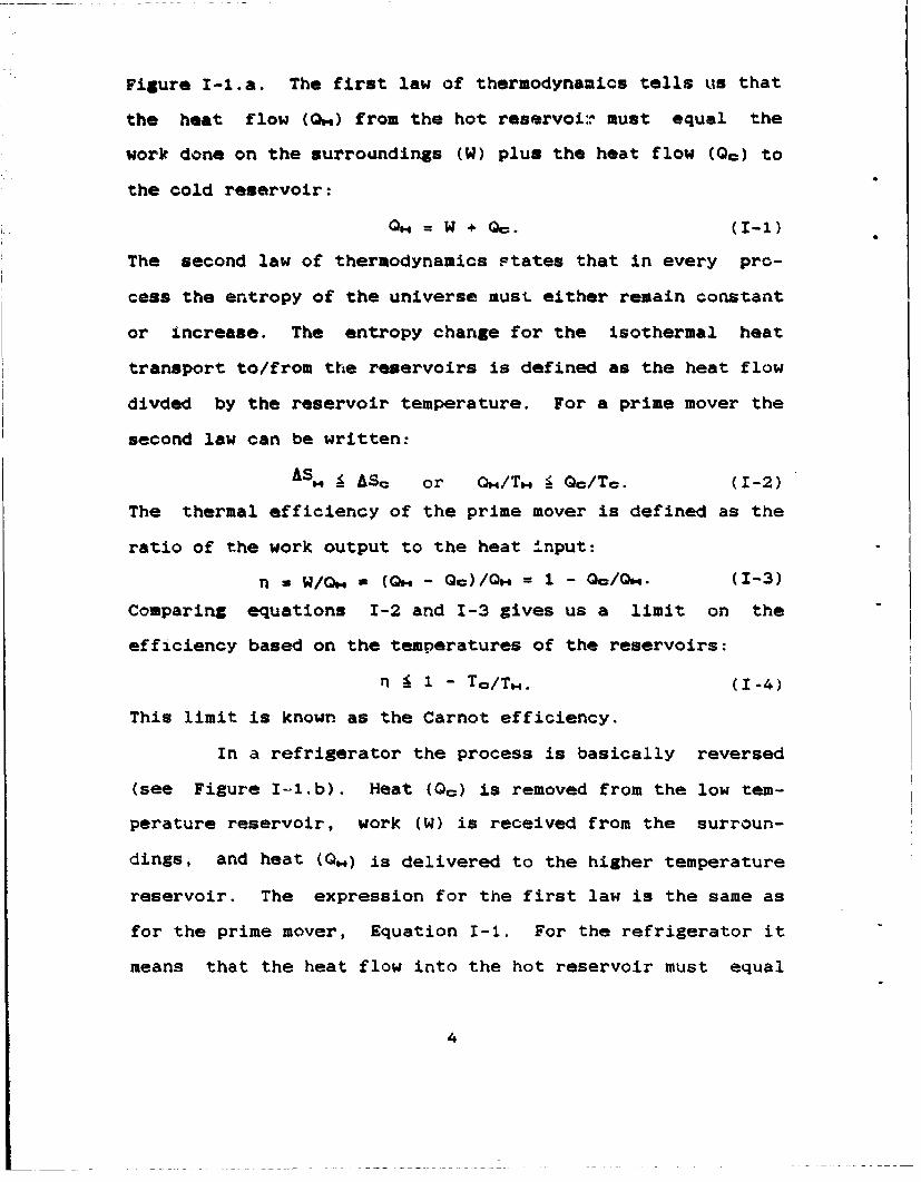
Figure I-l.a. The first law of thermodynamics tells us that

the heat flow (Q*..) from the hot reservoi:- must equal the

work done on the surroundings (W) plus the heat flow (Oc) to

the cold reservoir:

Q"= w ÷ . (I-i)

The second law of thermodynamics states that in every pro-

cess the entropy of the universe must either remain constant

or increase. The entropy change for the isothermal heat

transport to/from the reservoirs is defined as the heat flow

divded by the reservoir temperature. For a prime mover the

second law can be written:

ASH I ASC or OH/T. • Q0 /Tc. (1-2)

The thermal efficiency of the prime mover is defined as the

ratio of the work output to the heat input:

n = W/Qm = (QH - Qc)/QH = I - QO/Om. (1-3)

Comparing equations 1-2 and 1-3 gives us a limit on the

efficiency based on the temperatures of the reservoirs:

n A 1 - Ta/TH. (1-4)

This limit is known as the Carnot efficiency.

In a refrigerator the process is basically reversed

(see Figure I-1.b). Heat (0m) is removed from the low tem-

perature reservoir, work (W) is received from the surroun-

dings, and heat (Q") is delivered to the higher temperature

reservoir. The expression for the first law is the same as

for the prime mover, Equation I-1. For the refrigerator it

means that the heat flow into the hot reservoir must equal

4

T HOTFIRST LAW: 0 *V ac

OH SECON LAW:tb C

V cOEFF'CIDE4T o3n RF PV•OR N,:T -,'o

(a)

T. H1T FI LAW: ,V C

SECON LAW: t -200H

W EFFICIENCY:

CC am T"

OC7X

(b)

Figure I-1. The Thermodynamics of (a) Prime Moversand (b) Refrigerators.

5

the heat flow from the cold reservoir plus the work done to

the system. The second law for this case is:

ASwo I ASc or 0../T.. it Go/To. (1-5)

The efficiency parameter for the refrigerator is called the

coefficient of performance (COP). It is defined as the ratio

of the heat flow from the cold reservoir to the work input

to the refrigerator, or:

COP a QoW a Qc/ (C -Qo) S Tc/(TH-To). (-e)

The limit is known as the Carnot coefficient of performance.

The work in this thesis deals solely with refrigera-

tors. Even though prime movers are mentioned from time to

time, the primary focus of the rest of our discussion will

be refrigeratora.

3. Overall Ejgixc

According to Hofler (1986), the early thermoacourtic

work at Los Alamos focused on experimental refrigerating

engines. The performance of these engines fell short of

expectations, leading to simple experiments on basic th~rmo-

acoustic effects and a proof-of-principle experiment on

thermoacoustic refrigeration. Hofler then applied the Rott

theory to the experimental systems and solved the resulting

equations numerically. For his doctoral dissertation from

the University of California, San Diego, Hofler designed and

constructed a completely functional thermoacoustic refriger-

ator. He also made accurate measurements of its thermody-

namic efficiency, and used this efficiency to make compari-

6

sons to the Rott theory. After receiving his doctorate,

Hofler came to the Naval Postgraduate School (NPS) as a

p ost-doctoral fellow, and brought his prototype refrigerator

with him.

The purpose of this thesis, in conjunction with the

work of several other students, is to modify Hofler's re-

frigerator design in order to improve its overall efficien-

cy and make it suitable for space cryocooler applications.

The basic design of the thermoacoustic refrigerator is shown

schematically in Figure 1-2. The driver (A), which produces

the sound waves, is coupled via bolts to the resonator (D)

via a reducer cone (B) and bellows (C' Inside the resonator

is a stack of plastic plates (E) and their heat exchangers

(F) which allow the heat to be removed from the hot end and

absorbed by the cold end. It is the interaction between the

sound waves and the plastic plates that produces a tempera-

ture difference across the plates and/or pumps heat from the

cold heat exchanger to the hot heat exchanger. A brief

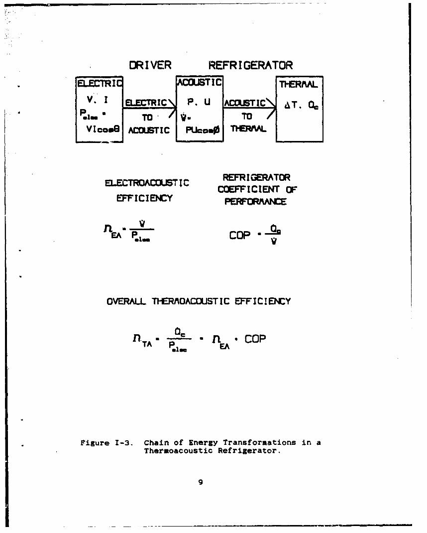
description of efficiency would be useful here. Figure 1-3

shows a diagram of the chain of energy transformations which

occurs in a thermoacoustic refrigerator. There are three

conjugate variable pairs (V and I; P and U; and AT and •&,

and two transformations (electrical-to-acoustical and acous-

tical-to-thermal).

We start with electrical input power to the driver,

which can be calculated (using r.m.s. values) with:

7

lotI

Figure 1-2. Basic Thersoacoustic Refrigerator Showing(A) Driver, (B) Reducer Cone, (C) Bellows,(D) Resonator, (E) Stack, and (F) HeatExchangers.

B

DR I VER REFR I GERATOR

E-ECTRIC AMTIC THERAAL

V.!I MEMIC P. U ACCUJTIC A T.Oel~m TO V.TOVIcoas AMCSTIC ptjcom0 THW

EL;CTROAWSTII C REFRI GERATORCOEFFICIENT OF

EFFICIENCY

EA aFt S COP 02

OVERALL TI-ERAOACOUST I C EFF I C ! ENCY

n. 0c *l 'COPTA PEA

Figure 1-3. Chain of Energy Transformations in aThermoacoustic Refrigerator.

9

P.am - 1 V con *, (-7)

where I is the current into the electroacoustic driver, V Is

the voltage across the driver terminal@, * is the phase

angle between I and V, and cos * is known as the "power

factor." An electrodynamic driver converts the electrical

power to acoustic power (the first transformation). Analo-

gous with the previous definition of the electrical input

power, the acoustic power is given by:

S• P U Cos#, (I-B)

where P is the acoustic pressure, U is the volumetric velo-

city which equals the product of particle velocity and

resonator cross-sectional area, and # is the phase angle

between them. The effinienay of this electroacoustic trans-

formation is given by:

n U - /p•~. (I-g)

In the aecond transformation, the refrigerator con-

verts the acoustic power to a temperature gradient (vT) and

heat flow (0). As discussed previously, the efficiency for

this transititt is &iven as the coefficient oZ performance:

COP M 00/W. (1-10)

The overall thermoacoustic efficiency is therefore the pro-

duct of thtý efficiencies for the two transformations:

n-Ta = num ' COP - 6=/Pnm.o-. (I-11)

Improvements in the overall. refrigerator efficiency

can thus he divided into two distinct, though interrelated,

efforts. The first is the suoJect of this thesis: modifica-

10

Stion to the driver to optimize the electroacoustic

efficiency. The second effort involves the optimization of

the coefficient of performance and is addressed by LT

Michael P. Susalla, USH, in his master's thesis.

B. SPACE THERMOACOUSTIC REFRIGERATOR (STAR)

1. motivation

In addition to improving overall efficiency, our

experimental refrigerator will be designed and built with

the intention of flying it on the Space Shuttle as part of

the National Aeronautics and Space Administration's (NASA)

Get Away Special (GAS) program. As of 3 February 1988, there

is a Memorandum of Agreement between the Naval Postgraduate

School (NPS) and the Air Force which provides funding for

the space flight and which assigns the NASA payload, number

G-337 to this project. The reason for testing the therso-

acoustic refrigerator in space is that the immediate appli-

cations of the STAR are expected to be the cooling of elec-

tronics, high T0 superconductors, and infrared detectors in

space.

There are currently two primary methods for cooling

satellite systems in space: (1) evaporation of expendable

cryogens (liquid helium, nitrogen, ammonia-methane, and

solid hydrogen, etc.), and (2) closed cycle refrigerators

(Stirling cycle, Vuilleumier cycle, etc.), which involve

large reciprocating piston masses operating at low

11

frequency. [Walker (1983) and Smith, et al. (1984)] The

disadvantages of these current cooling methods are their

short lifetimes (expendable cryogens) and high vibration

levels and low reliability (closed cycle refrigerators). The

advantages of the thermoacoustic refrigerator over these and

other systems lies in its simplicity and reliability. The

STAR has no sliding seals, efficient performance, low vibra-

tion levels, and (hopefully) a longer life span.

The thermoacoustic refrigerator needs to be surroun-

ded by a vacuum and insulation material to minimize heat

loss due to thermal conduction and radiation. The vacuum of

space will provide the best insulation to determine the

refrigerator's ultimate efficiency. The absence of gravity

removes the possibility of thermal convection as an addi-

tional nuisance heat transport mechanism.

2. get &" S tGAS) Pro ru

NASA's GAS program allows small, self-contained

payloads to fly on the Space Shuttle in GAS canisters for

relatively low cost ($10,000) (Get Away Special Team, 1984).

The GAS can is five cubic feet in volume and can house a

payload of up to 20C pounds. Each payload must contain its

own electrical power, control, data acquisition and storage

facilities, etc. The Shuttle's astronauts will turn a switch

on or off at designated times during the flight, but are

otherwise not involved with the experiment.

12

3. IkAL2SL Igk3ZI.s33 LMs V&% 2==a~Another- group of HP8 students and faculty (Boyd,

et al., 1967) have taken advantage of the GAS program to

measure the resonant acoustic modes of the shuttle payload

bay and the ambient acoustic environment produced as a

result of main engine and booster operation during launch.

This experiment is titled "The Space 3huttlu Ctr1o Bay

Vibroacoustics Experiment" and is designated by NASA as

payload G-313. Several subsystems that were developed for

NA•A 0-313 will be used by NASA 0-337 (STAR). A schematic of

the STAR in its GAS can is shown in Figure 1-4. One of the

systems borrowed from NASA G-313 is the electronics system

used to run the experiment and record the data, The recorder

system consists of the INTEL model BPK SV75 magnetic bubble

memory module and an NSC 800 microprocessor-based control-

ler. Two other NPS students, LT Charles B. Cameron, USN and

CPT Ronald Byrnes, USA, will be designing the analog elec-

tronics and software to integrate these systems into the

STAR experiment for their master's thesis. A block diagram

of the electronics is shown in Figure 1-5.

Another borrowed system is the power supply, which

consists of Gates brand lead acid battery cells (five

ampere-hour, two volts each). These gelled electrolyte bat-

teries are ideal for the STAR due to their high power den-

sity, low cost, and the absence of outgassing during dis-

charge cycles. NASA G-313 used a one layer battery of 68

13

rz-OWN

Figure 1-4. Sch~ematic of the Space ThermoacouuticRefrigerator in its Get Away SpecialCanriiuter.

14

*cwsutic Rfri~gerator Control end ftermemetrV-- - - - - -- - - - - -- - - - - - - - - - - - - - - - - - - -

* co~ao~ o -

CoGputr/Ontroter Acoe

PM a a a

Front CuC Auornacif Cftro

comes aa CV"Gap* ' : W llsOmt.bsl

Coto NSCV Controloceor~rom~r ~

integrator Phu*

I---- aE GF a"

*---------------------------------------------------------------- a --------------------- S

Figre -5 BlckDiara D-of th Fcroom c foroth

Spaceur Themoacoustic Rerdigeatr

Gap cr~911 o15

____ ____

cells providing 680 watt-hours of energy and weighing about

80 pounds (including the cells' support structure). We will

be using two battery layers with as many cells as we can, up

to 136. This will give us a minimum of 680 watt-hours and a

maximum of 1,360 watt-hours of available electrical energy,

and a battery weight between 80 and 160 pounds. The number

of battery cells we can use will depend on the total weight

of the driver-resonator assembly and its auxiliary equipment

(vacuum can, gas reservoir, etc.) and electronics.

The use of the GAS can imposes certain restrictions.

Since we are using batteries to supply the power, the refri-

gerator has to be energy efficient. Also, the GAS can setup

requ~res the STAR to be compact and lightweight. Figure 1-6

shows a photograph of Hofler's prototype refrigerator. This

setup is approximately six feet high. In comparison, the

maximum payload height for the GAS can is 28.25 inches, or

less than 2.5 feet. These considerations played a maj~or role

in the choice of equipment for and the design of the STAR.

C. SCOPE

Chapter II discusses basic acoustical and thermodynamic

theory as applied to STAR. The results of this theory deter-

mine the driver requirements. The theory of the selected

electrodynamic driver is given next. Following the driver

theory is a presentation and discussion of a computer

program that models the coupled system, which consists of

16

Figure 1-6. Photograph of Hofler's (1986)

Prototype Refrigerator.

17

*ft~lffwM-rlftAuft

the electrodynamic driver and the resonator containing the

Sas mixture and stack.

Chapter III describes the technique for measuring the

electrodynamic driver parameters. These parameters are used

as input for the driver design, the computer model, and the

efficiency calculations. This measurement technique was

developed using an Altec 290-16K electrodynamic driver and

was applied to the final driver.

Chapter IV describes the measurement of the STAR driver

parameters. The driver chosen for STAR is a custom unit,

built by Harmon-JBL!v"P', which uses neodimium-iron-boron

(NIB) magnets. The STAR driver is a minor modification of a

new line of compression drivers using NIB magnets and has

characteristics similar to the JBL 2450J.

Chapter V discusses the construction of the STAR driver,

including the housing and accessories (reducer, stiffener,

bellows, accelerometer, microphone, electrical feed-

throughs, etc.) necessary to integrate it with the resonator

and the GAS cannister system. Dimensional shop drawings for

the parts are included in Appendix C.

Chapter VI gives conclusions and recommendations for

further development.

18

11. THEORY

A. THERMOACOUSTIC THEORY

Thermoacoustic theory has been developed in detail by

Rott (1969, 1974, 1975 and 1980) and adapted to the thermo.-

acoustic refrigerator oy Wheatley et al. (1982, 1983a,

1983b, 1985 and 1986), Wheatley and Cox (M93S), Holler

(1986) and Swift (1989).

The space thermoacoustic refrigerator (STAR) basically

consists of an acoustic driver producing sound waves in a

resonant tube (see Figure 1-2). This resonator is filled

with a mixture of helium-xenon gas (12.5% xenon) pressurized

to ten atmospheres, and contains a stack of plastic plates.

This Chapter will present a qualitative model -or the ther-

moacoustic heat pumping process followed by a quantitative

development for heat and work flow at a plate. The Chapter

concludes with the efficiency of a stack of plates that are

very much shorter than one quarter of a wavelength.

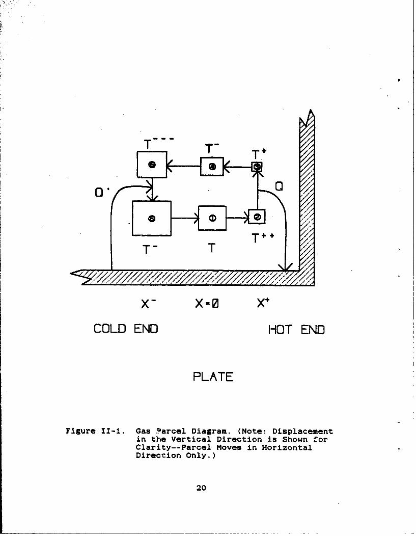
1. Qualitative Picture

Consider a parcel of jgas that moves back and forth

along one of the plates at the acoustic frequency (see

Figure II-1). As it moves, the gas parcel will experience

changes in temperature and volume. Part of the temperature

changes come from the adiabatic compression and expansion of

the gas by the sound pressure, and part as a consequence of

19

[~- ---- __-_ _ _ _ _

T --- T

T+÷0'0

T- T

Xe X=O X+

COLD END HOT END

PLATE

Figure II-I. Gas Parcel Diagram. (Note: Displacementin the Vertical Direction is Shown forClarity--Parcel Moves in HorizontalDirection Only.)

20

the local temperature of the plate itself. A temperature

gradient may develop along the plate as a resul.t of the

operation of the refrigerator. The temperature and volume

changes can be described by six separate steps (the changes

in volume are indicated by the change in size of the square

parcel in the figure).

Assume the plate is at a uniform temperature, T. The

parcel starts at position I. (X a 0) with a temperature of T.

The sound wave moves the parcel to the right to position 2.

The parcel has undergone adiabatic compression and its tem-

perature is now T". Since the temperature of the gas is

higher than that of the plate, heat (Q) will flow from the

gas parcel to the plate. The parcel's volume is decreased

and its temperature lowered to T*. This heat flow also

causes the plate's temperature to increase at the position

X+. Parcel position 3 is actually in the same location, as

position 2, but it is displaced verticalljy in the figure for

clarity. The parcel now moves to position 4 and expands

adiabatically to a new temperature of T-. A repeat of this

proces~s puts the parcel in position 5 with a temperatuire of

T--. Now the temperature of the gas is lower than that of

the plate and heat (Q') flows from the plate to the gas

6arcel, expanding the parcel and raising its temperature to

T-. This flow causes the plate's temperature to decrease at

position X-. The parcel moves to the right again under

adiabatic compression and we are back where we started in

21

position I with temperature T (adapted from Wheatley, et

al., 1985).

This gas parcel cycle is repeated at the resonator's

operating frequency. For the STAR this frequency is between

approximately 250 and 600 cycles per second, depending on

the gas mixture (specifically the speec of sound in the gas

mixture) and the length and shape of the resonator.

Notice that the temperature of the gas parcel at

position X a 0 is different depending on which direction the

gas parcel is moving. It is this phase shift in temperatu,.e

relative to motion that produces the thermoacoustic effect,

as we will show in the calculations that follow.

It is also important to note that in order for heat

to flow between the gas parcel and the plate, the parcel

must be vertically located within about a thermal penetra-

tion depth of the plate. The thermal penetration depth (8k)

. the distance that heat can diffuse through the fluid

di: nS a time 1/m, where * is the acoustic angular

frequency.

Wheatley et al. (1986) describe thermoacoustic en-

gin. as consisting of long trains of these gas parcels, all

about a thermal penetration depth from the plate. The par-

cels draw heat from the plate at one extreme of their oscil-

latory motion and deposit heat at the other extreme. Adja-

cent heat flows cancel except tt the ends. The net result is

22

that an amount of heat Q is passed from one end of the plate

to the other.

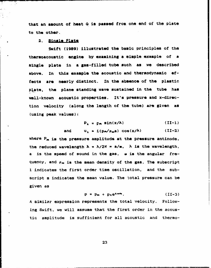
22. 1nlle Plat&

Swift (1989) illustrated the basic principles of the

thermoacoustic engine by examining a simple example of a

single plate in a gas-filled tube such as we described

above. In this example the acoustic and thermodynamic ef-

fects are nearly distinct. In the absence of the plastic

p;.ate, the plane standing wave sustained in the tube has

well-known acoustic properties. It's pressure and x-direc-

tion velocity (along the length of the tube) are given as

(using peak values):

P, = p,% sin(x/A) (11-1)

and U1 = i(p^/p.a) cos(x/N) (11-2)

where P, is the pressure amplitude at the pressure antinode,

the reduced wavelength A = A/2W - a/e, X is the wavelength,

a is the speed of sound in the gas, e is the angular fre-

quency, and p. is the mean density of the gas. The subscript

I indicates the first order time oscillation, and the sub-

script m indicates the mean value. The total pressure can be

given as

p = P. + piet-*. (11-3)

A similar expression represents the total velocity. Follow-

ing Swift, we will assume that the first order in the acous-

tic amplitude is sufficient for all acoustic and thermo-

23

dynamic variables (pressure, velocity, temperature, density,

and entropy).

The sound wave is adiabatic and has an oscillatory

temperature given by:

Ta - (T.*/mv.c) Pa, (11-4)

where 0 - - (dr/dT)w/r. is the isobaric thermal expansion

coefficient and cm is the isobaric (constant pressure) heat

capacity per unit mass. Note that T. and pa are in phase.

For ideal gasea, thermodynamics tells us that

TmO/rmcmm = (I-I)T./ip., (11-5)

where 1 - the ratio of isobaric to isochoric specific heats

(5/3 for monatomic gases, smaller, but greater than one, for

other games). Combining Equations 11-4 and I1-5 gives us:

T&/Tm = [(V-1)/1] p//p.. (11-6)

The introduction of the plastic plate into the

standing wave modifies the original, unperturbed temperature

oxcillations. This modification is due to the heat flow

between the gAs and the plate, as described previously. The

temperature is modified in both magnitude and phase for gas

about a thermal penetration depth away from the plate.

According to Swift, this results in two important effects:

1) a time-average heat flow near the surface of the plate,

along the direction of acoustic vibration, and 2) the

generation or absorption of real acoustic power near the

surface of the plate. In refrigerators the effect is an

absorption of acoustic power. In prime movers the acoustic

24

power is generated by the temperature gradient present in

the plate.

There are several assumptions we will make to

simplify calculations, again following Swift. We assume that

the plate is short enough compared to a reduced wavelength

(Ax 9 X) and far enough from both velocity and pressure

nodes that P, and u& can be considered uniform over the

entire plate. We assume the gas has zero viscosity, so that

ua does not depend on y jwp had already made this assumption

by looking at ux in the x-direction only). We assume that

the plate has a large enough heat capacity per unit area

that its temperature does not change appreciably at the

acoustic frequency. We assume that the plate has a mean

temperature gradient in the x-direction vT.. Finally, we

neglect the plate's and gas' thermal conductivity in the x-

direction.

Applying these assumptions, we see that the mean

fluid temperature (T.(x)) is the same as that of the plate.

Swift calculated the oscillating fluid temperature using

the general equation of heat transfer. He kept only first-

order terms, neglected thermal conduction along x, and

applied the boundary condition TI(O)=O imposed by the plate.

The resulting equation is:

TI(y)=[(T-0/r-c-.)Pz-(vT./o)u,][1-exp[-(1+i)y/8]]. (11-7)

To interpret this equation, we look at it in the limit that

25

the gas is far enough from the plate (y*&K) tO Rake nogli-

gible thermal contact with the plate. This gives:

T&(y)4(Tm$pmc")p-(vT./G)ut(l-B)

The first term in Equatios 11-8 is the temperature

oscillation due to the adiabatic compressions and expansions

of the gas (see Equation 11-4). The second term comes from

the mean temperature gradient in the gas. As the gas

oscillates along x with displacement amplitude uz/e, the

temperature at a given point In space oscillates by an

amount vT. u%/1 even if the temperature of a given piece of

fluid remains constant. The actual temperature oscillations

are a linear superposition of these two effects.

The y dependent part of equation 11-7 in complex. It

approaches I for y ) 8K, as given previously. It approaches

zero for y ( 8K, where the plate imposes the condlition

T,- 0. Most importantly, for y V 8K, its magnitude is still

of the order of 1, but it has a substantial imaginary part.

This phase shift in the oscillating temperature of the

standing wave at y a 8K, due to the thermal presence of the

plate, is an important result because it leads directly to

the time-averaged heat flow in the x-direction. It is the

same phase shift we emphasized in the description of the gas

parcel motion.

a. Heat Flow

Swift argues that since we are neglecting ordi-

nary thermal conductivity in the x direction, the only way

26

heat can be transported along x is by the h~ydrodynamic

transport of entropy, carried by the oscillatory velocity

Us:

4 - T.. pm rur a 1/2 pmc.m In (T] us. (11-9)

The line above the quantity *&us indicates the time-average

of the first-order entropy and velocity product. The heat

flow is a second order quantity, signified by the subscript

2.

The total heat flow 6a along the plate, in the x-

direction, is found by integrating qs over the y-z plane:

*a ia otql.m dy (11-10)

where if is the perimeter of the plate in the y-z plane.

Substituting for T1 and performing the integration gives:

S- -1/4 ff8x(TmO)pauz(r'-) (Il-il)

where IffK is the thermodynamically active area in a plane

perpendicular to the longitudinal acoustic notion, T.J is

the heat parameter of the gas, and r in defined as the ratio

of actual temperature gradient to the critial temperature

gradient (vT/vT=. ,t). The critical temperature gradient

occurs when the temperature change along the plate Just

matches the temperature change due to the adiabatic

compression of the gas, and no heat flows between the gas

and the plate. It is the boundary between the refrigerator

and prime mover functions of the thermoacoustic engines.

Equation !1-11 shows that when r < 1, heat flows

up the temperature gradient from cold to hot and work

27

(acoustic power) is absorbed, as for a refrigerator. When

r a I there is no heat flow. When r ) 1, heat flows down the

temperature gradient from hot to cold and acoustic power is

produced, an for a prime mover.

Note that the total heat flow in proportional to

the area ffax, and to TUA (a1 for ideal gases). It is also

proportional to the product plul, and so equals zero tf the

plate in at either a pressure node or a velocity node of the

standing wave. The maximum value of the product occurs

halfway between the nodes. Finally, the heat flow is

proportional to the temperature gradient factor r-i. For

7% ) 7TT,.,,, r-i ý 0 and the heat flow is toward the pres-

-- sure node, while for wT.., tvT',,, r-i t 0 and the heat flow

is away from the pressure node. If suitable heat exchangers

at temperatures Tm and To are installed at the ends of the

plate (with T., - To a vT= Ax), this heat flow carries heat

from one exchanger to the other.

The heat flow is smalý. under ordinary

circumstances. However, in closed resonators it is possible

to achieve sound amplitudes many orders of magnitude higher

than those of ordinary conversation. Since O* is

proportional to P^O, and since in practical acoustic engines

the entire cross section of the standing wave is filled with

plates (spaced roughly 4 &K apart), very high heat flows

and/or a large T. - Ta may be achieved.

28

b. Work Flow

The work flow (i.e. acoustic power) is given by

the work per cycle times the rate at which that work occurs

(the acoustic frequency f). From thermodynamics, the average

acoustic power produced per unit volume is:

w2 = -p i7e, = - 1/2 wO p, Im[T,]. (11-12)

The gas about a thermal penetration depth away

from the plate "breathes," because of thermal expansion and

contraction, with the right time phase with respect to

oscillating pressure to do (or absorb) net work. This is

exactly the same gas that we have seen is responsible for

the heat flow. Gas elsewhere is ineffective in doing (or

absorbing) work. The density oscillations for y SK and for

y D SK are in phase with the pressure oscillations, and

hence do (or absorb) no net work.

The total acoustic power Ma produced is found by

integrating &m over all space, as with the heat flow:

Wa= 1/4 ffSK (%-1) (piz/ewa) (r-1) Ax/A, (11-13)

where all the terms have been defined previously.

The acoustic power is proportional to the volume

TISKAX of fluid that is about a thermal penetration depth

from the plate. It is proportional to pa, and so is quad-

ratic in the acoustic amplitude (as was the heat flow) and

vanishes at pressure nodes. Finally, W2 is proportional to

(r-1), the same temperature gradient factor as appeared in

Oz (Equation II-11). When vT, = vT.-1,, (F-i) = 0, and there

29

are no temperature oscillations in the fluid other than

those due to adiabatic processes, and no acoustic power is

absorbed or generated. For vT. > vT.1,', r -1 > 0 and acous-

tic power is produced near the plate. Whether this power

increases the amplitude of the standing wave, is radiated

away to infinity, is simply absorbed, or flows through an

acoustic-to-electric transducer to generate electric power

depends on details of the resonator, not on the plate itself

or on the standing wave near the plate. For vTm ( vT.,,,, r-

1 < 0 and acoustic power is absorbed near the plate. For a

tube without plates which has a diameter less than the

wavelength, at constant temperature (vT = 0), this work flow

is responsible for the ordinary thermal attenuation of a

sound wave (Kinsler, et al., 1982).

c. Efficiency

We combine Equations II-11 and 11-13 to get the

efficiency of the plate with no viscous or longitudinal

conduction losses:

n = /Oa = (V-I)/(T.0) (w Ax pi)/(p.aaui). (11-14)

Since u, = uo sin x/A, and Ps = P.a uo cos x/A,

n = (1-1)/(T.0) (Ax/N tan x/A). (II-15)

For x I A, n = (%-1)/(TmO) (Ax/x), (II-16)

and n= -nm.,./r (11-17)

This efficiency approaches the Carnot efficiency

as the power output and heat transfer rates approach zero.

30

We can make a similar calculation for the

refrigerator mode of operation, where the relevant

efficiency is the coefficient of performance, COP =

We find that

COP a T COPr .. ,,. (II-18)

3. Short Stack

After developing the basic principles of the thermo-

acoustic cngine using a Rimplified example, Swift developed

a more realistic model by including viscosity, longitudinal

thermal conductivity, finite (instead of infinite) plate

heat capacity, and many plates. He still made the assump-

tions that the temperature spanned is much less than the

absolute temperature, that the length of the plates is much

shorter than the reduced wavelength, and that the spacing

between the plates is greater than a few penetration depths.

Using the equation of motion for the gas, the boun-

dary condition that the velocity at the gas-plate interface

is zero, the continuity equation of the gas, the heat flows

in the gas and plates, and basic thermodynamic properties,

Swift derived a wave equation for pressure Pl(x) in terms of

dT./dx, material properties and geometry. Swift also derived

an equation for enthalpy flow along x in terms of pi(x),

Tm(x), geometry, and material properties (including Prandtl

number of the gas 9 = CU/K, where u is the viscosity, and K

is the thermal conductivity of the gas).

31

Ir the boundary layur approximation, for a short

(Ax ( X) stack of plates, and neglecting viscosity, the heat

flux and acoustic power are given by expressions very simi-

lar to the simple results of the single plate example.

Practical engines can be expected to have all available

cross-sectional area filled with plates spaced about 4 8K

apart. The only effect of longitudinal (i.e., along x)

thermal conductivity is to add to the heat flow in the x

direction by simple conduction. For gases this effect is

normally negligible.

The inclusion of viscosity adds considerable

algebraic complication, and a little conceptual difficulty

as now ux is a function of y.

Without viscosity, vT=...,. is the temperature

gradient for which the temperature oscillation at a given x-

location is zero. But in the presence of viscosity, T.

depends %ýn x as well as y, so no well-defined vT=,.&4 , exists.

To the lowest order in VVV (where a is the fluid's

Prandtl number), the hydrodynamic heat flow is increased by

11(1-VT). This factor arises because the mean velocity (u,>

underestimates the velocity with which entropy is convected

along the stack. As we saw in the single plate calculations,

the convective entropy transport occurs mostly at a distance

SK from the plate. The velocity there is higher than the

mean velocity by 1/(1-vT).

32

The lowest order effect of viucority on the acoustic

power is the pouer dissipated by viscous shear in the fluid

* within the boundary layer, a well-known fluid mechanical

result.

For accurate calculations, the full general equation

must be used; but for rough estimates, the results presented

here are good approximations, and are much simpler to

compute with. In addition, the results presented here are

fairly easy to interpret physically. The expressions for

arbitrary viscosity are complicated, but those to lowest

order in viscosity are simple. It is easy to see the single

-plate expressions for heat flow and acoustic power about a

thermal penetration depth from the plates, modified as

longitudinal thermal conductance adds to the heat flow, as

viscous shear dissipates acoustic power, and as non-ideal

plate properties modify the thermal boundary condition at

the fluid-plate interface.

4. Design Considerations

One of the important considerations in the design of

a thermoacoustic refrigerator is the location of the stack

of plates with respect to the pressure and velocity nodes

and antinodes of the acoustic standing wave in the resonant

tube. Experiments performed by Wheatley, et al. (1986)

showed that the heat flow as a function of position fit a

simple sine curve whose spacial period is half the wave-

length of the acoustic standing wave. By noting how the sign

33

of the temperature difference varied with respect to the

plate's location in the sound wave, they saw that heat

always flows in the direction of the closest pressure anti-

node. This effect is expected because a parcel of gas moving

in the direction of a pressure antinode is compressionally

warmed and will transfer heat to the plate. A parcel moving

toward a pressure node is cooled by expansion and will draw

heat from the plate. At both the pressure nodes (velocity

antinodes) and antinodes (velocity nodes) heat flow drops to

zero. Thus the acoustic heat flow depends on both the acous-

tic pressure and the fluid velocity.

As a plate or stack of plates is moved away from the

pressure antinode, the temperature gradient developed

becomes smaller. At a quarter of a wavelength, no gradient

forms (the critical temperature gradient equals zero). This

positioning effect is important in the design of a refriger-

ator, because, together with the length of the plates, it

places an upper limit on the maximum temperature drop

possible across the stack.

B. DRIVER REQUIREMENTS

In order to drive the thermoacoustic refrigerator we

needed a device, a transducer, that would convert the elec-

trical energy of a battery pack to acoustic energy, as

discussed in Subsection I.A.3. We wanted as high a pressure

(or force) and volume velocity (or motion) as possible to

34

-• get the most acoustic power provided to the system. There

were several types of electroacoustic transducers to choose

from: electro-static, electret, electrodynamic, magneto-

strictive, electro-strictive, and piezoelectric. Only one of

these, the electrodynamic transducer, can provide our system

with both the large forces and velocities necessary. This

transducer will be described in the next section. The

remainder of this section describes the rest of the trans-

ducers and explains why each was not appropriat& for use in

the thermoacoustic refrigerator.

The electrostatic transducer vconsists of a pair of

charged electrodes, or capacitor plates, one of which is

held stationary while the other, the diaphragm, moves in

response to electrical excitation. The electret is a kind of

electrostatic transducer that has a diaphragm of polarized

plastic, and therefore does not need an external voltage

supply to the diaphragm (Kinsler, et al, 1982, p. 350). If

an alternating voltage is applied across the plates, the

diaphragm moves, thereby radiating an acoustic wave.

Unfortunately there is very little force (or pressure) and

displacement associated with this motion. This type of

transducer may be useful as a microphone but is not an

appropriate choice to drive the thermoacoustic refrigerator.

In a magnetostrictive transducer a change in the

magnetic polarization in the material causes an elastic

strain (Wilson, 1985, p. 3.). Although the forces are more

35

than adequate the strain produces too little motion to be

useful to us.

In electrostrict~.ve and piezoelectric transducers an

externally applied electric field causes a change in the

dielectric polarization of the material, which in turn

causes an elastic strain (Wilson, 198S, p. 3). Once again

there is sufficient force but the displacement due to the

strain is too small to be useful.

Because these techniques have sufficient force, it would

be possible to overcome the displacement limitation using

mechanical leverage or other forms of mechanical impedance

transformation. but this was not considered due to the

associated increase in device complexity.

C. ELECTRODYNAMIC THEORY

The electrodynamic driver is a moving coil

transducer -chconverts electrical energy to kinetic ener-

gy (motion). It consists of a diaphragm attached to a cylin-

drical coil of wire (voice coil) that is suspended in a

fixed magnetic field (see Figure 11-2). If an alternating

current is supplied to the coil, the interaction of the

current cs-'t..I r_:4 -.. tic field will induce a force on the

coil so that the diaphragm moves. The magnitude of the force

is F =B11, where B is the magnitude of the magnetic induc-

tion, 1 is the lenr', of the coil and I is the current. The

36

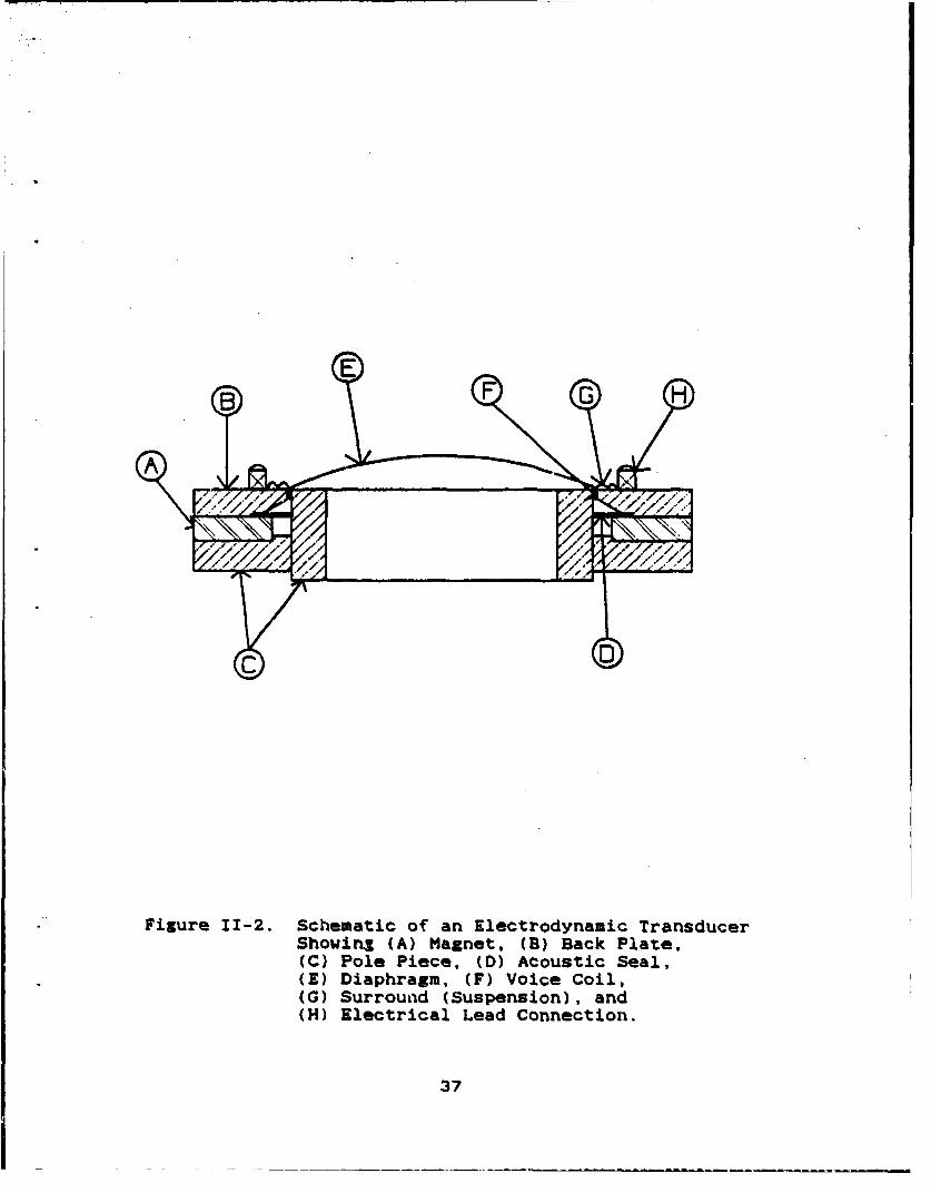
Figure 11-2. Schematic of an Electrodynamic TransducerShowing~ (A) Magnet, (8) Back Plate,(C) Pole Piece, (D) Acoustic Seal,(E) Diaphragm, (F Voice Coil,(G) Surroun~d (Suspension), and(H) Electrical Lead Connection.

37

direction of the force, liven by the cross product of the

current vector and the magnetic field (from Ampere's law E a

1,1 X 3), is everywhere orthogonal to the current and the

radial magnetic field. The motion of the diaphragm produces

sound waves with a frequency equal to that of the alterna-

ting current. Another important property of the electrodyna-

mic transducer is that the motion of tkie voice coil induces

an electromotive force (emf) which equals 81 times the

velocity of the voice coil (euf a Blv). This "back emf"

increases the electrical impedance of the driver and can be

used to monitor the driver motion as discussed in Section

III.B.

The driver is attached to the resonator via a

reducer and bellows. The reducer is a cone-shaped piece of

aluminum mechanically connecting the driver voice coil which

produces the force to the bellows, which in turn is in

contact with the gas in the resonator. The reducer is

designed to be lightweight, rigid, and strong for a direct

transfer of motion and energy from the moving coil to the

bellows. The bellows is a lightweight and flexible gastight

seal between the driver and the tube. An aluminum plate is

used as an interface between the reducer and the bellows to

keep the bellows face rigid. For the STAR driver the reducer

and plate are incorporated into a single unit machined from

aluminum bar stock.

38

Figure 11-3 shows a mechanical model of the

electrodynamic transducer as a forced simple harmonic

oscillator (SHO), which consists of a moving mass (m3),

stiffneoa (k), mechanical damping or resistance (Rm), and

driving force (F). Included in the moving mass are the

masses of the voice coil, reducer, stiffener, and bellows.

The stiffness includes the 3uspension stiffness of the voice

coil surround, the stiffness of the gas volume trapped

behind the diaphragm, and the stiffness of the bellows, The

equations governing the SHO can thus be used to determine

the moving mass and stiffness of the driver. The primary

relationship used is:

* *- k/a.,, (11-19)

or, the resonant angular frequency squared equals the

stiffness divided by the moving mass. The use of this and

other relationships will be discussed further in Chapter

III, Driver Parameter Measurements.

2. EgialotCici

An electrical circuit can be drawn that is

equivalent to an electromechanical system if the values

given for E6, La., and Cm in the circuit produce the same

electrical effects as the electromechanical system itself.

In the case of the electrodynamic driver, the equivalent

circuit is shown in Figure 114 with the values giv,9n by

Kinsler, et al. (1982) as:

39

A/chon±col AcousLco l

R(P, 0, U)

-- :---

K

a coil bellows ruducer

K=Kus +K blos+ KGsVlKKmuep balioe vol.

Figure 11-3. Electrodynamic Transducer--Forced Simple

Harmonic Oscillator Model.

40

* N

D-

w

wD

S-J

WII

Figure 11-4. Equivalent Electrical Circuit for theElectrodynamic Transducer.

41

Rm* (al):/Rn, (11-20)

L u (B1) /k, (11-21)

C. Ma/(83)a, (11-22)

where 51 is the transduction coefficient, Pt. is the

mechanical resistance, and k and a. are the stiffness and

moving man. as described previously.

The properties of the equivalent circuit allow us to

evaluate the performance of the electrodynamic driver as if

it were an entirely electrical system. The amount of power

the driver generates will depend on the load it ae.a. Since

one of the primary purposes of this thesis in to maximize

the ratio of the acoutic power delivered to the electrical

power provided (the electroacoustic efficiency), it is

necessary to provide a load to the system in order to

evaluate driver performance. This load is originally

represented as a complex electrical impedence in the

equivalent circuit. The actual value of the load will depend

on the design of the resonator but can be characterized by

an acoustic impedance which can be transformed to an

equivalent electrical load impedance.

3. Losses

In our search for the highest electroacoustic

efficiency it is useful to understand where possible losses

may occur and do what can be done to minimize them. Losses

that are an intrinsic part of the electrical driver are eddy

current losses in the magnetic structure generated by the

42

current in the voice coil, Joule heating losses due to the

drive current dissipated by the voice coil electrical

resistance, and mechanical losses due to the internal fric-

tion of the surround and the viscosity of the gas in the

"gap." These losses need to be taken into account. Very

little can be done about the eddy current losses and the

viscosity of the gas which is necessary to improve heat

removal from the voice coil. The losses due to surround

(suspension) mechanical resistance can be controlled by

choice of the materials and removal of extraneous suspension

material (see Section III.H).

D. COUPLED SYSTEM

1. Computer Model

Any discussion of the driver section of the

thermoacoustic refrigerator is incomplete without some

understanding of how the driver parameters are coupled to

the resonator (acoustic load). The equivalent electro-

mechanical circuit for the coupled system is the same as

that shown in Figure 11-4 with the acoustic load impedance:

Zz = -r..csj[(l+ja/k)/(1+(a/k)0) , (11-23)

((cos(kL)sin(kL) + j sinh(aL)cosh(aL)) +

(sinf(kL)cosha(aL) + cos 2 (kL)sinhm(aL)))],

where P,, is the density of the gas, c is the speed of sound

(labeled "a" in previous discussions), s is the cross-

sectional area of the resonator, k is the wave number

43

(. rn/c), U = ./(2Qc), Q is the quality factor of the reso-

nator, and L is the effective length of the resonator

(Kinsler, et al., 1982). This circuit combines the equiva-

lent circuit of the electrodynamic transducer with the com-

plex impedance load representing the resonator. One way to

examine this coupling is through computer modeling.

LT Michael P. Susalla, USN, developed a computer

program which models the thermoacoustic refrigerator as the

equivalent electrical circuit. The program models each of

the mechanical and acoustical components as equivalent

electrical components, as discussed above. Using the

electrical equation from the combined circuit we determine

the system performance as different parameters are varied.

a. Input

There are two sets of input parameters needed

....... for the model: (1) driver parameters and (2) resonator

parameters. The driver electrical parameters include the

voice coil inductance (LE) and resistance (RE), and the

current (I) supplied to the voice coil (which is held at one

ampere for all test cases). The driver mechanical parameters

used in the model are the same equivalent resistance, induc-

tance, and capacitance as those developed for the equivalent

circuit. Therefore the parameter values needed for input are

the transduction coefficient (BL), the mechanical resistance

(RM), the moving mass (M), the suspension stiffness (SSUP),

44

the volume of the gasn behind the diaphragm (VOL), and the

cross-sectional area of this volume (A).

The resonator parameters needed include the tube

quality factor (0), the speed of sound (, the resonance

frequency (F0), the density of the gas in the tube (RHO),

the resonator cross-sectional area (S), and the equivalent

length of the resonator (L). For this model the piston area

is set equal to the resonator cross-section (S). For the

tests reported here they were nearly equal but could differ

sustantially in other designs.

b. Output

Four output plots are generated by the graph

program that accompanies the model: (1) voltage across the

driver vs. frequency (since we put unit current into the

driver, this graph can also be read as the input electrical

impedance), (2) piston velocity vs. frequency, (3) acoustic

power delivered to the load (resonator) vs. frequency, and

(4) electroacoustic efficierý*'y vs. frequency. Each of these

plots should produce peaks at both the driver and the tube

resonant frequencies.

The model uses the electrical equation for the

coupled equivalent circuit to calculate voltage directly

(holding the current constant at one ampere) for the first

output plot. It also directly calculates the force on the

moving mass, F = BlI. From this force, the piston velocity

for the second plot is found by dividing the force by the

45

mechanical impedence (Z..M ,). Pressure is calculated as tube

impedence times volume velocity, and acoustic power is

pressure times volume velocity times the cosine of their

phase difference (Equation I-8) for the third plot. For the

final plot the electrical power is calculated as voltage

times current times the cosine of their phase difference

(Equation 1-7), ard the model takes a ratio of the electri-

cal to the acoustical powers for the electroacoustic effi-

ciency. Since the components of these powers are complex and

have phase differences, the actual powers are calculated as

one half the real part of [current times complex conjugate

of voltage], and one half the real part of [pressure times

the complex conjugate of volume velocity]. Each of the above

mentioned plots is the discussed output parameter versus

frequency.

2. Assumed TyPical Parameters

Table II-1 lists the input parameters with sample

values for the Altec 290-16K driver in air with a long

straight resonant tube attached (see Chapter III). Sample

outputs of the four plots using these input values are given

in Figures 11-5 through 11-8.

Figure II-S plots the driver voltage as a function

of frequency. Since the current is held constant at one

ampere, this plot actually gives us information on driver

electrical input impedance vs. frequency. Notice that there

are two peaks in this curve. The first peak occurs at a

46

TABLE II-1. MODEL INPUT VALUES--EXAMPLE DATA

Symbol Meaninx Units Value

RM Mechanical resistance kg/s 1.33

M Moving mass kg 0.0151

SSUP Spring constant N/M 9.2XiO0

RHO Density of gas kg/mrn 1.2

C Sound speed m/s 342.0

S Resonator X-sec. area ma 9.3SX10'l

BL Driver transduction factor N/A 21.5

Q Resonator quality factor 60.0

FO Resonator resonance freq. Hz 240.0.

A Back volume X-sec. area Ma 7.92X10-4

VOL Back volume MC 1.0X10-=

LE Voice coil inductance H 1.0X10-%

RE Voice coil DC resistance a 10.6

I Driver current A 1.0

L Resonator length m 0.712

47

00

S InIi II I I'

Figure II-5. Computer Model Sample Output--DriverVoltage vs. Frequency for One AmpereCurrent into Driver.

48

(W/M AfLLMA WO.IBd

Figure 11-6. Computer Model Sample Output--PistonVelocity vs. Frequency for One Ampereinto Driver.

49

0S

S'4,I

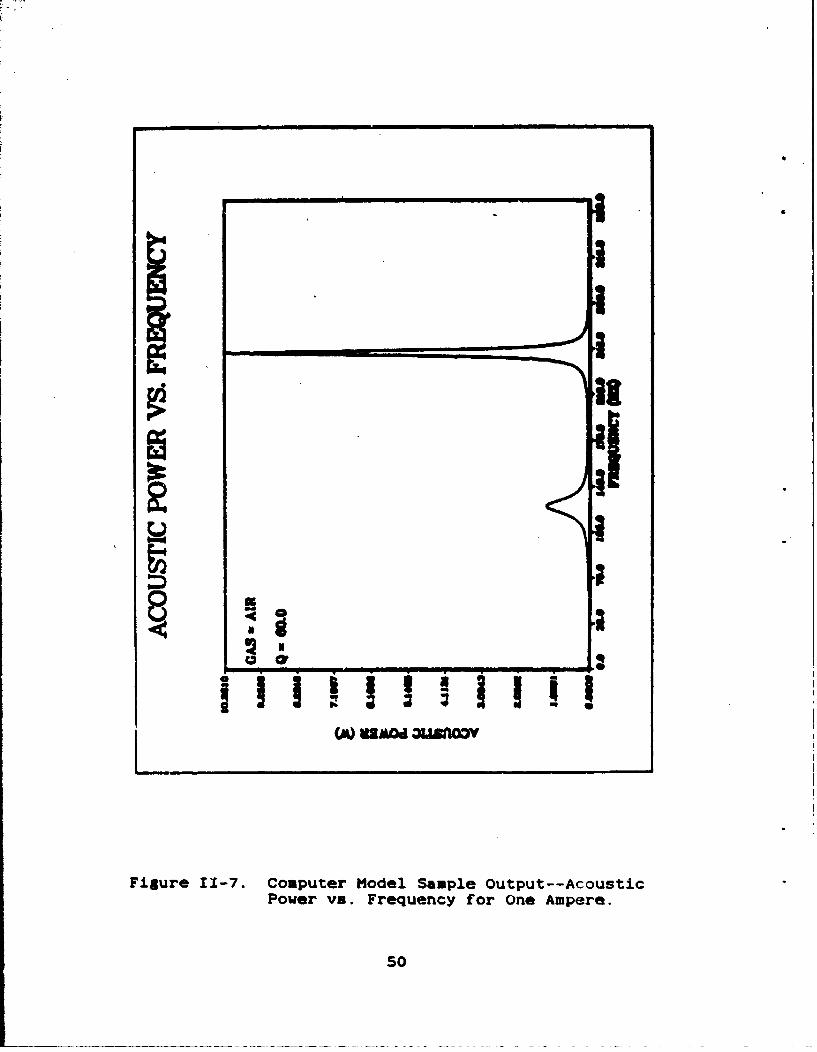
Figure 11-7. Computer Model Sample Output--Acoustic

Power vs. Frequency for One Ampere.

5o

.+.

VZA~d 31V Z /aAW 3US=V

Fi±ure 11-8. Computer Model Sample Output--Electroacoustic Efficiency vs.Frequency.

51

lower frequency and has a such higher amplitude than the

second. This higher amplitude peak occurs near the driver

resonant frequency (f. a (1/2w)[k/a.],'1a0 124 Hz). It

dominates the curve because it is the driver impedance that

we are plotting, and the voice coil motion, and consequently

the "back "mf," is the largest at that frequency. The fact

that there is a second peak near the tube resonance (FO

240 Hz) shows the effect of the coupling of the two parts of

the system.

In the plot of piston velocity vs. frequency (Figure

11-6), the dominant peak again occurs near the driver

rosonance for the reasons presented above. The smaller

coupled peak at the tube resonance is due to the change in

the load impedance which occurs near the tube resonance.

Figure 11-7 shows the plot of the acoustic power vs.

frequency. Now the dominant peak occurs at the tube

resonance because acoustic power is primarily a function of

the tube parameters. Here the secondary peak at the driver

resonance is a consequence of the greatly increased piston

velocity at the driver resonance putting energy into the

smaller non-resonant acoustic load of the tube.

In the plot of electroacoustic efficiency vs.

frequency, Figure 11-8, the primary peak at the tube

resonance is sharp and the secondary peak at the driver

resonance is small but visible. It is important to note that

the electroacoustic efficiency peaks at a value of nearly

52

60% even though the two individual resonances are separated

by nearly an octave in frequency. The peak acoustic power

for one &up as shown in Figure 11-7 is 10.3 W. The losses

(40%) are due primarily to Joule heating in the voice coil

DC resistance (PO a 1/2 (IsRoo) a S.3 W). This accounts for

341. The remaining loss can probably be attributed to

mechanical resistance losses in the suspension.

Appendix A contains a printout of the calculation

program. Appendix B contains a printout of the graph

program.

SS

DI". •AR- ETiL MRSUUHINTA

A. INTRODUCTION

In Sections IIB and II.C we discussed the choice of the

electrodynamic transducer to drive the thermoacoustic refri-

gerator. Given this choice, we needed to develop a system

for measuring the mechanical parameters of this type of

driver to be used in determining the electroacoustic effi-

ciency. rho relevant parameters (as discussed in Section

II.D) are: (1) moving mame, (2) suspension stiffness. (3)

transduction coefficient (el), and (4) mechanical resis-

tance.

The driver we selected for the preliminary measurements

is the Altec model 290-16K moving-coil loudspeaker. There

are several pieces of equipment needed to interface the

driver with the resonator. Three of these parts--the reducer

cone, stiffener, and dynamic bellows--become an integral

part of the driver, and their effects on the driver parame-

ters must be taken into accoiunt. We first measured the

parameters of the driver alone, then added the other parts

and determined the new parameters for the entire system. The

driver-bellows combination was then fitted to one end of a

resonant tube. The actual resonator used in the thermo-

acoustic refrigerator will be a complex structure that is

not easily modeled. For the purposes of the driver parameter

54

measurements we used a resonant tube of uniform cross-

section to allow easy comparison of experimental values to

theory. The non-driver end of the closed tube housed several

microphones. The electroacoustic efficiency of the system at

resonance was determined from measurements of electric power

delivered to the driver and the acoustic pressure at the

microphone. The acoustic power dissipation was determined

from the quality factor of the tube at resonance and the

microphone sensitivity (the relationship between,-the pres-

sure that the microphone senses and its voltage output).

B. IMPEDANCE ANALYZER

The primary instrument used in the testing and evalua-

tion of the electrodynamic driver was the Hewlett Packard

Model 419i2A LF Impedance Analyzer. According to the manufac-

turers operation and Service Manual. the 4192A is a fully

automatic,- high performance test instrument designed to

measure a wide range of impedance parameters as well as

gain, phase, and group delay. Its two measurement display

sections provide direct readout of the selected measurement

parameters with 4.S digit resolution along with the appro-

priate units. In normal mode operation, the 4192A performs

approximately five measurements per second. It also provides

an average measurement mode (one measurement per second) for

higher resolution and noise rejection. A high speed mode can

perform ten measurements per second.

55

The 4192A can provide measuring frequency, OSC voltage

level, and DC bias voltage (impedance measurements only)

equivalent to actual operating conditions. The sweep capa-

bility of the built-in frequency synthesizer and DC bias

source permits quick, convenient, and accurate measurements.

Measuring frequency or DC bias voltage can be automatically

or manually swept in either direction. 09C level can be

manually swept In either direction In InV increments. Actual

test voltage across or test signal current through the

device under test is also measured.

In amplitude/phase measurements, the 4192A can measure

four transmission parameters - gain/lous, level, phase, and

group delay. In impedance measurements, the 4192A can

measure eleven impedance parameters - abeolute value of

impedance, absolute value of admittance, phase angle, resin-

tance, reactance, conductance, susceptance, inductance,

capacitance, dissipation factor, and quality factor. All

impedence measurements have a basic accuracy of 0.1% and a

resolution of 4.5 digits. Also, the circuitry of the 4192A

provides direct and accurate impedance measurements of both

grounded and floated devices.

C. MECHANICAL PARAMETERS

The most important parameters for a moving coil trans-

ducer are the moving mass, suspension stiffness, and the Bi

(transduction) coefficient. The moving mass of the driver

56

includes the mass of the voice coil, the diaphragm, and the

hydrodynamic mass of' the air being pushed by the --diaphragm.

The masses of the reducer and stiffener are also important,

as are the moving mass and suspension stiffness of the

bellows. The moving mass and stiffness of the combined

driver-reducer-bellows system is also important. The values

for the combined system should equal the sum of the values

of the individual parts. The stiffness, mass, and 81 coeffi-

cient give us the information we need to construct the

equivalent electrical circuit, as discussed in Subsection

II.C.2. Also, we have to insure that the stiffness of the

driver system is just large enough to produce a mechanical

resonance at the tube resonant frequency, at which point the

driver piston looks like a soft (or open) tube end. This may

appear to be contradictory to having a velocity node of the

standing wave at the piston, but it is not. It is how we get

high efficiency.

The important design parameters of the tube are its

resonance frequency and quality factor. The length of the

tube and the speed of' sound in the contained gas determine

the resonance frequency.

1. Dynamic Mass Loading of Driver

We used the driver's similarity to a simple harmonic

oscillator to find the moving mass and suspension stiffness

of the driver by taking advantage of the fact that the.

re.zonance frequency squared equals the stiffness divided by

57

the mass. If we add mass to the driver, it should linearly

change the Inverse of the frequency (or period) squared:

T' - 1/f2 = 4Xa(u. + m)/k. (111-1)

where mw. is the moving mass, m is the added mass, and k is

the suspension stiffness. The instrument we used for this

measurement was the HP 4192A Low Frequency Impedance

Analyzer, described in section B. We added various masses of

putty (one to nine grams) to the diaphragm and found the

resonance frequency of the driver for each mass. The putty

mass was measured on the Sartorius model 2403 mass balance

(serial number 1287). This balance has an accuracy of±

0.00005 g. However, the putty could be expected to gain or

lose more mass than that due to handling. Based on mass

measurements of the putty after use, we expect an

experimental accuracy of ± 0.005 g for the masses. A more

significant uncertainty involving the masses arises from the

inability to place the masses evenly on the voice coil or to

produce a perfectly rigid coupling between the masses and

the voice coil. It is not possible to assign a specific

numerical percentage error to this uncertainty, but we must

take it into account when evaluating the data associated

with mass loading. A typical plot of the period squared vs.

added mass in air is shown in Figure III-1. We used the

least squares method to fit a straight line through the

data. We determined the suspension stiffness (k = 47r2 /Slope)

to be:

58

ALTEC 290-16K MASS LOADING30.

y 8.4947 + 1.4735x R 0.99

; 2o

w

a.

0''* I * i " i "

0 2 4 6 8 10

ADDED MASS (g)

Figure III-1. Least Squares Fit of Period Squared vs.Added Mass to Determine Stiffness andMoving Mass of the Altec 290-16K Driver.

59

k - 2.7 ± 0.1 X 10 N/S, (111-2)

and the moving mass tM u intercept/slope):

Me = 5.8 ± 0.1. , (III-3)

for this driver in air.

The moving mass of the driver in vacuum is expected

to be less than the value in air because in vacuum the

driver is not pushing a hydrodynamic mass. However, we did

not take any measurements of this driver in vacuum.

2. Bellow Paazmetrgs

The Servometer custom-designed dynamic bellows

(shown in Figure 111-2 with test stand) is used to provide a

flexible gas seal between the driver and the resonator.

The stiffness of the bellows was measured using two

independent methods - static and dynamic. For the static

method we used Hooke's law: k a -F/x. The force was deter-

mined by pulling a partial vacuum on the bellows and multi-

plying the vacuum pressure (read on a manometer) by the

surface area of the bellows (A = 1.1 ± 0.1 X 10-a ma). We

used a G. L. Collins Corporation model LMS-119V22-01 Linear

Variable Differential Transformer (LVDT) (serial 274674)

connected to an EG&G 128A Lock-in Analyzer to determine the

displacement of the bellows under a partial vacuum. Figure

111-3 shows the LVDT in its calibration stand. The calibra-

tion curve for the LVDT is shown in Figure 111-4. The least

squares fit slope of this curve gives us the calibration

constant for the LVDT:

60

Figure 111-2.'* Photograph o,, Servometer Custom-DesignedDynamic Bellows--With and WithoutTest Stan~d.

61

i9

Figure 111-3. Photograph of Linear VariableDifferential Transformer (LVDT)in its Calibration Stand.

62

LVDT CAUBRATION

-100/0.2 0.3 0.4 0.5 0.6 0.7 0.8

LVDT DISPLACEMENT (INCHES)

Figure 111-4. Calibration Data for LVDT Voltageoutput vs. Displacement.

: BELLOWS DYNAMIC MASS LOADING

700

YO y50.5616 + 8.69X R-1.000 600

0 500-

400

200 , • , . , . , . ,,20 30 40 5'0 60 70 80

ADDED MASS (g)Figure 111-5. Least Squares Fit of Period squared

vs. Added vass for Dynamic Loadine

of Bellows.

63

dV/dx - -0.378 O.O000S V/in - -14.9 t 0.02 V/i. (111-4)

Table III-1 gives the static test data for the stiffness

measurement. By averaging the values we obtained:

k - 4.3 t 0.2 X 100 N/s. (111-5)

TABLE 111-1. BELLOWS STIFFNESS--STATIC

MEASUREMENT RESULTS

LVDT Voltage Pressure Pressure Force (aPA) Stiffness

(mv) (2 Hz)J•_ (XiMPA)~ A•_ A ON/mJ

14.84 2.9 3.87 4.39 4.40

1S.62 3.1 4.13 4.69 4.47

12.89 2.3 3.07 3.48 4.02

The dynamic measurement was a mass loading technique

similar to that used for the driver. In this case, we

measured the period as a function of added mass using an

Endevco model 2225M2 accelerometer (serial FASO) and a

Nicolet model 3091 aigital storage oscilloscope to record

the free decay of the bellows after it had been disturbed by

the blunt wooden ead of a cotton swab. We then plotted

period squared versus added mass and found the stiffness and

moving mass from the slope and intercept of the least

squares fitted line (see Figure 111-5) as discussed in the

previous Section. This gave us values of:

64

k .56 * O.OS X jO0 e/n (111-6)

and m. . 945.6 * 0.05 . (t.S-7)

This value for moving mass includes the accelerometer cable

and is not representative of the actual soving mass of the

bellows. Subtracting the weight of the acceleromete: gives

us a value of approximately:

m. - 2.5 * 0.1 g. (11I-8)

for the bellows. We know the moving nano has to be less than

2.3 I, since that is the bellows' total mass--moving and

static. The values obtained for bellows stiffness using the

two different methods were within experimental error. We

therefore felt confident using a value of ka - 4.5 ± 0.1 X

100 N/n in our later calculations.

3. CombLne dSystem

After we glued the reducer (a a 4.8 g), stiffener

plate (m - 4.4 g) and bellows to the driver, we wanted to

find the stiffness and moving mass of the combined driver-

reducer-bellows system. We first tried a dynamic mass

loading measurement (same procedure as with the driver

alone), but found that the period squared versus added mass

plot (see Figure 111-6) gave unrealistic results. So instead

we used the relationship:

F - -kx = Bli (111-9)

or k = -BlI/x = Bi (di/dV)(dV/dx) (III-10)

and made a static measurement using the LVDT. We expected

the additional equipment (reducer, stiffener, and bellows)

65

UMAS LOADING DRPIEReCONEBELLOWS238

y 1.8M + 0.Q74 R 0-.9

146

Z2.0

0 2 4 6 a 10 12

ADDED MASS (g)

Figure 111-6. Least on aua Frt o Period Squaredvs. A~ccl Nias ror Colmb~oned Driver-Reducer-Sellous System.

ALTEC 29016K STATIC DISPLACEMENTy 3.6095+0.011Ollx R 1.00

w

41

3310

2

-200 -100 0 100 200

CURRENT IN VOICE COIL (mA dc)Figure 111-7. Driver Displacement vs. Voice Coil

Current an Measured wiith LVDT/Lock-in Analyzer.

66

to change the moving mass and suspension stiffness of the

system but not the transduction coefficient (11). We applied

a DC current to the driver and recorded the LVDT voltage

output, then changed the current and recorded the new vol-

tage. This process produced the values: Al a 283 * 0. S mA

and AV a 2.58 t 0.005 mV. We substitute these values and the

value of B1 = 21.5 t 0.5 N/A (experimental measurement of

this quantity In discussed In the next aection) into Iqua-

tion III-10 for a combined stiffness value of:

k - 3.S t 0.1 X 10d N/. (Ill-We)

If we add the stiffness values for the driver and bellows

together a total stiffness of k a 3.2 t 0.1 X 10' We/ for

the system is obtained. Thus the total experimental stiff-

ness for the combined system differs by about 101 from the

sum of the individual stiffnesses. Using the relationship

a. k/(29f)O, and a measured resonance frequency of

235 t 0.5 Hz, the combined moving mass is:

Me - 16.2 t 0.5 z, (111-12)

compared to a. f 15.9 ± 0.5 g for the individual masses

added together. The two types ef mass measurement agree

within 2%.

D. TRANSDUCTION COEFFICIENT (BL)

We determined the Bi coefficient of the driver using

three independent methods. The first method was to remove

the voice coil from the magnet and directly measure the

67

magnetic induction using a Dowdy RIL Industries model 912

Ouassmeter (serial So0) using a Hall effect probe model

912015 (serial 21122) (B a 2.2 t 0.05 Teals). We then

measured 1 (the length of the wire) by counting the number

of turns of wire in the coll (under a microscope) and

multiplying this number (44) by the circumference of the

coil (1 a 44 X W X diameter a 9.98 t O.OOS a). Combining

these two measurements gave us the value:

B1 a 22.0 t 0.7 N/A. (111-13)

In the second method we used the relationship:

F a 8I1 a -kx or 51 a -kx/I = -k(dx/dV)(dV/dI). (111-14)

We previously determined k for the driver alone (Equation

111-2), and now used the LVDT and lock-in analyzer to find

dx/di. The LVDT calibration war discussed in the previous

Section, with a calculated value of dV/dx a -14.9±0.05 V/m.

We then measured the diaphragm displacement as a function of

DC-current through the voice coil. This gave us a value of

dV/dI a 11.75 + 0.05 mV/A (see Figure 111-7). Using the

relation in Equation 111-14 we obtain the value:

Bl - 21.2 ± 0.1 N/A. (111-15)

In the third method we used the relationship:

F a Bli - ag or Bl = mg/i. (1II-16)

For this we measured the change in DC-current through the

coil as a function of added mass, using the LVDT as a

monitor to keep the displacement of the diaphragm constant.

68

Three different mass/current combinations (see Table 111-2)

produced an average value of:

al a 21.4 t O.S N/A. (111-17)

Averaging the results of these three methods gave us a

value of 51 a 21.S t O.S N/A with 21L deviation among the

three methods.

TABLE 111-2. STATIC M'KAS VIDDT Of ALTZC 290-IGK

TRANSDUCTON Cr IOEFFICIENT (BL)

As (R) ALi &I. 31 = mil (N/A)

132.5 64.4 20.2

1S7.S 74.0 20.9

257.5 108.2 23.3

E. MICROPHONE CALIBRATION

Microphone calibration in an important part of the

process leading to the measurement of the electroacoustic

efficiency. A microphone is used to measure the acoustic

pressure inside the resonator by converting the acoustic

pressure to an output voltage. The ratio of the open circuit

voltage to the pressure is called the open circuit

microphone sensitivity.

We used three microphones for the calibration: (1) a

General Radio (GR) model 1962-9611 half-inch electret

69

condenser microphone (serial 11811L) with OR preamplifler

model 1560-P42 (aerial 4061); (2) an Endeveo model 05100-S

p 0ezoresintiLve bridge microphone (serial 73M); and (3) an

1/0 Inch DUK model 4138 microphone (serial 19%63). We first

calibrated the GO using a GO type 1562-A sound-level call-

brator (serial 19663, 114dB SPL, 2SO 14), and obtained a OR

sensitivity of Hi a 7.42 mV/Pa. This compares within about

1t of the calibration certificate provided by the manufac-

turer of 7.SO mV/Pa. Additional checks were ade with a S&K

pistonphone calibrator which substantiated the GE calibra-

tion results.

To calibrate the other two microphones we attached the

resonator tube to the 290-16K driver. We used an HP 3325A

Synthesizer/Function Generator to excite the driver at 240

Hz, the resonant frequency of the tube. We recorded the

output voltages for all three microphones and used the

comparison relationship:

"I:/V, - tm/Va (111-18)

to determine the sensitivities of the 8&K and Indevco. The

36K sensitivity was determined to be ma a 0.463 mV/Pa,

comparing within 22 of the manufacturer's specification

value of 0.470 mV/Pa (adjusted to include the capacitance of

the B6K model VA0160 1/8" to 1/4" adapter with an expected 4

dB "line loss"). The sensitivity of the Kndevco microphone

was calculated to be 8.17 X 10-6 V/Pa, comparing within 1%

of the manufacturer's specification of 8.09 X 10-,& V/Pa. For

70

all three microphones we measured sensitivity values within

2% of the manufacturers' specifications.

F. ELECTROACOUSTIC EFFICIENCY

The electroacoustic efficiency is the ratio of the

acoustic power dissipated in the resonator to the electric

power delivered to the driver. The electric power was

determined using the relationship:

= V I cos 0, (III-19)

where V is the voltage across the driver terminals, I is the

current flowing in the driver, and e is the phase angle

between the voltage and the current. The values for voltage,

current and phase angl- delivered to the driver were

obtained using the HP 4192A.

Calculation of the acoustic power was a little more

complex. We started with the basic relationship for the

quality factor of the tube:

0 = 2taE-r/E,=, (IIT-20)

where EfT is the energy stored in the tube and EL= is the

energy lost per cycle. The acoustic power generated in the

tube is the energy lost per cycle times the number of cycles

per second, or frequency:

P^ = EL=f = 20ffEn-r/Q. (111-21)

Following Burmaster (1985) the energy Estored in a plane

standing sound wave is equal to the energy density

4tegratzd over the volume of gas in the tube (VOL):

71

Ear z (Pem 2 /2WPm).VOL, (111-22)

where P,.. is the root mean square acoustic pressure in the

tube, I is the ratio of the specific heats of the gas in the

tube (1.4 for air), and P. is the ambient pressure (one

atmosphere or 1.013 X 10s Pa for these measurements). The

r.m.s. acoustic pressure i-s the r.m.s. microphone output

voltage divided its sensitivity (V/M) as discussed in the

K previous Section. The expression for the acoustic power

becomes:

= (MfV=VOL)/(QMzvP.). (111-23)

The only remaining quantity in Equation 111-23 that

needs to be calculated separately from the efficiency

measurement is the quality factor of the tube (0). To

determine Q we removed the 290-16K driver from the resonator

and replaced it with an electret transducer to drive the

tube. This was necessary because there were losses due to

the 290-16K that made the tube Q appear to be lower than it

actually is (we discovered this problem while investgating

the reasons for the calculated efficiency to be greater than

one). We used the B&K microphone for the pressure (converted

to voltage) readings at the other end of the tube. We plot-

ted voltage as a function of frequency, and determined the

resonant frequeitcy (f.,) and frequencies of the half power

points (f. and fl). Using the relationship:

Q = f-e/(f.-fl) (III-24)

we obtained a value of 0 = 60 ± 1 for the tube.

72

To determine the electroacoustic efficiency we returned

the tube to the 290-,16K driver (see Figure Ill-B) and drove

the tube at resonance. We recorded the voltage, current, and

phase angle for the driver and the B&K output voltage. The

electroacoustic efficiency was then calculated using:

nufL = P•=/P,.ma. (111-25)

Table 111-3 lists the electric power, acoustic power, and

efficiency for five test runs at driver currents ranging

from 3-38 mA (with corresponding voltages 0.15-1.43 V). The

electroacoustic efficiency ranged from 84.2 for the lowest

driver current to 75.9 for the highest.

TABLE 111-3. ALTEC 290-16K ELECTROACOUSTIC

EFFICIENCY MEASUREMENTS

Wp,,.= (mW) nW M

o.s6 0.47 84.2

3.41 2.70 79.2

10.0 7.79 77.9

17.0 13.1 77.2

54.2 41.2 75.9

G. COMPARISON TO COMPUTER MODEL

The final task in the evaluation procedure for the

electrodynamic driver is to compare the measured electro-

acoustic efficiency to that predicted by the computer model

73

Figure 111-8. Photograph of Altec 290-16K DriverAssembly with Resonator Tube andEndevco Microphone.

74

a~ a~ ,fl.

discussed in Section II.D. We have already measured or

calculated all the input values for the model except for the

driver's mechanical resistance (R.).

1. Mechanical Resistance

We can determine Rm by using the relationship:

R. a 20fm./Q, (111-26)

where f, is the resonant frequency, m. is the moving mass

and 0 is the quality factor of the driver. There are several

methods available for determining the driver's quality

factor. One is to plot the magnitude of the modified driver

impedance vs. frequency and pick the half power points off

the graph. Then, as with the tube, Q is given by:

Q = fP/(f.A-fz), (111-27)

where f" and f, are the frequencies associated with the

upper and lower half power points (located at [Z].../v7,

where EZJ is the magnitude of the driver impedance which is

modified by subtracting the direct current (DC) resistance

from the measured complex impadance).

Another method is to use the relationship (Hofler,

1986]:

f = d f.dG/df, (111-28)

where 0 is the phase angle between driver resistance (R) and

reactance (X), the two components of modified impedance (Z =

R + iX, where R is the measured resistance minus the DC

(direct current) resistance). This mcodified impedance is

proportional to the voice coll velocity. The quantity dO/df

75

is the slope of the phase angle versus frequency curve

evaluated at the resonant frequency (where the curve is a

straight line). We used the HP4192A to obtain the data for

these measurements.

Figure III-9 shows a plot of modified impedance vs.

frequency for the Altec 290-16K in air. From this graph we

find f.-235.2 Hz, f..=249.6 Hz and fz=222.0 Hz. The Q for

these values is 8.52. Figure IIT-10 shows a plot of phase

angle vs. frequency for the same data set. Over this large

range of frequencies the phase angle curve approximates an

arctangent. At resonance, however, where de/df is evaluated,

the curve is linear (see Figure III-11). Equation 111-28 is

the slope of the arctangent at resonance (f.). The slope of

the plotted data is 71.8X10-= sec (de was converted from

degrees to radians). The Q calculated from this method is

8.44. These values for Q agree within 1%. From these valueswe get R,.2.77 kg/s.

We tried yet another method for determining driver

0. This third method measures the decay constant, %, using a

digital storage oscilloscope to record the "ring down" of

the driver. This technique takes less time to run the exper-

iment and reduce the data using the relationship:

Q = w%/2 or T = 2Q/o = QT/W (111-29)

where w is the resonant angular frequency in radians/sec, T

is the period in seconds, and % is the free decay time

76

ALTEC 290-16K IMPEDANCE110-

100-

90E

80-

- 70

80-

50 - •210 220 230 240 250 260

FREQUENCY (Hz)

Figure 111-9. Altec 290-16K Modified ImpedanceMagnitude vs. Frequency.

77"

ALTEC IMPEDENCE PHASE ANGLE

40

-2 0

00

2o

-40

__0___ _

210 220 230 240 250 260

FREQUENCY (Hz)

Figure III-10. Altec 290-16K Modified ImpedancePhase Angle vs. Frequency--FullFrequency Range.

ALTEC PHASE ANGLE - LINEAR SEGMENT40.

Y 910.9193 -3.897X R 1.00

~20S'1

0z 10-

w0

-10-

-20220 230 240 250

FREQUENCY (Hz)Figure IIl-11. Least Squares Fit of Altec 290-1foK

Modified Impedance Phase Angle as aFunction of Frequency Near Resonance.

78

constant in seconds. This method will be discussed in

greater detail in Chapter IV.

2. ode Results

Table 111-4 lists the computer model input values

for the Altec 290-16K. Figures 111-12 through 111-15 show

the output plots for these values as discussed in Section

lID. In this case the resonance peaks are much closer

together, and the magnitude of the secondary peak is closer

in value to the primary peak. Once again the driver reso-

nance is at a lower frequency than the resonator resonance.

It is interesting to note that the modeled efficiency (about

60%) is 1S-20% less than the measured efficiency reported in

the previous Section. We believe that this results from the

fact that for thg computer model, a high tube 0 means that

the driver losses, represented by R., play a more important

role in the efficiency calculation, and the results are very

sensitive to small errors in R,.. The primary ways for the

driver energy to be dissipated are: (1) Joule heating due to

DC resistance in voice coil and eddy currents induced in the

magnet structure due to the time-varying magnetic fields

generated by the AC voice coil current (small but not negli-

gible); (2) mechanical resistance of driver (R.); and (3)

energy transferred to acoustic load. Another possible reason

for the different efficiencies is that the efficiency is not

independent of current hence the real physical sys.,m has

some non-linearity, as Table 111-3 clearly shows. The

79

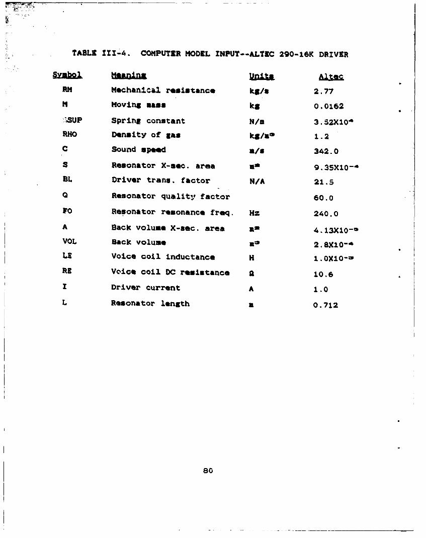
TABLE 111-4. COMPUTER MODEL INPUT--ALTIC 290-16K DRIVER

RM Mechanical resistance kW/e 2.77

M Moving mass kg 0.0162

",SUP Spring constant NI/ 3.52X10'4

RHO Density of gas kg/rla 1.2

C Sound speed r/8 342.0

S Resonator X-sec. area * 9.35X10-4

BL Driver trans. factor N/A 21.50 Resonator quality factor 60.0

FO Resonator resonance freq. Hz 240.0

A Back volume X-sec. area as 4.13X10-*

VOL Back volume so 2.8X10-,

LE Voice coil inductance H 1.0XlO-=

RE Voice coil DC resistance a 10.6

I Driver current A 1.0

L Resonator length a 0.712

80

rzCr

Figure 111-12. Computer Mddel Output forAltec 290-16K--Driver Voltagevs. Frequen~cy for One Amp.

81

~III iII..... .. ...

Figure 111-13. Computer Model Output forAltec 290-16K--Piston Velocity

vs. Frequency for One AMp.

82

Figure 111-14. Computer Model Output forAltec 290-16K--Acoustic Powervs. Frequency for One Amp.

83

Figure 111-15. Computer Model Output forAltec 290-16K--ElectroacoustlcEfficiency vs. Frequency.

84

R~t.' odl sbased on a linear theory and will have an

qua hi 1m independent of drive current.LIE.,•+L+T +•..

-it. DRIVER RKSOANCE ALTERATION

The ref riteator must operate at the resonant frequency

of the resonator to obtain the highest electroacoustic effi-

ciency and to maintain stack position with respect to the

standing acoustic wave (discussed in Sub-aection 'II.A.4). It-

appears from the computer model results and our experiments

so for that the operating frequency should a'lso be near the

driver's resonance to get the most power out of the driver.,

The resonant frequency of the resonator is determined by the

effective length of the resonator and the speed of sound in

the contained gas. The effective length for a tube of uni-

form cross-section and closed end is the actual measured

length. For the STAR resonator, however, the effective

length is the length that would produce the measured reso-

nant frequency for the given sound speed if the resonator

were a uniform cross-section closed-ended tuLe (see Figure

1-2 for approximate shape of resonator). The sound speed can

be altered by changing the percentage of xenon in the

helium-xenon mixture, since the sound speed depends on the

density of the mixture, and the density depends on the

percentages of the individual gases present (see Equations

IV-24 and IV-26). The gas mixture and effective resonator

length will be chosen to maximize the coefficient of

85

performarene at the refri•erator. Therefore4,f me want to

"match the reaonances,-woivill have to alter the resonance of

the driver once the resonant frequency of the resonator has

been determined.

*.The ret onant frequency of the Adiver Is pro~portional 'to

the square root of the stiffness divided by the moving mass.

If we want to raise the iresonant frequency of the driver we

-can either Increase the stiffness or d6crease the -ss.

Conversely, to lower the resonant frequency we can either

decrease the stiffness or increase the mass. Generally we

prefer to decrease stiffness and mass to get a larger

velocity. Reduction of stiffness usually also reduces the

mechanical. resistance.

For the Altec 290-16K attached to the uniform- cross-

section resonant tube in these preliminary experiments, the

frequencies were already well matched (note the closeness ofthe poaks in Figures 111-12 th.-ough 111-14) and changing the

driver frequency was not required. However, we know that in

future applications we may need to alter, most probably

lower, the driver resonant frequency. We developed an

experimental procedure to do this.

Adding moving mass to the driver would appear to be the

easiest way to lower the driver resonance. Unfortunately the

added mass would also reduce the velocity by increasing the

aecahnical impedance above resonance. We therefore chose to

experiment with decreasing the driver stiffness. Recall that

86

the driver-reducer-bellows system stiffness includes the

. tifffnuen of the bellows (4.5 X 100 Nl/m) and the suspension

stiffness of the driver phenolic surround (29 X 100 N/m).

'The driver suspension was the obvious choice for

experimental alteration for two reasons: (1) it is over six

times as large an the bellows stiffness, and (2) it would be

very difficult for us to change the bellows stiffness

without affecting its performance.

Since the 290-16K voice coil surround is made of a

phe;iolic material, it was relatively easy to cut through it

with an ordinary scalpel. We made a series of successive

cuts in the surround material and ran measurements of the

driver resonant frequency after each cut. The results of

this experiment are given in Table 111-5. We plotted the

phase angle between the driver's electromotive force (eaf)

and the voice coil displacement as a funtion of frequency.

For the emf we measured the voltage across the drivor termi-

nals in channel A of the HP 4192A Impedance Analyzer and

assumed that the emf was in phase with the driver current

and hence force. We used the photonic sensor to measure the

displacement by connecting its voltage output to channel 8.

The 4192A then displayed the phase angle between the two

voltages representing force and displacement. The driver is

at resonance when this phase angle equals 90 degrees. The

quality factor (Q) is equal to one-half the resonant fre-

quency times the slope of the phase angle vs. frequency

87

cuarve evaluated at -resonance (see Equation 111-28). Usitng

thei- previously deoeratined values tor moving mass (16 X) and

bellows stiffness, we calculated the suspension stiffness:

* - (111-30)

wh&r kq&, • 4Afb.* We calculated the mechanical

resistance (M) using equation 111-26. We stopped cutting

the surround when its stiffness was approximately equal to

that of the bellows and therefore the total stiffness was no*

longer suspension dominated.

TABLE III-S. RESULTS OF

DRIVER RESONANT FREQUENCY ALTERATION

Percent Surround Resonant Quality Suspension Mechanical

Remaining Frequency Factor Stiffness Resistance

100 241.0 8.55 32.2 2.83

100 (six slits) 229.5 8.09 28.8 2.85

80 213.5 5.17 24.3 4.15

50 183.5 8.65 16.8 2.13

20 119.5 8.56 4.52 1.40

Despite the anomoly at the 80% data point, we feel that

this experiment shows that partial removal of the surround

can reduce stiffness, resonant frequency, and mechanical

resistance. It appears from the above data that the flexing

88

of the pheno.l:c surround Li responsible for the majority of

the mechanical losses in the driLr.

89

IV. IIhDIVZ

A. VIMhOWTCTOK

This chapter discusses the selection of the electro-

dy'namicr driver, describes the parameter measurements on the

chosen driver, and estimates the electroacoustic efficiency

of -he STAR using the computer nodal descr'ibed in Section

1. IterikesW= AM MA Qa~nnhEaL

in addition to the maximum weight of 200 pounds

discussed in Section ID,. restrictions due to the Get Away

Special.(GAS) cannister dimensions give us a maximum payload

heiht(28.25 inches) and diameter (19.75 inches). In our

allowed height we must fit two battery layers, the driver

with its housing, the resonator assembir-, and its associated

vacuum space and thermal insulation. The battery layers are

each about four inches hith. for a total battery height of

eight inches. This leaves about 20 inches for the driver and

resonator assemblies (see Figure 1-4 for approximate

configuration). The electronics package and gan reservoir

should fit in the area radially surrounding the r'esonator,

and will therefore not add to the height. Although the

diameter of the cannister volume is 19.75 inches, the driver

housing must attach to the standard GAS can lid at a 9.5

inch diameter bolt circle, otherwise we would need a lid

90

-specially designed for our pr;;1ect. An far an weight in

."-" -aOm4, pproximately every pound we save elsewhere

allows us to carry an extra battery cell, which results in

an- tra ten watt-hours of available energy.

+ •In addition to the space and weight restrictions, we

want to maximize the electroacoustic efficiency of the

driver. We can do this by obtaining-the maximum value for

-the combination f parameters Bl/l•m.. A larger 81 will

give us a larger driving force (F-Bli), which in turn gives

us a larger acoustic volume velocity, one of the components

of acoustic power. For a given value of magnetic induction

(B), a longer voice coil (achieved by having a larger voice

coil diameter with the same number of turns, or the same

diameter and more turns) will result in a larger B1. Thic

longer 1 would also result in a greater voice coil

electrical resistance, so the two effects cancel. We also

want to minimize the moving mass (i.) to allow greater

velocities and minimize the driver's mechanical resistance

(Rm) in order to minimize mechanical losses in the driver.

3. DLIver Seecion

We had two off-the-shelf drivers available for con-

sideration. The Altec 260-16K was discussed in Chapter I11.

The other driver was a JBL 2445J. Both drivers were designed

for applications somewhat different from the STAR. Figure

IV-1 shows a side view of the 2445J driver. The hatched

g1

Figure IV-1. Schematic Drawing of JBL 24453 Driver.Hatched Area Shows Unnecessary ThroatSection.

92

area, known am the throat of the driver, is considered

w.miecessary for our application, and adds a lot of extra

weight to t.he driver. The Altec 290-16K has a similar excess

'throat voluae. We contacted JUL and asked if they would

custom-design a dtiver which would eliminate this excess

weight. Fortunately for our project, JBL was in the process

of designing a new driver, the 2430J, which uses neodyaium-

iron-boron magnets instead of the traditional ceramic. They

agreed to custom-design a vergiop of the 24SOJ for our use.

The resulting driver (hereafter referred to as NIB) is shown

in Figure IV-2. The NIB driver accepts the same voice coils

(four inch diameter, aluminum wire, and titanium suspen-

sion/diaphragm) as the 244SJ (ceramic magnet) driver. JBL

claims that it should also have the same properties,

including Bl.

In the remainder of this chapter we describe the

parameter tests on the NIB driver. We then compare the NIB

driver to the 290-16K driver. The results of the 2445J

parameter measurements are given for comparison. Finally we

present results generated by the computer model for the NIB

driver given various acoustic load impedances.

B. NIB DRIVER PARAMETERS

For the measurement of the NIB driver parameters, we

used the techniques we daveloped in Chapter III for the

measurement of the 290-16K driver parameters.

93

K )

Figure IV-2. Photographs of JBL Neodymium-

Iron-Boron Driver.

94

1. QLmoving n ~~LaIlWm

The moving mesa and suspension stiffness were

+ •calculated using the mass loading technique. We placed small

masses (0.5 to 3.5 grams) of black putty on top of the

voice coil in half-gran inokenents. For each added mass the

resonant frequencV of the driver was found using the HP

4192A LP Impedance Analyzer (see Section II.8 for a

description of thIs Instrument). Figure ZV-3 *r.own a sample

plot of period squared vs. added mass for the NIS driver in

air. The stiffness was found by calculating four pi squared

divided by the slope. The moving mess is equal to the

intercept divided by the slope. For the NIB in air these

values are:

k a 9.8 t 0.1 X 104 kg/s= (IV-1)

and 1m 7.8 t 0.1 S, (IV-2)

with a resonant frequency of 564 Hz. We repeated the

measurement in a vacuum chamber and found:

k - 8.6 * 0.1 X 10f ka/sl (IV-3)

and 0 a 3.2 1 0.1g, (IV-4)

with a resonant frequency of 833 Hz (see Figure IV-4).

The moving mass is greater in air because of the

driver having to move the air itself. The discrepancy in the

stiffness is not as easy to explain. To determine the actual

value of k, we used the static mass loading method. This

save us a value of:

95

IM NIB A LOADING AIR4.2

yu3&130*+.4022 Ral.O0

3AS

3A

3 ~3.4

K3.

0 12 3

ADDED MASS (0)Figure IV-3. Leasnt Squares Fit of Period Squared vs.I

Added Mass for NIS Driver in Air.

2.6 NIB MASS LOADING aVACUUM

y- 1.4403+ 0.46x R-0.99

2.4-

S 2.0-

0

1.6

0 1 2 3

ADDED MASS (G)Figure IV-4. Lea•t Squares Fit of Period Squared vs.

Added Mass for NIB Driver in Vacuum.

96

k - 6,4 ± 0.2 X 10' k6/az. (IV-5)

(The static loading measurements will be discussed in the

next Stib-section.)

This last value for suspension stiffness differs by

about 40% from the first two. We did not have sufficient

time to test this driver until we were sure we had the

"correct" value for the stiffness. We recommend that the

follow-on students do so. Lacking the correct value, we ran

the computer model for two sets of data: one set represen-

ting the "high" k (9.0 X 10- kg/sa) and one using the "low"

k (6.4 X 10s kg/sa).

2. Transduction Coefficient (B1)

The transduction coefficient (Bl) was calculated

using two methods. The first method was to measure 8 (magne-

tic induction in the voice coil gap) and 1 (length of the

voice coil)ý directly. We measured B with the Dowty RFL

Industries model 912 Guassmeter (serial 808) using a Hall

effect probe model 912015 (serial 21122). The maximum

reading using this probe was 18.7 kGauss = 1.87 Tesla (T).

This value differs by less than one percent from the value

stamped un the driver by the manufacturer: 1.858 T. We will

therfore use a value of B=1.86 ± 0.01 T for this driver. We

then counted the turns of aluminum wire on the voice coil (n.

= 30 ± 1 turns) and calculated 1 using the relationship:

1 = g d n. (IV-6)

97

For the 9.98 * 0.005 cm diameter coil we calculated a value

-of 1 = 9.4 ± 0.3 M. Multi.plying these two values together

gives us for the transduction coefficient:

91 a 17.5 ± 0.6 N/A. (IV-7)

The other m~thod used to determine Bl used the

relationship:

F = 911 = -kx or B1 = -kx/I, (IV-8)

where I is the direct current applied to the-coil, k is the

spring constant merasured earlier, and x is the displacement

of the voice coil produced by the current. For this measure-

ment on the 290-16K driver we had used a Linear Variable

Differential Transformer (LVDT). For the NIB driver,

however, we used Mechanical Technology Incorporated's MTI-

1000 photonic sensor (serial 38010818) with plug-in

cartridge model MTI-3812 (serial 1366) and probe model 125R.

Figure IV-5 shown the photonic sensor with the NIB driver.

One major advantage of the photonic sensor over the LVDT is

that the photonic does not need to make physical contact

with the surface it's measuring (it uses light) whereas the

LVDT does. With the Altec 290-16K's rigid phenolic dia-

phragm, the contact with the LVDT probably did not affect

the measurement. The NIB diaphragm, however, is made of thin

- titanium and in quite flexible. It would have been impos-

sible to get an accurate reading of the displacement of this

diaphragm using the LVDT. We calibrated the photonic sensor

using calibration fixture KD-CH-III A. The output voltage

98

Figure IV-5. MITI-1000 Photonic Sensor with NIB Driver.

99

from the sensor was read on a HP 3478A multimeter (serial

A110136). We then plotted DC voltage vs. displacement in

millimeters. The resulting graph is shown in Figure IV-6.

The slope of this line gives us the calibration constant:

dV/dx a -2.086 ± O.OO V/mm. (IV-9)

This value is within two percent 3f the calibration value

provided by the manufacturer of dV/dx a 2.045 V/mm (back

slope).

The next step was to run DC current through the coil

and record the displacement of the diaphragm (via a voltage

reading from the photonic sensor). For the voltage supply we

used the HP 467A power amplifier (serial 444-00243). We

found the current by measuring the voltage (with the HP

3476A digital multimeter, serial 292162) across a ten ohm

(10) resistor placed in series with the circuit, and

dividing the voltage by ten ohms. The resulting graph is

shown in Figure IV-7. The slope of the line gives us:

dI/dV = 2.10 t 0.005 A/V. (IV-10)

Combining the values ia Equations IV-9 and IV-10 with the

previously calculated high end value for the suspension

stiffness k = 9.2 t 0.6 X 10 kEg/s:2 gives:

B1 = k(dx/dV)(dV/dI' = 21.5 ± 1.4 N/A. (IV-11)

This 15% difference between the values of Bl using

the two independent methods is what prompted us to test for

BI and k using the static loading method. Our primary

concern is that we would expect the direct measurements of B

100

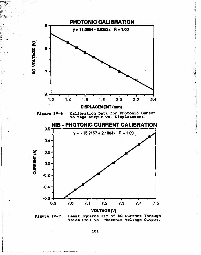
PHOTONIC CAUBRATION

y11.0854 2.0=5x R 1.00

2• 8

I- a

7-7

1.2 1.4 1.6 1.e 2.0 2.2 2.4

DISPLACEMENT (mm)

Figure IV-6. Calibration Data for Photonic SensorVoltage Output vs. Displacement.

NIB - PHOTONIC CURRENT CALIBRATION0.6

y" o15.2167+2.1004x R 1.00

0.4

-0.2

-0.4

-0.6 4 .

6.9 7.0 7.1 7.2 7.3 7.4 7.5

VOLTAGE (V)

Figure IV-7. Least Squares Fit of DC Current ThroughVoice Coil vs. Photonic Voltage Output.

101

a,. d 1 to give us the hghast possible value for 91. This is

"because the maxiom magnetic field may not be acting on the

full length of the coil. We did not expect the value of 91

calculated using the spring constant to be 15. higher than

the direct measurement value.

We were able to obtain static loading values for

both 81 and k using the same equipment setup and the

formulas:

81 Aug/Al and k . - Aug/Ax (IV-12)

For these measurements the voice coil is driven with a DC

current. We then add previously measured masses (putty and

soldering wire) to the voice coil, and measure the resulting

displacement of the diaphragm using the photonic sensor. To

measure BI we determine how much current is needed to bring

the voice coil back to its null displacement (original

output voltage reading from the photonic sen3or) after the

mass is added. We measure k by keeping the current constant

and measuring the difference in photonic output voltage

(multiplied by the calibration constant to get displacement)

resulting from the added mass. Table IV-1 lists the results

of these measurements.

The braCketed value in each k and Bl pair was

calculated using the measured value in the pair and the

relationship:

BII z -kx. (IV-13)

102

From thene measurements we net the value k a 6.1 * 0.2 kg/sa

"as reported earlier, and the transduction coefficient:

51 a 15.0 ±10.2 N/A. (IM-14)

For the model runs we used a value of B1 a 19.0 for the high

k and Bl - 15.0 for the low k.

TABLE IV-1. STATIC LOADING OF NIB DRIVER TO DETERMINE,

SUSOENSION STIFFNESS AND TRANSDUCTION COEFFICIENT

SALI. AL..(W AV (V) k (XIo* ka/sa_ I- (M

17.1 -- 5.2 6.7 (15.3] 3

17.1 -- 5.5 6.4 E14.6]

34.7 23.3 -- (6.4] 14.6

34.7 22.3 -- [6.7] 1S.3

34.7 -- .288 6.1 --

(front slope)

3. Mechbanial Resista~anceThe next parameter we measured was the mechanical

resistance (Rm) using the relationship:

Re - 2wf.ým./Q. (IV-15)

We attempted to find the driver quality factor (Q) using the

same modified impedance technique described in Section

III.G. As can be seen in Figure IV-8, the graph of the

modified impedance magnitude vs. frequency is not a smooth

resonance curve, as it was for the 290-16K (see Figure III-

9). In fact, it looks like the superposition of two

103

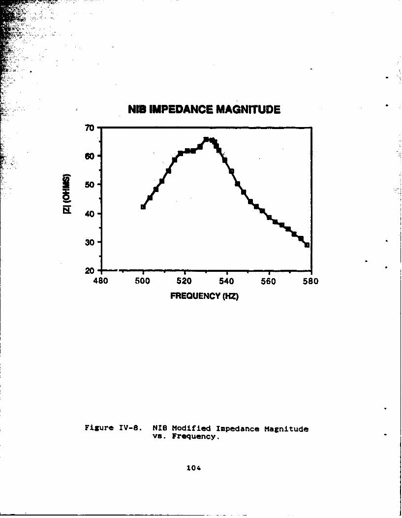
HN IMPEDANCE MAGNITUDE

70*

60-

150

FL40-

30-

20 - **

480 500 520 540 560 580

FREQUENCY (HZ)

Figure IV-S. NIB Modified Impedance Magnitudevs. Frequency.

1014

r 7,,7=o.,oL different 1iindanow curves, the first one shorter and fatter

ar- the second one taller and thinner. it was impossible to

accurately meazure half-power points from this curve, so we

chose the phasa angle method. (It is interesting to note

that the JBL 244SJ (ceramic) driver did have a smooth modi-

fted impedanoe curve similar to that of the 290-16K.) Figure

ZV-9 showw the graph of phase angle vs. frequency over -a

wide range of frequencies. Although this curve generally

approximptes an aretangent, the segment of the line imaedi-

ately adjacent to the resonant frequency (assumed to be the

frequency where 0-0, in this case 534.5 ± O05 Ha) is linear

(for a frequency range of about ten Hz). This segment is

plotted in Figure IV-lO. The slope of the line is do/df a -

42.0 * O.S X 10-s (after converting degrees to radians). As

in Section 11.0, Q is given by:

0 - -(f"/2)(d#/df) a 11.2 t 0.2. (IV-16)

Thir gives a value for R. (using the moving mass in air

m•.7.R * 0.1 a):

* 2.34 * O.OS kx/s. (IV-17)

We decided that a more accurate measurement of 0 and

R. could be found by making the 0 measurement in vacuum. For

this we used the open circuit free decay method. This method

consists of sending a signal to the driver at resonance with

an HP 3314A function generator (serial A342044), then

simultaneously switching off the signal and triggering a

Nicolet model 310 storage oscilloscope (serial 88004641) to

105

MIS N I EDANCE PHASE ANGLE

40

S20

40

y 784.8911 - 1.4576x R- 0.98.60" I- il ,r m5li I ~m F m qm

480 500 520 540 560 580

FREQUENCY (HZ)Figure !V-,). NIB Mcdified Impedance Phase Angle

as a Function of Frequency--FullFrequency Range.

NIB PHASE ANGLE- LINEAR SEGMENT20-

y -1219.5242 - 2.2815x R -1.00

wU 10-

_0-

-20 -520 530 540 550

FREQUENCY(HZ)Figures IV-10. NIB Modified Impedance Phase Angle

an a Function of Frequency--LinearSegment Near Resonance.

106

record the free decay. A sample of the output from this

process Is shown in Figure IV-11. The equation for a simple

harmonic oscillator experiencing free decay in:

A(t) a Aw exp (-t/') sin(mot÷#), (IV-18)

where AMt) is the amplitude as a function of time, A. is the

initial (maximum) amplitude, t is the time (a nT, or the

number of periods times the period), It is the free decay

constant (a QT/s, see Iquation 111-29), a is the angular

resonant frequency, and P is the phase ankle. We recorded

the peak amplitude as a function of period number, and

plotted the natural logarithm of the peak amplitude vs.

period number. The equation representing this line is:

In A(T)..1k M In A. - nT/%. (IV-19)

The slope of this line is t/% r nT/i - nx/Q. Therefore Q can

be found by dividing w by the slope of the line. Figure IV-

12 shows a semi-log plot for the NIB driver in air. The

value of 0 for this plot is 21.5, which is almost twice the

value we found using the modified impedance phase angle

measurements (Q = 11.2). Obviously the air strongly affects

the measurements. The scattering of the data points in this

figure is probably due to the same phenomena that causes the

double peaks in the impedance curve. Figure IV-13 shows the

semi-log plot of the amplitude vs. period number for vacuum.

This curve is much smoother and, we assume, more relfable.

The 0 for this data is:

Q = t/slope = 19.8 t 0.05. (IV-20)

107

i a

Figure IV-11. Sample of Free Decay Output from

Nicolet 310 Storage Oscilloscope.

108

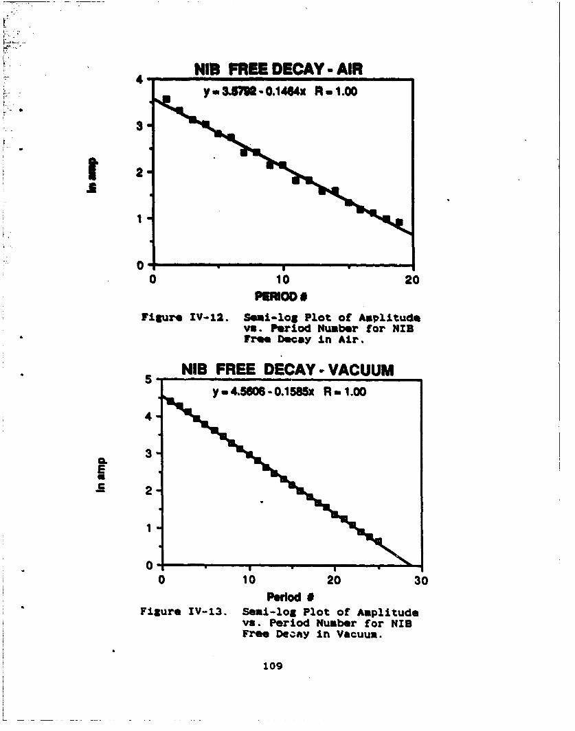
L• NIB FREE DECAY- AIRy.3.579-.0.1464X R..1.00

I 2-

£0

0 20

Figure IV-12. Semi-lo0 Plot of Amplitudevs. Period Number for NIBFree Decay in Air.

NIB FREE DECAY- VACUUMy-4.5606-0.l5x RI1.O0

4

CL 3ES

2

0-0 10 20 30

Period #Figure IV-13. Semi-log Plot of Amplitude

Va. Period Number for NIBFree Decay in Vacuum.

109

;A can also find the period from the free decay curve (and

tthus the resonant frequency as the inverse of the period).

We use the oscilloscope to measure the time for ten cycles

and divide this number by ten. For the vacuum run the

resonant frequency was 839 * O.S Hz. Theme values (and the

moving mass a 3.2 g in vacuum) give us the mechanical resls-

tance In vacuum:

Rm a 2wfmoa/Q a 0.83 * 0.01 kg/*. (IV-21)

.This is the value we used for the model.

Table IV-2 gives a comparison of applicable

parameters for tle three drivers. Notice that the parameter

Bl/R---a.m. is almost three times greater for the NIB driver

than the 290-16K. Thia is the parameter that we said (Sub-

section IV.A.2) we wanted to maximize to get the highest

thermoacoustic efficiency. Thus the driver that gives us the

best height and weight characteristics (see photograph of

the thi e drivers in Figure IV-14) also gives us the best

electroacoustic efficiency.

C. MODELED RFFICIENCY

In order to model the electroacoustic efficiency of the

driver, we need to know what acoustic load (impedance) it

will see. The final resonator and stack composition will not

have been determined by the time this thesis is completed.

We therefore assumed a range of possible values for the

110

TABLE IV-2. COMPARISON OF PARAMETERS FOR

THE THREE DRIVERS

PrOoprty (units) Ale 20 JL 2445J JBL NIB

Moving mass, a., (kg) 0.051i 0.015 0.015

Spring *constant (N/rn) 3.52X10,* *8.SX10*-o0I,

Magnetic Induction,P (Tesla) 2.1. 1.97 1.87

Voice CoilDiameter (cm) 7.22 9.98 9.98

B1 (N/A) 21.5 18.5 17.5

Voice coil DCresistance (2) 10.6 7.1 7.6

Mechanicalresistance (kg/s) 2.77 -1. 0.83

Voice coil±flducta ce (H) 1.0XIO104 1.14X10-4 11.14Xl10'

Mass (kg) 14.5 13.8 3.1

Height (in) 6.0 5.5 2.5

Magnetic energydensity (J/cma) '.0.5 -'.0. 3.2

510..l. i 1230 1410(m/Coul-kg)

Figure IV-14. Photographic Comparison of theThree Drivers--Altec 290-16K,JUL 2445J, and JBL NIB.

112

acoustic load based on the experimental data acquired to

date.

The model parameters that relate to the acoustic

load are the density of the gas, (RHO), the speed of sound in

the gas (C), the resonator quality factor (Q), the resonator

reaonant frequency (FO), and the resonator length (L). The

model was designed for a closed-ended tude of uniform cross-

section. The STAR resonator has an open tube (with a bulb

attached) and nonuniform cross-section. The problem of

applying the existing computer model to the STAR resonator

was solved by scaling the STAR parameters to make it look

like a closed-ended uniform cross-section tube.

1. Inrut Values for PureI Helium

For pure helium, the experimental data available was

the range of resonator quality factor values (10.-20), and

the speed of sound and gas density at room temperature

(about 300K) and ten atmospheres (cm. = 1024 m/s,

.= 618 kg/mi). Also available were four resonant fre-

quencies, two for a short resonator at warm (580 Hz) and

cold (520 Hz) temperatures, and two for a long resonator at

warm (520 Hz) and cold (470 Hz) temperatures. Using this

information, we first calculated the effective lengths of

the resonators at room temperature as if they were closed-

ended, uniform cross-section tubes. For this we used the

relationship:

A = 2L a c/f, or L.. = q/2f, (IV-22)

113

where X is the wavelength, L is the length of the tube, c is

the speed of sound, and f is the resonant frequency. This

calculation save us effective lengths for the resonators:

L, 0.883m and La o O.985m. For the computer runs we use a

convenient value of L.. - 0.90m. We then calculated the

speed of sound for the operating temperature of approxi-

mately 250K using the relationship:

c(T) - e, [T/Tnr]'. (IV-23)

This gives us a speed of sound c.. - 935 a/s. If we use

this sound speed and the effective resonator lengths to

estimate the resonant frequencies for 250K, we get f. = 529

Hz and f, = 474 Hz, which agree with the measured values. We

calculated the gas density at the operating temperature

using the relationship:

P - VP/c - 1.94 kg/mu, (IV-24)

where I is the ratio of the specific heats (1.667 for

helium) and P is the pressure.

Table IV-3 lists the input parameters for the pure

helium computer runs. Note that for the computer model, the

moving mass must take the mass of the reducer cone and

bellows into account (see Figure IV-15). The total moving

mass is expected to be approximately 15 S.

2. Input Va_a _ues for Helium-Xenon

There was somewhat less data available for the

helium-xenon mixture (12.5S Xe). We had the sound speed at

300K and ten atmospheres (c,v = 472 m/s). We also had

114

TABLE IV-3. COMPUTER MODEL INPUT--NIB DRIVER WITH NELIUM AT TEN ATMOSPHERES

V• AND TEMP-RAT•VRI 250K

5YAbo Menin Units NIBi

RN mechanical resistance kg/s 0.83

M Moving mass kg 0.015

SSUP Spring constant N/m 6.6, 9.0 X1O'

RHO Density of gas '.i/mo 1.94

C Sound speed m/s 935.0

S Resonator X-sec. area ma 1.14X10-*

BL Driver transduction factor N/A 15.0, 19.0

Q Resonator quality factor 10,15,20

FO Resonator resonance freq. Hz 519.4

A Back volume X-sec. area ma 4.42X10-*

VOL Back volume M= 3.28X10-

LE Voice coil inductance H 1.14X10-*

RE Voice coil DC resistance 2 7.6

I Driver current A 1.0

L Resonator length m 0.90

115

!i: ....

.4,,

(b)

Figure IV-15. Photograph of JBL NIB Driverwith (a) Reducer and (b) Bellows.

116

resonant frequencies for the same four conditions as for the

pure helium: short-warm (265 Hz), short-cold (230 Hz), long-* warm (235 Hz), and long-cold (21-5 Hz). We used Equation

IV-22 to find the effective resonator lengths (L. 0.891g

and La a 1.004m). However, once again we used a convenient

effective length of 0.90 a for the computer runs. We used

Equation IV-23 to find the sound speed for He-Xe at the

operating temperature, Cm. a 431 m/s. The estimated reso-

nant frequencies for the cold temperature were f,=242 Hz and

fa-215 Hz, once again comparing favorably with the measured

values. To find the density of the mixture at the operating

temperature we used a form of the ideal gas law:

r z PM/RT, (IV-25)

where M is the atomic mass of the mixture, R is the

universal gas constant, and P and T are the pressure and

temperature. We calculated the atomic mass of the mixture

using the equation:

M6f-M= MMMm..ix + MftxMM., (IV-26)where the M's are atomic masses (4 for helium and 131.3 for

xenon) and the x's are percentages of the gases in the

mixtures. This tquation gives us an atomic mass for the

12.5% Xe mixture of 19.9 g/mol, and a density of 9.70 kg/mim

at 250K and ten atmospheres. Table IV-4 lists the computer

input values for He-Xe, including a range of O's from 5 to

30. (We are not sure what to expect for the actual value of

0, since a new stack will also be used.)

117

TABLE IV-4. COMPUTER MODIL JNPUT--NIB DRIVER WITH HELIUM-XENON AT TEN ATMOSPHERES

MA1D TEMPERATURE u 250K

Symbol eaning nts

RM Mechanical resistance kg/s 0.83

M Moving mass kg 0.015

SSUP Spring constant N/I 6.6, 9.0 X104

RHO Density of gas kg/mW 9.70

C Sound speed a/s 431.0

S Resonator X-sec. area a= 1.14X10-

BL Driver trans. factor N/A 15.0. 19.0

Q Resonator quality factor 5,10,15,20,25,30

FO Resonator resonance freq. Hz 239.4

A Back volume X-sec. area ma 4.42XY10-

V-'L Back volume M* 3.28X10- 4

LE Voice coil inductance H 1.14X10-4

I Voice coil DC resistance a 7.6

Driver current A 1.0

L Resonator length m 0.90

118

3. C-omuter- Modl3kl Result

FIgures IV-16 through IV-19 are sample output plots

* for pure helium with 81 = 15 N/A, k = 6.4 X104 kg/*s, and

0 . 20. Notice that the peak values for the driver and

resonator are almost matched (the driver resonance is at the

lower frequency). The thermoacoustic efficiency for this set

of values is about 70.4%. figures IV-20 through IV-23 show

the corresponding plots for the helium-xenon mixture. This

time the peaks are not matched (the driver peak is off the

scale) and the electroacoustic efficiency is about 16.6%.

The primary reason for the difference between the two gases

is the lower sound speed, and therefore lower resonant fre-

quency, in the He-Xe mixture.

Table IV-5 lists the maximum value of

electroacoustic efficiency for each of the test runs. The

consistently low efficiencies for the He-Xe emphasize the

importance of matching the two resonant peaks. We recommend

that the driver frequency be adjusted to match the resonator

operating frequency. This can best be dorie by reducing the

stiffness of the titanium surround (see Section III.1).

119

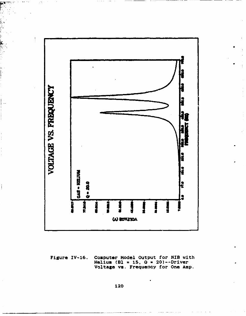
L2

Figure IV-16. Computer Model Output for NIB withHelium (Bl u 1S. 0 a 20)--DriverVoltage vs. Frequency for One AMP.

120

r

Figure IV-17. Computer Model Output for NIB withHelium (Bl -a 15, 0 -- 20)--PistonVelocity vs. Frequency for One Amp.

121

SP/i

(4) hhAU O&LfLaO~y

Figure IV,-18. Computer Model Output for NIB withHelium (BS - 15, 0 * 20)--AcousticPower vs. Frequency for One Amp.

122

II

0 UI

UIAOd 3nLLOR3 /U=h~d 3LUUaNO

Figure IV-19. Computer Model Output for NIB with Helium(Bi - 15, G a 20)--ElectroacousticEfficiency vs. Frequency.

123

Xeno (BI = 15, G a n n.. .... .I. Vla

124-i i

Figure XV-20. Computer Model Output ffor NIB luith Helium-Xenon (Bi a 15, 0 - 20)--Driver Voltagevs. Frequency for One Amp.

f 124

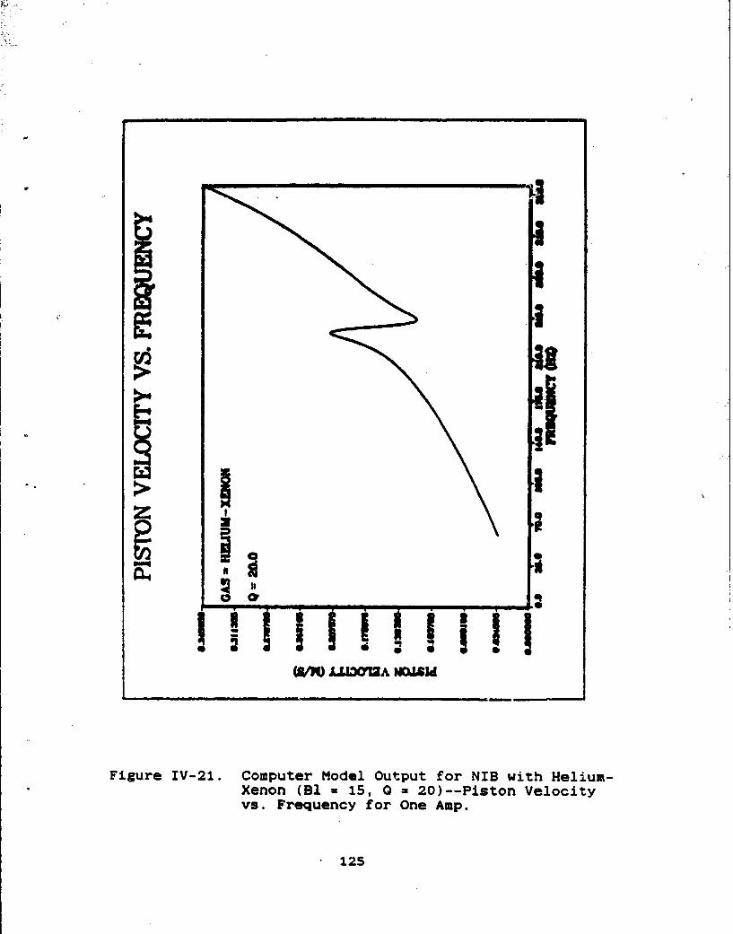
K I.

(AM UWMA W=N d

Figure IV-21. Computer Model Output for NIB with Helium-Xenon (BI = 15, Q = 20)--Piston Velocityvs. Frequency for One Amp.

125

R;1

Siij i i i

W0 WAOd aLWnAo-v

Figure IV-22. Computer Model Output for NIB with Helium-Xenon (BI = 15, Q = 20)--Acoustic Powervs. Frequency for One Amp.

126

rS

Figure IV-23. Computer Model Output for NIB with Helium-Xenon (BI - 15, 0 = 201--ElectroacousticEfficiency vs. Frequency.

127

TABLt IV-S. CO4PLTKR 4ODEL RESULTS FOR NIS DRIVER--

PEAK ELECTROACOUSTIC EFFICIENCY (•)

He (Blull He 1.2haigL He-Xe (alaIS) H.xe (Blnl2_S5 5 .1 5 .9

10 71.3 70.4 9.2 10.7

is 71.6 74.3 13.1 1.

20 70.4 76.2 16.6 19.1

25 19.6 22.7

30 22.8 26.0

128

A. INTRODUCTION

This chapter describes the construction of the STAR

driver. A large part of this thesis involved the design of

the parts necessary to integrate the NIB driver with the

resonator and GAS cannister, an illustrated in Figure 1-4.

The major design work was for the drivei- housing. The

requirements for the driver housing are:

I - lightweight,

2 - strong (pressurized to 210 psi),

3 - interface to GAS canister lid (12 10-32 bolt holes

centered at 9.5 inches diameter),

4 - interface with resonator (preferably interchangeable

with earlier test resonators),

5 - helium leak-tight feed-through ports for electrical

leads (driver electric power, accelerometer and

microphone outputs), and

6 - hold NIB magnet structure securely.

Figure V-1 shows a cross-sectional drawing of the driver

housing (not including any of the feed-through ports,- which

will be discussed later). Distinction between parts is shown

by different hatching. Part A is the NIB magnet structure

which was discussed in Chapter IV. Part B is the main body

of the driver housing, machined out of 6061-T6 aluminum.

129

Figure V-1. Cross-sectional Schematic of the STAR DriverHousing Showing (A) NIB Driver, (B) DriverHousing Main Body, (C) Aluminum Pusher Plate,(D) Pressure Lid, (K) Leak Test Lid,(F) Resonator Vacuum Housing, and (G) BoltHole. for Interface with Resonator.

130

Part C is a 6061-TG aluminum pusher plate used to hold the

magnet structure securely in the body using six 10/32 bolts.

Part D in the pressure lid, sealed a 1/16th inch diameter

lead o-ring and held in place with six 10/32 bolts. Part E

"represents part of the leak test lid (see Figure C-1). When

completed this will be replaced by the GAS can lid provided

by NASA. The driver housirg must match up with the GAS can

lid's 9.5 inch diameter 10-32 bolt circle. Part F is the

resonator section housing. The arrows labeled G point to the

bolt holes which form the driver-resonator interface.

B. DESIGN CONSIDERATIONS

The driver-resonator system will be pressurized to ten

atmospheres with a helium-xenon mixture (12.5w xenon).

NASA's regulations say that it must be pressure tested to

1.5 times the operating pressure (NASA, 1986a), or 15 atmo-

spheres (=1.S2X10 Pa - 220 psi). An added complication of

working with helium (or helium mixtures) is that it diffuses

through almost all materials except metals. As a result, we

are not able to use rubber o-rings to seal metal parts

together, but must use lead o-rinSs instead.

1. Electrical Feed-Throuahs

NASA's regulations prohibit us from leaking gases

into space, primarily to avoid contamination of other exper-

iments and for the safety of the Shuttle and astronauts.

This regulation is important not only for the major o-ring

131

K seals, but also for the microphone and accelerometer outputs

S~to the frequency control electr'onics (zoo Figure I-S), and

c onnecting the audio amplifier to the driver. There are

three individual wires and three co-axial connectors that

K" must penetrate the driver housing without allowing leakage.

The other housing penetrations are a DC pressure gage for

the driver housing and a fill line from a helium-xenon

bottle which will stabilize the pressure in the system

K against temperature changes in the environment and those

generated by the refrigerator.

Based on prior nxperience in other applications, we

decided that Emerson & Cuming's STYCAST4T"4 28SOFT epoxy

(Canton, MA 02021) •uld be the best choice for providing

the electrically insulating seal for the wires in the

housing. STYCASTTrm1 28509T is a quartz-filled epoxy formu-

lation with remarkably good over-all general properties. In

addition to saving excellent electrical grade insulation

properties, good adhesion, and excellent resistance to chem-

icals and solvents, 2850FT has unusually high thermal con-

ductivity and low thermal expansion. This combination of

properties makes this epoxy valuable for applications where

electrical insulati-n and mechdnical protection must be

maintained .ile ý.•ping with heat transfer considerations.

One definition for a sealed container is a helium

leak rate of less th-, 10-* standard cc's per second (NASA,

1986b). To test L..,t epoxy we designed and built a test

132

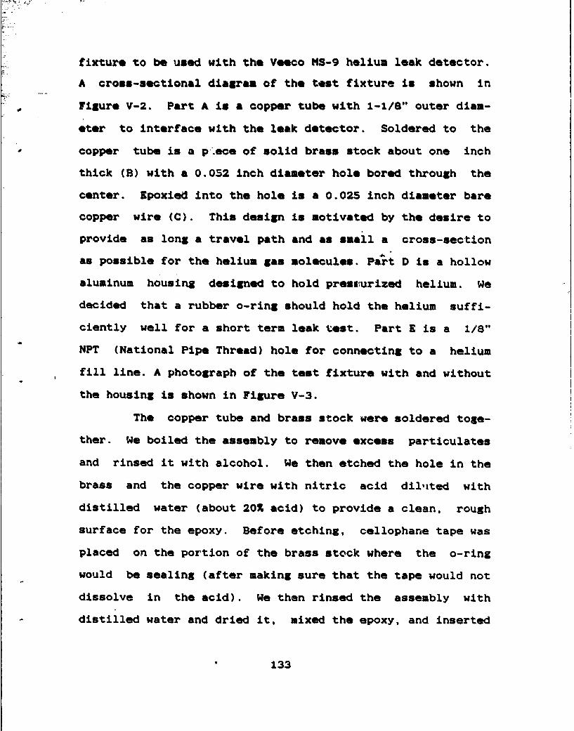
fixture to be used with the Veeco MS-9 helium leak detector.

A cross-sectional diagram of the test fixture is shown in

Figure V-2. Part A is a copper tube with 1-1/a" outer diam-

eter to interface with the leak detector. Soldered to the

copper tube is a p .ece of solid brass stock about one inch

thick (B) with a 0.052 inch diameter hole bored through the

center. Epoxied into the hole is a 0.025 inch diameter bare

copper wire (C). This design is motivated by the desire to

provide as long a travel path and as small a cross-section

as possible for the helium gas molecules. Part D is a hollow

aluminum housing designed to hold presturized helium. We

decided that a rubber o-ring should hold the helium suffi-

ciently well for a short term leak test. Part E is a 1/8"

NPT (National Pipe Thread) hole for connecting to a helium

fill line. A photograph of the test fixture with and without

the housing is shown in Figure V-3.

The copper tube and brass stock were soldered toge-

ther. We boiled the assembly to remove excess particulates

and rinsed it with alcohol. We then etched the hole in the

brass and the copper wire with nitric acid dilited with

distilled water (about 20% acid) to provide a clean, rough

surface for the epoxy. Before etching, cellophane tape was

placed on the portion of the brass stock where the o-ring

would be sealing (after making sure that the tape would not

dissolve in the acid). We then rinsed the assembly with

distilled water and dried it, mixed the epoxy, and inserted

"0 133

INN.

Figure V-2. Cross-sectional Schematic of the HeliumLeak Detector Test Fixture Showing(A) Copper Tube for Leak Detector Interface.(B) Solid Brass Stock, (C) Bare Copper Wire.(D) Aluminum Housing, and (E) Connection forHelium Fill Line.

134

Figure V-3. Photograph of the Helium Leak DetectorTeat Fixture.

135

S�the wire into the hole in the brass stock, making sure the

epoxy filled the gap.

K The following procedure was used to run the leak

detector tests: first zero the meter, then do a test run on

t I* sensitivity calibrator. The sensitivity calibrator used

was a Veeco- uype SC-4 serial number 3179 with a leak rate of

6,SXIO-1 std cc/sec (standard cubic centimeters per second).

We wouid then remove the calibrator, recheck the meter for

zero, attach the test fixture, read the meter, remove the

fixture, and recheck for zero.

The test fixture was initially pressurized to 115

psi with helium. We tried to test it immediately but found

that the detector would not draw enough of a vacuum to check

for helium. We thought that there might be outgassing from

flux or something in the tube. So we pulled a vacuum on the

tube overnight and the next day it worked fine. We tested

the fixture on the first, third, and sixth days after it had

been pressurized. The numerical results are listed in Table

V-1. Even after we had waited six days for the helium to

diffuse through the epoxy, the fixture leakage rate was an

order of magnitude less than the calibrator. The leakage

rate was therefore four orders of magnitude less than that

allowed by NASA to be considered leak-tight (1XO-4 std

cc/sec). After the third leak test we checked the pressure

in the aluminum chamber and found it to be within a few

percent of the original pressure. We therefore concluded

136

that the bare wire-epoxy method with a lenSth/diameter ratio

of about 20 could be used for the driver housing penetrating

electrical feed-througha.

TABLE V-1. HELIUM LEAK DETECTOR TEST RESULTS

ON COPPER WIRE-EPOXY FIXTURE.

Number days after null meter calibrator copper wire feed

Dressurization reading readier -throuhreading

1 0 1.1 0.02

3 0 1.2 0.08

6 0 1.1 0.10

Figure V-4 shows a close-up of the feed-through plug

for the wire leads. It will house a total of five wires

(with space available for a sixth if necessary). Two of the

leads will be for the voltage supply to the voice coil.

These leads will consist of bare copper wires epoxied into

the small holes seen in the figure. Each wire will then be

soldered to a 6/32 phillip-head screw with a 1-72 blind-

tapped hole in it. The screw will be glued into an 8/32

hole, forming a mechanically stable, demountable, electrical

terminal. The accelerometer and microphone leads will also

have bare copper wire epoxied into the small hole, and will

then be connected to Microdot(TM) coaxial fittings (Malco

137

4,4

* 2

Li

/i

S

/ /°',°p 42,

* 22

Figure V-k. Driver Housing Feed-Through Plugfor the Electrical Leads.

138

part number 031-0001-0001, South Passadena, CA 91030).

Figure V-5 shows an example of each of these leads.•!;.2. Measur,*e~nt-Devicas

The microphone and accelerometer used by STAR are

similar to those used by Hofler (1986 and 1988). In fact,

the resonator end of the driver housing was designed to

accept Hofler's resonator, calibration volume, and instru-

mentation for testing. The microphone used to measure the

acoustic pressure in the resonator is a small quartz-crystal

(Valpey-Fisher, Hopkinton, MA 01748) or PZT dynamic pressure

transducer (Piezoelectric Products lot number 4-9-84,

F013184, Metuchen, NJ). It is mounted in the driver housing

where the housing connects to the resonator flange. The

microphone will be calibrated by comparison to a standard

transducer, which will have been previously calibrated via a

reciprocity technique. The microphone will be connected to a

miniature FET follower circuit. The FET buffer (Eletec model

304 impedance converter, Daytona Beach, FL 32020) converts

the microphone's high impedance output signal to a low

impedance to reduce sensitivity to electrical noise and

maintain the output voltage and phase while driving the

cables necessary to reach the signal processing electronics.

The buffer's DC power supply and output cables are complete-

ly shielded through the driver housing to the buffer (see

Figures C-3 and C-7 for location of microphone and FET in

driver housing).

139

(a)

(b)

Figure V-S. Example of Wire Lead Connectorsfor Feed-Through Plug: (a) SingleWire and (b) Co-axial Cable.

140

The Endevco model 22 Picomin (1" accelerometer is

attached to the side of the bellows stiffener facing the

driver. The integrated accelerometer signal will be used as

a measure of the bellows velocity, which will be calibrated

by driving a small cavity of calcul.3ole acoustic impedance.

ThLs the product of the outputs from the microphone and

integrated accelerometer can be combined to yield the acous-

tic power and their relative phase can be used to keep the

driver frequency at the tube resonance. The operation of the

refrigerator at resonance is essential both to optimize the

acoustic power delivered to the "stack" and to guarantee

that the "stack" is always located at the proper position in

the standing wave as discussed in Sub-section II.A.4.

The DC pressure transducer is an Omega"'v PX-80

designed for high pressure applications requiring long-term

stability. Figure V-6 shows a drawing of the pressure trans-

ducer and its driver housing fitting.

The helium port in the housing is provided to

empty and fill the driver and resonator and so that a stable

pressure may be maintained in the driver and resonator

through the ballast volume provided by the reservoir (see

Figure 1-4).

There is a 1/32 inch diameter hole filled with a ten

thousandths inch inner diameter half inch long capillary in

the driver housing where it connects to the resonator. The

function of the capillary is to equilibriate the static

141

'DRIVE

TRANSD .UCER HOUS INGFITTING

Figure V-6. DC Pressure Transducer and DriverHousing Plug Fitting.

142

pressure between the driver and resonator during filling and

non-operating times while maintaining a pressure seal at

acoustic operating frequencies.

A complete met of dimensioned drawings for the

driver housing and its auxiliary equipment is given in

Appendix C. A list of materials for the driver portion of

* the STAR is given in Appendix D.

143

VI. CONCLUIONZQU 02M1 DEMII

The objective of the 3TAR project is to test and space

qualify a new continuous cycle cryogenic refrigeration

system for cooling of sensors and electronics which is based

upon the newly-diucovered thermoacoustic heat pumping

effect. The new refrigerator has no sliding seals, a cycle

frequency of about 300 Hz, and uses acoustic resonance to

enhance overall efficiency. This thesis is concerned speci-

fically with the design and testing of the electrodynamic

transducer which is responsible for the electro-acoustic

power conversion. A computer model of the driver/resonator

system was presented along with the techniques for measure-

sent of the electrical and mechanical parameters used as

input for the model.

A final driver design (including dimensional drawings)

utilizing a modified JBL 2450J neodymium-iron-boron

compression driver and associated leak-tight electrical

feed-throughs, microphone, accelerometer, pressure &age,

pressure housing, and resonator interface is provided.

Since we only received the NIB driver in late December

1987, there wasn't time to perform enough parameter

measurements to obtain accurate values for the suspension

stiffness Wk) and transduction coefficient (B1). The next

144

group of students should find these values for use in the

model and efficiency calculations.

The resonator experiments (not reported here) indicate

that Helium-Xenon may be the preferred gas mixture for the

--STAR. If this is the case, the NIB driver resonant frequency

will have to be lowered for it to match the operating

(resonant) frequency of the resonator. This could be

accomplished by adding moving mass to the voice coil-

reducer-bellows assembly, but that would decrease the

velocity and lower the electroacoustic efficiency. The

preferred option for driver resonance adJustment is to

decrease the suspension stiffness by cutting away part of

the surround (see Section III.1). Since the NIB voice coil

has a titanium surround and diaphragm this operation will

have to be performed carefully. The tithnium diaphragm

(dome) will also have to be removed. (The done's function is

performed by the reducer and bellows.)

The task for the next group of students is to assemble

the NIB driver with its housing and accessories (feed-

throughs, microphone, accelerometer, etc.) and perform

efficiency measurements on the ground similar to those that

will be performed in space. This series of measurements will

closely resemble those performed on the Altec 290-16K driver

as described in Chapter III.

145

APPENDIX A. COPUT MODEL ALULATIOM PROGRM

PROGRAM FRIDGE

C INTRODUCTION:CC THE PURPOSE OF THIS PROGRAM WRITTEN BY LT. MICHAEL P.C SUSALLA IS TO CALCULATE THE DATA POINTS AND PLOT THEC PERFORMANCE CHARACTERISTICS OF A CONCEPTUAL MODEL OF AC THERMOACOUSTIC HEAT ENGINE. THE COMMENTS INCORPORATED INTOC THIS PROGRAM AND THE COMMENTS INCORPORATED IN THE PLOTTINGC PROGRAM "GRAFRI FORTRAN Al". WILL ALLOW THE USER TO PRO-C DUCE FOUR GRAPHICAL PLOTS WHICH WILL CLOSELY APPROXIMATEC THE PERFORMANCE OF AN ACTUAL THERMOACOUSTIC HEAT ENGINE.C THE GOAL OF THE PROGRAM/SIMULATION IS TO ALLOW THEC OPERATOR TO VARY DIFFERENT PARAMETERS TO ACHIEVE WHAT ISC BELIEVED TO BE AN OPTIMUM CONDITION WHERE THE ENGINESC DRIVER RESONANCE IS HATCHED WITH THE TUBE RESONANCE.CC GENERAL INSTRUCTIONS:CC THIS PROGRAM IS SET UP TO PROVIDE FOUR PLOTS: VOLTAGEC VERSUS FREQUENCY, PISTON VELOCITY VERSUS FREQUENCY, ACOUS-C TIC POWER VERSUS FRZQUENCY, AND ELECTROACOUSTIC EFFICIENCYC VERSUS FREQUENCY. IN GENERAL THE PROGRAM HAS HARD INPUTC DATA SUCH THAT ALL YOU MUST DO TO GET A SET OF PLOTS ISC COMPILE "GRAFRI FORTRAN Al" IN FORTVS AND THEN RUN "FRIDGEC FORTRAN Al" IN WF77 FROM FLIST ON THE NPS MAINFRAME USINGC A TEKTRONICS 618 TERMINAL. THIS ACTION WILL GIVE YOU A SETC OF PLOTS FOR THE INPUT DATA. TO TRY OTHER DATA YOU MUST GOC TO XEDIT ON THE '"FRIDGE FORTRAN Al"° PROGRAM AND VARY THEC INPUT DATA. AS LONG AS YOUR CHANGES ARE RESTRICTED TO THE"C "FRIDGE" PROGRAM THE ONLY ACTION NECESSARY TO PRODUCE NEWC PLOTS IS TO RUN THE PROGRAM IN WF77. IF YOU FIND IT NECES-C SARY TO CHANGE THE PLOTTING PROGRAM, "GRAFRI", FOR WHAT-C EVER REASON, IT MUST BE RECOMPILED IN FORTVS PRIOR TO THEC NEXT ATTEMPT TO PLOT OR THE CHANGES WILL NOT BE SEEN BYC THE MACHINE.CC INPUT SECTION:C A. DEFINITION OF VARIABLES:C ALL OF THE VARIABLES HAVE BEEN ESTABLISHED AS REALC OR COMPLEX QUANTITIES BASED ON THE REQUIREMENTS OF THEC ARITHMETIC ALGORITHOM OF THE CONCEPTUAL MODEL. EACH OFC THE VARIABLES WILL NOW BE DEFINED.C LCOILuTHE IMAGINARY PART OF THE IMPEDANCE OF THE VOICEC COIL OF THE DRIVER. AND IS CALCULATED TO BE WmLE.C K=THE PROPAGATION CONSTANT OF THE WAVES IN THE TUBEC AND IS GIVEN BY W/C.

146

C INZMZTHE IMAGINARY PART Or THE MECHANICAL IMPEDANCE OFC THE TUUE/DRIVER COMBINATION. IT IS GIVEN BY A RATHER LONG

-,C .AHD _..COWVLEX EQUATION III THE CALCULATION SECTION OF THE-e PRORAtI.C MAGU-THE MAGNITUDE OF THE COMPLEX QUANTITY "U", INC METERS/SEC.C IMZTnTHE IMAGINARY PART OF THE TUBE MECHANICAL IMPE-C DANCE AND IS GIVEN BY SUBTRACTING THE DRIVER PORTIONS FROMC MzM."C M-THE MOVING MASS OF THE SYSTEM, AND IS THE SUM OF THEC VOICE COIL AND THE DIAPHRAGM MASSES OF THE DRIVER, INC KILOGRAMS.C LoTHE LENGTH OF THE TUBE IN METERS.C LE=THE INDUCTANCE OF THE VOICE COIL, IN HENRYS.C I-THE INPUT CURRENT FROM THE SOURCE, IN AMPS.C MAGV-THE MAGNITUDE OF THE COMPLEX QUANTITY "'V", INC VOLTS.C ZMnTHE MECHANICAL IMPEDANCE OF THE TUBE/DRIVER SYSTEM,C AND IT IS MADE UP OF THE REAL PART, REZM, AND THE IMAGI-C NARY PART, IMZM.C ZE-THE ELECTRICAL EQUIVALENT OF THE MECHANICAL IMPE-C DANCE OF THE TUBE/DRIVER SYSTEM. IT IS GIVEN BY TRANSFOR-C MING ZM ACROSS A TRANSFORMER USING THE BL COEFFICIENT OFC THE'DRIVER.C ZCOIL-THE COMPLEX ELECTRICAL IMPEDANCE OF THE VOICEC COIL.C ZTOT=THE TOTAL ELECTRICAL IMPEDANCE OF THE SYSTEM,C COMPLEX.C V-THE COMPLEX VOLTAGE OF THE SOURCE NECESSSARY TOC PRODUCE THE SELECTED INPUT CURRENT.C UuTHE VELOCITY OF THE PISTON,(DIAPHRAGM), OF THEC DRIVER IN M/S.C ZTUBE-THE COMPLEX MECHANICAL IMPEDANCE OF THE TUBEC ITSELF.C P-THE COMPLEX PRESSURE OF THE SYSTEM, IN NEWTONS/M**2.C PluA CONSTANT FOR CONVERSIONS TO AND FROM ANGULARC UNITS.C RM=THE MECHANICAL RESISTANCE OF THE MOVING MASS OF THEC SYSTEM.C SSUP-THE MECHANICAL STIFFNESS OF THE SYSTEM DUE TO THEC DRIVER SUSPENSION.C RHO-THE DENSITY OF THE GAS IN THE TUBE AT A SPECIFIEDC MEAN TEMPERATURE.C C=THE SPEED OF SOUND FOR THE SPECIFIED GAS ANDC TEMPERATURE.C S-THE CROSS SECTIONAL AREA OF THE TUBE.C BL-A COEFFICIENT OF THE DRIVER THAT IS BASED ON THEC STEADY AIR GAP FLUX DENSITY OF THE DRIVER AND THE LENGTHC OF ITS VOICE COIL.C Q-THE QUALITY FACTOR OF THE TUBE.C FO-THE RESONANCE FREQUENCY OF THE TUBE.C AuTHE CROSS SECTIONAL AREA OF THE BACK VOLUME OF THE

147

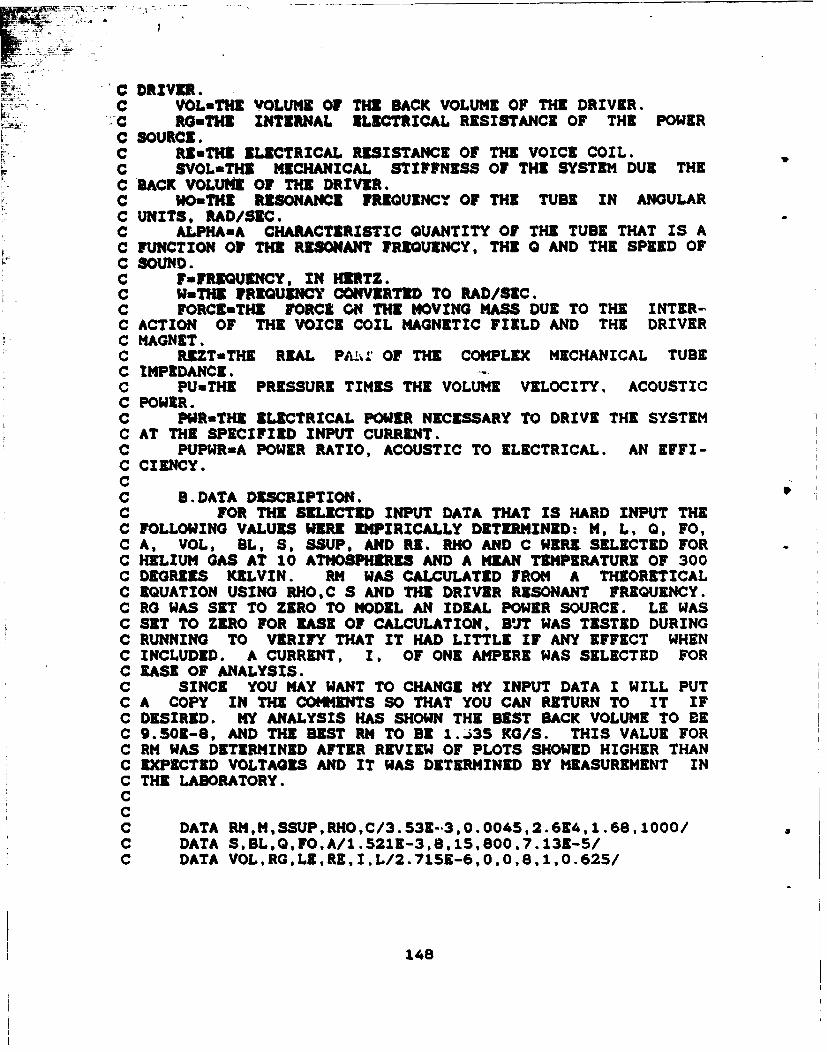
•"C DRIVER.

SC VOLwTHE VOLUME OF THE BACK VOLUME OF THE DRIVER.C + RG=THi INTERNAL ELECTRICAL RESISTANCE OF THE POWERC SOURCE.C R~nTHI ELECTRICAL RESISTANCE OF THE VOICE COIL.C SVOL*THE MECHANICAL STIFFNESS OF THE SYSTEM DUE THEC BACK VOLUME OF THE DRIVER.C WOuTHE RESONANCE FREQUENCY OF THE TUBE IN ANGULARC UNITS, MAD/SEC.C ALPHA-A CHARACTERISTIC QUANTITY OF THE TUBE THAT IS AC FUNCTION Of THE RESONANT FREQUENCY, THE Q AND THE SPEED OFC SOUND.C FaFREQUENCY, IN HERTZ.C WaTHE FREQUENCY CONVERTID TO MAD/SEC.C FORCE-THE FORCE ON THE MOVING MASS DUE TO THE INTER-C ACTION OF THE VOICE COIL MAGNETIC FIELD AND THE DRIVERC MAGNET.C REZT=THE REAL PA!M' OF THE COMPLEX MECHANICAL TUBEC IMPEDANCE. -

C PU-THE PRESSURE TIMES THE VOLUME VELOCITY. ACOUSTICC POWER.C PWRwTH, ELECTRICAL POWER NECESSARY TO DRIVE THE SYSTEMC AT THE SPECIFIED INPUT CURRENT.C PUPWRwA POWER RATIO, ACOUSTIC TO ELECTRICAL. AN EFFI-C CIENCY.CC B.DATA DESCRIPTION.C FOR THE SELECTED INPUT DATA THAT IS HARD INPUT THEC FOLLOWING VALUES WERE EMPIRICALLY DETERMINED: M, L, Q, FO,C A, VOL, BL, S, SSUP, AND RE. RHO AND C WERE SELECTED FORC HELIUM GAS AT 10 ATMOSPHERES AND A MEAN TEMPERATURE OF 300C DEGREES KELVIN. RM WAS CALCULATED FROM A THEORETICALC EQUATION USING RHOC S AND THE DRIVER RESONANT FREQUENCY.C RG WAS SET TO ZERO TO MODEL AN IDEAL POWER SOURCE. LE WASC SET TO ZERO FOR EASE OF CALCULATION, BUT WAS TESTED DURINGC RUNNING TO VERIFY THAT IT HAD LITTLE IF ANY EFFECT WHENC INCLUDED. A CURRENT, I, OF ONE AMPERE WAS SELECTED FORC EASE OF ANALYSIS.C SINCE YOU MAY WANT TO CHANGE MY INPUT DATA I WILL PUTC A COPY IN THE COMMENTS SO THAT YOU CAN RETURN TO IT IFC DESIRED. MY ANALYSIS HAS SHOWN THE BEST BACK VOLUME TO BEC 9.50E-8, AND THE BEST RM TO BE 1.j35 KG/S. THIS VALUE FORC RM WAS DETERMINED AFTER REVIEW OF PLOTS SHOWED HIGHER THANC EXPECTED VOLTAGES AND IT WAS DETERMINED BY MEASUREMENT INC THE LABORATORY.CCC DATA RM,M,SSUP,RHO,C/3.53E-,3,0.0045,2.6E4,1.68,1000/C DATA SBL,Q,FO,A/1.S21E-3,8,15,800,7.13E-5/C DATA VOL,RG,LE,RE,I.L/2.71SE-6,0,0,8.1,0.625/

148

REAL LCOIL.K,IMZM,MAGU,IMZT,ML,LE,I,MAGVCOMPLEX ZM,ZE,ZCOIL,ZTOT,V,U,ZTUBE,PPIw3.141S926S4DATA Rf1,M,SSUP,RHO,C/3.53E-3,0.004S,2.6E4,1.68,1 •0/DATA S,BL,Q,FO,A/.521E-3,8,15,SOO,7.13E-5/DATA VOL,RG,LE,REI,L/2.71SE-6,0,O,8,1,0.625/SVOL.(A*A*RNO*C*C)/VOLWO=2'PI SFOALPHA=WO/(2*Q'C)

C CALCULATION SECTION:C THE NEXT SIX LINES CREATE AN OUTPUT FILE FOR THE DATAC THAT IS NECESSARY TO PRODUCE THE DESIRED PLOTS, AND PLACESC HEADINGS ON THE DATA AS APPROPRIATE.

OPEN(UNITu69,FILE-'FRIDGE OUTPUT Al',IOSTAT-IOS)WRITE(69,*)' MASS VOLUME'WRITE(69,1)M,VOLWRITX(69,5) FREQUENCY PIST VEL PRESS'PIST VEL PWR RATIO

"* VOLTAGE'I FORMAT(E13.4,E13.4)

C THE FOLLOWING DO LOOP PROVIDES FOR THE CALCULATION OFC THREE HUNDRED DATA POINTS FOR EACH OF THE DESIRED PLOTS,C USING A FREQUENCY RANGE OF ONE QUARTER TUBE-RESONANCE TOC THREE HALVES TUBE RESONANCE.

DO 10 3J1,300F=(FO/4)÷((J-1)'(FO/240))

C THE NEXT THREE LINES CALCULATE VARIOUS QUANTITIES,C EXPLAINED ABOVE, THAT ARE FUNCTIONS OF FREQUENCY, FOR USEC IN FUTURE CALCULATIONS.

W=2*PI'FK=W/CLCOIL=W'LE

C THE NEXT NINE LINES CALCULATE THE REAL AND IMAGINARYC PARTS OF THE TUBE/DRIVER MECHANICAL IMPEDANCE AND COMBINEC THEM INTO A COMPLEX QUANTITY, ZM.

REZM=RM+(((RHO*C*S*ALPHA*COS(K*L)SIN(K*L))+(K*RHO*C*S"aSINH(ALPHA*L)XCOSH(ALPHA*L)))/(K*(l+(ALPHA/K)**2)*((((

149

* SINNi(ALPHA*L))**2)))))IMZH*a(WSH)-(SSUP'W)-'(SVOL/W),(((RHO*C*S*ALPHA*SINH(ALPHA8L)

* COSH(ALPHA*L))-(K&RHO'Cm S3COS(K'L)3tSIN(KSL)))/(K*(1,(ALPHA/K)'a2)8(((SI(IC(V.Ln)**2c((co*HcALPHA'L))**2)).(((COS(K*L)) -

3 **2)*((SINgH(ALPHA*L)p'*2)))))ZMaCMPLX (RREZMZM ZM)

C THE NEXT THREE LINES CONVERT ZN TO AN ELECTRICALC QUANTITY AND THEM COMBINE ALL OF THE ELECTRICAL IMPEDANCESC TO GET A TOTAL IMPEDANCE.

ZtudBL82)/ZMZCOZLuCMPLX(RE, LCOIL)ZTOT=RG+ZCOIL+ZR

C THE NEXT SIXTEEN LINES CALCULATE THE VALUES TO BEC PLOTTED, AND PUT THEM IN THE OUTPUT FILE, AND THEN CLOSEC THE FILE.

VumI*ZTOTFORC~mBL' IU-FORCE/ZMMAGUuCABS (U)REZTuREZM-RMIMZT=IMZM- (W*M) +(SSUP/W) +(SVOL/W)ZTUBE*CMPL'X (REZT.IMZT)P. (ZTUBE3 U) /SPU-.0.5(REAL(P*CONJG(U) )*S)PWR*O.S2(REAL(I*CONJG(V)))PUPWRaPU/PWRMAGV.CABS CV)WRITE(69,100)FMAGU,PU.PUPWRMAGV

100 FORMAT(El3.S,E13.S,El3.SEl3.S,13.S)10 CONTINUECLOSE(69)

C PLOTTING SECTION:C THE NEXT TWO LINES INTERFACE WITH MY PLOTTING PROGRAM,C "OGRAFRI FROTRAr4 Al". AND THE DISSPLA ROUTINE TO PLOT THEC DATA.

PAUSE 'PRESS ENTER TO START PLOTTING ROUTINE'CALL EXCMS ('EXEC DISSPLA GRAFRI')STOPEND

I50

APPENDIX B. OPUTE I MODEL GRAPH PROR

PROGRAM GRAFRI

C THIS IS LT. MICHAEL P. SUSALLA'S PLOTTING PROGRAM FORC USE IN CONJUNCTION WITH "FRIDGE FORTRAN Al" IN "THE THER-C MOACOUSTIC HEAT ENGINE SIMULALTION". THIS PROGRAM MUST BEC COMPILED IN FORTVS PRIOR TO RUNNING "FRIDGE FORTRAN Al" INC WF77.THIS PROGRAM IS FOR USE IN DISSPLA AND CALLS VARIOUSC DISSPLA SUBROUTINKS. THESE VARIOUS SUBROUTINES ARE IISEDC MORE THAN ONCE IN THE PROGRAM BUT WILL ONLY BE DESCRIBEDC ONCE EACH. IN ORDER TO USE DISSPLA YOU MUST HAVE ARRAYSC OF DATA POINTS TO BE PLOTTED. NY ARRAYS ARE ALL DIMEN-C SIONED TO 300 POINTS SINCE THAT IS THE NUMBER CALCULATEDC BY "FRIDGE FORTRAN Al". YOU SHOULD BE AWARE THAT IF YOUC CHANGE THE NUMBER OF POINTS TO BE -CALCULATED, AND THEC NUMBER IS GREATER THAN 300, YOU MUST REDIMENSION THEC ARRAYS. TWO CHARACTER STRINGS ARE USED IN THIS PROGRAM.C NEWI$ IS USED IN RENAMING FILES TO THE FORMAT NECESSARYC FOR DISSPLA, AND DUMMY$ IS USED TO READ THE HEADIN3S OUTC OF THE DATA FILE. ALL OF THE DATA TO BE PLOTTED IS IN THEC FORM OF REAL NUMBERS, SO ALL OF THE VARIABLES ARE MADEC REAL. D IS USED FOR THE FREQUENCY DATA, G IS USED FOR THEC PISTON VELOCITY DATA, H IS USED FOR THE ACOUSTIC POWERC DATA, 0 IS USED FOR THE ELECTROACOUSTIC EFFICIENCY DATAC AND, T IS USED FOR THE VOLTAGE DATA. THE XMAX AND YMAXC VARIABLES ARE INITIALIZED TO ZERO AND ARE USED TO CALCU-C LATE THE MAX VALUE OF EACH OF THE PARAMETERS AS THEY AREC READ INTO THE ARRAYS. THIS COMPLETES THE INTRODUCTION ANDC EXPLAINS THE FIRST FIVE LINES OF THE PROGRAM.

DIMENSION D(300),G(300),H(300),O(300),T(300)CHARACTER880 NEWI$, DUMMY$REAL D,G,H,O,T,MDATA XMAX,YMAXI,YMAX2,YMAX3,YMAX4/0.,O.,O.,O.,O./

C THE NEXT SEVEN LINES OF THE PROGRAM RENAME MY DATAC FILE TO THE FORMAT NECESSARY FOR USE IN DISSPLA, OPEN THEC FILE, READ THE MASS AND VOLUME OUT OF THE FILE AND, READC THE HEADINGS OUT OF THE FILE.

NEWl$='RENAME '//' FRIDGE OUTPUT Al'//' FILE XYZ1 Al'CALL EXCMS(NEW1$)OPEN (69,FILE='XYZl')READ (69,'(A8O)') DUMMY$

151

READ (69,1)NVOLREAD (69,'(Aeo)') DUMNY$

1 FORMAT (113.4,913.4)

C THE FOLLOWING DO LOOP READS THE PLOTTING DATA INTO THEC ABOVE SPECIFIED ARRAYS FOR USE IN THE DISSPLA SUBROUTINES,C AND ALSO CALCULATES THE MAXIMUM VALUE OIr 1ACH OF THEC ARRAYS FOR SETTING UP THE SCALES OF THE PLOT AX•S. THENC THE DATA FILE IS CLOSED. THESE VALUES ARE LEFT AS REALC NUMBERS VICE INTEGERS BECAUSE THE DATA FROM THE PROGRAMC CAN VARY SIGNIFICANTLY WITH DIFIEGNT INPUT VALUES, AND IFC THE MAX VALUE IS LESS THAN 10 AN INTXGtR RUZUIREMENT GIVESC A PLOTTING ERROR.

DO 20 J71,300READ (69,1S,ENDu21)D(J),G(3),H(31),O(J),T(J) t

1s FORMAT(E23.5,E13.S, 13.S,E13.S,E13.S)IF(D(J).GT.XMAX)THENXMAX-D(J)ENDIrIF(Q(J) .GT.YhAX1)THENYMAX1,G(J)ENDIF J!IF(H(J) .GT.YMAX2)THENYMAX2,H(J)ENDIFIF(O(J) .GT.YNAX3)THENYMAX3-O(J) -

ENDIFIF(T(J) .GT.YMAX4)THIEYMAX4-T(J)ENDIF

20 CONTINUE21 CLOSE(69)

C THE NEXT THREE LINKS TAKE CARE OF ANOTHER ODDITY OF"C THE DATA, IN THE CASE OF THE VOLTAGE PLOT. DEPENDING ON"C THE INPUT DATA THE VOLTAGE WILL LOCK IN AT 8 VOLTS, AS"C EXPECTED, BUT THIS IS ALSO THE MAX VALUE, SO YOU GET A"C STRAIGHT LINE AT THE TOP OF THE PLOT MARGIN. THE NEXT"C THREE LINES INCREASE THE MAX VALUE TO 9 VOLTS TO MAKE THIS"C PLOTTING CASE MORE CLEAR.

IF(YHAX4.LE.9.0)THRNYHAX4-9.0ENDIF

.52

C THE NEXT EIGHT LINES CALCULATE THE INCREMENTAL STEPSr C FOR EACH AXIS OF THE VARIOUS PLOTS. THE X AXIS IS THE

C SAME FOR ALL, AND IS LEFT IN INTEGER FORMAT FOR CLARITY.C EACH AXIS IS SET UP FOR TEN INCREMENTS. THE DATA FILE ISC THEN RENAMED TO THE DESIRED FORMAT FOR MY STORAGE.

INCaINT(XMAX/IO.)YINC1=YMAX1/lO.Y'NC2=YMAX2/10.YINC3=YMAX3/lO.YINC4=YMAX4/lO.MAX=INT(XMAX)NEWI$='RENAME '//' FILE XYZ1 Al'//' FRIDGE OUTPUT Al'CALL EXCMS(NEWI$)

C THIS IS, THE FIRST PLOTTING SECTION. IT DOES THEC INITIAL SET UP OF ALL OF THE CALLS THAT CAN BE COMMON AND'C PLOTS THE VOLTAGE VERSUS FREQUENCY PLOT. CALL TEK618 SETSC UP THE REQUIRED MACHINE FOR THE PLOTTING AND LINKS YOU TOC THE PLOTTER. CALL BLOWUP IS USED TO MAGNIFY THE PLOT FORC A BETTER PICTURE. CALL YAXANG PUTS THE AXIS NUMBERSC PERPINDICULAR TO THE PLOT AXIS TO PREVENT RUNNING INTOC EACH OTHER. CALL PAGE SETS UP THE PAGE SIZE IN INCHES.C CALL AREA2D SETS UP A TWO DIMENSIONAL PLOT AREA OF THEC SPECIFIED SIZE IN INCHES. CALL SCMPLX SELECTS THE LET-C TERING TYPE FOR THE HEADING. CALL MESSAG AND CALL REALNOC ALLOW ME TO PLACE A MESSAGE IN THE PLOT AREA AT A SPECIFICC POINT SPECIFIED IN INCHES IN THE CALL. CALL XNAME ANDC YNAME ALLOW ME TO LABEL THE AXES. CALL HEADIN ALLOWS MEC TO PLACE A TITLE ON THE PLOT. CALL THKFRM AND FRAME ALLOWC ME TO PUT FRAMES AROUND THE PLOT AREA AND THE WHOLE PLOTC OF A SET THICKNES.S. CALL GRAF SETS UP THE PHYSICAL ORIGINSC AND MAX VALUES AND THE INCREMENTS FOR EACH AXIS. CALLC CURVE TELLS THE MACHINE TO PLOT THE DESIRED ARRAYS OF DATAC POINTS. CALL ENDPL ENDS THAT SPECIFIC PLOT AND GIVES AC NEW PAGE FOR THE NEXT PLOT.

CALL TEK618CALL BLOWUP(1.5)CALL YAXANG(O)CALL PAGE(11,8.S)CALL AREA2D(8.,6.)CALL SCMPLXCALL MESSAG('MASS=$',IO0,O.1,5.5)CALL REALNO(M,-2,'ABUT','ABUT')CALL MESSAG('KG$',100,'ABUT','ABUT')CALL MESSAG('VOLUME=$',1O0,O.1,5.)CALL REALNO(VOL,-2,'ABUT','ABUT')"•ALL MESSAG('M**3$',100,'ABUT','ABUT')

153

F---W

CALL XNA~lt('FREQUENcY(IN HERTZ)$',100)CALL YNANZC'VOLTAOK (IN VOLTS)$',100)CALL HKADIN( 'VOLTAGE VS. FREQUENCY$' ,100,2. ,1)CALL THICFRM( .02)CALL FRAMKCALL ORAF(0.0,INC,NAX,7.5,YINC4,YMAX4)CALL CURVE(D,T,300,O)CALL KNDPL(O)

C THIS rECTION PLOTS PISTON VELOCITY VERSUS FREQUENCY.

CALL AREA2D(8.,G.)CALL NESSAG('MASS-4',100,0.1,5.S)CALL RKALNO(M,-2, 'ABUT' ,'ABUT')CALL NKSSAG('KG$',100,'ABUT','ABUT')CALL MESSAGC'VOLU14E=$',100,O.1,5.)CALL RZALNO(VOL,-2, 'ABUT', 'ABUT')CALL MESSAG('t4s3 $3',100,'Ae~rr','ABUT')CALL XNANK( 'FREOUKNCY(IN HERTZ)$' ,100)CALL YNA*E( 'PISTON VELOCITYCIN METERS/SEC)$' ,100)CALL HEADIN( PISTON VELOCITY VS. FREQUENCYS' ,100,2. .1)CALL THKFRM(.02)CALL FRAMECALL GRAF(0.O,INC,MAX,O.O,YINCI,YMAX1)CALL CURVE(D,0,300,0)CALL KNDPL(O)

C THIS SECTION PLOTS ACOUSTIC POWER VERSUS FREQUENCY.

CALL AREA2D(S. .6.)CALL MESSAG('MASS.$',100,0.1,5.5)CALL REALNO(M,-2, 'ABUT' ,'ABUT')CALL MKSSAG('KGS',100,'ABUT','ABUT')CALL KESSAG('VOLUHE=$',100,0.1,5.)CALL RKALNO(VOL,-2, 'ABUT' ,'ABUT')CALL MESSAG('M33 3$',100,'ABUT','ABUT')CALL XNAME('FREQUINCY(IN HERTZ)$' .100)CALL YNAMK('ACOUSTIC POWER (IN N-M/S)$',100)CALL HEADIN( ACOUSTIC POWER VS. FREQUENCY$' ,100, 2. .1)CALL THKFRM(.02)CALL FRAMECALL GRAF(0.0,INC,MAX,0.0,Y-INC2,YMAX2)CALL CURVE(D,H,300,0)CALL ENDPL(0)

C THIS SECTION PLOTS POWER RATIO VERSUS FREQUENCY.

154

CALL AREA2D(B.,6.)CALL MKSSAG('MASS*$',100,O.1,5.5)CALL RIALNO(1',-2,*ABUT','ABUT')CALL "SSAG('KOS',100,'ABUT','ABUT')CALL MSSSAG('VOLUNZ=$',100.0.1,5.)CALL RZALHO(VOL,-2,vABUTv,'ABUT')CALL MISSAG('Ms'33S,100,'AEUT','ABUT')CALL XNMAI('1'RSQUINCY(IN HIRTZ)$',100)CALL YWAKE('ACOUSTIC PWR/ ELECTRIC LPWRS',10OO)CALL HKADIN('POWhKR RATIO VS. FREQUENCY$',100,2.,)CALL THKFRM(.02)CALL FRAMECALL ORAF(O.O,INC,I4AX,O.O,YINC3,YHAX3)CALL CURVE(D,0,300,O)CALL ENDPL(O)

C CALL DONKPL ENDS THlE PLOTTING SEQUENCE AND SENDS YOUC BACK TO CNS.

CALL DONKPLSTOPEND

'.55

APPKNDIX C. EML QU1VL Rh3h1hSL QRAINGES

[ 'IG

156

2 i ..- n. .II

DRIVER HOUSING - RESONATOR VIEW

(D0mmnsaone in inches )

Figure C-2. Driver Housing--Resonator View.

157

VCLC Fa

U

E C

aL a

aU

WC E

o3* we

LIJ L

aU00

Figlure C-3. Driver Housing--Side View Section AAShowiLng Rlectrilcal Leads, Solt Holes,Microphone Penetration, and FETFollower Housing.

158

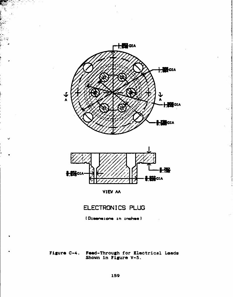
LALM

A IA

I ////. gpj''1 ,

fUJOIIA

/ ////~/,'.,/. r"., A

VIEV M

ELECTRONICS PLUG

( Dimenmsons ,n inches I

Figure C-4. Feed-Through for Electrical Leads

Shown in Figure V-5.

159

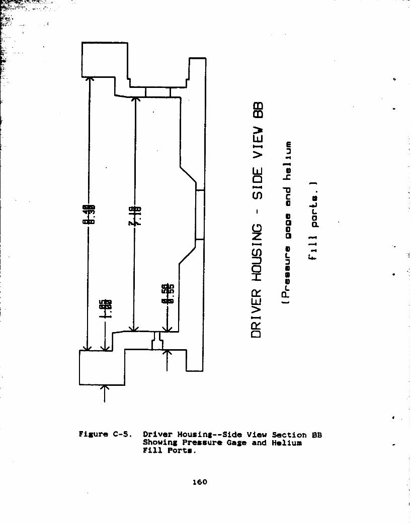
InIn

wE-3>2W

C) -C

I L

0

?*

L L..

C)

Figure C-S. Driver Housing--Side View Section BBShowing Pressure Gage and HeliumFill Ports.

160

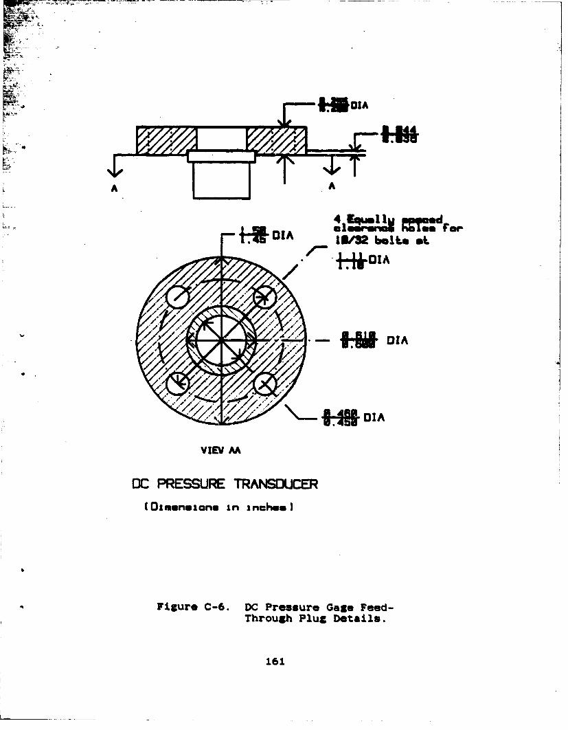
fWGIA

r', .1

A A

-- •L• OIA13/32 belF~s o.t

/4DI I&I- °el a

VIEV M

DC PRESSURE TRANSDUCER(0 Ammna I aonu I mnchum I

Figure C-6. DC Pressure Gage Feed-Through Plug Details.

161

40,

DRIVER HOUSING -LID VIEW

Figure C-7. Driver Housing--Lid View ShowingCapillary, Microphone, and Follower,and Bolt Circles f or ResonatorAttachment, Pusher Plat*, PressureLid and GAS Can Lid.

162

5 -

* Not:.e" Pla•.e is 3/10" wide andnd slopes 100 at. outer-

edbe. )

PUSHER PLATE (LID VIEW)

(Dimensions in inches).

Figure C-8. Aluminum Pusher Plate.

163

9*-

Groove For1/16' lead

S...:.:" -r ing at.

:'" ~DIA

.B DIA

INare: O-ring groove U.,18" wideand .035" deep:

lid in 1/2" wide)

PRESSURE LID (LID VIEW )

( olmensiorls in inches )

Figure C-9. Pressure Lid with LeadO-ring Groove.

164

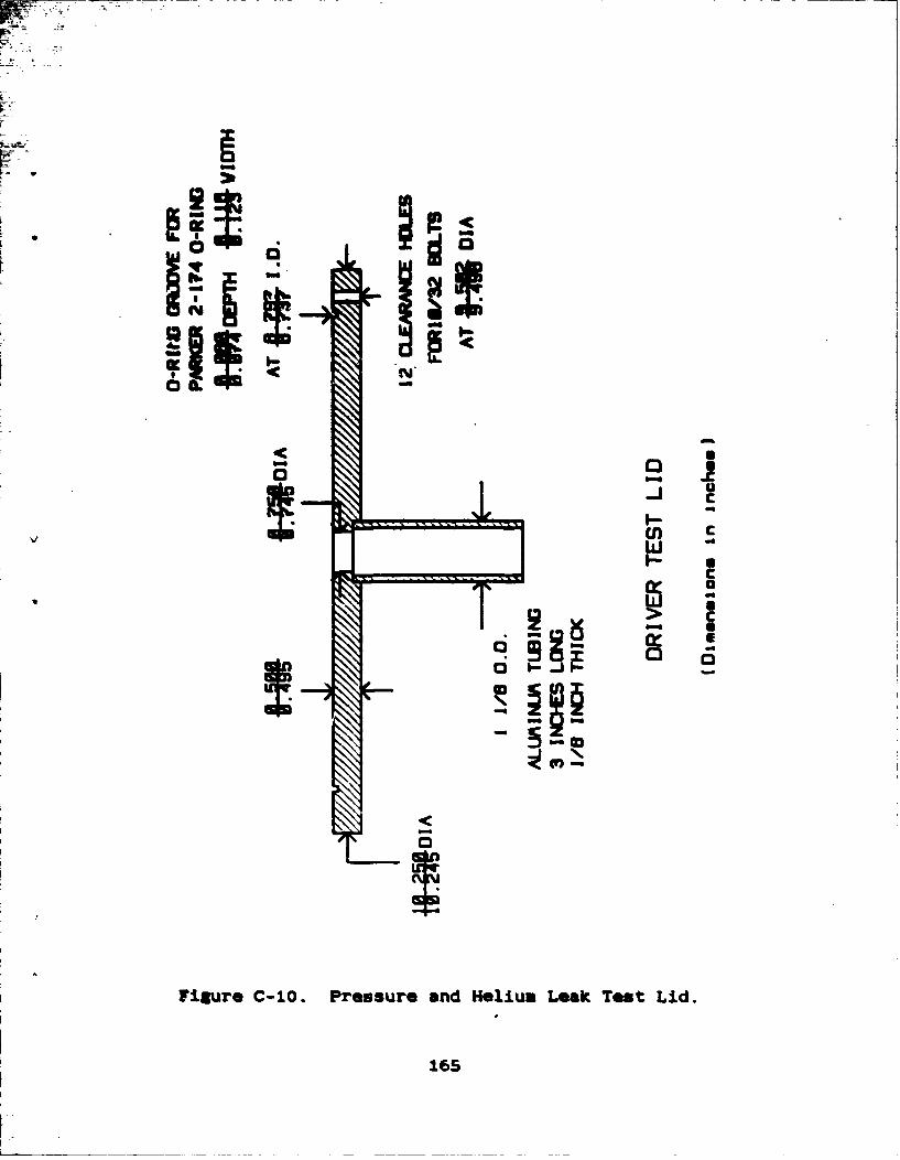
•2o

o

'I'm

616

UC)

LEMl

16S

Fr- aý

Am"Fn

&A=

LEER DF-~winlm~

Fiu*C1..~ue oO

APPENDIX D. I DRIVE I OF MTI

The driver consists of a modified JBL model 2450J neo-

- ciymium-iron-boron magnet with iron pole pieces on either

"side. The diaphragm is titanium and the voice coil is -t

a3.uainum.

The housing, pusher plate, pressure lid, and reducer

cone will all be machined from 6061-T6 aluminum. All open-

ings in the driver housing will be sealed with 1/16" or

1/32" diameter lead o-rings. The electrical feed-throughs

will be se&led with Emerson & Cuming's STYCAST<YFR 2850FT

epoxy. All wire leads are copper. The steel bolts connecting

the resonator to the driver are size 1/4-20. All other steel

bolts are size 10-32.

167

REFERENCES

BOY~d, A. _W., Kos~ndki, 9. P.- and Weston, R. L., "AutonomousMeasurement of Space Shuttle Payload Bay Acousticu DuringLaunch,"' -Nva Reeac Reviewys, vol. 39 (1), p. 9, 1987.

LQD1 Z-L ChD Dii ra n L.Pln WaveCAntg , PhD wettoNvlPsgaut coFr

""onterey, C, .7,Dcme 9S-Cpera-ey, P. H.. "A Pistonleaw Stirling Engine -The Travel-inHaeIeat Engine" ItJuia L Lft._A&2Jntical~J ftity~m~aVol. 66, p.''1506 917.

Got Away Spca ea GS

andL Space Adainistration, Goddard Space Flight Center,Special Payload* Division, Greenbelt, MD, July 1984.

Gif ford, W. K. and Longsworth, R. C., "Surface HeatPumping," In~nt^~ Advaogg in Croznn ineering,Vol.. 11, p. 171,~ Plenum, NY, 1966.

Gray, D. E., amrnnnla nstjt~t4& ot ~Physics Handbook, ThirdEdition, p. 5-165, arGraw-ilHiII19q72.

Faraday, M., QugrelJ Jora of Science, vol. 5, p. 274,

Hofler, T. J. Thtioaosi Rfieatio 21Jgl andPerformance, hD.DDissetation, University of California,San Diego, CA, 1986.

Hofler, T. J., "Accurate Acoustic Power Measurements with aHigh-intensity Driver," Jour~nalofthe Acoustical Society ofAmerica, vol. 83 (2), P. 777 , 1988.

Kempton, A. J., "Heat Diffusion as a Source of Aerodynai~icSound," Journal of Fluid Mechanics, vol. 78, p. 1, 1976.

Kinsler, L. E., Frey, A. R., Coppens, A. B., and Sanders,J. V., Fundamentals of AcousticsE, Third Edition, John Wiley& Sons, Inc., New York, NY, 1982.

Merkli, P. and Thomann, H., "Thermoacoustic Effects in aResonant Tube," Journal of Fluid Mechanics, vol. 70, p. 161,1975.

NASA George C. M~arshall Space Flight Center, MaterialsSe ton List for Spac Hardware Sytems, Report No. MSFC-R~B~52Rev T, -p. 1T7ffA9KR5FC AL, November, 1986 a.

168

... MS oddard Space Flight Center, . .... .. Payloads

A- Itay elth, Lord, Prq~g2Zui, U thgifoal jgie vol. VIII,S.53Sj Nature, ,l.XVIII, p. 3.9 1878.

Rayleigh Lord, TheorX gL Sound, Second Edition, Volume II,"Section A221, b'ver, New York, 1945.

Rijke, P. L., A 2L Physics (Leipzig), vol. 107, p. 339,1859.

Rott, N., "Damped and Tbirmally Driven Acoustic Oscillationsin Wide and Nlarrow Tubes," jotgrn &_ A1is Mathemajics &:And Pjhyms JMP), vol. 20, 1969.

Rott, N., "The Heating Effect Connected with Non-linearOscillations in a Resonant Tube," Journal of A Mathe-matics and Physics (ZAMJ), vol. 25, 1974i-'4

Rott, N., "Thermally Driven Acoustic Oscillations, Part III:Second-Order Heat Flux," J go Applied Mathematics andPhysics .(ZAMP), vol. 26, 1975.

Rott, N., "Thermoacoustics," Advances n Apiplied Mechanics.vol. 20, 1980.

Sears, F. W. and Salinger, G. L., Thermodynamics. KineticTheory, and Statlai Thermodynamics, Third Edition, pp.113-115, Addison-Wesley, 1975.

Smith, J. L. Jr., Robinson, G. Y. Jr., and Iwasa, Y., Survey2f the State-of-the- Art of Miniature Cryocoolers for Su2ar-condutc-ive Devices, Naval Research Laoraftory, `5a-9-Rington,D. C., 1984.

Sondhauss, C., Annals gf Physics and Chemistry, Volume 79,(1), 1850.

Swift, G. W., untitled article to be published in the Journalof the Acoustical Society of America, circa 1989.

Swift, G. W., Migliori, A., Garrett. S. L., and Wheatley, J.C., "Two Methods for Absolute Calibration of DynamicPressure Transducers," Review of Scientific Instruments,vol. 53 (1), p. 1906, 1982.

Taconis, K. W., Beenakker, J. J. M., Nier, A. 0. C.. andAldrich, L. T., "Measurements Concerning the Vapour-LiquidEquilibriu4 of Solutions of Hem in He, Below 2.19-K."Physica, vol. 15, p. 733, 1949.

169

W*lIX~r, G., "1Crocoolers, Parts I and 2," tratoaCr~dM~iA0._ Plenum Press, MY , 93

Jhe. --,C,- -ara, -Coxt, A. . "Ifttura.- E1niines, 99Pysc

Wheatley, 'J. _C., Hof ler, T. J. , 'Swift, 0. W., and flisliori,A , "tIcperim*)ts with an Intrinsically Irreversible Acodst;L`Heat Engine," PZhxA.aig Baviaw Letters, vol. SO (7), P. 499,_0ruary -I-983a.

Wheatley Jj.. o-flet, T. J.. Swift, G.46-*., and Ntgliori,F A.$ "An Intrinsically IrrevirJl The1eaoutic meat

"In '* j~urhal, to vol.

Wheatley, J. :C., Ho-fler, J_. J, -Swift, 4. W. an iliar*-.,,A., 'Underetainding Some Simple Phenomena in Therioacoustlicswith Applications to Acoustical Heat gagi-ns," Anr i12M.rnS1 2L P ice, vol. 53 (2), p-.147, February 98S.-,

Wheatley, j. C., Swift, G. W., and Migliori, A.. "TheNatural Heat Engine," I&&g hlaasScenca Number 14, 'Fail1986.

Wilson 0.R 6,n t

Yazaki, T., Tominaga, A., and tfarahara, Y., Journal2L-ýLQ9.vTo~rtr Phgis vol. 41, p. 45, 1980.

170

INITIAL DISTRIBUTION LIST N.Cpe

1 Defense Technical Information Center 2Cameron StationAlexandria, VA 22304-6145

2. .Ltbrary, Code 0142 2

'Naval. Postgradua~te SchoolýMonterey, CA 93943-5002

U. --S.-Coamt Guard Headquarters.2100 Second St-reet, S. W.

Washington, D. C. 20593

-4. P-rofessor Richard Crissuan 2 *iphysics DepartmentU. S. Ccast Guard AcademyNew London, CT 06320

S. Professor S. L. Garrett, Code GIOX 6Naval Postgraduate SchoolMonterey, CA 93943-5000

6. Dr. T. Hofler, Code 61HF -ANaval Postgraduate SchoolMonterey, CA 93943-5000

7. Professor A. Atchley, Code 61AY 1Naval Postgraduate SchoolMonterey, CA 93943-5000

8. Dr. L. E. Hargrove1Office of Naval ResearchPhysics Division - Code 1112800 N. Quincy StreetArlington, VA 22217

9. Professor 1. Rubrick1UCLA--Physics Dept.405 Hilgard Ave.Los Angeles, CA 90024

10. Commanding OfficerOffice of Naval TechnologyATTN: Dr. Philip Selwyn (Code 20)1

CAPT R. S. Fitch (Code 23D)1800 N. G'uincy StýreetArlington, VA 22217

171

11. commnding Officer- -Stval- Air Devflopuent Center

kITR . T. -riloon1Warminster, PA 18974

±.Commanding OfficerNaval Research Laborat~oryAThI: T. 0. 0"a3.orenui1

F. flelirich14555 Overlook AvenueWashington,'D. C. 20375-5000

-13. P~fewsor-A. H.- ---I Code 67FuAi~va3 otauslShoMonterey, CA '93943-5000

14. Prof essor R. Panholtzer, Code 62Px 2Naval Postgraduate SchoolMt~ctr~y, CA -93943-5000

15. 1). Rignaiden, Code 721Naval Postgraduate SchoolMonterey, CA 93943-5000

16. LT Scott Palmer 3,Space and Naval Warfare Systems CommandPDI 106/72AWashington, D. C. 20363-5100

17. Me. Carol Tanner IMail Station N4/910Aerospace CorporationP. 0. Box 92957Lox Angeles, CA 90009

18. Commodore Truly1Commander Naval Space CommandDahlgren, VA 22448-5170

19. Mr. Frank Deithrick 1Space and Naval Warfare Systems CommandWashington, D. C. 20363-5100

20. The University of Texas at AustinATTN: Prof. 1. Bunch-Vishniac (Mach. Eng.)1

Prof. W. D. McCormick (Physics) 1Austin, TX 78713-8029(

172

21. on. Al aaos Nat:Lonal.Laborat~ri**Candensed Matter and Thermal Physics (Group P-10)7ATTN: ~Dr. G. W4. Swift±

Dr. A Nigliri*P. 0. Box 1663/MS 764

-Los .Alaaos, NM 8754S

22. Cousanding OfficerLNoval.Weapons Center

3 Office of Counsel - Code 023ATTN:~ W. Thomas SkceerChina Lake, CA 9355S

22. LCDR Allen H~anson:Navy Space System ActivityP. 0. Box 92960 WUPLos-Angeles, CA 90009

24. LT Mary CoxDept. of the Air ForceASpace Test Program Office (SD/CLTPC)HO space bivisionP. 0. Box 92960Los Angeles, CA 90009-2960

25. Mr. Fancher Murray 3JBL Incorporated800 Balboa BoulevardNorthridge, CA 91329

26. Dr. S. F. WatanabeDirector, Technology AssessmentMcDonnell Douglas Corporation *1550 Wilson Blvd.,* Suite 550Arlington, VA 22209

27. The Aerospace CorporationATTN: Dr. Bruce C. Edgar (141/120)

Julie D. White (141/122)P. 0. Box 92957Los Angeles, CA 90009-2957

28. Cox Hobbies IncATTN: W. H. Selzer, President1525 East WarnerAve.Santa Ana, CA 92705

29. EndevcoATTN: W. H. Cooley1500 16th St., Suite 200San Francisco, CA 94103

173

:30.- ='T tI~hele Pitxpatrftk6?4Qrw9"anSt

ftttvill, W17901

31'ý. LT Michael Sumalla .Code -33 WN63*aval Postgraduate schoolHOpterey, CA 93"43

32. LT? R. Volkhert1Code 33,_UXNaval Postgraduaate SchoolMonterey,_CA 93"43

33.CPT D. Harris1- Code 33, UXNaval Pontgraduate SchoolMonterey, CA 93943

34. -National Center for Physical Acoustic*ATTN: Librarian1P. 0. Box 847Fraternity RowUniversity, NS 38677

174