posture regulation for unicycle-like robots with...
TRANSCRIPT

Universita degli Studi di Padova
Dipartimento di Ingegneria dell’InformazioneCorso di Laurea Magistrale
in Ingegneria dell’Automazione
Tesi di Laurea Magistrale
Posture regulation forunicycle-like robots withprescribed performance
guarantees
Laureanda Relatore
Martina Zambelli Ch.mo Prof. Giorgio Picci
Anno Accademico 2012/2013

ii
Dedicato ai miei genitori

iv

Abstract
This thesis focuses on control of nonholonomic system with particular refer-ence to the unicycle-like robots. These are common examples of WMRs(Wheeled Mobile Robots), increasingly present in industrial and servicerobotics, particularly when flexible motion capabilities are required.The major objective of this study is to solve the regulation problem for theunicycle model while guaranteeing prescribed performance. Different con-trollers based on either polar coordinates or time-varying laws are proposed.The main contribution is the combination of the standard control laws (bothwith polar coordinates and time-varying laws) that allow to achieve postureregulation for the unicycle model, with the prescribed performance controltechnique that imposes time-varying constraints to the system coordinates.The study also illustrates two different approaches to bind linear or angularcoordinates, one based on a particular error transformation, and the otherarising from a specific potential function.Simulations confirm the effectiveness of the proposed solutions.
v
vi ABSTRACT

Acknowledgements
I would like to express my gratitude to Dr. Dimos Dimarogonas, Assistantprofessor at the Automatic Control Department at KTH, and Dr. YiannisKarayiannidis, researcher at the Computer Science Department at KTH, forsupervising me in this project; their expertise, understanding, suggestionsand useful critics added considerably to the depelopement of my thesis work.My gratitude goes to Professor Giorgio Picci for giving me the opportunityto do my thesis in the Automatic Control Department of KTH.I also thank Lukas Buhler for his opposition at my presentation at KTH.
My heartfelt thanks to my parents, Fernanda and Alessandro, and to mybrother Marco, for their constant support and patience in all these years ofuniversity in Padova and in the six months of Erasmus in Stockholm.Many thanks also to Alberto and to my friends in Verona, Padova, Romaand Stockholm, who enriched my personal journey, making familiar eachplace and unique each moment.
Vorrei esprimere la mia gratitudine al Dr. Dimos Dimarogonas, Assis-tant professor presso il Dipartimento di Automazione al KTH, e il Dr. Yian-nis Karayiannidis, ricercatore presso il Dipartimento di Informatica al KTH,per la supervisione in questo progetto; la loro esperienza, la comprensione, isuggerimenti e le critiche utili hanno contribuito molto allo sviluppo del miolavoro di tesi.La mia gratitudine va al Professor Giorgio Picci per avermi dato l’opportunitadi svolgere la mia tesi di laurea presso il Dipartimento di Automazione delKTH.Ringrazio anche Lukas Buhler per la sua opposizione alla mia presentazioneal KTH.
Un sentito grazie ai miei genitori, Fernanda e Alessandro, e a miofratello Marco, per il loro costante supporto e la pazienza in tutti questianni di universita a Padova e nei sei mesi di Erasmus a Stoccolma.Molte grazie anche ad Alberto e ai miei amici di Verona, Padova, Roma eStoccolma, che hanno arricchito il mio percorso personale, rendendo fami-liare ogni luogo e unico ogni momento.
vii

viii ACKNOWLEDGEMENTS
Contents
Abstract v
Acknowledgements vii
1 Introduction 3
2 Preliminaries 7
2.1 Unicycle model and control overview . . . . . . . . . . . . . . 7
2.2 Prescribed performance overview . . . . . . . . . . . . . . . . 8
2.3 First example: Dynamic Feedback Linearization . . . . . . . . 14
3 Control with Polar Coordinates 17
3.1 Control with polar coordinates . . . . . . . . . . . . . . . . . 17
3.2 Prescribed performance on the distance vector . . . . . . . . 20
3.3 Bounds on the orientation . . . . . . . . . . . . . . . . . . . . 23
3.3.1 Bounds on γ or δ . . . . . . . . . . . . . . . . . . . . . 23
3.3.2 Overview of a practical possible solution . . . . . . . . 23
3.3.3 Bounds on the angle γ through a different Lyapunovfunction . . . . . . . . . . . . . . . . . . . . . . . . . . 24
3.4 Bounds on both radial and angle coordinate . . . . . . . . . . 29
4 Time-varying Control 35
4.1 Time-varying control . . . . . . . . . . . . . . . . . . . . . . . 35
4.2 Time-varying control without heating function . . . . . . . . 38
4.3 Control based on different Lyapunov function . . . . . . . . . 40
4.4 Bounds on orientation . . . . . . . . . . . . . . . . . . . . . . 43
4.4.1 Time invariant bounds on the orientation . . . . . . . 46
4.4.2 Time-varying bounds on the orientation . . . . . . . . 50
4.4.3 Performances of the designed time-varying controllers 53
5 ROS Simulations 55
5.1 Brief introduction to ROS . . . . . . . . . . . . . . . . . . . . 55
5.2 Implementation . . . . . . . . . . . . . . . . . . . . . . . . . . 56
1

2 CONTENTS
6 Conclusion 61
Bibliography 62
A Two approaches to impose PP bounds 67
B DFL: details and convergence proof. 71
C Control with Polar Coordinates: details and proofs. 73C.1 Details for section Prescribed performance on the distance
vector . . . . . . . . . . . . . . . . . . . . . . . . . . . . . . . 73C.2 Details for bounds on the angles . . . . . . . . . . . . . . . . 75C.3 Details and proof for section Bounds on the angle γ through
a different Lyapunov function . . . . . . . . . . . . . . . . . . 78C.4 Details for section Time-varying bounds on γ . . . . . . . . . 79C.5 Details and proof for section Bounds on both radial and angle
coordinate . . . . . . . . . . . . . . . . . . . . . . . . . . . . . 79
D Time-varying control: details and proofs. 81D.1 Details on the error definition . . . . . . . . . . . . . . . . . . 81D.2 Details and proof for section Time invariant bounds on the
orientation . . . . . . . . . . . . . . . . . . . . . . . . . . . . 82D.3 Details for section Time-varying bounds on the orientation . 83
E ROS Simulations: Code. 85E.1 Class UnicycleVelocityControllerNode . . . . . . . . . . . . . 85E.2 Class UnicycleVelocity . . . . . . . . . . . . . . . . . . . . . . 86

Chapter 1
Introduction
Over the past thirty years wheeled mobile robots (WMRs) have becomeincreasingly important in a wide variety of applications such as transporta-tion, security, inspection, planetary exploration, etc. WMRs are increasinglypresent in industrial and service robotics, particularly when flexible motioncapabilities are required. Several mobility configurations (wheel number andtype, their location and actuation, single- or multi-body vehicle structure)can be found in the applications. The most common for single-body robotsare differential drive and synchro drive (both kinematically equivalent to aunicycle), tricycle or car-like drive, and omnidirectional steering.
Beyond the relevance in applications, the problem of autonomous motionplanning and control of WMRs has some theoretical challenges. In particu-lar, these systems are a typical example of nonholonomic mechanisms dueto the perfect rolling constraints on the wheel motion (no longitudinal orlateral slipping).
Target problems for WMR are (i) regulation of position and orientationof the WMR to an arbitrary set point, (ii) tracking of a time-varying ref-erence trajectory ( the path following problem is a special case), and (iii)enhance robustness including the effects of the dynamic model during thecontrol design.
With regard to the control of nonholonomic systems, one of the tech-nical hurdles often cited is that the regulation problem cannot be solvedvia a smooth, time-invariant state feedback law due to the implications ofBrockett’s condition [1]. Brockett’s theorem provides a very useful necessarycondition for asymptotic stabilizability by continuous feedback. Intuitively,it means that, starting near zero and applying small controls, we must beable to move in all directions. Also, in other words, Brockett’s conditionstates that smooth stabilizability of a driftless regular system requires anumber of inputs equal to the number of states. Thus, to reach stabilizationof these systems we can use either time-varying or discontinuous controllers.
Many solutions can be found in literature. A very common and simple
3

4 CHAPTER 1. INTRODUCTION
model to analyze the stabilization of nonholonomic systems is the unicycle.Many solutions in literature refer to this model and it will be exploited alsoin this thesis.
There exist different approaches to control a nonholonomic system, suchas a unicycle-like robot. See for example [2] for discontinuous control, [3] fordynamic feedback linearization technique, [4] for discontinuous backstep-ping, [5] for an approach involving potential function, [6] for chained formsystems control and time-varying point-stabilization, [7] for control with po-lar coordinate, and also [8, 9] for an overview on nonholonomic systems andcontrol of wheeled robots.
The solution with polar coordinates allows to achieve very natural tra-jectories for the unicycle vehicle. It is based on the change of variables fromthe Cartesian (x, y, θ) to the polar (r, γ, δ) coordinates. With these coor-dinates, control inputs v (the driving linear velocity) and ω (the steeringangular velocity) can be designed. This type of control will be analyzed inthis thesis, and modification will be made on it in order to achieve bettertransient performance.
The time-varying control permits to achieve convergence but the ob-tained vehicle behavior is characterized by noticeable oscillations aroundthe desired position. This is an intrinsic issue for this type of controller,which involves oscillating functions in its design. This thesis will also analyzeand modify the time-varying controller in order to achieve better transientperformance, specifically for the convergence of the unicycle orientation.
The dynamic feedback linearization technique is used to obtain a lin-ear system starting from the original one. This type of control is brieflyrecalled in this thesis as a first example of control combined with prescribedperformance guarantees.
A different approach is the discontinuous control. It involves a differenttype of transformation of the nonholonomic system, based on σ-processes.As for other control techniques, this approach has to deal with singularitiesthat are intrinsic either in the controller or in the system to be controlled.This approach is not part of this thesis.
The reader is referred to the literature for further details and other con-trol techniques.
Prescribed performance controllers have recently been proposed in orderto guarantee the system transient performance. While usually the problemsare solved in the sense of asymptotic convergence of the position errors tozero, with the prescribed performance approach the aim is also to achievesystem performance in the transient phase. The reader is referred to therecent literature, e.g. [10], [11], [12], [13].
Prescribed performance guarantees mean that components of the errorevolve within predefined regions that are bounded by decaying functions oftime. A transformation on the error components is applied. This transfor-

5
mation consists first on modulating the error through the decaying functionof time, usually chosen as an exponential function; then a logarithmic func-tion is applied to the modulated error to obtain a transformed error. Theaforementioned transformations are based on preset values of convergencerate and overshoot of the response. Proving that the transformed error isbounded, then the error is guaranteed to stay within the predefined limits.
The cited literature is devoted mainly to robot joints or holonomic sys-tems. This thesis applies the concept of prescribed performance on a non-holonomic system, namely the unicycle. Controllers based on polar coordi-nates are proposed. Prescribed performance are imposed to bind the distanceof the unicycle from the desired position, the vehicle orientation, and even-tually both the position and the orientation. Time-varying controllers arealso designed in order to guarantee prescribed performance on the orien-tation. In this case, the controller is realized referring to a transformationof the error vector through a rotation matrix. This implies that not all the(Cartesian) coordinates are directly accessible, and the binding procedure isnot immediate. The approach is the same used for the orientation boundsin the case of polar coordinates.
This thesis addresses the regulation problem for a mobile robot of thetype of the unicycle. Different controllers are designed, in order to guaranteeprescribed performance guarantees. The main results are obtained by meanof the Lyapunov analysis.The thesis is organized as follows. In Section 2, we briefly recall the back-ground on which we develop our controllers. In Section 3, we address theregulation by mean of the polar coordinates. We modify the original controllaw in order to achieve prescribed performance on position, orientation andeventually on both of them at the same time. In Section 4, we design atime-varying control law to stabilize the unicycle to the desired position andorientation; the exploited technique is similar to the trajectory tracking one;we modify the original controller in order to bind the error component intopredefined regions. In Section 5 we present some simulations implementedin ROS environment. Conclusions follow. All the main proofs can be foundin Appendix.

6 CHAPTER 1. INTRODUCTION
Chapter 2
Preliminaries
2.1 Unicycle model and control overview
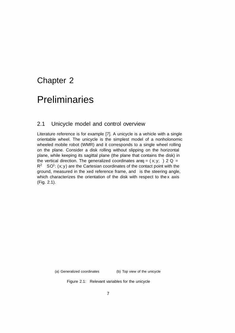
Literature reference is for example [7]. A unicycle is a vehicle with a singleorientable wheel. The unicycle is the simplest model of a nonholonomicwheeled mobile robot (WMR) and it corresponds to a single wheel rollingon the plane. Consider a disk rolling without slipping on the horizontalplane, while keeping its sagittal plane (the plane that contains the disk) inthe vertical direction. The generalized coordinates are q = (x, y, θ) ∈ Q =R2×SO1: (x, y) are the Cartesian coordinates of the contact point with theground, measured in the fixed reference frame, and θ is the steering angle,which characterizes the orientation of the disk with respect to the x axis(Fig. 2.1).
(a) Generalized coordinates (b) Top view of the unicycle
Figure 2.1: Relevant variables for the unicycle
7

8 CHAPTER 2. PRELIMINARIES
The pure rolling constraint for the disk can be expressed in the Pfaffianform as
x sin θ − y cos θ = [sin θ cos θ 0]q = 0.
This constrain is nonholonomic, because it implies no loss of accessibility inthe configuration space of the disk. Thus, the constraints on the wheel stateq = (x, y, θ) are of the type
A(q)q = 0, A(q) =
[sin θ − cos θ 0
0 0 1
]Considering the matrix
G(q) = [g1(q) g2(q)] =
cos θ 0sin θ 0
0 1
whose columns g1(q) and g2(q) are a basis of the null space of the matrixA(q), the kinematic model of the unicycle can be expressed in the followingform: xy
θ
=
cos θsin θ
0
v +
001
ω, (2.1)
where the inputs v and ω are, respectively, the driving velocity (the linearvelocity of the wheel) and the steering velocity (the angular velocity of thewheel around the vertical axis). This type of system is said to be driftless.Thus, while there are n = 3 degree of freedom of the considered system,only m = 2 inputs are assumed as available controls.
2.2 Prescribed performance overview
The prescribed performance control technique has been introduced in [14];see also [11, 12]. The goal of the prescribed performance controller is toguarantee that the error e evolves within certain a priori defined performancebounds defined by a decreasing function and an acceptable overshoot range.The performance bounds are defined by a function ρ(t), called performancefunction.
Given an acceptable overshoot range M , the performance bounds ∀t ≥ 0for each element ei, i = 1, . . . , n of the error are mathematically defined as:
−Miρi(t) < ei < ρi(t), if e0i ≥ 0,
−ρi(t) < ei < Miρi(t), if e0i ≤ 0,(2.2)
where e0i = ei(0), i = 1, . . . , n, 0 ≤ M ≤ 1, and ρ(t) is smooth, bounded,strictly positive decreasing function of time and satisfying limt→∞ ρ(t) =ρ∞ > 0. The performance function can be defined as:
ρ(t) = (ρ0 − ρ∞) exp(−lt) + ρ∞.

2.2. PRESCRIBED PERFORMANCE OVERVIEW 9
To unify the two control objectives, namely regulation and prescribedtransient and steady state behavioral bounds on the error, an error trans-formation is used. At first the error is modulated by ρ(t), and then a trans-formation function T (·) is applied.
The modulated error is defined as follows:
ei(t) ,eiρi(t)
. (2.3)
Then, the transformed error ε(t) ∈ Rn is defined through transformationfunctions Ti : Dei → R, i = 1, . . . , n:
εi(t) , Ti(ei(t)) (2.4)
where the transformations Ti(·), i = 1, . . . , n define increasing bijective map-pings of the performance domain:
Dei , {ei : ei ∈ (−Mi, 1)} if e0i ≥ 0,
Dei , {ei : ei ∈ (−1,Mi)} if e0i ≤ 0.
Differentiating (2.4) with respect to time we obtain:
εi(t) = JT i(t)[ei + αi(t)ei] (2.5)
where JT i(t) and αi(t) are respectively
JT i(t) ,∂Ti∂e(t)
1
ρi(t)> 0
αi(t) , −ρi(t)
ρi(t)> 0 with lim
t→+∞αi(t) = 0.
The transformation function is smooth and strictly increasing. Two trans-formation functions for (2.4) can be defined:
Tai [ei(t)] =
ln(Mi+ei(t)1−ei(t)
), if e0i ≥ 0
ln(
1+ei(t)Mi−ei(t)
), if e0i ≤ 0
Tbi [ei(t)] =
ln(
Mi+ei(t)Mi(1−ei(t))
), if e0i ≥ 0
ln(Mi(1+ei(t))Mi−ei(t)
), if e0i ≤ 0
(2.6)
If from the Lyapunov analysis εi is proved bounded (εi ∈ L∞), then theaforementioned transformation is bounded as well and this means that eistays within the predefined bounds.One way is to accommodate a potential of the form
1
2||ε||2. (2.7)
10 CHAPTER 2. PRELIMINARIES
Prescribed performance can also be defined through a different potentialof the form
ln(cos ei
), (2.8)
where ei is the error component to bind.While in the previous case we begin with the error transformation and thenuse a potential defined by the square of the transformed error ε, in thiscase we start from the potential. This approach is particularly convenient inthe case of bounds on an angle, for example the orientation of the unicycle.Notice that the potential (2.8) is well defined as
ei ∈(−π
2,π
2
). (2.9)
Employing this potential to define a candidate Lyapunov function V , it ispossible to design a control law such that V is negative semidefinite. Thus,one can prove that V is bounded and ln
(cos ei
)as well, hence ei stays within
the defined bounds.
The first thing to be defined is what we consider as error. Adoptingthe aforementioned transformations, the aim is to combine control objective(regulation) while guaranteeing prescribed performance bounds. In this the-sis, controllers are designed by mean of polar coordinates and time-varyinglaws, while applying prescribed performance control concept. The proof ofconvergence of the error e to zero can be achieved by appropriate Lyapunovfunctions.
Instrumental results
We briefly present here some results which will be instrumental for theconvergence proof of the proposed controllers.A first critical term to be analyzed is the ratio of the transformation of theerror component through the prescribed performance and the error itself:
ε
e
We here briefly show that this term turns out to be limited when choosingeither Ta with M = 0 or Tb for all M ∈ (0, 1).
Let’s consider first T (·) = Ta(·). If we take M = 0, then the error e,remaining bounded within prescribed performance bounds (PPB) and doesnot approach zero, not even asymptotically. Hence, we can have practicalconvergence, while avoiding the singularity. If M 6= 0 then calculating thelimit for e→ 0 (e0 ≥ 0), ε
e →∞. The same result is obtained if e0 ≤ 0.Let’s consider now T (·) = Tb(·). Applying L’Hopital’s rule, the limit for
e→ 0 (e0 ≥ 0) yields to
E ,1 +M
ρM.

2.2. PRESCRIBED PERFORMANCE OVERVIEW 11
The same result is obtained if e0 ≤ 0.
A graphical representation of this term is drawn in Figure 2.2: it depictsεe with respect to e for a fixed certain time.
−1 −0.8 −0.6 −0.4 −0.2 0 0.2 0.4 0.6 0.8 11.5
1.55
1.6
1.65
1.7
1.75
1.8
1.85
1.9
e
ε/e
Figure 2.2: The term εe is bounded and it is equal to E as e = 0. This plot is
obtained setting ρ0 = 10, ρ∞ = 0.1, L = 2, M = 0.8.
Another relevant expression is the following inequality (see [10]):
εJe ≥ µε2 (2.10)
with µ a positive constant. This relation is instrumental for convergenceproof, in particular see Appendix C.1.
Other motivation
Another motivation for introducing prescribed performance control conceptis that for nonholonomic system, as the unicycle model, it is not possibleto prove exponential convergence. That is there are no guarantees that theerror vanishes with exponential rate. This is related to the fact that thederivative of the Lyapunov function with respect to the time does not haveall the coordinates as the Lyapunov function has. This means that a relationof the type V ≤ −νV can not be obtained. Hence, V can not be expressedas
V ≤ V (0)e−νt
With prescribed performance approach, a predefined behavior can be achieved,given a maximum overshoot and a desired convergence rate. We design a con-troller that guarantees the fulfillment of prescribed performance constraintsand the convergence to the desired position (thus solving the regulationproblem), with the required rate of convergence.
12 CHAPTER 2. PRELIMINARIES
Analysis of the two approaches to impose prescribe performance
This paragraph analyzes the two different approaches that can be followedin order to impose prescribed performance. One begins with the error trans-formation and then uses a potential defined by the square of the transformederror ε, the other starts from the potential of the form (2.8).
Let us call V1 and V2 the defined potentials, and consider e, e, ε as scalarquantities: this is reasonable in view of the controllers we will design in thiswork. In the first case we have
V1 =1
2ε2 (2.11)
and in the second case
V2 = − ln cos e. (2.12)
Note that this potential corresponds to the case we apply a transformationof the form
ε = sign(e)√
ln(cos e)−2
As already mentioned, V2 is particularly convenient when binding angle co-ordinates. Furthermore, following the first approach that yields to V1 to bindangle coordinates, leads to find controllers which do not guarantee the con-vergence of all the variables according to Barbalat lemma.
The fact that the first approach does not solve the problem of regulationwhile binding an angle coordinate, whereas the second one is successful, isstrictly related to the unicycle model and its dynamics.We remark that this is a nonholonomic system, and the number of the co-ordinates is greater than the number of control inputs. In particular noticealso that the steering velocity ω appears only in γ in the case of polar coor-dinate control and only in e3 in the case of time-varying control.
Calculating the first derivative with respect to time of the potentials, inthe first case we have:
V1 =∂V1
∂εε = εε = εJ(e+ αe) = ε
∂T
∂e
1
ρ(e+ αe); (2.13)
in the second case:
V2 =∂V2
∂e˙e =
sin e
cos e˙e = tan e
1
ρ(e+ αe). (2.14)
What differentiates the two cases is related to the terms
ε∂T
∂eand tan e.

2.2. PRESCRIBED PERFORMANCE OVERVIEW 13
Also, notice that e multiplies in (2.13) and (2.14) respectively
ε and tan e.
In the first derivative of the Lyapunov function the following terms ap-pear, respectively in the first and in the second case:
ωε and ω tan e.
In order to design control laws that guarantee convergence to the desiredposture, ω is defined so as to cancel out some spurious terms deriving fromthe other coordinates or error components. This implies that the steeringvelocity depends on terms of the form
ω1 =e
εand ω2 =
e
tan e
in the first and second case respectively.
The convergence proof for the unicycle system is based on Barbalatlemma; in particular we are interested to prove that the second derivative ofthe Lyapunov function is bounded and thus in particular that V1 and V2 arebounded. We are now taking into consideration the problem of binding theorientation of the unicycle, through e = γ in the case of polar coordinatescontrol, or e = e3 in the case of time-varying control; we also recall that ωappears exactly only in the first derivative of those terms. Hence, in orderto complete the convergence proof exploiting Barbalat lemma, ω is neededto be bounded.In other words, to complete the convergence proof, ˙ω1 and ˙ω2 have to beproved bounded. Calculating these first derivatives, in the first case we have
˙ω1 =d
dt
e
ε=e
ε− e ε
ε2= e[1
ε− eJ
ε2
]− αJ
(eε
)2(2.15)
while in the second case
˙ω2 =d
dt
e
tan e=
e
tan e− e ˙e
1 + tan2 e
tan2 e= e[−e+
tan e− etan2 e
]− αee. (2.16)
In the first case, the term in the squared brackets is unbounded, and ˙ω1 aswell. In the second case, all the terms are bounded and in particular theterm tan e−e
tan2 eis bounded as long as e 6= 0 and
lime→0
tan e− etan2 e
= 0.
Hence, only ˙ω2 is proved bounded, and thus only the second approach is afeasible way to bind an angle coordinate by prescribed performance.
Details of this reasoning applied to the polar coordinates case and to thetime-varying control one, can be found in Appendix A.

14 CHAPTER 2. PRELIMINARIES
2.3 First example: Dynamic Feedback Lineariza-tion
This section introduces a first example of application of prescribed per-formance control to the DFL control technique that solves the regulationproblem of the unicycle.
The reader is referred to [9] for a more detailed treatise of DFL technique.The unicycle system can always be transformed via feedback into simpleintegrators (input- output linearization and decoupling). The choice of thelinearizing outputs is not unique.
Notice that in the case of linear systems, it is possible to prove expo-nential convergence. Thus, in this case prescribed performance control doesnot improve the performance of the obtained controller, unless the systemis affected by disturbances.
Define the linearizing output vector as η = (x, y) and introduce an inte-grator (whose state is denoted by ξ) on the linear velocity input
v = ξ, ξ = a
being a the linear acceleration, considered as new input.Provided that ξ 6= 0, the unicycle can be expressed as a linear system.In the new coordinates it is
z1 = x
z2 = y
z3 = x
z4 = y
⇒
{z1 = u1
z2 = u2
and a PD controller on the Cartesian error
u1 = −kp1x− kd1x
u2 = −kp2y − kd2y(2.17)
can yield exponential convergence, while kp1, kp2, kd1, kd2 are positive con-stants.
So as to have a more compact notation, define
e =
[e1
e2
]=
[xy
]Kp =
[kp1 00 kp2
]Kv =
[kd1 00 kd2
]ε =
[ε1
ε2
]Kε =
[kε1 00 kε2
]JT =
[JT1 00 JT2
] (2.18)
where Kp,Kv,Kε, JT are positive definite matrices. Thus,
z =
[z1
z2
]=
[xy
]= e = u.

2.3. FIRST EXAMPLE: DYNAMIC FEEDBACK LINEARIZATION 15
In order to introduce Prescribed performance, define the control law as
u = −Kv
(e+ α(t)e
)−KεJT ε− α(t)e− α(t)e (2.19)
and consider the Lyapunov function
V =1
2
∣∣∣∣e+ α(t)e∣∣∣∣2 +
1
2εTKεε. (2.20)
Differentiating (2.20) with respect to time, substituting the control law(2.19) and operating some cancellations we have
dV
dt= −eTKv e− eTα(t)TKvα(t)e ≤ 0. (2.21)
Exploiting Barbalat Lemma, it is possible to prove asymptotic convergenceof (e, e, ε) to zero. Details can be found in Appendix B.Figure 2.3.a shows the convergence of e, that is of x and y, to zero, whileFigure 2.3.b-2.3.c display x and y together with their bounds, pointing outthat the prescribed performance limits are fulfilled.
0 1 2 3 4 5 6−1
−0.8
−0.6
−0.4
−0.2
0
0.2
0.4
[time]
[m]
x
y
(a) Convergence of x and y with DFLcontrol law.
0 1 2 3 4 5 6−2
−1.5
−1
−0.5
0
0.5
1
1.5
2
[time]
[m]
x
Mρ(t)
ρ(t)
(b) x stays within prescribed bounds.
0 1 2 3 4 5 6−2
−1.5
−1
−0.5
0
0.5
1
1.5
2
[time]
[m]
y
Mρ(t)
−ρ(t)
(c) y stays within prescribed bounds.
Figure 2.3: Results of Matlab simulation of the designed controller.
16 CHAPTER 2. PRELIMINARIES
Chapter 3
Control with PolarCoordinates
3.1 Control with polar coordinates
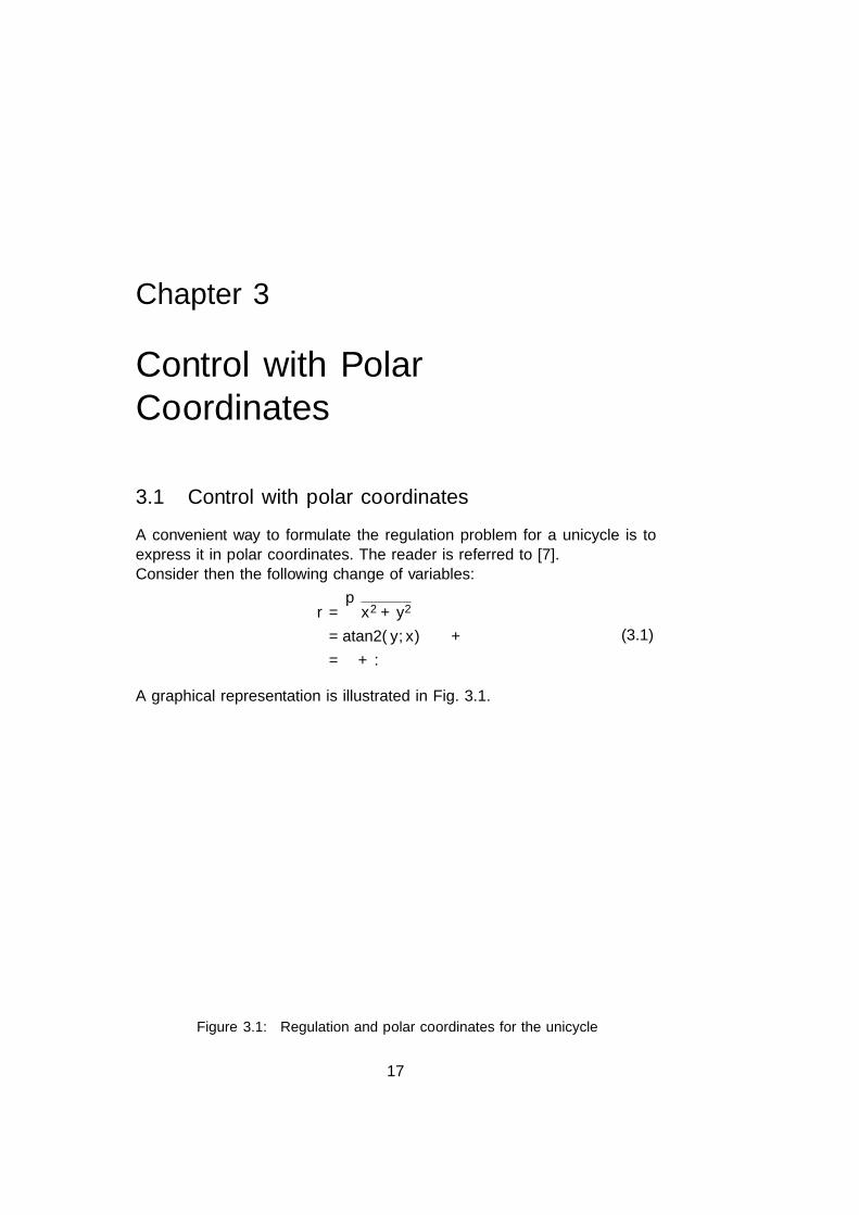
A convenient way to formulate the regulation problem for a unicycle is toexpress it in polar coordinates. The reader is referred to [7].Consider then the following change of variables:
r =√x2 + y2
γ = atan2(y, x)− θ + π
δ = γ + θ.
(3.1)
A graphical representation is illustrated in Fig. 3.1.
Figure 3.1: Regulation and polar coordinates for the unicycle
17

18 CHAPTER 3. CONTROL WITH POLAR COORDINATES
The first coordinate, r, represents the distance of the unicycle from theorigin of the fixed world Cartesian frame, or in other words the measure ofthe pointing vector individuated from the hub of the vehicle and the origin ofthe Cartesian reference; the second one, γ, is the angle between the forwarddirection vector of the unicycle and the pointing vector; the third coordinate,δ, is the angle between the x-axis and the pointing vector.In these coordinates, the kinematic model is expressed as:
r = −v cos γ
γ =sin γ
rv − ω
δ =sin γ
rv,
(3.2)
and the control law can be defined as
v = k1r cos γ
ω = k2γ + k1sin γ cos γ
γ(γ + k3δ),
(3.3)
where k1 > 0, k2 > 0, k3 > 0. The control inputs are bounded and welldefined for all the values of γ.
Notice that there is a singularity for r = 0. Specifically, the coordinatesγ and δ are not defined for x = y = 0. Also, the control law, once mappedback to the original coordinates, is discontinuous at the origin of the config-uration space, and the behavior of the controlled system is not continuouswith respect to the initial state.
The Lyapunov function V = 12(r2 + γ2 + k3δ
2) allows to conclude thatthe kinematic model (3.2) under the action of the given control law asymp-totically converges to the desired configuration (r, γ, δ)T = (0, 0, 0)T . In fact,differentiating V with respect to the time and considering the closed-loopsystem with control inputs (3.3), the obtained V is non-increasing:
V = −k1r2 cos2 γ − k2γ
2 ≤ 0.
Observing the form of V , notice that γ is guaranteed to be bounded andconvergent to zero. Thus the cosine multiplying r2 converges to one, hencealso r is guaranteed to converge to zero.More analytically, being V ≤ 0, the state is bounded in norm, V (t) is uni-formly continuous, and V (t) tends to a limit value. Exploiting Barbalatlemma, it is possible to conclude that V (t) tends to zero and thus also r andγ do. Also, analyzing the closed-loop system, r and δ converge to zero, δconverges to some finite limit δ while γ tends to the finite limit −k1k3δ andis uniformly continuous. This finite limit must be zero according to BarbalatLemma and thus also δ converges to zero.
3.1. CONTROL WITH POLAR COORDINATES 19
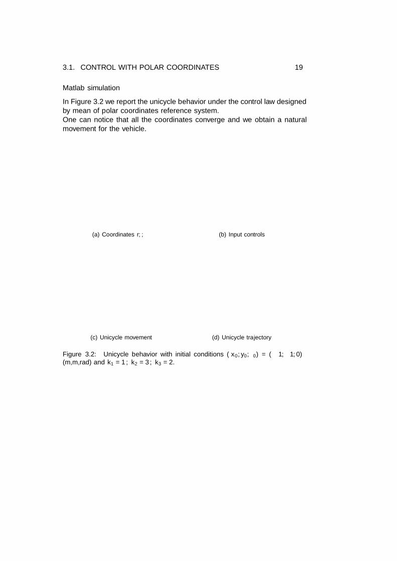
Matlab simulation
In Figure 3.2 we report the unicycle behavior under the control law designedby mean of polar coordinates reference system.One can notice that all the coordinates converge and we obtain a naturalmovement for the vehicle.
0 2 4 6 8 10 12 14 16 18 20−0.5
0
0.5
1
1.5
[time]
[m]
r
γ
δ
(a) Coordinates r, θ, δ
0 2 4 6 8 10 12 14 16 18 20−0.5
0
0.5
1
1.5
2
2.5
3
3.5
4
[time]
v
ω
(b) Input controls
−1 −0.8 −0.6 −0.4 −0.2 0 0.2−1.2
−1
−0.8
−0.6
−0.4
−0.2
0
0.2
(c) Unicycle movement
−1.4 −1.2 −1 −0.8 −0.6 −0.4 −0.2 0 0.2
−1.2
−1
−0.8
−0.6
−0.4
−0.2
0
0.2
0.4
[m]
[m]
(d) Unicycle trajectory
Figure 3.2: Unicycle behavior with initial conditions (x0, y0, θ0) = (−1,−1, 0)(m,m,rad) and k1 = 1, k2 = 3, k3 = 2.

20 CHAPTER 3. CONTROL WITH POLAR COORDINATES
3.2 Prescribed performance on the distance vector
In this section, we define a control law for the posture regulation of the uni-cycle, utilizing polar coordinates while guaranteeing prescribed performancefor the convergence of the first coordinate.
We define the error as e = r and its transformation ε(e) = T (e). Considerthe Lyapunov function
V =1
2(ε2 + γ2 + k3δ
2). (3.4)
Define the control law
v = k1ε cos γ + k3α(t)e cos γ
ω = k2γ +(k1ε
e+ k3α(t)
)sin γ cos γ
γ(γ + k3δ) + k3εJα(t)e
sin2 γ
γ.
(3.5)
Then the first derivative of the Lyapunov function wrt time is:
V = −k1ε2JT cos2 γ − k2γ
2 − εJα(t)e(k3 − 1). (3.6)
Exploiting the relation εJe ≥ µε2 with µ > 0, and provided that k3 ≥ 1,it is possible to conclude that V is non-increasing. Details can be found inAppendix C.1.
Proposition 3.1 Consider the polar coordinate description (3.2) of the uni-cycle and the feedback control (3.5) with k1, k2, k3 positive constants andk3 ≥ 1. The closed-loop system (3.2)-(3.5) is then globally asymptoticallydriven to the posture (r, γ, δ) = (0, 0, 0). Also, the polar coordinate r respectsthe prescribed limits.
Proof. The proof can be found in Appendix C.1.
MatLab simulations
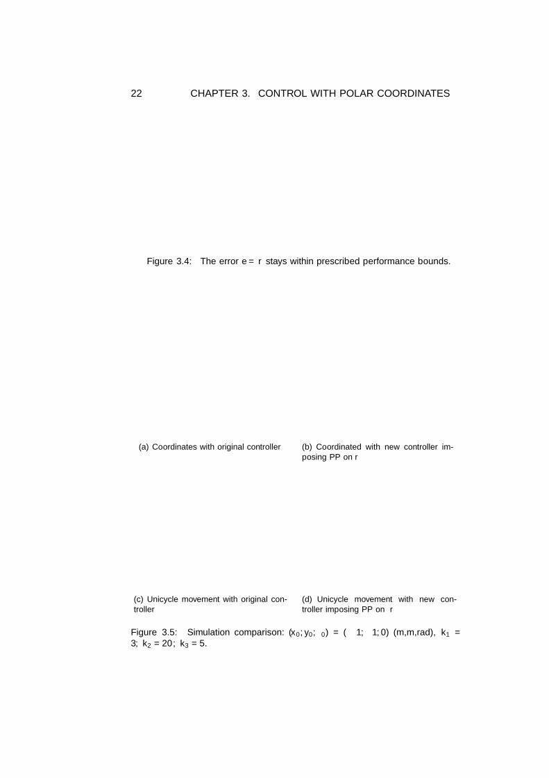
Simulations confirm the analysis developed in the previous paragraph. InFig. 3.3 is reported the unicycle behavior with initial conditions (x0, y0, θ0) =(−1,−1, 0)(m,m,rad).From Figure 3.3.a one can notice that all the polar coordinates converge tothe desired values, and the convergence is faster than in the previous case.The input signals vanish in short time as well, although higher values arerequired for the initial steering velocity. However, this fact is related to thecontrol coefficients k1, k2, k3: setting these coefficients equal to those usedfor the original controller simulation, the resulting behavior is less regular,but still faster than the original one. In other words, on equal terms, the

3.2. PRESCRIBED PERFORMANCE ON THE DISTANCE VECTOR21
achieved performance of the modified control law is faster than the originalone. Refer to Figure 3.5 for simulation comparison. In Figure 3.3.d a viewof the vehicle trajectory is depicted.
0 0.2 0.4 0.6 0.8 1 1.2 1.4 1.6 1.8 2−0.4
−0.2
0
0.2
0.4
0.6
0.8
1
1.2
1.4
1.6
[time]
[m]
r
γ
δ
(a) Coordinates r, γ, δ
0 0.2 0.4 0.6 0.8 1 1.2 1.4 1.6 1.8 2−10
0
10
20
30
40
50
60
70
[time]
v
ω
(b) Input controls
−1 −0.8 −0.6 −0.4 −0.2 0 0.2−1.2
−1
−0.8
−0.6
−0.4
−0.2
0
0.2
(c) Unicycle movement
−1.4 −1.2 −1 −0.8 −0.6 −0.4 −0.2 0 0.2 0.4
−1.2
−1
−0.8
−0.6
−0.4
−0.2
0
0.2
0.4
[m]
[m]
(d) Unicycle trajectory
Figure 3.3: Unicycle behavior with initial conditions (x0, y0, θ0) = (−1,−1, 0)(m,m,rad) and k1 = 0.02, k2 = 20, k3 = 2. PP bounds are imposed on r
Figure 3.4 shows that with the designed control law the first coordinater evolves within the prescribed performance predefined bounds, modulatedby the function ρ(t).
22 CHAPTER 3. CONTROL WITH POLAR COORDINATES
0 0.2 0.4 0.6 0.8 1 1.2 1.4 1.6 1.8 2−0.5
0
0.5
1
1.5
2
2.5
3
[time]
r
ρ(t)
−Mρ(t)
Figure 3.4: The error e = r stays within prescribed performance bounds.
0 0.5 1 1.5 2 2.5 3 3.5 4 4.5 5−0.5
0
0.5
1
1.5
[time]
[m]
r
γ
δ
(a) Coordinates with original controller
0 0.1 0.2 0.3 0.4 0.5 0.6 0.7 0.8 0.9 1−1
−0.5
0
0.5
1
1.5
[time]
[m]
r
γ
δ
(b) Coordinated with new controller im-posing PP on r
−1 −0.8 −0.6 −0.4 −0.2 0 0.2−1.2
−1
−0.8
−0.6
−0.4
−0.2
0
0.2
(c) Unicycle movement with original con-troller
−1 −0.8 −0.6 −0.4 −0.2 0 0.2−1.2
−1
−0.8
−0.6
−0.4
−0.2
0
0.2
(d) Unicycle movement with new con-troller imposing PP on r
Figure 3.5: Simulation comparison: (x0, y0, θ0) = (−1,−1, 0) (m,m,rad), k1 =3, k2 = 20, k3 = 5.

3.3. BOUNDS ON THE ORIENTATION 23
3.3 Bounds on the orientation
This section explores the problem of putting prescribed performance boundson the angles γ and/or δ.First of all, we notice that while putting (PP) bounds on r is a reasonableand intuitive way to proceed, imposing bounds on the angles needs somemore comments. We will first discuss about the angle γ and then we willbriefly comment the case with δ.
3.3.1 Bounds on γ or δ
We recall that γ is the angle that the robot’s frame makes with the envi-ronment (fixed) frame, i.e. the angle between the vehicle direction and thepointing vector that connects the unicycle position to the origin of the fixedframe.
From a physical point of view, imposing bounds on γ for example inorder to keep it in
(−π
2 ,π2
)implies also that the vehicle has constraints in
its motion. In particular, if γ is constrained to stay in(−π
2 ,π2
), the vehicle
must depart from the 2nd or 3rd quadrant, so that the motion can satisfythe constraints on γ while exploiting a linear velocity which makes it goforward. Also, we have to take care of δ in order to make it converge to zeroas well.
From a mathematical point of view, trying to apply the prescribed per-formance transformation T to the angle coordinates and carrying on ananalysis similar to that presented in the previous sections, yields to an un-bounded second derivative of γ (or δ). This fact does not allow to concludefor γ to be uniformly continuous, thus to prove the convergence (exploitingBarbalat Lemma) of γ to zero, and eventually the convergence of δ to zero.This analysis is given in Appendix C.2.
Similarly to what said for γ, bounds on δ do not find a trivial physicalmotivation, and the effect is to limit the movement of the vehicle.Analytical details can be found in Appendix C.2.
3.3.2 Overview of a practical possible solution
A reasonable approach to bind angle coordinates implies that we considersome precise configuration and we have an a priori knowledge of the initialconfiguration.Consider for example the following bounds:
γ ∈(−π
2,π
2
)γ ∈
(−π
2,π
2
)δ ∈
(−π
2,π
2
)

24 CHAPTER 3. CONTROL WITH POLAR COORDINATES
where γ , γ − π. We can split this constrains as follows:
A′, A′′ : γ, γ ∈(−π
2, 0)∪ B′, B′′ : γ, γ ∈
(0,π
2
)C : δ ∈
(−π
2, 0)∪ D : δ ∈
(0,π
2
) (3.7)
and design a driving velocity input that can either drive the vehicle forward(vF ) or backward (vB).Notice that C means that the vehicle is in the 2nd or 4th quadrant, while Dmeans that the vehicle is in the 1st or 3rd.
Thus, we have 16 possible feasible combinations:− C,A’,vF : 2rd quadrant, forward motion;− C,A’,vB: 4th quadrant, backward motion;− C,A”,vB: 2rd quadrant, backward motion;− C,A”,vF : 4th quadrant, forward motion;− C,B’,vF : 2rd quadrant, forward motion;− C,B’,vB: 4th quadrant, backward motion;− C,B”,vB: 2rd quadrant, backward motion;− C,B”,vF : 4th quadrant, forward motion;− D,A’,vF : 3rd quadrant, forward motion;− D,A’,vB: 1st quadrant, backward motion;− D,A”,vB: 3rd quadrant, backward motion;− D,A”,vF : 1st quadrant, forward motion;− D,B’,vF : 3rd quadrant, forward motion;− D,B’,vB: 1st quadrant, backward motion;− D,B”,vB: 3rd quadrant, backward motion;− D,B”,vF : 1st quadrant, forward motion;
Notice also that not all of this configurations allow to have a final orien-tation θ = 0: e.g. case (D,B”,vB) where the final vehicle orientation will beθ = π.
We remark that prescribed performance bounds on the angle variable(only on γ, only on δ or on both) set by mean of the transformation T (e),lead either to find controllers which do not guarantee the convergence of allthe variables, or to have positive terms in the first derivative of the Lyapunovfunction.
3.3.3 Bounds on the angle γ through a different Lyapunovfunction
As already mentioned in the Preliminaries section, another way to imposeprescribed performance is to use a different Lyapunov function of the form(2.8). This approach is particularly convenient when dealing with angle co-ordinates.We now set bounds on γ, and hence indirectly on the orientation of the

3.3. BOUNDS ON THE ORIENTATION 25
unicycle, following this different approach.First we take the candidate Lyapunov function defined as
V =1
2r2 − ln cos γ +
k3
2δ2. (3.8)
This function is positive definite for a specified range of value of γ, namelyγ ∈ (−π/2, π/2). This means that if the vehicle departs from a position withγ ∈ (−π/2, π/2), then this angle coordinate will evolve within the predefinedset of value, and it will never leave it.Define the control input as
v = k1r cos γ
ω = k2 tan γ + k1
(k3δ + tan γ
)cos2 γ
(3.9)
Then the first derivative of (3.8) is negative semidefinite:
V = −k1r2 cos2 γ − k2 tan2 γ ≤ 0. (3.10)
Proposition 3.2 Consider the polar coordinate description (3.2) of the uni-cycle and the feedback control (3.9) with k1, k2, k3 positive constants. Theclosed-loop system (3.2)-(3.9) is then globally asymptotically driven to theposture (r, γ, δ) = (0, 0, 0). Also, the polar coordinate γ respects the pre-scribed limits.
Note that being γ ∈ (−π/2, π/2), the cosine in V is never zero.The proof for the coordinates convergence can be carried on adopting LaSalletheorem and Barbalat lemma, as for the previous designed controllers. Thecontrol law (3.9) designed with the particular Lyapunov function defined by(3.8) guarantees that the angle coordinate γ stays within the predefined set(−π/2, π/2), as γ0 is chosen in this range of values.Details and a sketch of the proof of Proposition 3.2 can be found in AppendixC.3.
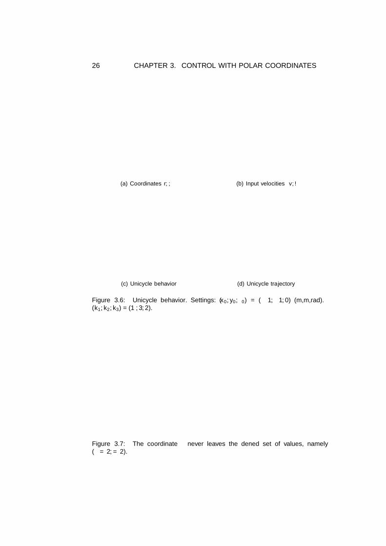
Matlab simulation
Matlab simulations are reported in Figures 3.6-3.7. Note that all the coor-dinates converge to the desired position and the vehicle performs a natu-ral maneuver. Also the input controllers vanish in short time and remainbounded. Moreover, the coordinate γ never leaves the defined set of values,namely (−π/2, π/2).
26 CHAPTER 3. CONTROL WITH POLAR COORDINATES
0 5 10 15−0.4
−0.2
0
0.2
0.4
0.6
0.8
1
1.2
1.4
1.6
[time]
[m]
r
γ
δ
(a) Coordinates r, γ, δ
0 5 10 15−0.5
0
0.5
1
1.5
2
2.5
3
3.5
4
4.5
[time]
v
ω
(b) Input velocities v, ω
−1 −0.8 −0.6 −0.4 −0.2 0 0.2−1.2
−1
−0.8
−0.6
−0.4
−0.2
0
0.2
(c) Unicycle behavior
−1.4 −1.2 −1 −0.8 −0.6 −0.4 −0.2 0 0.2
−1.2
−1
−0.8
−0.6
−0.4
−0.2
0
0.2
[m]
[m]
(d) Unicycle trajectory
Figure 3.6: Unicycle behavior. Settings: (x0, y0, θ0) = (−1,−1, 0) (m,m,rad).(k1, k2, k3) = (1, 3, 2).
0 5 10 15−2
−1.5
−1
−0.5
0
0.5
1
1.5
2
[time]
[m]
γ ∈ (−π/2,π/2)
Figure 3.7: The coordinate γ never leaves the defined set of values, namely(−π/2, π/2).

3.3. BOUNDS ON THE ORIENTATION 27
Time-varying bounds on γ
In order to achieve faster convergence, we define time-varying bounds onthe orientation. We now introduce a time-varying positive transformationfunction, namely ρ(t), such that
γ 7→ γ =γ
ρ(t).
The modulating function is defined, in the same way as in the prescribedperformance analysis, as a smooth, bounded, strictly positive decreasingfunction of time and satisfying limt→∞ ρ(t) = ρ∞ > 0:
ρ(t) = (ρ0 − ρ∞) exp(−Lt) + ρ∞. (3.11)
To unify the convergence and the time-varying bounds we consider a Lya-punov function, defined as in the previous paragraph but depending on γinstead of γ:
V =1
2r2 − ln cos γ +
k3
2δ2, with γ ∈
(−π
2ρ(t),
π
2ρ(t)
)(3.12)
This function is positive definite in the defined set of values that depends ontime. This fact permits to define more strict bounds, that evolve togetherwith the coordinate γ.Define the control velocity input as
v = k1r cos γ
ω = k2 tan γ + γα(t) + k1ρ(t)(k3δ +
1
ρ(t)tan γ
)cos γ cos γ
sin γ
sin γ
(3.13)
Then the first derivative of (3.12) wrt to time is negative semidefinite:
V = −k1r2 cos2 γ − k2
ρ(t)tan2 γ ≤ 0. (3.14)
The control inputs are bounded and well defined. Details can be found inAppendix C.4.The proof for the convergence of the coordinates can be carried on exploitingLaSalle theorem and Barbalat Lemma. Proving that V is bounded allowsalso to conclude that ln cos γ is bounded and hence γ respects the predefinedlimits.

28 CHAPTER 3. CONTROL WITH POLAR COORDINATES
Matlab simulation
Matlab simulations are reported in Figures 3.8-3.9.One can notice (from Fig. 3.8.a) that the convergence of the γ coordinateevolves faster than in the previous case, although its maximum oscillatingamplitude is bigger. We also notice that the convergence of δ is slower in thiscase, and the control requires higher initial values for the steering velocityinput. These facts are related to the modulating function, which affects alsothe evolution of ω. Moreover, since γ is vanishing faster, the coordinate δconverges later to zero in order to achieve the desired orientation θd = 0.The performances are also affected by the parameters. Tuning the constantparameters k1, k2, k3 and especially modifying the requirements for the time-varying bounds, that is replacing ρ0, ρ∞, L with other values, one can achievedifferent behaviors of the unicycle.
0 1 2 3 4 5 6 7 8 9 10−1
−0.5
0
0.5
1
1.5
[time]
[m]
r
γ
δ
(a) Coordinates r, γ, δ
0 1 2 3 4 5 6 7 8 9 10−2
0
2
4
6
8
10
12
[time]
v
ω
(b) Input velocities v, ω
−1 −0.8 −0.6 −0.4 −0.2 0 0.2−1.2
−1
−0.8
−0.6
−0.4
−0.2
0
0.2
(c) Unicycle behavior
−1.4 −1.2 −1 −0.8 −0.6 −0.4 −0.2 0 0.2
−1.2
−1
−0.8
−0.6
−0.4
−0.2
0
0.2
0.4
[m]
[m]
(d) Unicycle trajectory
Figure 3.8: Unicycle behavior. Settings: (x0, y0, θ0) = (−1,−1, 0) (m,m,rad).(k1, k2, k3) = (1, 0.05, 7), ρ0 = π/2, ρ∞ = 0.1, L = 2.

3.4. BOUNDS ON BOTH RADIAL AND ANGLE COORDINATE 29
Figure 3.9 shows the bounded coordinate behavior. Picture 3.9.a plotsthe evolution of − ln cos γ in the time: we are confirmed that this part ofLyapunov function converges to zero and also has a fast dynamics, so thatthe bounded coordinate can quickly reach convergence. Picture 3.9.b showsγ evolution in the time together with the bounds defined by the modulatingfunction ρ(t), pointing out that this bounds are fully satisfied.
0 1 2 3 4 5 6 7 8 9 100
0.02
0.04
0.06
0.08
0.1
0.12
0.14
0.16
[time]
−ln(cos(γ / ρ (t)))−TVbounds
(a) γ by the logarithmic function − ln cos γ
0 0.5 1 1.5 2 2.5−2
−1.5
−1
−0.5
0
0.5
1
1.5
2
[time]
γ
ρ(t)
−ρ(t)
(b) γ stays in the bounds designed by themodulating function ρ(t)
Figure 3.9: Bounds. Settings: (x0, y0, θ0) = (−1,−1, 0) (m,m,rad). (k1, k2, k3) =(1, 0.05, 7), ρ0 = π/2, ρ∞ = 0.1, L = 2.
3.4 Bounds on both radial and angle coordinate
In this paragraph we combine the control laws defined in the previous sec-tions. The first control law (defined by the equations in (3.5)) allows to setprescribed performance bounds on r while the second one (defined by theequations in (3.13)) permits to bind the angle γ and hence, indirectly, theorientation of the unicycle (θ = δ − γ).
The subscript r will be used for the terms referring to the first polar co-ordinate transformed by mean of prescribed performance bounds, and thesubscript γ for the terms referring to the homonym angle coordinate, trans-formed as shown in the previous section.Let’s consider the transformation for the first coordinate
r 7→ ε(e) = T (e), e =r
ρr(t), ρr(t) = (ρ0r − ρ∞r) exp(−Lrt) + ρ∞r
defined by prescribed performance through the modulating function ρr(t),and the transformation for the second coordinate
γ 7→ γ =γ
ργ(t), ργ(t) = (ρ0γ − ρ∞γ ) exp(−Lγt) + ρ∞γ

30 CHAPTER 3. CONTROL WITH POLAR COORDINATES
with the modulating function ργ(t).
We define the candidate Lyapunov function, inspired both by (3.4) and(3.12), as
V =1
2ε2 − ln cos γ +
k3
2δ2. (3.15)
This function is positive definite in a set of value that depends on time:
γ ∈(−π
2ργ(t),
π
2ργ(t)
)We design the control law as
v = k1 cos γεrJr + k3αrr cos γ;
ω = k2 tan γ + αγγ + ργ
(k3δ +
tan γ
ργ
)(k1Jr
εrr
+ αr
)cos γ cos γ
sin γ
sin γ(3.16)
Differentiating V wrt to time and substituting the defined controllers weobtain
V = −k1ε2J2r cos2 γ − k2
ργtan2 γ ≤ 0 (3.17)
where the time dependence of ργ from the time is implied, that is ργ = ργ(t).
The control inputs (3.16) are well defined and bounded, as shown inAppendix C.4.
The control law (3.16), designed with the particular Lyapunov functiondefined by (3.15) by means also of the prescribed performance transformationfor the first polar coordinate r and the time-varying transformation throughργ(t) of the first angle coordinate, guarantees the convergence to the desiredposition and orientation while satisfying the predefined bounds. Specifically,proving that V is bounded, it is possible to conclude that ε (as well as thetransformation T (e) ) and ln cos γ are also bounded. Hence, r and γ respectthe predefined limits.
Proposition 3.3 Consider the polar coordinate description (3.2) of the uni-cycle and the feedback control (3.16) with k1, k2, k3 positive constants. Theclosed-loop system (3.2)-(3.16) is then globally asymptotically driven to theposture (r, γ, δ) = (0, 0, 0). Also, the polar coordinates r and γ respect theprescribed limits.
Details and proof of convergence for Proposition 3.3 can be found inAppendix C.5.
3.4. BOUNDS ON BOTH RADIAL AND ANGLE COORDINATE 31
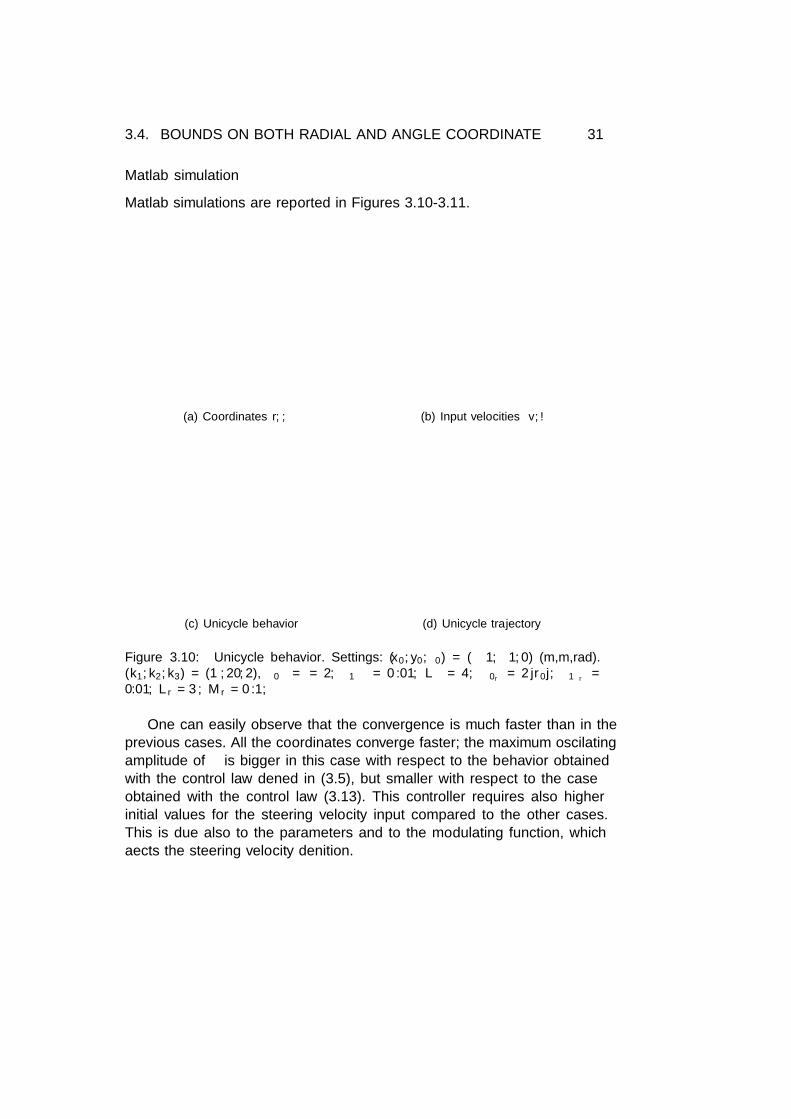
Matlab simulation
Matlab simulations are reported in Figures 3.10-3.11.
0 0.1 0.2 0.3 0.4 0.5 0.6 0.7 0.8 0.9 1−0.4
−0.2
0
0.2
0.4
0.6
0.8
1
1.2
1.4
1.6
[time]
[m]
r
γ
δ
(a) Coordinates r, γ, δ
0 0.1 0.2 0.3 0.4 0.5 0.6 0.7 0.8 0.9 1−10
0
10
20
30
40
50
[time]
v
ω
(b) Input velocities v, ω
−1 −0.8 −0.6 −0.4 −0.2 0 0.2−1.2
−1
−0.8
−0.6
−0.4
−0.2
0
0.2
(c) Unicycle behavior
−1.4 −1.2 −1 −0.8 −0.6 −0.4 −0.2 0 0.2 0.4
−1.2
−1
−0.8
−0.6
−0.4
−0.2
0
0.2
0.4
[m]
[m]
(d) Unicycle trajectory
Figure 3.10: Unicycle behavior. Settings: (x0, y0, θ0) = (−1,−1, 0) (m,m,rad).(k1, k2, k3) = (1, 20, 2), ρ0γ = π/2, ρ∞γ
= 0.01, Lγ = 4; ρ0r = 2|r0|, ρ∞r=
0.01, Lr = 3, Mr = 0.1;
One can easily observe that the convergence is much faster than in theprevious cases. All the coordinates converge faster; the maximum oscilatingamplitude of γ is bigger in this case with respect to the behavior obtainedwith the control law defined in (3.5), but smaller with respect to the caseobtained with the control law (3.13). This controller requires also higherinitial values for the steering velocity input compared to the other cases.This is due also to the parameters and to the modulating function, whichaffects the steering velocity definition.

32 CHAPTER 3. CONTROL WITH POLAR COORDINATES
Figure 3.11 shows the bounded coordinate behavior. Picture 3.11.a plotthe evolution of − ln cos γ in the time: we are confirmed that this part ofLyapunov function converges to zero and also has a fast dynamics, so thatthe bounded coordinate can quickly reach convergence. Pictures 3.11.b,3.11.cshow γ and r evolution respectively, together with the bounds defined bythe modulating functions ργ(t) and ρr(t), pointing out that these boundsare fully satisfied.
0 0.1 0.2 0.3 0.4 0.5 0.6 0.7 0.8 0.9 10
0.02
0.04
0.06
0.08
0.1
0.12
0.14
[time]
−lo
g(c
os(g
am
ma/r
ho(t
)))
−ln(cos(γ/ρ(t)))−TVbounds
(a) γ by the logarithmic function − ln cos γ
0 0.05 0.1 0.15 0.2 0.25−2
−1.5
−1
−0.5
0
0.5
1
1.5
2
[time]
[m]
γ
ρ(t)
−ρ(t)
(b) γ stays in the bounds designed by themodulating function ργ(t)
0 0.1 0.2 0.3 0.4 0.5 0.6 0.7 0.8 0.9 1−0.5
0
0.5
1
1.5
2
2.5
3
[time]
[m]
r
ρ(t)
−Mρ(t)
(c) r stays in the bounds designed by themodulating function ρr(t)
Figure 3.11: Bounds. Settings: (x0, y0, θ0) = (−1,−1, 0) (m,m,rad). (k1, k2, k3) =(1, 20, 2), ρ0γ = π/2, ρ∞γ
= 0.01, Lγ = 4; ρ0r = 2|r0|, ρ∞r= 0.01, Lr = 3, Mr =
0.1;

3.4. BOUNDS ON BOTH RADIAL AND ANGLE COORDINATE 33
In Figure 3.12 it is possible to compare the inputs needed to drive thevehicle to the desired posture, on equal convergence rate. Notice that theinitial velocities are greater in the case that the original controller is used.Also, applying the control law designed in order to guarantee prescribedperformance on both position and orientation, the obtained inputs and co-ordinates evolutions are smoother and better distributed over the time.
0 0.2 0.4 0.6 0.8 1 1.2 1.4 1.6 1.8 2−1
−0.5
0
0.5
1
1.5
[time]
[m]
r
γ
δ
0 0.2 0.4 0.6 0.8 1 1.2 1.4 1.6 1.8 2−10
0
10
20
30
40
[time]
v
ω
(a) Original control law
0 0.2 0.4 0.6 0.8 1 1.2 1.4 1.6 1.8 2−0.5
0
0.5
1
1.5
[time]
[m]
r
γ
δ
0 0.2 0.4 0.6 0.8 1 1.2 1.4 1.6 1.8 2−10
0
10
20
30
40
[time]
v
ω
(b) Control law guaranteeing PP bounds on r and γ
Figure 3.12: Inputs comparison, on equal convergence rate.

34 CHAPTER 3. CONTROL WITH POLAR COORDINATES

Chapter 4
Time-varying Control
4.1 Time-varying control
A feasible solution for posture stabilization for nonholonomic WMRs is basedon time-varying feedback. Refer to [7].The posture stabilization problem can be obtained using a fictitious time-varying reference asymptotically vanishing at the origin. Asymptotic stabi-lization of a state tracking error can be achieved provided that the nominalfeedforward commands vd(t) and ωd(t) do not both vanish in finite time. Thistwo desired inputs introduce a time-varying signal in the feedback controllaw:
v = vd cos e3 − u1
ω = ωd − u2,(4.1)
whereu1 = −k1(vd(t), ωd(t))e1
u2 = −k2vd(t)sin e3
e3e2 − k3(vd(t), ωd(t))e3,
(4.2)
with constant k2 > 0 and positive continuous gain functions k1(·, ·), k3(·, ·),and e defined as
e =
e1
e2
e3
=
cos θ sin θ 0− sin θ cos θ 0
0 0 1
xd − xyd − yθd − θ
.The error dynamics can be expressed as
e1 = vd cos e3 − v + e2ω
e2 = vd sin e3 + e1ω
e3 = ωd − ω(4.3)
and its derivation is reported extensively in Appendix D.1.
35

36 CHAPTER 4. TIME-VARYING CONTROL
In order to achieve posture stabilization, we set ∀t yd(t) = 0 and θd(t) = 0(and thus ωd(t) = 0), while vd is defined by
vd(t) = xd(t) = −k4xd(t) + g(e, t), (4.4)
being g(e, t) the heating function. This is a C2-function uniformly boundedwith respect to t, together with its partial derivative. For further detailssee [7]. The heating function g(e, t) plays a key role in guaranteeing asymp-totic stability. It sustains motion as long as the error is not zero and alsodetermines the transient behavior. Possible choices for its definition are:
• g(e, t) = ‖e‖2 sin t
• g(e, t) = exp(k5e2)−1exp(k5e2)+1 sin t, k5 > 0, if k1(·, ·), k3(·, ·) are strictly posi-
tive.
Merging the previous equations, the resulting control law can also be rewrit-ten as
v = vd cos(θd − θ) + k1(vd, ωd) [cos θ(xd − x) + sin θ(yd − y)]
ω = ωd + k2vdsin(θd − θ)θd − θ
[cos θ(xd − x)− sin θ(yd − y)] + k3(vd, ωd)(θd − θ)(4.5)
The proof for the stabilization related to this controller is based on the useof the Lyapunov function
V =k2
2
(e2
1 + e22
)+e2
3
2, (4.6)
whose time derivative along the solutions of the closed-loop system is non-increasing since
V = −k1k2e21 − k3e
23 ≤ 0. (4.7)
For more details the reader is referred to [7].
We test the time-varying control (4.1), with desired motion given by eq.(4.4), initialized at xd(0) = 0, and heating function
g(e, t) =exp(k5e2)− 1
exp(k5e2) + 1sin t.
Matlab simulation is depicted in Fig. 4.1. The gains has been set as k1 =0.5, k2 = 2, k3 = 1, k4 = 1, k5 = 50 and the initial conditions as q(0) =(−1,−1, 0) (m,m,rad).
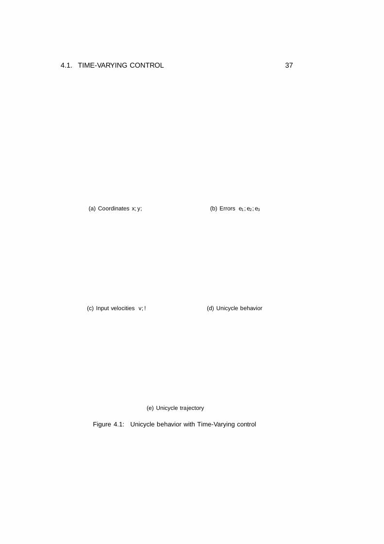
4.1. TIME-VARYING CONTROL 37
0 5 10 15 20 25 30 35 40 45 50−1
−0.8
−0.6
−0.4
−0.2
0
0.2
0.4
0.6
0.8
[time]
[m]
x
y
θ
(a) Coordinates x, y, θ
0 5 10 15 20 25 30 35 40 45 50−0.5
0
0.5
1
[time]
[m]
e1
e2
e3
(b) Errors e1, e2, e3
0 5 10 15 20 25 30 35 40 45 50−0.8
−0.6
−0.4
−0.2
0
0.2
0.4
0.6
0.8
1
[time]
v
ω
(c) Input velocities v, ω
−1 −0.8 −0.6 −0.4 −0.2 0 0.2 0.4 0.6 0.8 1−1.2
−1
−0.8
−0.6
−0.4
−0.2
0
0.2
(d) Unicycle behavior
−1 −0.5 0 0.5 1
−1.2
−1
−0.8
−0.6
−0.4
−0.2
0
0.2
[m]
[m]
(e) Unicycle trajectory
Figure 4.1: Unicycle behavior with Time-Varying control
38 CHAPTER 4. TIME-VARYING CONTROL
4.2 Time-varying control without heating function
The behavior of the unicycle driven by the time-varying control is intrinsi-cally oscillating. This is strictly related to the action of the heating function,which in fact is a modulated sine function.In order to have different performances, one can change the definition ofthe desired driving velocity vd = xd, that is to use a different dynamics todescribe the desired behavior of xd.
Define the dynamics of xd as a damped oscillator:
xd + kdxd + k2Nxd = 0 (4.8)
where kd represents the damping constant, k2N the natural frequency, and
kd < 2kN (strong damping condition). The second order dynamics can berewritten as a first order system:{
xd = vdx
vdx = −kdvdx − k2Nxd
(4.9)
Consider the control inputs
u1 = −k1(vd(t), ωd(t))e1 (4.10)
u2 = −k2vd(t)sin e3
e3e2 − k3(vd(t), ωd(t))e3 (4.11)
with
k1(vd(t), ωd(t)) = k3(vd(t), ωd(t)) = 2ζ√ω2d(t) + bv2
d(t)
k2 = b > 0 ζ ∈ (0, 1)
and set again yd(t) = 0, yd(t) = 0 and so ωd(t) = 0.
The unicycle behavior under the defined controller is shown in Fig. 4.2.With this controller we can achieve a different behavior and get a shortertransient. The convergence of the error components and of the Cartesiancoordinates is faster. We notice however that we have to use higher gainsto achieve convergence, and hence the required initial values for the inputvelocities are higher. The vehicle still needs some settling maneuvers nearbythe desired position, due to the oscillating nature of the designed desiredlinear velocity. However, they are less noticeable with respect to the previouscase based on the heating function.The unicycle behavior can be modified or adapted by tuning the parametersζ, b, k2, kd, k
2N .

4.2. TIME-VARYING CONTROL WITHOUT HEATING FUNCTION39
0 2 4 6 8 10 12 14 16 18 20−1
−0.8
−0.6
−0.4
−0.2
0
0.2
0.4
0.6
0.8
[time]
[m]
x
y
θ
(a) Coordinates x, y, θ
0 2 4 6 8 10 12 14 16 18 20−0.8
−0.6
−0.4
−0.2
0
0.2
0.4
0.6
0.8
1
1.2
[time][m
]
e1
e2
e3
(b) Errors e1, e2, e3
0 2 4 6 8 10 12 14 16 18 20−2
0
2
4
6
8
10
12
14
16
18
[time]
v
ω
(c) Input velocities v, ω
−1 −0.8 −0.6 −0.4 −0.2 0 0.2 0.4 0.6 0.8 1−1.2
−1
−0.8
−0.6
−0.4
−0.2
0
0.2
(d) Unicycle behavior
−1 −0.5 0 0.5 1
−1.2
−1
−0.8
−0.6
−0.4
−0.2
0
0.2
[m]
[m]
(e) Unicycle trajectory
Figure 4.2: Unicycle behavior with Time-Varying control without PP bounds andwithout heating function. Settings: ζ = 0.9, b = 18, (x0, y0, θ0) = (−1,−1, 0)(m,m,rad). kd = 0.4, k2N = 2
40 CHAPTER 4. TIME-VARYING CONTROL
4.3 Control based on different Lyapunov function
In this section, we adopt a different candidate Lyapunov function to designa control law guaranteeing a fair solution for the regulation problem. Thisapproach opens a new way to combine regulation problem and performancebounds guarantees.
Let’s consider the error dynamics (4.3) and take a different Lyapunovfunction, defined as
V =1
2
(e2
1 + e22
)+ k3
(1− cos e3
)> 0. (4.12)
One can observe that this Lyapunov function is similar to the natural can-didate Lyapunov function used to describe the pendulum. That is obtainedfrom the total energy E = Ep+Ek (where Ep is the potential energy and Ekthe kinematic energy). In the pendulum case the Lyapunov function, andthus the total energy, is given by
E = mgl(1− cosφ) +1
2ml2φ2,
where m and l are respectively the mass and the length of the pendulum, gthe gravity acceleration and φ the oscillation amplitude angle. In our case,the Lyapunov function has not a direct physical interpretation. However, wecan notice that the cosine function acts again on the angle that describesthe system (e3 = θ).Defining the control inputs as
v = k1e1 + vd cos e3
ω = ωd +1
k3vde2 + sin e3
(4.13)
substituting them into the expression of V and canceling out some terms weobtain
V = −k1e21 − k3 sin2 e3 ≤ 0. (4.14)
Lyapunov analysis allows to prove the convergence of the three error com-ponents to zero, and thus the convergence of the Cartesian coordinates tothe desired position.

4.3. CONTROL BASED ON DIFFERENT LYAPUNOV FUNCTION 41
Matlab simulations
The control law (4.13) has been implemented both with and without theheating function. In Figure 4.3 we report the unicycle behavior under theaction of the presented controller exploiting the heating function to definethe desired velocity. Notice that in this case the behavior is equivalent to theoriginal one. In Figure 4.4 we report the unicycle behavior under the actionof the same controller and a desired velocity defined without the heatingfunction, but the dynamics expressed in (4.9).
0 5 10 15 20 25 30 35 40 45 50−1
−0.8
−0.6
−0.4
−0.2
0
0.2
0.4
0.6
0.8
[time]
[m]
x
y
θ
(a) Coordinates x, y, θ
0 5 10 15 20 25 30 35 40 45 50−0.5
0
0.5
1
[time]
[m]
e1
e2
e3
(b) Errors e1, e2, e3
0 5 10 15 20 25 30 35 40 45 50−0.8
−0.6
−0.4
−0.2
0
0.2
0.4
0.6
0.8
1
[time]
v
ω
(c) Input velocities v, ω
−1 −0.8 −0.6 −0.4 −0.2 0 0.2 0.4 0.6 0.8 1−1.2
−1
−0.8
−0.6
−0.4
−0.2
0
0.2
(d) Unicycle behavior
Figure 4.3: Unicycle behavior with Time-Varying control law (4.13), without PPbounds and with heating function. Settings: (x0, y0, θ0) = (−1,−1, 0) (m,m,rad).k1 = 0.5, k2 = 2, k3 = 1, k4 = 1, k5 = 50
The convergence of the Cartesian coordinates and of the error vectorcomponents is guaranteed in both cases. The velocity control inputs arebounded and vanish in short time. The convergence is faster in the caseof the controller without heating function: this is due to the pronouncedoscillating behavior obtained with the heating function. However, differentperformance can be achieved modifying or adapting the parameters, namely

42 CHAPTER 4. TIME-VARYING CONTROL
k1, k2, k3, k4, k5 in the first case and k1, k2, k3, kd, k2N in the second one.
0 5 10 15 20 25 30 35 40 45 50−1
−0.8
−0.6
−0.4
−0.2
0
0.2
0.4
0.6
0.8
[time]
[m]
x
y
θ
(a) Coordinates x, y, θ
0 5 10 15 20 25 30 35 40 45 50−1
−0.5
0
0.5
1
1.5
[time]
[m]
e1
e2
e3
(b) Errors e1, e2, e3
0 5 10 15 20 25 30 35 40 45 50−2
0
2
4
6
8
10
[time]
v
ω
(c) Input velocities v, ω
−1 −0.8 −0.6 −0.4 −0.2 0 0.2 0.4 0.6−1.2
−1
−0.8
−0.6
−0.4
−0.2
0
0.2
(d) Unicycle behavior
Figure 4.4: Unicycle behavior with Time-Varying control law (4.13), without PPbounds and without heating function. Settings: (x0, y0, θ0) = (−1,−1, 0) (m,m,rad).k1 = 0.5, k2 = 1, k3 = 0.1, kd = 0.48, k2N = 1.6
−1 −0.5 0 0.5 1
−1.2
−1
−0.8
−0.6
−0.4
−0.2
0
0.2
[m]
[m]
(a) Control designed with heating func-tion.
−1.2 −1 −0.8 −0.6 −0.4 −0.2 0 0.2 0.4 0.6
−1.2
−1
−0.8
−0.6
−0.4
−0.2
0
0.2
0.4
[m]
[m]
(b) Control designed without heating func-tion.
Figure 4.5: Unicycle trajectories.

4.4. BOUNDS ON ORIENTATION 43
4.4 Bounds on orientation
In the previous section we have shown that a candidate Lyapunov functiondepending on the cosine of the third error component permits to design afair control law to regulate the unicycle to the desired position. We alreadyrevealed also in the Preliminaries section that this kind of Lyapunov functionis a fair approach to bind error components as angles.
In this section we put bounds on the unicycle orientation, exploitinganother different Lyapunov function, similar to that one used in the previoussection, and of the form (2.8).Consider the error dynamics defined as
e1 = ωde2 + u1 − e2u2
e2 = ωde1 + sin e3vd + e1u2
e3 = u2
(4.15)
with u1, u2 the inputs to design.Take the Lyapunov function
V =k2
2
(e2
1 + e22
)− k3 ln
(cos e3
)(4.16)
which is positive definite and well defined in a proper set of values of e3,namely e3 ∈
(−π
2 ,π2
). This Lyapunov function operates so that if e3 starts
within(−π
2 ,π2
)then its evolution remains limited by the constraints given
by ln(cos e3
).
Define nowu1 = −k1e1
u2 = −k2
k3vde2 cos e3 − tan e3
(4.17)
Substituting the designed controllers in the expression of V and cancelingout some terms we obtain
V = −k1k2e21 − k3 tan2 e3 ≤ 0. (4.18)
Proposition 4.1 Consider the unicycle description (2.1), the error dynam-ics (4.3) and the feedback control (4.1) with control inputs defined as (4.17)and k1, k2, k3 positive constants. The closed-loop system (2.1)-(4.1) is thenglobally asymptotically driven to the posture (x, y, θ) = (0, 0, 0). Also, theerror component e3 respects the prescribed limits.
The proof for convergence of Proposition 4.1 can be carried on adoptingLaSalle theorem and Barbalat lemma, as previously done for other con-trollers and system of coordinates.
44 CHAPTER 4. TIME-VARYING CONTROL
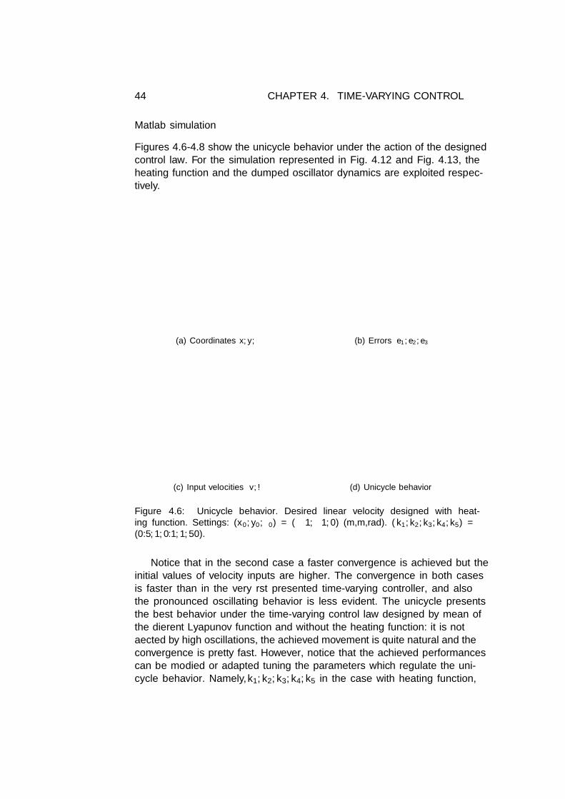
Matlab simulation
Figures 4.6-4.8 show the unicycle behavior under the action of the designedcontrol law. For the simulation represented in Fig. 4.12 and Fig. 4.13, theheating function and the dumped oscillator dynamics are exploited respec-tively.
0 5 10 15 20 25 30 35 40 45 50−1
−0.8
−0.6
−0.4
−0.2
0
0.2
0.4
0.6
0.8
[time]
[m]
x
y
θ
(a) Coordinates x, y, θ
0 5 10 15 20 25 30 35 40 45 50−0.8
−0.6
−0.4
−0.2
0
0.2
0.4
0.6
0.8
1
1.2
[time][m
]
e1
e2
e3
(b) Errors e1, e2, e3
0 5 10 15 20 25 30 35 40 45 50−1.5
−1
−0.5
0
0.5
1
1.5
[time]
v
ω
(c) Input velocities v, ω
−1 −0.8 −0.6 −0.4 −0.2 0 0.2 0.4 0.6 0.8−1.2
−1
−0.8
−0.6
−0.4
−0.2
0
0.2
(d) Unicycle behavior
Figure 4.6: Unicycle behavior. Desired linear velocity designed with heat-ing function. Settings: (x0, y0, θ0) = (−1,−1, 0) (m,m,rad). (k1, k2, k3, k4, k5) =(0.5, 1, 0.1, 1, 50).
Notice that in the second case a faster convergence is achieved but theinitial values of velocity inputs are higher. The convergence in both casesis faster than in the very first presented time-varying controller, and alsothe pronounced oscillating behavior is less evident. The unicycle presentsthe best behavior under the time-varying control law designed by mean ofthe different Lyapunov function and without the heating function: it is notaffected by high oscillations, the achieved movement is quite natural and theconvergence is pretty fast. However, notice that the achieved performancescan be modified or adapted tuning the parameters which regulate the uni-cycle behavior. Namely, k1, k2, k3, k4, k5 in the case with heating function,

4.4. BOUNDS ON ORIENTATION 45
and k1, k2, k3, kd, k2N in the case without heating function.
0 5 10 15−1
−0.8
−0.6
−0.4
−0.2
0
0.2
0.4
0.6
0.8
[time]
[m]
x
y
θ
(a) Coordinates x, y, θ
0 5 10 15−1
−0.5
0
0.5
1
1.5
[time]
[m]
e1
e2
e3
(b) Errors e1, e2, e3
0 5 10 15−5
0
5
10
15
20
25
[time]
v
ω
(c) Input velocities v, ω
−1 −0.8 −0.6 −0.4 −0.2 0 0.2 0.4 0.6−1.2
−1
−0.8
−0.6
−0.4
−0.2
0
0.2
(d) Unicycle behavior
Figure 4.7: Unicycle behavior. Desired linear velocity designed without heat-ing function. Settings: (x0, y0, θ0) = (−1,−1, 0) (m,m,rad). (k1, k2, k3, kd, k
2N ) =
(2, 2, 0.08, 1, 2) .
−1.2 −1 −0.8 −0.6 −0.4 −0.2 0 0.2 0.4 0.6 0.8
−1.2
−1
−0.8
−0.6
−0.4
−0.2
0
0.2
0.4
[m]
[m]
(a) Control designed with heating func-tion.
−1 −0.5 0 0.5 1
−1.2
−1
−0.8
−0.6
−0.4
−0.2
0
0.2
[m]
[m]
(b) Control designed without heating func-tion.
Figure 4.8: Unicycle trajectories.

46 CHAPTER 4. TIME-VARYING CONTROL
4.4.1 Time invariant bounds on the orientation
Given that adopting the candidate Lyapunov function (4.16) we are guar-anteed that e3 stays within the range (−π/2, π/2), the next step consists toreduce this interval by mean of a time invariant error transformation.We introduce a time-invariant (constant) positive coefficient, namely ρ, suchthat
e3 7→ e3 =e3
ρ
This transformation allows to define more strict bounds on the interval ofvariation of e3, and hence of the vehicle orientation. In particular now wehave
e3 ∈(−π
2ρ,π
2ρ).
Notice that this interval of values is still constant.Define the Lyapunov function as
V =k2
2
(e2
1 + e22
)− k3 ln
(cos e3
)(4.19)
which is positive definite for a specified range of value of e3, namely e3 ∈(−π
2 ρ,π2 ρ). This means that if we start from a position with e3 ∈ (−π
2 ρ,π2 ρ),
then this angle coordinate will evolve within the predefined set of value,without ever leaving it.Define the input controllers
u1 = −k1e1
u2 = −k2ρ
k3vde2
cos e3
sin e3sin e3 − tan e3
(4.20)
Differentiating V wrt time and substituting u1 and u2 with the expressionsin (4.20) we obtain
V = −k1k2e21 −
k3
ρtan2 e3 ≤ 0. (4.21)
Note that u2 is bounded and well defined.
Proposition 4.2 Consider the unicycle description (2.1), the error dynam-ics (4.3) and the feedback control (4.1) with control inputs defined as (4.20)and k1, k2, k3 positive constants. The closed-loop system (2.1)-(4.1) is thenglobally asymptotically driven to the posture (x, y, θ) = (0, 0, 0). Also, theerror component e3 respects the prescribed limits.
As in the previous case, the proof for the convergence of the error compo-nents and for the Cartesian coordinates can be carried on exploiting LaSalletheorem and Barbalat Lemma. Details and convergence proof for Proposi-tion 4.2 can be found in Appendix D.2.
4.4. BOUNDS ON ORIENTATION 47
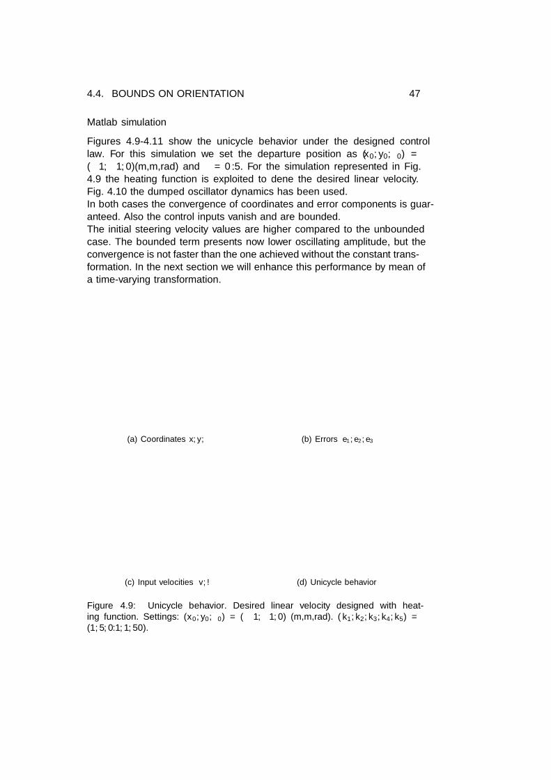
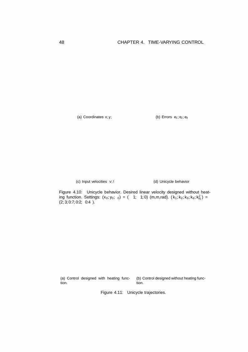
Matlab simulation
Figures 4.9-4.11 show the unicycle behavior under the designed controllaw. For this simulation we set the departure position as (x0, y0, θ0) =(−1,−1, 0)(m,m,rad) and ρ = 0.5. For the simulation represented in Fig.4.9 the heating function is exploited to define the desired linear velocity.Fig. 4.10 the dumped oscillator dynamics has been used.In both cases the convergence of coordinates and error components is guar-anteed. Also the control inputs vanish and are bounded.The initial steering velocity values are higher compared to the unboundedcase. The bounded term presents now lower oscillating amplitude, but theconvergence is not faster than the one achieved without the constant ρ trans-formation. In the next section we will enhance this performance by mean ofa time-varying transformation.
0 5 10 15 20 25 30 35 40 45 50−1
−0.8
−0.6
−0.4
−0.2
0
0.2
0.4
0.6
0.8
[time]
[m]
x
y
θ
(a) Coordinates x, y, θ
0 5 10 15 20 25 30 35 40 45 50−0.6
−0.4
−0.2
0
0.2
0.4
0.6
0.8
1
[time]
[m]
e1
e2
e3
(b) Errors e1, e2, e3
0 5 10 15 20 25 30 35 40 45 50−1
−0.5
0
0.5
1
1.5
[time]
v
ω
(c) Input velocities v, ω
−1 −0.5 0 0.5 1 1.5−1.2
−1
−0.8
−0.6
−0.4
−0.2
0
0.2
(d) Unicycle behavior
Figure 4.9: Unicycle behavior. Desired linear velocity designed with heat-ing function. Settings: (x0, y0, θ0) = (−1,−1, 0) (m,m,rad). (k1, k2, k3, k4, k5) =(1, 5, 0.1, 1, 50).
48 CHAPTER 4. TIME-VARYING CONTROL
0 5 10 15 20 25 30 35 40 45 50−1
−0.8
−0.6
−0.4
−0.2
0
0.2
0.4
0.6
0.8
[time]
[m]
x
y
θ
(a) Coordinates x, y, θ
0 5 10 15 20 25 30 35 40 45 50−0.6
−0.4
−0.2
0
0.2
0.4
0.6
0.8
1
1.2
[time]
[m]
e1
e2
e3
(b) Errors e1, e2, e3
0 5 10 15 20 25 30 35 40 45 50−2
0
2
4
6
8
10
12
14
[time]
v
ω
(c) Input velocities v, ω
−1 −0.8 −0.6 −0.4 −0.2 0 0.2 0.4 0.6 0.8 1−1.2
−1
−0.8
−0.6
−0.4
−0.2
0
0.2
(d) Unicycle behavior
Figure 4.10: Unicycle behavior. Desired linear velocity designed without heat-ing function. Settings: (x0, y0, θ0) = (−1,−1, 0) (m,m,rad). (k1, k2, k3, kd, k
2N ) =
(2, 3, 0.7, 0.2ρ, 0.4ρ).
−1 −0.5 0 0.5 1
−1.2
−1
−0.8
−0.6
−0.4
−0.2
0
0.2
[m]
[m]
(a) Control designed with heating func-tion.
−1 −0.5 0 0.5 1
−1.2
−1
−0.8
−0.6
−0.4
−0.2
0
0.2
[m]
[m]
(b) Control designed without heating func-tion.
Figure 4.11: Unicycle trajectories.

4.4. BOUNDS ON ORIENTATION 49
4.4.2 Time-varying bounds on the orientation
In order to achieve faster convergence and set more narrow bounds on theorientation, we introduce a time varying transformation through the modu-lating function ρ(t), such that
e3 7→ e3 =e3
ρ(t), ρ(t) = (ρ0 − ρ∞) exp(−Lt) + ρ∞.
Define the Lyapunov function as
V =k2
2
(e2
1 + e22
)− k3 ln
(cos e3
). (4.22)
This Lyapunov function is positive definite for a specified range of value ofe3, namely
e3 ∈(−π
2ρ(t),
π
2ρ(t)
).
Notice that the interval of values is now time-varying.If e30 ∈ (−π
2ρ(0), π2ρ(0)), then this angle coordinate will evolve within thepredefined set of value, without ever leaving it.
Define the input controllers
u1 = −k1e1
u2 = −e3α(t)− k2ρ(t)
k3vde2
cos e3
sin e3sin e3 − tan e3
(4.23)
Differentiating V wrt time, substituting the the designed controllers in (4.23)and canceling out some terms we obtain
V = −k1k2e21 −
k3
ρ(t)tan2 e3 ≤ 0. (4.24)
Proposition 4.3 Consider the unicycle description (2.1), the error dynam-ics (4.3) and the feedback control (4.1) with control inputs defined as (4.23)and k1, k2, k3 positive constants. The closed-loop system (2.1)-(4.1) is thenglobally asymptotically driven to the posture (x, y, θ) = (0, 0, 0). Also, theerror component e3 respects the prescribed limits.
As in the previous case, the proof for the convergence of the error compo-nents and of the Cartesian coordinates can be carried on exploiting LaSalletheorem and Barbalat Lemma. Details can be found in Appendix D.3.
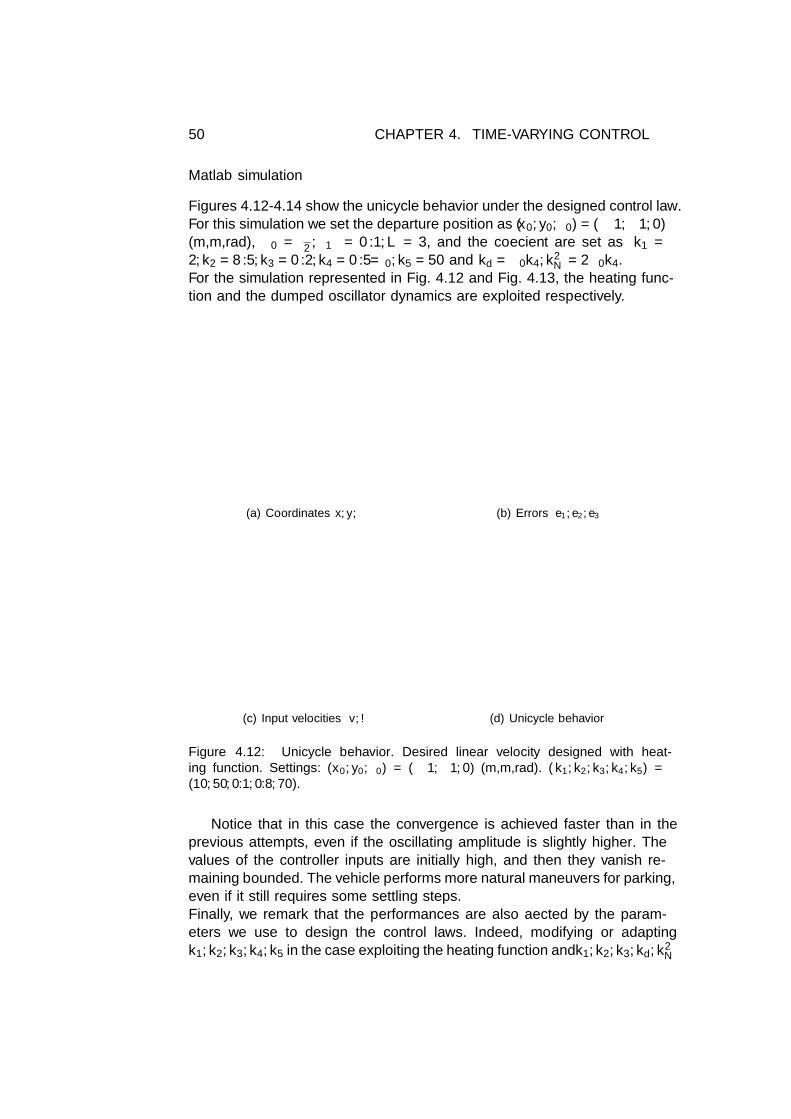
50 CHAPTER 4. TIME-VARYING CONTROL
Matlab simulation
Figures 4.12-4.14 show the unicycle behavior under the designed control law.For this simulation we set the departure position as (x0, y0, θ0) = (−1,−1, 0)(m,m,rad), ρ0 = π
2 , ρ∞ = 0.1, L = 3, and the coefficient are set as k1 =2, k2 = 8.5, k3 = 0.2, k4 = 0.5/ρ0, k5 = 50 and kd = ρ0k4, k
2N = 2ρ0k4.
For the simulation represented in Fig. 4.12 and Fig. 4.13, the heating func-tion and the dumped oscillator dynamics are exploited respectively.
0 2 4 6 8 10 12 14−1
−0.5
0
0.5
1
1.5
[time]
[m]
x
y
θ
(a) Coordinates x, y, θ
0 0.5 1 1.5 2 2.5 3 3.5 4−1.5
−1
−0.5
0
0.5
1
1.5
[time]
[m]
e1
e2
e3
(b) Errors e1, e2, e3
0 0.5 1 1.5 2 2.5 3 3.5 4−5
0
5
10
15
20
[time]
v
ω
(c) Input velocities v, ω
−1 −0.8 −0.6 −0.4 −0.2 0 0.2 0.4−1.2
−1
−0.8
−0.6
−0.4
−0.2
0
0.2
(d) Unicycle behavior
Figure 4.12: Unicycle behavior. Desired linear velocity designed with heat-ing function. Settings: (x0, y0, θ0) = (−1,−1, 0) (m,m,rad). (k1, k2, k3, k4, k5) =(10, 50, 0.1, 0.8, 70).
Notice that in this case the convergence is achieved faster than in theprevious attempts, even if the oscillating amplitude is slightly higher. Thevalues of the controller inputs are initially high, and then they vanish re-maining bounded. The vehicle performs more natural maneuvers for parking,even if it still requires some settling steps.Finally, we remark that the performances are also affected by the param-eters we use to design the control laws. Indeed, modifying or adaptingk1, k2, k3, k4, k5 in the case exploiting the heating function and k1, k2, k3, kd, k
2N

4.4. BOUNDS ON ORIENTATION 51
in the other one, it is possible to achieve different performances.
0 1 2 3 4 5 6 7 8 9 10−1
−0.8
−0.6
−0.4
−0.2
0
0.2
0.4
0.6
0.8
[time]
[m]
x
y
θ
(a) Coordinates x, y, θ
0 0.5 1 1.5 2 2.5 3−1
−0.5
0
0.5
1
1.5
[time]
[m]
e1
e2
e3
(b) Errors e1, e2, e3
0 0.5 1 1.5 2 2.5 3−20
0
20
40
60
80
100
[time]
v
ω
(c) Input velocities v, ω
−1.2 −1 −0.8 −0.6 −0.4 −0.2 0 0.2 0.4 0.6 0.8−1.2
−1
−0.8
−0.6
−0.4
−0.2
0
0.2
(d) Unicycle behavior
Figure 4.13: Unicycle behavior. Desired linear velocity designed without heat-ing function. Settings: (x0, y0, θ0) = (−1,−1, 0) (m,m,rad). (k1, k2, k3, kd, k
2N ) =
(7, 15, 0.4, 0.8ρ0, 1.6ρ0).
−1.2 −1 −0.8 −0.6 −0.4 −0.2 0 0.2 0.4 0.6
−1.2
−1
−0.8
−0.6
−0.4
−0.2
0
0.2
[m]
[m]
(a) Control designed with heating func-tion.
−1.2 −1 −0.8 −0.6 −0.4 −0.2 0 0.2 0.4 0.6
−1.2
−1
−0.8
−0.6
−0.4
−0.2
0
0.2
[m]
[m]
(b) Control designed without heating func-tion.
Figure 4.14: Unicycle trajectories.

52 CHAPTER 4. TIME-VARYING CONTROL
4.4.3 Performances of the designed time-varying controllers
In this section we report some figures depicting performances and in par-ticular the transient of the error component e3 when adopting the threedesigned time-varying controllers that guarantee prescribed bounds on e3.
It is not possible to directly make a fair comparison between the afore-mentioned controllers, since their reliance on parameters (e.g. k1, k2, ... etc.)is critical. Hence, we compare the performances of the proposed controllersin the event that they achieve fair convergence. This means that the follow-ing figures refer to controllers which have been properly tuned.
0 2 4 6 8 10 12 14 16 18 20−1.5
−1
−0.5
0
0.5
1
e3−original
e3−const.bounds
e3−TVbounds
0 2 4 6 8 10 12 14 16 18 200
0.2
0.4
0.6
0.8
−log(cos(e3))−original
−log(cos(e3/rho))−const.bounds
−log(cos(e3/rho(t)))−TVbounds
(a) Control with heating function
0 2 4 6 8 10 12 14 16 18 20−1
−0.5
0
0.5
e3−original
e3−const.bounds
e3−TVbounds
0 2 4 6 8 10 12 14 16 18 200
0.1
0.2
0.3
0.4
−log(cos(e3))−original
−log(cos(e3/rho))−const.bounds
−log(cos(e3/rho(t)))−TVbounds
(b) Control without heating function
Figure 4.15: Comparison of the three designed control law.

4.4. BOUNDS ON ORIENTATION 53
Figure 4.15 plots the bounded error component e3 evolution in the time:notice in particular that the convergence achieved by mean of time-varyingbounds is much faster than the other cases. In figure 4.15 the bounding term“− ln cos(e3)” (or “− ln cos(e3)”) with respect to the time are also reported:we are confirmed that this part of Lyapunov function converges to zero andalso has a fast dynamics, so that the bounded coordinate can quickly reachconvergence.Figure 4.15.a refers to the control adopting the heating function, and 4.15.bthe other one. One can notice that we achieve better results in the secondcase, both in term of speed of convergence and in term of oscillating am-plitude. We recall that the performances are affected from the choice of theparameters.
A measure of the results obtained by binding e3 by mean of a time-varying function ρ(t) is reported in Figure 4.16. This picture plots thebounded error component e3 evolution in the time together with the boundsdefined by the modulating function ρ(t), pointing out that this bounds arefully satisfied.
0 0.5 1 1.5 2 2.5 3 3.5 4 4.5 5−2
−1.5
−1
−0.5
0
0.5
1
1.5
2
[time]
e3
ρ(t)
−ρ(t)
Figure 4.16: Time-varying bounds case: the error e3 stays within the specifiedrange of value, defined by the ρ(t) function.

54 CHAPTER 4. TIME-VARYING CONTROL

Chapter 5
ROS Simulations
This section presents the simulations developed in ROS, Robot OperatingSystem. A brief introduction to the ROS framework is here reported. Formore details the reader is referred to the wiki available in Internet [15].ROS is a powerful and current tool to simulate robot behavior.
5.1 Brief introduction to ROS
ROS is an open-source, meta-operating system for robots. It provides theservices of an operating system, including hardware abstraction, low-leveldevice control, implementation of commonly-used functionality, message-passing between processes, and package management. It also provides toolsand libraries for obtaining, building, writing, and running code across mul-tiple computers.ROS supports code reuse in robotics research and development. It is a dis-tributed framework of processes (called Nodes) that can be grouped intoPackages and Stacks, which can be easily shared and distributed. Also it islanguage neutral and supports various modern programming languages asC++, Python, Lisp.There exists several releases of ROS: Electric, Fuerte, Groovy, Hydro.ROS currently only runs on Unix-based platforms. Software for ROS is testedon Ubuntu and Mac OS X systems. A list of robots that can be used withROS software can be found at http://www.ros.org/wiki/Robots.The peer-to-peer network of ROS processes is the Computation Graph. Thebasic Computation Graph concepts of ROS are Nodes, Master, ParameterServer, messages, services, topics, and bags. The ROS Master stores topicsand services registration information for ROS nodes. Nodes connect to eachother directly while the Master only provides lookup information. Nodescommunicate with the Master to report their information and to receive in-formation about other registered nodes and make connections. The Masterwill also make callbacks to these nodes when informations change, allowing
55

56 CHAPTER 5. ROS SIMULATIONS
dynamic connections between nodes.Topics are named buses over which nodes exchange messages, and they areintended for unidirectional, streaming communication. Topics have anony-mous publish/subscribe semantics, which decouples the production of infor-mation from its consumption. There can be multiple publishers and sub-scribers to a topic. A schematic representation is depicted in Figure 5.1.
Figure 5.1: Nodes connection: communication structure. Figure source://http://www.ros.org/wiki/ROS/Concepts
TurtleSim
TurtleSim is a ROS simulator for teaching. It is a simple tool, but effectivefor the purpose of testing and simulating the designed controllers for theunicycle-like robot.ROS structures are used to implement the controllers. Turtlesim node per-mits to visualize the moving vehicle, which in this case is a turtle. Witha view to future implementations, it is possible to reuse the code imple-menting the controller (control Node) and apply it on different models ofunicycle-like robot: as an example Pioneer.
5.2 Implementation
We perform simulations for the controllers designed by mean of polar coor-dinates. We use ROS Fuerte release and C++ language.A package turtle unicycle has been created. It contains a single Nodecalled /controller node. There are two classes: UnicycleVelocity andUnicycleVelocityControllerNode. The first one is responsible for calcu-lating the unicycle velocity while implementing the designed control lawsand the error transformations for prescribed performance constraints. Thesecond one implements all the necessary ROS components. For code docu-mentation see Appendix E.The main() function creates and initializes the Control Node. During the

5.2. IMPLEMENTATION 57
simulations, the Control Node receives as input the unicycle position, thatis the Cartesian coordinates x, y, θ, and calculates the unicycle velocitiesexploiting UnicycleVelocity class methods. The velocities are then used tovisualize the turtle movements. Figure 5.2 depicts what explained. In partic-ular note the three topics related to /turtlesim node: /command velocity,/pose, /color sensor. The position of the turtle is used to calculate thevelocities, which are given in input to the turtle node to generate its move-ment.
Figure 5.2: Graph obtained from ROS rqt graph: it shows topics flowing in andout of the /controller node and the /turtlesim node.
Simulation 1.
In the first simulation, we implement the standard control law with polarcoordinates, namely (3.3). The initial position of the turtle is (x, y, θ) =(5.544445, 5.544445, 0) while the goal position is set to (x, y, θ) = (9, 9, 0).Figure 5.3 shows the turtle behavior and the evolution in the time of thethree coordinates x, y, θ.
(a) Turtle movement
0 0.5 1 1.5 2 2.5 30
1
2
3
4
5
6
7
8
9
x
y
θ
(b) Coordinates x, y, θ
0 0.5 1 1.5 2 2.5 3−1
0
1
2
3
4
5
6
7
8
v
ω
(c) Inputs
Figure 5.3: Turtle behavior under the original control law (3.3) and time evolutionof the turtle coordinates.
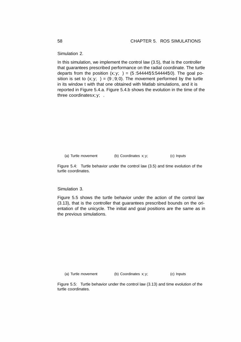
58 CHAPTER 5. ROS SIMULATIONS
Simulation 2.
In this simulation, we implement the control law (3.5), that is the controllerthat guarantees prescribed performance on the radial coordinate. The turtledeparts from the position (x, y, θ) = (5.544445, 5.544445, 0). The goal po-sition is set to (x, y, θ) = (9, 9, 0). The movement performed by the turtlein its window fit with that one obtained with Matlab simulations, and it isreported in Figure 5.4.a. Figure 5.4.b shows the evolution in the time of thethree coordinates x, y, θ.
(a) Turtle movement
0 0.05 0.1 0.15 0.2 0.25 0.3 0.35 0.4 0.45 0.50
1
2
3
4
5
6
7
8
9
x
y
θ
(b) Coordinates x, y, θ
0 0.005 0.01 0.015 0.02 0.025 0.03 0.035 0.04 0.045 0.05−10
−5
0
5
10
15
20
25
30
35
v
ω
(c) Inputs
Figure 5.4: Turtle behavior under the control law (3.5) and time evolution of theturtle coordinates.
Simulation 3.
Figure 5.5 shows the turtle behavior under the action of the control law(3.13), that is the controller that guarantees prescribed bounds on the ori-entation of the unicycle. The initial and goal positions are the same as inthe previous simulations.
(a) Turtle movement
0 0.5 1 1.5 2 2.50
1
2
3
4
5
6
7
8
9
x
y
θ
(b) Coordinates x, y, θ
0 0.05 0.1 0.15 0.2 0.25−2
0
2
4
6
8
10
v
ω
(c) Inputs
Figure 5.5: Turtle behavior under the control law (3.13) and time evolution of theturtle coordinates.
5.2. IMPLEMENTATION 59
Simulation 4.
Eventually, this simulation implements the controller that permits to bindboth radial and angle coordinate. Figure 5.6 shows the turtle behavior underthe action of the control law (3.16). The initial and goal positions are thesame as in the previous simulations. Note that in this case the convergenceto the desired posture is much faster than in the previous simulations.
(a) Turtle movement
0 0.1 0.2 0.3 0.4 0.5 0.6 0.70
1
2
3
4
5
6
7
8
9
x
y
θ
(b) Coordinates x, y, θ
0 0.01 0.02 0.03 0.04 0.05 0.06 0.07−5
0
5
10
15
20
25
30
v
ω
(c) Inputs
Figure 5.6: Turtle behavior under the control law (3.16) and time evolution of theturtle coordinates.
60 CHAPTER 5. ROS SIMULATIONS
Chapter 6
Conclusion
This thesis addresses the regulation problem for mobile robots of the type ofthe unicycle. Different controllers have been designed, in order to guaranteeprescribed performances. The main results and proofs of convergence havebeen obtained by mean of the Lyapunov analysis.WMRs are nonholonomic system, thus the regulation problem cannot besolved via a smooth, time-invariant state feedback law due to the implica-tions of Brockett’s condition.
The unicycle model has been introduced and two main approaches toits regulation have been examined: control with polar coordinates and time-varying control.The prescribed performance control concept has also been analyzed andemployed to design controllers that solve the regulation problem while guar-anteeing prescribed bounds.A first example of solution combining the regulation aim and the prescribedperformance control concepts has been given by the Dynamic Feedback Lin-earization.
The best performing presented control law has been designed by meanof polar coordinates. Prescribed performances have been imposed in orderto bind both the position and the orientation of the vehicle. The controllerbased on polar coordinates transformation performs very well. The resultingvehicle path is very natural and convergence is quite fast. This is one of themain result of this study. The convergence to the desired position is achievedwith natural maneuvers, while the polar coordinates r and γ are guaranteedto respect the predefined limits. This result also points out a relevant dif-ference between the approach followed to bind the distance r and the oneused to bind the orientation (through the angle γ). While in the first casewe begin with the error transformation and exploit the transformed errorin the potential to define the Lyapunov function, in the latter we bind the
61

62 CHAPTER 6. BIBLIOGRAPHY
coordinate starting from the definition of a different potential dependingfrom the cosine of the coordinate to bind.
Then, time-varying control laws has been introduced. Prescribed per-formances have been imposed to bind the vehicle orientation. The desireddriving velocity is defined by mean of oscillating functions: in the originalcase a heating function designed as a modulated sine function is exploited;a different solution is give defining the driving velocity with a dumped oscil-lator dynamics. Controllers have been tested both with and without heatingfunction. Different types of Lyapunov functions have been used. A controllaw as been designed exploiting a Lyapunov function recalling the pendu-lum candidate Lyapunov function. Also, a Lyapunov function including apotential term depending from the cosine of the component to bind e3 hasbeen employed to impose prescribed performance on the vehicle orientation.Time-varying controllers, both with and without heating function, exhibit arather slow final convergence to the goal. The dependence of the convergencerate on the available gains is critical. The oscillatory behavior of the vehicleis an intrinsic characteristic.
The last Section presented simulations implemented in ROS environ-ment. The controllers designed by mean of polar coordinates have beentested, exploiting the Turtlesim simulator.
Future work
Future directions of work should consider also different approaches to theregulation problem for the unicycle. For example discontinuous or non-smooth time-varying controllers can be analyzed in order to introduce pre-scribed performance.The prescribed performance control concept can be applied for the controlproblem of other type of nonholonomic systems, such as the car-like mobilerobot or more complex structures.Prescribed performance can be imposed also in the trajectory tracking prob-lem, and in the robust control approach.Time-varying controllers can be tested in ROS environment and simulationscan be also implemented employing real robot models, as for example Pio-neer.Also, the proposed control laws could be implemented on a real mobileunicycle-like robots.

Bibliography
[1] Roger W Brockett et al. Asymptotic stability and feedback stabilization.Defense Technical Information Center, 1983.
[2] Alessandro Astolfi. Discontinuous control of nonholonomic systems.Systems & Control Letters, 27(1):37–45, 1996.
[3] Giuseppe Oriolo, Alessandro De Luca, and Marilena Vendittelli. Wmrcontrol via dynamic feedback linearization: design, implementation, andexperimental validation. Control Systems Technology, IEEE Transac-tions on, 10(6):835–852, 2002.
[4] Herbert G Tanner and Kostas J Kyriakopoulos. Discontinuous back-stepping for stabilization of nonholonomic mobile robots. In Roboticsand Automation, 2002. Proceedings. ICRA’02. IEEE InternationalConference on, volume 4, pages 3948–3953. IEEE, 2002.
[5] Herbert G Tanner, Savvas Loizou, and Kostas J Kyriakopoulos. Non-holonomic stabilization with collision avoidance for mobile robots. InIntelligent Robots and Systems, 2001. Proceedings. 2001 IEEE/RSJ In-ternational Conference on, volume 3, pages 1220–1225. IEEE, 2001.
[6] Claude Samson. Control of chained systems application to path follow-ing and time-varying point-stabilization of mobile robots. AutomaticControl, IEEE Transactions on, 40(1):64–77, 1995.
[7] Lorenzo Sciavicco and Bruno Siciliano. Modelling and control of robotmanipulators. Springer Verlag, 2000.
[8] Ilya Kolmanovsky and N Harris McClamroch. Developments in non-holonomic control problems. Control Systems, IEEE, 15(6):20–36, 1995.
[9] Alessandro De Luca, Giuseppe Oriolo, and Marilena Vendittelli. Con-trol of wheeled mobile robots: An experimental overview. In Ramsete,pages 181–226. Springer, 2001.
[10] Y. Karayiannidis and Z. Doulgeri. Model-free robot joint position reg-ulation and tracking with prescribed performance guarantees. Roboticsand Autonomous Systems, 60(2):214–226, 2012.
63

64 BIBLIOGRAPHY
[11] Zoe Doulgeri and Yiannis Karayiannidis. Pid type robot joint positionregulation with prescribed performance guaranties. In Robotics andAutomation (ICRA), 2010 IEEE International Conference on, pages4137–4142. IEEE, 2010.
[12] Ch Bechlioulis, Zoe Doulgeri, and G Rovithakis. Prescribed perfor-mance adaptive control for robot force/position tracking. In ControlApplications,(CCA) & Intelligent Control,(ISIC), 2009 IEEE, pages920–925. IEEE, 2009.
[13] Zoe Doulgeri, Yiannis Karayiannidis, and Olga Zoidi. Prescribed per-formance control for robot joint trajectory tracking under parametricand model uncertainties. In Control and Automation, 2009. MED’09.17th Mediterranean Conference on, pages 1313–1318. IEEE, 2009.
[14] Charalampos P Bechlioulis and George A Rovithakis. Robust adaptivecontrol of feedback linearizable mimo nonlinear systems with prescribedperformance. Automatic Control, IEEE Transactions on, 53(9):2090–2099, 2008.
[15] URL //http://www.ros.org/wiki/.
[16] Daniel Liberzon. Switching in Systems and Control. SpringerBirkhauser, Boston, 2003.
[17] Herbert G Tanner and Kostas J Kyriakopoulos. Nonholonomic motionplanning for mobile manipulators. In Robotics and Automation, 2000.Proceedings. ICRA’00. IEEE International Conference on, volume 2,pages 1233–1238. IEEE, 2000.
[18] Anthony M Bloch, Mahmut Reyhanoglu, and N Harris McClamroch.Control and stabilization of nonholonomic dynamic systems. AutomaticControl, IEEE Transactions on, 37(11):1746–1757, 1992.
[19] Alessandro De Luca and Giuseppe Oriolo. Modeling and control ofnonholonomic mechanical systems. Kinematics and Dynamics of Multi-Body Systems, CISM Courses and Lectures, 360:277–342, 1995.
[20] Stern R.J. Brockett’s stabilization condition under state con-straints. Systems and Control Letters, 47(4):335–341, 2002. URLhttp://www.ingentaconnect.com/content/els/01676911/2002/
00000047/00000004/art00227.
[21] Bruno Siciliano, Lorenzo Sciavicco, Luigi Villani, and Giuseppe Ori-olo. Robotics: Modelling, Planning and Control. Springer Publish-ing Company, Incorporated, 1st edition, 2008. ISBN 1846286417,9781846286414.
BIBLIOGRAPHY 65
[22] G Campion, B d’Andrea Novel, and G Bastin. Controllability andstate feedback stabilizability of non holonomic mechanical systems. InAdvanced robot control, pages 106–124. Springer, 1991.
[23] C Canudas De Wit and OJ Sordalen. Exponential stabilization of mo-bile robots with nonholonomic constraints. Automatic Control, IEEETransactions on, 37(11):1791–1797, 1992.
[24] C Canudas De Wit, H Khennouf, C Samson, and OJ Sordalen. Non-linear control design for mobile robots. Recent trends in mobile robots,11:121–156, 1993.
[25] Jean-Michel Coron. Global asymptotic stabilization for controllablesystems without drift. Mathematics of Control, Signals and Systems, 5(3):295–312, 1992.
[26] Yiannis Karayiannidis, Dimos V Dimarogonas, and Danica Kragic.Multi-agent average consensus control with prescribed performanceguarantees. In Decision and Control (CDC), 2012 IEEE 51st AnnualConference on, pages 2219–2225. IEEE, 2012.

66 BIBLIOGRAPHY

Appendix A
Two approaches to imposePP bounds
Polar coordinate control case
Being e = γ,
e = γ =sin γ
rv − ω;
thus, in the first derivative of the Lyapunov function there are terms of theform
ε(sin γ
rv − ω
)and tan e
(sin γ
rv − ω
).
Given the polar description of the unicycle and its dynamics, the drivingvelocity is designed as
v = k1r cos γ.
This input allows to have a square term of r multiplied for a cos2 γ in thefirst derivative of the Lyapunov function. This is needed for the convergenceproof.Given this driving velocity and the δ dynamics, in the first derivative of theLyapunov function appears a term of the form
δsin γ
rv = δ
sin γ
r[k1r cos γ] = k1δ sin γ cos γ (A.1)
which is the derivative of the quadratic term 12δ
2 in the Lyapunov function.The steering velocity is designed in order to cancel out the term in (A.1),thus ω will depend on a term of the form
ω1 =1
εk1δ sin γ cos γ and ω2 =
1
tan ek1δ sin γ cos γ (A.2)
in the first and second approach respectively.Observe that in both the expression in (A.2) the terms δ/ε and δ/ tan γ are
67

68 APPENDIX A. TWO APPROACHES TO IMPOSE PP BOUNDS
unbounded, since both ε and e vanish faster than δ, due to the prescribedperformance bounds.The previous equations can be rewritten as
ω1 = k1δ
sin γ cos γγεγ
and ω2 = k1δ
sin γ cos γγ
tan γγ
(A.3)
which are well defined terms.The convergence proof for the unicycle system is based on Barbalat lemma;in particular we are interested to prove that γ is uniformly continuous. Todo that we check the boundedness of the second derivative γ.In the first case, the lack of convergence is related to the fact that ˙ω1 is notbounded and thus γ is not uniformly continuous, while in the second case˙ω2 is proved to be bounded and it is possible to conclude the convergenceproof. In details, ˙ω1 is given by
˙ω1 = k1
[δsγcγ/γ
ε/γ+ δ( ddt
(sγcγγ
))γε
+ δsγcγγ
d
dt
(γε
)](A.4)
where sγ , cγ indicate sin γ, cos γ. The only unbounded term in (A.4) is
d
dt
γ
ε=(sin γ
rv − ω
)(1
ε− Jγ
ε2
)︸ ︷︷ ︸unbounded
−αJ(γε
)2. (A.5)
In the second case, ˙ω2 is given by
˙ω1 = k1
[δsγcγ/γ
tan γ/γ+ δ( ddt
(sγcγγ
)) γ
tan γ+ δ
sγcγγ
d
dt
( γ
tan γ
)](A.6)
All the terms are well defined and bounded. In particular now
d
dt
γ
tan γ=(sin γ
rv − ω
)( 1
tan γ− γ
ρ
1 + tan2 γ
tan2 γ
)− α
ργ2
=(sin γ
rv − ω
)(−γ +
tan γ − γtan2 γ
)− α
ργ2
(A.7)
where the term tan γ−γtan2 γ
is bounded as long as γ is not null, and as γ → 0 thelimit gives
limγ→0
tan γ − γtan2 γ
= 0. (A.8)
Being ˙ω2 bounded, then also the derivative of the steering velocity is boundedand this fact allows to conclude the convergence proof.
69
We remark that this issue is not arising in the case we bind the radialcoordinate r. This is still related to the unicycle dynamics definition withpolar coordinates. The original Lyapunov function can be modified just sub-stituting e with ε = T (r/ρ), that is adopting a potential of the form (2.11).In this case the driving velocity v acts directly on ε, so that we have a squareterm ε2 needed for convergence proof. Then the steering velocity can easilycompensate the term deriving from 1
2δ2 and no unbounded terms arise: the
term ε/e appears, but this term is proved to be bounded.
Time-varying control case
In the case of time-varying control, the reasoning is analogous: a potentialdefined as in (2.12) allows to conclude the convergence proof according toBarbalat lemma.In the case of time-varying control we define the error through a rotation ofthe Cartesian error:
e =
e1
e2
e3
=
cos θ sin θ 0− sin θ cos θ 0
0 0 1
xd − xyd − yθd − θ
.The orientation of the unicycle is directly linked with the third error com-ponent e3, which is now the coordinate to bind. After some simplifications,the error dynamics can be written as
e1 = u1 − e2u2
e2 = sin e3vd + e1u2
e3 = u2
(A.9)
The input control u1 is designed in order to obtain a square term e21, needed
for the convergence proof. This input is defined as u1 = −k1e1 and does notcompensate the sinusoidal term related to e2.Considering the dynamics of e2, in the first derivative of the Lyapunov func-tion appears a term of the form
e2 sin e3vd (A.10)
The second input velocity u2 is designed in order to cancel out the term in(A.10), thus u2 will depend on a term of the form
u2 =1
εe2 sin e3vd and u2 =
1
tan ee2 sin e3vd (A.11)
in the first and second approach respectively.Observe that in both the expression in (A.11) the terms e2/ε and e2/ tan e

70 APPENDIX A. TWO APPROACHES TO IMPOSE PP BOUNDS
are unbounded, since both ε and e vanish faster than e2, due to the pre-scribed performance bounds.The first approach, based on defining the transformed error ε and employinga potential of the form (2.11), yields also in this case to unbounded termsthat cause the lack of convergence. On the other hand, the second approachis successful, since we can prove that the first derivative of u2 is boundedand e3 as well. This allows to conclude the convergence proof.

Appendix B
DFL: details andconvergence proof.
The first derivative of the Lyapunov function (2.20) is calculated as follow:
V =(e+ αe
)T (e+ αe+ αe
)+ εTKεε
=(e+ αe
)T (u+ αe+ αe
)+ εTKεJT
(e+ αe
)=(e+ αe
)T (−Kv
(e+ αe
)−KεJT ε−��αe−��αe+��αe+��αe
)+ εTKεJT
(e+ αe
)= −eTKv e−�����
eTKvαe−�����eTKεJT ε−�����
eTαTKv e− eTαTKvαe+
−������eTαTKεJT ε+�����
εTKεJT e+������εTKεJTαe
= −eTKv e− eTα(t)TKvα(t)e
(B.1)
where the input control law (2.19) has been substituted.Being V ≤ 0, the state is bounded in norm, V is uniformly continuous,and V tends to a limit value. Exploiting Barbalat lemma, it is possible toconclude that V tends to zero and thus e and αe tend to zero as well. Henceε tends to a finite value ε since
ε = JT(e+ αe
)→ 0 ⇒ ε→ ε.
The control input is bounded, since all its components are bounded. Also,e = u tends to the finite limit −KεJT ε and it is uniformly continuous, asu is bounded. Hence, the finite limit −KεJT ε must be zero, according toBarbalat Lemma and thus also ε→ 0. �
71

72 APPENDIX B. DFL: DETAILS AND CONVERGENCE PROOF.

Appendix C
Control with PolarCoordinates: details andproofs.
C.1 Details for section Prescribed performance onthe distance vector
Substituting (3.5) in (3.4) we obtain
V = −k1ε2JT cos2 γ − εJTα(t)e
(k3 cos2 γ − 1
)+
+(k1ε
e+ k3α(t)
)sin γ cos γ(γ + k3δ)− k2γ
2+
−(k1ε
e+ k3α(t)
)sin γ cos γ(γ + k3δ)− k3εJTα(t)e sin2 γ
= −k1ε2JT cos2 γ − k2γ
2 − εJα(t)e(k3(sin2 γ + cos2 γ)− 1
)= −k1ε
2JT cos2 γ − k2γ2 − εJα(t)e(k3 − 1)
The following inequality holds (see [10]):
εJe ≥ µε2 (C.1)
with µ a positive constant. Hence, provided that k3 ≥ 1 and taking µ > 0,then
V = −k1ε2JT cos2 γ − k2γ
2 − εJTα(t)e(k3 − 1)
≤ −k1ε2JT cos2 γ − k2γ
2 − µε2α(t)(k3 − 1)
≤ −k1ε2JT cos2 γ − k2γ
2 ≤ 0. (C.2)
73

74APPENDIX C. CONTROLWITH POLAR COORDINATES: DETAILS AND PROOFS.
Proof of Proposition 3.1
Since (3.6) holds, the state is bounded in norm, V (t) is uniformly continuous,and V (t) tends to a limit value. By Barbalat lemma, V (t) tends to zero and
thus also ε and γ do: q(t)→{q : V (x) = 0
}= {ε = 0, γ = 0, ∀δ}.
Analyzing the closed-loop system, we note that r and δ converge to zero.
In fact,r = −v cos γ = −k1ε cos2 γ − k3α(t)e cos2 γ → 0
as ε→ 0 (and consequently also e→ 0), and also
r = −v cos γ = −k1ε cos2 γ − k3α(t)e→ 0
as ε→ 0 (and consequently also e→ 0), and also
δ =sin γ
rv = k1
ε
esin γ cos γ + k3α(t) sin γ cos γ → 0
by the fact that, as γ → 0 then sin γ → 0, cos γ → 1.Also, δ converges to some finite limit δ.Then, substituting the expression of v and ω in the evolution equation
of γ we have
γ =sin γ
rv − ω
= k1ε
esin γ cos γ + k3α(t) sin γ cos γ+
− k2γ −(k1ε
e+ k3α(t)
)sin γ cos γ
γ(γ + k3δ)+
− k3εJα(t)esin2 γ
γ
As δ → δ, γ tends to the finite limit
γ → −k1k3ε
eδ − k2
3α(t)δ
provided that T (·) = Tb(·) or also T (·) = Ta(·) but choosing M = 0 (seesection 2.2). Since α(t)→ 0 and choosing T (·) = Tb(·)
γ → −k1k3M + 1
Mρδ
Also, γ is uniformly continuous since γ is bounded.Taking the second derivative of γ we obtain:
γ = − r
r2sin γv +
cos γγ
rv +
sin γ
rv − ω.
C.2. DETAILS FOR BOUNDS ON THE ANGLES 75
Both v and ω are bounded; hence r = −v cos γ is still bounded (and thusalso ε). If r 6= 0, also γ = sin γ
r v − ω is bounded. We can observe that r = 0is a singularity which intrinsically exists from the definition of the polarcoordinates system.Thus, also
v = k1εJ(r + αe) cos γ − k1ε sin γγ + k3αe cos γ + k3αe cos γ − k3αe sin γγ
is bounded. The last term to be checked is then ω. Writing extensively theexpression of ω we have:
ω = k2γ +(k1εe− εee2
+ k3α)sin γ cos γ
γ(γ + k3δ)+
+(k1ε
e+ k3α
)(−1
γ+
2 cos2 γ
γ− sin γ cos γ
γ2
)γ(γ + k3δ)+
+(k1ε
e+ k3α
)sin γ cos γ
γ(γ + k3δ) + k3εJαe
sin2 γ
γ+
+ k3εJαesin2 γ
γ+ k3εJαe
sin2 γ
γ+ k3εJαe
2 sin γ cos γ − sin2 γ
γ2γ.
(C.3)
All the terms are bounded or vanish as γ goes to zero. In particular,(− 1γ + 2 cos2 γ
γ − sin γ cos γγ2
)and 2 sin γ cos γ−sin2 γ
γ2remain bounded as long as γ
stays away from zero and tend to zero and 1 respectively as γ → 0.Eventually, γ is bounded.
According to the theoretical analysis carried out so far, since γ has afinite limit as t → ∞ and γ is uniformly continuous, then γ tends to zero.Being E 6= 0, it follows that δ must be zero, so that δ converges to zero.
From the previous analysis, ε is proved bounded, thus the transforma-tion T (e) is bounded. Hence, it is possible to conclude that r respects thepredefined limits. �
C.2 Details for bounds on the angles
Bounds on γ
If we bind γ and put prescribed performance on it, exploiting the transfor-mation
e = γ 7→ ε = T(eρ
)and consider the Lyapunov function
V =1
2
(r2 + ε2 + δ2
), (C.4)
76APPENDIX C. CONTROLWITH POLAR COORDINATES: DETAILS AND PROOFS.
differentiating (C.4) wrt to time and substituting the dynamics of the modelwritten with polar coordinates (3.2) we have
V = r(−v cos γ) + εJ(sin γ
rv − ω + αγ
)+ δ
sin γ
rv. (C.5)
We can define the following control law
v = k1r cos γ
ω = k2εJ + αγ +sin γ
rv + ω
(C.6)
with
ω =k1
Jδ
sin γ cos γγεγ
. (C.7)
We notice that (C.7) is well defined and the inputs are bounded.With this control law we have
V = −k1r2 cos2 γ − k2ε
2J2 ≤ 0. (C.8)
However, when we try to calculate the second derivative of γ we find
γ =d
dt
(sin γ
rv − ω
)=
d
dt
(sin γ
r
)v +
(sin γ
r
)v − ω.
(C.9)
All the terms are well defined and bounded, except for ω. In particular, thecritical term is ˙ω:
˙ω =k1
J
[δsγcγ/γ
ε/γ+ δ( ddt
(sγcγγ
))γε
+ δsγcγγ
d
dt
(γε
)](C.10)
where sγ , cγ indicate sin γ, cos γ. The only unbounded term in (C.10) is
d
dt
γ
ε=(sin γ
rv − ω
)(1
ε− Jγ
ε2
)︸ ︷︷ ︸unbounded
−αJ(γε
)2. (C.11)
The analysis carried on so far points out that with the control law (C.6) δdoes not converge to zero but it settles on another value.
It is possible to reach practical convergence, since δ multiplies sin γ.Hence, the only quadratic term that we can have for γ will always be mul-tiplied by (at least) a square sine. Namely, we are referring to a controllerof the form
v = k1r cos γ − k3δr sin γ
ω = k2εJ + αγ +sin γ
rv + ω
(C.12)

C.2. DETAILS FOR BOUNDS ON THE ANGLES 77
withω = (k1 − k3r
2)sγcγεJ
δ
With this control law we have
V = −k1r2 cos2 γ − k2ε
2J2 − k3δ2 sin2 γ ≤ 0 (C.13)
An alternative to this solution could be to define the linear velocity inputwith a component of the form
v = kδr
sin γδ. (C.14)
This would allow to have a square δ term in V , but we have to guaranteethat γ always remains away from zero (that is actually our initial goal).
Bounds on δ
From an analytical point of view, if we put PP bounds on δ exploiting thetransformation
e = δ 7→ ε = T(eρ
)and consider the Lyapunov function
V =1
2
(r2 + γ2 + ε2
), (C.15)
differentiating (C.15) wrt to time and substituting the dynamics of the modelwritten with polar coordinates (3.2) we have
V = r(−v cos γ) + γ(sin γ
rv − ω
)+ εJ
(sin γ
rv + αδ
). (C.16)
Notice that we have a term εJαδ that we can not cancel out: in order tocancel out this term we would define the following control law
v = k3rεJ sin γ
ω = k2γ + εJαδ
γ+ k3r
2 sγcγγ
εJ − k3rεJ sin2 γ,(C.17)
but in this way we would have a critical term δγ .
Substituting (C.17) in (C.16) we have
V = −k2γ2 − k3ε
2J2 sin2 γ ≤ 0. (C.18)
However, this result does not guarantee the convergence of r and allow toconclude just for a practical convergence of ε, by tuning k2, k3.
78APPENDIX C. CONTROLWITH POLAR COORDINATES: DETAILS AND PROOFS.
If we define a control law as
v = k3rεJ sin γ
ω = k2γ + k3r2 sγcγγ
εJ − k3rεJ sin2 γ,(C.19)
substituting (C.19) in (C.16) we have
V = −k2γ2 − k3ε
2J2 sin2 γ + εJαδ. (C.20)
Recalling that the following inequality holds:
εJe ≥ µε2
with µ a positive constant, it is easy to see that (C.20) can just be
V ≤ V ,
with V = εJαδ ≥ 0.
C.3 Details and proof for section Bounds on theangle γ through a different Lyapunov func-tion
Differentiating (3.8) wrt to time we obtain
V = r(−v cos γ) + tan γ(sin γ
rv − ω
)+ k3δ
sin γ
rv
= r(−v cos γ) + tan γ(−ω) +(k3δ + tan γ
)sin γ
rv.
(C.21)
Substituting the control inputs defined by eq. 3.9, one can easily obtain theexpression 3.10.
Proof of Convergence: [Sketch] Equation (3.10) implies that the state isbounded in norm, V (t) is uniformly continuous, and V (t) tends to a limitvalue. By Barbalat lemma, V (t) tends to zero and thus also r and γ do.Analyzing the closed-loop system, we note that r and δ converge to zeroand δ converges to a finite limit; γ tends to a finite limit also and it is uni-formly continuous since γ is bounded. Hence we can conclude that all thecoordinates converge to zero.
Also, from this analysis, we know that − ln(cos(γ)) is bounded. Hence,γ is guaranteed to respect the predefined bounds. �

C.4. DETAILS FOR SECTION TIME-VARYING BOUNDS ON γ 79
C.4 Details for section Time-varying bounds on γ
The first derivative of γ is
˙γ =γρ(t) + γρ(t)
ρ2(t)=
γ
ρ(t)− γ
ρ(t)
ρ(t)
ρ(t)=
1
ρ(t)γ + α(t)γ
So, differentiating V wrt to time we obtain
V = r(−v cos γ) + tan γ( 1
ρ(t)γ + α(t)γ
)+ k3δ
sin γ
rv
= r(−v cos γ) + tan γ( 1
ρ(t)
(sin γ
rv − ω
)+ α(t)γ
)+ k3δ
sin γ
rv
= r(−v cos γ) + tan γ(− 1
ρ(t)ω + α(t)γ
)+(k3δ +
tan γ
ρ(t)
)sin γ
rv.
(C.22)
Substituting the controllers defined by eq. (3.13) one can easily obtain
V = −k1r2 cos2 γ − k2
ρ(t)tan2 γ ≤ 0.
Notice that the control inputs are well defined and bounded. In particular,the term sin γ
sin γ , which appears in the steering velocity input, is bounded aslong as γ stays away from zero, and as γ → 0 we have
limγ→0
sin γ
sin γ= lim
γ→0
sin γ
sin( γρ(t)
) = ρ(t).
C.5 Details and proof for section Bounds on bothradial and angle coordinate
The control inputs (3.16) are well defined and bounded.
In details:
• εrr is bounded as long as r stays away from zero and converge to the
finite value Er = 1+MρrM
as r → 0 (see Section 2);
• sin γsin γ is bounded as long as γ stays away from zero and converge to thefinite value ργ(t) as γ (or in the same way γ) tends to zero (see Section3.3.3).
Substituting the designed controller in V we have
V = −k1ε2J2r cos2 γ − k2
ργtan2 γ ≤ 0. (C.23)

80APPENDIX C. CONTROLWITH POLAR COORDINATES: DETAILS AND PROOFS.
The proof for the convergence of the coordinates can be carried out exploit-ing LaSalle theorem and Barbalat Lemma.[Sketch] Equation (C.23) implies that the state is bounded in norm, V (t) isuniformly continuous, and V (t) tends to a limit value. By Barbalat lemma,V (t) tends to zero and thus also ε and γ do (and hence r and γ also). Ana-lyzing the closed-loop system, we note that r and δ converge to zero and δconverges to a finite limit; γ tends to a finite limit also and it is uniformlycontinuous since γ is bounded. To prove that γ is bounded we notice thatall its terms are bounded and in particular also ω. This term requires moreattention: specifically we have that
d
dt
sin γ
sin( γρ(t)
) =d
dt
sin γ
sin γ=
cos γ sin γγ − sin γ cos γ ˙γ
sin2 γ=
=cos γ
sin γγ − sin γ
sin γ
cos γ
sin γ
[ 1
ρ(t)γ + α(t)γ
]=
=[cos γ
sin γ− 1
ρ(t)
sin γ
sin γ
cos γ
sin γ
]γ + αγ
sin γ
sin γ
cos γ
sin γ=
=[cos γ
sin γ− 1
ρ(t)
sin γ
sin γ
cos γ
sin γ
]γ + α
γ
sin γ
sin γ
sin γcos γ
(C.24)
The second term is well defined and bounded, while term in the squaredbrackets
cos γ
sin γ− 1
ρ(t)
sin γ
sin γ
cos γ
sin γ
is bounded as γ 6= 0, and it tends to zero as γ → 0. Eventually, γ is bounded,γ is uniformly continuous and tends to zero. Hence we can conclude that allthe coordinates converge to zero. �
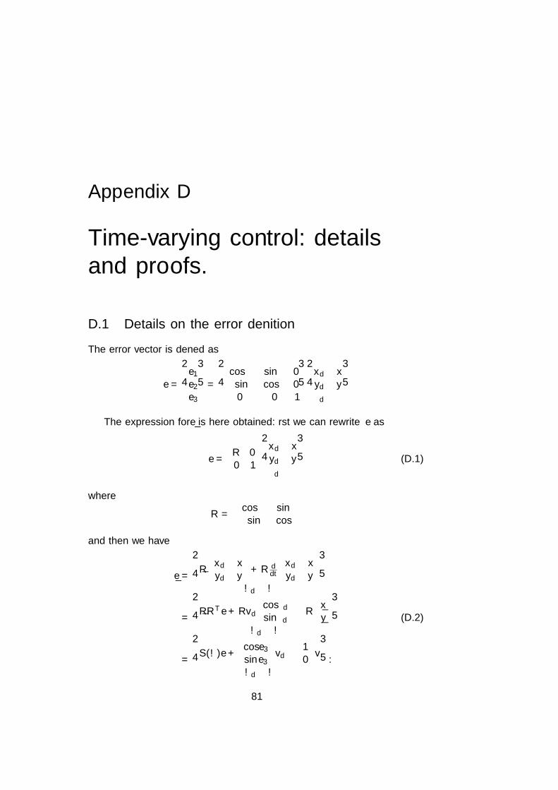
Appendix D
Time-varying control: detailsand proofs.
D.1 Details on the error definition
The error vector is defined as
e =
e1
e2
e3
=
cos θ sin θ 0− sin θ cos θ 0
0 0 1
xd − xyd − yθd − θ
The expression for e is here obtained: first we can rewrite e as
e =
[R 00 1
]xd − xyd − yθd − θ
(D.1)
where
R =
[cos θ sin θ− sin θ cos θ
]and then we have
e =
R [xd − xyd − y
]+R d
dt
[xd − xyd − y
]ωd − ω
=
RRT e+Rvd
[cos θdsin θd
]−R
[xy
]ωd − ω
=
S(ω)e+
[cos e3
sin e3
]vd −
[10
]v
ωd − ω
.(D.2)
81

82APPENDIX D. TIME-VARYING CONTROL: DETAILS AND PROOFS.
The last equality derives from the following relation:[cos θ sin θ− sin θ cos θ
] [cos θdsin θd
]=
[cos(θ − θd)sin(θd − θ)
](D.3)
and S(ω) is a skew-symmetric matrix:
S(ω) =
[0 ω−ω 0
]Substituting the defined inputs:
v = cos e3vd − u1
ω = ωd − u2
we find
e =
S(ωd)e− S(u2)e+
[0
sin e3
]vd +
[10
]u1
u2
=
0 ωd 0−ωd 0 0
0 0 0
e1
e2
e3
− 0 u2 0−u2 0 0
0 0 0
e1
e2
e3
+
0sin e3
0
vd +
1 00 00 1
[u1
u2
]
=
0 ωd 0−ωd 0 0
0 0 0
e1
e2
e3
+
0sin e3
0
vd +
1 −e2
0 e1
0 1
[u1
u2
].
(D.4)
D.2 Details and proof for section Time invariantbounds on the orientation
The input u2 is bounded and well defined. Indeed, it is bounded as long ase3 stays away from zero, and as e3 → 0 we have
lime3→0
sin e3
sin e3= lim
e3→0
sin e3
sin(e3ρ
) = ρ.
In order to exploit Barbalat Lemma, we need e3 to be uniformly continuous,so we have to check if its second derivative is bounded.The full expression for the second derivative of e3 is
e3 = u2 = −k2ρ
k3
[vde2
se3te3
+ vde2se3te3
+ vde2
( ddt
se3te3
)]−(1 + t2e3
)˙e3
where se3 = sin e3, te3 = tan e3 and the underlined term can be written as
d
dt
se3te3
=d
dt
(se3se3
)ce3 −
se3se3
se3˙e3
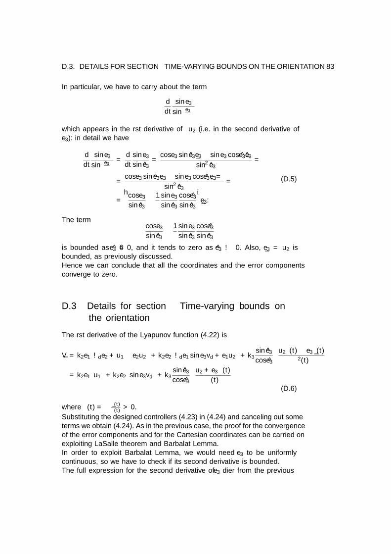
D.3. DETAILS FOR SECTION TIME-VARYING BOUNDS ON THE ORIENTATION 83
In particular, we have to carry about the term
d
dt
sin e3
sin(e3ρ
)which appears in the first derivative of u2 (i.e. in the second derivative ofe3): in detail we have
d
dt
sin e3
sin(e3ρ
) =d
dt
sin e3
sin e3=
cos e3 sin e3e3 − sin e3 cos e3˙e3
sin2 e3=
=cos e3 sin e3e3 − sin e3 cos e3e3/ρ
sin2 e3=
=[cos e3
sin e3− 1
ρ
sin e3
sin e3
cos e3
sin e3
]e3.
(D.5)
The termcos e3
sin e3− 1
ρ
sin e3
sin e3
cos e3
sin e3
is bounded as e3 6= 0, and it tends to zero as e3 → 0. Also, e3 = u2 isbounded, as previously discussed.Hence we can conclude that all the coordinates and the error componentsconverge to zero. �
D.3 Details for section Time-varying bounds onthe orientation
The first derivative of the Lyapunov function (4.22) is
V = k2e1
(ωde2 + u1 − e2u2
)+ k2e2
(ωde1 sin e3vd + e1u2
)+ k3
sin e3
cos e3
(u2ρ(t)− e3ρ(t)
ρ2(t)
)= k2e1
(u1
)+ k2e2
(sin e3vd
)+ k3
sin e3
cos e3
(u2 + e3α(t)
ρ(t)
)(D.6)
where α(t) = − ρ(t)ρ(t) > 0.
Substituting the designed controllers (4.23) in (4.24) and canceling out someterms we obtain (4.24). As in the previous case, the proof for the convergenceof the error components and for the Cartesian coordinates can be carried onexploiting LaSalle theorem and Barbalat Lemma.In order to exploit Barbalat Lemma, we would need e3 to be uniformlycontinuous, so we have to check if its second derivative is bounded.The full expression for the second derivative of e3 differ from the previous

84APPENDIX D. TIME-VARYING CONTROL: DETAILS AND PROOFS.
case because of the term which derive from the derivative of ρ = ρ(t) (nowtime-dependent):
e3 = u2 = −e3α(t)− k2ρ(t)
k3
[vde2
se3te3
+ vde2se3te3
+ vde2
( ddt
se3te3
)]−(1 + t2e3
)˙e3+
− k2ρ(t)
k3vde2
cos e3
sin e3sin e3 −
(1 + tan2 e3) ˙e3.
The derivative of e3 is
˙e3 =e3ρ(t) + e3ρ(t)
ρ2(t)=
u2
ρ(t)− e3
ρ(t)
ρ(t)
ρ(t)=
1
ρ(t)u2 + α(t)e3
and the underlined term, in this case, can be written as
d
dt
(sin e3
sin e3cos e3
)while
d
dt
sin e3
sin(e3ρ(t)
) =d
dt
sin e3
sin e3=
cos e3 sin e3e3 − sin e3 cos e3˙e3
sin2 e3=
=cos e3
sin e3u2 −
sin e3
sin e3
cos e3
sin e3
[ 1
ρ(t)u2 + α(t)e3
]=
=[cos e3
sin e3− 1
ρ(t)
sin e3
sin e3
cos e3
sin e3
]u2 + αe3
sin e3
sin e3
cos e3
sin e3
(D.7)
The termcos e3
sin e3− 1
ρ(t)
sin e3
sin e3
cos e3
sin e3
is bounded as e3 6= 0, and it tends to zero as e3 → 0. Also, e3 = u2 isbounded, as previously discussed. Also the term
e3sin e3
sin e3
cos e3
sin e3=
e3
sin e3
sin e3
sin e3cos e3
is well defined and bounded.
Appendix E
ROS Simulations: Code.
This appendix reports a brief description of the main parts of the code thatimplements the control laws in ROS environment.
E.1 Class UnicycleVelocityControllerNode
The UnicycleVelocityControllerNode class implements the controller node.
#include <ros/ros.h>
#include <turtlesim/Pose.h>
#include <turtlesim/Velocity.h>
#include "unicycle_velocity.hh"
Public Member Functions
• void getROSParameters()
gets all required parameters from the Parameter Server;
• void topicCallbackUnicycleStates(const turtlesim::Pose::ConstPtr&
msg): this is the call back, assuming that the node subscribes the uni-cycle states, that is the position;
• bool calculateUnicycleVel()
calculates the unicycle velocities and updates the unicycle position;
• void publishControlVel()
published the turtlesim::Velocity;
• std::vector<double> get unicycle pos()
returns the unicycle position, that is the Cartesian coordinates x, y, θ;
• std::vector<double> get unicycle vel()
returns the unicycle velocities v, ω.
85

86 APPENDIX E. ROS SIMULATIONS: CODE.
Public Attributes
• ros::NodeHandle n :this is the main access point to communications with the ROS system;
• ros::Publisher pub:topic to publish;
• ros::Subscriber sub:topic to subscribe;
• ros::Time last publish time:variable to stamp the last publish time;
• UnicycleVelocity unicycleVel:object instance of type UnicycleVelocity;
• bool initialized unicycleVel:set to true when unicycleVel is initialized;
• bool params OK:set to true if all required parameters are in the Parameter Server.
This documentation refers to the following files:
• include/unicycle velocity controller.hh
• src/unicycle velocity controller.cpp
E.2 Class UnicycleVelocity
The UnicycleVelocity class is responsible for calculating the unicycle velocitywhile implementing the designed control laws and the error transformationsfor prescribed performance constraints.
Public Member Functions
• void init(vector<double> initPos, vector<double> goalPos,
vector<double> controller parameters)
initializes the initial and goal unicycle positions, calculates the corre-sponding polar coordinates and initialized the tuning parameters;

E.2. CLASS UNICYCLEVELOCITY 87
• vector<double> calculateUnicycleVelocity(vector<double>
unicycle pose, double realTime)
calculates and returns the unicycle velocities implementing the controllaws designed with polar coordinates. This function calculates alsothe ρ function, the error transformation for prescribed performanceconstraints. It also performs the conversion to the polar coordinatesin order to define the input controllers v, ω;
• double getRho()
returns the ρ function;
• double getError()
return the error;
• bool isGoalReached()
returns true if the goal position is achieved.
This documentation refers to the following files:
• include/unicycle velocity.hh
• src/unicycle velocity.cpp