Potential and limits of numerical modelling forsupporting the development of HTS devices

Frederic Sirois1 and Francesco Grilli21Department of Electrical Engineering, Polytechnique Montreal, Montreal, Canada

2Institute for Technical Physics, Karlsruhe Institute of Technology, Karlsruhe, Germany

This is an author-created, un-copyedited version of an article accepted for publi-cation in Superconductor Science and Technology. The publisher is not responsiblefor any errors or omissions in this version of the manuscript or any version derivedfrom it. The Version of Record is available online at http://dx.doi.org/10.1088/0953-2048/28/4/043002.

Abstract

In this paper, we present a general review of the status of numericalmodelling applied to the design of high temperature superconductor (HTS)devices. The importance of this tool is emphasized at the beginning of thepaper, followed by formal definitions of the notions of models, numericalmethods and numerical models. The state-of-the-art models are listed, andthe main limitations of existing numerical models are reported. Those limi-tations are shown to concern two aspects: one the one hand, the numericalperformance (i.e. speed) of the methods themselves is not good enough yet;on the other hand, the availability of model file templates, material dataand benchmark problems is clearly insufficient. Paths for improving thoseelements are provided in the paper. Besides the technical aspects of theresearch to be further pursued, for instance in adaptive numerical meth-ods, most recommendations command for an increased collective effort forsharing files, data, codes and their documentation.

1 Introduction

The development of high temperature superconductor (HTS) devices has madesignificant progresses over the last few years, especially those based on second-generation (2G) HTS tapes. Prototypes are now close to commercial products, or

1

arX

iv:1

412.

2312

v3 [

cond

-mat

.sup

r-co

n] 2

9 M

ay 2

017

even already commercially available, as in the case of superconducting fault cur-rent limiters and cables. Although the cost of 2G HTS tapes makes devices stillexpensive, steady progress in materials science and in manufacturing processesbrings their price down every year. In parallel to materials improvements, it ispossible to further decrease the cost of devices by minimizing the quantity of HTSmaterial used in a given application. This is not an obvious exercise though, asHTS materials are highly nonlinear and present strong anisotropic field depen-dence. In most cases, only numerical methods allow relating power dissipation inHTS parts with their geometrical arrangement within the device.

In a general sense, numerical modelling in engineering is a mature discipline.Numerical methods such as the finite element method and others are well knownand documented in the literature. However, each engineering application has itsown specificities, which one can take advantage of in order to simplify the problemand reduce the associated computational size. This is of tremendous importance ina context of device optimization, where hundreds or even thousands of parametricsimulations are often required. This is also the reason why there are dozens ofvariants of the established numerical methods in the literature.

Combined to this variety of applications, the materials used in the various en-gineering devices introduce nonlinearities that significantly affect the numericalbehaviour of the problem, sometimes to the point where the mathematical theorybehind the numerical method must be revisited. This is particularly true in thecase of superconducting materials, where the disappearance of the resistivity atlow current leads to singular behaviour of the electromagnetic fields (moving cur-rent fronts). In practice, this does not mean classical methods cannot handle theproblem, but rather than blindly applying classical methods is by far sub-optimaland may lead to computation times that are much longer than required.

In this contribution, we start by reviewing briefly the modelling approchesand the numerical methods that are commonly used to solve problems involvingHTS materials. These problems usually represent a portion of an HTS device.After reviewing the most common models and numerical methods, their limitsare briefly outlined, in order to define working paths towards numerical methodsthat are specifically tailored for problems involving superconducting materials. Inparticular, we discuss the issue of necessary degrees of freedom and adaptive finiteelement methods that allow placing the unknowns where they are really needed. Itis shown that there is still a significant potential for making numerical simulationsfaster and therefore developing fast optimization tools that would significantlyspeed up HTS devices development.

Finally, we emphasize the need for a systematic benchmarking of the variousmodels and methods, ranging from detailed physical models to more macroscopiccircuit models. Only few existing benchmarks exist at the moment, so the whole

2

HTS community (industrialists and academics) is invited to contribute to thedevelopment of new benchmarks that are representative of the state of the art ofHTS device engineering. These benchmarks will greatly help focus the R&D effortof the numerical modelling community towards the most relevant approaches.

2 Context and need for numerical modelling

If we look at the status of development of HTS devices, we can see a steadyprogression over the last few years. Many prototypes have been built, and somecommercial devices already exist. While the need to reduce the cost of 2G HTSwires is widely recognized [1] and possible solutions to reach that goal proposed [2],other important practical aspects need to be considered for the manufacturing ofreal applications, for example the cost and reliability of cooling systems or themixture of high voltages and cryogenic temperatures, just to cite a few.

Regardless of the specific engineering problem to solve, numerical modelling isone common tool that comes to the rescue of engineers and scientists. Not onlydoes numerical modelling allow deepening the understanding of the behaviour of adevice under various excitations, but it also allows optimizing its performance, andin turn reducing its cost by 1) making the best use of materials and components,and 2) reducing the number of prototypes during the development stage. Thisis particularly true for devices based on HTS materials because their highly non-linear and often anisotropic behaviour makes it difficult to intuitively find the bestoperational configurations.

Beyond the behaviour and the optimization of the device itself, numerical mod-elling can also be used to predict how a device will perform in its environment oncein operation. In other words, a device rarely operates alone, but acts on its neigh-bourhood as one element of a system. A good example of this is a superconductingpower device installed in a power system. Since the final performance of a device isconditioned by the system in which it is installed, it is of the highest importance todevelop device models that are compatible with system simulators. These devicemodels, most often expressed in terms of electric circuits, are in general simplerthan those used for device optimization, for instance finite element models, butthey are nonetheless essential for comparing the performance of competing tech-nologies in a given system. An interesting discussion about the requirements formulti-scale modelling of magnetic devices (mostly electric motors in this case) ispresented in [3].

In this paper we limit the discussion to numerical tools related to electromag-netic problems involving superconductors, knowing that we could also talk aboutmany other types of physics (thermal, mechanical, etc.). The main reason for thischoice is that, without the intention of minimizing the difficulties associated to

3

other physics, we believe that electromagnetics is probably the most open mod-elling issue in the area of HTS materials. It will be seen that numerous choicesof mathematical formulations exists in electromagnetics, and no obvious criteriaallow identifying a “best method”. Despite this deliberate narrowing of the topic,the major part of this paper applies to numerical modelling in general.

3 Models, numerical methods and numerical mod-

els

3.1 Definitions and overview

It is beyond the scope of this paper to give a detailed list of all the numericaltools for modelling HTS. These can be found in dedicated publications [4, 5, 6].In this section we would rather like to give an overview of the general principlesof and differences between the various models and numerical methods availablein the literature and applicable to HTS materials. We start with the distinctionbetween models and numerical methods, two terms that are often interchanged inan improper way.

A model is a mathematical representation of a physical (or other) behavior,based on relevant hypothesis and simplifying assumptions. For example, in thecase of superconductors, we have the power-law model (PLM) and the criticalstate model (CSM): the former considers flux creep, whereas the latter does not.Another example is Maxwell’s equations, which provide a mathematical represen-tation to model electromagnetic fields, but can be written in several ways depend-ing on what matters for a specific problem, e.g. with or without the displacementcurrent term, written in terms of time harmonics (i.e. d/dt→ jω) or directly withthe time derivative terms, as required for superconductors since those materialsare non-linear and their state evolve in time.

A numerical method consists of a systematic approach to 1) express a model ina discrete form, 2) generate a system of equations that approximates this model,and 3) solve the resulting system of equations. There exists many examples ofnumerical methods, for instance the finite element method, the finite differencemethod, etc. (see section 3.4 for details). The choice of a given numerical methodshould have no impact of the physical meaning of the solution: all numericalmethods should theoretically converge towards the same result as the discretizationis progressively refined. On the other hand, the choice of a particular numericalmethod can have a drastic impact on the computation time required to solve themodel.

Finally, we define a numerical model as the combination of a model and anumerical method. The model establishes the physical representativeness of the

4

solution, whereas the numerical method defines the accuracy to which the modelcan be approximated, and determines in good part the computational speed. How-ever, since the model is a trade-off between physical relevance and complexity, thechoice of a model has also an implicit impact on the overall computation time.

3.2 Choice of a model

The quality of a model highly relies on the “smartness” of the assumptions behindit. In other words, if the model is “bad” (in terms of physical representativeness),the solution will be “bad”, regardless of the numerical method chosen to solve it.

Of course, the definition of “bad” is highly function of the modelling objectives.Typical considerations that need to be taken into account when choosing a modelare:

• Is it necessary to simulate the whole device? Can symmetries/periodicitiesbe used, or dimensionality of the problem be reduced (e.g. from 3-D to 2-Dor 2.5-D)?

• What level of physical representativeness is really required? Is a simple trendprediction sufficient? How accurate are the experimental results to validatethe model?

• Is it necessary to look in detail at local results (field, current density), ordoes one just need global quantities as output (e.g. AC losses)? What arethe needs of industrialists and manufacturers vs. those of academics?

Over the years, many “smart” models have been developed in the HTS appliedsuperconductivity community. The majority of models involving 2G HTS coatedconductors involve dimensional reduction, for instance:

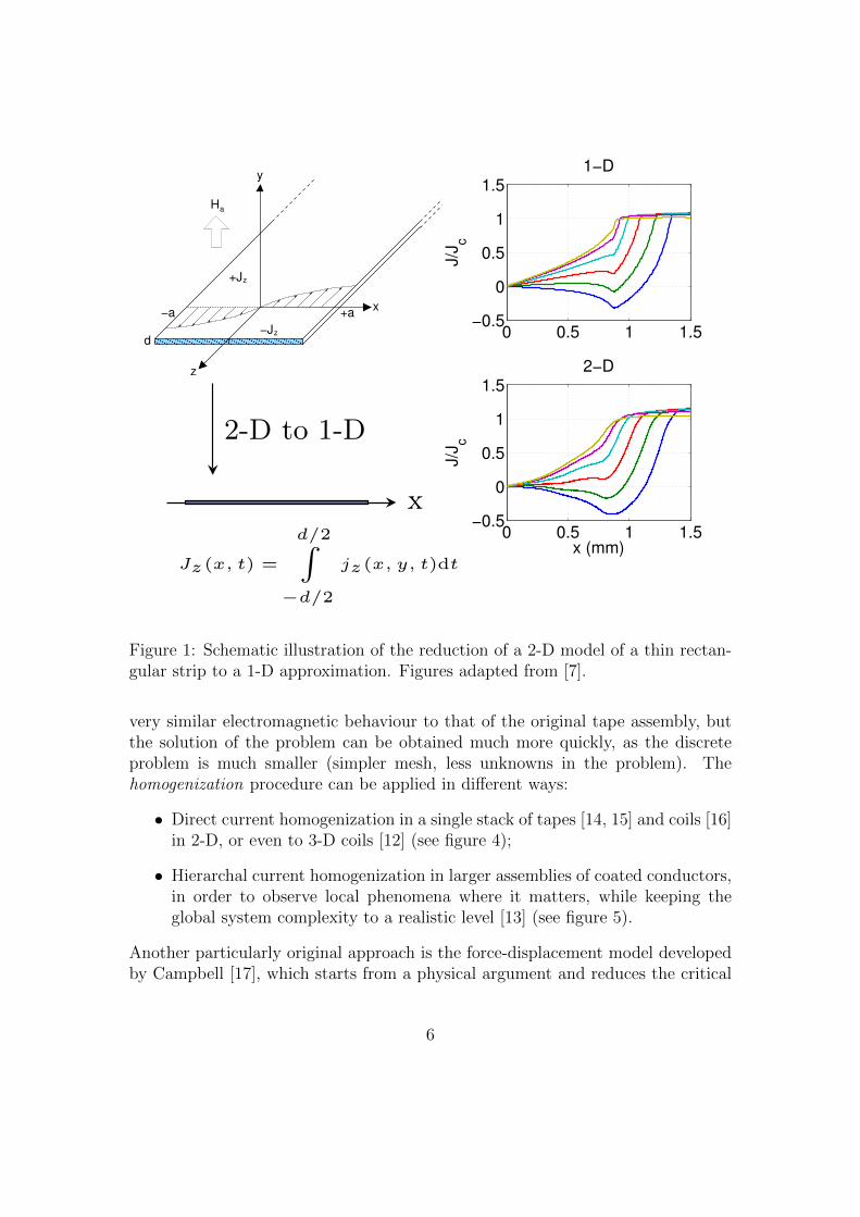
• Infinitely thin film approximation of 2G HTS coated conductors [7] (seefigure 1);

• 3-D modelling of 2-layer power cables or Roebel cables using a “2.5-D” model:infinitely thin tapes in a 3-D space [8, 9] (see figure 2);

• Use of thin interface conditions to reproduce the thermal and electrical be-haviour of buffer layers in coated conductors [10] (see figure 3).

In some cases, especially when many coated conductors are present and stackedon top of each other, one can homogenize the cross section of the stack, getting ridof the geometry of the individual tapes, while preserving their physical behaviourby means of special current constraints. The homogenized conductor has thus a

5

+a

z+J

−Jz

z

H

−a

a

d

y

x

0 0.5 1 1.5−0.5

0

0.5

1

1.51−D

J/J

c

0 0.5 1 1.5−0.5

0

0.5

1

1.52−D

x (mm)

J/J

c

x

Jz(x, t) =

d/2∫−d/2

jz(x, y, t)dt

2-D to 1-D

Figure 1: Schematic illustration of the reduction of a 2-D model of a thin rectan-gular strip to a 1-D approximation. Figures adapted from [7].

very similar electromagnetic behaviour to that of the original tape assembly, butthe solution of the problem can be obtained much more quickly, as the discreteproblem is much smaller (simpler mesh, less unknowns in the problem). Thehomogenization procedure can be applied in different ways:

• Direct current homogenization in a single stack of tapes [14, 15] and coils [16]in 2-D, or even to 3-D coils [12] (see figure 4);

• Hierarchal current homogenization in larger assemblies of coated conductors,in order to observe local phenomena where it matters, while keeping theglobal system complexity to a realistic level [13] (see figure 5).

Another particularly original approach is the force-displacement model developedby Campbell [17], which starts from a physical argument and reduces the critical

6

Figure 2: 3-D modelling of 2-layer spiraled cables made of 2G HTS coated con-ductors using a “2.5-D” model that considers the tapes as infinitely thin, whileallowing the current to flow in the transversal direction (y-direction in the figure).Exemplary current patterns in the tapes of the inner and outer layers are shown.Figures adapted from [8].

state model to a static problem that can be solved in a single shot, without theneed of time stepping algorithms.

3.3 Formulation of a model

Models are expressed as mathematical equations, which can be of different types,e.g. ordinary and/or partial differential equations (ODEs / PDEs), integral equa-tions (IEs), mixture of PDEs and IEs, algebraic constraints, etc. The exactchoice/combination of equations is often referred to as a formulation.

In computational electromagnetics, which forms the basis for the analysis ofsuperconductors, there exists many such formulations. This variety comes fromthe many options of state variables that one can choose to put a given problemin mathematical form [4]. For instance, one could choose to express the problemdirectly in terms of the field variables (e.g. the magnetic field H and/or the electric

7

Figure 3: Temperature distribution a 2G HTS coated conductor computed with afull 3-D model (left) and with a thin interface condition in a mixed dimensional3-D/2-D model (right). Figures adapted from [10] and a presentation of the sameauthors [11].

field E), or in terms of potentials (A− V , T− Ω, and many variants of these).While the choice of a formulation is in principle arbitrary, certain models are

more naturally expressed in terms of a specific formulation. As an example, Camp-bell’s force-displacement method [17] is naturally written in terms of the magneticvector potential A, so not using the A − V formulation in this case would becumbersome.

Another example that may dictate the use of a potential formulation is whenone needs to couple an electromagnetic model with an electric circuit [18, 19]. Thiscoupling requires computing global quantities, such as flux linkages or inductances,which is straightforward to do with a potential formulation, but harder whenworking in terms of field variables. On the other hand, it is often easier to writethe model in terms of field variables, as it makes everything more intuitive tointerpret.

In general, there is no clear choice when choosing a formulation, as it dependson many factors, including some of numerical nature. Indeed, some formulationswill generate more unknowns in the numerical problem, but may in turn be morestable (numerically speaking) than a less memory demanding formulation.

8

Figure 4: Top: concept of homogenization for a stack of tapes carrying the sametransport current. Bottom: magnetic flux density distribution (at different instantsof the sinusoidal current) calculated for the full geometry (16 stacked tapes) andwith homogenization. Figures adapted from [12].

9

Figure 5: Hierarchal, 3-D multi-scale tape model for the electro-magnetic-thermalbehavior of quench in coils. Figures adapted from [13].

3.4 Choice of a numerical method

A given model can be solved by different numerical methods. Once again, it is outof the scope of this paper to review all existing numerical methods, but table 1gives a brief summary of those encountered in modelling devices involving HTSmaterials. Acronyms used in table 1 are common, but not necessarily the onlyones used in literature.

Each method typically has many variants, which we shall not refer to in thispaper. However, there is one common point among all numerical methods: theirrole is to provide a discrete approximation of the exact solution of the model,whichever formulation one chooses to describe the original problem. This requiresto discretize a priori the geometry of the problem, either as a grid or as a mesh,depending of the method to be used afterwards. The dimension of this grid/mesh,i.e. number of nodes or edges in it, is directly related to the number of degrees offreedom (DOFs, or more simply, unknowns) of the problem. The number of DOFsobviously has a major impact on the computation time and memory requirements.

3.4.1 Solution of the model in its strong form

A pure strong form solution means that one solves a pointwise version of thedifferential or integral equations defining the model exactly at every grid point (for

10

FD and MoM). These types of methods are often referred to as point collocationmethods, as one freely interpolates the pointwise solution between each point ofthe grid to form a complete solution in space. A widely used strong form solutionin applied superconductivity is the so-called “Brandt method”, which is in facta method of moments (MoM) based on integral equations. The method is welldescribed in [20], and has been used by many authors over the years.

It is good to mention that, because integral equations (involving Green func-tions, which are defined everywhere in space) are by nature smoother than differ-ential equations (defined only locally), approximation errors naturally tend to bebetter distributed with the MoM than with FD. This is not a strict rule though, asGreen functions may involve singularities that can lead to very large errors whenthey are not treated properly.

Although strong form methods are very intuitive and among the easiest nu-merical methods to program, they have a very important drawback: they do notprovide good control on the approximation error over the domain. In addition, forcomplex geometric shapes, a simple grid discretization often provides a very poorapproximation of the boundaries of the different geometric objects.

One particularly important case of strong form methods is FV. This methodis somewhat midway between FD and FE (see next section), since the equationsto solve involve integrals of fluxes (e.g. electric currents) crossing the boundary ofevery elements (control volumes) of the mesh. This integration procedure recallsthe weak form encountered in FE, although equations are still solved in a pointwisemanner, so it remains in the category of point collocation methods. The majoradvantage of this method is that it implicitly makes the flux variable divergence-free by equating the flux integrals on every common edge (in 2-D) of face (in3-D) of mesh elements. Although this method is widely used in fluid mechanicsfor incompressible flow models, it has scarcely been applied to electromagneticproblems [21].

In brief, strong form methods, despite their simplicity of implementation, oftenpresent limitations when it comes to complex geometries or large scale problems.They are interesting approches to quickly start an investigation, but in general, itseems preferable to opt for a weak form or energy functionnal approach.

3.4.2 Solution of a weak form of the model

Instead of solving very strictly the equations defining the model, an interestingstrategy is to multiply the original equations by weighting functions (often calledtest functions), and then integrate those modified equations over the problemdomain. The modified equations are said to be written in weak form. Althoughthis modifies the original system of equations, it also brings up the option ofweighting the numerical error over the whole domain, which is impossible with

11

point collocation methods. In other words, the numerical solutions one can find inthis way do not provide optimal pointwise accuracy, but they minimize the erroron the overall domain, according to the chosen weighting pattern. This class ofmethod is called weighted residuals, and it entirely relies on functional analysis inits mathematical theory.

The basic principle of all weighted residual methods is to define shape functionsthat are used to approximate in a piecewise manner the continuous solution of aproblem on a discrete mesh. One usually refers to FE (finite elements) to describethis method, although the term is generally reserved for the case where one startsfrom PDEs to write the weak form. When dealing with integral equations, it ispossible to apply the same principle to get an equation system. In this paper,we use the IE acronym to distinguish it from FE. A particular case of IE is BE(boundary elements), which is expressed exactly as IE, except that we apply adimensionality reduction at the very beginning of the procedure in order to reducethe mesh complexity (from 3-D to 2-D, or from 2-D to 1-D). However, BE do notapply well to nonlinear problems, such as those with superconductors, and we shallnot discuss this method here.

Among all numerical methods used in engineering for design and analysis pur-poses, FE is by far the most popular one. This is due to the generality of its for-mulation, its ability to model geometries of complex shapes in any dimension (1-D,2-D, 3-D), and its relative simplicity of use, especially through many commercialsoftware packages. This observation also holds true in the applied superconduc-tivity community.

3.4.3 Minimization of an energy functional

One can define a third family of numerical method based on the minimization ofan energy functional. This approach is very intuitive, since it consists in defining afunctional that relates the total energy of a system (or a variation of energy withrespect to some initial conditions) with the variables that define the state of thissystem, e.g. potentials, field variables, source terms, etc. It allows more freedomin the way one chooses the shape functions used to approximate the solution. Italso allows solving classes of problems that would be quite hard to solve otherwise,namely the critical state problem, which is singular in its pure form, and thereforecan only be approximated to some extent when using a classical electromagneticformulation. Although at first sight this approach requires less mathematical for-malism than strictly applying the finite element method, the process of minimizinga functional in order to obtain a well-posed discrete equation system requires goodskills in functional analysis and optimization algorithms. Also, since it is generallybased on integral equations, its use in 3-D problems is often too time consumingto be useful.

12

In the HTS community, the use of the MoE method was first introduced byBossavit [22], then formalized by Prigozhin [23], who provided a systematic ap-proach to solve the J distribution in HTS domains based on the critical state model.A variant of the method, called MMEV, was later introduced by Sanchez [24] andgeneralized by Pardo [25] to include current constraints.

3.4.4 Differential vs. integral methods

It is interesting to look at numerical methods according to the way basic equationsare written. These can be expressed either as differential or integral equations(before any averaging, transformation to weak form, etc.). This very fundamentalchoice has a huge impact on the numerical performance of the method.

In the case of differential equations, the solution over one element is deter-mined solely by the values at the boundary of this element. Information is thuspropagated from element to element through their common boundaries, and even-tually, it is the boundary conditions imposed at the periphery of the model thatestablishes the complete solution. The consequence of this is that the connectivitybetween the degrees of freedom is only function of the nodes (in case of nodalbase functions) or edges (in case of vector base functions) shared by neighbouringelements, leading to sparse matrix patterns, and a more or less linear relationshipbetween the number of DOFs and the memory requirements.

In the case of integral equations, things are radically different: in this case, allregions containing source terms contribute to the solution on other elements. Forinstance, one can think about the Biot-Savart formula, which allows computingfield values anywhere in space, even if the source term is a punctual current. Thismeans that each degree of freedom in the problem is related to the others, andthe resulting matrix pattern is a full one. The consequence is that the memoryrequirements grows at least with the square of the number of DOFs. In counter-part, there is no more need for boundary conditions anywhere in the model, butit is not so easy in practice to take advantage of this fact.

A particular aspect of computational electromagnetism is that air regions,which contain no source term, still need to be meshed when using differentialmethods, whereas they can be discarded when using integral methods. Overall,the resulting requirement in term of memory and DOFs depends on the proportionof mesh that can be avoided in a given problem. In general tough, large problemsscale better with differential methods, and as soon as the number of DOFs exceedsa few thousands (which is very common in models of a practical device), differ-ential methods seem to be the only practical way in order to perform numericalsimulations, as shown in figure 6 [26].

13

Table 1: Summary of families of numerical methods and their main features.Acronyms stand for: Finite Differences (FD), Finite Volumes (FV), Finite Ele-ments (FE), Method of Moments (MoM), Integral Equations (IE), Boundary Ele-ments (BE), Minimization of Energy (MoE), Minimum Magnetic Energy Variation(MMEV).

Form of Strong form Strong form Weak form Energy Matrixequations (averaged) functional struct.

Differential FD FV FE SparseIntegral MoM IE, BE∗ MoE/MMEV Full

Discretization Grid Mesh Mesh MeshType of Point Point Weighted Error mini-method collocation collocation residuals mization

∗ Hardly applicable to nonlinear problems.

100 1000 10000100

101

102

103

104

105

tc ∝ n1.7e

tc ∝ n3.6e

Number of elements, ne

Com

putation

time,

t c(s)

Finite elementsMethod of Moments

Figure 6: Example of computational time growth of a differential method (FE)and an integral method (MoM) as the number of elements in a reference conductor.Figure adapted from [26].

14

Table 2: Typical numbers of DOFs and solution time of time-dependent FEMmodels.

Dimension # of DOFs Solution time

2-D 1,000 to >100,000 Minutes to hours

3-D 100,000 to >1,000,000 Hours to days

3.5 Computational performance of numerical methods

It is extremely difficult to provide a general relationship relating the computationtime (tc) of a numerical method to the number of DOFs (N) in a given problem:the relationship would typically take the form tc = a + N q, where q > 1 is theonly thing one can be sure of (q > 3 is common with integral methods). The exactrelationship depends on the algorithm chosen to solve the problem, the need forNewton iterations (if problem is nonlinear), the conditioning of the matrix, whichmay require pre-processing of the linear system, etc. Also, if the problem is verylarge, limitations in computer memory may dictate the use of an iterative solver,which may require many iterations to converge. Therefore, here we limit ourselvesto ball park figures of solution times obtained for typical electromagnetic problemsinvolving HTS devices (e.g. AC losses vs. transport current) and solved by FE, asshown in table 2.

These computational times, although relatively long in general, might be ac-ceptable for helping understand the behaviour of the simulated device, but they arestill too long to be used for optimizing devices, which typically require hundredsor even thousands of simulations.

3.6 Is there any optimal choice for modelling HTS devices?

Many numerical models for simulating the electromagnetic behaviour of supercon-ductors have been developed in the past, but they have been seldom compared.In this section, we briefly summarize the work of the few authors who have donesuch comparisons.

Sykulski et al. [27] modelled AC losses in HTS as a highly non-linear diffusionprocess (1-D only). They presented formulations in terms of both H and E andthey argued, using dimensional analysis, that working with E is numerically moreefficient. Results calculated using a finite-difference scheme were shown.

Vinot et al. [28] compared the A − V , T − Ω and E formulations within theFEM software package Flux3D (now simply called Flux [29]). They found thatthe T − Ω is the most efficient, although the E formulation can be used as well,provided that the index n in the power-law resistivity of the superconductor is not

15

too high (n < 20); on the other hand, the A formulation proved to be not verystable. Always in the framework of the Flux software, a table presenting a roughassessment of the A − V and T − Ω formulations for 2-D and 3-D problems isgiven in [30], although no detailed comparison is made in the paper.

In [31] the authors compare speed and accuracy of two FEM software packagesfor the 2-D simulation of a superconductor with rectangular cross-section in avariety of working conditions. In particular, they compare the A− V formulationwith second-order nodal elements implemented in FLUX and the H formulationwith first-order edge elements implemented in COMSOL. It was shown that bothprograms gave very similar results in terms of AC losses when the current or theapplied field are sufficiently large; however, some discrepancy in the result wasobserved for low fields and current. The adaptive time integration algorithm usedby COMSOL, based on [32] seems much more efficient than that used by Flux,except at large magnetic fields.

More recently, Lahtinen et al. [33] compared three self-programmed 2-D elec-tromagnetic formulations (H, T−φ and, A−V −J) that they programmed them-selves in a common computational environment. Their analysis focused on manyaspects of the problem, and different methods performed differently depending onthe context. Nevertheless, they concluded that the A−V − J formulation seemedto be the fastest one when the most general cases were considered (combinationof AC currents and AC fields).

The few above-mentioned references are not numerous enough to conclude any-thing about the best numerical models or formulations for a given use. Most com-parison were realized in a different context (different problems, dimensionality,constraints, etc.), which might explain why conclusions differ so much, in partic-ular regarding the choice of the most performant formulation. This indicates alack in benchmarking, i.e. well defined reference problems that can be used tocompare the numerical performances of various codes, either commercial or home-made, based on different formulations and numerical methods, and potentiallyimplemented on different platforms. Although benchmarks do not directly pro-vide solutions to the modelling difficulties, they certainly help focus the researchefforts and make faster progress, as demonstrated over the years in the T.E.A.M.project initiated about 30 years ago by the magnetic modelling community [34].

As far as the authors know, a comprehensive review of the various numericalmodels developed for modelling HTS devices does not exist, but a nice summaryis given in [4], in which a short section dedicated to the comparison of differentnumerical methods also reveals the lack of a proper benchmarking.

16

3.7 Availability of numerical models for modelling HTSdevices

Besides the performance of numerical models themselves, an important aspect toconsider is their availability. Simulators for HTS devices can be found both ashome-made proprietary codes ([35], [36] and many others) as well as commercialcodes (COMSOL, Flux, ANSYS, JMAG, MagNet, FlexPDE, etc.). There are prosand cons in both cases:

• Commercial codes are better supported, but they are generally expensive topurchase and maintain over time;

• Home-made codes are more flexible than commercial codes, which is impor-tant in a field in development, but they are generally poorly documented.

Besides the simulation tools themselves, it is worth noting that typical modelfiles are generally difficult to find. Typically, everybody has to create his/her ownmodels from scratch, as no file template is publicly available. This is true bothfor finite element models and circuit models for power system simulators (i.e. nolibrary of “HTS devices” exists yet).

These problems lead to a substantial bottleneck: because of the little access tomodel files, and to a lesser extent, to the simulators, the modelling of HTS devicesremains a specialized topic, mostly accessible to graduate students or researchers,and HTS devices remain an obscure object for most manufacturers and powerutilities.

4 Accuracy of current numerical models

A fundamental part of the numerical model is the material model itself. In prob-lems involving superconductors, this generally means that a good model for Jcis required, which can take various forms. For instance, in the case of quenchproblems, one models the temperature dependence Jc(T ) between the operatingtemperature and room temperature, which is not always easy to measure, espe-cially at high J values. However, this is more an experimental characterizationproblem than a modelling one [37].

In the case of applications not involving quench, most models are used tocompute AC losses, and the simplest materials models are based on a constantvalue for Jc, which is usually determined by dividing the measured critical currentby the cross-section of the wire/tape. However, wires and tapes used in realapplications, such as coils and cables, are exposed to a magnetic induction B that isgenerally too high to be negligible. An accurate description of the superconductor’s

17

properties should therefore include a Jc(B) dependence, such as the simple oneproposed by Kim for hard superconductors in the 1960s [38]

Jc =Jc0

1 + |B|B0

, (1)

where Jc0 and B0 are characteristic parameters.Increasingly complicated Jc(B) formulas have been proposed, in order to take

into account the peculiarities of the in-field behaviour, most notably the depen-dence of Jc on the orientation of the magnetic field (see for example [39]). For thispurpose, a commonly used formula is the elliptical field-dependence

Jc(B⊥, B‖) =Jc0(

1 +

√B2

⊥+B2‖/γ

2

B0

)β. (2)

where Jc depends on the components of the magnetic field parallel and perpen-dicular to the flat face of the tape by means of the anisotropy parameter γ (withγ > 1). The cut-off value at low fields and the rapidity of the Jc reduction are givenby B0 and β, respectively. With the introduction of artificial pinning centers in thesuperconductor, the simple description given by the four-parameter expression (2)is no longer adequate; more elaborated expressions are necessary to describe theexperimentally observed behavior of the samples [40].

Generally speaking, however, once the Jc(B) form is known, its introductioninto numerical models does not present particular difficulties, since the magneticfield variable is directly available (as in the H-formulation) or easily obtainablefrom the utilized state variables (as in potential formulations). The same commentholds true for the Jc(T ) relationship.

Another factor that is sometimes necessary to take into account for having anaccurate model, is the spatial variation of Jc inside the superconducting tape, mostnotably along the width of superconducting tapes. This can be the consequenceof the manufacturing process, see for example [41] and [42] for first and secondgeneration HTS tapes. Several techniques can be used to extract this lateraldependence. The use of a position-dependent Jc for AC loss calculations can oftengive a better agreement with experimental data [43, 44]. A position-dependentJc can also be used to simulate the presence of defects [45, 46]. Similarly tothe Jc(B) dependence, once the form for the spatial variation of Jc is chosen, itsimplementation in the model does not present particular obstacles.

Figures 7, 9 and 8 show practical cases of simulations involving HTS modelsthat have been compared to measurements. In all cases, the agreement withexperimental data is very good. This shows that, as long as good material modelsare available and that one chooses a numerical model that considers the relevant

18

physical properties of the problem, it is possible to achieve very good accuracy inthe predictions, generally within 20% of the experimental values.

It is worth mentioning that, although the implementation of complicated ma-terial properties in simulators is not difficult as such, obtaining those materialsproperties is not always easy, especially if one requires a model that depends onvarious physical parameters (field amplitude and angle, temperature, spatial in-homogeneity). A good material characterization may require a lot of a prioridedicated experiments, thus a lot of time and resources. An increased sharing ofmaterials data would therefore help a lot modellers to achieve their goals.

Besides the cases described above, there still remains some challenges in mate-rials modelling though, in particular with 3-D geometries, for instance when fluxcutting occurs [4]. In an attempt to solve this problem, Badıa-Majos and Lopezhave developed a general framework for handling the E − J characteristic at amacroscopic level in a 3-D environment, without having to consider explicitly themicroscopic effects related to vortex dynamics, but which still reproduce all rel-evant experimental phenomena such as flux cutting, flux flow and magneticallyanisotropic critical current densities [50]. Another case of interest is when thematerials operate in self-field conditions and one needs to extract a truly localJc(B) dependence, whereas the experiments only provide a Jc as a function of theapplied field Ha (see for example [51] and references therein).

10 10010−7

10−6

10−5

10−4

10−3

10−2

current amplitude (A)

AC

losses

(J/cycle/m)

measuredHTSsubstratetotal

HTSsubstrate

Figure 7: FEM and experimental results for the AC loss components in a 1 cm-wide RABiTS YBCO tape (Ic = 330 A) carrying an AC transport current [47].Here the substrate exhibits ferromagnetic hysteretic losses that were added to theHTS losses in order to reproduce accurately the total losses of the tape.

19

Figure 8: Calculated and measured AC losses in stacked pancakes of coils made ofHTS coated conductors. The number of pancakes are 1, 2, 3 and 4 in the arrowdirection. The agreement with experimental data is very good. Figure from [48].

102 10310−3

10−2

10−1

current (A)

AC

losses

(J/m

)

4 mm meas.4 mm FEM20 mm meas.20 mm FEM

Figure 9: Measured and calculated transport AC losses for Roebel cable coilswith separation between the turns of 4 and 20 mm separation between the turns.The simulation results include an anisotropic angular dependence of Jc and the3-D simulation of the copper contact for current injection, which influences themeasured losses [49].

20

5 Paths towards improvement

Based on the above review of the situation, we can summarize the situation ofmodelling in applied superconductivity as follows:

• numerous numerical models exists for modelling HTS devices; however, ma-terial data are not widely available;

• numerical simulators for HTS devices are either costly or poorly documented/supported;

• model files are even less available and require a lot of expertise to build fromscratch, which prevents potential users to simulate HTS devices in theircontext of application;

• the calculation times required for running models is still too long to be ofpractical use in device optimization;

• the accuracy of the solutions obtained by numerical simulation can be verygood, as long as one has access to good material models.

Therefore, besides the improvement of the models themselves, this essentiallydefines two paths for improvement, i.e.

1. improvement of the computational performances of the numerical simulators;

2. improvement of the availability and easiness-of-use of simulation tools (in-cluding model files and materials data).

Each path for improvement is discussed in more detail in the two sections thatfollow.

5.1 Computational performance of numerical simulators

As mentioned earlier in this article, there are two ingredients required for devisinga good numerical simulator: 1) a good model, and 2) a suitable numerical methodto solve this model. The choice of a proper model highly depends on the objectivesought. New models will certainly be proposed over the years, and there is plentyof room for smart modelling ideas in the applied superconductivity community(new ideas for dimensional reductions, symmetries, mathematical formulations,etc.).

Once the model is chosen, the main aspect that governs the computationalperformances is the choice of the numerical method used to solve the discretizedversion of the model. From a practical point of view, for a given level of accu-racy (determined by the user), the “optimal” numerical method should be able

21

to minimize the number of degrees of freedom (DOFs) in the problem. Since thenumber of DOFs (or unknowns) is the main factor affecting the simulation time,minimizing it is the key issue for achieving fast simulations.

Unfortunately, current simulators do not allow this optimization: they let theuser choose its discretization (e.g. the mesh) in an arbitrary manner. In addition,since the current and flux profiles in superconducting materials are singular andexhibit sharp fronts or cusps that move with time, there is a need to finely meshall superconducting domains (otherwise one would completely miss the physics),which increases dramatically the number of DOFs to solve for (see figure 10 as anexample). In addition, due to the strong nonlinearity of the problems, there is aneed for very small time steps in order to ensure the convergence of the solver.Therefore, even the simplest problems require many DOFs both in space and time,and the computational time explodes quickly as devices get complicated.

The solution to this problem is to use adaptivity in order to refine (or unrefine)the mesh (or the time step) as the solution progresses. The principle of adaptivityis best illustrated from a simple example: the superconducting slab in a parallelmagnetic field, as illustrated in figure 10. This figure was obtained by solvingthe electromagnetic problem on a very fine mesh (2000 DOFs). It shows thesolution for the current density J at an arbitrary time instant of a sinusoidalexcitation. One can see that we could approximate this solution to a great accuracyusing only a few well positioned linear segments. Of course, the position of thevertices defining those line segments has to be adjusted as the front moves, whichrequires an automated rule to reposition them. For this purpose, one requireserror estimators, which are the missing tool in today’s simulators. Indeed, errorestimators evaluate where in space (and/or time) the error is large, which allowsdeciding where to refine (or unrefine) the mesh. Of course, the computational costof the error estimator and of the mesh operations has to be as low as possible, butas a general rule, it is quicker (and less memory demanding) to solve a few smallproblems (the initial mesh and a few refinements) instead of a very big problemthat blindly provides good resolution everywhere, including where it is not needed.

Generic adaptive methods to adapt solutions in time exist for systems of ODEs(e.g. see [32]), but they are far less popular for PDE, which involve handling meshadaption. In fluid mechanics and some other fields, those methods have beenstudied to some extent, but they are in their infancy in computational electromag-netism. As this is a highly technical field, there is a need for the HTS modellingcommunity to increase its interactions with experts in the field, including math-ematicians and specialists in numerical analysis. The development of an errorestimator dedicated to superconductors would be highly beneficial for this com-munity. Testing of error estimators and adaptive techniques is expected to beeasier in home-made codes, as they are more flexible than commercial codes, but

22

x

y

z

B (t)

a0

a

B (t)a

-a

HTS slab

−1 −0.5 0 0.5 1−1

−0.5

0

0.5

1

x/a

J/J

c

Figure 10: Left: An infinite superconducting slab of width 2a subjected to asinusoidally varying magnetic field parallel to its surface; Right: Current densityprofile along the x-axis, after 2 complete cycles of full penetration of the field. The11 red line segments in red, when properly located, are sufficient to approximatethe current profile, despite the fact that it took approximately 1000 fixed segmentsin the finite element mesh in order to obtain the same accuracy (in blue) when noadaptivity of the mesh is used.

hopefully the specialized techniques will make their way to commercial codes asthey get mature, making them even more accessible to device designers from theindustry.

Finally, it is important to mention that more general progress in parallel com-puting and numerical solvers for linear systems to solve large problems will helpincrease computational speed over time. This topic is entirely in the hands of spe-cialists in scientific computing, and any progress on that front cannot really takeadvantage of the particularities of the problems involving HTS materials. The twoapproaches are therefore complementary.

5.2 Availability and easiness-of-use of the simulation tools

This second path towards improvement is more organizational than technical: theHTS modelling community needs to establish sharing tools and work methodologyin order to facilite the progress of everybody and avoid duplication of work orintensive familiarization on simulation tools that will have a short life time. There

23

are many ways to achieve this better collective coordination, for instance:

• establish a web depot for sharing templates of model files, source codes,material models, script files, etc.;

• share codes in an open source format (for code developers), and with properdocumentation;

• pursue the effort in developing benchmark models, which are needed to assessobjectively the performance of the various tools available;

• increase networking activities among the members of the HTS modellingcommunity: new workshops, summer schools, web forums, etc.

As a first step for sharing codes, models and documentation, the communityneeds a website, which already exists [52]. For instance, one section of this websitecontains description of benchmarks that were established during the First Inter-national Workshop on HTS Modelling [11]. New benchmarks are expected to beadded periodically, as simulations complexity evolve.

Similar sections of the web site can easily be added for templates of model files(especially demo files to be used with commercial software packages), materialsdata, source codes, etc. The benefits of this increased sharing is obvious: it willallow students, researchers and device designers to jump much more quickly to thecore of their analysis, stopping the perpetual reinvention of the wheel every timea new or even a common modelling problem arise.

It is worth mentioning that, despite the fact that a lot of physical model filesare available worldwide and could be shared easily, there is still a big gap inmacroscopic models, and in particular models that could be implemented directlyin a power system or circuit simulators, such as Simulink, EMPT-RV, etc. Thiskind of models is of prime importance for system engineers, since without them,they cannot assess the impact of a superconducting device in their systems.

Regarding the sharing of source codes, whenever possible, it seems preferableto build on top of existing tools (e.g. Sundials, GetDP, etc.) that are already welldocumented: that makes more realistic the objective of documenting home-madecodes, since the new documentation is then limited to the parts that are specificto HTS modelling. This also prevents reinventing pieces of code that are alreadymature and well optimized.

As a further organization step, shared codes should eventually become devel-oped in a collective way, with possibilities for different research group to contributeto it. This requires some coordination and the management of a versioning tool,but those are commonly available nowadays (GitHub, etc.), and relatively easyto manage. In addition, the development platform and the scripting tools should

24

be free of charges (for instance, Python is a free scripting language that works onany platform), in order to avoid any legal issue that would prevent contributors toparticipate in the developments.

Regarding home-made codes developed with the intent to be shared, theyshould come with examples of applications that are “ready-to-run” and docu-mented. Ideally, they should not be more complicated to run than a Maltab scriptfile, so the code could be used by non-expert programmers. This is particularlyimportant, as many device designers from the industry have not been trained ascomputer scientists, and therefore, they cannot spend time to learn a complexcode.

Finally, the real key to collective progress is a good communication betweenthe researchers: this can be achieved through specialized workshops and othercommunication means, in particular web forums, where device designers and re-searchers could share their thoughts. No forum on HTS modelling seem to existat the moment, but creating one would be easy.

6 Conclusion

In this paper, we attempted to review globally the current situation of numericalmodelling in the context of superconducting device development. Without anydoubt, numerical modelling is a key ingredient towards optimized HTS devices,and it is a field in development, especially regarding electromagnetic models.

The main conclusions of this paper are that, despite the fact that there existnumerous numerical models for accurately simulating the behaviour of HTS de-vices if one possesses accurate materials models, the computation times of realisticdevices are still too long. We also report on a lack of proper benchmarking betweenexisting numerical methods. An even biggest concern is about the availability ofmodels and modelling data themselves, in particular: model file templates, mate-rials data, power system librairies, documented open source simulators, low costcommercial codes, etc.

The unavailability of one or many of these elements considerably slows downthe development of HTS devices, and in this paper we suggest some paths towardimprovement. One of them is the set up of a website for sharing model files,materials data, modelling experience, benchmarks problems and results, etc. Thisinitiative has already started [52] and should improve as modellers get organizedin a more structured network.

Finally, regarding the performance of the numerical simulators themselves, fur-ther research should be conducted in the field of adaptive methods (both in spaceand time) and error estimators, in order to automate as much as possible the choiceof a minimum but meaningful discretization. Basic efforts in code development

25

should also be pursued collectively between the few groups worldwide who havean expertise in this area, and a good documentation of this work should be donein the short term.

References

References

[1] Melhem Z 2012 High temperature superconductors (HTS) for energy applica-tions (Cambridge, U.K.: Woodhead Publishing)

[2] Matias V and Hammond R H 2012 Physics Procedia 36 1440–1444

[3] Lowther D A 2013 IEEE Transactions on Magnetics 49 2375–2380

[4] Campbell A M 2011 Journal of Superconductivity and Novel Magnetism 2427–33

[5] Mikitik G P, Mawatari Y, Wan A T S and Sirois F 2013 IEEE Transactionson Applied Superconductivity 23 8001920

[6] Grilli F, Pardo E, Stenvall A, Nguyen D N, Yuan W and Gomory F 2014IEEE Transactions on Applied Superconductivity 24 8200433

[7] Brambilla R, Grilli F, Martini L and Sirois F 2008 Superconductor Scienceand Technology 21 105008

[8] Takeuchi K, Amemiya N, Nakamura T, Maruyama O and Ohkuma T 2011Superconductor Science and Technology 24 085014

[9] Amemiya N, Tsukamoto T, Nii M, Komeda T, Nakamura T and Jiang Z 2014Superconductor Science and Technology 27 035007

[10] Chan W K, Masson P J, Luongo C and Schwartz J 2010 IEEE Transactionson Applied Superconductivity 20 2370–2380

[11] First International Workshop on Modelling of HTS URL http://supra.

epfl.ch/modellinggroup/Workshop.asp

[12] Zermeno V M R, Abrahamsen A B, Mijatovic N, Jensen B B and SoerensenM P 2013 Journal of Applied Physics 114 173901

[13] Chan W K and Schwartz J 2012 IEEE Transactions on Applied Superconduc-tivity 22 4706010

26

[14] Clem J R, Claassen J H and Mawatari Y 2007 Superconductor Science andTechnology 20 1130–1139

[15] Prigozhin L and Sokolovsky V 2011 Superconductor Science and Technology24 075012

[16] Yuan W, Campbell A M and Coombs T A 2009 Superconductor Science andTechnology 22 075028

[17] Campbell A M 2007 Superconductor Science and Technology 20 292

[18] Meunier G, Le Floch Y and C Guerin 2003 IEEE Transactions on Magnetics39 1729–1732

[19] Le Floch Y, Meunier G, Guerin C, Labie P, Brunotte X and Boudaud D 2003IEEE Transactions on Magnetics 39 1725–1728

[20] Brandt E H 1996 Physical Review B 54 4246–4264

[21] Kameni A, Mezani S, Sirois F, Netter D, Leveque J and Douine B 2010 IEEETransactions on Magnetics 46 3445–3448

[22] Bossavit A 1994 IEEE Transactions on Magnetics 30 3363–3366

[23] Prigozhin L 1996 Journal of Computational Physics 129 190–200

[24] Sanchez A and Navau C 2001 Physical Review B 64 214506

[25] Pardo E, Gomory F, Souc J and Ceballos J M 2007 Superconductor Scienceand Technology 20 351–364

[26] Sirois F, Roy F and Dutoit B 2009 IEEE Transactions on Applied Supercon-ductivity 19 3600–3604

[27] Sykulski J K, Stoll R L, Mahdi A E and Please C P 1997 IEEE Transactionson Magnetics 33 1568–1571

[28] Vinot E, Meunier G and Tixador P 2000 IEEE Transactions on Magnetics36 1226–1229

[29] Finite-element software package Flux. http://www.cedrat.com/en/software/flux.html

[30] Grilli F, Stavrev S, Le Floch Y, Costa-Bouzo M, Vinot E, Klutsch I, MeunierG, Tixador P and Dutoit B 2005 IEEE Transactions on Applied Supercon-ductivity 15 17–25

27

[31] Sirois F, Dione M, Roy F, Grilli F and Dutoit B 2008 Journal of Physics:Conference Series 97 012030

[32] Brenan K E, Campbell S L and Petzold L R 1996 Numerical solution ofinitial-value problems in differential-algebraic equations (Philadelphia, PA:SIAM)

[33] Lahtinen V, Lyly M, Stenvall A and Tarhasaari T 2012 Superconductor Sci-ence and Technology 25 115001

[34] International Compumag Society: TEAM URL http://www.compumag.org/

jsite/team.html

[35] Pecher R, McCulloch M D, Chapman S J, Prigozhin L and Elliott C M2003 3D-modelling of bulk type-II superconductors using unconstrained H-formulation 11th European Conference on Applied Superconductivity (EU-CAS) (Sorrento, Italy, Sept. 14-18)

[36] Pellikka M, Suuriniemi S, Kettunen L and Geuzaine C 2013 SIAM Journalon Scientific Computing 35 B1195–B1214

[37] Sirois F, Coulombe J and Bernier A 2009 IEEE Transactions on AppliedSuperconductivity 19 3585–3590

[38] Kim Y, Hempstead C and Strnad A 1962 Physical Review Letters 9 306–309

[39] Stavrev S, Dutoit B and Nibbio N 2002 IEEE Transactions on Applied Su-perconductivity 3 1857–1865

[40] Pardo E, Vojenciak M, Gomory F and Souc J 2011 Superconductor Scienceand Technology 24 065007

[41] Grasso G, Hensel B, Jeremie A and Flukiger R 1995 Physica C 241

[42] Amemiya N, Maruyama O, Mori M, Kashima N, Watanabe T, Nagaya S andShiohara Y 2006 Physica C 445-448 712–716

[43] Grilli F, Brambilla R and Martini L 2007 IEEE Transactions on AppliedSuperconductivity 17 3155–3158

[44] Solovyov M, Pardo E, Souc J, Gomory F, Skarba M, Konopka P, PekarcıkovaM and Janovec J 2013 Superconductor Science and Technology 26 115013

[45] Grilli F, Brambilla R, Sirois F, Stenvall A and Memiaghe S 2013 Cryogenics53 142–147

28

[46] Lacroix C and Sirois F 2014 Superconductor Science and Technology 27035003

[47] Nguyen D N, Ashworth S P, Willis J O, Sirois F and Grilli F 2010 Supercon-ductor Science and Technology 23 025001

[48] Pardo E, Souc J and Kovac J 2012 Superconductor Science and Technology25 035003

[49] Grilli F, Zermeno V M R, Pardo E, Vojenciak M, Brand J, Kario A andGoldacker W 2014 IEEE Transactions on Applied Superconductivity 244801005

[50] Badıa-Majos A and Lopez C 2012 Superconductor Science and Technology 25104004 (16 pp.)

[51] Grilli F, Sirois F, Zermeno V M R and Vojenciak M 2014 IEEE Transactionson Applied Superconductivity

[52] HTS Modelling Workgroup URL http://www.htsmodelling.com/

29