POTENTIAL GOOD REDUCTION OF DEGREE 2 RATIONAL MAPS

A DISSERTATION SUBMITTED TO THE GRADUATE DIVISION OF THE

UNIVERSITY OF HAWAI‘I AT MANOA IN PARTIAL FULFILLMENT

OF THE REQUIREMENTS FOR THE DEGREE OF

DOCTOR OF PHILOSOPHY

IN

MATHEMATICS

DECEMBER 2012

By

Diane Yap

Dissertation Committee:

Michelle Manes, Chairperson

Kim BinstedRalph Freese

Pavel GuerzhoyJames B. Nation

Acknowledgments

These words cannot begin to describe the depths of my gratitude for the patience, generosity, bril-

liance and grace shown to me by my advisor, Michelle Manes. She is truly the most wonderful

advisor any student could hope for. I thank Jamie Sethian and Tobin Fricke for first sparking my

interest in mathematics. I would also like to thank David Lukas and the UH Astronomy cluster for

their help in making my computational work possible.

ii

Abstract

We give a complete characterization of degree two rational maps on P1 with potential good reduction

over local fields. We show this happens exactly when the map corresponds to an integral point in the

moduli space M2. The proof includes an algorithm by which to conjugate any degree two rational

map corresponding to an integral point in M2 into a map with unit resultant. The local fields result

is used to solve the same problem for number fields with class number 1. Some additional results

are given for degree 2 rational maps over Q. We also give a full description of post-critically finite

maps in M2(Q), including the algorithm used to find them.

iii

Table of Contents

Acknowledgments . . . . . . . . . . . . . . . . . . . . . . . . . . . . . . . . . . . . . . . ii

Abstract . . . . . . . . . . . . . . . . . . . . . . . . . . . . . . . . . . . . . . . . . . . . . iii

List of Tables . . . . . . . . . . . . . . . . . . . . . . . . . . . . . . . . . . . . . . . . . . vi

List of Figures . . . . . . . . . . . . . . . . . . . . . . . . . . . . . . . . . . . . . . . . . . vii

1 Introduction . . . . . . . . . . . . . . . . . . . . . . . . . . . . . . . . . . . . . . . . . 1

1.1 Rational Maps . . . . . . . . . . . . . . . . . . . . . . . . . . . . . . . . . . . . . 1

1.2 Motivation: Elliptic Curves . . . . . . . . . . . . . . . . . . . . . . . . . . . . . . 3

1.3 Good Reduction . . . . . . . . . . . . . . . . . . . . . . . . . . . . . . . . . . . . 6

2 Background . . . . . . . . . . . . . . . . . . . . . . . . . . . . . . . . . . . . . . . . . 8

2.1 Multipliers . . . . . . . . . . . . . . . . . . . . . . . . . . . . . . . . . . . . . . . 8

2.2 Normal forms . . . . . . . . . . . . . . . . . . . . . . . . . . . . . . . . . . . . . 11

2.3 Heights and PCF maps . . . . . . . . . . . . . . . . . . . . . . . . . . . . . . . . 14

3 Main Result . . . . . . . . . . . . . . . . . . . . . . . . . . . . . . . . . . . . . . . . . 16

4 Number Field Results . . . . . . . . . . . . . . . . . . . . . . . . . . . . . . . . . . . . 22

4.1 Quadratic Polynomials . . . . . . . . . . . . . . . . . . . . . . . . . . . . . . . . 22

4.2 Quadratic Rational Maps . . . . . . . . . . . . . . . . . . . . . . . . . . . . . . . 25

4.3 Results From Others . . . . . . . . . . . . . . . . . . . . . . . . . . . . . . . . . 27

5 Post-Critically Finite Maps . . . . . . . . . . . . . . . . . . . . . . . . . . . . . . . . . 30

iv

5.1 Algorithm . . . . . . . . . . . . . . . . . . . . . . . . . . . . . . . . . . . . . . . 32

5.2 List of Degree 2 Rational Maps with Potential Good Reduction . . . . . . . . . . . 35

5.3 Preperiodic Structures for Quadratic PCF Maps with Symmetries . . . . . . . . . . 35

A Sage Code . . . . . . . . . . . . . . . . . . . . . . . . . . . . . . . . . . . . . . . . . . 39

Bibliography . . . . . . . . . . . . . . . . . . . . . . . . . . . . . . . . . . . . . . . . . . 43

v

List of Tables

Table Page

5.1 PCF maps with nontrivial automorphisms (from [4]) . . . . . . . . . . . . . . . . 32

5.2 PCF maps with no nontrivial automorphisms . . . . . . . . . . . . . . . . . . . . . 36

5.3 Rational preperiodic points portrait . . . . . . . . . . . . . . . . . . . . . . . . . . 37

vi

List of Figures

Figure Page

1.1 Addition law on elliptic curves ([12]) . . . . . . . . . . . . . . . . . . . . . . . . . 5

5.1 All possible rational preperiodic graphs for φb(z) = z2 + b

z . . . . . . . . . . . . . . 38

5.2 All possible rational preperiodic graphs for θt(z) = t/z2. . . . . . . . . . . . . . . 38

5.3 More possibilities and their related maps . . . . . . . . . . . . . . . . . . . . . . . 38

5.4 φ(z) = 2z−1z2−1 has rational points on a three-cycle. . . . . . . . . . . . . . . . . . . 38

vii

Chapter 1

Introduction

1.1 Rational Maps

We review a few definitions from Silverman [12].

For convenience let K be a field and given a = (a0, . . . , ad) ∈ Kd+1, let

Fa(X,Y ) = a0Xd + a1X

d−1Y + · · ·+ adYd

be the associated homogeneous polynomial. Also, for (d+ 1)-tuples a and b we let [a,b] ∈ P2d+1

be the point in projective space with homogenous coordinates [a0, . . . , ad, b0, . . . , bd].

Definition A rational map φ : P1 7→ P1 of degree d is specified by two homogeneous polynomials

φ = [Fa, Fb] = [a0Xd + a1X

d−1Y + · · ·+ adYd, b0X

d + b1Xd−1Y + · · ·+ bdY

d]

such that Fa and Fb have no common factors.

Definition The resultant of a rational function [Fa, Fb] is a polynomial

Res(Fa, Fb) ∈ Z[a0, . . . , an, b0, . . . , bm]

with the property that Res(Fa, Fb) = 0 if and only if Fa and Fb have a common zero in P1(K). The

existence of such a polynomial is guaranteed by [12, Proposition 2.13].

1

Definition The set of rational functions φ = [Fa, Fb] : P1 → P1 of degree d is denoted by

Ratd(K).

It’s useful to note that there is a natural identification of Ratd with an open subset of P2d+1 via the

map

[a,b] ∈ P2d+1 : Res(Fa, Fb) 6= 0−→Ratd,

[a,b] 7−→ [Fa, Fb].

Definition The process of composing a map, φ : P1K → P1

K , with itself is known as iteration and

the following notation will be used throughout:

φn = φ φ . . . φ︸ ︷︷ ︸n times

= nth iterate of φ.

Definition We denote conjugation of a rational map φ by an element of f ∈ PGL2 as

φf (z) = f−1 φ f(z).

In our discourse, we consider rational maps up to conjugation, as this change of coordinates does

not affect the geometric properties of the map. To see that conjugation will not change the dynamics

of a map φ(z) ∈ K(z), observe that for f ∈ PGL2(K),

(φf )n = f−1 φn f = (φn)f .

Definition The moduli space of rational maps of degree d on P1 is the quotient space

Md = Ratd /PGL2

where PGL2 acts on Ratd via conjugation, φf = f−1 φ f .

This space exists as an affine integral scheme over Z [12, Remark 4.51].

Definition Let K be the algebraic closure of K and let φ(z) ∈ K(z) be a rational map. The

automorphism group of φ is the group

Aut(φ) = f ∈ PGL2(K) : φf (z) = φ(z).

2

Example Most rational maps do not admit non-trivial automorphisms, but an example of one which

does is φ(z) = 2z + 5/z, which has non-trivial automorphism f(z) = −z.

Definition The symmetry locus Sd ∈ Md consists of all conjugacy classes of polynomial maps

admitting non-trivial automorphisms.

Definition For a point α ∈ K, the forward orbit of α is the set

Oφ(α) = O(α) = φn(α) : n ≥ 0.

The point α is periodic if φn(α) = α for some n ≥ 1, and the smallest such n is known as the exact

period of α. The point α is preperiodic if some iterate φm(α) is periodic. A point of exact period 1

is called a fixed point. The sets of periodic, preperiodic and fixed points of φ in P1K are denoted as

follows:

Per(φ,P1K) = α ∈ P1

K : φn(α) = α for some n ≥ 1,

PrePer(φ,P1K) = α ∈ P1

K : φm+n(α) = φm(α) for some n ≥ 1

= α ∈ P1K : Oφ(α) is finite,

Fix(φ,P1K) = α ∈ P1

K : φ(α) = α.

When K is a fixed field, we write Per(φ), PrePer(φ) and Fix(φ). A fundamental goal of dynamics

to classify points α according to their forward orbits, Oφ(α).

1.2 Motivation: Elliptic Curves

Many questions in arithmetic dynamics arise from exploiting parallels between diophantine geom-

etry and dynamical systems.

Diophantine Equations Dynamical Systems

rational and integral

points on elliptic curves←−−−−−→

rational and integral

points in orbits

3

torsion points on

elliptic curves←−−−−−→

periodic and preperiodic

points of rational maps

Motivation for this work comes from classical results from elliptic curves. In particular, we focus on

finding a criterion in rational maps which gives us potential good reduction, the way that complex

multiplication implies potential good reduction in elliptic curves.

We remind the reader of a few concepts from elliptic curves, all of which are found in Silverman

[11].

Definition An elliptic curve E over a field K (of characteristic not equal to 2 or 3) is the set of

solutions (x, y) of the Weierstrass equation y2 = x3 + ax+ b with a, b ∈ K along with a specified

pointO. We also require thatE is nonsingular – that is, that the discriminant, ∆ = 4a3+27b2 6= 0.

This condition guarantees that the above cubic has distinct roots.

Definition The j-invariant j(E) of an elliptic curve is defined as j(E) = 1728 4a3

4a3+27b2and it

uniquely determines the isomorphism class to which E belongs. In fact, the moduli space of elliptic

curves is known as the j-line.

Example Let E/K : y2 = x3 + x be an elliptic curve, and K a field of characteristic not equal

to 2 or 3. We can calculate its j-invariant, j(E) = 1728. Substitute by the change of variables

x = x′ + 2 and y = y′ + 3x′ + 5 to get

E′/K : y′2 + 6x′y′ + 10y′ = x′3 − 3x′2 − 17x′ − 15.

We can put E′ back into normal form as E′ : y2 = x3 − 48x and compute the j-invariant j(E′) =

1728, as expected.

Definition Elliptic curves can also be thought of as groups with an addition law defined as follows:

Let P,Q ∈ E, L be the line connecting P and Q (L is the tangent line at P if P = Q), R the third

point of intersection of L with E and L′ the line connecting R with the point O at infinity. Then

P +Q is the third point at which L′ intersects E.

Figure 1.1 (from [12]) illustrates elliptic curve addition of distinct points P and Q, and of the point

P to itself.

4

Figure 1.1. Addition law on elliptic curves ([12])

Definition Let K be a local field, E/K an elliptic curve and let E be the reduced curve for a

minimal Weierstrass equation. Then E has good reduction over K if E is non-singular. E has

potential good reduction over K if there is a finite extension K ′/K such that E has good reduction

over K ′.

Definition The endomorphism ring of E, denoted End(E) is the set of isogenies from E to itself

with the following addition and multiplication rules

(ψ1 + ψ2)(P ) = ψ1(P ) + ψ2(P ), (ψ1ψ2)(P ) = ψ1(ψ2(P )).

An elliptic curve E has complex multiplication if End(E) is strictly larger than Z. Note that by the

addition law above, based on adding P to itself, it is clear that Z ⊆ End(E).

There are well-known results for elliptic curves which state the following:

Theorem 1.2.1. Let K be a local field with a discrete valuation, and let E/K be an elliptic curve.

Then E has potential good reduction if and only if its j-invariant is integral [11].

Theorem 1.2.2. Let E/C be an elliptic curve with complex multiplication. Then j(E) is an alge-

braic integer [9].

Sketch of proof. First, one shows that an elliptic curve E/K with complex multiplication, over a

number field K has potential good reduction at every prime p of K. Hence, the j-invariant is K-

rational and v-integral for every place v. Together with 1.2.1, this shows that the j-invariant is an

algebraic integer.

5

1.3 Good Reduction

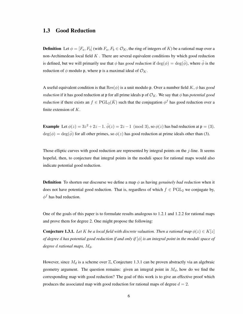
Definition Let φ = [Fa, Fb] (with Fa, Fb ∈ OK , the ring of integers of K) be a rational map over a

non-Archimedean local field K . There are several equivalent conditions by which good reduction

is defined, but we will primarily use that φ has good reduction if deg(φ) = deg(φ), where φ is the

reduction of φ modulo p, where p is a maximal ideal of OK .

A useful equivalent condition is that Res(φ) is a unit modulo p. Over a number field K, φ has good

reduction if it has good reduction at p for all prime ideals p ofOK . We say that φ has potential good

reduction if there exists an f ∈ PGL2(K) such that the conjugation φf has good reduction over a

finite extension of K.

Example Let φ(z) = 3z2 +2z−1. φ(z) = 2z−1 (mod 3), so φ(z) has bad reduction at p = (3).

deg(φ) = deg(φ) for all other primes, so φ(z) has good reduction at prime ideals other than (3).

Those elliptic curves with good reduction are represented by integral points on the j-line. It seems

hopeful, then, to conjecture that integral points in the moduli space for rational maps would also

indicate potential good reduction.

Definition To shorten our discourse we define a map φ as having genuinely bad reduction when it

does not have potential good reduction. That is, regardless of which f ∈ PGL2 we conjugate by,

φf has bad reduction.

One of the goals of this paper is to formulate results analogous to 1.2.1 and 1.2.2 for rational maps

and prove them for degree 2. One might propose the following:

Conjecture 1.3.1. Let K be a local field with discrete valuation. Then a rational map φ(z) ∈ K[z]

of degree d has potential good reduction if and only if [φ] is an integral point in the moduli space of

degree d rational maps, Md.

However, since Md is a scheme over Z, Conjecture 1.3.1 can be proven abstractly via an algebraic

geometry argument. The question remains: given an integral point in Md, how do we find the

corresponding map with good reduction? The goal of this work is to give an effective proof which

produces the associated map with good reduction for rational maps of degree d = 2.

6

Definition The multiplier of φ at a finite fixed point α is the derivative λα(φ) = φ′(α). For a more

precise definition, see Section 2.1.

We address the case d = 2, because it is known that M2∼= A2 (the affine plane) with natural

coordinates (σ1, σ2). That is, given a rational map φ, its corresponding coordinates in moduli

space, σ1 and σ2 are the first and second symmetric functions on the multipliers of the fixed points

of φ, respectively [13]. (See Section 2.1 for definitions and further details.) Knowing the structure

explicitly makes it possible to find an effective proof for Conjecture 1.3.1 in this case.

For larger d, we do not have an explicit description of the structure of Md, so it is currently unclear

what an integral point would be in higher dimensions.

Definition The rational map φ : P1(K) → P1(K) has a critical point at α if φ′(α) = 0. This

definition applies to finite α. For a more complete treatment, see Section 2.1.

Definition A map φ : P1 → P1 is postcritically finite, or PCF if the forward orbit of each of its

critical points is finite.

Silverman proposes in [10] that post-critically finite maps may be the correct dynamical analogue

to elliptic curves with complex multiplication. This is based on the correspondence between elliptic

curves and dynamical systems and the idea that the “special” points in the moduli space of ellip-

tic curves (those representing elliptic curves with complex multiplication) would be analogous to

“special” points in Md, the PCF maps. We thus propose the following, in analogy to 1.2.1:

Conjecture 1.3.2. If [φ] ∈ Md is post-critically finite, then [φ] corresponds to an integral point in

Md.

7

Chapter 2

Background

2.1 Multipliers

Recall that the multiplier of φ at a finite fixed point α is the derivative λα(φ) = φ′(α).

Definition A fixed point α is called

attracting if |λα(φ)| < 1,neutral if |λα(φ)| = 1,

repelling if |λα(φ)| > 1.

The multiplier of φ at infinity is given by the following lemma.

Lemma 2.1.1. When α =∞, we may take

λ∞(φ) = limz→0

z−2φ′(z−1)

φ(z−1)2.

Proof. When α =∞, we conjugate by f(z) = 1/z. To be in keeping with the above proposition, it

must hold that λ∞(φ) = (φf )′(f−1(∞)). By a chain rule calculation, we get the desired equation,

λ∞(φ) = limz→0

z−2φ′(z−1)

φ(z−1)2.

8

Example We can use Lemma 2.1.1 to determine that the multiplier at∞ of the map φ(z) = z2 + 1

is indeed 0.

λ∞(φ) = limz→0

z−22(z−1)

(z−2 + 1)2

= limz→0

2z−3

z−4 + 2z−2 + 1

= limz→0

2z

1 + 2z2 + z4

= 0.

Multipliers are conjugation invariant in PGL2 by the following proposition:

Proposition 2.1.2. (Proposition 1.9 in [12]) Let φ ∈ C(z) be a rational map and let α 6= ∞ be a

fixed point of φ. Let f ∈ PGL2(C) be a change of coordinates and set β = f−1(α) with β 6= ∞,

so β is a fixed point of the conjugate map φf = f−1 φ f . Then

λα(φ) = λβ(φf ).

Proof. Recall that since α is a fixed point, φ(α) = α. Then, by a chain rule calculation, we prove

the equivalent statement, φ′(α) = (φf )′(β).

(φf )′(β) = (f−1)′(φ(f(β))) · φ′(f(β)) · f ′(β)

= (f−1)′(φ(α)) · φ′(α) · f ′(β)

= (f−1 f)′(β) · φ′(α)

= φ′(α).

The notion of multiplier can be extended to a cycles of length n. Suppose that α is a critical point

of the map φ(z), and that α has exact period n. The following simple chain rule calculation shows

how multiplier is derived.

λα(φ) = (φn)′(α) = φ′(α) · φ′(φα) · φ′(φ2α) · · ·φ′(φn−1α).

The categorizations of fixed points based on their multipliers (attracting, repelling, neutral) also

apply in a similar manner to periodic points.

9

Theorem 2.1.3. (Theorem 1.14, in [12]) LetK be an algebraically closed field and let φ(z) ∈ K(z)

be a rational function of degree d ≥ 2. Assume that

λP 6= 1 for all P ∈ Fix(φ).

Then ∑P∈Fix(φ)

1

1− λP (φ)= 1.

Note: the above theorem only holds when φ has d + 1 distinct fixed points, since the condition

λP (φ) 6= 1 is equivalent to the condition that the fixed point P has multiplicity 1.

When d = 2, we can derive from Theorem 2.1.3 that the symmetric functions σ1, σ3 on the multi-

pliers fulfill the following relation:

σ1 = σ3 + 2. (2.1.1)

Though Theorem 2.1.3 does not hold when one or more of the multipliers is 1, Equation 2.1.1

still does. To see this, suppose one of the multipliers equals 1. Then one of the fixed points has

multiplicity greater than one, so at least two multipliers are 1. It is easy to see that Equation 2.1.1

holds when two or three of the multipliers are 1.

Note that (σ1, σ2) ∈ M2 is integral if and only if all three multipliers, λ1, λ2, λ3 are algebraic

integers. One direction is clear. For the other direction, suppose that σ1 and σ2 are integral. Since

σ1, σ2, σ3 are the symmetric functions on λ1, λ2, λ3, the latter are the roots of the monic polynomial

f(z) = z3 − σ1z2 + σ2z − σ3. We can conclude that the multipliers are algebraic integers. Since

the definition of potential good reduction allows us to go to an extension field, we can then assert

that an integral point in M2 is equivalent to integral multipliers.

We will make frequent use of the following lemma:

Lemma 2.1.4. (Corollary 5.3 in [8]) Let φ : P1K → P1

K be a rational map of degree d ≥ 2 with

good reduction at the prime p. Let P ∈ P1(K) be a periodic point for φ. Then P is p-adically

non-repelling.

Remark. In our discourse, we will be working over a local field and using the contrapositive to

Lemma 2.1.4 – that if φ has a p-adically repelling periodic point then it has genuinely bad reduction.

10

2.2 Normal forms

Throughout this work, proofs rely on normal forms which describe degree 2 rational maps up to

conjugation over PGL2. This assures that the results are applicable to the entire space, as the

normal forms give a complete representation of the desired maps. The use of normal forms also

spares us the more complicated task of attempting to use a fully general map such as

φ(z) =az2 + bz + c

dz2 + ez + f.

The first normal form, given in Lemma 2.2.1 will be used to prove the main result, which gives a

complete characterization of degree 2 rational maps with potential good reduction. However, note

that a map φ does not have a unique normal form via Lemma 2.2.1: most maps have 3 distinct

multipliers, so each map can have up to 6 representations in this normal form. Thus, since we only

wish to evaluate each map once, we use a different normal form (Theorem 2.2.3) in the algorithm

for finding PCF maps.

Lemma 2.2.1. (5.3, Normal Forms Lemma in [13]) Let φ ∈ Rat2(Ω) be a rational map of degree

2 over an algebraically closed field Ω, and let λ1, λ2, λ3 be the multipliers of its fixed points.

(a) If λ1λ2 6= 1, then there is an f ∈ PGL2(Ω) such that

φf (z) =z2 + λ1z

λ2z + 1.

Further, Res(z2 + λ1z, λ2z + 1) = 1− λ1λ2.

(b) If λ1λ2 = 1, then λ1 = λ2 = 1 and there is an f ∈ PGL2(Ω) such that

φf (z) = z +√

1− λ3 +1

z.

Proof. (a) Let φ(z) be a rational map of the following form:

φ(z) =a0z

2 + a1z + a2b0z2 + b1z + b2

.

The assumption that λ1λ2 6= 1 gives us that λ1 6= 1 and λ2 6= 1, meaning that the fixed points

corresponding to λ1 and λ2 are distinct. We can find an element of PGL2(Ω) that moves the fixed

points to 0 and∞, respectively. After the change of variables we have

φ(z) =a0z

2 + a1z

b1z + b2with a0b2 6= 0.

11

Since a0 6= 0, we can dehomogenize to get

φ(z) =z2 + b2λ1z

λ2z + b2with b2 6= 0.

Finally, we can replace φ(z) with b−12 φ(b2z) to get the desired form.

(b) In this case, we begin by moving the fixed point associated with λ1 to∞ to get

φ(z) =a0z

2 + a1z + a2b1z + b2

with a0 6= 0 andλ1 = λ∞(φ) =b1a0.

In fact, since λ1λ2 = 1, λ1 = λ2 = 1, so a0 = b2. Dehomogenizing a0 = 1 then replacing φ(z)

with φ(z − b2) + b2 gives us

φ(z) =z2 + a1z + a2

zwith a2 6= 0

Finally, we can replace φ(z) with φ(√a2z)/

√a2 to get the desired form

φ(z) =z2 + a1z + 1

z= z + a1 +

1

z.

To compute the value of a1, note that φ(z) has a double fixed point at∞ and its other fixed point

is at −a−11 . We can calculate the third multiplier λ3 = φ′(a−11 ) = 1 − a21, so a1 =√

1− λ3, as

desired.

Lemma 2.2.2. (Statement 4.12 in [12]) For K of characteristic not equal to 2, every quadratic

polynomial f(z) = Az2 +Bz + C ∈ K[z] is linearly conjugate over K to a unique polynomial of

the form φ(z) = z2 + c.

Proof. Let g(z) = (2z −B)/2A, then conjugate:

φ(z) = fg(z) = g−1 f g(z) = z2 +

(AC − 1

4B2 +

1

2B

)= z2 + c. (2.2.1)

It is known in the case of polynomial maps and maps of even degree that a K-rational point in M2

corresponds to a conjugacy class of quadratic rational maps [ψ] and there must be some map φ ∈ [ψ]

with coefficients in K ([12]). Each family [ψ] describes a conjugacy class of maps, but only within

12

an algebraically closed field K. It is possible to have a map φ defined overK but have the conjugate

map given by the normal form of Lemma 2.2.1 defined over a quadratic or cubic extension of K.

Later, we will be using the symmetric functions σ1 and σ2 of the multipliers to iterate through

equivalence classes of quadratic rational maps. However, having the symmetric functions defined

over K does not guarantee that the multipliers are also defined there. In particular, they may be

defined over a cubic extension of K. In fact, we can use Equation 2.1.1 to find that the field

extension required will be given by f(z) = z3 − σ1z2 + σ2z − (σ1 − 2), which consists of either

3 linear factors, a linear and an irreducible quadratic, or an irreducible cubic. We require a different

normal form to deal with the possibility of multipliers not in the original field. The following normal

form of Manes and Yasufuku facilitates our goal to list all rational degree 2 PCF maps.

Theorem 2.2.3. (Theorem 1 in [6]) Let K be a field with characteristic different from 2 and 3. Let

ψ(z) ∈ K(z) have degree 2, and let λ1, λ2, λ3 ∈ K be the multipliers of the fixed points of ψ

(counted with multiplicity).

(a) If the multipliers are distinct or if exactly two multipliers are 1, then ψ(z) is conjugate over K

to the map

φ(z) =2z2 + (2− σ1)z + (2− σ1)−z2 + (2 + σ1)z + 2− σ1 − σ2

∈ K(z),

where σ1 and σ2 are the first two symmetric functions of the multipliers. Furthermore, no two

distinct maps of this form are conjugate to each other over K.

(b) If λ1 = λ2 6= 1 and λ3 6= λ1 or if λ1 = λ2 = λ3 = 1, then ψ is conjugate over K to a map of

the form

φk,b(z) = kz +b

z

with k ∈ K r 0,−1/2 (in fact, k = λ1+12 ), and b ∈ K∗. Furthermore, two such maps φk,b

and φk′,b′ are conjugate over K if and only if k = k′; they are conjugate over K if in addition

b/b′ ∈ (K∗)2.

(c) If λ1 = λ2 = λ3 = −2, then ψ is conjugate over K to a map of the form

θd,k(z) =kz2 − 2dz + dk

z2 − 2kz + d, with k ∈ K, d ∈ K∗, and k2 6= d.

All such maps are conjugate over K. Furthermore, θd,k(z) and θd′,k′(z) are conjugate over K

if and only if

d′ = b2d, and

k′ ∈

bd

k,b(d2γ3 + 3dkγ2 + 3dγ + k

)dkγ3 + 3dγ2 + 3kγ + 1

13

for some γ ∈ K and b ∈ K∗.

Each quadratic rational map φ(z) ∈ K(z) must fall into exactly one of the cases above, so this

gives a complete description of the K-conjugacy classes of such maps.

2.3 Heights and PCF maps

Height is a notion of size and arithmetic complexity. We introduce height in order to have a mea-

sure of arithmetic size of points in projective space similar to how the size of a rational number is

measured by taking the larger of its numerator and denominator. For a number field K/Q and a

point P ∈ Pn(K), the height that we define takes into account the size of each of the coordinates

with respect to each absolute value over K.

To begin, we introduce some notation from [12]. For a point P = [x0, . . . , xN ] with coordinates in

K,

|P |v = max|x0|v, . . . , |xN |v.

The multiplicative height of P is then denoted

H(P ) =

∏v∈MK

|P |nvv

1/[K:Q]

Here, nv = [Kv : Qv] is the local degree of v.

It is easy to prove that if K/Q is a number this height has the property that for any constant B, the

following set is finite

P ∈ PN (K) : H(P ) ≤ B.

In particular, a height function should have the property that only finitely many points have bounded

size.

For further detail and proof, see Theorem 3.7 in [12]. The result which makes it feasible to enumer-

ate all PCF maps is derived from Corollary 4.12 in a paper of Ingram, Jones and Levy [3]:

Lemma 2.3.1. Let φ(z) ∈ Q(z) have degree 2, suppose that φ is PCF, and let λ be the multiplier

of any fixed point of φ. Then H(λ) ≤ 4.

14

This height bound for rational PCF maps, coupled with the normal form of Theorem 2.2.3 allows

us to determine a range for the possible coordinates (σ1, σ2) of a PCF function in M2. That is, we

are able to derive bounds for σ1 and σ2, then test a quadratic rational map from each equivalence

class to obtain the full list of rational PCF maps of degree 2. This new height bound is derived later

in Proposition 5.0.3.

15

Chapter 3

Main Result

We will be working with maps of the form φ : P1 → P1, and the following notation (from [12]) will

be used:

K a field with normalized discrete valuation v : K∗ Z.| · |v = c−v(x) for some c > 1, an absolute value associated to v.OK = α ∈ K : v(α) ≥ 0, the ring of integers of K.p = α ∈ K : v(α) ≥ 1, the maximal ideal of R.O∗K = α ∈ K : v(α) = 0, the group of units of R.k = R/p, the residue field of R.∼ reduction modulo p, i.e., R→ k, a 7→ a.π uniformizer of p.

In this section, we prove the main result, Theorem 3.0.3, which characterizes degree two rational

maps with potential good reduction over local fields K. The proof relies on the Lemma 2.2.1 and a

part of the proof requires the assumption that all three multipliers λ1, λ2, λ3 of a rational map are in

OK , the ring of integers of K, so we begin with a lemma detailing when this does not happen. The

main theorem itself is proved via two propositions, one for each normal form in Lemma 2.2.1.

Lemma 3.0.2. Let λ1 = a1πe1 and λ2 = a2π

e2 . If λ1λ2 6= 1 and λ1λ2 ≡ 1 (mod π), then

λ3 /∈ OK if and only if the following conditions all hold:

e1 = e2 = e

a1 + a2 = aπe, a ∈ O∗K

a+ a1a2 ≡ 0 (mod π).

16

Proof. Suppose λ1λ2 6= 1 and λ1λ2 ≡ 1 (mod π). By (2.1.3), we can represent λ3 in terms of the

other two multipliers:

λ3 =2− λ1 − λ2

1− λ1λ2=

a1πe1 + a2π

e2

a1πe1 + a2πe2 + a1a2πe1+e2.

Without loss of generality, suppose that e1 ≤ e2, and simplify to obtain

λ3 =a1 + a2π

e2−e1

a1 + a2πe2−e1 + a1a2πe2.

The condition λ3 /∈ OK occurs precisely when a higher power of π divides the denominator than the

numerator, which happens only when a1 + a2πe2−e1 and a1a2πe2 have the same π-adic valuation.

Since π - a1 and π - a2, we can simplify the statement to

|a1 + a2πe2−e1 |π = |πe2 |π.

However, since π - a1, we can conclude that e1 = e2 and represent a1 + a2 = aπe with a 6= 0 and

π - a. It follows that e2 = e. Rewriting with our new information, we get

λ3 =aπe

πe(a+ a1a2).

For the denominator to be divisible by a higher π power than the numerator gives us the final

condition, that a+ a1a2 ≡ 0 (mod π).

Theorem 3.0.3. A degree 2 rational map φ(z) over a local field K has potential good reduction if

and only if [φ] ∈M2(OK).

Suppose [φ] /∈M2(OK). We remind the reader that an integral point in the moduli space is equiva-

lent to integral multipliers if we allow for a field extension. If [φ] does not correspond to an integral

point in the moduli space, it must have a non-integral multiplier, λ. Equivalently, |λ|v > 1 so φ(z)

has a repelling fixed point. By Lemma 2.1.4, φ(z) has genuinely bad reduction.

The other direction will be proved using two propositions — one for each of the two forms in (2.2.1).

Suppose that the multipliers λ1, λ2, λ3 of φ(z) are all algebraic integers.

Proposition 3.0.4. Let

φ(z) = z +√

1− λ3 +1

z

with λ1λ2 = 1. Then φ(z) has good reduction.

17

Proof. Given λ3 ∈ OK , it follows trivially that 1 − λ3 ∈ OK , so√

1− λ3 is also integral as it’s

the root of the monic polynomial z2 + λ3− 1. Since the coefficients of φ(z) are all integral, we can

calculate the resultant Res(φf (z)) = Res(z2 +√

1− λ3z + 1, z) = 1. We can therefore conclude

that in this case φ(z) has good reduction.

Proposition 3.0.5. Let

φ(z) =z2 + λ1z

λ2z + 1.

If λ1λ2 6= 1 and λ3 ∈ OK , then φ(z) has potential good reduction.

Proof. Recall that by Lemma 2.2.1,

Res(z2 + λ1z, λ2z + 1, z) = 1− λ1λ2.

If λ1λ2 6≡ 1 (mod π), then Res(φ(z)) 6= 0 (mod π), so φ(z) has good reduction.

Now suppose λ1λ2 ≡ 1 (mod π).

Here, we can show by equation (2.1.1) that λ1 ≡ 1 (mod π) and λ2 ≡ 1 (mod π):

σ1 = σ3 + 2

λ1 + λ2 + λ3 = λ1λ2λ3 + 2

λ1 + λ2 ≡ 2 (mod π).

Now, we may substitute and use our assumption here that λ1λ2 ≡ 1 (mod π) to get the following:

λ1(2− λ1) ≡ 1 (mod π)

(λ1 − 1)2 ≡ 0 (mod π)

λ1 ≡ 1 (mod π).

It follows that λ2 ≡ 1 (mod π) must hold too. We can represent λ1 and λ2 as follows, with

a1, a2 ∈ OK , e1, e2 > 0, π - a1, and π - a2:

λ1 = 1 + a1πe1

λ2 = 1 + a2πe2 .

18

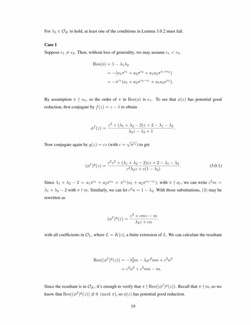
For λ3 ∈ OK to hold, at least one of the conditions in Lemma 3.0.2 must fail.

Case 1

Suppose e1 6= e2. Then, without loss of generality, we may assume e1 < e2.

Res(φ) = 1− λ1λ2

= −(a1πe1 + a2π

e2 + a1a2πe1+e2)

= −πe1(a1 + a2πe2−e1 + a1a2π

e2).

By assumption π - a1, so the order of π in Res(φ) is e1. To see that φ(z) has potential good

reduction, first conjugate by f(z) = z − 1 to obtain

φf (z) =z2 + (λ1 + λ2 − 2)z + 2− λ1 − λ2

λ2z − λ2 + 1.

Now conjugate again by g(z) = cz (with c =√πe1) to get

(φf )g(z) =c2z2 + (λ1 + λ2 − 2)cz + 2− λ1 − λ2

c2λ2z + c(1− λ2). (3.0.1)

Since λ1 + λ2 − 2 = a1πe1 + a2π

e2 = πe1(a1 + a2πe2−e1), with π - a1, we can write c2m =

λ1 + λ2 − 2 with π - m. Similarly, we can let c2n = 1− λ2. With those substitutions, (3) may be

rewritten as

(φf )g(z) =z2 + cmz −mλ2z + cn

.

with all coefficients in OL, where L = K(c), a finite extension of L. We can calculate the resultant

Res((φf )g(z)) = −λ22m− λ2c2mn+ c2n2

= c2n2 + c2mn−m.

Since the resultant is in OK , it’s enough to verify that π - Res((φf )g(z)). Recall that π - m, so we

know that Res((φf )g(z)) 6≡ 0 (mod π), so φ(z) has potential good reduction.

19

Using the above defined substitutions, λ1 = c2(m+ n) + 1 and λ2 = 1− c2n. In particular,

Res(φ) = 1− λ1λ2 = c2(c2n2 + c2mn−m).

Note that

Res(φ) = c2 Res((φf )g(z)). (3.0.2)

Case 2

Suppose that e1 = e2 = e, but a1 + a2 6= aπe for any a ∈ OK . We may write a1 + a2 = aπd with

d < e and π - a.

Res(φ) = 1− λ1λ2

= −πe(a1 + a2 + a1a2πe)

= −πe+d(a+ a1a2πe−d).

Now let f(z) = z − 1 and g(z) = cz with c =√πe+d. Conjugating by f then g gives us equation

(3). Now write λ1+λ2−2 = πe(a1+a2) = aπe+d = ac2 and 1−λ2 = a2πe = cn, then substitute

to get

(φf )g(z) =z2 + acz − aλ2z + n

.

The resultant is

Res((φf )g) = −λ22 − aλ2cn+ n2

= −a+ acn+ n2.

Since π divides both the 2nd and 3rd terms, but not a, Res((φf )g) 6≡ 0 (mod π). Thus φ(z) has

potential good reduction.

Using the above defined substitutions, λ1 = ac2 + 1 + cn and λ2 = 1− cn. In particular,

Res(φ) = 1− λ1λ2 = k2(−a+ acn+ n2).

20

Note that again, Res(φ) = c2 Res((φf )g(z)).

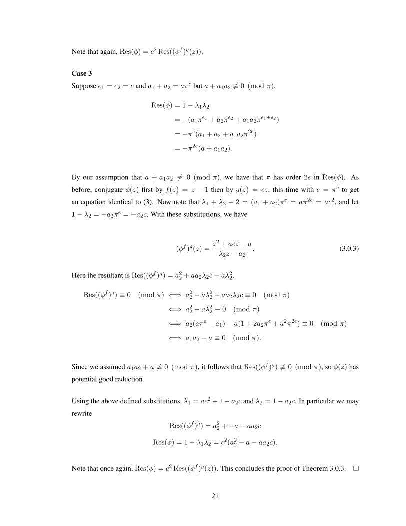
Case 3

Suppose e1 = e2 = e and a1 + a2 = aπe but a+ a1a2 6≡ 0 (mod π).

Res(φ) = 1− λ1λ2

= −(a1πe1 + a2π

e2 + a1a2πe1+e2)

= −πe(a1 + a2 + a1a2π2e)

= −π2e(a+ a1a2).

By our assumption that a + a1a2 6≡ 0 (mod π), we have that π has order 2e in Res(φ). As

before, conjugate φ(z) first by f(z) = z − 1 then by g(z) = cz, this time with c = πe to get

an equation identical to (3). Now note that λ1 + λ2 − 2 = (a1 + a2)πe = aπ2e = ac2, and let

1− λ2 = −a2πe = −a2c. With these substitutions, we have

(φf )g(z) =z2 + acz − aλ2z − a2

. (3.0.3)

Here the resultant is Res((φf )g) = a22 + aa2λ2c− aλ22.

Res((φf )g) ≡ 0 (mod π) ⇐⇒ a22 − aλ22 + aa2λ2c ≡ 0 (mod π)

⇐⇒ a22 − aλ22 ≡ 0 (mod π)

⇐⇒ a2(aπe − a1)− a(1 + 2a2π

e + a2π2e) ≡ 0 (mod π)

⇐⇒ a1a2 + a ≡ 0 (mod π).

Since we assumed a1a2 + a 6≡ 0 (mod π), it follows that Res((φf )g) 6≡ 0 (mod π), so φ(z) has

potential good reduction.

Using the above defined substitutions, λ1 = ac2 + 1− a2c and λ2 = 1− a2c. In particular we may

rewrite

Res((φf )g) = a22 +−a− aa2c

Res(φ) = 1− λ1λ2 = c2(a22 − a− aa2c).

Note that once again, Res(φ) = c2 Res((φf )g(z)). This concludes the proof of Theorem 3.0.3.

21

Chapter 4

Number Field Results

The shift from local fields to global fields requires us to show that a degree 2 rational map which

corresponds to an integral point in the moduli space but has bad reduction at more than one prime p

still has potential good reduction. The main result above only proved this for a single prime, so it is

now necessary to show that similar techniques can be applied to piece together the local results into

a global one.

We begin this section by proving stronger results for quadratic polynomials, since this family is of

great interest in research.

4.1 Quadratic Polynomials

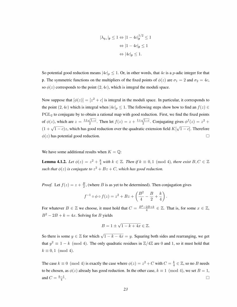
Theorem 4.1.1. Let φ(z) ∈ K[z] be a quadratic polynomial over a number field. Then φ has

potential good reduction if and only if [φ] is an integral point in the moduli space M2.

Proof. By Lemma 2.2.2, we may assume φ(z) = z2 + c.

The function φ(z) has fixed points at q± = 1±√1−4c2 , with corresponding multipliers λq± = 1 ±

√1− 4c.

Suppose that φ(z) has potential good reduction. Then by Theorem 3.0.3, all multipliers are p-

adically integral for every prime p. We can calculate:

22

|λq+ |p ≤ 1⇔ |1− 4c|1/2p ≤ 1

⇔ |1− 4c|p ≤ 1

⇔ |4c|p ≤ 1.

So potential good reduction means |4c|p ≤ 1. Or, in other words, that 4c is a p-adic integer for that

p. The symmetric functions on the multipliers of the fixed points of φ(z) are σ1 = 2 and σ2 = 4c,

so φ(z) corresponds to the point (2, 4c), which is integral the moduli space.

Now suppose that [φ(z)] = [z2 + c] is integral in the moduli space. In particular, it corresponds to

the point (2, 4c) which is integral when |4c|p ≤ 1. The following steps show how to find an f(z) ∈PGL2 to conjugate by to obtain a rational map with good reduction. First, we find the fixed points

of φ(z), which are z = 1±√1−c2 . Then let f(z) = z + 1+

√1−c2 . Conjugating gives φf (z) = z2 +

(1 +√

1− c)z, which has good reduction over the quadratic extension field K[√

1− c]. Therefore

φ(z) has potential good reduction.

We have some additional results when K = Q:

Lemma 4.1.2. Let φ(z) = z2 + k4 with k ∈ Z. Then if k ≡ 0, 1 (mod 4), there exist B,C ∈ Z

such that φ(z) is conjugate to z2 +Bz + C, which has good reduction.

Proof. Let f(z) = z + B2 , (where B is as yet to be determined). Then conjugation gives

f−1 φ f(z) = z2 +Bz +

(B2

4− B

2+k

4

).

For whatever B ∈ Z we choose, it must hold that C = B2−2B+k4 ∈ Z. That is, for some x ∈ Z,

B2 − 2B + k = 4x. Solving for B yields

B = 1±√

1− k + 4x ∈ Z.

So there is some y ∈ Z for which√

1− k − 4x = y. Squaring both sides and rearranging, we get

that y2 ≡ 1 − k (mod 4). The only quadratic residues in Z/4Z are 0 and 1, so it must hold that

k ≡ 0, 1 (mod 4).

The case k ≡ 0 (mod 4) is exactly the case where φ(z) = z2 +C with C = k4 ∈ Z, so no B needs

to be chosen, as φ(z) already has good reduction. In the other case, k ≡ 1 (mod 4), we set B = 1,

and C = k−14 .

23

Proposition 4.1.3. Let φ(z) = z2 + k4 with k ∈ Z. Then φ(z) is linearly conjugate to a morphism

ψ(z) ∈ Q(z) with good reduction over Q if only if k ≡ 0, 1 (mod 4).

Proof. The forward direction is a result of the previous lemma. For the other direction, suppose

φ(z) = z2 + k4 and f(z) = az+b

cz+d ∈ PGL2. Then the full conjugation, ψ(z) = φf (z) looks like:

(4a2d+ c2dk − 4bc2)z2 + (8abd+ 2cd2k − 8bcd)z + 4b2d+ d3k − 4bd2

(4ac2 − 4a2c− c3k)z2 + (8acd− 8abc− 2c2dk)z + 4ad2 − 4b2c− cd2k.

First, note that c and d cannot both be 0, since f(z) ∈ PGL2. Now consider the case c = 0.

Substituting and reducing in the above equation gives

ψ(z) =4a2z2 + 8abz + 4b2 + d2k − 4bd

4ad.

For ψ(z) to have good reduction, it must hold that d|a, d|2b and 2|d. So we can change notation

and replace a with ad and 2b with bd. Then we can rewrite ψ(z) as

ψ(z) =4a2z2 + 4abz + b2 − 2b+ k

4a.

Now we need b2−2b+k4a = x for some x ∈ Z. Solving for b, we get

b = 1±√

1− k + 4ax.

So there is some y ∈ Z such that y2 = 1 − k + 4ax. In other words, y2 ≡ 1 − k (mod 4). Since

the only quadratic residues in Z/4Z are 0 and 1, we have that k ≡ 0, 1 (mod 4) when c = 0.

Next, consider the case d = 0. Then we have

ψ(z) =4bcz2

(4a2 − 4ac+ c2k)z2 + 8abz + 4b2.

For ψ(z) to have good reduction the coefficient −4bc in the numerator must cancel. So we have

these divisibility properties: c|2a and c|b. As before, replace 2a with ac and b wtih bc. Then we can

rewrite ψ(z) as

ψ(z) =4bz2

(a2 − 2a+ k)z2 + 4abz + 4b2.

Now, we just need to ensure that a2−2a+k

4b = x for some x ∈ Z. Solving for a, we get

24

a = 1±√

1− k + 4bx.

There must be some y ∈ Z such that y2 = 1 − k − 4bx, i.e. y2 ≡ 1 − k (mod 4). Thus we have

that k ≡ 0, 1 (mod 4).

Now consider the case where both c and d are nonzero. Without cancellation, g(z) reduces to the

constant −dc in Z/2Z, indicating bad reduction. The only possibility for good reduction requires

that each monomial be divisible by 2, requiring that c and d both be even.

Knowing that c and d are both even, we may rewrite f(z) as f(z) = az+b2cz+2d . Then ψ(z) once

again reduces to −dc in Z/2Z unless there is cancellation. Suppose that 2n|c and 2n|d. Then we

can repeat the process, continuing to rewrite f(z) as above and recalculating ψ(z) , indicating that

ψ(z) reduces to −dc for arbitrarily large n. Since there are no c and d in Z which would permit

cancellation, φ(z) = z2 + k4 cannot be conjugate to a function with good reduction over Q unless

k ≡ 0, 1 (mod 4), as in the above cases.

4.2 Quadratic Rational Maps

Our result over number fields is a corollary to Theorem 3.0.3 and the proof follows an identical

format, so we will be brief.

Corollary 4.2.1. If degree 2 rational map φ(z) over a Q has potential good reduction, then [φ] ∈M2(Z). Conversely, if [φ] ∈ M2(Z) and φ has at least one multiplier in Z, then φ(z) has potential

good reduction.

Proof. Recall from the proof of the local fields case that the change of variables we employed gave

us a resultant which was no longer divisible by the prime π of bad reduction, or more precisely,

(3.0.2). Note that Proposition 3.0.4 holds as a global result.

To extend Proposition 3.0.5 to Q, recall our assumptions that [φ] ∈ M2(Z) and φ has at least one

multiplier, λ3, which is in Z. Then by Lemma 2.2.1, we may write our map as

φ(z) =z2 + λ1z

λ2z + 1

with Res(φ) = 1− λ1λ2. The multiplier polynomial in this case will factor over Z into z − λ3 and

at worse an irreducible quadratic z2 − (λ1 + λ2)z + λ1λ2. Since λ1λ2 ∈ Z, Res(φ) ∈ Z as well.

25

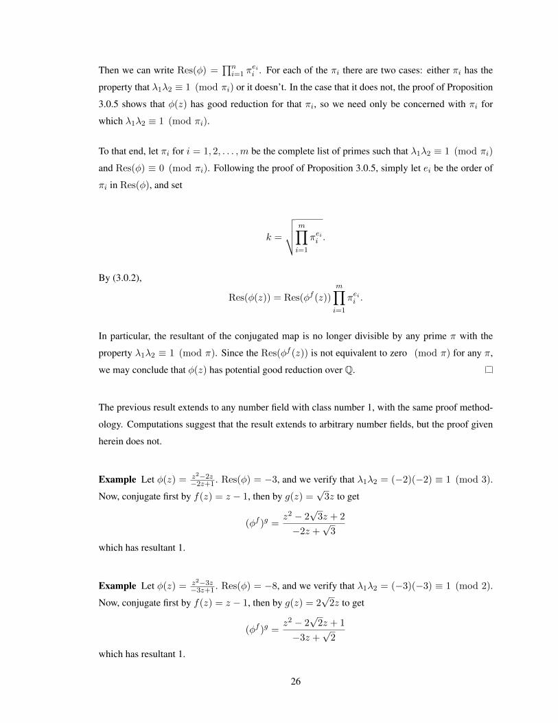
Then we can write Res(φ) =∏ni=1 π

eii . For each of the πi there are two cases: either πi has the

property that λ1λ2 ≡ 1 (mod πi) or it doesn’t. In the case that it does not, the proof of Proposition

3.0.5 shows that φ(z) has good reduction for that πi, so we need only be concerned with πi for

which λ1λ2 ≡ 1 (mod πi).

To that end, let πi for i = 1, 2, . . . ,m be the complete list of primes such that λ1λ2 ≡ 1 (mod πi)

and Res(φ) ≡ 0 (mod πi). Following the proof of Proposition 3.0.5, simply let ei be the order of

πi in Res(φ), and set

k =

√√√√ m∏i=1

πeii .

By (3.0.2),

Res(φ(z)) = Res(φf (z))

m∏i=1

πeii .

In particular, the resultant of the conjugated map is no longer divisible by any prime π with the

property λ1λ2 ≡ 1 (mod π). Since the Res(φf (z)) is not equivalent to zero (mod π) for any π,

we may conclude that φ(z) has potential good reduction over Q.

The previous result extends to any number field with class number 1, with the same proof method-

ology. Computations suggest that the result extends to arbitrary number fields, but the proof given

herein does not.

Example Let φ(z) = z2−2z−2z+1 . Res(φ) = −3, and we verify that λ1λ2 = (−2)(−2) ≡ 1 (mod 3).

Now, conjugate first by f(z) = z − 1, then by g(z) =√

3z to get

(φf )g =z2 − 2

√3z + 2

−2z +√

3

which has resultant 1.

Example Let φ(z) = z2−3z−3z+1 . Res(φ) = −8, and we verify that λ1λ2 = (−3)(−3) ≡ 1 (mod 2).

Now, conjugate first by f(z) = z − 1, then by g(z) = 2√

2z to get

(φf )g =z2 − 2

√2z + 1

−3z +√

2

which has resultant 1.

26

Example Let φ(z) = z2−3z−z+1 . Res(φ) = −2, and we verify that λ1λ2 = (−3)(−1) ≡ 1 (mod 2).

Now, conjugate first by f(z) = z − 1, then by g(z) =√

2z to get

(φf )g =z2 − 3

√2z + 3

−z +√

2

which has resultant 1.

Example Now for an example with bad reduction at two primes, let φ(z) = z2+13zz+1 . Res(φ) =

−12, and we verify that λ1λ2 = (1)(13) ≡ 1 (mod 2) and also λ1λ2 ≡ 1 (mod 3). Now, conju-

gate first by f(z) = z − 1, then by g(z) =√

12z to get

(φf )g =z2 + 2

√3z − 1

z

which has resultant −1.

4.3 Results From Others

Bruin and Molnar [1] describe an algorithm for finding a minimal model for rational maps of arbi-

trary degree d > 1. Their ultimate goal is to find maps with many integral points in an orbit. When

a rational map defined over K has a model with good reduction also defined over a local field K,

their algorithm can be used to find this model. Unlike their algorithm, the present work allows for

moving to a finite extension of K when necessary. See below for examples of this distinction.

The following lemma is referenced throughout, and is the basis of Bruin and Molnar’s algorithm for

finding minimal models:

Lemma 4.3.1. (Lemma 3.1 in [1]) If d is even and v(Resd(F,G)) < d or if d is odd and v(Resd(F,G)) <

2d then [F,G] is an R-minimal model for [φ].

Their algorithm begins with a rational function φ ∈ Ratd(K), given by a model [F,G] over a

discrete valuation ring R. They first prove the existence of a minimal model:

Proposition 4.3.2. (Proposition 2.12 in [1]) LetR be a discrete valuation ring with field of fractions

K and uniformizer π. Let φ ∈ Ratd(K) be a rational function given by a model [F,G] ∈ Md(K).

Then there are e1, e2, e3 ∈ Z and β ∈ K such that for any β′ ∈ β + πe3R we can set

(λ,A) = (πe1 ,

πe2 β′

0 1

) ∈ (Gm ×GL2)(K)

27

and have that [λFA, λGA] is an R-minimal model for φ.

The algorithm is seeded with initial values for e1 and e2, derived from the original map, then it tests

the map for minimality via Lemma 4.3.1. If the resulting conjugated map is not minimal, e1 and e2

are replaced by values based on the new map. This process is iterated until an R-minimal model is

found.

We give several examples of finding the minimal resultant of a given degree 2 rational map, first

using methods from [1], then also by using the algorithm from this dissertation. In each case, the

map is presented in the normal form of Lemma 2.2.1, where the coefficients correspond to two of

the three multipliers. Since both are integers, all three multipliers must be integral, therefore the

symmetric functions σ1 and σ2 are integral. In other words, each of these maps corresponds to an

integral point in the moduli space, so by Theorem 3.0.3, they have potential good reduction.

Example Let φ(z) = z2−2z−2z+1 . Res(φ) = −3. Since we are working with the 3-adic valuation,

v(Resd(F,G)) = 1 < 2 = d. By Lemma 4.3.1, φ(z) is already locally minimal, and the algorithm

of Bruin and Molnar would not change it.

However, we can find a conjugate map with good reduction, by letting f(z) = z−1 and g(z) =√

3z

to get

(φf )g =z2 − 2

√3z + 2

−2z +√

3

which has resultant 1.

Example Let φ(z) = z2+9zz+1 . Res(φ) = −8. Note that both the numerator and the denominator of

φ(z) are monic and that the degree of the denominator is half the degree of the numerator. By [1,

Remark 3.4], φ(z) is minimal according to the algorithm of Bruin and Molnar.

Our algorithm finds a map with good reduction, via conjugating first by f(z) = z − 1, then by

g(z) = 2√

2z to get

(φf )g =z2 + 2

√2z − 1

z

which has resultant −1.

Example Let φ(z) = z2−3z−z+1 . Res(φ) = −2. We are working with the 2-adic valuation, so

v(Resd(F,G)) = 1 < 2 = d. By Lemma 4.3.1, φ(z) is found by the algorithm of [1] to be

locally minimal.

28

However, to obtain a good reduction, we can conjugate first by f(z) = z − 1, then by g(z) =√

2z

to get

(φf )g =z2 − 3

√2z + 3

−z +√

2

which has resultant 1.

Finally, consider the following example which has a resultant divisible by more than one prime p:

Example Let φ(z) = z2+13zz+1 . Res(φ) = −12. Note that both the numerator and the denominator

of φ(z) are monic and that the degree of the denominator is half the degree of the numerator. Again

by [1, Remark 3.4], φ(z) is considered to be minimal.

Now, for a map with good reduction via our algorithm, conjugate first by f(z) = z − 1, then by

g(z) =√

12z to get

(φf )g =z2 + 2

√3z − 1

z

which has resultant −1.

29

Chapter 5

Post-Critically Finite Maps

In this section, we list all post critically finite maps of degree two over Q after showing that there

are only finitely many and that our search space is comprehensive.

Recall from Lemma 2.3.1 that if λ is a fixed-point multiplier of a degree 2 PCF map φ, then its

height is bounded by H(λ) ≤ 4. This provides us with a finite search space. For our algorithm,

we derive and use new height bounds of the first and second symmetric functions of the multipliers,

not the height of the multipliers themselves. Though this choice results in a large increase of the

height bound, it is necessary because we need the normal form of Theorem 2.2.3. The choice of this

normal form arises from the fact that it is possible for a map φ defined overK to have its multipliers

defined over a quadratic or cubic extension of K. In other words, the conjugate map in the normal

form of Lemma 2.2.1 might not be defined over K. Additionally, using the normal form of Lemma

2.2.1 would not give us a unique form for each set of multipliers as there are 6 ways to assign the

3 multipliers. The following is a height bound on the symmetric functions, derived from Lemma

2.3.1.

Proposition 5.0.3. Let φ(z) ∈ Q be a degree 2 PCF map and suppose that σ1 and σ2 are the first

and second symmetric functions on the multipliers, λ1, λ2, λ3, of φ(z). Then H(σ1) ≤ 192 and

H(σ2) ≤ 12288.

Proof. Working with the definition of height given in Section 2.3 and simplifying notation by setting

d = [K : Q]

H(σ1) =∏

v∈MK

(max|σ1|v, 1nv)1/d.

30

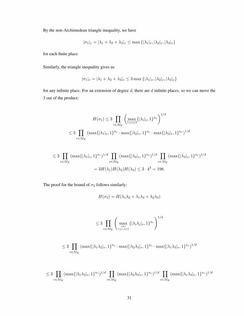
By the non-Archimedean triangle inequality, we have

|σ1|v = |λ1 + λ2 + λ3|v ≤ max |λ1|v, |λ2|v, |λ3|v

for each finite place.

Similarly, the triangle inequality gives us

|σ1|v = |λ1 + λ2 + λ3|v ≤ 3 max |λ1|v, |λ2|v, |λ3|v

for any infinite place. For an extension of degree d, there are d infinite places, so we can move the

3 out of the product:

H(σ1) ≤ 3∏

v∈MK

(max1≤i≤3

|λi|v, 1nv

)1/d

≤ 3∏

v∈MK

(max|λ1|v, 1nv ·max|λ2|v, 1nv ·max|λ3|v, 1nv)1/d

≤ 3∏

v∈MK

(max|λ1|v, 1nv)1/d∏

v∈MK

(max|λ2|v, 1nv)1/d∏

v∈MK

(max|λ3|v, 1nv)1/d

= 3H(λ1)H(λ2)H(λ3) ≤ 3 · 43 = 198.

The proof for the bound of σ2 follows similarly:

H(σ2) = H(λ1λ2 + λ1λ3 + λ2λ3)

≤ 3∏

v∈MK

(maxi 6=j

1≤i,j≤3

|λiλj |v, 1nv

)1/d

≤ 3∏

v∈MK

(max|λ1λ2|v, 1nv ·max|λ2λ3|v, 1nv ·max|λ1λ3|v, 1nv)1/d

≤ 3∏

v∈MK

(max|λ1λ2|v, 1nv)1/d∏

v∈MK

(max|λ2λ3|v, 1nv)1/d∏

v∈MK

(max|λ1λ3|v, 1nv)1/d

31

= 3H(λ1λ2)H(λ2λ3)H(λ1λ3) = 3H(λ1)2H(λ2)

2H(λ3)2 ≤ 3 · 46 = 12288.

In fact, our search space is much smaller than that. We know of an upcoming result which limits the

search to 2-integers – rationals with powers of 2 in the denominator [5]. The PCF maps included

herein are from a search over the integers, but calculations are currently running over the 2-integers.

To date, no additional (non-integral) PCF maps have been found, and we do not expect to find any.

We will allow the search to complete before submitting the complete list for publication.

In the algorithm, the normal form of Manes and Yasufuku (Theorem 2.2.3), only case (a) is used, as

this is the case of maps with no nontrivial automorphism groups. Those maps corresponding to the

point (σ1, σ2) where σ1 and σ2 fulfill the following equation exactly comprise the symmetry locus

S2, and have been described fully in [4]:

36− 12σ2 + 4σ22 = 12σ1 − σ21 + 2σ31 − 8σ1σ2 + σ21σ2.

The PCF maps defined over Q with nontrivial automorphisms are shown in Table 5.1.

φ(z) Critical Points Orbit Graph Conjugate mapwith good reduction

z2+12z −1, 1 •−1 •1

z2

z2+1−2z −1, 1 •−1 •144ss

1/z2

Table 5.1. PCF maps with nontrivial automorphisms (from [4])

5.1 Algorithm

The algorithm used was written in Sage [S+09] and uses a subroutine for finding orbits from the

ProjSpace package developed at ICERM [2]. It also relies on the following two theorems.

Theorem 5.1.1. (Theorem 2.21 from [12]) Let φ : P1 → P1 be a rational function of degree d ≥ 2

defined over a local field with a nonarchimedean absolute value | · |v. Assume that φ has good

reduction, let P ∈ P1(K) be a periodic point of φ, and define the following quantities:

32

n The exact period of P for the map φ.m The exact period of P for the map φ.r The order of λφ(P ) = (φm)′(P ) in k∗. (Set r =∞ if λφ(P ) is not a root of unity.)p The characteristic of the residue field k of K.

Then n has one of the following forms:

n = m or n = mr or n = mrpe.

Theorem 5.1.2. (Theorem 2.28 from [12]) We continue with the notation and assumptions from

Theorem 5.1.1. We further assume that K has characteristic 0 and we let v : K∗ Z be the

normalized valuation on K. If the period n of P ∈ P1(K) has the form n = mrpe , then the

exponent e satisfies

pe−1 ≤ 2v(p)

p− 1.

Since we are working over Q, ν(p) = 1 for all p, so Theorem 5.1.2 allows us to assert e = 0, when

p 6= 2 and e ∈ 0, 1 when p = 2. In the algorithm, we exclude p = 2 from consideration and use

the following possibilities for n:

n = m or n = mr.

We first sketch the flow of the algorithm. Iterating over all degree 2 rational maps φ not in the

symmetry locus, the algorithm:

(1) Finds the resultant R of φ.

(2) Lists the first n primes p such that gcd(R, p) = 1, the primes of good reduction.

(3) Finds the critical points of φ.

(4) Iterates over each critical point, finding sets of potential global period lengths for the orbits con-

taining the critical point.

(5) Intersects the potential critical point orbit lengths and discards the map if the intersection is

empty.

For further reference, the code itself is in Appendix A.

We make use of Theorem 5.1.1 in step (4) by finding possible global period lengths based on each

good prime p. Note that this algorithm filters out maps which are certainly not PCF, but does not

guarantee that the maps which remain are PCF. The initial run over all integers eliminated all but a

handful of maps. Of these, false positives were removed by increasing the number of primes n used

33

to seed the algorithm from n = 25 to n = 50. The remaining maps were verified to be PCF, and

their orbit graphs are included in the following tables.

Algorithm 1 — Filters out maps φ which are not PCFInput:

• a degree 2 rational map φ(z) ∈ Z(z)

• the number of primes to test

Output: φ(z), if it passes the filter

create a list P of good primes by taking the first n+ 10 primes and deleting the bad primes

for c a critical point of φ:

if c ∈ Q:

create list Lp of possible periods for each prime p in P

intersect all lists Lp

if the intersection is non-empty: continue

else: exit

else (if c /∈ Q):

for p ∈ P :

check that c ∈ Fpcreate list Lp of possible periods for p

intersect all lists Lp

if the intersection is non-empty: continue

else: exit

return φ(z)

Algorithm 2 — Executes Algorithm 1 (is PCF) over 2-integers

Input: [none]

Output: list of possible PCF maps

for σ2 a 2-integer of height ≤ 12288 :

for σ1 a 2-integer of height ≤ 192:

if φ(σ1, σ2) is not in the symmetry locus:

if is PCF(φ, 25):

print f

34

5.2 List of Degree 2 Rational Maps with Potential Good Reduction

The Table 5.2 lists all degree 2 PCF maps with no non-trivial automorphisms over Q in the normal

form from [6]. The three maps in the table without a simpler good reduction form do also, in fact,

have potential good reduction. To show this, we follow the format of the proof of Corollary 4.2.1

and write

φ(z) =z2 + λ1z

λ2z + 1.

In all three cases, we can calculate

Res(φ) = 1− λ1λ2 = (α)2,

where α is an integral principal ideal. Since the resultant is the square of a principal ideal, we can

follow the algorithm as outlined. Let c = α, and conjugate φ(z) first by f(z) = z − 1 then by

g(z) = cz to arrive at a map with good reduction.

5.3 Preperiodic Structures for Quadratic PCF Maps with Symmetries

Also of interest is the portrait of all rational preperiodic points for each PCF map. For those maps

with no nontrivial automorphisms, these structures are given in Table 5.3. As to the other case, the

only PCF maps in the symmetry locus are the ones conjugate to ψ1(z) = z2 and ψ2(z) = 1/z2

[4]. We depict all rational preperiodic structures for maps in these two families. Details on their

derivation will be available in an upcoming joint paper on quadratic PCF maps and their preperiodic

structures.

If φ is a rational map, ψ is a twist of φ if φf = ψ for some f ∈ PGL2(Q). The twist is nontrivial

if f 6∈ PGL2(Q). Since the rational preperiodic points are not preserved under the conjugation, to

form a complete description of the rational preperiodic structures, we must understand the possible

structures for all twists. Only maps in the symmetry locus have nontrivial twists [12, Proposition

4.73].

Throughout this section, ζn means a primitive nth root of unity. Preperiodic point portraits are given

for ψ1(z) = z2 in Figure 5.1. The remaining figures correspond to twists of ψ2(z) = 1/z2.

35

φ(z) Critical Points Orbit Graph Conjugate map withgood reduction

2z2

−z2+4z+8−4, 0 •0 •−4

•−4/3

•4

OO

OO

z2 − 2

2z2

−z2+4z+4−2, 0 •0 •−2 •−1

33

ssz2 − 1

2z2+8z+8−z2−4z−2 −2,∞ •∞ •−2 •0 •−4// // //

z2+(−1−i)z(i−1)z+1

2z2+8z+8−z2−4z+4

−2,∞ •∞ •−2 •0 •2 •−4// // // 33tt

2z2+4z+4−z2 −2, 0 •0 •∞ •−2 •−1// // 33

ss

2z2+8z+8−z2−4z −2,∞ •−2 •0

•∞

//

gg

ww

Table 5.2. PCF maps with no nontrivial automorphisms

36

φ(z) Rational Preperiodic Points Graph

2z2

−z2+4z+8•0 •∞

•−2

•−4

•−4/3

•4

OO

OO

OO

2z2

−z2+4z+4•0 •∞ •−2 •−1

// ss33

2z2+8z+8−z2−4z−2

•∞ •−2 •0 •−4// // //

2z2+8z+8−z2−4z+4

•∞ •−2 •0 •2 •−4 •−6// // // oo33tt

2z2+4z+4−z2

•0 •∞ •−2 •−1// // 33ss

2z2+8z+8−z2−4z •−2 •0

•∞

•−4

//

gg

ww

Table 5.3. Rational preperiodic points portrait

37

•∞

•0

OO

(a) b = 1

•∞

•0 •1 •−1

OO

(b) b = 1/2

•∞

•0 •−2

•−1

•2

•1OO ?? __44

ss

(c) b = −3/2

•∞

•0

•−1 •1

OO

__??

(d) b = −1/2

Figure 5.1. All possible rational preperiodic graphs for φb(z) = z2 + b

z .

•1

•−1

•0 •∞OO 33

tt

(a) θ1(z) = 1/z2

•0 •∞33tt

(b) θ2(z) = 2/z2

Figure 5.2. All possible rational preperiodic graphs for θt(z) = t/z2.

(a) φ(z) = z2−4z+2z2−2z+2

•1

•−1

OO

(b) φ(z) = − 4zz2+2

•1

•−1

•0 •∞

OO

:: dd

(c) φ(z) = −z2+2z+1z2+2z−1

•0

•2

•1

•−1

•∞

• 12

OO OO OO

(d) φ(z) = − (z−2)z2z−1

Figure 5.3. More possibilities and their related maps

•0

•1•∞

• 12

•2•−1

kk

66

gg77

Figure 5.4. φ(z) = 2z−1z2−1 has rational points on a three-cycle.

38

Appendix A

Sage Code

# This is based on orbit_structure_modp

# n is the number of primes you want to compare.

load "ProjSpace.sage"

PS.<x,y>=ProjSpace(1,QQ)

H = Hom(PS,PS)

def is_pcf(f, n):

def is_pcf(f, n):

a = gcd(f[0],f[1])

b = lcm(f[0].denominator(),f[1].denominator())

f.scale_by(b/a)

res = f.resultant()

bp = set(res.support())

primes = set(primes_first_n(n+10)).difference(bp)

plist = list(primes)[2:n]

cp = f.critical_points()

F = f.change_ring(ZZ)

wronskian = [F.wronskian().change_ring(ZZ), yˆ2]

39

for c in cp:

P = c[0]

P.scale_by(lcm(P[0].denominator(),P[1].denominator()))

# If the critical point is rational:

if P[0] in QQ:

Q=P.change_ring(ZZ)

if check_periods(F, Q, plist):

continue

else:

return False

# Non-rational critical points

else:

AS.<x>=AffSpace(1,QQ)

R = AS.coordinate_ring()

w = H(wronskian).dehomogenize(1)

d = R(w[0]).discriminant(x)

# find the good primes coprime to d

ps = []

for p in plist:

if kronecker(d,p) == 1:

ps.append(p)

# For each such p, solve for the critical point equation

for p in ps:

PF = PS.change_ring(GF(p))

G = Hom(PF, PF)

crits = G(wronskian).critical_points()

# check global periods

for c in crits:

C1 = c[0]

#C1.scale_by(lcm(C1[0].denominator(),C1[1].denominator()))

40

C = C1.change_ring(ZZ)

if check_periods(F, C, ps):

continue

else:

return False

return True

def check_periods(F, P, plist):

periods = []

copy = set(plist).copy()

p1 = copy.pop()

period1 = possible_periods(F, P, p1)

periods.extend(period1)

for p in copy:

new_periods = possible_periods(F, P, p)

periods = set(periods) & set(new_periods)

if len(periods) == 0:

return False

else:

return True

# Find possible period lengths of Q mod p

def possible_periods(F, Q, p):

orbit = F.orbit_structure_modp(Q,p)

tail = orbit[0]

m = orbit[1]

periods = []

periods.append(m)

if tail == 0:

return periods

else:

41

PF = PS.change_ring(GF(p))

HF = Hom(PF, PF)

R = Q.change_ring(GF(p))

G = HF([F[0],F[1]])

periodic_point = G.nth_iterate(R, tail)

multiplier = G.multiplier(periodic_point, m)

if mod(multiplier[0,0],p) == 0:

return periods

else:

r = multiplicative_order(mod(multiplier[0,0],p))

periods.append(m*r)

return periods

# For rational maps of the form F(z), with parameters s1,s2.

N1 = iter(IntegerRange(-192, 193, 1, 0))

for n1 in N1:

D1 = iter(IntegerRange(0,8))

for d1 in D1:

if d1 == 0 or n1/2 not in ZZ:

s1 = n1/2ˆd1

N2 = iter(IntegerRange(-12288, 12289, 1, 0))

for n2 in N2:

D2 = iter(IntegerRange(0,14))

for d2 in D2:

if d2 == 0 or n2/2 not in ZZ:

s2 = n2/2ˆd2

if 36-12*s2+4*s2ˆ2!=12*s1-s1ˆ2+2*s1ˆ3-8*s1*s2+s1ˆ2*s2:

f = H([2*xˆ2+(2-s1)*x*y+(2-s1)*yˆ2,

-xˆ2+(2+s1)*x*y+(2-s1-s2)*yˆ2])

if is_pcf(f, 25):

print "(s1, s2) = ", (s1, s2)

print f

42

Bibliography

[1] N. Bruin, A. Molnar. Minimal models for rational functions in a dynamical setting,

arXiv:1204.4967 [math.NT].

[2] ICERM, ProjSpace package for Sage, 2012, http://my.fit.edu/˜bhutz/.

[3] P. Ingram, R. Jones, A. Levy. Critical orbits and attracting cycles in p-adic dynamics,

arXiv:1201.1605v1 [math.NT].

[4] R. Jones, M. Manes. Galois theory of quadratic rational functions. arXiv:1101.4339v3

[math.NT].

[5] A. Levy, Personal communication.

[6] M. Manes, Y. Yasefuku, Explicit descriptions of quadratic maps on P1 defined over a field K,

Acta Arithmetica 148, 257–267.

[7] J. Milnor, Geometry and dynamics of quadratic rational maps, Experiement. Math. 2 (1993),

37-83.

[8] P. Morton, J.H. Silverman, Periodic points, multipliers, and dynamical units, J. reine angew.

Math. 461, 81–122.

[9] J.H. Silverman, Advanced Topics in the Arithmetic of Elliptic Curves, Springer-Verlag, New

York, NY, 1994.

[10] J.H. Silverman, Moduli Spaces and Arithmetic Dynamics, American Mathematical Society,

Providence, RI, 2012.

[11] J.H. Silverman, The Arithmetic of Elliptic Curves, Springer-Verlag, New York, NY, 1986.

[12] J.H. Silverman, The Arithmetic of Dynamical Systems, Springer-Verlag, New York, NY, 2007.

[13] J.H. Silverman, The space of rational maps on P1, Compos. Math. 98 (1995), 269-304.

43

[14] J.J. Sylvester, A Method of Determining By Mere Inspection the Derivatives from Two Equa-

tions of Any Degree, Phil. Mag. 16 (1840), 132–135.

[S+09] W. A. Stein et al., Sage Mathematics Software (Version 4.8), The Sage Development Team,

2011, http://www.sagemath.org.

44