potential in open rectangular channel with parallel sides

Potential in Open Rectangular Channel with Parallel Sides Grounded and Closed End at Potential Vo

PROBLEM:

In two-dimensional Cartesian coordinates, Laplace’s Equation becomes

∂2V

∂x2+

∂2V

∂y2= 0

Consider an infinitely long, two-dimensional channel formed by two grounded (conducting) plates, parallel to the z-x plane and separated by a distance a, that extend to ± infinity in z-direction and from 0 to +∞ in the x-direction. The channel between the two plates is terminated on the left by a non-conducting plate parallel to the y-z plane. The potential on the end-plate is a function of y only and is given by

Vzero[y] = Vo Sin[πy/a].

Note that the Vzero[y] potentials on the left-hand plate are measured with respect to the grounded upper and lower plates.

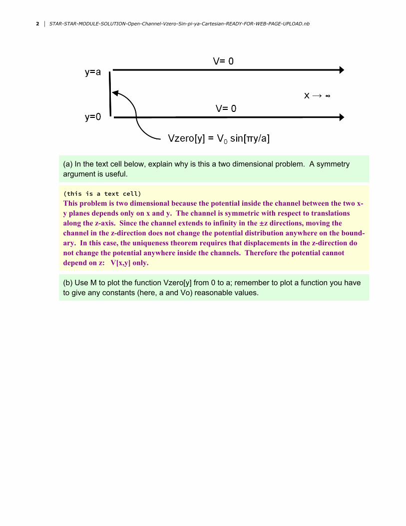
(a) In the text cell below, explain why is this a two dimensional problem. A symmetry argument is useful.

(this is a text cell)This problem is two dimensional because the potential inside the channel between the two x-y planes depends only on x and y. The channel is symmetric with respect to translations along the z-axis. Since the channel extends to infinity in the ±z directions, moving the channel in the z-direction does not change the potential distribution anywhere on the bound-ary. In this case, the uniqueness theorem requires that displacements in the z-direction do not change the potential anywhere inside the channels. Therefore the potential cannot depend on z: V[x,y] only.

(b) Use M to plot the function Vzero[y] from 0 to a; remember to plot a function you have to give any constants (here, a and Vo) reasonable values.

2 STAR-STAR-MODULE-SOLUTION-Open-Channel-Vzero-Sin-pi-ya-Cartesian-READY-FOR-WEB-PAGE-UPLOAD.nb

In[110]:= (* Assumptions →

y ∈ Reals && a ∈ Reals && a > 0 && 0 ⩽ y ≲ a && Vo ∈ Reals && Vo > 0; *)

a = 1; Vo = 1;

Vzero[y_] = Vo Sinπ y

a;

Plot[Vzero[y], {y, 0, a}, AxesLabel → {y, Sin[y]}]

Out[112]=

0.2 0.4 0.6 0.8 1.0y

0.2

0.4

0.6

0.8

1.0

sin(y)

(c) State the 2D boundary conditions that we will need to find V[x,y]

(this is a text cell)

(i) V[0,y] = Vzero[y] = Vo Sin π ya

(ii) V[x, 0] = 0(iii) V[x, a] = 0(iv) V[∞, y] = 0

(d) No Brainer-to nail an important point: Click inside the cell below (or select it by clicking on the bracket to the right) and execute it (Shift-Return); Answer Boxes will appear; Click on the one you think is correct answer for this question:

Question: What is the boundary condition on the right hand boundary (as x → ∞)?

STAR-STAR-MODULE-SOLUTION-Open-Channel-Vzero-Sin-pi-ya-Cartesian-READY-FOR-WEB-PAGE-UPLOAD.nb 3

Button["1 V inside the channel goes to ∞ as x-> ∞.",{Print[" Wrong. Sorry. "]}]

Button["2 V inside the channel goes to 0 as x-> ∞.",{Print[" Correct!! "]}]

Button["3 V inside the channel goes to Vo as x-> ∞.",{Print[" Wrong. Sorry. "]}]

1 V inside the channel goes to ∞ as x-> ∞.

2 V inside the channel goes to 0 as x-> ∞.

3 V inside the channel goes to Vo as x-> ∞.

Correct!!

Correct!!

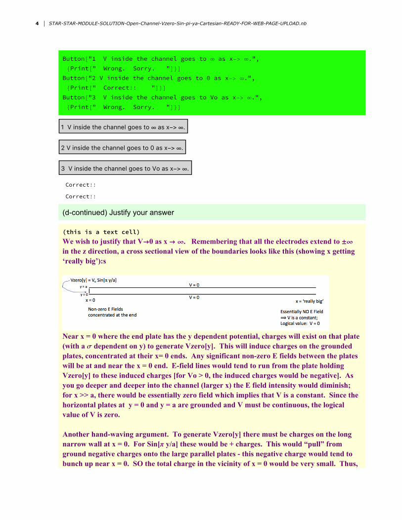
(d-continued) Justify your answer

(this is a text cell)We wish to justify that V→0 as x → ∞. Remembering that all the electrodes extend to ±∞ in the z direction, a cross sectional view of the boundaries looks like this (showing x getting ‘really big’):s

Near x = 0 where the end plate has the y dependent potential, charges will exist on that plate (with a σ dependent on y) to generate Vzero[y]. This will induce charges on the grounded plates, concentrated at their x= 0 ends. Any significant non-zero E fields between the plates will be at and near the x = 0 end. E-field lines would tend to run from the plate holding Vzero[y] to these induced charges [for Vo > 0, the induced charges would be negative]. As you go deeper and deeper into the channel (larger x) the E field intensity would diminish; for x >> a, there would be essentially zero field which implies that V is a constant. Since the horizontal plates at y = 0 and y = a are grounded and V must be continuous, the logical value of V is zero.

Another hand-waving argument. To generate Vzero[y] there must be charges on the long narrow wall at x = 0. For Sin[π y/a] these would be + charges. This would “pull” from ground negative charges onto the large parallel plates - this negative charge would tend to bunch up near x = 0. SO the total charge in the vicinity of x = 0 would be very small. Thus, as you go to larger and larger x (i.e., x >>a), the E field would be smaller and smaller, approaching zero which implies that V is a constant. AGAIN: Since the horizontal plates at y = 0 and y = a are grounded and V must be continuous, the logical value of V is zero.


(this is a text cell)We wish to justify that V→0 as x → ∞. Remembering that all the electrodes extend to ±∞ in the z direction, a cross sectional view of the boundaries looks like this (showing x getting ‘really big’):s

Near x = 0 where the end plate has the y dependent potential, charges will exist on that plate (with a σ dependent on y) to generate Vzero[y]. This will induce charges on the grounded plates, concentrated at their x= 0 ends. Any significant non-zero E fields between the plates will be at and near the x = 0 end. E-field lines would tend to run from the plate holding Vzero[y] to these induced charges [for Vo > 0, the induced charges would be negative]. As you go deeper and deeper into the channel (larger x) the E field intensity would diminish; for x >> a, there would be essentially zero field which implies that V is a constant. Since the horizontal plates at y = 0 and y = a are grounded and V must be continuous, the logical value of V is zero.

Another hand-waving argument. To generate Vzero[y] there must be charges on the long narrow wall at x = 0. For Sin[π y/a] these would be + charges. This would “pull” from ground negative charges onto the large parallel plates - this negative charge would tend to bunch up near x = 0. SO the total charge in the vicinity of x = 0 would be very small. Thus, as you go to larger and larger x (i.e., x >>a), the E field would be smaller and smaller, approaching zero which implies that V is a constant. AGAIN: Since the horizontal plates at y = 0 and y = a are grounded and V must be continuous, the logical value of V is zero.

A slight aside: How would you “construct” the electrode structures to approximate the problem we are working on??

First, all the plate coordinates that are supposed to be infinite, for practical purposes, means "much larger than a". So we cut two LARGE rectangles or squares of nice, flat sheet metal for these electrodes and mount them in parallel orientation. They could be insulated but in final form grounded so they are both at V = 0.

To approximate the plate holding the y dependent Vzero[y] is trickier.

Here is one scheme: Consider a set of very long parallel wires insulated from each other and from ground; label the wires with some index, say j. Let J (odd number) be the total number of wires. The spacing of the wires would be a/J so that the gap between the parallel plates (at x = 0) would be filled in uniform increments of y.

To get the Vo Sin π ya , we would apply the potential Vo on the center wire and connect

resistors between the wires with magnitudes that would drop the potential on the wires in sync with the Sin[ π ya ] function as you increase and decrease j from J/2 (going from the

center (y = a/2) to y = 0 and y = a).

Finding the magnitudes of these R's is assigned to the "loudest mouth in the class".

Details on Separation of Variables:

Unlike the 1-D Laplace’s equation, the 2-D equation is not an ordinary differential equation. That is, the derivatives are not total, but “partial”. The bad news is that partial differential equations seldom have closed, analytic solutions. The good news is that you can often construct an (infinite) series whose sum satisfies the boundary conditions.

The most straightforward way to find solutions to a partial differential equation is to “separate the vari-ables” in x and y. To separate the variables, we assume that the solution of the differential equation can be written as the product of two parts, one that depends on x only and one that depends on y only.

V(x,y) = X(x) Y(y)

Solutions that cannot be written in this form can usually be written as the sum of solutions with this form. When V(x,y) is substituted in Laplace’s equation

∂2V

∂x2+

∂2V

∂y2=

∂2 X

∂x2Y (y) + X (x)

∂2Y

∂x2+

∂2 X

∂y2Y (y) + X (x)

∂2Y

∂y2=

∂2 X

∂x2Y (y) + X (x)

∂2Y

∂y2= 0

(By construction dX/dy = dY/dx = 0.) If we divide through by the product, X(x)Y(y) we get two terms—one depending only on x and the other depending only on y.

1

X (x)

∂2 X

∂x2+

1

Y (x)

∂2Y

∂y2= 0

[Problems may occur at points where X(x)=0 and/or Y(y)=0. We can often work around such points if they are isolated.] Since x and y are independent variables, it is unreasonable to expect that a function that depends only on x to always be equal (with opposite sign) to a function that depends on y—unless the term in x is constant and the term in y equals (–1) times that constant. One term will be positive and the other negative. The sign seriously impacts the solutions X(x) and Y(y), and the wrong choice makes it impossible to satisfy the boundary conditions. In practice, you quickly run through the solutions for both sets of signs, then choose the solutions that work for your problem.

Since the choice of signs is important, we will set one constant to be something definitely positive, say, the square of a real number, λ2. The other constant will be –λ2. For instance,

1

X (x)

∂2 X

∂x2= λ2

1

Y (x)

∂2Y

∂y2= -λ2

This procedure has reduced the partial differential equation above to two, independent, ordinary differen-tial equations. We can solve ordinary differential equations. Any pair of solutions X(x) and Y(y) that satisfy the above ordinary differential equations will satisfy the partial differential equations above. The easiest way to solve the above equations is “by inspection.” Since each equation is second order, each equation has two independent solutions.


Details on Separation of Variables:

Unlike the 1-D Laplace’s equation, the 2-D equation is not an ordinary differential equation. That is, the derivatives are not total, but “partial”. The bad news is that partial differential equations seldom have closed, analytic solutions. The good news is that you can often construct an (infinite) series whose sum satisfies the boundary conditions.

The most straightforward way to find solutions to a partial differential equation is to “separate the vari-ables” in x and y. To separate the variables, we assume that the solution of the differential equation can be written as the product of two parts, one that depends on x only and one that depends on y only.

V(x,y) = X(x) Y(y)

Solutions that cannot be written in this form can usually be written as the sum of solutions with this form. When V(x,y) is substituted in Laplace’s equation

∂2V

∂x2+

∂2V

∂y2=

∂2 X

∂x2Y (y) + X (x)

∂2Y

∂x2+

∂2 X

∂y2Y (y) + X (x)

∂2Y

∂y2=

∂2 X

∂x2Y (y) + X (x)

∂2Y

∂y2= 0

(By construction dX/dy = dY/dx = 0.) If we divide through by the product, X(x)Y(y) we get two terms—one depending only on x and the other depending only on y.

1

X (x)

∂2 X

∂x2+

1

Y (x)

∂2Y

∂y2= 0

[Problems may occur at points where X(x)=0 and/or Y(y)=0. We can often work around such points if they are isolated.] Since x and y are independent variables, it is unreasonable to expect that a function that depends only on x to always be equal (with opposite sign) to a function that depends on y—unless the term in x is constant and the term in y equals (–1) times that constant. One term will be positive and the other negative. The sign seriously impacts the solutions X(x) and Y(y), and the wrong choice makes it impossible to satisfy the boundary conditions. In practice, you quickly run through the solutions for both sets of signs, then choose the solutions that work for your problem.

Since the choice of signs is important, we will set one constant to be something definitely positive, say, the square of a real number, λ2. The other constant will be –λ2. For instance,

1

X (x)

∂2 X

∂x2= λ2

1

Y (x)

∂2Y

∂y2= -λ2

This procedure has reduced the partial differential equation above to two, independent, ordinary differen-tial equations. We can solve ordinary differential equations. Any pair of solutions X(x) and Y(y) that satisfy the above ordinary differential equations will satisfy the partial differential equations above. The easiest way to solve the above equations is “by inspection.” Since each equation is second order, each equation has two independent solutions.

(e) In the space below, solve the two ordinary differential equations, either by inspection, or by using M.

(this is a text cell)Assuming λ, X1, X2, Y1 and Y2 are constants, inspection gives us.

X (x) = X1 Exp[λ x] + X2 Exp[-λ x]Y (y) = Y1 Cos[λ y] + Y2 Sin[λy]

Using M. You will need to assume that λ is real and is greater than or equal to zero. (You can omit the possibility that λ = 0 for now, because the corresponding solution would be trivial and uninteresting.)


In[113]:= $Assumptions → λ ∈ Reals && λ > 0 && y ∈ Reals &&a ∈ Reals && a > 0 && 0 ⩽ y ≲ a && Vo ∈ Reals && Vo > 0;

solx = DSolveX''[x] - λ2 X[x] ⩵ 0, X[x], x

soly = DSolveY''[y] + λ2 Y[y] ⩵ 0, Y[y], y

Out[114]= X[x] → ⅇx λ C[1] + ⅇ-x λ C[2]

Out[115]= {{Y[y] → C[1] Cos[y λ] + C[2] Sin[y λ]}}

To this point, we have four constants of integration and the unknown λ that are constrained by the boundary conditions.

We require V[x →∞,y] = 0. If C[1]≠0 in X[x], the Exp[λx] term will go to infinity and violate this constraint. Therefore C[1]=0 in X[x] no matter what λ is. (Note that the Exp[+λ] terms are needed to satisfy bound-ary conditions in other problems. Both the Exp[-λ] and Exp[+λ] terms may be needed.)

We require V[x,y=0] = 0. If If C[1]≠0 in Y[y], the Cos[λy] term will violate this constraint. Our solution must take the form:

X (x) = X2 Exp[-λx], and

Y (y) = Y2 Sin[λy]

But we also expect V[x,y=a] = 0. The Sin[λx] term will allow this only if λ = nπ/a, where n is a positive integer (n≠0). This constraint poses a problem in that we have an infinite number of λ’s. It also poses an opportunity, in that we may need an infinite number of them to satisfy our remaining boundary condition: Vzero[y] = Vo Sin[πy/a].

We proceed by assuming that Vzero[y] can be expressed as the sum of functions that satisfy the other boundary conditions; that is, for some set of coefficients {Cn , n = 1,2,3, ....}

Vzero[y] = n=1

∞

Cn Sinnπ y

a

This particular series expansion is known as a Fourier sine series. The existence and convergence of this kind of series is discussed in detail in most Applied or Engineering Mathematics texts. The con-stants {Cn} can be determined using the “Fourier trick”. The Fourier trick takes advantage of the fact that the set of functions {sin[nπy/a]} is orthogonal over the interval {0,a}. That is, the integral of the product of two members of this set over the interval {0,a} is zero unless they have the same n-value. This easily shown using the trig identity sinθ sinϕ = (1/2)[cos(θ-ϕ) - sin(θ+ϕ)].

0

aSin

nπ y

a Sin

n' π y

a ⅆy = 1

2 0

aCos

n - n' π y

a ⅆy - 1

2 0

aSin

n + n' π y

a ⅆy

Now the integral of any sine or cosine function over any number of complete cycles is equal to zero. Therefore both integrals equal zero for every choice of {n,n'} except for n = n', when Cos[0] = 1. Then the integral equals a/2. In summary:

0

aSin

nπ y

a Sin

n' π y

a ⅆy =

0 n ≠ n 'a /2 n = n '

This identity allows us to compute the coefficients {Cn}. If we multiply each side of the series expansion for V[x] by sin[n'π y/a] and Integrate from 0 to a, we have:

0

aV[y] Sin

n' πy

a ⅆy =

n=1

∞

Cn 0

aSin

nπy

a Sin

n' πy

a ⅆy =

a Cn'

2

Cn' =2

a

0

aV[y] Sin

n' πy

a ⅆy

Determining Cn for n = 1,2,3... produces an infinite series that converges to the solution of the 2-D Laplace’s equation that meets all the boundary conditions. (In general, the series may fail to converge at a finite number of points. We ignore these points.) The solution will include both X[x] and Y[y] fac-tors, so that:

V[x, y] = X[x] Y[y] = n=1

∞

Cn Exp-nπ x

a Sin

nπ y

a

We need to determine Cn for for the remaining boundary condition Vzero[y] = Vo Sin[πy/a]. Since Vzero[y] includes only one term, and that term corresponds to the n=1 term in our infinite series. Direct integration shows that C1 = Vo. More complicated cases benefit from M.


To this point, we have four constants of integration and the unknown λ that are constrained by the boundary conditions.

We require V[x →∞,y] = 0. If C[1]≠0 in X[x], the Exp[λx] term will go to infinity and violate this constraint. Therefore C[1]=0 in X[x] no matter what λ is. (Note that the Exp[+λ] terms are needed to satisfy bound-ary conditions in other problems. Both the Exp[-λ] and Exp[+λ] terms may be needed.)

We require V[x,y=0] = 0. If If C[1]≠0 in Y[y], the Cos[λy] term will violate this constraint. Our solution must take the form:

X (x) = X2 Exp[-λx], and

Y (y) = Y2 Sin[λy]

But we also expect V[x,y=a] = 0. The Sin[λx] term will allow this only if λ = nπ/a, where n is a positive integer (n≠0). This constraint poses a problem in that we have an infinite number of λ’s. It also poses an opportunity, in that we may need an infinite number of them to satisfy our remaining boundary condition: Vzero[y] = Vo Sin[πy/a].

We proceed by assuming that Vzero[y] can be expressed as the sum of functions that satisfy the other boundary conditions; that is, for some set of coefficients {Cn , n = 1,2,3, ....}

Vzero[y] = n=1

∞

Cn Sinnπ y

a

This particular series expansion is known as a Fourier sine series. The existence and convergence of this kind of series is discussed in detail in most Applied or Engineering Mathematics texts. The con-stants {Cn} can be determined using the “Fourier trick”. The Fourier trick takes advantage of the fact that the set of functions {sin[nπy/a]} is orthogonal over the interval {0,a}. That is, the integral of the product of two members of this set over the interval {0,a} is zero unless they have the same n-value. This easily shown using the trig identity sinθ sinϕ = (1/2)[cos(θ-ϕ) - sin(θ+ϕ)].

0

aSin

nπ y

a Sin

n' π y

a ⅆy = 1

2 0

aCos

n - n' π y

a ⅆy - 1

2 0

aSin

n + n' π y

a ⅆy

Now the integral of any sine or cosine function over any number of complete cycles is equal to zero. Therefore both integrals equal zero for every choice of {n,n'} except for n = n', when Cos[0] = 1. Then the integral equals a/2. In summary:

0

aSin

nπ y

a Sin

n' π y

a ⅆy =

0 n ≠ n 'a /2 n = n '

This identity allows us to compute the coefficients {Cn}. If we multiply each side of the series expansion for V[x] by sin[n'π y/a] and Integrate from 0 to a, we have:

0

aV[y] Sin

n' πy

a ⅆy =

n=1

∞

Cn 0

aSin

nπy

a Sin

n' πy

a ⅆy =

a Cn'

2

Cn' =2

a

0

aV[y] Sin

n' πy

a ⅆy

Determining Cn for n = 1,2,3... produces an infinite series that converges to the solution of the 2-D Laplace’s equation that meets all the boundary conditions. (In general, the series may fail to converge at a finite number of points. We ignore these points.) The solution will include both X[x] and Y[y] fac-tors, so that:

V[x, y] = X[x] Y[y] = n=1

∞

Cn Exp-nπ x

a Sin

nπ y

a

We need to determine Cn for for the remaining boundary condition Vzero[y] = Vo Sin[πy/a]. Since Vzero[y] includes only one term, and that term corresponds to the n=1 term in our infinite series. Direct integration shows that C1 = Vo. More complicated cases benefit from M.

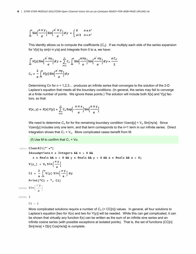
(f) Use M to confirm that C1 = Vo.

In[121]:= ClearAll["`*"]$Assumptions n ∈ Integers && n > 0 &&

x ∈ Reals && x > 0 && y ∈ Reals && y > 0 && a ∈ Reals && a > 0;

V[y_] = Vo Sinπ y

a

C1 =2

a0

aV[y] Sin

π y

a ⅆy

Print["C1 = ", C1]

Out[123]= Sinπ y

a

Out[124]= 1

C1 = 1

More complicated solutions require a number of Cn (= CC[n]) values. In general, all four solutions to Laplace’s equation [two for X(x) and two for Y(y)] will be needed. While this can get complicated, it can be shown that virtually any function f(x) can be written as the sum of an infinite sine series and an infinite cosine series (with possible exceptions at isolated points). That is, the set of functions {CC[n] Sin[πx/a] + D[n] Cos[πx/a]} is complete.

The same is true of the set of functions {A[n] Exp[πy/a] + B[n] Exp[-πy/a]} is complete: any function g(y) can be written in terms of an infinite series of terms with this form.

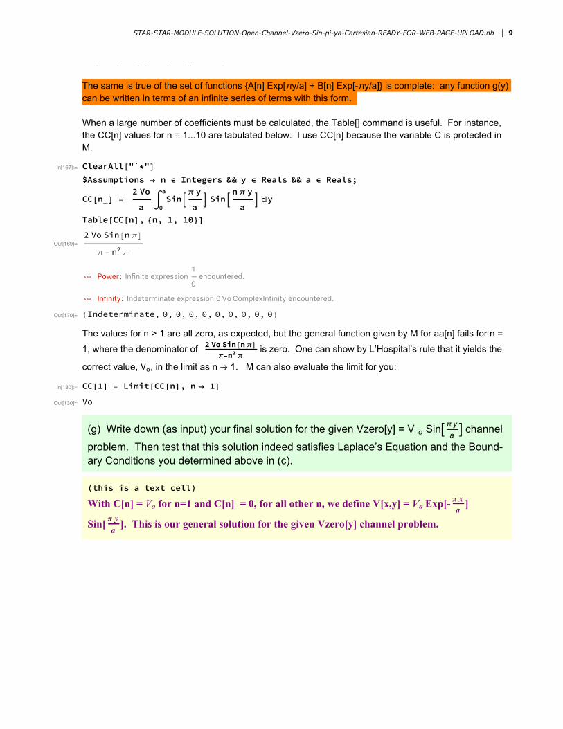
When a large number of coefficients must be calculated, the Table[] command is useful. For instance, the CC[n] values for n = 1...10 are tabulated below. I use CC[n] because the variable C is protected in M.


More complicated solutions require a number of Cn (= CC[n]) values. In general, all four solutions to Laplace’s equation [two for X(x) and two for Y(y)] will be needed. While this can get complicated, it can be shown that virtually any function f(x) can be written as the sum of an infinite sine series and an infinite cosine series (with possible exceptions at isolated points). That is, the set of functions {CC[n] Sin[πx/a] + D[n] Cos[πx/a]} is complete.

The same is true of the set of functions {A[n] Exp[πy/a] + B[n] Exp[-πy/a]} is complete: any function g(y) can be written in terms of an infinite series of terms with this form.

When a large number of coefficients must be calculated, the Table[] command is useful. For instance, the CC[n] values for n = 1...10 are tabulated below. I use CC[n] because the variable C is protected in M.

In[167]:= ClearAll["`*"]$Assumptions → n ∈ Integers && y ∈ Reals && a ∈ Reals;

CC[n_] =2 Vo

a0

aSin

π y

a Sin

n π y

a ⅆy

Table[CC[n], {n, 1, 10}]

Out[169]=2 Vo Sin[n π]

π - n2 π

Power: Infinite expression1

0encountered.

Infinity: Indeterminate expression 0 VoComplexInfinity encountered.

Out[170]= {Indeterminate, 0, 0, 0, 0, 0, 0, 0, 0, 0}

The values for n > 1 are all zero, as expected, but the general function given by M for aa[n] fails for n =

1, where the denominator of 2 Vo Sin[n π]

π-n2 π is zero. One can show by L’Hospital’s rule that it yields the

correct value, Vo, in the limit as n → 1. M can also evaluate the limit for you:

In[130]:= CC[1] = Limit[CC[n], n → 1]

Out[130]= Vo

(g) Write down (as input) your final solution for the given Vzero[y] = V o Sin π ya channel

problem. Then test that this solution indeed satisfies Laplace’s Equation and the Bound-ary Conditions you determined above in (c).

(this is a text cell)

With C[n] = Vo for n=1 and C[n] = 0, for all other n, we define V[x,y] = Vo Exp[- π xa ]

Sin[ π ya ]. This is our general solution for the given Vzero[y] channel problem.


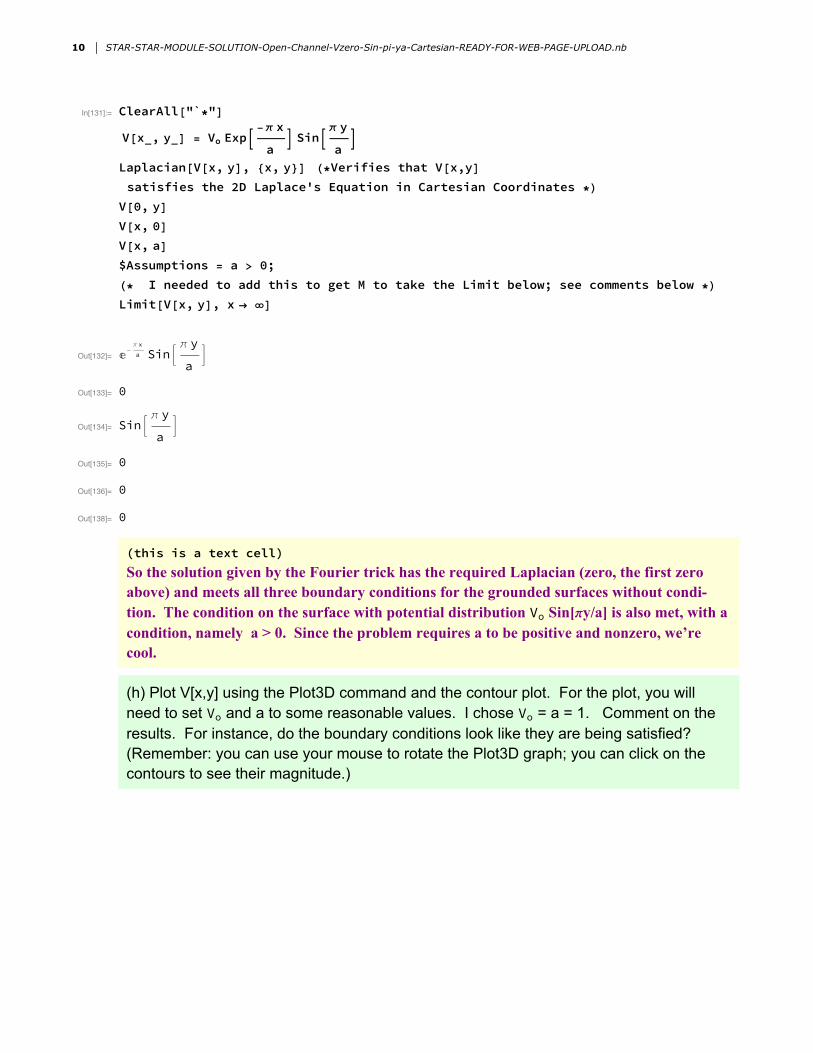
In[131]:= ClearAll["`*"]

V[x_, y_] = Vo Exp-π x

a Sin

π y

a

Laplacian[V[x, y], {x, y}] (*Verifies that V[x,y]satisfies the 2D Laplace's Equation in Cartesian Coordinates *)

V[0, y]V[x, 0]V[x, a]$Assumptions = a > 0;(* I needed to add this to get M to take the Limit below; see comments below *)

Limit[V[x, y], x → ∞]

Out[132]= ⅇ-π xa Sin

π y

a

Out[133]= 0

Out[134]= Sinπ y

a

Out[135]= 0

Out[136]= 0

Out[138]= 0

(this is a text cell)So the solution given by the Fourier trick has the required Laplacian (zero, the first zero above) and meets all three boundary conditions for the grounded surfaces without condi-tion. The condition on the surface with potential distribution Vo Sin[πy/a] is also met, with a condition, namely a > 0. Since the problem requires a to be positive and nonzero, we’re cool.

(h) Plot V[x,y] using the Plot3D command and the contour plot. For the plot, you will need to set Vo and a to some reasonable values. I chose Vo = a = 1. Comment on the results. For instance, do the boundary conditions look like they are being satisfied? (Remember: you can use your mouse to rotate the Plot3D graph; you can click on the contours to see their magnitude.)


In[139]:= Vo = 1; a = 1;

V[x_, y_] = Vo Exp-π x

a Sin

π y

a ;

Plot3D[V[x, y], {x, 0, 2 a}, {y, 0, a},PlotRange → {0, 1}, ColorFunction → "DarkRainbow"]

con = ContourPlot[V[x, y], {x, 0, a}, {y, 0, a}, Contours → 40, PlotRange → {0, 1}]

Out[141]=

Out[142]=

(this is a text cell)The x=0 cross section of the Plot3D graph looks like Sin[π y] consistent with the boundary condition for Vzero[y]. From all appearances, V(x, y=0) = V(x, y=a) = 0. It is worth noting that the curvature of V(x,y) is negative along the y-direction (concave downward, ∂2 V

∂ y2 < 0 )

and positive along the x-direction (concave upward, ∂2 V∂ x2 > 0). This is required by the 2-D

Laplace’s equation in Cartesian coordinates ( ∂2V∂x2 + ∂2V

∂y2 = 0) the two second derivatives

need opposite signs to cancel) and is always worth checking.

V[x,y] appears to decay exponentially with distance from the x=0 plane. The potential falls to 1/3 of its value in roughly 0.4 “a-units”, consistent with a decay constant of 1/π. (When x = 1/π in Exp[-π x], V[x] = V0/e ~ V0/3.) The contour plot shows the exponential decay in a less quantitative fashion. As the potential decreases, the equipotentials become more tan-gent to the upper and lower surfaces, and still extend all the way to the y-axis. This is consistent with the upper and lower surfaces being held at ground potential.

The exponential decay with distance away from the non-grounded surface illustrates a general principle. If the left-hand surface were grounded, like the other two, the potential everywhere between the plates would be zero. Introducing a non-grounded surface at one end produces a non-zero potential that decays exponentially with distance from the surface. Here the decay length is a/π. Saint-Venant proposed that the change in potential due to a localized change in the boundary conditions is also localized. The size of the changed bound-ary region (here characterized by the length a) is often simply related to the size of the affected regions (where the potential is changed). The amplitude of the changed potential also decays exponentially with the same decay constant (here a/π ≈ a). At distances far from the left end (distances >> a/π), the difference between the true potential and ground becomes small. One can often take advantage of this effect when changing the boundary conditions in a localized region would make for an easier problem. (The Saint in Saint-Venant is part the family name. He succeeded Coriolis at the prestigious French National School of Bridges and Roads.)


(this is a text cell)The x=0 cross section of the Plot3D graph looks like Sin[π y] consistent with the boundary condition for Vzero[y]. From all appearances, V(x, y=0) = V(x, y=a) = 0. It is worth noting that the curvature of V(x,y) is negative along the y-direction (concave downward, ∂2 V

∂ y2 < 0 )

and positive along the x-direction (concave upward, ∂2 V∂ x2 > 0). This is required by the 2-D

Laplace’s equation in Cartesian coordinates ( ∂2V∂x2 + ∂2V

∂y2 = 0) the two second derivatives

need opposite signs to cancel) and is always worth checking.

V[x,y] appears to decay exponentially with distance from the x=0 plane. The potential falls to 1/3 of its value in roughly 0.4 “a-units”, consistent with a decay constant of 1/π. (When x = 1/π in Exp[-π x], V[x] = V0/e ~ V0/3.) The contour plot shows the exponential decay in a less quantitative fashion. As the potential decreases, the equipotentials become more tan-gent to the upper and lower surfaces, and still extend all the way to the y-axis. This is consistent with the upper and lower surfaces being held at ground potential.

The exponential decay with distance away from the non-grounded surface illustrates a general principle. If the left-hand surface were grounded, like the other two, the potential everywhere between the plates would be zero. Introducing a non-grounded surface at one end produces a non-zero potential that decays exponentially with distance from the surface. Here the decay length is a/π. Saint-Venant proposed that the change in potential due to a localized change in the boundary conditions is also localized. The size of the changed bound-ary region (here characterized by the length a) is often simply related to the size of the affected regions (where the potential is changed). The amplitude of the changed potential also decays exponentially with the same decay constant (here a/π ≈ a). At distances far from the left end (distances >> a/π), the difference between the true potential and ground becomes small. One can often take advantage of this effect when changing the boundary conditions in a localized region would make for an easier problem. (The Saint in Saint-Venant is part the family name. He succeeded Coriolis at the prestigious French National School of Bridges and Roads.)

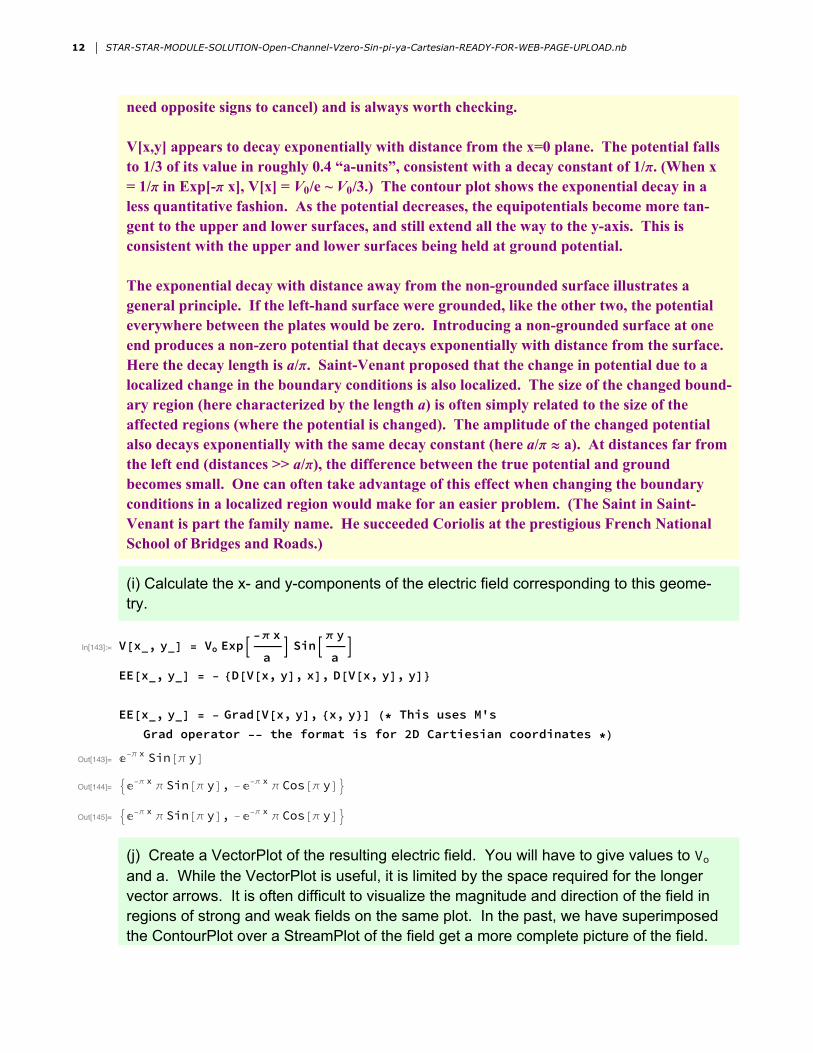
(i) Calculate the x- and y-components of the electric field corresponding to this geome-try.

In[143]:= V[x_, y_] = Vo Exp-π x

a Sin

π y

a

EE[x_, y_] = - {D[V[x, y], x], D[V[x, y], y]}

EE[x_, y_] = - Grad[V[x, y], {x, y}] (* This uses M'sGrad operator -- the format is for 2D Cartiesian coordinates *)

Out[143]= ⅇ-π x Sin[π y]

Out[144]= ⅇ-π x π Sin[π y], -ⅇ-π x π Cos[π y]


(j) Create a VectorPlot of the resulting electric field. You will have to give values to Vo and a. While the VectorPlot is useful, it is limited by the space required for the longer vector arrows. It is often difficult to visualize the magnitude and direction of the field in regions of strong and weak fields on the same plot. In the past, we have superimposed the ContourPlot over a StreamPlot of the field get a more complete picture of the field. The background color and spacing of the potential contours reflects the magnitude of the field, while the StreamPlot indicates its direction. In addition to the vector plot, superim-pose the corresponding ContourPlot and StreamPlot. Comment.


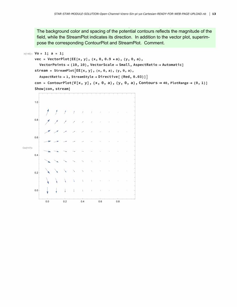
(j) Create a VectorPlot of the resulting electric field. You will have to give values to Vo and a. While the VectorPlot is useful, it is limited by the space required for the longer vector arrows. It is often difficult to visualize the magnitude and direction of the field in regions of strong and weak fields on the same plot. In the past, we have superimposed the ContourPlot over a StreamPlot of the field get a more complete picture of the field. The background color and spacing of the potential contours reflects the magnitude of the field, while the StreamPlot indicates its direction. In addition to the vector plot, superim-pose the corresponding ContourPlot and StreamPlot. Comment.

In[146]:= Vo = 1; a = 1;vec = VectorPlot[EE[x, y], {x, 0, 0.9 * a}, {y, 0, a},

VectorPoints → {10, 10}, VectorScale → Small, AspectRatio → Automatic]stream = StreamPlotEE[x, y], {x, 0, a}, {y, 0, a},

AspectRatio → 1, StreamStyle → Directive[ {Red, 0.03}]

con = ContourPlot[V[x, y], {x, 0, a}, {y, 0, a}, Contours → 40, PlotRange → {0, 1}]Show[con, stream]

Out[147]=

0.0 0.2 0.4 0.6 0.8

0.0

0.2

0.4

0.6

0.8

1.0


Out[148]=

0.0 0.2 0.4 0.6 0.8 1.0

0.0

0.2

0.4

0.6

0.8

1.0

Out[149]=


Out[150]=

(this is a text cell)As it should, the equipotentials and the field lines are everywhere perpendicular. The field lines are also perpendicular to the grounded conducting surfaces. This is required of con-ducting surfaces in electrostatic equilibrium because any parallel component of the field would drive currents along the surface (violating the assumption of equilibrium). Note that field lines are not perpendicular to the vertical surface on the left (at x = 0) where they intersect it. This surface is not a single piece of conductor. With the given boundary condi-tions, it cannot such. To achieve the specified boundary conditions, one would have to distribute charge in a special way along the surface that holds them in place. This requires an insulator (or our hokey set of parallel wires discussed above).

A brief comment on magnitudes is in order. The peak electric fields have magnitude (πVo/a). If Vo = 1 V/m and a = 1 m, the resulting peak fields are about 3 V/m. This is compa-rable to the peak potential (1 volt) divided by 1/2 the plate separation (a/2 = 0.5 m). Seems pretty reasonable.

Both the vector plot and the contour plot suggest that the magnitude of the electric field just next to the left hand plate is constant: the length of the vector arrows and the spacing of the potential contours are uniform to the eye—as near as I can see. The constant magnitude can be confirmed by calculation, using the field components for x = 0.

For a quick look at this, we can use a DensityPlot of the Magnitude of EE (this is given by Norm[EE[x,y]) I superimpose the VectorPlot and the DensityPlot below. You can see the bands of color are surprisingly uniform for a given value of y. Note that the vertical rows of EE arrows, although differing in direction, have similar lengths.


(this is a text cell)As it should, the equipotentials and the field lines are everywhere perpendicular. The field lines are also perpendicular to the grounded conducting surfaces. This is required of con-ducting surfaces in electrostatic equilibrium because any parallel component of the field would drive currents along the surface (violating the assumption of equilibrium). Note that field lines are not perpendicular to the vertical surface on the left (at x = 0) where they intersect it. This surface is not a single piece of conductor. With the given boundary condi-tions, it cannot such. To achieve the specified boundary conditions, one would have to distribute charge in a special way along the surface that holds them in place. This requires an insulator (or our hokey set of parallel wires discussed above).

A brief comment on magnitudes is in order. The peak electric fields have magnitude (πVo/a). If Vo = 1 V/m and a = 1 m, the resulting peak fields are about 3 V/m. This is compa-rable to the peak potential (1 volt) divided by 1/2 the plate separation (a/2 = 0.5 m). Seems pretty reasonable.

Both the vector plot and the contour plot suggest that the magnitude of the electric field just next to the left hand plate is constant: the length of the vector arrows and the spacing of the potential contours are uniform to the eye—as near as I can see. The constant magnitude can be confirmed by calculation, using the field components for x = 0.

For a quick look at this, we can use a DensityPlot of the Magnitude of EE (this is given by Norm[EE[x,y]) I superimpose the VectorPlot and the DensityPlot below. You can see the bands of color are surprisingly uniform for a given value of y. Note that the vertical rows of EE arrows, although differing in direction, have similar lengths.

In[151]:= density = DensityPlotNorm[EE[x, y]], {x, 0, a},

{y, 0, a}, AspectRatio → 1, ColorFunction → "SunsetColors";

Show[density,vec]

Out[152]=

(k) Charge Density. For -∞ < z < ∞, the charge density on the left hand surface of the channel (at x = 0) is a function of y only (σleft[y]). Find σleft[y] in units of Cm2 (so you

will need to introduce ϵ0 = 8.85 × 10-12 F/m). Note the magnitude of the values of σ dis-played.

Plot your resulting σ[y].


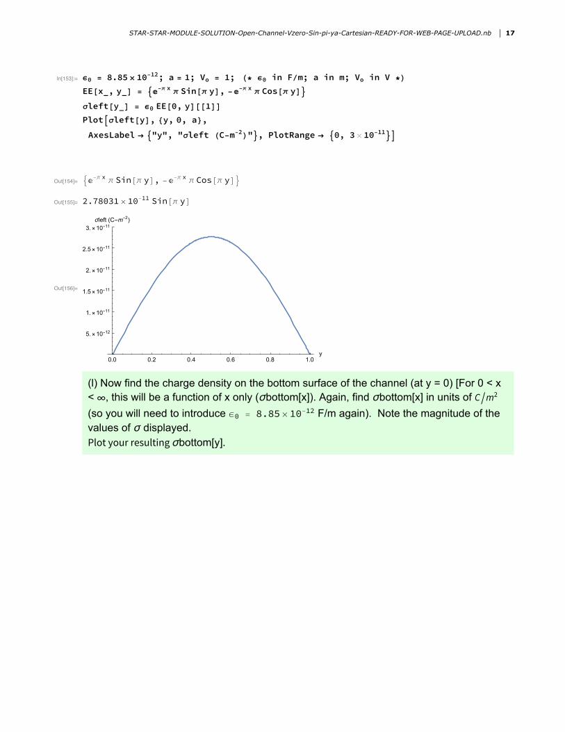
In[153]:= ϵ0 = 8.85 × 10-12; a = 1; Vo = 1; (* ϵ0 in F/m; a in m; Vo in V *)

EE[x_, y_] = ⅇ-π x π Sin[π y], -ⅇ-π x π Cos[π y]

σleft[y_] = ϵ0 EE[0, y][[1]]Plotσleft[y], {y, 0, a},

AxesLabel → "y", "σleft (C-m-2)", PlotRange → 0, 3 × 10-11


Out[155]= 2.78031 × 10-11 Sin[π y]

Out[156]=

0.0 0.2 0.4 0.6 0.8 1.0y

5.×10-12

1.×10-11

1.5×10-11

2.×10-11

2.5×10-11

3.×10-11σleft (C-m-2)

(l) Now find the charge density on the bottom surface of the channel (at y = 0) [For 0 < x < ∞, this will be a function of x only (σbottom[x]). Again, find σbottom[x] in units of Cm2 (so you will need to introduce ϵ0 = 8.85 × 10-12 F/m again). Note the magnitude of the values of σ displayed.Plot your resulting σbottom[y].


In[157]:= ϵ0 = 8.85 × 10-12; a = 1; Vo = 1;EE[x_, y_] = ⅇ-π x π Sin[π y], -ⅇ-π x π Cos[π y]

σbottom[x_] = ϵ0 EE[x, 0] . {0, 1}(* {0,1} is the surface normal vector for the BOTTOM horizontal electrode *)

Plotσbottom[x], {x, 0, 2 a}, PlotRange → -3 × 10-11, 0,

AxesLabel → "x", "σ (C-m-2)", "sigma_x = 0_plane"


Out[159]= -2.78031 × 10-11 ⅇ-π x

Out[160]=

0.5 1.0 1.5 2.0x

-3.×10-11

-2.5×10-11

-2.×10-11

-1.5×10-11

-1.×10-11

-5.×10-12

σ (C-m-2)

(this is a text cell)The surface charge density along a boundary is determined by the normal component of the electric field: σ = ϵo (Eabovesurface – Ebelowsurface)·n, from Griffiths Section 2.3.5), where the normal vector n points away from the surface in the “above” direction. I have chosen the “above” direction to point into the volume between the plates, but other choices are possible. The solution to Laplace’s equation gives us the electric field between the plates, so Eabovesurface is easy to calculate.

With these choices, Ebelowsurface is zero for each channel surface. This is clear for the conducting plates, as the field inside a conductor (here “below” the surface) must be zero. How about the insulating surface on the left? Above we argued that the net charge of the system was zero. If we construct a Gaussian surface just below the surface of all three plates (extending to infinity in the +x direction), the net flux through the surface must be zero. The flux due to the top and bottom plates must be zero (field must be zero here). Similarly, the flux through the vertical surface at x = ∞ is also be zero. Therefore the net flux through the Gaussian surface just below the left plate must also be zero. Since the left plate is charged positive everywhere (except zero at the ends), any E-field from the plate must extend away from the plate; any field directed to the left of the plate (in the negative x-direction) would result in a nonzero flux through our Gaussian surface on the left. This contradicts the conclusion that the net flux due to Ebelowsurface must be zero here. So Ebelowsurface must be zero everywhere for the left plate too.

Note how small the charge densities are corresponding to potentials near 1 V (Vo).


(this is a text cell)The surface charge density along a boundary is determined by the normal component of the electric field: σ = ϵo (Eabovesurface – Ebelowsurface)·n, from Griffiths Section 2.3.5), where the normal vector n points away from the surface in the “above” direction. I have chosen the “above” direction to point into the volume between the plates, but other choices are possible. The solution to Laplace’s equation gives us the electric field between the plates, so Eabovesurface is easy to calculate.

With these choices, Ebelowsurface is zero for each channel surface. This is clear for the conducting plates, as the field inside a conductor (here “below” the surface) must be zero. How about the insulating surface on the left? Above we argued that the net charge of the system was zero. If we construct a Gaussian surface just below the surface of all three plates (extending to infinity in the +x direction), the net flux through the surface must be zero. The flux due to the top and bottom plates must be zero (field must be zero here). Similarly, the flux through the vertical surface at x = ∞ is also be zero. Therefore the net flux through the Gaussian surface just below the left plate must also be zero. Since the left plate is charged positive everywhere (except zero at the ends), any E-field from the plate must extend away from the plate; any field directed to the left of the plate (in the negative x-direction) would result in a nonzero flux through our Gaussian surface on the left. This contradicts the conclusion that the net flux due to Ebelowsurface must be zero here. So Ebelowsurface must be zero everywhere for the left plate too.

Note how small the charge densities are corresponding to potentials near 1 V (Vo).

(m) I claim that the net charge of the system as a whole is zero.

We have a system where -∞ > z > ∞ so the total charge on the left hand surface would be infinite; likewise for the charges on the horizontal plates.

So first, calculate the charges/unit length (λ) in the z direction by integrating σleft over y and σbottom over x and compare them.

In[161]:= λleft = 0

aσleft[y] ⅆy

λbottom = 0

∞σbottom[x] ⅆx

Out[161]= 1.77 × 10-11

Out[162]= -8.85 × 10-12

If we multiply these λ’s by some length L >> a, we would get a total charge corresponding to a “real” channel. Let’s simply stay with charge/unit length (i.e., the λ’s).

They are not equal in magnitude, but obviously we have ignored the charge on the upper horizontal plate (at y = a).

So finding σtop[x] and integrating over x we get λtop:

In[163]:= σtop[x_] = ϵ0 EE[x, a]. {0, -1}(* {0, -1} is the surface normal vector for the TOP horizontal electrode *)

λtop = 0

∞σtop[x] ⅆx

Out[163]= -2.78031 × 10-11 ⅇ-π x

Out[164]= -8.85 × 10-12

Now add all three λ’s (remember this is charge per unit length in the z direction)

In[165]:= λTOTAL = λleft + λbottom + λtop;Print["The total charge per unit length in the z direction = ", λTOTAL]

The total charge per unit length in the z direction = 0.

Are you happy?? We are. Note that the charge on the top and bottom plates were equal which we would expect from symmetry.


potential in open rectangular channel with parallel sides

Documents