potential model of a two-dimensional bunsen flame
TRANSCRIPT
HAL Id: hal-00084901https://hal.archives-ouvertes.fr/hal-00084901
Submitted on 10 Jul 2006
HAL is a multi-disciplinary open accessarchive for the deposit and dissemination of sci-entific research documents, whether they are pub-lished or not. The documents may come fromteaching and research institutions in France orabroad, or from public or private research centers.
L’archive ouverte pluridisciplinaire HAL, estdestinée au dépôt et à la diffusion de documentsscientifiques de niveau recherche, publiés ou non,émanant des établissements d’enseignement et derecherche français ou étrangers, des laboratoirespublics ou privés.
Potential model of a two-dimensional Bunsen flameBruno Denet
To cite this version:Bruno Denet. Potential model of a two-dimensional Bunsen flame. Physics of Fluids, AmericanInstitute of Physics, 2002, 14(10), pp.3577-3583. �10.1063/1.1504448�. �hal-00084901�
ccsd
-000
8490
1, v
ersi
on 1
- 1
0 Ju
l 200
6
PF#2343
Potential model of a 2D Bunsen flame
Bruno Denet
IRPHE 49 rue Joliot Curie BP 146 Technopole de Chateau Gombert 13384 Marseille Cedex 13
France
submitted to Physics of Fluids
Abstract
The Michelson Sivashinsky equation, which models the non linear dynamics of premixed
flames, has been recently extended to describe oblique flames. This approach was extremely
successful to describe the behavior on one side of the flame, but some qualitative effects
involving the interaction of both sides of the front were left unexplained. We use here a
potential flow model, first introduced by Frankel, to study numerically this configuration.
Furthermore, this approach allows us to provide a physical explanation of the phenomena
occuring in this geometry by means of an electrostatic analogy.
Keywords: laminar reacting flows
1
1 Introduction
The Michelson Sivashinsky equation [1] forms the basis of non linear descriptions of laminar pre-
mixed flames. While originally developed for the case of plane on average flames, variants of this
equation have also been applied to spherical expanding flames [2] [3]. However, an extension of
this equation valid for oblique flames has been obtained only recently by Joulin in [4] by adding a
convective term to the original equation , which mimics the transverse velocity appearing as soon
as the flame is maintained oblique compared to the direction of propagation. The motivation of
this work can be found in the experimental setup of Truffaut and Searby [5], which the authors
have called an inverted V flame. Actually this configuration is a sort of 2D Bunsen burner laminar
flame, perturbed on one side by an applied electric field. A comparison of the model equation
with the experiment has been remarkably successful, even from a quantitative point of view, and
describes the development and saturation of wrinkles amplified by the Darrieus-Landau instability.
However, this equation is limited to one side of the front. Searby and Truffaut have been able to
exhibit an effect not described by the lagrangian Michelson Sivashinsky equation: when the flame is
excited on one side, relatively small cells develop on this face of the flame but an overall curvature
of the flame at large scale occurs.
This effect can only be explained by a model taking into account both sides of the flame. It
turns out that such a model already exists in the form of an equation derived by Frankel [6]. We
shall describe this model in more detail in section 2, but for the moment let us just say that the
model assumes a potential flow both ahead and behind the flame, and consists of a boundary
integral equation (the boundary is the flame front, seen as a discontinuity) involving electrostatic
potentials. Some numerical simulations of this equation can be found in the literature [7] [8] [9]
[10] in the case of expanding flames, but it has not been used for the moment in other geometries.
We use here a slightly modified version of this equation to study the 2D Bunsen flame case. With
this method, all the phenomena observed experimentally are recovered and it is possible to use an
2
electrostatic analogy in order to get a physical understanding of this problem.
In section 2 we present the Frankel equation in a form suitable to the present geometry and
we take the opportunity to show that this equation naturally leads to a qualitative interpretation
of the Darrieus Landau instability. In section 3 we present the results obtained in the 2D Bunsen
flame configuration for various values of the parameters. Finally section 4 contains a conclusion.
2 Model
Let us first introduce some notations. We use two different flame velocities, the flame velocity
relative to premixed gases ul and the flame velocity relative to burned gases ub . Without gas
expansion caused by the exothermic reactions, these two different velocities would have the same
value. However typically the density in burned gases is five to eight times lower than the density of
fresh gases, which is the main cause of the Darrieus-Landau instability of premixed flames. If we
define ρu the density of fresh gases, ρb the density of burnt gases, γ = ρu−ρb
ρu
a parameter measuring
gas expansion (γ = 0 without exothermic reactions), then ub = ul
1−γbecause of mass conservation.
In many articles, the notion of flame velocity relative to burned gases is never used, however in
the original Frankel paper, what is called flame velocity is actually ub. We obtain below a Frankel
equation relative to fresh gases, and this form of the equation will be simulated in the following
section. The derivation closely parallels the original one, except for the flame velocity used and
for the geometry . A sketch of the configuration can be found in Figure 1, the unburnt gases are
injected at the velocity U . The flame has a shape typical of a Bunsen burner and propagates
normally at a velocity ul in the direction of unburnt gases. We also consider that U is constant in
space and time and that the flame is attached at two constant position points.
The idea behind the Frankel equation is the following: the Michelson Sivashinsky equation is
obtained as a development with γ as an expansion parameter. It has been shown in [11] that
3
at the lowest order in γ, the equation obtained by neglecting vorticity reduces to the Michelson
Sivashinsky equation. So let us neglect vorticity everywhere, including in the burnt gases, we can
define a velocity potential (wu and wb in the fresh and burnt gases), which is solution of the 2D
Laplace equation:
wxx + wyy = 0
On the flame, which is a discontinuity in this formulation, the velocity potential has to satisfy
wu = wb
(
−
∂wb
∂n+ V −
−→
U .−→n
)
ρb =
(
−
∂wu
∂n+ V −
−→
U .−→n
)
ρu
−
∂wu
∂n+ V −
−→
U .−→n = ul + εκ
κ is the curvature at a given point on the flame , ε is a contant number proportional to the
Markstein length, −→n is the normal vector at the current point on the front, in the direction of
propagation. After some calculations, an evolution equation is obtained, valid for an arbitrary
shape of the front (the reader is referred to [6] for more details on the derivation, please remember
that the flame velocity used in this paper is ub ).
V (−→r , t) = ul + εκ +−→
U .−→n +1
2
γ
1 − γul −
ul
2π
γ
1 − γ
∫
S
(
−→
ξ −−→r
)
.−→n∣
∣
∣
−→
ξ −−→r
∣
∣
∣
2dlξ +
−→
V boundary.−→n (1)
4

This equation gives the value of the normal velocity V on the front as a sum of several terms,
the laminar flame velocity with curvature corrections, the velocity of the incoming velocity field
and an induced velocity field (all the terms where γ appears) which contains an integral over the
whole shape (indicated by the subscript S in the integral ). This integral is a sum of electrostatic
potentials.
Let us recall that, as is well-known, the formula for the induced velocity field at a position not
located on the front is given by a different formula, which we shall use to reconstruct the velocity
everywhere once the shape is known.
−→
V induced(−→r , t) = −
ul
2π
γ
1 − γ
∫
S
(
−→
ξ −−→r
)
∣
∣
∣
−→
ξ −−→r
∣
∣
∣
2dlξ (2)
i.e. compared to equation (1) the induced velocity term does not contain the constant term
1
2
γ1−γ
ul . The last term Vboundary is a potential velocity field (continuous across the flame) added
to the equation in order to satisfy the boundary conditions. Here the condition is simply that
(
−→
V induced +−→
V boundary
)
.−→n = 0
at the injection location, where −→n is parallel to−→
U , so that Vboundary is given by the same type
of integral as Vinduced , but over the image of the front, drawn as a dashed line in Figure 1.
Naturally, the shape evolves according to the velocity V (−→r , t) :
d−→r
dt= V −→n
where −→r denotes the position of the current point of the front.
We would like at this point to emphasize the analogy between the flame propagation problem
and electrostatics. Let us consider a plane flame, infinite in the transverse direction. If we inject
5
fresh gases with a velocity equal to ul, then the flame does not advance and the velocity in the
burnt gases is ub(left of Figure 2). As explained before we can add any potential velocity field which
does not generate a jump of velocity across the flame (which is already described by Vinduced) so
as to satisfy boudary conditions. In particular we can add a constant velocity field, which would
show that if the velocity field in fresh gases is zero, the flame propagates at ul, if the velocity
field in the burnt gases is zero, the apparent flame propagation velocity is ub. However equation
(1) corresponds to the symmetrical situation depicted in the middle of Figure 2: the velocity field
in the burnt and fresh gases has the same value (in the opposite direction) ub−ul
2= ul
2
γ1−γ
(the
constant value that appears in equation (1)) and the flame propagates at the apparent velocity
ub+ul
2. There is an analogy of this situation with a uniformly charged infinite plane in electrostatics
(Figure 2, right), which generates on both side an electric field of value σ2ε0
in the international
system of units.
One of the purposes of this paper is to show that this analogy enables us to have a physical
understanding of phenomena occurring in unstable premixed flames. Let us start in this section
by showing that we can explain qualitatively the Darrieus-Landau instability. We consider once
again an infinite plane flame. The induced velocity ub−ul
2just above the flame is simply obtained by
integration over the whole front (left of Figure 3). Just on the front , the integral term in equation
(1) vanishes because of symmetry reasons so that this termub−ul
2has to be added explicitely in
(1). Let us consider now a wrinkled flame (right of Figure 3). The induced velocity very close to
the flame is obtained as before by integration over the whole front. However now we can see in
the figure (point A) that a part of the integration produces a velocity in the direction opposite
to the previous induced velocity field, which tends to amplify the existing wrinkle. A similar
reasoning could be performed at point B, showing also an amplification. Furthermore, it is easily
seen that smaller wavelengths lead to a higher instability, a known property of the Darrieus Landau
instability when curvature effects are neglected. In conclusion of this paragraph, we can see that
6
the potential approximation leads to a physical explanation of the instability, which would be much
more difficult to achieve for the complete problem.
Before presenting the results, we can note that an approach equivalent to the Frankel equation
was used in [12] [13] [14] [15]; The idea leading to this equation was slightly different. In the Frankel
case the idea was to generalize the Michelson Sivashinsky equation which had a lot of success for
plane on average flames. Pindera and Talbot wanted to provide a complete numerical solution of
the flame problem when the flame is seen as a discontinuity. When baroclinity is neglected we
obtain exactly the Frankel equation problem, and it could be supplemented by resolutions with
vortex methods in order to have a rigorous description of the velocity field (with creation of vorticity
in the burnt gases). But this resolution is not very easy (i.e. not easier than a direct numerical
resolution of the problem). In this article, in the spirit of the Michelson-Sivashinsky equation, and
as in Ashurst’s work (see for instance [9]), we keep the potential approximation for the 2D Bunsen
flame case described in the introduction, and show that this description is qualitatively correct.
3 Results
In the Truffaut-Searby configuration that we try to model here, the 2D flame is perturbed on one
side, close to the base of the flame, by an electrostatic apparatus. As a result, 2D wrinkles are
created, with a wavelength depending on the frequency of the applied electric field, and propagate
along the flame because of the tangential velocity. During their trip from the base to the tip
of the flame, the perturbations are amplified by the Darrieus-Landau instability. A photograph
of an experiment is given in Figure 4. The displacement of the cells during the exposure time
can be seen, and gives an idea of the dynamics of the flame. A successful description of the
phenomena described above has been given by a Lagrangian Michelson-Sivashinsky equation in
[4]. However this approach is inherently limited to one side of the flame, and cannot describe
7
phenomena involving interaction of both sides, such as the large scale curvature of the flame that
can be observed in Figure 4.
We use here the Frankel equation [1] to study this problem. Let us first verify that we are
able to recover the experimental results with this model. We excite the flame by applying a
velocity vx = a cos(ωt) at the fourth point starting from the bottom of the flame, x is the direction
perpendicular to the injection velocity. As the flame front is described by a chain of markers
(technical details on the numerical method can be found in [10]) the position of this point is not
strictly constant, but the perturbations being small at this location, we have found that this type
of forcing is satisfactory i.e. it generates a well defined wavelength related to the frequency and the
tangential velocity. Figure 5 is obtained by a numerical simulation for parameters U = 10 L = 4
ε = 0.2 a = 1 γ = 0.8 ω = 50 (L is the distance at the base of the flame, in all the calculations
ul = 1) . The number of markers used in the simulation is not constant in time but is typically
around 900. On this figure are plotted both the shape of the front and the induced velocity field
(actually Vinduced + Vboundary , see equation (2)). Arrows very close to the front are not drawn in
this figure, as the formula for the induced velocity field cannot be applied when the distance from
the front is of the order of the distance between successive markers. Naturally the analogy with
Figure 4 is striking: both the wrinkle amplification and subsequent saturation by non linear effects
are observed, but also the large scale curvature (i.e. as we get closer to the tip, the side opposite to
the forcing gets more and more deflected). This progressive deviation of the right side of the flame
is a consequence of the induced velocity field, which has a component towards the right when one
approaches the tip, as can be seen in Figure 5.
This large scale deviation was observed by Truffaut and Searby, and for the moment the Frankel
equation succeeds in producing this effect. But a qualitative interpretation can also be obtained.
We have seen that it can be considered that the induced velocity is caused by a uniformly positively
charged front (the electrostatic analogy). As the wrinkle develops when we get closer to the tip,
8
the velocity has a sinusoidal component with the wrinkle wavelength in the direction parallel to
the front, and, as a solution of a Laplace equation, this component decays exponentially in the
perpendicular direction. So, the perturbation with the wrinkle wavelength will be small on the
side opposite to the forcing. Sufficiently far, the perturbed side can just be considered as a straight
unperturbed line, but with a charge higher than before (a consequence of the Gauss theorem: the
charge inside a small rectangle is higher because of the wrinkle). So the situation is close to the
sketch of Figure 6. At the base of the flame, the charge is the same for both sides of the flame. As
a result the velocities induced by both sides of the flame have the same absolute value, but are in
the opposite direction if we consider for simplicity both sides parallel. The total induced velocity
field nearly cancels in the fresh gases, and is high in the burnt gases. On the contrary, in a zone
with well-developed wrinkles, the charge is higher on the wrinkled side because of the previous
argument, and generates a velocity with a higher absolute value. The total induced velocity field
is thus directed towards the right, and tends to cause a deviation of both sides of the flame (see
Figure 5). There is also the fact that the front cannot be considered infinite close to the tip, which
generates a velocity upward because there is no compensation of the upward velocity field created
by the charges below (on the other hand, at the base of the flame the velocity is very small because
the downward Vinduced is compensated by Vboundary which is a velocity field created by the image
of the flame: see Figure 1).
The potential flow model is thus in very good qualitative agreement with the experiments of
Searby and Truffaut. However, it does not seem possible to obtain the same quantitative agreement
for the development of a wrinkle on one side, as in the lagrangian Michelson Sivashinsky case [4].
The reason can be understood in the following way : actually the results of [4] are obtained by a
Michelson Sivashinsky equation with modified coefficients. The dispersion relation is fitted in order
to be in agreement with the experimental results, then there is also a modification (compatible
with an expansion in γ) of the coefficient of the non linear term. With these modifications the
9
development of perturbations along the front can be described quantitatively. However in our case
a modification of the coefficients to fit the dispersion relation would have also an effect on the other
side on the front. It seems unlikely that the same set of coefficients can describe precisely both the
dispersion relation and the effect of one side on the other, although some kind of compromise can
perhaps be found.
So we will limit ourselves in this paper to qualitative results obtained by the Frankel equation.
A positive point of this model is that we can vary easily the physical parameters, contrary to
experiments. Of course changing the width at the base of the flame involves a whole new burner,
but it is also difficult experimentally to increase the injection velocity, because the flame has to be
anchored on the rod where the electric field is applied.
When perturbations of the 2D Bunsen flame do exist on both sides of the front, the question
arises of knowing the type of modes that will develop, sinuous or varicous. It is possible to impose
one of this mode by applying an electric field on both sides, with a well-defined phase relationship,
but we prefer here to study what will happen naturally. We apply now a white noise at the base
of the flame, at the same location as before, but on both sides. A typical front shape, for a small
width L = 1 and a large injection velocity U = 40 is shown in Figure 7. The other parameters are
ε = 0.2 and γ = 0.8, the amplitude of the white noise being a = 5, vx = a(random − 0.5) where
random is a random number (uniform distribution between 0 and 1), always imposed on the fourth
point from the base of the flame .The number of points used in the simulation is typically 7000.
The main conclusion of different calculations, which can be seen on the Figure, is the following:
in a first stage, perturbations develop on both sides in an independent way, neither the sinuous
nor the varicous mode are favored. However, for a sufficient length of the flame, close to the tip,
the sinuous mode is the dominant one. The sinuous zone corresponds to a distance between both
sides of the order of the wavelength, which is natural for a potential model. Actually, when this
distance is comparable to the wavelength, the perturbations have the following choice: be damped
10
because they do not have a sufficient distance to develop, or amplify as before but in a sinuous
mode. A similar sinuous mode has been obtained in [16] for twin flames in stagnation point flows.
Another interesting problem is the wavelength itself. For a planar on average flame without
gravity, perturbations with the most amplified wavelength emerge from a flat front, then non linear
effects come into play, cells merge and in the end only one cell remains. This effect is generally not
observed in oblique flames, simply because the available length is too short, and the wrinkles reach
the tip before merging. In order to observe the merging (in a lagrangian way) we consider a very
large flame: U = 10 L = 20 ε = 0.2 γ = 0.8. These conditions correspond either to a very large
flame at atmospheric pressure or to a flame at high pressure. We start the simulation from a flame
which has been submitted for some time to a white noise everywhere, not only at the base, as in
Figure 7. This front can be seen in Figure 8 which will be used as an initial condition. The small
cells of this flame evolve in the Figures 9 to 11 without any noise. The merging of the cells, similar
to the one observed in planar on average flame, appears, but occurs here in a lagrangian way, as
the cells are convected towards the tip. The reader can find a similar behavior obtained recently
with the lagrangian Michelson Sivashinsky equation in [17] (see also the corresponding animation
which can be found on the Combustion Theory and Modelling web site). The effect seen previously
exists also here, sinuous modes dominate at the tip. However as the perturbations develop, the
overall surface being more or less constant, the height of the flame becomes smaller, as seen in
Figure 11. The same effect is observed in turbulent flows, and as the available length on each side
of the mean flame is smaller, the merging of cells becomes more difficult. An example of turbulent
flames obtained in this configuration, which are relatively similar to the solutions obtained here in
the presence of noise, can be found in [18].
After this solution, we have not seen a continuation of the merging process, on the contrary
new cells appear on the front while some cells merge. Also we have seen no sign that the flame
will ultimately recover its unperturbed shape. The two last observations are related to the level of
11
numerical noise present in the simulation, for instance insertion and deletion of markers. Actually
we have found in another oblique configuration (V flame with initial perturbations) and for similar
sizes, that it is possible to recover a more or less stationary flame by using twice as many markers
in the simulation. In [4], it has been suggested that for a sufficient injection velocity (i.e. in normal
situations), the instability of the flame is convective, which seems to be the case with the potential
model used here. However, just as in the expanding flame case, it appears that for large sizes, the
flame is extremely sensitive to any external noise. Very small injection velocities, corresponding to
an absolute instability, could actually lead to flashback. We have seen some indications that this
phenomenon actually occurs, but it was not possible to describe correctly the evolution with the
current algorithm after the flame enters the tube.
4 Conclusion
In this article, we have studied the 2D Bunsen flame configuration proposed by Truffaut and
Searby by means of a model equation which considers the flow as potential both ahead and behind
the flame. It has been shown that this approximation gives a good qualitative description of the
phenomena observed. On the other hand, it is probably difficult to obtain a complete quantitative
agreement with experiments with this model, contrary to modified versions of the Michelson-
Sivashinsky equation, which do not describe the repulsion effect of the perturbed side of the front.
We expect however that other oblique flame geometries can be studied with this approach, such as
V flames or 3D premixed Bunsen burner flames. However the 3D case is very difficult technically,
because the treatment of reconnections implemented here in 2D is challenging in 3D (it is ironic
that these reconnections occurring close to the tip play a minor role in the physics, except for
symmetrical forcings, but are the main numerical difficulty of the problem). Another natural
extension of this work would be to consider a flame in a turbulent flow, in order to get an estimate
12
of the relative importance of turbulence and of the Darrieus-Landau instability. The author has
already done some work with turbulence and hydrodynamic instability for expanding flames, but
this could now be extended to oblique flames. We have also found in this article that the qualitative
behavior can be different for flames in different geometries. This effect is known in laminar flame
configurations, but certainly deserves attention also in the turbulent case.
Acknowledgments: the author would like to thank J.M. Truffaut, G. Searby and G. Joulin
for helpful discussions, and for the photograph included in this article.
References
[1] G.I. Sivashinsky. Nonlinear analysis of hydrodynamic instability in laminar flames: Part 1:
derivation of basic equations. Acta Astronautica, 4:1117, 1977.
[2] Y. D’Angelo, G. Joulin, and G. Boury. On model evolution equations for the whole surface of
three-dimensional expanding wrinkled premixed flames. Combust. Theory Modelling, 4:317,
2000.
[3] L. Filyand, G.I. Sivashinsky, and M.L. Frankel. On the self-acceleration of outward propagat-
ing wrinkled flames. Physica D, 72:110, 1994.
[4] G. Searby, J.M. Truffaut, and G. Joulin. Comparison of experiments and a non linear model
equation for spatially developing flame instability. Physics of Fluids, 13(11):3270, 2001.
[5] J.M. Truffaut and G. Searby. Experimental study of the Darrieus-Landau instability of an
inverted V flame, and measurement of the Markstein number. Combust Sci. Tech., 149:35,
1999.
[6] M.L. Frankel. An equation of surface dynamics modeling flame fronts as density discontinuities
in potential flows. Phys. Fluids A, 2(10):1879, 1990.
13
[7] M.L. Frankel and G.I Sivashinsky. Fingering instability in nonadiabatic low Lewis number
flames. Phys. Rev. E, 52(6):6154, 1995.
[8] S.I. Blinnikov and P. V. Sasorov. Landau Darrieus instability and the fractal dimension of
flame fronts. Phys. Rev. E, 53(5):4827, 1996.
[9] W.T. Ashurst. Darrieus-Landau instability, growing cycloids and expanding flame accelera-
tion. Combust. Theory Modelling, 1:405, 1997.
[10] B. Denet. Frankel equation for turbulent flames in the presence of a hydrodynamic instability.
Phys. Rev. E, 55(6):6911, 1997.
[11] G.I. Sivashinsky and P. Clavin. On the non linear theory of hydrodynamic instability in
flames. J. Phys. France, 48:193, 1987.
[12] M.Z. Pindera and L. Talbot. Flame induced vorticity: the effects of stretch. Proc. Combust.
Inst., 21:1357, 1986.
[13] W.T. Ashurst. Vortex simulation of unsteady wrinkled laminar flames. Combust. Sci. Tech.,
52:325, 1987.
[14] M.Z. Pindera and L. Talbot. Some fluid dynamic considerations in the modeling of flames.
Combust. Flame, 73:111, 1988.
[15] C.W. Rhee, L.Talbot, and J.A. Sethian. Dynamical behaviour of a premixed turbulent open
v flame. J. Fluid Mech., 300:87, 1995.
[16] G. Joulin and G.I. Sivashinsky. On the non linear hydrodynamic stability and response of
premixed flames in stagnation-point flows. Proc. Combustion Institute, 24:37, 1992.
[17] G. Boury and G. Joulin. Nonlinear response of premixed flame fronts to localized random
forcing in the presence of a stong tangential blowing. Combust. Theory Modelling, 6:243, 2002.
14
[18] H. Kobayashi, T. Tamura, K. Maruta, T. Niioka, and F.A. Williams. Burning velocity of
turbulent premixed flames in a high-pressure environment. Proc. Combustion Institute, 26:389,
1996.
List of Figures
Figure 1 : Configuration. Solid line: flame front, dashed line: electrostatic image of the front
Figure 2: Left: flame stabilized because of the velocity ul in the fresh gases. Middle: flame
seen in a reference frame with symmetrical velocities in burnt and fresh gases. Right: electrostatic
analogy with a uniformly charged plane
Figure 3: A qualitative explanation of the Darrieus-Landau instability : comparison of a plane
and a wrinkled flame. Effect of nearby points on the propagation velocity.
Figure 4: Photograph of an experimental 2D Bunsen flame submitted to a sinusoidal forcing
on one side (courtesy of J.M Truffaut and G. Searby)
Figure 5: A flame obtained numerically for a sinusoidal forcing on one side with the associated
induced flow field (including the flow field of the image front). Parameters U = 10 L = 4 ε = 0.2
a = 1 γ = 0.8 ω = 50
Figure 6: A qualitative explanation of the deviation observed in the previous figure. Because
of Gauss theorem, the perturbed flame can be seen sufficiently far as a plane with a higher charge.
Figure 7: Flame excited on both sides close to the base by a white noise. Parameters L = 1
U = 40 ε = 0.2 and γ = 0.8, the amplitude of the white noise being a = 5
Figure 8: Initial condition for a simulation with a large domain. The develoment of the per-
turbations can be seen in the next figures. Parameters U = 10 L = 20 ε = 0.2 γ = 0.8
Figure 9: Development of the instability for the initial condition given in Figure 8.
Figure 10: Development of the instability for the initial condition given in Figure 8
15
Figure 11: Development of the instability for the initial condition given in Figure 8
16
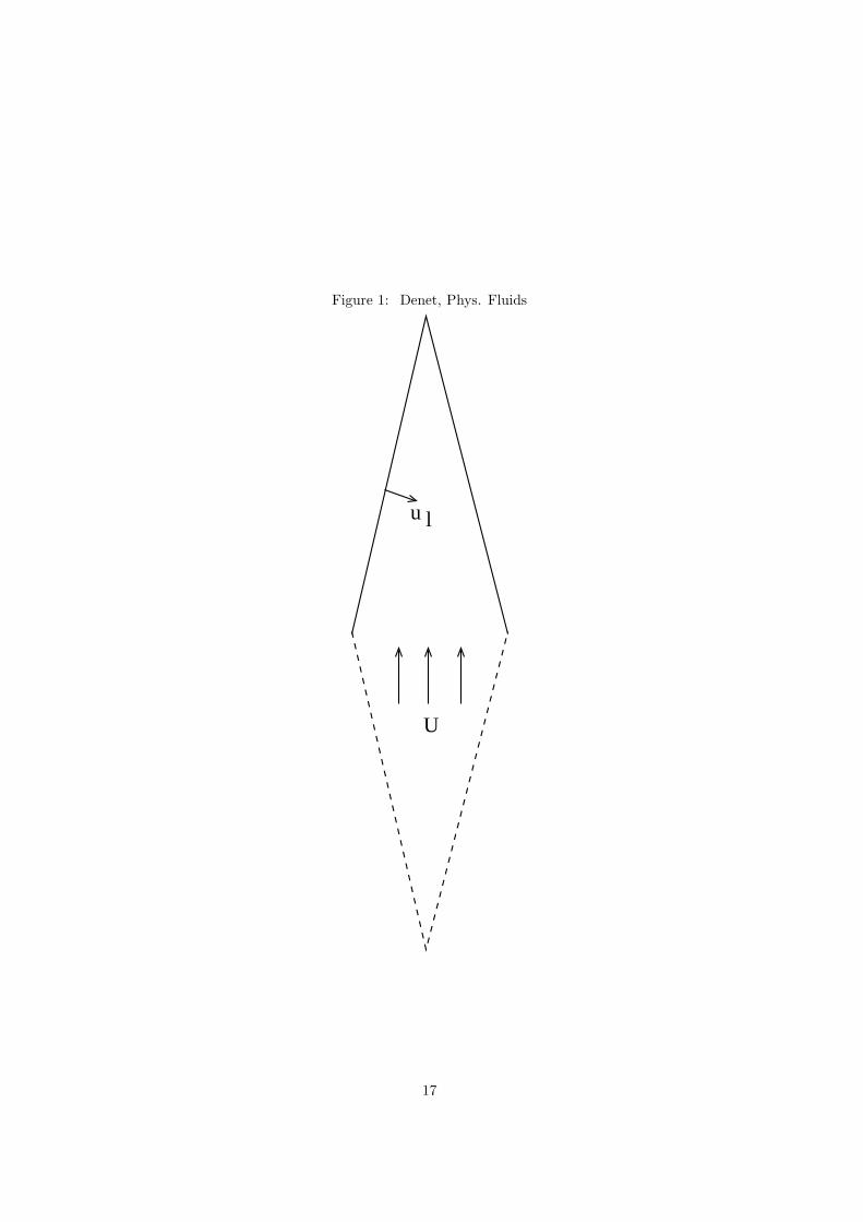
Figure 1: Denet, Phys. Fluids
U
u l
17
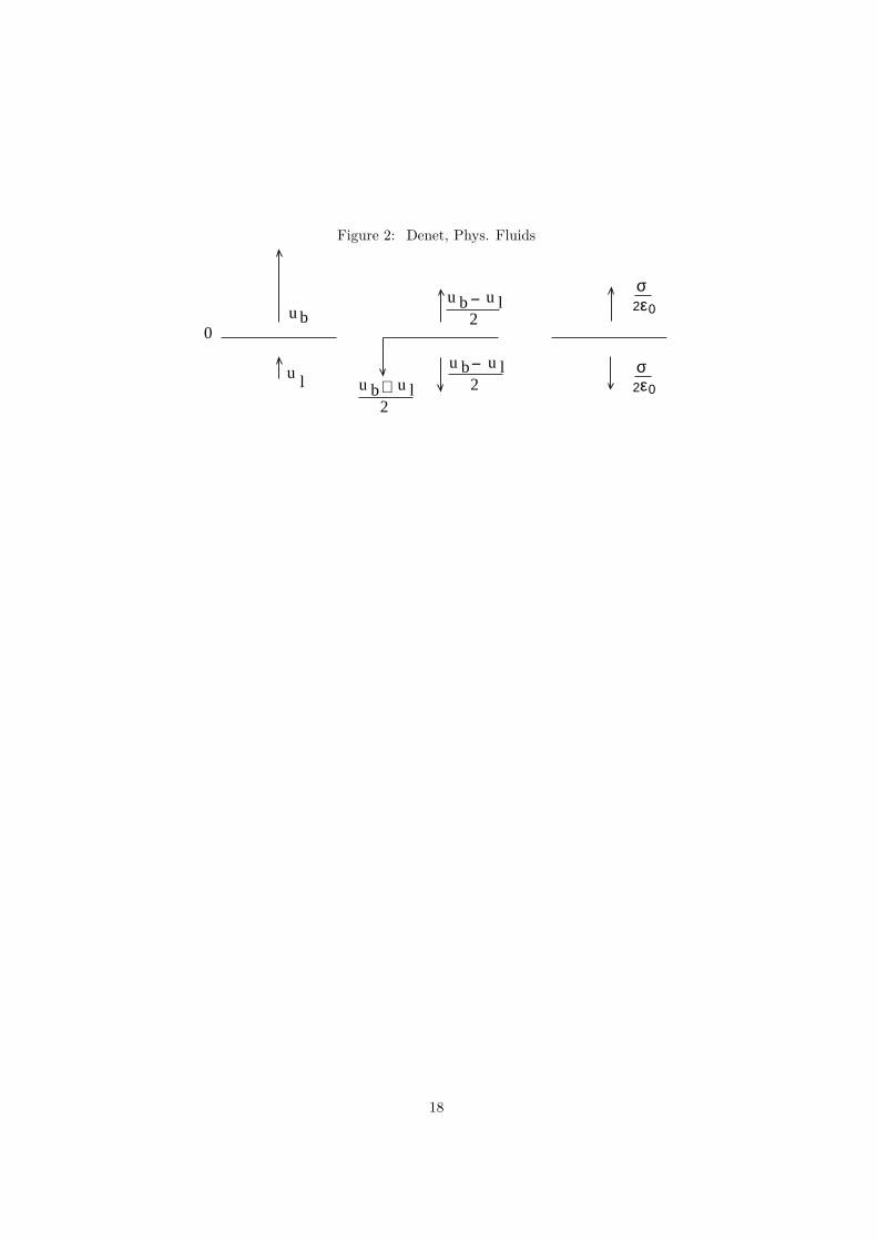
Figure 2: Denet, Phys. Fluids
0
u l
u bu lu b −
2
u lu b−2u lu b+
2
ε02σ
ε02σ
18
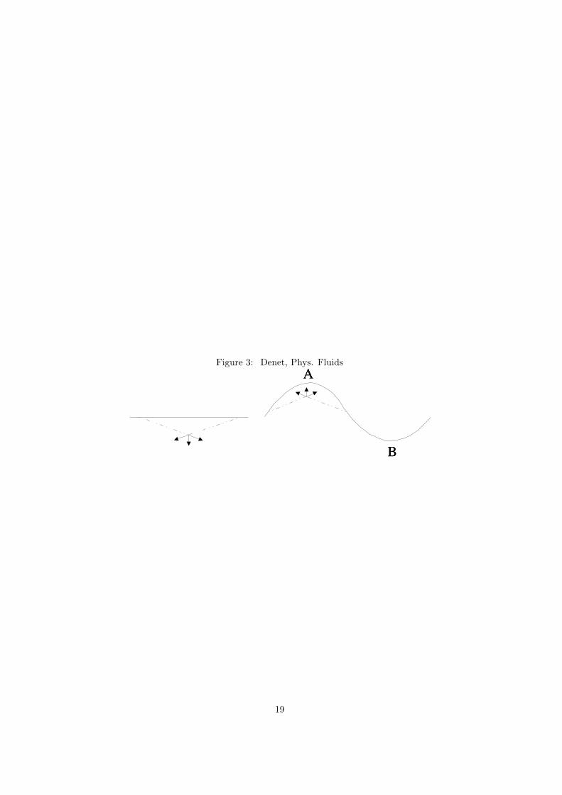
Figure 3: Denet, Phys. Fluids
AA
BB
19
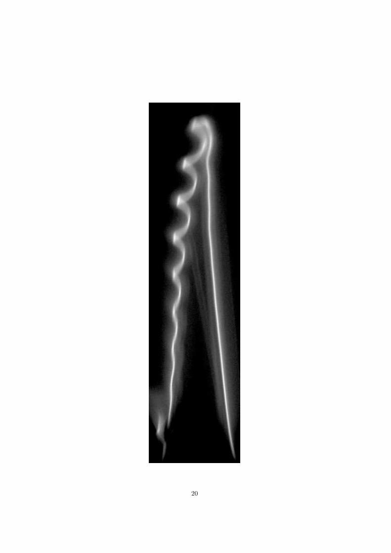
Figure 4: Denet, Phys. Fluids
20
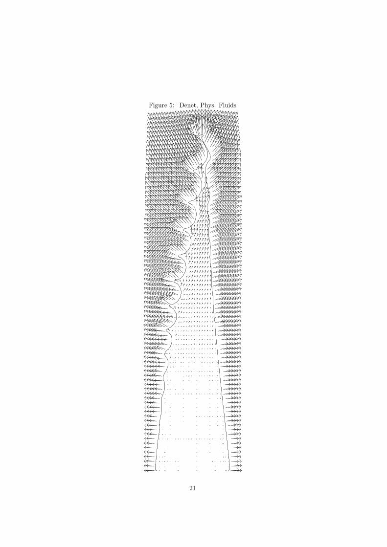
Figure 5: Denet, Phys. Fluids
21
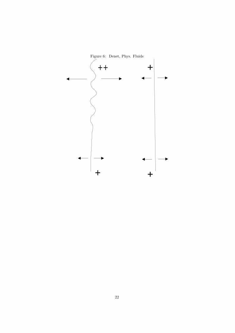
Figure 6: Denet, Phys. Fluids
++
++
++
++
22
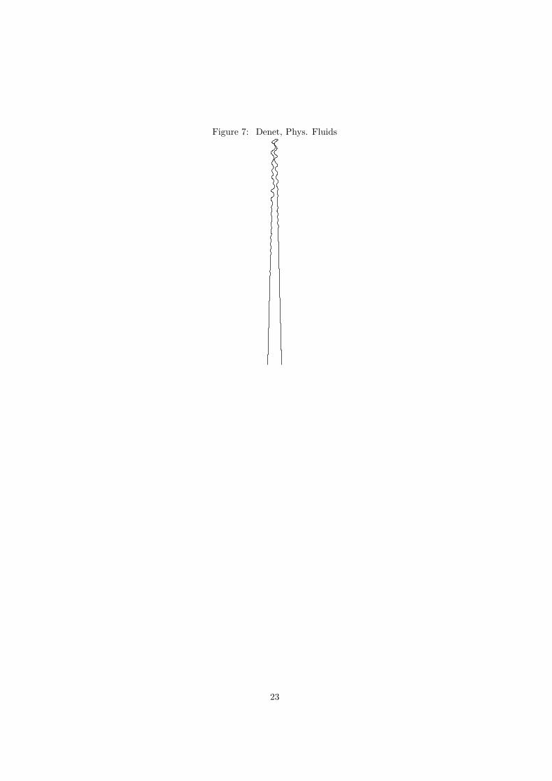
Figure 7: Denet, Phys. Fluids
23
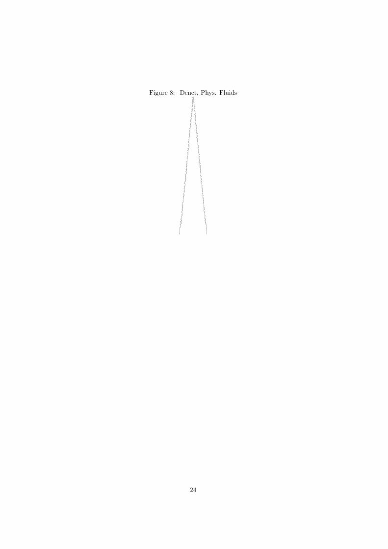
Figure 8: Denet, Phys. Fluids
24
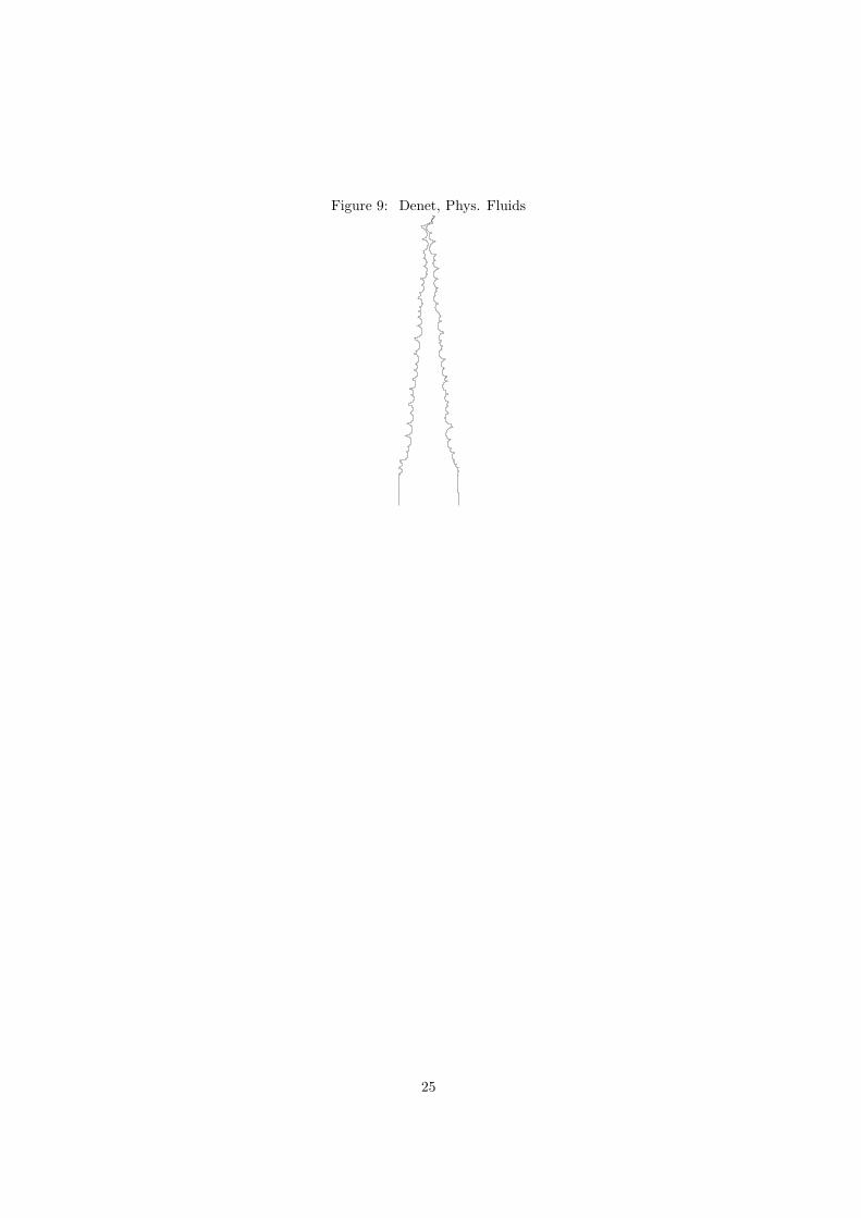
Figure 9: Denet, Phys. Fluids
25
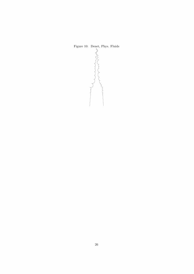
Figure 10: Denet, Phys. Fluids
26
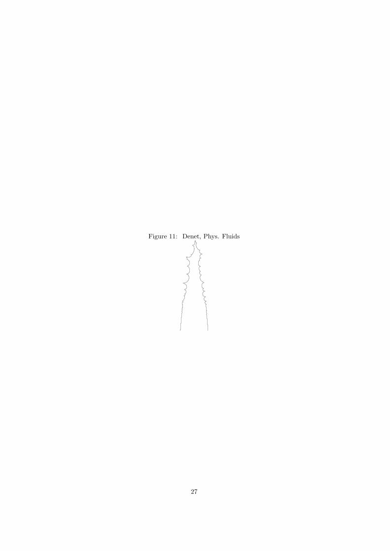
Figure 11: Denet, Phys. Fluids
27