poverty and inequality in uttar pradesh during 1993-94 to
TRANSCRIPT

WP-2010-014
Poverty and Inequality in Uttar Pradesh during 1993-94 to 2004-05 A Decomposition Analysis
Durgesh Chandra Pathak
Indira Gandhi Institute of Development Research, MumbaiAugust 2010
http://www.igidr.ac.in/pdf/publication/WP-2010-014.pdf

Poverty and Inequality in Uttar Pradesh during 1993-94 to 2004-05 A Decomposition Analysis
Durgesh Chandra PathakIndira Gandhi Institute of Development Research (IGIDR)
General Arun Kumar Vaidya Marg Goregaon (E), Mumbai- 400065, INDIA
Email (corresponding author): [email protected]
Abstract
This paper attempts a decomposition analysis of Poverty scenario in UP during 1993-94 and 2004-05. It
was found that poverty has decreased but inequality has increased between these years. The main
problems in the state are stark inter-region and intra-region differences. A positive observation is that
the poorest region in the state, the southern region or Bundelkhand, is making relatively impressive
progress in poverty reduction. The study also tries to highlight the way anti-poverty programmes are
generally being implemented in the state.
Keywords:
Uttar Pradesh (UP), Poverty, Inequality, Decomposition, Growth-Inequality Decomposition, SGSY, RGMVP.
JEL Code:
I32, I38
Acknowledgements:
The author thanks Srijit Mishra and Shovan Ray, his mentors here with the former also initiating him into NSS data and being a
sounding board, for discussions and comments. Comments from R. Nagaraj on an earlier version are acknowledged. Thanks are
due to S. Chandrashekhar for insights and helps with NSS data. The author also thanks G. Manjunath (Chief Librarian, IGIDR) for
speedy procurement of an otherwise unavailable article and Shatakhsee Dhongde (Rochester Institute of Technology) for sharing
her paper and explaining some concepts. Helps from Ankush is acknowledged during initial stages of understanding the NSS data.
i

1
Poverty and Inequality in Uttar Pradesh during 1993-94 to 2004-05: A Decomposition Analysis
In a country well governed, poverty is something to be ashamed of. In a country badly governed, wealth is something to be ashamed of.
Confucius (551-479 BC)
1. Introduction:
Despite more than fifty years of planned efforts to abolish poverty, India is still suffering
from high incidence of poverty. During 1993-94, about 37% individual in rural India were poor. The
corresponding number for urban India was about 32%. During 2004-05, these figures declined to be
28% in rural areas and 25% in urban areas. A sizable chunk of India’s poverty comes from Uttar
Pradesh (UP). As per Government of India (GOI) estimates, UP is home to sixty million poor and 20%
of total population of India. Based on an estimate by World Bank, about 8% of world’s poor lived in
UP during 19981. The very notion of the fact that it is one of the ‘BIMARU2’ states, gives a general
picture of poverty and lack of development in the state. With a large share in India’s population and
a deep rooted poverty within, UP acts as a drag on the Indian economy.
Riding on the high waves of Green Revolution, UP was performing well during 1970s, when
economic performance of most sector of this state were better than the rest of India (Kozel &
Parker, 2003). Rich in potential - in human and natural assets – Uttar Pradesh once appeared to a
pace setter for the country’s economic and social development (World Bank, 2002). Since then, the
economic pace in UP staggered and it lagged behind rest of India. Failing to seize opportunities
created by economic reforms in 1991 is cited as a reason (Kozel & Parker, 2003). A study by World
Bank (2003) opines that loss of effectiveness of public sector lies at the heart of loss of economic
momentum by UP. This inefficacy of public sector led to discouragement of private investment and
growth and to poor delivery of social and infrastructure services (World Bank, 2002). A lackluster
performance in UP would result in a similar show at country level as UP commands a large
population size in country.
Poverty in India has attracted much attention from researchers since long. Himanshu (2007)
uses the published data to analyse changes in poverty and inequality. His analysis considers all-India
and state level poverty and inequality using poverty gap index, squared poverty gap index as well as
the Head Count Ratio (HCR). He found that “poverty has declined between 1993-94 and 2004-05 in
rural areas of all states as well as in most urban areas except Orissa and Uttaranchal” (p.498). He
also commented that inequality has worsened during the same period in rural areas of most states
1 Based on International Poverty line of $1.08 per person per day.
2 A term coined by demographer Ashish Bose. It stands for Bihar, Madhya Pradesh, Rajasthan and Uttar Pradesh.

2
and all-India except Bihar, Jharkhand, Karnataka, Madhya Pradesh and Rajasthan. In urban areas,
inequality increased invariably for states and all-India. Dev and Ravi (2007) pointed out that
Himanshu (2007) has not used Mixed Recall Period (MRP) estimates. They estimated poverty ratios
using MRP monthly per capita expenditure (MPCE) assuming monotonicity between Uniform Recall
Period (URP) and MRP distributions. They divided 1983-2005 into two periods, pre-reform (1983-94)
and post-reform (1993-2005) and analysed the change in poverty and inequality using URP mpce.
They further divided the post reform period into two periods of 1993-2000 and 1999-2005 and used
MRP mpce. Their study found that using URP, the rate of decline in poverty at all-India is not higher
in post-reform period as compared to pre-reform period. This is true particularly for rural poverty
whereas urban poverty declined at slower pace in post-reform period. The analysis using MRP
showed that second period was more pro-poor than the first specially in rural areas (Dev & Ravi,
2007). There are arguments in favour and against reforms but since the main purpose of the present
paper is not analyzing reforms, we would stop here. Poverty decomposition has been attempted by
several scholars (Dev & Ravi, 2007; Jha, 2000; Jha & Sharma, 2003; and Kakwani & Subbarao, 1991).
Jha (2000) presented snapshot pictures of poverty and inequality using the Foster-Greer-Thorbecke
(FGT) measures and Gini index at NSS-Region level for all states. Dev and Ravi (2007) have attempted
growth-inequality decomposition of the change in poverty levels in all-India and state level.
Sundaram and Tendulkar (2003) have analysed levels and changes in poverty indicators of the rural
and urban population in India disaggregating it by social and economic groups. This study did not
analyse levels and change in poverty and inequality desegregated at state level. Mutatkar (2005)
presents a profile of poverty and deprivations among social groups and attempts to understand the
underlying cause for inter-group as well as intra-group differences in living conditions. Shastri (2003)
was the first to argue that district level poverty estimates can be obtained for a majority of districts
on the basis of relative standard error criteria from NSS-61st round data. Chaudhary and Gupta
(2009) have attempted to reach district level poverty estimates using NSS 61st Round (2004-05) data.
They found that “the critically high HCR districts were contained in states like Orissa, Chhattisgarh,
Jharkhand, Bihar, Madhya Pradesh, and eastern Uttar Pradesh” (p.98).
UP has always been a curious case as well as challenge to researchers. Drèze and Gazdar
(1996) opine that “Uttar Pradesh can also be seen as a case study of development in a region of
India that currently lags behind much of the rest of country in terms of a number of important
aspects of well-being and social progress” (p.33). By ‘region’, they meant region comprising of the
BIMARU states. Quite a few excellent research has been done and is being done on the poverty and
human development issues in UP. Diwakar (2009) attempts to identify dimensions of intra-regional
disparities, inequality and deprivations in poor households in the state. Singh, Muzammil and Nayak

3
(2010) have tried to understand the vicious circle of poverty in UP by analyzing data from various
sources. There is another set of studies on UP that undertake a holistic approach to poverty problem
in UP. These studies have tried to understand the problem of poverty by analyzing and interpreting
the other indicators and process of development beside data on income/expenditure. The study by
Drèze and Gazdar (ibid) is a holistic approach to understand the problem of poverty in UP. Poverty in
India: The Challenge of Uttar Pradesh (World Bank, 2002) is another attempt of the same kind. The
study by Kozel and Parker (2003) builds a ‘nuanced and complex’ yet lucid narrative about poverty in
UP using quantitative and qualitative data. The present paper tries to utilize both approaches. It
concentrates on UP and undertakes poverty and inequality decompositions at levels of NSS-regions
within the state, across social and occupation groups. It also attempts to explain the decomposition
results discussing works by other researchers.
The present paper has been divided into 5 broad sections including the introduction. The
second section is a brief discourse on poverty and inequality analysis, their decomposition and
relation with growth besides explaining the methodology followed and the data sources. Section
three deals extensively with exploring poverty and inequality situation in UP during 1993-94 and
2004-05. The plight of poverty alleviation efforts in UP has been highlighted using a case-study of
Swarnajayanti Gram Swarozgar Yojana (SGSY). It also takes a quick stock of Public Distribution
System (PDS) in the state. The fifth and last section concludes.
2. Methodological and Theoretical Underpinnings:
2.1 Poverty Lines:
The word ‘poverty’ has been used in two senses, in the broad and all encompassing one it
describes the whole spectrum of deprivation and illbeing, and in a narrow sense, it is used for
purposes of measurement and comparison has been defined as low income, or more specifically, as
low consumption which is considered more stable and easier to measure. In common parlance, this
(the second definition) is known as income poverty (Srivastava, 2001).
Poverty could be relative as well as absolute. People falling below some basic minimum level
of the chosen poverty indicator depict absolute poverty. For example, in India those who do not
meet nutrition level of 2400 Kilocalorie per day (kcal/day) in rural areas are poor (in absolute sense).
A measure of relative poverty defines “poverty” as being below some relative poverty threshold. For
instance, when poverty is defined as households that earn less than 50 percent of the median
income. Relative poverty compares two individuals on the chosen poverty indicator. In developing

4
countries like India, relative poverty is not taken to be as much a cause of concern as absolute
poverty is.
Regarding the method of choice to analyse poverty levels and changes, there are two broad
approaches: first, income/consumption approach and the second, participatory approach. Baulch
(1996) is of view that standard discussion of income/consumption and participatory approaches
ignore two critical measurement issues: aggregation and the dynamics of poverty. Although the
income/consumption approach may sometimes misidentify the poor, its well-understood
aggregation properties make it very useful for regional and national level policymaking. In contrast,
participatory methods are most valuable for identifying the other, more subjective dimensions of
poverty at project or village level.
The discourse on poverty largely revolves around the notion of a poverty line: a critical
threshold of income, consumption, or more generally, access to goods and services below which the
individuals are declared to be poor (Ray, 2002). Ravallion (1998) defines poverty line “as the
monetary cost to a given person, at a given place and time, of a reference level of welfare. People
who do not attain that level of welfare are deemed poor, and those who do are not” (p.3). People
whose income is below poverty line are said to be poor. The most common measure of poverty is
the 'Head-Count' ratio, defined as the percentage of population living below the poverty line.
One needs an index of household welfare to analyze poverty. This paper, for all analytical
purposes, would take per capita monthly consumption expenditure as the measure of economic
welfare of individuals and of the households to which they belong to. The paper is based on data
from various sources, mainly NSS 50th Round and 61st Round and various GOI reports. An individual is
defined as poor if his monthly per capita consumption expenditure falls below the official poverty
lines defined by the Planning Commission of India for that particular reference period. This paper
also uses two other poverty lines, one being for ultra-poor, as proposed by Lipton (1983) and the
other for possible poor. Lipton (ibid) has defined the ‘ultra-poor’ as those spending about 80 percent
of the household expenditure on food yet failing to get 80% of the minimum dietary energy
requirement for that Age-Sex-Activity Group. Following Kakwani and Subbarao (1993), this paper
would define ultra-poor as the individuals whose income falls short by 80% of the official poverty
line. So, we reach two different ultra-poverty lines, one for each NSS round. Further, this paper
proposes a different poverty line for people falling within range of 20% above the official poverty

5
line. They are the people who are most susceptible to fall into poverty given a single income shock.
We propose to call them ‘possible poor’3. Let I(.) be an indicator function such that
Where is the welfare measure of individual and is the poverty line or the minimum threshold
below that an individual would be classified as poor. This indicator function identifies who is poor
and who is not. Thus, for ultra poor
and similarly for possible poor
2.2 Poverty Measures:
For measuring and decomposing poverty across time and space, this paper uses the Foster-
Greer-Thorbecke (FGT) class of poverty measures as they, besides satisfying all the properties of a
poverty measure, are additively decomposable. A brief description of these measures is following.
The measures can be written in a general form as,
The higher the value of , the more sensitive the index is to the poverty.
When α=0, FGT becomes the head-count ratio (HCR). As widely discussed in literature, this
index suffers from a number of weaknesses like it doesn’t takes into account the intensity of
poverty, fails to tell how poor are the poor etc. But it has one very useful quality that it is intuitively
appealing to laymen and researchers alike.
When α takes value of 1, the FGT measure becomes the Poverty Gap Index. It is superior to
the simple HCR in that it takes into account the shortfall in poor’s income from the poverty line. For
3 Possible poor are different from ‘transient poor’ in that the farmer may not have been below the poverty line ever but are
most susceptible to fall below it given an income shock. Transient poor keep moving across the poverty line due to fluctuations in their income.

6
example, individual x and y both are poor as their incomes being `50 and `90 whereas the poverty
line is `100. Though both are poor by HCR as their income is below the poverty line, individual x’s
poverty gap is 50 whereas that of y is 10 only. In other words, it indicates how poor are poor. If the
government wants to make these people cross the poverty line, it has to transfer `50 to x and `10
to y. Aggregated Poverty gap of a population can give an idea of the income transfer that is needed
to make people non-poor.
If we weight the Poverty Gaps, weights being the proportionate poverty gaps, and sum it up,
we reach and this is the Squared Poverty Gap. Its weights emphasize the lower tail of the
income distribution. and are distribution sensitive measure of poverty as they take into
account the distribution of income.
is additively decomposable across population sub-groups as,
Where
=the number of persons in the subgroup divided by total number of persons
(subgroup population share),
= poverty of sub-group , calculated as if each sub-group is a separate population.
The paper further uses concept of subgroup poverty risk. This is the contribution of a
subgroup to poverty to its contribution in total population of the group. When its value is more than
unity, it indicates that the subgroup is sharing more of the total poverty than its share in population
warrants. Subgroup poverty risk can be calculated as
Where is the subgroup poverty risk for a population subgroup and and
are FGT measures of the subgroup and the population respectively. can also be expressed as a
ratio of subgroup population share ( ) and subgroup poverty share ( ) as following,

7
Where
and
.
2.3 Inequality Measures:
Inequality is a broader concept than poverty as it takes into account income distribution
over entire population rather than focusing only on the poor (Handbook of Poverty and Inequality,
p.101). Plato opined that “…if a state is to avoid the greatest plague of all – I mean civil war, though
civil disintegration would be a better term – extreme poverty and wealth must not be allowed to
arise in any sections of citizen body, because both lead to both these disasters” (as quoted in Cowell,
1995). Paul Shaffer (2008) mentions following reasons for inequality to be ‘rediscovered’ in recent
years,
1)Research results affirming that on average, the rate at which growth reduces poverty is higher, lower
the level of inequality (Ravallion, 1997); 2) a growing, though still inconclusive, body of evidence
suggesting the higher inequality reduces the rate of growth (Aghion et. al. 1999); 3) the fact that some
social ills, such as crime and conflict, appear to be a function of inequality and ‘absolute’ poverty levels
(Bourguignon, 1998); 4)the rapid rise in inequality in some OECD, transition and developing countries
in recent years (Cornia, 1999); 5) the apparent increase in global income inequality in recent years
(though it is sensitive to the time frame and measurement assumptions (Milanovic 1999, 2005).
Several measures, each with its own set of strengths and weaknesses has been proposed to
measure the extent of inequality. These measures range from the simplest measure, Range, to the
most sophisticated ones like the Generalized Entropy Measures. In the present paper, Thiel’s
inequality measure T has been used for measuring inequality, both between-groups and within-
group. This measure belongs to the family of sub-group decomposable Generalized measures of
Entropy, GE(1) and can be written as,
s
Where is total income of all individuals in the sample, is the mean income, i.e.,
, is
total income of the sub-group with members, is the mean income of the sub-group , i.e.,
, and is the Theil’s Index of inequality or
The overall inequality can be decomposed into its contributors (subgroups of population,
region etc.). The part of inequality that arises out of the inherent differences between subgroups is
8
called “Between groups” inequality. Anand (1983) defines the “between groups” component as “the
value of the inequality index when all within-group income differences are artificially suppressed”
(p.87). It is that part of total inequality that is calculated by assigning each individual within a group
the mean income of that group. Apart from this, subgroups are not homogenous in themselves and
this contributes to “Within group” inequality. The “within-group” component of total inequality is
the value of inequality index when all between-groups income differences are suppressed (Anand,
ibid). Such decomposition would be useful from policy point of view. They allow useful depictions of
patterns that can be a first step in identifying the proximate causes of inequality (Kanbur, 2006).
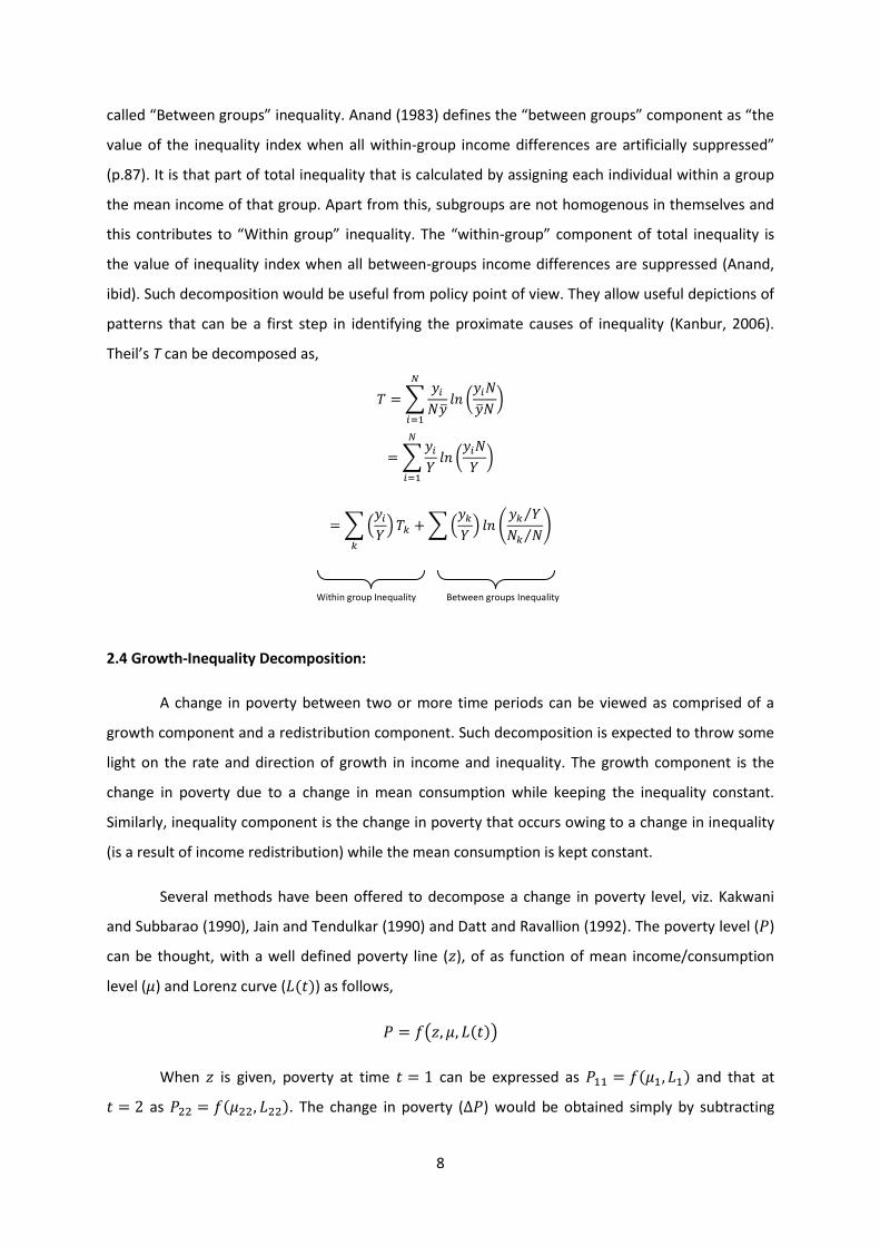
Theil’s T can be decomposed as,
2.4 Growth-Inequality Decomposition:
A change in poverty between two or more time periods can be viewed as comprised of a
growth component and a redistribution component. Such decomposition is expected to throw some
light on the rate and direction of growth in income and inequality. The growth component is the
change in poverty due to a change in mean consumption while keeping the inequality constant.
Similarly, inequality component is the change in poverty that occurs owing to a change in inequality
(is a result of income redistribution) while the mean consumption is kept constant.
Several methods have been offered to decompose a change in poverty level, viz. Kakwani
and Subbarao (1990), Jain and Tendulkar (1990) and Datt and Ravallion (1992). The poverty level ( )
can be thought, with a well defined poverty line ( ), of as function of mean income/consumption
level ( ) and Lorenz curve ( ) as follows,
When is given, poverty at time can be expressed as and that at
as . The change in poverty ( ) would be obtained simply by subtracting
Within group Inequality Between groups Inequality

9
these two poverty levels. But such a change would include mutual effect of both, change in mean
income/consumption and change in distribution. In order to achieve a decomposition of change in
poverty into a pure growth component and redistribution component, one can think of a
hypothetical situation where only one of these two components is allowed to change at a time.
Thus, the growth component would be that change in poverty when only mean
income/consumption is allowed to change and the distribution of income is held unchanged at .
Similarly, the redistribution component would be the change poverty level that occurs due to change
in income distribution while keeping mean income/consumption constant. Kakwani and
Subbarao (1990) achieved this decomposition as whereas
Jain and Tendulkar (1990) did it as . Datt and Ravallion
showed that these decompositions are not path independent4 and suggested following way5 to
achieves this,
where is the residual arising out of interaction between growth and redistribution. This
method though satisfies path independence, leaves a residual thus making the decomposition
incomplete. Following tradition of taking averages to make decomposition path independent
(Kakwani, 2000), Dhongde (2007) proposed a ‘method of averages6’ as following,
This paper has used the Datt-Ravallion decomposition using the method of averages.
2.5 Data Comparability Issue:
Uttar Pradesh (UP), during the NSS-50th Round (1993-94), comprised of five NSS-regions
namely, Himalayan, Western, Central, Eastern and Southern. The separate state of Uttrakhand was
formed by carving out the Himalayan region of UP less the Bareilly District. Thus, the present UP has
one less NSS-region than that of 50th Round. There has also been some reorganization of districts
within UP across NSS-regions. In order to make UP of 61st Round comparable with the UP of 50th
Round, the paper has removed the entire Himalayan region from UP of NSS-50th round. District
4 See Figure 1 in Bourguignon (2004) for an excellent exposition on path independency of the decomposition of growth and
redistribution components. 5 . Expanding this yields: .
6 Shorrocks (1999) has shown that this decomposition is equivalent to the Shapley values in cooperative game theory
(Dhongde, 2007).
Growth Component Redistribution Component

10
Bareilli has been dropped and district Sonbhadra has been moved to the Western region in the UP of
61st round. These modified UPs have been represented as UP throughout the paper and are
comparable to each other. The unmodified Uttar Pradesh of the 50th and 61st rounds of NSS are
represented with UP* Most of the analysis has been done taking the UP and figures for UP* as it was
in 1993-94 (50th Round of NSS) and 2004-05 (61st Round of NSS) has been given only at broad levels
for reference to other researchers.
3. Poverty Scenario in India and UP:
3.1. Sector wise distribution of Poverty:
Poverty has been higher, deeper as well as more severe in both rural and urban areas of UP
than in all-India average during 1993-94 and 2004-05 (Table A1.1). Given its largest share in total
population of India and a considerably higher poverty ratio, UP accounted for 19 per cent of India’s
total poor both in rural as well urban sector. Poverty declined by 24% for rural all-India in 2004-05
and corresponding figures for rural UP were about 22%. But poverty gap and squared poverty gap
declined more in rural UP than in all-India. This indicates that rural UP has made comparatively more
progress in reducing the depth and severity of poverty that rural all-India. Urban UP has registered a
slower poverty reduction than urban all-India during 1993-94 and 2004-05.
Within UP, poverty has been higher in rural areas (43%) than in urban areas (36%). Not only
poor were more concentrated in rural areas, they were also relatively far off the poverty line, as
indicated by poverty gap of 10% than their urban counterparts (9%). This trend reversed in 2004-05
when rural UP though still had a higher HCR, exhibited a relatively lower poverty gap and squared
poverty gap than urban UP. Figure 1 depicts how poverty situation has changed in rural and urban
areas of UP and all-India. Two observations can be made. First, Rural sector has shown a higher
decline in all indices of poverty than the urban sector in both UP and all-India. Second, UP has fared
better at rural poverty reduction than all-India while for urban poverty, all-India has registered a
more impressive change. UP Development Report ([UPDR] vol. I, p. 95) mentions following reasons
for this trend:
i. consistent though low growth in agricultural sector as against a decline in growth rates of
tertiary and industrial sectors in the state.
ii. informal manufacturing has significant presence in UP and it registered almost similar
growth as registered sector.

11
High poverty in rural UP has been accompanied with low scores on other non-income
indicators of development. Infant Mortality Rate (IMR) is a reflection of the general health scenario
in a state (UP-HDR, 2006). IMR is considerably higher in rural UP (77 per 1000 live births) than in
urban UP (57 per live 1000 births). Children in rural areas experience 80% higher risk of dying before
five years of age (ibid). As per NSS 61st Round, about 53% of individuals in rural UP and 29% in urban
UP are illiterate. The situation is even worse in case of women. 70% women in rural UP are illiterate.
Corresponding figure for urban UP is 39%. The quality of schooling is also questionable in UP. In a
survey, PRATHAM found that about 58% children in class I can read nothing while this number was
about 4% even in class V. 70% children in class I could do nothing in the arithmetic test in the same
survey. In class V, this number was about 9%.
3.2 Inequality:
The table A2.1 shows inequality figures (Theil’s T) for all-India and UP for the same period of
reference as for poverty indices. All-India average inequality has been higher than UP during 1993-94
and 2004-05 as evident from a higher Theils’s T. Analysing the comparative changes in inequality
reveals that
a. inequality have been rising over time for both rural and urban areas of all-India and UP. This
is in accordance with Himanshu’s (2007) observation that inequality has worsened, during
1993-94 and 2004-05, in rural areas of all states except Bihar Jharkhand, Karnataka, Madhya
-10
-9
-8
-7
-6
-5
-4
-3
-2
-1
0
India UP* India UP*
Rural Urban
-8.91
-9.71
-7.01
-5.75
-2.83
-4.03
-1.97-2.14
-1.12
-1.82
-0.81
-1
Fig. 1: Change in FGTs: India and UP (1993-94 to 2004-05)
α=0 α=1 α=2

12
Pradesh and Rajasthan. This indicates to a reversal in trend observed earlier (1983 to 1993).
For urban areas, inequality rose in all states and all-India.
b. The rise in inequality has been considerably higher in UP than in all-India. For rural UP, T
rose by about 27% while it was 20% for all-India. Urban UP registered a 35% increase in T
that is about twice that for all-India (18%).
c. Inequality in urban areas of UP rose higher than the rural areas. For all-India average, the
trend is the other way round.
Table 1 below gives a general idea of wide variability in average mpce and poverty situation
in UP. The difference in average mpce of the best mpce district and the worst mpce district in rural
UP is `569 that is about 88% of state’s average mpce in rural areas. The corresponding difference in
urban areas of UP is `957 and it is about 98% 0f the average mpce of the urban sector of the state.
Table 1: Average MPCE across Uttar Pradesh (2004-05) Sector State Av.
MPCE (`)
Best MPCE
District
Av.
MPCE
(`)
Worst
MPCE
District
Av.
MPCE
(`)
Least Poor
District
HCR
(%)
Most Poor
District
HCR
(%)
Rural 647 Faizabad 917 Chitrakoot 348 GB Nagar 2.6 Chitrakoot 81.5
Urban 978 Agra 1393 Banda 436 Shahjahanpur 3.6 Chaundli 74.5
Source: Table 7R and 7U (Chaudhary & Gupta, 2009)
The Table A6.1 presents proportion of ultra-poor in India and UP. Ultra poor face a deep
rooted poverty. Desegregating the simple head count ratio in ultra-poverty should reveal the extent
0.00
0.01
0.02
0.03
0.04
0.05
0.06
0.07
Δ T: Rural Δ T: Urban
0.03
0.040.04
0.07
Fig. 2: Change in Inequality: India & UP (1993-94 to 2004-05)
India UP

13
of extreme poverty. The incidence of ultra-poverty was higher in UP than all-India during 1993-94
and remained so during 2004-05. The difference in the incidence of ultra-poverty between UP and
all-India was much higher in rural areas during 1993-94 and in urban areas during 2004-05. This is
because rural UP witnessed a much higher reduction (more than 10%age points) in ultra poverty
than rural all-India (slightly more than 6%age points). For urban areas both all-India and UP
registered a similar decline (about 4%age points) in ultra-poverty.
Like the ultra-poor, it is possible to identify people just above the poverty line. These could
be called possible poor and are most susceptible to fall in poverty given an income shock. Though
they are clubbed as non-poor they share most characteristics, like high rate of illiteracy, of the poor
except consumption expenditure. As a group, they need attention if the government does not want
them to fall below poverty line and swell ranks of poor. To begin with, UP had either lower (in rural
areas) or almost equal (in urban areas) incidence of possible poverty (Table A6.1). But possible
poverty rose in rural UP by more than 9% and by 6% in urban UP whereas for all-India, it declined in
both rural as well as urban areas. There may be two reasons for an increase in possible poverty:
one, some people have just crossed the poverty line and are crowding around it, and the second,
some people have slipped down on the income ladder due to some exigencies or some other reason.
The first reason could prevail when the poverty rate is also falling indicating that government
programmes are helping the poor to cross the poverty line. If one witnesses an increasing rate of
ultra-poverty accompanying the above situation, it implies that the government programmes are
helping only those who are clustered around the poverty line and not the very poor. The reason for
the second possibility to materialize could be a shock to a particular group or to overall population
that affects their consumption expenditure adversely. Similarly, a decline in rate of possible poverty
also indicates either of the two facts: one, some people have fallen down the poverty line and they
would now be counted as poor and the second reason could be that some people who were
hovering just above the poverty line has done well economically and have crossed the threshold of
possible poverty. The first scenario occurs when one observe an increase in poverty rate and a
simultaneous decline in possible poor. The second scenario would be observed in case of rapid
growth that is also percolating deeper in economy.
3.3 Growth-Inequality Decomposition:
The paper has decomposed the total change in incidence of poverty for rural and urban
sectors of India and UP into growth and distribution components (Table A5.1). A negative sign before
a component indicates that this component has helped in reducing the incidence of poverty whereas
a positive sign indicates the other way. From 1993-94, HCR in rural all-India declined by 8.9

14
percentage points and decomposition based on method of averages shows that out of the total
change in poverty, 44.17% change can be attributed to rise in mean income/consumption level
while 35.25% change was a result of change in distribution of income/consumption. In urban all-
India, poverty has changed by 7% percentage points during 1993-94 to 2004-05. Decomposition
exercise reveals that 40.7% of this change has come from rise in mean income whereas change in
income distribution has contributed for 33.7% of the total change. Thus, the rural India has
registered both a higher rise in mean income and in income distribution (inequality) than the urban
India.
For rural UP, poverty has changed by 9.73% and the rise in mean income accounts for
45.68% of this change while 35.95% of the change is due to change in distribution component. In
urban UP, rise in mean income contributed 42.03% of total change in poverty (5.75 percentage
points) whereas change in distribution component accounted for 35.95% of the total change.
The most important point that comes out of this decomposition analysis is that income
growth has been the engine of poverty reduction while changes in inequality tried to raise the HCR.
This has been true for India as well as UP.
3.4. Decomposing Poverty NSS-region wise:
Now the paper would attempt to analyse the situation among various NSS-Region7. An
analysis at region level should help to understand the nature of poverty across the state. During the
50th round of NSS, Uttar Pradesh was divided into five NSS-regions, namely the Himalayan, Western,
Central, Eastern, and the Southern. The Himalayan region has been carved out on November 9, 2000
to form the state of Uttarakhand8 and thus Uttar Pradesh has been left with four NSS-regions.
The regions within UP exhibit much differences in almost all aspects of socio-economic
development. Geographically, about two third of state falls under Indo-Gangetic plain region and
includes the western, central and eastern regions. The western region has been the leading region in
agricultural as well industrial progress. This region acted as the springboard for the green revolution
in the 1960s and 1970s and helped Uttar Pradesh depart from its previous low levels of agricultural
growth (World Bank, 2002). Bajpai and Volavka (2003) opine that Green Revolution took place in the
Northwestern states (Panjab, Haryana and western part of UP) as they were rich in natural resources
and possessed good physical and institutional infrastructure. Riding on the strong performance by
7 NSS divides a State into some regions by grouping contiguous districts similar in population density and crop pattern
(Instrn_50_1.0_General, 50th
Round documents). 8 All districts under the Himalayan region shifted to Uttarakhand except the district Bareilly that joined the Western region
of Uttar Pradesh.

15
western and eastern region, most sectors of UP were performing better than the rest of India (Kozel
and Parker, 2003). But UP could not sustain this momentum and lagged behind Panjab and Haryana
during next decades and ‘the intra-state differences in U.P. have contributed to interstate
differences between U.P., Panjab and haryana’ (Bajpai and Volavka, 2003). As UP has been largely an
agrarian state till late, it is important to understand the changes in agricultural performance of its
regions.
Western region is characterized as the food and sugar basket of Uttar Pradesh (UPDR, p. 32)
has fertile soil and a good physical infrastructure for agricultural development. Western region was
the first in UP to join Green revolution. Though Eastern UP followed it and embarked on the path of
high agriculture growth joining Green revolution yet there are differences in the outcomes for the
two regions. Bajpai and Volavka (2003) point out that ‘in 1962-65, eastern U.P. was at least on par
with western U.P. as far as rice was concerned, as water conditions (flooding) in that part of the
state made it naturally suitable for rice cultivation’. Eastern UP has very high concentration of
marginal (less than 1 hectare) land holdings. As pointed out by Stokes (1978, as quoted in Bajpai &
Volvaka, 2003), different kind of systems of landholdings under British rule has been responsible for
it. Eastern UP had Zamindari system while western UP was under Bhaichara system. The Zamindari
system further stratified the rural society into tenant, sub-tenant and rentier landlords whereas the
Bhaichara system in western UP allowed peasant proprietorship (Stokes, ibid). Quoting CMIE (2004)
data, Bajpai and Volavka (ibid) mention that during 1961-62 62% of landholdings in about 19% of
operational land area were marginal in eastern UP while it was 52% of landholdings in about 11% of
operational land area in western UP. It further deteriorated in 1980-81 when 79% of landholdings in
34% of operational land area in eastern UP were marginal. The corresponding figure for western UP
was 62% of landholdings in 20% of area. Further, western region had a well-developed canal system
for irrigation. The eastern region tried to catch up after onset of the Green revolution and narrowed
the gap in canal irrigation, but at the same time western UP was investing in tube wells and thus
again managed to leave the eastern region behind (Sharma & Poleman, 1993 as quoted in Bajpai &
Volavka, ibid). Eastern region is also prone to water-logging due to receiving more rainfall than
western region and incapacity to deal with the excess water. Infrastructure wise also western UP has
been better the eastern UP. The southern region, also known as Bundelkhand region is characterized
by low rainfall and draught prone and very marginal lands (UPDR, 2007). This region has been
lagging behind in adoption of improved varieties and application of fertilizers and sparse irrigation
facilities.

16
Some regions of UP, especially western and eastern, are also facing problem of declining
water table. As on April 1998, out of 252 development blocks in western UP, 70 has been declared
‘dark9’ blocks while 64 are declared ‘grey’ blocks. In eastern UP, out of 294 development blocks, 26
are dark and 93 are grey. Thus agriculture cannot keep relying on groundwater for irrigation. This
indicates towards a need of agricultural diversification. The nature and scope of diversification also
varies among regions. UPDR observes that the share of food-related enterprises has been declining
in all but eastern region as this region exhibits high incidence of poverty and growing food crops has
been a compulsion for poor farmers.
Livelihood sector has been growing impressively in UP (UPDR, 2007). As per Livestock Census
(1991), UP has the highest livestock population in India. But livestock in the state are suffering from
low productivity per unit. UPDR (2007) considers the failure of artificial insemination, inadequate
nutrition, poor health and veterinary services along with unsatisfactory animal management as the
main reason behind this problem. It is worth mentioning that in a case-study of SGSY in two blocks
of Jaunpur district it was observed that most of the loans sanctioned were on livestock. Even if there
are no fraudulent practices and each beneficiary creates asset out of SGSY-loan in form of livestock,
the chances of her receiving very low returns are high considering the above mentioned problems
with livestock in the state.
UP-HDR (2006) has compared annual compound growth rates of Net Regional Domestic
Product for two periods (1980-81 to 1996-97 and 1993-94 to 2004-05). It found that during the first
period, all four regions of UP grew at around 4% per annum. It attributes growth during this period
to agricultural growth and Green Revolution. The second period of 1993-94 to 2004-05 witnessed
regional concentration of growth. The eastern and western regions grew at slower pace of 3.9% and
3.8% respectively whereas the central and southern regions registered growth rates of 4.6% and
5.2% per annum in Net Regional Domestic Product. The table 2 below shows the sectoral shift in
regions of UP. Growth in the southern and central regions has been driven by tertiary sector. The
southern region was relying more on agriculture in 1993-94 but it managed to reduce its share in
2004-05 and also to increase the share of secondary and tertiary sectors.
9 Depending upon the extent of groundwater exploitation, a block is classified as dark, grey or white. A dark
block is one where groundwater uses is above 85% of its utilizable groundwater recharge. In a grey block, the rate of exploitation lies between 65-85% whereas in a white block, the rate of exploitation of groundwater is below 65% (Dhawan, 1995).

17
Table 2: Sectoral Shift in Net Regional Domestic Product
Sector→ Primary Sector Secondary Sector Tertiary Sector NDDP
Region↓ 1993-94 2004-05 1993-94 2004-05 1993-94 2004-05 1993-94 2004-05
Western 41.10 36.85 19.94 22.56 38.96 40.59 100 100
Central 36.16 33.25 17.28 16.32 46.56 50.43 100 100
Eastern 40.04 35.75 19.32 15.69 40.64 48.56 100 100
Bundelkhand 46.76 44.45 12.5 13.99 40.74 41.55 100 100
Source: Table 5.4, UP-HDR: 2006.
Sectoral productivity of labour is very varied in UP. It rose at annual compound growth rate
of 2.16% in the state between 1993-94 and 2004-05. Tertiary sector registered the highest growth
rate (3.85%) followed by primary sector (1.51%) whereas the secondary sector witnessed a negative
growth rate of (0.33%). This stagnation in labour productivity in secondary sector is due to rapid
growth of enterprises in the unorganized sector (UP-HDR, 2006). Table 3 shows the sector wise
labour productivity for 1993-94 and 2004-05.
Table 3: Sector wise Per Worker NSDP
at Constant prices (1993-94)
Sector 1993-94 2004-05 CAGR (%)
Primary Sector 9096 10727 1.51
Secondary Sector 20794 20061 -0.33
Tertiary Sector 26875 40700 3.85
All Sectors 14601 18479 2.16
Source: Table 5.15, UP-HDR: 2006.
In their study of regional variations in agricultural productivity, Chand, R., Garg, S. and
Pandey, L. (2009) ranked districts across all states according to their agricultural productivities
(measured in `/hectare of Net Sown Area). 5 district of UP were in the Very Low productivity
category while 21 districts were in Low category. 18 and 19 districts were in Average and High
category respectively whereas only 7 districts were under Very High category.
3.5. Rural Poverty:
Table A1.2 shows decomposition of poverty indices for UP NSS-region wise. During 1993-94,
the Southern region of UP was the region with highest HCR (67 %) followed by the Central region (50
%). The Eastern region was only marginally better off with about 49 % of its population being below
the official poverty line. Poverty was also the deepest in the southern region and follows the
same trend as . Compared to these three regions, the western region is relatively better off.
Incidentally, these three regions are also regions with weakest industrial base. The eastern and
southern regions have been designated as backward regions officially (UP-HDR, 2006) Per capita

18
gross value of industrial output in 2000-01 was Rs. 1324 for the Eastern region, Rs. 7042 for Western
region, Rs. 3095 for Central region, and Rs. 1238 for Southern region (UP-HDR: 2003).
Poverty has reduced for all NSS-regions in 2004-05. The most notable point is that now the
eastern region has the highest proportion of people below the official poverty line (41 %) followed
by the southern region (38.86 %) and the central region (30.12 %). The depth of poverty is
also now highest for the eastern region and so is the severity of poverty . This change is
mainly due to 42% decline in HCR in southern region whereas it was 15% in eastern region. The
second highest percentage change has been exhibited by central region (40%). Incidence of poverty
declined by 19% in the western region.
Table A1.2 shows subgroup poverty risk for NSS-regions in UP People living in the Southern
region during 1993-94, had 59 % higher risk of poverty than the norm. Three regions, Central,
Eastern and Southern, had a risk of poverty that was above the norm. Their share in overall rural
poverty was more than what their population share warrants. The situation changed in 2004-05 and
the Eastern region faced the highest sub-group poverty risk. The Southern region underwent a rapid
decline in poverty and so its poverty risk also declined. This reason has caught attention of national
as well international development agencies and much aid is pouring in it. There also dedicated
government programmes like Swajaldhara for this region itself. Migration is also high in this region
and the remittances from it might be another reason of rapid poverty reduction in the southern
region.
3.6. Urban Poverty:
The Southern region, like in the rural UP, was the poorest in urban UP during 1993-94 and
remained so during 2004-05 also (Table A1.3). The poor are also the furthest from the poverty line in
this region. There was a huge difference of almost thirty six percentage points in HCR between the
poorest region and the second most poor. The southern region exhibited 42% change in HCR that is
the highest among all regions of urban UP. Similar decline has been registered in the poverty gap
and squared poverty gap for the region. The next highest decline in poverty indices has been
witnessed by the central region (27%). The important point is that for central region, decline in
depth and severity of poverty has been much more than the decline in HCR. This indicates decline in
extreme poverty in this region. Similar trends have been shown by western and eastern regions also.
Though eastern region registered an imperceptible decline of only 0.94 percentage points (about 2%
change), the depth and severity of poverty declined more relative to its incidence. Eastern region is
the most populous region and heavily dependent on land. This region has also witnessed the lowest

19
decline in HCR as well as the poverty gap. The Central region reduced not only the proportion of
persons below the poverty line but distance of its poor from the poverty line has also declined
considerably more than that for the Eastern region. The most industrialized among these is the
Western region. Noida and Ghaziabad districts of this region are developing very fast as industrial
centers.
As evident from Table A1.3, Sub-group poverty risk of western and eastern regions has
increased over 1993-94 to 2004-05 by 8% and 16% respectively indicating that they are now
accounting for UP’s poverty more than they account for population of UP. Southern region’s sharp
decline in poverty risk (31%) can be attributed to a rapid fall in the poverty count. Central region also
registered a decline by 14% in the poverty risk.
3.7. Inequality:
Inequality has been comparatively higher in urban areas than in rural areas during 1993-94
and 2004-05 in all NSS-regions except the Southern region (Table A2.2). All NSS-regions have
registered a marginal increase in inequality over time but rural areas in the Southern region and
urban areas in the Central region exhibited a sharp increase in inequality (103% and 97%
respectively). The figure 4 depicts change in inequality.
-35
-30
-25
-20
-15
-10
-5
0
α=0 α=1 α=2 α=0 α=1 α=2
Rural Urban-5.55
-2.3 -0.91
-2.82-1.39 -0.84
-20.05
-8.13
-3.45
-9.21
-3.36 -1.35
-7.16
-3.46
-1.44 -0.94 -0.65 -0.37
-28.49
-12.84
-6.07
-31.35
-9.03
-3.34
Fig.3: Change in FGTs: UP (1993-94 to 2004-05)
Western Central Eastern Southern

20
In general, within-group inequality component accounted for more than ninety four percent
of total inequality in NSS-regions across UP during both time periods whereas the between-groups
component has declined over years (Table A4.1). Within-group inequality has increased relatively
more in rural areas. Between-groups inequality has declined faster in rural areas than in urban areas.
Table A6.2 exhibits figures for ultra and possible poor across NSS-regions in UP. In general,
the rate of ultra-poverty has been higher in rural areas than in urban areas except for western
region, a fact in accordance with corresponding inequality figures. Rural areas of Southern region
had the highest percentage of people facing ultra-poverty during 1993-94 (almost two-third of poor
in the region). But this region also registered a very sharp reduction in ultra-poverty (63%).
Proportion of ultra-poor was also the highest in urban areas of the Southern region and it also
registered the highest change (40%). Thus, it can be assumed that the growth has percolated down
relatively better in this region. The highest decline in extreme poverty in rural areas has been
exhibited by the central region (64%) and the urban areas of this region followed the trend (32%
decline). The rural areas of eastern region showed impressive decline in extreme poverty by 34% but
the urban extreme poverty declined by a meager 9%. The western region exhibited similar trends
with 40% and 14% decline in extreme poverty in rural areas and urban areas respectively. The
percentage of individuals who are just in the vicinity of poverty line though above it, has increased in
all NSS-regions across rural and urban areas except urban areas of central region. This indicates
increasing crowding just above the poverty line.
Fig. 4: Change in Inequality (T): UP (1993-94 to 2004-05)
Rural
Urban0.00
0.02
0.04
0.06
0.08
0.10
0.12
0.14
0.16
0.18
0.20
WesternCentral
EasternSouthern
0.030.03
0.05
0.18
0.02
0.17
0.050.04

21
Widespread economic variability between the four regions of UP is also reflected in the
other indicators of development. Table 4 below presents IMR and CMR figures for regions in UP
during 1998-99.
Table 4: IMR and CMR in UP: Region wise
Region IMR CMR
Western 81.8 29.4 Central 122.4 60.3 Eastern 97.8 43.9
Southern 118.3 55.1 Source: NFHS-2, UP-Report
3.8. Growth-Inequality Decomposition:
Western region in rural UP registered 5.55%age point reduction in poverty between 1993-94
and 2004-05. 39.94% of this change has come from rise in mean income while 34.37% is accounted
by redistribution component (Table A5.2). Urban areas in western UP witnessed reduction in HCR by
2.82%age points and 37.87% of it was by growth component and 35.05% by changes in
redistribution component. Thus, growth in mean income has been slower in urban areas of western
UP than its rural counterpart whereas inequality exhibited the reverse pattern. Rural pat of the
central region registered reduction in HCR by 20.11%age points and growth component claimed
52.57% of this change in HCR while 32.47% is accounted for by redistribution component. Urban
areas in central UP witnessed 9.21%age point decline in HCR. 46.24% of this decline came from
growth component and 37.03% from redistribution component. Thus, rural central UP grew faster
and with lesser increases in inequality than urban central UP. HCR declined by 7.16%age point in
rural eastern UP and 46.50% of this change is accounted by rise in mean income whereas 39.34% by
change in redistribution component. Urban part of eastern region underwent a marginal decline in
HCR by 0.94%age points. 40.74% of this change was due to rise in mean income and 39.80% due to
rise in inequality. Thus, it was rise in inequality that eat up the rise in mean income in urban eastern
region. The southern region witnessed decline in HCR by 28.49%age points and 58.77% of it came
from growth component and 30.28% was from redistribution component. Urban areas in southern
region witnessed a decline in HCR by 31.36%age points. Rise in mean income accounted for 60.59%
of it and changes in redistribution component claimed 29.24%.
3.9. Social Groups:
“An intrinsic part of human life is group membership- in fact it is this that makes up the
identity (or multiple identities) of individuals- their family affiliations, cultural affinities and so on”
22
(Stewart, 2002, p.2). Individual identities can be based on family, location, age, culture and so on.
Stewart (ibid) asserts that “such identities are a fundamental influence on behavior (by the
individual and the group), on how they are treated by others and their own well being” (ibid).
Individuals can have differential access to opportunities and resources (economic, political as well as
social) based on their group identity. This is more so in developing countries. To highlight the
concept of inequalities faced due group identities, Stewart (ibid) propounds concept of Horizontal
inequality. She defines it as “inequalities between culturally defined groups” (p.3). Caste system in
India is such a socially defined identity. Drèze and Gazdar (1996) consider “the prominent position of
certain ‘high’ castes with combined privilege of land ownership” a distinguishing feature of the
agrarian structure of UP (p.103). Though with caste rigidities are slackening now due to
technological and polito-economic changes, they still matter in UP. Drèze, Lanjouw and Sharma
(1998) point out to the fact that in Palanpur, people of all castes can now sit together on a cot. This
change though seems small, matters much in caste realities in UP. The disappearance of many
traditional occupations has undermined the behavior of caste by behavior and associations
(Jayaraman and Lanjouw, 1999). Yet social identity has got a rebirth due to changing equations of
caste politics in UP.
The Constitution of India recognizes ST and SC as ‘socially disadvantaged classes. It duly
recognizes the relative backwardness of these weaker sections of the society, and guarantees
equality before the law (Article 14) and enjoins the State to make special provisions for the
advancement of any socially and educationally backward classes or for SCs (Article 15(4)).
Suryanarayana (2001), mentions that SC, ST and OBC lag behind the rest of the society due to their
social and economic backwardness. A state with relatively higher share of SC and ST, in general,
would perform relatively badly on development indicators and it needs to put more efforts for the
empowerment of these disadvantaged classes. This warrants a though analysis of incidence of
poverty and inequality, both horizontal and vertical, among various social groups in the state.
3.10. Social Group and Rural Poverty:
The rural society in India and more so in UP, is shackled with caste rigidities. A highly rigid
social structure bounded with horizontal inequalities makes it difficult to escape poverty. The table
A3.1 depicts caste structure of rural population in India and UP during 1993-94 and 2004-05.
SC population has been predominantly poor during 1993-94 in rural UP (Table A1.4) as about
60% of its population was below the poverty line. The poverty among SC was almost one and half

23
times and two times deeper than that in ST and Others respectively. This social class has also
witnessed highest decline in HCR by 26% from 1993-94 to 2004-05 followed by Others (22%) ad ST
(15%). Point worth noting is that though ST showed least percentage change in incidence of poverty,
they exhibited maximum decline in depth and severity of poverty.
Table A1.4 presents subgroup poverty risk for various social classes. SC were exhibiting
highest sub-group poverty risk during 1993-94 and 2004-05 though they registered marginal decline
in risk by 4% during this period. Sub-group poverty risk for ST and Others has gone up by 9% and 1%
respectively. The interesting observation is that though ST showed an increase in risk for HCR, they
show drastic decline in risk for depth and severity of poverty. This might be indicating that benefits
of anti-poverty programmes have percolated deeper at least in this social class. SC present contrary
position as their poverty depth and severity has declined by 8% and 9% only. Does this indicate that
poorer an individual in SC class, the lesser are the chances that it would come out of extreme
poverty? Also the better performance of SC in reducing HCR may be reflecting the ability to garner
more benefits from government schemes, however answering this question conclusively is beyond
the scope of this paper.
3.11. Social Group and Urban Poverty:
As evident from Table A1.5, SC has been the poorest social class with HCR of 60% and 43%
during 1993-94 and 2004-05 respectively. They also exhibited a higher depth of poverty (16%) than
ST (3%) and Others (8%) in 1993-94 and the same trend continued in 2004-05 also with exception
that now ST has a deeper poverty (about 10%) than Others (about 7%). Incidentally, SC has also
shown the maximum decline in all poverty indices10. ST has witnessed a sharp increase in all indices
of poverty over the same time-period and this increase in drastic in case of depth (214%) and
severity (318%) of poverty. However, this must be kept in mind that the number of ST in the sample
is very low and this prevents from making any conclusive comment about them. HCR has declined by
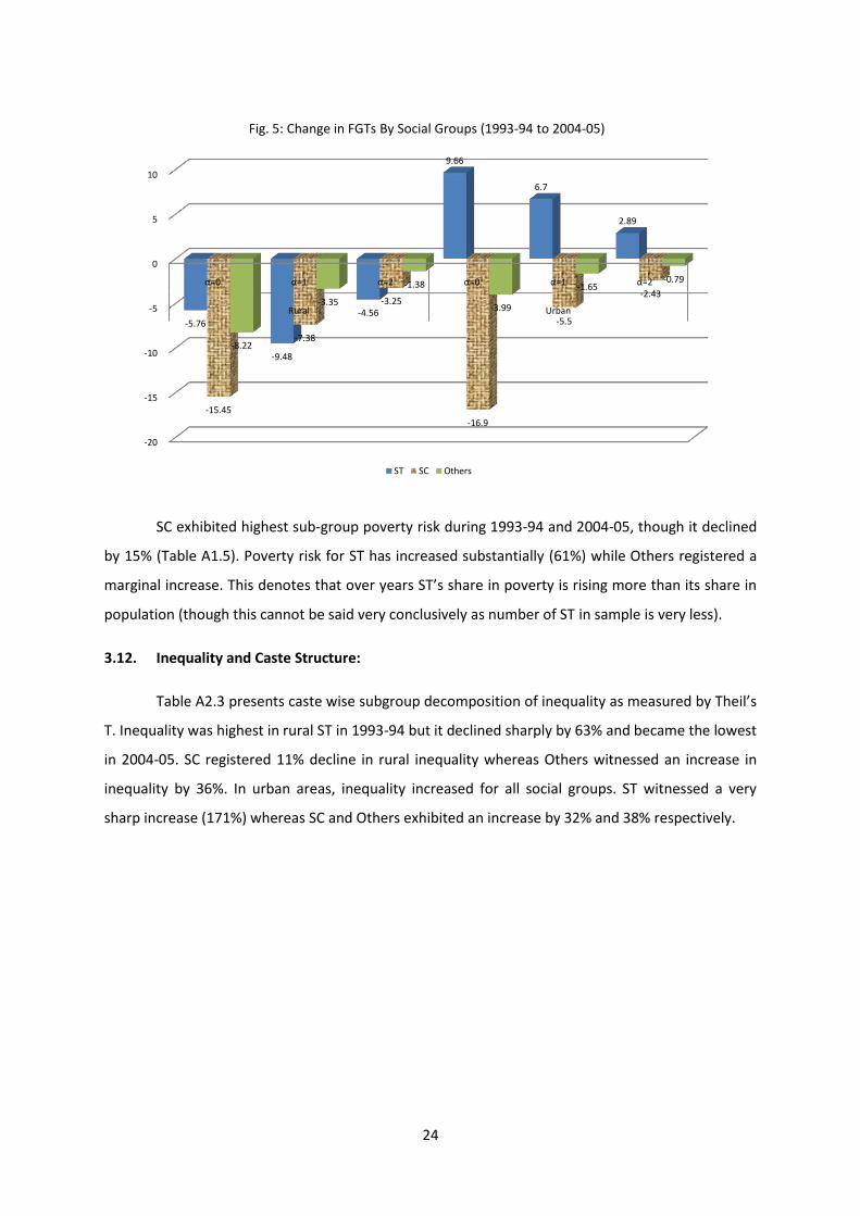
12% for Others during 1993-94 to 2004-05. The fig. 5 below depicts change in FGTs over years.
10
There is a view that SC are better equipped to garner benefit from government welfare schemes as they enjoy an exalted state of awareness than ST who are generally isolated from the mainstream culture and are bounded by rigid ways of life (Uttar Pradesh State Development Report-Vol-I).
24
SC exhibited highest sub-group poverty risk during 1993-94 and 2004-05, though it declined
by 15% (Table A1.5). Poverty risk for ST has increased substantially (61%) while Others registered a
marginal increase. This denotes that over years ST’s share in poverty is rising more than its share in
population (though this cannot be said very conclusively as number of ST in sample is very less).
3.12. Inequality and Caste Structure:
Table A2.3 presents caste wise subgroup decomposition of inequality as measured by Theil’s
T. Inequality was highest in rural ST in 1993-94 but it declined sharply by 63% and became the lowest
in 2004-05. SC registered 11% decline in rural inequality whereas Others witnessed an increase in
inequality by 36%. In urban areas, inequality increased for all social groups. ST witnessed a very
sharp increase (171%) whereas SC and Others exhibited an increase by 32% and 38% respectively.
-20
-15
-10
-5
0
5
10
α=0 α=1 α=2 α=0 α=1 α=2
Rural Urban
-5.76
-9.48
-4.56
9.66
6.7
2.89
-15.45
-7.38
-3.25
-16.9
-5.5
-2.43
-8.22
-3.35
-1.38
-3.99
-1.65-0.79
Fig. 5: Change in FGTs By Social Groups (1993-94 to 2004-05)
ST SC Others

25
Further decomposition of inequality into between-groups and within-group components has
been shown in Table A4.2. Between-groups component has been accounting only for two to four
percent of the total inequality while the within-group component has been responsible for more
than ninety-six percent of it. This indicates that as different social groups, SC, ST and Others are not
so much unequal as they are within themselves and thus exhibit high vertical inequality. Also within-
group inequality is increasing over years.
The Table A5.3 presents decomposition results of change in poverty for various social groups
into growth and distribution component. We would not comment anything about ST in case of UP as
their number in sample is too small to do any rigorous analysis. SC in rural UP registered about 15%
decline in poverty out of which 52% is due to rise in mean income and 37% is accounted by change
in income distribution. This is noteworthy that growth component of poverty change is higher and
redistribution component lower for SC in rural UP than rural all-India. This results in a larger decline
in poverty in SC class in rural UP than in all-India. Similar and even more pronounced patterns have
been observed for SC in rural UP. This indicates that SC in UP are doing better than SC in rest of
India. Others have registered a decline in poverty of 8% and 44% of it is claimed by growth
component while redistribution component accounts for 36%. Though the growth component in
higher in UP, a higher redistribution component makes the change in poverty for Others marginally
smaller in rural UP than in all-India. Others in urban UP have registered a 7% decline in poverty and
Fig. 6: Change in Inequality (T): 1993-94 to 2004-05
Rural
Urban
-0.15
-0.10
-0.05
0.00
0.05
0.10
0.15
0.20
STSC
Others
-0.12
0.010.05
0.20
0.040.08
26
increase in mean income accounts for 43% of it and 36% is due to change in income distribution.
Urban all-India average figures are lower than urban UP for Others.
Ultra-poverty was highest in SC during both 1993-94 and 2004-05 in both rural and urban
areas followed by Others (Table A6.3). Following main points can be mentioned about ultra-poverty:
a. Ultra-poverty was higher in rural areas than in urban areas.
b. Rural areas have registered a sharper decline in ultra-poverty (SC: 49%, Others: 42%).
c. SC witnessed sharper decline in ultra-poverty in urban areas also (26%) compared to Others
(19%).
Similarily, following observations sum up the trend in possible poverty across social groups:
a. In rural UP, possible poverty has increased in SC by 46% from 1993-94 and by 24% in Others.
This shows a crowding of individuals in vicinity of the poverty line.
b. SC registered a very marginal decline in possible poverty by 2% in urban UP while Others
witnessed an increase by 11% from 1993-94.
3. 13. Livelihood Pattern and Poverty:
The number of households by category of livelihood can throw some light on the nature of
economy of the state. NSS classifies households in rural and urban sectors on the basis of the major
source of their earnings during the last 365 days preceding the date of survey. For a rural household
if a single source contributes more than 50 percent of its total income during the reference period, it
would be assigned a type code of that activity. There are five types of households in rural areas
namely, (a) self-employed in agriculture (b) self-employed in non-agriculture (c) agricultural labour
(d) non-agricultural labour, and (e) others. Of these, agricultural and non-agricultural labour
constitute the pure labour supply in a village economy. It may be possible that they also own some
land but the major source of their earnings is their manual labour and not the land (for a good
discussion on economic classification of households in NSS, refer to Sundaram & Tendulkar, 2003).
The last category of ‘others’ is a residual from these activities. They may be getting their income
either from some contractual employment or some assets, transfer payments etc. (Sundaram &
Tendulkar, ibid).
For urban sector, NSS defines four categories of households: (a) self-employed households
(b) wage and salaried income households (c) casual labour households, and (d) others. Here again
the most heterogeneous category is that of ‘self-employed households’. This could include, for
example, a barber with just a mirror, a few combs, razor and scissor, sitting on roadside to an

27
expensive beauty parlour. It would also include the roadside fortune tellers with a parrot and few
cards if that is the major source of their earnings.
3.14. Livelihood and Poverty in Rural Sector:
Agricultural labour and self-employed in agriculture together constitute the proportion of
population directly dependent on agriculture. The Table A3.2.a presents occupational distribution of
population in rural UP. That agriculture was the main source of livelihood in rural India during 1993-
94 is evident from the high proportion of population earning their incomes mainly from agriculture
(about 69 percent). UP’s economy also depended primarily on agriculture and about 75 percent of
its rural population was engaged in it. Though population engaged in agriculture declined by more
than eleven percentage points in UP from 1993-94 to 2004-05, still agriculture was the predominant
employment (about sixty-four percent of population) here. Agriculture in UP has been characterized
by small farm size, labour intensive methods and largely dependence on monsoon rains. All this
makes it difficult for most of the farmers and especially for agricultural labour to escape poverty. In
line with argument are the HCR figures for the agricultural labour that is the highest (table A1.6).
They have been also the farthest from the poverty line during both 1993-94 and 2004-05.
The incidence, depth and severity of poverty were highest among Agricultural Labour (64%,
19%,7% respectively) followed by Other Labour (53%, 13% and 5% respectively) during 1993-94. Self-
Employed in Non-Agriculture (SENA) had the third highest incidence of poverty (45%) followed by
Self-Employed in Agriculture (SEA) and Others with HCR of 37% and 28% respectively. Poverty gap
and severity followed a similar pattern to HCR.
During 2004-05, all occupational classes registered a decline in poverty but the relative
ranking in HCR remained the same as in 1993-94. Agricultural Labour were still the group with the
highest poverty indices though it witnessed a 13% decline in HCR from 1993-94. The highest
percentage decline from 1993-94 has been exhibited by Others (30%) followed by SEA (28%) and
SENA (23%) whereas the least decline has been shown by Other Labour. Thus, poverty in labour
classes (agricultural+other) has been rampant and resistive to change during 1993-94 and 2004-05.
Table 25 shows the subgroup poverty risk for individuals in various occupations. Agricultural labour
had the highest sub-group poverty risk during 1993-94 clearly indicating that it was sharing
proportionately more of UP’s overall poverty than its share was in UP’s overall population. This fact
is also in consonance with a very high incidence of poverty among this class. The matter of concern is
that this risk has further increased by 19% during 2004-05. Similarly, for the next poorest class, i.e.,

28
the Other labour poverty risk has been not only very high but has also increased by 12% during
2004-05. All other occupational classes have registered a decline in sub-group poverty risk. Thus,
poverty in UP is concentrating itself into labour classes, be it agricultural labour or other labour.
Highest decline in poverty risk has been shown by Others like their performance in reducing HCR.
3.15. Livelihood and Poverty in Urban Sector:
Considerably higher proportion of people was self-employed in UP during 1993-94 than was
average for all-India (Table A1.7). The number of regular wage/salary earners was much higher for
all-India average than for UP. The situation almost reversed during 2004-05 when UP registered a
marginal decline in proportion of self-employed while all-India witness an increase and for regular
wage/salary earners, UP saw a marginal increase while all-India experienced a decline. Thus, the first
two occupation classes have always accounted for about 85 percent of UP’s population while they
accounted for about 80 percent of occupation in urban all-India.
Casual labour was the group with highest poverty incidence (67%) followed by Self-
Employed (41%), Others (28%) and Regular Wage/Salary Earners (RWSE) with HCR of 18% during
1993-94. These ranks remained unchanged during 2004-05 also. It is worth mentioning that though
the incidence of poverty declined in all occupation classes, it increased by 17% in RWSE. Even within
RWSE, though the HCR has increased, the depth and severity of poverty has declined by 10% and
28% respectively from what they were during 1993-94. The Fig. 7 depicts change in poverty indices
for various occupation groups during 1993-04 to 2004-05.
-16
-14
-12
-10
-8
-6
-4
-2
0
2
4
SENA AL OL SEA Others 9 SE RWSE CL Others
-10.32
-8.46
-4.03
-10.32
-8.3 -8.21
3
-14.26
-6.14
-4.55
-6.57
-2.83-3.57 -3.43
-1.76
-0.4
-7.12
-2.61
-1.9
-3.21
-1.54 -1.37 -1.38-0.61
-0.36
-3.72
-1.63
Fig. 7: Change in FGTs across Occupations: 1993-94 to 2004-05
α=0 α=1 α=2

29
During 1993-94, the casual labours were accounting for 85% more share of poverty than
their share of population and thus had the highest sub-group poverty risk (Table A1.7). The self-
employed faced the second highest poverty risk though it was only 13% higher than what their share
in population warranted. The other two occupational classes had a poverty risk below the norm. In
2004-05, poverty risk declined for the all occupation classes but RWSE where it increased by 41% of
its value in 1993-94.
3.17. Inequality:
Table A2.4a and A2.4b depict sub-group decomposition of inequality occupation wise for
rural and urban UP. In rural UP, Others had the highest inequality during 1993-94 that further
increased by about 86 % in 2004-05. Inequality was the least in Other Labour in 1993-94. Considering
the high poverty gap for this class, it seems this class was more or less homogenously poor. But this
class registered an increase in inequality by 42 % in 2004-05 and no longer remains as homogenous
as it was in 1993-94. The second least unequal occupational class in 1993-94 was Agricultural Labour
and it witnessed a decline in inequality by 10 %. This has been the only occupational class that
registered a decline in inequality in rural areas. Inequality was the highest in the Others class in
urban UP during 1993-94, followed by Self-employed class. While the farmer witnessed a decline in
inequality, the later registered an increase of 76 % to become the group with second highest income
inequality.
In Urban UP, inequality was the least in Casual Labour and it declined further by 6% in 2004-
05. Regular wage/salary earners saw an increase in inequality of about 42 %. Another group to
undergo decline in inequality was Others (14%). Both SE and RWSE had higher inequalities in 1993-
94 than Others and it further accentuated by 57% and 36% in 2004-05. Thus, while two occupational
groups witnessed decline in inequality, two other groups registered an increase. Since the increases
percentages are high and the base values were also high, it implies inequality has increased in urban
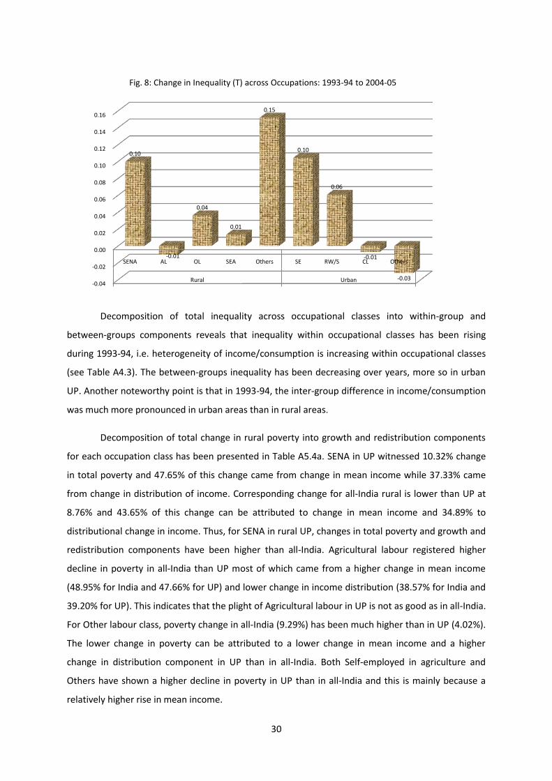
UP. The Fig. 8 shows the change in inequality from 1993-94 to 2004-05.
30
Decomposition of total inequality across occupational classes into within-group and
between-groups components reveals that inequality within occupational classes has been rising
during 1993-94, i.e. heterogeneity of income/consumption is increasing within occupational classes
(see Table A4.3). The between-groups inequality has been decreasing over years, more so in urban
UP. Another noteworthy point is that in 1993-94, the inter-group difference in income/consumption
was much more pronounced in urban areas than in rural areas.
Decomposition of total change in rural poverty into growth and redistribution components
for each occupation class has been presented in Table A5.4a. SENA in UP witnessed 10.32% change
in total poverty and 47.65% of this change came from change in mean income while 37.33% came
from change in distribution of income. Corresponding change for all-India rural is lower than UP at
8.76% and 43.65% of this change can be attributed to change in mean income and 34.89% to
distributional change in income. Thus, for SENA in rural UP, changes in total poverty and growth and
redistribution components have been higher than all-India. Agricultural labour registered higher
decline in poverty in all-India than UP most of which came from a higher change in mean income
(48.95% for India and 47.66% for UP) and lower change in income distribution (38.57% for India and
39.20% for UP). This indicates that the plight of Agricultural labour in UP is not as good as in all-India.
For Other labour class, poverty change in all-India (9.29%) has been much higher than in UP (4.02%).
The lower change in poverty can be attributed to a lower change in mean income and a higher
change in distribution component in UP than in all-India. Both Self-employed in agriculture and
Others have shown a higher decline in poverty in UP than in all-India and this is mainly because a
relatively higher rise in mean income.
-0.04
-0.02
0.00
0.02
0.04
0.06
0.08
0.10
0.12
0.14
0.16
SENA AL OL SEA Others SE RW/S CL Others
Rural Urban
0.10
-0.01
0.04
0.01
0.15
0.10
0.06
-0.01
-0.03
Fig. 8: Change in Inequality (T) across Occupations: 1993-94 to 2004-05

31
The decomposition of poverty change in Urban UP and all-India is shown in Table A5.4b. In
case of Self-Employed, poverty change has been marginally higher for all-India than for UP, the
reason being a higher change in distribution of income for UP. Situation is similar in case of Regular
Wage/Salary Earners mainly due to a lower increase in mean income and higher change in
redistribution component. Casual labour is the only occupational class that has registered a higher
decline in poverty for UP than for all-India. The reason is a much higher rise in mean income in UP
relative to all-India and considerably lower change in income distribution. UP witnessed considerably
lower decline in poverty for Others and the main reason for it has been a lower increase in mean
income than in all-India.
Tables A6.4a and A6.4b present proportion of ultra and possible poor in rural and urban UP
respectively. The existence of ultra-poverty in rural UP has been highest in Agricultural Labour (43%)
during 1993-94 though it declined by about 37% over years (Table 33). The maximum decline has
been registered by Others (52%), followed by SENA (49%) and SEA (46%). Possible poverty has
registered increase for all occupation classes except Other Labour and Others. The maximum
increase from 1993-94 has occurred in SENA (15%) followed by SEA (11%). In urban UP, casual labour
was the group with highest concentration of ultra poverty (57%) but it underwent a decline by about
17 %age points to become 36% in 2004-05. This change by about 31% was the highest exhibited by
any occupation group in urban UP. All other groups also registered a decline in ultra poverty in range
of 12 to 15% of their values in 1993-94. In case of possible poor, only one group (RWSE) registered a
decline by 31%. Rest of occupation groups witnessed increased incidence of possible poverty and
highest increase was in casual labour (by 69%).
4.1. Working of SGSY in Uttar Pradesh: Voices from Field:
This section attempts to give some overview of functioning of Swarnajayanti Gram
Swarozgar Yojana (SGSY) in two development blocks in District Jaunpur of Eastern UP. This study was
undertaken during May-August, 2006 and was the part of present author’s PhD thesis work. The
development blocks chosen were Mariahu and Ramnagar. Mariahu block consists of 12 Nyay
panchayats (NP) and we selected 7 of them to study. Total 16 villages were selected randomly from
these 7 NPs in Mariahu block. Similarly, Ramnagar block consists of 12 NPs and the study chose 6 out
of them. Total 16 villages were chosen from these 6 NPs in Ramanagar block. The design of study
was quasi-experimental. We chose one Treatment Group and one Comparison Group in each block.
The treatment group consisted of the beneficiaries of the SGSY in that block and the comparison
group was of the below poverty line people not included in the programme. Though we tried to
adopt as scientific and rigourous procedures of selecting the sample, the setup such a study itself

32
posits problems. Data was collected for two time periods, 1999 and 2006 and recall method was
used to get data for 1999. As expected the data came out to be statistically non-normal and thus we
prefer to use non-parametric tests on the data. Mann-Whitney and Wilcoxon test were used under
double-difference of means design to check the statistical significance of change in household
incomes of the treatment (SHG) and comparison groups.
4.2. The Scheme: SGSY
Puzzled by lacklustre performance of almost all anti-poverty programmes the Planning
Commission setup a committee under chairmanship of Prof. Hashim to suggested way out of poverty
impasse. On the recommendation of this committee, all rural self-employment anti-poverty
programmes were brought under one umbrella, the SGSY. Similarly, all rural wage-employment
programmes were clubbed to form the Jawahar Gram Samridhi Yojana. SGSY was launched on April
1, 1999, and it is a reformulated version of IRDP. SGSY is formed by merging IRDP, DWCRA, TRYSEM,
SITRA, GKY and MWS11. It is a holistic programme for poverty alleviation unlike IRDP. SGSY provides
the poor with micro finance. Micro credit is the small loan forwarded to the poor. Micro finance
includes support services along with the loan component (Pathak & Pant, 2007). Micro finance and
micro credit has reversed the view that poor are non-bankable. The programme focuses on Group
approach and training is an indispensible part of it.
4.3. Findings from the Field:
The study could not find any statistically significant change in household income of
treatment (SHG) and comparison (Non-SHG) groups in both development blocks (Pathak & Pant,
2007; Pathak & Pant, 2008). The plausible reasons cited were lack of proper training, emphasis on
individual rather than group approach, wide spread corruption in block officials as well as
beneficiaries, non-existent assets (either not created at all or dispersed off later), improper selection
of programme beneficiaries in, lack of awareness about the programme. As a proxy for awareness
and involvement of beneficiaries, they were asked to tell the name and year of formation of their
SHG. Shockingly, 16% could not tell the name of SHG and 32% could not tell the year of formation of
the SHG in Mariahu block. These figures were 22% and 28% respectively in the Ramnagar block. All
these factors had created an environment of distrust among individuals and a large proportion of
respondents answered in negative on being inquired about their willingness to form SHGs in future.
There were plenty of cases that should have been included in any SHG being formed in that area but
11
IRDP = Integrated Rural Development Programme; DWCRA = Development of Women and Children in Rural Areas; TRYSEM = Training of Rural Youth for Self-Employment; SITRA = Supply of Improved Toolkits to Rural Artisans; GKY = Ganga Kalyan Yojana; MWS = Million Wells Scheme.

33
they could not as the facilitator did not care to take them under SHG. There were even more cases
of fraudulent entry in SHGs. It was found that the average household income of the SHG group was
higher than that of the Non-SHG group.
Table 5: Responses from Some SHGs under SGSY
Mariahu Block Ramnagar Block
No Training 64% 74%
Individual Activity 76% 75%
Asset 42% 60%
Non-Transparent Selection 12% 12%
Could not Tell SHG-Name 18% 22%
Could not Tell Year of formation 32% 28%
Source: Field Survey
SGSY is not a tale of all black. There are some patches of white also. This scheme has made cheap
credit available for the poor. They claim this has added to their dignity as they need not go to village
money lenders any more or at least frequently. This also indicates that had the scheme
operationalised properly, it could have made dent in poverty problem also as it is doing in southern
states of India.
A field-survey was conducted in Amethi (UP) for studying the Rajiv Gandhi Mahila Vikas
Pariyojana (RGMVP)12 during December, 2009 to January, 2010. This scheme is similar to SGSY in
that it is a micro finance scheme and forms SHGs. It differs from SGSY mainly in that it does not have
a subsidy component unlike the former and in that SHGs can be only of women. RGMVP is the
flagship scheme for poverty alleviation by the Rajiv Gandhi Charitable Trust (RGCT). The researcher
was surprised to find that some of the women who formed the very first SHG under the RGMVP
were able to tell the date of formation of their SHG. This shows their involvement in the SHG-
activity. On being inquired whether they love their SHG and are there any benefit from it, some
women became emotional and responded, “Samuh hamara beta hai. Agar baki bete dhokha de
denge tab bhee ham iske sahare jindaagee kaat lenge. (The SHG is our Son. This will support us even
if other sons ditch us)”. This shows the attachment that is needed for any intervention to succeed.
The noteworthy point is that since RGMVP is a scheme by RGCT, the state government offers no
support to it. On the other hand, SGSY is a fully supported scheme by both the Center and the State
but has failed to make any impressive dent in problem of poverty.
Another example of failure in implementation is the Public Distribution System (PDS) which
is mean to be a safety net for the poor and deprived section of the society. There are several studies
on PDS highlighted various aspects of shortcomings (Dev, M.S. & Suryanarayana, M.H., 1991). The
12
A comparative study of SGSY and RGMVP has been undertaken in a companion paper.

34
present paper tried a very simple exercise with NSS-61st Round data. We tried to see how many of
ultra poor, poor and possible poor have a ration card and whether it is an Antyodya card, BPL card or
some other card. Data shows that only about 83% of ultra poor in rural UP had a ration card while in
urban UP, this figure was 84%. These number are more or less for all three categories of poor under
consideration (Table A7.1). A simple cross tabulation of type of ration card with average mpce
showed striking results (Table A7.2). In rural UP, while the least mpce for an Antyodaya crad holder
was about `147, the maximum MPCE in the same card holder category was about `2632. Similar
peculiarities can be observed in all card types.
The general attitude of the governments in the Centre and States are also very lukewarm
towards development initiative. Dev and Mooij (2002) mention an example of how governments
cross fund the development expenditure. The United Front government launched a programme for
basic minimum services (BMS) in 1996-97. The expenditure on BMS was increased from `2466 crore
in 1996-97 to `4048 crore in 1999-2000. Government claimed that BMS was an additional allocation
for social sector but Dev and Mooij (2002) doubt this and assert that this increased expenditure for
BMS was possibly financed by a decreased one on rural development. The problem with state
governments in UP is even more severe. “The problem of low commitment to social needs in terms
of government policy is amplified by ineffective implementation at the local level” (Drèze and
Gazdar, 1996, p. 93). The general notion of ‘inertia of development’ put forth by Drèze and Gazdar
(1996) is still valid in UP. The state is a case of governance problems. World Bank opines that
governance is the way in which power is exercised in the management of economic and social
resources of a country, notably with the aim of achieving development (as cited in UP-HDR, 2006).
The level and pattern of expenditure on social sector is an indicative of the priority assigned by the
government to human development. UP falls in middle category state (in which the ratio of social
sector expenditure13 to gross state domestic product [GSDP] is between 5% to 6%) whereas other
poor states like Bihar, Rajasthan and Orissa spend more than 8% of their GSDP on social sector.
Madhya Pradesh spends between 7% to 8% of its GSDP. The low ratio of expenditure on social sector
in UP depicts government’s inclination towards human development. UP-HDR (2007) mentions that
another indicator of fiscal priority accorded to social sector by a state is ratio of social sector
expenditure to total expenditure. UP belongs to low expenditure category (less than 30%) states in
this indicator.
13
Social sector expenditure is defined as “total expenditure on ‘social services’ and ‘rural development’ as given in central and state budgets.” (Dev & Mooij, 2002). Social services include education, health and family welfare, water supply and sanitation. Rural development relates mostly to anti-poverty programmes. See Dev and Mooij (2002) and Mooij and Dev (2004) for a lucid discussion on these topic.

35
UP has become a political chessboard and the main parties are Congress and Bahujan Samaj
Party (BSP). Bhartiya Janta Party (BJP) that underwent a meteoric rise from its base in UP, has
entered a phase of hibernation owning to its internal power struggle. Recently, Amethi that was in
district Sultanpur earlier has been made a new district. The reason cited is that it would develop
better as a district. But as per a news in ‘Times of India’ dated August 11, 2010 the Chief Minister of
the state has allocated `3.5 crore for development of Amethi as a district. In the same
supplementary budget, `509 crore for her dream project Kanshi Ram Eco Park and some other
ongoing works on Dalit Smaaraks. What does this skewed and irrational allocation of fund indicates
to? It seems politics in UP has become a means to power towards self-aggrandizement.
5. Conclusion:
This paper attempted a decomposition analysis of poverty scenario in Uttar Pradesh during
1993-94 and 2004-05. It was found that poverty has decreased but inequality has increased. It was
also observed that the decrease in poverty incidence was driven mainly by increase in the mean
income. The main problems in the state are stark inter-region and intra-region differences. A
positive observation is that the poorest region in the state, the southern region or Bundelkhand, is
making relatively more impressive progress in poverty reduction. The study also tried to highlight
the way anti-poverty programmes are generally being implemented in the state. A brief discussion of
the actual modus operandi of Swarnajayanti Gram Swarozgar Yojana as observed in a field study
gives some indication of the development inertia. At the same time, programmes like Rajiv Gandhi
Mahila Vikash Pariyojana are making a good impression without any visible support from state
government. This highlights role of political will in development of an area.
36
References:
Anand, S. (1983) Inequality and Poverty in Malaysia: Measurement and decomposition, Oxford
University Press, New York.
Bajpai, N. and Volavka (2003), “Agricultural Performance in Uttar Pradesh: A Historical Account”,
CGSD Working No. 23, Centre for Globalization and Sustainable Development, The Earth
Institute, University of Columbia, April 2005.
Baulch, B. (1996), “”Neglected Trade-off in Poverty Measurement”, IDS Bulletin, No. 27, Vol. 1, pp.
36-42.
Bourguignon, F. (2004): “The Poverty-Growth-Inequality Triangle”, The World Bank, download url:
http://www.cies.edu.ni/documentos/red/doc/cap02/33634_PovertyInequalityGrowthTriang
leFeb24.pdf
Chand, R., Garg, S. and Pandey, L. (2009), “Regional Variations in Agricultural Productivity: A District
Level Analysis”, Discussion Paper NPP01/2009, National Professor Project, National Council
for Agricultural Economics and Policy Research, New Delhi.
Chaudhury, S. and Gupta, N. (2009), “Levels of Living and Poverty Patterns: A District wise Analysis of
India”, Economic and Political Weekly, February 28, 2009, Vol. XLIV, No. 9, pp. 94-110.
Cornia G. A. and Stewart Francis (1993), “Two Errors of Targeting”, Innocenti Occasional Papers,
Spedale delgi Innocenti, Florence Italy, downloaded on 06 July, 2010.
Cowell, F.A. (1995) Measuring Inequality, LSE Handbooks in Economics Series, Prentice Hall
Harvester Wheatsheaf, London, 2nd edition
Dhawan , B.D. (1995) “Magnitude of Groundwater Exploitation”, Economic and Political Weekly, Vol.
30, No. 14, April 8, 1995, pp. 769-775.
Dhongde, S. (2007), “Measuring the Impact of Growth and Income Distribution on Poverty in India”,
Journal of Income Distribution, 16.2, pp.25-48.
Diwakar, D.M. (2009), “Intra-Regional Disparities, Inequality and Poverty in Uttar Pradesh”,
Economic and Political Weekly, Vol. XLIV, Nos. 26 and 27, pp.264-273.
Drèze, Jhon and H. Gazdar (1996), “Uttar Pradesh: The Burden of Inertia”, Indian Development:
Selected Regional Perspectives (eds. Jean Drèze and Amartya Sen), Oxford University Press,
Delhi.
Foster, Greer, and Erik Thorbecke (1984), “A Class of Decomposable Poverty Measures”,
Econometrica, Vol. 52, No. 3 (May, 1984), pp. 761-766.
Haughton J. and Shahidur R. Khandekar (2009) Handbook of Poverty and Inequality, The World Bank,
Washington, DC.
Himanshu (2007), “Recent Trends in Poverty and Inequality: Some Preliminary Results” Economic
and Political Weekly, February 10, 2007, pp. 497-508.

37
Hulme, D., Moore, K. and Shepherd, A. (2001), “Chronic Poverty: Meanings and Analytical
Framework”, CPRC Working Paper 2, International Development Department, Chronic
Poverty Research Centre, November.
Jayaraman, R. and Lanjouw, P. (1999) “The Evolution of Poverty and Inequality in Indian Villages”,
The World Bank Research Observer, vol. 14, no. 1 (February 1999), pp.1-30.
Kanbur, R. (2006): “The Policy significance of Inequality Decompositions”, Journal of Economic
Inequality, vol. 4, no. 3, December, 2006, pp. 367-374.
Kozel, V and Parker, B (2003), “A Profile and Diagnostics of Poverty in Uttar Pradesh”, Economic and
Political Weekly, January 25, 2003, pp. 385-403.
Lipton, M. (1988), “The Poor and the Poorest: Some Interim Findings”, World Bank Discussion Paper:
25, The World Bank, Washington D.C.
Mahendra Dev S and Mooij, Jos (2002). “Social Sector Expenditures in the 1990s: Analysis of Central
and State Budgets”, Economic and Political Weekly, 37 (9), pp. 853-866.
Mahendra Dev S, and Ravi, C.(2007), “Poverty and Inequality: All-India and States, 1983-2005”,
Economic and Political Weekly, February 10, 2007, pp. 509-521.
Mahendra Dev S. and M.H. Suryanarayan (1991): “Is PDS Urban Biased and Pro-Rich?: An
Evaluation”, Economic and Political Weekly, Vol. 26, No. 41 (Oct. 12, 1991) pp. 2357-2366.
Mooij Jos and Mahendra Dev S(2004), “Social Sector Priorities: An Analysis of Budgets and
Expenditures in India the 1990s”, Development Policy Review, 22 (1), pp. 97-120
Mutatkar, R. (2005), “Social Group Disparities and Poverty in India”, Working Paper Series No. WP-
2005-004, Indira Gandhi Institute of Development Research, Mumbai, India.
Pathak, D.C. and Pant, S.K.(2007), “Micro Finance- A Magic Wand for Poverty Alleviation: A Case-
Study of SGSY”, published in Conference Volume of Indian Economic Association (90th
Coneference).
Pathak, D.C. and Pant, S.K. (2008): “Micro Finance Matter…? Impact Evaluation of SGSY: A Case
Study of Jaunpur District” in Micro Finance and Poverty Eradication: Indian and Global
Experiences (eds. Lazar and Palanichammy), pp.469-491, New Century Publications, New
Delhi, India.
Planning Commission (2007), Uttar Pradesh Development Report (Vol. I and II), State Plan Division,
Government of India, Academic Foundation Press, New Delhi. Download url:
http://planning.up.nic.in/apd/hdr-2006/HDR.html
Radhakrishna, R. and Ray, S. (2005), Handbook of Poverty in India, Oxford University Press, New
Delhi.
Ravallion, M. (1998), “Poverty Lines in Theory and Practice”, LSMS working paper, No. 133, The
World Bank, Washington D.C.

38
Ray, D. (2002), Development Economics, India: Oxford University Press, 5th impression, p. 250.
Ray, S. (2010), Backwaters of Development: Six Deprived States of India, Oxford University Press, New
Delhi.
Sastry, N.S. (2003), “District Level Poverty Estimates: Feasibility of using NSS Household Consumer
Expenditure Survey Data”, Economic and Political Weekly, January 25, 2003, pp. 409-412.
Shaffer, P. (2008), “New Thinking on Poverty: Implications for Globalization and Poverty Reduction
Strategies”, Real World Economics Review, Issue no. 47, pp. 192-231.
Sharma and Poleman (1993), The New Economics of India’s Green Revolution: Income and
Employment Diffusion in Uttar Pradesh, Ithaca (New York): Cornell University Press, 1993.
Singh, A.K.(2009), “Poverty Trends and Correlates in Uttar Pradesh”, Giri Institute of Development
Studies, Discussion Note.
Srivastava, R. (2001), “Anti-Poverty Programmes in Uttar Pradesh: An Evaluation”, Planning
Commission, New Delhi.
STATA Technical Bulletin, March 1999, STB-48, Stata Corp., pp. 1-40.
Stewart, F. (2002) “Horizontal Inequalities: A Neglected Dimension of Development”, QEH Working
Paper Series – QEHWPS81, University of Oxford.
Stokes, E. (1978), The Peasant and the Raj: Studies in Agrarian Society and Peasant Rebellion in
Colonial India, Cambridge: Cambridge University Press.
Subbarao, K. (1992) “Interventions to Fill Nutrition Gaps at the Household Level: A Review of India’s
Experience”, Poverty in India: Research and Policy (eds.) Barbara Harriss, S. Guhan, R.H.
Cassen, Oxford University Press, Bombay, 1992.
Sundaram, K. and Suresh D. Tendulkar (2003), “Poverty among Social and Economic Groups in India
in 1990s”, Economic and Political Weekly, December 3, 2003, pp. 5263-5276.
Suryanarayana, M. H. (2001) “Schedule Castes, Their Disadvantages and Deprivations: A Rural all-
India Profile”, Artha Vijnana, vol. XLIII, no. 1-2, March-June 2001, pp- 89-97.
Varshney, D.(2010), “Employment and Poverty Linkages in Uttar Pradesh: A Household Level
Analysis”, Indian Development Review, Vol. 8, No. 1, January-December, 2010, pp. 69-94
World Bank (2002), Poverty in India: The Challenge of Uttar Pradesh, Report No. 22323-IN, Poverty
Reduction and Economic Management Sector, South Asia Region.

39
Annexure
Table A.1: Poverty Indices and Sub-group Poverty Risk
Table A. 1.1: Poverty Indices and Sub-group Poverty Risk: India and UP
1993-94: Rural 2004-05: Rural 1993-94: Urban 2004-05: Urban
India UP* UP India UP* UP India UP* UP India UP* UP
α=0 37.21 42.31 43.09 28.30 33.32 33.38 32.63 35.10 36.07 25.62 30.13 30.32
α=1 8.50 10.37 10.37 5.67 6.33 6.34 8.05 9.03 9.28 6.08 7.05 7.14
α=2 2.84 3.53 3.64 1.72 1.81 1.82 2.88 3.27 3.37 2.07 2.34 2.37
Table A.1.2: Poverty Indices and Sub-group Poverty Risk: NSS-region wise (Rural UP)
Poverty: 1993-94 Poverty: 2004-05 Pov. Risk: 1993-94 Pov. Risk: 2004-05
α=0 α=1 α=2 α=0 α=1 α=2 α=0 α=1 α=2 α=0 α=1 α=2
Western 29.29 6.08 1.85 23.74 3.78 0.94 0.68 0.57 0.51 0.71 0.6 0.51
Central 50.17 13.78 5.01 30.12 5.65 1.56 1.16 1.30 1.37 0.90 0.89 0.86
Eastern 48.78 11.98 4.03 41.62 8.52 2.59 1.13 1.13 1.11 1.25 1.34 1.43
Southern 67.36 20.17 8.09 38.87 7.33 2.02 1.56 1.9 2.22 1.16 1.16 1.11
Table A.1.3: Poverty Indices and Sub-group Poverty Risk: NSS-region wise (Urban UP)
Poverty: 1993-94 Poverty: 2004-05 Pov. Risk: 1993-94 Pov. Risk: 2004-05
α=0 α=1 α=2 α=0 α=1 α=2 α=0 α=1 α=2 α=0 α=1 α=2
Western 31.13 7.74 2.80 28.31 6.35 1.96 0.86 0.83 0.83 0.93 0.89 0.83
Central 33.85 9.52 3.60 24.64 6.16 2.25 0.94 1.03 1.07 0.81 0.86 0.96
Eastern 38.62 9.36 3.18 37.68 8.71 2.81 1.07 1.01 0.94 1.24 1.22 1.17
Southern 74.36 21.06 8.16 43.01 12.03 4.82 2.06 2.27 2.42 1.42 1.69 2.06
Table A.1.4: Poverty Indices and Sub-group Poverty Risk: Social Group wise (Rural UP)
Poverty: 1993-94 Poverty: 2004-05 Pov. Risk: 1993-94 Pov. Risk: 2004-05
FGT α=0 α=1 α=2 α=0 α=1 α=2 α=0 α=1 α=2 α=0 α=1 α=2
ST 37.94 12.68 5.10 32.18 3.20 0.54 0.88 1.19 1.39 0.96 0.50 0.30
SC 60.36 16.48 5.98 44.91 9.10 2.73 1.40 1.55 1.64 1.35 1.43 1.50
Others 37.62 8.75 2.88 29.40 5.40 1.50 0.87 0.82 0.79 0.88 0.85 0.82
Table A.1.5: Poverty Indices and Sub-group Poverty Risk: Social Group wise (Urban UP)
Poverty: 1993-94 Poverty: 2004-05 Pov. Risk: 1993-94 Pov. Risk: 2004-05
α=0 α=1 α=2 α=0 α=1 α=2 α=0 α=1 α=2 α=0 α=1 α=2
ST 27.93 3.13 0.91 27.93 3.13 0.91 0.77 0.34 0.27 1.24 1.38 1.60
SC 60.09 16.12 5.98 60.09 16.12 5.98 1.67 1.74 1.78 1.42 1.48 1.50
Others 32.20 8.21 2.96 32.20 8.21 2.96 0.89 0.88 0.88 0.93 0.92 0.92
Table A.1.6: Poverty Indices and Sub-group Poverty Risk: Occupation wise (Rural UP)
Poverty: 1993-94 Poverty: 2004-05 Pov. Risk: 1993-94 Pov. Risk: 2004-05
FGT α=0 α=1 α=2 α=0 α=1 α=2 α=0 α=1 α=2 α=0 α=1 α=2
SENA 44.73 10.71 3.58 34.41 6.16 1.68 1.04 1.01 0.98 1.03 0.97 0.92
AL 63.82 18.71 7.08 55.36 12.14 3.87 1.48 1.76 1.94 1.66 1.91 2.13
OL 53.24 13.03 4.66 49.21 10.20 3.12 1.24 1.22 1.28 1.47 1.61 1.71
SEA 36.91 8.24 2.61 26.59 4.67 1.24 0.86 0.77 0.72 0.80 0.74 0.68
Others 27.57 6.97 2.36 19.27 3.54 0.98 0.64 0.66 0.65 0.58 0.56 0.54
Table A.1.7: Poverty Indices and Sub-group Poverty Risk: Occupation wise (Urban UP)
Poverty: 1993-94 Poverty: 2004-05 Pov. Risk: 1993-94 Pov. Risk: 2004-05
FGT α=0 α=1 α=2 α=0 α=1 α=2 α=0 α=1 α=2 α=0 α=1 α=2
SE 40.89 9.61 3.25 32.68 7.85 2.64 1.13 1.04 0.96 1.09 1.11 1.12
RWSE 17.59 3.94 1.28 20.59 3.54 0.92 0.49 0.42 0.38 0.69 0.50 0.39
CL 66.66 22.75 9.64 52.40 15.63 5.92 1.85 2.45 2.86 1.75 2.21 2.51
Others 27.65 8.44 3.67 21.51 5.83 2.04 0.77 0.91 1.09 0.72 0.82 0.87 Source: Author’s calculations using Unit level data from NSS 50
th and 61
st Rounds.

40
Table A.2: Inequality in Monthly Per Capita Consumption Expenditure
Table A.2.1: Inequality: India and UP
Rural Urban
1993-94 2004-05 1993-94 2004-05
India 0.1711 0.2055 0.2391 0.2834
UP* 0.1474 0.1882 0.1936 0.2653
UP 0.1486 0.1896 0.1957 0.2644
Table A.2.2: UP: Inequality and NSS-Regions
Rural Urban
1993-94 2004-05 1993-94 2004-05
Western 0.1404 0.1703 0.2143 0.2299
Central 0.1505 0.1798 0.1757 0.3458
Eastern 0.1337 0.1793 0.1450 0.1903
Southern 0.1776 0.3609 0.1131 0.1516
Table A.2.3: UP: Inequality and Social Groups
Rural Urban
1993-94 2004-05 1993-94 2004-05
ST 0.1963 0.0729 0.1145 0.3105
SC 0.1347 0.1489 0.1163 0.1532
Others 0.1447 0.1966 0.1963 0.2713
Table A.2.4.a: UP: Inequality and Occupation (Rural)
Rural
1993-94 2004-05
SENA 0.1321 0.2321
AL 0.1091 0.0986
OL 0.0864 0.1226
SEA 0.1454 0.1588
Others 0.1769 0.3289
Table A.2.4.b: UP: Inequality and Occupation (Urban)
Urban
1993-94 2004-05
SE 0.1829 0.2875
RWSE 0.1681 0.2289
CL 0.1148 0.1078
Others 0.2285 0.1965
Source: Author’s calculations using Unit level data from NSS 50
th and 61
st Rounds.
Table A.3: Population Sub-Groups
Table A.3.1: Population Sub-Groups: Social Class
Rural Urban
1993-94 2004-05 1993-94 2004-05
India UP India UP India UP India UP
SC 10.82 0.76 10.57 0.5 3.21 0.69 2.92 0.46
ST 21.09 24.07 20.92 25.46 13.85 13.93 15.64 13.83
Others 68.03 75.15 68.46 73.93 82.9 85.36 81.42 85.71
Table A.3.2.a: Population Sub-Groups: Occupation (Rural)
Rural
1993-94 2004-05
India UP India UP
SENA 12.59 13.66 16.54 19.41
AL 27.58 18.22 24.89 12.9
OL 7.33 4.78 10.44 9.2
SEA 41.21 57.13 39.46 51.3
Others 7.93 6.2 8.68 7.19

41
Table A.3.2.b:Population Sub-Groups: Occupation (Urban)
Urban
1993-94 2004-05
India UP India UP
SE 38.15 54.34 42.99 53.32
RWSE 41.98 30.07 39.47 32
CL 12.76 10.91 11.71 9.12
Others 5.28 4.65 5.82 5.56
Table A.3.3: Population Sub-Groups: NSS-Regions
Rural Urban
1993-94 2004-05 1993-94 2004-05
Western 35.35 33.02 49.46 49.36
Central 18.04 18.12 20.15 22.75
Eastern 41.48 43.84 24.48 22.14
Southern 5.13 5.02 5.92 5.74 Source: Author’s calculations using Unit level data from NSS 50
th and 61
st Rounds.
Table A.4: Inequality Decomposition: UP
Table A.4.1: Inequality Decomposition for UP: NSS-Region wise
Rural Urban
Component (%) 1993-94 2004-05 1993-94 2004-05
Within-Group 94.91 97.67 95.53 95.79
Between Groups 5.09 2.33 4.47 4.21
Table A.4.2: Inequality Decomposition for UP: Social Group wise
Rural Urban
Component (%) 1993-94 2004-05 1993-94 2004-05
Within-Group 96.32 97.94 96.03 98.03
Between Groups 3.68 2.06 3.97 1.97
Table A.4.3: Inequality Decomposition for UP: Occupation wise
Rural Urban
Component (%) 1993-94 2004-05 1993-94 2004-05
Within-Group 93.35 95.00 89.63 94.63
Between Groups 6.65 5.00 10.32 5.37 Source: Author’s calculations using Unit level data from NSS 50
th and 61
st Rounds.
Table A.5: Decomposition of Change in Poverty Levels
Table A.5.1: India and UP
All-India UP
Rural Urban Rural Urban
Change in Poverty 8.92 7.01 -9.73 -5.75 Growth C. - 44.17 - 40.71 -45.68 -42.03 Redistribution C. 35.25 33.70 35.95 36.28
Table A.5.2: UP: NSS-Region wise
UP
Rural Urban
Western region
Change in Poverty -5.55 -2.82
Growth C. -39.94 -37.87
Redistribution C. 34.37 35.05
Central region
Change in Poverty -20.11 -9.21
Growth C. -52.57 -46.24
Redistribution C. 32.47 37.03
Eastern region
Change in Poverty -7.16 -0.94

42
Growth C. -46.50 -40.74
Redistribution C. 39.34 39.80
Southern region
Change in Poverty -28.49 -31.36
Growth C. -58.77 -60.59
Redistribution C. 30.28 29.24
Table A.5.3: UP: Social Group wise
All-India UP
Rural Urban Rural Urban
ST
Change in Poverty -4.32 -6.82 -5.76 9.67
Growth C. -42.96 -42.83 -37.24 -33.21
Redistribution C. 38.63 36.01 31.48 42.88
SC
Change in Poverty 11.52 -10.03 -15.46 -16.91
Growth C. -48.69 -47.69 -51.92 -52.02
Redistribution C. 37.18 37.67 36.46 35.11
Others
Change in Poverty -8.73 -6.84 -8.24 -3.97
Growth C. -42.79 -39.58 -44.01 -40.42
Redistribution C. 34.06 32.74 35.77 36.42
Table A.5.4.a: UP: Rural Occupation wise
India UP
SENA Rural Rural
Change in Poverty -8.76 -10.32
Growth C. -43.65 -47.65
Redistribution C. 34.89 37.33
AL
Change in Poverty -10.38 -8.46
Growth C. -48.95 -47.66
Redistribution C. 38.57 39.20
OL
Change in Poverty -9.29 -4.02
Growth C. -45.72 -45.06
Redistribution C. 36.43 41.04
SEA
Change in Poverty -7.67 -10.34
Growth C. -41.90 -44.92
Redistribution C. 34.23 34.58
Others
Change in Poverty -3.62 -8.30
Growth C. 33.41 -39.78
Redistribution C. 29.79 31.48
Table A.5.4.b: UP: Urban Occupation wise
India UP
SE Urban Urban
Change in Poverty -8.50 -8.21
Growth C. -42.89 -46.51
Redistribution C. 34.39 38.31
RWSE
Change in Poverty -5.64 2.99
Growth C. -36.68 -31.58
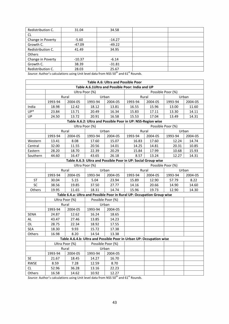
43
Redistribution C. 31.04 34.58
CL
Change in Poverty -5.60 -14.27
Growth C. -47.09 -49.22
Redistribution C. 41.49 34.95
Others
Change in Poverty -10.37 -6.14
Growth C. 38.39 -31.81
Redistribution C. 28.03 25.67 Source: Author’s calculations using Unit level data from NSS 50
th and 61
st Rounds.
Table A.6: Ultra and Possible Poor
Table A.6.1Ultra and Possible Poor: India and UP
Ultra Poor (%) Possible Poor (%)
Rural Urban Rural Urban
1993-94 2004-05 1993-94 2004-05 1993-94 2004-05 1993-94 2004-05
India 18.98 12.42 18.12 13.81 16.55 15.96 13.00 11.60
UP* 23.84 13.71 20.49 16.34 15.83 17.11 13.30 14.11
UP 24.50 13.72 20.91 16.58 15.53 17.04 13.49 14.31
Table A.6.2: Ultra and Possible Poor in UP: NSS-Region wise
Ultra Poor (%) Possible Poor (%)
Rural Urban Rural Urban
1993-94 2004-05 1993-94 2004-05 1993-94 2004-05 1993-94 2004-05
Western 13.41 8.08 17.60 15.07 16.83 17.60 12.24 14.74
Central 32.00 11.55 20.56 14.01 14.25 14.81 20.31 10.85
Eastern 28.20 18.70 22.39 20.29 15.84 17.99 10.68 15.93
Southern 44.60 16.47 43.65 26.18 8.57 13.24 12.27 14.31
Table A.6.3: Ultra and Possible Poor in UP: Social Group wise
Ultra Poor (%) Possible Poor (%)
Rural Urban Rural Urban
1993-94 2004-05 1993-94 2004-05 1993-94 2004-05 1993-94 2004-05
ST 30.04 5.15 5.04 23.94 15.89 12.90 57.79 8.22
SC 38.56 19.85 37.50 27.77 14.16 20.66 14.90 14.60
Others 19.95 11.65 18.31 14.74 15.96 19.73 12.90 14.30
Table 6.4.a: Ultra and Possible Poor in Rural UP: Occupation Group wise
Ultra Poor (%) Possible Poor (%)
Rural Urban
1993-94 2004-05 1993-94 2004-05
SENA 24.87 12.62 16.24 18.65
AL 43.47 27.46 13.85 14.23
OL 28.75 22.34 18.92 17.55
SEA 18.30 9.93 15.72 17.38
Others 16.98 8.20 14.54 13.38
Table A.6.4.b: Ultra and Possible Poor in Urban UP: Occupation wise
Ultra Poor (%) Possible Poor (%)
Rural Urban
1993-94 2004-05 1993-94 2004-05
SE 21.67 18.45 14.27 16.70
RWSE 8.59 7.28 12.59 8.70
CL 52.96 36.28 13.16 22.23
Others 16.58 14.62 10.92 12.27 Source: Author’s calculations using Unit level data from NSS 50
th and 61
st Rounds.

44
Table A.7: PDS Beneficiaries in UP
Table A.71.: % of Population by Type of Ration Card in UP (2004-05)
Ultra Poor Poor Possible Poor
Rural Urban Rural Urban Rural Urban
Have Card 83.45 84.11 83.90 85.33 84.94 78.32
Antyodaya 9.78 2.69 6.07 1.71 1.73 1.43
BPL 23.56 20.02 23.37 16.43 14.37 9.63
Others 66.65 77.29 70.55 81.86 83.89 88.96
Table A.7.2: Income Statistics of Card Holders in UP (2004-05)
Rural Urban
Card Type Mean Maximum Minimum Mean Maximum Minimum
Antyodaya 426.44 2631.83 146.67 493.69 2202.50 253.3
BPL 438.75 3500.25 122.67 569.88 4476.50 172.69
Others 554.46 44219.75 106.08 802.47 10674.67 41.00 Source: Author’s calculations using Unit level data from NSS 50
th and 61
st Rounds.