Power calculation

J-PAL Advanced course, Paris 2012

Prepared by Marc Gurgand and Roland Rathelot

Practical issue

Anticipate if sample size is enough for the expected effects

Interviews and treatment are expensive and you have a budget

→ You want to optimize the sample size w/r to budget

Sample size is limited by field constraints

Uncertainty

It is all a matter of statistics: you want to minimize the oddsthat something disappointing happens

You have to set acceptable probabilities and take the risk

Additional source of uncertainty: depends on parameterswhose values are unknown

Parameters of the power calculation

There is a true effect and you compare averages in control andtreatment groups

The chances that those averages are significantly different depend(primarily) on:

How large is the true effect

Sample sizes

Variance of the outcomes in the population

Significance criterion

Design

1 Significance test: reminder

2 Computing power

3 Imperfect compliance

4 Design effect

5 How to increase power

Notations

y : outcome

D: treatment dummy

N: sample size

Compare means of treated and untreated or OLS on:

y = c + βD + u

Standard error

Using usual formula or computing from means:

V (β) = σ2β

=1

D(1− D)

V (u)

N

NB: adding controls

y = c + βD + Xγ + u

Because D ⊥ X , does not affect β (asymptotically)But reduces V (u), so improves precision

Significance tests

Estimator β asymptotically normalwith mean β and variance σ2

β

If β = 0, then, for a risk α (e.g. 5%) we can define tα/2 such that:

P

(−tα/2 <

β

σβ< tα/2

)= 1− α

For α = 0.05, tα/2 = 1.96

If |β/σβ| > 1.96, we can reject the null β = 0

The power of the experiment

If the policy has an impact, we want to be able to see it

Unless the effect is very small, we want to reject the nullbut if a lot of imprecision (large estimator variance), we may fail todo so

Type II error: β > 0, but we fail to reject the null(i.e. β/σβ < 1.96)

This will happen sometimes, for some samples

Power= 1 minus the probability that this happens

The power of the experiment

Usual approach: set an acceptable power (often 80%)

Set a β that you feel you should be able to ”see”

And figure out the sample size that ensures that power for a trueeffect β

Computing the power

[β/σβ < tα/2|β] is random

P

(β

σβ> tα/2|β

)= κ

where κ is the power.

P

(β − βσβ

> tα/2 −β

σβ|β

)= κ

Φ

(β

σβ− tα/2

)= κ

Thusβ

σβ− tα/2 = t1−κ

Power illustration

Power illustration

Power illustration

Minimum detectable effect

The β that will be ”significant” 80% of the time (at 5% level)is such that:

β

σβ− tα/2 = t1−κ

or

βMDE = (tα/2 + t1−κ)σβ

with tα/2 = 1.96 if α = 0.05and t1−κ = 0.84 if κ = 0.80

(tα/2 + t1−κ)σβ is the minimum detectable effet (MDE)

Minimum detectable effect

Remember that

σ2β

=1

D(1− D)

V (u)

N

Thus

βMDE = (tα/2 + t1−κ)

√1

D(1− D)

V (u)

N

MDE: main ingredients

βMDE = (tα/2 + t1−κ)

√1

D(1− D)

V (u)

N

1 Sample sizes

2 Variance of the outcomes in the population

More homogenous = small differences unlikely in absence oftreatment effect

3 Significance criterion

4 Design

A 50% treated is optimal. But more design issues to come

Effect-size

A usefull metric for MDE is the s.d. of the outcome

βMDE

σu= (tα/2 + t1−κ)

√1

D(1− D)

1

N

Effect-size as a function of sample size in standard case

.2.4

.6.8

1M

DE

0 500 1000 1500N

Effect-size

An effect size of

is considered… …and it means that… Required N(under 50% treatment)size of… (under 50% treatment)

0.2 Modest The median member of thetreatment group had a better

900treatment group had a better outcome than the 58th percentile of the control group

0.5 Large The median member of thetreatment group had a better

144treatment group had a better outcome than the 69th percentile of the control group

0.8 VERY Large The median member of thetreatment group had a better 

56

outcome than the 79th percentile of the control group

Imperfect compliance

Whenever treatment assignment is not identical to treatment

Encouragement design

Some do not take up the program

Unassigned do take up the program

Then randomization status can serve as an instrument for actualtreatment

→ Loss of power of the IV estimator

Power with instrumental variable

y = c + βT + u

with T instrumented by D

Call π the net take up (π = E (T |D = 1)− E (T |D = 0))

σ2β

=1

D(1− D)

V (u)

N

1

π2

If take up is 50%, N must increase 4 times

Impact of imperfect compliance: 50% take-up

.2.4

.6.8

11.

2

0 500 1000 1500N

MDE MDE with take up 50%

Impact of imperfect compliance: 20% take-up

01

23

0 500 1000 1500N

MDE Take up 50%Take up 20%

Group-level randomization

Up to now, randomization at individual levelBut we may want to randomize at higher group level:Village, school, district, family

Individuals within each treatment group get the same treatment

May be required by field constraints or theoretical reasons

Impact of group-level randomization

Outcomes within each group may be correlated (teachereffect, local event,)

Each additional individual does not bring entirely newinformation

At the limit, imagine all outcomes within a strata are exactlythe same: effective sample size is number of strata, notnumber of individuals

Precision will depend on the 2 sample sizes and the withincorrelation

Design effect

Decompose residual into group and individual component

yig = c + βDig + µg + uig

βMDE = (tα/2 + t1−κ)

√1

D(1− D)

√V (µ)

Ng+

V (u)

N

where N is total and Ng is number of groups

Design effect

Call ρ = V (µ)/[V (µ) + V (u)] the intracluster correlation

The higher ρ, the less additional information there is in anadditional individual within each group

As compared to individual randomization, the loss in precision(thus the increase in MDE) is proportional to

D =√

1 + (n − 1)ρ

where n = N/Ng , the size of groups

Exemple of values of ρ in education

Madagascar Math + Language 0.5

Busia, Kenya Math + Language 0.22

Udaipur, India Math + Language 0.23

Mumbai, India Math + Language 0.29

Vadodara, India Math + Language 0.28

Busia, Kenya Math 0.62

How bad can it be?

Take ρ = 0.2

Think of an experiment with 50 schools and 30 pupils per school

Ng = 50, n = 30 and N = 1500

D = 2.61Standardized MDE with individual randomization: 0.15Standardized MDE with design effect: 0.15*2.61=0.39

Move from so-called small to so-called large

How to increase power

Asymptotically, randomization balances all characteristics betweentreatment and control

But at finite distance, not exactly true

We should force balancing at least against observed variables:Ensure that T and C are balanced at least in terms of some x ’s

Efficiency gains

Intuitively: if you don’t force balancing, x and D will be somewhatcorrelated

Introduces uncertainty as to whether differences are due to D or tox (even if you do control for x)

Efficiency gains: formally

Assume true model:

yi = c + βDi + γxi + ui

Rewrite in difference to the mean to simplify the algebra

yi − y = β(Di − D) + γ(xi − x) + u′i

= βDi + γxi + u′i

Efficiency gains: formally

V (β, γ) = V (u′)(M ′M)−1

withM = (D, x)

M ′M =

(ND(1− D)

∑Di xi∑

Di xi∑

x2i

)NB: ∑

D2i = ND(1− D)

Efficiency gains: formally

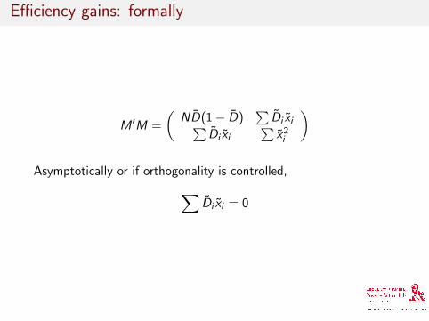
M ′M =

(ND(1− D)

∑Di xi∑

Di xi∑

x2i

)

Asymptotically or if orthogonality is controlled,∑Di xi = 0

Efficiency gains: formally

Inverting M ′M,

V (β) = V (u′)

∑x2i

ND(1− D)×∑

x2i − (

∑Di xi )2

When∑

Di xi = 0, back to previous formula

When∑

Di xi 6= 0, variance is larger

How to balance randomization

1 Stratification

2 Pair-wise matching

3 Re-randomization

Stratification

Randomize within strata

Simple, but limited number of variables can be used

→ use variables that are strongly related to the outcome or forwhich subgroup analysis is desired

Pair-wise matching

Form pairs (one T, one C) using matching methods

Can rely on large number of variables

If implementation issues or non-response, can drop the affectedpairs (external validity issues)

Re-randomization

A. Make a draw and test balance on observed variablesIf one equality test rejected, redraw

B. Make 1,000 draws and keep the one that minimizes themaximum t-stat

Simulations

D. McKenzie and M. Bruhn, “In Pursuit of Balance:Randomization in Practice in Development Field Experiments”,American Economic Journal: Applied Economics, 1(4): 200-32,2009.

Use several real data and allocate an artificial treatment; comparerandomization methods

Below N = 300, balancing methods increase balance,including on future outcomes, and raise power

Stratification and pair-wise better at reducing extremeimbalances

Recommend to control for strata or pair dummies or x (ifre-randomization)

Designs that imply stratification 1

Randomize classes within schools: for ex. half treated / halfcontrol

Schools act as strata:

Balanced over all school characteristics (but not classcharacteristics)

Include school dummies in the specifications

Designs that imply stratification 2

Randomize entire schools under a rotating design:

First graders in group A schools are treated date 1 and untreateddate 2First graders in group B schools are treated date 2 and untreateddate 1

Political value: all schools benefit to the same level

If there is no dynamics (A is not affected by treatment in date 2)T: (A,1) and (B,2) and C: (A,2) and (B,1)

Balanced over all school and date characteristics

Include school dummies and date dummies in thespecifications