power control games between anchor and jammer nodes in...

1

Power Control Games between Anchor and JammerNodes in Wireless Localization Networks

Ahmet Dundar Sezer,Student Member, IEEE, and Sinan Gezici,Senior Member, IEEE

Abstract—In this paper, a game theoretic framework is pro-posed for wireless localization networks that operate in thepresence of jammer nodes. In particular, power control gamesbetween anchor and jammer nodes are designed for a wirelesslocalization network in which each target node estimates its posi-tion based on received signals from anchor nodes while jammernodes aim to reduce localization performance of target nodes.Two different games are formulated for the considered wirelesslocalization network: In the first game, the average Cramer-Rao lower bound (CRLB) of the target nodes is considered asthe performance metric, and it is shown that at least one purestrategy Nash equilibrium exists in the power control game.Also, a method is presented to identify the pure strategy Nashequilibrium, and a sufficient condition is obtained to resolve theuniqueness of the pure Nash equilibrium. In the second game,the worst-case CRLBs for the anchor and jammer nodes areconsidered, and it is shown that the game admits at least onepure Nash equilibrium. Numerical examples are presented tocorroborate the theoretical results.

Index Terms—Localization, jammer, power allocation, Nashequilibrium, estimation, wireless network.

I. I NTRODUCTION

In recent years, research communities have developed asignificant interest in wireless localization networks, whichprovide important applications for various systems and ser-vices [1], [2]. To name a few, smart inventory tracking systems,location sensitive billing services, and intelligent autonomoustransport systems benefit from wireless localization networks[3]. In such a wide variety of applications, accurate androbust position estimation plays a crucial role in terms ofefficiency and reliability. In the literature, various theoreticaland experimental studies have been conducted in order toanalyze wireless position estimation in the context of accuracyrequirements and system constraints; e.g., [4], [5].

In a wireless localization network, there exist two typesof nodes in general; namely, anchor nodes and target nodes.Anchor nodes have known positions and their location in-formation is available at target nodes. On the other hand,target nodes have unknown positions, and each target nodein the network estimates its own position based on receivedsignals from anchor nodes (in the case of self localization[3]). In particular, position estimation of a target node isperformed by using various signal parameters extracted fromreceived signals (i.e., waveforms). Commonly employed signal

A. D. Sezer and S. Gezici are with the Department of Electricaland Electronics Engineering, Bilkent University, Bilkent, Ankara 06800,Turkey, Tel: +90 (312) 290-3139, Fax: +90 (312) 266-4192,e-mails:{adsezer,gezici}@ee.bilkent.edu.tr.

A. D. Sezer is supported by ASELSAN Graduate Scholarship forTurkishAcademicians.

parameters are time-of-arrival (TOA) [6], [7], time-difference-of-arrival (TDOA) [8], angle-of-arrival (AOA) [9], and re-ceived signal strength (RSS) [10]. TOA and TDOA are timebased parameters which measure the signal propagation time(difference) between nodes. AOA is obtained based on theangle at which the transmitted signal from one node arrives atanother node. RSS is another signal parameter which gathersinformation from power or energy of a signal that travelsbetween anchor and target nodes [4]. Since a signal travelingfrom an anchor node to a target node experiences multipathfading, shadowing, and path-loss, position estimates of targetnodes are subject to errors and uncertainty. As the Cramer-Raolower bound (CRLB) expresses a lower bound on the varianceof any unbiased estimator for a deterministic parameter, itisalso considered as a common performance metric for wirelesslocalization networks [11]–[13].

Besides anchor and target nodes, a wireless localization net-work can contain undesirable jammer nodes, the aim of whichis to degrade the localization performance (i.e., accuracy)of the network. In the literature, various studies have beenperformed on the jamming of wireless localization networks.The jamming and anti-jamming of the global positioningsystem (GPS) are studied in [14] for various jamming schemes.Similarly, in [15], an adaptive GPS anti-jamming algorithmisproposed. In addition, the optimal power allocation problem isinvestigated for jammer nodes in a given wireless localizationnetwork based on the CRLB metric, and the optimal jammingstrategies are obtained in the presence of peak power and totalpower constraints in [11].

In the literature, various studies have been conducted onpower allocation for wireless localization networks [16]–[19]. In [16], the optimal anchor power allocation strategiesare investigated together with anchor selection and anchordeployment strategies for the minimization of the squaredposition error bound (SPEB), which identifies fundamentallimits on localization accuracy. The work in [17] provides arobust power allocation framework for network localization inthe presence of imperfect knowledge of network parameters.Based on the performance metrics SPEB and the directionalposition error bound (DPEB), the optimal power allocationproblems are formulated in the consideration of limited powerresources and it is shown that the proposed problems canbe solved via conic programming. In [18], ranging energyoptimization problems are investigated for an unsynchronizedpositioning network based on two-way ranging between asensor and beacons. In [19], the work in [18] is extended for apositioning network in which the collaborative anchors addedto the system help sensors locate themselves.

In the presence of jammer nodes in a wireless localization

2

network, anchor nodes can adapt their power allocation strate-gies in response to the strategies employed by jammer nodesand enhance the localization performance of the network.On the other hand, jammer nodes can respond by updatingtheir corresponding power allocation strategies in order todegrade the localization performance. These conflicting inter-ests between anchor and jammer nodes can be analyzed byemploying game theory as a tool. In the literature, game the-oretic frameworks have been applied for investigating powerallocation strategies of users in a competitive system. In [20],competitive interactions between a secondary user transmitter-receiver pair and a jammer are analyzed by applying a game-theoretic framework in the presence of interference constraints,power constraints, and incomplete channel gain information.In particular, the strategic power allocation game betweenthetwo players is proposed first, and then it is presented that thesolution of the game corresponds to Nash equilibria points.In [21], a zero-sum game is modeled between a centralizeddetection network and a jammer in the presence of completeinformation. It is obtained that the jammer has no effect on theerror probability observed at the fusion center when it employspure strategies at the Nash equilibrium.

Although there exist research papers that analyze the non-cooperative behavior of system users and jammer nodesin wireless communication networks in terms of successfultransmissions under a minimum signal-to-interference-plus-noise ratio (SINR) constraint and error probability [20], [21],no studies in the literature have investigated the interactionsbetween anchor nodes and jammer nodes in a wireless local-ization network, where target nodes estimate their positionsbased on signals received from anchor nodes and jammernodes try to degrade the localization performance of thenetwork. In the field of wireless localization, there exist somerecent studies (e.g., [13] and [22]) that analyze the interactionsof entities in a wireless localization network. However, nojammer nodes are considered in those studies, which focuson a cooperative localization network where the target nodesshare information with each other to improve their positionestimates. Therefore, the theoretical analyses presentedthereindiffer from the ones performed in this paper, which considersnon-cooperative localization where anchor and jammer nodescompete for the localization performance of target nodes.

In this paper, power control games between anchor and jam-mer nodes are designed based on a game-theoretic frameworkby employing the CRLB metric. In particular, two differentgames are formulated for the considered wireless localizationnetwork: In the first game, the average CRLB of the targetnodes is considered as the performance metric whereas inthe second one, the worst-case CRLBs for the anchor andjammer nodes are employed. As a solution approach, Nashequilibria of the games are examined, and it is shown that apure Nash equilibrium exists in both of the proposed powercontrol games. In addition, for the game in which the anchorand jammer nodes compete according to the average CRLB, amethod is presented to obtain a pure strategy Nash equilibriumand a sufficient condition is provided to decide whether thepure strategy Nash equilibrium is unique. Finally, numericalexamples are presented to demonstrate the theoretical results.

The main contributions of this work can be summarized asfollows:

• A game theoretic formulation is developed between an-chor and jammer nodes in a wireless localization networkfor the first time in the literature.

• Two types of power control games between anchor andjammer nodes are proposed based on the average CRLBand the worst-case CRLBs for the anchor and jammernodes.

• In a game-theoretic framework, the Nash equilibria ofthe proposed games are analyzed and it is shown thatboth of the games have at least one pure strategy Nashequilibrium.

• For the game that employs the average CRLB as aperformance metric, an approach is developed to obtainthe pure strategy Nash equilibrium and a sufficient con-dition is derived to determine whether the obtained Nashequilibrium is a unique pure strategy Nash equilibrium.

The remainder of the paper is organized as follows: Sec-tion II describes the wireless localization network and intro-duces the network parameters. Section III first presents theproposed game formulations, and then provides detailed theo-retical analyses. Numerical results are described in Section IV,which is followed by the concluding remarks in Section V.

II. SYSTEM MODEL

Consider a wireless localization network withNA anchornodes andNT target nodes at locationsyi ∈ R

2 for i ∈{1, . . . , NA} andxi ∈ R

2 for i ∈ {1, . . . , NT }, respectively.Each target node in the system estimates its position basedon received signals from the anchor nodes, the locations ofwhich are known by the target nodes (i.e., the target nodesperform self-positioning [3]). Besides the anchor and targetnodes, there existNJ jammer nodes located atzi ∈ R

2 fori ∈ {1, . . . , NJ} in the system. Contrary to the anchor nodes,the aim of the jammer nodes is to reduce the localization per-formance of the target nodes. In accordance with the commonapproach in the literature [11], [23]–[25], it is assumed thatthe jammer nodes transmit zero-mean white Gaussian noisein order to distort the signals observed by the target nodes.The reasons behind the use of a Gaussian noise model can beexplained as follows: In wireless localization systems, whenthe knowledge of the ranging signals sent from the anchornodes to the target nodes is unavailable to the jammer nodes,the jammer nodes can continuously transmit noise to degradethe localization performance of the target nodes [11]. In theliterature, it is shown that the Gaussian noise is the worst-case noise for generic wireless networks modeled with additivenoise that is independent of the transmit signals [26]–[28].(In particular, the Gaussian distribution corresponds to theworst-case scenario among all possible noise distributions interms of some metrics such as the mutual information and themean squared error since it minimizes the mutual informationbetween the input and the output when the input is Gaussian,and maximizes the mean squared error of estimating the inputgiven the output for an additive noise channel with a Gaussianinput [29].) Therefore, the jammer nodes are expected to

3

transmit Gaussian noise for efficient jamming [11]. Also, anon-cooperative localization scenario is considered; that is, thetarget nodes do not receive any signals from each other forlocalization purposes.

Let Ai denote the connectivity set for target nodei, which is defined asAi , {j ∈ {1, . . . , NA} |anchor nodej is connected to target nodei} fori ∈ {1, . . . , NT }. Then, corresponding to the transmissionfrom anchor nodej, the received signal at target nodei canbe expressed as

rij(t) =

Lij∑

k=1

αkij

√

PAij s(t− τkij) +

NJ∑

l=1

γil

√

P Jl νilj(t) + nij(t)

(1)

for t ∈ [0, Tobs], i ∈ {1, . . . , NT}, and j ∈ Ai, whereTobs is the observation time,Lij is the number of pathsbetween anchor nodej and target nodei, αk

ij andτkij represent,respectively, the amplitude and the delay of thekth multipathcomponent between anchor nodej and target nodei, PA

ij

is the transmit power of the signal sent from anchor nodej to target nodei, andγil represents the channel coefficientbetween jammer nodel and target nodei, which has a transmitpower ofP J

l [11]. Also, during the reception from anchor nodej, nij(t) denotes the measurement noise at target nodei andνilj(t) represents the jammer noise at target nodei generatedby jammer nodel. It is assumed that the transmit signals(t) isa known signal with unit energy, and the measurement noisenij(t) and the jammer noiseνilj(t) are independent zero-mean white Gaussian random processes, where the spectraldensity levels ofnij(t) andνil(t) are equal toN0/2 and one,respectively [11]. In addition, for each target node,nij(t)’sare independent forj ∈ Ai, andvilj(t)’s are independent forl ∈ {1, . . . , NJ} and j ∈ Ai.1 The delayτkij is expressed asτkij , (‖yj −xi‖+ bkij)/c, wherebkij denotes the non-negativerange bias andc is the speed of propagation.

III. POWER CONTROL GAMES BETWEEN ANCHOR AND

JAMMER NODES

In this section, the aim is to design and analyze powercontrol games between anchor and jammer nodes. In theproposed setting, the anchor nodes set their power levels inorder to maximize the localization performance of the targetnodes whereas the jammer nodes try to minimize the local-ization performance via power allocation. The localizationperformance is quantified by the average CRLB for the targetnodes, which is the metric according to which the anchorand jammer nodes compete. In other words, the anchor nodes(jammer nodes) try to minimize (maximize) the average CRLBfor the target nodes to improve (deteriorate) the localizationperformance of the system. The use of the CRLB as theperformance metric can be justified based on the followingarguments: As investigated in [30], the ML location estimatorbecomes asymptotically unbiased and efficient for sufficiently

1As in [11], it is assumed that the anchor nodes transmit at different timeintervals to prevent interference at the target nodes [4], and during those timeintervals, the channel coefficient between a jammer node anda target node isassumed to be constant.

large SNRs and/or effective bandwidths, and consequently,itachieves a mean-squared error (MSE) close to the CRLB. Forother cases, the CRLB may not provide a tight bound forMSEs of ML estimators [31], [32]. Therefore, the CRLBsobtained based on the optimal power strategies of the anchorand jammer nodes provide performance bounds for the MSEsof the target nodes. Another reason for the use of the CRLBmetric is that it leads to compact closed form expressionsfor the optimization problems and consequently facilitatestheoretical analyses, which lead to intuitive explanations ofpower control games between anchor and jammer nodes.(Performance optimization based on the CRLB has beenconsidered in various studies in the literature such as [11],[13], [33].)

To obtain the formulation of the proposed problem, theCRLB expression for the target nodes is presented as a utilityfunction first, and then the game model is proposed.

A. CRLB for Location Estimation of Target Nodes

To provide the CRLB expression for target nodei, theunknown parameters related to target nodei are defined as[11]

θi ,

[

xTi bTiAi(1) · · · bTiAi(|Ai|) α

TiAi(1)

· · · αTiAi(|Ai|)

]T

(2)

whereAi(j) represents thejth element of setAi, |Ai| denotes

the cardinality of setAi, αij =[

α1ij · · ·α

Lij

ij

]T

, and bij isdefined as

bij =

[

b2ij · · · bLij

ij

]T

, if j ∈ ALi

[

b1ij · · · bLij

ij

]T

, if j ∈ ANLi

(3)

with ALi andANL

i representing the sets of anchors nodes thatare in the line-of-sight (LOS) and non-line-of-sight (NLOS) oftarget nodei, respectively [11]. Then, the CRLB for estimatingthe location of target nodei is given by

E{‖xi − xi‖2} ≥ tr

{

[

F−1i

]

2×2

}

, CRLBi (4)

wherexi denotes an unbiased estimate of the location of targetnodei, tr represents the trace operator, andF i is the Fisherinformation matrix for vectorθi in (2). From [4] and [11],[

F−1i

]

2×2can be expressed as

[

F−1i

]

2×2= J i

(

xi,pAi ,p

J)−1

(5)

whereJ i

(

xi,pAi ,p

J)

denotes the equivalent Fisher informa-tion matrix, which is calculated as

J i

(

xi,pAi ,p

J)

=∑

j∈ALi

PAij λij

N0/2 + aTi pJ

φijφTij (6)

4

with

λij ,4π2|α1

ij |2∫∞

−∞ f2|S(f)|2df

c2(1− ξj) , (7)

ai ,[

|γi1|2 · · · |γiNJ

|2]T

, (8)

pAi ,

[

PAiAi(1)

· · · PAiAi(|Ai|)

]T

, (9)

pJ ,[

P J1 · · · P J

NJ

]T, (10)

φij , [cos ϕij sin ϕij ]T

. (11)

In (7), S(f) denotes the Fourier transform ofs(t), and thepath-overlap coefficientξj is a number that satisfies0 ≤ ξj ≤1 [17]. Also, in (11),ϕij corresponds to the angle betweentarget nodei and anchor nodej.

B. Power Control Game Model

Let G = 〈N , (Si)i∈N , (ui)i∈N 〉 denote the power controlgame between anchor nodes (i.e., Player A) and jammer nodes(i.e., Player J), whereN = {A, J} is the index set for theplayers,Si is the strategy set for playeri, andui is the utilityfunction of playeri. For the anchor nodes, strategy setSA isdefined as

SA ,{

pA ∈ RK | 1TpA ≤ PA

T ∧ 0 ≤ eTi pA ≤ PA

peak ,

∀i ∈ {1, . . . ,K}} (12)

with

pA ,

[

(

pA1

)T· · ·

(

pANT

)T]T

(13)

wherepAi is as defined in (9),1 is the vector of ones,ei is

the unit vector whoseith element is one,K is the dimensionof pA, PA

T is the total available power of the anchor nodes,andPA

peak is the maximum allowed and attainable power (peakpower) for the anchor nodes. Similarly, strategy setSJ for thejammer nodes is defined as

SJ ,{

pJ ∈ RNJ | 1TpJ ≤ P J

T ∧ 0 ≤ eTi pJ ≤ P J

peak ,

∀i ∈ {1, . . . , NJ}} (14)

wherepJ is as defined in (10),P JT is the total available power

of the jammer nodes, andP Jpeak is the maximum allowed and

attainable power (peak power) for the jammer nodes.Let pA andpJ denote strategies of playerA and playerJ ,

respectively. Then, a strategy (action) profile of the game canbe denoted as(pA,pJ ) ∈ S, wherepA ∈ SA, pJ ∈ SJ , andS = SA × SJ . For a given action profile, the utility functionsof playerA and playerJ are defined as

uA(pA,pJ) = −

1

NT

NT∑

i=1

tr{

J i

(

xi,pAi ,p

J)−1

}

, (15)

uJ(pA,pJ) =

1

NT

NT∑

i=1

tr{

J i

(

xi,pAi ,p

J)−1

}

. (16)

Namely, the average CRLB of the target nodes is employed inthe utility functions (see (4) and (5)). SinceuA(p

A,pJ) anduJ(p

A,pJ) satisfy thatuA(pA,pJ)+uJ(p

A,pJ ) = 0 ∀pA ∈SA ∧ ∀pJ ∈ SJ , it is noted that the power control game

between playerA and playerJ corresponds to a two-playerzero-sum game.

C. Nash Equilibrium in Power Control Game

The Nash equilibrium is one of the solution approaches thatis commonly used for game theoretic problems [34]. In thegame-theoretic notation, a strategy profile of gameG, denotedas (pA

⋆ ,pJ⋆ ), is a Nash equilibrium if

uA(pA⋆ ,p

J⋆ ) ≥ uA(p

A,pJ⋆ ) , ∀pA ∈ SA , (17)

uJ(pA⋆ ,p

J⋆ ) ≥ uJ(p

A⋆ ,p

J) , ∀pJ ∈ SJ . (18)

At a Nash equilibrium, no player can improve its utility bychanging its strategy unilaterally. In other words, given thepower levels of playerJ (playerA), playerA (playerJ) doesnot have any incentive to deviate from its power strategy ata Nash equilibrium. Such an equilibrium does not necessarilyexist in infinite games. However, power control gameG admitsa pure Nash equilibrium as the following proposition states.

Proposition 1: A pure Nash equilibrium exists in powercontrol gameG.

Proof: The aim in the proof is to show that the gamehas at least one pure-strategy Nash equilibrium. For thatreason, it is first noted that power control gameG in strategicform 〈N , (Si)i∈N , (ui)i∈N 〉 admits at least one pure Nashequilibrium if the following conditions are satisfied [35]:

• Strategy setSi is compact and convex for alli ∈ N ,whereN = {A, J}.

• ui(pA,pJ) is a continuous function in the profile of

strategies(pA,pJ) ∈ S for all i ∈ N .• uA(p

A,pJ ) anduJ(pA,pJ ) are quasi-concave functions

in pA andpJ , respectively.

Since setSA in (12) and setSJ in (14) are closed and bounded,it can easily be shown that the sets in (12) and (14) arecompact and convex, which satisfies the first condition. Also,uA(p

A,pJ ) in (15) is a concave function ofpA based on theproof in [36] anduJ(p

A,pJ) in (16) is a linear (and concave)function ofpJ based on [33]. Consequently, (15) and (16) arecontinuous and quasi-concave functions, for which the secondand the third conditions hold. Therefore, it is concluded thatat least one Nash equilibrium exists in power control gameG.�

Based on Proposition 1, the proposed power control gamehas at least one Nash equilibrium. In order to analyze the Nashequilibrium, first, best response strategies of playerA andJare discussed and then, a fixed point equation is obtained.

For a given power strategy of playerJ (i.e., power levelsof jammer nodes), the best response function of playerA canbe expressed as

pABR = BRA(p

J)

, arg maxpA∈SA

−1

NT

NT∑

i=1

tr{

J i

(

xi,pAi ,p

J)−1

}

. (19)

5

On the other hand, for a given power strategy of playerA, thebest response function of playerJ is given as

pJBR = BRJ (p

A)

, arg maxpJ∈SJ

1

NT

NT∑

i=1

tr{

J i

(

xi,pAi ,p

J)−1

}

. (20)

Let BR = (BRA,BRJ ) : S = SA×SJ → S be a mapping ofa function (correspondence)BR(p), wherep = (pA,pJ) ∈S is a strategy profile of the power control game, andBRA

andBRJ are as in (19) and (20), respectively. Based on thedefinition of the Nash equilibrium, the following fixed pointequation holds for the Nash equilibrium:

p⋆ = BR(p⋆) . (21)

In addition, the utility function in (15) is a concave functionof pA and the utility function in (16) is a linear (and concave)function of pJ . Based on the utility functions in (15) and(16), the game between playerA and playerJ is calledconvex-concave game [37], [38]. In a convex-concave game,the Nash equilibrium becomes the saddle-point equilibrium,and if there exist multiple Nash equilibria, the value of thegame is unique for every Nash equilibrium. Therefore, the pureNash equilibrium of power control gameG can be obtainedas stated in the following proposition.

Proposition 2: Let p⋆ = (pA⋆ ,p

J⋆ ) denote the Nash equi-

librium of power control gameG in pure strategies. Then,p⋆

satisfies the following equation:

uJ(pA⋆ ,p

J⋆ ) = −uA(p

A⋆ ,p

J⋆ ) =

minpA∈SA

maxpJ∈SJ

1

NT

NT∑

i=1

tr{

J i

(

xi,pAi ,p

J)−1

}

(22)

Proof: Since power control gameG is a two-player zero-sum game anduA(p

A,pJ) in (15) is a concave function ofpA

anduJ(pA,pJ) in (16) is a linear (and concave) function of

pJ , the following equality holds by von Neumann’s MinimaxTheorem [37], [39]:

minpA∈SA

maxpJ∈SJ

1

NT

NT∑

i=1

tr{

J i

(

xi,pAi ,p

J)−1

}

=

maxpJ∈SJ

minpA∈SA

1

NT

NT∑

i=1

tr{

J i

(

xi,pAi ,p

J)−1

}

. (23)

In addition,p⋆ = (pA⋆ ,p

J⋆ ) satisfying the equality in (23) is a

Nash equilibrium of power control gameG. �

Proposition 1 states that power control gameG admits atleast one Nash equilibrium in pure strategies. In order tofurther analyze the equilibrium in power control gameG,the uniqueness of the Nash equilibrium is investigated in theconsideration of pure strategies. The following propositionprovides a sufficient condition for the uniqueness of the purestrategy Nash equilibrium.

Proposition 3: Suppose that the Fisher information matrix

in (6) is positive definite.2 Then, power control gameG has aunique Nash equilibrium in pure strategies if all the elementsof w ,

∑NT

i=1 riaTi are different, whereri is defined as

ri , tr

∑

j∈ALi

PAij λijφijφ

Tij

−1

. (24)

Proof: In order to prove that the Nash equilibrium ofpower control gameG is unique when the condition inProposition 3 is satisfied, it is first shown thatuA(p

A,pJ )in (15) is a strictly concave function ofpA for a fixed pJ .To that aim, choose arbitrarypA ∈ SA and pA ∈ SA withpA 6= pA. Then, the following relations can be obtained foranyα ∈ (0, 1):

uA(αpA + (1− α)pA,pJ )

= −1

NT

NT∑

i=1

tr{

J i

(

xi, αpAi + (1− α)pA

i ,pJ)−1 }

(25)

= −1

NT

NT∑

i=1

tr

{

[

∑

j∈ALi

(αPAij + (1− α)Pij)λij

N0/2 + aTi pJ

φijφTij

]−1}

(26)

= −1

NT

NT∑

i=1

tr

{

[

α∑

j∈ALi

PAij λij

N0/2 + aTi pJ

φijφTij

+ (1 − α)∑

j∈ALi

PAij λij

N0/2 + aTi pJ

φijφTij

]−1}

(27)

> −1

NT

NT∑

i=1

αtr

{

[

∑

j∈ALi

PAij λij

N0/2 + aTi pJ

φijφTij

]−1}

+ (1 − α)tr

{

[

∑

j∈ALi

PAij λij

N0/2 + aTi pJ

φijφTij

]−1}

(28)

= αuA(pA,pJ) + (1− α)uA(p

A,pJ ) (29)

where the equalities in (25) and (26) are due to the definitionsin (15) and (6), respectively, and the inequality in (28) followsfrom the fact thattr{X−1} is a strictly convex function ofXif X is a symmetric positive definite matrix [40]. It is notedthat α ∈ (0, 1), φijφ

Tij is a symmetric positive semidefinite

matrix, and(PAij λij)/(N0/2+aT

i pJ ) and(PAij λij)/(N0/2+

aTi pJ ) are always non-negative for alli ∈ {1, . . . , NT } and

j ∈ ALi . Based on the relations in (25)–(29), it is proved that

uA(pA,pJ ) in (15) is a strictly concave function ofpA for a

fixed pJ .

Next, it is obtained that there exists a unique maximizerof uJ(p

A,pJ) in (16) for a givenpA when the conditionin Proposition 3 is satisfied. To that aim, consider the bestresponse function of playerJ in (20). Based on a similarapproach to that in [33], the solution of the optimization

2The Fisher information matrix is always positive semidefinite by definition.The assumption in the proposition corresponds to practicalscenarios with asufficient number of anchor nodes and guarantees the invertibility of the Fisherinformation matrix.

6

problem in (20) can be expressed as

pJBR(h(j)) = min

{

P JT −

j−1∑

l=1

pJBR(h(l)), PJpeak

}

(30)

for j = 1, . . . , NJ , where h(j) denotes the index of thejth largest element of vectorw defined in Proposition 3,pJBR(h(j)) represents theh(j)th element ofpJBR, and

∑0l=1(·)

is defined as zero. For the condition that all the elements ofw

are different, index vectorh , [h(1)h(2) · · ·h(NJ)] becomesunique and consequently the solution in (30) turns into aunique maximizer ofuJ(p

A,pJ ) for a givenpA. Therefore,based on the properties of gameG presented in the proof ofProposition 1 and the statements proved above, it is concludedthat if the condition in Proposition 3 is satisfied, then the Nashequilibrium of power control gameG is unique. �

It is important to note that the Nash equilibrium obtainedby (22) based on Proposition 2 may not be unique. However,Proposition 3 provides a sufficient condition to check that theobtained Nash equilibrium is a unique equilibrium of powercontrol gameG. If the condition in Proposition 3 is satisfiedfor a given Nash equilibrium, then there exists a uniqueequilibrium of gameG. Otherwise, the Nash equilibrium mayor may not be unique. The condition in Proposition 3 dependson various system parameters such as the power strategy andthe locations of the anchor nodes, the properties of the signaltransmitted from the anchor nodes, the multipath componentsbetween the anchor nodes and the target nodes, and the channelcoefficients between the jammer nodes and the target nodes.

In the presence of multiple Nash equilibria, the anchorand jammer nodes may choose the desired Nash equilibriumdepending on the conditions and constraints in the specificapplication. Although the average CRLB of the target nodes(i.e., the value of the game) is the same for all Nash equilibriabased on Proposition 2, the anchor and jammer nodes mayprefer one Nash equilibrium over the others for the efficientuse of limited resources in the wireless localization network.

D. Power Control Game Based on Minimum and MaximumCRLB

Instead of employing the average CRLB as the performancemetric, it is also possible to use the worst-case CRLBs forthe anchor and jammer nodes as the performance metrics.In particular, from the viewpoint of the anchor nodes, thetarget node with the maximum CRLB (i.e., with the worstlocalization accuracy) can be considered with the aim ofminimizing the maximum CRLB (so that a certain levelof localization accuracy can be achieved by all the targetnodes). Similarly, the jammer nodes can aim to maximizethe minimum CRLB of the target nodes in order to degradethe localization performance of the system. For this setting,define a new gameG which has the same players and thesame strategy sets for the players asG does, except for theutility functions. For a given action profile, the utility functions

of playerA and playerJ in gameG are given by

uA(pA,pJ) = − max

i∈1,...,NT

tr{

J i

(

xi,pAi ,p

J)−1

}

, (31)

uJ(pA,pJ) = min

i∈1,...,NT

tr{

J i

(

xi,pAi ,p

J)−1

}

. (32)

As it can be noted from the utility functions for playerAand playerJ in (31) and (32), the power control game basedon these utility functions is not a zero-sum game; that is,uA(p

A,pJ ) + uJ(pA,pJ) 6= 0, ∃pA ∈ SA ∧ ∃pJ ∈ SJ .

The utility functions in this scenario do not facilitate de-tailed theoretical analyses as in the case of the average CRLBbased utility functions. However, the existence of a pure Nashequilibrium is still guaranteed based on the following result.

Proposition 4: There exists at least one pure Nash equilib-rium in gameG.

Proof: GameG admits at least one pure Nash equilibriumif the conditions presented in the proof of Proposition 1 aresatisfied. GameG satisfies the first condition since gameGhas the same strategy sets for the players asG does. Also,uA(p

A,pJ ) in (31) and uJ(pA,pJ ) in (32) are concave

functions of pA and pJ , respectively, since the minimum(maximum) of concave (convex) functions is also concave(convex). Therefore, gameG also satisfies the second andthird conditions. Consequently, based on the similar approachemployed in the proof of Proposition 1, it can be shown thatat least one pure-strategy Nash equilibrium exists in gameG.�

IV. N UMERICAL RESULTS

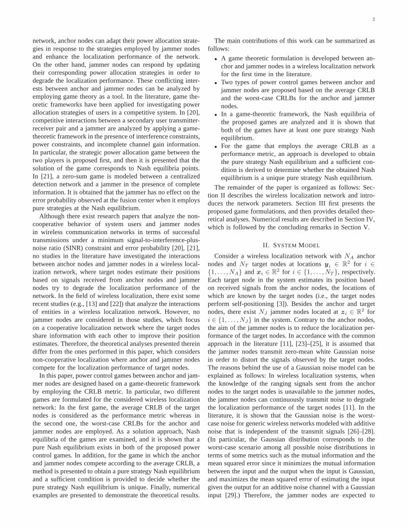
In this section, numerical examples are provided in orderto corroborate the theoretical results obtained in the previoussection. To that aim, consider a wireless localization networkin which four anchor nodes, three target nodes, and threejammer nodes are located as in Fig. 1. For the sake ofsimplicity, it is assumed that each target node has LOSconnections to all of the anchor nodes. Also, the free spacepropagation model is considered; that is,λij in (7) is equal toλij = 100N0‖xi − yj‖

−2/2 [17]. In addition,|γij |2 is givenby ‖xi − zj‖−2/2 andN0 is set to2 [11].

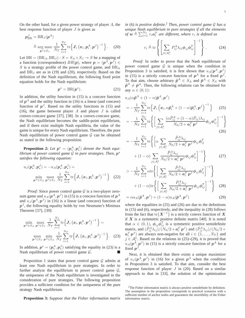
In Fig. 2, the average CRLBs of the three target nodes(i.e., the values of the game) are plotted versus the totalavailable power of the anchor nodes (i.e.,PA

T ) for variouspeak powers of the anchor nodes whenP J

T = 20, P Jpeak = 10,

and the anchor nodes and the jammer nodes operate at theNash equilibrium. From the figure, it is observed that as thetotal power of the anchor nodes increases, the average CRLBobtained in the Nash equilibrium reduces since more strategiesbecome available for the anchor nodes asPA

T increases. Also,it can be deduced from the figure that for lower values of thetotal power of the anchor nodes (e.g.,PA

T < 5), the averageCRLBs of the target nodes are the same for different values ofPApeak due to the dominant effect of the total power constraint

on the game value. On the other hand, for higher values of thetotal power of the anchor nodes (e.g.,PA

T ≥ 12 for PApeak = 1),

the average CRLB of the localization system does not changesince the peak power constraint of the anchor nodes limits theuse of total power available for the anchor nodes.

7

0 2 4 6 8 100

5

10

15

x (m)

y(m

)

Anchor NodeTarget NodeJammer Node

Fig. 1. The simulated network including four anchor nodes positioned at[0 0], [10 0], [0 10], and [10 10]m., three jammer nodes positioned at[2 15],[4 2], and[6 6]m., and three target nodes positioned at[2 4], [7 1], and[9 9]m.

0 5 10 15 20 25 30 35 400

0.5

1

1.5

2

2.5

3

3.5

4

Total Power for Anchor Nodes PTA

Ave

rage

CR

LB (

m2 )

PpeakA = 1

PpeakA = 2

PpeakA = 5

Fig. 2. Average CRLB of the target nodes versus total power ofthe anchornodes for the scenario in Fig. 1, whereP J

T= 20, P

J

peak= 10, and the

anchor nodes and the jammer nodes operate at Nash equilibrium in powercontrol gameG.

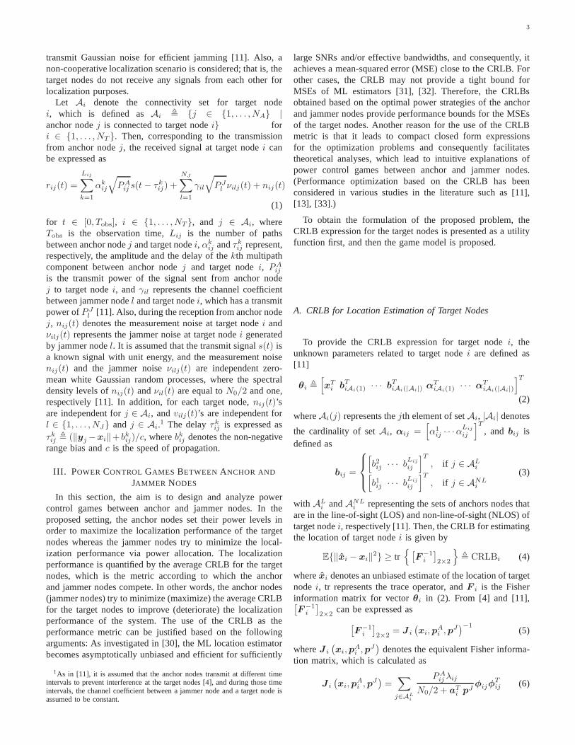
In order to observe the effects of the peak power constraintof the anchor nodes on the average CRLB of the target nodes,the average CRLBs of the target nodes are plotted in Fig. 3versus the peak power of the anchor nodes for various valuesof the total power of the anchor nodes whenP J

T = 20 andP Jpeak = 10. From Fig. 3, similar observations to those for

Fig. 2 are obtained. It is also stated that the average CRLBsfor different values of the total power of the anchor nodes arethe same when the peak power of the anchor nodes is belowa certain value since the peak power constraint of the anchornodes becomes more dominant than the total power constraintin that case.

Similar to Fig. 2 and Fig. 3, the average CRLBs are plotted

0 1 2 3 4 5 6 70

0.5

1

1.5

2

2.5

3

3.5

4

Peak Power for Anchor Nodes PpeakA

Ave

rage

CR

LB (

m2 )

PTA = 5

PTA = 10

PTA = 15

PTA = 20

Fig. 3. Average CRLB of the target nodes versus peak power of the anchornodes for the scenario in Fig. 1, whereP J

T= 20, P

J

peak= 10, and the


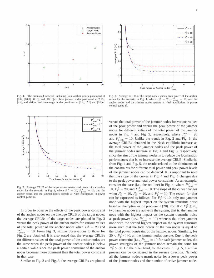
versus the total power of the jammer nodes for various valuesof the peak power and versus the peak power of the jammernodes for different values of the total power of the jammernodes in Fig. 4 and Fig. 5, respectively, wherePA

T = 20andPA

peak = 10. Unlike the trends in Fig. 2 and Fig. 3, theaverage CRLBs obtained in the Nash equilibria increase asthe total power of the jammer nodes and the peak power ofthe jammer nodes increase in Fig. 4 and Fig. 5, respectively,since the aim of the jammer nodes is to reduce the localizationperformance; that is, to increase the average CRLB. Similarly,from Fig. 4 and Fig. 5, the results related to the dominance ofthe constraints for different total power and peak power levelsof the jammer nodes can be deduced. It is important to notethat the slope of the curves in Fig. 4 and Fig. 5 changes dueto the peak power and total power constraints. As an example,consider the case (i.e., the red line) in Fig. 4, whereP J

peak =

10, PAT = 20, andPA

peak = 10. The slope of the curve changeswhenP J

T = 10, P JT = 20, andP J

T = 30. The reason for thatcan be expressed as follows: ForP J

T ≤ 10, only one jammernode with the highest impact on the system transmits noisebased on the optimization problem in (20). For10 < P J

T ≤ 20,two jammer nodes are active in the system; that is, the jammernode with the highest impact on the system transmits noiseat peak power (i.e.,P J

peak = 10) whereas the other jammernode with the second highest impact on the system transmitsnoise such that the total power of the two nodes is equal tothe total power constraint of the jammer nodes. Similarly, for20 < P J

T ≤ 30, all the jammer nodes operate. Due to the peakpower constraint (i.e.,P J

peak = 10 for each jammer node), thepower strategies of the jammer nodes remain the same forP JT > 30. On the other hand, for the cases in Fig. 5, a similar

process can be considered in the reverse direction. Namely,all the jammer nodes transmit noise for a lower peak powerof the jammer nodes and the number of active jammer nodes

8

0 10 20 30 40 500.2

0.3

0.4

0.5

0.6

0.7

0.8

0.9

1

Total Power for Jammer Nodes PTJ

Ave

rage

CR

LB (

m2 )

PpeakJ = 5

PpeakJ = 10

PpeakJ = 15

Fig. 4. Average CRLB of the target nodes versus total power ofthe jammernodes for the scenario in Fig. 1, wherePA

T= 20, PA

peak= 10, and the


0 5 10 15 20 250.25

0.3

0.35

0.4

0.45

0.5

0.55

0.6

0.65

Peak Power for Jammer Nodes PpeakJ

Ave

rage

CR

LB (

m2 )

PTJ = 5

PTJ = 10

PTJ = 15

PTJ = 20

Fig. 5. Average CRLB of the target nodes versus peak power of the jammernodes for the scenario in Fig. 1, wherePA

T= 20, PA

peak= 10, and the


in the system decreases gradually as the peak power for thejammer nodes increases.

Table I presents the Nash equilibrium strategies of theanchor and jammer nodes, which are located as in Fig. 1, forvarious peak power and total power constraints of the anchorand jammer nodes. It is important to note that in Table I, theNash equilibrium strategy of the anchor nodes (i.e., playerA)denoted bypA

⋆ corresponds to the reshaped version ofpA⋆ in

(17) and (18) for the purpose of a clear presentation. Namely,pA is assumed to be defined aspA ,

[

pA1 · · · pA

NT

]T

instead of the one in (13). Table I provides the strategiesfor the anchor node and the jammer node for one Nash

0 2 4 6 8 100

1

2

3

4

5

6

7

8

9

10

x (m)

y(m

)

Anchor NodeTarget NodeJammer Node

Fig. 6. The simulated network including four anchor nodes positioned at[0 0], [10 0], [10 10], and [0 10]m., three jammer nodes positioned at[5 3],[5 7], and[2 2]m., and three target nodes positioned at[3 5], [5 5], and[7 5]m.

equilibrium obtained in each case based on the peak powerand total power constraints. The results in Table I agreewith Proposition 1 on that power control gameG admits atleast one pure Nash equilibrium for each case as one Nashequilibrium is provided for each case in Table I. Also, itis obtained thatuJ(p

A⋆ ,p

J⋆ ) = −uA(p

A⋆ ,p

J⋆ ) for each case,

as Proposition 2 states. In addition, each obtained pure Nashequilibrium in Table I is a unique pure Nash equilibrium basedon Proposition 3 since all the elements ofw presented inTable I are different in each case.

In order to investigate that power control gameG can havemultiple pure Nash equilibria for some given peak powerand total power constraints, consider a wireless localizationnetwork including four anchor nodes, three target nodes, andthree jammer nodes which are located as in Fig. 6. In Table II,the Nash equilibria strategies of the anchor nodes and thejammer nodes in Fig. 6 are provided for certain peak powerand total power constraints. It is obtained from Table II thatthere exist multiple pure Nash equilibria for some peak powerand total power constraints of the anchor nodes and thejammer nodes (e.g.,PA

T = 15, PApeak = 10, P J

T = 15, andP Jpeak = 10). Also, the value of the game is unique for every

Nash equilibrium as Proposition 2 states. In addition, based onProposition 3, it can be argued that some of the elements ofw provided in Table II must be the same since power controlgameG has multiple pure strategy Nash equilibria for thatcase, which complies with the results in Table II.

At this point, it would be useful to mention that the con-ventional iterative algorithm based on best response dynamicsis employed in the numerical examples to obtain the Nashequilibrium. In the best response dynamics, one player choosesan arbitrary strategy first and then the other player plays thebest response to the opponent’s current best strategy. At eachround, each player employs the best response to the currentstrategy of the opponent iteratively and the algorithm termi-

9

TABLE IVARIOUS STRATEGIES OBTAINED FOR THE SCENARIO INFIG. 1 WHEN THE ANCHOR NODES AND THE JAMMER NODES ARE AT ANASH EQUILIBRIUM IN

POWER CONTROL GAMEG .

PAT

PApeak

P JT

P Jpeak

pA⋆ pJ

⋆ wT uJ(pA⋆ ,p

J⋆ )

(

−uA(pA⋆ ,p

J⋆ ))

20102010

2.3908 4.2860 0.8796 00 1.6703 0 5.01110 2.5912 2.5912 0.5797

01010

0.00650.05720.0371

0.5698

10102010

1.1954 2.1430 0.4398 00 0.8352 0 2.50560 1.2956 1.2956 0.2898

01010

0.01290.11450.0743

1.1396

20101010

2.4470 4.3868 0.9002 00 1.7309 0 5.19280 2.4024 2.4024 0.5375

0100

0.00660.05600.0378

0.4450

2012010

1 1 1 11 1 1 11 1 1 1

01010

0.01550.14200.0905

1.4031

2010206

2.3341 4.1844 0.8586 00 1.6473 0 4.94200 2.7133 2.7133 0.6070

666

0.00640.05810.0368

0.4564

nates when no players have an incentive to deviate from theirprevious strategies, which corresponds to a Nash equilibriumin the game. When the condition in Proposition 3 is satisfied,the obtained Nash equilibrium is guaranteed to be unique.On the other hand, when that condition is not satisfied, thatis, when some elements ofw are identical, the power levelsof the corresponding jammer nodes can be redistributed andthe resulting strategies for the anchor and jammer nodes arechecked to determine if another Nash equilibrium is achieved.In order to verify that the resulting strategies constituteadifferent Nash equilibrium, the best response strategy of theanchor nodes to the resulting strategy of the jammer nodesis determined first based on the best response function ofthe anchor nodes in (19). Then, if the obtained strategy ofthe anchor nodes does not differ from the strategy of theanchor nodes in the previous Nash equilibrium, it is concludedthat the resulting strategies for the anchor and jammer nodesobtained by redistributing the power levels of the jammernodes correspond to another Nash equilibrium. Otherwise, ifthe strategies of the anchor nodes do not match, the resultingstrategies cannot be considered as a Nash equilibrium and

other possible strategies of the jammer nodes produced basedon redistribution of the power levels may be examined to findanother Nash equilibrium. In this way, multiple Nash equilibriacan be obtained, as in Table II.

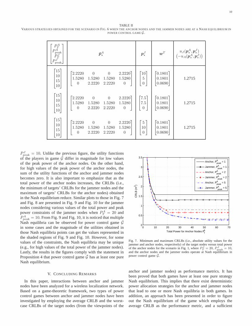
To analyze power control gameG in which the utility func-tions of the players are based on the minimum and maximumCRLBs instead of the average CRLB (see Section III-D),consider the wireless localization network in Fig. 1. In Fig. 7,the minimum and maximum CRLBs of the target nodes areplotted versus the total available power of the anchor nodesfor various values of the peak power constraint of the anchornodes whenP J

T = 20 andP Jpeak = 10. It is noted that for low

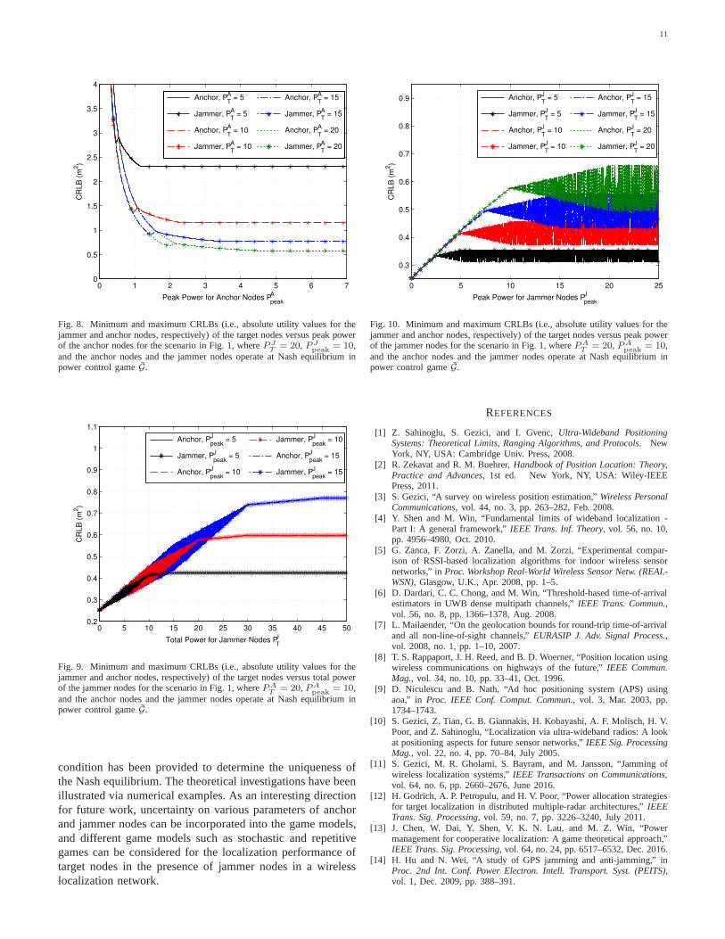
values of the total power constraint of the anchor nodes, theutility functions of the anchor nodes and the jammer nodesbecome equal in magnitude; that is, the sum of the utilityfunctions of the players is equal to zero. On the other hand,the utility functions of the anchor nodes and the jammer nodesare not equal for higher values of the total power constraintof the anchor nodes. Then, in Fig. 8, the minimum andmaximum CRLBs of the target nodes are plotted versus thepeak power of the anchor nodes when the anchor nodes and thejammer nodes operate at the Nash equilibrium,P J

T = 20, and

10

TABLE IIVARIOUS STRATEGIES OBTAINED FOR THE SCENARIO INFIG. 6 WHEN THE ANCHOR NODES AND THE JAMMER NODES ARE AT ANASH EQUILIBRIUM IN

POWER CONTROL GAMEG .

PAT

PApeak

P JT

P Jpeak

pA⋆ pJ

⋆ wT uJ(pA⋆ ,p

J⋆ )

(

−uA(pA⋆ ,p

J⋆ ))

15101510

2.2220 0 0 2.22201.5280 1.5280 1.5280 1.5280

0 2.2220 2.2220 0

1050

0.18010.18010.0690

1.2715

15101510

2.2220 0 0 2.22201.5280 1.5280 1.5280 1.5280

0 2.2220 2.2220 0

7.57.50

0.18010.18010.0690

1.2715

15101510

2.2220 0 0 2.22201.5280 1.5280 1.5280 1.5280

0 2.2220 2.2220 0

5100

0.18010.18010.0690

1.2715

P Jpeak = 10. Unlike the previous figure, the utility functions

of the players in gameG differ in magnitude for low valuesof the peak power of the anchor nodes. On the other hand,for high values of the peak power of the anchor nodes, thesum of the utility functions of the anchor and jammer nodesbecomes zero. It is also important to emphasize that as thetotal power of the anchor nodes increases, the CRLBs (i.e.,the minimum of targets’ CRLBs for the jammer nodes and themaximum of targets’ CRLBs for the anchor nodes) obtainedin the Nash equilibrium reduce. Similar plots to those in Fig. 7and Fig. 8 are presented in Fig. 9 and Fig. 10 for the jammernodes considering various values of the total power and peakpower constraints of the jammer nodes whenPA

T = 20 andPApeak = 10. From Fig. 9 and Fig. 10, it is noticed that multiple

Nash equilibria can be observed for power control gameGin some cases and the magnitude of the utilities obtained inthose Nash equilibria points can get the values representedinthe shaded regions of Fig. 9 and Fig. 10. However, for somevalues of the constraints, the Nash equilibria may be unique(e.g., for high values of the total power of the jammer nodes).Lastly, the results in the figures comply with the statement inProposition 4 that power control gameG has at least one pureNash equilibrium.

V. CONCLUDING REMARKS

In this paper, interactions between anchor and jammernodes have been analyzed for a wireless localization network.Based on a game-theoretic framework, two types of powercontrol games between anchor and jammer nodes have beeninvestigated by employing the average CRLB and the worst-case CRLBs of the target nodes (from the viewpoints of the

0 10 20 30 40 50 60 700

0.5

1

1.5

2

2.5

3

3.5

Total Power for Anchor Nodes PTA

CR

LB (

m2 )

Anchor, PpeakA = 1

Jammer, PpeakA = 1

Anchor, PpeakA = 2

Jammer, PpeakA = 2

Anchor, PpeakA = 5

Jammer, PpeakA = 5

Fig. 7. Minimum and maximum CRLBs (i.e., absolute utility values for thejammer and anchor nodes, respectively) of the target nodes versus total powerof the anchor nodes for the scenario in Fig. 1, whereP

J

T= 20, P J

peak= 10,

and the anchor nodes and the jammer nodes operate at Nash equilibrium inpower control gameG.

anchor and jammer nodes) as performance metrics. It hasbeen proved that both games have at least one pure strategyNash equilibrium. This implies that there exist deterministicpower allocation strategies for the anchor and jammer nodesthat lead to one or more Nash equilibria in both games. Inaddition, an approach has been presented in order to figureout the Nash equilibrium of the game which employs theaverage CRLB as the performance metric, and a sufficient

11

0 1 2 3 4 5 6 70

0.5

1

1.5

2

2.5

3

3.5

4

Peak Power for Anchor Nodes Ppeak

A

CR

LB

(m

2)

Anchor, PT

A = 5

Jammer, PT

A = 5

Anchor, PT

A = 10

Jammer, PT

A = 10

Anchor, PT

A = 15

Jammer, PT

A = 15

Anchor, PT

A = 20

Jammer, PT

A = 20

Fig. 8. Minimum and maximum CRLBs (i.e., absolute utility values for thejammer and anchor nodes, respectively) of the target nodes versus peak powerof the anchor nodes for the scenario in Fig. 1, whereP

J

T= 20, P J

peak= 10,


0 5 10 15 20 25 30 35 40 45 500.2

0.3

0.4

0.5

0.6

0.7

0.8

0.9

1

1.1

Total Power for Jammer Nodes PT

J

CR

LB

(m

2)

Anchor, Ppeak

J = 5

Jammer, Ppeak

J = 5

Anchor, Ppeak

J = 10

Jammer, Ppeak

J = 10

Anchor, Ppeak

J = 15

Jammer, Ppeak

J = 15

Fig. 9. Minimum and maximum CRLBs (i.e., absolute utility values for thejammer and anchor nodes, respectively) of the target nodes versus total powerof the jammer nodes for the scenario in Fig. 1, whereP

A

T= 20, PA

peak= 10,


condition has been provided to determine the uniqueness ofthe Nash equilibrium. The theoretical investigations havebeenillustrated via numerical examples. As an interesting directionfor future work, uncertainty on various parameters of anchorand jammer nodes can be incorporated into the game models,and different game models such as stochastic and repetitivegames can be considered for the localization performance oftarget nodes in the presence of jammer nodes in a wirelesslocalization network.

0 5 10 15 20 25

0.3

0.4

0.5

0.6

0.7

0.8

0.9

Peak Power for Jammer Nodes Ppeak

J

CR

LB

(m

2)

Anchor, PT

J = 5

Jammer, PT

J = 5

Anchor, PT

J = 10

Jammer, PT

J = 10

Anchor, PT

J = 15

Jammer, PT

J = 15

Anchor, PT

J = 20

Jammer, PT

J = 20

Fig. 10. Minimum and maximum CRLBs (i.e., absolute utility values for thejammer and anchor nodes, respectively) of the target nodes versus peak powerof the jammer nodes for the scenario in Fig. 1, whereP

A

T= 20, PA

peak= 10,


REFERENCES

[1] Z. Sahinoglu, S. Gezici, and I. Gvenc,Ultra-Wideband PositioningSystems: Theoretical Limits, Ranging Algorithms, and Protocols. NewYork, NY, USA: Cambridge Univ. Press, 2008.

[2] R. Zekavat and R. M. Buehrer,Handbook of Position Location: Theory,Practice and Advances, 1st ed. New York, NY, USA: Wiley-IEEEPress, 2011.

[3] S. Gezici, “A survey on wireless position estimation,”Wireless PersonalCommunications, vol. 44, no. 3, pp. 263–282, Feb. 2008.

[4] Y. Shen and M. Win, “Fundamental limits of wideband localization -Part I: A general framework,”IEEE Trans. Inf. Theory, vol. 56, no. 10,pp. 4956–4980, Oct. 2010.

[5] G. Zanca, F. Zorzi, A. Zanella, and M. Zorzi, “Experimental compar-ison of RSSI-based localization algorithms for indoor wireless sensornetworks,” inProc. Workshop Real-World Wireless Sensor Netw. (REAL-WSN), Glasgow, U.K., Apr. 2008, pp. 1–5.

[6] D. Dardari, C. C. Chong, and M. Win, “Threshold-based time-of-arrivalestimators in UWB dense multipath channels,”IEEE Trans. Commun.,vol. 56, no. 8, pp. 1366–1378, Aug. 2008.

[7] L. Mailaender, “On the geolocation bounds for round-trip time-of-arrivaland all non-line-of-sight channels,”EURASIP J. Adv. Signal Process.,vol. 2008, no. 1, pp. 1–10, 2007.

[8] T. S. Rappaport, J. H. Reed, and B. D. Woerner, “Position location usingwireless communications on highways of the future,”IEEE Commun.Mag., vol. 34, no. 10, pp. 33–41, Oct. 1996.

[9] D. Niculescu and B. Nath, “Ad hoc positioning system (APS) usingaoa,” in Proc. IEEE Conf. Comput. Commun., vol. 3, Mar. 2003, pp.1734–1743.

[10] S. Gezici, Z. Tian, G. B. Giannakis, H. Kobayashi, A. F. Molisch, H. V.Poor, and Z. Sahinoglu, “Localization via ultra-wideband radios: A lookat positioning aspects for future sensor networks,”IEEE Sig. ProcessingMag., vol. 22, no. 4, pp. 70–84, July 2005.

[11] S. Gezici, M. R. Gholami, S. Bayram, and M. Jansson, “Jamming ofwireless localization systems,”IEEE Transactions on Communications,vol. 64, no. 6, pp. 2660–2676, June 2016.

[12] H. Godrich, A. P. Petropulu, and H. V. Poor, “Power allocation strategiesfor target localization in distributed multiple-radar architectures,”IEEETrans. Sig. Processing, vol. 59, no. 7, pp. 3226–3240, July 2011.

[13] J. Chen, W. Dai, Y. Shen, V. K. N. Lau, and M. Z. Win, “Powermanagement for cooperative localization: A game theoretical approach,”IEEE Trans. Sig. Processing, vol. 64, no. 24, pp. 6517–6532, Dec. 2016.

[14] H. Hu and N. Wei, “A study of GPS jamming and anti-jamming,” inProc. 2nd Int. Conf. Power Electron. Intell. Transport. Syst. (PEITS),vol. 1, Dec. 2009, pp. 388–391.

12

[15] D. Lu, R. Wu, and H. Liu, “Global positioning system anti-jammingalgorithm based on period repetitive CLEAN,”IET Radar, Sonar, Navig.,vol. 7, no. 2, pp. 164–169, Feb. 2013.

[16] Y. Shen and M. Z. Win, “Energy efficient location-aware networks,” inProc. IEEE Int. Conf. Commun. (ICC), May 2008, pp. 2995–3001.

[17] W. W.-L. Li, Y. Shen, Y. J. Zhang, and M. Z. Win, “Robust powerallocation for energy-efficient location-aware networks,” IEEE/ACMTrans. Netw., vol. 21, no. 6, pp. 1918–1930, Dec. 2013.

[18] T. Wang, G. Leus, and L. Huang, “Ranging energy optimization forrobust sensor positioning based on semidefinite programming,” IEEETrans. Sig. Processing, vol. 57, no. 12, pp. 4777–4787, Dec. 2009.

[19] T. Wang and G. Leus, “Ranging energy optimization for robust sensorpositioning with collaborative anchors,” inProc. IEEE Int. Conf. Acoust.,Speech, and Sig. Processing (ICASSP), Mar. 2010, pp. 2714–2717.

[20] R. El-Bardan, S. Brahma, and P. K. Varshney, “Strategicpower allocationwith incomplete information in the presence of a jammer,”IEEE Trans.Commun., vol. 64, no. 8, pp. 3467–3479, Aug. 2016.

[21] V. S. S. Nadendla, V. Sharma, and P. K. Varshney, “On strategicmulti-antenna jamming in centralized detection networks,” IEEE SignalProcess. Lett., vol. 24, no. 2, pp. 186–190, Feb. 2017.

[22] J. Chen, W. Dai, Y. Shen, V. K. N. Lau, and M. Z. Win, “Resourcemanagement games for distributed network localization,”IEEE J. Sel.Areas Commun., vol. 35, no. 2, pp. 317–329, Feb. 2017.

[23] M. K. Simon, J. K. Omura, R. A. Scholtz, and B. K. Levitt,SpreadSpectrum Communications. Rockville, MD: Comput. Sci. Press, 1985.

[24] M. Weiss and S. C. Schwartz, “On optimal minimax jamminganddetection of radar signals,”IEEE Trans. Aeros. Elect. Sys., vol. AES-21,no. 3, pp. 385–393, May 1985.

[25] R. J. McEliece and W. E. Stark, “An information theoretic study ofcommunication in the presence of jamming,” inInt. Conf. Commun.(ICC’81), vol. 3, 1981, p. 45.

[26] I. Shomorony and A. S. Avestimehr, “Worst-case additive noise inwireless networks,”IEEE Trans. Inf. Theory, vol. 59, no. 6, pp. 3833–3847, June 2013.

[27] T. M. Cover and J. A. Thomas,Elements of Information Theory. Wiley-Interscience, 1991.

[28] A. Lapidoth, “Nearest neighbor decoding for additive non-Gaussiannoise channels,”IEEE Trans. Inf. Theory, vol. 42, no. 5, pp. 1520–1529,Sep. 1996.

[29] S. M. Kay, Fundamentals of Statistical Signal Processing: EstimationTheory. Upper Saddle River, NJ: Prentice Hall, Inc., 1993.

[30] Y. Qi, H. Kobayashi, and H. Suda, “Analysis of wireless geolocation in anon-line-of-sight environment,”IEEE Trans. Wireless Commun., vol. 5,no. 3, pp. 672–681, Mar. 2006.

[31] A. Mallat, S. Gezici, D. Dardari, C. Craeye, and L. Vandendorpe,“Statistics of the MLE and approximate upper and lower bounds - PartI: Application to TOA estimation,”IEEE Trans. Signal Process., vol. 62,no. 21, pp. 5663–5676, Nov. 2014.

[32] D. Dardari and M. Z. Win, “Ziv-Zakai bound on time-of-arrival estima-tion with statistical channel knowledge at the receiver,” in Proc. IEEEInt. Conf. Ultra-Wideband (ICUWB), Sep. 2009, pp. 624–629.

[33] S. Gezici, S. Bayram, M. N. Kurt, and M. R. Gholami, “Optimaljammer placement in wireless localization systems,”IEEE Trans. SignalProcess., vol. 64, no. 17, pp. 4534–4549, Sep. 2016.

[34] J. F. Nash, “Non-cooperative games,”Ann. Math., vol. 54, pp. 289–295,1951.

[35] Z. Han, Game Theory in Wireless and Communication Networks:Theory, Models, and Applications. Cambridge University Press, 2012.

[36] W. W. L. Li, Y. Shen, Y. J. Zhang, and M. Z. Win, “Robust powerallocation for energy-efficient location-aware networks,” IEEE/ACMTransactions on Networking, vol. 21, no. 6, pp. 1918–1930, Dec. 2013.

[37] A. Washburn,Two-Person Zero-Sum Games, ser. International Series inOperations Research & Management Science. Springer US, 2013.

[38] S. Boyd and L. Vandenberghe,Convex Optimization. Cambridge, UK:Cambridge University Press, 2004.

[39] J. v. Neumann, “Zur theorie der gesellschaftsspiele,”MathematischeAnnalen, vol. 100, pp. 295–320, 1928.

[40] A. Ghosh, S. Boyd, and A. Saberi, “Minimizing effectiveresistance ofa graph,”SIAM Review, vol. 50, no. 1, pp. 37–66, 2008.

Ahmet Dundar Sezer was born in 1989 in Emet,Kutahya, Turkey. He received both his B.S. and M.S.degrees in Electrical and Electronics Engineeringfrom Bilkent University, Ankara, Turkey, in 2011and 2013, respectively. He is currently workingtowards the Ph.D. degree at Bilkent University. Hiscurrent research interests include signal processing,wireless communications, and optimization.

Sinan Gezici(S’03–M’06–SM’11) received the B.S.degree from Bilkent University, Turkey in 2001,and the Ph.D. degree in Electrical Engineering fromPrinceton University in 2006. From 2006 to 2007,he worked at Mitsubishi Electric Research Labora-tories, Cambridge, MA. Since 2007, he has beenwith the Department of Electrical and ElectronicsEngineering at Bilkent University, where he is cur-rently a professor. Dr. Gezici’s research interestsare in the areas of detection and estimation theory,wireless communications, and localization systems.

Among his publications in these areas is the book Ultra-wideband PositioningSystems: Theoretical Limits, Ranging Algorithms, and Protocols (CambridgeUniversity Press, 2008). Dr. Gezici was an associate editorfor IEEE Trans-actions on Communications, IEEE Wireless Communications Letters, andJournal of Communications and Networks.

power control games between anchor and jammer nodes in...

Documents