power diagrams and interaction …people.math.aau.dk/~jm//unionofdiscs.pdfpower diagrams and...
TRANSCRIPT

30 July 2007
POWER DIAGRAMS AND INTERACTION PROCESSES FOR
UNIONS OF DISCS
JESPER MØLLER,∗ Aalborg University
KATERINA HELISOVA,∗∗ Charles University in Prague
Abstract
We study a flexible class of finite disc process models with interaction between
the discs. We let U denote the random set given by the union of discs,
and use for the disc process an exponential family density with the canonical
sufficient statistic only depending on geometric properties of U such as the area,
perimeter, Euler-Poincare characteristic, and number of holes. This includes
the quarmass-interaction process and the continuum random cluster model as
special cases. Viewing our model as a connected component Markov point
process, and thereby establish local and spatial Markov properties, becomes
useful for handling the problem of edge effects when only U is observed
within a bounded observation window. The power tessellation and its dual
graph become major tools when establishing inclusion-exclusion formulae,
formulae for computing geometric characteristics of U , and stability properties
of the underlying disc process density. Algorithms for constructing the power
tessellation of U and for simulating the disc process are discussed, and the
software is made public available.
Keywords: Area-interaction process, Boolean model; disc process; exponential
family; germ-grain model; local computations; local stability; Markov proper-
ties; inclusion-exclusion formulae; interaction; point process; power tessellation;
simulation; quarmass-interaction process; random closed set; Ruelle stability
AMS 2000 Subject Classification: Primary 60D05;60G55;60K35;62M30
Secondary 68U20
∗ Postal address: Department of Mathematical Sciences, Aalborg University Fredrik Bajers Vej 7G,
DK-9220 Aalborg, Denmark. Email address: [email protected]
∗∗ Postal address: Department of Probability and Mathematical Statistics, Charles University in
Prague, Sokolovska 83, 18675 Praha 8, Czech Republic. Email address: [email protected]
1

2 J. Møller and K. Helisova
1. Introduction
This paper concerns probabilistic results of statistical relevance for planar random
set models given by a finite union of discs U = UX, where X denotes the corresponding
finite process of discs. We distinguish between the case where we can observe the discs
in X and the random set case where only (or at most) U is observed. The latter case
occur frequently in applications and will be of main interest to us.
Our random closed set U is a particular example of a germ-grain model [17], with
the grains being discs. It is well-known that any random closed set whose realizations
are locally finite unions of compact convex sets is a germ-grain model with convex and
compact grains [41, 42]. However, in order to make statistical inference, one needs
to restrict attention to a much smaller class of models such as a random-disc process
model, and indeed random-disc Boolean models play the main role in practice, see [40]
and the references therein. The Boolean model is in an abstract setting given by a
Poisson process of compact sets (the grains) with no interaction between the grains.
Many authors (e.g. [2, 8, 9, 16, 19, 40]) have mentioned the need of developing flexible
germ-grain models with interaction between the grains.
We study a particular class of models for interaction among the discs, specified by
a point process density for X with respect to a reference Poisson process of discs.
The density is assumed to be of exponential family form, with the canonical sufficient
statistic T (X) = T (U) only depending on X through U , where T (U) is specified in terms
of geometric characteristics for the connected components of U , for example, the area
A(U), the perimeter L(U), the number of holes Nh(U), and the number of connected
components Ncc(U). Further geometric characteristics are specified in Section 4.1 in
terms of the power tessellation (e.g. [1]), which provides a subdivision of U (see Figure 2
in Section 3). An important special case of our models is the quarmass-interaction
process, first introduced in Kendall, van Lieshout and Baddeley [19], where T (U) =
(A(U), L(U), χ(U)) and χ(U) = Ncc(U) − Nh(U) is the Euler-Poincare characteristic
(quarmass-integrals in R2 are linear combinations of A,L, χ). Another special case is
the continuum random cluster model [15, 23, 28], where T (U) = Ncc(U).
We show that the power tessellation and its dual graph are extremely useful when
establishing

Power diagrams and interaction processes for unions of discs 3
(i) inclusion-exclusion formulae for T (U);
(ii) formulae for computing geometric characteristics of U ;
(iii) Ruelle and local stability of the density of X, and thereby convergence properties
of MCMC algorithms for simulating X.
Among other things we demonstrate that a main geometric result in [19] related to
the issue of Ruelle stability is easily derived by means of the power tessellation and its
dual graph. Furthermore, as explained in Section 4.5, it becomes useful to view our
models as connected component Markov point processes [2, 4, 7, 30] in a similar way
as the Markov connected component fields studied in [32]. In particular, we establish
(iv) local and spatial Markov properties of X, which become useful for handling the
problem of edge effects when only U is observed within a bounded observation
window.
The paper is organized as follows. Section 2 specifies our notation and assumptions,
and discusses a general position property of the discs in X. Section 3 defines and
studies the power tessellation of a union of discs in general position. The main section,
Section 4, studies exponential family properties and the above-mentioned issues (i)-(iv).
Also various examples of simulated realizations of our models are shown in Section 4.
Section 5 discusses extensions of our work and some open problems. Finally, most
algorithmic details are deferred to Appendices A-B.
A substantial part of this work has been the developments of codes in C and R for
constructing power tessellations and making simulations of our models. The codes are
available at www.math.aau.dk/~jm/Codes.union.of.discs.
2. Preliminaries
2.1. Setup
Throughout this paper we use the following notation and make the following as-
sumptions.
By a disc we mean more precisely a two-dimensional closed disc b = y ∈ R2 :
‖y − z‖ ≤ r with centre z ∈ R2 and positive radius r > 0, where ‖ · ‖ denotes usual

4 J. Møller and K. Helisova
Euclidean distance. We identify b with the point x = (z, r) in R2 × (0,∞), and write
b = b(x) = b(z, r). Similarly, we identify point processes of discs bi = b(zi, ri) with
point processes on R2 × (0,∞).
The reference point process will be a Poisson process Ψ of discs; thus the random
set given by the union of discs in Ψ is a Boolean model (e.g. [27]). Specifically, Ψ is
assumed to be a Poisson point process on R2 × (0,∞), with an intensity measure of
the form ρ(z) dz Q(dr), where dz is Lebesgue measure on R2 and Q is an arbitrary
probability measure on (0,∞). In other words, the point process Φ of centres of discs
given by Ψ is a Poisson process with intensity function ρ on R2, the radii of these
discs are mutually independent and identically distributed with distribution Q, and Φ
is independent of the radii. An example of a simulation from such a process is shown
in Figure 1. The concrete specification of ρ and Q is not important for most results
in this paper, but the specification is of course crucial for statistical inference, see [31].
Local integrability of ρ is assumed to ensure that with probability one, Φ ∩ S is finite
for any bounded region S ⊂ R2. Since we can view the radii as marks associated to
the points given by the centres of the discs, we refer to Q as the mark distribution. In
the special case where Q is degenerate at R > 0, we can consider R as a parameter
and identify Ψ with Φ.
Figure 1: A realization of a reference Poisson process with Q the uniform distribution on the
interval [0, 2], ρ(u) = 0.2 on a rectangular region S = [0, 30]× [0, 30], and ρ(u) = 0 outside S.
In the sequel, S denotes a given bounded planar region such that∫
Sρ(z) dz > 0.

Power diagrams and interaction processes for unions of discs 5
The object of primary interest is the random closed set
UX = ∪x∈Xb(x)
where X is a finite point process defined on S × (0,∞). If X = ∅ is the empty
configuration, we let UX = ∅ be the empty set. Note that the centres of the discs are
contained in S but the discs may extend outside S. We assume that X is absolutely
continuous with respect to the reference Poisson process Ψ, and denote the density
by f(x) for finite configurations x = x1, . . . , xn with xi = (zi, ri) ∈ S × (0,∞) and
0 ≤ n <∞ (if n = 0 then x is the empty configuration).
We focus on the case where the density is of the exponential family form
fθ(x) = exp (θ · T (Ux)) /cθ (1)
where θ is a real parameter vector, · denotes the usual inner product, T (U) is a statistic
of the same dimension as θ, and cθ is a normalizing constant depending on θ (and of
course also on (T, ρ, Q)). Note that fθ(x) > 0 for all x. Further details on the choice
of T and the parameter space for θ are given in Section 4. Note that (1) is also the
density of the random set UX with respect to the reference Boolean model, and
cθ =exp(−∫
S
ρ(z) dz
)×[
exp(θ · T (∅)) +∞∑
n=1
∫S
∫ ∞
0
· · ·∫
S
∫ ∞
0
exp(θ · T
(U(z1,r1),...,(zn,rn)
)) n∏1
ρ(zi) dz1 Q(dr1) · · · dzn Q(drn)]
(2)
is in general not expressible on closed form (unless θ 6= 0).
As noticed in Section 1, a quarmass-interaction process is obtained by taking T (U) =
(A(U), L(U), χ(U)), where A(U) is the area, L(U) the perimeter and χ(U) the Euler-
Poincare characteristic of U . We consider here the so-called additive extension of the
Euler-Poincare characteristic, which is also of primary interest in [19], i.e.
χ(U) = Ncc(U)−Nh(U) (3)
where Ncc(U) is the number of connected components of U and Nh(U) is the number of
holes of U . The special case where Q is degenerate and T (U) = A(U) is known as the
area-interaction point process, Widom-Rowlinson model or penetrable spheres model,
see e.g. [3, 15, 19, 43].
6 J. Møller and K. Helisova
2.2. General position of discs
It becomes essential in this paper that with probability one, the discs defined by
Ψ are in general position in the following sense. Identify R2 with the hyperplane of
R3 spanned by the first two coordinate axes. For each disc b(z, r), define the ghost
sphere s(z, r) = y ∈ R3 : ‖y − z‖ = r, i.e. the hypersphere in R3 with centre z and
radius r. A configuration of discs is said to be in general position if the intersection of
any k + 1 corresponding ghost spheres is either empty or a sphere of dimension 2− k,
where k = 1, 2, . . .. Note that the intersection is assumed to be empty if k > 2, and
a sphere of dimension 0 is assumed to consists of two points. The upper left panel
in Figure 2 shows a configuration of discs in general position; we shall use this as a
running example to illustrate forthcoming definitions.
Lemma 1. For almost all realizations of Ψ = x1, x2, . . ., the discs b1 = b(x1), b2 =
b(x2), . . . are in general position.
Proof. By Campbell’s theorem (see e.g. [40]), the mean number of sets of k+1 ghost
spheres whose intersection is neither empty nor of dimension 2− k is given by∫R2
∫ ∞
0
· · ·∫
R2
∫ ∞
0
1[∩k
0si 6= ∅, dim(∩k
0si
)6= 2− k
]∏k
0 ρ(zi)(k + 1)!
dz0 Q(dr0) · · · dzk Q(drk)
where 1[·] is the indicator function and si = s(zi, ri). This integral is zero, since for any
fixed values of r0 > 0, . . . , rk > 0, the indicator function is zero for Lebesgue almost
all (z0, . . . , zk) ∈ R2(k+1).
All point process models for discs considered in this paper have discs in general
position: by Lemma 1, the discs in X with density (1) are in general position almost
surely.
3. Power tessellation of a union of discs
This section defines and studies the power tessellation of a union of discs U = ∪i∈Ibi.
We assume that the discs bi, i ∈ I satisfy the general position assumption (henceforth
GPA).

Power diagrams and interaction processes for unions of discs 7
3.1. Basic definitions
In this section, there is no need for assuming that the index set I is finite, though
this will be the case in subsequent sections.
For each disc bi (i ∈ I) with ghost sphere si, let s+i = (y1, y2, y3) ∈ si : y3 ≥ 0
denote the corresponding upper hypersphere, and for u ∈ bi, let yi(u) denote the unique
point on s+i those orthogonal projection on R2 is u. The subset of s+
i consisting of
those points “we can see from above” is given by
Ci = yi(u) : u ∈ bi, ‖u− yi(u)‖ ≥ ‖u− yj(u)‖ whenever u ∈ bj , j ∈ I,
and the GPA implies that the non-empty Ci have disjoint 2-dimensional relative
interiors. Thus, as illustrated in the upper right panel in Figure 2, the non-empty
Ci form a tessellation (i.e. subdivision) of ∪Is+i corresponding to the 2-dimensional
pieces of upper ghost spheres “as seen from above”. Projecting this tessellation onto
R2, we obtain a tessellation of U , see the lower left panel in Figure 2. Below we specify
this tessellation in detail.
Let J = i ∈ I : Ci 6= ∅. For i ∈ I, define the power distance of a point u ∈ R2
from bi = b(zi, ri) by πi(u) = ‖u− zi‖2 − r2i , and define the power cell associated with
bi by
Vi = u ∈ R2 : πi(u) ≤ πj(u) for all j ∈ I.
For distinct i, j ∈ I, define the closed halfplane Hi,j = u ∈ R2 : πi(u) ≤ πj(u). Each
Vi is a convex polygon, since it is a finite intersection of closed halfplanes Hi,j . The
power cells have disjoint interiors, and by GPA, each Vi is either empty or of dimension
two. Consequently, the non-empty power cells Vi, i ∈ J constitute a tessellation of R2
called the power diagram (or Laguerre diagram), see [1] and the references therein. In
the special case where all radii ri are equal, we have I = J and the power diagram is a
Voronoi tessellation (e.g. [29, 35]) where each cell Vi contains zi in its interior. If the
radii are not equal, a power cell Vi may not contain zi, since Hi,j may not contain zi.
Let Bi denote the orthogonal projection of Ci on R2. By Pythagoras, for all u ∈ bi,
πi(u) + ‖u− yi(u)‖2 = 0. Consequently, for any i, j ∈ I and u ∈ bi ∩ bj ,
‖u− yi(u)‖ ≥ ‖u− yj(u)‖ if and only if πi(u) ≤ πj(u).
8 J. Møller and K. Helisova
Thus Bi = Vi∩bi. By GPA and the one-to-one correspondence between Bi and Ci, the
collection of sets Bi, i ∈ J constitutes a subdivision of U into 2-dimensional convex
sets with disjoint interiors. We call this the power tessellation of the union of discs and
denote it by B. Further, if i ∈ J , we call Bi the power cell restricted to its associated
disc bi (clearly, Bi = ∅ if i ∈ I \J). Since Vi may not contain zi, Bi may not contain zi;
an example of this is shown in the lower left panel in Figure 2. We say that a cell Bi is
isolated if Bi = bi. This means that any disc bj , j ∈ I, intersecting bi is contained in
bi; the disc bi is therefore also said to be a circular clump, see [27] and the references
therein.
It is illuminating to consider Figure 2 when making the following definitions. If the
intersection ei,j = Bi ∩ Bj between two cells of B is non-empty, then ei,j = [ui,j , vi,j ]
is a closed line segment, where ui,j and vi,j denote the endpoints, and we call ei,j an
interior edge of B. The vertices of B are given by all endpoints of interior edges. A
vertex of B lying on the boundary ∂U is called a boundary vertex, and it is called an
interior vertex otherwise. Each circular arc on B defined by two successive boundary
vertices is called a boundary edge of B. The circle given by the boundary of an isolated
cell of B is also called a boundary edge or sometimes an isolated boundary edge. The
connected components of ∂U are closed curves, and each such curve is a union of certain
boundary edges which either bound a hole, in which case the curve is called an inner
boundary curve, or bound a connected component of U , in which case the curve is
called an outer boundary curve. A generic boundary edge of B is written as bui, vie
if Bi 6= bi (a non-isolated cell), where the index means that ui and vi are boundary
vertices of Bi, or as ∂bi if Bi = bi. We order ui and vi such that bui, vie is the circular
arc from ui to vi when ∂bi is considered anti-clockwise.
By GPA, any intersection among four cells of B is empty, each interior vertex
corresponds to a non-empty intersection among three cells of B, and exactly three
edges emerge at each vertex. Note that each isolated cell has no vertices and one edge.
Each interior edge ei,j is contained in the bisector (or power line or radical axis) of bi
and bj defined by ∂Hi,j = u ∈ Rd : πi(u) = πj(u). This is the line perpendicular to
the line joining the centres of the two discs, and passing through the point
zi,j =12
(zi + zj +
r2j − r2
i
‖zi − zj‖2(zi − zj)
).

Power diagrams and interaction processes for unions of discs 9
Figure 2: Upper left panel: A configuration of discs in general position. Upper right panel:
The upper hemispheres as seen from above. Lower left panel: The power tessellation of the
union of discs. Lower right panel: The dual graph.
We call Ei,j ≡ ∂Hi,j ∩ bi = ∂Hi,j ∩ bj the chord of bi ∩ bj . Obviously, ei,j ⊆ Ei,j .
The dual graph D to B has nodes equal to the centres zi, i ∈ J of discs generating
non-empty cells, and each edge of D is given by two vertices zi and zj such that ei,j 6= ∅.
See the lower right panel in Figure 2. Note that there is a one-to-one correspondence

10 J. Møller and K. Helisova
between the edges of D and the interior edges of B.
3.2. Construction
We construct the power tessellation of a finite union of discs by successively adding
the discs one by one, keeping track on old and new edges and whether each disc
generates a non-empty cell or not. The updates are local in some sense and used in
the “birth-part” of the MCMC algorithm in Section 4.7. For details, see Appendix A.
4. Results for exponential family models
This section studies exponential family models for the point process X as specified
by the density f(x) in (1), assuming that the canonical sufficient statistic T (Ux) is a
linear combination of one or more of the geometric characteristics introduced in the
following paragraph. We let supp(Q) denote the support of Q,
Ω = (z, r) ∈ S × (0,∞) : ρ(z) > 0, r ∈ supp(Q)
the support of the intensity measure of the reference Poisson process Ψ, and N the
set of all finite subsets x (also called finite configurations) of Ω so that the discs given
by x are in general position. By Lemma 1, X ∈ N with probability one. For ease of
exposition we assume that all realizations of X are in N , and set f(x) = 0 if x 6∈ N .
We let T (x) be given by one or more of the following characteristics of U = Ux if
x ∈ N : the area A = A(U), the perimeter L = L(U), the Euler-Poincare characteristic
χ = χ(U), the number of isolated cells Nic = Nic(U), the number of connected
components Ncc = Ncc(U), the number of holes Nh = Nh(U), the number of boundary
edges (including isolated boundary edges) Nbe = Nbe(U), and the number of boundary
vertices Nbv = Nbv(U). In the general case,
T = (A,L, χ, Nh, Nic, Nbv) (4)
with corresponding canonical parameter θ = (θ1, . . . , θ6), and we call then X the T -
interaction process. If e.g. θ2 = . . . = θ6 = 0, we set T = A and refer then to the
A-interaction process. Similarly, for the L-interaction process we have θ1 = 0 and
θ3 = . . . = θ6 = 0, for the (A,L)-interaction process we have θ3 = . . . = θ6 = 0,
and so on. A quarmass-interaction process [19] is the special case T = (A,L, χ) and
Power diagrams and interaction processes for unions of discs 11
θ4 = θ5 = θ6 = 0. Note that (4) specifies Ncc = χ + Nh and Nbe = Nic + Nbv, cf.
Lemma 2 below. Thus a continuum random cluster model [15, 23, 28] is the special
case T = Ncc, θ1 = θ2 = θ5 = θ6 = 0, and θ3 = θ4.
4.1. Exponential family structure
Let
Θ = (θ1, . . . , θ6) ∈ R6 :∫
exp(πθ1r
2 + 2πθ2r)
Q(dr) <∞. (5)
Note that (−∞, 0]2 × R4 ⊆ Θ, and Θ = R6 if supp(Q) is bounded. The following
proposition states that under a weak condition on (S, ρ,Q), the exponential family
density has Θ as its full parameter space and T in (4) as its minimal canonical sufficient
statistic (for details on exponential family properties, see [5]).
Proposition 1. Suppose that S contains a set D = b(u, R1) \ b(u, R2), where ∞ >
R1 > R2 > 0, ρ(z) > 0 for all z ∈ D, and Q((0, R2]) > 0. Then the point process
densities
fθ(x) =1cθ
exp (θ1A(Ux) + θ2L(Ux) + θ3χ(Ux) + θ4Nh(Ux) + θ5Nic(Ux) + θ6Nbv(Ux))
(6)
with x ∈ N and θ = (θ1, . . . , θ6) ∈ Θ constitute a regular exponential family model.
Proof. Recall that an exponential family model is regular if it is full and of minimal
form [5]. We verify later in Proposition 6 that fθ is well-defined if and only if θ ∈ Θ,
so the model is full. Let ΨS denote the restriction of Ψ to S × (0,∞). Since
Θ ⊇ (−∞, 0]2 × R4 is of full dimension 6, and since there is a one-to-one linear
correspondence between T in (4) and (A,L,Ncc, Nic, Nbv, Nh), the model is on minimal
form if the statistics A, L, Nic, Ncc, Nbv, Nh are affinely independent with probability
one with respect to ΨS , see [5]. In other words, the model is on minimal form if for
any (α0, . . . , α6) ∈ R7, with probability one,
α1A(UΨS) + α2L(UΨS
) + α3Nic(UΨS) + α4Ncc(UΨS
) + α5Nbv(UΨS) + α6Nh(UΨS
)
=α0 ⇒ α0 = . . . = α6 = 0. (7)
We verify this, using the condition on (S, ρ,Q) imposed in the proposition, and con-
sidering realizations of ΨS as described below, where these realizations consist of

12 J. Møller and K. Helisova
configurations of discs with centres in D and radius ≤ R2. For such configurations,
given by either one disc, two non-overlapping discs, or two overlapping discs, and if
α5 = α6 = 0, we immediately obtain (7). Extending this to situations where only
α6 = 0 and we have three discs with pairwise overlap but no common intersection, we
also immediately obtain (7), and the set consisting of such configurations and where
Nh(UΨS) = 0 has a positive probability. The condition on (S, ρ,Q) also allow us with
a positive probability to construct a set of realizations of where Nh(UΨS) = 1, namely
by considering sequences of discs which only overlap pairwise and which form a single
connected component. Thereby, for any (α0, . . . , α6) ∈ R7, with probability one, (7) is
seen to hold.
4.2. Interpretation of parameters
This section discusses the meaning of the parameters θ1, . . . , θ6 in the T -interaction
process (6).
We first recall the definition of the Papangelou conditional intensity λ(x, v) for a
general finite point process X ⊂ S×(0,∞) with an hereditary density f with respect to
the distribution of Ψ (see [33] and the references therein). For all finite configurations
x ⊂ S× (0,∞) and all discs v = (z, r) ∈ S× (0,∞)\x, the hereditary condition means
that f(x) > 0 whenever f(x ∪ v) > 0, and by definition
λ(x, v) = f(x ∪ v)/f(x) if f(x) > 0, λ(x, v) = 0 otherwise.
This is in a one-to-one correspondence with the density f , and has the interpretation
that λ(x, v)ρ(z) dz Q(dr) is the conditional probability of X having a disc with centre
in an infinitesimal region containing z and of size dz and radius in an infinitesimal
region containing r and of size dr, given the rest of X is x.
For functionals W = A,L, . . ., define W (x, v) = W (Ux∪v) − W (Ux). The T -
interaction process (6) has an hereditary density, with Papangelou conditional intensity
λθ(x, v) = (8)
exp (θ1A(x, v) + θ2L(x, v) + θ3χ(x, v) + θ4Nh(x, v) + θ5Nic(x, v) + θ6Nbv(x, v))
if x ∪ v ∈ N , and λθ(x, v) = 0 otherwise. Note that N is hereditary, meaning that

Power diagrams and interaction processes for unions of discs 13
x ∈ N implies y ∈ N if y ⊂ x. The process X is said to be attractive if
λθ(x, v) ≥ λθ(y, v) whenever y ⊂ x, x ∈ N (9)
and repulsive if
λθ(x, v) ≤ λθ(y, v) whenever y ⊂ x, x ∈ N . (10)
Note that since quarmass integrals are additive,
A(x, v) = A(bv)−A(bv∩Ux), L(x, v) = L(bv)−L(bv∩Ux), χ(x, v) = 1−Nh(bv∩Ux).
(11)
Proposition 2. We have that
(a) the A-interaction process is attractive if θ1 < 0 and repulsive if θ1 > 0;
(b) under weak conditions, e.g. if S contains an open disc, the L-interaction process
is neither attractive nor repulsive if θ2 6= 0;
(c) under other weak conditions, basically meaning that S is not too small compared
to inf supp(Q) (as exemplified in the proof), the W -interaction processes with
W = χ,Nh, Nic, Nbv are neither attractive nor repulsive if θi 6= 0, i = 3, 4, 5, 6;
(d) under similar weak conditions as in (c), the continuum random cluster model
(i.e. the Ncc-interaction process, where θ3 = θ4 and θ1 = θ2 = θ5 = θ6 = 0) is
neither attractive nor repulsive if θ3 6= 0.
Proof. From (11) follows immediately (a), which is a well-known result [3]. We have
that L(bv∩Ux1) > 0 = L(bv∩U∅) if bv∩bx1 6= ∅. This provides a simple example where
λθ2(x, v) is decreasing or increasing in x if θ2 > 0 or θ2 < 0, respectively. On the other
hand, if S contains an open disc, we may obtain the opposite case. The left panel in
Figure 3 shows such an example, with four discs of equal radii, where the four centres
of the discs can be made arbitrary close, and where L(bv ∩ Ux1,x2,x3) < L(bv ∩ Ux1,x2).
Thereby (b) is verified.
To verify (c)-(d) we consider again discs bv, bx1 , bx2 , . . . of equal radii, since it may
be possible that Q is degenerate.
Suppose that bv∩bx1 = ∅, bv∩bx2 6= ∅, and bx1∩bx2 6= ∅, and let x = x1, x2. Then
χ(y, v) = 2 and χ(x, v) = 1 if y = x1, while χ(y, v) = 1 and χ(x, v) = 2 if y = x2.
14 J. Møller and K. Helisova
Since χ = Ncc in these examples, we obtain (c) in the case of the χ-interaction process
and (d) in the case of the Ncc-interaction process.
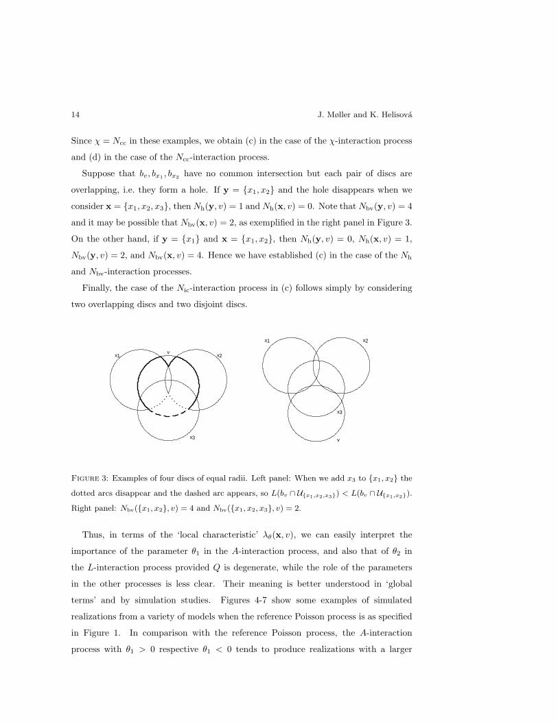
Suppose that bv, bx1 , bx2 have no common intersection but each pair of discs are
overlapping, i.e. they form a hole. If y = x1, x2 and the hole disappears when we
consider x = x1, x2, x3, then Nh(y, v) = 1 and Nh(x, v) = 0. Note that Nbv(y, v) = 4
and it may be possible that Nbv(x, v) = 2, as exemplified in the right panel in Figure 3.
On the other hand, if y = x1 and x = x1, x2, then Nh(y, v) = 0, Nh(x, v) = 1,
Nbv(y, v) = 2, and Nbv(x, v) = 4. Hence we have established (c) in the case of the Nh
and Nbv-interaction processes.
Finally, the case of the Nic-interaction process in (c) follows simply by considering
two overlapping discs and two disjoint discs.
x1 x2
x3
v
x1 x2
x3
v
Figure 3: Examples of four discs of equal radii. Left panel: When we add x3 to x1, x2 the
dotted arcs disappear and the dashed arc appears, so L(bv ∩ Ux1,x2,x3) < L(bv ∩ Ux1,x2).
Right panel: Nbv(x1, x2, v) = 4 and Nbv(x1, x2, x3, v) = 2.
Thus, in terms of the ‘local characteristic’ λθ(x, v), we can easily interpret the
importance of the parameter θ1 in the A-interaction process, and also that of θ2 in
the L-interaction process provided Q is degenerate, while the role of the parameters
in the other processes is less clear. Their meaning is better understood in ‘global
terms’ and by simulation studies. Figures 4-7 show some examples of simulated
realizations from a variety of models when the reference Poisson process is as specified
in Figure 1. In comparison with the reference Poisson process, the A-interaction
process with θ1 > 0 respective θ1 < 0 tends to produce realizations with a larger

Power diagrams and interaction processes for unions of discs 15
respective smaller area A(Ux), and similarly for the W -interaction process, with W =
L, χ,Nh, Nic, Nbv, Ncc, see Figures 4-5 and the upper left and right panels in Figure 6.
However, the interpretation of (θ1, θ2) in the (A,L)-interaction process depends on the
signs and how large these two parameters are, see the last four panels in Figure 6.
Figure 7 shows examples where the minimal sufficient statistic is given by three or
four geometric characteristics, whereby the meaning of the non-zero θi’s specifying the
process becomes even more complicated.
4.3. Geometric characteristics and inclusion-exclusion formulae
Lemmas 2-3 below concern various useful relations between certain geometric char-
acteristics of the union U = Ux and of its power tessellation B = Bx, assuming
x ∈ N . Among other things, the results become useful in connection to computation of
geometric characteristics in Section 4.4 and for the sequential constructions considered
in Sections 3.2 and 4.7 and Appendices A-B.
Define the following characteristics of B = Bx: the number of non-empty cells
Nc = Nc(B), the number of interior edges Nie = Nie(B), the number of edges Ne =
Nbe + Nie, the number of interior vertices Niv = Niv(B), and the number of vertices
Nv = Nbv + Niv. These statistics do not appear in the specification (4) since they
cannot be determined from U but only from B. Furthermore, let N = n(x) denote the
number of discs.
Lemma 2. We have
Nic ≤ Ncc ≤ Nc ≤ N, Nbv = 2Nie − 3Niv (12)
and
χ = Ncc −Nh = Nc −Nie + Niv. (13)
If Nc ≥ 2 and Ncc = 1, then
Nbe = Nbv ≤ 2Nie, 3Nv = 2Ne. (14)
If Nc ≥ 3 and Ncc = 1, then
Nie ≤ 3Nc − 6. (15)
Moreover,
Nbv ≤ 6N (16)

16 J. Møller and K. Helisova
Figure 4: Simulated realizations of the A-interaction process with θ1 = 0.1 (upper left panel)
and θ1 − 0.1 (upper right panel), the L-interaction process with θ2 = 0.2 (middle left panel)
and θ2 = −0.2 (middle right panel), and the χ-interaction process with θ3 = 1 (lower left
panel) and θ3 = −1 (lower right panel).

Power diagrams and interaction processes for unions of discs 17
Figure 5: Simulated realizations of the Nh-interaction process with θ4 = 3 (upper left panel)
and θ4 = −3 (upper right panel), the Nic-interaction process with θ5 = 0.7 (middle left panel)
and θ5 = −1 (middle right panel), and the Nbv-interaction process with θ6 = 0.2 (lower left
panel) and θ6 = −0.2 (lower right panel).

18 J. Møller and K. Helisova
Figure 6: Simulated realizations of the Ncc-interaction process with θ3 = θ4 = 0.5 (upper
left panel) and θ3 = θ4 = −0.5 (upper right panel), and the (A, L)-interaction process with
(θ1, θ2) = (1, 1) (middle left panel), (θ1, θ2) = (−1,−1) (middle right panel), (θ1, θ2) =
(0.6,−1) (lower left panel), and (θ1, θ2) = (−1, 1) (lower right panel).

Power diagrams and interaction processes for unions of discs 19
Figure 7: Simulated realizations of the (A, L, Ncc)-interaction process with (θ1, θ2) =
(0.6,−1) and θ3 = θ4 = 2 (upper left panel) or θ3 = θ4 = −1 (upper right panel), the
(A, L, Nic)-interaction process with (θ1, θ2) = (−1, 1) and θ5 = 5 (middle left panel) or
θ5 = −5 (middle right panel), and the (A, L, χ, Nic)-interaction process with (θ3, θ5) = (2,−2)
and (θ1, θ2) = (0.6,−1) (lower left panel) or (θ1, θ2) = (−1, 1) (lower right panel).

20 J. Møller and K. Helisova
and
Nh = 0 if Nc ≤ 2, Nh ≤ 2Nc − 5 if Nc ≥ 3. (17)
Proof. The inequalities in (12) clearly hold, and the identity in (12) follows from a
simple counting argument, using that each interior edge has two endpoints, and exactly
three interior edges emerge at each interior vertex.
The first identity in (13) is just the definition (3), and the second identity follows
from Euler’s formula.
Assuming Nc ≥ 2 and Ncc = 1, (14) follows from simple counting arguments, using
first that exactly two boundary edges emerge at each boundary vertex, second the
simple fact that Nbv ≤ Nv, and third that exactly three edges emerge at each vertex.
To verify (15), consider the dual graph D. Since we assume that Nc ≥ 3 and
Ncc = 1, D has Nie edges and Nc vertices, and so by planar graph theory [44], since D
is a connected graph without multiple edges, the number of dual edges is bounded by
3Nc − 6.
To verify (16), note that Nbv ≤ 2Nie, cf. (12). Using (15) and considering a sum over
all components, we obtain that Nie is bounded above by the number of components
with two cells plus three times the number of components with three or more cells.
Consequently, Nbv ≤ 6N .
Finally, to verify (17), note that Nh is given by the sum of number of holes of all
connected components of U , and a connected component consisting of one or two power
cells has no holes, so it suffices to consider the case where Ncc = 1 and Nc ≥ 3. Then
by (13), Nh is bounded above by 1 − (Nc − Nie), which in turn by (15) is bounded
above by 2Nc − 5.
Equation (17) is a main result in [19]. Our proof of (17) is much simpler and shorter,
demonstrating the usefulness of the power tessellation and its dual graph. The upper
bound in (17) can be obtained for any three or more discs: If x consists of three discs
b1, b2, b3 such that bi ∩ bj 6= ∅ for 1 ≤ i < j ≤ 3 and b1 ∩ b2 ∩ b3 = ∅, then Nh = 1 and
Nc = 3, so Nh = 2Nc − 5. Furthermore, we may add a fourth, fifth, . . . disc, where
each added disc generates two new holes—as illustrated in Figure 8 in the case of five
discs—whereby Nc = 3, 4, . . . and Nh = 2Nc − 5 in each case.
Kendall, van Lieshout and Baddeley [19] noticed the inclusion-exclusion formula for

Power diagrams and interaction processes for unions of discs 21
Figure 8: A configurations of five discs with exactly 2Nc − 5 holes.
the functionals W = A,L, χ:
W (Ux) =n∑1
W (bi)−∑
1≤i<j≤n
W (bi ∩ bj) + · · ·+ (−1)n−1W (b1 ∩ · · · ∩ bn) (18)
where the sums involve 2n− 1 terms. Using the power tessellation, inclusion-exclusion
formulae with much fewer terms are given by (12)-(13) for χ and Nbv, and by Lemma 3
below for A and L. In Lemma 3, I1(x), I2(x), and I3(x) denote index sets corresponding
to non-empty cells, interior edges, and interior vertices of Bx, respectively. For later
use in Section 4.5, note that I1(x) and I2(x) correspond to the cliques in the dual graph
Dx consisting of 1 and 2 nodes, respectively, while I3(x) corresponds to the subset of
3-cliques i, j, k ∈ Dx with bi ∩ bj ∩ bk 6= ∅ (i.e. bi ∪ bj ∪ bk has no hole). Note that
if i, j, k ∈ Dx, then bi ∩ bj ∩ bk 6= ∅ if and only if Ei,j ∩ Ei,k 6= ∅, where the latter
property is easily checked.
Lemma 3. The following inclusion-exclusion formulae hold for the area and perimeter
of the union of discs:
A(Ux) =∑
i∈I1(x)
A(bi)−∑
i,j∈I2(x)
A(bi ∩ bj) +∑
i,j,k∈I3(x)
A(bi ∩ bj ∩ bk) (19)
=∑
i∈I1(x)
A(Bi) (20)
and
L(Ux) =∑
i∈I1(x)
L(bi)−∑
i,j∈I2(x)
L(bi ∩ bj) +∑
i,j,k∈I3(x)
L(bi ∩ bj ∩ bk) (21)
=∑
e boundary edge of Bx
L(e). (22)
Proof. Equations (19) and (21) are due to Theorem 6.2 in [10], while (20) and (22)
follow immediately.

22 J. Møller and K. Helisova
Edelsbrunner [10] establishes extensions to Rd of the inclusion-exclusion formulae
given by the second identities in (12), (19), and (21). Note that we cannot replace the
sums in (19) by sums over all discs, pairs of discs, and triplets of discs from x.
4.4. Local calculations
For calculating the area and perimeter, the inclusion-exclusion formulae (20) and
(22) appear to be more suited than (19) and (21) when the computations are done in
combination with the sequential constructions considered in Sections 3.2 and 4.7 and
Appendices A-B. Note that we need only to do “local computations”.
For example, suppose we are given the power tessellation Bold of Uold = ∪n−11 bi and
add a new disc bn. When constructing the new power tessellation Bnew of Unew = ∪n1 bi,
we need only to consider the new set Bn and the old cells in Bold which are neighbours
to Bn with respect to the dual graph of Bnew (see Appendix A). Similarly, when a disc
is deleted and the new tessellation is constructed, we need only local computations
with respect to the discs intersecting the disc which is deleted (see Appendix B); we
study this neighbour relation given by overlapping discs in Section 4.5. Moreover, local
computations are only needed when calculating Nic and Nbv.
In order to calculate (χ,Nh) or equivalently (Ncc, Nh), we could keep track on the
inner and outer boundary curves in our sequential constructions, using a clockwise and
anti-clockwise orientation for the two different types of boundary curves. However,
in our MCMC simulation codes, we found it easier to keep track on Nc, Nie, Niv, and
Ncc, and thereby obtain χ by the second equality in (13), and hence Nh by the first
inequality in (13). In either case, this is another kind of local computation, where the
relevant neighbour relation is the connected component relation studied in Section 4.5.
Finally, let us explain in more detail how we can find the area A. We can easily
determine the total area of all isolated cells of B. Suppose that Bi is a non-empty,
non-isolated cell of B. Let ci denote the arithmetic average of the vertices of Bi. Then
ci ∈ Bi, since Bi is convex. For any three points c, u, v ∈ R2, let ∆(c, u, v) denote the
triangle with vertices c, u, v. If bu, ve is a boundary edge of Bi, let Γ(u, v) denote the
cap of bi bounded by the arc bu, ve and the line segment [u, v]. Then the area of Bi
is the sum of areas of all triangles ∆(ci, u, v), where u and v are defining an (interior
or boundary) edge of Bi, plus the sum of areas of all caps Γ(u, v), where u and v are

Power diagrams and interaction processes for unions of discs 23
defining a boundary edge of Bi.
4.5. Markov properties
The various Markov point process models considered in this section are either
specified by a local Markov property in terms of the Papangelou conditional intensity
or by a particular form of the density given by a Hammersley-Clifford type theorem
[2, 37]. Particularly, we show that it is useful to view the T -interaction process (6) as
a connected component Markov point process, where we show how a spatial Markov
property becomes useful for handling edge effects. Throughout Sections 4.5.1-4.5.5, we
let x ∈ N .
4.5.1. Local Markov property in terms of the overlap relation: Consider the overlap
relation ∼ defined on S × (0,∞) by u ∼ v if and only if b(u) ∩ b(v) 6= ∅. The T -
interaction process is said to be Markov with respect to ∼ if λθ(x, v) depends only on
x through u ∈ x : u ∼ v, i.e. the neighbours in x to v. Kendall, van Lieshout and
Baddeley [19] observed that the quarmass-interaction process is Markov with respect
to ∼. The following proposition generalizes this result.
Proposition 3. The T -interaction process with density (6) is Markov with respect to
the overlap relation if and only if θ4 = θ5 = 0.
Proof. In other words, with respect to the overlap relation ∼, we have to verify
that the A,L, χ, and Nbv-interaction processes are Markov, while the Nh and Nic-
interaction processes are not Markov. It follows immediately from (8) and (11) that
the A,L, and χ-interaction processes are Markov, and Figures 9-10 show that the Nh
and Nic-interaction processes are not Markov. If w is a boundary vertex of Ux but
not of Ux∪v, then w is contained in the disc v. If instead w is a boundary vertex of
Ux∪v but not of Ux, then w is given by the intersection of the boundaries of v and an
x-disc. Consequently, Nbv(x, v) = Nbv(Ux∪v)−Nbv(Ux) depends on x only through
u ∈ x : u ∼ v, so the Nbv-interaction process is Markov. This completes the proof.
As noticed in [19], using the inclusion-exclusion formula (18), the Hammersley-
Clifford representation [37] of the quarmass-interaction process is
f(θ1,θ2,θ3)(x) =∏y⊆x
φ(θ1,θ2,θ3)(y) (23)

24 J. Møller and K. Helisova
x1 x1
x1 x1
x2 x2
x2 x2
x3
x3
v v
v v
Figure 9: An example showing that Nh-interaction process is not Markov with respect to
the overlap relation: both Nh(x, v) = 0 (left panel) and Nh(x, v) = 1 (right panel) depend on
the disc x3 which is not overlapping the disc v.
x1 x1
x1 x1
x2 x2
x2 x2
x3
x3
v v
v v
Figure 10: An example showing that Nic-interaction process is not Markov with respect to
the overlap relation: both Nic(x, v) = −1 (left panel) and Nic(x, v) = 0 (right panel) depend
on the disc x2 which is not overlapping the disc v.
where the interaction function is given by
φ(θ1,θ2,θ3)(x) = exp ((−1)n (θ1A(∩n1 bi) + θ2L(∩n
1 bi) + θ3χ(∩n1 bi))) (24)
for non-empty x = (z1, r1), . . . , (zn, rn), and φ(θ1,θ2,θ3)(∅) = 1/c(θ1,θ2,θ3). However,
for at least two reasons, it is the density in (6) of the quarmass-interaction process
rather than the Hammersley-Clifford representation (23) which seems appealing. First,
the process has interactions of all orders, since log φ(θ1,θ2,θ3)(x) can be non-zero no
matter how many discs x specifies, so the calculation of the interaction function (24)
can be very time consuming. Second, (23) seems not to be of much relevance if we
cannot observe X but only UX. This indicates that another kind of neighbour relation
is needed when describing the Markov properties. Two other relations are therefore
discussed below.
4.5.2. Local Markov property in terms of the dual graph: Applying the inclusion-ex-
clusion formulae given by the last identity in (13), (19), and (21), we obtain another
representation of the quarmass-interaction process density, namely as a product of
terms corresponding to the cliques in the dual graph, excluding the case of 3-cliques

Power diagrams and interaction processes for unions of discs 25
i, j, k ∈ Dx with bi ∩ bj ∩ bk = ∅:
f(θ1,θ2,θ3)(x) =1
c(θ1,θ2,θ3)×
∏i∈I1(x)
φ(θ1,θ2,θ3)(xi)×∏
i,j∈I2(x)
φ(θ1,θ2,θ3)(xi, xj) (25)
×∏
i,j,k∈I3(x)
φ(θ1,θ2,θ3)(xi, xj , xk)
where now
φ(θ1,θ2,θ3)(xi) = exp (θ1A(bi) + θ2L(bi) + θ3) ,
φ(θ1,θ2,θ3)(xi, xj) = exp (−θ1A(bi ∩ bj)− θ2L(bi ∩ bj)− θ3) ,
φ(θ1,θ2,θ3)(xi, xj , xk) = exp (θ1A(bi ∩ bj ∩ bk) + θ2L(bi ∩ bj ∩ bk) + θ3) .
This is of a somewhat similar form as the Hammersley-Clifford representation for a
nearest-neighbour Markov point process [2] with respect to the neighbour relation
defined by the dual graph (it is not exactly of the required form, since in (25) we do
not have a product over all u ∈ x but only over those u generating non-empty cells
in Bx). In fact, since it can be verified that the relation satisfies certain consistency
conditions (Theorem 4.13 in [2]), the quarmass-interaction process is not exactly a
nearest-neighbour Markov point process with respect to the dual graph (but it is a
nearest-neighbour Markov point process if instead we consider a relation similar to the
iterated Dirichlet relation in [2]). On the other hand, the identity in (12) implies that
fθ6(x) =1
cθ6
×∏
i,j∈I2(x)
exp(2θ6)×∏
i,j,k∈I3(x)
exp(−3θ6) (26)
which shows that the Nbv-interaction process is a nearest-neighbour Markov point
process with respect to the dual graph. Moreover, for the Nh and Nic-interaction
processes, it seems not possible to obtain a kind of Hammersley-Clifford representation
with respect to the dual graph. Note that (25) and (26) seem not to be of much
relevance if we cannot observe X but only UX.
4.5.3. Local Markov property in terms of the connected components: In our opinion,
the most relevant results are Propositions 4-5 below, where the first proposition states
that X is a connected component Markov point process [2, 4, 7, 30], and the second
proposition specifies a spatial Markov property. As explained in further detail in [2],
for a connected component Markov point process, the Papangelou conditional intensity

26 J. Møller and K. Helisova
depends only on local information with respect to the connected component relation
∼x defined as follows: for u, v ∈ x, u ∼x v if and only if b(u) and b(v) are contained
in the same connected component K of Ux. Thereby MCMC computations become
“local”, as discussed further in Section 4.7. The spatial Markov property is discussed
in Sections 4.5.4-4.5.5.
Proposition 4. The T -interaction process with density (6) is a connected component
Markov point process.
Proof. The density is of the form
1cθ
∏K∈K(Ux)
exp (θ1A(K) + θ2L(K) + θ3χ(K) + θ4Nh(K) + θ5Nic(K) + θ6Nbv(K))
(27)
where K(Ux) is the set of connected components of Ux. Thus, by Lemma 1 in [4]), it
is a connected component Markov point process.
In the discrete case (discs replaced by pixels), a Markov connected component field
[32], which is also assumed to be a second order Markov random field, has a density of
a similar form as (27).
4.5.4. Spatial Markov property in terms of the overlap relation: Consider again the
quarmass-interaction process, and for the moment assume that R = supp(Q) < ∞.
Let W2R = u ∈ W : b(u, 2R) ⊆ W be the 2R-clipped window of points in W
so that almost surely no disc of X with centre in W2R intersect another disc of X
with centre in W c = S \ W . Split X into X(1), X(2), X(3) corresponding to discs
with centres in W2R, W \W2R, W c, respectively. The spatial Markov property [37]
states that X(1) and X(3) are conditionally independent given X(2), and the conditional
distribution X(1)|X(2) = x(2) has density
fθ1,θ2,θ3(x(1)|x(2)) = (28)
1cθ1,θ2,θ3(x(2))
exp (θ1A(Ux(1)∪x(2)) + θ2L(Ux(1)∪x(2)) + θ3χ(Ux(1)∪x(2)))
with respect to the reference Poisson process Ψ restricted to discs with centres in the
2R-clipped window. This is also a Markov point process with respect to the overlap
Power diagrams and interaction processes for unions of discs 27
relation restricted to W2R, since the Papangelou conditional intensity λθ(x(1), v|x(2))
corresponding to (28) is related to that in (8) by
λθ(x(1), v|x(2)) = λθ(x(1) ∪ x(2), v). (29)
However, it is problematic to use this conditional process in practice, since both (28)
and (29) depend on Ux(2) \W which is not observable.
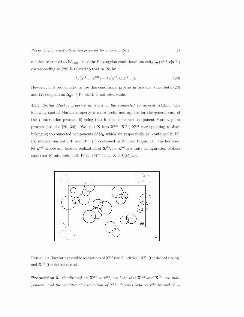
4.5.5. Spatial Markov property in terms of the connected component relation: The
following spatial Markov property is more useful and applies for the general case of
the T -interaction process (6) using that it is a connected component Markov point
process (see also [20, 30]). We split X into X(a), X(b), X(c) corresponding to discs
belonging to connected components of UX which are respectively (a) contained in W ,
(b) intersecting both W and W c, (c) contained in W c, see Figure 11. Furthermore,
let x(b) denote any feasible realization of X(b), i.e. x(b) is a finite configuration of discs
such that K intersects both W and W c for all K ∈ K(Ux(b)).
W
S
Figure 11: Illustrating possible realizations of X(a) (the full circles), X(b) (the dashed circles),
and X(c) (the dotted circles).
Proposition 5. Conditional on X(b) = x(b), we have that X(a) and X(c) are inde-
pendent, and the conditional distribution of X(a) depends only on x(b) through V =

28 J. Møller and K. Helisova
W ∩ Ux(b) and has density
fθ(x(a)|V ) =1
cθ(V )1[Ux(a) ⊆W \ V ] exp
(θ · T (x(a))
)(30)
with respect to the reference Poisson process of discs.
Proof. Let Π denote the distribution of Ψ restricted to those finite configurations
of discs with centres in S, and let hθ denote the unnormalized density given by the
exponential term in (27). Recall the ‘Poisson expansion’ (see e.g. [33])
P(X ∈ F ) =1cθ
∫F
hθ(x) Π(dx)
=1cθ
exp(−∫
S
ρ(u) du
)×
∞∑n=0
1n!
∫S
∫· · ·∫
S
∫hθ(x)1[x ∈ F ]ρ(u1) du1Q(dr1) · · · ρ(un) dunQ(drn)
(where the term with n = 0 is read as one if the empty configuration is in the event
F and zero otherwise). From this and (27) we obtain that (X(a),X(b),X(c)) has joint
density
f(x(a),x(b),x(c)) =1cθ
1[Ux(a) ⊆W \ Ux(b) ]hθ(x(a))1[Ux(c) ⊆W c \ Ux(b) ]hθ(x(c))
× 1[∀K ∈ K(Ux(b)) : K ∩W 6= ∅, K ∩W c 6= ∅]hθ(x(b))
with respect to the product measure exp(2∫
Sρ(u) du
)Π × Π × Π. Thereby the
proposition follows.
The density (30) may be useful for statistical applications, since it accounts for edge
effects and depends only on the union of discs intersected by the observation window
W . It is a hereditary density of a connected component Markov point process with
discs contained in W \ V . Its Papangelou conditional intensity λθ(x(a), v|V ) is simply
given by
λθ(x(a), v|V ) = λθ(x(a), v)1[Ux(a)∪v ⊆W \ V ]. (31)
4.6. Stability
Consider the ‘unnormalized density’ hθ(x) = exp(θ · T (x)) corresponding to the
T -interaction process with density fθ given in (6), and recall the definition (5) of the
parameter space Θ. In fact, we have yet not verified that cθ ≡ Ehθ(Ψ∩ (S× (0,∞)) is

Power diagrams and interaction processes for unions of discs 29
finite for θ ∈ Θ, and hence that fθ = hθ/cθ is a well-defined density with respect to the
reference Poisson process Ψ if θ ∈ Θ. This section discusses two stability properties
which imply integrability of hθ as well as other desirable properties.
4.6.1. Ruelle stability: This means that there exist positive constants α and β such
that hθ(x) ≤ αβn(x) for all x ∈ N (in fact, this and other stability properties
mentioned in this paper need only to hold almost surely with respect to Ψ, however,
for ease of presentation we shall ignore such nullsets). Ruelle stability implies that
cθ ≤ α exp((β − 1)
∫S
ρ(z) dz)
< ∞, and we say that fθ = hθ/cθ is a Ruelle stable
density. Other implications of Ruelle stability are discussed in Section 2.1 of [19] and
the references therein.
The main question addressed in [19] is to establish Ruelle stability of the quarmass-
interaction process, and the following proposition provides a very easy proof of this
issue in connection to the general case of the T -interaction process (6) (since the proof is
based on Lemma 2, the usefulness of the power tessellation is once again demonstrated).
Proposition 6. For all θ ∈ Θ, cθ < ∞ and fθ in (6) is a Ruelle stable density. If
θ ∈ R6 \Θ, then cθ =∞.
Proof. Note that a finite product of Ruelle stable functions is a Ruelle stable func-
tion. Let θ0 denote a real parameter. From Lemma 2 follows that χ, Nh, Nic, and
Nbv are bounded above by 6N , so the functions exp(θ0W ), W = χ,Nh, Nic, Nbv
are Ruelle stable for all θ0 ∈ R. Moreover, exp(θ1A + θ2L) is Ruelle stable if a ≡∫exp
(πθ1r
2 + 2πθ2r)
Q(dr) is finite, since exp(θ1A + θ2L) ≤ exp((a− 1)
∫S
ρ(z) dz).
On the other hand, the first term in the infinite sum in (2) is a times exp(θ3 +
θ5)∫
Sρ(z) dz, where
∫S
ρ(z) dz > 0, cf. Section 2.1. Consequently, cθ =∞ if a =∞.
4.6.2. Local stability: This means that there exists a constant β such that for all x ∈ N
and all v ∈ Ω \ x,
λθ(x, v) ≤ β. (32)
This property is clearly implying Ruelle stability. Local stability is useful when es-
tablishing geometric ergodicity of MCMC algorithms ([13, 33]; see also Section 4.7),
and it is needed in order to apply the dominating coupling from the past algorithm in
[18, 22] for making perfect simulations. Note that a finite product of locally stable

30 J. Møller and K. Helisova
functions is a locally stable function, since its Papangelou conditional intensity is
given by a product of uniformly bounded Papangelou conditional intensities. The
Papangelou conditional intensity (6) is a product of Papangelou conditional intensities
corresponding to functions hθ0(x) = exp(θ0W (Ux)), with W = A,L, . . . and θ0 =
θ1, θ2, . . ..
As shown below, the picture of whether local stability is satisfied or not depends
much on the particular type of model. When we in the following proposition write ‘in
general’, the proof of the proposition will show examples where locally stability is not
satisfied, depending on how S and supp(Q) are specified, and it should be obvious to
the reader that local stability will not be satisfied in many other cases as well. We let
ε = inf supp(Q) and R = sup supp(Q).
Proposition 7. Local stability is satisfied for
(a) the A-interaction process if and only if θ1 ≤ 0 or R <∞;
(b) the L-interaction process if θ2 = 0, or R < ∞ if θ2 > 0, or ε > 0 and R < ∞ if
θ2 < 0; otherwise in general it is not locally stable;
(c) the χ-interaction process if θ3 ≥ 0, while in general it is not locally stable if
θ3 < 0;
(d) the Ncc-interaction process if θ3 = θ4 ≥ 0 or both θ3 = θ4 < 0 and ε > 0, while it
is not locally stable if θ3 = θ4 < 0 and ε = 0;
(e) the Nic-interaction process if θ5 ≥ 0 or ε > 0, while it is not locally stable if
θ5 < 0 and ε = 0.
Moreover, local stability is in general not satisfied for
(f) the Nh-interaction process unless θ4 = 0;
(g) the Nbv-interaction process unless θ6 = 0.
Proof. Let x ∈ N and v ∈ Ω \ x.
It follows from (11) that λθ1(∅, v) = exp(πθ1r
2), λθ1(x, v) ≤ exp
(πθ1r
2)
if θ1 ≥ 0,
and λθ1(x, v) ≤ 1 if θ1 ≤ 0. Thereby (a) follows, and in a similar way we verify (b)

Power diagrams and interaction processes for unions of discs 31
in the case θ2 ≥ 0. It also follows from (11) that the χ-interaction process is locally
stable if θ3 ≥ 0.
To verify (b) in the case θ2 < 0, we suppose first that ε > 0 and R < ∞, and
use an argument which Wilfrid Kendall kindly has point out to us. A boundary edge
corresponding to an angle 0 < ϕ < 2π and a disc of radius r has length ϕr, and it
defines a sector of area ϕr2/2. Since such sectors have disjoint interiors,
A(Ux) ≥∑
j
ϕjr2j /2 ≥ (ε2/2)
∑j
ϕj
where the sum is over all boundary edges. Hence
L(Ux) =∑
j
ϕjrj ≤ R∑
j
ϕj ≤ (2R/ε2)A(Ux) < c
where c is a finite constant (since the discs specified by x have centres in the bounded
region S and their radii are bounded by R, A(Ux) has an upper bound). Consequently,
L(x, v) = L(bv)− L(bv ∩ Ux) ≥ 2πε− c
and so local stability is established when θ2 < 0, ε > 0, and R <∞.
On the other hand, suppose that ε = 0 or R = ∞. Let r denote the radius of bv,
let 0 < δ < r, and consider the infinite configuration of discs of radii δ and centres
at the sites of a equilateral triangular lattice of side length 2δ. The proportion of R2
covered by these discs is the so-called maximal packing degree p = π/√
12 (a number
independent on how δ is chosen). Now, suppose that x is the subconfiguration of all
such discs contained in bv. As either δ decreases to zero or r increases to infinity,
n(x)δ2/r2 converges to p, and so
L(x, v) = L(bv)− L(bv ∩ Ux) = 2πr − 2πδn(x)
is converging to −∞. Hence if θ2 < 0, the local stability condition is violated, and so
(b) is verified.
To show an example where the χ-interaction process is not locally stable if θ3 < 0,
consider Figure 12. Suppose x = x1, . . . , xn corresponds to the pairwise overlapping
small discs in the figure, and bv to the large disc. Then each pair xi, xi+1 together
with bv form one hole, and Nh(bv ∩Ux) = n− 1. Since n may be arbitrary large, using

32 J. Møller and K. Helisova
again (11), we obtain (c). Notice that bv does not need to be so large compared to
the other discs in Figure 12; it is only chosen in this way for illustrative purposes. For
example, all the discs may be of a very similar size so that still Nh(bv ∩ Ux) = n − 1
(then the discs in x will be much more overlapping than indicated in Figure 12). More
precisely, whether this holds or not depends on how large S is compared to supp(Q).
For instance, if S is a disc with radius R and Ω = S × 2R, then χ(Ux) = 1 for all
x ∈ N , and so the χ-interaction process is locally stable for all θ3 ∈ R.
For (d), we use that
Ncc(x, v) = 1−#connected components in Ux which are intersected by bv. (33)
Hence we immediately obtain local stability if θ3 = θ4 ≥ 0. Suppose instead that
θ3 = θ4 < 0. By (33), Ncc(x, v) has no lower bound if ε = 0, since the discs in x can
be disjoint and still all intersect bv. On the other hand, if ε > 0, then 1−Ncc(x, v) is
at most equal to the maximal number of disjoint discs with radius ε and centres in S.
Thereby (d) is verified. The proof of (e) is similar, using instead that
Nic(x, v) = 1ic(x, v)−#isolated cells in Ux which are contained in bv
where 1ic(x, v) is the indicator function which is one if Bv is an isolated cell in Bx∪v,
and zero otherwise.
The Nh-interaction process with θ4 = 0 and the Nbv-interaction process with θ6 = 0
are nothing but the Poisson process Ψ, and so local stability is obviously satisfied. By
similar arguments as above in the proof of (c) when θ3 < 0, there are in general no
uniform upper and lower bounds on neither Nh(x, v) nor Nbv(x, v). Thereby (f) and
(g) follow.
Figure 12: A configuration x of n = 6 discs intersected by another disc bv such that
#holes(bv ∩ Ux) = n− 1 = 5.

Power diagrams and interaction processes for unions of discs 33
Proposition 7 immediately extends to the conditional quarmass-interaction process
with density (28) and the conditional T -interaction process in (30). Note that if the
indicator term in (30) is one, it implies that the radius of any disc in x(a) is less than
a constant. Consequently, (a) the conditional A-interaction process given by (30) is
always locally stable, and (b) the L-interaction process given by (30) is locally stable
if either θ2 ≥ 0 or θ2 < 0 and ε > 0, and in general it is not locally stable if θ2 < 0 and
ε = 0.
4.7. MCMC algorithms
For simulation of the T -interaction process (6), the conditional quarmass-interaction
point process with density (28), or the conditional T -interaction process with density
(30), we use a simple version of the birth-death type Metropolis-Hastings algorithm
studied in [13, 14, 33]. For specificity, we consider first the T -interaction process X
with Papangelou conditional intensity λθ(x, v) given by (8).
In the Metropolis-Hastings algorithm, if x is the state at iteration t, we generate a
proposal which is either a ‘birth’ x∪ v of a new discs v = (z, r) or a ‘death’ x \ xi
of an old disc xi ∈ x. Each kind of proposal may happen with equal probability 1/2.
Define
rθ(x, v) = λθ(x, v)
∫S
ρ(s) ds
ρ(z)(n(x) + 1). (34)
In case of a birth-proposal, v follows the normalized intensity measure of Ψ, i.e. z
and r are independent, z has a density on S proportional to ρ, and r follows the mark
distribution Q. This proposal is accepted as the state at iteration t+1 with probability
min1,Hθ(x, v), where the Hastings ratio is given by Hθ(x, v) = rθ(x, v). In case of a
death-proposal, xi is a uniformly selected point from x, and the Hastings ratio in the
acceptance probability of the proposal is now given by Hθ(x, xi) = 1/rθ(x \ xi, xi)
(in the special case where x = ∅, we do nothing). Finally, if neither kind of proposal
is accepted, we retain x at iteration t + 1.
As verified in [14], the generated Markov chain is aperiodic and positive Harris
recurrent, the chain converges towards the distribution of X, and Birkhoff’s ergodic
theorem establishes convergence of Monte Carlo estimates of mean values with respect
to (6). If local stability is satisfied (see Proposition 7), the chain is geometrical
ergodic, and hence a central limit theorem applies for Monte Carlo estimates [6, 33, 38].

34 J. Møller and K. Helisova
Moreover, from a computational perspective, the important point of the algorithm is
that it only involves calculating the Papangelou conditional intensity, so only local
computations of the statistics appearing in (8) are needed, cf. Sections 4.3-4.5.
In theory we may use any state of N as the initial state of the algorithm, but we
have mainly used three kinds of initial states:
(i) the extreme case of the empty configuration ∅;
(ii) if local stability is satisfied, the other extreme case is given by a realization from
a Poisson process Ξ with intensity measure βρ(z) dz Q(dr), where β is the upper
bound in (32);
(iii) a realization of the reference Poisson process Ψ (an intermediate case of (i)-(ii)
if β > 1).
In fact local stability ensures that the Poisson process in (ii) can be coupled with X so
that X ⊆ Ξ, and this kind of domination can be exploited to make perfect simulations
of X, using a dominating coupling from the past algorithm [21, 22].
The algorithm for simulating from the conditional processes with densities (28) and
(30) is the same except that we replace λθ(x, v) in (34) by the Papangelou conditional
intensities in (29)-(31), and that the state space has of course to be in accordance
with (28) respective (30). The convergence properties and computations are therefore
similar to those discussed above. The initial states are of course slightly different,
where we modify the Poisson process in (ii) or (iii) above as follows. For (28), we
restrict the Poisson process in (ii) or (iii) so that centres are in W2R. For (30), we
first restrict the Poisson process in (ii) or (iii) so that centres are in W , and second
when we make a simulation from this Poisson process, we finally omit those discs which
are not included in W \ V .
5. Extensions and open problems
We conclude with some remarks on possible extensions of this work and on some
open problems.
We demonstrated the usefulness of the power tessellation in connection to the T -
interaction process (4), and argued why this model is best viewed as a connected

Power diagrams and interaction processes for unions of discs 35
component Markov point process. For the specification of the sufficient statistic T ,
other geometric characteristics than those in (4) may be of interest to include, e.g.
shape characteristic for the connected components K such as A(K)/L(K)2. The
power tessellation will also be a useful tool for such extensions, not least since local
calculations can be done as discussed in Section 4.4.
We confined ourselves to the case of discs in R2, though many concepts and results
can be extended to the general case of balls in Rd. The planar case d = 2 is already
complicated enough, and indeed the power tessellation in higher dimensions becomes
more complicated, cf. [10]. The planar case is of principal importance for applications
in spatial statistics and stochastic geometry (e.g. [8, 40]), and the spatial case d = 3 is
of particular importance in physics and computational biology (e.g. [11, 24, 25, 26]).
The T -interaction processes provide obviously a large and flexible class of random
models for unions of discs. It would be interesting to get a better understanding of the
importance of the parameters θ1, . . . , θ6, cf. Section 4.2. For instance, how different
are the models which have been simulated in Section 4.2, and how different would a
fitted L-interaction process be if the true model is an A-interaction process? Probably,
to answer such questions, an extensive simulation study will be required.
As noticed in Section 4.6, the dominating coupling from the past algorithm [18,
22] for making perfect simulations requires local stability. Moreover, to make this
algorithm work in practice, some monotonicity property like (9) or an antimonotonicity
property like (10) is useful, but apart from the A-interaction process, our models are
in general neither attractive nor repulsive, cf. Proposition 2. How difficult is it to make
a perfect simulation of e.g. the L-interaction process?
Also extensions of our T -interaction models to infinite configurations of discs would
be of interest, particularly for applications in statistical physics. Such extensions are
possible for quarmass-interaction models, at least if Q has bounded support (see [19]),
but how do we extend the other kind of T -interaction models? The usual approach is
to use a local specification in the sense of Preston [36] or equivalently to specify the
Papangelou conditional intensity for the infinite process [12, 34], but this would require
that the connected components are almost surely bounded. See the somewhat related
discussion in [32] concerning infinite extensions of Markov connected component fields.
A related problem to infinite extensions of T -interaction models is the issue of phase
36 J. Møller and K. Helisova
transition. The A-interaction model exhibits phase transition, at least if the radii are
all fixed at a constant value [15, 39], but what about other T -interaction models?
Finally, we are currently exploiting the results in this paper when studying the
statistical aspects, in particular likelihood based inference, in a follow up paper [31].
Acknowledgements
We are grateful to Lars Døvling Andersen, Herbert Edelsbrunner, and Wilfrid
Kendall for useful comments. Supported by the Danish Natural Science Research
Council, grant 272-06-0442, ”Point process modelling and statistical inference”, and
by grants GACR 201/06/0302 and GACR 201/05/H007.
Appendix: successive construction of power tessellations
This appendix explains how to construct a new power tessellation of a union of discs
by adding a new ball (Appendix A) or deleting an old ball (Appendix B), assuming
that the old power tessellation is known. The constructions can easily be extended to
keep track on the connected components of the union of discs, but to save space we
omit those details.
Appendix A: the case where a new disc is added
Suppose we want to construct a new power tessellation Bnew of a union Unew = ∪n1 bi
of n ≥ 1 discs in general position, where we are adding the disc bn and we have already
constructed the power tessellation Bold of Uold = ∪n−11 bi based on the n − 1 other
discs (if n = 1 then Bold and Uold are empty). More precisely, with respect to Bold,
we assume to know all the old edges. We denote old interior edges by [uoldi,j , vold
i,j ] and
old boundary edges by buoldi , vold
i e or ∂boldi . We want to construct the new tessellation
Bnew of Unew = Uold ∪ bn by finding its interior edges [unewi,n , vnew
i,n ] and boundary edges
bunewn , vnew
n e associated to the new cell Bnewn . This is done in steps (ii) and (iv) below.
Moreover, to obtain the remaining new edges, we modify old interior edges [uoldi,j , vold
i,j ]
and old boundary edges buoldi , vold
i e or ∂boldi , noticing that a “modified old edge” can
be unchanged, reduced or disappearing. This is done in steps (iii) and (v) below.
Notice that steps (i), (ii), and (iv) determine the new cells, i.e. which of the sets

Power diagrams and interaction processes for unions of discs 37
Bnew1 , . . . , Bnew
n are empty or not.
(i) Considering old discs intersecting the new disc: If bn is contained in some disc
bj with j < n, then Bnewn is empty and so Bnew = Bold is unchanged. Assume that
bn is not contained in any disc bj with j < n, and without loss of generality that bn
intersects Bold1 , . . . , Bold
i but not Boldi+1, . . . , B
oldn−1, where 0 ≤ i ≤ n− 1 (setting i = 0 if
bn has no intersection). Then Bnewj = Bold
j is unchanged for j = i + 1, . . . , n− 1, so it
suffices below to find the edges of Bnew1 , . . . , Bnew
i and Bnewn .
If i = 0 then Bnewn = bn is an isolated cell with boundary edge ∂bn. In (ii)-(v) we
assume that i ≥ 1.
(ii) Finding the interior edges of Bnewn : To obtain the interior edges of Bnew
n , for
j = 1, . . . , i, we start by assigning enewj,n ← [unew
j,n , vnewj,n ], considering unew
j,n and vnewj,n
as (potential) boundary vertices given by the endpoints of the chord Ej,n. Further,
for k = 1, . . . , i with k 6= j, if enewj,n ∩ Hn,k = ∅ (or equivalently unew
j,n 6∈ Hn,k and
vnewj,n 6∈ Hn,k, since Hn,k is convex) we obtain that enew
j,n ← ∅ and we can stop the
k-loop, else enewj,n ← enew
j,n ∩Hn,k. In the latter case, either both vertices are contained
in Hn,k and so the edge remains unchanged, or exactly one vertex is not contained
in Hn,k, e.g. unewj,n 6∈ Hn,k but vnew
j,n ∈ Hn,k, in which case unewj,n becomes an interior
vertex given by the point enewj,n ∩ ∂Hn,k while vnew
j,n is unchanged. In this way we find
all interior edges of Bnewn , and all interior and boundary vertices of Bnew
n .
Since we have assumed that i > 0, Bnewn is empty if and only if it has no interior
edges.
(iii) Modifying the old interior edges: At the same time as we do step (ii) above,
we also check whether each interior edge eoldj,k = [uold
j,k , voldj,k ] of Bold with j < k ≤ i
should be kept, reduced or omitted when we consider Bnew (recalling that enewj,k = eold
j,k
is unchanged if j > i or k > i). We have
enewj,k = eold
j,k ∩Hj,n = eoldj,k ∩Hk,n.
Thus enewj,k is empty if uold
j,k 6∈ Hk,n and voldj,k 6∈ Hk,n, while enew
j,k = eoldj,k if uold
j,k ∈ Hk,n and
voldj,k ∈ Hk,n. Further, if uold
j,k ∈ Hk,n and voldj,k 6∈ Hk,n, then enew
j,k = [uoldj,k , vnew
j,k ] where
vnewj,k is the point given by eold
j,k ∩ ∂Hk,n. Similarly, if uoldj,k 6∈ Hk,n and vold
j,k ∈ Hk,n, then
enewj,k = [unew
j,k , voldj,k ] where unew
j,k is the point given by eoldj,k ∩ ∂Hk,n.
Note that for each j ≤ i, Bnewj is empty if and only if it has no interior edge.

38 J. Møller and K. Helisova
(iv) Finding the boundary edges of Bnewn : Suppose that Bnew
n has m > 0 boundary
vertices wnew1 , . . . , wnew
m . Notice that m is an even number, and we can organize the
boundary vertices such that wnew1 = zn + rn(cos ϕnew
1 , sinϕnew1 ), . . ., wnew
m = zn +
rn(cos ϕnewm , sinϕnew
m ), where 0 ≤ ϕnew1 < · · · < ϕnew
m < 2π. Then Bnewn has m/2
boundary edges, namely
bwnew2 , wnew
3 e, bwnew4 , wnew
5 e, . . . , bwnewm , wnew
1 e if zn + (rn, 0) ∈ Hn,j for all j = 1, . . . , i
and
bwnew1 , wnew
2 e, bwnew3 , wnew
4 e, . . . , bwnewm−1, w
newm e otherwise.
(v) Modifying the old boundary edges: Finally, we modify the boundary edges
buoldj , vold
j e of Bold considering Bnew and j ≤ i (noticing that buoldj , vold
j e is a boundary
edge of Bnew too if j > i). This is done in a similar way as in step (iv). Suppose
that Bnewj has mj > 0 boundary vertices wnew
1 , . . . , wnewmj
, which we organize as in (iv).
Then Bnewj has boundary edges
bwnew2 , wnew
3 e, bwnew4 , wnew
5 e, . . . , bwnewmj
, wnew1 e
if zj + (rj , 0) ∈ Hj,k for all k ≤ n with k 6= j and bj ∩ bk 6= ∅
and
bwnew1 , wnew
2 e, bwnew3 , wnew
4 e, . . . , bwnewmj−1
, wnewmje otherwise.
Appendix B: the case where a disc is deleted
Suppose we are deleting the disc bn from a configuration b1, . . . , bn of n ≥ 1 discs,
which are assumed to be in general position. We also assume that we know the power
tessellation Bold of Uold = ∪n1 bi. Below we explain how to construct the new power
tessellation Bnew of Unew = ∪n−11 bi. More precisely, with respect to Bold, we assume
to know all the interior edges [uoldi,j , vold
i,j ] and all the boundary edges buoldi , vold
i e. We
want to construct the tessellation Bnew of Unew = Uold \ bn by finding the interior
edges [unewi,j , vnew
i,j ] and the boundary edges bunewi , vnew
i e associated to each new cell
Bnewi , noticing that Bnew
i either agrees with Boldi or is an enlargement of Bold
i or
is a completely new cell. One possibility could be to ”reverse” the construction in
Appendix A, where a new disc is added, however, we realized that it is easier to
create the new edges without reversing the construction in Appendix A but using a

Power diagrams and interaction processes for unions of discs 39
construction as described below. This is partly explained by the fact that an old empty
set Boldi may possibly be replaced by a non-empty set Bnew
i .
(i) Considering the discs intersecting the disc which is deleted: Clearly, if Boldn is
empty, then Bnew = Bold is unchanged. Assume that Boldn is a non-empty cell, and
without loss of generality that bn intersects b1, . . . , bi but not bi+1, . . . , bn−1, where
0 ≤ i ≤ n − 1 (setting i = 0 if bn has no intersection). Then it suffices to find the
edges of Bnew1 , . . . , Bnew
i , since Bnewj = Bold
j is unchanged for j = i + 1, . . . , n − 1. If
i = 0 then Boldn = bn is an isolated cell, and so Bnew
1 = Bold1 , . . . , Bnew
n−1 = Boldn−1 are
unchanged. In the following steps (ii)-(iv), suppose that i > 0.
(ii) Finding the new interior edges: If i = 1, no new interior edge appears. Suppose
that i ≥ 2. We want to determine each set enewj,k with j < k ≤ i. We start by assign-
ing all cells Bnew1 , . . . , Bnew
i to be non-empty, and by assigning enewj,k ← [unew
j,k , vnewj,k ],
considering unewj,k and vnew
j,k as (potential) boundary vertices given by the endpoints of
the chord Ej,k. Consider a loop with l = 1, . . . , i and l 6= j, k. If enewj,k ∩Hk,l = ∅ (or
equivalently unewj,k 6∈ Hk,l and vnew
j,k 6∈ Hk,l, since Hk,l is convex), we have that enewj,k is
empty and we can stop the l-loop. Otherwise assign enewj,k ← enew
j,k ∩Hk,l, where we notice
that only the following two cases can occur. First, if both vertices of enewj,k are contained
in Hk,l, the edge remains unchanged. Second, if exactly one vertex is not contained
in Hk,l, e.g. unewj,k 6∈ Hk,l but vnew
j,k ∈ Hk,l, then unewj,k becomes an interior vertex given
by the point enewj,k ∩ ∂Hk,l while vnew
j,k is unchanged. When the loop is finished, we
have determined all the new interior edges, including the information whether their
endpoints are interior or boundary vertices.
(iii) Determining the new cells: For each j ≤ i, we determine if Bnewj is a new cell
by checking if it has an edge. Suppose that Bnewj has no interior edge, i.e. it is either
an empty set or a new isolated cell. If an arbitrary fixed point of bj is included in Hj,l
for all l = 1, . . . , n− 1 with l 6= j, then Bj has exactly one boundary edge and it is an
isolated cell. Otherwise Bnewj is empty. In this way we determine whether each Bnew
j
is empty or a new cell, including whether it is an isolated cell.
(iv) Finding the new boundary edges: We have already determined the new isolated
boundary edges in step (iii). Consider a non-isolated cell Bnewj with j ≤ i with
boundary vertices wnewk = zj+rj(cos ϕnew
k , sinϕnewk ), k = 1, . . . ,mj . Recall that mj > 0
is an even number and we organize the vertices so that 0 ≤ ϕnew1 < · · · < ϕnew
mj< 2π,

40 J. Møller and K. Helisova
cf. (iv) in Appendix A. Then Bnewj has mj/2 boundary edges, namely
bwnew2 , wnew
3 e, bwnew4 , wnew
5 e, . . . , bwnewmj
, wnew1 e if zj + (rj , 0) ∈ Hj,l for all l = 1, . . . , i
and
bwnew1 , wnew
2 e, bwnew3 , wnew
4 e, . . . , bwnewmj−1, w
newmje otherwise.
References
[1] Aurenhammer, F. (1987). Power diagrams: properties, algorithms and
applications. SIAM Journal on Computing 16, 78–96.
[2] Baddeley, A. and Møller, J. (1989). Nearest-neighbour Markov point
processes and random sets. International Statistical Review 2, 89–121.
[3] Baddeley, A. J. and van Lieshout, M. N. M. (1995). Area-interaction point
processes. Annals of the Institute of Statistical Mathematics 46, 601–619.
[4] Baddeley, A. J., van Lieshout, M. N. M. and Møller, J. (1996). Markov
properties of cluster processes. Advances in Applied Probability 28, 346–355.
[5] Barndorff-Nielsen, O. E. (1978). Information and Exponential Families in
Statistical Theory. Wiley, Chichester.
[6] Chan, K. S. and Geyer, C. J. (1994). Discussion of the paper ‘Markov chains
for exploring posterior distributions’ by Luke Tierney. Annals of Statistics 22,
1747–1747.
[7] Chin, Y. C. and Baddeley, A. J. (2000). Markov interacting component
processes. Advances in Applied Probability 32, 597–619.
[8] Cressie, N. A. C. (1993). Statistics for Spatial Data second ed. Wiley, New
York.
[9] Diggle, P. (1981). Binary mosaics and the spatial pattern of heather. Biometrics
37, 531–539.
[10] Edelsbrunner, H. (1995). The union of balls and its dual shape. Discrete
Computational Geometry 13, 415–440.

Power diagrams and interaction processes for unions of discs 41
[11] Edelsbrunner, H. (2004). Biological applications of computational topology.
In Handbook of Discrete and Computational Geometry. ed. J. Goodman and
J. O’Rourke. Chapman and Hall/CRC, Boca Raton pp. 1395–1412.
[12] Georgii, H.-O. (1976). Canonical and grand canonical Gibbs states for
continuum systems. Communications of Mathematical Physics 48, 31–51.
[13] Geyer, C. J. (1999). Likelihood inference for spatial point processes. In
Stochastic Geometry: Likelihood and Computation. ed. O. E. Barndorff-Nielsen,
W. S. Kendall, and M. N. M. van Lieshout. Chapman & Hall/CRC, Boca Raton,
Florida. pp. 79–140.
[14] Geyer, C. J. and Møller, J. (1994). Simulation procedures and likelihood
inference for spatial point processes. Scandinavian Journal of Statistics 21, 359–
373.
[15] Haggstrom, O., van Lieshout, M. N. M. and Møller, J. (1999).
Characterization results and Markov chain Monte Carlo algorithms including
exact simulation for some spatial point processes. Bernoulli 5, 641–659.
[16] Hall, P. (1988). Introduction to the Theory of Coverage Processes. Wiley, New
York.
[17] Hanisch, K.-H. (1981). On classes of random sets and point processes. Serdica
7, 160–167.
[18] Kendall, W. (2004). Geometric ergodicity and perfect simulation. Electronic
Communications in Probability 9, 140–151.
[19] Kendall, W., van Lieshout, M. and Baddeley, A. (1999). Quermass-
interaction processes: conditions for stability. Advances in Applied Probability
31, 315–342.
[20] Kendall, W. S. (1990). A spatial Markov property for nearest-neighbour Markov
point processes. Journal of Applied Probability 28, 767–778.

42 J. Møller and K. Helisova
[21] Kendall, W. S. (1998). Perfect simulation for the area-interaction point process.
In Probability Towards 2000. ed. L. Accardi and C. Heyde. Springer Lecture Notes
in Statistics 128, Springer Verlag, New York pp. 218–234.
[22] Kendall, W. S. and Møller, J. (2000). Perfect simulation using dominating
processes on ordered spaces, with application to locally stable point processes.
Advances in Applied Probability 32, 844–865.
[23] Klein, W. (1982). Potts-model formulation of continuum percolation. Physical
Review B 26, 2677–2678.
[24] Likos, C., Mecke, K. and Wagner, H. (1995). Statistical morphological of
random interfaces in microemulsions. Journal of Chemical Physics 102, 9350–
9361.
[25] Mecke, K. (1994). Integralgeometrie in der Statistichen Physik. Reine Physik
Volume 25, Harri Deutsch, Frankfurt.
[26] Mecke, K. (1996). A morphological model for complex fluids. Journal of Physics:
Condensed Matters 8, 9663–9667.
[27] Molchanov, I. (1997). Statistics of the Boolean Model for Practitioners and
Mathematicians. Wiley, Chichester.
[28] Møller, J. (1994). Contribution to the discussion of N.L. Hjort and H. Omre
(1994): Topics in spatial statistics. Scandinavian Journal of Statistics 21, 346–
349.
[29] Møller, J. (1994). Lectures on Random Voronoi Tessellations. Lecture Notes
in Statistics 87. Springer-Verlag, New York.
[30] Møller, J. (1999). Markov chain Monte Carlo and spatial point processes. In
Stochastic Geometry: Likelihood and Computation. ed. O. E. Barndorff-Nielsen,
W. S. Kendall, and M. N. M. van Lieshout. Monographs on Statistics and Applied
Probability 80, Chapman & Hall/CRC, Boca Raton, Florida pp. 141–172.
[31] Møller, J. and Helisova, K. (2007). Likelihood inference for unions of
interacting discs. In preparation.

Power diagrams and interaction processes for unions of discs 43
[32] Møller, J. and Waagepetersen, R. P. (1998). Markov connected component
fields. Advances in Applied Probability 30, 1–35.
[33] Møller, J. and Waagepetersen, R. P. (2003). Statistical Inference and
Simulation for Spatial Point Processes. Chapman and Hall/CRC, Boca Raton.
[34] Nguyen, X. X. and Zessin, H. (1979). Integral and differential characterizations
of Gibbs processes. Mathematische Nachrichten 88, 105–115.
[35] Okabe, A., Boots, B., Sugihara, K. and Chiu, S. N. (2000). Spatial
Tessellations. Concepts and Applications of Voronoi Diagrams second ed. Wiley,
Chichester.
[36] Preston, C. J. (1977). Spatial birth-and-death processes. Bulletin of the
International Statistical Institute 46, 371–391.
[37] Ripley, B. D. and Kelly, F. P. (1977). Markov point processes. Journal of
the London Mathematical Society 15, 188–192.
[38] Roberts, G. O. and Rosenthal, J. S. (1997). Geometric ergodicity and hybrid
Markov chains. Electronic Communications in Probability 2, 13–25.
[39] Ruelle, D. (1971). Existence of a phase transition in a continuous classsical
system. Physical Review Letters 27, 1040–1041.
[40] Stoyan, D., Kendall, W. S. and Mecke, J. (1995). Stochastic Geometry and
Its Applications second ed. Wiley, Chichester.
[41] Weil, W. and Wieacker, J. (1984). Densities for stationary random sets and
point processes. Advances in Applied Probability 16, 324–346.
[42] Weil, W. and Wieacker, J. (1988). A representation theorem for random sets.
Probability and Mathematical Statistics 9, 147–151.
[43] Widom, B. and Rowlinson, J. S. (1970). A new model for the study of liquid-
vapor phase transitions. Journal of Chemical Physics 52, 1670–1684.
[44] Wilson, R. (1972). Introduction to Graph Theory. Oliver and Boyd, Edinburgh.