power, fdr and conservativeness of bb-sgof method for multiple

Power, FDR and conservativeness of BB-SGoF

method for multiple dependent tests: a

simulation study Irene Castro-Conde and Jacobo de Uña-Álvarez

Report 13/03

Discussion Papers in Statistics and Operation Research

Departamento de Estatística e Investigación Operativa

Facultade de Ciencias Económicas e Empresariales Lagoas-Marcosende, s/n · 36310 Vigo

Tfno.: +34 986 812440 - Fax: +34 986 812401 http://webs.uvigo.es/depc05/

E-mail: [email protected]

mailto:[email protected]



simulation study Irene Castro-Conde and Jacobo de Uña-Álvarez

Report 13/03

Discussion Papers in Statistics and Operation Research

Imprime: GAMESAL

Edita:

Facultade de CC. Económicas e Empresariales Departamento de Estatística e Investigación Operativa As Lagoas Marcosende, s/n 36310 Vigo Tfno.: +34 986 812440

I.S.S.N: 1888-5756

Depósito Legal: VG 1402-2007



simulation study

Irene Castro-Conde and Jacobo de Una-Alvarez

September 13, 2013

Abstract

Beta-Binomial SGoF (or BB-SGoF) method for multiple hypothesestesting has been recently proposed as a suitable modification of the Se-quential Goodness-of-Fit (SGoF) multitesting method when the tests arecorrelated in blocks. In this paper we investigate the power, the false dis-covery rate, and the conservativeness of BB-SGoF in an intensive MonteCarlo simulation study. Important features such as automatic selectionof the number of existing blocks and preliminary testing for independenceare explored. Our study reveals that (a) BB-SGoF method maintains theproperties of original SGoF in the dependent case; (b) BB-SGoF weaklycontrols for FDR even when the Beta-Binomial model is violated and thenumber of blocks k is unknown; and that (c) the loss of power of the auto-matic selector for the number of blocks relative to the benchmark methodwhich uses the true k varies depending on the proportion and the type(strong, intermediate or weak) of the effects, being strongly influenced bythe within-block correlation too.

1 Introduction

Multiple testing procedures have become more and more important in the lastyears due to the increasing availability of information in fields like genomics,transcriptomics, or proteomics. In many occasions the goal is to control forthe number of type I errors (or false positives) along a sequence of hundreds,thousands or tens of thousands of hypotheses which are tested simultaneously.Methods traditionally used in this setting control for the family-wise error rate(FWER) or for the false discovery rate (FDR) at a pre-specified level α. FWER-controlling procedures ensure that no type I error will be committed with prob-ability at least 1 − α; on the other hand, FDR-based methods control at levelα the expected proportion of false positives among the null hypotheses beingrejected. FWER methods include, among others, Bonferroni and Holm (step-down) procedures, while the standard approach for controlling the FDR is the

1

Benjamini-Hochberg method (Benjamini and Hochberg, 1995). See Nichols andHayasaka (2003) or Dudoit and van der Laan (2008) for a deeper introductionto this area.

Unfortunately, it has been quoted by several authors that FWER and FDRcontrolling methods sometimes exhibit a low power. Here, the power of a multi-testing method is defined as the proportion of non-true nulls which are rejected.This has motivated the introduction of alternative decision criteria. General-ized FWER criterion was studied in van der Laan et al. (2004) or Lehmannand Romano (2005), among others. Genovese and Wasserman (2002) suggestedto minimize the loss function FNR + λFDR, where FNR stands for the falsenon-discovery rate (which is the expected proportion of non-true null hypothe-ses among the accepted ones), while λ is a pre-specified penalty. Storey (2003)proposed as a possible thresholding criterion to minimize a weighted averageof the positive FDR and FNR, where the choice of the weight is left to theresearcher who must proceed according to the importance of the rate of falsediscoveries relative to that of false non-discoveries. Other approaches based onp-value thresholding are reviewed in Genovese and Wasserman (2004).

More recently, Carvajal-Rodrıguez et al. (2009) introduced a sequentialgoodness-of-fit (SGoF) test to make a decision on the number and allocation ofnon-true nulls. Carvajal-Rodrıguez et al.’s SGoF method starts by comparingthe observed amount of p-values below an initial threshold γ to the expectedamount under the intersection or complete null (i.e., under the assumption thatall the null hypotheses are true). Such a comparison is performed through abinomial test at level α; the excess of observed p-values below γ with respectto the critical point at level α in the binomial test is then used to identifythe non-true nulls. Statistical properties of this approach were explored in deUna-Alvarez (2011). SGoF’s procedure controls for FWER (and FDR) at levelα, but only in the weak sense (i.e. under the complete null), which makesa difference with other, more standard procedures. That is, SGoF method isliberal with respect to the strong control of FWER or FDR, which are nota priori bounded when some of the nulls are false. However, SGoF multitestcontrols at the pre-specified level α the probability that the number of falsepositives exceeds the number of false non-discoveries with p-value below γ (deUna-Alvarez, 2012). This property of conservativeness is unique to the SGoFapproach. SGoF method has become in short time a popular tool for appliedscientists; as an indicator, we mention that, according to the Web of Knowledge,the seminal paper Carvajal-Rodrıguez et al. (2009) has been cited 19 times onlyin one year (2012).

In practice, the test statistics along the multiple tests may be dependent. Anadaptation of SGoF method to the case of dependent tests based on the beta-binomial model was introduced by de Una-Alvarez (2012); this beta-binomialSGoF (or BB-SGoF) shares the main properties of original SGoF while tak-ing the serial dependence of the p-values into account. Unlike for SGoF, thepractical performance of its beta-binomial extension has not been extensivelyinvestigated so far. For example, evaluation of the FDR and the power ofBB-SGoF is presently missing; similarly, it is still unclear how BB-SGoF will

2

perform when the underlying assumptions for the beta-binomial model are vi-olated. Although de Una-Alvarez (2012) reported a simulation study, it wasrestricted to the beta-binomial case; besides, due to the design of that study, itdid not allow to distinguish the p-values coming from true and non-true nullsand, therefore, only the total amount of rejections and the family-wise rejectionrate (rather than FDR or power) could be computed. This paper aims to fillthese gaps.

In this paper we investigate the power, FDR and conservativeness of BB-SGoF methods through an intensive Monte Carlo simulation study. The orga-nization of the paper is as follows. In Section 2 we briefly revisit SGoF andBB-SGoF procedures. In Section 3 the simulated scenarios are described. Sim-ulation results are reported and commented in Section 4. Finally, in Section 5we give the main conclusions of our research.

2 SGoF and BB-SGoF revisited

2.1 SGoF method

Carvajal-Rodrıguez et al (2009) proposed a new method for p-value thresh-olding in multitesting problems. This method, called SGoF (from Sequential-Goodness-of-Fit), can be summarized as follows. Let Fn be the empirical distri-bution of the n p-values attached to the null hypotheses being tested, and let γbe an initial significance level, typically γ = 0.05. Under the complete null thatall the n null hypotheses are true, the expected amount of p-values below γ isjust nγ and therefore if nFn(γ) is much larger than nγ, one gets evidence aboutthe existence of a number of non-true nulls, or effects, among the n tests. Let Fbe the underlying distribution function of the p-values; SGoF multitest startsby performing a standard one-sided binomial test for H0 : F (γ) = γ versus thealternative H1 : F (γ) > γ at level α, based on the critical region

Fn(γ)− γ√V ar(0)(Fn(γ))

> zα,

where V ar(0)(Fn(γ)) = γ(1− γ)/n and zα is the 1−α quantile of the standardnormal. Here, the Gaussian distribution is used as an approximation to thebinomial model since, in practice, the number of hypotheses n will be large(hundreds, thousands, etc). If H0 is rejected, then the number of effects declaredby SGoF is given by

N (0)α (γ) = n[Fn(γ)− γ]− n

√V ar(0)(Fn(γ))zα + 1,

which is the excess in the number of observed p-values below the threshold γwhen compared to the expected amount, beyond the critical point zα. Then,

SGoF claims that the effects correspond to the N(0)α (γ) smallest p-values. In

this metatest, the FWER and the FDR are controlled at level α in the weaksense (Carvajal-Rodrıguez et al, 2009). SGoF method relates to the notion of

3

second level significance testing (or higher criticism) introduced by Tukey in1976, and further explored by Donoho and Jin (2004, 2008).

A more conservative version of SGoF is obtained when declaring as true

effects the N(1)α (γ) smallest p-values, where

N (1)α (γ) = n[Fn(γ)− γ]− n

√V ar(1)(Fn(γ))zα + 1,

and where V ar(1)(Fn(γ)) = Fn(γ)(1 − Fn(γ))/n. In this conservative ver-sion, the variance is estimated without any restriction, which has two im-portant consequences. First, since often γ < Fn(γ) < 0.5, it turns out that

V ar(1)(Fn(γ)) > V ar(0)(Fn(γ)) and, therefore, N(1)α (γ) < N

(0)α (γ), leading to

a smaller amount of rejections compared to original SGoF. Second, the value

N(1)α (γ) may be regarded as the lower bound of a 100(1−α)% confidence inter-

val for n(F (γ) − γ), which in its turn is smaller than the expected number ofnon-true nulls with p-value below γ; indeed, by using the conservative versionof SGoF, one ensures that the number of false discoveries among the p-valuesbelow γ is smaller than the number of non-discoveries with probability 1 − α,which is a reasonable error criterion (de Una-Alvarez, 2012).

Unlike for other multitesting procedures, the power of SGoF increases withthe number of tests n. The reason for this is in the −n

√V ar term appearing

in the number of rejection, which decreases as n grows. Besides, since SGoFimposes no strong control of FWER nor FDR, in many instances its power isoften greater than FWER- or FDR-controlling methods. Simulations and ex-amples provided in Carvajal-Rodrıguez et al (2009) and de Una-Alvarez (2011,2012) indicate that this is indeed the case when the number of tests is large, andthere is a relatively small to moderate proportion of weak effects. Summaryz-ing, SGoF provides a flexible criterion of significance for multitesting problems,offering a good balance between error control and power. Unfortunately, SGoFmethod (in both its original and conservative versions) is very sensitive to cor-relation among the tests and, indeed, it may be very anticonservative (it tendsto reject more than it should) in dependent scenarios, where it loses its weakFDR control (de Una-Alvarez, 2012). This motivates the correction of SGoFreviewed in the next section.

2.2 BB-SGoF method

BB-SGoF (from Beta-Binomial SGoF, de Una-Alvarez, 2012) is a correction ofSGoF for correlated tests. It assumes that there exist k independent blocks ofcorrelated p-values, where k is unknown. As SGoF, BB-SGoF makes a decisionon the number of effects with p-values smaller than γ, but depending on thenumber of blocks k and the within-block correlation.

Given the initial significance threshold γ, BB-SGoF starts by transformingthe initial set of p-values u1, ..., un into n realizations of a Bernoulli variable:Xi = I{ui≤γ}, i = 1, ..., n. Then, by assuming that there are k independentblocks of p-values of sizes n1, ..., nk (where n1 + ... + nk = n), the number of

4

successes sj within each block j, j = 1, ..., k, is computed. Here, Xi = 1 is calledsuccess. After that, a set of independent observations {(sj , nj), j = 1, ..., k} isavailable, where sj (j = 1, ..., k) is assumed to be a realization of a beta-binomialvariable with parameters (nj , p, η). In this setting, p = F (γ) represents theaverage proportion of p-values falling below γ, which under the complete nullis just γ; while η is the correlation between two different indicators Xi and Xj

inside the same block (i.e., the within-block correlation between indicators). Thebeta-binomial model can be regarded as a frailty model in which the randomprobability π of the event Xi = 1 is shared within each block of tests; a betadistribution is used for π, and the variance of this beta distribution is responsiblefor the within-block correlation η (de Una-Alvarez, 2012).

The main aim of BB-SGoF method is to construct a one-sided confidence in-terval for τn(γ) = n(p−γ) = n(F (γ)−γ), similarly as SGoF does but consideringthe possible existing correlation. This confidence interval may be constructedfrom the asymptotic normality of the maximum-likelihood estimator (MLE) pof p. In practice, in order to perform an unrestricted optimization of the beta-binomial likelihood function, the logit reparametrization β1 = log(p/(1−p)) andβ2 = log(η/(1 − η)) is used. Introduce the 100(1 − α)% one-sided confidenceinterval for τn(γ)

I(τn(γ)) = (n(exp(low1)/(1 + exp(low1))− γ),∞)

where low1 = β1 − se(β1)zα, with se(β1) the standard error of the MLE β1of β1. Formally, BB-SGoF acts as follows. If 0 ∈ I(τn(γ)), the complete nullis accepted and no effect is declared. On the contrary, if 0 /∈ I(τn(γ)), thenBB-SGoF declares as effects the smallest NBB

α (γ; k) p-values, where

NBBα (γ; k) = n(exp(low1)/(1 + exp(low1))− γ).

By definition, and according to the asymptotic normality of β1, BB-SGoFweakly controls the FWER at level α when the number of tests n is large (seede Una-Alvarez , 2012, for details.) A crucial issue of this method is how tochoose the value of k, because in practice it will be unknown. Another pointto consider is the size of the blocks. A reasonable automatic choice for k iskN = arg minkN

BBα (γ; k), corresponding to the most conservative decision of

declaring the smallest number of effects along k. In this criterion, minimizationmay be performed along a grid k = kmin, ..., kmax where kmin is the smallestnumber of existing blocks (i.e. the strongest allowed correlation), and kmax =n/nmin, where nmin is the smallest allowed amount of tests in each block. Here,for simplicity, it is assumed that all the blocks have the same size. This kNensures the weak control of FWER at the nominal level α when the number ofblocks is unknown, as long as it falls between kmin and kmax.

Of course, the application of the automatic criterion kN to choose the numberof blocks entails a certain loss of power. This issue was somehow illustrated ina preliminary simulation study (Una-Alvarez , 2012). Therefore, in practicea preliminary test for independence is recommended; if the p-values are notcorrelated, one may apply SGoF procedure for independent tests to increase

5

the power. In the setting of the beta-binomial model, Tarone (1979) introduceda procedure for testing HT

0 : η = 0 against HT1 : η > 0; if HT

0 is true, thenthe beta-binomial model collapse to the binomial model and SGoF multitestingmethod may be applied. In the case of equal nj ’s, Tarone’s test is based on theZ–statistic

Z =nηn − k√

2k,

where (recall) n =∑kj=1 nj and ηn is a estimator of the correlation η, rejecting

HT0 for large values of Z. That is, significant positive correlation is found when

ηn is large relative to its expected value under the binomial model (k/n). Theability of this test to detect dependencies in our setting is explored throughsimulations below.

3 Simulated scenarios

We have designed a simulated scenario similar to the study of Hedenfalk data(Hedenfalk , Duggan, et al., 2001), where the mean expression levels of about3000 genes in two different groups A and B of individuals (with sample sizes of7 and 8) were compared. In order to study the influence of the number of nullhypotheses in the performance of the multitesting procedures, we considered thecases n = 500, n = 1000, and n = 3000. Hedenfalk’s sample sizes of 7 and 8 weretaken for groups A and B respectively. The samples were drawn from n-variateGaussian populations with different correlation structures. The 2-sample t-testwas applied to test for each null hypothesis, the sequence of n p-values comingfrom the computation of two-sided tails of the Student’s t distribution with 13degrees of freedom. To summarize numerical results, 1000 Monte Carlo trialswere performed.

The proportion of true nulls (i.e. ’genes equally expressed’) Π0 was 1 (com-plete null), 0.9 (10% of effects), or 0.67 (33% of effects). Mean was always takenas zero in group A, while in group B it was µ for 1/3 of the effects and −µfor the other 2/3 of effects, with µ = 1 (weak effects), µ = 2 (intermediateeffects), or µ = 4 (strong effects). Random allocation of the effects among the ntests (’genes’) was considered. Within-block correlation levels of ρ = 0, 0.2 and0.8 were taken, where ρ = 0 means independence and ρ = 0.8 indicates strongcorrelation. With regard to the number of blocks, we considered k = 20, so wehad 25 tests per block when n = 500, 50 tests per block when n = 1000 and 150tests per block when n = 3000. For random generation, the function rmvnorm

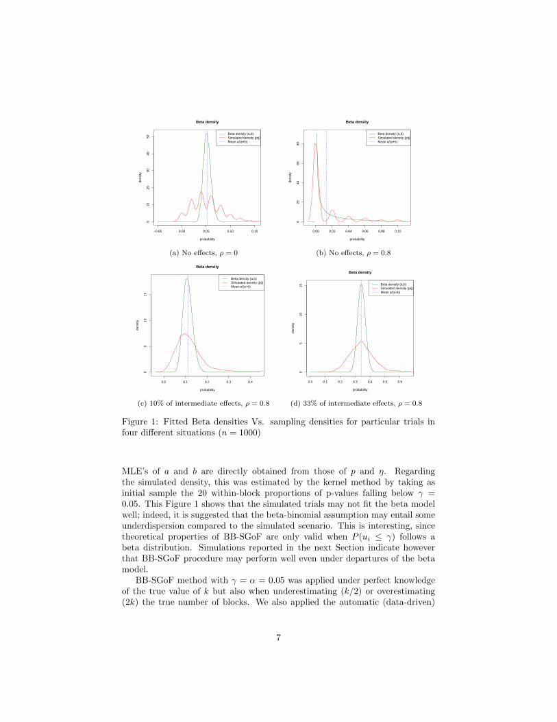
of the R software (R Core Team,2013) was used.In Figure 1, fitted beta densities are shown for particular Monte Carlo trials

in four different situations of the case n = 1000. The beta density was estimatedby maximizing the beta-binomial likelihood based on the true number of blocksk = 20 and the true numbers of block sizes (50 tests per block). For this, wejust note that, if P (ui ≤ γ) follows a Beta(a, b) distribution, then p = a/(a+ b)and η = 1/(a + b + 1) (in the notation of Section 2.2) and, therefore, the

6

−0.05 0.00 0.05 0.10 0.15

010

2030

4050

Beta density

probability

dens

ity

Beta density (a,b)Simulated density (pij)Mean a/(a+b)

(a) No effects, ρ = 0

0.00 0.02 0.04 0.06 0.08 0.10

020

4060

80

Beta density

probability

dens

ity


(b) No effects, ρ = 0.8

0.0 0.1 0.2 0.3 0.4

05

1015

Beta density

probability

dens

ity


(c) 10% of intermediate effects, ρ = 0.8

0.0 0.1 0.2 0.3 0.4 0.5 0.6

05

1015

Beta density

probability

dens

ity


(d) 33% of intermediate effects, ρ = 0.8

Figure 1: Fitted Beta densities Vs. sampling densities for particular trials infour different situations (n = 1000)

MLE’s of a and b are directly obtained from those of p and η. Regardingthe simulated density, this was estimated by the kernel method by taking asinitial sample the 20 within-block proportions of p-values falling below γ =0.05. This Figure 1 shows that the simulated trials may not fit the beta modelwell; indeed, it is suggested that the beta-binomial assumption may entail someunderdispersion compared to the simulated scenario. This is interesting, sincetheoretical properties of BB-SGoF are only valid when P (ui ≤ γ) follows abeta distribution. Simulations reported in the next Section indicate howeverthat BB-SGoF procedure may perform well even under departures of the betamodel.

BB-SGoF method with γ = α = 0.05 was applied under perfect knowledgeof the true value of k but also when underestimating (k/2) or overestimating(2k) the true number of blocks. We also applied the automatic (data-driven)

7

choice of k (kN ) by minimizing the number of effects declared by BB-SGoFalong the grid k = 2, ..., 61. Since the true number of blocks was k = 20, thegrid somehow represents the uncertainty one may have in practice.

For each situation, we computed the FDR, the power (both averaged alongthe 1000 Monte Carlo trials), and the proportion of trials for which the numberof declared effects was not larger than the number of effects with p-value belowγ (this is just 1-FDR under the complete null); as indicated in de Una-Alvarez(2012), under the beta-binomial model BB-SGoF guarantees that this propor-tion (labeled as COV in Tables below) is asymptotically (i.e. n → ∞) largerthan or equal to 1 − α, a property which is not shared by other multitestingmethods. Since the simulated models are not beta-binomial (Figure 1), it isinteresting to see to what extent COV differs from 95% in our simulations.Because of the same reason, there is not guarantee that the FDR of BB-SGoFwill bounded by α under the complete null, even when using the true value ofk (benchmark method). Computation of these quantities for the conservativeSGoF method for independent tests and for the BH method (with a nominalFDR of 5%) was also included to compare. The results are given in the followingsection.

4 Simulation results

Tables 1 to 3 report the results of the 1000 Monte Carlo simulations for thecase n=3000 (the results for n = 500, 1000 were similar and they are briefly dis-cussed in Section 4.4). In each table we report the FDR, Power (POW) and theCoverage (COV) of six methods: conservative SGoF (denoted by SGoF), BH,BB-SGoF(k) (BB-SGoF with the real number of blocks, benchmark method),BB-SGoF(k/2) (BB-SGoF when underestimating the real number of blocks),BB-SGoF(2k) (BB-SGoF when overestimating the real number of blocks), andAuto BB-SGoF (the automatic BB-SGoF procedure based on kN ). In thesetables we represent by Π0 the proportion of true nulls (1-proportion of effects).

4.1 Complete null hypothesis

First we analyze the case of no effects (Π0 = 1), i.e. we consider the com-plete null hypothesis. It should be recalled that, under the complete null, allthe rejected null hypotheses are Type I errors and therefore FDR = FWER.Obviously, the power in all these situations is 100% since there are no effects.Moreover, the coverage coincides to 1−FDR as indicated above. This explainswhy only figures corresponding to FDR are given in Table 1.

From Table 1 we see that all the methods respect the nominal FDR of 5%fairly well in the independent setting (ρ = 0). For example, SGoF, BH and BB-SGoF(k) report an FDR of 0.048, 0.057 and 0.039, respectively. The automaticBB-SGoF reports a FDR below nominal (0.003), something expected due to itsconservativeness. As correlation grows, original SGoF for independent tests losescontrol of FWER; for example, when ρ = 0.2, FDR = 0.178 and when ρ = 0.8

8

Table 1: Simulation results of n = 3000 tests and proportion of true nulls Π0 = 1ρ = 0 ρ = 0.2 ρ = 0.8

SGoF 0.048 0.178 0.358BH 0.057 0.051 0.036BB-SGoF(k) 0.039 0.056 0.07BB-SGoF(k/2) 0.033 0.056 0.033BB-SGoF(2k) 0.044 0.094 0.135Auto BB-SGoF 0.003 0.023 0.017

, FDR = 0.358, i.e., it is 7 times the nominal. Interestingly, BB-SGoF methodadapts well to the correlated settings; this is particularly true for the benchmarkmethod which uses the true k, and for BB-SGOF(k/2) which underestimatesthe number of existing blocks. For instance, in the case of strong correlation(ρ = 0.8) these methods report a FDR of 0.07 and 0.033, respectively. Again, theautomatic BB-SGoF reports a FDR below nominal, revealing its conservativenature.

On the other hand, when the researcher overestimates the number of blocks(BB-SGoF(2k)), the FDR is above the nominal (FDR=0.094 for ρ = 0.2 andFDR=0.135 for ρ = 0.8); this is because BB-SGoF decision becomes more liberalas the assumed dependence structure gets weaker. The BH method respects thenominal FDR regardless the value of ρ, something expected since the well-knownrobustness property of Benjamini-Hochberg method in dependence settings.

Summarizing, the results for the benchmark BB-SGoF are relevant, sincethey suggest FWER control (in the weak sense) even when the simulated modelis not beta-binomial. Besides, since in practice the true number of blocks willbe unknown, it is interesting to see that its automatic version preserves the levelwell.

4.2 Case of Π0 = 0.9 : 10% of effects

In this section we focus on the case of 10% of effects (Π0 = 0.9, Table 2).When the effects are weak (µ = 1), we can see that the only method whichrespects the FDR al level α is BH. BB-SGoF(k) shows a FDR as large as 33%,although decreasing as the correlation ρ grows. The same features are seen forthe automatic BB-SGoF method. This relatively large FDR is connected with alarger power; certainly, the power of automatic BB-SGoF relative to BH is above43 under independence (POW=0.175 and 0.004 respectively), and above 41 withρ = 0.2 (POW=0.167 and 0.004 respectively). With strong correlation (ρ = 0.8)this rate becomes smaller (about 9). In the independent setting, this poor powerof BH procedure with a large number of tests and a small proportion of weak tomoderate effects was reported in previous research (Carvajal-Rodrıguez et al.,2009); interestingly, the automatic BB-SGoF method is able to detect about17% of the existing non-true nulls in situations in which BH FDR-controllingmethod only reports less than 1% (ρ = 0, 0.2).

9

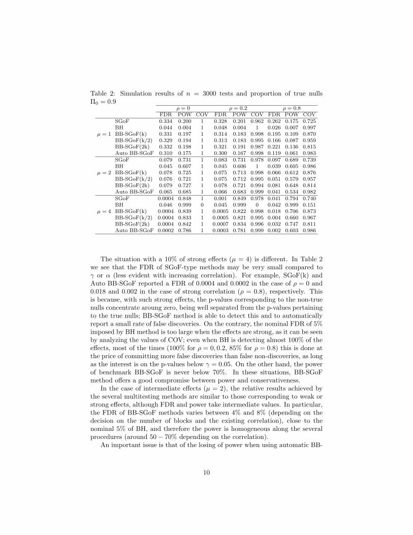
Table 2: Simulation results of n = 3000 tests and proportion of true nullsΠ0 = 0.9

ρ = 0 ρ = 0.2 ρ = 0.8FDR POW COV FDR POW COV FDR POW COV

SGoF 0.334 0.200 1 0.328 0.201 0.962 0.262 0.175 0.725BH 0.044 0.004 1 0.048 0.004 1 0.026 0.007 0.997

µ = 1 BB-SGoF(k) 0.331 0.197 1 0.314 0.183 0.998 0.195 0.109 0.870BB-SGoF(k/2) 0.329 0.194 1 0.313 0.183 0.995 0.166 0.087 0.959BB-SGoF(2k) 0.332 0.198 1 0.321 0.191 0.987 0.221 0.136 0.815Auto BB-SGoF 0.310 0.175 1 0.300 0.167 0.998 0.119 0.061 0.983SGoF 0.079 0.731 1 0.083 0.731 0.978 0.097 0.689 0.739BH 0.045 0.607 1 0.045 0.606 1 0.039 0.605 0.986

µ = 2 BB-SGoF(k) 0.078 0.725 1 0.075 0.713 0.998 0.066 0.612 0.876BB-SGoF(k/2) 0.076 0.721 1 0.075 0.712 0.995 0.051 0.579 0.957BB-SGoF(2k) 0.079 0.727 1 0.078 0.721 0.994 0.081 0.648 0.814Auto BB-SGoF 0.065 0.685 1 0.066 0.683 0.999 0.041 0.534 0.982SGoF 0.0004 0.848 1 0.001 0.849 0.978 0.041 0.794 0.740BH 0.046 0.999 0 0.045 0.999 0 0.042 0.999 0.151

µ = 4 BB-SGoF(k) 0.0004 0.839 1 0.0005 0.822 0.998 0.018 0.706 0.873BB-SGoF(k/2) 0.0004 0.833 1 0.0005 0.821 0.995 0.004 0.660 0.967BB-SGoF(2k) 0.0004 0.842 1 0.0007 0.834 0.996 0.032 0.747 0.811Auto BB-SGoF 0.0002 0.786 1 0.0003 0.781 0.999 0.002 0.603 0.986

The situation with a 10% of strong effects (µ = 4) is different. In Table 2we see that the FDR of SGoF-type methods may be very small compared toγ or α (less evident with increasing correlation). For example, SGoF(k) andAuto BB-SGoF reported a FDR of 0.0004 and 0.0002 in the case of ρ = 0 and0.018 and 0.002 in the case of strong correlation (ρ = 0.8), respectively. Thisis because, with such strong effects, the p-values corresponding to the non-truenulls concentrate aroung zero, being well separated from the p-values pertainingto the true nulls; BB-SGoF method is able to detect this and to automaticallyreport a small rate of false discoveries. On the contrary, the nominal FDR of 5%imposed by BH method is too large when the effects are strong, as it can be seenby analyzing the values of COV; even when BH is detecting almost 100% of theeffects, most of the times (100% for ρ = 0, 0.2, 85% for ρ = 0.8) this is done atthe price of committing more false discoveries than false non-discoveries, as longas the interest is on the p-values below γ = 0.05. On the other hand, the powerof benchmark BB-SGoF is never below 70%. In these situations, BB-SGoFmethod offers a good compromise between power and conservativeness.

In the case of intermediate effects (µ = 2), the relative results achieved bythe several multitesting methods are similar to those corresponding to weak orstrong effects, although FDR and power take intermediate values. In particular,the FDR of BB-SGoF methods varies between 4% and 8% (depending on thedecision on the number of blocks and the existing correlation), close to thenominal 5% of BH, and therefore the power is homogeneous along the severalprocedures (around 50− 70% depending on the correlation).

An important issue is that of the losing of power when using automatic BB-

10

SGoF compared to the benchmark method. From Table 2 we see that the powerof the auotmatic method relative BB-SGoF(k) is above 85%, with the case ofstrong correlation and weak effects as an exception, when it breaks down to 56%.In this case, automatic BB-SGoF deals unsuccessfully with the uncertainty onk together with the poor expectatives on the power, which are a consequence ofthe closeness of the alternative hypotheses to the nulls and the large correlation.One should note that a large value of ρ will result in a relatively large varianceand, consequently, in a lower number of rejections when applying BB-SGoFmethod. Finally, we see in Table 2 that coverage values of BB-SGoF are nicelylarge, although they become as low as 81% with strong correlation when thenumber of blocks is overestimated. For BB-SGoF(k), COV is always above 87%(99.8% when ρ ≤ 0.2), without reaching the nominal 95% in the case ρ = 0.8which holds asymptotically. Since the number of tests is large (n = 3000),one may wonder why the coverage of the benchmark method which makes useof the true number of blocks is below 95%. A possible explanation is foundin the departure of the simulated scenarios with respect to the beta-binomialassumption (Figure 1, bottom); we also mention that, with large correlation, alarger sample size n could be needed to reflect the asymptotic behaviour of agiven method. Coverages reported by the automatic BB-SGoF are above 98%regardless the correlation and, therefore, in practice it may be recommended asa conservative approach.

4.3 Case of Π0 = 0.67: 33% of effects

In Table 3 the results corresponding to a 33% of weak effects (Π0 = 0.67) aregiven. Compared to Table 2, it is seen that the FDR of all the methods decreases,while the power increases; this is because the existence of a larger amount ofnon-true nulls. As in Table 2, in Table 3 we see that nor SGoF neither BB-SGoFare controlling for FDR at any pre-specified level. Again, the FDR attained byBB-SGoF may be regarded as a suitable proportion of false discoveries given thesituation at hand; BB-SGoF(k), for example, reports a FDR of about 10− 13%with weak effects, but it goes down to about 3% and 0.01% with intermediateand strong effects respectively. The power of BB-SGoF method increases withthe effect level (from weak to strong) and it decreases as the correlation grows,similarly as in Table 2.

Compared to BH approach, BB-SGoF(k) reports a relative power of about8-13 with weak effects, being about 7-12 when comparing automatic BB-SGoFto BH; this reveals once more that BB-SGoF strategy may represent a largegain in power when the effect level is weak (true and non-true p-values wellmixed). When the effects are intermediate or strong, the situation is the oppo-site, according to the lower FDR of BB-SGoF. However, with strong effects forexample, the power of automatic BB-SGoF relative to BH is always above 84%,which again indicates a good balance between conservativeness and ability todetect true alternative hypotheses. On the other hand, conservativeness of BB-SGoF procedure may be assessed through the attained coverages; in this sense,benchmark BB-SGoF coverages are above 96% in all the situations (improving

11

Table 3: Simulation results of n = 3000 tests and proportion of true nullsΠ0 = 0.67


SGoF 0.135 0.301 1 0.135 0.302 1 0.124 0.301 0.901BH 0.036 0.023 1 0.032 0.023 1 0.024 0.031 1

µ = 1 BB-SGoF(k) 0.134 0.298 1 0.131 0.293 1 0.103 0.249 0.995BB-SGoF(k/2) 0.134 0.297 1 0.132 0.293 1 0.103 0.249 0.997BB-SGoF(2k) 0.135 0.299 1 0.133 0.297 1 0.111 0.269 0.979Auto BB-SGoF 0.129 0.286 1 0.128 0.284 1 0.097 0.233 0.997SGoF 0.032 0.826 1 0.032 0.826 1 0.034 0.823 0.932BH 0.033 0.831 1 0.033 0.831 1 0.031 0.832 0.961

µ = 2 BB-SGoF(k) 0.031 0.823 1 0.031 0.821 1 0.026 0.795 0.992BB-SGoF(k/2) 0.031 0.820 1 0.031 0.819 1 0.026 0.794 0.993BB-SGoF(2k) 0.032 0.824 1 0.032 0.823 1 0.029 0.807 0.979Auto BB-SGoF 0.028 0.805 1 0.028 0.803 1 0.024 0.776 0.995SGoF 0.0001 0.908 1 0.0001 0.907 1 0.003 0.902 0.933BH 0.033 0.999 0 0.033 0.999 0 0.032 0.999 0.011

µ = 4 BB-SGoF(k) 0.0001 0.903 1 0.0001 0.900 1 0.0004 0.864 0.994BB-SGoF(k/2) 0.0001 0.900 1 0.0001 0.898 1 0.0003 0.861 0.996BB-SGoF(2k) 0.0001 0.905 1 0.0001 0.903 1 0.001 0.881 0.978Auto BB-SGoF 0.0001 0.882 1 0.0001 0.879 1 0.0002 0.840 0.998

its results with 10% of effects, see Table 2), and this percentage increases to99.5% when considering automatic BB-SGoF. These figures may be as low as1% or even 0% for BH (strong effects), similarly as in Table 2, situations inwhich this method could be regarded as too anticonservative, at least as longas COV is concerned.

Regarding the power of automatic BB-SGoF relative to the benchmark BB-SGoF, from Table 3 we see that this rate is always above 94%, the worst situationbeing again the case with strongest correlation and weakest effects. This im-proves substantially the worst rate of 56% found from Table 2 and, therefore,the presence of a larger amount of non-true nulls is beneficial to the data-drivenBB-SGoF method. This improvement could be explained by the fact that, withµ = 1 and ρ = 0.8, the automatic number of blocks kN tends to be largerwith 33% of effects than with 10% (see Table 6 below) and, consequently, AutoBB-SGoF becomes more liberal.

4.4 Influence of the number of test (n)

As mentioned at the beginning of this Section, simulations with a lower numberof tests n = 500, 1000 were performed. In Table 4 we report the results corre-sponding to n = 500 in the case of no effects (complete null). The results inthis Table 4 are similar to those in Table 1 for the case n = 3000; all the meth-ods respect the nominal FDR of 5% but SGoF procedure for independent tests(which fail in the presence of correlation) and BB-SGoF when overestimatingthe number of blocks (it is anticonservative when ρ = 0.8). Results for n = 1000were roughly the same and they are not shown.

12

Table 4: Simulation results of n = 500 tests and proportion of true nulls Π0 = 1ρ = 0 ρ = 0.2 ρ = 0.8

SGoF 0.051 0.092 0.288BH 0.056 0.055 0.037BB-SGoF(k) 0.043 0.056 0.059BB-SGoF(k/2) 0.043 0.058 0.045BB-SGoF(2k) 0.041 0.070 0.136Auto BB-SGoF 0.013 0.017 0.025

In Table 5 we report the FDR, the power and the coverage of the severalmethods when the proportion of effects is 10% and n = 500. The featuresone can appreciate here are similar to those in Table 2. However, due to thesmaller number of tests, the FDR and power of BB-SGoF method are smaller.This is because the property of SGoF-type methods, for which the power is anincreasing function of n. According to this, the coverages of BB-SGoF get better;for example, for BB-SGoF(k) they are always above 93%, and this increases to98% for automatic BB-SGoF. These coverages may be very low for BH withstrong effects (similarly as in the case n = 3000), ranging from 11.6% in theindependent setting to 41.5% when ρ = 0.8.

Table 5: Simulation results of n = 500 tests and proportion of true nulls Π0 =0.9


SGoF 0.282 0.137 0.994 0.270 0.136 0.986 0.228 0.135 0.835BH 0.0425 0.012 1 0.050 0.013 1 0.023 0.016 0.997

µ = 1 BB-SGoF(k) 0.269 0.130 0.998 0.255 0.125 0.992 0.162 0.084 0.943BB-SGoF(k/2) 0.268 0.128 0.996 0.249 0.125 0.994 0.135 0.074 0.967BB-SGoF(2k) 0.272 0.132 0.996 0.261 0.123 0.991 0.185 0.106 0.909Auto BB-SGoF 0.219 0.093 1 0.209 0.089 0.998 0.095 0.050 0.989SGoF 0.053 0.623 0.999 0.057 0.622 0.995 0.077 0.603 0.861BH 0.044 0.607 1 0.045 0.607 1 0.042 0.609 0.972

µ = 2 BB-SGoF(k) 0.051 0.609 0.999 0.052 0.605 0.998 0.053 0.535 0.937BB-SGoF(k/2) 0.050 0.608 0.999 0.052 0.602 0.999 0.046 0.516 0.967BB-SGoF(2k) 0.051 0.613 0.999 0.054 0.611 0.997 0.062 0.566 0.913Auto BB-SGoF 0.039 0.537 1 0.040 0.539 0.999 0.037 0.455 0.982SGoF 0.0001 0.711 0.999 0.0006 0.711 0.995 0.022 0.699 0.869BH 0.044 0.999 0.116 0.045 0.999 0.130 0.042 0.999 0.415

µ = 4 BB-SGoF(k) 0.0001 0.695 0.999 0.0003 0.688 0.998 0.008 0.619 0.936BB-SGoF(k/2) 0.0001 0.692 0.999 0.0002 0.686 0.998 0.003 0.592 0.972BB-SGoF(2k) 9.573e-05 0.698 1 0.0004 0.696 0.997 0.011 0.655 0.917Auto BB-SGoF 9.924e-05 0.611 1 0.0001 0.609 0.999 0.001 0.519 0.988

The power of BB-SGoF(k) is about 5-11 times that of BH with weak effects,but it may be as low as 0.6 with strong effects and strong correlation. There-fore, performance of BB-SGoF relative to BH is poorer with a smaller n; this

13

reinforces the fact that BB-SGoF is more suitable for multitesting problems inhigh dimensions. Interestingly, the power of automatic BB-SGoF relative tobenchmark SGoF is above 60% in all the cases (the worst situation is againthat with weak effects and ρ = 0.8). Compared to the figures in Table 2, itis seen that a smaller number of tests is not beneficial for the automatic BB-SGoF criterion, for which the power relative to that of BB-SGoF(k) is 87% withn = 3000 (averaging the nine simulated scenarios) but only 81% with n = 500.

Results for n = 500 and 33% of effects were also obtained, as well as resultsfor the case n = 1000 with 10% or 33% of effects. These results (not shown)provided no other relevant evidences than those discussed above.

4.5 Automatic choice of the number of blocks

Automatic BB-SGoF implements a preliminary estimation of the number ofblocks of dependent p-values. Since this estimation is performed on the basis ofa conservative criterion (this is, to minimize the number of rejections), it doesnot lead in general to a precise approximation of the true k. In order to illustratethis point, we report in Table 6 the number of blocks detected on average (i.e.the mean of kN ) and its standard deviations (in brackets), in the case n = 3000.Recall that the true number of blocks is 20.

Table 6: Number of blocks detected on average and it standard deviations (inbrackets), n = 3000

µ = 1 µ = 2 µ = 4Π0 = 1 Π0 = 0.9 Π0 = 0.67 Π0 = 9 Π0 = 0.67 Π0 = 0.9 Π0 = 0.67

ρ = 0 6.43(11.30) 3.67(8.09) 1.93(4.51) 2.93(6.67) 1.25(1.23) 2.59(6.41) 1.25(1.84)ρ = 0.2 6.02(6.11) 4.63(5.45) 3.62(4.48) 3.02(4.51) 1.37(1.65) 3.04(4.19) 1.48(1.67)ρ = 0.8 6.09(5.46) 4.74(4.51) 7.62(6.39) 4.42(4.29) 5.71(5.54) 4.32(3.82) 5.35(5.03)

Results in Table 6 indicate that kN strongly underestimates the value of k,which is a result of the conservativeness of the underlying criterion. Note thatfewer blocks represents a situation with a stronger dependence structure and,consequently, a smaller number of rejections when applying BB-SGoF. Morespecifically, under the complete null, the average of kN is about 6, with a stan-dard deviation which decreases as the correlation increases. With weak effects,this average varies depending on the proportion of effects and the correlationdegree; the same happens with intermediate or strong effects. Roughly, it isseen that the average (also the standard deviation) of kN decreases as the ef-fect level changes from weak to strong, while it increases with the correlation.Therefore, it seems that kN is protecting BB-SGoF against situations in whichthe amount of rejections could be too large, due to the strength of the effectsor the low correlation. Interestingly, a larger proportion of effects results in asmaller value of kN when ρ = 0.2 but the opposite is true for ρ = 0.8, so nogeneral conclusion can be given to this regard. Overall, it can be said that kNplays an important role when looking for conservativeness but it is a biased,

14

highly dispersed estimator of the true number of blocks.

4.6 Tarone test

As mentioned in Section 2, Tarone (1979) introduced a test for the binomialmodel HT

0 : η = 0 against the beta-binomial alternative HT1 : η > 0. Here we

denote by η the correlation between Bernoulli outcomes I{ui≤γ} sharing the sameblock, which is different from ρ, the correlation between the normally distributed’gene expression levels’ in our simulations (but we have η = 0 when ρ = 0).In Figure 2 we show the rejection proportion (along the 1000 simulations) ofTarone’s test performed at level 0.05, in the case when the value of k is correctlyspecified, for several correlation degrees ρ = 0, 0.2, 0.8 (represented in the x axis)and n = 3000, 500 (top and bottom, respectively).

0.0 0.2 0.4 0.6 0.8

0.2

0.4

0.6

0.8

1.0

within−block correlation

reje

ctio

n pr

opor

tion

no effects10% strong effects33% strong effectslevel of the test: 0.05

(a) n = 3000

0.0 0.2 0.4 0.6 0.8

0.2

0.4

0.6

0.8

1.0


reje

ctio

n pr

opor

tion

10% weak effects33% weak effects10% intermediate effects33% intermediate effectslevel of the test: 0.05

(b) n = 3000

0.0 0.2 0.4 0.6 0.8

0.2

0.4

0.6

0.8


reje

ctio

n pr

opor

tion

no effects10% strong effects33% strong effectslevel of the test: 0.05

(c) n = 500

0.0 0.2 0.4 0.6 0.8

0.2

0.4

0.6

0.8


reje

ctio

n pr

opor

tion

10% weak effects33% weak effects10% intermediate effects33% intermediate effectslevel of the test: 0.05

(d) n = 500

Figure 2: Proportion of rejections of the Tarone’s test.

In Figure 2 we can see that, when ρ = 0, the rejection proportion is about5%, indicating that Tarone’s test respects the level well. As ρ departs from zero,

15

the rejection proportion grows, and the same happens when moving from thecase n = 500 to n = 1000; both features were of course expected. In general, thepower of Tarone’s test decreases as the proportion and/or the level of the effects(non-true nulls) increase; this suggests that the presence of effects introducesnoise when testing for correlation.

5 Main conclusions

BB-SGoF method may control the FWER in the weak sense even when theunderlying model is not beta-binomial. This suggests that the beta-binomialmodel may have enough flexibility to represent the correlation structure amongthe tests in practice. BB-SGoF method is also robust with respect to miss-specification of the number of existing blocks, although it becomes too liberalwhen this parameter is overestimated. The automatic BB-SGoF procedure per-forms well, with only a moderate loss of power (5 − 15%) with respect to thebenchmark version in most of the cases. However, when there is a small propor-tion (10%) of weak effects, this loss of power may be as large as 44%, particularlywhen the correlation within the blocks of tests is strong. Therefore, more ef-forts are needed to select the unknown number of blocks in an automatic (datadriven) way. Another interesting finding of our simulation study is the abilityof Tarone’s test to detect dependence in practice. When the null hypothesisof no correlation is accepted, application of original SGoF (rather than BB-SGoF) is recommended. As SGoF for independent tests, BB-SGoF method isliberal with respect to the FDR or the FWER, and this explains why it is ableto exhibit a good power in difficult situations where FWER and FDR control-ling procedures fail to detect non-true nulls (this is typically the case when thenumber of tests is large, and there is a small to moderate proportion of weakeffects). Furthermore, conservativeness of BB-SGoF has been assessed; morespecifically, BB-SGoF method ensures that, with large probability, the numberof false discoveries will not exceed the number of false non-discoveries (at leastwhen the focus is on the p-values below a given threshold), thus offering a goodcompromise between false discovery rate and power.

6 Acknowledgement

Work was supported by the Grant MTM2011-23204 (FEDER support included)of the Spanish Ministry of Science and Innovation.

References

[1] Benjamini, Y. and Hochberg, Y. (1995). Controlling the False DiscoveryRate: A Practical and Powerful Approach to Multiple Testing. Journal ofthe Royal Statistical Society Series B, 57, 289–300.

16

[2] Carvajal-Rodrıguez, A., de Una-Alvarez, J. and Rolan-Alvarez, E. (2009).A new multitest correction (SGoF) that increases its statistical power whenincreasing the number of tests. BMC Bioinformatics, 10, 1–14.

[3] de Una-Alvarez, J. (2011). On the statistical properties of SGoF multitest-ing method. Statistical Applications in Genetics and Molecular, 10, Issue1, Article 18.

[4] de Una-Alvarez, J. (2012). The Beta-Binomial SGoF method for multipledependent tests. Statistical Applications in Genetics and Molecular Biology,11, Issue 3, Article 14.

[5] Donoho, D. and Jin, J. (2004). Higher criticism for detecting sparse het-erogeneous mixtures. Annals of Statistics, 32, 962–994.

[6] Donoho, D. and Jin, J. (2008). Higher criticism thresholding: Optimalfeature selection when useful features are rare and weak. Proceedings ofNational Academy of Science 105, 14790–14795.

[7] Dudoit, S. and van der Laan, M. (2008). Multiple Testing Procedures withApplications to Genomics. New York: Springer.

[8] Genovese, C. and Wasserman, L. (2002). Operating characteristics andextensions of the FDR procedure. Journal of the Royal Statistical SocietyB, 64, 499–518.

[9] Genovese, C.and Wasserman, L. (2004). A stochastic process approach tofalse discovery control. Annals of Statistics 32, 1038–1061.

[10] Lehmann, E.L. and Romano, J.P. (2005). Generalizations of the familywiseerror rate. Annals of Statistics, 33, 1138–1154.

[11] Nichols, T. and Hayasaka, S. (2003). Controlling the familywise error ratein functional neuroimaging: a comparative review. Statistical Methods inMedical Research, 12, 419–446.

[12] R Core Team (2013). R: A language and environment for statistical com-puting. R Foundation for Statistical Computing, Vienna, Austria. URLhttp://www.R-project.org/.

[13] Storey, J.D. (2003). The positive false discovery rate: a Bayesian interpre-tation and the q-value.Annals of Statistics, 31, 2013–2035.

[14] Tarone, R.E.(1979). Testing the goodness of fit of the binomial distribution.Biometrika, 66, 585–590.

[15] van der Laan, M.J., Dudoit, S. and Pollard, K.S. (2004). Augmentationprocedures for control of the generalized family-wise error rate and tailprobabilities for the proportion of false positives. Statistical Applicationsin Genetics and Molecular Biology, 3, Article 15.

17

power, fdr and conservativeness of bb-sgof method for multiple

Documents