power flow studies - ee.unlv.edu
TRANSCRIPT

System Modeling and Power Flow Analysis
ECG 740
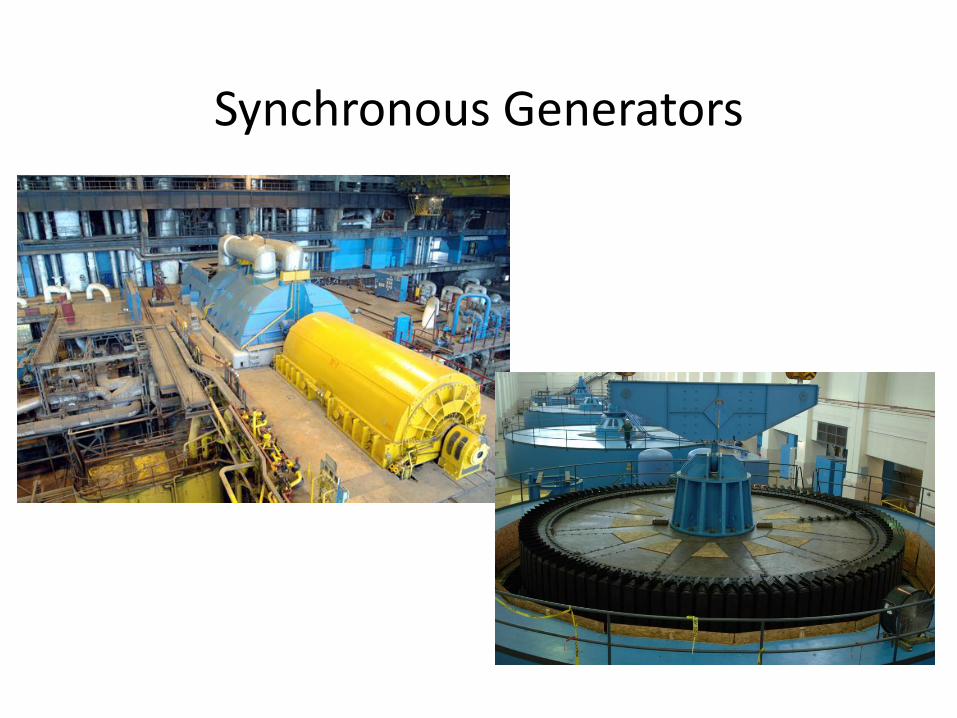
Synchronous Generators
Synchronous Generator Rating
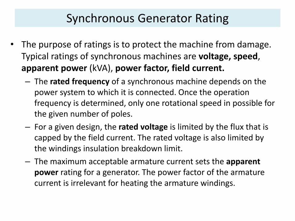
• The purpose of ratings is to protect the machine from damage. Typical ratings of synchronous machines are voltage, speed, apparent power (kVA), power factor, field current.
– The rated frequency of a synchronous machine depends on the power system to which it is connected. Once the operation frequency is determined, only one rotational speed in possible for the given number of poles.
– For a given design, the rated voltage is limited by the flux that is capped by the field current. The rated voltage is also limited by the windings insulation breakdown limit.
– The maximum acceptable armature current sets the apparent power rating for a generator. The power factor of the armature current is irrelevant for heating the armature windings.
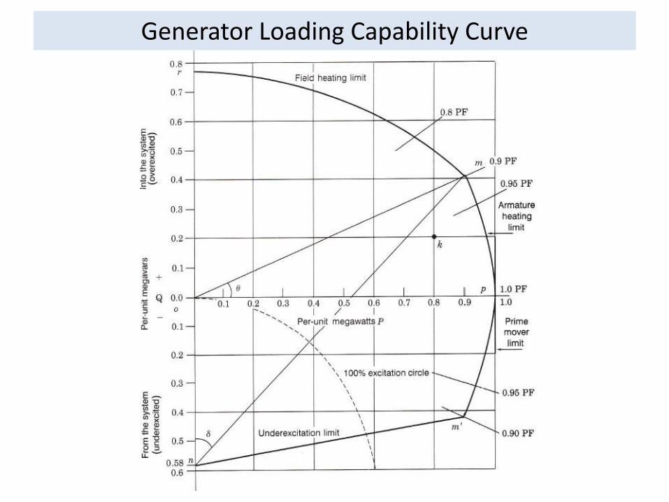
Generator Loading Capability Curve

Power Transformers
Transformer ratings: Voltage and Frequency
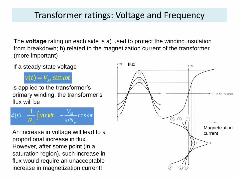
The voltage rating on each side is a) used to protect the winding insulation
from breakdown; b) related to the magnetization current of the transformer
(more important)
If a steady-state voltage
( ) sinMv t V t
is applied to the transformer’s
primary winding, the transformer’s
flux will be
( ) c) o1
s( M
p p
v t dV
t tN
tN
An increase in voltage will lead to a
proportional increase in flux.
However, after some point (in a
saturation region), such increase in
flux would require an unacceptable
increase in magnetization current!
flux
Magnetization
current

Transformer ratings: Voltage and Frequency
Therefore, the maximum applied voltage (and thus the rated voltage) is set by
the maximum acceptable magnetization current in the core.
We notice that the maximum flux is also related to the frequency:
maxmax
p
V
N
Therefore, to maintain the same maximum flux, a change in frequency (say, 50
Hz instead of 60 Hz) must be accompanied by the corresponding correction in
the maximum allowed voltage. This reduction in applied voltage with frequency
is called derating. As a result, a 50 Hz transformer may be operated at a 20%
higher voltage on 60 Hz if this would not cause insulation damage.

Transformer ratings: Apparent Power
The apparent power rating sets (together with the voltage rating) the
current through the windings. The current determines the i2R losses and,
therefore, the heating of the coils.
Overheating shortens the life of transformer’s insulation. Under any
circumstances, the temperature of the windings must be limited.
A typical power transformer rating would be OA/FA/FOA where • The OA (open-air) rating is the base power rating. • The FA (forced-air) rating is the power carrying capability when forced air
cooling (fans) are used. • The FOA (forced-oil-air) rating is the power carrying capability when forced
air cooling (fans) are used in addition to oil circulating pumps. Each cooling method provides nearly an additional 1/3 capability. For
example, a common substation transformer is rated at 21/28/35 MVA.
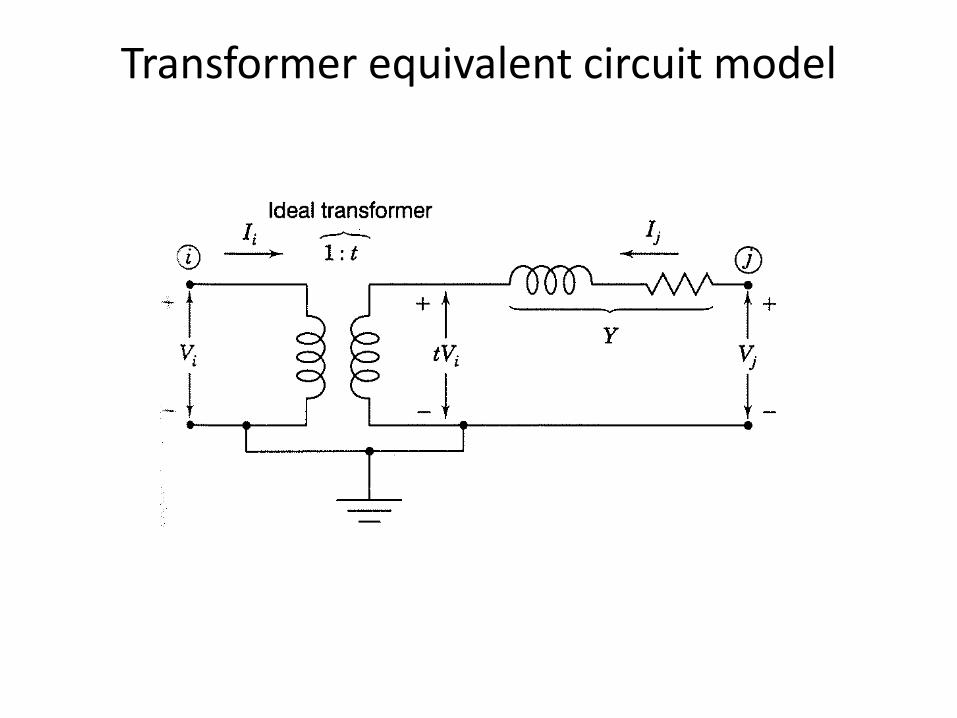
Transformer equivalent circuit model

Transmission Lines
10
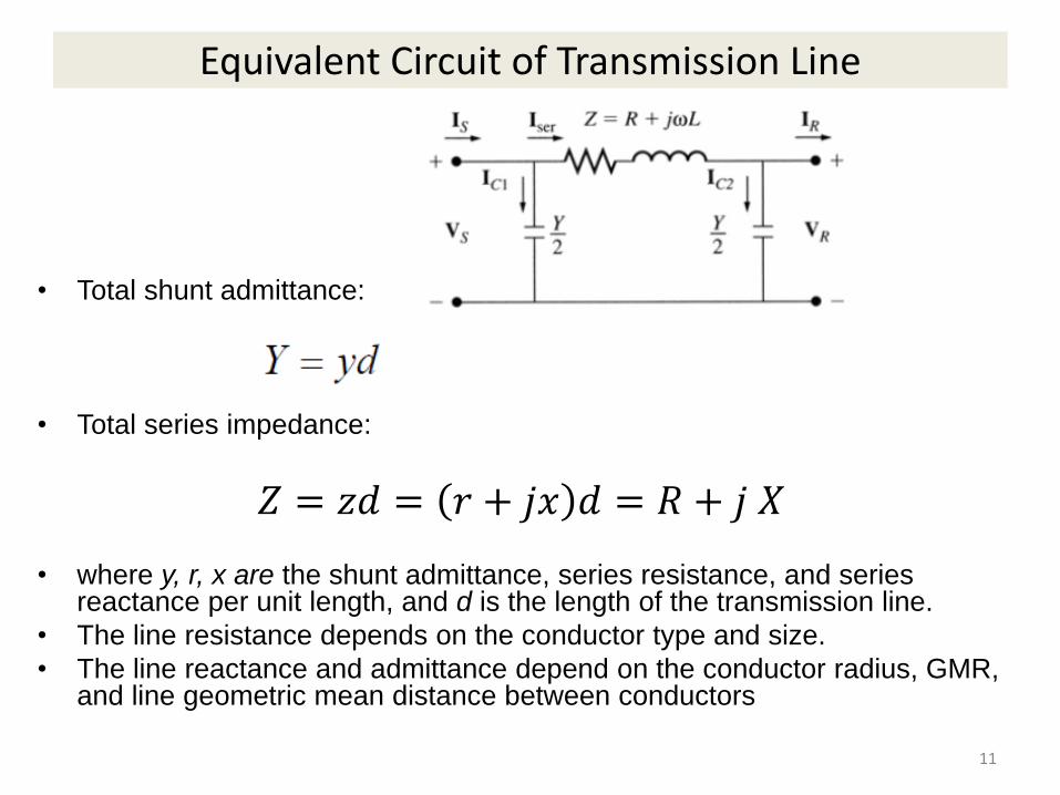
Equivalent Circuit of Transmission Line
• Total shunt admittance:
• Total series impedance:
𝑍 = 𝑧𝑑 = 𝑟 + 𝑗𝑥 𝑑 = 𝑅 + 𝑗 𝑋
• where y, r, x are the shunt admittance, series resistance, and series reactance per unit length, and d is the length of the transmission line.
• The line resistance depends on the conductor type and size.
• The line reactance and admittance depend on the conductor radius, GMR, and line geometric mean distance between conductors
11

Load Modeling in Power Flow Analysis
• ZIP model:
• For simplicity, we often represent the load by the constant power component (P,Q).
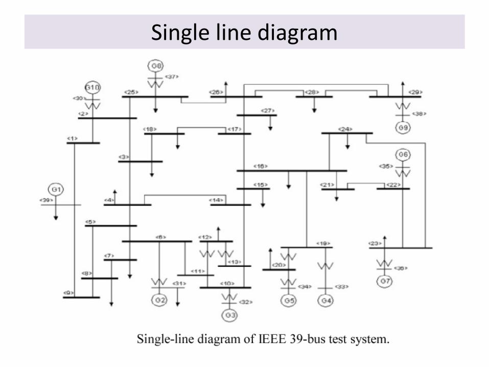
Single line diagram
Introduction to Power Flow
• A power flow study (load-flow study) is a steady-state analysis whose target is to determine the voltages, currents, and real and reactive power flows in a system under a given load conditions.
• The purpose of power flow studies is to plan ahead and account for various hypothetical situations. For example, if a transmission line is be taken off line for maintenance, can the remaining lines in the system handle the required loads without exceeding their rated values.
Power-flow analysis equations
11 12 13 14 1 1
21 22 23 24 2 2
31 32 33 34 3 3
41 42 43 44 4 4
Y Y Y Y V I
Y Y Y Y V I
Y Y Y Y V I
Y Y Y Y V I
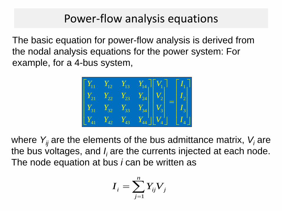
The basic equation for power-flow analysis is derived from
the nodal analysis equations for the power system: For
example, for a 4-bus system,
where Yij are the elements of the bus admittance matrix, Vi are
the bus voltages, and Ii are the currents injected at each node.
The node equation at bus i can be written as
n
j
jiji VYI1

Power-flow analysis equations
Relationship between per-unit real and reactive power
supplied to the system at bus i and the per-unit current
injected into the system at that bus:
where Vi is the per-unit voltage at the bus; Ii* - complex
conjugate of the per-unit current injected at the bus; Pi and Qi
are per-unit real and reactive powers. Therefore,
iiiii jQPIVS *
** /)(/)( iiiiiiii VjQPIVjQPI
n
j
ijij
n
j
jijiii VVYVYVjQP1
*
1
*

Power flow equations
Let
Then
Hence,
and
iiiijijij VVandYY ||||
)(||||||1
ijij
n
j
ijijii VVYjQP
)cos(||||||1
ijij
n
j
ijiji VVYP
)sin(||||||1
ijij
n
j
ijiji VVYQ

• There are 4 variables that are associated with each bus:
o P,
o Q,
o V,
o δ.
• Meanwhile, there are two power flow equations associated
with each bus.
• In a power flow study, two of the four variables are defined
an the other two are unknown. That way, we have the
same number of equations as the number of unknown.
• The known and unknown variables depend on the type of
bus.
Formulation of power-flow study

Each bus in a power system can be classified as one of three types:
1. Load bus (P-Q bus) – a buss at which the real and reactive
power are specified, and for which the bus voltage will be
calculated. All busses having no generators are load busses. In
here, V and δ are unknown.
2. Generator bus (P-V bus) – a bus at which the magnitude of the
voltage is defined and is kept constant by adjusting the field
current of a synchronous generator. We also assign real power
generation for each generator according to the economic
dispatch. In here, Q and δ are unknown
3. Slack bus (swing bus) – a special generator bus serving as the
reference bus. Its voltage is assumed to be fixed in both
magnitude and phase (for instance, 10˚ pu). In here, P and Q
are unknown.
Formulation of power-flow study

Formulation of power-flow study
• Note that the power flow equations are non-linear, thus cannot
be solved analytically. A numerical iterative algorithm is
required to solve such equations. A standard procedure
follows:
1. Create a bus admittance matrix Ybus for the power system;
2. Make an initial estimate for the voltages (both magnitude
and phase angle) at each bus in the system;
3. Substitute in the power flow equations and determine the
deviations from the solution.
4. Update the estimated voltages based on some commonly
known numerical algorithms (e.g., Newton-Raphson or
Gauss-Seidel).
5. Repeat the above process until the deviations from the
solution are minimal.
Example
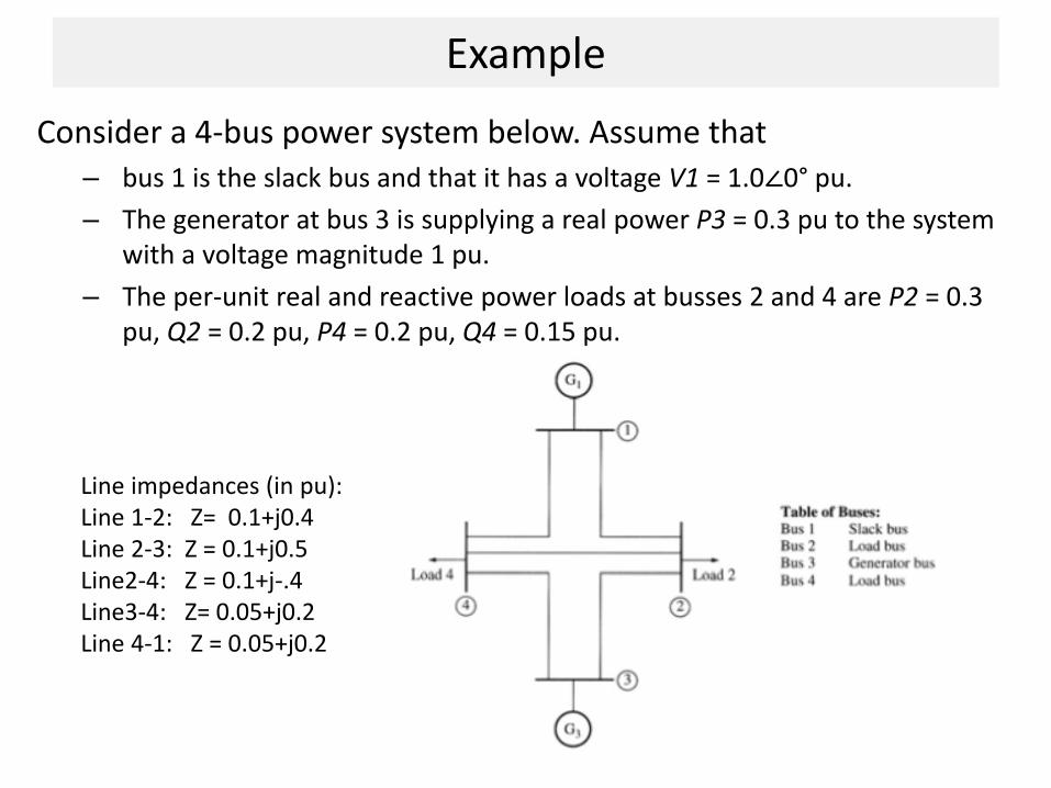
Consider a 4-bus power system below. Assume that
– bus 1 is the slack bus and that it has a voltage V1 = 1.0∠0° pu.
– The generator at bus 3 is supplying a real power P3 = 0.3 pu to the system with a voltage magnitude 1 pu.
– The per-unit real and reactive power loads at busses 2 and 4 are P2 = 0.3 pu, Q2 = 0.2 pu, P4 = 0.2 pu, Q4 = 0.15 pu.
Line impedances (in pu): Line 1-2: Z= 0.1+j0.4 Line 2-3: Z = 0.1+j0.5 Line2-4: Z = 0.1+j-.4 Line3-4: Z= 0.05+j0.2 Line 4-1: Z = 0.05+j0.2

Example (cont.)
• Y-bus matrix (refer to example in book)
• Power flow solution:
• By knowing the node voltages, the power flow (both active and reactive) in each branch of the circuit can easily be calculated.

Newton-Raphson Algorithm
• The key idea behind Newton-Raphson is to use sequential linearization
• Consider the case of one variable:
General form of problem: Find an such that
( ) 0
x
f x

Newton-Raphson Method (scalar)
( )
( )
( ) ( ) ( ) ( ) ( )
2 2( ) ( )
2
1. Represent by a Taylor series about the
current guess . Write for the deviation
from :
( ) ( ) ( )
1( )
2
higher order terms.
v v v v v
v v
f
x x
x
dff x x f x x x
dx
d fx x
dx

Newton-Raphson Method, cont’d
( ) ( ) ( ) ( ) ( )
( )
1( ) ( ) ( )
2. Approximate by neglecting all terms
except the first two
( ) ( ) ( )
3. Set linear approximation equal to zero
and solve for
( ) ( )
4. Sol
v v v
v
v v v
f
dff x x f x x x
dx
x
dfx x f x
dx
( 1) ( ) ( )
ve for a new estimate of solution:
v v vx x x

Newton-Raphson - Example
2
1( ) ( ) ( )
( ) ( ) 2
( )
( 1) ( ) ( )
( 1) ( ) ( ) 2
( )
Use Newton-Raphson to solve ( ) 0,
where: ( )= 2.
The iterative update is:
( ) ( )
1(( ) 2)
2
1(( ) 2).
2
v v v
v v
v
v v v
v v v
v
f x
f x x
dfx x f x
dx
x xx
x x x
x x xx

Newton-Raphson - Example (cont’d)
( 1) ( ) ( ) 2
( )
(0)
( ) ( ) ( )
3 3
6
1(( ) 2)
2
Matlab code: x=x0; x = x-(1/(2*x))*(x^2-2).
Guess 1. Iteratiting, we get:
( )
0 1 1 0.5
1 1.5 0.25 0.08333
2 1.41667 6.953 10 2.454 10
3 1.41422 6.024 10
v v v
v
v v v
x x xx
x
x f x x

Sequential Linear Approximations
Function is f(x) = x2 - 2. Solutions to f(x) = 0 are points where f(x) intersects x axis.
At each iteration the N-R method uses a linear approximation to determine the next value for x

Newton-Raphson Comments
• When close to the solution the error decreases quite quickly -- method has what is known as “quadratic” convergence:
– number of correct significant figures roughly doubles at each iteration.
• f(x(v)) is known as the “mismatch,” which we would like to drive to zero.
• Stopping criteria is when f(x(v)) <

Newton-Raphson Comments
• Results are dependent upon the initial guess. What if we had guessed x(0) = 0, or x(0) = -1?
• A solution’s region of attraction (ROA) is the set of initial guesses that converge to the particular solution.
• The ROA is often hard to determine.

Multi-Variable Newton-Raphson
1 1
2 2
Next we generalize to the case where is an -
dimension vector, and ( ) is an -dimensional
vector function:
( )
( )( )
( )
Again we seek a solution of ( ) 0.
n n
n
n
x f
x f
x f
x
f x
x
xx f x
x
f x

Multi-Variable Case, cont’d
i
1 11 1 1 2
1 2
1
1 21 2
The Taylor series expansion is written for each f ( )
( ) ( ) ( ) ( )
( ) higher order terms
( ) ( ) ( ) ( )
( ) higher order terms
nn
n nn n
nn
n
f ff x x f x x x x x
x x
fx x
x
f ff x x f x x x x x
x x
fx x
x
x

Multi-Variable Case, cont’d
1 1 1
1 21 1
2 2 22 2
1 2
1 2
This can be written more compactly in matrix form
( ) ( ) ( )
( )
( ) ( ) ( )( )( )
( )
( ) ( ) ( )
n
n
nn n n
n
f f f
x x xf x
f f ff x
x x x
ff f f
x x x
x x x
x
x x xxf x +Δx
x
x x x
higher order terms
nx

Jacobian Matrix
1 1 1
1 2
2 2 2
1 2
1 2
The by matrix of partial derivatives is known
as the Jacobian matrix, ( )
( ) ( ) ( )
( ) ( ) ( )( )
( ) ( ) ( )
n
n
n n n
n
n n
f f f
x x x
f f f
x x x
f f f
x x x
J x
x x x
x x xJ x
x x x
Multi-Variable N-R Procedure
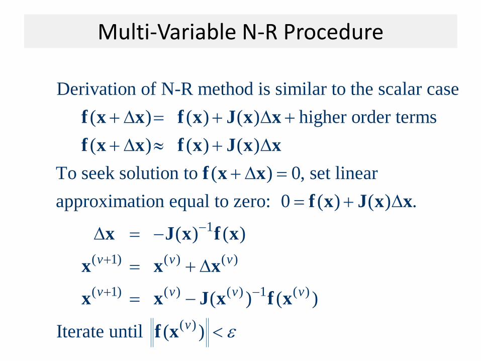
Derivation of N-R method is similar to the scalar case
( ) ( ) ( ) higher order terms
( ) ( ) ( )
To seek solution to ( ) 0, set linear
approximation equal to zero: 0 ( ) ( ) .
f x x f x J x x
f x x f x J x x
f x x
f x J x x
x1
( 1) ( ) ( )
( 1) ( ) ( ) 1 ( )
( )
( ) ( )
( ) ( )
Iterate until ( )
v v v
v v v v
v
J x f x
x x x
x x J x f x
f x

Multi-Variable - Example
1
2
2 21 1 2
2 22 1 2 1 2
1 1
1 2
2 2
1 2
Solve for = such that ( ) 0 where
( ) 2 8
( ) 4
First symbolically determine the Jacobian
( ) ( )
( ) =
( ) ( )
x
x
f x x x
f x x x x x
f fx x
x x
f fx x
x x
x f x
J x

Multi-variable Example, cont’d
1 2
1 2 1 2
11 1 2 1
2 1 2 1 2 2
4 2( ) =
2 2
4 2 ( )Then
2 2 ( )
Matlab code: x1=x10; x2=x20;
f1=2*x1^2+x2^2-8;
f2=x1^2-x2^2+x1*x2-4;
J = [4*x1 2*x2; 2*x1+x2 x1-2*x2];
[x1;x2] =
x x
x x x x
x x x f
x x x x x f
J x
x
x
[x1;x2]-inv(J)*[f1;f2].

Multi-variable Example, cont’d
(0)
1(1)
1(2)
( )
1Initial guess
1
1 4 2 5 2.1
1 3 1 3 1.3
2.1 8.40 2.60 2.51 1.8284
1.3 5.50 0.50 1.45 1.2122
At each iteration we check ( ) to see if it
x
x
x
f x
(2)
is
0.1556below our specified tolerance : ( )
0.0900
If = 0.2 then done. Otherwise continue iterating.
f x

Power Balance Equations
1
1
For convenience, write:
( ) ( cos sin )
( ) ( sin cos )
The power balance equations are then:
( ) 0
( ) 0
n
i i k ik ik ik ikk
n
i i k ik ik ik ikk
i Gi Di
i Gi Di
P V V G B
Q V V G B
P P P
Q Q Q
x
x
x
x

Power Flow Variables
2
n
2
Assume the slack bus is the first bus (with a fixed
voltage angle/magnitude). We then need to determine
the voltage angle/magnitude at the other buses.
We must solve ( ) , where:
n
V
V
f x 0
x
2 2 2
2 2 2
( )
( )( )
( )
( )
G D
n Gn Dn
G D
n Gn Dn
P P P
P P P
Q Q Q
Q Q Q
x
xf x
x
x

N-R Power Flow Solution
(0)
( )
( 1) ( ) ( ) 1 ( )
The power flow is solved using the same procedure
discussed previously for general equations:
For 0; make an initial guess of ,
While ( ) Do
[ ( )] ( )
1
End
v
v v v v
v
v v
x x
f x
x x J x f x

Power Flow Jacobian Matrix
1 1 1
1 2 2 2
2 2 2
1 2 2 2
2 2 2 2 2 2
1 2
The most difficult part of the algorithm is determining
and factorizing the Jacobian matrix, ( )
( ) ( ) ( )
( ) ( ) ( )( )
( ) ( )
n
n
n n n
f f f
x x x
f f f
x x x
f f f
x x x
J x
x x x
x x xJ x
x x2 2
( )n
x

Power Flow Jacobian Matrix, cont’d
1
Jacobian elements are calculated by differentiating
each function, ( ), with respect to each variable.
For example, if ( ) is the bus real power equation
( ) ( cos sin )
i
i
n
i i k ik ik ik ik Gik
f x
f x i
f x V V G B P P
1
( ) ( sin cos )
( ) ( sin cos ) ( )
Di
ni
i k ik ik ik iki k
k i
ii j ij ij ij ij
j
fx V V G B
fx V V G B j i

Two Bus Newton-Raphson - Example
Line Z = 0.1j
One Two 1.000 pu 1.000 pu
200 MW
100 MVR
0 MW
0 MVR
For the two bus power system shown below, use the Newton-Raphson power flow to determine the voltage magnitude and angle at bus two. Assume that bus one is the slack and SBase = 100 MVA.
2
2
10 10Unkown: , Also,
10 10bus
j j
V j j
x Y

Two Bus Example, cont’d
1
1
General power balance equations:
( cos sin ) 0
( sin cos ) 0
For bus two, the power balance equations are
(load real power is 2.0 per unit,
while react
n
i k ik ik ik ik Gi Dik
n
i k ik ik ik ik Gi Dik
V V G B P P
V V G B Q Q
2 1 2
22 1 2 2
ive power is 1.0 per unit):
(10sin ) 2.0 0
( 10cos ) (10) 1.0 0
V V
V V V

Two Bus Example, cont’d
2 2 2
22 2 2 2
2 2
2 2
2 2
2 2
2 2 2
2 2 2 2
( ) 2.0 (10sin ) 2.0
( ) 1.0 ( 10cos ) (10) 1.0
Now calculate the power flow Jacobian
( ) ( )
( )
( ) ( )
10 cos 10sin
10 sin 10cos 20
P V
Q V V
P Px x
V
Q Qx x
V
V
V V
x
x
J x

Two Bus Example, First Iteration
(0)2(0)
(0)2
(0) (0)2 2
(0)
2(0) (0) (0)2 2 2
(0) (0) (0)2 2 2(0)
(0) (0)2 2
0For 0, guess . Calculate:
1
(10sin ) 2.0 2.0( )
1.0( 10cos ) (10) 1.0
10 cos 10sin( )
10 sin 10cos
vV
V
V V
V
V
x
f x
J x(0) (0)2 2
1(1)
10 0
0 1020
0 10 0 2.0 0.2Solve
1 0 10 1.0 0.9
V
x
Two Bus Example, Next Iterations
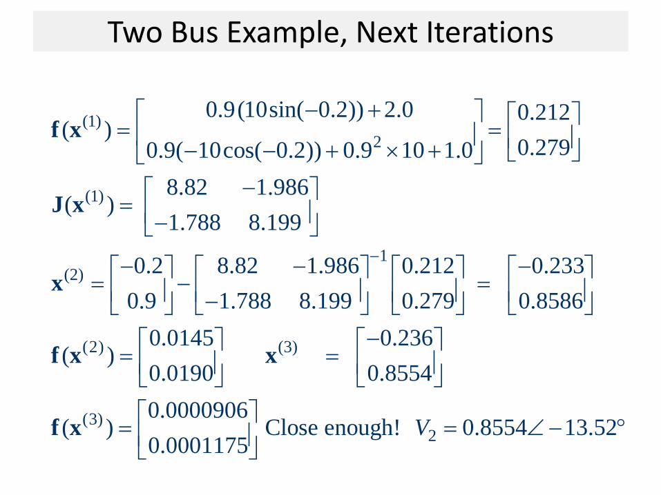
(1)
2
(1)
1(2)
0.9(10sin( 0.2)) 2.0 0.212( )
0.2790.9( 10cos( 0.2)) 0.9 10 1.0
8.82 1.986( )
1.788 8.199
0.2 8.82 1.986 0.212 0.233
0.9 1.788 8.199 0.279 0.8586
(
f x
J x
x
f(2) (3)
(3)2
0.0145 0.236)
0.0190 0.8554
0.0000906( ) Close enough! 0.8554 13.52
0.0001175V
x x
f x

Two Bus Solved Values
Line Z = 0.1j
One Two 1.000 pu 0.855 pu
200 MW
100 MVR
200.0 MW
168.3 MVR
-13.522 Deg
200.0 MW 168.3 MVR
-200.0 MW-100.0 MVR
Once the voltage angle and magnitude at bus 2 are known we can calculate all the other system values, such as the line flows and the generator real and reactive power output

Two Bus Case Low Voltage Solution
(0)
(0) (0)2 2
(0)
(0) (0) (02 2 2
This case actually has two solutions! The second
"low voltage" is found by using a low initial guess.
0Set 0, guess . Calculate:
0.25
(10sin ) 2.0
( )
( 10cos )
v
V
V V
x
f x2)
(0) (0) (0)2 2 2(0)
(0) (0) (0) (0)2 2 2 2
2
0.875(10) 1.0
10 cos 10sin 2.5 0( )
0 510 sin 10cos 20
V
V V
J x

Low Voltage Solution, cont'd
1(1)
(2) (2) (3)
0 2.5 0 2 0.8Solve
0.25 0 5 0.875 0.075
1.462 1.42 0.921( )
0.534 0.2336 0.220
x
f x x x
Line Z = 0.1j
One Two 1.000 pu 0.261 pu
200 MW
100 MVR
200.0 MW
831.7 MVR
-49.914 Deg
200.0 MW
831.7 MVR
-200.0 MW
-100.0 MVR
Low voltage solution

Two Bus Region of Convergence
Graph shows the region of convergence for different initial guesses of bus 2 angle (hor. axis) and magnitude (vertical axis).
Red region converges to the high voltage solution, while the yellow region converges to the low voltage solution
Maximum of 15
iterations

Solving Large Power Systems
Most difficult computational task is inverting the Jacobian matrix (or solving the update equation): – factorizing a full matrix is an order n3 operation,
meaning the amount of computation increases with the cube of the size of the problem.
– this amount of computation can be decreased substantially by recognizing that since Ybus is a sparse matrix, the Jacobian is also a sparse matrix.
– using sparse matrix methods results in a computational order of about n1.5.
– this is a substantial savings when solving systems with tens of thousands of buses.

Decoupled Power Flow
( ) ( )
( ) ( )( )
( )( ) ( ) ( )
( )2 2 2
( )
( )
Standard form of the Newton-Raphson update:
( )( )
( )
( )
where ( ) .
( )
Note
v v
v vv
vv v v
vD G
v
vn Dn Gn
P P P
P P P
P P
θθ V P xf x
Q xVQ Q
θ V
x
P x
x
that changes in angle and voltage magnitude
both affect (couple to) real and reactive power.

Decoupling Approximation
( ) ( )
( )
( ) ( )( )
( ) ( ) ( )
Usually the off-diagonal matrices, and
are small. Therefore we approximate them as zero:
( )( )
( )
Then the update c
v v
v
v vv
v v v
P Q
V θ
P0
θ P xθf x
Q Q xV0
V
1 1( ) ( )( )( ) ( ) ( )
an be decoupled into two separate updates:
( ), ( ).v v
vv v v
P Qθ P x V Q x
θ V
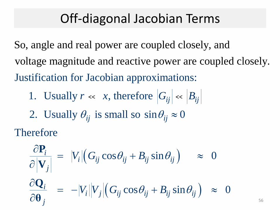
Off-diagonal Jacobian Terms
So, angle and real power are coupled closely, and
voltage magnitude and reactive power are coupled cl
Justification for Jacobian approximations:
1. Usually , therefore
2. U
os
su
ely.
ally is s
ij ij
ij
r x G B
mall so sin 0
Therefore
cos sin 0
cos sin 0
ij
ii ij ij ij ij
j
ii j ij ij ij ij
j
V G B
V V G B
P
V
Q
θ 56
<< <<

Fast Decoupled Power Flow
• By further approximating the Jacobian we obtain a typically reasonable approximation that is independent of the voltage magnitudes/angles.
• This means the Jacobian need only be built and factorized once.
• This approach is known as the fast decoupled power flow (FDPF)
• FDPF uses the same mismatch equations as standard power flow so it should have same solution if it converges
• The FDPF is widely used, particularly when we only need an approximate solution.

FDPF Approximations
( ) 1 ( ) 1 ( )
( ) 1 ( ) 1 ( )
The FDPF makes the following approximations:
1. 0
2. 1 (for some occurrences),
3. sin 0 cos 1
Then: {| | } ( ),
{| | } ( )
Where is just the imaginary pa
ij
i
ij ij
v v v
v v v
G
V
diag
diag
θ B V P x
V B V Q x
B bus bus bus
bus
( )
rt of the ,
except the slack bus row/column are omitted. That is,
is , but with the slack bus row and column deleted.
Sometimes approximate {| | } by identity. v
j
diag
Y G B
B B
V

FDPF Three Bus Example
Line Z = j0.07
Line Z = j0.05 Line Z = j0.1
One Two
200 MW
100 MVR
Three 1.000 pu
200 MW
100 MVR
Use the FDPF to solve the following three bus system
34.3 14.3 20
14.3 24.3 10
20 10 30
bus j
Y

FDPF Three Bus Example, cont’d
1
(0)(0)2 2
3 3
34.3 14.3 2024.3 10
14.3 24.3 1010 30
20 10 30
0.0477 0.0159
0.0159 0.0389
Iteratively solve, starting with an initial voltage guess
0 1
0 1
bus j
V
V
Y B
B
(1)2
3
0 0.0477 0.0159 2 0.1272
0 0.0159 0.0389 2 0.1091
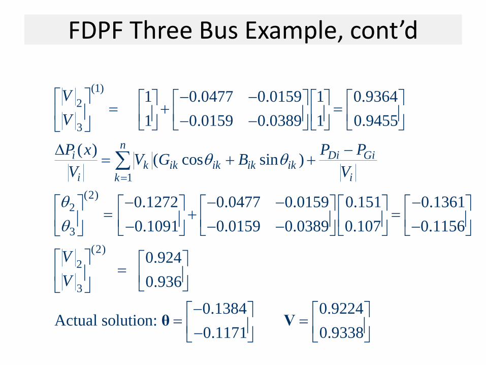
FDPF Three Bus Example, cont’d
(1)
2
3
1
(2)2
3
1 0.0477 0.0159 1 0.9364
1 0.0159 0.0389 1 0.9455
( )( cos sin )
0.1272 0.0477 0.0159
0.1091 0.0159 0.0389
ni Di Gi
k ik ik ik iki ik
V
V
P x P PV G B
V V
(2)
2
3
0.151 0.1361
0.107 0.1156
0.924
0.936
0.1384 0.9224Actual solution:
0.1171 0.9338
V
V
θ V

Assignment:
• Verify the solution on Example 6A in your book using PowerWorld software.