power generation scheduling - ntnuhuse/thesis.pdfisbn 82-471-0351-6 issn 0802-3271 power generation...
TRANSCRIPT

ISBN 82-471-0351-6 ISSN 0802-3271
Power Generation SchedulingA free market based procedure with
reserve constraints included
by
Einar Ståle Huse
A thesis submitted to:
The Norwegian University of Science and TechnologyFaculty of Electrical Engineering and Telecommunications
Department of Electrical Power Engineering
in partial fulfilment of the requirements for the degree:Doktor ingeniør
Academic advisers:Professor Hans H. Faanes (NTNU)
Professor Arne Johannesen (NTNU)


i
3UHIDFHThis thesis is submitted in partial fulfillment of the requirements for the degree of Doktor
Ingeniør at the Department of Electrical Power Engineering at the Norwegian University
of Science and Technology (NTNU).
The work was initiated in 1995, and is funded by the Research Council of Norway.
I would like to thank my supervisors Professor Hans H. Faanes and Professor Arne
Johannesen. Professor Hans H. Faanes has been my principal supervisor.
I would also like to thank colleagues at SINTEF Energy Research for useful discussions
about the topic.
Trondheim, November 1998
Einar Ståle Huse

ii

iii
6XPPDU\This thesis deals with the short-term scheduling of electric power generation in a com-
petitive market. This involves determination of start-ups and shut-downs, and produc-
tion levels of all units in all hours of the optimization period, considering unit
characteristics and system restrictions. The unit characteristics and restrictions that are
handled are: Minimum and maximum production levels, fuel cost function, start-up
costs, minimum up time and minimum down time. The system restrictions handled are
power balance (supply equal to demand in all hours) and spinning reserve requirement.
This thesis has two main contributions:
1. A new organization of an hourly electric power market, that simultaneously sets the
price of both energy and reserve power is proposed. A power exchange is used as a
trading place for electricity. The responsibilities of the power exchange is to balance
supply and demand bids, and to secure enough spinning reserve. Routines for bid-
ding and market clearing are developed.
2. A computer program that simulates the proposed electricity market has been imple-
mented. This program can also be used as a new method for solving the single owner
generation scheduling problem. Simulations show excellent performance; both low
computation time and good production schedules (i.e. low production cost).
The main simplifications that are applied:
1. Network restrictions neglected
2. Bid calculation by the units is based on a price forecast for the near future (24-168
hours). The units use only the expected value of future prices and treat them as if
they were deterministic
3. Emphasis has been set on the thermal units
With the proposed market, all optimization is done locally, by each generator. This
means that each optimization problem is small and can easily be solved. The tasks of the
power exchange are well defined, and involves no optimization. It is just the simple
matching of supply and demand bids.
A computer program simulating this market is developed, and used on several test cases.
This program, called SimCom (6LPulated &RPpetition), can also be used to solve the
single owner scheduling problem. and the solutions by this program are very good (i.e.

iv
low schedule cost). Results from three different test cases are reported. The cases vary
in number of units (9 to 110 units) and optimization period (24 and 168 hours). SimCom
has shown excellent performance, schedule cost has been near-optimal, and very good
compared to other optimization techniques. Computation time is at the same level as
Lagrangian Relaxation.
Simulations show that it is possible to reach efficient schedules through the proposed
electricity market.

v
&RQWHQWV
3UHIDFH���������������������������������������������������������������������������������������������������������������������������L
6XPPDU\���������������������������������������������������������������������������������������������������������������������LLL
&RQWHQWV �����������������������������������������������������������������������������������������������������������������������Y
1RWDWLRQ����������������������������������������������������������������������������������������������������������������������� L[
&KDSWHU��,QWURGXFWLRQ��������������������������������������������������������������������������������������������������������������
1.1 Background . . . . . . . . . . . . . . . . . . . . . . . . . . . . . . . . . . . . . . . . . . . . . . . . . .1
1.2 Objectives and scope of work . . . . . . . . . . . . . . . . . . . . . . . . . . . . . . . . . . . .1
1.3 Limitations . . . . . . . . . . . . . . . . . . . . . . . . . . . . . . . . . . . . . . . . . . . . . . . . . . .2
1.4 Organization of the thesis. . . . . . . . . . . . . . . . . . . . . . . . . . . . . . . . . . . . . . . .2
&KDSWHU��3UREOHP�GHILQLWLRQ��VKRUW�WHUP�VFKHGXOLQJ������������������������������������������������������������
2.1 Introduction . . . . . . . . . . . . . . . . . . . . . . . . . . . . . . . . . . . . . . . . . . . . . . . . . .5
2.2 Goal . . . . . . . . . . . . . . . . . . . . . . . . . . . . . . . . . . . . . . . . . . . . . . . . . . . . . . . .6
2.3 Global constraints. . . . . . . . . . . . . . . . . . . . . . . . . . . . . . . . . . . . . . . . . . . . . .6
2.3.1 Power balance . . . . . . . . . . . . . . . . . . . . . . . . . . . . . . . . . . . . . . . . . . . .6
2.3.2 Spinning reserve requirements . . . . . . . . . . . . . . . . . . . . . . . . . . . . . . .6
2.3.3 Transmission/distribution network influences . . . . . . . . . . . . . . . . . . .6
2.4 Unit constraints and cost functions . . . . . . . . . . . . . . . . . . . . . . . . . . . . . . . .7
2.5 Mathematical formulation . . . . . . . . . . . . . . . . . . . . . . . . . . . . . . . . . . . . . . .7
2.5.1 Cost functions used in this thesis . . . . . . . . . . . . . . . . . . . . . . . . . . . . .8
&KDSWHU��0DUNHW�VROXWLRQV �����������������������������������������������������������������������������������������������������
3.1 Introduction . . . . . . . . . . . . . . . . . . . . . . . . . . . . . . . . . . . . . . . . . . . . . . . . .11
3.1.1 The centralized scheduling model . . . . . . . . . . . . . . . . . . . . . . . . . . .11
3.1.2 The Bilateral model . . . . . . . . . . . . . . . . . . . . . . . . . . . . . . . . . . . . . .12
3.1.3 The Coordinated Multilateral Trade model . . . . . . . . . . . . . . . . . . . .12

vi
3.2 Norway, Sweden and Finland . . . . . . . . . . . . . . . . . . . . . . . . . . . . . . . . . . .14
3.2.1 The Nordic electricity market . . . . . . . . . . . . . . . . . . . . . . . . . . . . . . .15
3.3 United Kingdom. . . . . . . . . . . . . . . . . . . . . . . . . . . . . . . . . . . . . . . . . . . . . .19
3.3.1 The UK electricity system . . . . . . . . . . . . . . . . . . . . . . . . . . . . . . . . .19
3.3.2 The electricity market in England and Wales . . . . . . . . . . . . . . . . . . .20
3.4 The Californian electricity system . . . . . . . . . . . . . . . . . . . . . . . . . . . . . . . .23
3.4.1 The electricity market in California . . . . . . . . . . . . . . . . . . . . . . . . . .24
3.5 The electricity industry in South America . . . . . . . . . . . . . . . . . . . . . . . . . .25
3.5.1 The Argentinian electricity law . . . . . . . . . . . . . . . . . . . . . . . . . . . . .26
3.6 Differences and similarities of the market solutions . . . . . . . . . . . . . . . . . .27
&KDSWHU��'HFHQWUDOL]HG�RSWLPL]DWLRQ ������������������������������������������������������������������������������������
4.1 Introduction . . . . . . . . . . . . . . . . . . . . . . . . . . . . . . . . . . . . . . . . . . . . . . . . .29
4.1.1 Perfect competition . . . . . . . . . . . . . . . . . . . . . . . . . . . . . . . . . . . . . . .29
4.2 Shortcomings of the Nordic electricity market . . . . . . . . . . . . . . . . . . . . . .30
4.3 Proposal of a new electricity market . . . . . . . . . . . . . . . . . . . . . . . . . . . . . .31
4.3.1 Information . . . . . . . . . . . . . . . . . . . . . . . . . . . . . . . . . . . . . . . . . . . . .31
4.3.2 Network regime . . . . . . . . . . . . . . . . . . . . . . . . . . . . . . . . . . . . . . . . .32
4.3.3 The Power Exchange . . . . . . . . . . . . . . . . . . . . . . . . . . . . . . . . . . . . .33
4.3.4 Optimization by the single firm . . . . . . . . . . . . . . . . . . . . . . . . . . . . .36
4.3.5 Quantity determination with price on energy and reserve power. . . .41
4.3.6 Market clearing . . . . . . . . . . . . . . . . . . . . . . . . . . . . . . . . . . . . . . . . . .42
4.3.7 Payments for deviation from preferred production, p*. . . . . . . . . . . .46
4.4 Bilateral trade . . . . . . . . . . . . . . . . . . . . . . . . . . . . . . . . . . . . . . . . . . . . . . . .46
4.5 Bid calculation for hydro units. . . . . . . . . . . . . . . . . . . . . . . . . . . . . . . . . . .47
4.6 Practical implementation . . . . . . . . . . . . . . . . . . . . . . . . . . . . . . . . . . . . . . .48
4.6.1 Alternative solutions . . . . . . . . . . . . . . . . . . . . . . . . . . . . . . . . . . . . . .49
&KDSWHU��6LPXODWHG�&RPSHWLWLRQ�������������������������������������������������������������������������������������������
5.1 Simulated competition (SimCom) . . . . . . . . . . . . . . . . . . . . . . . . . . . . . . . .51
5.1.1 Dual value . . . . . . . . . . . . . . . . . . . . . . . . . . . . . . . . . . . . . . . . . . . . . .53
5.2 Summary . . . . . . . . . . . . . . . . . . . . . . . . . . . . . . . . . . . . . . . . . . . . . . . . . . .54

vii
&KDSWHU��7HVW�VLPXODWLRQV ������������������������������������������������������������������������������������������������������
6.1 Introduction . . . . . . . . . . . . . . . . . . . . . . . . . . . . . . . . . . . . . . . . . . . . . . . . .57
6.2 SimCom . . . . . . . . . . . . . . . . . . . . . . . . . . . . . . . . . . . . . . . . . . . . . . . . . . . .58
6.2.1 Test system 1 (10 units, 24 hours) . . . . . . . . . . . . . . . . . . . . . . . . . . .58
6.2.2 Test system 2 (110 units, 24 hours) . . . . . . . . . . . . . . . . . . . . . . . . . .59
6.2.3 Test system 3 (9 units, 168 hours) . . . . . . . . . . . . . . . . . . . . . . . . . . .60
6.3 Quality of the proposed market . . . . . . . . . . . . . . . . . . . . . . . . . . . . . . . . . .62
6.3.1 Test with different initial price forecasts . . . . . . . . . . . . . . . . . . . . . .63
6.3.2 Do the units earn any profits? . . . . . . . . . . . . . . . . . . . . . . . . . . . . . . .64
&KDSWHU��'LVFXVVLRQ�DQG�IXUWKHU�ZRUN����������������������������������������������������������������������������������
7.1 Introduction . . . . . . . . . . . . . . . . . . . . . . . . . . . . . . . . . . . . . . . . . . . . . . . . .67
7.1.1 SimCom as an optimization tool for the central scheduling problem.67
7.1.2 The quality of the proposed market . . . . . . . . . . . . . . . . . . . . . . . . . .68
7.2 Suggestion for future work. . . . . . . . . . . . . . . . . . . . . . . . . . . . . . . . . . . . . .70
&KDSWHU��&RQFOXVLRQV��������������������������������������������������������������������������������������������������������������
5HIHUHQFHV ��������������������������������������������������������������������������������������������������������������������
$SSHQGL[�$'\QDPLF�3URJUDPPLQJ��'3� ���������������������������������������������������������������������������������
A.1 Backward Dynamic Programming applied to single unit optimization . . .77
$SSHQGL[�%/DJUDQJLDQ�5HOD[DWLRQ�������������������������������������������������������������������������������������������
B.1 Lagrangian Relaxation (LR) . . . . . . . . . . . . . . . . . . . . . . . . . . . . . . . . . . . .83
$SSHQGL[�&&DVH�GDWD������������������������������������������������������������������������������������������������������������������
C.1 Test case 1 . . . . . . . . . . . . . . . . . . . . . . . . . . . . . . . . . . . . . . . . . . . . . . . . . .87
C.2 Test case 2 . . . . . . . . . . . . . . . . . . . . . . . . . . . . . . . . . . . . . . . . . . . . . . . . . .89
C.3 Test case 3 (9 units, 168 hours) . . . . . . . . . . . . . . . . . . . . . . . . . . . . . . . . . .92

viii
$SSHQGL[�'([DPSOHV������������������������������������������������������������������������������������������������������������������
D.1 Example of calculation of a units production quantity . . . . . . . . . . . . . . . .93
D.2 Example of Bid Calculation . . . . . . . . . . . . . . . . . . . . . . . . . . . . . . . . . . . .94
$SSHQGL[�(0RUH�UHVXOWV�IURP�VLPXODWLRQV�������������������������������������������������������������������������������

ix
1RWDWLRQ
Abbreviations
DP Dynamic Programming
LR Lagrangian Relaxation
MDT Minimum down time
MUT Minimum up time
NOK Norwegian Kroner (monetary unit)
PX Power Exchange
SAC Short-run Average Cost
SAVC Short-run Average Variable Cost
SMC Short-run Marginal Cost
Symbols
λ Price of energy (NOK/MWh or $/MWh)
µ Price of reserve power (NOK/MW or $/MW)
p Production level (in MW)
In equations, upper case letters is used for constants and lower case for variables.
Nomenclature
Ancillary services Services that the System Operator may develop, in cooperation
with market participants, to ensure reliability and to support the
transmission of energy from generation sites to customer loads.
Such services may include: regulation, spinning reserve, non-spin-
ning reserve, replacement reserve, voltage support, and black start
Deregulation The elimination of regulation from a previously regulated industry
or sector of an industry. In the electricity industry the production
and supply can be deregulated (prices no longer regulated),

x
whereas the natural monopolies transmission and distribution are
considered natural monopolies
Dispatch The decision of how much each of the committed units will produce
Distribution Distribution involves the transfer of electricity from the supply
points of transmitters (see Transmission) to consumers
Natural Monopoly A situation where one firm can produce a given level of output at a
lower total cost than can any combination of multiple firms. Natural
monopolies occur in industries which exhibit decreasing average
long-run costs due to size (economies of scale). According to eco-
nomic theory, a public monopoly governed by regulation is justi-
fied when an industry exhibits natural monopoly characteristics
Reregulation The design and implementation of regulatory practices to be
applied to the remaining regulated entities after restructuring of the
vertically-integrated electric utility. The remaining regulated enti-
ties would be those that continue to exhibit characteristics of a nat-
ural monopoly, where imperfections in the market prevent the
realization of more competitive results and where, in light of other
policy considerations, competitive results are unsatisfactory in one
or more respects. Reregulation could employ the same or different
regulatory practices as those used before restructuring.
Retail sales The sale of electricity to small end-users (households etc.)
Scheduling The decision of which units to operate, and their power output, dur-
ing a certain time period (typically from one day to one week).
Scheduling equals unit commitment plus dispatch
Spinning Reserve Unused capacity available from units connected to and synchro-
nized with the grid to serve additional demand
System Operator An operator responsible for maintaining instantaneous balance of
the grid system. The system operator performs its function by con-
trolling the dispatch of flexible plants to ensure that loads match
resources available to the system
Transmission Transmission involves the transfer of electricity from generators
over the main grid to supply points (from which distribution com-
panies transfer the electricity to the end-users)

xi
Unit commitment The decision of which units to operate during a certain time period
Water value Water value or incremental worth of water is the expected future
worth of water stored in the reservoir
References
(x.y) Reference to equation y in chapter x
[x] Literature reference

xii

1
Chapter 1
Introduction
7KLV�FKDSWHU�GHVFULEHV�WKH�EDFNJURXQG�DQG�WKH�REMHFWLYHV�IRU�WKLV�ZRUN��,W�DOVR�
SRLQWV�RXW�WKH�OLPLWDWLRQV�VLPSOLILFDWLRQV�WKDW�DUH�DSSOLHG��)LQDOO\�LW�GHVFULEHV�WKH�
RUJDQL]DWLRQ�RI�WKLV�WKHVLV�
1.1 Background
Deregulation and market competition is the new paradigm in the electricity sector. In
Norway the electricity sector was deregulated in 1991, but a spot market for power
exchange between generation companies had existed since 1971. Similar systems are
implemented or discussed in several countries around the world. Market systems (i.e.
bidding and market clearing procedures) that ensure efficient utilization of resources are
therefore of interest.
Concepts and solutions for coordinating production and extension of electric power sys-
tems exists today for hydro dominated systems, for thermal dominated systems and to a
certain extent also for the mixed hydro-thermal system in a monopolistic environment
(the single-owner-problem with central planning).
For the general hydro-thermal power system in a competitive market there is no “com-
plete solution”.
1.2 Objectives and scope of work
The goal is to create a system for hydro-thermal scheduling in a free market framework,
where all optimization is done locally. At present a simple supply-demand clearing pro-
cedure is used in the common electricity market of Norway and Sweden [9], and spin-
ning reserve requirements are not handled within the market clearing process.

2 1.3 Limitations
One of the main guidelines when designing the suggested electricity market has been
simplicity. The reason for simplicity is that the participants have to understand the mar-
ket rules for the market to function properly. The more complex the market rules are, the
more likely it is that it will not operate as intended.
1.3 Limitations
The work is limited to the short term scheduling of power plants, i.e. a planning horizon
of 24 to 168 hours. The object of short term planning is to create schedules for when to
commit and decommit units, and their production levels. Inflows to hydro reservoirs and
loads are assumed known in this time frame.
This work is restricted to the case when all power stations are feeding into a concentrated
network represented by a single bus bar. Transmission losses and transmission limits are
neglected.
Since the combined Nordic market can be seen as a well functioning electricity market
for a hydro dominated electricity production system, emphasis has been set on the ther-
mal problem. Another reason for focusing on thermal units is that the spinning reserve
requirement and the unit commitment problem (due to high start-up costs) are more
important in a thermal system. Bidding procedures for hydro units are only briefly dis-
cussed.
1.4 Organization of the thesis
Chapter 2 presents the problem definition. Existing theory and solutions are described in
chapter 3. In chapter 4, a new electricity market is proposed with procedures for market
clearing and bidding. This new market includes the spinning reserve requirement in the
market clearing process.
Chapter 5 contains a description of a computer program which simulates the proposed
market.
Results from simulations of the proposed market are shown in chapter 6. The results are
discussed in chapter 7, and topics for future research are identified. Chapter 8 contains
the final conclusions of the thesis.
Chapters 4 and 5 contains the original contribution of this thesis. Chapters 4 presents the

Chapter 1 Introduction 3
proposed electricity market, and chapter 5 presents a computer program which simulates
the proposed market. This computer program can also be used to solve the traditional
single owner scheduling problem.

4 1.4 Organization of the thesis

5
Chapter 2
Problem definition, short-term scheduling
7KLV�FKDSWHU�FRQWDLQV�D�GHVFULSWLRQ�RI�WKH�VKRUW�WHUP�JHQHUDWLRQ�VFKHGXOLQJ�
SUREOHP��,W�VWDUWV�ZLWK�D�JHQHUDO�RYHUYLHZ��DQG�HQGV�ZLWK�WKH�VSHFLILF�FRVW�IXQFWLRQV�
XVHG�ODWHU�LQ�WKLV�WKHVLV�
2.1 Introduction
The goal of this work is to design an short-term electricity market where all optimization
is done locally by each generating company (and each consumer). The work is limited
to the short term scheduling of the electricity production with time horizon from a day
to a week (24 to 168 hours). Long term impacts are not considered.
Short-term scheduling (1 day to 1 week) involves the hour-by-hour scheduling of all
generation in a system to achieve maximum social surplus (with firm load minimization
of production costs gives the same result). In such a scheduling problem, the load,
hydraulic inflows, and unit availabilities are assumed known.
Power transmission and distribution clearly exhibit economies of scale, and is therefore
considered as natural monopolies. As monopolies, transmission and distribution must be
regulated by a regulatory authority. Network restrictions, tariffs, etc. is not considered in
this thesis.
Power production and supply has considerably smaller economies of scale, and is an area
where competition is possible.

6 2.2 Goal
2.2 Goal
The goal is to design an electricity market that ensures efficient utilization of the elec-
tricity system. This means maximization of social surplus (which is the sum of consumer
and producer surplus), while taking care of the unit and system constraints.
The work is limited to the short-term scheduling of power plants. The unit schedules
shall be found through market mechanisms (by matching supply and demand bids). All
optimization should be done locally by each unit (in the bid calculation).
Long term effects are not considered.
2.3 Global constraints
2.3.1 Power balance
In a power system, power balance must be maintained, i.e. load demand must be bal-
anced by generation supply at all times.
The load forecast for a few days ahead is an important basis of the short term scheduling.
In order not to increase the complexity of the problem, most scheduling algorithms rep-
resent the forecasted load in the form of stepped curves; the load within a time step is
assumed to be constant.
The demand can be firm or price dependent.
2.3.2 Spinning reserve requirements
In power system operation, in addition to the requirement that power must be balanced
for the present situation, power balance must be maintained to guarantee continuity of
supply even after a disturbance in the system such as the failure of a generator or the out-
age of a transmission line. To ensure reliability, prudent measures must be taken from
both the generation side and the transmission side. More generation capacity than nec-
essary for the forecasted load is scheduled. This gives a readily available reserve to cover
unforeseen events if generation failure or sudden demand surge. [37]
2.3.3 Transmission/distribution network influences
In this work, a one bus bar model is used, i.e. all units (both load and generation) are con-

Chapter 2 Problem definition, short-term scheduling 7
nected to a single bus bar through a line with no losses. Power transfer capacity limits
and network losses are ignored. Network tariffing is also ignored.
2.4 Unit constraints and cost functions
Each generator has a set of constraints that must not be violated. The constraints consid-
ered in this work are:
• Unit rated minimum and maximum production levels
• Unit minimum up/down time
• Initial condition (whether the unit is running or not, and for how long)
The economics of each unit is described by two cost functions:
• Fuel costs as a function of the production level
• Start-up costs that are dependent on how long the unit has been down
2.5 Mathematical formulation
The generation scheduling problem involves the determination of the start-up and shut-
down times as well as the power output levels of all the generating units at each time
step, over a specified scheduling period T.
The fuel cost for unit i, FCi, in any given time interval is a function of the generator
power output.
Hydro units is in short term planning normally represented either by water values1 or by
weekly drawdown quantities set by the long term planning. With a predetermined water
value, hydro units can be described by a fuel cost function.
The generator start-up cost, SCi, depends on the time the unit has been off prior to start
up. Shut-down costs can be included in the start-up cost.
The total production cost, FT for the scheduling period is the sum of the running costs
and start up costs for all units:
1. The water value (or incremental worth of water) is the expected profit from an amount of water not currently used for power production, but left in storage. If the storage is full, the incre-mental worth of water is zero, since the water will be lost if it is not used for power production.

8 2.5 Mathematical formulation
(2.1)
In general, the overall objective is to maximize social surplus, subject to a number of
constraints (see below). In the simulations in this thesis, load is firm. With firm load min-
imizing total production cost will maximize social surplus. Production costs are there-
fore reported from the simulations.
Constraints:
• System hourly power balance. Total power generation must equal the load
demand, PD, in all hours
(2.2)
• Hourly spinning reserve requirements Rt must be met in each hour (uit = 1 if unit
i is running in hour t, otherwise uit = 0). In this formula, reserve is set equal to the
maximum production of the unit minus actual production for units that are
running. This is the way reserve is treated in the simulations later in this thesis.
(2.3)
• Unit rated minimum and maximum capacities must not be violated
(2.4)
• The initial unit states at the start of the scheduling period must be taken into
account
• Minimum up/down time limits of units (MUT/MDT) must not be violated
2.5.1 Cost functions used in this thesis
In this work, a quadratic function is used to represent the fuel costs (this is a frequently
FT FCi t, SCi t,+( )
i 1=
N
∑t 1=
T
∑=
pi t,
i 1=
N
∑ PD t,= t 1 2 …T, ,=
Pi t,max
ui t, pi t,–( ) ui t,⋅
i 1=
N
∑ Rt≥ t 1 2 …T, ,=
Pimin
ui t, pi t, Pimax
ui t,≤ ≤ i 1 2 …N t, , , 1 2 …T, ,= =

Chapter 2 Problem definition, short-term scheduling 9
used cost function for thermal units):
(2.5)
ai, bi, ci�represent unit cost coefficients, while pi is the unit power output.
The start up cost in any given time interval is represented by an exponential cost curve:
(2.6)
is the hot start-up cost, the cold start-up cost, the unit cooling time constant and
is the time the unit has been off.
With these cost functions and firm load, the problem definition is the same as in [24],
except that shut-down costs are added to the start-up costs.
Modeling of the generation scheduling problem are described in [1] and [6].
FCi ai bipi cipi2
+ +=
SCi σi δi 1Toff i,–
τi------------------
exp– +=
σi δi τi
Toff i,

10 2.5 Mathematical formulation

11
Chapter 3
Market solutions
7KLV�FKDSWHU�FRQWDLQV�D�VKRUW�GHVFULSWLRQ�RI�H[LVWLQJ�IUHH�PDUNHW�VROXWLRQV�LQ�WKH�HOHFWULF�
LW\�LQGXVWU\��7KLV�LQFOXGHV�WKH�1RUGLF�HOHFWULFLW\�PDUNHW�DQG�WKH�PDUNHWV�LQ�8.��$UJHQ�
WLQD�DQG�&DOLIRUQLD�
3.1 Introduction
Several countries in the world have deregulated, or are in the process of deregulating
their electricity supply industry. In each of these countries, the spot markets are based on
one out two models: The centralized scheduling model or the bilateral trade model. The
UK electricity market is based on the first, and the Nordic market is based on the latter.
These two models are briefly described here. In addition, an extension of the bilateral
model proposed in [37] called the Coordinated Multilateral Trade model is described.
3.1.1 The centralized scheduling model
In this model, all utilities combine to form a "super-utility" (a centralized pool), and the
market structure is altered to suit this super-utility. The centralized pool keeps the tradi-
tional responsibilities, such as ensuring instant power balance, maintaining network reli-
ability and security, and coordinating transmission access and services. Every trade is
now essentially required to be with the pool. The pool determines which trades to accept
and execute and which trades to reject so that the system is safe, and sets the price at
which trades are settled so as to promote economic efficiency (marginal cost pricing).
With its dictatorial power, the pool can, in principle, enforce any of a large number of
operating points. Advocates refer to this obvious point when they assert that the pool can
operate efficiently. However, the pool has no incentive to operate efficiently, and need
to be regulated.
Reference: [37]

12 3.1 Introduction
3.1.2 The Bilateral model
The bilateral model is based on the principle that free market competition is a route to
economic efficiency. In this model suppliers and consumers independently arrange
trades, setting by themselves the amount of generation and consumption and the corre-
sponding financial terms, with ideally no involvement or interference by the power sys-
tem operator. Economic incentives will lead generators to find the best-paying customers
and consumers to find the cheapest generators. So long as consumers or generators do
not have significant market power, these trades will lead to short term economic effi-
ciency.
A voluntary power exchange (as in the Nordic power market) does not conflict with the
bilateral model, as it is just another opportunity for the market participants to meet and
trade electricity.
The bilateral model faces a fundamental problem which detract from its ability to pro-
mote free market competition. The lack of coordination among the independent trades
can lead to a violation of transmission network constraints. The network constraints arise
from loading limits on transmission equipment and from the requirement that the net-
work must be operated in a secure state.
Reference: [37]
3.1.3 The Coordinated Multilateral Trade model
The Coordinated Multilateral Trade model is a proposal of a new operating paradigm in
which the decision mechanism regarding economics and reliability (security) of system
operation are separated. Economic decisions are carried out by private multilateral trades
among generators and consumers. The function of reliability is coordinated through the
system operator who provides publicly accessible data (load and loss vectors1), based on
which generators and consumers can determine profitable trades that meet the secure
transmission loading limits. Each trade accounts for its share of the losses. Efficiency is
attained through the invisible hand of the market2.
A broker arranges trades and bears responsibility for arranging generation to compensate
1. The load vector is used to calculate the net influence of a trade on a congested line. If the net influence is that the load on that line is reduced, the trade is feasible. The loss vector is used to calculate the trade’s share of the network losses.

Chapter 3 Market solutions 13
for losses and to insure that the trading is feasible. The broker can be any of the contract-
ing parties, or an independent third party. All trading is by bilateral or multilateral con-
tracts. The authors proves that with network restrictions included, multilateral contracts
are needed to reach the optimal solution. Situations can occur where there are no more
profitable bilateral trades, but where profitable multilateral trades (with three or more
participants in the trade) exist.
The power system operator evaluates if a trade is feasible or not. Unfeasible trades are
curtailed. The power system operator has no information about the economic aspects of
the trades. The responsibility of the power system operator is to curtail unfeasible trades,
and to calculate and distribute the load and loss vectors.
Trading model:
• Initial trading until a line becomes congested. Then the power system operator
curtails trades to reduce flow on the congested line to its transfer limit.
• The power system operator calculates the Loading vector and broadcast this set of
numbers to everyone (Data required for calculating the Loading vector is basically
what is required for a load flow study, i.e. transmission network data and power
generation and consumption data for the trades).
• Based on the loading vector, the participants can arrange new trades that does not
increase the loading on the congested line. It is possible that a profitable trade
between participants can result in overload of another transmission limit besides
the original congestion. Then the power system operator must curtail this trade to
ensure that the transfer limit is not exceeded, and then broadcast the Loading
vector corresponding to the additional congestion. In general, if several of
transmission transfers are congested, the power system operator can produce
Loading vectors, one for each transfer limit and participants can use these vectors
to ensure that their trade does not overload any of them.
• The sequence of coordinated multilateral trades continues until there is no more
profit to be made and an optimal solution is reached.
For a detailed description of the Coordinated Multilateral Trade model, see [37].
2. Adam Smith’s invisible hand hypothesis: In a competitive market, a powerful "invisible hand" assures that resources will find their way to where it is most valued, thereby enhancing the "wealth" of a nation

14 3.2 Norway, Sweden and Finland
3.2 Norway, Sweden and Finland
The electric power production in Norway in almost entirely based on hydro power. In
1997, 99.41% of the production was from hydro plants, 0.59% from fossil fired units and
0.01% from wind power. Total power production was 112 TWh.
In Sweden most of the electricity comes from hydro and nuclear units. In 1997, 46.17%
was from nuclear plants, 47.11% hydro, 6.58% from thermal other than nuclear and
0.14% from wind power. Total production was 145 TWh.
In Finland most of the electricity is generated by thermal units. In 1997, 30.41% was
from nuclear plants, 51.57% other thermal, 18.00% hydro and 0.03% wind power. Total
production was 66 TWh.
The Norwegian and Swedish electricity systems are interconnected by several AC con-
nections with a total capacity of ca. 3,500 MW. The exchange capacity between Sweden
and Finland is ca. 1,300 MW, and between Finland and Norway 70 MW (all AC-connec-
tions).
Fig. 3.1 Electricity production in Norway, Sweden and Finland in 1997 by energy source. Total production 323 TWh. Source: NORDEL

Chapter 3 Market solutions 15
The largest power producers are:
• Vattenfall (Sweden), ca. 22% of installed capacity
• Sydkraft (Sweden), ca. 11% of installed capacity
• Imatran Voima Oy (Finland), ca. 11% of installed capacity
• Statkraft (Norway), ca. 10% of installed capacity
There are 230 distribution companies in Norway, 270 in Sweden and 75 in Finland.
Some of these distribution companies also owns generation.
The national transmission grid is owned by Statnett in Norway, by Svenska Kraftnät in
Sweden and by Suomen Kantaverkko (Fingrid) in Finland.
3.2.1 The Nordic electricity market
This information is mainly extracted from [4].
Deregulation and market competition was introduced in Norway with the Energy Act of
June 1990 which was effective from January 1, 1991. Sweden joined the existing Nor-
wegian market structure January 1, 1996. Finland introduced competition with its Elec-
tricity Market Act of June 1 1995, and joined the Nordic spot market June 15 1998.
In contrast to deregulated systems in England and elsewhere, the Nordic system does not
include a central scheduling/dispatching entity. Scheduling is the responsibility of the
individual generating companies with a power exchange (Nord Pool) and system opera-
tor (Statnett in Norway, Svenska Kraftnät in Sweden and Suomen Kantaverkko in Fin-
land) being responsible for market clearing and system coordination respectively. [9]
Regulatory authorities for the transmission systems are NVE in Norway, Energimyn-
digheten in Sweden and Sähkömarkkinakeskus in Finland. Entities owning both gener-
ation and distribution are required to account for them separately in Norway and Finland,
and to separate operations organizationally in Sweden.
Nord Pool operates two markets, a futures market and a spot market. The national system
operators each operate their own regulating market for real-time operation (called the
balance service in Sweden). The futures market permits purchase of weekly base or peak
load contracts for up to three years in advance to manage price risk.
Nord Pool is a neutral and independent exchange for electric power where all partici-

16 3.2 Norway, Sweden and Finland
pants who wants to, can buy and sell electric power in a flexible and simple way. It is
optional to participate in the power exchange.
In addition to the organized markets it is possible to make bilateral contacts.
The spot market
The spot market accept bids for all 24 hours of each day until noon (12.00) of the pre-
ceding day. Bids are in the form of linear segment price versus quantity curves for both
generators and loads. Bids are accepted by FAX, or electronically using a communica-
tions package called EDIEL based on UN/EDIFACT, and X.400 e-mail. The market is
settled for each day by 15.00 on the preceding day. The bids are aggregated into separate
price versus quantity curves for supply and demand. These curves are crossed to obtain
a system price. Spot market participation is not mandatory. About 16 percent of energy
in the Nord Pool market area is traded on the spot market.
Main features of the spot market:
• Each day is divided into 24 hours with a price for each hour
• The spot market is active every day
• Participants are required to make balance by buying and selling in the spot market
• The price that creates balance (supply equals demand), disregarding network flow
restrictions, is defined as the system price
• Turnover in Nord Pools spot market in 1997: 43.6 TWh
The futures market
The futures market is a contract market for hedging or trading. Main features:
• Trading in week contracts, blocks (4 weeks) and seasons
• Hedging on future buying or selling
• Trading on price expectations between the participants
• Risk levelling between the participants
• Continuous trading every week day between 12.30 PM and 15.00 PM
• Daily calculation of profit and loss against daily price changes, and calculation of
margin
• Daily clearing against the system price in the delivery week (financial clearing)
• Turnover in Nord Pools futures market in 1997: 53.6 TWh

Chapter 3 Market solutions 17
The regulating power market
Unpredicted and unplanned deviations between generation and consumption is balanced
by the national system operators. The price is set by a market based price list. The regu-
lating object with the most favorable price is chosen first and so on in a up/down regu-
lation situation. It is exclusively used for real removal of deviations. It is a requirement
to have physical ability to regulate production to take part in this market.
The regulating market accepts bids from participants to raise or lower energy generation
from scheduled values. Bids are accepted for each day between 15.00 and 19.30 on the
preceding day. Participants must be able to respond within 15 minutes in Norway, and
within 10 minutes in Sweden. When the system operator decides that regulation is nec-
essary, it buys the cheapest block of regulating power. Dispatch is by telephone. At the
end of the hour, the system operator decides the price for purchased regulation at the
price of the most expensive purchased block. All network users are charged for regula-
tion based on deviation from scheduled hourly energy values.
The network regime
Each generator and load pays point tariffs to the network to which it is connected. There
are three network levels, national, regional and local. Each network pays a point tariff to
the higher level network to which it is connected. User point tariffs give the user access
to all network levels for buying or selling energy. Thus, a load attached to a local net-
work, paying the local network point tariff, can purchase energy from a generator
attached to the national grid.
The point tariff has three components. The investment charge is a one time charge
imposed for major new connections. The energy charge, per MWh, is based on incre-
mental loss coefficients (calculated in advance, bimonthly). The capacity charge, based
on peak MW consumed or generation capacity (physical ability in Norway, declared
capacity limit in Sweden), compensates the networks for their remaining expenses.
Congestion management
Sweden and Norway have different philosophies of congestion management. The exist-
ing system permits these philosophies to coexist without conflict. Norway seeks to effec-
tively prevent congestion by using the spot market settlement process. When congestion
is predicted, the system operator declares that the system is split into price areas at pre-

18 3.2 Norway, Sweden and Finland
dicted congestion bottlenecks. Spot market bidders must submit separate bids for each
price area in which they have generation or load. If no congestion occurs during market
settlement, the market will settle at one price, which will be the same as if no price areas
existed. If congestion does occur, price areas are separately settled at prices that satisfy
transmission constraints. Areas with excess generation will have lower prices, and areas
with excess load will have higher prices. Market income from price difference goes to
the system operator, and is used to reduce the capacity fee. Bilateral contracts that span
price areas must purchase the load’s energy inn its price area, in order to account for the
contribution to congestion, and to expose the contract to the financial consequences of
congestion. It is the only instance of mandatory spot market participation.
Sweden’s philosophy is that the transmission system should not affect the market solu-
tion. Consequently, Sweden is always one price area. However, Sweden varies the
capacity charge portion of its point tariff based on geography. Power flow in Sweden is
always from north to south, so generation is charged more, and load less, in the northern
part of the country. This affects generation costs, and thus the bids made to the market,
deterring some congestion. Congestion in post-market schedules or appearing in real
time is corrected by purchase of generation raise and lower energy blocks from the sys-
tem operator regulating markets. This is known as buyback.
Retail sales
All loads in Norway, Finland and Sweden, including individual residential loads, are
legally entitled to a free choice of energy supplier. Hourly energy consumption (MWh)
values are necessary for accounting among energy suppliers. In Sweden, consumers
choosing a supplier other than their directly connected distribution network must install
hourly energy metering to provide settlement values. In Norway and Finland, each net-
work is responsible for supplying hourly MWh values for loads connected to it, to the
suppliers of those loads. Loads without hourly metering are assigned a load profile based
on the load profile of all unmetered loads within their connected network, and have the
option to purchase hourly energy meters. No fee is charged by the network for changing
energy suppliers.
SINTEF Energy Research has made a report about the implementation and experiences
of the Nordic power market [20].
Chapter 3 Market solutions 19
3.3 United Kingdom
This is based on information contained in [5], [7], [8], [32], [33], [34], [35] and [36].
The statistics are available at the web pages of the Electricity Association1.
3.3.1 The UK electricity system
From an organizational viewpoint, there are three separate electricity systems in the
United Kingdom: England and Wales, Scotland, and Northern Ireland. The approximate
size of each market can be seen from the respective peak demands in 1995/96: England
and Wales 48,811 MW, Scotland 5,849 MW and Northern Ireland 1,515 MW. The
English and Scottish systems are interconnected with 1600 MW transmission capacity,
and there is also a 2,000 MW direct current link between England and France.
The largest power production companies are:
• National Power (fossil-fired), 31.38% market share in 1995/1996 fiscal year2
• PowerGen (fossil-fired), 23.1% market share in 1995/1996 fiscal year
• Nuclear Electric (nuclear), 22.49% market share in 1995/1996 fiscal year
The distribution system is divided into twelve regional electricity supply companies
(RECs), which are regulated monopolies.
The National Grid Company (NGC) provides transmission services from generators to
the RECs, coordinates transmission and dispatch of electricity generators and runs the
electricity spot market.
1. Web-pages of the Electricity Association (UK): http://www.electricity.org.uk/2. Fiscal years runs from April 1 to March 31 of the following year

20 3.3 United Kingdom
Fig. 3.2 Electricity production in UK in 1996 by energy source. Total production 347 TWh. (CCGT = combined cycle gas turbine)
3.3.2 The electricity market in England and Wales
The Electricity Act of 1989 introduced a competitive structure (effective from April 1,
1990), the completion of which is due to occur in 1998, when the entire supply market
is opened for competition. This market does not include Northern Ireland where a sepa-
rate regulatory regime exists. Scotland and France operates in this market as External
Pool Members (EPM).
In 1990 and 1991, the electricity companies in Great Britain were privatized, except for
the nuclear plants which are now owned by Nuclear Electric, a publicly owned company.
The competitive market was opened to customers of 1 MW and above. In April 1994 the
market opened to customers in the 100 kW-1 MW market. During 1998 the supply of
electricity to homes and small businesses is planned to be opened to full competition.
The restructuring has transformed the electricity supply industry into four separate sub-
industries:
1. Generation - the production of electricity
2. Transmission - the transfer of electricity in bulk across the country
51.2 %
27.3 %
19.3 %
2.3 % Conventional steam stations
Nuclear stations
CCGTs
Other (1.4% hydro, 0.8%other renewables and 0.1%gas turbines and oil engines)

Chapter 3 Market solutions 21
3. Distribution - the delivery of electricity over local networks
4. Retail sales - the acquisition of electricity and its sale to customers
Both transmission and distribution are identified as natural monopolies and prices are
thus regulated. Incentive regulation for these monopoly elements of the system is based
on the "RPI-X" formula used in utilities, including gas and telecoms, privatized previ-
ously. Under this formula, prices of the monopoly elements of the consumer price are
allowed to increase by the general rate of inflation as measured by the Retail Price Index
(RPI) minus a term, "X", which the utility must recover by increasing its internal effi-
ciency. The level of "X" is set for 3-5 years forward to allow a stable and predictable
financial framework for the utility and its customers.
Competition is introduced in generation and retail sales. RECs are required to allow
competitors to transfer electricity over their distribution systems at the same price they
charge to themselves to provide this service to their retail customers located in their own
service area. All RECs have an obligation to provide electricity to every customer in
their area. All competing supply companies have an obligation to publish their terms and
supply a customer on request.
NGC runs both the financial and physical side of the UK electricity market. NGC deter-
mines both half-hourly market clearing prices and it runs the physical national electricity
grid, making generator dispatch decisions in real-time to manage congestion on the grid
and provide the ancillary services necessary to guarantee reliable power to all final cus-
tomers.
The spot market is mandatory, and does not allow physical bilateral trades between gen-
erators and their customers. Unless a generating facility is dispatched by NGC as part of
the day-ahead spot market clearing process, that plant cannot produce electricity. A plant
that is dispatched by NGC will receive the market clearing price for all MWhs it produce
during that half-hour.
%LGGLQJ (from [32])
No later than 10:00 a.m. each day, all operators of generating stations subject to central

22 3.3 United Kingdom
despatch, i.e. of 100 MW DNC1 or over, will inform NGC of:
• the "offer prices". These are the prices at which each station’s operator is willing
to operate, at different levels of output, each separate available generating unit for
each half hour the next day. The offer price will consist of a start up price, a fixed
price and up to three "incremental prices" per unit of electricity produced
• the declared availability of their plant for each half-hour of the next day
• the prices at which they are willing to keep each unit in a standby mode
• the state of readiness of the unit, i.e. whether in operation, on standby or shut down
• the prices at which they are willing to operate the units for a limited period at
higher levels of output than the declared availability
There are no demand side bids. Demand is forecasted by NGC.
Based on the bids and the forecasted demand, NGC sets the production schedule and
determines the settlement prices.
'HULYDWLRQ�RI�3RRO�3ULFHV (from [32])
1. NGC will derive an operating regime for all the plants on the basis of the forecast
demand and declared availabilities of plants but DVVXPLQJ�WKDW�WKH�WUDQVPLVVLRQ�FRQ�
VWUDLQWV�GLG�QRW�H[LVW. The regime derived in this way is known as the "unconstrained
schedule" and is distinct from the schedule used to despatch plants.
2. Each generating unit’s offer prices will be converted into a "Generator Price" which
is the average price (per kWh) of providing power at the unit’s maximum declared
available output, excluding the start-up charge
3. In "Table A"2 periods, SMP (System Marginal Price) will be defined as the highest
Generator Price of plant required to operate in each half hour according to the uncon-
strained schedule, as long as the plant does not receive a "marginal plant adjust-
ment". In "Table B" periods, SMP will be the highest incremental price of a plant
that is not labelled "inflexible".
4. The capacity element is LOLP(VOLL-SMP)
where:
1. Declared Net Capability (DNC): The maximum power available for export on a continuous basis minus any power imported by the station from the network to run its own plant.2. There will be times, usually of low demand, when the aggregate offered capacity of the sched-uled sets exceeds demand by a predetermined margin. These times are known as Table B peri-ods; all other periods are Table A periods.

Chapter 3 Market solutions 23
LOLP is the "Loss of Load Probability". This is the probability of capacity being
inadequate to supply demand in the particular half hour because of a sudden unex-
pected increase in demand or a sudden failure of plant such as a generating station. It
will be calculated by NGC; and
VOLL is the "Value of Lost Load". It is a measure of the price that pool customers
are willing to pay to avoid a loss of supply. It will be set at a level to ensure that the
quality of supply will be maintained (see [32], page 25)
5. The prices paid every half hour to generators for each kWh produced, the "pool input
price", SLS, will be:
pip = SMP + capacity element = SMP + LOLP(VOLL-SMP)
6. Generators will also be paid for reserve, marginal plant operation, and for any ancil-
lary services. In addition, they will receive payments to recompense them for trans-
mission constraints and for forecasting errors and for having the plant available to
operate. Generators will be penalized if they do not follow NGC’s instructions.
7. The costs associated with 6. and the transmission constraints will be spread over the
units of electricity purchased through the pool during "Table A" periods. This results
in an "uplift" being added to SLS to arrive at "pool output price" (SRS). The difference
between SLS and SRS covers the costs of:
reserve
availability of plant
forecasting errors
transmission constraints
ancillary services
marginal plant adjustment
3.4 The Californian electricity system
The total consumption of electricity in California is ca. 250 TWh. Electricity is gener-
ated from natural gas, oil, nuclear, hydro, and geothermal resources. Electricity is also
imported into the state from neighboring states, Canada and Mexico.
The largest utilities in California are:
• Pacific Gas & Electric (PG&E)
• Southern California Edison (SCE)
• San Diego Gas & Electric (SDG&E)
24 3.4 The Californian electricity system
These three utilities provide almost 70 percent of the electricity in California.
3.4.1 The electricity market in California
The deregulation process of the US electricity industry was initiated by the 1978 passage
of the Public Utility Reform Policy Act (PURPA). The Energy Policy Act of 1992 was
a further step towards federal deregulation. Many states have initiated their own dereg-
ulatory efforts parallel to the federal initiatives. The 1996 signing of Assembly Bill AB
1890 put forth deregulation in California, establishing an Independent System Operator
and a Power Exchange, to start operations on January 1 1998. Market operations started
March 31 1998, after a delay of three months. The new deregulated market structure is
to be fully implemented by March 31 2002, after a transition period of 4 years.
California Power Exchange (PX)1
• The California Power Exchange is a non-profit corporation; its primary purpose is
to provide an efficient, competitive energy auction that meets the loads of PX
customers at market prices
• The PX is open on a nondiscriminatory basis to all suppliers and purchasers
• The Power Exchange’s rules and services are regulated by the Federal Energy
Regulatory Commission (FERC)
• PG&E, SCE and SDG&E must buy and sell electricity through the PX for the first
four years
• The PX determines the price of electricity on an hourly basis for the Day-Ahead
and Hour-Ahead markets, by matching the demand and supply bids submitted by
PX participants
California Independent System Operator (ISO) 2
• Although PG&E, SCE and SDG&E continue to own their electric transmission
facilities, operational control of these facilities is turned over to the ISO
• The ISO’s rules and service charges are regulated by the FERC
• The ISO will ensure that all electricity buyers and sellers have an opportunity to
use the transmission system
• The ISO procures ancillary services and performs real-time balancing of load and
generation
1. Information about the PX is available at their web-pages at http://www.calpx.com2. Information about the ISO is available at their web-pages at http://www.caiso.com

Chapter 3 Market solutions 25
Day-Ahead Market
For each hour of the 24-hour scheduling day (starts and ends at midnight):
1. Sellers bid a schedule of supply at various prices (price-quantity bid). Buyers bid a
schedule of demand at various prices
2. The price is determined by matching supply and demand bids
3. Then sellers specify the resources that will produce the power sold, and buyers spec-
ify the delivery points for the power purchased
4. PX schedules supply and demand with the ISO for delivery
5. Supply and demand are adjusted to account for congestion and ancillary services
6. The PX finalizes schedules
Hour-Ahead Market
The Hour-Ahead market provides a means for participants to buy and sell so as to adjust
their day-ahead commitments based on information closer to the transaction hour. It is
similar to Day-Ahead, except:
• Trades are for 1 hour (bid 2 hours ahead).
• Available transmission capacity is reduced by Day-Ahead trades.
In addition to these organized markets for wholesale power trade, competition is also
introduced in retail sales. Retail customers are free to choose their electricity provider.
The distribution companies are not allowed to charge switching fee from customers
choosing a supplier other than the local one.
References: [2] and [3].
3.5 The electricity industry in South America
Several countries in the South America has deregulated their electricity industry, with
Chile as the pioneer. Chile started its deregulation process in 1978 with a new electricity
law promulgated in 1982. Argentina followed with an aggressive process started in
1991, a new law approved in 1992 and a privatization process that is still going on. Sev-
eral South American countries followed, with Peru (1993), Bolivia (1994) and Colombia
(1994) promulgating deregulating laws in line with the Argentinean and Chilean initia-
tives. Brazil and Equador are undergoing similar processes. [26]
Here follows a brief description of the electricity market in Argentina.

26 3.5 The electricity industry in South America
3.5.1 The Argentinian electricity law
Argentina is a country with a population of 33 millions; it has two interconnected elec-
tricity systems, the main one delivering 10,000 MW and 60,000 GWh in 1994 through
a 500, 220 and 132 kV network. With a present total installed capacity of about 18,000
MW, 42% of the annual production is hydro, 43% thermal by natural gas and 15%
nuclear. After privatization, supply has been diverted to 39 generation companies (26
thermal + 13 hydro). There are 5 transmission companies (one for the high voltage net-
work and 4 for the regional grids) and 25 distribution companies (of which 6 are private,
the remaining 19 still owned by the Provinces (States)). [26]
The ‘Argentine Electricity Act’ of January 1992 divides the electricity industry into
three sectors: generation, transmission and distribution. These sectors are vertically dis-
integrated, and the controlling stake of a generation company, distribution company or a
large user can not control a transmission company. Generation companies are restricted
from holding any more than 10% of the market. Transmission companies and distribu-
tion companies require licences to operate. Hydroelectric plants require a licence for
exploitation of natural resources, thermal plants do not require a licence.
The generation sector is organized on a competitive basis with independent generation
companies selling their production on the Wholesale Electricity Market (WEM) or by
private contracts with certain other market participants (bilateral contracts).
Transmission is organized on a regulated basis. Transmission companies are required to
provide third parties access to the transmission systems they own and are authorized to
collect a toll for transmission services. Transmission companies are prohibited from gen-
erating or distributing electricity. The major transmission company is Compañía de
Transporte de Energía Eléctrica en Alta Tensión S.A.
Distribution involves the transfer of electricity from the supply points of transmitters to
consumers. Distribution companies operate as geographic monopolies, providing ser-
vice to almost all consumers within their specific region. Accordingly, distribution com-
panies are regulated as to rates and are subject to service specifications. Distribution
companies may acquire the electricity needed to meet consumer demand on the WEM
(by seasonal contracts) or from contracts with generation companies.
Large users (consumers of more than 1 MW of capacity) are free to choose eligible sup-

Chapter 3 Market solutions 27
plier, and are also allowed to buy at the WEM spot prices.
Generation scheduling is performed by the Argentinean pool, CAMMESA1, without
regard to the contracts among generation companies and distribution companies or large
users. All generation companies declare their variable costs of each generator, including
the energy price (water value) of the hydro plants. Both the variable cost declared by the
thermal units and the energy value declared by the hydro units have a regulated cap.
Additional information given to CAMMESA by the generators includes: Capacity, effi-
ciency, maintenance plan, internal consumption, availability, gas quota, fuel availability,
fuel prices, reservoir characteristics, historical and predicted river inflows, down stream
restrictions and water values. CAMMESA determines the generation schedule, and the
marginal cost of the last unit dispatched determines the market clearing spot price, which
is the basis for both the payments to generation companies and the price paid by distri-
bution companies and large users. Dispatched generation companies receive an ex-post
payment based on hourly prices at every network location. They are paid by supplied
energy and capacity. The capacity price is defined by the Secretariat of Energy. Distri-
bution companies pay a seasonal stabilized wholesale price arising from CAMMESA’s
"ex-ante" review based on the average marginal price foreseen in the next season. Should
these prices deviate from actual dispatch, they will be compensated in the next season.
Reference: [26]
3.6 Differences and similarities of the market solutions
Common features:
• Distribution and transmission are identified as natural monopolies, which implies
the need of regulations of these services
• Competition in supply
• All countries has free third party access to the transmission network, as they has
identified this as a necessary condition for competition
Differences:
• In Norway separate accounting is required for vertically integrated companies. In
1. Compania Administradora del Mercado Mayorista Electrico S.A. The web-pages of CAM-MESA is found at http://www.cammesa.com.ar/

28 3.6 Differences and similarities of the market solutions
Argentina vertical integration is not allowed
• Argentina has not introduced competition in retail sales
• Argentina and UK has implemented a pool model with centralized scheduling,
whereas Norway/Sweden and California has a voluntary power exchange with
simple matching of supply demand bids
For a comparative analysis of the reforms in Norway and the UK see [8] or [22].
Table 3.1. Characteristics of the UK and the Nordic electricity markets
UK market Nordic market
Decentralized data provisionCentral Scheduling
Decentralized schedulingCentral market clearing
Mandatory pooling + bilateral financial trade
Voluntary power exchange + bilateral physical and financial trade
Supply side bidding Supply and demand side bidding
Explicit capacity pricing No explicit capacity pricing

29
Chapter 4
Decentralized optimization
7KLV�FKDSWHU�SUHVHQWV�D�QHZ�HOHFWULFLW\�ZKROHVDOH�PDUNHW�WKDW�PDWFKHV�VXSSO\�DQG�
GHPDQG�ELGV��DQG�VLPXOWDQHRXVO\�VHFXUH�HQRXJK�VSLQQLQJ�UHVHUYH��7KLV�PDUNHW�
LQYROYHV�QR�FHQWUDO�RSWLPL]DWLRQ��DOO�RSWLPL]DWLRQ�LV�GRQH�ORFDOO\�E\�HDFK�XQLW��$�
SRZHU�H[FKDQJH�LV�XVHG�DV�DQ�RUJDQL]HG�PDUNHWSODFH�
4.1 Introduction
In this work, it is chosen to study a model with decentralized optimization, i.e. each unit
will optimize its production against the prices in the market. The prices will be set by
matching supply and demand bids.
The operation of the electricity system is divided into two roles:
• System operator: Operates the transmission network, procures ancillary services
and performs real-time balancing of load and generation. The system operator
determines the level of spinning reserve needed to ensure reliability of the system.
Spinning reserve will be purchased at the power exchange
• Power exchange: Operates the spot market. A neutral market place for sales and
purchase of electricity (electric energy and spinning reserve)
Real-time operation is not considered here, the spot market of the power exchange is.
The work presented here is based on the theory of perfect competition, and the condi-
tions for perfect competition in the short run is stated in the following section.
4.1.1 Perfect competition
The model of price determination under perfect competition was originally developed
by Alfred Marshall in the late nineteenth century.

30 4.2 Shortcomings of the Nordic electricity market
In short-run analysis the number of firms in an industry is fixed. However, firms are able
to adjust the quantity they are producing in response to changing conditions.
3HUIHFW�FRPSHWLWLRQ� A SHUIHFWO\�FRPSHWLWLYH�LQGXVWU\ is one that obeys the following
assumptions:
1. There are a number of firms, each producing the same homogenous product
2. Each firm attempts to maximize profits
3. Each firm is a price taker: It assumes that its actions have no effect on market price
4. Prices are assumed to be known by all market participants - information is perfect
5. Transactions are costless: Buyers and sellers incur no cost in making exchanges
Once price is determined in the market, each firm and each individual treat this price as
a fixed parameter in their decisions. Although individual firms and persons are impotent
in determining price, their interaction as a whole is the sole determinant of price.
A market with perfect competition will result in an allocation of resources that maxi-
mizes the sum of supplier profit and demander surplus; i.e. maximizes social surplus.
Reference: [23], chapter 15.
4.2 Shortcomings of the Nordic electricity market
Of the presently deregulated electricity markets, decentralized optimization is closest
related to the Norwegian model. It is therefore pointed out what the main shortcomings
of the system in Norway are, if the model should be used in a general hydrothermal envi-
ronment:
• Decoupling in time, each hour is treated independently from the others, when the
optimal solution indeed depend upon both past, present and future. Bids are
delivered for each of the 24 hours of the next day, and a price is calculated for each
hour not considering what happens in the other hours. This can lead to solutions
that are infeasible:
ex. The bids from a utility which owns only one generator, a thermal unit with
minimum down time of four hours, results in generation in hours 3 and 6, but not
in 4 and 5. Obviously an infeasible solution.
• Reserve power is not considered in the market clearing process. This is currently
not a problem in the Norwegian market, but is expected to become one in the near

Chapter 4 Decentralized optimization 31
future as Norway get closer connected to the rest of Europe which is dominated by
thermal units. In a system with more thermal production, spinning reserve is a
scarce resource.
4.3 Proposal of a new electricity market
The market model suggested here is based on the theory of perfect competition:
• All participants are assumed to behave rationally, i.e. seeks maximum utility/profit
• Each buyer and seller assumes that their decisions have no influence on the prices
(price-takers)
One hour is chosen as the time interval.
The commodities are electric energy and reserve power within the hour (the chosen time
interval). A price of energy (the $/MWh rate) and a price of reserve power ($/MW) will
be set for each hour.
There has been three guidelines in this work:
1. Simplicity
2. All optimization should be done by the local entity
3. No discrimination between different types of generation. All units shall be treated
equally
The reason for simplicity (first guideline) is that the participants have to understand the
market rules for the market to function properly. The more complex the market rules are,
the more likely it is that it will not operate as intended. The second guideline is a direct
consequence of the chosen path to follow (decentralized optimization), and the last
guideline should be obvious.
Financial instruments such as future contracts and options contracts are considered
purely as tools for risk management (and speculation), and are not treated here. Futures
and options contracts can be traded decoupled from the physical operation of electricity
supply system.
4.3.1 Information
One of the conditions for perfect competition is perfect knowledge; prices should be

32 4.3 Proposal of a new electricity market
known by all participants.
Information private to each unit (or more correctly, the company that owns it):
• Bids
• Unit fuel cost function and other plant characteristics (start-up costs, minimum up/
down time etc.)
• Resulting quantities for each unit
Information submitted to the Power Exchange
• Bids
• Marginal cost function and minimum and maximum production levels
Public information:
• Clearing prices of energy and reserve power
• Market clearing procedure
• Total scheduled supply/demand in each hour
With the clearing prices known, each buyer and seller can check if their quantity of con-
sumption/production is correct according to their bid.
4.3.2 Network regime
Network tariffing and handling of network restrictions are important elements of an elec-
tricity system. However, due to the limited time frame of this work, some sacrifices has
to be done, and it is chosen to neglect network restrictions and network tariffing.
A one bus bar model of the electricity system is used. All generation units and all load
points are assumed to be connected to the same bus bar by lossless connections (see fig.
4.1). Network tariffing and handling of network restrictions are identified as topics for
future research.

Chapter 4 Decentralized optimization 33
Fig. 4.1 One bus bar model of the electricity system
4.3.3 The Power Exchange
It is chosen to have a power exchange (PX) as an organized marketplace for electricity.
The responsibilities of the PX is to match supply and demand bids, and to satisfy the
spinning reserve requirement.
Due to constraints like minimum up time (MUT), minimum down time (MDT), start-up
costs as a function of down time, and volume constraints one cannot treat each hour inde-
pendently of the others. Therefore, the proposed model is based on an hour by hour bid-
ding and clearing process, i.e. hour t is cleared before bids for hour t+1 are collected.
This way, the market participants know their commitment in hour t before they submit
their bids for hour t+1; the history is known. The units use a price forecast to account for
the future. All intertemporal constraints can then be treated locally, by each unit.
Two prices will be set for each hour:
• A price of electric energy ($/MWh)
• A price of reserve power ($/MW)
The market clearing process handles the spinning reserve requirement and the power
balance simultaneously. The system operator sets the required level of spinning reserve
as to ensure the security of the system. Reserve power can be considered a public good
(see definition below), and the costs of providing it should be shared by all beneficiaries
(i.e. all loads).
Bus bar
Gen. 1
Load 1 Load 2
Gen. 2
Load M
Gen. N������
������

34 4.3 Proposal of a new electricity market
3XEOLF�*RRG� A good is a (pure) SXEOLF�JRRG if, once produced, no one can be excluded
from benefiting from its availability. [23]
Power producers are paid for the energy they produce within the hour (MWh) and the
amount of reserve power they provide, at the market clearing prices for that hour. The
price of energy in hour t is called λt, the price of reserve power in hour t is called µt. All
production is paid the same prices; the market clearing prices of energy and power (λc,t
and µc,t). Income for a unit i that is up and running in hour t is then:
(4.1)
A unit which is not running will not get paid.
Each unit (i.e. each generator) provides a bid, which is a monotonically increasing price-
quantity curve (all supply bids must be monotonically increasing to guarantee a single
equilibrium point). The bid describes the minimum energy price (λ) the unit requires for
producing, with the price of spinning reserve (µ) equalling zero. Figure 4.2 shows an
example of a bid submitted by a single generator. For prices below λ1 production will be
zero, for prices between λ1 and λ2 the production will be Pimin, for prices between λ2
and λ3 production is given by the line AB, and for prices above λ3 the production will
be Pimax. For a price equalling λ1, production will be either 0 or Pi
min. Both production
levels will yield the same profit; zero. λ1 is the indifference price, the price for which it
is indifferent of running vs. not running.
Incomei λc t, pi⋅ µc t, PiMax
pi–( )⋅+=
Fig. 4.2 Example of a bid submitted by a single generator
4XDQWLW\
3ULFH
PimaxPi
min
B
Aλ2
λ3
λ1

Chapter 4 Decentralized optimization 35
To provide spinning reserve, each generating unit must deliver a bid. With two products
(energy and spinning reserve) a three-dimensional bid is necessary to declare production
levels for all possible levels of λ and µ. This three dimensional bid can be calculated with
the supply curve for µ = 0 and the marginal cost function known. The marginal cost func-
tion is used for minor adjustments later, and it is therefore chosen that the generators sub-
mit their marginal cost function in addition to the bid for µ = 0. The marginal cost
function, MCi(pi), is the derivative of (2.5):
(4.2)
To summarize, each generator will submit the following information to the PX:
• The bid, a monotonically increasing price-quantity curve, which states the
production level for the unit for all possible values of λ with µ = 0
• Marginal cost function (includes information about minimum and maximum
production levels of the unit)
Demanders will be required to submit a price-quantity curve only.
The PX collects all supply and demand bids. The demand bids are vertical if demand is
assumed to be independent of price. For a given hour the PX calculates the prices of
energy and power that clears the market (power balance and enough reserve power).
Prices and quantities are then set, and bidding on the next hour starts.
Procedure for the PX:
1. t = starthour
2. Collect bids for hour t.
Information collected for each unit:
- Price-quantity curve (the bid)
- Marginal cost function
3. Calculate the prices of energy and reserve power that clears the market (described in
section 4.3.6)
4. Calculate quantities for each bidder (described in section 4.3.5)
5. Publish clearing prices of energy and reserve power. Inform bidders of their energy
and spinning reserve requirements for hour t
6. t = t + 1, go to 2.
MCi pi( ) ddpi-------- FCi( ) bi 2cipi+= = for Pi
minpi Pi
max≤ ≤

36 4.3 Proposal of a new electricity market
4.3.4 Optimization by the single firm
Bid routines for generators are developed here.
According to the theory of perfect competition, the following assumptions are made
[23]:
• Each firm attempts to maximize profits.
• Each firm is a price taker; i.e. it assumes that its actions have no effect on market
price.
The first assumption is a fairly good assumption we can make about the behavior of the
firms. The price taker assumption is rational when the number of firms is high.
To be able to account for minimum production of units and system reserve, it is chosen
that each generator unit calculates its own bid. A firm that owns several generators
should submit one bid for each generator to the power exchange.
For deciding production levels for different prices, each unit must have a description of
its costs. In short-run planning only the variable costs are of interest, since the firm has
no influence on fixed costs.
6KRUW�5XQ�)L[HG�DQG�9DULDEOH�&RVWV� )L[HG�FRVWV (FC) are costs associated with inputs
that cannot be varied in the short run. 9DULDEOH�FRVWV (VC) are costs of those inputs that
can be varied in order to change the firm’s output level.
In the short run a price-taking firm will produce the level of output for which the mar-
ginal cost (MC) equals the price. For prices below average variable cost (AVC), how-
ever, the firm will choose to produce no output. If the income is lower than the variable
costs, it will be more profitable to stop production. See [23], p.380-383, (or another text-
book in microeconomic theory) for details. A supply curve for a price-taking firm is
shown in fig. 4.3.
0DUJLQDO�FRVW� 0DUJLQDO�FRVW (MC) or LQFUHPHQWDO�FRVW is the additional cost of produc-
ing an additional unit

Chapter 4 Decentralized optimization 37
For a typical thermal plant with AVC higher than MC at all production levels, the supply
curve is given by the heavy lines in fig. 4.4. For prices lower than AVC the quantity
offered will be 0, and for higher prices the quantity offered will be Pmax.
Fig. 4.3 Supply curve for a price-taking firm
4XDQWLW\
3ULFH
Supply curve
AVC
MC
Pmin Pmax
4XDQWLW\
3
ULFH
Supply curve
AVC
MC
Pmin Pmax
Fig. 4.4 Supply curve for a typical thermal plant with variable cost described by a second order polynomial

38 4.3 Proposal of a new electricity market
Bid calculation
It is assumed here that the unit production costs can be described by a second order poly-
nomial. This is the most common way to describe thermal units. Hydro units with
enough reservoir capacity to assume a constant water value within the planning horizon
(24 to 168 hours) can also be described this way.
It is easily understood that a bid only based on average variable costs and marginal costs
will not give the optimal solution for the unit since it has start-up costs, minimum up time
and minimum down time, etc.
The history is known, so the unit knows if it is in a “cannot run” or “must run” situation
(due to minimum up/down time constraints or maintenance or some other reason). If the
unit cannot run, it does not give any bid. If the unit must run, it will offer Pimin as long
as the price is below the marginal cost at Pimin (= bi+2ciPi
min). For higher prices, the
quantity offered is given by the marginal cost function (4.2).
If the unit is not in a “cannot run” or “must run” situation, the minimum price that the
unit demands to run must be calculated.
Since the market clearing process is decoupled in time, the units must take the time-cou-
pling into account when making the bids. This is dealt with using a price forecast. As a
first approach, the prices are assumed known for future hours.
With the prices for future hours known, the impact on future profits from running vs. not
running (in the hour the bid is to be calculated for) can be calculated, Idiff,i. This is done
by running a backwards dynamic programming (DP) routine (see appendix A for
details).
Idiff,i = future profits if running - future profits if not running (4.3)
A unit which is running but can be shut down, will then correct its bid for the next hour
based on the impact on future profits from running vs. not running in this hour. A unit
which can be started will do the same, and will also include start up costs. The argument
for this is that the difference in future income caused by a decision of production level
in a specific hour should be accounted for in that hour, and not in the future (at the time
of payment).
Example: A unit is running in hour t-1, and will make $500 more in all future hours

Chapter 4 Decentralized optimization 39
(hours t+1 and beyond) if it runs in hour t than if it does not run in hour t. It can suffer a
loss of up to $500 in hour t and still be running. For greater losses it will shut down.
Thus, the total costs which must be covered in hour t is the sum of fuel costs and start-
up costs, minus the difference in future income of running vs. not running in hour t
(Idiff,i):
(4.4)
With a price of reserve power equalling zero, the income for the unit i is: pi . The price
which is to be calculated, is the minimum energy price the unit requires in order to pro-
duce in the given hour, and is called MinPrice. The unit is not willing to lose money, so
the income must be higher than the total costs to cover (4.4):
(4.5)
MinPrice is the minimum system energy price for which the unit does not loose money
(break-even). Unit i will thus produce if the energy price is above (or equal) to:
(4.6)
For prices below MinPrice, the quantity offered will be zero. If MinPrice is lower than
marginal cost at Pimin, Pi
min will be offered for prices between MinPrice and marginal
cost at Pimin. For quantities where marginal cost exceeds MinPrice, the quantity offered
is given by the marginal cost function.
Fig.4.5 shows the resulting bid when the calculated MinPrice is lower than the marginal
cost at Pimin. Fig. 4.6 shows the resulting bid when the calculated MinPrice is higher than
the marginal cost at Pimin. Fig. 4.7 shows the bid when MinPrice is between marginal
cost at Pimin and marginal cost at Pi
max. Note that the bids are not continuous. The dashed
lines indicate quantities that can be produced if paid extra, which will happen when a
price of reserve power is set. See the next section too see how the bid is interpreted with
a price for energy and reserve power.
TCi ai bipi cipi2
SCi Idiff i,–+ + +=
λ
λpi a≥i
bipi cipi2
SCi Idiff i,–+ + +
MinPriceiMin
Pimin pi Pi
max≤ ≤
=ai bipi cipi
2SCi Idiff i,–+ + +( )
pi----------------------------------------------------------------------------

40 4.3 Proposal of a new electricity market
Fig. 4.5 Bid when MinPrice is lower than marginal cost at Pimin
4XDQWLW\
3ULFH
PimaxPi
min
bi+2ciPimin
bi+2ciPimax
MinPricei
Fig. 4.6 Bid when MinPrice is higher than marginal cost. The marginal cost function is also shown (MC).
4XDQWLW\
3ULFH
PimaxPi
min
bi+2ciPimin
bi+2ciPimax
MinPricei
MC

Chapter 4 Decentralized optimization 41
4.3.5 Quantity determination with price on energy and reserve power
Maximizing income (given by (4.1)) minus fuel costs will maximize profits for a unit
that is set to run:
(4.7)
The solution of the maximization of this function is (MC = marginal cost):
• If MC i(Pimin) > (λc - µc), pi = Pi
min
• If (λc - µc) > MCi(Pimax), pi = Pi
max
• Otherwise production is given by MCi(pi) = λc - µc
With a price on both energy and reserve power, the marginal cost function gives the
information of the production quantity of the unit if it is set to run. With the bid it can be
decided whether it will produce this quantity or not.
Procedure to calculate quantity
A two-step procedure is used to calculate the production of a unit, given the market
clearing prices (λc and µc) and its bid and marginal cost function:
Fig. 4.7 Bid when MinPrice is between marginal cost at Pimin and marginal cost
at Pimax. The marginal cost function is also shown (MC).
4XDQWLW\
3ULFH
PimaxPi
min
bi+2ciPimin
bi+2ciPimax
MinPricei
MC
MaxPi
min pi Pimax≤ ≤
Ii λc pi⋅ µc Pimax pi–( )⋅ FCi pi( )–+=

42 4.3 Proposal of a new electricity market
1. Given λc and µc, find the production (pr,i) given by the marginal costs (4.2) with the
unit set to run:
• If MC i(Pimin) > (λc - µc), pr,i = Pmin
• If (λc - µc) > MCi(Pimax), pr,i = Pmax
• Otherwise production is given by MCi(pr,i) = λc - µc
2. Check if prices λc and µc are high enough for the unit to run:
• Income = λcpr,i +(Pimax-pr,i)µc
• For the calculated pr, find the corresponding bid-price. If this is on a flat segment
of the bid (dotted lines in fig. 4.6 and fig. 4.7), the right hand side quantity of this
segment is used (pb,i) with its corresponding price (λb,i). Income requirement
(Ireq,i) for the unit to run at pr,i is pb,iλb,i minus saved production cost of running
at pr,i instead of pb,i (= integral of marginal cost (4.2)):
(4.8)
• If income > Ireq,i, the production quantity of the unit is set to SU. Preferred
production p* = SU
• If income < Ireq,i, the production quantity of the unit is set to zero. Preferred
production p* = 0
• If income = Ireq,i, the unit is indifferent of running vs. not running (with the given
prices), and it is defined as an indifferent unit. Preferred production p* = SU
An example of this procedure is given in appendix D.1.
4.3.6 Market clearing
Some symbols are needed in the explanations here:
P1 = Sum preferred production (p*) for all units except indifferent ones
P2 = Sum preferred production (p*) for all units
P3 = P2 + sum reserve of units with p* > 0
PD = Sum demand
R = Reserve requirement
Market clearing involves the process of finding the clearing prices of energy and reserve
power. There can be a infinite number of (λ, µ) pairs that clears the market (i.e. supply
equals demand, and spinning reserve requirement satisfied). The market clearing prices
are defined as the minimum µ that satisfies the spinning reserve requirement and the cor-
Ireq i, pb i, λb i,MCi pr i,( ) MCi pb i,( )+
2-------------------------------------------------------- pb i, pr i,–( )⋅–=

Chapter 4 Decentralized optimization 43
responding price of energy λ. The clearing prices are called λc and µc.
Since the bids are not continuous, exact matching of supply and demand is not always
possible. The clearing price of energy is defined to be found if P1 ≤ PD ≤ P2.
An iterative procedure is used to calculate these clearing prices. This procedure is shown
in fig. 4.8 and fig. 4.9.
With the clearing prices found, a preliminary schedule is set:
• Production of all units but the indifferent ones is set to p*
• As many units as needed of the indifferent units to satisfy the spinning reserve
requirement and make sum production equal to or greater than demand are
committed (in no particular order). Production of the committed indifferent units
is set to p*.
With the clearing prices and the according preliminary schedule found, an adjustment
has to be made to make the schedule feasible. Sum production of the preliminary sched-
ule will be equal or higher than demand (due to discontinuous bids). If sum production
is higher than demand, production of the most expensive (highest marginal cost) units
are reduced to make supply equal to demand. The resulting schedule is final.
The units will be paid according to this final schedule. However, if the final schedule is
different from the preliminary one, extra payments are necessary. See section 4.3.7 for
how these extra payments are calculated.

44 4.3 Proposal of a new electricity market
Fig. 4.8 Flowchart for calculation of clearing prices
µ = 0∆ = start-incrementfoundMax = FALSEprecision = small value
For this value of µ, find λ thatmatches supply and demand, and thevalue of P3
µ = 0 and P3 ≥ PD + RYes
P3 ≥ PD + RYes
If foundMax, set ∆ = ∆ / 2If ∆ < precision, set ∆ = precisionµ = µ + ∆
No
No
∆ ≤ precision
∆ = ∆ / 2µ = µ - ∆foundMax = TRUE
Clearing prices found( λc and µc )
No
Yes

Chapter 4 Decentralized optimization 45
Fig. 4.9 Flowchart for calculation of clearing price of energy for a fixed price of reserve power
µ fixed∆ = start-increment λ = ∆foundMax = FALSE
For all units, find p* and identifyindifferent units.Calculate P1 and P2
P1 ≤ PD ≤ P2
Yes
P2 ≥ PD
Yes
If foundMax, set ∆ = ∆ / 2 λ = λ + ∆
No
No
∆ = ∆ / 2 λ = λ - ∆foundMax = TRUE
Clearing λ found for fixed µ
No
46 4.4 Bilateral trade
4.3.7 Payments for deviation from preferred production, p*
Those units that are set to produce a quantity other than p* must be paid to do this, so
that their net profits are unchanged from the preliminary schedule (the units should not
be made worse off by the adjustments of the schedule).
Income for preliminary schedule:
(4.9)
Income for final schedule:
(4.10)
Saved costs (given by integrating marginal costs):
(4.11)
Extra payment is equal to the reduction in income minus the reduction in costs:
(4.12)
This extra payment will be paid for all units with final schedule different from initial
schedule.
It is assumed that the costs associated with these extra payments will be very small com-
pared to total costs.
4.4 Bilateral trade
One question that arises is whether or not all power should be sold through the PX. With
the proposed market, there is nothing that makes it necessary to sell all power through
the PX. In the present Norwegian market it is also allowed to make bilateral contracts.
In this system with decentralized optimization, trading on the power exchange is not
mandatory. Since the production companies can be paid for making production available
(with a non-zero price of reserve power, µ), producers will profit on making bids to the
PX.
Example 1:
I1 λc p*⋅ µc PMax
p*–( )⋅+=
I2 λc pf⋅ µc PMax
pf–( )⋅+=
C1
MC pf( ) MC p*( )+
2----------------------------------------------- p*- pf( )=
Extra I1 I2 C1––=

Chapter 4 Decentralized optimization 47
A 100 MW unit has a bilateral contract of 60 MW in all hours. This does not prevent it
from participating in the power pool by declaring the remaining 40 MW of production
capacity available at marginal cost. By bidding on the PX, the unit has potential for addi-
tional income.
Example 2:
A unit which have sold all it’s production by bilateral contracts need not bid to the PX
at all.
4.5 Bid calculation for hydro units
Whereas fuel cost is a fairly well known parameter in thermal systems, there is no pre-
assigned value associated with a marginal amount of stored water. Due to this fact, the
short-term hydro scheduling is a problem of how to use the available water volume for
generation. [11]
Long-term reservoirs are meant to take advantage of variations in prices due to seasonal
and yearly variations of load and inflow. The optimization of hydro units is therefore
usually divided into a long-term problem and a short-term problem, since optimization
with a horizon of up to several years with a time step of one hour would be an enormous
task taking the stochastic nature of inflow into account. In the long term problem a week
is a normal time step.
The coupling between the long-term and short-term problem is normally either through
water values (expected value or incremental worth of water) or by water discharge quan-
tities for the week.
For long-term reservoirs, the water values can be treated as fixed in the short-term sched-
uling. When assigning water values to hydro units, the problem is equivalent to the ther-
mal problem, and bid calculation can be done according to section 4.3.4.
In river systems, discharge from one power station can be inflow to the next. This
hydraulic coupling means that the production scheduling of one unit cannot be done
independently from the other units in the same river system.
A full treatment of hydro units is not possible within the limited time of this project.
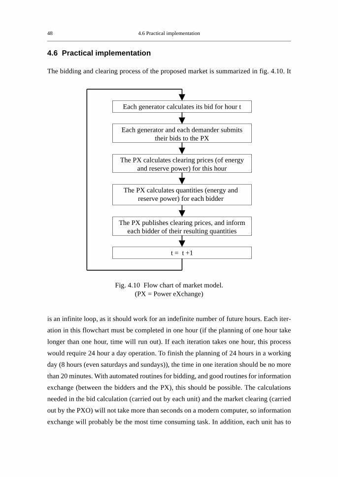
48 4.6 Practical implementation
4.6 Practical implementation
The bidding and clearing process of the proposed market is summarized in fig. 4.10. It
is an infinite loop, as it should work for an indefinite number of future hours. Each iter-
ation in this flowchart must be completed in one hour (if the planning of one hour take
longer than one hour, time will run out). If each iteration takes one hour, this process
would require 24 hour a day operation. To finish the planning of 24 hours in a working
day (8 hours (even saturdays and sundays)), the time in one iteration should be no more
than 20 minutes. With automated routines for bidding, and good routines for information
exchange (between the bidders and the PX), this should be possible. The calculations
needed in the bid calculation (carried out by each unit) and the market clearing (carried
out by the PXO) will not take more than seconds on a modern computer, so information
exchange will probably be the most time consuming task. In addition, each unit has to
Fig. 4.10 Flow chart of market model.(PX = Power eXchange)
Each generator calculates its bid for hour t
The PX publishes clearing prices, and informeach bidder of their resulting quantities
The PX calculates clearing prices (of energyand reserve power) for this hour
Each generator and each demander submitstheir bids to the PX
The PX calculates quantities (energy andreserve power) for each bidder
t = t +1

Chapter 4 Decentralized optimization 49
generate a price forecast (used in the bid calculation) for a number of hours ahead. How
many hours the price forecast must be for depends on the unit characteristics. E.g., a unit
with high start-up costs may have to consider a longer period than a unit with no or small
start-up costs.
The lead time should be as low as possible, to reduce uncertainties in load, plant avail-
ability etc.
A market that clears one hour per hour has the advantage that planning can be done close
to operation, thus reducing uncertainties. The disadvantage is the need for 24 hour man-
ning (if the bidding process is not automated). With all planning done within the working
day, the minimum lead time for the last hour planned will be 16 hours.
4.6.1 Alternative solutions
The simplest version of the market, and thereby appealing, is the one already described;
A one iteration only procedure, with moving horizon.
An alternative is to do this process for one day (24 hours), use the resulting prices to
update the price forecast and start over again. The number of iterations is limited by the
available time (24 hours to schedule the next 24 hours), but a few iterations (two or three)
should be possible.
Algorithm for running more than one iteration:
1. Iteration = 0
2. t = 1, iteration = iteration + 1
3. All units calculate bids for hour t and submit them to the PX
4. PX calculates clearing prices and quantities, and publishes the prices
5. t = t + 1
6. If t > 24 and iteration > max. no. of iterations then go to 8.
7. If t > 24 then go to 2 else go to 3
8. Publish clearing prices for the hole day, and inform each bidder of their energy and
reserve power requirements
Another possibility is to for the PX to publish a price forecast (which the units can
choose to use or not), and if the resulting clearing prices deviate more than some pre-
defined level, a new iteration is run. This way, the units can not speculate by giving

50 4.6 Practical implementation
incorrect bids in the first iteration, knowing that the bids for the first iterations in no way
are binding.

51
Chapter 5
Simulated Competition
7R�HYDOXDWH�WKH�TXDOLW\�RI�WKH�SURSRVHG�PDUNHW��D�FRPSXWHU�VLPXODWLRQ�SURJUDP�KDV�
EHHQ�GHYHORSHG��7KLV�SURJUDP�VLPXODWHV�WKH�SURSRVHG�PDUNHW�DFFRUGLQJ�WR�WKH�
ELGGLQJ�DQG�FOHDULQJ�UXOHV�GHVFULEHG�LQ�WKH�SUHYLRXV�FKDSWHU�
5.1 Simulated competition (SimCom)
A computer program based on the proposed market is developed. The program is called
Simulated Competition (or SimCom for short). SimCom is written in the Fortran 90 pro-
gramming language.
The critical factor in the proposed market is the price forecast. The price forecast consists
of the expected price of energy and the expected price of reserve power for all hours of
the optimizing horizon. A computer simulation program allows us to run several itera-
tions, where the price forecast is updated in each iteration. An initial price forecast must
be set, but it is not critical that it is a good one, as it will converge to a better price fore-
cast. The old price forecast together with the clearing prices (resulting from that old price
forecast) is used to calculate the new price forecast (one price of energy and one price of
reserve power for each hour of the optimization period):
new price forecast = old price forecast · (1-α) + resulting clearing price · α(5.1)
α is an update factor, and is usually set to 0.5, giving the new price forecast as the mean
of the old price forecast and the clearing prices resulting from that price forecast. All
units use the same price forecast.
SimCom can be used to solve the scheduling problem with minimum up/down times,
time varying start-up costs, minimum and maximum production levels and spinning
reserve requirement taken into account.

52 5.1 Simulated competition (SimCom)
Figure 5.1 shows the flowchart for SimCom:
Fig. 5.1 Flowchart for SimCom
Set initial price forecastSet update factor αSet t=0
t = t + 1
T > horizon
Yes
NoFor this hour: Calculate bids Find clearing prices (λc,t and µc,t) Find production schedule
Calculate production costsCalculate dual value
Solution goodenough
Yes
No
Write results
Update price forecastSet t = 0

Chapter 5 Simulated Competition 53
KRUL]RQ is the number of hours to simulate (usually between 24 and 168 hours)
λc,t is the clearing price of energy in hour t (in $/MWh)
µc,t is the clearing price of reserve power in hour t (in $/MW)
Bid calculation is described in section 4.3.4, market clearing (price and quantity deter-
mination) is described in section 4.3.6. The dual value is described in section 5.1.1.
In the bid calculation, the hours considered when calculating Idiff,i is from t+1 to the last
hour of the optimizing horizon. Recall that the difference in future income for running
vs. not running hour t has to be found (Idiff,i in (4.6)) to calculate the bid for hour t. See
the following example:
Example:
Optimizing horizon is 24 hours. For hour 1, the price forecast for hours 2-24 is used
when calculating the bids for all units for that hour. For hour 2, the price forecast for
hours 3-24 is used. In hour 23, the future is hour 24. In hour 24 there is no future to con-
sider, since hours beyond the optimizing horizon is not considered, and thus Idiff,i = 0.
There is no explicit convergence criterion in SimCom. When running the program, the
simulation is usually stopped after 20 iterations.
A paper about this method, called ’7KHUPDO�3RZHU�*HQHUDWLRQ�6FKHGXOLQJ�E\� 6LPXODWHG
&RPSHWLWLRQ¶, is accepted for publication in an IEEE Transactions, [14].
5.1.1 Dual value
Due to similarities with the Lagrangian Relaxation method (LR), the clearing prices in
SimCom can be used as the multipliers in LR to calculate the Lagrangian dual value. The
dual solution is not a feasible solution to the problem, but the dual value represents a
lower limit of total costs. The difference between the calculated cost and the dual value
represents an upper limit for the distance to the optimal solution.
With the problem definition from section 2.5, the dual function becomes (see appendix
B for details):
(5.2)D Minu
ip
i,
Ki u p,( ){ } λt PD t, µt Rt⋅+⋅( )t 1=
T
∑+
i 1=
N
∑=

54 5.2 Summary
where
(5.3)
ui,t = 1 if unit i is running in hour t, else 0
The value of the dual function is calculated in each iteration of SimCom using the clear-
ing prices as multipliers.
5.2 Summary
SimCom can be used to solve a standard scheduling problem, as formulated in section
2.5.
Input to SimCom:
• Unit data for all units (minimum production, maximum production, minimum up
time, minimum down time, fuel costs described by a second order polynomial,
linear or exponential start-up costs, and initial condition (on/off and for how long))
• Optimization horizon (number of hours to simulate)
• Load and reserve requirement for each hour of the optimization period (only firm
load is implemented in SimCom so far)
• Initial price forecast
• Update factor α (determines how the price forecast for the next iteration is set, see
equation (5.1))
With the input data given, SimCom runs for a given number of iterations (usually 20).
For each new iteration, the price forecast is updated.
Output from SimCom:
• Production cost (sum of fuel costs and start-up costs)
• Production plan (production level for each unit in each hour)
• Dual value (representing a lower limit of production cost, NOT a feasible solution)
• Resulting prices of energy and reserve power for each hour
Ki u p,( ) FC pi t,( ) SCi t, λt pi t, µt ui t, Pimax
pi t,–( )⋅ ⋅+⋅( )t 1=
T
∑–
t 1=
T
∑+
t 1=
T
∑=

Chapter 5 Simulated Competition 55
Fig. 5.2 Sample screen output while running SimCom

56 5.2 Summary

57
Chapter 6
Test simulations
6LP&RP��WKH�FRPSXWHU�SURJUDP�WKDW�VLPXODWHV�WKH�SURSRVHG�PDUNHW��KDV�EHHQ�
WHVWHG�RQ�VHYHUDO�FDVHV��ZKLFK�UHVXOWV�DUH�VKRZQ�KHUH��7KH�UHVXOWV�SURYLGH�
LQIRUPDWLRQ�DERXW�WKH�TXDOLW\�RI�6LP&RP�DV�D�SURJUDP�IRU�VROYLQJ�WKH�VLQJOH�
RZQHU�VFKHGXOLQJ�SUREOHP��DQG�DERXW�WKH�TXDOLW\�RI�WKH�SURSRVHG�PDUNHW��7KH�
UHVXOWV�ZLOO�EH�GLVFXVVHG�LQ�WKH�QH[W�FKDSWHU�
6.1 Introduction
To be able to evaluate the quality of the proposed market and of SimCom, simulations
with SimCom has been done. Simulations will provide information about convergence
properties, and the sensitivity of the assumption of known future prices can be examined.
The simulations are done to study the quality of the two different contributions of this
thesis:
1. SimCom as an optimization tool for the single owner scheduling problem/central
scheduling problem
2. The quality of the proposed scheduling market
Test results from 3 different cases is reported here: A 10 unit case and a 110 unit case,
both with data from [24], and a 9 unit case with known optimal solution. Optimization
horizon is 24 hours for the first two cases, and 168 hours for the third. Complete data for
all cases can be found in appendix C.
For comparison, the Unit Decommitment procedure described in [19] is implemented
with Criterion 1 as the decommitment criterion (see [19]). This Unit Decommitment pro-
cedure starts with all units committed, and then iteratively shuts down (in all or some
hours) one by one unit until no more cost savings are possible. A heuristic rule (Criterion

58 6.2 SimCom
1) is used to decide which unit to shut down in each iteration.
A lagrangian relaxation based program has also been available; SHARP. SHARP is
described in [17].
The schedule costs reported for solution methods other than SimCom, SHARP and Unit
Decommitment are from [24]. These are marked by a star (*) in the tables.
The initial forecast for price of reserve power is set to zero in all simulations.
The SimCom method is programmed in Fortran 90 and run on a PC with a Pentium 133
MHz processor.
The SimCom method and the economic results of test systems 1 and 2 is presented in a
paper that has been accepted for publication in IEEE Transaction on Power Systems
[14].
6.2 SimCom
6.2.1 Test system 1 (10 units, 24 hours)
Table 6.1 shows a comparison of SimCom best solution with the best solutions found by
other optimizing techniques. The Lagrangian dual value (see previous chapter) is also
reported. Table 6.2 shows the best unit commitment plan generated by SimCom and the
best generated by SHARP.
Table 6.1. Comparison of Simcom best solution with other solution methods
Solution method Schedule cost ($) % from bestDual value 47 134 -0.29 %SHARP 47 273
6LPXODWHG�&RPSHWLWLRQ ������ ������
Lagrangian Relaxation* 47 511 0.50 %Hybrid genetic algorithm* 47 576 0.64 %Normal genetic algorithm* 47 596 0.68 %Unit decommitment 47 704 0.91 %Artificial neural network* 48 293 2.16 %

Chapter 6 Test simulations 59
Solution time for 20 iterations with this case is 6 seconds.
6.2.2 Test system 2 (110 units, 24 hours)
For this system the reserve requirement is set to 700 MW in all hours (Pmax of largest
unit).
Units 101-110 are specified with shut-down costs in [24] (ranging from $15 to $75). In
the calculations with SimCom, SHARP and Unit Decommitment the shut-down costs
are added to the start-up costs. The maximum error caused by this is $163 (Shut-down
of those units which are initially running).
Table 6.2. Unit commitment plan for the best schedule generated by SimCom for test system 1 (Underlined where the solution differs from
SHARP’s solution)
Unit Hours (1-24)1 111111111111111111111111
2 111111111111000000000000
3 111100000000000000000000
4 111111111111111111111111
5 111111111111111111111111
6 000000000000000000000001
7 111111111111111111111111
8 000000000000000000000000
9 111111111111111111111111
10 111111111111111111111111
Table 6.3. Comparison of SimCom best solution with other solution methods for test system 2 (110 units)
Solution method Schedule cost ($) % from bestDual value 3 809 231 -0.04 %
6LPXODWHG�&RPSHWLWLRQ ���������
SHARP 3 813 057 0.06 %Unit decommitment 3 819 282 0.22 %Hybrid genetic algorithm* 3 826 775 0.42 %Normal genetic algorithm* 3 854 821 1.15 %

60 6.2 SimCom
Table 6.3 shows a comparison of SimCom best solution with the best solutions found by
other optimizing techniques. Figure 6.1 shows the results in each iteration of simulations
with different initial energy price forecasts (these results are also shown in tabular form
in table E.1. The initial price forecast is equal for all hours.
The solution time of 7HVW�V\VWHP�� is 1 minute for a run with 20 iterations.
6.2.3 Test system 3 (9 units, 168 hours)
This is a test case with 9 units, 7 thermal units and 2 hydro units. The hydro units are
assigned a water value (incremental worth of water) from the long term planning, and
can therefore be treated the same way as the thermal units.
The unit data and load data can be found in section C.3. Reserve requirement is 10% of
the load in all hours.
In this case the units have no minimum up or down time, and the start-up costs are con-
stant (not dependent on downtime). The problem can then be formulated as a shortest
path problem, and for a problem of this small size the optimal solution can be found. The
optimal solution is found by Dijkstra’s method1, and is provided by Professor Arne
1. Refer to a textbook in Operations Research for a description of Dijkstra’s method, for example [10], pages 191-194
Fig. 6.1 Production cost in each iteration of the SimCom for different initial price forecasts
3810
3815
3820
3825
3830
3835
3840
1 2 3 4 5 6 7 8 9 10,WHUDWLRQ
6FK
HGXOH�FRVW����
�����
Initial price forecast = 10
Initial price forecast = 15
Initial price forecast = 20

Chapter 6 Test simulations 61
Johannesen of SINTEF Energy Research. Shortest Path applied on the generation sched-
uling problem is described in [16].
The best solution found by SimCom has the following commitment plan:
• Units 1,2 and 3 are committed in all hours
• Unit 4 is committed in hours 6-119 (all weekdays)
• Unit 8 is committed in hours 8-23, 32-47, 56-71, 80-95, 104-119, 126-142 and
150-166 (once per day)
• Unit 9 is committed in hours 11-13, 35-37, 59-61, 83-85, 107-109, 128-133 and
152-157 (once per day)
This is illustrated in fig. 6.2 (since only 3 units are switched on and off, it is possible to
identify each start and stop in the figure). The only difference from the optimal solution
is that in the optimal solution, the smallest of the two hydro units (unit 9) is used instead
of the largest hydro unit (unit 8) in hours 17-18, 23, 41-42, 47, 65-66, 71, 89-90, 95, 113-
114, 119, 126, 142, 150, 166.
Table 6.4. SimCom best solution vs. optimal solution for test system 3(9 units, 168 hours)
Solution method Schedule cost (NOK) % from optimumDual value 8 871 637 -1.92 %Optimal solution 9 045 090
6LPXODWHG�&RPSHWLWLRQ ��������� ������
SHARP 9 074 970 0.33 %Unit decommitment 9 194 557 1.65 %

62 6.3 Quality of the proposed market
The solution time for 20 iterations is 29 seconds for this case
6.3 Quality of the proposed market
The simplest version of the market is the one-iteration-only procedure. Because of its
simplicity, it is attractive. A question is then; how good must the price forecast be to
reach near-optimal solutions in the first iteration? And, are there significant improve-
ments by running more than one iteration which justifies the increased complexity of the
market?
Another question is whether the units have an operating profit or not. If a unit does not
make any profits, it has no reason to participate in the market. The only reason for par-
ticipating in the market is that the unit believes in opportunities to make profits.
Test case 2 is used in the simulations reported here.
Fig. 6.2 Best solution found by Simulated Competition. The figure shows hydroand thermal production and reserve in each hour of the week
0
100
200
300
400
500
600
700
800
900
1 13 25 37 49 61 73 85 97 109 121 133 145 157
+RXU
3URGXFWLRQ�DQG�UHV
HUYH
��0:�
Excess reserve
Reserve demandHydro
Thermal
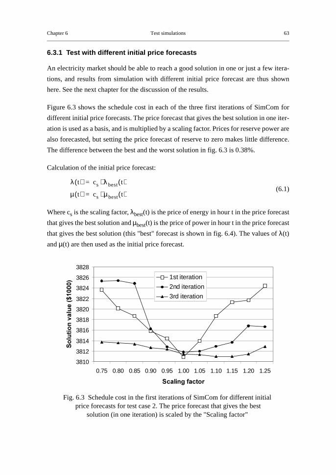
Chapter 6 Test simulations 63
6.3.1 Test with different initial price forecasts
An electricity market should be able to reach a good solution in one or just a few itera-
tions, and results from simulation with different initial price forecast are thus shown
here. See the next chapter for the discussion of the results.
Figure 6.3 shows the schedule cost in each of the three first iterations of SimCom for
different initial price forecasts. The price forecast that gives the best solution in one iter-
ation is used as a basis, and is multiplied by a scaling factor. Prices for reserve power are
also forecasted, but setting the price forecast of reserve to zero makes little difference.
The difference between the best and the worst solution in fig. 6.3 is 0.38%.
Calculation of the initial price forecast:
(6.1)
Where cs is the scaling factor, λbest(t) is the price of energy in hour t in the price forecast
that gives the best solution and µbest(t) is the price of power in hour t in the price forecast
that gives the best solution (this "best" forecast is shown in fig. 6.4). The values of λ(t)
and µ(t) are then used as the initial price forecast.
λ t( ) cs λbest t( )⋅=
µ t( ) cs µbest t( )⋅=
3810
3812
3814
3816
3818
3820
3822
3824
3826
3828
0.75 0.80 0.85 0.90 0.95 1.00 1.05 1.10 1.15 1.20 1.25
6FDOLQJ�IDFWRU
6ROXWLRQ�YDOXH�����
��� 1st iteration
2nd iteration
3rd iteration
Fig. 6.3 Schedule cost in the first iterations of SimCom for different initial price forecasts for test case 2. The price forecast that gives the best
solution (in one iteration) is scaled by the "Scaling factor"

64 6.3 Quality of the proposed market
6.3.2 Do the units earn any profits?
For the units to participate in the market, they must have opportunity to make profits.
The question is then: Do the units make any profits?
If the price forecast is correct (equals the resulting prices), all units will make profits
since their bids are optimized for the price forecast. However, since the price forecast is
uncertain, the units risk both loosing money and earning more than expected.
One iteration of SimCom is run, with the price forecast that gives the best schedule. This
price forecast and the resulting prices is shown is fig. 6.4 (all units use the same forecast).
The price forecast and resulting prices is shown in tabular form in table E.3.
The payment for delivered energy is $5,208,525 and the payment for reserve power are
$12,605 (0.24% of total payments). The extra payment for the difference between the
final schedule and the preliminary one totals to $233 (0.0045% of total payments), which
confirms that the assumption that these costs are small is valid (at least for this case).
The payments to the generators total $5,221,363 whereas the generation costs are
$3,810,851. This gives an operating profit of $1,410,512. However, profits are not
Fig. 6.4 Price forecast and resulting prices (best iteration of test case 2)
0
5
10
15
20
25
30
1 3 5 7 9 11 13 15 17 19 21 23
+RXU
3ULFH
Forecasted energy priceResulting energy priceForecasted reserve priceResulting reserve price

Chapter 6 Test simulations 65
equally distributed among the units, and the profit for each unit has to be checked.
Four units lose money in this case, the units are no. 14, 15, 103 and 109. Table 6.5 shows
the net income in each hour for these units. Start-up (and shut-down) costs are accounted
for in the hour of start-up.
Table 6.5. Income in each hour for selected units
These units lose money since the resulting prices are lower than they forecasted. Their
behavior is optimal according to the price forecast and the resulting price in the hour of
start-up, but since prices are lower than expected, they lose money.
Units 14, 15 and 103 have minimum up time of four hours, and unit 109 has minimum
up time of 5 hours. This explains why they are up in hours 22 and 23. The reason for unit
103 not shutting down in hours 2 and 3 is that it initially has been up for one hour only,
and therefore has to be up for three more hours (hours 1, 2 and 3).
Hour(s) 1 2 3 4-17 18 19 20 21 22 23 24 TotalUnit 14 -407 1 490 -255 -170 Unit 15 -143 481 -257 -285 -205 Unit 103 85 -155 -240 -350 -176 79 262 -496 Unit 109 -787 260 610 -447 -523 -888

66 6.3 Quality of the proposed market

67
Chapter 7
Discussion and further work
7.1 Introduction
There are two main contributions of this thesis:
1. A new method for decentralized scheduling and market clearing based on competitive
bidding. The market clearing handles power balance and spinning reserve require-
ment simultaneously
2. A new algorithm for central scheduling based on simulation of the above mentioned
process
This chapter discusses the quality of these two, and also identifies topics for future
research.
7.1.1 SimCom as an optimization tool for the central scheduling problem
SimCom can be used to solve the single owner scheduling problem (as stated in section
2.5), and the simulations show excellent results. For test case 1, the SimCom solution is
only 0.02% inferior to the solution provided by SHARP. For test cases 2 & 3, the simu-
lated competition method (SimCom) gives better schedules than the other methods
(0.06% better than the second best for test case 2, and 0.25% for test case 3). For test
case 3, the optimal solution is available, and the best solution provided by SimCom is
only 0.08% from the optimal solution.
Other cases differing in number of units, length of study time and system demand profile
has also been tested. All these cases have shown that SimCom provides excellent perfor-
mance: fast computation, fast convergence and low schedule costs.
Simulations have shown that the initial price forecast has little influence on the best solu-
tion found. Near optimal solutions are found regardless of what the initial price forecast
is.

68 7.1 Introduction
SimCom has great resemblances with the Lagrangian Relaxation (LR) method but also
some differences.
Similarities with LR:
• The prices (multipliers in LR) are the only coordination signals
• The convergence properties of SimCom seem to be similar to LR; the best solution
is found within a few iterations
• Since the size of units is not considered while committing units, results for small
systems (only a few units) can be poor. Performance is better for large systems
• Prices (multipliers in LR) seldom stabilize completely, but end up flip-flopping
between two or more sets of prices
The differences are:
• In LR the resulting commitment from the DP is binding, in SimCom only the
future earnings calculated by the DP are used in calculating the bid. The
commitment plan in SimCom is found by matching supply and demand bids (the
demand bids being price insensitive in the simulations here due to firm load)
• One drawback with LR is that equal units are always committed equally. This is
not the case with SimCom
• SimCom has one drawback: It is not checked that future loads can be covered
before shutting down a unit. This could lead to infeasibilities, but has not been a
problem in any of the cases tested so far
• LR solves the dual problem, and some heuristic rules are used to find a primal
feasible solution. SimCom give feasible solutions directly
7.1.2 The quality of the proposed market
The simulations show that the proposed market can lead to near-optimal performance,
when the units behave according to the perfect competition conditions (each firm has no
influence on the market clearing price).
The critical factor is the price forecast. If the price forecast is correct, each unit will have
its optimal schedule.
Optimal behavior in any given time interval is dependent on both past and future due to
start-up costs and minimum up/down time. The past is always known, and the future is
dealt with through the price forecast.

Chapter 7 Discussion and further work 69
Simulations have shown that good schedules can be reached in just one iteration if the
price forecast is not too far off. Figure 6.3 shows that for test case 2, the production cost
in the first iteration are less than 0.4% higher than for the best schedule even with the
price forecast 25% off. Since the gain in running more than one iteration is small, the one
iteration only procedure is the most appealing due to its simpleness.
However, the units are more sensitive to the difference between the price forecast and
the resulting prices. If a unit believes in high future prices, and the clearing prices are
lower than expected the unit risk losing money. If the price forecast is lower than the
clearing prices, the unit can lose the opportunity to make money.
In the simulations in chapter 6, all units use the same price forecast. In a real market it
can be discussed whether the PX should publish price forecasts or not. The arguments
against this is that the PX should be independent and neutral, and the PX will influence
the bids by setting the price forecast. The arguments for a public price forecast is that it
is efficient (instead of many units doing the same work one central agency makes the
price forecast), and the units can independently correct the public forecast according to
own beliefs. A conclusion is not drawn here, and this question is open for further discus-
sion.
In the proposed market, discontinuous bids are allowed. The discontinuities comes from
minimum production levels of units, and best operating points at higher levels of pro-
duction (see figs. 4.5, 4.6 and 4.7). Due to the discontinuities in the bids, exact matching
of supply and demand is not always achieved in the preliminary schedule. Adjustments
are then made to this preliminary schedule to reach the final schedule where supply
equals demand. With a large number of units, these adjustments will be small compared
to total production, and thus the economic effect will be small.
Because spinning reserve is included in the market clearing process, a bid must be
included for each unit. The market clearing then gives the resulting quantities for each
unit. A production company that owns several units need not use these quantities as a
final production schedule, since only the sum production and sum reserve for the units
it owns are binding for the company. The company can reschedule the production any
way it pleases.

70 7.2 Suggestion for future work
7.2 Suggestion for future work
One of the most interesting topics for future work would be to develop bidding routines
for hydraulically coupled hydro units (several hydro units in the same river system).
With bidding routines for hydro units, it would be possible to solve the whole hydro-
thermal scheduling problem.
Network restrictions (transfer limits and reliability) is not treated in this work. This is
another topic for future research.
Other topics for future work are:
• Investigate market imperfections. Market power. Gaming.
• How would a stochastic price forecast influence the bids?
• Tests on actual cases

71
Chapter 8
Conclusions
A new electricity spot market is proposed. This market balances power production with
demand and simultaneously ensures enough spinning reserve. Routines for bidding and
market clearing are developed. The unit characteristics and restrictions that are handled
are: Minimum and maximum production levels, fuel cost function, start-up costs, mini-
mum up time and minimum down time.
A computer program that simulates the proposed market has been developed. The sim-
ulations show that it is possible to reach economically efficient (i.e. near-optimal) gen-
eration plans through the proposed market. The critical factor is the quality of the price
forecast which is used in the bid calculations. With a reasonably good price forecast
good solutions are reached already in the first iteration of SimCom. If implemented in a
real market, a one iteration procedure would be preferable due to its simpleness.
A new method for solving the single owner short term scheduling problem is presented.
Simulation results show that it produces near optimal production schedules, and compu-
tation time is low (1 minute for scheduling 110 units for 24 hours on a Pentium 133 PC).

72

73
5HIHUHQFHV
[1] Beune, R. and Renaud, A. (CIGRE TF-38-04-01) 8QLW�&RPPLWPHQW�3UREOHP��DJHQHUDO�PRGHOLQJ� November 22, 1995
[2] &DOLIRUQLD¶V�1HZ�(OHFWULFLW\�PDUNHW��7KH�%DVLFV��+RZ�WKH�3;�:RUNV. Version 3,March 27, 1998, California Power Exchange
[3] CALPOL Market Report, Issue no. 1, June 1998, San Francisco
[4] Christie, Richard D. and Wangensteen, Ivar. 7KH�(QHUJ\�0DUNHW� LQ�1RUZD\�DQG6ZHGHQ��,QWURGXFWLRQ. IEEE Power Engineering Review, February 1998, p. 44-45.
[5] Clarke, Les. 7KH�RSHUDWLRQ�RI�WKH�SRRO�LQ�(QJODQG�DQG�:DOHV 3rd International Con-ference on Advances in Power System Control, Operation and Management (Conf.Publ. No.CP417) p. 7-23 vol.1, IEE, Hong Kong, 1995
[6] CIGRE Task Force 38-04-01: 8QLW� &RPPLWPHQW, Draft Final Report, February1997
[7] Dettmer, Roger. 7KH�8.�HOHFWULFLW\�SRRO��D�OHDS�LQ�WKH�GDUN" IEE Review, Septem-ber 1991.
[8] Eikeland, Per Ove. 1RUZD\�DQG�WKH�8.��$�&RPSDUDWLYH�,QVWLWXWLRQDO�$QDO\VLV�RI&RPSHWLWLYH� 5HIRUPV� LQ� WKH� (OHFWULFLW\� 6XSSO\� ,QGXVWULHV��The Fridtjof NansenInstitute, EED Report 1995/3, ISBN 82-7613-124-7
[9] Fosso, Olav B. et al. *HQHUDWLRQ�VFKHGXOLQJ�LQ�D�GHUHJXODWHG�V\VWHP��7KH�1RUZH�JLDQ�FDVH Paper presented at the IEEE PES Winter Meeting 1998.
[10] Foulds, L R 2SWLPL]DWLRQ�7HFKQLTXHV, Springer-Verlag, New York, 1981
[11] Gjengedal, Terje 6KRUW�WHUP�6FKHGXOLQJ�RI�+\GURHOHFWULF�3RZHU�6\VWHPV, Ph.D.-thesis, Norwegian University of Science and Technology, Trondheim 1987
[12] Gjengedal, Terje. /DJUDQJHGHNRPSRVLVMRQ, Working paper AN 90.20.10, SINTEFEnergy Research. (In Norwegian)
[13] Hunt, Sally and Shuttleworth, Graham 8QORFNLQJ�WKH�*ULG��IEEE Spectrum, July1996, p. 20-25
[14] Huse E S; Wangensteen I; and Faanes H H. 7KHUPDO�3RZHU�*HQHUDWLRQ�6FKHGXOLQJE\�6LPXODWHG�&RPSHWLWLRQ, paper accepted for publication in IEEE Transactions onPower Systems, paper no. PE-274-PWRS-0-06-1998
[15] Johannesen, Arne. 7KH�&KDOOHQJH�RI�+\GUR�7KHUPDO�6FKHGXOLQJ�LQ�D�'HUHJXODWHG3RZHU�0DUNHW�5HJLPH. Hydropower ‘97, Trondheim, Norway
[16] Johannesen, Arne. ([WHQGHG�8QLW�&RPPLWPHQW�E\�6KRUWHVW�3DWK�0HWKRG, TechnicalReport F4391, SINTEF Energy Research, Trondheim, 1996

74
[17] Larsen, Tellef Juell. 3URJUDP�IRU�SURGXNVMRQVSODQOHJJLQJ�L�WHUPLVNH�NUDIWV\VWHP�Working paper AN 97.11.13, SINTEF Energy Research, (in Norwegian)
[18] Lauer, G.S.; Bertsekas, D.P., 6ROXWLRQ�RI�/DUJH�6FDOH�2SWLPDO�8QLW�&RPPLWPHQW3UREOHPV, IEEE Transactions on Power Apparatus and Systems, Vol. PAS-101,No. 1 january 1982
[19] Li, Chao-an et al. $�1HZ�8QLW�&RPPLWPHQW�0HWKRG. IEEE Transactions on PowerSystems, Vol. 12, No. 1, February 1997
[20] Livik, Klaus and Fretheim, Stig (editors) 'HUHJXODWLRQ�RI�WKH�1RUGLF�SRZHU�PDUNHW�,PSOHPHQWDWLRQ�DQG�H[SHULHQFHV�������������SINTEF Energy Research report no.A4602, Trondheim, 1997
[21] Merlin, A.; Sandrin, P. $� 1HZ�0HWKRG� IRU� 8QLW� &RPPLWPHQW� DW� (OHFWULFLWH� GH)UDQFH, IEEE Transactions on Power Apparatus and Systems, Vol. PAS-102, No.5, May 1983
[22] Midttun, Atle and Thomas, Steve. 7KHRUHWLFDO�DPELJXLW\�DQG�WKH�ZHLJKW�RI�KLVWRU�LFDO�KHULWDJH��D�FRPSDUDWLYH�VWXG\�RI�WKH�%ULWLVK�DQG�1RUZHJLDQ�HOHFWULFLW\�OLEHU�DOLVDWLRQ. Energy Policy, Vol. 26, No. 3, pp. 179-197, 1998
[23] Nicholson, Walter. 0LFURHFRQRPLF�WKHRU\��%DVLF� WKHRU\�DQG�H[WHQVLRQV. 5th edi-tion. The Dryden Press, 1992.
[24] Orero, S O and Irving, M R. /DUJH�6FDOH�8QLW�&RPPLWPHQW�8VLQJ�D�+\EULG�*HQHWLF$OJRULWKP. Electrical Power & Energy Systems, Vol. 19, No. 1 pp 45-55, 1997
[25] Ravindran, Phillips and Solberg. 2SHUDWLRQV�5HVHDUFK���3ULQFLSOHV�DQG�SUDFWLFH,2nd edition, Wiley, 1986
[26] Rudnick H; Varela R; and Hogan W (YDOXDWLRQ�RI�$OWHUQDWLYHV�IRU�3RZHU�6\VWHP&RRUGLQDWLRQ�DQG�3RROLQJ�LQ�D�&RPSHWLWLYH�(QYLURQPHQW��IEEE Transactions onPower Systems, Vol 12, No. 2, May 1997, pp. 605-613
[27] Schweppe, Fred C. et al. 6SRW�SULFLQJ�RI�HOHFWULFLW\��Kluwer Academic Publishers,1987
[28] Sen, Subir and Kothari D P. 2SWLPDO� WKHUPDO� JHQHUDWLQJ� XQLW� FRPPLWPHQW�� DUHYLHZ� Electrical Power & Energy Systems, Vol. 20, No. 7, pp.443-451, 1998
[29] Sheble, G B and Fahd G N. 8QLW�&RPPLWPHQW�/LWHUDWXUH�6\QRSVLV. IEEE Transac-tions on Power Systems, Vol. 12, No. 1, February 1997, pp. 113-119
[30] Walker, Cody D. and Lough, W. T. $�FULWLFDO�UHYLHZ�RI�GHUHJXODWHG�IRUHLJQ�HOHFWULFXWLOLW\�PDUNHWV. Energy Policy, Vol. 25, No. 10, pp. 877-886, 1997
[31] Wangensteen, Ivar. 'HUHJXODWLRQ�RI�WKH�3RZHU�0DUNHW��,PSOHPHQWDWLRQ�DQG�([SH�ULHQFHV�LQ�WKH�1RUZHJLDQ�DQG�1RUGLF�0DUNHW��EFI TR F4562, 1996
[32] White, Anthony. 5HVKDSLQJ�WKH�(OHFWULFLW\�6XSSO\�,QGXVWU\�LQ�(QJODQG�DQG�:DOHV.James Capel & Co. Ltd., London, 1990.

75
[33] White, Anthony et al. 7KH�1HZ�(OHFWULFLW\�&RPSDQLHV. James Capel & Co. Ltd.,London, 1990.
[34] White, Anthony et al. 7KH�1HZ�(OHFWULFLW\�,QGXVWU\� James Capel & Co. Ltd., Lon-don, 1990.
[35] Wolak, Frank A. and Patrick, Robert H. 7KH�,PSDFW�RI�0DUNHW�5XOHV�DQG�0DUNHW6WUXFWXUH�RQ�WKH�3ULFH�'HWHUPLQDWLRQ�3URFHVV�LQ�WKH�(QJODQG�DQG�:DOHV�(OHFWULFLW\0DUNHW. POWER Working Paper, PWP-047, University of California, Berkeley,1997
[36] Wolak, Frank A. 0DUNHW�'HVLJQ�DQG�3ULFH�%HKDYLRU� LQ�5HVWUXFWXUHG�(OHFWULFLW\0DUNHWV��$Q�,QWHUQDWLRQDO�&RPSDULVRQ. POWER Working Paper, PWP-051, Uni-versity of California, Berkeley, 1997
[37] Wu, Felix and Varaiya, Pravin. &RRUGLQDWHG�0XOWLODWHUDO�7UDGHV�IRU�(OHFWULF�3RZHU1HWZRUNV��7KHRU\�DQG�,PSOHPHQWDWLRQ. Power (Program on workable energy reg-ulation), June 1995.

76

A77
Appendix A
Dynamic Programming (DP)
This is not a description of dynamic programming, but an explanation of how
it is used in the bid calculation (chapter 4.3.4).
A.1 Backward Dynamic Programming applied to single unit optimization
Dynamic programming is a technique for finding the optimal route (and the associated
optimal value) in a decision tree. If you are not familiar with DP, see a textbook in oper-
ations research, for example [25], chapter 10.
Dynamic programming is here used to find the difference in future income for the unit
resulting from the decision of running vs. not running in the hour the bid is to be calcu-
lated for (i.e. the optimal profit for two different initial states must be calculated). To use
DP, the problem has to be divided into stages, and a return function and transition func-
tion must be set.
With a given set of prices, each unit can find its optimal production plan. The unit wants
to maximize total profits for the planning horizon (income (4.1) minus fuel costs and
start-up costs):
(A.1)
With respect to its restrictions:
• Unit rated minimum and maximum production
• Minimum up time (MUT) and minimum down time (MDT)
Max Ii λt pi t,⋅ µt Pimax pi t,–( )⋅ FCi pi t,( ) SCi t,––+
t 1=
T
∑=

A78 A.1 Backward Dynamic Programming applied to single unit optimization
Meaning of symbols:
Ii = Net income for unit i
T = number of time intervals (planning horizon)
λt = price of electric energy in hour t ($/MWh)
µt = price of reserve power in hour t
pi,t = unit i’s production in hour t
Pimax = maximum output of unit i
FCi = the fuel cost function of unit i
SCi = start-up costs
The states in the DP is whether the unit is running or not, and for how long. The number
of up states is given by MUT, and the number of down states is the maximum of MDT
and the cooltime of the unit. The cooltime of the unit is when the start-up costs no longer
are increasing. With exponential start-up costs, see (2.6), cooltime is set equal to 4 times
the time constant in the exponential expression (e-4 = 0.018 which gives reasonable
accuracy).
Each hour is a stage at which a decision has to be made.
The return function, NI(t), is the net income in a given hour t (stage). NI = 0 if the unit
is not running, and if running:
(A.2)
The maximization of (A.2) is trivial when fuel costs are given by (2.5). First optimal pro-
duction without regard of min. and max. production, Pi,t*, is found:
(A.3)
(A.4)
With regard to min. and max. production the optimal production, Pi,t**, is found
τi
NI tMax
Pimin
pi t, Pimax≤ ≤
λt pi t,⋅ µt Pimax pi t,–( )⋅ FCi pi t,( )–+{ }=
∂NI t
∂pi t,----------- λt µt– bi 2aipi t,–– 0= =
Pi t,* λt µt– bi–
2ai--------------------------=

Appendix A Dynamic Programming (DP) A79
(A.5)
NI0 = 0 for all states, income in hour 0 is not to be considered.
The transition cost is equal to the start-up cost when start-up occurs, and zero if no start-
up occurs.
Figure A.1 shows the decision tree for a unit with MDT = MUT = 2 hours and start-up
cost dependent on downtime (start-up cost = C1 if tdown = 2 hours and start-up cost = C2
if tdown > 2). If the unit has been down for MDT or more, it has to decide whether to start
up or not, and if it has been up for MUT or more it can continue running or shut down.
The rectangles show the state of the unit, and the numbers has the following meaning:
-1: the unit has been down for 1 hour
-2: the unit has been down for 2 hours
Pi t,*
Pimin
Pi t,**⇒< Pi
min=
Pi t,*
Pimax
Pi t,**⇒> Pi
max=
Pimin
P≤ i t,*
Pimax
Pi t,**⇒≤ Pi t,
*=
Fig. A.1. Decision tree for a T-stage optimization problem. Unit with MDT = MUT = 2 and time dependent start cost.
-1 -1
+2 +2 +2
-3
+1
-2
-1
+2
-3
+1
-2
-1
t = 0 t = 1 t = 2 t = T
Up
Down
-3
+1
-2
-3
+1
-2
...
...
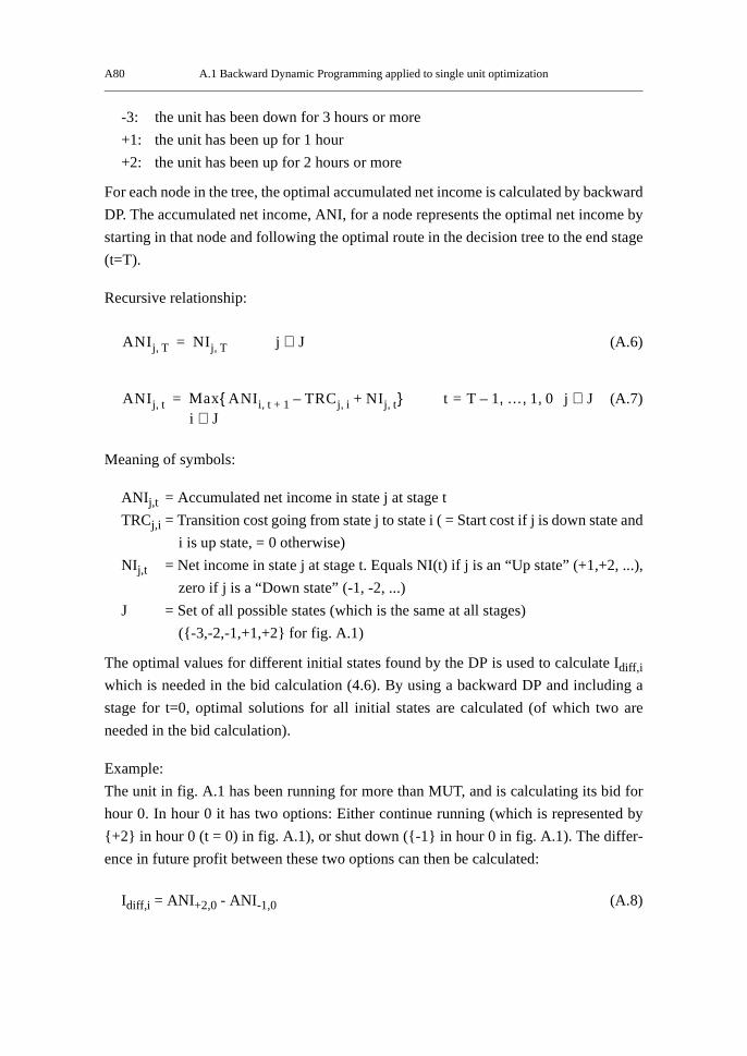
A80 A.1 Backward Dynamic Programming applied to single unit optimization
-3: the unit has been down for 3 hours or more
+1: the unit has been up for 1 hour
+2: the unit has been up for 2 hours or more
For each node in the tree, the optimal accumulated net income is calculated by backward
DP. The accumulated net income, ANI, for a node represents the optimal net income by
starting in that node and following the optimal route in the decision tree to the end stage
(t=T).
Recursive relationship:
(A.6)
(A.7)
Meaning of symbols:
ANIj,t = Accumulated net income in state j at stage t
TRCj,i = Transition cost going from state j to state i ( = Start cost if j is down state and
i is up state, = 0 otherwise)
NIj,t = Net income in state j at stage t. Equals NI(t) if j is an “Up state” (+1,+2, ...),
zero if j is a “Down state” (-1, -2, ...)
J = Set of all possible states (which is the same at all stages)
({-3,-2,-1,+1,+2} for fig. A.1)
The optimal values for different initial states found by the DP is used to calculate Idiff,i
which is needed in the bid calculation (4.6). By using a backward DP and including a
stage for t=0, optimal solutions for all initial states are calculated (of which two are
needed in the bid calculation).
Example:
The unit in fig. A.1 has been running for more than MUT, and is calculating its bid for
hour 0. In hour 0 it has two options: Either continue running (which is represented by
{+2} in hour 0 (t = 0) in fig. A.1), or shut down ({-1} in hour 0 in fig. A.1). The differ-
ence in future profit between these two options can then be calculated:
Idiff,i = ANI+2,0 - ANI-1,0 (A.8)
ANI j T, NI j T,= j J∈
ANI j t, Maxi J∈
ANI i t 1+, TRCj i,– NIj t,+{ }= t T 1– … 1 0, , ,= j J∈

Appendix A Dynamic Programming (DP) A81
Idiff,i is then used in calculating “MinPrice” in (4.6).

A82 A.1 Backward Dynamic Programming applied to single unit optimization

B83
Appendix B
Lagrangian Relaxation
For benchmarking of the computer program that has been developed
(SimCom), it is possible to calculate the dual value of the Lagrangian
Relaxation method using the clearing prices from SimCom as the lagrangian
multipliers. This dual value represent a lower value of the optimization
problem. For this reason, the lagrangian relaxation dual function is derived
here.
B.1 Lagrangian Relaxation (LR)
See [12] and [17] for details.
The optimization problem is stated in section 2.5. The first step of the Lagrangian Relax-
ation method is to include the global restrictions (2.2) and (2.3) in the object function
(2.1):
(B.1)
Local restrictions (unit restrictions) remains as before.
is the set of all ui,t (i.e. for all i and all t)
is the set of all pi,t
Since (2.2) is an equality constraint, each λt is a free variable, and since (2.3) is an ine-
quality constraint each µt must be non-negative. λ and µ are called the lagrangian mul-
tipliers (λ is the set of all λt, and µ is the set of all µt).
Since (B.1) is a relaxation of the original problem, the solution of (B.1) for any given set
MinLu p,
FCi t, SCi t,+( )i 1=
N
∑t 1=
T
∑ λt
t 1=
T
∑ PD t, pi t,
i 1=
N
∑–
µt Rt Pi t,maxui t, pi t,–( )
i 1=
N
∑–
⋅t 1=
T
∑+⋅+=
u
p

B84 B.1 Lagrangian Relaxation (LR)
of λ and µ, will be a lower limit to the original minimization problem.
Equation (B.1) is separable, and can be divided into a subproblem for each unit:
(B.2)
rewritten to:
(B.3)
where
(B.4)
(B.3) is called the dual function, since maximizing this function over λ and µ subject to
the local constraints gives a lower limit to the original problem.
Each subproblem is small, and can easily be solved by Dynamic Programming. The
value of the dual function can therefore easily be calculated when λ and µ are fixed.
The dual problem is:
(B.5)
subject to the local constraints.
In LR, the commitment plan ( ) generated from the solution of each subproblem is used
to generate a primal feasible solution. If the commitment plan cannot be used directly,
some heuristic rules are used to generate a feasible solution.
The multipliers are updated in each iteration of the LR. Several methods exists for updat-
D Minu p,
L Ki u p,( ) λt PD t, µt Rt⋅+⋅( )t 1=
T
∑+
i 1=
N
∑= =
D Minu
ip
i,
Ki u p,( ){ } λt PD t, µt Rt⋅+⋅( )t 1=
T
∑+
i 1=
N
∑=
Ki u p,( ) FC pi t,( ) SCi t, λt pi t, µt ui t, Pimax
pi t,–( )⋅ ⋅+⋅( )t 1=
T
∑–
t 1=
T
∑+
t 1=
T
∑=
Maxλ µ,
D Maxλ µ,
Minu p,
L =
u

Appendix B Lagrangian Relaxation B85
ing the multipliers.
The value of the primal function is always greater than or equal to the dual value (weak
duality). The difference between the two functions yields the duality gap. The duality
gap provides a measure of the near-optimality of the solution.
Examples of the Lagrangian Relaxation method to solve the short term scheduling prob-
lem are shown in [18] and [21].
For an overview of optimization algorithms for the scheduling problem see [28] and
[29].

B86 B.1 Lagrangian Relaxation (LR)

C87
Appendix C
Case data
Test cases 1 & 2 are both from [23]. Test case 3 is provided by Professor Arne
Johannesen of SINTEF Energy Research.
C.1 Test case 1
Table C.1 Data for test case 1. Exponential start-up cost function, see (2.6). IC = initial condition (number of hours up if positive value, else number of hours down)
Unit Pmax
(MW)Pmin
(MW)MDT(h)
MUT(h)
IC(h)
a($)
b($/MW)
c($/MW2)
σ($)
δ($)
τ(h)
1 60 15 2 3 3 15 1.400 0.0051 15 123 5
2 80 20 4 3 3 25 1.500 0.0040 15 123 5
3 100 30 4 4 4 40 1.350 0.0039 25 110 5
4 120 25 3 3 3 32 1.400 0.0038 12 100 5
5 150 50 3 1 -3 29 1.540 0.0021 30 130 5
6 280 75 3 6 -3 72 1.350 0.0026 30 146 6
7 520 250 4 10 10 105 1.395 0.0013 60 207 11
8 150 50 2 3 3 100 1.329 0.0014 80 202 11
9 320 120 5 7 7 49 1.264 0.0029 50 137 7
10 200 75 6 6 6 82 1.214 0.0015 70 157 9

C88 C.1 Test case 1
Table C.2 Load and reserve requirement for test case 1
Load (MW)Hours 1-6 1167 1097 1039 1028 1017 1051
Hours 7-12 1098 1051 1017 993 958 946
Hours 13-18 923 910 900 876 853 829
Hours 19-24 794 782 770 818 864 1167
Reserve (MW)Hours 1-6 350 329 329 300 300 300
Hours 7-12 300 300 300 300 280 280
Hours 13-18 280 270 270 260 260 250
Hours 19-24 240 240 240 240 260 350

Appendix C Case data C89
C.2 Test case 2
Table C.3 The unit characteristics and cost coefficients.Exponential start-up cost function, see (2.6). IC = initial condition (number
of hours up if positive value, else number of hours down)
Unit Pmax
(MW)Pmin
(MW)MDT(h)
MUT(h)
IC(h)
a($)
b($/MW)
c($/MW2)
σ($)
δ($)
τ(h)
SDC($)
1 12 2.4 0 0 -1 24.389 25.547 0.0253 0 0 1 02 12 2.4 0 0 -1 24.411 25.675 0.0265 0 0 1 03 12 2.4 0 0 -1 24.638 25.803 0.028 0 0 1 04 12 2.4 0 0 -1 24.76 25.932 0.0284 0 0 1 05 12 2.4 0 0 -1 24.888 26.061 0.0286 0 0 1 06 20 4 0 0 -1 117.755 37.551 0.012 20 20 2 07 20 4 0 0 -1 118.108 37.664 0.0126 20 20 2 08 20 4 0 0 -1 118.458 37.777 0.0136 20 20 2 09 20 4 0 0 -1 118.821 37.809 0.0143 20 20 2 0
10 76 15.2 2 3 3 81.136 13.327 0.0088 50 50 3 011 76 15.2 2 3 3 81.298 13.354 0.0089 50 50 3 012 76 15.2 2 3 3 81.464 13.38 0.0091 50 50 3 013 76 15.2 2 3 3 81.626 13.407 0.0093 50 50 3 014 100 25 2 4 -3 217.895 18 0.0062 70 70 4 015 100 25 2 4 -3 218.335 18.1 0.0061 70 70 4 016 100 25 2 4 -3 218.775 18.2 0.006 70 70 4 017 155 54.3 3 5 5 142.735 10.694 0.0046 150 150 6 018 155 54.3 3 5 5 143.029 10.715 0.0047 150 150 6 019 155 54.3 3 5 5 143.318 10.737 0.0048 150 150 6 020 155 54.3 3 5 5 143.597 10.758 0.0049 150 150 6 021 197 68.9 4 5 -4 259.131 23 0.0026 200 200 8 022 197 68.9 4 5 -4 259.649 23.1 0.0026 200 200 8 023 197 68.9 4 5 -4 260.176 23.2 0.0026 200 200 8 024 350 140 5 8 10 177.057 10.862 0.0015 300 200 8 025 400 100 5 8 10 210.002 7.492 0.0019 500 500 10 026 400 100 5 8 10 211.91 7.503 0.0019 500 500 10 027 500 140 5 8 5 210 12 0.0014 500 800 4 028 500 140 7 8 -2 180 12.1 0.0013 250 800 4 029 200 50 4 4 1 240 12.2 0.0026 40 300 3 030 100 25 3 2 -2 220 12.5 0.0039 10 60 2 031 50 10 2 1 -3 60 23 0.0051 25 10 1 032 20 5 1 1 -2 50 13.5 0.005 10 15 1 033 80 20 2 3 -4 200 13.2 0.0078 40 30 2 034 250 75 4 4 -1 140 12.4 0.0012 50 20 3 035 360 110 4 5 -2 120 10.3 0.0038 200 35 4 036 400 130 8 8 3 90 9.9 0.0043 400 30 5 037 40 10 1 1 -1 80 13.4 0.0011 10 20 1 038 70 20 1 1 -2 70 13.3 0.0023 50 300 1 039 100 25 2 2 -1 115 12.9 0.0034 10 150 2 0

C90 C.2 Test case 2
40 120 20 2 4 -3 150 12.8 0.0067 15 120 3 041 180 40 3 4 -5 40 12.7 0.0056 50 80 3 042 220 50 4 5 -1 300 12.6 0.0023 150 50 3 043 440 120 8 7 2 250 7.4 0.0012 450 30 4 044 560 160 8 8 -6 100 6.6 0.0045 300 45 5 045 660 150 9 9 4 160 6.5 0.0022 400 50 6 046 700 200 12 12 4 130 6.2 0.0067 650 70 8 047 32 5.4 0 0 -1 34.389 26.547 0.0353 0 0 1 048 32 5.4 0 0 -1 34.411 26.675 0.0365 0 0 1 049 52 8.4 1 1 -1 34.638 26.803 0.038 0 0 1 050 52 8.4 1 1 -1 34.761 26.932 0.0384 0 0 1 051 52 8.4 1 1 -1 34.888 17.061 0.0386 0 0 1 052 60 12 1 2 -1 127.755 38.551 0.032 30 30 2 053 60 12 1 2 -1 128.108 36.664 0.0326 30 30 2 054 60 12 1 2 -1 128.458 38.777 0.0236 30 30 2 055 60 12 1 2 -1 128.821 38.89 0.0243 30 30 2 056 96 25.2 2 3 3 82.136 14.327 0.0098 60 60 3 057 96 25.2 2 3 3 82.298 14.354 0.0099 60 60 3 058 100 35 3 3 3 82.464 14.38 0.0092 60 60 3 059 100 35 3 3 3 82.626 14.407 0.0094 60 60 3 060 120 45 3 4 -3 218.895 19 0.0072 80 80 4 061 120 45 3 4 -3 219.335 19.1 0.0071 80 80 4 062 120 45 3 4 -3 219.775 19.2 0.007 80 80 4 063 185 54.3 4 5 5 143.735 11.694 0.0066 160 160 6 064 185 54.3 4 5 5 144.029 11.715 0.0057 160 160 6 065 185 54.3 4 5 5 144.318 11.737 0.0058 160 160 6 066 185 54.3 4 5 5 144.597 11.758 0.0059 160 160 6 067 197 70 4 5 -4 269.131 24 0.0036 210 210 8 068 197 70 4 5 -4 269.649 24.1 0.0036 210 210 8 069 197 70 4 5 -4 270.176 24.2 0.0036 210 210 8 070 360 150 5 8 10 187.057 11.862 0.0025 210 210 8 071 400 160 6 8 9 320.002 8.492 0.0029 510 510 10 072 400 160 6 8 9 321.91 8.503 0.003 510 510 10 073 300 60 4 4 -1 52.136 13.327 0.0054 40 60 3 074 250 50 3 3 -1 42.298 12.354 0.0055 65 70 2 075 90 30 2 2 -1 32.464 11.38 0.0099 60 90 2 076 50 12 1 1 -1 23.626 9.407 0.0031 68 30 2 077 450 160 5 6 5 220 14 0.0024 600 900 4 078 600 150 7 8 -2 190 13.1 0.0023 350 900 4 079 200 50 4 4 1 250 13.2 0.0036 50 400 3 080 120 20 3 3 -2 230 13.5 0.0049 20 70 2 081 55 10 1 1 -3 70 24 0.0061 35 20 1 082 40 12 1 1 -2 60 14.5 0.007 40 25 1 0
Table C.3 The unit characteristics and cost coefficients.Exponential start-up cost function, see (2.6). IC = initial condition (number
of hours up if positive value, else number of hours down)

Appendix C Case data C91
83 80 20 2 2 -4 210 14.2 0.0088 50 40 2 084 200 50 4 4 1 150 13.4 0.0022 60 30 3 085 325 80 4 4 -2 130 11.3 0.0048 300 45 4 086 440 120 5 6 3 80 8.9 0.0053 500 40 5 087 35 10 0 0 -1 90 14.4 0.0021 20 30 1 088 55 20 1 1 -2 80 14.3 0.0033 60 400 1 089 100 20 3 2 -1 125 13.9 0.0034 20 160 2 090 220 40 2 3 -3 160 13.8 0.0037 25 130 3 091 140 30 3 3 -4 50 13.7 0.0066 60 90 3 092 100 40 3 2 -1 400 13.6 0.0043 160 40 3 093 440 100 6 6 2 260 8.4 0.0022 460 40 4 094 500 100 8 8 -6 110 7.6 0.0055 310 55 5 095 600 100 9 8 4 170 7.5 0.0032 410 60 6 096 700 200 12 12 4 140 7.2 0.0077 660 80 8 097 15 3.6 0 0 -1 26.389 26.547 0.0353 0 0 1 098 15 3.6 0 0 -1 25.411 26.675 0.0365 0 0 1 099 22 4.4 0 0 -1 25.638 26.803 0.038 0 0 1 0
100 22 4.4 0 0 -1 25.76 26.932 0.0384 0 0 1 0101 60 10 1 3 -1 65 15.3 0.021 20 85 5 15102 80 10 1 3 -1 82 16 0.023 20 101 5 25103 100 20 2 4 1 86 20.2 0.024 22 114 5 40104 120 20 2 4 5 84 20.2 0.035 10 84 5 32105 150 40 3 5 -7 75 25.6 0.034 18 113 5 29106 280 40 2 5 3 56 30.5 0.037 27 176 6 42107 520 50 7 7 -5 67 32.5 0.039 34 267 11 75108 150 30 2 4 3 68 26 0.035 45 282 11 49109 320 40 5 5 -6 69 25.8 0.028 38 187 7 70110 200 20 5 5 -3 72 27 0.026 26 227 9 62
Table C.3 The unit characteristics and cost coefficients.Exponential start-up cost function, see (2.6). IC = initial condition (number
of hours up if positive value, else number of hours down)
Load (MW)Hours 1-6 11600 10900 9500 9300 10500 11200Hours 7-12 12500 12900 13500 14500 14600 14000Hours 13-18 13200 13000 14500 14600 14000 14700Hours 19-24 15600 16200 16500 15000 14300 13500
Table C.4 The load demand in MW (110 unit test system)(Reserve requirement is 700 MW in all hours)

C92 C.3 Test case 3 (9 units, 168 hours)
C.3 Test case 3 (9 units, 168 hours)
Hour Weekdays Weekend1 340 3402 320 3203 310 3104 310 3105 370 3706 450 4507 560 5508 650 6109 670 620
10 690 63011 720 64012 750 64513 750 63014 700 58015 690 57016 680 52017 630 52018 640 56019 660 57020 690 58021 690 55022 670 48023 590 42024 380 380
Table C.6 Load demand in MW. Simulation period is 5 weekdays followed by 2 weekend days. Reserve requirement is 10% of load in all hours.
Unit Pmax Pmin IC a b c Startcost1 200 50 Up 720 78.42384 0.008486244 586052 170 60 Up 918 83.48580 0.006554664 535503 120 40 Up 864 80.19468 0.082522440 467034 150 50 Down 3780 47.78172 0.240727320 654555 100 30 Down 900 93.42864 0.175714200 540006 60 30 Down 576 111.30944 0.118170240 46087 50 10 Down 640 180.46080 0.134787840 10008 150 50 Down 9000 -23.44830 0.522605000 5009 70 20 Down 4200 -22.26240 1.477692000 200
Table C.7 Unit data for test case 3. The units have no minimum up-time or minimum down-time, and start-up cost is constant. (IC = initial condition)

D93
Appendix D
Examples
This appendix contains numeric examples of quantity determination and bid
calculation.
D.1 Example of calculation of a units production quantity
This procedure is described in section 4.3.5.
Consider a unit which has bid the price 20 for all production-quantities from Pmin to
Pmax. Its marginal cost function is MC(p) = 5 + 0.5p. Pmin = 10 and Pmax = 20. Market
clearing prices are λc = 19.6, µc = 7.6.
First, the quantity to produce if the unit is set to run (pr) is found from the marginal cost
curve: λc - µc = 5 + 0.5pr ⇒ pr = (19.6 - 7.6 - 5) / 0.5 = 14.0
Then it is checked whether the unit will run with the given prices. For the quantity of
14.0, the bid-price is 20, but since this is on a flat segment of the bid, pb is set to the end
of that segment; pb = Pmax = 20 and the price asked is λb = 20. The required income is
given by (4.8):
(D.1)
Ireq = 20·20 - (5+0.5·14.0 + 5+0.5·20)·(20-14.0)/2 = 319.0
Income = pr·λc + (Pmax - pr)·µc= 14.0 · 19.6 + (20-14.0)·7.6 = 320.0
Income > Ireq => p* = pr = 14.0
I req i, pb i, λb i,MCi pr i,( ) MCi pb i,( )+
2-------------------------------------------------------- pb i, pr i,–( )⋅–=

D94 D.2 Example of Bid Calculation
The unit will produce 14.0 at these clearing prices.
D.2 Example of Bid Calculation
Here is an example of how a thermal generator calculates its bid for the next hour (hour
1). It as a price forecast for the next 24 hour (the price forecast for hour 1 is not needed
and is not presented in the table below).
The unit in question shall calculate its bid for hour 1. Its price forecast is given by table
D.1 (λ and µ). The unit has minimum up time of 6 hours, minimum down time of 6
hours, start-up cost of $1800. Fuel cost function: FC(p) = 450+19.7p+0.004p², minimum
production of 25 MW and maximum production of 162 MW. The unit has been down for
more than 6 hours
Table D.1. Price forecast, production and net income in each hour with the unit set to run
Hour λ µ Prod Income Prod. cost Net income
2 17.4 0.0 25.0 435.0 945.0 -510.03 22.8 5.3 25.0 1296.1 945.0 351.14 20.0 0.0 37.7 753.8 1198.1 -444.35 22.0 1.6 87.9 2053.2 2213.2 -160.06 29.2 9.0 62.8 2726.8 1703.1 1023.77 17.5 0.0 25.0 437.5 945.0 -507.58 19.9 0.0 25.1 500.0 947.5 -447.59 28.3 7.8 100.5 3323.9 2470.1 853.810 35.4 12.6 162.0 5734.8 3745.9 1988.911 38.3 12.3 162.0 6204.6 3745.9 2458.712 39.9 13.5 162.0 6463.8 3745.9 2717.913 35.4 12.6 162.0 5734.8 3745.9 1988.914 28.3 7.8 100.5 3323.9 2470.1 853.815 22.2 1.3 150.8 3361.4 3510.3 -148.916 17.5 0.0 25.0 437.5 945.0 -507.517 17.4 0.0 25.0 435.0 945.0 -510.018 17.5 0.0 25.0 437.5 945.0 -507.519 19.9 0.0 25.1 500.0 947.5 -447.520 37.1 14.2 162.0 6010.2 3745.9 2264.321 33.5 13.0 100.5 4166.3 2470.1 1696.222 22.2 0.0 162.0 3596.4 3745.9 -149.523 20.7 3.1 25.0 942.2 945.0 -2.824 19.5 0.0 25.0 487.5 945.0 -457.5

Appendix D Examples D95
Table D.1 shows what the unit will produce in each hour if it is set to run. The production
level is given by the marginal cost function and the energy and power prices. The table
shows the net income in each hour at the calculated production levels.
Net income in each hour is also shown graphically in fig. D.1.
If the unit is set to run in hour 1, the optimal commitment plan for the unit will be to run
also in hours 2-21 (with the prices in table D.1). This gives an income of $12,006.6
It the unit is set to be down in hour 1, the optimal commitment plan is to run in the hours
from 6 to 21, and not run in hours 2-5 and 22-24. This gives an income of $10,969.8
Both optimal commitment plans are found by running a backwards Dynamic Program-
ming (DP) routine once (see appendix A).
Then the impact on future income from running vs. not running in hour 1 can be calcu-
lated:
Idiff = 12,006.6 -10,969.8 = 1,036.8
Then the minimum energy price required (for µ = 0) can be calculated from (4.6):
,QFRPH�LQ�HDFK�KRXU
-1000.0
-500.0
0.0
500.0
1000.0
1500.0
2000.0
2500.0
3000.0
2 4 6 8 10 12 14 16 18 20 22 24
+RXU
1HW�LQ
FRPH
Fig. D.1. Net income in each hour with the given price forecast

D96 D.2 Example of Bid Calculation
(D.2)
(D.3)
Solving this gives: MinPricei = 27.84
MinPriceimin
Pimin pi Pi
max≤ ≤
=ai bipi cipi
2SCi Idiff i,–+ + +( )
pi----------------------------------------------------------------------------
MinPriceimin
25 pi 162≤ ≤
=450 19.7pi 0.004pi
21800 1036.8–+ + +( )
pi------------------------------------------------------------------------------------------------------

E97
Appendix E
More results from simulations
This appendix contains the some of the same results that are shown as figures
in chapter 6, but here they are shown in tabular form.
Initial price forecastIteration 0 10 15 20 25 30
1 3893.2 3836.5 3820.2 3830.0 3833.9 3842.92 3841.3 3831.5 3819.1 3821.1 3825.1 3830.93 3816.0 3814.1 3812.8 3813.7 3818.8 3823.54 3826.0 3817.8 3811.3 3811.8 3813.3 3816.35 3813.4 3812.5 3812.3 3811.0 3812.7 3811.66 3813.0 3813.5 3812.4 3811.6 3811.0 3811.77 3812.3 3812.7 3812.2 3811.9 3811.6 3811.88 3812.4 3812.4 3812.4 3812.3 3811.8 3811.79 3812.3 3812.2 3812.2 3810.9 3812.2 3810.910 3812.4 3812.4 3812.4 3811.5 3810.9 3811.511 3812.2 3812.2 3812.2 3811.8 3811.5 3811.812 3812.4 3812.4 3812.4 3811.7 3811.8 3812.313 3812.2 3812.2 3812.2 3810.9 3811.7 3810.914 3812.4 3812.4 3812.4 3811.5 3810.9 3811.515 3812.2 3812.2 3812.2 3811.8 3811.5 3811.816 3812.4 3812.4 3812.4 3812.2 3811.8 3811.717 3812.2 3812.2 3812.2 3810.9 3812.2 3810.918 3812.4 3812.4 3812.4 3811.5 3810.9 3811.519 3812.2 3812.2 3812.2 3811.8 3811.5 3811.820 3812.4 3812.4 3812.4 3811.7 3811.8 3812.2
Best 3812.2 3812.2 3811.3 3810.9 3810.9 3810.9% from best 0.036 % 0.036 % 0.011 %
Table E.1. Schedule cost (in $1000) in each iteration of SimCom for differentinitial price forecasts (same price in all hours), for test case 2.

E98
Iter- Scaling factoration 0.75 0.80 0.85 0.90 0.95 1.00 1.05 1.10 1.15 1.20 1.25
1 3823.7 3820.1 3818.7 3815.8 3814.5 3810.9 3814.0 3818.7 3821.3 3821.7 3824.42 3825.4 3825.4 3824.9 3816.3 3812.8 3811.8 3812.0 3812.9 3813.7 3816.8 3816.63 3813.8 3813.6 3813.4 3812.7 3812.3 3811.4 3811.4 3811.0 3811.0 3811.5 3812.94 3811.3 3811.5 3812.0 3811.3 3812.4 3812.0 3812.4 3811.7 3811.7 3812.5 3812.15 3811.6 3811.7 3812.4 3812.3 3812.3 3811.2 3812.0 3811.9 3811.8 3812.1 3812.6
Table E.2. Schedule cost in the first iterations of SimCom for different initial price forecast. The price forecast equals the price forecast giving the best solution
multiplied by the scaling factor
HourForecastedenergy price
Resulting energy price
Forecastedreserve price
Resultingreserve price
1 21.918 21.90674 1.827 1.8257142 16.087 16.05286 0.216 0.29983523 12.983 12.983 0 04 13 12.99955 0 05 13.6 13.59974 0 06 13.968 13.96973 0.128 0.1276487 14.729 14.72855 0 08 15.021 15.02014 0.098 9.36E-029 15.12 15.08545 0.065 0
10 16.522 16.04431 1.104 0.670097811 17.405 16.40625 2.014 0.986980712 15.098 15.09033 0 013 14.673 14.67323 0 014 14.431 14.43089 0 015 16.329 16.01929 0.928 0.647735616 16.741 16.40625 1.285 0.986980717 14.876 14.87549 0 018 15.807 15.59326 0.295 8.62E-0219 17.344 16.18164 1.321 020 21.616 20.59937 2.315 2.07722121 27.832 25.7019 5.111 2.59830922 16.005 16.09863 0 0.197075523 15.658 15.56885 0.179 024 15.195 15.26398 0.093 0.3438227
Table E.3. Price forecast and resulting prices for test case 2 in the iteration that gives the best solution