power requirements for bi-harmonic amplitude and bias
TRANSCRIPT

Air Force Institute of TechnologyAFIT Scholar
Theses and Dissertations Student Graduate Works
3-21-2013
Power Requirements for Bi-harmonic Amplitudeand Bias Modulation Control of a Flapping WingMicro Air VehicleJustin R. Carl
Follow this and additional works at: https://scholar.afit.edu/etd
Part of the Aerospace Engineering Commons
This Thesis is brought to you for free and open access by the Student Graduate Works at AFIT Scholar. It has been accepted for inclusion in Theses andDissertations by an authorized administrator of AFIT Scholar. For more information, please contact [email protected].
Recommended CitationCarl, Justin R., "Power Requirements for Bi-harmonic Amplitude and Bias Modulation Control of a Flapping Wing Micro Air Vehicle"(2013). Theses and Dissertations. 818.https://scholar.afit.edu/etd/818
POWER REQUIREMENTS FOR BI-HARMONIC AMPLITUDE AND BIAS
MODULATION CONTROL OF A FLAPPING WING MICRO AIR VEHICLE
THESIS
Justin R. Carl, Captain, USAF
AFIT-ENY-13-M-37
DEPARTMENT OF THE AIR FORCEAIR UNIVERSITY
AIR FORCE INSTITUTE OF TECHNOLOGY
Wright-Patterson Air Force Base, Ohio
DISTRIBUTION STATEMENT A:APPROVED FOR PUBLIC RELEASE; DISTRIBUTION UNLIMITED

The views expressed in this thesis are those of the author anddo not reflect the officialpolicy or position of the United States Air Force, the Department of Defense, or the UnitedStates Government.
This material is declared a work of the U.S. Government and isnot subject to copyrightprotection in the United States.
AFIT-ENY-13-M-37
POWER REQUIREMENTS FOR BI-HARMONIC AMPLITUDE AND BIAS
MODULATION CONTROL OF A FLAPPING WING MICRO AIR VEHICLE
THESIS
Presented to the Faculty
Department of Aeronautical Engineering
Graduate School of Engineering and Management
Air Force Institute of Technology
Air University
Air Education and Training Command
in Partial Fulfillment of the Requirements for the
Degree of Master of Science in Aeronautical Engineering
Justin R. Carl, B.S.M.E.
Captain, USAF
March 2013
DISTRIBUTION STATEMENT A:APPROVED FOR PUBLIC RELEASE; DISTRIBUTION UNLIMITED
AFIT-ENY-13-M-37
POWER REQUIREMENTS FOR BI-HARMONIC AMPLITUDE AND BIAS
MODULATION CONTROL OF A FLAPPING WING MICRO AIR VEHICLE
Justin R. Carl, B.S.M.E.Captain, USAF
Approved:
Richard G. Cobb, PhD (Chairman)
Mark F. Reeder, PhD (Member)
David J. Bunker, PhD (Member)
Date
Date
Date

AFIT-ENY-13-M-37Abstract
Flapping wing micro air vehicles (FWMAV) have been a growingfield in the research
of micro air vehicles, but little emphasis has been placed oncontrol theory. Research
is ongoing on how to power FWMAVs where mass is a major area of concern. However,
there is little research on the power requirements for the controllers to manipulate the wings
of a FWMAV.
A novel control theory, bi-harmonic amplitude and bias modulation (BABM), allows
two actuators to produce forces and moments in five of the FWMAV’s six degrees of
freedom (DOF). Several FWMAV prototypes were constructed and tested on a six-
component balance. Data was collected for varying control parameters and the generated
forces were measured. The results mapped control parameters to different degrees of
freedom. The force required to generate desirable motion and power required to generate
that motion was plotted and evaluated. These results can be used to generate a minimum
power controller in the future.
The results showed that BABM control required a 26% increasein power in order to
increase lift by 22%. The lift increase was accomplished by increasing the amplitude by
10% over the established baseline. The data also showed thatvarying some parameters
actually decreased the power requirements, allowing otherparameters to increase which in
turn would enable more complex maneuvers. For instance, an asymmetric change in split-
cycle shift of±0.25 decreased the power required by 14% and decreased the lift by 25%.
Changing the stroke bias to±0.75 had a negligible effect on power but decreased the lift
by 27%. Furthermore, the data identified certain parameter combinations which resulted in
other forces and moments. These results identified how BABM be used as a control theory
for the control of FWMAVs.
iv

To God AlmightyWhose awesome creation drives
Our inspiration
To my loving wifeWho gave me strength and support
Throughout this process
v
Acknowledgments
I would like to thank Dr. Richard Cobb for his guidance in thisresearch and in my
pursuit of a Master’s degree and for pushing me to understandthe world we live in. I
would also like to thank Dr. Mark Reeder for his insight into the world of FWMAVs. To
all those who came before me who set up a process and method of FWMAV research
here at AFIT. To Capt Garrison Lindholm for his instruction into the control of FWMAVs.
Additionally to Nelson Freeman for helping a MS candidate learn the most basic skills of
building FWMAVs. Also to Lt Rob Lenzen for his companionshipas we accomplished
FWMAV work together. This would not have been possible without all the help of the
people around me.
Justin R. Carl
vi

Table of Contents
Page
Abstract . . . . . . . . . . . . . . . . . . . . . . . . . . . . . . . . . . . . . . . . . iv
Dedication . . . . . . . . . . . . . . . . . . . . . . . . . . . . . . . . . . . . . . . . v
Acknowledgments . . . . . . . . . . . . . . . . . . . . . . . . . . . . . . . . . . . .vi
Table of Contents . . . . . . . . . . . . . . . . . . . . . . . . . . . . . . . . . . . .vii
List of Figures . . . . . . . . . . . . . . . . . . . . . . . . . . . . . . . . . . . . . .x
List of Tables . . . . . . . . . . . . . . . . . . . . . . . . . . . . . . . . . . . . . . xiii
List of Symbols . . . . . . . . . . . . . . . . . . . . . . . . . . . . . . . . . . . . . xiv
List of Acronyms . . . . . . . . . . . . . . . . . . . . . . . . . . . . . . . . . . . . xvii
I. Introduction . . . . . . . . . . . . . . . . . . . . . . . . . . . . . . . . . . . . . 1
1.1 Motivation . . . . . . . . . . . . . . . . . . . . . . . . . . . . . . . . . . . 21.2 Research Goals . . . . . . . . . . . . . . . . . . . . . . . . . . . . . . . . 21.3 Organization of Thesis . . . . . . . . . . . . . . . . . . . . . . . . . . . .3
II. Background & Literature Review . . . . . . . . . . . . . . . . . . . . .. . . . . 4
2.1 TheManduca sexta. . . . . . . . . . . . . . . . . . . . . . . . . . . . . . 42.1.1 Mass . . . . . . . . . . . . . . . . . . . . . . . . . . . . . . . . . 52.1.2 Wings . . . . . . . . . . . . . . . . . . . . . . . . . . . . . . . . . 62.1.3 Locomotion . . . . . . . . . . . . . . . . . . . . . . . . . . . . . . 7
2.2 Design Considerations . . . . . . . . . . . . . . . . . . . . . . . . . . . .82.3 The AFIT FWMAV . . . . . . . . . . . . . . . . . . . . . . . . . . . . . . 13
2.3.1 Wings . . . . . . . . . . . . . . . . . . . . . . . . . . . . . . . . . 132.3.2 Locomotion . . . . . . . . . . . . . . . . . . . . . . . . . . . . . . 14
2.4 Control in FWMAVs . . . . . . . . . . . . . . . . . . . . . . . . . . . . . 152.4.1 Flapping at Resonance . . . . . . . . . . . . . . . . . . . . . . . . 182.4.2 Bi-harmonic Amplitude and Bias Modulation . . . . . . . . .. . . 18
2.5 Power . . . . . . . . . . . . . . . . . . . . . . . . . . . . . . . . . . . . . 232.5.1 Power System . . . . . . . . . . . . . . . . . . . . . . . . . . . . . 24
vii
Page
2.5.2 Proposed Power Boosters . . . . . . . . . . . . . . . . . . . . . . 252.5.3 Power Supply . . . . . . . . . . . . . . . . . . . . . . . . . . . . . 27
2.6 Chapter Summary . . . . . . . . . . . . . . . . . . . . . . . . . . . . . . . 28
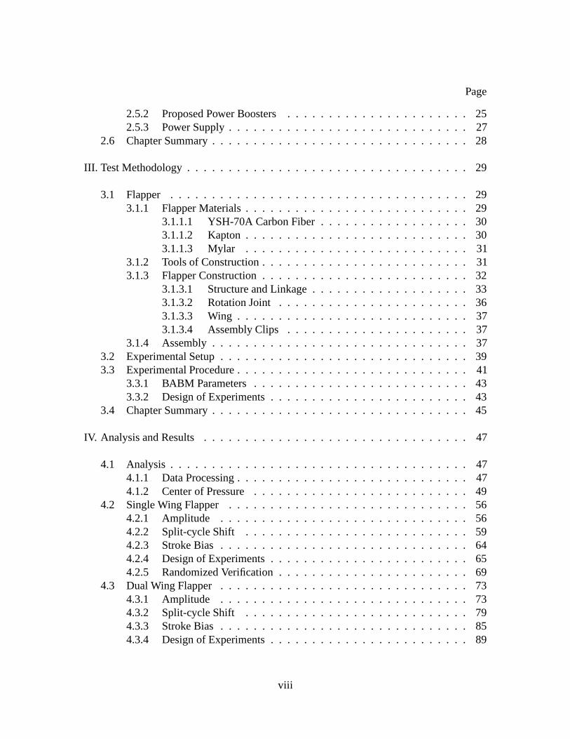
III. Test Methodology . . . . . . . . . . . . . . . . . . . . . . . . . . . . . . . .. . 29
3.1 Flapper . . . . . . . . . . . . . . . . . . . . . . . . . . . . . . . . . . . . 293.1.1 Flapper Materials . . . . . . . . . . . . . . . . . . . . . . . . . . . 29
3.1.1.1 YSH-70A Carbon Fiber . . . . . . . . . . . . . . . . . . 303.1.1.2 Kapton . . . . . . . . . . . . . . . . . . . . . . . . . . . 303.1.1.3 Mylar . . . . . . . . . . . . . . . . . . . . . . . . . . . 31
3.1.2 Tools of Construction . . . . . . . . . . . . . . . . . . . . . . . . . 313.1.3 Flapper Construction . . . . . . . . . . . . . . . . . . . . . . . . . 32
3.1.3.1 Structure and Linkage . . . . . . . . . . . . . . . . . . . 333.1.3.2 Rotation Joint . . . . . . . . . . . . . . . . . . . . . . . 363.1.3.3 Wing . . . . . . . . . . . . . . . . . . . . . . . . . . . . 373.1.3.4 Assembly Clips . . . . . . . . . . . . . . . . . . . . . . 37
3.1.4 Assembly . . . . . . . . . . . . . . . . . . . . . . . . . . . . . . . 373.2 Experimental Setup . . . . . . . . . . . . . . . . . . . . . . . . . . . . . . 393.3 Experimental Procedure . . . . . . . . . . . . . . . . . . . . . . . . . . .. 41
3.3.1 BABM Parameters . . . . . . . . . . . . . . . . . . . . . . . . . . 433.3.2 Design of Experiments . . . . . . . . . . . . . . . . . . . . . . . . 43
3.4 Chapter Summary . . . . . . . . . . . . . . . . . . . . . . . . . . . . . . . 45
IV. Analysis and Results . . . . . . . . . . . . . . . . . . . . . . . . . . . . . .. . 47
4.1 Analysis . . . . . . . . . . . . . . . . . . . . . . . . . . . . . . . . . . . . 474.1.1 Data Processing . . . . . . . . . . . . . . . . . . . . . . . . . . . . 474.1.2 Center of Pressure . . . . . . . . . . . . . . . . . . . . . . . . . . 49
4.2 Single Wing Flapper . . . . . . . . . . . . . . . . . . . . . . . . . . . . . 564.2.1 Amplitude . . . . . . . . . . . . . . . . . . . . . . . . . . . . . . 564.2.2 Split-cycle Shift . . . . . . . . . . . . . . . . . . . . . . . . . . . 594.2.3 Stroke Bias . . . . . . . . . . . . . . . . . . . . . . . . . . . . . . 644.2.4 Design of Experiments . . . . . . . . . . . . . . . . . . . . . . . . 654.2.5 Randomized Verification . . . . . . . . . . . . . . . . . . . . . . . 69
4.3 Dual Wing Flapper . . . . . . . . . . . . . . . . . . . . . . . . . . . . . . 734.3.1 Amplitude . . . . . . . . . . . . . . . . . . . . . . . . . . . . . . 734.3.2 Split-cycle Shift . . . . . . . . . . . . . . . . . . . . . . . . . . . 794.3.3 Stroke Bias . . . . . . . . . . . . . . . . . . . . . . . . . . . . . . 854.3.4 Design of Experiments . . . . . . . . . . . . . . . . . . . . . . . . 89
viii

Page
4.4 Comparison to Earlier Work . . . . . . . . . . . . . . . . . . . . . . . . .934.5 Chapter Summary . . . . . . . . . . . . . . . . . . . . . . . . . . . . . . . 93
V. Conclusions . . . . . . . . . . . . . . . . . . . . . . . . . . . . . . . . . . . . . 94
5.1 Research Goals . . . . . . . . . . . . . . . . . . . . . . . . . . . . . . . . 945.2 Summary of Results . . . . . . . . . . . . . . . . . . . . . . . . . . . . . . 94
5.2.1 Power . . . . . . . . . . . . . . . . . . . . . . . . . . . . . . . . . 955.2.2 Controllability . . . . . . . . . . . . . . . . . . . . . . . . . . . . 96
5.3 Future Work . . . . . . . . . . . . . . . . . . . . . . . . . . . . . . . . . . 97
Appendix: Explanation of MATLAB Scripts . . . . . . . . . . . . . . . .. . . . . . 99
Bibliography . . . . . . . . . . . . . . . . . . . . . . . . . . . . . . . . . . . . . . 106
Vita . . . . . . . . . . . . . . . . . . . . . . . . . . . . . . . . . . . . . . . . . . . 110
ix

List of Figures
Figure Page
2.1 Manduca sexta . . . . . . . . . . . . . . . . . . . . . . . . . . . . . . . . . . 5
2.2 Manduca sextaaverage mass distribution . . . . . . . . . . . . . . . . . . . . 7
2.3 Cross-sectional view of the primary flight muscles . . . . .. . . . . . . . . . . 8
2.4 Proposed FWMAV mass properties for a 1.55 g vehicle . . . . .. . . . . . . . 10
2.5 Simultaneous drive bimorph PZT actuator . . . . . . . . . . . . .. . . . . . . 15
2.6 Defined axis system . . . . . . . . . . . . . . . . . . . . . . . . . . . . . . . .17
2.7 Split-cycle wing trajectory . . . . . . . . . . . . . . . . . . . . . . .. . . . . 19
2.8 Effect of amplitude on drive signal . . . . . . . . . . . . . . . . . . . . . . . .22
2.9 Effect of split-cycle shift on drive signal . . . . . . . . . . . . . . . . .. . . . 23
2.10 Effect of stroke bias on drive signal . . . . . . . . . . . . . . . . . . . . . . .. 24
2.11 Hybrid voltage multiplier . . . . . . . . . . . . . . . . . . . . . . . .. . . . . 25
2.12 Boost converter with autotransformer . . . . . . . . . . . . . .. . . . . . . . 26
2.13 PT transformer equivalent circuit and amplifier . . . . . .. . . . . . . . . . . 28
3.1 Constructed flapper . . . . . . . . . . . . . . . . . . . . . . . . . . . . . . .. 30
3.2 LPKF Multipress S . . . . . . . . . . . . . . . . . . . . . . . . . . . . . . . . 32
3.3 LPKF Protolaser U . . . . . . . . . . . . . . . . . . . . . . . . . . . . . . . . 33
3.4 Flapper parts for assembly . . . . . . . . . . . . . . . . . . . . . . . . .. . . 34
3.5 Final linkage configuration . . . . . . . . . . . . . . . . . . . . . . . .. . . . 35
3.6 Layup for multipress to make parts for assembly . . . . . . . .. . . . . . . . . 36
3.7 Constructed flapper with piezoelectric actuator . . . . . .. . . . . . . . . . . 39
3.8 Experimental setup . . . . . . . . . . . . . . . . . . . . . . . . . . . . . . .. 40
3.9 Sample FRF for a flapper . . . . . . . . . . . . . . . . . . . . . . . . . . . . .42
x

Figure Page
4.1 Sample of raw lift data . . . . . . . . . . . . . . . . . . . . . . . . . . . . .. 48
4.2 Simulink model to compute power . . . . . . . . . . . . . . . . . . . . .. . . 49
4.3 Dual-wing flapper center of pressure and balance axes . . .. . . . . . . . . . . 50
4.4 Aerodynamic dimensions of FWMAV wing . . . . . . . . . . . . . . . .. . . 50
4.5 Actuator displacement vs. amplitude . . . . . . . . . . . . . . . .. . . . . . . 52
4.6 Actuator displacement vs. split-cycle shift,τ(n) . . . . . . . . . . . . . . . . . 53
4.7 Actuator displacement vs. stroke bias,η(n) . . . . . . . . . . . . . . . . . . . . 54
4.8 Measured pitch moment correction to center of pressure .. . . . . . . . . . . . 55
4.9 Power vs. amplitude . . . . . . . . . . . . . . . . . . . . . . . . . . . . . . .57
4.10 Forces and moments about the balance center vs. amplitude . . . . . . . . . . . 58
4.11 Power per lift vs. amplitude . . . . . . . . . . . . . . . . . . . . . . .. . . . . 59
4.12 Power vs. split-cycle shift . . . . . . . . . . . . . . . . . . . . . . .. . . . . . 60
4.13 Drive signal with a split-cycle shift ofπ/4 . . . . . . . . . . . . . . . . . . . . 61
4.14 Power vs. split-cycle shift . . . . . . . . . . . . . . . . . . . . . . .. . . . . . 61
4.15 Forces and moments about the balance center vs. split-cycle shift . . . . . . . . 62
4.16 Power per lift vs. split-cycle shift . . . . . . . . . . . . . . . .. . . . . . . . . 63
4.17 Power vs. stroke bias . . . . . . . . . . . . . . . . . . . . . . . . . . . . .. . 65
4.18 Forces and moments about the balance center vs. stroke bias . . . . . . . . . . 66
4.19 Power per lift vs. stroke bias . . . . . . . . . . . . . . . . . . . . . .. . . . . 67
4.20 DOE results for single-wing flapper . . . . . . . . . . . . . . . . .. . . . . . 68
4.21 BABM parameter effects on power for a single-wing flapper . . . . . . . . . . 70
4.22 BABM parameter effects on lift for a single-wing flapper . . . . . . . . . . . . 71
4.23 Power vs. amplitude, random sampling . . . . . . . . . . . . . . .. . . . . . 71
4.24 Power vs. split-cycle shift, random sampling . . . . . . . .. . . . . . . . . . . 72
4.25 Power vs. stroke bias . . . . . . . . . . . . . . . . . . . . . . . . . . . . .. . 72
xi

Figure Page
4.26 Power vs. amplitude, left wing . . . . . . . . . . . . . . . . . . . . .. . . . . 74
4.27 Power vs. amplitude, right wing . . . . . . . . . . . . . . . . . . . .. . . . . 75
4.28 Forces and moments about the balance center vs. amplitude, left wing . . . . . 76
4.29 Forces and moments about the balance center vs. amplitude, right wing . . . . 77
4.30 Power per lift vs. amplitude, left wing . . . . . . . . . . . . . .. . . . . . . . 78
4.31 Power per lift vs. amplitude, right wing . . . . . . . . . . . . .. . . . . . . . 78
4.32 Power vs. split-cycle shift, left wing . . . . . . . . . . . . . .. . . . . . . . . 79
4.33 Power vs. split-cycle shift, right wing . . . . . . . . . . . . .. . . . . . . . . 80
4.34 Forces and moments about the balance center vs. split-cycle shift, left wing . . 82
4.35 Forces and moments about the balance center vs. split-cycle shift, right wing . 83
4.36 Power per lift vs. split-cycle shift, left wing . . . . . . .. . . . . . . . . . . . 84
4.37 Power per lift vs. split-cycle shift, right wing . . . . . .. . . . . . . . . . . . 84
4.38 Power vs. stroke bias . . . . . . . . . . . . . . . . . . . . . . . . . . . . .. . 85
4.39 Forces and moments about the balance center vs. stroke bias . . . . . . . . . . 87
4.40 Power per lift vs. stroke bias . . . . . . . . . . . . . . . . . . . . . .. . . . . 88
4.41 DOE results for dual-wing flapper . . . . . . . . . . . . . . . . . . .. . . . . 90
4.42 BABM parameter effects on power for a dual-wing flapper . . . . . . . . . . . 91
4.43 BABM parameter effects on lift for a dual-wing flapper . . . . . . . . . . . . . 92
xii

List of Tables
Table Page
2.1 Manduca sextaClassification . . . . . . . . . . . . . . . . . . . . . . . . . . . 6
2.2 Two-winged MAV flapping mechanisms . . . . . . . . . . . . . . . . . .. . . 12
2.3 Linear actuator characteristics . . . . . . . . . . . . . . . . . . .. . . . . . . 15
2.4 Summary of aerodynamic forces and moments caused by control variables . . . 21
3.1 DOE parameters for a single-wing flapper . . . . . . . . . . . . . .. . . . . . 44
3.2 DOE parameters for a dual-wing flapper . . . . . . . . . . . . . . . .. . . . . 46
4.1 Baseline of aerodynamic forces and moments caused by BABM parameters . . 56
5.1 Effects of BABM parameters on power and lift . . . . . . . . . . . . . . . . .95
5.2 Summary of forces and moments generated by changing BABMparameter . . 96
xiii

List of Symbols
Symbol Definition
A Stroke Amplitude
E Elastic Modulus
L Roll Moment
M Pitch Moment
Mn nth Fourier Coefficient
Mx Moment About theX-axis
My Moment About theY-axis
Mz Moment About theZ-axis
Mωn Magnitude of the Wing Displacement at the First System Resonance
M2ωn Magnitude of the Wing Displacement at Twice the First SystemResonance
N Yaw Moment
P Power
R Wingspan
RBI Rotation Matrix from the Inertial Reference Frame to the Body Frame
Re Reynolds Number
S Wing Area
X Axial Force in the in theX-direction
Y Axial Force in the in theY-direction
Z Axial Force in the in theZ-direction
g Gravity
m Mass
n Sample
xiv

Symbol Definition
p Roll Angular Rate
q Pitch Angular Rate
r Yaw Angular Rate
u Translational Velocity in theX-direction
v Translational Velocity in theY-direction
w Translational Velocity in theZ-directionA Aspect Ratio
α Wing Angle of Attack
β Phase Shift
γ Phase Angle
δ Actuator Tip Deflection
η Stroke Bias
θ Wing Elevation Angle
τ Split-cycle Shift
φ Wing Stroke Angle
φωn Phase of the Wing Displacement at the First System Resonance
Subscripts
L Left Wing
R Right Wing
cp Center of Pressure
rms Root Mean Square
s Sample
xv

Symbol Definition
Superscripts
bal Balance Reference Frame
xvi

List of Acronyms
Acronym Definition
AFIT Air Force Institute of Technology
AFRL Air Force Research Laboratory
BABM Bi-harmonic amplitude and bias modulation
DAQ Data acquisition
DC Direct current
DHPC Discrete harmonic plant compensation
DLMs Dorsal longitudinal muscles
DOE Design of experiments
DOF Degrees of freedom
DVMs Dorsal ventral muscles
EAP Electro active polymers
FRF Frequency response function
FWMAV Flapping wing micro air vehicle
ISR Intelligence, surveillance, and reconnaissance
MAV Micro air vehicle
MEMS Microelectromechanical systems
PET Polyethylene terephthalate
PSD Power spectral density
PT Piezoelectric transformer
PVDF Piezo polymers
PZT Lead zirconate titanate
SMA Shape memory alloy
xvii

Acronym Definition
UAV Unmanned aerial vehicle
UV Ultraviolet
xviii
POWER REQUIREMENTS FOR BI-HARMONIC AMPLITUDE AND BIAS
MODULATION CONTROL OF A FLAPPING WING MICRO AIR VEHICLE
I. Introduction
Recent years have seen an increase in use for unmanned aerial vehicles (UAVs). It
is becoming apparent that they are now a major mainstay in American warfare.
UAVs play a pivotal role in the intelligence, surveillance,and reconnaissance (ISR) mission
affording troops unrivaled capabilities. UAVs also supportedtroops by serving as local
weather sensors and communication relays. In that class falls the micro air vehicle (MAV).
A key role that often comes to mind is the MAV’s capability to fulfill the stealthy, persistent,
perch, and stare mission. This calls for a MAV capable of flying to difficult targets,
landing in a perched position, conducting surveillance, and returning to home base. [38]
Furthermore, the possible roles of MAVs are ever expanding with new potentials such as
the delivery of computer viruses without putting troops in harm’s way. Multiple ideas have
been investigated to generate a MAV to fulfill this mission toinclude fixed wing, rotary
wing, and flapping wing aircraft.
A bio-inspired MAV, one whose design is based on nature, would have the inherent
benefit of stealth through mimicry of insects. Such a MAV is referred to as a flapping
wing micro air vehicle (FWMAV). A FWMAV takes advantage of several unsteady
aerodynamic effects in the low Reynolds number regime. [3] A FWMAV could meet
mission requirements while being unobtrusive and pervasive.
1

1.1 Motivation
The Air Force Institute of Technology (AFIT) has dedicated much research to the
development of a bio-inspired FWMAVs. It was evident very early on that the miniscule
mass of the FWMAV was a major concern. As such, there is a desire to focus research
on reducing the power requirements of the FWMAV therefore reducing the mass of the
power supply. However, as of now, there is not a clear understanding of the current power
requirements of the FWMAV. AFIT has developed a control theory called bi-harmonic
amplitude and bias modulation (BABM) based on wing-beat shape modulation developed
by the Air Force Research Laboratory (AFRL). [5, 14, 15] Research is under way to identify
how the BABM scheme will be implemented to achieve mission worthiness. It is known
that through BABM, five parameters can control the FWMAV in 5 degrees of freedom
(DOF) but little is known about how much power is required to vary those five parameters.
[6] Without knowledge of the power requirements, control logic cannot be designed to
maneuver the FWMAV and minimize the mass of the power supply.This research focused
on characterizing those power requirements for the BABM control scheme.
1.2 Research Goals
As stated above, the goal of this research was to investigatethe power requirements of
AFIT’s current FWMAV using the BABM control scheme. Gathered data was processed
and will be provided to other researchers for use in trajectory and control optimization and
control optimization. With this data, the trajectories canbe optimized to require the least
amount of power and the control logic can be optimized to manipulate the five BABM
parameters to minimize the power needed.
Data was collected on a single-wing flapper at first. Trends were applied to the model,
and consistency among wings was verified. These practices removed any suspicion that
the manufacturing process provides a large amount of variation between test samples.
2
The single-wing flapper also verified that the research approach is valid. After those
requirements were met on the single-wing flapper, testing began on a dual-wing flapper.
Testing was similar to that of the single-wing flapper but with expanded goals. The data
collected from the dual-wing flapper indicated variations between the left and right wing.
It also provided moment and force data more representative of an operational FWMAV.
Succinctly, the thesis statement for this research is:How much power is required to
vary each parameter and maintain lift? How do those power requirements relate to
controllability?
This work assumed that the results acquired will be representative of an operational
FWMAV. It was also assumed that the measured power results are valid for any given
set of electronics driving the actuator. There are some limitations to this research. To
accelerate the development time of the AFIT FWMAV, multipleareas of research are
being investigated simultaneously. As such, any findings from other research areas that
affect the design or production of the FWMAV will not be represented in this research.
It is important to state that the test methodology will remain the same for future testing
of different FWMAV designs. The results were expected to show that an increase in
any BABM control parameter would result in greater or equal power requirements. The
conclusions developed during this research will aid in the control logic development.
1.3 Organization of Thesis
The organization of this thesis is chronological and increasing in technical detail.
Chapter II discusses previous research in the area and lays the groundwork for this research.
Chapter III dives into the methodology used for data collection. Chapter IV presents the
processed data collected from testing and provides the basis for the conclusions. Chapter V
presents the conclusions drawn from the data and suggestions for future work.
3

II. Background & Literature Review
The history of research into FWMAVs is extensive. One may say it began when the
military first started to investigate unmanned aircraft or it may have started when
man first began to study the flight of our winged friends in hopes of achieving flight.
The recent ramp in technology has brought UAVs into the forefront of military leadership.
For instance, UAVs flew over 100,000 total flight hours by September 2004 in support of
Operation ENDURING FREEDOM and Operation IRAQI FREEDOM. [37] An increased
focus on ISR missions to clandestine or denied entry locations has concentrated research
on biomimicry. [2] By studying our cohabitants, researchers have gained insight into small-
scale aerodynamics. Bio-inspired MAVs may one day offer unparalleled capability. As
such, a lot of previous research has been done on the development of FWMAVs.
AFIT researchers have found a niche to fulfill in the FWMAV community. The
research conducted at AFIT focuses on a FWMAV with a wingspanaround 10 centimeters
and a mass around 1.5 grams. Multiple researchers have focused on smaller or larger
FWMAVs. AFIT also developed the BABM control scheme and discrete harmonic plant
compensation (DHPC) to manipulate the wings of the FWMAV. A clear understanding of
what research has been done in all of the previous topics is required to place the research
conducted herein in context.
2.1 The Manduca sexta
The first step to any bio-inspired system is a thorough understanding of the creation
who serves as the inspiration. The FWMAV used for this research has been inspired by
theManduca sexta, or hawkmoth, shown in Figure 2.1. TheM. sextais a North American
moth with long forewings, short hind wings, and the ability to hover and move side-to-side.
[29] This extraordinary ability made theM. sextathe perfect candidate. [39] They are also
4

easily reared in a laboratory, have short life cycles, and arelarge, all of which aide in many
scientific investigations. Due to these qualities, there is no shortage of literature on the
study ofM. sexta. The biological classification of theM. sextais found in Table 2.1.
Figure 2.1:Manduca sexta[23]
2.1.1 Mass.
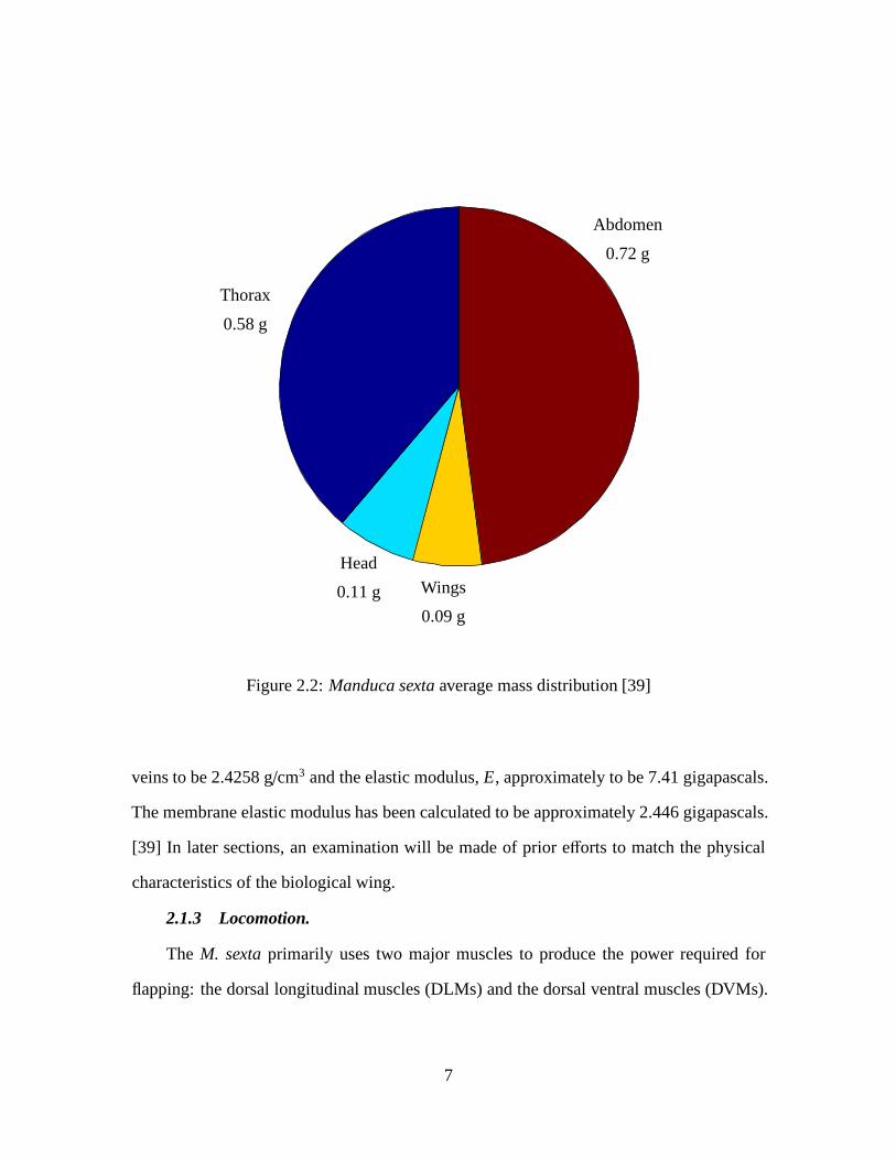
The size of theM. sexta, like with most creatures, varies based on gender. Figure 2.2
shows average mass values obtained for theM. sextabased on 30 samples. The total mass
of theM. sextaaverages only 1.55±0.05 grams. [39] In order to create a FWMAV based
on theM. sexta, the FWMAV must be of similar mass. The limitations to the FWMAV
mass will be discussed later.
5
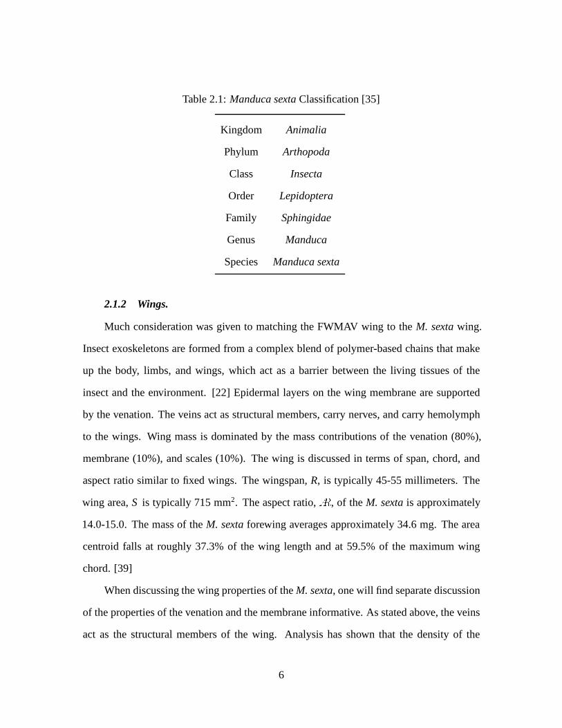
Table 2.1:Manduca sextaClassification [35]
Kingdom Animalia
Phylum Arthopoda
Class Insecta
Order Lepidoptera
Family Sphingidae
Genus Manduca
Species Manduca sexta
2.1.2 Wings.
Much consideration was given to matching the FWMAV wing to the M. sextawing.
Insect exoskeletons are formed from a complex blend of polymer-based chains that make
up the body, limbs, and wings, which act as a barrier between the living tissues of the
insect and the environment. [22] Epidermal layers on the wing membrane are supported
by the venation. The veins act as structural members, carry nerves, and carry hemolymph
to the wings. Wing mass is dominated by the mass contributions of the venation (80%),
membrane (10%), and scales (10%). The wing is discussed in terms of span, chord, and
aspect ratio similar to fixed wings. The wingspan,R, is typically 45-55 millimeters. The
wing area,S is typically 715 mm2. The aspect ratio,A, of theM. sextais approximately
14.0-15.0. The mass of theM. sextaforewing averages approximately 34.6 mg. The area
centroid falls at roughly 37.3% of the wing length and at 59.5% of the maximum wing
chord. [39]
When discussing the wing properties of theM. sexta, one will find separate discussion
of the properties of the venation and the membrane informative. As stated above, the veins
act as the structural members of the wing. Analysis has shownthat the density of the
6
Abdomen
0.72 g
Wings
0.09 g
Head
0.11 g
Thorax
0.58 g
Figure 2.2:Manduca sextaaverage mass distribution [39]
veins to be 2.4258 g/cm3 and the elastic modulus,E, approximately to be 7.41 gigapascals.
The membrane elastic modulus has been calculated to be approximately 2.446 gigapascals.
[39] In later sections, an examination will be made of prior efforts to match the physical
characteristics of the biological wing.
2.1.3 Locomotion.
The M. sextaprimarily uses two major muscles to produce the power required for
flapping: the dorsal longitudinal muscles (DLMs) and the dorsal ventral muscles (DVMs).
7

These are common to the majority of flying insects and are located in the thorax. When the
DVMs contract, they pull the dorsal surface of the thorax downward and the wings rotate
upward. When the DLMs contract, they bow the dorsal surface upward and the wings
rotate downward. The constant contraction and relaxationsof these two muscles power
the flapping wings of flying insects. Figure 2.3 shows the muscle motions and how they
produce flapping.
(a) DVMs contracting (b) Transition (c) DLMs contracting
Figure 2.3: Cross-sectional view of the primary flight muscles (reproduced from [12])
The DLMs are the largest muscle in theM. sexta, comprising 5-8% of the total
body mass. [43] Both the DVMs and the DLMs are comprised of multiple muscle units.
The DLMs have five muscle units and the DVMs have six muscle units. Most research
concludes that the power output of theM. sextamuscle structure outputs 81-202 W/kg.
[12]
2.2 Design Considerations
The next step to the design of a bio-inspired system is to mimic the properties of the
biological creature as closely as possible. The techniquesused to manufacture FWMAVs
must be simple enough to be repeatable and durable enough to operate for multiple testing
cycles.
8
Manufacturing is a major concern when considering the development of a FWMAV.
Without the capability to manufacture a FWMAV test bed, testing is not possible and so
manufacturing is discussed. Above everything else in the design considerations is weight.
Materials must be used that are durable to withstand the physics of small-scale flight but
light enough to achieve flight. As a prefatory step, the FWMAVwas split into similar
proportions as theM. sextaresulting in the proposal in Figure 2.4. The thorax actuatesthe
wings on theM. sextaand was therefore likened to the actuator; the abdomen holdsthe
organs that process energy and was therefore likened to the power source; and, the head
holds the eyes and antennae and was therefore likened to the sensors. The similarities can
easily be seen between Figure 2.2 and Figure 2.4 and they simply demonstrate a reasonable
mass allocation based on biomimicry.
Analysis showed that composites was an appropriate material for the structure and
wings to obtain the mass and elastic modulus requirements. [39] They provide the strength
to weight ratios desired for sustained flight in the insect-sized regime. Composites also
simplify manufacturing compared to other methods. The choice of a composite relies on
matching the characteristics of theM. sexta.
Once the FWMAV has been assembled with a reliable repeatableprocess, discussed in
Chapter III, the wings must be actuated to achieve flight. There are two types of actuators
being used in FWMAVs: linear and rotary. Much work has been done on the comparison
of the two types of actuators for FWMAVs. Many designs use rotary direct current (DC)
motors for actuation. [11, 13, 28] However, DC motors typically operate around 15,000
rpm so a gear reduction must be used to make them suitable for this application. A complex
crank-rocker mechanism is then used to transform the rotarymotion into the required linear
motion. The crank-rocker must be designed so that it is only partially constrained allowing
for some degree of controllability. [11] An unavoidable drawback to DC motors is the
9

Power Source
0.72 g
48%
Wings
0.09 g
6%
Sensors
0.11 g
7%
Actuator
0.58 g
39%
Figure 2.4: Proposed FWMAV mass properties for a 1.55 g vehicle
minimum size lower bound. The smallest DC motors currently weight approximately 200
mg. [3] The large size of DC motors places a lower bound on the size of FWMAVs, a
lower bound that is larger than desired. An often overlookedkey design goal is a low
acoustic signature to make vehicles less susceptible to detection. [37] Current DC driven
FWMAVs have significant acoustic noise, lowering their stealth capability. [27] Another
option is the linear actuator. With the linear actuator, there is no need for a crank-rocker
mechanism, which significantly simplifies the design. Linear acutators also have lower
acoustic signatures than DC motors. Table 2.2 summarizes the actuator options and the
10

crank-rocker mechanisms. Note that Conn et al. published this summary in 2007, prior to
the control scheme discussed in Section 2.4. From Table 2.2,the linear actuators provide
the greatest number of adjustable parameters.
11

Tab
le2
.2:
Co
mp
lexi
tyan
dp
erfo
rman
cecl
assi
ficat
ion
oft
wo
-win
ged
MAV
flap
pin
gm
ech
anis
ms
[11
]
Mec
han
ism
Fiv
e-
bar
cou
ple
r
with
fou
r-b
ar
Fo
ur-
bar
cou
ple
ran
d
Gen
eva
wh
eel
Sco
tch
Yo
ke
Do
ub
le
sco
tch
yoke
and
Gen
eva
wh
eel
No
n-p
lan
ar
cran
k-
rock
er
Par
alle
l
cran
k-
rock
er
Par
alle
l
fou
r-b
ars
Dip
tera
n
(tw
o-
win
ged
inse
ct)
Com
plex
ity
Inp
utT
ype
Ro
tary
Ro
tary
Ro
tary
Ro
tary
Ro
tary
Ro
tary
Lin
ear
Lin
ear
Co
ntr
olI
np
uts
11
11
13
81
2
Act
uat
ors
11
11
13
85
0
Per
form
ance
Win
gtr
ajec
tory
Fix
edtw
o
DO
F
Fix
edtw
o
DO
F
Fix
edo
ne
DO
F
Fix
edtw
o
DO
F
Fix
edo
ne
DO
F
Fix
edo
ne
DO
F
Ad
just
able
on
eD
OF
Ad
just
able
two
DO
F
An
gle
ofA
ttack
,αF
ixed
Fix
edF
ixed
Fix
edF
ixed
Ad
just
able
Ad
just
able
Ad
just
able
Str
oke
amp
litu
de,Φ
Fix
edF
ixed
Fix
edF
ixed
Fix
edF
ixed
Ad
just
able
Ad
just
able
Co
ntr
olla
ble
bo
dy
DO
F
11
11
14
44
12

2.3 The AFIT FWMAV
AFIT researchers have dedicated considerable time and resources to matching
the characteristics of theM. sexta, and those efforts will be summarized here. The
manufacturing techniques adopted by AFIT will also be reviewed in this section. For
a more detailed discussion of the development of the AFIT FWMAV, the reader is
encouraged to read reference 39.
2.3.1 Wings.
Previous work has been done to mimic theM. sextawings. The goal of the engineered
wing structure is to match the structural properties and thedynamic response of theM.
sexta. The materials of the wings were investigated with relationto two parts of the wing:
the venation and the membrane.
For the wing venation, AFIT researched multiple materials including isotropic metals,
shape memory alloys, ultraviolet (UV) cured polymers and composite high modulus thin
ply laminates. It was discovered early on that isotropic metals and shape memory alloys
would be too massive to meet the requirements of a FWMAV. It was found that UV
cured polymers did not provide the strength required to match the biological wing. The
experimentation did prove that a composite high modulus lamina, YSH-70A, was identified
as a potential match to the biological wing. YSH-70A fibers are a high modulus fiber that
are produced with a larger yield size. The YSH-70A fibers are manufactured with a RS-
3C epoxy resin embedded. To match theM. sextacharacteristics, the YSH-70A fibers are
layered in a 0-90-0 orientation. After further testing, this material and orientation were
found to be a nearly ideal material for engineering wing venation. [39]
For the wing membrane, a focus was based on the mass and strength of possible
choices. Two primary materials were investigated: Kapton and Mylar. Kapton is a
polyimide film manufactured by DuPont. Kapton is available in thicknesses of 12.5, 25,
and 75µm. Measurements found that a Kapton membrane would weigh approximately
13

22.5 mg for an engineered wing similarly sized to a biological wing. This large mass
proved to be too large. Mylar is a polyester film manufacturedby DuPont used for high
strength applications and its dimensional stability properties. The Mylar used is 2.5µm
thick with an elastic modulus of 3.7 gigapascals, which is similar to the representative
biological value of 2.4 gigapascals. Measurements found that a Mylar membrane would
weigh approximately 4.5 mg making it the best choice for the engineered wing. [39]
2.3.2 Locomotion.
AFIT researchers have chosen to pursue the use of two linear actuators over a single
rotary actuator since linear actuators provide lower mass,provide lower acoustic signature,
and simplify the transmission. Table 2.3 taken from [3] (adapted from [10]) shows a
comparison between linear actuator options and the insect flight muscle. Since the table
is taken from many varying sources, it was used as a general comparison tool. From the
table, lead zirconate titanate (PZT) actuators are superior to insect muscles in all categories
except strain. A linkage was created to increase the magnitude of the piezoelectric actuator
tip displacement to overcome the strain deficiency.
AFIT researchers have chosen to use a bimorph piezoelectricactuator made of PZT to
drive the FWMAV. A bimorph piezoelectric actuator uses two layers of PZT material and
a passive layer sandwiched between them. [44] A bimorph piezoelectric actuator is shown
in Figure 2.5. The piezoelectric actuator is driven using simultaneous drive. Simultaneous
drive, also shown in Figure 2.5, is a more economical technique and prevents hysteresis
techniques associated with other driving schemes. This method initially charges each
actuator with a bias voltage,Vb, and then charges the central passive layer with the drive
voltage,Vd. [45]
14

Table 2.3: Linear actuator characteristics [3]
Actuator Type Strain (%) Stress (MPa) Frequency
(Hz)
Specific
Energy
Density (J/g)
Efficiency
(%)
Synchronous Flight
Muscle
17 0.35 5.5-100 0.003 2-13%
Asynchronous Flight
Muscle
2 - 100-1046 0.002 5-29%
PZT 0.2 110 108 0.013 90
PVDF 0.1 4.8 107 0.0013 90
SMA (TiNi) 5 200 101 15 10
Solenoid 50 0.1 102 0.003 90
EAP (Dielectric Elas-
tomer)
63 3 104 0.75 90
Vb
Vd
Figure 2.5: Simultaneous drive bimorph PZT actuator
2.4 Control in FWMAVs
An emphasis has been placed on reducing weight, increasing agility, and integrating
robotics in future forces. [38] Increasing agility and integrating robotics indicates that
control is a pivotal part of the future of MAVs. In the past, the aerodynamics and
manufacturing proved to be such daunting tasks that controlwas set aside. However, as
15

our understanding of the flight mechanisms has increased as well as our ability to micro-
fabricate small structures, control theory must make leapsand bounds to catch-up. In
Design and Control of Flapping Wing Micro Air Vehicles, Anderson introduced a new
method of control for FWMAVs actuated with piezoelectric actuators called bi-harmonic
amplitude and bias modulation (BABM). [3] BABM control withDHPC allows two
actuators to produce forces and moments in five DOF. It is withBABM that the AFIT
FWMAV would be controlled.
The axis system taken from Doman et al. is used and defined in Figure 2.6. [14]
Therefore, lift is in the positiveX direction during hover and thrust is in the negativeZ
direction during hover. Note that theX andZ-axes are relative to the FWMAV and thus
only align with lift and thrust direction while hovering. The side-force is out the FWMAV’s
right wing. Perhaps the most confusing aspect of transferring knowledge from fixed wing
aircraft to flapping wing aircraft is the difference in moment definitions. A moment about
theX-axis is still referred to as the rolling moment but it controls the direction of the thrust
vector in a plane parallel to the ground during hover. A moment about theY-axis is still
referred to as the pitching moment but it controls the direction of the thrust vector in a plane
perpendicular to the ground during hover. A moment about theZ-axis is still referred to as
the yawing moment but it controls the direction of the lift vector in a plane perpendicular to
the ground during hover. [36] Three angles define the wing position at any point during the
flapping cycle: the wing angle of attack,α, the wing stroke angle,φ, and the wing elevation
angle,θ. [8] Figure 2.6 identifies these three angles.
The rigid body equations of motion are presented here in the FWMAV body frame:
I
p
q
r
=
L
M
N
−
p
q
r
× I
p
q
r
(2.1)
16

Figure 2.6: Defined axis system [30]
u
v
w
=
qw− rv
ru − pw
pv− qu
+
(
1m
)
X
Y
Z
− RBI
0
0
−g
(2.2)
whereI is the inertia matrix,[
p q r]T
are roll, pitch, and yaw angular rates,[
L M N]T
are the roll, pitch, and yaw moments,[
u v w]T
are the translational velocities,m is the
mass,[
X Y Z]T
are the axial forces,RBI is a rotation matrix from the inertial frame to
the body frame, andg is the gravitational acceleration. [41] This notation is common in
aircraft control.
There is no commonly agreed-upon control scheme for FWMAVs and so each
FWMAV designer has developed a unique control scheme to meettheir requirements.
Research has shown that discussions of FWMAV control can be split into two categories:
single-DOF control and multi-DOF control. The only necessary angle for wing flapping
is the wing stroke angle, and therefore, all controllers usethat as a DOF. In the case of
single-DOF controllers, it is the only DOF. Beyond that, developers have added the wing
17

angle of attack and the wing elevation angle, usually in thatorder, to achieve further control.
The FWMAV with the most controllable DOF will be the most controllable vehicle. [6]
2.4.1 Flapping at Resonance.
Research shows that most biological fliers flap their wings atthe first natural frequency
of their muscle system. There is a tendency of a species to flapat a consistent frequency
across all flight regimes. Furthermore, researchers found that by artificially shortening
the insect’s wings, the wing beat frequency increases. Thisagrees with the hypothesis that
insects flap at their resonant frequency since the frequencyvaries inversely with the load on
the system. There is advantageous energetic expenditure when mechanical systems operate
at resonance. [16]
The advantage of low energetic expenditure is very useful tothe designer of the power
system for the FWMAV. Since the power system may be one of the heavier components,
any reductions will be manifested as benefits in range, endurance, speed, and payload.
Flapping at resonance does generate some concerns for the control developer though. For
instance, vehicles flapping at resonance will make it difficult to drive the wings in a pattern
other than harmonic motion. However, the need for energeticefficiency may overcome the
desire to avoid resonance and therefore, techniques must bedeveloped for non-harmonic
resonant flapping. [6]
2.4.2 Bi-harmonic Amplitude and Bias Modulation.
The control used for this research will be BABM. BABM generates non-harmonic
wing flapping creating non-zero cycle-averaged forces resulting in aerodynamic forces and
moments. [5] BABM was adapted from the split-cycle theory presented by Doman et al.
in reference 15. The idea is to combine two cosine waves with differing frequencies to
create one wing beat cycle allowing control over the translational and rotational degrees
of freedom of the vehicle. An example is shown in Figure 2.7. The blue line represents a
18

symmetric cosine wave and the green line represents a split-cycle cosine wave. The up and
down-strokes are not symmetric, that is, the wing travels faster in one than the other.
Split-cycle Cosine WaveSymmetric Cosine Wave
No
rmal
ized
Sig
nal
Normalized Time0 0.2 0.4 0.6 0.8 1
−1
−0.5
0
0.5
1
Figure 2.7: Split-cycle wing trajectory,τ = 0.25
BABM control allows two piezoelectric actuators to produceforces and moments
in five DOF. The piezoelectric actuators operate in one DOF, the stroke angle. The
equations defining BABM were developed in reference 6. The stroke angle function,φ,
in Equation 2.3, is used to define the wing stroke angle.
φ (t) = A{M1 (τ) cos[
ωt + β (τ)]
− M2 (τ) sin[
2ωt + 2β (τ)]
} + η (2.3)
whereA is the stroke amplitude,τ is the split-cycle shift,η is the stroke bias, andω is the
flapping frequency.M1 and M2 are the Fourier coefficients andβ is the phase shift. The
first two Fourier terms provide an approximation to the split-cycle equations and provide
19
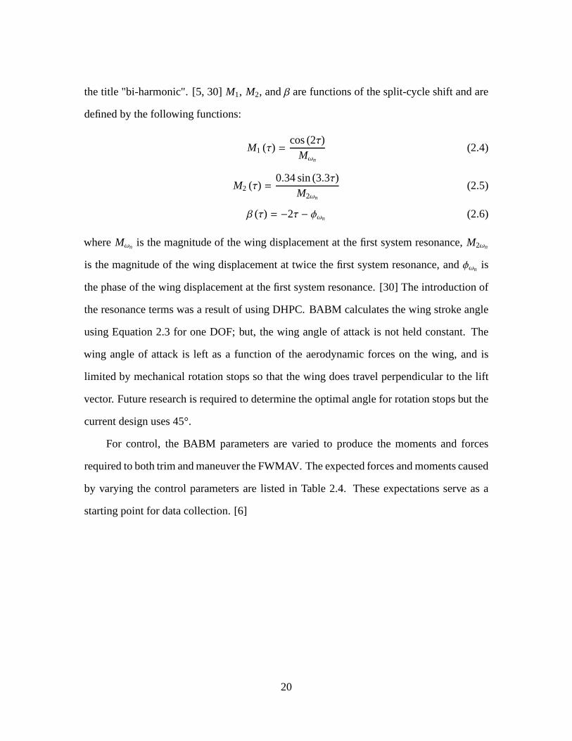
the title "bi-harmonic". [5, 30]M1, M2, andβ are functions of the split-cycle shift and are
defined by the following functions:
M1 (τ) =cos(2τ)
Mωn
(2.4)
M2 (τ) =0.34 sin(3.3τ)
M2ωn
(2.5)
β (τ) = −2τ − φωn (2.6)
whereMωn is the magnitude of the wing displacement at the first system resonance,M2ωn
is the magnitude of the wing displacement at twice the first system resonance, andφωn is
the phase of the wing displacement at the first system resonance. [30] The introduction of
the resonance terms was a result of using DHPC. BABM calculates the wing stroke angle
using Equation 2.3 for one DOF; but, the wing angle of attack is not held constant. The
wing angle of attack is left as a function of the aerodynamic forces on the wing, and is
limited by mechanical rotation stops so that the wing does travel perpendicular to the lift
vector. Future research is required to determine the optimal angle for rotation stops but the
current design uses 45°.
For control, the BABM parameters are varied to produce the moments and forces
required to both trim and maneuver the FWMAV. The expected forces and moments caused
by varying the control parameters are listed in Table 2.4. These expectations serve as a
starting point for data collection. [6]
20

Tab
le2
.4:
Su
mm
ary
ofa
ero
dyn
amic
forc
esan
dm
om
ents
cau
sed
by
con
tro
lvar
iab
les
[6]
Inse
cts
Ber
kele
yC
alte
chH
arva
rd1
Har
vard
2A
FR
L1
AF
RL
2A
FI
TB
AB
M
Req
uir
edA
ctu
ato
rsD
oze
ns?
46
?3
23
22
Lift
,X
Sym
met
ric
Am
plit
ud
eS
ymm
etri
cA
mp
litu
de
Sym
met
ric
Am
plit
ud
eS
ymm
etri
cA
mp
litu
de
Sym
met
ric
Am
plit
ud
eS
ymm
etri
cA
mp
litu
de
Sym
met
ric
Am
plit
ud
eS
ymm
etri
cA
mp
litu
de
Sid
eF
orc
e,Y?
--
--
-A
sym
met
ric
Str
oke
Bia
s-
Th
rust
,Z?
--
--
Sym
met
ric
Sp
lit-c
ycle
Sym
met
ric
Sp
lit-c
ycle
Sym
met
ric
Bi-
har
mo
nic
Sp
lit-c
ycle
Ro
ll,L
Asy
mm
etri
cS
tro
keP
lan
eA
ng
le&
Am
plit
ud
e
Asy
mm
etri
cR
ota
tion
Tim
ing
Asy
mm
etri
cS
tro
keP
lan
eA
ng
le
--
Asy
mm
etri
cS
plit
-cyc
leA
sym
met
ric
Sp
lit-c
ycle
Asy
mm
etri
cB
i-h
arm
on
icS
plit
-cyc
le
Pitc
h,M
?S
ymm
etri
cA
mp
litu
de
&R
ota
tion
Tim
ing
Sym
met
ric
Str
oke
Bia
sS
ymm
etri
cS
tro
keB
ias
Sym
met
ric
Str
oke
Bia
sB
ob
Wei
gh
tS
ymm
etri
cS
tro
keB
ias
Sym
met
ric
Str
oke
Bia
s
Yaw
,NA
sym
met
ric
Str
oke
Pla
ne
An
gle
&A
mp
litu
de
Asy
mm
etri
cA
mp
litu
de
Asy
mm
etri
cA
mp
litu
de
Asy
mm
etri
cA
mp
litu
de
Asy
mm
etri
cA
mp
litu
de
Asy
mm
etri
cF
req
uen
cyA
sym
met
ric
Fre
qu
ency
Asy
mm
etri
cA
mp
litu
de
21

The amplitude controls the overall stroke angle of the FWMAV. It can be thought of
as a scaling factor. Amplitude has units of voltage; for thisresearch, the value of amplitude
directly correlated to the voltage from the computer to the amplifier. An amplitude of 1
denotes a maximum and minimum value of the cosine wave. Therefore, a wave with an
amplitude of 2 will have a maximum twice as high as a wave with an amplitude of 1. This
is represented in Figure 2.8.
A=2A=1
Driv
eS
ign
al(V
)
Normalized Time0 0.2 0.4 0.6 0.8 1
−1.5
−1
−0.5
0
0.5
1
1.5
2
Figure 2.8: Effect of amplitude,A, on drive signal,τ = 0, η = 0 V
The split-cycle shift controls how much the cosine wave is shifted. It has been shown
that control could be achieved by limiting the split-cycle shift to a maximum of±0.3 and
that the negative values exactly mirror the positive values. [4] The split-cycle shift effect
on the drive signal is shown in Figure 2.9. Note thatτ = 0 is a pure sinusoid.
22

τ=0.25τ=0
No
rmal
ized
Sig
nal
Normalized Time0 0.2 0.4 0.6 0.8 1
−0.8
−0.6
−0.4
−0.2
0
0.2
0.4
0.6
0.8
1
Figure 2.9: Effect of split-cycle shift,τ, on drive signal,A = 1 V, η = 0 V
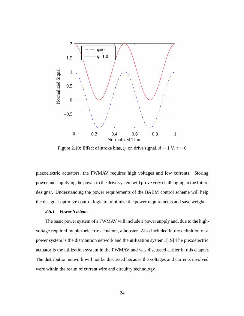
While the amplitude scales the magnitude of the signal, the stroke bias adds a constant
bias to the drive signal. The stroke bias is in the same units as the signal, and therefore
a stroke bias of 1 shifts the signal 1 volt in the positive direction. This effect is shown in
Figure 2.10.
2.5 Power
The focus on this paper is the cost of power. The power sourcesmust also be low
weight, and are, in this author’s opinion, the greatest obstacle facing the future of FWMAVs.
Recall that Figure 2.4 shows the mass properties of the FWMAV. The primary use of
power is the locomotion of the FWMAV with secondary uses including powering the
ISR sensors and communications. These secondary uses are disregarded for this research
mostly due to uncertainty of future technological advancements. To power the selected
23
η=1.0η=0
No
rmal
ized
Sig
nal
Normalized Time0 0.2 0.4 0.6 0.8 1
−0.5
0
0.5
1
1.5
2
Figure 2.10: Effect of stroke bias,η, on drive signal,A = 1 V, τ = 0
piezoelectric actuators, the FWMAV requires high voltagesand low currents. Storing
power and supplying the power to the drive system will prove very challenging to the future
designer. Understanding the power requirements of the BABMcontrol scheme will help
the designer optimize control logic to minimize the power requirements and save weight.
2.5.1 Power System.
The basic power system of a FWMAV will include a power supply and, due to the high-
voltage required by piezoelectric actuators, a booster. Also included in the definition of a
power system is the distribution network and the utilization system. [19] The piezoelectric
actuator is the utilization system in the FWMAV and was discussed earlier in this chapter.
The distribution network will not be discussed because the voltages and currents involved
were within the realm of current wire and circuitry technology.
24

2.5.2 Proposed Power Boosters.
Karpelson et al. eloquently offer three techniques to achieve the high voltage/low
current requirement: a boost converter/voltage multiplier hybrid, a boost converter
combined with an autotransformer, and a power amplifier using a piezoelectric transformer.
The following explanations appear in reference 26.
1. Hybrid Voltage Multiplier
A hybrid circuit consisting of a conventional boost converter cascaded
with a switched-capacitor charge pump circuit, as shown in Figure 2.11,
has been considered previously for piezoelectric microrobots and electro-
static microelectromechanical systems (MEMS) devices. Operating in a
regime of high efficiency, the boost converter stage provides a moderate
boost to the input voltage, while its pulsed output naturally charges up
the capacitor ladder through the diodes. The charge pump multiplies the
boost converter’s output voltage, ideally by a factor equalto the number
of charge pump stages. The maximum output power is limited bythe
size of the charge pump capacitors and the maximum output power of the
boost converter.
Figure 2.11: Hybrid voltage multiplier [26]
25

2. Converter with Autotransformer
Replacing the inductor in the standard boost converter withan autotrans-
former, as shown in Figure 2.12, results in a combination of the boost
and flyback voltage converter topologies. Similar to the boost converter,
current ramps up in the primary winding of the transformer when the
switching transistor is conducting. When the switch turns off, the recti-
fier diode sees a combination of the input voltage, the primary winding
voltage, and the secondary winding voltage, which depends on the turn
ratio between the primary and secondary windings. Voltage gain is there-
fore determined by the duty cycle of the switching transistor and the turn
ratio of the transformer. Maximum output power is limited bythe current
rating of the switching transistor and the transformer. Forhigh voltage
gains, this method has a much lower parts count than the hybrid con-
verter. However, the rectifier diode and output capacitor must be rated for
the output voltage. Additionally, a custom transformer maybe required,
since no commercial parts under 2g could be identified.
Figure 2.12: Boost converter with autotransformer [26]
3. Power Amplifier
Piezoelectric transformer (PT) have a high voltage gain ratio and high
power density (up to 40 W/cm3). Due to their simple geometries, they
26

scale better to small sizes than magnetic transformers and hold potential
for on-chip integration. Many geometries exist with the same basic
operating principle - the "primary" side of the PT excites mechanical
oscillations in the piezoelectric material, while the “secondary” side
generates a voltage. In order to obtain high voltage gain andefficiency,
a PT has to operate close to the mechanical resonance frequency, where
its electrical response can be approximated by the equivalent circuit in
Figure 2.13(a). The gain of a PT is also highest at low loads, making
it a good candidate for the high-voltage, low-current requirements of
voltage-mode actuators. In order to reduce switching losses, as well as
losses associated with charging and discharging the input capacitance
of the PT, a resonant driving stage is used. Figure 2.13(b) shows the
Class "E" resonant topology, selected here because it has a low number
of additional components. The inductor is selected to resonate with the
input capacitanceCin of the PT at a frequency close to the mechanical
resonance frequency. The resonance transfers energy to thePT from the
inductor when the switch is off. The switch is turned on again as soon
as the voltage acrossCin back down to zero. Regulation of the output
voltage is achieved by varying the switching frequency. [25]
The first two options were tested by Karpelson et al. and foundto be viable options for
powering a FWMAV. The third option, a PT, was not able to be manufactured with
sufficient voltage gain.
2.5.3 Power Supply.
During the development of other MAVs, researchers have investigated using power
sources including internal combustion engines, fuel cells, micro turbines, solar cells, and
27
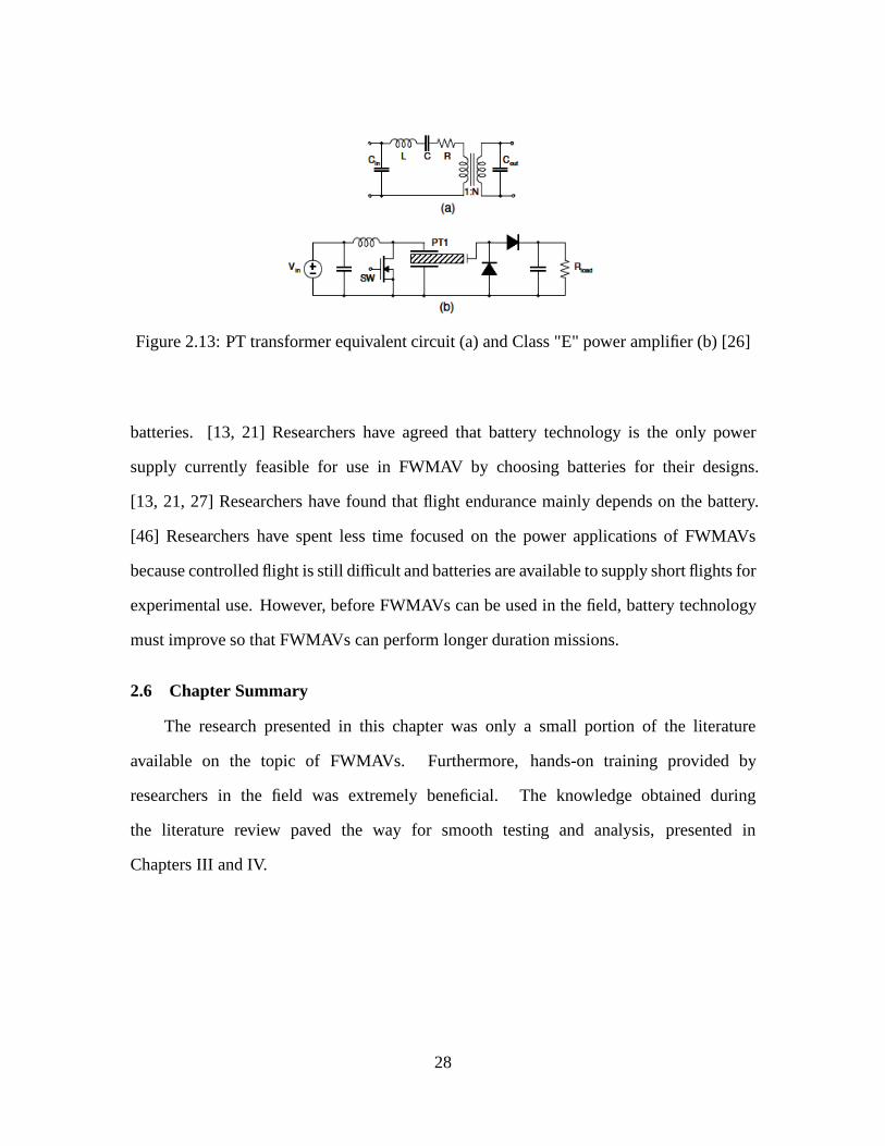
Figure 2.13: PT transformer equivalent circuit (a) and Class "E" power amplifier (b) [26]
batteries. [13, 21] Researchers have agreed that battery technology is the only power
supply currently feasible for use in FWMAV by choosing batteries for their designs.
[13, 21, 27] Researchers have found that flight endurance mainly depends on the battery.
[46] Researchers have spent less time focused on the power applications of FWMAVs
because controlled flight is still difficult and batteries are available to supply short flights for
experimental use. However, before FWMAVs can be used in the field, battery technology
must improve so that FWMAVs can perform longer duration missions.
2.6 Chapter Summary
The research presented in this chapter was only a small portion of the literature
available on the topic of FWMAVs. Furthermore, hands-on training provided by
researchers in the field was extremely beneficial. The knowledge obtained during
the literature review paved the way for smooth testing and analysis, presented in
Chapters III and IV.
28

III. Test Methodology
This chapter will focus on the methodology used to collect data for analysis. AFIT
researchers have been working on the FWMAV project for many years and has
seen many iterations of the fabrication process. This research used the most recent
iteration, described in reference 39. Furthermore, a proven testing technique was previously
developed for collecting the force, moment, and power data of the FWMAV. A more
detailed explanation of the methods used can be found in References 3, 39, and 40.
3.1 Flapper
AFIT researchers have been developing the manufacture of engineered wings for many
iterations and understanding the process was key to this research. As mentioned in Chapter
II, AFIT researchers use a YSH-70A carbon fiber for the majority of structural members.
The flapper tested, pictured in Figure 3.1, was constructed in multiple parts and assembled
later. This flapper differs from the one that will likely be used in an operational FWMAV
but serves as a good test-bed for experimentation.
3.1.1 Flapper Materials.
Few materials were used in the FWMAV construction, which simplified the
manufacturing process. The flapper shown in Figure 3.1 was constructed of three main
materials. The YSH-70A carbon fiber served as the main structural component. Kapton
served as a flexible joint to allow for movement between carbon fiber parts. Mylar served
as the wing membrane. Pyralux is a sheet adhesive that was used to bond the Kapton to the
carbon fiber.
29

Figure 3.1: Constructed flapper
3.1.1.1 YSH-70A Carbon Fiber.
As stated above, the main structure of the flapper was made of YSH-70A carbon
fiber. The carbon fiber provides an excellent stiffness-to-weight ratio. The carbon fiber
was purchased in a roll of 12-inch wide "tape" that was pre-impregnated with RS-3C resin.
All the fibers in the tape are oriented in the same direction. The fiber orientation provided
excellent strength in one direction and allowed various layup orientations to determine the
appropriate configuration. The carbon fiber was cut into appropriate size sheets to fit in the
multilayer press. The sheets were oriented in the 0-90-0 configuration and inserted into the
multilayer press. A multipress heats the carbon fiber to 192°C and applies 100 N/cm2 for
120 minutes to cure the carbon fiber. These 3-layer carbon fiber sheets form the basis for
construction.
3.1.1.2 Kapton.
As stated above, the Kapton was used as the flexible joints between carbon fiber
parts. Kapton is a tough, aromatic polyimide film with a balance of properties over a
30
wide temperature range. [17] The Kapton used is Kapton HN 50 and 100. Kapton HN 50
is 12.7µm thick and the Kapton HN 100 is 25µm thick. Kapton HN 50 was used for the
linkage and Kapton HN 100 was used for the passive rotation joint. Kapton HN 50 was
also used as the joints for a fold-able main support structure as shown in Figure 3.1.
3.1.1.3 Mylar.
As stated above, the Mylar was used as the wing membrane. Mylar is a polyester film
made from polyethylene terephthalate (PET) used for a broadarray of applications. [18]
Mylar was chosen for this application mainly for its superior weight qualities. It also bonds
well with the RS-3C resin found in the carbon fiber.
3.1.2 Tools of Construction.
A few key apparatuses were required for the construction of the FWMAV. As
expected, small hand tools such as razor blades, magnifyingglasses, vises, medical
harpoons, and picks were used in the assembly. These tools and their uses were semi-
dependent on the assembler. Other than that, the multipressmentioned earlier, and a laser-
machining center were all that was needed.
The multipress used is a LPKF MultiPress S, shown in Figure 3.2. The MultiPress
S was designed to laminate multilayer composites. The user has the ability to program
different profiles, consisting of different pressure, temperature, and durations settings, into
the MultiPress S. [32] The MultiPress S was used to laminate the sheets of carbon fiber, to
bond the Kapton to the carbon fiber via Pyralux, and to bond theMylar to the carbon fiber.
The laser-machining center used is a LPKF Protolaser U, shown in Figure 3.3. The
LPKF Protolaser U is designed to process micro-material by using an UV laser to ablate
materials. [33] It allows the user the ability to program specific laser settings and tool
31

Figure 3.2: LPKF Multipress S
paths for repeatable results. The Protolaser U was used to cut carbon fiber and carbon
fiber-Kapton layups into the parts needed for assembly.
3.1.3 Flapper Construction.
The flapper was constructed from a modular design. Parts werecreated and then
assembled into the final product. The different parts are the structure (Figure 3.4a),
the linkage (Figure 3.4b), the rotation joint (Figure 3.4c), the wing (Figure 3.4d), the
passive rotation stops (Figure 3.4e), and the assembly clips (Figure 3.4f). Once the
flapper was assembled, it was attached to a rapid prototyped base with a manufactured
piezoelectric actuator. The piezoelectric actuator used was an 60/20/0.6 strip actuator
(bimorph equivalent) purchased from Omega Piezo Technologies, Inc. since research is
ongoing to optimize in-house PZT actuators.
32

Figure 3.3: LPKF Protolaser U
3.1.3.1 Structure and Linkage.
The structure and linkage, once constructed separately, are now constructed together
to increase repeatability and reliability. The structure serves as the connection between
the linkage and the mounting base. The structure was built sothat the wing has room to
33

(a) Structure (b) Linkage (c) Rotation joint
(d) Wing (e) Rotation stops (f) Assorted assembly clips
Figure 3.4: Flapper parts for assembly
actuate without interfering with the testing base. The structure was aligned in the positive
Z-direction; for an operational FWMAV, the structure will likely be oriented in the negative
Y-direction to provide static stability. The linkage was effectively the transmission for the
FWMAV. The linkage connects the piezoelectric actuator to the rotation joint and translates
the linear motion of the piezoelectric actuator to rotational motion of the wing. The linkage
is a collection of four beams of different length, shown in Figure 3.5. These four lengths
define the ratio between deflection and rotation. The linkagewas designed to translate±1
mm deflection to±60°travel with lengths of:
l1 = 2.96 mm,l2 = 2.36 mm,l3 = 1.25 mm,l4 = 2.50 mm.
34

Figure 3.5: Final linkage configuration
To construct the structure/linkage, two sheets of Pyralux were applied to two 3-layer
sheets of carbon fiber and were cured in the multipress at 192°C and 100 N/m2 for 4 minutes.
This step eases working with the fragile Pyralux. Kapton HN 50 was sandwiched between
the two sheets of carbon fiber/Pyralux. That was loaded into the multipress and cured at
192°C and 30 N/m2 for 60 minutes. The entire layup is shown in Figure 3.6. The final
product was a large sheet that can then be machined to the proper dimensions. The final
layup was loaded into the laser-machining center and the dimensions were loaded into the
software. The laser-machining center follows the cutting routine and the structure/linkage
was complete as shown in Figures 3.4a and 3.4b.
35
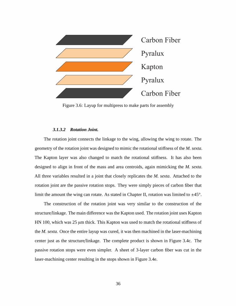
Carbon Fiber
Carbon Fiber
Pyralux
Kapton
Pyralux
Figure 3.6: Layup for multipress to make parts for assembly
3.1.3.2 Rotation Joint.
The rotation joint connects the linkage to the wing, allowing the wing to rotate. The
geometry of the rotation joint was designed to mimic the rotational stiffness of theM. sexta.
The Kapton layer was also changed to match the rotational stiffness. It has also been
designed to align in front of the mass and area centroids, again mimicking theM. sexta.
All three variables resulted in a joint that closely replicates theM. sexta. Attached to the
rotation joint are the passive rotation stops. They were simply pieces of carbon fiber that
limit the amount the wing can rotate. As stated in Chapter II,rotation was limited to±45°.
The construction of the rotation joint was very similar to the construction of the
structure/linkage. The main difference was the Kapton used. The rotation joint uses Kapton
HN 100, which was 25µm thick. This Kapton was used to match the rotational stiffness of
theM. sexta. Once the entire layup was cured, it was then machined in the laser-machining
center just as the structure/linkage. The complete product is shown in Figure 3.4c. The
passive rotation stops were even simpler. A sheet of 3-layercarbon fiber was cut in the
laser-machining center resulting in the stops shown in Figure 3.4e.
36

3.1.3.3 Wing.
The wing was discussed in detail in Chapter II. Much researchwas focused on the
wing design. The result is a close match to theM. sexta.. The construction of the wing
was also simple. The wing was machined from a 3-layer sheet ofcarbon fiber on the laser-
machining center. The result was the venation pattern of thewing. A piece of Mylar was
then cured on the wing venation in the multipress at 192°C and30 N/m2 for 60 minutes.
The remaining Mylar was then cut off in the laser-machining center resulting in Figure 3.4d.
A recent effort has been made to combine the wing and rotation joint. The effort has
resulted in a more repeatable design. For the testing performed herein, both configurations
were used. No variation in the performance was found betweenthe non-combined and
combined wing/rotation joint assemblies.
3.1.3.4 Assembly Clips.
The assembly clips were manufactured in the same way as the passive rotation stops.
They come in three different configurations for different purposes. E-clips are shaped
like an "E" and were used to make the square box of the linkage.The size of E-clips is
dependent on the size ofl3 for the linkage. C-clips are shaped like a "C" and were used
to attach the wing to the rotation joint. The last configuration was a modification of the
E-clip, the extended E-clip is a taller E-clip, on which a tracking disc can be placed to
measure the stroke angle using image-processing techniques. All configurations are shown
in Figure 3.4f.
3.1.4 Assembly.
A systematic process for the flapper assembly can be found in Reference 39. The steps
are summarized here for completeness.
1. Collect precut parts shown in Figure 3.4.
2. Fold the sides of the triangular part of structure shown inFigure 3.4a.
37

3. Bond the rectangular front plate of structure to the triangular part.
4. Bond the linkage shown in Figure 3.4b to the top of the assembled structure.
5. Fold the linkage into the shape shown in Figure 3.5 using a straight pin.
6. Insert and bond E-clips, Figure 3.4f, to the linkage to hold the shape.
7. Bond the passive rotation joint, Figure 3.4c, to the top ofthe linkage using the secured
E-clips as guides.
8. Position the wing, Figure 3.4d, on the passive rotation joint using a straight pin.
9. Secure the wing to the passive rotation joint by bonding C-clips, Figure 3.4f, to the
wing and passive rotation joint.
10. Attach the passive rotation stop, Figure 3.4e.
11. If an extended E-clip was used, attach the tracking disc.The assembled flapper is
shown in Figure 3.1.
12. Attach assembled structure to plastic base and piezoelectric actuator.
13. Use pins to secure the structure to the base.
14. Prepare actuator tip with a thermoplastic adhesive.
15. Use heat gun to attach the linkage to the piezoelectric actuator so the wing is parallel
to the floor.
16. The flapper is completed as shown in Figure 3.7.
38
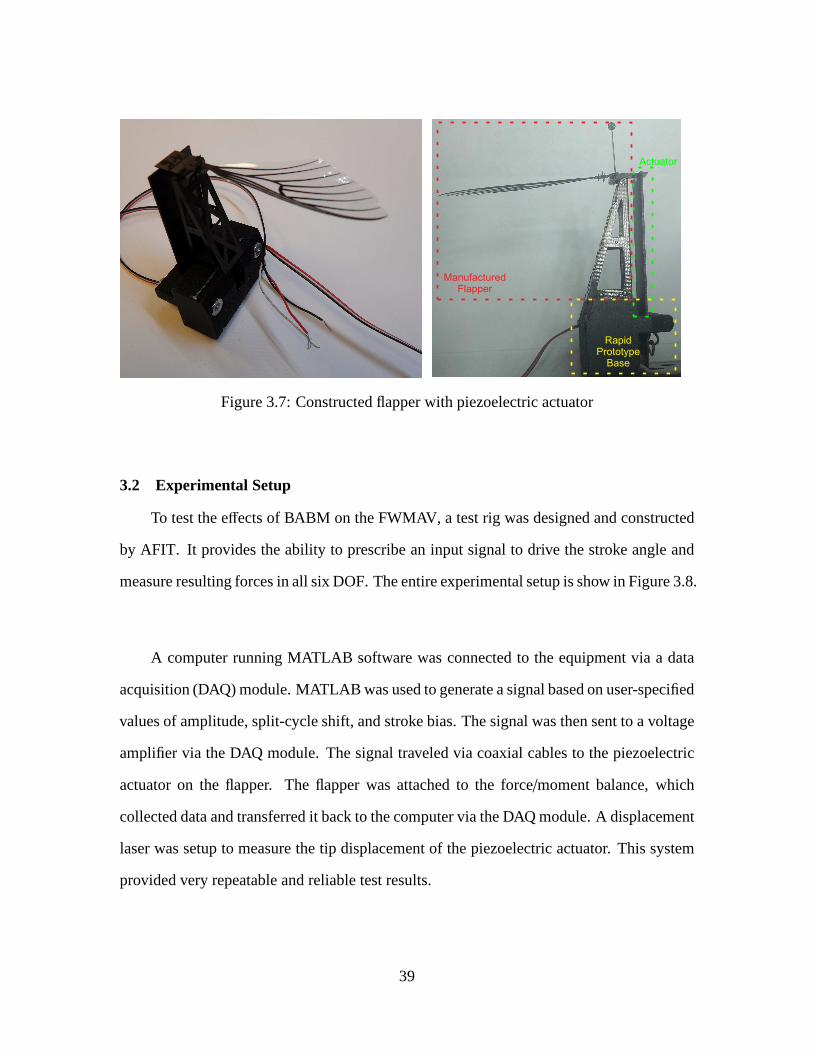
RapidPrototype
Base
ManufacturedFlapper
Actuator
Figure 3.7: Constructed flapper with piezoelectric actuator
3.2 Experimental Setup
To test the effects of BABM on the FWMAV, a test rig was designed and constructed
by AFIT. It provides the ability to prescribe an input signalto drive the stroke angle and
measure resulting forces in all six DOF. The entire experimental setup is show in Figure 3.8.
A computer running MATLAB software was connected to the equipment via a data
acquisition (DAQ) module. MATLAB was used to generate a signal based on user-specified
values of amplitude, split-cycle shift, and stroke bias. The signal was then sent to a voltage
amplifier via the DAQ module. The signal traveled via coaxialcables to the piezoelectric
actuator on the flapper. The flapper was attached to the force/moment balance, which
collected data and transferred it back to the computer via the DAQ module. A displacement
laser was setup to measure the tip displacement of the piezoelectric actuator. This system
provided very repeatable and reliable test results.
39

Figure 3.8: Experimental setup
The DAQ module used is a National Instrument USB-6229. This DAQ allows for
inclusion of all data with 16 inputs and 4 outputs. The DAQ module also interfaces
easily with the computer and MATLAB. [9] The amplifier used isTrek’s PZD700A. The
PZD700A is specifically designed to drive piezoelectric actuators. It offers adjustable
voltage gain by use of a potentiometer. [42] The voltage gainwas set to 30 V/V for all
tests in this report. The voltage and current sent to the piezoelectric actuator was directly
measured from the amplifier out port. The displacement sensor used is an optoNCDT 1800.
This non-contact displacement sensor uses optical triangulation to measure distance and
has a measuring range of 20 mm with a resolution of 2µm at a measuring rate of 5000 Hz.
[34]
40

A very sensitive force/moment balance was needed to measure the small forces and
moments created by the FWMAV. The force/moment balance used is an ATI Nano17
Titanium. The ATI Nano17 Titanium was the most sensitive commercially available six
DOF balance to AFIT’s knowledge at the time of purchase. Prior testing at AFIT has
shown that this transducer is able to sense forces in thex, y, andz directions greater than
3.3 mg, 2.8 mg, and 1.91 mg. [7] The ATI Nano17 Titanium was mounted to a stand with
an interface for the flapper. Previous AFIT research has validated the measured values of
the force/moment balance. The balance used, like most six DOF balances, has interactions
between the forces and moments. Those interactions were corrected in post processing.
The data were collected by an ATI Netbox at 5000 Hz and provided to the computer for
processing.
3.3 Experimental Procedure
After the entire flapper was assembled and attached to the rapid prototyped base and
piezoelectric actuator, it was attached to the test rig. Thefirst step was to determine
the natural frequency of the system so that the flapper could be driven at resonance. A
frequency response function (FRF) was calculated by exciting the flapper with a linearly
swept chirp between 0 Hz and 100 Hz. The output of the piezoelectric actuator was
recorded and the input voltage was recorded. The data was split into five samples with
no overlap. A Hanning window was then applied to the data. Theauto and cross power
spectral density (PSD) were calculated for each of the five samples and then averaged. The
FRFs were calculated from the PSDs. A sample FRF is shown in Figure 3.9. Resonant
frequencies of the system were around 20-25 Hz. A state-space model of the system was
obtained using an eigenvalue realization algorithm. The natural frequency of the system
was determined from the FRF and the state-space model was used to generate the drive
signal with BABM. The signal would last for sixty cycles, approximately three seconds.
41
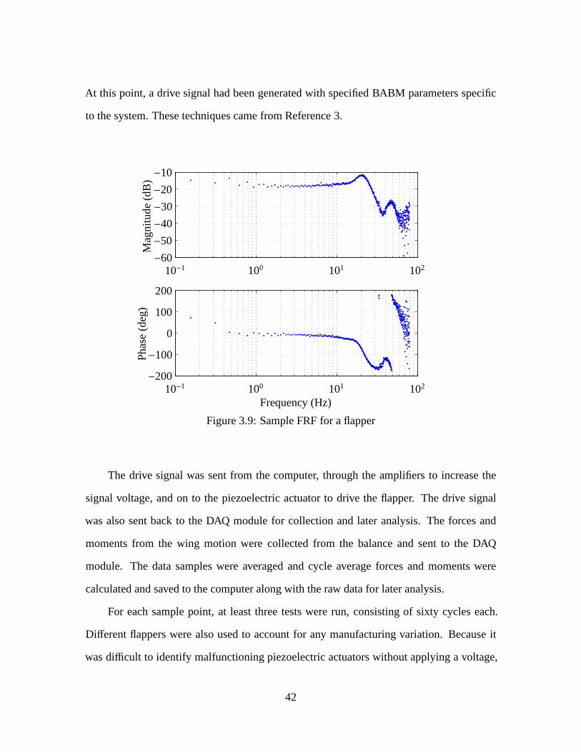
At this point, a drive signal had been generated with specified BABM parameters specific
to the system. These techniques came from Reference 3.
Frequency (Hz)
Ph
ase
(deg
)M
agn
itud
e(d
B)
10−1 100 101 102
10−1 100 101 102
−200
−100
0
100
200
−60
−50
−40
−30
−20
−10
Figure 3.9: Sample FRF for a flapper
The drive signal was sent from the computer, through the amplifiers to increase the
signal voltage, and on to the piezoelectric actuator to drive the flapper. The drive signal
was also sent back to the DAQ module for collection and later analysis. The forces and
moments from the wing motion were collected from the balanceand sent to the DAQ
module. The data samples were averaged and cycle average forces and moments were
calculated and saved to the computer along with the raw data for later analysis.
For each sample point, at least three tests were run, consisting of sixty cycles each.
Different flappers were also used to account for any manufacturing variation. Because it
was difficult to identify malfunctioning piezoelectric actuators without applying a voltage,
42

before each test, the actuators were excited and the deflection was qualitatively assessed
for proper functionality.
3.3.1 BABM Parameters.
A benefit of first completing single-wing flapper testing was obtaining an understand-
ing of the BABM parameters. From examining Equations 2.3 to 2.6, some conclusions can
be drawn on the values of the BABM parameters. It can be seen from Equations 2.4 and 2.6
that a split-cycle shift from−π/2 to π/2 would affect the stroke angle. From Equation 2.3,
it can be seen that a stroke bias from−π to π would affect the stroke angle. For the au-
thor’s and reader’s edification, these ranges were evaluated with a single-wing flapper, at
least where possible. Voltage limitations on the actuator placed limitations on the BABM
parameter values available for testing and ultimately for later implementation. These tests
identified the limitations of the split-cycle shift originally identified by Anderson and will
be discussed in Chapter IV. [4] In a dual-wing flapper, only the operationally representative
ranges of the BABM parameters were used for testing.
3.3.2 Design of Experiments.
Critical to the analysis were any interactions between the power and the forces/mo-
ments of the flapper. A design of experiments (DOE) was made with the help of a statisti-
cal analysis program. The DOE would identify any second-order interactions not predicted
between the BABM parameters and the resulting forces and moments. For the DOE, JMP
was used. JMP is statistical software that gave a graphical interface to display and analyze
data. [24] Two DOEs were made, one for a single flapper and one for a dual-wing flapper.
They are presented below in Tables 3.1 and 3.2.
JMP provided two main services used in these analyses: theprediction profilerand the
screeningtool. Both tools were based off of actual data. The prediction profiler provided
a trace for each of the adjustable variables, the BABM parameters, and returns predictions
43

Table 3.1: DOE parameters for a single-wing flapper
Amplitude,A Split-cycle Shift,τ Stroke Bias,η
0.5 -0.3927 -0.7854
0.5 -0.3927 0.7854
0.5 0 0
0.5 0.3927 -0.7854
0.5 0.3927 0.7854
1.5 0 0
1.5 0 -0.7854
1.5 0 0
1.5 0 0
1.5 0 0.7854
1.5 0.3927 0
2.5 -0.3927 -0.7854
2.5 0.3927 0.7854
2.5 0 0
2.5 0.3927 -0.7854
2.5 0.3927 0.7854
for each of the outputs, the power, and the forces and moments. This proved very useful
in determining the relations of variables and outputs. The screening tool identified which
parameter(s) had second-order effects on the outputs. This proved helpful to determine
which BABM parameter had the greatest effect on power and lift. [24]
44

3.4 Chapter Summary
A foundation has been set to proceed with testing. This chapter was laid out to prepare
the reader for Chapter IV where the results are presented.
45

Table 3.2: DOE parameters for a dual-wing flapper
Amplitude Split-cycle ShiftStroke Bias,η
Right Wing,AR Left Wing, AL Right Wing,τR Left Wing, τL
0 0 -0.25 -0.25 0.75
0 0 -0.25 0 0
0 0 -0.25 0.25 -0.75
0 0 0.25 -0.25 -0.75
0 0 0.25 0.25 0.75
0 1.25 0 -0.25 0.75
0 1.25 0.25 0.25 0
0 2.5 -0.25 -0.25 -0.75
0 2.5 -0.25 0.25 0.75
0 2.5 0.25 -0.25 0.75
0 2.5 0.25 0.25 -0.75
1.25 0 0 0.25 -0.75
1.25 0 0.25 -0.25 0
1.25 1.25 -0.25 -0.25 -0.75
1.25 1.25 -0.25 0.25 0.75
1.25 2.5 0.25 0 0.75
2.5 0 -0.25 -0.25 -0.75
2.5 0 -0.25 0.25 0.75
2.5 0 0 0 0.75
2.5 0 0.25 -0.25 0.75
2.5 0 0.25 0.25 -0.75
2.5 1.25 0.25 0 -0.75
2.5 2.5 -0.25 -0.25 0.75
2.5 2.5 -0.25 0.25 -0.75
2.5 2.5 0 -0.25 -0.75
2.5 2.5 0 0.25 0
2.5 2.5 0.25 -0.25 -0.75
2.5 2.5 0.25 0.25 0.75
46
IV. Analysis and Results
Data collected according to the process outlined in Chapter III are presented here. This
chapter follows a chronological layout, testing first a single-wing flapper and then a
dual-wing flapper. Analysis techniques are presented priorto their use to prevent repeated
figures and confusion. The importance of each figure is also discussed in this chapter.
4.1 Analysis
Once raw data was collected, a series of data processing techniques were applied.
These techniques averaged multiple tests, generated cycleaverage values, and centered the
moments on the center of pressure.
4.1.1 Data Processing.
The data collected by the DAQ module immediately went through post-processing in
MATLAB. The data from the balance came in six columns (one foreach force and moment)
of voltage measurements. Tare data was removed from the dataand averaged to obtain an
average tare to remove from the data. The tare value was also removed from the sample
data. The sample data were then passed through a balance interaction matrix to remove
coupling between the sensors in the balance. The balance interaction matrix also converts
the voltages measured by the balance into forces and moments. The result was sample data
in nanograms and nanogram-millimeters for the entire sample. The output of the amplifier
(input to the flapper) was central to this research. The data was received as voltage and
current measurements in voltage. The measurements was converted to the correct units per
manufacturer specifications and tare data were removed. A sample of raw data for two flap
cycles is presented in Figure 4.1.
47

Lift
Fo
rce
(g)
Time (s)1.46 1.47 1.48 1.49 1.5 1.51 1.52 1.53 1.54
×10−7
−1−0.8−0.6−0.4−0.2
00.20.40.60.8
1
Figure 4.1: Sample of raw lift data
Since this data occurred over multiple wing cycles and therewas no good way to
account for instantaneous aerodynamic forces and moments that the flapping generates,
cycle-averaged values for forces and moments were used. Only 80% of the collected data
was used in the cycle-averaging to avoid any ramp up or down transients associated with
the flapper as the sample begins and ends. The cycle-average lift for the data in Figure 4.1
is 115 milligrams. Since multiple tests were taken at each sample, the data were then
averaged over the tests resulting in one value. The power wascalculated from the collected
voltage and current values from the amplifier. The data was passed through the Simulink
model shown in Figure 4.2. The power equation for each cycle that is incorporated into the
model is given by
P =1T
t∑
t−T
Vrms(ωst) Irms (ωst) cos(γ)∆t (4.1)
whereP is the power,T is the cycle period,t is the instantaneous time,Vrms is the root
mean square of the voltage data,ωs is the sample rate,Irms is the root mean square of
the current data,γ is the phase angle between the current and voltage, and∆t is the time
between samples. The power data was then cycle-averaged in the same manner as the force
and moment data. These data sets were later analyzed.
48

Terminator1
TerminatorSignal ToWorkspace
power
FromWorkspace1
[S.SampleTime’ I(:,i)]
FromWorkspace
[S.SampleTime’ V(:,i)]
Discrete Active & Reactive
Power
V
I
Mag_V_I
P_Q
Figure 4.2: Simulink model to compute power
4.1.2 Center of Pressure.
To evaluate the true effect that the BABM parameters had on the moments generated
by the flappers, the measured moments had to be calculated about the center of
pressure. The nomenclature used in this section is a combination of nomenclature from
References 1 and 14. Figure 4.3 shows the dual-wing flapper and the center of pressure and
balance axes systems. Since the wing moves, the center of pressure for a flapping wing is
varies over the stroke of the wing. The center of pressure canbe approximated on the wing
by
xcp =−c5
(
3b2 + 2bR+ R2
b2 + bR+ R2
)
(4.2)
ycp =35
(
b3 + b2R+ bR2 + R3
3b2 + 2bR+ R2
)
(4.3)
zcp = 0 (4.4)
wherec is the maximum chord length,b is the distance from the wing root to the wing
break point (the point were the chord length begins to decrease) along they-axis, andR
is the length of the wingspan. [14] Figure 4.4 shows the dimensions of the wing used for
49

testing. These measurements resulted inxcp = −10.41 mm,ycp = 20.16 mm, andzcp = 0
mm. These measurements defined the location of the center of pressure on the wing, but
the center of pressure in relation to the balance was needed.
x
y
z
x
y
z
xbal
ybal
zbal
cp,R
cp,R
cp,R
cp,L
cp,L
cp,L
Figure 4.3: Dual-wing flapper center of pressure and balanceaxes
20.0
0 m
m
50.05 mm
27.54 mm
Figure 4.4: Aerodynamic dimensions of FWMAV wing
50

In order to find the center of pressure in relation to the balance, the instantaneous
location of the wing was needed. To determine the stroke angle of the wing, the deflection
of the piezoelectric actuator was used with Equation 4.5. [20, 39]
θ = −π
2+ arccos
{
[
l23 + (l1 + l2 − l4 − δ)2 + l23 + (l2 − l4)
2 − l21]
×
[
2√
l23 + (l2 − l4)2 ×
√
l23 + (l1 + l2 − l4 − δ)2
]−1 }
+ arctan
(
l3l1 + l2 − l4 − δ
)
+ arctan
(
l2 − l4l3
)
(4.5)
For the dual-wing flapper, the displacement sensor could notrecord deflection because
the second flapping wing was obstructing it and so an approximation was used. An
approximation for cycle-average displacement was developed for amplitude, split-cycle
shift, and stroke bias. Figures 4.5, 4.6, and 4.7 show the actual measurements and the tests.
Recall that, for this research, the amplitude voltage directly correlates to the signal sent to
the amplifier. The red lines are polynomial fits of the data. The resulting approximations
are
dA = −0.037A3 + 0.116A2 + 0.153A+ 0.028
dτ = 0.002τ − 0.002
dη = 0.157η − 0.003
(4.6)
wheredparameteris the displacement of the actuator. The total displacementis simply the
summation of the parameter displacements. The data showed that the contribution of split-
cycle shift was minimal and was therefore ignored. From the equations above, a cycle-
average displacement for the actuator was calculated and used for Equation 4.5 for the dual-
wing flapper. The total distance including contributions from the mounting configuration
and the wing angle were summed to get an average distance between the center of pressure
and the balance.
51

3rd Order Fit,R2 = 0.99
Actual DataAve
rag
eD
isp
lace
men
t(m
m)
Amplitude (V)0 0.5 1 1.5 2 2.5 3
0
0.1
0.2
0.3
0.4
0.5
0.6
0.7
Figure 4.5: Actuator displacement vs. amplitude,A(n)
From this point, Equations 4.7, 4.8, and 4.9 were used to remove the lift, side force,
and thrust contributions from the roll, pitch, and yaw moments.
L = Mbalx − cRdR,zY− cLdL,zY− cRdR,yZ + cLdL,yZ (4.7)
M = Mbaly + cRdR,zX + cLdL,zX − cRdR,xZ − cLdL,xZ (4.8)
N = Mbalz + cRdR,xY+ cLdL,xY+ cRdR,yX − cLdL,yX (4.9)
whereL, M, andN are the roll, pitch, and yaw moments respectively;Mbali is the balance
measured moment about thei-axis; cR andcL are the contribution factors of the right and
left wing respectively;dR,i anddL,i is the distance to the center of pressure along thei-axis to
the right and left wing respectively; and,X, Y, andZ are the axial forces. The contribution
factor accounted for the difference in amplitude between the left and right wing and were
52

1st Order Fit,R2 = 0.50
Actual Data
Ave
rag
eD
isp
lace
men
t(m
m)
Split-cycle Shift−0.2 −0.1 0 0.1 0.2 0.3
−0.2
−0.15
−0.1
−0.05
0
0.05
0.1
0.15
0.2
Figure 4.6: Actuator displacement vs. split-cycle shift,τ(n)
calculated from
cR =AR
AR + ALcL =
AL
AR + AL
For example, when the amplitudes were symmetric, the contributions were each 0.5 and
half the force was attributed to the left wing and half the force was attributed to the right
wing. These calculations were performed at each sample point and then cycle-average
values were calculated as described in Chapter III.
A sample of the results of correcting the moments is shown in Figure 4.8. These data
points were obtained by varying the amplitude of the right wing. The resulting data from
that test is shown in Figure 4.29. The pitch moment about the balance closely followed
the trend of the lift data, which makes sense because it was the largest force with the
53
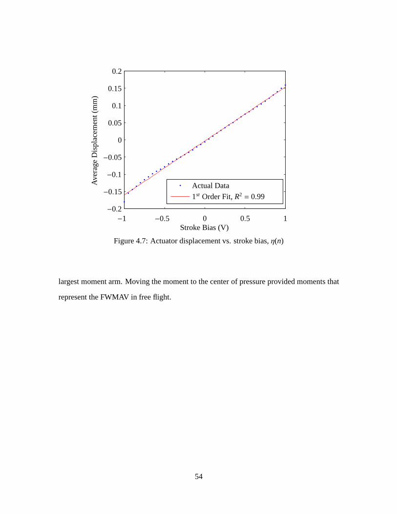
1st Order Fit,R2 = 0.99
Actual DataAve
rag
eD
isp
lace
men
t(m
m)
Stroke Bias (V)−1 −0.5 0 0.5 1
−0.2
−0.15
−0.1
−0.05
0
0.05
0.1
0.15
0.2
Figure 4.7: Actuator displacement vs. stroke bias,η(n)
largest moment arm. Moving the moment to the center of pressure provided moments that
represent the FWMAV in free flight.
54
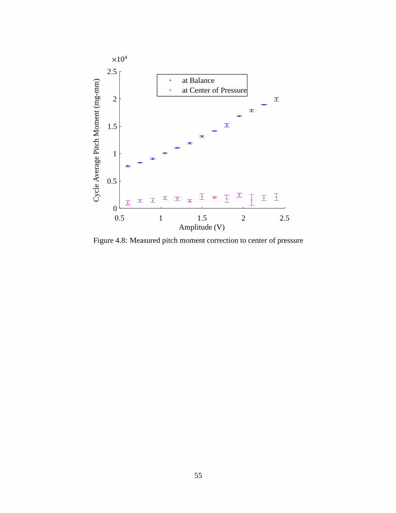
at Center of Pressureat Balance
Cyc
leA
vera
ge
Pitc
hM
om
ent(
mg
-mm
)
Amplitude (V)0.5 1 1.5 2 2.5
×104
0
0.5
1
1.5
2
2.5
Figure 4.8: Measured pitch moment correction to center of pressure
55
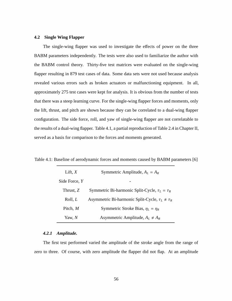
4.2 Single Wing Flapper
The single-wing flapper was used to investigate the effects of power on the three
BABM parameters independently. The tests were also used to familiarize the author with
the BABM control theory. Thirty-five test matrices were evaluated on the single-wing
flapper resulting in 879 test cases of data. Some data sets were not used because analysis
revealed various errors such as broken actuators or malfunctioning equipment. In all,
approximately 275 test cases were kept for analysis. It is obvious from the number of tests
that there was a steep learning curve. For the single-wing flapper forces and moments, only
the lift, thrust, and pitch are shown because they can be correlated to a dual-wing flapper
configuration. The side force, roll, and yaw of single-wing flapper are not correlatable to
the results of a dual-wing flapper. Table 4.1, a partial reproduction of Table 2.4 in Chapter II,
served as a basis for comparison to the forces and moments generated.
Table 4.1: Baseline of aerodynamic forces and moments caused by BABM parameters [6]
Lift, X Symmetric Amplitude,AL = AR
Side Force,Y -
Thrust,Z Symmetric Bi-harmonic Split-Cycle,τL = τR
Roll, L Asymmetric Bi-harmonic Split-Cycle,τL , τR
Pitch,M Symmetric Stroke Bias,ηL = ηR
Yaw, N Asymmetric Amplitude,AL , AR
4.2.1 Amplitude.
The first test performed varied the amplitude of the stroke angle from the range of
zero to three. Of course, with zero amplitude the flapper did not flap. At an amplitude
56
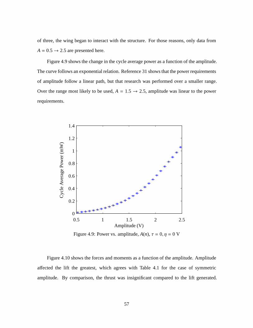
of three, the wing began to interact with the structure. For those reasons, only data from
A = 0.5→ 2.5 are presented here.
Figure 4.9 shows the change in the cycle average power as a function of the amplitude.
The curve follows an exponential relation. Reference 31 shows that the power requirements
of amplitude follow a linear path, but that research was performed over a smaller range.
Over the range most likely to be used,A = 1.5→ 2.5, amplitude was linear to the power
requirements.
Cyc
leA
vera
ge
Pow
er(m
W)
Amplitude (V)0.5 1 1.5 2 2.50
0.2
0.4
0.6
0.8
1
1.2
1.4
Figure 4.9: Power vs. amplitude,A(n), τ = 0, η = 0 V
Figure 4.10 shows the forces and moments as a function of the amplitude. Amplitude
affected the lift the greatest, which agrees with Table 4.1 for the case of symmetric
amplitude. By comparison, the thrust was insignificant compared to the lift generated.
57
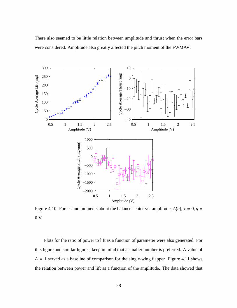
There also seemed to be little relation between amplitude and thrust when the error bars
were considered. Amplitude also greatly affected the pitch moment of the FWMAV.
Amplitude (V)
Cyc
leA
vera
ge
Lift
(mg
)
0.5 1 1.5 2 2.50
50
100
150
200
250
300
Amplitude (V)
Cyc
leA
vera
ge
Th
rust
(mg
)0.5 1 1.5 2 2.5
−40
−30
−20
−10
0
10
Amplitude (V)
Cyc
leA
vera
ge
Pitc
h(m
g-m
m)
0.5 1 1.5 2 2.5−2000
−1500
−1000
−500
0
500
1000
Figure 4.10: Forces and moments about the balance center vs.amplitude,A(n), τ = 0, η =
0 V
Plots for the ratio of power to lift as a function of parameterwere also generated. For
this figure and similar figures, keep in mind that a smaller number is preferred. A value of
A = 1 served as a baseline of comparison for the single-wing flapper. Figure 4.11 shows
the relation between power and lift as a function of the amplitude. The data showed that
58

increasing the amplitude resulted in more power per lift, orthe power requirement rose
faster than the lift provided.
Pow
er/L
ift(m
W/m
g)
Amplitude (V)0.5 1 1.5 2 2.5
×10−6
0
2
4
Ch
ang
ein
Pow
er/Lift
(mW/m
g)
Amplitude (V)0.5 1 1.5 2 2.5
×10−6
0
2
4
Figure 4.11: Power per lift vs. amplitude,A(n), τ = 0, η = 0 V
4.2.2 Split-cycle Shift.
For the split-cycle shift and the stroke bias, power was evaluated as a change in power
from the case with zero split-cycle shift and stroke bias. Asstated earlier, a split-cycle shift
of ±0.3 is sufficient for control, but for the author’s edification, split-cycle was evaluated
from −π/2 to π/2. The results are shown in Figure 4.12. A clear spike in power could be
seen that correlated toπ/4. This could more accurately be seen when a cosine with split-
cycle shift of π/4 was compared to a symmetric cosine wave, shown in Figure 4.13. A
split-cycle shift ofπ/4 changes the frequency of the cosine wave causing the wing to flap
faster drawing more power.
Figure 4.14 shows change in power as a function of the split-cycle shift for a more
reasonable range. One could see that in the range ofτ = −0.3→ 0.3, the split-cycle shift
was inversely related to the change in power. In comparing the ordinate to the ordinate in
59

Ch
ang
ein
Cyc
leA
vera
ge
Pow
er(m
W)
Split-cycle Shift−π/2 −π/4 0 π/4
π/2
−0.02
−0.01
0
0.01
0.02
0.03
0.04
Figure 4.12: Power vs. split-cycle shift,τ(n), A = 1, η = 0 V
Figure 4.9, it can be observed that the change in power was multiple orders of magnitude
less than the overall power. It is also important to note thatthe relation was symmetric
about zero split-cycle shift. The symmetry will be important when designing a controller.
Figure 4.15 shows forces and moments as a function of the split-cycle shift. These
tests were performed with an amplitude of one. With no split-cycle shift, the flapper
should produce a lift of approximately 58 mg, a thrust of approximately -23 mg, and a
pitch of approximately -300 mg-mm (from Figure 4.10). Thesevalues match closely with
the values in Figure 4.15. Furthermore, the lower power requirements of split-cycle shift
were manifested as a loss of lift and pitch control. It appears that split-cycle shift has little
effect on the thrust, which remains at much lower values than thelift. This did not agree
with the predictions in Table 4.1.
60
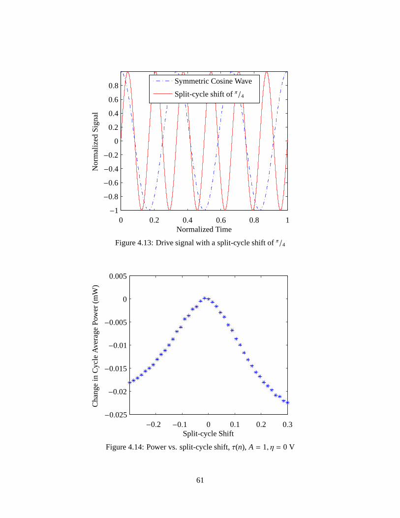
Split-cycle shift ofπ/4
Symmetric Cosine Wave
No
rmal
ized
Sig
nal
Normalized Time0 0.2 0.4 0.6 0.8 1
−1
−0.8
−0.6
−0.4
−0.2
0
0.2
0.4
0.6
0.8
Figure 4.13: Drive signal with a split-cycle shift ofπ/4
Ch
ang
ein
Cyc
leA
vera
ge
Pow
er(m
W)
Split-cycle Shift−0.2 −0.1 0 0.1 0.2 0.3
−0.025
−0.02
−0.015
−0.01
−0.005
0
0.005
Figure 4.14: Power vs. split-cycle shift,τ(n), A = 1, η = 0 V
61

Split-cycle Shift
Cyc
leA
vera
ge
Lift
(mg
)
−0.2 −0.1 0 0.1 0.220
30
40
50
60
70
Split-cycle Shift
Cyc
leA
vera
ge
Th
rust
(mg
)
−0.2 −0.1 0 0.1 0.2−80
−60
−40
−20
0
20
Split-cycle Shift
Cyc
leA
vera
ge
Pitc
h(m
g-m
m)
−0.2 −0.1 0 0.1 0.2−2000
−1500
−1000
−500
0
500
1000
Figure 4.15: Forces and moments about the balance center vs.split-cycle shift, τ(n),
A = 1, η = 0 V
62
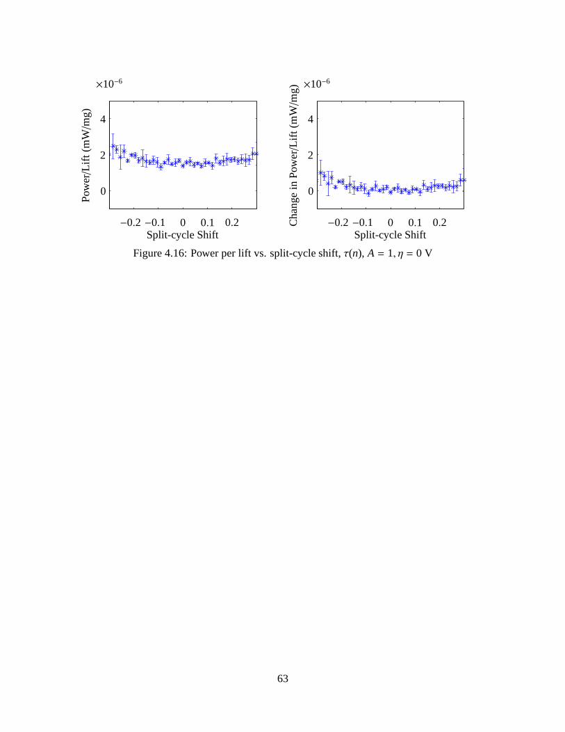
Pow
er/L
ift(m
W/m
g)
Split-cycle Shift−0.2 −0.1 0 0.1 0.2
×10−6
0
2
4
Ch
ang
ein
Pow
er/Lift
(mW/m
g)
Split-cycle Shift−0.2 −0.1 0 0.1 0.2
×10−6
0
2
4
Figure 4.16: Power per lift vs. split-cycle shift,τ(n), A = 1, η = 0 V
63
Figure 4.16 shows the relation between power and lift as a function of the split-cycle
shift. Note that the range of the ordinate for the change in power per lift is an order of
magnitude lower that that of Figure 4.11. The data showed that increasing the split-cycle
shift resulted in more power per lift. Since additional split-cycle shift resulted in lower
power requirements, the increasing power per lift indicates that the lift produced decreased
more rapidly than the power requirements.
4.2.3 Stroke Bias.
Stroke bias was evaluated from -1 to 1 for a single-wing flapper. These tests were
also performed with an amplitude of one. Greater values of stroke bias caused the wing
to interfere with the structure. The data showed that the power requirements of stroke bias
were not symmetric about zero, as shown in Figure 4.17. To ensure that this was not an
effect of the bimorph nature of the piezoelectric actuator, thetest was performed in reverse
order. Figure 4.17 also shows the data from that test. The data showed that the results were
not a function of the testing order but rather that the power did in fact decrease as stroke
bias increased. This is counter-intuitive and is explainedin detail later when the dual-wing
flapper results are presented. It is important to note that the change was on the order of 1%
of the total power. This information will be very useful to the control designer.
Data was also collected for the effect that stroke bias had on forces and moments.
Figure 4.18 shows that data. Recall that an amplitude of 1 would supply lift of
approximately 58 mg, thrust of approximately -23 mg, and pitch moment of approximately
3100 mg-mm (from Figure 4.10). The stroke bias had a detrimental effect on lift. The
stroke bias did not have an effect on the thrust. Stroke bias did affect the pitch moment,
reducing the pitch moment by approximately 130 mg-mm as the stroke bias was increased
or decreased to 0.75 as indicated by a best fit curve. These results agreed with the prediction
for symmetric stroke bias in Table 4.1.
64

Varied from 1–>-1Varied from -1–>1
Ch
ang
ein
Cyc
leA
vera
ge
Pow
er(m
W)
Stroke Bias (V)−1 −0.5 0 0.5 1
−0.01
−0.005
0
0.005
0.01
0.015
0.02
Figure 4.17: Power vs. stroke bias,η(n), A = 1, τ = 0
Figure 4.19 shows the relation between power and lift as a function of the stroke bias.
Again, note that the range of the ordinate for the change in power per lift is an order of
magnitude lower that that of Figure 4.11. The data showed that increasing the stroke bias
resulted in less power per lift, but at smaller magnitudes than amplitude and split-cycle
shift.
4.2.4 Design of Experiments.
Figure 4.20 shows the results from the DOE run accomplished using Table 3.1.
The data showed the correlation between the three BABM parameters and the four
measurements: power, lift, thrust, and pitch moment. The blue dashed lines represent
confidence intervals to one standard deviation. The importance of the parameter can be
assessed by the slope of the relation. Figure 4.20 also places all three parameters on the
65

Stroke Bias (V)
Cyc
leA
vera
ge
Lift
(mg
)
−0.5 0 0.530
40
50
60
70
Stroke Bias (V)
Cyc
leA
vera
ge
Th
rust
(mg
)
−0.5 0 0.5−50
−40
−30
−20
−10
0
10
Stroke Bias (V)
Cyc
leA
vera
ge
Pitc
h(m
g-m
m)
−0.5 0 0.5−1500
−1000
−500
0
500
1000
Figure 4.18: Forces and moments about the balance center vs.stroke bias,η(n), A = 1, τ =
0
66

Pow
er/L
ift(m
W/m
g)
Stroke Bias (V)−1 −0.5 0 0.5 1
×10−6
0
2
4
Ch
ang
ein
Pow
er/Lift
(mW/m
g)
Stroke Bias (V)−1 −0.5 0 0.5 1
×10−6
0
2
4
Figure 4.19: Power per lift vs. stroke bias,η(n), A = 1, τ = 0
67
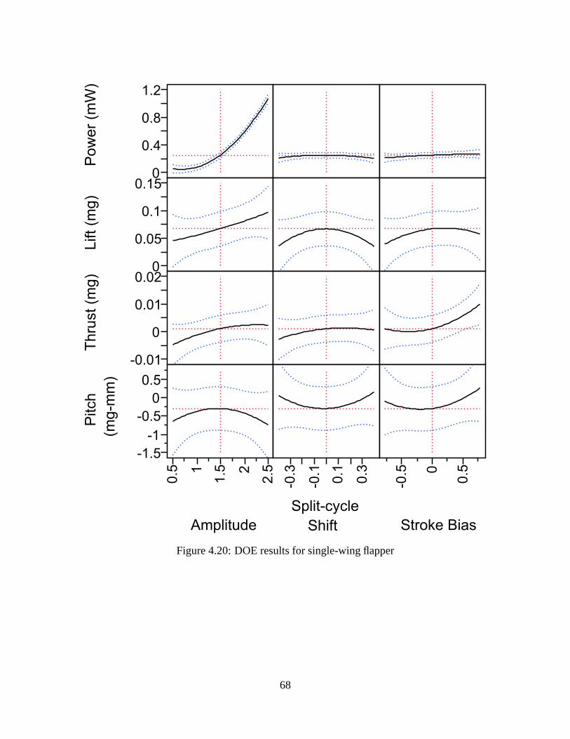
0
0.4
0.8
1.2P
ow
er
(mW
)
0
0.05
0.1
0.15
Lift (m
g)
-0.01
0
0.01
0.02
Thru
st (m
g)
-1.5
-1
-0.5
0
0.5
Pitch
(mg-m
m)
0.5 1
1.5 2
2.5
Amplitude
-0.3
-0.1
0.1
0.3
Split-cycle
Shift
-0.5 0
0.5
Stroke Bias
Figure 4.20: DOE results for single-wing flapper
68

same scale. It was easy to determine that amplitude had the greatest effect on power. The
data also showed that the stroke bias had the greatest effect on thrust, unlike predicted in
Table 4.1. The data show that symmetric split-cycle shift may be most useful to control the
pitch moment.
Figures 4.21 and 4.22 show the relations for the power and lift. The bars are scaled
estimates normalized between -1 and 1 where a negative relationship is detrimental to the
output. The blue lines on the charts mark a value of 0.2 indicating a strong relationship. The
figures also show secondary interactions. The data agreed that amplitude had the strongest
effect on power. The data also agreed that amplitude had the greatest effect on lift but a
strong secondary interaction appeared between amplitude and stroke bias squared. This
indicates that changes in amplitude and large changes in stroke bias may detrimentally
affect lift in a significant way.
4.2.5 Randomized Verification.
In order to ensure that the testing methodology was sound prior to moving forward
with dual-wing flapper testing, data were collected for randomly selected values of the
BABM parameters. Figures 4.23, 4.24, and 4.25 show the results of those tests. The data
was in close correlation with the other data. These results helped verify that the data for the
single-wing flapper was collected and analyzed properly.
69
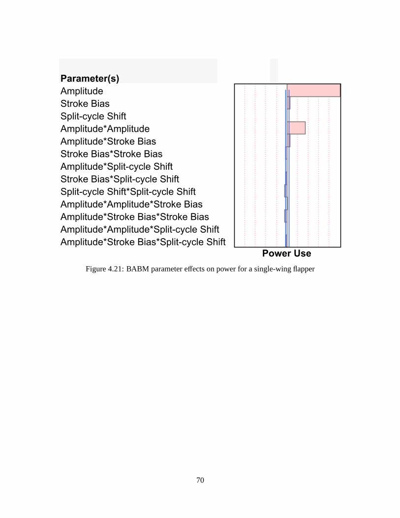
Amplitude
Stroke Bias
Split-cycle Shift
Amplitude*Amplitude
Amplitude*Stroke Bias
Stroke Bias*Stroke Bias
Amplitude*Split-cycle Shift
Stroke Bias*Split-cycle Shift
Split-cycle Shift*Split-cycle Shift
Amplitude*Amplitude*Stroke Bias
Amplitude*Stroke Bias*Stroke Bias
Amplitude*Amplitude*Split-cycle Shift
Amplitude*Stroke Bias*Split-cycle Shift
Parameter(s)
Power Use
Figure 4.21: BABM parameter effects on power for a single-wing flapper
70

Amplitude
Stroke Bias
Split-cycle Shift
Amplitude*Amplitude
Amplitude*Stroke Bias
Stroke Bias*Stroke Bias
Amplitude*Split-cycle Shift
Stroke Bias*Split-cycle Shift
Split-cycle Shift*Split-cycle Shift
Amplitude*Amplitude*Stroke Bias
Amplitude*Stroke Bias*Stroke Bias
Amplitude*Amplitude*Split-cycle Shift
Amplitude*Stroke Bias*Split-cycle Shift
Parameter(s)
Lift
Figure 4.22: BABM parameter effects on lift for a single-wing flapper
Cyc
leA
vera
ge
Pow
er(m
W)
Amplitude (V)0.5 1 1.5 2 2.50
0.5
1
1.5
Lift
(mg
)
Amplitude (V)0.5 1 1.5 2 2.50
50
100
150
200
250
Figure 4.23: Power vs. amplitude,A(n), random sampling,τ = 0, η = 0 V
71
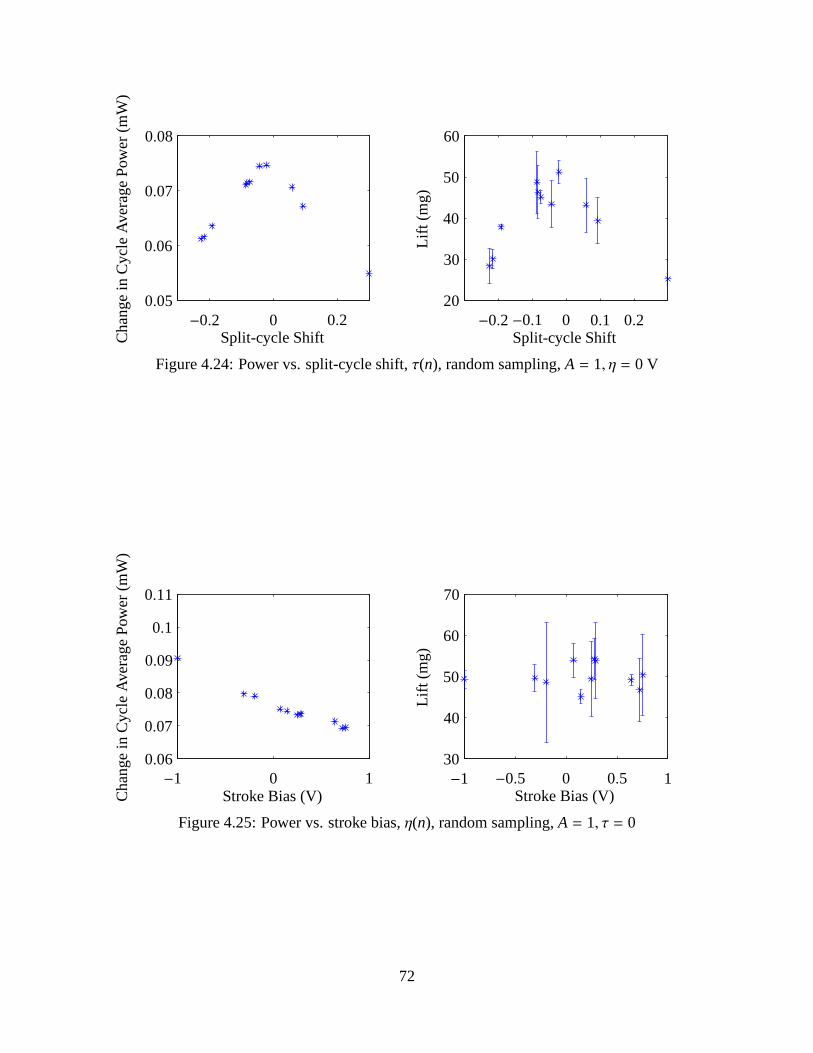
Ch
ang
ein
Cyc
leA
vera
ge
Pow
er(m
W)
Split-cycle Shift−0.2 0 0.2
0.05
0.06
0.07
0.08
Lift
(mg
)
Split-cycle Shift−0.2 −0.1 0 0.1 0.2
20
30
40
50
60
Figure 4.24: Power vs. split-cycle shift,τ(n), random sampling,A = 1, η = 0 V
Ch
ang
ein
Cyc
leA
vera
ge
Pow
er(m
W)
Stroke Bias (V)−1 0 1
0.06
0.07
0.08
0.09
0.1
0.11
Lift
(mg
)
Stroke Bias (V)−1 −0.5 0 0.5 1
30
40
50
60
70
Figure 4.25: Power vs. stroke bias,η(n), random sampling,A = 1, τ = 0
72

4.3 Dual Wing Flapper
After completion of the single-wing flapper testing, a dual-wing flapper was
constructed to test. The dual-wing flapper allowed investigation into the side force, the
rolling moment, and the yaw moment. Testing on the dual-wingflapper was much quicker
due to the lessons learned with the single-wing flapper, mostly in regards to proper test
setup. Fifteen test matrices were run resulting in 226 test cases. Approximately 133 cases
were used for final analysis. The test setup allowed for separate power measurements on
the left and right wing so the results were split into power requirements for each wing.
Since power was calculated in Watts as described in Chapter III, the two were additive for
total power required. Table 4.1 again served as a basis for comparison to the forces and
moments generated.
4.3.1 Amplitude.
Figures 4.26 and 4.27 show the power requirements as a function of the amplitude.
Data were collected by varying amplitude from 0.5 to 2.5. Thedata showed a good trend
when compared to the single-wing flapper shown in Figure 4.9.Data agreed between the
wings, as the amplitude increased on either wing the power increased in an exponential
manner. In addition, the power required matched when both wing amplitudes were at 2.
Data were also collected for the forces and moments as a function of amplitude for
each wing. Figures 4.28 and 4.29 show these data. Knowing that theM. sextahas a mass
averaging 1.55 grams, a lift equal to that would be required to result in flight. From either
Figure 4.28 or 4.29, it could be seen that, with this flapper configuration, an amount of
lift was not achievable to overcome the mass. As such, an amplitude of 2 was selected
to serve as a baseline for later comparison. The plots in Figures 4.28 and 4.29 show,
like in the single-wing flapper case, that there was strong correlation between amplitude
and lift and between amplitude and pitch with little correlation between amplitude and
73
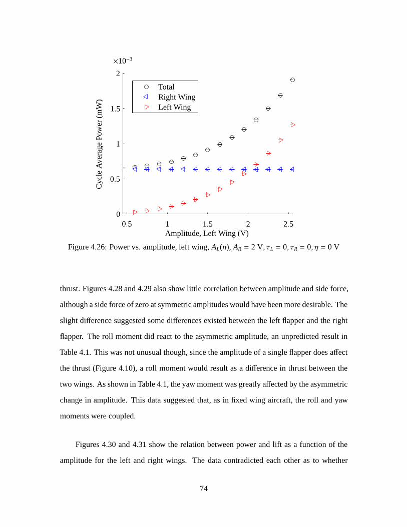
Left WingRight WingTotal
Cyc
leA
vera
ge
Pow
er(m
W)
Amplitude, Left Wing (V)0.5 1 1.5 2 2.5
×10−3
0
0.5
1
1.5
2
Figure 4.26: Power vs. amplitude, left wing,AL(n), AR = 2 V, τL = 0, τR = 0, η = 0 V
thrust. Figures 4.28 and 4.29 also show little correlation between amplitude and side force,
although a side force of zero at symmetric amplitudes would have been more desirable. The
slight difference suggested some differences existed between the left flapper and the right
flapper. The roll moment did react to the asymmetric amplitude, an unpredicted result in
Table 4.1. This was not unusual though, since the amplitude of a single flapper does affect
the thrust (Figure 4.10), a roll moment would result as a difference in thrust between the
two wings. As shown in Table 4.1, the yaw moment was greatly affected by the asymmetric
change in amplitude. This data suggested that, as in fixed wing aircraft, the roll and yaw
moments were coupled.
Figures 4.30 and 4.31 show the relation between power and lift as a function of the
amplitude for the left and right wings. The data contradicted each other as to whether
74

Left WingRight WingTotal
Cyc
leA
vera
ge
Pow
er(m
W)
Amplitude, Right Wing (V)0.5 1 1.5 2 2.5
×10−3
0
0.5
1
1.5
2
Figure 4.27: Power vs. amplitude, right wing,AR(n), AL = 2 V, τL = 0, τR = 0, η = 0 V
75
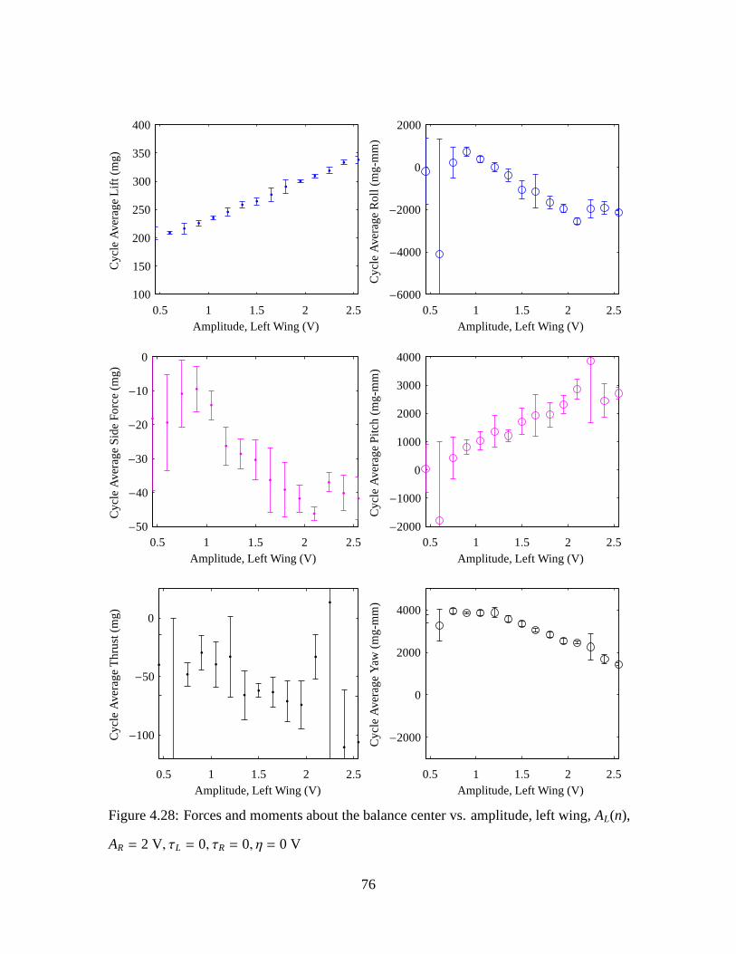
Amplitude, Left Wing (V)
Cyc
leA
vera
ge
Lift
(mg
)
0.5 1 1.5 2 2.5100
150
200
250
300
350
400
Amplitude, Left Wing (V)
Cyc
leA
vera
ge
Ro
ll(m
g-m
m)
0.5 1 1.5 2 2.5−6000
−4000
−2000
0
2000
Amplitude, Left Wing (V)
Cyc
leA
vera
ge
Sid
eF
orc
e(m
g)
0.5 1 1.5 2 2.5−50
−40
−30
−20
−10
0
Amplitude, Left Wing (V)
Cyc
leA
vera
ge
Pitc
h(m
g-m
m)
0.5 1 1.5 2 2.5−2000
−1000
0
1000
2000
3000
4000
Amplitude, Left Wing (V)
Cyc
leA
vera
ge
Th
rust
(mg
)
0.5 1 1.5 2 2.5
−100
−50
0
Amplitude, Left Wing (V)
Cyc
leA
vera
ge
Yaw
(mg
-mm
)
0.5 1 1.5 2 2.5
−2000
0
2000
4000
Figure 4.28: Forces and moments about the balance center vs.amplitude, left wing,AL(n),
AR = 2 V, τL = 0, τR = 0, η = 0 V
76

Amplitude, Right Wing (V)
Cyc
leA
vera
ge
Lift
(mg
)
0.5 1 1.5 2 2.5100
150
200
250
300
350
400
Amplitude, Right Wing (V)
Cyc
leA
vera
ge
Ro
ll(m
g-m
m)
0.5 1 1.5 2 2.5−6000
−4000
−2000
0
2000
Amplitude, Right Wing (V)
Cyc
leA
vera
ge
Sid
eF
orc
e(m
g)
0.5 1 1.5 2 2.5−50
−40
−30
−20
−10
0
Amplitude, Right Wing (V)
Cyc
leA
vera
ge
Pitc
h(m
g-m
m)
0.5 1 1.5 2 2.5−2000
−1000
0
1000
2000
3000
4000
Amplitude, Right Wing (V)
Cyc
leA
vera
ge
Th
rust
(mg
)
0.5 1 1.5 2 2.5
−100
−50
0
Amplitude, Right Wing (V)
Cyc
leA
vera
ge
Yaw
(mg
-mm
)
0.5 1 1.5 2 2.5
−2000
0
2000
4000
Figure 4.29: Forces and moments about the balance center vs.amplitude, right wing,AR(n),
AL = 2 V, τL = 0, τR = 0, η = 0 V
77
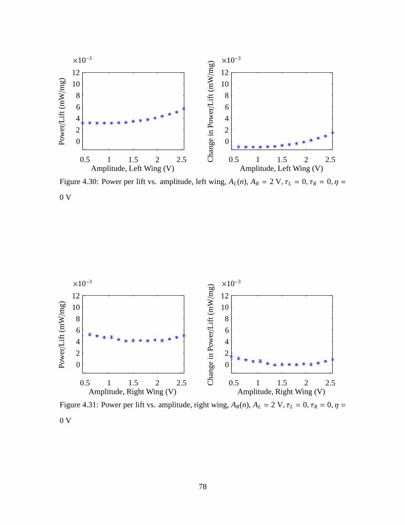
Pow
er/L
ift(m
W/m
g)
Amplitude, Left Wing (V)0.5 1 1.5 2 2.5
×10−3
0
2
4
6
8
10
12
Ch
ang
ein
Pow
er/Lift
(mW/m
g)
Amplitude, Left Wing (V)0.5 1 1.5 2 2.5
×10−3
0
2
4
6
8
10
12
Figure 4.30: Power per lift vs. amplitude, left wing,AL(n), AR = 2 V, τL = 0, τR = 0, η =
0 V
Pow
er/L
ift(m
W/m
g)
Amplitude, Right Wing (V)0.5 1 1.5 2 2.5
×10−3
0
2
4
6
8
10
12
Ch
ang
ein
Pow
er/Lift
(mW/m
g)
Amplitude, Right Wing (V)0.5 1 1.5 2 2.5
×10−3
0
2
4
6
8
10
12
Figure 4.31: Power per lift vs. amplitude, right wing,AR(n), AL = 2 V, τL = 0, τR = 0, η =
0 V
78

increasing the amplitude resulted in more or less power per lift. Again, the difference
suggested some differences existed between the left flapper and the right flapperand were
magnified in the power per lift data.
4.3.2 Split-cycle Shift.
Figures 4.32 and 4.33 show the power requirements as a function of the split-cycle
shift. Data were collected by varying the split-cycle shiftfrom -0.25 to 0.25, the expected
values of usefulness. The power here is not shown as a change from the case of zero
split-cycle but rather the total power of the system. As expected, the wing with a constant
split-cycle shift of zero required constant power while thewing with varying split-cycle
shift required less power. These results agreed with the results of the single-wing flapper.
Left WingRight WingTotal
Cyc
leA
vera
ge
Pow
er(m
W)
Split-cycle Shift, Left Wing−0.2 −0.1 0 0.1 0.2
×10−4
4
6
8
10
12
14
Figure 4.32: Power vs. split-cycle shift, left wing,τL(n), AL = 2,AR = 2 V, τR = 0, η = 0 V
79
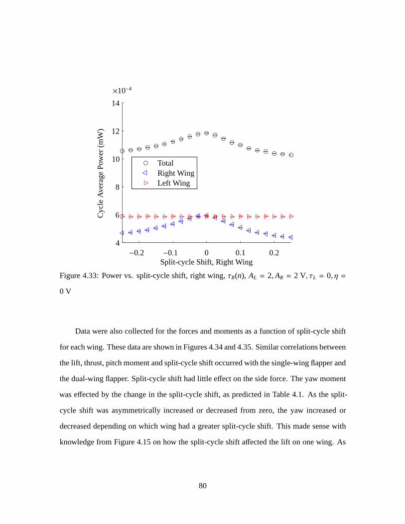
Left WingRight WingTotal
Cyc
leA
vera
ge
Pow
er(m
W)
Split-cycle Shift, Right Wing−0.2 −0.1 0 0.1 0.2
×10−4
4
6
8
10
12
14
Figure 4.33: Power vs. split-cycle shift, right wing,τR(n), AL = 2,AR = 2 V, τL = 0, η =
0 V
Data were also collected for the forces and moments as a function of split-cycle shift
for each wing. These data are shown in Figures 4.34 and 4.35. Similar correlations between
the lift, thrust, pitch moment and split-cycle shift occurred with the single-wing flapper and
the dual-wing flapper. Split-cycle shift had little effect on the side force. The yaw moment
was effected by the change in the split-cycle shift, as predicted inTable 4.1. As the split-
cycle shift was asymmetrically increased or decreased fromzero, the yaw increased or
decreased depending on which wing had a greater split-cycleshift. This made sense with
knowledge from Figure 4.15 on how the split-cycle shift affected the lift on one wing. As
80

suggested by the dual-wing flapper amplitude tests, the yaw and roll moments were again
coupled.
Figures 4.36 and 4.37 show the relation between power and lift as a function of the
split-cycle shift for the left and right wings. The data showed that increasing or decreasing
the split-cycle shift on either wing resulted in more power per lift. The results agreed with
the results shown in Figure 4.16.
81
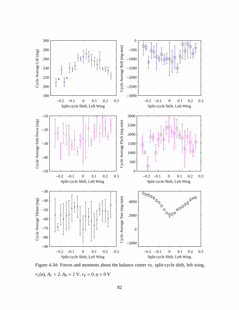
Split-cycle Shift, Left Wing
Cyc
leA
vera
ge
Lift
(mg
)
−0.2 −0.1 0 0.1 0.2 0.3180
200
220
240
260
280
300
Split-cycle Shift, Left Wing
Cyc
leA
vera
ge
Ro
ll(m
g-m
m)
−0.2 −0.1 0 0.1 0.2 0.3−3000
−2500
−2000
−1500
−1000
−500
0
Split-cycle Shift, Left Wing
Cyc
leA
vera
ge
Sid
eF
orc
e(m
g)
−0.2 −0.1 0 0.1 0.2 0.3−50
−40
−30
−20
−10
Split-cycle Shift, Left Wing
Cyc
leA
vera
ge
Pitc
h(m
g-m
m)
−0.2 −0.1 0 0.1 0.2 0.30
500
1000
1500
2000
2500
3000
Split-cycle Shift, Left Wing
Cyc
leA
vera
ge
Th
rust
(mg
)
−0.2 −0.1 0 0.1 0.2 0.3−90
−80
−70
−60
−50
−40
−30
Split-cycle Shift, Left Wing
Cyc
leA
vera
ge
Yaw
(mg
-mm
)
−0.2 −0.1 0 0.1 0.2 0.3
−2000
0
2000
4000
Figure 4.34: Forces and moments about the balance center vs.split-cycle shift, left wing,
τL(n), AL = 2,AR = 2 V, τR = 0, η = 0 V
82

Split-cycle Shift, Right Wing
Cyc
leA
vera
ge
Lift
(mg
)
−0.2 −0.1 0 0.1 0.2 0.3180
200
220
240
260
280
300
Split-cycle Shift, Right Wing
Cyc
leA
vera
ge
Ro
ll(m
g-m
m)
−0.2 −0.1 0 0.1 0.2 0.3−3000
−2500
−2000
−1500
−1000
−500
0
Split-cycle Shift, Right Wing
Cyc
leA
vera
ge
Sid
eF
orc
e(m
g)
−0.2 −0.1 0 0.1 0.2 0.3−50
−40
−30
−20
−10
Split-cycle Shift, Right Wing
Cyc
leA
vera
ge
Pitc
h(m
g-m
m)
−0.2 −0.1 0 0.1 0.2 0.30
500
1000
1500
2000
2500
3000
Split-cycle Shift, Right Wing
Cyc
leA
vera
ge
Th
rust
(mg
)
−0.2 −0.1 0 0.1 0.2 0.3−90
−80
−70
−60
−50
−40
−30
Split-cycle Shift, Right Wing
Cyc
leA
vera
ge
Yaw
(mg
-mm
)
−0.2 −0.1 0 0.1 0.2 0.3
−2000
0
2000
4000
Figure 4.35: Forces and moments about the balance center vs.split-cycle shift, right wing,
τR(n), AL = 2,AR = 2 V, τL = 0, η = 0 V
83
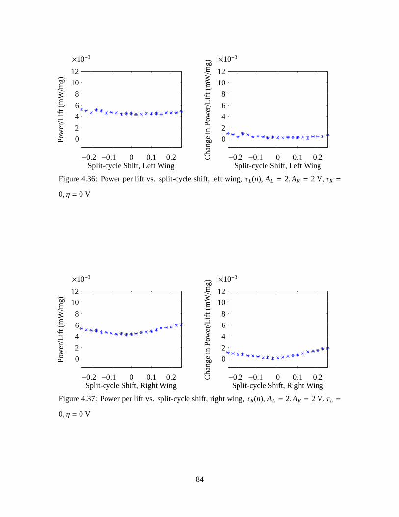
Pow
er/L
ift(m
W/m
g)
Split-cycle Shift, Left Wing−0.2 −0.1 0 0.1 0.2
×10−3
0
2
4
6
8
10
12
Ch
ang
ein
Pow
er/Lift
(mW/m
g)
Split-cycle Shift, Left Wing−0.2 −0.1 0 0.1 0.2
×10−3
0
2
4
6
8
10
12
Figure 4.36: Power per lift vs. split-cycle shift, left wing, τL(n), AL = 2,AR = 2 V, τR =
0, η = 0 V
Pow
er/L
ift(m
W/m
g)
Split-cycle Shift, Right Wing−0.2 −0.1 0 0.1 0.2
×10−3
0
2
4
6
8
10
12
Ch
ang
ein
Pow
er/Lift
(mW/m
g)
Split-cycle Shift, Right Wing−0.2 −0.1 0 0.1 0.2
×10−3
0
2
4
6
8
10
12
Figure 4.37: Power per lift vs. split-cycle shift, right wing, τR(n), AL = 2,AR = 2 V, τL =
0, η = 0 V
84
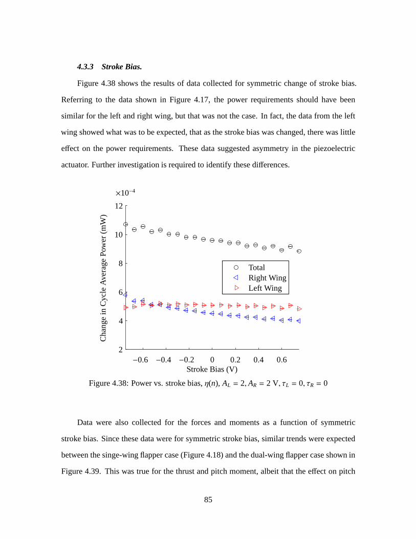
4.3.3 Stroke Bias.
Figure 4.38 shows the results of data collected for symmetric change of stroke bias.
Referring to the data shown in Figure 4.17, the power requirements should have been
similar for the left and right wing, but that was not the case.In fact, the data from the left
wing showed what was to be expected, that as the stroke bias was changed, there was little
effect on the power requirements. These data suggested asymmetry in the piezoelectric
actuator. Further investigation is required to identify these differences.
Left WingRight WingTotal
Ch
ang
ein
Cyc
leA
vera
ge
Pow
er(m
W)
Stroke Bias (V)−0.6 −0.4 −0.2 0 0.2 0.4 0.6
×10−4
2
4
6
8
10
12
Figure 4.38: Power vs. stroke bias,η(n), AL = 2,AR = 2 V, τL = 0, τR = 0
Data were also collected for the forces and moments as a function of symmetric
stroke bias. Since these data were for symmetric stroke bias, similar trends were expected
between the singe-wing flapper case (Figure 4.18) and the dual-wing flapper case shown in
Figure 4.39. This was true for the thrust and pitch moment, albeit that the effect on pitch
85

moment was magnified. But in this case, stroke bias had a smalldetrimental effect on lift
that may not have been detectable in the single-wing flapper case. Even more interesting,
was the effect stroke bias had on roll and, by coupling, yaw moment. Which of these effects
were due to stroke bias and which were a result of power difference were difficult to discern.
More testing is required, preferably once a final piezoelectric actuator has been chosen.
Figure 4.40 shows the relation between power and lift as a function of the stroke bias.
The data showed that increasing or decreasing the stroke bias resulted in more power per
lift. The results are much closer to what was expected but didnot agree with the results
presented in Figure 4.19. This further suggested that asymmetries where present between
the flappers.
86
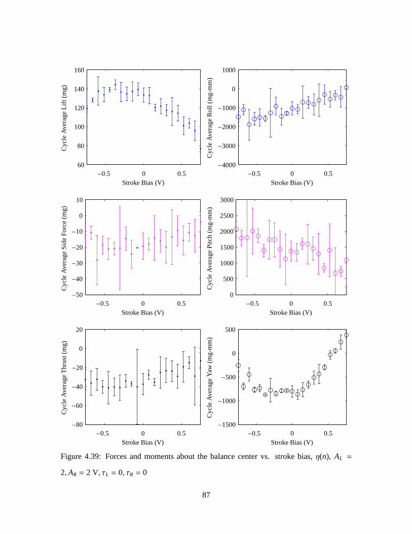
Stroke Bias (V)
Cyc
leA
vera
ge
Lift
(mg
)
−0.5 0 0.560
80
100
120
140
160
Stroke Bias (V)
Cyc
leA
vera
ge
Ro
ll(m
g-m
m)
−0.5 0 0.5−4000
−3000
−2000
−1000
0
1000
Stroke Bias (V)
Cyc
leA
vera
ge
Sid
eF
orc
e(m
g)
−0.5 0 0.5−50
−40
−30
−20
−10
0
10
Stroke Bias (V)
Cyc
leA
vera
ge
Pitc
h(m
g-m
m)
−0.5 0 0.50
500
1000
1500
2000
2500
3000
Stroke Bias (V)
Cyc
leA
vera
ge
Th
rust
(mg
)
−0.5 0 0.5−80
−60
−40
−20
0
20
Stroke Bias (V)
Cyc
leA
vera
ge
Yaw
(mg
-mm
)
−0.5 0 0.5−1500
−1000
−500
0
500
Figure 4.39: Forces and moments about the balance center vs.stroke bias,η(n), AL =
2,AR = 2 V, τL = 0, τR = 0
87

Pow
er/L
ift(m
W/m
g)
Stroke Bias (V)−0.5 0 0.5
×10−3
0
2
4
6
8
10
12
Ch
ang
ein
Pow
er/Lift
(mW/m
g)
Stroke Bias (V)−0.5 0 0.5
×10−3
0
2
4
6
8
10
12
Figure 4.40: Power per lift vs. stroke bias,η(n), AL = 2,AR = 2 V, τL = 0, τR = 0
88

4.3.4 Design of Experiments.
Figure 4.41 shows the results from the DOE run accomplished using Table 3.2.
The data showed the correlation between all five BABM parameters and the seven
measurements. Again, the blue dashed lines represent confidence intervals to one standard
deviation. It is important to note that fewer data runs were accomplished to generate the
plots in Figure 4.41. Examining data for the amplitude from both left and right flapper and
its effect on side force produce some concerns. In fact, close analysis of all the data from
the left and right flapper indicate the conclusion made abovewhen investigating the stroke
bias on the dual-wing flapper; that there were asymmetries inthe piezoelectric actuators.
Ideally, these tests would be performed again, but piezoelectric actuators were in low supply
when these differences manifested. In any case, these relations were important, because
consistent operation in the field is difficult to ensure. An emphasis was placed on the results
for the left flapper since the left piezoelectric actuator was less used. The data indicated that
to manipulate the roll moment, an asymmetric amplitude would be most affective, contrary
to Table 4.1. The data also shows that asymmetric split-cycle shift may be as effective as
asymmetric amplitude to control yaw.
Figures 4.42 and 4.43 show the relations for power and lift associated with a dual-
wing flapper. Recall that the bars are scaled estimates normalized between -1 and 1 where
a negative relationship is detrimental to the output and that the blue lines on the charts
mark a value of 0.2 indicating a strong relationship. The data agreed that amplitude has the
greatest and only significant affect on the power. The lift data identified a strong effect from
stroke bias squared and split-cycle squared. The lift data also identified a strong benefit
from right wing amplitude and stroke bias, but the fact that it was not symmetric with left
wing amplitude and stroke bias cause further speculation ofthe stroke bias measurements.
89
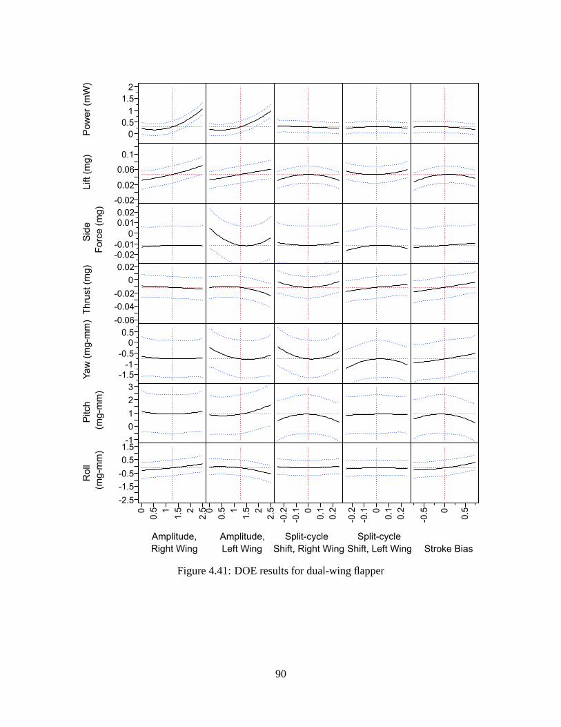
0
0.5
1
1.5
2P
ow
er
(mW
)
-0.02
0.02
0.06
0.1
Lift (m
g)
-0.02-0.01
0
0.010.02
Sid
e
Forc
e (
mg)
-0.06
-0.04
-0.02
0
0.02
Thru
st (m
g)
-1.5-1
-0.5
00.5
Yaw
(m
g-m
m)
-1
0
1
2
3
Pitch
(mg-m
m)
-2.5
-1.5
-0.5
0.5
1.5
Roll
(mg-m
m)
0
0.5 1
1.5 2
2.5
Amplitude,
Right Wing
0
0.5 1
1.5 2
2.5
Amplitude,
Left Wing
-0.2
-0.1 0
0.1
0.2
Split-cycle
Shift, Right Wing
-0.2
-0.1 0
0.1
0.2
Split-cycle
Shift, Left Wing
-0.5 0
0.5
Stroke Bias
Figure 4.41: DOE results for dual-wing flapper
90
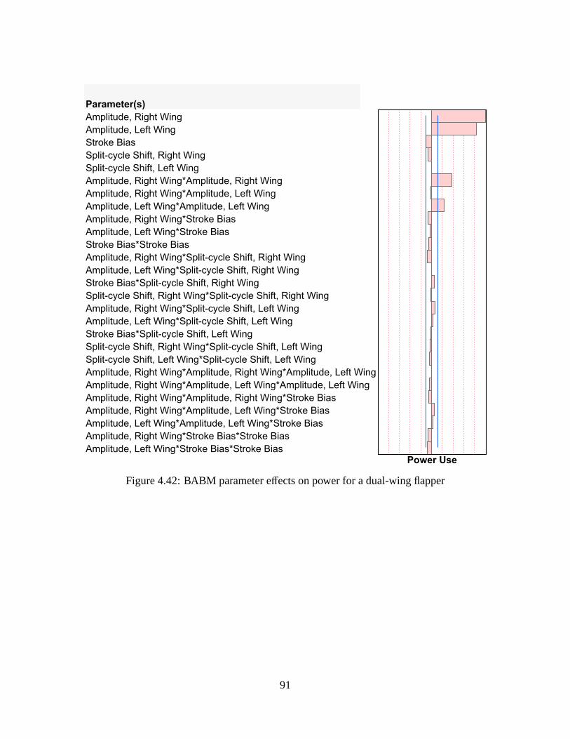
Amplitude, Right Wing
Amplitude, Left Wing
Stroke Bias
Split-cycle Shift, Right Wing
Split-cycle Shift, Left Wing
Amplitude, Right Wing*Amplitude, Right Wing
Amplitude, Right Wing*Amplitude, Left Wing
Amplitude, Left Wing*Amplitude, Left Wing
Amplitude, Right Wing*Stroke Bias
Amplitude, Left Wing*Stroke Bias
Stroke Bias*Stroke Bias
Amplitude, Right Wing*Split-cycle Shift, Right Wing
Amplitude, Left Wing*Split-cycle Shift, Right Wing
Stroke Bias*Split-cycle Shift, Right Wing
Split-cycle Shift, Right Wing*Split-cycle Shift, Right Wing
Amplitude, Right Wing*Split-cycle Shift, Left Wing
Amplitude, Left Wing*Split-cycle Shift, Left Wing
Stroke Bias*Split-cycle Shift, Left Wing
Split-cycle Shift, Right Wing*Split-cycle Shift, Left Wing
Split-cycle Shift, Left Wing*Split-cycle Shift, Left Wing
Amplitude, Right Wing*Amplitude, Right Wing*Amplitude, Left Wing
Amplitude, Right Wing*Amplitude, Left Wing*Amplitude, Left Wing
Amplitude, Right Wing*Amplitude, Right Wing*Stroke Bias
Amplitude, Right Wing*Amplitude, Left Wing*Stroke Bias
Amplitude, Left Wing*Amplitude, Left Wing*Stroke Bias
Amplitude, Right Wing*Stroke Bias*Stroke Bias
Amplitude, Left Wing*Stroke Bias*Stroke Bias
Parameter(s)
Power Use
Figure 4.42: BABM parameter effects on power for a dual-wing flapper
91
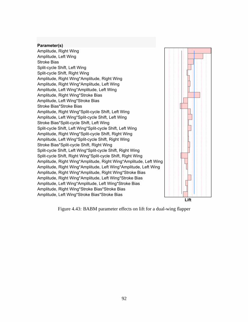
Amplitude, Right Wing
Amplitude, Left Wing
Stroke Bias
Split-cycle Shift, Left Wing
Split-cycle Shift, Right Wing
Amplitude, Right Wing*Amplitude, Right Wing
Amplitude, Right Wing*Amplitude, Left Wing
Amplitude, Left Wing*Amplitude, Left Wing
Amplitude, Right Wing*Stroke Bias
Amplitude, Left Wing*Stroke Bias
Stroke Bias*Stroke Bias
Amplitude, Right Wing*Split-cycle Shift, Left Wing
Amplitude, Left Wing*Split-cycle Shift, Left Wing
Stroke Bias*Split-cycle Shift, Left Wing
Split-cycle Shift, Left Wing*Split-cycle Shift, Left Wing
Amplitude, Right Wing*Split-cycle Shift, Right Wing
Amplitude, Left Wing*Split-cycle Shift, Right Wing
Stroke Bias*Split-cycle Shift, Right Wing
Split-cycle Shift, Left Wing*Split-cycle Shift, Right Wing
Split-cycle Shift, Right Wing*Split-cycle Shift, Right Wing
Amplitude, Right Wing*Amplitude, Right Wing*Amplitude, Left Wing
Amplitude, Right Wing*Amplitude, Left Wing*Amplitude, Left Wing
Amplitude, Right Wing*Amplitude, Right Wing*Stroke Bias
Amplitude, Right Wing*Amplitude, Left Wing*Stroke Bias
Amplitude, Left Wing*Amplitude, Left Wing*Stroke Bias
Amplitude, Right Wing*Stroke Bias*Stroke Bias
Amplitude, Left Wing*Stroke Bias*Stroke Bias
Parameter(s)
Lift
Figure 4.43: BABM parameter effects on lift for a dual-wing flapper
92
4.4 Comparison to Earlier Work
Little work as been done in this area for comparison. Reference 31 tested a small
range of amplitude and stroke bias and a similar range to split-cycle shift tested here. The
power results, the only ones presented in Reference 31, followed similar trends as the power
results presented here except in the case of stroke bias. Theresults presented in Reference
31 showed no correlation between stroke bias and power, similar to the left wing in the
dual-wing flapper case above. This further suggested that the power amplifier provided
asymmetric signals when supplied the same input.
Some of the results presented in Reference 6, Table 4.1 did not hold true for this flapper
configuration. It is important to note that the results foundin this work does not dispute the
work in Reference 6, this work in fact compliments it. The data gathered in Reference 6
was on a different wing configuration and flapper structure. Recall that the wing used for
this research was optimized to match the inertial moments oftheM. sexta.
4.5 Chapter Summary
A lot of data was presented in this chapter, but few conclusions were discussed.
Chapter V will discuss the impacts these results will have onthe way forward for the AFIT
FWMAV.
93

V. Conclusions
Conclusions from the data presented in the previous chapters are presented here. The
data was combined with the knowledge from the research to draw conclusions that
address the research goals.
5.1 Research Goals
Recall the goals stated in Chapter I:How much power is required to vary each
parameter and maintain lift? How do those power requirements relate to controllability?
These goals were set forth to provide future researchers andcontrol designers a reference
when considering the power requirements of the FWMAV. Sinceone mission of the
FWMAV is ISR, which is inherently lengthy, then power concerns are of high importance,
especially when a FWMAV uses the same power source for flight and sensors. Therefore,
this research was performed to quantify the power requirements of BABM, the control
scheme proposed by AFIT.
5.2 Summary of Results
The data from the figures in Chapter IV are summarized in Table5.1. The only data
that was inconclusive was in regards to the stroke bias. An understanding of the dynamics at
play might indicate that the power and lift should not changeas the stroke bias is changed.
Data indicated that power was constant with varying stroke bias in the left wing during
dual-wing flapper testing, Figure 4.38, but not in the right wing. Data further indicated that
lift was constant with varying stroke bias for the single-wing flapper, Figure 4.18, but not
for the dual-wing flapper, Figure 4.39. Recall that the condition with AL = AR = 2 and
τL = τR = η = 0 was chosen as a baseline for hover. This condition providedP = 1.24 mW,
X = 297 mg,Y = 37 mg,Z = 68 mg,L = 1650 mg-mm,M = 2300 mg-mm,N = 2800 mg-
94

mm. Ideally, this condition would provide lift exclusivelybut since it did not, a routine will
have to be incorporated in the future to trim the FWMAV.
Table 5.1: Effects of BABM parameters on power and lift
BABM Parameter Effect on Power Effect on Lift
Amplitude↑ ↑ ↑
Amplitude↓ ↓ ↓
Split-cycle Shift↑ ↓ ↓
Split-cycle Shift↓ ↓ ↓
Stroke Bias↑ Inconclusive Inconclusive
Stroke Bias↓ Inconclusive Inconclusive
5.2.1 Power.
From the data, some specific relations between power and the BABM parameters can
be identified. A symmetric increase of amplitude by 10% required an increase in power by
0.38 milliwatts, approximately 30%. A symmetric decrease of amplitude by 10% allowed
a decrease in power by 0.33 milliwatts, approximately 26%. An asymmetric increase
of amplitude by 10% required an increase in power by 0.20 milliwatts, approximately
16%. An asymmetric decrease of amplitude by 10% allowed a decrease in power by
0.16 milliwatts, approximately 13%. A symmetric change of split-cycle shift to±0.3 (the
maximum change) allowed a decrease in power by approximately 25%. An asymmetric
change of split-cycle shift to±0.25 allowed a decrease in power by approximately 14%.
A change of stroke bias to±0.75 (the maximum tested on the dual-wing flapper) required
95

an increase in power by approximately 1%. Clearly, amplitude has the greatest effect on
power while the effect of stroke bias may be negligible.
5.2.2 Controllability.
Some of the results presented in Reference 6 did not hold truefor this flapper
configuration. Table 5.2 summarizes the effects of control on the forces and moments for
the current wing and structure of the AFIT FWMAV. In some cases, the side-force, thrust,
and moments were not zero, indicating that the FWMAV would need to be trimmed. Since
there is currently no trim routine, the forces and moments will be discussed as percentages.
Furthermore, the research demonstrated what has been know about fixed-wing aircraft for
decades, that moments are closely coupled and an active control scheme is required for
stability.
Table 5.2: Summary of forces and moments generated by changing BABM parameter
BABM
Lift, X Symmetric Amplitude (Very Strong Correlation)
Side Force,Y Asymmetric Amplitude (Very Weak Correlation)
Thrust,Z Symmetric Split-Cycle (Weak Correlation)& Symmetric
Stroke Bias (Weak Correlation)
Roll, L Asymmetric Split-Cycle (Weak Correlation)
Pitch,M Symmetric Stroke Bias (Strong Correlation)& Asymmetric
Split-Cycle (Weak Correlation)
Yaw, N Asymmetric Amplitude (Strong Correlation)& Asymmetric
Split-Cycle (Strong Correlation)
96

From the data, specific relations between control and the BABM parameters can be
identified. A symmetric increase in amplitude by 10% provided an increase in lift by
approximately 22%, while requiring an increase in power by approximately 30%. An
asymmetric increase in amplitude by 10% provided more lift but the goal is to maintain lift.
The data showed that an asymmetric change of equal magnitude, i.e. increasing one wing
by 10% and decreasing the opposite wing by 10%, would maintain lift and power at the
baseline. An asymmetric change in amplitude by 10% in both wings provided an increase in
side-force by approximately 12%. An asymmetric change of split-cycle to±0.25 increased
the roll moment by approximately 14%, increased the pitch moment by approximately 29%,
and decreased the yaw moment by approximately 100%. The asymmetric split-cycle shift
also decreased the lift by approximately 25%, which would require an increase in amplitude
to maintain lift. While the asymmetric split-cycle shift requires less power, the increase in
amplitude to maintain lift would require a net increase in power by approximately 16%
over the baseline. A change of stroke bias to±0.75 provided a change in thrust by 56%.
The change in stroke bias also caused a loss of lift by approximately 27% but did not affect
the power required. The loss of lift would have to over come byan increase in amplitude.
5.3 Future Work
The author suggests that some of these tests be completed again once the piezoelectric
actuator and the passive rotation stops are finalized. In addition, an effort should be made
to mount the final flight vehicle to the balance rather than using a different structure. Since
power and control are such complex problems associated withFWMAV flight, it would be
best to finalize other aspects of design prior to designing a controller.
Research is on going to study the aerodynamic effects of flight on a FWMAV. Once
conclusions are made regarding these effects, the forces and moments can be related to
actual maneuverability of the FWMAV.
97
As stated earlier, a routine to trim the FWMAV will be required prior to flight. Such
a routine should be designed using this research to simulateexpected forces and moments
given certain BABM parameters. If changes to the vehicle design are made, the model can
then be updated to reflect the most current design iteration.
Efforts should also be made to design control logic for minimum power path
optimization based on the data obtained in this research. During those efforts, careful
documentation should be taken to ease the future redesigns should the FWMAV change
significantly.
98
Appendix: Explanation of MATLAB Scripts
TheMATLAB code that was used for this research is summarized here. This appendix
identifies the custom code prepared and outlines the required inputs and outputs for
each of the scripts.
I. DWF_Test_non_Bias.m
This script performed the designed set of experiments on a dual-wing flapper without
a bias drive. It would perform single test cases or multiple cases by varying the
frequency or the BABM parameters. The data was stored in a array of structures. The
script is largely based on the work of Captain Garrison Lindholm.
Inputs
maxA→Maximum voltage for PZT actuator
w→Frequency (rad/sec)
eta→Stroke bias
AR→Amplitude, right wing
tauR→Split-cycle shift, right wing
AL→Amplitude, left wing
tauL→Split-cycle shift, left wing
M1pR→Magnitude 1st harmonic, right wing
M2pR→Magnitude 2nd harmonic, right wing
beta1pR→Phase 1st harmonic, right wing
beta2pR→Phase 2nd harmonic, right wing
M1pL→Magnitude 1st harmonic, left wing
99
M2pL→Magnitude 2nd harmonic, left wing
beta1pL→Phase 1st harmonic, left wing
beta2pL→Phase 2nd harmonic, left wing
samples→Number of sample runs per test point
simFlag→1 = simulation, 0= hardware test
testFlag→2 = BABM test, 1= Frequency test, 0= Single test case
Outputs
data →Data structure with inputs, outputs, units, and information pertaining
to the tests
II. DWFt.m
This script ran the tests forDWF_Test_non_Bias.m with the selected number of
sample runs. This script also performed the cycle-average analysis. The script is
largely based on the work of Captain Garrison Lindholm.
Inputs
maxA→Vector of time
w→Frequency (rad/sec)
BABMs→A structure containing BABM constants for each test case
samples→Number of samples at test case
simFlag→1 = simulation, 0= hardware test
Outputs
out→Data structure with inputs, outputs, units, and information pertaining to
the tests
100

III. DWFs.m
This script ran the individual test runs forDWFt.m. The script is largely based on the
work of Captain Garrison Lindholm.
Inputs
maxA→Vector of time
w→Frequency (rad/sec)
BABMs→A structure containing BABM constants
simFlag→1 = true (simulation), 0= false (hardware test)
Outputs
P→Power in amps
V→Raw voltage
I→Raw current
forceX→Tared forces in x-direction in grams
forceZ→Tared forces in z-direction in grams
forceY→Tared forces in y-direction in grams
input→Input parameters used in this sample run
dis→Tared displacement in millimeters
S→Sampling information used in this sample run
IV. SWF_Test_non_Bias.m
This script performed the designed set of experiments on a dual-wing flapper without
a bias drive. It would perform single test cases or multiple cases by varying the
frequency or the BABM parameters. The data was stored in a array of structures. The
script is largely based on the work of Captain Garrison Lindholm.
101

Inputs
maxA→Maximum voltage for PZT actuator
w→Frequency (rad/sec)
eta→Stroke bias
A→Amplitude
tau→Split-cycle shift
M1pR→Magnitude 1st harmonic
M2pR→Magnitude 2nd harmonic
beta1pR→Phase 1st harmonic
beta2pR→Phase 2nd harmonic
samples→Number of sample runs per test point
simFlag→1 = simulation, 0= hardware test
testFlag→2 = BABM test, 1= Frequency test, 0= Single test case
Outputs
data →Data structure with inputs, outputs, units, and information pertaining
to the tests
V. SWFt.m
This script ran the tests forSWF_Test_non_Bias.m with the selected number of
sample runs. This script also performed the cycle-average analysis. The script is
largely based on the work of Captain Garrison Lindholm.
Inputs
maxA→Vector of time
102
w→Frequency (rad/sec)
BABMs→A structure containing BABM constants for each test case
samples→Number of samples at test case
simFlag→1 = simulation, 0= hardware test
Outputs
out→Data structure with inputs, outputs, units, and information pertaining to
the tests
VI. SWFs.m
This script ran the individual test runs forSWFt.m. The script is largely based on the
work of Captain Garrison Lindholm.
Inputs
maxA→Vector of time
w→Frequency (rad/sec)
BABMs→A structure containing BABM constants
simFlag→1 = true (simulation), 0= false (hardware test)
Outputs
P→Power in amps
V→Raw voltage
I→Raw current
forceX→Tared forces in x-direction in grams
forceZ→Tared forces in z-direction in grams
forceY→Tared forces in y-direction in grams
103

input→Input parameters used in this sample run
dis→Tared displacement in millimeters
S→Sampling information used in this sample run
VII. BABM.m
Function was designed to take the desired signal length, drive frequency, BABM
parameters, and FRF plant information and then output the DHPC compensated
signals corresponding to the BABM parameters. Used with inDWFs.m andSWFs.m.
The script was written by Captain Garrison Lindholm.
Inputs
t→Vector of time
w→Frequency (rad/sec)
eta→Stroke bias
AR→Amplitude, right wing
AL→Amplitude, left wing
tauR→Split-cycle shift, right wing
tauL→Split-cycle shift, left wing
M1pR→Magnitude 1st harmonic, right wing
M2pR→Magnitude 2nd harmonic, right wing
beta1pR→Phase 1st harmonic, right wing
beta2pR→Phase 2nd harmonic, right wing
M1pL→Magnitude 1st harmonic, left wing
M2pL→Magnitude 2nd harmonic, left wing
104

beta1pL→Phase 1st harmonic, left wing
beta2pL→Phase 2nd harmonic, left wing
Outputs
VR→Voltage signal to drive the right wing
VL→Voltage signal to drive the left wing
VIII. M_cp.m
This script was a designed to move the moments to the center ofpressure. It was a
post-processing function ran on the data file.
Inputs
file→File name of data structure
Outputs
data →Data structure with inputs, outputs, units, and information pertaining
to the tests
105

Bibliography
[1] AIAA. Nomenclature and Axis Systems for Aerodynamic Wind Tunnel Testing. AIAAG-129-2012. American Institute of Aeronautics and Astronautics, 2012. ISBN 978-1-60086-915-0.
[2] Air Force Research Laboratory. “US Air Force Flapping Wing Micro Air Vehicle”,2009. URL http://www.youtube.com/watch?v=_5YkQ9w3PJ4.
[3] Anderson, Michael L. Design and Control of Flapping Wing Micro Air Vehicles.Ph.D. thesis, Air Force Institute of Technology, 2950 Hobson Way, Bldg 641, Wright-Patterson AFB OH 45433, September 2011.
[4] Anderson, Michael L. and Richard G. Cobb. “Frequency Response of a MicroAir Vehicle Wing Flapping Mechanism to Non-Harmonic Forcing”. 51st AIAA/AS-ME/ASCE/AHS/ASC Structures, Structural Dynamics, and Materials Conference,0(2010-2708), April 2010.
[5] Anderson, Michael L. and Richard G. Cobb. “Techniques for Non-Harmonic WingFlapping for the Control of Micro Air Vehicles”.AIAA Guidance, Navigation, andControl Conference, 0(2010-7555), August 2010.
[6] Anderson, Michael L. and Richard G. Cobb. “Towards Flapping Wing Control ofMicro Air Vehicles”. Journal of Guidance and Control, 35:296–308, 2012.
[7] Anderson, Michael L., Nathanael J. Sladek, and Richard G. Cobb. “Aero andStructural-dynamic Repeatability of a Novel MAV Wing Manufacturing Process”.AIAA. AIAA, 2011.
[8] Anderson, Michael L., Nathanael J. Sladek, and Richard G. Cobb. “Evaluation of Bi-Harmonic Amplitude and Bias Modulation for Flapping Wing MAV Control”. 49thAIAA Aerospace Sciences Meeting including the New HorizonsForum and AerospaceExposition, 0(2011-1161), January 2011.
[9] ATI Industrial Automation, Inc. “ATI Force/ Torque Sensor: Nano17 Titanium”.URL http://www.ati-ia.com/products/ft/ft_models.aspx?id=Nano17+Titanium.
[10] Bar-Cohen, Y.Electroactive polymer (EAP) actuators as artificial muscles: reality,potential, and challenges. SPIE Press monograph. SPIE Press, 2001. ISBN9780819440549.
[11] Conn, Andrew T., Stuart C. Burgess, and Chung S. Ling. “Design of a parallel crank-rocker flapping mechanism for insect-inspired micro air vehicles”. Proceedings of the
106

I MECH E Part C Journal of Mechanical Engineering Science, 221(10):1211–1222,2007. ISSN 0954-4062.
[12] Cranston, Brian C.Evaluation of the thorax of the Manduca sexta for flapping wingmicro air vehicle applications. Master’s thesis, Air Force Institute of Technology,December 2012.
[13] de Croon, G. C. H. E., K. M. E. de Clercq, R. Ruijsink, B. Remes, and C. de Wagter.“Design, aerodynamics, and vision-based control of the DelFly”. InternationalJournal of Micro Air Vehicles, 1(2):71–97, June 2009.
[14] Doman, David B., Michael W. Oppenheimer, and David O. Sigthorsson. “Dynamicsand Control of a Minimally Actuated Biomimetic Vehicle: Part I - AerodynamicModel”. AIAA Guidance, Navigation, and Control Conference, 0(6160), August2009.
[15] Doman, David B., Michael W. Oppenheimer, and David O. Sigthorsson. “Dynamicsand Control of a Minimally Actuated Biomimetic Vehicle: Part II - Control”. AIAAGuidance, Navigation, and Control Conference, 0(6161), August 2009.
[16] Dudley, R.The Biomechanics of Insect Flight: Form, Function, Evolution. Princetonpaperbacks. Princeton University Press, 2002. ISBN 9780691094915.
[17] DuPont.DuPont Kapton®Polyimide Film.
[18] DuPont.DuPont Teijin Films™.
[19] El-Hawary, M.E. Introduction to Electrical Power Systems. IEEE Press Series onPower Engineering. Wiley, 2008. ISBN 9780470411360.
[20] Finio, Benjamin M., Jessica K. Shang, and Robert J. Wood. “Body torque modulationfor a microrobotic fly”. ICRA, 3449–3456. IEEE, 2009.
[21] Grasmeyer, Joel M., Matthew T. Keennon, and Aerovironment Inc. “Development ofthe Black Widow Micro Air Vehicle”. 39th AIAA Aerospace Sciences Meeting andExhibit. 2001.
[22] Gullan, P.J. and P.S. Cranston.The Insectons: An Outline of Entomology 3rd Edition.Blackwell Publishing, 2005.
[23] Hanrahan, Shawn. “Manduca Sexta”.
[24] JMP. JMP 8 User Guide, second edition.
[25] Karpelson, Michael, Gu-Yeon Wei, and Robert J. Wood. “Areview of actuation andpower electronics options for flapping-wing robotic insects”. ICRA, 779–786, 2008.
107

[26] Karpelson, Michael, Gu-Yeon Wei, and Robert J. Wood. “Milligram-scale high-voltage power electronics for piezoelectric microrobots”. ICRA, 2217–2224. IEEE,2009.
[27] Keennon, Matthew, Karl Klingebiel, Henry Won, , and Alexander Andriukov.“Development of the Nano Hummingbird: A Tailless Flapping Wing Micro AirVehicle”. 50th AIAA Aerospace Sciences Meeting including the New Horizons Forumand Aerospace Exposition, January 2012.
[28] Khan, Zaeem, Kyle Steelman, and Sunil Agrawal. “Development of insect thoraxbased flapping mechanism”.ICRA, 3651–3656. IEEE, 2009.
[29] Kitching, Ian J. “The phylogenetic relationships of Morgan’s Sphinx, Xanthopanmorganii (Walker), the tribe Acherontiini, and allied long-tongued hawkmoths(Lepidoptera: Sphingidae, Sphinginae)”.Zoological Journal of the Linnean Society,135(4):471–527, 2002. ISSN 1096-3642.
[30] Lindholm, Garrison J. and Richard G. Cobb. “Closed-Loop Control of a Constrained,Resonant-Flapping Micro Air Vehicle”.AIAA Guidance, Navigation, and ControlConference, 0(2012-4980), August 2012.
[31] Lindholm, Garrison J., Ryan P. O’Hara, Mark F. Reeder, and Richard G. Cobb.“Power Requirements for Control of Flapping Wing Micro Air Vehicle usingPiezoelectric Actuators”.AIAA, 2012-0917. 2012.
[32] LPKF. In-House Rapid PCB Prototyping Product Catalog.
[33] LPKF. Micro-Material Processing with the LPKF ProtoLaser U3.
[34] Micro-Epsilon. “Position Sensor, CCD-Sensor, Laser Sensor: MICRO-EPSILON”.URL http://www.optoncdt.com/.
[35] Myers, P., R. Espinosa, C. S. Parr, T. Jones, G. S. Hammond,and T. A. Dewey. “The Animal Diversity Web”, 2013. URLhttp://animaldiversity.ummz.umich.edu/accounts/Manduca_sexta/classification/.
[36] Nelson, R.C.Flight stability and automatic control. WCB/McGraw Hill, 1998. ISBN9780070462731.
[37] Office of Secretary of Defense. “UAS ROADMAP 2005”. Print, August 2005.
[38] Office of Secretary of Defense. “FY2009–2034 Unmanned Systems IntegratedRoadmap”. Print, April 2009.
108

[39] O’Hara, Ryan P. The Characterization of Material Properties and StructuralDynamics of the Manduca Sexta Forewing for Application to Flapping Wing MicroAir Vehicle Design. Ph.D. thesis, Air Force Institute of Technology, 2950 HobsonWay, Bldg 641, Wright-Patterson AFB OH 45433, September 2012.
[40] Sladek, Nathanael J.Flapping wing micro air vehicle wing manufacture and forcetesting. Master’s thesis, Air Force Institute of Technology, 2011.
[41] Stevens, B.L. and F.L. Lewis.Aircraft Control and Simulation. Wiley, 2003. ISBN9780471371458.
[42] Trek. Trek Model PZD700A M/S.
[43] Tu, Michael S. and Thomas L. Daniel. “Submaximal power output from thedorsolongitudinal flight muscles of the hawkmoth Manduca sexta”. Journal ofExperimental Biology, 207(26):4651–4662, 2004.
[44] Wang, Qing-Ming and L Eric Cross. “Performance analysis of piezoelectric cantileverbending actuators”.Ferroelectrics, 215(1):187–213, 1998.
[45] Wood, Robert J., Erik Steltz, and Ronald S. Fearing. “Nonlinear Performance Limitsfor High Energy Density Piezoelectric Bending Actuators.”ICRA, 3633–3640. IEEE,2005.
[46] Wu, Huaiyu, Dong Sun, and Zhaoying Zhou. “Micro air vehicle: configuration,analysis, fabrication, and test”.Mechatronics, IEEE/ASME Transactions on, 9(1):108–117, March 2004. ISSN 1083-4435.
109

Vita
Captain Justin R. Carl graduated from Lovejoy High School inHampton, Georgia.
He performed undergraduate studies at Texas A&M Universityin College Station, Texas
where he graduated with a Bachelor of Science degree in Mechanical Engineering in May
2008. He was a member of the Corps of Cadets Squadron 8 and obtained his commission
through AFROTC Detachment 805 at Texas A&M University.
Upon commissioning, he was assigned to Edwards AFB, California where he served
as the Executive Officer of the USAF Test Pilot School. He then served as a flight test
engineer for the 418th Flight Test Squadron performing upgrade testing on the C-5 Galaxy.
In September 2011, he entered the Graduate School of Engineering and Management, Air
Force Institute of Technology. Upon graduation, he will be assigned to the Air Force
Research Laboratory, Wright-Patterson AFB, Ohio.
110
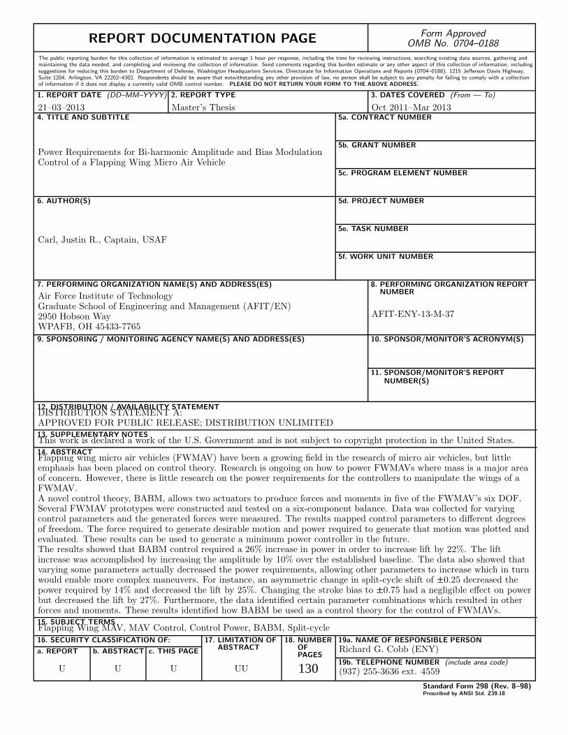
REPORT DOCUMENTATION PAGE Form ApprovedOMB No. 0704–0188
The public reporting burden for this collection of information is estimated to average 1 hour per response, including the time for reviewing instructions, searching existing data sources, gathering andmaintaining the data needed, and completing and reviewing the collection of information. Send comments regarding this burden estimate or any other aspect of this collection of information, includingsuggestions for reducing this burden to Department of Defense, Washington Headquarters Services, Directorate for Information Operations and Reports (0704–0188), 1215 Jefferson Davis Highway,Suite 1204, Arlington, VA 22202–4302. Respondents should be aware that notwithstanding any other provision of law, no person shall be subject to any penalty for failing to comply with a collectionof information if it does not display a currently valid OMB control number. PLEASE DO NOT RETURN YOUR FORM TO THE ABOVE ADDRESS.
1. REPORT DATE (DD–MM–YYYY) 2. REPORT TYPE 3. DATES COVERED (From — To)
4. TITLE AND SUBTITLE 5a. CONTRACT NUMBER
5b. GRANT NUMBER
5c. PROGRAM ELEMENT NUMBER
5d. PROJECT NUMBER
5e. TASK NUMBER
5f. WORK UNIT NUMBER
6. AUTHOR(S)
7. PERFORMING ORGANIZATION NAME(S) AND ADDRESS(ES) 8. PERFORMING ORGANIZATION REPORTNUMBER
9. SPONSORING / MONITORING AGENCY NAME(S) AND ADDRESS(ES) 10. SPONSOR/MONITOR’S ACRONYM(S)
11. SPONSOR/MONITOR’S REPORTNUMBER(S)
16. SECURITY CLASSIFICATION OF:
a. REPORT b. ABSTRACT c. THIS PAGE
17. LIMITATION OFABSTRACT
18. NUMBEROFPAGES
19a. NAME OF RESPONSIBLE PERSON
19b. TELEPHONE NUMBER (include area code)
Standard Form 298 (Rev. 8–98)Prescribed by ANSI Std. Z39.18
21–03–2013 Master’s Thesis Oct 2011–Mar 2013
Power Requirements for Bi-harmonic Amplitude and Bias ModulationControl of a Flapping Wing Micro Air Vehicle
Carl, Justin R., Captain, USAF
Air Force Institute of TechnologyGraduate School of Engineering and Management (AFIT/EN)2950 Hobson WayWPAFB, OH 45433-7765
AFIT-ENY-13-M-37
12. DISTRIBUTION / AVAILABILITY STATEMENTDISTRIBUTION STATEMENT A:APPROVED FOR PUBLIC RELEASE; DISTRIBUTION UNLIMITED13. SUPPLEMENTARY NOTESThis work is declared a work of the U.S. Government and is not subject to copyright protection in the United States.14. ABSTRACTFlapping wing micro air vehicles (FWMAV) have been a growing field in the research of micro air vehicles, but littleemphasis has been placed on control theory. Research is ongoing on how to power FWMAVs where mass is a major areaof concern. However, there is little research on the power requirements for the controllers to manipulate the wings of aFWMAV.A novel control theory, BABM, allows two actuators to produce forces and moments in five of the FWMAV’s six DOF.Several FWMAV prototypes were constructed and tested on a six-component balance. Data was collected for varyingcontrol parameters and the generated forces were measured. The results mapped control parameters to different degreesof freedom. The force required to generate desirable motion and power required to generate that motion was plotted andevaluated. These results can be used to generate a minimum power controller in the future.The results showed that BABM control required a 26% increase in power in order to increase lift by 22%. The liftincrease was accomplished by increasing the amplitude by 10% over the established baseline. The data also showed thatvarying some parameters actually decreased the power requirements, allowing other parameters to increase which in turnwould enable more complex maneuvers. For instance, an asymmetric change in split-cycle shift of ±0.25 decreased thepower required by 14% and decreased the lift by 25%. Changing the stroke bias to ±0.75 had a negligible effect on powerbut decreased the lift by 27%. Furthermore, the data identified certain parameter combinations which resulted in otherforces and moments. These results identified how BABM be used as a control theory for the control of FWMAVs.15. SUBJECT TERMSFlapping Wing MAV, MAV Control, Control Power, BABM, Split-cycle
U U U UU 130
Richard G. Cobb (ENY)
(937) 255-3636 ext. 4559