power system dynamic prof. m. l. kothari department of...

Power System Dynamic

Prof. M. L. Kothari

Department of Electrical Engineering

Indian Institute of Technology, Delhi

Lecture - 06

The Equal Area Criterion for Stability (Contd…)

Friends, we shall continue our discussion on equal area criteria of stability.

(Refer Slide Time: 01:07)

Today, we will cover I will address the following problems. The basic definitions of a transient

stability limit, the meaning of critical clearing angle and critical clearing time then we shall study

the effect of fault clearing time on transient stability limit, next we shall study the effect of type

of fault on stability when we talk about the type of fault on stability we, I shall introduce the

concept of fault shunts then we will study the effect of grounding on stability.

Now, before I address these issues I would like to mention that this subject has been very well

addressed in power system stability written by Edward Wilson Kimbark there are 3 volumes,

volume 1, volume 2 and third volume is now known as synchronous machines. These basic

concepts are very well addressed in volume 1.


Now, let us define what the transient stability limit. We have defined earlier the transient

stability, now today we will emphasize on this word transient stability limit. The transient

stability limit refers to the amount of power that can be transmitted through some point in the

system with stability when the system is subjected to severe aperiodic disturbance that here the

stability limit is referred in terms of the amount of power that is what is the power in mega watts

that can be transmitted and this is referred to some point in the system.

Now the emphasis here is on some point in the system. Now if you take a machine infinite bus

system then there is only one transmission line and therefore whatsoever power that can be

transmitted on that line with stability becomes the transient stability limit. However when I

consider a multi machine system okay, in that system this limit refers to a point in the power

system that is there may be number of transmission lines and you may refer that in this particular

transmission line how much power can be transmitted for a given operating condition with given

type of severe disturbance, given type of severe disturbance here.

Now here we emphasize the word aperiodic the disturbance is disturbance comes not in

periodical manner but it comes in aperiodic manner it comes and goes it is not actually that after

every 5 second the disturbance keeps on coming. Okay, this is what is the meaning of transient

stability limit therefore, any power system when we operate, we have to operate below transient

stability limit.

Okay so that it will withstand the the particular type of disturbance for which the system is

designed. Now next term is the critical clearing angle. This critical clearing angle is specifically

referred to a machine infinite bus system because in the multi-machine system, you will have

number of angles right and therefore the definition to a multi-machine system is not that easily

available.


Now for a given system and for a given initial load, there is a critical clearing angle, if the actual

clearing angle is smaller than the critical value a system is stable and if larger the system is

unstable. I will explain this point in detail okay in our further discussion that here the meaning is

that there is some critical clearing angle and actual clearing angle, if it is less than this value

system is stable in case the actual clearing angle is more than the critical clearing angle system

will become unstable.


Similarly, we define another term critical fault clearing time again for a given system and for

given initial loading there is a critical fault clearing time, if actual fault clearing time is smaller

than the critical value the system is stable, if larger then the system is unstable. Now this

definition is applicable to machine infinite bus system or a multi-machine system because

whenever a system is operating okay and if fault occurs on a particular element of the system

then this fault is cleared by removing the faulted element by operating the circuit breaker at the

two ends and therefore there is certain time required to clear this fault.

In case this actual fault clearing time is less than the critical clearing time system is stable

otherwise, it is unstable further if suppose the critical clearing time for a system comes out to be

say .2 second and actual fault clearing time is say .1 second then the difference .1 second is

called the stability margin. Okay therefore, we have been discussing in these days in terms of

what is the stability margin and stability margin can be quantified in terms of difference in the

critical clearing time for the system and actual fault clearing time because actual fault clearing

time depends upon the operating time of the protection system and circuit breaker fault

interruption time.


Now let us understand what is the effect of fault clearing time on transient stability limit, now

here when I say it is a transient stability limit it means it is a certain amount of power that can be

transmitted without loss of stability. The transient stability limit depends on type of fault and the

duration of fault, a very we shall state these aspects type of fault and duration of fault. The power

limit can be determined as a function of clearing angle suppose it is a machine infinite bus

system we can find out the transient stability limit or power limit as a function of clearing angle

and clearing time can be found by solving the swing equation up to the time of fault clearing that

if I want to know know the transient stability limit as a function of fault clearing time.

The approach we will discuss here but for a machine infinite bus system the simple approach is

that you first apply the equal area criteria, find out for a given power what is the critical clearing

angle and then once we know the angle, we solve the swing equation up to the up to the fault

clearing angle and corresponding to that we read the value of time and that becomes our critical

clearing time and therefore when I say here, when I discussed earlier that when you apply this

graphical method that is equal area criteria of stability.

We do not completely diverse the need for solving swing equation but partially we do it wholly

or partially this is what we are the they are partially means partly you have to solve it and

suppose a swing curve is required to be solved for say 2 seconds for normal stability steady

analysis but in this particular case the time for which it is to be solved is very small suppose the

for critical fault clearing time comes out to be it is a .2 second okay, then I solve it from 0 to .2

second not from 0 to 2 second and therefore this saves my time or computation time.


As I have stated that fault clearing time is sum of the time that the protective relays take to close

the circuit breaker trip circuit and the time required for the circuit breaker to interrupt the fault

current.

The general conclusion that decrease in fault clearing time improves stability and increases

transient stability limit is just as valid for a multi machine system as for a 2 machine system.

This point I stated earlier also again we reiterate that general conclusion is the decrease in fault

clearing time improves stability and it improves the transient stability limit okay.


Now this conclusion is valid for machine infinite bus system 2 machine system and even for a

multi machine system and that is why the efforts have been made all through to reduce the fault

clearing time this has been possible by applying fast acting protective relays and fast acting

circuit breakers.


Now to illustrate this that how do we calculate the transient stability limit and obtain a curve

relating the transient stability limit and the fault clearing time, we will consider these 2 machine

system and a generator infinite bus and consider that the fault occurred at the middle of the line.

Now for this system we can find out the 3 power angle curves, pre fault, during the fault and post

fault, once we know this power angle curves we can apply the equal area criteria and determine

the certain points on the transient stability limit versus the fault clearing time.


Now we will consider the 2 extreme cases, first case we will consider that the fault is

instantaneously clear. Suppose fault occurs in the system and the time which it takes to clear the

fault is instantaneous it does not have any time practically it does not happen okay. Now this can

also be considered similar to that one transmission line is stripped, okay by operating the circuit

breakers.

Now in that case if you want to find out what is the transient stability limit then the approach

would be you make use of these two power angle characteristic, pre fault output characteristic

and the post fault output where during fault we do not require it because the system has not

operated with fault on the system.

Now in this case what we will do is, this mechanical input line, the mechanical input line Pm is

moved up and down, Pm is moved up and down till these two areas are equal that is a1 and a2 is

the area bounded by mechanical input line, the post fault power angle curve that is from delta

naught to delta 1 and a2 is again the area bounded by the post fault power angle curve and the

mechanical input line but they have opposite signs.

Now when these two areas are equal that will give us the stability limit that is this Pm becomes

the stability limit you have, what a what is to be done is that you have to move this mechanical

input line up and down you have to do 1 or 2 you know iterations and the movement these two

areas becomes equal that becomes the stability limit because here the fault has been cleared

instantaneously.


Now we will take another extreme case, where the the sustained fault on the system, that is fault

is not cleared in this situation we require the two power angle curves, one is the pre fault another

is the during the fault power angle curve. Now these 2 curves are plotted here again the approach

will be that you move the mechanical input line up and down till these 2 areas a1a2 are equal that

is when you do this computations you assume some value of Pm.

You know the value of delta naught initial operating angle, you can find out what is the value of

this angle delta 1 that will depend upon the intersection of mechanical input and fault on power

angle curve. Okay similarly, you can find out delta m which is equal to phi minus delta 1, okay

now you find out this area by process of integration and you equate this with the area a2, in case

these 2 areas are equal then this Pm becomes the transient stability limit with sustained fault.

Now the third situation will be that the fault is clear infinite time.


Now under this situation we require all the 3 power angle curves, okay. Now one way is that you

move this mechanical input line Pm up and down and see that these 2 areas are equal and but this

there actually we required the information and what is the fault clearing angle there were 2

parameters involved, one is the fault clearing angle another is the mechanical input line. The

easiest process will be we assume some value of Pm and instead of moving this mechanical input

line up and down you adjust this clearing angle, you will you move this line either on left or on

right it means you assume some value of fault clearing angle and see whether these 2 areas are

equal.

In case you find actually that for a assumed value of angle a1 is greater than a2 move this line on

left so that a1 decreases and a2 increases right and you do this exercise still these 2 areas are

equal it means what we have done now here is for given input Pm we have obtained the critical

clearing angle and then we integrate the swing equation from this point delta naught up to this

critical clearing angle and find out the corresponding value of critical clearing time.

Now this is the way you can find out a number of points assume some value, suppose the value

of Pm is small you will find that delta c will be very large and a stage may come when delta c

will coincide with delta m right that is the case for sustained fault that is when you are moving

here right and if this fault you find actually that Pm is such that system is stable when delta c

equal to delta m that is the condition for sustained fault then when you, if you are moving if the

Pm is moved up and when you are you have to move this line the moment you find actually the

delta critical clearing angle delta c same as delta naught that become the instantaneous occurring

time and therefore by this approach we can plot the curve relating the transient stability limit

versus the fault clearing time in seconds.


For example, this graph shows for a typical system on this x axis by plotting the fault clearing

time in seconds, y axis we are plotting the stability limit in per unit and the stability limit of the

system when the fault is cleared instantaneously is denoted as 1 per unit and for all other fault

clearing time it is going to be less than this okay.

Now here actually this .2 shows the sustained condition because there is a break here in the graph

right because when the fault is sustained the stability limit is going to very small, sustained fault

condition there is a fault is there and system is not losing stability it means that is the situation

which occurs only when the fault, I am sorry a a the power output is small right. Further as we

have seen that the post fault, I am sorry the post fault power angle characteristic depends upon

the element which has been removed and the remaining system.

Similarly, the during the fault power angle curve is concerned it depends upon the location of

fault on the transmission line. Suppose you consider the 2 machine system and for the whole

analysis what we have done is we have assumed the fault in the middle of the line suppose I shift

the fault location from the middle toward the sending end of the line or you shift this from

middle to the receiving end of the line in that case you will find that the stability limit will be

different the curve relating the stability limit versus the fault clearing time will be different.


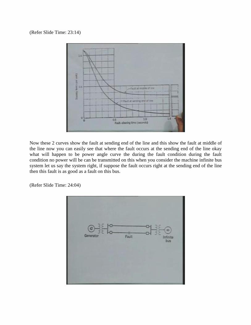
Now these 2 curves show the fault at sending end of the line and this show the fault at middle of

the line now you can easily see that where the fault occurs at the sending end of the line okay

what will happen to be power angle curve the during the fault condition during the fault

condition no power will be can be transmitted on this when you consider the machine infinite bus

system let us say the system right, if suppose the fault occurs right at the sending end of the line

then this fault is as good as a fault on this bus.


Okay and therefore the voltage at this bus becomes 0 or it collapses because I am considering

here a balanced 3-phase fault and therefore no power can be transmitted from generator to the

infinite bus right, therefore you will find actually the r2 r2 which is multiplying r2 Pmax sin delta r2

will become 0. This is a very special case and you will find that the transient stability limit will

be less as compared to where the fault occurs in any other point on the transmission line that is

why these 2 curves have been plotted to illustrate the effect of location of fault on the

transmission line.



Now by applying the equal area criteria of stability, we can find out for a given value of

mechanical input and for given fault location we can compute the value of the angle fault

clearing angle delta at which the system just stable that is we can compute the critical clearing

angle for computing the critical clearing angle what is to be done is that you find out this area a1

that is you integrate, you integrate that is a1 can be written as integral of delta naught to delta c

Pm mechanical input minus Pe1 not P1 Pe2 d delta where Pe2 is equal to r2 times Pmax sin delta

okay.



Then the area a2 can be computed integral delta c to delta M, here we will be writing this as Pe3

minus Pm d delta where Pe3 is equal to r2 Pmax sin. Okay, if you equate these 2 areas that is you

equate a1 with a2 and you can find the expression for critical clearing angle or the equation for

computing critical clearing angle. This equation has been obtained and it is a cos delta c equal to

delta m minus delta o, sin delta o minus r1 cos delta o plus r2 cos delta m divided by r2 minus r1

this, this expression can be derived without any difficulty by equating those 2 expressions.

Now, when you apply this formula, you have ensure that these angles are the delta m delta

naught they are they are yes substituted in radians sometimes people committed mistake they put

directly in degrees and therefore the result will be observed.


Now this angle delta m has to be calculated by using this formula delta m is equal to phi minus

sin inverse Pm divided by r2Pmax because delta m is delta m is obtained where the where the post

fault power angle characteristic intersects with mechanical input line like it intersect at 2 points

one is the angle which is given by this this equation and another will be phi minus this, therefore

delta m is equal to phi minus this therefore another sometime people commit mistake in

computing the value of delta m correctly and where this r1 is the x12 before fault and x12 during

fault r2 is x12 before fault x12 after fault, that is x12 is the reactance connecting the nodes that is

internal voltage of the generator to the infinite bus voltage and this formula is applicable to a 2

machine system only we do not have such formula for a multi machine system.


Now next point we have to address is how to determine power angle curve for unsymmetrical

fault, till now till now we have assumed a balanced 3-phase fault for our analysis and we also

assume that this 3-phase fault is a metallic short circuit there is no fault impedance involved,

under this situation the, the faulted point is directly connected to the reference bus in the

equivalent network and we analyze it but the moment you have unbalanced fault then things

cannot be as simple as in a 3-phase system because as you know actually that unbalanced faults

can be analyzed by by using the method of symmetrical components.

Okay and when we apply the method of symmetrical components we will come across positive

sequence network negative sequence network zero sequence network and we can compute

depending upon the type of fault the positive sequence currents, negative sequence currents, zero

sequence currents.

We also know that how to draw for a given system the positive sequence network, negative

sequence network and zero sequence networks before I tell you how to account for the

unsymmetrical fault for determining power angle curve during fault condition. We have to

understand some basic concepts one basic concept is which I will introduce and explain in

subsequent discussion.


The concept of fault shunt now here to ah before we understand this fault shunt, let us understand

a since the internal electromotive forces of 3-phase synchronous machine are of positive

sequence that is so for the three phase synchronous generators are concerned we always generate

positive sequence voltages. We do not generate negative sequence or zero sequence voltages, no

power results from interaction of positive sequence voltages with negative or zero sequence

currents. Although, the stator may be carrying negative sequence current, zero sequence current

but when this negative sequence current interacts with the positive sequence voltages no power is

generated no average power is generated.

Similarly, no average power is generated when positive sequence voltages interact with 0

sequence current, okay and therefore to compute the power angle characteristic which basically

relates with the power transfer from machine to the infinite bus okay. We are we have to, we

have to compute primarily the positive sequence currents okay and to compute the positive

sequence currents as we know actually that during fault condition the positive sequence, negative

sequence zero sequence networks are connected in a particular fashion if suppose there is a line

to ground fault these three networks will be connected in series if it is a line to line fault then

these two networks will be connected in parallel looking into the looking into the faulted

terminals.

We have to look where do we connect in parallel where the fault occurs in two faulted points

similarly, we have it is a double line to ground fault then the three networks will be connected in

parallel.


The simplest approach to account for the unbalanced or unsymmetrical fault is by connecting

shunt impedance ZF at the point of fault that is in the positive sequence network we return the

positive sequence network as it is earlier between the fault point and the reference we were

connecting zero impedance that is directly connected.


However, when unbalanced or unsymmetrical fault is there we have to connect an impedance of

value ZF that is called fault shunt ZF. The value of ZF depends upon the impedance Z2 and Zo

of the negative and zero sequence networks viewed from the point of fault that is ZF is function

of positive sequence I am sorry, negative sequence and zero sequence impedances. Here, I will

without a derivation right now I am just giving the result the this table shows the type of short

circuit and the fault shunt ZF is the impedance of the fault shunt, if it is a line to ground fault the

value of ZF is Z0 plus Z2, if it is a line to line fault the fault shunt impedance is Z2, if it is a

double line to ground fault if the fault shunt is the parallel combination of Z0 and Z2 and if it is 3

phase fault ZF is 0 okay.

Now this table is very important and I will show you a list through illustration, how do we get

this in time, now a typical statistics of the occurrence of type of faults or frequency of occurrence

type of fault.


A typical 132 K. V system the data were obtained and out of the total 72 faults which occurred

on the system, 58 were lined to ground faults double line to ground faults were 8 and 3-phase

faults were 6 in fact line to line faults generally gets converted into line to line to ground fault.

You can see very easily here that the frequency of occurrence of 3- phase fault is lowest and the

the frequency of occurrence of line to ground fault is the highest and therefore, in case you

design your system or operating condition of the system is design, considering 3- phase fault it

means we are very very pessimistic in our approach, it may be assumed actually that faults are

would be very severe and we are taking a very safe margin.

However, if you apply only considering line to ground fault definitely you are optimistic where

you feel that these faults may not occur because if you design considering line to ground fault

and if 3- phase fault occurs, system is going to lose stability similarly double line to ground fault

occurs it is going to loose stability in case you do not have any margin right and therefore the

practices I will tell you what are the practices which are as followed ah for designing the system

because we have to make a balance.

We have, we should not be very optimistic we should not be very pessimistic in our approach

before I tell you about the effect of grounding, let us just see how do we account and compute

the value of fault shunt impedance ZF okay. I have told you actually that fault shunt impedance

ZF is different for different fault and the the table had been shown to show you the expressions.


Okay let us take this the simple machine infinite bus problem where you have generator neutral

of the generate is grounded double circuit transmission line. In this case I have taken only one

transformer there is no transformer shown here but if that is there is a transformer here that can

also be considered this delta star connected transformer start point grounded infinite bus system.

Now when you solve the problem considering unsymmetrical fault we need information about

positive negative and zero sequence reactance’s of the system components for generator Xd

prime is 0.35, the negative sequence reactance of the generator is less than Xd prime is 0.24, X

naught is the lowest that is zero sequence reactance is always low 0.06, for the transmission line

is concerned its positive and negative sequence reactance’s are equal that is Z 1 is 0.4 and j times

0.4 the and the negative sequence reactance is also 0.4 the zero sequence reactance of the

transmission line is always more than the positive or negative sequence reactance, in this case it

is 0.65 the typical values it may be even more it may be sometimes 2 to 2.5 times even 2 to 3

three times it all depends upon this system. For a transformer we can assume this X1 X2 X0 equal

to .1 that is they are equal, with this the data’s which we have assumed let us first obtain the

positive sequence, negative sequence and zero sequence networks.

The positive sequence network is simple is same as what you do actually for analyzing for

balance 3-phase fault condition, this is the internal voltage E prime the direct axis transient

reactance I am putting the reactance value only 0.35 transmission line reactance 0.4, 0.4 and the

transformer reactance here 0.1 and the infinite bus voltage okay this is the voltage V. I am

showing this as a voltage V, now V we shall consider that the fault occurs at the sending end of

one of the transmission lines right at this point.



This is the sending end of the line and therefore I will added this is as good as the fault occurring

at the bus therefore let us call this point as the point P on the series and this is our reference. Now

so far the negative sequence network is concerned it is it will have the same structure except that

the sources will not be present there are no sources because we do not generate the negative

sequence voltages and therefore the negative sequence network can be drawn.

This is my reference bus, okay we call this o this point continues to be P now what we will do

here is that this point we will call as P2 that is the fault point in the negative sequence network

and we will call this point as P1 in the positive sequence network, the points are same P1 and P2

are same on the physical system. The values here are now because in a zero sequence, a negative

sequence network, the generator reactance is 0.24 per unit, the transmission line is same 0.4, 0.4

transformer is also 0.1 okay.

Now we can find out the equivalent reactance of the negative sequence network looking into this

points P2 and o, this exercise when you do you will find actually that equivalent comes out to be

a reactance whose value is 0.133 for this problem you can say this is P2 and you can even call

this as a o2 the reference bus for the negative sequence network, therefore these 2 terminals are

important for us. The next step is to draw zero sequence I mean to draw the zero sequence

network for the system.

When we draw the zero sequence network, we have to consider the connection of transformers

because transformers may be connected in different modes and we have to also consider the

neutral impedance. In case you have put a impedance, in the neutral circuit in the equivalent

circuit that impedance will appear as 3 times the actual value in this particular case, the neutral

have been solidly grounded therefore they do not appear.


In this particular case if you draw this zero sequence network it will come out to be this value is

0.65, this is also 0.65, this is 0.1 this is 0.06, this is the zero sequence reactance of the generator.

This is our reference bus incidentally in this connection, the generator neutrally is grounded

therefore we can connect a neutral point to the reference. Okay if you had it not been grounded

this would have been open the transformer is a start delta transformer with start point grounded

and therefore again this point will be connected.

Now those who do not have the practice of drawing the zero sequence network, I will advice

them to refresh their knowledge about drawing the positive negative in zero sequence networks

particularly zero sequence networks, considering the different types of transformer connections

now here this is the fault point I will call this as a P000 and the equivalent impedance looking into

these two terminals has been computed it comes out to be equal to 0.053 these points are Po and

okay this so far we have obtained the positive negative in zero sequence networks and we have

also obtained the equivalent value of the positive, negative sequence impedances for the network

considering the fault location.

Now in order to consider the effect of different type of fault in the system right, these 3 networks

have to be connected in a proper fashion. They for line to ground fault which we have considered

these 3 networks can be connected in this fashion.


This diagram shows the positive sequence network and here we have not simplified this network,

the fault occurs at the point P1 in the negative sequence network is shown in the terminals P2 and

O2, well while zero sequence impedance is on between the terminals Po and Oo.

Now for simulating line to ground fault the 3 networks positive, negative and zero sequence

networks are connected in series that how we can connect these 3 networks in series that is O1 is

connected to P2, O2 is connected to Po and Oo is connected to P1 this becomes a series

connection. It can be very clearly seen here that the positive sequence network is modified and

here we have now and the impedance connected between P1 and O1 for line to ground fault, the

value of the impedance connected is Z2 plus Z0 and this becomes the fault shunt.



Now this network can be simplified, I will put in this simple form here between the node 1 and 3

the reactance is the transient direct axis transient reactance of the generator, this is the equivalent

reactance of transmission line and the transformer and between this node 3 and O, reference node

we have connected the fault shunt. If we have considered the lossless system then the fault shunt

impedance becomes a pure reactance that is j times XF. This network can be further transformed

that is the start connected three impedances can be replaced by an equivalent delta connected

impedances.

This figure shows the equivalent delta the nodes 1 and 2 are retained, the reference node is also

retained as it is now the reactance connecting the node 1and 2 is X12 and the reactance which is

directly coming across the E prime source E prime is shown here. Similarly, the reactance

coming directly across the infinite bus voltage is also coming and is shown here now know that

these 2 reactance’s do not affect the power transfer capability or power transmission capability of

the system therefore we concentrate only on the reactance connecting the nodes 1and 2. Now for

line to ground fault X12 is equal to 0.35 plus 0.3 plus 0.35 into 0.3 divided by XF where XF will

be the sum of the 2 impedances that is zero sequence and negative sequence impedance.

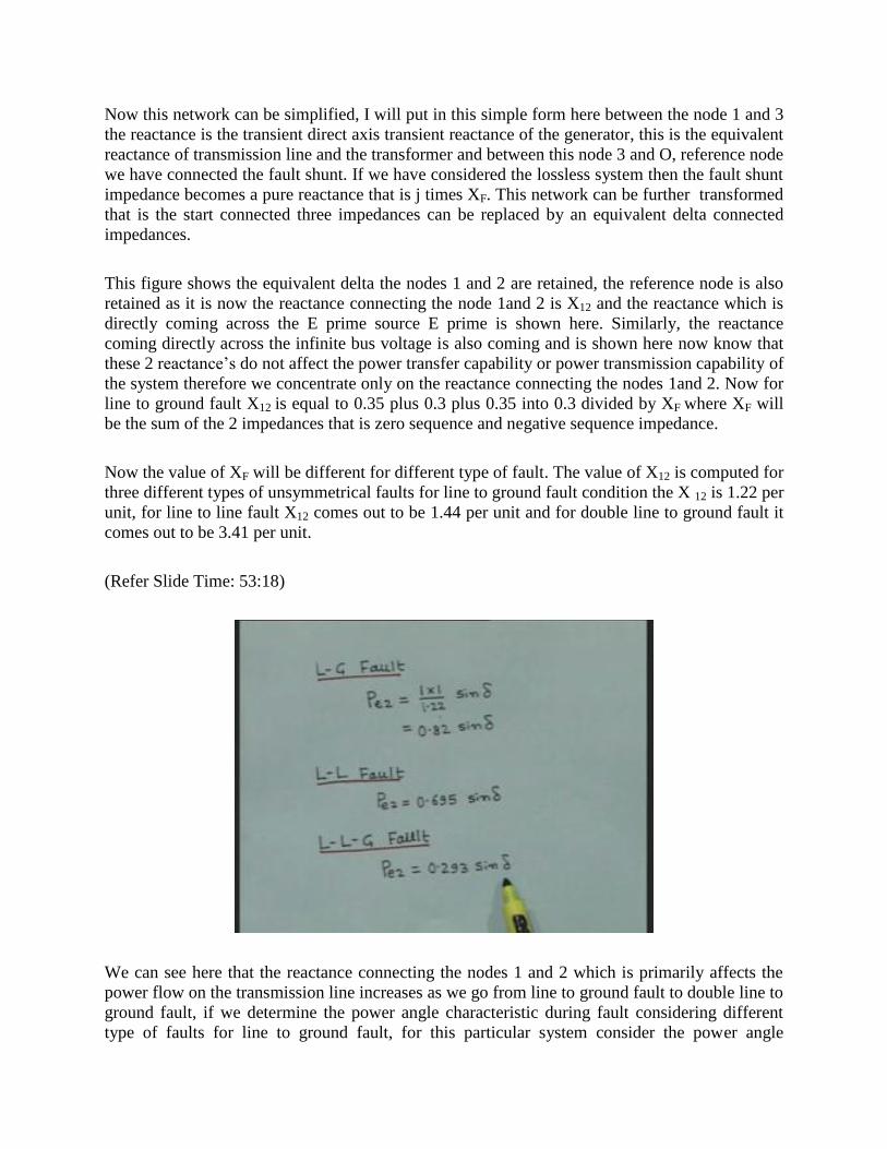
Now the value of XF will be different for different type of fault. The value of X12 is computed for

three different types of unsymmetrical faults for line to ground fault condition the X 12 is 1.22 per

unit, for line to line fault X12 comes out to be 1.44 per unit and for double line to ground fault it

comes out to be 3.41 per unit.


We can see here that the reactance connecting the nodes 1 and 2 which is primarily affects the

power flow on the transmission line increases as we go from line to ground fault to double line to

ground fault, if we determine the power angle characteristic during fault considering different

type of faults for line to ground fault, for this particular system consider the power angle

characteristic comes out to be P2 equal to 0.82 sin delta, for line to line fault the power angle

curve is P2 equal to 0.695 sin delta and double line to ground fault P2 is 0.293 sin delta that is if

you examine these 3 power angle curves we find that the power angle curve with line to ground

fault has the highest amplitude while the power angle curve corresponding to line to line to

ground fault or double line to ground fault is having the smallest amplitude or and hence the,

from the consideration of the transient stability limit or the power which can be transferred

without loss of synchronism, the line to ground fault will provide more transient stability limit as

compared to double line to ground fault.


This figure shows the plot of transient stability limit or power limit as a function of fault duration

in seconds. This curve shows the relationship between transient stability limit and fault duration

for line to ground fault, the second curve is for line to line fault, third curve is for 2 line to

ground fault and the last curve is plotted for a 3- phase fault.

Now we can easily see here that in case the fault is clear instantaneously that is when the fault

duration is 0, then the transient stability limit is same in all the 4 cases and therefore we can

conclude that the transient stability limit is not affected by the type of fault, if the fault is cleared

instantaneously.

However, if the fault is cleared the time delay then it is very clear actually that the transient

stability limit is lowest when 3- phase fault occurs and transient stability limit is highest for line

to ground fault therefore, we can see that from the point of view of severity the line to ground

fault is the least severe as compared to 3- phase fault or we can say that 3- phase fault is the

severest fault from the stability consideration.


Now we study the effect of grounding on stability the methods of grounding of a power system

modify the 0 sequence impedance this affects the impedance of the fault shunts for representing

the ground faults and thereby affect the severity of such faults.


A typical to a system has been examined and transient stability limit is computed for different

values of ZS and ZR for a 2 machine system.


Here the value of ZS and ZR are varied from resistive to the reactance value and this stable

shows that as the as the value of the impedance connected in the neutral of the receiving end side

and in the sending end side are varied from ohmic value to the reactance value, the stability limit

varies thus we can say that is grounding affects the stability. Now I can say conclude my

presentation that today we have examined the affect of fault duration type of fault location of

fault and the grounding on the stability of the system, thank you.

power system dynamic prof. m. l. kothari department of...

Documents