power system security analysis using reinforcement learning

.

Power System Security Analysis usingReinforcement Learning

.

By

José María Sunyer Nestares

.

Senior Thesis in Electrical Engineering

University of Illinois at Urbana-Champaign

Advisor: Richard Y. Zhang

May 2020

1

.

Abstract

The challenge of controlling and guaranteeing the security of the power system is con-stantly evolving, particularly in light of significant predicted growth in the deploymentof renewable energy, and increasing use of electric vehicles.

Existing power systems are made secure, in part, using the N-1 criterion, in which thesystem is required to remain within operational limits with the loss of any individualcomponent. This does not assess the risk of cascading failure, which is likely to becomemore commonplace with the large-scale, distributed integration of small, stochastic com-ponents, such as renewable generators or electric vehicles.

In this thesis, we describe an AI-based advisory tool to verify the N − k criterion overtransmission lines, meaning that the system is required to be secure with the disconnec-tion of k out of N total transmission lines. The tool is designed to identify cascadingmechanisms, in which the disconnection of one line overloads another, thereby resultingin a sequence of disconnections downstream. Our key insight is to formulate this cascad-ing problem as an instance of the shortest path, a classic problem in dynamic program-ming and reinforcement learning with a number of standard solutions. The assumptionsof the formulation are validated on small-scale IEEE test cases using exhaustive search.Finally, we investigate simulation-based techniques from the reinforcement learning lit-erature, as a means of overcoming the curse of dimensionality for large-scale, real-worldpower systems.

Keywords: power system security, cascading failure, reinforcement learning, dynamicprogramming, security analysis, N-k criterion

2

Contents

I Motivation and Introduction 5

1 How grid operators work 6

2 How the network operates 7

2.1 Thermal limits of transmission equipment . . . . . . . . . . . . . . . . . 7

2.2 Voltage maintenance within a safe range . . . . . . . . . . . . . . . . . . 9

2.3 Generation, supply and frequency balance . . . . . . . . . . . . . . . . . 9

II Theoretical Framework 10

3 Reinforcement Learning 10

3.1 RL within Artificial Intelligence and Machine Learning . . . . . . . . . . 10

3.2 Examples of RL . . . . . . . . . . . . . . . . . . . . . . . . . . . . . . . . 11

3.3 Attack threat problem . . . . . . . . . . . . . . . . . . . . . . . . . . . . 12

3.4 Markov Decision Process . . . . . . . . . . . . . . . . . . . . . . . . . . . 13

3.5 Value of states and actions . . . . . . . . . . . . . . . . . . . . . . . . . 16

3.6 Dynamic Programming . . . . . . . . . . . . . . . . . . . . . . . . . . . . 17

3.6.1 Backward Induction . . . . . . . . . . . . . . . . . . . . . . . . . 18

3.6.2 Policy iteration . . . . . . . . . . . . . . . . . . . . . . . . . . . . 18

3.6.3 Value iteration . . . . . . . . . . . . . . . . . . . . . . . . . . . . 19

3.7 Monte-Carlo Method . . . . . . . . . . . . . . . . . . . . . . . . . . . . . 20

4 Power Systems 23

4.1 Electric grid . . . . . . . . . . . . . . . . . . . . . . . . . . . . . . . . . . 23

4.2 Power Flow equations . . . . . . . . . . . . . . . . . . . . . . . . . . . . 24

4.3 Newton-Raphson Method for Power Flow . . . . . . . . . . . . . . . . . 27

III Problem Formulation 30

5 Model description 30

6 Cascading failure simulation 32

7 Dynamic Programming 33

7.1 Exhaustive search . . . . . . . . . . . . . . . . . . . . . . . . . . . . . . . 33

7.2 Backward induction . . . . . . . . . . . . . . . . . . . . . . . . . . . . . 33

8 Monte-Carlo Algorithm 35

IV Software Implementation 37

9 Python 37

3

10 Pandapower 38

10.1 Network elements . . . . . . . . . . . . . . . . . . . . . . . . . . . . . . . 38

10.2 Power flow solver . . . . . . . . . . . . . . . . . . . . . . . . . . . . . . . 42

V Numerical Results 45

11 Small-size power system examples 45

11.1 4-bus power system . . . . . . . . . . . . . . . . . . . . . . . . . . . . . . 45

11.2 9-bus power system . . . . . . . . . . . . . . . . . . . . . . . . . . . . . . 49

12 Medium-size power system examples 51

12.1 39-bus power system . . . . . . . . . . . . . . . . . . . . . . . . . . . . . 51

12.2 89-bus power system . . . . . . . . . . . . . . . . . . . . . . . . . . . . . 53

VI Conclusion 55

4

Part I

Motivation and IntroductionThe challenge of controlling and guaranteeing the security of the power system is constantly evolv-ing. With the growth of renewable energy in the grid, the intensive penetration of distributedenergy resources and changes in demand characteristics, new challenges for power grid operatorsarise. According to the International Energy Agency (IEA), low-carbon sources are expected toprovide more than half of the total electricity throughout the world by 2040, with wind and solarPV becoming the main renewable energy sources (see Figure 1). Another key driver in the futuretransformation of the power systems is the electrification of the transportation sector. As shown inFigure 2, also taken from the IEA, the global stock of electric vehicles has increased by a factor of13 between 2013 and 2018 and is expected to keep growing in the next years1. These present newchallenges to the grid, in the form of increasing uncertainty and variability. At the same time, theypresent new opportunities for developing new tools and technologies to improve the security of thepower system.

�� ,QVWDOOHG�SRZHU�JHQHUDWLRQ�FDSDFLW\�E\�VRXUFH�LQ�WKH�6WDWHG�3ROLFLHV�6FHQDULR��²¬&KDUWV�²�'DWD��6WDWLVWLFV��,($

KWWSV��ZZZ�LHD�RUJ�GDWD�DQG�VWDWLVWLFV�FKDUWV�LQVWDOOHG�SRZHU�JHQHUDWLRQ�FDSDFLW\�E\�VRXUFH�LQ�WKH�VWDWHG�SROLFLHV�VFHQDULR��

&LWH 6KDUH

$SSHDUV�LQ

,QVWDOOHG�SRZHU�JHQHUDWLRQ�FDSDFLW\�E\�VRXUFH�LQ�WKH�6WDWHG�3ROLFLHV�6FHQDULR��/DVW�XSGDWHG��-DQ��

'RZQORDG�FKDUW

*:

,($��$OO�5LJKWV�5HVHUYHG

&RDO *DV 2LO 1XFOHDU :LQG 6RODU�39 2WKHU�UHQHZDEOHV +\GUR %DWWHU\�VWRUDJH

&RDO *DV

2LO

1XFOHDU

:LQG

6RODU�39

2WKHU�UHQHZDEOHV

+\GUR

%DWWHU\�VWRUDJH

��

��

��

��

��

��

��

�� 3URMHFWLRQV

5HODWHG�FKDUWV

(OHFWULFLW\�PL[�LQ�WKH�8QLWHG�6WDWHV��-DQXDU\�$SULO��

�

&RDO *DV 1XFOHDU 5HQHZDEOHV

/RFNGRZQ

��

&RDO

*DV

1XFOHDU 5HQHZDEOHV

:HHN��

:HHN��

:HHN��

:HHN��

:HHN��

:HHN��

:HHN��

:HHN��

:HHN��

�

��

��

��

��

2SHQ

5HGXFWLRQV�RI�HOHFWULFLW\�GHPDQG�DIWHU�LPSOHPHQWLQJ�ORFNGRZQ�PHDVXUHV�LQ�VHOHFWHG�FRXQWULHV��ZHDWKHU�FRUUHFWHG��WR��GD\V

�

)UDQFH *HUPDQ\ ,WDO\ 6SDLQ 8. ,QGLD &KLQD

1XPEHU�RI�GD\V�VLQFH�ORFNGRZQ�EHJDQ

)UDQFH

*HUPDQ\

,WDO\

6SDLQ8.

,QGLD

&KLQD

'DVKHG�OLQH�UHSUHVHQWV�FORVXUHV�DQG�SDUWLDO�ORFNGRZQ��VROLG�OLQH�UHSUHVHQWV

IXOO�ORFNGRZQ

� � � ��

��

��

�

��

2SHQ

(OHFWULFLW\�PL[�LQ�,QGLD��-DQXDU\�$SULO��

�

2SHQ

:RUOG�(QHUJ\�2XWORRN��

%URZVH

&RXQWULHV)XHOV�DQG�WHFKQRORJLHV7RSLFV

([SORUH

$QDO\VLV'DWD�DQG�VWDWLVWLFV

)ROORZ

j,($b��7HUPV 3ULYDF\

/HDUQ

$ERXW

$UHDV�RI�ZRUN

1HZV�DQG�HYHQWV

&RQQHFW

&RQWDFW

-REV

'HOHJDWHV

�� ,QVWDOOHG�SRZHU�JHQHUDWLRQ�FDSDFLW\�E\�VRXUFH�LQ�WKH�6WDWHG�3ROLFLHV�6FHQDULR��²¬&KDUWV�²�'DWD��6WDWLVWLFV��,($

KWWSV��ZZZ�LHD�RUJ�GDWD�DQG�VWDWLVWLFV�FKDUWV�LQVWDOOHG�SRZHU�JHQHUDWLRQ�FDSDFLW\�E\�VRXUFH�LQ�WKH�VWDWHG�SROLFLHV�VFHQDULR��

&LWH 6KDUH

$SSHDUV�LQ

,QVWDOOHG�SRZHU�JHQHUDWLRQ�FDSDFLW\�E\�VRXUFH�LQ�WKH�6WDWHG�3ROLFLHV�6FHQDULR��/DVW�XSGDWHG��-DQ��

'RZQORDG�FKDUW

*:


&RDO *DV 2LO 1XFOHDU :LQG 6RODU�39 2WKHU�UHQHZDEOHV +\GUR %DWWHU\�VWRUDJH

&RDO *DV

2LO

1XFOHDU

:LQG

6RODU�39

2WKHU�UHQHZDEOHV

+\GUR

%DWWHU\�VWRUDJH

��

��

��

��

��

��

��

�� 3URMHFWLRQV

5HODWHG�FKDUWV

(OHFWULFLW\�PL[�LQ�WKH�8QLWHG�6WDWHV��-DQXDU\�$SULO��

�

&RDO *DV 1XFOHDU 5HQHZDEOHV

/RFNGRZQ

��

&RDO

*DV

1XFOHDU 5HQHZDEOHV

:HHN��

:HHN��

:HHN��

:HHN��

:HHN��

:HHN��

:HHN��

:HHN��

:HHN��

�

��

��

��

��

2SHQ

5HGXFWLRQV�RI�HOHFWULFLW\�GHPDQG�DIWHU�LPSOHPHQWLQJ�ORFNGRZQ�PHDVXUHV�LQ�VHOHFWHG�FRXQWULHV��ZHDWKHU�FRUUHFWHG��WR��GD\V

�

)UDQFH *HUPDQ\ ,WDO\ 6SDLQ 8. ,QGLD &KLQD

1XPEHU�RI�GD\V�VLQFH�ORFNGRZQ�EHJDQ

)UDQFH

*HUPDQ\

,WDO\

6SDLQ8.

,QGLD

&KLQD

'DVKHG�OLQH�UHSUHVHQWV�FORVXUHV�DQG�SDUWLDO�ORFNGRZQ��VROLG�OLQH�UHSUHVHQWV

IXOO�ORFNGRZQ

� � � ��

��

��

�

��

2SHQ

(OHFWULFLW\�PL[�LQ�,QGLD��-DQXDU\�$SULO��

�

2SHQ

:RUOG�(QHUJ\�2XWORRN��

%URZVH

&RXQWULHV)XHOV�DQG�WHFKQRORJLHV7RSLFV

([SORUH

$QDO\VLV'DWD�DQG�VWDWLVWLFV

)ROORZ

j,($b��7HUPV 3ULYDF\

/HDUQ

$ERXW

$UHDV�RI�ZRUN

1HZV�DQG�HYHQWV

&RQQHFW

&RQWDFW

-REV

'HOHJDWHV

2000 2005 2010 2015 2020 2025 2030 2035 20400

3500

3000

2500

2000

1500

1000

500

GW

Coal Gas Oil Nuclear Wind Solar PV Other renewables Hydro Battery storage

Projections

Coal

Gas

Oil Nuclear

Wind

Solar PV

Other renewables

Battery storage

Hydro

Figure 1: World installed power generation capacity by source between 2000 and 2040 from theInternational Energy Agency

Artificial intelligence (AI) has seen tremendous success in recent years, over applications aswide-ranging as software, healthcare, autonomous vehicles, natural language processing, finance,marketing, and within many more industrial sectors. One of the most famous applications of AItook place in 1997, when Deep Blue, a chess-playing computer developed by IBM, defeated forthe first time in history, the reigning world chess champion at the time, Garry Kasparov [16]. AIagain captured the imagination of the public in 2011, when the supercomputer “Watson” [18], aquestion-answering computer system capable of answering questions in natural language, defeatedtwo world champions in “Jeopardy”, a popular and well-known TV show in which contestants provetheir intelligence by answering different quiz questions. If beating the world’s best player in chesswas not enough, in 2017, AlphaGo, a Google DeepMind project, beat Ke Jie, who at the time wasranked number one in the world. The most impressive aspect of this is that, if chess has around10120 possible chessboard configurations [25], Go presents a shocking estimated number of boardpositions of around 10172.

The maturing of AI technologies presents a perfect opportunity to address the new challengeswe have presented for power systems. As we have seen, AI has offered solutions to very large andcomplex problems in short computational time and has proven to be able to learn from experience,eventually developing an intuition that is comparable, or in some cases even exceeding, that of

1In this figure, BEV stands for Battery Electric Vehicle while PHEV stands for Plug-in Hybrid Electric Vehicle

5

*OREDO�(9�2XWORRN��6FDOLQJ�XS�WKH�WUDQVLWLRQ�WR�HOHFWULF�PRELOLW\

7HFKQRORJ\�UHSRUW�Ř�0D\��

7KH�*OREDO�(9�2XWORRN�LV�DQ�DQQXDO�SXEOLFDWLRQ�WKDW�LGHQWLȋLHV�DQG�GLVFXVVHV�UHFHQW�GHYHORSPHQWV�LQ�HOHFWULF�PRELOLW\�DFURVV�WKH�JOREH��,W�LV�GHYHORSHG�ZLWK�WKH�VXSSRUW�RI�WKH�PHPEHUV�RI�WKH�(OHFWULF�9HKLFOHV�,QLWLDWLYH��(9,��&RPELQLQJ�KLVWRULFDO�DQDO\VLV�ZLWK�SURMHFWLRQV�WR��WKH�UHSRUW�H[DPLQHV�NH\�DUHDV�RI�LQWHUHVW�VXFK�DV�HOHFWULF�YHKLFOH�DQGFKDUJLQJ�LQIUDVWUXFWXUH�GHSOR\PHQW��RZQHUVKLS�FRVW��HQHUJ\�XVH��FDUERQ�GLR[LGH�HPLVVLRQV�DQG�EDWWHU\�PDWHULDO�GHPDQG��7KH�UHSRUW�LQFOXGHV�SROLF\�UHFRPPHQGDWLRQV�WKDW�LQFRUSRUDWH�OHDUQLQJ�IURP�IURQWUXQQHU�PDUNHWV�WR�LQIRUP�SROLF\�PDNHUV�DQG�VWDNHKROGHUV�WKDW�FRQVLGHU�SROLF\�IUDPHZRUNV�DQG�PDUNHW�V\VWHPV�IRU�HOHFWULF�YHKLFOH�DGRSWLRQ��7KLVHGLWLRQ�IHDWXUHV�D�VSHFLȋLF�DQDO\VLV�RI�WKH�SHUIRUPDQFH�RI�HOHFWULF�FDUV�DQG�FRPSHWLQJ�SRZHUWUDLQ�RSWLRQV�LQ�WHUPV�RI�JUHHQKRXVH�JDV�HPLVVLRQV�RYHU�WKHLU�OLIH�F\FOH��$V�ZHOO��LW�GLVFXVVHV�NH\�FKDOOHQJHV�LQ�WKH�WUDQVLWLRQ�WR�HOHFWULF�PRELOLW\�DQG�VROXWLRQV�WKDW�DUH�ZHOO�VXLWHG�WR�DGGUHVV�WKHP��7KLV�LQFOXGHV�YHKLFOH�DQG�EDWWHU\�FRVW�GHYHORSPHQWV��VXSSO\�DQGYDOXH�FKDLQ�VXVWDLQDELOLW\�RI�EDWWHU\�PDWHULDOV��LPSOLFDWLRQV�RI�HOHFWULF�PRELOLW\�IRU�SRZHU�V\VWHPV��JRYHUQPHQW�UHYHQXH�IURP�WD[DWLRQ��DQG�WKH�LQWHUSOD\�EHWZHHQ�HOHFWULF��VKDUHG�DQG�DXWRPDWHG�PRELOLW\�RSWLRQV�

(OHFWULF�FDU�GHSOR\PHQW�KDV�EHHQ�JURZLQJ�UDSLGO\�RYHU�WKH�SDVW�WHQ�\HDUV��ZLWK�WKH�JOREDO�VWRFN�RI�HOHFWULF�SDVVHQJHU�FDUVbSDVVLQJ��PLOOLRQ�LQ��DQ�LQFUHDVH�RI��IURP�WKH�SUHYLRXV�\HDU��$URXQG��RI�HOHFWULF�FDUV�RQ�WKH�URDG�LQ��ZHUH�LQ�&KLQD�ŗ�D�WRWDO�RI��PLOOLRQ�ŗ�FRPSDUHG�WR��LQ��,Q�FRPSDULVRQ��(XURSH�DFFRXQWHG�IRU��RI�WKHJOREDO�ȋOHHW��DQG�WKH�8QLWHG�6WDWHV��

(9�JURZWK�DURXQG�WKH�ZRUOG

7KH�QXPEHU�RI�FKDUJLQJ�SRLQWV�ZRUOGZLGH�ZDV�HVWLPDWHG�WR�EH�DSSUR[LPDWHO\��bPLOOLRQ�DW�WKH�HQG�RI��XS��IURP�WKH�\HDU�EHIRUH�

0RVW�RI�WKLV�LQFUHDVH�ZDV�LQ�SULYDWH�FKDUJLQJ�SRLQWV��DFFRXQWLQJ�IRU�PRUH�WKDQ��RI�WKH��bPLOOLRQ�LQVWDOODWLRQV�ODVW�\HDU�

,Q�WKLV�UHSRUW

.H\�ILQGLQJV

(OHFWULF�FDU�GHSOR\PHQW�LQ�VHOHFWHG�FRXQWULHV��

PLOOLRQV


&KLQD�%(9 &KLQD�3+(9 (XURSH�%(9 (XURSH�3+(9 8QLWHG�6WDWHV�%(9 8QLWHG�6WDWHV�3+(9 2WKHU�%(9 2WKHU�3+(9 :RUOG�%(9

��

�

�

�

�

�

�

2SHQ

3UHVV�UHOHDVH

)LJXUHV�DUFKLYH

.H\�ȋLQGLQJV

+LJKOLJKWV

([HFXWLYH�VXPPDU\

&RQWHQWV &LWH 6KDUH 'RZQORDG

*OREDO�(9�2XWORRN��6FDOLQJ�XS�WKH�WUDQVLWLRQ�WR�HOHFWULF�PRELOLW\

7HFKQRORJ\�UHSRUW�Ř�0D\��

7KH�*OREDO�(9�2XWORRN�LV�DQ�DQQXDO�SXEOLFDWLRQ�WKDW�LGHQWLȋLHV�DQG�GLVFXVVHV�UHFHQW�GHYHORSPHQWV�LQ�HOHFWULF�PRELOLW\�DFURVV�WKH�JOREH��,W�LV�GHYHORSHG�ZLWK�WKH�VXSSRUW�RI�WKH�PHPEHUV�RI�WKH�(OHFWULF�9HKLFOHV�,QLWLDWLYH��(9,��&RPELQLQJ�KLVWRULFDO�DQDO\VLV�ZLWK�SURMHFWLRQV�WR��WKH�UHSRUW�H[DPLQHV�NH\�DUHDV�RI�LQWHUHVW�VXFK�DV�HOHFWULF�YHKLFOH�DQGFKDUJLQJ�LQIUDVWUXFWXUH�GHSOR\PHQW��RZQHUVKLS�FRVW��HQHUJ\�XVH��FDUERQ�GLR[LGH�HPLVVLRQV�DQG�EDWWHU\�PDWHULDO�GHPDQG��7KH�UHSRUW�LQFOXGHV�SROLF\�UHFRPPHQGDWLRQV�WKDW�LQFRUSRUDWH�OHDUQLQJ�IURP�IURQWUXQQHU�PDUNHWV�WR�LQIRUP�SROLF\�PDNHUV�DQG�VWDNHKROGHUV�WKDW�FRQVLGHU�SROLF\�IUDPHZRUNV�DQG�PDUNHW�V\VWHPV�IRU�HOHFWULF�YHKLFOH�DGRSWLRQ��7KLVHGLWLRQ�IHDWXUHV�D�VSHFLȋLF�DQDO\VLV�RI�WKH�SHUIRUPDQFH�RI�HOHFWULF�FDUV�DQG�FRPSHWLQJ�SRZHUWUDLQ�RSWLRQV�LQ�WHUPV�RI�JUHHQKRXVH�JDV�HPLVVLRQV�RYHU�WKHLU�OLIH�F\FOH��$V�ZHOO��LW�GLVFXVVHV�NH\�FKDOOHQJHV�LQ�WKH�WUDQVLWLRQ�WR�HOHFWULF�PRELOLW\�DQG�VROXWLRQV�WKDW�DUH�ZHOO�VXLWHG�WR�DGGUHVV�WKHP��7KLV�LQFOXGHV�YHKLFOH�DQG�EDWWHU\�FRVW�GHYHORSPHQWV��VXSSO\�DQGYDOXH�FKDLQ�VXVWDLQDELOLW\�RI�EDWWHU\�PDWHULDOV��LPSOLFDWLRQV�RI�HOHFWULF�PRELOLW\�IRU�SRZHU�V\VWHPV��JRYHUQPHQW�UHYHQXH�IURP�WD[DWLRQ��DQG�WKH�LQWHUSOD\�EHWZHHQ�HOHFWULF��VKDUHG�DQG�DXWRPDWHG�PRELOLW\�RSWLRQV�

(OHFWULF�FDU�GHSOR\PHQW�KDV�EHHQ�JURZLQJ�UDSLGO\�RYHU�WKH�SDVW�WHQ�\HDUV��ZLWK�WKH�JOREDO�VWRFN�RI�HOHFWULF�SDVVHQJHU�FDUVbSDVVLQJ��PLOOLRQ�LQ��DQ�LQFUHDVH�RI��IURP�WKH�SUHYLRXV�\HDU��$URXQG��RI�HOHFWULF�FDUV�RQ�WKH�URDG�LQ��ZHUH�LQ�&KLQD�ŗ�D�WRWDO�RI��PLOOLRQ�ŗ�FRPSDUHG�WR��LQ��,Q�FRPSDULVRQ��(XURSH�DFFRXQWHG�IRU��RI�WKHJOREDO�ȋOHHW��DQG�WKH�8QLWHG�6WDWHV��

(9�JURZWK�DURXQG�WKH�ZRUOG

7KH�QXPEHU�RI�FKDUJLQJ�SRLQWV�ZRUOGZLGH�ZDV�HVWLPDWHG�WR�EH�DSSUR[LPDWHO\��bPLOOLRQ�DW�WKH�HQG�RI��XS��IURP�WKH�\HDU�EHIRUH�

0RVW�RI�WKLV�LQFUHDVH�ZDV�LQ�SULYDWH�FKDUJLQJ�SRLQWV��DFFRXQWLQJ�IRU�PRUH�WKDQ��RI�WKH��bPLOOLRQ�LQVWDOODWLRQV�ODVW�\HDU�

,Q�WKLV�UHSRUW

.H\�ILQGLQJV

(OHFWULF�FDU�GHSOR\PHQW�LQ�VHOHFWHG�FRXQWULHV��

PLOOLRQV


&KLQD�%(9 &KLQD�3+(9 (XURSH�%(9 (XURSH�3+(9 8QLWHG�6WDWHV�%(9 8QLWHG�6WDWHV�3+(9 2WKHU�%(9 2WKHU�3+(9 :RUOG�%(9

��

�

�

�

�

�

�

2SHQ

3UHVV�UHOHDVH

)LJXUHV�DUFKLYH

.H\�ȋLQGLQJV

+LJKOLJKWV

([HFXWLYH�VXPPDU\

&RQWHQWV &LWH 6KDUH 'RZQORDG

2013 2014 2015 2016 2017 20181

2

3

4

5

6

7

millions

China BEV China PHEV Europe BEV Europe PHEV USA BEV USA PHEV Other BEV World BEVOther PHEV

Figure 2: Electric car deployment in indicated countries 2013-2018

human experts. Through this project, we aim to create a tool to help operators analyze a perennialsecurity threat facing power systems: cascading failures. We will develop a specific AI frameworkcalled reinforcement learning (RL) which aims to mimic the intuition developed by grid operatorsfrom experience and use it to generate information in real-time (on-demand) and assess the risk ofcascading failures.

In order to understand how this AI tool could help grid operators in guaranteeing a safe powersystem operation, we will explain how grid operators work in Section 1 and how a network operatessafely in Section 2.

1 How grid operators workThe control room (see Figure 3) is the central nervous system of the electric grid. Here is whereoperators make decisions round the clock that are critical for maintaining the electric reliabilityof the system and ensuring the balance of supply and demand power. Each of these operators isstructured within different “desks” which have a different role and responsibility with the powersystem network [14]:

1. The real-time desk monitors and maintains a frequency of 60 or 50 Hz depending on thecountry and ensures generation resources are fulfilling their obligations.

2. The transmission and security desk makes sure the transmission system is operatingsafely and reliably by monitoring real-time flows on transmission lines and taking actionwhen congestions, outages or voltages issues occur. The AI framework we aim to build in thisproject is mainly based on their work.

3. The resource operations deskmonitors the performance of generation resources and makessure that there are sufficient operating reserves available.

4. The reliability unit commitment desk ensures sufficient generation capacity is committedto reliably serve the forecasted demand.

5. The interconnection desk is responsible for energy transactions into and out of the gridbetween interconnected grids.

6. The supervisor desk monitors and directs actions for all control center desk activities.

6

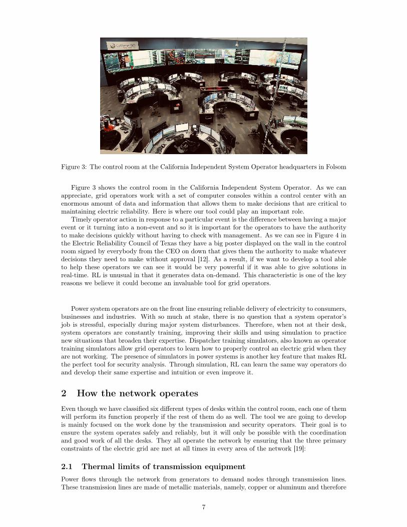
Figure 3: The control room at the California Independent System Operator headquarters in Folsom

Figure 3 shows the control room in the California Independent System Operator. As we canappreciate, grid operators work with a set of computer consoles within a control center with anenormous amount of data and information that allows them to make decisions that are critical tomaintaining electric reliability. Here is where our tool could play an important role.

Timely operator action in response to a particular event is the difference between having a majorevent or it turning into a non-event and so it is important for the operators to have the authorityto make decisions quickly without having to check with management. As we can see in Figure 4 inthe Electric Reliability Council of Texas they have a big poster displayed on the wall in the controlroom signed by everybody from the CEO on down that gives them the authority to make whateverdecisions they need to make without approval [12]. As a result, if we want to develop a tool ableto help these operators we can see it would be very powerful if it was able to give solutions inreal-time. RL is unusual in that it generates data on-demand. This characteristic is one of the keyreasons we believe it could become an invaluable tool for grid operators.

Power system operators are on the front line ensuring reliable delivery of electricity to consumers,businesses and industries. With so much at stake, there is no question that a system operator’sjob is stressful, especially during major system disturbances. Therefore, when not at their desk,system operators are constantly training, improving their skills and using simulation to practicenew situations that broaden their expertise. Dispatcher training simulators, also known as operatortraining simulators allow grid operators to learn how to properly control an electric grid when theyare not working. The presence of simulators in power systems is another key feature that makes RLthe perfect tool for security analysis. Through simulation, RL can learn the same way operators doand develop their same expertise and intuition or even improve it.

2 How the network operatesEven though we have classified six different types of desks within the control room, each one of themwill perform its function properly if the rest of them do as well. The tool we are going to developis mainly focused on the work done by the transmission and security operators. Their goal is toensure the system operates safely and reliably, but it will only be possible with the coordinationand good work of all the desks. They all operate the network by ensuring that the three primaryconstraints of the electric grid are met at all times in every area of the network [19]:

2.1 Thermal limits of transmission equipmentPower flows through the network from generators to demand nodes through transmission lines.These transmission lines are made of metallic materials, namely, copper or aluminum and therefore

7

1

Recognition of Authority

The Electric Reliability Council of Texas recognizes the need and grants full authority to ERCOT System Operators to act within the realm of NERC Standards, ERCOT Protocols, and ERCOT Operating Guides to maintain the Reliability and Integrity of the ERCOT System during normal and emergency conditions.

Within their area of responsibility, the System Operators are authorized to take appropiate and necessary real-time actions to ensure the stable and reliable operation of the Bulk Electric System without obtaining approval from mangament.

System Operators have the authority to take or direct timely and appropiate real-time actions, up to and including shedding of firm load to prevent or alleviate System Operating Limit violations.

Figure 4: Recognition of Authority for System Operators in the Electric Reliability Council of Texas

they have cooling and heating limits. The power through the lines dissipates energy in the form ofheat according to Ohm’s law:

Ploss = IR2 (1)

This power, combined with solar radiation and a high ambient temperature can overheat theline and cause it to sag closer to the ground (see Figure 5). The risk becomes greater as the lengthof the lines increases. When lines start to sag they can end up touching a tree or the ground causinga short circuit. Due to the voltage difference, a circulation of large currents would originate fromthe supply sources and also from the loads. To prevent this, grid operators set different power orcurrent limits to every line as we can see in equations (2) and (3) where n is the total number ofnodes in a power system:

Ii,j < Ii,j < Ii,j ∀ i, j ∈ {1, ..., n}\i = j (2)

P i,j < Pi,j < P i,j ∀ i, j ∈ {1, ..., n}\i = j (3)

Grid operators install protection mechanisms to automatically disconnect the lines which exceedthese limits with a certain margin to prevent potentially dangerous and costly system problems.This causes the power flows to find new routes between the supply and the demand. When thishappens other lines can increase their load and can eventually trigger more overloaded lines thatneed to be disconnected and so on. This is known as the cascading failure and results in the lossof power supply to the end-user, which is known as a blackout. Examples of these blackouts arespread throughout the history of power systems. The most recent large-scale blackout happenedon 16 June 2019 and struck Argentina, Uruguay, and Paraguay, leaving an estimated total of 48million people without electrical supply [15].

The objective of the RL model in this thesis is to anticipate potentially vulnerable lines thatcan cause cascading failures. Situational awareness about vulnerable lines within the system couldhelp operators to quickly respond to threats and restore the power grid to safe operating conditions.In the model, due to the significant importance of overloading with respect to underloading fromequations (2) and (3), we will just consider the upper-bounds Pij and Iij and we will ignore Pijand Iij .

8

Figure 2: An example of the dangers of overheating power-lines, by transportingtoo much current, the metallic conductor heats and sags close to the groundcausing a flash over to ground and endangering human life.

power networks can be described in terms of generation sources, network linesand loads. A simple electrical power network analogous to a simple electriccircuit is shown in Figure 3.

Figure 3: A simple electricity network, showing the circuit nature of a powernetwork, the currents I flowing in the lines and the interconnectedness betweengenerators denoted g, customer loads denoted c and substation nodes denoteds.

Circuit analysis is the goal of estimating the parameters in a circuit givena combination of the voltages, currents and resistances and the fundamentalEquations (1), (2) and (3). The more complex the circuit or network, themore complex the analysis will be. Within a circuit, a series of laws known asKirchho↵’s law also help us in the analysis:

5

Figure 5: An example of the dangers of overheating power-lines by transporting too much current.

2.2 Voltage maintenance within a safe rangeThe key challenge of voltage levels is to step them up or down to optimize power flow while main-taining them close to the nominal value. Voltages out of range have caused systems to collapse andeventually have caused blackouts as well. They are mainly controlled by adjusting reactive power:a correct distribution of reactive power between generators that generate it, loads that absorb itand transmission elements that can either generate or consume it are essential for guaranteeing asafe voltage profile in a network. A system-wide voltage collapse, known as a brownout, may resultfrom a disruption in an electrical grid, or may occasionally be imposed to reduce load and preventblackouts. Usual limits are between 110% and 90% of the nominal voltage of each of the elementsin the grid. In a grid with a total of n nodes, all the i-nodes must satisfy equation (4) to ensuresafe voltage operation:

V i < Vi < V i ∀ i ∈ {1, ..., n} (4)

Despite its importance for ensuring the reliability of a power system, in our RL framework, wewill not consider the voltage limits due to the additional complexity that could introduce into theproblem. Nevertheless, the model we will present can easily be modified and adjusted to also satisfythe voltage requirements. Voltage control could be introduced in future versions of this project.

2.3 Generation, supply and frequency balanceThe third constraint to consider is the power balance between supply and demand. For this purpose,frequency is typically used as a measure of how the power is balanced. Without going into too muchdetail, when the supply exceeds demand, the frequency increases and when the opposite happens(the demand is larger than supply) it decreases. If the frequency, f , deviates too much from itsnominal value (approximately 2 Hz) it will likely collapse the entire grid. To avoid variations infrequency, the grid must supply enough power for compensating both the real power demand andthe losses generated according to equation (1). If we assume a network is made up of a total of nnodes where the first m of them are generators we can present equation (5):

m∑i=1

Pgen i =

n∑i=m+1

Pload i + Plosses ⇐⇒df

dt= 0 (5)

Here the real-time desk operators presented in Section 1 play a key role in ensuring that powerbalance at all times. In order to maintain it, they dispatch the generation sources accordingly tomeet the demand by end-users. In our RL framework, we will ensure power balance at all timesusing a slack bus, the details of which we will present in Section 4.2.

9

Part II

Theoretical FrameworkAs we have already stated, we will use a RL framwork to create a tool to provide awareness aboutpotential cascading failures in a power system. In order to understand the theory underlying bothRL and power systems, we will explain it in detail in Sections 3 and 4 respectively. Our reviewof RL is mainly based the on the book Reinforcement Learning: An Introduction from Richard S.Sutton and Andrew G. Barto on Chapters 4, 5 and 6.

3 Reinforcement Learning

3.1 RL within Artificial Intelligence and Machine LearningArtificial Intelligence (AI) is a field within computer science that can be defined as the intelligencedemonstrated by machines in contrast to the natural intelligence displayed by humans and animals.Intuitively, it can be understood as the study of “intelligent agents”, meaning any device thatperceives its environment and takes actions that maximize its chances of successfully achievingits goals [21]. AI is often used to describe machines or computers that mimic functions that weassociate with the human mind, such as “learning” and “problem-solving”.

Machine Learning (ML) is a set of statistical techniques widely used in AI based around theidea that we should just be able to give machines access to data and let them learn for themselves[24]. The main goal of ML is to develop techniques to allow machines to learn from experience. Inorder to give some general background to the reader about ML we will shortly present the threedifferent learning techniques used within the field:

• Supervised learning: learns a mathematical model for a given dataset to relate inputinformation of data represented as x(i) with output information, also known as labeled data,represented as y(i). A training data with the form shown in (6) is given to training aninferred function used for making predictions about output values. Linear regression, logisticregression, decision trees, neural networks, k-nearest neighbor and support vector machinesare examples of this type. Within this project, neural networks will appear as an alternativeapproach for our RL model.

D = {(x(i), y(i))}Ni=1 (6)

• Unsupervised learning: is used to group unlabeled data based on similar attributes, nat-urally occurring trends, patterns, or relationships. The system explores the data in the formof (7) and draws inferences to describe hidden structures. The most used techniques are prin-cipal component analysis (PCA) and cluster analysis like k-means, hierarchical clustering orgaussian mixture models (GMM). This learning approach will not appear within this projectand is just presented for setting the background of reinforcement learning.

D = {(x(i))}Ni=1 (7)

• Reinforcement learning (RL): trains machine models to make a sequence of decisions inorder to achieve the desired goal. It is concerned with how agents ought to take actions in anenvironment to maximize the notion of cumulative reward. An RL agent learns by interactingwith its environment, it receives rewards by performing correctly and penalties for performingincorrectly. The agent learns without intervention from a human by maximizing its rewardand minimizing its penalties [19]. RL applied to power systems is the main contribution ofthis project and so it will be explained with more detail in Section 3.2. In comparison withsupervised learning and unsupervised learning we will see that RL data is often represented asa Markov Decision Process where data is structured as a tuple of states, actions, transitionalprobabilities and rewards:

D = (S,A,P,R) (8)

10

54 CHAPTER 3. FINITE MARKOV DECISION PROCESSES

Agent

Environment

actionAt

rewardRt

stateSt

Rt+1

St+1

Figure 3.1: The agent–environment interaction in reinforcement learning.

gives rise to rewards, special numerical values that the agent tries to maximizeover time. A complete specification of an environment defines a task , oneinstance of the reinforcement learning problem.

More specifically, the agent and environment interact at each of a sequenceof discrete time steps, t = 0, 1, 2, 3, . . ..2 At each time step t, the agent receivessome representation of the environment’s state, St ∈ S, where S is the set ofpossible states, and on that basis selects an action, At ∈ A(St), where A(St)is the set of actions available in state St. One time step later, in part asa consequence of its action, the agent receives a numerical reward , Rt+1 ∈R ⊂ R, and finds itself in a new state, St+1.

3 Figure 3.1 diagrams the agent–environment interaction.

At each time step, the agent implements a mapping from states to prob-abilities of selecting each possible action. This mapping is called the agent’spolicy and is denoted πt, where πt(a|s) is the probability that At = a if St = s.Reinforcement learning methods specify how the agent changes its policy asa result of its experience. The agent’s goal, roughly speaking, is to maximizethe total amount of reward it receives over the long run.

This framework is abstract and flexible and can be applied to many differentproblems in many different ways. For example, the time steps need not referto fixed intervals of real time; they can refer to arbitrary successive stages ofdecision-making and acting. The actions can be low-level controls, such as thevoltages applied to the motors of a robot arm, or high-level decisions, suchas whether or not to have lunch or to go to graduate school. Similarly, thestates can take a wide variety of forms. They can be completely determinedby low-level sensations, such as direct sensor readings, or they can be more

wider audience.2We restrict attention to discrete time to keep things as simple as possible, even though

many of the ideas can be extended to the continuous-time case (e.g., see Bertsekas andTsitsiklis, 1996; Werbos, 1992; Doya, 1996).

3We use Rt+1 instead of Rt to denote the reward due to At because it emphasizes thatthe next reward and next state, Rt+1 and St+1, are jointly determined.

Figure 6: The agent-environment interaction in RL

3.2 Examples of RLAs we have stated, RL is structured as an agent that takes actions in a certain environment. Thisagent decides the actions it takes based on his experience and with the goal of maximizing the sumof the rewards he expects to get in the future. Before explaining in detail what are the elementsthat make up an RL model lets get some examples of possible applications:

• Playing chess: a chess player can be modeled as an agent who decides which movements tomake in the chessboard in each turn. The goal of this agent is to checkmate the opponent’sking and to do so the agent needs to know which actions will most likely take him to hisvictory, which check boards are the most valuable to get to and which ones should better beavoided.

• Autonomous cars: car drivers can also be modeled as RL agents that decide which roads totake or avoid to move from one place to another within the shortest possible time. Based onwhat the agent sees driving, he decides whether to use one path or the other to get to his finaldestination on time. For example, this agent should learn to avoid traffic jams, closed roads,long highways and red traffic signals and should learn to use empty roads and shortcuts tominimize the traveling time.

• Portfolio management: professional investors can be modeled as agents which continuouslymake decisions on reallocating its resources into a number of different financial investmentassets to maximize its profits [28].

• Play Atari games: where the agent is modeled as a player that needs to know which movesare the most convenient ones to get to the goal state, winning the game. For example, inPacman, the agent’s goal is to eat all the dots placed in the maze while avoiding coloredghosts. The agent will move from one scenario to another as he plays the game and, if he is aproper learner, he should learn which directions are most convenient for him to take in eachscenario in order to win the game [20].

What all these examples have in common is the structure we can see in Figure 6. We can seewhat each of the elements is in the shown structure for the given examples in Table 1. The agentis a software program that makes intelligent decisions with its surroundings which we refer to asits environment and they are the learners in RL. As we can appreciate, all the examples have incommon an interaction between an agent and an environment. Within this interaction, theseagents take different actions transitioning from one state in the environment to another and everytime they take an action they get some feedback from the environment, a reward. This rewardis a number that determines which are the good and the bad events for the agent. The goal of anagent in RL is to get the maximum reward possible when interacting with the environment.

In order to explain how RL can be applied to power systems, we will present the problem we aimto solve in this thesis in the form of a third-person attacker. We will use this problem to illustrateall the key concepts of RL.

11

Example Agent Actions Environment States

Chess chess player chess move chess game chessboardconfiguration

Autonomous car autonomousdriver choosing a route road network car location

Porfoliomanagement investor investments and

divestments stock market specific portfolio

Atari games(e.g. Pacman) Atari player which key to press

in the controller Atari game screen snaphshot

Table 1: Elements of the agent-environment interaction for each example

3.3 Attack threat problemLet’s imagine we have an attacker that is trying to turn off a whole power system and, to achievethis goal, he disconnects lines from the system. Let’s assume this adversary will not stop damagingthe system until all the lines in a system are inoperative. So using the RL nomenclature we havejust presented we could model this attacker as the agent and the power grid as the environmentwhere this agent interacts. The interaction he has with a power system by disconnecting lineswould be the actions this agent can take. Every time this agent takes an action over the powersystem it transitions from one configuration to a new one. In this example, we could model thestates as the different configurations that the power systems can have. We can assume, as we havestated in equations (2) and (3), that every time the power systems have overloaded lines, protectionmechanisms automatically disconnect these lines as a security procedure. If we model the numberof disconnected lines by these mechanisms as the reward signal then we would have all the elementsneeded to build a RL framework. This framework is presented in Figure 7.

Power Sytem SecurityAnalysis using Reinforcement LearningJoséMaríaSunyer Nestares 3/13

1

2

3

8

1011

14

19

14

16

17

20

18

7

4

5 6

129

13

3.Reinforcement Learning applied topower system

! Wewillillustratetheapplicationthroughanexample:

AGENTENVIRONMENTAction:

shutaline

Reward:

Overloadedlines

NewState:

Newpowersystem

configuration

3

Figure 7: The proposed agent-environment interaction in RL applied to power systems

To better illustrate how this presented interaction would work, we could present an example asthe one shown in Figure 8. Let’s imagine this attacker initially decides to disconnect line 3 and afterthat, lines 1 and 2 overloaded and therefore are switched off. The system would have 3 inoperativelines and the node between lines 2 and 3 completely isolated from the grid. If immediately afterthis adversary decides to disconnect line 8, which was a very important line for the system, thenlines 9, 10, 11 and 12 would be disconnected due to overloading. This agent would continue todisconnect lines until some point where all the lines would be already turned off and so he wouldhave achieved his goal. We call this final state of the system a terminal state and we refer to thiscomplete sequence of transitions between an initial step and a terminal state as an episode.

12

Power Sytem SecurityAnalysis using Reinforcement LearningJoséMaríaSunyer Nestares 4/13

First action Second action N-action

…

…

3.Episode simulation

1

2

3

8

1011

14

19

141617

2018

7

4

5 6

129

13

Action: line 3

Reward: 2 Reward: 4

Action: line 8

Reward: 4

Action: line 19

Howcanhefindtheoptimalpath?

Figure 8: Complete episode in the attack threat problem

If this adversary was smart enough he would be interested in finding the optimal combinationof disconnected lines that guarantee him arriving at a terminal state as soon as possible. Usinga decision tree he could plot all the possible episodes he could imagine and analyze what are themost promising ones. In RL, we call this decision tree a Markov Decision Process and it will be theformal framework we will use in this project to define the interaction between the learning agentand its environment.

3.4 Markov Decision ProcessA Markov Decision Process (MDP), is a discrete-time stochastic control process. It provides amathematical framework for modeling decision making of an agent in situations where outcomesare partly random and partly under the control of a decision-maker. MDPs are particularly useful forstudying optimization problems solved via dynamic programming and RL [17]. As we have shownin equation (8), MDPs are defined by a tuple of states (S), actions (A), transitional probabilities(P) and rewards (R). Continuing with our attack threat problem and assuming the attacker hasfull knowledge of the MDP as shown in Figure 9, we will explain in detail the 4 elements that makeup an MDP:

States The state, denoted by S when presenting it as a variable and by s when we refer to it asthe realization of S, describes the complete situation of the environment. In this project, there aredifferent possible ways of describing a state and we will explain them elaborately in Part III, fornow, we will move on considering that states are a complete characterization of the power systemconfiguration. If we denote by t each of the discrete time-steps in an episode we will use St to definethe state S at time t. Also, we will use S+ to refer to the set of all possible states, S ⊂ S+ to referto all the terminal and |S| and |S+| to refer to the total number of states within each set. So inFigure 9, we would have:

S+ = {s(i)}|S+|

i=0 : |S+| = 38

S = {s(i)}|S|i=0 \ s(9) : |S| = 16

Actions Actions, denoted either as a variable A or as a realization of the variable as a, aredeliberated operations executed by the agent. An action taken at time t is modeled as At andit defines the transition from state St to St+1. Through actions, the agent can interact with theenvironment and receive a reward. In the presented problem actions are defined as the operationof shutting down a line. We will denote by A to the set of all possible actions in an MDP and byA(s) ⊂ A to the set of possible actions from St = s(i). Using the MDP in Figure 9:

13

(0)

(1)

(2)

(3)

(1)

(0)

(3)

(2)

𝑠!

𝑠"

𝑠#

𝑠$

𝑠%

𝑠&

𝑠'

𝑠$!

𝑠(

𝑠)

𝑠$%

𝑠$$

𝑠*

𝑠$"

𝑠$(

𝑠$)

𝑠$#

𝑠#"

𝑠#$

𝑠#%

𝑠$*

𝑠$'

𝑠"$

𝑠#(

𝑠"!

𝑠"(

𝑠"%

𝑠#'

𝑠##

𝑠#)

𝑠#!

𝑠$&

𝑠""

𝑠#&

𝑠"#

𝑠"'

𝑠")

𝑠#*

𝑎$

𝑎#

𝑎"

𝑎%

𝑎#

𝑎)

𝑎$

𝑎%

𝑎)

𝑎'

𝑎&

𝑎(

𝑎'

𝑎&

𝑎%

𝑎"

𝑎#

𝑎"

𝑎)

𝑎(

𝑎%

𝑎"

𝑎)

𝑎"

𝑎%

𝑎$

𝑎#

𝑎"

𝑎%

𝑎"

𝑎)

((), (), F)

((0,), (), F)

((1,), (3,), F)

((2,), (), F)

((3,), (1,), F)

((0, 2), (), F)

((0, 1), (), F)

((0, 3), (1,), F)

((1, 0), (3,), F)

((1, 2), (3,), F)

((2, 0), (), F)

((2, 1), (), F)

((2, 3), (1,), F)

((3, 0), (1,), F)

((3, 2), (1,), F)

((0, 1, 3), (), F)

((0, 1, 2), (), F)

((0, 2, 1), (), F)

((0, 2, 3), (1,), T)

((0, 3, 2), (1,), T)

((2, 0, 1), (), F)

(2, 0, 3), (1,), T)

((2, 1, 0), (), F)

((2, 3, 0), (1,), T)

((3, 2, 0), (1,), T)

((1, 0, 2), (3,), T)

((1, 2, 0), (3,), T)

((2, 1, 3), (), F)

((3, 0, 2), (1,), T)

((0, 1, 2, 3), (), T)

((0, 1, 3, 2), (), T)

((0, 2, 1, 3), (), T)

((2, 0, 1, 3), (), T)

((2, 1, 0, 3), (), T)

((2, 1, 3, 0), (), T)

+1

+1 +1

+1

+1

(2)

(3)

(3)

(3)

(3)

(0)

(2)

(2)

(2)

(3)

(0)

(3)

(1)

(3)

(0)

(0)

(0)

(1)

(3)

(0)

(1)

(3)

(2)

(0)

(0)

(2)

Figure 9: An example of a Markov Decision Process for the Attack threat problem on a small-sizepower system

14

A = {a(i)}|A|i=1 : |A| = 8

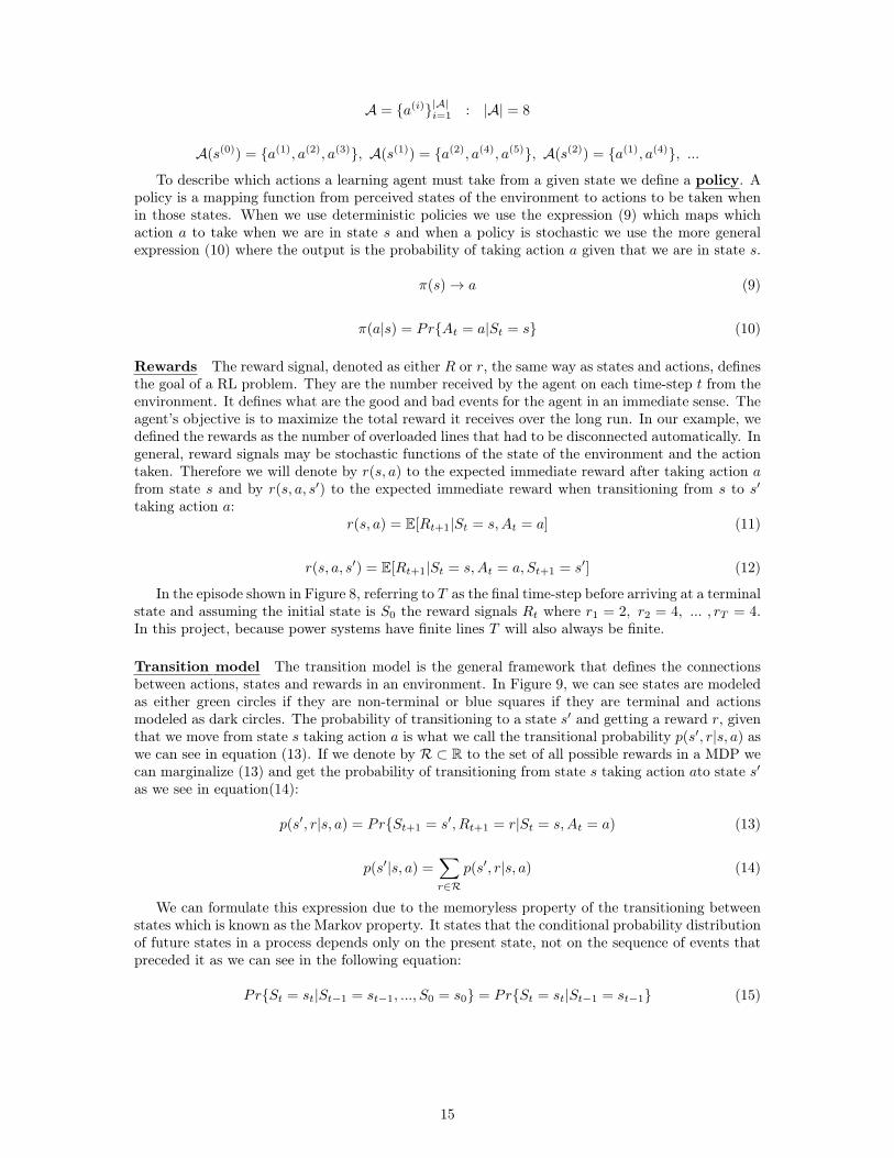
A(s(0)) = {a(1), a(2), a(3)}, A(s(1)) = {a(2), a(4), a(5)}, A(s(2)) = {a(1), a(4)}, ...To describe which actions a learning agent must take from a given state we define a policy. A

policy is a mapping function from perceived states of the environment to actions to be taken whenin those states. When we use deterministic policies we use the expression (9) which maps whichaction a to take when we are in state s and when a policy is stochastic we use the more generalexpression (10) where the output is the probability of taking action a given that we are in state s.

π(s)→ a (9)

π(a|s) = Pr{At = a|St = s} (10)

Rewards The reward signal, denoted as either R or r, the same way as states and actions, definesthe goal of a RL problem. They are the number received by the agent on each time-step t from theenvironment. It defines what are the good and bad events for the agent in an immediate sense. Theagent’s objective is to maximize the total reward it receives over the long run. In our example, wedefined the rewards as the number of overloaded lines that had to be disconnected automatically. Ingeneral, reward signals may be stochastic functions of the state of the environment and the actiontaken. Therefore we will denote by r(s, a) to the expected immediate reward after taking action afrom state s and by r(s, a, s′) to the expected immediate reward when transitioning from s to s′taking action a:

r(s, a) = E[Rt+1|St = s,At = a] (11)

r(s, a, s′) = E[Rt+1|St = s,At = a, St+1 = s′] (12)

In the episode shown in Figure 8, referring to T as the final time-step before arriving at a terminalstate and assuming the initial state is S0 the reward signals Rt where r1 = 2, r2 = 4, ... , rT = 4.In this project, because power systems have finite lines T will also always be finite.

Transition model The transition model is the general framework that defines the connectionsbetween actions, states and rewards in an environment. In Figure 9, we can see states are modeledas either green circles if they are non-terminal or blue squares if they are terminal and actionsmodeled as dark circles. The probability of transitioning to a state s′ and getting a reward r, giventhat we move from state s taking action a is what we call the transitional probability p(s′, r|s, a) aswe can see in equation (13). If we denote by R ⊂ R to the set of all possible rewards in a MDP wecan marginalize (13) and get the probability of transitioning from state s taking action ato state s′as we see in equation(14):

p(s′, r|s, a) = Pr{St+1 = s′, Rt+1 = r|St = s,At = a) (13)

p(s′|s, a) =∑r∈R

p(s′, r|s, a) (14)

We can formulate this expression due to the memoryless property of the transitioning betweenstates which is known as the Markov property. It states that the conditional probability distributionof future states in a process depends only on the present state, not on the sequence of events thatpreceded it as we can see in the following equation:

Pr{St = st|St−1 = st−1, ..., S0 = s0} = Pr{St = st|St−1 = st−1} (15)

15

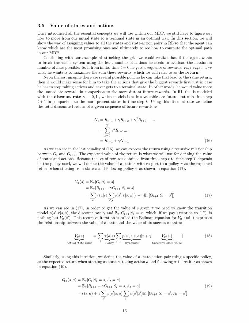
3.5 Value of states and actionsOnce introduced all the essential concepts we will use within our MDP, we still have to figure outhow to move from our initial state to a terminal state in an optimal way. In this section, we willshow the way of assigning values to all the states and state-action pairs in RL so that the agent canknow which are the most promising ones and ultimately to see how to compute the optimal pathin our MDP.

Continuing with our example of attacking the grid we could realize that if the agent wantsto break the whole system using the least number of actions he needs to overload the maximumnumber of lines possible. So if from initial time t = 0 he gets a sequence of rewards: rt+1, rt+2, ..., rTwhat he wants is to maximize the sum these rewards, which we will refer to as the return.

Nevertheless, imagine there are several possible policies he can take that lead to the same return,then it would make sense for him to take the actions that give the biggest rewards first just in casehe has to stop taking actions and never gets to a terminal state. In other words, he would value morethe immediate rewards in comparison to the more distant future rewards. In RL this is modeledwith the discount rate γ ∈ [0, 1], which models how less valuable are future states in time-stept + 1 in comparison to the more present states in time-step t. Using this discount rate we definethe total discounted return of a given sequence of future rewards as:

Gt = Rt+1 + γRt+2 + γ2Rt+3 + ...

=

T∑k=0

γkRt+1+k

= Rt+1 + γGt+1 (16)

As we can see in the last equality of (16), we can express the return using a recursive relationshipbetween Gt and Gt+1. The expected value of the return is what we will use for defining the valueof states and actions. Because the set of rewards obtained from time-step t to time-step T dependson the policy used, we will define the value of a state s with respect to a policy π as the expectedreturn when starting from state s and following policy π as shown in equation (17).

Vπ(s) = Eπ[Gt|St = s]

= Eπ[Rt+1 + γGt+1|St = s]

=∑a

π(a|s)∑s′,r

p(s′, r|s, a)[r + γEπ[Gt+1|St = s′]] (17)

As we can see in (17), in order to get the value of s given π we need to know the transitionmodel p(s′, r|s, a), the discount rate γ and Eπ[Gt+1|St = s′] which, if we pay attention to (17), isnothing but Vπ(s′). This recursive iteration is called the Bellman equation for Vπ and it expressesthe relationship between the value of a state and the value of its successor states:

Vπ(s)︸︷︷︸Actual state value

=∑a

π(a|s)︸︷︷︸Policy

∑s′,r

p(s′, r|s, a)︸︷︷︸Dynamics

[r + γ Vπ(s′)︸︷︷︸Succesive state value

] (18)

Similarly, using this intuition, we define the value of a state-action pair using a specific policy,as the expected return when starting at state s, taking action a and following π thereafter as shownin equation (19).

Qπ(s, a) = Eπ[Gt|St = s,At = a]

= Eπ[Rt+1 + γGt+1|St = s,At = a] (19)

= r(s, a) + γ∑s′

p(s′|s, a)∑a′

π(a′|s′)Eπ[Gt+1|St = s′, At = a′]

16

This can also be formulated using a recursive relationship as the Bellman equation for Qπ wherewe can see that actual state-action value function depends on the successive state-action pairs asshown in (20).

Qπ(s, a)︸︷︷︸Actual action value

= r(s, a)︸︷︷︸Expected reward

+γ∑s′

p(s′|s, a)︸︷︷︸Dynamics

∑a′

π(a′|s′)︸︷︷︸Policy

Qπ(s′, a′)︸︷︷︸Succesive action value

(20)

Following our example, now that we have presented the value functions Vπ(s) and Qπ(s, a) theagent would be able to see how promising are every state and every state-action for a fixed policyπ. Nevertheless, he is not interested in this but in finding the optimal policy he needs to take inthe MDP to get the maximum total expected return. If we denote by V ∗(s) and Q∗(s, a) to themaximum expected discounted return for every state and state action pair we can define them as:

V ∗(s) = maxπ

Vπ(s)

= maxa

Q∗(s, a)

= maxa

E[Rt+1 + γV ∗(St+1)|St = s,At = a] (21)

= maxa

∑s′,r

p(s′, r|s, a)[r + γV ∗(s′)] s.t. a ∈ A(s)

Q∗(s, a) = maxπ

Qπ(s, a)

= E[Rt+1 + γmaxa′

Q∗(St+1, a′)|St = s,At = a]

= r(s, a) + γ∑s′

p(s′|s, a) maxa′

Q∗(s′, a′) s.t. a ∈ A(s) (22)

Once we have defined the optimal value functions we know that the agent has to take theactions that lead him to the maximum expected discounted return and so we can compute theoptimal policy, π∗, as follows:

π∗(a|s) =

{1 if a = arg maxaQ

∗(s, a)

0(23)

If the attacker follows the optimal policy π∗, he is guaranteed to be taking the optimal pathtowards reaching his goal of maximizing the expected discounted return. It is important to noticethat in a stochastic environment where there exist s ∈ S and a ∈ A(s) such that p(s′, r|s, a) 6= 1if this adversary decides to follow π∗ he is not guaranteed to get to the maximum return possibledue to this stochasticity but to get the maximum expected return a priori, which is different.

Now that we have defined the optimal solutions (21), (22) and (23) to the MDP model we willanalyze the different techniques and procedures used in RL to compute them. Within RL threedifferent techniques are the most used for solving MDP: Dynamic Programming, the Monte-Carlomethod and Temporal Difference learning. In this project, as a first step towards implementingRL techniques in power systems, we will just describe the two first techniques and encourage thereader to consider Temporal Difference learning for possible future versions of this tool.

3.6 Dynamic ProgrammingBy Dynamic Programming (DP), we refer to the collection of algorithms that can be used tocompute optimal policies given a perfect model of the environment as a MDP [27]. These algorithmsassume full knowledge of the MDP model which means it knows the 4-tuple presented in (8) whereP is the set of transition probabilities p(s′, r|s, a) for all s ∈ S, a ∈ A(s), r ∈ R and s′ ∈ S+.For the purpose of this project, we will present three algorithms within DP which will prove to beuseful within our framework: backward induction, policy iteration and policy iteration.

17

3.6.1 Backward Induction

Backward induction is the first and most basic algorithm within DP we will present. This algorithmsolves the Bellman equation (21) by computing the optimal actions and value functions from thelast possible decision at time-step T in a MDP to the initial one t = 0. If we take a close lookat (21) and we use the value of the terminal states V (s) which are defined by the nature of theMDP we can create a system of |S| equations (one for every s ∈ S) with a total of |S| variablesV ∗(s). This set of non-linear equations cannot be solved with linear techniques but can be solvedby reasoning computing the solutions backward in time, starting from the end step until the initialone. So if we denote by S(t) to the set of all possible states achieved at time-step t starting fromthe initial state and Tmax to the maximum value of the last possible time-step t in the MDP wecan describe this technique as shown in Algorithm 1.

Algorithm 1 Backward induction with V ∗(s)

1. Initialization:V ∗(s) ∈ R for all s ∈ S+, s /∈ S

2. Backward reasoning:Loop for each time-step: t = Tmax − 1, Tmax − 2, ..., 0:

Loop for each s ∈ S(t):V ∗(s)← maxa

∑s′,r p(s

′, r|s, a)[r + γV ∗(s′)]

In this project, we will use this algorithm but applied Q∗(s, a) instead of V ∗(s). In the backwardinduction model we will present in Part III the terminal states will have value zero and thereforewe will perform the initialization step in Algorithm 1 as Q∗(s, ·) = 0 for all terminal states and wewill use equation (22) in the last line of code instead of (21).

Backward induction presents the advantage of finding the optimal solution at once, neverthe-less over large state-spaces some problems may become really inefficient and therefore other moreefficient iterative algorithms are used, namely, policy iteration and value iteration. Even though wewill not implement these algorithms we will present them in this project because they could easilybe implemented in our tool and because they use a general framework that will help us understandthe Monte-Carlo method in Section 3.7.

3.6.2 Policy iteration

This algorithm can compute the optimal policy π∗ and optimal value function V ∗ for a MDP bystarting with an initial solution guess V0 and π0 and iteratively improving them as vπk

and πk untilconvergence is achieved and therefore optimal solution obtained: Vπk

= V ∗ and πk = π∗. We cansketch the basic skeleton of Policy iteration as shown in equation (24) and Figure 10 where we usevπk

as an approximated value function of Vπ (vπk≈ Vπk

). As we can see, this algorithm is madeup of two parts: policy evaluation and policy improvement.

π0Evaluation−−−−−−−→ vπ0

Iteration−−−−−→ π1Evaluation−−−−−−−→ vπ1

Iteration−−−−−→ ...Iteration−−−−−→ π∗

Evaluation−−−−−−−→ v∗ (24)4.7. E�ciency of Dynamic Programming 87

v⇤,⇡⇤

⇡ = greedy(v)

v,⇡

v = v⇡

One might also think of the interaction betweenthe evaluation and improvement processes in GPIin terms of two constraints or goals—for example,as two lines in two-dimensional space as suggestedby the diagram to the right. Although the realgeometry is much more complicated than this, thediagram suggests what happens in the real case.Each process drives the value function or policytoward one of the lines representing a solution toone of the two goals. The goals interact because the two lines are not orthogonal. Drivingdirectly toward one goal causes some movement away from the other goal. Inevitably,however, the joint process is brought closer to the overall goal of optimality. The arrowsin this diagram correspond to the behavior of policy iteration in that each takes thesystem all the way to achieving one of the two goals completely. In GPI one could alsotake smaller, incomplete steps toward each goal. In either case, the two processes togetherachieve the overall goal of optimality even though neither is attempting to achieve itdirectly.

4.7 E�ciency of Dynamic Programming

DP may not be practical for very large problems, but compared with other methods forsolving MDPs, DP methods are actually quite e�cient. If we ignore a few technical details,then the (worst case) time DP methods take to find an optimal policy is polynomial inthe number of states and actions. If n and k denote the number of states and actions, thismeans that a DP method takes a number of computational operations that is less thansome polynomial function of n and k. A DP method is guaranteed to find an optimalpolicy in polynomial time even though the total number of (deterministic) policies is kn.In this sense, DP is exponentially faster than any direct search in policy space couldbe, because direct search would have to exhaustively examine each policy to provide thesame guarantee. Linear programming methods can also be used to solve MDPs, and insome cases their worst-case convergence guarantees are better than those of DP methods.But linear programming methods become impractical at a much smaller number of statesthan do DP methods (by a factor of about 100). For the largest problems, only DPmethods are feasible.

DP is sometimes thought to be of limited applicability because of the curse of dimen-sionality, the fact that the number of states often grows exponentially with the numberof state variables. Large state sets do create di�culties, but these are inherent di�cultiesof the problem, not of DP as a solution method. In fact, DP is comparatively bettersuited to handling large state spaces than competing methods such as direct search andlinear programming.

In practice, DP methods can be used with today’s computers to solve MDPs withmillions of states. Both policy iteration and value iteration are widely used, and it is notclear which, if either, is better in general. In practice, these methods usually convergemuch faster than their theoretical worst-case run times, particularly if they are started

𝑉!, 𝜋

86 Chapter 4: Dynamic Programming

to determine the states to which the DP algorithm applies its updates. At the same time,the latest value and policy information from the DP algorithm can guide the agent’sdecision making. For example, we can apply updates to states as the agent visits them.This makes it possible to focus the DP algorithm’s updates onto parts of the state set thatare most relevant to the agent. This kind of focusing is a repeated theme in reinforcementlearning.

4.6 Generalized Policy Iteration

Policy iteration consists of two simultaneous, interacting processes, one making the valuefunction consistent with the current policy (policy evaluation), and the other makingthe policy greedy with respect to the current value function (policy improvement). Inpolicy iteration, these two processes alternate, each completing before the other begins,but this is not really necessary. In value iteration, for example, only a single iteration ofpolicy evaluation is performed in between each policy improvement. In asynchronous DPmethods, the evaluation and improvement processes are interleaved at an even finer grain.In some cases a single state is updated in one process before returning to the other. Aslong as both processes continue to update all states, the ultimate result is typically thesame—convergence to the optimal value function and an optimal policy.

evaluation

improvement

⇡ � greedy(V )

V⇡

V � v⇡

v⇤⇡⇤

We use the term generalized policy iteration (GPI) to re-fer to the general idea of letting policy-evaluation and policy-improvement processes interact, independent of the granularityand other details of the two processes. Almost all reinforcementlearning methods are well described as GPI. That is, all haveidentifiable policies and value functions, with the policy alwaysbeing improved with respect to the value function and the valuefunction always being driven toward the value function for thepolicy, as suggested by the diagram to the right. If both theevaluation process and the improvement process stabilize, thatis, no longer produce changes, then the value function and policymust be optimal. The value function stabilizes only when itis consistent with the current policy, and the policy stabilizesonly when it is greedy with respect to the current value function.Thus, both processes stabilize only when a policy has been found that is greedy withrespect to its own evaluation function. This implies that the Bellman optimality equation(4.1) holds, and thus that the policy and the value function are optimal.

The evaluation and improvement processes in GPI can be viewed as both competingand cooperating. They compete in the sense that they pull in opposing directions. Makingthe policy greedy with respect to the value function typically makes the value functionincorrect for the changed policy, and making the value function consistent with the policytypically causes that policy no longer to be greedy. In the long run, however, thesetwo processes interact to find a single joint solution: the optimal value function and anoptimal policy.





evaluation

improvement

⇡ � greedy(V )

V⇡

V � v⇡

v⇤⇡⇤







evaluation

improvement

⇡ � greedy(V )

V⇡

V � v⇡

v⇤⇡⇤







evaluation

improvement

⇡ � greedy(V )

V⇡

V � v⇡

v⇤⇡⇤







evaluation

improvement

⇡ � greedy(V )

V⇡

V � v⇡

v⇤⇡⇤



Policy Evaluation

Policy Improvement

4.7. E�ciency of Dynamic Programming 87

v⇤,⇡⇤

⇡ = greedy(v)

v,⇡

v = v⇡

One might also think of the interaction betweenthe evaluation and improvement processes in GPIin terms of two constraints or goals—for example,as two lines in two-dimensional space as suggestedby the diagram to the right. Although the realgeometry is much more complicated than this, thediagram suggests what happens in the real case.Each process drives the value function or policytoward one of the lines representing a solution toone of the two goals. The goals interact because the two lines are not orthogonal. Drivingdirectly toward one goal causes some movement away from the other goal. Inevitably,however, the joint process is brought closer to the overall goal of optimality. The arrowsin this diagram correspond to the behavior of policy iteration in that each takes thesystem all the way to achieving one of the two goals completely. In GPI one could alsotake smaller, incomplete steps toward each goal. In either case, the two processes togetherachieve the overall goal of optimality even though neither is attempting to achieve itdirectly.

4.7 E�ciency of Dynamic Programming

DP may not be practical for very large problems, but compared with other methods forsolving MDPs, DP methods are actually quite e�cient. If we ignore a few technical details,then the (worst case) time DP methods take to find an optimal policy is polynomial inthe number of states and actions. If n and k denote the number of states and actions, thismeans that a DP method takes a number of computational operations that is less thansome polynomial function of n and k. A DP method is guaranteed to find an optimalpolicy in polynomial time even though the total number of (deterministic) policies is kn.In this sense, DP is exponentially faster than any direct search in policy space couldbe, because direct search would have to exhaustively examine each policy to provide thesame guarantee. Linear programming methods can also be used to solve MDPs, and insome cases their worst-case convergence guarantees are better than those of DP methods.But linear programming methods become impractical at a much smaller number of statesthan do DP methods (by a factor of about 100). For the largest problems, only DPmethods are feasible.

DP is sometimes thought to be of limited applicability because of the curse of dimen-sionality, the fact that the number of states often grows exponentially with the numberof state variables. Large state sets do create di�culties, but these are inherent di�cultiesof the problem, not of DP as a solution method. In fact, DP is comparatively bettersuited to handling large state spaces than competing methods such as direct search andlinear programming.

In practice, DP methods can be used with today’s computers to solve MDPs withmillions of states. Both policy iteration and value iteration are widely used, and it is notclear which, if either, is better in general. In practice, these methods usually convergemuch faster than their theoretical worst-case run times, particularly if they are started

Figure 10: Policy evaluation and policy improvement in Monte-Carlo

1. Policy Evaluation: in the first part, as its name suggests, we evaluate all the states withrespect to a given policy πk. Following the reasoning developed with backward induction, this

18

could easily be accomplished by setting a linear system of equations made up of |S| equationswith the form of (18) and |S| variables Vπ(s). Nevertheless, this is not very efficient as statedin backward induction and so this procedure uses an iterative approach. Given a policy π,and using an initial value function approximation v(0)π , we iteratively improve it by using theBellman equation (18). Each improvement of v(k)π to v(k+1)

π is done by updating the valueof a state s ∈ S using the values v(k−1)π for states s′ in the Bellman equation. Formally thisv(k)π is guaranteed to converge as k → ∞, nevertheless in practice, for efficiency reasons, weusually stop before the iteration converges and give an approximate solution vπ ≈ v

(k)π to

policy improvement. This is called the truncated policy evaluation.

2. Policy Improvement: this second part consists of computing the optimal policy for aspecific value function V , which we refer to as the greedy policy. This is done straightforwardas shown in line 4 of part 3 in Algorithm 2.

So if we want to compute V ∗ and π0 we can use an initial guess V0 and π0 and iteratively use policyevaluation and policy improvement to get a sequence of monotonically improving policies πk andvπk

which is guaranteed to converge to the optimal solution. This is exactly what policy iterationdoes as we can see in Algorithm 24 where, instead of computing Vπ in policy evaluation we use thetruncated policy evaluation which stops when |v − V (s)| is less than an input parameter θ.

Algorithm 2 Policy Iteration

1. Initialization:Algorithm parameter: a small threshold θ > 0 determining the accuracy of estimation.V (s) ∈ R and π(s) ∈ A(s) arbitrarity for all s ∈ S+ except V (terminal) = 1

2. Policy Evaluation:Loop:

∆← 0Loop for each s ∈ S:

v ← V (s)V (s)←∑

s′,r p(s′, r|s, π(s))[r + γV (s′)]

∆← max(∆, |v − V (s)|)until ∆ < θ (a small positive number determining the accuracy of estimation

3. Policy Improvement:policy-stable← trueFor each s ∈ S:

old-action← π(s)π(s)← arg maxa

∑s′,r p(s

′, r|s, a)[r + γV (s′)]If old-action 6= π(s), then policy-stable ← false

If policy-stable, then stop an return V ≈ V ∗ and π ≈ π∗, else go to 2.

As we can see in the Algorithm within the policy evaluation part, the amount of iterations wecompute depends on the value of θ. The bigger this value is the fewer iterations needed to finishpolicy iteration so if this algorithm converges regardless of the value of θ then it must convergeregardless of the number of iterations within policy evaluation.

3.6.3 Value iteration

Value iteration takes advantage of the fact policy iteration converges regardless of the number ofiterations within policy evaluation to combines policy evaluation and policy improvement into onesingle step. Value iteration is the same policy iteration but computing just one update to all thestates (which we denote by a sweep) in policy evaluation. If instead of updating all the values afterevery sweep we update them every time we compute V (s) we would get a version of value iterationwhich is shown in Algorithm 3.

Like policy iteration, value iteration is also guaranteed to converge to the optimal solution andtherefore, both of them are suited for solving a known MDP. Both algorithms are widely used andis not known which, if either, is better in general.

19

Algorithm 3 Value Iteration

1. Initialization:Algorithm parameter: a small threshold θ > 0 determining the accuracy of estimation.V (s) ∈ R arbitrarity for all s ∈ S+ except V (terminal) = 1

2. Value iteration update:Loop:

∆← 0Loop for each s ∈ S:

v ← V (s)V (s)← maxa

∑s′,r p(s

′, r|s, a)[r + γV (s′)]∆← max(∆, |v − V (s)|)

until ∆ < θOutput a deterministic policy, π ≈ π∗, such that: π(s) = arg maxa

∑s′,r p(s

′, r|s, a)[r+ γV (s′)]

Despite the fact that value iteration and policy iteration are DP algorithms that may convergeto the optimal solution after a long time they present the advantage of being able to offer solutionsin real-time with the last best solutions obtained in comparison to backward induction. Thischaracteristic of generating data on-demand is very appealing when applying RL to power systemsand we will see it as we move forward again in the Monte-Carlo method. This presented DPtechniques can be very useful in many applications but sometimes other techniques for solvingMDPs are needed due to three main limitations:

• Operations over entire state-space of MDP: with large state-spaces this can eitherbe unfeasible computationally (e.g. Chess or Go) or not efficient. Also, this means thatby exploring the entire state-space we lose the chance of focusing on specific areas of thestate-space if we know they are relevant a priori.

• Full knowledge of the environment dynamics: this assumption is a very strong assump-tion that limits the possible applications DP considerably. In most real-life applications we donot know the full model and transitional probabilities p(s′, r|s, a) ahead of time and thereforemethods that assume no known model (model-free) need to be developed for this applications.

• No learn from experience interaction: DP techniques plan the optimal solutions orapproximations without the need for interacting with the environment. These solutions arecomputed without any experience in the environment and therefore offer solutions which havenever been tried.

To offer solutions to these three limitations of DP other methods like Monte-Carlo and TemporalDifference have been developed. In the next section, we will explain the Monte-Carlo method inRL in detail.

3.7 Monte-Carlo MethodThe Monte Carlo method learns from experience, which is modeled as a set of episodes. By episodes,which we will denote as E, we refer to any sequence of states, actions and rewards which end in aterminal state as shown in (25). The fact that these episodes can either be generated by an actualenvironment or by a simulation makes Monte-Carlo especially appealing for applying it to powersystems.

E = {(si, ai, ri+1)}T−1i=0 (25)

This method does not require the full knowledge of the 4-tuple (S,A,P,R) and therefore doesnot need the four-argument joint distribution p, it just needs sufficient knowledge of the model tocompute sample transitions to get episodes. The Monte-Carlo method computes estimates of theexpected discounted returns for the value functions Q and V by averaging their sampled returnsfrom episodes. So for example, if we want to evaluate the value function Vπ, Monte-Carlo would

20

generate episodes following that policy π and then would compute the average return for each stateto compute the value estimations vπ just as shown in Algorithm 4.

Algorithm 4 Monte Carlo for estimating V ≈ Vπ1. Initialization:

Input: a policy π to be evaluatedInitialize:

V (s) ∈ R, arbitrarily, ∀s ∈ SReturns(s)← empty list, ∀s ∈ S

2. Learning from experience:Repeat forever (for each episode):

Choose S0 ∈ S randomly so that all states have probability > 0Generate an episode following π : S0, A0, R1, ...ST−1, AT−1, RT

G← 0Loop for each step of episode, t = T − 1, T − 2, ..., 0

G← γG+Rt+1

Append G to Returns(St, At)V (St)← average(Returns(St))

This algorithm procedure is guaranteed to converge to the true expected value Vπ as the visits toall the states grow to infinity. Nevertheless, visiting every state following a specific policy can onlybe accomplished either when the episodes start from random states S0, as is the case of Algorithm4, or when evaluating stochastic policies which assign a nonzero probability to every action for allthe states, which we refer to as soft policies.

Within the Monte-Carlo method, we can distinguish first-visit and every-visit methods depend-ing on whether the estimates of vπ (or qπ) are the average of the returns following the first visit orevery visit for every state (or every state-action pair). In our project, in the MDP we will use, thereis no possibility of visiting a state several times and therefore first-visit and every-visit methodswill give us the same solutions.

The Monte-Carlo algorithm for computing the optimal solution to an MDP has the same struc-ture of policy evaluation and policy improvement shown in Figure 10 but using q instead of v aswe can see in (26). It uses q because for computing the greedy policy of v the transitional proba-bilities P are needed and they are unknown. On the contrary, computing the greedy policy of q isstraightforward as we can see in (23).

π0Evaluate−−−−−→ qπ0

Improve−−−−−→ π1Evaluate−−−−−→ qπ1

Improve−−−−−→ ...Evaluate−−−−−→ π∗

Improve−−−−−→ q∗ (26)

Similarly to DP, in Monte-Carlo, the action value function qπkis repeatedly updated to a more

close approximation qπk+1of Qπk

, and the policy is constantly improved with respect to the currentvalue function to approach optimality. Just as we did in DP, we will explain policy evaluation andpolicy improvement separately and then we will show the pseudocode for the complete algorithm.

1. Policy evaluation: when evaluating a policy Qπkwe can use a similar approach to the

one shown in Algorithm 4 but with actions instead of states. This algorithm procedure forcomputing qπ would be guaranteed to converge to Qπ as the visits to all the states-actionpairs grow to infinity. Nevertheless, in this case, instead of using a random state-actioninitialization, we will use a soft policy called ε-greedy policy starting from the initial statein the MDP for ensuring visits to all the states when computing the episodes. This ε-greedypolicy will assign a probability of 1−ε to the action we estimate to be optimal and a probabilityof ε to the rest of actions. In this project, we will use equal distribution probabilities for theexpected non-optimal actions and so for example if we have a state with π∗(s(3)) = a andA(s) = {a(i)}4i=1 and we use ε = 0.4 we would get the ε-greedy policy π(a(i)|s) as shown inFigure 11.

2. Policy improvement: in this step, just as we did in DP, we will update the greedy policyand transform it to a ε-greedy policy just as shown in the last 3 lines of code in Algorithm 5.

21

e 0,4E-greedy E-soft

a1 0,1 0,1a2 0,1 0,1a3 0,60 0,1a4 0,1 0,1total 1,00,13 0,13

0,60

0,13

0,00

0,10

0,20

0,30

0,40

0,50

0,60

0,70

a1 a2 a3 a4

E-greedy E-soft

0.70

0.60

0.50

0.40

0.30

0.20

0.10

0.00

0.100.13 0.13 0.13

0.60

!-greedy !-soft minimum probabilities

𝜋(𝑎 ! |𝑠) 𝜋(𝑎 " |𝑠)𝜋(𝑎 # |𝑠)𝜋(𝑎 $ |𝑠)

Figure 11: ε-greedy policy example for ε = 0.4, π∗(s) = a(3) and A(s) = {a(i)}4i=1

As we can see while in DP we used the greedy policy for converging to the optimal solution in theMonte-Carlo method we will use ε-greedy policies and therefore we will not converge to the optimalpolicy but to the ε-greedy optimal policy. And just as happened with truncated policy evaluationin DP where the solution converged to optimality regardless of the number of iterations used inthis step we will take advantage of this in Monte-Carlo. The version we will use of Monte-Carlocomputes the updates qπk

and πk+1 for every episode just as shown in Algorithm 5. This algorithmis the one we will apply for our power system framework and will be the key contribution of thisthesis.

Algorithm 5 Monte Carlo

1. Initialization:Algorithm parameter: small ε > 0Initialize:

π ← an arbitrary ε-soft policyQ(s, a) ∈ R (arbitrarily), ∀s ∈ S, a ∈ A(s)Returns(s, a)← empty list, ∀s ∈ S, a ∈ A(s)

2. Learning from experience:Repeat forever (for each episode):

Generate an episode following π : S0, A0, R1, ...ST−1, AT−1, RTG← 0Loop for each step of episode, t = T − 1, T − 2, ..., 0

G← γG+Rt+1

Append G to returns(St, At)Q(St, At)← average(Returns(St, At))A∗ ← arg maxaQ(St, a) (with ties broken arbitrarily)For all a ∈ A(St) :

π(a|St)←{

1− ε+ ε/|A(St)| if a = A∗

ε/|A(St)| if a 6= A∗

22

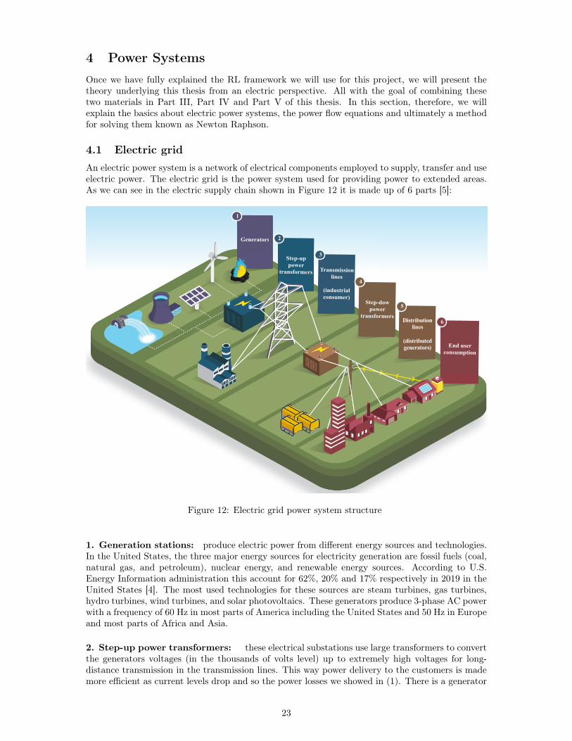
4 Power SystemsOnce we have fully explained the RL framework we will use for this project, we will present thetheory underlying this thesis from an electric perspective. All with the goal of combining thesetwo materials in Part III, Part IV and Part V of this thesis. In this section, therefore, we willexplain the basics about electric power systems, the power flow equations and ultimately a methodfor solving them known as Newton Raphson.

4.1 Electric gridAn electric power system is a network of electrical components employed to supply, transfer and useelectric power. The electric grid is the power system used for providing power to extended areas.As we can see in the electric supply chain shown in Figure 12 it is made up of 6 parts [5]:

Generators

Step-up power

transformers Transmission lines

(industrial consumer)

Step-dow power

transformers

Distribution lines

End user consumption

1

2

3

4

5

6Distributionlines

(distributedgenerators)

Figure 12: Electric grid power system structure

1. Generation stations: produce electric power from different energy sources and technologies.In the United States, the three major energy sources for electricity generation are fossil fuels (coal,natural gas, and petroleum), nuclear energy, and renewable energy sources. According to U.S.Energy Information administration this account for 62%, 20% and 17% respectively in 2019 in theUnited States [4]. The most used technologies for these sources are steam turbines, gas turbines,hydro turbines, wind turbines, and solar photovoltaics. These generators produce 3-phase AC powerwith a frequency of 60 Hz in most parts of America including the United States and 50 Hz in Europeand most parts of Africa and Asia.

2. Step-up power transformers: these electrical substations use large transformers to convertthe generators voltages (in the thousands of volts level) up to extremely high voltages for long-distance transmission in the transmission lines. This way power delivery to the customers is mademore efficient as current levels drop and so the power losses we showed in (1). There is a generator

23

transformer for each generating unit and it has a voltage and power rating according to the size ofthat unit.

3. Transmission lines: they travel long distances form the generation locations to the distri-bution grid located in populated areas with typical voltages in the range of 155 kV to 765 kV[3].Approximately, transmission lines with a length less than 50 km are considered short, between50 km and 200 km are considered medium and longer than 200 km are considered long. Thesetransmission lines are supported by transmission towers which height can vary from 15 m to 55 m.Some large industrial consumers take their supply at this point.

4. Step-down power transformers: these distribution substations convert high-voltage elec-tricity to low voltage for primary distribution lines. These primary lines have medium voltagesranging from 2.3 kV to 39 kV [26].

5. Distribution lines: they carry the electricity from the transmission system to the individualconsumers. This is known as the distribution system and is made up of primary lines with mediumvoltages which, once near the customer, are step down to consumer level voltages in the secondarylines. This low voltage ranges usually from 120 to 240 V in the United States for residentialcustomers [26]. As we can see in Figure 12, small-scaled technologies such as solar panels andcombined heat and power may generate in the distribution system. This generation, known as thedistribution generation accounts for approximately one-sixth of the capacity of the nation’s existingcentralized power plants [2].

6. End-user consumption: homes, offices and factories use electricity for lighting, for heatingand for power appliances. Some homes as shown in Figure 12 have solar panels and some have theirbattery storage system. In 2018, the average annual electricity consumption for a US residentialutility customer was 10,972 kWh, an average of about 914 kWh per month [6].

4.2 Power Flow equationsOnce we have explained completely how electric systems work and which are their main parts, thefirst thing we need to understand if we want to see what is happening in the grid is the power flowequations. These will allow us to compute the voltages, currents and power flows in every node andevery line in a system and therefore will allow us to check the three primary constraints presented inSection 2. The power flow equations give fundamental information for the operation, exploitationand planification of energy systems and are the previous step for many possible analyses. They willprove to be essential for our security and contingency analysis we aim to build in this project.

In Figure 13 we show an example of a power system made up of 14 buses. These buses are thepoints where the terminals of two or more elements meet and they are represented with verticaland horizontal lines in bold. These nodes can be connected through lines between them or to otherelements such as generators (like buses 2, 12 and 13), transformers (like buses 1 to 7 and 11 to 14),supply nodes (buses 7, 8 and 10) or to a special type of generator known as the slack generator(bus 3).

For this model we will denote as Ii and Vi to the total current flowing out of bus i and to thevoltage in bus i respectively. Both of these variables are complex numbers that represent phasors,for example, I = I√

2ejθ represents a sinusoidal function with an amplitude of I, a frequency

determined by the grid (f = 60 Hz in the United States) and an initial phase θ. Also for referringto the current flowing from bus i to bus j we will use Iij and similarly we will denote as Zij andYij to the impedance and the admittance between this buses. Using this notation and assumingsome basic knowledge about phasors and about the Ohm’s law applied with phasors we can stateequation (27) where K denotes the set of buses connected to bus i:

24

SISTEMAS ELÉCTRICOS DE POTENCIA - 3º IEM Francisco M. Echavarren Cerezo Apuntes sobre Flujo de Cargas Andrés D. Díaz Casado

versión: 30 de marzo de 2016 3

En el caso de la potencia reactiva ocurre algo similar. De entrada es imposible conocer el balance de potencia reactiva en la red, con lo que no se pueden especificar todas las potencias reactivas producidas por las unidades de generación. Sin embargo, en el caso de la reactiva la forma de proceder es distinta. En este caso, todos los nudos con recursos de generación quedan libres de su mismatch de potencia reactiva, es decir que no se especifica potencia reactiva en ninguno de ellos. En vez de eso, los generadores emplean el sistema de excitación para controlar la tensión de su nudo, conocida como tensión de consigna. De esta forma, desaparecen todos los mismatches de potencia reactiva de los nudos con generación, y a cambio los módulos de sus tensiones dejan de ser variables al estar fijadas de antemano. Estos nudos se conocen como nudos PV.

El resto de nudos, es decir, aquellos sin recursos de generación, se denominan PQ, y en ellos se definen tanto los mismatches de potencia activa como los de potencia reactiva. Al mismo tiempo, tanto el ángulo como el módulo de sus tensiones representan variables del sistema. Considerando N nudos en la red y teniendo M de ellos recursos de generación, los tipos de nudo de la red se clasifican de la siguiente forma.

TABLA I: CLASIFICACIÓN DE TIPOS DE NUDOS EN EL PROBLEMA DE FLUJO DE CARGAS

tipo número existe MP? existe MQ? T variable? V variable?

swing/slack 1 NO NO NO NO

PV M-1 SI NO SI NO

PQ N-M SI SI SI SI

TOTAL N N-1 N-M N-1 N-M

De la TABLA I se deduce que el problema completo de flujo de cargas consta de un total de 2N-M-1 ecuaciones (N-1 mismatches de potencia activa y N-M de potencia reactiva) con 2N-M-1 variables (N-1 ángulos de tensiones y N-M módulos de tensiones).

Ejemplo

Se muestra a continuación el unifilar de una red de transporte. Se pide identificar los distintos tipos de nudos, y cuáles son las ecuaciones y variables del correspondiente flujo de cargas.

SwingGenerator

Demand

12

34

5

6

7

9

10

1112

13148

Swing

Generator

Demand

Figure 13: 14-bus power system

Ii =∑k∈K

Vi − VkZij

=∑k∈K

Yij(Vi − Vk) (27)

This simple linear relation between Ii and the voltage differences Vi−Vk could by stated for eachbus of a power system with a total of n buses and therefore we could get a system of n equations,relating Vi and Ii for every i = 1, ..., n. If we use the following notation I =

[I1 I2 · · · In

]>and V =

[V1 V2 · · · Vn

]we could define a matrix called the admittance matrix denoted as Y

to relate I and V as:

I = Y V (28)

Where:

• Y ij is the negative sum of all the series admittances connected between i and j.

• Y ii is the sum of all the admittances connected to node i.

So if we use (28) we can compute the current Ii for any node in the network as:

Ii =

n∑k=1

Y ikVk (29)

Also if we denote by Si to the apparent power entering in a network through bus i, Pi to itsreal part, the real power, and Qi to its imaginary part, the reactive power, we can get the initialequality shown in (30). If we express Si in terms of V and I and we use the admittance matrix Ywe could develop equation this equation:

Si = Pi + jQi

= ViI∗i

= Vi(∑

YikVk)∗ (30)

If we express the module and the argument of Vi as Vi and θi respectively and we separate thereal part from the imaginary part for each element in the admittance matrix we have:

25

{Vi = Vie

jθi

Y ik = Gik + jBik

(31)

So by substituting (31) in (30) we can get:

Pi + jQi = Viejθi(

n∑k=1

(Gik + jBik)Vkejθk)∗ (32)

As we can conclude from this equation, the active and the reactive power are completely de-termined when we have the complete admittance matrix, which is given by the power system, andthe variables V and θ =

[θ1 θ2 · · · θn

]. So if we reconfigure (32) and we separate the real part

from the imaginary part we can get the functions pi(θ, V ) and qi(θ, V ) as:{pi(θ, V ) =

∑nk=1 ViVk(Gik cos(θi − θk) + Bik sin(θi − θk))

qi(θ, V ) =∑nk=1 ViVk(Gik sin(θi − θk)−Bik cos(θi − θk))

(33)

We can appreciate in (29) and (33) that when we have V and θ we can get the active power,the reactive power and the currents for every bus in a system and, hence, define the completestate of the system. Power systems are made to satisfy specific power demands by the consumerand therefore they use equations to the relate active and the reactive power of the buses with thevariables V and θ. These equations are known as the power flow equations which we can simplifyas: {

Pi = pi(θ, V )

Qi = qi(θ, V )(34)

These power flow equations can be used as long as the number of equations is equal or smallerto the number of unknown variables. If we classify the types of buses according to the known andunknown variables Pi, Qi, θi and Vi in a system of n buses and m generators, we can get threetypes of nodes: PV buses, PQ buses and the slack bus, also known as the swing bus of the referencebus.

• PQ buses: these nodes are the ones we would get in parts 3 and 6 in Figure 12 where theenergy is supplied to the consumer. They are the load buses and they specify an active andreactive power demand. There are a total of n−m of these buses where Pi and Qi are knownas shown in Table 2.

• PV buses: this type of nodes are the generators, the ones we would get in part 1 and 5 inFigure 12. These buses are known as the generation buses or the voltage control buses. Theyprovide a constant real power Pi, controlled through a prime mover, and maintain a constantvoltage magnitude by controlling the injection of reactive power. There are a total of m nodesof this type where Pi and Vi are determined.

• Slack bus: this is a special node where a generator is modeled as the angle reference for allthe buses in a system and also modeled to account for the unknown power losses presentedin (1). These power losses, which we will denote as ξ, are equal to the total sum of powerinjections in a network as we can see in 35. As the PV buses, they maintain a constant voltageby injection of reactive power. There is only 1 bus of this type in a power system where Viand θi are known and Pi and Qi completely unknown just as shown in Table 2.

ξ =

n∑i=1

pi(θ, V ) (35)

In conclusion, as shown in Table 2, using the presented notation, we could get a total of 2n−m−1equations for Pi and Qi, and a total of 2n−m−1 variables from the 2n voltage and angle variables(only m + 1 of them are known). This would make a system of non-linear equations which couldgive us complete information about the state of a system. Due to the non-linearity, they are usuallysolved by using iterative numerical methods. In this thesis, we will use the most used one which isthe Newton-Raphson method.

26

Number Pi Qi Vi θi

PQ buses m− 1 X X x xPV buses n−m X x X xSlack bus 1 x x X XTotal n n − 1 n − m m 1︸︷︷︸

2n − m − 1 equations︸︷︷︸

2n − m − 1variables

Table 2: Classification of nodes according to the known variables in the power flow equations

4.3 Newton-Raphson Method for Power Flow

Newton-Raphson for a one-variable single equation f(x) = 0

ECE 476: Power System Analysis Fall 2019

Lecture 16: October 22Alejandro D. Domınguez-Garcıa

• NUMERICAL SOLUTION OF THE POWER FLOW

NUMERICAL SOLUTION OF THE POWER FLOW

It is rare the case when it is possible to find an analytical solution to the power flow equations;thus, one needs to resort to numerical computation schemes. One such scheme is the Newton-Raphson (N-R) method (sometimes referred to as Newton’s method) which is actually theindustry standard implemented in most commercial power flow solvers. Next, we review thebasic ideas behind the N-R method.

1x 0x

( )f x

x2x*x

0'( )f x1'( )f x

†x

0( )f x

1( )f x

1x' 0x'

Figure 16.1:

The Newton-Raphson Method

Consider the real-valued function f(x) depicted in Fig. 16.1. We would like to find thevalues of x for which f(x) = 0; in the specific case of the function f(x) in Fig. 16.1, thereexists two such values, x⇤ and x†. We will now discuss an iterative algorithm known asNewton-Raphson method that solves the problem.

16-1

Figure 14: Application of Newton-Raphson to a one-variable single equation f(x)

In order to easily understand the Newton-Raphson method we will explain it by first applyingit to a simple equation f : R → R . This method solves equations stated in the form of (36) andtakes advantage of the first-order Taylor approximation of f(x) to try to compute the solution ofx.

f(x) = 0 (36)

Given a point (x(k), f(x(k))) we can approximate the value of f(x(k+1)) well when x(k+1) is nearx(k) as shown in (37). Both the function f(x) and its linear approximation in x(0) and x(1) arerepresented in Figure 14.

f(x(k+1)) ≈ f(x(k)) +∂f

∂x

∣∣∣∣x(k)

(x(k+1) − x(k)) (37)

If we want to compute the root of this linearization we could get x(k+1) as:

x(k+1) = x(k) +

(∂f

∂x

∣∣∣∣x(k)

)−1f(x(k))

This is how the Newton-Raphson method works, it starts with an initial point (x(0), f(x(0))) andit iteratively computes the linear approximation of f(x) at point x(k) and calculates it’s root x(k+1)

for k = 0, 1, 2, ... until it eventually gives a approximate solution. This iteration can be computedindefinitely unless we set a stopping criteria. In this project, we will define a maximum toleranceε for |x(k) − x(k−1)|. If this criterion is not satisfied within a maximum number of iterations n wewill state that the Newton-Raphson method has not converged and therefore we will not get anysolution. As we can see in Figure 14, this method, depending on the initial point (x(0), f(x(0))),can converge to different solutions and therefore a proper initial point will be essential for achievingthe solution we want.

27

Newton-Raphson for the power flow equations

Similarly, as we did with the case of one function f : R → R, we can apply the Newton-Raphsonmethod to a more general function f : Rn → Rn and ultimately use it for solving the power flowequations. If we define the power flow equations as functions equal to zero, we can define thefunctions MPi and MQi as mismatches between the specific active and reactive power, Pi and Qi,and the calculated power pi(θ, V ) and qi(θ, V ) dependant on θ and V as:{

MPi = Pi − pi(θ, V ) ∀i = 1, ..., n

MQj = Qi − qi(θ, V ) ∀i = 1, ..., n

Then the solution we are seeking is the one for which MPi = 0 and MQi = 0 for all i = 1, ..., n.For notation simplicity, we will use, from now on, bus 1 to refer to the slack bus, buses 2 to m torefer to the PV nodes and buses m+ 1 to n for the PQ nodes. As we have already seen, the stateof a system is completely determined by V and θ, therefore, if we reduce these 2n equations forjust computing every Vi and θi we can compute a reduced system of equations. For this purpose,we will compute the active power mismatches for all the nodes and the reactive power mismatchesjust for nodes PQ as shown: {

MPi = 0 ∀i = 1, ..., n

MQj = 0 ∀i = m+ 1, ..., n(38)

Using these equations we would have a total of 2n−m equations and a total of 2n−m variablesas shown in (39) and (40).

• Equations:MP1︸︷︷︸

Slack bus(1)

,MP2, ...,MPm︸︷︷︸PV buses

(m-1)

,MPm+1,MQm+1, ...,MPn,MQn︸︷︷︸PQ buses2(n-m)

(39)

• Variables:ξ︸︷︷︸

Losses(1)

, θ2, ..., θm︸︷︷︸PV buses

(m-1)

, θm+1, Vm+1, ..., θn, Vn︸︷︷︸PQ buses2(n-m)

(40)

We will express this system of equations using a function F : R2n−m → R2n−m for the mismatchesand a vector variable X ∈ R2n−m for the set of unknown variables as:

F (ξ, θ, V ) =

[fp(ξ, θ, V )fq(θ, V )

]=

MP1

...MPn

MQm+1

...MQn

ξ,θ,V

X =

ξθV

=

ξθ2...θn

Vm+1

...Vn

(41)

It is worth noting that, from now on, we will denote as θ and V to the vector which elements arejust the unknown θi and Vi for all i = 1, ..., n. Using the presented notation, similarly to the onesingle equation example, we can express the first-order Taylor approximation of F (X) at X = X(k)

as:

F (X(k+1)) ≈ F (X(k)) + J(X(k))(X(k+1) −X(k)) (42)

Where J(X(k)) is the jacobian matrix of F (X) with respect to X computed at X = X(k):

J(X(k)) =

[∂fp∂ξ

∂fp∂θ

∂fp∂V

0∂fq∂θ

∂fq∂V

]X=X(k)

Hence, if we compute the root solution of the linearization we would get:

28

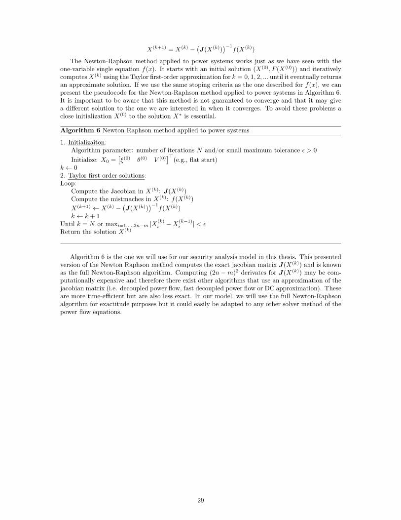
X(k+1) = X(k) −(J(X(k))

)−1f(X(k))

The Newton-Raphson method applied to power systems works just as we have seen with theone-variable single equation f(x). It starts with an initial solution (X(0), F (X(0))) and iterativelycomputesX(k) using the Taylor first-order approximation for k = 0, 1, 2, ... until it eventually returnsan approximate solution. If we use the same stoping criteria as the one described for f(x), we canpresent the pseudocode for the Newton-Raphson method applied to power systems in Algorithm 6.It is important to be aware that this method is not guaranteed to converge and that it may givea different solution to the one we are interested in when it converges. To avoid these problems aclose initialization X(0) to the solution X∗ is essential.

Algorithm 6 Newton Raphson method applied to power systems

1. Initializaiton:Algorithm parameter: number of iterations N and/or small maximum tolerance ε > 0

Initialize: X0 =[ξ(0) θ(0) V (0)

]>(e.g., flat start)k ← 02. Taylor first order solutions:Loop:

Compute the Jacobian in X(k): J(X(k))Compute the mistmaches in X(k): f(X(k))

X(k+1) ← X(k) −(J(X(k))

)−1f(X(k))

k ← k + 1Until k = N or maxi=1,...,2n−m |X(k)

i −X(k−1)i | < ε

Return the solution X(k)

Algorithm 6 is the one we will use for our security analysis model in this thesis. This presentedversion of the Newton Raphson method computes the exact jacobian matrix J(X(k)) and is knownas the full Newton-Raphson algorithm. Computing (2n −m)2 derivates for J(X(k)) may be com-putationally expensive and therefore there exist other algorithms that use an approximation of thejacobian matrix (i.e. decoupled power flow, fast decoupled power flow or DC approximation). Theseare more time-efficient but are also less exact. In our model, we will use the full Newton-Raphsonalgorithm for exactitude purposes but it could easily be adapted to any other solver method of thepower flow equations.

29

Part III

Problem Formulation5 Model descriptionSo now that we have presented all the necessary background in both RL in Section 3 and powersystems in Section 4 we will combine everything together into a framework able to provide situationalawareness to the grid operators of the risk of cascading failure. These cascading failures are aperennial security threat for power systems as they are the usual mechanism by which failurespropagate to cause large blackouts. Providing a device able to anticipate potentially dangerouslines that can cause these cascading failures could be an invaluable advisory tool for power gridoperators.

Cascading failure is a process in a system of interconnected parts in which the failure of oneor a few parts can trigger the failure of other parts and so on. In power transmission, they arenormally caused by initial incidents, such as an electrical fault at a particular transmission line,and through fast propagation, they can lead to large-scale blackouts which can cause astronomicalfinancial losses and affect countless people [29]. Through this project, we aim to create a tool ableto assess the risk of cascading failure that would entail the loss of any transmission line.

In this manner, we assign an index to every line contingency assessing the risk of cascadingfailure in the power system. We pose this problem as a MDP, just as we did in Section 3.3, wherewe model an agent disconnecting lines one by one until all the lines are inoperative and a powersystem as an environment losing the lines disconnected by the agent plus the ones shut down dueto possible cascading failures.

We will define the rewards as the number of cascaded lines after each disconnection by the agent.By doing so, the value of the functions Q∗ and V ∗ will give us information about the maximumdiscounted sum of future cascading failures that can take place for every power system state andevery line disconnection. This way the value functions with the highest values will be those wherethe cascading failures could be more severe. The value function V ∗ will asses the risk of cascadefor a particular state of the system and Q∗ will asses the risk of cascading failure associated witha line contingency in a particular state. These solutions will allow us to sort the lines from themost vulnerable ones to the most secure and also to differentiate between vulnerable power systemconfigurations and more secure ones.

201720162015 2014

20132012

201920202018

00:00 06:00 12:00 18:00 24:00

10

28

12

14

16

18

20

22

24

26

Figure 15: Typical spring day demand in California (GW) by California ISO

To completely set the MDP we first need to establish how we will define the states. As we haveseen in Section 4.2, a power system is completely defined when we have V and θ determined. Thesevalues are computed by using the power flow equations and by fixing the corresponding knownvariables for the PQ nodes, the PV nodes and the slack bus. Nevertheless, because the power

30

demand is dynamic, these values change over time. We illustrate this in Figure 15, where we cansee the power demand profile in a typical spring day in California between 2012 and 2020 [22].Considering V and θ in the definition of a state in our MDP model would involve a continuousinfinite-state rather than a discrete finite one. For simplicity purposes, in this project, we willassume a constant demand profile and therefore we will not include V and θ in the definition of astate.

Considering this simplification, if we want to analyze the maximum number of cascaded lines wecan achieve by disconnecting lines in a system, a state could be simplified to the set of inoperativelines and a binary variable specifying whether the state is terminal or not. In this project, for clarityand simplicity purposes, we will separate the set of inoperative lines into two different subsets andwe will define a state as a tuple of three components:

S = (D, C, T ) (43)

Where:

• The disconnected lines, denoted by D2, refer to the set of disconnected lines by the agentto get to a certain state. Initially, D = ∅. every time-step the agent is allowed to disconnectone line and, therefore, the total number of lines in D is equal to the time-step t, |D| = t. Ifwe assign an identification number to each of the lines in a system and denote as di to eachof the lines disconnected by an agent we can express D as:

D =(d1 d2 · · · dt

)• The cascaded lines, denoted as C, refer to the set of cascaded lines until arriving at the

state S. Initially, this value is C = ∅. We want to analyze the episodes that lead to thelargest cascaded lines possible, meaning the ones with the largest possible |C|. If we assignan identification number to each line, we can express C as we show in (44). It is importantto realize that D and C are mutually exclusive sets and therefore D ∩ C = ∅. Also, we shouldappreciate that the maximum number of lines within both sets is nL: max |D|+ |C| = nL.

C =(c1 c2 · · · c|C|

)(44)

• The terminal state indicator, which we will refer to as T , refers to the boolean variablewhich expresses whether a state is terminal (T = 1) or not (T = 0) as shown in (45). We willconsider terminal the states where all the lines are inoperative and therefore |D|+ |C| = nL.Additionally, because the full Newton-Raphson method is not guaranteed to find a solution,we will classify as terminal the cases where a non-convergence is achieved. This means thatwe won’t explore states where we can’t identify the overloaded lines and therefore we will justfocus on the states where V and θ are obtained. This problem of non-convergence could besolved by changing the Newton Raphson stopping criteria or by using another method for thepower flow equations. In this project, for accuracy and simplicity, we will classify these casesas terminal. We will assign a value of zero to these states as shown in (46).

T ∈ {0, 1} (45)

V ∗(s) = 0 s ∈ S+, s /∈ S (46)

Considering this notation we will define an action, at, as the identification number of the linethe agent disconnects after arriving at state st. As we express in (47), the set of possible actionsto take from a state, denoted as A(st), are the set of operative lines at state st.

A(st) = {at : at ∈ {1, ..., nL}, at /∈ Dt, a /∈ Ct} (47)

Also, we will denote as ∆Ct+1 to the set lines which fail due to the cascade effect after takingaction at. Therefore, when we take an action at from a non-terminal state st = (Dt, Ct, Tt), where

2The introduced D is completely different from the one presented in Section 3.1 which denoted the structure ofthe information in the different learning techniques used within Machine Learning.

31

0,00,10,2

0,30,40,50,60,7

0,80,91,0

1 2 3 4 5 6 7 8 9 10 11 12 13 14 15 16 17 18 19 20

Dis

coun

t fac

tor

Time-step (t)

0.0

0.1

0.2

0.3

0.4

0.5

0.6

0.7

0.8

0.9

1.0

Figure 16: Discount factor γk used for computing V (s) and Q(s, a) with γ = 0.9

Tt = 0, we arrive at a new state st+1 where Dt+1 = Dt ∪ at and Ct+1 = Ct ∪∆Ct+1. Consideringthis, the reward function can be formulated as:

rt = |∆Ct+1| (48)

As we showed in equation (16), to compute the expected return for any state or any state-actionpair we need the summation of all the future rewards discounted by a certain factor γk. To illustratean example, in Figure 16 we show the values of this discount factor for γ = 0.9 and k = 1, ..., 20. Aswe can see, this parameter allows us to compute different indexes for assessing the cascading riskdepending on how much we care about the future cascades relative to the more immediate ones.

In this project, because we will assume a fixed demand profile with no variation, we will get adeterministic environment just as we show in (49). This means that every time the power system isin a specific state s and we disconnect a specific line a, the cascaded lines will always be the sameand therefore the new state s′ and the reward obtained r.

p(s′, r|s, a) ∈ {1, 0} ∀ s ∈ S, a ∈ A (49)

Hence, the reward function r(s, a) and the next-state function s′(s, a), which we will define asthe expected next state St after taking action a from state s, change from stochastic functions todeterministic expressions as follows:{

r(s, a) = rt+1 subject to: St = s,At = a

s′(s, a) = st+1 subject to: St = s,At = a(50)

Now that we have presented the model we will use to asses the cascading failure risk in a powersystem, we will first explain in Section 6 how we will simulate these cascading failures and afterward,in Sections 7 and 8, how we will apply Dynamic Programming and the Monte-Carlo Algorithm tosolve the presented MDP.

6 Cascading failure simulationIn order to compute (50) for any s ∈ S and any a ∈ A(s) we will need to create a tool able tocompute the possible cascading failures. In Algorithm 7 we present the algorithm we will use tocompute cascading failures simulations for our model. In the first step of the algorithm, we initializethe state-action pair as st and at, where st must be a non-terminal state. And in the second andfinal step, we iteratively run the Newton Raphson algorithm and check every time we run it wetherthere are overloaded lines or not. This iteration keeps running until either no overloaded lines arefound or until we reach a terminal state, in which case we return T = 1. In the algorithm, we cansee how we append the set of cascaded lines ∆Ct+1 to Ct+1 and we add up to the reward |∆Ct+1|every time we run the iteration.

This algorithm will allow us to compute the transitions between the different states of the powersystem and will give us the necessary information for computing the value functions for every stateand every state-action pair in the MDP.

32

Algorithm 7 Cascading failure simulation for computing s′(s, a) and r(s, a)

1. Initialization:

Input:

{st = (Dt, Ct, Tt)at

with Tt = False

Initialize next state: Dt+1 ← Dt , Ct+1 ← Ct, Tt+1 ← Ttrt+1 ← 0

2. Cascade simulation:Loop:

Compute Newton-Raphson with lines in D′ and C′ switched offIf it converges:

∆Ct+1 ← compute overloaded lines in the networkrt+1 ← rt+1 + |∆Ct+1|Dt+1 ← Dt ∪∆Dt+1

If it doesn’t converge or all the lines already switched off (|Dt+1|+ |Ct+1| = nL):T ← True

Until T = True or |∆Ct+1| = 0

Output:

{st+1 = (Dt+1, Ct‘+1, Tt+1)

rt+1

7 Dynamic ProgrammingDynamic programming, as we stated in Section 3.6, is a model-based technique and therefore needscomplete knowledge of the MDP. In presented MDP, without any historical information or anysimulations of cascading failures, the model is completely unknown. In order to completely definethe MDP, considering that it is a completely deterministic model, we will just need to define r(s, a)and s′(s, a) for every s ∈ S and every a ∈ A(s). Therefore to be able to apply any techniquepresented in Section 3.6, we will first need to learn these two functions. To this end, we will use anexhaustive search technique called breadth-first search to completely learn the model.

7.1 Exhaustive searchIf we exhaustively compute all the possible state-action in the MDP, we would be able to com-pletely define it and therefore apply Dynamic Programming techniques. There are different waysto compute every s ∈ S and every a ∈ A(s), in this project, we will apply an exhaustive searchalgorithm known as breadth-first search.

This search technique iteratively computes all the state-action pairs in s ∈ S(t) and a ∈ A(s)for t = 0, 1, 2, ... until all the non-terminal state actions are computed. Therefore it computes everystate-action pair in the MDP sorted by time-step t. As we show in Algorithm 8, it uses a queueof states for sorting them properly. This queue applies the method first-in-first-out. It picks theinitial state in the queue to compute all its possible next states and append these at the end of thequeue as they are being visited. Also, iteratively removes the states in which all the actions havebeen computed until this queue is empty.

As we can see in Algorithm 8, this technique allows us to define s′(s, a) and r(s, a) for everys ∈ S and every a ∈ A(s) and therefore gives us the complete knowledge of the model needed forusing Dynamic Programming.

7.2 Backward inductionOnce we have the model completely defined, we can compute any algorithm within Dynamic Pro-gramming we have presented. In this project, we will apply the backward induction algorithm toget the optimal solution Q∗ and π∗ and use it to evaluate how well the Monte-Carlo converges tothis solution. This algorithm has the drawback of not being very time-efficient and therefore maybecome infeasible over large state-spaces. Nevertheless, it also presents the advantage of returningthe optimal solution, when obtained, at once, and thus we will use it in this thesis when possible.

33

Algorithm 8 Breadth-First Search

Queue = list with s0 as the single componentLoop:

s = first element in QueueFor a ∈ A(s):

s′(s, a)← compute next state with cascading failure simulation for s and ar′(s, a)← compute reward with cascading failure simulation for s and aIf s′ is not terminal: append s′ to final position in Queue

Delete s from QueueUntil Queue is empty

Number of lines Maximum number of states5 32610 ≈ 9.9 · 106

25 ≈ 4.2 · 1025

50 ≈ 8.3 · 1064

100 ≈ 2.5 · 10158

Table 3: Maximum number of states per number of lines in a power system

It is intuitive to realize that the more cascading failures that happen in a system, the fewer stateswe have to analyze in our model. Therefore, if we assume a MDP where no cascading failures occurat all, we could get the maximum number of states in a power system by simply using permutations.If we denote as P n

k to the k-permutations without repetition of n elements, we can add up all thek−permutations of nL lines for k = 1, ..., nL, and compute the maximum number of states in aMDP as follows:

max |S+| =nL∑i=1

P nL

k (51)

=

nL∑i=1

nL!

(nL − k)!(52)

In order to have a general idea of the maximum size of the state-space depending on the numberof lines in a system, we show some evaluations of (51) in Table 3. The factorial function increasesfaster than all the polynomial and exponential functions and that is why the maximum state-spacesize increases so rapidly. As we can see, even just with 25 lines we get a state-space with a maximumsize of ≈ 4.2 · 1025 which may become infeasible within reasonable time horizons for many usualcomputers. As we will see in Part V, this will restrict us from using Dynamic Programming andforce us to use iterative methods such as the Monte-Carlo algorithm for medium-size power systems.

In this project, backward induction will allow us to compute Q∗, V ∗ and π∗ for every stateand every state-action pair in our MDP. By computing the action values of the initial statesQ(s0, a) ∀a ∈ A(s0) we will be able to asses the cascading risk for every line contingency. Also,V (s0) will allow us to assess the risk of cascading failure for the system configuration s0. For ourMDP, we will compute the action values and use them afterwards to compute the state values whenneeded. As we show in case i in Figure 17, we will store the action values in a hash table with twoentries: the states and the actions.

In the presented model, the state-space can become so big as the number of lines increases thatusing a hash table may become a major challenge for memory. As we present in Figure 17 in caseii, neural networks can be used as an alternative approach to hash tables. While they compute anapproximation of Q, they present the advantages of only storing its parameters and of being able tocompute the action values for infinite state-spaces. In this project, we will focus on obtaining theexact value function and therefore we will use hash tables instead of neural networks. Nevertheless,the use of neural networks is encouraged in future versions of this project.

34

Q-valuesStates

1 2 … |𝒮|

Actions

1 0 0 … 02 0 0 … 0… … … … 0|𝒜| 0 0 0 0

State

Action

State

Q-value

Q-value Action 1

Q-value Action 2

Q-value Action |𝒜|

…

i. Hash table

ii. Neural Network

Figure 17: Action value function in RL (case i) and action value function in deep RL (case ii)

8 Monte-Carlo AlgorithmDynamic Programming, as we have stated in the previous section, works under the assumption thatthe model is completely known. This assumption is not initially true for our MDP and achievingit through exhaustive search can easily become an infeasible option as the number of lines increasein a power system. For this reason, model-free techniques are needed to deal with these largestate-spaces. The most well-known methods within model-free techniques are the Monte-Carlomethod and Temporal Difference learning. In this project, we will apply the Monte-Carlo Methodto initially apply RL to power systems. Nevertheless, we encourage testing the implementation ofTemporal Difference learning in future versions of this project.

By using this method, we will compute episodes E using an ε-greedy policy as the one wepresented in the example in Figure 11. These episodes, in contrast to Dynamic Programming, donot need to traverse the complete MDP diagram and can just compute sections of it. Applyingthe Monte-Carlo method to power systems presents the advantage of being able to use any episodeboth from historical data and from simulation to iteratively converge to the optimal solution. Thispresents a key opportunity for the application of the Monte-Carlo method to power systems.

This method starts from an initial value function Q0 and an initial ε-greedy policy π0 and,just as we explained in Figure 10, iteratively improves them with episodes using policy evaluationand policy improvement. This technique is guaranteed to converge to the optimal ε-greedy policyπ∗ and to its corresponding optimal action value function Q∗ as the number of episodes grows toinfinity. This method offers the advantage of being able to assess an approximation of the presentedcascading failure risk indexes at any time. This possibility of generating data on-demand allows gridoperators to consider this tool and quickly respond accordingly to security threats. The solutiongiven may be suboptimal but, considering the infeasibility to compute exact solutions in reasonabletime, this technique, among other model-free techniques, becomes the only option when dealingwith large state-spaces.

Additionally, the Monte-Carlo method presents the advantage of being able to use previous in-formation about the vulnerable line contingencies for the initialization of Q0 and π0. The possibilityto choose this initiazation allows us to consider information from other power system security anal-ysis, such as the N − k analysis, to focus on the parts we believe to be more relevant in the MDP.In this project, we will use a random initialization for both the action value function and the policyin order to test the complete and purest version of the Monte-Carlo method. Nevertheless, it isimportant to realize that the possibility of using previous information makes this method especiallyappealing when applying it to power system security analysis.

Finally, as we can see, this method offers us a tool to efficiently deal with massive state-spaces.

35

Nevertheless, a possibility to reduce significantly the state space could be to reduce the depth ofthe MDP by defining a maximum time-step Tmax and therefore defining the states s ∈ S(Tmax) asterminal. As we can see in Figure 16, when γ < 1 the discount factor decreases as the time-step tincreases. A possibility when implementing the Monte-Carlo method could be to ignore the cascaderewards which have a discount factor less than a specific value. For example, in the presented Figure16, we could establish to ignore discount factors less than 0.2 and, therefore, assign a 0 discountingfactor to time-steps t > 16. In this project we will not use this approximation as we will testthe complete version of Monte-Carlo, nevertheless we encourage the reader to consider this as areasonable approach when dealing with large state-spaces.

36

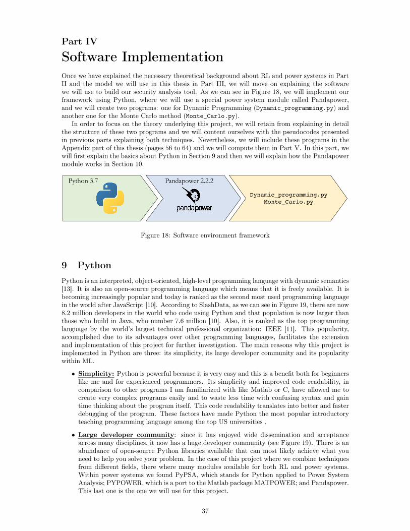
Part IV

Software ImplementationOnce we have explained the necessary theoretical background about RL and power systems in PartII and the model we will use in this thesis in Part III, we will move on explaining the softwarewe will use to build our security analysis tool. As we can see in Figure 18, we will implement ourframework using Python, where we will use a special power system module called Pandapower,and we will create two programs: one for Dynamic Programming (Dynamic_programming.py) andanother one for the Monte Carlo method (Monte_Carlo.py).

In order to focus on the theory underlying this project, we will retain from explaining in detailthe structure of these two programs and we will content ourselves with the pseudocodes presentedin previous parts explaining both techniques. Nevertheless, we will include these programs in theAppendix part of this thesis (pages 56 to 64) and we will compute them in Part V. In this part, wewill first explain the basics about Python in Section 9 and then we will explain how the Pandapowermodule works in Section 10.

Dynamic_programming.pyMonte_Carlo.py

Python 3.7 Pandapower 2.2.2

Figure 18: Software environment framework

9 PythonPython is an interpreted, object-oriented, high-level programming language with dynamic semantics[13]. It is also an open-source programming language which means that it is freely available. It isbecoming increasingly popular and today is ranked as the second most used programming languagein the world after JavaScript [10]. According to SlashData, as we can see in Figure 19, there are now8.2 million developers in the world who code using Python and that population is now larger thanthose who build in Java, who number 7.6 million [10]. Also, it is ranked as the top programminglanguage by the world’s largest technical professional organization: IEEE [11]. This popularity,accomplished due to its advantages over other programming languages, facilitates the extensionand implementation of this project for further investigation. The main reasons why this project isimplemented in Python are three: its simplicity, its large developer community and its popularitywithin ML.

• Simplicity: Python is powerful because it is very easy and this is a benefit both for beginnerslike me and for experienced programmers. Its simplicity and improved code readability, incomparison to other programs I am familiarized with like Matlab or C, have allowed me tocreate very complex programs easily and to waste less time with confusing syntax and gaintime thinking about the program itself. This code readability translates into better and fasterdebugging of the program. These factors have made Python the most popular introductoryteaching programming language among the top US universities .

• Large developer community: since it has enjoyed wide dissemination and acceptanceacross many disciplines, it now has a huge developer community (see Figure 19). There is anabundance of open-source Python libraries available that can most likely achieve what youneed to help you solve your problem. In the case of this project where we combine techniquesfrom different fields, there where many modules available for both RL and power systems.Within power systems we found PyPSA, which stands for Python applied to Power SystemAnalysis; PYPOWER, which is a port to the Matlab package MATPOWER; and Pandapower.This last one is the one we will use for this project.

37

��

67$7(�2)�7+(�'(9(/23(5�

1$7,21�4��

'(9(/23(5�(&2120,&6

)IZIPSTIV�*GSRSQMGW�`��XEXI�SJ�XLI�)IZIPSTIV�3EXMSR�6��`�l��PEWL)EXE�`�&PP�VMKLXW�VIWIVZIH

-DYD��&��DQG�&�&��JURZ�VORZHU�WKDQ�WKH�GHYHORSHU�SRSXODWLRQ1XPEHU�RI�DFWLYH�VRIWZDUH�GHYHORSHUV��JOREDOO\��LQ�PLOOLRQV��4��Q ��

� ��-DYD6FULSW�LQFOXGHV�&RǖHH6FULSW��7\SH6FULSW

:HE��&ORXG 0/��,R7�GHYLFHV

0RELOH��&ORXG ,R7�GHYLFHV��0/��:HE

0DFKLQH�OHDUQLQJ��,R7�DSSV 0RELOH��*DPLQJ��:HE

'HVNWRS��$5�95��*DPLQJ ,R7�GHYLFHV��0DFKLQH�OHDUQLQJ

:HE��&ORXG ,R7�GHYLFHV��0/

'HVNWRS��,R7��*DPLQJ��$5�95 :HE��0RELOH��&ORXG

$5�95��*DPLQJ &ORXG

$5�95��0RELOH &ORXG

$5�95��0RELOH

0RELOH��,R7�GHYLFHV&ORXG��,R7�DSSV

0RELOH��$5�95 'HVNWRS��,R7�GHYLFHV

*DPLQJ��$5�95 0RELOH

$FWLYH�GHYHORSHUV0RVW�SRSXODU�LQ /HDVW�SRSXODU�LQ

7KH�ƥOHDVW�SRSXODUƦ�FROXPQ�RQO\�LQFOXGHV�VHFWRUV�IRU�ZKLFK�ZH�KDYH�GDWD�RQ�WKH�ODQJXDJH�LQ�TXHVWLRQ��

4��

4��

4��

4��

��0

��0

��0

��0

��0

��0

��0

��0

��0

��0

��0

��0

-DYD6FULSW

3\WKRQ

-DYD

&�

&�&��

3+3

9LVXDO�WRROV

6ZLIW

5XE\

.RWOLQ

2EMHFWLYH�&

/XD

&ORXG

8LI�IWXMQEXIW�[I�TVIWIRX�LIVI�PSSO�EX�EGXMZI�WSJX[EVI�HIZIPSTIVW�YWMRK�IEGL�TVSKVEQQMRK�PERKYEKI��EGVSWW�XLI�KPSFI�ERH�EGVSWW�EPP�OMRHW�SJ�TVSKVEQQIVW��8LI]�EVI�FEWIH�SR�X[S�TMIGIW�SJ�HEXE��+MVWX��SYV�MRHITIRHIRX�IWXMQEXI�SJ�XLI�KPSFEP�RYQFIV�SJ�WSJX[EVI�HIZIPSTIVW��[LMGL�[I�TYFPMWLIH�JSV�XLI�ǻVWX�XMQI�MR��IGSRH��SYV�PEVKI�WGEPI��PS[�FMEW�WYVZI]W�[LMGL�VIEGL�QSVI�XLER��HIZIPSTIVW�IZIV]�WM\�QSRXLW��.R�XLI�WYVZI]��[I�GSRWMWXIRXP]�EWO�HIZIPSTIVW�EFSYX�XLIMV�YWI�SJ�

TVSKVEQQMRK�PERKYEKIW�EGVSWW�RMRI�EVIEW�SJ��

HIZIPSTQIRX ��KMZMRK�YW�VMGL�ERH�VIPMEFPI�MRJSVQEXMSR�EFSYX�[LS�YWIW�IEGL�PERKYEKI�ERH�MR�[LMGL�GSRXI\X��

5]XLSR�LEW�VIEGLIH��2�EGXMZI�HIZIPSTIVW�ERH�LEW�RS[�WYVTEWWIH�/EZE�MR�XIVQW�SJ�TSTYPEVMX]��.X�MW�XLI�WIGSRH�JEWXIWX�KVS[MRK�

.X�GER�FI�LEVH�XS�EWWIWW�LS[�[MHIP]�YWIH�E�TVSKVEQQMRK�PERKYEKI�MW��8LI�MRHMGIW�EZEMPEFPI�JVSQ�TPE]IVW�PMOI�8MSFI��7IHQSRO��XEGO�4ZIVǼS[�W�]IEVP]�WYVZI]��SV�,MXLYF�W�4GXSZIVWI�EVI�KVIEX��FYX�QSWXP]�SǺIV�SRP]�VIPEXMZI�GSQTEVMWSRW�FIX[IIR�PERKYEKIW��TVSZMHMRK�RS�WIRWI�SJ�XLI�EFWSPYXI�WM^I�SJ�IEGL�GSQQYRMX]��8LI]�QE]�EPWS�FI�FMEWIH�KISKVETLMGEPP]��SV�WOI[IH�XS[EVHW�GIVXEMR�ǻIPHW�SJ�WSJX[EVI�HIZIPSTQIRX��SV�STIR�WSYVGI�HIZIPSTIVW��

/EZE�GVMTX�MW�ERH�VIQEMRW�XLI�UYIIR�SJ�TVSKVEQQMRK�PERKYEKIW��.XW�GSQQYRMX]�SJ��2�HIZIPSTIVW�MW�XLI�PEVKIWX�SJ�EPP�PERKYEKIW��.R��2�HIZIPSTIVW�NSMRIH�XLI�GSQQYRMX]��XLI�LMKLIWX�KVS[XL�MR�EFWSPYXI�RYQFIVW�ERH�QSVI�XLER�XLI�IRXMVI�TSTYPEXMSR�SJ��[MJX��7YF]��SV�0SXPMR�HIZIPSTIVW��EQSRKWX�SXLIVW��3I[�HIZIPSTIVW�WII�MX�EW�ER�EXXVEGXMZI�IRXV]�PIZIP�PERKYEKI��FYX�EPWS�I\MWXMRK�HIZIPSTIVW�EVI�EHHMRK�MX�XS�XLIMV�WOMPPWIX��*ZIR�MR�WSJX[EVI�WIGXSVW�[LIVI�/EZEWGVMTX�MW�PIEWX�TSTYPEV�PMOI�QEGLMRI�PIEVRMRK�SV�SR�HIZMGI�GSHI�MR�.S8��SZIV�E�UYEVXIV�SJ�HIZIPSTIVW�YWI�MX�JSV�XLIMV�TVSNIGXW��

PERKYEKI�GSQQYRMX]�MR�EFWSPYXI�XIVQW�[MXL��2�RIX�RI[�5]XLSR�HIZIPSTIVW�MR��8LI�VMWI�SJ�QEGLMRI�PIEVRMRK�MW�E�GPIEV�JEGXSV�MR�MXW�TSTYPEVMX]��&�[LSTTMRK��SJ�QEGLMRI�PIEVRMRK�HIZIPSTIVW�ERH�HEXE�WGMIRXMWXW�RS[�YWI�5]XLSR� GSQTEVIH�XS��SJ�XLIQ�YWMRK�7��

/EZE� ��2�EGXMZI�HIZIPSTIVW��(�� 2��ERH�(�(�� 2��EVI�JEMVP]�GPSWI�XSKIXLIV�MR�XIVQW�SJ�GSQQYRMX]�WM^I�ERH�EVI�GIVXEMRP]�[IPP�IWXEFPMWLIH�PERKYEKIW��-S[IZIV��EPP�XLVII�EVI�RS[�KVS[MRK�EX�E�WPS[IV�VEXI�XLER�XLI�KIRIVEP�HIZIPSTIV�TSTYPEXMSR��;LMPI�XLI]�EVI�RSX�I\EGXP]�WXEKREXMRK��XLI]�EVI�RS�PSRKIV�XLI�ǻVWX�PERKYEKIW�XLEX� RI[��HIZIPSTIVW�PSSO�XS��

/EZE�MW�ZIV]�TSTYPEV�MR�XLI�QSFMPI�IGSW]WXIQ�ERH�MXW�SǺWLSSXW� &RHVSMH��FYX�RSX�JSV�.S8�HIZMGIW��(��MW�E�GSVI�TEVX�SJ�XLI�2MGVSWSJX�IGSW]WXIQ��8LVSYKLSYX�SYV�VIWIEVGL��[I�WII�E�GSRWMWXIRX�GSVVIPEXMSR�FIX[IIR�XLI�YWI�SJ�(��ERH�XLI�YWI�SJ�2MGVSWSJX�HIZIPSTIV�TVSHYGXW��.X�W�RS�WYVTVMWI�XS�WII�HIWOXST�ERH�&7�:7� -SPSPIRW��EW�EVIEW�[LIVI�(��MW�TSTYPEV��(�(��MW�E�GSVI�PERKYEKI�JEQMP]�JSV�KEQI�IRKMRIW�ERH�MR�.S8��[LIVI�TIVJSVQERGI�ERH�PS[�PIZIP�EGGIWW�QEXXIV� &7�:7�I\MWXW�SR�XLI�FSYRHEV]�FIX[IIR�KEQIW�ERH�.S8��

5-5�MW�RS[�XLI�WIGSRH�QSWX�TSTYPEV�PERKYEKI�JSV�[IF�HIZIPSTQIRX�ERH�XLI�ǻJXL�QSWX�TSTYPEV�PERKYEKI�SZIVEPP��[MXL��2�HIZIPSTIVW��1MOI�5]XLSR��MX�W�KVS[MRK�WMKRMǻGERXP]�JEWXIV�XLER�XLI�SZIVEPP�HIZIPSTIV�TSTYPEXMSR��LEZMRK�EHHIH��QSVI�HIZIPSTIVW�XS�MXW�VEROW�MR��)IWTMXI�LEZMRK� EVKYEFP]��E�WSQI[LEX�FEH�VITYXEXMSR��XLI�JEGX�XLEX�5-5�MW�IEW]�XS�PIEVR�ERH�[MHIP]�HITPS]IH�WXMPP�TVSTIPW�MX�JSV[EVH�EW�E�QENSV�PERKYEKI�JSV�XLI�QSHIVR�.RXIVRIX��

8LI�JEWXIWX�KVS[MRK�PERKYEKI�GSQQYRMX]�MR�TIVGIRXEKI�XIVQW�MW�0SXPMR��.X�KVI[�F]��MR��JVSQ��2�XS��2�HIZIPSTIVW��MRGI�,SSKPI�LEW�QEHI�0SXPMR�E�ǻVWX�GPEWW�PERKYEKI�JSV�&RHVSMH�HIZIPSTQIRX��[I�GER�I\TIGX�XLMW�KVS[XL�XS�GSRXMRYI��MR�E�WMQMPEV�[E]�XS�LS[��[MJX�SZIVXSSO�4FNIGXMZI�(�JSV�M4��HIZIPSTQIRX��

4XLIV�RMGLI�PERKYEKIW�HSR�X�WIIQ�XS�FI�EHHMRK�QER]�HIZIPSTIVW��MJ�ER]��[MJX�ERH�4FNIGXMZI�(�EVI�MQTSVXERX�PERKYEKIW�XS�XLI�&TTPI�GSQQYRMX]��FYX�EVI�WXEFPI�MR�XIVQW�SJ�XLI�RYQFIV�SJ�HIZIPSTIVW�XLEX�YWI�XLIQ��7YF]�ERH�1YE�EVI�RSX�KVS[MRK�XLIMV�GSQQYRMXMIW�UYMGOP]�IMXLIV�

4PHIV�ERH�QSVI�TSTYPEV�TVSKVEQQMRK�PERKYEKIW�LEZI�ZSGEP�GVMXMGW��[LMPI�RI[��I\GMXMRK�PERKYEKIW�SJXIR�LEZI�IRXLYWMEWXMG�WYTTSVXIVW��8LMW�HEXE�[SYPH�WYKKIWX�XLEX�MX�W�RSX�IEW]�JSV�RI[�PERKYEKIW�XS�KVS[�FI]SRH�XLIMV�RMGLI�ERH�FIGSQI�XLI�RI\X�FMK�XLMRK��;LEX�HSIW�XLMW�QIER�JSV�XLI�JYXYVI�SJ�XLIWI�PERKYEKIW�ERH�SXLIVW�PMOI�,S�SV��GEPE$�;I�[MPP�GIVXEMRP]�OIIT�XVEGOMRK�XLMW�IZSPYXMSR�ERH�TPER�XS�OIIT�]SY�MRJSVQIH��

�;I�LEZI�TVSKVEQQMRK�PERKYEKI�MRJSVQEXMSR�JSV�IEGL�SJ�XLI�JSPPS[MRK�ǻIPHW��[IF��GPSYH��QSFMPI��HIWOXST��.S8�ETTPMGEXMSRW��.S8�HIZMGI�WMHI�GSHI��KEQI�HIZIPSTQIRX��&7�:7��ERH�QEGLMRI�PIEVRMRK��HEXE�WGMIRGI��.R�XLMW�VITSVX��[I�PSSO�EX�FVSEHP]�YWIH�PERKYEKIW��TVIWIRX�MR��SV�QSVI�SJ�XLIWI�EVIEW��GSYRXMRK�HIZIPSTIVW�[LS�YWI�IEGL�PERKYEKI�MR�EX�PIEWX�SRI�EVIE��)IZIPSTIVW�HSR�X�LEZI�XS�TVMSVMXMWI�E�TVSKVEQQMRK�PERKYEKI�JSV�MX�XS�GSYRX �MX�QE]�FI�XLEX�XLI]�SRP]�YWI�E�PERKYEKI�SGGEWMSREPP]��

JavaScript

Python

Java

C#

C/C++

PHP

Visual tools

Ruby

Kotlin

Objective C

Lua

Web, Cloud

Machine learning, IoT apps

Mobile, Cloud

Desktop, AR/VR, Gaming

Desktop, IoT, Gaming, AR/VR

Web, Cloud

AR/VR, Gaming

AR/VR, Mobile

Cloud, IoT apps

AR/VR, Mobile

Mobile, AR/VR

ML, IoT devices

Mobile, Gaming, Web

IoT devices, ML, Web

IoT devices, Machine learning

Web, Mobile, Cloud

IoT devices, ML

Cloud

Cloud

Mobile, IoT devices

Cloud

Desktop, IoT devices

Mobile

Q4 2018Q2 2018

Q4 2018Q2 2018

Active developers Most popular in Least popular in

11.7 M

8.2 M

7.6 M

6.7 M

2.1 M

3.1 M

5.9 M

1.8 M

1.7 M

1.6 M

0.9 M

6.3 M

Swift

Gaming, AR/VR

Figure 19: Number of active software developers globally in millions in 2017 and 2018 obtainedfrom SlashData

• ML applications: when it comes to AI programming languages Python leads the pack withits unparalleled community support and pre-built libraries: NumPy, Pybrain, SciPy, Pandasand much more. In this project, we will use the Pandas library to compute the correspondinghash tables as we will see in Part V. Its flexibility and predefined libraries and frameworksallow many AI and ML projects to develop. Among the top companies within the field, wesee Google and Facebook, which both have created their libraries for this type of application:TensorFlow and PyTorch. Python is becoming so powerful and used that Google has created afree cloud service with free GPU for running computationally expensive Python codes: GoogleColab.

10 PandapowerPandapower is an easy to use open-source tool for power system modeling, analysis and optimizationwith a high degree of automation [8]. It works through the Python data analysis library Pandas andthe power system analysis toolbox PYPOWER. It started as an instrument around PYPOWER andhas evolved into an independent power systems analysis toolbox with an extensive power systemmodel library, an improved power flow solver and many other power system analysis functions [1].

Pandapower was developed to close the gap between commercial power systems like Sincal,PowerFactory or Nepal and open-source power systems analysis tools like MATPOWER and PY-POWER. As we can see in Table 39, Pandapower combines the advantages of commercial toolswith the ones of open-source tools [1].

Pandapower is all written in Python and, therefore, it offers all the possibilities and advantagesthis language presents. In the following Sections 10.1 and 10.2 we will show some code computationof Pandapower in order to explain how the elements that make up a power system are modeled andhow its power flow solver works.

10.1 Network elementsAs we have previously stated, Python is an object-oriented language and Pandapower, within thisprogramming language, can be understood as an “object”, with its functionalities and its informationwhich can be accessed and modified just as “physical objects”. In Python, we call these “objects”

38

Electric Models Automation Customization

Commercialtools

X Throughly validated andeasy to parametrizeelectric models

x Graphical user interfaceapplications difficultto automate.

x Restricted possibilities forcustomization due topropietary codebase.

Open-sourcetools

x Basic models that requireexpert knowledge forparametrization

X Console application de-signed for automatedevaluations.

X Free modifiable and cus-tomizable code

PandapowerX Throughly validated and

easy to parametrizeelectric models

X Console application de-signed for automatedevaluations.

X Free modifiable and cus-tomizable code

Table 4: Comparison between Pandapower and commercial and open-source tools

modules and they contain functions, classes and variables.Within Pandapower we will use two modules, one is called pandapower and the other one is

called pandapower.networks which is a submodule of the first one. In the pandapower.networksmodule there are grids completely modeled such as CIGRE test grids or IEEE case files. Also,the pandapower module offers the possibility to create and model your own network. Just as wedid with pandapower.networks if we want to access a module we will just type the name of themodule followed by a dot and the name of the class, variable or function we want to access.

In order to show an example and explain the structure of a network within Pandapower we willimport the two mentioned modules, which we will rename as pp and nw for code readability, and wewill access to a function case89pegase() which will return an 89-bus Pandapower network class:

>‌>‌> import pandapower as pp>‌>‌> import pandapower.networks as nw>‌>‌> net = nw.case89pegase()>‌>‌> net.fn

50>‌>‌> net.sn_mva

1>‌>‌> net

This pandapower network includes the following parameter tables:- bus (89 elements)- load (29 elements)- sgen (6 elements)- gen (11 elements)- shunt (44 elements)- ext_grid (1 element)- line (160 elements)- trafo (50 elements)- poly_cost (12 elements)- bus_geodata (89 elements)

In Python, classes are a type of “object” which can be defined in a code or can be importedfrom a module, as shown in this example. In this computed simple code nw.case89pegase() is aclass “object” and net is an individual object of this class, which is known in Python programminglanguage as an instance of the class. In the ran code, we can see that net is made up of a variablefor the frequency (fn), a variable for the nominal power of the system in MVA (sn_mva) and afunction that prints the information about the classes we can find within net.

39

4.4. NEW TOOL PANDAPOWER 39

res_load

index name vn_kv type TrueTrueTrue0 Bus 1 110.0 b

1 Bus 2 20.0 b

2 Bus 3 20.0 k

res_trafo


1 Bus 2 20.0 b

2 Bus 3 20.0 k

res_line

index name vn_kv type in_servTrueTrueTrue

0 Bus 1 110.0 b

1 Bus 2 20.0 b

2 Bus 3 20.0 k

res_busindex vm_pu va_degree p_kw q_kvar

0 1.000 110.0 120.0 37.21 1.012 20.0 0.0 0.02 1.031 20.0 -10.0 0··· ··· ·········

standard type dictionaries

result tables

parameters

load


1 Bus 2 20.0 b

2 Bus 3 20.0 k

trafo


1 Bus 2 20.0 b

2 Bus 3 20.0 k

line


0 Bus 1 110.0 b

1 Bus 2 20.0 b

2 Bus 3 20.0 k

busindex name vn_kv type in_service

0 Bus 1 110.0 b True1 Bus 2 20.0 b True2 Bus 3 20.0 k True··· ··· ·········

······

···

element tables

trafo3w

pandapower net

······

···trafoline fn_hz sn_kva name

Figure 4.2: Schematic overview of the pandapower grid representation [51]

4.4.2 Power System Analysis

With the possibility to conduct power flow, optimal power flow, state estimation andshort circuit calculations, pandapower provides all of the most commonly used staticgrid analysis features. In addition to electric power system analysis, pandapower alsoprovides the possibility of analysing the graph structure of electric grids.

4.4.2.1 Power Flow

The power flow is the most important electric analysis function for power system plan-ning. It allows to calculate the current flows and voltages in the grid, which are relevantfor the grid layout. The pandapower power flow solver is based on the Newton-Raphsonmethod [66]. The implementation is originally based on pypower, but has been im-proved with respect to robustness, run time and usability. The Newton-Raphson solverhas been accelerated using the just-in-time compiler numba [67], so that pandapower issignificantly faster than pypower [51]. Internal power flow parameters, such as nodetype for the power flow calculation (slack, PV or PQ node) or per unit conversions, arecarried out automatically by pandapower. This improves user convenience and reducesthe risk of incoherent input data.

Element tables:

Result tables:


res_load


1 Bus 2 20.0 b

2 Bus 3 20.0 k

res_trafo


1 Bus 2 20.0 b

2 Bus 3 20.0 k

res_line


0 Bus 1 110.0 b

1 Bus 2 20.0 b

2 Bus 3 20.0 k


0 1.000 110.0 120.0 37.21 1.012 20.0 0.0 0.02 1.031 20.0 -10.0 0··· ··· ·········


result tables

parameters

load


1 Bus 2 20.0 b

2 Bus 3 20.0 k

trafo


1 Bus 2 20.0 b

2 Bus 3 20.0 k

line


0 Bus 1 110.0 b

1 Bus 2 20.0 b

2 Bus 3 20.0 k



······

···

element tables

trafo3w

pandapower net

······

···

trafoline fn_hz sn_kva name




4.4.2.1 Power Flow


Element tables:

Result tables:


res_load


1 Bus 2 20.0 b

2 Bus 3 20.0 k

res_trafo


1 Bus 2 20.0 b

2 Bus 3 20.0 k

res_line


0 Bus 1 110.0 b

1 Bus 2 20.0 b

2 Bus 3 20.0 k


0 1.000 110.0 120.0 37.21 1.012 20.0 0.0 0.02 1.031 20.0 -10.0 0··· ··· ·········


result tables

parameters

load


1 Bus 2 20.0 b

2 Bus 3 20.0 k

trafo


1 Bus 2 20.0 b

2 Bus 3 20.0 k

line


0 Bus 1 110.0 b

1 Bus 2 20.0 b

2 Bus 3 20.0 k



······

···

element tables

trafo3w

pandapower net

······

···

trafoline fn_hz sn_kva name




4.4.2.1 Power Flow


Standard type dictionaries:Parameters:

Figure 20: Dataframe structure of network class in Pandapower

As shown in Figure 20, we can see that the structure of a Pandapower network consists of 4parts: the main parameters defining the network which are its name, its frequency and its nominalpower; a standard type dictionary for modeling networks and two sets of tables: one for storing theinformation implicit to the system (element tables) and the other one for storing the results aftera power flow calculation (result tables) [7].

Within the element tables, we will focus on the following in this project: bus, line, load,sgen,gen and ext_grid. Other tables for elements like: transformers, shunt elements, switches,impedances and some more may be within a Pandapower network and could appear in our model.Nevertheless, because the goal of this thesis is not the technical details of power systems but topresent RL applied to power security analysis we will not present these tables. Also, within theresult tables, we will present the tables res_bus and res_line.

If we continue with the previous code, we can compute the mentioned tables present in net tosee their parameters and analyze the ones we will use for our model. In the computed tables, wewill indicate with an asterisk the variables used for the power flow solution and we will show thenumerical values rounded with a maximum of three decimals.

>‌>‌> net.busin_service* max_vm_pu min_vm_pu name type vn_kv* zone

0 1 1.1 0.9 88 b 380 01 1 1.1 0.9 227 b 150 02 1 1.1 0.9 270 b 150 0... ... ... ... ... ... ... ...88 1 1.1 0.9 9238 b 380 0

Bus: in this table, we will use the boolean variable indicating whether the buses are in service ornot and the nominal voltage for each bus for the power flow equations. These nominal voltages,combined with the nominal power of the system, sn_mva, will allow us to transform differentvariables from unit quantities to per-unit quantities and vice versa. Additionally, the table givesus information about the type of each node (n: node, b: busbar, m: muff), the zone it belongs, astring name for identifying each node and the upper and lower-bound voltages for each node. Aswe stated in Section 2.2, in this project we won’t consider these limits.

40

>‌>‌> net.linefrom_bus* to_bus* r_ohm_per_km* x_ohm_per_km* c_nf_per_km* g_us_per_km*

0 31 4 1.054 13.07 0 01 84 43 2.772 33.15 0 02 18 57 6.926 28.55 0 0... ... ... ... ... ...159 15 77 0 0.05 0 0

length_km* parallel* in_service* max_i_ka* df* max_loading_percent ...1 1 1 1.830 1 100.0 ...1 1 1 1.381 1 100.0 ...1 1 1 99999 1 100.0 ...... ... ... ... 100.0 ...1 1 1 2.179 1 100.0 ...

Line: this table shows the necessary information about the impedance parameters per unit lengthand the length of the lines so that Pandapower can calculate the admittance matrix Y presented in(28) by considering (53). Also, this table gives us information about the maximum thermal limits foreach line just as we showed in Section 2.1. The derating factor, df ∈ (0, 1], is the maximal currentof each line in relation to its nominal current. This parameter, along with the number of parallellines (parallel) and the maximal thermal current in kA (max_i_ka), will allow us to compute theloading percentage for each line after computing the power flow equations. This result, comparedwith the parameter max_loading_percent, will allow us to compute which lines are overloadedafter every line contingency and, therefore, simulate the possible cascading failures in this project.

{Zij = (r_ohm_per_km + j · x_ohm_per_km) · length_km/parallelYij = (g_us_per_km · 10−6 + j · 2πf · c_nf_per_km · 10−9) · length_km · parallel (53)

>‌>‌> net.loadbus* ct_i_percent* ct_z_percent* in_service* p_mw* q_mvar* scaling* ...

0 2 0 0 1 96.7 26.8 1 ...1 5 0 0 1 295.3 41.9 1 ...2 7 0 0 1 244.2 152.7 1 ...... ... ... ... ... ... ... ... ...28 87 0 0 1 17.92 23.3 1 ...

Load (PQ bus): this table shows the information about the PQ nodes and allows us to definethe active and reactive power demand for the power flow equations as shown in (54) and (55). Aswe can see, these loads do not show a fixed active and reactive power demand, as stated in Section4.2, but a more complex expression known as the ZIP model. These loads are represented by acomposition of a constant impedance (Z), a constant current (I) and a constant power (P ). Onecan easily account for this ZIP model in the power flow equations by taking some minor adjustmentsover the F (x) and X presented in Section 4.2. Nevertheless, to avoid getting lost in these finerdetails we will not explain them in this project.{

Pload = p_mw · scaling · (pconst + zconst · V 2 + iconst · V )

Qload = q_mvar · scaling · (pconst + zconst · V 2 + iconst · V )(54)

zconst = ct_z_percent/100

iconst = ct_i_percent/100

pconst = (1− zconst − iconst)(55)

41

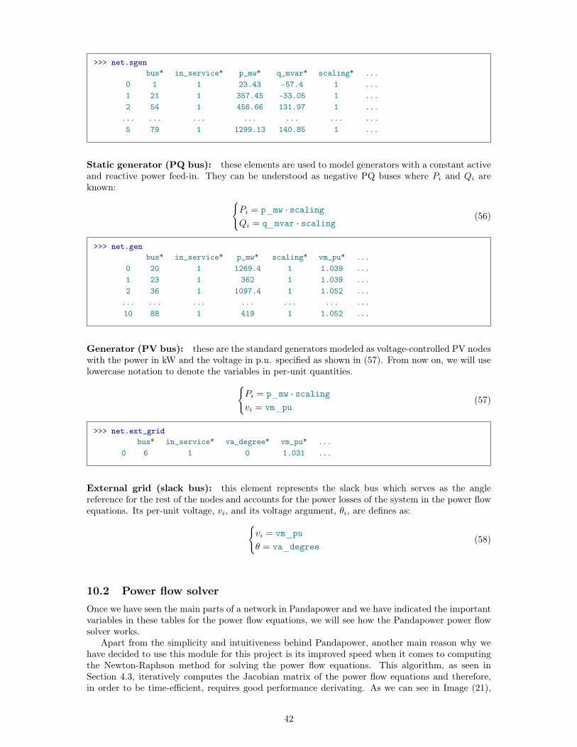
>‌>‌> net.sgenbus* in_service* p_mw* q_mvar* scaling* ...

0 1 1 23.43 -57.4 1 ...1 21 1 357.45 -33.05 1 ...2 54 1 456.66 131.97 1 ...... ... ... ... ... ... ...5 79 1 1299.13 140.85 1 ...

Static generator (PQ bus): these elements are used to model generators with a constant activeand reactive power feed-in. They can be understood as negative PQ buses where Pi and Qi areknown: {

Pi = p_mw · scalingQi = q_mvar · scaling (56)

>‌>‌> net.genbus* in_service* p_mw* scaling* vm_pu* ...

0 20 1 1269.4 1 1.039 ...1 23 1 362 1 1.039 ...2 36 1 1097.4 1 1.052 ...... ... ... ... ... ... ...10 88 1 419 1 1.052 ...

Generator (PV bus): these are the standard generators modeled as voltage-controlled PV nodeswith the power in kW and the voltage in p.u. specified as shown in (57). From now on, we will uselowercase notation to denote the variables in per-unit quantities.{

Pi = p_mw · scalingvi = vm_pu

(57)

>‌>‌> net.ext_gridbus* in_service* va_degree* vm_pu* ...

0 6 1 0 1.031 ...

External grid (slack bus): this element represents the slack bus which serves as the anglereference for the rest of the nodes and accounts for the power losses of the system in the power flowequations. Its per-unit voltage, vi, and its voltage argument, θi, are defines as:{

vi = vm_puθ = va_degree

(58)

10.2 Power flow solverOnce we have seen the main parts of a network in Pandapower and we have indicated the importantvariables in these tables for the power flow equations, we will see how the Pandapower power flowsolver works.

Apart from the simplicity and intuitiveness behind Pandapower, another main reason why wehave decided to use this module for this project is its improved speed when it comes to computingthe Newton-Raphson method for solving the power flow equations. This algorithm, as seen inSection 4.3, iteratively computes the Jacobian matrix of the power flow equations and therefore,in order to be time-efficient, requires good performance derivating. As we can see in Image (21),

42

Pandapower is considerable more time-efficient than other power flow solvers like Matpower orPypower when using the Newton-Raphson method [23].

a) Calculation of derivatives and creation of the Jaco-bian matrix: In Fig. 2 the absolute time in ms of the calcu-lation of the derivatives ∂Vm and ∂Va (top) and the creationof the Jacobian matrix (bottom) for each implementation areshown.

Fig. 2: Computational time to calculate the derivatives and tocreate the Jacobian matrix

In relation to pandapower and MATPOWER, the PYPOWERimplementation needs longer to calculate the derivatives andto create the Jacobian in every analysed case. The maincomputational effort results from the creation of the diag-onal matrices from the vectors (eq. (10) and (11)) and themathematical operations on these matrices. Also the stack-ing of the partial Jacobian matrices is slower compared tothe other implementations. In dependency of the number ofbuses, the calculations in PYPOWER need more than 20x thetime in relation to the pandapower implementation. Also theMATPOWER implementation takes up to 4-7x the amount oftime compared to the pandapower version, which includes thepresented algorithm.

b) Total computational time of the Newton-Raphsonsolver: In Fig. 3 the total computational time of the Newton-Raphson solvers are compared. In case118 the PYPOWER im-plementation needs 8.6 times as long as the Numba compiledpandapower version to find a solution. Also for the calculationof cases 1345 and 9241, the PYPOWER implementation needsmore than twice the time even though the same linear solveris used. MATPOWER is generally faster than the PYPOWERversion and slower than pandapower for the analysed cases.For the calculation of the case with the highest quantityof buses (9241), MATPOWER needs 1.6x the time to find asolution in relation to pandapower.

c) Linear solver: The computational time shown in Fig.3 do not explicitly portray the time needed by the linearsolver. It must be noted, that the linear solver implemented inMATLAB is based on UMFPACK [9], whereas SCIPY (Python)uses SuperLU as the default solver [8]. This results in a

Fig. 3: Computational time of the Newton-Raphson solver intotal

difference in the time needed to solve the linear problem.Fig. 4 shows the computational time of the linear solversimplemented in SCIPY and MATLAB. The default settings forthe linear solvers were used for the comparison. Depending onthe case, the MATLAB linear solver can take up 1.6x the time tofind a solution of the problem. Nevertheless, the MATPOWERimplementation needs less time to find a solution than thePYPOWER version, since the calculation of the Jacobian matrixis very time consuming in PYPOWER v5.0.1.

Fig. 4: Computational time of the linear solver

d) Linear problem: To compare only the computationaltime necessary to create the linear problem, the time neededby the solver is subtracted from the total computational time.Fig. 5 shows the absolute time in ms for all cases. This figureoutlines the difference in computational time achieved by thepresented algorithm and the increase in speed gained throughthe Numba jit compiler. Compared to the pandapower im-plementation, the PYPOWER Newton-Raphson method needs14x− 21x the time to calculate the linear problem. The MAT-POWER implementation needs 1.8−3x as long as the algorithmimplemented in pandapower. A shorter computational timeis especially relevant if multiple power flow calculations arenecessary or for grids with a high quantity of buses, as incase9241. For this case, pandapower needs 27.2ms to createthe linear problem in comparison to 381.0ms (PYPOWER) and84.4ms (MATPOWER).

C. Concluding summary

Fig. 6 shows the relative computational time of the Newton-Raphson subfunctions implemented in pandapower, MAT-POWER and PYPOWER. Jacobian is the combined computa-tional time for calculating the voltage derivatives and to createJacobian matrix from these. Solver is the time needed to solvethe linear problem and Other the computational time of all

pypowerpandapower

600

400

200

0case118 case1354 case9241

2.6 22.4 3.9 25.272.7 44.9

350.7

699.3

653.8

Tim

e (m

s)

matpower

Figure 21: Computational time of the Newton-Raphson solver in total for three different powersystems

The power flow solver in Pandapower is a function called runpp within the module pandapower.This function uses as input a Pandapower network and reconfigures it to append or change theresults tables in this network as shown in Figure 20. We can compute a Newton-Raphson powerflow calculation in Pandapower as:

>‌>‌> pp.runpp(net, algorithm=”nr”, init=”dc”, max_iteration=10, tolerance_mva=1e-8)This pandapower network includes the following parameter tables:- bus (89 elements)- load (29 elements)- sgen (6 elements)- gen (11 elements)- shunt (44 elements)- ext_grid (1 element)- line (160 elements)- trafo (50 elements)- poly_cost (12 elements)- bus_geodata (89 elements)and the following results tables:- res_bus (89 elements)- res_line (160 elements)- res_trafo (50 elements)- res_ext_grid (1 element)- res_load (29 elements)- res_sgen (6 elements)- res_shunt (44 elements)- res_gen (11 elements)

As we can see in this execution, we can configure different arguments in the runpp function forsolving the power flow equations. The executed line really would have been the same as executingpp.runpp(net) because in the shown code we have set the default arguments. Nevertheless, forillustrating the possibilities of this solver, we have shown four of its possible arguments. With Pan-dapower, apart from choosing different algorithms for solving the power flow equations, we can easilycustomize the initialization forX(0) (init), the maximum number of iterationsN (max_iteration),and the maximum mismatch tolerance ε (tolerance_mva) among other possibilities. If we showthe computed results in res_bus we can see the computed vi, θi, Pi and Qi after iteratively solvingthe power flow equations as:

43

>‌>‌> net.res_busvm pu va degree p mw q mvar

0 0.999 -2.728 0.199 -4.5181 1.052 -6.262 -23.430 57.4002 1.039 4.860 149.300 -24.404... ... ... ... ...88 1.052 7.895 -419.000 -154.105

Also, by applying equation (29) and with the admittance matrix Y and the voltages V , Pan-dapower can compute the current flowing through every line as shown in table res_line. In thistable, we can also see the active and reactive power calculated from every bus in every line ob-tained by applying the Kirchhoff’s Current Law and the active and reactive power losses (pl_mwand ql_mvar) for every line.

>‌>‌> net.res_linep_from_mw q_from_mvar p_to_mw q_to_mvar pl_mw ql_mvar i_from_ka

0 -361.910 6.667 362.780 4.114 0.870 10.781 0.5241 -250.634 49.821 251.755 -36.422 1.120 13.399 0.3672 73.686 -38.262 -72.804 41.897 0.882 3.634 0.20688 -35.019 14.695 37.093 -8.186 2.074 6.509 0.141

i_to_ka i_ka vm_from_pu va_from_degree vm_to_pu va_to_degree loading_percent0.524 0.524 1.049 6.053 1.051 7.758 28.6440.367 0.367 1.058 3.598 1.053 6.608 26.5760.206 0.206 1.058 1.930 1.070 -0.548 0.0000.141 0.141 1.034 -11.211 1.034 -0.892 0.000

In this project, the most important information after we have solved the power flow equationswill be the loading percentage calculated for every line as we show in (59). When comparing thisresult with max_loading_percent in net.line we will be able to see the overloaded lines andchange their corresponding parameter in_service in net.line from true (1) to false (0). Thisway we will be able to compute the cascaded simulations as we stated in Section 6 and create outRL framework for assessing the risk of cascading failure.

loading_percent =max(i_from, i_to)

i_max_ka · df · parallel · 100 (59)

44

Part V

Numerical ResultsFinally, once we have completely explained the model and the software we will use for assessingthe risk of cascading failures within a power system, we will present some numerical results forboth Dynamic Programming and the Monte-Carlo method. We will test four different IEEE casesextracted from pandapower.networks. We will initially test two small-size cases: case4gs andcase9, and then, to see how these methods scale to medium-size cases we will test case39 andcase89pegase [9]. We will apply to each of them the programs of Dynamic_programming.py andMonte_Carlo.py which we have included in the Appendix part of this thesis (pages 56 to 64).

In order to have a general idea of the state-spaces of these cases, we show in Table 5 the totalnumber of lines of each case, nL, and the maximum possible size of the state-space for each caseapplying equation (52).

Network nL Maximum number of statescase4gs 4 65case9 9 ≈ 9.9 · 105

case39 35 ≈ 2.8 · 1040

case89pegase 160 ≈ 1.3 · 10285

Table 5: Maximum number of states for each network

11 Small-size power system examples

11.1 4-bus power systemIn order to illustrate in detail the presented tool for assessing the risk of cascading failure in powersystems, we will start with the simplest possible case: the IEEE network 4-bus network case4gs.This power system was imported by Pandapower from PYPOWER and was originally presented inthe book Power System Analysis (J. J. Grainger and W. D. Stevenson, 1994).

If we apply the exhaustive breadth-first search algorithm within Dynamic_Programming.py tothis network, in just a few seconds, we can obtain the functions r(s, a) and s′(s, a) and, therefore,have the MDP model completely defined. By doing so, we have observed a total state-space sizeof 35, which is about half of the maximum possible size we presented in Table 5. Because thisstate-space is small enough, we have been able to plot the complete MDP diagram in Figure 22.In this diagram, we can clearly distinguish the terminal states in blue from the non-terminal statesin green. As we can see, all the terminal states verify that |D| + |C| = nL, and therefore we canconclude that all the cases have converged when using the Newton-Raphson method. Also, in thediagram, we can see in yellow the five only possible rewards achievable in this power system, in therest of the state-action pairs, we can see no cascading failure propagation at all.

Nevertheless, the program Dynamic_programming.py does not compute the rewards and tran-sitions as the diagram shown in Figure 22, but as a hash table which we can see in Table 6. Forsimplicity, this table shows two hash tables combined together: one for the next-state functions′(s, a) and another one for the reward function r(s, a). This way, if we are interested in checkingthe state configuration of the 4-bus power system after disconnecting any line a from any state s,we can check the next configuration of the system and the number of cascaded lines by going tothe corresponding cell in row s and column a. As we can see, some of the cells in the table areempty. This is because we can’t disconnect lines already inoperative in a system and, therefore,A(s) 6= A ∀s ∈ S, s 6= s0.

As we show, all the states are defined using the 3-tuple (D, C, T ) we presented in (43) where Ddenoted the disconnected lines by the agent, C the cascaded lines after each action and T the booleanvariable indicating whether a state is terminal (F) or not (T). In this section, when computing thetwo programs Dynamic_programming.py and Monte_Carlo.py, we will express the actions as tuples

45

(0)

(1)

(2)

(3)

(1)

(0)

(3)

(2)

𝑠!

𝑠"

𝑠#

𝑠$

𝑠%

𝑠&

𝑠'

𝑠$!

𝑠(

𝑠)

𝑠$%

𝑠$$

𝑠*

𝑠$"

𝑠$(

𝑠$)

𝑠$#

𝑠#"

𝑠#$

𝑠#%

𝑠$*

𝑠$'

𝑠"$

𝑠#(

𝑠"!

𝑠"(

𝑠"%

𝑠#'

𝑠##

𝑠#)

𝑠#!

𝑠$&

𝑠""

𝑠#&

𝑠"#

𝑠"'

𝑠")

𝑠#*

𝑎$

𝑎#

𝑎"

𝑎%

𝑎#

𝑎)

𝑎$

𝑎%

𝑎)

𝑎'

𝑎&

𝑎(

𝑎'

𝑎&

𝑎%

𝑎"

𝑎#

𝑎"

𝑎)

𝑎(

𝑎%

𝑎"

𝑎)

𝑎"

𝑎%

𝑎$

𝑎#

𝑎"

𝑎%

𝑎"

𝑎)

((), (), F)

((0,), (), F)

((1,), (3,), F)

((2,), (), F)

((3,), (1,), F)

((0, 2), (), F)

((0, 1), (), F)

((0, 3), (1,), F)

((1, 0), (3,), F)

((1, 2), (3,), F)

((2, 0), (), F)

((2, 1), (), F)

((2, 3), (1,), F)

((3, 0), (1,), F)

((3, 2), (1,), F)

((0, 1, 3), (), F)

((0, 1, 2), (), F)

((0, 2, 1), (), F)

((0, 2, 3), (1,), T)

((0, 3, 2), (1,), T)

((2, 0, 1), (), F)

(2, 0, 3), (1,), T)

((2, 1, 0), (), F)

((2, 3, 0), (1,), T)

((3, 2, 0), (1,), T)

((1, 0, 2), (3,), T)

((1, 2, 0), (3,), T)

((2, 1, 3), (), F)

((3, 0, 2), (1,), T)

((0, 1, 2, 3), (), T)

((0, 1, 3, 2), (), T)

((0, 2, 1, 3), (), T)

((2, 0, 1, 3), (), T)

((2, 1, 0, 3), (), T)

((2, 1, 3, 0), (), T)

+1

+1 +1

+1

+1

(2)

(3)

(3)

(3)

(3)

(0)

(2)

(2)

(2)

(3)

(0)

(3)

(1)

(3)

(0)

(0)

(0)

(1)

(3)

(0)

(1)

(3)

(2)

(0)

(0)

(2)

Figure 22: Markov Decision Process diagram for Case4gs

46

of single elements containing the index of the line to disconnect. In this example, therefore the statespace would be expressed as A = {(0), (1), (2), (3)}.

Once we have computed the breadth-first search algorithm, we have the MDP completely definedand, therefore, we can apply backward induction to compute Q∗ and π∗. In Table 7, we can seethese two hash tables for this power system after using a discount rate of γ = 0.9. The Q∗(s, a) hashtable containing the risk associated with each line contingency for every possible state configurationof the system. We can appreciate that at the initial state s0 = ((), (), F ), the most vulnerable linesto the system are lines 1 and 3, with a risk index of 1. Also, we can see that lines 0 and 2 have arisk index of 0.9. This way, by computing expression (60) we can compute a risk index of value 1to the initial state.

V (s0) = maxa∈A(s0)

Q(s0, a) (60)

Despite the possibility to use Dynamic Programming in this example, if we apply the Monte-Carlo method presented in Algorithm 5 we can test how this algorithm convergences to the optimalsolution. In Figure 23, we show ten different executions of the Monte-Carlo method using ε = 0.2,γ = 0.9 and a total of 50 episodes for each execution. In this figure, we can appreciate how therisk assessment of the initial state of the system converges to the optimal index of 1 for all theexecutions.

In Table 8, we can compare the risk index of cascading failure associated with each line con-tingency in the initial state computed by Dynamic Programming with the one obtained using theMonte Carlo method. In this table, Q∗ represents the optimal solution computed by DynamicProgramming and qε,500 represents the average return computed by the Monte-Carlo method whenimproving an ε-greedy policy with ε = 0.2 after 500 episodes. As we can see, the indexes are thesame for lines 1 and 3 but differ by about 0.4 for lines 0 and 2. Nevertheless, this approximationcan perform well when sorting the lines from the most vulnerable ones to the most secure ones.

State: s π∗(s) State\Action (0) (1) (2) (3)((), (), F) (1) ((), (), F) 0.9 1 0.9 1((0), (), F) (3) ((0), (), F) 0 0.9 1((1), (3), F) (0) ((1), (3), F) 0 0((2), (), F) (3) ((2), (), F) 0.9 0 1((3), (1), F) (0) ((3), (1), F) 0 0((0, 1), (), F) (2) ((0, 1), (), F) 0 0((0, 2), (), F) (3) ((0, 2), (), F) 0 1((0, 3), (1), F) (2) ((0, 3), (1), F) 0((1, 0), (3), F) (2) ((1, 0), (3), F) 0((1, 2), (3), F) (0) ((1, 2), (3), F) 0((2, 0), (), F) (3) ((2, 0), (), F) 0 1((2, 1), (), F) (0) ((2, 1), (), F) 0 0((2, 3), (1), F) (0) ((2, 3), (1), F) 0((3, 0), (1), F) (2) ((3, 0), (1), F) 0((3, 2), (1), F) (0) ((3, 2), (1), F) 0((0, 1, 2), (), F) (3) ((0, 1, 2), (), F) 0((0, 1, 3), (), F) (2) ((0, 1, 3), (), F) 0((0, 2, 1), (), F) (3) ((0, 2, 1), (), F) 0((2, 0, 1), (), F) (3) ((2, 0, 1), (), F) 0((2, 1, 0), (), F) (3) ((2, 1, 0), (), F) 0((2, 1, 3), (), F) (0) ((2, 1, 3), (), F) 0

Table 7: Backward induction results for the optimal policy π∗(s) and the optimal Q∗(s, a) forCase4gs with γ = 0.9

47

State Action: (0) Action: (1) Action: (2) Action: (3)

((), (), F) ((0), (), F) 0 ((1), (3), F) 1 ((2), (), F) 0 ((3), (1), F) 1((0), (), F) ((0, 1), (), F) 0 ((0, 2), (), F) 0 ((0, 3), (1), F) 1((1), (3), F) ((1, 0), (3), F) 0 ((1, 2), (3), F) 0((2), (), F) ((2, 0), (), F) 0 ((2, 1), (), F) 0 ((2, 3), (1), F) 1((3), (1), F) ((3, 0), (1), F) 0 ((3, 2), (1), F) 0((0, 1), (), F) ((0, 1, 2), (), F) 0 ((0, 1, 3), (), F) 0((0, 2), (), F) ((0, 2, 1), (), F) 0 ((0, 2, 3), (1), T) 1((0, 3), (1), F) ((0, 3, 2), (1), T) 0((1, 0), (3), F) ((1, 0, 2), (3), T) 0((1, 2), (3), F) ((1, 2, 0), (3), T) 0((2, 0), (), F) ((2, 0, 1), (), F) 0 ((2, 0, 3), (1), T) 1((2, 1), (), F) ((2, 1, 0), (), F) 0 ((2, 1, 3), (), F) 0((2, 3), (1), F) ((2, 3, 0), (1), T) 0((3, 0), (1), F) ((3, 0, 2), (1), T) 0((3, 2), (1), F) ((3, 2, 0), (1), T) 0((0, 1, 2), (), F) ((0, 1, 2, 3), (), T) 0((0, 1, 3), (), F) ((0, 1, 3, 2), (), T) 0((0, 2, 1), (), F) ((0, 2, 1, 3), (), T) 0((2, 0, 1), (), F) ((2, 0, 1, 3), (), T) 0((2, 1, 0), (), F) ((2, 1, 0, 3), (), T) 0((2, 1, 3), (), F) ((2, 1, 3, 0), (), T) 0

Table 6: Bread-first search results of s′(s, a) and r(s, a) for Case4gs

Number of episodes10 20 30 40 50

Risk

ass

essm

ent!(#!) Optimal value

Execution 1Execution 2Execution 3Execution 4Execution 5Execution 6Execution 7Execution 8Execution 9Execution 10

00.0

0.2

0.4

0.6

0.8

1.0

Figure 23: Risk assessment of initial state using the Monte-Carlo method with 50 episodes forCase4gs with γ = 0.9 and ε = 0.2

Action Q∗(s0, a) qε,500(s0, a)

(0) 0.9 0.55(1) 1 1(2) 0.9 0.54(3) 1 1

Table 8: Risk assessment of each line contingency at the initial state s0 using Dynamic Programmingand the Monte-Carlo method with 500 episodes for Case4gs with γ = 0.9 and ε = 0.2

48

11.2 9-bus power systemOnce, we have computed our tool for the small network, case4gs, we will move on with anothersmall-size power system network made up of 9 buses: the IEEE case9 network. This network wasfirst published in Power System Control and Stability (Anderson and Fouad’s, 1980) and has beenimported from PYPOWER to Pandapower.

As we can see in Table 5, this network approximately has a maximum state-space size of 9.9·105,which is a considerably larger size in comparison with the previous network case4gs. Using thispower system case, we have been able to compute breadth-first search over all the state space inaround 3.5 hours and we have observed a state space with a size of 749, 756 states. Afterwards, wehave computed the backward induction algorithm and we have computed the risk index Q∗ in 5.6hours. We can see in Table 9 the results for Q∗ where we can notice that the three most vulnerablelines are 1 and 6 with a risk index of 1.8 followed by line 3 with an index of 0.9. Therefore, using(60) we can see that the initial state has an index risk of 1.8.

If we now compute the Monte-Carlo method, we can see in Figure 24 the evolution of the initialstate value function associated with the deterministic version of the ε-greedy used for policy whichiteratively improves using policy evaluation and policy improvement respectively. In this figure, wecan see how, after 500 episodes and using γ = 0.9 and ε = 0.2, nine out of ten executions convergeto the optimal risk index of 1.8. Considering that each computation has taken a total of 2 minutesin comparison with a total of 8.1 hours for Dynamic Programming, the Monte-Carlo seems to havethe potential to achieve acceptable results in a reasonable amount of time.

Nevertheless, if we analyze the average return from execution 1 in Figure 24, we can see inTable 9 that the average return for 500 episodes, which we will denote as qε,500(s0, a), only detectsa cascading failure risk in line 6. If we increase the Monte-Carlo experience to 1, 000 and 10, 000episodes respectively, we can see in Table 9 how the computed indexes become better and betterapproximations of the optimal solution.

Action Q∗(s0, a) qε,500(s0, a) qε,103(s0, a) qε,104(s0, a)

(0) 0 0 0 0(1) 1.8 0 1.41 1.37(2) 0 0 0 0(3) 0.9 0 0 0.40(4) 0 0 0 0(5) 0 0 0 0(6) 1.8 0.96 0.50 1.51(7) 0 0 0 0(8) 0 0 0 0

Table 9: Risk assessment for each line contingency at the initial state s0 using Dynamic Program-ming and the Monte-Carlo method with 500, 1,000 and 10,000 episodes for Case9 with γ = 0.9 andε = 0.2

49

Number of episodes0 100 200 300 400 500

Risk

ass

essm

ent!(#!) Optimal value


0.00

0.25

0.50

1.00

1.50

1.75

0.75

1.25

Figure 24: Risk assessment of initial state using the Monte-Carlo method with 500 episodes forCase9 with γ = 0.9 and ε = 0.2

50

12 Medium-size power system examples

12.1 39-bus power systemContinuing increasing the state-space complexity of our MDP model, we will move on to analyzethe cascading failure risk in a 39-bus power system. This IEEE network was published for thefirst time in G. Bills et al., On-line stability analysis study, RP 90-1, North American RockwellCorporation, Edison Electric Institute, Ed. IEEE Press, Oct. 1970 and has been imported toPandapower from PYPOWER. This network is made of a total of 35 lines and has a maximumstate-space of approximately 2.8 · 1040.

We have not been able to compute Dynamic Programming in this network due to the unrea-sonable amount of time required for computing the optimal solution. Therefore we can concludethat the use of Dynamic Programming does not scale well to large state spaces and that there isan actual need for other approaches.

As we did with case4gs and case9, we have computed the Monte-Carlo method using 2, 000episodes and the same parameter values we have been using so far (γ = 0.9 and ε = 0.2). Wecan show the results in Figure 25, where after just 2, 000 episodes we can see no clear convergenceamong the different techniques and, therefore, we cannot guarantee to have achieved any optimalsolution. Nevertheless, we can see that all these executions surely seem to never stop improvingand, therefore, in light of the results computed for the small cases, we can expect them to finallyconverge to optimality as the number of episodes increases.

In Table 10, we show the risk index qε,2000 for execution 3 for all the lines in the initial powersystem configuration. As we can see, we have been able to sort the most vulnerable lines and wehave found a way to achieve the best solution possible given limited experience available despitethe high dimensionality of this case.

In light of these results, we can state that this 39-bus power system has a cascading risk indexof 14.12 at its initial configuration and that it has a great vulnerability in line 28 which has thepotential to become the worst possible cascading failure in this system.

Risk

ass

essm

ent!(#!)

Number of episodes0 250 750 1250 1750 2000


2

4

6

10

8

12

14

500 1000 1500

Figure 25: Risk assessment of initial state using the Monte-Carlo method with 2, 000 episodes forCase39 with γ = 0.9 and ε = 0.2

51

Action: a qε,2000(s0, a)

1 (26) 14.122 (7) 8.273 (28) 7.914 (16) 7.915 (21) 7.296 (24) 7.227 (2) 6.908 (0) 6.759 (27) 5.9810 (29) 5.9511 (22) 5.5012 (11) 4.9213 (4) 4.7514 (31) 4.6015 (18) 4.4416 (8) 4.3817 (23) 4.2518 (25) 4.2319 (9) 4.0020 (13) 4.0021 (19) 3.9122 (34) 3.8623 (14) 3.5524 (10) 3.4625 (32) 3.3526 (5) 2.9227 (30) 2.8128 (17) 2.7329 (20) 2.5830 (3) 2.2331 (6) 2.1832 (1) 2.1233 (15) 2.0434 (33) 2.0435 (12) 1.62

Table 10: Sorted risk assessment for each line contingecy at the initial state s0 using the Monte-Carlo method with 2, 000 episodes for case Case39 with γ = 0.9 and ε = 0.2

52

12.2 89-bus power systemFinally, to test how far this algorithm can get, we will compute our tool for the IEEE networkcase89pegase. This network was obtained trough MATPOWER from the paper AC Power FlowData in MATPOWER and QCQP Format: iTesla, RTE Snapshots, and PEGASE (C. Josz, S.Fliscounakis, J. Maenght, P. Panciatici; 2016). As we can see in Table 5, it has a total of 160 linesand a massive maximum state-size of approximately 1.3 · 10285.

If we compute the Monte-Carlo algorithm with 2, 000 episodes, we will visit, considering thatthe system has 160 lines, a total number of states less than 3.2 · 105 states which is considerablyfar from 1.3 · 10285. As we show in Figure 26, despite the insignificant experience it has simulatingcascading failures with respect to the total state-space we can see that there is still a process oflearning in which we can see the algorithm improves the risk index of the initial state over time.This constant improvement regardless of the state-space size allows us to believe in the potentialof RL within power systems. In order to just focus on the top 10 vulnerable lines of this system interms of cascading failure, we have we show them in Table 11 sorted by risk index using execution4. In light of this short experience of 2, 000 iterations, we could say that this power system seemsmore prepared for cascading failures than the previous IEEE case39 which had an index of 14.12and less than 4 times the number of possible lines to cascade in comparison to case89pegase. Fromthe results we get from 11, we can clearly see, by comparing the obtained risk index of 8.01 forthe initial state with the last computed indexes in Figure 26, that execution 4 has not achieved asolution as good as the other iterations.

For cases like this, where the state-space can become a major challenge, reducing the statespace by setting a maximum time-step Tmax as we proposed in Section 8, may become necessary.In this example, if we had established a limit of 10 disconnections by the agent we would havegot a maximum state space of approximately 8.3 · 1021 which could not only be more affordablebut also more appropriate for detecting major immediate security threats. As we have stated inthe introduction of this thesis, the games of Go and chess present maximum state-spaces of 10120

and 10172 states respectively, and, despite this dimensionality, RL models have been able to learnenough to improve the human performance in both games.

From these results we can also conclude, that the use of random initialization can postponesignificantly the early detection of major threats in a system. As the dimension of the powersystems increase it becomes essential to properly initialize the Monte-Carlo method using simplepower system considerations like the loading percent of each line of more complex techniques likethe N − k security analysis.

53

Risk

ass

essm

ent!(#!)

Number of episodes0 500 1000 1500 2000


2

6

10

8

12

14

250 750 1250 1750

Figure 26: Risk assessment of initial state using the Monte-Carlo method with 2, 000 episodes forCase89pegase with γ = 0.9 and ε = 0.2

Action Q1 (61) 8.012 (84) 3.933 (19) 3.284 (119) 3.255 (7) 3.006 (17) 3.007 (67) 3,008 (76) 3.009 (145) 2.9510 (50) 2.87

Table 11: Sorted risk assessment for the ten most dangerous line contingencies at the initial state s0using the Monte-Carlo method with 2, 000 episodes for case Case89pegase with γ = 0.9 and ε = 0.2

54

Part VI

ConclusionTo address new challenges arising to power systems security in the upcoming years, this thesisdevelops a tool to assess the risk of cascading failures, a major threat to power systems. The tooltakes advantage of the maturing of AI in recent years, applying a reinforcement learning frameworkthat has proven to be successful among other fields.

The tool poses the problem of assessing the risk of cascading failure as a Markov DecisionProcess where we model an agent disconnecting lines from a power system and obtaining rewardsin the form of the number of cascaded lines after each line disconnection. This way, we analyzethe most critical sequences of cascading failures and assess the risk of cascading failure associatedwith each individual line contingency and each power system configuration. Our model assumes aconstant power demand profile in order to focus our attention on the reinforcement learning aspectof the problem. We consider two methods for solving the problem: Dynamic Programming and theMonte-Carlo algorithm.

Within Dynamic Programming, we consider three different model-based techniques: backwardinduction, policy iteration and value iteration. Since these techniques require complete informationof the Markov Decision Process model, we also present a breadth-first search algorithm to exhaus-tively learn the 4-tuple (S,A,P,R). We test breadth-first search and backward induction on a4-bus power system and a 9-bus power system. For the 4-bus power system with a state-space sizeof 35, this approach computes the optimal solution in just a few seconds. Nevertheless, the 9-buspower system contains 749, 756 states and requires around 9 hours to solve to optimality. Clearly,Dynamic Programming cannot scale to real-world power systems, so we must investigate alternativeapproaches.

Instead, our tool uses the Monte Carlo method for larger state-spaces that are intractablefor Dynamic Programming. This method works by generating random episodes and computingestimates of the optimal action value functions and the optimal policy. For the 4-bus systemand the 9-bus system, Monte Carlo converges to the same solution as Dynamic Programming inconsiderably less time. Using Monte Carlo, we analyze a 39-bus and an 89-bus system with up to2.8 · 1040 and 1.28 · 10285 states respectively, and give numerical evidence that the algorithm learnsand improves its estimation over time as it acquires more experience.

In conclusion, reinforcement learning has the potential to be an invaluable advisory tool for gridoperators for three main reasons. First, it learns with experience and improves its estimations overtime. In power systems where simulation models are completely available, the tool can eventuallygain a human-like intuition, similar to that of the grid operators. Second, reinforcement learninguses information from other analyses to enhance its estimations, and therefore stands to benefitfrom other power security and contingency analysis already in existence. Finally, the ability toadjust the maximum time-step, the discounting rate, and the epsilon parameter open the door to agreat number of options and possibilities for customizing this technique according to the needs ofeach individual power system.

55

AppendixDynamic_programming.py

1. import pandapower as pp

2. import pandapower.networks as nw

3. import pandas as pd

4. import time

5. initial_time = time.time()

6. # Dictionaries:

7. # state = ((shutted_ines),(cascade lines),(terminal_node))

8. # reward[state][action]

9. # next_state[state][action]

10. # action is a list

11. # state-space is a list with all the possible states

12. def compute_state_action(state, action):

13. global num_lines

14. global net

15. disconnect = list(action)

16. total_cascade = []

17. off_lines = list(state[0]) + list(state[1]) + disconnect

18. terminal = len(off_lines) == num_lines

19. i = 0

20. while i == 0 or not terminal and len(disconnect):

21. net.line.loc[off_lines, "in_service"] = False

22. try:

23. pp.runpp(net)

24. disconnect = list(net.res_line.loc[net.res_line.loading_percent >net.line.max_loading_percent].index)

25. total_cascade += disconnect

26. off_lines += disconnect


28. except pp.powerflow.LoadflowNotConverged:

29. terminal = True

30. i += 1

31. net.line.loc[off_lines, "in_service"] = True

32. next_state = (tuple(list(state[0]) + list(action)), tuple(list(state[1]) + total_cascade),terminal)

33. reward = len(total_cascade)

34. return next_state, reward

35. def getactions(state):


37. off_lines = list(state[0]) + list(state[1])

38. actions = [tuple([i]) for i in range(num_lines) if i not in off_lines]

56

39. return actions

40. pd.options.display.max_columns = 500

41. pd.options.display.max_rows = 5

42. net = nw.case9()

43. num_lines = len(net.line)

44. non_terminal_states = []

45. terminal_states = []

46. reward = dict()

47. reward[((), (), False)] = dict()

48. next_state = dict()

49. next_state[((), (), False)] = dict()

50. initial_state = compute_state_action(((), (), False), [])[0]

51. non_terminal_states.append(initial_state)

52. print("1. Learning model: ")

53. queue = [initial_state]

54. while len(queue) != 0:

55. leaf_state = queue[0]

56. reward[leaf_state] = dict()

57. next_state[leaf_state] = dict()

58. for action in getactions(leaf_state):

59. next_state[leaf_state][action], reward[leaf_state][action] = compute_state_action(leaf_state,action)

60. terminal = next_state[leaf_state][action][2]

61. if terminal is False:

62. queue.append(next_state[leaf_state][action])

63. non_terminal_states.append(next_state[leaf_state][action])

64. else:

65. terminal_states.append(next_state[leaf_state][action])

66. if len(next_state[leaf_state][action][0]) != len(leaf_state[0]):

67. print("- Stage: " + str(len(next_state[leaf_state][action][0]))+ "/"+str(num_lines),end ="")

68. print("\r", end="")

69. queue.pop(0)

70. model_time = time.time()

71. print("Model computed in ", round(model_time-initial_time, 3), " s.")

72. print("Non terminal states: ", len(non_terminal_states))

73. print("Terminal states: ", len(terminal_states),"\n\n")

74. Q_optimal = dict()

75. gamma = 0.9

76. print("2. Computing Q-values: ")

77. for state in reversed(non_terminal_states):

78. Q_optimal[state] = dict()

57

79. for action in getactions(state):

80. if next_state[state][action] in terminal_states:

81. max_Q = 0

82. else:

83. max_Q = -1

84. for next_action in getactions(next_state[state][action]):

85. if Q_optimal[next_state[state][action]][next_action] > max_Q:

86. max_Q = Q_optimal[next_state[state][action]][next_action]

87. Q_optimal[state][action] = reward[state][action]+gamma*max_Q

88. print("- Stage: " + str(num_lines-len(state[0])) + "/" + str(num_lines), end="")

89. print("\r", end="")

90. final_time = time.time()

91. print("Q-values computed in ", round(final_time-model_time, 3), " s.\n\n")

92. # Trajectory: S1;A1;R2;S2;

93. print("3. Optimal trajectory: ")

94. optimal_trajectory = [initial_state]

95. reached = False

96. state = initial_state

97. while reached is False:

98. max_Q = -1


100. if Q_optimal[state][action] > max_Q:

101. optimal_action = action

102. max_Q = Q_optimal[state][action]

103. optimal_trajectory += [optimal_action, reward[state][optimal_action], next_state[state][optimal_action]]

104. state = optimal_trajectory[-1]

105. if state in terminal_states:

106. reached = True

107. print(optimal_trajectory, "\n\n")

108. print("4. Value of initial state: ", max([Q_optimal[initial_state][action] for actionin getactions(initial_state)]))

109. # Save Q(s,a), s’(s,a) and r(s,a) into excel files:

110. # Q-table


112. data = []

113. all_actions = [tuple([i]) for i in range(num_lines)]

114. for state in non_terminal_states:

115. data.append([state]+[Q_optimal[state].get(tuple([i]), None) for i in range(num_lines)])

116. df = pd.DataFrame(data, columns = [’State’]+[’Action ’ + str(i) for i in range(num_lines)])

117. df.to_excel("DP Q optimal.xlsx")

118. # s’(s,a)

58

119. data = []



122. data.append([state]+[next_state[state].get(tuple([i]), None) for i in range(num_lines)])


124. df.to_excel("DP Next states.xlsx")

125. # r’(s,a)

126. data = []



129. data.append([state]+[reward[state].get(tuple([i]), None) for i in range(num_lines)])


131. df.to_excel("DP Reward.xlsx")

59

Monte_Carlo.py1. import pandapower as pp

2. import pandapower.networks as nw


4. import time

5. import random

6. import numpy as np

7. initial_time = time.time()

8. def pi_optimal(state):

9. if state in pi_optimal_dict:

10. action = pi_optimal_dict[state]

11. else:

12. found = False


14. k = -1

15. while found is False:

16. k += 1

17. found = k not in off_lines

18. action = tuple([k])

19. return action

20. def pi_epsilon(state):

21. global epsilon

22. optimal_action = pi_optimal(state)

23. all_actions = getactions(state)

24. num_actions = len(all_actions)

25. non_optimal_actions = all_actions+[]

26. non_optimal_actions.remove(optimal_action)

27. action = random_action([1-epsilon+epsilon/num_actions]+[epsilon/num_actions]*(num_actions-1),[optimal_action]+non_optimal_actions)

28. return action

29. def random_action(pmf, list):

30. p = random.uniform(0, 1)

31. found = False

32. i = 0

33. cdf = pmf[0]

34. while found is False:

35. if p < cdf:

36. action = list[i]

37. found = True

38. else:

39. cdf += pmf[i+1]

40. i += 1

60

41. return action

42. def PI(state):

43. global pi_optimal_dict


45. if pi_optimal_dict.get(state) is not None:

46. action = pi_optimal_dict[state]

47. else:

48. actions = getactions(state)

49. num_actions = len(actions)

50. action = np.random.choice(actions, 1, p=[1/num_actions]*num_actions).tolist()[0]

51. return action

52. def Q(state, action):

53. global Q_dict

54. if Q_dict.get(state).get(action) is not None:

55. result = Q_dict[state][action]

56. else:

57. result = 0

58. return result

59. def generate_episode():


61. global initial_state


63. terminal = state[2]

64. episode_states = []

65. episode_actions = []

66. episode_rewards = []

67. while state[2] is False:

68. action = pi_epsilon(state)

69. next_state, reward = compute_state_action(state, action)

70. episode_states.append(state)

71. episode_actions.append(action)

72. episode_rewards.append(reward)

73. state = next_state

74. return episode_states, episode_actions, episode_rewards

75. def returns_append (G, state, action):

76. global returns

77. if returns.get(state) is not None:

78. if returns.get(state).get(action) is not None:

79. returns[state][action].append(G)

80. else:

81. returns[state][action] = [G]

61

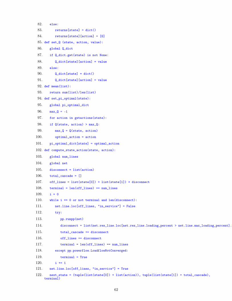
82. else:

83. returns[state] = dict()

84. returns[state][action] = [G]

85. def set_Q (state, action, value):

86. global Q_dict

87. if Q_dict.get(state) is not None:

88. Q_dict[state][action] = value

89. else:

90. Q_dict[state] = dict()

91. Q_dict[state][action] = value

92. def mean(list):

93. return sum(list)/len(list)

94. def set_pi_optimal(state):


96. max_Q = -1


98. if Q(state, action) > max_Q:

99. max_Q = Q(state, action)

100. optimal_action = action

101. pi_optimal_dict[state] = optimal_action

102. def compute_state_action(state, action):


104. global net

105. disconnect = list(action)

106. total_cascade = []

107. off_lines = list(state[0]) + list(state[1]) + disconnect


109. i = 0

110. while i == 0 or not terminal and len(disconnect):

111. net.line.loc[off_lines, "in_service"] = False

112. try:

113. pp.runpp(net)

114. disconnect = list(net.res_line.loc[net.res_line.loading_percent > net.line.max_loading_percent].index)

115. total_cascade += disconnect

116. off_lines += disconnect


118. except pp.powerflow.LoadflowNotConverged:

119. terminal = True

120. i += 1

121. net.line.loc[off_lines, "in_service"] = True

122. next_state = (tuple(list(state[0]) + list(action)), tuple(list(state[1]) + total_cascade),terminal)

62

123. reward = len(total_cascade)

124. return next_state, reward

125. def getactions(state):



128. actions = [tuple([i]) for i in range(num_lines) if i not in off_lines]

129. return actions

130. def V_optimal_initial_state():

131. global initial_state


133. episode_states = []

134. episode_actions = []

135. episode_rewards = []

136. while state[2] is False:

137. action = pi_optimal(state)

138. next_state, reward = compute_state_action(state, action)

139. episode_rewards.append(reward)

140. state = next_state

141. discount_vector = [gamma**i for i in range(len(episode_rewards))]

142. return np.dot(episode_rewards, discount_vector)

143. net = nw.case89pegase()

144. num_episodes = 2000

145. num_computations = 10

146. gamma = 0.9

147. epsilon = 0.2

148. num_lines = len(net.line)

149. initial_state = compute_state_action(((), (), False), [])[0]

150. ydata = []

151. for i in range(num_computations):

152. pi_optimal_dict = dict()

153. Q_dict = dict()

154. returns = dict()

155. error_G = []

156. V_optimal_evolution = []

157. print(" Monte Carlo computation: "+ str(i) + " | episodes: " + str(num_episodes) )

158. for i in range(num_episodes):

159. episode_states, episode_actions, episode_rewards = generate_episode()

160. G = 0

161. for t in reversed(range(len(episode_rewards))):

162. print("- Episode: " + str(i) + " | t: " + str(t), end="")

163. print("\r", end="")

63

164. G = G*gamma+episode_rewards[t]

165. returns_append(G, episode_states[t], episode_actions[t])

166. set_Q(episode_states[t], episode_actions[t], mean(returns[episode_states[t]][episode_actions[t]]))

167. set_pi_optimal(episode_states[t])

168. V_optimal_evolution.append(V_optimal_initial_state())

169. ydata.append(V_optimal_evolution)

170. import matplotlib.pyplot as plt

171. xdata = [i for i in range(num_episodes)]

172. #yoptimal = [1.8 for i in range(num_episodes)]

173. #plt.plot(xdata, yoptimal, ’r--’)

174. for i in range(num_computations):

175. plt.plot(xdata, ydata[i], label="Line "+str(i))

176. plt.plot()

177. #plt.legend(["Optimal value"]+["Execution "+str(i+1) for i in range(num_computations)],loc="center right")

178. plt.legend(["Execution "+str(i+1) for i in range(num_computations)], loc="center right")

179. plt.xlabel(’Number of episodes’)

180. plt.ylabel(’Value of initial state following obtained policy’)

181. plt.show()

182. """""

183. # Save pi_optimal into an excel file:

184. from DP import non_terminal_states


186. data = []


188. data.append([state, pi_optimal(state)])

189. df = pd.DataFrame(data, columns = [’State’, ’PI (state)’])

190. df.to_excel("MC policy.xlsx")

191. """

192. # Save Q for initial state and actions into an excel file:

193. df = pd.DataFrame(columns=[’Action’, ’Q’])

194. for a in getactions(initial_state):

195. df = df.append({’Action’: a,’Q’: Q(initial_state,a)},ignore_index=True)

196. df.to_excel("MC initial Q values 10000 89.xlsx")

64

References[1] About pandapower. http://www.pandapower.org/about/.

[2] Distributed generation electricity and its environmental impacts. https://www.epa.gov/energy/distributed-generation-electricity-and-its-environmental-impacts#ref1.

[3] Does eia publish the location of electric power plants and transmission lines? https://www.eia.gov/tools/faqs/faq.php?id=567&t=3.

[4] Electricity in the united states. https://www.eia.gov/energyexplained/electricity/electricity-in-the-us.php.

[5] Energy queensland: The facts and myths around electricity pricesand consumption. https://www.townsvilleenterprise.com.au/energy-queensland-the-facts-myths-around-electricity-prices-and-consumption/.

[6] How much electricity does an american home use? https://www.eia.gov/tools/faqs/faq.php?id=97&t=3.

[7] Pandapower: Data structure and elements. https://pandapower.readthedocs.io/en/v2.2.1/elements.html.

[8] Pandapower official website:. http://www.pandapower.org/.

[9] Power system test cases. https://pandapower.readthedocs.io/en/latest/networks/power_system_test_cases.html.

[10] State of the developer nation. https://slashdata-website-cms.s3.amazonaws.com/sample_reports/ZAamt00SbUZKwB9j.pdfs.

[11] The top programming languages 2019. https://spectrum.ieee.org/computing/software/the-top-programming-languages-2019.

[12] What is a system operator. http://www.incsys.com/power4vets/what-is-a-system-operator/.

[13] What is python? executive summary. https://www.python.org/doc/essays/blurb/.

[14] Ercot control room video, October 2014. https://www.youtube.com/watch?v=TlsfItQc05o.

[15] Julie Allen. South america power cut leaves 48 million people withoutelectricity. June 2019. https://www.telegraph.co.uk/news/2019/06/17/south-america-power-cut-leaves-48-million-people-without-electricity/.

[16] Murray Campbell, A Joseph Hoane Jr, and Feng-hsiung Hsu. Deep blue. Artificial intelligence,134(1-2):57–83, 2002.

[17] Transformational Disruptor and Andreas François Vermeulen. Industrial machine learning.

[18] D. A. Ferrucci. Introduction to "this is watson". IBM Journal of Research and Development,56(3.4):1:1–1:15, 2012.

[19] Adrian Kelly, Aidan O’Sullivan, Patrick de Mars, and Antoine Marot. Reinforcement learningfor electricity network operation. arXiv preprint arXiv:2003.07339, 2020.

[20] Volodymyr Mnih, Koray Kavukcuoglu, David Silver, Alex Graves, Ioannis Antonoglou, DaanWierstra, and Martin Riedmiller. Playing atari with deep reinforcement learning. arXivpreprint arXiv:1312.5602, 2013.

[21] P Russel Norvig and S Artificial Intelligence. A modern approach. Prentice Hall, 2002.

[22] Mark Rothleder. Renewable integration, May 2017. https://www.caiso.com/Documents/RenewableIntegrationUnlockingDividends.pdf.

65

[23] Florian Schäfer and Martin Braun. An efficient open-source implementation to compute thejacobian matrix for the newton-raphson power flow algorithm. In 2018 IEEE PES InnovativeSmart Grid Technologies Conference Europe (ISGT-Europe), pages 1–6. IEEE, 2018.

[24] Surajbhan Sevda and Anoop Singh. Mathematical and Statistical Applications in Food Engi-neering. CRC Press, 2020.

[25] Claude E Shannon. Xxii. programming a computer for playing chess. The London, Edinburgh,and Dublin Philosophical Magazine and Journal of Science, 41(314):256–275, 1950.

[26] Thomas Allen Short. Electric power distribution handbook. CRC press, 2014.

[27] Richard S Sutton and Andrew G Barto. Reinforcement learning: An introduction. MIT press,2018.

[28] Ruohan Zhan, Tianchang He, and Yunpo Li. Cs221 project final report deep reinforcementlearning in portfolio management.

[29] Guidong Zhang, Samson Shenglong Yu, Siyuan Zou, Herbert Ho-Ching Iu, Tyrone Fernando,and Yun Zhang. An investigation into cascading failure in large-scale electric grids: A load-redistribution approach. Applied Sciences, 8(7):1033, 2018.

66