power system simulation lab lab manual - · pdf file02 a. formation of y- bus using singular...

QMP 7.1 D/F Channabasaveshwara Institute of Technology

(An ISO 9001:2015 Certified Institution) NH 206 (B.H. Road), Gubbi, Tumkur – 572 216. Karnataka.

Department of Electrical & Electronics Engineering

Power System Simulation Lab

Lab Manual

10EEL78

B.E - VII Semester

Lab Manual 2017-18

Name : __________________________________________________

USN : ___________________________________________________

Batch : ___________________ Section : ________________

Channabasaveshwara Institute of Technology (An ISO 9001:2015 Certified Institution)

NH 206 (B.H. Road), Gubbi, Tumkur – 572 216. Karnataka.

Department of Electrical & Electronics Engineering

Power System Simulation Lab Manual

Version 2.0 August 2017

Prepared by: Reviewed by:

Mr. M S Lokanathan Mr. M S Lokanathan

Assistant professor Assistant Professor

Ms. Tejaswini M V

Assistant professor

Approved by:

V.C Kumar

Professor & Head,

Dept. of EEE

INDEX PAGE

Note:

If the student fails to attend the regular lab, the experiment has

to be completed in the same week. Then the

manual/observation and record will be evaluated for 50% of

maximum marks.

Sl.

No Name of the Experiment

Date

Man

ual

Marks

(M

ax .

25

)

Reco

rd

M

arks

(M

ax.

10

)

Sig

natu

re

(S

tud

en

t)

Sig

natu

re

(Facu

lty)

Conduction Repetition Submission of

Record

01

02

03

04

05

06

07

08

09

10

11

12

13

Average

POWER SYSTEM SIMULATION LAB-10EEL78 2017-2018

Contents

Program

No.

Experiment Name Page no

01 A. Abcd parameters for t network 02

B. Abcd parameters for long transmission network 06

02 A. Formation of y- bus using singular transformation method with and

without mutual coupling

08

B. Formation of ‘y- bus’ by inspection method 12

03 Z-bus building algorithm 14

04 Determination of power angle curve for non- salient pole synchronous

machines

16

05 Determination of power angle curve salient pole synchronous machines 18

06 Program for swing curve when the fault is cleared 20

07 Swing curve for sustained fault and critical clearing angle & time 24

08 Formation of jacobian for the system not exceeding 4 buses (no pv buses)

in polar coordinates

28

09 Gauss-seidel method 30

10 Determination of bus currents, bus power & line flows for a specified

system voltage (bus) profile

34

11 Load flow studies for a given power system using software package 38

12 Fault studies for a given power system using software package 52

13 Optimal generator scheduling for thermal power plants using software

package

64

PROGRAM: %program to calculate ABCD parameters for T network for Medium line clear all

length=140 Z=(0.2+0.408i)*length; Y=(0+3.14e-6i)*length;

fprintf('\n Medium line T network');

fprintf('A B C D parameter for medium line T network'); A=1+((Y*Z)/2) B=Z*(1+((Y*Z)/4)) C=Y D=A

check=(A*D)-(B*C)

k2=input('\n enter 1- to read Vr, Ir and compute Vs, Is\n 2-

to read Vs, Is and compute Vr, Ir'); switch k2,

case 1

vr=input('enter Vr/phase='); ir=input('enter ir/phase='); vr=vr*1e3/sqrt(3); vs=(A*vr+B*ir)/1e3; is=C*vr+D*ir;

fprintf('\n Sending end voltage/ph=%f%+fi KV',

real(vs),imag(vs));

fprintf('\n Sending end current/ph=%f%+fi Amp',

real(is),imag(is)); vs=vs*1e3; case 2,

vs=input('enter Vs/phase='); is=input('enter is/phase='); vs=vs*1e3/sqrt(3.0); vr=(D*vs-B*is)/1e3; ir=-C*vs+D*is;

fprintf('\n Receiving end voltage/ph=%f%+fi KV',

real(vr),imag(vr));

fprintf('\n Receiving end current/ph=%f%+fi Amp',

real(ir),imag(ir)); vr=vr*1e3;

DEPARTMENT OF E&EE , CIT, GUBBI 1


Exp: 1.a Date: ___/___/_____

ABCD PARAMETERS FOR T NETWORK.

AIM: i) Formation for symmetric configuration.

ii) Verification of AD-BC = 1.

iii) Determination of Efficiency & regulation.

PROCEDURE:

Enter the command window of the MATLAB.

Create a new M – file by selecting File - New – M – File

Type and save the program in the editor window.

Execute the program by pressing Tools – Run.

View the results.

Note 1:

1. For short line, length=40 2. For medium line, length=140

Note 2:

1. “short transmission network” fprintf('A B C D parameter for short transmission line');

A=1 B=Z C=0 D=1

2. fprintf('A B C D parameter for medium line PI network');

A=1+((Y*Z)/2)

B=Z

C=Y*(1+((Y*Z)/4)) D=A



otherwise

disp('wrong choice'); end

rec_pow=3*real(vr*conj(ir))/1e6;

send_pow=3*real(vs*conj(is))/1e6;

eff=rec_pow/send_pow*100;

reg=(abs(vs)/abs(A)-abs(vr))/abs(vr)*100;

fprintf('\n Recieving end power=%.2fKVA',rec_pow);

fprintf('\n sending end power=%.2fKVA',send_pow);

fprintf('\n efficiency=%.2f%%',eff);

fprintf('\n voltage regulation=%.2f%%',reg);

EXPECTED RESULT for T network:

length =140

A B C D parameter for T network

A = 0.9874 + 0.0062i

B = 27.6485 +56.8476i

C = 0 +4.3960e-004i

D = 0.9874 + 0.0062i

check = 1.0000 + 0.0000i

enter 1- to read Vr, Ir and compute Vs,

Is 2- to read Vs, Is and compute Vr, Ir1

enter Vr/phase=132

enter ir/phase=174.96-131.22i

Sending end voltage/ph=87.550333+6.787052i KV

Sending end current/ph=173.570962-94.993743i

Amp Recieving end power=40.00KVA

sending end power=43.65KVA

efficiency=91.63%

voltage regulation=16.69%



EXPECTED RESULT for Pi network:

length = 140

A B C D parameter for medium line PI network

A = 0.9874 + 0.0062i

B = 28.0000 +57.1200i

C = -1.3527e-006 +4.3684e-004i

D = 0.9874 + 0.0062i

check = 1.0000 + 0.0000i

enter 1- to read Vr, Ir and compute Vs, Is

2- to read Vs, Is and compute Vr, Ir2

enter Vs/phase=132+0i

enter is/phase=174.96-131.22i

Receiving end voltage/ph=62.859251-5.850527i KV

Receiving end current/ph=173.674054-161.787473i Amp

Recieving end power=35.59KVA

sending end power=40.00KVA

efficiency=88.97%




PROGRAM: %program to calculate ABCD parameters for long line network

clc

clear all

length=300;

Z=(0.2+0.408i)*length;

Y=(0+3.14e-6i)*length;

fprintf('A B C D parameter for long transmission line network');

zc=sqrt(Z/Y);

gam=sqrt(Z*Y); A=cosh(gam)

B=zc*sinh(gam)

C=1/zc*sinh(gam)

D=A

check=(A*D)-(B*C)

k2=input('\n enter 1- to read Vr, Ir and compute Vs, Is\n 2- to

read Vs, Is and compute Vr, Ir'); switch k2,

case 1

vr=input('enter Vr/phase='); ir=input('enter ir/phase=');

vr=vr*1e3/sqrt(3);

vs=(A*vr+B*ir)/1e3;

is=C*vr+D*ir; fprintf('\n Sending end voltage/ph=%f%+fi KV',

real(vs),imag(vs)); fprintf('\n Sending end current/ph=%f%+fi Amp',

real(is),imag(is));

vs=vs*1e3;

case 2,

vs=input('enter Vs/phase=');

is=input('enter is/phase=');

vs=vs*1e3/sqrt(3.0); vr=(D*vs-B*is)/1e3;

ir=-C*vs+D*is; fprintf('\n Receiving end voltage/ph=%f%+fi KV',

real(vr),imag(vr)); fprintf('\n Receiving end current/ph=%f%+fi Amp',

real(ir),imag(ir));

vr=vr*1e3; otherwise

disp('wrong choice');

end rec_pow=3*real(vr*conj(ir))/1e6;

send_pow=3*real(vs*conj(is))/1e6;

eff=rec_pow/send_pow*100; reg=(abs(vs)/abs(A)-

abs(vr))/abs(vr)*100; fprintf('\n Recieving end

power=%.2fKVA',rec_pow); fprintf('\n sending end

power=%.2fKVA',send_pow); fprintf('\n

efficiency=%.2f%%',eff); fprintf('\n voltage

regulation=%.2f%%',reg);



Exp: 1.b Date: ___/___/_____

ABCD PARAMETERS FOR LONG TRANSMISSION

NETWORK.

AIM: i) Formation for symmetric configuration.

ii) Verification of AD-BC = 1.

iii) Determination of Efficiency & regulation.

PROCEDURE:





View the results.

Note: For long line, length=300

EXPECTED RESULT for Pi network: A B C D parameter for long transmission line network

A = 0.9428 + 0.0277i

B = 5.7712e+001 +1.2062e+002i

C = -8.7717e-006 +9.2398e-004i D = 0.9428 + 0.0277i

check = 1.0000

enter 1- to read Vr, Ir and compute Vs, Is

2- to read Vs, Is and compute Vr, Ir1

enter Vr/phase=132+0i

enter ir/phase=174.96-131.22i

Sending end voltage/ph=97.773395+15.642655i KV

Sending end current/ph=167.915908-48.443896i

Amp Recieving end power=40.00KVA sending end

power=46.98KVA

efficiency=85.15%




PROGRAM:

%FORMATION OF Ybus USING SINGULAR TRANSFORMATION

METHOD %WITHOUT MUTUAL COUPLING:

% p q Z hlcY(ADM)

z=[5 4 0.02+0.06i 0.03i

5 1 0.08+0.24i 0.025i

4 1 0.06+0.18i 0.02i

4 2 0.06+0.18i 0.02i

4 3 0.04+0.12i 0.015i

1 2 0.01+0.03i 0.01i

2 3 0.08+0.24i 0.025i];

fb=z(:,1);

tb=z(:,2);

Z=z(:,3);

hlcy=z(:,4);

y=1./Z;

nbus=max(max(fb),max(tb));

Y=zeros(nbus);

nline=length(fb);

nlb=nline+nbus;

A=zeros(nlb,nbus);

for k=1:nbus

A(k,k)=1;

end

for k=1:nline

A(nbus+k,fb(k))=1;

A(nbus+k,tb(k))=-1;

end

sh=zeros(nbus);

for k=1:nline

sh(fb(k))=sh(fb(k))+hlcy(k);

sh(tb(k))=sh(tb(k))+hlcy(k);

end

ypr=zeros(nlb,nlb);

for k=1:nbus

ypr(k,k)=sh(k);

end

for k=1:nline

ypr(nbus+k,nbus+k)=y(k);

end

format short;

Ybus=A'*ypr*A

V(1) =1.024532-0.08729i;

V(2)=1.02394-0.931i;

V(3)=1.01825-0.1074i;

V(4)=1.0476-0.049i;

V(5)=1.06+0i;

I=Ybus*V'



Exp: 2.a Date: ___/___/_____

FORMATION OF Y- BUS USING SINGULAR TRANSFORMATION

METHOD WITH AND WITHOUT MUTUAL COUPLING,

AIM: Y bus formation for systems, without mutual coupling, by singular

transformation.

THEORY:

FORMATION OF Y BUS MATRIX Bus admittance is often used in power system studies. In most of the power system studies it is required to form y- bus matrix of the system by considering certain power system parameters depending upon the type of analysis.

Y-bus may be formed by inspection method only if there is no mutual coupling between the lines. Every transmission line should be represented by - equivalent. Shunt impedances are added to diagonal element corresponding to the buses at which these are connected. The off diagonal elements are unaffected. The equivalent circuit of Tap changing transformers is included while forming Y-bus matrix.

Generalized Y-bus = Yii ……….. Yid Ydi ……… Ydd

where, Yii = Self admittance Ydi = Transfer admittance

.

PROCEDURE:





View the results.



%FORMATION OF Ybus USING SINGULAR TRANSFORMATON METHOD

%WITH MUTUAL COUPLING & WITHOUT LINE CHARGING:

% p qZmno mutual(imp)

z=[0 1 0.6i 0 0

0 2 0.5i 1 0.1i

2 3 0.5i 0 0

0 1 0.4i 1 0.2i

1 3 0.2i 0 0]; p=z(:,1);

q=z(:,2);

Z=z(:,3);

mno=z(:,4);

zmc=z(:,5);

nbus=max(max(p),max(q));

Y=zeros(nbus);

nline=length(p);

A=zeros(nline,nbus);

for k=1:nline,

if(q(k)==0)

A(k,p(k))=1;

elseif(p(k)==0)

A(k,q(k))=-1;

end

if(p(k)~=0&q(k)~=0)

A(k,p(k))=1;

A(k,q(k))=-1;

end

end

zpr=zeros(nline,nline);

for k=1:nline

zpr(k,k)=Z(k);

if(mno(k))

zpr(k,mno(k))=zmc(k);

zpr(mno(k),k)=zmc(k);

end

end

ypr=inv(zpr);

format short;

Ybus=A'*ypr*A



EXPECTED RESULT:

FORMATION OF Ybus USING SINGULAR TRANSFORMATION METHOD WITHOUT

MUTUAL COUPLING:

Ybus =

12.9167 -38.6950i -10.0000 +30.0000i 0 -1.6667 + 5.0000i -1.2500 + 3.7500i

-10.0000 +30.0000i 12.9167 -38.6950i -1.2500 + 3.7500i -1.6667 + 5.0000i 0

0 -1.2500 + 3.7500i 3.7500 -11.2100i -2.5000 + 7.5000i 0

-1.6667 + 5.0000i -1.6667 + 5.0000i -2.5000 + 7.5000i 10.8333 -32.4150i -5.0000 +15.0000i

-1.2500 + 3.7500i 0 0 -5.0000 +15.0000i 6.2500 -18.6950i

I =

-24.8742 - 7.9772i

32.7204 +11.1076i

-2.7353 - 0.6013i

-4.2194 - 1.6135i

-0.9560 - 0.6148i

FORMATION OF Ybus USING SINGULAR TRANSFORMATON METHOD WITH

MUTUAL COUPLING & WITHOUT LINE CHARGING:

Ybus =

0 - 8.0208i 0 + 0.2083i 0 + 5.0000i

0 + 0.2083i 0 - 4.0833i 0 + 2.0000i

0 + 5.0000i 0 + 2.0000i 0 - 7.0000i



PROGRAM:

% p q z hlc(ADM) a

z=[5 4 0.02+0.06i 0.03i 0.9

5 1 0.08+0.24i 0.025i 1

4 1 0.06+0.18i 0.02i 1

4 2 0.06+0.18i 0.02i 1

4 3 0.04+0.12i 0.015i 1

1 2 0.01+0.03i 0.01i 0.8

2 3 0.08+0.24i 0.025i 1 ];

%function yb(z);

fb=z(:,1);

tb=z(:,2);

Z=z(:,3);

hlc=z(:,4);

a=z(:,5);

y=1./Z;

nbus=max(max(fb),max(tb));

Y=zeros(nbus);

nline=length(fb);

for k=1:nline,

p=fb(k);q=tb(k);

y(k)=y(k)/a(k);

Y(p,p)=Y(p,p)+y(k)+hlc(k)+(1-a(k))/a(k)*y(k);

Y(q,q)=Y(q,q)+y(k)+hlc(k)+(a(k)-1)*y(k);

Y(p,q)=Y(p,q)-y(k);

Y(q,p)=Y(p,q);

end

Ybus=Y



Exp: 2.b Date: ___/___/_____

FORMATION OF ‘Y- BUS’ BY INSPECTION METHOD.

AIM: Y bus formation for systems,by inspection method.

PROCEDURE:





View the results.

EXPECTED RESULT:

Ybus =

18.5417 -55.5700i -12.5000 +37.5000i 0 -1.6667 + 5.0000i -1.2500 + 3.7500i

-12.5000 +37.5000i 12.9167 -38.6950i -1.2500 + 3.7500i -1.6667 + 5.0000i 0

0 -1.2500 + 3.7500i 3.7500 -11.2100i -2.5000 + 7.5000i 0

-1.6667 + 5.0000 -1.6667 + 5.0000i -2.500 + 7.5000i 10.8333 -32.4150i -5.5556 -16.6667i

-1.2500 + 3.7500i 0 0 -5.5556 +16.6667i 7.4228 -22.2135i



PROGRAM: %Zprim=[Element no. from to Value] clc

clear all

Z= [ 1 1 0 0.25

2 2 1 0.1

3 3 1 0.1

4 2 0 0.25

5 2 3 0.1];

[m n]= size(Z);

Zbus=[ ] ;%Let Zbus be a null matrix to begin with

currentbusno=0;

for count = 1:m,

[rows cols]=size(Zbus);

fb=Z(count,2);

tb=Z(count,3); value=Z(count,4);

newbus=max(fb,tb); ref=min(fb,tb); % Type 1 Modification

if newbus>currentbusno & ref==0 Type=1

Zbus=[Zbus zeros(rows,1) zeros(1,cols) value]

currentbusno=newbus;

continue end

% Type 2 Modification

if newbus>currentbusno & ref~=0 Type=2 Zbus=[Zbus Zbus(:,ref)

Zbus(ref,:) value+Zbus(ref,ref)]

currentbusno=newbus; continue

end % Type 3 Modification

if newbus<=currentbusno & ref==0 Zbus=Zbus-

1/(Zbus(newbus,newbus)+value)*Zbus(:,newbus)*Zbus(newbus,:)

continue end % Type 4 Modification

if newbus<=currentbusno & ref~=0 Zbus=Zbus-

1/(value+Zbus(fb,fb)+Zbus(tb,tb)- 2*Zbus(fb,tb))*((Zbus(:,fb)-Zbus(:,tb))*((Zbus(fb,:)-

Zbus(tb,:)))) continue

end

end



Exp:3. Date: ___/___/_____

Z-BUS BUILDING ALGORITHEM

AIM: Formation of Z-bus, using Z-bus build Algorithm without mutual.

PROCEDURE:





View the results.

EXPECTED RESULT

Type = 1

Zbus = 0.2500

Type = 2

Zbus =

0.2500 0.2500

0.2500 0.3500

Type = 2

Zbus =

0.2500 0.2500 0.2500

0.2500 0.3500 0.2500

0.2500 0.2500 0.3500

Zbus =

0.1458 0.1042 0.1458

0.1042 0.1458 0.1042

0.1458 0.1042 0.2458

Zbus =

0.1397 0.1103 0.1250

0.1103 0.1397 0.1250

0.1250 0.1250 0.1750



PROGRAM: %power angle characteristics cylindrical rotor syn.m/c

%enter the values of x,v,Ia; clc

clear all x=0.3;

v=1.0;

e=1.2;

pm=abs(e)*abs(v)/x;

del=0:0.1:pi;

plot(del,pm*sin(del),'r');

title('power angle characteristics of cylindrical rotor

syn.m/c');

xlabel('Delta');

ylabel('power,p');

legend('pm*sin(delta)');

del=0:0.1:pi/2;

line(del,pm);

y=0:0.1:pm;

line(pi/2,y);

reg=(abs(e)-abs(v))/abs(v)*100;

fprintf('\n the excitation Voltage = %f%%\n',e);

fprintf('\n the peak power = %f%%\n',pm);

fprintf('\n the Voltage regulation = %f%%\n',reg);



Exp:4. Date: ___/___/_____

DETERMINATION OF POWER ANGLE CURVE FOR NON- SALIENT

POLE SYNCHRONOUS MACHINES.

AIM: To determine the power angle diagram , reluctance power, excitation, emf and regulation for non- salient pole synchronous machines,.

PROCEDURE:





View the results.

EXPECTED RESULT:

the excitation Voltage = 1.200000%

the peak power = 4.000000%

the Voltage regulation = 20.000000%

power angle characteristics of cylindrical rotor syn.m/c 4

pm*sin(delta) 3.5

3

2.5

2

1.5

1

0.5

00 0.5 1 1.5 2 2.5 3 3.5

Delta



PROGRAM: clc

clear all

xd=1;

xq=0.6;

v=1.0;

ia=0.5000-0.3750i;

theta=abs(angle(ia));

del=atan((xq*abs(ia)*cos(theta))/(abs(v)+xq*abs(ia)*sin(theta))

);

e=abs(v)*cos(del)+xd*abs(ia)*sin(del+theta);

p=(e)*abs(v)/xd;

pr=abs(v)^2*(xd-xq)/(2*xd*xq);

del=0:0.01:pi;

line(del,0);

hold on;

pe=p*sin(del)+pr*sin(2*del);

plot(del,p*sin(del),del,pr*sin(2*del),del,p*sin(del)+pr*sin(2*d

el));

title('power angle characteristics of salient pole syn.m/c');

xlabel('Delta');

ylabel('power,p');

legend('p*sin(delta)','pr*sin(2*del)','p*sin(del)+pr*sin(2*del)

');

[pmax,k]=max(pe);

fprintf('\n maximum power = %f and the corresponding angle=

%f',pmax,del(k)*180/pi);

del=0:0.01:del(k);

line(del,pmax);

y=0:0.01:pmax;

line(del(k),y);

reg=(abs(e)-abs(v))/abs(v)*100;

text(-0.4,pmax,'pmax');

text(del(k),-0.1,'deltamax');

fprintf('\n the excitation Voltage = %f pu',abs(e));

fprintf('\n the Reluctance power = %f pu\n',pr);

fprintf('\n the Voltage regulation = %f%%\n',reg);



Exp:5. Date: ___/___/_____

DETERMINATION OF POWER ANGLE CURVE SALIENT POLE

SYNCHRONOUS MACHINES.

AIM: To determine the power angle diagram , reluctance power, excitation, emf and regulation for salient pole synchronous machines,.

PROCEDURE:





View the results.

EXPECTED RESULT:

maximum power = 1.581035 and the corresponding angle= 69.900851 the excitation Voltage = 1.454468 pu the Reluctance power = 0.333333 pu

the Voltage regulation = 45.446817%

power angle characteristics of salient pole syn.m/c 1.6 pmax

p*sin(delta)

1.4 pr*sin(2*del)

1.2

p*sin(del)+pr*sin(2*del)

1

po

we

r,p

0.8

0.6

0.4

0.2

0 deltamax

-0.2

-0.40 0.5 1 1.5 2 2.5 3 3.5

Delta



PROGRAM: clc

clear all

%program for swing curve when the fault is

cleared ps=0.9;e=1.1;v=1.0;m=0.00028;

xe=0.35;xL=0.2;

%function swing2(ps,e,v,m,xe,xL)

x1=xe+xL/2;

ch=input('enter 1-for fault at the beginning of line

\n 2-for fault at the middle of line '); switch ch

case 1,

x2=inf;

case 2,

x2=(xe*xL+xe*xL/2+xL*xL/2)/(xL/2);

otherwise

disp('wrong input');

end

x3=xe+xL;

dt=0.05;

%ct=ct/50; //conversion from cycles to sec

ct=input('\n enter clearing time in secs ');

k=ct/dt;

r=ct-floor(k)*dt;

if(r==0)

fprintf('FAULT IS CLEARED AT THE BEGINNING OF

AN INTERVEL');

else

fprintf('FAULT IS CLEARED AT THE MIDDLE OF AN

INTERVEL');

end

rr=180/pi;

f=dt^2/m;

deld=0;

it=1; t(it)=0;

pm1=e*v/x1;

del(it)=asin(ps/pm1);

pm2=e*v/x2;

pm3=e*v/x3;

fprintf('\n TIME PMAX DELTA'); pm=pm1;

pe=pm*sin(del(it));

pa=(ps-pe);



Exp: 6. Date: ___/___/_____

PROGRAM FOR SWING CURVE WHEN THE FAULT IS

CLEARED.

AIM: To determine the Swing curve when the fault is cleared

i) At the beginning of the Line

ii) At the middle of the line

PROCEDURE:





View the results.



fprintf('\n %5.3f %5.2f %5.2f',

t(it),pm,del(it)* rr);

pm=pm2;

pe=pm*sin(del(it));

pa=(ps-pe)/2;

while(t(it)<=0.5)

ft=f*pa/rr;

deld=deld+ft;

fprintf('\n %5.3f %5.2f %5.2f',

t(it),pm,del(it)* rr);

it=it+1;

t(it)=t(it-1)+dt;

del(it)=del(it-1)+deld;

pm=pm2;

if(t(it)==ct)

pm=(pm2+pm3)/2;

elseif(t(it)>ct)

pm=pm3;

end

pe=pm*sin(del(it));

pa=ps-pe;

end

plot(t,del*rr,'r');

title('swing curve');

xlabel('Time');

ylabel('Delta');

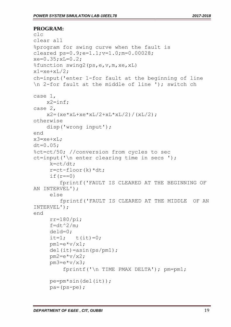
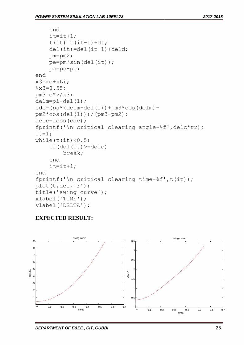
EXPECTED RESULT:

swing curve swing curve

45 60

40 50

35

30

De

lta

25

20

15

100 0.1 0.2 0.3 0.4 0.5 0.6 0.7

Time

De

lta

40

30

20

10

0

0 0.1 0.2 0.3 0.4 0.5 0.6 0.7

enter 1-for fault at the beginning of line Time

2-for fault at the middle of line 1



enter clearing time in secs 0.05

FAULT IS CLEARED AT THE

BEGINNING OF AN INTERVEL

TIME PMAX DELTA

0.000 2.44 21.60

0.000 0.00 21.60

0.050 1.00 25.62

0.100 2.00 33.81

0.150 2.00 40.10

0.200 2.00 42.93

0.250 2.00 41.62

0.300 2.00 36.50

0.350 2.00 28.78

0.400 2.00 20.51

0.450 2.00 14.01

0.500 2.00 11.23

enter 1-for fault at the beginning of line

2-for fault at the middle of line 2

enter clearing time in secs 0.125 FAULT IS CLEARED AT THE

MIDDLE OF AN INTERVEL

TIME PMAX DELTA

0.000 2.44 21.60

0.000 0.88 21.60

0.050 0.88 24.17

0.100 0.88 31.56

0.150 2.00 42.88

0.200 2.00 50.07

0.250 2.00 51.61

0.300 2.00 47.19

0.350 2.00 37.70

0.400 2.00 25.33

0.450 2.00 13.35

0.500 2.00 5.29



PROGRAM: clc

clear all

%swing curve for sustained fault and critical clearing

time.

%ps=mech. power input xe=xg+xt, x1=reactance before

fault x2=reactance after fault

ps=0.9;e=1.1;v=1.0;m=0.00028;xe=0.35;xLi=0.2;

%function swing(ps,e,v,m,xe,xLi) x1=xe+xLi/2;

ch=input('enter 1-for fault at the beginning \n 2-for

fault at the middle');

switch ch

case 1

x2=inf;

case 2

x2=(xe*xLi+xe*xLi/2+xLi*xLi/2)/(xLi/2);

otherwise

disp('wrong input');

end

dt=0.05;

rr=180/pi;

f=dt^2/m;

it=1;

t(it)=0;

deld=0;

pm1=e*v/x1;

del(it)=asin(ps/pm1);

fprintf('\n SUSTAINED FAULT');

fprintf('\n TIME PMAX DELTA');

fprintf('\n----------------');

pm=pm1;

fprintf('\n %5.3f %5.2f %5.2f',t(it),pm,del(it)*rr);

pm2=e*v/x2;

pm=pm2;

pe=pm*sin(del(it));

pa=(ps-pe)/2;

t1=0;

while(t(it)<=0.5)

ft=f*pa/rr;

deld=deld+ft;

if(t1-t(it)<=0.5)

fprintf('\n %5.3f %5.2f

%5.2f',t(it),pm,del(it)*rr);



Exp: 7. Date: ___/___/_____

SWING CURVE FOR SUSTAINED FAULT AND CRITICAL

CLEARING ANGLE & TIME.

AIM: To determine swing curve for sustained fault and critical clearing angle & time.

PROCEDURE:





View the results.



end

it=it+1;

t(it)=t(it-1)+dt;

del(it)=del(it-1)+deld;

pm=pm2;

pe=pm*sin(del(it));

pa=ps-pe;

end

x3=xe+xLi;

%x3=0.55;

pm3=e*v/x3;

delm=pi-del(1);

cdc=(ps*(delm-del(1))+pm3*cos(delm)-

pm2*cos(del(1)))/(pm3-pm2);

delc=acos(cdc);

fprintf('\n critical clearing angle-%f',delc*rr);

it=1;

while(t(it)<0.5)

if(del(it)>=delc)

break;

end

it=it+1;

end

fprintf('\n critical clearing time-%f',t(it));

plot(t,del,'r');

title('swing curve');

xlabel('TIME');

ylabel('DELTA');

EXPECTED RESULT:

DE

LT

A

swing curve

9 8

7

6

5

4

3

2

1

0

0 0.1 0.2 0.3 0.4 0.5 0.6 0.7 TIME

DE

LT

A

swing curve

3.5

3

2.5

2

1.5

1

0.5

0

0 0.1 0.2 0.3 0.4 0.5 0.6 0.7 TIME



enter 1-for fault at the beginning

2-for fault at the middle1

SUSTAINED FAULT

TIME PMAX DELTA

----------------

0.000 2.44 21.60

0.000 0.00 21.60

0.050 0.00 25.62

0.100 0.00 37.67

0.150 0.00 57.76

0.200 0.00 85.89

0.250 0.00 122.05

0.300 0.00 166.25

0.350 0.00 218.48

0.400 0.00 278.75

0.450 0.00 347.05

0.500 0.00 423.39

critical clearing angle-81.684989

critical clearing time-0.200000

enter 1-for fault at the beginning

2-for fault at the middle2

SUSTAINED FAULT

TIME PMAX DELTA

----------------

0.000 2.44 21.60

0.000 0.88 21.60

0.050 0.88 24.17

0.100 0.88 31.56

0.150 0.88 42.88

0.200 0.88 56.88

0.250 0.88 72.34

0.300 0.88 88.34

0.350 0.88 104.53

0.400 0.88 121.15

0.450 0.88 139.08

0.500 0.88 159.89

critical clearing angle-118.182332

critical clearing time-0.400000



PROGRAM:

% Formation of Jacobian matrix clc clear all

nb=3; Y=[65-45j -40+20i -25+25i; -

40+20i 60-60i -20+40i; -

25+25i -20+40i 45-65i]; V = [1.0 0;1.0 0.0 ;1.0 0.0 ];

J1 = zeros(nb-1,nb-1) ; J2 = zeros(nb-1,nb-1) ;

J3 = zeros(nb-1,nb-1) ; J4 = zeros(nb-1,nb-1) ;

for p = 2:nb

Vp = V(p,1); delta_p = V(p,2) * pi/180;

Ypp = abs(Y(p,p)); theta_pp = angle(Y(p,p));

V1 = V(1,1); delta_1 = V(1,2) * pi/180;

Yp1 = abs( Y(p,1) );

theta_p1 = angle( Y(p,1));

J1 (p-1,p-1) = Vp * V1 * Yp1 * sin( theta_p1 - delta_p + delta_1 ); J2 (p-1,p-1) = 2*Vp*Ypp*cos(theta_pp) + V1*Yp1*cos(theta_p1 - delta_p + delta_1); J3 (p-1,p-1) = Vp*V1*Yp1*cos(theta_p1 - delta_p + delta_1); J4 (p-1,p-1) = -2*Vp*Ypp*sin(theta_pp) - Vp*Yp1*sin(theta_p1 - delta_p + delta_1);

for q = 2:nb

Vq = V(q,1) ; delta_q = V(q,2) * pi/180;

Ypq = abs ( Y(p,q) ); theta_pq = angle( Y(p,q) );

temp1 = -Vp * Vq * Ypq * sin( theta_pq - delta_p + delta_q) ;

temp2 = Vq * Ypq * cos( theta_pq - delta_p + delta_q) ; temp3

= -Vp * Vq * Ypq * cos( theta_pq - delta_p + delta_q) ; temp4

= -Vp * Ypq * sin( theta_pq - delta_p + delta_q) ;

if q ~= p

J1(p-1,q-1) = temp1 ;

J1(p-1,p-1) = J1(p-1,p-1) - temp1 ;

J2(p-1,q-1) = temp2 ; J2(p-1,p-1) = J2(p-1,p-1) + temp2 ; cont…



Exp:8. Date: ___/___/_____

FORMATION OF JACOBIAN FOR THE SYSTEM NOT EXCEEDING 4

BUSES (no PV BUSES) IN POLAR COORDINATES

Aim: A Three-Bus system is given. Form a Jacobian matrix for the system in polar coordinates.

PROCEDURE:





View the results.

cont…

J3(p-1,q-1) = temp3 ;

J3(p-1,p-1) = J3(p-1,p-1) - temp3 ;

J4(p-1,q-1) = temp4 ; J4(p-1,p-1) = J4(p-1,p-1) + temp4 ;

end

end

end

J = [J1 J2; J3 J4]

EXPECTED RESULT

J =

60.0000 -40.0000 60.0000 -20.0000

-40.0000 65.0000 -20.0000 45.0000

-60.0000 20.0000 60.0000 -40.0000

20.0000 -45.0000 -40.0000 65.0000



PROGRAM:

clc

clear all

% enter Y-bus of the system

Y=[3-12i -2+8i -1+4i 0

-2+8i 3.66-14.664i -0.666+2.664i -1+4i

-1+4i -0.666+2.664i 3.66-14.664i -2+8i

0 -1+4i -2+8i 3-12i];

%enter no. of buses, slack bus no, no.of pq buses, no of pv buses

nbus=4;

sbno=1;

npq=2;

npv=1;

% assume bus no 1 as slack bus, next npq buses as pq buses and the remaining as pv buses

%enter slack bus voltage

v(1)=1.06+0i;

%assume voltages at all other buses as 1+j0

v(2)=1;v(3)=1;v(4)=1;

%enter p & q at all pq buses P(2)=-

0.5;P(3)=-0.4;Q(2)=-0.2;Q(3)=-0.3;

%enter p ,vsp and q limits at pv buses

P(4)=0.3;

vsp(4)=1.04;Qmin(4)=0.1;Qmax(4)=1.0;

%enter accuracy of convergence

acc=0.001;

for it=1:5

%to find voltages at pq buses

for p=2:npq+1,

v1(p)=v(p); pq=(P(p)-

Q(p)*i)/conj(v(p)); ypq=0;

for q=1:nbus

if(p==q) continue;

end

ypq=ypq+Y(p,q)*v(q)

;

end v(p)=(pq-

ypq)/Y(p,p);

end

%to find voltages at pv buses

for p=npq+2:nbus,

v1(p)=v(p);

s=0;

for q=1:nbus,

if(p~=q)

s=s+Y(p,q)*v(q);

else

vp=v(q);



Exp:9. Date: ___/___/_____

GAUSS-SEIDEL METHOD

AIM: To perform load flow analysis using Gauss- Seidel method (only pq bus)

PROCEDURE:





View the results.



ang=angle(v(q));

v(q)=complex(vsp(q)*cos(ang),vsp(q)*sin(ang));

s=s+Y(p,q)*v(q);

end

end

Qc(p)=-1*imag(conj(v(p))*s);

if(Qc(p)>=Qmin(p)& Qc(p)<=Qmax(p))

pq=(P(p)-Qc(p)*i)/conj(v(p));

ypq=0;

for q=1:nbus

if(p==q) continue;

end

ypq=ypq+Y(p,q)*v(q);

end v(p)=(pq-ypq)/Y(p,p);

ang=angle(v(p));

v(p)=complex(vsp(p)*cos(ang),vsp(p)*sin(ang));

else

if(Qc(p)<Qmin(p))

Q(p)=Qmin(p);

else

Q(p)=Qmax(p);

end

pq=(P(p)-Q(p)*i)/conj(vp);

ypq=0;

for q=1:nbus

if(p==q) continue;

end

ypq=ypq+Y(p,q)*v(q);

end

v(p)=(pq-ypq)/Y(p,p);

end

end

%to find the votages at all buses and Q at pv busses

fprintf('\nThe votages at all buses and Q at pv busses after

iteration no %d',it);

for p=1:npq+1

fprintf('\nV(%d)=%.4f

at%.2fdeg',p,abs(v(p)),angle(v(p))*180/pi);

end

for p=npq+2:nbus fprintf('\nV(%d)=%.4f at%.2fdeg

Q(%d)=%+.3f\n',p,abs(v(p)),angle(v(p))*180/pi,p,Qc(p));

end

%to check for convergence for p=2:nbus

diff(p)=abs(v(p)-v1(p));

end

err=max(diff);

if(err<=acc)



break;

end

end

EXPECTED RESULT:

The votages at all buses and Q at pv busses after iteration no 1

V(1)=1.0600 at0.00deg

V(2)=1.0124 at-1.61deg

V(3)=0.9933 at-1.48deg

V(4)=1.0400 at-0.66deg Q(4)=+0.425


V(1)=1.0600 at0.00deg

V(2)=1.0217 at-1.99deg

V(3)=1.0162 at-1.86deg

V(4)=1.0400 at-0.85deg Q(4)=+0.208


V(1)=1.0600 at0.00deg

V(2)=1.0259 at-2.09deg

V(3)=1.0175 at-1.94deg

V(4)=1.0400 at-0.91deg Q(4)=+0.185


V(1)=1.0600 at0.00deg

V(2)=1.0261 at-2.11deg

V(3)=1.0175 at-1.98deg

V(4)=1.0400 at-0.95deg Q(4)=+0.185



Case study:

256.6 + j 110.2 G1

(1) 0.02 + j 0.04

(2)

1.05<0

0.98183<-3.5

0.01 + j 0.03 0.0125 + j 0.025

(3)

1.00125<-2.8624

138.6 + j 45.2

Program:

clc;

clear;

linedata = [1 2 0.02 0.04 0

1 3 0.01 0.03 0

2 3 0.0125 0.025 0];

fr=linedata(:,1);

to=linedata(:,2);

R=linedata(:,3);

X=linedata(:,4);

B_half=linedata(:,5);

nb=max(max(fr),max(to));

nbr=length(R);

bus_data = [1 1.05 0

2 0.98183 -3.5 3 1.00125 -2.8624];

bus_no=bus_data(:,1); volt_mag=bus_data(:,2); angle_d=bus_data(:,3);

Z = R + j*X; %branch impedance y= ones(nbr,1)./Z; %branch admittance Vbus=(volt_mag.*cos(angle_d*pi/180))+ (j*volt_mag.*sin(angle_d*pi/180)); %line current

for k=1:nbr Ifr(k)=(Vbus(fr(k))-Vbus(to(k)))*y(k) + (Vbus(fr(k))*j*B_half(k)); Ito(k)=(Vbus(to(k))-Vbus(fr(k)))*y(k) + (Vbus(to(k))*j*B_half(k)); end

%line flows % S=P+jQ

for k=1:nbr



Exp: 10. Date: ___/___/_____

DETERMINATION OF BUS CURRENTS, BUS POWER & LINE FLOWS

FOR A SPECIFIED SYSTEM VOLTAGE (BUS) PROFILE.\

AIM: Determination of bus currents, bus power and line flow for a

specified system voltage (Bus) Profile

PROCEDURE:





View the results.



Sfr(k)=Vbus(fr(k))*Ifr(k)'; Sto(k)=Vbus(to(k))*Ito(k)';

end %line losses

for k=1:nbr SL(k)=Sfr(k)+Sto(k);

end %bus power

Sbus=zeros(nb,1); for n=1:nb

for k=1:nbr if fr(k)==n

Sbus(n)=Sbus(n)+Sfr(k); elseif to(k)==n

Sbus(n)=Sbus(n)+Sto(k); end

end end

%Bus current %P+jQ=V*I'

Ibus=(Sbus./Vbus)'; fprintf(' OUTPUT DATA \n');

fprintf('------------------------------\n'); fprintf(' Line Currents\n');

fprintf('------------------------------\n'); for k=1:nbr

fprintf(' I%d%d= %4.3f (+) %4.3f \n',fr(k),to(k),real(Ifr(k)),imag(Ifr(k))); fprintf(' I%d%d= %4.3f (+) %4.3f \n', to(k),fr(k),real(Ito(k)),imag(Ito(k)));

end fprintf('------------------------------\n');

fprintf(' Line Flows\n')

fprintf('------------------------------\n'); for k=1:nbr

fprintf(' S%d%d= %4.3f (+) %4.3f \n',fr(k),to(k),real(Sfr(k)),imag(Sfr(k))); fprintf(' S%d%d= %4.3f (+) %4.3f \n', to(k),fr(k),real(Sto(k)),imag(Sto(k)));

end fprintf('------------------------------\n');

fprintf(' Line Losses\n') fprintf('------------------------------\n');

for k=1:nbr fprintf(' SL%d%d= %4.3f (+) %4.3f \n',fr(k),to(k),real(SL(k)),imag(SL(k)));

end fprintf('------------------------------\n');

fprintf(' Bus Power\n') fprintf('------------------------------\n');

for k=1:nb fprintf(' P%d= %4.3f (+) %4.3f \n',k,real(Sbus(k)),imag(Sbus(k)));

end fprintf(' Bus Current\n')

fprintf('------------------------------\n'); for k=1:nb



fprintf(' I%d= %4.3f (+) %4.3f \n',k,real(Ibus(k)),imag(Ibus(k)));

end

fprintf('------------------------------ \n');

EXPECTED RESULT:

OUTPUT DATA ------------------------------

Line Currents ------------------------------

I12= 1.899 (+) -0.801 I21= -1.899 (+) 0.801

I13= 2.000 (+) -1.000 I31= -2.000 (+) 1.000

I23= -0.638 (+) 0.481 I32= 0.638 (+) -0.481

------------------------------ Line Flows

------------------------------ S12= 1.994 (+) 0.841

S21= -1.909 (+) -0.671 S13= 2.100 (+) 1.050

S31= -2.050 (+) -0.900 S23= -0.654 (+) -0.433

S32= 0.662 (+) 0.449 ------------------------------

Line Losses ------------------------------

SL12= 0.085 (+) 0.170 SL13= 0.050 (+) 0.150

SL23= 0.008 (+) 0.016 ------------------------------

Bus Power ------------------------------

P1= 4.094 (+) 1.891 P2= -2.563 (+) -1.104

P3= -1.388 (+) -0.451 Bus Current

------------------------------ I1= 3.899 (+) -1.801

I2= -2.537 (+) 1.282 I3= -1.362 (+) 0.519

------------------------------



Power System

Simulation using

MiPower™



Exp: 11. Date: ___/___/_____

LOAD FLOW STUDIES FOR A GIVEN POWER SYSTEM USING

SOFTWARE PACKAGE

Figure below shows a single line diagram of a 5bus system with 2 generating units, 7 lines.

Per unit transmission line series impedances and shunt susceptances are given on 100MVA

Base, real power generation, real & reactive power loads in MW and MVAR are given in the

accompanying table with bus1 as slack, obtain a load flow solution with Y-bus using Gauss-

Siedel method and Newton Raphson method. Take acceleration factors as 1.4 and tolerances

of 0.0001 and 0.0001 per unit for the real and imaginary components of voltage and 0.01 per

unit tolerance for the change in the real and reactive bus powers.

G

(1) (3) (4)

(2) (5) G

IMPEDANCES AND LINE CHARGING ADMITTANCES FOR THE SYSTEM

Table: 1.1

Bus cone Impedance Line Charging

From-To R+jX B/2

1-2 0.02+j0.06 j 0.030

1-3 0.08+j0.24 j 0.025

2-3 0.06+j0.18 j 0.020

2-4 0.06+j0.18 j 0.020

2-5 0.04+j0.12 j 0.015

3-4 0.01+j0.03 j 0.010

4-5 0.08+j0.24 j 0.025

GENERATION, LOADS AND BUS VOLTAGES FOR THE SYSTEM



Table: 1.2

Bus Bus Generation Generation Load Load

No Voltage MW MVAR MW MVAR

1 1.06+j0.0 0 0 0 0

2 1.00+j0.0 40 30 20 10

3 1.00+j0.0 0 0 45 15

4 1.00+j0.0 0 0 40 5

5 1.00+j0.0 0 0 60 10

General procedure for using Mi-Power software 1. Double click on the MiPower icon present in the desktop. 2. Click ok and click on MiPower button, then select super user than click ok.

3. A blue screen MiPower window will appear, then double click on the power

system editor to get MiGui window.

Load flow studies

1. Select menu option Database Configure. Configure Database dialog

is popped, Click Browse button.

2. Open dialog box is popped up, then browse the desired directory and

specify the name of the database (file name). 3. Create the Bus-bar structure as given in the single line diagram.

Note: since the voltages are mentioned in the PU, any KV can be assumed. So

the base voltage is chosen as 220 KV 4. After creating the Buses draw the transmission line according to the single

line diagram given. 5. Place the generator and enter it’s ratings on the respective Bus number

mentioned in the single line diagram. 6. Similarly as generator place the load and its data. 7. Go to solve menu in that select load flow analysis, select case (as no 1),

select study info.. 8. Load flow studies window will appear in that select gauss seidel method (,

then enter the accretion factor 1.4 or 1.6, then mention slack bus as Bus no 1,

finally select print option as detailed results with data then press ok. 9. Click on execute button, then click on the report. Select standard finally

click on OK.

Procedure to enter the data for performing studies using MiPower

MiPower - Database Configuration

Open Power System Network Editor. Select menu option Database Configure.

Configure Database dialog is popped up as shown below. Click Browse button.



Open dialog box is popped up as shown below, where you are going to browse the desired

directory and specify the name of the database to be associated with the single line diagram. Click Open button after entering the hired database name. Configure Database

dialog will appear with path chosen.

Note: Do not work in the MiPower directory. Click OK button on the Configure database dialog. The dialog shown below appears.



Uncheck the Power System Libraries and Standard Relay Libraries. For this example these

standard libraries are not needed, because all the data is given on pu for power system libraries

(like transformer, line\cable, generator), and relay libraries are required only for relay co-

ordinate studies. If Libraries are selected, standard libraries will be loaded along with the

database. Click Electrical Information tab. Since the impedances are given on 100 MVA

base, check the pu status. Enter the Base and Base frequency as shown below. Click on

Breaker Ratings button to give breaker ratings. Click OK to create the database to return to

Network Editor.

Bus Base Voltage Configuration

In the network editor, configure the base voltages for the single line diagram. Select menu option Configure→Base voltage. The dialog shown below appears. If necessary change the Base-voltages, color, Bus width and click OK.



Procedure to Draw First Element - Bus

Click on Bus icon provided on power system tool bar. Draw a bus and a dialog appears

prompting to give the Bus ID and Bus Name. Click OK. Database manager with

corresponding Bus Data form will appear. Modify the Area number, Zone number and

Contingency Weightage data if it is other than the default values. If this data is not furnished,

keep the default values. Usually the minimum and maximum voltage ratings are ± 5% of the

rated voltage. If these ratings are other than this, modify these fields. Otherwise keep the

default values. Bus description field can be effectively used if the bus name is more than 8 characters. If bus name is more than 8 characters, then a short name is given in the bus name field and the bus description field can be used to abbreviate the bus name. For example let us say the bus name is Northeast, then bus name can be given as NE and the bus description field can be North East.



Exercise Problems: 1. Using the available software package conduct load flow analysis for the given power

system using Gauss-Siedel / Newton-Raphson / Fast decoupled load flow method.

Determine (a) Voltage at all buses

(b) Line flows (c) Line losses and

(d) Slack bus power. Also draw the necessary flow chart ( general flow chart)

2. Using the available software package conduct load flow analysis for the given power system using Gauss-Siedel / Newton-Raphson / Fast decoupled load flow method. Determine

(a) Voltage at all buses (b) Line flows

(c) Line losses and (d) Slack bus power.

Also draw the necessary flow chart ( general flow chart), Compare the results with the results obtained when (i) a line is removed (ii) a load is removed.

Refer below question for Q.(1) & Q(2) Consider the 3 bus system of figure each of the line has a series impedence of (0.02 + j0.08) p.u. & a total shunt admittance of j 0.02 p.u. The specified quantities at the buses are tabulated below on 100 MVA base.



Bus Real Load Reactive Load Real Power Reactive Power Voltage

No. Demand PD Demand QD Generation PG Generation QG Specification

1 2.0 1.0 Unspesified Unspesified V1 = (1.04 + j 0)

(Slack Bus)

2 0.0 0.0 0.5 1.0 Unspesified

(PQ Bus)

3 0.5 0.6 0.0 QG3 = ? V3 = 1.04

(PV Bus)

Controllable reactive power source is available at bus 3 with the constraint 0 ≤ QG3 ≤ 1.5 p.u.

Find the load flow solution using N R method. Use a tolerance of 0.01 for power mismatch.

G1 G2

(1) (2)

(3)

G3

3. Figure shows the one line diagram of a simple three bus system with generation at bus 1,

the voltage at bus 1 is V1 = 1.0<00 pu. The scheduled loads on buses 2 and 3 are marked on

diagram. Line impedances are marked in pu on a 100MVA base. For the purpose of hand calculations line resistances and line charging susceptances are neglected. Using Gauss-Seidel

method and initial estimates of V2 = 1.0<00 pu & V3 = 1.0<0

0 pu. Conduct load flow analysis.

Slack bus G

Bus 2

V1=1.0+j0.0 j0.03333 (400+j320) MW

j0.0125 j0.05

Bus 3

(300+j270) MW



Exp: 12. Date: ___/___/_____

FAULT STUDIES FOR A GIVEN POWER SYSTEM USING SOFTWARE PACKAGE

Figure shows a single line diagram of a 6-bus system with two identical generating units, five

lines and two transformers. Per-unit transmission line series impedances and shunt susceptances are given on 100 MVA base, generator's transient impedance and transformer

leakage reactances are given in the accompanying table.

If a 3-phase to ground fault occurs at bus 5, find the fault MVA. The data is given below.

Bus-code Impedance Line Charging

p-q Zpq Y’pq/2

3-4 0.00+j0.15 0

3-5 0.00+j0.10 0

3-6 0.00+j0.20 0

5-6 0.00+j0.15 0

4-6 0.00+j0.10 0

Generator details:

G1= G2 = 100MVA, 11KV with X’d =10%

Transformer details: T1= T2 = 11/110KV , 100MVA, leakage reactance = X = 5%

**All impedances are on 100MVA base

Mi Power Data Interpretation:

SOLUTION:

In transmission line data, elements 3 – 4 & 5 – 6 have common parameters. Elements 3 - 5 & 4 – 6 have common parameters. Therefore 3 libraries are required for transmission line.



As generators G1 and G2 have same parameters, only one generator library is required. The same applies for transformers also.

General procedure for using Mi-Power software

1. Double click on the MiPower icon present in the desktop. 2. Click ok and click on MiPower button, then select super user than click ok.

3. A blue screen MiPower window will appear, then double click on the power

system editor to get MiGui window

Short Circuit Analysis

1. Select menu option Database Configure. Configure Database dialog

is popped, Click Browse button.

2. Open dialog box is popped up, then browse the desired directory and

specify the name of the database (file name). 3. Create the Bus-bar structure as given in the single line diagram. 4. After creating the Buses draw the transmission line according to the single line

diagram given. 5. Place the generator and transformer; enter its ratings on the respective Bus

number mentioned in the single line diagram. 6. Similarly as generator place the load and its data. 7. Go to solve menu in that select Short Circuit analysis, select case (as no 1),

select study info.. 8. In short circuit data select: 3 phase to ground fault, then in option select

‘select buses’ in that select which bus fault has to be created 9. Click on execute button and then click on the report. Select standard finally

click on OK.

Procedure to enter the data for performing studies using Mi Power

Mi Power - Database Configuration

Open Power System Network Editor. Select menu option Database→Configure. Configure Database dialog is popped up. Click Browse button.

Enter here to

specify the name



Open dialog box is popped up as shown below, where you are going to browse the desired

directory and specify the name of the database to be associated with the single line diagram.

Click Open button after entering the desired database name. Configure Database dialog will appear with path chosen.

Select the folder and give database name in File name window with .Mdb extension. And now click on Open.

Click OK

Click on OK button in the Configure database dialog, the following dialog appears.

Uncheck the Power System Libraries and Standard Relay Libraries. For this example these standard libraries are not needed, because all the data is given on p u for power system

libraries (like transformer, line\cable, generator), and relay libraries are required only for relay co-ordination studies. If Libraries are selected, standard libraries will be loaded along with the

database. Click electrical information tab.



Since the impedances are given on 100 MVA

base, check the pu status. Enter the Base MVA

and Base frequency as shown below. Click

Breaker Ratings tab. If the data is furnished,

modify the breaker ratings for required voltage

levels. Otherwise accept the default values. Click

OK button to create the database to return to

Network Editor.

Bus Base Voltage Configuration In the network editor, configure the base voltages for the single line diagram. Select menu option

Configure Base voltage. Dialog shown below

appears. If necessary change the Base-voltages,

color, Bus width and click OK.

Procedure to Draw First Element - Bus Click on Bus icon provided on power system tool bar. Draw a bus and a dialog appears

prompting to give the Bus ID and Bus Name. Click OK. Database manager with

corresponding Bus Data form will appear. Modify the Area number, Zone number and

Contingency Weightage data if it is other than the default values. If this data is not furnished,

keep the default values. Usually the minimum and maximum voltage ratings are ± 5% of the

rated voltage. If these ratings are other than this, modify these fields. Otherwise keep the

default values.

Bus description field can be effectively used if the bus name is more than 8 characters. If bus

name is more than 8 characters, then a short name is given in the bus name field and the bus

description field can be used to abbreviate the bus name. For example let us say the bus name

is Northeast, then bus name can be given as NE and the bus description field can be North

East.



After entering data click save, which invokes Network Editor. Follow the same procedure for remaining buses. Following table gives the data for other buses.

Bus data

Bus Number 1 2 3 4 5 6

Bus Name Bus1 Bus2 Bus3 Bus4 Bus5 Bus6

Nominal voltage 11 11 110 110 110 110

Area number 1 1 1 1 1 1

Zone number 1 1 1 1 1 1

Contingency Weightage 1 1 1 1 1 1

Procedure to Draw Transmission Line

Click on Transmission Line icon provided

on power system tool bar. To draw the line

click in between two buses and to connect to

the from bus, double click LMB (Left Mouse

Button) on the From Bus and join it to

another bus by double clicking the mouse

button on the To Bus .Element ID dialog

will appear.

Enter Element ID number and click OK. Database manager with corresponding Line\Cable Data form will be open. Enter the details of that line as shown below.

Enter Structure Ref No. as 1 and click on Transmission Line Library >> button. Line & Cable Library form will appear. Enter transmission line library data in the form as shown for Line3-4. After entering data, Save and Close. Line\Cable Data form will appear. Click Save, which

invokes network editor. Data for remaining elements given in the following table. Follow the same procedure for rest of the elements.



Transmission Line Element Data

Line Number 1 2 3 4 5

Line Name Line3-4 Line3-5 Line3-6 Line4-6 Line5-6

De-Rated MVA 100 100 100 100 100

No. Of Circuits 1 1 1 1 1

From Bus No. 3 3 3 4 5

To Bus No. 4 5 6 6 6

Line Length 1 1 1 1 1

From Breaker Rating 5000 5000 5000 5000 5000

To Breaker Rating 5000 5000 5000 5000 5000

Structure Ref No. 1 2 3 2 1

Transmission Line Library Data

Structure Ref. No. 1 2 3

Structure Ref. Name Line3-4 & 5-6 Line3-5 & 4-6 Line3-6

Positive Sequence Resistance 0 0 0

Positive Sequence Reactance 0.15 0.1 0.2

Positive Sequence Susceptance 0 0 0

Thermal Rating 100 100 100

Procedure to Draw Transformer

Click on Two Winding Transformer icon provided on power system tool bar. To draw the transformer click in between two buses and to connect to the from bus, double click LMB (Left Mouse Button) on the From Bus and join it to another bus by double clicking the mouse button on the To Bus Element ID dialog will appear. Click OK.



Transformer Element Data form will be open. Enter the Manufacturer Ref. Number as 30.

Enter transformer data in the form as shown below. Click on Transformer Library >>button.

Transformer library form will be open. Enter the data as shown below. Save and close library screen.

Transformer element data form will appear. Click Save button, which invokes network editor. In the similar way enter other transformer details.



2nd

Transformer details

Transformer Number 2

Transformer Name 2T2

From Bus Number 6

To Bus Number 2

Control Bus Number 2

Number of Units in Parallel 1

Manufacturer ref. Number 30

De Rated MVA 100

From Breaker Rating 5000

To Breaker Rating 350

Nominal Tap Position 5

Procedure to Draw Generator

Click on Generator icon provided on power system tool bar. Draw the generator by clicking LMB (Left Mouse Button) on the Bus1. Element ID dialog will appear. Click OK.

Generator Data form will be opened. Enter the Manufacturer Ref. Number as 20. Enter Generator data in the form as shown below.

Click on Generator Library >> button. Enter generator library details as shown below.

Save and Close the library screen. Generator data screen will be reopened. Click Save button, which invokes Network Editor. Connect another generator to Bus 2. Enter its details as given in the following table.



2nd

Generator details

Name GEN-2

Bus Number 2

Manufacturer Ref. Number 20

Number of Generators in Parallel 1

Capability Curve Number 0

De-Rated MVA 100

Specified Voltage 11

Scheduled Power 20

Reactive Power Minimum 0

Reactive Power Maximum 60

Breaker Rating 350

Type of Modeling Infinite

Note: To neglect the transformer resistance, in the multiplication factor table give the X to R

Ratio as 9999.

TO solve short circuit studies choose menu option Solve →Short Circuit Analysis or click on SCS button on the toolbar on the right side of the screen. Short circuit analysis screen appears.

2 Click here to open short circuit studies screen

1 Click here to select case no



Study Information. 3. Click here

1. Click here

2. Click here

In Short Circuit Output Options select the following.

Click OK

Afterwards click Execute. Short circuit study will be executed. Click on Report to view the report file.

1 Click here to execute

2 Click here

for report



Exercise: Simulate single line to ground fault, line to line fault for the above case.

Exercise problems:

1. Using the available software package determine (a) fault current (b) post fault voltages at all buses (c) fault MVA , when a line to ground fault with / with out Zf = ___ occurring at _____ bus for a given test system.( Assume pre fault voltages at all buses to be 1 pu) compare the results with the symmetrical fault.

2. Using the available software package determine (a) fault current (b) post fault voltages at all buses (c) fault MVA , when a line to line & ground fault with / with out Zf = ___ occurring at _____ bus for a given test system.( Assume pre fault voltages at all buses to be 1 pu) compare the results with the symmetrical fault.

Refer below question for Q.(1) & Q(2)

Reactance of all transformers and transmission lines = 0.1 pu

Zero sequence reactance of transmission line = 0.25 pu Negative sequence reactance of generator = Subtransient reactace

Zero sequence reactance of generator = 0.1 pu

G2 G1

X’’= 0.2

X’’

= 0.3

G3

X’’

= 0.1

3. For the given circuit, find the fault currents, voltages for the following type of faults at Bus3. 1. Single Line to Ground Fault 2. Line to Line Fault

3. Double line to Ground Fault For the transmission line assume X 1=X 1, X 0=2.5 XL



Bus 1 Bus 2 Bus 3

∆ Y G

X’d= 0.3

X’t = 0.1

XL= 0.4

4. For the given circuit, find the fault currents, voltages for the following type of faults at Specified location.

1. Single Line to Ground Fault

2. Double line to Ground Fault 3. Line to Line Fault

Bus 1 Bus 2 Bus 3 Bus 4

∆ Y Y ∆ G1

X1= X2= 20Ω G2

100MVA

100MVA X0= 60Ω 100MVA 13.8kV/138kV

13.8 kV 13.8 kV

X = 0.1pu

X’’

= 0.15 X’’

= 0.2

X2 = 0.17 X2 = 0.21

X0= 0.05 X0= 0.1

Xn = 0.05pu



Exp: 13. Date: ___/___/_____

OPTIMAL GENERATOR SCHEDULING FOR THERMAL POWER

PLANTS USING SOFTWARE PACKAGE

General procedure for using Mi-Power software

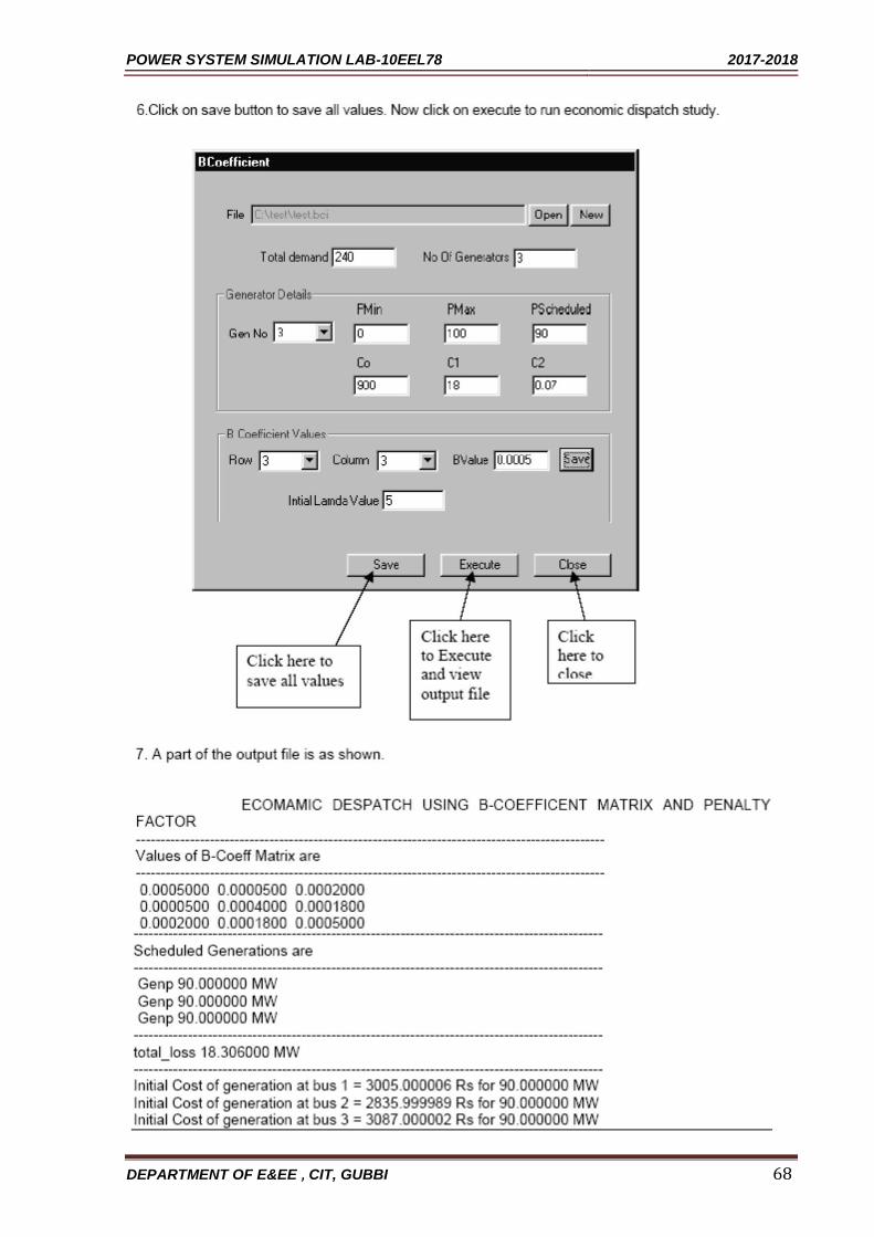
Economic dispatch 1. Double click on the MiPower icon present in the desktop. 2. Click ok and click on MiPower button, then select super user than click ok. 3. Click on tools menu and select economic dispatch by B-coefficient. 4. Click on new button create a new file, and save it. 5. Enter the value of load demand, number of generators and B-Coefficient and save. 6. Enter initial lamda value as 5. 7. Click on save and then execute.

Note: B-coefficient B00= B01= B10= B02= B20= B30= B03=0



Exercise Problems:

1. Data given:

Total No. of Generators : 2

Total Demand : 100MW

GENERATOR RATINGS:

GENERATOR 1: Pscheduled = 70 MW ; Pmin= 0.0MW; Pmax= 100MW

C0 = 50 ; C1 = 16 ; C2 = 0.015

Cg1 = 50 + 16 P1 + 0.015 P12 Rs / hr

GENERATOR 2: Pscheduled = 70 MW; Pmin= 0.0MW; Pmax= 100MW

C0 = 30 ; C1 = 12 ; C2 = 0.025

Cg1 = 30 + 12 P1 + 0.025 P12 Rs / hr

Loss ( or B) Co- efficients :

B11 = 0.005; B12 = B21 = 0.0012; B22 = 0.002

2. Given the cost equation and loss Co-efficient of different units in a plant determine

economic generation using the available software package for a total load demand of _____ MW ( typically 150 MW for 2 units and 250 MW for 3 Units) neglecting transmission losses.

3. Given the cost equation and loss Co-efficient of different units in a plant determine

penalty factor, economic generation and total transmission loss using the available

software package for a total load demand of _____ MW ( typically 150 MW for 2



units and 250 MW for 3 Units) .

Refer below questions for Q(2) & Q(3)

A)

Unit No. Cost of Fuel input in Rs./ hr.

1 C1 = 800 + 20 P1 + 0.05 P12

0 ≤ P1 ≤ 100

2 C2 = 1000 + 15 P2 + 0.06 P22

0 ≤ P2 ≤ 100

3 C3 = 900 + 18 P3 + 0.07 P32

0 ≤ P3 ≤ 100


B11 = 0.0005 B12 = 0.00005 B13 = 0.0002

B22 = 0.0004 B23 = 0.00018 B33 = 0.0005

B21 = B12 B32 = B23 B13 = B31

B)

Unit No. Cost of Fuel input in Rs./ hr.

1 C1 = 50 + 16 P1 + 0.015 P12

0 ≤ P1 ≤ 100

2 C2 = 30 + 12 P2 + 0.025 P22

0 ≤ P2 ≤ 100


B11 = 0.005 B12 = B21 = -0.0012 B22 = 0.002



Viva Questions

1. What is Single line diagram? 2. What are the components of Power system?

3. What is a bus? 4. What is bus admittance matrix?

5. What is bus impedance matrix? 6. What is load flow study?

7. What are the information that obtained from a load flow study? 8. What is the need for load flow study?

9. What are quantities that are associated with each bus in a system? 10. What are the different types of buses in a power system?

11. Define Voltage controlled bus. 12. What is PQ-bus?

13. What is Swing (or Slack) bus? 14. What is the need for Slack bus?

15. What are the iterative methods mainly used for the solution of load flow problems? 16. Why do we go for iterative methods to solve load flow problems?

17. What do you mean by flat voltage start? 18. When the generator bus is treated as load bus? 19. What will be the reactive power and bus voltage when the generator bus is treated

as load bus? 20. What are the advantages and disadvantages of Gauss-Seidel method? 21. How approximation is performed in Newton-Raphson method?

22. What is Jacobian matrix? 23. What are the advantages and disadvantages of Newton-Raphson method?

24. What is the need for voltage control in a Power system? 25. What is the reason for changes in bus voltage?

26. What is infinite bus? 27. How the reactive power of a generator is controlled?

28. What is the draw back in series connected capacitor? 29. What is synchronous capacitor?

30. What is tap changing transformer? How Voltage control is achieved in it? 31. What is regulating transformer?

32. What is Booster transformer? 33. What is off-nominal transformer ratio?

34. What is meant by a fault? 35. Why fault occurs in a power system?

36. How the faults are classified? 37. List the various types of Shunt and Series faults.

38. List the Symmetrical and unsymmetrical faults. 39. Name any two methods of reducing short-circuit current. 40. Name the main difference in representation of power system for load flow and

short circuit studies. 41. Write the relative frequency of occurrence of various types of faults. 42. What is meant by fault calculation?

43. What is the need for short circuit studies or fault analysis? 44. What is the reason for transients during short circuits?

45. What is meant by doubling effect? 46. Define DC off-set current.

47. What is synchronous reactance?



48. Define sub transient reactance? 49. Define transient reactance?

50. What is the significance of sub transient reactance in short circuit studies? 51. What is the significance of transient reactance in short circuit studies?

52. Why the armature current decreases when the flux diminishes? 53. Give one application of sub transient reactance. 54. Name the fault in which positive, negative and zero sequence component currents

are equal. 55. Name the fault in which positive and negative sequence component currents are

together is equal and zero sequence current in magnitude 56. Define negative sequence impedance. 57. Name the faults which do not have zero sequence current flowing.

58. Name the faults involving ground. 59. Define positive sequence impedance 60. In what type of fault the positive sequence component of current is equal in

magnitude but opposite in phase to negative sequence components of current? 61. In which fault negative and zero sequence currents are absent? 62. Define stability.

63. Define steady state stability. 64. Define transient stability.

65. What is steady state stability limit? 66. What is transient stability limit?

67. How stability studies are classified? What are they? 68. Define synchronizing coefficient.

69. Define swing curve. 70. What is the use of swing curve?

71. Define power angle. 72. For the swing equation M d2δ/dt2 = Pa, What will be the value of Pa during

steady state operation? 73. Name the two ways by which transient stability study can be made in a system where

one machine is swinging with respect to an infinite bus. 74. Define critical clearing time and critical clearing angle.

75. List the methods of improving the transient stability limit of a power system. 76. State equal area criterion.

77. Define efficiency of lines. 78. Define regulation of lines. 79. In Which method, for a long transmission line, for a particular receiving end

voltage, when sending end voltage is calculated, it is more than the actual value. 80. What will be the power factor of the load if, in a short transmission line, resistance

and inductive reactance are found to be equal and regulation appears to be zero. 81. In which of the models of Transmission lines, is the full charging current assumed to

flow over half the length of the line only? 82. What is infinite line? 83. What is Short Transmission line?

84. What is Medium Transmission line? 85. What is Long Transmission line?



MODEL QUESTIONS

1. Formation of Jacobian for a system not exceeding 4 buses * (no PV buses) in polar. A

Three-Bus system is given below. The system parameters are given in the Table A and

the load and generation data in Table B . Line impedances are marked in per unit on a

100MVA Base, and line charging susceptances are neglected. Taking bus 1 as Slack

bus. Obtain the load

G Slack [1] 1

PQ[2]

PQ [3]

Bus No Bus Voltage Generation Load

MW Mvar MW Mvar

1 1.05+j0.0 -- -- 0 0

2 -- 0 0 50 20

3 -- 0 0 60 25

Bus Code (i-k) Impedance (p.u) Zik Line charging

Admittance (p.u) Yi

1-2 0.08+j0.24 0

1-3 0.02+j0.06 0

2-3 0.06+j0.18 0



2. Figure below shows a single line diagram of a 5bus system with 2 generating units, 7

lines. Per unit transmission line series impedances and shunt susceptances are given on

100MVA Base, real power generation, real & reactive power loads in MW and MVAR

are given in the accompanying table with bus1 as slack, obtain a load flow solution

with Y-bus using Gauss-Siedel method and Newton Rapson method. Take acceleration

factors as 1.4 and tolerances of 0.0001 and 0.0001 per unit for the real and imaginary

components of voltage and 0.01 per unit tolerance for the change in the real and

reactive bus powers.

G

(3) (4)

(1) Table: 1.1

Bus code Impedance Line

From-To R+jX Charging

B/2

1-2 0.02+j0.06 j 0.030

1-3 0.08+j0.24 j 0.025

2-3 0.06+j0.18 j 0.020

2-4 0.06+j0.18 j 0.020

2-5 0.04+j0.12 j 0.015 (2)

(5)

G 3-4 0.01+j0.03 j 0.010

4-5 0.08+j0.24 j 0.025

Table: 1.2

Bus Bus Generation Generation Load LoadMV

No Voltage MW MVAR MW AR

1 1.00+j0.0 0 0 0 0

2 1.00+j0.0 40 30 20 10

3 1.00+j0.0 0 0 45 15

4 1.00+j0.0 0 0 40 5

5 1.00+j0.0 0 0 60 10



3. Determine the power angle curve and obtain the Graph for the given detail

Terminal Voltage = 1 p.u

Terminal Angle = 17.455 degree

Infinite bus voltage = 1 p.u

Xe = 0.2 p.u

X1 = 0.3

4. Cost equation & loss co-efficients of different units in a plant are given. Determine

economic Generation for a total load demand of 240MW.

C1 = 0.05 P12+20P1+800 0<=P1<=100

C2 = 0.06P22+15P2+1000 0<=P2<=100

C3 = 0.07P32+18P3+900 0<=P3<=100

Loss co-efficients:

B11=0.0005; B12=0.00005; B13=0.0002;

B22=0.0004; B23=0.00018; B33=0.0005;

B21=B12; B23=B32; B13=B31

5. Write a program to find ABCD parameters for short line. Calculate Vr& Ir for the

given Vs and Is or Calculate Vs& Is for the given Vr and Ir.

Z=0.2+0.408i; Y=0+3.14e-6i.Vs=132 Is=174.96- 131.22i

6. Write a program to find ABCD parameters for long line network Calculate Vr & Ir for

the given Vs and Is or Calculate Vs& Is for the given Vr and Ir.

Z=0.2+0.408i; Y=0+3.14e-6i. Vs=132 Is=174.96-131.22i

7. Write a program to find ABCD parameters for medium line PI network Calculate Vr &

Ir for the given Vs and Is or Calculate Vs& Is for the given Vr and Ir.

Z= 2+0.408i; Y=0+3.14e-6i. Vs=132 Is=174.96- 131.22i

8. Write a program to find ABCD parameters for medium line T network Calculate Vr & Ir

for the given Vs and Is or Calculate Vs& Is for the given Vr and Ir.

Z= 2+0.408i; Y=0+3.14e-6i. Vs=132 Is=174.96- 131.22i



9. Figure shown below represents the single line diagram of 6-bus system with two

identical Generating units, five lines and two transformers per unit transmission line

series impedances and shunt susceptances are given on 100MVA base, generator’s

transient impedance and Transformer leakage reactances are given in accompanying

table.

G

1

3 4

5 6

2

G

If a 3-phase to ground fault occurs at bus5, find the fault MVA. The data is given below.


p-q Zpq Y’pq/2

3-4 0.00+j0.15 0

3-5 0.00+j0.10 0

3-6 0.00+j0.20 0

5-6 0.00+j0.15 0

4-6 0.00+j0.10 0

Generator details:

G1=G2=100MVA, 11KV with X’d=10%

Transformer details:

T1=T2= 11/110KV, 100MVA, leakage reactance= X = 5%

All impedances are on 100MVA base



10. Write a program to form Y-bus using singular transformation method without

mutual Coupling.

p q Z hlc Y(ADM)

Z= [ 5 4 0.02+0.06i 0.03i

5 1 0.08+0.24i 0.025i

4 1 0.06+0.18i 0.02i

4 2 0.06+0.18i 0.02i

4 3 0.04+0.12i 0.015i

1 2 0.01+0.03i 0.01i

2 3 0.08+0.24i 0.025i ]

11. Write a program to form Y-bus using singular transformation method with mutual

coupling.

p qZ mno mutual

Z= [ 0 1 0.6i 0 0

0 2 0.5i 1 0.1i

2 3 0.5i 0 0

0 1 0.4i 1 0.2i

1 3 0.2i 0 0];

12. Write a program to form Y-bus using Inspection method

p q Z hlc Y(ADM)

Z= [ 5 4 0.02+0.06i 0.03i 0.9

5 1 0.08+0.24i 0.025i 1

4 1 0.06+0.18i 0.02i 1

4 2 0.06+0.18i 0.02i 1

4 3 0.04+0.12i 0.015i 1

1 2 0.01+0.03i 0.01i 0.8

2 3 0.08+0.24i 0.025i 1]

13. Write a program to obtain swing curve when the fault is

cleared Ps=0.9,e=1,v=1,m=0.00028,xe=0.35,xl=0.2



14. Write a program to obtain swing curve for the sustained

fault Ps=0.9,e=1,v=1,m=0.00028,xe=0.35,xl=0.3

15. Write a program for Determination of bus currents, bus power &line flows for a

specified system voltage (bus) profile.

INPUT Data:

Line data= [3 3

1 2 0.02 0.04 0

1 3 0.01 0.03 0

2 3 0.0125 0.025 0]

Bus data= [1 1.05 0

2 0.98183 -3.5

3 1.00125 -2.8624]

16. Write a program to perform load flow analysis using Gauss siedel method.

Y = [3-12i -2+8i -1+4i 0

-2+8i 3.66-14.664i -0.666+2.664i -1+4i

-1+4i -0.666+2.664i 3.66-14.664i -2+8i

0 -1+4i -2+8i 3-12i]

17. Write program for the formation of Zbus using Zbus building

algorithm Z= [ 1 1 0 0.25

2 2 1 0.1

3 3 1 0.1

4 2 0 0.25

5 2 3 0.1];



ADDITIONAL PROGRAMS


identical Generating units, seven lines and two transformers per unit transmission line



table

If a 1-phase to ground fault occurs at bus5, find the fault MVA. The data is given below.


p-q Zpq Y’pq/2

1-2 0.005+j0.0563 0.079

1-3 0.0057+j0.0714 0

1-6 0.005+j0.045 0

3-4 0.0045+j0.0409 0.179

4-5 0.0044+j0.05 0.153

5-6 0.004+j0.05 0.0745

2-6 0.005+j0.05 0

Generator details:








identical Generating units, five lines and two transformers per unit transmission line



table.

If a 3-phase occurs at bus4, find the fault MVA. The data is given below.

Generator details:







3. For the given circuit, find the fault currents, voltages for the following type of faults

at Specified location.

1. Single Line to Ground Fault

2. Double line to Ground Fault 3. Line to Line Fault

4. Double line fault

Bus 1 Bus 2 Bus 3 Bus 4

∆ Y Y ∆ G1

X1= X2= 10Ω G2

100MVA

100MVA X0= 50Ω 100MVA

22.5kV/265kV

22.5 kV 22.5 kV

X = 0.1pu

X’’

= 0.17 X’’

= 0.4

X2 = 0.19 X2 = 0.45

X0= 0.05 X0= 0.15

Xn = 0.07pu

4. Write a program to form Y-bus using Inspection method

p q Z hlc Y(ADM)

Z= [ 5 4 0.01+0.05i 0.02i 0.8

5 1 0.08+0.24i 0.025i 1

4 1 0.06+0.15i 0.03i 1

4 2 0.02+0.18i 0.03i 1

4 3 0.05+0.14i 0.013i 1

1 2 0.03+0.03i 0.02i 0.9

2 3 0.09+0.24i 0.025i 1]

5. Write a program to obtain swing curve when the fault is

cleared Ps=0.8,e=1,v=1,m=0.00058,xe=0.25,xl=0.1


power system simulation lab lab manual - · pdf file02 a. formation of y- bus using singular...

Documents