power system simulation lab
TRANSCRIPT

Power Systems Simulation Lab GRIETEEE
1
POWER SYSTEMS SIMULATION LAB
IV YEAR I SEM
EEE
By
Dr J Sridevi
Syed Sarfaraz Nawaz
GSandhya Rani
Gokaraju Rangaraju Institute of Engineering amp
Technology
Bachupally
Power Systems Simulation Lab GRIETEEE
2
GOKARAJU RANGARAJU INSTITUTE OF
ENGINEERING AND TECHNOLOGY
(Autonomous)
Bachupally Hyderabad-500 072
CERTIFICATE
This is to certify that it is a record of practical work done in
the Power Systems Simulation Laboratory in I sem of IV
year during the year ________________________
Name
Roll No
Branch EEE
Signature of staff member
Power Systems Simulation Lab GRIETEEE
3
INDEX
SNo Date Topic Page no Signature of
the Faculty
1 Sinusoidal Voltages and Currents 1
2 Equivalent circuit of a Transformer 6
3 Determination of voltage and power at
the sending end voltage regulation using
medium line model
14
4 Determination of line performance when
loaded at receiving end
19
5 Formation of bus Admittance matrix 25
6 Load flow Solution using Gauss Seidel
Method
30
7 Load flow solution using Newton
Raphson method in Rectangular
Coordinates
37
8 a) Optimal dispatch neglecting Losses
b) Optimal dispatch including Losses
41
47
9 Transient Response of an RLC Circuit 51
10 Three phase short circuit analysis in a
Synchronous Machine
57
11 Unsymmetrical Fault Analysis 63
12 Zbus Building Algorithm 73
Power Systems Simulation Lab GRIETEEE
4
13 a) Obtain Symmetrical components of a
set of Unbalanced currents
b) Obtain the original Unbalanced phase
voltages from Symmetrical Components
78
82
14 Short Circuit Analysis of 14 bus system 86
15 Load Frequency control of a single area
system
90
16 Load frequency control of a two area
system
95
17 Step response of rotor angle and
generator frequency of a Synchronous
Machine
100
18
19
20
21
22
23
24
25
26
27
Power Systems Simulation Lab GRIETEEE
1
Date Experiment-1
SINUSOIDAL VOLTAGES AND CURRENTS
Aim To determine sinusoidal voltages and currents
Apparatus MATLAB
Theory The RMS Voltage of an AC Waveform
The RMS value is the square root of the mean (average) value of the squared function of the
instantaneous values The symbols used for defining an RMS value are VRMS or IRMS
The term RMS refers to time-varying sinusoidal voltages currents or complex waveforms were
the magnitude of the waveform changes over time and is not used in DC circuit analysis or
calculations were the magnitude is always constant When used to compare the equivalent RMS
voltage value of an alternating sinusoidal waveform that supplies the same electrical power to a
given load as an equivalent DC circuit the RMS value is called the ldquoeffective valuerdquo and is
presented as Veffor Ieff
In other words the effective value is an equivalent DC value which tells you how many volts or
amps of DC that a time-varying sinusoidal waveform is equal to in terms of its ability to produce
the same power For example the domestic mains supply in the United Kingdom is 240Vac This
value is assumed to indicate an effective value of ldquo240 Volts RMSrdquo This means then that the
sinusoidal RMS voltage from the wall sockets of a UK home is capable of producing the same
average positive power as 240 volts of steady DC voltage as shown below
RMS Voltage Equivalent
Power Systems Simulation Lab GRIETEEE
2
Circuit diagram
Fig Simulink model for voltage and current measurement
Procedure
1 Open Matlab--gtSimulink--gt File ---gt New---gt Model
2 Open Simulink Library and browse the components
3 Connect the components as per circuit diagram
4 Set the desired voltage and required frequency
5 Simulate the circuit using MATLAB
6 Plot the waveforms
Power Systems Simulation Lab GRIETEEE
3
Graph
Calculations
Power Systems Simulation Lab GRIETEEE
4
Power Systems Simulation Lab GRIETEEE
5
Result
Power Systems Simulation Lab GRIETEEE
6
Signature of the faculty
Date Experiment-2
EQUIVALENT CIRCUIT OF TRANSFORMER
Aim To determine the parameters of equivalent circuit of transformer from OC SC test
data
Apparatus MATLAB
Theory Equivalent Circuit of Transformer
Equivalent impedance of transformer is essential to be calculated because the electrical power
transformer is an electrical power system equipment for estimating different parameters of
electrical power system which may be required to calculate total internal impedance of an
electrical power transformer viewing from primary side or secondary side as per requirement
This calculation requires equivalent circuit of transformer referred to primary or equivalent
circuit of transformer referred to secondary sides respectively
Equivalent Circuit of Transformer Referred to Primary
Let us consider the transformation ratio be
In the figure right the applied voltage to the primary is V1 and
voltage across the primary winding is E1 Total electric current
supplied to primary is I1 So the voltage V1 applied to the
primary is partly dropped by I1Z1 or I1R1 + jI1X1 before it
appears across primary winding The voltage appeared across
winding is countered by primary induced emf E1 So voltage
equation of this portion of the transformer can be written as
From the vector diagram above it is found that the total
primary current I1 has two components one is no - load
component Io and the other is load component I2prime As this
Power Systems Simulation Lab GRIETEEE
7
primary current has two components or branches so there must be a parallel path with
primary winding of transformer This parallel path of electric current is known as excitation
branch of equivalent circuit of transformer The resistive and reactive branches of the
excitation circuit can be represented as
The load component I2prime flows through the
primary winding of transformer and induced
voltage across the winding is E1as shown in
the figure right This induced voltage
E1 transforms to secondary and it is E2 and
load component of primary current I2prime is
transformed to secondary as secondary
current I2 Current of secondary is I2 So the
voltage E2 across secondary winding is
partly dropped by I2Z2 or I2R2 +
jI2X2 before it appears across load The load
voltage is V2
Now if we see the voltage drop in secondary from primary side then it would be primeKprime times
greater and would be written as KZ2I2
Again I2primeN1 = I2N2
Therefore
Power Systems Simulation Lab GRIETEEE
8
From above equation secondary impedance of transformer referred to primary is
So the complete equivalent circuit of transformer referred to primary is shown in the figure
below
Approximate Equivalent Circuit of
Transformer
Since Io is very small compared to I1 it
is less than 5 of full load primary
current Io changes the voltage drop
insignificantly Hence it is good
approximation to ignore the excitation
circuit in approximate equivalent circuit
of transformer The winding resistance
and reactance being in series can now
be combined into equivalent resistance
and reactance of transformer referred to
any particular side In this case it is side 1 or primary side
Equivalent Circuit of Transformer Referred to Secondary
In similar way approximate equivalent circuit of transformer referred to secondary can be
drawn
Where equivalent impedance of transformer referred to secondary can be derived as
Power Systems Simulation Lab GRIETEEE
9
Circuit Diagram
Power Systems Simulation Lab GRIETEEE
10
Procedure
1 Open Matlab--gtSimulink--gt File ---gt New---gt Model
2 Open Simulink Library and browse the components
3 Connect the components as per circuit diagram
4 Set the desired voltage and current
5 Simulate the circuit using MATLAB
6 Plot the waveforms
Graph
Calculations
Power Systems Simulation Lab GRIETEEE
11
Power Systems Simulation Lab GRIETEEE
12
Power Systems Simulation Lab GRIETEEE
13
Result
Signature of the faculty
Power Systems Simulation Lab GRIETEEE
14
Date Experiment-3
VOLTAGE REGULATION OF A MEDIUM LINE MODEL
Aim To determine voltage and power at the sending end and to regulate the voltage using
medium line model
Apparatus MATLAB
Theory The transmission line having its effective length more than 80 km but less than
250 km is generally referred to as a medium transmission line Due to the line length being
considerably high admittance Y of the network does play a role in calculating the effective
circuit parameters unlike in the case of short transmission lines For this reason the modelling
of a medium length transmission line is done using lumped shunt admittance along with the
lumped impedance in series to the circuit
These lumped parameters of a medium length transmission line can be represented using two
different models namely-
1)Nominal Π representation
2)Nominal T representation
Letrsquos now go into the detailed discussion of these above mentioned models
Nominal Π Representation of a Medium Transmission Line
In case of a nominal Π representation
the lumped series impedance is placed
at the middle of the circuit where as
the shunt admittances are at the ends
As we can see from the diagram of the
Π network below the total lumped
shunt admittance is divided into 2
equal halves and each half with value
Y frasl 2 is placed at both the sending and the receiving end while the entire circuit impedance is
between the two The shape of the circuit so formed resembles that of a symbol Π and for
this reason it is known as the nominal Π representation of a medium transmission line It is
mainly used for determining the general circuit parameters and performing load flow analysis
Power Systems Simulation Lab GRIETEEE
15
As we can see here VS and VR is the supply and receiving end voltages respectively and
Is is the current flowing through the supply end
IR is the current flowing through the receiving end of the circuit
I1 and I3 are the values of currents flowing through the admittances And
I2 is the current through the impedance Z
Now applying KCL at node P we get
Similarly applying KCL to node Q
Now substituting equation (2) to equation (1)
Now by applying KVL to the circuit
Comparing equation (4) and (5) with the standard ABCD parameter equations
Power Systems Simulation Lab GRIETEEE
16
We derive the parameters of a medium transmission line as
Voltage regulation of transmission line is measure of change of receiving end voltage from
no-load to full load condition
Circuit Diagram
Power Systems Simulation Lab GRIETEEE
17
PROCEDURE
1 Open Matlab--gtSimulink--gt File ---gt New---gt Model
2 Open Simulink Library and browse the components
3 Connect the components as per circuit diagram
4 Set the desired voltage and required frequency
5 Simulate the circuit using MATLAB
6 Calculate the voltage regulation of medium line model
Calculations
Power Systems Simulation Lab GRIETEEE
18
Result
Signature of the faculty
Power Systems Simulation Lab GRIETEEE
19
Date Experiment-4
LINE PERFORMANCE WHEN LOADED AT RECEIVING END
Aim To determine line performance when loaded at receiving end
Apparatus MATLAB
Theory Nominal Π Representation of a Medium Transmission Line
In case of a nominal Π representation
the lumped series impedance is placed
at the middle of the circuit where as
the shunt admittances are at the ends
As we can see from the diagram of the
Π network below the total lumped
shunt admittance is divided into 2
equal halves and each half with value
Y frasl 2 is placed at both the sending and the receiving end while the entire circuit impedance is
between the two The shape of the circuit so formed resembles that of a symbol Π and for
this reason it is known as the nominal Π representation of a medium transmission line It is
mainly used for determining the general circuit parameters and performing load flow analysis
As we can see here VS and VR is the supply and receiving end voltages respectively and
Is is the current flowing through the supply end
IR is the current flowing through the receiving end of the circuit
I1 and I3 are the values of currents flowing through the admittances And
I2 is the current through the impedance Z
Now applying KCL at node P we get
(1)
Similarly applying KCL to node Q
(2)
Power Systems Simulation Lab GRIETEEE
20
Now substituting equation (2) to equation (1)
Now by applying KVL to the circuit
Comparing equation (4) and (5) with the standard ABCD parameter equations
We derive the parameters of a medium transmission line as
Voltage regulation of transmission line is measure of change of receiving end voltage from
no-load to full load condition
Power Systems Simulation Lab GRIETEEE
21
Circuit Diagram
PROCEDURE
1 Open Matlab--gtSimulink--gt File ---gt New---gt Model
2 Open Simulink Library and browse the components
3 Connect the components as per circuit diagram
4 Set the desired voltage and required frequency
5 Simulate the circuit using MATLAB
6 Obtain the line performance of a line
Graph
Power Systems Simulation Lab GRIETEEE
22
Power Systems Simulation Lab GRIETEEE
23
Power Systems Simulation Lab GRIETEEE
24
Result
Signature of the faculty
Power Systems Simulation Lab GRIETEEE
25
Date Experiment-5
FORMATION OF BUS ADMITTANCE MATRIX USING MATLAB
Aim To determine the bus admittance matrix for the given power system Network
Apparatus MATLAB 77
Theory
Formation of Y BUS matrix
Bus admittance matrix is often used in power system studiesIn most of power system
studies it is necessary to form Y-bus matrix of the system by considering certain power system
parameters depending upon the type of analysis For example in load flow analysis it is necessary
to form Y-bus matrix without taking into account the generator impedance and load impedance
In short circuit analysis the generator transient reactance and transformer impedance taken in
account in addition to line data Y-bus may be computed by inspection method only if there is
no natural coupling between the lines Shunt admittance are added to the diagonal elements
corresponding to the buses at which these are connected The off diagonal elements are
unaffected The equivalent circuit of tap changing transformer may be considered in forming[y-
bus] matrix
There are b independent equations (b = no of buses) relating the bus vectors of currents
and voltages through the bus impedance matrix and bus admittance matrix
EBUS = ZBUS IBUS
IBUS = YBUS EBUS
The relation of equation can be represented in the form
IBUS = YBUS EBUS
Where YBUS is the bus admittance matrix IBUS amp EBUS are the bus current and bus
voltage vectors respectively
Diagonal elements A diagonal element (Yii) of the bus admittance matrix YBUS is equal to
the sum total of the admittance values of all the elements incident at the busnode i
Off Diagonal elements An off-diagonal element (Yij) of the bus admittance matrix YBUS is
equal to the negative of the admittance value of the connecting element present between the
buses I and j if any
This is the principle of the rule of inspection Thus the algorithmic equations for the rule of
inspection are obtained as
Yii = Σ yij (j = 12helliphellipn)
Yij = - yij (j = 12helliphellipn)
Power Systems Simulation Lab GRIETEEE
26
For i = 12hellipn n = no of buses of the given system yij is the admittance of element
connected between buses i and j and yii is the admittance of element connected
between bus i and ground (reference bus)
Read the no Of buses no of
lines and line data
START
Initialize the Y- BUS Matrix
Consider line l = 1
i = sb(1) I= eb(1)
Y(ii) =Y(ii)+Yseries(l) +05Yseries(l)
Y(jj) =Y(jj)+Yseries(l) +05Yseries(l)
Y(ij) = -Yseries(l)
Y(ji) =Y(ij)
Is l =NL
l = l+1
Stop
NO YES
Print Y -Bus
Power Systems Simulation Lab GRIETEEE
27
MATLAB PROGRAM
function[Ybus] = ybus(zdata)
nl=zdata(1) nr=zdata(2) R=zdata(3) X=zdata(4)
nbr=length(zdata(1)) nbus = max(max(nl) max(nr))
Z = R + jX branch impedance
y= ones(nbr1)Z branch admittance
Ybus=zeros(nbusnbus) initialize Ybus to zero
for k = 1nbr formation of the off diagonal elements
if nl(k) gt 0 amp nr(k) gt 0
Ybus(nl(k)nr(k)) = Ybus(nl(k)nr(k)) - y(k)
Ybus(nr(k)nl(k)) = Ybus(nl(k)nr(k))
end
end
for n = 1nbus formation of the diagonal elements
for k = 1nbr
if nl(k) == n | nr(k) == n
Ybus(nn) = Ybus(nn) + y(k)
else end
end
end
Calculations
Power Systems Simulation Lab GRIETEEE
28
Power Systems Simulation Lab GRIETEEE
29
Result
Signature of the faculty
Power Systems Simulation Lab GRIETEEE
30
Date Experiment-6
LOAD FLOW ANALYSIS BY GAUSS SEIDEL METHOD
Aim
To carry out load flow analysis of the given power system network by Gauss Seidel
method
Apparatus MATLAB
Theory
Load flow analysis is the study conducted to determine the steady state operating
condition of the given system under given conditions A large number of numerical algorithms
have been developed and Gauss Seidel method is one of such algorithm
Problem Formulation
The performance equation of the power system may be written of
[I bus] = [Y bus][V bus] (1)
Selecting one of the buses as the reference bus we get (n-1) simultaneous equations The bus
loading equations can be written as
Ii = Pi-jQi Vi (i=123helliphelliphelliphellipn) (2)
Where
n
Pi=Re [ Σ ViYik Vk] (3)
k=1
n
Qi= -Im [ Σ ViYik Vk] (4)
k=1
The bus voltage can be written in form of
n
Vi=(10Yii)[Ii- Σ Yij Vj] (5)
j=1
jnei(i=12helliphelliphelliphellipn)amp ineslack bus
Substituting Ii in the expression for Vi we get
n
Vi new=(10Yii)[Pi-JQi Vio - Σ Yij Vio] (6)
J=1
The latest available voltages are used in the above expression we get n n
Vi new=(10Yii)[Pi-JQi Voi - Σ YijVj
n- Σ Yij Vio] (7) J=1 j=i+1
The above equation is the required formula this equation can be solved for voltages in
interactive manner During each iteration we compute all the bus voltage and check for
Power Systems Simulation Lab GRIETEEE
31
convergence is carried out by comparison with the voltages obtained at the end of previous
iteration After the solutions is obtained The stack bus real and reactive powers the reactive
power generation at other generator buses and line flows can be calculated
Algorithm
Step1 Read the data such as line data specified power specified voltages Q limits at the
generator buses and tolerance for convergences
Step2 Compute Y-bus matrix
Step3 Initialize all the bus voltages
Step4 Iter=1
Step5 Consider i=2 where irsquo is the bus number
Step6 check whether this is PV bus or PQ bus If it is PQ bus goto step 8 otherwise go to next
step
Step7 Compute Qi check for q limit violation QGi=Qi+QLi
7)a)If QGigtQi max equate QGi = Qimax Then convert it into PQ bus
7)b)If QGiltQi min equate QGi = Qi min Then convert it into PQ bus
Step8 Calculate the new value of the bus voltage using gauss seidal formula i=1 n
Vi=(10Yii) [(Pi-j Qi)vi0- Σ Yij Vj- Σ YijVj0] J=1 J=i+1
Adjust voltage magnitude of the bus to specify magnitude if Q limits are not violated
Step9 If all buses are considered go to step 10 otherwise increments the bus no i=i+1 and Go to
step6
Step10 Check for convergence If there is no convergence goes to step 11 otherwise go to
step12
Step11 Update the bus voltage using the formula
Vinew=Vi old+ α(vinew-Viold) (i=12hellipn) ine slackbus α is the acceleration factor=14
Step12 Calculate the slack bus power Q at P-V buses real and reactive give flows real and
reactance line losses and print all the results including all the bus voltages and all the
bus angles
Step13 Stop
Power Systems Simulation Lab GRIETEEE
32
START
Read
1 Primitive Y matrix
2 Bus incidence matrix A
3 Slack bus voltages
4 Real and reactive bus powers Piamp Qi
5 Voltage magnitudes and their limits
Form Ybus
Make initial assumptions
Compute the parameters Ai for i=m+1hellipn and Bik for i=12hellipn
k=12hellipn
Set iteration count r=0
Set bus count i=2 and ΔVmax=0
Test for
type of bus
Qi(r+1)
gtQi max Qi(r+1)
lt Qimin
Compute Qi(r+1)
Qi(r+1)
= Qimax Qi
(r+1) = Qimin Compute Ai
(r+1)
Compute Ai
Compute Vi
(r+1)
Compute δi(r+1)
and
Vi(r+1)
=|Vis|δi
(r+1)
Power Systems Simulation Lab GRIETEEE
33
FLOW CHART FOR GAUSS SEIDEL METHOD
Procedure
Enter the command window of the MATLAB
Create a new M ndash file by selecting File - New ndash M ndash File
Type and save the program in the editor Window
Execute the program by pressing Tools ndash Run
View the results
MATLAB program
clear
basemva=100
accuracy=0001 maxiter=100
no code mag degree MW Mvar MW Mvar Qmin Qmax Mvar
busdata=[1 1 105 00 00 00 00 00 0 0 0
2 0 10 00 25666 1102 00 00 0 0 0
3 0 10 00 1386 452 00 00 0 0 0]
bus bus R X 12B =1 for lines
linedata=[1 2 002 004 00 1
1 3 001 003 00 1
Replace Vir by Vi
(r+1) and
advance bus count i = i+1
Is ilt=n
Is
ΔVmaxlt=ε
Advance iteration
count r = r+1
Compute slack bus power P1+jQ1 and all line flows
B
A
Power Systems Simulation Lab GRIETEEE
34
2 3 00125 0025 00 1]
lfybus
lfgauss
busout
lineflow
Calculations
Power Systems Simulation Lab GRIETEEE
35
Power Systems Simulation Lab GRIETEEE
36
Result
Signature of the faculty
Power Systems Simulation Lab GRIETEEE
37
Date Experiment-7
LOAD FLOW ANALYSIS BY NEWTON RAPSHON METHOD
Aim
To carry out load flow analysis of the given power system by Newton Raphson method
Apparatus MATLAB 77
Theory
The Newton Raphson method of load flow analysis is an iterative method which approximates
the set of non-linear simultaneous equations to a set of linear simultaneous equations using
Taylorrsquos series expansion and the terms are limited to first order approximation The load flow
equations for Newton Raphson method are non-linear equations in terms of real and imaginary
part of bus voltages
where ep = Real part of Vp
fp = Imaginary part of Vp
Gpq Bpq = Conductance and Susceptances of admittance Ypq respectively
Algorithm
Step1 Input the total number of buses Input the details of series line impendence and line
charging admittance to calculate the Y-bus matrix
Step2 Assume all bus voltage as 1 per unit except slack bus
Step3 Set the iteration count as k=0 and bus count as p=1
Step4 Calculate the real and reactive power pp and qp using the formula
P=ΣvpqYpqcos(Qpq+εp-εq)
Qp=ΣVpqYpasin(qpq+εp-εa)
Evalute pp=psp-pp
Power Systems Simulation Lab GRIETEEE
38
Step5 If the bus is generator (PV) bus check the value of Qpis within the limitsIf it Violates
the limits then equate the violated limit as reactive power and treat it as PQ bus If limit is not
isolated then calculate
|vp|^r=|vgp|^rspe-|vp|r Qp=qsp-qp
Step6 Advance bus count by 1 and check if all the buses have been accounted if not go to step5
Step7 Calculate the elements of Jacobean matrix
Step8 Calculate new bus voltage increment pk and fpk
Step9 Calculate new bus voltage eph+ ep
Fp^k+1=fpK+fpK
Step10 Advance iteration count by 1 and go to step3
Step11 Evaluate bus voltage and power flows through the line
Procedure
Enter the command window of the MATLAB
Create a new M ndash file by selecting File - New ndash M ndash File
Type and save the program in the editor Window
Execute the program by pressing Tools ndash Run
View the results
MATLAB program
clear
basemva=100accuracy=0001maxiter=100
no code mag degree MW Mvar MW Mvar Qmin Qmax Mvar
busdata=[1 1 105 00 00 00 00 00 0 0 0
2 0 10 00 25666 1102 00 00 0 0 0
3 0 10 00 1386 452 00 00 0 0 0]
bus bus R X 12B =1 for lines
linedata=[1 2 002 004 00 1
1 3 001 003 00 1
2 3 00125 0025 00 1]
lfybus
lfnewton
Power Systems Simulation Lab GRIETEEE
39
busout
lineflow
Calculations
Power Systems Simulation Lab GRIETEEE
40
Result
Signature of the faculty
Power Systems Simulation Lab GRIETEEE
41
Date Experiment-8(a)
OPTIMAL DISPATCH NEGLECTING LOSSES
Aim To develop a program for solving economic dispatch problem without transmission
losses for a given load condition using direct method and Lambda-iteration method
Apparatus MATLAB
Theory
As the losses are neglected the system model can be understood as shown in Fig here n number
of generating units are connected to a common bus bar collectively meeting the total power
demand PD It should be understood that share of power demand by the units does not involve
losses
Since transmission losses are neglected total demand PD is the sum of all generations of n-
number of units For each unit a cost functions Ci is assumed and the sum of all costs computed
from these cost functions gives the total cost of production CT
Fig System with n-generators
where the cost function of the ith unit from Eq (11) is
Ci = αi + βiPi + γ
iPi
2
Now the ED problem is to minimize CT subject to the satisfaction of the following equality and
inequality constraints
Equality constraint
The total power generation by all the generating units must be equal to the power demand
Power Systems Simulation Lab GRIETEEE
42
where Pi = power generated by ith unit
PD = total power demand
Inequality constraint
Each generator should generate power within the limits imposed
Pi
min le Pi le Pi
max i = 1 2 hellip n
Economic dispatch problem can be carried out by excluding or including generator power
limits ie the inequality constraint
The constrained total cost function can be converted into an unconstrained function by using
the Lagrange multiplier as
The conditions for minimization of objective function can be found by equating partial
differentials of the unconstrained function to zero as
Since Ci = C1 + C2+hellip+Cn
From the above equation the coordinate equations can be written as
The second condition can be obtained from the following equation
Power Systems Simulation Lab GRIETEEE
43
Equations Required for the ED solution
For a known value of λ the power generated by the ith unit from can be written as
which can be written as
The required value of λ is
The value of λ can be calculated and compute the values of Pi for i = 1 2hellip n for optimal
scheduling of generation
POWER WORLD bus diagram
Power Systems Simulation Lab GRIETEEE
44
Procedure
Create a new file in edit mode by selecting File - New File
Browse the components and build the bus sytem
Execute the program in run mode by selecting tools-opf areas-select opf
Run the primal lp
View the results in case information-Generator fuel costs
Tabulate the results
Results
Generator
Name
Gen
MW IOA IOB IOC
Min
MW
Max
MW
Cost
$Hr Lambda
1 7952 150 5 011 10 250 124312 2249
2 126 600 12 0085 10 300 210066 2262
3 114 335 1 01225 10 270 204101 2893
Total Cost = 5384 79$hr
Power Systems Simulation Lab GRIETEEE
45
Calculations
Power Systems Simulation Lab GRIETEEE
46
Result
Signature of the faculty
Power Systems Simulation Lab GRIETEEE
47
Date Experiment-8(b)
OPTIMAL DISPATCH INCLUDING LOSSES
Aim To develop a program for solving economic dispatch problem including transmission
losses for a given load condition using direct method and Lambda-iteration method
Apparatus MATLAB
Theory When the transmission losses are included in the economic dispatch problem we can
modify (54) as
LOSSNT PPPPP 21
where PLOSS is the total line loss Since PT is assumed to be constant we have
LOSSN dPdPdPdP 210
In the above equation dPLOSS includes the power loss due to every generator ie
N
N
LOSSLOSSLOSSLOSS dP
P
PdP
P
PdP
P
PdP
2
2
1
1
Also minimum generation cost implies dfT = 0 as given Multiplying by and combing we get
N
N
LOSSLOSSLOSS dPP
PdP
P
PdP
P
P
2
2
1
1
0
Adding with we obtain
N
i
i
i
LOSS
i
T dPP
P
P
f
1
0
The above equation satisfies when
NiP
P
P
f
i
LOSS
i
T 10
Again since
NiP
df
P
f
i
T
i
T 1
Power Systems Simulation Lab GRIETEEE
48
we get
N
N
N
i
LdP
dfL
dP
dfL
dP
df 2
2
21
1
where Li is called the penalty factor of load-i and is given by
NiPP
LiLOSS
i 11
1
Consider an area with N number of units The power generated are defined by the vector
TNPPPP 21
Then the transmission losses are expressed in general as
BPPP T
LOSS
where B is a symmetric matrix given by
NNNN
N
N
BBB
BBB
BBB
B
21
22212
11211
The elements Bij of the matrix B are called the loss coefficients These coefficients are not
constant but vary with plant loading However for the simplified calculation of the penalty factor
Li these coefficients are often assumed to be constant
Power Systems Simulation Lab GRIETEEE
49
Circuit Diagram
`
Power Systems Simulation Lab GRIETEEE
50
Procedure
Create a new file in edit mode by selecting File - New File
Browse the components and build the bus sytem
Execute the program in run mode by selecting tools-opf areas-select opf
Run the primal lp
View the results in case information-Generator fuel costs
Tabulate the results
Results
Generator
Name
Gen
MW IOA IOB IOC IOD
Min
MW
Max
MW
Cost
$Hr Lambda
1 10638 150 5 011 0 10 250 192666 284
2 126 600 12 0085 0 10 300 210066 2262
3 8622 335 1 01225 0 10 270 133184 2212
Total Cost =
535915$hr
Power Systems Simulation Lab GRIETEEE
51
Power Systems Simulation Lab GRIETEEE
52
Result
Signature of the faculty
Power Systems Simulation Lab GRIETEEE
53
Date Experiment-9
TRANSIENT RESPONSE OF A RLC CIRCUIT
Aim To obtain the transient response of an RLC circuit with its damping frequency and
damping ratio using MATLAB
Apparatus MATLAB
Theory RLC circuits are widely used in a variety of applications such as filters in
communications systems ignition systems in automobiles defibrillator circuits in biomedical
applications etc The analysis of RLC circuits is more complex than of the RC circuits we have
seen in the previous lab RLC circuits have a much richer and interesting response than the
previously studied RC or RL circuits A summary of the response is given below
Lets assume a series RLC circuit The discussion is also applicable to other RLC circuits such as
the parallel circuit
Figure 1 Series RLC circuit
By writing KVL one gets a second order differential equation The solution consists of two parts
x(t) = xn(t) + xp(t)
in which xn(t) is the complementary solution (=solution of the homogeneous differential equation
also called the natural response) and a xp(t) is the particular solution (also called forced
response) Lets focus on the complementary solution The form of this solution depends on the
roots of the characteristic equation
in which is the damping ratio and is the undamped resonant frequency The roots of the
quadratic equation are equal to
For the example of the series RLC circuit one has the following characteristic equation for the
current iL(t) or vC(t)
s2 + RLs + 1LC =0
Depending on the value of the damping ratio one has three possible cases
Case 1 Critically damped response two equal roots s= s1= s2
Power Systems Simulation Lab GRIETEEE
54
The total response consists of the sum of the
complementary and the particular solution The case of
a critically damped response to a unit input step
function
Case 2 Overdamped response two real and unequal roots s1 and
s2
Case 3 Underdamped response two complex roots
Procedure
Enter the command window of the MATLAB
Create a new M ndash file by selecting File - New ndash M ndash File
Type and save the program in the editor Window
Execute the program by pressing Tools ndash Run
View the results
MATLAB Program
wn = input(Enter value of undamped natural frequency)
z = input(Enter value of damping ratio)
n = [wnwn]
p = sqrt(1-z^2)
Power Systems Simulation Lab GRIETEEE
55
wd = wnp
h = [pz]
k = atan(h)
m = pi-k
tr = [mwd]
tp = [piwd]
q = zwn
ts = [4q]
r = zpi
f = [rp]
mp = exp(-f)
num = [0 0 n]
den = [1 zzwn n]
s = tf(numden)
hold on
step(s)
impulse(s)
hold off
Result
Enter value of undamped natural frequency 16
wn = 16
Enter value of damping ratio05
z = 05000
n = 256
Power Systems Simulation Lab GRIETEEE
56
p = 08660
k = 10472
tr = 01511
tp = 02267
q = 8
ts = 05000
r = 15708
f = 18138
mp = 01630
num = 0 0 256
den = 1 4 256
Transfer function
256
---------------
s^2 + 4 s + 256
Graph
Power Systems Simulation Lab GRIETEEE
57
Calculations
Power Systems Simulation Lab GRIETEEE
58
Result
Signature of the faculty
Power Systems Simulation Lab GRIETEEE
59
Date Experiment-10
THREE PHASE SHORT CIRCUIT ANALYSIS OF A SYNCHRONOUS
MACHINE
Aim To Analyze symmetrical fault
Apparatus MATLAB
Theory The response of the armature current when a three-phase symmetrical short circuit
occurs at the terminals of an unloaded synchronous generator
It is assumed that there is no dc offset in the armature current The magnitude of the current
decreases exponentially from a high initial value The instantaneous expression for the fault
current is given by
where Vt is the magnitude of the terminal voltage α is its phase angle and
is the direct axis subtransient reactance
is the direct axis transient reactance
is the direct axis synchronous reactance
with
The time constants are
Power Systems Simulation Lab GRIETEEE
60
is the direct axis subtransient time constant
is the direct axis transient time constant
we have neglected the effect of the armature resistance hence α = π2 Let us assume that the
fault occurs at time t = 0 From (69) we get the rms value of the
current as
which is called the subtransient fault current The duration of the subtransient current is
dictated by the time constant Td As the time progresses and Td´´lt t lt Td´ the first
exponential term will start decaying and will eventually vanish However since t is still nearly
equal to zero we have the following rms value of the current
This is called the transient fault current Now as the time progress further and the second
exponential term also decays we get the following rms value of the current for the sinusoidal
steady state
In addition to the ac the fault currents will also contain the dc offset Note that a symmetrical
fault occurs when three different phases are in three different locations in the ac cycle
Therefore the dc offsets in the three phases are different The maximum value of the dc offset
is given by
where TA is the armature time constant
Procedure
1 Open Matlab--gtSimulink--gt File ---gt New---gt Model
2 Open Simulink Library and browse the components
3 Connect the components as per circuit diagram
4 Set the desired voltage and required frequency
5 Simulate the circuit using MATLAB
6 Plot the waveforms
Power Systems Simulation Lab GRIETEEE
61
Circuit Diagram
Graph
Power Systems Simulation Lab GRIETEEE
62
Calculations
Power Systems Simulation Lab GRIETEEE
63
Power Systems Simulation Lab GRIETEEE
64
Result
Signature of the faculty
Power Systems Simulation Lab GRIETEEE
65
Date Experiment-11
UNSYMMETRICAL FAULT ANALYSIS
Aim To analyze unsymmetrical fault
Apparatus MATLAB
Theory
Single Line-to-Ground Fault
The single line-to-ground fault is usually referred as ldquoshort circuitrdquo fault and occurs when one
conductor falls to ground or makes contact with the neutral wire The general representation
of a single line-to-ground fault is shown in Figure 310 where F is the fault point with
impedances Zf Figure 311 shows the sequences network diagram Phase a is usually
assumed to be the faulted phase this is for simplicity in the fault analysis calculations [1]
a
c
b
+
Vaf
-
F
Iaf Ibf = 0 Icf = 0
n
Zf
F0
Z0
N0
+
Va0
-
Ia0
F1
Z1
N1
+
Va1
-
Ia1
+
10
-
F2
Z2
N2
+
Va2
-
Ia2
3Zf
Iaf
General representation of a single Sequence network diagram of a
line-to-ground fault single line-to-ground fault
Since the zero- positive- and negative-sequence currents are equals as it can be observed
in Figure 311 Therefore
0 1 2
0 1 2
10 0
3a a a
f
I I IZ Z Z Z
Power Systems Simulation Lab GRIETEEE
66
With the results obtained for sequence currents the sequence voltages can be obtained
from
0 0
2
1 1
2
22
0 1 1 1
10 0 1
0 1
a a
b a
ac
V I
V a a I
a a IV
By solving Equation
0 0 0
1 1 1
2 2 2
10
a a
a a
a a
V Z I
V Z I
V Z I
If the single line-to-ground fault occurs on phase b or c the voltages can be found by the
relation that exists to the known phase voltage components
0
2
1
2
2
1 1 1
1
1
af a
bf a
cf a
V V
V a a V
V a a V
as
2
0 1 2
2
0 1 2
bf a a a
cf a a a
V V a V aV
V V aV a V
Line-to-Line Fault
A line-to-line fault may take place either on an overhead andor underground
transmission system and occurs when two conductors are short-circuited One of the
characteristic of this type of fault is that its fault impedance magnitude could vary over a wide
range making very hard to predict its upper and lower limits It is when the fault impedance is
zero that the highest asymmetry at the line-to-line fault occurs
The general representation of a line-to-line fault is shown in Figure 312 where F is the
fault point with impedances Zf Figure 313 shows the sequences network diagram Phase b and
c are usually assumed to be the faulted phases this is for simplicity in the fault analysis
calculations [1]
Power Systems Simulation Lab GRIETEEE
67
a
c
b
F
Iaf = 0 Ibf Icf = -Ibf
Zf
F0
Z0
N0
+
Va0 = 0
-
Ia0 = 0
Zf
F1
Z1
N1
+
Va1
-
Ia1
F2
Z2
N2
+
Va2
-
Ia2
+
10 0o
-
Sequence network diagram of a line-to-line fault Sequence network diagram of a single
line-to-line fault
It can be noticed that
0afI
bf cfI I
bc f bfV Z I
And the sequence currents can be obtained as
0 0aI
1 2
1 2
10 0a a
f
I IZ Z Z
If Zf = 0
1 2
1 2
10 0a aI I
Z Z
The fault currents for phase b and c can be obtained as
13 90bf cf aI I I
The sequence voltages can be found as
0
1 1 1
2 2 2 2 1
0
10 -
a
a a
a a a
V
V Z I
V Z I Z I
Power Systems Simulation Lab GRIETEEE
68
Finally the line-to-line voltages for a line-to-line fault can be expressed as
ab af bf
bc bf cf
ca cf af
V V V
V V V
V V V
Double Line-to-Ground Fault
A double line-to-ground fault represents a serious event that causes a significant
asymmetry in a three-phase symmetrical system and it may spread into a three-phase fault when
not clear in appropriate time The major problem when analyzing this type of fault is the
assumption of the fault impedance Zf and the value of the impedance towards the ground Zg
The general representation of a double line-to-ground fault is shown in Figure 314 where
F is the fault point with impedances Zf and the impedance from line to ground Zg Figure 315
shows the sequences network diagram Phase b and c are assumed to be the faulted phases this is
for simplicity in the fault analysis calculations
a
c
b
F
Iaf = 0 Ibf Icf
n
Zf Zf
Zg Ibf +Icf
N
Zf +3Zg
F0
Z0
N0
+
Va0
-
Ia0 Zf
F1
Z1
N1
+
Va1
-
Ia1 Zf
F2
Z2
N2
+
Va2
-
Ia2
+
10 0o
-
General representation of a Sequence network diagram
double line-to-ground fault of a double line-to-ground fault
It can be observed that
0
( )
( )
af
bf f g bf g cf
cf f g cf g bf
I
V Z Z I Z I
V Z Z I Z I
The positive-sequence currents can be found as
12 0
1
2 0
10 0
( )( 3 )( )
( ) ( 3 )
af f g
f
f f g
IZ Z Z Z Z
Z ZZ Z Z Z Z
Power Systems Simulation Lab GRIETEEE
69
02 1
2 0
( 3 )[ ]( ) ( 3 )
f ga a
f f g
Z Z ZI I
Z Z Z Z Z
20 1
2 0
( )[ ]( ) ( 3 )
fa a
f f g
Z ZI I
Z Z Z Z Z
An alternative method is
0 1 2
0 1 2
0
( )
af a a a
a a a
I I I I
I I I
If Zf and Zg are both equal to zero then the positive- negative- and zero-sequences can
be obtained from
12 0
1
2 0
10 0
( )( )( )
( )
aIZ Z
ZZ Z
02 1
2 0
( )[ ]( )
a aZ
I IZ Z
20 1
2 0
( )[ ]( )
a aZ
I IZ Z
The current for phase a is
0afI
2
0 1 2
2
0 1 2
bf a a a
cf a a a
I I a I aI
I I aI a I
The total fault current flowing into the neutral is
03n a bf cfI I I I
The resultant phase voltages from the relationship given in Equation 378 can be
expressed as
0 1 2 13
0
af a a a a
bf cf
V V V V V
V V
Power Systems Simulation Lab GRIETEEE
70
And the line-to-line voltages are
0
abf af bf af
bcf bf cf
caf cf af af
V V V V
V V V
V V V V
Circuit Diagram
Procedure
1 Open Matlab--gtSimulink--gt File ---gt New---gt Model
2 Open Simulink Library and browse the components
3 Connect the components as per circuit diagram
4 Set the desired voltage and required frequency
5 Simulate the circuit using MATLAB
6 Plot the waveforms
Power Systems Simulation Lab GRIETEEE
71
Graph
Power Systems Simulation Lab GRIETEEE
72
Power Systems Simulation Lab GRIETEEE
73
Power Systems Simulation Lab GRIETEEE
74
Result
Signature of the faculty
Power Systems Simulation Lab GRIETEEE
75
Date Experiment-12
FORMATION OF BUS IMPEDANCE MATRIX USING MATLAB
Aim To determine the bus impedance matrix for the given power system Network
Apparatus MATLAB 77
Theory
Formation of Z BUS matrix
Z-bus matrix is an important matrix used in different kinds of power system study such as
short circuit study load flow study etc In short circuit analysis the generator uses transformer
impedance must be taken into account In quality analysis the two-short element are neglected by
forming the z-bus matrix which is used to compute the voltage distribution factor This can be
largely obtained by reversing the y-bus formed by inspection method or by analytical method
Taking inverse of the y-bus for large system in time consuming Moreover modification in the
system requires whole process to be repeated to reflect the changes in the system In such cases
is computed by z-bus building algorithm
Algorithm
Step 1 Read the values such as number of lines number of buses and line data generator data
and transformer data
Step 2 Initialize y-bus matrix y-bus[i] [j] =complex(0000)
Step 3 Compute y-bus matrix by considering only line data
Step 4 Modifies the y-bus matrix by adding the transformer and the generator admittance to the
respective diagonal elements of y-bus matrix
Step 5 Compute the z-bus matrix by inverting the modified y-bus matrix
Step 6 Check the inversion by multiplying modified y-bus and z-bus matrices to check whether
the resulting matrix is unit matrix or not
Step 7 Print the z-bus matrix
Power Systems Simulation Lab GRIETEEE
76
Procedure
Enter the command window of the MATLAB
Create a new M ndash file by selecting File - New ndash M ndash File
Type and save the program in the editor Window
Execute the program by pressing Tools ndash Run
Read the no Of buses no of
lines and line data
START
Form Y bus matrix using the algorithm
Y(ii) =Y(ii)+Yseries(l) +05Yseries(l)
Y(jj) =Y(jj)+Yseries(l) +05Yseries(l)
Y(ij) = -Yseries(l)
Y(ji) =Y(ij)
Modifying the y bus by adding generator
and transformer admittances to respective
diagonal elements
Compute Z bus matrix by inverting
modified Y bus
Multiply modified Y bus and Z bus and check
whether the product is a unity matrix
Print all the results
STOP
Power Systems Simulation Lab GRIETEEE
77
View the results
MATLAB Program
function[Ybus] = ybus(zdata)
zdata(1)) nbus = max(max(nl) max(nr))
Z = R + jX branch impedance
y= ones(nbr1)Z branch admittance
Ybus=zeros(nbusnbus) initialize Ybus to zero
for k = 1nbr formation of the off diagonal elements
if nl(k) gt 0 amp nr(k) gt 0
Ybus(nl(k)nr(k)) = Ybus(nl(k)nr(k)) - y(k)
Ybus(nr(k)nl(k)) = Ybus(nl(k)nr(k))
end
end
for n = 1nbus formation of the diagonal elements
for k = 1nbr
if nl(k) == n | nr(k) == n
Ybus(nn) = Ybus(nn) + y(k)
else end
end
end
Zbus= inv(Y)
Ibus=[-j11-j12500]
Vbus=ZbusIbus
OUTPUT
Power Systems Simulation Lab GRIETEEE
78
Power Systems Simulation Lab GRIETEEE
79
Result
Signature of the faculty
Power Systems Simulation Lab GRIETEEE
80
Date Experiment-13(a)
SYMMETRICAL COMPONENTS
Aim To obtain symmetrical components of set of unbalanced currents
Apparatus MATLAB
Theory
Before we discuss the symmetrical component transformation let us first define the a-
operator
2
3
2
10120 jea j
Note that for the above operator the following relations hold
on so and
1
2
3
2
1
22403606005
1203604804
3603
2402
000
000
0
0
aeeea
aeeea
ea
ajea
jjj
jjj
j
j
Also note that we have
02
3
2
1
2
3
2
111 2 jjaa
Using the a-operator we can write from Fig 71 (b)
111
2
1 and acab aVVVaV
Similarly
2
2
222 and acab VaVaVV
Finally
000 cba VVV
The symmetrical component transformation matrix is then given by
Power Systems Simulation Lab GRIETEEE
81
c
b
a
a
a
a
V
V
V
aa
aa
V
V
V
2
2
2
1
0
1
1
111
3
1
Defining the vectors Va012 and Vabc as
c
b
a
abc
a
a
a
a
V
V
V
V
V
V
V
V
2
1
0
012
Program
V012 = [06 90
10 30
08 -30]
rankV012=length(V012(1))
if rankV012 == 2
mag= V012(1) ang=pi180V012(2)
V012r=mag(cos(ang)+jsin(ang))
elseif rankV012 ==1
V012r=V012
else
fprintf(n Symmetrical components must be expressed in a one column array in rectangular
complex form n)
fprintf( or in a two column array in polar form with 1st column magnitude amp 2nd column
n)
fprintf( phase angle in degree n)
return end
a=cos(2pi3)+jsin(2pi3)
A = [1 1 1 1 a^2 a 1 a a^2]
Vabc= AV012r
Vabcp= [abs(Vabc) 180piangle(Vabc)]
fprintf( n Unbalanced phasors n)
fprintf( Magnitude Angle Degn)
disp(Vabcp)
Vabc0=V012r(1)[1 1 1]
Vabc1=V012r(2)[1 a^2 a]
Vabc2=V012r(3)[1 a a^2]
Power Systems Simulation Lab GRIETEEE
82
Procedure
1 Open Matlab--gt File ---gt New---gt Script
2 Write the program
3 Enter F5 to run the program
4 Observe the results in MATLAB command window
Result
Vabc =
15588 + 07000i
-00000 + 04000i
-15588 + 07000i
Unbalanced phasors
Magnitude Angle Deg
17088 241825
04000 900000
17088 1558175
Power Systems Simulation Lab GRIETEEE
83
Result
Signature of the faculty
Power Systems Simulation Lab GRIETEEE
84
Date Experiment-13(b)
UNBALANCED VOLTAGES FROM SYMMETRICAL COMPONENTS
Aim To obtain the original unbalanced phase voltages from symmetrical components
Apparatus MATLAB
Theory
abca CVV 012
where C is the symmetrical component transformation matrix and is given by
aa
aaC2
2
1
1
111
3
1
The original phasor components can also be obtained from the inverse symmetrical
component transformation ie
012
1
aabc VCV
Inverting the matrix C we get
2
1
0
1
2
1
0
2
2
1
1
111
a
a
a
a
a
a
c
b
a
V
V
V
C
V
V
V
aa
aa
V
V
V
210 aaaa VVVV
21021
2
0 bbbaaab VVVaVVaVV
2102
2
10 cccaaac VVVVaaVVV
Finally if we define a set of unbalanced current phasors as Iabc and their symmetrical
components as Ia012 we can then define
012
1
012
aabc
abca
ICI
CII
Power Systems Simulation Lab GRIETEEE
85
Program
Iabc = [16 25
10 180
09 132]
rankIabc=length(Iabc(1))
if rankIabc == 2
mag= Iabc(1) ang=pi180Iabc(2)
Iabcr=mag(cos(ang)+jsin(ang))
elseif rankIabc ==1
Iabcr=Iabc
else
fprintf(n Three phasors must be expressed in a one column array in rectangular complex
form n)
fprintf( or in a two column array in polar form with 1st column magnitude amp 2nd column
n)
fprintf( phase angle in degree n)
return end
a=cos(2pi3)+jsin(2pi3)
A = [1 1 1 1 a^2 a 1 a a^2]
I012=inv(A)Iabcr
symcomp= I012
I012p = [abs(I012) 180piangle(I012)]
fprintf( n Symmetrical components n)
fprintf( Magnitude Angle Degn)
disp(I012p)
Iabc0=I012(1)[1 1 1]
Iabc1=I012(2)[1 a^2 a]
Iabc2=I012(3)[1 a a^2]
Result
symcomp =
-00507 + 04483i
09435 - 00009i
05573 + 02288i
Symmetrical components
Magnitude Angle Deg
04512 964529
09435 -00550
06024 223157
Power Systems Simulation Lab GRIETEEE
86
Power Systems Simulation Lab GRIETEEE
87
Result
Signature of the faculty
Power Systems Simulation Lab GRIETEEE
88
Date Experiment-14
SHORT CIRCUIT ANALYSIS OF 14 BUS SYSTEM
Aim To obtain the short circuit analysis for a IEEE 14 bus system
Apparatus POWERWORLD
Theory
ff IZV 44
32144
44 iV
Z
ZIZV f
ifii
We further assume that the system is unloaded before the fault occurs and that the magnitude and
phase angles of all the generator internal emfs are the same Then there will be no current
circulating anywhere in the network and the bus voltages of all the nodes before the fault will be
same and equal to Vf Then the new altered bus voltages due to the fault will be given from by
41144
4
iV
Z
ZVVV f
iifi
14 bus system
Power Systems Simulation Lab GRIETEEE
89
Procedure
Create a new file in edit mode by selecting File - New File
Browse the components and build the bus sytem
Execute the program in run mode by selecting tools-fault analysis
Select the fault on which bus and calculate
Tabulate the results
Results 3-phase fault is applied on bus 3
Bus
Number Va Vb Vc Ang A Ang B Ang C
1 041937 041937 041937 1964 -10036 13964
2 034862 034862 034862 1087 -10913 13087
3 0 0 0 0 0 0
4 029602 029602 029602 -225 -12225 11775
5 032956 032956 032956 058 -11942 12058
Power Systems Simulation Lab GRIETEEE
90
6 047538 047538 047538 -1063 -13063 10937
7 042742 042742 042742 -844 -12844 11156
8 055864 055864 055864 -1006 -13006 10994
9 041373 041373 041373 -95 -1295 1105
10 042145 042145 042145 -994 -12994 11006
11 044639 044639 044639 -1037 -13037 10963
12 046474 046474 046474 -1144 -13144 10856
13 045879 045879 045879 -1127 -13127 10873
14 042532 042532 042532 -113 -1313 1087
Fault current = 445 pu
= 186167 A
Fault current angle = -7774 deg
Power Systems Simulation Lab GRIETEEE
91
Result
Signature of the faculty
Power Systems Simulation Lab GRIETEEE
92
Date Experiment-15
LOAD FREQUENCY CONTROL OF A SINGLE AREA POWER SYSTEM
Aim To obtain the frequency response of single and two area power system using MATLAB
Apparatus MATLAB 61
Formula used
1)
2)
3)
4)
Where
D = damping coefficient
GG ndash gain of generator GT - gain of turbine
GP - gain of power
KP ndash power system constant
KT- turbine constant
KG- generator constant
TP ndash power system time constant
TG- generator time constant
Procedure
1 Open Matlab--gtSimulink--gt File ---gt New---gt Model
2 Open Simulink Library and browse the components
3 Connect the components as per circuit diagram
4 Set the desired voltage and required frequency
5 Simulate the circuit using MATLAB
6 Plot the waveforms
Power Systems Simulation Lab GRIETEEE
93
SIMULINK RESULTS
Single Area Power System Block Diagram
Graph
Power Systems Simulation Lab GRIETEEE
94
Power Systems Simulation Lab GRIETEEE
95
Power Systems Simulation Lab GRIETEEE
96
RESULT
Signature of the faculty
Power Systems Simulation Lab GRIETEEE
97
Date Experiment-16
LOAD FREQUENCY CONTROL OF A TWO AREA POWER SYSTEM
Aim To obtain the frequency response of two area power system using MATLAB
Apparatus MATLAB
Formula used
1)
2)
3)
4)
Where
D = damping coefficient
GG ndash gain of generator GT - gain of turbine
GP - gain of power
KP ndash power system constant
KT- turbine constant
KG- generator constant
TP ndash power system time constant
TG- generator time constant
Procedure
1 Open Matlab--gtSimulink--gt File ---gt New---gt Model
2 Open Simulink Library and browse the components
3 Connect the components as per circuit diagram
4 Set the desired voltage and required frequency
5 Simulate the circuit using MATLAB
6 Plot the waveforms
Power Systems Simulation Lab GRIETEEE
98
SIMULINK RESULTS
Single Area Power System Block Diagram
Graphs
Power Systems Simulation Lab GRIETEEE
99
Power Systems Simulation Lab GRIETEEE
100
Power Systems Simulation Lab GRIETEEE
101
Result
Signature of the faculty
Power Systems Simulation Lab GRIETEEE
102
Date Experiment-17
STEP RESPONSE OF A SYNCHRONOUS MACHINE
Aim To obtain step response of rotor angle and generator frequency of a synchronous
machine
Apparatus MATLAB
Circuit Diagram
Procedure
1 Open File ---gt New---gt Model
2 Open Simulink Library and browse the components
3 Connect the components as per circuit diagram
4 Set the desired voltage and required frequency
5 Simulate the circuit using MATLAB
6 Plot the waveforms
Power Systems Simulation Lab GRIETEEE
103
Graph
Power Systems Simulation Lab GRIETEEE
104
Power Systems Simulation Lab GRIETEEE
105
Result
Signature of the faculty

Power Systems Simulation Lab GRIETEEE
2
GOKARAJU RANGARAJU INSTITUTE OF
ENGINEERING AND TECHNOLOGY
(Autonomous)
Bachupally Hyderabad-500 072
CERTIFICATE
This is to certify that it is a record of practical work done in
the Power Systems Simulation Laboratory in I sem of IV
year during the year ________________________
Name
Roll No
Branch EEE
Signature of staff member
Power Systems Simulation Lab GRIETEEE
3
INDEX
SNo Date Topic Page no Signature of
the Faculty
1 Sinusoidal Voltages and Currents 1
2 Equivalent circuit of a Transformer 6
3 Determination of voltage and power at
the sending end voltage regulation using
medium line model
14
4 Determination of line performance when
loaded at receiving end
19
5 Formation of bus Admittance matrix 25
6 Load flow Solution using Gauss Seidel
Method
30
7 Load flow solution using Newton
Raphson method in Rectangular
Coordinates
37
8 a) Optimal dispatch neglecting Losses
b) Optimal dispatch including Losses
41
47
9 Transient Response of an RLC Circuit 51
10 Three phase short circuit analysis in a
Synchronous Machine
57
11 Unsymmetrical Fault Analysis 63
12 Zbus Building Algorithm 73
Power Systems Simulation Lab GRIETEEE
4
13 a) Obtain Symmetrical components of a
set of Unbalanced currents
b) Obtain the original Unbalanced phase
voltages from Symmetrical Components
78
82
14 Short Circuit Analysis of 14 bus system 86
15 Load Frequency control of a single area
system
90
16 Load frequency control of a two area
system
95
17 Step response of rotor angle and
generator frequency of a Synchronous
Machine
100
18
19
20
21
22
23
24
25
26
27
Power Systems Simulation Lab GRIETEEE
1
Date Experiment-1
SINUSOIDAL VOLTAGES AND CURRENTS
Aim To determine sinusoidal voltages and currents
Apparatus MATLAB
Theory The RMS Voltage of an AC Waveform
The RMS value is the square root of the mean (average) value of the squared function of the
instantaneous values The symbols used for defining an RMS value are VRMS or IRMS
The term RMS refers to time-varying sinusoidal voltages currents or complex waveforms were
the magnitude of the waveform changes over time and is not used in DC circuit analysis or
calculations were the magnitude is always constant When used to compare the equivalent RMS
voltage value of an alternating sinusoidal waveform that supplies the same electrical power to a
given load as an equivalent DC circuit the RMS value is called the ldquoeffective valuerdquo and is
presented as Veffor Ieff
In other words the effective value is an equivalent DC value which tells you how many volts or
amps of DC that a time-varying sinusoidal waveform is equal to in terms of its ability to produce
the same power For example the domestic mains supply in the United Kingdom is 240Vac This
value is assumed to indicate an effective value of ldquo240 Volts RMSrdquo This means then that the
sinusoidal RMS voltage from the wall sockets of a UK home is capable of producing the same
average positive power as 240 volts of steady DC voltage as shown below
RMS Voltage Equivalent
Power Systems Simulation Lab GRIETEEE
2
Circuit diagram
Fig Simulink model for voltage and current measurement
Procedure
1 Open Matlab--gtSimulink--gt File ---gt New---gt Model
2 Open Simulink Library and browse the components
3 Connect the components as per circuit diagram
4 Set the desired voltage and required frequency
5 Simulate the circuit using MATLAB
6 Plot the waveforms
Power Systems Simulation Lab GRIETEEE
3
Graph
Calculations
Power Systems Simulation Lab GRIETEEE
4
Power Systems Simulation Lab GRIETEEE
5
Result
Power Systems Simulation Lab GRIETEEE
6
Signature of the faculty
Date Experiment-2
EQUIVALENT CIRCUIT OF TRANSFORMER
Aim To determine the parameters of equivalent circuit of transformer from OC SC test
data
Apparatus MATLAB
Theory Equivalent Circuit of Transformer
Equivalent impedance of transformer is essential to be calculated because the electrical power
transformer is an electrical power system equipment for estimating different parameters of
electrical power system which may be required to calculate total internal impedance of an
electrical power transformer viewing from primary side or secondary side as per requirement
This calculation requires equivalent circuit of transformer referred to primary or equivalent
circuit of transformer referred to secondary sides respectively
Equivalent Circuit of Transformer Referred to Primary
Let us consider the transformation ratio be
In the figure right the applied voltage to the primary is V1 and
voltage across the primary winding is E1 Total electric current
supplied to primary is I1 So the voltage V1 applied to the
primary is partly dropped by I1Z1 or I1R1 + jI1X1 before it
appears across primary winding The voltage appeared across
winding is countered by primary induced emf E1 So voltage
equation of this portion of the transformer can be written as
From the vector diagram above it is found that the total
primary current I1 has two components one is no - load
component Io and the other is load component I2prime As this
Power Systems Simulation Lab GRIETEEE
7
primary current has two components or branches so there must be a parallel path with
primary winding of transformer This parallel path of electric current is known as excitation
branch of equivalent circuit of transformer The resistive and reactive branches of the
excitation circuit can be represented as
The load component I2prime flows through the
primary winding of transformer and induced
voltage across the winding is E1as shown in
the figure right This induced voltage
E1 transforms to secondary and it is E2 and
load component of primary current I2prime is
transformed to secondary as secondary
current I2 Current of secondary is I2 So the
voltage E2 across secondary winding is
partly dropped by I2Z2 or I2R2 +
jI2X2 before it appears across load The load
voltage is V2
Now if we see the voltage drop in secondary from primary side then it would be primeKprime times
greater and would be written as KZ2I2
Again I2primeN1 = I2N2
Therefore
Power Systems Simulation Lab GRIETEEE
8
From above equation secondary impedance of transformer referred to primary is
So the complete equivalent circuit of transformer referred to primary is shown in the figure
below
Approximate Equivalent Circuit of
Transformer
Since Io is very small compared to I1 it
is less than 5 of full load primary
current Io changes the voltage drop
insignificantly Hence it is good
approximation to ignore the excitation
circuit in approximate equivalent circuit
of transformer The winding resistance
and reactance being in series can now
be combined into equivalent resistance
and reactance of transformer referred to
any particular side In this case it is side 1 or primary side
Equivalent Circuit of Transformer Referred to Secondary
In similar way approximate equivalent circuit of transformer referred to secondary can be
drawn
Where equivalent impedance of transformer referred to secondary can be derived as
Power Systems Simulation Lab GRIETEEE
9
Circuit Diagram
Power Systems Simulation Lab GRIETEEE
10
Procedure
1 Open Matlab--gtSimulink--gt File ---gt New---gt Model
2 Open Simulink Library and browse the components
3 Connect the components as per circuit diagram
4 Set the desired voltage and current
5 Simulate the circuit using MATLAB
6 Plot the waveforms
Graph
Calculations
Power Systems Simulation Lab GRIETEEE
11
Power Systems Simulation Lab GRIETEEE
12
Power Systems Simulation Lab GRIETEEE
13
Result
Signature of the faculty
Power Systems Simulation Lab GRIETEEE
14
Date Experiment-3
VOLTAGE REGULATION OF A MEDIUM LINE MODEL
Aim To determine voltage and power at the sending end and to regulate the voltage using
medium line model
Apparatus MATLAB
Theory The transmission line having its effective length more than 80 km but less than
250 km is generally referred to as a medium transmission line Due to the line length being
considerably high admittance Y of the network does play a role in calculating the effective
circuit parameters unlike in the case of short transmission lines For this reason the modelling
of a medium length transmission line is done using lumped shunt admittance along with the
lumped impedance in series to the circuit
These lumped parameters of a medium length transmission line can be represented using two
different models namely-
1)Nominal Π representation
2)Nominal T representation
Letrsquos now go into the detailed discussion of these above mentioned models
Nominal Π Representation of a Medium Transmission Line
In case of a nominal Π representation
the lumped series impedance is placed
at the middle of the circuit where as
the shunt admittances are at the ends
As we can see from the diagram of the
Π network below the total lumped
shunt admittance is divided into 2
equal halves and each half with value
Y frasl 2 is placed at both the sending and the receiving end while the entire circuit impedance is
between the two The shape of the circuit so formed resembles that of a symbol Π and for
this reason it is known as the nominal Π representation of a medium transmission line It is
mainly used for determining the general circuit parameters and performing load flow analysis
Power Systems Simulation Lab GRIETEEE
15
As we can see here VS and VR is the supply and receiving end voltages respectively and
Is is the current flowing through the supply end
IR is the current flowing through the receiving end of the circuit
I1 and I3 are the values of currents flowing through the admittances And
I2 is the current through the impedance Z
Now applying KCL at node P we get
Similarly applying KCL to node Q
Now substituting equation (2) to equation (1)
Now by applying KVL to the circuit
Comparing equation (4) and (5) with the standard ABCD parameter equations
Power Systems Simulation Lab GRIETEEE
16
We derive the parameters of a medium transmission line as
Voltage regulation of transmission line is measure of change of receiving end voltage from
no-load to full load condition
Circuit Diagram
Power Systems Simulation Lab GRIETEEE
17
PROCEDURE
1 Open Matlab--gtSimulink--gt File ---gt New---gt Model
2 Open Simulink Library and browse the components
3 Connect the components as per circuit diagram
4 Set the desired voltage and required frequency
5 Simulate the circuit using MATLAB
6 Calculate the voltage regulation of medium line model
Calculations
Power Systems Simulation Lab GRIETEEE
18
Result
Signature of the faculty
Power Systems Simulation Lab GRIETEEE
19
Date Experiment-4
LINE PERFORMANCE WHEN LOADED AT RECEIVING END
Aim To determine line performance when loaded at receiving end
Apparatus MATLAB
Theory Nominal Π Representation of a Medium Transmission Line
In case of a nominal Π representation
the lumped series impedance is placed
at the middle of the circuit where as
the shunt admittances are at the ends
As we can see from the diagram of the
Π network below the total lumped
shunt admittance is divided into 2
equal halves and each half with value
Y frasl 2 is placed at both the sending and the receiving end while the entire circuit impedance is
between the two The shape of the circuit so formed resembles that of a symbol Π and for
this reason it is known as the nominal Π representation of a medium transmission line It is
mainly used for determining the general circuit parameters and performing load flow analysis
As we can see here VS and VR is the supply and receiving end voltages respectively and
Is is the current flowing through the supply end
IR is the current flowing through the receiving end of the circuit
I1 and I3 are the values of currents flowing through the admittances And
I2 is the current through the impedance Z
Now applying KCL at node P we get
(1)
Similarly applying KCL to node Q
(2)
Power Systems Simulation Lab GRIETEEE
20
Now substituting equation (2) to equation (1)
Now by applying KVL to the circuit
Comparing equation (4) and (5) with the standard ABCD parameter equations
We derive the parameters of a medium transmission line as
Voltage regulation of transmission line is measure of change of receiving end voltage from
no-load to full load condition
Power Systems Simulation Lab GRIETEEE
21
Circuit Diagram
PROCEDURE
1 Open Matlab--gtSimulink--gt File ---gt New---gt Model
2 Open Simulink Library and browse the components
3 Connect the components as per circuit diagram
4 Set the desired voltage and required frequency
5 Simulate the circuit using MATLAB
6 Obtain the line performance of a line
Graph
Power Systems Simulation Lab GRIETEEE
22
Power Systems Simulation Lab GRIETEEE
23
Power Systems Simulation Lab GRIETEEE
24
Result
Signature of the faculty
Power Systems Simulation Lab GRIETEEE
25
Date Experiment-5
FORMATION OF BUS ADMITTANCE MATRIX USING MATLAB
Aim To determine the bus admittance matrix for the given power system Network
Apparatus MATLAB 77
Theory
Formation of Y BUS matrix
Bus admittance matrix is often used in power system studiesIn most of power system
studies it is necessary to form Y-bus matrix of the system by considering certain power system
parameters depending upon the type of analysis For example in load flow analysis it is necessary
to form Y-bus matrix without taking into account the generator impedance and load impedance
In short circuit analysis the generator transient reactance and transformer impedance taken in
account in addition to line data Y-bus may be computed by inspection method only if there is
no natural coupling between the lines Shunt admittance are added to the diagonal elements
corresponding to the buses at which these are connected The off diagonal elements are
unaffected The equivalent circuit of tap changing transformer may be considered in forming[y-
bus] matrix
There are b independent equations (b = no of buses) relating the bus vectors of currents
and voltages through the bus impedance matrix and bus admittance matrix
EBUS = ZBUS IBUS
IBUS = YBUS EBUS
The relation of equation can be represented in the form
IBUS = YBUS EBUS
Where YBUS is the bus admittance matrix IBUS amp EBUS are the bus current and bus
voltage vectors respectively
Diagonal elements A diagonal element (Yii) of the bus admittance matrix YBUS is equal to
the sum total of the admittance values of all the elements incident at the busnode i
Off Diagonal elements An off-diagonal element (Yij) of the bus admittance matrix YBUS is
equal to the negative of the admittance value of the connecting element present between the
buses I and j if any
This is the principle of the rule of inspection Thus the algorithmic equations for the rule of
inspection are obtained as
Yii = Σ yij (j = 12helliphellipn)
Yij = - yij (j = 12helliphellipn)
Power Systems Simulation Lab GRIETEEE
26
For i = 12hellipn n = no of buses of the given system yij is the admittance of element
connected between buses i and j and yii is the admittance of element connected
between bus i and ground (reference bus)
Read the no Of buses no of
lines and line data
START
Initialize the Y- BUS Matrix
Consider line l = 1
i = sb(1) I= eb(1)
Y(ii) =Y(ii)+Yseries(l) +05Yseries(l)
Y(jj) =Y(jj)+Yseries(l) +05Yseries(l)
Y(ij) = -Yseries(l)
Y(ji) =Y(ij)
Is l =NL
l = l+1
Stop
NO YES
Print Y -Bus
Power Systems Simulation Lab GRIETEEE
27
MATLAB PROGRAM
function[Ybus] = ybus(zdata)
nl=zdata(1) nr=zdata(2) R=zdata(3) X=zdata(4)
nbr=length(zdata(1)) nbus = max(max(nl) max(nr))
Z = R + jX branch impedance
y= ones(nbr1)Z branch admittance
Ybus=zeros(nbusnbus) initialize Ybus to zero
for k = 1nbr formation of the off diagonal elements
if nl(k) gt 0 amp nr(k) gt 0
Ybus(nl(k)nr(k)) = Ybus(nl(k)nr(k)) - y(k)
Ybus(nr(k)nl(k)) = Ybus(nl(k)nr(k))
end
end
for n = 1nbus formation of the diagonal elements
for k = 1nbr
if nl(k) == n | nr(k) == n
Ybus(nn) = Ybus(nn) + y(k)
else end
end
end
Calculations
Power Systems Simulation Lab GRIETEEE
28
Power Systems Simulation Lab GRIETEEE
29
Result
Signature of the faculty
Power Systems Simulation Lab GRIETEEE
30
Date Experiment-6
LOAD FLOW ANALYSIS BY GAUSS SEIDEL METHOD
Aim
To carry out load flow analysis of the given power system network by Gauss Seidel
method
Apparatus MATLAB
Theory
Load flow analysis is the study conducted to determine the steady state operating
condition of the given system under given conditions A large number of numerical algorithms
have been developed and Gauss Seidel method is one of such algorithm
Problem Formulation
The performance equation of the power system may be written of
[I bus] = [Y bus][V bus] (1)
Selecting one of the buses as the reference bus we get (n-1) simultaneous equations The bus
loading equations can be written as
Ii = Pi-jQi Vi (i=123helliphelliphelliphellipn) (2)
Where
n
Pi=Re [ Σ ViYik Vk] (3)
k=1
n
Qi= -Im [ Σ ViYik Vk] (4)
k=1
The bus voltage can be written in form of
n
Vi=(10Yii)[Ii- Σ Yij Vj] (5)
j=1
jnei(i=12helliphelliphelliphellipn)amp ineslack bus
Substituting Ii in the expression for Vi we get
n
Vi new=(10Yii)[Pi-JQi Vio - Σ Yij Vio] (6)
J=1
The latest available voltages are used in the above expression we get n n
Vi new=(10Yii)[Pi-JQi Voi - Σ YijVj
n- Σ Yij Vio] (7) J=1 j=i+1
The above equation is the required formula this equation can be solved for voltages in
interactive manner During each iteration we compute all the bus voltage and check for
Power Systems Simulation Lab GRIETEEE
31
convergence is carried out by comparison with the voltages obtained at the end of previous
iteration After the solutions is obtained The stack bus real and reactive powers the reactive
power generation at other generator buses and line flows can be calculated
Algorithm
Step1 Read the data such as line data specified power specified voltages Q limits at the
generator buses and tolerance for convergences
Step2 Compute Y-bus matrix
Step3 Initialize all the bus voltages
Step4 Iter=1
Step5 Consider i=2 where irsquo is the bus number
Step6 check whether this is PV bus or PQ bus If it is PQ bus goto step 8 otherwise go to next
step
Step7 Compute Qi check for q limit violation QGi=Qi+QLi
7)a)If QGigtQi max equate QGi = Qimax Then convert it into PQ bus
7)b)If QGiltQi min equate QGi = Qi min Then convert it into PQ bus
Step8 Calculate the new value of the bus voltage using gauss seidal formula i=1 n
Vi=(10Yii) [(Pi-j Qi)vi0- Σ Yij Vj- Σ YijVj0] J=1 J=i+1
Adjust voltage magnitude of the bus to specify magnitude if Q limits are not violated
Step9 If all buses are considered go to step 10 otherwise increments the bus no i=i+1 and Go to
step6
Step10 Check for convergence If there is no convergence goes to step 11 otherwise go to
step12
Step11 Update the bus voltage using the formula
Vinew=Vi old+ α(vinew-Viold) (i=12hellipn) ine slackbus α is the acceleration factor=14
Step12 Calculate the slack bus power Q at P-V buses real and reactive give flows real and
reactance line losses and print all the results including all the bus voltages and all the
bus angles
Step13 Stop
Power Systems Simulation Lab GRIETEEE
32
START
Read
1 Primitive Y matrix
2 Bus incidence matrix A
3 Slack bus voltages
4 Real and reactive bus powers Piamp Qi
5 Voltage magnitudes and their limits
Form Ybus
Make initial assumptions
Compute the parameters Ai for i=m+1hellipn and Bik for i=12hellipn
k=12hellipn
Set iteration count r=0
Set bus count i=2 and ΔVmax=0
Test for
type of bus
Qi(r+1)
gtQi max Qi(r+1)
lt Qimin
Compute Qi(r+1)
Qi(r+1)
= Qimax Qi
(r+1) = Qimin Compute Ai
(r+1)
Compute Ai
Compute Vi
(r+1)
Compute δi(r+1)
and
Vi(r+1)
=|Vis|δi
(r+1)
Power Systems Simulation Lab GRIETEEE
33
FLOW CHART FOR GAUSS SEIDEL METHOD
Procedure
Enter the command window of the MATLAB
Create a new M ndash file by selecting File - New ndash M ndash File
Type and save the program in the editor Window
Execute the program by pressing Tools ndash Run
View the results
MATLAB program
clear
basemva=100
accuracy=0001 maxiter=100
no code mag degree MW Mvar MW Mvar Qmin Qmax Mvar
busdata=[1 1 105 00 00 00 00 00 0 0 0
2 0 10 00 25666 1102 00 00 0 0 0
3 0 10 00 1386 452 00 00 0 0 0]
bus bus R X 12B =1 for lines
linedata=[1 2 002 004 00 1
1 3 001 003 00 1
Replace Vir by Vi
(r+1) and
advance bus count i = i+1
Is ilt=n
Is
ΔVmaxlt=ε
Advance iteration
count r = r+1
Compute slack bus power P1+jQ1 and all line flows
B
A
Power Systems Simulation Lab GRIETEEE
34
2 3 00125 0025 00 1]
lfybus
lfgauss
busout
lineflow
Calculations
Power Systems Simulation Lab GRIETEEE
35
Power Systems Simulation Lab GRIETEEE
36
Result
Signature of the faculty
Power Systems Simulation Lab GRIETEEE
37
Date Experiment-7
LOAD FLOW ANALYSIS BY NEWTON RAPSHON METHOD
Aim
To carry out load flow analysis of the given power system by Newton Raphson method
Apparatus MATLAB 77
Theory
The Newton Raphson method of load flow analysis is an iterative method which approximates
the set of non-linear simultaneous equations to a set of linear simultaneous equations using
Taylorrsquos series expansion and the terms are limited to first order approximation The load flow
equations for Newton Raphson method are non-linear equations in terms of real and imaginary
part of bus voltages
where ep = Real part of Vp
fp = Imaginary part of Vp
Gpq Bpq = Conductance and Susceptances of admittance Ypq respectively
Algorithm
Step1 Input the total number of buses Input the details of series line impendence and line
charging admittance to calculate the Y-bus matrix
Step2 Assume all bus voltage as 1 per unit except slack bus
Step3 Set the iteration count as k=0 and bus count as p=1
Step4 Calculate the real and reactive power pp and qp using the formula
P=ΣvpqYpqcos(Qpq+εp-εq)
Qp=ΣVpqYpasin(qpq+εp-εa)
Evalute pp=psp-pp
Power Systems Simulation Lab GRIETEEE
38
Step5 If the bus is generator (PV) bus check the value of Qpis within the limitsIf it Violates
the limits then equate the violated limit as reactive power and treat it as PQ bus If limit is not
isolated then calculate
|vp|^r=|vgp|^rspe-|vp|r Qp=qsp-qp
Step6 Advance bus count by 1 and check if all the buses have been accounted if not go to step5
Step7 Calculate the elements of Jacobean matrix
Step8 Calculate new bus voltage increment pk and fpk
Step9 Calculate new bus voltage eph+ ep
Fp^k+1=fpK+fpK
Step10 Advance iteration count by 1 and go to step3
Step11 Evaluate bus voltage and power flows through the line
Procedure
Enter the command window of the MATLAB
Create a new M ndash file by selecting File - New ndash M ndash File
Type and save the program in the editor Window
Execute the program by pressing Tools ndash Run
View the results
MATLAB program
clear
basemva=100accuracy=0001maxiter=100
no code mag degree MW Mvar MW Mvar Qmin Qmax Mvar
busdata=[1 1 105 00 00 00 00 00 0 0 0
2 0 10 00 25666 1102 00 00 0 0 0
3 0 10 00 1386 452 00 00 0 0 0]
bus bus R X 12B =1 for lines
linedata=[1 2 002 004 00 1
1 3 001 003 00 1
2 3 00125 0025 00 1]
lfybus
lfnewton
Power Systems Simulation Lab GRIETEEE
39
busout
lineflow
Calculations
Power Systems Simulation Lab GRIETEEE
40
Result
Signature of the faculty
Power Systems Simulation Lab GRIETEEE
41
Date Experiment-8(a)
OPTIMAL DISPATCH NEGLECTING LOSSES
Aim To develop a program for solving economic dispatch problem without transmission
losses for a given load condition using direct method and Lambda-iteration method
Apparatus MATLAB
Theory
As the losses are neglected the system model can be understood as shown in Fig here n number
of generating units are connected to a common bus bar collectively meeting the total power
demand PD It should be understood that share of power demand by the units does not involve
losses
Since transmission losses are neglected total demand PD is the sum of all generations of n-
number of units For each unit a cost functions Ci is assumed and the sum of all costs computed
from these cost functions gives the total cost of production CT
Fig System with n-generators
where the cost function of the ith unit from Eq (11) is
Ci = αi + βiPi + γ
iPi
2
Now the ED problem is to minimize CT subject to the satisfaction of the following equality and
inequality constraints
Equality constraint
The total power generation by all the generating units must be equal to the power demand
Power Systems Simulation Lab GRIETEEE
42
where Pi = power generated by ith unit
PD = total power demand
Inequality constraint
Each generator should generate power within the limits imposed
Pi
min le Pi le Pi
max i = 1 2 hellip n
Economic dispatch problem can be carried out by excluding or including generator power
limits ie the inequality constraint
The constrained total cost function can be converted into an unconstrained function by using
the Lagrange multiplier as
The conditions for minimization of objective function can be found by equating partial
differentials of the unconstrained function to zero as
Since Ci = C1 + C2+hellip+Cn
From the above equation the coordinate equations can be written as
The second condition can be obtained from the following equation
Power Systems Simulation Lab GRIETEEE
43
Equations Required for the ED solution
For a known value of λ the power generated by the ith unit from can be written as
which can be written as
The required value of λ is
The value of λ can be calculated and compute the values of Pi for i = 1 2hellip n for optimal
scheduling of generation
POWER WORLD bus diagram
Power Systems Simulation Lab GRIETEEE
44
Procedure
Create a new file in edit mode by selecting File - New File
Browse the components and build the bus sytem
Execute the program in run mode by selecting tools-opf areas-select opf
Run the primal lp
View the results in case information-Generator fuel costs
Tabulate the results
Results
Generator
Name
Gen
MW IOA IOB IOC
Min
MW
Max
MW
Cost
$Hr Lambda
1 7952 150 5 011 10 250 124312 2249
2 126 600 12 0085 10 300 210066 2262
3 114 335 1 01225 10 270 204101 2893
Total Cost = 5384 79$hr
Power Systems Simulation Lab GRIETEEE
45
Calculations
Power Systems Simulation Lab GRIETEEE
46
Result
Signature of the faculty
Power Systems Simulation Lab GRIETEEE
47
Date Experiment-8(b)
OPTIMAL DISPATCH INCLUDING LOSSES
Aim To develop a program for solving economic dispatch problem including transmission
losses for a given load condition using direct method and Lambda-iteration method
Apparatus MATLAB
Theory When the transmission losses are included in the economic dispatch problem we can
modify (54) as
LOSSNT PPPPP 21
where PLOSS is the total line loss Since PT is assumed to be constant we have
LOSSN dPdPdPdP 210
In the above equation dPLOSS includes the power loss due to every generator ie
N
N
LOSSLOSSLOSSLOSS dP
P
PdP
P
PdP
P
PdP
2
2
1
1
Also minimum generation cost implies dfT = 0 as given Multiplying by and combing we get
N
N
LOSSLOSSLOSS dPP
PdP
P
PdP
P
P
2
2
1
1
0
Adding with we obtain
N
i
i
i
LOSS
i
T dPP
P
P
f
1
0
The above equation satisfies when
NiP
P
P
f
i
LOSS
i
T 10
Again since
NiP
df
P
f
i
T
i
T 1
Power Systems Simulation Lab GRIETEEE
48
we get
N
N
N
i
LdP
dfL
dP
dfL
dP
df 2
2
21
1
where Li is called the penalty factor of load-i and is given by
NiPP
LiLOSS
i 11
1
Consider an area with N number of units The power generated are defined by the vector
TNPPPP 21
Then the transmission losses are expressed in general as
BPPP T
LOSS
where B is a symmetric matrix given by
NNNN
N
N
BBB
BBB
BBB
B
21
22212
11211
The elements Bij of the matrix B are called the loss coefficients These coefficients are not
constant but vary with plant loading However for the simplified calculation of the penalty factor
Li these coefficients are often assumed to be constant
Power Systems Simulation Lab GRIETEEE
49
Circuit Diagram
`
Power Systems Simulation Lab GRIETEEE
50
Procedure
Create a new file in edit mode by selecting File - New File
Browse the components and build the bus sytem
Execute the program in run mode by selecting tools-opf areas-select opf
Run the primal lp
View the results in case information-Generator fuel costs
Tabulate the results
Results
Generator
Name
Gen
MW IOA IOB IOC IOD
Min
MW
Max
MW
Cost
$Hr Lambda
1 10638 150 5 011 0 10 250 192666 284
2 126 600 12 0085 0 10 300 210066 2262
3 8622 335 1 01225 0 10 270 133184 2212
Total Cost =
535915$hr
Power Systems Simulation Lab GRIETEEE
51
Power Systems Simulation Lab GRIETEEE
52
Result
Signature of the faculty
Power Systems Simulation Lab GRIETEEE
53
Date Experiment-9
TRANSIENT RESPONSE OF A RLC CIRCUIT
Aim To obtain the transient response of an RLC circuit with its damping frequency and
damping ratio using MATLAB
Apparatus MATLAB
Theory RLC circuits are widely used in a variety of applications such as filters in
communications systems ignition systems in automobiles defibrillator circuits in biomedical
applications etc The analysis of RLC circuits is more complex than of the RC circuits we have
seen in the previous lab RLC circuits have a much richer and interesting response than the
previously studied RC or RL circuits A summary of the response is given below
Lets assume a series RLC circuit The discussion is also applicable to other RLC circuits such as
the parallel circuit
Figure 1 Series RLC circuit
By writing KVL one gets a second order differential equation The solution consists of two parts
x(t) = xn(t) + xp(t)
in which xn(t) is the complementary solution (=solution of the homogeneous differential equation
also called the natural response) and a xp(t) is the particular solution (also called forced
response) Lets focus on the complementary solution The form of this solution depends on the
roots of the characteristic equation
in which is the damping ratio and is the undamped resonant frequency The roots of the
quadratic equation are equal to
For the example of the series RLC circuit one has the following characteristic equation for the
current iL(t) or vC(t)
s2 + RLs + 1LC =0
Depending on the value of the damping ratio one has three possible cases
Case 1 Critically damped response two equal roots s= s1= s2
Power Systems Simulation Lab GRIETEEE
54
The total response consists of the sum of the
complementary and the particular solution The case of
a critically damped response to a unit input step
function
Case 2 Overdamped response two real and unequal roots s1 and
s2
Case 3 Underdamped response two complex roots
Procedure
Enter the command window of the MATLAB
Create a new M ndash file by selecting File - New ndash M ndash File
Type and save the program in the editor Window
Execute the program by pressing Tools ndash Run
View the results
MATLAB Program
wn = input(Enter value of undamped natural frequency)
z = input(Enter value of damping ratio)
n = [wnwn]
p = sqrt(1-z^2)
Power Systems Simulation Lab GRIETEEE
55
wd = wnp
h = [pz]
k = atan(h)
m = pi-k
tr = [mwd]
tp = [piwd]
q = zwn
ts = [4q]
r = zpi
f = [rp]
mp = exp(-f)
num = [0 0 n]
den = [1 zzwn n]
s = tf(numden)
hold on
step(s)
impulse(s)
hold off
Result
Enter value of undamped natural frequency 16
wn = 16
Enter value of damping ratio05
z = 05000
n = 256
Power Systems Simulation Lab GRIETEEE
56
p = 08660
k = 10472
tr = 01511
tp = 02267
q = 8
ts = 05000
r = 15708
f = 18138
mp = 01630
num = 0 0 256
den = 1 4 256
Transfer function
256
---------------
s^2 + 4 s + 256
Graph
Power Systems Simulation Lab GRIETEEE
57
Calculations
Power Systems Simulation Lab GRIETEEE
58
Result
Signature of the faculty
Power Systems Simulation Lab GRIETEEE
59
Date Experiment-10
THREE PHASE SHORT CIRCUIT ANALYSIS OF A SYNCHRONOUS
MACHINE
Aim To Analyze symmetrical fault
Apparatus MATLAB
Theory The response of the armature current when a three-phase symmetrical short circuit
occurs at the terminals of an unloaded synchronous generator
It is assumed that there is no dc offset in the armature current The magnitude of the current
decreases exponentially from a high initial value The instantaneous expression for the fault
current is given by
where Vt is the magnitude of the terminal voltage α is its phase angle and
is the direct axis subtransient reactance
is the direct axis transient reactance
is the direct axis synchronous reactance
with
The time constants are
Power Systems Simulation Lab GRIETEEE
60
is the direct axis subtransient time constant
is the direct axis transient time constant
we have neglected the effect of the armature resistance hence α = π2 Let us assume that the
fault occurs at time t = 0 From (69) we get the rms value of the
current as
which is called the subtransient fault current The duration of the subtransient current is
dictated by the time constant Td As the time progresses and Td´´lt t lt Td´ the first
exponential term will start decaying and will eventually vanish However since t is still nearly
equal to zero we have the following rms value of the current
This is called the transient fault current Now as the time progress further and the second
exponential term also decays we get the following rms value of the current for the sinusoidal
steady state
In addition to the ac the fault currents will also contain the dc offset Note that a symmetrical
fault occurs when three different phases are in three different locations in the ac cycle
Therefore the dc offsets in the three phases are different The maximum value of the dc offset
is given by
where TA is the armature time constant
Procedure
1 Open Matlab--gtSimulink--gt File ---gt New---gt Model
2 Open Simulink Library and browse the components
3 Connect the components as per circuit diagram
4 Set the desired voltage and required frequency
5 Simulate the circuit using MATLAB
6 Plot the waveforms
Power Systems Simulation Lab GRIETEEE
61
Circuit Diagram
Graph
Power Systems Simulation Lab GRIETEEE
62
Calculations
Power Systems Simulation Lab GRIETEEE
63
Power Systems Simulation Lab GRIETEEE
64
Result
Signature of the faculty
Power Systems Simulation Lab GRIETEEE
65
Date Experiment-11
UNSYMMETRICAL FAULT ANALYSIS
Aim To analyze unsymmetrical fault
Apparatus MATLAB
Theory
Single Line-to-Ground Fault
The single line-to-ground fault is usually referred as ldquoshort circuitrdquo fault and occurs when one
conductor falls to ground or makes contact with the neutral wire The general representation
of a single line-to-ground fault is shown in Figure 310 where F is the fault point with
impedances Zf Figure 311 shows the sequences network diagram Phase a is usually
assumed to be the faulted phase this is for simplicity in the fault analysis calculations [1]
a
c
b
+
Vaf
-
F
Iaf Ibf = 0 Icf = 0
n
Zf
F0
Z0
N0
+
Va0
-
Ia0
F1
Z1
N1
+
Va1
-
Ia1
+
10
-
F2
Z2
N2
+
Va2
-
Ia2
3Zf
Iaf
General representation of a single Sequence network diagram of a
line-to-ground fault single line-to-ground fault
Since the zero- positive- and negative-sequence currents are equals as it can be observed
in Figure 311 Therefore
0 1 2
0 1 2
10 0
3a a a
f
I I IZ Z Z Z
Power Systems Simulation Lab GRIETEEE
66
With the results obtained for sequence currents the sequence voltages can be obtained
from
0 0
2
1 1
2
22
0 1 1 1
10 0 1
0 1
a a
b a
ac
V I
V a a I
a a IV
By solving Equation
0 0 0
1 1 1
2 2 2
10
a a
a a
a a
V Z I
V Z I
V Z I
If the single line-to-ground fault occurs on phase b or c the voltages can be found by the
relation that exists to the known phase voltage components
0
2
1
2
2
1 1 1
1
1
af a
bf a
cf a
V V
V a a V
V a a V
as
2
0 1 2
2
0 1 2
bf a a a
cf a a a
V V a V aV
V V aV a V
Line-to-Line Fault
A line-to-line fault may take place either on an overhead andor underground
transmission system and occurs when two conductors are short-circuited One of the
characteristic of this type of fault is that its fault impedance magnitude could vary over a wide
range making very hard to predict its upper and lower limits It is when the fault impedance is
zero that the highest asymmetry at the line-to-line fault occurs
The general representation of a line-to-line fault is shown in Figure 312 where F is the
fault point with impedances Zf Figure 313 shows the sequences network diagram Phase b and
c are usually assumed to be the faulted phases this is for simplicity in the fault analysis
calculations [1]
Power Systems Simulation Lab GRIETEEE
67
a
c
b
F
Iaf = 0 Ibf Icf = -Ibf
Zf
F0
Z0
N0
+
Va0 = 0
-
Ia0 = 0
Zf
F1
Z1
N1
+
Va1
-
Ia1
F2
Z2
N2
+
Va2
-
Ia2
+
10 0o
-
Sequence network diagram of a line-to-line fault Sequence network diagram of a single
line-to-line fault
It can be noticed that
0afI
bf cfI I
bc f bfV Z I
And the sequence currents can be obtained as
0 0aI
1 2
1 2
10 0a a
f
I IZ Z Z
If Zf = 0
1 2
1 2
10 0a aI I
Z Z
The fault currents for phase b and c can be obtained as
13 90bf cf aI I I
The sequence voltages can be found as
0
1 1 1
2 2 2 2 1
0
10 -
a
a a
a a a
V
V Z I
V Z I Z I
Power Systems Simulation Lab GRIETEEE
68
Finally the line-to-line voltages for a line-to-line fault can be expressed as
ab af bf
bc bf cf
ca cf af
V V V
V V V
V V V
Double Line-to-Ground Fault
A double line-to-ground fault represents a serious event that causes a significant
asymmetry in a three-phase symmetrical system and it may spread into a three-phase fault when
not clear in appropriate time The major problem when analyzing this type of fault is the
assumption of the fault impedance Zf and the value of the impedance towards the ground Zg
The general representation of a double line-to-ground fault is shown in Figure 314 where
F is the fault point with impedances Zf and the impedance from line to ground Zg Figure 315
shows the sequences network diagram Phase b and c are assumed to be the faulted phases this is
for simplicity in the fault analysis calculations
a
c
b
F
Iaf = 0 Ibf Icf
n
Zf Zf
Zg Ibf +Icf
N
Zf +3Zg
F0
Z0
N0
+
Va0
-
Ia0 Zf
F1
Z1
N1
+
Va1
-
Ia1 Zf
F2
Z2
N2
+
Va2
-
Ia2
+
10 0o
-
General representation of a Sequence network diagram
double line-to-ground fault of a double line-to-ground fault
It can be observed that
0
( )
( )
af
bf f g bf g cf
cf f g cf g bf
I
V Z Z I Z I
V Z Z I Z I
The positive-sequence currents can be found as
12 0
1
2 0
10 0
( )( 3 )( )
( ) ( 3 )
af f g
f
f f g
IZ Z Z Z Z
Z ZZ Z Z Z Z
Power Systems Simulation Lab GRIETEEE
69
02 1
2 0
( 3 )[ ]( ) ( 3 )
f ga a
f f g
Z Z ZI I
Z Z Z Z Z
20 1
2 0
( )[ ]( ) ( 3 )
fa a
f f g
Z ZI I
Z Z Z Z Z
An alternative method is
0 1 2
0 1 2
0
( )
af a a a
a a a
I I I I
I I I
If Zf and Zg are both equal to zero then the positive- negative- and zero-sequences can
be obtained from
12 0
1
2 0
10 0
( )( )( )
( )
aIZ Z
ZZ Z
02 1
2 0
( )[ ]( )
a aZ
I IZ Z
20 1
2 0
( )[ ]( )
a aZ
I IZ Z
The current for phase a is
0afI
2
0 1 2
2
0 1 2
bf a a a
cf a a a
I I a I aI
I I aI a I
The total fault current flowing into the neutral is
03n a bf cfI I I I
The resultant phase voltages from the relationship given in Equation 378 can be
expressed as
0 1 2 13
0
af a a a a
bf cf
V V V V V
V V
Power Systems Simulation Lab GRIETEEE
70
And the line-to-line voltages are
0
abf af bf af
bcf bf cf
caf cf af af
V V V V
V V V
V V V V
Circuit Diagram
Procedure
1 Open Matlab--gtSimulink--gt File ---gt New---gt Model
2 Open Simulink Library and browse the components
3 Connect the components as per circuit diagram
4 Set the desired voltage and required frequency
5 Simulate the circuit using MATLAB
6 Plot the waveforms
Power Systems Simulation Lab GRIETEEE
71
Graph
Power Systems Simulation Lab GRIETEEE
72
Power Systems Simulation Lab GRIETEEE
73
Power Systems Simulation Lab GRIETEEE
74
Result
Signature of the faculty
Power Systems Simulation Lab GRIETEEE
75
Date Experiment-12
FORMATION OF BUS IMPEDANCE MATRIX USING MATLAB
Aim To determine the bus impedance matrix for the given power system Network
Apparatus MATLAB 77
Theory
Formation of Z BUS matrix
Z-bus matrix is an important matrix used in different kinds of power system study such as
short circuit study load flow study etc In short circuit analysis the generator uses transformer
impedance must be taken into account In quality analysis the two-short element are neglected by
forming the z-bus matrix which is used to compute the voltage distribution factor This can be
largely obtained by reversing the y-bus formed by inspection method or by analytical method
Taking inverse of the y-bus for large system in time consuming Moreover modification in the
system requires whole process to be repeated to reflect the changes in the system In such cases
is computed by z-bus building algorithm
Algorithm
Step 1 Read the values such as number of lines number of buses and line data generator data
and transformer data
Step 2 Initialize y-bus matrix y-bus[i] [j] =complex(0000)
Step 3 Compute y-bus matrix by considering only line data
Step 4 Modifies the y-bus matrix by adding the transformer and the generator admittance to the
respective diagonal elements of y-bus matrix
Step 5 Compute the z-bus matrix by inverting the modified y-bus matrix
Step 6 Check the inversion by multiplying modified y-bus and z-bus matrices to check whether
the resulting matrix is unit matrix or not
Step 7 Print the z-bus matrix
Power Systems Simulation Lab GRIETEEE
76
Procedure
Enter the command window of the MATLAB
Create a new M ndash file by selecting File - New ndash M ndash File
Type and save the program in the editor Window
Execute the program by pressing Tools ndash Run
Read the no Of buses no of
lines and line data
START
Form Y bus matrix using the algorithm
Y(ii) =Y(ii)+Yseries(l) +05Yseries(l)
Y(jj) =Y(jj)+Yseries(l) +05Yseries(l)
Y(ij) = -Yseries(l)
Y(ji) =Y(ij)
Modifying the y bus by adding generator
and transformer admittances to respective
diagonal elements
Compute Z bus matrix by inverting
modified Y bus
Multiply modified Y bus and Z bus and check
whether the product is a unity matrix
Print all the results
STOP
Power Systems Simulation Lab GRIETEEE
77
View the results
MATLAB Program
function[Ybus] = ybus(zdata)
zdata(1)) nbus = max(max(nl) max(nr))
Z = R + jX branch impedance
y= ones(nbr1)Z branch admittance
Ybus=zeros(nbusnbus) initialize Ybus to zero
for k = 1nbr formation of the off diagonal elements
if nl(k) gt 0 amp nr(k) gt 0
Ybus(nl(k)nr(k)) = Ybus(nl(k)nr(k)) - y(k)
Ybus(nr(k)nl(k)) = Ybus(nl(k)nr(k))
end
end
for n = 1nbus formation of the diagonal elements
for k = 1nbr
if nl(k) == n | nr(k) == n
Ybus(nn) = Ybus(nn) + y(k)
else end
end
end
Zbus= inv(Y)
Ibus=[-j11-j12500]
Vbus=ZbusIbus
OUTPUT
Power Systems Simulation Lab GRIETEEE
78
Power Systems Simulation Lab GRIETEEE
79
Result
Signature of the faculty
Power Systems Simulation Lab GRIETEEE
80
Date Experiment-13(a)
SYMMETRICAL COMPONENTS
Aim To obtain symmetrical components of set of unbalanced currents
Apparatus MATLAB
Theory
Before we discuss the symmetrical component transformation let us first define the a-
operator
2
3
2
10120 jea j
Note that for the above operator the following relations hold
on so and
1
2
3
2
1
22403606005
1203604804
3603
2402
000
000
0
0
aeeea
aeeea
ea
ajea
jjj
jjj
j
j
Also note that we have
02
3
2
1
2
3
2
111 2 jjaa
Using the a-operator we can write from Fig 71 (b)
111
2
1 and acab aVVVaV
Similarly
2
2
222 and acab VaVaVV
Finally
000 cba VVV
The symmetrical component transformation matrix is then given by
Power Systems Simulation Lab GRIETEEE
81
c
b
a
a
a
a
V
V
V
aa
aa
V
V
V
2
2
2
1
0
1
1
111
3
1
Defining the vectors Va012 and Vabc as
c
b
a
abc
a
a
a
a
V
V
V
V
V
V
V
V
2
1
0
012
Program
V012 = [06 90
10 30
08 -30]
rankV012=length(V012(1))
if rankV012 == 2
mag= V012(1) ang=pi180V012(2)
V012r=mag(cos(ang)+jsin(ang))
elseif rankV012 ==1
V012r=V012
else
fprintf(n Symmetrical components must be expressed in a one column array in rectangular
complex form n)
fprintf( or in a two column array in polar form with 1st column magnitude amp 2nd column
n)
fprintf( phase angle in degree n)
return end
a=cos(2pi3)+jsin(2pi3)
A = [1 1 1 1 a^2 a 1 a a^2]
Vabc= AV012r
Vabcp= [abs(Vabc) 180piangle(Vabc)]
fprintf( n Unbalanced phasors n)
fprintf( Magnitude Angle Degn)
disp(Vabcp)
Vabc0=V012r(1)[1 1 1]
Vabc1=V012r(2)[1 a^2 a]
Vabc2=V012r(3)[1 a a^2]
Power Systems Simulation Lab GRIETEEE
82
Procedure
1 Open Matlab--gt File ---gt New---gt Script
2 Write the program
3 Enter F5 to run the program
4 Observe the results in MATLAB command window
Result
Vabc =
15588 + 07000i
-00000 + 04000i
-15588 + 07000i
Unbalanced phasors
Magnitude Angle Deg
17088 241825
04000 900000
17088 1558175
Power Systems Simulation Lab GRIETEEE
83
Result
Signature of the faculty
Power Systems Simulation Lab GRIETEEE
84
Date Experiment-13(b)
UNBALANCED VOLTAGES FROM SYMMETRICAL COMPONENTS
Aim To obtain the original unbalanced phase voltages from symmetrical components
Apparatus MATLAB
Theory
abca CVV 012
where C is the symmetrical component transformation matrix and is given by
aa
aaC2
2
1
1
111
3
1
The original phasor components can also be obtained from the inverse symmetrical
component transformation ie
012
1
aabc VCV
Inverting the matrix C we get
2
1
0
1
2
1
0
2
2
1
1
111
a
a
a
a
a
a
c
b
a
V
V
V
C
V
V
V
aa
aa
V
V
V
210 aaaa VVVV
21021
2
0 bbbaaab VVVaVVaVV
2102
2
10 cccaaac VVVVaaVVV
Finally if we define a set of unbalanced current phasors as Iabc and their symmetrical
components as Ia012 we can then define
012
1
012
aabc
abca
ICI
CII
Power Systems Simulation Lab GRIETEEE
85
Program
Iabc = [16 25
10 180
09 132]
rankIabc=length(Iabc(1))
if rankIabc == 2
mag= Iabc(1) ang=pi180Iabc(2)
Iabcr=mag(cos(ang)+jsin(ang))
elseif rankIabc ==1
Iabcr=Iabc
else
fprintf(n Three phasors must be expressed in a one column array in rectangular complex
form n)
fprintf( or in a two column array in polar form with 1st column magnitude amp 2nd column
n)
fprintf( phase angle in degree n)
return end
a=cos(2pi3)+jsin(2pi3)
A = [1 1 1 1 a^2 a 1 a a^2]
I012=inv(A)Iabcr
symcomp= I012
I012p = [abs(I012) 180piangle(I012)]
fprintf( n Symmetrical components n)
fprintf( Magnitude Angle Degn)
disp(I012p)
Iabc0=I012(1)[1 1 1]
Iabc1=I012(2)[1 a^2 a]
Iabc2=I012(3)[1 a a^2]
Result
symcomp =
-00507 + 04483i
09435 - 00009i
05573 + 02288i
Symmetrical components
Magnitude Angle Deg
04512 964529
09435 -00550
06024 223157
Power Systems Simulation Lab GRIETEEE
86
Power Systems Simulation Lab GRIETEEE
87
Result
Signature of the faculty
Power Systems Simulation Lab GRIETEEE
88
Date Experiment-14
SHORT CIRCUIT ANALYSIS OF 14 BUS SYSTEM
Aim To obtain the short circuit analysis for a IEEE 14 bus system
Apparatus POWERWORLD
Theory
ff IZV 44
32144
44 iV
Z
ZIZV f
ifii
We further assume that the system is unloaded before the fault occurs and that the magnitude and
phase angles of all the generator internal emfs are the same Then there will be no current
circulating anywhere in the network and the bus voltages of all the nodes before the fault will be
same and equal to Vf Then the new altered bus voltages due to the fault will be given from by
41144
4
iV
Z
ZVVV f
iifi
14 bus system
Power Systems Simulation Lab GRIETEEE
89
Procedure
Create a new file in edit mode by selecting File - New File
Browse the components and build the bus sytem
Execute the program in run mode by selecting tools-fault analysis
Select the fault on which bus and calculate
Tabulate the results
Results 3-phase fault is applied on bus 3
Bus
Number Va Vb Vc Ang A Ang B Ang C
1 041937 041937 041937 1964 -10036 13964
2 034862 034862 034862 1087 -10913 13087
3 0 0 0 0 0 0
4 029602 029602 029602 -225 -12225 11775
5 032956 032956 032956 058 -11942 12058
Power Systems Simulation Lab GRIETEEE
90
6 047538 047538 047538 -1063 -13063 10937
7 042742 042742 042742 -844 -12844 11156
8 055864 055864 055864 -1006 -13006 10994
9 041373 041373 041373 -95 -1295 1105
10 042145 042145 042145 -994 -12994 11006
11 044639 044639 044639 -1037 -13037 10963
12 046474 046474 046474 -1144 -13144 10856
13 045879 045879 045879 -1127 -13127 10873
14 042532 042532 042532 -113 -1313 1087
Fault current = 445 pu
= 186167 A
Fault current angle = -7774 deg
Power Systems Simulation Lab GRIETEEE
91
Result
Signature of the faculty
Power Systems Simulation Lab GRIETEEE
92
Date Experiment-15
LOAD FREQUENCY CONTROL OF A SINGLE AREA POWER SYSTEM
Aim To obtain the frequency response of single and two area power system using MATLAB
Apparatus MATLAB 61
Formula used
1)
2)
3)
4)
Where
D = damping coefficient
GG ndash gain of generator GT - gain of turbine
GP - gain of power
KP ndash power system constant
KT- turbine constant
KG- generator constant
TP ndash power system time constant
TG- generator time constant
Procedure
1 Open Matlab--gtSimulink--gt File ---gt New---gt Model
2 Open Simulink Library and browse the components
3 Connect the components as per circuit diagram
4 Set the desired voltage and required frequency
5 Simulate the circuit using MATLAB
6 Plot the waveforms
Power Systems Simulation Lab GRIETEEE
93
SIMULINK RESULTS
Single Area Power System Block Diagram
Graph
Power Systems Simulation Lab GRIETEEE
94
Power Systems Simulation Lab GRIETEEE
95
Power Systems Simulation Lab GRIETEEE
96
RESULT
Signature of the faculty
Power Systems Simulation Lab GRIETEEE
97
Date Experiment-16
LOAD FREQUENCY CONTROL OF A TWO AREA POWER SYSTEM
Aim To obtain the frequency response of two area power system using MATLAB
Apparatus MATLAB
Formula used
1)
2)
3)
4)
Where
D = damping coefficient
GG ndash gain of generator GT - gain of turbine
GP - gain of power
KP ndash power system constant
KT- turbine constant
KG- generator constant
TP ndash power system time constant
TG- generator time constant
Procedure
1 Open Matlab--gtSimulink--gt File ---gt New---gt Model
2 Open Simulink Library and browse the components
3 Connect the components as per circuit diagram
4 Set the desired voltage and required frequency
5 Simulate the circuit using MATLAB
6 Plot the waveforms
Power Systems Simulation Lab GRIETEEE
98
SIMULINK RESULTS
Single Area Power System Block Diagram
Graphs
Power Systems Simulation Lab GRIETEEE
99
Power Systems Simulation Lab GRIETEEE
100
Power Systems Simulation Lab GRIETEEE
101
Result
Signature of the faculty
Power Systems Simulation Lab GRIETEEE
102
Date Experiment-17
STEP RESPONSE OF A SYNCHRONOUS MACHINE
Aim To obtain step response of rotor angle and generator frequency of a synchronous
machine
Apparatus MATLAB
Circuit Diagram
Procedure
1 Open File ---gt New---gt Model
2 Open Simulink Library and browse the components
3 Connect the components as per circuit diagram
4 Set the desired voltage and required frequency
5 Simulate the circuit using MATLAB
6 Plot the waveforms
Power Systems Simulation Lab GRIETEEE
103
Graph
Power Systems Simulation Lab GRIETEEE
104
Power Systems Simulation Lab GRIETEEE
105
Result
Signature of the faculty

Power Systems Simulation Lab GRIETEEE
3
INDEX
SNo Date Topic Page no Signature of
the Faculty
1 Sinusoidal Voltages and Currents 1
2 Equivalent circuit of a Transformer 6
3 Determination of voltage and power at
the sending end voltage regulation using
medium line model
14
4 Determination of line performance when
loaded at receiving end
19
5 Formation of bus Admittance matrix 25
6 Load flow Solution using Gauss Seidel
Method
30
7 Load flow solution using Newton
Raphson method in Rectangular
Coordinates
37
8 a) Optimal dispatch neglecting Losses
b) Optimal dispatch including Losses
41
47
9 Transient Response of an RLC Circuit 51
10 Three phase short circuit analysis in a
Synchronous Machine
57
11 Unsymmetrical Fault Analysis 63
12 Zbus Building Algorithm 73
Power Systems Simulation Lab GRIETEEE
4
13 a) Obtain Symmetrical components of a
set of Unbalanced currents
b) Obtain the original Unbalanced phase
voltages from Symmetrical Components
78
82
14 Short Circuit Analysis of 14 bus system 86
15 Load Frequency control of a single area
system
90
16 Load frequency control of a two area
system
95
17 Step response of rotor angle and
generator frequency of a Synchronous
Machine
100
18
19
20
21
22
23
24
25
26
27
Power Systems Simulation Lab GRIETEEE
1
Date Experiment-1
SINUSOIDAL VOLTAGES AND CURRENTS
Aim To determine sinusoidal voltages and currents
Apparatus MATLAB
Theory The RMS Voltage of an AC Waveform
The RMS value is the square root of the mean (average) value of the squared function of the
instantaneous values The symbols used for defining an RMS value are VRMS or IRMS
The term RMS refers to time-varying sinusoidal voltages currents or complex waveforms were
the magnitude of the waveform changes over time and is not used in DC circuit analysis or
calculations were the magnitude is always constant When used to compare the equivalent RMS
voltage value of an alternating sinusoidal waveform that supplies the same electrical power to a
given load as an equivalent DC circuit the RMS value is called the ldquoeffective valuerdquo and is
presented as Veffor Ieff
In other words the effective value is an equivalent DC value which tells you how many volts or
amps of DC that a time-varying sinusoidal waveform is equal to in terms of its ability to produce
the same power For example the domestic mains supply in the United Kingdom is 240Vac This
value is assumed to indicate an effective value of ldquo240 Volts RMSrdquo This means then that the
sinusoidal RMS voltage from the wall sockets of a UK home is capable of producing the same
average positive power as 240 volts of steady DC voltage as shown below
RMS Voltage Equivalent
Power Systems Simulation Lab GRIETEEE
2
Circuit diagram
Fig Simulink model for voltage and current measurement
Procedure
1 Open Matlab--gtSimulink--gt File ---gt New---gt Model
2 Open Simulink Library and browse the components
3 Connect the components as per circuit diagram
4 Set the desired voltage and required frequency
5 Simulate the circuit using MATLAB
6 Plot the waveforms
Power Systems Simulation Lab GRIETEEE
3
Graph
Calculations
Power Systems Simulation Lab GRIETEEE
4
Power Systems Simulation Lab GRIETEEE
5
Result
Power Systems Simulation Lab GRIETEEE
6
Signature of the faculty
Date Experiment-2
EQUIVALENT CIRCUIT OF TRANSFORMER
Aim To determine the parameters of equivalent circuit of transformer from OC SC test
data
Apparatus MATLAB
Theory Equivalent Circuit of Transformer
Equivalent impedance of transformer is essential to be calculated because the electrical power
transformer is an electrical power system equipment for estimating different parameters of
electrical power system which may be required to calculate total internal impedance of an
electrical power transformer viewing from primary side or secondary side as per requirement
This calculation requires equivalent circuit of transformer referred to primary or equivalent
circuit of transformer referred to secondary sides respectively
Equivalent Circuit of Transformer Referred to Primary
Let us consider the transformation ratio be
In the figure right the applied voltage to the primary is V1 and
voltage across the primary winding is E1 Total electric current
supplied to primary is I1 So the voltage V1 applied to the
primary is partly dropped by I1Z1 or I1R1 + jI1X1 before it
appears across primary winding The voltage appeared across
winding is countered by primary induced emf E1 So voltage
equation of this portion of the transformer can be written as
From the vector diagram above it is found that the total
primary current I1 has two components one is no - load
component Io and the other is load component I2prime As this
Power Systems Simulation Lab GRIETEEE
7
primary current has two components or branches so there must be a parallel path with
primary winding of transformer This parallel path of electric current is known as excitation
branch of equivalent circuit of transformer The resistive and reactive branches of the
excitation circuit can be represented as
The load component I2prime flows through the
primary winding of transformer and induced
voltage across the winding is E1as shown in
the figure right This induced voltage
E1 transforms to secondary and it is E2 and
load component of primary current I2prime is
transformed to secondary as secondary
current I2 Current of secondary is I2 So the
voltage E2 across secondary winding is
partly dropped by I2Z2 or I2R2 +
jI2X2 before it appears across load The load
voltage is V2
Now if we see the voltage drop in secondary from primary side then it would be primeKprime times
greater and would be written as KZ2I2
Again I2primeN1 = I2N2
Therefore
Power Systems Simulation Lab GRIETEEE
8
From above equation secondary impedance of transformer referred to primary is
So the complete equivalent circuit of transformer referred to primary is shown in the figure
below
Approximate Equivalent Circuit of
Transformer
Since Io is very small compared to I1 it
is less than 5 of full load primary
current Io changes the voltage drop
insignificantly Hence it is good
approximation to ignore the excitation
circuit in approximate equivalent circuit
of transformer The winding resistance
and reactance being in series can now
be combined into equivalent resistance
and reactance of transformer referred to
any particular side In this case it is side 1 or primary side
Equivalent Circuit of Transformer Referred to Secondary
In similar way approximate equivalent circuit of transformer referred to secondary can be
drawn
Where equivalent impedance of transformer referred to secondary can be derived as
Power Systems Simulation Lab GRIETEEE
9
Circuit Diagram
Power Systems Simulation Lab GRIETEEE
10
Procedure
1 Open Matlab--gtSimulink--gt File ---gt New---gt Model
2 Open Simulink Library and browse the components
3 Connect the components as per circuit diagram
4 Set the desired voltage and current
5 Simulate the circuit using MATLAB
6 Plot the waveforms
Graph
Calculations
Power Systems Simulation Lab GRIETEEE
11
Power Systems Simulation Lab GRIETEEE
12
Power Systems Simulation Lab GRIETEEE
13
Result
Signature of the faculty
Power Systems Simulation Lab GRIETEEE
14
Date Experiment-3
VOLTAGE REGULATION OF A MEDIUM LINE MODEL
Aim To determine voltage and power at the sending end and to regulate the voltage using
medium line model
Apparatus MATLAB
Theory The transmission line having its effective length more than 80 km but less than
250 km is generally referred to as a medium transmission line Due to the line length being
considerably high admittance Y of the network does play a role in calculating the effective
circuit parameters unlike in the case of short transmission lines For this reason the modelling
of a medium length transmission line is done using lumped shunt admittance along with the
lumped impedance in series to the circuit
These lumped parameters of a medium length transmission line can be represented using two
different models namely-
1)Nominal Π representation
2)Nominal T representation
Letrsquos now go into the detailed discussion of these above mentioned models
Nominal Π Representation of a Medium Transmission Line
In case of a nominal Π representation
the lumped series impedance is placed
at the middle of the circuit where as
the shunt admittances are at the ends
As we can see from the diagram of the
Π network below the total lumped
shunt admittance is divided into 2
equal halves and each half with value
Y frasl 2 is placed at both the sending and the receiving end while the entire circuit impedance is
between the two The shape of the circuit so formed resembles that of a symbol Π and for
this reason it is known as the nominal Π representation of a medium transmission line It is
mainly used for determining the general circuit parameters and performing load flow analysis
Power Systems Simulation Lab GRIETEEE
15
As we can see here VS and VR is the supply and receiving end voltages respectively and
Is is the current flowing through the supply end
IR is the current flowing through the receiving end of the circuit
I1 and I3 are the values of currents flowing through the admittances And
I2 is the current through the impedance Z
Now applying KCL at node P we get
Similarly applying KCL to node Q
Now substituting equation (2) to equation (1)
Now by applying KVL to the circuit
Comparing equation (4) and (5) with the standard ABCD parameter equations
Power Systems Simulation Lab GRIETEEE
16
We derive the parameters of a medium transmission line as
Voltage regulation of transmission line is measure of change of receiving end voltage from
no-load to full load condition
Circuit Diagram
Power Systems Simulation Lab GRIETEEE
17
PROCEDURE
1 Open Matlab--gtSimulink--gt File ---gt New---gt Model
2 Open Simulink Library and browse the components
3 Connect the components as per circuit diagram
4 Set the desired voltage and required frequency
5 Simulate the circuit using MATLAB
6 Calculate the voltage regulation of medium line model
Calculations
Power Systems Simulation Lab GRIETEEE
18
Result
Signature of the faculty
Power Systems Simulation Lab GRIETEEE
19
Date Experiment-4
LINE PERFORMANCE WHEN LOADED AT RECEIVING END
Aim To determine line performance when loaded at receiving end
Apparatus MATLAB
Theory Nominal Π Representation of a Medium Transmission Line
In case of a nominal Π representation
the lumped series impedance is placed
at the middle of the circuit where as
the shunt admittances are at the ends
As we can see from the diagram of the
Π network below the total lumped
shunt admittance is divided into 2
equal halves and each half with value
Y frasl 2 is placed at both the sending and the receiving end while the entire circuit impedance is
between the two The shape of the circuit so formed resembles that of a symbol Π and for
this reason it is known as the nominal Π representation of a medium transmission line It is
mainly used for determining the general circuit parameters and performing load flow analysis
As we can see here VS and VR is the supply and receiving end voltages respectively and
Is is the current flowing through the supply end
IR is the current flowing through the receiving end of the circuit
I1 and I3 are the values of currents flowing through the admittances And
I2 is the current through the impedance Z
Now applying KCL at node P we get
(1)
Similarly applying KCL to node Q
(2)
Power Systems Simulation Lab GRIETEEE
20
Now substituting equation (2) to equation (1)
Now by applying KVL to the circuit
Comparing equation (4) and (5) with the standard ABCD parameter equations
We derive the parameters of a medium transmission line as
Voltage regulation of transmission line is measure of change of receiving end voltage from
no-load to full load condition
Power Systems Simulation Lab GRIETEEE
21
Circuit Diagram
PROCEDURE
1 Open Matlab--gtSimulink--gt File ---gt New---gt Model
2 Open Simulink Library and browse the components
3 Connect the components as per circuit diagram
4 Set the desired voltage and required frequency
5 Simulate the circuit using MATLAB
6 Obtain the line performance of a line
Graph
Power Systems Simulation Lab GRIETEEE
22
Power Systems Simulation Lab GRIETEEE
23
Power Systems Simulation Lab GRIETEEE
24
Result
Signature of the faculty
Power Systems Simulation Lab GRIETEEE
25
Date Experiment-5
FORMATION OF BUS ADMITTANCE MATRIX USING MATLAB
Aim To determine the bus admittance matrix for the given power system Network
Apparatus MATLAB 77
Theory
Formation of Y BUS matrix
Bus admittance matrix is often used in power system studiesIn most of power system
studies it is necessary to form Y-bus matrix of the system by considering certain power system
parameters depending upon the type of analysis For example in load flow analysis it is necessary
to form Y-bus matrix without taking into account the generator impedance and load impedance
In short circuit analysis the generator transient reactance and transformer impedance taken in
account in addition to line data Y-bus may be computed by inspection method only if there is
no natural coupling between the lines Shunt admittance are added to the diagonal elements
corresponding to the buses at which these are connected The off diagonal elements are
unaffected The equivalent circuit of tap changing transformer may be considered in forming[y-
bus] matrix
There are b independent equations (b = no of buses) relating the bus vectors of currents
and voltages through the bus impedance matrix and bus admittance matrix
EBUS = ZBUS IBUS
IBUS = YBUS EBUS
The relation of equation can be represented in the form
IBUS = YBUS EBUS
Where YBUS is the bus admittance matrix IBUS amp EBUS are the bus current and bus
voltage vectors respectively
Diagonal elements A diagonal element (Yii) of the bus admittance matrix YBUS is equal to
the sum total of the admittance values of all the elements incident at the busnode i
Off Diagonal elements An off-diagonal element (Yij) of the bus admittance matrix YBUS is
equal to the negative of the admittance value of the connecting element present between the
buses I and j if any
This is the principle of the rule of inspection Thus the algorithmic equations for the rule of
inspection are obtained as
Yii = Σ yij (j = 12helliphellipn)
Yij = - yij (j = 12helliphellipn)
Power Systems Simulation Lab GRIETEEE
26
For i = 12hellipn n = no of buses of the given system yij is the admittance of element
connected between buses i and j and yii is the admittance of element connected
between bus i and ground (reference bus)
Read the no Of buses no of
lines and line data
START
Initialize the Y- BUS Matrix
Consider line l = 1
i = sb(1) I= eb(1)
Y(ii) =Y(ii)+Yseries(l) +05Yseries(l)
Y(jj) =Y(jj)+Yseries(l) +05Yseries(l)
Y(ij) = -Yseries(l)
Y(ji) =Y(ij)
Is l =NL
l = l+1
Stop
NO YES
Print Y -Bus
Power Systems Simulation Lab GRIETEEE
27
MATLAB PROGRAM
function[Ybus] = ybus(zdata)
nl=zdata(1) nr=zdata(2) R=zdata(3) X=zdata(4)
nbr=length(zdata(1)) nbus = max(max(nl) max(nr))
Z = R + jX branch impedance
y= ones(nbr1)Z branch admittance
Ybus=zeros(nbusnbus) initialize Ybus to zero
for k = 1nbr formation of the off diagonal elements
if nl(k) gt 0 amp nr(k) gt 0
Ybus(nl(k)nr(k)) = Ybus(nl(k)nr(k)) - y(k)
Ybus(nr(k)nl(k)) = Ybus(nl(k)nr(k))
end
end
for n = 1nbus formation of the diagonal elements
for k = 1nbr
if nl(k) == n | nr(k) == n
Ybus(nn) = Ybus(nn) + y(k)
else end
end
end
Calculations
Power Systems Simulation Lab GRIETEEE
28
Power Systems Simulation Lab GRIETEEE
29
Result
Signature of the faculty
Power Systems Simulation Lab GRIETEEE
30
Date Experiment-6
LOAD FLOW ANALYSIS BY GAUSS SEIDEL METHOD
Aim
To carry out load flow analysis of the given power system network by Gauss Seidel
method
Apparatus MATLAB
Theory
Load flow analysis is the study conducted to determine the steady state operating
condition of the given system under given conditions A large number of numerical algorithms
have been developed and Gauss Seidel method is one of such algorithm
Problem Formulation
The performance equation of the power system may be written of
[I bus] = [Y bus][V bus] (1)
Selecting one of the buses as the reference bus we get (n-1) simultaneous equations The bus
loading equations can be written as
Ii = Pi-jQi Vi (i=123helliphelliphelliphellipn) (2)
Where
n
Pi=Re [ Σ ViYik Vk] (3)
k=1
n
Qi= -Im [ Σ ViYik Vk] (4)
k=1
The bus voltage can be written in form of
n
Vi=(10Yii)[Ii- Σ Yij Vj] (5)
j=1
jnei(i=12helliphelliphelliphellipn)amp ineslack bus
Substituting Ii in the expression for Vi we get
n
Vi new=(10Yii)[Pi-JQi Vio - Σ Yij Vio] (6)
J=1
The latest available voltages are used in the above expression we get n n
Vi new=(10Yii)[Pi-JQi Voi - Σ YijVj
n- Σ Yij Vio] (7) J=1 j=i+1
The above equation is the required formula this equation can be solved for voltages in
interactive manner During each iteration we compute all the bus voltage and check for
Power Systems Simulation Lab GRIETEEE
31
convergence is carried out by comparison with the voltages obtained at the end of previous
iteration After the solutions is obtained The stack bus real and reactive powers the reactive
power generation at other generator buses and line flows can be calculated
Algorithm
Step1 Read the data such as line data specified power specified voltages Q limits at the
generator buses and tolerance for convergences
Step2 Compute Y-bus matrix
Step3 Initialize all the bus voltages
Step4 Iter=1
Step5 Consider i=2 where irsquo is the bus number
Step6 check whether this is PV bus or PQ bus If it is PQ bus goto step 8 otherwise go to next
step
Step7 Compute Qi check for q limit violation QGi=Qi+QLi
7)a)If QGigtQi max equate QGi = Qimax Then convert it into PQ bus
7)b)If QGiltQi min equate QGi = Qi min Then convert it into PQ bus
Step8 Calculate the new value of the bus voltage using gauss seidal formula i=1 n
Vi=(10Yii) [(Pi-j Qi)vi0- Σ Yij Vj- Σ YijVj0] J=1 J=i+1
Adjust voltage magnitude of the bus to specify magnitude if Q limits are not violated
Step9 If all buses are considered go to step 10 otherwise increments the bus no i=i+1 and Go to
step6
Step10 Check for convergence If there is no convergence goes to step 11 otherwise go to
step12
Step11 Update the bus voltage using the formula
Vinew=Vi old+ α(vinew-Viold) (i=12hellipn) ine slackbus α is the acceleration factor=14
Step12 Calculate the slack bus power Q at P-V buses real and reactive give flows real and
reactance line losses and print all the results including all the bus voltages and all the
bus angles
Step13 Stop
Power Systems Simulation Lab GRIETEEE
32
START
Read
1 Primitive Y matrix
2 Bus incidence matrix A
3 Slack bus voltages
4 Real and reactive bus powers Piamp Qi
5 Voltage magnitudes and their limits
Form Ybus
Make initial assumptions
Compute the parameters Ai for i=m+1hellipn and Bik for i=12hellipn
k=12hellipn
Set iteration count r=0
Set bus count i=2 and ΔVmax=0
Test for
type of bus
Qi(r+1)
gtQi max Qi(r+1)
lt Qimin
Compute Qi(r+1)
Qi(r+1)
= Qimax Qi
(r+1) = Qimin Compute Ai
(r+1)
Compute Ai
Compute Vi
(r+1)
Compute δi(r+1)
and
Vi(r+1)
=|Vis|δi
(r+1)
Power Systems Simulation Lab GRIETEEE
33
FLOW CHART FOR GAUSS SEIDEL METHOD
Procedure
Enter the command window of the MATLAB
Create a new M ndash file by selecting File - New ndash M ndash File
Type and save the program in the editor Window
Execute the program by pressing Tools ndash Run
View the results
MATLAB program
clear
basemva=100
accuracy=0001 maxiter=100
no code mag degree MW Mvar MW Mvar Qmin Qmax Mvar
busdata=[1 1 105 00 00 00 00 00 0 0 0
2 0 10 00 25666 1102 00 00 0 0 0
3 0 10 00 1386 452 00 00 0 0 0]
bus bus R X 12B =1 for lines
linedata=[1 2 002 004 00 1
1 3 001 003 00 1
Replace Vir by Vi
(r+1) and
advance bus count i = i+1
Is ilt=n
Is
ΔVmaxlt=ε
Advance iteration
count r = r+1
Compute slack bus power P1+jQ1 and all line flows
B
A
Power Systems Simulation Lab GRIETEEE
34
2 3 00125 0025 00 1]
lfybus
lfgauss
busout
lineflow
Calculations
Power Systems Simulation Lab GRIETEEE
35
Power Systems Simulation Lab GRIETEEE
36
Result
Signature of the faculty
Power Systems Simulation Lab GRIETEEE
37
Date Experiment-7
LOAD FLOW ANALYSIS BY NEWTON RAPSHON METHOD
Aim
To carry out load flow analysis of the given power system by Newton Raphson method
Apparatus MATLAB 77
Theory
The Newton Raphson method of load flow analysis is an iterative method which approximates
the set of non-linear simultaneous equations to a set of linear simultaneous equations using
Taylorrsquos series expansion and the terms are limited to first order approximation The load flow
equations for Newton Raphson method are non-linear equations in terms of real and imaginary
part of bus voltages
where ep = Real part of Vp
fp = Imaginary part of Vp
Gpq Bpq = Conductance and Susceptances of admittance Ypq respectively
Algorithm
Step1 Input the total number of buses Input the details of series line impendence and line
charging admittance to calculate the Y-bus matrix
Step2 Assume all bus voltage as 1 per unit except slack bus
Step3 Set the iteration count as k=0 and bus count as p=1
Step4 Calculate the real and reactive power pp and qp using the formula
P=ΣvpqYpqcos(Qpq+εp-εq)
Qp=ΣVpqYpasin(qpq+εp-εa)
Evalute pp=psp-pp
Power Systems Simulation Lab GRIETEEE
38
Step5 If the bus is generator (PV) bus check the value of Qpis within the limitsIf it Violates
the limits then equate the violated limit as reactive power and treat it as PQ bus If limit is not
isolated then calculate
|vp|^r=|vgp|^rspe-|vp|r Qp=qsp-qp
Step6 Advance bus count by 1 and check if all the buses have been accounted if not go to step5
Step7 Calculate the elements of Jacobean matrix
Step8 Calculate new bus voltage increment pk and fpk
Step9 Calculate new bus voltage eph+ ep
Fp^k+1=fpK+fpK
Step10 Advance iteration count by 1 and go to step3
Step11 Evaluate bus voltage and power flows through the line
Procedure
Enter the command window of the MATLAB
Create a new M ndash file by selecting File - New ndash M ndash File
Type and save the program in the editor Window
Execute the program by pressing Tools ndash Run
View the results
MATLAB program
clear
basemva=100accuracy=0001maxiter=100
no code mag degree MW Mvar MW Mvar Qmin Qmax Mvar
busdata=[1 1 105 00 00 00 00 00 0 0 0
2 0 10 00 25666 1102 00 00 0 0 0
3 0 10 00 1386 452 00 00 0 0 0]
bus bus R X 12B =1 for lines
linedata=[1 2 002 004 00 1
1 3 001 003 00 1
2 3 00125 0025 00 1]
lfybus
lfnewton
Power Systems Simulation Lab GRIETEEE
39
busout
lineflow
Calculations
Power Systems Simulation Lab GRIETEEE
40
Result
Signature of the faculty
Power Systems Simulation Lab GRIETEEE
41
Date Experiment-8(a)
OPTIMAL DISPATCH NEGLECTING LOSSES
Aim To develop a program for solving economic dispatch problem without transmission
losses for a given load condition using direct method and Lambda-iteration method
Apparatus MATLAB
Theory
As the losses are neglected the system model can be understood as shown in Fig here n number
of generating units are connected to a common bus bar collectively meeting the total power
demand PD It should be understood that share of power demand by the units does not involve
losses
Since transmission losses are neglected total demand PD is the sum of all generations of n-
number of units For each unit a cost functions Ci is assumed and the sum of all costs computed
from these cost functions gives the total cost of production CT
Fig System with n-generators
where the cost function of the ith unit from Eq (11) is
Ci = αi + βiPi + γ
iPi
2
Now the ED problem is to minimize CT subject to the satisfaction of the following equality and
inequality constraints
Equality constraint
The total power generation by all the generating units must be equal to the power demand
Power Systems Simulation Lab GRIETEEE
42
where Pi = power generated by ith unit
PD = total power demand
Inequality constraint
Each generator should generate power within the limits imposed
Pi
min le Pi le Pi
max i = 1 2 hellip n
Economic dispatch problem can be carried out by excluding or including generator power
limits ie the inequality constraint
The constrained total cost function can be converted into an unconstrained function by using
the Lagrange multiplier as
The conditions for minimization of objective function can be found by equating partial
differentials of the unconstrained function to zero as
Since Ci = C1 + C2+hellip+Cn
From the above equation the coordinate equations can be written as
The second condition can be obtained from the following equation
Power Systems Simulation Lab GRIETEEE
43
Equations Required for the ED solution
For a known value of λ the power generated by the ith unit from can be written as
which can be written as
The required value of λ is
The value of λ can be calculated and compute the values of Pi for i = 1 2hellip n for optimal
scheduling of generation
POWER WORLD bus diagram
Power Systems Simulation Lab GRIETEEE
44
Procedure
Create a new file in edit mode by selecting File - New File
Browse the components and build the bus sytem
Execute the program in run mode by selecting tools-opf areas-select opf
Run the primal lp
View the results in case information-Generator fuel costs
Tabulate the results
Results
Generator
Name
Gen
MW IOA IOB IOC
Min
MW
Max
MW
Cost
$Hr Lambda
1 7952 150 5 011 10 250 124312 2249
2 126 600 12 0085 10 300 210066 2262
3 114 335 1 01225 10 270 204101 2893
Total Cost = 5384 79$hr
Power Systems Simulation Lab GRIETEEE
45
Calculations
Power Systems Simulation Lab GRIETEEE
46
Result
Signature of the faculty
Power Systems Simulation Lab GRIETEEE
47
Date Experiment-8(b)
OPTIMAL DISPATCH INCLUDING LOSSES
Aim To develop a program for solving economic dispatch problem including transmission
losses for a given load condition using direct method and Lambda-iteration method
Apparatus MATLAB
Theory When the transmission losses are included in the economic dispatch problem we can
modify (54) as
LOSSNT PPPPP 21
where PLOSS is the total line loss Since PT is assumed to be constant we have
LOSSN dPdPdPdP 210
In the above equation dPLOSS includes the power loss due to every generator ie
N
N
LOSSLOSSLOSSLOSS dP
P
PdP
P
PdP
P
PdP
2
2
1
1
Also minimum generation cost implies dfT = 0 as given Multiplying by and combing we get
N
N
LOSSLOSSLOSS dPP
PdP
P
PdP
P
P
2
2
1
1
0
Adding with we obtain
N
i
i
i
LOSS
i
T dPP
P
P
f
1
0
The above equation satisfies when
NiP
P
P
f
i
LOSS
i
T 10
Again since
NiP
df
P
f
i
T
i
T 1
Power Systems Simulation Lab GRIETEEE
48
we get
N
N
N
i
LdP
dfL
dP
dfL
dP
df 2
2
21
1
where Li is called the penalty factor of load-i and is given by
NiPP
LiLOSS
i 11
1
Consider an area with N number of units The power generated are defined by the vector
TNPPPP 21
Then the transmission losses are expressed in general as
BPPP T
LOSS
where B is a symmetric matrix given by
NNNN
N
N
BBB
BBB
BBB
B
21
22212
11211
The elements Bij of the matrix B are called the loss coefficients These coefficients are not
constant but vary with plant loading However for the simplified calculation of the penalty factor
Li these coefficients are often assumed to be constant
Power Systems Simulation Lab GRIETEEE
49
Circuit Diagram
`
Power Systems Simulation Lab GRIETEEE
50
Procedure
Create a new file in edit mode by selecting File - New File
Browse the components and build the bus sytem
Execute the program in run mode by selecting tools-opf areas-select opf
Run the primal lp
View the results in case information-Generator fuel costs
Tabulate the results
Results
Generator
Name
Gen
MW IOA IOB IOC IOD
Min
MW
Max
MW
Cost
$Hr Lambda
1 10638 150 5 011 0 10 250 192666 284
2 126 600 12 0085 0 10 300 210066 2262
3 8622 335 1 01225 0 10 270 133184 2212
Total Cost =
535915$hr
Power Systems Simulation Lab GRIETEEE
51
Power Systems Simulation Lab GRIETEEE
52
Result
Signature of the faculty
Power Systems Simulation Lab GRIETEEE
53
Date Experiment-9
TRANSIENT RESPONSE OF A RLC CIRCUIT
Aim To obtain the transient response of an RLC circuit with its damping frequency and
damping ratio using MATLAB
Apparatus MATLAB
Theory RLC circuits are widely used in a variety of applications such as filters in
communications systems ignition systems in automobiles defibrillator circuits in biomedical
applications etc The analysis of RLC circuits is more complex than of the RC circuits we have
seen in the previous lab RLC circuits have a much richer and interesting response than the
previously studied RC or RL circuits A summary of the response is given below
Lets assume a series RLC circuit The discussion is also applicable to other RLC circuits such as
the parallel circuit
Figure 1 Series RLC circuit
By writing KVL one gets a second order differential equation The solution consists of two parts
x(t) = xn(t) + xp(t)
in which xn(t) is the complementary solution (=solution of the homogeneous differential equation
also called the natural response) and a xp(t) is the particular solution (also called forced
response) Lets focus on the complementary solution The form of this solution depends on the
roots of the characteristic equation
in which is the damping ratio and is the undamped resonant frequency The roots of the
quadratic equation are equal to
For the example of the series RLC circuit one has the following characteristic equation for the
current iL(t) or vC(t)
s2 + RLs + 1LC =0
Depending on the value of the damping ratio one has three possible cases
Case 1 Critically damped response two equal roots s= s1= s2
Power Systems Simulation Lab GRIETEEE
54
The total response consists of the sum of the
complementary and the particular solution The case of
a critically damped response to a unit input step
function
Case 2 Overdamped response two real and unequal roots s1 and
s2
Case 3 Underdamped response two complex roots
Procedure
Enter the command window of the MATLAB
Create a new M ndash file by selecting File - New ndash M ndash File
Type and save the program in the editor Window
Execute the program by pressing Tools ndash Run
View the results
MATLAB Program
wn = input(Enter value of undamped natural frequency)
z = input(Enter value of damping ratio)
n = [wnwn]
p = sqrt(1-z^2)
Power Systems Simulation Lab GRIETEEE
55
wd = wnp
h = [pz]
k = atan(h)
m = pi-k
tr = [mwd]
tp = [piwd]
q = zwn
ts = [4q]
r = zpi
f = [rp]
mp = exp(-f)
num = [0 0 n]
den = [1 zzwn n]
s = tf(numden)
hold on
step(s)
impulse(s)
hold off
Result
Enter value of undamped natural frequency 16
wn = 16
Enter value of damping ratio05
z = 05000
n = 256
Power Systems Simulation Lab GRIETEEE
56
p = 08660
k = 10472
tr = 01511
tp = 02267
q = 8
ts = 05000
r = 15708
f = 18138
mp = 01630
num = 0 0 256
den = 1 4 256
Transfer function
256
---------------
s^2 + 4 s + 256
Graph
Power Systems Simulation Lab GRIETEEE
57
Calculations
Power Systems Simulation Lab GRIETEEE
58
Result
Signature of the faculty
Power Systems Simulation Lab GRIETEEE
59
Date Experiment-10
THREE PHASE SHORT CIRCUIT ANALYSIS OF A SYNCHRONOUS
MACHINE
Aim To Analyze symmetrical fault
Apparatus MATLAB
Theory The response of the armature current when a three-phase symmetrical short circuit
occurs at the terminals of an unloaded synchronous generator
It is assumed that there is no dc offset in the armature current The magnitude of the current
decreases exponentially from a high initial value The instantaneous expression for the fault
current is given by
where Vt is the magnitude of the terminal voltage α is its phase angle and
is the direct axis subtransient reactance
is the direct axis transient reactance
is the direct axis synchronous reactance
with
The time constants are
Power Systems Simulation Lab GRIETEEE
60
is the direct axis subtransient time constant
is the direct axis transient time constant
we have neglected the effect of the armature resistance hence α = π2 Let us assume that the
fault occurs at time t = 0 From (69) we get the rms value of the
current as
which is called the subtransient fault current The duration of the subtransient current is
dictated by the time constant Td As the time progresses and Td´´lt t lt Td´ the first
exponential term will start decaying and will eventually vanish However since t is still nearly
equal to zero we have the following rms value of the current
This is called the transient fault current Now as the time progress further and the second
exponential term also decays we get the following rms value of the current for the sinusoidal
steady state
In addition to the ac the fault currents will also contain the dc offset Note that a symmetrical
fault occurs when three different phases are in three different locations in the ac cycle
Therefore the dc offsets in the three phases are different The maximum value of the dc offset
is given by
where TA is the armature time constant
Procedure
1 Open Matlab--gtSimulink--gt File ---gt New---gt Model
2 Open Simulink Library and browse the components
3 Connect the components as per circuit diagram
4 Set the desired voltage and required frequency
5 Simulate the circuit using MATLAB
6 Plot the waveforms
Power Systems Simulation Lab GRIETEEE
61
Circuit Diagram
Graph
Power Systems Simulation Lab GRIETEEE
62
Calculations
Power Systems Simulation Lab GRIETEEE
63
Power Systems Simulation Lab GRIETEEE
64
Result
Signature of the faculty
Power Systems Simulation Lab GRIETEEE
65
Date Experiment-11
UNSYMMETRICAL FAULT ANALYSIS
Aim To analyze unsymmetrical fault
Apparatus MATLAB
Theory
Single Line-to-Ground Fault
The single line-to-ground fault is usually referred as ldquoshort circuitrdquo fault and occurs when one
conductor falls to ground or makes contact with the neutral wire The general representation
of a single line-to-ground fault is shown in Figure 310 where F is the fault point with
impedances Zf Figure 311 shows the sequences network diagram Phase a is usually
assumed to be the faulted phase this is for simplicity in the fault analysis calculations [1]
a
c
b
+
Vaf
-
F
Iaf Ibf = 0 Icf = 0
n
Zf
F0
Z0
N0
+
Va0
-
Ia0
F1
Z1
N1
+
Va1
-
Ia1
+
10
-
F2
Z2
N2
+
Va2
-
Ia2
3Zf
Iaf
General representation of a single Sequence network diagram of a
line-to-ground fault single line-to-ground fault
Since the zero- positive- and negative-sequence currents are equals as it can be observed
in Figure 311 Therefore
0 1 2
0 1 2
10 0
3a a a
f
I I IZ Z Z Z
Power Systems Simulation Lab GRIETEEE
66
With the results obtained for sequence currents the sequence voltages can be obtained
from
0 0
2
1 1
2
22
0 1 1 1
10 0 1
0 1
a a
b a
ac
V I
V a a I
a a IV
By solving Equation
0 0 0
1 1 1
2 2 2
10
a a
a a
a a
V Z I
V Z I
V Z I
If the single line-to-ground fault occurs on phase b or c the voltages can be found by the
relation that exists to the known phase voltage components
0
2
1
2
2
1 1 1
1
1
af a
bf a
cf a
V V
V a a V
V a a V
as
2
0 1 2
2
0 1 2
bf a a a
cf a a a
V V a V aV
V V aV a V
Line-to-Line Fault
A line-to-line fault may take place either on an overhead andor underground
transmission system and occurs when two conductors are short-circuited One of the
characteristic of this type of fault is that its fault impedance magnitude could vary over a wide
range making very hard to predict its upper and lower limits It is when the fault impedance is
zero that the highest asymmetry at the line-to-line fault occurs
The general representation of a line-to-line fault is shown in Figure 312 where F is the
fault point with impedances Zf Figure 313 shows the sequences network diagram Phase b and
c are usually assumed to be the faulted phases this is for simplicity in the fault analysis
calculations [1]
Power Systems Simulation Lab GRIETEEE
67
a
c
b
F
Iaf = 0 Ibf Icf = -Ibf
Zf
F0
Z0
N0
+
Va0 = 0
-
Ia0 = 0
Zf
F1
Z1
N1
+
Va1
-
Ia1
F2
Z2
N2
+
Va2
-
Ia2
+
10 0o
-
Sequence network diagram of a line-to-line fault Sequence network diagram of a single
line-to-line fault
It can be noticed that
0afI
bf cfI I
bc f bfV Z I
And the sequence currents can be obtained as
0 0aI
1 2
1 2
10 0a a
f
I IZ Z Z
If Zf = 0
1 2
1 2
10 0a aI I
Z Z
The fault currents for phase b and c can be obtained as
13 90bf cf aI I I
The sequence voltages can be found as
0
1 1 1
2 2 2 2 1
0
10 -
a
a a
a a a
V
V Z I
V Z I Z I
Power Systems Simulation Lab GRIETEEE
68
Finally the line-to-line voltages for a line-to-line fault can be expressed as
ab af bf
bc bf cf
ca cf af
V V V
V V V
V V V
Double Line-to-Ground Fault
A double line-to-ground fault represents a serious event that causes a significant
asymmetry in a three-phase symmetrical system and it may spread into a three-phase fault when
not clear in appropriate time The major problem when analyzing this type of fault is the
assumption of the fault impedance Zf and the value of the impedance towards the ground Zg
The general representation of a double line-to-ground fault is shown in Figure 314 where
F is the fault point with impedances Zf and the impedance from line to ground Zg Figure 315
shows the sequences network diagram Phase b and c are assumed to be the faulted phases this is
for simplicity in the fault analysis calculations
a
c
b
F
Iaf = 0 Ibf Icf
n
Zf Zf
Zg Ibf +Icf
N
Zf +3Zg
F0
Z0
N0
+
Va0
-
Ia0 Zf
F1
Z1
N1
+
Va1
-
Ia1 Zf
F2
Z2
N2
+
Va2
-
Ia2
+
10 0o
-
General representation of a Sequence network diagram
double line-to-ground fault of a double line-to-ground fault
It can be observed that
0
( )
( )
af
bf f g bf g cf
cf f g cf g bf
I
V Z Z I Z I
V Z Z I Z I
The positive-sequence currents can be found as
12 0
1
2 0
10 0
( )( 3 )( )
( ) ( 3 )
af f g
f
f f g
IZ Z Z Z Z
Z ZZ Z Z Z Z
Power Systems Simulation Lab GRIETEEE
69
02 1
2 0
( 3 )[ ]( ) ( 3 )
f ga a
f f g
Z Z ZI I
Z Z Z Z Z
20 1
2 0
( )[ ]( ) ( 3 )
fa a
f f g
Z ZI I
Z Z Z Z Z
An alternative method is
0 1 2
0 1 2
0
( )
af a a a
a a a
I I I I
I I I
If Zf and Zg are both equal to zero then the positive- negative- and zero-sequences can
be obtained from
12 0
1
2 0
10 0
( )( )( )
( )
aIZ Z
ZZ Z
02 1
2 0
( )[ ]( )
a aZ
I IZ Z
20 1
2 0
( )[ ]( )
a aZ
I IZ Z
The current for phase a is
0afI
2
0 1 2
2
0 1 2
bf a a a
cf a a a
I I a I aI
I I aI a I
The total fault current flowing into the neutral is
03n a bf cfI I I I
The resultant phase voltages from the relationship given in Equation 378 can be
expressed as
0 1 2 13
0
af a a a a
bf cf
V V V V V
V V
Power Systems Simulation Lab GRIETEEE
70
And the line-to-line voltages are
0
abf af bf af
bcf bf cf
caf cf af af
V V V V
V V V
V V V V
Circuit Diagram
Procedure
1 Open Matlab--gtSimulink--gt File ---gt New---gt Model
2 Open Simulink Library and browse the components
3 Connect the components as per circuit diagram
4 Set the desired voltage and required frequency
5 Simulate the circuit using MATLAB
6 Plot the waveforms
Power Systems Simulation Lab GRIETEEE
71
Graph
Power Systems Simulation Lab GRIETEEE
72
Power Systems Simulation Lab GRIETEEE
73
Power Systems Simulation Lab GRIETEEE
74
Result
Signature of the faculty
Power Systems Simulation Lab GRIETEEE
75
Date Experiment-12
FORMATION OF BUS IMPEDANCE MATRIX USING MATLAB
Aim To determine the bus impedance matrix for the given power system Network
Apparatus MATLAB 77
Theory
Formation of Z BUS matrix
Z-bus matrix is an important matrix used in different kinds of power system study such as
short circuit study load flow study etc In short circuit analysis the generator uses transformer
impedance must be taken into account In quality analysis the two-short element are neglected by
forming the z-bus matrix which is used to compute the voltage distribution factor This can be
largely obtained by reversing the y-bus formed by inspection method or by analytical method
Taking inverse of the y-bus for large system in time consuming Moreover modification in the
system requires whole process to be repeated to reflect the changes in the system In such cases
is computed by z-bus building algorithm
Algorithm
Step 1 Read the values such as number of lines number of buses and line data generator data
and transformer data
Step 2 Initialize y-bus matrix y-bus[i] [j] =complex(0000)
Step 3 Compute y-bus matrix by considering only line data
Step 4 Modifies the y-bus matrix by adding the transformer and the generator admittance to the
respective diagonal elements of y-bus matrix
Step 5 Compute the z-bus matrix by inverting the modified y-bus matrix
Step 6 Check the inversion by multiplying modified y-bus and z-bus matrices to check whether
the resulting matrix is unit matrix or not
Step 7 Print the z-bus matrix
Power Systems Simulation Lab GRIETEEE
76
Procedure
Enter the command window of the MATLAB
Create a new M ndash file by selecting File - New ndash M ndash File
Type and save the program in the editor Window
Execute the program by pressing Tools ndash Run
Read the no Of buses no of
lines and line data
START
Form Y bus matrix using the algorithm
Y(ii) =Y(ii)+Yseries(l) +05Yseries(l)
Y(jj) =Y(jj)+Yseries(l) +05Yseries(l)
Y(ij) = -Yseries(l)
Y(ji) =Y(ij)
Modifying the y bus by adding generator
and transformer admittances to respective
diagonal elements
Compute Z bus matrix by inverting
modified Y bus
Multiply modified Y bus and Z bus and check
whether the product is a unity matrix
Print all the results
STOP
Power Systems Simulation Lab GRIETEEE
77
View the results
MATLAB Program
function[Ybus] = ybus(zdata)
zdata(1)) nbus = max(max(nl) max(nr))
Z = R + jX branch impedance
y= ones(nbr1)Z branch admittance
Ybus=zeros(nbusnbus) initialize Ybus to zero
for k = 1nbr formation of the off diagonal elements
if nl(k) gt 0 amp nr(k) gt 0
Ybus(nl(k)nr(k)) = Ybus(nl(k)nr(k)) - y(k)
Ybus(nr(k)nl(k)) = Ybus(nl(k)nr(k))
end
end
for n = 1nbus formation of the diagonal elements
for k = 1nbr
if nl(k) == n | nr(k) == n
Ybus(nn) = Ybus(nn) + y(k)
else end
end
end
Zbus= inv(Y)
Ibus=[-j11-j12500]
Vbus=ZbusIbus
OUTPUT
Power Systems Simulation Lab GRIETEEE
78
Power Systems Simulation Lab GRIETEEE
79
Result
Signature of the faculty
Power Systems Simulation Lab GRIETEEE
80
Date Experiment-13(a)
SYMMETRICAL COMPONENTS
Aim To obtain symmetrical components of set of unbalanced currents
Apparatus MATLAB
Theory
Before we discuss the symmetrical component transformation let us first define the a-
operator
2
3
2
10120 jea j
Note that for the above operator the following relations hold
on so and
1
2
3
2
1
22403606005
1203604804
3603
2402
000
000
0
0
aeeea
aeeea
ea
ajea
jjj
jjj
j
j
Also note that we have
02
3
2
1
2
3
2
111 2 jjaa
Using the a-operator we can write from Fig 71 (b)
111
2
1 and acab aVVVaV
Similarly
2
2
222 and acab VaVaVV
Finally
000 cba VVV
The symmetrical component transformation matrix is then given by
Power Systems Simulation Lab GRIETEEE
81
c
b
a
a
a
a
V
V
V
aa
aa
V
V
V
2
2
2
1
0
1
1
111
3
1
Defining the vectors Va012 and Vabc as
c
b
a
abc
a
a
a
a
V
V
V
V
V
V
V
V
2
1
0
012
Program
V012 = [06 90
10 30
08 -30]
rankV012=length(V012(1))
if rankV012 == 2
mag= V012(1) ang=pi180V012(2)
V012r=mag(cos(ang)+jsin(ang))
elseif rankV012 ==1
V012r=V012
else
fprintf(n Symmetrical components must be expressed in a one column array in rectangular
complex form n)
fprintf( or in a two column array in polar form with 1st column magnitude amp 2nd column
n)
fprintf( phase angle in degree n)
return end
a=cos(2pi3)+jsin(2pi3)
A = [1 1 1 1 a^2 a 1 a a^2]
Vabc= AV012r
Vabcp= [abs(Vabc) 180piangle(Vabc)]
fprintf( n Unbalanced phasors n)
fprintf( Magnitude Angle Degn)
disp(Vabcp)
Vabc0=V012r(1)[1 1 1]
Vabc1=V012r(2)[1 a^2 a]
Vabc2=V012r(3)[1 a a^2]
Power Systems Simulation Lab GRIETEEE
82
Procedure
1 Open Matlab--gt File ---gt New---gt Script
2 Write the program
3 Enter F5 to run the program
4 Observe the results in MATLAB command window
Result
Vabc =
15588 + 07000i
-00000 + 04000i
-15588 + 07000i
Unbalanced phasors
Magnitude Angle Deg
17088 241825
04000 900000
17088 1558175
Power Systems Simulation Lab GRIETEEE
83
Result
Signature of the faculty
Power Systems Simulation Lab GRIETEEE
84
Date Experiment-13(b)
UNBALANCED VOLTAGES FROM SYMMETRICAL COMPONENTS
Aim To obtain the original unbalanced phase voltages from symmetrical components
Apparatus MATLAB
Theory
abca CVV 012
where C is the symmetrical component transformation matrix and is given by
aa
aaC2
2
1
1
111
3
1
The original phasor components can also be obtained from the inverse symmetrical
component transformation ie
012
1
aabc VCV
Inverting the matrix C we get
2
1
0
1
2
1
0
2
2
1
1
111
a
a
a
a
a
a
c
b
a
V
V
V
C
V
V
V
aa
aa
V
V
V
210 aaaa VVVV
21021
2
0 bbbaaab VVVaVVaVV
2102
2
10 cccaaac VVVVaaVVV
Finally if we define a set of unbalanced current phasors as Iabc and their symmetrical
components as Ia012 we can then define
012
1
012
aabc
abca
ICI
CII
Power Systems Simulation Lab GRIETEEE
85
Program
Iabc = [16 25
10 180
09 132]
rankIabc=length(Iabc(1))
if rankIabc == 2
mag= Iabc(1) ang=pi180Iabc(2)
Iabcr=mag(cos(ang)+jsin(ang))
elseif rankIabc ==1
Iabcr=Iabc
else
fprintf(n Three phasors must be expressed in a one column array in rectangular complex
form n)
fprintf( or in a two column array in polar form with 1st column magnitude amp 2nd column
n)
fprintf( phase angle in degree n)
return end
a=cos(2pi3)+jsin(2pi3)
A = [1 1 1 1 a^2 a 1 a a^2]
I012=inv(A)Iabcr
symcomp= I012
I012p = [abs(I012) 180piangle(I012)]
fprintf( n Symmetrical components n)
fprintf( Magnitude Angle Degn)
disp(I012p)
Iabc0=I012(1)[1 1 1]
Iabc1=I012(2)[1 a^2 a]
Iabc2=I012(3)[1 a a^2]
Result
symcomp =
-00507 + 04483i
09435 - 00009i
05573 + 02288i
Symmetrical components
Magnitude Angle Deg
04512 964529
09435 -00550
06024 223157
Power Systems Simulation Lab GRIETEEE
86
Power Systems Simulation Lab GRIETEEE
87
Result
Signature of the faculty
Power Systems Simulation Lab GRIETEEE
88
Date Experiment-14
SHORT CIRCUIT ANALYSIS OF 14 BUS SYSTEM
Aim To obtain the short circuit analysis for a IEEE 14 bus system
Apparatus POWERWORLD
Theory
ff IZV 44
32144
44 iV
Z
ZIZV f
ifii
We further assume that the system is unloaded before the fault occurs and that the magnitude and
phase angles of all the generator internal emfs are the same Then there will be no current
circulating anywhere in the network and the bus voltages of all the nodes before the fault will be
same and equal to Vf Then the new altered bus voltages due to the fault will be given from by
41144
4
iV
Z
ZVVV f
iifi
14 bus system
Power Systems Simulation Lab GRIETEEE
89
Procedure
Create a new file in edit mode by selecting File - New File
Browse the components and build the bus sytem
Execute the program in run mode by selecting tools-fault analysis
Select the fault on which bus and calculate
Tabulate the results
Results 3-phase fault is applied on bus 3
Bus
Number Va Vb Vc Ang A Ang B Ang C
1 041937 041937 041937 1964 -10036 13964
2 034862 034862 034862 1087 -10913 13087
3 0 0 0 0 0 0
4 029602 029602 029602 -225 -12225 11775
5 032956 032956 032956 058 -11942 12058
Power Systems Simulation Lab GRIETEEE
90
6 047538 047538 047538 -1063 -13063 10937
7 042742 042742 042742 -844 -12844 11156
8 055864 055864 055864 -1006 -13006 10994
9 041373 041373 041373 -95 -1295 1105
10 042145 042145 042145 -994 -12994 11006
11 044639 044639 044639 -1037 -13037 10963
12 046474 046474 046474 -1144 -13144 10856
13 045879 045879 045879 -1127 -13127 10873
14 042532 042532 042532 -113 -1313 1087
Fault current = 445 pu
= 186167 A
Fault current angle = -7774 deg
Power Systems Simulation Lab GRIETEEE
91
Result
Signature of the faculty
Power Systems Simulation Lab GRIETEEE
92
Date Experiment-15
LOAD FREQUENCY CONTROL OF A SINGLE AREA POWER SYSTEM
Aim To obtain the frequency response of single and two area power system using MATLAB
Apparatus MATLAB 61
Formula used
1)
2)
3)
4)
Where
D = damping coefficient
GG ndash gain of generator GT - gain of turbine
GP - gain of power
KP ndash power system constant
KT- turbine constant
KG- generator constant
TP ndash power system time constant
TG- generator time constant
Procedure
1 Open Matlab--gtSimulink--gt File ---gt New---gt Model
2 Open Simulink Library and browse the components
3 Connect the components as per circuit diagram
4 Set the desired voltage and required frequency
5 Simulate the circuit using MATLAB
6 Plot the waveforms
Power Systems Simulation Lab GRIETEEE
93
SIMULINK RESULTS
Single Area Power System Block Diagram
Graph
Power Systems Simulation Lab GRIETEEE
94
Power Systems Simulation Lab GRIETEEE
95
Power Systems Simulation Lab GRIETEEE
96
RESULT
Signature of the faculty
Power Systems Simulation Lab GRIETEEE
97
Date Experiment-16
LOAD FREQUENCY CONTROL OF A TWO AREA POWER SYSTEM
Aim To obtain the frequency response of two area power system using MATLAB
Apparatus MATLAB
Formula used
1)
2)
3)
4)
Where
D = damping coefficient
GG ndash gain of generator GT - gain of turbine
GP - gain of power
KP ndash power system constant
KT- turbine constant
KG- generator constant
TP ndash power system time constant
TG- generator time constant
Procedure
1 Open Matlab--gtSimulink--gt File ---gt New---gt Model
2 Open Simulink Library and browse the components
3 Connect the components as per circuit diagram
4 Set the desired voltage and required frequency
5 Simulate the circuit using MATLAB
6 Plot the waveforms
Power Systems Simulation Lab GRIETEEE
98
SIMULINK RESULTS
Single Area Power System Block Diagram
Graphs
Power Systems Simulation Lab GRIETEEE
99
Power Systems Simulation Lab GRIETEEE
100
Power Systems Simulation Lab GRIETEEE
101
Result
Signature of the faculty
Power Systems Simulation Lab GRIETEEE
102
Date Experiment-17
STEP RESPONSE OF A SYNCHRONOUS MACHINE
Aim To obtain step response of rotor angle and generator frequency of a synchronous
machine
Apparatus MATLAB
Circuit Diagram
Procedure
1 Open File ---gt New---gt Model
2 Open Simulink Library and browse the components
3 Connect the components as per circuit diagram
4 Set the desired voltage and required frequency
5 Simulate the circuit using MATLAB
6 Plot the waveforms
Power Systems Simulation Lab GRIETEEE
103
Graph
Power Systems Simulation Lab GRIETEEE
104
Power Systems Simulation Lab GRIETEEE
105
Result
Signature of the faculty

Power Systems Simulation Lab GRIETEEE
4
13 a) Obtain Symmetrical components of a
set of Unbalanced currents
b) Obtain the original Unbalanced phase
voltages from Symmetrical Components
78
82
14 Short Circuit Analysis of 14 bus system 86
15 Load Frequency control of a single area
system
90
16 Load frequency control of a two area
system
95
17 Step response of rotor angle and
generator frequency of a Synchronous
Machine
100
18
19
20
21
22
23
24
25
26
27
Power Systems Simulation Lab GRIETEEE
1
Date Experiment-1
SINUSOIDAL VOLTAGES AND CURRENTS
Aim To determine sinusoidal voltages and currents
Apparatus MATLAB
Theory The RMS Voltage of an AC Waveform
The RMS value is the square root of the mean (average) value of the squared function of the
instantaneous values The symbols used for defining an RMS value are VRMS or IRMS
The term RMS refers to time-varying sinusoidal voltages currents or complex waveforms were
the magnitude of the waveform changes over time and is not used in DC circuit analysis or
calculations were the magnitude is always constant When used to compare the equivalent RMS
voltage value of an alternating sinusoidal waveform that supplies the same electrical power to a
given load as an equivalent DC circuit the RMS value is called the ldquoeffective valuerdquo and is
presented as Veffor Ieff
In other words the effective value is an equivalent DC value which tells you how many volts or
amps of DC that a time-varying sinusoidal waveform is equal to in terms of its ability to produce
the same power For example the domestic mains supply in the United Kingdom is 240Vac This
value is assumed to indicate an effective value of ldquo240 Volts RMSrdquo This means then that the
sinusoidal RMS voltage from the wall sockets of a UK home is capable of producing the same
average positive power as 240 volts of steady DC voltage as shown below
RMS Voltage Equivalent
Power Systems Simulation Lab GRIETEEE
2
Circuit diagram
Fig Simulink model for voltage and current measurement
Procedure
1 Open Matlab--gtSimulink--gt File ---gt New---gt Model
2 Open Simulink Library and browse the components
3 Connect the components as per circuit diagram
4 Set the desired voltage and required frequency
5 Simulate the circuit using MATLAB
6 Plot the waveforms
Power Systems Simulation Lab GRIETEEE
3
Graph
Calculations
Power Systems Simulation Lab GRIETEEE
4
Power Systems Simulation Lab GRIETEEE
5
Result
Power Systems Simulation Lab GRIETEEE
6
Signature of the faculty
Date Experiment-2
EQUIVALENT CIRCUIT OF TRANSFORMER
Aim To determine the parameters of equivalent circuit of transformer from OC SC test
data
Apparatus MATLAB
Theory Equivalent Circuit of Transformer
Equivalent impedance of transformer is essential to be calculated because the electrical power
transformer is an electrical power system equipment for estimating different parameters of
electrical power system which may be required to calculate total internal impedance of an
electrical power transformer viewing from primary side or secondary side as per requirement
This calculation requires equivalent circuit of transformer referred to primary or equivalent
circuit of transformer referred to secondary sides respectively
Equivalent Circuit of Transformer Referred to Primary
Let us consider the transformation ratio be
In the figure right the applied voltage to the primary is V1 and
voltage across the primary winding is E1 Total electric current
supplied to primary is I1 So the voltage V1 applied to the
primary is partly dropped by I1Z1 or I1R1 + jI1X1 before it
appears across primary winding The voltage appeared across
winding is countered by primary induced emf E1 So voltage
equation of this portion of the transformer can be written as
From the vector diagram above it is found that the total
primary current I1 has two components one is no - load
component Io and the other is load component I2prime As this
Power Systems Simulation Lab GRIETEEE
7
primary current has two components or branches so there must be a parallel path with
primary winding of transformer This parallel path of electric current is known as excitation
branch of equivalent circuit of transformer The resistive and reactive branches of the
excitation circuit can be represented as
The load component I2prime flows through the
primary winding of transformer and induced
voltage across the winding is E1as shown in
the figure right This induced voltage
E1 transforms to secondary and it is E2 and
load component of primary current I2prime is
transformed to secondary as secondary
current I2 Current of secondary is I2 So the
voltage E2 across secondary winding is
partly dropped by I2Z2 or I2R2 +
jI2X2 before it appears across load The load
voltage is V2
Now if we see the voltage drop in secondary from primary side then it would be primeKprime times
greater and would be written as KZ2I2
Again I2primeN1 = I2N2
Therefore
Power Systems Simulation Lab GRIETEEE
8
From above equation secondary impedance of transformer referred to primary is
So the complete equivalent circuit of transformer referred to primary is shown in the figure
below
Approximate Equivalent Circuit of
Transformer
Since Io is very small compared to I1 it
is less than 5 of full load primary
current Io changes the voltage drop
insignificantly Hence it is good
approximation to ignore the excitation
circuit in approximate equivalent circuit
of transformer The winding resistance
and reactance being in series can now
be combined into equivalent resistance
and reactance of transformer referred to
any particular side In this case it is side 1 or primary side
Equivalent Circuit of Transformer Referred to Secondary
In similar way approximate equivalent circuit of transformer referred to secondary can be
drawn
Where equivalent impedance of transformer referred to secondary can be derived as
Power Systems Simulation Lab GRIETEEE
9
Circuit Diagram
Power Systems Simulation Lab GRIETEEE
10
Procedure
1 Open Matlab--gtSimulink--gt File ---gt New---gt Model
2 Open Simulink Library and browse the components
3 Connect the components as per circuit diagram
4 Set the desired voltage and current
5 Simulate the circuit using MATLAB
6 Plot the waveforms
Graph
Calculations
Power Systems Simulation Lab GRIETEEE
11
Power Systems Simulation Lab GRIETEEE
12
Power Systems Simulation Lab GRIETEEE
13
Result
Signature of the faculty
Power Systems Simulation Lab GRIETEEE
14
Date Experiment-3
VOLTAGE REGULATION OF A MEDIUM LINE MODEL
Aim To determine voltage and power at the sending end and to regulate the voltage using
medium line model
Apparatus MATLAB
Theory The transmission line having its effective length more than 80 km but less than
250 km is generally referred to as a medium transmission line Due to the line length being
considerably high admittance Y of the network does play a role in calculating the effective
circuit parameters unlike in the case of short transmission lines For this reason the modelling
of a medium length transmission line is done using lumped shunt admittance along with the
lumped impedance in series to the circuit
These lumped parameters of a medium length transmission line can be represented using two
different models namely-
1)Nominal Π representation
2)Nominal T representation
Letrsquos now go into the detailed discussion of these above mentioned models
Nominal Π Representation of a Medium Transmission Line
In case of a nominal Π representation
the lumped series impedance is placed
at the middle of the circuit where as
the shunt admittances are at the ends
As we can see from the diagram of the
Π network below the total lumped
shunt admittance is divided into 2
equal halves and each half with value
Y frasl 2 is placed at both the sending and the receiving end while the entire circuit impedance is
between the two The shape of the circuit so formed resembles that of a symbol Π and for
this reason it is known as the nominal Π representation of a medium transmission line It is
mainly used for determining the general circuit parameters and performing load flow analysis
Power Systems Simulation Lab GRIETEEE
15
As we can see here VS and VR is the supply and receiving end voltages respectively and
Is is the current flowing through the supply end
IR is the current flowing through the receiving end of the circuit
I1 and I3 are the values of currents flowing through the admittances And
I2 is the current through the impedance Z
Now applying KCL at node P we get
Similarly applying KCL to node Q
Now substituting equation (2) to equation (1)
Now by applying KVL to the circuit
Comparing equation (4) and (5) with the standard ABCD parameter equations
Power Systems Simulation Lab GRIETEEE
16
We derive the parameters of a medium transmission line as
Voltage regulation of transmission line is measure of change of receiving end voltage from
no-load to full load condition
Circuit Diagram
Power Systems Simulation Lab GRIETEEE
17
PROCEDURE
1 Open Matlab--gtSimulink--gt File ---gt New---gt Model
2 Open Simulink Library and browse the components
3 Connect the components as per circuit diagram
4 Set the desired voltage and required frequency
5 Simulate the circuit using MATLAB
6 Calculate the voltage regulation of medium line model
Calculations
Power Systems Simulation Lab GRIETEEE
18
Result
Signature of the faculty
Power Systems Simulation Lab GRIETEEE
19
Date Experiment-4
LINE PERFORMANCE WHEN LOADED AT RECEIVING END
Aim To determine line performance when loaded at receiving end
Apparatus MATLAB
Theory Nominal Π Representation of a Medium Transmission Line
In case of a nominal Π representation
the lumped series impedance is placed
at the middle of the circuit where as
the shunt admittances are at the ends
As we can see from the diagram of the
Π network below the total lumped
shunt admittance is divided into 2
equal halves and each half with value
Y frasl 2 is placed at both the sending and the receiving end while the entire circuit impedance is
between the two The shape of the circuit so formed resembles that of a symbol Π and for
this reason it is known as the nominal Π representation of a medium transmission line It is
mainly used for determining the general circuit parameters and performing load flow analysis
As we can see here VS and VR is the supply and receiving end voltages respectively and
Is is the current flowing through the supply end
IR is the current flowing through the receiving end of the circuit
I1 and I3 are the values of currents flowing through the admittances And
I2 is the current through the impedance Z
Now applying KCL at node P we get
(1)
Similarly applying KCL to node Q
(2)
Power Systems Simulation Lab GRIETEEE
20
Now substituting equation (2) to equation (1)
Now by applying KVL to the circuit
Comparing equation (4) and (5) with the standard ABCD parameter equations
We derive the parameters of a medium transmission line as
Voltage regulation of transmission line is measure of change of receiving end voltage from
no-load to full load condition
Power Systems Simulation Lab GRIETEEE
21
Circuit Diagram
PROCEDURE
1 Open Matlab--gtSimulink--gt File ---gt New---gt Model
2 Open Simulink Library and browse the components
3 Connect the components as per circuit diagram
4 Set the desired voltage and required frequency
5 Simulate the circuit using MATLAB
6 Obtain the line performance of a line
Graph
Power Systems Simulation Lab GRIETEEE
22
Power Systems Simulation Lab GRIETEEE
23
Power Systems Simulation Lab GRIETEEE
24
Result
Signature of the faculty
Power Systems Simulation Lab GRIETEEE
25
Date Experiment-5
FORMATION OF BUS ADMITTANCE MATRIX USING MATLAB
Aim To determine the bus admittance matrix for the given power system Network
Apparatus MATLAB 77
Theory
Formation of Y BUS matrix
Bus admittance matrix is often used in power system studiesIn most of power system
studies it is necessary to form Y-bus matrix of the system by considering certain power system
parameters depending upon the type of analysis For example in load flow analysis it is necessary
to form Y-bus matrix without taking into account the generator impedance and load impedance
In short circuit analysis the generator transient reactance and transformer impedance taken in
account in addition to line data Y-bus may be computed by inspection method only if there is
no natural coupling between the lines Shunt admittance are added to the diagonal elements
corresponding to the buses at which these are connected The off diagonal elements are
unaffected The equivalent circuit of tap changing transformer may be considered in forming[y-
bus] matrix
There are b independent equations (b = no of buses) relating the bus vectors of currents
and voltages through the bus impedance matrix and bus admittance matrix
EBUS = ZBUS IBUS
IBUS = YBUS EBUS
The relation of equation can be represented in the form
IBUS = YBUS EBUS
Where YBUS is the bus admittance matrix IBUS amp EBUS are the bus current and bus
voltage vectors respectively
Diagonal elements A diagonal element (Yii) of the bus admittance matrix YBUS is equal to
the sum total of the admittance values of all the elements incident at the busnode i
Off Diagonal elements An off-diagonal element (Yij) of the bus admittance matrix YBUS is
equal to the negative of the admittance value of the connecting element present between the
buses I and j if any
This is the principle of the rule of inspection Thus the algorithmic equations for the rule of
inspection are obtained as
Yii = Σ yij (j = 12helliphellipn)
Yij = - yij (j = 12helliphellipn)
Power Systems Simulation Lab GRIETEEE
26
For i = 12hellipn n = no of buses of the given system yij is the admittance of element
connected between buses i and j and yii is the admittance of element connected
between bus i and ground (reference bus)
Read the no Of buses no of
lines and line data
START
Initialize the Y- BUS Matrix
Consider line l = 1
i = sb(1) I= eb(1)
Y(ii) =Y(ii)+Yseries(l) +05Yseries(l)
Y(jj) =Y(jj)+Yseries(l) +05Yseries(l)
Y(ij) = -Yseries(l)
Y(ji) =Y(ij)
Is l =NL
l = l+1
Stop
NO YES
Print Y -Bus
Power Systems Simulation Lab GRIETEEE
27
MATLAB PROGRAM
function[Ybus] = ybus(zdata)
nl=zdata(1) nr=zdata(2) R=zdata(3) X=zdata(4)
nbr=length(zdata(1)) nbus = max(max(nl) max(nr))
Z = R + jX branch impedance
y= ones(nbr1)Z branch admittance
Ybus=zeros(nbusnbus) initialize Ybus to zero
for k = 1nbr formation of the off diagonal elements
if nl(k) gt 0 amp nr(k) gt 0
Ybus(nl(k)nr(k)) = Ybus(nl(k)nr(k)) - y(k)
Ybus(nr(k)nl(k)) = Ybus(nl(k)nr(k))
end
end
for n = 1nbus formation of the diagonal elements
for k = 1nbr
if nl(k) == n | nr(k) == n
Ybus(nn) = Ybus(nn) + y(k)
else end
end
end
Calculations
Power Systems Simulation Lab GRIETEEE
28
Power Systems Simulation Lab GRIETEEE
29
Result
Signature of the faculty
Power Systems Simulation Lab GRIETEEE
30
Date Experiment-6
LOAD FLOW ANALYSIS BY GAUSS SEIDEL METHOD
Aim
To carry out load flow analysis of the given power system network by Gauss Seidel
method
Apparatus MATLAB
Theory
Load flow analysis is the study conducted to determine the steady state operating
condition of the given system under given conditions A large number of numerical algorithms
have been developed and Gauss Seidel method is one of such algorithm
Problem Formulation
The performance equation of the power system may be written of
[I bus] = [Y bus][V bus] (1)
Selecting one of the buses as the reference bus we get (n-1) simultaneous equations The bus
loading equations can be written as
Ii = Pi-jQi Vi (i=123helliphelliphelliphellipn) (2)
Where
n
Pi=Re [ Σ ViYik Vk] (3)
k=1
n
Qi= -Im [ Σ ViYik Vk] (4)
k=1
The bus voltage can be written in form of
n
Vi=(10Yii)[Ii- Σ Yij Vj] (5)
j=1
jnei(i=12helliphelliphelliphellipn)amp ineslack bus
Substituting Ii in the expression for Vi we get
n
Vi new=(10Yii)[Pi-JQi Vio - Σ Yij Vio] (6)
J=1
The latest available voltages are used in the above expression we get n n
Vi new=(10Yii)[Pi-JQi Voi - Σ YijVj
n- Σ Yij Vio] (7) J=1 j=i+1
The above equation is the required formula this equation can be solved for voltages in
interactive manner During each iteration we compute all the bus voltage and check for
Power Systems Simulation Lab GRIETEEE
31
convergence is carried out by comparison with the voltages obtained at the end of previous
iteration After the solutions is obtained The stack bus real and reactive powers the reactive
power generation at other generator buses and line flows can be calculated
Algorithm
Step1 Read the data such as line data specified power specified voltages Q limits at the
generator buses and tolerance for convergences
Step2 Compute Y-bus matrix
Step3 Initialize all the bus voltages
Step4 Iter=1
Step5 Consider i=2 where irsquo is the bus number
Step6 check whether this is PV bus or PQ bus If it is PQ bus goto step 8 otherwise go to next
step
Step7 Compute Qi check for q limit violation QGi=Qi+QLi
7)a)If QGigtQi max equate QGi = Qimax Then convert it into PQ bus
7)b)If QGiltQi min equate QGi = Qi min Then convert it into PQ bus
Step8 Calculate the new value of the bus voltage using gauss seidal formula i=1 n
Vi=(10Yii) [(Pi-j Qi)vi0- Σ Yij Vj- Σ YijVj0] J=1 J=i+1
Adjust voltage magnitude of the bus to specify magnitude if Q limits are not violated
Step9 If all buses are considered go to step 10 otherwise increments the bus no i=i+1 and Go to
step6
Step10 Check for convergence If there is no convergence goes to step 11 otherwise go to
step12
Step11 Update the bus voltage using the formula
Vinew=Vi old+ α(vinew-Viold) (i=12hellipn) ine slackbus α is the acceleration factor=14
Step12 Calculate the slack bus power Q at P-V buses real and reactive give flows real and
reactance line losses and print all the results including all the bus voltages and all the
bus angles
Step13 Stop
Power Systems Simulation Lab GRIETEEE
32
START
Read
1 Primitive Y matrix
2 Bus incidence matrix A
3 Slack bus voltages
4 Real and reactive bus powers Piamp Qi
5 Voltage magnitudes and their limits
Form Ybus
Make initial assumptions
Compute the parameters Ai for i=m+1hellipn and Bik for i=12hellipn
k=12hellipn
Set iteration count r=0
Set bus count i=2 and ΔVmax=0
Test for
type of bus
Qi(r+1)
gtQi max Qi(r+1)
lt Qimin
Compute Qi(r+1)
Qi(r+1)
= Qimax Qi
(r+1) = Qimin Compute Ai
(r+1)
Compute Ai
Compute Vi
(r+1)
Compute δi(r+1)
and
Vi(r+1)
=|Vis|δi
(r+1)
Power Systems Simulation Lab GRIETEEE
33
FLOW CHART FOR GAUSS SEIDEL METHOD
Procedure
Enter the command window of the MATLAB
Create a new M ndash file by selecting File - New ndash M ndash File
Type and save the program in the editor Window
Execute the program by pressing Tools ndash Run
View the results
MATLAB program
clear
basemva=100
accuracy=0001 maxiter=100
no code mag degree MW Mvar MW Mvar Qmin Qmax Mvar
busdata=[1 1 105 00 00 00 00 00 0 0 0
2 0 10 00 25666 1102 00 00 0 0 0
3 0 10 00 1386 452 00 00 0 0 0]
bus bus R X 12B =1 for lines
linedata=[1 2 002 004 00 1
1 3 001 003 00 1
Replace Vir by Vi
(r+1) and
advance bus count i = i+1
Is ilt=n
Is
ΔVmaxlt=ε
Advance iteration
count r = r+1
Compute slack bus power P1+jQ1 and all line flows
B
A
Power Systems Simulation Lab GRIETEEE
34
2 3 00125 0025 00 1]
lfybus
lfgauss
busout
lineflow
Calculations
Power Systems Simulation Lab GRIETEEE
35
Power Systems Simulation Lab GRIETEEE
36
Result
Signature of the faculty
Power Systems Simulation Lab GRIETEEE
37
Date Experiment-7
LOAD FLOW ANALYSIS BY NEWTON RAPSHON METHOD
Aim
To carry out load flow analysis of the given power system by Newton Raphson method
Apparatus MATLAB 77
Theory
The Newton Raphson method of load flow analysis is an iterative method which approximates
the set of non-linear simultaneous equations to a set of linear simultaneous equations using
Taylorrsquos series expansion and the terms are limited to first order approximation The load flow
equations for Newton Raphson method are non-linear equations in terms of real and imaginary
part of bus voltages
where ep = Real part of Vp
fp = Imaginary part of Vp
Gpq Bpq = Conductance and Susceptances of admittance Ypq respectively
Algorithm
Step1 Input the total number of buses Input the details of series line impendence and line
charging admittance to calculate the Y-bus matrix
Step2 Assume all bus voltage as 1 per unit except slack bus
Step3 Set the iteration count as k=0 and bus count as p=1
Step4 Calculate the real and reactive power pp and qp using the formula
P=ΣvpqYpqcos(Qpq+εp-εq)
Qp=ΣVpqYpasin(qpq+εp-εa)
Evalute pp=psp-pp
Power Systems Simulation Lab GRIETEEE
38
Step5 If the bus is generator (PV) bus check the value of Qpis within the limitsIf it Violates
the limits then equate the violated limit as reactive power and treat it as PQ bus If limit is not
isolated then calculate
|vp|^r=|vgp|^rspe-|vp|r Qp=qsp-qp
Step6 Advance bus count by 1 and check if all the buses have been accounted if not go to step5
Step7 Calculate the elements of Jacobean matrix
Step8 Calculate new bus voltage increment pk and fpk
Step9 Calculate new bus voltage eph+ ep
Fp^k+1=fpK+fpK
Step10 Advance iteration count by 1 and go to step3
Step11 Evaluate bus voltage and power flows through the line
Procedure
Enter the command window of the MATLAB
Create a new M ndash file by selecting File - New ndash M ndash File
Type and save the program in the editor Window
Execute the program by pressing Tools ndash Run
View the results
MATLAB program
clear
basemva=100accuracy=0001maxiter=100
no code mag degree MW Mvar MW Mvar Qmin Qmax Mvar
busdata=[1 1 105 00 00 00 00 00 0 0 0
2 0 10 00 25666 1102 00 00 0 0 0
3 0 10 00 1386 452 00 00 0 0 0]
bus bus R X 12B =1 for lines
linedata=[1 2 002 004 00 1
1 3 001 003 00 1
2 3 00125 0025 00 1]
lfybus
lfnewton
Power Systems Simulation Lab GRIETEEE
39
busout
lineflow
Calculations
Power Systems Simulation Lab GRIETEEE
40
Result
Signature of the faculty
Power Systems Simulation Lab GRIETEEE
41
Date Experiment-8(a)
OPTIMAL DISPATCH NEGLECTING LOSSES
Aim To develop a program for solving economic dispatch problem without transmission
losses for a given load condition using direct method and Lambda-iteration method
Apparatus MATLAB
Theory
As the losses are neglected the system model can be understood as shown in Fig here n number
of generating units are connected to a common bus bar collectively meeting the total power
demand PD It should be understood that share of power demand by the units does not involve
losses
Since transmission losses are neglected total demand PD is the sum of all generations of n-
number of units For each unit a cost functions Ci is assumed and the sum of all costs computed
from these cost functions gives the total cost of production CT
Fig System with n-generators
where the cost function of the ith unit from Eq (11) is
Ci = αi + βiPi + γ
iPi
2
Now the ED problem is to minimize CT subject to the satisfaction of the following equality and
inequality constraints
Equality constraint
The total power generation by all the generating units must be equal to the power demand
Power Systems Simulation Lab GRIETEEE
42
where Pi = power generated by ith unit
PD = total power demand
Inequality constraint
Each generator should generate power within the limits imposed
Pi
min le Pi le Pi
max i = 1 2 hellip n
Economic dispatch problem can be carried out by excluding or including generator power
limits ie the inequality constraint
The constrained total cost function can be converted into an unconstrained function by using
the Lagrange multiplier as
The conditions for minimization of objective function can be found by equating partial
differentials of the unconstrained function to zero as
Since Ci = C1 + C2+hellip+Cn
From the above equation the coordinate equations can be written as
The second condition can be obtained from the following equation
Power Systems Simulation Lab GRIETEEE
43
Equations Required for the ED solution
For a known value of λ the power generated by the ith unit from can be written as
which can be written as
The required value of λ is
The value of λ can be calculated and compute the values of Pi for i = 1 2hellip n for optimal
scheduling of generation
POWER WORLD bus diagram
Power Systems Simulation Lab GRIETEEE
44
Procedure
Create a new file in edit mode by selecting File - New File
Browse the components and build the bus sytem
Execute the program in run mode by selecting tools-opf areas-select opf
Run the primal lp
View the results in case information-Generator fuel costs
Tabulate the results
Results
Generator
Name
Gen
MW IOA IOB IOC
Min
MW
Max
MW
Cost
$Hr Lambda
1 7952 150 5 011 10 250 124312 2249
2 126 600 12 0085 10 300 210066 2262
3 114 335 1 01225 10 270 204101 2893
Total Cost = 5384 79$hr
Power Systems Simulation Lab GRIETEEE
45
Calculations
Power Systems Simulation Lab GRIETEEE
46
Result
Signature of the faculty
Power Systems Simulation Lab GRIETEEE
47
Date Experiment-8(b)
OPTIMAL DISPATCH INCLUDING LOSSES
Aim To develop a program for solving economic dispatch problem including transmission
losses for a given load condition using direct method and Lambda-iteration method
Apparatus MATLAB
Theory When the transmission losses are included in the economic dispatch problem we can
modify (54) as
LOSSNT PPPPP 21
where PLOSS is the total line loss Since PT is assumed to be constant we have
LOSSN dPdPdPdP 210
In the above equation dPLOSS includes the power loss due to every generator ie
N
N
LOSSLOSSLOSSLOSS dP
P
PdP
P
PdP
P
PdP
2
2
1
1
Also minimum generation cost implies dfT = 0 as given Multiplying by and combing we get
N
N
LOSSLOSSLOSS dPP
PdP
P
PdP
P
P
2
2
1
1
0
Adding with we obtain
N
i
i
i
LOSS
i
T dPP
P
P
f
1
0
The above equation satisfies when
NiP
P
P
f
i
LOSS
i
T 10
Again since
NiP
df
P
f
i
T
i
T 1
Power Systems Simulation Lab GRIETEEE
48
we get
N
N
N
i
LdP
dfL
dP
dfL
dP
df 2
2
21
1
where Li is called the penalty factor of load-i and is given by
NiPP
LiLOSS
i 11
1
Consider an area with N number of units The power generated are defined by the vector
TNPPPP 21
Then the transmission losses are expressed in general as
BPPP T
LOSS
where B is a symmetric matrix given by
NNNN
N
N
BBB
BBB
BBB
B
21
22212
11211
The elements Bij of the matrix B are called the loss coefficients These coefficients are not
constant but vary with plant loading However for the simplified calculation of the penalty factor
Li these coefficients are often assumed to be constant
Power Systems Simulation Lab GRIETEEE
49
Circuit Diagram
`
Power Systems Simulation Lab GRIETEEE
50
Procedure
Create a new file in edit mode by selecting File - New File
Browse the components and build the bus sytem
Execute the program in run mode by selecting tools-opf areas-select opf
Run the primal lp
View the results in case information-Generator fuel costs
Tabulate the results
Results
Generator
Name
Gen
MW IOA IOB IOC IOD
Min
MW
Max
MW
Cost
$Hr Lambda
1 10638 150 5 011 0 10 250 192666 284
2 126 600 12 0085 0 10 300 210066 2262
3 8622 335 1 01225 0 10 270 133184 2212
Total Cost =
535915$hr
Power Systems Simulation Lab GRIETEEE
51
Power Systems Simulation Lab GRIETEEE
52
Result
Signature of the faculty
Power Systems Simulation Lab GRIETEEE
53
Date Experiment-9
TRANSIENT RESPONSE OF A RLC CIRCUIT
Aim To obtain the transient response of an RLC circuit with its damping frequency and
damping ratio using MATLAB
Apparatus MATLAB
Theory RLC circuits are widely used in a variety of applications such as filters in
communications systems ignition systems in automobiles defibrillator circuits in biomedical
applications etc The analysis of RLC circuits is more complex than of the RC circuits we have
seen in the previous lab RLC circuits have a much richer and interesting response than the
previously studied RC or RL circuits A summary of the response is given below
Lets assume a series RLC circuit The discussion is also applicable to other RLC circuits such as
the parallel circuit
Figure 1 Series RLC circuit
By writing KVL one gets a second order differential equation The solution consists of two parts
x(t) = xn(t) + xp(t)
in which xn(t) is the complementary solution (=solution of the homogeneous differential equation
also called the natural response) and a xp(t) is the particular solution (also called forced
response) Lets focus on the complementary solution The form of this solution depends on the
roots of the characteristic equation
in which is the damping ratio and is the undamped resonant frequency The roots of the
quadratic equation are equal to
For the example of the series RLC circuit one has the following characteristic equation for the
current iL(t) or vC(t)
s2 + RLs + 1LC =0
Depending on the value of the damping ratio one has three possible cases
Case 1 Critically damped response two equal roots s= s1= s2
Power Systems Simulation Lab GRIETEEE
54
The total response consists of the sum of the
complementary and the particular solution The case of
a critically damped response to a unit input step
function
Case 2 Overdamped response two real and unequal roots s1 and
s2
Case 3 Underdamped response two complex roots
Procedure
Enter the command window of the MATLAB
Create a new M ndash file by selecting File - New ndash M ndash File
Type and save the program in the editor Window
Execute the program by pressing Tools ndash Run
View the results
MATLAB Program
wn = input(Enter value of undamped natural frequency)
z = input(Enter value of damping ratio)
n = [wnwn]
p = sqrt(1-z^2)
Power Systems Simulation Lab GRIETEEE
55
wd = wnp
h = [pz]
k = atan(h)
m = pi-k
tr = [mwd]
tp = [piwd]
q = zwn
ts = [4q]
r = zpi
f = [rp]
mp = exp(-f)
num = [0 0 n]
den = [1 zzwn n]
s = tf(numden)
hold on
step(s)
impulse(s)
hold off
Result
Enter value of undamped natural frequency 16
wn = 16
Enter value of damping ratio05
z = 05000
n = 256
Power Systems Simulation Lab GRIETEEE
56
p = 08660
k = 10472
tr = 01511
tp = 02267
q = 8
ts = 05000
r = 15708
f = 18138
mp = 01630
num = 0 0 256
den = 1 4 256
Transfer function
256
---------------
s^2 + 4 s + 256
Graph
Power Systems Simulation Lab GRIETEEE
57
Calculations
Power Systems Simulation Lab GRIETEEE
58
Result
Signature of the faculty
Power Systems Simulation Lab GRIETEEE
59
Date Experiment-10
THREE PHASE SHORT CIRCUIT ANALYSIS OF A SYNCHRONOUS
MACHINE
Aim To Analyze symmetrical fault
Apparatus MATLAB
Theory The response of the armature current when a three-phase symmetrical short circuit
occurs at the terminals of an unloaded synchronous generator
It is assumed that there is no dc offset in the armature current The magnitude of the current
decreases exponentially from a high initial value The instantaneous expression for the fault
current is given by
where Vt is the magnitude of the terminal voltage α is its phase angle and
is the direct axis subtransient reactance
is the direct axis transient reactance
is the direct axis synchronous reactance
with
The time constants are
Power Systems Simulation Lab GRIETEEE
60
is the direct axis subtransient time constant
is the direct axis transient time constant
we have neglected the effect of the armature resistance hence α = π2 Let us assume that the
fault occurs at time t = 0 From (69) we get the rms value of the
current as
which is called the subtransient fault current The duration of the subtransient current is
dictated by the time constant Td As the time progresses and Td´´lt t lt Td´ the first
exponential term will start decaying and will eventually vanish However since t is still nearly
equal to zero we have the following rms value of the current
This is called the transient fault current Now as the time progress further and the second
exponential term also decays we get the following rms value of the current for the sinusoidal
steady state
In addition to the ac the fault currents will also contain the dc offset Note that a symmetrical
fault occurs when three different phases are in three different locations in the ac cycle
Therefore the dc offsets in the three phases are different The maximum value of the dc offset
is given by
where TA is the armature time constant
Procedure
1 Open Matlab--gtSimulink--gt File ---gt New---gt Model
2 Open Simulink Library and browse the components
3 Connect the components as per circuit diagram
4 Set the desired voltage and required frequency
5 Simulate the circuit using MATLAB
6 Plot the waveforms
Power Systems Simulation Lab GRIETEEE
61
Circuit Diagram
Graph
Power Systems Simulation Lab GRIETEEE
62
Calculations
Power Systems Simulation Lab GRIETEEE
63
Power Systems Simulation Lab GRIETEEE
64
Result
Signature of the faculty
Power Systems Simulation Lab GRIETEEE
65
Date Experiment-11
UNSYMMETRICAL FAULT ANALYSIS
Aim To analyze unsymmetrical fault
Apparatus MATLAB
Theory
Single Line-to-Ground Fault
The single line-to-ground fault is usually referred as ldquoshort circuitrdquo fault and occurs when one
conductor falls to ground or makes contact with the neutral wire The general representation
of a single line-to-ground fault is shown in Figure 310 where F is the fault point with
impedances Zf Figure 311 shows the sequences network diagram Phase a is usually
assumed to be the faulted phase this is for simplicity in the fault analysis calculations [1]
a
c
b
+
Vaf
-
F
Iaf Ibf = 0 Icf = 0
n
Zf
F0
Z0
N0
+
Va0
-
Ia0
F1
Z1
N1
+
Va1
-
Ia1
+
10
-
F2
Z2
N2
+
Va2
-
Ia2
3Zf
Iaf
General representation of a single Sequence network diagram of a
line-to-ground fault single line-to-ground fault
Since the zero- positive- and negative-sequence currents are equals as it can be observed
in Figure 311 Therefore
0 1 2
0 1 2
10 0
3a a a
f
I I IZ Z Z Z
Power Systems Simulation Lab GRIETEEE
66
With the results obtained for sequence currents the sequence voltages can be obtained
from
0 0
2
1 1
2
22
0 1 1 1
10 0 1
0 1
a a
b a
ac
V I
V a a I
a a IV
By solving Equation
0 0 0
1 1 1
2 2 2
10
a a
a a
a a
V Z I
V Z I
V Z I
If the single line-to-ground fault occurs on phase b or c the voltages can be found by the
relation that exists to the known phase voltage components
0
2
1
2
2
1 1 1
1
1
af a
bf a
cf a
V V
V a a V
V a a V
as
2
0 1 2
2
0 1 2
bf a a a
cf a a a
V V a V aV
V V aV a V
Line-to-Line Fault
A line-to-line fault may take place either on an overhead andor underground
transmission system and occurs when two conductors are short-circuited One of the
characteristic of this type of fault is that its fault impedance magnitude could vary over a wide
range making very hard to predict its upper and lower limits It is when the fault impedance is
zero that the highest asymmetry at the line-to-line fault occurs
The general representation of a line-to-line fault is shown in Figure 312 where F is the
fault point with impedances Zf Figure 313 shows the sequences network diagram Phase b and
c are usually assumed to be the faulted phases this is for simplicity in the fault analysis
calculations [1]
Power Systems Simulation Lab GRIETEEE
67
a
c
b
F
Iaf = 0 Ibf Icf = -Ibf
Zf
F0
Z0
N0
+
Va0 = 0
-
Ia0 = 0
Zf
F1
Z1
N1
+
Va1
-
Ia1
F2
Z2
N2
+
Va2
-
Ia2
+
10 0o
-
Sequence network diagram of a line-to-line fault Sequence network diagram of a single
line-to-line fault
It can be noticed that
0afI
bf cfI I
bc f bfV Z I
And the sequence currents can be obtained as
0 0aI
1 2
1 2
10 0a a
f
I IZ Z Z
If Zf = 0
1 2
1 2
10 0a aI I
Z Z
The fault currents for phase b and c can be obtained as
13 90bf cf aI I I
The sequence voltages can be found as
0
1 1 1
2 2 2 2 1
0
10 -
a
a a
a a a
V
V Z I
V Z I Z I
Power Systems Simulation Lab GRIETEEE
68
Finally the line-to-line voltages for a line-to-line fault can be expressed as
ab af bf
bc bf cf
ca cf af
V V V
V V V
V V V
Double Line-to-Ground Fault
A double line-to-ground fault represents a serious event that causes a significant
asymmetry in a three-phase symmetrical system and it may spread into a three-phase fault when
not clear in appropriate time The major problem when analyzing this type of fault is the
assumption of the fault impedance Zf and the value of the impedance towards the ground Zg
The general representation of a double line-to-ground fault is shown in Figure 314 where
F is the fault point with impedances Zf and the impedance from line to ground Zg Figure 315
shows the sequences network diagram Phase b and c are assumed to be the faulted phases this is
for simplicity in the fault analysis calculations
a
c
b
F
Iaf = 0 Ibf Icf
n
Zf Zf
Zg Ibf +Icf
N
Zf +3Zg
F0
Z0
N0
+
Va0
-
Ia0 Zf
F1
Z1
N1
+
Va1
-
Ia1 Zf
F2
Z2
N2
+
Va2
-
Ia2
+
10 0o
-
General representation of a Sequence network diagram
double line-to-ground fault of a double line-to-ground fault
It can be observed that
0
( )
( )
af
bf f g bf g cf
cf f g cf g bf
I
V Z Z I Z I
V Z Z I Z I
The positive-sequence currents can be found as
12 0
1
2 0
10 0
( )( 3 )( )
( ) ( 3 )
af f g
f
f f g
IZ Z Z Z Z
Z ZZ Z Z Z Z
Power Systems Simulation Lab GRIETEEE
69
02 1
2 0
( 3 )[ ]( ) ( 3 )
f ga a
f f g
Z Z ZI I
Z Z Z Z Z
20 1
2 0
( )[ ]( ) ( 3 )
fa a
f f g
Z ZI I
Z Z Z Z Z
An alternative method is
0 1 2
0 1 2
0
( )
af a a a
a a a
I I I I
I I I
If Zf and Zg are both equal to zero then the positive- negative- and zero-sequences can
be obtained from
12 0
1
2 0
10 0
( )( )( )
( )
aIZ Z
ZZ Z
02 1
2 0
( )[ ]( )
a aZ
I IZ Z
20 1
2 0
( )[ ]( )
a aZ
I IZ Z
The current for phase a is
0afI
2
0 1 2
2
0 1 2
bf a a a
cf a a a
I I a I aI
I I aI a I
The total fault current flowing into the neutral is
03n a bf cfI I I I
The resultant phase voltages from the relationship given in Equation 378 can be
expressed as
0 1 2 13
0
af a a a a
bf cf
V V V V V
V V
Power Systems Simulation Lab GRIETEEE
70
And the line-to-line voltages are
0
abf af bf af
bcf bf cf
caf cf af af
V V V V
V V V
V V V V
Circuit Diagram
Procedure
1 Open Matlab--gtSimulink--gt File ---gt New---gt Model
2 Open Simulink Library and browse the components
3 Connect the components as per circuit diagram
4 Set the desired voltage and required frequency
5 Simulate the circuit using MATLAB
6 Plot the waveforms
Power Systems Simulation Lab GRIETEEE
71
Graph
Power Systems Simulation Lab GRIETEEE
72
Power Systems Simulation Lab GRIETEEE
73
Power Systems Simulation Lab GRIETEEE
74
Result
Signature of the faculty
Power Systems Simulation Lab GRIETEEE
75
Date Experiment-12
FORMATION OF BUS IMPEDANCE MATRIX USING MATLAB
Aim To determine the bus impedance matrix for the given power system Network
Apparatus MATLAB 77
Theory
Formation of Z BUS matrix
Z-bus matrix is an important matrix used in different kinds of power system study such as
short circuit study load flow study etc In short circuit analysis the generator uses transformer
impedance must be taken into account In quality analysis the two-short element are neglected by
forming the z-bus matrix which is used to compute the voltage distribution factor This can be
largely obtained by reversing the y-bus formed by inspection method or by analytical method
Taking inverse of the y-bus for large system in time consuming Moreover modification in the
system requires whole process to be repeated to reflect the changes in the system In such cases
is computed by z-bus building algorithm
Algorithm
Step 1 Read the values such as number of lines number of buses and line data generator data
and transformer data
Step 2 Initialize y-bus matrix y-bus[i] [j] =complex(0000)
Step 3 Compute y-bus matrix by considering only line data
Step 4 Modifies the y-bus matrix by adding the transformer and the generator admittance to the
respective diagonal elements of y-bus matrix
Step 5 Compute the z-bus matrix by inverting the modified y-bus matrix
Step 6 Check the inversion by multiplying modified y-bus and z-bus matrices to check whether
the resulting matrix is unit matrix or not
Step 7 Print the z-bus matrix
Power Systems Simulation Lab GRIETEEE
76
Procedure
Enter the command window of the MATLAB
Create a new M ndash file by selecting File - New ndash M ndash File
Type and save the program in the editor Window
Execute the program by pressing Tools ndash Run
Read the no Of buses no of
lines and line data
START
Form Y bus matrix using the algorithm
Y(ii) =Y(ii)+Yseries(l) +05Yseries(l)
Y(jj) =Y(jj)+Yseries(l) +05Yseries(l)
Y(ij) = -Yseries(l)
Y(ji) =Y(ij)
Modifying the y bus by adding generator
and transformer admittances to respective
diagonal elements
Compute Z bus matrix by inverting
modified Y bus
Multiply modified Y bus and Z bus and check
whether the product is a unity matrix
Print all the results
STOP
Power Systems Simulation Lab GRIETEEE
77
View the results
MATLAB Program
function[Ybus] = ybus(zdata)
zdata(1)) nbus = max(max(nl) max(nr))
Z = R + jX branch impedance
y= ones(nbr1)Z branch admittance
Ybus=zeros(nbusnbus) initialize Ybus to zero
for k = 1nbr formation of the off diagonal elements
if nl(k) gt 0 amp nr(k) gt 0
Ybus(nl(k)nr(k)) = Ybus(nl(k)nr(k)) - y(k)
Ybus(nr(k)nl(k)) = Ybus(nl(k)nr(k))
end
end
for n = 1nbus formation of the diagonal elements
for k = 1nbr
if nl(k) == n | nr(k) == n
Ybus(nn) = Ybus(nn) + y(k)
else end
end
end
Zbus= inv(Y)
Ibus=[-j11-j12500]
Vbus=ZbusIbus
OUTPUT
Power Systems Simulation Lab GRIETEEE
78
Power Systems Simulation Lab GRIETEEE
79
Result
Signature of the faculty
Power Systems Simulation Lab GRIETEEE
80
Date Experiment-13(a)
SYMMETRICAL COMPONENTS
Aim To obtain symmetrical components of set of unbalanced currents
Apparatus MATLAB
Theory
Before we discuss the symmetrical component transformation let us first define the a-
operator
2
3
2
10120 jea j
Note that for the above operator the following relations hold
on so and
1
2
3
2
1
22403606005
1203604804
3603
2402
000
000
0
0
aeeea
aeeea
ea
ajea
jjj
jjj
j
j
Also note that we have
02
3
2
1
2
3
2
111 2 jjaa
Using the a-operator we can write from Fig 71 (b)
111
2
1 and acab aVVVaV
Similarly
2
2
222 and acab VaVaVV
Finally
000 cba VVV
The symmetrical component transformation matrix is then given by
Power Systems Simulation Lab GRIETEEE
81
c
b
a
a
a
a
V
V
V
aa
aa
V
V
V
2
2
2
1
0
1
1
111
3
1
Defining the vectors Va012 and Vabc as
c
b
a
abc
a
a
a
a
V
V
V
V
V
V
V
V
2
1
0
012
Program
V012 = [06 90
10 30
08 -30]
rankV012=length(V012(1))
if rankV012 == 2
mag= V012(1) ang=pi180V012(2)
V012r=mag(cos(ang)+jsin(ang))
elseif rankV012 ==1
V012r=V012
else
fprintf(n Symmetrical components must be expressed in a one column array in rectangular
complex form n)
fprintf( or in a two column array in polar form with 1st column magnitude amp 2nd column
n)
fprintf( phase angle in degree n)
return end
a=cos(2pi3)+jsin(2pi3)
A = [1 1 1 1 a^2 a 1 a a^2]
Vabc= AV012r
Vabcp= [abs(Vabc) 180piangle(Vabc)]
fprintf( n Unbalanced phasors n)
fprintf( Magnitude Angle Degn)
disp(Vabcp)
Vabc0=V012r(1)[1 1 1]
Vabc1=V012r(2)[1 a^2 a]
Vabc2=V012r(3)[1 a a^2]
Power Systems Simulation Lab GRIETEEE
82
Procedure
1 Open Matlab--gt File ---gt New---gt Script
2 Write the program
3 Enter F5 to run the program
4 Observe the results in MATLAB command window
Result
Vabc =
15588 + 07000i
-00000 + 04000i
-15588 + 07000i
Unbalanced phasors
Magnitude Angle Deg
17088 241825
04000 900000
17088 1558175
Power Systems Simulation Lab GRIETEEE
83
Result
Signature of the faculty
Power Systems Simulation Lab GRIETEEE
84
Date Experiment-13(b)
UNBALANCED VOLTAGES FROM SYMMETRICAL COMPONENTS
Aim To obtain the original unbalanced phase voltages from symmetrical components
Apparatus MATLAB
Theory
abca CVV 012
where C is the symmetrical component transformation matrix and is given by
aa
aaC2
2
1
1
111
3
1
The original phasor components can also be obtained from the inverse symmetrical
component transformation ie
012
1
aabc VCV
Inverting the matrix C we get
2
1
0
1
2
1
0
2
2
1
1
111
a
a
a
a
a
a
c
b
a
V
V
V
C
V
V
V
aa
aa
V
V
V
210 aaaa VVVV
21021
2
0 bbbaaab VVVaVVaVV
2102
2
10 cccaaac VVVVaaVVV
Finally if we define a set of unbalanced current phasors as Iabc and their symmetrical
components as Ia012 we can then define
012
1
012
aabc
abca
ICI
CII
Power Systems Simulation Lab GRIETEEE
85
Program
Iabc = [16 25
10 180
09 132]
rankIabc=length(Iabc(1))
if rankIabc == 2
mag= Iabc(1) ang=pi180Iabc(2)
Iabcr=mag(cos(ang)+jsin(ang))
elseif rankIabc ==1
Iabcr=Iabc
else
fprintf(n Three phasors must be expressed in a one column array in rectangular complex
form n)
fprintf( or in a two column array in polar form with 1st column magnitude amp 2nd column
n)
fprintf( phase angle in degree n)
return end
a=cos(2pi3)+jsin(2pi3)
A = [1 1 1 1 a^2 a 1 a a^2]
I012=inv(A)Iabcr
symcomp= I012
I012p = [abs(I012) 180piangle(I012)]
fprintf( n Symmetrical components n)
fprintf( Magnitude Angle Degn)
disp(I012p)
Iabc0=I012(1)[1 1 1]
Iabc1=I012(2)[1 a^2 a]
Iabc2=I012(3)[1 a a^2]
Result
symcomp =
-00507 + 04483i
09435 - 00009i
05573 + 02288i
Symmetrical components
Magnitude Angle Deg
04512 964529
09435 -00550
06024 223157
Power Systems Simulation Lab GRIETEEE
86
Power Systems Simulation Lab GRIETEEE
87
Result
Signature of the faculty
Power Systems Simulation Lab GRIETEEE
88
Date Experiment-14
SHORT CIRCUIT ANALYSIS OF 14 BUS SYSTEM
Aim To obtain the short circuit analysis for a IEEE 14 bus system
Apparatus POWERWORLD
Theory
ff IZV 44
32144
44 iV
Z
ZIZV f
ifii
We further assume that the system is unloaded before the fault occurs and that the magnitude and
phase angles of all the generator internal emfs are the same Then there will be no current
circulating anywhere in the network and the bus voltages of all the nodes before the fault will be
same and equal to Vf Then the new altered bus voltages due to the fault will be given from by
41144
4
iV
Z
ZVVV f
iifi
14 bus system
Power Systems Simulation Lab GRIETEEE
89
Procedure
Create a new file in edit mode by selecting File - New File
Browse the components and build the bus sytem
Execute the program in run mode by selecting tools-fault analysis
Select the fault on which bus and calculate
Tabulate the results
Results 3-phase fault is applied on bus 3
Bus
Number Va Vb Vc Ang A Ang B Ang C
1 041937 041937 041937 1964 -10036 13964
2 034862 034862 034862 1087 -10913 13087
3 0 0 0 0 0 0
4 029602 029602 029602 -225 -12225 11775
5 032956 032956 032956 058 -11942 12058
Power Systems Simulation Lab GRIETEEE
90
6 047538 047538 047538 -1063 -13063 10937
7 042742 042742 042742 -844 -12844 11156
8 055864 055864 055864 -1006 -13006 10994
9 041373 041373 041373 -95 -1295 1105
10 042145 042145 042145 -994 -12994 11006
11 044639 044639 044639 -1037 -13037 10963
12 046474 046474 046474 -1144 -13144 10856
13 045879 045879 045879 -1127 -13127 10873
14 042532 042532 042532 -113 -1313 1087
Fault current = 445 pu
= 186167 A
Fault current angle = -7774 deg
Power Systems Simulation Lab GRIETEEE
91
Result
Signature of the faculty
Power Systems Simulation Lab GRIETEEE
92
Date Experiment-15
LOAD FREQUENCY CONTROL OF A SINGLE AREA POWER SYSTEM
Aim To obtain the frequency response of single and two area power system using MATLAB
Apparatus MATLAB 61
Formula used
1)
2)
3)
4)
Where
D = damping coefficient
GG ndash gain of generator GT - gain of turbine
GP - gain of power
KP ndash power system constant
KT- turbine constant
KG- generator constant
TP ndash power system time constant
TG- generator time constant
Procedure
1 Open Matlab--gtSimulink--gt File ---gt New---gt Model
2 Open Simulink Library and browse the components
3 Connect the components as per circuit diagram
4 Set the desired voltage and required frequency
5 Simulate the circuit using MATLAB
6 Plot the waveforms
Power Systems Simulation Lab GRIETEEE
93
SIMULINK RESULTS
Single Area Power System Block Diagram
Graph
Power Systems Simulation Lab GRIETEEE
94
Power Systems Simulation Lab GRIETEEE
95
Power Systems Simulation Lab GRIETEEE
96
RESULT
Signature of the faculty
Power Systems Simulation Lab GRIETEEE
97
Date Experiment-16
LOAD FREQUENCY CONTROL OF A TWO AREA POWER SYSTEM
Aim To obtain the frequency response of two area power system using MATLAB
Apparatus MATLAB
Formula used
1)
2)
3)
4)
Where
D = damping coefficient
GG ndash gain of generator GT - gain of turbine
GP - gain of power
KP ndash power system constant
KT- turbine constant
KG- generator constant
TP ndash power system time constant
TG- generator time constant
Procedure
1 Open Matlab--gtSimulink--gt File ---gt New---gt Model
2 Open Simulink Library and browse the components
3 Connect the components as per circuit diagram
4 Set the desired voltage and required frequency
5 Simulate the circuit using MATLAB
6 Plot the waveforms
Power Systems Simulation Lab GRIETEEE
98
SIMULINK RESULTS
Single Area Power System Block Diagram
Graphs
Power Systems Simulation Lab GRIETEEE
99
Power Systems Simulation Lab GRIETEEE
100
Power Systems Simulation Lab GRIETEEE
101
Result
Signature of the faculty
Power Systems Simulation Lab GRIETEEE
102
Date Experiment-17
STEP RESPONSE OF A SYNCHRONOUS MACHINE
Aim To obtain step response of rotor angle and generator frequency of a synchronous
machine
Apparatus MATLAB
Circuit Diagram
Procedure
1 Open File ---gt New---gt Model
2 Open Simulink Library and browse the components
3 Connect the components as per circuit diagram
4 Set the desired voltage and required frequency
5 Simulate the circuit using MATLAB
6 Plot the waveforms
Power Systems Simulation Lab GRIETEEE
103
Graph
Power Systems Simulation Lab GRIETEEE
104
Power Systems Simulation Lab GRIETEEE
105
Result
Signature of the faculty

Power Systems Simulation Lab GRIETEEE
1
Date Experiment-1
SINUSOIDAL VOLTAGES AND CURRENTS
Aim To determine sinusoidal voltages and currents
Apparatus MATLAB
Theory The RMS Voltage of an AC Waveform
The RMS value is the square root of the mean (average) value of the squared function of the
instantaneous values The symbols used for defining an RMS value are VRMS or IRMS
The term RMS refers to time-varying sinusoidal voltages currents or complex waveforms were
the magnitude of the waveform changes over time and is not used in DC circuit analysis or
calculations were the magnitude is always constant When used to compare the equivalent RMS
voltage value of an alternating sinusoidal waveform that supplies the same electrical power to a
given load as an equivalent DC circuit the RMS value is called the ldquoeffective valuerdquo and is
presented as Veffor Ieff
In other words the effective value is an equivalent DC value which tells you how many volts or
amps of DC that a time-varying sinusoidal waveform is equal to in terms of its ability to produce
the same power For example the domestic mains supply in the United Kingdom is 240Vac This
value is assumed to indicate an effective value of ldquo240 Volts RMSrdquo This means then that the
sinusoidal RMS voltage from the wall sockets of a UK home is capable of producing the same
average positive power as 240 volts of steady DC voltage as shown below
RMS Voltage Equivalent
Power Systems Simulation Lab GRIETEEE
2
Circuit diagram
Fig Simulink model for voltage and current measurement
Procedure
1 Open Matlab--gtSimulink--gt File ---gt New---gt Model
2 Open Simulink Library and browse the components
3 Connect the components as per circuit diagram
4 Set the desired voltage and required frequency
5 Simulate the circuit using MATLAB
6 Plot the waveforms
Power Systems Simulation Lab GRIETEEE
3
Graph
Calculations
Power Systems Simulation Lab GRIETEEE
4
Power Systems Simulation Lab GRIETEEE
5
Result
Power Systems Simulation Lab GRIETEEE
6
Signature of the faculty
Date Experiment-2
EQUIVALENT CIRCUIT OF TRANSFORMER
Aim To determine the parameters of equivalent circuit of transformer from OC SC test
data
Apparatus MATLAB
Theory Equivalent Circuit of Transformer
Equivalent impedance of transformer is essential to be calculated because the electrical power
transformer is an electrical power system equipment for estimating different parameters of
electrical power system which may be required to calculate total internal impedance of an
electrical power transformer viewing from primary side or secondary side as per requirement
This calculation requires equivalent circuit of transformer referred to primary or equivalent
circuit of transformer referred to secondary sides respectively
Equivalent Circuit of Transformer Referred to Primary
Let us consider the transformation ratio be
In the figure right the applied voltage to the primary is V1 and
voltage across the primary winding is E1 Total electric current
supplied to primary is I1 So the voltage V1 applied to the
primary is partly dropped by I1Z1 or I1R1 + jI1X1 before it
appears across primary winding The voltage appeared across
winding is countered by primary induced emf E1 So voltage
equation of this portion of the transformer can be written as
From the vector diagram above it is found that the total
primary current I1 has two components one is no - load
component Io and the other is load component I2prime As this
Power Systems Simulation Lab GRIETEEE
7
primary current has two components or branches so there must be a parallel path with
primary winding of transformer This parallel path of electric current is known as excitation
branch of equivalent circuit of transformer The resistive and reactive branches of the
excitation circuit can be represented as
The load component I2prime flows through the
primary winding of transformer and induced
voltage across the winding is E1as shown in
the figure right This induced voltage
E1 transforms to secondary and it is E2 and
load component of primary current I2prime is
transformed to secondary as secondary
current I2 Current of secondary is I2 So the
voltage E2 across secondary winding is
partly dropped by I2Z2 or I2R2 +
jI2X2 before it appears across load The load
voltage is V2
Now if we see the voltage drop in secondary from primary side then it would be primeKprime times
greater and would be written as KZ2I2
Again I2primeN1 = I2N2
Therefore
Power Systems Simulation Lab GRIETEEE
8
From above equation secondary impedance of transformer referred to primary is
So the complete equivalent circuit of transformer referred to primary is shown in the figure
below
Approximate Equivalent Circuit of
Transformer
Since Io is very small compared to I1 it
is less than 5 of full load primary
current Io changes the voltage drop
insignificantly Hence it is good
approximation to ignore the excitation
circuit in approximate equivalent circuit
of transformer The winding resistance
and reactance being in series can now
be combined into equivalent resistance
and reactance of transformer referred to
any particular side In this case it is side 1 or primary side
Equivalent Circuit of Transformer Referred to Secondary
In similar way approximate equivalent circuit of transformer referred to secondary can be
drawn
Where equivalent impedance of transformer referred to secondary can be derived as
Power Systems Simulation Lab GRIETEEE
9
Circuit Diagram
Power Systems Simulation Lab GRIETEEE
10
Procedure
1 Open Matlab--gtSimulink--gt File ---gt New---gt Model
2 Open Simulink Library and browse the components
3 Connect the components as per circuit diagram
4 Set the desired voltage and current
5 Simulate the circuit using MATLAB
6 Plot the waveforms
Graph
Calculations
Power Systems Simulation Lab GRIETEEE
11
Power Systems Simulation Lab GRIETEEE
12
Power Systems Simulation Lab GRIETEEE
13
Result
Signature of the faculty
Power Systems Simulation Lab GRIETEEE
14
Date Experiment-3
VOLTAGE REGULATION OF A MEDIUM LINE MODEL
Aim To determine voltage and power at the sending end and to regulate the voltage using
medium line model
Apparatus MATLAB
Theory The transmission line having its effective length more than 80 km but less than
250 km is generally referred to as a medium transmission line Due to the line length being
considerably high admittance Y of the network does play a role in calculating the effective
circuit parameters unlike in the case of short transmission lines For this reason the modelling
of a medium length transmission line is done using lumped shunt admittance along with the
lumped impedance in series to the circuit
These lumped parameters of a medium length transmission line can be represented using two
different models namely-
1)Nominal Π representation
2)Nominal T representation
Letrsquos now go into the detailed discussion of these above mentioned models
Nominal Π Representation of a Medium Transmission Line
In case of a nominal Π representation
the lumped series impedance is placed
at the middle of the circuit where as
the shunt admittances are at the ends
As we can see from the diagram of the
Π network below the total lumped
shunt admittance is divided into 2
equal halves and each half with value
Y frasl 2 is placed at both the sending and the receiving end while the entire circuit impedance is
between the two The shape of the circuit so formed resembles that of a symbol Π and for
this reason it is known as the nominal Π representation of a medium transmission line It is
mainly used for determining the general circuit parameters and performing load flow analysis
Power Systems Simulation Lab GRIETEEE
15
As we can see here VS and VR is the supply and receiving end voltages respectively and
Is is the current flowing through the supply end
IR is the current flowing through the receiving end of the circuit
I1 and I3 are the values of currents flowing through the admittances And
I2 is the current through the impedance Z
Now applying KCL at node P we get
Similarly applying KCL to node Q
Now substituting equation (2) to equation (1)
Now by applying KVL to the circuit
Comparing equation (4) and (5) with the standard ABCD parameter equations
Power Systems Simulation Lab GRIETEEE
16
We derive the parameters of a medium transmission line as
Voltage regulation of transmission line is measure of change of receiving end voltage from
no-load to full load condition
Circuit Diagram
Power Systems Simulation Lab GRIETEEE
17
PROCEDURE
1 Open Matlab--gtSimulink--gt File ---gt New---gt Model
2 Open Simulink Library and browse the components
3 Connect the components as per circuit diagram
4 Set the desired voltage and required frequency
5 Simulate the circuit using MATLAB
6 Calculate the voltage regulation of medium line model
Calculations
Power Systems Simulation Lab GRIETEEE
18
Result
Signature of the faculty
Power Systems Simulation Lab GRIETEEE
19
Date Experiment-4
LINE PERFORMANCE WHEN LOADED AT RECEIVING END
Aim To determine line performance when loaded at receiving end
Apparatus MATLAB
Theory Nominal Π Representation of a Medium Transmission Line
In case of a nominal Π representation
the lumped series impedance is placed
at the middle of the circuit where as
the shunt admittances are at the ends
As we can see from the diagram of the
Π network below the total lumped
shunt admittance is divided into 2
equal halves and each half with value
Y frasl 2 is placed at both the sending and the receiving end while the entire circuit impedance is
between the two The shape of the circuit so formed resembles that of a symbol Π and for
this reason it is known as the nominal Π representation of a medium transmission line It is
mainly used for determining the general circuit parameters and performing load flow analysis
As we can see here VS and VR is the supply and receiving end voltages respectively and
Is is the current flowing through the supply end
IR is the current flowing through the receiving end of the circuit
I1 and I3 are the values of currents flowing through the admittances And
I2 is the current through the impedance Z
Now applying KCL at node P we get
(1)
Similarly applying KCL to node Q
(2)
Power Systems Simulation Lab GRIETEEE
20
Now substituting equation (2) to equation (1)
Now by applying KVL to the circuit
Comparing equation (4) and (5) with the standard ABCD parameter equations
We derive the parameters of a medium transmission line as
Voltage regulation of transmission line is measure of change of receiving end voltage from
no-load to full load condition
Power Systems Simulation Lab GRIETEEE
21
Circuit Diagram
PROCEDURE
1 Open Matlab--gtSimulink--gt File ---gt New---gt Model
2 Open Simulink Library and browse the components
3 Connect the components as per circuit diagram
4 Set the desired voltage and required frequency
5 Simulate the circuit using MATLAB
6 Obtain the line performance of a line
Graph
Power Systems Simulation Lab GRIETEEE
22
Power Systems Simulation Lab GRIETEEE
23
Power Systems Simulation Lab GRIETEEE
24
Result
Signature of the faculty
Power Systems Simulation Lab GRIETEEE
25
Date Experiment-5
FORMATION OF BUS ADMITTANCE MATRIX USING MATLAB
Aim To determine the bus admittance matrix for the given power system Network
Apparatus MATLAB 77
Theory
Formation of Y BUS matrix
Bus admittance matrix is often used in power system studiesIn most of power system
studies it is necessary to form Y-bus matrix of the system by considering certain power system
parameters depending upon the type of analysis For example in load flow analysis it is necessary
to form Y-bus matrix without taking into account the generator impedance and load impedance
In short circuit analysis the generator transient reactance and transformer impedance taken in
account in addition to line data Y-bus may be computed by inspection method only if there is
no natural coupling between the lines Shunt admittance are added to the diagonal elements
corresponding to the buses at which these are connected The off diagonal elements are
unaffected The equivalent circuit of tap changing transformer may be considered in forming[y-
bus] matrix
There are b independent equations (b = no of buses) relating the bus vectors of currents
and voltages through the bus impedance matrix and bus admittance matrix
EBUS = ZBUS IBUS
IBUS = YBUS EBUS
The relation of equation can be represented in the form
IBUS = YBUS EBUS
Where YBUS is the bus admittance matrix IBUS amp EBUS are the bus current and bus
voltage vectors respectively
Diagonal elements A diagonal element (Yii) of the bus admittance matrix YBUS is equal to
the sum total of the admittance values of all the elements incident at the busnode i
Off Diagonal elements An off-diagonal element (Yij) of the bus admittance matrix YBUS is
equal to the negative of the admittance value of the connecting element present between the
buses I and j if any
This is the principle of the rule of inspection Thus the algorithmic equations for the rule of
inspection are obtained as
Yii = Σ yij (j = 12helliphellipn)
Yij = - yij (j = 12helliphellipn)
Power Systems Simulation Lab GRIETEEE
26
For i = 12hellipn n = no of buses of the given system yij is the admittance of element
connected between buses i and j and yii is the admittance of element connected
between bus i and ground (reference bus)
Read the no Of buses no of
lines and line data
START
Initialize the Y- BUS Matrix
Consider line l = 1
i = sb(1) I= eb(1)
Y(ii) =Y(ii)+Yseries(l) +05Yseries(l)
Y(jj) =Y(jj)+Yseries(l) +05Yseries(l)
Y(ij) = -Yseries(l)
Y(ji) =Y(ij)
Is l =NL
l = l+1
Stop
NO YES
Print Y -Bus
Power Systems Simulation Lab GRIETEEE
27
MATLAB PROGRAM
function[Ybus] = ybus(zdata)
nl=zdata(1) nr=zdata(2) R=zdata(3) X=zdata(4)
nbr=length(zdata(1)) nbus = max(max(nl) max(nr))
Z = R + jX branch impedance
y= ones(nbr1)Z branch admittance
Ybus=zeros(nbusnbus) initialize Ybus to zero
for k = 1nbr formation of the off diagonal elements
if nl(k) gt 0 amp nr(k) gt 0
Ybus(nl(k)nr(k)) = Ybus(nl(k)nr(k)) - y(k)
Ybus(nr(k)nl(k)) = Ybus(nl(k)nr(k))
end
end
for n = 1nbus formation of the diagonal elements
for k = 1nbr
if nl(k) == n | nr(k) == n
Ybus(nn) = Ybus(nn) + y(k)
else end
end
end
Calculations
Power Systems Simulation Lab GRIETEEE
28
Power Systems Simulation Lab GRIETEEE
29
Result
Signature of the faculty
Power Systems Simulation Lab GRIETEEE
30
Date Experiment-6
LOAD FLOW ANALYSIS BY GAUSS SEIDEL METHOD
Aim
To carry out load flow analysis of the given power system network by Gauss Seidel
method
Apparatus MATLAB
Theory
Load flow analysis is the study conducted to determine the steady state operating
condition of the given system under given conditions A large number of numerical algorithms
have been developed and Gauss Seidel method is one of such algorithm
Problem Formulation
The performance equation of the power system may be written of
[I bus] = [Y bus][V bus] (1)
Selecting one of the buses as the reference bus we get (n-1) simultaneous equations The bus
loading equations can be written as
Ii = Pi-jQi Vi (i=123helliphelliphelliphellipn) (2)
Where
n
Pi=Re [ Σ ViYik Vk] (3)
k=1
n
Qi= -Im [ Σ ViYik Vk] (4)
k=1
The bus voltage can be written in form of
n
Vi=(10Yii)[Ii- Σ Yij Vj] (5)
j=1
jnei(i=12helliphelliphelliphellipn)amp ineslack bus
Substituting Ii in the expression for Vi we get
n
Vi new=(10Yii)[Pi-JQi Vio - Σ Yij Vio] (6)
J=1
The latest available voltages are used in the above expression we get n n
Vi new=(10Yii)[Pi-JQi Voi - Σ YijVj
n- Σ Yij Vio] (7) J=1 j=i+1
The above equation is the required formula this equation can be solved for voltages in
interactive manner During each iteration we compute all the bus voltage and check for
Power Systems Simulation Lab GRIETEEE
31
convergence is carried out by comparison with the voltages obtained at the end of previous
iteration After the solutions is obtained The stack bus real and reactive powers the reactive
power generation at other generator buses and line flows can be calculated
Algorithm
Step1 Read the data such as line data specified power specified voltages Q limits at the
generator buses and tolerance for convergences
Step2 Compute Y-bus matrix
Step3 Initialize all the bus voltages
Step4 Iter=1
Step5 Consider i=2 where irsquo is the bus number
Step6 check whether this is PV bus or PQ bus If it is PQ bus goto step 8 otherwise go to next
step
Step7 Compute Qi check for q limit violation QGi=Qi+QLi
7)a)If QGigtQi max equate QGi = Qimax Then convert it into PQ bus
7)b)If QGiltQi min equate QGi = Qi min Then convert it into PQ bus
Step8 Calculate the new value of the bus voltage using gauss seidal formula i=1 n
Vi=(10Yii) [(Pi-j Qi)vi0- Σ Yij Vj- Σ YijVj0] J=1 J=i+1
Adjust voltage magnitude of the bus to specify magnitude if Q limits are not violated
Step9 If all buses are considered go to step 10 otherwise increments the bus no i=i+1 and Go to
step6
Step10 Check for convergence If there is no convergence goes to step 11 otherwise go to
step12
Step11 Update the bus voltage using the formula
Vinew=Vi old+ α(vinew-Viold) (i=12hellipn) ine slackbus α is the acceleration factor=14
Step12 Calculate the slack bus power Q at P-V buses real and reactive give flows real and
reactance line losses and print all the results including all the bus voltages and all the
bus angles
Step13 Stop
Power Systems Simulation Lab GRIETEEE
32
START
Read
1 Primitive Y matrix
2 Bus incidence matrix A
3 Slack bus voltages
4 Real and reactive bus powers Piamp Qi
5 Voltage magnitudes and their limits
Form Ybus
Make initial assumptions
Compute the parameters Ai for i=m+1hellipn and Bik for i=12hellipn
k=12hellipn
Set iteration count r=0
Set bus count i=2 and ΔVmax=0
Test for
type of bus
Qi(r+1)
gtQi max Qi(r+1)
lt Qimin
Compute Qi(r+1)
Qi(r+1)
= Qimax Qi
(r+1) = Qimin Compute Ai
(r+1)
Compute Ai
Compute Vi
(r+1)
Compute δi(r+1)
and
Vi(r+1)
=|Vis|δi
(r+1)
Power Systems Simulation Lab GRIETEEE
33
FLOW CHART FOR GAUSS SEIDEL METHOD
Procedure
Enter the command window of the MATLAB
Create a new M ndash file by selecting File - New ndash M ndash File
Type and save the program in the editor Window
Execute the program by pressing Tools ndash Run
View the results
MATLAB program
clear
basemva=100
accuracy=0001 maxiter=100
no code mag degree MW Mvar MW Mvar Qmin Qmax Mvar
busdata=[1 1 105 00 00 00 00 00 0 0 0
2 0 10 00 25666 1102 00 00 0 0 0
3 0 10 00 1386 452 00 00 0 0 0]
bus bus R X 12B =1 for lines
linedata=[1 2 002 004 00 1
1 3 001 003 00 1
Replace Vir by Vi
(r+1) and
advance bus count i = i+1
Is ilt=n
Is
ΔVmaxlt=ε
Advance iteration
count r = r+1
Compute slack bus power P1+jQ1 and all line flows
B
A
Power Systems Simulation Lab GRIETEEE
34
2 3 00125 0025 00 1]
lfybus
lfgauss
busout
lineflow
Calculations
Power Systems Simulation Lab GRIETEEE
35
Power Systems Simulation Lab GRIETEEE
36
Result
Signature of the faculty
Power Systems Simulation Lab GRIETEEE
37
Date Experiment-7
LOAD FLOW ANALYSIS BY NEWTON RAPSHON METHOD
Aim
To carry out load flow analysis of the given power system by Newton Raphson method
Apparatus MATLAB 77
Theory
The Newton Raphson method of load flow analysis is an iterative method which approximates
the set of non-linear simultaneous equations to a set of linear simultaneous equations using
Taylorrsquos series expansion and the terms are limited to first order approximation The load flow
equations for Newton Raphson method are non-linear equations in terms of real and imaginary
part of bus voltages
where ep = Real part of Vp
fp = Imaginary part of Vp
Gpq Bpq = Conductance and Susceptances of admittance Ypq respectively
Algorithm
Step1 Input the total number of buses Input the details of series line impendence and line
charging admittance to calculate the Y-bus matrix
Step2 Assume all bus voltage as 1 per unit except slack bus
Step3 Set the iteration count as k=0 and bus count as p=1
Step4 Calculate the real and reactive power pp and qp using the formula
P=ΣvpqYpqcos(Qpq+εp-εq)
Qp=ΣVpqYpasin(qpq+εp-εa)
Evalute pp=psp-pp
Power Systems Simulation Lab GRIETEEE
38
Step5 If the bus is generator (PV) bus check the value of Qpis within the limitsIf it Violates
the limits then equate the violated limit as reactive power and treat it as PQ bus If limit is not
isolated then calculate
|vp|^r=|vgp|^rspe-|vp|r Qp=qsp-qp
Step6 Advance bus count by 1 and check if all the buses have been accounted if not go to step5
Step7 Calculate the elements of Jacobean matrix
Step8 Calculate new bus voltage increment pk and fpk
Step9 Calculate new bus voltage eph+ ep
Fp^k+1=fpK+fpK
Step10 Advance iteration count by 1 and go to step3
Step11 Evaluate bus voltage and power flows through the line
Procedure
Enter the command window of the MATLAB
Create a new M ndash file by selecting File - New ndash M ndash File
Type and save the program in the editor Window
Execute the program by pressing Tools ndash Run
View the results
MATLAB program
clear
basemva=100accuracy=0001maxiter=100
no code mag degree MW Mvar MW Mvar Qmin Qmax Mvar
busdata=[1 1 105 00 00 00 00 00 0 0 0
2 0 10 00 25666 1102 00 00 0 0 0
3 0 10 00 1386 452 00 00 0 0 0]
bus bus R X 12B =1 for lines
linedata=[1 2 002 004 00 1
1 3 001 003 00 1
2 3 00125 0025 00 1]
lfybus
lfnewton
Power Systems Simulation Lab GRIETEEE
39
busout
lineflow
Calculations
Power Systems Simulation Lab GRIETEEE
40
Result
Signature of the faculty
Power Systems Simulation Lab GRIETEEE
41
Date Experiment-8(a)
OPTIMAL DISPATCH NEGLECTING LOSSES
Aim To develop a program for solving economic dispatch problem without transmission
losses for a given load condition using direct method and Lambda-iteration method
Apparatus MATLAB
Theory
As the losses are neglected the system model can be understood as shown in Fig here n number
of generating units are connected to a common bus bar collectively meeting the total power
demand PD It should be understood that share of power demand by the units does not involve
losses
Since transmission losses are neglected total demand PD is the sum of all generations of n-
number of units For each unit a cost functions Ci is assumed and the sum of all costs computed
from these cost functions gives the total cost of production CT
Fig System with n-generators
where the cost function of the ith unit from Eq (11) is
Ci = αi + βiPi + γ
iPi
2
Now the ED problem is to minimize CT subject to the satisfaction of the following equality and
inequality constraints
Equality constraint
The total power generation by all the generating units must be equal to the power demand
Power Systems Simulation Lab GRIETEEE
42
where Pi = power generated by ith unit
PD = total power demand
Inequality constraint
Each generator should generate power within the limits imposed
Pi
min le Pi le Pi
max i = 1 2 hellip n
Economic dispatch problem can be carried out by excluding or including generator power
limits ie the inequality constraint
The constrained total cost function can be converted into an unconstrained function by using
the Lagrange multiplier as
The conditions for minimization of objective function can be found by equating partial
differentials of the unconstrained function to zero as
Since Ci = C1 + C2+hellip+Cn
From the above equation the coordinate equations can be written as
The second condition can be obtained from the following equation
Power Systems Simulation Lab GRIETEEE
43
Equations Required for the ED solution
For a known value of λ the power generated by the ith unit from can be written as
which can be written as
The required value of λ is
The value of λ can be calculated and compute the values of Pi for i = 1 2hellip n for optimal
scheduling of generation
POWER WORLD bus diagram
Power Systems Simulation Lab GRIETEEE
44
Procedure
Create a new file in edit mode by selecting File - New File
Browse the components and build the bus sytem
Execute the program in run mode by selecting tools-opf areas-select opf
Run the primal lp
View the results in case information-Generator fuel costs
Tabulate the results
Results
Generator
Name
Gen
MW IOA IOB IOC
Min
MW
Max
MW
Cost
$Hr Lambda
1 7952 150 5 011 10 250 124312 2249
2 126 600 12 0085 10 300 210066 2262
3 114 335 1 01225 10 270 204101 2893
Total Cost = 5384 79$hr
Power Systems Simulation Lab GRIETEEE
45
Calculations
Power Systems Simulation Lab GRIETEEE
46
Result
Signature of the faculty
Power Systems Simulation Lab GRIETEEE
47
Date Experiment-8(b)
OPTIMAL DISPATCH INCLUDING LOSSES
Aim To develop a program for solving economic dispatch problem including transmission
losses for a given load condition using direct method and Lambda-iteration method
Apparatus MATLAB
Theory When the transmission losses are included in the economic dispatch problem we can
modify (54) as
LOSSNT PPPPP 21
where PLOSS is the total line loss Since PT is assumed to be constant we have
LOSSN dPdPdPdP 210
In the above equation dPLOSS includes the power loss due to every generator ie
N
N
LOSSLOSSLOSSLOSS dP
P
PdP
P
PdP
P
PdP
2
2
1
1
Also minimum generation cost implies dfT = 0 as given Multiplying by and combing we get
N
N
LOSSLOSSLOSS dPP
PdP
P
PdP
P
P
2
2
1
1
0
Adding with we obtain
N
i
i
i
LOSS
i
T dPP
P
P
f
1
0
The above equation satisfies when
NiP
P
P
f
i
LOSS
i
T 10
Again since
NiP
df
P
f
i
T
i
T 1
Power Systems Simulation Lab GRIETEEE
48
we get
N
N
N
i
LdP
dfL
dP
dfL
dP
df 2
2
21
1
where Li is called the penalty factor of load-i and is given by
NiPP
LiLOSS
i 11
1
Consider an area with N number of units The power generated are defined by the vector
TNPPPP 21
Then the transmission losses are expressed in general as
BPPP T
LOSS
where B is a symmetric matrix given by
NNNN
N
N
BBB
BBB
BBB
B
21
22212
11211
The elements Bij of the matrix B are called the loss coefficients These coefficients are not
constant but vary with plant loading However for the simplified calculation of the penalty factor
Li these coefficients are often assumed to be constant
Power Systems Simulation Lab GRIETEEE
49
Circuit Diagram
`
Power Systems Simulation Lab GRIETEEE
50
Procedure
Create a new file in edit mode by selecting File - New File
Browse the components and build the bus sytem
Execute the program in run mode by selecting tools-opf areas-select opf
Run the primal lp
View the results in case information-Generator fuel costs
Tabulate the results
Results
Generator
Name
Gen
MW IOA IOB IOC IOD
Min
MW
Max
MW
Cost
$Hr Lambda
1 10638 150 5 011 0 10 250 192666 284
2 126 600 12 0085 0 10 300 210066 2262
3 8622 335 1 01225 0 10 270 133184 2212
Total Cost =
535915$hr
Power Systems Simulation Lab GRIETEEE
51
Power Systems Simulation Lab GRIETEEE
52
Result
Signature of the faculty
Power Systems Simulation Lab GRIETEEE
53
Date Experiment-9
TRANSIENT RESPONSE OF A RLC CIRCUIT
Aim To obtain the transient response of an RLC circuit with its damping frequency and
damping ratio using MATLAB
Apparatus MATLAB
Theory RLC circuits are widely used in a variety of applications such as filters in
communications systems ignition systems in automobiles defibrillator circuits in biomedical
applications etc The analysis of RLC circuits is more complex than of the RC circuits we have
seen in the previous lab RLC circuits have a much richer and interesting response than the
previously studied RC or RL circuits A summary of the response is given below
Lets assume a series RLC circuit The discussion is also applicable to other RLC circuits such as
the parallel circuit
Figure 1 Series RLC circuit
By writing KVL one gets a second order differential equation The solution consists of two parts
x(t) = xn(t) + xp(t)
in which xn(t) is the complementary solution (=solution of the homogeneous differential equation
also called the natural response) and a xp(t) is the particular solution (also called forced
response) Lets focus on the complementary solution The form of this solution depends on the
roots of the characteristic equation
in which is the damping ratio and is the undamped resonant frequency The roots of the
quadratic equation are equal to
For the example of the series RLC circuit one has the following characteristic equation for the
current iL(t) or vC(t)
s2 + RLs + 1LC =0
Depending on the value of the damping ratio one has three possible cases
Case 1 Critically damped response two equal roots s= s1= s2
Power Systems Simulation Lab GRIETEEE
54
The total response consists of the sum of the
complementary and the particular solution The case of
a critically damped response to a unit input step
function
Case 2 Overdamped response two real and unequal roots s1 and
s2
Case 3 Underdamped response two complex roots
Procedure
Enter the command window of the MATLAB
Create a new M ndash file by selecting File - New ndash M ndash File
Type and save the program in the editor Window
Execute the program by pressing Tools ndash Run
View the results
MATLAB Program
wn = input(Enter value of undamped natural frequency)
z = input(Enter value of damping ratio)
n = [wnwn]
p = sqrt(1-z^2)
Power Systems Simulation Lab GRIETEEE
55
wd = wnp
h = [pz]
k = atan(h)
m = pi-k
tr = [mwd]
tp = [piwd]
q = zwn
ts = [4q]
r = zpi
f = [rp]
mp = exp(-f)
num = [0 0 n]
den = [1 zzwn n]
s = tf(numden)
hold on
step(s)
impulse(s)
hold off
Result
Enter value of undamped natural frequency 16
wn = 16
Enter value of damping ratio05
z = 05000
n = 256
Power Systems Simulation Lab GRIETEEE
56
p = 08660
k = 10472
tr = 01511
tp = 02267
q = 8
ts = 05000
r = 15708
f = 18138
mp = 01630
num = 0 0 256
den = 1 4 256
Transfer function
256
---------------
s^2 + 4 s + 256
Graph
Power Systems Simulation Lab GRIETEEE
57
Calculations
Power Systems Simulation Lab GRIETEEE
58
Result
Signature of the faculty
Power Systems Simulation Lab GRIETEEE
59
Date Experiment-10
THREE PHASE SHORT CIRCUIT ANALYSIS OF A SYNCHRONOUS
MACHINE
Aim To Analyze symmetrical fault
Apparatus MATLAB
Theory The response of the armature current when a three-phase symmetrical short circuit
occurs at the terminals of an unloaded synchronous generator
It is assumed that there is no dc offset in the armature current The magnitude of the current
decreases exponentially from a high initial value The instantaneous expression for the fault
current is given by
where Vt is the magnitude of the terminal voltage α is its phase angle and
is the direct axis subtransient reactance
is the direct axis transient reactance
is the direct axis synchronous reactance
with
The time constants are
Power Systems Simulation Lab GRIETEEE
60
is the direct axis subtransient time constant
is the direct axis transient time constant
we have neglected the effect of the armature resistance hence α = π2 Let us assume that the
fault occurs at time t = 0 From (69) we get the rms value of the
current as
which is called the subtransient fault current The duration of the subtransient current is
dictated by the time constant Td As the time progresses and Td´´lt t lt Td´ the first
exponential term will start decaying and will eventually vanish However since t is still nearly
equal to zero we have the following rms value of the current
This is called the transient fault current Now as the time progress further and the second
exponential term also decays we get the following rms value of the current for the sinusoidal
steady state
In addition to the ac the fault currents will also contain the dc offset Note that a symmetrical
fault occurs when three different phases are in three different locations in the ac cycle
Therefore the dc offsets in the three phases are different The maximum value of the dc offset
is given by
where TA is the armature time constant
Procedure
1 Open Matlab--gtSimulink--gt File ---gt New---gt Model
2 Open Simulink Library and browse the components
3 Connect the components as per circuit diagram
4 Set the desired voltage and required frequency
5 Simulate the circuit using MATLAB
6 Plot the waveforms
Power Systems Simulation Lab GRIETEEE
61
Circuit Diagram
Graph
Power Systems Simulation Lab GRIETEEE
62
Calculations
Power Systems Simulation Lab GRIETEEE
63
Power Systems Simulation Lab GRIETEEE
64
Result
Signature of the faculty
Power Systems Simulation Lab GRIETEEE
65
Date Experiment-11
UNSYMMETRICAL FAULT ANALYSIS
Aim To analyze unsymmetrical fault
Apparatus MATLAB
Theory
Single Line-to-Ground Fault
The single line-to-ground fault is usually referred as ldquoshort circuitrdquo fault and occurs when one
conductor falls to ground or makes contact with the neutral wire The general representation
of a single line-to-ground fault is shown in Figure 310 where F is the fault point with
impedances Zf Figure 311 shows the sequences network diagram Phase a is usually
assumed to be the faulted phase this is for simplicity in the fault analysis calculations [1]
a
c
b
+
Vaf
-
F
Iaf Ibf = 0 Icf = 0
n
Zf
F0
Z0
N0
+
Va0
-
Ia0
F1
Z1
N1
+
Va1
-
Ia1
+
10
-
F2
Z2
N2
+
Va2
-
Ia2
3Zf
Iaf
General representation of a single Sequence network diagram of a
line-to-ground fault single line-to-ground fault
Since the zero- positive- and negative-sequence currents are equals as it can be observed
in Figure 311 Therefore
0 1 2
0 1 2
10 0
3a a a
f
I I IZ Z Z Z
Power Systems Simulation Lab GRIETEEE
66
With the results obtained for sequence currents the sequence voltages can be obtained
from
0 0
2
1 1
2
22
0 1 1 1
10 0 1
0 1
a a
b a
ac
V I
V a a I
a a IV
By solving Equation
0 0 0
1 1 1
2 2 2
10
a a
a a
a a
V Z I
V Z I
V Z I
If the single line-to-ground fault occurs on phase b or c the voltages can be found by the
relation that exists to the known phase voltage components
0
2
1
2
2
1 1 1
1
1
af a
bf a
cf a
V V
V a a V
V a a V
as
2
0 1 2
2
0 1 2
bf a a a
cf a a a
V V a V aV
V V aV a V
Line-to-Line Fault
A line-to-line fault may take place either on an overhead andor underground
transmission system and occurs when two conductors are short-circuited One of the
characteristic of this type of fault is that its fault impedance magnitude could vary over a wide
range making very hard to predict its upper and lower limits It is when the fault impedance is
zero that the highest asymmetry at the line-to-line fault occurs
The general representation of a line-to-line fault is shown in Figure 312 where F is the
fault point with impedances Zf Figure 313 shows the sequences network diagram Phase b and
c are usually assumed to be the faulted phases this is for simplicity in the fault analysis
calculations [1]
Power Systems Simulation Lab GRIETEEE
67
a
c
b
F
Iaf = 0 Ibf Icf = -Ibf
Zf
F0
Z0
N0
+
Va0 = 0
-
Ia0 = 0
Zf
F1
Z1
N1
+
Va1
-
Ia1
F2
Z2
N2
+
Va2
-
Ia2
+
10 0o
-
Sequence network diagram of a line-to-line fault Sequence network diagram of a single
line-to-line fault
It can be noticed that
0afI
bf cfI I
bc f bfV Z I
And the sequence currents can be obtained as
0 0aI
1 2
1 2
10 0a a
f
I IZ Z Z
If Zf = 0
1 2
1 2
10 0a aI I
Z Z
The fault currents for phase b and c can be obtained as
13 90bf cf aI I I
The sequence voltages can be found as
0
1 1 1
2 2 2 2 1
0
10 -
a
a a
a a a
V
V Z I
V Z I Z I
Power Systems Simulation Lab GRIETEEE
68
Finally the line-to-line voltages for a line-to-line fault can be expressed as
ab af bf
bc bf cf
ca cf af
V V V
V V V
V V V
Double Line-to-Ground Fault
A double line-to-ground fault represents a serious event that causes a significant
asymmetry in a three-phase symmetrical system and it may spread into a three-phase fault when
not clear in appropriate time The major problem when analyzing this type of fault is the
assumption of the fault impedance Zf and the value of the impedance towards the ground Zg
The general representation of a double line-to-ground fault is shown in Figure 314 where
F is the fault point with impedances Zf and the impedance from line to ground Zg Figure 315
shows the sequences network diagram Phase b and c are assumed to be the faulted phases this is
for simplicity in the fault analysis calculations
a
c
b
F
Iaf = 0 Ibf Icf
n
Zf Zf
Zg Ibf +Icf
N
Zf +3Zg
F0
Z0
N0
+
Va0
-
Ia0 Zf
F1
Z1
N1
+
Va1
-
Ia1 Zf
F2
Z2
N2
+
Va2
-
Ia2
+
10 0o
-
General representation of a Sequence network diagram
double line-to-ground fault of a double line-to-ground fault
It can be observed that
0
( )
( )
af
bf f g bf g cf
cf f g cf g bf
I
V Z Z I Z I
V Z Z I Z I
The positive-sequence currents can be found as
12 0
1
2 0
10 0
( )( 3 )( )
( ) ( 3 )
af f g
f
f f g
IZ Z Z Z Z
Z ZZ Z Z Z Z
Power Systems Simulation Lab GRIETEEE
69
02 1
2 0
( 3 )[ ]( ) ( 3 )
f ga a
f f g
Z Z ZI I
Z Z Z Z Z
20 1
2 0
( )[ ]( ) ( 3 )
fa a
f f g
Z ZI I
Z Z Z Z Z
An alternative method is
0 1 2
0 1 2
0
( )
af a a a
a a a
I I I I
I I I
If Zf and Zg are both equal to zero then the positive- negative- and zero-sequences can
be obtained from
12 0
1
2 0
10 0
( )( )( )
( )
aIZ Z
ZZ Z
02 1
2 0
( )[ ]( )
a aZ
I IZ Z
20 1
2 0
( )[ ]( )
a aZ
I IZ Z
The current for phase a is
0afI
2
0 1 2
2
0 1 2
bf a a a
cf a a a
I I a I aI
I I aI a I
The total fault current flowing into the neutral is
03n a bf cfI I I I
The resultant phase voltages from the relationship given in Equation 378 can be
expressed as
0 1 2 13
0
af a a a a
bf cf
V V V V V
V V
Power Systems Simulation Lab GRIETEEE
70
And the line-to-line voltages are
0
abf af bf af
bcf bf cf
caf cf af af
V V V V
V V V
V V V V
Circuit Diagram
Procedure
1 Open Matlab--gtSimulink--gt File ---gt New---gt Model
2 Open Simulink Library and browse the components
3 Connect the components as per circuit diagram
4 Set the desired voltage and required frequency
5 Simulate the circuit using MATLAB
6 Plot the waveforms
Power Systems Simulation Lab GRIETEEE
71
Graph
Power Systems Simulation Lab GRIETEEE
72
Power Systems Simulation Lab GRIETEEE
73
Power Systems Simulation Lab GRIETEEE
74
Result
Signature of the faculty
Power Systems Simulation Lab GRIETEEE
75
Date Experiment-12
FORMATION OF BUS IMPEDANCE MATRIX USING MATLAB
Aim To determine the bus impedance matrix for the given power system Network
Apparatus MATLAB 77
Theory
Formation of Z BUS matrix
Z-bus matrix is an important matrix used in different kinds of power system study such as
short circuit study load flow study etc In short circuit analysis the generator uses transformer
impedance must be taken into account In quality analysis the two-short element are neglected by
forming the z-bus matrix which is used to compute the voltage distribution factor This can be
largely obtained by reversing the y-bus formed by inspection method or by analytical method
Taking inverse of the y-bus for large system in time consuming Moreover modification in the
system requires whole process to be repeated to reflect the changes in the system In such cases
is computed by z-bus building algorithm
Algorithm
Step 1 Read the values such as number of lines number of buses and line data generator data
and transformer data
Step 2 Initialize y-bus matrix y-bus[i] [j] =complex(0000)
Step 3 Compute y-bus matrix by considering only line data
Step 4 Modifies the y-bus matrix by adding the transformer and the generator admittance to the
respective diagonal elements of y-bus matrix
Step 5 Compute the z-bus matrix by inverting the modified y-bus matrix
Step 6 Check the inversion by multiplying modified y-bus and z-bus matrices to check whether
the resulting matrix is unit matrix or not
Step 7 Print the z-bus matrix
Power Systems Simulation Lab GRIETEEE
76
Procedure
Enter the command window of the MATLAB
Create a new M ndash file by selecting File - New ndash M ndash File
Type and save the program in the editor Window
Execute the program by pressing Tools ndash Run
Read the no Of buses no of
lines and line data
START
Form Y bus matrix using the algorithm
Y(ii) =Y(ii)+Yseries(l) +05Yseries(l)
Y(jj) =Y(jj)+Yseries(l) +05Yseries(l)
Y(ij) = -Yseries(l)
Y(ji) =Y(ij)
Modifying the y bus by adding generator
and transformer admittances to respective
diagonal elements
Compute Z bus matrix by inverting
modified Y bus
Multiply modified Y bus and Z bus and check
whether the product is a unity matrix
Print all the results
STOP
Power Systems Simulation Lab GRIETEEE
77
View the results
MATLAB Program
function[Ybus] = ybus(zdata)
zdata(1)) nbus = max(max(nl) max(nr))
Z = R + jX branch impedance
y= ones(nbr1)Z branch admittance
Ybus=zeros(nbusnbus) initialize Ybus to zero
for k = 1nbr formation of the off diagonal elements
if nl(k) gt 0 amp nr(k) gt 0
Ybus(nl(k)nr(k)) = Ybus(nl(k)nr(k)) - y(k)
Ybus(nr(k)nl(k)) = Ybus(nl(k)nr(k))
end
end
for n = 1nbus formation of the diagonal elements
for k = 1nbr
if nl(k) == n | nr(k) == n
Ybus(nn) = Ybus(nn) + y(k)
else end
end
end
Zbus= inv(Y)
Ibus=[-j11-j12500]
Vbus=ZbusIbus
OUTPUT
Power Systems Simulation Lab GRIETEEE
78
Power Systems Simulation Lab GRIETEEE
79
Result
Signature of the faculty
Power Systems Simulation Lab GRIETEEE
80
Date Experiment-13(a)
SYMMETRICAL COMPONENTS
Aim To obtain symmetrical components of set of unbalanced currents
Apparatus MATLAB
Theory
Before we discuss the symmetrical component transformation let us first define the a-
operator
2
3
2
10120 jea j
Note that for the above operator the following relations hold
on so and
1
2
3
2
1
22403606005
1203604804
3603
2402
000
000
0
0
aeeea
aeeea
ea
ajea
jjj
jjj
j
j
Also note that we have
02
3
2
1
2
3
2
111 2 jjaa
Using the a-operator we can write from Fig 71 (b)
111
2
1 and acab aVVVaV
Similarly
2
2
222 and acab VaVaVV
Finally
000 cba VVV
The symmetrical component transformation matrix is then given by
Power Systems Simulation Lab GRIETEEE
81
c
b
a
a
a
a
V
V
V
aa
aa
V
V
V
2
2
2
1
0
1
1
111
3
1
Defining the vectors Va012 and Vabc as
c
b
a
abc
a
a
a
a
V
V
V
V
V
V
V
V
2
1
0
012
Program
V012 = [06 90
10 30
08 -30]
rankV012=length(V012(1))
if rankV012 == 2
mag= V012(1) ang=pi180V012(2)
V012r=mag(cos(ang)+jsin(ang))
elseif rankV012 ==1
V012r=V012
else
fprintf(n Symmetrical components must be expressed in a one column array in rectangular
complex form n)
fprintf( or in a two column array in polar form with 1st column magnitude amp 2nd column
n)
fprintf( phase angle in degree n)
return end
a=cos(2pi3)+jsin(2pi3)
A = [1 1 1 1 a^2 a 1 a a^2]
Vabc= AV012r
Vabcp= [abs(Vabc) 180piangle(Vabc)]
fprintf( n Unbalanced phasors n)
fprintf( Magnitude Angle Degn)
disp(Vabcp)
Vabc0=V012r(1)[1 1 1]
Vabc1=V012r(2)[1 a^2 a]
Vabc2=V012r(3)[1 a a^2]
Power Systems Simulation Lab GRIETEEE
82
Procedure
1 Open Matlab--gt File ---gt New---gt Script
2 Write the program
3 Enter F5 to run the program
4 Observe the results in MATLAB command window
Result
Vabc =
15588 + 07000i
-00000 + 04000i
-15588 + 07000i
Unbalanced phasors
Magnitude Angle Deg
17088 241825
04000 900000
17088 1558175
Power Systems Simulation Lab GRIETEEE
83
Result
Signature of the faculty
Power Systems Simulation Lab GRIETEEE
84
Date Experiment-13(b)
UNBALANCED VOLTAGES FROM SYMMETRICAL COMPONENTS
Aim To obtain the original unbalanced phase voltages from symmetrical components
Apparatus MATLAB
Theory
abca CVV 012
where C is the symmetrical component transformation matrix and is given by
aa
aaC2
2
1
1
111
3
1
The original phasor components can also be obtained from the inverse symmetrical
component transformation ie
012
1
aabc VCV
Inverting the matrix C we get
2
1
0
1
2
1
0
2
2
1
1
111
a
a
a
a
a
a
c
b
a
V
V
V
C
V
V
V
aa
aa
V
V
V
210 aaaa VVVV
21021
2
0 bbbaaab VVVaVVaVV
2102
2
10 cccaaac VVVVaaVVV
Finally if we define a set of unbalanced current phasors as Iabc and their symmetrical
components as Ia012 we can then define
012
1
012
aabc
abca
ICI
CII
Power Systems Simulation Lab GRIETEEE
85
Program
Iabc = [16 25
10 180
09 132]
rankIabc=length(Iabc(1))
if rankIabc == 2
mag= Iabc(1) ang=pi180Iabc(2)
Iabcr=mag(cos(ang)+jsin(ang))
elseif rankIabc ==1
Iabcr=Iabc
else
fprintf(n Three phasors must be expressed in a one column array in rectangular complex
form n)
fprintf( or in a two column array in polar form with 1st column magnitude amp 2nd column
n)
fprintf( phase angle in degree n)
return end
a=cos(2pi3)+jsin(2pi3)
A = [1 1 1 1 a^2 a 1 a a^2]
I012=inv(A)Iabcr
symcomp= I012
I012p = [abs(I012) 180piangle(I012)]
fprintf( n Symmetrical components n)
fprintf( Magnitude Angle Degn)
disp(I012p)
Iabc0=I012(1)[1 1 1]
Iabc1=I012(2)[1 a^2 a]
Iabc2=I012(3)[1 a a^2]
Result
symcomp =
-00507 + 04483i
09435 - 00009i
05573 + 02288i
Symmetrical components
Magnitude Angle Deg
04512 964529
09435 -00550
06024 223157
Power Systems Simulation Lab GRIETEEE
86
Power Systems Simulation Lab GRIETEEE
87
Result
Signature of the faculty
Power Systems Simulation Lab GRIETEEE
88
Date Experiment-14
SHORT CIRCUIT ANALYSIS OF 14 BUS SYSTEM
Aim To obtain the short circuit analysis for a IEEE 14 bus system
Apparatus POWERWORLD
Theory
ff IZV 44
32144
44 iV
Z
ZIZV f
ifii
We further assume that the system is unloaded before the fault occurs and that the magnitude and
phase angles of all the generator internal emfs are the same Then there will be no current
circulating anywhere in the network and the bus voltages of all the nodes before the fault will be
same and equal to Vf Then the new altered bus voltages due to the fault will be given from by
41144
4
iV
Z
ZVVV f
iifi
14 bus system
Power Systems Simulation Lab GRIETEEE
89
Procedure
Create a new file in edit mode by selecting File - New File
Browse the components and build the bus sytem
Execute the program in run mode by selecting tools-fault analysis
Select the fault on which bus and calculate
Tabulate the results
Results 3-phase fault is applied on bus 3
Bus
Number Va Vb Vc Ang A Ang B Ang C
1 041937 041937 041937 1964 -10036 13964
2 034862 034862 034862 1087 -10913 13087
3 0 0 0 0 0 0
4 029602 029602 029602 -225 -12225 11775
5 032956 032956 032956 058 -11942 12058
Power Systems Simulation Lab GRIETEEE
90
6 047538 047538 047538 -1063 -13063 10937
7 042742 042742 042742 -844 -12844 11156
8 055864 055864 055864 -1006 -13006 10994
9 041373 041373 041373 -95 -1295 1105
10 042145 042145 042145 -994 -12994 11006
11 044639 044639 044639 -1037 -13037 10963
12 046474 046474 046474 -1144 -13144 10856
13 045879 045879 045879 -1127 -13127 10873
14 042532 042532 042532 -113 -1313 1087
Fault current = 445 pu
= 186167 A
Fault current angle = -7774 deg
Power Systems Simulation Lab GRIETEEE
91
Result
Signature of the faculty
Power Systems Simulation Lab GRIETEEE
92
Date Experiment-15
LOAD FREQUENCY CONTROL OF A SINGLE AREA POWER SYSTEM
Aim To obtain the frequency response of single and two area power system using MATLAB
Apparatus MATLAB 61
Formula used
1)
2)
3)
4)
Where
D = damping coefficient
GG ndash gain of generator GT - gain of turbine
GP - gain of power
KP ndash power system constant
KT- turbine constant
KG- generator constant
TP ndash power system time constant
TG- generator time constant
Procedure
1 Open Matlab--gtSimulink--gt File ---gt New---gt Model
2 Open Simulink Library and browse the components
3 Connect the components as per circuit diagram
4 Set the desired voltage and required frequency
5 Simulate the circuit using MATLAB
6 Plot the waveforms
Power Systems Simulation Lab GRIETEEE
93
SIMULINK RESULTS
Single Area Power System Block Diagram
Graph
Power Systems Simulation Lab GRIETEEE
94
Power Systems Simulation Lab GRIETEEE
95
Power Systems Simulation Lab GRIETEEE
96
RESULT
Signature of the faculty
Power Systems Simulation Lab GRIETEEE
97
Date Experiment-16
LOAD FREQUENCY CONTROL OF A TWO AREA POWER SYSTEM
Aim To obtain the frequency response of two area power system using MATLAB
Apparatus MATLAB
Formula used
1)
2)
3)
4)
Where
D = damping coefficient
GG ndash gain of generator GT - gain of turbine
GP - gain of power
KP ndash power system constant
KT- turbine constant
KG- generator constant
TP ndash power system time constant
TG- generator time constant
Procedure
1 Open Matlab--gtSimulink--gt File ---gt New---gt Model
2 Open Simulink Library and browse the components
3 Connect the components as per circuit diagram
4 Set the desired voltage and required frequency
5 Simulate the circuit using MATLAB
6 Plot the waveforms
Power Systems Simulation Lab GRIETEEE
98
SIMULINK RESULTS
Single Area Power System Block Diagram
Graphs
Power Systems Simulation Lab GRIETEEE
99
Power Systems Simulation Lab GRIETEEE
100
Power Systems Simulation Lab GRIETEEE
101
Result
Signature of the faculty
Power Systems Simulation Lab GRIETEEE
102
Date Experiment-17
STEP RESPONSE OF A SYNCHRONOUS MACHINE
Aim To obtain step response of rotor angle and generator frequency of a synchronous
machine
Apparatus MATLAB
Circuit Diagram
Procedure
1 Open File ---gt New---gt Model
2 Open Simulink Library and browse the components
3 Connect the components as per circuit diagram
4 Set the desired voltage and required frequency
5 Simulate the circuit using MATLAB
6 Plot the waveforms
Power Systems Simulation Lab GRIETEEE
103
Graph
Power Systems Simulation Lab GRIETEEE
104
Power Systems Simulation Lab GRIETEEE
105
Result
Signature of the faculty

Power Systems Simulation Lab GRIETEEE
2
Circuit diagram
Fig Simulink model for voltage and current measurement
Procedure
1 Open Matlab--gtSimulink--gt File ---gt New---gt Model
2 Open Simulink Library and browse the components
3 Connect the components as per circuit diagram
4 Set the desired voltage and required frequency
5 Simulate the circuit using MATLAB
6 Plot the waveforms
Power Systems Simulation Lab GRIETEEE
3
Graph
Calculations
Power Systems Simulation Lab GRIETEEE
4
Power Systems Simulation Lab GRIETEEE
5
Result
Power Systems Simulation Lab GRIETEEE
6
Signature of the faculty
Date Experiment-2
EQUIVALENT CIRCUIT OF TRANSFORMER
Aim To determine the parameters of equivalent circuit of transformer from OC SC test
data
Apparatus MATLAB
Theory Equivalent Circuit of Transformer
Equivalent impedance of transformer is essential to be calculated because the electrical power
transformer is an electrical power system equipment for estimating different parameters of
electrical power system which may be required to calculate total internal impedance of an
electrical power transformer viewing from primary side or secondary side as per requirement
This calculation requires equivalent circuit of transformer referred to primary or equivalent
circuit of transformer referred to secondary sides respectively
Equivalent Circuit of Transformer Referred to Primary
Let us consider the transformation ratio be
In the figure right the applied voltage to the primary is V1 and
voltage across the primary winding is E1 Total electric current
supplied to primary is I1 So the voltage V1 applied to the
primary is partly dropped by I1Z1 or I1R1 + jI1X1 before it
appears across primary winding The voltage appeared across
winding is countered by primary induced emf E1 So voltage
equation of this portion of the transformer can be written as
From the vector diagram above it is found that the total
primary current I1 has two components one is no - load
component Io and the other is load component I2prime As this
Power Systems Simulation Lab GRIETEEE
7
primary current has two components or branches so there must be a parallel path with
primary winding of transformer This parallel path of electric current is known as excitation
branch of equivalent circuit of transformer The resistive and reactive branches of the
excitation circuit can be represented as
The load component I2prime flows through the
primary winding of transformer and induced
voltage across the winding is E1as shown in
the figure right This induced voltage
E1 transforms to secondary and it is E2 and
load component of primary current I2prime is
transformed to secondary as secondary
current I2 Current of secondary is I2 So the
voltage E2 across secondary winding is
partly dropped by I2Z2 or I2R2 +
jI2X2 before it appears across load The load
voltage is V2
Now if we see the voltage drop in secondary from primary side then it would be primeKprime times
greater and would be written as KZ2I2
Again I2primeN1 = I2N2
Therefore
Power Systems Simulation Lab GRIETEEE
8
From above equation secondary impedance of transformer referred to primary is
So the complete equivalent circuit of transformer referred to primary is shown in the figure
below
Approximate Equivalent Circuit of
Transformer
Since Io is very small compared to I1 it
is less than 5 of full load primary
current Io changes the voltage drop
insignificantly Hence it is good
approximation to ignore the excitation
circuit in approximate equivalent circuit
of transformer The winding resistance
and reactance being in series can now
be combined into equivalent resistance
and reactance of transformer referred to
any particular side In this case it is side 1 or primary side
Equivalent Circuit of Transformer Referred to Secondary
In similar way approximate equivalent circuit of transformer referred to secondary can be
drawn
Where equivalent impedance of transformer referred to secondary can be derived as
Power Systems Simulation Lab GRIETEEE
9
Circuit Diagram
Power Systems Simulation Lab GRIETEEE
10
Procedure
1 Open Matlab--gtSimulink--gt File ---gt New---gt Model
2 Open Simulink Library and browse the components
3 Connect the components as per circuit diagram
4 Set the desired voltage and current
5 Simulate the circuit using MATLAB
6 Plot the waveforms
Graph
Calculations
Power Systems Simulation Lab GRIETEEE
11
Power Systems Simulation Lab GRIETEEE
12
Power Systems Simulation Lab GRIETEEE
13
Result
Signature of the faculty
Power Systems Simulation Lab GRIETEEE
14
Date Experiment-3
VOLTAGE REGULATION OF A MEDIUM LINE MODEL
Aim To determine voltage and power at the sending end and to regulate the voltage using
medium line model
Apparatus MATLAB
Theory The transmission line having its effective length more than 80 km but less than
250 km is generally referred to as a medium transmission line Due to the line length being
considerably high admittance Y of the network does play a role in calculating the effective
circuit parameters unlike in the case of short transmission lines For this reason the modelling
of a medium length transmission line is done using lumped shunt admittance along with the
lumped impedance in series to the circuit
These lumped parameters of a medium length transmission line can be represented using two
different models namely-
1)Nominal Π representation
2)Nominal T representation
Letrsquos now go into the detailed discussion of these above mentioned models
Nominal Π Representation of a Medium Transmission Line
In case of a nominal Π representation
the lumped series impedance is placed
at the middle of the circuit where as
the shunt admittances are at the ends
As we can see from the diagram of the
Π network below the total lumped
shunt admittance is divided into 2
equal halves and each half with value
Y frasl 2 is placed at both the sending and the receiving end while the entire circuit impedance is
between the two The shape of the circuit so formed resembles that of a symbol Π and for
this reason it is known as the nominal Π representation of a medium transmission line It is
mainly used for determining the general circuit parameters and performing load flow analysis
Power Systems Simulation Lab GRIETEEE
15
As we can see here VS and VR is the supply and receiving end voltages respectively and
Is is the current flowing through the supply end
IR is the current flowing through the receiving end of the circuit
I1 and I3 are the values of currents flowing through the admittances And
I2 is the current through the impedance Z
Now applying KCL at node P we get
Similarly applying KCL to node Q
Now substituting equation (2) to equation (1)
Now by applying KVL to the circuit
Comparing equation (4) and (5) with the standard ABCD parameter equations
Power Systems Simulation Lab GRIETEEE
16
We derive the parameters of a medium transmission line as
Voltage regulation of transmission line is measure of change of receiving end voltage from
no-load to full load condition
Circuit Diagram
Power Systems Simulation Lab GRIETEEE
17
PROCEDURE
1 Open Matlab--gtSimulink--gt File ---gt New---gt Model
2 Open Simulink Library and browse the components
3 Connect the components as per circuit diagram
4 Set the desired voltage and required frequency
5 Simulate the circuit using MATLAB
6 Calculate the voltage regulation of medium line model
Calculations
Power Systems Simulation Lab GRIETEEE
18
Result
Signature of the faculty
Power Systems Simulation Lab GRIETEEE
19
Date Experiment-4
LINE PERFORMANCE WHEN LOADED AT RECEIVING END
Aim To determine line performance when loaded at receiving end
Apparatus MATLAB
Theory Nominal Π Representation of a Medium Transmission Line
In case of a nominal Π representation
the lumped series impedance is placed
at the middle of the circuit where as
the shunt admittances are at the ends
As we can see from the diagram of the
Π network below the total lumped
shunt admittance is divided into 2
equal halves and each half with value
Y frasl 2 is placed at both the sending and the receiving end while the entire circuit impedance is
between the two The shape of the circuit so formed resembles that of a symbol Π and for
this reason it is known as the nominal Π representation of a medium transmission line It is
mainly used for determining the general circuit parameters and performing load flow analysis
As we can see here VS and VR is the supply and receiving end voltages respectively and
Is is the current flowing through the supply end
IR is the current flowing through the receiving end of the circuit
I1 and I3 are the values of currents flowing through the admittances And
I2 is the current through the impedance Z
Now applying KCL at node P we get
(1)
Similarly applying KCL to node Q
(2)
Power Systems Simulation Lab GRIETEEE
20
Now substituting equation (2) to equation (1)
Now by applying KVL to the circuit
Comparing equation (4) and (5) with the standard ABCD parameter equations
We derive the parameters of a medium transmission line as
Voltage regulation of transmission line is measure of change of receiving end voltage from
no-load to full load condition
Power Systems Simulation Lab GRIETEEE
21
Circuit Diagram
PROCEDURE
1 Open Matlab--gtSimulink--gt File ---gt New---gt Model
2 Open Simulink Library and browse the components
3 Connect the components as per circuit diagram
4 Set the desired voltage and required frequency
5 Simulate the circuit using MATLAB
6 Obtain the line performance of a line
Graph
Power Systems Simulation Lab GRIETEEE
22
Power Systems Simulation Lab GRIETEEE
23
Power Systems Simulation Lab GRIETEEE
24
Result
Signature of the faculty
Power Systems Simulation Lab GRIETEEE
25
Date Experiment-5
FORMATION OF BUS ADMITTANCE MATRIX USING MATLAB
Aim To determine the bus admittance matrix for the given power system Network
Apparatus MATLAB 77
Theory
Formation of Y BUS matrix
Bus admittance matrix is often used in power system studiesIn most of power system
studies it is necessary to form Y-bus matrix of the system by considering certain power system
parameters depending upon the type of analysis For example in load flow analysis it is necessary
to form Y-bus matrix without taking into account the generator impedance and load impedance
In short circuit analysis the generator transient reactance and transformer impedance taken in
account in addition to line data Y-bus may be computed by inspection method only if there is
no natural coupling between the lines Shunt admittance are added to the diagonal elements
corresponding to the buses at which these are connected The off diagonal elements are
unaffected The equivalent circuit of tap changing transformer may be considered in forming[y-
bus] matrix
There are b independent equations (b = no of buses) relating the bus vectors of currents
and voltages through the bus impedance matrix and bus admittance matrix
EBUS = ZBUS IBUS
IBUS = YBUS EBUS
The relation of equation can be represented in the form
IBUS = YBUS EBUS
Where YBUS is the bus admittance matrix IBUS amp EBUS are the bus current and bus
voltage vectors respectively
Diagonal elements A diagonal element (Yii) of the bus admittance matrix YBUS is equal to
the sum total of the admittance values of all the elements incident at the busnode i
Off Diagonal elements An off-diagonal element (Yij) of the bus admittance matrix YBUS is
equal to the negative of the admittance value of the connecting element present between the
buses I and j if any
This is the principle of the rule of inspection Thus the algorithmic equations for the rule of
inspection are obtained as
Yii = Σ yij (j = 12helliphellipn)
Yij = - yij (j = 12helliphellipn)
Power Systems Simulation Lab GRIETEEE
26
For i = 12hellipn n = no of buses of the given system yij is the admittance of element
connected between buses i and j and yii is the admittance of element connected
between bus i and ground (reference bus)
Read the no Of buses no of
lines and line data
START
Initialize the Y- BUS Matrix
Consider line l = 1
i = sb(1) I= eb(1)
Y(ii) =Y(ii)+Yseries(l) +05Yseries(l)
Y(jj) =Y(jj)+Yseries(l) +05Yseries(l)
Y(ij) = -Yseries(l)
Y(ji) =Y(ij)
Is l =NL
l = l+1
Stop
NO YES
Print Y -Bus
Power Systems Simulation Lab GRIETEEE
27
MATLAB PROGRAM
function[Ybus] = ybus(zdata)
nl=zdata(1) nr=zdata(2) R=zdata(3) X=zdata(4)
nbr=length(zdata(1)) nbus = max(max(nl) max(nr))
Z = R + jX branch impedance
y= ones(nbr1)Z branch admittance
Ybus=zeros(nbusnbus) initialize Ybus to zero
for k = 1nbr formation of the off diagonal elements
if nl(k) gt 0 amp nr(k) gt 0
Ybus(nl(k)nr(k)) = Ybus(nl(k)nr(k)) - y(k)
Ybus(nr(k)nl(k)) = Ybus(nl(k)nr(k))
end
end
for n = 1nbus formation of the diagonal elements
for k = 1nbr
if nl(k) == n | nr(k) == n
Ybus(nn) = Ybus(nn) + y(k)
else end
end
end
Calculations
Power Systems Simulation Lab GRIETEEE
28
Power Systems Simulation Lab GRIETEEE
29
Result
Signature of the faculty
Power Systems Simulation Lab GRIETEEE
30
Date Experiment-6
LOAD FLOW ANALYSIS BY GAUSS SEIDEL METHOD
Aim
To carry out load flow analysis of the given power system network by Gauss Seidel
method
Apparatus MATLAB
Theory
Load flow analysis is the study conducted to determine the steady state operating
condition of the given system under given conditions A large number of numerical algorithms
have been developed and Gauss Seidel method is one of such algorithm
Problem Formulation
The performance equation of the power system may be written of
[I bus] = [Y bus][V bus] (1)
Selecting one of the buses as the reference bus we get (n-1) simultaneous equations The bus
loading equations can be written as
Ii = Pi-jQi Vi (i=123helliphelliphelliphellipn) (2)
Where
n
Pi=Re [ Σ ViYik Vk] (3)
k=1
n
Qi= -Im [ Σ ViYik Vk] (4)
k=1
The bus voltage can be written in form of
n
Vi=(10Yii)[Ii- Σ Yij Vj] (5)
j=1
jnei(i=12helliphelliphelliphellipn)amp ineslack bus
Substituting Ii in the expression for Vi we get
n
Vi new=(10Yii)[Pi-JQi Vio - Σ Yij Vio] (6)
J=1
The latest available voltages are used in the above expression we get n n
Vi new=(10Yii)[Pi-JQi Voi - Σ YijVj
n- Σ Yij Vio] (7) J=1 j=i+1
The above equation is the required formula this equation can be solved for voltages in
interactive manner During each iteration we compute all the bus voltage and check for
Power Systems Simulation Lab GRIETEEE
31
convergence is carried out by comparison with the voltages obtained at the end of previous
iteration After the solutions is obtained The stack bus real and reactive powers the reactive
power generation at other generator buses and line flows can be calculated
Algorithm
Step1 Read the data such as line data specified power specified voltages Q limits at the
generator buses and tolerance for convergences
Step2 Compute Y-bus matrix
Step3 Initialize all the bus voltages
Step4 Iter=1
Step5 Consider i=2 where irsquo is the bus number
Step6 check whether this is PV bus or PQ bus If it is PQ bus goto step 8 otherwise go to next
step
Step7 Compute Qi check for q limit violation QGi=Qi+QLi
7)a)If QGigtQi max equate QGi = Qimax Then convert it into PQ bus
7)b)If QGiltQi min equate QGi = Qi min Then convert it into PQ bus
Step8 Calculate the new value of the bus voltage using gauss seidal formula i=1 n
Vi=(10Yii) [(Pi-j Qi)vi0- Σ Yij Vj- Σ YijVj0] J=1 J=i+1
Adjust voltage magnitude of the bus to specify magnitude if Q limits are not violated
Step9 If all buses are considered go to step 10 otherwise increments the bus no i=i+1 and Go to
step6
Step10 Check for convergence If there is no convergence goes to step 11 otherwise go to
step12
Step11 Update the bus voltage using the formula
Vinew=Vi old+ α(vinew-Viold) (i=12hellipn) ine slackbus α is the acceleration factor=14
Step12 Calculate the slack bus power Q at P-V buses real and reactive give flows real and
reactance line losses and print all the results including all the bus voltages and all the
bus angles
Step13 Stop
Power Systems Simulation Lab GRIETEEE
32
START
Read
1 Primitive Y matrix
2 Bus incidence matrix A
3 Slack bus voltages
4 Real and reactive bus powers Piamp Qi
5 Voltage magnitudes and their limits
Form Ybus
Make initial assumptions
Compute the parameters Ai for i=m+1hellipn and Bik for i=12hellipn
k=12hellipn
Set iteration count r=0
Set bus count i=2 and ΔVmax=0
Test for
type of bus
Qi(r+1)
gtQi max Qi(r+1)
lt Qimin
Compute Qi(r+1)
Qi(r+1)
= Qimax Qi
(r+1) = Qimin Compute Ai
(r+1)
Compute Ai
Compute Vi
(r+1)
Compute δi(r+1)
and
Vi(r+1)
=|Vis|δi
(r+1)
Power Systems Simulation Lab GRIETEEE
33
FLOW CHART FOR GAUSS SEIDEL METHOD
Procedure
Enter the command window of the MATLAB
Create a new M ndash file by selecting File - New ndash M ndash File
Type and save the program in the editor Window
Execute the program by pressing Tools ndash Run
View the results
MATLAB program
clear
basemva=100
accuracy=0001 maxiter=100
no code mag degree MW Mvar MW Mvar Qmin Qmax Mvar
busdata=[1 1 105 00 00 00 00 00 0 0 0
2 0 10 00 25666 1102 00 00 0 0 0
3 0 10 00 1386 452 00 00 0 0 0]
bus bus R X 12B =1 for lines
linedata=[1 2 002 004 00 1
1 3 001 003 00 1
Replace Vir by Vi
(r+1) and
advance bus count i = i+1
Is ilt=n
Is
ΔVmaxlt=ε
Advance iteration
count r = r+1
Compute slack bus power P1+jQ1 and all line flows
B
A
Power Systems Simulation Lab GRIETEEE
34
2 3 00125 0025 00 1]
lfybus
lfgauss
busout
lineflow
Calculations
Power Systems Simulation Lab GRIETEEE
35
Power Systems Simulation Lab GRIETEEE
36
Result
Signature of the faculty
Power Systems Simulation Lab GRIETEEE
37
Date Experiment-7
LOAD FLOW ANALYSIS BY NEWTON RAPSHON METHOD
Aim
To carry out load flow analysis of the given power system by Newton Raphson method
Apparatus MATLAB 77
Theory
The Newton Raphson method of load flow analysis is an iterative method which approximates
the set of non-linear simultaneous equations to a set of linear simultaneous equations using
Taylorrsquos series expansion and the terms are limited to first order approximation The load flow
equations for Newton Raphson method are non-linear equations in terms of real and imaginary
part of bus voltages
where ep = Real part of Vp
fp = Imaginary part of Vp
Gpq Bpq = Conductance and Susceptances of admittance Ypq respectively
Algorithm
Step1 Input the total number of buses Input the details of series line impendence and line
charging admittance to calculate the Y-bus matrix
Step2 Assume all bus voltage as 1 per unit except slack bus
Step3 Set the iteration count as k=0 and bus count as p=1
Step4 Calculate the real and reactive power pp and qp using the formula
P=ΣvpqYpqcos(Qpq+εp-εq)
Qp=ΣVpqYpasin(qpq+εp-εa)
Evalute pp=psp-pp
Power Systems Simulation Lab GRIETEEE
38
Step5 If the bus is generator (PV) bus check the value of Qpis within the limitsIf it Violates
the limits then equate the violated limit as reactive power and treat it as PQ bus If limit is not
isolated then calculate
|vp|^r=|vgp|^rspe-|vp|r Qp=qsp-qp
Step6 Advance bus count by 1 and check if all the buses have been accounted if not go to step5
Step7 Calculate the elements of Jacobean matrix
Step8 Calculate new bus voltage increment pk and fpk
Step9 Calculate new bus voltage eph+ ep
Fp^k+1=fpK+fpK
Step10 Advance iteration count by 1 and go to step3
Step11 Evaluate bus voltage and power flows through the line
Procedure
Enter the command window of the MATLAB
Create a new M ndash file by selecting File - New ndash M ndash File
Type and save the program in the editor Window
Execute the program by pressing Tools ndash Run
View the results
MATLAB program
clear
basemva=100accuracy=0001maxiter=100
no code mag degree MW Mvar MW Mvar Qmin Qmax Mvar
busdata=[1 1 105 00 00 00 00 00 0 0 0
2 0 10 00 25666 1102 00 00 0 0 0
3 0 10 00 1386 452 00 00 0 0 0]
bus bus R X 12B =1 for lines
linedata=[1 2 002 004 00 1
1 3 001 003 00 1
2 3 00125 0025 00 1]
lfybus
lfnewton
Power Systems Simulation Lab GRIETEEE
39
busout
lineflow
Calculations
Power Systems Simulation Lab GRIETEEE
40
Result
Signature of the faculty
Power Systems Simulation Lab GRIETEEE
41
Date Experiment-8(a)
OPTIMAL DISPATCH NEGLECTING LOSSES
Aim To develop a program for solving economic dispatch problem without transmission
losses for a given load condition using direct method and Lambda-iteration method
Apparatus MATLAB
Theory
As the losses are neglected the system model can be understood as shown in Fig here n number
of generating units are connected to a common bus bar collectively meeting the total power
demand PD It should be understood that share of power demand by the units does not involve
losses
Since transmission losses are neglected total demand PD is the sum of all generations of n-
number of units For each unit a cost functions Ci is assumed and the sum of all costs computed
from these cost functions gives the total cost of production CT
Fig System with n-generators
where the cost function of the ith unit from Eq (11) is
Ci = αi + βiPi + γ
iPi
2
Now the ED problem is to minimize CT subject to the satisfaction of the following equality and
inequality constraints
Equality constraint
The total power generation by all the generating units must be equal to the power demand
Power Systems Simulation Lab GRIETEEE
42
where Pi = power generated by ith unit
PD = total power demand
Inequality constraint
Each generator should generate power within the limits imposed
Pi
min le Pi le Pi
max i = 1 2 hellip n
Economic dispatch problem can be carried out by excluding or including generator power
limits ie the inequality constraint
The constrained total cost function can be converted into an unconstrained function by using
the Lagrange multiplier as
The conditions for minimization of objective function can be found by equating partial
differentials of the unconstrained function to zero as
Since Ci = C1 + C2+hellip+Cn
From the above equation the coordinate equations can be written as
The second condition can be obtained from the following equation
Power Systems Simulation Lab GRIETEEE
43
Equations Required for the ED solution
For a known value of λ the power generated by the ith unit from can be written as
which can be written as
The required value of λ is
The value of λ can be calculated and compute the values of Pi for i = 1 2hellip n for optimal
scheduling of generation
POWER WORLD bus diagram
Power Systems Simulation Lab GRIETEEE
44
Procedure
Create a new file in edit mode by selecting File - New File
Browse the components and build the bus sytem
Execute the program in run mode by selecting tools-opf areas-select opf
Run the primal lp
View the results in case information-Generator fuel costs
Tabulate the results
Results
Generator
Name
Gen
MW IOA IOB IOC
Min
MW
Max
MW
Cost
$Hr Lambda
1 7952 150 5 011 10 250 124312 2249
2 126 600 12 0085 10 300 210066 2262
3 114 335 1 01225 10 270 204101 2893
Total Cost = 5384 79$hr
Power Systems Simulation Lab GRIETEEE
45
Calculations
Power Systems Simulation Lab GRIETEEE
46
Result
Signature of the faculty
Power Systems Simulation Lab GRIETEEE
47
Date Experiment-8(b)
OPTIMAL DISPATCH INCLUDING LOSSES
Aim To develop a program for solving economic dispatch problem including transmission
losses for a given load condition using direct method and Lambda-iteration method
Apparatus MATLAB
Theory When the transmission losses are included in the economic dispatch problem we can
modify (54) as
LOSSNT PPPPP 21
where PLOSS is the total line loss Since PT is assumed to be constant we have
LOSSN dPdPdPdP 210
In the above equation dPLOSS includes the power loss due to every generator ie
N
N
LOSSLOSSLOSSLOSS dP
P
PdP
P
PdP
P
PdP
2
2
1
1
Also minimum generation cost implies dfT = 0 as given Multiplying by and combing we get
N
N
LOSSLOSSLOSS dPP
PdP
P
PdP
P
P
2
2
1
1
0
Adding with we obtain
N
i
i
i
LOSS
i
T dPP
P
P
f
1
0
The above equation satisfies when
NiP
P
P
f
i
LOSS
i
T 10
Again since
NiP
df
P
f
i
T
i
T 1
Power Systems Simulation Lab GRIETEEE
48
we get
N
N
N
i
LdP
dfL
dP
dfL
dP
df 2
2
21
1
where Li is called the penalty factor of load-i and is given by
NiPP
LiLOSS
i 11
1
Consider an area with N number of units The power generated are defined by the vector
TNPPPP 21
Then the transmission losses are expressed in general as
BPPP T
LOSS
where B is a symmetric matrix given by
NNNN
N
N
BBB
BBB
BBB
B
21
22212
11211
The elements Bij of the matrix B are called the loss coefficients These coefficients are not
constant but vary with plant loading However for the simplified calculation of the penalty factor
Li these coefficients are often assumed to be constant
Power Systems Simulation Lab GRIETEEE
49
Circuit Diagram
`
Power Systems Simulation Lab GRIETEEE
50
Procedure
Create a new file in edit mode by selecting File - New File
Browse the components and build the bus sytem
Execute the program in run mode by selecting tools-opf areas-select opf
Run the primal lp
View the results in case information-Generator fuel costs
Tabulate the results
Results
Generator
Name
Gen
MW IOA IOB IOC IOD
Min
MW
Max
MW
Cost
$Hr Lambda
1 10638 150 5 011 0 10 250 192666 284
2 126 600 12 0085 0 10 300 210066 2262
3 8622 335 1 01225 0 10 270 133184 2212
Total Cost =
535915$hr
Power Systems Simulation Lab GRIETEEE
51
Power Systems Simulation Lab GRIETEEE
52
Result
Signature of the faculty
Power Systems Simulation Lab GRIETEEE
53
Date Experiment-9
TRANSIENT RESPONSE OF A RLC CIRCUIT
Aim To obtain the transient response of an RLC circuit with its damping frequency and
damping ratio using MATLAB
Apparatus MATLAB
Theory RLC circuits are widely used in a variety of applications such as filters in
communications systems ignition systems in automobiles defibrillator circuits in biomedical
applications etc The analysis of RLC circuits is more complex than of the RC circuits we have
seen in the previous lab RLC circuits have a much richer and interesting response than the
previously studied RC or RL circuits A summary of the response is given below
Lets assume a series RLC circuit The discussion is also applicable to other RLC circuits such as
the parallel circuit
Figure 1 Series RLC circuit
By writing KVL one gets a second order differential equation The solution consists of two parts
x(t) = xn(t) + xp(t)
in which xn(t) is the complementary solution (=solution of the homogeneous differential equation
also called the natural response) and a xp(t) is the particular solution (also called forced
response) Lets focus on the complementary solution The form of this solution depends on the
roots of the characteristic equation
in which is the damping ratio and is the undamped resonant frequency The roots of the
quadratic equation are equal to
For the example of the series RLC circuit one has the following characteristic equation for the
current iL(t) or vC(t)
s2 + RLs + 1LC =0
Depending on the value of the damping ratio one has three possible cases
Case 1 Critically damped response two equal roots s= s1= s2
Power Systems Simulation Lab GRIETEEE
54
The total response consists of the sum of the
complementary and the particular solution The case of
a critically damped response to a unit input step
function
Case 2 Overdamped response two real and unequal roots s1 and
s2
Case 3 Underdamped response two complex roots
Procedure
Enter the command window of the MATLAB
Create a new M ndash file by selecting File - New ndash M ndash File
Type and save the program in the editor Window
Execute the program by pressing Tools ndash Run
View the results
MATLAB Program
wn = input(Enter value of undamped natural frequency)
z = input(Enter value of damping ratio)
n = [wnwn]
p = sqrt(1-z^2)
Power Systems Simulation Lab GRIETEEE
55
wd = wnp
h = [pz]
k = atan(h)
m = pi-k
tr = [mwd]
tp = [piwd]
q = zwn
ts = [4q]
r = zpi
f = [rp]
mp = exp(-f)
num = [0 0 n]
den = [1 zzwn n]
s = tf(numden)
hold on
step(s)
impulse(s)
hold off
Result
Enter value of undamped natural frequency 16
wn = 16
Enter value of damping ratio05
z = 05000
n = 256
Power Systems Simulation Lab GRIETEEE
56
p = 08660
k = 10472
tr = 01511
tp = 02267
q = 8
ts = 05000
r = 15708
f = 18138
mp = 01630
num = 0 0 256
den = 1 4 256
Transfer function
256
---------------
s^2 + 4 s + 256
Graph
Power Systems Simulation Lab GRIETEEE
57
Calculations
Power Systems Simulation Lab GRIETEEE
58
Result
Signature of the faculty
Power Systems Simulation Lab GRIETEEE
59
Date Experiment-10
THREE PHASE SHORT CIRCUIT ANALYSIS OF A SYNCHRONOUS
MACHINE
Aim To Analyze symmetrical fault
Apparatus MATLAB
Theory The response of the armature current when a three-phase symmetrical short circuit
occurs at the terminals of an unloaded synchronous generator
It is assumed that there is no dc offset in the armature current The magnitude of the current
decreases exponentially from a high initial value The instantaneous expression for the fault
current is given by
where Vt is the magnitude of the terminal voltage α is its phase angle and
is the direct axis subtransient reactance
is the direct axis transient reactance
is the direct axis synchronous reactance
with
The time constants are
Power Systems Simulation Lab GRIETEEE
60
is the direct axis subtransient time constant
is the direct axis transient time constant
we have neglected the effect of the armature resistance hence α = π2 Let us assume that the
fault occurs at time t = 0 From (69) we get the rms value of the
current as
which is called the subtransient fault current The duration of the subtransient current is
dictated by the time constant Td As the time progresses and Td´´lt t lt Td´ the first
exponential term will start decaying and will eventually vanish However since t is still nearly
equal to zero we have the following rms value of the current
This is called the transient fault current Now as the time progress further and the second
exponential term also decays we get the following rms value of the current for the sinusoidal
steady state
In addition to the ac the fault currents will also contain the dc offset Note that a symmetrical
fault occurs when three different phases are in three different locations in the ac cycle
Therefore the dc offsets in the three phases are different The maximum value of the dc offset
is given by
where TA is the armature time constant
Procedure
1 Open Matlab--gtSimulink--gt File ---gt New---gt Model
2 Open Simulink Library and browse the components
3 Connect the components as per circuit diagram
4 Set the desired voltage and required frequency
5 Simulate the circuit using MATLAB
6 Plot the waveforms
Power Systems Simulation Lab GRIETEEE
61
Circuit Diagram
Graph
Power Systems Simulation Lab GRIETEEE
62
Calculations
Power Systems Simulation Lab GRIETEEE
63
Power Systems Simulation Lab GRIETEEE
64
Result
Signature of the faculty
Power Systems Simulation Lab GRIETEEE
65
Date Experiment-11
UNSYMMETRICAL FAULT ANALYSIS
Aim To analyze unsymmetrical fault
Apparatus MATLAB
Theory
Single Line-to-Ground Fault
The single line-to-ground fault is usually referred as ldquoshort circuitrdquo fault and occurs when one
conductor falls to ground or makes contact with the neutral wire The general representation
of a single line-to-ground fault is shown in Figure 310 where F is the fault point with
impedances Zf Figure 311 shows the sequences network diagram Phase a is usually
assumed to be the faulted phase this is for simplicity in the fault analysis calculations [1]
a
c
b
+
Vaf
-
F
Iaf Ibf = 0 Icf = 0
n
Zf
F0
Z0
N0
+
Va0
-
Ia0
F1
Z1
N1
+
Va1
-
Ia1
+
10
-
F2
Z2
N2
+
Va2
-
Ia2
3Zf
Iaf
General representation of a single Sequence network diagram of a
line-to-ground fault single line-to-ground fault
Since the zero- positive- and negative-sequence currents are equals as it can be observed
in Figure 311 Therefore
0 1 2
0 1 2
10 0
3a a a
f
I I IZ Z Z Z
Power Systems Simulation Lab GRIETEEE
66
With the results obtained for sequence currents the sequence voltages can be obtained
from
0 0
2
1 1
2
22
0 1 1 1
10 0 1
0 1
a a
b a
ac
V I
V a a I
a a IV
By solving Equation
0 0 0
1 1 1
2 2 2
10
a a
a a
a a
V Z I
V Z I
V Z I
If the single line-to-ground fault occurs on phase b or c the voltages can be found by the
relation that exists to the known phase voltage components
0
2
1
2
2
1 1 1
1
1
af a
bf a
cf a
V V
V a a V
V a a V
as
2
0 1 2
2
0 1 2
bf a a a
cf a a a
V V a V aV
V V aV a V
Line-to-Line Fault
A line-to-line fault may take place either on an overhead andor underground
transmission system and occurs when two conductors are short-circuited One of the
characteristic of this type of fault is that its fault impedance magnitude could vary over a wide
range making very hard to predict its upper and lower limits It is when the fault impedance is
zero that the highest asymmetry at the line-to-line fault occurs
The general representation of a line-to-line fault is shown in Figure 312 where F is the
fault point with impedances Zf Figure 313 shows the sequences network diagram Phase b and
c are usually assumed to be the faulted phases this is for simplicity in the fault analysis
calculations [1]
Power Systems Simulation Lab GRIETEEE
67
a
c
b
F
Iaf = 0 Ibf Icf = -Ibf
Zf
F0
Z0
N0
+
Va0 = 0
-
Ia0 = 0
Zf
F1
Z1
N1
+
Va1
-
Ia1
F2
Z2
N2
+
Va2
-
Ia2
+
10 0o
-
Sequence network diagram of a line-to-line fault Sequence network diagram of a single
line-to-line fault
It can be noticed that
0afI
bf cfI I
bc f bfV Z I
And the sequence currents can be obtained as
0 0aI
1 2
1 2
10 0a a
f
I IZ Z Z
If Zf = 0
1 2
1 2
10 0a aI I
Z Z
The fault currents for phase b and c can be obtained as
13 90bf cf aI I I
The sequence voltages can be found as
0
1 1 1
2 2 2 2 1
0
10 -
a
a a
a a a
V
V Z I
V Z I Z I
Power Systems Simulation Lab GRIETEEE
68
Finally the line-to-line voltages for a line-to-line fault can be expressed as
ab af bf
bc bf cf
ca cf af
V V V
V V V
V V V
Double Line-to-Ground Fault
A double line-to-ground fault represents a serious event that causes a significant
asymmetry in a three-phase symmetrical system and it may spread into a three-phase fault when
not clear in appropriate time The major problem when analyzing this type of fault is the
assumption of the fault impedance Zf and the value of the impedance towards the ground Zg
The general representation of a double line-to-ground fault is shown in Figure 314 where
F is the fault point with impedances Zf and the impedance from line to ground Zg Figure 315
shows the sequences network diagram Phase b and c are assumed to be the faulted phases this is
for simplicity in the fault analysis calculations
a
c
b
F
Iaf = 0 Ibf Icf
n
Zf Zf
Zg Ibf +Icf
N
Zf +3Zg
F0
Z0
N0
+
Va0
-
Ia0 Zf
F1
Z1
N1
+
Va1
-
Ia1 Zf
F2
Z2
N2
+
Va2
-
Ia2
+
10 0o
-
General representation of a Sequence network diagram
double line-to-ground fault of a double line-to-ground fault
It can be observed that
0
( )
( )
af
bf f g bf g cf
cf f g cf g bf
I
V Z Z I Z I
V Z Z I Z I
The positive-sequence currents can be found as
12 0
1
2 0
10 0
( )( 3 )( )
( ) ( 3 )
af f g
f
f f g
IZ Z Z Z Z
Z ZZ Z Z Z Z
Power Systems Simulation Lab GRIETEEE
69
02 1
2 0
( 3 )[ ]( ) ( 3 )
f ga a
f f g
Z Z ZI I
Z Z Z Z Z
20 1
2 0
( )[ ]( ) ( 3 )
fa a
f f g
Z ZI I
Z Z Z Z Z
An alternative method is
0 1 2
0 1 2
0
( )
af a a a
a a a
I I I I
I I I
If Zf and Zg are both equal to zero then the positive- negative- and zero-sequences can
be obtained from
12 0
1
2 0
10 0
( )( )( )
( )
aIZ Z
ZZ Z
02 1
2 0
( )[ ]( )
a aZ
I IZ Z
20 1
2 0
( )[ ]( )
a aZ
I IZ Z
The current for phase a is
0afI
2
0 1 2
2
0 1 2
bf a a a
cf a a a
I I a I aI
I I aI a I
The total fault current flowing into the neutral is
03n a bf cfI I I I
The resultant phase voltages from the relationship given in Equation 378 can be
expressed as
0 1 2 13
0
af a a a a
bf cf
V V V V V
V V
Power Systems Simulation Lab GRIETEEE
70
And the line-to-line voltages are
0
abf af bf af
bcf bf cf
caf cf af af
V V V V
V V V
V V V V
Circuit Diagram
Procedure
1 Open Matlab--gtSimulink--gt File ---gt New---gt Model
2 Open Simulink Library and browse the components
3 Connect the components as per circuit diagram
4 Set the desired voltage and required frequency
5 Simulate the circuit using MATLAB
6 Plot the waveforms
Power Systems Simulation Lab GRIETEEE
71
Graph
Power Systems Simulation Lab GRIETEEE
72
Power Systems Simulation Lab GRIETEEE
73
Power Systems Simulation Lab GRIETEEE
74
Result
Signature of the faculty
Power Systems Simulation Lab GRIETEEE
75
Date Experiment-12
FORMATION OF BUS IMPEDANCE MATRIX USING MATLAB
Aim To determine the bus impedance matrix for the given power system Network
Apparatus MATLAB 77
Theory
Formation of Z BUS matrix
Z-bus matrix is an important matrix used in different kinds of power system study such as
short circuit study load flow study etc In short circuit analysis the generator uses transformer
impedance must be taken into account In quality analysis the two-short element are neglected by
forming the z-bus matrix which is used to compute the voltage distribution factor This can be
largely obtained by reversing the y-bus formed by inspection method or by analytical method
Taking inverse of the y-bus for large system in time consuming Moreover modification in the
system requires whole process to be repeated to reflect the changes in the system In such cases
is computed by z-bus building algorithm
Algorithm
Step 1 Read the values such as number of lines number of buses and line data generator data
and transformer data
Step 2 Initialize y-bus matrix y-bus[i] [j] =complex(0000)
Step 3 Compute y-bus matrix by considering only line data
Step 4 Modifies the y-bus matrix by adding the transformer and the generator admittance to the
respective diagonal elements of y-bus matrix
Step 5 Compute the z-bus matrix by inverting the modified y-bus matrix
Step 6 Check the inversion by multiplying modified y-bus and z-bus matrices to check whether
the resulting matrix is unit matrix or not
Step 7 Print the z-bus matrix
Power Systems Simulation Lab GRIETEEE
76
Procedure
Enter the command window of the MATLAB
Create a new M ndash file by selecting File - New ndash M ndash File
Type and save the program in the editor Window
Execute the program by pressing Tools ndash Run
Read the no Of buses no of
lines and line data
START
Form Y bus matrix using the algorithm
Y(ii) =Y(ii)+Yseries(l) +05Yseries(l)
Y(jj) =Y(jj)+Yseries(l) +05Yseries(l)
Y(ij) = -Yseries(l)
Y(ji) =Y(ij)
Modifying the y bus by adding generator
and transformer admittances to respective
diagonal elements
Compute Z bus matrix by inverting
modified Y bus
Multiply modified Y bus and Z bus and check
whether the product is a unity matrix
Print all the results
STOP
Power Systems Simulation Lab GRIETEEE
77
View the results
MATLAB Program
function[Ybus] = ybus(zdata)
zdata(1)) nbus = max(max(nl) max(nr))
Z = R + jX branch impedance
y= ones(nbr1)Z branch admittance
Ybus=zeros(nbusnbus) initialize Ybus to zero
for k = 1nbr formation of the off diagonal elements
if nl(k) gt 0 amp nr(k) gt 0
Ybus(nl(k)nr(k)) = Ybus(nl(k)nr(k)) - y(k)
Ybus(nr(k)nl(k)) = Ybus(nl(k)nr(k))
end
end
for n = 1nbus formation of the diagonal elements
for k = 1nbr
if nl(k) == n | nr(k) == n
Ybus(nn) = Ybus(nn) + y(k)
else end
end
end
Zbus= inv(Y)
Ibus=[-j11-j12500]
Vbus=ZbusIbus
OUTPUT
Power Systems Simulation Lab GRIETEEE
78
Power Systems Simulation Lab GRIETEEE
79
Result
Signature of the faculty
Power Systems Simulation Lab GRIETEEE
80
Date Experiment-13(a)
SYMMETRICAL COMPONENTS
Aim To obtain symmetrical components of set of unbalanced currents
Apparatus MATLAB
Theory
Before we discuss the symmetrical component transformation let us first define the a-
operator
2
3
2
10120 jea j
Note that for the above operator the following relations hold
on so and
1
2
3
2
1
22403606005
1203604804
3603
2402
000
000
0
0
aeeea
aeeea
ea
ajea
jjj
jjj
j
j
Also note that we have
02
3
2
1
2
3
2
111 2 jjaa
Using the a-operator we can write from Fig 71 (b)
111
2
1 and acab aVVVaV
Similarly
2
2
222 and acab VaVaVV
Finally
000 cba VVV
The symmetrical component transformation matrix is then given by
Power Systems Simulation Lab GRIETEEE
81
c
b
a
a
a
a
V
V
V
aa
aa
V
V
V
2
2
2
1
0
1
1
111
3
1
Defining the vectors Va012 and Vabc as
c
b
a
abc
a
a
a
a
V
V
V
V
V
V
V
V
2
1
0
012
Program
V012 = [06 90
10 30
08 -30]
rankV012=length(V012(1))
if rankV012 == 2
mag= V012(1) ang=pi180V012(2)
V012r=mag(cos(ang)+jsin(ang))
elseif rankV012 ==1
V012r=V012
else
fprintf(n Symmetrical components must be expressed in a one column array in rectangular
complex form n)
fprintf( or in a two column array in polar form with 1st column magnitude amp 2nd column
n)
fprintf( phase angle in degree n)
return end
a=cos(2pi3)+jsin(2pi3)
A = [1 1 1 1 a^2 a 1 a a^2]
Vabc= AV012r
Vabcp= [abs(Vabc) 180piangle(Vabc)]
fprintf( n Unbalanced phasors n)
fprintf( Magnitude Angle Degn)
disp(Vabcp)
Vabc0=V012r(1)[1 1 1]
Vabc1=V012r(2)[1 a^2 a]
Vabc2=V012r(3)[1 a a^2]
Power Systems Simulation Lab GRIETEEE
82
Procedure
1 Open Matlab--gt File ---gt New---gt Script
2 Write the program
3 Enter F5 to run the program
4 Observe the results in MATLAB command window
Result
Vabc =
15588 + 07000i
-00000 + 04000i
-15588 + 07000i
Unbalanced phasors
Magnitude Angle Deg
17088 241825
04000 900000
17088 1558175
Power Systems Simulation Lab GRIETEEE
83
Result
Signature of the faculty
Power Systems Simulation Lab GRIETEEE
84
Date Experiment-13(b)
UNBALANCED VOLTAGES FROM SYMMETRICAL COMPONENTS
Aim To obtain the original unbalanced phase voltages from symmetrical components
Apparatus MATLAB
Theory
abca CVV 012
where C is the symmetrical component transformation matrix and is given by
aa
aaC2
2
1
1
111
3
1
The original phasor components can also be obtained from the inverse symmetrical
component transformation ie
012
1
aabc VCV
Inverting the matrix C we get
2
1
0
1
2
1
0
2
2
1
1
111
a
a
a
a
a
a
c
b
a
V
V
V
C
V
V
V
aa
aa
V
V
V
210 aaaa VVVV
21021
2
0 bbbaaab VVVaVVaVV
2102
2
10 cccaaac VVVVaaVVV
Finally if we define a set of unbalanced current phasors as Iabc and their symmetrical
components as Ia012 we can then define
012
1
012
aabc
abca
ICI
CII
Power Systems Simulation Lab GRIETEEE
85
Program
Iabc = [16 25
10 180
09 132]
rankIabc=length(Iabc(1))
if rankIabc == 2
mag= Iabc(1) ang=pi180Iabc(2)
Iabcr=mag(cos(ang)+jsin(ang))
elseif rankIabc ==1
Iabcr=Iabc
else
fprintf(n Three phasors must be expressed in a one column array in rectangular complex
form n)
fprintf( or in a two column array in polar form with 1st column magnitude amp 2nd column
n)
fprintf( phase angle in degree n)
return end
a=cos(2pi3)+jsin(2pi3)
A = [1 1 1 1 a^2 a 1 a a^2]
I012=inv(A)Iabcr
symcomp= I012
I012p = [abs(I012) 180piangle(I012)]
fprintf( n Symmetrical components n)
fprintf( Magnitude Angle Degn)
disp(I012p)
Iabc0=I012(1)[1 1 1]
Iabc1=I012(2)[1 a^2 a]
Iabc2=I012(3)[1 a a^2]
Result
symcomp =
-00507 + 04483i
09435 - 00009i
05573 + 02288i
Symmetrical components
Magnitude Angle Deg
04512 964529
09435 -00550
06024 223157
Power Systems Simulation Lab GRIETEEE
86
Power Systems Simulation Lab GRIETEEE
87
Result
Signature of the faculty
Power Systems Simulation Lab GRIETEEE
88
Date Experiment-14
SHORT CIRCUIT ANALYSIS OF 14 BUS SYSTEM
Aim To obtain the short circuit analysis for a IEEE 14 bus system
Apparatus POWERWORLD
Theory
ff IZV 44
32144
44 iV
Z
ZIZV f
ifii
We further assume that the system is unloaded before the fault occurs and that the magnitude and
phase angles of all the generator internal emfs are the same Then there will be no current
circulating anywhere in the network and the bus voltages of all the nodes before the fault will be
same and equal to Vf Then the new altered bus voltages due to the fault will be given from by
41144
4
iV
Z
ZVVV f
iifi
14 bus system
Power Systems Simulation Lab GRIETEEE
89
Procedure
Create a new file in edit mode by selecting File - New File
Browse the components and build the bus sytem
Execute the program in run mode by selecting tools-fault analysis
Select the fault on which bus and calculate
Tabulate the results
Results 3-phase fault is applied on bus 3
Bus
Number Va Vb Vc Ang A Ang B Ang C
1 041937 041937 041937 1964 -10036 13964
2 034862 034862 034862 1087 -10913 13087
3 0 0 0 0 0 0
4 029602 029602 029602 -225 -12225 11775
5 032956 032956 032956 058 -11942 12058
Power Systems Simulation Lab GRIETEEE
90
6 047538 047538 047538 -1063 -13063 10937
7 042742 042742 042742 -844 -12844 11156
8 055864 055864 055864 -1006 -13006 10994
9 041373 041373 041373 -95 -1295 1105
10 042145 042145 042145 -994 -12994 11006
11 044639 044639 044639 -1037 -13037 10963
12 046474 046474 046474 -1144 -13144 10856
13 045879 045879 045879 -1127 -13127 10873
14 042532 042532 042532 -113 -1313 1087
Fault current = 445 pu
= 186167 A
Fault current angle = -7774 deg
Power Systems Simulation Lab GRIETEEE
91
Result
Signature of the faculty
Power Systems Simulation Lab GRIETEEE
92
Date Experiment-15
LOAD FREQUENCY CONTROL OF A SINGLE AREA POWER SYSTEM
Aim To obtain the frequency response of single and two area power system using MATLAB
Apparatus MATLAB 61
Formula used
1)
2)
3)
4)
Where
D = damping coefficient
GG ndash gain of generator GT - gain of turbine
GP - gain of power
KP ndash power system constant
KT- turbine constant
KG- generator constant
TP ndash power system time constant
TG- generator time constant
Procedure
1 Open Matlab--gtSimulink--gt File ---gt New---gt Model
2 Open Simulink Library and browse the components
3 Connect the components as per circuit diagram
4 Set the desired voltage and required frequency
5 Simulate the circuit using MATLAB
6 Plot the waveforms
Power Systems Simulation Lab GRIETEEE
93
SIMULINK RESULTS
Single Area Power System Block Diagram
Graph
Power Systems Simulation Lab GRIETEEE
94
Power Systems Simulation Lab GRIETEEE
95
Power Systems Simulation Lab GRIETEEE
96
RESULT
Signature of the faculty
Power Systems Simulation Lab GRIETEEE
97
Date Experiment-16
LOAD FREQUENCY CONTROL OF A TWO AREA POWER SYSTEM
Aim To obtain the frequency response of two area power system using MATLAB
Apparatus MATLAB
Formula used
1)
2)
3)
4)
Where
D = damping coefficient
GG ndash gain of generator GT - gain of turbine
GP - gain of power
KP ndash power system constant
KT- turbine constant
KG- generator constant
TP ndash power system time constant
TG- generator time constant
Procedure
1 Open Matlab--gtSimulink--gt File ---gt New---gt Model
2 Open Simulink Library and browse the components
3 Connect the components as per circuit diagram
4 Set the desired voltage and required frequency
5 Simulate the circuit using MATLAB
6 Plot the waveforms
Power Systems Simulation Lab GRIETEEE
98
SIMULINK RESULTS
Single Area Power System Block Diagram
Graphs
Power Systems Simulation Lab GRIETEEE
99
Power Systems Simulation Lab GRIETEEE
100
Power Systems Simulation Lab GRIETEEE
101
Result
Signature of the faculty
Power Systems Simulation Lab GRIETEEE
102
Date Experiment-17
STEP RESPONSE OF A SYNCHRONOUS MACHINE
Aim To obtain step response of rotor angle and generator frequency of a synchronous
machine
Apparatus MATLAB
Circuit Diagram
Procedure
1 Open File ---gt New---gt Model
2 Open Simulink Library and browse the components
3 Connect the components as per circuit diagram
4 Set the desired voltage and required frequency
5 Simulate the circuit using MATLAB
6 Plot the waveforms
Power Systems Simulation Lab GRIETEEE
103
Graph
Power Systems Simulation Lab GRIETEEE
104
Power Systems Simulation Lab GRIETEEE
105
Result
Signature of the faculty

Power Systems Simulation Lab GRIETEEE
3
Graph
Calculations
Power Systems Simulation Lab GRIETEEE
4
Power Systems Simulation Lab GRIETEEE
5
Result
Power Systems Simulation Lab GRIETEEE
6
Signature of the faculty
Date Experiment-2
EQUIVALENT CIRCUIT OF TRANSFORMER
Aim To determine the parameters of equivalent circuit of transformer from OC SC test
data
Apparatus MATLAB
Theory Equivalent Circuit of Transformer
Equivalent impedance of transformer is essential to be calculated because the electrical power
transformer is an electrical power system equipment for estimating different parameters of
electrical power system which may be required to calculate total internal impedance of an
electrical power transformer viewing from primary side or secondary side as per requirement
This calculation requires equivalent circuit of transformer referred to primary or equivalent
circuit of transformer referred to secondary sides respectively
Equivalent Circuit of Transformer Referred to Primary
Let us consider the transformation ratio be
In the figure right the applied voltage to the primary is V1 and
voltage across the primary winding is E1 Total electric current
supplied to primary is I1 So the voltage V1 applied to the
primary is partly dropped by I1Z1 or I1R1 + jI1X1 before it
appears across primary winding The voltage appeared across
winding is countered by primary induced emf E1 So voltage
equation of this portion of the transformer can be written as
From the vector diagram above it is found that the total
primary current I1 has two components one is no - load
component Io and the other is load component I2prime As this
Power Systems Simulation Lab GRIETEEE
7
primary current has two components or branches so there must be a parallel path with
primary winding of transformer This parallel path of electric current is known as excitation
branch of equivalent circuit of transformer The resistive and reactive branches of the
excitation circuit can be represented as
The load component I2prime flows through the
primary winding of transformer and induced
voltage across the winding is E1as shown in
the figure right This induced voltage
E1 transforms to secondary and it is E2 and
load component of primary current I2prime is
transformed to secondary as secondary
current I2 Current of secondary is I2 So the
voltage E2 across secondary winding is
partly dropped by I2Z2 or I2R2 +
jI2X2 before it appears across load The load
voltage is V2
Now if we see the voltage drop in secondary from primary side then it would be primeKprime times
greater and would be written as KZ2I2
Again I2primeN1 = I2N2
Therefore
Power Systems Simulation Lab GRIETEEE
8
From above equation secondary impedance of transformer referred to primary is
So the complete equivalent circuit of transformer referred to primary is shown in the figure
below
Approximate Equivalent Circuit of
Transformer
Since Io is very small compared to I1 it
is less than 5 of full load primary
current Io changes the voltage drop
insignificantly Hence it is good
approximation to ignore the excitation
circuit in approximate equivalent circuit
of transformer The winding resistance
and reactance being in series can now
be combined into equivalent resistance
and reactance of transformer referred to
any particular side In this case it is side 1 or primary side
Equivalent Circuit of Transformer Referred to Secondary
In similar way approximate equivalent circuit of transformer referred to secondary can be
drawn
Where equivalent impedance of transformer referred to secondary can be derived as
Power Systems Simulation Lab GRIETEEE
9
Circuit Diagram
Power Systems Simulation Lab GRIETEEE
10
Procedure
1 Open Matlab--gtSimulink--gt File ---gt New---gt Model
2 Open Simulink Library and browse the components
3 Connect the components as per circuit diagram
4 Set the desired voltage and current
5 Simulate the circuit using MATLAB
6 Plot the waveforms
Graph
Calculations
Power Systems Simulation Lab GRIETEEE
11
Power Systems Simulation Lab GRIETEEE
12
Power Systems Simulation Lab GRIETEEE
13
Result
Signature of the faculty
Power Systems Simulation Lab GRIETEEE
14
Date Experiment-3
VOLTAGE REGULATION OF A MEDIUM LINE MODEL
Aim To determine voltage and power at the sending end and to regulate the voltage using
medium line model
Apparatus MATLAB
Theory The transmission line having its effective length more than 80 km but less than
250 km is generally referred to as a medium transmission line Due to the line length being
considerably high admittance Y of the network does play a role in calculating the effective
circuit parameters unlike in the case of short transmission lines For this reason the modelling
of a medium length transmission line is done using lumped shunt admittance along with the
lumped impedance in series to the circuit
These lumped parameters of a medium length transmission line can be represented using two
different models namely-
1)Nominal Π representation
2)Nominal T representation
Letrsquos now go into the detailed discussion of these above mentioned models
Nominal Π Representation of a Medium Transmission Line
In case of a nominal Π representation
the lumped series impedance is placed
at the middle of the circuit where as
the shunt admittances are at the ends
As we can see from the diagram of the
Π network below the total lumped
shunt admittance is divided into 2
equal halves and each half with value
Y frasl 2 is placed at both the sending and the receiving end while the entire circuit impedance is
between the two The shape of the circuit so formed resembles that of a symbol Π and for
this reason it is known as the nominal Π representation of a medium transmission line It is
mainly used for determining the general circuit parameters and performing load flow analysis
Power Systems Simulation Lab GRIETEEE
15
As we can see here VS and VR is the supply and receiving end voltages respectively and
Is is the current flowing through the supply end
IR is the current flowing through the receiving end of the circuit
I1 and I3 are the values of currents flowing through the admittances And
I2 is the current through the impedance Z
Now applying KCL at node P we get
Similarly applying KCL to node Q
Now substituting equation (2) to equation (1)
Now by applying KVL to the circuit
Comparing equation (4) and (5) with the standard ABCD parameter equations
Power Systems Simulation Lab GRIETEEE
16
We derive the parameters of a medium transmission line as
Voltage regulation of transmission line is measure of change of receiving end voltage from
no-load to full load condition
Circuit Diagram
Power Systems Simulation Lab GRIETEEE
17
PROCEDURE
1 Open Matlab--gtSimulink--gt File ---gt New---gt Model
2 Open Simulink Library and browse the components
3 Connect the components as per circuit diagram
4 Set the desired voltage and required frequency
5 Simulate the circuit using MATLAB
6 Calculate the voltage regulation of medium line model
Calculations
Power Systems Simulation Lab GRIETEEE
18
Result
Signature of the faculty
Power Systems Simulation Lab GRIETEEE
19
Date Experiment-4
LINE PERFORMANCE WHEN LOADED AT RECEIVING END
Aim To determine line performance when loaded at receiving end
Apparatus MATLAB
Theory Nominal Π Representation of a Medium Transmission Line
In case of a nominal Π representation
the lumped series impedance is placed
at the middle of the circuit where as
the shunt admittances are at the ends
As we can see from the diagram of the
Π network below the total lumped
shunt admittance is divided into 2
equal halves and each half with value
Y frasl 2 is placed at both the sending and the receiving end while the entire circuit impedance is
between the two The shape of the circuit so formed resembles that of a symbol Π and for
this reason it is known as the nominal Π representation of a medium transmission line It is
mainly used for determining the general circuit parameters and performing load flow analysis
As we can see here VS and VR is the supply and receiving end voltages respectively and
Is is the current flowing through the supply end
IR is the current flowing through the receiving end of the circuit
I1 and I3 are the values of currents flowing through the admittances And
I2 is the current through the impedance Z
Now applying KCL at node P we get
(1)
Similarly applying KCL to node Q
(2)
Power Systems Simulation Lab GRIETEEE
20
Now substituting equation (2) to equation (1)
Now by applying KVL to the circuit
Comparing equation (4) and (5) with the standard ABCD parameter equations
We derive the parameters of a medium transmission line as
Voltage regulation of transmission line is measure of change of receiving end voltage from
no-load to full load condition
Power Systems Simulation Lab GRIETEEE
21
Circuit Diagram
PROCEDURE
1 Open Matlab--gtSimulink--gt File ---gt New---gt Model
2 Open Simulink Library and browse the components
3 Connect the components as per circuit diagram
4 Set the desired voltage and required frequency
5 Simulate the circuit using MATLAB
6 Obtain the line performance of a line
Graph
Power Systems Simulation Lab GRIETEEE
22
Power Systems Simulation Lab GRIETEEE
23
Power Systems Simulation Lab GRIETEEE
24
Result
Signature of the faculty
Power Systems Simulation Lab GRIETEEE
25
Date Experiment-5
FORMATION OF BUS ADMITTANCE MATRIX USING MATLAB
Aim To determine the bus admittance matrix for the given power system Network
Apparatus MATLAB 77
Theory
Formation of Y BUS matrix
Bus admittance matrix is often used in power system studiesIn most of power system
studies it is necessary to form Y-bus matrix of the system by considering certain power system
parameters depending upon the type of analysis For example in load flow analysis it is necessary
to form Y-bus matrix without taking into account the generator impedance and load impedance
In short circuit analysis the generator transient reactance and transformer impedance taken in
account in addition to line data Y-bus may be computed by inspection method only if there is
no natural coupling between the lines Shunt admittance are added to the diagonal elements
corresponding to the buses at which these are connected The off diagonal elements are
unaffected The equivalent circuit of tap changing transformer may be considered in forming[y-
bus] matrix
There are b independent equations (b = no of buses) relating the bus vectors of currents
and voltages through the bus impedance matrix and bus admittance matrix
EBUS = ZBUS IBUS
IBUS = YBUS EBUS
The relation of equation can be represented in the form
IBUS = YBUS EBUS
Where YBUS is the bus admittance matrix IBUS amp EBUS are the bus current and bus
voltage vectors respectively
Diagonal elements A diagonal element (Yii) of the bus admittance matrix YBUS is equal to
the sum total of the admittance values of all the elements incident at the busnode i
Off Diagonal elements An off-diagonal element (Yij) of the bus admittance matrix YBUS is
equal to the negative of the admittance value of the connecting element present between the
buses I and j if any
This is the principle of the rule of inspection Thus the algorithmic equations for the rule of
inspection are obtained as
Yii = Σ yij (j = 12helliphellipn)
Yij = - yij (j = 12helliphellipn)
Power Systems Simulation Lab GRIETEEE
26
For i = 12hellipn n = no of buses of the given system yij is the admittance of element
connected between buses i and j and yii is the admittance of element connected
between bus i and ground (reference bus)
Read the no Of buses no of
lines and line data
START
Initialize the Y- BUS Matrix
Consider line l = 1
i = sb(1) I= eb(1)
Y(ii) =Y(ii)+Yseries(l) +05Yseries(l)
Y(jj) =Y(jj)+Yseries(l) +05Yseries(l)
Y(ij) = -Yseries(l)
Y(ji) =Y(ij)
Is l =NL
l = l+1
Stop
NO YES
Print Y -Bus
Power Systems Simulation Lab GRIETEEE
27
MATLAB PROGRAM
function[Ybus] = ybus(zdata)
nl=zdata(1) nr=zdata(2) R=zdata(3) X=zdata(4)
nbr=length(zdata(1)) nbus = max(max(nl) max(nr))
Z = R + jX branch impedance
y= ones(nbr1)Z branch admittance
Ybus=zeros(nbusnbus) initialize Ybus to zero
for k = 1nbr formation of the off diagonal elements
if nl(k) gt 0 amp nr(k) gt 0
Ybus(nl(k)nr(k)) = Ybus(nl(k)nr(k)) - y(k)
Ybus(nr(k)nl(k)) = Ybus(nl(k)nr(k))
end
end
for n = 1nbus formation of the diagonal elements
for k = 1nbr
if nl(k) == n | nr(k) == n
Ybus(nn) = Ybus(nn) + y(k)
else end
end
end
Calculations
Power Systems Simulation Lab GRIETEEE
28
Power Systems Simulation Lab GRIETEEE
29
Result
Signature of the faculty
Power Systems Simulation Lab GRIETEEE
30
Date Experiment-6
LOAD FLOW ANALYSIS BY GAUSS SEIDEL METHOD
Aim
To carry out load flow analysis of the given power system network by Gauss Seidel
method
Apparatus MATLAB
Theory
Load flow analysis is the study conducted to determine the steady state operating
condition of the given system under given conditions A large number of numerical algorithms
have been developed and Gauss Seidel method is one of such algorithm
Problem Formulation
The performance equation of the power system may be written of
[I bus] = [Y bus][V bus] (1)
Selecting one of the buses as the reference bus we get (n-1) simultaneous equations The bus
loading equations can be written as
Ii = Pi-jQi Vi (i=123helliphelliphelliphellipn) (2)
Where
n
Pi=Re [ Σ ViYik Vk] (3)
k=1
n
Qi= -Im [ Σ ViYik Vk] (4)
k=1
The bus voltage can be written in form of
n
Vi=(10Yii)[Ii- Σ Yij Vj] (5)
j=1
jnei(i=12helliphelliphelliphellipn)amp ineslack bus
Substituting Ii in the expression for Vi we get
n
Vi new=(10Yii)[Pi-JQi Vio - Σ Yij Vio] (6)
J=1
The latest available voltages are used in the above expression we get n n
Vi new=(10Yii)[Pi-JQi Voi - Σ YijVj
n- Σ Yij Vio] (7) J=1 j=i+1
The above equation is the required formula this equation can be solved for voltages in
interactive manner During each iteration we compute all the bus voltage and check for
Power Systems Simulation Lab GRIETEEE
31
convergence is carried out by comparison with the voltages obtained at the end of previous
iteration After the solutions is obtained The stack bus real and reactive powers the reactive
power generation at other generator buses and line flows can be calculated
Algorithm
Step1 Read the data such as line data specified power specified voltages Q limits at the
generator buses and tolerance for convergences
Step2 Compute Y-bus matrix
Step3 Initialize all the bus voltages
Step4 Iter=1
Step5 Consider i=2 where irsquo is the bus number
Step6 check whether this is PV bus or PQ bus If it is PQ bus goto step 8 otherwise go to next
step
Step7 Compute Qi check for q limit violation QGi=Qi+QLi
7)a)If QGigtQi max equate QGi = Qimax Then convert it into PQ bus
7)b)If QGiltQi min equate QGi = Qi min Then convert it into PQ bus
Step8 Calculate the new value of the bus voltage using gauss seidal formula i=1 n
Vi=(10Yii) [(Pi-j Qi)vi0- Σ Yij Vj- Σ YijVj0] J=1 J=i+1
Adjust voltage magnitude of the bus to specify magnitude if Q limits are not violated
Step9 If all buses are considered go to step 10 otherwise increments the bus no i=i+1 and Go to
step6
Step10 Check for convergence If there is no convergence goes to step 11 otherwise go to
step12
Step11 Update the bus voltage using the formula
Vinew=Vi old+ α(vinew-Viold) (i=12hellipn) ine slackbus α is the acceleration factor=14
Step12 Calculate the slack bus power Q at P-V buses real and reactive give flows real and
reactance line losses and print all the results including all the bus voltages and all the
bus angles
Step13 Stop
Power Systems Simulation Lab GRIETEEE
32
START
Read
1 Primitive Y matrix
2 Bus incidence matrix A
3 Slack bus voltages
4 Real and reactive bus powers Piamp Qi
5 Voltage magnitudes and their limits
Form Ybus
Make initial assumptions
Compute the parameters Ai for i=m+1hellipn and Bik for i=12hellipn
k=12hellipn
Set iteration count r=0
Set bus count i=2 and ΔVmax=0
Test for
type of bus
Qi(r+1)
gtQi max Qi(r+1)
lt Qimin
Compute Qi(r+1)
Qi(r+1)
= Qimax Qi
(r+1) = Qimin Compute Ai
(r+1)
Compute Ai
Compute Vi
(r+1)
Compute δi(r+1)
and
Vi(r+1)
=|Vis|δi
(r+1)
Power Systems Simulation Lab GRIETEEE
33
FLOW CHART FOR GAUSS SEIDEL METHOD
Procedure
Enter the command window of the MATLAB
Create a new M ndash file by selecting File - New ndash M ndash File
Type and save the program in the editor Window
Execute the program by pressing Tools ndash Run
View the results
MATLAB program
clear
basemva=100
accuracy=0001 maxiter=100
no code mag degree MW Mvar MW Mvar Qmin Qmax Mvar
busdata=[1 1 105 00 00 00 00 00 0 0 0
2 0 10 00 25666 1102 00 00 0 0 0
3 0 10 00 1386 452 00 00 0 0 0]
bus bus R X 12B =1 for lines
linedata=[1 2 002 004 00 1
1 3 001 003 00 1
Replace Vir by Vi
(r+1) and
advance bus count i = i+1
Is ilt=n
Is
ΔVmaxlt=ε
Advance iteration
count r = r+1
Compute slack bus power P1+jQ1 and all line flows
B
A
Power Systems Simulation Lab GRIETEEE
34
2 3 00125 0025 00 1]
lfybus
lfgauss
busout
lineflow
Calculations
Power Systems Simulation Lab GRIETEEE
35
Power Systems Simulation Lab GRIETEEE
36
Result
Signature of the faculty
Power Systems Simulation Lab GRIETEEE
37
Date Experiment-7
LOAD FLOW ANALYSIS BY NEWTON RAPSHON METHOD
Aim
To carry out load flow analysis of the given power system by Newton Raphson method
Apparatus MATLAB 77
Theory
The Newton Raphson method of load flow analysis is an iterative method which approximates
the set of non-linear simultaneous equations to a set of linear simultaneous equations using
Taylorrsquos series expansion and the terms are limited to first order approximation The load flow
equations for Newton Raphson method are non-linear equations in terms of real and imaginary
part of bus voltages
where ep = Real part of Vp
fp = Imaginary part of Vp
Gpq Bpq = Conductance and Susceptances of admittance Ypq respectively
Algorithm
Step1 Input the total number of buses Input the details of series line impendence and line
charging admittance to calculate the Y-bus matrix
Step2 Assume all bus voltage as 1 per unit except slack bus
Step3 Set the iteration count as k=0 and bus count as p=1
Step4 Calculate the real and reactive power pp and qp using the formula
P=ΣvpqYpqcos(Qpq+εp-εq)
Qp=ΣVpqYpasin(qpq+εp-εa)
Evalute pp=psp-pp
Power Systems Simulation Lab GRIETEEE
38
Step5 If the bus is generator (PV) bus check the value of Qpis within the limitsIf it Violates
the limits then equate the violated limit as reactive power and treat it as PQ bus If limit is not
isolated then calculate
|vp|^r=|vgp|^rspe-|vp|r Qp=qsp-qp
Step6 Advance bus count by 1 and check if all the buses have been accounted if not go to step5
Step7 Calculate the elements of Jacobean matrix
Step8 Calculate new bus voltage increment pk and fpk
Step9 Calculate new bus voltage eph+ ep
Fp^k+1=fpK+fpK
Step10 Advance iteration count by 1 and go to step3
Step11 Evaluate bus voltage and power flows through the line
Procedure
Enter the command window of the MATLAB
Create a new M ndash file by selecting File - New ndash M ndash File
Type and save the program in the editor Window
Execute the program by pressing Tools ndash Run
View the results
MATLAB program
clear
basemva=100accuracy=0001maxiter=100
no code mag degree MW Mvar MW Mvar Qmin Qmax Mvar
busdata=[1 1 105 00 00 00 00 00 0 0 0
2 0 10 00 25666 1102 00 00 0 0 0
3 0 10 00 1386 452 00 00 0 0 0]
bus bus R X 12B =1 for lines
linedata=[1 2 002 004 00 1
1 3 001 003 00 1
2 3 00125 0025 00 1]
lfybus
lfnewton
Power Systems Simulation Lab GRIETEEE
39
busout
lineflow
Calculations
Power Systems Simulation Lab GRIETEEE
40
Result
Signature of the faculty
Power Systems Simulation Lab GRIETEEE
41
Date Experiment-8(a)
OPTIMAL DISPATCH NEGLECTING LOSSES
Aim To develop a program for solving economic dispatch problem without transmission
losses for a given load condition using direct method and Lambda-iteration method
Apparatus MATLAB
Theory
As the losses are neglected the system model can be understood as shown in Fig here n number
of generating units are connected to a common bus bar collectively meeting the total power
demand PD It should be understood that share of power demand by the units does not involve
losses
Since transmission losses are neglected total demand PD is the sum of all generations of n-
number of units For each unit a cost functions Ci is assumed and the sum of all costs computed
from these cost functions gives the total cost of production CT
Fig System with n-generators
where the cost function of the ith unit from Eq (11) is
Ci = αi + βiPi + γ
iPi
2
Now the ED problem is to minimize CT subject to the satisfaction of the following equality and
inequality constraints
Equality constraint
The total power generation by all the generating units must be equal to the power demand
Power Systems Simulation Lab GRIETEEE
42
where Pi = power generated by ith unit
PD = total power demand
Inequality constraint
Each generator should generate power within the limits imposed
Pi
min le Pi le Pi
max i = 1 2 hellip n
Economic dispatch problem can be carried out by excluding or including generator power
limits ie the inequality constraint
The constrained total cost function can be converted into an unconstrained function by using
the Lagrange multiplier as
The conditions for minimization of objective function can be found by equating partial
differentials of the unconstrained function to zero as
Since Ci = C1 + C2+hellip+Cn
From the above equation the coordinate equations can be written as
The second condition can be obtained from the following equation
Power Systems Simulation Lab GRIETEEE
43
Equations Required for the ED solution
For a known value of λ the power generated by the ith unit from can be written as
which can be written as
The required value of λ is
The value of λ can be calculated and compute the values of Pi for i = 1 2hellip n for optimal
scheduling of generation
POWER WORLD bus diagram
Power Systems Simulation Lab GRIETEEE
44
Procedure
Create a new file in edit mode by selecting File - New File
Browse the components and build the bus sytem
Execute the program in run mode by selecting tools-opf areas-select opf
Run the primal lp
View the results in case information-Generator fuel costs
Tabulate the results
Results
Generator
Name
Gen
MW IOA IOB IOC
Min
MW
Max
MW
Cost
$Hr Lambda
1 7952 150 5 011 10 250 124312 2249
2 126 600 12 0085 10 300 210066 2262
3 114 335 1 01225 10 270 204101 2893
Total Cost = 5384 79$hr
Power Systems Simulation Lab GRIETEEE
45
Calculations
Power Systems Simulation Lab GRIETEEE
46
Result
Signature of the faculty
Power Systems Simulation Lab GRIETEEE
47
Date Experiment-8(b)
OPTIMAL DISPATCH INCLUDING LOSSES
Aim To develop a program for solving economic dispatch problem including transmission
losses for a given load condition using direct method and Lambda-iteration method
Apparatus MATLAB
Theory When the transmission losses are included in the economic dispatch problem we can
modify (54) as
LOSSNT PPPPP 21
where PLOSS is the total line loss Since PT is assumed to be constant we have
LOSSN dPdPdPdP 210
In the above equation dPLOSS includes the power loss due to every generator ie
N
N
LOSSLOSSLOSSLOSS dP
P
PdP
P
PdP
P
PdP
2
2
1
1
Also minimum generation cost implies dfT = 0 as given Multiplying by and combing we get
N
N
LOSSLOSSLOSS dPP
PdP
P
PdP
P
P
2
2
1
1
0
Adding with we obtain
N
i
i
i
LOSS
i
T dPP
P
P
f
1
0
The above equation satisfies when
NiP
P
P
f
i
LOSS
i
T 10
Again since
NiP
df
P
f
i
T
i
T 1
Power Systems Simulation Lab GRIETEEE
48
we get
N
N
N
i
LdP
dfL
dP
dfL
dP
df 2
2
21
1
where Li is called the penalty factor of load-i and is given by
NiPP
LiLOSS
i 11
1
Consider an area with N number of units The power generated are defined by the vector
TNPPPP 21
Then the transmission losses are expressed in general as
BPPP T
LOSS
where B is a symmetric matrix given by
NNNN
N
N
BBB
BBB
BBB
B
21
22212
11211
The elements Bij of the matrix B are called the loss coefficients These coefficients are not
constant but vary with plant loading However for the simplified calculation of the penalty factor
Li these coefficients are often assumed to be constant
Power Systems Simulation Lab GRIETEEE
49
Circuit Diagram
`
Power Systems Simulation Lab GRIETEEE
50
Procedure
Create a new file in edit mode by selecting File - New File
Browse the components and build the bus sytem
Execute the program in run mode by selecting tools-opf areas-select opf
Run the primal lp
View the results in case information-Generator fuel costs
Tabulate the results
Results
Generator
Name
Gen
MW IOA IOB IOC IOD
Min
MW
Max
MW
Cost
$Hr Lambda
1 10638 150 5 011 0 10 250 192666 284
2 126 600 12 0085 0 10 300 210066 2262
3 8622 335 1 01225 0 10 270 133184 2212
Total Cost =
535915$hr
Power Systems Simulation Lab GRIETEEE
51
Power Systems Simulation Lab GRIETEEE
52
Result
Signature of the faculty
Power Systems Simulation Lab GRIETEEE
53
Date Experiment-9
TRANSIENT RESPONSE OF A RLC CIRCUIT
Aim To obtain the transient response of an RLC circuit with its damping frequency and
damping ratio using MATLAB
Apparatus MATLAB
Theory RLC circuits are widely used in a variety of applications such as filters in
communications systems ignition systems in automobiles defibrillator circuits in biomedical
applications etc The analysis of RLC circuits is more complex than of the RC circuits we have
seen in the previous lab RLC circuits have a much richer and interesting response than the
previously studied RC or RL circuits A summary of the response is given below
Lets assume a series RLC circuit The discussion is also applicable to other RLC circuits such as
the parallel circuit
Figure 1 Series RLC circuit
By writing KVL one gets a second order differential equation The solution consists of two parts
x(t) = xn(t) + xp(t)
in which xn(t) is the complementary solution (=solution of the homogeneous differential equation
also called the natural response) and a xp(t) is the particular solution (also called forced
response) Lets focus on the complementary solution The form of this solution depends on the
roots of the characteristic equation
in which is the damping ratio and is the undamped resonant frequency The roots of the
quadratic equation are equal to
For the example of the series RLC circuit one has the following characteristic equation for the
current iL(t) or vC(t)
s2 + RLs + 1LC =0
Depending on the value of the damping ratio one has three possible cases
Case 1 Critically damped response two equal roots s= s1= s2
Power Systems Simulation Lab GRIETEEE
54
The total response consists of the sum of the
complementary and the particular solution The case of
a critically damped response to a unit input step
function
Case 2 Overdamped response two real and unequal roots s1 and
s2
Case 3 Underdamped response two complex roots
Procedure
Enter the command window of the MATLAB
Create a new M ndash file by selecting File - New ndash M ndash File
Type and save the program in the editor Window
Execute the program by pressing Tools ndash Run
View the results
MATLAB Program
wn = input(Enter value of undamped natural frequency)
z = input(Enter value of damping ratio)
n = [wnwn]
p = sqrt(1-z^2)
Power Systems Simulation Lab GRIETEEE
55
wd = wnp
h = [pz]
k = atan(h)
m = pi-k
tr = [mwd]
tp = [piwd]
q = zwn
ts = [4q]
r = zpi
f = [rp]
mp = exp(-f)
num = [0 0 n]
den = [1 zzwn n]
s = tf(numden)
hold on
step(s)
impulse(s)
hold off
Result
Enter value of undamped natural frequency 16
wn = 16
Enter value of damping ratio05
z = 05000
n = 256
Power Systems Simulation Lab GRIETEEE
56
p = 08660
k = 10472
tr = 01511
tp = 02267
q = 8
ts = 05000
r = 15708
f = 18138
mp = 01630
num = 0 0 256
den = 1 4 256
Transfer function
256
---------------
s^2 + 4 s + 256
Graph
Power Systems Simulation Lab GRIETEEE
57
Calculations
Power Systems Simulation Lab GRIETEEE
58
Result
Signature of the faculty
Power Systems Simulation Lab GRIETEEE
59
Date Experiment-10
THREE PHASE SHORT CIRCUIT ANALYSIS OF A SYNCHRONOUS
MACHINE
Aim To Analyze symmetrical fault
Apparatus MATLAB
Theory The response of the armature current when a three-phase symmetrical short circuit
occurs at the terminals of an unloaded synchronous generator
It is assumed that there is no dc offset in the armature current The magnitude of the current
decreases exponentially from a high initial value The instantaneous expression for the fault
current is given by
where Vt is the magnitude of the terminal voltage α is its phase angle and
is the direct axis subtransient reactance
is the direct axis transient reactance
is the direct axis synchronous reactance
with
The time constants are
Power Systems Simulation Lab GRIETEEE
60
is the direct axis subtransient time constant
is the direct axis transient time constant
we have neglected the effect of the armature resistance hence α = π2 Let us assume that the
fault occurs at time t = 0 From (69) we get the rms value of the
current as
which is called the subtransient fault current The duration of the subtransient current is
dictated by the time constant Td As the time progresses and Td´´lt t lt Td´ the first
exponential term will start decaying and will eventually vanish However since t is still nearly
equal to zero we have the following rms value of the current
This is called the transient fault current Now as the time progress further and the second
exponential term also decays we get the following rms value of the current for the sinusoidal
steady state
In addition to the ac the fault currents will also contain the dc offset Note that a symmetrical
fault occurs when three different phases are in three different locations in the ac cycle
Therefore the dc offsets in the three phases are different The maximum value of the dc offset
is given by
where TA is the armature time constant
Procedure
1 Open Matlab--gtSimulink--gt File ---gt New---gt Model
2 Open Simulink Library and browse the components
3 Connect the components as per circuit diagram
4 Set the desired voltage and required frequency
5 Simulate the circuit using MATLAB
6 Plot the waveforms
Power Systems Simulation Lab GRIETEEE
61
Circuit Diagram
Graph
Power Systems Simulation Lab GRIETEEE
62
Calculations
Power Systems Simulation Lab GRIETEEE
63
Power Systems Simulation Lab GRIETEEE
64
Result
Signature of the faculty
Power Systems Simulation Lab GRIETEEE
65
Date Experiment-11
UNSYMMETRICAL FAULT ANALYSIS
Aim To analyze unsymmetrical fault
Apparatus MATLAB
Theory
Single Line-to-Ground Fault
The single line-to-ground fault is usually referred as ldquoshort circuitrdquo fault and occurs when one
conductor falls to ground or makes contact with the neutral wire The general representation
of a single line-to-ground fault is shown in Figure 310 where F is the fault point with
impedances Zf Figure 311 shows the sequences network diagram Phase a is usually
assumed to be the faulted phase this is for simplicity in the fault analysis calculations [1]
a
c
b
+
Vaf
-
F
Iaf Ibf = 0 Icf = 0
n
Zf
F0
Z0
N0
+
Va0
-
Ia0
F1
Z1
N1
+
Va1
-
Ia1
+
10
-
F2
Z2
N2
+
Va2
-
Ia2
3Zf
Iaf
General representation of a single Sequence network diagram of a
line-to-ground fault single line-to-ground fault
Since the zero- positive- and negative-sequence currents are equals as it can be observed
in Figure 311 Therefore
0 1 2
0 1 2
10 0
3a a a
f
I I IZ Z Z Z
Power Systems Simulation Lab GRIETEEE
66
With the results obtained for sequence currents the sequence voltages can be obtained
from
0 0
2
1 1
2
22
0 1 1 1
10 0 1
0 1
a a
b a
ac
V I
V a a I
a a IV
By solving Equation
0 0 0
1 1 1
2 2 2
10
a a
a a
a a
V Z I
V Z I
V Z I
If the single line-to-ground fault occurs on phase b or c the voltages can be found by the
relation that exists to the known phase voltage components
0
2
1
2
2
1 1 1
1
1
af a
bf a
cf a
V V
V a a V
V a a V
as
2
0 1 2
2
0 1 2
bf a a a
cf a a a
V V a V aV
V V aV a V
Line-to-Line Fault
A line-to-line fault may take place either on an overhead andor underground
transmission system and occurs when two conductors are short-circuited One of the
characteristic of this type of fault is that its fault impedance magnitude could vary over a wide
range making very hard to predict its upper and lower limits It is when the fault impedance is
zero that the highest asymmetry at the line-to-line fault occurs
The general representation of a line-to-line fault is shown in Figure 312 where F is the
fault point with impedances Zf Figure 313 shows the sequences network diagram Phase b and
c are usually assumed to be the faulted phases this is for simplicity in the fault analysis
calculations [1]
Power Systems Simulation Lab GRIETEEE
67
a
c
b
F
Iaf = 0 Ibf Icf = -Ibf
Zf
F0
Z0
N0
+
Va0 = 0
-
Ia0 = 0
Zf
F1
Z1
N1
+
Va1
-
Ia1
F2
Z2
N2
+
Va2
-
Ia2
+
10 0o
-
Sequence network diagram of a line-to-line fault Sequence network diagram of a single
line-to-line fault
It can be noticed that
0afI
bf cfI I
bc f bfV Z I
And the sequence currents can be obtained as
0 0aI
1 2
1 2
10 0a a
f
I IZ Z Z
If Zf = 0
1 2
1 2
10 0a aI I
Z Z
The fault currents for phase b and c can be obtained as
13 90bf cf aI I I
The sequence voltages can be found as
0
1 1 1
2 2 2 2 1
0
10 -
a
a a
a a a
V
V Z I
V Z I Z I
Power Systems Simulation Lab GRIETEEE
68
Finally the line-to-line voltages for a line-to-line fault can be expressed as
ab af bf
bc bf cf
ca cf af
V V V
V V V
V V V
Double Line-to-Ground Fault
A double line-to-ground fault represents a serious event that causes a significant
asymmetry in a three-phase symmetrical system and it may spread into a three-phase fault when
not clear in appropriate time The major problem when analyzing this type of fault is the
assumption of the fault impedance Zf and the value of the impedance towards the ground Zg
The general representation of a double line-to-ground fault is shown in Figure 314 where
F is the fault point with impedances Zf and the impedance from line to ground Zg Figure 315
shows the sequences network diagram Phase b and c are assumed to be the faulted phases this is
for simplicity in the fault analysis calculations
a
c
b
F
Iaf = 0 Ibf Icf
n
Zf Zf
Zg Ibf +Icf
N
Zf +3Zg
F0
Z0
N0
+
Va0
-
Ia0 Zf
F1
Z1
N1
+
Va1
-
Ia1 Zf
F2
Z2
N2
+
Va2
-
Ia2
+
10 0o
-
General representation of a Sequence network diagram
double line-to-ground fault of a double line-to-ground fault
It can be observed that
0
( )
( )
af
bf f g bf g cf
cf f g cf g bf
I
V Z Z I Z I
V Z Z I Z I
The positive-sequence currents can be found as
12 0
1
2 0
10 0
( )( 3 )( )
( ) ( 3 )
af f g
f
f f g
IZ Z Z Z Z
Z ZZ Z Z Z Z
Power Systems Simulation Lab GRIETEEE
69
02 1
2 0
( 3 )[ ]( ) ( 3 )
f ga a
f f g
Z Z ZI I
Z Z Z Z Z
20 1
2 0
( )[ ]( ) ( 3 )
fa a
f f g
Z ZI I
Z Z Z Z Z
An alternative method is
0 1 2
0 1 2
0
( )
af a a a
a a a
I I I I
I I I
If Zf and Zg are both equal to zero then the positive- negative- and zero-sequences can
be obtained from
12 0
1
2 0
10 0
( )( )( )
( )
aIZ Z
ZZ Z
02 1
2 0
( )[ ]( )
a aZ
I IZ Z
20 1
2 0
( )[ ]( )
a aZ
I IZ Z
The current for phase a is
0afI
2
0 1 2
2
0 1 2
bf a a a
cf a a a
I I a I aI
I I aI a I
The total fault current flowing into the neutral is
03n a bf cfI I I I
The resultant phase voltages from the relationship given in Equation 378 can be
expressed as
0 1 2 13
0
af a a a a
bf cf
V V V V V
V V
Power Systems Simulation Lab GRIETEEE
70
And the line-to-line voltages are
0
abf af bf af
bcf bf cf
caf cf af af
V V V V
V V V
V V V V
Circuit Diagram
Procedure
1 Open Matlab--gtSimulink--gt File ---gt New---gt Model
2 Open Simulink Library and browse the components
3 Connect the components as per circuit diagram
4 Set the desired voltage and required frequency
5 Simulate the circuit using MATLAB
6 Plot the waveforms
Power Systems Simulation Lab GRIETEEE
71
Graph
Power Systems Simulation Lab GRIETEEE
72
Power Systems Simulation Lab GRIETEEE
73
Power Systems Simulation Lab GRIETEEE
74
Result
Signature of the faculty
Power Systems Simulation Lab GRIETEEE
75
Date Experiment-12
FORMATION OF BUS IMPEDANCE MATRIX USING MATLAB
Aim To determine the bus impedance matrix for the given power system Network
Apparatus MATLAB 77
Theory
Formation of Z BUS matrix
Z-bus matrix is an important matrix used in different kinds of power system study such as
short circuit study load flow study etc In short circuit analysis the generator uses transformer
impedance must be taken into account In quality analysis the two-short element are neglected by
forming the z-bus matrix which is used to compute the voltage distribution factor This can be
largely obtained by reversing the y-bus formed by inspection method or by analytical method
Taking inverse of the y-bus for large system in time consuming Moreover modification in the
system requires whole process to be repeated to reflect the changes in the system In such cases
is computed by z-bus building algorithm
Algorithm
Step 1 Read the values such as number of lines number of buses and line data generator data
and transformer data
Step 2 Initialize y-bus matrix y-bus[i] [j] =complex(0000)
Step 3 Compute y-bus matrix by considering only line data
Step 4 Modifies the y-bus matrix by adding the transformer and the generator admittance to the
respective diagonal elements of y-bus matrix
Step 5 Compute the z-bus matrix by inverting the modified y-bus matrix
Step 6 Check the inversion by multiplying modified y-bus and z-bus matrices to check whether
the resulting matrix is unit matrix or not
Step 7 Print the z-bus matrix
Power Systems Simulation Lab GRIETEEE
76
Procedure
Enter the command window of the MATLAB
Create a new M ndash file by selecting File - New ndash M ndash File
Type and save the program in the editor Window
Execute the program by pressing Tools ndash Run
Read the no Of buses no of
lines and line data
START
Form Y bus matrix using the algorithm
Y(ii) =Y(ii)+Yseries(l) +05Yseries(l)
Y(jj) =Y(jj)+Yseries(l) +05Yseries(l)
Y(ij) = -Yseries(l)
Y(ji) =Y(ij)
Modifying the y bus by adding generator
and transformer admittances to respective
diagonal elements
Compute Z bus matrix by inverting
modified Y bus
Multiply modified Y bus and Z bus and check
whether the product is a unity matrix
Print all the results
STOP
Power Systems Simulation Lab GRIETEEE
77
View the results
MATLAB Program
function[Ybus] = ybus(zdata)
zdata(1)) nbus = max(max(nl) max(nr))
Z = R + jX branch impedance
y= ones(nbr1)Z branch admittance
Ybus=zeros(nbusnbus) initialize Ybus to zero
for k = 1nbr formation of the off diagonal elements
if nl(k) gt 0 amp nr(k) gt 0
Ybus(nl(k)nr(k)) = Ybus(nl(k)nr(k)) - y(k)
Ybus(nr(k)nl(k)) = Ybus(nl(k)nr(k))
end
end
for n = 1nbus formation of the diagonal elements
for k = 1nbr
if nl(k) == n | nr(k) == n
Ybus(nn) = Ybus(nn) + y(k)
else end
end
end
Zbus= inv(Y)
Ibus=[-j11-j12500]
Vbus=ZbusIbus
OUTPUT
Power Systems Simulation Lab GRIETEEE
78
Power Systems Simulation Lab GRIETEEE
79
Result
Signature of the faculty
Power Systems Simulation Lab GRIETEEE
80
Date Experiment-13(a)
SYMMETRICAL COMPONENTS
Aim To obtain symmetrical components of set of unbalanced currents
Apparatus MATLAB
Theory
Before we discuss the symmetrical component transformation let us first define the a-
operator
2
3
2
10120 jea j
Note that for the above operator the following relations hold
on so and
1
2
3
2
1
22403606005
1203604804
3603
2402
000
000
0
0
aeeea
aeeea
ea
ajea
jjj
jjj
j
j
Also note that we have
02
3
2
1
2
3
2
111 2 jjaa
Using the a-operator we can write from Fig 71 (b)
111
2
1 and acab aVVVaV
Similarly
2
2
222 and acab VaVaVV
Finally
000 cba VVV
The symmetrical component transformation matrix is then given by
Power Systems Simulation Lab GRIETEEE
81
c
b
a
a
a
a
V
V
V
aa
aa
V
V
V
2
2
2
1
0
1
1
111
3
1
Defining the vectors Va012 and Vabc as
c
b
a
abc
a
a
a
a
V
V
V
V
V
V
V
V
2
1
0
012
Program
V012 = [06 90
10 30
08 -30]
rankV012=length(V012(1))
if rankV012 == 2
mag= V012(1) ang=pi180V012(2)
V012r=mag(cos(ang)+jsin(ang))
elseif rankV012 ==1
V012r=V012
else
fprintf(n Symmetrical components must be expressed in a one column array in rectangular
complex form n)
fprintf( or in a two column array in polar form with 1st column magnitude amp 2nd column
n)
fprintf( phase angle in degree n)
return end
a=cos(2pi3)+jsin(2pi3)
A = [1 1 1 1 a^2 a 1 a a^2]
Vabc= AV012r
Vabcp= [abs(Vabc) 180piangle(Vabc)]
fprintf( n Unbalanced phasors n)
fprintf( Magnitude Angle Degn)
disp(Vabcp)
Vabc0=V012r(1)[1 1 1]
Vabc1=V012r(2)[1 a^2 a]
Vabc2=V012r(3)[1 a a^2]
Power Systems Simulation Lab GRIETEEE
82
Procedure
1 Open Matlab--gt File ---gt New---gt Script
2 Write the program
3 Enter F5 to run the program
4 Observe the results in MATLAB command window
Result
Vabc =
15588 + 07000i
-00000 + 04000i
-15588 + 07000i
Unbalanced phasors
Magnitude Angle Deg
17088 241825
04000 900000
17088 1558175
Power Systems Simulation Lab GRIETEEE
83
Result
Signature of the faculty
Power Systems Simulation Lab GRIETEEE
84
Date Experiment-13(b)
UNBALANCED VOLTAGES FROM SYMMETRICAL COMPONENTS
Aim To obtain the original unbalanced phase voltages from symmetrical components
Apparatus MATLAB
Theory
abca CVV 012
where C is the symmetrical component transformation matrix and is given by
aa
aaC2
2
1
1
111
3
1
The original phasor components can also be obtained from the inverse symmetrical
component transformation ie
012
1
aabc VCV
Inverting the matrix C we get
2
1
0
1
2
1
0
2
2
1
1
111
a
a
a
a
a
a
c
b
a
V
V
V
C
V
V
V
aa
aa
V
V
V
210 aaaa VVVV
21021
2
0 bbbaaab VVVaVVaVV
2102
2
10 cccaaac VVVVaaVVV
Finally if we define a set of unbalanced current phasors as Iabc and their symmetrical
components as Ia012 we can then define
012
1
012
aabc
abca
ICI
CII
Power Systems Simulation Lab GRIETEEE
85
Program
Iabc = [16 25
10 180
09 132]
rankIabc=length(Iabc(1))
if rankIabc == 2
mag= Iabc(1) ang=pi180Iabc(2)
Iabcr=mag(cos(ang)+jsin(ang))
elseif rankIabc ==1
Iabcr=Iabc
else
fprintf(n Three phasors must be expressed in a one column array in rectangular complex
form n)
fprintf( or in a two column array in polar form with 1st column magnitude amp 2nd column
n)
fprintf( phase angle in degree n)
return end
a=cos(2pi3)+jsin(2pi3)
A = [1 1 1 1 a^2 a 1 a a^2]
I012=inv(A)Iabcr
symcomp= I012
I012p = [abs(I012) 180piangle(I012)]
fprintf( n Symmetrical components n)
fprintf( Magnitude Angle Degn)
disp(I012p)
Iabc0=I012(1)[1 1 1]
Iabc1=I012(2)[1 a^2 a]
Iabc2=I012(3)[1 a a^2]
Result
symcomp =
-00507 + 04483i
09435 - 00009i
05573 + 02288i
Symmetrical components
Magnitude Angle Deg
04512 964529
09435 -00550
06024 223157
Power Systems Simulation Lab GRIETEEE
86
Power Systems Simulation Lab GRIETEEE
87
Result
Signature of the faculty
Power Systems Simulation Lab GRIETEEE
88
Date Experiment-14
SHORT CIRCUIT ANALYSIS OF 14 BUS SYSTEM
Aim To obtain the short circuit analysis for a IEEE 14 bus system
Apparatus POWERWORLD
Theory
ff IZV 44
32144
44 iV
Z
ZIZV f
ifii
We further assume that the system is unloaded before the fault occurs and that the magnitude and
phase angles of all the generator internal emfs are the same Then there will be no current
circulating anywhere in the network and the bus voltages of all the nodes before the fault will be
same and equal to Vf Then the new altered bus voltages due to the fault will be given from by
41144
4
iV
Z
ZVVV f
iifi
14 bus system
Power Systems Simulation Lab GRIETEEE
89
Procedure
Create a new file in edit mode by selecting File - New File
Browse the components and build the bus sytem
Execute the program in run mode by selecting tools-fault analysis
Select the fault on which bus and calculate
Tabulate the results
Results 3-phase fault is applied on bus 3
Bus
Number Va Vb Vc Ang A Ang B Ang C
1 041937 041937 041937 1964 -10036 13964
2 034862 034862 034862 1087 -10913 13087
3 0 0 0 0 0 0
4 029602 029602 029602 -225 -12225 11775
5 032956 032956 032956 058 -11942 12058
Power Systems Simulation Lab GRIETEEE
90
6 047538 047538 047538 -1063 -13063 10937
7 042742 042742 042742 -844 -12844 11156
8 055864 055864 055864 -1006 -13006 10994
9 041373 041373 041373 -95 -1295 1105
10 042145 042145 042145 -994 -12994 11006
11 044639 044639 044639 -1037 -13037 10963
12 046474 046474 046474 -1144 -13144 10856
13 045879 045879 045879 -1127 -13127 10873
14 042532 042532 042532 -113 -1313 1087
Fault current = 445 pu
= 186167 A
Fault current angle = -7774 deg
Power Systems Simulation Lab GRIETEEE
91
Result
Signature of the faculty
Power Systems Simulation Lab GRIETEEE
92
Date Experiment-15
LOAD FREQUENCY CONTROL OF A SINGLE AREA POWER SYSTEM
Aim To obtain the frequency response of single and two area power system using MATLAB
Apparatus MATLAB 61
Formula used
1)
2)
3)
4)
Where
D = damping coefficient
GG ndash gain of generator GT - gain of turbine
GP - gain of power
KP ndash power system constant
KT- turbine constant
KG- generator constant
TP ndash power system time constant
TG- generator time constant
Procedure
1 Open Matlab--gtSimulink--gt File ---gt New---gt Model
2 Open Simulink Library and browse the components
3 Connect the components as per circuit diagram
4 Set the desired voltage and required frequency
5 Simulate the circuit using MATLAB
6 Plot the waveforms
Power Systems Simulation Lab GRIETEEE
93
SIMULINK RESULTS
Single Area Power System Block Diagram
Graph
Power Systems Simulation Lab GRIETEEE
94
Power Systems Simulation Lab GRIETEEE
95
Power Systems Simulation Lab GRIETEEE
96
RESULT
Signature of the faculty
Power Systems Simulation Lab GRIETEEE
97
Date Experiment-16
LOAD FREQUENCY CONTROL OF A TWO AREA POWER SYSTEM
Aim To obtain the frequency response of two area power system using MATLAB
Apparatus MATLAB
Formula used
1)
2)
3)
4)
Where
D = damping coefficient
GG ndash gain of generator GT - gain of turbine
GP - gain of power
KP ndash power system constant
KT- turbine constant
KG- generator constant
TP ndash power system time constant
TG- generator time constant
Procedure
1 Open Matlab--gtSimulink--gt File ---gt New---gt Model
2 Open Simulink Library and browse the components
3 Connect the components as per circuit diagram
4 Set the desired voltage and required frequency
5 Simulate the circuit using MATLAB
6 Plot the waveforms
Power Systems Simulation Lab GRIETEEE
98
SIMULINK RESULTS
Single Area Power System Block Diagram
Graphs
Power Systems Simulation Lab GRIETEEE
99
Power Systems Simulation Lab GRIETEEE
100
Power Systems Simulation Lab GRIETEEE
101
Result
Signature of the faculty
Power Systems Simulation Lab GRIETEEE
102
Date Experiment-17
STEP RESPONSE OF A SYNCHRONOUS MACHINE
Aim To obtain step response of rotor angle and generator frequency of a synchronous
machine
Apparatus MATLAB
Circuit Diagram
Procedure
1 Open File ---gt New---gt Model
2 Open Simulink Library and browse the components
3 Connect the components as per circuit diagram
4 Set the desired voltage and required frequency
5 Simulate the circuit using MATLAB
6 Plot the waveforms
Power Systems Simulation Lab GRIETEEE
103
Graph
Power Systems Simulation Lab GRIETEEE
104
Power Systems Simulation Lab GRIETEEE
105
Result
Signature of the faculty

Power Systems Simulation Lab GRIETEEE
4
Power Systems Simulation Lab GRIETEEE
5
Result
Power Systems Simulation Lab GRIETEEE
6
Signature of the faculty
Date Experiment-2
EQUIVALENT CIRCUIT OF TRANSFORMER
Aim To determine the parameters of equivalent circuit of transformer from OC SC test
data
Apparatus MATLAB
Theory Equivalent Circuit of Transformer
Equivalent impedance of transformer is essential to be calculated because the electrical power
transformer is an electrical power system equipment for estimating different parameters of
electrical power system which may be required to calculate total internal impedance of an
electrical power transformer viewing from primary side or secondary side as per requirement
This calculation requires equivalent circuit of transformer referred to primary or equivalent
circuit of transformer referred to secondary sides respectively
Equivalent Circuit of Transformer Referred to Primary
Let us consider the transformation ratio be
In the figure right the applied voltage to the primary is V1 and
voltage across the primary winding is E1 Total electric current
supplied to primary is I1 So the voltage V1 applied to the
primary is partly dropped by I1Z1 or I1R1 + jI1X1 before it
appears across primary winding The voltage appeared across
winding is countered by primary induced emf E1 So voltage
equation of this portion of the transformer can be written as
From the vector diagram above it is found that the total
primary current I1 has two components one is no - load
component Io and the other is load component I2prime As this
Power Systems Simulation Lab GRIETEEE
7
primary current has two components or branches so there must be a parallel path with
primary winding of transformer This parallel path of electric current is known as excitation
branch of equivalent circuit of transformer The resistive and reactive branches of the
excitation circuit can be represented as
The load component I2prime flows through the
primary winding of transformer and induced
voltage across the winding is E1as shown in
the figure right This induced voltage
E1 transforms to secondary and it is E2 and
load component of primary current I2prime is
transformed to secondary as secondary
current I2 Current of secondary is I2 So the
voltage E2 across secondary winding is
partly dropped by I2Z2 or I2R2 +
jI2X2 before it appears across load The load
voltage is V2
Now if we see the voltage drop in secondary from primary side then it would be primeKprime times
greater and would be written as KZ2I2
Again I2primeN1 = I2N2
Therefore
Power Systems Simulation Lab GRIETEEE
8
From above equation secondary impedance of transformer referred to primary is
So the complete equivalent circuit of transformer referred to primary is shown in the figure
below
Approximate Equivalent Circuit of
Transformer
Since Io is very small compared to I1 it
is less than 5 of full load primary
current Io changes the voltage drop
insignificantly Hence it is good
approximation to ignore the excitation
circuit in approximate equivalent circuit
of transformer The winding resistance
and reactance being in series can now
be combined into equivalent resistance
and reactance of transformer referred to
any particular side In this case it is side 1 or primary side
Equivalent Circuit of Transformer Referred to Secondary
In similar way approximate equivalent circuit of transformer referred to secondary can be
drawn
Where equivalent impedance of transformer referred to secondary can be derived as
Power Systems Simulation Lab GRIETEEE
9
Circuit Diagram
Power Systems Simulation Lab GRIETEEE
10
Procedure
1 Open Matlab--gtSimulink--gt File ---gt New---gt Model
2 Open Simulink Library and browse the components
3 Connect the components as per circuit diagram
4 Set the desired voltage and current
5 Simulate the circuit using MATLAB
6 Plot the waveforms
Graph
Calculations
Power Systems Simulation Lab GRIETEEE
11
Power Systems Simulation Lab GRIETEEE
12
Power Systems Simulation Lab GRIETEEE
13
Result
Signature of the faculty
Power Systems Simulation Lab GRIETEEE
14
Date Experiment-3
VOLTAGE REGULATION OF A MEDIUM LINE MODEL
Aim To determine voltage and power at the sending end and to regulate the voltage using
medium line model
Apparatus MATLAB
Theory The transmission line having its effective length more than 80 km but less than
250 km is generally referred to as a medium transmission line Due to the line length being
considerably high admittance Y of the network does play a role in calculating the effective
circuit parameters unlike in the case of short transmission lines For this reason the modelling
of a medium length transmission line is done using lumped shunt admittance along with the
lumped impedance in series to the circuit
These lumped parameters of a medium length transmission line can be represented using two
different models namely-
1)Nominal Π representation
2)Nominal T representation
Letrsquos now go into the detailed discussion of these above mentioned models
Nominal Π Representation of a Medium Transmission Line
In case of a nominal Π representation
the lumped series impedance is placed
at the middle of the circuit where as
the shunt admittances are at the ends
As we can see from the diagram of the
Π network below the total lumped
shunt admittance is divided into 2
equal halves and each half with value
Y frasl 2 is placed at both the sending and the receiving end while the entire circuit impedance is
between the two The shape of the circuit so formed resembles that of a symbol Π and for
this reason it is known as the nominal Π representation of a medium transmission line It is
mainly used for determining the general circuit parameters and performing load flow analysis
Power Systems Simulation Lab GRIETEEE
15
As we can see here VS and VR is the supply and receiving end voltages respectively and
Is is the current flowing through the supply end
IR is the current flowing through the receiving end of the circuit
I1 and I3 are the values of currents flowing through the admittances And
I2 is the current through the impedance Z
Now applying KCL at node P we get
Similarly applying KCL to node Q
Now substituting equation (2) to equation (1)
Now by applying KVL to the circuit
Comparing equation (4) and (5) with the standard ABCD parameter equations
Power Systems Simulation Lab GRIETEEE
16
We derive the parameters of a medium transmission line as
Voltage regulation of transmission line is measure of change of receiving end voltage from
no-load to full load condition
Circuit Diagram
Power Systems Simulation Lab GRIETEEE
17
PROCEDURE
1 Open Matlab--gtSimulink--gt File ---gt New---gt Model
2 Open Simulink Library and browse the components
3 Connect the components as per circuit diagram
4 Set the desired voltage and required frequency
5 Simulate the circuit using MATLAB
6 Calculate the voltage regulation of medium line model
Calculations
Power Systems Simulation Lab GRIETEEE
18
Result
Signature of the faculty
Power Systems Simulation Lab GRIETEEE
19
Date Experiment-4
LINE PERFORMANCE WHEN LOADED AT RECEIVING END
Aim To determine line performance when loaded at receiving end
Apparatus MATLAB
Theory Nominal Π Representation of a Medium Transmission Line
In case of a nominal Π representation
the lumped series impedance is placed
at the middle of the circuit where as
the shunt admittances are at the ends
As we can see from the diagram of the
Π network below the total lumped
shunt admittance is divided into 2
equal halves and each half with value
Y frasl 2 is placed at both the sending and the receiving end while the entire circuit impedance is
between the two The shape of the circuit so formed resembles that of a symbol Π and for
this reason it is known as the nominal Π representation of a medium transmission line It is
mainly used for determining the general circuit parameters and performing load flow analysis
As we can see here VS and VR is the supply and receiving end voltages respectively and
Is is the current flowing through the supply end
IR is the current flowing through the receiving end of the circuit
I1 and I3 are the values of currents flowing through the admittances And
I2 is the current through the impedance Z
Now applying KCL at node P we get
(1)
Similarly applying KCL to node Q
(2)
Power Systems Simulation Lab GRIETEEE
20
Now substituting equation (2) to equation (1)
Now by applying KVL to the circuit
Comparing equation (4) and (5) with the standard ABCD parameter equations
We derive the parameters of a medium transmission line as
Voltage regulation of transmission line is measure of change of receiving end voltage from
no-load to full load condition
Power Systems Simulation Lab GRIETEEE
21
Circuit Diagram
PROCEDURE
1 Open Matlab--gtSimulink--gt File ---gt New---gt Model
2 Open Simulink Library and browse the components
3 Connect the components as per circuit diagram
4 Set the desired voltage and required frequency
5 Simulate the circuit using MATLAB
6 Obtain the line performance of a line
Graph
Power Systems Simulation Lab GRIETEEE
22
Power Systems Simulation Lab GRIETEEE
23
Power Systems Simulation Lab GRIETEEE
24
Result
Signature of the faculty
Power Systems Simulation Lab GRIETEEE
25
Date Experiment-5
FORMATION OF BUS ADMITTANCE MATRIX USING MATLAB
Aim To determine the bus admittance matrix for the given power system Network
Apparatus MATLAB 77
Theory
Formation of Y BUS matrix
Bus admittance matrix is often used in power system studiesIn most of power system
studies it is necessary to form Y-bus matrix of the system by considering certain power system
parameters depending upon the type of analysis For example in load flow analysis it is necessary
to form Y-bus matrix without taking into account the generator impedance and load impedance
In short circuit analysis the generator transient reactance and transformer impedance taken in
account in addition to line data Y-bus may be computed by inspection method only if there is
no natural coupling between the lines Shunt admittance are added to the diagonal elements
corresponding to the buses at which these are connected The off diagonal elements are
unaffected The equivalent circuit of tap changing transformer may be considered in forming[y-
bus] matrix
There are b independent equations (b = no of buses) relating the bus vectors of currents
and voltages through the bus impedance matrix and bus admittance matrix
EBUS = ZBUS IBUS
IBUS = YBUS EBUS
The relation of equation can be represented in the form
IBUS = YBUS EBUS
Where YBUS is the bus admittance matrix IBUS amp EBUS are the bus current and bus
voltage vectors respectively
Diagonal elements A diagonal element (Yii) of the bus admittance matrix YBUS is equal to
the sum total of the admittance values of all the elements incident at the busnode i
Off Diagonal elements An off-diagonal element (Yij) of the bus admittance matrix YBUS is
equal to the negative of the admittance value of the connecting element present between the
buses I and j if any
This is the principle of the rule of inspection Thus the algorithmic equations for the rule of
inspection are obtained as
Yii = Σ yij (j = 12helliphellipn)
Yij = - yij (j = 12helliphellipn)
Power Systems Simulation Lab GRIETEEE
26
For i = 12hellipn n = no of buses of the given system yij is the admittance of element
connected between buses i and j and yii is the admittance of element connected
between bus i and ground (reference bus)
Read the no Of buses no of
lines and line data
START
Initialize the Y- BUS Matrix
Consider line l = 1
i = sb(1) I= eb(1)
Y(ii) =Y(ii)+Yseries(l) +05Yseries(l)
Y(jj) =Y(jj)+Yseries(l) +05Yseries(l)
Y(ij) = -Yseries(l)
Y(ji) =Y(ij)
Is l =NL
l = l+1
Stop
NO YES
Print Y -Bus
Power Systems Simulation Lab GRIETEEE
27
MATLAB PROGRAM
function[Ybus] = ybus(zdata)
nl=zdata(1) nr=zdata(2) R=zdata(3) X=zdata(4)
nbr=length(zdata(1)) nbus = max(max(nl) max(nr))
Z = R + jX branch impedance
y= ones(nbr1)Z branch admittance
Ybus=zeros(nbusnbus) initialize Ybus to zero
for k = 1nbr formation of the off diagonal elements
if nl(k) gt 0 amp nr(k) gt 0
Ybus(nl(k)nr(k)) = Ybus(nl(k)nr(k)) - y(k)
Ybus(nr(k)nl(k)) = Ybus(nl(k)nr(k))
end
end
for n = 1nbus formation of the diagonal elements
for k = 1nbr
if nl(k) == n | nr(k) == n
Ybus(nn) = Ybus(nn) + y(k)
else end
end
end
Calculations
Power Systems Simulation Lab GRIETEEE
28
Power Systems Simulation Lab GRIETEEE
29
Result
Signature of the faculty
Power Systems Simulation Lab GRIETEEE
30
Date Experiment-6
LOAD FLOW ANALYSIS BY GAUSS SEIDEL METHOD
Aim
To carry out load flow analysis of the given power system network by Gauss Seidel
method
Apparatus MATLAB
Theory
Load flow analysis is the study conducted to determine the steady state operating
condition of the given system under given conditions A large number of numerical algorithms
have been developed and Gauss Seidel method is one of such algorithm
Problem Formulation
The performance equation of the power system may be written of
[I bus] = [Y bus][V bus] (1)
Selecting one of the buses as the reference bus we get (n-1) simultaneous equations The bus
loading equations can be written as
Ii = Pi-jQi Vi (i=123helliphelliphelliphellipn) (2)
Where
n
Pi=Re [ Σ ViYik Vk] (3)
k=1
n
Qi= -Im [ Σ ViYik Vk] (4)
k=1
The bus voltage can be written in form of
n
Vi=(10Yii)[Ii- Σ Yij Vj] (5)
j=1
jnei(i=12helliphelliphelliphellipn)amp ineslack bus
Substituting Ii in the expression for Vi we get
n
Vi new=(10Yii)[Pi-JQi Vio - Σ Yij Vio] (6)
J=1
The latest available voltages are used in the above expression we get n n
Vi new=(10Yii)[Pi-JQi Voi - Σ YijVj
n- Σ Yij Vio] (7) J=1 j=i+1
The above equation is the required formula this equation can be solved for voltages in
interactive manner During each iteration we compute all the bus voltage and check for
Power Systems Simulation Lab GRIETEEE
31
convergence is carried out by comparison with the voltages obtained at the end of previous
iteration After the solutions is obtained The stack bus real and reactive powers the reactive
power generation at other generator buses and line flows can be calculated
Algorithm
Step1 Read the data such as line data specified power specified voltages Q limits at the
generator buses and tolerance for convergences
Step2 Compute Y-bus matrix
Step3 Initialize all the bus voltages
Step4 Iter=1
Step5 Consider i=2 where irsquo is the bus number
Step6 check whether this is PV bus or PQ bus If it is PQ bus goto step 8 otherwise go to next
step
Step7 Compute Qi check for q limit violation QGi=Qi+QLi
7)a)If QGigtQi max equate QGi = Qimax Then convert it into PQ bus
7)b)If QGiltQi min equate QGi = Qi min Then convert it into PQ bus
Step8 Calculate the new value of the bus voltage using gauss seidal formula i=1 n
Vi=(10Yii) [(Pi-j Qi)vi0- Σ Yij Vj- Σ YijVj0] J=1 J=i+1
Adjust voltage magnitude of the bus to specify magnitude if Q limits are not violated
Step9 If all buses are considered go to step 10 otherwise increments the bus no i=i+1 and Go to
step6
Step10 Check for convergence If there is no convergence goes to step 11 otherwise go to
step12
Step11 Update the bus voltage using the formula
Vinew=Vi old+ α(vinew-Viold) (i=12hellipn) ine slackbus α is the acceleration factor=14
Step12 Calculate the slack bus power Q at P-V buses real and reactive give flows real and
reactance line losses and print all the results including all the bus voltages and all the
bus angles
Step13 Stop
Power Systems Simulation Lab GRIETEEE
32
START
Read
1 Primitive Y matrix
2 Bus incidence matrix A
3 Slack bus voltages
4 Real and reactive bus powers Piamp Qi
5 Voltage magnitudes and their limits
Form Ybus
Make initial assumptions
Compute the parameters Ai for i=m+1hellipn and Bik for i=12hellipn
k=12hellipn
Set iteration count r=0
Set bus count i=2 and ΔVmax=0
Test for
type of bus
Qi(r+1)
gtQi max Qi(r+1)
lt Qimin
Compute Qi(r+1)
Qi(r+1)
= Qimax Qi
(r+1) = Qimin Compute Ai
(r+1)
Compute Ai
Compute Vi
(r+1)
Compute δi(r+1)
and
Vi(r+1)
=|Vis|δi
(r+1)
Power Systems Simulation Lab GRIETEEE
33
FLOW CHART FOR GAUSS SEIDEL METHOD
Procedure
Enter the command window of the MATLAB
Create a new M ndash file by selecting File - New ndash M ndash File
Type and save the program in the editor Window
Execute the program by pressing Tools ndash Run
View the results
MATLAB program
clear
basemva=100
accuracy=0001 maxiter=100
no code mag degree MW Mvar MW Mvar Qmin Qmax Mvar
busdata=[1 1 105 00 00 00 00 00 0 0 0
2 0 10 00 25666 1102 00 00 0 0 0
3 0 10 00 1386 452 00 00 0 0 0]
bus bus R X 12B =1 for lines
linedata=[1 2 002 004 00 1
1 3 001 003 00 1
Replace Vir by Vi
(r+1) and
advance bus count i = i+1
Is ilt=n
Is
ΔVmaxlt=ε
Advance iteration
count r = r+1
Compute slack bus power P1+jQ1 and all line flows
B
A
Power Systems Simulation Lab GRIETEEE
34
2 3 00125 0025 00 1]
lfybus
lfgauss
busout
lineflow
Calculations
Power Systems Simulation Lab GRIETEEE
35
Power Systems Simulation Lab GRIETEEE
36
Result
Signature of the faculty
Power Systems Simulation Lab GRIETEEE
37
Date Experiment-7
LOAD FLOW ANALYSIS BY NEWTON RAPSHON METHOD
Aim
To carry out load flow analysis of the given power system by Newton Raphson method
Apparatus MATLAB 77
Theory
The Newton Raphson method of load flow analysis is an iterative method which approximates
the set of non-linear simultaneous equations to a set of linear simultaneous equations using
Taylorrsquos series expansion and the terms are limited to first order approximation The load flow
equations for Newton Raphson method are non-linear equations in terms of real and imaginary
part of bus voltages
where ep = Real part of Vp
fp = Imaginary part of Vp
Gpq Bpq = Conductance and Susceptances of admittance Ypq respectively
Algorithm
Step1 Input the total number of buses Input the details of series line impendence and line
charging admittance to calculate the Y-bus matrix
Step2 Assume all bus voltage as 1 per unit except slack bus
Step3 Set the iteration count as k=0 and bus count as p=1
Step4 Calculate the real and reactive power pp and qp using the formula
P=ΣvpqYpqcos(Qpq+εp-εq)
Qp=ΣVpqYpasin(qpq+εp-εa)
Evalute pp=psp-pp
Power Systems Simulation Lab GRIETEEE
38
Step5 If the bus is generator (PV) bus check the value of Qpis within the limitsIf it Violates
the limits then equate the violated limit as reactive power and treat it as PQ bus If limit is not
isolated then calculate
|vp|^r=|vgp|^rspe-|vp|r Qp=qsp-qp
Step6 Advance bus count by 1 and check if all the buses have been accounted if not go to step5
Step7 Calculate the elements of Jacobean matrix
Step8 Calculate new bus voltage increment pk and fpk
Step9 Calculate new bus voltage eph+ ep
Fp^k+1=fpK+fpK
Step10 Advance iteration count by 1 and go to step3
Step11 Evaluate bus voltage and power flows through the line
Procedure
Enter the command window of the MATLAB
Create a new M ndash file by selecting File - New ndash M ndash File
Type and save the program in the editor Window
Execute the program by pressing Tools ndash Run
View the results
MATLAB program
clear
basemva=100accuracy=0001maxiter=100
no code mag degree MW Mvar MW Mvar Qmin Qmax Mvar
busdata=[1 1 105 00 00 00 00 00 0 0 0
2 0 10 00 25666 1102 00 00 0 0 0
3 0 10 00 1386 452 00 00 0 0 0]
bus bus R X 12B =1 for lines
linedata=[1 2 002 004 00 1
1 3 001 003 00 1
2 3 00125 0025 00 1]
lfybus
lfnewton
Power Systems Simulation Lab GRIETEEE
39
busout
lineflow
Calculations
Power Systems Simulation Lab GRIETEEE
40
Result
Signature of the faculty
Power Systems Simulation Lab GRIETEEE
41
Date Experiment-8(a)
OPTIMAL DISPATCH NEGLECTING LOSSES
Aim To develop a program for solving economic dispatch problem without transmission
losses for a given load condition using direct method and Lambda-iteration method
Apparatus MATLAB
Theory
As the losses are neglected the system model can be understood as shown in Fig here n number
of generating units are connected to a common bus bar collectively meeting the total power
demand PD It should be understood that share of power demand by the units does not involve
losses
Since transmission losses are neglected total demand PD is the sum of all generations of n-
number of units For each unit a cost functions Ci is assumed and the sum of all costs computed
from these cost functions gives the total cost of production CT
Fig System with n-generators
where the cost function of the ith unit from Eq (11) is
Ci = αi + βiPi + γ
iPi
2
Now the ED problem is to minimize CT subject to the satisfaction of the following equality and
inequality constraints
Equality constraint
The total power generation by all the generating units must be equal to the power demand
Power Systems Simulation Lab GRIETEEE
42
where Pi = power generated by ith unit
PD = total power demand
Inequality constraint
Each generator should generate power within the limits imposed
Pi
min le Pi le Pi
max i = 1 2 hellip n
Economic dispatch problem can be carried out by excluding or including generator power
limits ie the inequality constraint
The constrained total cost function can be converted into an unconstrained function by using
the Lagrange multiplier as
The conditions for minimization of objective function can be found by equating partial
differentials of the unconstrained function to zero as
Since Ci = C1 + C2+hellip+Cn
From the above equation the coordinate equations can be written as
The second condition can be obtained from the following equation
Power Systems Simulation Lab GRIETEEE
43
Equations Required for the ED solution
For a known value of λ the power generated by the ith unit from can be written as
which can be written as
The required value of λ is
The value of λ can be calculated and compute the values of Pi for i = 1 2hellip n for optimal
scheduling of generation
POWER WORLD bus diagram
Power Systems Simulation Lab GRIETEEE
44
Procedure
Create a new file in edit mode by selecting File - New File
Browse the components and build the bus sytem
Execute the program in run mode by selecting tools-opf areas-select opf
Run the primal lp
View the results in case information-Generator fuel costs
Tabulate the results
Results
Generator
Name
Gen
MW IOA IOB IOC
Min
MW
Max
MW
Cost
$Hr Lambda
1 7952 150 5 011 10 250 124312 2249
2 126 600 12 0085 10 300 210066 2262
3 114 335 1 01225 10 270 204101 2893
Total Cost = 5384 79$hr
Power Systems Simulation Lab GRIETEEE
45
Calculations
Power Systems Simulation Lab GRIETEEE
46
Result
Signature of the faculty
Power Systems Simulation Lab GRIETEEE
47
Date Experiment-8(b)
OPTIMAL DISPATCH INCLUDING LOSSES
Aim To develop a program for solving economic dispatch problem including transmission
losses for a given load condition using direct method and Lambda-iteration method
Apparatus MATLAB
Theory When the transmission losses are included in the economic dispatch problem we can
modify (54) as
LOSSNT PPPPP 21
where PLOSS is the total line loss Since PT is assumed to be constant we have
LOSSN dPdPdPdP 210
In the above equation dPLOSS includes the power loss due to every generator ie
N
N
LOSSLOSSLOSSLOSS dP
P
PdP
P
PdP
P
PdP
2
2
1
1
Also minimum generation cost implies dfT = 0 as given Multiplying by and combing we get
N
N
LOSSLOSSLOSS dPP
PdP
P
PdP
P
P
2
2
1
1
0
Adding with we obtain
N
i
i
i
LOSS
i
T dPP
P
P
f
1
0
The above equation satisfies when
NiP
P
P
f
i
LOSS
i
T 10
Again since
NiP
df
P
f
i
T
i
T 1
Power Systems Simulation Lab GRIETEEE
48
we get
N
N
N
i
LdP
dfL
dP
dfL
dP
df 2
2
21
1
where Li is called the penalty factor of load-i and is given by
NiPP
LiLOSS
i 11
1
Consider an area with N number of units The power generated are defined by the vector
TNPPPP 21
Then the transmission losses are expressed in general as
BPPP T
LOSS
where B is a symmetric matrix given by
NNNN
N
N
BBB
BBB
BBB
B
21
22212
11211
The elements Bij of the matrix B are called the loss coefficients These coefficients are not
constant but vary with plant loading However for the simplified calculation of the penalty factor
Li these coefficients are often assumed to be constant
Power Systems Simulation Lab GRIETEEE
49
Circuit Diagram
`
Power Systems Simulation Lab GRIETEEE
50
Procedure
Create a new file in edit mode by selecting File - New File
Browse the components and build the bus sytem
Execute the program in run mode by selecting tools-opf areas-select opf
Run the primal lp
View the results in case information-Generator fuel costs
Tabulate the results
Results
Generator
Name
Gen
MW IOA IOB IOC IOD
Min
MW
Max
MW
Cost
$Hr Lambda
1 10638 150 5 011 0 10 250 192666 284
2 126 600 12 0085 0 10 300 210066 2262
3 8622 335 1 01225 0 10 270 133184 2212
Total Cost =
535915$hr
Power Systems Simulation Lab GRIETEEE
51
Power Systems Simulation Lab GRIETEEE
52
Result
Signature of the faculty
Power Systems Simulation Lab GRIETEEE
53
Date Experiment-9
TRANSIENT RESPONSE OF A RLC CIRCUIT
Aim To obtain the transient response of an RLC circuit with its damping frequency and
damping ratio using MATLAB
Apparatus MATLAB
Theory RLC circuits are widely used in a variety of applications such as filters in
communications systems ignition systems in automobiles defibrillator circuits in biomedical
applications etc The analysis of RLC circuits is more complex than of the RC circuits we have
seen in the previous lab RLC circuits have a much richer and interesting response than the
previously studied RC or RL circuits A summary of the response is given below
Lets assume a series RLC circuit The discussion is also applicable to other RLC circuits such as
the parallel circuit
Figure 1 Series RLC circuit
By writing KVL one gets a second order differential equation The solution consists of two parts
x(t) = xn(t) + xp(t)
in which xn(t) is the complementary solution (=solution of the homogeneous differential equation
also called the natural response) and a xp(t) is the particular solution (also called forced
response) Lets focus on the complementary solution The form of this solution depends on the
roots of the characteristic equation
in which is the damping ratio and is the undamped resonant frequency The roots of the
quadratic equation are equal to
For the example of the series RLC circuit one has the following characteristic equation for the
current iL(t) or vC(t)
s2 + RLs + 1LC =0
Depending on the value of the damping ratio one has three possible cases
Case 1 Critically damped response two equal roots s= s1= s2
Power Systems Simulation Lab GRIETEEE
54
The total response consists of the sum of the
complementary and the particular solution The case of
a critically damped response to a unit input step
function
Case 2 Overdamped response two real and unequal roots s1 and
s2
Case 3 Underdamped response two complex roots
Procedure
Enter the command window of the MATLAB
Create a new M ndash file by selecting File - New ndash M ndash File
Type and save the program in the editor Window
Execute the program by pressing Tools ndash Run
View the results
MATLAB Program
wn = input(Enter value of undamped natural frequency)
z = input(Enter value of damping ratio)
n = [wnwn]
p = sqrt(1-z^2)
Power Systems Simulation Lab GRIETEEE
55
wd = wnp
h = [pz]
k = atan(h)
m = pi-k
tr = [mwd]
tp = [piwd]
q = zwn
ts = [4q]
r = zpi
f = [rp]
mp = exp(-f)
num = [0 0 n]
den = [1 zzwn n]
s = tf(numden)
hold on
step(s)
impulse(s)
hold off
Result
Enter value of undamped natural frequency 16
wn = 16
Enter value of damping ratio05
z = 05000
n = 256
Power Systems Simulation Lab GRIETEEE
56
p = 08660
k = 10472
tr = 01511
tp = 02267
q = 8
ts = 05000
r = 15708
f = 18138
mp = 01630
num = 0 0 256
den = 1 4 256
Transfer function
256
---------------
s^2 + 4 s + 256
Graph
Power Systems Simulation Lab GRIETEEE
57
Calculations
Power Systems Simulation Lab GRIETEEE
58
Result
Signature of the faculty
Power Systems Simulation Lab GRIETEEE
59
Date Experiment-10
THREE PHASE SHORT CIRCUIT ANALYSIS OF A SYNCHRONOUS
MACHINE
Aim To Analyze symmetrical fault
Apparatus MATLAB
Theory The response of the armature current when a three-phase symmetrical short circuit
occurs at the terminals of an unloaded synchronous generator
It is assumed that there is no dc offset in the armature current The magnitude of the current
decreases exponentially from a high initial value The instantaneous expression for the fault
current is given by
where Vt is the magnitude of the terminal voltage α is its phase angle and
is the direct axis subtransient reactance
is the direct axis transient reactance
is the direct axis synchronous reactance
with
The time constants are
Power Systems Simulation Lab GRIETEEE
60
is the direct axis subtransient time constant
is the direct axis transient time constant
we have neglected the effect of the armature resistance hence α = π2 Let us assume that the
fault occurs at time t = 0 From (69) we get the rms value of the
current as
which is called the subtransient fault current The duration of the subtransient current is
dictated by the time constant Td As the time progresses and Td´´lt t lt Td´ the first
exponential term will start decaying and will eventually vanish However since t is still nearly
equal to zero we have the following rms value of the current
This is called the transient fault current Now as the time progress further and the second
exponential term also decays we get the following rms value of the current for the sinusoidal
steady state
In addition to the ac the fault currents will also contain the dc offset Note that a symmetrical
fault occurs when three different phases are in three different locations in the ac cycle
Therefore the dc offsets in the three phases are different The maximum value of the dc offset
is given by
where TA is the armature time constant
Procedure
1 Open Matlab--gtSimulink--gt File ---gt New---gt Model
2 Open Simulink Library and browse the components
3 Connect the components as per circuit diagram
4 Set the desired voltage and required frequency
5 Simulate the circuit using MATLAB
6 Plot the waveforms
Power Systems Simulation Lab GRIETEEE
61
Circuit Diagram
Graph
Power Systems Simulation Lab GRIETEEE
62
Calculations
Power Systems Simulation Lab GRIETEEE
63
Power Systems Simulation Lab GRIETEEE
64
Result
Signature of the faculty
Power Systems Simulation Lab GRIETEEE
65
Date Experiment-11
UNSYMMETRICAL FAULT ANALYSIS
Aim To analyze unsymmetrical fault
Apparatus MATLAB
Theory
Single Line-to-Ground Fault
The single line-to-ground fault is usually referred as ldquoshort circuitrdquo fault and occurs when one
conductor falls to ground or makes contact with the neutral wire The general representation
of a single line-to-ground fault is shown in Figure 310 where F is the fault point with
impedances Zf Figure 311 shows the sequences network diagram Phase a is usually
assumed to be the faulted phase this is for simplicity in the fault analysis calculations [1]
a
c
b
+
Vaf
-
F
Iaf Ibf = 0 Icf = 0
n
Zf
F0
Z0
N0
+
Va0
-
Ia0
F1
Z1
N1
+
Va1
-
Ia1
+
10
-
F2
Z2
N2
+
Va2
-
Ia2
3Zf
Iaf
General representation of a single Sequence network diagram of a
line-to-ground fault single line-to-ground fault
Since the zero- positive- and negative-sequence currents are equals as it can be observed
in Figure 311 Therefore
0 1 2
0 1 2
10 0
3a a a
f
I I IZ Z Z Z
Power Systems Simulation Lab GRIETEEE
66
With the results obtained for sequence currents the sequence voltages can be obtained
from
0 0
2
1 1
2
22
0 1 1 1
10 0 1
0 1
a a
b a
ac
V I
V a a I
a a IV
By solving Equation
0 0 0
1 1 1
2 2 2
10
a a
a a
a a
V Z I
V Z I
V Z I
If the single line-to-ground fault occurs on phase b or c the voltages can be found by the
relation that exists to the known phase voltage components
0
2
1
2
2
1 1 1
1
1
af a
bf a
cf a
V V
V a a V
V a a V
as
2
0 1 2
2
0 1 2
bf a a a
cf a a a
V V a V aV
V V aV a V
Line-to-Line Fault
A line-to-line fault may take place either on an overhead andor underground
transmission system and occurs when two conductors are short-circuited One of the
characteristic of this type of fault is that its fault impedance magnitude could vary over a wide
range making very hard to predict its upper and lower limits It is when the fault impedance is
zero that the highest asymmetry at the line-to-line fault occurs
The general representation of a line-to-line fault is shown in Figure 312 where F is the
fault point with impedances Zf Figure 313 shows the sequences network diagram Phase b and
c are usually assumed to be the faulted phases this is for simplicity in the fault analysis
calculations [1]
Power Systems Simulation Lab GRIETEEE
67
a
c
b
F
Iaf = 0 Ibf Icf = -Ibf
Zf
F0
Z0
N0
+
Va0 = 0
-
Ia0 = 0
Zf
F1
Z1
N1
+
Va1
-
Ia1
F2
Z2
N2
+
Va2
-
Ia2
+
10 0o
-
Sequence network diagram of a line-to-line fault Sequence network diagram of a single
line-to-line fault
It can be noticed that
0afI
bf cfI I
bc f bfV Z I
And the sequence currents can be obtained as
0 0aI
1 2
1 2
10 0a a
f
I IZ Z Z
If Zf = 0
1 2
1 2
10 0a aI I
Z Z
The fault currents for phase b and c can be obtained as
13 90bf cf aI I I
The sequence voltages can be found as
0
1 1 1
2 2 2 2 1
0
10 -
a
a a
a a a
V
V Z I
V Z I Z I
Power Systems Simulation Lab GRIETEEE
68
Finally the line-to-line voltages for a line-to-line fault can be expressed as
ab af bf
bc bf cf
ca cf af
V V V
V V V
V V V
Double Line-to-Ground Fault
A double line-to-ground fault represents a serious event that causes a significant
asymmetry in a three-phase symmetrical system and it may spread into a three-phase fault when
not clear in appropriate time The major problem when analyzing this type of fault is the
assumption of the fault impedance Zf and the value of the impedance towards the ground Zg
The general representation of a double line-to-ground fault is shown in Figure 314 where
F is the fault point with impedances Zf and the impedance from line to ground Zg Figure 315
shows the sequences network diagram Phase b and c are assumed to be the faulted phases this is
for simplicity in the fault analysis calculations
a
c
b
F
Iaf = 0 Ibf Icf
n
Zf Zf
Zg Ibf +Icf
N
Zf +3Zg
F0
Z0
N0
+
Va0
-
Ia0 Zf
F1
Z1
N1
+
Va1
-
Ia1 Zf
F2
Z2
N2
+
Va2
-
Ia2
+
10 0o
-
General representation of a Sequence network diagram
double line-to-ground fault of a double line-to-ground fault
It can be observed that
0
( )
( )
af
bf f g bf g cf
cf f g cf g bf
I
V Z Z I Z I
V Z Z I Z I
The positive-sequence currents can be found as
12 0
1
2 0
10 0
( )( 3 )( )
( ) ( 3 )
af f g
f
f f g
IZ Z Z Z Z
Z ZZ Z Z Z Z
Power Systems Simulation Lab GRIETEEE
69
02 1
2 0
( 3 )[ ]( ) ( 3 )
f ga a
f f g
Z Z ZI I
Z Z Z Z Z
20 1
2 0
( )[ ]( ) ( 3 )
fa a
f f g
Z ZI I
Z Z Z Z Z
An alternative method is
0 1 2
0 1 2
0
( )
af a a a
a a a
I I I I
I I I
If Zf and Zg are both equal to zero then the positive- negative- and zero-sequences can
be obtained from
12 0
1
2 0
10 0
( )( )( )
( )
aIZ Z
ZZ Z
02 1
2 0
( )[ ]( )
a aZ
I IZ Z
20 1
2 0
( )[ ]( )
a aZ
I IZ Z
The current for phase a is
0afI
2
0 1 2
2
0 1 2
bf a a a
cf a a a
I I a I aI
I I aI a I
The total fault current flowing into the neutral is
03n a bf cfI I I I
The resultant phase voltages from the relationship given in Equation 378 can be
expressed as
0 1 2 13
0
af a a a a
bf cf
V V V V V
V V
Power Systems Simulation Lab GRIETEEE
70
And the line-to-line voltages are
0
abf af bf af
bcf bf cf
caf cf af af
V V V V
V V V
V V V V
Circuit Diagram
Procedure
1 Open Matlab--gtSimulink--gt File ---gt New---gt Model
2 Open Simulink Library and browse the components
3 Connect the components as per circuit diagram
4 Set the desired voltage and required frequency
5 Simulate the circuit using MATLAB
6 Plot the waveforms
Power Systems Simulation Lab GRIETEEE
71
Graph
Power Systems Simulation Lab GRIETEEE
72
Power Systems Simulation Lab GRIETEEE
73
Power Systems Simulation Lab GRIETEEE
74
Result
Signature of the faculty
Power Systems Simulation Lab GRIETEEE
75
Date Experiment-12
FORMATION OF BUS IMPEDANCE MATRIX USING MATLAB
Aim To determine the bus impedance matrix for the given power system Network
Apparatus MATLAB 77
Theory
Formation of Z BUS matrix
Z-bus matrix is an important matrix used in different kinds of power system study such as
short circuit study load flow study etc In short circuit analysis the generator uses transformer
impedance must be taken into account In quality analysis the two-short element are neglected by
forming the z-bus matrix which is used to compute the voltage distribution factor This can be
largely obtained by reversing the y-bus formed by inspection method or by analytical method
Taking inverse of the y-bus for large system in time consuming Moreover modification in the
system requires whole process to be repeated to reflect the changes in the system In such cases
is computed by z-bus building algorithm
Algorithm
Step 1 Read the values such as number of lines number of buses and line data generator data
and transformer data
Step 2 Initialize y-bus matrix y-bus[i] [j] =complex(0000)
Step 3 Compute y-bus matrix by considering only line data
Step 4 Modifies the y-bus matrix by adding the transformer and the generator admittance to the
respective diagonal elements of y-bus matrix
Step 5 Compute the z-bus matrix by inverting the modified y-bus matrix
Step 6 Check the inversion by multiplying modified y-bus and z-bus matrices to check whether
the resulting matrix is unit matrix or not
Step 7 Print the z-bus matrix
Power Systems Simulation Lab GRIETEEE
76
Procedure
Enter the command window of the MATLAB
Create a new M ndash file by selecting File - New ndash M ndash File
Type and save the program in the editor Window
Execute the program by pressing Tools ndash Run
Read the no Of buses no of
lines and line data
START
Form Y bus matrix using the algorithm
Y(ii) =Y(ii)+Yseries(l) +05Yseries(l)
Y(jj) =Y(jj)+Yseries(l) +05Yseries(l)
Y(ij) = -Yseries(l)
Y(ji) =Y(ij)
Modifying the y bus by adding generator
and transformer admittances to respective
diagonal elements
Compute Z bus matrix by inverting
modified Y bus
Multiply modified Y bus and Z bus and check
whether the product is a unity matrix
Print all the results
STOP
Power Systems Simulation Lab GRIETEEE
77
View the results
MATLAB Program
function[Ybus] = ybus(zdata)
zdata(1)) nbus = max(max(nl) max(nr))
Z = R + jX branch impedance
y= ones(nbr1)Z branch admittance
Ybus=zeros(nbusnbus) initialize Ybus to zero
for k = 1nbr formation of the off diagonal elements
if nl(k) gt 0 amp nr(k) gt 0
Ybus(nl(k)nr(k)) = Ybus(nl(k)nr(k)) - y(k)
Ybus(nr(k)nl(k)) = Ybus(nl(k)nr(k))
end
end
for n = 1nbus formation of the diagonal elements
for k = 1nbr
if nl(k) == n | nr(k) == n
Ybus(nn) = Ybus(nn) + y(k)
else end
end
end
Zbus= inv(Y)
Ibus=[-j11-j12500]
Vbus=ZbusIbus
OUTPUT
Power Systems Simulation Lab GRIETEEE
78
Power Systems Simulation Lab GRIETEEE
79
Result
Signature of the faculty
Power Systems Simulation Lab GRIETEEE
80
Date Experiment-13(a)
SYMMETRICAL COMPONENTS
Aim To obtain symmetrical components of set of unbalanced currents
Apparatus MATLAB
Theory
Before we discuss the symmetrical component transformation let us first define the a-
operator
2
3
2
10120 jea j
Note that for the above operator the following relations hold
on so and
1
2
3
2
1
22403606005
1203604804
3603
2402
000
000
0
0
aeeea
aeeea
ea
ajea
jjj
jjj
j
j
Also note that we have
02
3
2
1
2
3
2
111 2 jjaa
Using the a-operator we can write from Fig 71 (b)
111
2
1 and acab aVVVaV
Similarly
2
2
222 and acab VaVaVV
Finally
000 cba VVV
The symmetrical component transformation matrix is then given by
Power Systems Simulation Lab GRIETEEE
81
c
b
a
a
a
a
V
V
V
aa
aa
V
V
V
2
2
2
1
0
1
1
111
3
1
Defining the vectors Va012 and Vabc as
c
b
a
abc
a
a
a
a
V
V
V
V
V
V
V
V
2
1
0
012
Program
V012 = [06 90
10 30
08 -30]
rankV012=length(V012(1))
if rankV012 == 2
mag= V012(1) ang=pi180V012(2)
V012r=mag(cos(ang)+jsin(ang))
elseif rankV012 ==1
V012r=V012
else
fprintf(n Symmetrical components must be expressed in a one column array in rectangular
complex form n)
fprintf( or in a two column array in polar form with 1st column magnitude amp 2nd column
n)
fprintf( phase angle in degree n)
return end
a=cos(2pi3)+jsin(2pi3)
A = [1 1 1 1 a^2 a 1 a a^2]
Vabc= AV012r
Vabcp= [abs(Vabc) 180piangle(Vabc)]
fprintf( n Unbalanced phasors n)
fprintf( Magnitude Angle Degn)
disp(Vabcp)
Vabc0=V012r(1)[1 1 1]
Vabc1=V012r(2)[1 a^2 a]
Vabc2=V012r(3)[1 a a^2]
Power Systems Simulation Lab GRIETEEE
82
Procedure
1 Open Matlab--gt File ---gt New---gt Script
2 Write the program
3 Enter F5 to run the program
4 Observe the results in MATLAB command window
Result
Vabc =
15588 + 07000i
-00000 + 04000i
-15588 + 07000i
Unbalanced phasors
Magnitude Angle Deg
17088 241825
04000 900000
17088 1558175
Power Systems Simulation Lab GRIETEEE
83
Result
Signature of the faculty
Power Systems Simulation Lab GRIETEEE
84
Date Experiment-13(b)
UNBALANCED VOLTAGES FROM SYMMETRICAL COMPONENTS
Aim To obtain the original unbalanced phase voltages from symmetrical components
Apparatus MATLAB
Theory
abca CVV 012
where C is the symmetrical component transformation matrix and is given by
aa
aaC2
2
1
1
111
3
1
The original phasor components can also be obtained from the inverse symmetrical
component transformation ie
012
1
aabc VCV
Inverting the matrix C we get
2
1
0
1
2
1
0
2
2
1
1
111
a
a
a
a
a
a
c
b
a
V
V
V
C
V
V
V
aa
aa
V
V
V
210 aaaa VVVV
21021
2
0 bbbaaab VVVaVVaVV
2102
2
10 cccaaac VVVVaaVVV
Finally if we define a set of unbalanced current phasors as Iabc and their symmetrical
components as Ia012 we can then define
012
1
012
aabc
abca
ICI
CII
Power Systems Simulation Lab GRIETEEE
85
Program
Iabc = [16 25
10 180
09 132]
rankIabc=length(Iabc(1))
if rankIabc == 2
mag= Iabc(1) ang=pi180Iabc(2)
Iabcr=mag(cos(ang)+jsin(ang))
elseif rankIabc ==1
Iabcr=Iabc
else
fprintf(n Three phasors must be expressed in a one column array in rectangular complex
form n)
fprintf( or in a two column array in polar form with 1st column magnitude amp 2nd column
n)
fprintf( phase angle in degree n)
return end
a=cos(2pi3)+jsin(2pi3)
A = [1 1 1 1 a^2 a 1 a a^2]
I012=inv(A)Iabcr
symcomp= I012
I012p = [abs(I012) 180piangle(I012)]
fprintf( n Symmetrical components n)
fprintf( Magnitude Angle Degn)
disp(I012p)
Iabc0=I012(1)[1 1 1]
Iabc1=I012(2)[1 a^2 a]
Iabc2=I012(3)[1 a a^2]
Result
symcomp =
-00507 + 04483i
09435 - 00009i
05573 + 02288i
Symmetrical components
Magnitude Angle Deg
04512 964529
09435 -00550
06024 223157
Power Systems Simulation Lab GRIETEEE
86
Power Systems Simulation Lab GRIETEEE
87
Result
Signature of the faculty
Power Systems Simulation Lab GRIETEEE
88
Date Experiment-14
SHORT CIRCUIT ANALYSIS OF 14 BUS SYSTEM
Aim To obtain the short circuit analysis for a IEEE 14 bus system
Apparatus POWERWORLD
Theory
ff IZV 44
32144
44 iV
Z
ZIZV f
ifii
We further assume that the system is unloaded before the fault occurs and that the magnitude and
phase angles of all the generator internal emfs are the same Then there will be no current
circulating anywhere in the network and the bus voltages of all the nodes before the fault will be
same and equal to Vf Then the new altered bus voltages due to the fault will be given from by
41144
4
iV
Z
ZVVV f
iifi
14 bus system
Power Systems Simulation Lab GRIETEEE
89
Procedure
Create a new file in edit mode by selecting File - New File
Browse the components and build the bus sytem
Execute the program in run mode by selecting tools-fault analysis
Select the fault on which bus and calculate
Tabulate the results
Results 3-phase fault is applied on bus 3
Bus
Number Va Vb Vc Ang A Ang B Ang C
1 041937 041937 041937 1964 -10036 13964
2 034862 034862 034862 1087 -10913 13087
3 0 0 0 0 0 0
4 029602 029602 029602 -225 -12225 11775
5 032956 032956 032956 058 -11942 12058
Power Systems Simulation Lab GRIETEEE
90
6 047538 047538 047538 -1063 -13063 10937
7 042742 042742 042742 -844 -12844 11156
8 055864 055864 055864 -1006 -13006 10994
9 041373 041373 041373 -95 -1295 1105
10 042145 042145 042145 -994 -12994 11006
11 044639 044639 044639 -1037 -13037 10963
12 046474 046474 046474 -1144 -13144 10856
13 045879 045879 045879 -1127 -13127 10873
14 042532 042532 042532 -113 -1313 1087
Fault current = 445 pu
= 186167 A
Fault current angle = -7774 deg
Power Systems Simulation Lab GRIETEEE
91
Result
Signature of the faculty
Power Systems Simulation Lab GRIETEEE
92
Date Experiment-15
LOAD FREQUENCY CONTROL OF A SINGLE AREA POWER SYSTEM
Aim To obtain the frequency response of single and two area power system using MATLAB
Apparatus MATLAB 61
Formula used
1)
2)
3)
4)
Where
D = damping coefficient
GG ndash gain of generator GT - gain of turbine
GP - gain of power
KP ndash power system constant
KT- turbine constant
KG- generator constant
TP ndash power system time constant
TG- generator time constant
Procedure
1 Open Matlab--gtSimulink--gt File ---gt New---gt Model
2 Open Simulink Library and browse the components
3 Connect the components as per circuit diagram
4 Set the desired voltage and required frequency
5 Simulate the circuit using MATLAB
6 Plot the waveforms
Power Systems Simulation Lab GRIETEEE
93
SIMULINK RESULTS
Single Area Power System Block Diagram
Graph
Power Systems Simulation Lab GRIETEEE
94
Power Systems Simulation Lab GRIETEEE
95
Power Systems Simulation Lab GRIETEEE
96
RESULT
Signature of the faculty
Power Systems Simulation Lab GRIETEEE
97
Date Experiment-16
LOAD FREQUENCY CONTROL OF A TWO AREA POWER SYSTEM
Aim To obtain the frequency response of two area power system using MATLAB
Apparatus MATLAB
Formula used
1)
2)
3)
4)
Where
D = damping coefficient
GG ndash gain of generator GT - gain of turbine
GP - gain of power
KP ndash power system constant
KT- turbine constant
KG- generator constant
TP ndash power system time constant
TG- generator time constant
Procedure
1 Open Matlab--gtSimulink--gt File ---gt New---gt Model
2 Open Simulink Library and browse the components
3 Connect the components as per circuit diagram
4 Set the desired voltage and required frequency
5 Simulate the circuit using MATLAB
6 Plot the waveforms
Power Systems Simulation Lab GRIETEEE
98
SIMULINK RESULTS
Single Area Power System Block Diagram
Graphs
Power Systems Simulation Lab GRIETEEE
99
Power Systems Simulation Lab GRIETEEE
100
Power Systems Simulation Lab GRIETEEE
101
Result
Signature of the faculty
Power Systems Simulation Lab GRIETEEE
102
Date Experiment-17
STEP RESPONSE OF A SYNCHRONOUS MACHINE
Aim To obtain step response of rotor angle and generator frequency of a synchronous
machine
Apparatus MATLAB
Circuit Diagram
Procedure
1 Open File ---gt New---gt Model
2 Open Simulink Library and browse the components
3 Connect the components as per circuit diagram
4 Set the desired voltage and required frequency
5 Simulate the circuit using MATLAB
6 Plot the waveforms
Power Systems Simulation Lab GRIETEEE
103
Graph
Power Systems Simulation Lab GRIETEEE
104
Power Systems Simulation Lab GRIETEEE
105
Result
Signature of the faculty

Power Systems Simulation Lab GRIETEEE
10
Procedure
1 Open Matlab--gtSimulink--gt File ---gt New---gt Model
2 Open Simulink Library and browse the components
3 Connect the components as per circuit diagram
4 Set the desired voltage and current
5 Simulate the circuit using MATLAB
6 Plot the waveforms
Graph
Calculations
Power Systems Simulation Lab GRIETEEE
11
Power Systems Simulation Lab GRIETEEE
12
Power Systems Simulation Lab GRIETEEE
13
Result
Signature of the faculty
Power Systems Simulation Lab GRIETEEE
14
Date Experiment-3
VOLTAGE REGULATION OF A MEDIUM LINE MODEL
Aim To determine voltage and power at the sending end and to regulate the voltage using
medium line model
Apparatus MATLAB
Theory The transmission line having its effective length more than 80 km but less than
250 km is generally referred to as a medium transmission line Due to the line length being
considerably high admittance Y of the network does play a role in calculating the effective
circuit parameters unlike in the case of short transmission lines For this reason the modelling
of a medium length transmission line is done using lumped shunt admittance along with the
lumped impedance in series to the circuit
These lumped parameters of a medium length transmission line can be represented using two
different models namely-
1)Nominal Π representation
2)Nominal T representation
Letrsquos now go into the detailed discussion of these above mentioned models
Nominal Π Representation of a Medium Transmission Line
In case of a nominal Π representation
the lumped series impedance is placed
at the middle of the circuit where as
the shunt admittances are at the ends
As we can see from the diagram of the
Π network below the total lumped
shunt admittance is divided into 2
equal halves and each half with value
Y frasl 2 is placed at both the sending and the receiving end while the entire circuit impedance is
between the two The shape of the circuit so formed resembles that of a symbol Π and for
this reason it is known as the nominal Π representation of a medium transmission line It is
mainly used for determining the general circuit parameters and performing load flow analysis
Power Systems Simulation Lab GRIETEEE
15
As we can see here VS and VR is the supply and receiving end voltages respectively and
Is is the current flowing through the supply end
IR is the current flowing through the receiving end of the circuit
I1 and I3 are the values of currents flowing through the admittances And
I2 is the current through the impedance Z
Now applying KCL at node P we get
Similarly applying KCL to node Q
Now substituting equation (2) to equation (1)
Now by applying KVL to the circuit
Comparing equation (4) and (5) with the standard ABCD parameter equations
Power Systems Simulation Lab GRIETEEE
16
We derive the parameters of a medium transmission line as
Voltage regulation of transmission line is measure of change of receiving end voltage from
no-load to full load condition
Circuit Diagram
Power Systems Simulation Lab GRIETEEE
17
PROCEDURE
1 Open Matlab--gtSimulink--gt File ---gt New---gt Model
2 Open Simulink Library and browse the components
3 Connect the components as per circuit diagram
4 Set the desired voltage and required frequency
5 Simulate the circuit using MATLAB
6 Calculate the voltage regulation of medium line model
Calculations
Power Systems Simulation Lab GRIETEEE
18
Result
Signature of the faculty
Power Systems Simulation Lab GRIETEEE
19
Date Experiment-4
LINE PERFORMANCE WHEN LOADED AT RECEIVING END
Aim To determine line performance when loaded at receiving end
Apparatus MATLAB
Theory Nominal Π Representation of a Medium Transmission Line
In case of a nominal Π representation
the lumped series impedance is placed
at the middle of the circuit where as
the shunt admittances are at the ends
As we can see from the diagram of the
Π network below the total lumped
shunt admittance is divided into 2
equal halves and each half with value
Y frasl 2 is placed at both the sending and the receiving end while the entire circuit impedance is
between the two The shape of the circuit so formed resembles that of a symbol Π and for
this reason it is known as the nominal Π representation of a medium transmission line It is
mainly used for determining the general circuit parameters and performing load flow analysis
As we can see here VS and VR is the supply and receiving end voltages respectively and
Is is the current flowing through the supply end
IR is the current flowing through the receiving end of the circuit
I1 and I3 are the values of currents flowing through the admittances And
I2 is the current through the impedance Z
Now applying KCL at node P we get
(1)
Similarly applying KCL to node Q
(2)
Power Systems Simulation Lab GRIETEEE
20
Now substituting equation (2) to equation (1)
Now by applying KVL to the circuit
Comparing equation (4) and (5) with the standard ABCD parameter equations
We derive the parameters of a medium transmission line as
Voltage regulation of transmission line is measure of change of receiving end voltage from
no-load to full load condition
Power Systems Simulation Lab GRIETEEE
21
Circuit Diagram
PROCEDURE
1 Open Matlab--gtSimulink--gt File ---gt New---gt Model
2 Open Simulink Library and browse the components
3 Connect the components as per circuit diagram
4 Set the desired voltage and required frequency
5 Simulate the circuit using MATLAB
6 Obtain the line performance of a line
Graph
Power Systems Simulation Lab GRIETEEE
22
Power Systems Simulation Lab GRIETEEE
23
Power Systems Simulation Lab GRIETEEE
24
Result
Signature of the faculty
Power Systems Simulation Lab GRIETEEE
25
Date Experiment-5
FORMATION OF BUS ADMITTANCE MATRIX USING MATLAB
Aim To determine the bus admittance matrix for the given power system Network
Apparatus MATLAB 77
Theory
Formation of Y BUS matrix
Bus admittance matrix is often used in power system studiesIn most of power system
studies it is necessary to form Y-bus matrix of the system by considering certain power system
parameters depending upon the type of analysis For example in load flow analysis it is necessary
to form Y-bus matrix without taking into account the generator impedance and load impedance
In short circuit analysis the generator transient reactance and transformer impedance taken in
account in addition to line data Y-bus may be computed by inspection method only if there is
no natural coupling between the lines Shunt admittance are added to the diagonal elements
corresponding to the buses at which these are connected The off diagonal elements are
unaffected The equivalent circuit of tap changing transformer may be considered in forming[y-
bus] matrix
There are b independent equations (b = no of buses) relating the bus vectors of currents
and voltages through the bus impedance matrix and bus admittance matrix
EBUS = ZBUS IBUS
IBUS = YBUS EBUS
The relation of equation can be represented in the form
IBUS = YBUS EBUS
Where YBUS is the bus admittance matrix IBUS amp EBUS are the bus current and bus
voltage vectors respectively
Diagonal elements A diagonal element (Yii) of the bus admittance matrix YBUS is equal to
the sum total of the admittance values of all the elements incident at the busnode i
Off Diagonal elements An off-diagonal element (Yij) of the bus admittance matrix YBUS is
equal to the negative of the admittance value of the connecting element present between the
buses I and j if any
This is the principle of the rule of inspection Thus the algorithmic equations for the rule of
inspection are obtained as
Yii = Σ yij (j = 12helliphellipn)
Yij = - yij (j = 12helliphellipn)
Power Systems Simulation Lab GRIETEEE
26
For i = 12hellipn n = no of buses of the given system yij is the admittance of element
connected between buses i and j and yii is the admittance of element connected
between bus i and ground (reference bus)
Read the no Of buses no of
lines and line data
START
Initialize the Y- BUS Matrix
Consider line l = 1
i = sb(1) I= eb(1)
Y(ii) =Y(ii)+Yseries(l) +05Yseries(l)
Y(jj) =Y(jj)+Yseries(l) +05Yseries(l)
Y(ij) = -Yseries(l)
Y(ji) =Y(ij)
Is l =NL
l = l+1
Stop
NO YES
Print Y -Bus
Power Systems Simulation Lab GRIETEEE
27
MATLAB PROGRAM
function[Ybus] = ybus(zdata)
nl=zdata(1) nr=zdata(2) R=zdata(3) X=zdata(4)
nbr=length(zdata(1)) nbus = max(max(nl) max(nr))
Z = R + jX branch impedance
y= ones(nbr1)Z branch admittance
Ybus=zeros(nbusnbus) initialize Ybus to zero
for k = 1nbr formation of the off diagonal elements
if nl(k) gt 0 amp nr(k) gt 0
Ybus(nl(k)nr(k)) = Ybus(nl(k)nr(k)) - y(k)
Ybus(nr(k)nl(k)) = Ybus(nl(k)nr(k))
end
end
for n = 1nbus formation of the diagonal elements
for k = 1nbr
if nl(k) == n | nr(k) == n
Ybus(nn) = Ybus(nn) + y(k)
else end
end
end
Calculations
Power Systems Simulation Lab GRIETEEE
28
Power Systems Simulation Lab GRIETEEE
29
Result
Signature of the faculty
Power Systems Simulation Lab GRIETEEE
30
Date Experiment-6
LOAD FLOW ANALYSIS BY GAUSS SEIDEL METHOD
Aim
To carry out load flow analysis of the given power system network by Gauss Seidel
method
Apparatus MATLAB
Theory
Load flow analysis is the study conducted to determine the steady state operating
condition of the given system under given conditions A large number of numerical algorithms
have been developed and Gauss Seidel method is one of such algorithm
Problem Formulation
The performance equation of the power system may be written of
[I bus] = [Y bus][V bus] (1)
Selecting one of the buses as the reference bus we get (n-1) simultaneous equations The bus
loading equations can be written as
Ii = Pi-jQi Vi (i=123helliphelliphelliphellipn) (2)
Where
n
Pi=Re [ Σ ViYik Vk] (3)
k=1
n
Qi= -Im [ Σ ViYik Vk] (4)
k=1
The bus voltage can be written in form of
n
Vi=(10Yii)[Ii- Σ Yij Vj] (5)
j=1
jnei(i=12helliphelliphelliphellipn)amp ineslack bus
Substituting Ii in the expression for Vi we get
n
Vi new=(10Yii)[Pi-JQi Vio - Σ Yij Vio] (6)
J=1
The latest available voltages are used in the above expression we get n n
Vi new=(10Yii)[Pi-JQi Voi - Σ YijVj
n- Σ Yij Vio] (7) J=1 j=i+1
The above equation is the required formula this equation can be solved for voltages in
interactive manner During each iteration we compute all the bus voltage and check for
Power Systems Simulation Lab GRIETEEE
31
convergence is carried out by comparison with the voltages obtained at the end of previous
iteration After the solutions is obtained The stack bus real and reactive powers the reactive
power generation at other generator buses and line flows can be calculated
Algorithm
Step1 Read the data such as line data specified power specified voltages Q limits at the
generator buses and tolerance for convergences
Step2 Compute Y-bus matrix
Step3 Initialize all the bus voltages
Step4 Iter=1
Step5 Consider i=2 where irsquo is the bus number
Step6 check whether this is PV bus or PQ bus If it is PQ bus goto step 8 otherwise go to next
step
Step7 Compute Qi check for q limit violation QGi=Qi+QLi
7)a)If QGigtQi max equate QGi = Qimax Then convert it into PQ bus
7)b)If QGiltQi min equate QGi = Qi min Then convert it into PQ bus
Step8 Calculate the new value of the bus voltage using gauss seidal formula i=1 n
Vi=(10Yii) [(Pi-j Qi)vi0- Σ Yij Vj- Σ YijVj0] J=1 J=i+1
Adjust voltage magnitude of the bus to specify magnitude if Q limits are not violated
Step9 If all buses are considered go to step 10 otherwise increments the bus no i=i+1 and Go to
step6
Step10 Check for convergence If there is no convergence goes to step 11 otherwise go to
step12
Step11 Update the bus voltage using the formula
Vinew=Vi old+ α(vinew-Viold) (i=12hellipn) ine slackbus α is the acceleration factor=14
Step12 Calculate the slack bus power Q at P-V buses real and reactive give flows real and
reactance line losses and print all the results including all the bus voltages and all the
bus angles
Step13 Stop
Power Systems Simulation Lab GRIETEEE
32
START
Read
1 Primitive Y matrix
2 Bus incidence matrix A
3 Slack bus voltages
4 Real and reactive bus powers Piamp Qi
5 Voltage magnitudes and their limits
Form Ybus
Make initial assumptions
Compute the parameters Ai for i=m+1hellipn and Bik for i=12hellipn
k=12hellipn
Set iteration count r=0
Set bus count i=2 and ΔVmax=0
Test for
type of bus
Qi(r+1)
gtQi max Qi(r+1)
lt Qimin
Compute Qi(r+1)
Qi(r+1)
= Qimax Qi
(r+1) = Qimin Compute Ai
(r+1)
Compute Ai
Compute Vi
(r+1)
Compute δi(r+1)
and
Vi(r+1)
=|Vis|δi
(r+1)
Power Systems Simulation Lab GRIETEEE
33
FLOW CHART FOR GAUSS SEIDEL METHOD
Procedure
Enter the command window of the MATLAB
Create a new M ndash file by selecting File - New ndash M ndash File
Type and save the program in the editor Window
Execute the program by pressing Tools ndash Run
View the results
MATLAB program
clear
basemva=100
accuracy=0001 maxiter=100
no code mag degree MW Mvar MW Mvar Qmin Qmax Mvar
busdata=[1 1 105 00 00 00 00 00 0 0 0
2 0 10 00 25666 1102 00 00 0 0 0
3 0 10 00 1386 452 00 00 0 0 0]
bus bus R X 12B =1 for lines
linedata=[1 2 002 004 00 1
1 3 001 003 00 1
Replace Vir by Vi
(r+1) and
advance bus count i = i+1
Is ilt=n
Is
ΔVmaxlt=ε
Advance iteration
count r = r+1
Compute slack bus power P1+jQ1 and all line flows
B
A
Power Systems Simulation Lab GRIETEEE
34
2 3 00125 0025 00 1]
lfybus
lfgauss
busout
lineflow
Calculations
Power Systems Simulation Lab GRIETEEE
35
Power Systems Simulation Lab GRIETEEE
36
Result
Signature of the faculty
Power Systems Simulation Lab GRIETEEE
37
Date Experiment-7
LOAD FLOW ANALYSIS BY NEWTON RAPSHON METHOD
Aim
To carry out load flow analysis of the given power system by Newton Raphson method
Apparatus MATLAB 77
Theory
The Newton Raphson method of load flow analysis is an iterative method which approximates
the set of non-linear simultaneous equations to a set of linear simultaneous equations using
Taylorrsquos series expansion and the terms are limited to first order approximation The load flow
equations for Newton Raphson method are non-linear equations in terms of real and imaginary
part of bus voltages
where ep = Real part of Vp
fp = Imaginary part of Vp
Gpq Bpq = Conductance and Susceptances of admittance Ypq respectively
Algorithm
Step1 Input the total number of buses Input the details of series line impendence and line
charging admittance to calculate the Y-bus matrix
Step2 Assume all bus voltage as 1 per unit except slack bus
Step3 Set the iteration count as k=0 and bus count as p=1
Step4 Calculate the real and reactive power pp and qp using the formula
P=ΣvpqYpqcos(Qpq+εp-εq)
Qp=ΣVpqYpasin(qpq+εp-εa)
Evalute pp=psp-pp
Power Systems Simulation Lab GRIETEEE
38
Step5 If the bus is generator (PV) bus check the value of Qpis within the limitsIf it Violates
the limits then equate the violated limit as reactive power and treat it as PQ bus If limit is not
isolated then calculate
|vp|^r=|vgp|^rspe-|vp|r Qp=qsp-qp
Step6 Advance bus count by 1 and check if all the buses have been accounted if not go to step5
Step7 Calculate the elements of Jacobean matrix
Step8 Calculate new bus voltage increment pk and fpk
Step9 Calculate new bus voltage eph+ ep
Fp^k+1=fpK+fpK
Step10 Advance iteration count by 1 and go to step3
Step11 Evaluate bus voltage and power flows through the line
Procedure
Enter the command window of the MATLAB
Create a new M ndash file by selecting File - New ndash M ndash File
Type and save the program in the editor Window
Execute the program by pressing Tools ndash Run
View the results
MATLAB program
clear
basemva=100accuracy=0001maxiter=100
no code mag degree MW Mvar MW Mvar Qmin Qmax Mvar
busdata=[1 1 105 00 00 00 00 00 0 0 0
2 0 10 00 25666 1102 00 00 0 0 0
3 0 10 00 1386 452 00 00 0 0 0]
bus bus R X 12B =1 for lines
linedata=[1 2 002 004 00 1
1 3 001 003 00 1
2 3 00125 0025 00 1]
lfybus
lfnewton
Power Systems Simulation Lab GRIETEEE
39
busout
lineflow
Calculations
Power Systems Simulation Lab GRIETEEE
40
Result
Signature of the faculty
Power Systems Simulation Lab GRIETEEE
41
Date Experiment-8(a)
OPTIMAL DISPATCH NEGLECTING LOSSES
Aim To develop a program for solving economic dispatch problem without transmission
losses for a given load condition using direct method and Lambda-iteration method
Apparatus MATLAB
Theory
As the losses are neglected the system model can be understood as shown in Fig here n number
of generating units are connected to a common bus bar collectively meeting the total power
demand PD It should be understood that share of power demand by the units does not involve
losses
Since transmission losses are neglected total demand PD is the sum of all generations of n-
number of units For each unit a cost functions Ci is assumed and the sum of all costs computed
from these cost functions gives the total cost of production CT
Fig System with n-generators
where the cost function of the ith unit from Eq (11) is
Ci = αi + βiPi + γ
iPi
2
Now the ED problem is to minimize CT subject to the satisfaction of the following equality and
inequality constraints
Equality constraint
The total power generation by all the generating units must be equal to the power demand
Power Systems Simulation Lab GRIETEEE
42
where Pi = power generated by ith unit
PD = total power demand
Inequality constraint
Each generator should generate power within the limits imposed
Pi
min le Pi le Pi
max i = 1 2 hellip n
Economic dispatch problem can be carried out by excluding or including generator power
limits ie the inequality constraint
The constrained total cost function can be converted into an unconstrained function by using
the Lagrange multiplier as
The conditions for minimization of objective function can be found by equating partial
differentials of the unconstrained function to zero as
Since Ci = C1 + C2+hellip+Cn
From the above equation the coordinate equations can be written as
The second condition can be obtained from the following equation
Power Systems Simulation Lab GRIETEEE
43
Equations Required for the ED solution
For a known value of λ the power generated by the ith unit from can be written as
which can be written as
The required value of λ is
The value of λ can be calculated and compute the values of Pi for i = 1 2hellip n for optimal
scheduling of generation
POWER WORLD bus diagram
Power Systems Simulation Lab GRIETEEE
44
Procedure
Create a new file in edit mode by selecting File - New File
Browse the components and build the bus sytem
Execute the program in run mode by selecting tools-opf areas-select opf
Run the primal lp
View the results in case information-Generator fuel costs
Tabulate the results
Results
Generator
Name
Gen
MW IOA IOB IOC
Min
MW
Max
MW
Cost
$Hr Lambda
1 7952 150 5 011 10 250 124312 2249
2 126 600 12 0085 10 300 210066 2262
3 114 335 1 01225 10 270 204101 2893
Total Cost = 5384 79$hr
Power Systems Simulation Lab GRIETEEE
45
Calculations
Power Systems Simulation Lab GRIETEEE
46
Result
Signature of the faculty
Power Systems Simulation Lab GRIETEEE
47
Date Experiment-8(b)
OPTIMAL DISPATCH INCLUDING LOSSES
Aim To develop a program for solving economic dispatch problem including transmission
losses for a given load condition using direct method and Lambda-iteration method
Apparatus MATLAB
Theory When the transmission losses are included in the economic dispatch problem we can
modify (54) as
LOSSNT PPPPP 21
where PLOSS is the total line loss Since PT is assumed to be constant we have
LOSSN dPdPdPdP 210
In the above equation dPLOSS includes the power loss due to every generator ie
N
N
LOSSLOSSLOSSLOSS dP
P
PdP
P
PdP
P
PdP
2
2
1
1
Also minimum generation cost implies dfT = 0 as given Multiplying by and combing we get
N
N
LOSSLOSSLOSS dPP
PdP
P
PdP
P
P
2
2
1
1
0
Adding with we obtain
N
i
i
i
LOSS
i
T dPP
P
P
f
1
0
The above equation satisfies when
NiP
P
P
f
i
LOSS
i
T 10
Again since
NiP
df
P
f
i
T
i
T 1
Power Systems Simulation Lab GRIETEEE
48
we get
N
N
N
i
LdP
dfL
dP
dfL
dP
df 2
2
21
1
where Li is called the penalty factor of load-i and is given by
NiPP
LiLOSS
i 11
1
Consider an area with N number of units The power generated are defined by the vector
TNPPPP 21
Then the transmission losses are expressed in general as
BPPP T
LOSS
where B is a symmetric matrix given by
NNNN
N
N
BBB
BBB
BBB
B
21
22212
11211
The elements Bij of the matrix B are called the loss coefficients These coefficients are not
constant but vary with plant loading However for the simplified calculation of the penalty factor
Li these coefficients are often assumed to be constant
Power Systems Simulation Lab GRIETEEE
49
Circuit Diagram
`
Power Systems Simulation Lab GRIETEEE
50
Procedure
Create a new file in edit mode by selecting File - New File
Browse the components and build the bus sytem
Execute the program in run mode by selecting tools-opf areas-select opf
Run the primal lp
View the results in case information-Generator fuel costs
Tabulate the results
Results
Generator
Name
Gen
MW IOA IOB IOC IOD
Min
MW
Max
MW
Cost
$Hr Lambda
1 10638 150 5 011 0 10 250 192666 284
2 126 600 12 0085 0 10 300 210066 2262
3 8622 335 1 01225 0 10 270 133184 2212
Total Cost =
535915$hr
Power Systems Simulation Lab GRIETEEE
51
Power Systems Simulation Lab GRIETEEE
52
Result
Signature of the faculty
Power Systems Simulation Lab GRIETEEE
53
Date Experiment-9
TRANSIENT RESPONSE OF A RLC CIRCUIT
Aim To obtain the transient response of an RLC circuit with its damping frequency and
damping ratio using MATLAB
Apparatus MATLAB
Theory RLC circuits are widely used in a variety of applications such as filters in
communications systems ignition systems in automobiles defibrillator circuits in biomedical
applications etc The analysis of RLC circuits is more complex than of the RC circuits we have
seen in the previous lab RLC circuits have a much richer and interesting response than the
previously studied RC or RL circuits A summary of the response is given below
Lets assume a series RLC circuit The discussion is also applicable to other RLC circuits such as
the parallel circuit
Figure 1 Series RLC circuit
By writing KVL one gets a second order differential equation The solution consists of two parts
x(t) = xn(t) + xp(t)
in which xn(t) is the complementary solution (=solution of the homogeneous differential equation
also called the natural response) and a xp(t) is the particular solution (also called forced
response) Lets focus on the complementary solution The form of this solution depends on the
roots of the characteristic equation
in which is the damping ratio and is the undamped resonant frequency The roots of the
quadratic equation are equal to
For the example of the series RLC circuit one has the following characteristic equation for the
current iL(t) or vC(t)
s2 + RLs + 1LC =0
Depending on the value of the damping ratio one has three possible cases
Case 1 Critically damped response two equal roots s= s1= s2
Power Systems Simulation Lab GRIETEEE
54
The total response consists of the sum of the
complementary and the particular solution The case of
a critically damped response to a unit input step
function
Case 2 Overdamped response two real and unequal roots s1 and
s2
Case 3 Underdamped response two complex roots
Procedure
Enter the command window of the MATLAB
Create a new M ndash file by selecting File - New ndash M ndash File
Type and save the program in the editor Window
Execute the program by pressing Tools ndash Run
View the results
MATLAB Program
wn = input(Enter value of undamped natural frequency)
z = input(Enter value of damping ratio)
n = [wnwn]
p = sqrt(1-z^2)
Power Systems Simulation Lab GRIETEEE
55
wd = wnp
h = [pz]
k = atan(h)
m = pi-k
tr = [mwd]
tp = [piwd]
q = zwn
ts = [4q]
r = zpi
f = [rp]
mp = exp(-f)
num = [0 0 n]
den = [1 zzwn n]
s = tf(numden)
hold on
step(s)
impulse(s)
hold off
Result
Enter value of undamped natural frequency 16
wn = 16
Enter value of damping ratio05
z = 05000
n = 256
Power Systems Simulation Lab GRIETEEE
56
p = 08660
k = 10472
tr = 01511
tp = 02267
q = 8
ts = 05000
r = 15708
f = 18138
mp = 01630
num = 0 0 256
den = 1 4 256
Transfer function
256
---------------
s^2 + 4 s + 256
Graph
Power Systems Simulation Lab GRIETEEE
57
Calculations
Power Systems Simulation Lab GRIETEEE
58
Result
Signature of the faculty
Power Systems Simulation Lab GRIETEEE
59
Date Experiment-10
THREE PHASE SHORT CIRCUIT ANALYSIS OF A SYNCHRONOUS
MACHINE
Aim To Analyze symmetrical fault
Apparatus MATLAB
Theory The response of the armature current when a three-phase symmetrical short circuit
occurs at the terminals of an unloaded synchronous generator
It is assumed that there is no dc offset in the armature current The magnitude of the current
decreases exponentially from a high initial value The instantaneous expression for the fault
current is given by
where Vt is the magnitude of the terminal voltage α is its phase angle and
is the direct axis subtransient reactance
is the direct axis transient reactance
is the direct axis synchronous reactance
with
The time constants are
Power Systems Simulation Lab GRIETEEE
60
is the direct axis subtransient time constant
is the direct axis transient time constant
we have neglected the effect of the armature resistance hence α = π2 Let us assume that the
fault occurs at time t = 0 From (69) we get the rms value of the
current as
which is called the subtransient fault current The duration of the subtransient current is
dictated by the time constant Td As the time progresses and Td´´lt t lt Td´ the first
exponential term will start decaying and will eventually vanish However since t is still nearly
equal to zero we have the following rms value of the current
This is called the transient fault current Now as the time progress further and the second
exponential term also decays we get the following rms value of the current for the sinusoidal
steady state
In addition to the ac the fault currents will also contain the dc offset Note that a symmetrical
fault occurs when three different phases are in three different locations in the ac cycle
Therefore the dc offsets in the three phases are different The maximum value of the dc offset
is given by
where TA is the armature time constant
Procedure
1 Open Matlab--gtSimulink--gt File ---gt New---gt Model
2 Open Simulink Library and browse the components
3 Connect the components as per circuit diagram
4 Set the desired voltage and required frequency
5 Simulate the circuit using MATLAB
6 Plot the waveforms
Power Systems Simulation Lab GRIETEEE
61
Circuit Diagram
Graph
Power Systems Simulation Lab GRIETEEE
62
Calculations
Power Systems Simulation Lab GRIETEEE
63
Power Systems Simulation Lab GRIETEEE
64
Result
Signature of the faculty
Power Systems Simulation Lab GRIETEEE
65
Date Experiment-11
UNSYMMETRICAL FAULT ANALYSIS
Aim To analyze unsymmetrical fault
Apparatus MATLAB
Theory
Single Line-to-Ground Fault
The single line-to-ground fault is usually referred as ldquoshort circuitrdquo fault and occurs when one
conductor falls to ground or makes contact with the neutral wire The general representation
of a single line-to-ground fault is shown in Figure 310 where F is the fault point with
impedances Zf Figure 311 shows the sequences network diagram Phase a is usually
assumed to be the faulted phase this is for simplicity in the fault analysis calculations [1]
a
c
b
+
Vaf
-
F
Iaf Ibf = 0 Icf = 0
n
Zf
F0
Z0
N0
+
Va0
-
Ia0
F1
Z1
N1
+
Va1
-
Ia1
+
10
-
F2
Z2
N2
+
Va2
-
Ia2
3Zf
Iaf
General representation of a single Sequence network diagram of a
line-to-ground fault single line-to-ground fault
Since the zero- positive- and negative-sequence currents are equals as it can be observed
in Figure 311 Therefore
0 1 2
0 1 2
10 0
3a a a
f
I I IZ Z Z Z
Power Systems Simulation Lab GRIETEEE
66
With the results obtained for sequence currents the sequence voltages can be obtained
from
0 0
2
1 1
2
22
0 1 1 1
10 0 1
0 1
a a
b a
ac
V I
V a a I
a a IV
By solving Equation
0 0 0
1 1 1
2 2 2
10
a a
a a
a a
V Z I
V Z I
V Z I
If the single line-to-ground fault occurs on phase b or c the voltages can be found by the
relation that exists to the known phase voltage components
0
2
1
2
2
1 1 1
1
1
af a
bf a
cf a
V V
V a a V
V a a V
as
2
0 1 2
2
0 1 2
bf a a a
cf a a a
V V a V aV
V V aV a V
Line-to-Line Fault
A line-to-line fault may take place either on an overhead andor underground
transmission system and occurs when two conductors are short-circuited One of the
characteristic of this type of fault is that its fault impedance magnitude could vary over a wide
range making very hard to predict its upper and lower limits It is when the fault impedance is
zero that the highest asymmetry at the line-to-line fault occurs
The general representation of a line-to-line fault is shown in Figure 312 where F is the
fault point with impedances Zf Figure 313 shows the sequences network diagram Phase b and
c are usually assumed to be the faulted phases this is for simplicity in the fault analysis
calculations [1]
Power Systems Simulation Lab GRIETEEE
67
a
c
b
F
Iaf = 0 Ibf Icf = -Ibf
Zf
F0
Z0
N0
+
Va0 = 0
-
Ia0 = 0
Zf
F1
Z1
N1
+
Va1
-
Ia1
F2
Z2
N2
+
Va2
-
Ia2
+
10 0o
-
Sequence network diagram of a line-to-line fault Sequence network diagram of a single
line-to-line fault
It can be noticed that
0afI
bf cfI I
bc f bfV Z I
And the sequence currents can be obtained as
0 0aI
1 2
1 2
10 0a a
f
I IZ Z Z
If Zf = 0
1 2
1 2
10 0a aI I
Z Z
The fault currents for phase b and c can be obtained as
13 90bf cf aI I I
The sequence voltages can be found as
0
1 1 1
2 2 2 2 1
0
10 -
a
a a
a a a
V
V Z I
V Z I Z I
Power Systems Simulation Lab GRIETEEE
68
Finally the line-to-line voltages for a line-to-line fault can be expressed as
ab af bf
bc bf cf
ca cf af
V V V
V V V
V V V
Double Line-to-Ground Fault
A double line-to-ground fault represents a serious event that causes a significant
asymmetry in a three-phase symmetrical system and it may spread into a three-phase fault when
not clear in appropriate time The major problem when analyzing this type of fault is the
assumption of the fault impedance Zf and the value of the impedance towards the ground Zg
The general representation of a double line-to-ground fault is shown in Figure 314 where
F is the fault point with impedances Zf and the impedance from line to ground Zg Figure 315
shows the sequences network diagram Phase b and c are assumed to be the faulted phases this is
for simplicity in the fault analysis calculations
a
c
b
F
Iaf = 0 Ibf Icf
n
Zf Zf
Zg Ibf +Icf
N
Zf +3Zg
F0
Z0
N0
+
Va0
-
Ia0 Zf
F1
Z1
N1
+
Va1
-
Ia1 Zf
F2
Z2
N2
+
Va2
-
Ia2
+
10 0o
-
General representation of a Sequence network diagram
double line-to-ground fault of a double line-to-ground fault
It can be observed that
0
( )
( )
af
bf f g bf g cf
cf f g cf g bf
I
V Z Z I Z I
V Z Z I Z I
The positive-sequence currents can be found as
12 0
1
2 0
10 0
( )( 3 )( )
( ) ( 3 )
af f g
f
f f g
IZ Z Z Z Z
Z ZZ Z Z Z Z
Power Systems Simulation Lab GRIETEEE
69
02 1
2 0
( 3 )[ ]( ) ( 3 )
f ga a
f f g
Z Z ZI I
Z Z Z Z Z
20 1
2 0
( )[ ]( ) ( 3 )
fa a
f f g
Z ZI I
Z Z Z Z Z
An alternative method is
0 1 2
0 1 2
0
( )
af a a a
a a a
I I I I
I I I
If Zf and Zg are both equal to zero then the positive- negative- and zero-sequences can
be obtained from
12 0
1
2 0
10 0
( )( )( )
( )
aIZ Z
ZZ Z
02 1
2 0
( )[ ]( )
a aZ
I IZ Z
20 1
2 0
( )[ ]( )
a aZ
I IZ Z
The current for phase a is
0afI
2
0 1 2
2
0 1 2
bf a a a
cf a a a
I I a I aI
I I aI a I
The total fault current flowing into the neutral is
03n a bf cfI I I I
The resultant phase voltages from the relationship given in Equation 378 can be
expressed as
0 1 2 13
0
af a a a a
bf cf
V V V V V
V V
Power Systems Simulation Lab GRIETEEE
70
And the line-to-line voltages are
0
abf af bf af
bcf bf cf
caf cf af af
V V V V
V V V
V V V V
Circuit Diagram
Procedure
1 Open Matlab--gtSimulink--gt File ---gt New---gt Model
2 Open Simulink Library and browse the components
3 Connect the components as per circuit diagram
4 Set the desired voltage and required frequency
5 Simulate the circuit using MATLAB
6 Plot the waveforms
Power Systems Simulation Lab GRIETEEE
71
Graph
Power Systems Simulation Lab GRIETEEE
72
Power Systems Simulation Lab GRIETEEE
73
Power Systems Simulation Lab GRIETEEE
74
Result
Signature of the faculty
Power Systems Simulation Lab GRIETEEE
75
Date Experiment-12
FORMATION OF BUS IMPEDANCE MATRIX USING MATLAB
Aim To determine the bus impedance matrix for the given power system Network
Apparatus MATLAB 77
Theory
Formation of Z BUS matrix
Z-bus matrix is an important matrix used in different kinds of power system study such as
short circuit study load flow study etc In short circuit analysis the generator uses transformer
impedance must be taken into account In quality analysis the two-short element are neglected by
forming the z-bus matrix which is used to compute the voltage distribution factor This can be
largely obtained by reversing the y-bus formed by inspection method or by analytical method
Taking inverse of the y-bus for large system in time consuming Moreover modification in the
system requires whole process to be repeated to reflect the changes in the system In such cases
is computed by z-bus building algorithm
Algorithm
Step 1 Read the values such as number of lines number of buses and line data generator data
and transformer data
Step 2 Initialize y-bus matrix y-bus[i] [j] =complex(0000)
Step 3 Compute y-bus matrix by considering only line data
Step 4 Modifies the y-bus matrix by adding the transformer and the generator admittance to the
respective diagonal elements of y-bus matrix
Step 5 Compute the z-bus matrix by inverting the modified y-bus matrix
Step 6 Check the inversion by multiplying modified y-bus and z-bus matrices to check whether
the resulting matrix is unit matrix or not
Step 7 Print the z-bus matrix
Power Systems Simulation Lab GRIETEEE
76
Procedure
Enter the command window of the MATLAB
Create a new M ndash file by selecting File - New ndash M ndash File
Type and save the program in the editor Window
Execute the program by pressing Tools ndash Run
Read the no Of buses no of
lines and line data
START
Form Y bus matrix using the algorithm
Y(ii) =Y(ii)+Yseries(l) +05Yseries(l)
Y(jj) =Y(jj)+Yseries(l) +05Yseries(l)
Y(ij) = -Yseries(l)
Y(ji) =Y(ij)
Modifying the y bus by adding generator
and transformer admittances to respective
diagonal elements
Compute Z bus matrix by inverting
modified Y bus
Multiply modified Y bus and Z bus and check
whether the product is a unity matrix
Print all the results
STOP
Power Systems Simulation Lab GRIETEEE
77
View the results
MATLAB Program
function[Ybus] = ybus(zdata)
zdata(1)) nbus = max(max(nl) max(nr))
Z = R + jX branch impedance
y= ones(nbr1)Z branch admittance
Ybus=zeros(nbusnbus) initialize Ybus to zero
for k = 1nbr formation of the off diagonal elements
if nl(k) gt 0 amp nr(k) gt 0
Ybus(nl(k)nr(k)) = Ybus(nl(k)nr(k)) - y(k)
Ybus(nr(k)nl(k)) = Ybus(nl(k)nr(k))
end
end
for n = 1nbus formation of the diagonal elements
for k = 1nbr
if nl(k) == n | nr(k) == n
Ybus(nn) = Ybus(nn) + y(k)
else end
end
end
Zbus= inv(Y)
Ibus=[-j11-j12500]
Vbus=ZbusIbus
OUTPUT
Power Systems Simulation Lab GRIETEEE
78
Power Systems Simulation Lab GRIETEEE
79
Result
Signature of the faculty
Power Systems Simulation Lab GRIETEEE
80
Date Experiment-13(a)
SYMMETRICAL COMPONENTS
Aim To obtain symmetrical components of set of unbalanced currents
Apparatus MATLAB
Theory
Before we discuss the symmetrical component transformation let us first define the a-
operator
2
3
2
10120 jea j
Note that for the above operator the following relations hold
on so and
1
2
3
2
1
22403606005
1203604804
3603
2402
000
000
0
0
aeeea
aeeea
ea
ajea
jjj
jjj
j
j
Also note that we have
02
3
2
1
2
3
2
111 2 jjaa
Using the a-operator we can write from Fig 71 (b)
111
2
1 and acab aVVVaV
Similarly
2
2
222 and acab VaVaVV
Finally
000 cba VVV
The symmetrical component transformation matrix is then given by
Power Systems Simulation Lab GRIETEEE
81
c
b
a
a
a
a
V
V
V
aa
aa
V
V
V
2
2
2
1
0
1
1
111
3
1
Defining the vectors Va012 and Vabc as
c
b
a
abc
a
a
a
a
V
V
V
V
V
V
V
V
2
1
0
012
Program
V012 = [06 90
10 30
08 -30]
rankV012=length(V012(1))
if rankV012 == 2
mag= V012(1) ang=pi180V012(2)
V012r=mag(cos(ang)+jsin(ang))
elseif rankV012 ==1
V012r=V012
else
fprintf(n Symmetrical components must be expressed in a one column array in rectangular
complex form n)
fprintf( or in a two column array in polar form with 1st column magnitude amp 2nd column
n)
fprintf( phase angle in degree n)
return end
a=cos(2pi3)+jsin(2pi3)
A = [1 1 1 1 a^2 a 1 a a^2]
Vabc= AV012r
Vabcp= [abs(Vabc) 180piangle(Vabc)]
fprintf( n Unbalanced phasors n)
fprintf( Magnitude Angle Degn)
disp(Vabcp)
Vabc0=V012r(1)[1 1 1]
Vabc1=V012r(2)[1 a^2 a]
Vabc2=V012r(3)[1 a a^2]
Power Systems Simulation Lab GRIETEEE
82
Procedure
1 Open Matlab--gt File ---gt New---gt Script
2 Write the program
3 Enter F5 to run the program
4 Observe the results in MATLAB command window
Result
Vabc =
15588 + 07000i
-00000 + 04000i
-15588 + 07000i
Unbalanced phasors
Magnitude Angle Deg
17088 241825
04000 900000
17088 1558175
Power Systems Simulation Lab GRIETEEE
83
Result
Signature of the faculty
Power Systems Simulation Lab GRIETEEE
84
Date Experiment-13(b)
UNBALANCED VOLTAGES FROM SYMMETRICAL COMPONENTS
Aim To obtain the original unbalanced phase voltages from symmetrical components
Apparatus MATLAB
Theory
abca CVV 012
where C is the symmetrical component transformation matrix and is given by
aa
aaC2
2
1
1
111
3
1
The original phasor components can also be obtained from the inverse symmetrical
component transformation ie
012
1
aabc VCV
Inverting the matrix C we get
2
1
0
1
2
1
0
2
2
1
1
111
a
a
a
a
a
a
c
b
a
V
V
V
C
V
V
V
aa
aa
V
V
V
210 aaaa VVVV
21021
2
0 bbbaaab VVVaVVaVV
2102
2
10 cccaaac VVVVaaVVV
Finally if we define a set of unbalanced current phasors as Iabc and their symmetrical
components as Ia012 we can then define
012
1
012
aabc
abca
ICI
CII
Power Systems Simulation Lab GRIETEEE
85
Program
Iabc = [16 25
10 180
09 132]
rankIabc=length(Iabc(1))
if rankIabc == 2
mag= Iabc(1) ang=pi180Iabc(2)
Iabcr=mag(cos(ang)+jsin(ang))
elseif rankIabc ==1
Iabcr=Iabc
else
fprintf(n Three phasors must be expressed in a one column array in rectangular complex
form n)
fprintf( or in a two column array in polar form with 1st column magnitude amp 2nd column
n)
fprintf( phase angle in degree n)
return end
a=cos(2pi3)+jsin(2pi3)
A = [1 1 1 1 a^2 a 1 a a^2]
I012=inv(A)Iabcr
symcomp= I012
I012p = [abs(I012) 180piangle(I012)]
fprintf( n Symmetrical components n)
fprintf( Magnitude Angle Degn)
disp(I012p)
Iabc0=I012(1)[1 1 1]
Iabc1=I012(2)[1 a^2 a]
Iabc2=I012(3)[1 a a^2]
Result
symcomp =
-00507 + 04483i
09435 - 00009i
05573 + 02288i
Symmetrical components
Magnitude Angle Deg
04512 964529
09435 -00550
06024 223157
Power Systems Simulation Lab GRIETEEE
86
Power Systems Simulation Lab GRIETEEE
87
Result
Signature of the faculty
Power Systems Simulation Lab GRIETEEE
88
Date Experiment-14
SHORT CIRCUIT ANALYSIS OF 14 BUS SYSTEM
Aim To obtain the short circuit analysis for a IEEE 14 bus system
Apparatus POWERWORLD
Theory
ff IZV 44
32144
44 iV
Z
ZIZV f
ifii
We further assume that the system is unloaded before the fault occurs and that the magnitude and
phase angles of all the generator internal emfs are the same Then there will be no current
circulating anywhere in the network and the bus voltages of all the nodes before the fault will be
same and equal to Vf Then the new altered bus voltages due to the fault will be given from by
41144
4
iV
Z
ZVVV f
iifi
14 bus system
Power Systems Simulation Lab GRIETEEE
89
Procedure
Create a new file in edit mode by selecting File - New File
Browse the components and build the bus sytem
Execute the program in run mode by selecting tools-fault analysis
Select the fault on which bus and calculate
Tabulate the results
Results 3-phase fault is applied on bus 3
Bus
Number Va Vb Vc Ang A Ang B Ang C
1 041937 041937 041937 1964 -10036 13964
2 034862 034862 034862 1087 -10913 13087
3 0 0 0 0 0 0
4 029602 029602 029602 -225 -12225 11775
5 032956 032956 032956 058 -11942 12058
Power Systems Simulation Lab GRIETEEE
90
6 047538 047538 047538 -1063 -13063 10937
7 042742 042742 042742 -844 -12844 11156
8 055864 055864 055864 -1006 -13006 10994
9 041373 041373 041373 -95 -1295 1105
10 042145 042145 042145 -994 -12994 11006
11 044639 044639 044639 -1037 -13037 10963
12 046474 046474 046474 -1144 -13144 10856
13 045879 045879 045879 -1127 -13127 10873
14 042532 042532 042532 -113 -1313 1087
Fault current = 445 pu
= 186167 A
Fault current angle = -7774 deg
Power Systems Simulation Lab GRIETEEE
91
Result
Signature of the faculty
Power Systems Simulation Lab GRIETEEE
92
Date Experiment-15
LOAD FREQUENCY CONTROL OF A SINGLE AREA POWER SYSTEM
Aim To obtain the frequency response of single and two area power system using MATLAB
Apparatus MATLAB 61
Formula used
1)
2)
3)
4)
Where
D = damping coefficient
GG ndash gain of generator GT - gain of turbine
GP - gain of power
KP ndash power system constant
KT- turbine constant
KG- generator constant
TP ndash power system time constant
TG- generator time constant
Procedure
1 Open Matlab--gtSimulink--gt File ---gt New---gt Model
2 Open Simulink Library and browse the components
3 Connect the components as per circuit diagram
4 Set the desired voltage and required frequency
5 Simulate the circuit using MATLAB
6 Plot the waveforms
Power Systems Simulation Lab GRIETEEE
93
SIMULINK RESULTS
Single Area Power System Block Diagram
Graph
Power Systems Simulation Lab GRIETEEE
94
Power Systems Simulation Lab GRIETEEE
95
Power Systems Simulation Lab GRIETEEE
96
RESULT
Signature of the faculty
Power Systems Simulation Lab GRIETEEE
97
Date Experiment-16
LOAD FREQUENCY CONTROL OF A TWO AREA POWER SYSTEM
Aim To obtain the frequency response of two area power system using MATLAB
Apparatus MATLAB
Formula used
1)
2)
3)
4)
Where
D = damping coefficient
GG ndash gain of generator GT - gain of turbine
GP - gain of power
KP ndash power system constant
KT- turbine constant
KG- generator constant
TP ndash power system time constant
TG- generator time constant
Procedure
1 Open Matlab--gtSimulink--gt File ---gt New---gt Model
2 Open Simulink Library and browse the components
3 Connect the components as per circuit diagram
4 Set the desired voltage and required frequency
5 Simulate the circuit using MATLAB
6 Plot the waveforms
Power Systems Simulation Lab GRIETEEE
98
SIMULINK RESULTS
Single Area Power System Block Diagram
Graphs
Power Systems Simulation Lab GRIETEEE
99
Power Systems Simulation Lab GRIETEEE
100
Power Systems Simulation Lab GRIETEEE
101
Result
Signature of the faculty
Power Systems Simulation Lab GRIETEEE
102
Date Experiment-17
STEP RESPONSE OF A SYNCHRONOUS MACHINE
Aim To obtain step response of rotor angle and generator frequency of a synchronous
machine
Apparatus MATLAB
Circuit Diagram
Procedure
1 Open File ---gt New---gt Model
2 Open Simulink Library and browse the components
3 Connect the components as per circuit diagram
4 Set the desired voltage and required frequency
5 Simulate the circuit using MATLAB
6 Plot the waveforms
Power Systems Simulation Lab GRIETEEE
103
Graph
Power Systems Simulation Lab GRIETEEE
104
Power Systems Simulation Lab GRIETEEE
105
Result
Signature of the faculty

Power Systems Simulation Lab GRIETEEE
18
Result
Signature of the faculty
Power Systems Simulation Lab GRIETEEE
19
Date Experiment-4
LINE PERFORMANCE WHEN LOADED AT RECEIVING END
Aim To determine line performance when loaded at receiving end
Apparatus MATLAB
Theory Nominal Π Representation of a Medium Transmission Line
In case of a nominal Π representation
the lumped series impedance is placed
at the middle of the circuit where as
the shunt admittances are at the ends
As we can see from the diagram of the
Π network below the total lumped
shunt admittance is divided into 2
equal halves and each half with value
Y frasl 2 is placed at both the sending and the receiving end while the entire circuit impedance is
between the two The shape of the circuit so formed resembles that of a symbol Π and for
this reason it is known as the nominal Π representation of a medium transmission line It is
mainly used for determining the general circuit parameters and performing load flow analysis
As we can see here VS and VR is the supply and receiving end voltages respectively and
Is is the current flowing through the supply end
IR is the current flowing through the receiving end of the circuit
I1 and I3 are the values of currents flowing through the admittances And
I2 is the current through the impedance Z
Now applying KCL at node P we get
(1)
Similarly applying KCL to node Q
(2)
Power Systems Simulation Lab GRIETEEE
20
Now substituting equation (2) to equation (1)
Now by applying KVL to the circuit
Comparing equation (4) and (5) with the standard ABCD parameter equations
We derive the parameters of a medium transmission line as
Voltage regulation of transmission line is measure of change of receiving end voltage from
no-load to full load condition
Power Systems Simulation Lab GRIETEEE
21
Circuit Diagram
PROCEDURE
1 Open Matlab--gtSimulink--gt File ---gt New---gt Model
2 Open Simulink Library and browse the components
3 Connect the components as per circuit diagram
4 Set the desired voltage and required frequency
5 Simulate the circuit using MATLAB
6 Obtain the line performance of a line
Graph
Power Systems Simulation Lab GRIETEEE
22
Power Systems Simulation Lab GRIETEEE
23
Power Systems Simulation Lab GRIETEEE
24
Result
Signature of the faculty
Power Systems Simulation Lab GRIETEEE
25
Date Experiment-5
FORMATION OF BUS ADMITTANCE MATRIX USING MATLAB
Aim To determine the bus admittance matrix for the given power system Network
Apparatus MATLAB 77
Theory
Formation of Y BUS matrix
Bus admittance matrix is often used in power system studiesIn most of power system
studies it is necessary to form Y-bus matrix of the system by considering certain power system
parameters depending upon the type of analysis For example in load flow analysis it is necessary
to form Y-bus matrix without taking into account the generator impedance and load impedance
In short circuit analysis the generator transient reactance and transformer impedance taken in
account in addition to line data Y-bus may be computed by inspection method only if there is
no natural coupling between the lines Shunt admittance are added to the diagonal elements
corresponding to the buses at which these are connected The off diagonal elements are
unaffected The equivalent circuit of tap changing transformer may be considered in forming[y-
bus] matrix
There are b independent equations (b = no of buses) relating the bus vectors of currents
and voltages through the bus impedance matrix and bus admittance matrix
EBUS = ZBUS IBUS
IBUS = YBUS EBUS
The relation of equation can be represented in the form
IBUS = YBUS EBUS
Where YBUS is the bus admittance matrix IBUS amp EBUS are the bus current and bus
voltage vectors respectively
Diagonal elements A diagonal element (Yii) of the bus admittance matrix YBUS is equal to
the sum total of the admittance values of all the elements incident at the busnode i
Off Diagonal elements An off-diagonal element (Yij) of the bus admittance matrix YBUS is
equal to the negative of the admittance value of the connecting element present between the
buses I and j if any
This is the principle of the rule of inspection Thus the algorithmic equations for the rule of
inspection are obtained as
Yii = Σ yij (j = 12helliphellipn)
Yij = - yij (j = 12helliphellipn)
Power Systems Simulation Lab GRIETEEE
26
For i = 12hellipn n = no of buses of the given system yij is the admittance of element
connected between buses i and j and yii is the admittance of element connected
between bus i and ground (reference bus)
Read the no Of buses no of
lines and line data
START
Initialize the Y- BUS Matrix
Consider line l = 1
i = sb(1) I= eb(1)
Y(ii) =Y(ii)+Yseries(l) +05Yseries(l)
Y(jj) =Y(jj)+Yseries(l) +05Yseries(l)
Y(ij) = -Yseries(l)
Y(ji) =Y(ij)
Is l =NL
l = l+1
Stop
NO YES
Print Y -Bus
Power Systems Simulation Lab GRIETEEE
27
MATLAB PROGRAM
function[Ybus] = ybus(zdata)
nl=zdata(1) nr=zdata(2) R=zdata(3) X=zdata(4)
nbr=length(zdata(1)) nbus = max(max(nl) max(nr))
Z = R + jX branch impedance
y= ones(nbr1)Z branch admittance
Ybus=zeros(nbusnbus) initialize Ybus to zero
for k = 1nbr formation of the off diagonal elements
if nl(k) gt 0 amp nr(k) gt 0
Ybus(nl(k)nr(k)) = Ybus(nl(k)nr(k)) - y(k)
Ybus(nr(k)nl(k)) = Ybus(nl(k)nr(k))
end
end
for n = 1nbus formation of the diagonal elements
for k = 1nbr
if nl(k) == n | nr(k) == n
Ybus(nn) = Ybus(nn) + y(k)
else end
end
end
Calculations
Power Systems Simulation Lab GRIETEEE
28
Power Systems Simulation Lab GRIETEEE
29
Result
Signature of the faculty
Power Systems Simulation Lab GRIETEEE
30
Date Experiment-6
LOAD FLOW ANALYSIS BY GAUSS SEIDEL METHOD
Aim
To carry out load flow analysis of the given power system network by Gauss Seidel
method
Apparatus MATLAB
Theory
Load flow analysis is the study conducted to determine the steady state operating
condition of the given system under given conditions A large number of numerical algorithms
have been developed and Gauss Seidel method is one of such algorithm
Problem Formulation
The performance equation of the power system may be written of
[I bus] = [Y bus][V bus] (1)
Selecting one of the buses as the reference bus we get (n-1) simultaneous equations The bus
loading equations can be written as
Ii = Pi-jQi Vi (i=123helliphelliphelliphellipn) (2)
Where
n
Pi=Re [ Σ ViYik Vk] (3)
k=1
n
Qi= -Im [ Σ ViYik Vk] (4)
k=1
The bus voltage can be written in form of
n
Vi=(10Yii)[Ii- Σ Yij Vj] (5)
j=1
jnei(i=12helliphelliphelliphellipn)amp ineslack bus
Substituting Ii in the expression for Vi we get
n
Vi new=(10Yii)[Pi-JQi Vio - Σ Yij Vio] (6)
J=1
The latest available voltages are used in the above expression we get n n
Vi new=(10Yii)[Pi-JQi Voi - Σ YijVj
n- Σ Yij Vio] (7) J=1 j=i+1
The above equation is the required formula this equation can be solved for voltages in
interactive manner During each iteration we compute all the bus voltage and check for
Power Systems Simulation Lab GRIETEEE
31
convergence is carried out by comparison with the voltages obtained at the end of previous
iteration After the solutions is obtained The stack bus real and reactive powers the reactive
power generation at other generator buses and line flows can be calculated
Algorithm
Step1 Read the data such as line data specified power specified voltages Q limits at the
generator buses and tolerance for convergences
Step2 Compute Y-bus matrix
Step3 Initialize all the bus voltages
Step4 Iter=1
Step5 Consider i=2 where irsquo is the bus number
Step6 check whether this is PV bus or PQ bus If it is PQ bus goto step 8 otherwise go to next
step
Step7 Compute Qi check for q limit violation QGi=Qi+QLi
7)a)If QGigtQi max equate QGi = Qimax Then convert it into PQ bus
7)b)If QGiltQi min equate QGi = Qi min Then convert it into PQ bus
Step8 Calculate the new value of the bus voltage using gauss seidal formula i=1 n
Vi=(10Yii) [(Pi-j Qi)vi0- Σ Yij Vj- Σ YijVj0] J=1 J=i+1
Adjust voltage magnitude of the bus to specify magnitude if Q limits are not violated
Step9 If all buses are considered go to step 10 otherwise increments the bus no i=i+1 and Go to
step6
Step10 Check for convergence If there is no convergence goes to step 11 otherwise go to
step12
Step11 Update the bus voltage using the formula
Vinew=Vi old+ α(vinew-Viold) (i=12hellipn) ine slackbus α is the acceleration factor=14
Step12 Calculate the slack bus power Q at P-V buses real and reactive give flows real and
reactance line losses and print all the results including all the bus voltages and all the
bus angles
Step13 Stop
Power Systems Simulation Lab GRIETEEE
32
START
Read
1 Primitive Y matrix
2 Bus incidence matrix A
3 Slack bus voltages
4 Real and reactive bus powers Piamp Qi
5 Voltage magnitudes and their limits
Form Ybus
Make initial assumptions
Compute the parameters Ai for i=m+1hellipn and Bik for i=12hellipn
k=12hellipn
Set iteration count r=0
Set bus count i=2 and ΔVmax=0
Test for
type of bus
Qi(r+1)
gtQi max Qi(r+1)
lt Qimin
Compute Qi(r+1)
Qi(r+1)
= Qimax Qi
(r+1) = Qimin Compute Ai
(r+1)
Compute Ai
Compute Vi
(r+1)
Compute δi(r+1)
and
Vi(r+1)
=|Vis|δi
(r+1)
Power Systems Simulation Lab GRIETEEE
33
FLOW CHART FOR GAUSS SEIDEL METHOD
Procedure
Enter the command window of the MATLAB
Create a new M ndash file by selecting File - New ndash M ndash File
Type and save the program in the editor Window
Execute the program by pressing Tools ndash Run
View the results
MATLAB program
clear
basemva=100
accuracy=0001 maxiter=100
no code mag degree MW Mvar MW Mvar Qmin Qmax Mvar
busdata=[1 1 105 00 00 00 00 00 0 0 0
2 0 10 00 25666 1102 00 00 0 0 0
3 0 10 00 1386 452 00 00 0 0 0]
bus bus R X 12B =1 for lines
linedata=[1 2 002 004 00 1
1 3 001 003 00 1
Replace Vir by Vi
(r+1) and
advance bus count i = i+1
Is ilt=n
Is
ΔVmaxlt=ε
Advance iteration
count r = r+1
Compute slack bus power P1+jQ1 and all line flows
B
A
Power Systems Simulation Lab GRIETEEE
34
2 3 00125 0025 00 1]
lfybus
lfgauss
busout
lineflow
Calculations
Power Systems Simulation Lab GRIETEEE
35
Power Systems Simulation Lab GRIETEEE
36
Result
Signature of the faculty
Power Systems Simulation Lab GRIETEEE
37
Date Experiment-7
LOAD FLOW ANALYSIS BY NEWTON RAPSHON METHOD
Aim
To carry out load flow analysis of the given power system by Newton Raphson method
Apparatus MATLAB 77
Theory
The Newton Raphson method of load flow analysis is an iterative method which approximates
the set of non-linear simultaneous equations to a set of linear simultaneous equations using
Taylorrsquos series expansion and the terms are limited to first order approximation The load flow
equations for Newton Raphson method are non-linear equations in terms of real and imaginary
part of bus voltages
where ep = Real part of Vp
fp = Imaginary part of Vp
Gpq Bpq = Conductance and Susceptances of admittance Ypq respectively
Algorithm
Step1 Input the total number of buses Input the details of series line impendence and line
charging admittance to calculate the Y-bus matrix
Step2 Assume all bus voltage as 1 per unit except slack bus
Step3 Set the iteration count as k=0 and bus count as p=1
Step4 Calculate the real and reactive power pp and qp using the formula
P=ΣvpqYpqcos(Qpq+εp-εq)
Qp=ΣVpqYpasin(qpq+εp-εa)
Evalute pp=psp-pp
Power Systems Simulation Lab GRIETEEE
38
Step5 If the bus is generator (PV) bus check the value of Qpis within the limitsIf it Violates
the limits then equate the violated limit as reactive power and treat it as PQ bus If limit is not
isolated then calculate
|vp|^r=|vgp|^rspe-|vp|r Qp=qsp-qp
Step6 Advance bus count by 1 and check if all the buses have been accounted if not go to step5
Step7 Calculate the elements of Jacobean matrix
Step8 Calculate new bus voltage increment pk and fpk
Step9 Calculate new bus voltage eph+ ep
Fp^k+1=fpK+fpK
Step10 Advance iteration count by 1 and go to step3
Step11 Evaluate bus voltage and power flows through the line
Procedure
Enter the command window of the MATLAB
Create a new M ndash file by selecting File - New ndash M ndash File
Type and save the program in the editor Window
Execute the program by pressing Tools ndash Run
View the results
MATLAB program
clear
basemva=100accuracy=0001maxiter=100
no code mag degree MW Mvar MW Mvar Qmin Qmax Mvar
busdata=[1 1 105 00 00 00 00 00 0 0 0
2 0 10 00 25666 1102 00 00 0 0 0
3 0 10 00 1386 452 00 00 0 0 0]
bus bus R X 12B =1 for lines
linedata=[1 2 002 004 00 1
1 3 001 003 00 1
2 3 00125 0025 00 1]
lfybus
lfnewton
Power Systems Simulation Lab GRIETEEE
39
busout
lineflow
Calculations
Power Systems Simulation Lab GRIETEEE
40
Result
Signature of the faculty
Power Systems Simulation Lab GRIETEEE
41
Date Experiment-8(a)
OPTIMAL DISPATCH NEGLECTING LOSSES
Aim To develop a program for solving economic dispatch problem without transmission
losses for a given load condition using direct method and Lambda-iteration method
Apparatus MATLAB
Theory
As the losses are neglected the system model can be understood as shown in Fig here n number
of generating units are connected to a common bus bar collectively meeting the total power
demand PD It should be understood that share of power demand by the units does not involve
losses
Since transmission losses are neglected total demand PD is the sum of all generations of n-
number of units For each unit a cost functions Ci is assumed and the sum of all costs computed
from these cost functions gives the total cost of production CT
Fig System with n-generators
where the cost function of the ith unit from Eq (11) is
Ci = αi + βiPi + γ
iPi
2
Now the ED problem is to minimize CT subject to the satisfaction of the following equality and
inequality constraints
Equality constraint
The total power generation by all the generating units must be equal to the power demand
Power Systems Simulation Lab GRIETEEE
42
where Pi = power generated by ith unit
PD = total power demand
Inequality constraint
Each generator should generate power within the limits imposed
Pi
min le Pi le Pi
max i = 1 2 hellip n
Economic dispatch problem can be carried out by excluding or including generator power
limits ie the inequality constraint
The constrained total cost function can be converted into an unconstrained function by using
the Lagrange multiplier as
The conditions for minimization of objective function can be found by equating partial
differentials of the unconstrained function to zero as
Since Ci = C1 + C2+hellip+Cn
From the above equation the coordinate equations can be written as
The second condition can be obtained from the following equation
Power Systems Simulation Lab GRIETEEE
43
Equations Required for the ED solution
For a known value of λ the power generated by the ith unit from can be written as
which can be written as
The required value of λ is
The value of λ can be calculated and compute the values of Pi for i = 1 2hellip n for optimal
scheduling of generation
POWER WORLD bus diagram
Power Systems Simulation Lab GRIETEEE
44
Procedure
Create a new file in edit mode by selecting File - New File
Browse the components and build the bus sytem
Execute the program in run mode by selecting tools-opf areas-select opf
Run the primal lp
View the results in case information-Generator fuel costs
Tabulate the results
Results
Generator
Name
Gen
MW IOA IOB IOC
Min
MW
Max
MW
Cost
$Hr Lambda
1 7952 150 5 011 10 250 124312 2249
2 126 600 12 0085 10 300 210066 2262
3 114 335 1 01225 10 270 204101 2893
Total Cost = 5384 79$hr
Power Systems Simulation Lab GRIETEEE
45
Calculations
Power Systems Simulation Lab GRIETEEE
46
Result
Signature of the faculty
Power Systems Simulation Lab GRIETEEE
47
Date Experiment-8(b)
OPTIMAL DISPATCH INCLUDING LOSSES
Aim To develop a program for solving economic dispatch problem including transmission
losses for a given load condition using direct method and Lambda-iteration method
Apparatus MATLAB
Theory When the transmission losses are included in the economic dispatch problem we can
modify (54) as
LOSSNT PPPPP 21
where PLOSS is the total line loss Since PT is assumed to be constant we have
LOSSN dPdPdPdP 210
In the above equation dPLOSS includes the power loss due to every generator ie
N
N
LOSSLOSSLOSSLOSS dP
P
PdP
P
PdP
P
PdP
2
2
1
1
Also minimum generation cost implies dfT = 0 as given Multiplying by and combing we get
N
N
LOSSLOSSLOSS dPP
PdP
P
PdP
P
P
2
2
1
1
0
Adding with we obtain
N
i
i
i
LOSS
i
T dPP
P
P
f
1
0
The above equation satisfies when
NiP
P
P
f
i
LOSS
i
T 10
Again since
NiP
df
P
f
i
T
i
T 1
Power Systems Simulation Lab GRIETEEE
48
we get
N
N
N
i
LdP
dfL
dP
dfL
dP
df 2
2
21
1
where Li is called the penalty factor of load-i and is given by
NiPP
LiLOSS
i 11
1
Consider an area with N number of units The power generated are defined by the vector
TNPPPP 21
Then the transmission losses are expressed in general as
BPPP T
LOSS
where B is a symmetric matrix given by
NNNN
N
N
BBB
BBB
BBB
B
21
22212
11211
The elements Bij of the matrix B are called the loss coefficients These coefficients are not
constant but vary with plant loading However for the simplified calculation of the penalty factor
Li these coefficients are often assumed to be constant
Power Systems Simulation Lab GRIETEEE
49
Circuit Diagram
`
Power Systems Simulation Lab GRIETEEE
50
Procedure
Create a new file in edit mode by selecting File - New File
Browse the components and build the bus sytem
Execute the program in run mode by selecting tools-opf areas-select opf
Run the primal lp
View the results in case information-Generator fuel costs
Tabulate the results
Results
Generator
Name
Gen
MW IOA IOB IOC IOD
Min
MW
Max
MW
Cost
$Hr Lambda
1 10638 150 5 011 0 10 250 192666 284
2 126 600 12 0085 0 10 300 210066 2262
3 8622 335 1 01225 0 10 270 133184 2212
Total Cost =
535915$hr
Power Systems Simulation Lab GRIETEEE
51
Power Systems Simulation Lab GRIETEEE
52
Result
Signature of the faculty
Power Systems Simulation Lab GRIETEEE
53
Date Experiment-9
TRANSIENT RESPONSE OF A RLC CIRCUIT
Aim To obtain the transient response of an RLC circuit with its damping frequency and
damping ratio using MATLAB
Apparatus MATLAB
Theory RLC circuits are widely used in a variety of applications such as filters in
communications systems ignition systems in automobiles defibrillator circuits in biomedical
applications etc The analysis of RLC circuits is more complex than of the RC circuits we have
seen in the previous lab RLC circuits have a much richer and interesting response than the
previously studied RC or RL circuits A summary of the response is given below
Lets assume a series RLC circuit The discussion is also applicable to other RLC circuits such as
the parallel circuit
Figure 1 Series RLC circuit
By writing KVL one gets a second order differential equation The solution consists of two parts
x(t) = xn(t) + xp(t)
in which xn(t) is the complementary solution (=solution of the homogeneous differential equation
also called the natural response) and a xp(t) is the particular solution (also called forced
response) Lets focus on the complementary solution The form of this solution depends on the
roots of the characteristic equation
in which is the damping ratio and is the undamped resonant frequency The roots of the
quadratic equation are equal to
For the example of the series RLC circuit one has the following characteristic equation for the
current iL(t) or vC(t)
s2 + RLs + 1LC =0
Depending on the value of the damping ratio one has three possible cases
Case 1 Critically damped response two equal roots s= s1= s2
Power Systems Simulation Lab GRIETEEE
54
The total response consists of the sum of the
complementary and the particular solution The case of
a critically damped response to a unit input step
function
Case 2 Overdamped response two real and unequal roots s1 and
s2
Case 3 Underdamped response two complex roots
Procedure
Enter the command window of the MATLAB
Create a new M ndash file by selecting File - New ndash M ndash File
Type and save the program in the editor Window
Execute the program by pressing Tools ndash Run
View the results
MATLAB Program
wn = input(Enter value of undamped natural frequency)
z = input(Enter value of damping ratio)
n = [wnwn]
p = sqrt(1-z^2)
Power Systems Simulation Lab GRIETEEE
55
wd = wnp
h = [pz]
k = atan(h)
m = pi-k
tr = [mwd]
tp = [piwd]
q = zwn
ts = [4q]
r = zpi
f = [rp]
mp = exp(-f)
num = [0 0 n]
den = [1 zzwn n]
s = tf(numden)
hold on
step(s)
impulse(s)
hold off
Result
Enter value of undamped natural frequency 16
wn = 16
Enter value of damping ratio05
z = 05000
n = 256
Power Systems Simulation Lab GRIETEEE
56
p = 08660
k = 10472
tr = 01511
tp = 02267
q = 8
ts = 05000
r = 15708
f = 18138
mp = 01630
num = 0 0 256
den = 1 4 256
Transfer function
256
---------------
s^2 + 4 s + 256
Graph
Power Systems Simulation Lab GRIETEEE
57
Calculations
Power Systems Simulation Lab GRIETEEE
58
Result
Signature of the faculty
Power Systems Simulation Lab GRIETEEE
59
Date Experiment-10
THREE PHASE SHORT CIRCUIT ANALYSIS OF A SYNCHRONOUS
MACHINE
Aim To Analyze symmetrical fault
Apparatus MATLAB
Theory The response of the armature current when a three-phase symmetrical short circuit
occurs at the terminals of an unloaded synchronous generator
It is assumed that there is no dc offset in the armature current The magnitude of the current
decreases exponentially from a high initial value The instantaneous expression for the fault
current is given by
where Vt is the magnitude of the terminal voltage α is its phase angle and
is the direct axis subtransient reactance
is the direct axis transient reactance
is the direct axis synchronous reactance
with
The time constants are
Power Systems Simulation Lab GRIETEEE
60
is the direct axis subtransient time constant
is the direct axis transient time constant
we have neglected the effect of the armature resistance hence α = π2 Let us assume that the
fault occurs at time t = 0 From (69) we get the rms value of the
current as
which is called the subtransient fault current The duration of the subtransient current is
dictated by the time constant Td As the time progresses and Td´´lt t lt Td´ the first
exponential term will start decaying and will eventually vanish However since t is still nearly
equal to zero we have the following rms value of the current
This is called the transient fault current Now as the time progress further and the second
exponential term also decays we get the following rms value of the current for the sinusoidal
steady state
In addition to the ac the fault currents will also contain the dc offset Note that a symmetrical
fault occurs when three different phases are in three different locations in the ac cycle
Therefore the dc offsets in the three phases are different The maximum value of the dc offset
is given by
where TA is the armature time constant
Procedure
1 Open Matlab--gtSimulink--gt File ---gt New---gt Model
2 Open Simulink Library and browse the components
3 Connect the components as per circuit diagram
4 Set the desired voltage and required frequency
5 Simulate the circuit using MATLAB
6 Plot the waveforms
Power Systems Simulation Lab GRIETEEE
61
Circuit Diagram
Graph
Power Systems Simulation Lab GRIETEEE
62
Calculations
Power Systems Simulation Lab GRIETEEE
63
Power Systems Simulation Lab GRIETEEE
64
Result
Signature of the faculty
Power Systems Simulation Lab GRIETEEE
65
Date Experiment-11
UNSYMMETRICAL FAULT ANALYSIS
Aim To analyze unsymmetrical fault
Apparatus MATLAB
Theory
Single Line-to-Ground Fault
The single line-to-ground fault is usually referred as ldquoshort circuitrdquo fault and occurs when one
conductor falls to ground or makes contact with the neutral wire The general representation
of a single line-to-ground fault is shown in Figure 310 where F is the fault point with
impedances Zf Figure 311 shows the sequences network diagram Phase a is usually
assumed to be the faulted phase this is for simplicity in the fault analysis calculations [1]
a
c
b
+
Vaf
-
F
Iaf Ibf = 0 Icf = 0
n
Zf
F0
Z0
N0
+
Va0
-
Ia0
F1
Z1
N1
+
Va1
-
Ia1
+
10
-
F2
Z2
N2
+
Va2
-
Ia2
3Zf
Iaf
General representation of a single Sequence network diagram of a
line-to-ground fault single line-to-ground fault
Since the zero- positive- and negative-sequence currents are equals as it can be observed
in Figure 311 Therefore
0 1 2
0 1 2
10 0
3a a a
f
I I IZ Z Z Z
Power Systems Simulation Lab GRIETEEE
66
With the results obtained for sequence currents the sequence voltages can be obtained
from
0 0
2
1 1
2
22
0 1 1 1
10 0 1
0 1
a a
b a
ac
V I
V a a I
a a IV
By solving Equation
0 0 0
1 1 1
2 2 2
10
a a
a a
a a
V Z I
V Z I
V Z I
If the single line-to-ground fault occurs on phase b or c the voltages can be found by the
relation that exists to the known phase voltage components
0
2
1
2
2
1 1 1
1
1
af a
bf a
cf a
V V
V a a V
V a a V
as
2
0 1 2
2
0 1 2
bf a a a
cf a a a
V V a V aV
V V aV a V
Line-to-Line Fault
A line-to-line fault may take place either on an overhead andor underground
transmission system and occurs when two conductors are short-circuited One of the
characteristic of this type of fault is that its fault impedance magnitude could vary over a wide
range making very hard to predict its upper and lower limits It is when the fault impedance is
zero that the highest asymmetry at the line-to-line fault occurs
The general representation of a line-to-line fault is shown in Figure 312 where F is the
fault point with impedances Zf Figure 313 shows the sequences network diagram Phase b and
c are usually assumed to be the faulted phases this is for simplicity in the fault analysis
calculations [1]
Power Systems Simulation Lab GRIETEEE
67
a
c
b
F
Iaf = 0 Ibf Icf = -Ibf
Zf
F0
Z0
N0
+
Va0 = 0
-
Ia0 = 0
Zf
F1
Z1
N1
+
Va1
-
Ia1
F2
Z2
N2
+
Va2
-
Ia2
+
10 0o
-
Sequence network diagram of a line-to-line fault Sequence network diagram of a single
line-to-line fault
It can be noticed that
0afI
bf cfI I
bc f bfV Z I
And the sequence currents can be obtained as
0 0aI
1 2
1 2
10 0a a
f
I IZ Z Z
If Zf = 0
1 2
1 2
10 0a aI I
Z Z
The fault currents for phase b and c can be obtained as
13 90bf cf aI I I
The sequence voltages can be found as
0
1 1 1
2 2 2 2 1
0
10 -
a
a a
a a a
V
V Z I
V Z I Z I
Power Systems Simulation Lab GRIETEEE
68
Finally the line-to-line voltages for a line-to-line fault can be expressed as
ab af bf
bc bf cf
ca cf af
V V V
V V V
V V V
Double Line-to-Ground Fault
A double line-to-ground fault represents a serious event that causes a significant
asymmetry in a three-phase symmetrical system and it may spread into a three-phase fault when
not clear in appropriate time The major problem when analyzing this type of fault is the
assumption of the fault impedance Zf and the value of the impedance towards the ground Zg
The general representation of a double line-to-ground fault is shown in Figure 314 where
F is the fault point with impedances Zf and the impedance from line to ground Zg Figure 315
shows the sequences network diagram Phase b and c are assumed to be the faulted phases this is
for simplicity in the fault analysis calculations
a
c
b
F
Iaf = 0 Ibf Icf
n
Zf Zf
Zg Ibf +Icf
N
Zf +3Zg
F0
Z0
N0
+
Va0
-
Ia0 Zf
F1
Z1
N1
+
Va1
-
Ia1 Zf
F2
Z2
N2
+
Va2
-
Ia2
+
10 0o
-
General representation of a Sequence network diagram
double line-to-ground fault of a double line-to-ground fault
It can be observed that
0
( )
( )
af
bf f g bf g cf
cf f g cf g bf
I
V Z Z I Z I
V Z Z I Z I
The positive-sequence currents can be found as
12 0
1
2 0
10 0
( )( 3 )( )
( ) ( 3 )
af f g
f
f f g
IZ Z Z Z Z
Z ZZ Z Z Z Z
Power Systems Simulation Lab GRIETEEE
69
02 1
2 0
( 3 )[ ]( ) ( 3 )
f ga a
f f g
Z Z ZI I
Z Z Z Z Z
20 1
2 0
( )[ ]( ) ( 3 )
fa a
f f g
Z ZI I
Z Z Z Z Z
An alternative method is
0 1 2
0 1 2
0
( )
af a a a
a a a
I I I I
I I I
If Zf and Zg are both equal to zero then the positive- negative- and zero-sequences can
be obtained from
12 0
1
2 0
10 0
( )( )( )
( )
aIZ Z
ZZ Z
02 1
2 0
( )[ ]( )
a aZ
I IZ Z
20 1
2 0
( )[ ]( )
a aZ
I IZ Z
The current for phase a is
0afI
2
0 1 2
2
0 1 2
bf a a a
cf a a a
I I a I aI
I I aI a I
The total fault current flowing into the neutral is
03n a bf cfI I I I
The resultant phase voltages from the relationship given in Equation 378 can be
expressed as
0 1 2 13
0
af a a a a
bf cf
V V V V V
V V
Power Systems Simulation Lab GRIETEEE
70
And the line-to-line voltages are
0
abf af bf af
bcf bf cf
caf cf af af
V V V V
V V V
V V V V
Circuit Diagram
Procedure
1 Open Matlab--gtSimulink--gt File ---gt New---gt Model
2 Open Simulink Library and browse the components
3 Connect the components as per circuit diagram
4 Set the desired voltage and required frequency
5 Simulate the circuit using MATLAB
6 Plot the waveforms
Power Systems Simulation Lab GRIETEEE
71
Graph
Power Systems Simulation Lab GRIETEEE
72
Power Systems Simulation Lab GRIETEEE
73
Power Systems Simulation Lab GRIETEEE
74
Result
Signature of the faculty
Power Systems Simulation Lab GRIETEEE
75
Date Experiment-12
FORMATION OF BUS IMPEDANCE MATRIX USING MATLAB
Aim To determine the bus impedance matrix for the given power system Network
Apparatus MATLAB 77
Theory
Formation of Z BUS matrix
Z-bus matrix is an important matrix used in different kinds of power system study such as
short circuit study load flow study etc In short circuit analysis the generator uses transformer
impedance must be taken into account In quality analysis the two-short element are neglected by
forming the z-bus matrix which is used to compute the voltage distribution factor This can be
largely obtained by reversing the y-bus formed by inspection method or by analytical method
Taking inverse of the y-bus for large system in time consuming Moreover modification in the
system requires whole process to be repeated to reflect the changes in the system In such cases
is computed by z-bus building algorithm
Algorithm
Step 1 Read the values such as number of lines number of buses and line data generator data
and transformer data
Step 2 Initialize y-bus matrix y-bus[i] [j] =complex(0000)
Step 3 Compute y-bus matrix by considering only line data
Step 4 Modifies the y-bus matrix by adding the transformer and the generator admittance to the
respective diagonal elements of y-bus matrix
Step 5 Compute the z-bus matrix by inverting the modified y-bus matrix
Step 6 Check the inversion by multiplying modified y-bus and z-bus matrices to check whether
the resulting matrix is unit matrix or not
Step 7 Print the z-bus matrix
Power Systems Simulation Lab GRIETEEE
76
Procedure
Enter the command window of the MATLAB
Create a new M ndash file by selecting File - New ndash M ndash File
Type and save the program in the editor Window
Execute the program by pressing Tools ndash Run
Read the no Of buses no of
lines and line data
START
Form Y bus matrix using the algorithm
Y(ii) =Y(ii)+Yseries(l) +05Yseries(l)
Y(jj) =Y(jj)+Yseries(l) +05Yseries(l)
Y(ij) = -Yseries(l)
Y(ji) =Y(ij)
Modifying the y bus by adding generator
and transformer admittances to respective
diagonal elements
Compute Z bus matrix by inverting
modified Y bus
Multiply modified Y bus and Z bus and check
whether the product is a unity matrix
Print all the results
STOP
Power Systems Simulation Lab GRIETEEE
77
View the results
MATLAB Program
function[Ybus] = ybus(zdata)
zdata(1)) nbus = max(max(nl) max(nr))
Z = R + jX branch impedance
y= ones(nbr1)Z branch admittance
Ybus=zeros(nbusnbus) initialize Ybus to zero
for k = 1nbr formation of the off diagonal elements
if nl(k) gt 0 amp nr(k) gt 0
Ybus(nl(k)nr(k)) = Ybus(nl(k)nr(k)) - y(k)
Ybus(nr(k)nl(k)) = Ybus(nl(k)nr(k))
end
end
for n = 1nbus formation of the diagonal elements
for k = 1nbr
if nl(k) == n | nr(k) == n
Ybus(nn) = Ybus(nn) + y(k)
else end
end
end
Zbus= inv(Y)
Ibus=[-j11-j12500]
Vbus=ZbusIbus
OUTPUT
Power Systems Simulation Lab GRIETEEE
78
Power Systems Simulation Lab GRIETEEE
79
Result
Signature of the faculty
Power Systems Simulation Lab GRIETEEE
80
Date Experiment-13(a)
SYMMETRICAL COMPONENTS
Aim To obtain symmetrical components of set of unbalanced currents
Apparatus MATLAB
Theory
Before we discuss the symmetrical component transformation let us first define the a-
operator
2
3
2
10120 jea j
Note that for the above operator the following relations hold
on so and
1
2
3
2
1
22403606005
1203604804
3603
2402
000
000
0
0
aeeea
aeeea
ea
ajea
jjj
jjj
j
j
Also note that we have
02
3
2
1
2
3
2
111 2 jjaa
Using the a-operator we can write from Fig 71 (b)
111
2
1 and acab aVVVaV
Similarly
2
2
222 and acab VaVaVV
Finally
000 cba VVV
The symmetrical component transformation matrix is then given by
Power Systems Simulation Lab GRIETEEE
81
c
b
a
a
a
a
V
V
V
aa
aa
V
V
V
2
2
2
1
0
1
1
111
3
1
Defining the vectors Va012 and Vabc as
c
b
a
abc
a
a
a
a
V
V
V
V
V
V
V
V
2
1
0
012
Program
V012 = [06 90
10 30
08 -30]
rankV012=length(V012(1))
if rankV012 == 2
mag= V012(1) ang=pi180V012(2)
V012r=mag(cos(ang)+jsin(ang))
elseif rankV012 ==1
V012r=V012
else
fprintf(n Symmetrical components must be expressed in a one column array in rectangular
complex form n)
fprintf( or in a two column array in polar form with 1st column magnitude amp 2nd column
n)
fprintf( phase angle in degree n)
return end
a=cos(2pi3)+jsin(2pi3)
A = [1 1 1 1 a^2 a 1 a a^2]
Vabc= AV012r
Vabcp= [abs(Vabc) 180piangle(Vabc)]
fprintf( n Unbalanced phasors n)
fprintf( Magnitude Angle Degn)
disp(Vabcp)
Vabc0=V012r(1)[1 1 1]
Vabc1=V012r(2)[1 a^2 a]
Vabc2=V012r(3)[1 a a^2]
Power Systems Simulation Lab GRIETEEE
82
Procedure
1 Open Matlab--gt File ---gt New---gt Script
2 Write the program
3 Enter F5 to run the program
4 Observe the results in MATLAB command window
Result
Vabc =
15588 + 07000i
-00000 + 04000i
-15588 + 07000i
Unbalanced phasors
Magnitude Angle Deg
17088 241825
04000 900000
17088 1558175
Power Systems Simulation Lab GRIETEEE
83
Result
Signature of the faculty
Power Systems Simulation Lab GRIETEEE
84
Date Experiment-13(b)
UNBALANCED VOLTAGES FROM SYMMETRICAL COMPONENTS
Aim To obtain the original unbalanced phase voltages from symmetrical components
Apparatus MATLAB
Theory
abca CVV 012
where C is the symmetrical component transformation matrix and is given by
aa
aaC2
2
1
1
111
3
1
The original phasor components can also be obtained from the inverse symmetrical
component transformation ie
012
1
aabc VCV
Inverting the matrix C we get
2
1
0
1
2
1
0
2
2
1
1
111
a
a
a
a
a
a
c
b
a
V
V
V
C
V
V
V
aa
aa
V
V
V
210 aaaa VVVV
21021
2
0 bbbaaab VVVaVVaVV
2102
2
10 cccaaac VVVVaaVVV
Finally if we define a set of unbalanced current phasors as Iabc and their symmetrical
components as Ia012 we can then define
012
1
012
aabc
abca
ICI
CII
Power Systems Simulation Lab GRIETEEE
85
Program
Iabc = [16 25
10 180
09 132]
rankIabc=length(Iabc(1))
if rankIabc == 2
mag= Iabc(1) ang=pi180Iabc(2)
Iabcr=mag(cos(ang)+jsin(ang))
elseif rankIabc ==1
Iabcr=Iabc
else
fprintf(n Three phasors must be expressed in a one column array in rectangular complex
form n)
fprintf( or in a two column array in polar form with 1st column magnitude amp 2nd column
n)
fprintf( phase angle in degree n)
return end
a=cos(2pi3)+jsin(2pi3)
A = [1 1 1 1 a^2 a 1 a a^2]
I012=inv(A)Iabcr
symcomp= I012
I012p = [abs(I012) 180piangle(I012)]
fprintf( n Symmetrical components n)
fprintf( Magnitude Angle Degn)
disp(I012p)
Iabc0=I012(1)[1 1 1]
Iabc1=I012(2)[1 a^2 a]
Iabc2=I012(3)[1 a a^2]
Result
symcomp =
-00507 + 04483i
09435 - 00009i
05573 + 02288i
Symmetrical components
Magnitude Angle Deg
04512 964529
09435 -00550
06024 223157
Power Systems Simulation Lab GRIETEEE
86
Power Systems Simulation Lab GRIETEEE
87
Result
Signature of the faculty
Power Systems Simulation Lab GRIETEEE
88
Date Experiment-14
SHORT CIRCUIT ANALYSIS OF 14 BUS SYSTEM
Aim To obtain the short circuit analysis for a IEEE 14 bus system
Apparatus POWERWORLD
Theory
ff IZV 44
32144
44 iV
Z
ZIZV f
ifii
We further assume that the system is unloaded before the fault occurs and that the magnitude and
phase angles of all the generator internal emfs are the same Then there will be no current
circulating anywhere in the network and the bus voltages of all the nodes before the fault will be
same and equal to Vf Then the new altered bus voltages due to the fault will be given from by
41144
4
iV
Z
ZVVV f
iifi
14 bus system
Power Systems Simulation Lab GRIETEEE
89
Procedure
Create a new file in edit mode by selecting File - New File
Browse the components and build the bus sytem
Execute the program in run mode by selecting tools-fault analysis
Select the fault on which bus and calculate
Tabulate the results
Results 3-phase fault is applied on bus 3
Bus
Number Va Vb Vc Ang A Ang B Ang C
1 041937 041937 041937 1964 -10036 13964
2 034862 034862 034862 1087 -10913 13087
3 0 0 0 0 0 0
4 029602 029602 029602 -225 -12225 11775
5 032956 032956 032956 058 -11942 12058
Power Systems Simulation Lab GRIETEEE
90
6 047538 047538 047538 -1063 -13063 10937
7 042742 042742 042742 -844 -12844 11156
8 055864 055864 055864 -1006 -13006 10994
9 041373 041373 041373 -95 -1295 1105
10 042145 042145 042145 -994 -12994 11006
11 044639 044639 044639 -1037 -13037 10963
12 046474 046474 046474 -1144 -13144 10856
13 045879 045879 045879 -1127 -13127 10873
14 042532 042532 042532 -113 -1313 1087
Fault current = 445 pu
= 186167 A
Fault current angle = -7774 deg
Power Systems Simulation Lab GRIETEEE
91
Result
Signature of the faculty
Power Systems Simulation Lab GRIETEEE
92
Date Experiment-15
LOAD FREQUENCY CONTROL OF A SINGLE AREA POWER SYSTEM
Aim To obtain the frequency response of single and two area power system using MATLAB
Apparatus MATLAB 61
Formula used
1)
2)
3)
4)
Where
D = damping coefficient
GG ndash gain of generator GT - gain of turbine
GP - gain of power
KP ndash power system constant
KT- turbine constant
KG- generator constant
TP ndash power system time constant
TG- generator time constant
Procedure
1 Open Matlab--gtSimulink--gt File ---gt New---gt Model
2 Open Simulink Library and browse the components
3 Connect the components as per circuit diagram
4 Set the desired voltage and required frequency
5 Simulate the circuit using MATLAB
6 Plot the waveforms
Power Systems Simulation Lab GRIETEEE
93
SIMULINK RESULTS
Single Area Power System Block Diagram
Graph
Power Systems Simulation Lab GRIETEEE
94
Power Systems Simulation Lab GRIETEEE
95
Power Systems Simulation Lab GRIETEEE
96
RESULT
Signature of the faculty
Power Systems Simulation Lab GRIETEEE
97
Date Experiment-16
LOAD FREQUENCY CONTROL OF A TWO AREA POWER SYSTEM
Aim To obtain the frequency response of two area power system using MATLAB
Apparatus MATLAB
Formula used
1)
2)
3)
4)
Where
D = damping coefficient
GG ndash gain of generator GT - gain of turbine
GP - gain of power
KP ndash power system constant
KT- turbine constant
KG- generator constant
TP ndash power system time constant
TG- generator time constant
Procedure
1 Open Matlab--gtSimulink--gt File ---gt New---gt Model
2 Open Simulink Library and browse the components
3 Connect the components as per circuit diagram
4 Set the desired voltage and required frequency
5 Simulate the circuit using MATLAB
6 Plot the waveforms
Power Systems Simulation Lab GRIETEEE
98
SIMULINK RESULTS
Single Area Power System Block Diagram
Graphs
Power Systems Simulation Lab GRIETEEE
99
Power Systems Simulation Lab GRIETEEE
100
Power Systems Simulation Lab GRIETEEE
101
Result
Signature of the faculty
Power Systems Simulation Lab GRIETEEE
102
Date Experiment-17
STEP RESPONSE OF A SYNCHRONOUS MACHINE
Aim To obtain step response of rotor angle and generator frequency of a synchronous
machine
Apparatus MATLAB
Circuit Diagram
Procedure
1 Open File ---gt New---gt Model
2 Open Simulink Library and browse the components
3 Connect the components as per circuit diagram
4 Set the desired voltage and required frequency
5 Simulate the circuit using MATLAB
6 Plot the waveforms
Power Systems Simulation Lab GRIETEEE
103
Graph
Power Systems Simulation Lab GRIETEEE
104
Power Systems Simulation Lab GRIETEEE
105
Result
Signature of the faculty
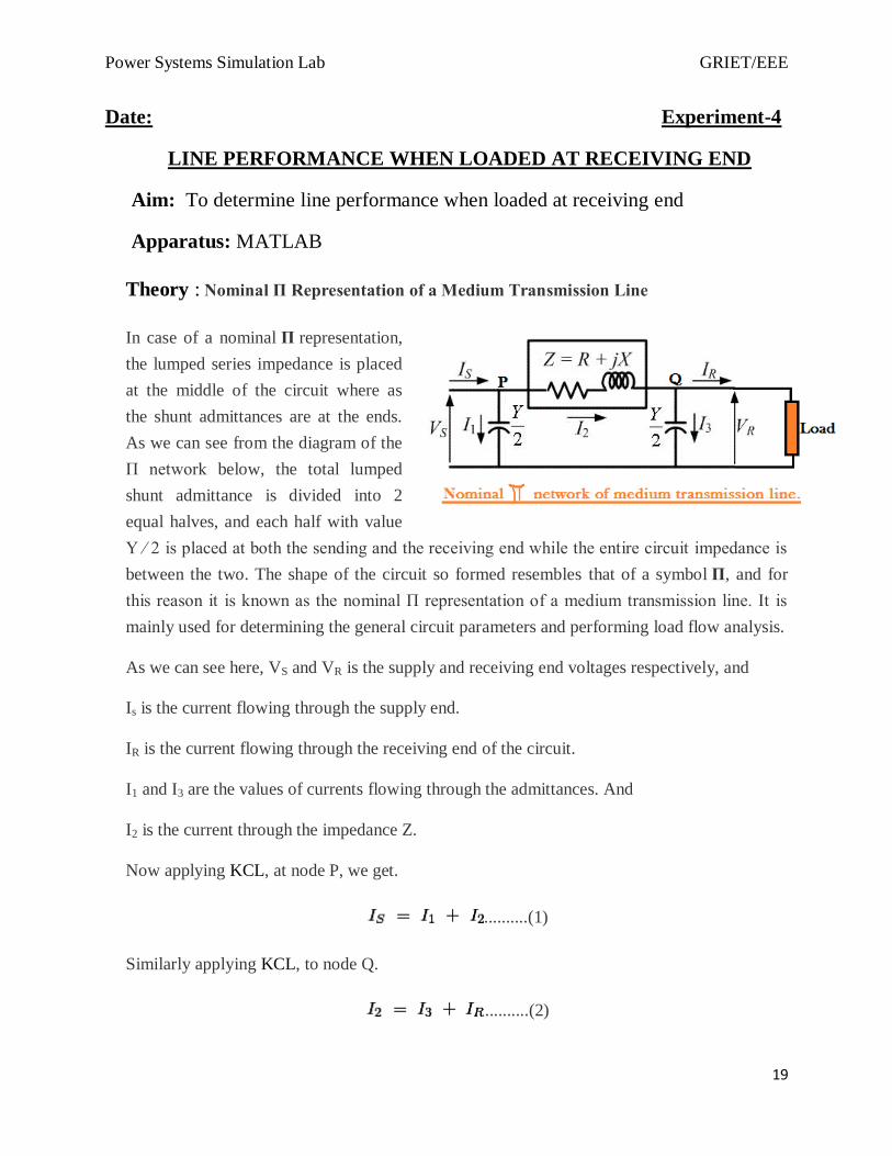
Power Systems Simulation Lab GRIETEEE
21
Circuit Diagram
PROCEDURE
1 Open Matlab--gtSimulink--gt File ---gt New---gt Model
2 Open Simulink Library and browse the components
3 Connect the components as per circuit diagram
4 Set the desired voltage and required frequency
5 Simulate the circuit using MATLAB
6 Obtain the line performance of a line
Graph
Power Systems Simulation Lab GRIETEEE
22
Power Systems Simulation Lab GRIETEEE
23
Power Systems Simulation Lab GRIETEEE
24
Result
Signature of the faculty
Power Systems Simulation Lab GRIETEEE
25
Date Experiment-5
FORMATION OF BUS ADMITTANCE MATRIX USING MATLAB
Aim To determine the bus admittance matrix for the given power system Network
Apparatus MATLAB 77
Theory
Formation of Y BUS matrix
Bus admittance matrix is often used in power system studiesIn most of power system
studies it is necessary to form Y-bus matrix of the system by considering certain power system
parameters depending upon the type of analysis For example in load flow analysis it is necessary
to form Y-bus matrix without taking into account the generator impedance and load impedance
In short circuit analysis the generator transient reactance and transformer impedance taken in
account in addition to line data Y-bus may be computed by inspection method only if there is
no natural coupling between the lines Shunt admittance are added to the diagonal elements
corresponding to the buses at which these are connected The off diagonal elements are
unaffected The equivalent circuit of tap changing transformer may be considered in forming[y-
bus] matrix
There are b independent equations (b = no of buses) relating the bus vectors of currents
and voltages through the bus impedance matrix and bus admittance matrix
EBUS = ZBUS IBUS
IBUS = YBUS EBUS
The relation of equation can be represented in the form
IBUS = YBUS EBUS
Where YBUS is the bus admittance matrix IBUS amp EBUS are the bus current and bus
voltage vectors respectively
Diagonal elements A diagonal element (Yii) of the bus admittance matrix YBUS is equal to
the sum total of the admittance values of all the elements incident at the busnode i
Off Diagonal elements An off-diagonal element (Yij) of the bus admittance matrix YBUS is
equal to the negative of the admittance value of the connecting element present between the
buses I and j if any
This is the principle of the rule of inspection Thus the algorithmic equations for the rule of
inspection are obtained as
Yii = Σ yij (j = 12helliphellipn)
Yij = - yij (j = 12helliphellipn)
Power Systems Simulation Lab GRIETEEE
26
For i = 12hellipn n = no of buses of the given system yij is the admittance of element
connected between buses i and j and yii is the admittance of element connected
between bus i and ground (reference bus)
Read the no Of buses no of
lines and line data
START
Initialize the Y- BUS Matrix
Consider line l = 1
i = sb(1) I= eb(1)
Y(ii) =Y(ii)+Yseries(l) +05Yseries(l)
Y(jj) =Y(jj)+Yseries(l) +05Yseries(l)
Y(ij) = -Yseries(l)
Y(ji) =Y(ij)
Is l =NL
l = l+1
Stop
NO YES
Print Y -Bus
Power Systems Simulation Lab GRIETEEE
27
MATLAB PROGRAM
function[Ybus] = ybus(zdata)
nl=zdata(1) nr=zdata(2) R=zdata(3) X=zdata(4)
nbr=length(zdata(1)) nbus = max(max(nl) max(nr))
Z = R + jX branch impedance
y= ones(nbr1)Z branch admittance
Ybus=zeros(nbusnbus) initialize Ybus to zero
for k = 1nbr formation of the off diagonal elements
if nl(k) gt 0 amp nr(k) gt 0
Ybus(nl(k)nr(k)) = Ybus(nl(k)nr(k)) - y(k)
Ybus(nr(k)nl(k)) = Ybus(nl(k)nr(k))
end
end
for n = 1nbus formation of the diagonal elements
for k = 1nbr
if nl(k) == n | nr(k) == n
Ybus(nn) = Ybus(nn) + y(k)
else end
end
end
Calculations
Power Systems Simulation Lab GRIETEEE
28
Power Systems Simulation Lab GRIETEEE
29
Result
Signature of the faculty
Power Systems Simulation Lab GRIETEEE
30
Date Experiment-6
LOAD FLOW ANALYSIS BY GAUSS SEIDEL METHOD
Aim
To carry out load flow analysis of the given power system network by Gauss Seidel
method
Apparatus MATLAB
Theory
Load flow analysis is the study conducted to determine the steady state operating
condition of the given system under given conditions A large number of numerical algorithms
have been developed and Gauss Seidel method is one of such algorithm
Problem Formulation
The performance equation of the power system may be written of
[I bus] = [Y bus][V bus] (1)
Selecting one of the buses as the reference bus we get (n-1) simultaneous equations The bus
loading equations can be written as
Ii = Pi-jQi Vi (i=123helliphelliphelliphellipn) (2)
Where
n
Pi=Re [ Σ ViYik Vk] (3)
k=1
n
Qi= -Im [ Σ ViYik Vk] (4)
k=1
The bus voltage can be written in form of
n
Vi=(10Yii)[Ii- Σ Yij Vj] (5)
j=1
jnei(i=12helliphelliphelliphellipn)amp ineslack bus
Substituting Ii in the expression for Vi we get
n
Vi new=(10Yii)[Pi-JQi Vio - Σ Yij Vio] (6)
J=1
The latest available voltages are used in the above expression we get n n
Vi new=(10Yii)[Pi-JQi Voi - Σ YijVj
n- Σ Yij Vio] (7) J=1 j=i+1
The above equation is the required formula this equation can be solved for voltages in
interactive manner During each iteration we compute all the bus voltage and check for
Power Systems Simulation Lab GRIETEEE
31
convergence is carried out by comparison with the voltages obtained at the end of previous
iteration After the solutions is obtained The stack bus real and reactive powers the reactive
power generation at other generator buses and line flows can be calculated
Algorithm
Step1 Read the data such as line data specified power specified voltages Q limits at the
generator buses and tolerance for convergences
Step2 Compute Y-bus matrix
Step3 Initialize all the bus voltages
Step4 Iter=1
Step5 Consider i=2 where irsquo is the bus number
Step6 check whether this is PV bus or PQ bus If it is PQ bus goto step 8 otherwise go to next
step
Step7 Compute Qi check for q limit violation QGi=Qi+QLi
7)a)If QGigtQi max equate QGi = Qimax Then convert it into PQ bus
7)b)If QGiltQi min equate QGi = Qi min Then convert it into PQ bus
Step8 Calculate the new value of the bus voltage using gauss seidal formula i=1 n
Vi=(10Yii) [(Pi-j Qi)vi0- Σ Yij Vj- Σ YijVj0] J=1 J=i+1
Adjust voltage magnitude of the bus to specify magnitude if Q limits are not violated
Step9 If all buses are considered go to step 10 otherwise increments the bus no i=i+1 and Go to
step6
Step10 Check for convergence If there is no convergence goes to step 11 otherwise go to
step12
Step11 Update the bus voltage using the formula
Vinew=Vi old+ α(vinew-Viold) (i=12hellipn) ine slackbus α is the acceleration factor=14
Step12 Calculate the slack bus power Q at P-V buses real and reactive give flows real and
reactance line losses and print all the results including all the bus voltages and all the
bus angles
Step13 Stop
Power Systems Simulation Lab GRIETEEE
32
START
Read
1 Primitive Y matrix
2 Bus incidence matrix A
3 Slack bus voltages
4 Real and reactive bus powers Piamp Qi
5 Voltage magnitudes and their limits
Form Ybus
Make initial assumptions
Compute the parameters Ai for i=m+1hellipn and Bik for i=12hellipn
k=12hellipn
Set iteration count r=0
Set bus count i=2 and ΔVmax=0
Test for
type of bus
Qi(r+1)
gtQi max Qi(r+1)
lt Qimin
Compute Qi(r+1)
Qi(r+1)
= Qimax Qi
(r+1) = Qimin Compute Ai
(r+1)
Compute Ai
Compute Vi
(r+1)
Compute δi(r+1)
and
Vi(r+1)
=|Vis|δi
(r+1)
Power Systems Simulation Lab GRIETEEE
33
FLOW CHART FOR GAUSS SEIDEL METHOD
Procedure
Enter the command window of the MATLAB
Create a new M ndash file by selecting File - New ndash M ndash File
Type and save the program in the editor Window
Execute the program by pressing Tools ndash Run
View the results
MATLAB program
clear
basemva=100
accuracy=0001 maxiter=100
no code mag degree MW Mvar MW Mvar Qmin Qmax Mvar
busdata=[1 1 105 00 00 00 00 00 0 0 0
2 0 10 00 25666 1102 00 00 0 0 0
3 0 10 00 1386 452 00 00 0 0 0]
bus bus R X 12B =1 for lines
linedata=[1 2 002 004 00 1
1 3 001 003 00 1
Replace Vir by Vi
(r+1) and
advance bus count i = i+1
Is ilt=n
Is
ΔVmaxlt=ε
Advance iteration
count r = r+1
Compute slack bus power P1+jQ1 and all line flows
B
A
Power Systems Simulation Lab GRIETEEE
34
2 3 00125 0025 00 1]
lfybus
lfgauss
busout
lineflow
Calculations
Power Systems Simulation Lab GRIETEEE
35
Power Systems Simulation Lab GRIETEEE
36
Result
Signature of the faculty
Power Systems Simulation Lab GRIETEEE
37
Date Experiment-7
LOAD FLOW ANALYSIS BY NEWTON RAPSHON METHOD
Aim
To carry out load flow analysis of the given power system by Newton Raphson method
Apparatus MATLAB 77
Theory
The Newton Raphson method of load flow analysis is an iterative method which approximates
the set of non-linear simultaneous equations to a set of linear simultaneous equations using
Taylorrsquos series expansion and the terms are limited to first order approximation The load flow
equations for Newton Raphson method are non-linear equations in terms of real and imaginary
part of bus voltages
where ep = Real part of Vp
fp = Imaginary part of Vp
Gpq Bpq = Conductance and Susceptances of admittance Ypq respectively
Algorithm
Step1 Input the total number of buses Input the details of series line impendence and line
charging admittance to calculate the Y-bus matrix
Step2 Assume all bus voltage as 1 per unit except slack bus
Step3 Set the iteration count as k=0 and bus count as p=1
Step4 Calculate the real and reactive power pp and qp using the formula
P=ΣvpqYpqcos(Qpq+εp-εq)
Qp=ΣVpqYpasin(qpq+εp-εa)
Evalute pp=psp-pp
Power Systems Simulation Lab GRIETEEE
38
Step5 If the bus is generator (PV) bus check the value of Qpis within the limitsIf it Violates
the limits then equate the violated limit as reactive power and treat it as PQ bus If limit is not
isolated then calculate
|vp|^r=|vgp|^rspe-|vp|r Qp=qsp-qp
Step6 Advance bus count by 1 and check if all the buses have been accounted if not go to step5
Step7 Calculate the elements of Jacobean matrix
Step8 Calculate new bus voltage increment pk and fpk
Step9 Calculate new bus voltage eph+ ep
Fp^k+1=fpK+fpK
Step10 Advance iteration count by 1 and go to step3
Step11 Evaluate bus voltage and power flows through the line
Procedure
Enter the command window of the MATLAB
Create a new M ndash file by selecting File - New ndash M ndash File
Type and save the program in the editor Window
Execute the program by pressing Tools ndash Run
View the results
MATLAB program
clear
basemva=100accuracy=0001maxiter=100
no code mag degree MW Mvar MW Mvar Qmin Qmax Mvar
busdata=[1 1 105 00 00 00 00 00 0 0 0
2 0 10 00 25666 1102 00 00 0 0 0
3 0 10 00 1386 452 00 00 0 0 0]
bus bus R X 12B =1 for lines
linedata=[1 2 002 004 00 1
1 3 001 003 00 1
2 3 00125 0025 00 1]
lfybus
lfnewton
Power Systems Simulation Lab GRIETEEE
39
busout
lineflow
Calculations
Power Systems Simulation Lab GRIETEEE
40
Result
Signature of the faculty
Power Systems Simulation Lab GRIETEEE
41
Date Experiment-8(a)
OPTIMAL DISPATCH NEGLECTING LOSSES
Aim To develop a program for solving economic dispatch problem without transmission
losses for a given load condition using direct method and Lambda-iteration method
Apparatus MATLAB
Theory
As the losses are neglected the system model can be understood as shown in Fig here n number
of generating units are connected to a common bus bar collectively meeting the total power
demand PD It should be understood that share of power demand by the units does not involve
losses
Since transmission losses are neglected total demand PD is the sum of all generations of n-
number of units For each unit a cost functions Ci is assumed and the sum of all costs computed
from these cost functions gives the total cost of production CT
Fig System with n-generators
where the cost function of the ith unit from Eq (11) is
Ci = αi + βiPi + γ
iPi
2
Now the ED problem is to minimize CT subject to the satisfaction of the following equality and
inequality constraints
Equality constraint
The total power generation by all the generating units must be equal to the power demand
Power Systems Simulation Lab GRIETEEE
42
where Pi = power generated by ith unit
PD = total power demand
Inequality constraint
Each generator should generate power within the limits imposed
Pi
min le Pi le Pi
max i = 1 2 hellip n
Economic dispatch problem can be carried out by excluding or including generator power
limits ie the inequality constraint
The constrained total cost function can be converted into an unconstrained function by using
the Lagrange multiplier as
The conditions for minimization of objective function can be found by equating partial
differentials of the unconstrained function to zero as
Since Ci = C1 + C2+hellip+Cn
From the above equation the coordinate equations can be written as
The second condition can be obtained from the following equation
Power Systems Simulation Lab GRIETEEE
43
Equations Required for the ED solution
For a known value of λ the power generated by the ith unit from can be written as
which can be written as
The required value of λ is
The value of λ can be calculated and compute the values of Pi for i = 1 2hellip n for optimal
scheduling of generation
POWER WORLD bus diagram
Power Systems Simulation Lab GRIETEEE
44
Procedure
Create a new file in edit mode by selecting File - New File
Browse the components and build the bus sytem
Execute the program in run mode by selecting tools-opf areas-select opf
Run the primal lp
View the results in case information-Generator fuel costs
Tabulate the results
Results
Generator
Name
Gen
MW IOA IOB IOC
Min
MW
Max
MW
Cost
$Hr Lambda
1 7952 150 5 011 10 250 124312 2249
2 126 600 12 0085 10 300 210066 2262
3 114 335 1 01225 10 270 204101 2893
Total Cost = 5384 79$hr
Power Systems Simulation Lab GRIETEEE
45
Calculations
Power Systems Simulation Lab GRIETEEE
46
Result
Signature of the faculty
Power Systems Simulation Lab GRIETEEE
47
Date Experiment-8(b)
OPTIMAL DISPATCH INCLUDING LOSSES
Aim To develop a program for solving economic dispatch problem including transmission
losses for a given load condition using direct method and Lambda-iteration method
Apparatus MATLAB
Theory When the transmission losses are included in the economic dispatch problem we can
modify (54) as
LOSSNT PPPPP 21
where PLOSS is the total line loss Since PT is assumed to be constant we have
LOSSN dPdPdPdP 210
In the above equation dPLOSS includes the power loss due to every generator ie
N
N
LOSSLOSSLOSSLOSS dP
P
PdP
P
PdP
P
PdP
2
2
1
1
Also minimum generation cost implies dfT = 0 as given Multiplying by and combing we get
N
N
LOSSLOSSLOSS dPP
PdP
P
PdP
P
P
2
2
1
1
0
Adding with we obtain
N
i
i
i
LOSS
i
T dPP
P
P
f
1
0
The above equation satisfies when
NiP
P
P
f
i
LOSS
i
T 10
Again since
NiP
df
P
f
i
T
i
T 1
Power Systems Simulation Lab GRIETEEE
48
we get
N
N
N
i
LdP
dfL
dP
dfL
dP
df 2
2
21
1
where Li is called the penalty factor of load-i and is given by
NiPP
LiLOSS
i 11
1
Consider an area with N number of units The power generated are defined by the vector
TNPPPP 21
Then the transmission losses are expressed in general as
BPPP T
LOSS
where B is a symmetric matrix given by
NNNN
N
N
BBB
BBB
BBB
B
21
22212
11211
The elements Bij of the matrix B are called the loss coefficients These coefficients are not
constant but vary with plant loading However for the simplified calculation of the penalty factor
Li these coefficients are often assumed to be constant
Power Systems Simulation Lab GRIETEEE
49
Circuit Diagram
`
Power Systems Simulation Lab GRIETEEE
50
Procedure
Create a new file in edit mode by selecting File - New File
Browse the components and build the bus sytem
Execute the program in run mode by selecting tools-opf areas-select opf
Run the primal lp
View the results in case information-Generator fuel costs
Tabulate the results
Results
Generator
Name
Gen
MW IOA IOB IOC IOD
Min
MW
Max
MW
Cost
$Hr Lambda
1 10638 150 5 011 0 10 250 192666 284
2 126 600 12 0085 0 10 300 210066 2262
3 8622 335 1 01225 0 10 270 133184 2212
Total Cost =
535915$hr
Power Systems Simulation Lab GRIETEEE
51
Power Systems Simulation Lab GRIETEEE
52
Result
Signature of the faculty
Power Systems Simulation Lab GRIETEEE
53
Date Experiment-9
TRANSIENT RESPONSE OF A RLC CIRCUIT
Aim To obtain the transient response of an RLC circuit with its damping frequency and
damping ratio using MATLAB
Apparatus MATLAB
Theory RLC circuits are widely used in a variety of applications such as filters in
communications systems ignition systems in automobiles defibrillator circuits in biomedical
applications etc The analysis of RLC circuits is more complex than of the RC circuits we have
seen in the previous lab RLC circuits have a much richer and interesting response than the
previously studied RC or RL circuits A summary of the response is given below
Lets assume a series RLC circuit The discussion is also applicable to other RLC circuits such as
the parallel circuit
Figure 1 Series RLC circuit
By writing KVL one gets a second order differential equation The solution consists of two parts
x(t) = xn(t) + xp(t)
in which xn(t) is the complementary solution (=solution of the homogeneous differential equation
also called the natural response) and a xp(t) is the particular solution (also called forced
response) Lets focus on the complementary solution The form of this solution depends on the
roots of the characteristic equation
in which is the damping ratio and is the undamped resonant frequency The roots of the
quadratic equation are equal to
For the example of the series RLC circuit one has the following characteristic equation for the
current iL(t) or vC(t)
s2 + RLs + 1LC =0
Depending on the value of the damping ratio one has three possible cases
Case 1 Critically damped response two equal roots s= s1= s2
Power Systems Simulation Lab GRIETEEE
54
The total response consists of the sum of the
complementary and the particular solution The case of
a critically damped response to a unit input step
function
Case 2 Overdamped response two real and unequal roots s1 and
s2
Case 3 Underdamped response two complex roots
Procedure
Enter the command window of the MATLAB
Create a new M ndash file by selecting File - New ndash M ndash File
Type and save the program in the editor Window
Execute the program by pressing Tools ndash Run
View the results
MATLAB Program
wn = input(Enter value of undamped natural frequency)
z = input(Enter value of damping ratio)
n = [wnwn]
p = sqrt(1-z^2)
Power Systems Simulation Lab GRIETEEE
55
wd = wnp
h = [pz]
k = atan(h)
m = pi-k
tr = [mwd]
tp = [piwd]
q = zwn
ts = [4q]
r = zpi
f = [rp]
mp = exp(-f)
num = [0 0 n]
den = [1 zzwn n]
s = tf(numden)
hold on
step(s)
impulse(s)
hold off
Result
Enter value of undamped natural frequency 16
wn = 16
Enter value of damping ratio05
z = 05000
n = 256
Power Systems Simulation Lab GRIETEEE
56
p = 08660
k = 10472
tr = 01511
tp = 02267
q = 8
ts = 05000
r = 15708
f = 18138
mp = 01630
num = 0 0 256
den = 1 4 256
Transfer function
256
---------------
s^2 + 4 s + 256
Graph
Power Systems Simulation Lab GRIETEEE
57
Calculations
Power Systems Simulation Lab GRIETEEE
58
Result
Signature of the faculty
Power Systems Simulation Lab GRIETEEE
59
Date Experiment-10
THREE PHASE SHORT CIRCUIT ANALYSIS OF A SYNCHRONOUS
MACHINE
Aim To Analyze symmetrical fault
Apparatus MATLAB
Theory The response of the armature current when a three-phase symmetrical short circuit
occurs at the terminals of an unloaded synchronous generator
It is assumed that there is no dc offset in the armature current The magnitude of the current
decreases exponentially from a high initial value The instantaneous expression for the fault
current is given by
where Vt is the magnitude of the terminal voltage α is its phase angle and
is the direct axis subtransient reactance
is the direct axis transient reactance
is the direct axis synchronous reactance
with
The time constants are
Power Systems Simulation Lab GRIETEEE
60
is the direct axis subtransient time constant
is the direct axis transient time constant
we have neglected the effect of the armature resistance hence α = π2 Let us assume that the
fault occurs at time t = 0 From (69) we get the rms value of the
current as
which is called the subtransient fault current The duration of the subtransient current is
dictated by the time constant Td As the time progresses and Td´´lt t lt Td´ the first
exponential term will start decaying and will eventually vanish However since t is still nearly
equal to zero we have the following rms value of the current
This is called the transient fault current Now as the time progress further and the second
exponential term also decays we get the following rms value of the current for the sinusoidal
steady state
In addition to the ac the fault currents will also contain the dc offset Note that a symmetrical
fault occurs when three different phases are in three different locations in the ac cycle
Therefore the dc offsets in the three phases are different The maximum value of the dc offset
is given by
where TA is the armature time constant
Procedure
1 Open Matlab--gtSimulink--gt File ---gt New---gt Model
2 Open Simulink Library and browse the components
3 Connect the components as per circuit diagram
4 Set the desired voltage and required frequency
5 Simulate the circuit using MATLAB
6 Plot the waveforms
Power Systems Simulation Lab GRIETEEE
61
Circuit Diagram
Graph
Power Systems Simulation Lab GRIETEEE
62
Calculations
Power Systems Simulation Lab GRIETEEE
63
Power Systems Simulation Lab GRIETEEE
64
Result
Signature of the faculty
Power Systems Simulation Lab GRIETEEE
65
Date Experiment-11
UNSYMMETRICAL FAULT ANALYSIS
Aim To analyze unsymmetrical fault
Apparatus MATLAB
Theory
Single Line-to-Ground Fault
The single line-to-ground fault is usually referred as ldquoshort circuitrdquo fault and occurs when one
conductor falls to ground or makes contact with the neutral wire The general representation
of a single line-to-ground fault is shown in Figure 310 where F is the fault point with
impedances Zf Figure 311 shows the sequences network diagram Phase a is usually
assumed to be the faulted phase this is for simplicity in the fault analysis calculations [1]
a
c
b
+
Vaf
-
F
Iaf Ibf = 0 Icf = 0
n
Zf
F0
Z0
N0
+
Va0
-
Ia0
F1
Z1
N1
+
Va1
-
Ia1
+
10
-
F2
Z2
N2
+
Va2
-
Ia2
3Zf
Iaf
General representation of a single Sequence network diagram of a
line-to-ground fault single line-to-ground fault
Since the zero- positive- and negative-sequence currents are equals as it can be observed
in Figure 311 Therefore
0 1 2
0 1 2
10 0
3a a a
f
I I IZ Z Z Z
Power Systems Simulation Lab GRIETEEE
66
With the results obtained for sequence currents the sequence voltages can be obtained
from
0 0
2
1 1
2
22
0 1 1 1
10 0 1
0 1
a a
b a
ac
V I
V a a I
a a IV
By solving Equation
0 0 0
1 1 1
2 2 2
10
a a
a a
a a
V Z I
V Z I
V Z I
If the single line-to-ground fault occurs on phase b or c the voltages can be found by the
relation that exists to the known phase voltage components
0
2
1
2
2
1 1 1
1
1
af a
bf a
cf a
V V
V a a V
V a a V
as
2
0 1 2
2
0 1 2
bf a a a
cf a a a
V V a V aV
V V aV a V
Line-to-Line Fault
A line-to-line fault may take place either on an overhead andor underground
transmission system and occurs when two conductors are short-circuited One of the
characteristic of this type of fault is that its fault impedance magnitude could vary over a wide
range making very hard to predict its upper and lower limits It is when the fault impedance is
zero that the highest asymmetry at the line-to-line fault occurs
The general representation of a line-to-line fault is shown in Figure 312 where F is the
fault point with impedances Zf Figure 313 shows the sequences network diagram Phase b and
c are usually assumed to be the faulted phases this is for simplicity in the fault analysis
calculations [1]
Power Systems Simulation Lab GRIETEEE
67
a
c
b
F
Iaf = 0 Ibf Icf = -Ibf
Zf
F0
Z0
N0
+
Va0 = 0
-
Ia0 = 0
Zf
F1
Z1
N1
+
Va1
-
Ia1
F2
Z2
N2
+
Va2
-
Ia2
+
10 0o
-
Sequence network diagram of a line-to-line fault Sequence network diagram of a single
line-to-line fault
It can be noticed that
0afI
bf cfI I
bc f bfV Z I
And the sequence currents can be obtained as
0 0aI
1 2
1 2
10 0a a
f
I IZ Z Z
If Zf = 0
1 2
1 2
10 0a aI I
Z Z
The fault currents for phase b and c can be obtained as
13 90bf cf aI I I
The sequence voltages can be found as
0
1 1 1
2 2 2 2 1
0
10 -
a
a a
a a a
V
V Z I
V Z I Z I
Power Systems Simulation Lab GRIETEEE
68
Finally the line-to-line voltages for a line-to-line fault can be expressed as
ab af bf
bc bf cf
ca cf af
V V V
V V V
V V V
Double Line-to-Ground Fault
A double line-to-ground fault represents a serious event that causes a significant
asymmetry in a three-phase symmetrical system and it may spread into a three-phase fault when
not clear in appropriate time The major problem when analyzing this type of fault is the
assumption of the fault impedance Zf and the value of the impedance towards the ground Zg
The general representation of a double line-to-ground fault is shown in Figure 314 where
F is the fault point with impedances Zf and the impedance from line to ground Zg Figure 315
shows the sequences network diagram Phase b and c are assumed to be the faulted phases this is
for simplicity in the fault analysis calculations
a
c
b
F
Iaf = 0 Ibf Icf
n
Zf Zf
Zg Ibf +Icf
N
Zf +3Zg
F0
Z0
N0
+
Va0
-
Ia0 Zf
F1
Z1
N1
+
Va1
-
Ia1 Zf
F2
Z2
N2
+
Va2
-
Ia2
+
10 0o
-
General representation of a Sequence network diagram
double line-to-ground fault of a double line-to-ground fault
It can be observed that
0
( )
( )
af
bf f g bf g cf
cf f g cf g bf
I
V Z Z I Z I
V Z Z I Z I
The positive-sequence currents can be found as
12 0
1
2 0
10 0
( )( 3 )( )
( ) ( 3 )
af f g
f
f f g
IZ Z Z Z Z
Z ZZ Z Z Z Z
Power Systems Simulation Lab GRIETEEE
69
02 1
2 0
( 3 )[ ]( ) ( 3 )
f ga a
f f g
Z Z ZI I
Z Z Z Z Z
20 1
2 0
( )[ ]( ) ( 3 )
fa a
f f g
Z ZI I
Z Z Z Z Z
An alternative method is
0 1 2
0 1 2
0
( )
af a a a
a a a
I I I I
I I I
If Zf and Zg are both equal to zero then the positive- negative- and zero-sequences can
be obtained from
12 0
1
2 0
10 0
( )( )( )
( )
aIZ Z
ZZ Z
02 1
2 0
( )[ ]( )
a aZ
I IZ Z
20 1
2 0
( )[ ]( )
a aZ
I IZ Z
The current for phase a is
0afI
2
0 1 2
2
0 1 2
bf a a a
cf a a a
I I a I aI
I I aI a I
The total fault current flowing into the neutral is
03n a bf cfI I I I
The resultant phase voltages from the relationship given in Equation 378 can be
expressed as
0 1 2 13
0
af a a a a
bf cf
V V V V V
V V
Power Systems Simulation Lab GRIETEEE
70
And the line-to-line voltages are
0
abf af bf af
bcf bf cf
caf cf af af
V V V V
V V V
V V V V
Circuit Diagram
Procedure
1 Open Matlab--gtSimulink--gt File ---gt New---gt Model
2 Open Simulink Library and browse the components
3 Connect the components as per circuit diagram
4 Set the desired voltage and required frequency
5 Simulate the circuit using MATLAB
6 Plot the waveforms
Power Systems Simulation Lab GRIETEEE
71
Graph
Power Systems Simulation Lab GRIETEEE
72
Power Systems Simulation Lab GRIETEEE
73
Power Systems Simulation Lab GRIETEEE
74
Result
Signature of the faculty
Power Systems Simulation Lab GRIETEEE
75
Date Experiment-12
FORMATION OF BUS IMPEDANCE MATRIX USING MATLAB
Aim To determine the bus impedance matrix for the given power system Network
Apparatus MATLAB 77
Theory
Formation of Z BUS matrix
Z-bus matrix is an important matrix used in different kinds of power system study such as
short circuit study load flow study etc In short circuit analysis the generator uses transformer
impedance must be taken into account In quality analysis the two-short element are neglected by
forming the z-bus matrix which is used to compute the voltage distribution factor This can be
largely obtained by reversing the y-bus formed by inspection method or by analytical method
Taking inverse of the y-bus for large system in time consuming Moreover modification in the
system requires whole process to be repeated to reflect the changes in the system In such cases
is computed by z-bus building algorithm
Algorithm
Step 1 Read the values such as number of lines number of buses and line data generator data
and transformer data
Step 2 Initialize y-bus matrix y-bus[i] [j] =complex(0000)
Step 3 Compute y-bus matrix by considering only line data
Step 4 Modifies the y-bus matrix by adding the transformer and the generator admittance to the
respective diagonal elements of y-bus matrix
Step 5 Compute the z-bus matrix by inverting the modified y-bus matrix
Step 6 Check the inversion by multiplying modified y-bus and z-bus matrices to check whether
the resulting matrix is unit matrix or not
Step 7 Print the z-bus matrix
Power Systems Simulation Lab GRIETEEE
76
Procedure
Enter the command window of the MATLAB
Create a new M ndash file by selecting File - New ndash M ndash File
Type and save the program in the editor Window
Execute the program by pressing Tools ndash Run
Read the no Of buses no of
lines and line data
START
Form Y bus matrix using the algorithm
Y(ii) =Y(ii)+Yseries(l) +05Yseries(l)
Y(jj) =Y(jj)+Yseries(l) +05Yseries(l)
Y(ij) = -Yseries(l)
Y(ji) =Y(ij)
Modifying the y bus by adding generator
and transformer admittances to respective
diagonal elements
Compute Z bus matrix by inverting
modified Y bus
Multiply modified Y bus and Z bus and check
whether the product is a unity matrix
Print all the results
STOP
Power Systems Simulation Lab GRIETEEE
77
View the results
MATLAB Program
function[Ybus] = ybus(zdata)
zdata(1)) nbus = max(max(nl) max(nr))
Z = R + jX branch impedance
y= ones(nbr1)Z branch admittance
Ybus=zeros(nbusnbus) initialize Ybus to zero
for k = 1nbr formation of the off diagonal elements
if nl(k) gt 0 amp nr(k) gt 0
Ybus(nl(k)nr(k)) = Ybus(nl(k)nr(k)) - y(k)
Ybus(nr(k)nl(k)) = Ybus(nl(k)nr(k))
end
end
for n = 1nbus formation of the diagonal elements
for k = 1nbr
if nl(k) == n | nr(k) == n
Ybus(nn) = Ybus(nn) + y(k)
else end
end
end
Zbus= inv(Y)
Ibus=[-j11-j12500]
Vbus=ZbusIbus
OUTPUT
Power Systems Simulation Lab GRIETEEE
78
Power Systems Simulation Lab GRIETEEE
79
Result
Signature of the faculty
Power Systems Simulation Lab GRIETEEE
80
Date Experiment-13(a)
SYMMETRICAL COMPONENTS
Aim To obtain symmetrical components of set of unbalanced currents
Apparatus MATLAB
Theory
Before we discuss the symmetrical component transformation let us first define the a-
operator
2
3
2
10120 jea j
Note that for the above operator the following relations hold
on so and
1
2
3
2
1
22403606005
1203604804
3603
2402
000
000
0
0
aeeea
aeeea
ea
ajea
jjj
jjj
j
j
Also note that we have
02
3
2
1
2
3
2
111 2 jjaa
Using the a-operator we can write from Fig 71 (b)
111
2
1 and acab aVVVaV
Similarly
2
2
222 and acab VaVaVV
Finally
000 cba VVV
The symmetrical component transformation matrix is then given by
Power Systems Simulation Lab GRIETEEE
81
c
b
a
a
a
a
V
V
V
aa
aa
V
V
V
2
2
2
1
0
1
1
111
3
1
Defining the vectors Va012 and Vabc as
c
b
a
abc
a
a
a
a
V
V
V
V
V
V
V
V
2
1
0
012
Program
V012 = [06 90
10 30
08 -30]
rankV012=length(V012(1))
if rankV012 == 2
mag= V012(1) ang=pi180V012(2)
V012r=mag(cos(ang)+jsin(ang))
elseif rankV012 ==1
V012r=V012
else
fprintf(n Symmetrical components must be expressed in a one column array in rectangular
complex form n)
fprintf( or in a two column array in polar form with 1st column magnitude amp 2nd column
n)
fprintf( phase angle in degree n)
return end
a=cos(2pi3)+jsin(2pi3)
A = [1 1 1 1 a^2 a 1 a a^2]
Vabc= AV012r
Vabcp= [abs(Vabc) 180piangle(Vabc)]
fprintf( n Unbalanced phasors n)
fprintf( Magnitude Angle Degn)
disp(Vabcp)
Vabc0=V012r(1)[1 1 1]
Vabc1=V012r(2)[1 a^2 a]
Vabc2=V012r(3)[1 a a^2]
Power Systems Simulation Lab GRIETEEE
82
Procedure
1 Open Matlab--gt File ---gt New---gt Script
2 Write the program
3 Enter F5 to run the program
4 Observe the results in MATLAB command window
Result
Vabc =
15588 + 07000i
-00000 + 04000i
-15588 + 07000i
Unbalanced phasors
Magnitude Angle Deg
17088 241825
04000 900000
17088 1558175
Power Systems Simulation Lab GRIETEEE
83
Result
Signature of the faculty
Power Systems Simulation Lab GRIETEEE
84
Date Experiment-13(b)
UNBALANCED VOLTAGES FROM SYMMETRICAL COMPONENTS
Aim To obtain the original unbalanced phase voltages from symmetrical components
Apparatus MATLAB
Theory
abca CVV 012
where C is the symmetrical component transformation matrix and is given by
aa
aaC2
2
1
1
111
3
1
The original phasor components can also be obtained from the inverse symmetrical
component transformation ie
012
1
aabc VCV
Inverting the matrix C we get
2
1
0
1
2
1
0
2
2
1
1
111
a
a
a
a
a
a
c
b
a
V
V
V
C
V
V
V
aa
aa
V
V
V
210 aaaa VVVV
21021
2
0 bbbaaab VVVaVVaVV
2102
2
10 cccaaac VVVVaaVVV
Finally if we define a set of unbalanced current phasors as Iabc and their symmetrical
components as Ia012 we can then define
012
1
012
aabc
abca
ICI
CII
Power Systems Simulation Lab GRIETEEE
85
Program
Iabc = [16 25
10 180
09 132]
rankIabc=length(Iabc(1))
if rankIabc == 2
mag= Iabc(1) ang=pi180Iabc(2)
Iabcr=mag(cos(ang)+jsin(ang))
elseif rankIabc ==1
Iabcr=Iabc
else
fprintf(n Three phasors must be expressed in a one column array in rectangular complex
form n)
fprintf( or in a two column array in polar form with 1st column magnitude amp 2nd column
n)
fprintf( phase angle in degree n)
return end
a=cos(2pi3)+jsin(2pi3)
A = [1 1 1 1 a^2 a 1 a a^2]
I012=inv(A)Iabcr
symcomp= I012
I012p = [abs(I012) 180piangle(I012)]
fprintf( n Symmetrical components n)
fprintf( Magnitude Angle Degn)
disp(I012p)
Iabc0=I012(1)[1 1 1]
Iabc1=I012(2)[1 a^2 a]
Iabc2=I012(3)[1 a a^2]
Result
symcomp =
-00507 + 04483i
09435 - 00009i
05573 + 02288i
Symmetrical components
Magnitude Angle Deg
04512 964529
09435 -00550
06024 223157
Power Systems Simulation Lab GRIETEEE
86
Power Systems Simulation Lab GRIETEEE
87
Result
Signature of the faculty
Power Systems Simulation Lab GRIETEEE
88
Date Experiment-14
SHORT CIRCUIT ANALYSIS OF 14 BUS SYSTEM
Aim To obtain the short circuit analysis for a IEEE 14 bus system
Apparatus POWERWORLD
Theory
ff IZV 44
32144
44 iV
Z
ZIZV f
ifii
We further assume that the system is unloaded before the fault occurs and that the magnitude and
phase angles of all the generator internal emfs are the same Then there will be no current
circulating anywhere in the network and the bus voltages of all the nodes before the fault will be
same and equal to Vf Then the new altered bus voltages due to the fault will be given from by
41144
4
iV
Z
ZVVV f
iifi
14 bus system
Power Systems Simulation Lab GRIETEEE
89
Procedure
Create a new file in edit mode by selecting File - New File
Browse the components and build the bus sytem
Execute the program in run mode by selecting tools-fault analysis
Select the fault on which bus and calculate
Tabulate the results
Results 3-phase fault is applied on bus 3
Bus
Number Va Vb Vc Ang A Ang B Ang C
1 041937 041937 041937 1964 -10036 13964
2 034862 034862 034862 1087 -10913 13087
3 0 0 0 0 0 0
4 029602 029602 029602 -225 -12225 11775
5 032956 032956 032956 058 -11942 12058
Power Systems Simulation Lab GRIETEEE
90
6 047538 047538 047538 -1063 -13063 10937
7 042742 042742 042742 -844 -12844 11156
8 055864 055864 055864 -1006 -13006 10994
9 041373 041373 041373 -95 -1295 1105
10 042145 042145 042145 -994 -12994 11006
11 044639 044639 044639 -1037 -13037 10963
12 046474 046474 046474 -1144 -13144 10856
13 045879 045879 045879 -1127 -13127 10873
14 042532 042532 042532 -113 -1313 1087
Fault current = 445 pu
= 186167 A
Fault current angle = -7774 deg
Power Systems Simulation Lab GRIETEEE
91
Result
Signature of the faculty
Power Systems Simulation Lab GRIETEEE
92
Date Experiment-15
LOAD FREQUENCY CONTROL OF A SINGLE AREA POWER SYSTEM
Aim To obtain the frequency response of single and two area power system using MATLAB
Apparatus MATLAB 61
Formula used
1)
2)
3)
4)
Where
D = damping coefficient
GG ndash gain of generator GT - gain of turbine
GP - gain of power
KP ndash power system constant
KT- turbine constant
KG- generator constant
TP ndash power system time constant
TG- generator time constant
Procedure
1 Open Matlab--gtSimulink--gt File ---gt New---gt Model
2 Open Simulink Library and browse the components
3 Connect the components as per circuit diagram
4 Set the desired voltage and required frequency
5 Simulate the circuit using MATLAB
6 Plot the waveforms
Power Systems Simulation Lab GRIETEEE
93
SIMULINK RESULTS
Single Area Power System Block Diagram
Graph
Power Systems Simulation Lab GRIETEEE
94
Power Systems Simulation Lab GRIETEEE
95
Power Systems Simulation Lab GRIETEEE
96
RESULT
Signature of the faculty
Power Systems Simulation Lab GRIETEEE
97
Date Experiment-16
LOAD FREQUENCY CONTROL OF A TWO AREA POWER SYSTEM
Aim To obtain the frequency response of two area power system using MATLAB
Apparatus MATLAB
Formula used
1)
2)
3)
4)
Where
D = damping coefficient
GG ndash gain of generator GT - gain of turbine
GP - gain of power
KP ndash power system constant
KT- turbine constant
KG- generator constant
TP ndash power system time constant
TG- generator time constant
Procedure
1 Open Matlab--gtSimulink--gt File ---gt New---gt Model
2 Open Simulink Library and browse the components
3 Connect the components as per circuit diagram
4 Set the desired voltage and required frequency
5 Simulate the circuit using MATLAB
6 Plot the waveforms
Power Systems Simulation Lab GRIETEEE
98
SIMULINK RESULTS
Single Area Power System Block Diagram
Graphs
Power Systems Simulation Lab GRIETEEE
99
Power Systems Simulation Lab GRIETEEE
100
Power Systems Simulation Lab GRIETEEE
101
Result
Signature of the faculty
Power Systems Simulation Lab GRIETEEE
102
Date Experiment-17
STEP RESPONSE OF A SYNCHRONOUS MACHINE
Aim To obtain step response of rotor angle and generator frequency of a synchronous
machine
Apparatus MATLAB
Circuit Diagram
Procedure
1 Open File ---gt New---gt Model
2 Open Simulink Library and browse the components
3 Connect the components as per circuit diagram
4 Set the desired voltage and required frequency
5 Simulate the circuit using MATLAB
6 Plot the waveforms
Power Systems Simulation Lab GRIETEEE
103
Graph
Power Systems Simulation Lab GRIETEEE
104
Power Systems Simulation Lab GRIETEEE
105
Result
Signature of the faculty

Power Systems Simulation Lab GRIETEEE
22
Power Systems Simulation Lab GRIETEEE
23
Power Systems Simulation Lab GRIETEEE
24
Result
Signature of the faculty
Power Systems Simulation Lab GRIETEEE
25
Date Experiment-5
FORMATION OF BUS ADMITTANCE MATRIX USING MATLAB
Aim To determine the bus admittance matrix for the given power system Network
Apparatus MATLAB 77
Theory
Formation of Y BUS matrix
Bus admittance matrix is often used in power system studiesIn most of power system
studies it is necessary to form Y-bus matrix of the system by considering certain power system
parameters depending upon the type of analysis For example in load flow analysis it is necessary
to form Y-bus matrix without taking into account the generator impedance and load impedance
In short circuit analysis the generator transient reactance and transformer impedance taken in
account in addition to line data Y-bus may be computed by inspection method only if there is
no natural coupling between the lines Shunt admittance are added to the diagonal elements
corresponding to the buses at which these are connected The off diagonal elements are
unaffected The equivalent circuit of tap changing transformer may be considered in forming[y-
bus] matrix
There are b independent equations (b = no of buses) relating the bus vectors of currents
and voltages through the bus impedance matrix and bus admittance matrix
EBUS = ZBUS IBUS
IBUS = YBUS EBUS
The relation of equation can be represented in the form
IBUS = YBUS EBUS
Where YBUS is the bus admittance matrix IBUS amp EBUS are the bus current and bus
voltage vectors respectively
Diagonal elements A diagonal element (Yii) of the bus admittance matrix YBUS is equal to
the sum total of the admittance values of all the elements incident at the busnode i
Off Diagonal elements An off-diagonal element (Yij) of the bus admittance matrix YBUS is
equal to the negative of the admittance value of the connecting element present between the
buses I and j if any
This is the principle of the rule of inspection Thus the algorithmic equations for the rule of
inspection are obtained as
Yii = Σ yij (j = 12helliphellipn)
Yij = - yij (j = 12helliphellipn)
Power Systems Simulation Lab GRIETEEE
26
For i = 12hellipn n = no of buses of the given system yij is the admittance of element
connected between buses i and j and yii is the admittance of element connected
between bus i and ground (reference bus)
Read the no Of buses no of
lines and line data
START
Initialize the Y- BUS Matrix
Consider line l = 1
i = sb(1) I= eb(1)
Y(ii) =Y(ii)+Yseries(l) +05Yseries(l)
Y(jj) =Y(jj)+Yseries(l) +05Yseries(l)
Y(ij) = -Yseries(l)
Y(ji) =Y(ij)
Is l =NL
l = l+1
Stop
NO YES
Print Y -Bus
Power Systems Simulation Lab GRIETEEE
27
MATLAB PROGRAM
function[Ybus] = ybus(zdata)
nl=zdata(1) nr=zdata(2) R=zdata(3) X=zdata(4)
nbr=length(zdata(1)) nbus = max(max(nl) max(nr))
Z = R + jX branch impedance
y= ones(nbr1)Z branch admittance
Ybus=zeros(nbusnbus) initialize Ybus to zero
for k = 1nbr formation of the off diagonal elements
if nl(k) gt 0 amp nr(k) gt 0
Ybus(nl(k)nr(k)) = Ybus(nl(k)nr(k)) - y(k)
Ybus(nr(k)nl(k)) = Ybus(nl(k)nr(k))
end
end
for n = 1nbus formation of the diagonal elements
for k = 1nbr
if nl(k) == n | nr(k) == n
Ybus(nn) = Ybus(nn) + y(k)
else end
end
end
Calculations
Power Systems Simulation Lab GRIETEEE
28
Power Systems Simulation Lab GRIETEEE
29
Result
Signature of the faculty
Power Systems Simulation Lab GRIETEEE
30
Date Experiment-6
LOAD FLOW ANALYSIS BY GAUSS SEIDEL METHOD
Aim
To carry out load flow analysis of the given power system network by Gauss Seidel
method
Apparatus MATLAB
Theory
Load flow analysis is the study conducted to determine the steady state operating
condition of the given system under given conditions A large number of numerical algorithms
have been developed and Gauss Seidel method is one of such algorithm
Problem Formulation
The performance equation of the power system may be written of
[I bus] = [Y bus][V bus] (1)
Selecting one of the buses as the reference bus we get (n-1) simultaneous equations The bus
loading equations can be written as
Ii = Pi-jQi Vi (i=123helliphelliphelliphellipn) (2)
Where
n
Pi=Re [ Σ ViYik Vk] (3)
k=1
n
Qi= -Im [ Σ ViYik Vk] (4)
k=1
The bus voltage can be written in form of
n
Vi=(10Yii)[Ii- Σ Yij Vj] (5)
j=1
jnei(i=12helliphelliphelliphellipn)amp ineslack bus
Substituting Ii in the expression for Vi we get
n
Vi new=(10Yii)[Pi-JQi Vio - Σ Yij Vio] (6)
J=1
The latest available voltages are used in the above expression we get n n
Vi new=(10Yii)[Pi-JQi Voi - Σ YijVj
n- Σ Yij Vio] (7) J=1 j=i+1
The above equation is the required formula this equation can be solved for voltages in
interactive manner During each iteration we compute all the bus voltage and check for
Power Systems Simulation Lab GRIETEEE
31
convergence is carried out by comparison with the voltages obtained at the end of previous
iteration After the solutions is obtained The stack bus real and reactive powers the reactive
power generation at other generator buses and line flows can be calculated
Algorithm
Step1 Read the data such as line data specified power specified voltages Q limits at the
generator buses and tolerance for convergences
Step2 Compute Y-bus matrix
Step3 Initialize all the bus voltages
Step4 Iter=1
Step5 Consider i=2 where irsquo is the bus number
Step6 check whether this is PV bus or PQ bus If it is PQ bus goto step 8 otherwise go to next
step
Step7 Compute Qi check for q limit violation QGi=Qi+QLi
7)a)If QGigtQi max equate QGi = Qimax Then convert it into PQ bus
7)b)If QGiltQi min equate QGi = Qi min Then convert it into PQ bus
Step8 Calculate the new value of the bus voltage using gauss seidal formula i=1 n
Vi=(10Yii) [(Pi-j Qi)vi0- Σ Yij Vj- Σ YijVj0] J=1 J=i+1
Adjust voltage magnitude of the bus to specify magnitude if Q limits are not violated
Step9 If all buses are considered go to step 10 otherwise increments the bus no i=i+1 and Go to
step6
Step10 Check for convergence If there is no convergence goes to step 11 otherwise go to
step12
Step11 Update the bus voltage using the formula
Vinew=Vi old+ α(vinew-Viold) (i=12hellipn) ine slackbus α is the acceleration factor=14
Step12 Calculate the slack bus power Q at P-V buses real and reactive give flows real and
reactance line losses and print all the results including all the bus voltages and all the
bus angles
Step13 Stop
Power Systems Simulation Lab GRIETEEE
32
START
Read
1 Primitive Y matrix
2 Bus incidence matrix A
3 Slack bus voltages
4 Real and reactive bus powers Piamp Qi
5 Voltage magnitudes and their limits
Form Ybus
Make initial assumptions
Compute the parameters Ai for i=m+1hellipn and Bik for i=12hellipn
k=12hellipn
Set iteration count r=0
Set bus count i=2 and ΔVmax=0
Test for
type of bus
Qi(r+1)
gtQi max Qi(r+1)
lt Qimin
Compute Qi(r+1)
Qi(r+1)
= Qimax Qi
(r+1) = Qimin Compute Ai
(r+1)
Compute Ai
Compute Vi
(r+1)
Compute δi(r+1)
and
Vi(r+1)
=|Vis|δi
(r+1)
Power Systems Simulation Lab GRIETEEE
33
FLOW CHART FOR GAUSS SEIDEL METHOD
Procedure
Enter the command window of the MATLAB
Create a new M ndash file by selecting File - New ndash M ndash File
Type and save the program in the editor Window
Execute the program by pressing Tools ndash Run
View the results
MATLAB program
clear
basemva=100
accuracy=0001 maxiter=100
no code mag degree MW Mvar MW Mvar Qmin Qmax Mvar
busdata=[1 1 105 00 00 00 00 00 0 0 0
2 0 10 00 25666 1102 00 00 0 0 0
3 0 10 00 1386 452 00 00 0 0 0]
bus bus R X 12B =1 for lines
linedata=[1 2 002 004 00 1
1 3 001 003 00 1
Replace Vir by Vi
(r+1) and
advance bus count i = i+1
Is ilt=n
Is
ΔVmaxlt=ε
Advance iteration
count r = r+1
Compute slack bus power P1+jQ1 and all line flows
B
A
Power Systems Simulation Lab GRIETEEE
34
2 3 00125 0025 00 1]
lfybus
lfgauss
busout
lineflow
Calculations
Power Systems Simulation Lab GRIETEEE
35
Power Systems Simulation Lab GRIETEEE
36
Result
Signature of the faculty
Power Systems Simulation Lab GRIETEEE
37
Date Experiment-7
LOAD FLOW ANALYSIS BY NEWTON RAPSHON METHOD
Aim
To carry out load flow analysis of the given power system by Newton Raphson method
Apparatus MATLAB 77
Theory
The Newton Raphson method of load flow analysis is an iterative method which approximates
the set of non-linear simultaneous equations to a set of linear simultaneous equations using
Taylorrsquos series expansion and the terms are limited to first order approximation The load flow
equations for Newton Raphson method are non-linear equations in terms of real and imaginary
part of bus voltages
where ep = Real part of Vp
fp = Imaginary part of Vp
Gpq Bpq = Conductance and Susceptances of admittance Ypq respectively
Algorithm
Step1 Input the total number of buses Input the details of series line impendence and line
charging admittance to calculate the Y-bus matrix
Step2 Assume all bus voltage as 1 per unit except slack bus
Step3 Set the iteration count as k=0 and bus count as p=1
Step4 Calculate the real and reactive power pp and qp using the formula
P=ΣvpqYpqcos(Qpq+εp-εq)
Qp=ΣVpqYpasin(qpq+εp-εa)
Evalute pp=psp-pp
Power Systems Simulation Lab GRIETEEE
38
Step5 If the bus is generator (PV) bus check the value of Qpis within the limitsIf it Violates
the limits then equate the violated limit as reactive power and treat it as PQ bus If limit is not
isolated then calculate
|vp|^r=|vgp|^rspe-|vp|r Qp=qsp-qp
Step6 Advance bus count by 1 and check if all the buses have been accounted if not go to step5
Step7 Calculate the elements of Jacobean matrix
Step8 Calculate new bus voltage increment pk and fpk
Step9 Calculate new bus voltage eph+ ep
Fp^k+1=fpK+fpK
Step10 Advance iteration count by 1 and go to step3
Step11 Evaluate bus voltage and power flows through the line
Procedure
Enter the command window of the MATLAB
Create a new M ndash file by selecting File - New ndash M ndash File
Type and save the program in the editor Window
Execute the program by pressing Tools ndash Run
View the results
MATLAB program
clear
basemva=100accuracy=0001maxiter=100
no code mag degree MW Mvar MW Mvar Qmin Qmax Mvar
busdata=[1 1 105 00 00 00 00 00 0 0 0
2 0 10 00 25666 1102 00 00 0 0 0
3 0 10 00 1386 452 00 00 0 0 0]
bus bus R X 12B =1 for lines
linedata=[1 2 002 004 00 1
1 3 001 003 00 1
2 3 00125 0025 00 1]
lfybus
lfnewton
Power Systems Simulation Lab GRIETEEE
39
busout
lineflow
Calculations
Power Systems Simulation Lab GRIETEEE
40
Result
Signature of the faculty
Power Systems Simulation Lab GRIETEEE
41
Date Experiment-8(a)
OPTIMAL DISPATCH NEGLECTING LOSSES
Aim To develop a program for solving economic dispatch problem without transmission
losses for a given load condition using direct method and Lambda-iteration method
Apparatus MATLAB
Theory
As the losses are neglected the system model can be understood as shown in Fig here n number
of generating units are connected to a common bus bar collectively meeting the total power
demand PD It should be understood that share of power demand by the units does not involve
losses
Since transmission losses are neglected total demand PD is the sum of all generations of n-
number of units For each unit a cost functions Ci is assumed and the sum of all costs computed
from these cost functions gives the total cost of production CT
Fig System with n-generators
where the cost function of the ith unit from Eq (11) is
Ci = αi + βiPi + γ
iPi
2
Now the ED problem is to minimize CT subject to the satisfaction of the following equality and
inequality constraints
Equality constraint
The total power generation by all the generating units must be equal to the power demand
Power Systems Simulation Lab GRIETEEE
42
where Pi = power generated by ith unit
PD = total power demand
Inequality constraint
Each generator should generate power within the limits imposed
Pi
min le Pi le Pi
max i = 1 2 hellip n
Economic dispatch problem can be carried out by excluding or including generator power
limits ie the inequality constraint
The constrained total cost function can be converted into an unconstrained function by using
the Lagrange multiplier as
The conditions for minimization of objective function can be found by equating partial
differentials of the unconstrained function to zero as
Since Ci = C1 + C2+hellip+Cn
From the above equation the coordinate equations can be written as
The second condition can be obtained from the following equation
Power Systems Simulation Lab GRIETEEE
43
Equations Required for the ED solution
For a known value of λ the power generated by the ith unit from can be written as
which can be written as
The required value of λ is
The value of λ can be calculated and compute the values of Pi for i = 1 2hellip n for optimal
scheduling of generation
POWER WORLD bus diagram
Power Systems Simulation Lab GRIETEEE
44
Procedure
Create a new file in edit mode by selecting File - New File
Browse the components and build the bus sytem
Execute the program in run mode by selecting tools-opf areas-select opf
Run the primal lp
View the results in case information-Generator fuel costs
Tabulate the results
Results
Generator
Name
Gen
MW IOA IOB IOC
Min
MW
Max
MW
Cost
$Hr Lambda
1 7952 150 5 011 10 250 124312 2249
2 126 600 12 0085 10 300 210066 2262
3 114 335 1 01225 10 270 204101 2893
Total Cost = 5384 79$hr
Power Systems Simulation Lab GRIETEEE
45
Calculations
Power Systems Simulation Lab GRIETEEE
46
Result
Signature of the faculty
Power Systems Simulation Lab GRIETEEE
47
Date Experiment-8(b)
OPTIMAL DISPATCH INCLUDING LOSSES
Aim To develop a program for solving economic dispatch problem including transmission
losses for a given load condition using direct method and Lambda-iteration method
Apparatus MATLAB
Theory When the transmission losses are included in the economic dispatch problem we can
modify (54) as
LOSSNT PPPPP 21
where PLOSS is the total line loss Since PT is assumed to be constant we have
LOSSN dPdPdPdP 210
In the above equation dPLOSS includes the power loss due to every generator ie
N
N
LOSSLOSSLOSSLOSS dP
P
PdP
P
PdP
P
PdP
2
2
1
1
Also minimum generation cost implies dfT = 0 as given Multiplying by and combing we get
N
N
LOSSLOSSLOSS dPP
PdP
P
PdP
P
P
2
2
1
1
0
Adding with we obtain
N
i
i
i
LOSS
i
T dPP
P
P
f
1
0
The above equation satisfies when
NiP
P
P
f
i
LOSS
i
T 10
Again since
NiP
df
P
f
i
T
i
T 1
Power Systems Simulation Lab GRIETEEE
48
we get
N
N
N
i
LdP
dfL
dP
dfL
dP
df 2
2
21
1
where Li is called the penalty factor of load-i and is given by
NiPP
LiLOSS
i 11
1
Consider an area with N number of units The power generated are defined by the vector
TNPPPP 21
Then the transmission losses are expressed in general as
BPPP T
LOSS
where B is a symmetric matrix given by
NNNN
N
N
BBB
BBB
BBB
B
21
22212
11211
The elements Bij of the matrix B are called the loss coefficients These coefficients are not
constant but vary with plant loading However for the simplified calculation of the penalty factor
Li these coefficients are often assumed to be constant
Power Systems Simulation Lab GRIETEEE
49
Circuit Diagram
`
Power Systems Simulation Lab GRIETEEE
50
Procedure
Create a new file in edit mode by selecting File - New File
Browse the components and build the bus sytem
Execute the program in run mode by selecting tools-opf areas-select opf
Run the primal lp
View the results in case information-Generator fuel costs
Tabulate the results
Results
Generator
Name
Gen
MW IOA IOB IOC IOD
Min
MW
Max
MW
Cost
$Hr Lambda
1 10638 150 5 011 0 10 250 192666 284
2 126 600 12 0085 0 10 300 210066 2262
3 8622 335 1 01225 0 10 270 133184 2212
Total Cost =
535915$hr
Power Systems Simulation Lab GRIETEEE
51
Power Systems Simulation Lab GRIETEEE
52
Result
Signature of the faculty
Power Systems Simulation Lab GRIETEEE
53
Date Experiment-9
TRANSIENT RESPONSE OF A RLC CIRCUIT
Aim To obtain the transient response of an RLC circuit with its damping frequency and
damping ratio using MATLAB
Apparatus MATLAB
Theory RLC circuits are widely used in a variety of applications such as filters in
communications systems ignition systems in automobiles defibrillator circuits in biomedical
applications etc The analysis of RLC circuits is more complex than of the RC circuits we have
seen in the previous lab RLC circuits have a much richer and interesting response than the
previously studied RC or RL circuits A summary of the response is given below
Lets assume a series RLC circuit The discussion is also applicable to other RLC circuits such as
the parallel circuit
Figure 1 Series RLC circuit
By writing KVL one gets a second order differential equation The solution consists of two parts
x(t) = xn(t) + xp(t)
in which xn(t) is the complementary solution (=solution of the homogeneous differential equation
also called the natural response) and a xp(t) is the particular solution (also called forced
response) Lets focus on the complementary solution The form of this solution depends on the
roots of the characteristic equation
in which is the damping ratio and is the undamped resonant frequency The roots of the
quadratic equation are equal to
For the example of the series RLC circuit one has the following characteristic equation for the
current iL(t) or vC(t)
s2 + RLs + 1LC =0
Depending on the value of the damping ratio one has three possible cases
Case 1 Critically damped response two equal roots s= s1= s2
Power Systems Simulation Lab GRIETEEE
54
The total response consists of the sum of the
complementary and the particular solution The case of
a critically damped response to a unit input step
function
Case 2 Overdamped response two real and unequal roots s1 and
s2
Case 3 Underdamped response two complex roots
Procedure
Enter the command window of the MATLAB
Create a new M ndash file by selecting File - New ndash M ndash File
Type and save the program in the editor Window
Execute the program by pressing Tools ndash Run
View the results
MATLAB Program
wn = input(Enter value of undamped natural frequency)
z = input(Enter value of damping ratio)
n = [wnwn]
p = sqrt(1-z^2)
Power Systems Simulation Lab GRIETEEE
55
wd = wnp
h = [pz]
k = atan(h)
m = pi-k
tr = [mwd]
tp = [piwd]
q = zwn
ts = [4q]
r = zpi
f = [rp]
mp = exp(-f)
num = [0 0 n]
den = [1 zzwn n]
s = tf(numden)
hold on
step(s)
impulse(s)
hold off
Result
Enter value of undamped natural frequency 16
wn = 16
Enter value of damping ratio05
z = 05000
n = 256
Power Systems Simulation Lab GRIETEEE
56
p = 08660
k = 10472
tr = 01511
tp = 02267
q = 8
ts = 05000
r = 15708
f = 18138
mp = 01630
num = 0 0 256
den = 1 4 256
Transfer function
256
---------------
s^2 + 4 s + 256
Graph
Power Systems Simulation Lab GRIETEEE
57
Calculations
Power Systems Simulation Lab GRIETEEE
58
Result
Signature of the faculty
Power Systems Simulation Lab GRIETEEE
59
Date Experiment-10
THREE PHASE SHORT CIRCUIT ANALYSIS OF A SYNCHRONOUS
MACHINE
Aim To Analyze symmetrical fault
Apparatus MATLAB
Theory The response of the armature current when a three-phase symmetrical short circuit
occurs at the terminals of an unloaded synchronous generator
It is assumed that there is no dc offset in the armature current The magnitude of the current
decreases exponentially from a high initial value The instantaneous expression for the fault
current is given by
where Vt is the magnitude of the terminal voltage α is its phase angle and
is the direct axis subtransient reactance
is the direct axis transient reactance
is the direct axis synchronous reactance
with
The time constants are
Power Systems Simulation Lab GRIETEEE
60
is the direct axis subtransient time constant
is the direct axis transient time constant
we have neglected the effect of the armature resistance hence α = π2 Let us assume that the
fault occurs at time t = 0 From (69) we get the rms value of the
current as
which is called the subtransient fault current The duration of the subtransient current is
dictated by the time constant Td As the time progresses and Td´´lt t lt Td´ the first
exponential term will start decaying and will eventually vanish However since t is still nearly
equal to zero we have the following rms value of the current
This is called the transient fault current Now as the time progress further and the second
exponential term also decays we get the following rms value of the current for the sinusoidal
steady state
In addition to the ac the fault currents will also contain the dc offset Note that a symmetrical
fault occurs when three different phases are in three different locations in the ac cycle
Therefore the dc offsets in the three phases are different The maximum value of the dc offset
is given by
where TA is the armature time constant
Procedure
1 Open Matlab--gtSimulink--gt File ---gt New---gt Model
2 Open Simulink Library and browse the components
3 Connect the components as per circuit diagram
4 Set the desired voltage and required frequency
5 Simulate the circuit using MATLAB
6 Plot the waveforms
Power Systems Simulation Lab GRIETEEE
61
Circuit Diagram
Graph
Power Systems Simulation Lab GRIETEEE
62
Calculations
Power Systems Simulation Lab GRIETEEE
63
Power Systems Simulation Lab GRIETEEE
64
Result
Signature of the faculty
Power Systems Simulation Lab GRIETEEE
65
Date Experiment-11
UNSYMMETRICAL FAULT ANALYSIS
Aim To analyze unsymmetrical fault
Apparatus MATLAB
Theory
Single Line-to-Ground Fault
The single line-to-ground fault is usually referred as ldquoshort circuitrdquo fault and occurs when one
conductor falls to ground or makes contact with the neutral wire The general representation
of a single line-to-ground fault is shown in Figure 310 where F is the fault point with
impedances Zf Figure 311 shows the sequences network diagram Phase a is usually
assumed to be the faulted phase this is for simplicity in the fault analysis calculations [1]
a
c
b
+
Vaf
-
F
Iaf Ibf = 0 Icf = 0
n
Zf
F0
Z0
N0
+
Va0
-
Ia0
F1
Z1
N1
+
Va1
-
Ia1
+
10
-
F2
Z2
N2
+
Va2
-
Ia2
3Zf
Iaf
General representation of a single Sequence network diagram of a
line-to-ground fault single line-to-ground fault
Since the zero- positive- and negative-sequence currents are equals as it can be observed
in Figure 311 Therefore
0 1 2
0 1 2
10 0
3a a a
f
I I IZ Z Z Z
Power Systems Simulation Lab GRIETEEE
66
With the results obtained for sequence currents the sequence voltages can be obtained
from
0 0
2
1 1
2
22
0 1 1 1
10 0 1
0 1
a a
b a
ac
V I
V a a I
a a IV
By solving Equation
0 0 0
1 1 1
2 2 2
10
a a
a a
a a
V Z I
V Z I
V Z I
If the single line-to-ground fault occurs on phase b or c the voltages can be found by the
relation that exists to the known phase voltage components
0
2
1
2
2
1 1 1
1
1
af a
bf a
cf a
V V
V a a V
V a a V
as
2
0 1 2
2
0 1 2
bf a a a
cf a a a
V V a V aV
V V aV a V
Line-to-Line Fault
A line-to-line fault may take place either on an overhead andor underground
transmission system and occurs when two conductors are short-circuited One of the
characteristic of this type of fault is that its fault impedance magnitude could vary over a wide
range making very hard to predict its upper and lower limits It is when the fault impedance is
zero that the highest asymmetry at the line-to-line fault occurs
The general representation of a line-to-line fault is shown in Figure 312 where F is the
fault point with impedances Zf Figure 313 shows the sequences network diagram Phase b and
c are usually assumed to be the faulted phases this is for simplicity in the fault analysis
calculations [1]
Power Systems Simulation Lab GRIETEEE
67
a
c
b
F
Iaf = 0 Ibf Icf = -Ibf
Zf
F0
Z0
N0
+
Va0 = 0
-
Ia0 = 0
Zf
F1
Z1
N1
+
Va1
-
Ia1
F2
Z2
N2
+
Va2
-
Ia2
+
10 0o
-
Sequence network diagram of a line-to-line fault Sequence network diagram of a single
line-to-line fault
It can be noticed that
0afI
bf cfI I
bc f bfV Z I
And the sequence currents can be obtained as
0 0aI
1 2
1 2
10 0a a
f
I IZ Z Z
If Zf = 0
1 2
1 2
10 0a aI I
Z Z
The fault currents for phase b and c can be obtained as
13 90bf cf aI I I
The sequence voltages can be found as
0
1 1 1
2 2 2 2 1
0
10 -
a
a a
a a a
V
V Z I
V Z I Z I
Power Systems Simulation Lab GRIETEEE
68
Finally the line-to-line voltages for a line-to-line fault can be expressed as
ab af bf
bc bf cf
ca cf af
V V V
V V V
V V V
Double Line-to-Ground Fault
A double line-to-ground fault represents a serious event that causes a significant
asymmetry in a three-phase symmetrical system and it may spread into a three-phase fault when
not clear in appropriate time The major problem when analyzing this type of fault is the
assumption of the fault impedance Zf and the value of the impedance towards the ground Zg
The general representation of a double line-to-ground fault is shown in Figure 314 where
F is the fault point with impedances Zf and the impedance from line to ground Zg Figure 315
shows the sequences network diagram Phase b and c are assumed to be the faulted phases this is
for simplicity in the fault analysis calculations
a
c
b
F
Iaf = 0 Ibf Icf
n
Zf Zf
Zg Ibf +Icf
N
Zf +3Zg
F0
Z0
N0
+
Va0
-
Ia0 Zf
F1
Z1
N1
+
Va1
-
Ia1 Zf
F2
Z2
N2
+
Va2
-
Ia2
+
10 0o
-
General representation of a Sequence network diagram
double line-to-ground fault of a double line-to-ground fault
It can be observed that
0
( )
( )
af
bf f g bf g cf
cf f g cf g bf
I
V Z Z I Z I
V Z Z I Z I
The positive-sequence currents can be found as
12 0
1
2 0
10 0
( )( 3 )( )
( ) ( 3 )
af f g
f
f f g
IZ Z Z Z Z
Z ZZ Z Z Z Z
Power Systems Simulation Lab GRIETEEE
69
02 1
2 0
( 3 )[ ]( ) ( 3 )
f ga a
f f g
Z Z ZI I
Z Z Z Z Z
20 1
2 0
( )[ ]( ) ( 3 )
fa a
f f g
Z ZI I
Z Z Z Z Z
An alternative method is
0 1 2
0 1 2
0
( )
af a a a
a a a
I I I I
I I I
If Zf and Zg are both equal to zero then the positive- negative- and zero-sequences can
be obtained from
12 0
1
2 0
10 0
( )( )( )
( )
aIZ Z
ZZ Z
02 1
2 0
( )[ ]( )
a aZ
I IZ Z
20 1
2 0
( )[ ]( )
a aZ
I IZ Z
The current for phase a is
0afI
2
0 1 2
2
0 1 2
bf a a a
cf a a a
I I a I aI
I I aI a I
The total fault current flowing into the neutral is
03n a bf cfI I I I
The resultant phase voltages from the relationship given in Equation 378 can be
expressed as
0 1 2 13
0
af a a a a
bf cf
V V V V V
V V
Power Systems Simulation Lab GRIETEEE
70
And the line-to-line voltages are
0
abf af bf af
bcf bf cf
caf cf af af
V V V V
V V V
V V V V
Circuit Diagram
Procedure
1 Open Matlab--gtSimulink--gt File ---gt New---gt Model
2 Open Simulink Library and browse the components
3 Connect the components as per circuit diagram
4 Set the desired voltage and required frequency
5 Simulate the circuit using MATLAB
6 Plot the waveforms
Power Systems Simulation Lab GRIETEEE
71
Graph
Power Systems Simulation Lab GRIETEEE
72
Power Systems Simulation Lab GRIETEEE
73
Power Systems Simulation Lab GRIETEEE
74
Result
Signature of the faculty
Power Systems Simulation Lab GRIETEEE
75
Date Experiment-12
FORMATION OF BUS IMPEDANCE MATRIX USING MATLAB
Aim To determine the bus impedance matrix for the given power system Network
Apparatus MATLAB 77
Theory
Formation of Z BUS matrix
Z-bus matrix is an important matrix used in different kinds of power system study such as
short circuit study load flow study etc In short circuit analysis the generator uses transformer
impedance must be taken into account In quality analysis the two-short element are neglected by
forming the z-bus matrix which is used to compute the voltage distribution factor This can be
largely obtained by reversing the y-bus formed by inspection method or by analytical method
Taking inverse of the y-bus for large system in time consuming Moreover modification in the
system requires whole process to be repeated to reflect the changes in the system In such cases
is computed by z-bus building algorithm
Algorithm
Step 1 Read the values such as number of lines number of buses and line data generator data
and transformer data
Step 2 Initialize y-bus matrix y-bus[i] [j] =complex(0000)
Step 3 Compute y-bus matrix by considering only line data
Step 4 Modifies the y-bus matrix by adding the transformer and the generator admittance to the
respective diagonal elements of y-bus matrix
Step 5 Compute the z-bus matrix by inverting the modified y-bus matrix
Step 6 Check the inversion by multiplying modified y-bus and z-bus matrices to check whether
the resulting matrix is unit matrix or not
Step 7 Print the z-bus matrix
Power Systems Simulation Lab GRIETEEE
76
Procedure
Enter the command window of the MATLAB
Create a new M ndash file by selecting File - New ndash M ndash File
Type and save the program in the editor Window
Execute the program by pressing Tools ndash Run
Read the no Of buses no of
lines and line data
START
Form Y bus matrix using the algorithm
Y(ii) =Y(ii)+Yseries(l) +05Yseries(l)
Y(jj) =Y(jj)+Yseries(l) +05Yseries(l)
Y(ij) = -Yseries(l)
Y(ji) =Y(ij)
Modifying the y bus by adding generator
and transformer admittances to respective
diagonal elements
Compute Z bus matrix by inverting
modified Y bus
Multiply modified Y bus and Z bus and check
whether the product is a unity matrix
Print all the results
STOP
Power Systems Simulation Lab GRIETEEE
77
View the results
MATLAB Program
function[Ybus] = ybus(zdata)
zdata(1)) nbus = max(max(nl) max(nr))
Z = R + jX branch impedance
y= ones(nbr1)Z branch admittance
Ybus=zeros(nbusnbus) initialize Ybus to zero
for k = 1nbr formation of the off diagonal elements
if nl(k) gt 0 amp nr(k) gt 0
Ybus(nl(k)nr(k)) = Ybus(nl(k)nr(k)) - y(k)
Ybus(nr(k)nl(k)) = Ybus(nl(k)nr(k))
end
end
for n = 1nbus formation of the diagonal elements
for k = 1nbr
if nl(k) == n | nr(k) == n
Ybus(nn) = Ybus(nn) + y(k)
else end
end
end
Zbus= inv(Y)
Ibus=[-j11-j12500]
Vbus=ZbusIbus
OUTPUT
Power Systems Simulation Lab GRIETEEE
78
Power Systems Simulation Lab GRIETEEE
79
Result
Signature of the faculty
Power Systems Simulation Lab GRIETEEE
80
Date Experiment-13(a)
SYMMETRICAL COMPONENTS
Aim To obtain symmetrical components of set of unbalanced currents
Apparatus MATLAB
Theory
Before we discuss the symmetrical component transformation let us first define the a-
operator
2
3
2
10120 jea j
Note that for the above operator the following relations hold
on so and
1
2
3
2
1
22403606005
1203604804
3603
2402
000
000
0
0
aeeea
aeeea
ea
ajea
jjj
jjj
j
j
Also note that we have
02
3
2
1
2
3
2
111 2 jjaa
Using the a-operator we can write from Fig 71 (b)
111
2
1 and acab aVVVaV
Similarly
2
2
222 and acab VaVaVV
Finally
000 cba VVV
The symmetrical component transformation matrix is then given by
Power Systems Simulation Lab GRIETEEE
81
c
b
a
a
a
a
V
V
V
aa
aa
V
V
V
2
2
2
1
0
1
1
111
3
1
Defining the vectors Va012 and Vabc as
c
b
a
abc
a
a
a
a
V
V
V
V
V
V
V
V
2
1
0
012
Program
V012 = [06 90
10 30
08 -30]
rankV012=length(V012(1))
if rankV012 == 2
mag= V012(1) ang=pi180V012(2)
V012r=mag(cos(ang)+jsin(ang))
elseif rankV012 ==1
V012r=V012
else
fprintf(n Symmetrical components must be expressed in a one column array in rectangular
complex form n)
fprintf( or in a two column array in polar form with 1st column magnitude amp 2nd column
n)
fprintf( phase angle in degree n)
return end
a=cos(2pi3)+jsin(2pi3)
A = [1 1 1 1 a^2 a 1 a a^2]
Vabc= AV012r
Vabcp= [abs(Vabc) 180piangle(Vabc)]
fprintf( n Unbalanced phasors n)
fprintf( Magnitude Angle Degn)
disp(Vabcp)
Vabc0=V012r(1)[1 1 1]
Vabc1=V012r(2)[1 a^2 a]
Vabc2=V012r(3)[1 a a^2]
Power Systems Simulation Lab GRIETEEE
82
Procedure
1 Open Matlab--gt File ---gt New---gt Script
2 Write the program
3 Enter F5 to run the program
4 Observe the results in MATLAB command window
Result
Vabc =
15588 + 07000i
-00000 + 04000i
-15588 + 07000i
Unbalanced phasors
Magnitude Angle Deg
17088 241825
04000 900000
17088 1558175
Power Systems Simulation Lab GRIETEEE
83
Result
Signature of the faculty
Power Systems Simulation Lab GRIETEEE
84
Date Experiment-13(b)
UNBALANCED VOLTAGES FROM SYMMETRICAL COMPONENTS
Aim To obtain the original unbalanced phase voltages from symmetrical components
Apparatus MATLAB
Theory
abca CVV 012
where C is the symmetrical component transformation matrix and is given by
aa
aaC2
2
1
1
111
3
1
The original phasor components can also be obtained from the inverse symmetrical
component transformation ie
012
1
aabc VCV
Inverting the matrix C we get
2
1
0
1
2
1
0
2
2
1
1
111
a
a
a
a
a
a
c
b
a
V
V
V
C
V
V
V
aa
aa
V
V
V
210 aaaa VVVV
21021
2
0 bbbaaab VVVaVVaVV
2102
2
10 cccaaac VVVVaaVVV
Finally if we define a set of unbalanced current phasors as Iabc and their symmetrical
components as Ia012 we can then define
012
1
012
aabc
abca
ICI
CII
Power Systems Simulation Lab GRIETEEE
85
Program
Iabc = [16 25
10 180
09 132]
rankIabc=length(Iabc(1))
if rankIabc == 2
mag= Iabc(1) ang=pi180Iabc(2)
Iabcr=mag(cos(ang)+jsin(ang))
elseif rankIabc ==1
Iabcr=Iabc
else
fprintf(n Three phasors must be expressed in a one column array in rectangular complex
form n)
fprintf( or in a two column array in polar form with 1st column magnitude amp 2nd column
n)
fprintf( phase angle in degree n)
return end
a=cos(2pi3)+jsin(2pi3)
A = [1 1 1 1 a^2 a 1 a a^2]
I012=inv(A)Iabcr
symcomp= I012
I012p = [abs(I012) 180piangle(I012)]
fprintf( n Symmetrical components n)
fprintf( Magnitude Angle Degn)
disp(I012p)
Iabc0=I012(1)[1 1 1]
Iabc1=I012(2)[1 a^2 a]
Iabc2=I012(3)[1 a a^2]
Result
symcomp =
-00507 + 04483i
09435 - 00009i
05573 + 02288i
Symmetrical components
Magnitude Angle Deg
04512 964529
09435 -00550
06024 223157
Power Systems Simulation Lab GRIETEEE
86
Power Systems Simulation Lab GRIETEEE
87
Result
Signature of the faculty
Power Systems Simulation Lab GRIETEEE
88
Date Experiment-14
SHORT CIRCUIT ANALYSIS OF 14 BUS SYSTEM
Aim To obtain the short circuit analysis for a IEEE 14 bus system
Apparatus POWERWORLD
Theory
ff IZV 44
32144
44 iV
Z
ZIZV f
ifii
We further assume that the system is unloaded before the fault occurs and that the magnitude and
phase angles of all the generator internal emfs are the same Then there will be no current
circulating anywhere in the network and the bus voltages of all the nodes before the fault will be
same and equal to Vf Then the new altered bus voltages due to the fault will be given from by
41144
4
iV
Z
ZVVV f
iifi
14 bus system
Power Systems Simulation Lab GRIETEEE
89
Procedure
Create a new file in edit mode by selecting File - New File
Browse the components and build the bus sytem
Execute the program in run mode by selecting tools-fault analysis
Select the fault on which bus and calculate
Tabulate the results
Results 3-phase fault is applied on bus 3
Bus
Number Va Vb Vc Ang A Ang B Ang C
1 041937 041937 041937 1964 -10036 13964
2 034862 034862 034862 1087 -10913 13087
3 0 0 0 0 0 0
4 029602 029602 029602 -225 -12225 11775
5 032956 032956 032956 058 -11942 12058
Power Systems Simulation Lab GRIETEEE
90
6 047538 047538 047538 -1063 -13063 10937
7 042742 042742 042742 -844 -12844 11156
8 055864 055864 055864 -1006 -13006 10994
9 041373 041373 041373 -95 -1295 1105
10 042145 042145 042145 -994 -12994 11006
11 044639 044639 044639 -1037 -13037 10963
12 046474 046474 046474 -1144 -13144 10856
13 045879 045879 045879 -1127 -13127 10873
14 042532 042532 042532 -113 -1313 1087
Fault current = 445 pu
= 186167 A
Fault current angle = -7774 deg
Power Systems Simulation Lab GRIETEEE
91
Result
Signature of the faculty
Power Systems Simulation Lab GRIETEEE
92
Date Experiment-15
LOAD FREQUENCY CONTROL OF A SINGLE AREA POWER SYSTEM
Aim To obtain the frequency response of single and two area power system using MATLAB
Apparatus MATLAB 61
Formula used
1)
2)
3)
4)
Where
D = damping coefficient
GG ndash gain of generator GT - gain of turbine
GP - gain of power
KP ndash power system constant
KT- turbine constant
KG- generator constant
TP ndash power system time constant
TG- generator time constant
Procedure
1 Open Matlab--gtSimulink--gt File ---gt New---gt Model
2 Open Simulink Library and browse the components
3 Connect the components as per circuit diagram
4 Set the desired voltage and required frequency
5 Simulate the circuit using MATLAB
6 Plot the waveforms
Power Systems Simulation Lab GRIETEEE
93
SIMULINK RESULTS
Single Area Power System Block Diagram
Graph
Power Systems Simulation Lab GRIETEEE
94
Power Systems Simulation Lab GRIETEEE
95
Power Systems Simulation Lab GRIETEEE
96
RESULT
Signature of the faculty
Power Systems Simulation Lab GRIETEEE
97
Date Experiment-16
LOAD FREQUENCY CONTROL OF A TWO AREA POWER SYSTEM
Aim To obtain the frequency response of two area power system using MATLAB
Apparatus MATLAB
Formula used
1)
2)
3)
4)
Where
D = damping coefficient
GG ndash gain of generator GT - gain of turbine
GP - gain of power
KP ndash power system constant
KT- turbine constant
KG- generator constant
TP ndash power system time constant
TG- generator time constant
Procedure
1 Open Matlab--gtSimulink--gt File ---gt New---gt Model
2 Open Simulink Library and browse the components
3 Connect the components as per circuit diagram
4 Set the desired voltage and required frequency
5 Simulate the circuit using MATLAB
6 Plot the waveforms
Power Systems Simulation Lab GRIETEEE
98
SIMULINK RESULTS
Single Area Power System Block Diagram
Graphs
Power Systems Simulation Lab GRIETEEE
99
Power Systems Simulation Lab GRIETEEE
100
Power Systems Simulation Lab GRIETEEE
101
Result
Signature of the faculty
Power Systems Simulation Lab GRIETEEE
102
Date Experiment-17
STEP RESPONSE OF A SYNCHRONOUS MACHINE
Aim To obtain step response of rotor angle and generator frequency of a synchronous
machine
Apparatus MATLAB
Circuit Diagram
Procedure
1 Open File ---gt New---gt Model
2 Open Simulink Library and browse the components
3 Connect the components as per circuit diagram
4 Set the desired voltage and required frequency
5 Simulate the circuit using MATLAB
6 Plot the waveforms
Power Systems Simulation Lab GRIETEEE
103
Graph
Power Systems Simulation Lab GRIETEEE
104
Power Systems Simulation Lab GRIETEEE
105
Result
Signature of the faculty

Power Systems Simulation Lab GRIETEEE
40
Result
Signature of the faculty
Power Systems Simulation Lab GRIETEEE
41
Date Experiment-8(a)
OPTIMAL DISPATCH NEGLECTING LOSSES
Aim To develop a program for solving economic dispatch problem without transmission
losses for a given load condition using direct method and Lambda-iteration method
Apparatus MATLAB
Theory
As the losses are neglected the system model can be understood as shown in Fig here n number
of generating units are connected to a common bus bar collectively meeting the total power
demand PD It should be understood that share of power demand by the units does not involve
losses
Since transmission losses are neglected total demand PD is the sum of all generations of n-
number of units For each unit a cost functions Ci is assumed and the sum of all costs computed
from these cost functions gives the total cost of production CT
Fig System with n-generators
where the cost function of the ith unit from Eq (11) is
Ci = αi + βiPi + γ
iPi
2
Now the ED problem is to minimize CT subject to the satisfaction of the following equality and
inequality constraints
Equality constraint
The total power generation by all the generating units must be equal to the power demand
Power Systems Simulation Lab GRIETEEE
42
where Pi = power generated by ith unit
PD = total power demand
Inequality constraint
Each generator should generate power within the limits imposed
Pi
min le Pi le Pi
max i = 1 2 hellip n
Economic dispatch problem can be carried out by excluding or including generator power
limits ie the inequality constraint
The constrained total cost function can be converted into an unconstrained function by using
the Lagrange multiplier as
The conditions for minimization of objective function can be found by equating partial
differentials of the unconstrained function to zero as
Since Ci = C1 + C2+hellip+Cn
From the above equation the coordinate equations can be written as
The second condition can be obtained from the following equation
Power Systems Simulation Lab GRIETEEE
43
Equations Required for the ED solution
For a known value of λ the power generated by the ith unit from can be written as
which can be written as
The required value of λ is
The value of λ can be calculated and compute the values of Pi for i = 1 2hellip n for optimal
scheduling of generation
POWER WORLD bus diagram
Power Systems Simulation Lab GRIETEEE
44
Procedure
Create a new file in edit mode by selecting File - New File
Browse the components and build the bus sytem
Execute the program in run mode by selecting tools-opf areas-select opf
Run the primal lp
View the results in case information-Generator fuel costs
Tabulate the results
Results
Generator
Name
Gen
MW IOA IOB IOC
Min
MW
Max
MW
Cost
$Hr Lambda
1 7952 150 5 011 10 250 124312 2249
2 126 600 12 0085 10 300 210066 2262
3 114 335 1 01225 10 270 204101 2893
Total Cost = 5384 79$hr
Power Systems Simulation Lab GRIETEEE
45
Calculations
Power Systems Simulation Lab GRIETEEE
46
Result
Signature of the faculty
Power Systems Simulation Lab GRIETEEE
47
Date Experiment-8(b)
OPTIMAL DISPATCH INCLUDING LOSSES
Aim To develop a program for solving economic dispatch problem including transmission
losses for a given load condition using direct method and Lambda-iteration method
Apparatus MATLAB
Theory When the transmission losses are included in the economic dispatch problem we can
modify (54) as
LOSSNT PPPPP 21
where PLOSS is the total line loss Since PT is assumed to be constant we have
LOSSN dPdPdPdP 210
In the above equation dPLOSS includes the power loss due to every generator ie
N
N
LOSSLOSSLOSSLOSS dP
P
PdP
P
PdP
P
PdP
2
2
1
1
Also minimum generation cost implies dfT = 0 as given Multiplying by and combing we get
N
N
LOSSLOSSLOSS dPP
PdP
P
PdP
P
P
2
2
1
1
0
Adding with we obtain
N
i
i
i
LOSS
i
T dPP
P
P
f
1
0
The above equation satisfies when
NiP
P
P
f
i
LOSS
i
T 10
Again since
NiP
df
P
f
i
T
i
T 1
Power Systems Simulation Lab GRIETEEE
48
we get
N
N
N
i
LdP
dfL
dP
dfL
dP
df 2
2
21
1
where Li is called the penalty factor of load-i and is given by
NiPP
LiLOSS
i 11
1
Consider an area with N number of units The power generated are defined by the vector
TNPPPP 21
Then the transmission losses are expressed in general as
BPPP T
LOSS
where B is a symmetric matrix given by
NNNN
N
N
BBB
BBB
BBB
B
21
22212
11211
The elements Bij of the matrix B are called the loss coefficients These coefficients are not
constant but vary with plant loading However for the simplified calculation of the penalty factor
Li these coefficients are often assumed to be constant
Power Systems Simulation Lab GRIETEEE
49
Circuit Diagram
`
Power Systems Simulation Lab GRIETEEE
50
Procedure
Create a new file in edit mode by selecting File - New File
Browse the components and build the bus sytem
Execute the program in run mode by selecting tools-opf areas-select opf
Run the primal lp
View the results in case information-Generator fuel costs
Tabulate the results
Results
Generator
Name
Gen
MW IOA IOB IOC IOD
Min
MW
Max
MW
Cost
$Hr Lambda
1 10638 150 5 011 0 10 250 192666 284
2 126 600 12 0085 0 10 300 210066 2262
3 8622 335 1 01225 0 10 270 133184 2212
Total Cost =
535915$hr
Power Systems Simulation Lab GRIETEEE
51
Power Systems Simulation Lab GRIETEEE
52
Result
Signature of the faculty
Power Systems Simulation Lab GRIETEEE
53
Date Experiment-9
TRANSIENT RESPONSE OF A RLC CIRCUIT
Aim To obtain the transient response of an RLC circuit with its damping frequency and
damping ratio using MATLAB
Apparatus MATLAB
Theory RLC circuits are widely used in a variety of applications such as filters in
communications systems ignition systems in automobiles defibrillator circuits in biomedical
applications etc The analysis of RLC circuits is more complex than of the RC circuits we have
seen in the previous lab RLC circuits have a much richer and interesting response than the
previously studied RC or RL circuits A summary of the response is given below
Lets assume a series RLC circuit The discussion is also applicable to other RLC circuits such as
the parallel circuit
Figure 1 Series RLC circuit
By writing KVL one gets a second order differential equation The solution consists of two parts
x(t) = xn(t) + xp(t)
in which xn(t) is the complementary solution (=solution of the homogeneous differential equation
also called the natural response) and a xp(t) is the particular solution (also called forced
response) Lets focus on the complementary solution The form of this solution depends on the
roots of the characteristic equation
in which is the damping ratio and is the undamped resonant frequency The roots of the
quadratic equation are equal to
For the example of the series RLC circuit one has the following characteristic equation for the
current iL(t) or vC(t)
s2 + RLs + 1LC =0
Depending on the value of the damping ratio one has three possible cases
Case 1 Critically damped response two equal roots s= s1= s2
Power Systems Simulation Lab GRIETEEE
54
The total response consists of the sum of the
complementary and the particular solution The case of
a critically damped response to a unit input step
function
Case 2 Overdamped response two real and unequal roots s1 and
s2
Case 3 Underdamped response two complex roots
Procedure
Enter the command window of the MATLAB
Create a new M ndash file by selecting File - New ndash M ndash File
Type and save the program in the editor Window
Execute the program by pressing Tools ndash Run
View the results
MATLAB Program
wn = input(Enter value of undamped natural frequency)
z = input(Enter value of damping ratio)
n = [wnwn]
p = sqrt(1-z^2)
Power Systems Simulation Lab GRIETEEE
55
wd = wnp
h = [pz]
k = atan(h)
m = pi-k
tr = [mwd]
tp = [piwd]
q = zwn
ts = [4q]
r = zpi
f = [rp]
mp = exp(-f)
num = [0 0 n]
den = [1 zzwn n]
s = tf(numden)
hold on
step(s)
impulse(s)
hold off
Result
Enter value of undamped natural frequency 16
wn = 16
Enter value of damping ratio05
z = 05000
n = 256
Power Systems Simulation Lab GRIETEEE
56
p = 08660
k = 10472
tr = 01511
tp = 02267
q = 8
ts = 05000
r = 15708
f = 18138
mp = 01630
num = 0 0 256
den = 1 4 256
Transfer function
256
---------------
s^2 + 4 s + 256
Graph
Power Systems Simulation Lab GRIETEEE
57
Calculations
Power Systems Simulation Lab GRIETEEE
58
Result
Signature of the faculty
Power Systems Simulation Lab GRIETEEE
59
Date Experiment-10
THREE PHASE SHORT CIRCUIT ANALYSIS OF A SYNCHRONOUS
MACHINE
Aim To Analyze symmetrical fault
Apparatus MATLAB
Theory The response of the armature current when a three-phase symmetrical short circuit
occurs at the terminals of an unloaded synchronous generator
It is assumed that there is no dc offset in the armature current The magnitude of the current
decreases exponentially from a high initial value The instantaneous expression for the fault
current is given by
where Vt is the magnitude of the terminal voltage α is its phase angle and
is the direct axis subtransient reactance
is the direct axis transient reactance
is the direct axis synchronous reactance
with
The time constants are
Power Systems Simulation Lab GRIETEEE
60
is the direct axis subtransient time constant
is the direct axis transient time constant
we have neglected the effect of the armature resistance hence α = π2 Let us assume that the
fault occurs at time t = 0 From (69) we get the rms value of the
current as
which is called the subtransient fault current The duration of the subtransient current is
dictated by the time constant Td As the time progresses and Td´´lt t lt Td´ the first
exponential term will start decaying and will eventually vanish However since t is still nearly
equal to zero we have the following rms value of the current
This is called the transient fault current Now as the time progress further and the second
exponential term also decays we get the following rms value of the current for the sinusoidal
steady state
In addition to the ac the fault currents will also contain the dc offset Note that a symmetrical
fault occurs when three different phases are in three different locations in the ac cycle
Therefore the dc offsets in the three phases are different The maximum value of the dc offset
is given by
where TA is the armature time constant
Procedure
1 Open Matlab--gtSimulink--gt File ---gt New---gt Model
2 Open Simulink Library and browse the components
3 Connect the components as per circuit diagram
4 Set the desired voltage and required frequency
5 Simulate the circuit using MATLAB
6 Plot the waveforms
Power Systems Simulation Lab GRIETEEE
61
Circuit Diagram
Graph
Power Systems Simulation Lab GRIETEEE
62
Calculations
Power Systems Simulation Lab GRIETEEE
63
Power Systems Simulation Lab GRIETEEE
64
Result
Signature of the faculty
Power Systems Simulation Lab GRIETEEE
65
Date Experiment-11
UNSYMMETRICAL FAULT ANALYSIS
Aim To analyze unsymmetrical fault
Apparatus MATLAB
Theory
Single Line-to-Ground Fault
The single line-to-ground fault is usually referred as ldquoshort circuitrdquo fault and occurs when one
conductor falls to ground or makes contact with the neutral wire The general representation
of a single line-to-ground fault is shown in Figure 310 where F is the fault point with
impedances Zf Figure 311 shows the sequences network diagram Phase a is usually
assumed to be the faulted phase this is for simplicity in the fault analysis calculations [1]
a
c
b
+
Vaf
-
F
Iaf Ibf = 0 Icf = 0
n
Zf
F0
Z0
N0
+
Va0
-
Ia0
F1
Z1
N1
+
Va1
-
Ia1
+
10
-
F2
Z2
N2
+
Va2
-
Ia2
3Zf
Iaf
General representation of a single Sequence network diagram of a
line-to-ground fault single line-to-ground fault
Since the zero- positive- and negative-sequence currents are equals as it can be observed
in Figure 311 Therefore
0 1 2
0 1 2
10 0
3a a a
f
I I IZ Z Z Z
Power Systems Simulation Lab GRIETEEE
66
With the results obtained for sequence currents the sequence voltages can be obtained
from
0 0
2
1 1
2
22
0 1 1 1
10 0 1
0 1
a a
b a
ac
V I
V a a I
a a IV
By solving Equation
0 0 0
1 1 1
2 2 2
10
a a
a a
a a
V Z I
V Z I
V Z I
If the single line-to-ground fault occurs on phase b or c the voltages can be found by the
relation that exists to the known phase voltage components
0
2
1
2
2
1 1 1
1
1
af a
bf a
cf a
V V
V a a V
V a a V
as
2
0 1 2
2
0 1 2
bf a a a
cf a a a
V V a V aV
V V aV a V
Line-to-Line Fault
A line-to-line fault may take place either on an overhead andor underground
transmission system and occurs when two conductors are short-circuited One of the
characteristic of this type of fault is that its fault impedance magnitude could vary over a wide
range making very hard to predict its upper and lower limits It is when the fault impedance is
zero that the highest asymmetry at the line-to-line fault occurs
The general representation of a line-to-line fault is shown in Figure 312 where F is the
fault point with impedances Zf Figure 313 shows the sequences network diagram Phase b and
c are usually assumed to be the faulted phases this is for simplicity in the fault analysis
calculations [1]
Power Systems Simulation Lab GRIETEEE
67
a
c
b
F
Iaf = 0 Ibf Icf = -Ibf
Zf
F0
Z0
N0
+
Va0 = 0
-
Ia0 = 0
Zf
F1
Z1
N1
+
Va1
-
Ia1
F2
Z2
N2
+
Va2
-
Ia2
+
10 0o
-
Sequence network diagram of a line-to-line fault Sequence network diagram of a single
line-to-line fault
It can be noticed that
0afI
bf cfI I
bc f bfV Z I
And the sequence currents can be obtained as
0 0aI
1 2
1 2
10 0a a
f
I IZ Z Z
If Zf = 0
1 2
1 2
10 0a aI I
Z Z
The fault currents for phase b and c can be obtained as
13 90bf cf aI I I
The sequence voltages can be found as
0
1 1 1
2 2 2 2 1
0
10 -
a
a a
a a a
V
V Z I
V Z I Z I
Power Systems Simulation Lab GRIETEEE
68
Finally the line-to-line voltages for a line-to-line fault can be expressed as
ab af bf
bc bf cf
ca cf af
V V V
V V V
V V V
Double Line-to-Ground Fault
A double line-to-ground fault represents a serious event that causes a significant
asymmetry in a three-phase symmetrical system and it may spread into a three-phase fault when
not clear in appropriate time The major problem when analyzing this type of fault is the
assumption of the fault impedance Zf and the value of the impedance towards the ground Zg
The general representation of a double line-to-ground fault is shown in Figure 314 where
F is the fault point with impedances Zf and the impedance from line to ground Zg Figure 315
shows the sequences network diagram Phase b and c are assumed to be the faulted phases this is
for simplicity in the fault analysis calculations
a
c
b
F
Iaf = 0 Ibf Icf
n
Zf Zf
Zg Ibf +Icf
N
Zf +3Zg
F0
Z0
N0
+
Va0
-
Ia0 Zf
F1
Z1
N1
+
Va1
-
Ia1 Zf
F2
Z2
N2
+
Va2
-
Ia2
+
10 0o
-
General representation of a Sequence network diagram
double line-to-ground fault of a double line-to-ground fault
It can be observed that
0
( )
( )
af
bf f g bf g cf
cf f g cf g bf
I
V Z Z I Z I
V Z Z I Z I
The positive-sequence currents can be found as
12 0
1
2 0
10 0
( )( 3 )( )
( ) ( 3 )
af f g
f
f f g
IZ Z Z Z Z
Z ZZ Z Z Z Z
Power Systems Simulation Lab GRIETEEE
69
02 1
2 0
( 3 )[ ]( ) ( 3 )
f ga a
f f g
Z Z ZI I
Z Z Z Z Z
20 1
2 0
( )[ ]( ) ( 3 )
fa a
f f g
Z ZI I
Z Z Z Z Z
An alternative method is
0 1 2
0 1 2
0
( )
af a a a
a a a
I I I I
I I I
If Zf and Zg are both equal to zero then the positive- negative- and zero-sequences can
be obtained from
12 0
1
2 0
10 0
( )( )( )
( )
aIZ Z
ZZ Z
02 1
2 0
( )[ ]( )
a aZ
I IZ Z
20 1
2 0
( )[ ]( )
a aZ
I IZ Z
The current for phase a is
0afI
2
0 1 2
2
0 1 2
bf a a a
cf a a a
I I a I aI
I I aI a I
The total fault current flowing into the neutral is
03n a bf cfI I I I
The resultant phase voltages from the relationship given in Equation 378 can be
expressed as
0 1 2 13
0
af a a a a
bf cf
V V V V V
V V
Power Systems Simulation Lab GRIETEEE
70
And the line-to-line voltages are
0
abf af bf af
bcf bf cf
caf cf af af
V V V V
V V V
V V V V
Circuit Diagram
Procedure
1 Open Matlab--gtSimulink--gt File ---gt New---gt Model
2 Open Simulink Library and browse the components
3 Connect the components as per circuit diagram
4 Set the desired voltage and required frequency
5 Simulate the circuit using MATLAB
6 Plot the waveforms
Power Systems Simulation Lab GRIETEEE
71
Graph
Power Systems Simulation Lab GRIETEEE
72
Power Systems Simulation Lab GRIETEEE
73
Power Systems Simulation Lab GRIETEEE
74
Result
Signature of the faculty
Power Systems Simulation Lab GRIETEEE
75
Date Experiment-12
FORMATION OF BUS IMPEDANCE MATRIX USING MATLAB
Aim To determine the bus impedance matrix for the given power system Network
Apparatus MATLAB 77
Theory
Formation of Z BUS matrix
Z-bus matrix is an important matrix used in different kinds of power system study such as
short circuit study load flow study etc In short circuit analysis the generator uses transformer
impedance must be taken into account In quality analysis the two-short element are neglected by
forming the z-bus matrix which is used to compute the voltage distribution factor This can be
largely obtained by reversing the y-bus formed by inspection method or by analytical method
Taking inverse of the y-bus for large system in time consuming Moreover modification in the
system requires whole process to be repeated to reflect the changes in the system In such cases
is computed by z-bus building algorithm
Algorithm
Step 1 Read the values such as number of lines number of buses and line data generator data
and transformer data
Step 2 Initialize y-bus matrix y-bus[i] [j] =complex(0000)
Step 3 Compute y-bus matrix by considering only line data
Step 4 Modifies the y-bus matrix by adding the transformer and the generator admittance to the
respective diagonal elements of y-bus matrix
Step 5 Compute the z-bus matrix by inverting the modified y-bus matrix
Step 6 Check the inversion by multiplying modified y-bus and z-bus matrices to check whether
the resulting matrix is unit matrix or not
Step 7 Print the z-bus matrix
Power Systems Simulation Lab GRIETEEE
76
Procedure
Enter the command window of the MATLAB
Create a new M ndash file by selecting File - New ndash M ndash File
Type and save the program in the editor Window
Execute the program by pressing Tools ndash Run
Read the no Of buses no of
lines and line data
START
Form Y bus matrix using the algorithm
Y(ii) =Y(ii)+Yseries(l) +05Yseries(l)
Y(jj) =Y(jj)+Yseries(l) +05Yseries(l)
Y(ij) = -Yseries(l)
Y(ji) =Y(ij)
Modifying the y bus by adding generator
and transformer admittances to respective
diagonal elements
Compute Z bus matrix by inverting
modified Y bus
Multiply modified Y bus and Z bus and check
whether the product is a unity matrix
Print all the results
STOP
Power Systems Simulation Lab GRIETEEE
77
View the results
MATLAB Program
function[Ybus] = ybus(zdata)
zdata(1)) nbus = max(max(nl) max(nr))
Z = R + jX branch impedance
y= ones(nbr1)Z branch admittance
Ybus=zeros(nbusnbus) initialize Ybus to zero
for k = 1nbr formation of the off diagonal elements
if nl(k) gt 0 amp nr(k) gt 0
Ybus(nl(k)nr(k)) = Ybus(nl(k)nr(k)) - y(k)
Ybus(nr(k)nl(k)) = Ybus(nl(k)nr(k))
end
end
for n = 1nbus formation of the diagonal elements
for k = 1nbr
if nl(k) == n | nr(k) == n
Ybus(nn) = Ybus(nn) + y(k)
else end
end
end
Zbus= inv(Y)
Ibus=[-j11-j12500]
Vbus=ZbusIbus
OUTPUT
Power Systems Simulation Lab GRIETEEE
78
Power Systems Simulation Lab GRIETEEE
79
Result
Signature of the faculty
Power Systems Simulation Lab GRIETEEE
80
Date Experiment-13(a)
SYMMETRICAL COMPONENTS
Aim To obtain symmetrical components of set of unbalanced currents
Apparatus MATLAB
Theory
Before we discuss the symmetrical component transformation let us first define the a-
operator
2
3
2
10120 jea j
Note that for the above operator the following relations hold
on so and
1
2
3
2
1
22403606005
1203604804
3603
2402
000
000
0
0
aeeea
aeeea
ea
ajea
jjj
jjj
j
j
Also note that we have
02
3
2
1
2
3
2
111 2 jjaa
Using the a-operator we can write from Fig 71 (b)
111
2
1 and acab aVVVaV
Similarly
2
2
222 and acab VaVaVV
Finally
000 cba VVV
The symmetrical component transformation matrix is then given by
Power Systems Simulation Lab GRIETEEE
81
c
b
a
a
a
a
V
V
V
aa
aa
V
V
V
2
2
2
1
0
1
1
111
3
1
Defining the vectors Va012 and Vabc as
c
b
a
abc
a
a
a
a
V
V
V
V
V
V
V
V
2
1
0
012
Program
V012 = [06 90
10 30
08 -30]
rankV012=length(V012(1))
if rankV012 == 2
mag= V012(1) ang=pi180V012(2)
V012r=mag(cos(ang)+jsin(ang))
elseif rankV012 ==1
V012r=V012
else
fprintf(n Symmetrical components must be expressed in a one column array in rectangular
complex form n)
fprintf( or in a two column array in polar form with 1st column magnitude amp 2nd column
n)
fprintf( phase angle in degree n)
return end
a=cos(2pi3)+jsin(2pi3)
A = [1 1 1 1 a^2 a 1 a a^2]
Vabc= AV012r
Vabcp= [abs(Vabc) 180piangle(Vabc)]
fprintf( n Unbalanced phasors n)
fprintf( Magnitude Angle Degn)
disp(Vabcp)
Vabc0=V012r(1)[1 1 1]
Vabc1=V012r(2)[1 a^2 a]
Vabc2=V012r(3)[1 a a^2]
Power Systems Simulation Lab GRIETEEE
82
Procedure
1 Open Matlab--gt File ---gt New---gt Script
2 Write the program
3 Enter F5 to run the program
4 Observe the results in MATLAB command window
Result
Vabc =
15588 + 07000i
-00000 + 04000i
-15588 + 07000i
Unbalanced phasors
Magnitude Angle Deg
17088 241825
04000 900000
17088 1558175
Power Systems Simulation Lab GRIETEEE
83
Result
Signature of the faculty
Power Systems Simulation Lab GRIETEEE
84
Date Experiment-13(b)
UNBALANCED VOLTAGES FROM SYMMETRICAL COMPONENTS
Aim To obtain the original unbalanced phase voltages from symmetrical components
Apparatus MATLAB
Theory
abca CVV 012
where C is the symmetrical component transformation matrix and is given by
aa
aaC2
2
1
1
111
3
1
The original phasor components can also be obtained from the inverse symmetrical
component transformation ie
012
1
aabc VCV
Inverting the matrix C we get
2
1
0
1
2
1
0
2
2
1
1
111
a
a
a
a
a
a
c
b
a
V
V
V
C
V
V
V
aa
aa
V
V
V
210 aaaa VVVV
21021
2
0 bbbaaab VVVaVVaVV
2102
2
10 cccaaac VVVVaaVVV
Finally if we define a set of unbalanced current phasors as Iabc and their symmetrical
components as Ia012 we can then define
012
1
012
aabc
abca
ICI
CII
Power Systems Simulation Lab GRIETEEE
85
Program
Iabc = [16 25
10 180
09 132]
rankIabc=length(Iabc(1))
if rankIabc == 2
mag= Iabc(1) ang=pi180Iabc(2)
Iabcr=mag(cos(ang)+jsin(ang))
elseif rankIabc ==1
Iabcr=Iabc
else
fprintf(n Three phasors must be expressed in a one column array in rectangular complex
form n)
fprintf( or in a two column array in polar form with 1st column magnitude amp 2nd column
n)
fprintf( phase angle in degree n)
return end
a=cos(2pi3)+jsin(2pi3)
A = [1 1 1 1 a^2 a 1 a a^2]
I012=inv(A)Iabcr
symcomp= I012
I012p = [abs(I012) 180piangle(I012)]
fprintf( n Symmetrical components n)
fprintf( Magnitude Angle Degn)
disp(I012p)
Iabc0=I012(1)[1 1 1]
Iabc1=I012(2)[1 a^2 a]
Iabc2=I012(3)[1 a a^2]
Result
symcomp =
-00507 + 04483i
09435 - 00009i
05573 + 02288i
Symmetrical components
Magnitude Angle Deg
04512 964529
09435 -00550
06024 223157
Power Systems Simulation Lab GRIETEEE
86
Power Systems Simulation Lab GRIETEEE
87
Result
Signature of the faculty
Power Systems Simulation Lab GRIETEEE
88
Date Experiment-14
SHORT CIRCUIT ANALYSIS OF 14 BUS SYSTEM
Aim To obtain the short circuit analysis for a IEEE 14 bus system
Apparatus POWERWORLD
Theory
ff IZV 44
32144
44 iV
Z
ZIZV f
ifii
We further assume that the system is unloaded before the fault occurs and that the magnitude and
phase angles of all the generator internal emfs are the same Then there will be no current
circulating anywhere in the network and the bus voltages of all the nodes before the fault will be
same and equal to Vf Then the new altered bus voltages due to the fault will be given from by
41144
4
iV
Z
ZVVV f
iifi
14 bus system
Power Systems Simulation Lab GRIETEEE
89
Procedure
Create a new file in edit mode by selecting File - New File
Browse the components and build the bus sytem
Execute the program in run mode by selecting tools-fault analysis
Select the fault on which bus and calculate
Tabulate the results
Results 3-phase fault is applied on bus 3
Bus
Number Va Vb Vc Ang A Ang B Ang C
1 041937 041937 041937 1964 -10036 13964
2 034862 034862 034862 1087 -10913 13087
3 0 0 0 0 0 0
4 029602 029602 029602 -225 -12225 11775
5 032956 032956 032956 058 -11942 12058
Power Systems Simulation Lab GRIETEEE
90
6 047538 047538 047538 -1063 -13063 10937
7 042742 042742 042742 -844 -12844 11156
8 055864 055864 055864 -1006 -13006 10994
9 041373 041373 041373 -95 -1295 1105
10 042145 042145 042145 -994 -12994 11006
11 044639 044639 044639 -1037 -13037 10963
12 046474 046474 046474 -1144 -13144 10856
13 045879 045879 045879 -1127 -13127 10873
14 042532 042532 042532 -113 -1313 1087
Fault current = 445 pu
= 186167 A
Fault current angle = -7774 deg
Power Systems Simulation Lab GRIETEEE
91
Result
Signature of the faculty
Power Systems Simulation Lab GRIETEEE
92
Date Experiment-15
LOAD FREQUENCY CONTROL OF A SINGLE AREA POWER SYSTEM
Aim To obtain the frequency response of single and two area power system using MATLAB
Apparatus MATLAB 61
Formula used
1)
2)
3)
4)
Where
D = damping coefficient
GG ndash gain of generator GT - gain of turbine
GP - gain of power
KP ndash power system constant
KT- turbine constant
KG- generator constant
TP ndash power system time constant
TG- generator time constant
Procedure
1 Open Matlab--gtSimulink--gt File ---gt New---gt Model
2 Open Simulink Library and browse the components
3 Connect the components as per circuit diagram
4 Set the desired voltage and required frequency
5 Simulate the circuit using MATLAB
6 Plot the waveforms
Power Systems Simulation Lab GRIETEEE
93
SIMULINK RESULTS
Single Area Power System Block Diagram
Graph
Power Systems Simulation Lab GRIETEEE
94
Power Systems Simulation Lab GRIETEEE
95
Power Systems Simulation Lab GRIETEEE
96
RESULT
Signature of the faculty
Power Systems Simulation Lab GRIETEEE
97
Date Experiment-16
LOAD FREQUENCY CONTROL OF A TWO AREA POWER SYSTEM
Aim To obtain the frequency response of two area power system using MATLAB
Apparatus MATLAB
Formula used
1)
2)
3)
4)
Where
D = damping coefficient
GG ndash gain of generator GT - gain of turbine
GP - gain of power
KP ndash power system constant
KT- turbine constant
KG- generator constant
TP ndash power system time constant
TG- generator time constant
Procedure
1 Open Matlab--gtSimulink--gt File ---gt New---gt Model
2 Open Simulink Library and browse the components
3 Connect the components as per circuit diagram
4 Set the desired voltage and required frequency
5 Simulate the circuit using MATLAB
6 Plot the waveforms
Power Systems Simulation Lab GRIETEEE
98
SIMULINK RESULTS
Single Area Power System Block Diagram
Graphs
Power Systems Simulation Lab GRIETEEE
99
Power Systems Simulation Lab GRIETEEE
100
Power Systems Simulation Lab GRIETEEE
101
Result
Signature of the faculty
Power Systems Simulation Lab GRIETEEE
102
Date Experiment-17
STEP RESPONSE OF A SYNCHRONOUS MACHINE
Aim To obtain step response of rotor angle and generator frequency of a synchronous
machine
Apparatus MATLAB
Circuit Diagram
Procedure
1 Open File ---gt New---gt Model
2 Open Simulink Library and browse the components
3 Connect the components as per circuit diagram
4 Set the desired voltage and required frequency
5 Simulate the circuit using MATLAB
6 Plot the waveforms
Power Systems Simulation Lab GRIETEEE
103
Graph
Power Systems Simulation Lab GRIETEEE
104
Power Systems Simulation Lab GRIETEEE
105
Result
Signature of the faculty
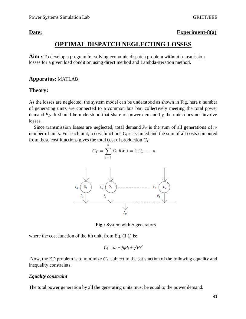
Power Systems Simulation Lab GRIETEEE
103
Graph
Power Systems Simulation Lab GRIETEEE
104
Power Systems Simulation Lab GRIETEEE
105
Result
Signature of the faculty

Power Systems Simulation Lab GRIETEEE
104
Power Systems Simulation Lab GRIETEEE
105
Result
Signature of the faculty

Power Systems Simulation Lab GRIETEEE
105
Result
Signature of the faculty