power to choose: an analysis of consumer behavior in the ... · power to choose: an analysis of...

Power to Choose:An Analysis of Consumer

Behavior in the Texas Retail Electric Market

Ali Hortacsu (University of Chicago and NBER) Seyed Ali Madanizadeh (University of Chicago)

Steve Puller (Texas A&M and NBER)

Power to Choose:An Analysis of Consumer


Power to Choose?!?!:An Analysis of Consumer


Residential Market Shares….0

.2.4

.6.8

1S

hare

of M

onth

ly R

esid

entia

l Loa

d

Jan 2002 Jan 2003 Jan 2004 Jan 2005 Jan 2006

Evolution of Market Shares: TNMP

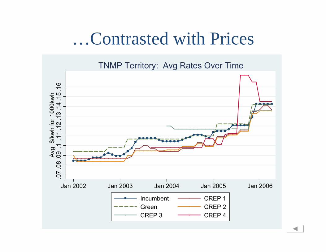
…Contrasted with Prices.0

7.0

8.0

9.1

.11

.12

.13

.14

.15

.16

Avg

. $/k

wh

for 1

000k

wh


Incumbent CREP 1Green CREP 2CREP 3 CREP 4

TNMP Territory: Avg Rates Over Time

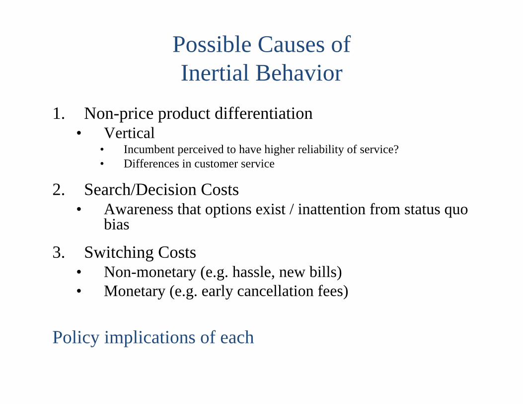
Possible Causes of Inertial Behavior

1. Non-price product differentiation• Vertical

• Incumbent perceived to have higher reliability of service?• Differences in customer service

2. Search/Decision Costs• Awareness that options exist / inattention from status quo

bias

3. Switching Costs• Non-monetary (e.g. hassle, new bills)• Monetary (e.g. early cancellation fees)

Policy implications of each

Research Questions

• How large are product differentiation, search costs, and switching costs?

• Do choice frictions and preference heterogeneity vary by demographics (income, race, age, education)?

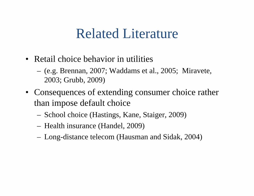
Related Literature

• Retail choice behavior in utilities – (e.g. Brennan, 2007; Waddams et al., 2005; Miravete,

2003; Grubb, 2009)

• Consequences of extending consumer choice rather than impose default choice – School choice (Hastings, Kane, Staiger, 2009)– Health insurance (Handel, 2009)– Long-distance telecom (Hausman and Sidak, 2004)

Outline• Descriptive statistics on switching

• Model of Consumer Switching– Allows for product differentiation, search costs &

switching costs

• We find:– Incumbent has a brand advantage (erodes over time)– Decision to consider alternatives is infrequent, but seasonal– Incumbent brand advantage & price sensitivity vary by

demographics

Texas Retail Market• Prior to 2002, residential customers served by

“regulated utility”

• Starting Jan 1, 2002, customers could choose provider– By default, assigned to incumbent that was

affiliated with the old utility (“AREP”)– Incumbent required to charge “price-to-beat” (6%

reduction from previous rates)• Ended up being above competitive rates (“headroom”)

– Price-to-beat adjustments indexed to natural gas price

Texas Retail Market (contd)

• Competitive retailers (CREPs)– Procure wholesale power and market to residential

(and other types) of customers– Largest CREPs were the AREPs from other

service territories– In 2002: 3-5 CREPs in each service territory– By 2006: 10+ CREPs

Information for Consumers

• www.powertochoose.com– (and www.poderdeescoger.org)– 2005-2006: ≈ 100K unique visitors/month

• Various media– Radio, TV, billboards– PUC public information campaign

Our Sample • TNMP service territory (“First Choice”) • January 2002-April 2006

– Approx. 192,000 residential customers.

We Study

Data• For each residential meter in TNMP from

January 2002-April 2006:– History of retail provider– Monthly consumption– Address to match to:

• Census data on block group characteristics

• For each retailer:– PUC monthly data on rate plan(s) offered

• We focus on 6 retailers with > 1% share

Switching: Time Trend and Seasonality0

1000

2000

3000

4000

Tota

l Sw

itche

s


Total Switches Over Time: TNMP

Descriptive Statistics of Potential Savings

• How much would households with incumbent have saved if purchased from lowest-priced REP?– Assume:

• Consumption perfectly inelastic & predictable• Switching costless

• Obviously, not a welfare analysis, but provides some magnitude of consumer surplus gains

Descriptive Statistics of Potential Savings

• What if households with incumbent had switched only once (in Jan ’02) to a large REP?

– Large #1: Mean = $7.65/HH-mo– Large #2: Mean = $9.92/HH-mo

• What if households with incumbent switched to cheapest CREP every month? – Mean = $12.41/HH-mo

• For comparison, Waxman-Markey= $14.58/HH-mo (CBO)

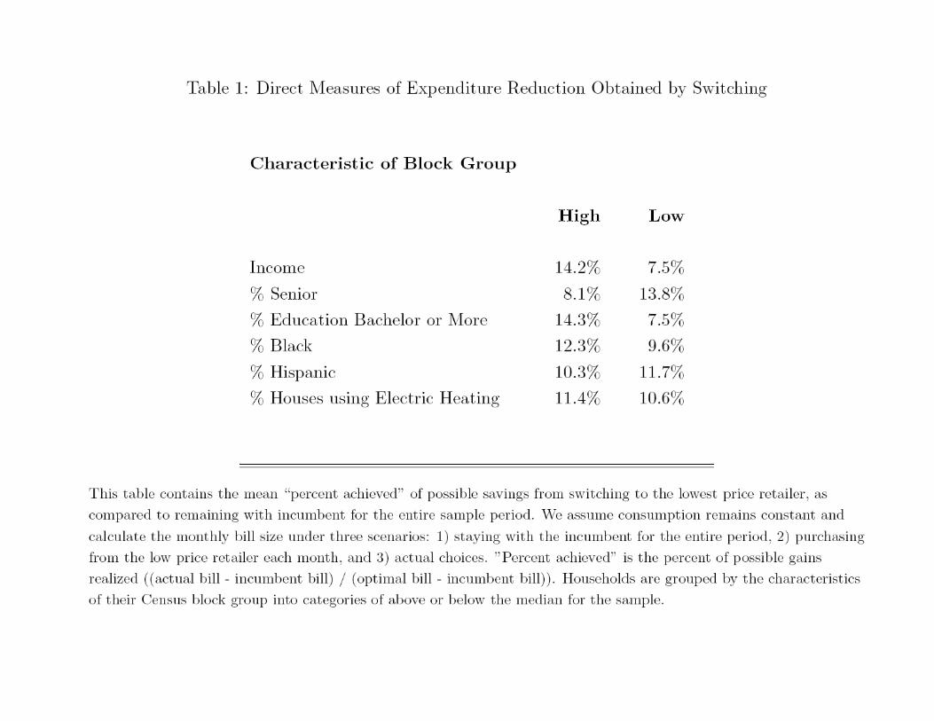
Descriptive Evidence of Effect on Different Populations

• Fraction of potential savings realized by switching

$Bill under incumbent rate

(consumption held constant)

Bill under month’s lowest priced REP(consumption held constant)

Actual bill

Pct Achieved Actual bill - Incumbent billLowest bill - Incumbent bill

(When incumbent is cheapest, we throw out because no potential savings)

Higher percent of potential savingsare realized in neighborhoods with:

More college educatedMore AAsFewer HispanicsFewer Senior CitizensLower Poverty

HHs w/ higher usage

Model of Household-Level Choice

• In each month:– Stage 1: Decision to Choose

• Household with provider k chooses whether to consider alternative retailers

– Stage 2: Choice• Households that decide to choose will observe (all)

providers’ product characteristics, and choose provider that maximizes utility

• Can choose to stay with current provider k

– Allow for heterogeneity across households in decision and choice probabilities

Model (contd)

• “Movers”– Households that move-in during month t– Must choose; there is no default

• In stage 1, “decide” with probability = 1

Simplified Illustration• 3 retailers• Consumers identical• Observe only 2 months of data (“last month” and

“this month”)

• Each household currently with retailer k searches with pr = λk– Heterogeneity due to k’s service

• Conditional upon “deciding”, household chooses retailer j with pr = Pj

5 probabilities (λ1, λ2 , λ3, P1, P2)

Simplified Illustration


= N(1)


N P( ) ( )11 1 11

non deciders deciders choosing 1

= N(1)


N P( ) ( )11 1 11


= N(1)

N P( )11 2

deciders choosing 2


N P( ) ( )11 1 11


= N(1)

N P( )11 2

deciders choosing 2

N P P( ) ( )11 1 21

deciders choosing 3


N P( ) ( )11 1 11


= N(1)

N P( )11 2

deciders choosing 2

N P P( ) ( )11 1 21

deciders choosing 3

9 moments e.g. E[#(k=1, j=1)] = N(1)[(1-λ1)+λ1P1](1 redundant moment in each set – any customer not going to 2 or 3 stays with 1)

5 probabilities and 6 moments (use the “off-diagonal” moments)

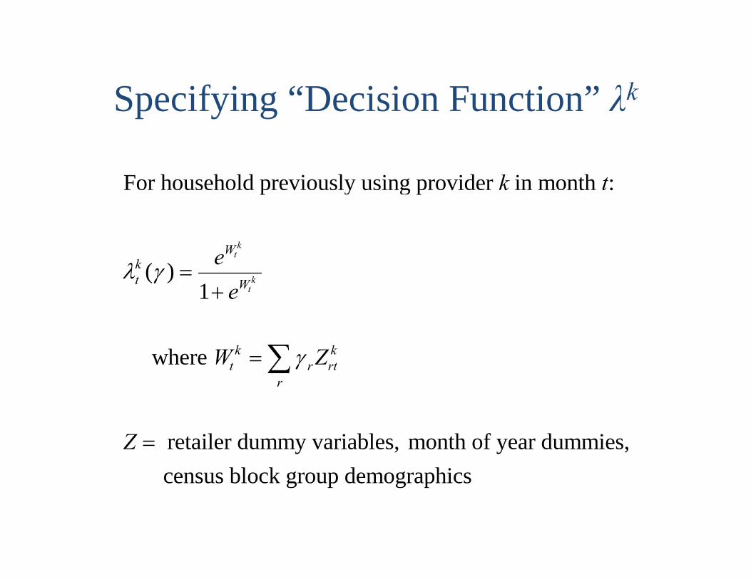
Specifying “Decision Function” λk

For household previously using provider in month :

where

retailer dummy variables, month of year dummies, census block group demographics

k t

ee

W Z

Z

tk

W

W

tk

r rtk

r

tk

tk

( )

1

Specifying “Choice Function” Pj

For each household whose provider was in AND decides to search, it chooses the retailer that maximizes utility:

where is Type I Extreme Value i.i.d. across consumer, provider, and time.

price , (Incumbent) , (Incumbent) Month , (j = (k)) not mover))

In future: (1) additional covariates for CREPs, (2) IVs for price Distributi

jt j j t

No Switching Costs

k t-

U X

X I I I I i

ijtk

s ijt sk

ijts

ijt

ijt

1

( ),

( )

(

onal assumption implies that:

PX

Xijt

s ijt sk

s

s ikt sk

sk

( )exp( )

exp( )

,( )

,( )

1

GMM EstimationEstimate decision parameters ( ) and choice parameters ( ) via GMM:

where and

,

min

( ) ( )

( ) ( )

( )

( )

W

N P

Njtk

jtk

jtk

itk

ijti B

tk

tk

Estimate for January 2004 – April 2006 when all 6 retailers present(20% sample to ease computation)

Identification: Product Differentiation,

Search Costs, and Switching Costs

• Search costs = e.g. “inattentiveness”• Switching costs = e.g. hassle

• Identification of Search Costs (separate from choice/brand effects)– Flow from REP k to REP j allows separate identification of

probability of search (λk) and probability of choice (Pj)• Parameters/probabilities O(J) and moments O(J2)

– Key assumptions: • “Deciding” is a function of the last provider (and not the next one)

– E.g. high bill, bad service. Rules out advertising?• “Choosing” is a function of the next provider (and not the last one)

Identification: Product Differentiation,

Search Costs, and Switching Costs

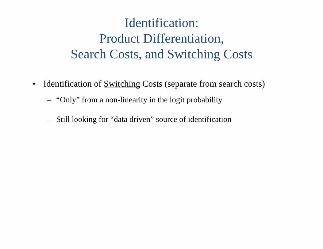
• Identification of Switching Costs (separate from search costs)

– “Only” from a non-linearity in the logit probability

– Still looking for “data driven” source of identification

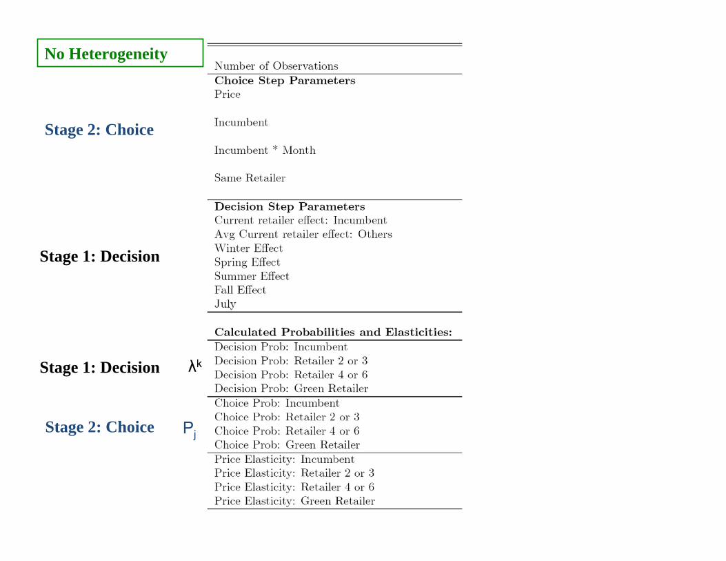
Stage 1: Decision

Stage 2: Choice

Stage 1: Decision

Stage 2: Choice

λk

Pj

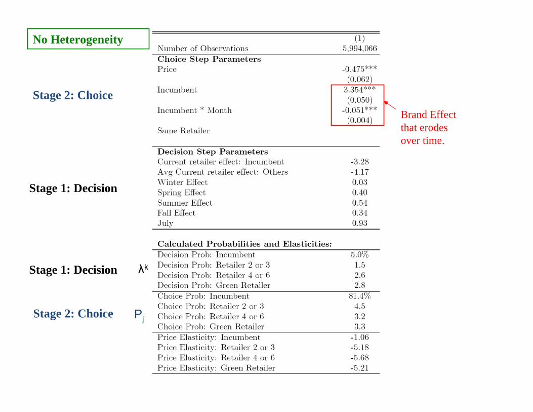
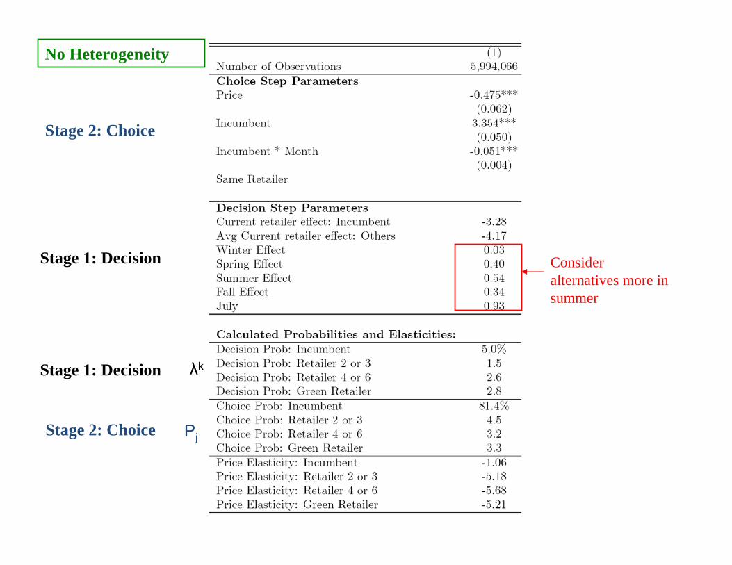
No Heterogeneity

Stage 1: Decision

Stage 2: Choice

Stage 1: Decision

Stage 2: Choice

λk

Pj

No Heterogeneity

Brand Effectthat erodesover time.

Stage 1: Decision

Stage 2: Choice

Stage 1: Decision

Stage 2: Choice

λk

Pj

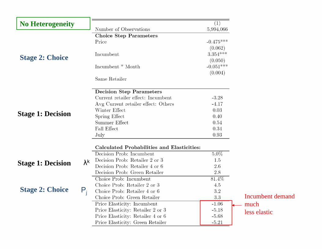
No Heterogeneity

Incumbent demand much less elastic

Stage 1: Decision

Stage 2: Choice

Stage 1: Decision

Stage 2: Choice

λk

Pj

No Heterogeneity

Consider alternatives more in summer

Stage 1: Decision

Stage 2: Choice

Stage 1: Decision

Stage 2: Choice

λk

Pj

No Heterogeneity

…but it’s still rare

Consider alternatives more in summer

Stage 1: Decision

Stage 2: Choice

Stage 1: Decision

Stage 2: Choice

λk

Pj

No Heterogeneity

Evidence ofswitchingcosts

First Cut Distributional Analysis

• How do brand effects, searching and switching costs vary by demographics?– Caveat: using Census block group characteristics

• Later: welfare calculations

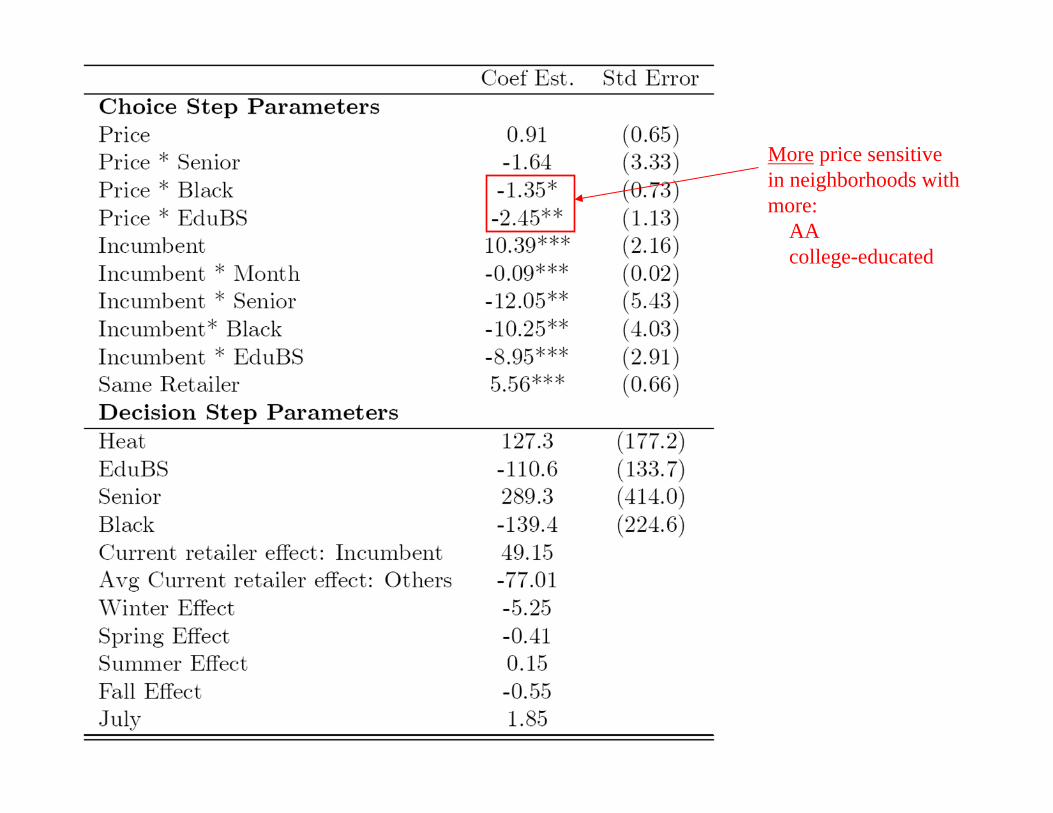
More price sensitive in neighborhoods with more:

AA college-educated

Brand advantage lower in neighborhoods with more:

seniors, AA, college educated

Conclusions• Raw data:

– $7-$12/month left on table by not switching from incumbent to competitive retailer

• Model-driven:– Inertial behavior due to each of:

• (1) brand advantage, • (2) infrequent consideration of alternatives, • (3) switching costs

– Incumbent has brand effect but erodes over time• Potentially large implications for consumer surplus if “it counts” &

profits for incumbent– Brand advantage varies by neighborhood

The End

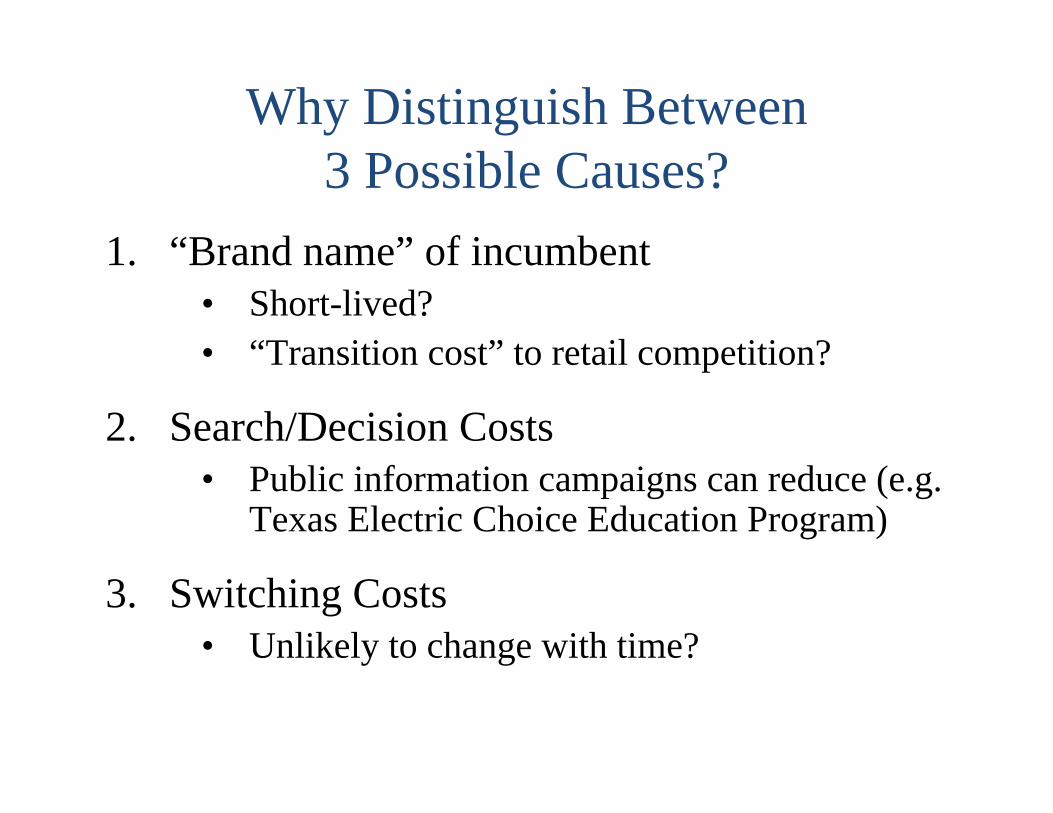
Why Distinguish Between 3 Possible Causes?

1. “Brand name” of incumbent• Short-lived? • “Transition cost” to retail competition?

2. Search/Decision Costs• Public information campaigns can reduce (e.g.

Texas Electric Choice Education Program)

3. Switching Costs• Unlikely to change with time?

Broad Arguments For and Against Retail Competition

• Advocates:– New retailers will create value-added services (e.g. risk

hedging, real-time pricing)– May help break utility’s monopsony power in wholesale

market

• Opponents:– Value-added services/retail innovations are more limited in

electricity (as compared to e.g. telecom)– Economies of scale in retail billing/customer service

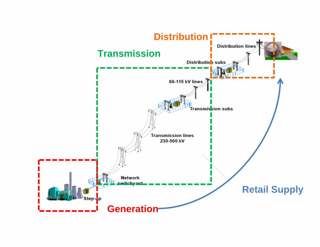
Transmission

Distribution

Generation

Retail Supply

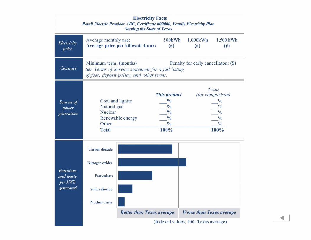
Possible Sources of Product Differentiation

• Perceived reliability for CREPs• Customer service quality• Renewable energy content• Term of rate structure (“hedging”)

Data (contd)

• We focus on 6 retailers with > 1% share– the incumbent, 2 “incumbents” from other service

territories, 3 others (1 green)

• For each retailer:– PUC monthly data on rate plan(s) offered

• 4 retailers offered only 1 rate plan• Other 2 retailers – chose plan guessed most popular by

industry analyst

Note: Excludes “New Meters” and “Move-ins”

0.2

.4.6

.81

Sha

re o

f Mon

thly

Res

iden

tial L

oad


Market Shares for New Meters and Movers: TNMP

Incumbent Share Not Driven Entirely By Search Costs

Median = $7.56Mean = $12.4175th pctile = about $1690th pctile = about $29

Monthly Savings for Customers with Incumbent

Are these Savings Large (In Terms of Energy Policy)?

• Estimated cost of Waxman-Markey– $14.58/HH-mo (CBO)– $6.66 - $9.25 /HH-mo (EPA)

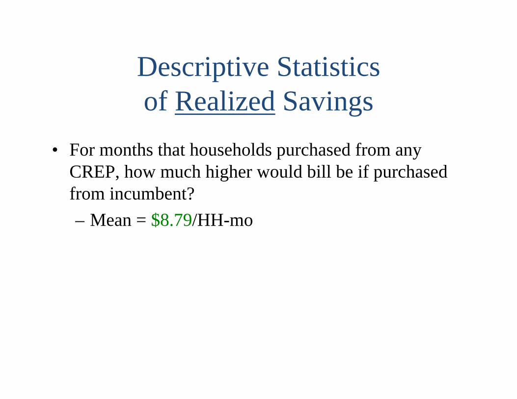
Descriptive Statistics of Realized Savings

• For months that households purchased from any CREP, how much higher would bill be if purchased from incumbent?– Mean = $8.79/HH-mo

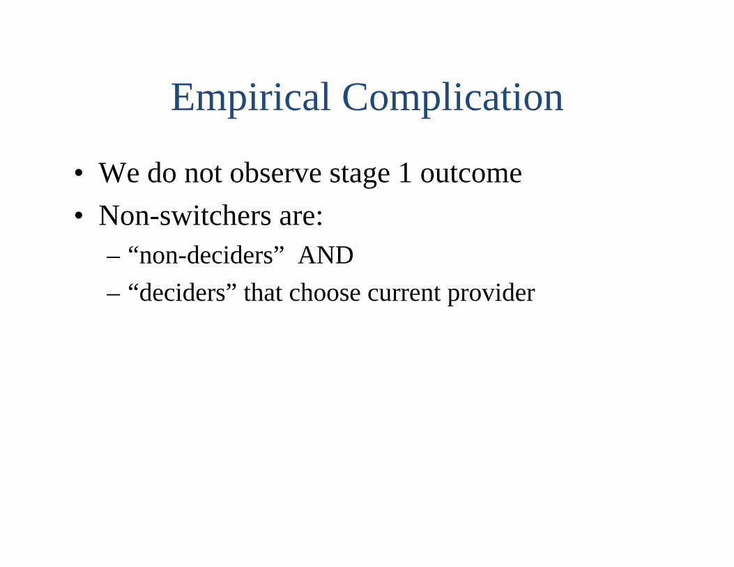
Empirical Complication

• We do not observe stage 1 outcome• Non-switchers are:

– “non-deciders” AND – “deciders” that choose current provider

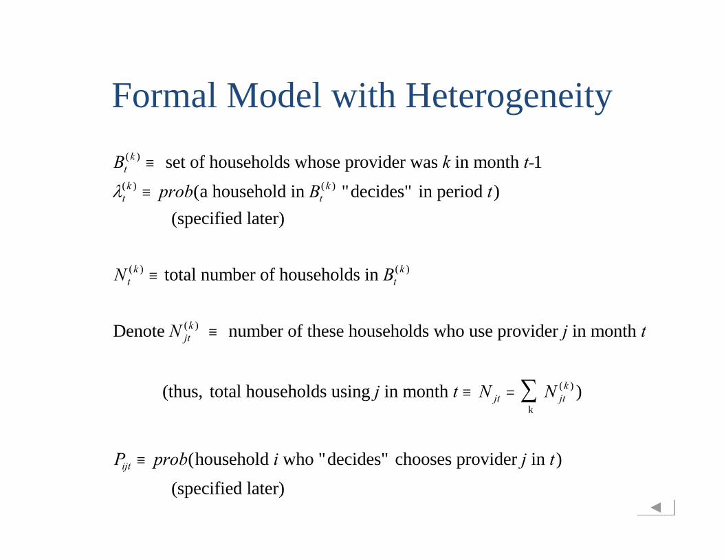
Formal Model with Heterogeneity

B k t-prob B t

N B

N j t

j t N N

P prob i j t

tk

tk

tk

tk

tk

jtk

jt jtk

ijt

( )

( ) ( )

( ) ( )

( )

( )

(

)

(

set of households whose provider was in month a household in "decides" in period )

(specified later)

total number of households in

Denote number of these households who use provider in month

(thus, total households using in month

household who "decides" chooses provider in ) (specified later)

k

1

Formal Model with HeterogeneityFor each agent in set , let uses in month )For agents changing retailers (j k

and

Our moment equations:

where can include household - level data

moments for each time

i B d i j t

E d P

N d

E N P P

J J t

tk

ijtk

t ijtk

itk

ijt

jtk

ijtk

i B

t jtk

itk

i Bijt ijt

tk

tk

( ) ( )

( ) ( )

( ) ( )

( ) ( )

(),

[ ]

[ ]

( )

( )

( )

1

1

1

1

Our Measure of Price

• The price per kwh for 1000kwh visible on Facts Label & powertochoose.com– Median usage = 968kwh

• Rationale:– Most salient– Average price (rather than marginal price) may drive

behavior (Ito, 2010)

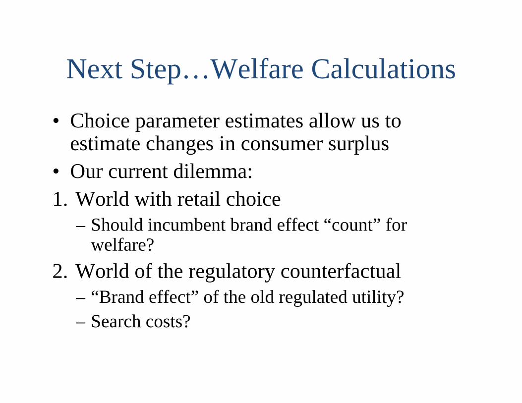
Next Step…Welfare Calculations

• Choice parameter estimates allow us to estimate changes in consumer surplus

• Our current dilemma:1. World with retail choice

– Should incumbent brand effect “count” for welfare?

2. World of the regulatory counterfactual– “Brand effect” of the old regulated utility?– Search costs?

Broader Literature on Consumer Decisionmaking

• Is this just “stupid consumer tricks?”• Chetty – tax• Grubb – cellphone• Einav & Cohen• Handel

Search Rates: Comparing Estimate to Outside Data

• # unique webhits / approx # HHs = 0.0181.8% search rate on

powertochoose

• Season pattern consistent with estimated pattern

020

0040

0060

0080

00U

niqu

e V

isito

rs

Sep 05 Oct Nov Dec Jan 06 Feb Mar Apr May Jun Jul Aug

Unique Visitors to Powertochoose.com in FY 2006

power to choose: an analysis of consumer behavior in the ... · power to choose: an analysis of...

Documents