power vs money: alternative approaches to reducing child ... · power vs money: alternative...

Power vs Money: Alternative Approaches to Reducing Child

Marriage in Bangladesh, a Randomized Control Trial

Nina Buchmann, Erica Field, Rachel Glennerster, Shahana Nazneen,

Svetlana Pimkina, Iman Sen∗

May 12, 2017

Abstract

A clustered randomized trial in Bangladesh examines alternative strategies to reducechild marriage and teenage childbearing and increase girls’ education. Communities wererandomized into three treatment and one control group in a 2:1:1:2 ratio. From 2008,girls in treatment communities received either i) a six-month empowerment program, ii)a financial incentive to delay marriage, or iii) empowerment plus incentive. Data from15,739 girls 4.5 years after program completion show that girls eligible for the incentivefor at least two years were 25% (-9.2ppts, p<0.01) less likely to be married under 18, 16%(-5.0ppts, p<0.01) less likely to have given birth under 20, and 24% (6.8ppts, p<0.01)more likely to be in school at age 22. Unlike other incentive programs that are conditionalon girls staying in school, an incentive conditional on marriage alone has the potential tobenefit out-of-school girls. We find insignificantly different effects for girls in and out ofschool at baseline. The empowerment program did not decrease child marriage or teenagechildbearing. However, girls eligible for the empowerment program were 10% (2.9ppts,p<0.10) more likely to be in-school.

JEL:

∗The authors are from Duke (Buchmann and Field), JPAL (Glennerster and Sen), IPA(Nazneen) and EPoD(Pimkina). Please direct correspondence to [email protected].

1

The study was funded by the International Initiative for Impact Evaluation, the US Na-

tional Institutes of Health, the Nike Foundation, and the International Development Research

Center. We thank colleagues at Save the Children and Bangladesh Development Society who

were an integral part of designing this evaluation particularly Jahirul Alam Azad, Winnifride

Mwebesa, Veronica Torres, Mary Beth Powers, Elizabeth Pearce, and Barbara Burroughs as

well as Shoraez Shahjahan (IPA) and Diva Dhar (JPAL). Invaluable research assistance was

provided by Libby Abbott, Michael Duthie, Rahin Khandker, Elizabeth Linos, Parendi Mehta,

Rudmila Rahman, Akshay Dixit, Rizwana Shahnaz, Pauline Shoemaker, Saffana Humaira,

Mihir Bhaskar, and Jintao Sun. All errors are our own.

2

Contents

1 Introduction 4

2 Methods 5

2.1 Study design and Participants . . . . . . . . . . . . . . . . . . . . . . . . . . . . 5

2.2 Procedures . . . . . . . . . . . . . . . . . . . . . . . . . . . . . . . . . . . . . . . 6

2.3 Outcomes . . . . . . . . . . . . . . . . . . . . . . . . . . . . . . . . . . . . . . . 8

2.4 Statistical Analysis . . . . . . . . . . . . . . . . . . . . . . . . . . . . . . . . . . 8

3 Results 12

4 Discussion 17

5 Appendix 19

5.1 A1: Program Timeline . . . . . . . . . . . . . . . . . . . . . . . . . . . . . . . . 19

5.2 A2: Program Outreach . . . . . . . . . . . . . . . . . . . . . . . . . . . . . . . . 20

5.3 A3: Attrition and Non-Response Analyses . . . . . . . . . . . . . . . . . . . . . 21

5.4 A4: Compliance . . . . . . . . . . . . . . . . . . . . . . . . . . . . . . . . . . . . 23

5.5 A5: Verification of Marriage Status and Marriage Age . . . . . . . . . . . . . . . 24

5.6 A6: Estimating Equations . . . . . . . . . . . . . . . . . . . . . . . . . . . . . . 26

5.7 A7: Inter-household spillovers . . . . . . . . . . . . . . . . . . . . . . . . . . . . 27

5.8 A8: First-Stage Effects . . . . . . . . . . . . . . . . . . . . . . . . . . . . . . . . 28

5.9 A9: Robustness Checks . . . . . . . . . . . . . . . . . . . . . . . . . . . . . . . . 29

5.9.1 Tables A9a: Excluding Controls . . . . . . . . . . . . . . . . . . . . . . . 29

5.9.2 Tables A9b: Including Washed-Out Communities . . . . . . . . . . . . . 31

5.9.3 Tables A9c: Intention-to-treat Specification . . . . . . . . . . . . . . . . 33

5.9.4 Tables A9d: Treatment Arm Dummies . . . . . . . . . . . . . . . . . . . 35

5.10 A10: Results of the Cost-Benefit and Cost-Effectiveness Analyses . . . . . . . . 37

3

1 Introduction

While most of the world has instituted laws prohibiting marriage under 18, child marriage

remains the norm in many countries, with 142 million girls projected to become child brides in

developing countries between 2011-2020 (Loaiza Sr and Wong, 2012).

Girls who marry early are more likely to be socially isolated, have early and high-risk

pregnancies, be at risk of sexually transmitted infections, and experience intimate partner

violence (Mathur et al., 2003; Jain and Kurz, 2007; UNICEF et al., 2001). Childbearing during

adolescence is associated with severe complications such as obstructed labor or obstetric fistula

(EngenderHealth, 2003), and complications in pregnancy and delivery are a leading cause of

death among girls aged 15-19 (Nour, 2009). Child marriage may also impact health through

behavioral channels, as young mothers are often less informed and less likely to seek care (Raj,

2010). There is strong evidence that child marriage results in lower schooling attainment (Field

and Ambrus, 2008), which could further impact health.

Other than legal bans, which have proven to be infeasible to enforce in developing countries,

there are limited policy approaches to reducing child marriage. There is some evidence that

encouraging girls to stay in-school is effective in reducing child marriage (Duflo et al., 2015;

Angrist et al., 2006; Hong and Sarr, 2012; Hahn et al., 2015). However, this approach fails to

reach the most vulnerable girls who leave school early due to poverty or those with insufficient

access to secondary schools. One high quality study showed that an unconditional transfer could

reduce child marriage and teenage childbearing in a very different context to ours (Malawi)

(Baird et al., 2011).

A more inclusive approach to reducing child marriage that is growing in popularity is to

strengthen girls’ ability to negotiate later marriage or childbearing through empowerment or

skills training. Yet there is little evidence on the impact of such programs on girls’ long-run

wellbeing. One experiment in Uganda found that empowerment and skills training reduces

teenage pregnancy (Bandiera et al., 2014), while another empowerment program in Tanzania

did not have significant effects on marriage outcomes (Buehren et al., 2015). Meanwhile, there

are no impact evaluations in peer-reviewed journals of empowerment programs to reduce child

marriage in South Asia where child marriage is most common and age of marriage and age of

sexual onset are largely determined by parents.

An alternative approach is providing conditional incentives to parents to delay girls’ mar-

riage. Conditional incentives may be particularly important in societies like Bangladesh where

the cost of marrying a daughter in the form of the dowry payment made by a bride’s family

is believed to increase with age (Field and Ambrus, 2008; Bruce and Sebstad, 2004). While

incentives conditional on marital status have been tried on a large scale in Haryana, India,

there is no rigorous evidence on their effectiveness.1

1The Apni Beti Apni Dhan program in Haryana provided bonds to mothers of newly-born girls, redeemable

4

This study conducts a clustered randomized trial in rural Bangladesh to evaluate the impact

of two very different policy approaches to reducing child marriage and teenage childbearing – an

adolescent empowerment training program and a conditional incentive program. Bangladesh

has the second highest child marriage rate in the world: 74% of women aged 20-49 were mar-

ried before age 18 (UNICEF et al., 2014), and in 2014, 31% of all 15-19-year-olds had begun

childbearing (Mitra et al., 2016). One experimental arm tests the effectiveness of financial

incentives conditional on marriage, the first randomized trial of this approach. Alongside, we

also evaluate the impact of a standard empowerment program, and test whether combining the

empowerment program and the conditional incentives program is more powerful than either

program alone. Our findings indicate that conditional incentive programs are highly effective

in increasing age at marriage and schooling attainment, while empowerment programs have no

effect on marriage timing, but do encourage unmarried and older married girls to stay in school.

We find no evidence of complementarities between the incentive and empowerment program on

schooling or child marriage.

2 Methods

2.1 Study design and Participants

Between January 2007 and September 2015 we ran a clustered randomized trial in collabo-

ration with Save the Children (USA) to examine alternative strategies to reduce child marriage

and teenage childbearing and increase education. The study was carried out in six sub-districts

(Daulatkhan, Babuganj, Muladi, Patuakhali Sadar, Bauphal and Bhola Sadar) in south central

Bangladesh, where Save the Children was managing a food security program that provided

transfers to pregnant and lactating mothers. The conditional incentive program that we evalu-

ate used the distribution infrastructure of this existing program, which operated in all treatment

and control communities in our study. To determine which communities were included in the

study, we collected census data in all 610 communities in the six sub-districts between January

and February 2007. Communities were excluded from our study if they were too remote for

distribution or had less than 40 or more than 490 adolescent girls, leaving 460 eligible com-

munities in five subdistricts that were randomized into i) a basic empowerment program, ii)

a conditional incentive to delay marriage, iii) empowerment plus conditional incentive, or iv)

the status quo using a stratified randomized design in the ratio 2:1:1:2.2 The objective was

to compare the effect of an empowerment program with that of a conditional incentive and

when the girl was 18 and unmarried, with additional bonuses for education. The most rigorous non-experimentalevaluation of the program only examined education outcomes and found no significant gains in-schooling (Sinhaand Yoong, 2009). For a full review of the literature see supplementary appendix S1.

2Experimental assignment was carried out by MIT staff without the involvement of Save the Children usingStata. Save the Children staff were informed of the treatment allocation of study communities.

5

to test whether a combined empowerment and incentive program is more powerful than either

program alone. Randomization at the community level reduced the risk of inter-household

spillovers. We stratified by union, an administrative grouping of roughly 10 communities, and

within union by community size (supplementary appendix S5).

In communities randomized to receive the empowerment program, called Kishoree Kontha

(KK), or “Adolescent Girl’s Voice”, all girls aged 10-19 were invited to take part in one of

four six-month cycles of the program that ran between December 2007 and August 2010. In

conditional incentive communities, girls whose reported age at baseline (before the program

was announced) meant that they would be age 15-17 at the start of the oil distribution were

eligible to receive the conditional incentive until the age of 18 if they remained unmarried.

Every four months from April 2008 to August 2010 marital status was verified by interviewing

family members, neighbors and community leaders and cooking oil was distributed to eligible

girls. We attempted to resurvey all households with girls age 15-17 at distribution start 4.5

years after program completion (between May and September 2015). Parents of each daughter

were asked about her history of marriage, childbearing and education.

The sample analyzed in this paper consists of 15,739 girls from 438 communities: 5,239 in

the empowerment arm, 2,372 in the conditional incentive arm, 2,745 in the empowerment plus

incentive arm and 5,383 in control. Participation in the empowerment and incentive programs

was voluntary. Oral consent was collected from subjects for survey participation. Institutional

review boards of Innovations for Poverty Action and MIT approved this project.

2.2 Procedures

The Bangladesh Development Society (BDS) implemented the empowerment program under

the direction of Save the Children. Communities assigned to the empowerment program first

underwent a community mobilization phase that informed parents, teachers, and community

leaders about the activities and potential benefits of the program, mobilized their support and

found locations for “Safe Spaces” – meeting places where girls could meet, socialize, and receive

training. Safe Space committees were organized with adult members of the community to help

troubleshoot any potential problems, for example if a girl’s parents did not want her to attend.

The empowerment curriculum included education support and social competency training. The

education component aimed to enhance the basic literacy, numeracy, and oral communication of

both school-attending and illiterate girls. The social competency component trained girls in life

skills and nutritional and reproductive health knowledge via a curriculum designed by Save the

Children USA. In randomly selected communities (50%), financial literacy and encouragement

to generate own income was added to the curricula. Overall, the empowerment curriculum was

similar in content to many empowerment programs being implemented worldwide, including

those designed by BRAC and Unicef.

6

Each Safe Space had a target of 20 girls, two to four of which were selected to be peer

educators. Peer educators were given between 24 and 40 hours of training on the curriculum,

which they delivered with the aid of specially designed books that included stories and examples

to be read aloud, questions to be discussed, and participatory activities and games to perform.

Safe Space groups were designed to meet five or six days a week for two hours each day for

six months. Groups could continue to meet once the curriculum was complete but there was

no support or new curricula after six months. At the end of the cycle, field staff repeated the

mobilization and selection process until the entire community population had been reached.

Thus, communities received up to four cycles and 24 safe spaces, depending on the number of

girls living there. Monitoring data show Safe Spaces averaged six meetings, or 7.8 hours, per

week, and 45,149 girls, or 84%, of girls in target communities were reached (appendix A2). This

makes KK one of the largest adolescent empowerment programs implemented in the developing

world.

The conditional incentive program was an in-kind transfer of cooking oil to encourage par-

ents to postpone daughters’ marriage until the legal age of consent (18). The value of the

incentive was approximately $16 per year, an amount chosen to offset the estimated financial

cost of higher dowry (Bruce and Sebstad, 2004). Cooking oil was chosen as an incentive because

it is purchased regularly by every family in Bangladesh and thus has close to cash equivalent

value, yet it is less susceptible to theft and graft than cash because of its bulk. It also has a

high value to volume ratio, which minimized transport costs. Girls estimated to be age 15-17

at distribution start and confirmed to be unmarried by Community Health Volunteers (CHVs)

were issued ration cards to collect the oil. Only girls (not their parents) were permitted to

collect the oil by presenting their ration card, which was checked against a separate beneficiary

list at distribution points. A total of 5,617 unmarried adolescent girls received the conditional

incentive at least once, or 71% of the girls eligible at baseline (appendix A2). Marriage condi-

tionality was checked before each distribution round by CHVs and independent monitors who

asked beneficiaries, neighbors and community leaders about marital status. Those found to be

married or who had reached 18 (according to their age at baseline) had their names removed

from the eligibility list and their cards taken away.

Four and a half years after program completion, we conducted a follow-up study of all girls

age 15-17 and unmarried at distribution start. Parents were asked about all daughters’ current

marital status.3 Parents of married or previously married girls were also asked “How long

ago did she marry?” or “How long ago did she first marry?”, respectively. Parents were also

asked whether the girl had ever given birth and the age of each child. In addition, parents

were asked whether their daughters were still in school and which class they were currently

attending and/or last completed.

3Possible responses were “Married”, “Single, never married”, “Widowed”, “Divorced”, “Separated” or“Abandoned”.

7

2.3 Outcomes

The primary outcomes of the study are child marriage (under 18), teenage childbearing

(under 20) and current school enrollment. We use binary outcomes as opposed to continuous

measures of marriage and birth age to avoid censored data problems that arise from exclud-

ing girls that have never been married or given birth. Secondary outcomes are marriage age,

marriage rates under 16, and last class completed. Marriage age is calculated by comparing

reported marriage duration with girls’ age collected at baseline to avoid misreporting of under-

age marriages. Age at first birth is calculated using baseline age and the reported age of the

girl’s oldest living or deceased child. Data were collected from the household where the girl was

living at the time of the baseline survey (usually the girl’s parents).

2.4 Statistical Analysis

The study was powered to detect a 2.4ppts decrease in child marriage among girls receiving

the empowerment program and a 2.5ppts decrease among girls receiving the incentive from a

control mean of 58.7% with 80% power, 0.05 alpha, 15% attrition, and an intracluster correlation

of 0.010. The study also had power to detect a 2.4ppts decrease in teenage childbearing for

the empowerment program and a 2.5ppts decrease for the incentive from a control mean of

50.8%, and an intracluster correlation of 0.010. Finally, the study could detect an increase of

2.0ppts in school enrollment for the empowerment program and 2.1ppts for the incentive from

a control mean of 25.3%, and an intracluster correlation of 0.050.4 Means were taken from the

2004 Demographic and Health Survey data. The trial was registered at the AEA Registry prior

to endline data collection, #204 (https://www.socialscienceregistry.org/trials/204).

A team of monitors, data quality control officers, and research associates monitored the data

throughout data collection by conducting consistency checks across answers, analyzing variable

distributions and monitoring differences between survey responses and responses of parents

in a second separate backcheck survey conducted for 7% of all observations. In this sample,

marriage status differed in 1.5% of the cases, birth status in 1.3% and ever-schooled in 0.8%. We

recollected data through phone interviews from households with very high overall backcheck

error rates across all variables. Backcheck error rates are balanced across treatment arms.

We also intensively verified marriage status (including by talking to the girls themselves) for

6% of the girls in the baseline sample (excluding washed-out villages) 1.5 years after program

completion. We found no significant differences between initial and verified reports and the

number of mismatches between initial and verified reports were balanced across treatment

arms. In the few cases where marriage certificates were available at endline, marriage age

differed by 3.0 months on average and the discrepancy was balanced across treatment arms

4Intracluster correlation in our survey data was 0.03 for child marriage, 0.03 for teenage childbearing and0.05 for schooling status.

8

(appendix A5).

CHVs only issued eligibility cards to girls, who had been identified as eligible in the census

and were still unmarried at program launch. Thus, girls, which could not be found by CHVs

and girls who had been married before the program were not issued eligibility cards. We are

thus excluding girls from all treatment arms with insufficient baseline tracking information and

girls whose reported marriage date is before the first oil distribution (19%, balanced by treat-

ment arm). In addition, we estimate the impact of the incentive using two-stage least squares

(2SLS) regressions (see appendix A6 for precise specification). In the first stage, program

inclusion (card issuance) is predicted by treatment assignment in an ordinary least squares

regression (OLS; linear probability). In the second stage, marriage, childbearing and educa-

tion outcomes are regressed against predicted inclusion from the first stage. Under plausible

assumptions, this method accounts for errors in program inclusion and produces unbiased and

consistent estimates of treatment assignment under full compliance. The most important as-

sumption is that of no cross-household spillovers onto adolescent girls in the same cohort. A

comparison of girls in households who did not receive an eligibility card relative to controls

suggests that this assumption is valid (see appendix A7). We regress all outcomes on dum-

mies representing eligibility for the incentive, eligibility for the empowerment program, and

an interacted dummy representing eligibility for both. Both first and second stage regressions

include controls measured at baseline for strata, household size, an older unmarried sister in the

household, school enrollment, mother’s level of education, distance from the community center

to the closest neighboring community center (a proxy for remoteness), number of schools in the

community, and the ratio of adult boys to adult girls in the community (a proxy for marriage

market conditions). Errors are clustered at the unit of randomization (community). Table 2

compares impacts on child marriage using an intention-to-treat specification (ITT), using the

ITT specification after excluding married girls and girls with insufficient tracking information,

and using the 2SLS specification after excluding married girls and girls with insufficient track-

ing information. Results excluding controls, and including washed-out communities, as well as

analysis using ITT specification for all outcomes are reported in appendix A8, and yield similar

results. We also find no differences when regressing outcomes on dummies for each treatment

arm (empowerment, incentive, empowerment plus incentive) as opposed to eligibility for each

program.

Our analysis sample constitutes all 15,739 girls aged 15-17 and unmarried at program launch

that were followed-up at endline. To assess dose response, we compare effects on the whole

sample with effects on girls eligible to receive the incentive for at least two years (aged 15 at

distribution start). We also check for differential effects according to whether a girl was in

school at baseline to test whether the most vulnerable girls can potentially benefit from one of

the policy approaches.

9

Figure 1: Trial profile

10

Table 1: Baseline characteristics

Empowerment Incentive Empow.+Incen. Control Total

Married & Unmarried at Baseline

N 8,739 4,176 4,503 8,990 26,408

Mean S.D. Diff. Mean S.D. Diff. Mean S.D. Diff. Mean S.D. Mean S.D.

Ever Married (%)

Still in-school (%)

Highest Class Passed

8.5

60.2

6.2

28.0

48.9

2.6

-0.1

-0.9

0.0

9.4

59.2

6.1

29.1

49.2

2.7

0.7

-2.0

-0.1

8.8

60.2

6.3

28.4

48.9

2.7

0.2

-0.9

0.1

8.7

61.2

6.2

28.1

48.7

2.7

8.8

60.4

6.2

28.3

48.9

2.6

Unmarried at Baseline

N 7,992 3,785 4,106 8,212 24,095


Still in-school (%)

Highest Class Passed

Age

Father Education (0-17)

Mother Education (0-17)

HH Size (members)

Unmarried older sister in HH (%)

Community Boys/Girls Ratio

Community size (girls age 10 to 19)

64.6

6.4

14.9

4.2

3.2

6.1

18.9

1.0

265.9

47.8

2.6

0.8

4.4

3.3

2.0

39.1

0.3

121.3

-1.2

0.0

-0.0

0.2

0.1

0.0

0.3

-0.0

-9.2

64.1

6.3

14.9

3.8

3.0

6.1

18.0

1.0

251.2

48.0

2.6

0.8

4.1

3.3

2.0

38.5

0.3

119.4

-1.7

-0.1

0.0

-0.1

-0.1

0.1

-0.5

-0.0

-23.9

65.1

6.4

14.9

4.0

3.0

6.1

18.0

1.1

261.3

47.7

2.6

0.8

4.2

3.1

2.0

38.4

0.3

118.6

-0.8

0.1

-0.0

0.0

-0.0

0.0

-0.5

0.0

-13.8

65.8

6.4

14.9

3.9

3.1

6.0

18.5

1.0

275.1

47.4

2.6

0.8

4.2

3.3

2.1

38.9

0.3

126.2

65.0

6.4

14.9

4.0

3.1

6.1

18.5

1.0

265.9

47.7

2.6

0.8

4.2

3.3

2.0

38.8

0.3

122.5

Differences from OLS regressions with modified Huber-White SEs clustered at the community level. Significance levels are * p<0.10 , ** p<0.05 and *** p<0.01.

11

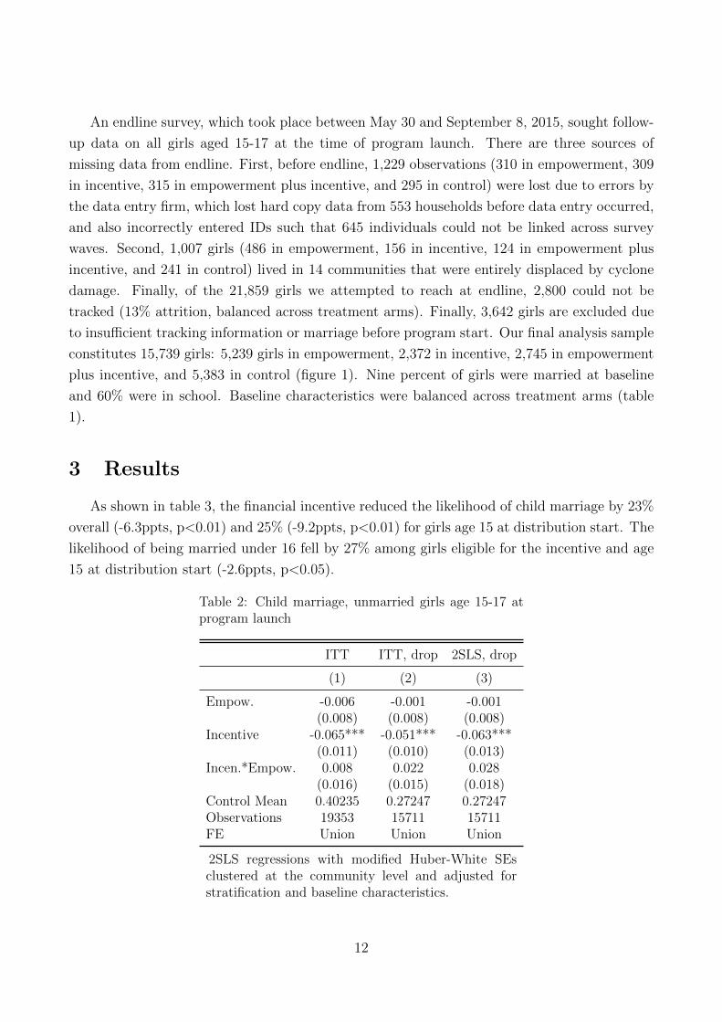
An endline survey, which took place between May 30 and September 8, 2015, sought follow-

up data on all girls aged 15-17 at the time of program launch. There are three sources of

missing data from endline. First, before endline, 1,229 observations (310 in empowerment, 309

in incentive, 315 in empowerment plus incentive, and 295 in control) were lost due to errors by

the data entry firm, which lost hard copy data from 553 households before data entry occurred,

and also incorrectly entered IDs such that 645 individuals could not be linked across survey

waves. Second, 1,007 girls (486 in empowerment, 156 in incentive, 124 in empowerment plus

incentive, and 241 in control) lived in 14 communities that were entirely displaced by cyclone

damage. Finally, of the 21,859 girls we attempted to reach at endline, 2,800 could not be

tracked (13% attrition, balanced across treatment arms). Finally, 3,642 girls are excluded due

to insufficient tracking information or marriage before program start. Our final analysis sample

constitutes 15,739 girls: 5,239 girls in empowerment, 2,372 in incentive, 2,745 in empowerment

plus incentive, and 5,383 in control (figure 1). Nine percent of girls were married at baseline

and 60% were in school. Baseline characteristics were balanced across treatment arms (table

1).

3 Results

As shown in table 3, the financial incentive reduced the likelihood of child marriage by 23%

overall (-6.3ppts, p<0.01) and 25% (-9.2ppts, p<0.01) for girls age 15 at distribution start. The

likelihood of being married under 16 fell by 27% among girls eligible for the incentive and age

15 at distribution start (-2.6ppts, p<0.05).

Table 2: Child marriage, unmarried girls age 15-17 atprogram launch

ITT ITT, drop 2SLS, drop

(1) (2) (3)

Empow. -0.006 -0.001 -0.001(0.008) (0.008) (0.008)

Incentive -0.065*** -0.051*** -0.063***(0.011) (0.010) (0.013)

Incen.*Empow. 0.008 0.022 0.028(0.016) (0.015) (0.018)

Control Mean 0.40235 0.27247 0.27247Observations 19353 15711 15711FE Union Union Union

2SLS regressions with modified Huber-White SEsclustered at the community level and adjusted forstratification and baseline characteristics.

12

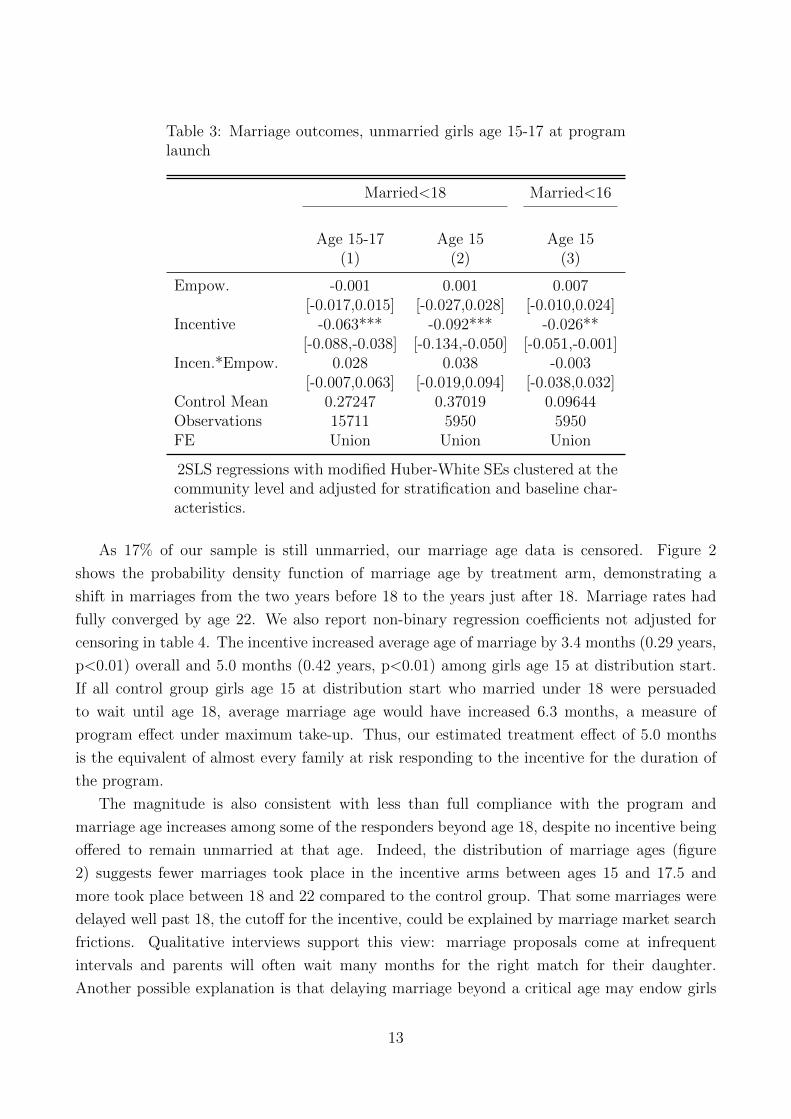
Table 3: Marriage outcomes, unmarried girls age 15-17 at programlaunch

Married<18 Married<16

Age 15-17 Age 15 Age 15(1) (2) (3)

Empow. -0.001 0.001 0.007[-0.017,0.015] [-0.027,0.028] [-0.010,0.024]

Incentive -0.063*** -0.092*** -0.026**[-0.088,-0.038] [-0.134,-0.050] [-0.051,-0.001]

Incen.*Empow. 0.028 0.038 -0.003[-0.007,0.063] [-0.019,0.094] [-0.038,0.032]

Control Mean 0.27247 0.37019 0.09644Observations 15711 5950 5950FE Union Union Union

2SLS regressions with modified Huber-White SEs clustered at thecommunity level and adjusted for stratification and baseline char-acteristics.

As 17% of our sample is still unmarried, our marriage age data is censored. Figure 2

shows the probability density function of marriage age by treatment arm, demonstrating a

shift in marriages from the two years before 18 to the years just after 18. Marriage rates had

fully converged by age 22. We also report non-binary regression coefficients not adjusted for

censoring in table 4. The incentive increased average age of marriage by 3.4 months (0.29 years,

p<0.01) overall and 5.0 months (0.42 years, p<0.01) among girls age 15 at distribution start.

If all control group girls age 15 at distribution start who married under 18 were persuaded

to wait until age 18, average marriage age would have increased 6.3 months, a measure of

program effect under maximum take-up. Thus, our estimated treatment effect of 5.0 months

is the equivalent of almost every family at risk responding to the incentive for the duration of

the program.

The magnitude is also consistent with less than full compliance with the program and

marriage age increases among some of the responders beyond age 18, despite no incentive being

offered to remain unmarried at that age. Indeed, the distribution of marriage ages (figure

2) suggests fewer marriages took place in the incentive arms between ages 15 and 17.5 and

more took place between 18 and 22 compared to the control group. That some marriages were

delayed well past 18, the cutoff for the incentive, could be explained by marriage market search

frictions. Qualitative interviews support this view: marriage proposals come at infrequent

intervals and parents will often wait many months for the right match for their daughter.

Another possible explanation is that delaying marriage beyond a critical age may endow girls

13

with greater bargaining power in negotiating marriage proposals, which they can then parlay

into even further marriage delays once the program is over, simply on account of being older

and more experienced.

We do not observe a separate or additional effect of the empowerment program on marriage

outcomes.

Figure 2: Distribution of marriage age, girls age 15 and unmarried at pro-gram launch

We also find strong effects of the incentive on age at first birth (table 5). The incentive

reduced the likelihood of teenage childbearing by 13% (-2.9ppts, p<0.05) overall and 16% (-

5.0ppts, p<0.01) among girls age 15 at distribution start. We again do not observe a separate

or additional effect of the empowerment program.

The incentive to delay marriage also has a large positive impact on school enrollment (table

6). We restrict our sample to girls in school at program launch because it is extremely rare

for girls to return to school once they have unenrolled.5 Girls aged 15-17 at distribution start

and eligible for the incentive were 12% (3.3ppts, p<0.10) more likely to be in school at age

22-25 and had completed 2.2 months (0.19 years, p>0.10) of additional schooling. Girls eligible

for the empowerment program were 6% (1.8ppts, p>0.10) more likely to be in school and had

5We test this assumption and find no evidence of impact of the incentive on schooling for those girls whowere out of school at program start. However, the confidence intervals are large.

14

Table 4: Marriage age, married girls, age 15-17and unmarried at program launch

Age 15-17 Age 15(1) (2)

Empow. -0.010 -0.021[-0.093,0.073] [-0.144,0.102]

Incentive 0.286*** 0.415***[0.145,0.428] [0.243,0.588]

Incen.*Empow. -0.099 -0.140[-0.292,0.094] [-0.398,0.118]

Control Mean 19.07285 18.36518Observations 13018 4807FE Union Union

2SLS regressions with modified Huber-WhiteSEs clustered at the community level and ad-justed for stratification and baseline character-istics.

Table 5: Teenage childbearing, unmarried girls age15-17 at program launch

Age 15-17 Age 15(1) (2)

Empow. 0.005 0.003[-0.010,0.020] [-0.022,0.027]

Incentive -0.029** -0.050***[-0.053,-0.005] [-0.086,-0.014]

Incen.*Empow. 0.012 0.022[-0.022,0.046] [-0.030,0.073]

Control Mean 0.22946 0.31638Observations 15651 5934FE Union Union

2SLS regressions with modified Huber-White SEsclustered at the community level and adjusted forstratification and baseline characteristics.

15

completed 2.4 months (0.20 years, p<0.05) of additional schooling. We observe significant dose

response both among girls eligible for the incentive and the empowerment program: Girls 15

at distribution start in the incentive group are 24% (6.8ppts, p<0.01) more likely to be in

school and have completed 3.8 months (0.31 years, p>0.10) of additional schooling. Girls 15

at distribution start in the empowerment group are 10% (2.9ppts, p<0.10) more likely to be in

school and have completed 2.0 months (0.17 years, p>0.10) of additional schooling.

Table 6: Education outcomes, unmarried girls age 15-17 and in school at programlaunch

In school Last class passed

Age 15-17 Age 15 Age 15-17 Age 15(1) (2) (3) (4)

Empow. 0.018 0.029* 0.202** 0.168[-0.005,0.041] [-0.003,0.060] [0.002,0.403] [-0.103,0.440]

Incentive 0.033* 0.068*** 0.186 0.314[-0.003,0.069] [0.019,0.117] [-0.139,0.511] [-0.176,0.805]

Incen.*Empow. -0.003 -0.039 -0.151 -0.232[-0.052,0.046] [-0.104,0.026] [-0.617,0.316] [-0.844,0.381]

Control Mean 0.28680 0.28366 11.64867 11.12043Observations 11052 4603 10969 4574FE Union Union Union Union

2SLS regressions with modified Huber-White SEs clustered at the communitylevel and adjusted for stratification and baseline characteristics.

The coefficient on the interaction term between the incentive and empowerment program is

insignificantly different from zero in all specifications.

Unlike other incentive programs that are conditional on girls staying in school, an incentive

conditional on marriage alone has the potential to benefit out-of-school girls. On the other

hand, the incentive may only be sufficient to discourage child marriage if a girl has the option

of staying in school while she waits. We compare the effects of the incentive conditional on

staying unmarried on child marriage and teenage childbearing outcomes for girls in school and

out of school at baseline (table 7). We find insignificantly different effects for girls in and out of

school at baseline: The conditional incentive decreased the likelihood of child marriage by 6%

(-2.1ppts) among girls out of school at baseline and by 31% (-7.7ppts, p<0.01) among girls in

school at baseline. We again do not observe a separate or additional effect of the empowerment

program on marriage and childbearing outcomes in either subsample.

These results imply that marriage age influences childbearing and other outcomes not only

through its impact on education. Even when there is no possibility of attaining more schooling,

16

Table 7: Marriage and childbearing outcomes, by baseline schooling status, unmarried girls age 15-17 at programlaunch

Girls out of school at BL Girls in school at BL

Married<18 Married<16 Birth<20 Married<18 Married<16 Birth<20(1) (2) (3) (4) (5) (6)

Empow. 0.012 0.016 0.030** -0.007 0.005 -0.005[-0.018,0.042] [-0.031,0.063] [0.000,0.061] [-0.024,0.011] [-0.013,0.022] [-0.022,0.012]

Incentive -0.021 -0.007 0.008 -0.077*** -0.032** -0.044***[-0.074,0.032] [-0.077,0.063] [-0.040,0.057] [-0.106,-0.048] [-0.058,-0.006] [-0.069,-0.018]

Incen.*Empow. 0.004 -0.026 -0.041 0.034* 0.004 0.030[-0.070,0.078] [-0.132,0.080] [-0.109,0.027] [-0.002,0.071] [-0.031,0.039] [-0.007,0.067]

Control Mean 0.32924 0.06615 0.27857 0.24954 0.04462 0.20964Observations 4656 1346 4639 11055 4604 11012FE Union Union Union Union Union Union

2SLS regressions with modified Huber-White SEs clustered at the community level and adjusted for stratifica-tion and baseline characteristics.

girls are made better off by postponing marriage.

4 Discussion

These results provide novel evidence that a relatively inexpensive conditional incentive tar-

geted to families of adolescent girls in a setting with high rates of underage marriage is effective

in substantially reducing child marriage and teenage childbearing. It also increased the per-

centage of girls still in school at age 22 to 25 and increased years of schooling completed. A

well-crafted and quite intensive adolescent girls’ empowerment program did not decrease child

marriage or teenage childbearing but was effective in increasing schooling.

We show that a financial incentive conditional on marriage and not education can also delay

marriage and childbearing for out-of-school girls. This is important because the most popular

incentive programs focus on keeping girls in school and thus are unavailable to out-of-school

girls. This focus may stem from the assumption that once out of school a girl will inevitably

marry and there is little that policy can do to change this. Our results suggest this vulnerable

population can still benefit from incentives.

One possible concern with the validity of our estimates is the loss of observations from data

entry errors and cyclone damage. However, the problem was not driven by treatment status,

minimizing risk of bias. Attrition among households that enumerators attempted to find was

just 13%, which is low given the 9-year study duration (appendix A3).

Another possible concern is parents lying about marriage timing because of the incentive.

We consider this unlikely as the program had finished 4.5 years before endline surveying, girls

were far too old to qualify, and marriage rates are similar in a verification survey where mar-

17

riage was carefully verified (appendix A5). Finally, childbearing and school enrollment results

provide strong evidence that the marriage effects are real, as there was no incentive to lie about

childbearing or schooling 4.5 years after the program ended.

Our results complement the growing literature suggesting that incentives can help change

long-held behaviors often believed to be culturally entrenched and immutable. Incentives con-

ditional on education have been criticized for failing to help the most marginal girls who cannot

continue in school. Our results suggest a way to promote education and reach the most vul-

nerable.

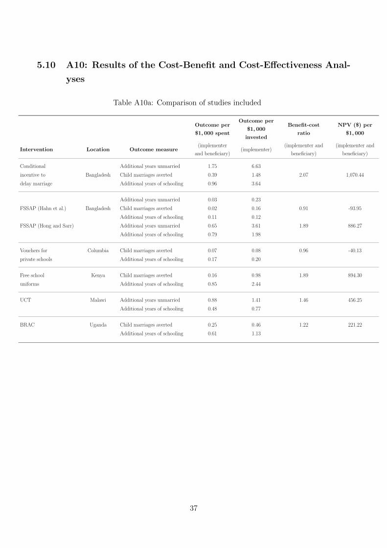
Our results also imply that the conditional incentive is highly cost-effective. The conditional

incentive translates into 6.6 years of delayed marriage, 1.5 averted child marriages, and 3.6 years

of schooling for every $1,000 invested by the implementer, generating $1,070 in Net Present

Value for every $1,000 spent (costs to implementer and beneficiary) – the highest impacts

among rigorously evaluated interventions in a comprehensive cost-efficacy analysis (appendix

A10).

We find an impact of a well-crafted and -implemented empowerment program on education

outcomes only. However, it is possible that the empowerment program will translate into

gains in reproductive health outcomes or marital bargaining power later in a woman’s life.

Furthermore, empowerment programs may be much more effective in settings in which girls

have some agency over marriage timing.

18

5 Appendix

5.1 A1: Program Timeline

Figure A1: Program timeline

19

5.2 A2: Program Outreach

Table A2: Program take-up, take-up by upazila of girls age 10-19 at baseline for the empower-ment treatment arm and girls age 15-17 and unmarried at distribution start for the incentivetreatment arms

Sub-district KK Enrollment KK Attendance Oil Take-up(%) (%) (%)

Babuganj 79.1 77.5 69.6(21.1) (4.3) (22.7)

Bauphal 78.3 81.6 72.0(22.5) (5.1) (15.5)

Bhola Sadar 79.5 82.6 83.5(20.7) (6.0) (7.1)

Patuakhali Sadar 89.5 76.9 64.1(17.1) (4.4) (10.0)

Muladi 73.4 81.5 65.7(20.5) (4.5) (22.7)

Average of girls enrolled in/attending KK as well as oil take-up based on monitoring data.Data are % (SD).

Participation in KK

Monitoring data suggests that 45,149 adolescent girls were reached (enrolled) through peer

education sessions in the four learning cycles, or 84% of eligible girls age 10-19 at baseline.

Average total attendance rate was 80%.

Oil Incentive

In total, 5,617 unmarried adolescent girls received the oil incentive at least once, or 71% of

girls eligible at baseline.

20

5.3 A3: Attrition and Non-Response Analyses

Table A3a: Attrition analysis, girls age 15-17 and unmarried at distribution start

Empowerment (%) Incentive (%) Enpow.+Incen. (%) Control (%) Total (%)

Households

N 7,523 3,581 3,845 7,718 22,667


Total 19.0 39.2 0.3 22.1 41.5 3.4 18.8 39.1 0.0 18.7 39.0 19.4 39.5

Girls

N 7,992 3,785 4,106 8,212 24,095


Total

Excluding data entry errors

Excluding data entry errors and

washed-out communities

19.3

16.0

12.3

39.4

36.7

32.9

0.4

0.1

-1.6

22.5

15.7

12.5

41.8

36.3

33.1

3.6

-0.2

-1.4

18.8

12.0

11.7

39.0

32.5

32.1

-0.1

-3.9*

-2.3

18.9

15.9

13.9

39.1

36.5

34.6

19.6

15.2

12.8

39.7

35.9

33.4

Differences from OLS regressions with modified Huber-White SEs clustered at the community level. Significance levels are * p<0.10 , ** p<0.05 and *** p<0.01.

21

Table A3b: Non-response analysis, percentage of missing or “don’t know” responses by outcome, by treatment. Girls age 15-17and unmarried at distribution start

Empowerment (%) Incentive (%) Empow.+Incen. (%) Control (%) Total (%)


Whether married

Marriage age (married girls)

Child marriage

Whether birth (married girls)

Age at first birth (girls who gave birth)

Teenage childbearing

Still in school

Last class passed

0.1

0.1

0.2

0.2

0.2

0.4

0.2

0.9

3.0

2.7

3.9

4.2

4.8

6.3

4.1

9.3

0.0

-0.0

0.0

-0.1

0.1

-0.0

0.1

0.0

0.1

0.0

0.1

0.3

0.2

0.4

0.1

0.6

2.6

2.0

3.2

5.3

4.0

6.4

2.6

7.6

-0.0

-0.0

-0.0

-0.0

0.0

-0.0

-0.0

-0.2

0.0

0.1

0.1

0.4

1.0

1.0

0.0

0.7

1.7

3.8

3.9

6.5

9.8

10.0

1.7

8.5

-0.0

0.1

-0.0

0.1

0.9

0.6

-0.1

-0.1

0.1

0.1

0.2

0.3

0.1

0.4

0.1

0.8

2.7

3.0

3.9

5.6

3.3

6.5

3.2

9.0

0.1

0.1

0.1

0.3

0.3

0.5

0.1

0.8

2.7

2.7

3.8

3.8

5.5

7.2

3.3

8.8

Significance levels are * p<0.10 , ** p<0.05 and *** p<0.01.

22

5.4 A4: Compliance

Table A4: Compliance, self-reported take-up in the midline verification survey. Any empower-ment includes girls in empowerment and empowerment plus incentive treatment groups. Anyincentive includes girls in the incentive and empowerment plus incentive treatment groups.Girls age 15-17 and unmarried at distribution start

Attended at least Member of KK Oil Take-up

Treatment Group 1 KK session (%) (%) (%)

Mean S.D. Mean S.D. Mean S.D.

Empowerment

Incentive

Empowerment+Incentive

Control

54.8

35.8

75.3

9.2

49.9

48.1

43.3

29.0

46.8

29.2

68.6

5.8

49.9

48.1

43.3

29.0

0.4

72.3

80.2

1.0

49.9

48.1

43.3

29.0

Any Empowerment

Any Incentive

62.2

.

62.2

.

54.7

.

49.8

.

.

76.1

.

42.7

Table A4 reports whether a girl that was unmarried and between the age of 15-17 and thus

eligible for all treatments attended at least one session of KK, was a member of KK, and/or

received the incentive. The table lists rates for any empowerment communities (comprised

of empowerment, and empowerment plus incentive communities), any incentive communities

(comprised of incentive, and empowerment plus incentive communities) as well as the rates

broken down by the different treatment types. The results highlight that KK attendance and

membership rates were higher in empowerment plus incentive treatment communities than in

empowerment communities. Even the percentage of spillovers, as defined by girls who attended

KK sessions or were KK members in any of the non-empowerment communities, was higher

in communities that received the conditional incentive: About 29.2% of girls in incentive com-

munities reported they were KK members, while the rate was 5.8% in control communities.

This could be due to three reasons: i) girls in communities in which cooking oil was also dis-

tributed could have been much more favorable towards the project and thus also sought KK

participation, ii) girls in the conditional incentive communities may have remained unmarried

for a longer time and thus be allowed to participate, and iii) girls that remembered having

received oil may also assume that they participated in other programs administered in their

community and thus overreport KK membership. Noncompliance was very low in non-incentive

communities, in which fewer than 1% of non-eligible girls report to have received oil.

23

5.5 A5: Verification of Marriage Status and Marriage Age

Table A5: Marriage status and age checks, comparison of marriage status and marriage age using verified reports and marriagecertificates. Girls age 15-17 and unmarried at distribution start

Empowerment (%) Incentive (%) Empow.+Incen. (%) Control (%) Total (%)


Marriage Rate

Married girls in initial survey

Married girls in verification survey

Difference between surveys

Difference in marital status between surveys

57.2

55.6

1.6

6.9

49.5

49.7

3.4

25.4

.

.

-0.4

-0.7

49.1

46.0

3.1

10.2

50.1

50.0

4.7

30.3

.

.

1.0

2.6

53.4

51.7

1.7

6.5

50.0

50.1

4.6

24.6

.

.

-0.8

-1.1

56.0

54.1

1.9

7.6

49.7

49.9

3.4

26.5

54.7

52.8

2.0

7.6

49.8

49.9

1.9

26.6

Marriage age difference

(certificate-reported marriage age; months)4.1 15.5 1.9 2.6 11.3 0.4 3.1 14.1 0.9 2.2 9.9 3.0 12.8

For each treatment arm, the differences between surveys are compared to the difference between surveys in the control arm.

Significance levels are * p<0.10 , ** p<0.05 and *** p<0.01.

24

First, to check the validity of parents’ reporting of marriage, we extensively followed up a

subsample 1.5 years after program completion and took several steps to verify marriage status.

Among those girls for which we were able to match initial and verified reports, we found no

significant differences between initial and verified reporting, and the number of mismatches

between initial and verified reporting were balanced across treatment arms. Given that this

suggested that reporting was accurate, we do not think that parents were underreporting child

marriage or teenage childbearing 4.5 years after program completion.

Second, for a small sample of 512 girls we have two separate estimates of marriage age: one

is based on the date of marriage from marriage certificates and the other is based on parents’

reports of marriage duration. On average marriage age derived from marriage certificates is 3.0

months greater than that calculated from reported marriage durations, and this difference is

balanced across treatment arms (table A5). This provides some encouraging support for our

measure of marriage age as it suggests parents are not systematically reducing their estimate

of marriage duration to avoid accusations of child marriage (if anything they aren’t underesti-

mating marriage age). However, we should note that the 512 girls for whom we can calculate

this discrepancy is not random and is based on a very small sample. The vast majority of

households did not have a copy of the marriage certificate. Interviews with some of those

who did not have marriage certificates suggested that certificates were often not collected from

the register’ office unless there was a specific need, such as divorce or separation, to reclaim

denmeher, or for taking any other legal actions. In other cases, households reported they had

collected certificates without this need for legal recourse but that they were not easily accessible

or could not be found.

25

5.6 A6: Estimating Equations

Our first- and second-stage estimations are:

Iti = γ0t + γ1tIi + γ2tEi + γ3tIi × Ei + γ′4tXiv + µuti +$vti + υti (1)

Yi = α + β1I1i + β2I2i + β3Ei + β′4Xiv + µui +$vi + εi (2)

where I1i is predicted program inclusion of person i to the incentive only program, and I2i

predicted inclusion of person i to the empowerment plus incentive program. Ii is assignment

to either of the incentive treatment arms, and Ei assignment to either of the empowerment

treatment arms. Yi is outcome for person i.

Both first and second stage regressions include a vector of individual and community controls

measured at baseline for strata, household size, an older unmarried sister in the household,

school enrollment, mother’s level of education, distance from the community center to the closest

neighboring community center (a proxy for remoteness), number of schools in the community,

and the ratio of adult boys to adult girls in the community (a proxy for marriage market

conditions), as well as union fixed-effects.

26

5.7 A7: Inter-household spillovers

Table 5.1: Married<18, by age at distribution start

Age 11-12 Age 13-14 Age 18 Whole sample

(1) (2) (3) (4)

Empow. -0.015 0.004 0.009* -0.009

[-0.036,0.006] [-0.019,0.026] [-0.001,0.019] [-0.026,0.008]

Incentive -0.016 0.020 -0.004 0.003

[-0.042,0.011] [-0.007,0.048] [-0.011,0.003] [-0.018,0.025]

Empow.*Incen. 0.034* -0.029 -0.010 0.007

[-0.005,0.072] [-0.068,0.010] [-0.021,0.002] [-0.024,0.038]

Control Mean 0.55349 0.49582 0.00454 0.48777

Observations 12506 12210 1943 26659

FE Union Union Union Union

2SLS regressions with modified Huber-White SEs clustered at the community

level and adjusted for stratification and baseline characteristics.

27

5.8 A8: First-Stage Effects

Table A8: First stage effects, girls age 15-17 and unmarried atdistribution start

Distribution list Distribution list * Empow.

(1) (2)

Incentive

assignment0.817*** 0.003

[0.784,0.850] [-0.005,0.011]

Incentive

assignment *

empowerment

0.029 0.845***

[-0.013,0.070] [0.818,0.872]

Constant 0.021 0.002

[-0.024,0.066] [-0.032,0.036]

F-statistic 717.04 486.95

Observations 15739 15739

FE Union Union

OLS regressions with modified Huber-White SEs clustered at the

community level and adjusted for stratification.

28

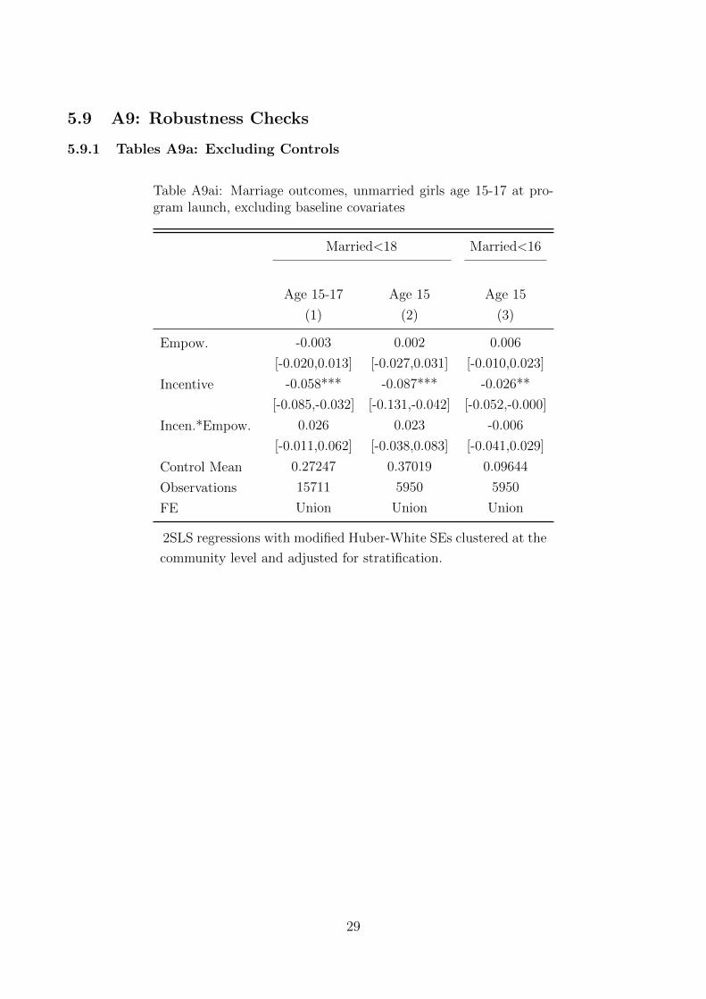
5.9 A9: Robustness Checks

5.9.1 Tables A9a: Excluding Controls

Table A9ai: Marriage outcomes, unmarried girls age 15-17 at pro-gram launch, excluding baseline covariates


Age 15-17 Age 15 Age 15

(1) (2) (3)

Empow. -0.003 0.002 0.006

[-0.020,0.013] [-0.027,0.031] [-0.010,0.023]

Incentive -0.058*** -0.087*** -0.026**

[-0.085,-0.032] [-0.131,-0.042] [-0.052,-0.000]

Incen.*Empow. 0.026 0.023 -0.006

[-0.011,0.062] [-0.038,0.083] [-0.041,0.029]

Control Mean 0.27247 0.37019 0.09644

Observations 15711 5950 5950

FE Union Union Union

2SLS regressions with modified Huber-White SEs clustered at the

community level and adjusted for stratification.

29

Table A9aii: Teenage childbearing, unmarried girlsage 15-17 at program launch, excluding baselinecovariates

Age 15-17 Age 15

(1) (2)

Empow. 0.004 0.001

[-0.011,0.019] [-0.024,0.027]

Incentive -0.023* -0.047**

[-0.048,0.001] [-0.085,-0.009]

Incen.*Empow. 0.008 0.011

[-0.028,0.043] [-0.043,0.065]

Control Mean 0.22946 0.31638


FE Union Union

2SLS regressions with modified Huber-White

SEs clustered at the community level and ad-

justed for stratification.

Table A9aiii: Education outcomes, unmarried girls age 15-17 and in school atprogram launch, excluding baseline covariates


Age 15-17 Age 15 Age 15-17 Age 15

(1) (2) (3) (4)

Empow. 0.020* 0.029* 0.224** 0.225

[-0.004,0.043] [-0.004,0.062] [0.014,0.434] [-0.059,0.509]

Incentive 0.019 0.058** 0.067 0.275

[-0.021,0.059] [0.004,0.112] [-0.282,0.415] [-0.244,0.793]

Incen.*Empow. 0.007 -0.029 -0.060 -0.201

[-0.045,0.060] [-0.099,0.041] [-0.552,0.432] [-0.846,0.444]

Control Mean 0.28680 0.28366 11.64867 11.12043

Observations 11052 4603 10969 4574



level and adjusted for stratification.

30

5.9.2 Tables A9b: Including Washed-Out Communities

Table A9bi: Marriage outcomes, unmarried girls age 15-17 at pro-gram launch, excluding washed-out communities


Age 15-17 Age 15 Age 15

(1) (2) (3)

Empow. -0.001 0.001 0.007

[-0.017,0.015] [-0.027,0.028] [-0.010,0.024]

Incentive -0.063*** -0.092*** -0.026**

[-0.088,-0.038] [-0.134,-0.050] [-0.051,-0.001]

Incen.*Empow. 0.028 0.038 -0.003

[-0.007,0.063] [-0.019,0.094] [-0.038,0.032]

Control Mean 0.27247 0.37019 0.09644



2SLS regressions with modified Huber-White SEs clustered at the

community level and adjusted for stratification and baseline char-

acteristics.

31

Table A9bii: Teenage childbearing, unmarried girlsage 15-17 at program launch, excluding washed-outcommunities

Age 15-17 Age 15

(1) (2)

Empow. 0.005 0.003

[-0.010,0.020] [-0.022,0.027]

Incentive -0.029** -0.050***

[-0.053,-0.005] [-0.086,-0.014]

Incen.*Empow. 0.012 0.022

[-0.022,0.046] [-0.030,0.073]

Control Mean 0.22946 0.31638


FE Union Union

2SLS regressions with modified Huber-White SEs

clustered at the community level and adjusted for

stratification and baseline characteristics.

Table A9biii: Education outcomes, unmarried girls age 15-17 and in school atprogram launch, excluding washed-out communities


Age 15-17 Age 15 Age 15-17 Age 15

(1) (2) (3) (4)

Empow. 0.018 0.029* 0.202** 0.168

[-0.005,0.041] [-0.003,0.060] [0.002,0.403] [-0.103,0.440]

Incentive 0.033* 0.068*** 0.186 0.314

[-0.003,0.069] [0.019,0.117] [-0.139,0.511] [-0.176,0.805]

Incen.*Empow. -0.003 -0.039 -0.151 -0.232

[-0.052,0.046] [-0.104,0.026] [-0.617,0.316] [-0.844,0.381]

Control Mean 0.28680 0.28366 11.64867 11.12043

Observations 11052 4603 10969 4574




32

5.9.3 Tables A9c: Intention-to-treat Specification

Table A9ci: Marriage outcomes, unmarried girls age 15-17 at pro-gram launch, intention-to-treat specification


Age 15-17 Age 15 Age 15

(1) (2) (3)

Emp. -0.001 0.001 0.007

[-0.017,0.015] [-0.027,0.028] [-0.010,0.024]

Incentive -0.051*** -0.077*** -0.022**

[-0.072,-0.031] [-0.112,-0.042] [-0.043,-0.001]

Inc.*Emp. 0.022 0.030 -0.003

[-0.007,0.051] [-0.018,0.078] [-0.033,0.027]

Control Mean 0.27247 0.37019 0.09644





acteristics.

33

Table A9cii: Teenage childbearing, unmarried girlsage 15-17 at program launch, intention-to-treatspecification

Age 15-17 Age 15

(1) (2)

Emp. 0.005 0.003

[-0.010,0.020] [-0.022,0.027]

Incentive -0.024** -0.042***

[-0.043,-0.004] [-0.073,-0.011]

Inc.*Emp. 0.009 0.018

[-0.019,0.038] [-0.027,0.062]

Control Mean 0.22946 0.31638


FE Union Union

OLS regressions with modified Huber-White SEs



Table A9ciii: Education outcomes, unmarried girls age 15-17 and in school atprogram launch, intention-to-treat specification


Age 15-17 Age 15 Age 15-17 Age 15

(1) (2) (3) (4)

Emp. 0.018 0.029* 0.202** 0.168

[-0.005,0.041] [-0.003,0.061] [0.000,0.403] [-0.106,0.442]

Incentive 0.027* 0.057*** 0.153 0.265

[-0.003,0.057] [0.015,0.099] [-0.119,0.426] [-0.161,0.691]

Inc.*Emp. -0.001 -0.032 -0.123 -0.192

[-0.043,0.041] [-0.088,0.025] [-0.524,0.277] [-0.730,0.346]

Control Mean 0.28680 0.28366 11.64867 11.12043

Observations 11052 4603 10969 4574


OLS regressions with modified Huber-White SEs clustered at the community


34

5.9.4 Tables A9d: Treatment Arm Dummies

Table A9di: Marriage outcomes, unmarried girls age 15-17 at pro-gram launch, regressing on treatment arm dummies


Age 15-17 Age 15 Age 15

(1) (2) (3)

Empow. -0.001 0.001 0.007

[-0.017,0.015] [-0.026,0.028] [-0.010,0.024]

Incentive -0.063*** -0.092*** -0.026**

[-0.088,-0.038] [-0.134,-0.050] [-0.051,-0.001]

Incen.*Empow. -0.036*** -0.054** -0.021

[-0.061,-0.011] [-0.096,-0.012] [-0.047,0.005]

Control Mean 0.27247 0.37019 0.09644





acteristics.

35

Table A9dii: Teenage childbearing, unmarried girlsage 15-17 at program launch, regressing on treat-ment arm dummies

Age 15-17 Age 15

(1) (2)

Empow. 0.005 0.003

[-0.010,0.020] [-0.022,0.027]

Incentive -0.029** -0.050***

[-0.053,-0.006] [-0.086,-0.014]

Incen.*Empow. -0.011 -0.025

[-0.036,0.014] [-0.064,0.014]

Control Mean 0.22946 0.31638


FE Union Union

OLS regressions with modified Huber-White SEs



Table A9diii: Education outcomes, unmarried girls age 15-17 and in school atprogram launch, regressing on treatment arm dummies


Age 15-17 Age 15 Age 15-17 Age 15

(1) (2) (3) (4)

Empow. 0.018 0.029* 0.202** 0.168

[-0.005,0.041] [-0.003,0.060] [0.002,0.402] [-0.103,0.439]

Incentive 0.033* 0.068*** 0.185 0.315

[-0.003,0.069] [0.019,0.117] [-0.140,0.511] [-0.176,0.806]

Incen.*Empow. 0.051*** 0.061** 0.267 0.273

[0.015,0.086] [0.012,0.110] [-0.079,0.613] [-0.145,0.691]

Control Mean 0.28680 0.28366 11.64867 11.12043

Observations 11052 4603 10969 4574


OLS regressions with modified Huber-White SEs clustered at the community


36

5.10 A10: Results of the Cost-Benefit and Cost-Effectiveness Anal-

yses

Table A10a: Comparison of studies included

Outcome per

$1, 000 spent

Outcome per

$1, 000

invested

Benefit-cost

ratio

NPV ($) per

$1, 000

Intervention Location Outcome measure(implementer

and beneficiary)(implementer)

(implementer and

beneficiary)

(implementer and

beneficiary)

Conditional Additional years unmarried 1.75 6.63

incentive to Bangladesh Child marriages averted 0.39 1.48 2.07 1,070.44

delay marriage Additional years of schooling 0.96 3.64

Additional years unmarried 0.03 0.23

FSSAP (Hahn et al.) Bangladesh Child marriages averted 0.02 0.16 0.91 -93.95

Additional years of schooling 0.11 0.12

FSSAP (Hong and Sarr) Additional years unmarried 0.65 3.61 1.89 886.27


Vouchers for Columbia Child marriages averted 0.07 0.08 0.96 -40.13

private schools Additional years of schooling 0.17 0.20

Free school Kenya Child marriages averted 0.16 0.98 1.89 894.30

uniforms Additional years of schooling 0.85 2.44

UCT Malawi Additional years unmarried 0.88 1.41 1.46 456.25


BRAC Uganda Child marriages averted 0.25 0.46 1.22 221.22


37

Table A10b: Cost-effectiveness of the oil incentive

Outcome measure Discount rateOutcome per

$1, 000 spent

Outcome per

$1, 000 invested

(%)(implementer and

beneficiary)(implementer)

Additional years unmarried

3

5

10

1.51

1.75

2.30

6.51

6.63

6.92

Child marriage averted

3

5

10

0.34

0.39

0.51

1.45

1.48

1.54

Additional years of schooling

3

5

10

0.83

0.96

1.26

3.58

3.64

3.80

Table A10c: Cost-benefit of the oil Incentive

Discount rate Benefit-cost ratio NPV($) per $1, 000

(%) (implementer and beneficiary) (implementer and beneficiary)

3

5

10

2.90

2.07

1.10

1,895.59

1,070.44

98.18

38

Figure A10a: Comparison of years unmarried/$1,000 of interventions affecting marriage. Stud-ies with marriage age outcome included. Costs include costs to implementer only

Figure A10b: Comparison of child marriages averted/$1000 of interventions affecting marriage.Studies with child marriage outcome included. Costs include costs to implementer only

39

Figure A10c: Comparison of benefit-cost-ratios of interventions affecting marriage. Costs in-clude costs to implementer and beneficiary

Figure A10d: Comparison of NPV/$1000 of interventions affecting marriage. Costs includecosts to implementer and beneficiary

40

References

Joshua Angrist, Eric Bettinger, and Michael Kremer. Long-term Educational Consequences

of Secondary School Vouchers: Evidence from Administrative Records in Colombia. The

American Economic Review, 96(3):847–862, 2006.

Sarah Baird, Craig McIntosh, and Berk Ozler. Cash or Condition? Evidence from a Cash

Transfer Experiment. The Quarterly Journal of Economics, qjr032, 2011.

Oriana Bandiera, Robin Burgess, Markus Goldstein, Niklas Buehren, Selim Gulesci, Imran Ra-

sul, and Munshi Sulaiman. Womens Empowerment in Action: Evidence from a Randomized

Control Trial in Africa. The London School of Economics and Political Science, Suntory and

Toyota International Centres for Economics and Related Disciplines, 2014.

J Bruce and J Sebstad. building assets for safe and productive lives: a report on a workshop

on adolescent girls’ livelihoods. In Adolescent Girls Livelihoods Meeting, 2004.

Niklas Buehren, Markus Goldstein, Selim Gulesci, Sulaiman Munshi, and Yam Venus. Evalua-

tion of Layering Microfinance on an Adolescent Development Program for Girls in Tanzania.

Working Paper, 2015.

Esther Duflo, Pascaline Dupas, and Michael Kremer. Education, HIV, and Early Fertility:

Experimental Evidence from Kenya. The American Economic Review, 105(9):2757–2797,

2015.

UNFPA EngenderHealth. Obstetric Fistula Needs Assessment Report: Findings from Nine

African Countries, 2003.

Erica Field and Attila Ambrus. Early Marriage, Age of Menarche, and Female Schooling

Attainment in Bangladesh. Journal of Political Economy, 116(5):881–930, 2008.

Youjin Hahn, Asadul Islam, Kanti Nuzhat, Russell Smyth, Hee-Seung Yang, et al. Education,

Marriage and Fertility: Long-Term Evidence from a Female Stipend Program in Bangladesh.

Melbourne: Monash University, 2015.

Seo Yeon Hong and Leopold Remi Sarr. Long-term impacts of the free tuition and female

stipend programs on education attainment, age of marriage, and married womens labor

market participation in Bangladesh., 2012.

Saranga Jain and Kathleen Kurz. New Insights on Preventing Child Marriage: a Global Anal-

ysis of Factors and Programs. Washington DC International Center for Research on Women

[ICRW] 2007 Apr., 2007.

41

E Loaiza Sr and Sylvia Wong. Marrying too young. End child marriage. New York New York

United Nations Population Fund [UNFPA] 2012., 2012.

Sanyukta Mathur, Margaret Greene, and Anju Malhotra. Too young to Wed: the Lives, Rights

and Health of Young Married Girls. Citeseer, 2003.

Mitra, National Institute of Population Research Associates, and ICF International Train-

ing (NIPORT). Bangladesh Demographic and Health Survey 2014. Dhaka, Bangladesh, and

Rockville, Maryland, USA: NIPORT, Mitra and Associates, and ICF International, 2016.

Nawal M Nour. Child Marriage: a Silent Health and Human Rights Issue. Rev Obstet Gynecol,

2(1):51–56, 2009.

Anita Raj. When the mother is a child: the impact of child marriage on the health and human

rights of girls. Archives of Disease in Childhood, page archdischild178707, 2010.

Nistha Sinha and Joanne Yoong. Long-Term Financial Incentives and Investment in Daughters:

Evidence From Conditional Cash Transfers in North India. World Bank Policy Research

Working Paper Series, Vol, 2009.

UNICEF, UNICEF, et al. Ending Child Marriage: Progress and prospects. New York:

UNICEF, 2014.

UNICEF et al. Early Marriage: Child Spouses., 2001.

42

power vs money: alternative approaches to reducing child ... · power vs money: alternative...

Documents