powergraph: distributed graph-parallel computation on natural graphs

USENIX Association 10th USENIX Symposium on Operating Systems Design and Implementation (OSDI ’12) 17

PowerGraph: Distributed Graph-Parallel Computation on Natural Graphs

Joseph E. Gonzalez

Carnegie Mellon University

[email protected]

Yucheng Low


[email protected]

Haijie Gu


[email protected]

Danny Bickson


[email protected]

Carlos Guestrin

University of Washington

[email protected]

Abstract

Large-scale graph-structured computation is central to

tasks ranging from targeted advertising to natural lan-

guage processing and has led to the development of

several graph-parallel abstractions including Pregel and

GraphLab. However, the natural graphs commonly found

in the real-world have highly skewed power-law degree

distributions, which challenge the assumptions made by

these abstractions, limiting performance and scalability.

In this paper, we characterize the challenges of compu-

tation on natural graphs in the context of existing graph-

parallel abstractions. We then introduce the PowerGraph

abstraction which exploits the internal structure of graph

programs to address these challenges. Leveraging the

PowerGraph abstraction we introduce a new approach

to distributed graph placement and representation that

exploits the structure of power-law graphs. We provide

a detailed analysis and experimental evaluation compar-

ing PowerGraph to two popular graph-parallel systems.

Finally, we describe three different implementation strate-

gies for PowerGraph and discuss their relative merits with

empirical evaluations on large-scale real-world problems

demonstrating order of magnitude gains.

1 Introduction

The increasing need to reason about large-scale graph-

structured data in machine learning and data mining

(MLDM) presents a critical challenge. As the sizes of

datasets grow, statistical theory suggests that we should

apply richer models to eliminate the unwanted bias of

simpler models, and extract stronger signals from data. At

the same time, the computational and storage complexity

of richer models coupled with rapidly growing datasets

have exhausted the limits of single machine computation.

The resulting demand has driven the development

of new graph-parallel abstractions such as Pregel [30]

and GraphLab [29] that encode computation as vertex-

programs which run in parallel and interact along edges

in the graph. Graph-parallel abstractions rely on each ver-

tex having a small neighborhood to maximize parallelism

and effective partitioning to minimize communication.

However, graphs derived from real-world phenomena,

like social networks and the web, typically have power-

law degree distributions, which implies that a small subset

of the vertices connects to a large fraction of the graph.

Furthermore, power-law graphs are difficult to partition

[1, 28] and represent in a distributed environment.

To address the challenges of power-law graph compu-

tation, we introduce the PowerGraph abstraction which

exploits the structure of vertex-programs and explicitly

factors computation over edges instead of vertices. As a

consequence, PowerGraph exposes substantially greater

parallelism, reduces network communication and storage

costs, and provides a new highly effective approach to dis-

tributed graph placement. We describe the design of our

distributed implementation of PowerGraph and evaluate it

on a large EC2 deployment using real-world applications.

In particular our key contributions are:

1. An analysis of the challenges of power-law graphs

in distributed graph computation and the limitations

of existing graph parallel abstractions (Sec. 2 and 3).

2. The PowerGraph abstraction (Sec. 4) which factors

individual vertex-programs.

3. A delta caching procedure which allows computation

state to be dynamically maintained (Sec. 4.2).

4. A new fast approach to data layout for power-law

graphs in distributed environments (Sec. 5).

5. An theoretical characterization of network and stor-

age (Theorem 5.2, Theorem 5.3).

6. A high-performance open-source implementation of

the PowerGraph abstraction (Sec. 7).

7. A comprehensive evaluation of three implementa-

tions of PowerGraph on a large EC2 deployment

using real-world MLDM applications (Sec. 6 and 7).

1

18 10th USENIX Symposium on Operating Systems Design and Implementation (OSDI ’12) USENIX Association

2 Graph-Parallel Abstractions

A graph-parallel abstraction consists of a sparse graph

G = {V,E} and a vertex-program Q which is executed

in parallel on each vertex v ∈ V and can interact (e.g.,

through shared-state in GraphLab, or messages in Pregel)

with neighboring instances Q(u) where (u,v) ∈ E . In con-

trast to more general message passing models, graph-

parallel abstractions constrain the interaction of vertex-

program to a graph structure enabling the optimization

of data-layout and communication. We focus our discus-

sion on Pregel and GraphLab as they are representative

of existing graph-parallel abstractions.

2.1 Pregel

Pregel [30] is a bulk synchronous message passing ab-

straction in which all vertex-programs run simultaneously

in a sequence of super-steps. Within a super-step each

program instance Q(v) receives all messages from the pre-

vious super-step and sends messages to its neighbors in

the next super-step. A barrier is imposed between super-

steps to ensure that all program instances finish processing

messages from the previous super-step before proceed-

ing to the next. The program terminates when there are

no messages remaining and every program has voted to

halt. Pregel introduces commutative associative message

combiners which are user defined functions that merge

messages destined to the same vertex. The following is an

example of the PageRank vertex-program implemented in

Pregel. The vertex-program receives the single incoming

message (after the combiner) which contains the sum of

the PageRanks of all in-neighbors. The new PageRank is

then computed and sent to its out-neighbors.

Message combiner(Message m1, Message m2) :

return Message(m1.value() + m2.value());

void PregelPageRank(Message msg) :

float total = msg.value();

vertex.val = 0.15 + 0.85*total;

foreach(nbr in out_neighbors) :

SendMsg(nbr, vertex.val/num_out_nbrs);

2.2 GraphLab

GraphLab [29] is an asynchronous distributed shared-

memory abstraction in which vertex-programs have shared

access to a distributed graph with data stored on every ver-

tex and edge. Each vertex-program may directly access

information on the current vertex, adjacent edges, and

adjacent vertices irrespective of edge direction. Vertex-

programs can schedule neighboring vertex-programs to

be executed in the future. GraphLab ensures serializabil-

ity by preventing neighboring program instances from

running simultaneously. The following is an example of

the PageRank vertex-program implemented in GraphLab.

The GraphLab vertex-program directly reads neighboring

vertex values to compute the sum.

void GraphLabPageRank(Scope scope) :

float accum = 0;

foreach (nbr in scope.in_nbrs) :

accum += nbr.val / nbr.nout_nbrs();

vertex.val = 0.15 + 0.85 * accum;

By eliminating messages, GraphLab isolates the user

defined algorithm from the movement of data, allowing

the system to choose when and how to move program

state. By allowing mutable data to be associated with both

vertices and edges GraphLab allows the algorithm de-

signer to more precisely distinguish between data shared

with all neighbors (vertex data) and data shared with a

particular neighbor (edge data).

2.3 Characterization

While the implementation of MLDM vertex-programs

in GraphLab and Pregel differ in how they collect and

disseminate information, they share a common overall

structure. To characterize this common structure and dif-

ferentiate between vertex and edge specific computation

we introduce the GAS model of graph computation.

The GAS model represents three conceptual phases

of a vertex-program: Gather, Apply, and Scatter. In the

gather phase, information about adjacent vertices and

edges is collected through a generalized sum over the

neighborhood of the vertex u on which Q(u) is run:

Σ ←⊕

v∈Nbr[u]

g(

Du,D(u,v),Dv

)

. (2.1)

where Du, Dv, and D(u,v) are the values (program state

and meta-data) for vertices u and v and edge (u,v). The

user defined sum ⊕ operation must be commutative and

associative and can range from a numerical sum to the

union of the data on all neighboring vertices and edges.

The resulting value Σ is used in the apply phase to

update the value of the central vertex:

Dnewu ← a(Du,Σ) . (2.2)

Finally the scatter phase uses the new value of the central

vertex to update the data on adjacent edges:

∀v ∈ Nbr[u] :(

D(u,v)

)

← s(

Dnewu ,D(u,v),Dv

)

. (2.3)

The fan-in and fan-out of a vertex-program is determined

by the corresponding gather and scatter phases. For in-

stance, in PageRank, the gather phase only operates on

in-edges and the scatter phase only operates on out-edges.

However, for many MLDM algorithms the graph edges

encode ostensibly symmetric relationships, like friend-

ship, in which both the gather and scatter phases touch all

edges. In this case the fan-in and fan-out are equal. As we

will show in Sec. 3, the ability for graph parallel abstrac-

tions to support both high fan-in and fan-out computation

is critical for efficient computation on natural graphs.

2


(a) Twitter In-Degree (b) Twitter Out-Degree

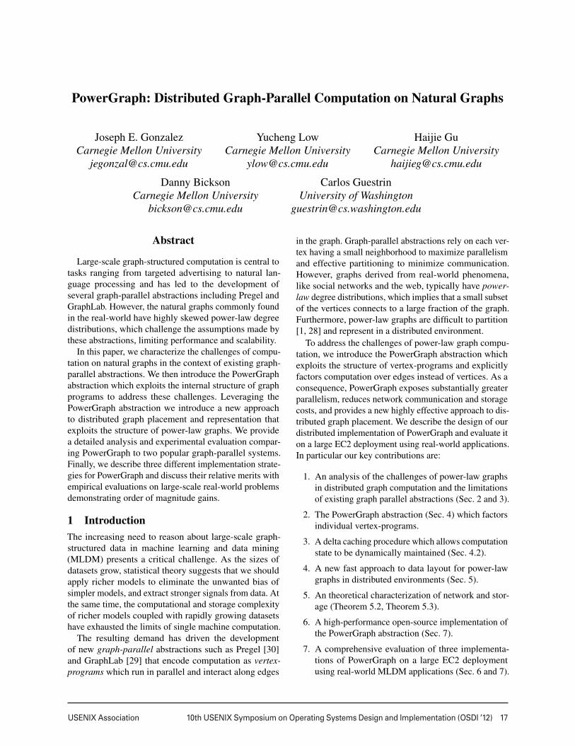
Figure 1: The in and out degree distributions of the Twitter

follower network plotted in log-log scale.

GraphLab and Pregel express GAS programs in very

different ways. In the Pregel abstraction the gather phase

is implemented using message combiners and the apply

and scatter phases are expressed in the vertex program.

Conversely, GraphLab exposes the entire neighborhood to

the vertex-program and allows the user to define the gather

and apply phases within their program. The GraphLab ab-

straction implicitly defines the communication aspects of

the gather/scatter phases by ensuring that changes made

to the vertex or edge data are automatically visible to ad-

jacent vertices. It is also important to note that GraphLab

does not differentiate between edge directions.

3 Challenges of Natural Graphs

The sparsity structure of natural graphs presents a unique

challenge to efficient distributed graph-parallel compu-

tation. One of the hallmark properties of natural graphs

is their skewed power-law degree distribution[16]: most

vertices have relatively few neighbors while a few have

many neighbors (e.g., celebrities in a social network). Un-

der a power-law degree distribution the probability that a

vertex has degree d is given by:

P(d) ∝ d−α , (3.1)

where the exponent α is a positive constant that controls

the “skewness” of the degree distribution. Higher α im-

plies that the graph has lower density (ratio of edges to

vertices), and that the vast majority of vertices are low

degree. As α decreases, the graph density and number

of high degree vertices increases. Most natural graphs

typically have a power-law constant around α ≈ 2. For

example, Faloutsos et al. [16] estimated that the inter-

domain graph of the Internet has a power-law constant

α ≈ 2.2. One can visualize the skewed power-law de-

gree distribution by plotting the number of vertices with a

given degree in log-log scale. In Fig. 1, we plot the in and

out degree distributions of the Twitter follower network

demonstrating the characteristic linear power-law form.

While power-law degree distributions are empirically

observable, they do not fully characterize the properties of

natural graphs. While there has been substantial work (see

[27]) in more sophisticated natural graph models, the tech-

niques in this paper focus only on the degree distribution

and do not require any other modeling assumptions.

The skewed degree distribution implies that a small

fraction of the vertices are adjacent to a large fraction

of the edges. For example, one percent of the vertices

in the Twitter web-graph are adjacent to nearly half of

the edges. This concentration of edges results in a star-

like motif which presents challenges for existing graph-

parallel abstractions:

Work Balance: The power-law degree distribution can

lead to substantial work imbalance in graph parallel ab-

stractions that treat vertices symmetrically. Since the stor-

age, communication, and computation complexity of the

Gather and Scatter phases is linear in the degree, the run-

ning time of vertex-programs can vary widely [36].

Partitioning: Natural graphs are difficult to

partition[26, 28]. Both GraphLab and Pregel de-

pend on graph partitioning to minimize communication

and ensure work balance. However, in the case of natural

graphs both are forced to resort to hash-based (random)

partitioning which has extremely poor locality (Sec. 5).

Communication: The skewed degree distribution of

natural-graphs leads to communication asymmetry and

consequently bottlenecks. In addition, high-degree ver-

tices can force messaging abstractions, such as Pregel, to

generate and send many identical messages.

Storage: Since graph parallel abstractions must locally

store the adjacency information for each vertex, each

vertex requires memory linear in its degree. Consequently,

high-degree vertices can exceed the memory capacity of

a single machine.

Computation: While multiple vertex-programs may

execute in parallel, existing graph-parallel abstractions do

not parallelize within individual vertex-programs, limiting

their scalability on high-degree vertices.

4 PowerGraph Abstraction

To address the challenges of computation on power-law

graphs, we introduce PowerGraph, a new graph-parallel

abstraction that eliminates the degree dependence of the

vertex-program by directly exploiting the GAS decom-

position to factor vertex-programs over edges. By lifting

the Gather and Scatter phases into the abstraction, Pow-

erGraph is able to retain the natural “think-like-a-vertex”

philosophy [30] while distributing the computation of a

single vertex-program over the entire cluster.

PowerGraph combines the best features from both

Pregel and GraphLab. From GraphLab, PowerGraph bor-

rows the data-graph and shared-memory view of compu-

tation eliminating the need for users to architect the move-

ment of information. From Pregel, PowerGraph borrows

the commutative, associative gather concept. PowerGraph

3

michele

Sticky Note

Completed set by michele


interface GASVertexProgram(u) {

// Run on gather_nbrs(u)

gather(Du, D(u,v), Dv) → Accum

sum(Accum left, Accum right) → Accum

apply(Du,Accum) → Dnewu

// Run on scatter_nbrs(u)

scatter(Dnewu ,D(u,v),Dv) → (Dnew

(u,v), Accum)

}

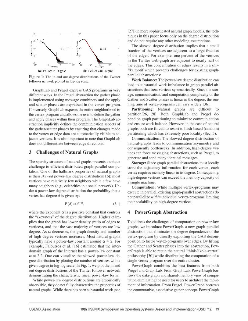
Figure 2: All PowerGraph programs must implement the state-

less gather, sum, apply, and scatter functions.

Algorithm 1: Vertex-Program Execution Semantics

Input: Center vertex u

if cached accumulator au is empty then

foreach neighbor v in gather nbrs(u) do

au ← sum(au, gather(Du, D(u,v), Dv))

end

end

Du ← apply(Du, au)

foreach neighbor v scatter nbrs(u) do

(D(u,v),∆a)← scatter(Du, D(u,v), Dv)

if av and ∆a are not Empty then av ← sum(av, ∆a)

else av ← Empty

end

supports both the highly-parallel bulk-synchronous Pregel

model of computation as well as the computationally effi-

cient asynchronous GraphLab model of computation.

Like GraphLab, the state of a PowerGraph program

factors according to a data-graph with user defined ver-

tex data Dv and edge data D(u,v). The data stored in the

data-graph includes both meta-data (e.g., urls and edge

weights) as well as computation state (e.g., the PageRank

of vertices). In Sec. 5 we introduce vertex-cuts which al-

low PowerGraph to efficiently represent and store power-

law graphs in a distributed environment. We now describe

the PowerGraph abstraction and how it can be used to

naturally decompose vertex-programs. Then in Sec. 5

through Sec. 7 we discuss how to implement the Power-

Graph abstraction in a distributed environment.

4.1 GAS Vertex-Programs

Computation in the PowerGraph abstraction is encoded

as a state-less vertex-program which implements the

GASVertexProgram interface (Fig. 2) and therefore

explicitly factors into the gather, sum, apply, and scat-

ter functions. Each function is invoked in stages by the

PowerGraph engine following the semantics in Alg. 1.

By factoring the vertex-program, the PowerGraph execu-

tion engine can distribute a single vertex-program over

multiple machines and move computation to the data.

During the gather phase the gather and sum func-

tions are used as a map and reduce to collect information

about the neighborhood of the vertex. The gather func-

tion is invoked in parallel on the edges adjacent to u. The

particular set of edges is determined by gather nbrs

which can be none, in, out, or all. The gather func-

tion is passed the data on the adjacent vertex and edge

and returns a temporary accumulator (a user defined type).

The result is combined using the commutative and associa-

tive sum operation. The final result au of the gather phase

is passed to the apply phase and cached by PowerGraph.

After the gather phase has completed, the apply func-

tion takes the final accumulator and computes a new ver-

tex value Du which is atomically written back to the graph.

The size of the accumulator au and complexity of the ap-

ply function play a central role in determining the network

and storage efficiency of the PowerGraph abstraction and

should be sub-linear and ideally constant in the degree.

During the scatter phase, the scatter function is in-

voked in parallel on the edges adjacent to u producing

new edge values D(u,v) which are written back to the data-

graph. As with the gather phase, the scatter nbrs

determines the particular set of edges on which scatter is

invoked. The scatter function returns an optional value ∆a

which is used to dynamically update the cached accumu-

lator av for the adjacent vertex (see Sec. 4.2).

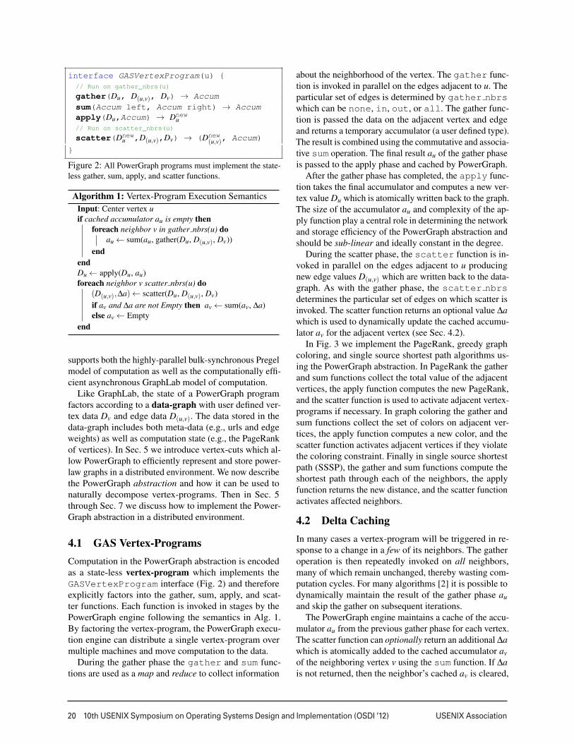
In Fig. 3 we implement the PageRank, greedy graph

coloring, and single source shortest path algorithms us-

ing the PowerGraph abstraction. In PageRank the gather

and sum functions collect the total value of the adjacent

vertices, the apply function computes the new PageRank,

and the scatter function is used to activate adjacent vertex-

programs if necessary. In graph coloring the gather and

sum functions collect the set of colors on adjacent ver-

tices, the apply function computes a new color, and the

scatter function activates adjacent vertices if they violate

the coloring constraint. Finally in single source shortest

path (SSSP), the gather and sum functions compute the

shortest path through each of the neighbors, the apply

function returns the new distance, and the scatter function

activates affected neighbors.

4.2 Delta Caching

In many cases a vertex-program will be triggered in re-

sponse to a change in a few of its neighbors. The gather

operation is then repeatedly invoked on all neighbors,

many of which remain unchanged, thereby wasting com-

putation cycles. For many algorithms [2] it is possible to

dynamically maintain the result of the gather phase au

and skip the gather on subsequent iterations.

The PowerGraph engine maintains a cache of the accu-

mulator au from the previous gather phase for each vertex.

The scatter function can optionally return an additional ∆a

which is atomically added to the cached accumulator av

of the neighboring vertex v using the sum function. If ∆a

is not returned, then the neighbor’s cached av is cleared,

4


PageRank

// gather_nbrs: IN_NBRS

gather(Du, D(u,v), Dv):

return Dv.rank / #outNbrs(v)

sum(a, b): return a + b

apply(Du, acc):

rnew = 0.15 + 0.85 * acc

Du.delta = (rnew - Du.rank)/

#outNbrs(u)

Du.rank = rnew

// scatter_nbrs: OUT_NBRS

scatter(Du,D(u,v),Dv):

if(|Du.delta|>ε) Activate(v)

return delta

Greedy Graph Coloring

// gather_nbrs: ALL_NBRS


return set(Dv)

sum(a, b): return union(a, b)

apply(Du, S):

Du = min c where c /∈ S

// scatter_nbrs: ALL_NBRS


// Nbr changed since gather

if(Du == Dv)

Activate(v)

// Invalidate cached accum

return NULL

Single Source Shortest Path (SSSP)

// gather_nbrs: ALL_NBRS


return Dv + D(v,u)

sum(a, b): return min(a, b)

apply(Du, new_dist):

Du = new_dist

// scatter_nbrs: ALL_NBRS


// If changed activate neighbor

if(changed(Du)) Activate(v)

if(increased(Du))

return NULL

else return Du + D(u,v)

Figure 3: The PageRank, graph-coloring, and single source shortest path algorithms implemented in the PowerGraph abstraction.

Both the PageRank and single source shortest path algorithms support delta caching in the gather phase.

forcing a complete gather on the subsequent execution

of the vertex-program on the vertex v. When executing

the vertex-program on v the PowerGraph engine uses the

cached av if available, bypassing the gather phase.

Intuitively, ∆a acts as an additive correction on-top of

the previous gather for that edge. More formally, if the

accumulator type forms an abelian group: has a com-

mutative and associative sum (+) and an inverse (−)operation, then we can define (shortening gather to g):

∆a = g(Du,Dnew(u,v),D

newv )−g(Du,D(u,v),Dv). (4.1)

In the PageRank example (Fig. 3) we take advantage of

the abelian nature of the PageRank sum operation. For

graph coloring the set union operation is not abelian and

so we invalidate the accumulator.

4.3 Initiating Future Computation

The PowerGraph engine maintains a set of active vertices

on which to eventually execute the vertex-program. The

user initiates computation by calling Activate(v) or

Activate all(). The PowerGraph engine then pro-

ceeds to execute the vertex-program on the active vertices

until none remain. Once a vertex-program completes the

scatter phase it becomes inactive until it is reactivated.

Vertices can activate themselves and neighboring ver-

tices. Each function in a vertex-program can only activate

vertices visible in the arguments to that function. For ex-

ample the scatter function invoked on the edge (u,v) can

only activate the vertices u and v. This restriction is es-

sential to ensure that activation events are generated on

machines on which they can be efficiently processed.

The order in which activated vertices are executed is up

to the PowerGraph execution engine. The only guarantee

is that all activated vertices are eventually executed. This

flexibility in scheduling enables PowerGraph programs

to be executed both synchronously and asynchronously,

leading to different tradeoffs in algorithm performance,

system performance, and determinism.

4.3.1 Bulk Synchronous Execution

When run synchronously, the PowerGraph engine exe-

cutes the gather, apply, and scatter phases in order. Each

phase, called a minor-step, is run synchronously on all

active vertices with a barrier at the end. We define a super-

step as a complete series of GAS minor-steps. Changes

made to the vertex data and edge data are committed at

the end of each minor-step and are visible in the subse-

quent minor-step. Vertices activated in each super-step

are executed in the subsequent super-step.

The synchronous execution model ensures a determin-

istic execution regardless of the number of machines and

closely resembles Pregel. However, the frequent barriers

and inability to operate on the most recent data can lead

to an inefficient distributed execution and slow algorithm

convergence. To address these limitations PowerGraph

also supports asynchronous execution.

4.3.2 Asynchronous Execution

When run asynchronously, the PowerGraph engine exe-

cutes active vertices as processor and network resources

become available. Changes made to the vertex and edge

data during the apply and scatter functions are immedi-

ately committed to the graph and visible to subsequent

computation on neighboring vertices.

By using processor and network resources as they

become available and making any changes to the data-

graph immediately visible to future computation, an asyn-

chronous execution can more effectively utilize resources

and accelerate the convergence of the underlying algo-

rithm. For example, the greedy graph-coloring algorithm

in Fig. 3 will not converge when executed synchronously

but converges quickly when executed asynchronously.

The merits of asynchronous computation have been stud-

ied extensively in the context of numerical algorithms

[4]. In [18, 19, 29] we demonstrated that asynchronous

computation can lead to both theoretical and empirical

5


gains in algorithm and system performance for a range of

important MLDM applications.

Unfortunately, the behavior of the asynchronous exe-

cution depends on the number machines and availability

of network resources leading to non-determinism that can

complicate algorithm design and debugging. Furthermore,

for some algorithms, like statistical simulation, the result-

ing non-determinism, if not carefully controlled, can lead

to instability or even divergence [17].

To address these challenges, GraphLab automati-

cally enforces serializability: every parallel execution

of vertex-programs has a corresponding sequential execu-

tion. In [29] it was shown that serializability is sufficient to

support a wide range of MLDM algorithms. To achieve se-

rializability, GraphLab prevents adjacent vertex-programs

from running concurrently using a fine-grained locking

protocol which requires sequentially grabbing locks on

all neighboring vertices. Furthermore, the locking scheme

used by GraphLab is unfair to high degree vertices.

PowerGraph retains the strong serializability guaran-

tees of GraphLab while addressing its limitations. We

address the problem of sequential locking by introducing

a new parallel locking protocol (described in Sec. 7.4)

which is fair to high degree vertices. In addition, the

PowerGraph abstraction exposes substantially more fined

grained (edge-level) parallelism allowing the entire cluster

to support the execution of individual vertex programs.

4.4 Comparison with GraphLab / Pregel

Surprisingly, despite the strong constraints imposed by

the PowerGraph abstraction, it is possible to emulate both

GraphLab and Pregel vertex-programs in PowerGraph. To

emulate a GraphLab vertex-program, we use the gather

and sum functions to concatenate all the data on adjacent

vertices and edges and then run the GraphLab program

within the apply function. Similarly, to express a Pregel

vertex-program, we use the gather and sum functions to

combine the inbound messages (stored as edge data) and

concatenate the list of neighbors needed to compute the

outbound messages. The Pregel vertex-program then runs

within the apply function generating the set of messages

which are passed as vertex data to the scatter function

where they are written back to the edges.

In order to address the challenges of natural graphs,

the PowerGraph abstraction requires the size of the ac-

cumulator and the complexity of the apply function to

be sub-linear in the degree. However, directly executing

GraphLab and Pregel vertex-programs within the apply

function leads the size of the accumulator and the com-

plexity of the apply function to be linear in the degree

eliminating many of the benefits on natural graphs.

3 2

1

D

A

C

B 2 3

C

D

B A

1

D

A

C C

B

(a) Edge-Cut

B A 1

C D3

C B 2

C D

B A 1

3

(b) Vertex-Cut

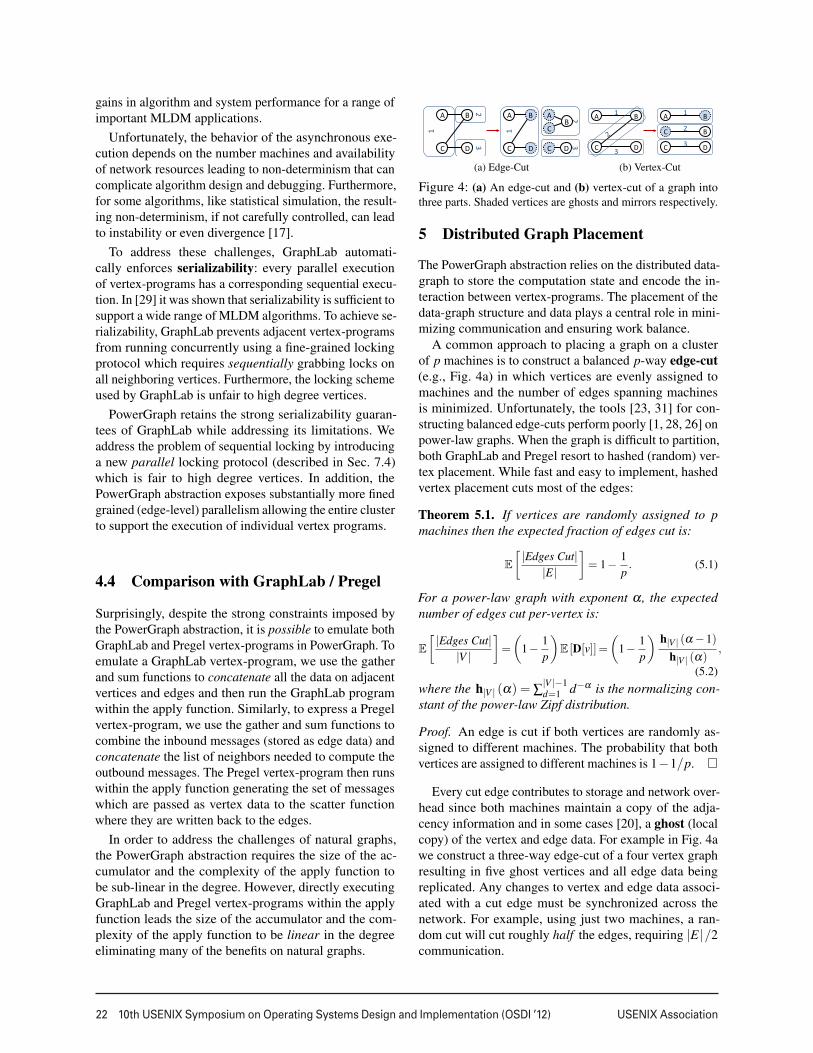
Figure 4: (a) An edge-cut and (b) vertex-cut of a graph into

three parts. Shaded vertices are ghosts and mirrors respectively.

5 Distributed Graph Placement

The PowerGraph abstraction relies on the distributed data-

graph to store the computation state and encode the in-

teraction between vertex-programs. The placement of the

data-graph structure and data plays a central role in mini-

mizing communication and ensuring work balance.

A common approach to placing a graph on a cluster

of p machines is to construct a balanced p-way edge-cut

(e.g., Fig. 4a) in which vertices are evenly assigned to

machines and the number of edges spanning machines

is minimized. Unfortunately, the tools [23, 31] for con-

structing balanced edge-cuts perform poorly [1, 28, 26] on

power-law graphs. When the graph is difficult to partition,

both GraphLab and Pregel resort to hashed (random) ver-

tex placement. While fast and easy to implement, hashed

vertex placement cuts most of the edges:

Theorem 5.1. If vertices are randomly assigned to p

machines then the expected fraction of edges cut is:

E

[

|Edges Cut|

|E|

]

= 1−1

p. (5.1)

For a power-law graph with exponent α , the expected

number of edges cut per-vertex is:

E

[

|Edges Cut|

|V |

]

=

(

1−1

p

)

E [D[v]] =

(

1−1

p

)

h|V | (α −1)

h|V | (α),

(5.2)

where the h|V | (α) = ∑|V |−1

d=1 d−α is the normalizing con-

stant of the power-law Zipf distribution.

Proof. An edge is cut if both vertices are randomly as-

signed to different machines. The probability that both

vertices are assigned to different machines is 1−1/p.

Every cut edge contributes to storage and network over-

head since both machines maintain a copy of the adja-

cency information and in some cases [20], a ghost (local

copy) of the vertex and edge data. For example in Fig. 4a

we construct a three-way edge-cut of a four vertex graph

resulting in five ghost vertices and all edge data being

replicated. Any changes to vertex and edge data associ-

ated with a cut edge must be synchronized across the

network. For example, using just two machines, a ran-

dom cut will cut roughly half the edges, requiring |E|/2

communication.

6


Machine(1( Machine(2(

Accumulator((Par4al(Sum)(

Updated((Vertex(Data(

Gather( Mirror(Sca>er(

Gather(

Apply(

Sca>er(

(1)(Gather(

(3)(Apply(

(5)(Sca>er(

(2)(

(4)(

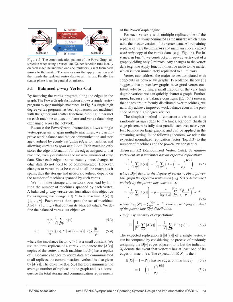
Figure 5: The communication pattern of the PowerGraph ab-

straction when using a vertex-cut. Gather function runs locally

on each machine and then one accumulators is sent from each

mirror to the master. The master runs the apply function and

then sends the updated vertex data to all mirrors. Finally the

scatter phase is run in parallel on mirrors.

5.1 Balanced p-way Vertex-Cut

By factoring the vertex program along the edges in the

graph, The PowerGraph abstraction allows a single vertex-

program to span multiple machines. In Fig. 5 a single high

degree vertex program has been split across two machines

with the gather and scatter functions running in parallel

on each machine and accumulator and vertex data being

exchanged across the network.

Because the PowerGraph abstraction allows a single

vertex-program to span multiple machines, we can im-

prove work balance and reduce communication and stor-

age overhead by evenly assigning edges to machines and

allowing vertices to span machines. Each machine only

stores the edge information for the edges assigned to that

machine, evenly distributing the massive amounts of edge

data. Since each edge is stored exactly once, changes to

edge data do not need to be communicated. However,

changes to vertex must be copied to all the machines it

spans, thus the storage and network overhead depend on

the number of machines spanned by each vertex.

We minimize storage and network overhead by lim-

iting the number of machines spanned by each vertex.

A balanced p-way vertex-cut formalizes this objective

by assigning each edge e ∈ E to a machine A(e) ∈{1, . . . , p}. Each vertex then spans the set of machines

A(v)⊆ {1, . . . , p} that contain its adjacent edges. We de-

fine the balanced vertex-cut objective:

minA

1

|V | ∑v∈V

|A(v)| (5.3)

s.t. maxm

|{e ∈ E | A(e) = m}| ,< λ|E|

p(5.4)

where the imbalance factor λ ≥ 1 is a small constant. We

use the term replicas of a vertex v to denote the |A(v)|copies of the vertex v: each machine in A(v) has a replica

of v. Because changes to vertex data are communicated

to all replicas, the communication overhead is also given

by |A(v)|. The objective (Eq. 5.3) therefore minimizes the

average number of replicas in the graph and as a conse-

quence the total storage and communication requirements

of the PowerGraph engine.

For each vertex v with multiple replicas, one of the

replicas is randomly nominated as the master which main-

tains the master version of the vertex data. All remaining

replicas of v are then mirrors and maintain a local cached

read only copy of the vertex data. (e.g., Fig. 4b). For in-

stance, in Fig. 4b we construct a three-way vertex-cut of a

graph yielding only 2 mirrors. Any changes to the vertex

data (e.g., the Apply function) must be made to the master

which is then immediately replicated to all mirrors.

Vertex-cuts address the major issues associated with

edge-cuts in power-law graphs. Percolation theory [3]

suggests that power-law graphs have good vertex-cuts.

Intuitively, by cutting a small fraction of the very high

degree vertices we can quickly shatter a graph. Further-

more, because the balance constraint (Eq. 5.4) ensures

that edges are uniformly distributed over machines, we

naturally achieve improved work balance even in the pres-

ence of very high-degree vertices.

The simplest method to construct a vertex cut is to

randomly assign edges to machines. Random (hashed)

edge placement is fully data-parallel, achieves nearly per-

fect balance on large graphs, and can be applied in the

streaming setting. In the following theorem, we relate the

expected normalized replication factor (Eq. 5.3) to the

number of machines and the power-law constant α .

Theorem 5.2 (Randomized Vertex Cuts). A random

vertex-cut on p machines has an expected replication:

E

[

1

|V | ∑v∈V

|A(v)|

]

=p

|V | ∑v∈V

(

1−

(

1−1

p

)D[v])

. (5.5)

where D[v] denotes the degree of vertex v. For a power-

law graph the expected replication (Fig. 6a) is determined

entirely by the power-law constant α:

E

[

1

|V | ∑v∈V

|A(v)|

]

= p−p

h|V | (α)

|V |−1

∑d=1

(

p−1

p

)d

d−α ,

(5.6)

where h|V | (α) = ∑|V |−1

d=1 d−α is the normalizing constant

of the power-law Zipf distribution.

Proof. By linearity of expectation:

E

[

1

|V | ∑v∈V

|A(v)|

]

=1

|V | ∑v∈V

E [|A(v)|] , (5.7)

The expected replication E [|A(v)|] of a single vertex v

can be computed by considering the process of randomly

assigning the D[v] edges adjacent to v. Let the indicator

Xi denote the event that vertex v has at least one of its

edges on machine i. The expectation E [Xi] is then:

E [Xi] = 1−P(v has no edges on machine i) (5.8)

= 1−

(

1−1

p

)D[v]

, (5.9)

7


0 50 100 150

2

4

6

8

10α = 1.65

α = 1.7

α = 1.8

α = 2

Number of Machines

Replic

ation F

acto

r

(a) V-Sep. Bound

0 50 100 1505

10

20

50

100

200

500

α = 1.65α = 1.7

α = 1.8

α = 2

Number of Machines

Fa

cto

r Im

pro

ve

me

nt

(b) V-Sep. Improvement

Figure 6: (a) Expected replication factor for different power-

law constants. (b) The ratio of the expected communication and

storage cost of random edge cuts to random vertex cuts as a

function of the number machines. This graph assumes that edge

data and vertex data are the same size.

The expected replication factor for vertex v is then:

E [|A(v)|] =p

∑i=1

E [Xi] = p

(

1−

(

1−1

p

)D[v])

. (5.10)

Treating D[v] as a Zipf random variable:

E

[

1

|V | ∑v∈V

|A(v)|

]

=p

|V | ∑v∈V

(

1−E

[

(

p−1

p

)D[v]])

,

(5.11)

and taking the expectation under P(d) = d−α/h|V | (α):

E

[

(

1−1

p

)D[v]]

=1

h|V | (α)

|V |−1

∑d=1

(

1−1

p

)d

d−α .

(5.12)

While lower α values (more high-degree vertices) im-

ply a higher replication factor (Fig. 6a) the effective gains

of vertex-cuts relative to edge cuts (Fig. 6b) actually in-

crease with lower α . In Fig. 6b we plot the ratio of the

expected costs (comm. and storage) of random edge-cuts

(Eq. 5.2) to the expected costs of random vertex-cuts

(Eq. 5.6) demonstrating order of magnitude gains.

Finally, the vertex cut model is also highly effective for

regular graphs since in the event that a good edge-cut can

be found it can be converted to a better vertex cut:

Theorem 5.3. For a given an edge-cut with g ghosts, any

vertex cut along the same partition boundary has strictly

fewer than g mirrors.

Proof of Theorem 5.3. Consider the two-way edge cut

which cuts the set of edges E ′ ∈ E and let V ′ be the set

of vertices in E ′. The total number of ghosts induced by

this edge partition is therefore |V ′|. If we then select and

delete arbitrary vertices from V ′ along with their adja-

cent edges until no edges remain, then the set of deleted

vertices corresponds to a vertex-cut in the original graph.

Since at most |V ′|−1 vertices may be deleted, there can

be at most |V ′|−1 mirrors.

Graph |V | |E|Twitter [24] 41M 1.4B

UK [7] 132.8M 5.5B

Amazon [6, 5] 0.7M 5.2M

LiveJournal [12] 5.4M 79M

Hollywood [6, 5] 2.2M 229M

(a) Real world graphs

α # Edges

1.8 641,383,778

1.9 245,040,680

2.0 102,838,432

2.1 57,134,471

2.2 35,001,696

(b) Synthetic Graphs

Table 1: (a) A collection of Real world graphs. (b) Randomly

constructed ten-million vertex power-law graphs with varying

α . Smaller α produces denser graphs.

5.2 Greedy Vertex-Cuts

We can improve upon the randomly constructed vertex-

cut by de-randomizing the edge-placement process. The

resulting algorithm is a sequential greedy heuristic which

places the next edge on the machine that minimizes the

conditional expected replication factor. To construct the

de-randomization we consider the task of placing the i+1

edge after having placed the previous i edges. Using the

conditional expectation we define the objective:

argmink

E

[

∑v∈V

|A(v)|

∣

∣

∣

∣

∣

Ai,A(ei+1) = k

]

, (5.13)

where Ai is the assignment for the previous i edges. Using

Theorem 5.2 to evaluate Eq. 5.13 we obtain the following

edge placement rules for the edge (u,v):

Case 1: If A(u) and A(v) intersect, then the edge should be

assigned to a machine in the intersection.

Case 2: If A(u) and A(v) are not empty and do not intersect,

then the edge should be assigned to one of the machines

from the vertex with the most unassigned edges.

Case 3: If only one of the two vertices has been assigned, then

choose a machine from the assigned vertex.

Case 4: If neither vertex has been assigned, then assign the

edge to the least loaded machine.

Because the greedy-heuristic is a de-randomization it is

guaranteed to obtain an expected replication factor that is

no worse than random placement and in practice can be

much better. Unlike the randomized algorithm, which is

embarrassingly parallel and easily distributed, the greedy

algorithm requires coordination between machines. We

consider two distributed implementations:

Coordinated: maintains the values of Ai(v) in a dis-

tributed table. Then each machine runs the greedy

heuristic and periodically updates the distributed ta-

ble. Local caching is used to reduce communication

at the expense of accuracy in the estimate of Ai(v).

Oblivious: runs the greedy heuristic independently on

each machine. Each machine maintains its own esti-

mate of Ai with no additional communication.

8


Twitter HWood UK LJournal Amazon0

5

10

15

20

Re

plic

atio

n F

acto

r

RandomObliviousCoordinated

(a) Actual Replication

Coloring SSSP ALS PageRank0

0.2

0.4

0.6

0.8

1

Ru

ntim

e R

ela

tive

to

Ra

nd

om

Rand.Obliv.Coord.

(b) Effect of Partitioning

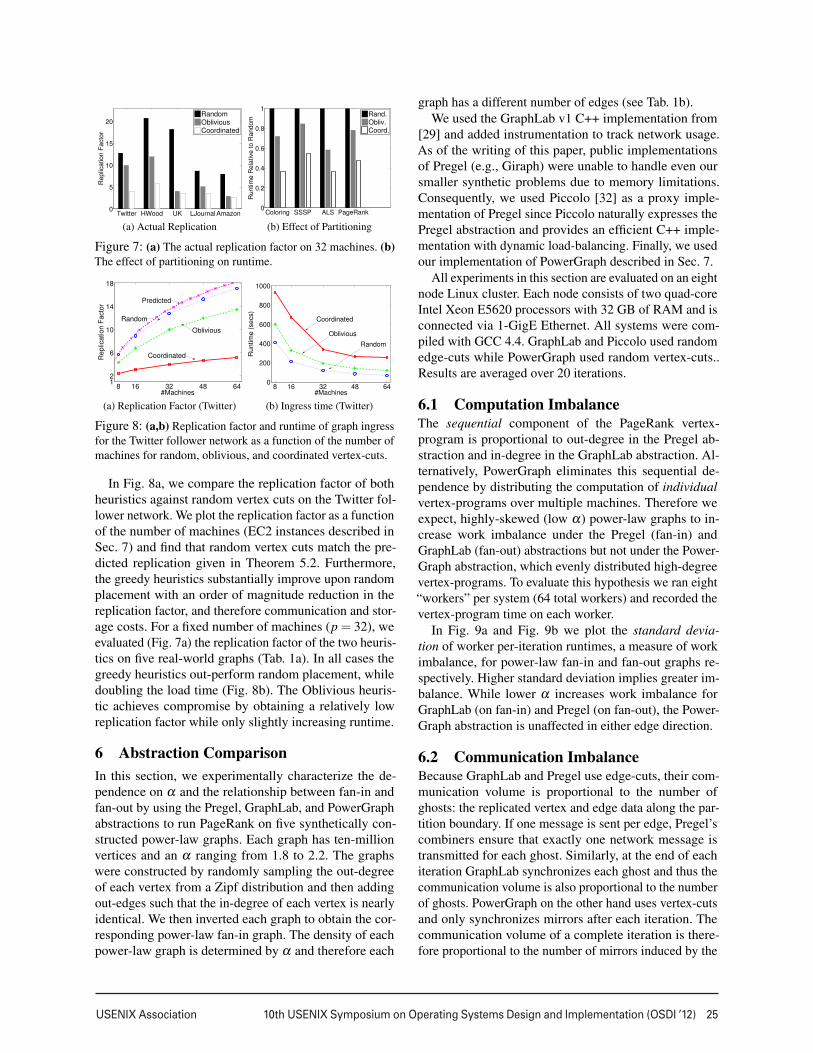
Figure 7: (a) The actual replication factor on 32 machines. (b)

The effect of partitioning on runtime.

8 16 32 48 6412

6

10

14

18

#Machines

Replic

ation F

acto

r

Predicted

Oblivious

Coordinated

Random

(a) Replication Factor (Twitter)

8 16 32 48 640

200

400

600

800

1000

#Machines

Runtim

e (

secs)

Coordinated

Oblivious

Random

(b) Ingress time (Twitter)

Figure 8: (a,b) Replication factor and runtime of graph ingress

for the Twitter follower network as a function of the number of

machines for random, oblivious, and coordinated vertex-cuts.

In Fig. 8a, we compare the replication factor of both

heuristics against random vertex cuts on the Twitter fol-

lower network. We plot the replication factor as a function

of the number of machines (EC2 instances described in

Sec. 7) and find that random vertex cuts match the pre-

dicted replication given in Theorem 5.2. Furthermore,

the greedy heuristics substantially improve upon random

placement with an order of magnitude reduction in the

replication factor, and therefore communication and stor-

age costs. For a fixed number of machines (p = 32), we

evaluated (Fig. 7a) the replication factor of the two heuris-

tics on five real-world graphs (Tab. 1a). In all cases the

greedy heuristics out-perform random placement, while

doubling the load time (Fig. 8b). The Oblivious heuris-

tic achieves compromise by obtaining a relatively low

replication factor while only slightly increasing runtime.

6 Abstraction Comparison

In this section, we experimentally characterize the de-

pendence on α and the relationship between fan-in and

fan-out by using the Pregel, GraphLab, and PowerGraph

abstractions to run PageRank on five synthetically con-

structed power-law graphs. Each graph has ten-million

vertices and an α ranging from 1.8 to 2.2. The graphs

were constructed by randomly sampling the out-degree

of each vertex from a Zipf distribution and then adding

out-edges such that the in-degree of each vertex is nearly

identical. We then inverted each graph to obtain the cor-

responding power-law fan-in graph. The density of each

power-law graph is determined by α and therefore each

graph has a different number of edges (see Tab. 1b).

We used the GraphLab v1 C++ implementation from

[29] and added instrumentation to track network usage.

As of the writing of this paper, public implementations

of Pregel (e.g., Giraph) were unable to handle even our

smaller synthetic problems due to memory limitations.

Consequently, we used Piccolo [32] as a proxy imple-

mentation of Pregel since Piccolo naturally expresses the

Pregel abstraction and provides an efficient C++ imple-

mentation with dynamic load-balancing. Finally, we used

our implementation of PowerGraph described in Sec. 7.

All experiments in this section are evaluated on an eight

node Linux cluster. Each node consists of two quad-core

Intel Xeon E5620 processors with 32 GB of RAM and is

connected via 1-GigE Ethernet. All systems were com-

piled with GCC 4.4. GraphLab and Piccolo used random

edge-cuts while PowerGraph used random vertex-cuts..

Results are averaged over 20 iterations.

6.1 Computation ImbalanceThe sequential component of the PageRank vertex-

program is proportional to out-degree in the Pregel ab-

straction and in-degree in the GraphLab abstraction. Al-

ternatively, PowerGraph eliminates this sequential de-

pendence by distributing the computation of individual

vertex-programs over multiple machines. Therefore we

expect, highly-skewed (low α) power-law graphs to in-

crease work imbalance under the Pregel (fan-in) and

GraphLab (fan-out) abstractions but not under the Power-

Graph abstraction, which evenly distributed high-degree

vertex-programs. To evaluate this hypothesis we ran eight

“workers” per system (64 total workers) and recorded the

vertex-program time on each worker.

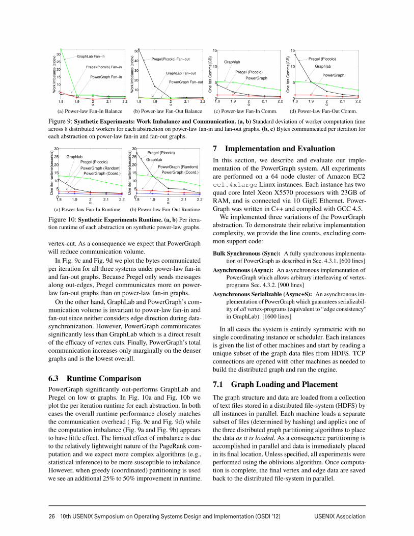
In Fig. 9a and Fig. 9b we plot the standard devia-

tion of worker per-iteration runtimes, a measure of work

imbalance, for power-law fan-in and fan-out graphs re-

spectively. Higher standard deviation implies greater im-

balance. While lower α increases work imbalance for

GraphLab (on fan-in) and Pregel (on fan-out), the Power-

Graph abstraction is unaffected in either edge direction.

6.2 Communication ImbalanceBecause GraphLab and Pregel use edge-cuts, their com-

munication volume is proportional to the number of

ghosts: the replicated vertex and edge data along the par-

tition boundary. If one message is sent per edge, Pregel’s

combiners ensure that exactly one network message is

transmitted for each ghost. Similarly, at the end of each

iteration GraphLab synchronizes each ghost and thus the

communication volume is also proportional to the number

of ghosts. PowerGraph on the other hand uses vertex-cuts

and only synchronizes mirrors after each iteration. The

communication volume of a complete iteration is there-

fore proportional to the number of mirrors induced by the

9


1.8 1.9 2 2.1 2.2

5

10

15

20

25

30

α

Wo

rk I

mb

ala

nce

(std

ev) GraphLab Fan−in

PowerGraph Fan−in

Pregel(Piccolo) Fan−in

(a) Power-law Fan-In Balance

1.8 1.9 2 2.1 2.2

10

20

30

40

50

α

Wo

rk I

mb

ala

nce

(std

ev)

Pregel(Piccolo) Fan−out

GraphLab Fan−out

PowerGraph Fan−out

(b) Power-law Fan-Out Balance

1.8 1.9 2 2.1 2.20

5

10

15

α

One ite

r C

om

ms(G

B)

Pregel (Piccolo)

PowerGraph

Graphlab

(c) Power-law Fan-In Comm.

1.8 1.9 2 2.1 2.20

5

10

15

α

One ite

r C

om

ms(G

B)

Pregel (Piccolo)

Graphlab

PowerGraph

(d) Power-law Fan-Out Comm.

Figure 9: Synthetic Experiments: Work Imbalance and Communication. (a, b) Standard deviation of worker computation time

across 8 distributed workers for each abstraction on power-law fan-in and fan-out graphs. (b, c) Bytes communicated per iteration for

each abstraction on power-law fan-in and fan-out graphs.

1.8 1.9 2 2.1 2.20

5

10

15

20

25

30

α

One ite

r ru

ntim

e(s

econds)

Graphlab

Pregel (Piccolo)

PowerGraph (Random)

PowerGraph (Coord.)

(a) Power-law Fan-In Runtime

1.8 1.9 2 2.1 2.20

5

10

15

20

25

30

α

One ite

r ru

ntim

e(s

econds)

Pregel (Piccolo)

Graphlab

PowerGraph (Random)

PowerGraph (Coord.)

(b) Power-law Fan-Out Runtime

Figure 10: Synthetic Experiments Runtime. (a, b) Per itera-

tion runtime of each abstraction on synthetic power-law graphs.

vertex-cut. As a consequence we expect that PowerGraph

will reduce communication volume.

In Fig. 9c and Fig. 9d we plot the bytes communicated

per iteration for all three systems under power-law fan-in

and fan-out graphs. Because Pregel only sends messages

along out-edges, Pregel communicates more on power-

law fan-out graphs than on power-law fan-in graphs.

On the other hand, GraphLab and PowerGraph’s com-

munication volume is invariant to power-law fan-in and

fan-out since neither considers edge direction during data-

synchronization. However, PowerGraph communicates

significantly less than GraphLab which is a direct result

of the efficacy of vertex cuts. Finally, PowerGraph’s total

communication increases only marginally on the denser

graphs and is the lowest overall.

6.3 Runtime Comparison

PowerGraph significantly out-performs GraphLab and

Pregel on low α graphs. In Fig. 10a and Fig. 10b we

plot the per iteration runtime for each abstraction. In both

cases the overall runtime performance closely matches

the communication overhead ( Fig. 9c and Fig. 9d) while

the computation imbalance (Fig. 9a and Fig. 9b) appears

to have little effect. The limited effect of imbalance is due

to the relatively lightweight nature of the PageRank com-

putation and we expect more complex algorithms (e.g.,

statistical inference) to be more susceptible to imbalance.

However, when greedy (coordinated) partitioning is used

we see an additional 25% to 50% improvement in runtime.

7 Implementation and Evaluation

In this section, we describe and evaluate our imple-

mentation of the PowerGraph system. All experiments

are performed on a 64 node cluster of Amazon EC2

cc1.4xlarge Linux instances. Each instance has two

quad core Intel Xeon X5570 processors with 23GB of

RAM, and is connected via 10 GigE Ethernet. Power-

Graph was written in C++ and compiled with GCC 4.5.

We implemented three variations of the PowerGraph

abstraction. To demonstrate their relative implementation

complexity, we provide the line counts, excluding com-

mon support code:

Bulk Synchronous (Sync): A fully synchronous implementa-

tion of PowerGraph as described in Sec. 4.3.1. [600 lines]

Asynchronous (Async): An asynchronous implementation of

PowerGraph which allows arbitrary interleaving of vertex-

programs Sec. 4.3.2. [900 lines]

Asynchronous Serializable (Async+S): An asynchronous im-

plementation of PowerGraph which guarantees serializabil-

ity of all vertex-programs (equivalent to “edge consistency”

in GraphLab). [1600 lines]

In all cases the system is entirely symmetric with no

single coordinating instance or scheduler. Each instances

is given the list of other machines and start by reading a

unique subset of the graph data files from HDFS. TCP

connections are opened with other machines as needed to

build the distributed graph and run the engine.

7.1 Graph Loading and Placement

The graph structure and data are loaded from a collection

of text files stored in a distributed file-system (HDFS) by

all instances in parallel. Each machine loads a separate

subset of files (determined by hashing) and applies one of

the three distributed graph partitioning algorithms to place

the data as it is loaded. As a consequence partitioning is

accomplished in parallel and data is immediately placed

in its final location. Unless specified, all experiments were

performed using the oblivious algorithm. Once computa-

tion is complete, the final vertex and edge data are saved

back to the distributed file-system in parallel.

10


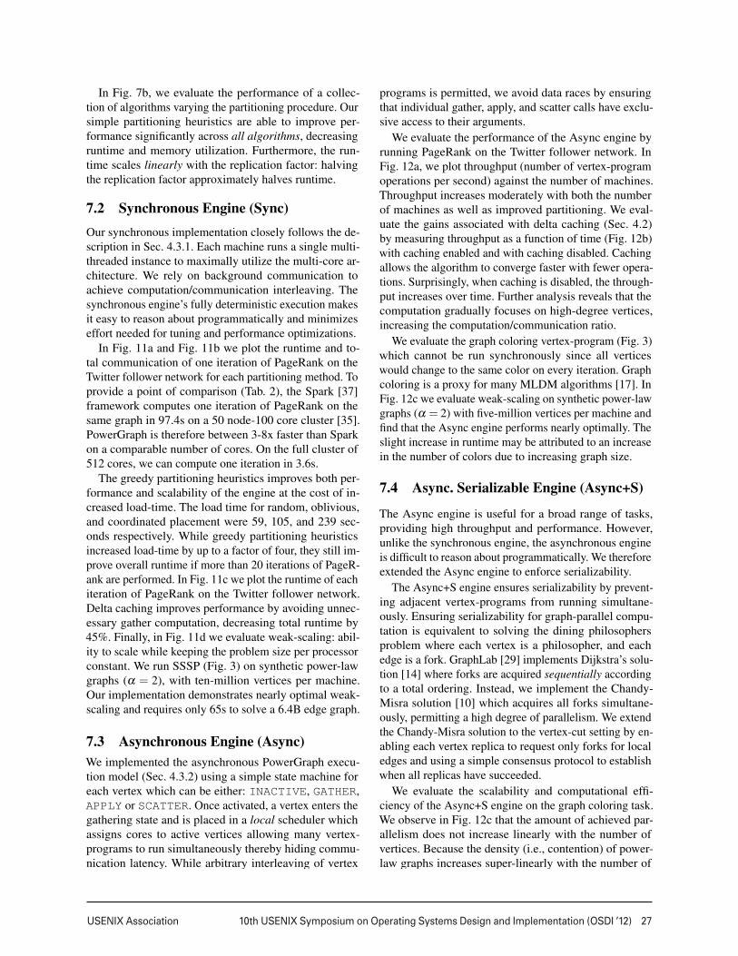
In Fig. 7b, we evaluate the performance of a collec-

tion of algorithms varying the partitioning procedure. Our

simple partitioning heuristics are able to improve per-

formance significantly across all algorithms, decreasing

runtime and memory utilization. Furthermore, the run-

time scales linearly with the replication factor: halving

the replication factor approximately halves runtime.

7.2 Synchronous Engine (Sync)

Our synchronous implementation closely follows the de-

scription in Sec. 4.3.1. Each machine runs a single multi-

threaded instance to maximally utilize the multi-core ar-

chitecture. We rely on background communication to

achieve computation/communication interleaving. The

synchronous engine’s fully deterministic execution makes

it easy to reason about programmatically and minimizes

effort needed for tuning and performance optimizations.

In Fig. 11a and Fig. 11b we plot the runtime and to-

tal communication of one iteration of PageRank on the

Twitter follower network for each partitioning method. To

provide a point of comparison (Tab. 2), the Spark [37]

framework computes one iteration of PageRank on the

same graph in 97.4s on a 50 node-100 core cluster [35].

PowerGraph is therefore between 3-8x faster than Spark

on a comparable number of cores. On the full cluster of

512 cores, we can compute one iteration in 3.6s.

The greedy partitioning heuristics improves both per-

formance and scalability of the engine at the cost of in-

creased load-time. The load time for random, oblivious,

and coordinated placement were 59, 105, and 239 sec-

onds respectively. While greedy partitioning heuristics

increased load-time by up to a factor of four, they still im-

prove overall runtime if more than 20 iterations of PageR-

ank are performed. In Fig. 11c we plot the runtime of each

iteration of PageRank on the Twitter follower network.

Delta caching improves performance by avoiding unnec-

essary gather computation, decreasing total runtime by

45%. Finally, in Fig. 11d we evaluate weak-scaling: abil-

ity to scale while keeping the problem size per processor

constant. We run SSSP (Fig. 3) on synthetic power-law

graphs (α = 2), with ten-million vertices per machine.

Our implementation demonstrates nearly optimal weak-

scaling and requires only 65s to solve a 6.4B edge graph.

7.3 Asynchronous Engine (Async)

We implemented the asynchronous PowerGraph execu-

tion model (Sec. 4.3.2) using a simple state machine for

each vertex which can be either: INACTIVE, GATHER,

APPLY or SCATTER. Once activated, a vertex enters the

gathering state and is placed in a local scheduler which

assigns cores to active vertices allowing many vertex-

programs to run simultaneously thereby hiding commu-

nication latency. While arbitrary interleaving of vertex

programs is permitted, we avoid data races by ensuring

that individual gather, apply, and scatter calls have exclu-

sive access to their arguments.

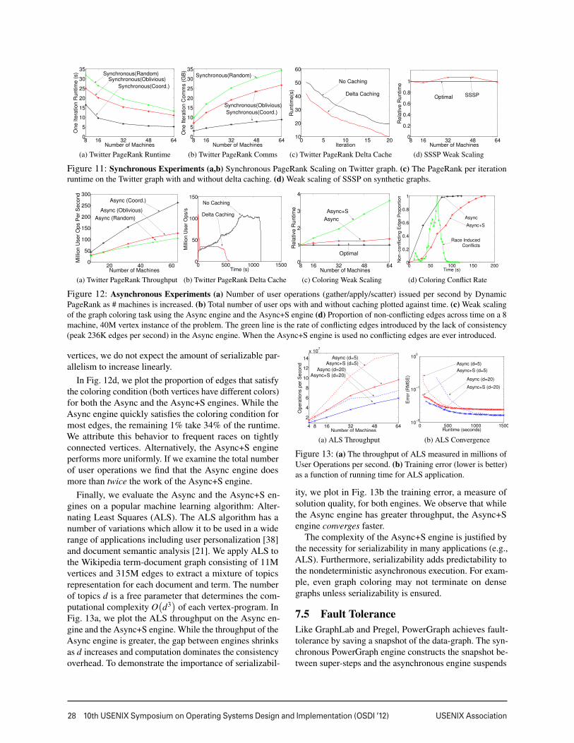
We evaluate the performance of the Async engine by

running PageRank on the Twitter follower network. In

Fig. 12a, we plot throughput (number of vertex-program

operations per second) against the number of machines.

Throughput increases moderately with both the number

of machines as well as improved partitioning. We eval-

uate the gains associated with delta caching (Sec. 4.2)

by measuring throughput as a function of time (Fig. 12b)

with caching enabled and with caching disabled. Caching

allows the algorithm to converge faster with fewer opera-

tions. Surprisingly, when caching is disabled, the through-

put increases over time. Further analysis reveals that the

computation gradually focuses on high-degree vertices,

increasing the computation/communication ratio.

We evaluate the graph coloring vertex-program (Fig. 3)

which cannot be run synchronously since all vertices

would change to the same color on every iteration. Graph

coloring is a proxy for many MLDM algorithms [17]. In

Fig. 12c we evaluate weak-scaling on synthetic power-law

graphs (α = 2) with five-million vertices per machine and

find that the Async engine performs nearly optimally. The

slight increase in runtime may be attributed to an increase

in the number of colors due to increasing graph size.

7.4 Async. Serializable Engine (Async+S)

The Async engine is useful for a broad range of tasks,

providing high throughput and performance. However,

unlike the synchronous engine, the asynchronous engine

is difficult to reason about programmatically. We therefore

extended the Async engine to enforce serializability.

The Async+S engine ensures serializability by prevent-

ing adjacent vertex-programs from running simultane-

ously. Ensuring serializability for graph-parallel compu-

tation is equivalent to solving the dining philosophers

problem where each vertex is a philosopher, and each

edge is a fork. GraphLab [29] implements Dijkstra’s solu-

tion [14] where forks are acquired sequentially according

to a total ordering. Instead, we implement the Chandy-

Misra solution [10] which acquires all forks simultane-

ously, permitting a high degree of parallelism. We extend

the Chandy-Misra solution to the vertex-cut setting by en-

abling each vertex replica to request only forks for local

edges and using a simple consensus protocol to establish

when all replicas have succeeded.

We evaluate the scalability and computational effi-

ciency of the Async+S engine on the graph coloring task.

We observe in Fig. 12c that the amount of achieved par-

allelism does not increase linearly with the number of

vertices. Because the density (i.e., contention) of power-

law graphs increases super-linearly with the number of

11


8 16 32 48 640

5

10

15

20

25

30

35

Number of Machines

On

e I

tera

tio

n R

un

tim

e (

s) Synchronous(Random)

Synchronous(Oblivious)

Synchronous(Coord.)

(a) Twitter PageRank Runtime

8 16 32 48 640

5

10

15

20

25

30

35

Number of Machines

On

e I

tera

tio

n C

om

ms (

GB

)

Synchronous(Oblivious)

Synchronous(Coord.)

Synchronous(Random)

(b) Twitter PageRank Comms

0 5 10 15 2010

20

30

40

50

60

Iteration

Ru

ntim

e(s

)

No Caching

Delta Caching

(c) Twitter PageRank Delta Cache

8 16 32 48 640

0.2

0.4

0.6

0.8

1

Number of Machines

Re

lative

Ru

ntim

e

Optimal SSSP

(d) SSSP Weak Scaling

Figure 11: Synchronous Experiments (a,b) Synchronous PageRank Scaling on Twitter graph. (c) The PageRank per iteration

runtime on the Twitter graph with and without delta caching. (d) Weak scaling of SSSP on synthetic graphs.

20 40 600

50

100

150

200

250

300

Number of Machines

Mill

ion

Use

r O

ps P

er

Se

co

nd

Async (Coord.)

Async (Random)

Async (Oblivious)

(a) Twitter PageRank Throughput

0 500 1000 15000

50

100

150

Time (s)

Mill

ion

Use

r O

ps/s

No Caching

Delta Caching

(b) Twitter PageRank Delta Cache

8 16 32 48 640

1

2

3

4

Number of Machines

Re

lative

Ru

ntim

e

Async+S

Async

Optimal

(c) Coloring Weak Scaling

0 50 100 150 2000

0.2

0.4

0.6

0.8

1

Time (s)

No

n−

co

nflic

tin

g E

dg

e P

rop

ort

ion

Async

Async+S

Race InducedConflicts

(d) Coloring Conflict Rate

Figure 12: Asynchronous Experiments (a) Number of user operations (gather/apply/scatter) issued per second by Dynamic

PageRank as # machines is increased. (b) Total number of user ops with and without caching plotted against time. (c) Weak scaling

of the graph coloring task using the Async engine and the Async+S engine (d) Proportion of non-conflicting edges across time on a 8

machine, 40M vertex instance of the problem. The green line is the rate of conflicting edges introduced by the lack of consistency

(peak 236K edges per second) in the Async engine. When the Async+S engine is used no conflicting edges are ever introduced.

vertices, we do not expect the amount of serializable par-

allelism to increase linearly.

In Fig. 12d, we plot the proportion of edges that satisfy

the coloring condition (both vertices have different colors)

for both the Async and the Async+S engines. While the

Async engine quickly satisfies the coloring condition for

most edges, the remaining 1% take 34% of the runtime.

We attribute this behavior to frequent races on tightly

connected vertices. Alternatively, the Async+S engine

performs more uniformly. If we examine the total number

of user operations we find that the Async engine does

more than twice the work of the Async+S engine.

Finally, we evaluate the Async and the Async+S en-

gines on a popular machine learning algorithm: Alter-

nating Least Squares (ALS). The ALS algorithm has a

number of variations which allow it to be used in a wide

range of applications including user personalization [38]

and document semantic analysis [21]. We apply ALS to

the Wikipedia term-document graph consisting of 11M

vertices and 315M edges to extract a mixture of topics

representation for each document and term. The number

of topics d is a free parameter that determines the com-

putational complexity O(

d3)

of each vertex-program. In

Fig. 13a, we plot the ALS throughput on the Async en-

gine and the Async+S engine. While the throughput of the

Async engine is greater, the gap between engines shrinks

as d increases and computation dominates the consistency

overhead. To demonstrate the importance of serializabil-

4 8 16 32 48 64

2

4

6

8

10

12

14

x 107

Number of Machines

Opera

tions p

er

Second Async+S (d=5)

Async (d=5)

Async (d=20)Async+S (d=20)

(a) ALS Throughput

0 500 1000 150010

−2

10−1

100

Runtime (seconds)

Err

or

(RM

SE

)

Async (d=5)

Async+S (d=20)

Async (d=20)

Async+S (d=5)

(b) ALS Convergence

Figure 13: (a) The throughput of ALS measured in millions of

User Operations per second. (b) Training error (lower is better)

as a function of running time for ALS application.

ity, we plot in Fig. 13b the training error, a measure of

solution quality, for both engines. We observe that while

the Async engine has greater throughput, the Async+S

engine converges faster.

The complexity of the Async+S engine is justified by

the necessity for serializability in many applications (e.g.,

ALS). Furthermore, serializability adds predictability to

the nondeterministic asynchronous execution. For exam-

ple, even graph coloring may not terminate on dense

graphs unless serializability is ensured.

7.5 Fault Tolerance

Like GraphLab and Pregel, PowerGraph achieves fault-

tolerance by saving a snapshot of the data-graph. The syn-

chronous PowerGraph engine constructs the snapshot be-

tween super-steps and the asynchronous engine suspends

12


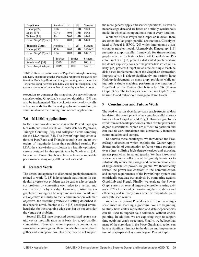
PageRank Runtime |V | |E| System

Hadoop [22] 198s – 1.1B 50x8

Spark [37] 97.4s 40M 1.5B 50x2

Twister [15] 36s 50M 1.4B 64x4

PowerGraph (Sync) 3.6s 40M 1.5B 64x8

Triangle Count Runtime |V | |E| System

Hadoop [36] 423m 40M 1.4B 1636x?

PowerGraph (Sync) 1.5m 40M 1.4B 64x16

LDA Tok/sec Topics System

Smola et al. [34] 150M 1000 100x8

PowerGraph (Async) 110M 1000 64x16

Table 2: Relative performance of PageRank, triangle counting,

and LDA on similar graphs. PageRank runtime is measured per

iteration. Both PageRank and triangle counting were run on the

Twitter follower network and LDA was run on Wikipedia. The

systems are reported as number of nodes by number of cores.

execution to construct the snapshot. An asynchronous

snapshot using GraphLab’s snapshot algorithm [29] can

also be implemented. The checkpoint overhead, typically

a few seconds for the largest graphs we considered, is

small relative to the running time of each application.

7.6 MLDM Applications

In Tab. 2 we provide comparisons of the PowerGraph sys-

tem with published results on similar data for PageRank,

Triangle Counting [36], and collapsed Gibbs sampling

for the LDA model [34]. The PowerGraph implementa-

tions of PageRank and Triangle counting are one to two

orders of magnitude faster than published results. For

LDA, the state-of-the-art solution is a heavily optimized

system designed for this specific task by Smola et al. [34].

In contrast, PowerGraph is able to achieve comparable

performance using only 200 lines of user code.

8 Related Work

The vertex-cut approach to distributed graph placement is

related to work [9, 13] in hypergraph partitioning. In par-

ticular, a vertex-cut problem can be cast as a hypergraph-

cut problem by converting each edge to a vertex, and

each vertex to a hyper-edge. However, existing hyper-

graph partitioning can be very time intensive. While our

cut objective is similar to the “communication volume”

objective, the streaming vertex cut setting described in

this paper is novel. Stanton et al, in [35] developed several

heuristics for the streaming edge-cuts but do not consider

the vertex-cut problem.

Several [8, 22] have proposed generalized sparse ma-

trix vector multiplication as a basis for graph-parallel

computation. These abstractions operate on commutative

associative semi-rings and therefore also have generalized

gather and sum operations. However, they do not support

the more general apply and scatter operations, as well as

mutable edge-data and are based on a strictly synchronous

model in which all computation is run in every iteration.

While we discuss Pregel and GraphLab in detail, there

are other similar graph-parallel abstractions. Closely re-

lated to Pregel is BPGL [20] which implements a syn-

chronous traveler model. Alternatively, Kineograph [11]

presents a graph-parallel framework for time-evolving

graphs which mixes features from both GraphLab and Pic-

colo. Pujol et al. [33] present a distributed graph database

but do not explicitly consider the power-law structure. Fi-

nally, [25] presents GraphChi: an efficient single-machine

disk-based implementation of the GraphLab abstraction.

Impressively, it is able to significantly out-perform large

Hadoop deployments on many graph problems while us-

ing only a single machine: performing one iteration of

PageRank on the Twitter Graph in only 158s (Power-

Graph: 3.6s). The techniques described in GraphChi can

be used to add out-of-core storage to PowerGraph.

9 Conclusions and Future Work

The need to reason about large-scale graph-structured data

has driven the development of new graph-parallel abstrac-

tions such as GraphLab and Pregel. However graphs de-

rived from real-world phenomena often exhibit power-law

degree distributions, which are difficult to partition and

can lead to work imbalance and substantially increased

communication and storage.

To address these challenges, we introduced the Pow-

erGraph abstraction which exploits the Gather-Apply-

Scatter model of computation to factor vertex-programs

over edges, splitting high-degree vertices and exposing

greater parallelism in natural graphs. We then introduced

vertex-cuts and a collection of fast greedy heuristics to

substantially reduce the storage and communication costs

of large distributed power-law graphs. We theoretically

related the power-law constant to the communication

and storage requirements of the PowerGraph system and

empirically evaluate our analysis by comparing against

GraphLab and Pregel. Finally, we evaluate the Power-

Graph system on several large-scale problems using a 64

node EC2 cluster and demonstrating the scalability and

efficiency and in many cases order of magnitude gains

over published results.

We are actively using PowerGraph to explore new large-

scale machine learning algorithms. We are beginning

to study how vertex replication and data-dependencies

can be used to support fault-tolerance without check-

pointing. In addition, we are exploring ways to support

time-evolving graph structures. Finally, we believe that

many of the core ideas in the PowerGraph abstraction can

have a significant impact in the design and implementa-

tion of graph-parallel systems beyond PowerGraph.

13


Acknowledgments

This work is supported by the ONR Young Investiga-

tor Program grant N00014-08-1-0752, the ARO under

MURI W911NF0810242, the ONR PECASE-N00014-

10-1-0672, the National Science Foundation grant IIS-

0803333 as well as the Intel Science and Technology Cen-

ter for Cloud Computing. Joseph Gonzalez is supported

by the Graduate Research Fellowship from the NSF. We

would like to thank Alex Smola, Aapo Kyrola, Lidong

Zhou, and the reviewers for their insightful guidance.

References

[1] ABOU-RJEILI, A., AND KARYPIS, G. Multilevel algorithms for

partitioning power-law graphs. In IPDPS (2006).

[2] AHMED, A., ALY, M., GONZALEZ, J., NARAYANAMURTHY, S.,

AND SMOLA, A. J. Scalable inference in latent variable models.

In WSDM (2012), pp. 123–132.

[3] ALBERT, R., JEONG, H., AND BARABASI, A. L. Error and

attack tolerance of complex networks. In Nature (2000), vol. 406,

pp. 378—482.

[4] BERTSEKAS, D. P., AND TSITSIKLIS, J. N. Parallel and dis-

tributed computation: numerical methods. Prentice-Hall, 1989.

[5] BOLDI, P., ROSA, M., SANTINI, M., AND VIGNA, S. Layered

label propagation: A multiresolution coordinate-free ordering for

compressing social networks. In WWW (2011), pp. 587–596.

[6] BOLDI, P., AND VIGNA, S. The WebGraph framework I: Com-

pression techniques. In WWW (2004), pp. 595–601.

[7] BORDINO, I., BOLDI, P., DONATO, D., SANTINI, M., AND

VIGNA, S. Temporal evolution of the uk web. In ICDM Workshops

(2008), pp. 909–918.

[8] BULUC, A., AND GILBERT, J. R. The combinatorial blas: design,

implementation, and applications. IJHPCA 25, 4 (2011), 496–509.

[9] CATALYUREK, U., AND AYKANAT, C. Decomposing irregu-

larly sparse matrices for parallel matrix-vector multiplication. In

IRREGULAR (1996), pp. 75–86.

[10] CHANDY, K. M., AND MISRA, J. The drinking philosophers

problem. ACM Trans. Program. Lang. Syst. 6, 4 (Oct. 1984),

632–646.

[11] CHENG, R., HONG, J., KYROLA, A., MIAO, Y., WENG, X.,

WU, M., YANG, F., ZHOU, L., ZHAO, F., AND CHEN, E. Kineo-

graph: taking the pulse of a fast-changing and connected world.

In EuroSys (2012), pp. 85–98.

[12] CHIERICHETTI, F., KUMAR, R., LATTANZI, S., MITZEN-

MACHER, M., PANCONESI, A., AND RAGHAVAN, P. On com-

pressing social networks. In KDD (2009), pp. 219–228.

[13] DEVINE, K. D., BOMAN, E. G., HEAPHY, R. T., BISSELING,

R. H., AND CATALYUREK, U. V. Parallel hypergraph partitioning

for scientific computing. In IPDPS (2006).

[14] DIJKSTRA, E. W. Hierarchical ordering of sequential processes.

Acta Informatica 1 (1971), 115–138.

[15] EKANAYAKE, J., LI, H., ZHANG, B., GUNARATHNE, T., BAE,

S., QIU, J., AND FOX, G. Twister: A runtime for iterative MapRe-

duce. In HPDC (2010), ACM.

[16] FALOUTSOS, M., FALOUTSOS, P., AND FALOUTSOS, C. On

power-law relationships of the internet topology. ACM SIGCOMM

Computer Communication Review 29, 4 (1999), 251–262.

[17] GONZALEZ, J., LOW, Y., GRETTON, A., AND GUESTRIN, C.

Parallel gibbs sampling: From colored fields to thin junction trees.

In AISTATS (2011), vol. 15, pp. 324–332.

[18] GONZALEZ, J., LOW, Y., AND GUESTRIN, C. Residual splash

for optimally parallelizing belief propagation. In AISTATS (2009),

vol. 5, pp. 177–184.

[19] GONZALEZ, J., LOW, Y., GUESTRIN, C., AND O’HALLARON,

D. Distributed parallel inference on large factor graphs. In UAI

(2009).

[20] GREGOR, D., AND LUMSDAINE, A. The parallel BGL: A generic

library for distributed graph computations. POOSC (2005).

[21] HOFMANN, T. Probabilistic latent semantic indexing. In SIGIR

(1999), pp. 50–57.

[22] KANG, U., TSOURAKAKIS, C. E., AND FALOUTSOS, C. Pe-

gasus: A peta-scale graph mining system implementation and

observations. In ICDM (2009), pp. 229 –238.

[23] KARYPIS, G., AND KUMAR, V. Multilevel k-way partitioning

scheme for irregular graphs. J. Parallel Distrib. Comput. 48, 1

(1998), 96–129.

[24] KWAK, H., LEE, C., PARK, H., AND MOON, S. What is twitter,

a social network or a news media? In WWW (2010), pp. 591–600.

[25] KYROLA, A., BLELLOCH, G., AND GUESTRIN, C. GraphChi:

Large-scale graph computation on just a PC. In OSDI (2012).

[26] LANG, K. Finding good nearly balanced cuts in power law graphs.

Tech. Rep. YRL-2004-036, Yahoo! Research Labs, Nov. 2004.

[27] LESKOVEC, J., KLEINBERG, J., AND FALOUTSOS, C. Graph

evolution: Densification and shrinking diameters. ACM Trans.

Knowl. Discov. Data 1, 1 (mar 2007).

[28] LESKOVEC, J., LANG, K. J., DASGUPTA, A., , AND MAHONEY,

M. W. Community structure in large networks: Natural cluster

sizes and the absence of large well-defined clusters. Internet

Mathematics 6, 1 (2008), 29–123.

[29] LOW, Y., GONZALEZ, J., KYROLA, A., BICKSON, D.,

GUESTRIN, C., AND HELLERSTEIN, J. M. Distributed GraphLab:

A Framework for Machine Learning and Data Mining in the Cloud.

PVLDB (2012).

[30] MALEWICZ, G., AUSTERN, M. H., BIK, A. J., DEHNERT, J.,

HORN, I., LEISER, N., AND CZAJKOWSKI, G. Pregel: a system

for large-scale graph processing. In SIGMOD (2010).

[31] PELLEGRINI, F., AND ROMAN, J. Scotch: A software package

for static mapping by dual recursive bipartitioning of process and

architecture graphs. In HPCN Europe (1996), pp. 493–498.

[32] POWER, R., AND LI, J. Piccolo: building fast, distributed pro-

grams with partitioned tables. In OSDI (2010).

[33] PUJOL, J. M., ERRAMILLI, V., SIGANOS, G., YANG, X.,

LAOUTARIS, N., CHHABRA, P., AND RODRIGUEZ, P. The little

engine(s) that could: scaling online social networks. In SIGCOMM

(2010), pp. 375–386.

[34] SMOLA, A. J., AND NARAYANAMURTHY, S. An Architecture

for Parallel Topic Models. PVLDB 3, 1 (2010), 703–710.

[35] STANTON, I., AND KLIOT, G. Streaming graph partitioning

for large distributed graphs. Tech. Rep. MSR-TR-2011-121, Mi-

crosoft Research, November 2011.

[36] SURI, S., AND VASSILVITSKII, S. Counting triangles and the

curse of the last reducer. In WWW (2011), pp. 607–614.

[37] ZAHARIA, M., CHOWDHURY, M., FRANKLIN, M. J., SHENKER,

S., AND STOICA, I. Spark: Cluster computing with working sets.

In HotCloud (2010).

[38] ZHOU, Y., WILKINSON, D., SCHREIBER, R., AND PAN, R.

Large-scale parallel collaborative filtering for the netflix prize.

In AAIM (2008), pp. 337–348.

14

powergraph: distributed graph-parallel computation on natural graphs

Documents