powerpoint to accompany chapter 3 where prices come from: the interaction of demand and supply

PowerPoint

to accompany

Chapter 3

Where Prices Come From: The

Interaction of Demand and

Supply

Hubbard, Garnett, Lewis and O’Brien: Essentials of Economics © 2010 Pearson Australia

Learning Objectives

1. Understand the factors that influence the demand for goods and services.

2. Understand the factors that influence the supply of goods and services.

3. Explain how equilibrium in a market is reached and use a graph to illustrate equilibrium.

4. Use demand and supply graphs to predict changes in prices and quantities.


How Hewlett-Packard manages the demand for printers

H-P’s success, like that of any firm, depends on its ability to manage changes in demand and supply. H-P has responded to changing market conditions so that printers, and not PCs, are now the firm’s most successful product.


The demand of an individual buyer

Quantity demanded: The amount of a good or service that a consumer is willing and able to buy at a given price.

LEARNING OBJECTIVE 1

The demand side of the market

Price (dollars per

printer)

Quantity (printers per month)

05

$125

Plotting a price-quantity combination on a graph: Figure 3.1



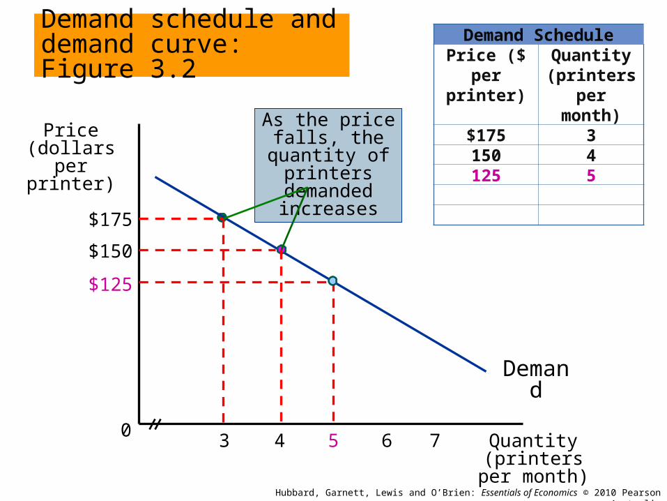
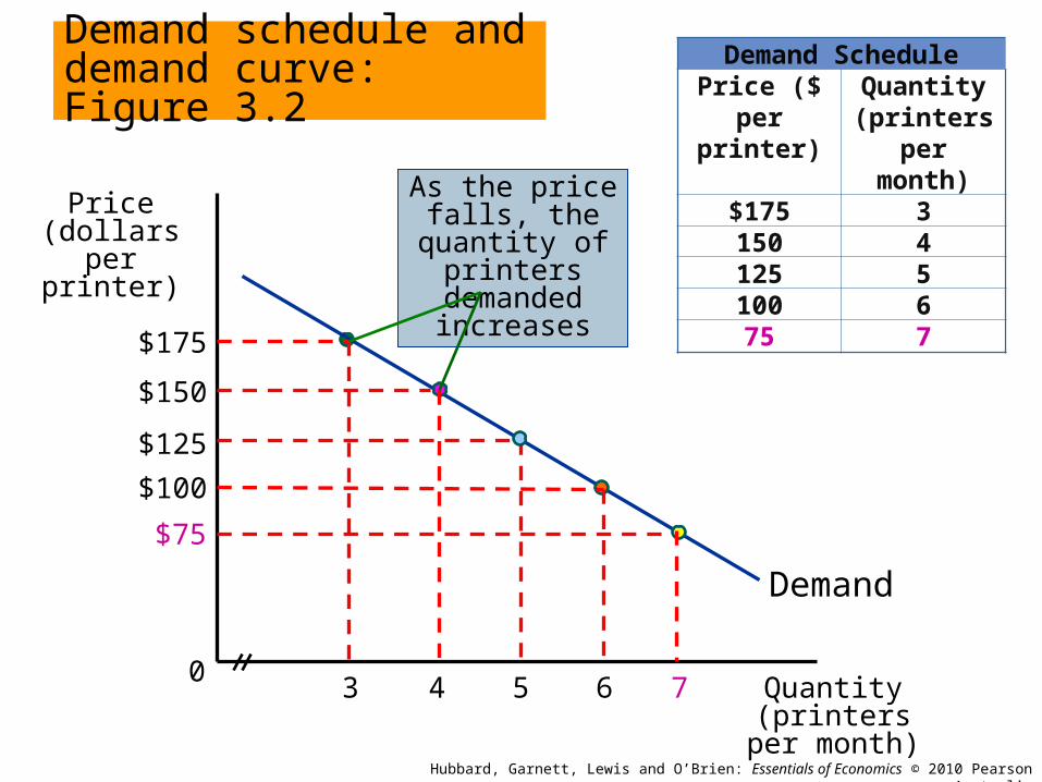
Demand schedule: A table showing the relationship between the price of a product and the quantity of the product demanded.

Demand curve: A curve that shows the relationship between the price of a product and the quantity of the product demanded.



Price (dollars per

printer)


04

Demand schedule and demand curve: Figure 3.2


Demand SchedulePrice ($ per

printer)Quantity (printers

per month)

$175 3

Demand

$175

5 6 73

At a price of $175, three printers will be purchased per month

Price (dollars per

printer)


04





per month)

$175 3 150 4

Demand

$175

$150

5 6 73

As the price falls, the quantity of

printers demanded increases

Price (dollars per

printer)


04

$125





per month)

$175 3150 4125 5

Demand

$175

$150

5 6 73



Price (dollars per

printer)


04

$125





per month)

$175 3150 4125 5100 6

Demand

$175

$150

$100

5 6 73



Price (dollars per

printer)


04

$125





per month)

$175 3150 4125 5100 675 7

Demand

$175

$150

$100

$75

5 6 73




Individual and market demand

Market demand: The demand by all the consumers of a given good or service.

The market demand curve is derived by horizontally summing all the individual demand curves for a good or service.



Deriving the market demand curve from individual curves: Figure 3.3



Deriving the market demand curve from individual curves: Figure 3.3, continued


The law of demand: Holding everything else constant, when the price of a product falls, the quantity demanded will increase, and when the price of a product rises, the quantity demanded will decrease.




Holding everything else constant: the ceteris paribus condition.

Ceteris paribus (‘all else being equal’):

The requirement that when analysing the relationship between two variables, such as price and quantity demanded, other variables must be held constant.




What explains the law of demand?

1. The substitution effect: The change in the quantity demanded of a good or service that results from a change in price, making the good or service more or less expensive relative to other goods and services that are substitutes, (holding constant the effect of the price change on consumer purchasing power).




What explains the law of demand?

2. The income effect: The change in the quantity demanded of a good or service that results from the effect of a change in price on consumer purchasing power, (holding all other factors constant).




Variables that shift market demand

The five most important variables are:

1. Prices of related goods.

2. Income

3. Tastes

4. Population and demographics

5. Expected future prices



Demand 2

Price

P

0 Q1 Q2 Quantity

Demand 1

An increase in demand: Figure 3.4a


P

0 Q3 Q1 Quantity

A decrease in demand: Figure 3.4bPrice

Demand 3

Demand 1



1. Prices of related goods –

Substitutes: Goods or services that can be used in place of other goods or services.

Complements: Goods and services that are consumed together.




2. Income –

Normal good: A good for which the demand increases as income rises and decreases as income falls.

Inferior good: A good for which the demand increases as income falls and decreases as income rises.




3. Tastes –

A broad category that refers to the many subjective elements that can influence a consumer’s plans to buy a good or service.

– Seasons

– Trends/fashion




4. Population and demographics -

Population: As population increases the demand for most goods and services will increase.

Demographics: Changes in the characteristics of the population (age, race and gender) will influence demand for various goods and services.




5. Expected future prices -

Consumers choose when to buy goods and services based on their expectations regarding future prices relative to present prices.

If consumers expect prices to increase in the future, they have an incentive to increase purchases now, and vice versa.




Petrol prices don’t just affect the demand for petrol

High petrol prices reduced the demand for 4WDs.

Table 3.1: Variables that shift the market demand curve



A change in demand versus a change in quantity demanded

A change in demand refers to a shift in the demand curve.

Occurs due to a change in variables, other than the product’s own price, that affect demand.

A change in the quantity demanded refers to a movement along the demand curve as a result of a change in the product’s price.



Price (dollars per

printer)


060 000

A change in demand versus a change in the quantity demanded: Figure 3.5


Demand, D1

$175

$150

70 00050 000

A shift in the demand curve is a change in

demand

D2

A movement along the demand

curve is a change in quantity

demanded

A

B

C


Changes in quantity demanded versus changes in demand

Explain whether each of the following causes a movement along or a shift in the demand curve for Dell laptops. Indicate the direction of the shift in demand or the movement along the curve and the reason for the change.

a) The price of Toshiba laptops decreases.

b) A fall in the value of the Australian dollar against the US dollar increases the price of Dell laptops in Australia.

c) Dell’s customised laptops become increasingly appealing.



Solving the problem:

STEP 1: Review the material. The problem addresses the difference between changes in demand and changes in quantity demanded, and the determinants of both. This material is covered on pages 65 – 70 of the text.

STEP 2: Answer (a): Toshiba laptops are a substitute for Dell laptops. A decrease in the price of Toshiba laptops will decrease demand for Dell laptops, shifting the demand curve for Dell laptops to the left.





STEP 3: Answer (b): The reason for the change in price is not significant (at this stage). The important issue is that the price of Dell laptops has increased. As a result, quantity demanded will decrease, resulting in a movement up the demand curve.





STEP 4: Answer (c): This change is an example of a change in consumer tastes. The result will be an increase in demand for Dell laptops, which will shift the demand curve to the right.




Individual supply

Quantity supplied: the amount of a good or service that a firm is willing and able to supply at a given price.


The supply side of the market


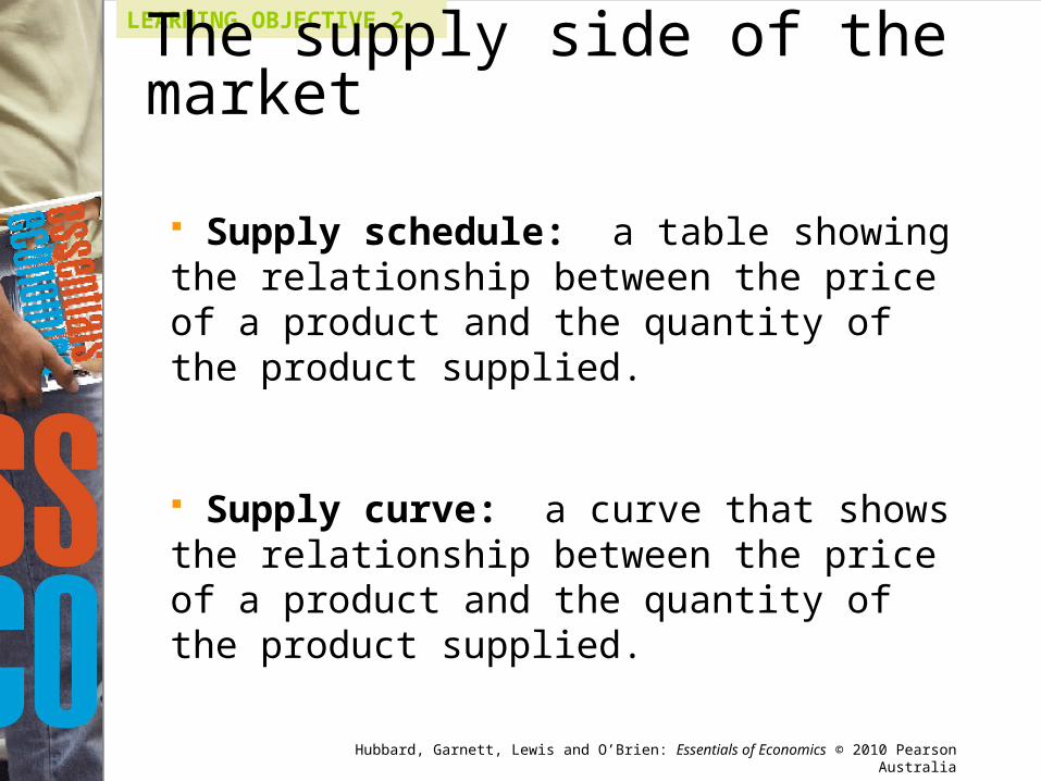
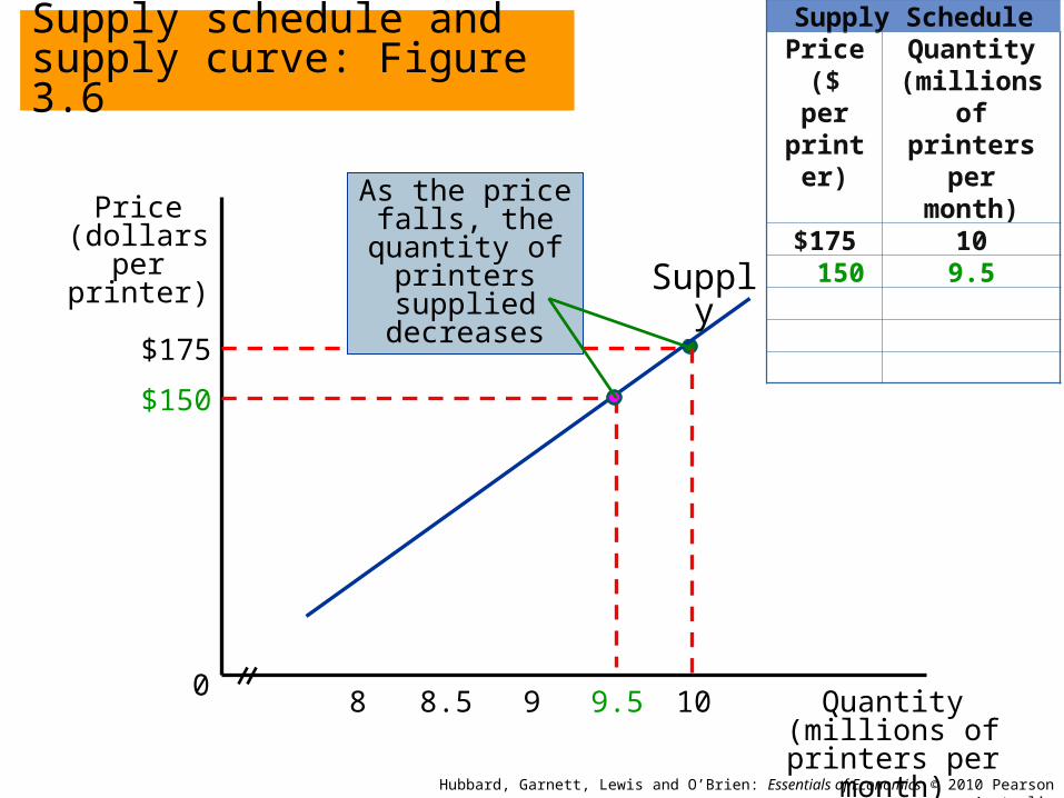
Supply schedule: a table showing the relationship between the price of a product and the quantity of the product supplied.

Supply curve: a curve that shows the relationship between the price of a product and the quantity of the product supplied.



Price (dollars per

printer)

Quantity (millions of printers per

month)

08.5

Supply schedule and supply curve: Figure 3.6


Supply SchedulePrice ($ per

printer)


month)$175 10

Supply

$175

9 9.5 108

At a price of $175, 10 million printers would

be supplied per month

Price (dollars per

printer)


month)

08.5




printer)


month)$175 10 150 9.5

Supply

$175

9 9.5 108

$150


printers supplied decreases

Price (dollars per

printer)


month)

08.5




printer)


month)$175 10 150 9.5 125 9

Supply

$175

9 9.5 108

$150



$125

Price (dollars per

printer)


month)

08.5




printer)


month)$175 10 150 9.5 125 9 100 8.5Supply

$175

9 9.5 108

$150



$125

$100

Price (dollars per

printer)


month)

08.5




printer)


month)$175 10 150 9.5 125 9 100 8.5 75 8

Supply

$175

9 9.5 108

$150



$125

$100

$75


Individual and market supply

Market supply: The supply by all the firms of a given good or service.

The market supply curve is derived by horizontally summing all the individual supply curves for a good or service.



Deriving the market supply curve from individual curves: Figure 3.7


Deriving the market supply curve from individual curves: Figure 3.7, continued



The law of supply: Holding everything else constant, increases in the price of a product cause increases in the quantity supplied, and decreases in price cause decreases in the quantity supplied.




Variables that shift supply

The five most important variables are:

1. Prices of inputs

2. Technological change

3. Prices of substitutes in production


5. Number of firms in the market



Price

Quantity0

Supply2 Supply1

Decrease

P

Q2 Q1

A decrease in supply: Figure 3.8a


P

Quantity0

Supply1Supply3

Increase

Price

Q3Q1

An increase in supply: Figure 3.8b



1. Prices of inputs

An input is anything used in the production of a good or service.

An increase in the cost of an input increases the cost of production. The firm supplies less.

A decrease in the cost of an input decreases the cost of production at every price. The firm supplies more at every price.




2. Technological change

A change in the ability of a firm to produce a given level of output with a given quantity of inputs.

Positive technological change allows the firm to produce more outputs with the same amount of inputs.

Negative technological change is rare.




3. Prices of substitutes in production

Alternative products a firm can produce with the same resources are substitutes in production.

An increase in the price of a substitute in production decreases the supply of the initial good, while a decrease in the price of a substitute in production increases the supply of the initial good.





If firms expect the price of its product will increase in the future they have an incentive to decrease supply now.

5. Number of firms in the market

When new firms enter the market supply increases.

When firms exit the market, supply decreases.



Price (dollars per

printer)

Quantity (millions of printers per month)

023.5


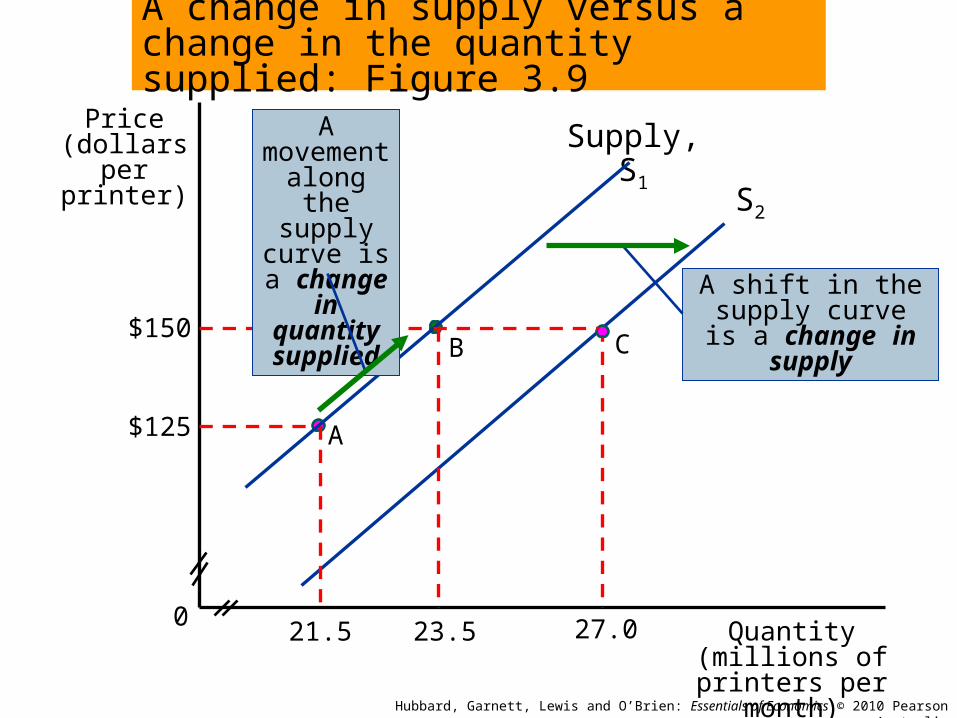
Supply, S1

$150

$125

27.021.5

A shift in the supply curve is a change in

supply

S2

A movement along the

supply curve is a change in quantity supplied

A change in supply versus a change in the quantity supplied: Figure 3.9

CB

A


Market equilibrium: A situation in which quantity demanded equals quantity supplied.

Competitive market equilibrium: A market equilibrium with many buyers and many sellers.


Market equilibrium

Price (dollars per

printer)


019.5


$100

Supply

Market equilibrium: Figure 3.10

Demand

Market equilibriumEquilibrium price

Equilibrium quantity


Surplus: A situation in which the quantity supplied is greater than the quantity demanded.

Shortage: A situation in which the quantity demanded is greater than the quantity supplied.


Market equilibrium

Price (dollars per

printer)


019.5


$100

Supply

The effect of surpluses and shortages on the market price: Figure 3.11

Demand

Surplus of 3 million printers resulting from price above

equilibrium

$125

$75

20.5 21.518.517.5

Shortage of 3 million printers resulting from price below equilibrium

Price (dollars per

printer)


0Q1


P1

Supply1

The effect of a decrease in supply on equilibrium: Figure 3.12

Demand

1. As Xerox exits the market for printers, the supply curve shifts to

the left …

2. …increasing the equilibrium

price…

3. …and decreasing the equilibrium

quantity

Supply2

P2

Q2

Price (dollars per

printer)


0Q1


P1

Supply

The effect of an increase in demand on equilibrium: Figure 3.13

Demand1

1. As population and income grow, the

demand curve shifts to the right …

2. …increasing the equilibrium

price…

3. …and also increasing the

equilibrium quantity

Demand2

P2

Q2

Figure 3.14: Shifts in demand and supply over time


Figure 3.15: The demand for chicken has increased more than the supply



The falling price of large flat-screen televisions

Corning’s breakthrough spurred the manufacture of LCD televisions in Taiwan, South Korea and Japan, and an eventual decline in price.


Demand and supply both count: the market for flat-screen televisions.

Demand for flat-screen televisions has increased significantly over recent years, however, the price of these televisions has decreased. Clearly this is an example of an exception to the “law of demand”. Do you agree?



Demand and supply both count: the market for flat-screen televisions.


STEP 1: Review the material. The problem examines simultaneous shifts in the demand and supply curves and the resulting impact on equilibrium price. This material is covered on pages 82-83 of the text.





STEP 2: To answer this question we need to look at changes in both demand and supply. If we begin from the demand side, it is clear that demand for flat-screen televisions has increased. This would cause a rightward shift of the demand curve, and, all else held constant, the equilibrium price would increase.





STEP 3: In the real world, it is common for more than one variable to change at the same time. In the case of flat-screen televisions, production technology has improved, decreasing the cost of production and causing the supply curve to shift to the right. In addition, there are many more producers in the industry, for example, from Japan, South Korea and China, which further increases supply. A rightward shift in supply alone would lead to a decrease in equilibrium price.





STEP 4: If we compare the shifts in demand and supply, we can see that a right shift in demand increases price and a right shift in supply decreases price. In this case, both shifts have occurred simultaneously, but the shift in supply has been of a greater magnitude than the shift in demand. As a consequence, the supply effect has dominated the outcome, resulting in a decrease in the equilibrium price for flat-screen televisions.





STEP 5: Our result is not an example of an exception to the ‘law of demand’. The ‘law of demand’ relates to the inverse relationship between the price of a good and the quantity of the good demanded. The case of ‘flat screen televisions’ is an example of changes in tastes leading to an increase in demand and, simultaneously, an increase in the number of suppliers and improvements in production technology increasing supply.



An Inside LookFigure 1: The fall in the price of PCs causes the demand for printers to shift to the right


An Inside LookFigure 2: A fall in the cost of PCs shifts the supply curve for PCs to the right


Key Terms Ceteris paribus (all else

being constant)

Competitive market equilibrium

Complements

Demand curve

Demand schedule

Demographics

Income effect

Inferior good

Law of demand

Law of supply

Market demand

Market equilibrium

Normal good

Quantity demanded

Quantity supplied

Shortage

Substitutes

Substitution effect

Supply curve

Supply schedule

Surplus

Technological change


Agricultural products are typically sold in international markets where their prices frequently fluctuate in response to changes in demand and supply.

The Australian Broadcasting Commission’s regular Sunday program Landline allows viewers to see many examples of changing agricultural markets.

Go to the program’s website at

www.abc.net.au/landline

and search the Program Archives for an overview of changes in demand and supply conditions for agricultural products of interest to you. Some examples are: the wine industry, beef, wheat, water, and even the fertiliser industry in Australia’s Pacific neighbour Nauru.

Get Thinking!


Q1. Which of the following establishes the inverse relationship between the price of a product and the quantity of the product demanded?

a. The substitution effect.

b. The income effect.

c. The law of demand.

d. The price effect.

Check Your Knowledge


Q2. When analysing the relationship between the price of a good and quantity demanded, other variables must be held constant. Which term best describes such an assumption?

a. The substitution effect.

b. The income effect.

c. The law of demand

d. The term ceteris paribus.



Q3. When two goods, X and Y, are complements, which of the following occurs?

a. An increase in the price of good X leads to an increase in the price of good Y.

b. An increase in the price of good X leads to decrease in the quantity demanded of good Y.

c. An increase in the price of good X leads to a decrease in demand for good Y.

d. An increase in the price of good X leads to an increase in demand for good Y.



Q4. Which of the following is correct?

a. Individual supply curves can be derived from a market supply curve.

b. To derive a market supply curve, we add the prices that producers must obtain in order to produce a given quantity of output.

c. To derive a market supply curve, we add individual supply curves.

d. All of the above procedures are correct.



Q4. Which of the following is correct?

a. Individual supply curves can be derived from a market supply curve.

b. To derive a market supply curve, we add the prices that producers must obtain in order to produce a given quantity of output.

c. To derive a market supply curve, we add individual supply curves.

d. All of the above are correct.


powerpoint to accompany chapter 3 where prices come from: the interaction of demand and supply

Documents

quantity of printers

demand curve

printer quantity printers

interaction of demand

price dollars

pricequantity combination

price falls

month slide