PP-77-4

A NEW APPROACH IN ENERGY DEMAND

PART I: METHODOLOGY AND ILLUSTRATIVE EXAMPLES

J.M. Beaujean

B. Chaix

J.P. Charpentier

J. Ledo1ter

March 1977

Professional Papers are not official publications of the International Institutefor Applied Systems Analysis, but are reproduced and distributed by theInstitute as an aid to staff members in furthering their professional activities.Views or opinions expressed herein are those of the author and should not beinterpreted as representing the view of either the Institute or the NationalMember Organizations supporting the Institute.

ABSTRACT

A great deal of work has been carried out on the relationbetween per capita GNP and per capita energy consumption.

In this short paper we substitute the structure of GNP toits absolute level. Three sectors were only retained: namelyagriculture, industry and services (including transportation).The relation between per capita energy consumption and GNPstructure explicitly constructed and adjusted on data is apotential in the space of GNP structures.

- iii -

I

II

III

TABLE OF CONTENTS

Classical analytical tools • • . . • . . • • . • • . •

Methodology•..

Relation between per capita energy consumption andGNP structure for each group of homogenous countries •

1

2

5

A.

B.

C.

Economic assumptions for the developingcountries. . . . .. . .

Economic assumptions for developed countries

The curves cannot intersect.

6

9

11

IV The dynamics of development. . .

-v-

. . . . . . . . . . . 12

LIST OF FIGURES

Representation of GNP structure 'in triangularcoordinates . . . . . . . . . . . . . . . . . 3

2. Ranking of partial derivatives of energy consumptionto GNP structure for developing countries • • • • • • • 7

3. Vector representation of possible variation in servicesand industry shares (agriculture remaining constant). . 8

4. Convexity of iso energy consumption per capita and GNPstructure in developing countries • •••• • • •• 9

5. Ranking of partial derivation of energy consumptionper capita to GNP structure for developed countries 10

6. Convexity of iso energy consumption per' capita and GNPstructure in developed countries. • . • • • • • •• 10

7. Intersection of two iso curves of per capita energyconsumption and possible variation in GNP structure • 11

8. Two isocurves of per capita energy consumption inter-secting at only one point . . • . • • • •• 11

9. Long trend evolution in GNr structure • 12

10. Network of iso "energy demand per capita" curves. • 14

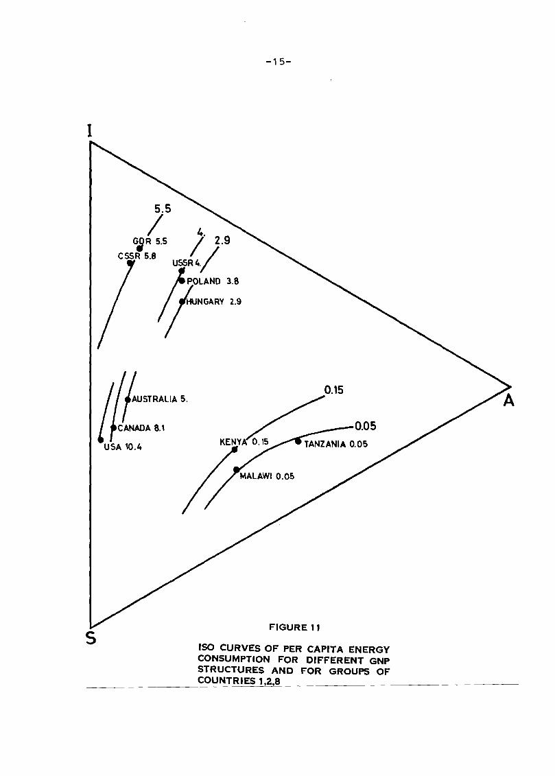
11. Iso curves of per capita energy consumption fordifferent GNP structures and for groups of countries1, 2, 8 . .. ... . . . . . . . . . . . ... 15

12. Iso curves of per capita energy consumption fordifferent GNP structures and for groups of countries3,6. . . . .

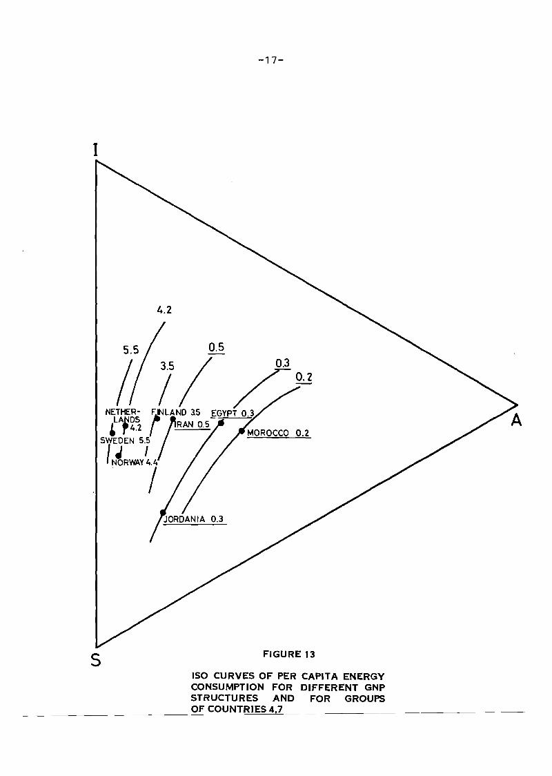
13. Iso curves of per capita energy consumption fordifferent GNP structures and for groups of countries4, 7. . . . .

• 16

.17

14. Iso curves of per capita energy consumption fordifferent GNP structures and for groups of countries5, 9. .. ... . . . . . . . . . . . . .. .. 18

15. Evolution of GNP structure and energy potential forUnited Kingdom, Germany, Italy and France during thelast two centuries••...•.•.....••••.• 19

Appendix

16.

17.

Parameterization for groups 1, 2, 3 •

Parameterization for groups 4 and 5 • •

-vii-

• • 29

30

18.

19.

20.

Parameterization for groups 6 and 8 .

Parameterization for group 7. • ..

Parameterization for group 9•••••••

-viii-

. . . . . . .. . . . . .

. . .

31

32

33

A NEW APPROACH IN ENERGY DEMAND

PART I. METHODOLOGY AND ILLUSTRATIVE EXAMPLES

To make sound forecasting on world energy consumption, onehas to embed the energy systems in the overall economic strataand to take development strategies, especially for developingcountries, into account. Many methodological reports have beenpublished on the subject. In the first part, we will reviewthese techniques and point out their weak points. In the secondpart, we will present an alternative approach. In the thirdpart, we will apply it to a sample of a given year and tohistorical data, whose results will be used to build strategiesfor probable scenarios of development. However, this analysishas remained more or less qualitative, and we will suggest someguidelines for formalization.

I CLASSICAL ANALYTICAL TOOLS

The classical analytical tools used to forecast energydemand are based on:

1. econometric analysis,2. engineering analysis of systems,3. energy content and energy basket approach.

Some studies using one of these approaches are very detailedand go down to microeconomic levels; some are broader and usemacroeconomic indicators or variables. Therefore, we can builda classification of approaches and degrees of analysis.

Table 1. Classification of possible methodologieswhich might be used in energy demand study.

scole of World Country or group Sectorsana ysis (global of countries (micro

approaches analysis) (macro analysis) analysis}

GNP/cap-energy Estimation of the Elasticity/Econometric coefficients of aconsumption/cap theoretical formula prices

Engineering World average Average energy Diagram offigures input per output energy flows

Energy I - 0Process

Scenarios analysis "acontent Herendeen & Bullard la Slesser"

-2-

Our aim is to make an energy demand forecast for the world.This table shows that the only tool commonly used is the corre­lation between GNP/cap and energy cons~ption/cap. All othermethods (column 3) could be employed and their results aggregatedJhowever, the number of equations and variables would become toolarge.

The global econometric approach is too broad to give accu­rate results. Mainly because the linear equation holds betweenupper and lower bounds: e.g. GNP/cap < energy consumption <3 GNP/cap. - -

Therefore, we look for other variables. We found that theGNP structure is more significant for energy demand forecaststhan its absolute level. This is mainly due to the fact thatindustry, services and agriculture have very different energyconsumption patterns. So, we divided the GNP in these threesectors:

a) agriculture,b) industry,c) services.

This three-dimensional vector is a better indicator ofdevelopment than the gross value of GNP/cap. It allows us tocapture final energy demand over long term in more detail,given development scenarios and explicit relations among energyper capita, GNP structure and development level.

II. METHODOLOGY

If we define:

A as agriculture share in GNP,I as industry share in GNP,S as services and transportation shares in GNP,

then every country is defined by a vector (!) which can be

represented as a point in nR 3• Given that A + I + S = 1, the

set of points is in a sub-domain defined by this equation.

The summits of the triangle are the extremities of theunitary vectors:

-to(1 , 0)e, = 0,

-to(0, 0)e 2 = 1 ,

-to(0, 1)e 3 = 0,

The new coordinates (a, s, i) are defined by (a, s, i) =A (A, S, I) and are the usual triangular coordinates.

-3-

S ,J.-_--~;...;::::I~~--.. A

Figure 1. Representation of GNP structure in triangularcoordinates.

The plotting program we use directly yields this triangularrepresentation, as is shown in Figure 1. This graph presentsfive groups of countries:

1.1 Highly developed market economy countries,1.2 Highly developed planned economy countries,2. Developed countries,3. Third world,4. Fourth world.

To make broad distinctions, the following comments can bemade :

1.1 This group gathers all countries which have relativelysmall shares of agriculture. This means that agriculture hereis very efficient and does not pose any problem in contrast togroups 3 and 4. They are more service-oriented than group 1.2,which shows the importance of the service sub-sector composedof banking, financial institutions, consumer services, leisureservices, etc.

Highly developed market economy countries:

Austria, Australia, Canada, Chile, Denmark, France, F.R.G.,Israel, Japan, Luxemburg, Netherlands, Republic of SouthAfrica, Sweden, United Kingdom, U.S.A.

1.2 Countries in this group exhibit a relatively moreimportant share of industry in the GNP, and a correlated lowerlevel of agriculture and services. This is easily explained bythe fact that the development strategy of most of these countriesemphasized the heavy industry. Because of their socio-economicparticularities, services did not take the place they have inmarket economy countries.

Third world countries

-4-

Highly developed planned economy countries

C.S.S.R., G.D.R., Hungary, Poland, Rumania, U.S.S.R.

2. This group, compared with the group 1.1. has more'important shares of agriculture and industry. As J.-P.Charpentier shows in his article 1, these countries are charac­terized by their growth rates, and are on the verge of attainingthe same standard as groups 1.1. and 1.2. in the near future.

Developed countries

Argentina, Bolivia, Finland, Greece, Irak, Iran, Ireland,Mexico, Portugal, Rhodesia, Spain, Yugoslavia.

3. This group is balanced between shares of services andagriculture, in contrast to the industry-intensive countries ofgroup 1.1. The four more service-oriented countries are Jordan,Syria, Panama and Guatemala. Jordan is known to have a chronicdeficit in its balance of payments2 . Syria has many installationsfor transporting energy products from Irak, thus providing greatrevenues. Panama is well known for its revenues from both thecanal and pavilion facility fees.\

Burma, Brazil, Columbia, Ecuador, Egypt, Guatemala, Kenya,South Korea, Malaysia, Malawi, Morocco, Nicaragua, Panama,Paraguay, Peru, Philippines, Sri Lanka, Syria, Thailand.

4. This group is characterized by a share of agriculturehigher than 45%. We find countries in this group from SouthEast Asia and Africa, but none from Latin America. Their mostfrequent and most important problem is the prOVision of goodto the population because of the imbalance between growth ofGNP and population growth.

Thus, we rediscover the well-known classification ofcountries. Apart from this clarification and for the analysisand sound forecasts of their energy demand, we suggest todivide these countries according to social, cultural and climaticfactors. For instance, we do not hesitate to group AustriaEngland, France, F.R.G., Japan and South Korea together. Ourclassification is shown below.

Grouping of countries according to their socio-cultural

Climatic shares

1. C.S.S.R., G.D.R., Hungary, Poland, U.S.S.R.,2. Australia, Canada, U.S.A.,3. Austria, England, France, F.R.G., Japan, South Korea,

1J ._p • Charpentier, Toward a Better Understanding ofEnergy Consumption II, Factor Analysis: a New Approach toEnergy Demand, Energy, Pergamon Press 1976,

2And this deficit is counted for in the services share.

-5-

,4. Finland, Netherlands, Norway, Sweden,5. Greece, Italy, Portugal, Rumania, Republic of South

Africa, Spain, Turkey, Yugoslavia,6. Argentina, Brazil, Ecuador, Guatemala, Nicaragua,

Mexico,7. Egypt, Jordan, Iran, Morocco,8. Ethiopia, Kenya, Malawi, Tanzania,9. Burma, India, Indonesia, Malaysia, Pakistan, Philippines,

Thailand, Sri Lanka.

One may notice that this is quite similar to the tenregions of Pestel and Mesarovic, which are essentially basedon geographical considerations.

III RELATION BETWEEN ENERGY/CAP AND GNP STRUCTURE FOR EACH

GROUP OF HOMOGENEOUS COUNTRIES

We associate to each country an energy consumption percapita, which seems to be distributed on levels.

Let us take, for example, the Mediterranean countries(group 5) shown in Figure 14; we are looking for a family ofcurves which could correspond to these levels. There arenumerous possibilities for such curves, especially because wehave 7 points and 5 curves. But we will demonstrate that twocurves cannot intersect and that they have a special convexity.

Convexity of the curves

Suppose there exists a potential E, i.e. a function

E=1R 3 -to1R+

(x, y, z) -to E(x, y, z)

where

x = % agriculturey = % servicesz = % industries.

If E is differentiable, we can write:

dE oE dx + oE d + oE dz= ox oy y 6Z .As

x + Y + z = 1 ,

we have

dx + dy + dz = 0

( 1 )

(2)

(3)

-6-I

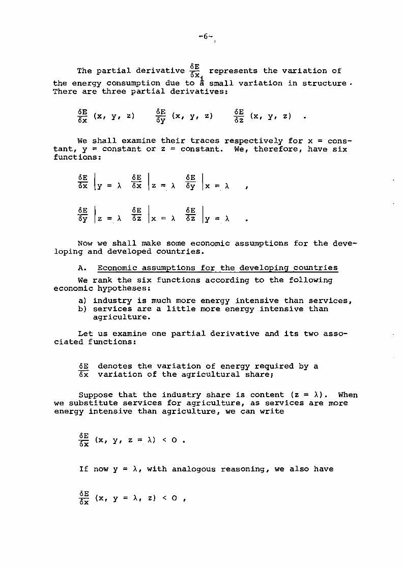
The partial derivative ~E represents the variation ofuX.

the energy consumption due to a small variation in structure.There are three partial derivatives:

eEex (x, y, z)eEey (x, y, z)

eE6Z (x, y, z)

We shall examine their traces respectively for x = cons­tant, y = constant or z = constant. We, therefore, have sixfunctions:

eE I~ y=A

eE Iey Z=A

eE Iex Z=A

eE I6Z x = A

eE Iey X=A

eE I~ y=A

,

Now we shall make some economic assumptions for the deve­loping and developed countries.

A. Economic assumptions for the developing countries

We rank the six functions according to the followingeconomic hypotheses:

a) industry is much more energy intensive than services,b) services are a little more energy intensive than

agriculture.

Let us examine one partial derivative and its two asso­ciated functions:

eE denotes the variation of energy required by aex variation of the agricultural share;

Suppose that the industry share is content (z = A). Whenwe substitute services for agriculture, as services are moreenergy intensive than agriculture, we can write

eEex (x, y, Z = A) < 0 •

If now y = A, with analogous reasoning, we also have

eEex (x, y = A, z) < 0 ,

-7-

and

oE oEOX (x, Y = A, z) < ox (x, y, z = A)

Doing so for the two other partial derivatives, we havethe following order:

~EI~EI~EI~EIx y=y x y=y y x=y y z z x=y z ~=y

0I.. (3) ...I- -

I~ (1) -I" ...

L. (2) -~ ..

~El

Figure 2. Ranking of partial derivatives of energyconsumption to GNP structure for developingcountries.

given

dE = oE dx + oE d + OE dzox oy y 6Z (1 )

We shall examine for an additional share of energy(dE > 0), the three possible deplacements along each variable.

If we choose x = constant, we arrive at dx = 0; so (1)becomes

dE = ~~ (x=Y, y, z) dy + ~~ (x=y, y, z) dz , (2)

and (3) yields dy + dz = o.

So we can calculate

dydE

=

OEI OEIoy x=y - 6Z x=y

and

dz = - dE

OE oEoy x=y -'6Z x=y

,

, .

x=:\ L1 = dY + dz

-8-

according to the assumptions dy < 0 and dz > 0

+z~ .z~

Figure 3. Vector representation of possible variationin services and industry shares (agricultureremaining constant).

if

and

111:1 11r:. dE

= ,,3 e5EI

e5EIe5y x=~ e5z x=:\

,

-+-L

1is oriented towards z on the line x=:\.

-+-We shall call+L2 the deplacement along y=:\ towards

increasing z, and L3 the deplacement along z~:\ orientedtowards increasing y.

Using the same assumptions we have

-9-

X=A

Figure 4. Convexity of iso energy consumption percapita and GNP structure in developingcountries.

B. Economic assumptions for developed countries

The basic assumptions are:

a) industry is still more energy intensive than services;b) but services become far more energy intensive than

agriculture and get closer to the industry energyintensiveness.

These could be imaged by the deplacement of the valuesof the partial derivatives which become as follows:

.. .

-10-

• lit-oE oE oE oE oE oEox y=>.. ox z=>.. oy x=>.. oy z=>.. 6Z x=>.. 6Z y=>..

L 30

I~ ..I"' r L

2La ..L

1I.... ...

~ ...... -Figure 5. Ranking of partial derivation of energy

consumption per capita to GNP structurefor developed countries

Making the same calculation one can demonstrate that

Pigure 6. Convexity of iso energy consumption percapita and GNP structure in developedcountries.

-11-

c. The curves cannot intersect

Suppose that two energy levels E1 , E2 intersect. In a firststep we choose E2=E1+dE with dF>O

Figure 7. Intersection of two iso curves of percapita energy consumption and possiblevariation in GNP structure.

We showed earlier that L2 must be oriented towards increas­ing values of z.

This condition is satisfied when the points move fromA to AI but is invalid when it goes from B to B I

• Therefore,the only possibility is this:

c

Figure 8. Two isocurves of per capita energyconsumption intersecting at only one point.

-12-

but in point C as dE> 0 we proved before II L2 II :f 0 which isa contradiction. This result is extended to the full spaceby local continuous propagation.

Therefore, the energy potential can be represented by afamily of iso-energy per capita curves which spreads out(Figure 10). The fa~mily of curves has been parametrized foreach group of countries as shown in Figures 11-14 3.

For each group, one can observe that the energy potentialdoubles for equi-distance gaps.

IV THE DYNM~ICS OF DEVELOPMENT

Historical data have been obtained for France, U.K.,Germany and Italy over the period 1789-1969. Figure 15 showstheir development paths.

They all approximately start from the position where thedeveloping countries are nowadays and are all now in the leftgroup of the developed countries: one can notice that theindividual paths fluctuate around a trend except for Italy,the path of which till 1914 looks more stochastic. But theygot there by different speeds and at different points in time.In their order of arrival, there are U.K., Germany, France andItaly. The region to where all the countries try to go couldbe called, if we use the resilience theory, an attractor whichstands between industry and services with a preference in timefor industry rather than services.

I

S

trend

A

~__~starting area

Figure 9. Long trend evolution in GNP structure.(cf. Figure 15 for details)

Let's examine for instance, the effect of the 1929 crisison the developed countries. Both France and Italy reacted tothe crisis in the same way; their attractors remained orientedtowards services. The U.K. at that time was in the positionwhere Italy is nowadays. This country also drops towards the

3In Figure 2 of the Appendix, the isocurves intersect becausetwo statistical adjustments have been made for groups 4 and 5.

-13-

services attractor but with a deep slope. Germany, on thecontrary, steps back to its early position it acquired in1913. The direction of the regression path is opposed toindustry; the crisis did not attach relatively more importanceto services as in other countries. That means that the attrac­tor is not services, and that the German system was not resi­lient and could not absorb the shock smoothly. In five yearsGermany went the same path as in the previous 16 years (1913­1929) .

During the same period, France absorbed the shock butwas affected longer. Italy, after 1933, went backwards andagriculture became its attractor. The after-war period hasbeen characterized in the five countries by a great attractiontowards the industry and after 1950-1955, the attractor changedto services. However, if there is a general trend to theservices attractor, it can be shown in the figure that fluc­tuations occur between industry and services.

If we now look at the iso-energy consumption per capitacurves on Figure 15, one can see that for all countries thehistorical energy consumption data we had* fit very well intoour network.

*mainly postwar period. We can conjecture that the assump­tion remains valid for periods without great shock or deepstructural modifications such as the periods: 1945-1973, 1929­1939, 1918-1929, etc.

I

5

-14-

FIGURE 10

NETWORK OF ISO" ENERGY DEMAND PER CAPITA"

CURVES: AN EXAMPLE OF PARAMETERIZATION

FOR ONE GROUP OF COUNTRIES

-15-

1

ISO CURVES OF PER CAPITA ENERGYCONSUMPTION FOR DIFFERENT GNPSTRUCTURES AND FOR GROUPS OFCOUNTRIES 1,2,8

0.05

0.15

FIGURE 11

5.5

/ 4. 9GtV R 5.5 I 2.

CSSR 5.8 U55R4/

POLAND 3.8

tNJSTRALIA S.

CANADA 8.1

5

I

5

-16-

FIGURE 12

ISO CURVES OF PER CAPITA ENERGY. CONSUMPTION FOR DIFFERENT GNP

STRUCTURES AND FOR GROUPS OF_CJ'-UN.J~IES3-'6 -

I

-17-

5 FIGURE 13

ISO CURVES OF PER CAPITA ENERGYCONSUMPTION FOR DIFFERENT GNPSTRUCTURES AND FOR GROUPSOF COUNTRIES 4,7

-18-

I

//

ROUMANIA 2.9

•I/

//

/I

P/ / 1.0

/ /-/ / /

/ / // YUGOSLAVIA 1.3 0.4

,It / ./ 0.45/ 1/ /'

/ / GREECE 13 ~SOUTH AFRICA02.7 /'~ 0.2.' I /tITA':.lpXIN 1.3 TURKEY .45 INDONESIA 0.2

T / ~PHJ.LLlP~S 0.3 "'INDIA 0.1 0.1/ / LI' IA oy~ .~.PAKISTAN 0.1/ ~1)7ND SRILANKA 0.1

/~ / ~MAO.05

5 FIGURE 14

ISO CURVES OF PER CAPITA ENERGYCONSUMPTION FOR DIFFERENT GNP·STRUCTURES AND FOR GROUPS OFCOUNTRIES 5.9

h969

11't

Iv~

1960

I"'

r,,"

-""

"'@

(1"-

:ti9 'h

• • • • •

1196

g• •

._.-.

--..-..

.....

••-. •• •• •• •• ::

~-:..

.••···t

·1178

81••

•••

e.•

•.

..-18

0r···

··181

1

LEG

EN

D:

ITA

LY

-·-

,GE

RM

AN

Y-,

FR

AN

CE

---

,UK

••••

••

FIG

UR

E15

@

I -> \0 I

EV

OL

UT

ION

OF

GN

PS

TR

UC

TU

RE

AN

DE

NE

RG

YP

OT

EN

TIA

LF

OR

UN

ITE

DK

ING

DO

M,

GE

RM

AN

Y,

ITA

LY

AN

DF

RA

NC

ED

UR

ING

TH

EL

AS

TT

WO

CE

NT

UR

IES

.

-20-

APPENDIX

In this appendix (Memo of Ledolter to Hafele, Balinskiand Beaujean, of September 13, 1976), a statistical analysisof country specific energy consumption data related to the GNPstructure (share of agriculture, industry, services and trans­portation) is given. Second order models relating the expla­natory variables (GNP structure) to the dependent variable(energy consumption) are shown to be adequate. Parameters inthis model are estimated using observations on 47 countries.

Furthermore an interpretation of second order models isgiven and it is shown how they can be used in deriving isoenergy consumption per capita curves.

Introduction

Since industry, services and agricultur.e have differentenergy consumption patterns, it was pointed out by Beaujeanand Chaix that the GNP structure might be more significant indetermining the per capita energy consumption than its absolutelevel.

GNP is thus divided into its share corresponding to

(i)(ii)

(iii)

industryservices and transportationagriculture.

In this appendix we investigate the relationship betweencountry specific energy consumption and GNP structure. In thefirst part of the appendix we give an outline of the used data.The second part deals with statistical model building techniques(response surface analysis) and in the third section we applythese techniques to our data. Parameters are estimated and isoenergy consumption curves are drawn.

1. Description of the data

In our analysis we use observations on n = 47 countries,measuring GNP structure and per capita energy consumption. Thedata, together with grouping into social, cultural and climaticclasses, is given in the Appendix.

The following notation is used:

A. share of GNP in agriculture (of country j)I~ share of GNP in industry (of country j)S~ share of GNP in services (of country j)Y3 energy consumption (of country j).

The GNP structure of country j can be represented indifferent ways:

(i)

-21-

In the three dimensional space as triple (A.,I.,S.).J J J

Since there are only two independent components (dueto the restriction that A. + I. + S. = 1 (1 < j < n»

J J J --the countries are restricted to the triangle whosesummits are the endpoints of the unitary vectors.

(ii) In the two dimensional space in terms of three trian­gular coordinates defined by (a,i,s)= A(A,I,S) ·whereA is given bY~

I

A

(iii) In the two dimensional space in terms of two indepen­dent coordinates.

It is shown below that the GNP structure of country j canbe described by

and (1. 1 )

Proof: The triangular coordinates of P are given by ~ (A,I,S)

(i)

-22-

-

(_ 1.- II _1.12~S2~2' 2

It is easi y seen that

x, = - ~~ +~ A =~ (~ - I - S)

(ii) It can be seen that

, 1,.Since cos 600 = - = -- 1t follows that2 12

,1,=---('-A)

12

Furthermore

(1, -2 (~ s)2 + 1

2 and1, - x2x2 ) = 13 =3 2

Thus

(~ S) 2 +

2

(1 -2 (1, - x2 )

x2 ) =, 4

-23-

q.e.d.(I - S)1

122 S =(1 - A) -

t (1.,-X2 )2 = (# 5)2i 1 - x 2 = 12 S

Substituting i 1 results in

1

12

2. Comments on Statistical Model Building

In the following section we study the relationship betweena set of independent variables x1 ' x 2 ' ••• , xk and a dependent

variable y. We are interested in describing the response func­tion (response surface)

n· = f (x1 . ,x2 . , ••• ,xk ·)J J J J

(2. 1 )

relating the levels X1j,X2j, ••• ,Xkj to its response n j . Althougha certain amount of prior knowledge as to the nature of theresponse surface may be available from physical or economictheories, the exact form of the surface will often be unkown.In such cases an exact determination of the response surfaceis usually impossible for the following reasons:

(i) there is generally an error involved in the measure­ment of the true response n. This error is commonlycalled "sampling error".

(ii) There may be an error in the measurement of the inde­pendent variables.

(iii) The exact form of the true response function may beextremely complicated.

Inspite of all these above mentioned difficulties one maybe able to find some simplified representation of the responsesurface, one which would approximate key characteristics ofthe true surface over a limited region of the space spannedby the independent variables (region of interest R).

A great number of functions can be represented quite close­ly over a limited region R by some type of polynomial. Thiscomes from the fact that if the true response function iscontinuous and has continuous derivatives over the region R,then it can be approximated to any degree of accuracy by afinite number of terms of its Taylor series expansion (whichof course are polynomials) about some point in R. This appro­ximation would usually involve many terms if we wished to

-24-

represent the response over a large region of R. In practice,however, we are often concerned with the behavior of the res­ponse function over a relatively small region. In such casesit is usually possible to obtain good approximations to thetrue function by means of a relatively simple polynomial,perhaps one involving just linear (first order) or linear andquadratic (second order) terms.

We hope that the above discussion provides some basis for.an approach which attempts to approximate the true responsefunction by a polynomial in the independent variables (x1 ,x

2'

.•• ,xk). Polynomials have the added advantage that they are

fairly easy to work with due to well known procedures to fitpolynomials to data and to analyze the properly fitted poly­nomials.

We thus suppose to represent the true response surface

by a polynomial of degree m in the variables (x1 ,x2 ' ••• ,xk ).

Denoting this polynomial by Pm(x1 ,x2

, ••• ,xk), we can write the

observed response for the jth observation as

(i)

(ii)

y.-n. represents the difference between observed andJ J

true response. This is the sampling error as referredto above. Usually this error is a composite of manysmall errors; it arises due to factors beyond controland is thus assumed completely random.

The term n j - Pm(x1j, ••• ,Xkj) represents the differencebetween the true response function and the polynomialwhich was chosen to represent it at the point (x1j , ••• ,

xkj ). This discrepancy is called lack of fit which

may result from the fact that Pm(x1 , ••. ,xk ) is still

only an approximation to the true response functionwhich may actually be more complex (e.g., of higherorder than m) •

Writing down the model we combine the discrepancy due tosampling error and lack of fit into a single error term denotedby E .•

J

y. = P (x1

·, ••• , xk

.) + E.J m J J J

(2.3)

-25-

Dropping the subscript j provides the general form

(2.4)

By making assumptions about the error terms we specify thenature of error randomness. A common initial assumption isthat £ is a random variable with mean zero and constantvariance a 2 ; furthermore it is usually assumed that the errorsare independent and Normally distributed. Two important kindsof deviations from these assumptions which can occur are theserial dependence of the errors (especially when the observa­tions are ordered in time) and non Normality of the distribu­tion. These situations are discussed in detail in the statis­tical literature, but are not investigated further at thispoint.

Statistical model building is necessarily iterative. Theoriginal model will often have to be modified as new informa­tion about the response function is derived. In the absenceof prior information about the response function, the modelbuilder will start out by entertaining a relatively simplemodel. If the model, however, does not appear consistent withthe data (e.g., residual analysis indicates lack of fit), ithas to be revised until the data under study seems to confirmthe model. Even then, one cannot say that the model is thecorrect one; one can only say that the data which were inves­tigated have not offered evidence that the model is false.

Models which are using parameters parsimoniously and whichhave been shown to provide adequate approximations to manycommon response functions are the first and second order models.

(i) First order model

(2.5)

A model which includes only linear terms in the variables xl'••• ,xk is called a first order model. The unknown parameters

are estimated from the data so as to give the best fit of themodel to the data (best fit in terms of least squares fit).It can be shown that the least square estimates of Bi, let'scall them bi, are minimum variance linear unbiased if theerrors E are independently distributed with mean zero andconstant variance. For further details of least squaresestimation see Draper and Smith4•

4-Draper, N.R. and Smith, H., "Applied Regression Analysis",Wiley, New York, 1966.

-26-

The function of the x j obtained by replacing

model by their estimates b. and disregarding the1

defines the fitted surface

the B. in the1

error term

(2.6)

The residuals are the deviations of the observed and fittedresponse

(2.7)

In cases where our initial model will not be adequate enough toaccount for the variation in the data, one might investigate amore complex model, perhaps including quadratic terms in the xi.

(ii) Second order model

= a +okl

i=1a·x. +1 1 (2.8)

In total we thus need (k+1) (k+2)/2 parameters to describe themodel. The additional second order terms in the model provideconsiderable flexibility for graduating surfaces. Again, themethod of least squares can be used to provide estimates ofthe coefficients and the fitted equation is given by

y = y (x1 ' • • • , x k )

k k 2= b O + I b.x. + I b .. x. + II b

1· ox1.'xo

i=1 1. 1. . i=1 11 1. i < R. ~ ~(2.9)

"Canonical analysis" enables us to reduce the above equation toan alternative form which can be readily interpreted.

The method of canonical analysis consists of

(a) moving the origin of the measured variables (x1, •.• ,xk)= (0, ... ,0) to the center of the contour system re­presented by the fitted equation and

(b) rotating the coordinate axes until they coincide withmajor axes of the contour system.

-27-

Then the fitted contours can be expressed as

y - Yc = A1X1 *2 +••. + AkXk2 (2.10)

where the new coordinates xi are expressible as linear combina­tions of (x1, ... ,Xk) and a constant. Yc is the fitted responseat the center of the contour system. The sizes and the signsof the A can be examined and main features of the fitted surfacecan be readily understood.

To illustrate this more clearly we consider the case ofk = 2 independent variables: Equation (2.10) can representseveral types of surfaces (such as elliptical contours, statio­nary ridge, rising ridge, saddle situations which arise fromhyperbolic curves). Which of these types of contours willarise depends on the values of the bls.

For the second order model it can be shown that the centerof the new coordinate system is given by

and

the surface then takes the form

where

x*2

For example if A1 > 0, A2 > 0 th7 cont0';lrs (iso curves) areellipses centered at x 1c ' x 2c w1th sem1-axes A

1, A

2•

-28-

3. Analysis of data

In this section we report on the analysis of the datagiven in the Appendix.

y. = P (x 1 · ,X 2 .) + E: •_J m J J J

(3. 1 )

where X1j and X2j are measuring the position of country j inthe triangle described in Section 1.

Several models were investigated. The details of thevarious regression runs are not reported here. It was foundthat the first order model (m = 1) showed significant contri­bution of the cross product term could be found. Furthermorethe 9 chosen groups appeared different in their level and

curvature in xf. Dummy variables for different levels andcurvature were included (for further di~cussion of the useof dummy variables see Draper and Smith ). Some of the esti­mated coefficients were not significant and could be droppedfrom the model.

A model which describes the data well (residual analysiscould not detect serious inadequacy of the model; multiplecorrelation coefficient of .99) is given by

13 (1) 13(2) 9 (i) 2 2Y = o z1 + o z2 + f3 1x 1 + f3 2x 2 + l 13 11 x 1v i + f3 22x2 + E:i=1

where

={~if country is from 2nd group

z1otherwise

={:if country is from 2nd group

z2otherwise

v. ={1 if country is from ith group

1 0 otherwise., ,

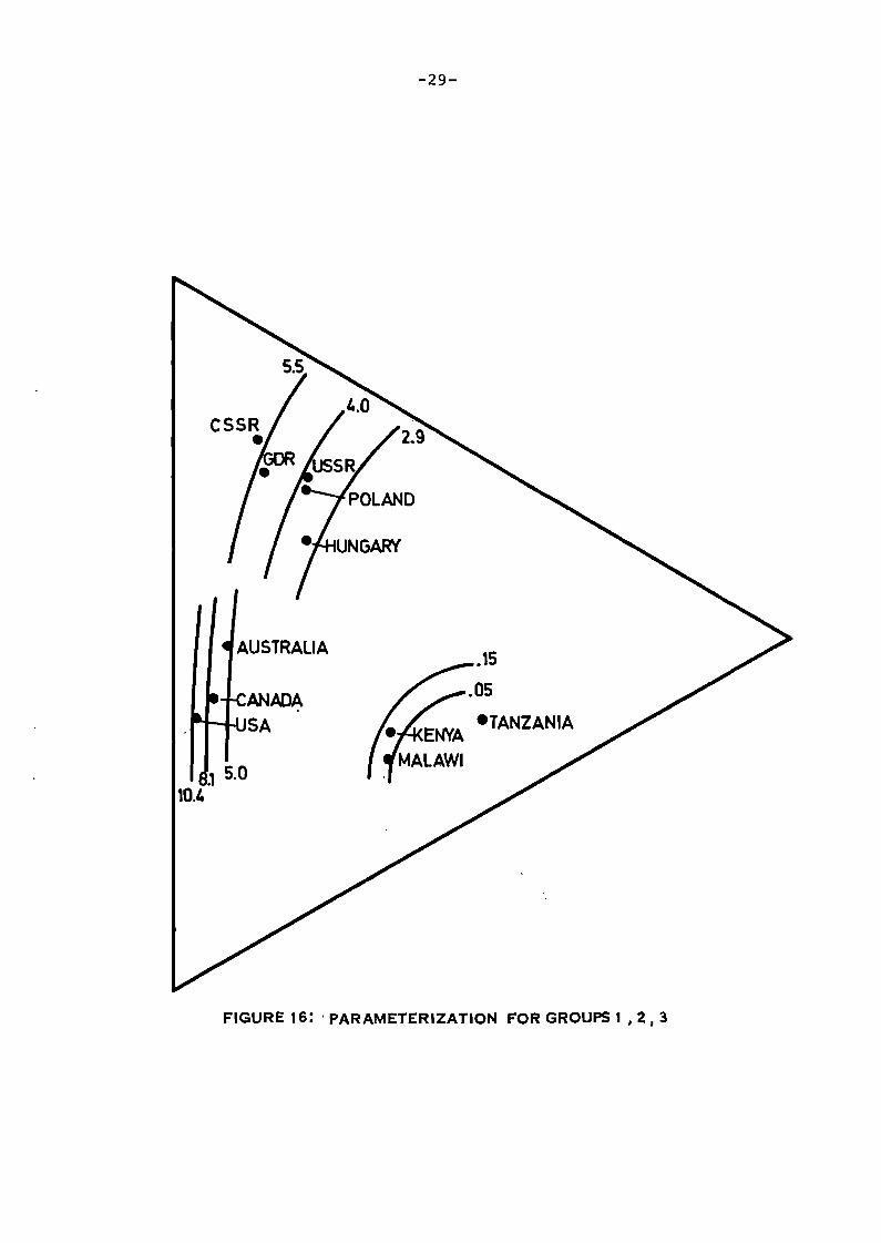
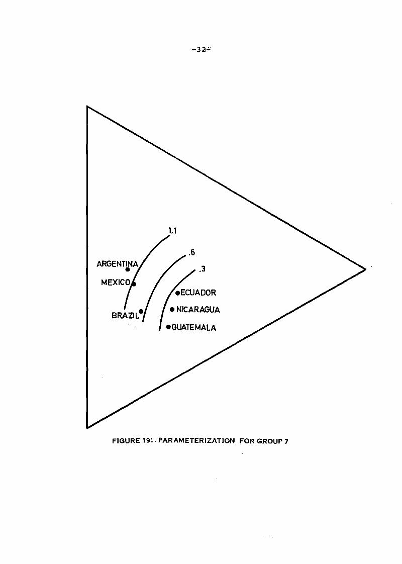
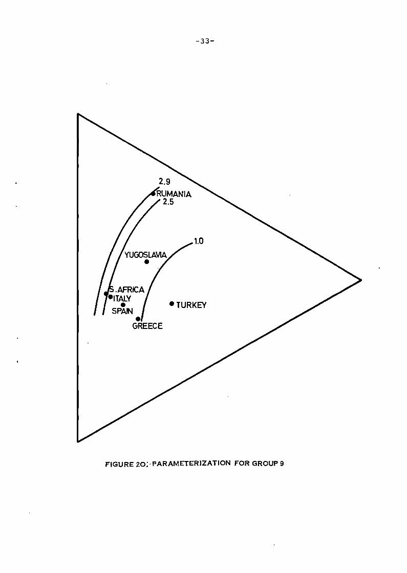
The unkonwn parameters are estimated by least squares andiso energy consumption curves are plotted for the differentgroups in Figures 16-20. Using canonical analysis these curvescan be represented as ellipses with from group to group changingcenter and semi axes.

ANADA~-'SA

.1 5.010.4

-29-

.15

.05

-TANZANIA

FIGURE 16: 'PARAMETERIZATION FOR GROUPS 1 ,2 , 3

-30-

eJORDANlA

.3 .2

EGYPTeMOROCCO

FIGURE 17: PARAMETERIZATION FOR GROUPS 4 AND 5

4.6

-31-

.4

.2 .INDIALUPINES• INDONESIA

• ·PAKISTANSRILANKA

THAILAND

·BURMA

FIGURE 18~ PARAMETERIZA1·ION FOR GROUPS 6 AND 8

1.1

.6

.3

eNICARAGUA

eGUATEMALA

FIGURE 19:· PARAMETERIZATION FOR GROUP 7

-33-

1.0

2.9RUMANIA

2.5

.AFRICA-ITALYSP1N -TURKEY

-GREECE

FIGURE 20:-PARAMETERIZATION FOR GROUP 9

-34-

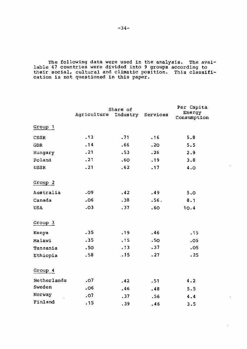
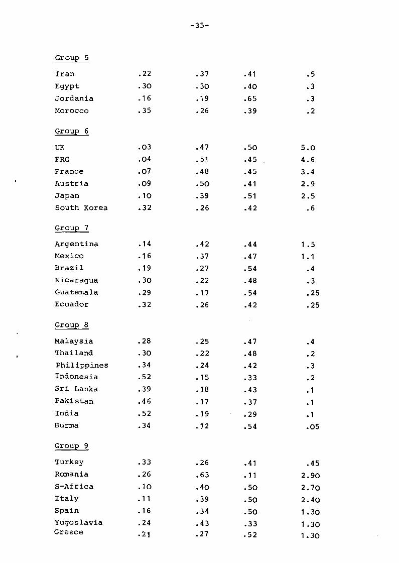
The following data were used in the analysis. The avai­lable 47 countries were divided into 9 groups according totheir social, cultural and climatic position. This classifi­cation is not questioned in this paper.

Share of Per Capita

Agriculture Industry Services EnergyConsumption

Group 1

CSSR .13 .71 .16 5.8

GDR .14 .66 .20 5.5

Hungary .21 .53 .26 2.9

Poland .21 .60 .19 3.8

USSR .21 .62 .17 4.0

Group 2

Australia .09 .42 .49 5.0

Canada .06 .38 .56. 8.1

USA .03 .37 .60 10.4

Group 3

Kenya .35 .19 .46 .15

Malawi .35 .15 .50 .05

Tanzania .50 .13 .37 .05

Ethiopia .58 .. 15 .27 .25

Group 4

Netherlands .07 .42 .51 4.2Sweden .06 .46 .48 5.5Norway .07 .37 .56 4.4Finland .15 .39 .46 3.5

-35-

Group 5

Iran .22 .37 .41 .5

Egypt .30 .30 .40 .3

Jordania .16 .19 .65 .3

Morocco .35 .26 .39 .2

Group 6

UK .03 .47 .50 5.0

FRG .04 .51 .45 4.6

France .07 .48 .45 3.4

Austria .09 .50 .41 2.9

Japan .10 .39 .51 2.5

South Korea .32 .26 .42 .6

Group 7

Argentina .14 .42 .44 1 .5

Mexico .16 .37 .47 1.1

Brazil .19 .27 .54 .4

Nicaragua .30 .22 .48 .3

Guatemala .29 .17 .54 .25

Ecuador .32 .26 .42 .25

Group 8

Malaysia .28 .25 .47 .4

Thailand .30 .22 .48 .2

Philippines .34 .24 .42 .3Indonesia .52 .15 .33 .2Sri Lanka .39 .18 .43 • 1Pakistan .46 .17 .37 • 1India .52 .19 .29 .1Burma .34 .12 .54 .05

Group 9

Turkey .33 .26 .41 .45Romania .26 .63 • 11 2.90S-Africa .10 .40 .50 2.70Italy • 11 .39 .50 2.40Spain .16 .34 .50 1 .30Yugoslavia .24 .43 .33 1 .30Greece .21 .27 .52 1.30