PPT 21 -1

ADVANCED MANAGEMENT ACCOUNTING

PPT 21 -2

Capital Investment Decisions

PPT 21 -3

Learning Objectives

Explain what a capital investment decision is and distinguish between independent and mutually exclusive capital investment decisions.

Compute the payback period and accounting rate of return for a proposed investment, and explain their roles in capital investment decisions.

PPT 21 -4

Learning Objectives (continued)

Use net present value analysis for capital investment decisions involving independent projects.

Use the internal rate of return to assess the acceptability of an independent project.

Explain why NPV is better than IRR for capital investment decisions involving mutually exclusive projects.

PPT 21 -5

Learning Objectives (continued)

Convert gross cash flows to after-tax cash flows.

Describe capital investment for advanced technology and environmental impact settings.

PPT 21 -6

Capital Budgeting

Capital budgeting is the process of making capital investment decisions.

Two types of capital budgeting projects:

Independent projects: Projects that, if accepted or rejected, will not affect the cash flows of another project.

Mutually exclusive projects: Projects that, if accepted, preclude the acceptance of competing projects.

PPT 21 -7

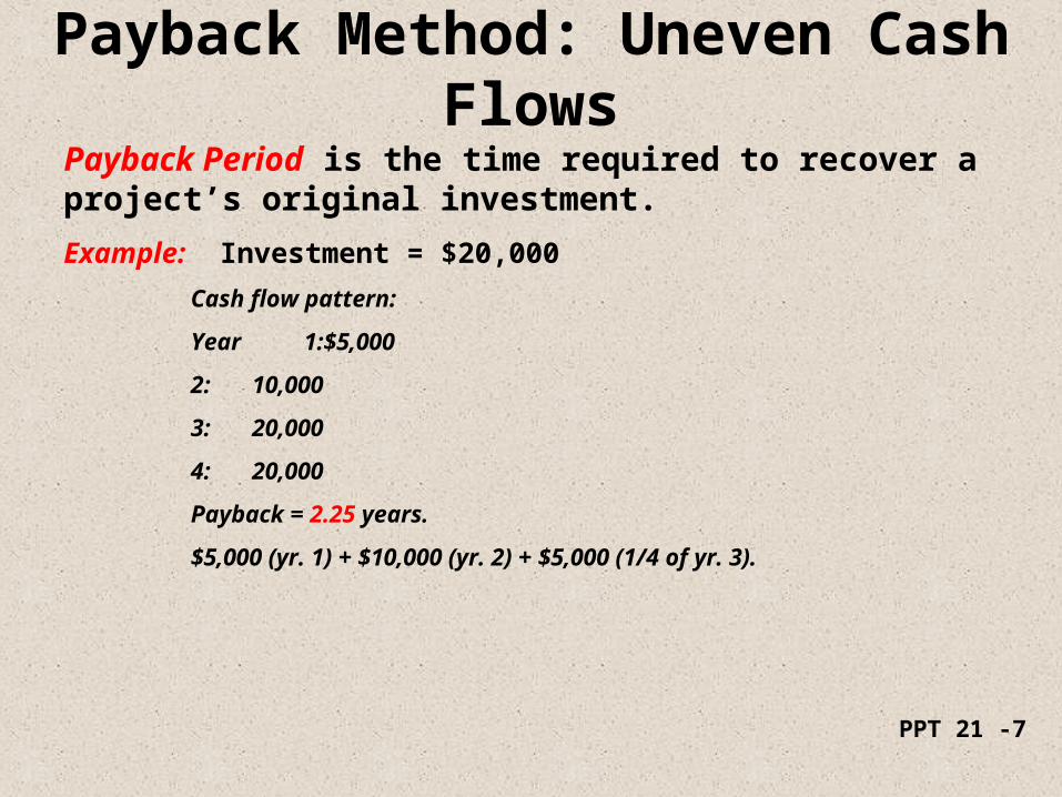
Payback Method: Uneven Cash Flows

Payback Period is the time required to recover a project’s original investment.

Example: Investment = $20,000

Cash flow pattern:

Year 1: $5,000

2: 10,000

3: 20,000

4: 20,000

Payback = 2.25 years.

$5,000 (yr. 1) + $10,000 (yr. 2) + $5,000 (1/4 of yr. 3).

PPT 21 -8

Payback Method Possible reasons for use

To help control the risks associated with the uncertainty of future cash flows

To help minimize the impact of an investment on firm’s liquidity problems

To help control the risk of obsolescence

To help control the effect of the investment on performance measures

PPT 21 -9

Payback Method Major deficiencies

Ignores the time value of money

Ignores the performance of the investment beyond the payback period

PPT 21 -10

Accounting Rate Of Return (ARR)

ARR = Average Income/Investment

Average income equals average annual net cash flows, less average depreciation.

Example: Suppose that some new equipment requires an initial outlay of $80,000 and promises total cash flows of $120,000 over the next five years (the life of the machine). What is the ARR?

PPT 21 -11

Accounting Rate Of Return (ARR) (continued)

Answer: The average cash flow is $24,000 ($120,000/5) and the average depreciation is $16,000 ($80,000/5).

ARR = ($24,000 - $16,000)/$80,000= $8,000/$80,000= 10%

PPT 21 -12

Accounting Rate Of Return (ARR)Possible reasons for use

A screening measure to ensure that new investment will not adversely affect net income

To ensure a favorable effect on net income so that bonuses can be earned (increased)

PPT 21 -13

Accounting Rate Of Return (ARR)

The major deficiency of the accounting rate of return is that it ignores the time value of money.

PPT 21 -14

Net Present Value (NPV)

Definition:

NPV = P - I

where:

P = the present value of the project’s future cash inflows

I = the present value of the project’s cost (usually the initial outlay)

NPV IS A MEASURE OF THE PROFITABILITY OF AN INVESTMENT, EXPRESSED IN CURRENT DOLLARS.

PPT 21 -15

Net Present Value (NPV): Example

A project promises to return $10,000 after one year and $20,000 after two years. The project also requires an initial investment of $22,000. Calculate its net present value assuming a 12% discount rate.

Discount PresentYearCash Flow Factor Value

0 $(22,000) 1.000 $(22,000)

1 10,000 0.893 8,930

2 20,000 0.797 15,940

$2,870 ===

PPT 21 -16

Decision Criteria for NPV (continued)

If the NPV >0 this indicates:

1. The initial investment has been recovered

2. The required rate of return has been recovered

3. A return in excess of 1. and 2. has been received

Thus, the project should be accepted.

PPT 21 -17

Decision Criteria for NPV (continued)

If NPV = 0, this indicates:

1. The initial investment has been recovered

2. The required rate of return has been recovered

Thus, break even has been achieved and we are indifferent about the project.

PPT 21 -18

Decision Criteria for NPV (continued)

If NPV < 0, this indicates:

1. The initial investment may or may not be recovered

2. The required rate of return has not been recovered

Thus, the project should be rejected.

PPT 21 -19

Reinvestment Assumption

The NPV model assumes that all cash flows generated by a project are immediately reinvested to earn the required rate of return throughout the life of the project.

PPT 21 -20

Internal Rate Of Return (IRR)

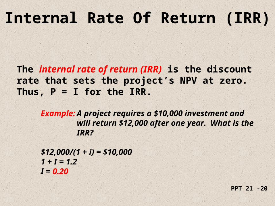
The internal rate of return (IRR) is the discount rate that sets the project’s NPV at zero. Thus, P = I for the IRR.

Example: A project requires a $10,000 investment and will return $12,000 after one year. What is the IRR?

$12,000/(1 + i) = $10,0001 + I = 1.2I = 0.20

PPT 21 -21

Internal Rate Of Return (IRR)

Decision criteria

If the IRR > Cost of Capital, the project should be accepted.

If the IRR = Cost of Capital, acceptance or rejection is equal.

If the IRR < Cost of Capital, the project should be rejected.

PPT 21 -22

Internal Rate Of Return (IRR) Reinvestment Assumption

The cash inflows received from the project are immediately reinvested to earn a return equal to the IRR for the remaining life of the project.

PPT 21 -23

NPV versus IRR

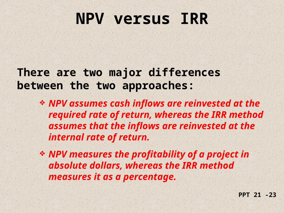
There are two major differences between the two approaches:

NPV assumes cash inflows are reinvested at the required rate of return, whereas the IRR method assumes that the inflows are reinvested at the internal rate of return.

NPV measures the profitability of a project in absolute dollars, whereas the IRR method measures it as a percentage.

PPT 21 -24

NPV versus IRR (continued)

Conflicting Signals (required rate of return) = 10%

Year Project A Project B

0 $(10,000) $(10,000)

1 -------- 6,000

2 13,924 7,200

IRR 18% 20%

NPV $ 1,501 $ 1,401

PPT 21 -25

NPV versus IRR (continued)

Which project should be selected?

IRR signals Project B, whereas NPV signals Project A.

The terminal value of Project A is $13,924.

To calculate the future value of B, assume that the $6,000 received at the end of year one is invested at the cost of capital. Thus, the future value of B is $7,200 + (1.1)$6,000 = $13,800.

Project A provides the most wealth and should be selected (AS SIGNALED BY NPV). IRR assumes the $6,000 can be reinvested at 20% when in actuality it is reinvested at 10%.

PPT 21 -26

Discount Rate: The Cost Of Capital

The appropriate discount rate to use for NPV computations is the cost of capital. The cost of capital is the weighted average of the returns expected by the different parties contributing funds. The weights are determined by the proportion of funds provided by each source.

PPT 21 -27

Discount Rate: The Cost Of Capital

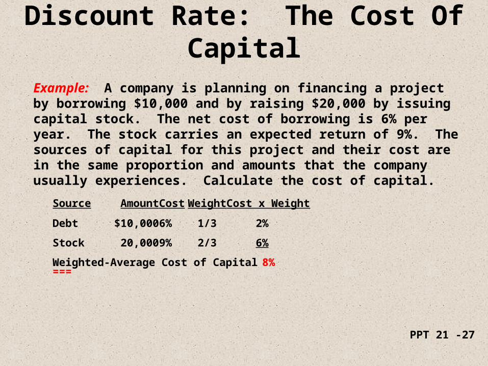
Example: A company is planning on financing a project by borrowing $10,000 and by raising $20,000 by issuing capital stock. The net cost of borrowing is 6% per year. The stock carries an expected return of 9%. The sources of capital for this project and their cost are in the same proportion and amounts that the company usually experiences. Calculate the cost of capital.

Source Amount Cost Weight Cost x Weight

Debt $10,000 6% 1/3 2%

Stock 20,000 9% 2/3 6%

Weighted-Average Cost of Capital 8%===

PPT 21 -28

Inflationary AdjustmentAn Illustrative Example

Assume that the rate of inflation is 6% per year.

Analysis Without Inflationary Adjustment (assumes a 12% discount rate)Year CF DF P

0 $(10,000 ) 1.000$(10,000 )1-2 5,500 1.690 9,295

NPV $ (705 ) ======Analysis with Inflationary Adjustment

Year CF DF P 0 $(10,000 ) 1.000$(10,000 )1 5,830 * 0.8935,2062 6,180 **0.797 4,925

NPV $ 131 ======* 1.06 x $5,500** 1.06 x 1.06 x $5,500

Notice that adjustment for inflation can affect the decision.

PPT 21 -29

After-Tax Operating Cash Flows The Income Approach

After-tax cash flow = After-tax net income + Noncash expenses

Example:

Revenues $1,000,000

Less: Operating expenses* 600,000

Income before taxes $ 400,000

Less: Income taxes 136,000

Net income $ 264,000========

* $100,000 is depreciation

After-tax cash flow = $264,000 + $100,000

= $364,000

PPT 21 -30

After-Tax FlowsDecomposition Approach

After-tax cash revenues = (1 - Tax rate) x Cash revenues

After-tax cash expense = (1 - Tax rate) x Cash expenses

Tax savings (noncash expenses) = (Tax rate) x Noncash expenses

Total operating cash is equal to the after-tax cash revenues, less the after-tax cash expenses, plus the tax savings on noncash expenses.

Example: Revenues = $1,000,000, cash expenses = $500,000, and depreciation = $100,000. Tax rate = 34%.

After-tax cash revenues (1 - .34) ($1,000,000) = $660,000

Less: After-tax cash expenses (1 - .34) ($500,000) = (330,000)

Add: Tax savings (noncash exp.) .34 ($100,000) = 34,000

Total $364,000 =======

PPT 21 -31

DepreciationTax-Shielding Effect

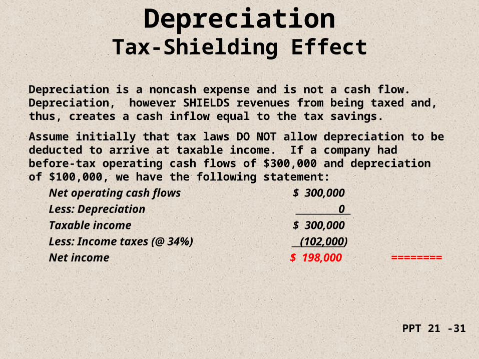
Depreciation is a noncash expense and is not a cash flow. Depreciation, however SHIELDS revenues from being taxed and, thus, creates a cash inflow equal to the tax savings.

Assume initially that tax laws DO NOT allow depreciation to be deducted to arrive at taxable income. If a company had before-tax operating cash flows of $300,000 and depreciation of $100,000, we have the following statement:

Net operating cash flows $ 300,000

Less: Depreciation 0

Taxable income $ 300,000

Less: Income taxes (@ 34%) (102,000)

Net income $ 198,000 ========

PPT 21 -32

DepreciationTax-Shielding Effect

Now assume that the tax laws allow a deduction for depreciation:

Net operating cash flows $300,000

Less: Depreciation 100,000 Taxable income $200,000

Less: Income taxes (@ 34%) (68,000)

Net income $132,000 =======

Notice that the taxes saved are $34,000 ($102,000 - $68,000). Thus, the firm has additional cash available of $34,000.

This savings can be computed by multiplying the tax rate by the amount of depreciation claimed:

.34 x $100,000 = $34,000

PPT 21 -33

Tax Laws: Depreciation

The tax laws classify most assets into the following three classes (class = Allowable years):

Class Types of Assets3 Most small tools5 Cars, light trucks, and computer equip.7 Most equip, machinery, office equip.

Assets in any of the three classes can be depreciated using either straight-line or MACRS (Modified Accelerated Cost Recovery System) with a half-year convention.

PPT 21 -34

Tax Laws: Depreciation (continued)

Half-year convention: (1) Half the depreciation for the first year can be claimed regardless of when the asset is actually placed in service; (2) the other half year of depreciation is claimed in the year following the end of the asset’s class life; (3) if the asset is disposed of before the end of its class life, only half of the depreciation for that year can be claimed.

PPT 21 -35

Tax Laws: Depreciation

Example (straight-line): A company acquired a five-year property for $100,000

Depreciation YearAllowed

1 $10,000

2 20,000

3 20,000

4 20,000

5 20,000

6 10,000

PPT 21 -36

Tax Laws: Depreciation

MACRS uses double-declining balance with a half-year convention. This method also switches to straight-line depreciation whenever the straight-line amount exceeds the double-declining balance amount. EXHIBIT 21-11 provides the MACRS depreciation rates for three-, five- and seven-year assets.

PPT 21 -37

Tax Laws: DepreciationExample (MACRS): Assume five-year property costing $100,000:

Depreciation Year Allowed

1 $20,000

2 32,000

3 19,200

4 11,520

5 11,520

6 5,760

Example: Suppose the asset was disposed of in Year 2. How much depreciation can be claimed?

Answer: Only half for that year:

0.5 x $32,000 = $16,000

PPT 21 -38

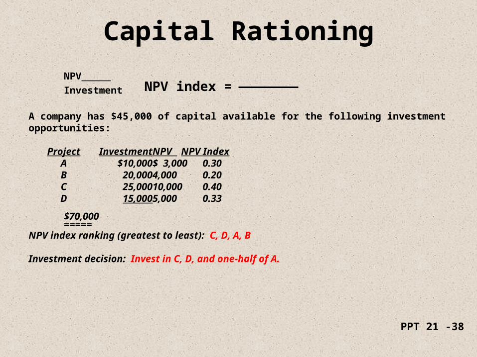
Capital Rationing

NPV

Investment

A company has $45,000 of capital available for the following investment opportunities:

Project InvestmentNPV NPV IndexA $10,000$ 3,000 0.30 B 20,0004,000 0.20 C 25,00010,000 0.40 D 15,0005,000 0.33

$70,000=====

NPV index ranking (greatest to least): C, D, A, B

Investment decision: Invest in C, D, and one-half of A.

NPV index =

PPT 21 -39

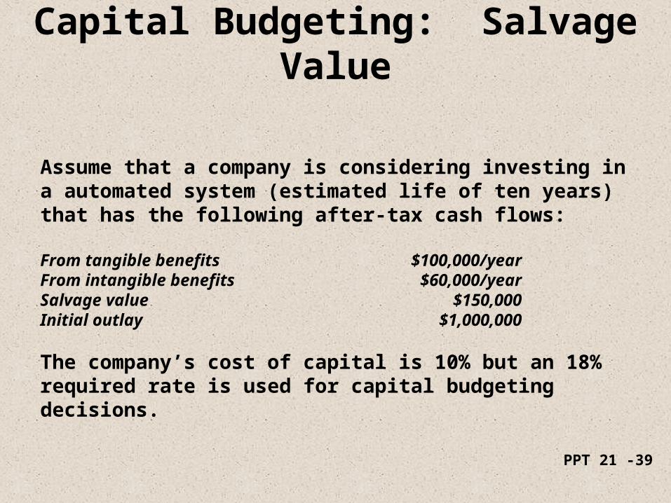
Capital Budgeting: Salvage Value

Assume that a company is considering investing in a automated system (estimated life of ten years) that has the following after-tax cash flows:

From tangible benefits $100,000/yearFrom intangible benefits $60,000/yearSalvage value $150,000Initial outlay $1,000,000

The company’s cost of capital is 10% but an 18% required rate is used for capital budgeting decisions.

PPT 21 -40

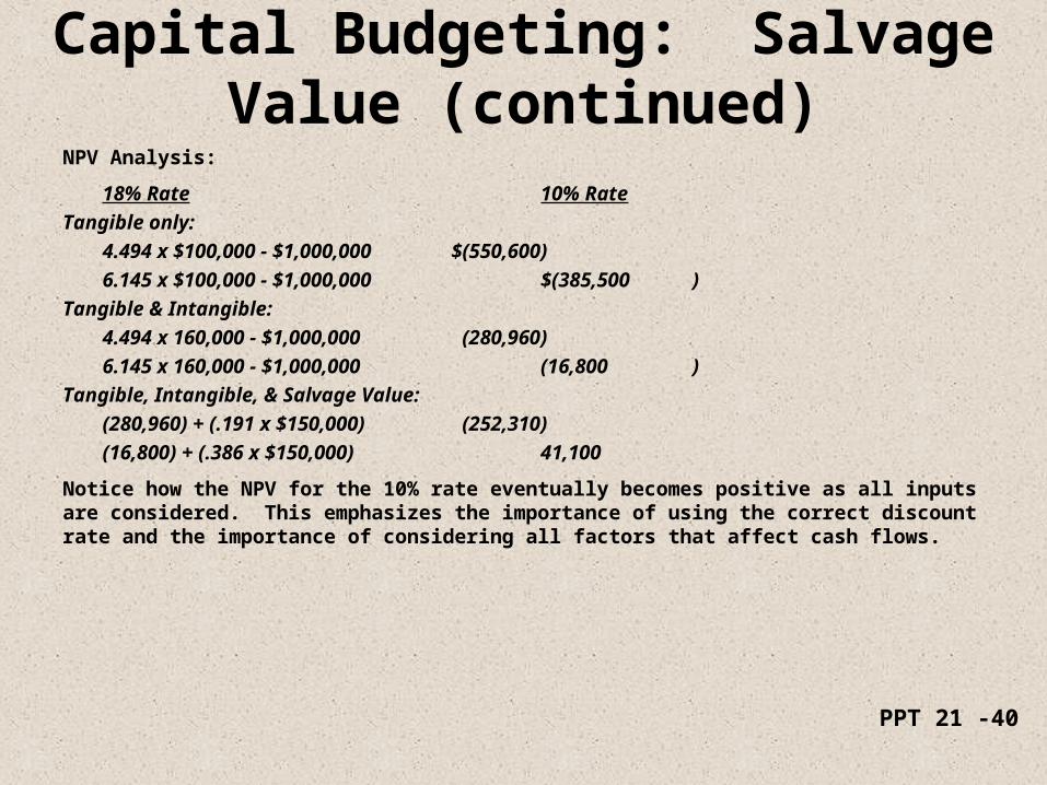
Capital Budgeting: Salvage Value (continued)

NPV Analysis:

18% Rate10% Rate

Tangible only:

4.494 x $100,000 - $1,000,000 $(550,600)

6.145 x $100,000 - $1,000,000 $(385,500 )

Tangible & Intangible:

4.494 x 160,000 - $1,000,000 (280,960)

6.145 x 160,000 - $1,000,000 (16,800 )

Tangible, Intangible, & Salvage Value:

(280,960) + (.191 x $150,000) (252,310)

(16,800) + (.386 x $150,000) 41,100

Notice how the NPV for the 10% rate eventually becomes positive as all inputs are considered. This emphasizes the importance of using the correct discount rate and the importance of considering all factors that affect cash flows.

PPT 21 -41

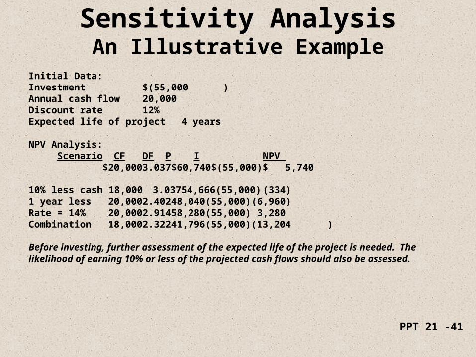
Sensitivity AnalysisAn Illustrative Example

Initial Data:Investment $(55,000)Annual cash flow 20,000Discount rate 12%Expected life of project 4 years

NPV Analysis: Scenario CF DF P I NPV

$20,000 3.037 $60,740 $(55,000) $ 5,740

10% less cash 18,000 3.037 54,666 (55,000) (334)1 year less 20,000 2.402 48,040 (55,000) (6,960)Rate = 14% 20,000 2.914 58,280 (55,000) 3,280Combination 18,000 2.322 41,796 (55,000) (13,204)

Before investing, further assessment of the expected life of the project is needed. The likelihood of earning 10% or less of the projected cash flows should also be assessed.

PPT 21 -42

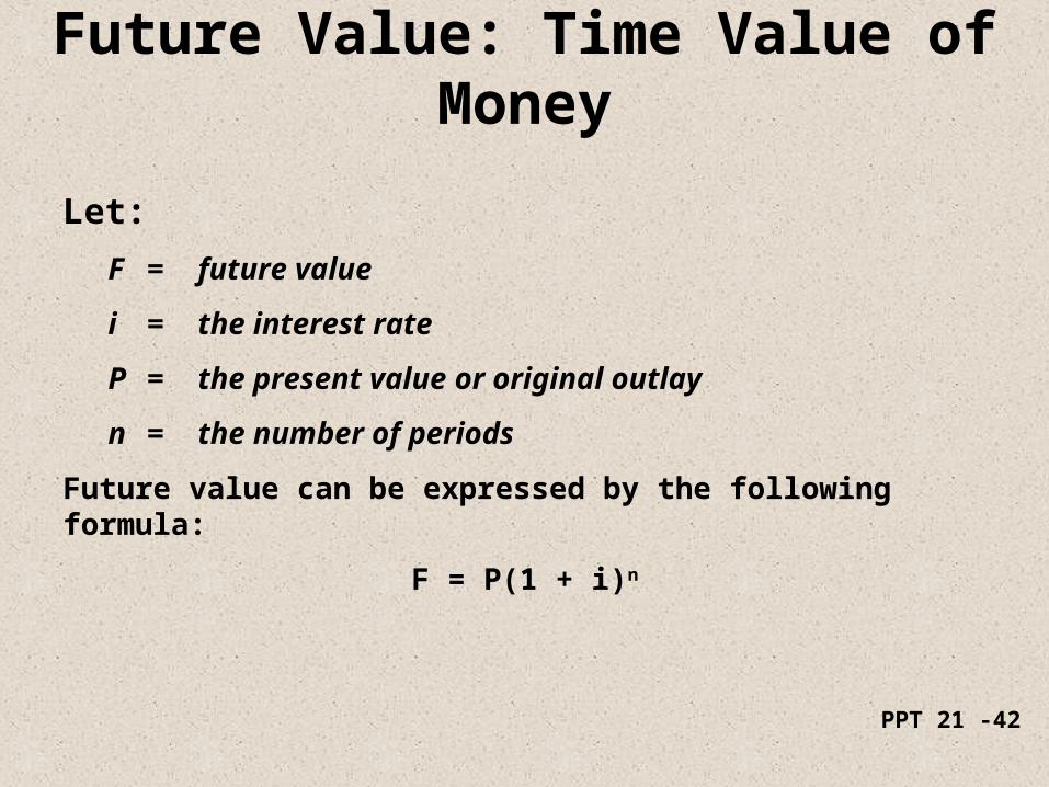
Future Value: Time Value of Money

Let:

F = future value

i = the interest rate

P = the present value or original outlay

n = the number of periods

Future value can be expressed by the following formula:

F = P(1 + i)n

PPT 21 -43

Future Value: Example

Assume the investment is $1,000. The interest rate is 8%. What is the future value if the money is invested for one year? Two? Three?

PPT 21 -44

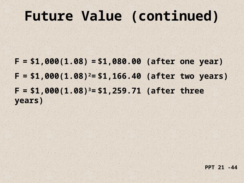
Future Value (continued)

F = $1,000(1.08) = $1,080.00 (after one year)

F = $1,000(1.08)2 = $1,166.40 (after two years)

F = $1,000(1.08)3 = $1,259.71 (after three years)

PPT 21 -45

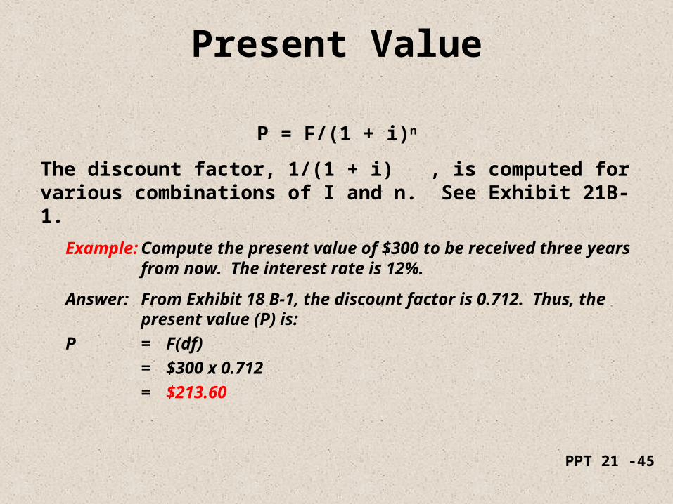
Present Value

P = F/(1 + i)n

The discount factor, 1/(1 + i) , is computed for various combinations of I and n. See Exhibit 21B-1.

Example: Compute the present value of $300 to be received three years from now. The interest rate is 12%.

Answer: From Exhibit 18 B-1, the discount factor is 0.712. Thus, the present value (P) is:

P = F(df)

= $300 x 0.712

= $213.60

PPT 21 -46

Present Value (continued)

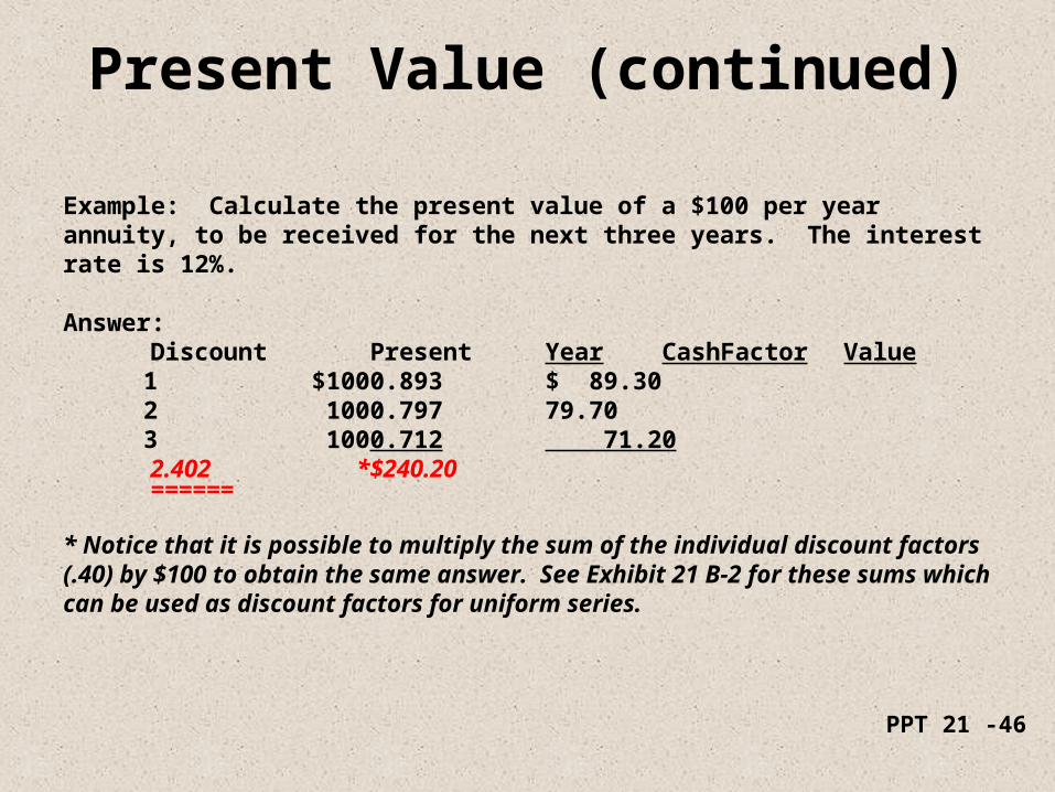
Example: Calculate the present value of a $100 per year annuity, to be received for the next three years. The interest rate is 12%.

Answer:Discount Present Year

CashFactor Value1 $100 0.893 $ 89.302 100 0.797 79.703 100 0.712 71.20

2.402 * $240.20======

* Notice that it is possible to multiply the sum of the individual discount factors (.40) by $100 to obtain the same answer. See Exhibit 21 B-2 for these sums which can be used as discount factors for uniform series.

PPT 21 -47

End of Week