Master of Science Thesis

KTH School of Industrial Engineering and Management

Energy Technology EGI-2016-004MSC

Division of Applied Thermodynamics and Refrigeration

SE-100 44 STOCKHOLM

Practical evaluation of borehole heat

exchanger models in TRNSYS

Åsa Thorén

An example of a TRNYS model with borehole heat exchangers and dry coolers.

-1-

Master of Science Thesis EGI-2016-004MSC

Practical evaluation of borehole heat

exchanger models in TRNSYS

Åsa Thorén

Approved

Examiner

Hatef Madani Larijani

Supervisor

José Acuña

Commissioner

Contact person

Abstract

Vertical ground source heat pumps are established and still growing on the global market. The modelling of

these systems is important for system design and optimization. This is an active field of research, and many

models are often built into system simulation software such as TRNSYS. With the intention of having a

better sensibility for existing TRNSYS tools, three different cases are simulated with several TRNSYS tools,

so called Types. A Thermal Response Test, a large borehole field of an IKEA building complex in Sweden,

as well as the Marine Corps Logistic Base in Albany, USA. The vertical ground heat exchanger types 203,

244, 243, 246, 451, 55a and 557b are used. Most of the simulations are investigated and evaluated by

comparing them to measured data. The result shows that, for these specific cases, the DTS types 557a and

557b can underestimate the heat transfer early on due to a poor consideration of the thermal capacity inside

the borehole. Depending on how the thermal resistance is calculated by a module, the fluid mean

temperature simulation is affected by a constant throughout the simulation time. The simulation results

indicate that the type 557b, where the borehole resistance is pre-set as an input and known from

experimental data, is the most accurate of the types for groundwater filled boreholes. On short term, type

451 provides a good coherence with the measured data, with a relative deviation of 10.3 %. The borehole

models that consider the borehole thermal capacity overestimate the short term heat transfer rate, whereas

those that neglect the borehole capacity underestimate the short term thermal heat transfer on short term.

Existing Types describe successfully the long term behaviour of large borehole fields. Serial versus parallel

coupled BHE fields show relatively small differences in performance when simulated with type 557b for a

specific study case.

-2-

Acknowledgement

I would like to thank my supervisor José Acuña for his guidance through the work. I would also like to

thank Willem Mazzotti for his help. Both José and Willem supplied me with data and information for the

investigated borehole installations.

I would also like to thank Patricia Maria Monzo who helped me get going with TRNSYS, Nelson

Sommerfeldt who helped me get access to some of the modules I have used. Finally I thank Stephen E.

Sullens for suppling data and information for the Marine Corps Logistic Base borehole installation.

Abbreviations

BHE Borehole heat exchanger CSH Cylinder source model COP Coefficient of performance DST Duct ground heat storage model DTRT Distributed thermal response test EED Earth Energy Design EWS “Erdwärmesonden” model FLS Finite line source model GSHP Ground source heat pump ICM Infinite cylinder source model ILS Infinite line source model MLAA Multiple Load Aggregation Algorithm SBM Superposition borehole model TRNSYS TRaNsient SYstems Simulation Program TRT Thermal response test

Nomenclature

B Distance between boreholes [m]

cp Thermal Capacity [J/(kg K)]

g The response function of dimensionless time, i.e. the current time divided by the stabilisation time.

H Borehole length [m]

�̇� Mass flow [kg/h]

q’ The injected heat flux per unit length [W/m] qt Injected heat per hour [W/h] r Distance to the source in radial direction [m] R1 Thermal resistance between the down going pipe to the borehole wall [K/(W/m)] R2 Thermal resistance between the up going pipe to the borehole wall [K/(W/m)]

�̃�𝑏 Borehole radius [m] Rb Borehole resistance (fluid to borehole wall) [K/(W/m)] t Time [s] T0 The temperature of the undisturbed ground[°C] T1 Fluid temperature in down going pipe [°C] T2 Fluid temperature in up going pipe[°C] Tb The borehole wall temperature Tf Fluid temperature [°C]

Tf,t Fluid temperature that has been prevailing during the past hour [°C] Tp,t Temperature penalty [°C] ts time at thermal stability (H2/9α) [s] α Thermal diffusivity (m2s−1 ) ρ Density [ kg/m3 ] λ Ground Thermal Conductivity [W/(m K)]

-3-

Table of Contents

1 Introduction .......................................................................................................................................................... 4

1.1 Modelling of vertical borehole heat exchangers ..................................................................................... 4

1.1.1 G-functions ......................................................................................................................................... 6

1.1.2 Temporal Superposition and Load aggregation scheme ............................................................. 7

1.1.3 Duct Heat Storage model ................................................................................................................. 8

1.2 TRNSYS and its vertical ground source heat exchanger models ........................................................ 8

1.2.1 Type 557 ............................................................................................................................................10

1.2.2 Type 203, 243, 244 and 246............................................................................................................10

1.2.3 Type 451 ............................................................................................................................................10

2 Goals with the project .......................................................................................................................................11

3 Method .................................................................................................................................................................11

4 Simulated Thermal response test .....................................................................................................................12

4.1 Modelling ....................................................................................................................................................12

4.2 Results .........................................................................................................................................................14

5 Borehole heat exchanger modelling of an IKEA department store ..........................................................17

5.1 System configuration ................................................................................................................................17

5.1.1 Modelling ...........................................................................................................................................18

5.1.2 Results ................................................................................................................................................21

6 Modelling of the Marine Corps Logistic Base ...............................................................................................24

6.1 Simulation of the system ..........................................................................................................................24

6.1.1 Load profile .......................................................................................................................................25

Results ..................................................................................................................................................................27

6.1.2 Serial versus parallel coupling ........................................................................................................27

7 Conclusions .........................................................................................................................................................29

8 Discussion and final remarks............................................................................................................................30

Bibliography .................................................................................................................................................................31

-4-

1 Introduction

Ground source heat pumps (GSHP) are established and still growing on the market, in Sweden as well as

other parts of the world. The benefits of ground source heat pumps, in comparison to other types of heat

pumps are the favourable bed rock temperature which is more stable than the ambient temperature

throughout the year, and not least heat storage opportunities in the bedrock. This offers economic and

environmental gains. A possible reason for the popularity in Sweden, also in city-regions, is the high

operation cost of the alternative heating and cooling systems.

In a GSHP-system, the ground is used as a heat sink or heat source to supply cooling or heating to a building

facility. The ground can work as a thermal storage where heat is alternately injected during the cold season

and extracted during the warm season. The heat flux from the earth’s core has less impact than the stored

solar energy and the active heat exchange normally imposed by GSHP systems BHE.

GSHP installations are specifically designed for each site, which is normally done with a modelling software.

The number of borehole, the borehole- to-borehole spacing, their depth and inclination are selected.

Accurate modelling is an important part of the design process and optimization. There are several modelling

tools for simulating and designing GSHPs available on the market. Examples are GLD (Ground Loop

Design), EED (Earth Energy Designer), GLHEPRO and TRNSYS.

Under sizing can make the heat carrier temperature (and thereby ground temperatures) be below or above

desired levels, or leaves the ground unable to thermally recover in an acceptable way. The heat transfer of

the BHE and the COP of a GSHP decreases along with the ground being cooled down for a system with a

heating load, or heated up for a system with a cooling load.

When modelling GSHP and more specifically BHEs, the heating and/or cooling load of the building is a

parameter hard to predict due to its complexity and dependency on how the building will be operated. At

the same time as the heating and cooling loads are essential for the borehole design. Ground thermal

properties and land availability are also key design aspects.

Improving the modelling accuracy is an active research topic. Some design tools for GSHP, such as EED

and GLHEPRO, use long term models with monthly averaged loads and hourly peak loads and its duration,

in order to ensure the fluid temperature doesn't go out of the design temperature limits. It serves to confirm

that the fluid temperature in the BHE stays within desired values. The short term impact is often neglected.

How the system is controlled has great impact on the entire system performance (Eslami-Nejad and Bernier,

2011; Pahud, 2012; Ochs, Carbonell and Haller, 2013; Safa, Fung and Kumar, 2015). One important field

of research has been the thermal response properties of BHE on short term (Lamarche, 2007). The thermal

mass of the borehole makes the borehole temperature change faster than the ground in early operation

periods, which makes the transient effects in the BHE significant. For a typical two-pipe configuration, the

annual COP predicted with a short term model is approximately 4.5% higher when borehole thermal

capacity is included (Bernier and Shirazi, 2013).

1.1 Modelling of vertical borehole heat exchangers

Today's BHEs are generally simple u-pipes, made of high density polyethylene (HDPE) surrounded by

either groundwater or a filling (or so-called grouting) material. One or two sets of these pipes are placed

inside boreholes. The circulating fluid consists of water mixed with an antifreeze such as ethyl alcohol, glycol

or salt if needed.

Low borehole resistance (Rb) has a positive impact on the thermal heat transfer in the BHE. It is achieved

by the high thermal conductivity of the pipe and grout and a decreased borehole radius with as much spacing

as possible between the pipes. There are also other ways to minimize the borehole resistance e.g. changing

the geometry from U-pipe to certain coaxial profiles.

-5-

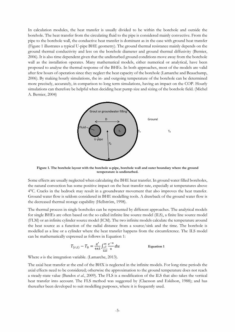
In calculation modules, the heat transfer is usually divided to be within the borehole and outside the

borehole. The heat transfer from the circulating fluid to the pipe is considered mainly convective. From the

pipe to the borehole wall, the conductive heat transfer is dominant as in the case with ground heat transfer

(Figure 1 illustrates a typical U-pipe BHE geometry). The ground thermal resistance mainly depends on the

ground thermal conductivity and less on the borehole diameter and ground thermal diffusivity (Bernier,

2006). It is also time dependent given that the undisturbed ground conditions move away from the borehole

wall as the installation operates. Many mathematical models, either numerical or analytical, have been

proposed to analyse the thermal response of the BHEs. In both approaches, most of the models are valid

after few hours of operation since they neglect the heat capacity of the borehole (Lamarche and Beauchamp,

2006). By making hourly simulations, the in- and outgoing temperature of the borehole can be determined

more precisely, accurately, in comparison to long term simulations, having an impact on the COP. Hourly

simulations can therefore be helpful when deciding heat pump size and sizing of the borehole field. (Michel

A. Bernier, 2004)

Figure 1. The borehole layout with the borehole u-pipe, borehole wall and outer boundary where the ground temperature is undisturbed.

Some effects are usually neglected when calculating the BHE heat transfer. In ground water filled boreholes,

the natural convection has some positive impact on the heat transfer rate, especially at temperatures above

4°C. Cracks in the bedrock may result in a groundwater movement that also improves the heat transfer.

Ground water flow is seldom considered in BHE modelling tools. A drawback of the ground water flow is

the decreased thermal storage capability (Hellström, 1998).

The thermal process in single boreholes can be represented by different approaches. The analytical models

for single BHEs are often based on the so called infinite line source model (ILS), a finite line source model

(FLM) or an infinite cylinder source model (ICM). The two infinite models calculate the temperature around

the heat source as a function of the radial distance from a source/sink and the time. The borehole is

modelled as a line or a cylinder where the heat transfer happens from the circumference. The ILS model

can be mathematically expressed as follows in Equation 1:

𝑇(𝑟,𝑡) − 𝑇0 =𝑞′

4𝜋𝜆∫

𝑒−𝑢

𝑢𝑑𝑢

∞𝑟2

4𝛼𝑡

Equation 1

Where u is the integration variable. (Lamarche, 2013).

The axial heat transfer at the end of the BHX is neglected in the infinite models. For long-time periods the

axial effects need to be considered; otherwise the approximation to the ground temperature does not reach

a steady-state value (Bandos et al., 2009). The FLS is a modification of the ILS that also takes the vertical

heat transfer into account. The FLS method was suggested by (Claesson and Eskilson, 1988); and has

thereafter been developed to suit modelling purposes, where it is frequently used.

-6-

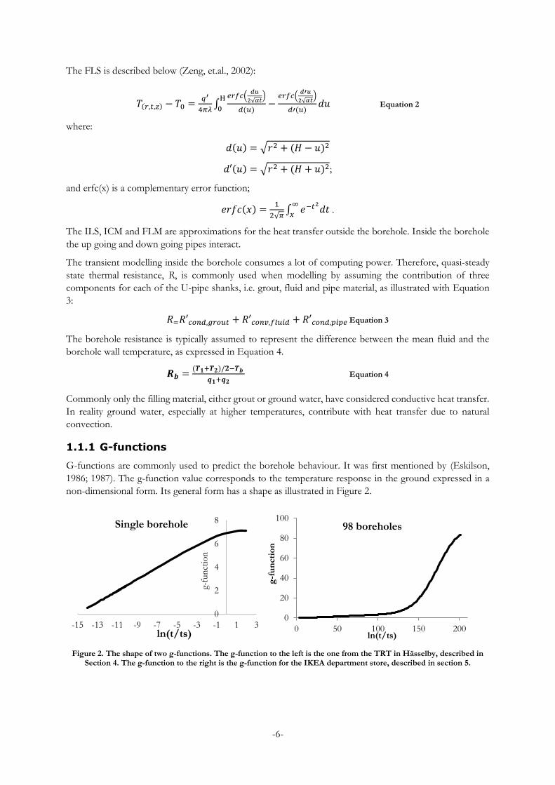
The FLS is described below (Zeng, et.al., 2002):

𝑇(𝑟,𝑡,𝑧) − 𝑇0 =𝑞′

4𝜋𝜆∫

𝑒𝑟𝑓𝑐(𝑑𝑢

2√𝛼𝑡)

𝑑(𝑢)−

𝑒𝑟𝑓𝑐(𝑑′𝑢

2√𝛼𝑡)

𝑑′(𝑢)𝑑𝑢

H

0 Equation 2

where:

𝑑(𝑢) = √𝑟2 + (𝐻 − 𝑢)2

𝑑′(𝑢) = √𝑟2 + (𝐻 + 𝑢)2;

and erfc(x) is a complementary error function;

𝑒𝑟𝑓𝑐(𝑥) =1

2√𝜋∫ 𝑒−𝑡2

𝑑𝑡∞

𝑥 .

The ILS, ICM and FLM are approximations for the heat transfer outside the borehole. Inside the borehole

the up going and down going pipes interact.

The transient modelling inside the borehole consumes a lot of computing power. Therefore, quasi-steady

state thermal resistance, R, is commonly used when modelling by assuming the contribution of three

components for each of the U-pipe shanks, i.e. grout, fluid and pipe material, as illustrated with Equation

3:

𝑅=𝑅′𝑐𝑜𝑛𝑑,𝑔𝑟𝑜𝑢𝑡 + 𝑅′𝑐𝑜𝑛𝑣,𝑓𝑙𝑢𝑖𝑑 + 𝑅′𝑐𝑜𝑛𝑑,𝑝𝑖𝑝𝑒 Equation 3

The borehole resistance is typically assumed to represent the difference between the mean fluid and the

borehole wall temperature, as expressed in Equation 4.

𝑹𝒃 =(𝑻𝟏+𝑻𝟐)/𝟐−𝑻𝒃

𝒒𝟏+𝒒𝟐 Equation 4

Commonly only the filling material, either grout or ground water, have considered conductive heat transfer.

In reality ground water, especially at higher temperatures, contribute with heat transfer due to natural

convection.

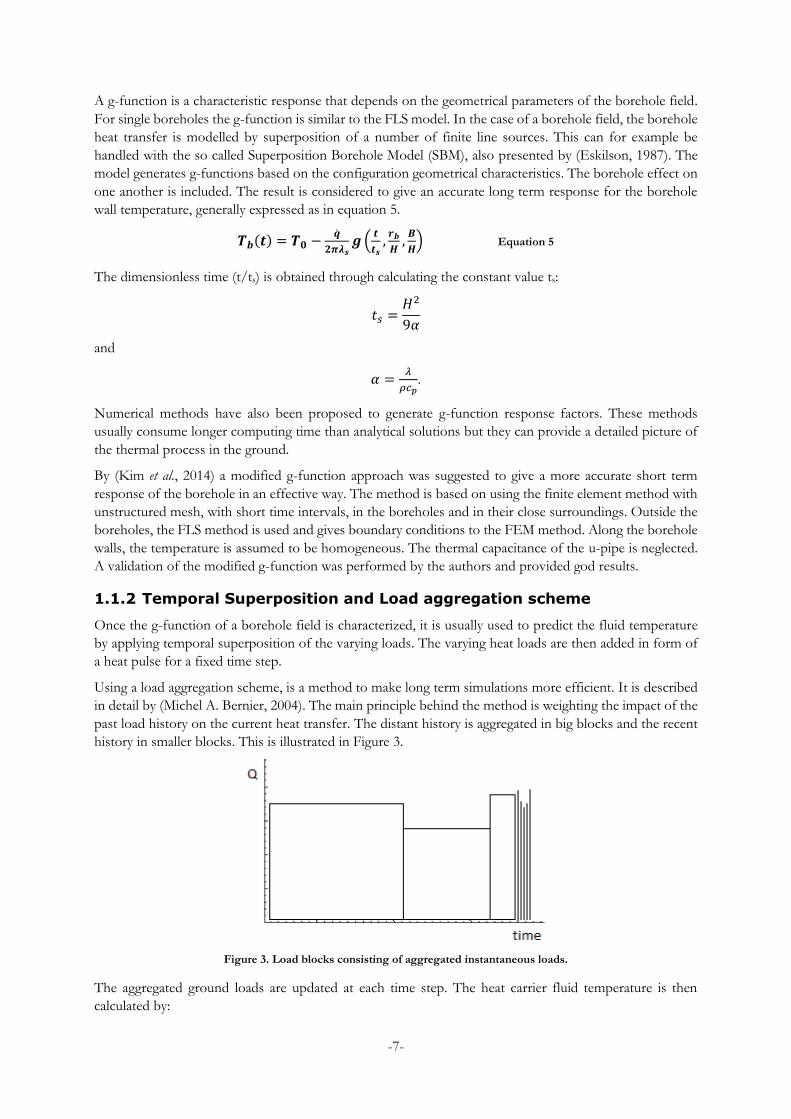
1.1.1 G-functions

G-functions are commonly used to predict the borehole behaviour. It was first mentioned by (Eskilson,

1986; 1987). The g-function value corresponds to the temperature response in the ground expressed in a

non-dimensional form. Its general form has a shape as illustrated in Figure 2.

Figure 2. The shape of two g-functions. The g-function to the left is the one from the TRT in Hässelby, described in Section 4. The g-function to the right is the g-function for the IKEA department store, described in section 5.

0

2

4

6

8

-15 -13 -11 -9 -7 -5 -3 -1 1 3

g-fu

nct

ion

ln(t/ts)

Single borehole

0

20

40

60

80

100

0 50 100 150 200

g-f

un

cti

on

ln(t/ts)

98 boreholes

-7-

A g-function is a characteristic response that depends on the geometrical parameters of the borehole field.

For single boreholes the g-function is similar to the FLS model. In the case of a borehole field, the borehole

heat transfer is modelled by superposition of a number of finite line sources. This can for example be

handled with the so called Superposition Borehole Model (SBM), also presented by (Eskilson, 1987). The

model generates g-functions based on the configuration geometrical characteristics. The borehole effect on

one another is included. The result is considered to give an accurate long term response for the borehole

wall temperature, generally expressed as in equation 5.

𝑻𝒃(𝒕) = 𝑻𝟎 −�̇�

𝟐𝝅𝝀𝒔𝒈 (

𝒕

𝒕𝒔,

𝒓𝒃

𝑯,

𝑩

𝑯) Equation 5

The dimensionless time (t/ts) is obtained through calculating the constant value ts:

𝑡𝑠 =𝐻2

9𝛼

and

𝛼 =𝜆

𝜌𝑐𝑝.

Numerical methods have also been proposed to generate g-function response factors. These methods

usually consume longer computing time than analytical solutions but they can provide a detailed picture of

the thermal process in the ground.

By (Kim et al., 2014) a modified g-function approach was suggested to give a more accurate short term

response of the borehole in an effective way. The method is based on using the finite element method with

unstructured mesh, with short time intervals, in the boreholes and in their close surroundings. Outside the

boreholes, the FLS method is used and gives boundary conditions to the FEM method. Along the borehole

walls, the temperature is assumed to be homogeneous. The thermal capacitance of the u-pipe is neglected.

A validation of the modified g-function was performed by the authors and provided god results.

1.1.2 Temporal Superposition and Load aggregation scheme

Once the g-function of a borehole field is characterized, it is usually used to predict the fluid temperature

by applying temporal superposition of the varying loads. The varying heat loads are then added in form of

a heat pulse for a fixed time step.

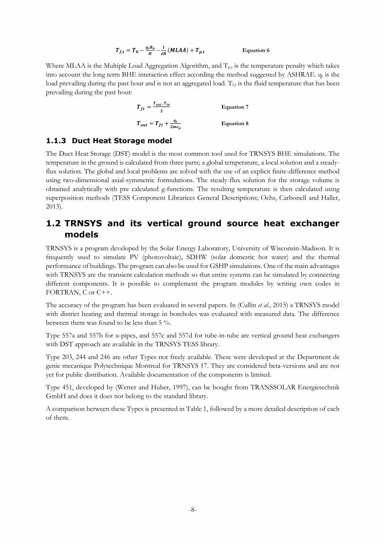
Using a load aggregation scheme, is a method to make long term simulations more efficient. It is described

in detail by (Michel A. Bernier, 2004). The main principle behind the method is weighting the impact of the

past load history on the current heat transfer. The distant history is aggregated in big blocks and the recent

history in smaller blocks. This is illustrated in Figure 3.

Figure 3. Load blocks consisting of aggregated instantaneous loads.

The aggregated ground loads are updated at each time step. The heat carrier fluid temperature is then

calculated by:

-8-

𝑻𝒇,𝒕 = 𝑻𝟎 −𝒒𝒕𝑹𝒃

𝑯 –

𝟏

𝝀𝑯(𝑴𝑳𝑨𝑨) + 𝑻𝒑,𝒕 Equation 6

Where MLAA is the Multiple Load Aggregation Algorithm, and Tp,t is the temperature penalty which takes

into account the long term BHE interaction effect according the method suggested by ASHRAE. qt is the

load prevailing during the past hour and is not an aggregated load. Tf,t is the fluid temperature that has been

prevailing during the past hour:

𝑻𝒇𝒕 =𝑻𝒐𝒖𝒕−𝑻𝒊𝒏

𝟐 Equation 7

𝑻𝒐𝒖𝒕 = 𝑻𝒇𝒕 +𝒒𝒕

𝟐�̇�𝒄𝒑 Equation 8

1.1.3 Duct Heat Storage model

The Duct Heat Storage (DST) model is the most common tool used for TRNSYS BHE simulations. The

temperature in the ground is calculated from three parts; a global temperature, a local solution and a steady-

flux solution. The global and local problems are solved with the use of an explicit finite-difference method

using two-dimensional axial-symmetric formulations. The steady-flux solution for the storage volume is

obtained analytically with pre calculated g-functions. The resulting temperature is then calculated using

superposition methods (TESS Component Librariees General Descriptions; Ochs, Carbonell and Haller,

2013).

1.2 TRNSYS and its vertical ground source heat exchanger

models

TRNSYS is a program developed by the Solar Energy Laboratory, University of Wisconsin-Madison. It is

frequently used to simulate PV (photovoltaic), SDHW (solar domestic hot water) and the thermal

performance of buildings. The program can also be used for GSHP simulations. One of the main advantages

with TRNSYS are the transient calculation methods so that entire systems can be simulated by connecting

different components. It is possible to complement the program modules by writing own codes in

FORTRAN, C or C++.

The accuracy of the program has been evaluated in several papers. In (Cullin et al., 2015) a TRNSYS model

with district heating and thermal storage in boreholes was evaluated with measured data. The difference

between them was found to be less than 5 %.

Type 557a and 557b for u-pipes, and 557c and 557d for tube-in-tube are vertical ground heat exchangers

with DST approach are available in the TRNSYS TESS library.

Type 203, 244 and 246 are other Types not freely available. These were developed at the Department de

genie mecanique Polytechnique Montreal for TRNSYS 17. They are considered beta-versions and are not

yet for public distribution. Available documentation of the components is limited.

Type 451, developed by (Wetter and Huber, 1997), can be bought from TRANSSOLAR Energietechnik

GmbH and does it does not belong to the standard library.

A comparison between these Types is presented in Table 1, followed by a more detailed description of each

of them.

-9-

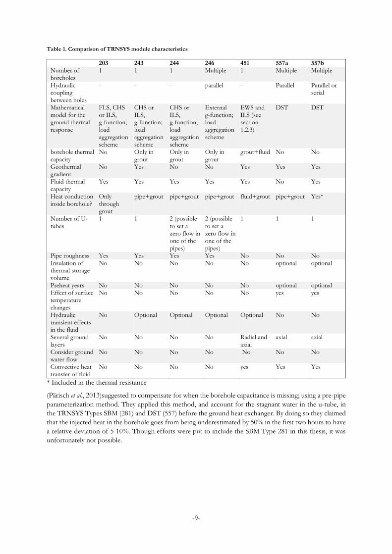
Table 1. Comparison of TRNSYS module characteristics

203 243 244 246 451 557a 557b Number of boreholes

1 1 1 Multiple 1 Multiple Multiple

Hydraulic coupling between holes

- - - parallel - Parallel Parallel or serial

Mathematical model for the ground thermal response

FLS, CHS or ILS, g-function; load aggregation scheme

CHS or ILS, g-function; load aggregation scheme

CHS or ILS, g-function; load aggregation scheme

External g-function; load aggregation scheme

EWS and ILS (see section 1.2.3)

DST DST

borehole thermal capacity

No Only in grout

Only in grout

Only in grout

grout+fluid No No

Geothermal gradient

No Yes No No Yes Yes Yes

Fluid thermal capacity

Yes Yes Yes Yes Yes No Yes

Heat conduction inside borehole?

Only through grout

pipe+grout pipe+grout pipe+grout fluid+grout pipe+grout Yes*

Number of U-tubes

1 1 2 (possible to set a zero flow in one of the pipes)

2 (possible to set a zero flow in one of the pipes)

1 1 1

Pipe roughness Yes Yes Yes Yes No No No Insulation of thermal storage volume

No No No No No optional optional

Preheat years No No No No No optional optional Effect of surface temperature changes

No No No No No yes yes

Hydraulic transient effects in the fluid

No Optional Optional Optional Optional No No

Several ground layers

No No No No Radial and axial

axial axial

Consider ground water flow

No No No No No No No

Convective heat transfer of fluid

No No No No yes Yes Yes

* Included in the thermal resistance

(Pärisch et al., 2013)suggested to compensate for when the borehole capacitance is missing; using a pre-pipe

parameterization method. They applied this method, and account for the stagnant water in the u-tube, in

the TRNSYS Types SBM (281) and DST (557) before the ground heat exchanger. By doing so they claimed

that the injected heat in the borehole goes from being underestimated by 50% in the first two hours to have

a relative deviation of 5-10%. Though efforts were put to include the SBM Type 281 in this thesis, it was

unfortunately not possible.

-10-

1.2.1 Type 557

Two components are available in the TESS library in TRNSYS: 557a and 557b. They are based on the DST

methodology developed by (Hellström, 1989). The implementation in TRNSYS is described in detailed by

Pahud et al., 1997. Steady-state is assumed and the internal capacitance of the borehole is neglected. In 557a,

the thermal resistance between the carrier fluid and the ground is calculated by the program, based on the

geometry and thermal conductivity of the pipes and the grout. The shank spacing is also considered. In

557b, on the other hand, the thermal resistance has to be known and is set as an input parameter. The

thermal resistance can for example be obtained from a thermal response test.

For 557a and 557b, the boreholes are placed uniformly in a cylindrical storage volume. Within this cylindrical

storage volume the ground is considered to be uniform. Outside the storage volume the ground can be

divided in layers with different thermal properties. The layout of the borehole field for the 557 types, is fixed

hexagonally and uniformly within the storage volume in the simulation. This is seldom the case in reality.

1.2.2 Type 203, 243, 244 and 246

The components 203, 244 and 246 are developed at École Polytechnique de Montreal. The documentation

of the components is as earlier mentioned limited and the models are still not publicly distributed. They are

based on a load aggregation scheme and use g-functions to take care of the borehole field geometry. The

load aggregation scheme is based on three blocks: one large block, one medium block and one small block

with regarding the load and time period. The number of individual heat extraction/injection rates to be

added in one small load block, the number of small blocks that will be added in one medium block and the

number of medium blocks to be added in one large block is set in the parameter properties of the

components.

In type 203, 243 and 244 the analytical model can be selected (Bernier, 2004). It can be set to ILC or CSM.

For type 203 the FLS can also be chosen.

Type 203 is for single boreholes with one circuit and does not consider the borehole capacity. Type 243 is

like type 203 but considers the borehole thermal capacity. Types 244 and 246 simulate double u-pipes, with

the borehole capacity taken into account. How double u-pipes can be modelled is described in (Eslami-

Nejad and Bernier, 2011). Type 244 can only handle single boreholes while 246 can handle entire fields. To

type 246, the g-function for the specific field has to be attached by the user through an external file, in order

to simulate the field in a correct way.

1.2.3 Type 451

(Wetter and Huber, 1997) modelled in the component 451 the transient behaviour of a double U-tube

borehole. A single equivalent pipe diameter is set that does not allow modelling of two independent circuits

in one borehole, as of (Eslami-Nejad and Bernier, 2011). The “Erdwärmesonden” model (EWS), developed

by (Huber and Schuler, 1997) is applied in this TRNSYS vertical heat exchanger component. It was

developed to improve the transient behaviour in the vertical heat exchanger. It does not belong to the

standard library but can be ordered from Transsolar Energietechnik GmbH. It simulates the transient heat

flux in the earth within a user selected radius around the borehole with the numerical Crank-Nicolson

algorithm and the model uses time superposition of the heat loads for different time steps.

-11-

2 Goals with the project

The project intends to compare the different borehole heat exchanger tools that are available in TRNSYS

and to model three different borehole sites with some of these. These sites are: a single borehole to compare

to a thermal response test (TRT), a borehole field installation in operation at an IKEA department store in

Uppsala, Sweden; and a newly installed borehole field with serial coupling at the Marine Corps Logistics

base in Albany, Georgia. The goals with this project are to use the TRNYS software to:

1. Compare the simulations using the modules to measured data, to see how they perform on long

and short term.

2. Evaluate the borehole temperatures for a large multiple borehole field at IKEA Uppsala.

3. Evaluate the borehole field at the Marine Corps Logistics base with TRNSYS for a hypothetical

operation scenario.

3 Method

First, as many TRNSYS BHE models as possible will be collected and compared in a comprehensive way.

A simple system with a single borehole and a constant load will be modelled with the vertical ground heat

exchangers 203, 243, 244, 246, 557a, 557b, 451 in TRNSYS. This TRNSYS model is a simulation of a TRT

made in Hässelby outside Stockholm, Sweden. The input values are set to correspond to the real

circumstances at the TRT. For the types 203, 243 and 244 the use of different analytical solutions are

compared (FLS, ILS, CHS).

Secondly, a simulation is made with a borehole field for an IKEA department store in UPPSALA. The types

246 and 557 which can handle entire borehole fields are compared with measured data for the borehole

temperature. For type 246 the use of single and double u-pipes are compared as well.

Thirdly, a borehole field at the Marine Corps Logistics base in Albany, Georgia is modelled. It has 306

boreholes in 102 parallel loops with 3 serial coupled boreholes in each. The TRNSYS type 557b, which can

handle serial coupled boreholes is used. The installation is recently finished and operation data is preliminary.

-12-

4 Simulated Thermal response test

A TRT test was carried out at Växthusvägen, Hässelby, Stockholm, in order to prepare for GSHPs. In the

TRT a constant load was injected with a constant flow rate. The test is simulated in a simple model to

compare the vertical ground source heat exchanger types in TRNSYS; 203, 243, 244, 246, 557a and 557b;

and hopefully recreate the measured results. The simulated fluid temperature profile is compared to the

measured values from the TRT in order to verify the accuracy of the types.

4.1 Modelling

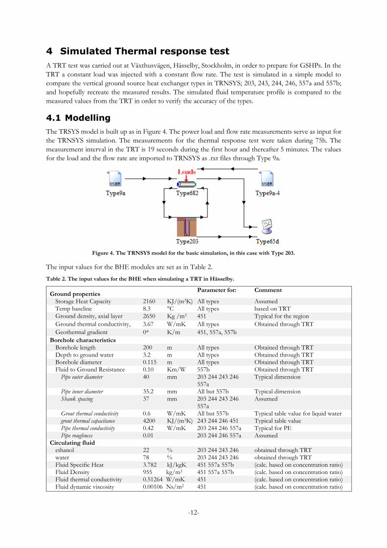
The TRSYS model is built up as in Figure 4. The power load and flow rate measurements serve as input for

the TRNSYS simulation. The measurements for the thermal response test were taken during 75h. The

measurement interval in the TRT is 19 seconds during the first hour and thereafter 5 minutes. The values

for the load and the flow rate are imported to TRNSYS as .txt files through Type 9a.

Figure 4. The TRNSYS model for the basic simulation, in this case with Type 203.

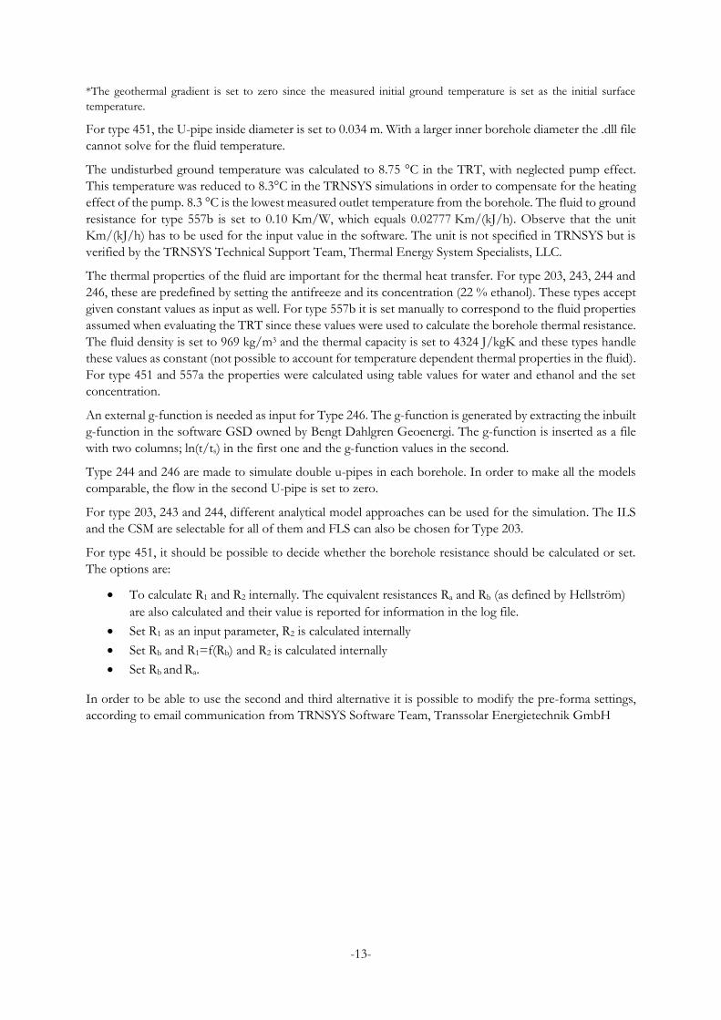
The input values for the BHE modules are set as in Table 2.

Table 2. The input values for the BHE when simulating a TRT in Hässelby.

Ground properties Parameter for: Comment

Storage Heat Capacity 2160 KJ/(m3K) All types Assumed Temp baseline 8.3 °C All types based on TRT Ground density, axial layer 2650 Kg /m3 451 Typical for the region

Ground thermal conductivity, 3.67 W/mK All types Obtained through TRT

Geothermal gradient 0* K/m 451, 557a, 557b

Borehole characteristics Borehole length 200 m All types Obtained through TRT Depth to ground water 3.2 m All types Obtained through TRT Borehole diameter 0.115 m All types Obtained through TRT Fluid to Ground Resistance 0.10 Km/W 557b Obtained through TRT

Pipe outer diameter 40 mm 203 244 243 246 557a

Typical dimension

Pipe inner diameter 35.2 mm All but 557b Typical dimension Shank spacing 37 mm 203 244 243 246

557a Assumed

Grout thermal conductivity 0.6 W/mK All but 557b Typical table value for liquid water grout thermal capacitance 4200 KJ/(m3K) 243 244 246 451 Typical table value Pipe thermal conductivity 0.42 W/mK 203 244 246 557a Typical for PE Pipe roughness 0.01 203 244 246 557a Assumed

Circulating fluid ethanol 22 % 203 244 243 246 obtained through TRT water 78 % 203 244 243 246 obtained through TRT Fluid Specific Heat 3.782 kJ/kgK 451 557a 557b (calc. based on concentration ratio) Fluid Density 955 kg/m3 451 557a 557b (calc. based on concentration ratio) Fluid thermal conductivity 0.51264 W/mK 451 (calc. based on concentration ratio) Fluid dynamic viscosity 0.00106 Ns/m2 451 (calc. based on concentration ratio)

-13-

*The geothermal gradient is set to zero since the measured initial ground temperature is set as the initial surface

temperature.

For type 451, the U-pipe inside diameter is set to 0.034 m. With a larger inner borehole diameter the .dll file

cannot solve for the fluid temperature.

The undisturbed ground temperature was calculated to 8.75 °C in the TRT, with neglected pump effect.

This temperature was reduced to 8.3°C in the TRNSYS simulations in order to compensate for the heating

effect of the pump. 8.3 °C is the lowest measured outlet temperature from the borehole. The fluid to ground

resistance for type 557b is set to 0.10 Km/W, which equals 0.02777 Km/(kJ/h). Observe that the unit

Km/(kJ/h) has to be used for the input value in the software. The unit is not specified in TRNSYS but is

verified by the TRNSYS Technical Support Team, Thermal Energy System Specialists, LLC.

The thermal properties of the fluid are important for the thermal heat transfer. For type 203, 243, 244 and

246, these are predefined by setting the antifreeze and its concentration (22 % ethanol). These types accept

given constant values as input as well. For type 557b it is set manually to correspond to the fluid properties

assumed when evaluating the TRT since these values were used to calculate the borehole thermal resistance.

The fluid density is set to 969 kg/m3 and the thermal capacity is set to 4324 J/kgK and these types handle

these values as constant (not possible to account for temperature dependent thermal properties in the fluid).

For type 451 and 557a the properties were calculated using table values for water and ethanol and the set

concentration.

An external g-function is needed as input for Type 246. The g-function is generated by extracting the inbuilt

g-function in the software GSD owned by Bengt Dahlgren Geoenergi. The g-function is inserted as a file

with two columns; ln(t/ts) in the first one and the g-function values in the second.

Type 244 and 246 are made to simulate double u-pipes in each borehole. In order to make all the models

comparable, the flow in the second U-pipe is set to zero.

For type 203, 243 and 244, different analytical model approaches can be used for the simulation. The ILS

and the CSM are selectable for all of them and FLS can also be chosen for Type 203.

For type 451, it should be possible to decide whether the borehole resistance should be calculated or set.

The options are:

To calculate R1 and R2 internally. The equivalent resistances Ra and Rb (as defined by Hellström)

are also calculated and their value is reported for information in the log file.

Set R1 as an input parameter, R2 is calculated internally

Set Rb and R1=f(Rb) and R2 is calculated internally

Set Rb and Ra.

In order to be able to use the second and third alternative it is possible to modify the pre-forma settings,

according to email communication from TRNSYS Software Team, Transsolar Energietechnik GmbH

-14-

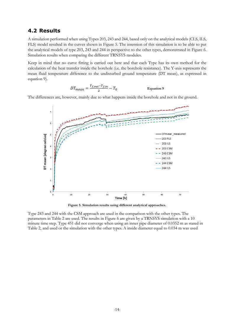
4.2 Results

A simulation performed when using Types 203, 243 and 244, based only on the analytical models (CLS, ILS,

FLS) model resulted in the curves shown in Figure 5. The intention of this simulation is to be able to put

the analytical models of type 203, 243 and 244 in perspective to the other types, demonstrated in Figure 6.

Simulation results when comparing the different TRNSYS modules.

Keep in mind that no curve fitting is carried out here and that each Type has its own method for the

calculation of the heat transfer inside the borehole (i.e. the borehole resistance). The Y-axis represents the

mean fluid temperature difference to the undisturbed ground temperature (DT mean), as expressed in

equation 9).

𝐷𝑇𝑚𝑒𝑎𝑛 =𝑇𝑓,𝑜𝑢𝑡−𝑇𝑓,𝑖𝑛

2− 𝑇0 Equation 9

The differences are, however, mainly due to what happens inside the borehole and not in the ground.

Figure 5. Simulation results using different analytical approaches.

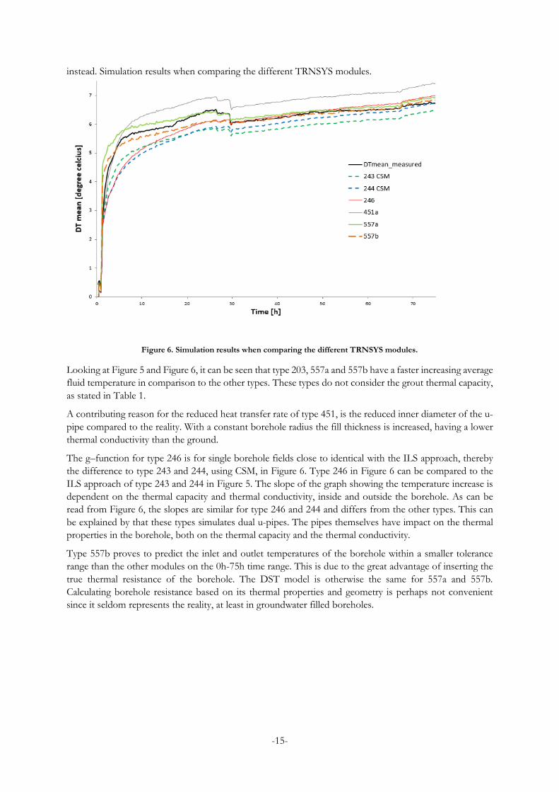
Type 243 and 244 with the CSM approach are used in the comparison with the other types. The parameters in Table 2 are used. The results in Figure 6 are given by a TRNSYS simulation with a 10 minute time step. Type 451 did not converge when using an inner pipe diameter of 0.0352 m as stated in Table 2, and used or the simulation with the other types. A inside diameter equal to 0.034 m was used

-15-

instead. Simulation results when comparing the different TRNSYS modules.

Figure 6. Simulation results when comparing the different TRNSYS modules.

Looking at Figure 5 and Figure 6, it can be seen that type 203, 557a and 557b have a faster increasing average

fluid temperature in comparison to the other types. These types do not consider the grout thermal capacity,

as stated in Table 1.

A contributing reason for the reduced heat transfer rate of type 451, is the reduced inner diameter of the u-

pipe compared to the reality. With a constant borehole radius the fill thickness is increased, having a lower

thermal conductivity than the ground.

The g–function for type 246 is for single borehole fields close to identical with the ILS approach, thereby

the difference to type 243 and 244, using CSM, in Figure 6. Type 246 in Figure 6 can be compared to the

ILS approach of type 243 and 244 in Figure 5. The slope of the graph showing the temperature increase is

dependent on the thermal capacity and thermal conductivity, inside and outside the borehole. As can be

read from Figure 6, the slopes are similar for type 246 and 244 and differs from the other types. This can

be explained by that these types simulates dual u-pipes. The pipes themselves have impact on the thermal

properties in the borehole, both on the thermal capacity and the thermal conductivity.

Type 557b proves to predict the inlet and outlet temperatures of the borehole within a smaller tolerance

range than the other modules on the 0h-75h time range. This is due to the great advantage of inserting the

true thermal resistance of the borehole. The DST model is otherwise the same for 557a and 557b.

Calculating borehole resistance based on its thermal properties and geometry is perhaps not convenient

since it seldom represents the reality, at least in groundwater filled boreholes.

-16-

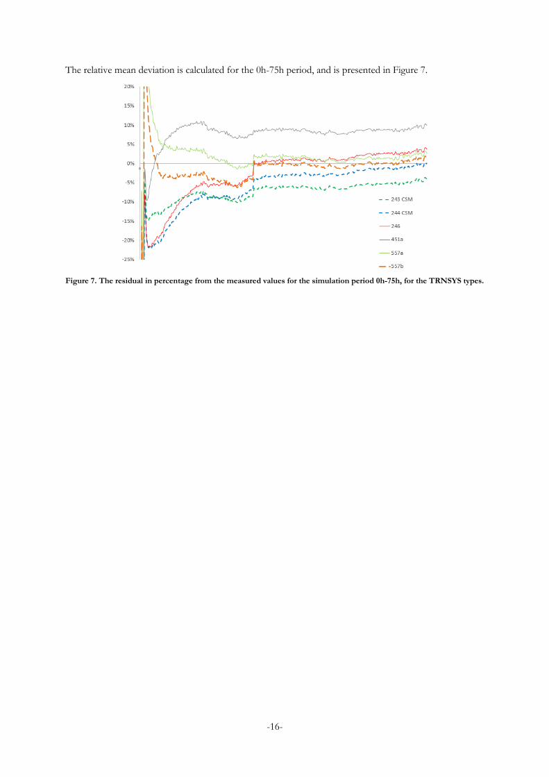
The relative mean deviation is calculated for the 0h-75h period, and is presented in Figure 7.

Figure 7. The residual in percentage from the measured values for the simulation period 0h-75h, for the TRNSYS types.

-17-

5 Borehole heat exchanger modelling of an IKEA

department store

The Ikea department store in Uppsala has operating data that have been logged since the site was put into

operation in 2009. The facility is simulated in TRNSYS using type 246, 557a and 557b. The accuracy of

these types is then evaluated based on how the fluid temperature corresponds to the measured data from

the boreholes.

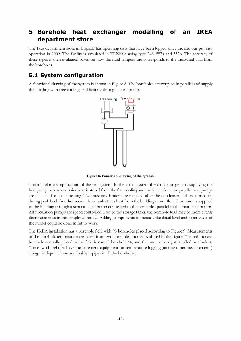
5.1 System configuration

A functional drawing of the system is shown in Figure 8. The boreholes are coupled in parallel and supply

the building with free cooling; and heating through a heat pump.

Figure 8. Functional drawing of the system.

The model is a simplification of the real system. In the actual system there is a storage tank supplying the

heat pumps where excessive heat is stored from the free cooling and the boreholes. Two parallel heat pumps

are installed for space heating. Two auxiliary heaters are installed after the condenser and are turned on

during peak load. Another accumulator tank stores heat from the building return flow. Hot water is supplied

to the building through a separate heat pump connected to the boreholes parallel to the main heat pumps.

All circulation pumps are speed controlled. Due to the storage tanks, the borehole load may be more evenly

distributed than in this simplified model. Adding components to increase the detail level and preciseness of

the model could be done in future work.

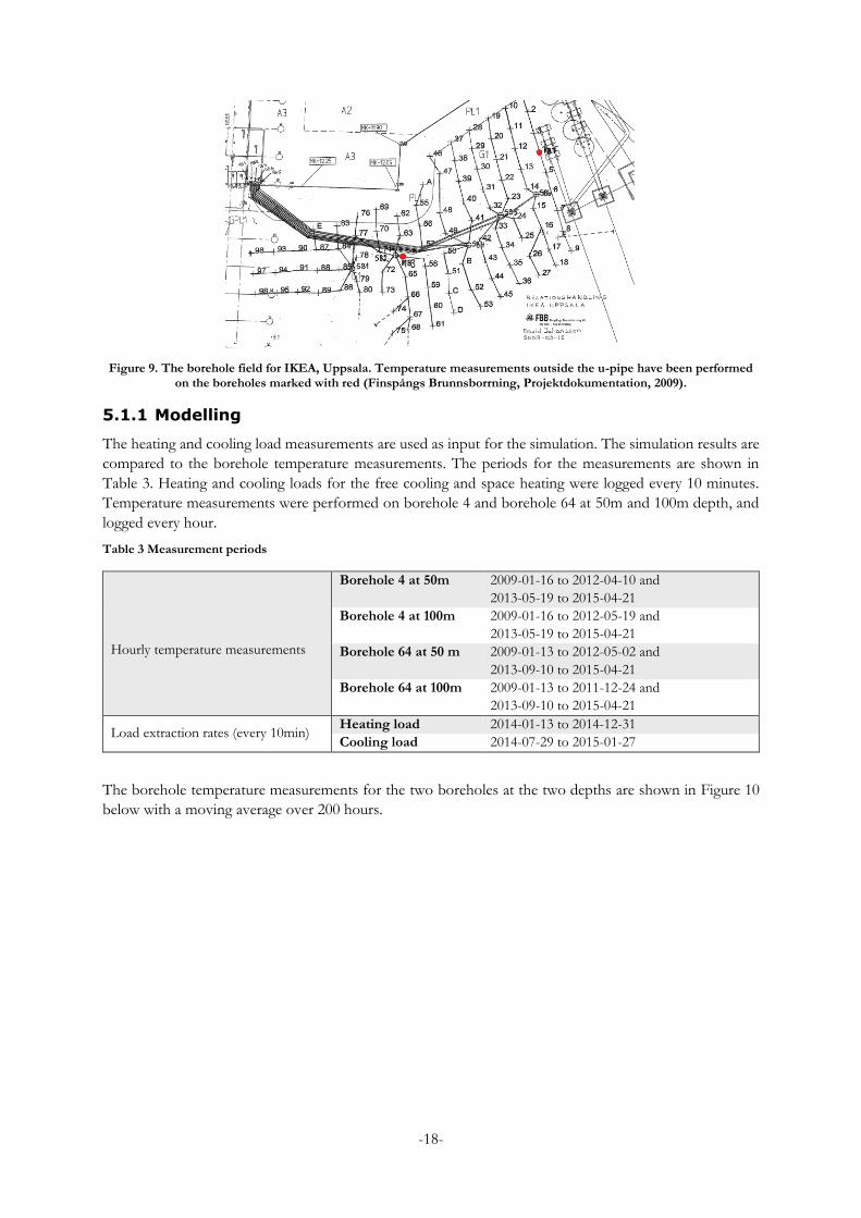
The IKEA installation has a borehole field with 98 boreholes placed according to Figure 9. Measurements

of the borehole temperature are taken from two boreholes marked with red in the figure. The red marked

borehole centrally placed in the field is named borehole 64; and the one to the right is called borehole 4.

These two boreholes have measurement equipment for temperature logging (among other measurements)

along the depth. There are double u-pipes in all the boreholes.

-18-

Figure 9. The borehole field for IKEA, Uppsala. Temperature measurements outside the u-pipe have been performed on the boreholes marked with red (Finspångs Brunnsborrning, Projektdokumentation, 2009).

5.1.1 Modelling

The heating and cooling load measurements are used as input for the simulation. The simulation results are

compared to the borehole temperature measurements. The periods for the measurements are shown in

Table 3. Heating and cooling loads for the free cooling and space heating were logged every 10 minutes.

Temperature measurements were performed on borehole 4 and borehole 64 at 50m and 100m depth, and

logged every hour.

Table 3 Measurement periods

Hourly temperature measurements

Borehole 4 at 50m 2009-01-16 to 2012-04-10 and

2013-05-19 to 2015-04-21

Borehole 4 at 100m 2009-01-16 to 2012-05-19 and

2013-05-19 to 2015-04-21

Borehole 64 at 50 m 2009-01-13 to 2012-05-02 and

2013-09-10 to 2015-04-21

Borehole 64 at 100m 2009-01-13 to 2011-12-24 and

2013-09-10 to 2015-04-21

Load extraction rates (every 10min) Heating load 2014-01-13 to 2014-12-31

Cooling load 2014-07-29 to 2015-01-27

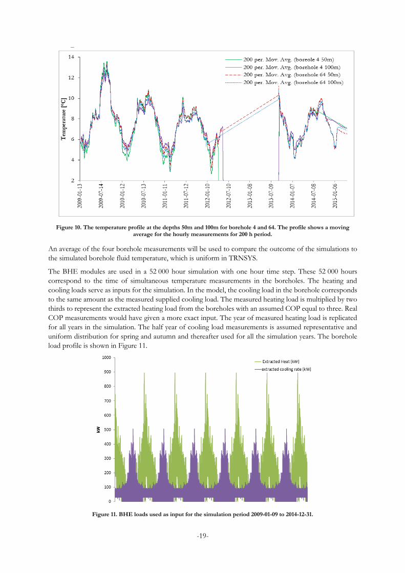
The borehole temperature measurements for the two boreholes at the two depths are shown in Figure 10

below with a moving average over 200 hours.

-19-

Figure 10. The temperature profile at the depths 50m and 100m for borehole 4 and 64. The profile shows a moving average for the hourly measurements for 200 h period.

An average of the four borehole measurements will be used to compare the outcome of the simulations to

the simulated borehole fluid temperature, which is uniform in TRNSYS.

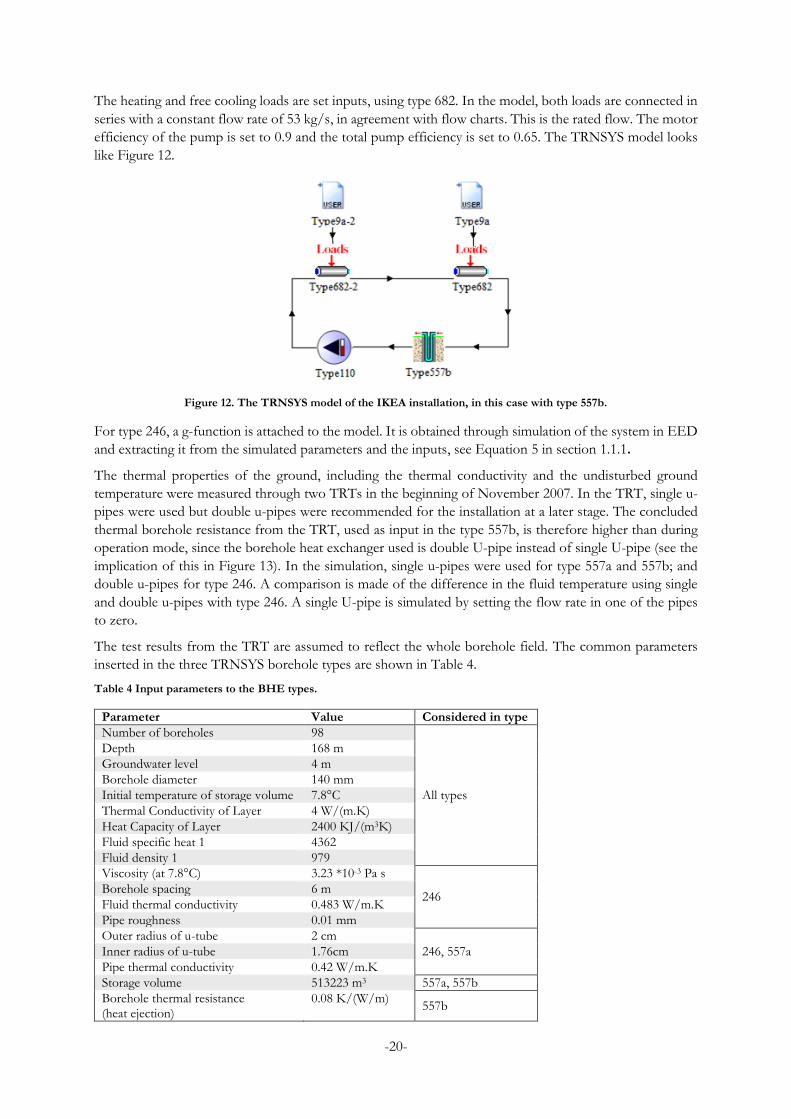
The BHE modules are used in a 52 000 hour simulation with one hour time step. These 52 000 hours

correspond to the time of simultaneous temperature measurements in the boreholes. The heating and

cooling loads serve as inputs for the simulation. In the model, the cooling load in the borehole corresponds

to the same amount as the measured supplied cooling load. The measured heating load is multiplied by two

thirds to represent the extracted heating load from the boreholes with an assumed COP equal to three. Real

COP measurements would have given a more exact input. The year of measured heating load is replicated

for all years in the simulation. The half year of cooling load measurements is assumed representative and

uniform distribution for spring and autumn and thereafter used for all the simulation years. The borehole

load profile is shown in Figure 11.

Figure 11. BHE loads used as input for the simulation period 2009-01-09 to 2014-12-31.

-20-

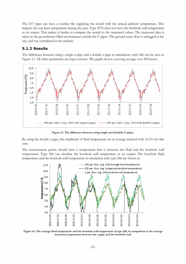
The heating and free cooling loads are set inputs, using type 682. In the model, both loads are connected in

series with a constant flow rate of 53 kg/s, in agreement with flow charts. This is the rated flow. The motor

efficiency of the pump is set to 0.9 and the total pump efficiency is set to 0.65. The TRNSYS model looks

like Figure 12.

Figure 12. The TRNSYS model of the IKEA installation, in this case with type 557b.

For type 246, a g-function is attached to the model. It is obtained through simulation of the system in EED

and extracting it from the simulated parameters and the inputs, see Equation 5 in section 1.1.1.

The thermal properties of the ground, including the thermal conductivity and the undisturbed ground

temperature were measured through two TRTs in the beginning of November 2007. In the TRT, single u-

pipes were used but double u-pipes were recommended for the installation at a later stage. The concluded

thermal borehole resistance from the TRT, used as input in the type 557b, is therefore higher than during

operation mode, since the borehole heat exchanger used is double U-pipe instead of single U-pipe (see the

implication of this in Figure 13). In the simulation, single u-pipes were used for type 557a and 557b; and

double u-pipes for type 246. A comparison is made of the difference in the fluid temperature using single

and double u-pipes with type 246. A single U-pipe is simulated by setting the flow rate in one of the pipes

to zero.

The test results from the TRT are assumed to reflect the whole borehole field. The common parameters

inserted in the three TRNSYS borehole types are shown in Table 4.

Table 4 Input parameters to the BHE types.

Parameter Value Considered in type

Number of boreholes 98

All types

Depth 168 m

Groundwater level 4 m

Borehole diameter 140 mm

Initial temperature of storage volume 7.8°C

Thermal Conductivity of Layer 4 W/(m.K)

Heat Capacity of Layer 2400 KJ/(m3K)

Fluid specific heat 1 4362

Fluid density 1 979

Viscosity (at 7.8°C) 3.23 *10-3 Pa s

246 Borehole spacing 6 m

Fluid thermal conductivity 0.483 W/m.K

Pipe roughness 0.01 mm

Outer radius of u-tube 2 cm

246, 557a Inner radius of u-tube 1.76cm

Pipe thermal conductivity 0.42 W/m.K

Storage volume 513223 m3 557a, 557b

Borehole thermal resistance (heat ejection)

0.08 K/(W/m) 557b

-21-

The 557 types can have a weather file supplying the model with the annual ambient temperature. This

impacts the top layer temperature during the year. Type 557b does not have the borehole wall temperature

as an output. This makes it harder to compare the model to the measured values. The measured data is

taken in the groundwater filled environment outside the U-pipes. The ground water flow is unlogged at the

site, and not considered in the analysis.

5.1.2 Results

The difference between using a single u-pipe and a double u-pipe in simulations with 246 can be seen in

Figure 13. All other parameters are kept constant. The graph shows a moving average over 200 hours.

Figure 13. The difference between using single and doubble U-pipes.

By using the double u-pipe, the amplitude of fluid temperature are in average reduced with 16.3% for this

case.

The measurement points should have a temperature that is between the fluid and the borehole wall

temperature. Type 246 can simulate the borehole wall temperature as an output. The borehole fluid

temperature and the borehole wall temperature in simulation with type 246 are shown in

Figure 14. The average fluid temperature and the borehole wall temperature of type 246, in comparison to the average measured temperature between the u-pipe and the borehole wall.

-22-

The simulated average difference between the fluid temperature and the borehole wall is 0.70°C. The

difference is about one degree Celsius during the summer and a half degree Celsius during the winter. The

point for the measurements should have a temperature closer to the fluid temperature than to the borehole

wall.

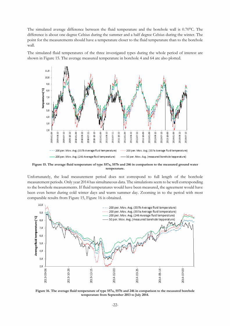
The simulated fluid temperatures of the three investigated types during the whole period of interest are

shown in Figure 15. The average measured temperature in borehole 4 and 64 are also plotted.

Figure 15. The average fluid temperature of type 557a, 557b and 246 in comparison to the measured ground water temperature.

Unfortunately, the load measurement period does not correspond to full length of the borehole

measurement periods. Only year 2014 has simultaneous data. The simulations seem to be well corresponding

to the borehole measurements. If fluid temperatures would have been measured, the agreement would have

been even better during cold winter days and warm summer day. Zooming in to the period with most

comparable results from Figure 15, Figure 16 is obtained.

Figure 16. The average fluid temperature of type 557a, 557b and 246 in comparison to the measured borehole temperature from September 2013 to July 2014.

-23-

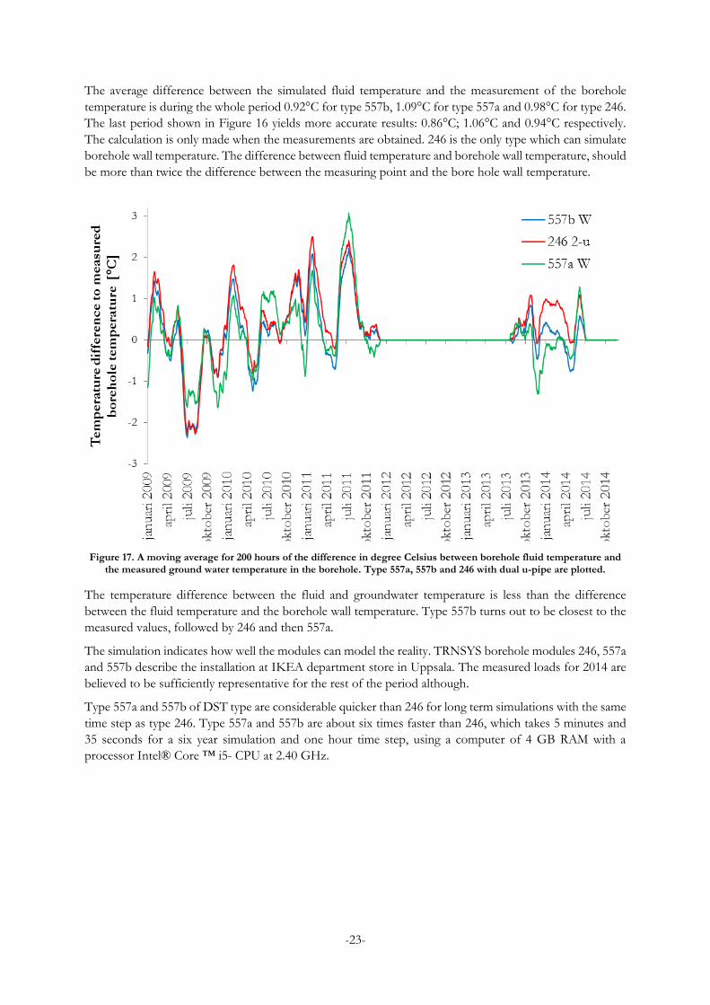
The average difference between the simulated fluid temperature and the measurement of the borehole

temperature is during the whole period 0.92°C for type 557b, 1.09°C for type 557a and 0.98°C for type 246.

The last period shown in Figure 16 yields more accurate results: 0.86°C; 1.06°C and 0.94°C respectively.

The calculation is only made when the measurements are obtained. 246 is the only type which can simulate

borehole wall temperature. The difference between fluid temperature and borehole wall temperature, should

be more than twice the difference between the measuring point and the bore hole wall temperature.

Figure 17. A moving average for 200 hours of the difference in degree Celsius between borehole fluid temperature and the measured ground water temperature in the borehole. Type 557a, 557b and 246 with dual u-pipe are plotted.

The temperature difference between the fluid and groundwater temperature is less than the difference

between the fluid temperature and the borehole wall temperature. Type 557b turns out to be closest to the

measured values, followed by 246 and then 557a.

The simulation indicates how well the modules can model the reality. TRNSYS borehole modules 246, 557a

and 557b describe the installation at IKEA department store in Uppsala. The measured loads for 2014 are

believed to be sufficiently representative for the rest of the period although.

Type 557a and 557b of DST type are considerable quicker than 246 for long term simulations with the same

time step as type 246. Type 557a and 557b are about six times faster than 246, which takes 5 minutes and

35 seconds for a six year simulation and one hour time step, using a computer of 4 GB RAM with a

processor Intel® Core ™ i5- CPU at 2.40 GHz.

-24-

6 Modelling of the Marine Corps Logistic Base

The Marine Corps logistic base in Albany, Georgia, began the installation of a field of vertical BHE for

thermal storage, attached to the buildings’ HVAC system in 2013. The installation was recently finished and

has been operating during a few months. There are 306 boreholes in 102 parallel loops containing three

serial coupled boreholes. The borehole spacing is 5.715 m and the circulating fluid is water. Optical fibre is

installed in some of the boreholes in order to be able to log the ground temperature in the future. The

installation is simulated with TRNSYS and the vertical ground source heat exchanger type 557b, which is

the only model that can handle boreholes coupled in series. Operation measurements have not been

available to validate the modelling yet, therefore this is only a predictive study.

A distributed thermal response test (DTRT) was performed at the site from the 12th of May 2015 at 21.36,

to the 14th of May 2015 at 12.00, which is 36.4 h. The test borehole was 110 m deep. The flow rate was 0.34

l/s and the injected power was 6999 W. The DTRT analysis resulted in a thermal conductivity of 1.92

W/mK and a borehole resistance of 0.107 Km/W.

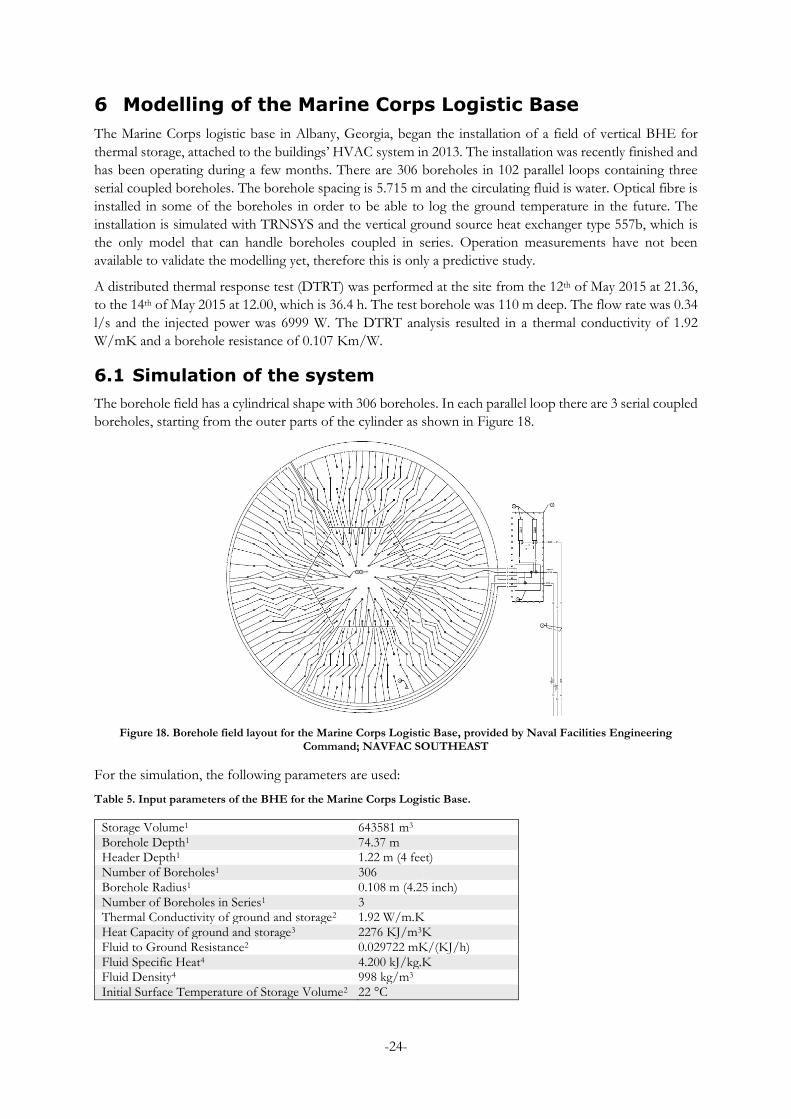
6.1 Simulation of the system

The borehole field has a cylindrical shape with 306 boreholes. In each parallel loop there are 3 serial coupled

boreholes, starting from the outer parts of the cylinder as shown in Figure 18.

Figure 18. Borehole field layout for the Marine Corps Logistic Base, provided by Naval Facilities Engineering Command; NAVFAC SOUTHEAST

For the simulation, the following parameters are used:

Table 5. Input parameters of the BHE for the Marine Corps Logistic Base.

Storage Volume1 643581 m3 Borehole Depth1 74.37 m Header Depth1 1.22 m (4 feet) Number of Boreholes1 306 Borehole Radius1 0.108 m (4.25 inch) Number of Boreholes in Series1 3 Thermal Conductivity of ground and storage2 1.92 W/m.K Heat Capacity of ground and storage3 2276 KJ/m3K Fluid to Ground Resistance2 0.029722 mK/(KJ/h) Fluid Specific Heat4 4.200 kJ/kg.K Fluid Density4 998 kg/m3 Initial Surface Temperature of Storage Volume2 22 °C

-25-

1information comes from drawings of the installation provided by Naval Facilities Engineering Command; NAVFAC SOUTHEAST 2the information is provided by the DTRT 3Properties for lime stone (Eppelbaum, et.al., 2014) 4Properties for liquid water

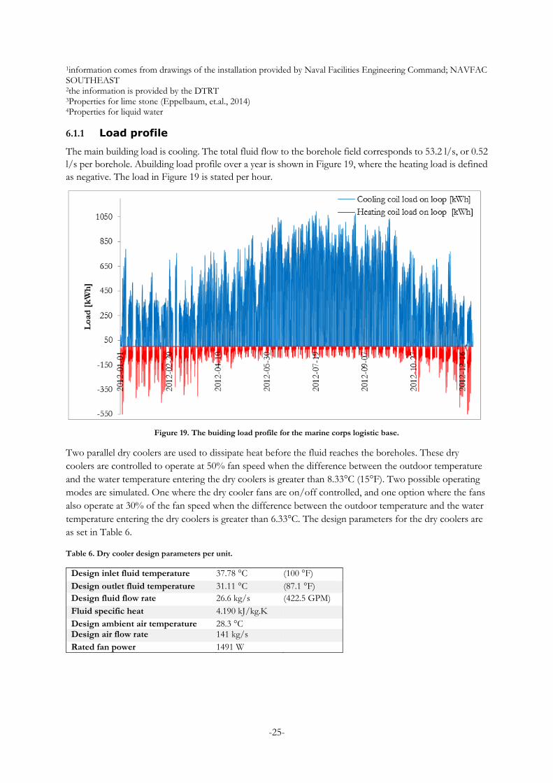
6.1.1 Load profile

The main building load is cooling. The total fluid flow to the borehole field corresponds to 53.2 l/s, or 0.52

l/s per borehole. Abuilding load profile over a year is shown in Figure 19, where the heating load is defined

as negative. The load in Figure 19 is stated per hour.

Figure 19. The buiding load profile for the marine corps logistic base.

Two parallel dry coolers are used to dissipate heat before the fluid reaches the boreholes. These dry

coolers are controlled to operate at 50% fan speed when the difference between the outdoor temperature

and the water temperature entering the dry coolers is greater than 8.33°C (15°F). Two possible operating

modes are simulated. One where the dry cooler fans are on/off controlled, and one option where the fans

also operate at 30% of the fan speed when the difference between the outdoor temperature and the water

temperature entering the dry coolers is greater than 6.33°C. The design parameters for the dry coolers are

as set in Table 6.

Table 6. Dry cooler design parameters per unit.

Design inlet fluid temperature 37.78 °C (100 °F)

Design outlet fluid temperature 31.11 °C (87.1 °F)

Design fluid flow rate 26.6 kg/s (422.5 GPM)

Fluid specific heat 4.190 kJ/kg.K

Design ambient air temperature 28.3 °C Design air flow rate 141 kg/s

Rated fan power 1491 W

-26-

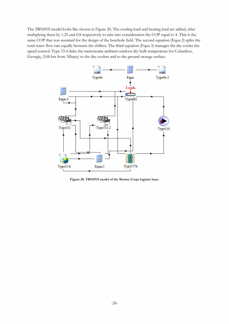
The TRNSYS model looks like shown in Figure 20. The cooling load and heating load are added, after

multiplying them by 1.25 and 0.8 respectively to take into consideration the COP equal to 4. This is the

same COP that was assumed for the design of the borehole field. The second equation (Equa 2) splits the

total water flow rate equally between the chillers. The third equation (Equa 3) manages the dry cooler fan

speed control. Type 15-6 links the metronome ambient outdoor dry bulb temperature for Columbus,

Georgia, (168 km from Albany) to the dry coolers and to the ground storage surface.

Figure 20. TRNSYS model of the Marine Corps logistic base.

-27-

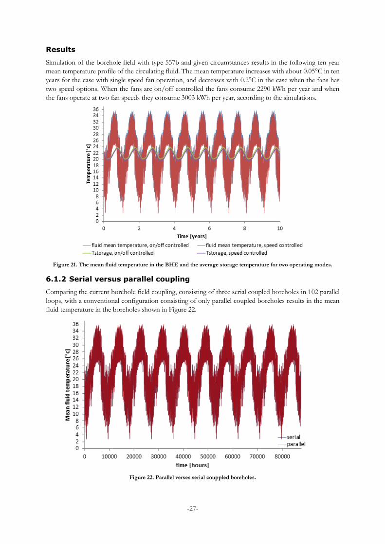
Results

Simulation of the borehole field with type 557b and given circumstances results in the following ten year

mean temperature profile of the circulating fluid. The mean temperature increases with about 0.05°C in ten

years for the case with single speed fan operation, and decreases with 0.2°C in the case when the fans has

two speed options. When the fans are on/off controlled the fans consume 2290 kWh per year and when

the fans operate at two fan speeds they consume 3003 kWh per year, according to the simulations.

Figure 21. The mean fluid temperature in the BHE and the average storage temperature for two operating modes.

6.1.2 Serial versus parallel coupling

Comparing the current borehole field coupling, consisting of three serial coupled boreholes in 102 parallel

loops, with a conventional configuration consisting of only parallel coupled boreholes results in the mean

fluid temperature in the boreholes shown in Figure 22.

Figure 22. Parallel verses serial couppled boreholes.

-28-

The way the boreholes are coupled with three serial loops per parallel loop gives different possibilities than

if all loops would have been coupled in parallel. In the simulation, the total flow rate is set the same for the

two serial and parallel coupled options. Whether the flow goes from the circumference of the borehole field

or in the other direction, is not considered by the 557b module since the storage volume temperature is

considered to be constant.

The simulations show no significant difference between using parallel versus seral coupled BHE, using type

557b. The effect of having serial coupled boreholes could be investigated further, using other tools,

specifically when information about measured load profile is available.

-29-

7 Conclusions

When the modules are used for simulations of a single borehole and compared to measured data, to see

how they perform on long and short term. Type 203, 557a and 557b have a quicker changing average fluid

temperature in comparison to measured data and type 243, 244, 246 and 451, after a changed load, see

Figure 5, Figure 6 and Figure 7. This due to the neglect ion of borehole thermal capacity in these modules.

The analytical approach, i.e. FLS, ILS or CSM, has impact on type 243, 244 and 246. Using type 244 or

246 with dual u-pipes, for simulations of boreholes with single u-pipes gives a different borehole thermal

resistance and conductivity within the borehole. Type 557b proves to predict the inlet and outlet

temperatures of the borehole within a smaller tolerance range than the other modules on the 0h-75h time

range, see figure 6 and figure 7. This is due to the great advantage of inserting the true thermal resistance

of the borehole.

The fluid temperature were simulated for multiple borehole fields with type 246, 557a and 557b, and

compared to measured borehole temperature. In the simulation of the IKEA installation in Uppsala the

types diverged about 1°c from each other when after five years. All three modulus appears suitable for

installations with a balanced heating and cooling load over the year, and where the borehole distribution is

compact. Type 557b can model serial coupled borehole fields. Type 557b uses a storage volume with

uniform temperature, and therefore the impact of the direction of the flow, i.e. inwards or outwards from

the centre of the borehole field is not considered in the module.

-30-

8 Discussion and final remarks

One of the main advantages with TRNSYS is the possibility to combine predefined components to model

a complete system configuration that takes the dynamic behaviour of the processes into account. The

control has great impact on the system performance and this is something that can be investigated using

the software. Nevertheless, the design of borehole fields is usually done in early stages of the construction

process. At this point, the design parameters are commonly roughly estimated and the final control

strategy yet not determined. The resulting ground and fluid temperatures are dependent on, except from a

good BHE model, the accuracy of other parameters, such as load profiles, how the system is controlled

etc.

If a borehole field installation is to be simulated where the distribution of the boreholes is not cylindrical

nor can be estimated as it, type 246 should be considered. This is the only evaluated module for borehole

fields where the layout of the boreholes can be freely set and is managed by the attached g-function.

Using the TRNSYS for design of vertical borehole installations can be done, but possibilities of finding the

best design for the borehole field layout are limited. Of the types that can manage borehole fields; type 557a

and 557b has a fixed layout, and for type 246 a g-function has to be generated for each installation.

Therefore, optimization of the system might be more easily be done in other software. Verification and

analysis of the suitability of a set design is, however, a suitable area of use for TRNSYS.

The TRNSYS program also has some drawbacks. It does not always solve for a solution for the modelled

system as desired. Using a too short time step often results in problems to solve for the solution and division

by zero in some of the .dll files Other issues appear in the types and their source code. When flow rates

were set to low values, in the simulations preformed for this investigation, the fluid temperature in the u-

pipe soon converged to vertical asymptotes. When using type 451, the desired inner u-pipe diameter could

not be set and had to be reduced by 1.5mm, which is an issue with the type.

One has to be cautious about which units are used for the parameter and input values. For example, the

borehole thermal resistance must be entered in Km/(kJ/h) for type 557b and the ground specific heat is

volumetric for type 541 and not based on mass as the case for the other types. One also has to make sure

that the outputs from one unit supplying input values for another unit uses the same unit.

The Types 557a and 557b of DST type are considerable quicker for long term simulations with many time

steps. The Types 557 are about six times faster than type 246.

Bibliography

BANDOS, T. V. et al. Finite line-source model for borehole heat exchangers: effect of vertical temperature variations 2009.

BERNIER, M.; SHIRAZI, A. S. Thermal capacity effects in borehole ground heat exchangers. École Polytechnique de Montréal, Département de Génie Mécanique, Case postale 6079, succursale «centre-ville», Montréal, Québec, Canada H3C 3A7 2013.

BERNIER, M. A. Closed-Loop Ground-Coupled Heat Pump Systems: ASHRAE Journal: 8 p. 2006.

CLAESSON, J.; ESKILSON, P. Conductive heat extraction to a deep borehole: thermal analyses and dimensioning rules. Department of Building Technology, Lund Institute of Technology, Lund, Sweden 1988.

CULLIN, J. R. et al. Validation of vertical ground heat exchanger design methodologies 2015.

EPPELBAUM, L.; KUTASOV, I.; PILCHIN, A. Applied Geothermics. 2014.

ESKILSON, P. Superposition Borehole Model. Manual for Computer Code. Lund, Sweden: Department of Mathematical Physics, Lund Institute of technology 1986.

ESKILSON, P. Thermal analysis of heat extraction boreholes. 1987. (Doctor). Mathematical Physics and building technology, University of Lud, Sweden.

ESLAMI-NEJAD, P.; BERNIER, M. Coupling of geothermal heat pumps with thermal solar collectors using double U-tube boreholes with twoindependent circuits 2011.

Finspångs Brunnsborrning, Projektdokumentation. 2009.

HELLSTRÖM, G. Duct Ground Heat Storage Model, Manual for Computer CodeDepartment of Mathematical Physics. University of Lund, Box 118, SE-211 00 Lund, Sweden 1989.

Hellström, G. Thermal performance of borehole heat exchangers. Department of Mathematical Physics, Lund Institute of Technology 1998.

HUBER, A.; SCHULER, O. Berechnungsmodul für Erdwärmesonden. Im Auftrag des Bundesamtes für Energiewirtschaft. Zürich 1997.

KIM, E.-J. et al. A hybrid reduced model for borehole heat exchangers over different time-scales and regions 2014.

-32-

LAMARCHE, L. A fast algorithm for the hourly simulations of ground-source heat pumps using arbitrary response factors. E´cole de Technologie Supe´rieure, 1100 Notre-Dame Ouest, Montre´al, Canada H3C 1K3 2007.

LAMARCHE, L. Short-term behavior of classical analytic solutions for the design of ground-source heat pumps. 1100 Notre-Dame Ouest, Montréal, Canada H3C 1K3: École de Technologie Supérieure 2013.

LAMARCHE, L.; BEAUCHAMP, B. New solutions for the short-time analysis of geothermal vertical boreholes. Ecole de Technologie Supe´reure, 1100 Notre-Dame Ouest, Montre´ al, Canada H3C 1K3 2006.

MICHEL A. BERNIER, P. P., RICHARD LABIB & RAPHAËL PAILLOT. A Multiple Load Aggregation Algorithm for Annual Hourly Simulations of GCHP Systems: HVAC&R Research 2004.

OCHS, F.; CARBONELL, D.; HALLER, M. Models of Sub-Components and Validation for the IEA SHC Task 44 / HPP Annex 38 Part D: Ground Heat Exchangers. 2013

PAHUD, D. D. The Superposition Borehole Model for TRNSYS 16 or 17 (TRNSBM). User manual for the April 2012 version Internal Report. Lugano: Scuola universitaria professionale della Svezzera italiana, Dipartimiento ambiente costruzionie design 2012.

PÄRISCH, P. et al. Short-term experiments with borehole heat exchangers and model validation in TRNSYS: Institut für Solarenergieforschung Hameln GmbH (ISFH), Am Ohrberg 1, D-31860 Emmerthal, Germany, Universität Göttingen, Geowissenschaftliches Zentrum, Goldschmidtstraße 3, D-37077 Göttingen, Germany 2013.

SAFA, A. A.; FUNG, A. S.; KUMAR, R. Heating and cooling performance characterisation of ground source heat pump system by testing and TRNSYS simulation. Ryerson University, Toronto ON M5B 2K3, Canada: Department of Mechanical and Industrial Engineering, Ryerson University,: 11 p. 2015.

TESS Component Librariees General Descriptions.

WETTER, M.; HUBER, A. TRNSYS Type 451 Vertical Borehole Heat Exchanger EWS Model 1997.

ZENG, H.; DIAO, N.; FANG, Z. A finite line-source model for boreholes in geothermal heat exchangers Heat Transfer - Asian Research. 31: 558-567 p. 2002.