practical genetic algorithmsyag.es/genetic-algorithm/r.l.haupt, s.e.haupt - practical genetic... ·...
TRANSCRIPT

PRACTICAL GENETIC ALGORITHMS
PRACTICAL GENETICALGORITHMSSECOND EDITION
Randy L. HauptSue Ellen Haupt
A JOHN WILEY & SONS, INC., PUBLICATION
The book is printed on acid-free paper.
Copyright © 2004 by John Wiley & Sons, Inc. All rights reserved.
Published by John Wiley & Sons, Inc., Hoboken, New Jersey.Published simultaneously in Canada.
No part of this publication may be reproduced, stored in a retrieval system, or transmitted inany form or by any means, electronic, mechanical, photocopying, recording, scanning, or other-wise, except as permitted under Section 107 or 108 of the 1976 United States Copyright Act,without either the prior written permission of the Publisher, or authorization through paymentof the appropriate per-copy fee to the Copyright Clearance Center, Inc., 222 Rosewood Drive,Danvers, MA 01923, 978-750-8400, fax 978-646-8600, or on the web at www.copyright.com.Requests to the Publisher for permission should be addressed to the Permissions Department,John Wiley & Sons, Inc., 111 River Street, Hoboken, NJ 07030, (201) 748-6011,fax (201) 748-6008.
Limit of Liability/Disclaimer of Warranty: While the publisher and author have used their bestefforts in preparing this book, they make no representations or warranties with respect to theaccuracy or completeness of the contents of this book and specifically disclaim any impliedwarranties of merchantability or fitness for a particular purpose. No warranty may be createdor extended by sales representatives or written sales materials. The advice and strategies con-tained herein may not be suitable for your situation. You should consult with a professionalwhere appropriate. Neither the publisher nor author shall be liable for any loss of profit or anyother commercial damages, including but not limited to special, incidental, consequential, orother damages.
For general information on our other products and services please contact our Customer Care Department within the U.S. at 877-762-2974, outside the U.S. at 317-572-3993 or fax 317-572-4002.
Wiley also publishes its books in a variety of electronic formats. Some content that appears inprint, however, may not be available in electronic format.
Library of Congress Cataloging-in-Publication Data:Haupt, Randy L.
Practical genetic algorithms / Randy L. Haupt, Sue Ellen Haupt.—2nd ed.p. cm.
Red. ed. of: Practical genetic algorithms. c1998.“A Wiley-Interscience publication.”Includes bibliographical references and index.ISBN 0-471-45565-21. Genetic algorithms. I. Haupt, S. E. II. Haupt, Randy L. Practical genetic algorithms.
III. Title.QA402.5.H387 2004519.6¢2—dc22 2004043360
Printed in the Untied States of America
10 9 8 7 6 5 4 3 2 1

To our parents Anna Mae and Howard Haupt
Iona and Charles Slagle and
our offspring,Bonny Ann and Amy Jean Haupt
CONTENTS
Preface xi
Preface to First Edition xiii
List of Symbols xv
1 Introduction to Optimization 1
1.1 Finding the Best Solution 11.1.1 What Is Optimization? 21.1.2 Root Finding versus Optimization 31.1.3 Categories of Optimization 3
1.2 Minimum-Seeking Algorithms 51.2.1 Exhaustive Search 51.2.2 Analytical Optimization 71.2.3 Nelder-Mead Downhill Simplex Method 101.2.4 Optimization Based on Line Minimization 13
1.3 Natural Optimization Methods 181.4 Biological Optimization: Natural Selection 191.5 The Genetic Algorithm 22Bibliography 24Exercises 25
2 The Binary Genetic Algorithm 27
2.1 Genetic Algorithms: Natural Selection on a Computer 272.2 Components of a Binary Genetic Algorithm 28
2.2.1 Selecting the Variables and the Cost Function 30
2.2.2 Variable Encoding and Decoding 322.2.3 The Population 362.2.4 Natural Selection 362.2.5 Selection 382.2.6 Mating 412.2.7 Mutations 432.2.8 The Next Generation 442.2.9 Convergence 47
vii
viii CONTENTS
2.3 A Parting Look 47Bibliography 49Exercises 49
3 The Continuous Genetic Algorithm 51
3.1 Components of a Continuous Genetic Algorithm 523.1.1 The Example Variables and Cost Function 523.1.2 Variable Encoding, Precision, and Bounds 533.1.3 Initial Population 543.1.4 Natural Selection 543.1.5 Pairing 563.1.6 Mating 563.1.7 Mutations 603.1.8 The Next Generation 623.1.9 Convergence 64
3.2 A Parting Look 65Bibliography 65Exercises 65
4 Basic Applications 67
4.1 “Mary Had a Little Lamb” 674.2 Algorithmic Creativity—Genetic Art 714.3 Word Guess 754.4 Locating an Emergency Response Unit 774.5 Antenna Array Design 814.6 The Evolution of Horses 864.5 Summary 92Bibliography 92
5 An Added Level of Sophistication 95
5.1 Handling Expensive Cost Functions 955.2 Multiple Objective Optimization 97
5.2.1 Sum of Weighted Cost Functions 995.2.2 Pareto Optimization 99
5.3 Hybrid GA 1015.4 Gray Codes 1045.5 Gene Size 1065.6 Convergence 1075.7 Alternative Crossovers for Binary GAs 1105.8 Population 1175.9 Mutation 1215.10 Permutation Problems 1245.11 Selecting GA Parameters 127
CONTENTS ix
5.12 Continuous versus Binary GA 1355.13 Messy Genetic Algorithms 1365.14 Parallel Genetic Algorithms 137
5.14.1 Advantages of Parallel GAs 1385.14.2 Strategies for Parallel GAs 1385.14.3 Expected Speedup 1415.14.4 An Example Parallel GA 1445.14.5 How Parallel GAs Are Being Used 145
Bibliography 145Exercises 148
6 Advanced Applications 151
6.1 Traveling Salesperson Problem 1516.2 Locating an Emergency Response Unit Revisited 1536.3 Decoding a Secret Message 1556.4 Robot Trajectory Planning 1566.5 Stealth Design 1616.6 Building Dynamic Inverse Models—The Linear Case 1656.7 Building Dynamic Inverse Models—The Nonlinear Case 1706.8 Combining GAs with Simulations—Air Pollution
Receptor Modeling 1756.9 Optimizing Artificial Neural Nets with GAs 1796.10 Solving High-Order Nonlinear Partial Differential
Equations 182Bibliography 184
7 More Natural Optimization Algorithms 187
7.1 Simulated Annealing 1877.2 Particle Swarm Optimization (PSO) 1897.3 Ant Colony Optimization (ACO) 1907.4 Genetic Programming (GP) 1957.5 Cultural Algorithms 1997.6 Evolutionary Strategies 1997.7 The Future of Genetic Algorithms 200Bibliography 201Exercises 202
Appendix I Test Functions 205
Appendix II MATLAB Code 211
Appendix III High-Performance Fortran Code 233
Glossary 243
Index 251
PREFACE
When we agreed to edit this book for a second edition, we looked forward toa bit of updating and including some of our latest research results. However,the effort grew rapidly beyond our original vision. The use of genetic algo-rithms (GAs) is a quickly evolving field of research, and there is much new torecommend. Practitioners are constantly dreaming up new ways to improveand use GAs. Therefore this book differs greatly from the first edition.
We continue to emphasize the “Practical” part of the title. This book waswritten for the practicing scientist, engineer, economist, artist, and whoevermight possibly become interested in learning the basics of GAs. We make noclaims of including the latest research on convergence theory: instead, we referthe reader to references that do. We do, however, give the reader a flavor for how GAs are being used and how to fiddle with them to get the best performance.
The biggest addition is including code—both MATLAB and a bit of High-Performance Fortran. We hope the readers find these a useful start to theirown applications. There has also been a good bit of updating and expanding.Chapter 1 has been rewritten to give a more complete picture of traditionaloptimization. Chapters 2 and 3 remain dedicated to introducing the mechan-ics of the binary and continuous GA. The examples in those chapters, as wellas throughout the book, now reflect our more recent research on choosing GAparameters. Examples have been added to Chapters 4 and 6 that broaden theview of problems being solved. Chapter 5 has greatly expanded its recom-mendations of methods to improve GA performance. Sections have beenadded on hybrid GAs, parallel GAs, and messy GAs. Discussions of parame-ter selection reflect new research. Chapter 7 is new. Its purpose is to give thereader a flavor for other artificial intelligence methods of optimization, likesimulated annealing, ant colony optimization, and evolutionary strategies. Wehope this will help put GAs in context with other modern developments. Weincluded code listings and test functions in the appendixes. Exercises appearat the end of each chapter. There is no solution manual because the exercisesare open-ended. These should be helpful to anyone wishing to use this bookas a text.
In addition to the people thanked in the first edition, we want to recognizethe students and colleagues whose insight has contributed to this effort. BonnyHaupt did the work included in Section 4.6 on horse evolution. Jaymon Knighttranslated our GA to High-Performance Fortran. David Omer and Jesse
xi

xii PREFACE
Warrick each had a hand in the air pollution problem of Section 6.8. We’vediscussed our applications with numerous colleagues and appreciate theirfeedback.
We wish the readers well in their own forays into using GAs. We lookforward to seeing their interesting applications in the future.
Randy L. HauptState College, Pennsylvania Sue Ellen HauptFebruary 2004
PREFACE TO FIRST EDITION
The book has been organized to take the genetic algorithm in stages. Chapter1 lays the foundation for the genetic algorithm by discussing numerical opti-mization and introducing some of the traditional minimum seeking algorithms.Next, the idea of modeling natural processes on the computer is introducedthrough a discussion of annealing and the genetic algorithm. A brief geneticsbackground is supplied to help the reader understand the terminology andrationale for the genetic operators.The genetic algorithm comes in two flavors:binary parameter and real parameter. Chapter 2 provides an introduction tothe binary genetic algorithm, which is the most common form of the algorithm.Parameters are quantized, so there are a finite number of combinations. Thisform of the algorithm is ideal for dealing with parameters that can assumeonly a finite number of values. Chapter 3 introduces the continuous parame-ter genetic algorithm.This algorithm allows the parameters to assume any realvalue within certain constraints. Chapter 4 uses the algorithms developed inthe previous chapters to solve some problems of interest to engineers and sci-entists. Chapter 5 returns to building a good genetic algorithm, extending andexpanding upon some of the components of the genetic algorithm. Chapter 6attacks more difficult technical problems. Finally, Chapter 7 surveys some ofthe current extensions to genetic algorithms and applications, and gives adviceon where to get more information on genetic algorithms. Some aids are sup-plied to further help the budding genetic algorithmist. Appendix I lists somegenetic algorithm routines in pseudocode.A glossary and a list of symbols usedin this book are also included.
We are indebted to several friends and colleagues for their help. First, ourthanks goes to Dr. Christopher McCormack of Rome Laboratory for intro-ducing us to genetic algorithms several years ago. The idea for writing thisbook and the encouragement to write it, we owe to Professor Jianming Jin ofthe University of Illinois. Finally, the excellent reviews by Professor DanielPack, Major Cameron Wright, and Captain Gregory Toussaint of the UnitedStates Air Force Academy were invaluable in the writing of this manuscript.
Randy L. HauptSue Ellen Haupt
Reno, NevadaSeptember 1997
xiii
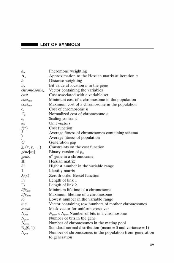
LIST OF SYMBOLS
aN Pheromone weightingAn Approximation to the Hessian matrix at iteration nb Distance weightingbn Bit value at location n in the genechromosomen Vector containing the variablescost Cost associated with a variable setcostmin Minimum cost of a chromosome in the populationcostmax Maximum cost of a chromosome in the populationcn Cost of chromosome nCn Normalized cost of chromosome ncs Scaling constanteN Unit vectorsf(*) Cost functionf� Average fitness of chromosomes containing schemaf Average fitness of populationG Generation gapgm(x, y, . . .) Constraints on the cost functiongene[m] Binary version of pn
genen nth gene in a chromosomeH Hessian matrixhi Highest number in the variable rangeI Identity matrixJ0(x) Zeroth-order Bessel functionG1 Length of link 1G2 Length of link 2lifemin Minimum lifetime of a chromosomelifemax Maximum lifetime of a chromosomelo Lowest number in the variable rangema Vector containing row numbers of mother chromosomesmask Mask vector for uniform crossoverNbits Ngene ¥ Npar. Number of bits in a chromosomeNgene Number of bits in the geneNkeep Number of chromosomes in the mating poolNn(0, 1) Standard normal distribution (mean = 0 and variance = 1)Npop Number of chromosomes in the population from generation
to generation
xv
Nvar Number of variablesoffspringn Child created from mating two chromosomespa Vector containing row numbers of father chromosomesparentn A parent selected to matepdn Continuous variable n in the father chromosome pmn Continuous variable n in the mother chromosomepm,n
local best Best local solutionpm,n
global best Best global solutionpn Variable npnew New variable in offspring from crossover in a continuous GApnorm Normalized variablepquant Quantized variableplo Smallest variable valuephi Highest variable valueP Number of processorsPc Probability of crossoverPm Probability of mutation of a single bitPn Probability of chromosome n being selected for matingPopt Number of processors to optimize speedup of a parallel GAPt Probability of the schema being selected to survive to the next
generationP0 Initial guess for Nelder-Mead algorithmqn Quantized version of Pn
Q Quantization vector = [2-1 2-2 . . . ]Qi Number of different values that variable i can haveQt Probability of the schema being selected to mater Uniform random numberRt Probability of the schema not being destroyed by crossoveror
mutations sin jst Number of schemata in generation tT Temperature in simulated annealingTc CPU time required for communicationTf CPU time required to evaluate a fitness functionT0 Beginning temperature in simulated annealingTN Ending temperature in simulated annealingTP Total execution time for a generation of a parallel GAu cos jV Number of different variable combinationsnn Search direction at step nnm,n Particle velocitywn Weight nXrate Crossover ratex, y, z Unit vectors in the x, y, and z directionsa Parameter where crossover occurs
2 -Ngene
xvi LIST OF SYMBOLS
ak Step size at iteration kb Mixing value for continuous variable crossoverd Distance between first and last digit in schema
—f
—2f
e Elite path weighting constantgn Nonnegative scalar that minimizes the function in the
direction of the gradientk Lagrange multiplierl Wavelengthz Number of defined digits in schemah 1–
2(lifemax - lifemin)m Mutation rates Standard deviation of the normal distributiont Pheromone strengthtk
mn Pheromone laid by ant k between city m and city ntmn
elite Pheromone laid on the best path found by the algorithm to this point
x Pheromone evaporation constant
∂∂
+∂∂
+∂∂
2
2
2
2
2
2
fx
fy
fz
∂+
∂∂
+∂∂
fx
xfy
yfz
z∂
ˆ ˆ ˆ
LIST OF SYMBOLS xvii
CHAPTER 1
Introduction to Optimization
1
Optimization is the process of making something better. An engineer or sci-entist conjures up a new idea and optimization improves on that idea. Opti-mization consists in trying variations on an initial concept and using theinformation gained to improve on the idea. A computer is the perfect tool foroptimization as long as the idea or variable influencing the idea can be inputin electronic format. Feed the computer some data and out comes the solu-tion. Is this the only solution? Often times not. Is it the best solution? That’sa tough question. Optimization is the math tool that we rely on to get theseanswers.
This chapter begins with an elementary explanation of optimization, thenmoves on to a historical development of minimum-seeking algorithms. Aseemingly simple example reveals many shortfalls of the typical minimumseekers. Since the local optimizers of the past are limited, people have turnedto more global methods based upon biological processes. The chapter endswith some background on biological genetics and a brief introduction to thegenetic algorithm (GA).
1.1 FINDING THE BEST SOLUTION
The terminology “best” solution implies that there is more than one solutionand the solutions are not of equal value. The definition of best is relative tothe problem at hand, its method of solution, and the tolerances allowed. Thusthe optimal solution depends on the person formulating the problem. Educa-tion, opinions, bribes, and amount of sleep are factors influencing the defini-tion of best. Some problems have exact answers or roots, and best has a specificdefinition. Examples include best home run hitter in baseball and a solutionto a linear first-order differential equation. Other problems have variousminimum or maximum solutions known as optimal points or extrema, and bestmay be a relative definition. Examples include best piece of artwork or bestmusical composition.
Practical Genetic Algorithms, Second Edition, by Randy L. Haupt and Sue Ellen Haupt.ISBN 0-471-45565-2 Copyright © 2004 John Wiley & Sons, Inc.
1.1.1 What Is Optimization?
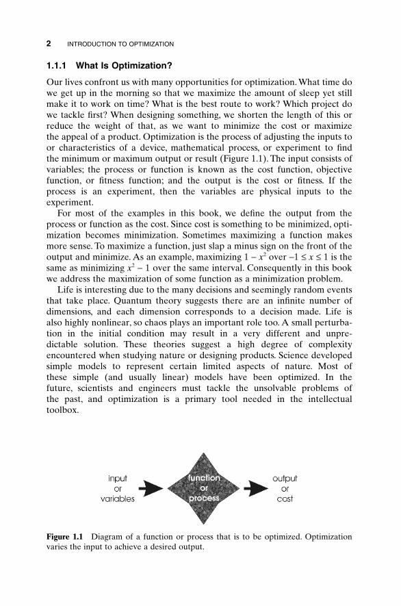
Our lives confront us with many opportunities for optimization. What time dowe get up in the morning so that we maximize the amount of sleep yet stillmake it to work on time? What is the best route to work? Which project dowe tackle first? When designing something, we shorten the length of this orreduce the weight of that, as we want to minimize the cost or maximize the appeal of a product. Optimization is the process of adjusting the inputs toor characteristics of a device, mathematical process, or experiment to find the minimum or maximum output or result (Figure 1.1). The input consists ofvariables; the process or function is known as the cost function, objective function, or fitness function; and the output is the cost or fitness. If the process is an experiment, then the variables are physical inputs to the experiment.
For most of the examples in this book, we define the output from theprocess or function as the cost. Since cost is something to be minimized, opti-mization becomes minimization. Sometimes maximizing a function makesmore sense. To maximize a function, just slap a minus sign on the front of theoutput and minimize. As an example, maximizing 1 - x2 over -1 £ x £ 1 is thesame as minimizing x2 - 1 over the same interval. Consequently in this bookwe address the maximization of some function as a minimization problem.
Life is interesting due to the many decisions and seemingly random eventsthat take place. Quantum theory suggests there are an infinite number ofdimensions, and each dimension corresponds to a decision made. Life is also highly nonlinear, so chaos plays an important role too. A small perturba-tion in the initial condition may result in a very different and unpre-dictable solution. These theories suggest a high degree of complexity encountered when studying nature or designing products. Science developedsimple models to represent certain limited aspects of nature. Most of these simple (and usually linear) models have been optimized. In the future, scientists and engineers must tackle the unsolvable problems of the past, and optimization is a primary tool needed in the intellectual toolbox.
2 INTRODUCTION TO OPTIMIZATION
Figure 1.1 Diagram of a function or process that is to be optimized. Optimizationvaries the input to achieve a desired output.
1.1.2 Root Finding versus Optimization
Approaches to optimization are akin to root or zero finding methods, onlyharder. Bracketing the root or optimum is a major step in hunting it down.For the one-variable case, finding one positive point and one negative pointbrackets the zero. On the other hand, bracketing a minimum requires threepoints, with the middle point having a lower value than either end point. Inthe mathematical approach, root finding searches for zeros of a function, whileoptimization finds zeros of the function derivative. Finding the function deriv-ative adds one more step to the optimization process. Many times the deriva-tive does not exist or is very difficult to find. We like the simplicity of rootfinding problems, so we teach root finding techniques to students of engi-neering, math, and science courses. Many technical problems are formulatedto find roots when they might be more naturally posed as optimization problems; except the toolbox containing the optimization tools is small andinadequate.
Another difficulty with optimization is determining if a given minimum isthe best (global) minimum or a suboptimal (local) minimum. Root findingdoesn’t have this difficulty. One root is as good as another, since all roots forcethe function to zero.
Finding the minimum of a nonlinear function is especially difficult. Typicalapproaches to highly nonlinear problems involve either linearizing theproblem in a very confined region or restricting the optimization to a smallregion. In short, we cheat.
1.1.3 Categories of Optimization
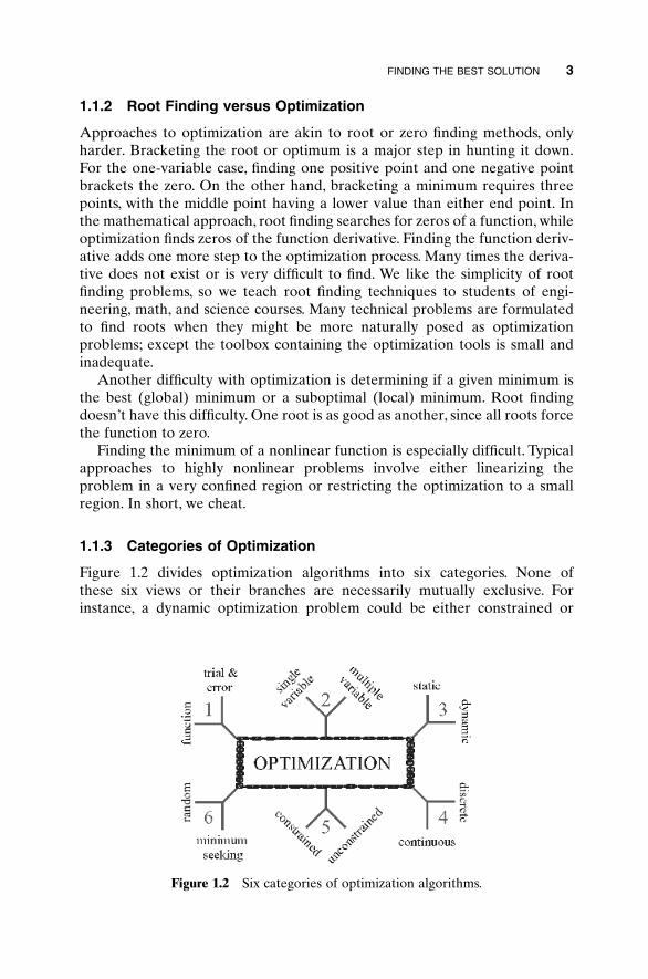
Figure 1.2 divides optimization algorithms into six categories. None of these six views or their branches are necessarily mutually exclusive. Forinstance, a dynamic optimization problem could be either constrained or
FINDING THE BEST SOLUTION 3
Figure 1.2 Six categories of optimization algorithms.
unconstrained. In addition some of the variables may be discrete and otherscontinuous. Let’s begin at the top left of Figure 1.2 and work our way aroundclockwise.
1. Trial-and-error optimization refers to the process of adjusting variablesthat affect the output without knowing much about the process that producesthe output. A simple example is adjusting the rabbit ears on a TV to get thebest picture and audio reception. An antenna engineer can only guess at whycertain contortions of the rabbit ears result in a better picture than other con-tortions. Experimentalists prefer this approach. Many great discoveries, likethe discovery and refinement of penicillin as an antibiotic, resulted from thetrial-and-error approach to optimization. In contrast, a mathematical formuladescribes the objective function in function optimization. Various mathemat-ical manipulations of the function lead to the optimal solution. Theoreticianslove this theoretical approach.
2. If there is only one variable, the optimization is one-dimensional. Aproblem having more than one variable requires multidimensional optimiza-tion. Optimization becomes increasingly difficult as the number of dimensionsincreases. Many multidimensional optimization approaches generalize to aseries of one-dimensional approaches.
3. Dynamic optimization means that the output is a function of time, whilestatic means that the output is independent of time.When living in the suburbsof Boston, there were several ways to drive back and forth to work. What wasthe best route? From a distance point of view, the problem is static, and thesolution can be found using a map or the odometer of a car. In practice, thisproblem is not simple because of the myriad of variations in the routes. Theshortest route isn’t necessarily the fastest route. Finding the fastest route is adynamic problem whose solution depends on the time of day, the weather,accidents, and so on. The static problem is difficult to solve for the best solu-tion, but the added dimension of time increases the challenge of solving thedynamic problem.
4. Optimization can also be distinguished by either discrete or continuousvariables. Discrete variables have only a finite number of possible values,whereas continuous variables have an infinite number of possible values. If weare deciding in what order to attack a series of tasks on a list, discrete opti-mization is employed. Discrete variable optimization is also known as com-binatorial optimization, because the optimum solution consists of a certaincombination of variables from the finite pool of all possible variables.However, if we are trying to find the minimum value of f(x) on a number line,it is more appropriate to view the problem as continuous.
5. Variables often have limits or constraints. Constrained optimizationincorporates variable equalities and inequalities into the cost function. Uncon-strained optimization allows the variables to take any value. A constrainedvariable often converts into an unconstrained variable through a transforma-
4 INTRODUCTION TO OPTIMIZATION
tion of variables. Most numerical optimization routines work best with uncon-strained variables. Consider the simple constrained example of minimizing f(x) over the interval -1 £ x £ 1. The variable converts x into an unconstrainedvariable u by letting x = sin(u) and minimizing f(sin(u)) for any value of u.When constrained optimization formulates variables in terms of linear equations and linear constraints, it is called a linear program. When the costequations or constraints are nonlinear, the problem becomes a nonlinear programming problem.
6. Some algorithms try to minimize the cost by starting from an initial set of variable values. These minimum seekers easily get stuck in local minimabut tend to be fast. They are the traditional optimization algorithms and aregenerally based on calculus methods. Moving from one variable set to anotheris based on some determinant sequence of steps. On the other hand, randommethods use some probabilistic calculations to find variable sets. They tend tobe slower but have greater success at finding the global minimum.
1.2 MINIMUM-SEEKING ALGORITHMS
Searching the cost surface (all possible function values) for the minimum costlies at the heart of all optimization routines. Usually a cost surface has manypeaks, valleys, and ridges. An optimization algorithm works much like a hikertrying to find the minimum altitude in Rocky Mountain National Park. Start-ing at some random location within the park, the goal is to intelligentlyproceed to find the minimum altitude. There are many ways to hike or glis-sade to the bottom from a single random point. Once the bottom is found,however, there is no guarantee that an even lower point doesn’t lie over thenext ridge. Certain constraints, such as cliffs and bears, influence the path ofthe search as well. Pure downhill approaches usually fail to find the globaloptimum unless the cost surface is quadratic (bowl-shaped).
There are many good texts that describe optimization methods (e.g.,Press et al., 1992; Cuthbert, 1987). A history is given by Boyer and Merzbach(1991). Here we give a very brief review of the development of optimizationstrategies.
1.2.1 Exhaustive Search
The brute force approach to optimization looks at a sufficiently fine sam-pling of the cost function to find the global minimum. It is equivalent to spend-ing the time, effort, and resources to thoroughly survey Rocky MountainNational Park. In effect a topographical map can be generated by connectinglines of equal elevation from an interpolation of the sampled points.This exhaustive search requires an extremely large number of cost functionevaluations to find the optimum. For example, consider solving the two-dimensional problem
MINIMUM-SEEKING ALGORITHMS 5
(1.1)
(1.2)
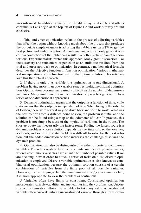
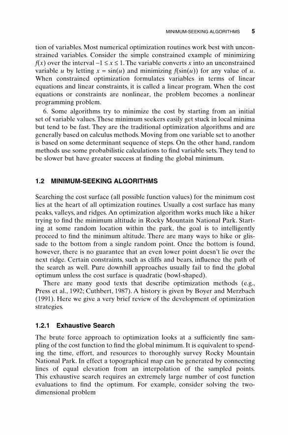
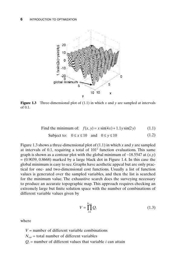
Figure 1.3 shows a three-dimensional plot of (1.1) in which x and y are sampledat intervals of 0.1, requiring a total of 1012 function evaluations. This samegraph is shown as a contour plot with the global minimum of -18.5547 at (x,y)= (0.9039, 0.8668) marked by a large black dot in Figure 1.4. In this case theglobal minimum is easy to see. Graphs have aesthetic appeal but are only prac-tical for one- and two-dimensional cost functions. Usually a list of functionvalues is generated over the sampled variables, and then the list is searchedfor the minimum value. The exhaustive search does the surveying necessaryto produce an accurate topographic map. This approach requires checking anextremely large but finite solution space with the number of combinations ofdifferent variable values given by
(1.3)
where
V = number of different variable combinationsNvar = total number of different variablesQi = number of different values that variable i can attain
V Qii
Nvar
==
’1
Subject to: and0 10 0 10£ £ £ £x y
Find the minimum of: f x y x x y y, sin . sin( ) = ( ) + ( )4 1 1 2
6 INTRODUCTION TO OPTIMIZATION
Figure 1.3 Three-dimensional plot of (1.1) in which x and y are sampled at intervalsof 0.1.
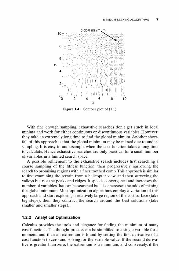
With fine enough sampling, exhaustive searches don’t get stuck in localminima and work for either continuous or discontinuous variables. However,they take an extremely long time to find the global minimum. Another short-fall of this approach is that the global minimum may be missed due to under-sampling. It is easy to undersample when the cost function takes a long timeto calculate. Hence exhaustive searches are only practical for a small numberof variables in a limited search space.
A possible refinement to the exhaustive search includes first searching acoarse sampling of the fitness function, then progressively narrowing thesearch to promising regions with a finer toothed comb.This approach is similarto first examining the terrain from a helicopter view, and then surveying thevalleys but not the peaks and ridges. It speeds convergence and increases thenumber of variables that can be searched but also increases the odds of missingthe global minimum. Most optimization algorithms employ a variation of thisapproach and start exploring a relatively large region of the cost surface (takebig steps); then they contract the search around the best solutions (takesmaller and smaller steps).
1.2.2 Analytical Optimization
Calculus provides the tools and elegance for finding the minimum of manycost functions. The thought process can be simplified to a single variable for amoment, and then an extremum is found by setting the first derivative of acost function to zero and solving for the variable value. If the second deriva-tive is greater than zero, the extremum is a minimum, and conversely, if the
MINIMUM-SEEKING ALGORITHMS 7
Figure 1.4 Contour plot of (1.1).
second derivative is less than zero, the extremum is a maximum. One way tofind the extrema of a function of two or more variables is to take the gradi-ent of the function and set it equal to zero, �f(x, y) = 0. For example, takingthe gradient of equation (1.1) results in
(1.4a)
and
(1.4b)
Next these equations are solved for their roots, xm and ym, which is a family oflines. Extrema occur at the intersection of these lines. Note that these tran-scendental equations may not always be separable, making it very difficult tofind the roots. Finally, the Laplacian of the function is calculated.
(1.5a)
and
(1.5b)
The roots are minima when �2f(xm, ym) > 0. Unfortunately, this process doesn’tgive a clue as to which of the minima is a global minimum. Searching the listof minima for the global minimum makes the second step of finding �2f(xm,ym) redundant. Instead, f(xm, ym) is evaluated at all the extrema; then the listof extrema is searched for the global minimum. This approach is mathemati-cally elegant compared to the exhaustive or random searches. It quickly findsa single minimum but requires a search scheme to find the global minimum.Continuous functions with analytical derivatives are necessary (unless deriv-atives are taken numerically, which results in even more function evaluationsplus a loss of accuracy). If there are too many variables, then it is difficult tofind all the extrema. The gradient of the cost function serves as the com-pass heading pointing to the steepest downhill path. It works well when theminimum is nearby, but cannot deal well with cliffs or boundaries, where thegradient can’t be calculated.
In the eighteenth century, Lagrange introduced a technique for incorpo-rating the equality constraints into the cost function. The method, now knownas Lagrange multipliers, finds the extrema of a function f(x, y, . . .) with con-straints gm(x, y, . . .) = 0, by finding the extrema of the new function F(x, y,. . . , k1, k2, . . .) = f(x, y, . . .) + SM
m=1kmgm(x, y, . . .) (Borowski and Borwein, 1991).
∂∂
= - £ £2
24 4 2 4 4 2 0 10
fy
y y y y. . sin ,cos
∂∂
= - £ £2
28 4 16 4 0 10
fx
x x x xcos sin ,
∂∂
= ( ) + ( ) = £ £fy
y y y ym m m1 1 2 2 2 2 0 0 10. sin . cos ,
∂∂
= ( ) + ( ) = £ £fx
x x x xm msin cos ,4 4 4 0 0 10
8 INTRODUCTION TO OPTIMIZATION
Then, when gradients are taken in terms of the new variables km, the con-straints are automatically satisfied.
As an example of this technique, consider equation (1.1) with the constraintx + y = 0. The constraints are added to the cost function to produce the newcost function
(1.6)
Taking the gradient of this function of three variables yields
(1.7)
Subtracting the second equation from the first and employing ym = -xm fromthe third equation gives
(1.8)
where (xm, -xm) are the minima of equation (1.6). The solution is once againa family of lines crossing the domain.
The many disadvantages to the calculus approach make it an unlikely can-didate to solve most optimization problems encountered in the real world.Even though it is impractical, most numerical approaches are based on it. Typ-ically an algorithm starts at some random point in the search space, calculatesa gradient, and then heads downhill to the bottom. These numerical methodshead downhill fast; however, they often find the wrong minimum (a localminimum rather than the global minimum) and don’t work well with discretevariables. Gravity helps us find the downhill direction when hiking, but we willstill most likely end up in a local valley in the complex terrain.
Calculus-based methods were the bag of tricks for optimization theory untilvon Neumann developed the minimax theorem in game theory (Thompson,1992). Games require an optimum move strategy to guarantee winning. Thatsame thought process forms the basis for more sophisticated optimizationtechniques. In addition techniques were needed to find the minimum of costfunctions having no analytical gradients. Shortly before and during World WarII, Kantorovich, von Neumann, and Leontief solved linear problems in thefields of transportation, game theory, and input-output models (Anderson,1992). Linear programming concerns the minimization of a linear function ofmany variables subject to constraints that are linear equations and equalities.In 1947 Dantzig introduced the simplex method, which has been the work-
4 4 4 1 1 2 2 2 2 0x x x x x xm m m m m mcos sin . sin . cos( ) + ( ) + ( ) + ( ) =
∂∂
= ( ) + ( ) + =
∂∂
= ( ) + ( ) + =
∂∂
= + =
fx
x x x
fy
y y y
fx y
m m m
m m m
m m
sin cos
. sin . cos
4 4 4 0
1 1 2 2 2 2 0
0
k
k
k
f x x y y x yl k= ( ) + ( ) + +( )sin . sin4 1 1 2
MINIMUM-SEEKING ALGORITHMS 9
horse for solving linear programming problems (Williams, 1993). This methodhas been widely implemented in computer codes since the mid-1960s.
Another category of methods is based on integer programming, an exten-sion of linear programming in which some of the variables can only takeinteger values (Williams, 1993). Nonlinear techniques were also under inves-tigation during World War II. Karush extended Lagrange multipliers to con-straints defined by equalities and inequalities, so a much larger category ofproblems could be solved. Kuhn and Tucker improved and popularized thistechnique in 1951 (Pierre, 1992). In the 1950s Newton’s method and themethod of steepest descent were commonly used.
1.2.3 Nelder-Mead Downhill Simplex Method
The development of computers spurred a flurry of activity in the 1960s. In 1965Nelder and Mead introduced the downhill simplex method (Nelder and Mead,1965), which doesn’t require the calculation of derivatives. A simplex is themost elementary geometrical figure that can be formed in dimension N andhas N + 1 sides (e.g., a triangle in two-dimensional space). The downhillsimplex method starts at N + 1 points that form the initial simplex. Only onepoint of the simplex, P0, is specified by the user. The other N points are foundby
(1.9)
where en are N unit vectors and cs is a scaling constant.The goal of this methodis to move the simplex until it surrounds the minimum, and then to contractthe simplex around the minimum until it is within an acceptable error. Thesteps used to trap the local minimum inside a small simplex are as follows:
1. Creation of the initial triangle. Three vertices start the algorithm:A = (x1,y1), B = (x2,y2), and C = (x3,y3) as shown in Figure 1.5.
2. Reflection. A new point, D = (x4,y4), is found as a reflection of the lowestminimum (in this case A) through the midpoint of the line connectingthe other two points (B and C). As shown in Figure 1.5, D is found by
(1.10)
3. Expansion. If the cost of D is smaller than that at A, then the move wasin the right direction and another step is made in that same direction asshown in Figure 1.5. The formula is given by
(1.11)EB C
A=
+( )-
32 2
D B C A= + -
P P c en s n= +0
10 INTRODUCTION TO OPTIMIZATION
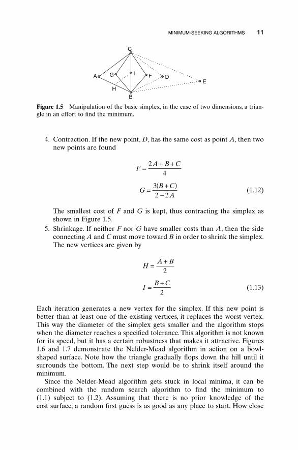
4. Contraction. If the new point, D, has the same cost as point A, then twonew points are found
(1.12)
The smallest cost of F and G is kept, thus contracting the simplex asshown in Figure 1.5.
5. Shrinkage. If neither F nor G have smaller costs than A, then the sideconnecting A and C must move toward B in order to shrink the simplex.The new vertices are given by
(1.13)
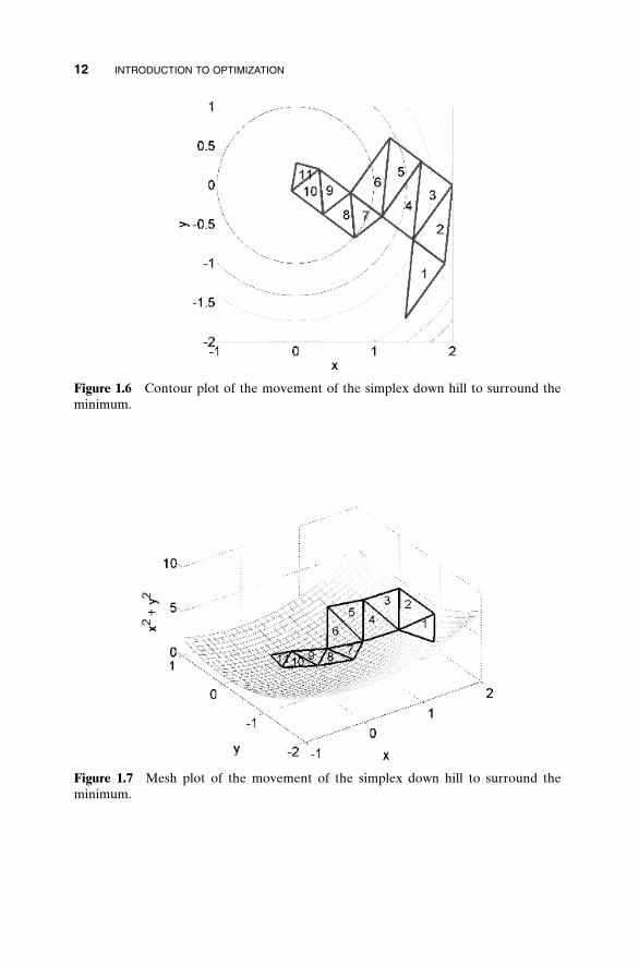
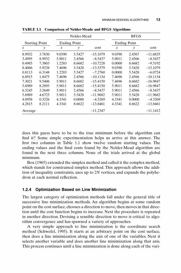
Each iteration generates a new vertex for the simplex. If this new point isbetter than at least one of the existing vertices, it replaces the worst vertex.This way the diameter of the simplex gets smaller and the algorithm stopswhen the diameter reaches a specified tolerance. This algorithm is not knownfor its speed, but it has a certain robustness that makes it attractive. Figures1.6 and 1.7 demonstrate the Nelder-Mead algorithm in action on a bowl-shaped surface. Note how the triangle gradually flops down the hill until it surrounds the bottom. The next step would be to shrink itself around theminimum.
Since the Nelder-Mead algorithm gets stuck in local minima, it can be combined with the random search algorithm to find the minimum to (1.1) subject to (1.2). Assuming that there is no prior knowledge of the cost surface, a random first guess is as good as any place to start. How close
HA B
IB C
=+
=+
2
2
FA B C
GB C
A
=+ +
=+( )
-
24
32 2
MINIMUM-SEEKING ALGORITHMS 11
EA
C
G F DI
H
B
Figure 1.5 Manipulation of the basic simplex, in the case of two dimensions, a trian-gle in an effort to find the minimum.
12 INTRODUCTION TO OPTIMIZATION
Figure 1.6 Contour plot of the movement of the simplex down hill to surround theminimum.
Figure 1.7 Mesh plot of the movement of the simplex down hill to surround theminimum.
does this guess have to be to the true minimum before the algorithm can find it? Some simple experimentation helps us arrive at this answer. The first two columns in Table 1.1 show twelve random starting values. The ending values and the final costs found by the Nelder-Mead algorithm arefound in the next three columns. None of the trials arrived at the globalminimum.
Box (1965) extended the simplex method and called it the complex method,which stands for constrained simplex method. This approach allows the addi-tion of inequality constraints, uses up to 2N vertices, and expands the polyhe-dron at each normal reflection.
1.2.4 Optimization Based on Line Minimization
The largest category of optimization methods fall under the general title ofsuccessive line minimization methods. An algorithm begins at some randompoint on the cost surface, chooses a direction to move, then moves in that direc-tion until the cost function begins to increase. Next the procedure is repeatedin another direction. Devising a sensible direction to move is critical to algo-rithm convergence and has spawned a variety of approaches.
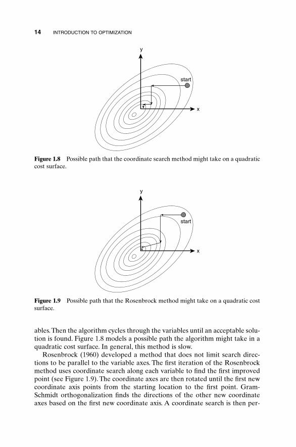
A very simple approach to line minimization is the coordinate searchmethod (Schwefel, 1995). It starts at an arbitrary point on the cost surface,then does a line minimization along the axis of one of the variables. Next itselects another variable and does another line minimization along that axis.This process continues until a line minimization is done along each of the vari-
MINIMUM-SEEKING ALGORITHMS 13
TABLE 1.1 Comparison of Nelder-Meade and BFGS Algorithms
Nelder-Mead BFGS
Starting Point Ending Point Ending Pointx y x y cost x y cost
8.9932 3.7830 9.0390 5.5427 -15.1079 9.0390 2.4567 -11.68353.4995 8.9932 5.9011 2.4566 -8.5437 5.9011 2.4566 -8.54370.4985 7.3803 1.2283 8.6682 -10.7228 0.0000 8.6682 -9.51928.4066 5.9238 7.4696 5.5428 -13.5379 9.0390 5.5428 -15.10790.8113 6.3148 1.2283 5.5427 -7.2760 0.0000 5.5428 -6.07246.8915 1.8475 7.4696 2.4566 -10.1134 7.4696 2.4566 -10.11347.3021 9.5406 5.9011 8.6682 -15.4150 7.4696 8.6682 -16.98475.6989 8.2893 5.9011 8.6682 -15.4150 5.9011 8.6682 -16.98476.3245 3.2649 5.9011 2.4566 -8.5437 5.9011 2.4566 -8.54375.6989 4.6725 5.9011 5.5428 -11.9682 5.9011 5.5428 -11.96824.0958 0.3226 4.3341 0.0000 -4.3269 4.3341 0.0000 -4.32694.2815 8.2111 4.3341 8.6622 -13.8461 4.3341 8.6622 -13.8461
Average -11.2347 -11.1412
14 INTRODUCTION TO OPTIMIZATION
start
x
y
Figure 1.8 Possible path that the coordinate search method might take on a quadraticcost surface.
start
x
y
Figure 1.9 Possible path that the Rosenbrock method might take on a quadratic costsurface.
ables.Then the algorithm cycles through the variables until an acceptable solu-tion is found. Figure 1.8 models a possible path the algorithm might take in aquadratic cost surface. In general, this method is slow.
Rosenbrock (1960) developed a method that does not limit search direc-tions to be parallel to the variable axes. The first iteration of the Rosenbrockmethod uses coordinate search along each variable to find the first improvedpoint (see Figure 1.9). The coordinate axes are then rotated until the first newcoordinate axis points from the starting location to the first point. Gram-Schmidt orthogonalization finds the directions of the other new coordinateaxes based on the first new coordinate axis. A coordinate search is then per-
MINIMUM-SEEKING ALGORITHMS 15
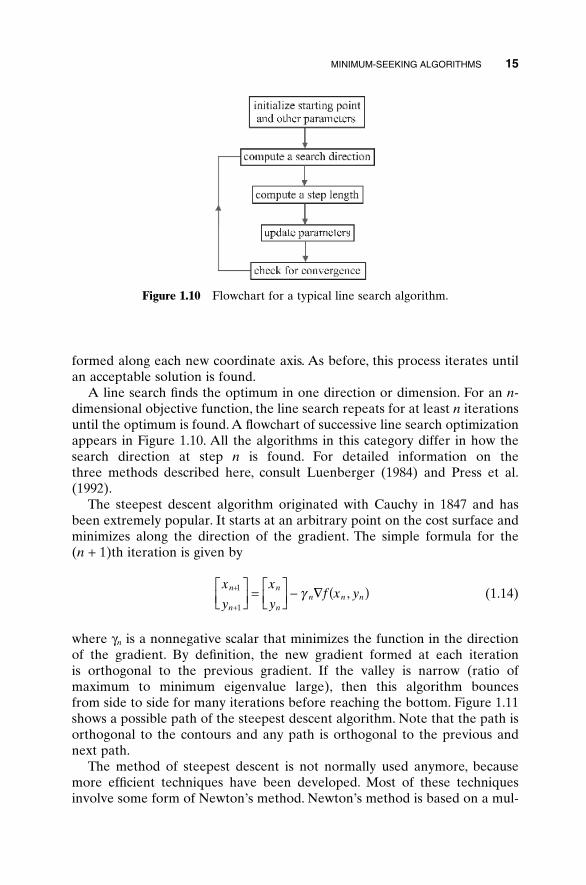
Figure 1.10 Flowchart for a typical line search algorithm.
formed along each new coordinate axis. As before, this process iterates untilan acceptable solution is found.
A line search finds the optimum in one direction or dimension. For an n-dimensional objective function, the line search repeats for at least n iterationsuntil the optimum is found. A flowchart of successive line search optimizationappears in Figure 1.10. All the algorithms in this category differ in how thesearch direction at step n is found. For detailed information on the three methods described here, consult Luenberger (1984) and Press et al.(1992).
The steepest descent algorithm originated with Cauchy in 1847 and hasbeen extremely popular. It starts at an arbitrary point on the cost surface andminimizes along the direction of the gradient. The simple formula for the (n + 1)th iteration is given by
(1.14)
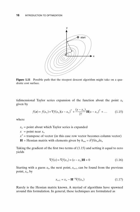
where gn is a nonnegative scalar that minimizes the function in the directionof the gradient. By definition, the new gradient formed at each iteration is orthogonal to the previous gradient. If the valley is narrow (ratio ofmaximum to minimum eigenvalue large), then this algorithm bounces from side to side for many iterations before reaching the bottom. Figure 1.11shows a possible path of the steepest descent algorithm. Note that the path isorthogonal to the contours and any path is orthogonal to the previous andnext path.
The method of steepest descent is not normally used anymore, becausemore efficient techniques have been developed. Most of these techniquesinvolve some form of Newton’s method. Newton’s method is based on a mul-
x
y yn
n
n
nn n n
xf x y+1
+
ÈÎÍ
˘˚
= ÈÎÍ
˘˚
- — ( )1
g ,
tidimensional Taylor series expansion of the function about the point xk
given by
(1.15)
where
xn = point about which Taylor series is expandedx = point near xn
xT = transpose of vector (in this case row vector becomes column vector)H = Hessian matrix with elements given by hmn = ∂2f/∂xm∂xn
Taking the gradient of the first two terms of (1.15) and setting it equal to zeroyields
(1.16)
Starting with a guess x0, the next point, xn+1, can be found from the previouspoint, xn, by
(1.17)
Rarely is the Hessian matrix known. A myriad of algorithms have spawnedaround this formulation. In general, these techniques are formulated as
x x f xn n n+-= - — ( )1
1H
— ( ) = — ( ) + -( ) =f x f x x xn n H 0
f f x f x x xx x
x xn n nT n
nT
x( ) = ( ) + — ( ) -( ) +-( )
-( ) +2!
. . .H
16 INTRODUCTION TO OPTIMIZATION
start
x
y
Figure 1.11 Possible path that the steepest descent algorithm might take on a qua-dratic cost surface.

(1.18)
where
an = step size at iteration nAn= approximation to the Hessian matrix at iteration n
Note that when An = I, the identity matrix (1.18) becomes the method of steep-est descent, and when An = H-1, (1.18) becomes Newton’s method.
Two excellent quasi-Newton techniques that construct a sequence ofapproximations to the Hessian, such that
(1.19)
The first approach is called the Davidon-Fletcher-Powell (DFP) algorithm(Powell, 1964). Powell developed a method that finds a set of line minimiza-tion directions that are linearly independent, mutually conjugate directions(Powell, 1964). The direction assuring the current direction does not “spoil”the minimization of the prior direction is the conjugate direction. The conju-gate directions are chosen so that the change in the gradient of the cost func-tion remains perpendicular to the previous direction. If the cost function isquadratic, then the algorithm converges in Nvar iterations (see Figure 1.12). Ifthe cost function is not quadratic, then repeating the Nvar iterations severaltimes usually brings the algorithm closer to the minimum. The second algo-rithm is named the Broyden-Fletcher-Goldfarb-Shanno (BFGS) algorithm,
limn
nƕ
-=A H 1
x x f xn n n n n+ = - — ( )1 a A
MINIMUM-SEEKING ALGORITHMS 17
start
x
y
Figure 1.12 Possible path that a conjugate directions algorithm might take on a qua-dratic cost surface.
discovered by its four namesakes independently in the mid-1960s (Broyden,1965; Fletcher, 1963; Goldfarb, 1968; Shanno, 1970). Both approaches find away to approximate this matrix and employ it in determining the appropriatedirections of movement. This algorithm is “quasi-Newton” in that it is equiv-alent to Newton’s method for prescribing the next best point to use for theiteration, yet it doesn’t use an exact Hessian matrix. The BFGS algorithm isrobust and quickly converges, but it requires an extra step to approximate theHessian compared to the DFP algorithm. These algorithms have the advan-tages of being fast and working with or without the gradient or Hessian. Onthe other hand, they have the disadvantages of finding minimum close to thestarting point and having an approximation to the Hessian matrix that is closeto singular.
Quadratic programming assumes that the cost function is quadratic (variables are squared) and the constraints are linear. This technique is basedon Lagrange multipliers and requires derivatives or approximations to derivatives. One powerful method known as recursive quadratic programmingsolves the quadratic programming problem at each iteration to find the direction of the next step (Luenberger, 1984). The approach of these methods is similar to using very refined surveying tools, which unfortunatelystill does not guarantee that the hiker will find the lowest point in the park.
1.3 NATURAL OPTIMIZATION METHODS
The methods already discussed take the same basic approach of headingdownhill from an arbitrary starting point. They differ in deciding in whichdirection to move and how far to move. Successive improvements increase thespeed of the downhill algorithms but don’t add to the algorithm’s ability tofind a global minimum instead of a local minimum.
All hope is not lost! Some outstanding algorithms have surfaced in recenttimes. Some of these methods include the genetic algorithm (Holland, 1975),simulated annealing (Kirkpatrick et al., 1983), particle swarm optimization(Parsopoulos and Vrahatis, 2002), ant colony optimization (Dorigo and Maria,1997), and evolutionary algorithms (Schwefel, 1995). These methods generatenew points in the search space by applying operators to current points andstatistically moving toward more optimal places in the search space. They relyon an intelligent search of a large but finite solution space using statisticalmethods. The algorithms do not require taking cost function derivatives and can thus deal with discrete variables and noncontinuous cost functions.They represent processes in nature that are remarkably successful at optimiz-ing natural phenomena. A selection of these algorithms is presented inChapter 7.
18 INTRODUCTION TO OPTIMIZATION
1.4 BIOLOGICAL OPTIMIZATION: NATURAL SELECTION
This section introduces the current scientific understanding of the naturalselection process with the purpose of gaining an insight into the construction,application, and terminology of genetic algorithms. Natural selection is dis-cussed in many texts and treatises. Much of the information summarized hereis from Curtis (1975) and Grant (1985).
Upon observing the natural world, we can make several generalizations that lead to our view of its origins and workings. First, there is a tremendousdiversity of organisms. Second, the degree of complexity in the organisms isstriking. Third, many of the features of these organisms have an apparent use-fulness. Why is this so? How did they come into being?
Imagine the organisms of today’s world as being the results of many itera-tions in a grand optimization algorithm. The cost function measures surviv-ability, which we wish to maximize. Thus the characteristics of the organismsof the natural world fit into this topological landscape (Grant, 1985). The levelof adaptation, the fitness, denotes the elevation of the landscape. The highestpoints correspond to the most-fit conditions. The environment, as well as howthe different species interact, provides the constraints. The process of evolu-tion is the grand algorithm that selects which characteristics produce a speciesof organism fit for survival.The peaks of the landscape are populated by livingorganisms. Some peaks are broad and hold a wide range of characteristicsencompassing many organisms, while other peaks are very narrow and allowonly very specific characteristics. This analogy can be extended to includesaddles between peaks as separating different species. If we take a veryparochial view and assume that intelligence and ability to alter the environ-ment are the most important aspects of survivability, we can imagine the globalmaximum peak at this instance in biological time to contain humankind.
To begin to understand the way that this natural landscape was populatedinvolves studying the two components of natural selection: genetics and evo-lution. Modern biologists subscribe to what is known as the synthetic theoryof natural selection—a synthesis of genetics with evolution. There are twomain divisions of scale in this synthetic evolutionary theory: macroevolution,which involves the process of division of the organisms into major groups, andmicroevolution, which deals with the process within specific populations. Wewill deal with microevolution here and consider macroevolution to be beyondour scope.
First, we need a bit of background on heredity at the cellular level. A geneis the basic unit of heredity. An organism’s genes are carried on one of a pairof chromosomes in the form of deoxyribonucleic acid (DNA). The DNA is inthe form of a double helix and carries a symbolic system of base-pairsequences that determine the sequence of enzymes and other proteins in anorganism. This sequence does not vary and is known as the genetic code of theorganism. Each cell of the organism contains the same number of chromo-
BIOLOGICAL OPTIMIZATION: NATURAL SELECTION 19
somes. For instance, the number of chromosomes per body cell is 6 for mos-quitoes, 26 for frogs, 46 for humans, and 94 for goldfish. Genes often occur withtwo functional forms, each representing a different characteristic. Each ofthese forms is known as an allele. For instance, a human may carry one allelefor brown eyes and another for blue eyes. The combination of alleles on thechromosomes determines the traits of the individual. Often one allele is dom-inant and the other recessive, so that the dominant allele is what is manifestedin the organism, although the recessive one may still be passed on to its off-spring. If the allele for brown eyes is dominant, the organism will have browneyes. However, it can still pass the blue allele to its offspring. If the secondallele from the other parent is also for blue eyes, the child will be blue-eyed.
The study of genetics began with the experiments of Gregor Mendel. Bornin 1822, Mendel attended the University of Vienna, where he studied bothbiology and mathematics. After failing his exams, he became a monk. It wasin the monastery garden where he performed his famous pea plant experi-ments. Mendel revolutionized experimentation by applying mathematics andstatistics to analyzing and predicting his results. By his hypothesizing andcareful planning of experiments, he was able to understand the basic conceptsof genetic inheritance for the first time, publishing his results in 1865. As withmany brilliant discoveries, his findings were not appreciated in his own time.
Mendel’s pea plant experiments were instrumental in delineating how traitsare passed from one generation to another. One reason that Mendel’s exper-iments were so successful is that pea plants are normally self-pollinating andseldom cross-pollinate without intervention. The self-pollination is easily pre-vented. Another reason that Mendel’s experiments worked was the fact thathe spent several years prior to the actual experimentation documenting theinheritable traits and which ones were easily separable and bred pure. Thisallowed him to crossbreed his plants and observe the characteristics of the off-spring and of the next generation. By carefully observing the distribution oftraits, he was able to hypothesize his first law—the principle of segregation;that is, that there must be factors that are inherited in pairs, one from eachparent. These factors are indeed the genes and their different realizations arethe alleles. When both alleles of a gene pair are the same, they are homozy-gous. When they are different, they are heterozygous. The brown-blue allelefor eye color of a parent was heterozygous while the blue-blue combinationof the offspring is homozygous. The trait actually observed is the phenotype,but the actual combination of alleles is the genotype. Although the parentorganism had a brown-blue eye color phenotype, its genotype is for browneyes (the dominant form). The genotype must be inferred from the phenotypepercentages of the succeeding generation as well as the parent itself. Since theoffspring had blue eyes, we can infer that each parent had a blue allele to passalong, even though the phenotype of each parent was brown eyes. Therefore,since the offspring was homozygous, carrying two alleles for blue eyes, bothparents must be heterozygous, having one brown and one blue allele. Mendel’ssecond law is the principle of independent assortment. This principle states
20 INTRODUCTION TO OPTIMIZATION
that the inheritance of the allele for one trait is independent of that for another. The eye color is irrelevant when determining the size of the individual.
To understand how genes combine into phenotypes, it is helpful to under-stand some basics of cell division. Reproduction in very simple, single-celledorganisms occurs by cell division, known as mitosis. During the phases ofmitosis, the chromosome material is exactly copied and passed onto the off-spring. In such simple organisms the daughter cells are identical to the parent.There is little opportunity for evolution of such organisms. Unless a mutationoccurs, the species propagates unchanged. Higher organisms have developeda more efficient method of passing on traits to their offspring—sexual repro-duction. The process of cell division that occurs then is called meiosis. Thegamete, or reproductive cell, has half the number of chromosomes as the otherbody cells. Thus the gametes cells are called haploid, while the body cells arediploid. Only these diploid body cells contain the full genetic code.The diploidnumber of chromosomes is reduced by half to form the haploid number forthe gametes. In preparation for meiosis, the gamete cells are duplicated. Thenthe gamete cells from the mother join with those from the father (this processis not discussed here). They arrange themselves in homologous pairs; that is,each chromosome matches with one of the same length and shape. As theymatch up, they join at the kinetochore, a random point on this matched chro-mosome pair (or actually tetrad in most cases).As meiosis progresses, the kine-tochores divide so that a left portion of the mother chromosome is conjoinedwith the right portion of the father, and visa versa for the other portions. Thisprocess is known as crossing over.The resulting cell has the full diploid numberof chromosomes. Through this crossing over, the genetic material of themother and father has been combined in a manner to produce a unique indi-vidual offspring. This process allows changes to occur in the species.
Now we turn to discussing the second component of natural selection—evo-lution—and one of its first proponents, Charles Darwin. Darwin refined hisideas during his voyage as naturalist on the Beagle, especially during his visitsto the Galapagos Islands. Darwin’s theory of evolution was based on fourprimary premises. First, like begets like; equivalently, an offspring has many ofthe characteristics of its parents. This premise implies that the population isstable. Second, there are variations in characteristics between individuals thatcan be passed from one generation to the next. The third premise is that onlya small percentage of the offspring produced survive to adulthood. Finally,which of the offspring survive depends on their inherited characteristics.Thesepremises combine to produce the theory of natural selection. In modern evo-lutionary theory an understanding of genetics adds impetus to the explanationof the stages of natural selection.
A group of interbreeding individuals is called a population. Under staticconditions the characteristics of the population are defined by the Hardy-Weinberg Law. This principle states that the frequency of occurrence of thealleles will stay the same within an inbreeding population if there are no per-
BIOLOGICAL OPTIMIZATION: NATURAL SELECTION 21
turbations. Thus, although the individuals show great variety, the statistics ofthe population remain the same. However, we know that few populations arestatic for very long. When the population is no longer static, the proportion ofallele frequencies is no longer constant between generations and evolutionoccurs. This dynamic process requires an external forcing. The forcing may begrouped into four specific types. (1) Mutations may occur; that is, a randomchange occurs in the characteristics of a gene.This change may be passed alongto the offspring. Mutations may be spontaneous or due to external factors suchas exposure to environmental factors. (2) Gene flow may result from intro-duction of new organisms into the breeding population. (3) Genetic drift mayoccur solely due to chance. In small populations certain alleles may sometimesbe eliminated in the random combinations. (4) Natural selection operates tochoose the most fit individuals for further reproduction. In this process certainalleles may produce an individual that is more prepared to deal with its envi-ronment. For instance, fleeter animals may be better at catching prey orrunning from predators, thus being more likely to survive to breed. Thereforecertain characteristics are selected into the breeding pool.
Thus we see that these ideas return to natural selection.The important com-ponents have been how the genes combine and cross over to produce newindividuals with combinations of traits and how the dynamics of a large pop-ulation interact to select for certain traits. These factors may move this off-spring either up toward a peak or down into the valley. If it goes too far intothe valley, it may not survive to mate—better adapted ones will. After a longperiod of time the pool of organisms becomes well adapted to its environment.However, the environment is dynamic. The predators and prey, as well asfactors such as the weather and geological upheaval, are also constantly chang-ing. These changes act to revise the optimization equation. That is what makeslife (and genetic algorithms) interesting.
1.5 THE GENETIC ALGORITHM
The genetic algorithm (GA) is an optimization and search technique based on the principles of genetics and natural selection. A GA allows a populationcomposed of many individuals to evolve under specified selection rules to a state that maximizes the “fitness” (i.e., minimizes the cost function).The method was developed by John Holland (1975) over the course of the 1960s and 1970s and finally popularized by one of his students, David Goldberg, who was able to solve a difficult problem involving the control of gas-pipeline transmission for his dissertation (Goldberg, 1989). Holland’s orig-inal work was summarized in his book. He was the first to try to develop a theoretical basis for GAs through his schema theorem. The work of De Jong (1975) showed the usefulness of the GA for function optimization andmade the first concerted effort to find optimized GA parameters. Goldberghas probably contributed the most fuel to the GA fire with his successful appli-
22 INTRODUCTION TO OPTIMIZATION
cations and excellent book (1989). Since then, many versions of evolutionaryprogramming have been tried with varying degrees of success.
Some of the advantages of a GA include that it
• Optimizes with continuous or discrete variables,• Doesn’t require derivative information,• Simultaneously searches from a wide sampling of the cost surface,• Deals with a large number of variables,• Is well suited for parallel computers,• Optimizes variables with extremely complex cost surfaces (they can jump
out of a local minimum),• Provides a list of optimum variables, not just a single solution,• May encode the variables so that the optimization is done with the en-
coded variables, and• Works with numerically generated data, experimental data, or analytical
functions.
These advantages are intriguing and produce stunning results when traditionaloptimization approaches fail miserably.
Of course, the GA is not the best way to solve every problem. For instance,the traditional methods have been tuned to quickly find the solution of a well-behaved convex analytical function of only a few variables. For such cases thecalculus-based methods outperform the GA, quickly finding the minimumwhile the GA is still analyzing the costs of the initial population. For theseproblems the optimizer should use the experience of the past and employthese quick methods. However, many realistic problems do not fall into thiscategory. In addition, for problems that are not overly difficult, other methodsmay find the solution faster than the GA. The large population of solutionsthat gives the GA its power is also its bane when it comes to speed on a serialcomputer—the cost function of each of those solutions must be evaluated.However, if a parallel computer is available, each processor can evaluate a separate function at the same time. Thus the GA is optimally suited for suchparallel computations.
This book shows how to use a GA to optimize problems. Chapter 2 introduces the binary form while using the algorithm to find the highest pointin Rocky Mountain National Park. Chapter 3 describes another version of the algorithm that employs continuous variables. We demonstrate this method with a GA solution to equation (1.1) subject to constraints (1.2).The remainder of the book presents refinements to the algorithm by solving more problems, winding its way from easier, less technical problemsinto more difficult problems that cannot be solved by other methods. Our goal is to give specific ways to deal with certain types of problems that may be typical of the ones faced by scientists and engineers on a day-to-daybasis.
THE GENETIC ALGORITHM 23
BIBLIOGRAPHY
Anderson, D. Z. 1992. Linear programming. In McGraw-Hill Encyclopedia of Scienceand Technology 10. New York: McGraw-Hill, pp. 86–88.
Borowski, E. J., and J. M. Borwein. 1991. Mathematics Dictionary. New York:HarperCollins.
Box, M. J. 1965. A comparison of several current optimization methods and the use oftransformations in constrained problems. Comput. J. 8:67–77.
Boyer, C. B., and U. C. Merzbach. 1991. A History of Mathematics. New York:Wiley.
Broyden, G. C. 1965. A class of methods for solving nonlinear simultaneous equations.Math. Comput. 19:577–593.
Curtis, H. 1975. Biology, 2nd ed. New York: Worth.Cuthbert, T. R. Jr. 1987. Optimization Using Personal Computers. New York: Wiley.De Jong, K. A. 1975. Analysis of the behavior of a class of genetic adaptive systems.
Ph.D. Dissertation. University of Michigan, Ann Arbor.Dorigo, M., and G. Maria. 1997. Ant colony system: a cooperative learning approach to
the traveling salesman problem. IEEE Trans. Evol. Comput. 1:53–66.Fletcher, R. 1963. Generalized inverses for nonlinear equations and optimization. In
R. Rabinowitz (ed.), Numerical Methods for Non-linear Algebraic Equations.London: Gordon and Breach.
Goldberg, D. E. 1989. Genetic Algorithms in Search, Optimization, and Machine Learn-ing. Reading, MA: Addison-Wesley.
Goldfarb, D., and B. Lapidus. 1968. Conjugate gradient method for nonlinear pro-gramming problems with linear constraints. I&EC Fundam. 7:142–151.
Grant, V. 1985. The Evolutionary Process. New York: Columbia University Press.Holland, J. H. 1975. Adaptation in Natural and Artificial Systems. Ann Arbor: Univer-
sity of Michigan Press.Kirkpatrick, S., C. D. Gelatt Jr., and M. P. Vecchi. 1983. Optimization by simulated
annealing. Science 220:671–680.Luenberger, D. G. 1984. Linear and Nonlinear Programming, Reading, MA: Addison-
Wesley.Nelder, J.A., and R. Mead. 1965.A simplex method for function minimization. Comput.
J. 7:308–313.Parsopoulos, K. E., and M. N. Vrahatis. 2002. Recent approaches to global optimization
problems through particle swarm optimization. In Natural Computing. Netherlands:Kluwer Academic, pp. 235–306.
Pierre, D. A. 1992. Optimization. In McGraw-Hill Encyclopedia of Science and Tech-nology 12. New York: McGraw-Hill, pp. 476–482.
Powell, M. J. D. 1964. An efficient way for finding the minimum of a function of severalvariables without calculating derivatives. Comput. J. 7:155–162.
Press,W. H., S.A.Teukolsky,W.T.Vettering, and B. P. Flannery. 1992. Numerical Recipes.New York: Cambridge University Press.
Rosenbrock, H. H. 1960. An automatic method for finding the greatest or least valueof a function. Comput. J. 3:175–184.
24 INTRODUCTION TO OPTIMIZATION
Schwefel, H. 1995. Evolution and Optimum Seeking. New York: Wiley.Shanno, D. F. 1970. An accelerated gradient projection method for linearly constrained
nonlinear estimation. SIAM J. Appl. Math. 18:322–334.Thompson, G. L. 1992. Game theory. In McGraw-Hill Encyclopedia of Science and
Technology 7. New York: McGraw-Hill, pp. 555–560.Williams, H. P. 1993. Model Solving in Mathematical Programming. New York:
Wiley.
EXERCISES
Use the following local optimizers:
a. Nelder-Mead downhill simplexb. BFGSc. DFPd. Steepest descente. Random search
1. Find the minimum of _____ (one of the functions in Appendix I) using_____ (one of the local optimizers).
2. Try _____ different random starting values to find the minimum. What doyou observe?
3. Combine 1 and 2, and find the minimum 25 times using random startingpoints. How often is the minimum found?
4. Compare the following algorithms:_____
5. Since local optimizers often decrease the step size when approaching theminimum, running the algorithm again after it has found a minimumincreases the odds of getting a better solution. Repeat 3 in such a way thatthe solution is used as a starting point by the algorithm on a second run.Does this help? With which functions? Why?
6. Some of the MATLAB optimization routines give you a choice of provid-ing the exact derivatives. Do these algorithms converge better with theexact derivatives or approximate numerical derivatives?
7. Find the minimum of f = u2 + 2v2 + w2 + x2 subject to u + 3v - w + x = 2 and2u - v + w + 2x = 4 using Lagrange multipliers. Assume no constraints.(Answer: u = 67/69, v = 6/69, w = 14/69, x = 67/69 with k1 = -26/69,k2 = -54/69.)
8. Many problems have constraints on the variables. Using a transformationof variables, convert (1.1) and (1.2) into an unconstrained optimizationproblem, and try one of the local optimizers. Does the transformation usedaffect the speed of convergence?
EXERCISES 25
CHAPTER 2
The Binary Genetic Algorithm
27
2.1 GENETIC ALGORITHMS: NATURAL SELECTION ON A COMPUTER
If the previous chapter whet your appetite for something better than the tra-ditional optimization methods, this and the next chapter give step-by-step pro-cedures for implementing two flavors of a GA. Both algorithms follow thesame menu of modeling genetic recombination and natural selection. One rep-resents variables as an encoded binary string and works with the binary stringsto minimize the cost, while the other works with the continuous variablesthemselves to minimize the cost. Since GAs originated with a binary repre-sentation of the variables, the binary method is presented first.
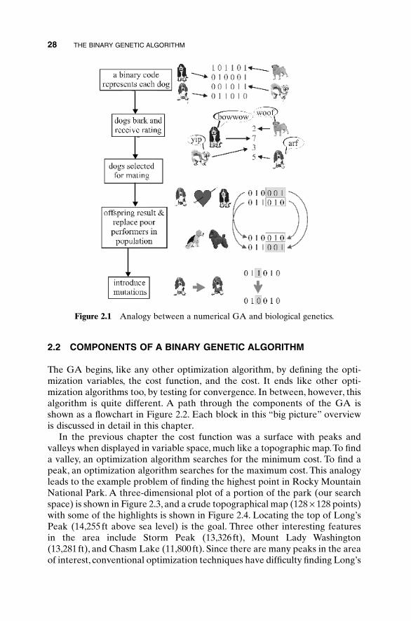
Figure 2.1 shows the analogy between biological evolution and a binaryGA. Both start with an initial population of random members. Each row ofbinary numbers represents selected characteristics of one of the dogs in thepopulation. Traits associated with loud barking are encoded in the binarysequence associated with these dogs. If we are trying to breed the dog withthe loudest bark, then only a few of the loudest, (in this case, four loudest)barking dogs are kept for breeding. There must be some way of determiningthe loudest barkers—the dogs may audition while the volume of their bark ismeasured. Dogs with loud barks receive low costs. From this breeding popu-lation of loud barkers, two are randomly selected to create two new puppies.The puppies have a high probability of being loud barkers because both theirparents have genes that make them loud barkers. The new binary sequencesof the puppies contain portions of the binary sequences of both parents. Thesenew puppies replace two discarded dogs that didn’t bark loud enough. Enoughpuppies are generated to bring the population back to its original size. Iterat-ing on this process leads to a dog with a very loud bark. This natural opti-mization process can be applied to inanimate objects as well.
Practical Genetic Algorithms, Second Edition, by Randy L. Haupt and Sue Ellen Haupt.ISBN 0-471-45565-2 Copyright © 2004 John Wiley & Sons, Inc.
28 THE BINARY GENETIC ALGORITHM
2.2 COMPONENTS OF A BINARY GENETIC ALGORITHM
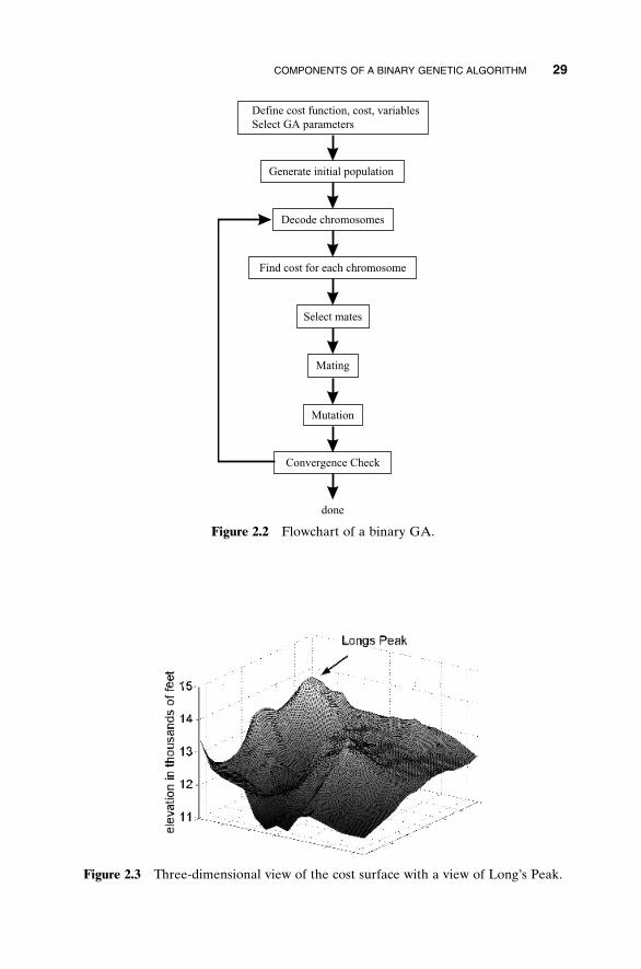
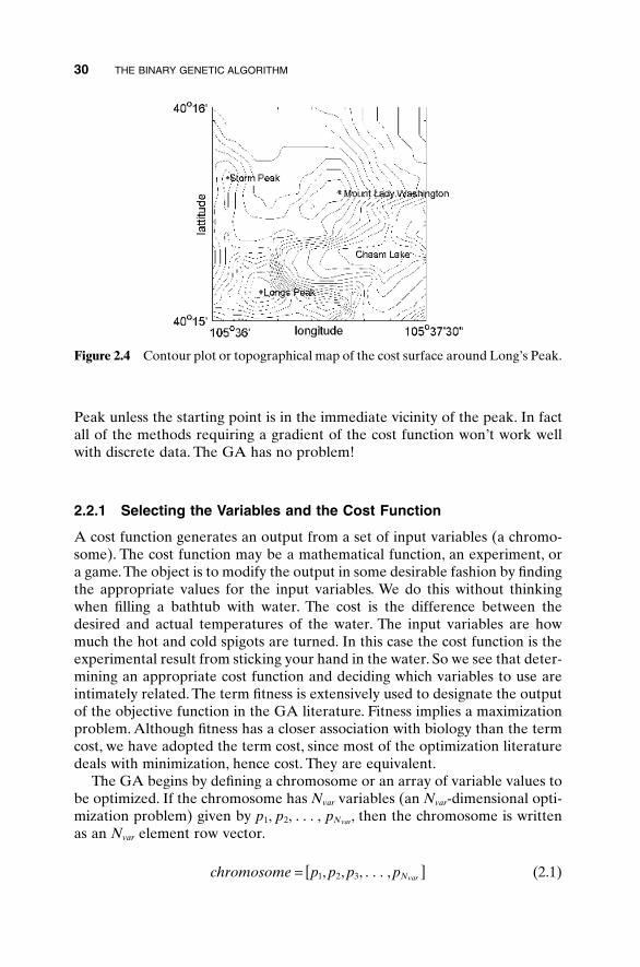
The GA begins, like any other optimization algorithm, by defining the opti-mization variables, the cost function, and the cost. It ends like other opti-mization algorithms too, by testing for convergence. In between, however, thisalgorithm is quite different. A path through the components of the GA isshown as a flowchart in Figure 2.2. Each block in this “big picture” overviewis discussed in detail in this chapter.
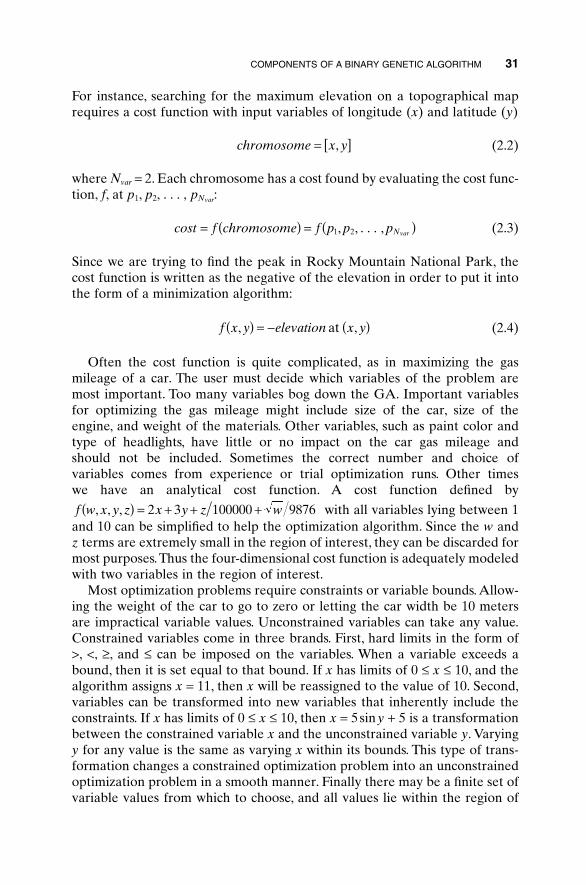
In the previous chapter the cost function was a surface with peaks andvalleys when displayed in variable space, much like a topographic map. To finda valley, an optimization algorithm searches for the minimum cost. To find apeak, an optimization algorithm searches for the maximum cost. This analogyleads to the example problem of finding the highest point in Rocky MountainNational Park. A three-dimensional plot of a portion of the park (our searchspace) is shown in Figure 2.3, and a crude topographical map (128 ¥ 128 points)with some of the highlights is shown in Figure 2.4. Locating the top of Long’sPeak (14,255 ft above sea level) is the goal. Three other interesting features in the area include Storm Peak (13,326 ft), Mount Lady Washington (13,281 ft), and Chasm Lake (11,800 ft). Since there are many peaks in the areaof interest, conventional optimization techniques have difficulty finding Long’s
Figure 2.1 Analogy between a numerical GA and biological genetics.
COMPONENTS OF A BINARY GENETIC ALGORITHM 29
Mating
Mutation
Convergence Check
done
Define cost function, cost, variables Select GA parameters
Generate initial population
Decode chromosomes
Find cost for each chromosome
Select mates
Figure 2.2 Flowchart of a binary GA.
Figure 2.3 Three-dimensional view of the cost surface with a view of Long’s Peak.
30 THE BINARY GENETIC ALGORITHM
Figure 2.4 Contour plot or topographical map of the cost surface around Long’s Peak.
Peak unless the starting point is in the immediate vicinity of the peak. In factall of the methods requiring a gradient of the cost function won’t work wellwith discrete data. The GA has no problem!
2.2.1 Selecting the Variables and the Cost Function
A cost function generates an output from a set of input variables (a chromo-some). The cost function may be a mathematical function, an experiment, ora game.The object is to modify the output in some desirable fashion by findingthe appropriate values for the input variables. We do this without thinkingwhen filling a bathtub with water. The cost is the difference between thedesired and actual temperatures of the water. The input variables are howmuch the hot and cold spigots are turned. In this case the cost function is theexperimental result from sticking your hand in the water. So we see that deter-mining an appropriate cost function and deciding which variables to use areintimately related. The term fitness is extensively used to designate the outputof the objective function in the GA literature. Fitness implies a maximizationproblem. Although fitness has a closer association with biology than the termcost, we have adopted the term cost, since most of the optimization literaturedeals with minimization, hence cost. They are equivalent.
The GA begins by defining a chromosome or an array of variable values tobe optimized. If the chromosome has Nvar variables (an Nvar-dimensional opti-mization problem) given by p1, p2, . . . , , then the chromosome is writtenas an Nvar element row vector.
(2.1)chromosome p p p pNvar= [ ]1 2 3, , , . . . ,
pNvar
For instance, searching for the maximum elevation on a topographical maprequires a cost function with input variables of longitude (x) and latitude (y)
(2.2)
where Nvar = 2. Each chromosome has a cost found by evaluating the cost func-tion, f, at p1, p2, . . . , :
(2.3)
Since we are trying to find the peak in Rocky Mountain National Park, thecost function is written as the negative of the elevation in order to put it intothe form of a minimization algorithm:
(2.4)
Often the cost function is quite complicated, as in maximizing the gas mileage of a car. The user must decide which variables of the problem are most important. Too many variables bog down the GA. Important variables for optimizing the gas mileage might include size of the car, size of the engine, and weight of the materials. Other variables, such as paint color and type of headlights, have little or no impact on the car gas mileage and should not be included. Sometimes the correct number and choice of variables comes from experience or trial optimization runs. Other times we have an analytical cost function. A cost function defined by
with all variables lying between 1and 10 can be simplified to help the optimization algorithm. Since the w andz terms are extremely small in the region of interest, they can be discarded formost purposes.Thus the four-dimensional cost function is adequately modeledwith two variables in the region of interest.
Most optimization problems require constraints or variable bounds. Allow-ing the weight of the car to go to zero or letting the car width be 10 metersare impractical variable values. Unconstrained variables can take any value.Constrained variables come in three brands. First, hard limits in the form of>, <, ≥, and £ can be imposed on the variables. When a variable exceeds abound, then it is set equal to that bound. If x has limits of 0 £ x £ 10, and thealgorithm assigns x = 11, then x will be reassigned to the value of 10. Second,variables can be transformed into new variables that inherently include theconstraints. If x has limits of 0 £ x £ 10, then x = 5sin y + 5 is a transformationbetween the constrained variable x and the unconstrained variable y. Varyingy for any value is the same as varying x within its bounds. This type of trans-formation changes a constrained optimization problem into an unconstrainedoptimization problem in a smooth manner. Finally there may be a finite set ofvariable values from which to choose, and all values lie within the region of
f w x y z x y z w, , ,( ) = + + +2 3 100000 9876
f x y elevation x y, ,( ) = - ( )at
cost f chromosome f p p pNvar= ( ) = ( )1 2, , ,. . .
pNvar
chromosome x y= [ ],
COMPONENTS OF A BINARY GENETIC ALGORITHM 31
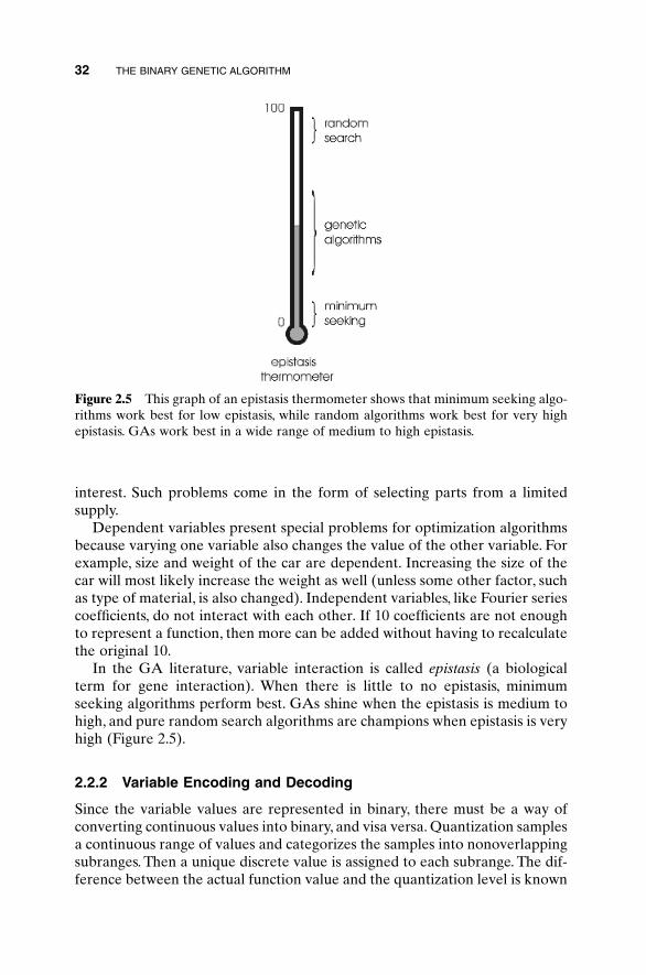
32 THE BINARY GENETIC ALGORITHM
interest. Such problems come in the form of selecting parts from a limitedsupply.
Dependent variables present special problems for optimization algorithmsbecause varying one variable also changes the value of the other variable. Forexample, size and weight of the car are dependent. Increasing the size of thecar will most likely increase the weight as well (unless some other factor, suchas type of material, is also changed). Independent variables, like Fourier seriescoefficients, do not interact with each other. If 10 coefficients are not enoughto represent a function, then more can be added without having to recalculatethe original 10.
In the GA literature, variable interaction is called epistasis (a biologicalterm for gene interaction). When there is little to no epistasis, minimumseeking algorithms perform best. GAs shine when the epistasis is medium tohigh, and pure random search algorithms are champions when epistasis is veryhigh (Figure 2.5).
2.2.2 Variable Encoding and Decoding
Since the variable values are represented in binary, there must be a way ofconverting continuous values into binary, and visa versa. Quantization samplesa continuous range of values and categorizes the samples into nonoverlappingsubranges. Then a unique discrete value is assigned to each subrange. The dif-ference between the actual function value and the quantization level is known
Figure 2.5 This graph of an epistasis thermometer shows that minimum seeking algo-rithms work best for low epistasis, while random algorithms work best for very highepistasis. GAs work best in a wide range of medium to high epistasis.
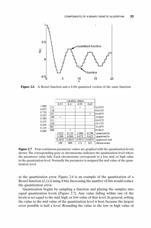
COMPONENTS OF A BINARY GENETIC ALGORITHM 33
as the quantization error. Figure 2.6 is an example of the quantization of aBessel function (J0 (x)) using 4 bits. Increasing the number of bits would reducethe quantization error.
Quantization begins by sampling a function and placing the samples intoequal quantization levels (Figure 2.7). Any value falling within one of thelevels is set equal to the mid, high, or low value of that level. In general, settingthe value to the mid value of the quantization level is best, because the largesterror possible is half a level. Rounding the value to the low or high value of
Figure 2.6 A Bessel function and a 6-bit quantized version of the same function.
Figure 2.7 Four continuous parameter values are graphed with the quantization levelsshown. The corresponding gene or chromosome indicates the quantization level wherethe parameter value falls. Each chromosome corresponds to a low, mid, or high valuein the quantization level. Normally the parameter is assigned the mid value of the quan-tization level.
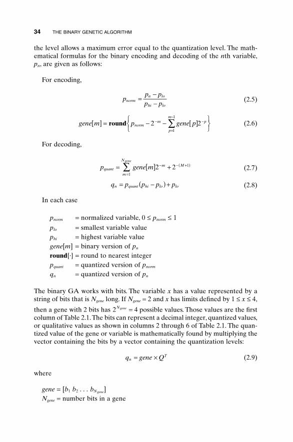
34 THE BINARY GENETIC ALGORITHM
the level allows a maximum error equal to the quantization level. The math-ematical formulas for the binary encoding and decoding of the nth variable,pn, are given as follows:
For encoding,
(2.5)
(2.6)
For decoding,
(2.7)
(2.8)
In each case
pnorm = normalized variable, 0 £ pnorm £ 1
plo = smallest variable valuephi = highest variable valuegene[m] = binary version of pn
round{·} = round to nearest integerpquant = quantized version of pnorm
qn = quantized version of pn
The binary GA works with bits. The variable x has a value represented by astring of bits that is Ngene long. If Ngene = 2 and x has limits defined by 1 £ x £ 4,
then a gene with 2 bits has = 4 possible values. Those values are the firstcolumn of Table 2.1.The bits can represent a decimal integer, quantized values,or qualitative values as shown in columns 2 through 6 of Table 2.1. The quan-tized value of the gene or variable is mathematically found by multiplying thevector containing the bits by a vector containing the quantization levels:
(2.9)
where
gene = [b1 b2 . . . ]Ngene = number bits in a gene
bNgene
q gene QnT= ¥
2Ngene
q p p p pn quant hi lo lo= -( ) +
p gene mquantm M
m
Ngene
= [ ] +- - +( )
=Â 2 2 1
1
gene m p gene pnormm p
p
m
[ ] = - - [ ]ÏÌÓ
¸˝˛
- -
=
-
Âround 2 21
1
pp pp pnorm
n lo
hi lo
=--
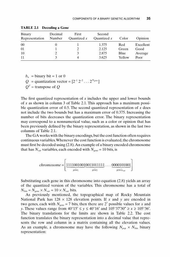
COMPONENTS OF A BINARY GENETIC ALGORITHM 35
bn = binary bit = 1 or 0Q = quantization vector = [2-1 2-2 . . . ]QT = transpose of Q
The first quantized representation of x includes the upper and lower boundsof x as shown in column 3 of Table 2.1. This approach has a maximum possi-ble quantization error of 0.5. The second quantized representation of x doesnot include the two bounds but has a maximum error of 0.375. Increasing thenumber of bits decreases the quantization error. The binary representationmay correspond to a nonnumerical value, such as a color or opinion that hasbeen previously defined by the binary representation, as shown in the last twocolumns of Table 2.1.
The GA works with the binary encodings,but the cost function often requirescontinuous variables.Whenever the cost function is evaluated, the chromosomemust first be decoded using (2.8).An example of a binary encoded chromosomethat has Nvar variables, each encoded with Ngene = 10 bits, is
Substituting each gene in this chromosome into equation (2.8) yields an arrayof the quantized version of the variables. This chromosome has a total of Nbits = Ngene ¥ Nvar = 10 ¥ Nvar bits.
As previously mentioned, the topographical map of Rocky MountainNational Park has 128 ¥ 128 elevation points. If x and y are encoded in two genes, each with Ngene = 7 bits, then there are 27 possible values for x andy. These values range from 40°15¢ £ y £ 40°16¢ and 105°37¢30≤ ≥ x ≥ 105°36¢.The binary translations for the limits are shown in Table 2.2. The cost function translates the binary representation into a decimal value that repre-sents the row and column in a matrix containing all the elevation values.As an example, a chromosome may have the following Npop ¥ Nbits binary representation:
chromosomegene gene geneNvar
= ◊ ◊ ◊È
ÎÍÍ
˘
˚˙˙
11110010010011011111 00001010011 2
1 244 344 1 244 344 1 244 344
2Ngene
TABLE 2.1 Decoding a Gene
Binary Decimal First SecondRepresentation Number Quantized x Quantized x Color Opinion
00 0 1 1.375 Red Excellent01 1 2 2.125 Green Good10 2 3 2.875 Blue Average11 3 4 3.625 Yellow Poor
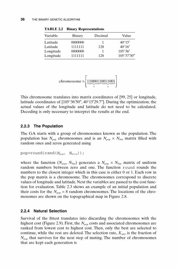
36 THE BINARY GENETIC ALGORITHM
This chromosome translates into matrix coordinates of [99, 25] or longitude,latitude coordinates of [105°36¢50≤, 40°15¢29.7≤]. During the optimization, theactual values of the longitude and latitude do not need to be calculated.Decoding is only necessary to interpret the results at the end.
2.2.3 The Population
The GA starts with a group of chromosomes known as the population. Thepopulation has Npop chromosomes and is an Npop ¥ Nbits matrix filled withrandom ones and zeros generated using
pop=round(rand(Npop, Nbits));
where the function (Npop, Nbits) generates a Npop ¥ Nbits matrix of uniformrandom numbers between zero and one. The function round rounds thenumbers to the closest integer which in this case is either 0 or 1. Each row inthe pop matrix is a chromosome. The chromosomes correspond to discretevalues of longitude and latitude. Next the variables are passed to the cost func-tion for evaluation. Table 2.3 shows an example of an initial population andtheir costs for the Npop = 8 random chromosomes. The locations of the chro-mosomes are shown on the topographical map in Figure 2.8.
2.2.4 Natural Selection
Survival of the fittest translates into discarding the chromosomes with thehighest cost (Figure 2.9). First, the Npop costs and associated chromosomes areranked from lowest cost to highest cost. Then, only the best are selected tocontinue, while the rest are deleted. The selection rate, Xrate, is the fraction ofNpop that survives for the next step of mating. The number of chromosomesthat are kept each generation is
chromosomex y
=È
ÎÍÍ
˘
˚˙˙
110001100110011 24 34 1 24 34
TABLE 2.2 Binary Representations
Variable Binary Decimal Value
Latitude 0000000 1 40°15¢Latitude 1111111 128 40°16¢Longitude 0000000 1 105°36¢Longitude 1111111 128 105°37¢30≤
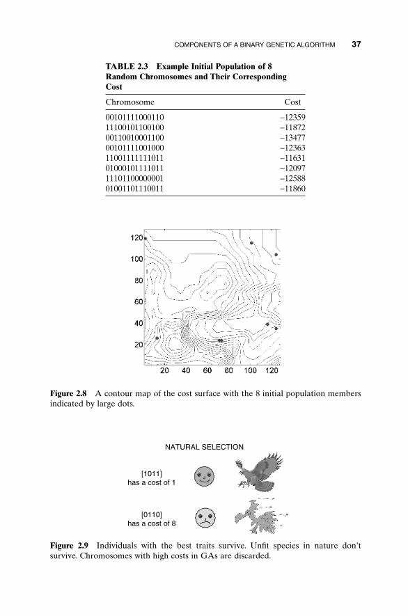
COMPONENTS OF A BINARY GENETIC ALGORITHM 37
TABLE 2.3 Example Initial Population of 8Random Chromosomes and Their CorrespondingCost
Chromosome Cost
00101111000110 -1235911100101100100 -1187200110010001100 -1347700101111001000 -1236311001111111011 -1163101000101111011 -1209711101100000001 -1258801001101110011 -11860
Figure 2.8 A contour map of the cost surface with the 8 initial population membersindicated by large dots.
[1011]has a cost of 1
[0110]has a cost of 8
NATURAL SELECTION
Figure 2.9 Individuals with the best traits survive. Unfit species in nature don’tsurvive. Chromosomes with high costs in GAs are discarded.
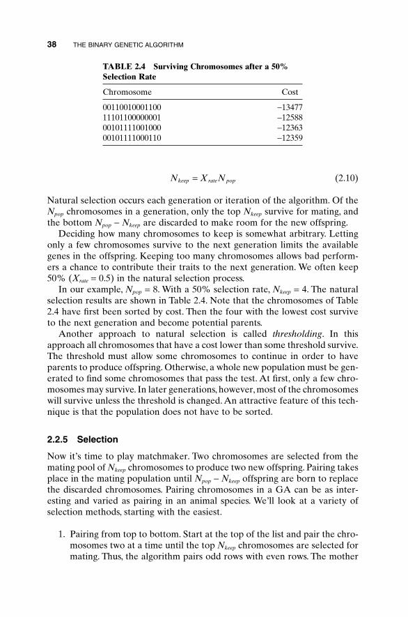
(2.10)
Natural selection occurs each generation or iteration of the algorithm. Of theNpop chromosomes in a generation, only the top Nkeep survive for mating, andthe bottom Npop - Nkeep are discarded to make room for the new offspring.
Deciding how many chromosomes to keep is somewhat arbitrary. Lettingonly a few chromosomes survive to the next generation limits the availablegenes in the offspring. Keeping too many chromosomes allows bad perform-ers a chance to contribute their traits to the next generation. We often keep50% (Xrate = 0.5) in the natural selection process.
In our example, Npop = 8. With a 50% selection rate, Nkeep = 4. The naturalselection results are shown in Table 2.4. Note that the chromosomes of Table2.4 have first been sorted by cost. Then the four with the lowest cost surviveto the next generation and become potential parents.
Another approach to natural selection is called thresholding. In thisapproach all chromosomes that have a cost lower than some threshold survive.The threshold must allow some chromosomes to continue in order to haveparents to produce offspring. Otherwise, a whole new population must be gen-erated to find some chromosomes that pass the test. At first, only a few chro-mosomes may survive. In later generations, however, most of the chromosomeswill survive unless the threshold is changed. An attractive feature of this tech-nique is that the population does not have to be sorted.
2.2.5 Selection
Now it’s time to play matchmaker. Two chromosomes are selected from themating pool of Nkeep chromosomes to produce two new offspring. Pairing takesplace in the mating population until Npop - Nkeep offspring are born to replacethe discarded chromosomes. Pairing chromosomes in a GA can be as inter-esting and varied as pairing in an animal species. We’ll look at a variety ofselection methods, starting with the easiest.
1. Pairing from top to bottom. Start at the top of the list and pair the chro-mosomes two at a time until the top Nkeep chromosomes are selected formating. Thus, the algorithm pairs odd rows with even rows. The mother
N X Nkeep rate pop=
38 THE BINARY GENETIC ALGORITHM
TABLE 2.4 Surviving Chromosomes after a 50%Selection Rate
Chromosome Cost
00110010001100 -1347711101100000001 -1258800101111001000 -1236300101111000110 -12359
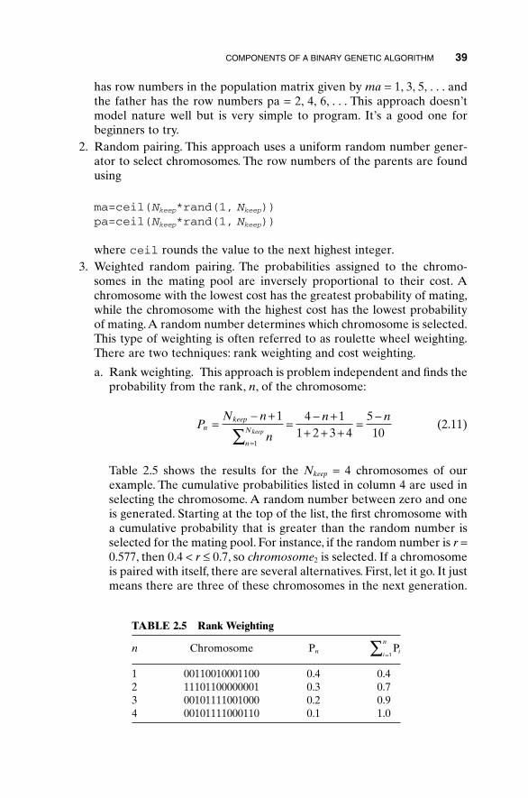
has row numbers in the population matrix given by ma = 1, 3, 5, . . . andthe father has the row numbers pa = 2, 4, 6, . . . This approach doesn’tmodel nature well but is very simple to program. It’s a good one forbeginners to try.
2. Random pairing. This approach uses a uniform random number gener-ator to select chromosomes. The row numbers of the parents are foundusing
ma=ceil(Nkeep*rand(1, Nkeep))pa=ceil(Nkeep*rand(1, Nkeep))
where ceil rounds the value to the next highest integer.3. Weighted random pairing. The probabilities assigned to the chromo-
somes in the mating pool are inversely proportional to their cost. A chromosome with the lowest cost has the greatest probability of mating,while the chromosome with the highest cost has the lowest probabilityof mating.A random number determines which chromosome is selected.This type of weighting is often referred to as roulette wheel weighting.There are two techniques: rank weighting and cost weighting.
a. Rank weighting. This approach is problem independent and finds theprobability from the rank, n, of the chromosome:
(2.11)
Table 2.5 shows the results for the Nkeep = 4 chromosomes of ourexample. The cumulative probabilities listed in column 4 are used inselecting the chromosome. A random number between zero and oneis generated. Starting at the top of the list, the first chromosome witha cumulative probability that is greater than the random number isselected for the mating pool. For instance, if the random number is r =0.577, then 0.4 < r £ 0.7, so chromosome2 is selected. If a chromosomeis paired with itself, there are several alternatives. First, let it go. It justmeans there are three of these chromosomes in the next generation.
PN n
n
n nn
keep
n
Nkeep=
- +=
- ++ + +
=-
=Â1 4 1
1 2 3 4510
1
COMPONENTS OF A BINARY GENETIC ALGORITHM 39
TABLE 2.5 Rank Weighting
n Chromosome Pn
1 00110010001100 0.4 0.42 11101100000001 0.3 0.73 00101111001000 0.2 0.94 00101111000110 0.1 1.0
Pii
n
=Â 1
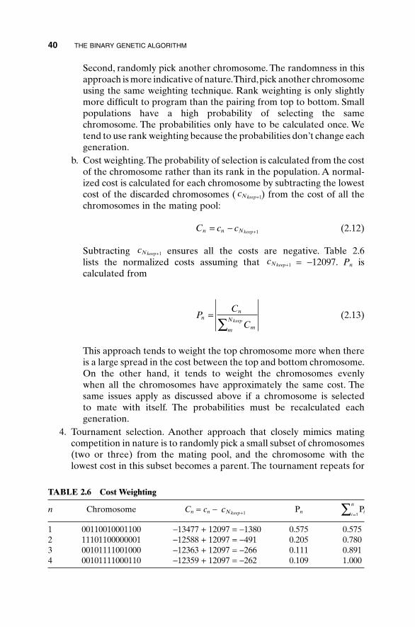
Second, randomly pick another chromosome. The randomness in thisapproach is more indicative of nature.Third,pick another chromosomeusing the same weighting technique. Rank weighting is only slightlymore difficult to program than the pairing from top to bottom. Smallpopulations have a high probability of selecting the same chromosome. The probabilities only have to be calculated once. Wetend to use rank weighting because the probabilities don’t change eachgeneration.
b. Cost weighting.The probability of selection is calculated from the costof the chromosome rather than its rank in the population. A normal-ized cost is calculated for each chromosome by subtracting the lowestcost of the discarded chromosomes ( ) from the cost of all thechromosomes in the mating pool:
(2.12)
Subtracting ensures all the costs are negative. Table 2.6 lists the normalized costs assuming that = -12097. Pn is calculated from
(2.13)
This approach tends to weight the top chromosome more when thereis a large spread in the cost between the top and bottom chromosome.On the other hand, it tends to weight the chromosomes evenly when all the chromosomes have approximately the same cost. The same issues apply as discussed above if a chromosome is selected to mate with itself. The probabilities must be recalculated each generation.
4. Tournament selection. Another approach that closely mimics matingcompetition in nature is to randomly pick a small subset of chromosomes(two or three) from the mating pool, and the chromosome with thelowest cost in this subset becomes a parent. The tournament repeats for
PC
Cn
n
mm
Nkeep=
Â
cNkeep+1
cNkeep+1
C c cn n Nkeep= - +1
cNkeep+1
40 THE BINARY GENETIC ALGORITHM
TABLE 2.6 Cost Weighting
n Chromosome Cn = cn - Pn
1 00110010001100 -13477 + 12097 = -1380 0.575 0.5752 11101100000001 -12588 + 12097 = -491 0.205 0.7803 00101111001000 -12363 + 12097 = -266 0.111 0.8914 00101111000110 -12359 + 12097 = -262 0.109 1.000
Pii
n
=Â 1cNkeep+1
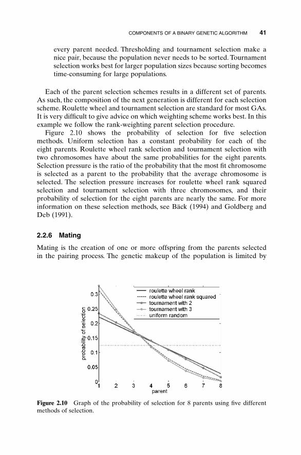
every parent needed. Thresholding and tournament selection make anice pair, because the population never needs to be sorted. Tournamentselection works best for larger population sizes because sorting becomestime-consuming for large populations.
Each of the parent selection schemes results in a different set of parents.As such, the composition of the next generation is different for each selectionscheme. Roulette wheel and tournament selection are standard for most GAs.It is very difficult to give advice on which weighting scheme works best. In thisexample we follow the rank-weighting parent selection procedure.
Figure 2.10 shows the probability of selection for five selection methods. Uniform selection has a constant probability for each of the eight parents. Roulette wheel rank selection and tournament selection withtwo chromosomes have about the same probabilities for the eight parents.Selection pressure is the ratio of the probability that the most fit chromosomeis selected as a parent to the probability that the average chromosome isselected. The selection pressure increases for roulette wheel rank squaredselection and tournament selection with three chromosomes, and their probability of selection for the eight parents are nearly the same. For moreinformation on these selection methods, see Bäck (1994) and Goldberg andDeb (1991).
2.2.6 Mating
Mating is the creation of one or more offspring from the parents selected in the pairing process. The genetic makeup of the population is limited by
COMPONENTS OF A BINARY GENETIC ALGORITHM 41
Figure 2.10 Graph of the probability of selection for 8 parents using five differentmethods of selection.
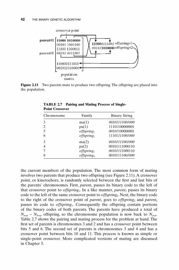
the current members of the population. The most common form of matinginvolves two parents that produce two offspring (see Figure 2.11). A crossoverpoint, or kinetochore, is randomly selected between the first and last bits ofthe parents’ chromosomes. First, parent1 passes its binary code to the left ofthat crossover point to offspring1. In a like manner, parent2 passes its binarycode to the left of the same crossover point to offspring2. Next, the binary codeto the right of the crossover point of parent1 goes to offspring2 and parent2
passes its code to offspring1. Consequently the offspring contain portions of the binary codes of both parents. The parents have produced a total of Npop - Nkeep offspring, so the chromosome population is now back to Npop.Table 2.7 shows the pairing and mating process for the problem at hand. Thefirst set of parents is chromosomes 3 and 2 and has a crossover point betweenbits 5 and 6. The second set of parents is chromosomes 3 and 4 and has acrossover point between bits 10 and 11. This process is known as simple orsingle-point crossover. More complicated versions of mating are discussed in Chapter 5.
42 THE BINARY GENETIC ALGORITHM
Figure 2.11 Two parents mate to produce two offspring. The offspring are placed intothe population.
TABLE 2.7 Pairing and Mating Process of Single-Point Crossover
Chromosome Family Binary String
3 ma(1) 001011110010002 pa(1) 111011000000015 offspring1 001011000000016 offspring2 11101111001000
3 ma(2) 001011110010004 pa(2) 001011110001107 offspring3 001011110001108 offspring4 00101111001000
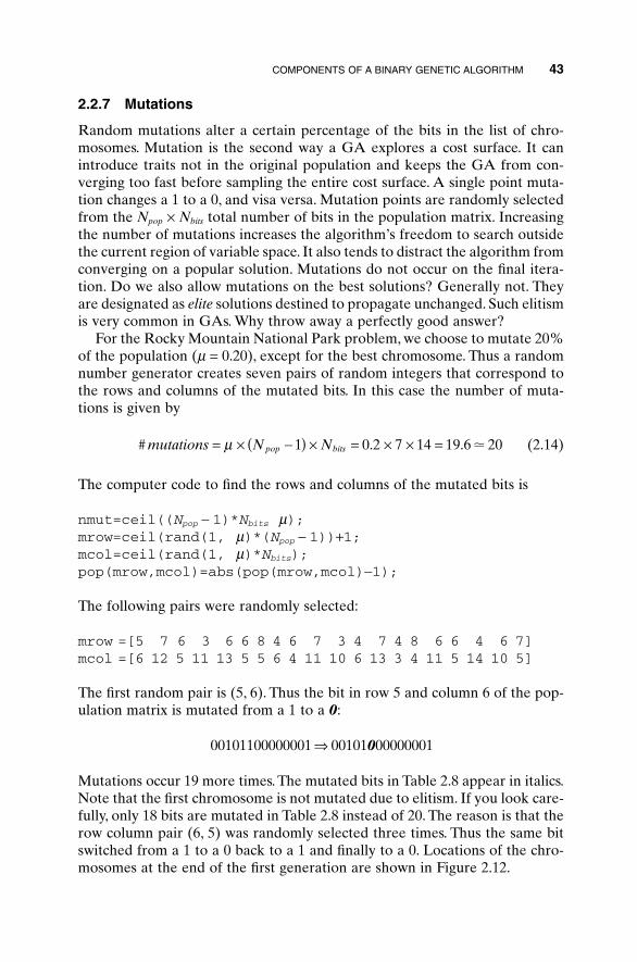
2.2.7 Mutations
Random mutations alter a certain percentage of the bits in the list of chro-mosomes. Mutation is the second way a GA explores a cost surface. It canintroduce traits not in the original population and keeps the GA from con-verging too fast before sampling the entire cost surface. A single point muta-tion changes a 1 to a 0, and visa versa. Mutation points are randomly selectedfrom the Npop ¥ Nbits total number of bits in the population matrix. Increasingthe number of mutations increases the algorithm’s freedom to search outsidethe current region of variable space. It also tends to distract the algorithm fromconverging on a popular solution. Mutations do not occur on the final itera-tion. Do we also allow mutations on the best solutions? Generally not. Theyare designated as elite solutions destined to propagate unchanged. Such elitismis very common in GAs. Why throw away a perfectly good answer?
For the Rocky Mountain National Park problem, we choose to mutate 20%of the population (m = 0.20), except for the best chromosome. Thus a randomnumber generator creates seven pairs of random integers that correspond tothe rows and columns of the mutated bits. In this case the number of muta-tions is given by
(2.14)
The computer code to find the rows and columns of the mutated bits is
nmut=ceil((Npop - 1)*Nbits m);mrow=ceil(rand(1, m)*(Npop - 1))+1;mcol=ceil(rand(1, m)*Nbits);pop(mrow,mcol)=abs(pop(mrow,mcol)-1);
The following pairs were randomly selected:
mrow =[5 7 6 3 6 6 8 4 6 7 3 4 7 4 8 6 6 4 6 7]mcol =[6 12 5 11 13 5 5 6 4 11 10 6 13 3 4 11 5 14 10 5]
The first random pair is (5, 6). Thus the bit in row 5 and column 6 of the pop-ulation matrix is mutated from a 1 to a 0:
Mutations occur 19 more times. The mutated bits in Table 2.8 appear in italics.Note that the first chromosome is not mutated due to elitism. If you look care-fully, only 18 bits are mutated in Table 2.8 instead of 20. The reason is that therow column pair (6, 5) was randomly selected three times. Thus the same bitswitched from a 1 to a 0 back to a 1 and finally to a 0. Locations of the chro-mosomes at the end of the first generation are shown in Figure 2.12.
00101100000001 00101 00000001fi 0
# . .mutations N Npop bits= ¥ -( ) ¥ = ¥ ¥ =m 1 0 2 7 14 19 6 20�
COMPONENTS OF A BINARY GENETIC ALGORITHM 43
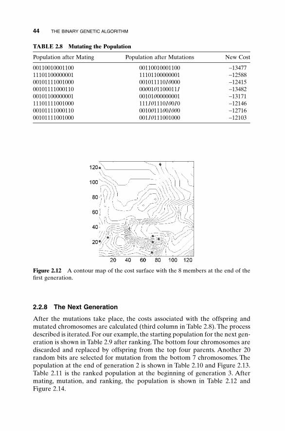
2.2.8 The Next Generation
After the mutations take place, the costs associated with the offspring andmutated chromosomes are calculated (third column in Table 2.8). The processdescribed is iterated. For our example, the starting population for the next gen-eration is shown in Table 2.9 after ranking. The bottom four chromosomes arediscarded and replaced by offspring from the top four parents. Another 20random bits are selected for mutation from the bottom 7 chromosomes. Thepopulation at the end of generation 2 is shown in Table 2.10 and Figure 2.13.Table 2.11 is the ranked population at the beginning of generation 3. Aftermating, mutation, and ranking, the population is shown in Table 2.12 andFigure 2.14.
44 THE BINARY GENETIC ALGORITHM
TABLE 2.8 Mutating the Population
Population after Mating Population after Mutations New Cost
00110010001100 00110010001100 -1347711101100000001 11101100000001 -1258800101111001000 00101111010000 -1241500101111000110 00001011000111 -1348200101100000001 00101000000001 -1317111101111001000 11110111010010 -1214600101111000110 00100111001000 -1271600101111001000 00110111001000 -12103
Figure 2.12 A contour map of the cost surface with the 8 members at the end of thefirst generation.
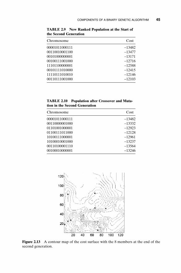
COMPONENTS OF A BINARY GENETIC ALGORITHM 45
TABLE 2.9 New Ranked Population at the Start ofthe Second Generation
Chromosome Cost
00001011000111 -1348200110010001100 -1347700101000000001 -1317100100111001000 -1271611101100000001 -1258800101111010000 -1241511110111010010 -1214600110111001000 -12103
TABLE 2.10 Population after Crossover and Muta-tion in the Second Generation
Chromosome Cost
00001011000111 -1348200110000001000 -1333201101001000001 -1292301100111011000 -1212810100111000001 -1296110100010001000 -1323700110100001110 -1356400100010000001 -13246
Figure 2.13 A contour map of the cost surface with the 8 members at the end of thesecond generation.
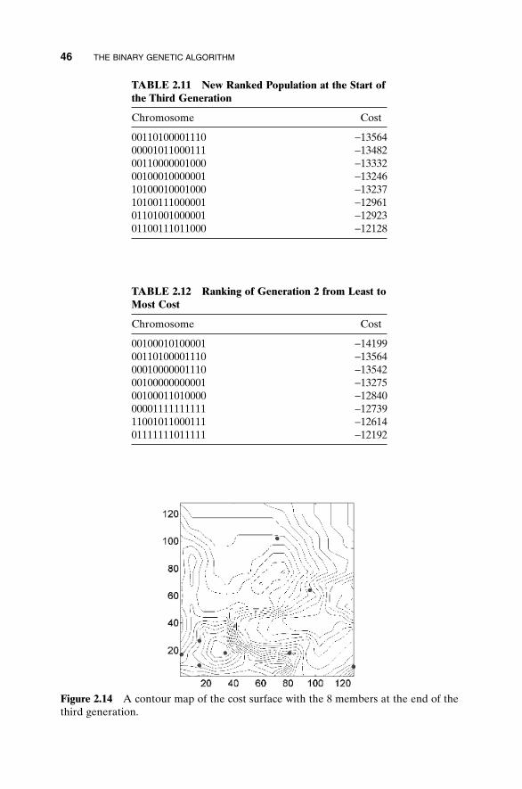
46 THE BINARY GENETIC ALGORITHM
TABLE 2.11 New Ranked Population at the Start ofthe Third Generation
Chromosome Cost
00110100001110 -1356400001011000111 -1348200110000001000 -1333200100010000001 -1324610100010001000 -1323710100111000001 -1296101101001000001 -1292301100111011000 -12128
TABLE 2.12 Ranking of Generation 2 from Least toMost Cost
Chromosome Cost
00100010100001 -1419900110100001110 -1356400010000001110 -1354200100000000001 -1327500100011010000 -1284000001111111111 -1273911001011000111 -1261401111111011111 -12192
Figure 2.14 A contour map of the cost surface with the 8 members at the end of thethird generation.
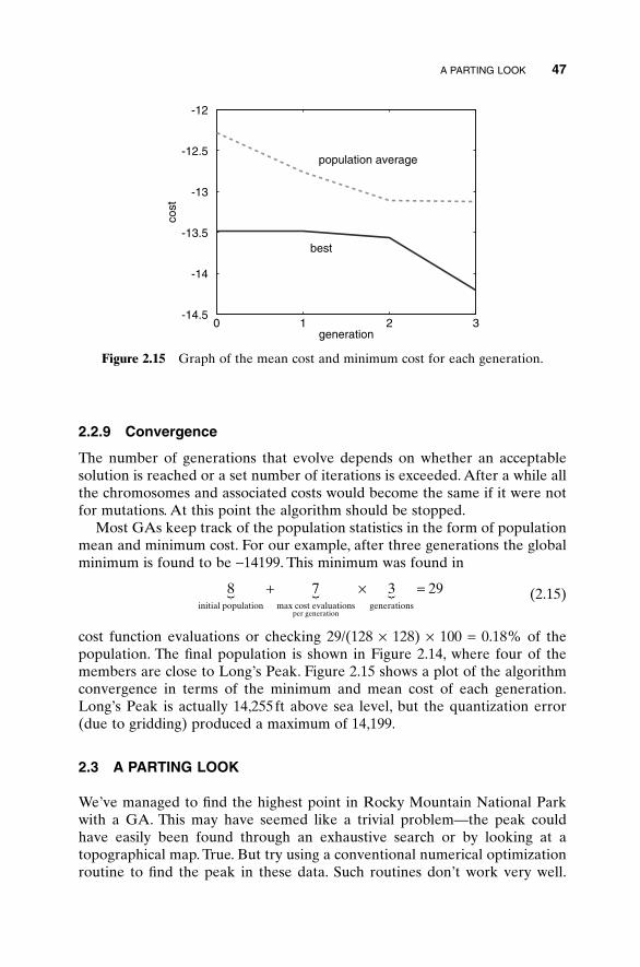
2.2.9 Convergence
The number of generations that evolve depends on whether an acceptablesolution is reached or a set number of iterations is exceeded. After a while allthe chromosomes and associated costs would become the same if it were notfor mutations. At this point the algorithm should be stopped.
Most GAs keep track of the population statistics in the form of populationmean and minimum cost. For our example, after three generations the globalminimum is found to be -14199. This minimum was found in
(2.15)
cost function evaluations or checking 29/(128 ¥ 128) ¥ 100 = 0.18% of the population. The final population is shown in Figure 2.14, where four of themembers are close to Long’s Peak. Figure 2.15 shows a plot of the algorithmconvergence in terms of the minimum and mean cost of each generation.Long’s Peak is actually 14,255 ft above sea level, but the quantization error(due to gridding) produced a maximum of 14,199.
2.3 A PARTING LOOK
We’ve managed to find the highest point in Rocky Mountain National Parkwith a GA. This may have seemed like a trivial problem—the peak could have easily been found through an exhaustive search or by looking at a topographical map. True. But try using a conventional numerical optimizationroutine to find the peak in these data. Such routines don’t work very well.
8 7 3 29initial population max cost evaluations generations
per generation
{ { {+ ¥ =
A PARTING LOOK 47
0 1 2 3-14.5
-14
-13.5
-13
-12.5
-12
generation
cost
best
population average
Figure 2.15 Graph of the mean cost and minimum cost for each generation.
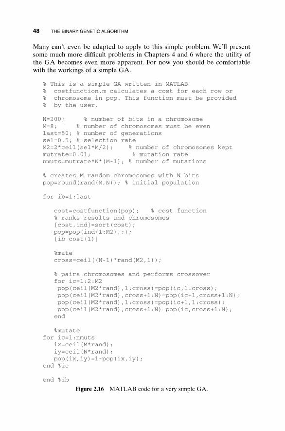
Many can’t even be adapted to apply to this simple problem. We’ll presentsome much more difficult problems in Chapters 4 and 6 where the utility ofthe GA becomes even more apparent. For now you should be comfortablewith the workings of a simple GA.
48 THE BINARY GENETIC ALGORITHM
% This is a simple GA written in MATLAB% costfunction.m calculates a cost for each row or% chromosome in pop. This function must be provided% by the user.
N=200; % number of bits in a chromosomeM=8; % number of chromosomes must be evenlast=50; % number of generationssel=0.5; % selection rateM2=2*ceil(sel*M/2); % number of chromosomes keptmutrate=0.01; % mutation ratenmuts=mutrate*N*(M-1); % number of mutations
% creates M random chromosomes with N bitspop=round(rand(M,N)); % initial population
for ib=1:last
cost=costfunction(pop); % cost function % ranks results and chromosomes [cost,ind]=sort(cost); pop=pop(ind(1:M2),:); [ib cost(1)]
%mate cross=ceil((N-1)*rand(M2,1));
% pairs chromosomes and performs crossover for ic=1:2:M2 pop(ceil(M2*rand),1:cross)=pop(ic,1:cross); pop(ceil(M2*rand),cross+1:N)=pop(ic+1,cross+1:N); pop(ceil(M2*rand),1:cross)=pop(ic+1,1:cross); pop(ceil(M2*rand),cross+1:N)=pop(ic,cross+1:N); end
%mutatefor ic=1:nmuts ix=ceil(M*rand); iy=ceil(N*rand); pop(ix,iy)=1-pop(ix,iy);end %ic
end %ib
Figure 2.16 MATLAB code for a very simple GA.
EXERCISES 49
It’s very simple to program a GA. An extremely short GA in MATLAB isshown in Figure 2.16. This GA uses pairing from top to bottom when select-ing mates. The cost function must be provided by the user and converts thebinary strings into usable variable values.
BIBLIOGRAPHY
Angeline, P. J. 1995. Evolution revolution: An introduction to the special track ongenetic and evolutionary programming. IEEE Exp. Intell. Syst. Appl. 10:6–10.
Bäck, T. 1994. Selective pressure in evolutionary algorithms: A characterization ofselection mechanisms. In Proc. 1st IEEE Conf. on Evolutionary Computation.Piscataway, NJ: IEEE Press, pp. 57–62.
Goldberg, D. E., and K. Deb. 1991. A comparative analysis of selection schemes used in genetic algorithms. In Foundations of Genetic Algorithms. San Mateo, CA:Morgan Kaufmann, pp. 69–93.
Goldberg, D. E. 1993. Making genetic algorithms fly: A lesson from the Wright brothers. Adv. Technol. Dev. 2:1–8.
Holland, J. H. 1992. Genetic algorithms. Sci. Am. 267:66–72.Janikow, C. Z., and D. St. Clair. 1995. Genetic algorithms simulating nature’s methods
of evolving the best design solution. IEEE Potentials 14:31–35.Malasri, S., J. R. Martin, and L. Y. Lin. 1995. Hands-on software for teaching genetic
algorithms. Comput. Educ. J. 6:42–47.
EXERCISES
1. Write a binary GA that uses:
a. Single-point crossoverb. Double-point crossoverc. Uniform crossover
2. Write a binary GA that uses:
a. Pairing parents from top to bottomb. Random pairingc. Pairing based on costd. Roulette wheel rank weightinge. Tournament selection
3. Find the minimum of _____ (from Appendix I) using your binary GA.
4. Experiment with different population sizes and mutation rates.Which com-bination seems to work best for you? Explain.
5. Compare your binary GA with the following local optimizers:
a. Nelder-Mead downhill simplexb. BFGSc. DFPd. Steepest descente. Random search
6. Since the GA has many random components, it is important to average theresults over multiple runs. Write a program that will average the results ofyour GA. Then do another one of the exercises and compare results.
7. Plot the convergence of the GA. Do a sensitivity analysis on parameterssuch as m and Npop. Which GA parameters have the most effect on conver-gence? A convergence plot could be: best minimum in the populationversus the number of function calls or the best minimum in the populationversus generation. Which method is better?
50 THE BINARY GENETIC ALGORITHM
CHAPTER 3
The Continuous Genetic Algorithm
51
Now that you are convinced (perhaps) that the binary GA solves many opti-mization problems that stump traditional techniques, let’s look a bit closer atthe quantization limitation. What if you are attempting to solve a problemwhere the values of the variables are continuous and you want to know themto the full machine precision? In such a problem each variable requires manybits to represent it. If the number of variables is large, the size of the chro-mosome is also large. Of course, 1s and 0s are not the only way to representa variable. One could, in principle, use any representation conceivable forencoding the variables. When the variables are naturally quantized, the binaryGA fits nicely. However, when the variables are continuous, it is more logicalto represent them by floating-point numbers. In addition, since the binary GAhas its precision limited by the binary representation of variables, using float-ing point numbers instead easily allows representation to the machine preci-sion. This continuous GA also has the advantage of requiring less storage thanthe binary GA because a single floating-point number represents the variableinstead of Nbits integers.The continuous GA is inherently faster than the binaryGA, because the chromosomes do not have to be decoded prior to the eval-uation of the cost function.
The purpose of this chapter is to introduce the continuous GA. Mostsources call this version of the GA a real-valued GA. We use the term con-tinuous rather than real-valued to avoid confusion between real and complexnumbers. The development here closely parallels the last chapter. We primar-ily dwell upon the differences in the two algorithms. The continuous exampleintroduced in Chapter 1 is our primary example problem. This allows thereader to compare the continuous GA performance with the more traditionaloptimization algorithms introduced in Chapter 1.
Practical Genetic Algorithms, Second Edition, by Randy L. Haupt and Sue Ellen Haupt.ISBN 0-471-45565-2 Copyright © 2004 John Wiley & Sons, Inc.
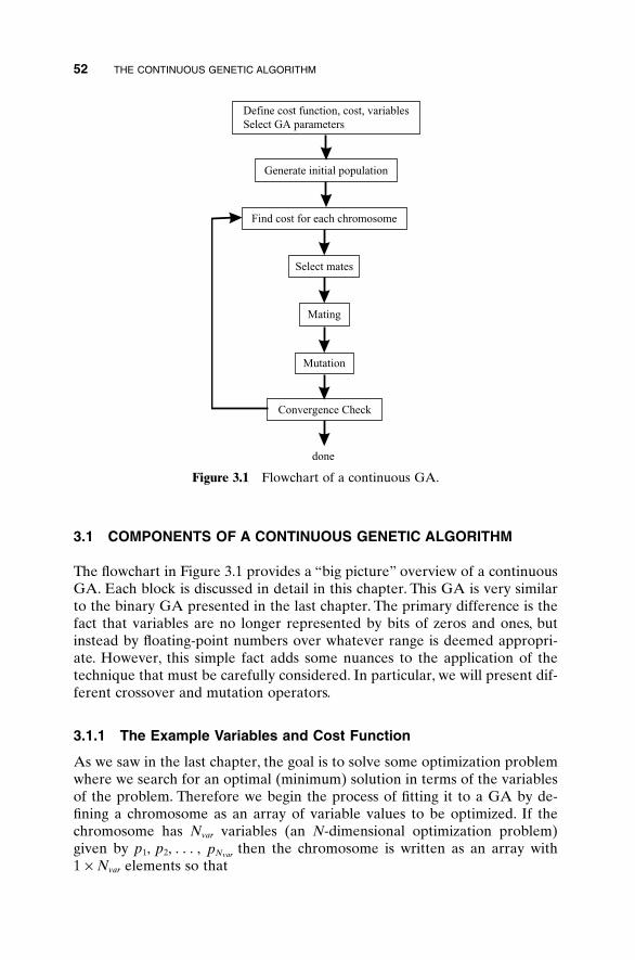
52 THE CONTINUOUS GENETIC ALGORITHM
3.1 COMPONENTS OF A CONTINUOUS GENETIC ALGORITHM
The flowchart in Figure 3.1 provides a “big picture” overview of a continuousGA. Each block is discussed in detail in this chapter. This GA is very similarto the binary GA presented in the last chapter. The primary difference is thefact that variables are no longer represented by bits of zeros and ones, butinstead by floating-point numbers over whatever range is deemed appropri-ate. However, this simple fact adds some nuances to the application of thetechnique that must be carefully considered. In particular, we will present dif-ferent crossover and mutation operators.
3.1.1 The Example Variables and Cost Function
As we saw in the last chapter, the goal is to solve some optimization problemwhere we search for an optimal (minimum) solution in terms of the variablesof the problem. Therefore we begin the process of fitting it to a GA by de-fining a chromosome as an array of variable values to be optimized. If thechromosome has Nvar variables (an N-dimensional optimization problem)given by p1, p2, . . . , then the chromosome is written as an array with 1 ¥ Nvar elements so that
pNvar
Figure 3.1 Flowchart of a continuous GA.
Mating
Mutation
Convergence Check
done
Define cost function, cost, variables Select GA parameters
Generate initial population
Find cost for each chromosome
Select mates
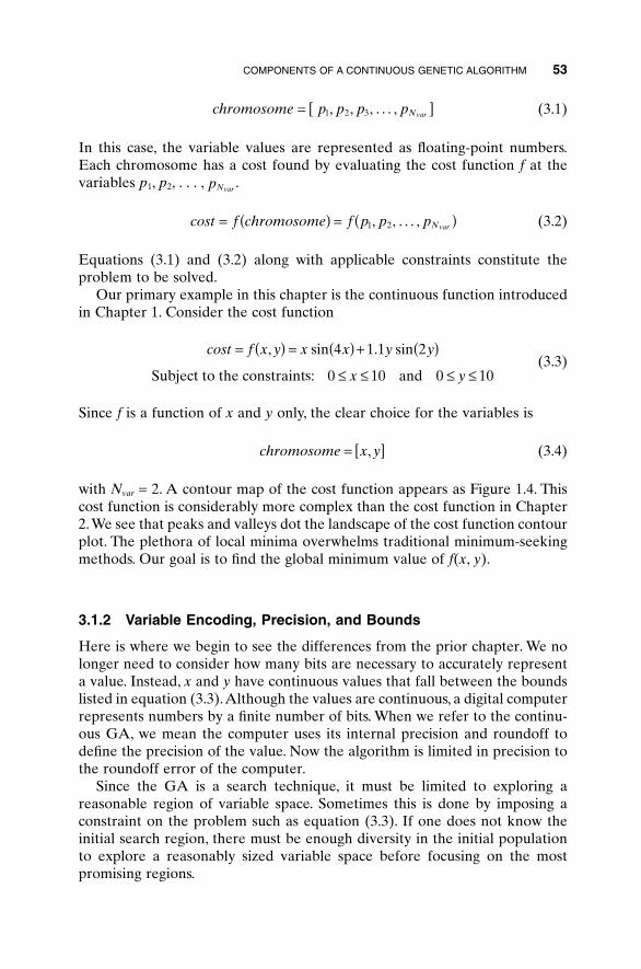
(3.1)
In this case, the variable values are represented as floating-point numbers.Each chromosome has a cost found by evaluating the cost function f at thevariables p1, p2, . . . , .
(3.2)
Equations (3.1) and (3.2) along with applicable constraints constitute theproblem to be solved.
Our primary example in this chapter is the continuous function introducedin Chapter 1. Consider the cost function
(3.3)
Since f is a function of x and y only, the clear choice for the variables is
(3.4)
with Nvar = 2. A contour map of the cost function appears as Figure 1.4. Thiscost function is considerably more complex than the cost function in Chapter2.We see that peaks and valleys dot the landscape of the cost function contourplot. The plethora of local minima overwhelms traditional minimum-seekingmethods. Our goal is to find the global minimum value of f(x, y).
3.1.2 Variable Encoding, Precision, and Bounds
Here is where we begin to see the differences from the prior chapter. We nolonger need to consider how many bits are necessary to accurately representa value. Instead, x and y have continuous values that fall between the boundslisted in equation (3.3).Although the values are continuous, a digital computerrepresents numbers by a finite number of bits. When we refer to the continu-ous GA, we mean the computer uses its internal precision and roundoff todefine the precision of the value. Now the algorithm is limited in precision tothe roundoff error of the computer.
Since the GA is a search technique, it must be limited to exploring a reasonable region of variable space. Sometimes this is done by imposing a constraint on the problem such as equation (3.3). If one does not know theinitial search region, there must be enough diversity in the initial populationto explore a reasonably sized variable space before focusing on the mostpromising regions.
chromosome x y= [ ],
cost f x y x x y y
x y
= ( ) = ( ) + ( )£ £ £ £
, sin . sin4 1 1 2
10 10Subject to the constraints: 0 and 0
cost f chromosome f p p pNvar= ( ) = ( )1 2, , . . . ,
pNvar
chromosome p p p pNvar= [ ]1 2 3, , , . . . ,
COMPONENTS OF A CONTINUOUS GENETIC ALGORITHM 53
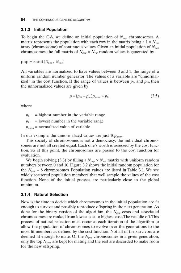
3.1.3 Initial Population
To begin the GA, we define an initial population of Npop chromosomes. Amatrix represents the population with each row in the matrix being a 1 ¥ Nvar
array (chromosome) of continuous values. Given an initial population of Npop
chromosomes, the full matrix of Npop ¥ Nvar random values is generated by
pop = rand(Npop, Nvar)
All variables are normalized to have values between 0 and 1, the range of auniform random number generator. The values of a variable are “unnormal-ized” in the cost function. If the range of values is between plo and phi, thenthe unnormalized values are given by
(3.5)
where
plo = highest number in the variable range
phi = lowest number in the variable rangepnorm = normalized value of variable
In our example, the unnormalized values are just 10pnorm.This society of chromosomes is not a democracy: the individual chromo-
somes are not all created equal. Each one’s worth is assessed by the cost func-tion. So at this point, the chromosomes are passed to the cost function forevaluation.
We begin solving (3.3) by filling a Npop ¥ Nvar matrix with uniform randomnumbers between 0 and 10. Figure 3.2 shows the initial random population forthe Npop = 8 chromosomes. Population values are listed in Table 3.1. We seewidely scattered population members that well sample the values of the costfunction. None of the initial guesses are particularly close to the globalminimum.
3.1.4 Natural Selection
Now is the time to decide which chromosomes in the initial population are fitenough to survive and possibly reproduce offspring in the next generation. Asdone for the binary version of the algorithm, the Npop costs and associatedchromosomes are ranked from lowest cost to highest cost.The rest die off.Thisprocess of natural selection must occur at each iteration of the algorithm toallow the population of chromosomes to evolve over the generations to themost fit members as defined by the cost function. Not all of the survivors aredeemed fit enough to mate. Of the Npop chromosomes in a given generation,only the top Nkeep are kept for mating and the rest are discarded to make roomfor the new offspring.
p p p p phi lo norm lo= -( ) +
54 THE CONTINUOUS GENETIC ALGORITHM
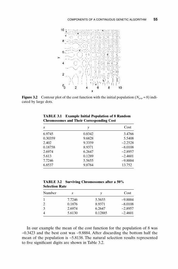
COMPONENTS OF A CONTINUOUS GENETIC ALGORITHM 55
In our example the mean of the cost function for the population of 8 was-0.3423 and the best cost was -9.8884. After discarding the bottom half themean of the population is -5.8138. The natural selection results representedto five significant digits are shown in Table 3.2.
Figure 3.2 Contour plot of the cost function with the initial population (Npop = 8) indi-cated by large dots.
TABLE 3.1 Example Initial Population of 8 RandomChromosomes and Their Corresponding Cost
x y Cost
6.9745 0.8342 3.47660.30359 9.6828 5.54082.402 9.3359 -2.25280.18758 8.9371 -8.01082.6974 6.2647 -2.89575.613 0.1289 -2.46017.7246 5.5655 -9.88846.8537 9.8784 13.752
TABLE 3.2 Surviving Chromosomes after a 50%Selection Rate
Number x y Cost
1 7.7246 5.5655 -9.88842 0.1876 8.9371 -8.01083 2.6974 6.2647 -2.89574 5.6130 0.12885 -2.4601
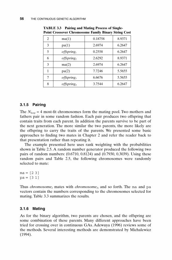
56 THE CONTINUOUS GENETIC ALGORITHM
3.1.5 Pairing
The Nkeep = 4 most-fit chromosomes form the mating pool. Two mothers andfathers pair in some random fashion. Each pair produces two offspring thatcontain traits from each parent. In addition the parents survive to be part ofthe next generation. The more similar the two parents, the more likely are the offspring to carry the traits of the parents. We presented some basicapproaches to finding two mates in Chapter 2 and refer the reader back tothat presentation rather than repeating it.
The example presented here uses rank weighting with the probabilitiesshown in Table 2.5. A random number generator produced the following twopairs of random numbers: (0.6710, 0.8124) and (0.7930, 0.3039). Using theserandom pairs and Table 2.5, the following chromosomes were randomlyselected to mate:
ma = [2 3]pa = [3 1]
Thus chromosome2 mates with chromosome3, and so forth. The ma and pavectors contain the numbers corresponding to the chromosomes selected formating. Table 3.3 summarizes the results.
3.1.6 Mating
As for the binary algorithm, two parents are chosen, and the offspring aresome combination of these parents. Many different approaches have beentried for crossing over in continuous GAs. Adewuya (1996) reviews some ofthe methods. Several interesting methods are demonstrated by Michalewicz(1994).
TABLE 3.3 Pairing and Mating Process of Single-Point Crossover Chromosome Family Binary String Cost
2 ma(1) 0.18758 8.9371
3 pa(1) 2.6974 6.2647
5 offspring1 0.2558 6.2647
6 offspring2 2.6292 8.9371
3 ma(2) 2.6974 6.2647
1 pa(2) 7.7246 5.5655
7 offspring3 6.6676 5.5655
8 offspring4 3.7544 6.2647
The simplest methods choose one or more points in the chromosome tomark as the crossover points. Then the variables between these points aremerely swapped between the two parents. For example purposes, consider thetwo parents to be
(3.6)
Crossover points are randomly selected, and then the variables in between areexchanged:
(3.7)
The extreme case is selecting Nvar points and randomly choosing which of thetwo parents will contribute its variable at each position. Thus one goes downthe line of the chromosomes and, at each variable, randomly chooses whetheror not to swap information between the two parents. This method is calleduniform crossover:
(3.8)
The problem with these point crossover methods is that no new informationis introduced: each continuous value that was randomly initiated in the initialpopulation is propagated to the next generation, only in different combina-tions. Although this strategy worked fine for binary representations, there isnow a continuum of values, and in this continuum we are merely interchang-ing two data points. These approaches totally rely on mutation to introducenew genetic material.
The blending methods remedy this problem by finding ways to combinevariable values from the two parents into new variable values in the offspring.A single offspring variable value, pnew, comes from a combination of the twocorresponding offspring variable values (Radcliff, 1991)
(3.9)
where
b = random number on the interval [0, 1]pmn = nth variable in the mother chromosomepdn = nth variable in the father chromosome
p p pnew mn dn= + -( )b b1
offspring p p p p p p p
offspring p p p p p p p
m d d d d m dN
d m m m m d mN
var
var
1 1 2 3 4 5 6
2 1 2 3 4 5 6
= [ ]= [ ]
, , , , , , ,
, , , , , , ,
. . .
. . .
offspring p p p p p p p
offspring p p p p p p p
m m d d m m mN
d d m m d d dN
var
var
1 1 2 3 4 5 6
2 1 2 3 4 5 6
= [ ]= [ ]
≠ ≠
≠ ≠
, , , , , , ,
, , , , , , ,
. . .
. . .
parent p p p p p p p
parent p p p p p p p
m m m m m m mN
d d d d d d dN
var
var
1 1 2 3 4 5 6
2 1 2 3 4 5 6
= [ ]= [ ]
, , , , , , ,
, , , , , , ,
. . .
. . .
COMPONENTS OF A CONTINUOUS GENETIC ALGORITHM 57
The same variable of the second offspring is merely the complement of thefirst (i.e., replacing b by 1 - b). If b = 1, then pmn propagates in its entirety andpdn dies. In contrast, if b = 0, then pdn propagates in its entirety and pmn dies.When b = 0.5 (Davis, 1991), the result is an average of the variables of the twoparents.This method is demonstrated to work well on several interesting prob-lems by Michalewicz (1994). Choosing which variables to blend is the nextissue. Sometimes, this linear combination process is done for all variables tothe right or to the left of some crossover point. Any number of points can bechosen to blend, up to Nvar values where all variables are linear combinationsof those of the two parents. The variables can be blended by using the sameb for each variable or by choosing different b’s for each variable. These blend-ing methods effectively combine the information from the two parents andchoose values of the variables between the values bracketed by the parents;however, they do not allow introduction of values beyond the extremesalready represented in the population. To do this requires an extrapolatingmethod. The simplest of these methods is linear crossover (Wright, 1991). Inthis case three offspring are generated from the two parents by
(3.10)
Any variable outside the bounds is discarded in favor of the other two. Thenthe best two offspring are chosen to propagate. Of course, the factor 0.5 is not the only one that can be used in such a method. Heuristic crossover(Michalewicz, 1991) is a variation where some random number, b, is chosenon the interval [0, 1] and the variables of the offspring are defined by
(3.11)
Variations on this theme include choosing any number of variables tomodify and generating different b for each variable. This method also allowsgeneration of offspring outside of the values of the two parent variables. Some-times values are generated outside of the allowed range. If this happens, theoffspring is discarded and the algorithm tries another b. The blend crossover(BLX-a) method (Eshelman and Shaffer, 1993) begins by choosing some para-meter a that determines the distance outside the bounds of the two parentvariables that the offspring variable may lie. This method allows new valuesoutside of the range of the parents without letting the algorithm stray too far.Many codes combine the various methods to use the strengths of each. Newmethods, such as quadratic crossover (Adewuya, 1996), do a numerical fit tothe fitness function. Three parents are necessary to perform a quadratic fit.
The algorithm used in this book is a combination of an extrapolationmethod with a crossover method. We wanted to find a way to closely
p p p pnew mn dn mn= -( ) +b
p p p
p p p
p p p
new mn dn
new mn dn
new mn dn
1
2
3
0 5 0 5
1 5 0 5
0 5 1 5
= +
= -
= - +
. .
. .
. .
58 THE CONTINUOUS GENETIC ALGORITHM
mimic the advantages of the binary GA mating scheme. It begins by randomlyselecting a variable in the first pair of parents to be the crossover point
(3.12)
We’ll let
(3.13)
where the m and d subscripts discriminate between the mom and the dadparent. Then the selected variables are combined to form new variables thatwill appear in the children:
(3.14)
where b is also a random value between 0 and 1. The final step is to completethe crossover with the rest of the chromosome as before:
(3.15)
If the first variable of the chromosomes is selected, then only the variables tothe right of the selected variable are swapped. If the last variable of the chro-mosomes is selected, then only the variables to the left of the selected vari-able are swapped. This method does not allow offspring variables outside thebounds set by the parent unless b > 1.
For our example problem, the first set of parents are given by
A random number generator selects p1 as the location of the crossover. Therandom number selected for b is b = 0.0272. The new offspring are given by
offspring
offspring
1
2
0 18758 0 0272 0 18758 0 0272 2 6974 6 26470 2558 6 2647
2 6974 0 0272 0 18758 0 0272 2 6974 8 93712 6292 8 9371
= - ¥ + ¥[ ]= [ ]= + ¥ - ¥[ ]= [ ]
. . . . . , .. , .
. . . . . , .
. , .
chromosome
chromosome
2
3
0 1876 8 9371
2 6974 6 2647
= [ ]= [ ]
. , .
. , .
offspring p p p p
offspring p p p p
m m new dN
d d new mN
var
var
1 1 2 1
2 1 2 2
= [ ]= [ ]
K K
K K
p p p p
p p p p
new m m d
new d m d
1
2
= - -[ ]= + -[ ]
a a a
a a a
b
b
parent p p p p
parent p p p p
m m m mN
d d d dN
var
var
1 1 2
2 1 2
= [ ]= [ ]
K K
K K
a
a
a = { }roundup random * Nvar
COMPONENTS OF A CONTINUOUS GENETIC ALGORITHM 59
Continuing this process once more with a b = 0.7898. The new offspring aregiven by
3.1.7 Mutations
Here, as in the last chapter, we can sometimes find our method working toowell. If care is not taken, the GA can converge too quickly into one region ofthe cost surface. If this area is in the region of the global minimum, that isgood. However, some functions, such as the one we are modeling, have manylocal minima. If we do nothing to solve this tendency to converge quickly, wecould end up in a local rather than a global minimum. To avoid this problemof overly fast convergence, we force the routine to explore other areas of thecost surface by randomly introducing changes, or mutations, in some of thevariables. For the binary GA, this amounted to just changing a bit from a 0 toa 1, and vice versa. The basic method of mutation is not much more compli-cated for the continuous GA. For more complicated methods, see Michalewicz(1994).
As with the binary GA, we chose a mutation rate of 20%. Multiplying themutation rate by the total number of variables that can be mutated in the pop-ulation gives 0.20 ¥ 7 ¥ 2 � 3 mutations. Next random numbers are chosen toselect the row and columns of the variables to be mutated. A mutated vari-able is replaced by a new random variable. The following pairs were randomlyselected:
The first random pair is (4, 1). Thus the value in row 4 and column 1 of thepopulation matrix is replaced with a uniform random number between oneand ten:
Mutations occur two more times. The first two columns in Table 3.4 show thepopulation after mating. The next two columns display the population aftermutation. Associated costs after the mutations appear in the last column. Themutated values in Table 3.4 appear in italics. Note that the first chromosome
5.6130 fi 9 8190.
mrow = 4 4 7
mcol = 1 2 1
[ ][ ]
offspring
offspring
3
4
2 6974 0 7898 2 6974 0 7898 7 7246 6 26476 6676 5 5655
7 7246 0 7898 2 6974 0 7898 7 7246 8 93713 7544 6 2647
= - ¥ + ¥[ ]= [ ]= + ¥ - ¥[ ]= [ ]
. . . . . , .
. , .
. . . . . , .
. , .
60 THE CONTINUOUS GENETIC ALGORITHM
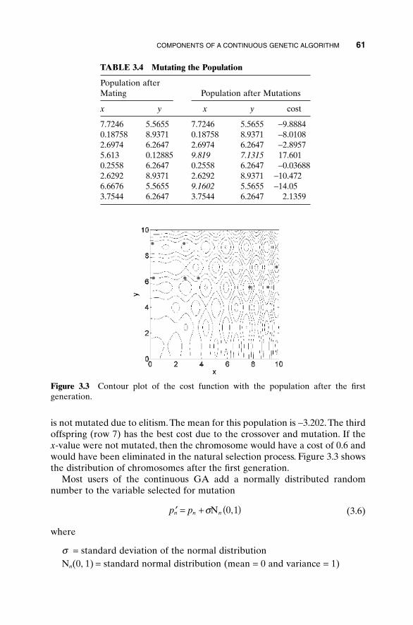
COMPONENTS OF A CONTINUOUS GENETIC ALGORITHM 61
is not mutated due to elitism. The mean for this population is -3.202. The thirdoffspring (row 7) has the best cost due to the crossover and mutation. If thex-value were not mutated, then the chromosome would have a cost of 0.6 andwould have been eliminated in the natural selection process. Figure 3.3 showsthe distribution of chromosomes after the first generation.
Most users of the continuous GA add a normally distributed randomnumber to the variable selected for mutation
(3.6)
where
s = standard deviation of the normal distributionNn(0, 1) = standard normal distribution (mean = 0 and variance = 1)
p pn n n¢ = + ( )sN 0 1,
TABLE 3.4 Mutating the Population
Population afterPopulation after MutationsMating
x y x y cost
7.7246 5.5655 7.7246 5.5655 -9.88840.18758 8.9371 0.18758 8.9371 -8.01082.6974 6.2647 2.6974 6.2647 -2.89575.613 0.12885 9.819 7.1315 17.6010.2558 6.2647 0.2558 6.2647 -0.036882.6292 8.9371 2.6292 8.9371 -10.4726.6676 5.5655 9.1602 5.5655 -14.053.7544 6.2647 3.7544 6.2647 2.1359
Figure 3.3 Contour plot of the cost function with the population after the first generation.
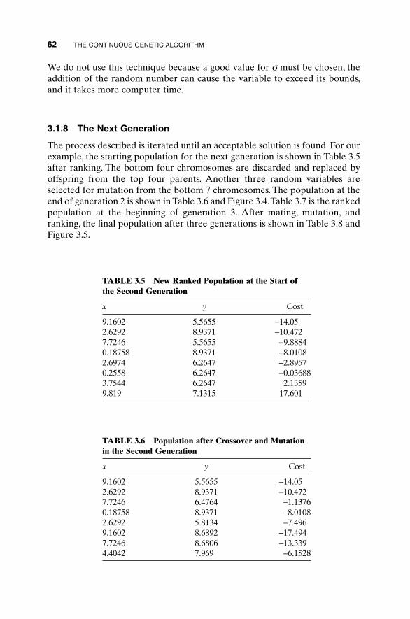
62 THE CONTINUOUS GENETIC ALGORITHM
We do not use this technique because a good value for s must be chosen, theaddition of the random number can cause the variable to exceed its bounds,and it takes more computer time.
3.1.8 The Next Generation
The process described is iterated until an acceptable solution is found. For ourexample, the starting population for the next generation is shown in Table 3.5after ranking. The bottom four chromosomes are discarded and replaced byoffspring from the top four parents. Another three random variables areselected for mutation from the bottom 7 chromosomes. The population at theend of generation 2 is shown in Table 3.6 and Figure 3.4.Table 3.7 is the rankedpopulation at the beginning of generation 3. After mating, mutation, andranking, the final population after three generations is shown in Table 3.8 andFigure 3.5.
TABLE 3.5 New Ranked Population at the Start ofthe Second Generation
x y Cost
9.1602 5.5655 -14.052.6292 8.9371 -10.4727.7246 5.5655 -9.88840.18758 8.9371 -8.01082.6974 6.2647 -2.89570.2558 6.2647 -0.036883.7544 6.2647 2.13599.819 7.1315 17.601
TABLE 3.6 Population after Crossover and Mutationin the Second Generation
x y Cost
9.1602 5.5655 -14.052.6292 8.9371 -10.4727.7246 6.4764 -1.13760.18758 8.9371 -8.01082.6292 5.8134 -7.4969.1602 8.6892 -17.4947.7246 8.6806 -13.3394.4042 7.969 -6.1528
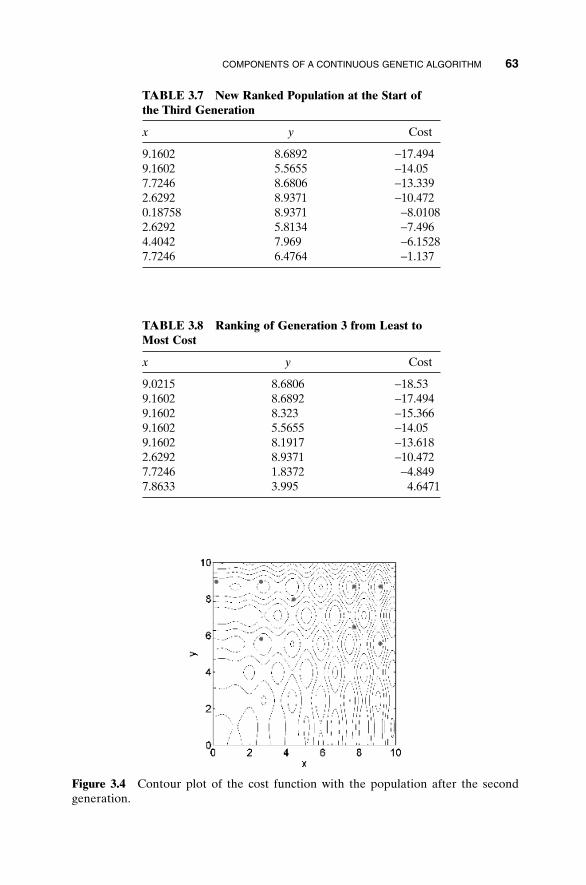
COMPONENTS OF A CONTINUOUS GENETIC ALGORITHM 63
TABLE 3.7 New Ranked Population at the Start ofthe Third Generation
x y Cost
9.1602 8.6892 -17.4949.1602 5.5655 -14.057.7246 8.6806 -13.3392.6292 8.9371 -10.4720.18758 8.9371 -8.01082.6292 5.8134 -7.4964.4042 7.969 -6.15287.7246 6.4764 -1.137
TABLE 3.8 Ranking of Generation 3 from Least toMost Cost
x y Cost
9.0215 8.6806 -18.539.1602 8.6892 -17.4949.1602 8.323 -15.3669.1602 5.5655 -14.059.1602 8.1917 -13.6182.6292 8.9371 -10.4727.7246 1.8372 -4.8497.8633 3.995 4.6471
Figure 3.4 Contour plot of the cost function with the population after the second generation.
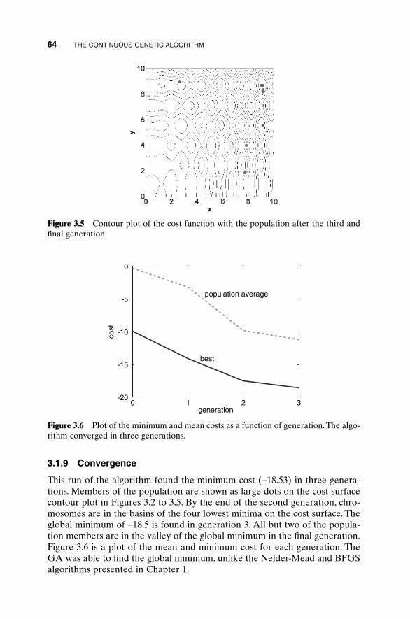
64 THE CONTINUOUS GENETIC ALGORITHM
3.1.9 Convergence
This run of the algorithm found the minimum cost (-18.53) in three genera-tions. Members of the population are shown as large dots on the cost surfacecontour plot in Figures 3.2 to 3.5. By the end of the second generation, chro-mosomes are in the basins of the four lowest minima on the cost surface. Theglobal minimum of -18.5 is found in generation 3. All but two of the popula-tion members are in the valley of the global minimum in the final generation.Figure 3.6 is a plot of the mean and minimum cost for each generation. TheGA was able to find the global minimum, unlike the Nelder-Mead and BFGSalgorithms presented in Chapter 1.
Figure 3.5 Contour plot of the cost function with the population after the third andfinal generation.
0 1 2 3-20
-15
-10
-5
0
generation
cost
best
population average
Figure 3.6 Plot of the minimum and mean costs as a function of generation. The algo-rithm converged in three generations.
3.2 A PARTING LOOK
The binary GA could have been used in this example as well as a continuousGA. Since the problem used continuous variables, it seemed more natural touse the continuous GA. The next chapter presents some practical optimiza-tion problems for both the binary and continuous GAs. Selecting the variousGA parameters, such as mutation rate and type of crossover, is still more ofan art than a science and will be discussed in Chapter 5.
BIBLIOGRAPHY
Adewuya, A. A. 1996. New methods in genetic search with real-valued chromosomes.Master’s thesis. Massachusetts Institute of Technology, Cambridge.
Davis, L. 1991. Hybridization and numerical representation. In L. Davis (ed.), TheHandbook of Genetic Algorithms. New York: Van Nostrand Reinhold, pp. 61–71.
Eshelman, L. J., and D. J. Shaffer. 1993. Real-coded genetic algorithms and interval-schemata. In D. L. Whitley (ed.), Foundations of Genetic Algorithms 2. San Mateo,CA: Morgan Kaufman, pp. 187–202.
Michalewicz, Z. 1994. Genetic Algorithms + Data Structures = Evolution Programs, 2nded. New York: Springer-Verlag.
Radcliff, N. J. 1991. Forma analysis and random respectful recombination. In Proc. 4thInt. Conf. on Genetic Algorithms, San Mateo, CA: Morgan Kauffman.
Wright,A. 1991. Genetic algorithms for real parameter optimization. In G. J. E. Rawlins(ed.), Foundations of Genetic Algorithms. San Mateo, CA: Morgan Kaufmann,pp. 205–218.
EXERCISES
1. Write a continuous GA that uses the following crossover:
a. (3.7)b. (3.8)c. (3.9)d. (3.10)e. (3.14)
2. Write a continuous GA that uses:
a. Pairing parents from top to bottomb. Random pairingc. Pairing based on costd. Roulette wheel rank weightinge. Tournament selection
EXERCISES 65
3. Find the minimum of _____ (from Appendix I) using your continuous GA.
4. Experiment with different population sizes and mutation rates.Which com-bination seems to work best for you? Explain.
5. Compare your GA with one of the following local optimizers:
a. Nelder-Mead downhill simplexb. BFGSc. DFPd. Steepest descente. Random search
6. Since the GA has many random components, it is important to average theresults of several runs. Write a program that will average the results ofseveral GA runs. Now, do another one of the exercises and compare results.
7. Plot the convergence of the GA. Which GA parameters have the mosteffect on convergence?
8. Compare the performance of the binary and continuous GAs. Which doyou prefer and why? Does the type of problem make a difference?
66 THE CONTINUOUS GENETIC ALGORITHM
CHAPTER 4
Basic Applications
67
The examples in this chapter make use of the GAs introduced in Chapters 2and 3. Enough details are provided for the user to try the problems themselves,and examples of the cost function are provided in some cases. Remember, theGA uses a random number generator, so the exact results won’t be repro-ducible. The first five examples are somewhat generic, using methods directlyapplicable to a wide range of problems. They are specifically designed to showthe wide range of applicability of both the binary and the continuous GA.They begin with use of the GA in the arts and games before moving onto anot too difficult mathematical problem. The next example is more arcane inthat it deals with an extremely problem-specific cost function. However, thesolution method is very straightforward, and the subroutine for the cost function could be replaced to solve many problems in the same vein. The last example demonstrates using a GA to simulate natural evolution of ananimal—the horse.
4.1 “MARY HAD A LITTLE LAMB”
In the first example, we’ll test the musical talent of the GA to see if it can learnthe first four measures of “Mary Had a Little Lamb.” This song is in the keyof C with 4/4 time and only has quarter and half notes. In addition the fre-quency variation of the notes is less than an octave. A chromosome for thisproblem has 4 ¥ 4 = 16 genes (one gene for each beat). The binary GA isperfect because there are eight distinct notes, seven possible frequencies, andone hold. The encoding is given in Table 4.1. A hold indicates the previousnote is a half note. (It is possible to devote one bit to indicate a quarter or halfnote. However, this approach would require variable-length chromosomes.)The actual solution only makes use of the C, D, E, and G notes and the hold.Therefore the binary encoding is only 62.5% efficient. Since the exact notesin the song may not be known, the inefficiency is only evident in hindsight. An
Practical Genetic Algorithms, Second Edition, by Randy L. Haupt and Sue Ellen Haupt.ISBN 0-471-45565-2 Copyright © 2004 John Wiley & Sons, Inc.
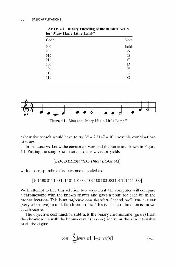
68 BASIC APPLICATIONS
exhaustive search would have to try 816 = 2.8147 ¥ 1014 possible combinationsof notes.
In this case we know the correct answer, and the notes are shown in Figure4.1. Putting the song parameters into a row vector yields
with a corresponding chromosome encoded as
We’ll attempt to find this solution two ways. First, the computer will comparea chromosome with the known answer and gives a point for each bit in theproper location. This is an objective cost function. Second, we’ll use our ear(very subjective) to rank the chromosomes.This type of cost function is knownas interactive.
The objective cost function subtracts the binary chromosome (guess) fromthe chromosome with the known result (answer) and sums the absolute valueof all the digits:
(4.1)cost answer n guess nn
= [ ] - [ ]=
Â1
48
101 100 011 100 101 101 101 000 100 100 100 000 101 111 111 000[ ]
EDCDEEEholdDDDholdEGGhold[ ]
TABLE 4.1 Binary Encoding of the Musical Notesfor “Mary Had a Little Lamb”
Code Note
000 hold001 A010 B011 C100 D101 E110 F111 G
Figure 4.1 Music to “Mary Had a Little Lamb.”
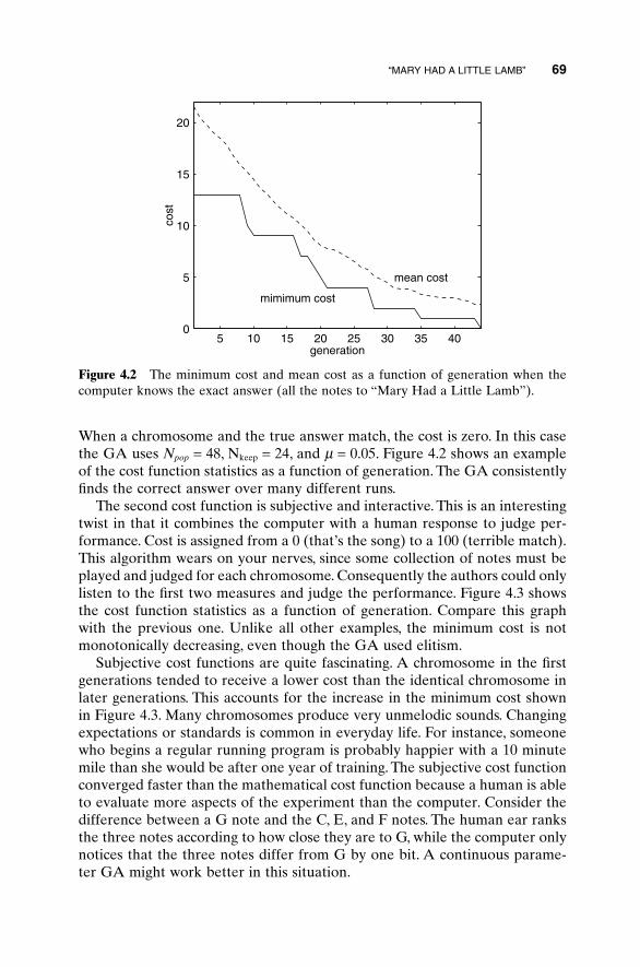
“MARY HAD A LITTLE LAMB” 69
When a chromosome and the true answer match, the cost is zero. In this casethe GA uses Npop = 48, Nkeep = 24, and m = 0.05. Figure 4.2 shows an exampleof the cost function statistics as a function of generation. The GA consistentlyfinds the correct answer over many different runs.
The second cost function is subjective and interactive. This is an interestingtwist in that it combines the computer with a human response to judge per-formance. Cost is assigned from a 0 (that’s the song) to a 100 (terrible match).This algorithm wears on your nerves, since some collection of notes must beplayed and judged for each chromosome. Consequently the authors could onlylisten to the first two measures and judge the performance. Figure 4.3 showsthe cost function statistics as a function of generation. Compare this graph with the previous one. Unlike all other examples, the minimum cost is notmonotonically decreasing, even though the GA used elitism.
Subjective cost functions are quite fascinating. A chromosome in the firstgenerations tended to receive a lower cost than the identical chromosome inlater generations. This accounts for the increase in the minimum cost shownin Figure 4.3. Many chromosomes produce very unmelodic sounds. Changingexpectations or standards is common in everyday life. For instance, someonewho begins a regular running program is probably happier with a 10 minutemile than she would be after one year of training. The subjective cost functionconverged faster than the mathematical cost function because a human is ableto evaluate more aspects of the experiment than the computer. Consider thedifference between a G note and the C, E, and F notes. The human ear ranksthe three notes according to how close they are to G, while the computer onlynotices that the three notes differ from G by one bit. A continuous parame-ter GA might work better in this situation.
5 10 15 20 25 30 35 400
5
10
15
20
generation
cost
mimimum cost
mean cost
Figure 4.2 The minimum cost and mean cost as a function of generation when thecomputer knows the exact answer (all the notes to “Mary Had a Little Lamb”).
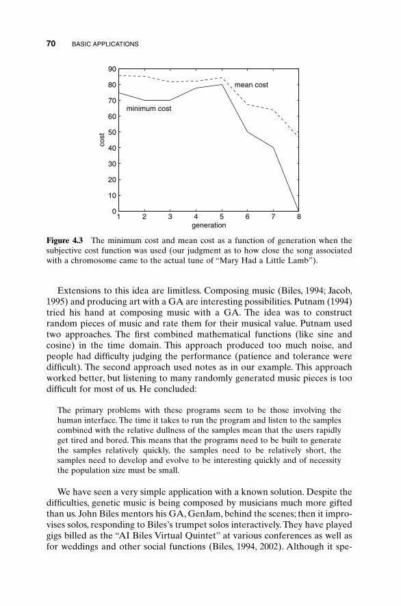
70 BASIC APPLICATIONS
Extensions to this idea are limitless. Composing music (Biles, 1994; Jacob,1995) and producing art with a GA are interesting possibilities. Putnam (1994)tried his hand at composing music with a GA. The idea was to constructrandom pieces of music and rate them for their musical value. Putnam usedtwo approaches. The first combined mathematical functions (like sine andcosine) in the time domain. This approach produced too much noise, andpeople had difficulty judging the performance (patience and tolerance weredifficult). The second approach used notes as in our example. This approachworked better, but listening to many randomly generated music pieces is toodifficult for most of us. He concluded:
The primary problems with these programs seem to be those involving thehuman interface. The time it takes to run the program and listen to the samplescombined with the relative dullness of the samples mean that the users rapidlyget tired and bored. This means that the programs need to be built to generatethe samples relatively quickly, the samples need to be relatively short, thesamples need to develop and evolve to be interesting quickly and of necessitythe population size must be small.
We have seen a very simple application with a known solution. Despite thedifficulties, genetic music is being composed by musicians much more giftedthan us. John Biles mentors his GA, GenJam, behind the scenes; then it impro-vises solos, responding to Biles’s trumpet solos interactively. They have playedgigs billed as the “AI Biles Virtual Quintet” at various conferences as well asfor weddings and other social functions (Biles, 1994, 2002). Although it spe-
1 2 3 4 5 6 7 80
10
20
30
40
50
60
70
80
90
generation
cost
minimum cost
mean cost
Figure 4.3 The minimum cost and mean cost as a function of generation when thesubjective cost function was used (our judgment as to how close the song associatedwith a chromosome came to the actual tune of “Mary Had a Little Lamb”).
cializes in Jazz and Latin tunes, it includes some New Age in its repertoire.Spector and Alpern (1995) trained a neural network on Charlie Parker frag-ments, and then used that as a fitness function for a genetic programmingsystem.The simplest applications did not produce pleasing melodies, but whenmore refined methods were used, they began to produce acceptable musicfragments. In essence, by defining what makes “good” music, these musiciansare coding the process of decision making. Wiggens et al. (1999) trained a GAto generate four-part harmony for given melodies using precoded criteriarather than a human interface. A music professor deemed the results of somevery basic trials more successful than most first-year undergraduate music students. Using different encoded composition rules, a GA was also able toproduce acceptable solos. However, they concluded that the GA was limitedin ability due to the combination of its inherent stochasticity and its inabilityto structure the reasoning process in the way that human composers can. Arethese limitations only due to our current abilities to define the rules that makepleasant music? Or will humans never be surpassed by genetic composers?
The idea of a subjective cost function is closely tied to work with fuzzy setsand logic (Ross, 1995). In classical set theory, an element is either a memberor not. In fuzzy set theory, an element can have various degrees of member-ship. Thus the boundaries between fuzzy sets are vague and ambiguous. Is thispiece of art or music good? We’re likely to be fuzzy about our decision andassign a cost between zero and one rather than either a zero or a one. Sincethe GA carries a list of answers in descending order of preference, it is perfectfor fuzzy design applications. These sorts of interactive processes are becom-ing more a popular as we try to use computers to simulate and interact withhuman thought processes.
4.2 ALGORITHMIC CREATIVITY—GENETIC ART
Let’s build on the artistic creativity of Section 4.1, but now in terms of visualart. Creativity is a right-brained activity and is often considered mutuallyexclusive of the more left-brained functions like logic and math that are asso-ciated with computers. Art is probably one of the most creative human func-tions. Can a computer actually create or improve a work of art? Improving isequivalent to optimizing. What better optimization tool to use for the creativeprocess than one that is based on natural selection—the GA.
There are currently a plethora of applications of evolutionary algorithmsapplied to art. The Web is a rich source of information and examples on artcreation using GAs, including many sites with galleries for browsing geneticart. Others even include an option to vote for your favorite designs. A brief review of the use of GAs in visual art and music was presented byJohnson and Romero Cardalda (2002). Karl Sims (1991) provided an earlydemonstration of how effectively evolutionary algorithms could be used tocreate computer graphics and animation. Todd and Latham (1992) produced
ALGORITHMIC CREATIVITY—GENETIC ART 71
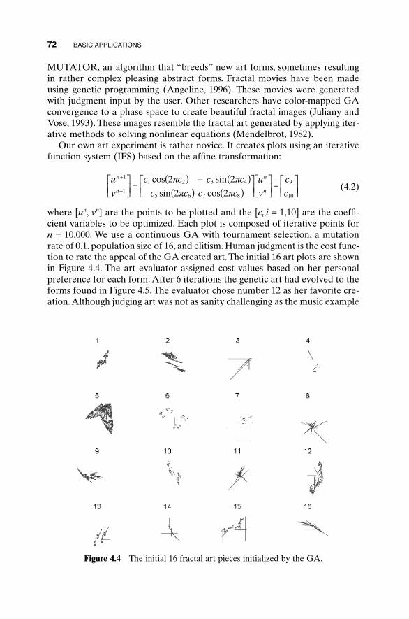
72 BASIC APPLICATIONS
MUTATOR, an algorithm that “breeds” new art forms, sometimes resultingin rather complex pleasing abstract forms. Fractal movies have been madeusing genetic programming (Angeline, 1996). These movies were generatedwith judgment input by the user. Other researchers have color-mapped GAconvergence to a phase space to create beautiful fractal images (Juliany andVose, 1993). These images resemble the fractal art generated by applying iter-ative methods to solving nonlinear equations (Mendelbrot, 1982).
Our own art experiment is rather novice. It creates plots using an iterativefunction system (IFS) based on the affine transformation:
(4.2)
where [un, vn] are the points to be plotted and the [ci,i = 1,10] are the coeffi-cient variables to be optimized. Each plot is composed of iterative points forn = 10,000. We use a continuous GA with tournament selection, a mutationrate of 0.1, population size of 16, and elitism. Human judgment is the cost func-tion to rate the appeal of the GA created art. The initial 16 art plots are shownin Figure 4.4. The art evaluator assigned cost values based on her personalpreference for each form. After 6 iterations the genetic art had evolved to theforms found in Figure 4.5. The evaluator chose number 12 as her favorite cre-ation.Although judging art was not as sanity challenging as the music example
u
v
c c c c
c c c c
u
v
c
c
n
n
n
n
+
+
ÈÎÍ
˘˚
=( ) - ( )
( ) ( )ÈÎÍ
˘˚ÈÎÍ
˘˚
+ ÈÎÍ
˘˚
1
1
1 2 3 4
5 6 7 8
9
10
2 2
2 2
cos sin
sin cos
p pp p
Figure 4.4 The initial 16 fractal art pieces initialized by the GA.
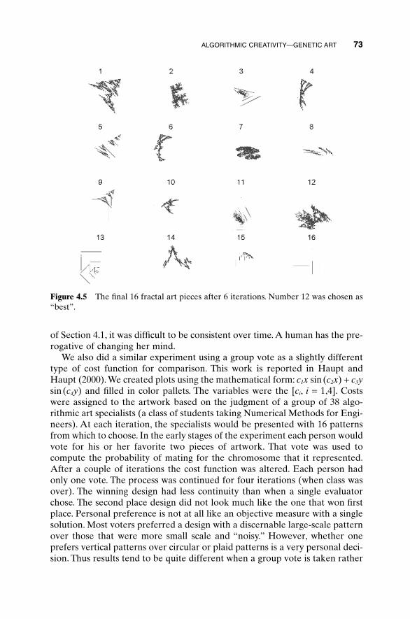
ALGORITHMIC CREATIVITY—GENETIC ART 73
Figure 4.5 The final 16 fractal art pieces after 6 iterations. Number 12 was chosen as“best”.
of Section 4.1, it was difficult to be consistent over time. A human has the pre-rogative of changing her mind.
We also did a similar experiment using a group vote as a slightly differenttype of cost function for comparison. This work is reported in Haupt andHaupt (2000). We created plots using the mathematical form: c1x sin (c2x) + c3ysin(c4y) and filled in color pallets. The variables were the [ci, i = 1,4]. Costswere assigned to the artwork based on the judgment of a group of 38 algo-rithmic art specialists (a class of students taking Numerical Methods for Engi-neers). At each iteration, the specialists would be presented with 16 patternsfrom which to choose. In the early stages of the experiment each person wouldvote for his or her favorite two pieces of artwork. That vote was used tocompute the probability of mating for the chromosome that it represented.After a couple of iterations the cost function was altered. Each person hadonly one vote. The process was continued for four iterations (when class wasover). The winning design had less continuity than when a single evaluatorchose. The second place design did not look much like the one that won firstplace. Personal preference is not at all like an objective measure with a singlesolution. Most voters preferred a design with a discernable large-scale patternover those that were more small scale and “noisy.” However, whether oneprefers vertical patterns over circular or plaid patterns is a very personal deci-sion. Thus results tend to be quite different when a group vote is taken rather
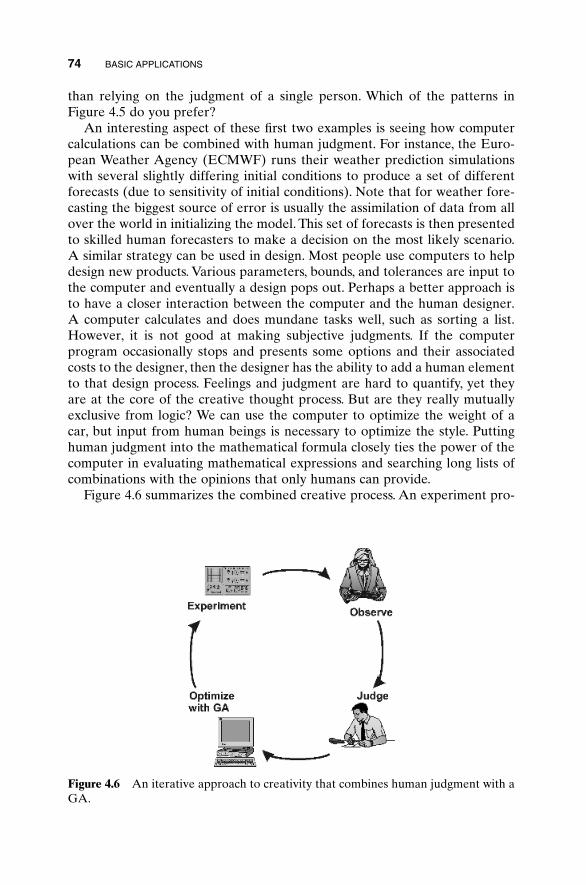
74 BASIC APPLICATIONS
than relying on the judgment of a single person. Which of the patterns inFigure 4.5 do you prefer?
An interesting aspect of these first two examples is seeing how computercalculations can be combined with human judgment. For instance, the Euro-pean Weather Agency (ECMWF) runs their weather prediction simulationswith several slightly differing initial conditions to produce a set of differentforecasts (due to sensitivity of initial conditions). Note that for weather fore-casting the biggest source of error is usually the assimilation of data from allover the world in initializing the model. This set of forecasts is then presentedto skilled human forecasters to make a decision on the most likely scenario.A similar strategy can be used in design. Most people use computers to helpdesign new products. Various parameters, bounds, and tolerances are input tothe computer and eventually a design pops out. Perhaps a better approach isto have a closer interaction between the computer and the human designer.A computer calculates and does mundane tasks well, such as sorting a list.However, it is not good at making subjective judgments. If the computerprogram occasionally stops and presents some options and their associatedcosts to the designer, then the designer has the ability to add a human elementto that design process. Feelings and judgment are hard to quantify, yet theyare at the core of the creative thought process. But are they really mutuallyexclusive from logic? We can use the computer to optimize the weight of acar, but input from human beings is necessary to optimize the style. Puttinghuman judgment into the mathematical formula closely ties the power of thecomputer in evaluating mathematical expressions and searching long lists ofcombinations with the opinions that only humans can provide.
Figure 4.6 summarizes the combined creative process. An experiment pro-
Figure 4.6 An iterative approach to creativity that combines human judgment with aGA.
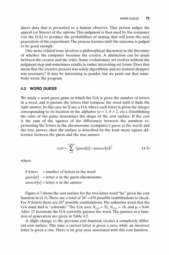
duces data that is presented to a human observer. That person judges theappeal (or fitness) of the options. This judgment is then used by the computer(via the GA) to produce the probabilities of mating that will form the nextgeneration of the experiment. The process iterates until the outcome is judgedto be good enough.
One more related issue involves a philosophical discussion in the literatureof whether the computer becomes the creator. A distinction can be madebetween the creator and the critic. Some evolutionary art evolves without thejudgment step and sometimes results in rather interesting art forms. Does thatmean that the creative process was solely algorithmic and no sentient designerwas necessary? It may be interesting to ponder, but we point out that some-body wrote the program.
4.3 WORD GUESS
We made a word guess game in which the GA is given the number of lettersin a word, and it guesses the letters that compose the word until it finds theright answer. In this case we’ll use a GA where each letter is given the integercorresponding to its location in the alphabet (a = 1, b = 2, etc.). Establishingthe rules of the game determines the shape of the cost surface. If the cost is the sum of the squares of the differences between the numbers re-presenting the letters in the chromosome (computer’s guess at the word) andthe true answer, then the surface is described by the least mean square dif-ference between the guess and the true answer:
(4.3)
where
# letters = number of letters in the wordguess[n] = letter n in the guess chromosomeanswer[n] = letter n in the answer
Figure 4.7 shows the cost surface for the two-letter word “he” given the costfunction in (4.3). There are a total of 262 = 676 possible combinations to check.For N letters there are 26N possible combinations. The unknown word that theGA must find is “colorado.” The GA uses Npop = 32, Nkeep = 16, and m = 0.04.After 27 iterations the GA correctly guesses the word. The guesses as a func-tion of generation are given in Table 4.2.
A slight change to the previous cost function creates a completely differ-ent cost surface. This time a correct letter is given a zero, while an incorrectletter is given a one. There is no gray area associated with this cost function.
cost guess n answer nn
letters
= [ ] - [ ]( )=
 2
1
#
WORD GUESS 75
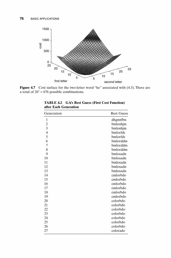
76 BASIC APPLICATIONS
510
1520
25
510
1520
250
500
1000
1500
second letterfirst letter
cost
Figure 4.7 Cost surface for the two-letter word “he” associated with (4.3). There area total of 262 = 676 possible combinations.
TABLE 4.2 GA’s Best Guess (First Cost Function)after Each Generation
Generation Best Guess
1 dhgmtfbn2 bmloshjm3 bmloshjm4 bmlorfds5 bmlorfds6 bmlorddm7 bmlorddm8 bmlorddm9 bmlosadn
10 bmlosadn11 bmlosadn12 bmlosadn13 bmlosadn14 cmlorbdo15 cmlorbdo16 cmlorbdo17 cmlorbdo18 cmlorbdo19 cmlorbdo20 colorbdo21 colorbdo22 colorbdo23 colorbdo24 colorbdo25 colorbdo26 colorbdo27 colorado
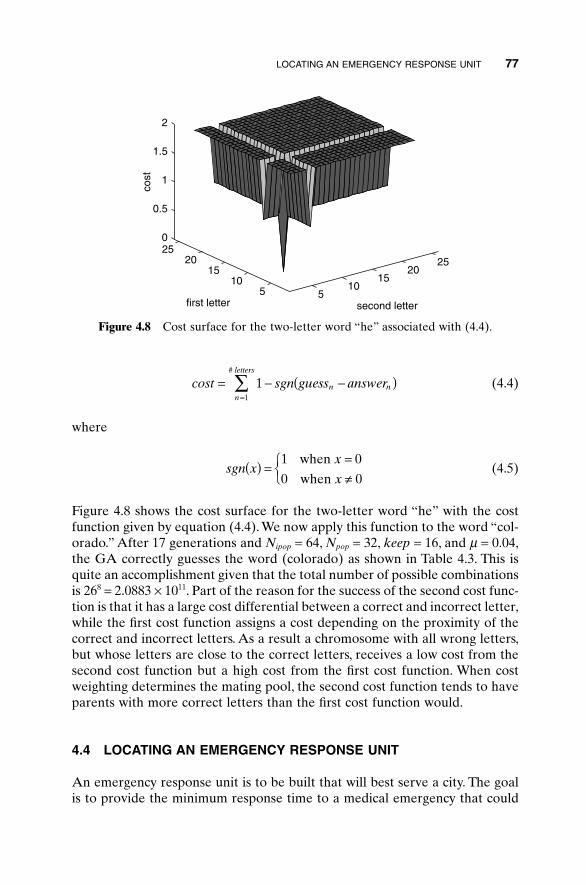
LOCATING AN EMERGENCY RESPONSE UNIT 77
(4.4)
where
(4.5)
Figure 4.8 shows the cost surface for the two-letter word “he” with the costfunction given by equation (4.4). We now apply this function to the word “col-orado.” After 17 generations and Nipop = 64, Npop = 32, keep = 16, and m = 0.04,the GA correctly guesses the word (colorado) as shown in Table 4.3. This isquite an accomplishment given that the total number of possible combinationsis 268 = 2.0883 ¥ 1011. Part of the reason for the success of the second cost func-tion is that it has a large cost differential between a correct and incorrect letter,while the first cost function assigns a cost depending on the proximity of thecorrect and incorrect letters. As a result a chromosome with all wrong letters,but whose letters are close to the correct letters, receives a low cost from thesecond cost function but a high cost from the first cost function. When costweighting determines the mating pool, the second cost function tends to haveparents with more correct letters than the first cost function would.
4.4 LOCATING AN EMERGENCY RESPONSE UNIT
An emergency response unit is to be built that will best serve a city. The goalis to provide the minimum response time to a medical emergency that could
sgn xx
x( ) =
=π
ÏÌÓ1 0
0 0
when
when
cost sgn guess answern nn
letters
= - -( )=
 11
#
510
1520
25
510
1520
250
0.5
1
1.5
2
second letterfirst letter
cost
Figure 4.8 Cost surface for the two-letter word “he” associated with (4.4).
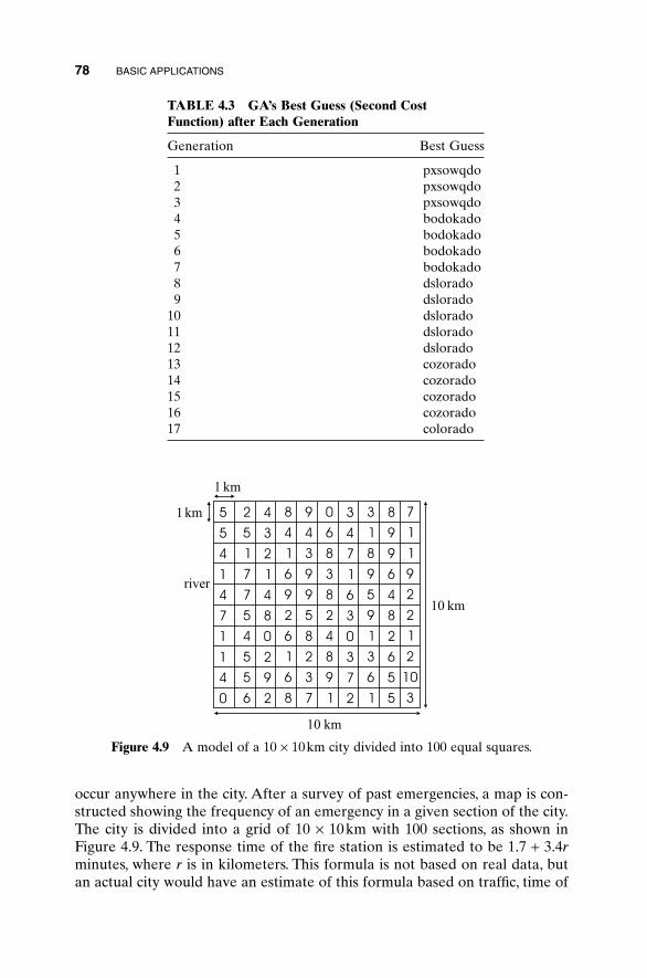
78 BASIC APPLICATIONS
occur anywhere in the city. After a survey of past emergencies, a map is con-structed showing the frequency of an emergency in a given section of the city.The city is divided into a grid of 10 ¥ 10km with 100 sections, as shown inFigure 4.9. The response time of the fire station is estimated to be 1.7 + 3.4rminutes, where r is in kilometers. This formula is not based on real data, butan actual city would have an estimate of this formula based on traffic, time of
TABLE 4.3 GA’s Best Guess (Second Cost Function) after Each Generation
Generation Best Guess
1 pxsowqdo2 pxsowqdo3 pxsowqdo4 bodokado5 bodokado6 bodokado7 bodokado8 dslorado9 dslorado
10 dslorado11 dslorado12 dslorado13 cozorado14 cozorado15 cozorado16 cozorado17 colorado
Figure 4.9 A model of a 10 ¥ 10km city divided into 100 equal squares.
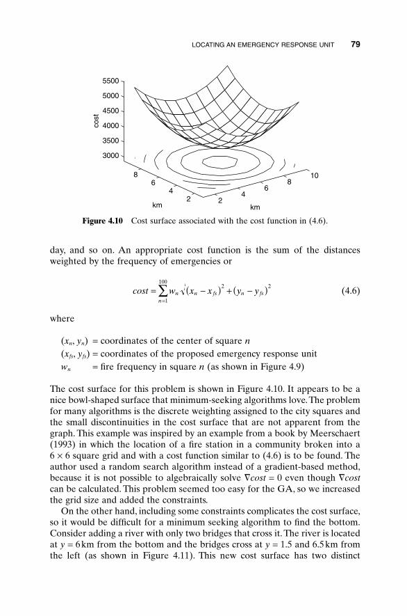
LOCATING AN EMERGENCY RESPONSE UNIT 79
day, and so on. An appropriate cost function is the sum of the distancesweighted by the frequency of emergencies or
(4.6)
where
(xn, yn) = coordinates of the center of square n(xfs, yfs) = coordinates of the proposed emergency response unitwn = fire frequency in square n (as shown in Figure 4.9)
The cost surface for this problem is shown in Figure 4.10. It appears to be anice bowl-shaped surface that minimum-seeking algorithms love.The problemfor many algorithms is the discrete weighting assigned to the city squares andthe small discontinuities in the cost surface that are not apparent from thegraph. This example was inspired by an example from a book by Meerschaert(1993) in which the location of a fire station in a community broken into a 6 ¥ 6 square grid and with a cost function similar to (4.6) is to be found. Theauthor used a random search algorithm instead of a gradient-based method,because it is not possible to algebraically solve �cost = 0 even though �costcan be calculated. This problem seemed too easy for the GA, so we increasedthe grid size and added the constraints.
On the other hand, including some constraints complicates the cost surface,so it would be difficult for a minimum seeking algorithm to find the bottom.Consider adding a river with only two bridges that cross it. The river is locatedat y = 6km from the bottom and the bridges cross at y = 1.5 and 6.5km fromthe left (as shown in Figure 4.11). This new cost surface has two distinct
cost w x x y yn n fs n fsn
= -( ) + -( )=
 2 2
1
100
24
68
10
24
68
3000
3500
4000
4500
5000
5500
kmkm
cost
Figure 4.10 Cost surface associated with the cost function in (4.6).
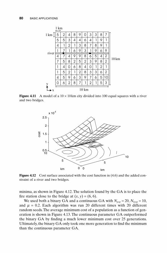
80 BASIC APPLICATIONS
minima, as shown in Figure 4.12. The solution found by the GA is to place thefire station close to the bridge at (x, y) = (6, 6).
We used both a binary GA and a continuous GA with Npop = 20, Nkeep = 10,and m = 0.2. Each algorithm was run 20 different times with 20 differentrandom seeds.The average minimum cost of a population as a function of gen-eration is shown in Figure 4.13. The continuous parameter GA outperformedthe binary GA by finding a much lower minimum cost over 25 generations.Ultimately, the binary GA only took one more generation to find the minimumthan the continuous parameter GA.
Figure 4.11 A model of a 10 ¥ 10km city divided into 100 equal squares with a riverand two bridges.
0
5
10
0
5
100.5
1
1.5
2
2.5x 10 4
kmkm
cost
Figure 4.12 Cost surface associated with the cost function in (4.6) and the added con-straint of a river and two bridges.
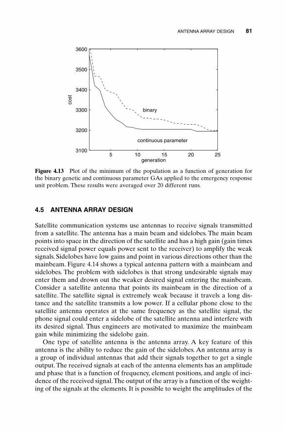
ANTENNA ARRAY DESIGN 81
4.5 ANTENNA ARRAY DESIGN
Satellite communication systems use antennas to receive signals transmittedfrom a satellite. The antenna has a main beam and sidelobes. The main beampoints into space in the direction of the satellite and has a high gain (gain timesreceived signal power equals power sent to the receiver) to amplify the weaksignals. Sidelobes have low gains and point in various directions other than themainbeam. Figure 4.14 shows a typical antenna pattern with a mainbeam andsidelobes. The problem with sidelobes is that strong undesirable signals mayenter them and drown out the weaker desired signal entering the mainbeam.Consider a satellite antenna that points its mainbeam in the direction of asatellite. The satellite signal is extremely weak because it travels a long dis-tance and the satellite transmits a low power. If a cellular phone close to thesatellite antenna operates at the same frequency as the satellite signal, thephone signal could enter a sidelobe of the satellite antenna and interfere withits desired signal. Thus engineers are motivated to maximize the mainbeamgain while minimizing the sidelobe gain.
One type of satellite antenna is the antenna array. A key feature of thisantenna is the ability to reduce the gain of the sidelobes. An antenna array isa group of individual antennas that add their signals together to get a singleoutput. The received signals at each of the antenna elements has an amplitudeand phase that is a function of frequency, element positions, and angle of inci-dence of the received signal.The output of the array is a function of the weight-ing of the signals at the elements. It is possible to weight the amplitudes of the
5 10 15 20 253100
3200
3300
3400
3500
3600
generation
cost
continuous parameter
binary
Figure 4.13 Plot of the minimum of the population as a function of generation forthe binary genetic and continuous parameter GAs applied to the emergency responseunit problem. These results were averaged over 20 different runs.
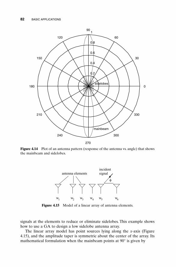
82 BASIC APPLICATIONS
signals at the elements to reduce or eliminate sidelobes. This example showshow to use a GA to design a low sidelobe antenna array.
The linear array model has point sources lying along the x-axis (Figure4.15), and the amplitude taper is symmetric about the center of the array. Itsmathematical formulation when the mainbeam points at 90° is given by
0.2
0.4
0.6
0.8
1
30
210
60
240
90
270
120
300
150
330
180 0
mainbeam
sidelobes
Figure 4.14 Plot of an antenna pattern (response of the antenna vs. angle) that showsthe mainbeam and sidelobes.
Figure 4.15 Model of a linear array of antenna elements.
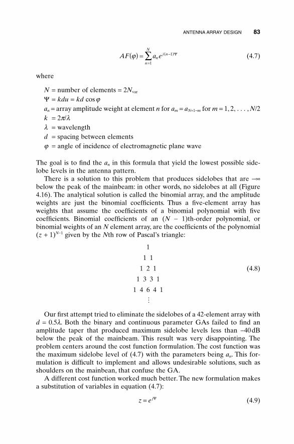
ANTENNA ARRAY DESIGN 83
(4.7)
where
N = number of elements = 2Nvar
Y = kdu = kd cos jan = array amplitude weight at element n for am = aN+1-m for m = 1, 2, . . . , N/2k = 2p/ll = wavelengthd = spacing between elementsj = angle of incidence of electromagnetic plane wave
The goal is to find the an in this formula that yield the lowest possible side-lobe levels in the antenna pattern.
There is a solution to this problem that produces sidelobes that are -•below the peak of the mainbeam: in other words, no sidelobes at all (Figure4.16). The analytical solution is called the binomial array, and the amplitudeweights are just the binomial coefficients. Thus a five-element array hasweights that assume the coefficients of a binomial polynomial with five coefficients. Binomial coefficients of an (N - 1)th-order polynomial, or binomial weights of an N element array, are the coefficients of the polynomial(z + 1)N-1 given by the Nth row of Pascal’s triangle:
1
1 1
1 2 1 (4.8)
1 3 3 1
1 4 6 4 1
Our first attempt tried to eliminate the sidelobes of a 42-element array withd = 0.5l. Both the binary and continuous parameter GAs failed to find anamplitude taper that produced maximum sidelobe levels less than -40dBbelow the peak of the mainbeam. This result was very disappointing. Theproblem centers around the cost function formulation. The cost function wasthe maximum sidelobe level of (4.7) with the parameters being an. This for-mulation is difficult to implement and allows undesirable solutions, such asshoulders on the mainbean, that confuse the GA.
A different cost function worked much better. The new formulation makesa substitution of variables in equation (4.7):
(4.9)z e j= Y
M
AF a enj n
n
N
j( ) = -( )
=Â 1
1
Y
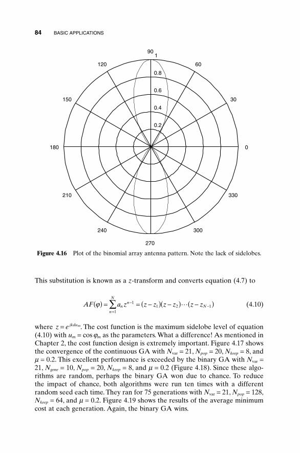
84 BASIC APPLICATIONS
This substitution is known as a z-transform and converts equation (4.7) to
(4.10)
where . The cost function is the maximum sidelobe level of equation(4.10) with um = cos jm as the parameters. What a difference! As mentioned inChapter 2, the cost function design is extremely important. Figure 4.17 showsthe convergence of the continuous GA with Nvar = 21, Npop = 20, Nkeep = 8, andm = 0.2. This excellent performance is exceeded by the binary GA with Nvar =21, Ngene = 10, Npop = 20, Nkeep = 8, and m = 0.2 (Figure 4.18). Since these algo-rithms are random, perhaps the binary GA won due to chance. To reduce the impact of chance, both algorithms were run ten times with a differentrandom seed each time. They ran for 75 generations with Nvar = 21, Npop = 128,Nkeep = 64, and m = 0.2. Figure 4.19 shows the results of the average minimumcost at each generation. Again, the binary GA wins.
z e jkdum=
AF a z z z z z z znn
n
N
Nj( ) = = -( ) -( ) -( )-
=-Â 1
11 2 1L
0.2
0.4
0.6
0.8
1
30
210
60
240
90
270
120
300
150
330
180 0
Figure 4.16 Plot of the binomial array antenna pattern. Note the lack of sidelobes.
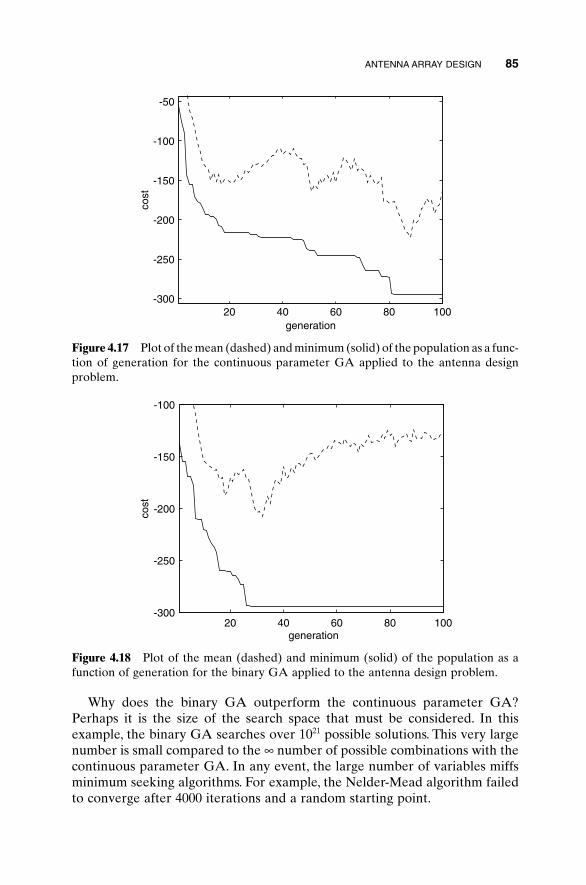
ANTENNA ARRAY DESIGN 85
Why does the binary GA outperform the continuous parameter GA?Perhaps it is the size of the search space that must be considered. In thisexample, the binary GA searches over 1021 possible solutions. This very largenumber is small compared to the • number of possible combinations with thecontinuous parameter GA. In any event, the large number of variables miffsminimum seeking algorithms. For example, the Nelder-Mead algorithm failedto converge after 4000 iterations and a random starting point.
20 40 60 80 100-300
-250
-200
-150
-100
-50
generation
cost
Figure 4.17 Plot of the mean (dashed) and minimum (solid) of the population as a func-tion of generation for the continuous parameter GA applied to the antenna designproblem.
20 40 60 80 100-300
-250
-200
-150
-100
generation
cost
Figure 4.18 Plot of the mean (dashed) and minimum (solid) of the population as afunction of generation for the binary GA applied to the antenna design problem.
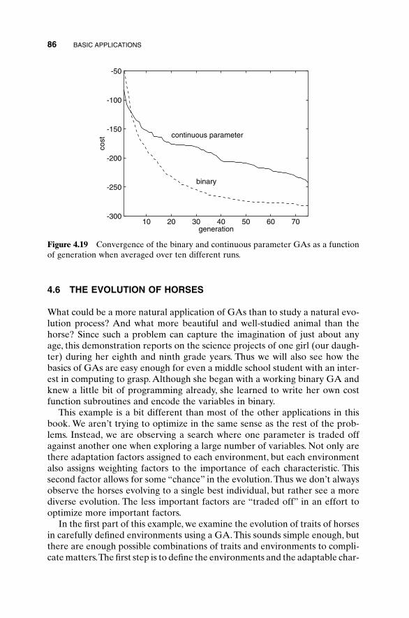
86 BASIC APPLICATIONS
4.6 THE EVOLUTION OF HORSES
What could be a more natural application of GAs than to study a natural evo-lution process? And what more beautiful and well-studied animal than thehorse? Since such a problem can capture the imagination of just about anyage, this demonstration reports on the science projects of one girl (our daugh-ter) during her eighth and ninth grade years. Thus we will also see how thebasics of GAs are easy enough for even a middle school student with an inter-est in computing to grasp. Although she began with a working binary GA andknew a little bit of programming already, she learned to write her own costfunction subroutines and encode the variables in binary.
This example is a bit different than most of the other applications in thisbook. We aren’t trying to optimize in the same sense as the rest of the prob-lems. Instead, we are observing a search where one parameter is traded offagainst another one when exploring a large number of variables. Not only arethere adaptation factors assigned to each environment, but each environmentalso assigns weighting factors to the importance of each characteristic. Thissecond factor allows for some “chance” in the evolution. Thus we don’t alwaysobserve the horses evolving to a single best individual, but rather see a morediverse evolution. The less important factors are “traded off” in an effort tooptimize more important factors.
In the first part of this example, we examine the evolution of traits of horsesin carefully defined environments using a GA. This sounds simple enough, butthere are enough possible combinations of traits and environments to compli-cate matters.The first step is to define the environments and the adaptable char-
10 20 30 40 50 60 70-300
-250
-200
-150
-100
-50
generation
cost
continuous parameter
binary
Figure 4.19 Convergence of the binary and continuous parameter GAs as a functionof generation when averaged over ten different runs.
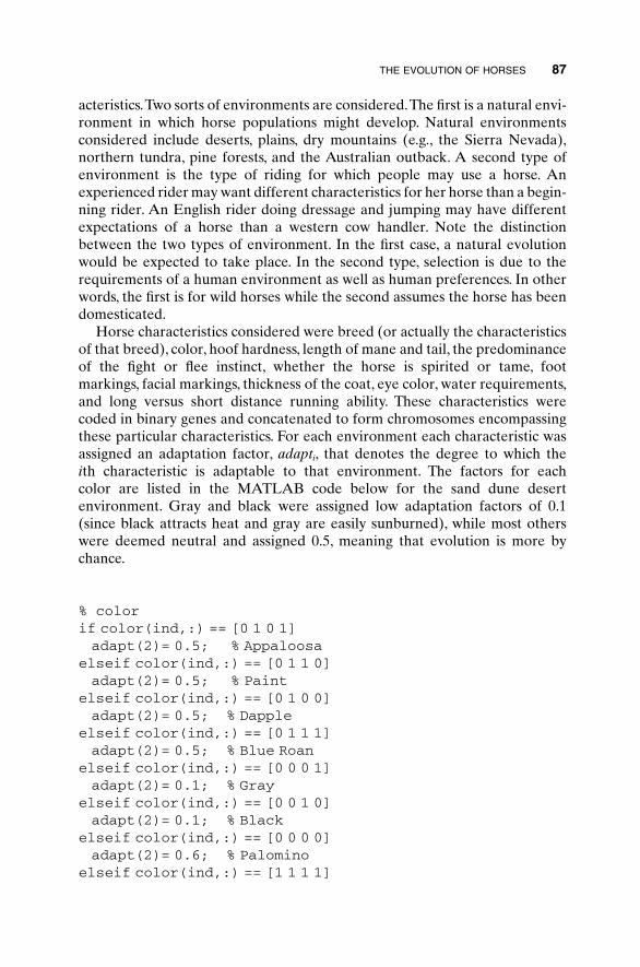
acteristics.Two sorts of environments are considered.The first is a natural envi-ronment in which horse populations might develop. Natural environments considered include deserts, plains, dry mountains (e.g., the Sierra Nevada),northern tundra, pine forests, and the Australian outback. A second type ofenvironment is the type of riding for which people may use a horse. An experienced rider may want different characteristics for her horse than a begin-ning rider. An English rider doing dressage and jumping may have differentexpectations of a horse than a western cow handler. Note the distinctionbetween the two types of environment. In the first case, a natural evolutionwould be expected to take place. In the second type, selection is due to therequirements of a human environment as well as human preferences. In otherwords, the first is for wild horses while the second assumes the horse has beendomesticated.
Horse characteristics considered were breed (or actually the characteristicsof that breed), color, hoof hardness, length of mane and tail, the predominanceof the fight or flee instinct, whether the horse is spirited or tame, foot markings, facial markings, thickness of the coat, eye color, water requirements,and long versus short distance running ability. These characteristics werecoded in binary genes and concatenated to form chromosomes encompassingthese particular characteristics. For each environment each characteristic wasassigned an adaptation factor, adapti, that denotes the degree to which the ith characteristic is adaptable to that environment. The factors for each color are listed in the MATLAB code below for the sand dune desert environment. Gray and black were assigned low adaptation factors of 0.1(since black attracts heat and gray are easily sunburned), while most otherswere deemed neutral and assigned 0.5, meaning that evolution is more bychance.
% colorif color(ind,:) == [0 1 0 1]adapt(2)= 0.5; % Appaloosa
elseif color(ind,:) == [0 1 1 0]adapt(2)= 0.5; % Paint
elseif color(ind,:) == [0 1 0 0]adapt(2)= 0.5; % Dapple
elseif color(ind,:) == [0 1 1 1]adapt(2)= 0.5; % Blue Roan
elseif color(ind,:) == [0 0 0 1]adapt(2)= 0.1; % Gray
elseif color(ind,:) == [0 0 1 0]adapt(2)= 0.1; % Black
elseif color(ind,:) == [0 0 0 0]adapt(2)= 0.6; % Palomino
elseif color(ind,:) == [1 1 1 1]
THE EVOLUTION OF HORSES 87
adapt(2)= 0.6; % Buckskinelseif color(ind,:) == [0 0 1 1]adapt(2)= 0.5; % Chestnut
elseif color(ind,:) == [1 1 1 0]adapt(2)= 0.5; % Bay
elseif color(ind,:) == [1 0 0 1]adapt(2)= 0.5; % Flaxen Maned Sorrel
elseadapt(2)= 0;
end
The importance of each characteristic to each environment would beexpected to vary. For instance, it may be extremely important for a desert horseto be able to go long periods without water. Yet for a domestic riding horsethat is watered regularly, this characteristic may not matter. For horses in thenorthern tundra a thick coat may be quite important, while it would actuallybe a detriment in a desert. A horse on the plains would do best with a thickcoat in the winter that thins in the summer. Color may not matter much fordomesticated horses, while it could be an important adaptation factor for wildhorses. The color adaptability, however, is highly dependent on the environ-ment. A white coat would reflect the sunlight and be an advantage in a hotdesert environment. However, in a northern tundra a dark coat could be usefulfor absorbing sunlight. Therefore a weighting function is necessary to definethe relative importance of each characteristic in each environment. Forinstance, the weighting factor for the sand dune desert appears below with theweights being in the same order as the characteristics listed above. We see thathoof hardness, length of mane and tail, number of socks, and facial markingsare given weightings of wti = 0.1, meaning that they are relatively unimpor-tant. In contrast, water requirements are weighted as the most important at0.9, and coat thickness was next most important at 0.8.
Function cost=sandundes(chrom)% parameter weighting (importance factor) for thisenvironmentwts=[.5,.6,.1,.1,.3,.4,.1,.1,.8,.6,.9,.5];
The cost function for each horse is then computed as the sum of the prod-ucts of the adaptation factors of the horse characteristics with the weightingfactors of how important each characteristic is for the particular environmentconsidered:
(4.11)cost adapt wti ii
= - ¥=Â
1
12
88 BASIC APPLICATIONS
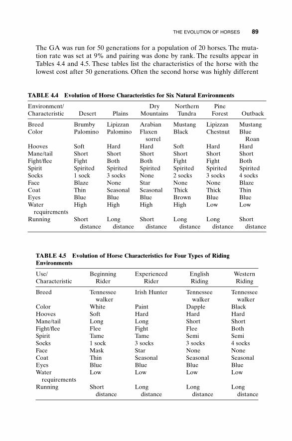
THE EVOLUTION OF HORSES 89
The GA was run for 50 generations for a population of 20 horses. The muta-tion rate was set at 9% and pairing was done by rank. The results appear inTables 4.4 and 4.5. These tables list the characteristics of the horse with thelowest cost after 50 generations. Often the second horse was highly different
TABLE 4.4 Evolution of Horse Characteristics for Six Natural Environments
Environment/ Dry Northern PineCharacteristic Desert Plains Mountains Tundra Forest Outback
Breed Brumby Lipizzan Arabian Mustang Lipizzan MustangColor Palomino Palomino Flaxen Black Chestnut Blue
sorrel RoanHooves Soft Hard Hard Soft Hard HardMane/tail Short Short Short Short Short ShortFight/flee Fight Both Both Fight Fight BothSpirit Spirited Spirited Spirited Spirited Spirited SpiritedSocks 1 sock 3 socks None 2 socks 3 socks 4 socksFace Blaze None Star None None BlazeCoat Thin Seasonal Seasonal Thick Thick ThinEyes Blue Blue Blue Brown Blue BlueWater High High High High Low Low
requirementsRunning Short Long Short Long Long Short
distance distance distance distance distance distance
TABLE 4.5 Evolution of Horse Characteristics for Four Types of Riding Environments
Use/ Beginning Experienced English WesternCharacteristic Rider Rider Riding Riding
Breed Tennessee Irish Hunter Tennessee Tennesseewalker walker walker
Color White Paint Dapple BlackHooves Soft Hard Hard HardMane/tail Long Long Short ShortFight/flee Flee Fight Flee BothSpirit Tame Tame Semi SemiSocks 1 sock 3 socks 3 socks 4 socksFace Mask Star None NoneCoat Thin Seasonal Seasonal SeasonalEyes Blue Blue Blue BlueWater Low Low Low Low
requirementsRunning Short Long Long Long
distance distance distance distance
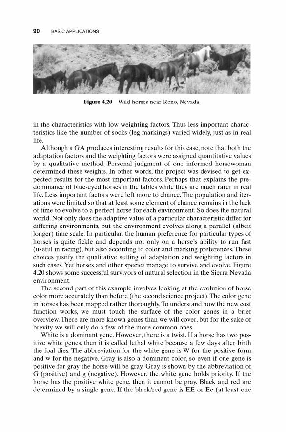
90 BASIC APPLICATIONS
in the characteristics with low weighting factors. Thus less important charac-teristics like the number of socks (leg markings) varied widely, just as in reallife.
Although a GA produces interesting results for this case, note that both theadaptation factors and the weighting factors were assigned quantitative valuesby a qualitative method. Personal judgment of one informed horsewomandetermined these weights. In other words, the project was devised to get ex-pected results for the most important factors. Perhaps that explains the pre-dominance of blue-eyed horses in the tables while they are much rarer in reallife. Less important factors were left more to chance. The population and iter-ations were limited so that at least some element of chance remains in the lackof time to evolve to a perfect horse for each environment. So does the naturalworld. Not only does the adaptive value of a particular characteristic differ fordiffering environments, but the environment evolves along a parallel (albeitlonger) time scale. In particular, the human preference for particular types ofhorses is quite fickle and depends not only on a horse’s ability to run fast(useful in racing), but also according to color and marking preferences. Thesechoices justify the qualitative setting of adaptation and weighting factors in such cases. Yet horses and other species manage to survive and evolve. Figure4.20 shows some successful survivors of natural selection in the Sierra Nevadaenvironment.
The second part of this example involves looking at the evolution of horsecolor more accurately than before (the second science project).The color genein horses has been mapped rather thoroughly.To understand how the new costfunction works, we must touch the surface of the color genes in a briefoverview. There are more known genes than we will cover, but for the sake ofbrevity we will only do a few of the more common ones.
White is a dominant gene. However, there is a twist. If a horse has two pos-itive white genes, then it is called lethal white because a few days after birththe foal dies. The abbreviation for the white gene is W for the positive formand w for the negative. Gray is also a dominant color, so even if one gene ispositive for gray the horse will be gray. Gray is shown by the abbreviation ofG (positive) and g (negative). However, the white gene holds priority. If thehorse has the positive white gene, then it cannot be gray. Black and red aredetermined by a single gene. If the black/red gene is EE or Ee (at least one
Figure 4.20 Wild horses near Reno, Nevada.
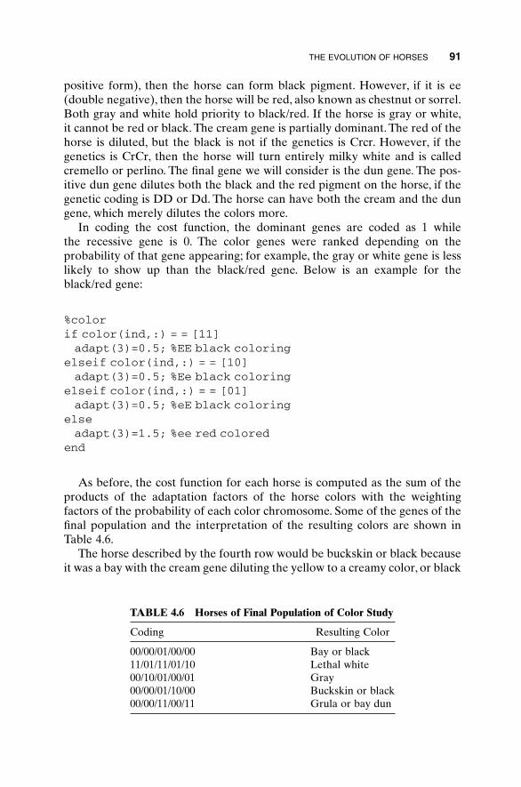
THE EVOLUTION OF HORSES 91
positive form), then the horse can form black pigment. However, if it is ee(double negative), then the horse will be red, also known as chestnut or sorrel.Both gray and white hold priority to black/red. If the horse is gray or white,it cannot be red or black. The cream gene is partially dominant. The red of thehorse is diluted, but the black is not if the genetics is Crcr. However, if thegenetics is CrCr, then the horse will turn entirely milky white and is calledcremello or perlino. The final gene we will consider is the dun gene. The pos-itive dun gene dilutes both the black and the red pigment on the horse, if thegenetic coding is DD or Dd. The horse can have both the cream and the dungene, which merely dilutes the colors more.
In coding the cost function, the dominant genes are coded as 1 while the recessive gene is 0. The color genes were ranked depending on the probability of that gene appearing; for example, the gray or white gene is lesslikely to show up than the black/red gene. Below is an example for theblack/red gene:
%colorif color(ind,:) = = [11]adapt(3)=0.5; %EE black coloring
elseif color(ind,:) = = [10]adapt(3)=0.5; %Ee black coloring
elseif color(ind,:) = = [01]adapt(3)=0.5; %eE black coloring
elseadapt(3)=1.5; %ee red colored
end
As before, the cost function for each horse is computed as the sum of theproducts of the adaptation factors of the horse colors with the weightingfactors of the probability of each color chromosome. Some of the genes of thefinal population and the interpretation of the resulting colors are shown inTable 4.6.
The horse described by the fourth row would be buckskin or black becauseit was a bay with the cream gene diluting the yellow to a creamy color, or black
TABLE 4.6 Horses of Final Population of Color Study
Coding Resulting Color
00/00/01/00/00 Bay or black11/01/11/01/10 Lethal white00/10/01/00/01 Gray00/00/01/10/00 Buckskin or black00/00/11/00/11 Grula or bay dun
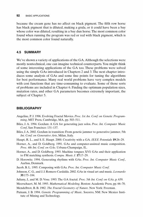
because the cream gene has no affect on black pigment. The fifth row horsehas black pigment that is diluted, making a grula, or it could have been a baywhose color was diluted, resulting in a bay dun horse. The most common colorfound when running the program was red or red with black pigment, which isthe most common color found naturally.
4.5 SUMMARY
We’ve shown a variety of applications of the GA.Although the selections weremostly nontechnical, one can imagine technical counterparts. You might thinkof some interesting applications of the GA too. These problems were solvedusing the simple GAs introduced in Chapters 2 and 3. The next chapter intro-duces some analysis of GAs and some fine points for tuning the algorithmsfor best performance. Many real world problems have very complex modelswith cost functions that are time-consuming to evaluate. Some of those sortsof problems are included in Chapter 6. Finding the optimum population sizes,mutation rates, and other GA parameters becomes extremely important, thesubject of Chapter 5.
BIBLIOGRAPHY
Angeline, P. J. 1996. Evolving Fractal Movies. Proc. 1st An. Conf. on Genetic Program-ming, MIT Press, Cambridge, MA, pp. 503–511.
Biles, J. A. 1994. GenJam: A GA for generating jazz solos. Proc. Int. Computer MusicConf, San Francisco: 131–137.
Biles, J. A. 2002. GenJam in transition: From genetic jammer to generative jammer, 5thInt. Conf. on Generative Arts, Milan, Italy.
Haupt, R. L., and S. E. Haupt. 2000. Creativity with a GA. IEEE Potentials 19:26–29.Horner, A., and D. Goldberg. 1991. GAs and computer-assisted music composition.
Proc. 4th Int. Conf. on GAs. Urbana-Champaign, IL.Horner, A., and D. Goldberg. 1993. Machine tongues XVI: GAs and their application
to FM matching synthesis. Compu. Music J. 17:17–29.D. Horowitz. 1994. Generating rhythms with GAs. Proc. Int. Computer Music Conf.,
Aarhus, Denmark.Jacob, B. L. 1995. Composing with GAs. Proc. Int. Computer Music Conf.Johnson, C. G., and J. J. Romero Cardalda. 2002. GAs in visual art and music. Leonardo
35:175–184.Juliany, J., and M. D. Vose. 1993. The GA fractal. Proc. 5th Int. Conf. on GAs, p. 639.Meerschaert, M. M. 1993. Mathematical Modeling. Boston: Academic Press, pp. 66–70.Mendelbrot, B. B. 1982. The Fractal Geometry of Nature. New York: Freeman.Putnam, J. B. 1994. Genetic Programming of Music. Socorro, NM: New Mexico Insti-
tute of Mining and Technology.
92 BASIC APPLICATIONS

Ross, T. J. 1995. Fuzzy Logic with Engineering Applications. New York: McGraw-Hill.Sims, K. 1991.Artificial evolution for computer graphics. Siggraph ’91 Proc. 25:319–328.Spector, L., and A. Alpern. 1995. Induction and recapitulation of deep musical struc-
ture. In Working Notes of the IJCAI-95 Workshop on Artificial Intelligence andMusic, pp. 41–48.
Todd, S., and W. Latham. 1992. Evolutionary Art and Computers. San Diego, CA:Academic Press.
Wiggins, G., G. Papadopoulos, S. Phon-Amnuaisuk, and A. Tuson. 1999. Evolutionarymethods for musical composition. Int. J. Comput. Anticipat. Syst.
BIBLIOGRAPHY 93
CHAPTER 5
An Added Level of Sophistication
95
Now that we have introduced the GA and discussed in detail the workings ofboth the binary and the continuous GA, it is time to look at some of the tricksof the trade. At times there may be a cost function that is difficult or expen-sive to evaluate. Other times we may notice that one crossover technique ispreferable. Deciding on the optimum population size is a controversial subject.How do we decide when the GA is done? Are there better ways to executethe genetic operators—crossover and mutation? Can a GA deal with prob-lems that require a specific ordering of the solution? Although there are notalways clear-cut solutions to all of these questions, we discuss possible answersin this chapter. We give hints and strategies on running a GA as well as someuseful additions to the codes. We discuss how to implement GAs on parallelmachines. The literature is full of other helpful ideas that can be applied to aplethora of problems.
5.1 HANDLING EXPENSIVE COST FUNCTIONS
Sometimes the cost function is extremely complicated and time-consuming toevaluate. As a result some care must be taken to minimize the number of costfunction evaluations. One step toward reducing the number of function eval-uations is to ensure that identical chromosomes are not evaluated more thanonce. There are several approaches to avoiding twins. First, the initial popula-tion can be created with no two chromosomes alike. Generally, this is only a problem for the binary GA, since the continuous GA has very low odds of generating identical random variables in two different chromosomes.However, checking the random population for repetitions is time-consumingin itself. Fortunately there are more efficient approaches. One approach is tobegin each chromosome with a different pattern. To illustrate, consider aninitial population of eight chromosomes:
Practical Genetic Algorithms, Second Edition, by Randy L. Haupt and Sue Ellen Haupt.ISBN 0-471-45565-2 Copyright © 2004 John Wiley & Sons, Inc.
Observe that the first 3 bits are uniquely prescribed, so each chromosome isguaranteed to be different from all others in the population. Perhaps thisapproach is not the best, since it only guarantees that the first gene or so isdifferent. A variation is to prescribe some other combination of bits. Forexample, if the chromosomes are three genes made up of 3 bits each, the first(or some other) bit in each gene could be set, as in
Either approach guarantees an initial population of unique chromosomes but doesn’t ensure that identical chromosomes are not evaluated in later generations.
Some GA users advocate populations with all unique members(Michalewicz, 1992). New members of the population (offspring or mutatedchromosomes) are checked against the chromosomes in the current popula-tion. If the new chromosome is a duplicate, then it is discarded. This approachrequires searching the population for each new member. Searching the popu-lation for identical twins is only worth the effort if the cost function evalua-tion takes longer than the population search. A new generation consists ofnonmutated parents, mutated parents, offspring, and mutated offspring. Ifthere is an identical chromosome that already has an associated cost, then thiscost is assigned to the new chromosome. Otherwise, the cost must be calcu-lated from the cost function. An alternative is to not allow identical chromo-somes to mate, therefore saving some computer time while helping maintaindiversity in the population.
1 1 1
1 1 0
1 0 1
1 0 0
0 1 1
0 1 0
0 0 1
0 0 0
11 11 11
0 0 0
11 11 0
0 0 11
0 0 0
0 0 0
1 1 0
1 0 1
0 0 0
0
0 0
0 0 0
0 0 0
0 0 1
1 1 1
000
001
010
011
100
101
110
111
1 0
1 0
0 1
0 1
1 0
0 1
1 0
0 0
01 10
01 10
10 01
01 00
10 11
00 11
11 00
11 11
96 AN ADDED LEVEL OF SOPHISTICATION
Another way to reduce the number of cost function evaluations is to only evaluate the costs of offspring of mutated chromosomes. Nonmutatedparents already have an associated cost, so they don’t have to be evaluatedagain. The simplicity of the approach suggests that it should be included inevery GA whether the cost function is time-consuming to calculate or not.Also the cost of a chromosome with multiple mutations needs only one evaluation.
A third approach keeps track of every chromosome and cost calculatedover all the generations. Any newborn chromosome is compared with otherchromosomes on the master list. If it has a twin in the big list, then the cost ofthat twin is assigned to the chromosome, thus saving the computation of the cost. This approach is the most drastic, being reserved for the most diffi-cult to evaluate cost functions, because the big list must be searched every generation.
There are some other interesting tricks to play with complicated cost func-tions. One technique is to find a way to simplify the cost function for the bulkof the runs. This approach is akin to doing an initial calculation on a coarsegrid, then fine-tuning it on a much finer grid. Here we merely define a simpleror lower order cost function in the initial generations and increase the costfunction accuracy as the GA progresses through the generations. The lowerorder model takes less time to calculate and can get the algorithm into theballpark of the solution.This approach proved very successful in Haupt (1995).In this case collocation was done at only one-fifth of the grid points. Thus a matrix on the order of 100 ¥ 100 was used in the early generations, while a matrix on the order of 500 ¥ 500 was used in the final generations. Anotherapproach is to use the GA to find the valley of the global minimum, then enlist the help of a fast local optimizer to find the bottom of the valley. Thishybrid method only works if the local optimizer can be applied to the costfunction.
So we have seen that there are a variety of methods to save computer timeby minimizing the number of evaluations of the cost function. Just be carefulthat the method does not require more time for searching than it saves in costfunction evaluations. Most of the cost functions presented in this book takelittle computer time to evaluate, so repeated evaluation of the same chromo-some has little impact on speed.
5.2 MULTIPLE OBJECTIVE OPTIMIZATION
In many applications the cost function has multiple, often times conflicting,objectives. Let’s take a look an example of a multiobjective optimization(MOO?) problem. Suppose a couple is looking for the ideal place to live. Oneis from Montana and the other is from Florida, so they have slightly differentideas of what is ideal. The two cost functions are approximately described by
MULTIPLE OBJECTIVE OPTIMIZATION 97
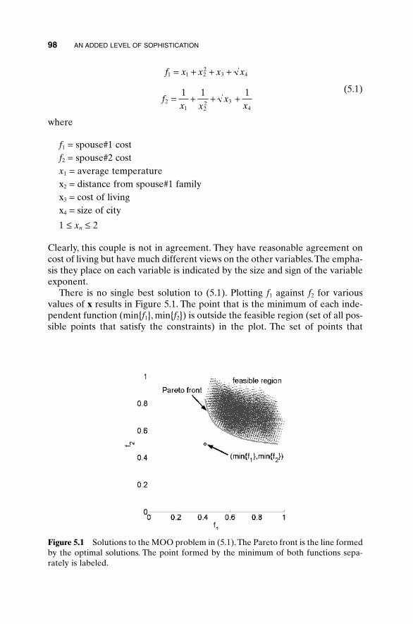
(5.1)
where
f1 = spouse#1 costf2 = spouse#2 costx1 = average temperaturex2 = distance from spouse#1 familyx3 = cost of livingx4 = size of city
1 £ xn £ 2
Clearly, this couple is not in agreement. They have reasonable agreement oncost of living but have much different views on the other variables.The empha-sis they place on each variable is indicated by the size and sign of the variableexponent.
There is no single best solution to (5.1). Plotting f1 against f2 for variousvalues of x results in Figure 5.1. The point that is the minimum of each inde-pendent function (min{f1}, min{f2}) is outside the feasible region (set of all pos-sible points that satisfy the constraints) in the plot. The set of points that
f x x x x
fx x
xx
1 1 22
3 4
21 2
2 34
1 1 1
= + + +
= + + +
98 AN ADDED LEVEL OF SOPHISTICATION
Figure 5.1 Solutions to the MOO problem in (5.1).The Pareto front is the line formedby the optimal solutions. The point formed by the minimum of both functions sepa-rately is labeled.
bounds the bottom of the feasible region is known as the Pareto front. A lineconnects the points on the Pareto front in Figure 5.1. In the next two subsec-tions we will discuss two approaches to MOO: weighted cost functions andfinding the Pareto front.
5.2.1 Sum of Weighted Cost Functions
The most straightforward approach to MOO is to weight each function andadd them together.
(5.2)
where
fn cost function n and 0 £ fn £ 1
wn weighting factor and
The problem with this method is determining appropriate values of wn. Dif-ferent weights produce different costs for the same fn. In the example theseweights are multiplied by the cost value and added together to obtain a singlescalar value that the GA minimizes. This approach requires assumptions onthe relative worth of the cost functions prior to running the GA.
Implementing this MOO approach in a GA only requires modifying thecost function to fit the form of (5.2) and does not require any modification tothe GA. Thus (5.1) becomes
(5.3)
This approach is not computationally intensive and results in a single best solu-tion based on the assigned weights.
5.2.2 Pareto Optimization
In MOO there is usually no single solution that is optimum with respect to allobjectives. Consequently there are a set of optimal solutions, known as Pareto-optimal solutions, noninferior solutions, or effective solutions. Without addi-tional information, all these solutions are equally satisfactory. The goal ofMOO is to find as many of these solutions as possible. If reallocation ofresources cannot improve one cost without raising another cost, then the solu-tion is Pareto optimal.
A Pareto GA returns a population with many members on the Pareto front.The population is ordered based on dominance. Solution A dominates solu-
cost wf w f= + -( )1 21
wnn
N
==
 11
cost w fnn
N
n==
Â1
MULTIPLE OBJECTIVE OPTIMIZATION 99
tion B if A has a lower cost than B for at least one of the objective functionsand is not worse with respect to the remaining objective functions. In otherwords, x1 dominates x2 if
(5.4)
or
(5.5)
A solution is Pareto optimal if no other solution dominates that solution withrespect to the cost functions. A solution is nondominated if no solution can befound that dominates it. Once this set of solutions is found, then the user canselect a single solution based on various postoptimization trade-offs ratherthan weighting the costs. One way of finding the Pareto front is to run a GAfor many different combinations of the cost function weights in (5.2). Eachoptimal solution is on the Pareto front. This approach requires too many runsto estimate the Pareto set.
David Schaffer first implemented a multi-objective evolutionary algorithmcalled the vector-evaluated GA or VEGA in 1984 (Schaffer, 1984). His algo-rithm started off fine but tended to converge to a single solution. To preventconvergence to a single solution, Goldberg and Richardson (1987) suggestedusing a nondominated sorting procedure coupled with a niching strategy calledsharing. Sharing takes into account that individuals in the same niche mustshare the available resources. This concept is integrated into the Pareto GAby increasing the cost of chromosomes as a function of their distance fromeach other. Closely grouped chromosomes will find their costs increased morethan chromosomes that are spaced far apart.
The multi-objective GA (MOGA) (Fonesca and Flemming, 1993) starts byfinding all nondominated chromosomes of a population and gives them a rankof one. These chromosomes are removed from the population. Next all the nondominated chromosomes of this smaller population are found andassigned a rank of two. This process continues until all the chromosomes areassigned a rank. The largest rank will be less than or equal to the size of thepopulation. Usually there are many solutions that have the same rank. Theselection procedure uses the chromosome ranking to determine the matingpool. MOGA also uses niching on the cost to distribute the population overthe Pareto-optimal region.
A nondominated sorting GA (NSGA) ranks chromosomes in the samemanner as MOGA. The NSGA algorithm then calculates a uniqueness value.This uniqueness value is related to the distance between each solution and itstwo closest neighbors. Distance may be calculated from the variable values orthe associated costs. The resulting values are scaled between 0 and 1 and sub-tracted from the cost. A newer version (NSGA-II) improves the NSGA algo-rithm in a few ways:
f x f x f x f x1 1 1 2 2 1 2 2( ) £ ( ) ( ) < ( )and
f x f x f x f x1 1 1 2 2 1 2 2( ) < ( ) ( ) £ ( )and
100 AN ADDED LEVEL OF SOPHISTICATION
HYBRID GA 101
• Reduces the computational complexity of the nondominated sorting.• Introduces elitism.• Replaces sharing with crowded-comparison to reduce computations and
the need for a user-defined sharing parameter.
Details on NSGA-II can be found in Deb et al. (2002).The Pareto GA introduced here works with two cost functions. It can be
easily modified to work with more.A Pareto GA needs a large population sizeto work well, since it is trying to define the Pareto front. Consequently we onlyinclude tournament selection in the GA. Figure 5.2 shows a flowchart of thisPareto GA. The GA used to find the Pareto front for (5.1) had Npop = 500, dis-cards 50% of the population, m = 0.1, and tournament selection. Figure 5.3 displays the final population.Those chromosomes on the Pareto front are con-nected by a line. Although not perfect, the GA did find a very reasonableapproximation to the Pareto front. This approach allows an easier way totradeoff the infinite number of optimal solutions to the MOO problem.
A study was done to compare the performance of various MOO algorithms(Zitzler and Thiele, 1999). It compared the VEGA, NSGA, niched Pareto GA,the weighted-sum approach, and their newly proposed strength Pareto ap-proach (SPEA). They found SPEA to be best on various runs with the knap-sack problem. They found VEGA and NSGA to be the next best performerswith VEGA having a slight advantage.
5.3 HYBRID GA
A hybrid GA combines the power of the GA with the speed of a local optimizer. The GA excels at gravitating toward the global minimum. It is notespecially fast at finding the minimum when in a locally quadratic region.Thus the GA finds the region of the optimum, and then the local optimizertakes over to find the minimum. Hybrid GA can take one of the followingforms:
1. Running a GA until it slows down, then letting a local optimizer takeover. Hopefully the GA is very close to the global minimum.
2. Seeding the GA population with some local minima found from randomstarting points in the population.
3. Every so many iterations, running a local optimizer on the best solutionor the best few solutions and adding the resulting chromosomes to thepopulation.
The continuous GA will easily couple to a local optimizer, since local opti-mizers use continuous variables. Some authors have even used a micro GA(GA with small population) as the local optimizer (Kazarlis et al., 2001).
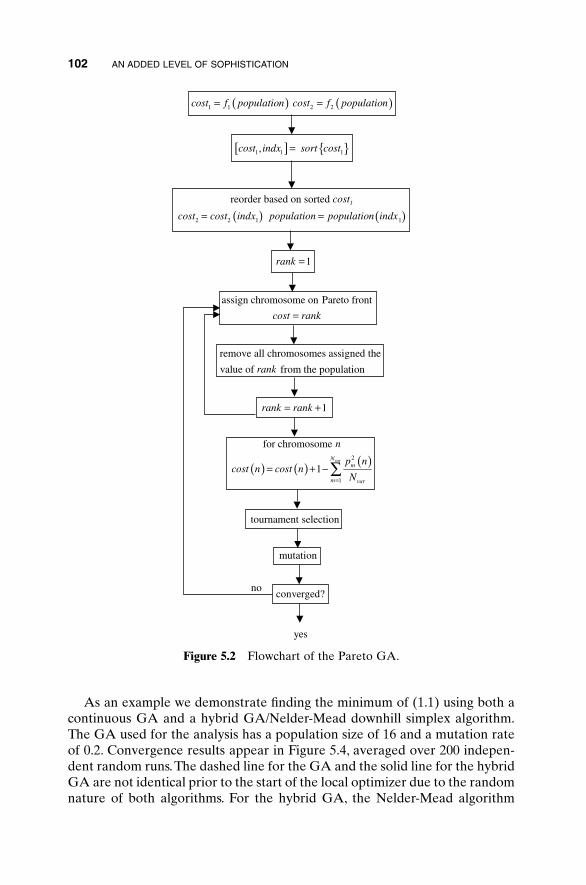
102 AN ADDED LEVEL OF SOPHISTICATION
( ) ( )1 1 2 2cost f population cost f population= =
[ ] { }1 1 1, cost indx sort cost=
= ( ) )(2 2 1 1
reorder based on sorted 1cost
cost cost indx population population indx
assign chromosome on Pareto front
cost rank=
1rank =
( ) ( ) ( )2
1
for chromosome
1varN
m
m var
n
p ncost n cost n
N=
= + − ∑
remove all chromosomes assigned the
value of from the populationrank
1rank rank= +
tournament selection
mutation
converged?no
yes
==
Figure 5.2 Flowchart of the Pareto GA.
As an example we demonstrate finding the minimum of (1.1) using both acontinuous GA and a hybrid GA/Nelder-Mead downhill simplex algorithm.The GA used for the analysis has a population size of 16 and a mutation rateof 0.2. Convergence results appear in Figure 5.4, averaged over 200 indepen-dent random runs.The dashed line for the GA and the solid line for the hybridGA are not identical prior to the start of the local optimizer due to the randomnature of both algorithms. For the hybrid GA, the Nelder-Mead algorithm
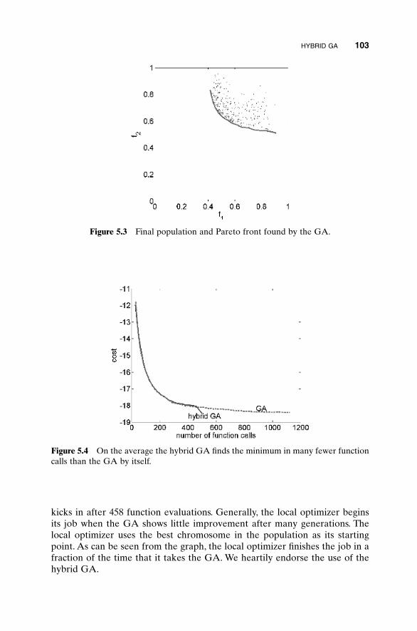
kicks in after 458 function evaluations. Generally, the local optimizer beginsits job when the GA shows little improvement after many generations. Thelocal optimizer uses the best chromosome in the population as its startingpoint. As can be seen from the graph, the local optimizer finishes the job in afraction of the time that it takes the GA. We heartily endorse the use of thehybrid GA.
HYBRID GA 103
Figure 5.3 Final population and Pareto front found by the GA.
Figure 5.4 On the average the hybrid GA finds the minimum in many fewer functioncalls than the GA by itself.
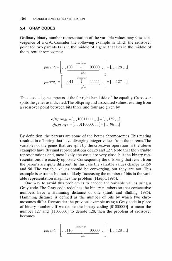
5.4 GRAY CODES
Ordinary binary number representation of the variable values may slow con-vergence of a GA. Consider the following example in which the crossoverpoint for two parents falls in the middle of a gene that lies in the middle ofthe parent chromosomes:
The decoded gene appears at the far right-hand side of the equality. Crossoversplits the genes as indicated.The offspring and associated values resulting froma crossover point between bits three and four are given by
By definition, the parents are some of the better chromosomes. This matingresulted in offspring that have diverging integer values from the parents. Thevariables of the genes that are split by the crossover operation in the aboveexamples have decimal representations of 128 and 127. Note that the variablerepresentations and, most likely, the costs are very close, but the binary rep-resentations are exactly opposite. Consequently the offspring that result fromthe parents are quite different. In this case the variable values change to 159and 96. The variable values should be converging, but they are not. Thisexample is extreme, but not unlikely. Increasing the number of bits in the vari-able representation magnifies the problem (Haupt, 1996).
One way to avoid this problem is to encode the variable values using a Gray code. The Gray code redefines the binary numbers so that consecutivenumbers have a Hamming distance of one (Taub and Shilling, 1986).Hamming distance is defined as the number of bits by which two chro-mosomes differ. Reconsider the previous example using a Gray code in placeof binary numbers. If we define the binary coding [01000000] to mean thenumber 127 and [11000000] to denote 128, then the problem of crossoverbecomes
offspringoffspring
1
2
10011111 15901100000 96
= ◊ ◊ ◊ ◊ ◊ ◊[ ] = ◊ ◊ ◊ ◊ ◊ ◊[ ]= ◊ ◊ ◊ ◊ ◊ ◊[ ] = ◊ ◊ ◊ ◊ ◊ ◊[ ]
parent
parent
crossover
gene
crossover
gene
1
2
100 00000 128
011 11111 127
= ◊ ◊ ◊ Ø ◊ ◊ ◊È
ÎÍÍ
˘
˚˙˙
= ◊ ◊ ◊ ◊ ◊ ◊[ ]
= ◊ ◊ ◊ Ø ◊ ◊ ◊È
ÎÍÍ
˘
˚˙˙
= ◊ ◊ ◊ ◊ ◊ ◊[ ]
1 2444 3444
1 2444 3444
104 AN ADDED LEVEL OF SOPHISTICATION
parentcrossover
gene
1 110 00000 128= ◊ ◊ ◊ Ø ◊ ◊ ◊È
ÎÍÍ
˘
˚˙˙
= ◊ ◊ ◊ ◊ ◊ ◊[ ]1 2444 3444
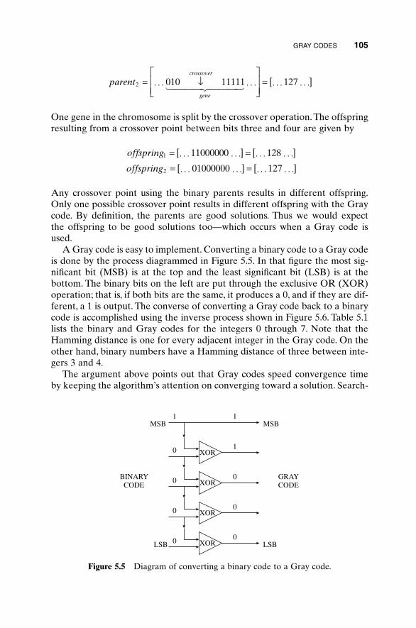
One gene in the chromosome is split by the crossover operation. The offspringresulting from a crossover point between bits three and four are given by
Any crossover point using the binary parents results in different offspring.Only one possible crossover point results in different offspring with the Graycode. By definition, the parents are good solutions. Thus we would expect the offspring to be good solutions too—which occurs when a Gray code isused.
A Gray code is easy to implement. Converting a binary code to a Gray codeis done by the process diagrammed in Figure 5.5. In that figure the most sig-nificant bit (MSB) is at the top and the least significant bit (LSB) is at thebottom. The binary bits on the left are put through the exclusive OR (XOR)operation; that is, if both bits are the same, it produces a 0, and if they are dif-ferent, a 1 is output. The converse of converting a Gray code back to a binarycode is accomplished using the inverse process shown in Figure 5.6. Table 5.1lists the binary and Gray codes for the integers 0 through 7. Note that theHamming distance is one for every adjacent integer in the Gray code. On theother hand, binary numbers have a Hamming distance of three between inte-gers 3 and 4.
The argument above points out that Gray codes speed convergence timeby keeping the algorithm’s attention on converging toward a solution. Search-
offspring
offspring
1
2
11000000 128
01000000 127
= ◊ ◊ ◊ ◊ ◊ ◊[ ] = ◊ ◊ ◊ ◊ ◊ ◊[ ]= ◊ ◊ ◊ ◊ ◊ ◊[ ] = ◊ ◊ ◊ ◊ ◊ ◊[ ]
parentcrossover
gene
2 010 11111 127= ◊ ◊ ◊ Ø ◊ ◊ ◊È
ÎÍÍ
˘
˚˙˙
= ◊ ◊ ◊ ◊ ◊ ◊[ ]1 2444 3444
GRAY CODES 105
XOR
XOR
XOR
XOR
BINARYCODE
GRAYCODE
MSB
LSB
MSB
LSB
1
0
0
0
0
1
1
0
0
0
Figure 5.5 Diagram of converting a binary code to a Gray code.
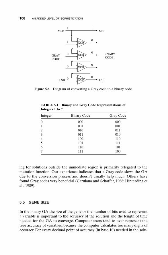
ing for solutions outside the immediate region is primarily relegated to themutation function. Our experience indicates that a Gray code slows the GAdue to the conversion process and doesn’t usually help much. Others havefound Gray codes very beneficial (Carulana and Schaffer, 1988; Hinterding etal., 1989).
5.5 GENE SIZE
In the binary GA the size of the gene or the number of bits used to representa variable is important to the accuracy of the solution and the length of timeneeded for the GA to converge. Computer users tend to over represent thetrue accuracy of variables, because the computer calculates too many digits ofaccuracy. For every decimal point of accuracy (in base 10) needed in the solu-
106 AN ADDED LEVEL OF SOPHISTICATION
XOR
XOR
XOR
XOR
BINARYCODE
GRAYCODE
MSB
LSB
MSB
LSB
1
0
0
0
0
1
1
0
0
0
Figure 5.6 Diagram of converting a Gray code to a binary code.
TABLE 5.1 Binary and Gray Code Representations ofIntegers 1 to 7
Integer Binary Code Gray Code
0 000 0001 001 0012 010 0113 011 0104 100 1105 101 1116 110 1017 111 100
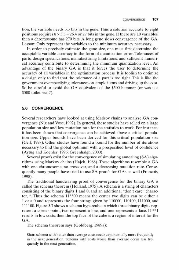
tion, the variable needs 3.3 bits in the gene. Thus a solution accurate to eightpositions requires 8 ¥ 3.3 = 26.4 or 27 bits in the gene. If there are 10 variables,then a chromosome has 270 bits. A long gene slows convergence of the GA.Lesson: Only represent the variables to the minimum accuracy necessary.
In order to precisely estimate the gene size, one must first determine theacceptable variable accuracy in the form of quantization error. Tolerances ofparts, design specifications, manufacturing limitations, and sufficient numeri-cal accuracy contribute to determining the minimum quantization level. Anadvantage of the binary GA is that it forces the user to determine the accuracy of all variables in the optimization process. It is foolish to optimizea design only to find that the tolerance of a part is too tight. This is like thegovernment overspecifying tolerances on simple items and driving up the cost.So be careful to avoid the GA equivalent of the $500 hammer (or was it a$500 toilet seat?).
5.6 CONVERGENCE
Several researchers have looked at using Markov chains to analyze GA con-vergence (Nix and Vose, 1992). In general, these studies have relied on a largepopulation size and low mutation rate for the statistics to work. For instance,it has been shown that convergence can be achieved above a critical popula-tion size. Upper bounds have been derived for this critical population size(Cerf, 1998). Other studies have found a bound for the number of iterationsnecessary to find the global optimum with a prespecified level of confidence(Aytug and Koehler, 1996; Greenhalgh, 2000).
Several proofs exist for the convergence of simulating annealing (SA) algo-rithms using Markov chains (Hajek, 1988). These algorithms resemble a GAwith one chromosome, no crossover, and a decreasing mutation rate. Conse-quently many people have tried to use SA proofs for GAs as well (Francois,1998).
The traditional handwaving proof of convergence for the binary GA iscalled the schema theorem (Holland, 1975). A schema is a string of charactersconsisting of the binary digits 1 and 0, and an additional “don’t care” charac-ter, *. Thus the schema 11**00 means the center two digits can be either a 1 or a 0 and represents the four strings given by 110000, 110100, 111000, and111100. Figure 5.7 shows a schema hypercube in which three binary digits rep-resent a corner point, two represent a line, and one represents a face. If **1results in low costs, then the top face of the cube is a region of interest for theGA.
The schema theorem says (Goldberg, 1989a):
Short schema with better than average costs occur exponentially more frequentlyin the next generation. Schema with costs worse than average occur less fre-quently in the next generation.
CONVERGENCE 107
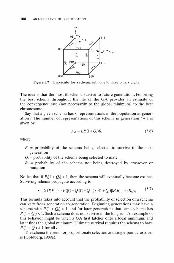
The idea is that the most fit schema survive to future generations. Followingthe best schema throughout the life of the GA provides an estimate of the convergence rate (not necessarily to the global minimum) to the best chromosome.
Say that a given schema has st representations in the population at gener-ation t. The number of representations of this schema in generation t + 1 isgiven by
(5.6)
where
Pt = probability of the schema being selected to survive to the next generation
Qt = probability of the schema being selected to mateRt = probability of the schema not being destroyed by crossover or
mutation
Notice that if Pt(1 + Qt) < 1, then the schema will eventually become extinct.Surviving schema propagate according to
(5.7)
This formula takes into account that the probability of selection of a schemacan vary from generation to generation. Beginning generations may have aschema with Pt(1 + Qt) > 1, and for later generations that same schema hasPt(1 + Qt) < 1. Such a schema does not survive in the long run. An example ofthis behavior might be when a GA first latches onto a local minimum, andlater finds the global minimum. Ultimate survival requires the schema to havePt(1 + Qt) > 1 for all t.
The schema theorem for proportionate selection and single-point crossoveris (Goldberg, 1989a).
s P P P Q Q Q R R R st t t t t t t+ - - -≥ ( ) +( ) +( ) +( )[ ]( )1 1 1 1 1 1 1 11 1 1. . . . . . . . .
s s P Q Rt t t t t+ = +( )1 1
108 AN ADDED LEVEL OF SOPHISTICATION
Figure 5.7 Hypercube for a schema with one to three binary digits.
(5.8)
where
f�= average fitness of chromosomes containing schemaf = average fitness of populationPc = probability of crossoverPm = probability of mutation of a single bitd = distance between the first and last digit in schemaNbits = number of possible crossover sitesz = number of defined digits in schema
Many variations to this fundamental theorem appear in the literature.In practice, when do you stop the algorithm? Well . . . We don’t have a good
answer. This is one of the fuzzy aspects of using the GA. Consider some goodpossibilities:
1. Correct answer. This may sound silly and simple. Make sure you checkyour best chromosome to see if it is the answer or an acceptable answerto the problem. If it is, then stop.
2. No improvement. If the GA continues with the same best chromosomefor X number of iterations, then stop. Either the algorithm found a goodanswer or it is stuck in a local minimum. Be careful here. Sometimes thebest solution will stay in the same spot for quite a while before a fortu-itous crossover or mutation generates a better one.
3. Statistics. If the mean or standard deviation of the population’s costreaches a certain level, then stop the algorithm. This means the valuesare no longer changing.
4. Number of iterations. If the algorithm doesn’t stop for one of the reasonsabove, then limit the maximum number of iterations. It can go on foreverunless stopped.
5. Local optimizer. Use a local optimizer. Stop if there is no improvement.
If your algorithm isn’t converging to a good solution, try changing the GA parameters like population size and mutation rate. Maybe a differentcrossover method or switching from a continuous GA to a binary GA is the answer. When the local optimizer finishes, then declare convergence.We do not advocate the GA as an answer to every problem. Sometimes it performs poorly in comparison with other methods. Don’t be afraid to jumpship to a minimum-seeking algorithm when your GA is sinking. Note that formany problems, we don’t really need the minimum. Instead, we are happy tosee improvement over previous best results.
s sff
PN
Pt t cbits
m+ ≥ --
ÈÎÍ
˘˚
-ÏÌÓ
¸˛1 1
1
)d
z
CONVERGENCE 109
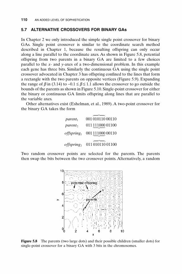
5.7 ALTERNATIVE CROSSOVERS FOR BINARY GAs
In Chapter 2 we only introduced the simple single point crossover for binaryGAs. Single point crossover is similar to the coordinate search methoddescribed in Chapter 1, because the resulting offspring can only occur along a line parallel to the coordinate axes. As shown in Figure 5.8, potentialoffspring from two parents in a binary GA are limited to a few choices parallel to the x- and y-axes of a two-dimensional problem. In this exampleeach gene has three bits. Similarly the continuous GA using the single pointcrossover advocated in Chapter 3 has offspring confined to the lines that forma rectangle with the two parents on opposite vertices (Figure 5.9). Expandingthe range of b in (3.14) to -0.1 £ b £ 1.1 allows the crossover to go outside thebounds of the parents as shown in Figure 5.10. Single-point crossover for eitherthe binary or continuous GA limits offspring along lines that are parallel tothe variable axes.
Other alternatives exist (Eshelman, et al., 1989). A two-point crossover forthe binary GA takes the form
Two random crossover points are selected for the parents. The parents then swap the bits between the two crossover points. Alternatively, a random
parent
parent
offspring
offspring
1
2
1
2
001 010110 00110
011 111000 01100
001 111000 00110
011 010110 01100
674 84
124 34
124 34674 84
110 AN ADDED LEVEL OF SOPHISTICATION
Figure 5.8 The parents (two large dots) and their possible children (smaller dots) forsingle-point crossover for a binary GA with 3 bits in the chromosomes.
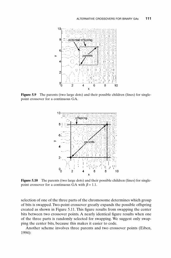
selection of one of the three parts of the chromosome determines which groupof bits is swapped. Two-point crossover greatly expands the possible offspringcreated as shown in Figure 5.11. This figure results from swapping the centerbits between two crossover points. A nearly identical figure results when oneof the three parts is randomly selected for swapping. We suggest only swap-ping the center bits, because this makes it easier to code.
Another scheme involves three parents and two crossover points (Eiben,1994):
ALTERNATIVE CROSSOVERS FOR BINARY GAs 111
Figure 5.9 The parents (two large dots) and their possible children (lines) for single-point crossover for a continuous GA.
Figure 5.10 The parents (two large dots) and their possible children (lines) for single-point crossover for a continuous GA with b = 1.1.
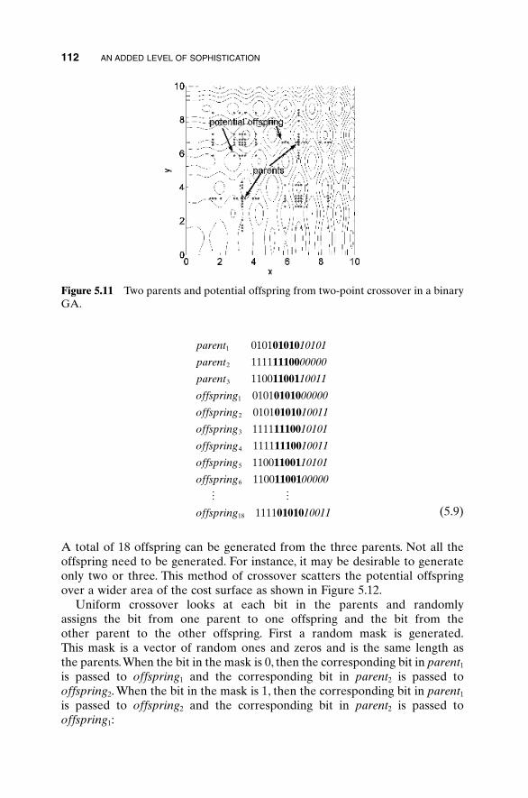
(5.9)
A total of 18 offspring can be generated from the three parents. Not all theoffspring need to be generated. For instance, it may be desirable to generateonly two or three. This method of crossover scatters the potential offspringover a wider area of the cost surface as shown in Figure 5.12.
Uniform crossover looks at each bit in the parents and randomly assigns the bit from one parent to one offspring and the bit from the other parent to the other offspring. First a random mask is generated.This mask is a vector of random ones and zeros and is the same length as the parents.When the bit in the mask is 0, then the corresponding bit in parent1
is passed to offspring1 and the corresponding bit in parent2 is passed to offspring2. When the bit in the mask is 1, then the corresponding bit in parent1
is passed to offspring2 and the corresponding bit in parent2 is passed to offspring1:
parent 10101
parent 00000
parent 10011
offspring 00000
offspring 10011
offspring 10101
offspring 10011
offspring 10101
offspring 00000
offspring 10011
1
2
3
1
2
3
4
5
6
18
0101
1111
1100
0101
0101
1111
1111
1100
1100
1111
01010
11100
11001
01010
01010
11100
11100
11001
11001
01010
M M
112 AN ADDED LEVEL OF SOPHISTICATION
Figure 5.11 Two parents and potential offspring from two-point crossover in a binaryGA.
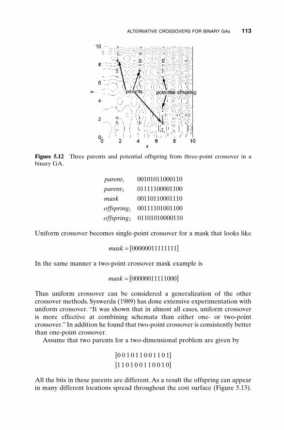
Uniform crossover becomes single-point crossover for a mask that looks like
In the same manner a two-point crossover mask example is
Thus uniform crossover can be considered a generalization of the othercrossover methods. Syswerda (1989) has done extensive experimentation withuniform crossover. “It was shown that in almost all cases, uniform crossover is more effective at combining schemata than either one- or two-pointcrossover.” In addition he found that two-point crossover is consistently betterthan one-point crossover.
Assume that two parents for a two-dimensional problem are given by
All the bits in these parents are different. As a result the offspring can appearin many different locations spread throughout the cost surface (Figure 5.13).
0 0 1 0 1 1 0 0 1 1 0 1
1 1 0 1 0 0 1 1 0 0 1 0
[ ][ ]
mask = [ ]00000011111000
mask = [ ]00000011111111
parent
parent
mask
offspring
offspring
1
2
1
2
00101011000110
01111100001100
00110110001110
00111101001100
01101010000110
ALTERNATIVE CROSSOVERS FOR BINARY GAs 113
Figure 5.12 Three parents and potential offspring from three-point crossover in abinary GA.
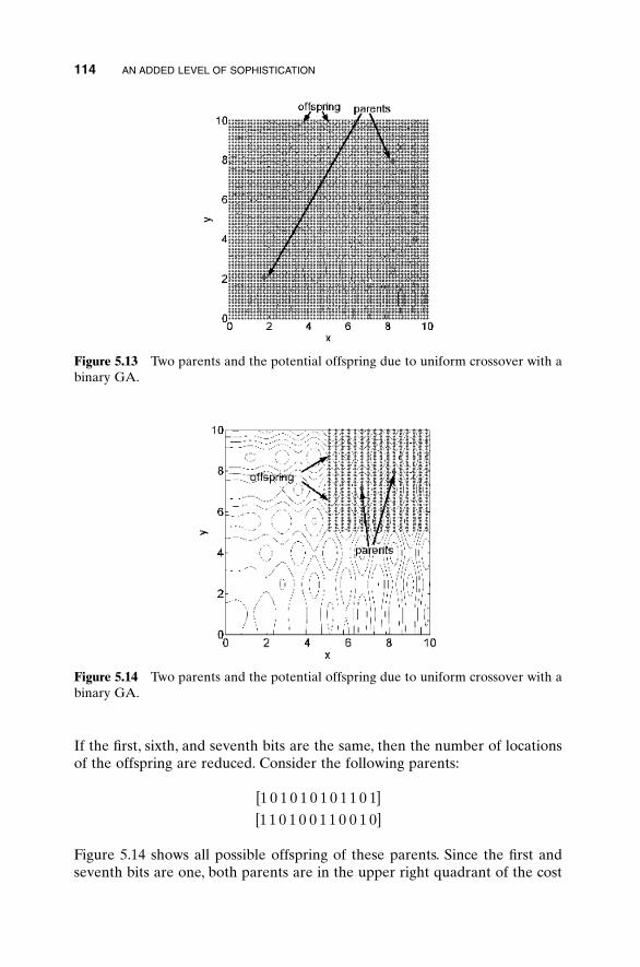
If the first, sixth, and seventh bits are the same, then the number of locationsof the offspring are reduced. Consider the following parents:
Figure 5.14 shows all possible offspring of these parents. Since the first andseventh bits are one, both parents are in the upper right quadrant of the cost
1 0 1 0 1 0 1 0 1 1 0 1
1 1 0 1 0 0 1 1 0 0 1 0
[ ][ ]
114 AN ADDED LEVEL OF SOPHISTICATION
Figure 5.13 Two parents and the potential offspring due to uniform crossover with abinary GA.
Figure 5.14 Two parents and the potential offspring due to uniform crossover with abinary GA.
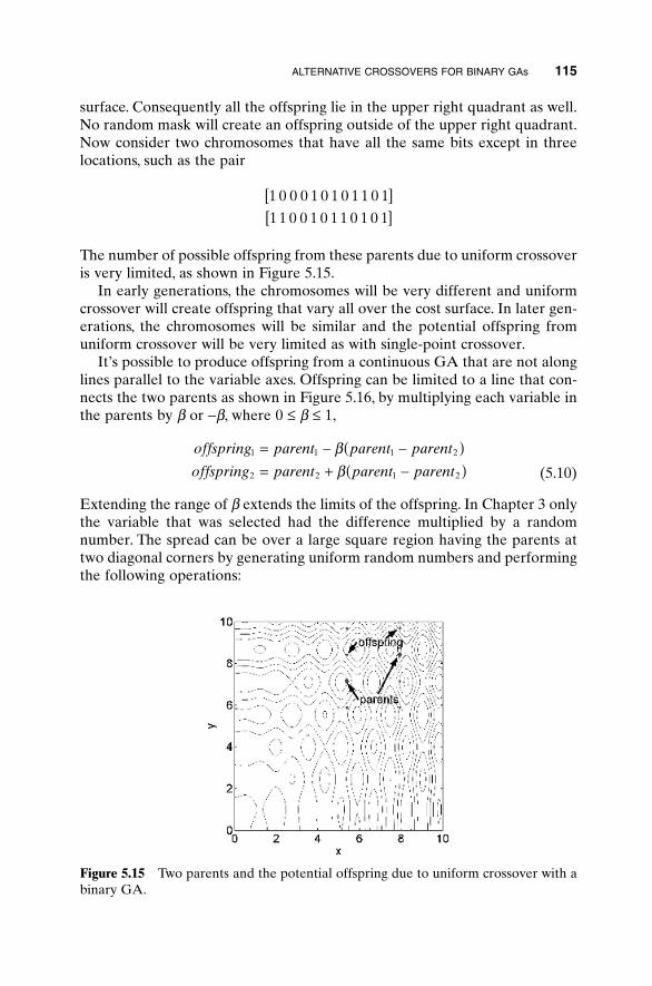
surface. Consequently all the offspring lie in the upper right quadrant as well.No random mask will create an offspring outside of the upper right quadrant.Now consider two chromosomes that have all the same bits except in threelocations, such as the pair
The number of possible offspring from these parents due to uniform crossoveris very limited, as shown in Figure 5.15.
In early generations, the chromosomes will be very different and uniformcrossover will create offspring that vary all over the cost surface. In later gen-erations, the chromosomes will be similar and the potential offspring fromuniform crossover will be very limited as with single-point crossover.
It’s possible to produce offspring from a continuous GA that are not alonglines parallel to the variable axes. Offspring can be limited to a line that con-nects the two parents as shown in Figure 5.16, by multiplying each variable inthe parents by b or -b, where 0 £ b £ 1,
(5.10)
Extending the range of b extends the limits of the offspring. In Chapter 3 onlythe variable that was selected had the difference multiplied by a randomnumber. The spread can be over a large square region having the parents attwo diagonal corners by generating uniform random numbers and performingthe following operations:
offspring parent parent parent
offspring parent parent parent1 1 1 2
2 2 1 2
= - -( )= + -( )
bb
1 0 0 0 1 0 1 0 1 1 0 1
1 1 0 0 1 0 1 1 0 1 0 1
[ ][ ]
ALTERNATIVE CROSSOVERS FOR BINARY GAs 115
Figure 5.15 Two parents and the potential offspring due to uniform crossover with abinary GA.
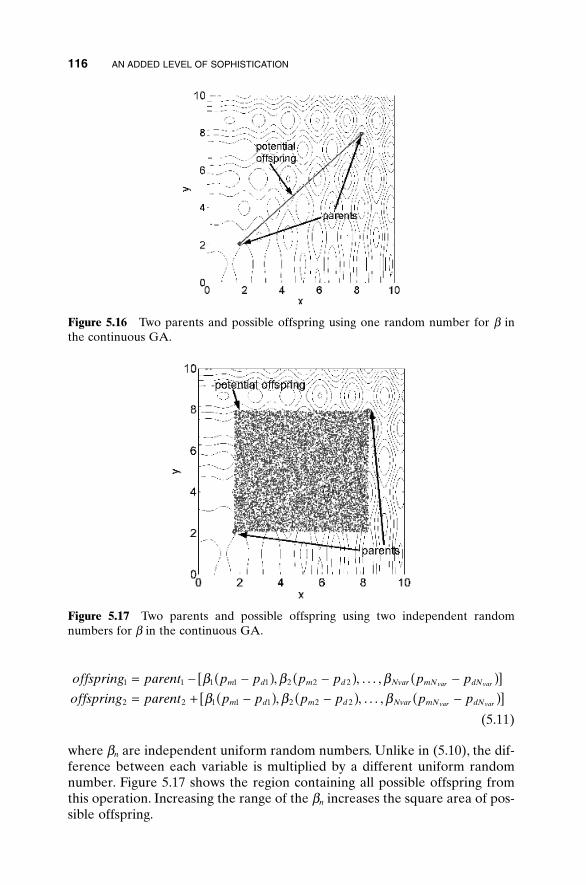
(5.11)
where bn are independent uniform random numbers. Unlike in (5.10), the dif-ference between each variable is multiplied by a different uniform randomnumber. Figure 5.17 shows the region containing all possible offspring fromthis operation. Increasing the range of the bn increases the square area of pos-sible offspring.
offspring parent p p p p p p
offspring parent p p p p p pm d m d Nvar mN dN
m d m d Nvar mN dN
var var
var var
1 1 1 1 1 2 2 2
2 2 1 1 1 2 2 2
= - -( ) -( ) -( )[ ]= + -( ) -( ) -( )[ ]
b b bb b b
, , . . . ,
, , . . . ,
116 AN ADDED LEVEL OF SOPHISTICATION
Figure 5.16 Two parents and possible offspring using one random number for b inthe continuous GA.
Figure 5.17 Two parents and possible offspring using two independent randomnumbers for b in the continuous GA.
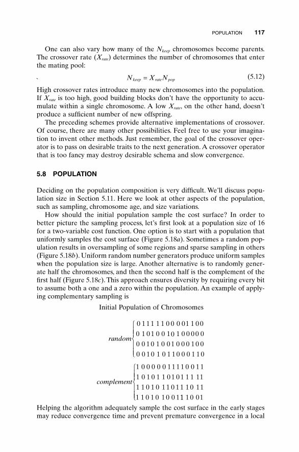
POPULATION 117
One can also vary how many of the Nkeep chromosomes become parents.The crossover rate (Xrate) determines the number of chromosomes that enterthe mating pool:
`(5.12)
High crossover rates introduce many new chromosomes into the population.If Xrate is too high, good building blocks don’t have the opportunity to accu-mulate within a single chromosome. A low Xrate, on the other hand, doesn’tproduce a sufficient number of new offspring.
The preceding schemes provide alternative implementations of crossover.Of course, there are many other possibilities. Feel free to use your imagina-tion to invent other methods. Just remember, the goal of the crossover oper-ator is to pass on desirable traits to the next generation. A crossover operatorthat is too fancy may destroy desirable schema and slow convergence.
5.8 POPULATION
Deciding on the population composition is very difficult. We’ll discuss popu-lation size in Section 5.11. Here we look at other aspects of the population,such as sampling, chromosome age, and size variations.
How should the initial population sample the cost surface? In order tobetter picture the sampling process, let’s first look at a population size of 16for a two-variable cost function. One option is to start with a population thatuniformly samples the cost surface (Figure 5.18a). Sometimes a random pop-ulation results in oversampling of some regions and sparse sampling in others(Figure 5.18b). Uniform random number generators produce uniform sampleswhen the population size is large. Another alternative is to randomly gener-ate half the chromosomes, and then the second half is the complement of thefirst half (Figure 5.18c). This approach ensures diversity by requiring every bitto assume both a one and a zero within the population. An example of apply-ing complementary sampling is
Helping the algorithm adequately sample the cost surface in the early stagesmay reduce convergence time and prevent premature convergence in a local
random
complement
0 1 1 1 1 1 0 0 0 01 1 0 0
0 1 0 1 0 0 10 1 0 0 0 0 0
0 0 1 0 1 0 0 1 0 0 0 1 0 0
0 0 1 0 1 0 1 1 0 0 0 1 1 0
1 0 0 0 0 0 1 1 1 1 0 0 1 1
1 0 1 0 1 1 0 1 0 1 1 1 11
1 1 0 1 0 1 1 0 1 1 1 0 11
1 1 0 1 0 1 0 0 1
Ï
ÌÔÔ
ÓÔÔ
11 1 0 01
Ï
ÌÔÔ
ÓÔÔ
N X Nkeep rate pop=
Initial Population of Chromosomes
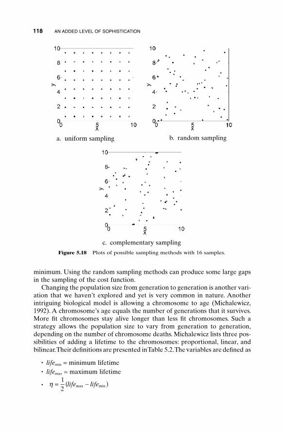
minimum. Using the random sampling methods can produce some large gapsin the sampling of the cost function.
Changing the population size from generation to generation is another vari-ation that we haven’t explored and yet is very common in nature. Anotherintriguing biological model is allowing a chromosome to age (Michalewicz,1992). A chromosome’s age equals the number of generations that it survives.More fit chromosomes stay alive longer than less fit chromosomes. Such astrategy allows the population size to vary from generation to generation,depending on the number of chromosome deaths. Michalewicz lists three pos-sibilities of adding a lifetime to the chromosomes: proportional, linear, andbilinear.Their definitions are presented inTable 5.2.The variables are defined as
• lifemin = minimum lifetime• lifemax = maximum lifetime
• h = -( )12
life lifemax min
118 AN ADDED LEVEL OF SOPHISTICATION
Figure 5.18 Plots of possible sampling methods with 16 samples.
a. uniform sampling b. random sampling
c. complementary sampling
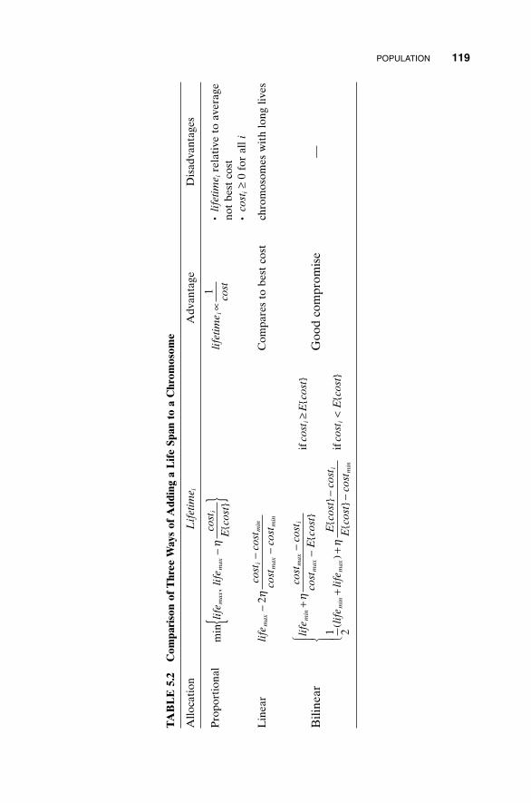
POPULATION 119
TAB
LE
5.2
Com
pari
son
of T
hree
Way
s of
Add
ing
a L
ife
Span
to
a C
hrom
osom
e
Allo
cati
onL
ifet
ime i
Adv
anta
geD
isad
vant
ages
Pro
port
iona
l•
lifet
ime i
rela
tive
to
aver
age
not
best
cos
t•
cost
i≥
0 fo
r al
l i
Lin
ear
Com
pare
s to
bes
t co
stch
rom
osom
es w
ith
long
live
s
Bili
near
Goo
d co
mpr
omis
e—
life
cost
cost
cost
Eco
stco
stE
cost
life
life
Eco
stco
stE
cost
cost
cost
Eco
st
min
max
i
max
i
min
max
i
min
i
+- -
{}
≥{
}
+(
) +{
}-
{}
-<
{}
Ï ÌÔ ÓÔ
h
h
if if1 2
life
cost
cost
cost
cost
max
im
in
max
min
-- -
2h
lifet
ime
cost
iµ
1m
in,
life
life
cost
Eco
stm
axm
axi
-{
}{
}h
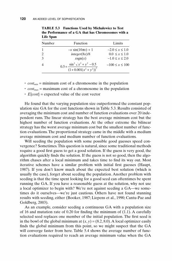
• costmin = minimum cost of a chromosome in the population• costmax = maximum cost of a chromosome in the population• E{cost} = expected value of the cost vector
He found that the varying population size outperformed the constant pop-ulation size GA for the cost functions shown in Table 5.3. Results consisted ofaveraging the minimum cost and number of function evaluations over 20 inde-pendent runs. The linear strategy has the best average minimum cost but thehighest number of function evaluations. At the other extreme the bilinearstrategy has the worst average minimum cost but the smallest number of func-tion evaluations. The proportional strategy came in the middle with a mediumaverage minimum cost and medium number of function evaluations.
Will seeding the population with some possible good guesses speed con-vergence? Sometimes.This question is natural, since some traditional methodsrequire a good first guess to get a good solution. If the guess is very good, thealgorithm quickly finds the solution. If the guess is not so good, then the algo-rithm chases after a local minimum and takes time to find its way out. Mostiterative schemes have a similar problem with initial first guesses (Haupt,1987). If you don’t know much about the expected best solution (which isusually the case), forget about seeding the population. Another problem withseeding is that the time spent looking for a good seed can oftentimes be spentrunning the GA. If you have a reasonable guess at the solution, why not usea local optimizer to begin with? We’re not against seeding a GA—we some-times do it ourselves—we’re just cautious. Others have not found stunningresults with seeding, either (Booker, 1987; Liepens et al., 1990; Cantu-Paz andGoldberg, 2003).
As an example, consider seeding a continuous GA with a population sizeof 16 and mutation rate of 0.20 for finding the minimum of (1.1). A carefullyselected seed replaces one member of the initial population. The first seed isin the bowl of the global minimum at (x, y) = (8.2, 8.0).A local optimizer easilyfinds the global minimum from this point, so we might suspect that the GAwill converge faster from here. Table 5.4 shows the average number of func-tion evaluations required to reach an average minimum value when the GA
120 AN ADDED LEVEL OF SOPHISTICATION
TABLE 5.3 Functions Used by Michalewicz to Testthe Performance of a GA that has Chromosomes with aLife Span
Number Function Limits
1 -x sin(10px) + 1 -2.0 £ x £ 1.02 integer(8x)/8 0.0 £ x £ 1.03 xsgn(x) -1.0 £ x £ 2.0
4 -100 £ x £ 1000 50 5
1 0 001
2 2 2
2 2 2.sin .
.+
+ -+ +( )( )
x y
x y
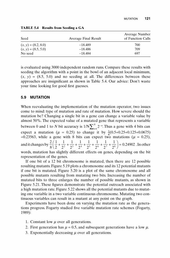
MUTATION 121
TABLE 5.4 Results from Seeding a GA
Average NumberSeed Average Final Result of Function Calls
(x, y) = (8.2, 8.0) -18.489 700(x, y) = (8.5, 5.0) -18.486 709No seed -18.484 697
is evaluated using 3000 independent random runs. Compare these results withseeding the algorithm with a point in the bowl of an adjacent local minimum,(x, y) = (8.5, 5.0) and no seeding at all. The differences between theseapproaches are insignificant as shown in Table 5.4. Our advice: Don’t wasteyour time looking for good first guesses.
5.9 MUTATION
When reevaluating the implementation of the mutation operator, two issuescome to mind: type of mutation and rate of mutation. How severe should themutation be? Changing a single bit in a gene can change a variable value byalmost 50%. The expected value of a mutated gene that represents a variable
between 0 and 1 to N bit accuracy is 1/N . Thus a gene with 4 bits can
expect a mutation (m = 0.25) to change it by 1–4(0.5+0.25+0.125+0.0675)
=0.23563, while a gene with 8 bits can expect two mutations (m = 0.25),
and it changes by .In other
words, mutation has slightly different effects on genes, depending on the bitrepresentation of the genes.
If one bit of a 12 bit chromosome is mutated, then there are 12 possibleresulting mutants. Figure 5.19 plots a chromosome and its 12 potential mutantsif one bit is mutated. Figure 5.20 is a plot of the same chromosome and allpossible mutants resulting from mutating two bits. Increasing the number ofmutated bits to three enlarges the number of possible mutants, as shown inFigure 5.21. These figures demonstrate the potential outreach associated witha high mutation rate. Figure 5.22 shows all the potential mutants due to mutat-ing one variable in a two variable continuous chromosome. Mutating two con-tinuous variables can result in a mutant at any point on the graph.
Experiments have been done on varying the mutation rate as the genera-tions progress. Fogarty studied five variable mutation rate schemes (Fogarty,1989):
1. Constant low m over all generations.2. First generation has m = 0.5, and subsequent generations have a low m.3. Exponentially decreasing m over all generations.
28
12
12
12
12
12
12
12
12
0 249022 3 4 5 6 7 8
+ + + + + + +ÊË
ˆ¯ = .
21
-=Â n
n
N
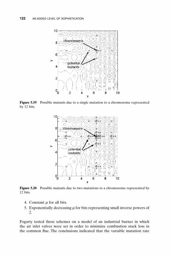
4. Constant m for all bits.5. Exponentially decreasing m for bits representing small inverse powers of
2.
Fogarty tested these schemes on a model of an industrial burner in which the air inlet valves were set in order to minimize combustion stack loss in the common flue. The conclusions indicated that the variable mutation rate
122 AN ADDED LEVEL OF SOPHISTICATION
Figure 5.19 Possible mutants due to a single mutation to a chromosome representedby 12 bits.
Figure 5.20 Possible mutants due to two mutations to a chromosome represented by12 bits.
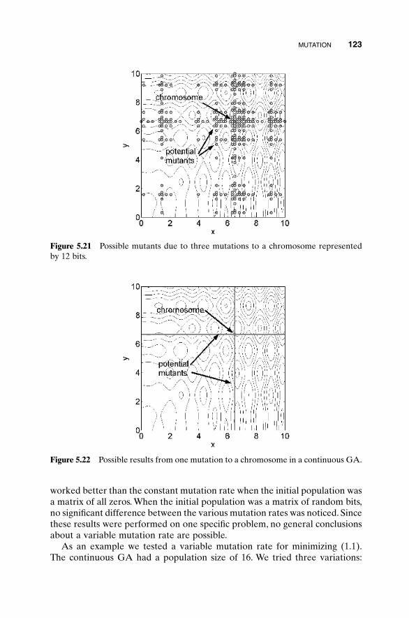
worked better than the constant mutation rate when the initial population wasa matrix of all zeros. When the initial population was a matrix of random bits,no significant difference between the various mutation rates was noticed. Sincethese results were performed on one specific problem, no general conclusionsabout a variable mutation rate are possible.
As an example we tested a variable mutation rate for minimizing (1.1).The continuous GA had a population size of 16. We tried three variations:
MUTATION 123
Figure 5.22 Possible results from one mutation to a chromosome in a continuous GA.
Figure 5.21 Possible mutants due to three mutations to a chromosome representedby 12 bits.
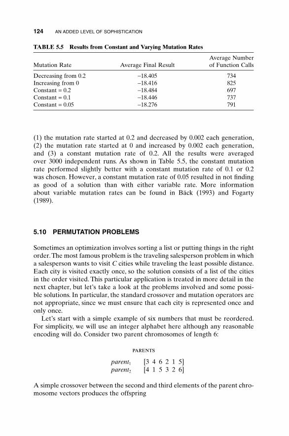
(1) the mutation rate started at 0.2 and decreased by 0.002 each generation,(2) the mutation rate started at 0 and increased by 0.002 each generation,and (3) a constant mutation rate of 0.2. All the results were averaged over 3000 independent runs. As shown in Table 5.5, the constant mutation rate performed slightly better with a constant mutation rate of 0.1 or 0.2 was chosen. However, a constant mutation rate of 0.05 resulted in not findingas good of a solution than with either variable rate. More information about variable mutation rates can be found in Bäck (1993) and Fogarty (1989).
5.10 PERMUTATION PROBLEMS
Sometimes an optimization involves sorting a list or putting things in the rightorder.The most famous problem is the traveling salesperson problem in whicha salesperson wants to visit C cities while traveling the least possible distance.Each city is visited exactly once, so the solution consists of a list of the citiesin the order visited. This particular application is treated in more detail in thenext chapter, but let’s take a look at the problems involved and some possi-ble solutions. In particular, the standard crossover and mutation operators arenot appropriate, since we must ensure that each city is represented once andonly once.
Let’s start with a simple example of six numbers that must be reordered.For simplicity, we will use an integer alphabet here although any reasonableencoding will do. Consider two parent chromosomes of length 6:
parents
parent1 [3 4 6 2 1 5]parent2 [4 1 5 3 2 6]
A simple crossover between the second and third elements of the parent chro-mosome vectors produces the offspring
124 AN ADDED LEVEL OF SOPHISTICATION
TABLE 5.5 Results from Constant and Varying Mutation Rates
Average NumberMutation Rate Average Final Result of Function Calls
Decreasing from 0.2 -18.405 734Increasing from 0 -18.416 825Constant = 0.2 -18.484 697Constant = 0.1 -18.446 737Constant = 0.05 -18.276 791
simple crossover (incorrect)
offspring1 [3 4 | 5 3 2 6]offspring2 [4 1 | 6 2 1 5]
Obviously this won’t work, since offspring1 contains two 3s and no 1 while off-spring2 has two 1s, and no 3. Goldberg (1989a) discusses several possible solu-tions to this problem, which are briefly summarized here. The first is known aspartially matched crossover (PMX) (Goldberg and Lingle, 1985). In thismethod two crossover points are chosen, and we begin by exchanging thevalues of the parents between these points. If crossover points are betweenelements 1 and 2, and 3 and 4, then string K from parent2 is switched with stringJ from parent1:
partially matched crossover (step a)
offspring1A [3 | | 2 1 5]
offspring2A [4 | | 3 2 6]
All values exchanged between parents are shown in bold type. So far we stillhave the problem of having doubles of some integers and none of others. Theswitched strings, J and K, remain untouched throughout the rest of the pro-cedure. The original doubles in offspring2A are exchanged for the originaldoubles in offspring1A (the original 4 in offspring2A exchanged with the origi-nal 1 in offspring1A, and the original 6 in offspring2A with the original 5 in offspring1A) to obtain the final solution:
partially matched crossover (step b)
offspring1B [3 1 5 2 4 6]offspring2B [1 4 6 3 2 5]
Each offspring contains part of the initial parent in the same position (unem-phasized numbers) and includes each integer once and only once.
Order crossover (OX) is somewhat different than PMX. It attempts tomaintain the order of integers as if the chromosome vector were wrapped ina circle, so the last element is followed by the first element. Thus [1 2 3 4] isthe same as [2 3 4 1]. It begins, like PMX, by choosing two crossover pointsand exchanging the integers between them. This time, however, holes are left(denoted below by X’s) in the spaces where integers are repeated. If thecrossover points are after the second and fourth integers, the first stage leavesoffspring that look like
4 6k{
1 5J
{
PERMUTATION PROBLEMS 125
ordered crossover (first stage)
offspring1L [X 4 | | 1 X]
offspring2L [4 1 | | X X]
At this point the holes are pushed to the beginning of the offspring. All inte-gers that were in those positions are pushed off the left of the chromosomeand wrap around to the end of the offspring. At the same time strings J andK that were exchanged maintain their positions:
ordered crossover (second stage)
offspring1M [X X 5 3 1 4]offspring2M [X X 6 2 4 1]
For the final stage the X’s are replaced with strings J and K:
ordered crossover (final stage)
offspring1N [ ]
offspring2N [ ]
OX has the advantage that the relative ordering is preserved, although theabsolute position within the string is not.
The final method discussed by Goldberg (1989a) is the cycle crossover(CX). In this method the information exchange begins at the left of the stringand the first two digits are exchanged. For our example, this gives
cycle crossover (first step)
offspring1W [4 4 6 2 1 5]offspring2W [3 1 5 3 2 6]
Now that the first offspring has two 4s, we progress to the second 4 andexchange with the other offspring to get
cycle crossover (second step)
offspring1X [4 1 6 2 1 5]offspring2X [3 4 5 3 2 6]
Since there are two 1s in the first offspring, we exchange position 5 with thesecond offspring:
5 3 6 2J k
{ { 4 1
62 5 3k J{ { 1 4
6 2k{
5 3J
{
126 AN ADDED LEVEL OF SOPHISTICATION
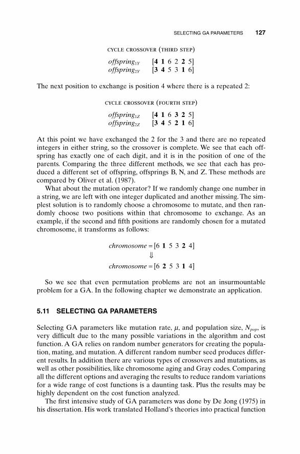
cycle crossover (third step)
offspring1Y [4 1 6 2 2 5]offspring2Y [3 4 5 3 1 6]
The next position to exchange is position 4 where there is a repeated 2:
cycle crossover (fourth step)
offspring1Z [4 1 6 3 2 5]offspring2Z [3 4 5 2 1 6]
At this point we have exchanged the 2 for the 3 and there are no repeatedintegers in either string, so the crossover is complete. We see that each off-spring has exactly one of each digit, and it is in the position of one of theparents. Comparing the three different methods, we see that each has pro-duced a different set of offspring, offsprings B, N, and Z. These methods arecompared by Oliver et al. (1987).
What about the mutation operator? If we randomly change one number ina string, we are left with one integer duplicated and another missing. The sim-plest solution is to randomly choose a chromosome to mutate, and then ran-domly choose two positions within that chromosome to exchange. As anexample, if the second and fifth positions are randomly chosen for a mutatedchromosome, it transforms as follows:
So we see that even permutation problems are not an insurmountableproblem for a GA. In the following chapter we demonstrate an application.
5.11 SELECTING GA PARAMETERS
Selecting GA parameters like mutation rate, m, and population size, Npop, isvery difficult due to the many possible variations in the algorithm and costfunction. A GA relies on random number generators for creating the popula-tion, mating, and mutation. A different random number seed produces differ-ent results. In addition there are various types of crossovers and mutations, aswell as other possibilities, like chromosome aging and Gray codes. Comparingall the different options and averaging the results to reduce random variationsfor a wide range of cost functions is a daunting task. Plus the results may behighly dependent on the cost function analyzed.
The first intensive study of GA parameters was done by De Jong (1975) inhis dissertation. His work translated Holland’s theories into practical function
chromosome
chromosome
= [ ]fl= [ ]
6 5 3 4
6 5 3 4
1 2
2 1
SELECTING GA PARAMETERS 127
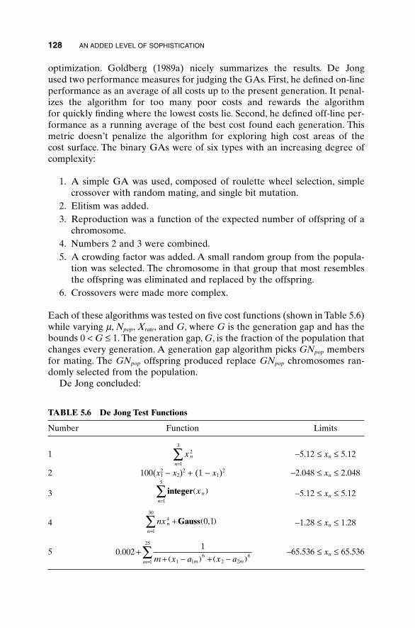
optimization. Goldberg (1989a) nicely summarizes the results. De Jong used two performance measures for judging the GAs. First, he defined on-lineperformance as an average of all costs up to the present generation. It penal-izes the algorithm for too many poor costs and rewards the algorithm for quickly finding where the lowest costs lie. Second, he defined off-line per-formance as a running average of the best cost found each generation. Thismetric doesn’t penalize the algorithm for exploring high cost areas of the cost surface. The binary GAs were of six types with an increasing degree ofcomplexity:
1. A simple GA was used, composed of roulette wheel selection, simplecrossover with random mating, and single bit mutation.
2. Elitism was added.3. Reproduction was a function of the expected number of offspring of a
chromosome.4. Numbers 2 and 3 were combined.5. A crowding factor was added. A small random group from the popula-
tion was selected. The chromosome in that group that most resemblesthe offspring was eliminated and replaced by the offspring.
6. Crossovers were made more complex.
Each of these algorithms was tested on five cost functions (shown in Table 5.6)while varying m, Npop, Xrate, and G, where G is the generation gap and has thebounds 0 < G £ 1. The generation gap, G, is the fraction of the population thatchanges every generation. A generation gap algorithm picks GNpop membersfor mating. The GNpop offspring produced replace GNpop chromosomes ran-domly selected from the population.
De Jong concluded:
128 AN ADDED LEVEL OF SOPHISTICATION
TABLE 5.6 De Jong Test Functions
Number Function Limits
1 -5.12 £ xn £ 5.12
2 100(x12 - x2)2 + (1 - x1)2 -2.048 £ xn £ 2.048
3 -5.12 £ xn £ 5.12
4 -1.28 £ xn £ 1.28
5 -65.536 £ xn £ 65.5360 0021
1 16
2 26
1
25
. ++ -( ) + -( )=
 m x a x am mm
nx n
n
4
1
30
+ ( )=
 Gauss 0,1
integer x n
n
( )=
Â1
5
x n
n
2
1
3
=Â
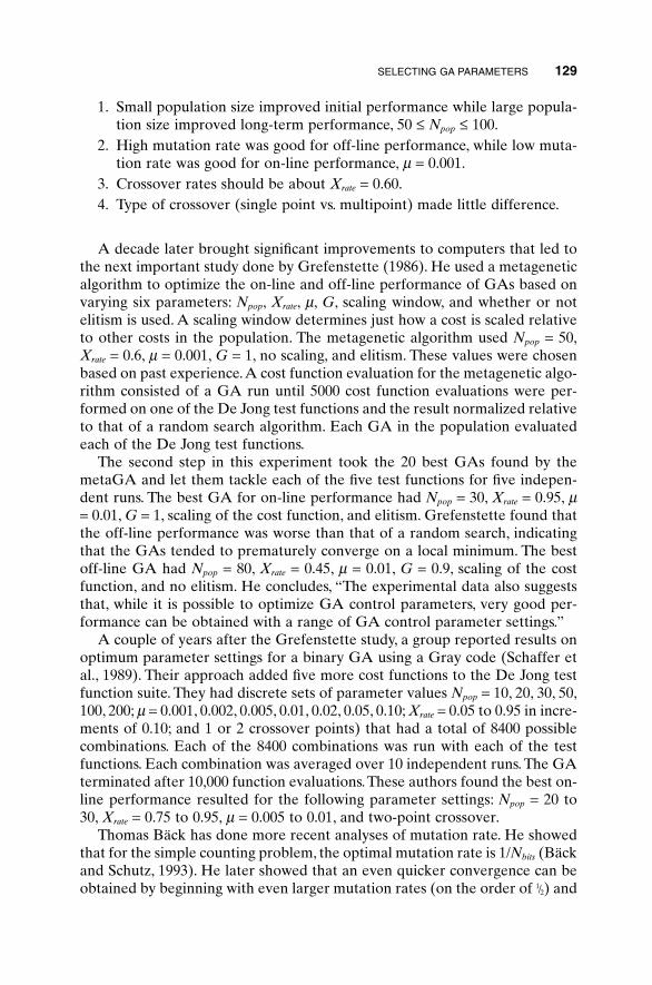
1. Small population size improved initial performance while large popula-tion size improved long-term performance, 50 £ Npop £ 100.
2. High mutation rate was good for off-line performance, while low muta-tion rate was good for on-line performance, m = 0.001.
3. Crossover rates should be about Xrate = 0.60.4. Type of crossover (single point vs. multipoint) made little difference.
A decade later brought significant improvements to computers that led tothe next important study done by Grefenstette (1986). He used a metageneticalgorithm to optimize the on-line and off-line performance of GAs based onvarying six parameters: Npop, Xrate, m, G, scaling window, and whether or notelitism is used. A scaling window determines just how a cost is scaled relativeto other costs in the population. The metagenetic algorithm used Npop = 50,Xrate = 0.6, m = 0.001, G = 1, no scaling, and elitism. These values were chosenbased on past experience.A cost function evaluation for the metagenetic algo-rithm consisted of a GA run until 5000 cost function evaluations were per-formed on one of the De Jong test functions and the result normalized relativeto that of a random search algorithm. Each GA in the population evaluatedeach of the De Jong test functions.
The second step in this experiment took the 20 best GAs found by themetaGA and let them tackle each of the five test functions for five indepen-dent runs. The best GA for on-line performance had Npop = 30, Xrate = 0.95, m= 0.01, G = 1, scaling of the cost function, and elitism. Grefenstette found thatthe off-line performance was worse than that of a random search, indicatingthat the GAs tended to prematurely converge on a local minimum. The bestoff-line GA had Npop = 80, Xrate = 0.45, m = 0.01, G = 0.9, scaling of the costfunction, and no elitism. He concludes, “The experimental data also suggeststhat, while it is possible to optimize GA control parameters, very good per-formance can be obtained with a range of GA control parameter settings.”
A couple of years after the Grefenstette study, a group reported results onoptimum parameter settings for a binary GA using a Gray code (Schaffer etal., 1989). Their approach added five more cost functions to the De Jong testfunction suite. They had discrete sets of parameter values Npop = 10, 20, 30, 50,100, 200; m = 0.001, 0.002, 0.005, 0.01, 0.02, 0.05, 0.10; Xrate = 0.05 to 0.95 in incre-ments of 0.10; and 1 or 2 crossover points) that had a total of 8400 possiblecombinations. Each of the 8400 combinations was run with each of the testfunctions. Each combination was averaged over 10 independent runs. The GAterminated after 10,000 function evaluations. These authors found the best on-line performance resulted for the following parameter settings: Npop = 20 to30, Xrate = 0.75 to 0.95, m = 0.005 to 0.01, and two-point crossover.
Thomas Bäck has done more recent analyses of mutation rate. He showedthat for the simple counting problem, the optimal mutation rate is 1/Nbits (Bäckand Schutz, 1993). He later showed that an even quicker convergence can beobtained by beginning with even larger mutation rates (on the order of 1/2) and
SELECTING GA PARAMETERS 129
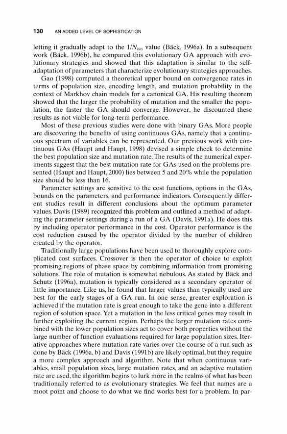
letting it gradually adapt to the 1/Nbits value (Bäck, 1996a). In a subsequentwork (Bäck, 1996b), he compared this evolutionary GA approach with evo-lutionary strategies and showed that this adaptation is similar to the self-adaptation of parameters that characterize evolutionary strategies approaches.
Gao (1998) computed a theoretical upper bound on convergence rates interms of population size, encoding length, and mutation probability in thecontext of Markhov chain models for a canonical GA. His resulting theoremshowed that the larger the probability of mutation and the smaller the popu-lation, the faster the GA should converge. However, he discounted theseresults as not viable for long-term performance.
Most of these previous studies were done with binary GAs. More peopleare discovering the benefits of using continuous GAs, namely that a continu-ous spectrum of variables can be represented. Our previous work with con-tinuous GAs (Haupt and Haupt, 1998) devised a simple check to determinethe best population size and mutation rate.The results of the numerical exper-iments suggest that the best mutation rate for GAs used on the problems pre-sented (Haupt and Haupt, 2000) lies between 5 and 20% while the populationsize should be less than 16.
Parameter settings are sensitive to the cost functions, options in the GAs,bounds on the parameters, and performance indicators. Consequently differ-ent studies result in different conclusions about the optimum parametervalues. Davis (1989) recognized this problem and outlined a method of adapt-ing the parameter settings during a run of a GA (Davis, 1991a). He does thisby including operator performance in the cost. Operator performance is thecost reduction caused by the operator divided by the number of childrencreated by the operator.
Traditionally large populations have been used to thoroughly explore com-plicated cost surfaces. Crossover is then the operator of choice to exploitpromising regions of phase space by combining information from promisingsolutions. The role of mutation is somewhat nebulous. As stated by Bäck andSchutz (1996a), mutation is typically considered as a secondary operator oflittle importance. Like us, he found that larger values than typically used arebest for the early stages of a GA run. In one sense, greater exploration isachieved if the mutation rate is great enough to take the gene into a differentregion of solution space. Yet a mutation in the less critical genes may result infurther exploiting the current region. Perhaps the larger mutation rates com-bined with the lower population sizes act to cover both properties without thelarge number of function evaluations required for large population sizes. Iter-ative approaches where mutation rate varies over the course of a run such asdone by Bäck (1996a, b) and Davis (1991b) are likely optimal, but they requirea more complex approach and algorithm. Note that when continuous vari-ables, small population sizes, large mutation rates, and an adaptive mutationrate are used, the algorithm begins to lurk more in the realms of what has beentraditionally referred to as evolutionary strategies. We feel that names are amoot point and choose to do what we find works best for a problem. In par-
130 AN ADDED LEVEL OF SOPHISTICATION
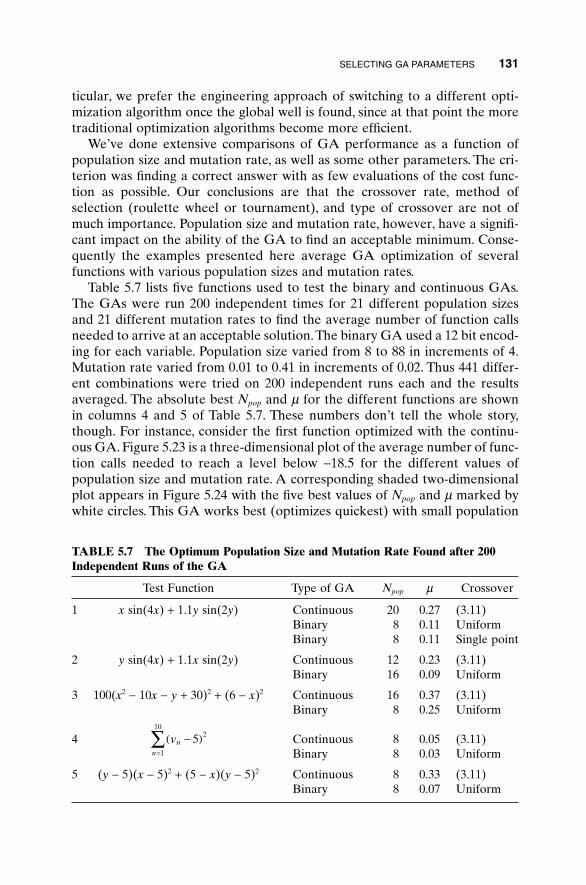
ticular, we prefer the engineering approach of switching to a different opti-mization algorithm once the global well is found, since at that point the moretraditional optimization algorithms become more efficient.
We’ve done extensive comparisons of GA performance as a function ofpopulation size and mutation rate, as well as some other parameters. The cri-terion was finding a correct answer with as few evaluations of the cost func-tion as possible. Our conclusions are that the crossover rate, method ofselection (roulette wheel or tournament), and type of crossover are not ofmuch importance. Population size and mutation rate, however, have a signifi-cant impact on the ability of the GA to find an acceptable minimum. Conse-quently the examples presented here average GA optimization of severalfunctions with various population sizes and mutation rates.
Table 5.7 lists five functions used to test the binary and continuous GAs.The GAs were run 200 independent times for 21 different population sizesand 21 different mutation rates to find the average number of function callsneeded to arrive at an acceptable solution.The binary GA used a 12 bit encod-ing for each variable. Population size varied from 8 to 88 in increments of 4.Mutation rate varied from 0.01 to 0.41 in increments of 0.02. Thus 441 differ-ent combinations were tried on 200 independent runs each and the resultsaveraged. The absolute best Npop and m for the different functions are shownin columns 4 and 5 of Table 5.7. These numbers don’t tell the whole story,though. For instance, consider the first function optimized with the continu-ous GA. Figure 5.23 is a three-dimensional plot of the average number of func-tion calls needed to reach a level below -18.5 for the different values ofpopulation size and mutation rate. A corresponding shaded two-dimensionalplot appears in Figure 5.24 with the five best values of Npop and m marked bywhite circles. This GA works best (optimizes quickest) with small population
SELECTING GA PARAMETERS 131
TABLE 5.7 The Optimum Population Size and Mutation Rate Found after 200Independent Runs of the GA
Test Function Type of GA Npop m Crossover
1 x sin(4x) + 1.1y sin(2y) Continuous 20 0.27 (3.11)Binary 8 0.11 UniformBinary 8 0.11 Single point
2 y sin(4x) + 1.1x sin(2y) Continuous 12 0.23 (3.11)Binary 16 0.09 Uniform
3 100(x2 - 10x - y + 30)2 + (6 - x)2 Continuous 16 0.37 (3.11)Binary 8 0.25 Uniform
4 Continuous 8 0.05 (3.11)Binary 8 0.03 Uniform
5 (y - 5)(x - 5)2 + (5 - x)(y - 5)2 Continuous 8 0.33 (3.11)Binary 8 0.07 Uniform
vn
n
-( )=
 5 2
1
10
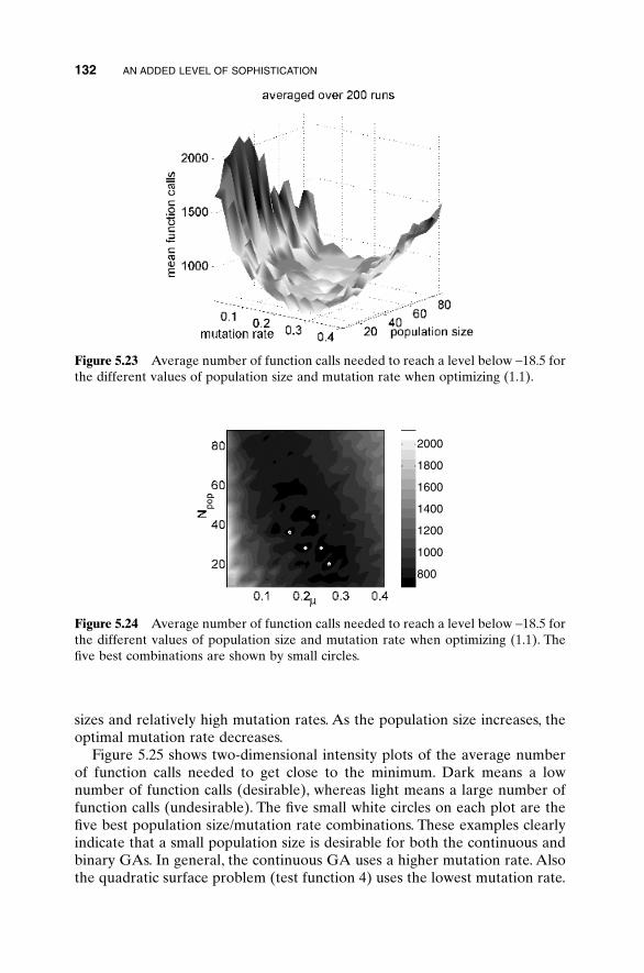
sizes and relatively high mutation rates. As the population size increases, theoptimal mutation rate decreases.
Figure 5.25 shows two-dimensional intensity plots of the average numberof function calls needed to get close to the minimum. Dark means a lownumber of function calls (desirable), whereas light means a large number offunction calls (undesirable). The five small white circles on each plot are thefive best population size/mutation rate combinations. These examples clearlyindicate that a small population size is desirable for both the continuous andbinary GAs. In general, the continuous GA uses a higher mutation rate. Alsothe quadratic surface problem (test function 4) uses the lowest mutation rate.
132 AN ADDED LEVEL OF SOPHISTICATION
2000
1800
1600
1400
1200
1000
800
Figure 5.23 Average number of function calls needed to reach a level below -18.5 forthe different values of population size and mutation rate when optimizing (1.1).
Figure 5.24 Average number of function calls needed to reach a level below -18.5 forthe different values of population size and mutation rate when optimizing (1.1). Thefive best combinations are shown by small circles.
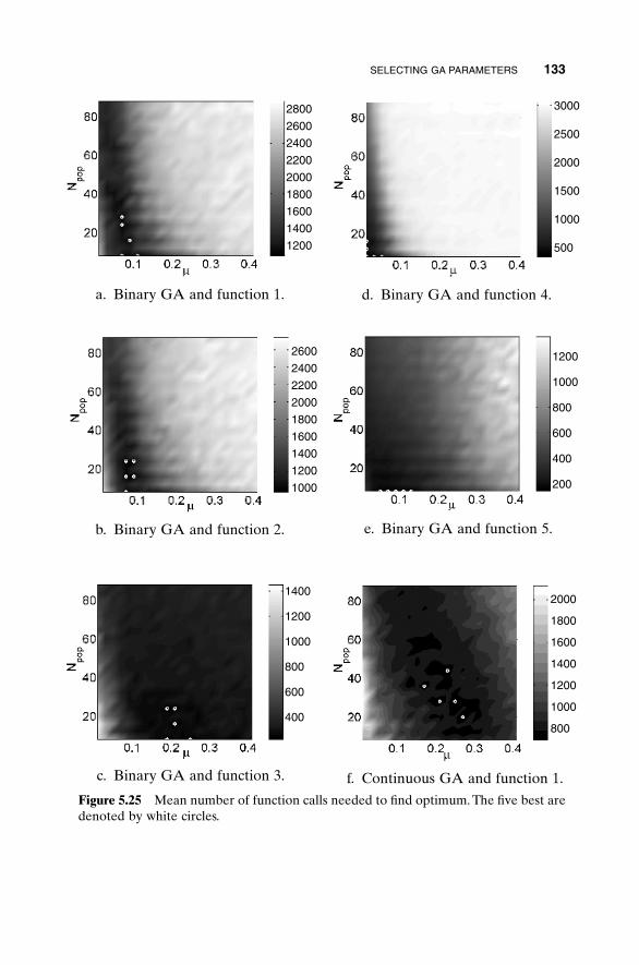
SELECTING GA PARAMETERS 133
2800
2600
2400
2200
2000
1800
1600
1400
1200
a. Binary GA and function 1.
2000
1800
1600
1400
1200
1000
800
f. Continuous GA and function 1.
2600
2400
2200
2000
1800
1600
1400
1200
1000
b. Binary GA and function 2.
1400
1200
1000
800
600
400
c. Binary GA and function 3.
3000
2500
2000
1500
1000
500
d. Binary GA and function 4.
1200
1000
800
600
400
200
e. Binary GA and function 5.
Figure 5.25 Mean number of function calls needed to find optimum. The five best aredenoted by white circles.
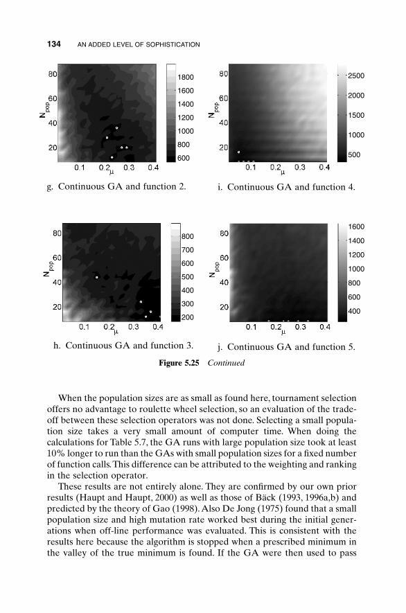
134 AN ADDED LEVEL OF SOPHISTICATION
2500
2000
1500
1000
500
1600
1400
1200
1000
800
600
400
i. Continuous GA and function 4.
j. Continuous GA and function 5.
Figure 5.25 Continued
When the population sizes are as small as found here, tournament selectionoffers no advantage to roulette wheel selection, so an evaluation of the trade-off between these selection operators was not done. Selecting a small popula-tion size takes a very small amount of computer time. When doing thecalculations for Table 5.7, the GA runs with large population size took at least10% longer to run than the GAs with small population sizes for a fixed numberof function calls.This difference can be attributed to the weighting and rankingin the selection operator.
These results are not entirely alone. They are confirmed by our own priorresults (Haupt and Haupt, 2000) as well as those of Bäck (1993, 1996a,b) andpredicted by the theory of Gao (1998).Also De Jong (1975) found that a smallpopulation size and high mutation rate worked best during the initial gener-ations when off-line performance was evaluated. This is consistent with theresults here because the algorithm is stopped when a prescribed minimum inthe valley of the true minimum is found. If the GA were then used to pass
1800
1600
1400
1200
1000
800
600
g. Continuous GA and function 2.
800
700
600
500
400
300
200
h. Continuous GA and function 3.
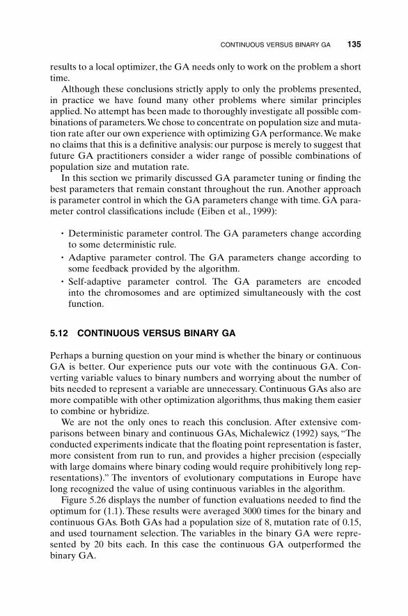
CONTINUOUS VERSUS BINARY GA 135
results to a local optimizer, the GA needs only to work on the problem a shorttime.
Although these conclusions strictly apply to only the problems presented,in practice we have found many other problems where similar principlesapplied. No attempt has been made to thoroughly investigate all possible com-binations of parameters.We chose to concentrate on population size and muta-tion rate after our own experience with optimizing GA performance.We makeno claims that this is a definitive analysis: our purpose is merely to suggest thatfuture GA practitioners consider a wider range of possible combinations ofpopulation size and mutation rate.
In this section we primarily discussed GA parameter tuning or finding thebest parameters that remain constant throughout the run. Another approachis parameter control in which the GA parameters change with time. GA para-meter control classifications include (Eiben et al., 1999):
• Deterministic parameter control. The GA parameters change accordingto some deterministic rule.
• Adaptive parameter control. The GA parameters change according tosome feedback provided by the algorithm.
• Self-adaptive parameter control. The GA parameters are encoded into the chromosomes and are optimized simultaneously with the costfunction.
5.12 CONTINUOUS VERSUS BINARY GA
Perhaps a burning question on your mind is whether the binary or continuousGA is better. Our experience puts our vote with the continuous GA. Con-verting variable values to binary numbers and worrying about the number ofbits needed to represent a variable are unnecessary. Continuous GAs also aremore compatible with other optimization algorithms, thus making them easierto combine or hybridize.
We are not the only ones to reach this conclusion. After extensive com-parisons between binary and continuous GAs, Michalewicz (1992) says, “Theconducted experiments indicate that the floating point representation is faster,more consistent from run to run, and provides a higher precision (especiallywith large domains where binary coding would require prohibitively long rep-resentations).” The inventors of evolutionary computations in Europe havelong recognized the value of using continuous variables in the algorithm.
Figure 5.26 displays the number of function evaluations needed to find theoptimum for (1.1). These results were averaged 3000 times for the binary andcontinuous GAs. Both GAs had a population size of 8, mutation rate of 0.15,and used tournament selection. The variables in the binary GA were repre-sented by 20 bits each. In this case the continuous GA outperformed thebinary GA.
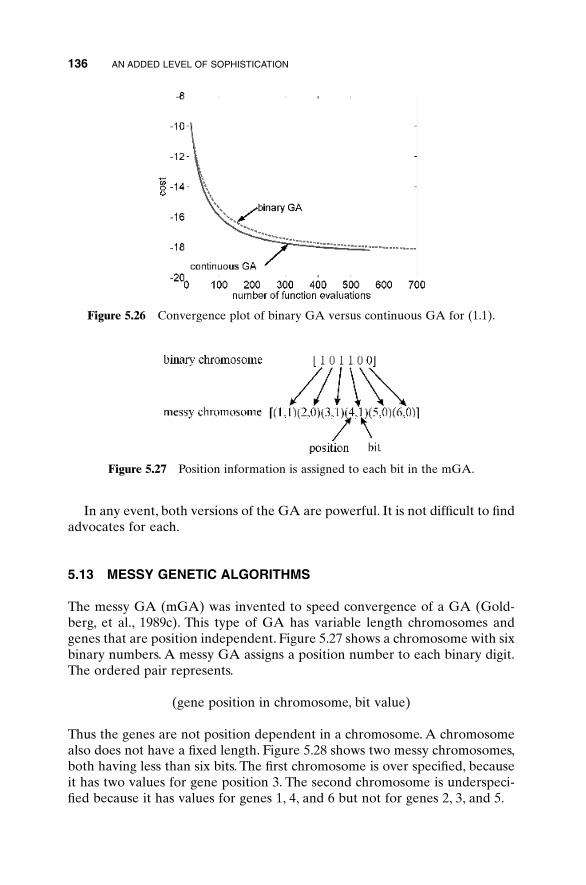
136 AN ADDED LEVEL OF SOPHISTICATION
Figure 5.26 Convergence plot of binary GA versus continuous GA for (1.1).
In any event, both versions of the GA are powerful. It is not difficult to findadvocates for each.
5.13 MESSY GENETIC ALGORITHMS
The messy GA (mGA) was invented to speed convergence of a GA (Gold-berg, et al., 1989c). This type of GA has variable length chromosomes andgenes that are position independent. Figure 5.27 shows a chromosome with sixbinary numbers. A messy GA assigns a position number to each binary digit.The ordered pair represents.
(gene position in chromosome, bit value)
Thus the genes are not position dependent in a chromosome. A chromosomealso does not have a fixed length. Figure 5.28 shows two messy chromosomes,both having less than six bits. The first chromosome is over specified, becauseit has two values for gene position 3. The second chromosome is underspeci-fied because it has values for genes 1, 4, and 6 but not for genes 2, 3, and 5.
Figure 5.27 Position information is assigned to each bit in the mGA.
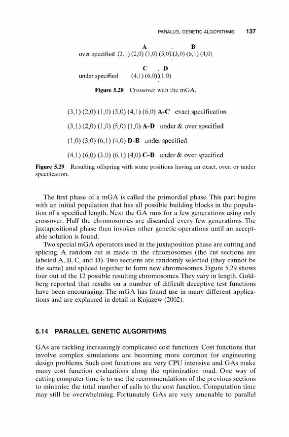
PARALLEL GENETIC ALGORITHMS 137
Figure 5.28 Crossover with the mGA.
The first phase of a mGA is called the primordial phase. This part beginswith an initial population that has all possible building blocks in the popula-tion of a specified length. Next the GA runs for a few generations using onlycrossover. Half the chromosomes are discarded every few generations. Thejuxtapositional phase then invokes other genetic operations until an accept-able solution is found.
Two special mGA operators used in the juxtaposition phase are cutting andsplicing. A random cut is made in the chromosomes (the cut sections arelabeled A, B, C, and D). Two sections are randomly selected (they cannot bethe same) and spliced together to form new chromosomes. Figure 5.29 showsfour out of the 12 possible resulting chromosomes. They vary in length. Gold-berg reported that results on a number of difficult deceptive test functionshave been encouraging. The mGA has found use in many different applica-tions and are explained in detail in Knjazew (2002).
5.14 PARALLEL GENETIC ALGORITHMS
GAs are tackling increasingly complicated cost functions. Cost functions thatinvolve complex simulations are becoming more common for engineeringdesign problems. Such cost functions are very CPU intensive and GAs makemany cost function evaluations along the optimization road. One way ofcutting computer time is to use the recommendations of the previous sectionsto minimize the total number of calls to the cost function. Computation timemay still be overwhelming. Fortunately GAs are very amenable to parallel
Figure 5.29 Resulting offspring with some positions having an exact, over, or underspecification.
implementation. The cost function evaluations are independent and can bedone concurrently with very minor changes in code. Such simple adaptationswork quite well for cost functions that take a lot of computer time. However,for cost functions with moderate to low CPU requirements, communicationsbetween processors use up the speedup, as we will see below. This is because,for a standard GA, sorting and selection often occur within the full matingpopulation. Thus parallelizing GAs requires careful consideration of whichoperations really must be done with the entire chromosome array versus whatcan be done using subpopulations.
5.14.1 Advantages of Parallel GAs
Speedup is the most often cited reason to use a parallel GA. If function eval-uations can be farmed out to different processors, they can be completed concurrently. However, that is not the only motivation for parallelization. Aswe will discuss below, there are parallel strategies where groups of chromo-somes are sent to separate processors to evolve apart from the rest of the population. Communication between these “islands” of chromosomes occursoccasionally. This separation into subpopulations can prevent premature convergence by allowing each island to search in different combinations,preventing a single highly fit individual from dominating the entire popula-tion. Sometimes multiple solutions can be found for the problem in thismanner. In addition we note that nature uses parallel evolution of subpopu-lations, yet allows occasional migration between these groups. To the extentthat GAs are patterned after nature, it makes sense to explore this aspect ofevolution.
5.14.2 Strategies for Parallel GAs
So how do you parallelize your code to take best advantage of multiple proces-sors without becoming so bogged down in communication time between theprocessors? There are actually some very good tried and true strategies to helpsolve this problem. Much work has been done on analyzing different ways toparallelize GAs (e.g., Alba and Tomassini, 2002; Nowastawski and Poli, 1999;Watson, 1999; Gordon and Whitley, 1993). Which method works best dependson the nature of the problem and the architecture of the parallel machine.Ter-minology of the various methods is not yet standardized, but we attempt togive a sampling of the most successful methods being used.
The simplest method of building a parallel GA is the master–slave algo-rithm, which is basically a parallel implementation of a standard GA. Oneprocessor is the master and controls communication, sorting, and pairing. Itsends the cost function out to the slave processors for parallel evaluations.Thismethod is arguably the simplest to program. The disadvantages are that themaster is often left waiting for the results from the slaves, and the algorithmis only as fast as communication from the slowest node. Since selection occurs
138 AN ADDED LEVEL OF SOPHISTICATION
globally, these algorithms are known as “panmictic” or “micro-grained.” Thereare several subclassifications within the master–slave parallel GA, which areprimarily related to the replacement strategy. The generational model is oneextreme: the entire population is replaced with new offspring each generation.The opposite extreme is the steady state model, where only one or two newindividuals replace less fit parents each generation. In between these extremesare the generation gap models where some percentage of the population is replaced with offspring.This type of algorithm is analogous to using a certaincrossover percentage of the most-fit parents that remain in the population andmate. Most master–slave algorithms are synchronous: the slave processorseach do the same operation on a subset of data at the same time while the master waits for feedback. Such algorithms can experience the bottleneckeffect when one processor holds up progression. An asynchronousmaster–slave algorithm is possible. In this case the master begins the selectionstep of the algorithm as slave nodes send back their fitness evaluations.One of the easiest ways to do this is to employ tournament selection on the population that has returned from the slaves. A disadvantage of themaster-slave algorithms is that, since they are global in nature, they don’tinclude the advantages associated with separate evolution of subpopulations.Sometimes a single, very fit individual dominates the population from an earlystage.
A second major class of parallel GA divides the population into subpopu-lations or islands, also referred to as demes. This GA is known as a coarse-grained, distributed, or island GA. Each processor houses a separatepopulation of chromosomes that reproduces and is evaluated for fitness apartfrom any of the remaining population. The process resembles species evolu-tion. This model is ideally suited for distributed memory MIMD (multipleinstructions, multiple data) machines, such as the Beowulf clusters that arebecoming prevalent. If there is never any communication between nodes, thenthis island model is equivalent to performing many runs of the GA on severalsmall populations at once. However, there is usually periodic communicationbetween nodes following the punctuated equilibria theory of evolution. In thistheory some forcing in the species acts to allow change at a quicker rate thanwould normally occur without an external input. The forcing in this case isperiodic migration between the subpopulation islands, increasing local diver-sity. The topology determines connections between islands. Which individualsmigrate can vary. Some algorithms randomly switch members of the subpop-ulations. Others choose to exchange the most-fit individuals (as recommendedby Cantu Paz, 1999). A migration rate must be chosen to determine how oftenindividuals migrate to other subpopulations. Synchronous island GAsexchange members between subpopulations at the same time, typically everyn iterations. On a distributed memory computer, it is more convenient to useasynchronous migration where each population independently decides whento send current members and receive new ones. Some algorithms merelyexchange members between populations, while others clone members to allow
PARALLEL GENETIC ALGORITHMS 139
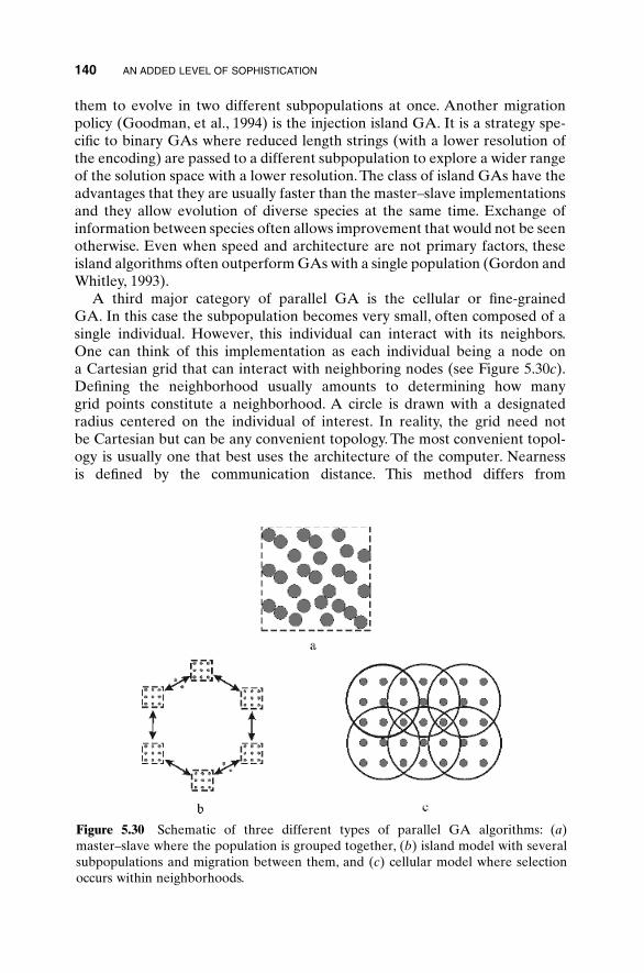
them to evolve in two different subpopulations at once. Another migrationpolicy (Goodman, et al., 1994) is the injection island GA. It is a strategy spe-cific to binary GAs where reduced length strings (with a lower resolution ofthe encoding) are passed to a different subpopulation to explore a wider rangeof the solution space with a lower resolution. The class of island GAs have theadvantages that they are usually faster than the master–slave implementationsand they allow evolution of diverse species at the same time. Exchange ofinformation between species often allows improvement that would not be seenotherwise. Even when speed and architecture are not primary factors, theseisland algorithms often outperform GAs with a single population (Gordon andWhitley, 1993).
A third major category of parallel GA is the cellular or fine-grained GA. In this case the subpopulation becomes very small, often composed of asingle individual. However, this individual can interact with its neighbors.One can think of this implementation as each individual being a node on a Cartesian grid that can interact with neighboring nodes (see Figure 5.30c).Defining the neighborhood usually amounts to determining how many grid points constitute a neighborhood. A circle is drawn with a designatedradius centered on the individual of interest. In reality, the grid need not be Cartesian but can be any convenient topology. The most convenient topol-ogy is usually one that best uses the architecture of the computer. Nearness is defined by the communication distance. This method differs from
140 AN ADDED LEVEL OF SOPHISTICATION
Figure 5.30 Schematic of three different types of parallel GA algorithms: (a)master–slave where the population is grouped together, (b) island model with severalsubpopulations and migration between them, and (c) cellular model where selectionoccurs within neighborhoods.
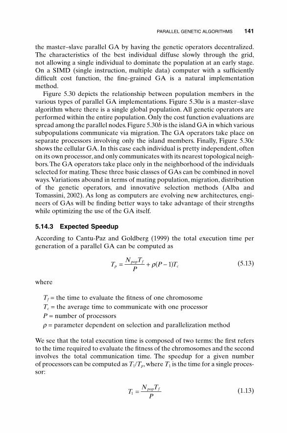
the master–slave parallel GA by having the genetic operators decentralized.The characteristics of the best individual diffuse slowly through the grid,not allowing a single individual to dominate the population at an early stage.On a SIMD (single instruction, multiple data) computer with a sufficiently difficult cost function, the fine-grained GA is a natural implementationmethod.
Figure 5.30 depicts the relationship between population members in thevarious types of parallel GA implementations. Figure 5.30a is a master–slavealgorithm where there is a single global population. All genetic operators areperformed within the entire population. Only the cost function evaluations arespread among the parallel nodes. Figure 5.30b is the island GA in which varioussubpopulations communicate via migration. The GA operators take place onseparate processors involving only the island members. Finally, Figure 5.30cshows the cellular GA. In this case each individual is pretty independent, oftenon its own processor,and only communicates with its nearest topological neigh-bors.The GA operators take place only in the neighborhood of the individualsselected for mating.These three basic classes of GAs can be combined in novelways. Variations abound in terms of mating population, migration, distributionof the genetic operators, and innovative selection methods (Alba andTomassini, 2002). As long as computers are evolving new architectures, engi-neers of GAs will be finding better ways to take advantage of their strengthswhile optimizing the use of the GA itself.
5.14.3 Expected Speedup
According to Cantu-Paz and Goldberg (1999) the total execution time pergeneration of a parallel GA can be computed as
(5.13)
where
Tf = the time to evaluate the fitness of one chromosomeTc = the average time to communicate with one processorP = number of processorsr = parameter dependent on selection and parallelization method
We see that the total execution time is composed of two terms: the first refersto the time required to evaluate the fitness of the chromosomes and the secondinvolves the total communication time. The speedup for a given number of processors can be computed as T1/Tp, where T1 is the time for a single proces-sor:
(1.13)TN T
Ppop f
1 =
TN T
PP Tp
pop fc= + -( )r 1
PARALLEL GENETIC ALGORITHMS 141
That speedup depends on the ratio of the time to compute the fitness relativeto the communication time (Tf/Tc), the number of processors, the populationsize, and the variable r, which depends on the details of the code and the parallelization technique. Here we use r = 1, which is appropriate for amaster–slave GA application. Figure 5.31 plots the speedup as a function ofthe number of processors used for three different Tf/Tc ratios (Tf/Tc = 1, 10,and 100) for a population size of Npop = 100. Perfect speedup would be thestraight line T1/TP = P. The larger Tf/Tc, the closer we get to perfect speedup.When communication costs are equal to the cost of evaluating the fitness func-tion (Tf/Tc = 1), a maximum speedup is reached, and then the time per proces-sor begins to decrease. Figure 5.32 is the same type of plot with N = 1000. Wesee that for a larger population size, the speedup is greater. One can computethe optimum number of processors to maximize the speedup curve (Popt) bytaking the derivative of (5.13) with respect to P, and setting it to 0 to obtain
(5.14)
Figure 5.33 plots Popt as a function of Tf/Tc for values of N = 16, 100, and 1000.As expected, the optimal number of processors increases monotonically withboth Npop and Tf/Tc.
There has been further work on the theoretical basis for different parallelimplementations of the GA (e.g., see Cantu-Paz 1999, 2000; Cantu-Paz and
PN T
Toptpop f
c
=r
142 AN ADDED LEVEL OF SOPHISTICATION
Figure 5.31 Theoretical speedup of GA with Npop = 100.
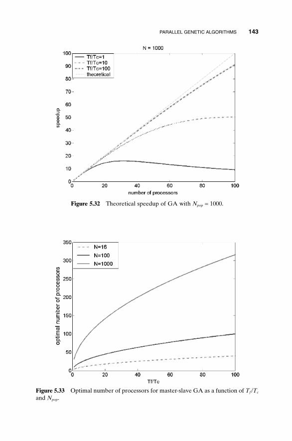
PARALLEL GENETIC ALGORITHMS 143
Figure 5.32 Theoretical speedup of GA with Npop = 1000.
Figure 5.33 Optimal number of processors for master-slave GA as a function of Tf /Tc
and Npop.
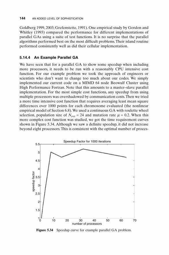
144 AN ADDED LEVEL OF SOPHISTICATION
Goldberg 1999, 2003; Grefenstette, 1991). One empirical study by Gordon andWhitley (1993) compared the performance for different implementations ofparallel GAs using a suite of test functions. It is no surprise that the parallelalgorithms performed best on the most difficult problems. Their island routineperformed consistently well as did their cellular implementation.
5.14.4 An Example Parallel GA
We have seen that for a parallel GA to show some speedup when includingmore processors, it needs to be run with a reasonably CPU intensive cost function. For our example problem we took the approach of engineers or scientists who don’t want to change too much about our codes. We simplyimplemented our current code on a MIMD 64 node Beowulf Cluster usingHigh Performance Fortran. Note that this amounts to a master–slave parallelimplementation. For the most simple cost functions, any speedup from usingmultiple processors was overshadowed by communication costs.Then we trieda more time intensive cost function that requires averaging least mean squaredifferences over 1000 points for each chromosome evaluated (the nonlinearempirical model of Section 6.8).We used a continuous GA with roulette wheelselection, population size of Npop = 24 and mutation rate m = 0.2. When thismore complex cost function was studied, we got the time requirement curvesshown in Figure 5.34. Although we saw a definite speedup, it did not increasebeyond eight processors. This is consistent with the optimal number of proces-
5.5
5
4.5
4
3.5
3
2.5
2
1.5
10 10 20 30 40 50 60 70
number of processors
Speedup Factor for 1000 iterations
spee
dup
fact
or
Figure 5.34 Speedup curve for example parallel GA problem.
sors computed in (5.14) and demonstrated in Figure 5.33 for this small popu-lation size.We would expect to see better speedup curves with an island imple-mentation and with larger population sizes.
5.14.5 How Parallel GAs Are Being Used
Parallel GAs are becoming important as the number of parallel machinesincreases. Particularly for very expensive cost functions, such as full simula-tions, parallel implementations are making GAs a competitive strategy. Just afew of the many examples include solution to the satisfiability problem (Folinoet al., 2001), optimizing supersonic wings via running an Euler equation model(Obayashi et al., 2000), optimal design of elastic flywheels (Eby et al., 1999),and many others. The number of parallel GA applications is expanding expo-nentially and may be the wave of the future.
BIBLIOGRAPHY
Alga, E., and M. Tomassini. 2002. Parallelism and evolutionary algorithms. IEEE Trans.Evol. Comput. 6:443–462.
Aytug, H., and G. J. Koehler. 1996. Stopping criteria for finite length genetic algorithms.ORSA J. Comp. 8:183–191.
Bäck, T. 1993. Optimal mutation rates in genetic search. In S. Forrest (ed.), Proc. 5thInt. Conf. on Genetic Algorithms, San Mates, CA: Morgan Kaufmann, pp. 2–9.
Bäck, T., and M. Schutz. 1996a. Intelligent mutation rate control in canonical geneticalgorithms. In Z. W. Ras and M. Michalewicz (eds.), Foundations of IntelligentSystems 9th Int. Symp. Berlin: Springer-Verlag, pp. 158–167.
Bäck, T. 1996b. Evolution strategies: An alternative evolutionary algorithm. In J. M.Alliot et al. (eds.), Artificial Evolution. Berlin: Springer-Verlag, pp. 3–20.
Booker, L. 1987. Improving search in genetic algorithms. In L. Davis (ed.), GeneticAlgorithms and Simulated Annealing. London: Pitman, pp. 61–73.
Cantu-Paz, E., and D. E. Goldberg. 1999. On the scalability of parallel genetic algo-rithms. Evol. Comput. 7:429–449.
Cantu-Paz, E., and D. E. Goldberg. 2003.Are multiple runs of genetic algorithms betterthan one? In GECCO 2003, Berlin: Springer-Verlag, pp. 801–812.
Cantu-Paz, E. 1999. Migration policies, selection pressure, and parallel evolutionaryalgorithms. J. Heurist. 7:311–334.
Cantu-Paz, E. 2000. Efficient and Accurate Parallel Genetic Algorithms. Dordrecht:Kluwer Academic.
Cantu-Paz. 2000. Markov chain models of parallel genetic algorithms. IEEE Trans.Evol. Comput. 4:216–226.
Caruana, R.A., and J. D. Schaffer. 1988. Representation and hidden bias: Gray vs. binarycoding for genetic algorithms. Proc. 5th Int. Conf. on Machine Learning, Los Altos,CA: Morgan Kaufmann, pp. 153–161.
Cerf, R. 1998. Asymptotic convergence of genetic algorithms. Adv. Appl. Prov. 30:521–550.
BIBLIOGRAPHY 145
Davis, L. 1989. Adapting operator probabilities in genetic algorithms. In J. D. Schaffer(ed.), Proc. 3rd Int. Conf. on Genetic Algorithms. Los Altos, CA: Morgan Kaufmann,pp. 61–67.
Davis, L. 1991a. Parameterizing a genetic algorithm. In L. Davis (ed.), Handbook ofGenetic Algorithms. New York: Van Nostrand Reinhold.
Davis, L. 1991b. Performance enhancements. In L. Davis (ed.), Handbook of GeneticAlgorithms. New York: Van Nostrand Reinhold.
Deb, K., et al. 2002. A fast and elitist multiobjective genetic algorithm: NSGA-II. IEEETrans. Evol. Comput. 6:182–197.
Deb, K., S. Agrawal, A. Pratab, and T. Meyarivan. 2000. A fast elitist non-dominatedsorting genetic algorithm for multi-objective optimization: NSGA-II. In M.Schoenauer (ed.), Proc. PPSN-6. Berlin: Springer-Verlag, pp. 849–858.
Deb, K., and D. E. Goldberg. 1991. mGA in C: A Messy Genetic Algorithm in C.IlliGAL Report 91008.
De Jong, K. A. 1975. Analysis of the behavior of a class of genetic adaptive systems.Ph.D. Dissertation. University of Michigan, Ann Arbor.
Eby, D., R. Averill, W. Punch, and E. E. Goodman. 1999. Optimal design of flywheelsusing an injection island genetic algorithm. Art. Intell. Eng. Des. Manuf. 13:289–402.
Eiben, A. E., R. Hinterding, and Z. Michalewicz. 1999. Parameter control in evolu-tionary algorithms. IEEE Trans. Evol. Comput. 3:124–141.
Eiben, A. E., P. E. Raue, and S. Ruttkay. 1994. Genetic algorithms with multi-parentrecombination. In Parallel Problem Solving from Nature—PPSN III, Int. Conf. onEvolutionary Computation. Berlin: Springer-Verlag, pp. 78–87.
Eshelman, L. J., R. A. Caruna, and J. D. Schaffer. 1989. Biases in the crossover land-scape. In Proc. 3rd Int. Conf. on Genetic Algorithms. San Mateo, CA: Morgan Kaufmann, pp. 10–19.
Fogarty, T. C. 1989. Varying the probability of mutation in the genetic algorithm. In J.D. Schaffer (ed.), Proc. 3rd Int. Conf. on Genetic Algorithms. Los Altos, CA: MorganKaufmann, pp. 104–109.
Folino, G., C. Pizzuti, and G. Spezzano. 2001. Parallel hybrid method for SAT thatcouples genetic algorithms and local search. IEEE Trans. Evol. Comput. 5:323–334.
Foneseca, C. M., and P. J. Flemming. 1993. Genetic algorithms for multi-objective opti-mization: Formulation, discussion, and generalization. Proc. 5th Int. Conf. on GeneticAlgorithms. San Francisco, CA: Morgan Kaufmann, pp. 416–423.
Francois, O. 1998. An evolutionary strategy for global minimization and its Markovchain analysis. IEEE Trans. Evol. Comput. 2:77–90.
Gao,Y. 1998.An upper bound on the convergence rates of canonical genetic algorithms.Complexity Int. 5.
Goldberg, D. E. 1989a. Genetic Algorithms in Search, Optimization, and Machine Learn-ing. Reading, MA: Addison-Wesley.
Goldberg, D. E. 1989b. Sizing populations for serial and parallel genetic algorithms.In J. D. Schaffer (ed.), Proc. 3rd Int. Conf. on Genetic Algorithms. Los Altos, CA:Morgan Kaufmann, pp. 70–79.
Goldberg, D. E., K. Deb, and B. Korb. 1989c. Messy genetic algorithms: Motivation,analysis and rst results. Complex Syst. 3:493–530.
146 AN ADDED LEVEL OF SOPHISTICATION
Goldberg, D. E., and J. Richardson. 1987. Genetic algorithms with sharing for multi-modal function optimization. In J. J. Grefenstette (ed.), Genetic Algorithms and TheirApplications: Proc. 2nd Int. Conf. on Genetic Algorithms. Hillsdale, NJ: LawrenceErlbaum, pp. 41–49.
Goldberg, D. E., and R. Lingle. 1985. Alleles, loci, and the traveling salesman problem.Proc. Int. Conf. on Genetic Algorithms and Their Applications, Mahwah, NJ:Lawrence Eribaum Associate, pp. 154–159.
Goodman, E. D.,W. F. Punch, and S. Lin. 1994. Coarse-grain parallel genetic algorithms:Categorization and new approach. Sixth IEEE Parallel and Distributed Processing,pp. 28–37.
Gordon, V. S., and D. Whitley. 1993. Serial and parallel genetic algorithms as functionoptimizers. In S. Forrest (ed.), ICGA-90: 5th Int. Conf. on Genetic Algorithms. LosAltos, CA: Morgan Kaufmann, pp. 177–183.
Greenhalgh, D. 2000. Convergence criteria for genetic algorithms. SIAM J. Comput.30:269–282.
Grefenstette, J. J. 1986. Optimization of control parameters for genetic algorithms.IEEE Trans. Syst. Man Cybernet. 16:128.
Grefenstette, J. J. 1991. Conditions for implicit parallelism. In G. J. E. Rawlins (ed.),Foundations of Genetic Algorithms. San Mateo, CA: Morgan Kaufmann, pp. 252–261.
Hajek, B. 1988. Cooling schedules for optimal annealing. Math. Oper. Res. 13:311–329.
Haupt, R. L. 1987. Synthesis of resistive tapers to control scattering patterns of strips.Ph.D. dissertation. University of Michigan, Ann Arbor.
Haupt, R. L. 1995. Optimization of aperiodic conducting grids. 11th An. Rev. Progressin Applied Computational Electromagnetics Conf. Monterey, CA.
Haupt, R. L. 1996. Speeding convergence of genetic algorithms for optimizing antennaarrays. 12th An. Rev. Progress in Applied Computational Electromagnetics Confer-ence. Monterey, CA.
Haupt,R.L.,and S.E.Haupt.2000.Practical Genetic Algorithms,1st ed.New York:Wiley.
Haupt, R. L., and S. E. Haupt. 2000. Optimum population size and mutation rate for asimple real genetic algorithm that optimizes array factors. Appl. Comput. Electro-magn. Soc. J. 15:94–102.
Hinterding, R., H. Gielewski, and T. C. Peachey. 1989.The nature of mutation in geneticalgorithms. In L. J. Eshelman (ed.), Proc. 6th Int. Conf. on Genetic Algorithms. LosAltos, CA: Morgan Kaufmann, pp. 70–79.
Holland, J. H. 1975. Adaptation in Natural and Artificial Systems. Ann Arbor: Univer-sity of Michigan Press.
Kazarlis, S. A., et al. 2001. Microgenetic algorithms as generalized hill-climbing opera-tors for GA optimization. IEEE Trans. Evol. Comp. 5:204–217.
Knjazew, D. 2002. OmeGA: A Competent Genetic Algorithm for Solving Permutationand Scheduling Problems: Genetic Algorithms and Evolutionary Computation, Vol.6. Norwell, MA: Kluwer Academic.
Liepins, G. E., et al. 1990. Genetic algorithm applications to set covering and travelingsalesman problems. In Operations Research and Artificial Intelligence, D. E. Brownand C. C. White (eds.), OR/AI: The Integration of Problem Solving Strategies.Norwell, MA: Kluwer Academic, pp. 29–57.
BIBLIOGRAPHY 147
Michalewicz, Z. 1992. Genetic Algorithms + Data Structures = Evolution Programs. NewYork: Springer-Verlag.
Nix, A., and M. D. Vose. 1992. Modeling genetic algorithms with Markov chains. An.Math. Art. Intell. 5:79–88.
Nowostawski, M., and R. Poli. 1999. Parallel genetic algorithm taxonomy. KES¢99,Adelaide, South Australia.
Obayashi, S., D. Sasaki, Y. Takeguchi, and N. Hirose. 2000. Multiobjective evolutionarycomputation for supersonic wing-shape optimization. IEEE Trans. Evol. Comput.4:182–187.
Oliver, I. M., D. J. Smith, and J. R. C. Holland. 1987. A study of permutation crossoveroperators on the traveling salesman problem. Genetic Algorithms and Their Appli-cations: Proc. 2nd Int. Conf. on Genetic Algorithms, Cambridge, MA: LawrenceErlbaum Associates, pp. 224–230.
Schaffer, J. D. 1984. Some experiments in machine learning using vector evaluatedgenetic algorithms. Ph.D. dissertation. Vanderbilt University, Nashville, TN.
Schaffer, J. D., et al., 1989. A study of control parameters affecting online performanceof genetic algorithms for function optimization. In J. D. Schaffer (ed.), Proc. 3rd Int.Conf. on Genetic Algorithms. Los Altos, CA: Morgan Kaufmann, pp. 51–60.
Syswerda, G. 1989. Uniform crossover in genetic algorithms. In J. D. Schaffer (ed.), Proc.3rd Int. Conf. on Genetic Algorithms. Los Altos, CA: Morgan Kaufmann, pp. 2–9.
Syswerda, G. 1991. Schedule optimization using genetic algorithms. In L. Davis (ed.),Handbook of Genetic Algorithms. New York: Van Nostrand Reinhold, p. 347.
Taub, H., and D. L. Schilling. 1986. Principles of Communication Systems. New York:McGraw-Hill.
Watson, J.-P. 1999. A performance assessment of modern niching methods for parameter optimization problems. Genetic and Evolutionary Computation Conf.GECCO-1999, Orlando, FL: Morgan Kaufmann.
Zitzler, E., and L. Thiele. 1999. Multiobjective evolutionary algorithms: a comparativecase study and the strength Pareto approach. IEEE Trans. Evol. Comput. 3:257–271.
EXERCISES
1. Modify a binary GA to avoid repeated chromosomes by:
a. Making all the initial population members unique.b. Checking to make sure that a chromosome is only ever evaluated once.
2. Solve (5.1) with the following weights: 0.1, 0.2, 0.3, 0.4, 0.5, 0.6, 0.7, 0.8, 0.9.
3. Use the Pareto GA to solve (5.1).
4. How do the following affect the Pareto GA:
a. Population sizeb. Mutation ratec. Type of crossoverd. Binary versus continuous GAs
148 AN ADDED LEVEL OF SOPHISTICATION
5. Write a continuous or binary hybrid GA that uses one of the followinglocal optimizers:
a. Nelder-Mead downhill simplexb. BFGSc. DFPd. Steepest descente. Random search
6. Compare the performances of the GA with the various local optimizersusing the function _____ from Appendix I.
7. Compare the performance of the hybrid GA with local optimizer _____against a binary and/or continuous GA using the function _____ fromAppendix I.
8. Compare the convergence of a binary GA with and without a Gray code.Use function _____ in Appendix I.
9. How does the number of bits in a gene effect the performance of a GA?
10. Modify your binary GA for two-point crossover. Does this improve theperformance of the GA over single-point crossover? Demonstrate byaveraging the performance over several different test functions.
11. Modify your binary GA for two-point crossover. Does it matter which seg-ments are swapped in the crossover? Should the segments be randomlyswapped or is it sufficient to just swap the middle segment?
12. Modify your binary GA for two-point crossover with three parents. Doesthis improve the performance of the GA over single-point crossover?Demonstrate by averaging the performance over several different testfunctions.
13. Modify the binary GA to do uniform crossover. Does this improve theperformance of the GA over single- or double-point crossover? Demon-strate by averaging the performance over several different test functions.
14. Implement (5.10) as a crossover scheme for your continuous GA. Doesthis improve performance?
15. Implement (5.11) as a crossover scheme for your continuous GA. Doesthis improve performance?
16. Compare several different methods of sampling the initial population. Useaveraging and three different test functions. Does one method work betterthan the others?
17. Add a life span to your chromosomes. Does this improve GA performance?
EXERCISES 149
18. Try placing an initial first guess close to the global minimum of test func-tion _____ from Appendix I. How does it affect the convergence of
a. Nelder-Mead downhill simplexb. BFGSc. DFPd. Steepest descente. Random searchf. Binary GAg. Continuous GA
What happens if your seed is not in the bowl of the global minimum?
19. For a (i) binary GA and (ii) continuous GA, implement one of the following variable mutation rates:
a. First generation has m = 0.5, and subsequent generations have a low m.b. Exponentially decreasing m over all generations.c. Linearly decreasing m over all generations.d. Exponentially increasing m over all generations.e. Linearly increasing m over all generations.
Compare and make recommendations using some of the cost functions inAppendix I.
20. Write your own permutation GA. Test it on the traveling salespersonproblem for 8, 12, 16, and 20 cities. Do you get the same solution for eachindependent run?
21. For a (i) binary GA and (ii) continuous GA, perform a study of the fol-lowing GA parameters, using the test functions:
a. Population sizeb. Mutation ratec. Crossover rated. Selection rate
22. Does the selection of test function matter when comparing the perfor-mance of GAs?
23. Write a mGA.Does it improve the performance compared to a binary GA?
24. Write a master–slave parallel GA. Test it on varying numbers of proces-sors. Plot a speedup curve.
25. Write a cellular parallel GA.Test it on varying numbers of processors. Plota speedup curve.
26. Write an island parallel GA.Test it on varying numbers of processors. Plota speedup curve.
150 AN ADDED LEVEL OF SOPHISTICATION
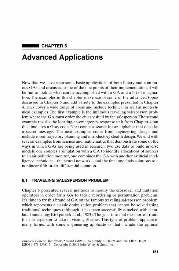
CHAPTER 6
Advanced Applications
151
Now that we have seen some basic applications of both binary and continu-ous GAs and discussed some of the fine points of their implementation, it willbe fun to look at what can be accomplished with a GA and a bit of imagina-tion. The examples in this chapter make use of some of the advanced topicsdiscussed in Chapter 5 and add variety to the examples presented in Chapter4. They cover a wide range of areas and include technical as well as nontech-nical examples. The first example is the infamous traveling salesperson prob-lem where the GA must order the cities visited by the salesperson.The secondexample revisits the locating-an-emergency-response unit from Chapter 4 butthis time uses a Gray code. Next comes a search for an alphabet that decodesa secret message. The next examples come from engineering design andinclude robot trajectory planning and introductory stealth design.We end withseveral examples from science and mathematics that demonstrate some of theways in which GAs are being used in research: two use data to build inversemodels, one couples a simulation with a GA to identify allocations of sourcesto an air pollution monitor, one combines the GA with another artificial intel-ligence technique—the neural network—and the final one finds solutions to anonlinear fifth-order differential equation.
6.1 TRAVELING SALESPERSON PROBLEM
Chapter 5 presented several methods to modify the crossover and mutationoperators in order for a GA to tackle reordering or permutation problems.It’s time to try this brand of GA on the famous traveling salesperson problem,which represents a classic optimization problem that cannot be solved usingtraditional techniques (although it has been successfully attacked with simu-lated annealing; Kirkpatrick et al., 1983). The goal is to find the shortest routefor a salesperson to take in visiting N cities. This type of problem appears inmany forms, with some engineering applications that include the optimal
Practical Genetic Algorithms, Second Edition, by Randy L. Haupt and Sue Ellen Haupt.ISBN 0-471-45565-2 Copyright © 2004 John Wiley & Sons, Inc.
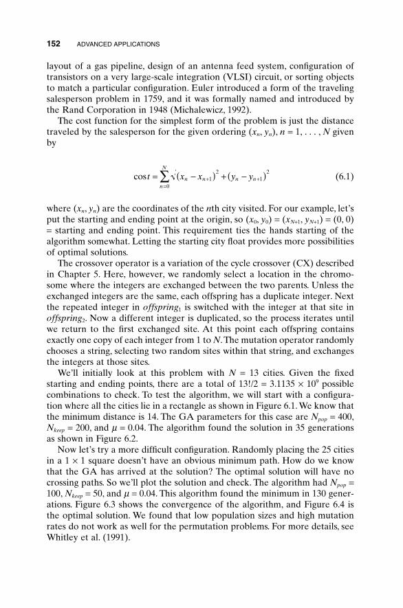
layout of a gas pipeline, design of an antenna feed system, configuration oftransistors on a very large-scale integration (VLSI) circuit, or sorting objectsto match a particular configuration. Euler introduced a form of the travelingsalesperson problem in 1759, and it was formally named and introduced bythe Rand Corporation in 1948 (Michalewicz, 1992).
The cost function for the simplest form of the problem is just the distancetraveled by the salesperson for the given ordering (xn, yn), n = 1, . . . , N given by
(6.1)
where (xn, yn) are the coordinates of the nth city visited. For our example, let’sput the starting and ending point at the origin, so (x0, y0) = (xN+1, yN+1) = (0, 0)= starting and ending point. This requirement ties the hands starting of thealgorithm somewhat. Letting the starting city float provides more possibilitiesof optimal solutions.
The crossover operator is a variation of the cycle crossover (CX) describedin Chapter 5. Here, however, we randomly select a location in the chromo-some where the integers are exchanged between the two parents. Unless theexchanged integers are the same, each offspring has a duplicate integer. Nextthe repeated integer in offspring1 is switched with the integer at that site inoffspring2. Now a different integer is duplicated, so the process iterates untilwe return to the first exchanged site. At this point each offspring containsexactly one copy of each integer from 1 to N.The mutation operator randomlychooses a string, selecting two random sites within that string, and exchangesthe integers at those sites.
We’ll initially look at this problem with N = 13 cities. Given the fixed starting and ending points, there are a total of 13!/2 = 3.1135 ¥ 109 possiblecombinations to check. To test the algorithm, we will start with a configura-tion where all the cities lie in a rectangle as shown in Figure 6.1. We know thatthe minimum distance is 14. The GA parameters for this case are Npop = 400,Nkeep = 200, and m = 0.04. The algorithm found the solution in 35 generationsas shown in Figure 6.2.
Now let’s try a more difficult configuration. Randomly placing the 25 citiesin a 1 ¥ 1 square doesn’t have an obvious minimum path. How do we knowthat the GA has arrived at the solution? The optimal solution will have nocrossing paths. So we’ll plot the solution and check. The algorithm had Npop =100, Nkeep = 50, and m = 0.04. This algorithm found the minimum in 130 gener-ations. Figure 6.3 shows the convergence of the algorithm, and Figure 6.4 isthe optimal solution. We found that low population sizes and high mutationrates do not work as well for the permutation problems. For more details, seeWhitley et al. (1991).
cos t x x y yn n n nn
N
= -( ) + -( )+ +=
 12
12
0
152 ADVANCED APPLICATIONS
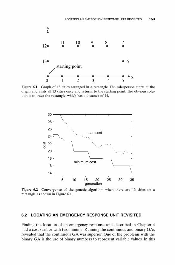
6.2 LOCATING AN EMERGENCY RESPONSE UNIT REVISITED
Finding the location of an emergency response unit described in Chapter 4had a cost surface with two minima. Running the continuous and binary GAsrevealed that the continuous GA was superior. One of the problems with thebinary GA is the use of binary numbers to represent variable values. In this
LOCATING AN EMERGENCY RESPONSE UNIT REVISITED 153
Figure 6.1 Graph of 13 cities arranged in a rectangle. The salesperson starts at theorigin and visits all 13 cities once and returns to the starting point. The obvious solu-tion is to trace the rectangle, which has a distance of 14.
5 10 15 20 25 30 35
14
16
18
20
22
24
26
28
30
generation
cost
minimum cost
mean cost
Figure 6.2 Convergence of the genetic algorithm when there are 13 cities on a rectangle as shown in Figure 6.1.
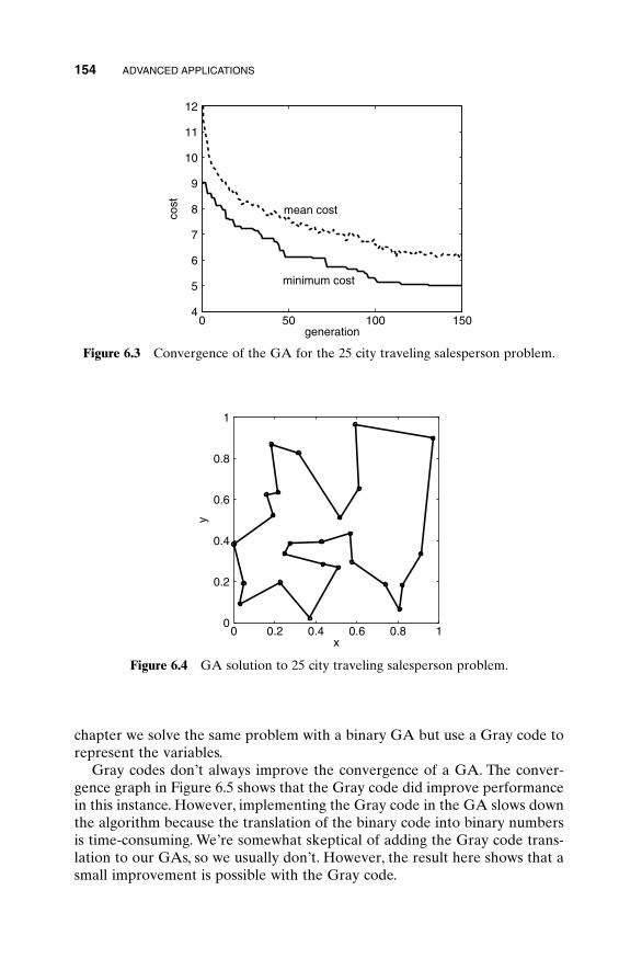
chapter we solve the same problem with a binary GA but use a Gray code torepresent the variables.
Gray codes don’t always improve the convergence of a GA. The conver-gence graph in Figure 6.5 shows that the Gray code did improve performancein this instance. However, implementing the Gray code in the GA slows downthe algorithm because the translation of the binary code into binary numbersis time-consuming. We’re somewhat skeptical of adding the Gray code trans-lation to our GAs, so we usually don’t. However, the result here shows that asmall improvement is possible with the Gray code.
154 ADVANCED APPLICATIONS
0 50 100 1504
5
6
7
8
9
10
11
12
generation
cost mean cost
minimum cost
Figure 6.3 Convergence of the GA for the 25 city traveling salesperson problem.
0 0.2 0.4 0.6 0.8 10
0.2
0.4
0.6
0.8
1
x
y
Figure 6.4 GA solution to 25 city traveling salesperson problem.
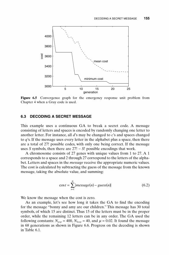
6.3 DECODING A SECRET MESSAGE
This example uses a continuous GA to break a secret code. A message consisting of letters and spaces is encoded by randomly changing one letter toanother letter. For instance, all d’s may be changed to c’s and spaces changedto q’s. If the message uses every letter in the alphabet plus a space, then thereare a total of 27! possible codes, with only one being correct. If the messageuses S symbols, then there are 27! - S! possible encodings that work.
A chromosome consists of 27 genes with unique values from 1 to 27. A 1corresponds to a space and 2 through 27 correspond to the letters of the alpha-bet. Letters and spaces in the message receive the appropriate numeric values.The cost is calculated by subtracting the guess of the message from the knownmessage, taking the absolute value, and summing:
(6.2)
We know the message when the cost is zero.As an example, let’s see how long it takes the GA to find the encoding
for the message “bonny and amy are our children.” This message has 30 totalsymbols, of which 15 are distinct. Thus 15 of the letters must be in the properorder, while the remaining 12 letters can be in any order. The GA used thefollowing constants: Npop = 400, Nkeep = 40, and m = 0.02. It found the messagein 68 generations as shown in Figure 6.6. Progress on the decoding is shownin Table 6.1.
cos t message n guess nn
N
= ( ) - ( )=
Â1
DECODING A SECRET MESSAGE 155
5 10 15 20 253000
3200
3400
3600
3800
4000
generation
cost
minimum cost
mean cost
Figure 6.5 Convergence graph for the emergency response unit problem fromChapter 4 when a Gray code is used.
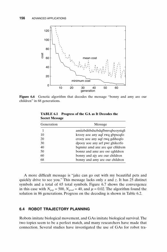
156 ADVANCED APPLICATIONS
10 20 30 40 50 600
20
40
60
80
100
120
generation
cost
minimum cost
mean cost
Figure 6.6 Genetic algorithm that decodes the message “bonny and amy are our children” in 68 generations.
A more difficult message is “jake can go out with my beautiful pets andquickly drive to see you.” This message lacks only x and z. It has 25 distinctsymbols and a total of 65 total symbols. Figure 6.7 shows the convergence in this case with Npop = 500, Ngood = 40, and m = 0.02. The algorithm found thesolution in 86 generations. Progress on the decoding is shown in Table 6.2.
6.4 ROBOT TRAJECTORY PLANNING
Robots imitate biological movement, and GAs imitate biological survival. Thetwo topics seem to be a perfect match, and many researchers have made thatconnection. Several studies have investigated the use of GAs for robot tra-
TABLE 6.1 Progress of the GA as It Decodes theSecret Message
Generation Message
1 amiizbditbdxzbdqfbmvqbeoystqfi10 krooy aoe any aqf rwq gbpseqfo20 crooy aoe any aqf rwq gdiheqfo30 dpooy aoe any arf pwr ghikerfo40 bqmmz amd anz are qur cfildrem50 bonnz and amz are osr cghldren60 bonny and ajy are our children68 bonny and amy are our children
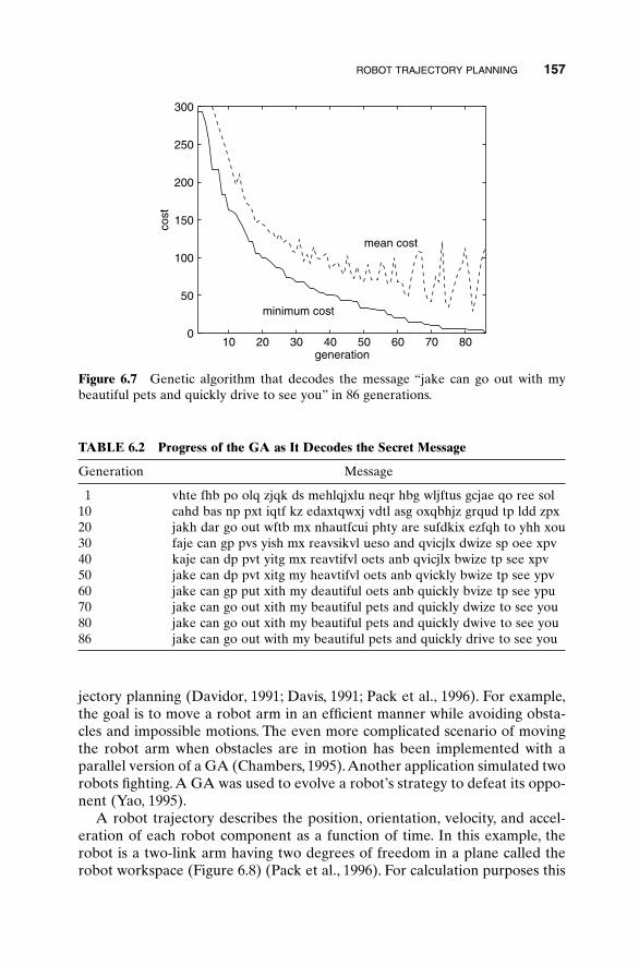
jectory planning (Davidor, 1991; Davis, 1991; Pack et al., 1996). For example,the goal is to move a robot arm in an efficient manner while avoiding obsta-cles and impossible motions. The even more complicated scenario of movingthe robot arm when obstacles are in motion has been implemented with a parallel version of a GA (Chambers, 1995).Another application simulated tworobots fighting. A GA was used to evolve a robot’s strategy to defeat its oppo-nent (Yao, 1995).
A robot trajectory describes the position, orientation, velocity, and accel-eration of each robot component as a function of time. In this example, therobot is a two-link arm having two degrees of freedom in a plane called therobot workspace (Figure 6.8) (Pack et al., 1996). For calculation purposes this
ROBOT TRAJECTORY PLANNING 157
10 20 30 40 50 60 70 800
50
100
150
200
250
300
generation
cost
minimum cost
mean cost
Figure 6.7 Genetic algorithm that decodes the message “jake can go out with mybeautiful pets and quickly drive to see you” in 86 generations.
TABLE 6.2 Progress of the GA as It Decodes the Secret Message
Generation Message
1 vhte fhb po olq zjqk ds mehlqjxlu neqr hbg wljftus gcjae qo ree sol10 cahd bas np pxt iqtf kz edaxtqwxj vdtl asg oxqbhjz grqud tp ldd zpx20 jakh dar go out wftb mx nhautfcui phty are sufdkix ezfqh to yhh xou30 faje can gp pvs yish mx reavsikvl ueso and qvicjlx dwize sp oee xpv40 kaje can dp pvt yitg mx reavtifvl oets anb qvicjlx bwize tp see xpv50 jake can dp pvt xitg my heavtifvl oets anb qvickly bwize tp see ypv60 jake can gp put xith my deautiful oets anb quickly bvize tp see ypu70 jake can go out xith my beautiful pets and quickly dwize to see you80 jake can go out xith my beautiful pets and quickly dwive to see you86 jake can go out with my beautiful pets and quickly drive to see you
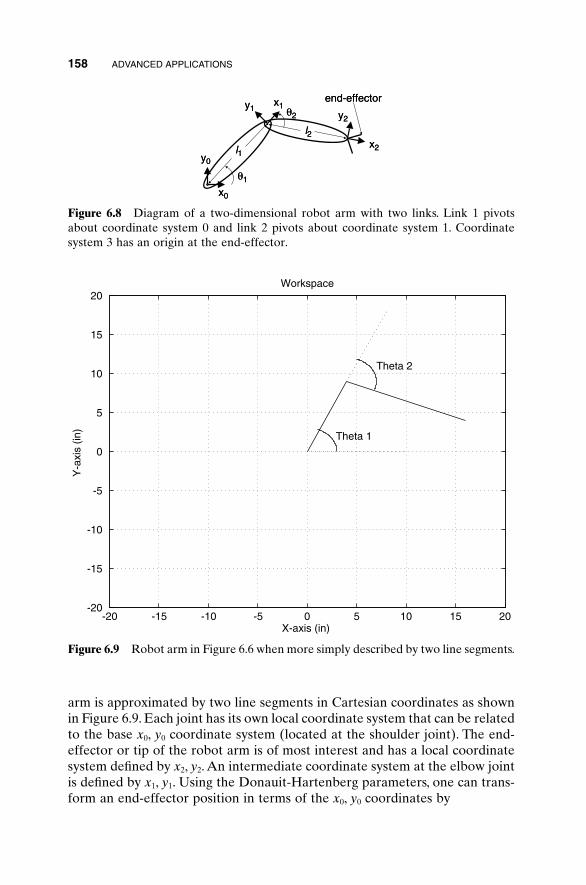
arm is approximated by two line segments in Cartesian coordinates as shownin Figure 6.9. Each joint has its own local coordinate system that can be relatedto the base x0, y0 coordinate system (located at the shoulder joint). The end-effector or tip of the robot arm is of most interest and has a local coordinatesystem defined by x2, y2. An intermediate coordinate system at the elbow jointis defined by x1, y1. Using the Donauit-Hartenberg parameters, one can trans-form an end-effector position in terms of the x0, y0 coordinates by
158 ADVANCED APPLICATIONS
end-effector
y2
y1
y0
x1
x0
x2
l2
q2
q1
l1
end-effector
y2
y1
y0
x1
x0
x2
l2
q2
q1
l1
Figure 6.8 Diagram of a two-dimensional robot arm with two links. Link 1 pivotsabout coordinate system 0 and link 2 pivots about coordinate system 1. Coordinatesystem 3 has an origin at the end-effector.
-20 -15 -10 -5 0 5 10 15 20-20
-15
-10
-5
0
5
10
15
20Workspace
X-axis (in)
Y-a
xis
(in)
Theta 1
Theta 2
Figure 6.9 Robot arm in Figure 6.6 when more simply described by two line segments.
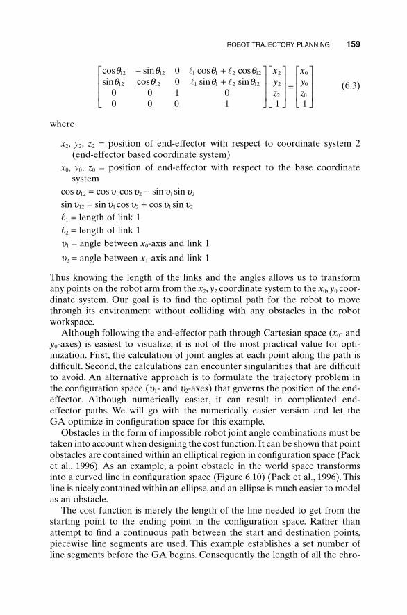
(6.3)
where
x2, y2, z2 = position of end-effector with respect to coordinate system 2 (end-effector based coordinate system)
x0, y0, z0 = position of end-effector with respect to the base coordinatesystem
cos u12 = cos u1 cos u2 - sinu1 sin u2
sin u12 = sinu1 cos u2 + cos u1 sinu2
�1 = length of link 1�2 = length of link 1u1 = angle between x0-axis and link 1
u2 = angle between x1-axis and link 1
Thus knowing the length of the links and the angles allows us to transformany points on the robot arm from the x2, y2 coordinate system to the x0, y0 coor-dinate system. Our goal is to find the optimal path for the robot to movethrough its environment without colliding with any obstacles in the robotworkspace.
Although following the end-effector path through Cartesian space (x0- andy0-axes) is easiest to visualize, it is not of the most practical value for opti-mization. First, the calculation of joint angles at each point along the path isdifficult. Second, the calculations can encounter singularities that are difficultto avoid. An alternative approach is to formulate the trajectory problem in the configuration space (u1- and u2-axes) that governs the position of the end-effector. Although numerically easier, it can result in complicated end-effector paths. We will go with the numerically easier version and let the GA optimize in configuration space for this example.
Obstacles in the form of impossible robot joint angle combinations must betaken into account when designing the cost function. It can be shown that pointobstacles are contained within an elliptical region in configuration space (Packet al., 1996). As an example, a point obstacle in the world space transformsinto a curved line in configuration space (Figure 6.10) (Pack et al., 1996). Thisline is nicely contained within an ellipse, and an ellipse is much easier to modelas an obstacle.
The cost function is merely the length of the line needed to get from thestarting point to the ending point in the configuration space. Rather thanattempt to find a continuous path between the start and destination points,piecewise line segments are used. This example establishes a set number ofline segments before the GA begins. Consequently the length of all the chro-
cos sin cos cossin cos sin sin
q q q qq q q q
12 12 1 1 2 12
12 12 1 1 2 12
2
2
2
0
0
0
00
0 0 1 00 0 0 1 1 1
- ++
È
Î
ÍÍÍ
˘
˚
˙˙˙
È
Î
ÍÍÍ
˘
˚
˙˙˙
=
È
Î
ÍÍÍ
˘
˚
˙˙˙
l ll l
xyz
xyz
ROBOT TRAJECTORY PLANNING 159
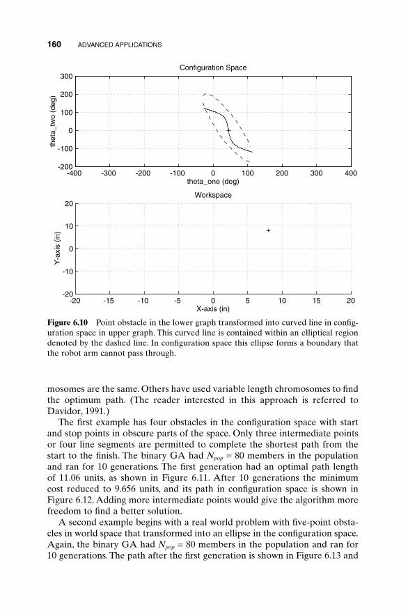
mosomes are the same. Others have used variable length chromosomes to findthe optimum path. (The reader interested in this approach is referred toDavidor, 1991.)
The first example has four obstacles in the configuration space with startand stop points in obscure parts of the space. Only three intermediate pointsor four line segments are permitted to complete the shortest path from thestart to the finish. The binary GA had Npop = 80 members in the populationand ran for 10 generations. The first generation had an optimal path length of 11.06 units, as shown in Figure 6.11. After 10 generations the minimum cost reduced to 9.656 units, and its path in configuration space is shown inFigure 6.12. Adding more intermediate points would give the algorithm morefreedom to find a better solution.
A second example begins with a real world problem with five-point obsta-cles in world space that transformed into an ellipse in the configuration space.Again, the binary GA had Npop = 80 members in the population and ran for10 generations. The path after the first generation is shown in Figure 6.13 and
160 ADVANCED APPLICATIONS
-400 -300 -200 -100 0 100 200 300 400-200
-100
0
100
200
300
theta_one (deg)
thet
a_tw
o (d
eg)
Configuration Space
-20 -15 -10 -5 0 5 10 15 20-20
-10
0
10
20Workspace
X-axis (in)
Y-a
xis
(in)
Figure 6.10 Point obstacle in the lower graph transformed into curved line in config-uration space in upper graph. This curved line is contained within an elliptical regiondenoted by the dashed line. In configuration space this ellipse forms a boundary thatthe robot arm cannot pass through.
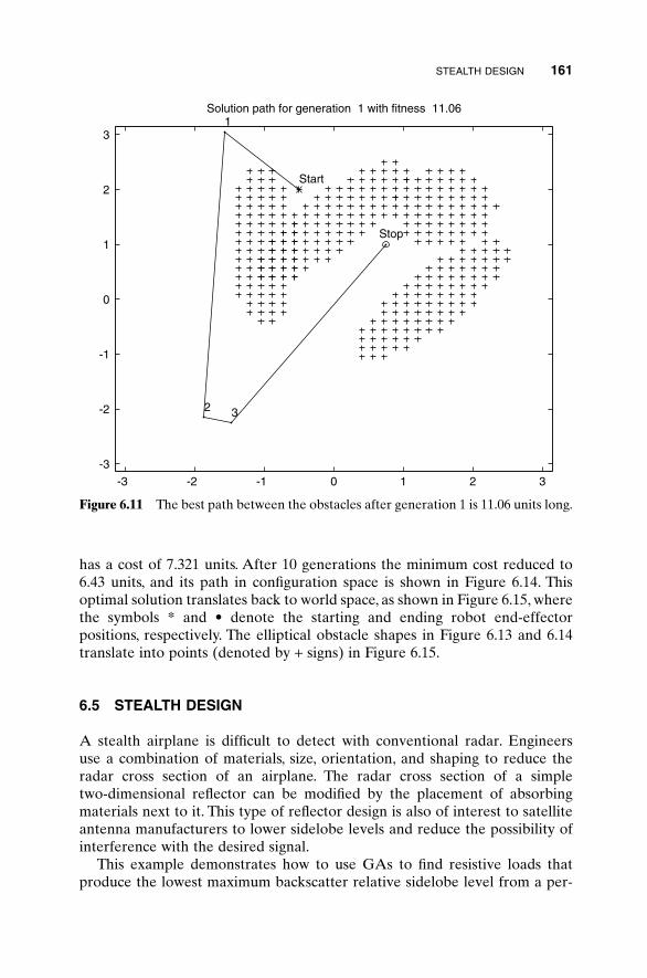
STEALTH DESIGN 161
-3 -2 -1 0 1 2 3
-3
-2
-1
0
1
2
3
Start
Stop
Solution path for generation 1 with fitness 11.061
2 3
Figure 6.11 The best path between the obstacles after generation 1 is 11.06 units long.
has a cost of 7.321 units. After 10 generations the minimum cost reduced to6.43 units, and its path in configuration space is shown in Figure 6.14. Thisoptimal solution translates back to world space, as shown in Figure 6.15, wherethe symbols * and • denote the starting and ending robot end-effector positions, respectively. The elliptical obstacle shapes in Figure 6.13 and 6.14translate into points (denoted by + signs) in Figure 6.15.
6.5 STEALTH DESIGN
A stealth airplane is difficult to detect with conventional radar. Engineers use a combination of materials, size, orientation, and shaping to reduce theradar cross section of an airplane. The radar cross section of a simple two-dimensional reflector can be modified by the placement of absorbingmaterials next to it. This type of reflector design is also of interest to satelliteantenna manufacturers to lower sidelobe levels and reduce the possibility ofinterference with the desired signal.
This example demonstrates how to use GAs to find resistive loads thatproduce the lowest maximum backscatter relative sidelobe level from a per-
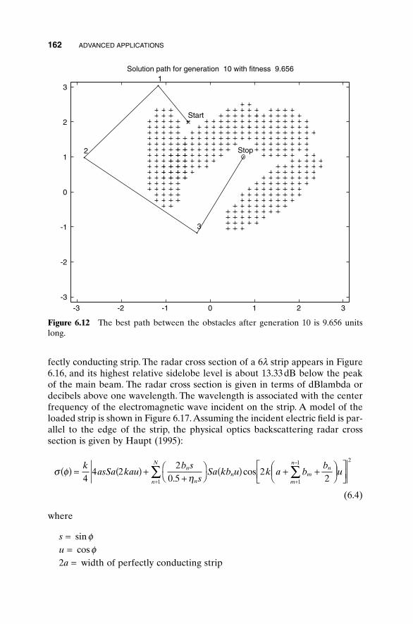
162 ADVANCED APPLICATIONS
-3 -2 -1 0 1 2 3
-3
-2
-1
0
1
2
3
Start
Stop
Solution path for generation 10 with fitness 9.6561
2
3
Figure 6.12 The best path between the obstacles after generation 10 is 9.656 unitslong.
fectly conducting strip. The radar cross section of a 6l strip appears in Figure6.16, and its highest relative sidelobe level is about 13.33dB below the peakof the main beam. The radar cross section is given in terms of dBlambda ordecibels above one wavelength. The wavelength is associated with the centerfrequency of the electromagnetic wave incident on the strip. A model of theloaded strip is shown in Figure 6.17.Assuming the incident electric field is par-allel to the edge of the strip, the physical optics backscattering radar crosssection is given by Haupt (1995):
(6.4)
where
s = sin fu = cos f2a = width of perfectly conducting strip
s fh
( ) = ( ) ++
ÊË
ˆ¯ ( ) + +Ê
ËÁˆ¯
ÈÎÍ
˘˚+ +
-
 ÂkasSa kau
b ss
Sa kb u k a bb
un
nn
N
n mn
m
n
44 2
20 5
221 1
1 2
.cos
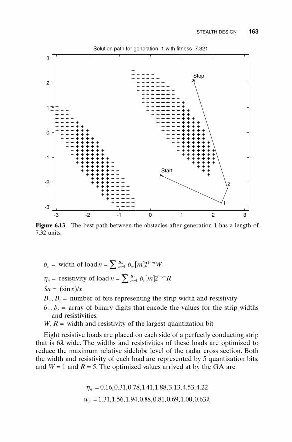
STEALTH DESIGN 163
-3 -2 -1 0 1 2 3
-3
-2
-1
0
1
2
3
Start
Stop
Solution path for generation 1 with fitness 7.321
1
2
Figure 6.13 The best path between the obstacles after generation 1 has a length of7.32 units.
bn = width of load
hn = resistivity of load
Sa = (sinx)/xBw, Br = number of bits representing the strip width and resistivitybw, br = array of binary digits that encode the values for the strip widths
and resistivities.W, R = width and resistivity of the largest quantization bit
Eight resistive loads are placed on each side of a perfectly conducting stripthat is 6l wide. The widths and resistivities of these loads are optimized toreduce the maximum relative sidelobe level of the radar cross section. Boththe width and resistivity of each load are represented by 5 quantization bits,and W = 1 and R = 5. The optimized values arrived at by the GA are
h
l
n
nw
=
=
0 16 0 31 0 78 1 41 1 88 3 13 4 53 4 22
1 31 1 56 1 94 0 88 0 81 0 69 1 00 0 63
. , . , . , . , . , . , . , .
. , . , . , . , . , . , . , .
n b m RmB
rmr= [ ]=
-Â 112
n b m WmB
wmw= [ ]=
-Â 112
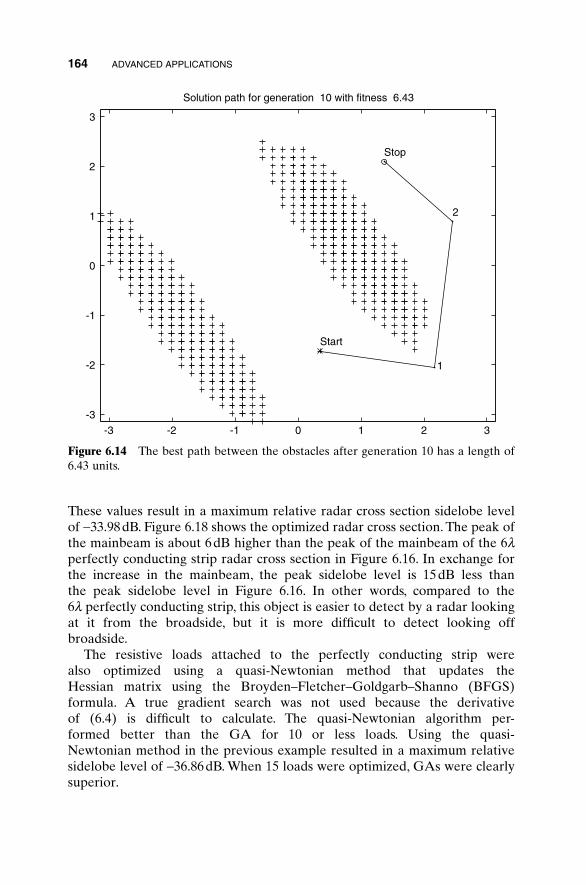
164 ADVANCED APPLICATIONS
-3 -2 -1 0 1 2 3
-3
-2
-1
0
1
2
3
Start
Stop
Solution path for generation 10 with fitness 6.43
1
2
Figure 6.14 The best path between the obstacles after generation 10 has a length of6.43 units.
These values result in a maximum relative radar cross section sidelobe levelof -33.98dB. Figure 6.18 shows the optimized radar cross section. The peak ofthe mainbeam is about 6dB higher than the peak of the mainbeam of the 6lperfectly conducting strip radar cross section in Figure 6.16. In exchange forthe increase in the mainbeam, the peak sidelobe level is 15dB less than the peak sidelobe level in Figure 6.16. In other words, compared to the 6l perfectly conducting strip, this object is easier to detect by a radar lookingat it from the broadside, but it is more difficult to detect looking off broadside.
The resistive loads attached to the perfectly conducting strip were also optimized using a quasi-Newtonian method that updates the Hessian matrix using the Broyden–Fletcher–Goldgarb–Shanno (BFGS)formula. A true gradient search was not used because the derivative of (6.4) is difficult to calculate. The quasi-Newtonian algorithm per-formed better than the GA for 10 or less loads. Using the quasi-Newtonian method in the previous example resulted in a maximum relativesidelobe level of -36.86dB. When 15 loads were optimized, GAs were clearlysuperior.
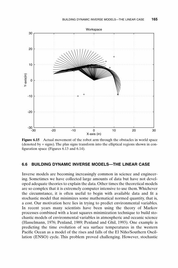
6.6 BUILDING DYNAMIC INVERSE MODELS—THE LINEAR CASE
Inverse models are becoming increasingly common in science and engineer-ing. Sometimes we have collected large amounts of data but have not devel-oped adequate theories to explain the data. Other times the theoretical modelsare so complex that it is extremely computer intensive to use them.Whicheverthe circumstance, it is often useful to begin with available data and fit a stochastic model that minimizes some mathematical normed quantity, that is,a cost. Our motivation here lies in trying to predict environmental variables.In recent years many scientists have been using the theory of Markovprocesses combined with a least squares minimization technique to build sto-chastic models of environmental variables in atmospheric and oceanic science(Hasselmann, 1976; Penland, 1989; Penland and Ghil, 1993). One example ispredicting the time evolution of sea surface temperatures in the westernPacific Ocean as a model of the rises and falls of the El Nino/Southern Oscil-lation (ENSO) cycle. This problem proved challenging. However, stochastic
BUILDING DYNAMIC INVERSE MODELS—THE LINEAR CASE 165
-30 -20 -10 0 10 20 30-30
-20
-10
0
10
20
30
X-axis (in)
Y-a
xis(
in)
Workspace
Figure 6.15 Actual movement of the robot arm through the obstacles in world space(denoted by + signs). The plus signs transform into the elliptical regions shown in con-figuration space (Figures 6.13 and 6.14).
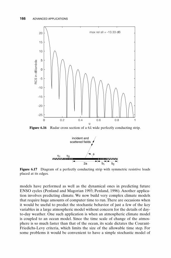
models have performed as well as the dynamical ones in predicting futureENSO cycles (Penland and Magorian 1993; Penland, 1996). Another applica-tion involves predicting climate. We now build very complex climate modelsthat require huge amounts of computer time to run. There are occasions whenit would be useful to predict the stochastic behavior of just a few of the keyvariables in a large atmospheric model without concern for the details of day-to-day weather. One such application is when an atmospheric climate modelis coupled to an ocean model. Since the time scale of change of the atmos-phere is so much faster than that of the ocean, its scale dictates the Courant-Friedichs-Levy criteria, which limits the size of the allowable time step. Forsome problems it would be convenient to have a simple stochastic model of
166 ADVANCED APPLICATIONS
0 0.20.2 0.40.4 0.60.6 0.80.8 1
-25-25
-20-20
-15-15
-10-10
-5-5
0
5
1010
1515
2020
u
RC
S in
dB
lam
bda
RC
S in
dB
lam
bda
max rel sll =max rel sll = - -13.33 dB13.33 dB
Figure 6.16 Radar cross section of a 6l wide perfectly conducting strip.
2a b1 b2
incident and scattered fields
fh1 h2
Figure 6.17 Diagram of a perfectly conducting strip with symmetric resistive loadsplaced at its edges.
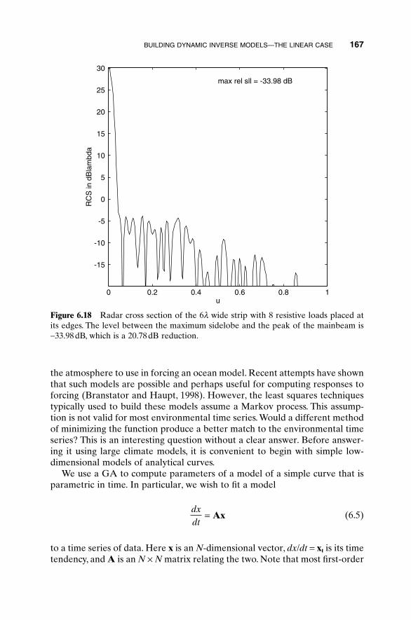
the atmosphere to use in forcing an ocean model. Recent attempts have shownthat such models are possible and perhaps useful for computing responses toforcing (Branstator and Haupt, 1998). However, the least squares techniquestypically used to build these models assume a Markov process. This assump-tion is not valid for most environmental time series. Would a different methodof minimizing the function produce a better match to the environmental timeseries? This is an interesting question without a clear answer. Before answer-ing it using large climate models, it is convenient to begin with simple low-dimensional models of analytical curves.
We use a GA to compute parameters of a model of a simple curve that isparametric in time. In particular, we wish to fit a model
(6.5)
to a time series of data. Here x is an N-dimensional vector, dx/dt = xt is its timetendency, and A is an N ¥ N matrix relating the two. Note that most first-order
dxdt
= Ax
BUILDING DYNAMIC INVERSE MODELS—THE LINEAR CASE 167
0 0.2 0.4 0.6 0.8 1
-15
-10
-5
0
5
10
15
20
25
30
u
RC
S in
dB
lam
bda
max rel sll = -33.98 dB
Figure 6.18 Radar cross section of the 6l wide strip with 8 resistive loads placed atits edges. The level between the maximum sidelobe and the peak of the mainbeam is-33.98 dB, which is a 20.78 dB reduction.
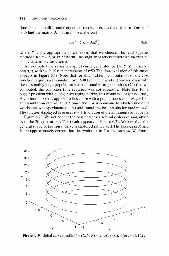
time-dependent differential equations can be discretized to this form. Our goalis to find the matrix A that minimizes the cost
(6.6)
where P is any appropriate power norm that we choose. The least squaresmethods use P = 2, or an L2 norm. The angular brackets denote a sum over allof the data in the time series.
An example time series is a spiral curve generated by (X, Y, Z) = (sin(t),cos(t), t), with t = [0, 10p] in increments of p/50.The time evolution of this curveappears in Figure 6.19. Note that for this problem, computation of the costfunction requires a summation over 500 time increments. However, even withthe reasonably large population size and number of generations (70) that wecomputed, the computer time required was not excessive. (Note that for abigger problem with a longer averaging period, this would no longer be true.)A continuous GA is applied to this curve with a population size of Npop = 100,and a mutation rate of m = 0.2. Since the GA is oblivious to which value of Pwe choose, we experimented a bit and found the best results for moderate P.The solution displayed here uses P = 4. Evolution of the minimum cost appearsin Figure 6.20. We notice that the cost decreases several orders of magnitudeover the 70 generations. The result appears in Figure 6.21. We see that thegeneral shape of the spiral curve is captured rather well. The bounds in X andY are approximately correct, but the evolution in Z = t is too slow. We found
cos tp= -( )x Axt
168 ADVANCED APPLICATIONS
-1-0.5
00.5
1
-1
-0.5
0
0.5
10
5
10
15
20
25
30
35
XY
t
Figure 6.19 Spiral curve specified by (X, Y, Z) = [cos(t), sin(t), t] for t = [1, 10p].
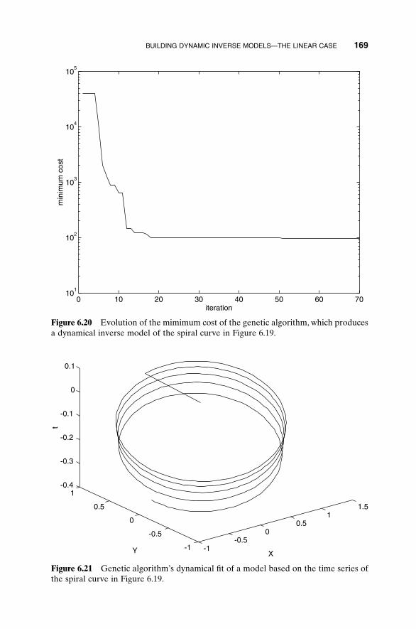
BUILDING DYNAMIC INVERSE MODELS—THE LINEAR CASE 169
0 10 20 30 40 50 60 7010
1
102
103
104
105
iteration
min
imum
cos
t
Figure 6.20 Evolution of the mimimum cost of the genetic algorithm, which producesa dynamical inverse model of the spiral curve in Figure 6.19.
-1-0.5
00.5
11.5
-1
-0.5
0
0.5
1-0.4
-0.3
-0.2
-0.1
0
0.1
XY
t
Figure 6.21 Genetic algorithm’s dynamical fit of a model based on the time series ofthe spiral curve in Figure 6.19.
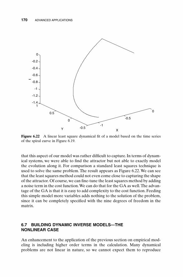
170 ADVANCED APPLICATIONS
-1
-0.5
0
-0.5
0
0.5
1-1.4
-1.2
-1
-0.8
-0.6
-0.4
-0.2
0
XY
t
Figure 6.22 A linear least square dynamical fit of a model based on the time seriesof the spiral curve in Figure 6.19.
that this aspect of our model was rather difficult to capture. In terms of dynam-ical systems, we were able to find the attractor but not able to exactly modelthe evolution along it. For comparison a standard least squares technique isused to solve the same problem. The result appears as Figure 6.22. We can seethat the least squares method could not even come close to capturing the shapeof the attractor. Of course, we can fine-tune the least squares method by addinga noise term in the cost function.We can do that for the GA as well.The advan-tage of the GA is that it is easy to add complexity to the cost function. Feedingthis simple model more variables adds nothing to the solution of the problem,since it can be completely specified with the nine degrees of freedom in thematrix.
6.7 BUILDING DYNAMIC INVERSE MODELS—THE NONLINEAR CASE
An enhancement to the application of the previous section on empirical mod-eling is including higher order terms in the calculation. Many dynamical problems are not linear in nature, so we cannot expect them to reproduce
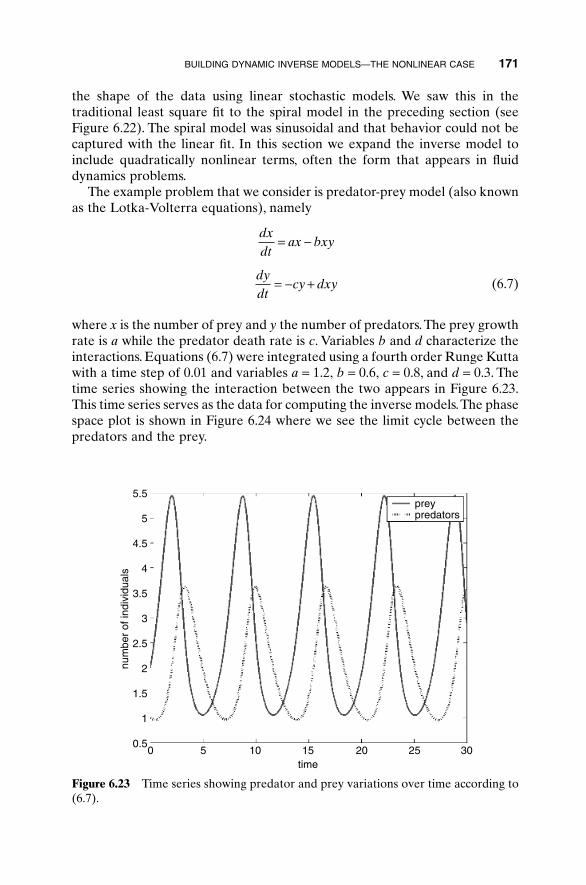
the shape of the data using linear stochastic models. We saw this in the traditional least square fit to the spiral model in the preceding section (seeFigure 6.22). The spiral model was sinusoidal and that behavior could not becaptured with the linear fit. In this section we expand the inverse model toinclude quadratically nonlinear terms, often the form that appears in fluiddynamics problems.
The example problem that we consider is predator-prey model (also knownas the Lotka-Volterra equations), namely
(6.7)
where x is the number of prey and y the number of predators.The prey growthrate is a while the predator death rate is c. Variables b and d characterize theinteractions. Equations (6.7) were integrated using a fourth order Runge Kuttawith a time step of 0.01 and variables a = 1.2, b = 0.6, c = 0.8, and d = 0.3. Thetime series showing the interaction between the two appears in Figure 6.23.This time series serves as the data for computing the inverse models.The phasespace plot is shown in Figure 6.24 where we see the limit cycle between thepredators and the prey.
dxdt
ax bxy
dydt
cy dxy
= -
= - +
BUILDING DYNAMIC INVERSE MODELS—THE NONLINEAR CASE 171
5.5
5
4.5
4
3.5
3
2.5
2
1.5
1
0.5 0 5 10 15 20 3025
time
num
ber
of in
divi
dual
s
preypredators
Figure 6.23 Time series showing predator and prey variations over time according to(6.7).
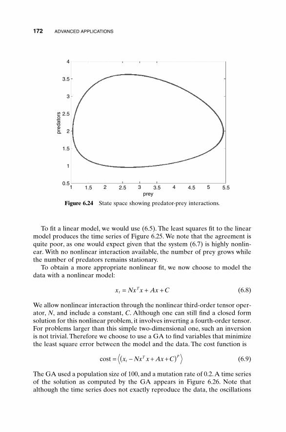
172 ADVANCED APPLICATIONS
4
3.5
3
2.5
2
1.5
1
0.5
prey
pred
ator
s
1 21.5 2.5 3 3.5 4 4.5 5 5.5
Figure 6.24 State space showing predator-prey interactions.
To fit a linear model, we would use (6.5). The least squares fit to the linearmodel produces the time series of Figure 6.25. We note that the agreement isquite poor, as one would expect given that the system (6.7) is highly nonlin-ear. With no nonlinear interaction available, the number of prey grows whilethe number of predators remains stationary.
To obtain a more appropriate nonlinear fit, we now choose to model thedata with a nonlinear model:
(6.8)
We allow nonlinear interaction through the nonlinear third-order tensor oper-ator, N, and include a constant, C. Although one can still find a closed formsolution for this nonlinear problem, it involves inverting a fourth-order tensor.For problems larger than this simple two-dimensional one, such an inversionis not trivial. Therefore we choose to use a GA to find variables that minimizethe least square error between the model and the data. The cost function is
(6.9)
The GA used a population size of 100, and a mutation rate of 0.2.A time seriesof the solution as computed by the GA appears in Figure 6.26. Note thatalthough the time series does not exactly reproduce the data, the oscillations
cost = - + +( )x Nx x Ax CtT p
x Nx x Ax CtT= + +
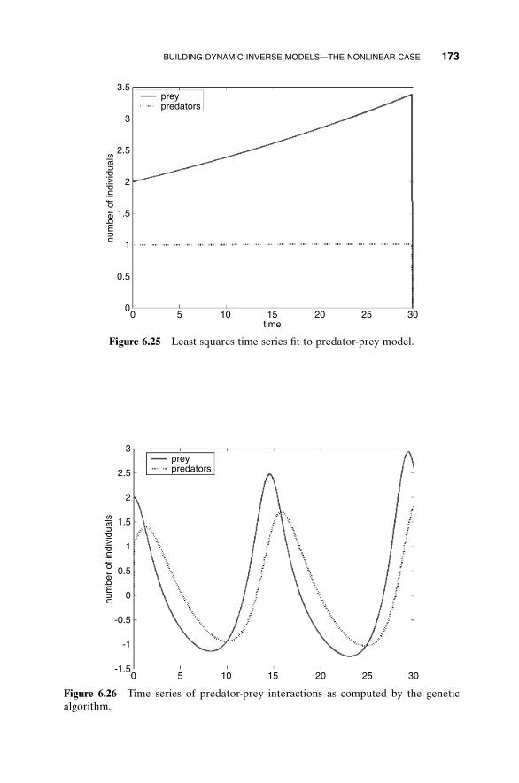
BUILDING DYNAMIC INVERSE MODELS—THE NONLINEAR CASE 173
3.5
3
2.5
2
1.5
1
0.5
00 5 10 15 20 3025
time
num
ber
of in
divi
dual
spreypredators
Figure 6.25 Least squares time series fit to predator-prey model.
3
2.5
2
1.5
1
0.5
0
-0.5
-1
-1.50 5 10 15 20 3025
num
ber
of in
divi
dual
s
preypredators
Figure 6.26 Time series of predator-prey interactions as computed by the geneticalgorithm.
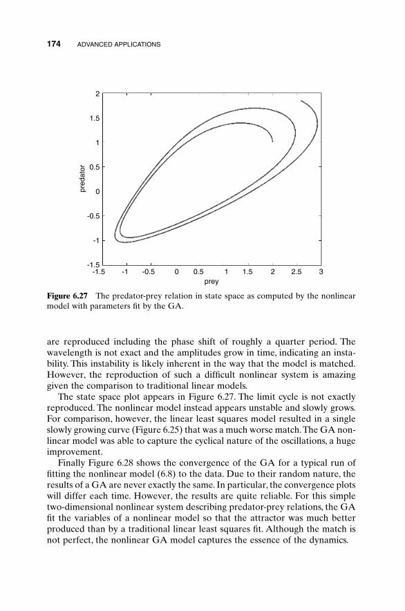
174 ADVANCED APPLICATIONS
-1.5 -1 -0.5 0.50 1 1.5 2 32.5prey
pred
ator
2
1.5
1
0.5
0
-0.5
-1
-1.5
Figure 6.27 The predator-prey relation in state space as computed by the nonlinearmodel with parameters fit by the GA.
are reproduced including the phase shift of roughly a quarter period. Thewavelength is not exact and the amplitudes grow in time, indicating an insta-bility. This instability is likely inherent in the way that the model is matched.However, the reproduction of such a difficult nonlinear system is amazinggiven the comparison to traditional linear models.
The state space plot appears in Figure 6.27. The limit cycle is not exactlyreproduced. The nonlinear model instead appears unstable and slowly grows.For comparison, however, the linear least squares model resulted in a singleslowly growing curve (Figure 6.25) that was a much worse match.The GA non-linear model was able to capture the cyclical nature of the oscillations, a hugeimprovement.
Finally Figure 6.28 shows the convergence of the GA for a typical run offitting the nonlinear model (6.8) to the data. Due to their random nature, theresults of a GA are never exactly the same. In particular, the convergence plotswill differ each time. However, the results are quite reliable. For this simpletwo-dimensional nonlinear system describing predator-prey relations, the GAfit the variables of a nonlinear model so that the attractor was much betterproduced than by a traditional linear least squares fit. Although the match isnot perfect, the nonlinear GA model captures the essence of the dynamics.
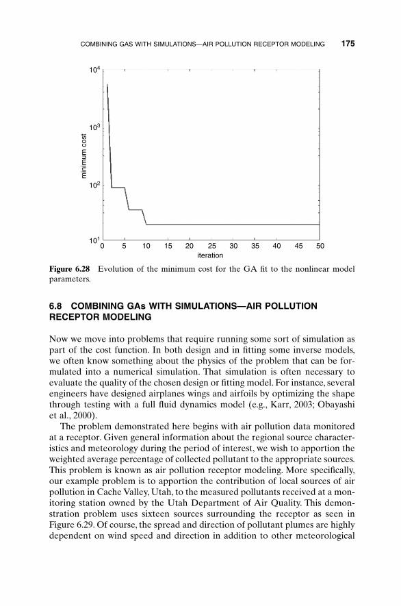
6.8 COMBINING GAs WITH SIMULATIONS—AIR POLLUTIONRECEPTOR MODELING
Now we move into problems that require running some sort of simulation aspart of the cost function. In both design and in fitting some inverse models,we often know something about the physics of the problem that can be for-mulated into a numerical simulation. That simulation is often necessary toevaluate the quality of the chosen design or fitting model. For instance, severalengineers have designed airplanes wings and airfoils by optimizing the shapethrough testing with a full fluid dynamics model (e.g., Karr, 2003; Obayashi et al., 2000).
The problem demonstrated here begins with air pollution data monitoredat a receptor. Given general information about the regional source character-istics and meteorology during the period of interest, we wish to apportion theweighted average percentage of collected pollutant to the appropriate sources.This problem is known as air pollution receptor modeling. More specifically,our example problem is to apportion the contribution of local sources of airpollution in Cache Valley, Utah, to the measured pollutants received at a mon-itoring station owned by the Utah Department of Air Quality. This demon-stration problem uses sixteen sources surrounding the receptor as seen inFigure 6.29. Of course, the spread and direction of pollutant plumes are highlydependent on wind speed and direction in addition to other meteorological
COMBINING GAS WITH SIMULATIONS—AIR POLLUTION RECEPTOR MODELING 175
104
103
102
1010 5 10 15 20 3025 4035 5045
iteration
min
imum
cos
t
Figure 6.28 Evolution of the minimum cost for the GA fit to the nonlinear modelparameters.
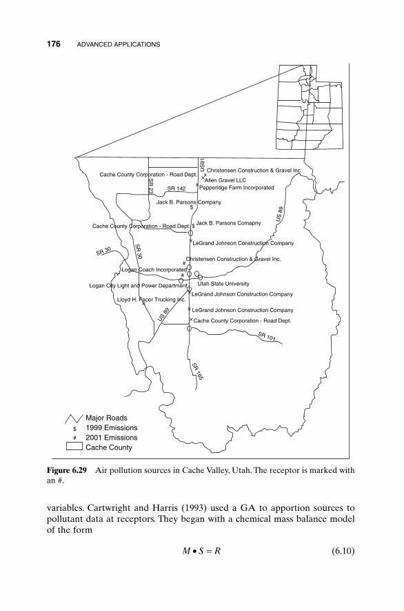
variables. Cartwright and Harris (1993) used a GA to apportion sources topollutant data at receptors. They began with a chemical mass balance modelof the form
(6.10)M S R∑ =
176 ADVANCED APPLICATIONS
#
#
Cache County Corporation - Road Dept.
US
91
Christensen Construction & Gravel Inc.
Allen Gravel LLCPepperidge Farm Incorporated
SR
23 SR 142
Jack B. Parsons Company$
$ Jack B. Parsons Comapny
LeGrand Johnson Construction Company
LeGrand Johnson Construction Company
LeGrand Johnson Construction Company
Christensen Construction & Gravel Inc.
Cache County Corporation - Road Dept.
SR 101
SR
165
US 89
Logan City Light and Power Department
Lloyd H. Facer Trucking Inc.
1999 Emissions2001 EmissionsCache County
Major Roads
Cache County Corporation - Road Dept.
SR 30
SR
30Logan Coach Incorporated
US
89
Utah State University
$
#
Figure 6.29 Air pollution sources in Cache Valley, Utah. The receptor is marked withan #.
where M is the source profile matrix, which denotes the effective strength ofpollutant from a given source at the receptor; S is the fraction of the sourcethat contributes to the concentration at the receptor, the unknown appor-tionments; and R is the concentration of each pollutant measured at a givenreceptor. In theory, these matrices are whatever size can incorporate as manysources, receptors, and pollutants as necessary. Here we demonstrate the tech-nique with a single pollutant at a single receptor. Cartwright and Harris (1993)chose to use uniform dispersion in all directions, with a decrease of concen-tration with distance according to a r-2.5 power law, where r is the distance fromthe source to the receptor. Here we, instead, choose to use the more refineddispersion law as found in Beychok (1994), together with actual wind data forthe time period modeled:
(6.11)
where
C = concentration of emissions at a receptor(x, y, zr) = Cartesian coordinates of the receptor in the downwind direction
from the sourceQ = source emission rateu = wind speedHe = effective height of the plume centerline above ground
sy, sz = standard deviations of the emission distribution in the y and zdirections
Note that there are a myriad of assumptions hidden behind the problem.First, we assume that the wind speed and direction are constant over the entiretime period. Although we know a priori that this assumption is poor, it is bal-anced by the assumption of Gaussian dispersion in a single direction.Althougha plume of pollutants may meander throughout the time period, we only careabout the weighted average statistical distribution of the concentrations. Nextwe are forced to assume a constant emission rate, in this case an averageannual rate. The hourly rate is much different. Another major difficulty is inestimating reasonable average values for the dispersion coefficients, sy and sz.Again, we must assume a weighted average over time and use dispersion coefficients computed by
(6.12)
where x is the downwind distance (in km) and I, J, and K are empirical co-efficients dependent on the Pasquill stability class (documented in a lookuptable; Beychok, 1994). The Pasquill stability class depends on wind speed,
s = + ( ) + ( )( )([ ]exp ln lnI J x K x2
CQ
uy z H z H
z y y
r e
x
r e
z
=-Ê
ˈ¯
- -( )ÊËÁ
ˆ¯
+- +( )Ê
ËÁˆ¯
È
ÎÍ
˘
˚˙s s p s s s2 2 2 2
2
2
2
2
2
2exp exp exp
COMBINING GAS WITH SIMULATIONS—AIR POLLUTION RECEPTOR MODELING 177
direction, and insolation. For this demonstration problem, we assumed neutralstability (class D).
Equations (6.10) and (6.11) together with two lookup tables and (6.12)convert the source emission rates into the elements of the source matrix, M,which indicates an expected average concentration due to each source for aconstant emission rate and actual hourly average wind data. This process isrepeated for each source at each time. The measured concentrations are alsotime averaged (in this case over a three-day period) and go into the matrix,R. The goal is to solve for the fractions, S, that apportion the pollution to eachsource. That is where the GA comes in. If R and S were constant one-dimensional vectors, one could easily solve for S. However, the need to sum the matrix times the factors hourly for differing meteorological conditions precludes a simple matrix inversion. The chromosomes of the GAin this case represent the unknown elements of matrix S. The cost function isthe difference between the pollutant values at the receptor and the summation of the hourly concentrations predicted for each source as computed from the dispersion model (6.11) times the apportionment factorssupplied by the GA:
(6.13)
where with the Ch computed from (6.11).
The receptor model was run using actual meteorological data for three-day periods in 2002 and comparing predicted weighted average con-centrations of PM10 (particulate matter less than 10 micrometers in diameter) measured at the receptor. The dispersion coefficients were computed assuming a Pasquill stability class D. Three to four runs of the GA were done for each time period using a population size of 12 and mutation rate of 0.2. The fractions in the unknown vector, S, were normalized to sum to 1. Runs were made for 1000 generations. Four different runs were made for each of five different days and results appear in Table 6.3 for the run with the best convergence for each day. Those days were chosen to represent different concentrations and meteorology conditions, although we were careful to choose days where the assumption of stability D appeared to be good. For many of the runs the factors converged on the heaviest weighting of source 13, the Utah State Universityheating plant. Note that this does not necessarily imply that it contributed the most pollutant but rather that its average emission rate, when dis-persed according to (6.11) using actual wind data, must have a heavier weighting to account for the monitored PM10. The second highest weighted source was number 9, a local construction company.
The point of this exercise is to demonstrate that the GA is a useful tool for problems that require including another model, in this case a dis-
M Chh
H
==
Â1
cost = - ∑R M S
178 ADVANCED APPLICATIONS
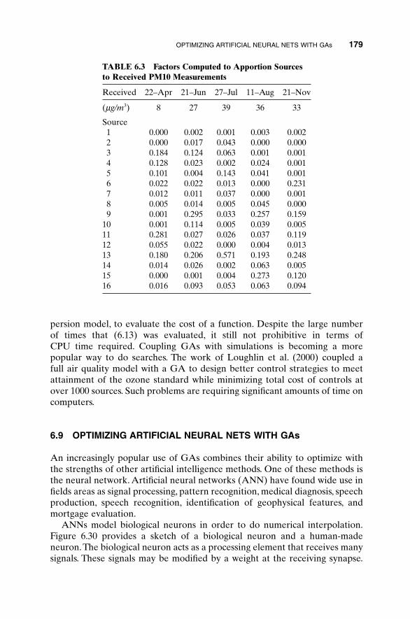
persion model, to evaluate the cost of a function. Despite the large number of times that (6.13) was evaluated, it still not prohibitive in terms of CPU time required. Coupling GAs with simulations is becoming a morepopular way to do searches. The work of Loughlin et al. (2000) coupled a full air quality model with a GA to design better control strategies to meetattainment of the ozone standard while minimizing total cost of controls atover 1000 sources. Such problems are requiring significant amounts of time oncomputers.
6.9 OPTIMIZING ARTIFICIAL NEURAL NETS WITH GAs
An increasingly popular use of GAs combines their ability to optimize withthe strengths of other artificial intelligence methods. One of these methods isthe neural network. Artificial neural networks (ANN) have found wide use infields areas as signal processing, pattern recognition, medical diagnosis, speechproduction, speech recognition, identification of geophysical features, andmortgage evaluation.
ANNs model biological neurons in order to do numerical interpolation.Figure 6.30 provides a sketch of a biological neuron and a human-madeneuron. The biological neuron acts as a processing element that receives manysignals. These signals may be modified by a weight at the receiving synapse.
OPTIMIZING ARTIFICIAL NEURAL NETS WITH GAs 179
TABLE 6.3 Factors Computed to Apportion Sourcesto Received PM10 Measurements
Received 22–Apr 21–Jun 27–Jul 11–Aug 21–Nov
(mg/m3) 8 27 39 36 33
Source1 0.000 0.002 0.001 0.003 0.0022 0.000 0.017 0.043 0.000 0.0003 0.184 0.124 0.063 0.001 0.0014 0.128 0.023 0.002 0.024 0.0015 0.101 0.004 0.143 0.041 0.0016 0.022 0.022 0.013 0.000 0.2317 0.012 0.011 0.037 0.000 0.0018 0.005 0.014 0.005 0.045 0.0009 0.001 0.295 0.033 0.257 0.159
10 0.001 0.114 0.005 0.039 0.00511 0.281 0.027 0.026 0.037 0.11912 0.055 0.022 0.000 0.004 0.01313 0.180 0.206 0.571 0.193 0.24814 0.014 0.026 0.002 0.063 0.00515 0.000 0.001 0.004 0.273 0.12016 0.016 0.093 0.053 0.063 0.094
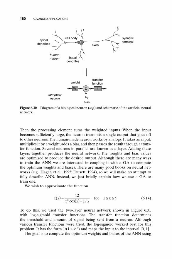
180 ADVANCED APPLICATIONS
apicaldendrites
cell body
basaldendrites
axon
humanneuron
computerneuron
synapticterminal
transferfunctionweight
bias
f
b1
W1 S
Figure 6.30 Diagram of a biological neuron (top) and schematic of the artificial neuralnetwork.
Then the processing element sums the weighted inputs. When the inputbecomes sufficiently large, the neuron transmits a single output that goes offto other neurons.The human-made neuron works by analogy. It takes an input,multiplies it by a weight, adds a bias, and then passes the result through a trans-fer function. Several neurons in parallel are known as a layer. Adding theselayers together produces the neural network. The weights and bias values are optimized to produce the desired output. Although there are many waysto train the ANN, we are interested in coupling it with a GA to compute the optimum weights and biases. There are many good books on neural net-works (e.g., Hagan et al., 1995; Fausett, 1994), so we will make no attempt tofully describe ANN. Instead, we just briefly explain how we use a GA to train one.
We wish to approximate the function
(6.14)
To do this, we used the two-layer neural network shown in Figure 6.31 with log-sigmoid transfer functions. The transfer function determines the threshold and amount of signal being sent from a neuron. Althoughvarious transfer functions were tried, the log-sigmoid worked best for thisproblem. It has the form 1/(1 + e-n) and maps the input to the interval [0, 1].
The goal is to compute the optimum weights and biases of the ANN using
f for 1 x 5xx x x
( ) = ( ) +£ £
1212 cos /
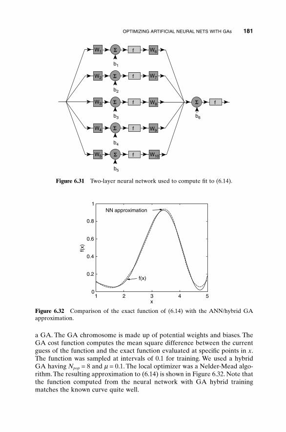
a GA. The GA chromosome is made up of potential weights and biases. TheGA cost function computes the mean square difference between the currentguess of the function and the exact function evaluated at specific points in x.The function was sampled at intervals of 0.1 for training. We used a hybridGA having Npop = 8 and m = 0.1. The local optimizer was a Nelder-Mead algo-rithm. The resulting approximation to (6.14) is shown in Figure 6.32. Note thatthe function computed from the neural network with GA hybrid trainingmatches the known curve quite well.
OPTIMIZING ARTIFICIAL NEURAL NETS WITH GAs 181
W1
W2
W3
W4
W5
b1
b3
b4
b5
b2
W6
W7
W9
W10
W8
fS
fS
fS
b6
fS
fS
fS
Figure 6.31 Two-layer neural network used to compute fit to (6.14).
01 2 3 4 5
x
0.2
0.4
0.6
f(x)
f(x)
0.8
1NN approximation
Figure 6.32 Comparison of the exact function of (6.14) with the ANN/hybrid GAapproximation.
6.10 SOLVING HIGH-ORDER NONLINEAR PARTIALDIFFERENTIAL EQUATIONS
Two mathematical tools of scientists and engineers are ordinary and partialdifferential equations (ODEs and PDEs). Normally we don’t think of theseequations as minimization problems. However, if we want to find values wherea differential equation is zero (a form in which we can always cast the system),we can look for the minimum of its absolute value. Koza (1992) demonstratedthat a GA could solve a simple differential equation by minimizing the valueof the solution at 200 points. To do this, he numerically differentiated at eachpoint and fit the appropriate solution using a GA. Karr et al. (2001) used GAsto solve inverse initial boundary value problems and found a large improve-ment in matching measured values.That technique was demonstrated on ellip-tic, parabolic, and hyperbolic PDEs.
We demonstrate here that a GA can be a useful technique for solving ahighly nonlinear differential equation that is formally nonintegrable. For com-parison, we do know its solitary wave approximate solution. Solitary waves, orsolitons,are permanent-form waves for which the nonlinearity balances the dis-persion to produce a coherent structure. We examine the super Korteweg-deVries equation (SKDV), a fifth-order nonlinear partial differential equation:
(6.15)
The functional form is denoted by u; time derivative by the t subscript; spatialderivative by the x subscript; and a, m, and n are variables of the problem. Wewish to solve for waves that are steadily translating, so we write the t varia-tion using a Galilean tranformation, X = x - ct, where c is the phase speed ofthe wave. Thus our SKDV becomes a fifth-order, nonlinear ordinary differen-tial equation:
(6.16)
Boyd (1986) extensively studied methods of solving this equation. Heexpanded the solution in terms of Fourier series to find periodic cnoidal wavesolutions (solitons that are repeated periodically). Among the methods usedare the analytical Stokes’s expansion, which intrinsically assumes small ampli-tude waves, and the numerical Newton-Kantorovich iterative method, whichcan go beyond the small amplitude regime if care is taken to provide a verygood first guess. Haupt and Boyd (1988a) were able to extend these methodsto deal with resonance conditions. These methods were generalized to twodimensions to find double-cnoidal waves (two waves of differing wave numberon each period) for the integrable Korteweg-de Vries equation (1988b) andthe nonintegrable regularized long wave equation (Haupt, 1988). However,these methods require careful analytics and programming that is very problemspecific. Here we are able to add a simple modification to the cost function ofour GA to obtain a similar result.
a mu c u u vuX XXX XXXX-( ) + - = 0
u uu u vut x xxx xxx+ + - =a m 0
182 ADVANCED APPLICATIONS
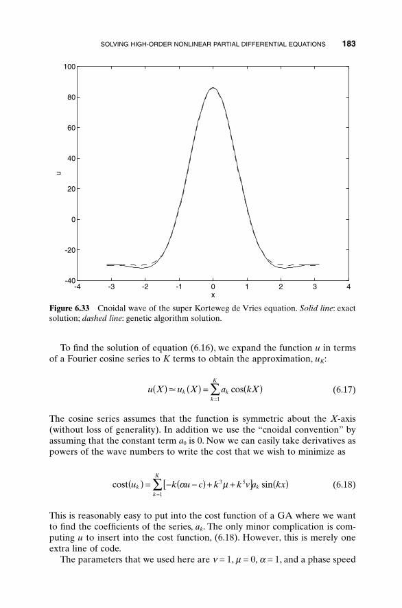
To find the solution of equation (6.16), we expand the function u in termsof a Fourier cosine series to K terms to obtain the approximation, uK:
(6.17)
The cosine series assumes that the function is symmetric about the X-axis(without loss of generality). In addition we use the “cnoidal convention” byassuming that the constant term a0 is 0. Now we can easily take derivatives aspowers of the wave numbers to write the cost that we wish to minimize as
(6.18)
This is reasonably easy to put into the cost function of a GA where we wantto find the coefficients of the series, ak. The only minor complication is com-puting u to insert into the cost function, (6.18). However, this is merely oneextra line of code.
The parameters that we used here are n = 1, m = 0, a = 1, and a phase speed
cost u k u c k k v a kxkk
K
k( ) = - -( ) + +[ ] ( )=
 a m3 5
1
sin
u X u X a kXk kk
K
( ) ( ) = ( )=
� cos1
SOLVING HIGH-ORDER NONLINEAR PARTIAL DIFFERENTIAL EQUATIONS 183
-4 -3 -2 -1 0 1 2 3 4-40
-20
0
20
40
60
80
100
x
u
Figure 6.33 Cnoidal wave of the super Korteweg de Vries equation. Solid line: exactsolution; dashed line: genetic algorithm solution.
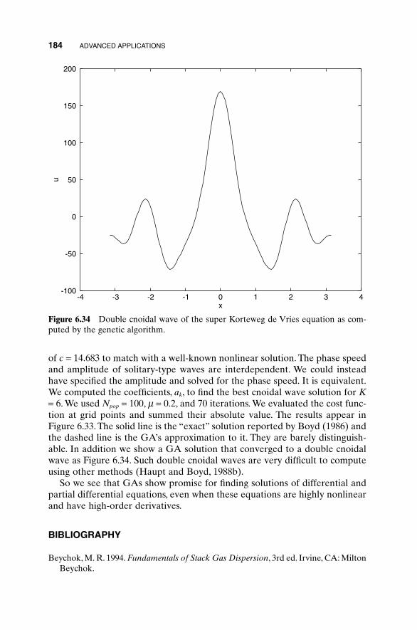
184 ADVANCED APPLICATIONS
of c = 14.683 to match with a well-known nonlinear solution. The phase speedand amplitude of solitary-type waves are interdependent. We could insteadhave specified the amplitude and solved for the phase speed. It is equivalent.We computed the coefficients, ak, to find the best cnoidal wave solution for K= 6. We used Npop = 100, m = 0.2, and 70 iterations. We evaluated the cost func-tion at grid points and summed their absolute value. The results appear inFigure 6.33. The solid line is the “exact” solution reported by Boyd (1986) andthe dashed line is the GA’s approximation to it. They are barely distinguish-able. In addition we show a GA solution that converged to a double cnoidalwave as Figure 6.34. Such double cnoidal waves are very difficult to computeusing other methods (Haupt and Boyd, 1988b).
So we see that GAs show promise for finding solutions of differential andpartial differential equations, even when these equations are highly nonlinearand have high-order derivatives.
BIBLIOGRAPHY
Beychok, M. R. 1994. Fundamentals of Stack Gas Dispersion, 3rd ed. Irvine, CA: MiltonBeychok.
-4 -3 -2 -1 0 1 2 3 4-100
-50
0
50
100
150
200
x
u
Figure 6.34 Double cnoidal wave of the super Korteweg de Vries equation as com-puted by the genetic algorithm.
Boyd, J. P. 1986. Solitons from sine waves: Analytical and numerical methods for non-integrable solitary and cnoidal waves. Physica 21D:227–246.
Branstator, G., and S. E. Haupt. 1998. An empirical model of barotropic atmosphericdynamics and its response to forcing. J. Climate 11:2645–2667.
Cartwright, H. M., and S. P. Harris. 1993. Analysis of the distribution of airborne pol-lution using GAs. Atmos. Environ 27A:1783–1791.
Chambers, L. (ed.). 1995. GAs, Applications, Vol. 1. New York: CRC Press.Davidor, Y. 1991. GAs and Robotics. River Edge, NJ: World Scientific.Davis, L. 1991. Handbook of GAs. New York: Van Nostrand Reinhold.Fausett, L. 1994. Fundamentals of Neural Networks: Architectures, Algorithms, and
Applications. Upper Saddle River, NJ: Prentice Hall.Hagan, M. T., H. B. Demuth, and M. Beale. 1995. Neural Network Design. Boston: PWS.Hasselmann, K. 1976. Stochastic climate models. Part I: Theory. Tellus 28:473–485.Haupt, R. L. 1995. An introduction to GAs for electromagnetics. IEEE Ant. Propagat.
Mag. 37:7–15.Haupt, S. E. 1988. Solving nonlinear wave problems with spectral boundary value tech-
niques. Ph.D. dissertation. University of Michigan, Ann Arbor.Haupt, S. E., and J. P. Boyd. 1988a. Modeling nonlinear resonance: A modification to
the Stokes’ perturbation expansion. Wave Motion 10:83–98.Haupt, S. E., and J. P. Boyd. 1988b. Double cnoidal waves of the Korteweg De Vries
equation: Solution by the spectral boundary value approach. Physica 50D:117–134.Holland, J. H. 1992. Genetic Algorithms. Sci. Am. 267:66–72.Karr, C. L. 2003. Minimization of sonic boom using an evolutionary algorithm. Paper
AIAA 2003-0463. 40st AIAA Aerospace Sciences Meeting and Exhibit, Reno, NV.Karr, C. L., I. Yakushin, and K. Nicolosi. 2001. Solving inverse initial-value, boundary-
value problems via GA. Eng. Appl. Art. Intell. 13:625–633.Kirkpatrick, S., C. D. Gelatt, and M. P. Vecchi. 1983. Optimization by simulated anneal-
ing. Science 220:671–680.Koza, J. R. 1992. The Genetic Programming Paradigm: Genetically Breeding Popula-
tions of Computer Programs to Solve Problems. In B. Soucek (ed.), Dynamic,Genetic, and Chaotic Programming: The Sixth Generation. New York: J. Wiley, pp.203–321.
Loughlin, D. H., S. R. Ranjithan, J. W. Baugh, Jr., and E. D. Brill Jr. 2000. Applicationof GAs for the design of ozone control strategies. J. Air Waste Manage. Assoc.50:1050–1063.
Michalewicz, Z. 1992. Genetic Algorithms + Data Structures = Evolution Programs. NewYork: Springer-Verlag.
Obayashi, S., D. Sasaki, Y. Takeguchi, and N. Hirose. 2000. Multiobjective evolutionarycomputation for supersonic wing-shape optimization. IEEE Trans. Evol. Comput.4:182–187.
Pack, D., G. Toussaint, and R. Haupt. 1996. Robot trajectory planning using a GA. Int.Symp. on Optical Science, Engineering, and Instrumentation. SPIE’s AnnualMeeting, Denver, CO.
Penland, C. 1989. Random forcing and forecasting using principal oscillation patternanalysis. Mon. Weather Rev. 117:2165–2185.
BIBLIOGRAPHY 185

Penland, C. 1996. A stochasic model of IndoPacific sea surface temperature anomalies.Physica 98D:534–558.
Penland, C., and M. Ghil. 1993. Forecasting northern hemisphere 700 mb geopotentialheight anomalies using empirical normal modes. Mon. Weather Rev. 121:2355.
Penland, C., and T. Magorian. 1993. Prediction of NINO3 sea-surface temperaturesusing linear inverse modeling. J. Climate 6:1067.
Whitley, D., T. Starkweather, and D. Shaner. 1991. The traveling salesman and sequencescheduling: Quality solutions using genetic edge recombination. In L. Davis (ed.),Handbook of GAs. New York: Van Nostrand Reinhold.
Widrow, B., and S. D. Sterns, 1985. Adaptive Signal Processing. Upper Saddle River, NJ:Prentice-Hall.
Yao, X. (ed.). 1995. Progress in Evolutionary Computation. New York: Springer-Verlag.
186 ADVANCED APPLICATIONS
CHAPTER 7
More Natural Optimization Algorithms
187
The GA is not the only optimization algorithm that models natural processes.In this chapter we briefly present some of the current algorithms being usedfor global optimization. Some introductory programs are included for youramusement. Which algorithm is best? We tend to like the GA and some of the local optimization algorithms. The “No Free Lunch Theorem” says that the averaged performance of all search algorithms over all problems is equal(Wolpert, 1997). In other words, the GA performs no better than a totallyrandom search when applied to all problems. Thus the idea is to use the rightalgorithm for the right problem.
7.1 SIMULATED ANNEALING
In the early 1980s the method of simulated annealing (SA) was introduced byKirkpatrick and coworkers (1983), based on ideas formulated in the early1950s (Metropolis, 1953). This method simulates the annealing process inwhich a substance is heated above its melting temperature and then graduallycooled to produce the crystalline lattice, which minimizes its energy probabil-ity distribution.This crystalline lattice, composed of millions of atoms perfectlyaligned, is a beautiful example of nature finding an optimal structure. How-ever, quickly cooling or quenching the liquid retards the crystal formation, andthe substance becomes an amorphous mass with a higher than optimumenergy state. The key to crystal formation is carefully controlling the rate ofchange of temperature.
The algorithmic analog to this process begins with a random guess of thecost function variable values. Heating means randomly modifying the variablevalues. Higher heat implies greater random fluctuations. The cost functionreturns the output, f, associated with a set of variables. If the output decreases,then the new variable set replaces the old variable set. If the output increases,then the output is accepted provided that
Practical Genetic Algorithms, Second Edition, by Randy L. Haupt and Sue Ellen Haupt.ISBN 0-471-45565-2 Copyright © 2004 John Wiley & Sons, Inc.
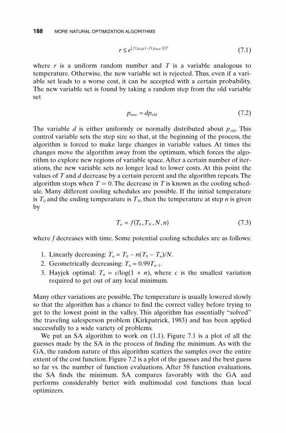
(7.1)
where r is a uniform random number and T is a variable analogous to temperature. Otherwise, the new variable set is rejected. Thus, even if a vari-able set leads to a worse cost, it can be accepted with a certain probability.The new variable set is found by taking a random step from the old variableset
(7.2)
The variable d is either uniformly or normally distributed about pold. Thiscontrol variable sets the step size so that, at the beginning of the process, thealgorithm is forced to make large changes in variable values. At times thechanges move the algorithm away from the optimum, which forces the algo-rithm to explore new regions of variable space. After a certain number of iter-ations, the new variable sets no longer lead to lower costs. At this point thevalues of T and d decrease by a certain percent and the algorithm repeats. Thealgorithm stops when T � 0. The decrease in T is known as the cooling sched-ule. Many different cooling schedules are possible. If the initial temperatureis T0 and the ending temperature is TN, then the temperature at step n is givenby
(7.3)
where f decreases with time. Some potential cooling schedules are as follows:
1. Linearly decreasing: Tn = T0 - n(T0 - Tn)/N.2. Geometrically decreasing: Tn = 0.99Tn-1.3. Hayjek optimal: Tn = c/log(1 + n), where c is the smallest variation
required to get out of any local minimum.
Many other variations are possible. The temperature is usually lowered slowlyso that the algorithm has a chance to find the correct valley before trying toget to the lowest point in the valley. This algorithm has essentially “solved”the traveling salesperson problem (Kirkpatrick, 1983) and has been appliedsuccessfully to a wide variety of problems.
We put an SA algorithm to work on (1.1). Figure 7.1 is a plot of all theguesses made by the SA in the process of finding the minimum. As with theGA, the random nature of this algorithm scatters the samples over the entireextent of the cost function. Figure 7.2 is a plot of the guesses and the best guessso far vs. the number of function evaluations. After 58 function evaluations,the SA finds the minimum. SA compares favorably with the GA and performs considerably better with multimodal cost functions than local optimizers.
T f T T N nn N= ( )0 , , ,
p dpnew old=
r e f p f p Told new£ ( )- ( )[ ]/
188 MORE NATURAL OPTIMIZATION ALGORITHMS
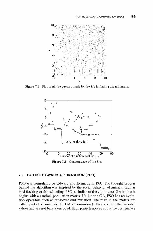
7.2 PARTICLE SWARM OPTIMIZATION (PSO)
PSO was formulated by Edward and Kennedy in 1995. The thought processbehind the algorithm was inspired by the social behavior of animals, such asbird flocking or fish schooling. PSO is similar to the continuous GA in that itbegins with a random population matrix. Unlike the GA, PSO has no evolu-tion operators such as crossover and mutation. The rows in the matrix arecalled particles (same as the GA chromosome). They contain the variablevalues and are not binary encoded. Each particle moves about the cost surface
PARTICLE SWARM OPTIMIZATION (PSO) 189
Figure 7.1 Plot of all the guesses made by the SA in finding the minimum.
Figure 7.2 Convergence of the SA.
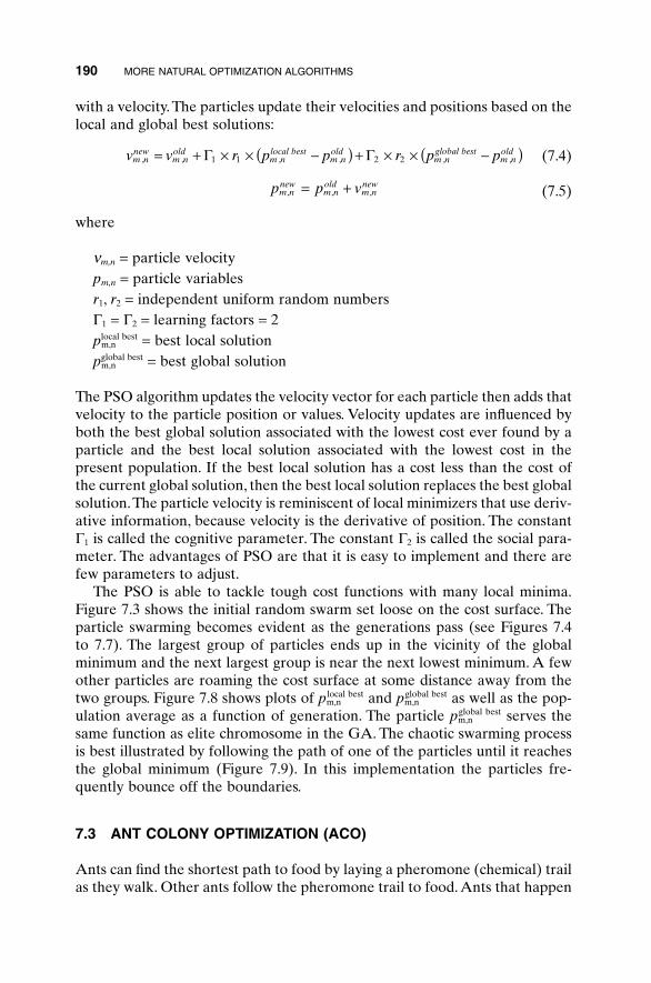
with a velocity.The particles update their velocities and positions based on thelocal and global best solutions:
(7.4)
(7.5)
where
nm,n = particle velocitypm,n = particle variablesr1, r2 = independent uniform random numbersG1 = G2 = learning factors = 2pm,n
local best = best local solutionpm,n
global best = best global solution
The PSO algorithm updates the velocity vector for each particle then adds thatvelocity to the particle position or values. Velocity updates are influenced byboth the best global solution associated with the lowest cost ever found by aparticle and the best local solution associated with the lowest cost in thepresent population. If the best local solution has a cost less than the cost ofthe current global solution, then the best local solution replaces the best globalsolution.The particle velocity is reminiscent of local minimizers that use deriv-ative information, because velocity is the derivative of position. The constantG1 is called the cognitive parameter. The constant G2 is called the social para-meter. The advantages of PSO are that it is easy to implement and there arefew parameters to adjust.
The PSO is able to tackle tough cost functions with many local minima.Figure 7.3 shows the initial random swarm set loose on the cost surface. Theparticle swarming becomes evident as the generations pass (see Figures 7.4 to 7.7). The largest group of particles ends up in the vicinity of the globalminimum and the next largest group is near the next lowest minimum. A fewother particles are roaming the cost surface at some distance away from thetwo groups. Figure 7.8 shows plots of pm,n
local best and pm,nglobal best as well as the pop-
ulation average as a function of generation. The particle pm,nglobal best serves the
same function as elite chromosome in the GA. The chaotic swarming processis best illustrated by following the path of one of the particles until it reachesthe global minimum (Figure 7.9). In this implementation the particles fre-quently bounce off the boundaries.
7.3 ANT COLONY OPTIMIZATION (ACO)
Ants can find the shortest path to food by laying a pheromone (chemical) trailas they walk. Other ants follow the pheromone trail to food. Ants that happen
p p vm nnew
m nold
m nnew
, , ,= +
v v r p p r p pm nnew
m nold
m nlocal best
m nold
m nglobal best
m nold
, , , , , ,= + ¥ ¥ -( ) + ¥ ¥ -( )G G1 1 2 2
190 MORE NATURAL OPTIMIZATION ALGORITHMS
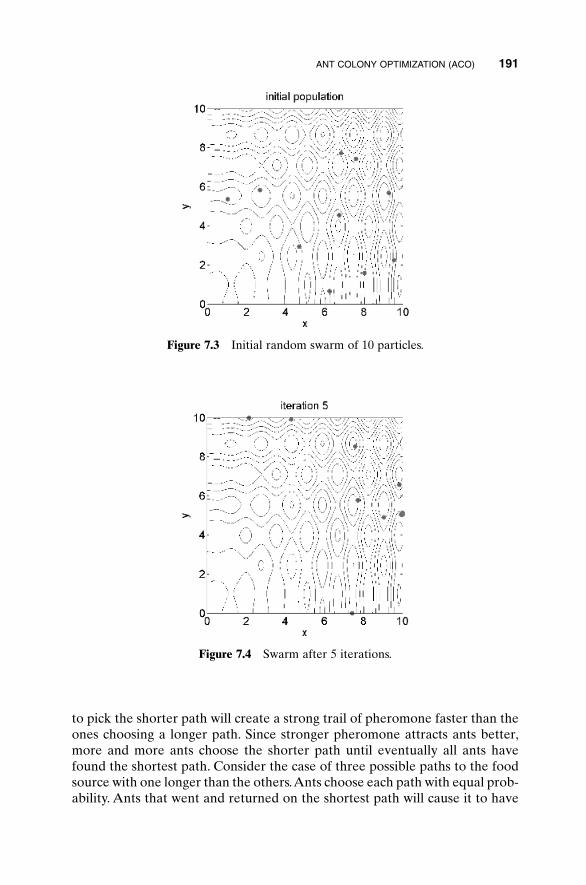
to pick the shorter path will create a strong trail of pheromone faster than theones choosing a longer path. Since stronger pheromone attracts ants better,more and more ants choose the shorter path until eventually all ants havefound the shortest path. Consider the case of three possible paths to the foodsource with one longer than the others.Ants choose each path with equal prob-ability. Ants that went and returned on the shortest path will cause it to have
ANT COLONY OPTIMIZATION (ACO) 191
Figure 7.3 Initial random swarm of 10 particles.
Figure 7.4 Swarm after 5 iterations.
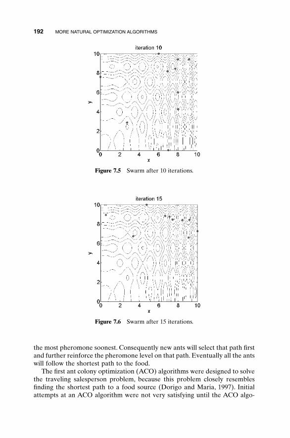
192 MORE NATURAL OPTIMIZATION ALGORITHMS
Figure 7.5 Swarm after 10 iterations.
Figure 7.6 Swarm after 15 iterations.
the most pheromone soonest. Consequently new ants will select that path firstand further reinforce the pheromone level on that path. Eventually all the antswill follow the shortest path to the food.
The first ant colony optimization (ACO) algorithms were designed to solvethe traveling salesperson problem, because this problem closely resemblesfinding the shortest path to a food source (Dorigo and Maria, 1997). Initialattempts at an ACO algorithm were not very satisfying until the ACO algo-
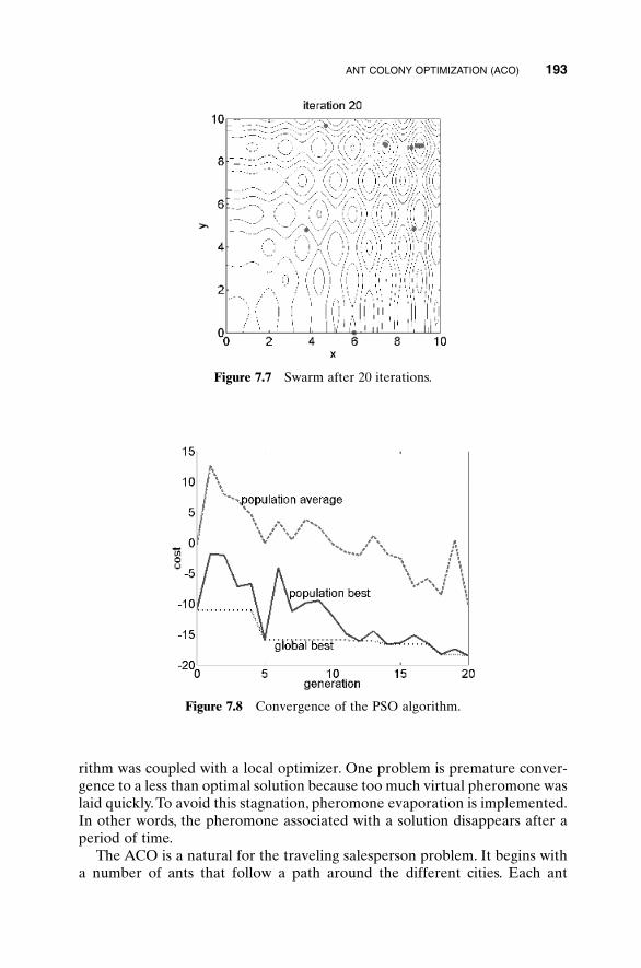
ANT COLONY OPTIMIZATION (ACO) 193
Figure 7.7 Swarm after 20 iterations.
Figure 7.8 Convergence of the PSO algorithm.
rithm was coupled with a local optimizer. One problem is premature conver-gence to a less than optimal solution because too much virtual pheromone waslaid quickly. To avoid this stagnation, pheromone evaporation is implemented.In other words, the pheromone associated with a solution disappears after aperiod of time.
The ACO is a natural for the traveling salesperson problem. It begins witha number of ants that follow a path around the different cities. Each ant
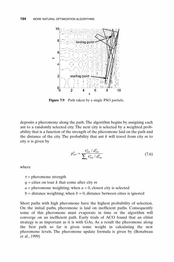
deposits a pheromone along the path. The algorithm begins by assigning eachant to a randomly selected city. The next city is selected by a weighted prob-ability that is a function of the strength of the pheromone laid on the path andthe distance of the city. The probability that ant k will travel from city m tocity n is given by
(7.6)
where
t = pheromone strengthq = cities on tour k that come after city ma = pheromone weighting; when a = 0, closest city is selectedb = distance weighting; when b = 0, distance between cities is ignored
Short paths with high pheromone have the highest probability of selection.On the initial paths, pheromone is laid on inefficient paths. Consequently some of this pheromone must evaporate in time or the algorithm will converge on an inefficient path. Early trials of ACO found that an elitist strategy is as important as it is with GAs. As a result the pheromone along the best path so far is given some weight in calculating the new pheromone levels. The pheromone update formula is given by (Bonabeau et al., 1999)
pd
dmnk mn
amnb
mqa
mqb
q
= Ât
t/
/
194 MORE NATURAL OPTIMIZATION ALGORITHMS
Figure 7.9 Path taken by a single PSO particle.
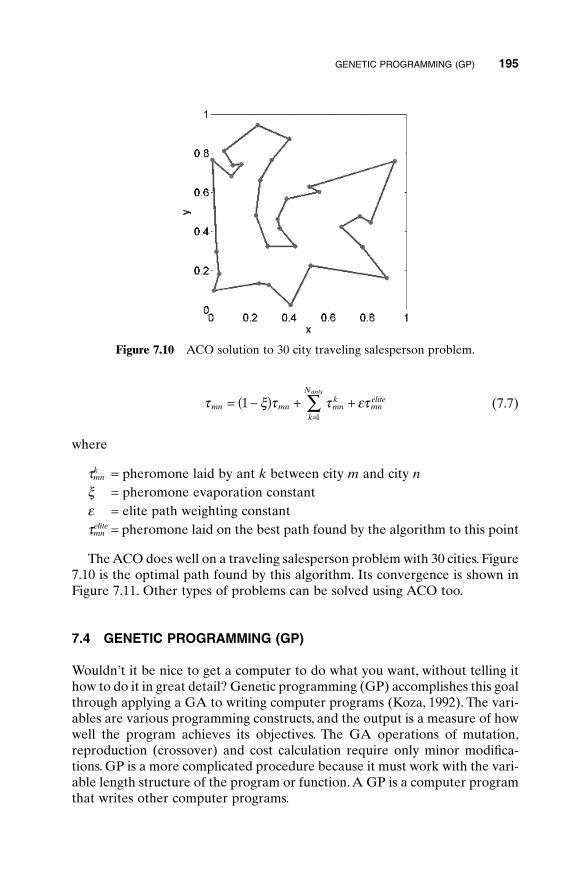
(7.7)
where
tkmn = pheromone laid by ant k between city m and city n
x = pheromone evaporation constante = elite path weighting constanttmn
elite = pheromone laid on the best path found by the algorithm to this point
The ACO does well on a traveling salesperson problem with 30 cities. Figure7.10 is the optimal path found by this algorithm. Its convergence is shown inFigure 7.11. Other types of problems can be solved using ACO too.
7.4 GENETIC PROGRAMMING (GP)
Wouldn’t it be nice to get a computer to do what you want, without telling ithow to do it in great detail? Genetic programming (GP) accomplishes this goalthrough applying a GA to writing computer programs (Koza, 1992). The vari-ables are various programming constructs, and the output is a measure of howwell the program achieves its objectives. The GA operations of mutation,reproduction (crossover) and cost calculation require only minor modifica-tions. GP is a more complicated procedure because it must work with the vari-able length structure of the program or function. A GP is a computer programthat writes other computer programs.
t x t t etmn mn mnk
mnelite
k
Nants
= -( ) + +=
Â11
GENETIC PROGRAMMING (GP) 195
Figure 7.10 ACO solution to 30 city traveling salesperson problem.

The computer programs written by GP are not in common languages suchas MATLAB or Fortran but in the more obscure artificial intelligence lan-guage (AI) LISP (LISt Processor). Unlike most other languages, LISP usesexpressions but not program statements (Graham, 1995). The value resultingfrom evaluating an expression can be embedded in other expressions. Schemeis a more recent AI language and is a derivative of LISP that stresses con-ceptual elegance and simplicity (Harvey and Wright, 1994). It is much morecompact than LISP. The list in LISP is an ordered sequence of elements. Ele-ments are functions, names, numbers, or other lists. Lists are flexible becausethe number or type of elements does not have to be specified in advance.
Each chromosome in the initial population of a GP is a program comprisedof random functions and terminals. Some examples of functions are addition,subtraction, division, multiplication, and trigonometric functions. The terminalset consists of the variables and constants of the programs. Figure 7.12 shows
196 MORE NATURAL OPTIMIZATION ALGORITHMS
Figure 7.11 ACO convergence of the traveling salesperson problem.
Figure 7.12 Population of four polynomial functions.
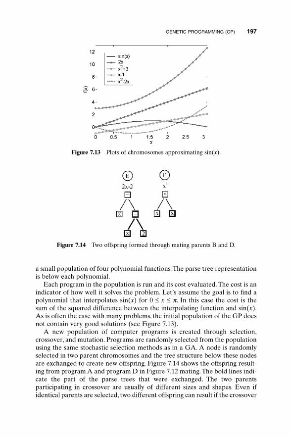
a small population of four polynomial functions.The parse tree representationis below each polynomial.
Each program in the population is run and its cost evaluated. The cost is anindicator of how well it solves the problem. Let’s assume the goal is to find apolynomial that interpolates sin(x) for 0 £ x £ p. In this case the cost is thesum of the squared difference between the interpolating function and sin(x).As is often the case with many problems, the initial population of the GP doesnot contain very good solutions (see Figure 7.13).
A new population of computer programs is created through selection,crossover, and mutation. Programs are randomly selected from the populationusing the same stochastic selection methods as in a GA. A node is randomlyselected in two parent chromosomes and the tree structure below these nodesare exchanged to create new offspring. Figure 7.14 shows the offspring result-ing from program A and program D in Figure 7.12 mating. The bold lines indi-cate the part of the parse trees that were exchanged. The two parentsparticipating in crossover are usually of different sizes and shapes. Even ifidentical parents are selected, two different offspring can result if the crossover
GENETIC PROGRAMMING (GP) 197
Figure 7.13 Plots of chromosomes approximating sin(x).
Figure 7.14 Two offspring formed through mating parents B and D.
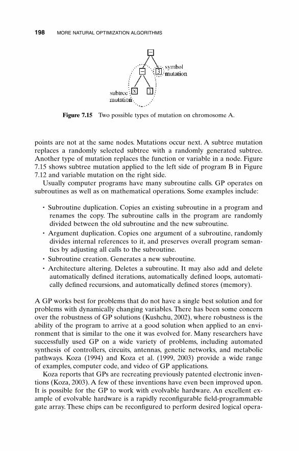
points are not at the same nodes. Mutations occur next. A subtree mutationreplaces a randomly selected subtree with a randomly generated subtree.Another type of mutation replaces the function or variable in a node. Figure7.15 shows subtree mutation applied to the left side of program B in Figure7.12 and variable mutation on the right side.
Usually computer programs have many subroutine calls. GP operates onsubroutines as well as on mathematical operations. Some examples include:
• Subroutine duplication. Copies an existing subroutine in a program andrenames the copy. The subroutine calls in the program are randomlydivided between the old subroutine and the new subroutine.
• Argument duplication. Copies one argument of a subroutine, randomlydivides internal references to it, and preserves overall program seman-tics by adjusting all calls to the subroutine.
• Subroutine creation. Generates a new subroutine.• Architecture altering. Deletes a subroutine. It may also add and delete
automatically defined iterations, automatically defined loops, automati-cally defined recursions, and automatically defined stores (memory).
A GP works best for problems that do not have a single best solution and forproblems with dynamically changing variables. There has been some concernover the robustness of GP solutions (Kushchu, 2002), where robustness is theability of the program to arrive at a good solution when applied to an envi-ronment that is similar to the one it was evolved for. Many researchers havesuccessfully used GP on a wide variety of problems, including automated synthesis of controllers, circuits, antennas, genetic networks, and metabolicpathways. Koza (1994) and Koza et al. (1999, 2003) provide a wide range of examples, computer code, and video of GP applications.
Koza reports that GPs are recreating previously patented electronic inven-tions (Koza, 2003). A few of these inventions have even been improved upon.It is possible for the GP to work with evolvable hardware. An excellent ex-ample of evolvable hardware is a rapidly reconfigurable field-programmablegate array. These chips can be reconfigured to perform desired logical opera-
198 MORE NATURAL OPTIMIZATION ALGORITHMS
Figure 7.15 Two possible types of mutation on chromosome A.
tions via commands from a computer. Although circuit designs developed bythe GP may outperform previous “best” designs, understanding how or whythey work is often difficult. In addition the GP designs may contain redundantor extraneous components.
7.5 CULTURAL ALGORITHMS
The advancement or optimization of the human race cannot be totally attrib-uted to genetics and evolution. Human interactions, societal behaviors, andother factors play major roles in the optimization process as well. Since socialinteractions allow for faster adaptation and improvement than genetics andevolution, an optimization algorithm should include those societal factors thatwould help speed convergence. These algorithms are known as cultural algo-rithms (Reynolds, 1994).
As with a GA, these algorithms begin with a random population called a civilization. The civilization has societies that consist of clusters of points or individuals. Each society has a leader. Individuals within a society onlyinteract with others in the same society. This behavior is analogous to a local search. Society leaders, however, interact not only with other individualsin the same society but with leaders from other societies as well. A leader may leave its current society to join a society that performing at a higher level.This leader migration allows high-performing societies to flourish while diminishing low-performing societies. This behavior is analogous to globalsearch.
The hope is that these algorithms will produce excellent results faster thana GA. They are reminiscent of the parallel island GAs. The interested readercan find pseudocode for this type of algorithm in the literature (Ray and Liew,2003).
7.6 EVOLUTIONARY STRATEGIES
GAs are not the only type of evolutionary computing methods. Modeling bio-logical evolution on a computer began in the 1960s. Rechenberg (1965) intro-duced evolutionary strategies in Europe. His first versions of the algorithmsused real-valued parameters and began with a parent and a mutated versionof a parent. Whichever had the highest cost was discarded. The winner pro-duced a mutated version and the process repeated. Populations and crossoverwere not incorporated until later years. A general version of the algorithm,known as the (m + l) evolution strategy, was developed (Back, 1997). In thisstrategy, m parents produce l offspring. In succeeding generations only the bestm of the l offspring and m parents are allowed to survive until the next gen-eration.Another variant known as the (m, l) replaces the parents with the bestm offspring. None of the parents from the previous generation are allowed to
EVOLUTIONARY STRATEGIES 199
produce offspring again. This approach does not use elitism. It accepts a lowercost at a given generation in the hope that a better cost will be found in afuture generation. Fogel introduced the concept of evolutionary programmingin the United States at about the same time as Rechenberg’s work (Fogel etal., 1966). For more detailed information on evolutionary algorithms, see(Schwefel, 1995).
7.7 THE FUTURE OF GENETIC ALGORITHMS
Some optimization problems are so big that they have not been totally solvedto date. Ahuja and Orlin (2003) report how new optimization algorithms aresuccessfully improving solutions to very large problems. In this case very large-scale neighborhood (VLSN) techniques were used on the airline fleet sched-uling problem. In this problem an airline has to schedule planes into and outof airports in an efficient manner that maximizes revenue minus operatingcosts while satisfying constraints such as size of plane, number of expected passengers, and number of planes leaving an airport matching the numberarriving. At the same time flight crews must be scheduled for all planes. Theassignments are broken into four separate problems: (1) fleet assignment, (2)through assignment (a plane that stops in one city then proceeds to anothercity), (3) aircraft routing, and (4) crew scheduling. Although these are eachseparate models, they must be coupled to obtain the best overall solution. Reallife problems such as this will continue to challenge optimization routines foryears to come.
We return to the hiking analogy of Chapter 1 and imagine ourselves search-ing for the lowest point in Rocky Mountain National Park. We can think ofthe GA as a new tool to use, analogous to carrying a global positioning system(GPS) device. We can take this new tool to any position in the park and takea reading of the three-dimensional coordinates. We know the result of the costfunction (the elevation) as well as the latitude and longitude of the location.The GA has methods such as crossover and mutation to steer us into thecorrect portions of the solution space, akin to the topographic maps that canbe stored in many GPS systems to point us in the direction of the lowest point.The tool itself is rapidly evolving to work in new ways to solve bigger prob-lems in much larger topological landscapes. Koza et al. (2003) have submittedpatent applications on genetically programmed inventions. Yet they have onlyscratched the surface of genetic programming and evolvable hardware. Howmany of the inventions of the future will be done with computer intelligence?We saw in Chapter 4 how GAs are being used to produce new forms of musicand art. Many of those applications (but not all) had some interface with ahuman critic to help train the algorithm on what is “good.” Does the computerbecome the artist?
We humans are constantly evolving new ways of looking at the world anddoing things. We are always inventing new problems and new ways of solving
200 MORE NATURAL OPTIMIZATION ALGORITHMS
them. That is what we call progress. The relatively new invention of the GPShas revolutionized our ability to know exactly where we are when hiking. TheGA has demonstrated that it can easily solve many traditionally challengingoptimization problems. We immediately found new uses for our new tools. Wecombine our new tools with other evolving tools. We put GPS devices in cellphones in the same way we use GAs to train artificial neural networks. Auto-motive navigation is being revolutionized by the GPS, just as major schedul-ing problems are being solved by the GA. The GPS is being used in guidingsatellite clusters and the GA is being used to improve the design of airplanes.It is a never ending process and that is what makes life, and its changes,interesting.
BIBLIOGRAPHY
Ahuja, R. K., and J. B. Orlin. 2003. Very large-scale neighborhood search in airline fleetscheduling. SIAM News 35:11–13.
Bäck, T. 1997. Evolutionary computation: comments on the history and current state.IEEE Trans. Evol. Comput. 1:3–17.
Bonabeau, E., M. Dorigo, and G. Theraulaz. 1999. Swarm Intelligence from Natural toArtificial Systems. New York: Oxford University Press.
Dorigo, M., and G. Maria. 1997. Ant colony system: a cooperative learning approach tothe traveling salesman problem. IEEE Trans. Evol. Comput. 1:53–66.
Fogel, L. J., A. J. Owens, and M. J. Walsh. 1966. Artificial Intelligence through SimulatedEvolution. New York: Wiley.
Graham, P. 1995. ANSI Common LISP. Upper Saddle River, NJ: Prentice Hall.Harvey, B., and M. Wright. 1994. Simply Scheme: Introducing Computer Science.
Cambridge: MIT Press.Holland, J. H. 1975. Adaptation in Natural and Artificial Systems. Ann Arbor: Univer-
sity of Michigan Press.Kennedy, J., and R. C. Eberhart. 2001. Swarm Intelligence. San Francisco: Morgan
Kaufmann.Kennedy, J., and R. C. Eberhart. 1995. Particle swarm optimization. Proc. IEEE Int.
Conf. on Neural Networks, IV. Piscataway, NJ: IEEE Service Center, pp. 1942–1948.Kirkpatrick, S., C. D. Gelatt Jr., and M. P. Vecchi. 1983. Optimization by simulated
annealing. Science 220:671–680.Koza, J. R. 1992. Genetic Programming: On the Programming of Computers by Means
of Natural Selection. Cambridge: MIT Press.Koza, J. R. 1994. Genetic Programming II: Automatic Discovery of Reusable Programs,
Cambridge: MIT Press.Koza, J. R., et al. 1999. Genetic Programming III: Darwinian Invention and Problem
Solving. San Francisco: Morgan Kaufmann.Koza, J. R., et al. 2003. Genetic Programming IV: Routine Human-Competitive Machine
Intelligence. Hingham, MA: Kluwer Academic.
BIBLIOGRAPHY 201
Koza, J. R., M. A. Keane, and J. M. Streeter. 2003. Evolving inventions. Sci. Am. 288:52–59.
Kushchu, I. 2002. Genetic programming and evolutionary generalization. IEEE Trans.Evol. Comput. 6:431–442.
Metropolis, N., et al. 1953. Equation of state calculations by fast computing machines.J. Chem. Phys. 21:1087–1092.
Parsopoulos, K. E., and M. N. Vrahatis. 2002. Recent approaches to global optimizationproblems through particle swarm optimization. In Natural Computing. Netherlands:Kluwer Academic, 1:235–306.
Ray,T., and K. M. Liew. 2003. Society and civilization:An optimization algorithm basedon the simulation of social behavior. IEEE Trans. Evol. Comput. 7:386–396.
Rechenberg, I. 1965. Cybernetic solution path of an experimental problem.In Royal Aircraft Establishment, Library Translation 1122. Farnborough, Hants,England.
Reynolds, R. G. 1994. An Introduction to Cultural Algorithms. In A. V. Sebald and L. J.Fogel (eds), Proc. 3rd An. Conf. on Evolutionary Programming. River Edge, NJ:World Scientific, pp. 131–139.
Schwefel, H. 1995. Evolution and Optimum Seeking. New York: Wiley.Wolpert, D. H., and W. G. Macready. 1997. No free lunch theorems for optimization.
IEEE Trans. Evol. Comput. 1:67–82.
EXERCISES
1. Use SA to find the minimum of function _____ in Appendix I using thefollowing cooling schedules:
a. Linearly decreasing: Tn = T0 - n(T0 - Tn)/Nb. Geometrically decreasing: Tn = 0.99Tn-1
c. Hayjek optimal: Tn = c/log(1 + n), where c is the smallest variation re-quired to get out of any local minimum.
Which schedule works best?
2. What values do you recommend for the PSO learning factors? Averageruns for several different cost functions to justify your conclusions.
3. Find the minimum of _____ (from Appendix I) using PSO.
4. Develop a hybrid PSO algorithm and test it.
5. Compare ACO with a GA for solving the traveling salesperson problemas a function of the number of cities.
6. Demonstrate the importance using ACO of the evaporation constant insolving the traveling salesperson problem.
7. Modify the ACO code to optimize the function _____ in Appendix I.
202 MORE NATURAL OPTIMIZATION ALGORITHMS
8. Implement a cultural algorithm to optimize the function _____ in Appendix I.
9. Write a (m + l) evolution strategy algorithm to optimize the function _____in Appendix I.
10. Write a (m, l) evolution strategy algorithm to optimize the function _____in Appendix I.
11. Compare the (m, l) and (m + l) evolution strategy optimization algorithms.Which do you recommend and why?
12. For optimizing the function _____ in Appendix I, compare one or more ofthe following algorithms:
a. Nelder-Mead downhill simplexb. BFGSc. DFPd. Steepest descente. Random searchf. Binary GAg. Continuous GAh. mGAi. SAj. PSOk. ACOl. (m, l) evolution strategy algorithm
m. (m + l) evolution strategy algorithm
EXERCISES 203
APPENDIX I
Test Functions
205
In order to determine how well an optimization algorithm works, a variety oftest functions have been used as a check. We’ve listed 16 in this appendix. Ineach case we give a general form of the function, plot its value in one or twodimensions, give the global optimum in one or two dimensions, and list thedomain. Some of the functions are generalizable to N dimensions. MATLABcode for these functions appear in Appendix II. Some of the research intodeveloping test functions is reported in the references.
BIBLIOGRAPHY
De Jong, K. A. 1975. Analysis of the behavior of a class of genetic adaptive systems.Ph.D. Dissertation. University of Michigan, Ann Arbor.
Michalewicz, Z. 1992. Genetic Algorithms + Data Structures = Evolution Programs.New York: Springer-Verlag.
Schwefel, H. 1995. Evolution and Optimum Seeking. New York: Wiley.Whitley, D., K. Mathias, S. Rana, and J. Dzubera. 1996. Evaluating Evolutionary
Algorithms. Artificial Intelligence Journal 85:1–32.Whitley, D., R. Beveridge, C. Graves, and K. Mathias. 1995. Test Driving Three 1995
Genetic Algorithms: New Test Functions and Geometric Matching. Journal ofHeuristics 1:77–104.
Practical Genetic Algorithms, Second Edition, by Randy L. Haupt and Sue Ellen Haupt.ISBN 0-471-45565-2 Copyright © 2004 John Wiley & Sons, Inc.
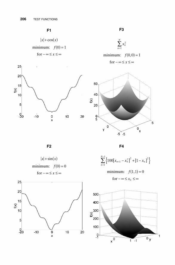
206 TEST FUNCTIONS
x x
f
x
+ ( )
( ) =
- • £ £ •
cos
minimum:
for
0 1
F1
x x
f
x
+ ( )
( ) =
- • £ £ •
sin
minimum: 0
for
0
F2
x
f
x
nn
N2
1
1
=Â
( ) =
- • £ £ •
minimum: 0,0
for
F3
100 1
0
12 2 2
1
1
x x x
f
x
n n nn
N
n
+=
-
-[ ] + -[ ]{ }( ) =
- • £ £ •
Â
minimum: 1,1
for
F4
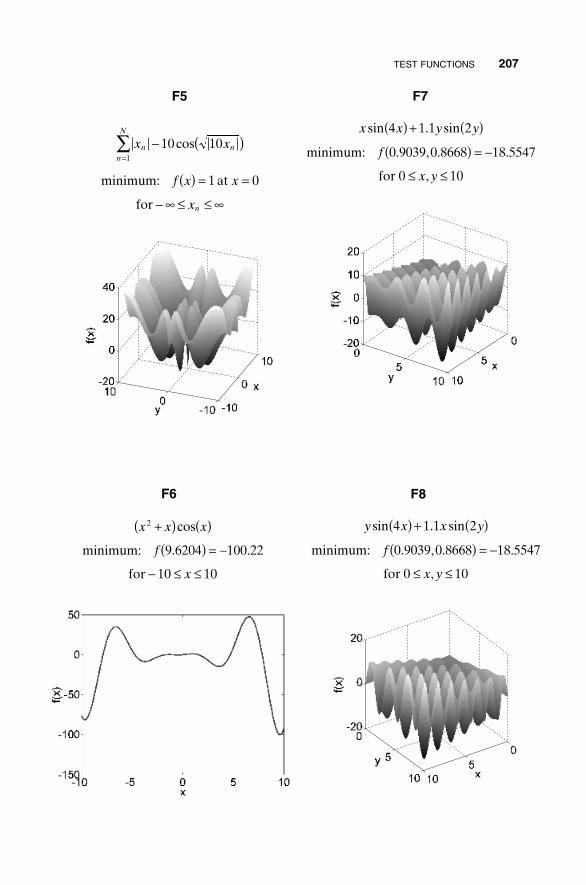
TEST FUNCTIONS 207
x x
f x x
x
nn
N
n
n
=Â - ( )
( ) = =
- • £ £ •
1
10 10
1 0
cos
minimum: at
for
F5
x x y y
f
x y
sin . sin
. , . .
,
4 1 1 2
0 9039 0 8668 18 5547
0 10
( ) + ( )( ) = -
£ £
minimum:
for
F7
x x x
f
x
2
9 6204 100 22
10 10
+( ) ( )( ) = -
- £ £
cos
. .minimum:
for
F6
y x x y
f
x y
sin . sin
. , . .
,
4 1 1 2
0 9039 0 8668 18 5547
0 10
( ) + ( )( ) = -
£ £
minimum:
for
F8
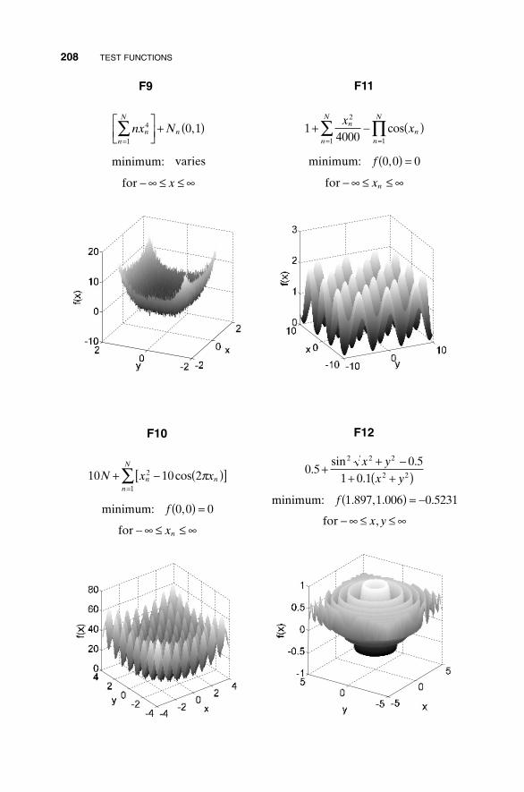
208 TEST FUNCTIONS
nx N
x
nn
N
n4
1
0 1=
ÂÈÎÍ
˘˚
+ ( )
- • £ £ •
,
minimum: varies
for
F9
14000
0
2
11
+ - ( )
( ) =
- • £ £ •
==’Â x
x
f
x
nn
n
N
n
N
n
cos
minimum: 0,0
for
F11
10 10 2
0
2
1
N x x
f
x
n nn
N
n
+ - ( )[ ]
( ) =
- • £ £ •
=Â cos p
minimum: 0,0
for
F10
0 50 5
1 0 1
0 5231
2 2 2
2 2.
sin ..
.
,
++ -
+ +( )( ) = -
- • £ £ •
x yx y
f
x y
minimum: 1.897,1.006
for
F12
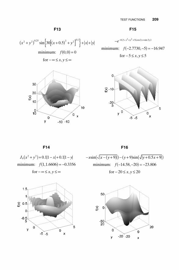
TEST FUNCTIONS 209
x y x y x y
f
x y
2 2 0 25 2 20 1
30 0 5
0 0 0
+( ) +( ) +[ ]{ } + +
( ) =
- • £ £ •
. .sin .
,
,
minimum:
for
F13
J x y x y
f
x y
02 2 0 11 0 11
1 1 6606 0 3356
+( ) + - + -
( ) = -
- • £ £ •
. .
, . .
,
minimum:
for
F14
-
- -( ) = -
- £ £
- + + +( )e
f
x y
x y x y0 2 3 2 22 2
2 7730 5 16 947
5 5
. cos sin
. , .
,
minimum:
for
F15
- - +( )( ) - +( ) + +( )- -( ) = -
- £ £
x x y y y x
f
x y
sin 9 9 sin 0.5 9
minimum: 14.58, 20 23.806
for 20 , 20
F16
APPENDIX II
MATLAB Code
MATLAB is a commonly used program for computer modeling. Its code isrelatively straightforward. So even though you may not use MATLAB, it hasa pseudocode flavor that should be easy to translate into your favorite pro-gramming language. If you wish to learn about MATLAB or reference all themanuals on line, go to www.mathworks.com for help. There are many demos,free software, and other useful items as well as all the MATLAB documenta-tion you would ever need. An excellent version is also available for students.Many of the programs we have used in this book are listed in this appendixand come on the included CD. All the plots and graphs in this book werecreated with MATLAB version 6.5. We have listed the MATLAB code in theappendix in case the CD gets separated from the book.
PROGRAM 1: BINARY GENETIC ALGORITHM
% Binary Genetic Algorithm%% minimizes the objective function designated in ff% Before beginning, set all the parameters in parts
I, II, and III% Haupt & Haupt% 2003
clear%_______________________________________________________% I. Setup the GAff=’testfunction’; % objective functionnpar=2; % number of optimization variables
%_______________________________________________________% II. Stopping criteriamaxit=100; % max number of iterationsmincost=-9999999; % minimum cost
Practical Genetic Algorithms, Second Edition, by Randy L. Haupt and Sue Ellen Haupt.ISBN 0-471-45565-2 Copyright © 2004 John Wiley & Sons, Inc.
211
212 MATLAB CODE
%_______________________________________________________% III. GA parameterspopsize=16; % set population sizemutrate=.15; % set mutation rateselection=0.5; % fraction of population
% keptnbits=8; % number of bits in each
% parameterNt=nbits*npar; % total number of bits
% in a chormosomekeep=floor(selection*popsize); % #population members
% that survive
%_______________________________________________________% Create the initial populationiga=0; % generation counter
% initializedpop=round(rand(popsize,Nt)); % random population of
% 1s and 0spar=gadecode(pop,0,10,nbits); % convert binary to
% continuous valuescost=feval(ff,par); % calculates population
% cost using ff[cost,ind]=sort(cost); % min cost in element 1par=par(ind,:);pop=pop(ind,:); % sorts population with
% lowest cost firstminc(1)=min(cost); % minc contains min of
% populationmeanc(1)=mean(cost); % meanc contains mean
% of population
%_______________________________________________________% Iterate through generationswhile iga<maxit
iga=iga+1; % increments generation counter
%_______________________________________________________% Pair and mateM=ceil((popsize-keep)/2); % number of matingsprob=flipud([1:keep]’/sum([1:keep]));% weights
% chromosomes based % upon position in % list
odds=[0 cumsum(prob(1:keep))’]; % probabilitydistribution function
PROGRAM I: BINARY GENETIC ALGORTHIM 213
pick1=rand(1,M); % mate #1pick2=rand(1,M); % mate #2
% ma and pa contain the indicies of the chromosomes % that will mateic=1;while ic<=Mfor id=2:keep+1
if pick1(ic)<=odds(id) & pick1(ic)>odds(id-1)ma(ic)=id-1;
end % ifif pick2(ic)<=odds(id) & pick2(ic)>odds(id-1)
pa(ic)=id-1;end % if
end % idic=ic+1;
end % while
%_______________________________________________________% Performs mating using single point crossoverix=1:2:keep; % index of mate #1xp=ceil(rand(1,M)*(Nt-1)); % crossover pointpop(keep+ix,:)=[pop(ma,1:xp) pop(pa,xp+1:Nt)];
% first offspringpop(keep+ix+1,:)=[pop(pa,1:xp) pop(ma,xp+1:Nt)];
% second offspring
%_______________________________________________________% Mutate the populationnmut=ceil((popsize-1)*Nt*mutrate); % total number
% of mutationsmrow=ceil(rand(1,nmut)*(popsize-1))+1; % row to mutatemcol=ceil(rand(1,nmut)*Nt); % column to mutatefor ii=1:nmut
pop(mrow(ii),mcol(ii))=abs(pop(mrow(ii),mcol(ii))-1);% toggles bits
end % ii
%_______________________________________________________% The population is re-evaluated for costpar(2:popsize,:)=gadecode(pop(2:popsize,:),0,10,nbits);% decodecost(2:popsize)=feval(ff,par(2:popsize,:));
%_______________________________________________________% Sort the costs and associated parameters[cost,ind]=sort(cost);par=par(ind,:); pop=pop(ind,:);
%_______________________________________________________% Do statistics for a single nonaveraging runminc(iga+1)=min(cost);meanc(iga+1)=mean(cost);
%_______________________________________________________% Stopping criteriaif iga>maxit | cost(1)<mincost
breakend
[iga cost(1)]
end %iga
%_______________________________________________________% Displays the outputday=clock;disp(datestr(datenum(day(1),day(2),day(3),day(4),day(5),day(6)),0))disp([‘optimized function is ‘ ff])format short gdisp([‘popsize = ‘ num2str(popsize) ‘ mutrate = ‘num2str(mutrate) ‘ # par = ‘ num2str(npar)])disp([‘#generations=’ num2str(iga) ‘ best cost=’num2str(cost(1))])disp([‘best solution’])disp([num2str(par(1,:))])disp(‘binary genetic algorithm’)disp([‘each parameter represented by ‘ num2str(nbits)‘ bits’])figure(24)iters=0:length(minc)-1;plot(iters,minc,iters,meanc,’–’);xlabel(‘generation’);ylabel(‘cost’);text(0,minc(1),’best’);text(1,minc(2),’populationaverage’)
214 MATLAB CODE
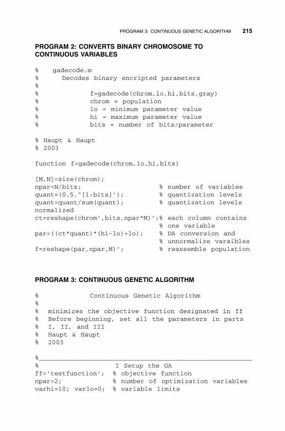
PROGRAM 2: CONVERTS BINARY CHROMOSOME TO CONTINUOUS VARIABLES
% gadecode.m% Decodes binary encripted parameters%% f=gadecode(chrom,lo,hi,bits,gray)% chrom = population% lo = minimum parameter value% hi = maximum parameter value% bits = number of bits/parameter
% Haupt & Haupt% 2003
function f=gadecode(chrom,lo,hi,bits)
[M,N]=size(chrom);npar=N/bits; % number of variablesquant=(0.5.^[1:bits]’); % quantization levelsquant=quant/sum(quant); % quantization levelsnormalizedct=reshape(chrom’,bits,npar*M)’;% each column contains
% one variablepar=((ct*quant)*(hi-lo)+lo); % DA conversion and
% unnormalize varaiblesf=reshape(par,npar,M)’; % reassemble population
PROGRAM 3: CONTINUOUS GENETIC ALGORITHM
% Continuous Genetic Algorithm%% minimizes the objective function designated in ff% Before beginning, set all the parameters in parts % I, II, and III% Haupt & Haupt% 2003
%_______________________________________________________% I Setup the GAff=’testfunction’; % objective functionnpar=2; % number of optimization variablesvarhi=10; varlo=0; % variable limits
PROGRAM 3: CONTINUOUS GENETIC ALGORITHM 215
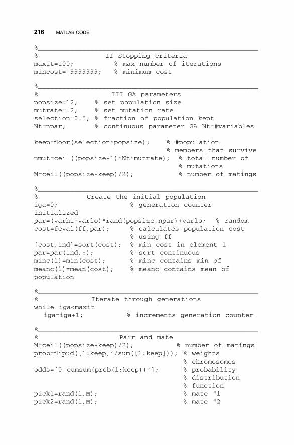
%_______________________________________________________% II Stopping criteriamaxit=100; % max number of iterationsmincost=-9999999; % minimum cost
%_______________________________________________________% III GA parameterspopsize=12; % set population sizemutrate=.2; % set mutation rateselection=0.5; % fraction of population keptNt=npar; % continuous parameter GA Nt=#variables
keep=floor(selection*popsize); % #population% members that survive
nmut=ceil((popsize-1)*Nt*mutrate); % total number of % mutations
M=ceil((popsize-keep)/2); % number of matings
%_______________________________________________________% Create the initial populationiga=0; % generation counterinitializedpar=(varhi-varlo)*rand(popsize,npar)+varlo; % randomcost=feval(ff,par); % calculates population cost
% using ff[cost,ind]=sort(cost); % min cost in element 1par=par(ind,:); % sort continuousminc(1)=min(cost); % minc contains min ofmeanc(1)=mean(cost); % meanc contains mean ofpopulation
%_______________________________________________________% Iterate through generationswhile iga<maxit
iga=iga+1; % increments generation counter
%_______________________________________________________% Pair and mateM=ceil((popsize-keep)/2); % number of matingsprob=flipud([1:keep]’/sum([1:keep])); % weights
% chromosomesodds=[0 cumsum(prob(1:keep))’]; % probability
% distribution % function
pick1=rand(1,M); % mate #1pick2=rand(1,M); % mate #2
216 MATLAB CODE
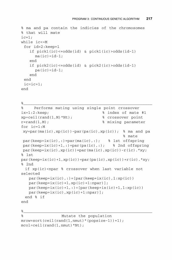
% ma and pa contain the indicies of the chromosomes % that will mateic=1;while ic<=Mfor id=2:keep+1
if pick1(ic)<=odds(id) & pick1(ic)>odds(id-1)ma(ic)=id-1;
endif pick2(ic)<=odds(id) & pick2(ic)>odds(id-1)
pa(ic)=id-1;end
endic=ic+1;
end
%_______________________________________________________% Performs mating using single point crossoverix=1:2:keep; % index of mate #1xp=ceil(rand(1,M)*Nt); % crossover pointr=rand(1,M); % mixing parameterfor ic=1:Mxy=par(ma(ic),xp(ic))-par(pa(ic),xp(ic)); % ma and pa
% matepar(keep+ix(ic),:)=par(ma(ic),:); % 1st offspringpar(keep+ix(ic)+1,:)=par(pa(ic),:); % 2nd offspringpar(keep+ix(ic),xp(ic))=par(ma(ic),xp(ic))-r(ic).*xy;% 1stpar(keep+ix(ic)+1,xp(ic))=par(pa(ic),xp(ic))+r(ic).*xy;% 2ndif xp(ic)<npar % crossover when last variable not
selectedpar(keep+ix(ic),:)=[par(keep+ix(ic),1:xp(ic))par(keep+ix(ic)+1,xp(ic)+1:npar)];par(keep+ix(ic)+1,:)=[par(keep+ix(ic)+1,1:xp(ic))par(keep+ix(ic),xp(ic)+1:npar)];
end % ifend
%_______________________________________________________% Mutate the populationmrow=sort(ceil(rand(1,nmut)*(popsize-1))+1);mcol=ceil(rand(1,nmut)*Nt);
PROGRAM 3: CONTINUOUS GENETIC ALGORITHM 217
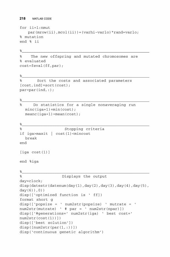
for ii=1:nmutpar(mrow(ii),mcol(ii))=(varhi-varlo)*rand+varlo;
% mutationend % ii
%_______________________________________________________
% The new offspring and mutated chromosomes are % evaluatedcost=feval(ff,par);
%_______________________________________________________% Sort the costs and associated parameters[cost,ind]=sort(cost);par=par(ind,:);
%_______________________________________________________% Do statistics for a single nonaveraging run
minc(iga+1)=min(cost);meanc(iga+1)=mean(cost);
%_______________________________________________________% Stopping criteriaif iga>maxit | cost(1)<mincost
breakend
[iga cost(1)]
end %iga
%_______________________________________________________% Displays the outputday=clock;disp(datestr(datenum(day(1),day(2),day(3),day(4),day(5),day(6)),0))disp([‘optimized function is ‘ ff])format short gdisp([‘popsize = ‘ num2str(popsize) ‘ mutrate = ‘num2str(mutrate) ‘ # par = ‘ num2str(npar)])disp([‘#generations=’ num2str(iga) ‘ best cost=’num2str(cost(1))])disp([‘best solution’])disp([num2str(par(1,:))])disp(‘continuous genetic algorithm’)
218 MATLAB CODE
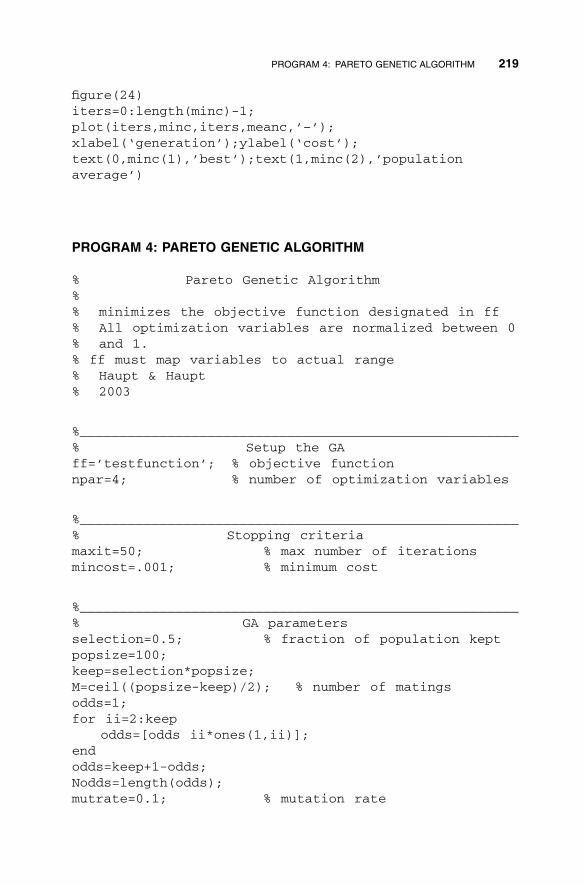
figure(24)iters=0:length(minc)-1;plot(iters,minc,iters,meanc,’–’);xlabel(‘generation’);ylabel(‘cost’);text(0,minc(1),’best’);text(1,minc(2),’populationaverage’)
PROGRAM 4: PARETO GENETIC ALGORITHM
% Pareto Genetic Algorithm%% minimizes the objective function designated in ff% All optimization variables are normalized between 0% and 1.% ff must map variables to actual range% Haupt & Haupt% 2003
%_______________________________________________________% Setup the GAff=’testfunction’; % objective functionnpar=4; % number of optimization variables
%_______________________________________________________% Stopping criteriamaxit=50; % max number of iterationsmincost=.001; % minimum cost
%_______________________________________________________% GA parametersselection=0.5; % fraction of population keptpopsize=100;keep=selection*popsize;M=ceil((popsize-keep)/2); % number of matingsodds=1;for ii=2:keep
odds=[odds ii*ones(1,ii)];endodds=keep+1-odds;Nodds=length(odds);mutrate=0.1; % mutation rate
PROGRAM 4: PARETO GENETIC ALGORITHM 219
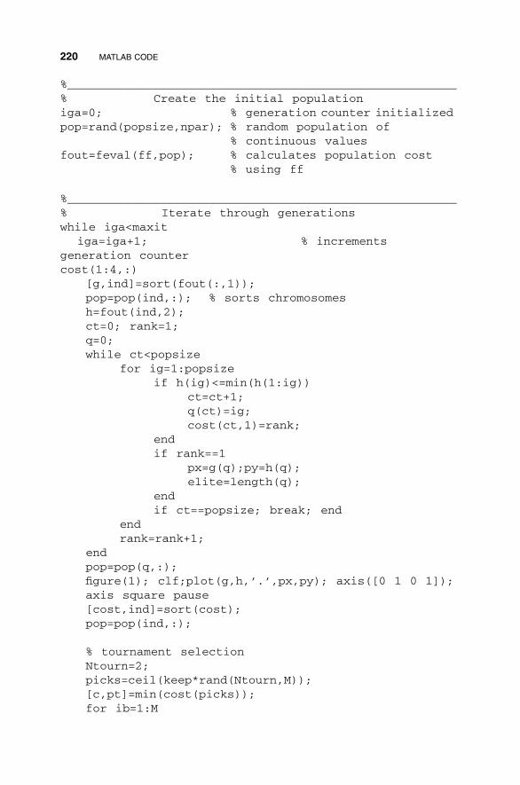
%_______________________________________________________% Create the initial populationiga=0; % generation counter initializedpop=rand(popsize,npar); % random population of
% continuous valuesfout=feval(ff,pop); % calculates population cost
% using ff
%_______________________________________________________% Iterate through generationswhile iga<maxit
iga=iga+1; % incrementsgeneration countercost(1:4,:)
[g,ind]=sort(fout(:,1));pop=pop(ind,:); % sorts chromosomesh=fout(ind,2);ct=0; rank=1;q=0;while ct<popsize
for ig=1:popsizeif h(ig)<=min(h(1:ig))
ct=ct+1;q(ct)=ig;cost(ct,1)=rank;
endif rank==1
px=g(q);py=h(q);elite=length(q);
endif ct==popsize; break; end
endrank=rank+1;
endpop=pop(q,:);figure(1); clf;plot(g,h,’.’,px,py); axis([0 1 0 1]);axis square pause[cost,ind]=sort(cost);pop=pop(ind,:);
% tournament selectionNtourn=2;picks=ceil(keep*rand(Ntourn,M));[c,pt]=min(cost(picks));for ib=1:M
220 MATLAB CODE
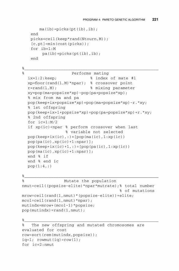
ma(ib)=picks(pt(ib),ib);endpicks=ceil(keep*rand(Ntourn,M));[c,pt]=min(cost(picks));for ib=1:M
pa(ib)=picks(pt(ib),ib);end
%_______________________________________________________% Performs mating
ix=1:2:keep; % index of mate #1xp=floor(rand(1,M)*npar); % crossover pointr=rand(1,M); % mixing parameterxy=pop(ma+popsize*xp)-pop(pa+popsize*xp);% mix from ma and papop(keep+ix+popsize*xp)=pop(ma+popsize*xp)-r.*xy;% 1st offspringpop(keep+ix+1+popsize*xp)=pop(pa+popsize*xp)+r.*xy;% 2nd offspringfor ic=1:M/2if xp(ic)<npar % perform crossover when last
% variable not selectedpop(keep+ix(ic),:)=[pop(ma(ic),1:xp(ic))pop(pa(ic),xp(ic)+1:npar)];pop(keep+ix(ic)+1,:)=[pop(pa(ic),1:xp(ic))pop(ma(ic),xp(ic)+1:npar)];end % ifend % end icpop(1:4,:)
%_______________________________________________________% Mutate the populationnmut=ceil((popsize-elite)*npar*mutrate);% total number
% of mutationsmrow=ceil(rand(1,nmut)*(popsize-elite))+elite;mcol=ceil(rand(1,nmut)*npar);mutindx=mrow+(mcol-1)*popsize;pop(mutindx)=rand(1,nmut);
%_______________________________________________________% The new offspring and mutated chromosomes areevaluated for costrow=sort(rem(mutindx,popsize));iq=1; rowmut(iq)=row(1);for ic=2:nmut
PROGRAM 4: PARETO GENETIC ALGORITHM 221
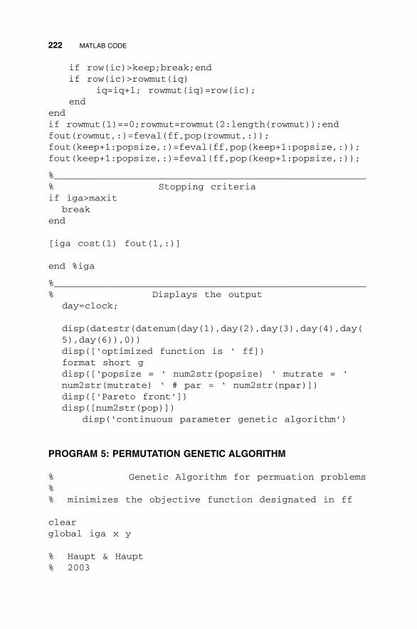
if row(ic)>keep;break;endif row(ic)>rowmut(iq)
iq=iq+1; rowmut(iq)=row(ic);end
endif rowmut(1)==0;rowmut=rowmut(2:length(rowmut));endfout(rowmut,:)=feval(ff,pop(rowmut,:));fout(keep+1:popsize,:)=feval(ff,pop(keep+1:popsize,:));fout(keep+1:popsize,:)=feval(ff,pop(keep+1:popsize,:));
%_______________________________________________________% Stopping criteriaif iga>maxit
breakend
[iga cost(1) fout(1,:)]
end %iga
%_______________________________________________________% Displays the output
day=clock;
disp(datestr(datenum(day(1),day(2),day(3),day(4),day(5),day(6)),0))disp([‘optimized function is ‘ ff])format short gdisp([‘popsize = ‘ num2str(popsize) ‘ mutrate = ‘num2str(mutrate) ‘ # par = ‘ num2str(npar)])disp([‘Pareto front’])disp([num2str(pop)])
disp(‘continuous parameter genetic algorithm’)
PROGRAM 5: PERMUTATION GENETIC ALGORITHM
% Genetic Algorithm for permuation problems%% minimizes the objective function designated in ff
clearglobal iga x y
% Haupt & Haupt% 2003
222 MATLAB CODE
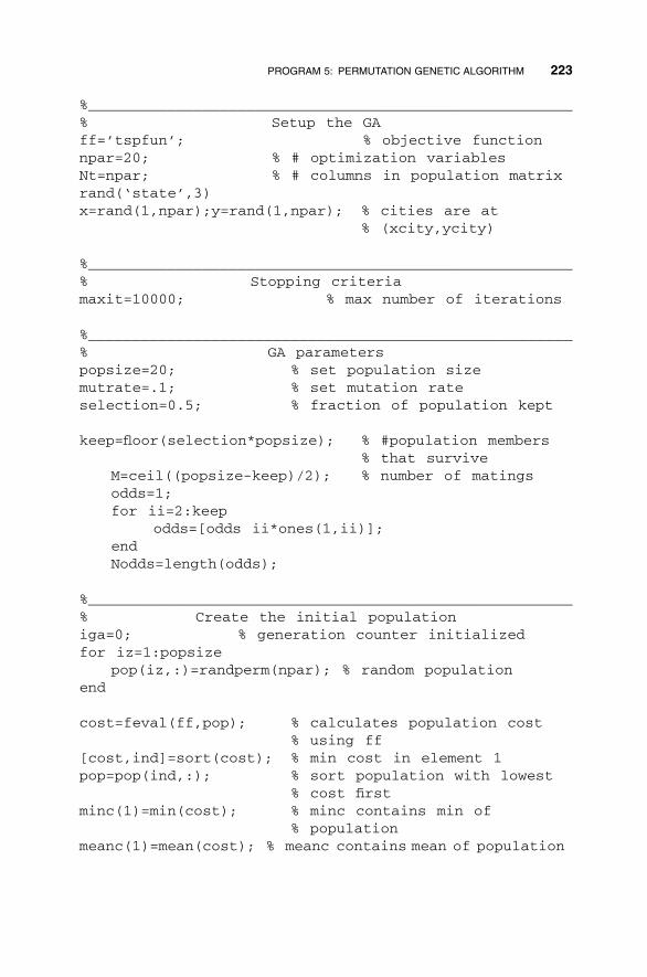
%_______________________________________________________% Setup the GAff=’tspfun’; % objective functionnpar=20; % # optimization variablesNt=npar; % # columns in population matrixrand(‘state’,3)x=rand(1,npar);y=rand(1,npar); % cities are at
% (xcity,ycity)
%_______________________________________________________% Stopping criteriamaxit=10000; % max number of iterations
%_______________________________________________________% GA parameterspopsize=20; % set population sizemutrate=.1; % set mutation rateselection=0.5; % fraction of population kept
keep=floor(selection*popsize); % #population members % that survive
M=ceil((popsize-keep)/2); % number of matingsodds=1;for ii=2:keep
odds=[odds ii*ones(1,ii)];endNodds=length(odds);
%_______________________________________________________% Create the initial populationiga=0; % generation counter initializedfor iz=1:popsize
pop(iz,:)=randperm(npar); % random populationend
cost=feval(ff,pop); % calculates population cost % using ff
[cost,ind]=sort(cost); % min cost in element 1pop=pop(ind,:); % sort population with lowest
% cost firstminc(1)=min(cost); % minc contains min of
% populationmeanc(1)=mean(cost); % meanc contains mean of population
PROGRAM 5: PERMUTATION GENETIC ALGORITHM 223
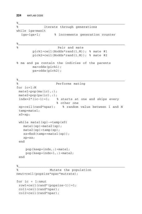
%_______________________________________________________% Iterate through generationswhile iga<maxit
iga=iga+1; % increments generation counter
%_______________________________________________________% Pair and mate
pick1=ceil(Nodds*rand(1,M)); % mate #1pick2=ceil(Nodds*rand(1,M)); % mate #2
% ma and pa contain the indicies of the parentsma=odds(pick1);pa=odds(pick2);
%_______________________________________________________% Performs matingfor ic=1:Mmate1=pop(ma(ic),:);mate2=pop(pa(ic),:);indx=2*(ic-1)+1; % starts at one and skips every
% other onexp=ceil(rand*npar); % random value between 1 and Ntemp=mate1;x0=xp;
while mate1(xp)~=temp(x0)mate1(xp)=mate2(xp);mate2(xp)=temp(xp);xs=find(temp==mate1(xp));xp=xs;
end
pop(keep+indx,:)=mate1;pop(keep+indx+1,:)=mate2;
end
%_______________________________________________________% Mutate the populationnmut=ceil(popsize*npar*mutrate);
for ic = 1:nmutrow1=ceil(rand*(popsize-1))+1;col1=ceil(rand*npar);col2=ceil(rand*npar);
224 MATLAB CODE
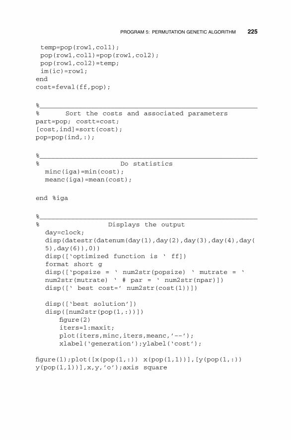
temp=pop(row1,col1);pop(row1,col1)=pop(row1,col2);pop(row1,col2)=temp;im(ic)=row1;
endcost=feval(ff,pop);
%_______________________________________________________% Sort the costs and associated parameterspart=pop; costt=cost;[cost,ind]=sort(cost);pop=pop(ind,:);
%_______________________________________________________% Do statistics
minc(iga)=min(cost);meanc(iga)=mean(cost);
end %iga
%_______________________________________________________% Displays the output
day=clock;disp(datestr(datenum(day(1),day(2),day(3),day(4),day(5),day(6)),0))disp([‘optimized function is ‘ ff])format short gdisp([‘popsize = ‘ num2str(popsize) ‘ mutrate = ‘num2str(mutrate) ‘ # par = ‘ num2str(npar)])disp([‘ best cost=’ num2str(cost(1))])
disp([‘best solution’])disp([num2str(pop(1,:))])
figure(2)iters=1:maxit;plot(iters,minc,iters,meanc,’––’);xlabel(‘generation’);ylabel(‘cost’);
figure(1);plot([x(pop(1,:)) x(pop(1,1))],[y(pop(1,:))y(pop(1,1))],x,y,’o’);axis square
PROGRAM 5: PERMUTATION GENETIC ALGORITHM 225
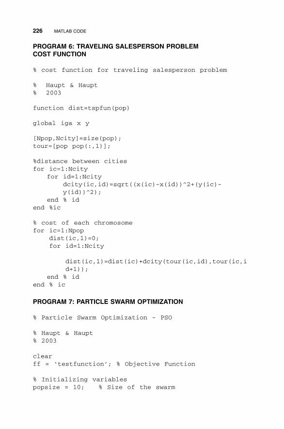
PROGRAM 6: TRAVELING SALESPERSON PROBLEM COST FUNCTION
% cost function for traveling salesperson problem
% Haupt & Haupt% 2003
function dist=tspfun(pop)
global iga x y
[Npop,Ncity]=size(pop);tour=[pop pop(:,1)];
%distance between citiesfor ic=1:Ncity
for id=1:Ncitydcity(ic,id)=sqrt((x(ic)-x(id))^2+(y(ic)-y(id))^2);
end % idend %ic
% cost of each chromosomefor ic=1:Npop
dist(ic,1)=0;for id=1:Ncity
dist(ic,1)=dist(ic)+dcity(tour(ic,id),tour(ic,id+1));
end % idend % ic
PROGRAM 7: PARTICLE SWARM OPTIMIZATION
% Particle Swarm Optimization - PSO
% Haupt & Haupt% 2003
clearff = ‘testfunction’; % Objective Function
% Initializing variablespopsize = 10; % Size of the swarm
226 MATLAB CODE
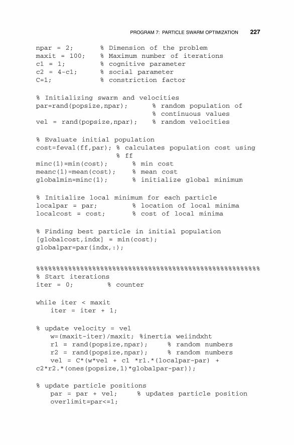
npar = 2; % Dimension of the problemmaxit = 100; % Maximum number of iterationsc1 = 1; % cognitive parameterc2 = 4-c1; % social parameterC=1; % constriction factor
% Initializing swarm and velocitiespar=rand(popsize,npar); % random population of
% continuous valuesvel = rand(popsize,npar); % random velocities
% Evaluate initial populationcost=feval(ff,par); % calculates population cost using
% ffminc(1)=min(cost); % min costmeanc(1)=mean(cost); % mean costglobalmin=minc(1); % initialize global minimum
% Initialize local minimum for each particlelocalpar = par; % location of local minimalocalcost = cost; % cost of local minima
% Finding best particle in initial population[globalcost,indx] = min(cost);globalpar=par(indx,:);
%%%%%%%%%%%%%%%%%%%%%%%%%%%%%%%%%%%%%%%%%%%%%%%%%%%%%%%%% Start iterationsiter = 0; % counter
while iter < maxititer = iter + 1;
% update velocity = velw=(maxit-iter)/maxit; %inertia weiindxhtr1 = rand(popsize,npar); % random numbersr2 = rand(popsize,npar); % random numbersvel = C*(w*vel + c1 *r1.*(localpar-par) +
c2*r2.*(ones(popsize,1)*globalpar-par));
% update particle positionspar = par + vel; % updates particle positionoverlimit=par<=1;
PROGRAM 7: PARTICLE SWARM OPTIMIZATION 227
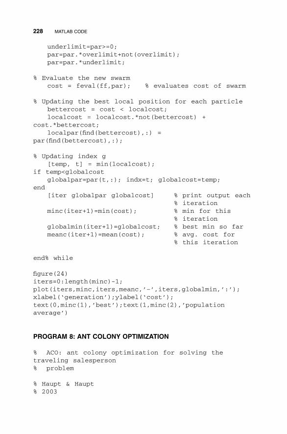
underlimit=par>=0;par=par.*overlimit+not(overlimit);par=par.*underlimit;
% Evaluate the new swarmcost = feval(ff,par); % evaluates cost of swarm
% Updating the best local position for each particlebettercost = cost < localcost;localcost = localcost.*not(bettercost) +
cost.*bettercost;localpar(find(bettercost),:) =
par(find(bettercost),:);
% Updating index g[temp, t] = min(localcost);
if temp<globalcostglobalpar=par(t,:); indx=t; globalcost=temp;
end[iter globalpar globalcost] % print output each
% iterationminc(iter+1)=min(cost); % min for this
% iterationglobalmin(iter+1)=globalcost; % best min so farmeanc(iter+1)=mean(cost); % avg. cost for
% this iteration
end% while
figure(24)iters=0:length(minc)-1;plot(iters,minc,iters,meanc,’–’,iters,globalmin,’:’);xlabel(‘generation’);ylabel(‘cost’);text(0,minc(1),’best’);text(1,minc(2),’populationaverage’)
PROGRAM 8: ANT COLONY OPTIMIZATION
% ACO: ant colony optimization for solving thetraveling salesperson% problem
% Haupt & Haupt% 2003
228 MATLAB CODE
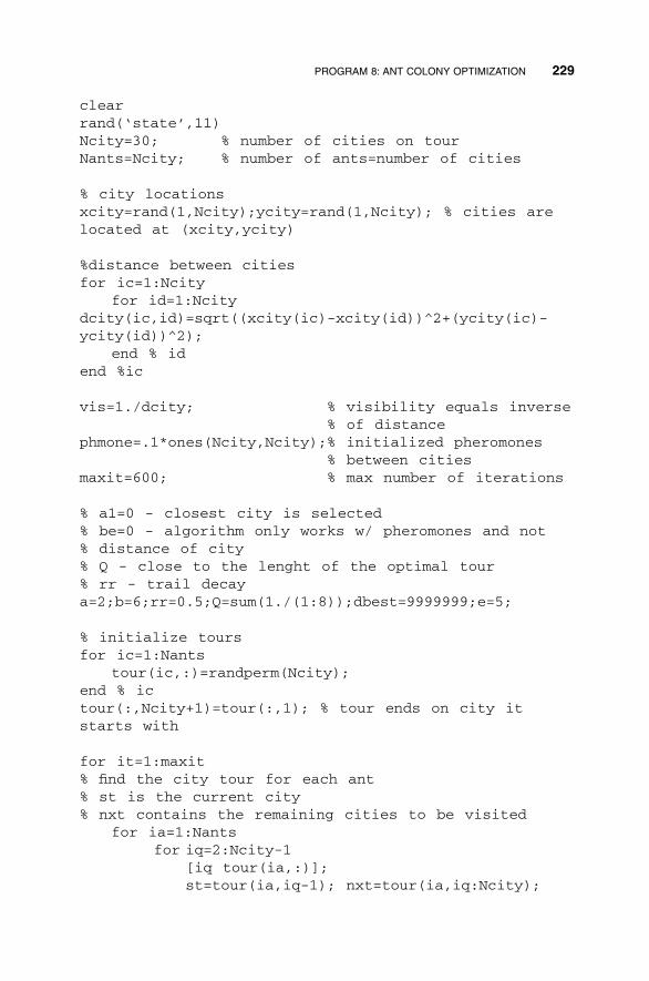
clearrand(‘state’,11)Ncity=30; % number of cities on tourNants=Ncity; % number of ants=number of cities
% city locationsxcity=rand(1,Ncity);ycity=rand(1,Ncity); % cities arelocated at (xcity,ycity)
%distance between citiesfor ic=1:Ncity
for id=1:Ncitydcity(ic,id)=sqrt((xcity(ic)-xcity(id))^2+(ycity(ic)-ycity(id))^2);
end % idend %ic
vis=1./dcity; % visibility equals inverse % of distance
phmone=.1*ones(Ncity,Ncity);% initialized pheromones % between cities
maxit=600; % max number of iterations
% a1=0 - closest city is selected% be=0 - algorithm only works w/ pheromones and not % distance of city% Q - close to the lenght of the optimal tour% rr - trail decaya=2;b=6;rr=0.5;Q=sum(1./(1:8));dbest=9999999;e=5;
% initialize toursfor ic=1:Nants
tour(ic,:)=randperm(Ncity);end % ictour(:,Ncity+1)=tour(:,1); % tour ends on city itstarts with
for it=1:maxit% find the city tour for each ant% st is the current city% nxt contains the remaining cities to be visited
for ia=1:Nantsfor iq=2:Ncity-1
[iq tour(ia,:)];st=tour(ia,iq-1); nxt=tour(ia,iq:Ncity);
PROGRAM 8: ANT COLONY OPTIMIZATION 229
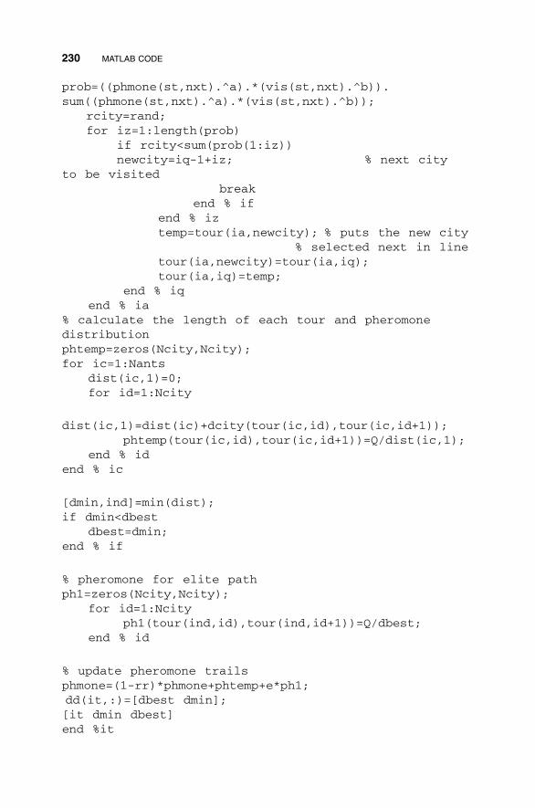
prob=((phmone(st,nxt).^a).*(vis(st,nxt).^b)).sum((phmone(st,nxt).^a).*(vis(st,nxt).^b));
rcity=rand;for iz=1:length(prob)
if rcity<sum(prob(1:iz))newcity=iq-1+iz; % next city
to be visitedbreak
end % ifend % iztemp=tour(ia,newcity); % puts the new city
% selected next in linetour(ia,newcity)=tour(ia,iq);tour(ia,iq)=temp;
end % iqend % ia
% calculate the length of each tour and pheromonedistributionphtemp=zeros(Ncity,Ncity);for ic=1:Nants
dist(ic,1)=0;for id=1:Ncity
dist(ic,1)=dist(ic)+dcity(tour(ic,id),tour(ic,id+1));phtemp(tour(ic,id),tour(ic,id+1))=Q/dist(ic,1);
end % idend % ic
[dmin,ind]=min(dist);if dmin<dbest
dbest=dmin;end % if
% pheromone for elite pathph1=zeros(Ncity,Ncity);
for id=1:Ncityph1(tour(ind,id),tour(ind,id+1))=Q/dbest;
end % id
% update pheromone trailsphmone=(1-rr)*phmone+phtemp+e*ph1;dd(it,:)=[dbest dmin];[it dmin dbest]end %it
230 MATLAB CODE
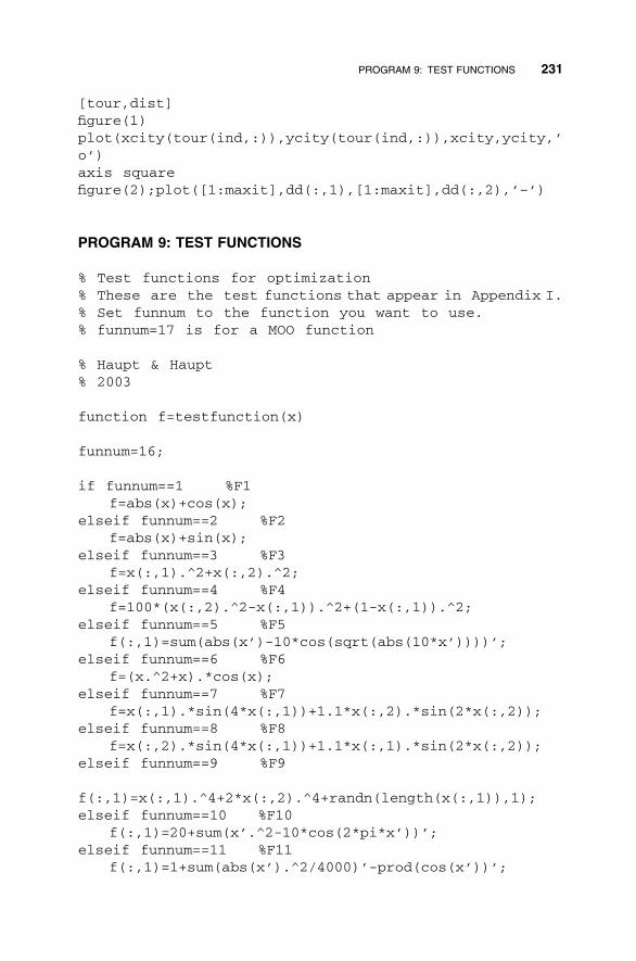
[tour,dist]figure(1)plot(xcity(tour(ind,:)),ycity(tour(ind,:)),xcity,ycity,’o’)axis squarefigure(2);plot([1:maxit],dd(:,1),[1:maxit],dd(:,2),’–’)
PROGRAM 9: TEST FUNCTIONS
% Test functions for optimization% These are the test functions that appear in Appendix I.% Set funnum to the function you want to use.% funnum=17 is for a MOO function
% Haupt & Haupt% 2003
function f=testfunction(x)
funnum=16;
if funnum==1 %F1f=abs(x)+cos(x);
elseif funnum==2 %F2f=abs(x)+sin(x);
elseif funnum==3 %F3f=x(:,1).^2+x(:,2).^2;
elseif funnum==4 %F4f=100*(x(:,2).^2-x(:,1)).^2+(1-x(:,1)).^2;
elseif funnum==5 %F5f(:,1)=sum(abs(x’)-10*cos(sqrt(abs(10*x’))))’;
elseif funnum==6 %F6f=(x.^2+x).*cos(x);
elseif funnum==7 %F7f=x(:,1).*sin(4*x(:,1))+1.1*x(:,2).*sin(2*x(:,2));
elseif funnum==8 %F8f=x(:,2).*sin(4*x(:,1))+1.1*x(:,1).*sin(2*x(:,2));
elseif funnum==9 %F9
f(:,1)=x(:,1).^4+2*x(:,2).^4+randn(length(x(:,1)),1);elseif funnum==10 %F10
f(:,1)=20+sum(x’.^2-10*cos(2*pi*x’))’;elseif funnum==11 %F11
f(:,1)=1+sum(abs(x’).^2/4000)’-prod(cos(x’))’;
PROGRAM 9: TEST FUNCTIONS 231
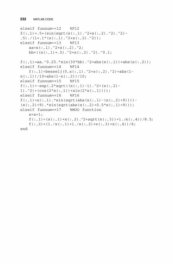
elseif funnum==12 %F12f(:,1)=.5+(sin(sqrt(x(:,1).^2+x(:,2).^2).^2)-.5)./(1+.1*(x(:,1).^2+x(:,2).^2));elseif funnum==13 %F13
aa=x(:,1).^2+x(:,2).^2;bb=((x(:,1)+.5).^2+x(:,2).^2).^0.1;
f(:,1)=aa.^0.25.*sin(30*bb).^2+abs(x(:,1))+abs(x(:,2));elseif funnum==14 %F14
f(:,1)=besselj(0,x(:,1).^2+x(:,2).^2)+abs(1-x(:,1))/10+abs(1-x(:,2))/10;elseif funnum==15 %F15f(:,1)=-exp(.2*sqrt((x(:,1)-1).^2+(x(:,2)-1).^2)+(cos(2*x(:,1))+sin(2*x(:,1))));elseif funnum==16 %F16f(:,1)=x(:,1).*sin(sqrt(abs(x(:,1)-(x(:,2)+9))))-(x(:,2)+9).*sin(sqrt(abs(x(:,2)+0.5*x(:,1)+9)));elseif funnum==17 %MOO function
x=x+1;f(:,1)=(x(:,1)+x(:,2). 2+sqrt(x(:,3))+1./x(:,4))/8.5;f(:,2)=(1./x(:,1)+1./x(:,2)+x(:,3)+x(:,4))/6;
end
232 MATLAB CODE
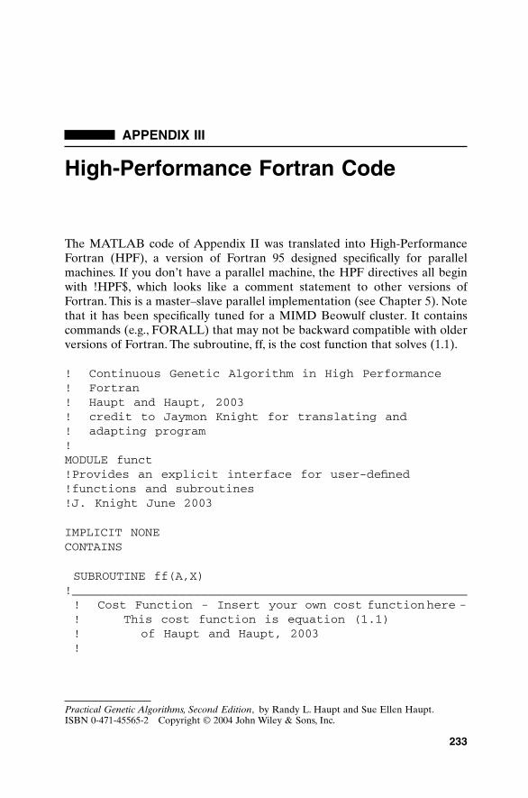
APPENDIX III
High-Performance Fortran Code
The MATLAB code of Appendix II was translated into High-PerformanceFortran (HPF), a version of Fortran 95 designed specifically for parallelmachines. If you don’t have a parallel machine, the HPF directives all beginwith !HPF$, which looks like a comment statement to other versions ofFortran. This is a master–slave parallel implementation (see Chapter 5). Notethat it has been specifically tuned for a MIMD Beowulf cluster. It containscommands (e.g., FORALL) that may not be backward compatible with olderversions of Fortran. The subroutine, ff, is the cost function that solves (1.1).
! Continuous Genetic Algorithm in High Performance ! Fortran! Haupt and Haupt, 2003! credit to Jaymon Knight for translating and ! adapting program!MODULE funct!Provides an explicit interface for user-defined!functions and subroutines!J. Knight June 2003
IMPLICIT NONECONTAINS
SUBROUTINE ff(A,X)!_______________________________________________________! Cost Function - Insert your own cost functionhere -! This cost function is equation (1.1)! of Haupt and Haupt, 2003!
Practical Genetic Algorithms, Second Edition, by Randy L. Haupt and Sue Ellen Haupt.ISBN 0-471-45565-2 Copyright © 2004 John Wiley & Sons, Inc.
233
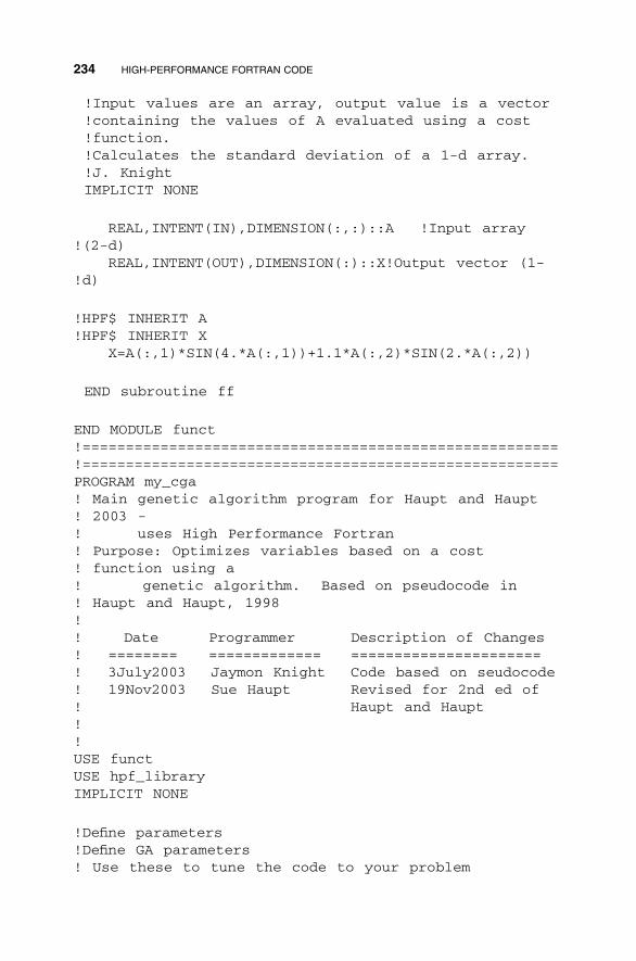
!Input values are an array, output value is a vector!containing the values of A evaluated using a cost !function.!Calculates the standard deviation of a 1-d array.!J. KnightIMPLICIT NONE
REAL,INTENT(IN),DIMENSION(:,:)::A !Input array !(2-d)
REAL,INTENT(OUT),DIMENSION(:)::X!Output vector (1-!d)
!HPF$ INHERIT A!HPF$ INHERIT X
X=A(:,1)*SIN(4.*A(:,1))+1.1*A(:,2)*SIN(2.*A(:,2))
END subroutine ff
END MODULE funct!=======================================================!=======================================================PROGRAM my_cga! Main genetic algorithm program for Haupt and Haupt ! 2003 -! uses High Performance Fortran! Purpose: Optimizes variables based on a cost ! function using a! genetic algorithm. Based on pseudocode in ! Haupt and Haupt, 1998!! Date Programmer Description of Changes! ======== ============= ======================! 3July2003 Jaymon Knight Code based on seudocode! 19Nov2003 Sue Haupt Revised for 2nd ed of ! Haupt and Haupt!!USE functUSE hpf_libraryIMPLICIT NONE
!Define parameters!Define GA parameters! Use these to tune the code to your problem
234 HIGH-PERFORMANCE FORTRAN CODE
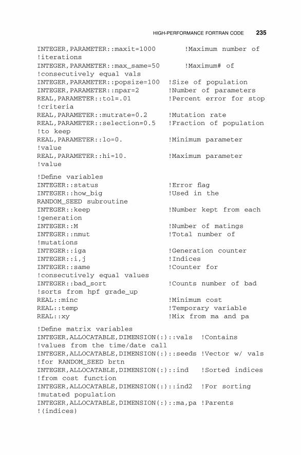
INTEGER,PARAMETER::maxit=1000 !Maximum number of !iterationsINTEGER,PARAMETER::max_same=50 !Maximum# of !consecutively equal valsINTEGER,PARAMETER::popsize=100 !Size of populationINTEGER,PARAMETER::npar=2 !Number of parametersREAL,PARAMETER::tol=.01 !Percent error for stop !criteriaREAL,PARAMETER::mutrate=0.2 !Mutation rateREAL,PARAMETER::selection=0.5 !Fraction of population !to keepREAL,PARAMETER::lo=0. !Minimum parameter !valueREAL,PARAMETER::hi=10. !Maximum parameter !value
!Define variablesINTEGER::status !Error flagINTEGER::how_big !Used in theRANDOM_SEED subroutineINTEGER::keep !Number kept from each !generationINTEGER::M !Number of matingsINTEGER::nmut !Total number of !mutationsINTEGER::iga !Generation counterINTEGER::i,j !IndicesINTEGER::same !Counter for !consecutively equal valuesINTEGER::bad_sort !Counts number of bad !sorts from hpf grade_upREAL::minc !Minimum costREAL::temp !Temporary variableREAL::xy !Mix from ma and pa
!Define matrix variablesINTEGER,ALLOCATABLE,DIMENSION(:)::vals !Contains !values from the time/date callINTEGER,ALLOCATABLE,DIMENSION(:)::seeds !Vector w/ vals !for RANDOM_SEED brtnINTEGER,ALLOCATABLE,DIMENSION(:)::ind !Sorted indices !from cost functionINTEGER,ALLOCATABLE,DIMENSION(:)::ind2 !For sorting !mutated populationINTEGER,ALLOCATABLE,DIMENSION(:)::ma,pa !Parents!(indices)
HIGH-PERFORMANCE FORTRAN CODE 235
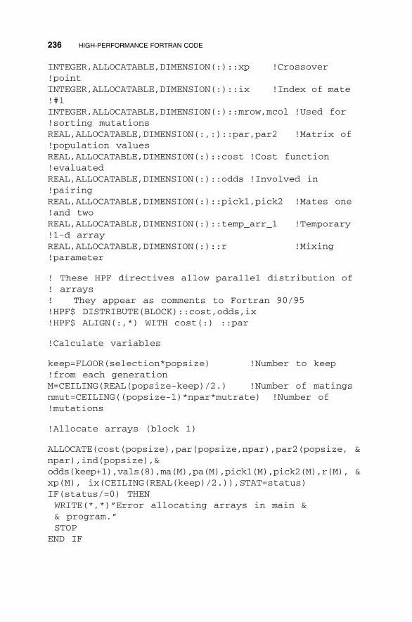
INTEGER,ALLOCATABLE,DIMENSION(:)::xp !Crossover !pointINTEGER,ALLOCATABLE,DIMENSION(:)::ix !Index of mate !#1INTEGER,ALLOCATABLE,DIMENSION(:)::mrow,mcol !Used for !sorting mutationsREAL,ALLOCATABLE,DIMENSION(:,:)::par,par2 !Matrix of !population valuesREAL,ALLOCATABLE,DIMENSION(:)::cost !Cost function !evaluatedREAL,ALLOCATABLE,DIMENSION(:)::odds !Involved in !pairingREAL,ALLOCATABLE,DIMENSION(:)::pick1,pick2 !Mates one !and twoREAL,ALLOCATABLE,DIMENSION(:)::temp_arr_1 !Temporary !1-d arrayREAL,ALLOCATABLE,DIMENSION(:)::r !Mixing!parameter
! These HPF directives allow parallel distribution of ! arrays! They appear as comments to Fortran 90/95!HPF$ DISTRIBUTE(BLOCK)::cost,odds,ix!HPF$ ALIGN(:,*) WITH cost(:) ::par
!Calculate variables
keep=FLOOR(selection*popsize) !Number to keep !from each generationM=CEILING(REAL(popsize-keep)/2.) !Number of matingsnmut=CEILING((popsize-1)*npar*mutrate) !Number of !mutations
!Allocate arrays (block 1)
ALLOCATE(cost(popsize),par(popsize,npar),par2(popsize, &npar),ind(popsize),&odds(keep+1),vals(8),ma(M),pa(M),pick1(M),pick2(M),r(M), &xp(M), ix(CEILING(REAL(keep)/2.)),STAT=status)IF(status/=0) THENWRITE(*,*)”Error allocating arrays in main && program.”STOP
END IF
236 HIGH-PERFORMANCE FORTRAN CODE
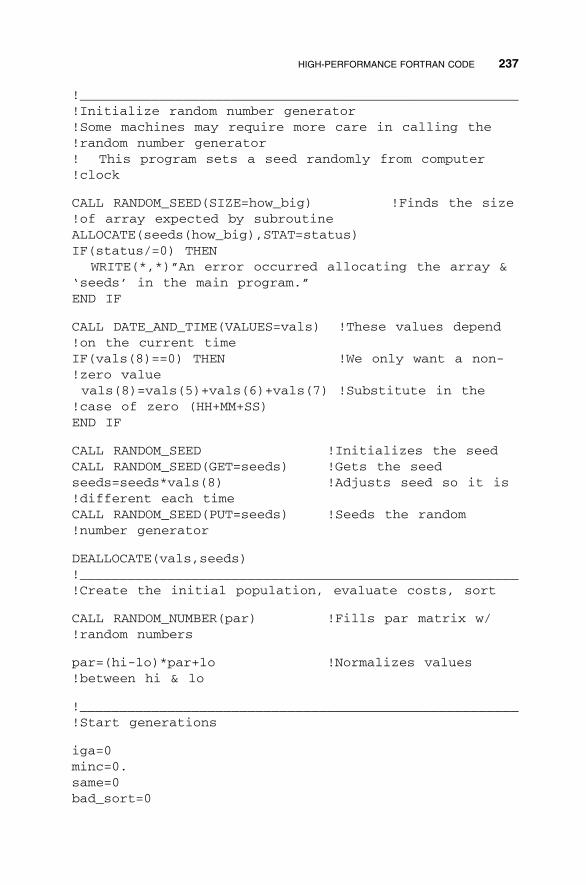
!_______________________________________________________!Initialize random number generator!Some machines may require more care in calling the !random number generator! This program sets a seed randomly from computer !clock
CALL RANDOM_SEED(SIZE=how_big) !Finds the size !of array expected by subroutineALLOCATE(seeds(how_big),STAT=status)IF(status/=0) THEN
WRITE(*,*)”An error occurred allocating the array &‘seeds’ in the main program.”END IF
CALL DATE_AND_TIME(VALUES=vals) !These values depend !on the current timeIF(vals(8)==0) THEN !We only want a non-!zero valuevals(8)=vals(5)+vals(6)+vals(7) !Substitute in the
!case of zero (HH+MM+SS)END IF
CALL RANDOM_SEED !Initializes the seedCALL RANDOM_SEED(GET=seeds) !Gets the seedseeds=seeds*vals(8) !Adjusts seed so it is !different each timeCALL RANDOM_SEED(PUT=seeds) !Seeds the random !number generator
DEALLOCATE(vals,seeds)!_______________________________________________________!Create the initial population, evaluate costs, sort
CALL RANDOM_NUMBER(par) !Fills par matrix w/ !random numbers
par=(hi-lo)*par+lo !Normalizes values !between hi & lo
!_______________________________________________________!Start generations
iga=0minc=0.same=0bad_sort=0
HIGH-PERFORMANCE FORTRAN CODE 237
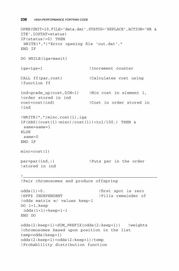
OPEN(UNIT=10,FILE=’data.dat’,STATUS=’REPLACE’,ACTION=’WR &ITE’,IOSTAT=status)IF(status/=0) THENWRITE(*,*)”Error opening file ‘out.dat’.”
END IF
DO WHILE(iga<maxit)
iga=iga+1 !Increment counter
CALL ff(par,cost) !Calculates cost using !function ff
ind=grade_up(cost,DIM=1) !Min cost in element 1, !order stored in indcost=cost(ind) !Cost in order stored in !ind
!WRITE(*,*)minc,cost(1),igaIF(ABS((cost(1)-minc)/cost(1))<tol/100.) THEN &same=same+1
ELSEsame=0
END IF
minc=cost(1)
par=par(ind,:) !Puts par in the order !stored in ind
!_______________________________________________________!Pair chromosomes and produce offspring
odds(1)=0. !first spot is zero!HPF$ INDEPENDENT !Fills remainder of !odds matrix w/ values keep-1DO i=1,keepodds(i+1)=keep+1-i
END DO
odds(2:keep+1)=SUM_PREFIX(odds(2:keep+1)) !weights !chromosomes based upon position in the listtemp=odds(keep+1)odds(2:keep+1)=odds(2:keep+1)/temp!Probablility distribution function
238 HIGH-PERFORMANCE FORTRAN CODE
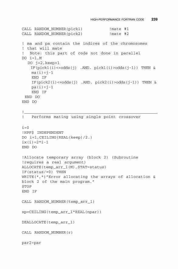
CALL RANDOM_NUMBER(pick1) !mate #1CALL RANDOM_NUMBER(pick2) !mate #2
! ma and pa contain the indices of the chromosomes ! that will mate! Note: this part of code not done in parallelDO i=1,M
DO j=2,keep+1IF(pick1(i)<=odds(j) .AND. pick1(i)>odds(j-1)) THEN &ma(i)=j-1END IFIF(pick2(i)<=odds(j) .AND. pick2(i)>odds(j-1)) THEN &pa(i)=j-1END IF
END DOEND DO
!_______________________________________________________! Performs mating using single point crossover
i=0!HPF$ INDEPENDENTDO i=1,CEILING(REAL(keep)/2.)ix(i)=2*i-1END DO
!Allocate temporary array (block 2) (Subroutine !requires a real argument)ALLOCATE(temp_arr_1(M),STAT=status)IF(status/=0) THENWRITE(*,*)”Error allocating the arrays of allocation &block 2 of the main program.”STOPEND IF
CALL RANDOM_NUMBER(temp_arr_1)
xp=CEILING(temp_arr_1*REAL(npar))
DEALLOCATE(temp_arr_1)
CALL RANDOM_NUMBER(r)
par2=par
HIGH-PERFORMANCE FORTRAN CODE 239
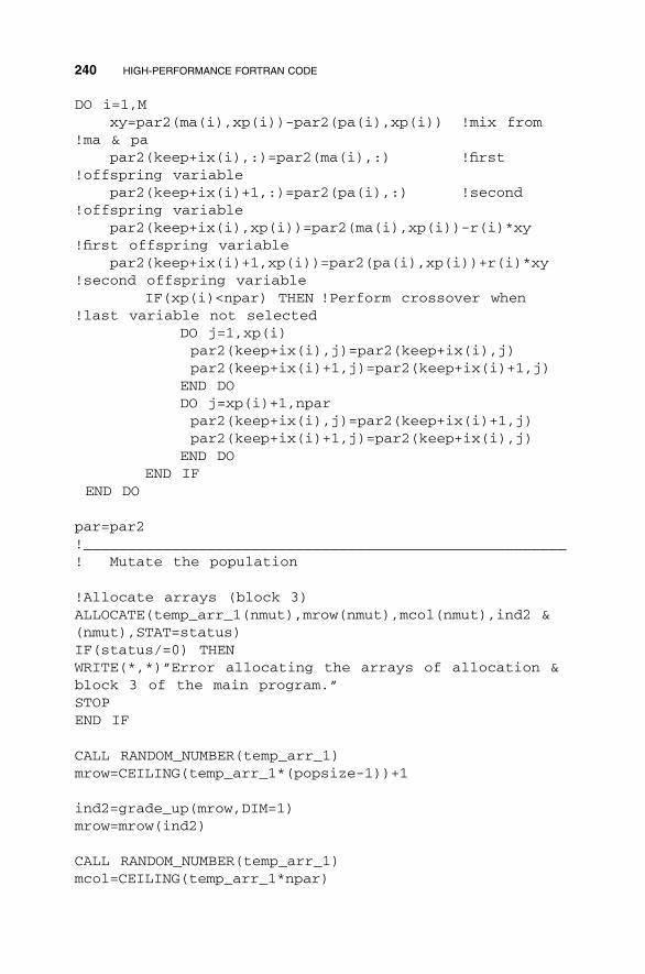
DO i=1,Mxy=par2(ma(i),xp(i))-par2(pa(i),xp(i)) !mix from
!ma & papar2(keep+ix(i),:)=par2(ma(i),:) !first
!offspring variablepar2(keep+ix(i)+1,:)=par2(pa(i),:) !second
!offspring variablepar2(keep+ix(i),xp(i))=par2(ma(i),xp(i))-r(i)*xy
!first offspring variablepar2(keep+ix(i)+1,xp(i))=par2(pa(i),xp(i))+r(i)*xy
!second offspring variableIF(xp(i)<npar) THEN !Perform crossover when
!last variable not selectedDO j=1,xp(i)par2(keep+ix(i),j)=par2(keep+ix(i),j)par2(keep+ix(i)+1,j)=par2(keep+ix(i)+1,j)
END DODO j=xp(i)+1,nparpar2(keep+ix(i),j)=par2(keep+ix(i)+1,j)par2(keep+ix(i)+1,j)=par2(keep+ix(i),j)
END DOEND IF
END DO
par=par2!_______________________________________________________! Mutate the population
!Allocate arrays (block 3)ALLOCATE(temp_arr_1(nmut),mrow(nmut),mcol(nmut),ind2 &(nmut),STAT=status)IF(status/=0) THENWRITE(*,*)”Error allocating the arrays of allocation &block 3 of the main program.”STOPEND IF
CALL RANDOM_NUMBER(temp_arr_1)mrow=CEILING(temp_arr_1*(popsize-1))+1
ind2=grade_up(mrow,DIM=1)mrow=mrow(ind2)
CALL RANDOM_NUMBER(temp_arr_1)mcol=CEILING(temp_arr_1*npar)
240 HIGH-PERFORMANCE FORTRAN CODE
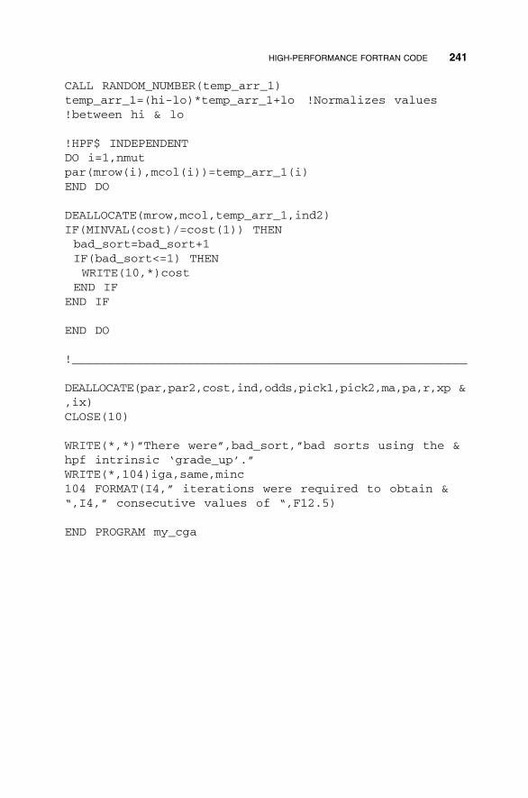
CALL RANDOM_NUMBER(temp_arr_1)temp_arr_1=(hi-lo)*temp_arr_1+lo !Normalizes values !between hi & lo
!HPF$ INDEPENDENTDO i=1,nmutpar(mrow(i),mcol(i))=temp_arr_1(i)END DO
DEALLOCATE(mrow,mcol,temp_arr_1,ind2)IF(MINVAL(cost)/=cost(1)) THENbad_sort=bad_sort+1IF(bad_sort<=1) THENWRITE(10,*)cost
END IFEND IF
END DO
!_______________________________________________________
DEALLOCATE(par,par2,cost,ind,odds,pick1,pick2,ma,pa,r,xp &,ix)CLOSE(10)
WRITE(*,*)”There were”,bad_sort,”bad sorts using the &hpf intrinsic ‘grade_up’.”WRITE(*,104)iga,same,minc104 FORMAT(I4,” iterations were required to obtain &“,I4,” consecutive values of “,F12.5)
END PROGRAM my_cga
HIGH-PERFORMANCE FORTRAN CODE 241
GLOSSARY
243
This book has a mixture of biology, mathematics, and computer terms. Thisglossary is provided to help the reader keep the terminology straight.
Allele The value of a gene. In biology, one of the functional forms of a gene.Age of a chromosome The number of generations that a chromosome has
existed.Ant colony optimization A global optimization method that mimics the
optimal path laid by ants to a food source.Building block Short schemata that give a chromosome a high fitness and
increase in number as the GA progresses.Chromosome An array of parameters or genes that is passed to the cost
function.Coarse-grained genetic algorithm A parallel GA implementation in which
subpopulations are housed on individual processors and evolve separatelywith limited communication between the subpopulations.Also known as anisland GA.
Cellular genetic algorithm A parallel GA implementation where each indi-vidual is housed on its own processor and communication lines are limitedto the nearest neighbors. Also called fine grained.
Comma strategy The process in which the parents are discarded and the offspring compete.
Converge Arrive at the solution.A gene is said to have converged when 95%of the chromosomes contain the same allele for that gene. GAs are con-sidered converged when they stop finding better solutions.
Convergence rate The speed at which the algorithm approaches a solution.Cooperation The behavior of two or more individuals acting to increase the
gains of all participating individuals.Cost Output of the cost function.Cost function Function to be optimized.Cost surface Hypersurface that displays the cost for all possible parameter
values.
Practical Genetic Algorithms, Second Edition, by Randy L. Haupt and Sue Ellen Haupt.ISBN 0-471-45565-2 Copyright © 2004 John Wiley & Sons, Inc.
Crowding factor model An algorithm in which an offspring replaces a chromosome that closely resembles the offspring.
Crossover An operator that forms a new chromosome from two parent chromosomes by combining part of the information from each.
Crossover rate A number between zero and one that indicates how frequently crossover is applied to a given population.
Cycle crossover A method of crossover for permutation problems in whicha point is initially chosen for exchange of genes between the parents; thenthe remainder of the operator involves “cycling” through the parents toeliminate doubles in the offspring.
Darwinism Theory founded by Charles Darwin that evolution occursthrough random variation of heritable characteristics, coupled with naturalselection (survival of the fittest).
Deceptive functions Functions that are difficult for the genetic algorithm tooptimize.
Diploid A pair of chromosomes carrying the full genetic code of an organism.
Dynamic parameter encoding The GA increases the binary precision withtime, or the GA keeps the same number of bits in a gene but narrows thesearch space.
Elitism The chromosome with the best cost is kept from generation to generation.
Environment That which surrounds an organism.Epistasis The interaction or coupling between different parameters of a cost
function. The extent to which the contribution to fitness of one genedepends on the values of other genes. Highly epistatic problems are diffi-cult to solve, even for GAs. High epistasis means that building blocks cannotform, and there will be deception.
ES See evolution strategy.Evolution A series of genetic changes in which living organisms acquire the
characteristics that distinguish it from other organisms.Evolution strategy (ES) A type of evolutionary algorithm developed in the
early 1960s in Germany. It typically uses deterministic selection, crossover,continuous parameters, and mutation.
Evolutionary algorithm Any computer program that uses the concept of biological evolution to solve problems. Examples include genetic algo-rithms, genetic programming, evolutionary strategies, and evolutionary programming.
Evolutionary computation Design or calculations done using an evolution-ary algorithm.
Evolutionary programming (EP) An evolutionary algorithm developed byLawrence J. Fogel in 1960. It typically uses tournament selection, continuousvariables, and no crossover.
244 GLOSSARY
Extremum A maximum or a minimum.Fine-grained GA A parallel GA implementation where each individual is
housed on its own processor and communication lines are limited to thenearest neighbors. Often called cellular GA.
Fitness Opposite of cost. A value associated with a chromosome that assignsa relative merit to that chromosome.
Fitness function Has the negative output of the cost function. Mathematicalsubroutine that assigns a value or fitness to a set of variables.
Fitness landscape The inverted cost surface. The hypersurface obtained byapplying the fitness function to every point in the search space.
Fitness proportionate selection Chromosomes are assigned a probability ofselection based upon their rank in the population.
Function optimization Process of finding the best extremum of a function.Function set A group of functions that are available for a GP to use.Gamete Cells with haploid chromosomes that carry genetic information
from their parents for the purposes of sexual reproduction. In animals, malegametes are called sperm and female gametes are called ova.
Gene The binary encoding of a single parameter. A unit of heredity that is transmitted in a chromosome and controls the development of a trait.
Gene flow Introduction of new genetic information by introducing new indi-viduals into the breeding population.
Gene frequency The incidence of a particular allele in a population.Generation One iteration of the genetic algorithm.Generation gap A generation gap algorithm picks a subset of the current
population for mating.Genetic algorithm (GA) A type of evolutionary computation devised by
John Holland. It models the biological genetic process by includingcrossover and mutation operators.
Genetic drift Changes in gene/allele frequencies in a population over manygenerations, resulting from chance rather than selection. Occurs mostrapidly in small populations. Can lead to some genes becoming “extinct,”thus reducing the genetic variability in the population.
Genetic programming (GP) Genetic algorithms applied to computer programs.
Genotype The genetic composition of an organism. The information con-tained in the genome.
Genome The entire collection of genes (and hence chromosomes) possessedby an organism.
Global minimum True minimum of the entire search space.Global optimization Finding the true optimum in the entire search
space.
GLOSSARY 245
Gray code Binary representation of a parameter in which only one bitchanges between adjacent quantization levels.
Hamming distance The number of bits by which two codes (chromosomes)differ.
Haploid chromosome A chromosome consisting of a single sequence ofgenes. The number of chromosomes contained in the gamete. Half thediploid number.
Hard selection When only the best available individuals are retained for generating future progeny.
Heterozygous The members of a gene pair are different.Hillclimbing Investigates adjacent points in the search space, and moves in
the direction giving the greatest increase in fitness. Exploitation techniquesthat are good at finding local extrema.
Homozygous Both members of a gene pair are the same.Hybrid genetic algorithm A genetic algorithm combined with other opti-
mization techniques.Individual A single member of a population that consists of a chromosome
and its cost function.Inversion A reordering operator that works by selecting two cut points in a
chromosome, and reversing the order of all the genes between those twopoints.
Island genetic algorithm A parallel GA implementation in which subpopu-lations are housed on individual processors and evolve separately withlimited communication between the subpopulations. Also referred to ascourse-grained GA.
Kinetochore The random point on a chromosome at which crossover occurs.
Lamarckism Theory of evolution that preceded Darwin’s. Lamarck believedthat evolution resulted from the inheritance of acquired characteristics.Theskills or physical features acquired by an individual during its lifetime canbe passed on to its offspring.
Lifetime How many generations a chromosome stays in the population untilit is eliminated.
Local minimum A minimum in a subspace of the search space.Master–slave genetic algorithm A parallel GA implementation in which the
primary control is maintained by a master processor and cost function eval-uations are sent out to slave processors. Also known as global, panmictic,or micrograined GA.
Mating pool A subset of the population selected for potential parents.Meiosis The type of cell division that occurs in sexual reproduction.Messy genetic algorithm Invented to conquer deceptive functions. The first
step (primordial phase) initializes the population so it contains all possible
246 GLOSSARY
building blocks of a given length. In this phase only reproduction is used to enrich the set of good building blocks. The second step (juxtapositionphase) uses various genetic operators to converge.
Micro genetic algorithm A GA that uses small populations sizes.Migration The transfer of the genes of an individual from one subpopula-
tion to another.MIMD Multiple instructions, multiple data. A parallel computer with each
processor working independently on its own dataMitosis Reproduction of a single cell by splitting. Asexual reproduction.Multimodal Cost surface with multiple minima.Multiple objective optimization (MOO) Optimization in which the objective
function returns more than a single value.Mutation A reproduction operator that randomly alters the values of genes
in a parent chromosome.Mutation rate Percentage of bits in a population mutated each iteration of
the GA.Natural selection The most-fit individuals reproduce, passing their genetic
information on to their offspring.Nelder-mead downhill simplex algorithm A nonderivative, robust local opti-
mization method developed in 1965.Neural network An algorithm modeling biological nervous systems consist-
ing of a large number of highly interconnected processing elements calledneurons that have weighted connections called synapses.
Niche The survival strategy of an organism (grazing, hunting, on the ground,in trees, etc.). Species in different niches (e.g., one eating plants, the othereating insects) may coexist side by side without competition. If two speciesoccupy the same niche, the weaker species will be made extinct. Diversityof species depends different niches or geographical separation. Each peakin the cost function is analogous to a niche.
Objective function The function to be optimized.Object variables Parameters that are directly involved in assessing the rela-
tive worth of an individual.Off-line performance An average of all costs up to the present generation.
It penalizes the algorithm for too many poor costs, and rewards the algo-rithm for quickly finding where the lowest costs lie.
Offspring An individual generated by any process of reproduction.On-line performance The best cost found up to the present generation.Optimization The process of iteratively improving the solution to a problem
with respect to a specified objective function.Order-based problem A problem where the solution must be specified in
terms of an arrangement (e.g., a linear ordering) of specific items, forexample, traveling salesperson problem, computer process scheduling.
GLOSSARY 247
Order-based problems are a class of combinatorial optimization problemsin which the entities to be combined are already determined.
Order crossover (OX) A crossover method for dealing with a permutationoperator that strives to preserve portions of the absolute ordering of eachparent.
Ontogeny The developmental history (birth to death) of a single organism.Panmictic genetic algorithm A parallel GA implementation in which the
primary control is maintained by a master processor and cost function eval-uations are sent out to slave processors. Also known as a master–slave GA.
Parallel genetic algorithm A genetic algorithm written to run on a parallel-processing computer.
Parent An individual that reproduces to generate one or more other indi-viduals, known as offspring, or children.
Pareto front All Pareto optimal solutions for a given problem.Pareto genetic algorithm A GA whose population approximates the Pareto
front.Pareto optimal A point is Pareto optimal if decreasing the cost of one cost
function causes an increase in cost for at least one of the other cost functions.
Parse tree A method of following the flow of a computer program.Partially matched crossover (PMX) A reordering operator where two
crossover points are chosen, the values between these points exchanged,then a careful procedure followed to eliminate any repeated numbers fromthe solution.
Particle swarm optimization A global optimization method that mimics theoptimal swarm behavior of animals such as birds and bees.
Performance Usually some statistical evaluation of the cost or fitness overall generations.
Permutation problem A problem that involves reordering a list.Phenotype The environmentally and genetically determined traits of an
organism. These traits are actually observed.Phylogeny The developmental history of a group of organisms.Plus strategy The process in which the parents and offspring compete.Point mutation Alters a single feature to some random value.Population A group of individuals that interact (breed) together.Quadratic surface Bowl-shaped surface.Random seed A number passed to a random number generator that the
random number generator uses to initialize its production of randomnumbers.
Rank selection Chromosomes are assigned a probability of selection basedon their rank in the population.
248 GLOSSARY
Recombination Combining the information from two parent chromosomesvia crossover.
Reordering Changing the order of genes in a chromosome to try to bringrelated genes closer together and aid in the formation of building blocks.
Reproduction The creation of offspring from two parents (sexual reproduc-tion) or from a single parent (asexual reproduction).
Reproduction operator The algorithmic technique used to implement reproduction.
Roulette wheel selection Picks a particular population member to be aparent with a probability equal to its fitness divided by the total fitness ofthe population.
Scaling Used to bring the range of costs into a desirable range. Often usedto make all the costs positive or negative.
Schema (pl. schemata) Bit pattern in a chromosome. For instance, the pat-terns 1100110 and 1000011 both match the schema 1**0011, where * indi-cates a 1 or a 0.
Schema theorem A GA gives exponentially increasing reproductive trials toschemata with above average fitness. Because each chromosome containsa great many schemata, the rate of schema processing in the population isvery high, leading to a phenomenon known as implicit parallelism. Thisgives a GA with a population of size N a speedup by a factor of N cubed,compared to a random search.
Search space All possible values of all parameters under consideration.Search operators Processes used to generate new chromosomes.Seeding Placing good guesses to the optimum parameter values in the initial
population.Selection The process of choosing parents for reproduction (usually based
on fitness).Selection pressure Ratio of the probability that the most fit chromosome is
selected as a parent to the probability that the average chromosome isselected.
Self-adaptation The inclusion of a mechanism to evolve not only the objectvariables of a solution but simultaneously information on how each solu-tion will generate new offspring.
Simple genetic algorithm A GA with a population, selection, crossover, andmutation.
Simulated annealing A stochastic global optimization technique derivedfrom statistical mechanics.
Single-point crossover A random point in two chromosomes (parents) isselected. Offspring are formed by joining the genetic material to the rightof the crossover point of one parent with the genetic material to the left ofthe crossover point of the other parent.
GLOSSARY 249
Simulation The act of modeling a process.SISD Single instruction, multiple data. A parallel computer performing the
same operation, on different items of data at the same time in lockstep.Soft selection Some inferior individuals in a population are allowed to
survive into future generations.Speciation The process of developing a new species. The most common form
of speciation occurs when a species is geographically separated from themain population long enough for their genes to diverge due to differencesin selection pressures or genetic drift. Eventually the genetic differences aregreat enough for the subpopulation to become a new species.
Species A group of organisms that interbreed and are reproductively iso-lated from all other groups. A subset of the population.
Stagnation The algorithm no longer finds an improved solution, even thoughit has not found the best solution.
Steady state genetic algorithm Every new offspring produced replaces ahigh-cost chromosome in the population.
Subpopulation A subset of the main population in which individuals mayonly mate with others in the same subset.
Survival of the fittest Only the individuals with the highest fitness valuesurvive.
Tabu search A search algorithm that keeps track of high-cost regions, thenavoids those regions.
Terminal set Variables and constants that are available for manipulation bythe GP.
Test function A cost or fitness function used to gauge the performance of aGA.
Tournament selection Picks a subset of the population at random, thenselects the member with the best fitness.
Truncation selection Chromosomes whose cost is below a certain value (thetruncation point) are selected as parents for the next generation.
Two-point crossover A crossover scheme that selects two points in the chro-mosome and exchanges bits between those two points.
Uniform crossover Randomly assigns the bit from one parent to one off-spring and the bit from the other parent to the other offspring.
250 GLOSSARY
AAir pollution model 175Allele 20Analytical optimization 7Ant colony optimization (ACO) 18,
190Antenna 81Art 71Artificial neural networks 179Attractor 170
BBeowulf cluster 144Binary crossover 42, 110Binary GA 27, 135Binary GA flowchart 29Binomial 83Blending 57BLX-a 58Bracketing 3Broyden-Fletcher-Goldfarb-Shanno
(BFGS) algorithm 17, 164
CCellular GA 140Chromosome 19, 30, 35Chromosome age 118Chromosome life 118Cognitive parameter 190Complementary sampling 117Constraints 4, 31Continuous crossover 56, 111Continuous GA 51, 135Continuous GA flowchart 52Continuous optimization 4Contraction 11
Convergence 47, 64, 107Cooling schedule 188Coordinate search 13Cost function 30Cost function reformulation 83Cost function weighting 99Cost weighting 40Creative process 74Crossover mask 112Crossover point 42, 57, 105, 197Crossover rate 117Cultural algorithms 199Cycle crossover (CX) 126, 152
DDavidon-Fletcher–Powell (DFP)
algorithm 17De Jong test functions 128Decoding a secret message 155Demes 139Discrete optimization 4Dispersion law 177Dogs 28Dominant gene 90Dominating solution 100Dynamic optimization 4Dynamical problems 170
EElitism 43, 61Emergency response unit 77, 153End-effector 159Epistasis 32Evolution 19Evolutionary strategies 18, 199Exhaustive search 5
INDEX
251
Practical Genetic Algorithms, Second Edition, by Randy L. Haupt and Sue Ellen Haupt.ISBN 0-471-45565-2 Copyright © 2004 John Wiley & Sons, Inc.
252 INDEX
Expansion 10Expensive cost function 95Extrapolating 58
FFeasible region 98Fine-grained GA 140Fitness 30
GGA advantages 23GA advantages 23GA parameters 109, 127Gene 19Gene size 106Genetic programming (GP) 195Genotype 20Global minimum 3Gradient 8, 15Gray codes 104, 154
HHamming distance 104Hessian 16Horses 86Hybrid GA 101
IIdentical chromosomes 95Initial population 27, 54, 96, 117Injection island GA 140Integer programming 10Inverse model 165Islands 139Iterative function system 72
JJuxtaposition 137
KKorteweg-de Vries equation 182
LLagrange multiplier 8, 18Laplacian 8Learning factor 190Line minimization 13Linear programming 9LISP 196
Local minimum 3Log-sigmoid transfer function 180
MMary Had a Little Lamb 67Master-slave algorithm 138Mating 41, 56, 197MATLAB 211Messy GA 136Metagenetic algorithm 129Migration rate 139Minimum-seeking algorithms 5(m + l) evolution strategy 199(m,l) evolution strategy 199Multi-objective GA 100Multiple objective optimization 97Music 67Mutation 43, 60, 121, 198
NNatural optimization 18, 54Natural selection 19, 36Nelder-Mead downhill simplex
algorithm 10, 102, 181Newton’s method 15No free lunch theorem 187Nondominated sorting GA 100Normalized cost 40Normalized variables 54
OObjective function 30Off-line performance 128Offspring 42, 115On-line performance 128Optimization 2Optimum mutation rate131Optimum population size 131Order crossover (OX) 125
PPairing 38, 56Panmictic GA 139Parallel GA 137Parallel GA advantages 137Parameter control 135Pareto front 98Pareto GA 99Pareto GA flowchart 102
INDEX 253
Pareto optimal solution 99Pareto optimization 99Partially matched crossover (PMX) 125Particle swarm optimization (PSO) 189Particle velocity 190Permutation problems 124, 151Phenotype 20Pheromone 193Pollution 175Population 21, 36, 117Predator-prey model 171Primordial phase 137
QQuadratic programming 18Quantization 33–35Quantization error 35, 107Quantization levels 34Quasi-Newton techniques 17
RRadar cross section 161Random pairing 39Rank weighting 39Reflection 10Robot trajectory planning 156Rocky Mountain National Park 28Root finding 3Rosenbrock method 14Roulette wheel selection 39, 134
SSchema 108Schema theorem 107Seeding 120Selecting GA parameters 127Selection 38Selection rate 36Sharing 100Shrinkage 11
Simplex 10Simulated annealing 187Single point crossover 110Social parameter 190Solitary wave 182Speedup curve 142Standard normal distribution 61Static optimization 4Stealth airplane 161Steepest descent algorithm 15Subjective cost function 69Subpopulations 139Synchronous island GA 139
TTaylor series 16Test functions 205Thresholding 38Tournament selection 40, 134Traveling salesperson problem 151, 193Two point crossover 110
UUniform crossover 112Unnormalized variable 54
VVariable decoding 32, 34Variable encoding 32, 34Variable mutation rate 121, 135Variable population size 120, 135Vector-evaluated GA 100
WWeighted random pairing 39Weighting factors 88Word guess 75
Zz-transform 83