WP/06/81

Practical Model-Based Monetary Policy Analysis—A How-To Guide

Andrew Berg, Philippe Karam, and Douglas Laxton

© 2006 International Monetary Fund WP/06/81

IMF Working Paper

Policy Development and Review Department, Research Department, and IMF Institute

Practical Model-Based Monetary Policy Analysis—A How-To Guide

Prepared by Andrew Berg, Philippe Karam, and Douglas Laxton

Authorized for distribution by Andrew Berg, Gian Maria Milesi-Ferretti, and Ralph Chami

March 2006

Abstract

This Working Paper should not be reported as representing the views of the IMF. The views expressed in this Working Paper are those of the author(s) and do not necessarily represent those of the IMF or IMF policy. Working Papers describe research in progress by the author(s) and are published to elicit comments and to further debate.

This paper provides a how-to guide to model-based forecasting and monetary policy analysis.It describes a simple structural model, along the lines of those in use in a number of central banks. This workhorse model consists of an aggregate demand (or IS) curve, a price-setting (or Phillips) curve, a version of the uncovered interest parity condition, and a monetary policy reaction function. The paper discusses how to parameterize the model and use it for forecasting and policy analysis, illustrating with an application to Canada. It also introduces aset of useful software tools for conducting a model-consistent forecast. JEL Classification Numbers: E52, E47, C51, C63 Keywords: Monetary Policy, Forecasting and Simulation, Model construction and estimation,

computational techniques Author(s) E-Mail Address: aberg@imf.org, dlaxton@imf.org, pkaram@imf.org

- 2 -

Contents Page

I. Introduction ............................................................................................................................4

II. The Model .............................................................................................................................6 A. Output Gap Equation ................................................................................................7 B. Phillips Curve............................................................................................................8 C. Exchange Rate.........................................................................................................10 D. Monetary Policy Rule .............................................................................................11 E. Solving the Model ...................................................................................................13

III. Building the Model ............................................................................................................13

IV. Forecasting and Policy Analysis........................................................................................18

V. An Example.........................................................................................................................21 A. Overview.................................................................................................................21 B. Building the Model..................................................................................................24 C. Using the Model ......................................................................................................29

VI. Conclusions........................................................................................................................34

References................................................................................................................................62 Tables 1. Structural Parameters – Canada..........................................................................................51 2. Structural Parameters – United States ................................................................................52 3. Baseline Forecast with Desk Judgment – WEO Scenario ..................................................53 4. Temporary 50 Percent Increase in Oil Price, 2005–07.......................................................54 5. United States: Temporary 50 Percent Increase in Oil Price, 2005–07 ..............................55 6. Canada: Temporary 50 Percent Increase in Oil Price, 2005–07........................................56 7. Canada: Canadian Interest Rate Shock – One Quarter Increase of 100 b.p. .....................57 8. United States: U.S. Interest Rate Shock – One Quarter Increase of 100 b.p. ....................58 9. Canada: Temporary Canadian Dollar Depreciation Shock................................................59 10. United States: U.S. Demand Shock – Temporary 0.5 p.p. Increase .................................60 11. Canada: U.S. Demand Shock – Temporary 0.5 p.p. Increase...........................................61 Figures 1. Output Growth, Inflation, Interest Rates, and Exchange Rates...........................................45 2. Inflation in Canada Compared to the Inflation Target Path.................................................46 3. Model Variables for Canada................................................................................................47 4. Model Variables for the United States.................................................................................48 5. Dynamic Responses of Output, Inflation, and Short-Term Interest Rates in Canada.........49 6. Dynamic Responses of Output, Inflation, and Short-Term Interest Rates in the United States....................................................................................................................50

- 3 -

Appendices I. Programs to Implement the Forecasting and Policy Analysis System .................................36 II. Complete Model Equations.................................................................................................39 III. On The Supply Side of The Model ....................................................................................41 IV. Calculating of the Long-Run Equilibrium and the LRX Filter..........................................43

- 4 -

“All models are wrong! Some are useful” –George Box

I. INTRODUCTION The goal of this paper is to describe a macro-model-based approach to forecasting and monetary policy analysis and to introduce a set of tools that are designed to facilitate this approach. We hope that many economists engaged in applied policy analysis at the Fund will adopt and eventually develop and enrich these tools, moving on to richer models as necessary. We also expect that insights these economists gain will in turn be useful to the broader academic community. A companion (Berg, Karam, and Laxton 2006) paper provides a broader overview of this approach and contrasts it with both the financial programming approach, which emphasizes the role of monetary aggregates in analyzing the monetary sector, and with more econometrically driven analyses.1 The model presented here ignores a number of critical issues. It abstracts from issues related to aggregate supply and fiscal solvency and does not explore the determinants of the current account, the equilibrium levels of real GDP, the real exchange rate, or the real interest rate. Its advantage is that it can be relatively transparent and simple and still allow consideration of the key features of the economy for monetary policy analysis. Broader considerations are of course essential to policy analysis and forecasting. The framework described below allows judgment about them to be incorporated into the model’s forecasts and the implications of different assumptions to be explored. But the model itself provides little direct help in articulating their determinants. Because the model abstracts from so many issues, there may be a tendency to add various features to the model. One attractive feature of the general approach we suggest is that such models are, in somewhat more complicated form, at the heart of both central bank practice and current research efforts worldwide. Thus, there is enormous scope to develop the model further. It is important, though, that additions not detract from the clarity of the model. Where the skills and resources are available, the model may be extended to include full microeconomic foundations, stock-flow dynamics, nontraded sectors, and other features that allow explicit treatment of a number of additional issues.2 The model should not be allowed to become a “black box” however. One intermediate approach may be to build an auxiliary model for, say, fiscal policy, which considers the expenditure component of government spending, the implications for households’ intertemporal savings decisions, and so on. The

1There is substantial overlap between the two papers. The overview paper targets mainly newcomers to modern structural macroeconomic modeling and potential consumers. This paper contains more nuts-and-bolts detail for modelers. The overview paper thus expands on the material in the introduction to this paper and contains an abbreviated treatments of the remaining sections. 2The IMF’s Global Economy Model (GEM), described in Laxton and Pesenti (2003), for example, represents such a model. The set of tools that we rely upon for our simple model, described in Appendix I, are similar to those required to work with the GEM.

- 5 -

overall implications of policy for aggregate demand could then be integrated into the core model.3 We present here a simple model that blends the New Keynesian emphasis on nominal and real rigidities and a role of aggregate demand in output determination, with the real business cycle tradition methods of dynamic stochastic general equilibrium (DSGE) modeling with rational expectations. The model is structural because each of its equations has an economic interpretation. Causality and identification are not in question. Policy interventions have counterparts in changes in parameters or shocks, and their influence can be analyzed by studying the resulting changes in the model’s outcomes. It is general equilibrium because the main variables of interest are endogenous and depend on each other. It is stochastic in that random shocks affect each endogenous variable and it is possible to use the model to derive measures of uncertainty in the underlying baseline forecasts. It incorporates rational expectations because expectations depend on the model's own forecasts, so that there is no way to consistently fool economic agents.4 There is a significant literature emerging where models are derived explicitly from microeconomic foundations.5 The core elements include consumers who maximize expected utility and firms that are subject to monopolistic competition and adjust prices only periodically. Micro-foundations are ultimately critical and should play a central role in determining the model's specification. More generally, the purpose of the model is to organize thoughts and data coherently, and so the model itself must be coherent and embody the economic ideas the modeler seeks to emphasize. However, we do not derive our baseline model below from microeconomic foundations. We allow for adaptive as well as rational expectations and substantial inertia in the equations. We could appeal to theory to justify these features, but we do not believe that, in practice, appealing to specific micro foundations serves to tie down magnitudes. We believe that this pragmatic approach to modeling represents the current state of the art in many policymaking institutions, where “modelers embrace theory but do not feel compelled to marry it.”6 We take an eclectic approach to parameterizing the model. In our view, and as reflected in the practice of most central banks, a purely econometric approach is not generally feasible. The economy is characterized by a high degree of simultaneity and forward-looking

3The IMF has also developed a multicountry, new-open-economy macro model to study the medium-term and long-term implications of fiscal policies. See Botman and others (2005).

4We say “consistently” because it may be appropriate to extend the model to incorporate an element of adaptive expectations.

5See Gali and Monacelli (2002) and Monacelli (2004) for micro-founded models along these lines.

6Leeper (2003) uses this terminology to describe model building in central banks. As discussed in footnote 2, many central banks recently have been developing models with stronger micro-foundations that can be relied upon as their core analytical framework. However, until these models have been taken to the data and tested thoroughly, it may be premature to try to jump to them, particularly in the absence of experience with simpler models with less rigid theoretical structures.

- 6 -

behavior, while data series are generally short and subject to structural change, for example in the monetary policy regime. In this context, it is not possible to reliably estimate parameters and infer cause and effect. More fundamentally, purely empirically based models do not permit the analysis of changes in policy rules or changes in the assumptions about how the economy works. For purposes of policy analysis, the model must first be identified, meaning that each of the equations must have a clear economic interpretation. Thus, rather than estimate a reduced-form, empirically based model whose structural interpretation is doubtful, we suggest using a broader collection of information to help parameterize a structural macroeconomic model. This eclectic approach dominates the practice of most central banks engaged in inflation targeting. Perhaps the only novelty in what we suggest, from this point of view, is an emphasis on Bayesian estimation techniques which helps to formalize the estimation/calibration process that takes place in central banks. New tools are only just appearing that allow the analyst to easily ask the extent to which available data is consistent with her priors about the parameters of the model. For our purposes, this is the right question to ask, rather than allowing the data alone to identify or parameterize the model, or to test classical hypotheses such as whether interest rates affect the economy or not.7 The next section introduces and discusses a simple benchmark model. Section III discusses how to match the model with reality. Section IV describes how to conduct a forecasting and monetary policy analysis with the model. Section V puts the model through its paces, parameterizing it for Canada and carrying out a forecasting and risk assessment exercise. Section VI concludes. Appendix I describes tools available from the authors that implement the procedures described in the paper. Appendix II lists the main behavioral equations, identities, and statistical assumptions of the core model. Appendix III discusses the rudimentary supply-side features of the model, and Appendix IV describes the filtering methodologies in calculating the long-run or equilibrium notions of some main macroeconomic variables.

II. THE MODEL At its core, the model has four equations: (1) an aggregate demand or IS curve that relates the level of real activity to expected and past real activity, the real interest rate, and the real exchange rate; (2) a price-setting or Phillips curve that relates inflation to past and expected inflation, the output gap, and the exchange rate; (3) an uncovered interest parity condition for the exchange rate, with some allowance for backward-looking expectations; and (4) a rule for

7The Bayesian approach has a number of obvious advantages, but the main one is that it improves the transparency of the model-building process by forcing the model builder to reveal her priors—see Sims (2002), among others. With the development of more powerful and user-friendly programs, we anticipate that a growing number of economists will be relying upon these techniques. To download programs for analysis and Bayesian estimation using DYNARE (a highly specialized toolbox for simulating and estimating dynamic stochastic general equilibrium models), go to http://www.cepremap.cnrs.fr/dynare/.

- 7 -

setting the policy interest rate as a function of the output gap and expected inflation.8 The model expresses each variable in terms of its deviation from equilibrium, in other words in “gap” terms. The model itself does not attempt to explain movements in equilibrium real output, the real exchange rate, the real interest rate, or the inflation target. Rather, these are taken as given. In all, it is an “aggregated” model that accentuates the flow dynamics of the model and leaves the full integration of stocks and flows for future research or a possible extension to this paper.

A. Output Gap Equation

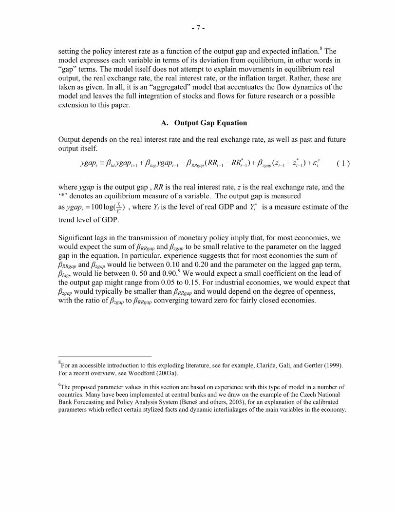
Output depends on the real interest rate and the real exchange rate, as well as past and future output itself.

ytttzgapttRRgaptlagtldt zzRRRRygapygapygap εββββ +−+−−+≡ −−−−−+ )()( *

11*

1111 ( 1 )

where ygap is the output gap , RR is the real interest rate, z is the real exchange rate, and the ‘*’ denotes an equilibrium measure of a variable. The output gap is measured as 100log( )t

t

Yt Y

ygap ∗= , where Yt is the level of real GDP and ∗tY is a measure estimate of the

trend level of GDP. Significant lags in the transmission of monetary policy imply that, for most economies, we would expect the sum of βRRgap and βzgap to be small relative to the parameter on the lagged gap in the equation. In particular, experience suggests that for most economies the sum of βRRgap and βzgap would lie between 0.10 and 0.20 and the parameter on the lagged gap term, βlag, would lie between 0. 50 and 0.90.9 We would expect a small coefficient on the lead of the output gap might range from 0.05 to 0.15. For industrial economies, we would expect that βzgap would typically be smaller than βRRgap and would depend on the degree of openness, with the ratio of βzgap to βRRgap converging toward zero for fairly closed economies.

8For an accessible introduction to this exploding literature, see for example, Clarida, Gali, and Gertler (1999). For a recent overview, see Woodford (2003a).

9The proposed parameter values in this section are based on experience with this type of model in a number of countries. Many have been implemented at central banks and we draw on the example of the Czech National Bank Forecasting and Policy Analysis System (Beneš and others, 2003), for an explanation of the calibrated parameters which reflect certain stylized facts and dynamic interlinkages of the main variables in the economy.

- 8 -

B. Phillips Curve

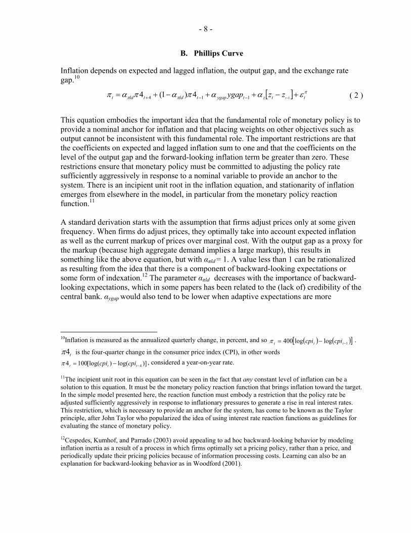
Inflation depends on expected and lagged inflation, the output gap, and the exchange rate gap.10

[ ] πππ εααπαπαπ ttztygaptldtldt tzzygap +−++−+= −−−+ 1114 4)1(4 ( 2 )

This equation embodies the important idea that the fundamental role of monetary policy is to provide a nominal anchor for inflation and that placing weights on other objectives such as output cannot be inconsistent with this fundamental role. The important restrictions are that the coefficients on expected and lagged inflation sum to one and that the coefficients on the level of the output gap and the forward-looking inflation term be greater than zero. These restrictions ensure that monetary policy must be committed to adjusting the policy rate sufficiently aggressively in response to a nominal variable to provide an anchor to the system. There is an incipient unit root in the inflation equation, and stationarity of inflation emerges from elsewhere in the model, in particular from the monetary policy reaction function.11 A standard derivation starts with the assumption that firms adjust prices only at some given frequency. When firms do adjust prices, they optimally take into account expected inflation as well as the current markup of prices over marginal cost. With the output gap as a proxy for the markup (because high aggregate demand implies a large markup), this results in something like the above equation, but with απld = 1. A value less than 1 can be rationalized as resulting from the idea that there is a component of backward-looking expectations or some form of indexation.12 The parameter απld decreases with the importance of backward-looking expectations, which in some papers has been related to the (lack of) credibility of the central bank. αygap would also tend to be lower when adaptive expectations are more

10Inflation is measured as the annualized quarterly change, in percent, and so ( ) ( )[ ]1loglog400 −−= ttt cpicpiπ .

t4π is the four-quarter change in the consumer price index (CPI), in other words

)]log()[log(1004 4−−= ttt cpicpiπ , considered a year-on-year rate.

11The incipient unit root in this equation can be seen in the fact that any constant level of inflation can be a solution to this equation. It must be the monetary policy reaction function that brings inflation toward the target. In the simple model presented here, the reaction function must embody a restriction that the policy rate be adjusted sufficiently aggressively in response to inflationary pressures to generate a rise in real interest rates. This restriction, which is necessary to provide an anchor for the system, has come to be known as the Taylor principle, after John Taylor who popularized the idea of using interest rate reaction functions as guidelines for evaluating the stance of monetary policy.

12Cespedes, Kumhof, and Parrado (2003) avoid appealing to ad hoc backward-looking behavior by modeling inflation inertia as a result of a process in which firms optimally set a pricing policy, rather than a price, and periodically update their pricing policies because of information processing costs. Learning can also be an explanation for backward-looking behavior as in Woodford (2001).

- 9 -

important, because the output gap works in part through its influence on expected future price changes.13 The behavior of the economy depends critically on the value of απld. If απld is equal to 1, inflation is equal to the sum of all future gaps. A small but persistent increase in interest rates will have a large and immediate effect on current inflation. In this “speedboat” economy, small recalibrations of the monetary-policy wheel, if perceived to be persistent, will cause large jumps in inflation through forward-looking inflation expectations effects. If απld is close to 0, on the other hand, current inflation is a function of all lagged values of the gaps, and only an accumulation of many periods of interest rate adjustments can move current inflation toward some desired path. In this “aircraft carrier” economy, the wheel must be turned well in advance of the date at which inflation will begin to change substantially.14 Where price-setting is flexible and the monetary authorities are fully credible, high values of απld might be reasonable, but for most countries, values of απld significantly below 0.50 seem to produce results that are usually considered to be more consistent with the data. The value of αz determines the effects of exchange rate changes on inflation. It should be expected to be larger in economies that are very open and in cases when there is a high proportion of imported goods (either final or intermediate goods) that are eventually consumed after processing and then distributed as final consumption goods. Higher pass-through is generally observed in countries where monetary policy credibility is low and where the value-added of the distribution sector is low. There is also significant evidence of

13We can make the adaptive expectations more explicit by nesting rational expectations in a formulation according to which expected inflation at one period is assumed to be some weighted average of model-consistent rationally expected inflation and lagged inflation. Thus, replace 14 4)1(4 −+ −+ tldtld παπα ππ with

∑ = ++ =4

144j

ejt

et ππ , where

( ) 11 4 j

e ej j

et j t j t t

π

π ππ α π α π ε+ + −= + − +

where, as usual , jt+π is model-consistent forecast of inflation at time t+j. This captures the reasonable possibility that agents may over time place different weights on the model-consistent rational inflation forecast (i.e., the best one, given the model) and history. For example, if there is learning about the nature of the model or the monetary policy reaction function, e

jπα might increase with j.

When we apply the model to the data, we can associate survey or other direct measures of inflation expectations with e

t 44 +π .

14Woodford (2003a and 2003b) shows that smoothing in the policy rate is optimal in models where steering future inflation expectations is important. Generally, the optimal amount of interest rate smoothing will be less in models with more intrinsic inertia in the inflation process, but the general understanding is that the behavior of the entire system is important in generating desirable outcomes for inflation expectations.

- 10 -

pricing-to-market behavior in many economies, suggesting that αz would be considerably smaller than the import weight in the CPI basket.15

C. Exchange Rate

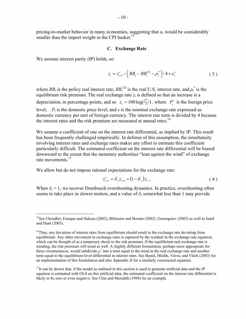
We assume interest parity (IP) holds, so:

*1 / 4e US z

t t t t t tz z RR RR ρ ε+ ⎡ ⎤= − − − +⎣ ⎦ ( 3 )

where RRt is the policy real interest rate, RRt

US is the real U.S. interest rate, and ρt* is the

equilibrium risk premium. The real exchange rate zt is defined so that an increase is a depreciation, in percentage points, and so )log(100

t

FtP

sPtz = , where F

tP is the foreign price

level, Pt is the domestic price level, and s is the nominal exchange rate expressed as domestic currency per unit of foreign currency. The interest rate term is divided by 4 because the interest rates and the risk premium are measured at annual rates.16 We assume a coefficient of one on the interest rate differential, as implied by IP. This result has been frequently challenged empirically. In defense of this assumption, the simultaneity involving interest rates and exchange rates makes any effort to estimate this coefficient particularly difficult. The estimated coefficient on the interest rate differential will be biased downward to the extent that the monetary authorities “lean against the wind” of exchange rate movements.17

We allow but do not impose rational expectations for the exchange rate:

( ) 111 1 −++ −+= tztzet zzz δδ ( 4 )

When δz = 1, we recover Dornbusch overshooting dynamics. In practice, overshooting often seems to take place in slower motion, and a value of δz somewhat less than 1 may provide

15See Choudhri, Faruqee and Hakura (2002), Billmeier and Bonato (2002), Gueorguiev (2003) as well as Isard and Hunt (2003). 16Thus, any deviation of interest rates from equilibrium should result in the exchange rate deviating from equilibrium. Any other movement in exchange rates is captured by the residual in the exchange rate equation, which can be thought of as a temporary shock to the risk premium. If the equilibrium real exchange rate is trending, the risk premium will trend as well. A slightly different formulation, perhaps more appropriate for these circumstances, would subdivide ρt

* into a term equal to the trend in the real exchange rate and another term equal to the equilibrium level differential in interest rates. See Beneš, Hlédik, Vávra, and Vlček (2003) for an implementation of this formulation and also Appendix II for a similarly constructed equation.

17It can be shown that, if the model as outlined in this section is used to generate artificial data and the IP equation is estimated with OLS on this artificial data, the estimated coefficient on the interest rate differential is likely to be zero or even negative. See Chin and Meredith (1998) for an example.

- 11 -

more realistic dynamics. Unfortunately, there is little consensus across countries or observers on a reasonable value for δz .18

D. Monetary Policy Rule

We assume that the monetary policy instrument is based on some short-term nominal interest rate, and that the central bank sets this instrument in order to achieve a target level for inflation, π*. It may also react to deviations of output from equilibrium: * *

1 4 4(1 )*( 4 4 ) RS

t RSlag t RSlag t t t ygap t ttRS RS RR ygapπγ γ π γ π π γ ε− + +

⎡ ⎤= + − + + − + +⎣ ⎦ ( 5) The structure and parameters of this equation have a variety of implications, which have been explored in a large numbers of papers.19 An important conclusion from assessments of monetary policy in the 1970s, and one embedded in the structure of this model, is that a stable inflation rate implies a positive πγ .20 Beyond this, our framework does not allow explicit discussion of optimality, because of the absence of microeconomic foundations.21 But it may be useful to note that how strongly the authorities should react depends on the other features of the economy. If the economy is very forward-looking, for example, as implied by the “speedboat” version of the Phillips curve above, then only mild but persistent reactions to expected inflation should be enough to keep inflation close to target. If, on the other hand, the Phillips curve is of the “aircraft carrier” type, then a more aggressive reaction in the short run may be appropriate. In setting policy, it is important to consider the potential losses stemming from making the wrong set of assumptions about the nature of the economy. If the economy is a speedboat (high απld), and the authorities assume otherwise and react aggressively to inflation deviations, the costs may not be too high. If the economy is an aircraft carrier (low απld) and the policymaker assumes it is a speedboat, small interventions (low γπ) that are expected to

18The value of δz matters for forecasting and policy analysis. When δz = 1, the real exchange rate will be a function of the future sum of real interest differentials (and risk premia) and will provide a very direct and forward-looking channel through which monetary policy will operate. Some policymakers have argued that more robust policies should assume a much smaller value of δz because it may be imprudent to rely so heavily on these forward-looking linkages in the face of uncertainty. Isard and Laxton (2000) show that under uncertainty about the value of δz ,it will be prudent to assume that δz is slightly below 0.5 because of larger and asymmetric costs that would result from assuming extreme values such as zero or one.

19For a brief introduction to the vast literature evaluating alternative monetary policy rules, see Hunt and Orr (1999) and Taylor (1999).

20See Clarida, Gali, and Gertler (1999) for a summary of this issue. The original 1993 Taylor rule imposed a zero weight on interest rate smoothing ( RSlagγ = 0) and implied a πγ (a backward-looking, year-on-year

measure of inflation in that case) of 0.5 and a value for ygapγ of 0.5.

21The analyst could create a loss function that depends on the variance of output and inflation deviations from equilibrium and use stochastic simulations of the model to determine how, in the face of a given pattern of shocks, a particular rule performs. See, for example, Svensson (2000), Hunt and Orr (1999) and Taylor (1999).

- 12 -

be adequate turn out to be inadequate in keeping the inflation rate from moving well away from the target. The implication is that it may be better to assume that the economy behaves a bit more like an aircraft carrier, just to be safe. We assume that the central bank smoothes interest rates, adjusting them fairly slowly to the desired value based on deviations from equilibrium of inflation and output. This feature is not easily rationalized, though it is widely observed (a typical smoothing value for RSlagγ in empirically based reaction functions generally falls between 0.50 and 1.0). Woodford (2003b) emphasizes that high weights on the lagged interest rate in the reaction function may represent optimal inertia in the policy rate, as it allows smaller current changes in short-term rates to have larger effects on rates of returns in financial markets and the real economy, if they generate expectations that the changes will persist. It is unclear whether uncertainty also contributes to inertia in the policy rate, with some approaches suggesting it does and other approaches suggesting that concerns about uncertainty should make policy actions more aggressive in some circumstances and less constrained by past policy rates.22 Instruments other than the interest rate can be accommodated, and arguments other than inflation and output may belong in the reaction function. A variety of papers have explored in particular the question of whether the exchange rate belongs in the reaction function.23 The exchange rate does not belong directly in the objective function as long as the exchange rate is a purely forward-looking variable, as it contains no unique information about the state of the economy. In a broader formulation, though, this may be the case.24

22For a comparison of results in both linear and nonlinear models with endogenous policy credibility and NAIRU uncertainty, see Isard and Laxton (1998). 23For example, Parrado (2004) estimates a reaction function for Singapore in which the instrument is the change in the exchange rate. See also Lubik and Schorfheide (2003) for an extensive assessment of this issue, in an estimated Bayesian model. Ho and McCauley (2003) discuss the not so widely appreciated “Singaporean view.” It holds that when an economy is sufficiently open, and the pass-through sufficiently high, stabilizing inflation requires close management of the effective exchange rate (Monetary Authority of Singapore, 2001). This is in essence what inspired the estimation of an alternative version of the Taylor rule that uses the effective exchange rate rather than the short-term interest rate as the policy instrument. 24When δz = 1, the real exchange rate is fully determined by the future sum of the real interest rate differential and risk premium, and so it is not a state variable. Not surprisingly, in linear macro models, it is generally found that the optimal weight on the exchange rate in simple reaction functions such as the Taylor rule is very small, especially in cases that allow for model-consistent forecasts of inflation in the reaction function. However, in models that allow for serially correlated errors in exchange rate expectations (δz < 1), there will be a role for monetary policy to respond directly to exchange rate changes. In addition, in nonlinear models where there can be first-order welfare implications from allowing excessive variability in exchange rates, there will be an additional role for monetary policy to prevent large swings in exchange rates. See Hunt, Isard, and Laxton (2003) as well as Elekdag and Tchakarov (2004).

- 13 -

E. Solving the Model

Software tools now exist that largely automate solving the types of models that we are considering.25 It may nonetheless be useful to provide a brief overview of what is involved. The first step is to find the steady-state solution of the model. This can be found by replacing all leads and lags of each endogenous variable by the contemporaneous values, and then solving this transformed system of equations (in other words, replace ygapt, ygapt+1, and ygapt-1 with ygap and so on.) In our case, we find that ygap = 0, πgap = 0, RRgap = 0, and zgap = 0. The second step is to unravel the dynamic properties of the model. Since the equations have leads and lags, it is not obvious where to start in tracing out the effects of a change in say εy. An approach that does not rely on linearity or other features of this particular model is to solve the model as a two-point boundary problem. The model is assumed to start in long-run equilibrium at some initial date and to end in equilibrium at some future date. A solution is a trajectory for the endogenous variables, given a set of values for the parameters and the exogenous variables (here, the shocks), that achieve these two end-point conditions. A useful diagnostic device for understanding the properties of a model is to examine how the endogenous variables respond to a particular shock. For purposes of deriving such an impulse response, the shocks are set to zero except for one contemporaneous shock, and the model is solved as described above. It may also be interesting to carry out a stochastic simulation, in which the shocks are drawn many times from assumed distributions and the model solved each time. The resulting variability in the endogenous variables may shed light on various properties of the model. For example, as described above, the implications of different monetary policy rules for output variability can be explored.

III. BUILDING THE MODEL We have argued that a simple New Keynesian monetary model of the sort we outlined above can be useful for answering some important policy questions and can represent a redundant initial building block for an institution striving to develop a better set of tools to support more rigorous, consistent, and logical policy analysis. But the answers it produces will depend critically on the parameter values as well the type of model that is being constructed. The older conventional approach to econometric estimation focused extensively on time series data, and the objective was to identify stable parameters across both time and the

25The main software we have used for this paper is TROLL (www.intex.com) and FAME (www.fame.com). All of the programs we have used to solve the model and study its properties are described in Appendix I and can be obtained from the authors. See Armstrong and others (1998) and Juillard and others (1998) for a description of the properties of the two Newton-based simulation algorithms available in TROLL.

- 14 -

potential regime changes being considered by the analysts. This methodology, while useful for characterizing patterns in data, has failed systematically as a single unifying methodology for parameterizing macro models and for using such models for policy analysis. Consequently, some policymaking institutions have rejected estimation approaches based on fitting individual equations and placed more emphasis on the process of calibration in the design of macro models.26 Unfortunately, the word “calibration” initially was connected to the early real business cycle (RBC) literature at the time, which largely ignored some basic regularities in the time series data. Inside policymaking institutions, however, the shift to calibration did not mean that conventional estimation exercises were abandoned entirely, but simply that at the end of the day parameters were chosen based partly on econometric results and partly on examining the system properties of the models. Calibration procedures continued to be developed in both academic and policymaking institutions. First, rather than focusing on a simple set of summary diagnostic statistics on macroeconomic variability, they were gradually extended to replicate impulse response functions in vector auto regressive (VAR) and other models. Second, in cases where calibrated models were successful at building on past empirical work by replicating macroeconomic dynamics that were not inconsistent with previous models, or disagreed in ways that simply pointed out the logical failures of earlier models, it represented an important argument for their use both inside and outside of policymaking institutions. The fact that several important opinion leaders threw their support behind the calibration approach also provided encouragement. However, the disadvantages of calibration methods remain well known. While it is possible to do logical and informal inferences about macro dynamics, the methodology does not lend itself very easily to formal statistical inference, which has always been an important priority in both academic and policymaking circles. In this vein, there have been some very useful developments in Bayesian econometrics. Bayesian estimation theory has always offered a number of advantages over conventional estimation approaches, but was considered impractical because of enormous computational costs and complexity. However, the recent development of more efficient and user-friendly estimation procedures are making it more and more the technique of choice for applied macro modelers. Still, Bayesian techniques have only been tested on relatively small macro models and it may take some time to develop a critical mass of highly trained specialists who can use such methods in day-to-day work. Because it is necessary to develop sensible priors and models before enduring the expensive computational investment that is required to simply estimate one model with Bayesian techniques, the strategy seems clear in the short run. Based on our own, albeit, limited personal experiences with these techniques, we suggest the following six-step strategy for

26For a discussion of estimation issues of models designed for monetary policy analysis, see Coletti and others (1996), Hunt, Rose, and Scott (2000), Beneš and others (2003), Faust and Whiteman (1997), and Kapetanios, Pagan, and Scott (2005).

- 15 -

economists who are interested in developing these small models for monetary policy analysis. 1. Look at existing models and how they have been used to address interesting and

relevant policy questions. Does a small model like the one suggested here have anything to offer, or is it necessary to move to a different type of model? How many resources will it take? Would it perhaps be useful to start with a smaller model even though one would hope to extend it relatively quickly to address a larger range of questions? Many policymaking institutions have preferred to follow this approach out of a fear that large-scale model projects may be difficult to implement, use extensive resources, and end up becoming black boxes that only the modelers really understand.

2. As a practical step, it may be best to look at the properties of existing models and

to use this as a guide for calibration and model design. This may be particularly useful in cases where different institutions may have a comparative advantage in certain aspects of the model-building process. For example, central banks with years of experience working under flexible exchange rate regimes will usually have invested significant resources building models and subjecting them to tests. In fact, in some cases they may have highly specialized information to help out with the calibration when it comes to identifying particular shocks or episodes where monetary policy was important in initiating a disturbance to the economy, such as in a disinflation process.

3. Develop an initial working version of the model. Choose coefficients that seem

reasonable based on economic principles, available econometric evidence, and an understanding of the functioning of the economy, and then assess the system properties of the resulting model. An iterative process evolves in which reasonable coefficient values are chosen, the properties of the model are examined, and changes are made to the structure of the model until the model behaves appropriately.

4. Consider a formal model comparison exercise in which the model’s properties

are compared with other models. In some cases this will suggest weaknesses in the model’s structure, while in many other cases there will simply be legitimate differences in views that are embodied in the models. In the latter case, these differences in views can be used as a rough, but perhaps very useful, measure of model uncertainty, and in such cases the model can be generalized to study the policy implications of alternative views. Indeed, a major benefit of using models for policy analysis is that they can provide a more systematic and structured approach for studying the policy implications of uncertainty.

5. When resources are available, the next stage should be to consider a formal

Bayesian estimation strategy. The Bayesian approach essentially formalizes the approach that practitioners have been using, but in a manner that allows for statistical inference because probabilities can be assigned to alternative models. However, even if the ultimate goal is to develop a model that is estimated with formal Bayesian

- 16 -

techniques, it may be prudent to follow steps 1-4 as a method for developing experience in designing sensible models and priors.

6. It is important to understand that model-building projects can contribute to the

development of institutional knowledge and that this process of building a model and using a model for forecasting and policy analysis usually evolves over a period of years. Without models that embody the basic economic principles, policy advice runs the risk of being inconsistent across time in ways that sometimes defy logic and reason. In the first instance, the model project should seek to establish the basic guiding principles of the model or family of models to be considered based on the particular issues to be addressed. The model does not have to be perfect to be useful. Again, a very useful strategy is to start simple and then to extend the model over time as suggested by experience.

Two sorts of practical questions immediately emerge. How do we choose reasonable coefficients, and how do we judge the resulting performance of the model? Turning to the last question first, the adequacy of a model for policy analysis will depend on how well it captures key aspects of the monetary policy transmission mechanism. For example, the model should provide reasonable estimates of: how long it takes a shock to the exchange rate to feed into the price level; the size of the "sacrifice ratio," in other words the amount of output that must be foregone to achieve a given permanent reduction in the rate of inflation; and how the inflation rate responds to the output gap. A developer or user of the model should have a “good feel” for the performance of the economy in these terms. Indeed, a major advantage of this approach is that it forces attention on a few basic questions and places less emphasis in the short run on complicated technical econometric issues, which in many cases in the past have been more distracting than useful. We should emphasize that we would encourage model builders to eventually move to formal estimation procedures as long as the approach does not become captured by some inappropriate econometric methodology that is incapable of answering the right questions.27 Some of this “feel,” may come from an examination of “natural experiments,” in which the analyst effectively identifies a shock based on specialized knowledge of the policy process and can trace out its effects. For example, a look at past disinflation episodes may shed some light on measures of the historical sacrifice ratio. Another approach is to examine the properties of models that have been developed over time in central banks and other policy institutions. In cases where such models are used for day-to-day policy analysis, the results may correspond with the collective judgment of the policymakers and thus may represent a convenient insight into that judgment.28 A comparison with well-established models from 27For a critical assessment of approaches that are based excessively on letting the data speak for designing policy models see Coletti and others (1996); Faust and Whiteman (1997); Hunt, Rose, and Scott (2000), Coats, Laxton, and Rose (2003); and Berg, Karam, and Laxton (2006a).

28 See also Schmidt-Hebbel and Tapia (2002), who have compiled views about the monetary policy transmission mechanism and other features of the economy from twenty central banks. We are not arguing that all models should try to replicate the exact properties or policy insights of other models because such a process

(continued…)

- 17 -

similar countries may be helpful, and also where statistical approaches such as structural vector auto regressive (SVAR) model can shed light on some of these questions. Having first focused on the overall performance of the resulting model, we next tackle the question of how to bring as much garnered information to bear as possible on the structure of the model and the choice of coefficients. The accumulated experience with similar models and theory as discussed in Section III and the variety of more systematic tools available can provide some guidance In traditional calibration exercises of models with explicit micro-foundations, estimates of structural parameters such as the intertemporal elasticity of substitution and degree of habit persistence can be drawn from other studies. It is critical that the model we use be reasonably well grounded in theory, given that we do not apply a data-driven specification process. Moreover, an understanding of the underlying structural determinants of the main parameters may help with parameterization. However, while theory can rationalize for example the hump-shaped dynamics that are observed in the economy, at this point it does not serve to tie down precise magnitudes.29 A variety of econometric techniques can be useful in parameterizing the model. Single equation estimates can sometimes shed substantial light. For example, Orphanides (2003) provides reasonably clean estimates of the monetary policy reaction function of the U.S. Federal Reserve, using survey measures and the Fed’s Greenbook forecasts of expected inflation and the output gap to avoid the typical endogeneity and measurement problems associated with estimating forward-looking monetary policy reaction functions.30 Moreover, the application of various system estimation techniques to parameterize DSGE models and assess their performance is an active area of research. Recent developments in the application of Bayesian estimation to DSGE models of the economy represent a particularly promising

would be not be very productive. However, part of the process of convincing others is to first understand alternative views. For many countries where data samples are short and regimes have been evolving over time, significant insights can be gleaned by studying the experiences of other countries rather than investing solely in one econometric approach that focuses on one data set and one particular econometric strategy. Obviously, in cases where ample resources are available, researchers may want to pursue alternative strategies to develop perspectives that are not biased by previous approaches.

29 Research is now directed at improving the microeconomic foundations of these sorts of models to make them more consistent with the inertia in the data. For example, Cespedes, Kumhof, and Parrado (2003) provide a model of inflation inertia. A choice-theoretic optimizing intertemporal framework such as the IMF's GEM possesses a well-defined macroeconomic structure with the full set of features required to reproduce the data––see Laxton and Pesenti (2003). Many smaller policy models now make reference to larger structural models that are more complex than the models we consider here in their nonlinear structure and solution methods. In certain policy settings, these larger models have been considered as complements to the small model constructs and as a check to their validity.

30 We use a similar inflation-forecast-based (IFB) rule that Orphanides estimates and allow the user to choose his estimated rule as an option. Another recent example is Parrado (2004), who estimates a monetary policy reaction function and a Phillips curve for Singapore.

- 18 -

way to permit the data to speak in a way that is consistent with the practical approach we suggest.31 Bayesian methodology involves posterior estimation and an evaluation of data likelihood given the parameters, the model, and a prior density. The analyst first approaches the data with a set of prior views on the appropriate model and the values of the parameters of the model, then asks whether those views ought to be modified in light of the data at hand—i.e., in what way do the data suggest a modification of those views? The methodology we have outlined can be thought of as the procedure for developing this prior information. At this point we do not see the Bayesian estimation, or any econometric techniques, as alternatives to the parameterization techniques described here. An overly econometric approach to model-building does not as yet lead to the simple, identified, useful sort of models we have in mind. Indeed, an emphasis on data fitting can lead, in practice, to models that lack critical features such as forward-looking inflation expectations, on the grounds that such features are much harder to implement empirically. The absence of such features leaves estimated models misspecified and, of course, also more vulnerable to the Lucas critique, in that changes in the monetary policy reaction function, for example, lose a channel through which to influence other equations. While the goal is not to merely fit the data, one piece of the parameterization puzzle will be to ask what the data say about the parameters. The analyst incorporates this information into the model and moves on to the next step.

IV. FORECASTING AND POLICY ANALYSIS A model of the sort we describe can be very helpful in the process of forecasting and making monetary policy, judging from the successful experience of a large number of central banks. The model itself does not make the central forecast. The forecast itself may come from some combination of several sources: forecasting models of various sorts; market expectations; judgments of senior policymakers; and, most importantly for the IMF, interactions with the country authorities themselves.32 The model can serve, however, to frame the discussion about the forecast, risks to the forecast, appropriate responses to a variety of shocks, and dependencies of the forecast and policy recommendations on various sorts of assumptions about the functioning of the economy. In this section we outline a four-step procedure for creating and using model-based forecasts for monetary policy analysis, given that a model has already been developed:33 31See Smets and Wouters (2004) and Juillard and others (2005) for some recent applications. 32It can be very useful to have a model-based forecast that abstracts from all this judgmental input so that it can be compared with the actual forecast to measure the value added by basing forecasts on many different types of information that are deliberately not included in the model. For an illustrative study of the important role of judgmental pooling of information in the Fed’s Greenbook forecasts, see Sims (2002).

33The programs are described in Appendix I and available from the authors on request. Also available are detailed “help” files.

- 19 -

1. The analyst starts with actual data on real GDP, the CPI (headline and perhaps core), the policy interest rate, the exchange rate, and the world interest rate and world CPI.34 This HNTF database (for historical and near-term forecast) may also contain purely judgmental forecasts out several quarters for these same variables. There are two distinct reasons for including pure judgment forecasts in this database. • It is usually appropriate to treat judgmental near-term forecasts as actual data,

allowing the model forecasts to “kick in” only subsequently. For example, in many central banks, it is recognized that the model cannot do remotely as well as experts at forecasting the first one or two quarters. These are often based on preliminary related data (e.g., GDP may lag several months, but retail sales, industrial production etc. come out much more quickly).

• The database may contain a much longer judgmental forecast, for example several

years out, which may be interesting to analyze in light of the model. This could be a forecast provided by the authorities to Fund staff, for example.

2. The analyst creates estimates (over the period covered by the HNTF database) of the inflation target, potential output, and equilibrium real interest and exchange rates. As described in Appendix IV, these estimates should be based on a variety of sources. Of course, the monetary authorities often announce an inflation target. Estimates for the other series may come from including smoothing the original series and/or judgment-based assessments. 3. To carry out a forecasting exercise with the model, the analyst must know where the economy is at the start of the forecast period, from the point of view of the model. This includes the values of endogenous variables, which are in the database, and the current values of the residuals. One simple approach to finding these residuals is to create a “residual model” in which the residuals are declared to be endogenous and the normally endogenous variables such as the output gap and inflation are defined as exogenous. The model can then be solved for the values of the residuals that rationalize the paths of the endogenous variables in terms of the model.35

34In principle, the exchange rate that matters for the IS curve would be a trade-weighted real effective exchange rate, with a world CPI measured as a trade-weighted average of partner CPIs. For the exchange rate equation, the world interest rate and inflation might also be an average of world interest rates and inflation. In practice, it is often convenient and an acceptable approximation to use a bilateral exchange rate with the major trading partner and the trading partner CPI for the IS curve, and the same trading partner CPI and policy interest rate for the exchange rate equation.

35 In order to carry out this step, the forecasts in the HNTF database are first extended forward mechanically through the entire forecast period under the assumption that the endogenous values converge gradually to their equilibrium values. This preliminary “forecast” is required to calculate the residuals because the model is forward looking. In the “residual model,” the values of the residuals depend on the entire past and future trajectories of the normally endogenous variables. The tools made available to desk economists describe this procedure in more detail. Appendix I provides a quick description of the files needed to run the required programs.

- 20 -

The analyst now has a set of values for the residuals, past, present, and future, that is consistent with the model and the values of the endogenous variables in the HNTF database. The resulting historical residuals can be examined to see if they make sense, in other words to see if there are systematic deviations from the model that cannot be satisfactorily explained by factors known to be outside the model. For example, a large movement in the exchange rate that results from a fiscal crisis should cause large residuals in the exchange rate equation, because fiscal policy is not explicitly modeled. On the other hand, a consistent under-prediction of inflation would typically suggest that the model still needed work.36 4. We now turn to generating the forecasts. Three types of forecasts may be interesting: • A pure judgment forecast maintains the residuals as they were calculated in step 3.

Because of the way these residuals were calculated, the forecasts for the endogenous variables are exactly the values entered into the HNTF database. Where the HNTF database contains a several-year forecast of interest, these residuals are a measure of how much “twisting” is required to rationalize the forecast in terms of the model. The model is a gross simplification of reality, and the existence of residuals should not be a surprise. But sizable, serially correlated errors might suggest that the forecast may be ignoring the tensions inherent in the normal dynamic processes of the economy. Various experiments may be interesting, such as modifying the model itself to see under what assumptions the forecasts make more sense.

• A pure model-based forecast results from solving the model under the assumption

that all future residuals are zero.

• The forecast can be a hybrid of that implied by the judgmental forecast and the model. The analyst manipulates the future residuals (these judgmental residuals are often called add-factors, temps, or constant-term adjustment factors) or directly sets certain future values of endogenous variables (“tunes”) to create a forecast that combines judgment with the model. For example, the residuals from the end of the HNTF database are a measure of how far the current situation is away from the predictions of the model. It may be prudent to allow these residuals to shrink over a few quarters to zero rather than jump to the model forecasts, on the grounds that the model is missing something about the current situation and whatever this is should not be expected to disappear overnight.37 More generally, the analyst may be interested in fixing a path for, say, the policy interest rate for two or three quarters and observing the outcome of the model. Or, the analyst may believe that the model is underestimating growth may and adjust the forecasts accordingly.

36One should not fall into the trap of thinking of this model as an empirically driven data-fitting exercise. The maintained assumption of the model is that expectations are rational and shocks follow certain statistical patterns, including typically being zero mean. When the model is matched to a historical sample, the solution of the model is derived under assumptions that imply that the agents in the model "know" all the actual outcomes when forming expectations. 37This of course depends on the interpretation of the residuals, and in some cases, positive residuals may be expected to become negative in future periods depending on to what the forecaster ascribes them.

- 21 -

The hybrid forecast is at the heart of the forecasting and policy analysis exercise. First, it is in this context that the central forecast emerges, given that this forecast will rarely be purely model based but will involve substantial judgment about the evolution of the economy. Second, alternative scenarios, policies, and shocks can be examined. These would typically include: • Sensitivities to alternative assumptions. For example, the analyst might consider

alternative paths for the exchange rate and examine the effects of these alternative assumptions on the forecast, under the view that the link between interest rates and exchange rates is both difficult to predict and not well captured by the model. The analyst might also explore sensitivities to changes in the parameters or structure of the model or assumptions about equilibrium values such as potential output.

• Implications of various shocks. Where the model explicitly incorporates the shock in

question, such as with aggregate demand, prices, or the exchange rate, this is straightforward. Otherwise, substantial judgment is required to decide how, say, a supply shock might manifest itself in terms of the model.

• Alternative policy responses, including “add-factors” or “tunes” to the interest rate or

changes in the monetary policy reaction function.

V. AN EXAMPLE

A. Overview

We now demonstrate the entire process. First, we design, parameterize and test a model of the Canadian and U.S. economies.38 Second, we carry out a forecasting exercise, including a variety of sensitivity analyses and risk assessments. We base our forecasting exercise on a set of judgmental forecasts for Canadian and U.S. variables that extends through 2009. We will use the model to assess and carry out sensitivity analysis with respect to this purely judgmental forecast. On our part, we choose the Canadian and U.S. economies in part to emphasize that calibration and use of this sort of model is not a mechanical exercise, but one that requires significant familiarity and experience working on these economies, as is essential to develop and use any model wisely.39

38We have begun work to formally estimate the simple model using Bayesian methods. However, since the first step in Bayesian estimation is to specify sensible priors, it is necessary to have a good working knowledge of the model’s properties under sensible parameter values before proceeding to estimation.

39A more extensive example of the implementation of a similar model can be found in Coats, Laxton, and Rose (2003).

- 22 -

Most of the key equations of the model are presented in Appendix II. The equations follow a similar structure as in the canonical model presented in Section II, except that they have been modified to reflect a key feature of the Canadian economy, its dependence on the U.S. economy and the importance of oil prices. The simple canonical model presented earlier has been extended so that the Canadian output gap also depends on the U.S. output gap. In addition, to control for the effects in changes in the real price of oil on inflation and real GDP in both economies, the model has been augmented in the following way. First, we add the contemporaneous and lagged value of changes in the real price of oil to the inflation equations in both countries.40 Second, to control for effects on aggregate demand and supply on real GDP, we add a four-quarter moving average of the price of oil to the equation that determines potential output. The output gap for Canada becomes:

1 1 1 1US ygap

t ld t lag t RRgap t zgap t USygap t tygap ygap ygap RRgap zgap ygapβ β β β β ε+ − − −= + − + + + (6)

where the parameter βUSygap measures the importance of demand conditions in the United States on the Canadian economy. The equation for output gap for the U.S. economy has the same structure except the real exchange rate gap and the external output gap have been removed from the equation.41 The extended inflation equations for headline CPI inflation for both the Canadian and U.S. economies become,

[ ] πππ επαπαααπαπαπ ttrpoiltrpoiltztygaptldtldt tzzygap +++−++−+= −−−+ − 1,1,0114 14)1(4 (7)

where πrpoil,t = 400[log(poilt/cpit)-log(poilt-1/cpit-1)] and the two additional parameters (α0, α1) are based to a large extent on the importance of value added of oil and gas in the respective CPI baskets of the two countries. Because policymakers in both countries also focus on a core measure of inflation that excludes volatile items such as energy prices, we also include

40This specification picks up the relatively short lags at the quarterly frequency between oil prices and how they feed into energy prices in the CPI. In forecasting mode, significant information may be obtained by looking at the recent monthly movements in oil prices and trying to understand their pass-through into the recent monthly movements in the energy components of the CPI. This information can then be used to add judgmental adjustments to the quarterly forecast that better links monthly movements between these variables.

41We have recently developed another version of this basic model for the United States, Japan, and the euro area where each economy’s output gap depends on a weighted sum of the output gaps in the other economies.

- 23 -

another equation that has a very similar structure except we eliminate the direct effects of oil prices in this equation.42 The equation for core inflation is:

[ ] πππ εππαααπαπαπ tctctctzctyctcldctcldctc tzzygap ,1,13,,1,1,,4,,, ]44[4)1(4 1 +−+−++−+= −−−−+ − (8)

where an additional term [π4t-1- π4c,t-1] has been added to the simple canonical inflation equation to allow for the possibility of relative price and real wage resistance; or more precisely that workers and other price setters may try to partially keep their prices rising in pace with past movements in the headline CPI. Note, if the parameter αc,3 is zero, oil price shocks in the model will have no effect on core inflation and may not necessitate an increase in interest rates. However, to the extent that higher oil prices are an important input into the production costs of many consumer goods, or if workers resist the reduction in their real wages in response to an increase in oil prices, there should be a role for oil prices to play in the model.43

The equation that determines the evolution of potential output in both economies becomes:

** * *

1 ,400[ ] 4 yt t t rpoil rpoil t ty y g υ π ε−− = − + , (9)

where π4rpoil,t is the four-quarter moving average in the relative (real) price of oil and the parameter υ determines the effects of the relative price of oil on aggregate real GDP.

*tg represents the growth of potential output, as specified in Appendix II. The specifications

of these equations were chosen to approximately replicate the effects of oil price shocks in deeper structural models of the economy where oil is modeled explicitly as an input into the production process of tradables and nontradables as well as an input into an energy bundle that is combined with distribution services to produce a final energy bundle that enters the CPI.44

42 We had to add a measure of core inflation to the model because the Bank of Canada’s Quarterly Projection Model (QPM) uses this as its key inflation variable, and we wanted to do some comparisons across the two models.

43Of course, in theory it would always be better to have a more elaborate structural model to make these mechanisms clearer. For example, it would be better to have a more elaborate model with a wage-price sector. While it would not be difficult to build such a model for economies such as the United States and Canada, because of rich data sources and a large body of previous research, the development of little models like this one is motivated more by practical concerns such as transparency, data availability, and the amount of time economists have to allocate to model-based analysis.

44See Hunt (2005). Ben Hunt has extended the GEM to study the effects of oil price shocks on the U.S. economy, but he has also shared some simulation results with us for a model calibrated to Canada. We have chosen this very simple specification because it roughly mimics the properties of the GEM and other models like the Federal Reserve Board’s (FRB-US) that model oil as a factor of production.

- 24 -

B. Building the Model

Some history and data The top three panels of Figure 1 report year-on-year output growth, CPI inflation, and short-term interest rates for Canada, and, for reference, the United States. The bottom panel of Figure 1 reports the bilateral exchange rate between Canada and the United States. The close connection with U.S. GDP, interest rates, and inflation is evident. This sample covers a period of a flexible exchange rate regime, transitions between low (high) and high (low) inflation regimes in both countries, as well as a period for Canada that includes a formal inflation-targeting regime that started in 1992. Figure 2 reports CPI inflation for Canada, but in this case we have also included the numerical values for the inflation target as well as one-percentage-point bands so that outcomes can be compared with the target path. Inflation has been slightly below the inflation target path, but has remained inside the bands about two-thirds of the time. Figure 3 plots the trend and detrended measures of output, real interest rates, and the real exchange rate that will be used in the model. The trend measures of output in both countries were constructed using the LRX filter. The technical details of the LRX filter is explained in which Appendix III, which is simply a more general version of the original Hodrick-Prescott filter (1980) allows the analyst to impose priors for the trend values in situations where they believe they have more information than a naive univariate filter. In this case, for example, to be consistent with the staff’s view about the value of the output gap at the end of the sample, the trend value of output has been imposed to be 1.7 percent above actual output in 2004Q2 in the United States and 0.4 percent in the case of Canada.45 The historical values of the output gap are based on an HP smoothing parameter of 1600 (or higher). The trend real exchange rate is derived in a similar manner and is supposed to be equal to the actual real exchange rate in 2004Q1. The equilibrium short-term real interest rate is assumed to be constant at 2.5 percent in Canada and 2.25 percent in the United States, implying a steady-state, small-country risk premium of 25 basis points. Parameterization All of the parameters of the models for Canada and the United States are reported in Tables 1 and 2, respectively. They have been calibrated on the basis of the model’s system properties and by comparing the dynamics of the model with other models of the U.S. and Canadian economies.46 45Obviously, there is considerable uncertainty about these estimates. The advantage of having a model-based Forecasting and Policy Analysis System (dubbed FPAS) is that it is relatively easy to study the implications of different initial conditions for the output gap.

46For the model of the Canadian economy, we mainly examined the simulation properties of the Bank of Canada’s QPM model, although we also looked at the properties of a model called NAOMI developed by Steve Murchison at the Department of Finance, Canada. See Coletti and others (1996) and Murchison (2001). For the model of the U.S. economy, we looked at the properties of the FRB-US model. Good overviews of the structure

(continued…)

- 25 -

Output gap equations The first set of parameters in the tables report the values for the output gap equations for the two countries. For Canada in Table 1, we employ values of 0.10 and 0.05 for the parameters on the lagged real interest rate terms and real exchange rate (βRRgap and βzgap). This implies that the effect of a 100-basis-point increase in the real interest rates on the output gap would be equivalent to a 2 percent appreciation in the real exchange rate. These two parameters combined with a large values on the lagged gap term (βlag= 0.85) and a small value on the lead of the output gap (βlead = 0.10) result in hump-shaped dynamics in response to monetary induced interest rate shocks that do a satisfactory job replicating what is found in the Bank of Canada’s QPM model of the Canadian economy. To explain the strong correlation between the U.S. and the Canadian output gaps, we employ a fairly large parameter on the U.S. output gap in the Canadian output gap (βUSygap= 0.25). For the United States economy, we simply turn off the open-economy linkages in the model by eliminating the real exchange rate effect. Because we impose the same values on the lead and the lag of the output gap, the presence of the exchange rate channel results in a slightly faster and stronger monetary transmission mechanism in the model for Canada. Headline CPI inflation equations We set the weight on the lead terms in the inflation equation (απld) to 0.20 in both economies. This implies weights on the lagged inflation terms (1-απld) of 0.80, implying significant intrinsic inertia in the inflation process. These parameters, combined with the weight on the output gap, will be the principal determinants of the output costs of disinflation.47 We set the weights on the output gaps in both countries at 0.30, yielding a sacrifice ratio of around 1.3 in both countries.48 This sacrifice ratio is significantly lower than reduced-form econometric estimates of the sacrifice ratio that were estimated over sample periods that included transitions from low to high inflation in the late 1960s and early 1970s, or from high to low inflation in the early 1980s. Using quarterly data from 1964 to 1988, Cozier and Wilkinson estimate the sacrifice ratio to be around 2. A very similar sacrifice ratio is embodied in the Department of Finance’s NAOMI model and an even larger estimate of 3 is in the Bank of Canada’s QPM model. This is by design, as these econometric estimates reflect the experiences of slow learning associated with moving between high and low levels of

and properties of FRB-US can be found in Reifschneider, Tetlow, and Williams (1999) and Brayton and others (1997), but for a more complete description of the FRB-US model, see Brayton and Tinsley (1996). 47The output costs of disinflation in a model with rational expectations will depend on a number of parameters such as the speed at which inflation is being reduced, but the degree of inertia in the inflation equation as well as the weight on the output gap will be the principal determinants within plausible ranges for other parameters in the model.

48The sacrifice ratio is defined as the cumulative output losses associated with a permanent one percentage point decline in inflation. In quarterly models, this is computed by doing an experiment where the inflation target is reduced by one percentage point forever and then cumulating the effects on the annual output gap.

- 26 -

inflation regimes in the 1980s.49 As will be shown below when we do a formal analysis of the monetary transmission mechanism of Small Monetary Policy Models (dubbed SMPMOD) , this implies that inflation will respond more strongly to monetary-induced interest rate hikes than in the Bank of Canada’s QPM or the Federal Reserve Board’s FRB-US model. The next parameters in Table 1 and Table 2 are the weights on changes in the contemporaneous and lagged change in the real price of oil. These parameters are determined mainly on the basis of importance of energy in the headline CPI baskets as well as the importance of oil in the production of final energy components such as gasoline and fuel oil. For Canada, the weight of the energy component in the CPI that is most directly affected by oil prices is 5.2 percent.50 The share of valued added in the production of these final energy products in the CPI that is represented by crude oil costs is estimated to be 30 percent, producing an elasticity of 1.6.51 We assume that two-thirds of this effect is observed after the first two quarters and that this direct pass-through effect is split evenly in the first two quarters. Thus, the two parameters on the oil price terms (α0, α1) in the Canadian headline inflation equations that determine the contemporaneous as well as the first lag effects of oil prices have both been set equal to .0053, or 2/3*1/2*.016. For the United States, the estimates of these two parameters are slightly higher (0.006 instead of 0.0053) and are based on analysis of the FRB-US model. There it is estimated that roughly 5.0 percent of the CPI is accounted for energy prices that are highly sensitive to the price of crude oil. However, because the share of crude in value added is significantly higher (mainly because of lower taxes in the United States), the resulting elasticity ends up being slightly higher for the United States (1.8 instead of 1.6). We employ the same assumption that two-thirds of this effect is observed in the first two quarters. Based on this assumption, our oil price pass-through is slightly higher and faster in the short run than in the FRB-US model and has been adjusted upwards to reflect the views of analysts that follow high frequency movements in the data. The parameter on the change in the real exchange rate in the headline CPI inflation for Canada has been imposed to be 0.10. This is a parameter where there is considerable uncertainty in our base-case calibration. This assumption assumes very weak short-run exchange rate pass through, given that imported goods represent around 30 percent of the CPI basket. However, this assumption is consistent with empirical evidence for countries such as Canada where there are large distribution services in taking these goods to markets as well as significant local currency pricing, where final goods prices are sticky in the retail 49 See Erceg and Levin (2001). See also Laxton and N’Diaye (2002) for evidence about how the forecast of reduced-form inflation equations can be improved by allowing explicitly for credibility effects.

50The three subcomponents in the CPI are: fuel oil and other fuel (0.43); gasoline (4.48); and fuel, parts, and supplies for recreational vehicles (0.24). 51We thank Jaimie Armour and Hope Pioro at the Bank of Canada for providing these data and estimates. The Bank of Canada has recently completed two useful studies on the effects of oil prices. See Stuber (2001) and Chacra (2002).

- 27 -

markets in which they are sold. Despite this small parameter, the aggressiveness of monetary policy in the model may still represent an extremely powerful mechanism that can generate either very large or very small reduced-form exchange rate multipliers, depending on how much monetary policy is assumed to accommodate the initial shock in the exchange rate. Core CPI inflation equations The next set of parameters in Tables 1 and 2 reports the parameter values used in the core inflation equations.52 To maintain balanced dynamics with the headline inflation equation we impose the same parameters on the output gap as well as the leads and lags on inflation. However, we reduce the parameter on the real exchange rate by a factor of 3, in proportion with the importance of imported goods for this bundle of the CPI, which is approximately 10 percent relative to almost 30 percent for the headline CPI. The last parameter αc,3 measures the extent of catch-up in terms of past movements in headline CPI inflation. It has been set at 0.25 and provides a small mechanism through which supply shocks such as oil can feed into core inflation and necessitate an increase in interest rates. Potential output equation With the equations discussed so far, the only mechanism for higher oil prices to reduce output is through its effects on inflation, which necessitates adjustments in real monetary conditions and a temporary contraction in output to contain inflationary pressures. One way to build in additional effects is to allow potential output to decline in response to oil price hikes. To calibrate these additional effects, we have looked at some simulation results generated by a version of GEM where oil was modeled explicitly as a factor of production. It suggested a very simple specification where the growth rate of potential output is a function of a four-quarter moving average of past changes in the real price of oil. The parameter υ governs the magnitude of the effects and was set at 0.016 for the United States and 0.008 for Canada. The smaller effect of GDP on Canada reflects the fact that Canada is a net exporter of oil, which means there are significant offsetting effects that arise from an improvement in its terms of trade. The reaction functions Because a measure of core inflation was added to the model, we modified the simple reaction function so that interest rates in both countries depend on a weighted sum of headline inflation and core inflation. We assumed the same parameters in both countries. The weight on the lagged interest rate term γRSlag has been set to 0.50. This is significantly below the estimates provided by Orphanides (2003) and reflects an argument that this parameter is

52Core inflation for Canada is based on the CPI but excludes the eight most volatile components and the effect of changes in indirect taxes. For the United States, it is simply the CPI excluding food and energy. It may be useful to consider an alternative measure for the United States that is based on the core personal consumption expenditures (PCE) index, which attracts attention from policymakers.

- 28 -

probably biased upwards because of misspecification errors.53 The weights on inflation and the output gap (γπ and γygap) have been set at 2.0 and 0.5, respectively. This produces plausible dynamics, but users of SMPMOD should feel free to experiment with these values to study the implications of alternative monetary policy responses on the dynamics of the model. Responses of the model to interest rate shocks To assess the speed and strength of the monetary transmission mechanism in SMPMOD, we compare the responses of output and inflation to monetary-induced interest rate shocks with the QPM model and the FRB-US model. Figure 5 reports the results for a temporary 100-basis-point hike in the short-term interest rate in Canada. After the 100-basis-point hike in the first quarter, interest rates are then governed by the interest rate reaction function.54 The figure reports the shock-minus-baseline results for the year-on-year core CPI inflation because this is the measure that it is available from the Bank of Canada’s model. As indicated earlier, SMPMOD has a slightly stronger and faster monetary transmission mechanism than models that were calibrated (or estimated) based on sample periods that include transitions between high and low inflation regimes. As can be seen in Figure 5, the output gap responds somewhat more in SMPMOD, but there is a significant difference in the path for core inflation in the two models. The larger response of inflation in SMPMOD is simply a reflection of a smaller sacrifice ratio, where output gaps have more pronounced effects on the inflation process, and as emphasized this is by design because we believe the effects in existing models may be too small and too slow.55 Figure 6 reports the results for a temporary 100-basis-point hike in the short-term interest rate in the United States. In this case to make the results comparable to some results made available from the FRB-US model, we have assumed that interest rates are higher by 100 basis points for four quarters before returning to the values determined by the interest rate

53For example, Rudebusch (2002) argues that a high weight on the lagged interest rate estimated in reaction functions is inconsistent with information from the bond market.

54The larger response of the interest rate in the Bank of Canada’s QPM model in the very first quarter is simply because the shock was added to the reaction function rather than tuned exactly to 100 basis points. Very similar results for the Bank of Canada’s QPM model are reported by Schmidt-Hebbel and Matias (2002), where the shock was calibrated to produce exactly 100 basis points.

55There are two additional reasons why inflation may be more responsive now to current and future output gaps. One is that the level of competition has risen over time in both the labor market and product market. As shown in Bayoumi, Laxton, and Pesenti (2004), in the GEM this will work to reduce the sacrifice ratio and increase the sensitivity of inflation to current and future output gaps. Second, the weight on the forward-looking inflation terms in the inflation equation may have increased, which will have a similar type of effect. For some empirical evidence on the latter for the United States, see Bayoumi and Sgherri (2004).

- 29 -

reaction function.56 A very similar picture emerges, with SMPMOD having a slightly stronger and faster monetary transmission mechanism than FRB-US. Of course, this represents a fairly cursory effort to explore the properties of the model. We are in the process of developing estimates of the model based on Bayesian methods. While such methods are becoming easy to apply on countries like the United States and Canada, it remains to be seen how useful such methods will be on other countries where data samples are short and there are a host of econometric pitfalls related to regime shifts and structural change.

C. Using the Model

In this section we show how a model like SMPMOD can be used for forecasting and policy analysis at the Fund. The first part discusses how baseline forecast scenarios can be created with the model, while the second section discusses some experiments that can be conducted after a baseline scenario is constructed. We relate the process to the existing procedures whereby country teams provide annual and quarterly forecasts for the World Economic Outlook (WEO) forecasts, producing the so-called WEO Baseline forecast. Replicating the WEO baseline The current WEO baseline is constructed mainly on the basis of judgment by the desks. Table 3 provides an example of a SMPMOD report that is generated from a solution to the model where the results for the main variables (GDP, inflation, interest rates, the price of oil, and the Canadian dollar) have been tuned so that the model exactly replicates the WEO solution. This is done by computing the residuals of all the behavioral equations so that the equations are consistent with the WEO baseline. The bottom panel of Table 3 reports the values of the historical residuals as well as the implicit judgment that has been added to the model over the forecast horizon to make it consistent with the WEO baseline. This is an example of how the desks could use a model as a consistency check on their own judgment, by examining the future values of the residuals that are consistent with their judgment. Interestingly, all of the residuals tend toward zero, suggesting that the desk’s judgment is not inconsistent with the structure of the model, at least in the long run. However, equally interesting, the model is calling for larger hikes in interest rates (negative implicit judgment is being added to the interest rate reaction function). This should not be surprising, as the timing of hikes toward the neutral rate in both Canada and the United States has reflected concerns about the real economy (initially, concerns over deflation, and more recently, high oil prices and concerns over consumer and business sentiment).

56In the next section, we report exactly the same interest rate shocks in both economies to make it easier to do a comparison of the open-economy linkages in the Canadian model and the closed-economy assumption that has been imposed on the U.S. model. In addition, we report the complete list of SMPMOD variables so that it is easier to see how real growth and the different measures of inflation are affected by interest rate shocks.

- 30 -

One possibility, which is in the spirit with how models are used in inflation-targeting central banks, is to consider the judgmental scenario as an initial starting point from which further judgment can be added to the residuals. The main purpose of this type of exercise is usually to try to use the structure of the model to make the baseline more consistent with the underlying assumptions of a model as well as to make the process of developing the forecast more systematic and transparent. For example, if the leading indicators were coming in weaker than in the existing scenario, the desk may want to consider an alternative scenario where the analyst added negative judgment to the output gap to see the implications for inflation and interest rates. In central banks that use similar types of models for building forecast scenarios, the final baseline scenarios are usually a combination of model solutions and judgmental input that is based in setting values of the residuals that eventually converge to zero over time, so that the weight on the judgmental input is much larger at the beginning of the forecast than over the medium term. This reflects a view that near-term forecasting accuracy can be improved substantially over pure model-based forecasts by looking at a broad array of information that is not included in the model.57 However, usually there is no fixed point where judgmental input stops and the model takes over, as this will depend on the types of factors that are affecting either the state of the economy or irregular movements in the data. Moreover, in organizing the forecast, the role of data analysis plays a much bigger role than the model in backcasting the past quarter and forecasting the next quarter, but even then the model can provide some useful input as a consistency check. The same is true of forecasts over the first two years of the forecast. While the model usually plays a much bigger role over this period than the analysis of the current data and the initial state of the economy, many of the stories that help explain the current state of the economy (say related to weak consumer and business sentiment) will have to make a logical transition into the medium term. But, after the first quarter, this judgment is usually entered through the residuals of the model rather than by tuning the model’s endogenous variables to an exact path based on a judgmental forecast. It is unclear if this approach for constructing the baseline would work best for the Fund given significant resource constraints and the other demands on the desks’ time.58

57This includes looking at higher frequency data, the effects of special factors that may have caused spikes in the data, understanding problems with seasonal adjustment, etc.

58Desk economists cover issues other than monetary policy. The approach that central banks use has been tailored to suit their needs. However, we are hoping that the system we have developed is simple enough that it will not impose a large resource burden and that we will be able to experience some of the benefits that central banks achieve from using models to help organize their forecasting process and deliberations.

- 31 -

A simple step forward for achieving more consistency in the baseline scenarios A simple step forward would be to continue to determine the baseline on the basis of judgmental input and to use models more intensively on the desk for risk assessments to quantify the importance of shocks as deviations from the last WEO baseline.59 As institutional views develop on the effects of shocks, and as the models start to be used more on the desks, following such an approach may result in an improvement in consistency over time even if a model is not used formally to construct the exact numbers in the WEO baseline. Using the model for risk assessments Putting the construction of the baseline aside, a major strength of using a model is that it can be relied upon to more efficiently generate risk assessments around the WEO baseline. We illustrate the use of the model for this purpose by incorporating a few shocks to highlight how the model might be used in practice. Implications of a 50 percent increase in oil prices We consider the implications of a temporary 50 percent increase in oil prices starting in 2005Q1. Rather than discussing the earlier detailed report (Table 4 is attached for those who are interested) which is designed for model operators and analysts, we turn to a brief set of summary tables and figures that are automatically updated after the experiments are run to illustrate the results. Table 5 reports results for the United States and Table 6 reports results for Canada. The panels on the left side of the tables report results on a quarterly basis, while the right side reports results on an annual basis. The shock to oil prices is assumed to be persistent. Oil prices measured in U.S. dollars are 47.3 percent higher in 2005 and then gradually return to baseline by 2008. This results in a 0.6 percentage point increase in headline inflation in the United States in 2005. Interest rates increase by 100 basis points in 2005 and this is sufficient to contain inflationary forces in the second year to 0.4 percentage points. This fairly aggressive response to oil price hikes results in a larger negative output gap (-0.2 in 2005 and 2006) and, combined with the increase in the real price of oil, results in slower growth in 2005 and 2006 (-0.4 and -0.2). In addition, the response is so aggressive that inflation undershoots the assumed long-run inflation objective in 2007 and 2008 and then requires an easing in monetary conditions. A few points need to be made here. First, if one was very confident that the oil price shock was going to be temporary and that no further shocks were going to occur, one might

59This approach has been followed for years but the types of models used in many cases were not designed for both forecasting and policy analysis. For example, this approach was practiced in the Research Department with MULTIMOD. By contrast, country teams may have estimated reduced-form forecasting models, but these do not lend themselves to systematic analysis of different shocks and policies across several countries. SMPMOD is an attempt to bridge this gap, at least for monetary policy issues.

- 32 -

reasonably argue for a less aggressive policy response. However, it is important not to suffer from the illusion that the simulation analysis provides a certain forecast; there is always a risk that future negative shocks could aggravate the effect of the initial oil price shock, especially if the increase in inflation resulted in an increase in inflation expectations that threatened credibility. The second point is that no model result should be used mechanically. For example, in the current environment a rise in oil prices might result in a fall in consumer and business confidence. This may have been the case last year when the appropriate policy response was to delay the hike in interest rates and to learn more about how the economy was adjusting to higher oil prices. Third, policy rules calibrated for an average set of shocks may not work well in response to very specific shocks. Table 6 reports the results for Canada. The effects on the real economy are slightly less than in the United States because Canada is a net exporter of oil and so there will be an offsetting effect on aggregate demand and supply—a positive terms of trade shock has effects on wealth and profits in the energy sector. One of the responses in Table 6 is problematic. The response of the exchange rate, which typically appreciates in response to a rise in commodity prices in commodity-exporting countries, falls in response to the rise in the oil price shock. While a positive effect could be accommodated in the model by developing a link between the real oil price and the equilibrium value of the real exchange rate, we decided to leave this effect for the analyst to incorporate judgmentally until we have a better understanding of its magnitude and more experience about how to incorporate such effects into SMPMOD. Interest rate shocks in the United States and Canada In Figures 5 and 6, we compared the lag and the intensity in the responses of the core inflation and output gap to a one percentage point increase in the policy interest rates in Canada and in the United States, respectively. There we highlighted the properties of the monetary policy transmission for SMPMOD and for the relevant central banks’ models. We noted a slower and less intense response in the central banks models, which has to do somewhat with their larger reported sacrifice ratios. Table 7 illustrates the responses of the model variables to an interest rate shock in Canada. This tightening results in an excess supply position with potential remaining above actual output for about two years. Core inflation troughs at 0.11 percent below target at the end of the second year and the decline is slightly longer for inflation than for output. This is consistent with what is reported in Hebbel-Schmidt and Tapia (2002), where the inflation response is slower than the output response, as many channels of monetary policy transmission to inflation go through the expenditure and the output gap.60 To counter the

60Hebbel-Schmidt and Tapia (2002) report a 15-country sample median for the time lag at which monetary policy hits 50 percent of the maximum output decline of 2.2 quarters. This is relatively brief compared to the median inflation response that occurs after almost one year. The results show in general a more intense and faster output responses than inflation.

- 33 -

slowdown in the economy, the interest rates are lowered with a -0.3 percentage point below control (equilibrium) in 2006 following immediately the conclusion of the positive shock in 2005. Aggregate demand reacts upwards to about 0.15 percent by the third year. The exchange rate appreciates on impact of the raise in the interest rate (through arbitrage asset pricing, modified IP condition) before depreciating in the following years in response to the decline in the interest rates. This depreciation is combined with the effects of a loose monetary policy to return the output gap to equilibrium in a relatively shorter period compared to a more closed economy. Table 8 discusses the effects of a similar one-quarter interest rate shock in the United States. Again, the tightening in policy creates a negative gap and reduces inflation below target before policy is loosened again to close the gap, with inflation taking longer to return to equilibrium compared to the Canadian scenario. The absence of a direct exchange rate channel in the U.S. output gap equation results in a smaller peak increase in aggregate demand. Exchange rate shock—10 percent depreciation in the Canadian Dollar In Table 9, the effect of a 10 percent depreciation of the Canadian dollar results in an increase in inflation (the core and headline inflation equations) and stimulates output (aggregate demand equation). We note that the effect of depreciation on impact is about one-third in the case of core inflation compared to headline inflation, in accordance with our previous specification of the coefficients in the two respective equations in the model, to highlight the lesser importance of imported goods in the core CPI bundle. Core inflation peaks at about 0.5 percent above target by the end of the second year and output goes up by 0.4 percent above potential in the same period. In light of this stimulus effect, monetary authorities react accordingly and raise the policy rate quite rapidly and strongly with a peak of 1.3 percent above control in the second year. In response to such an increase in interest rates, the exchange rate returns to its baseline by the beginning of the second year and appreciates after. The combined effects of higher interest rates and an appreciating currency closes the excess demand position by the third year and goes into a negative gap before returning to initial levels. Here, we note the long-lasting effect of a weaker Canadian dollar in light of the increased price level in Canada compared to the United States. Positive demand shock in the United States—domestic and foreign effects In Table 10, we start with the effect of a temporary one-quarter shock of a half percentage point in aggregate demand, introduced via the add-factor in the aggregate demand equation (through the disturbance term). Hence, the endogenous output gap variable is not pinned down by that magnitude. This is a temporary but persistent shock as we assume a root of 0.85 in the persistence parameter. What is notable here is the huge increase in interest rates exhibited in the first three years as policy seems to be aggressively raising interest rates to bring output gap back to zero. The excess demand shock translates into a higher inflation rate which peaks at over 1 percent above control by the third year. Higher interest rates work to

- 34 -

close the gap by the beginning of the third year. Inflation takes a long time to return to target, and accordingly, short term interest rates continue to rise in the third year. This actually provides for an interesting example of the various weights placed in the monetary reaction rule. Some times, even if no strong excess demand exists in the system, an inflation forecast above target can lead the central bank to act by pushing rates up. There have also been situations in which, despite inflation being under control, a strong excess demand in the system can also lead policy to push up rates as well.61 In order to understand the dynamic responses here, we conducted a similar demand shock in Canada (not reported). There, we observe an inflation peak of 0.46 percent above target by the second year, with a necessary increase in interest rates that is far more muted in comparison to the interest rate responses in Table 10. One reason, of course, is the allowance of the exchange rate channel to have an impact on the aggregate demand in the Canadian economy, in light of its open economy status. An appreciation of 4 percent above control by the second year works with a tighter policy to close the gap, rather than leaving it for the interest rate channel to solely affect demand. The impact of such a foreign (U.S.) shock on Canada is illustrated in Table 11. Indeed, the closely correlated business cycle feature of the two economies is all too clear.

VI. CONCLUSIONS This paper provides a how-to guide to model-based forecasting and monetary policy analysis. It describes a simple structural model along the lines of those in use in a number of central banks. This workhorse model consists of an aggregate demand (or IS) curve, a price-setting (or Phillips) curve, a version of uncovered interest parity, and a monetary policy reaction function. The paper discusses how to parameterize the model and use it for forecasting and policy analysis, illustrating with an application to Canada. It also introduces a set of useful software tools. A companion paper provides a broad overview of this approach and contrasts it with financial programming and its emphasis on monetary aggregates, as well as with more econometrically driven analyses. The companion paper also discusses some of the limitations of the suggested model and of the structural macroeconomic model-based approach to forecasting and policy analysis more generally, and proposes priorities for extensions and further work. This paper does not pretend to be more than an introduction to the issues associated with macroeconomic modeling for monetary policy analysis. Indeed, a key potential advantage of the approach we propose is that, unlike traditional applications of financial programming, it

61A different situation arose in inflation-targeting Brazil, where against the backdrop of heightening domestic and regional tensions, the central bank began to cut interest rates in early 2002 to address growth and debt concerns, even though inflation had already breached the target for the year. The bank cut rates again in July, despite a renewed decline of the “real” to all-times lows. At times of emergency, it seems other objectives may take precedence.

- 35 -

is fully embedded in the booming modern academic literature and policymaking practice. The IMF’s wealth of experience in the conduct of monetary policy in a large number of economies, particularly in emerging markets, has allowed its staff to both benefit from and contribute substantially to thinking about monetary policy analysis. A spread of the techniques such as we discuss here into more general practice within the Fund would surely accelerate this process. 62

62A number of Fund country teams are now exploring the application of the framework, mostly to emerging market economies.

- 36 - APPENDIX I

I. PROGRAMS TO IMPLEMENT THE FORECASTING AND POLICY ANALYSIS SYSTEM This appendix provides an overview of the example programs, available from the authors, that are designed to carry out both the model-building and forecasting exercises described in the text. These programs require the TROLL programming environment for solving the model, and the FAME data analysis package for manipulating data and producing reports.63 Of course, other software packages are available that can produce similar results. There are two main directories of files: modelbuilding and FPAS. modelbuilding is a set of files for building and examining the properties of models, while FPAS is for carrying out a forecasting and policy analysis exercise that is model-based and uses actual data. The example directories are set up for a two-country Canada-U.S. example, as described in Section VI of the paper. The equations of the model are written in a TROLL input file called (TROLLMOD1.INP) which can be found in both main directories. To use the same model for both exercises, simply copy the file over. The parameter values are contained in several lines at the beginning of FAMESS_DATA.INP in the modelbuilding directory, and in the identical set of lines in FAME_EXTEND.INP in the FPAS directory (these sets of lines can be delimited by “*****” in both files). These lines can be copied from one file to the other to parameterize the model identically for the two directories. An additional file Troll cheat sheet.doc, contains notes on TROLL commands used in these programs and is organized thematically (“search” for a particular command). References to commands in this document are primarily related mostly to the code used in (TROLL_DRIVER.INP) in the FPAS directory, (TROLLMOD1.INP), and (MODELBUILDING_SIMPLE.INP). In organizing the work, it is sensible to employ one directory for the model-building exercise and one for forecasting. Under each of these main directories, subdirectories can be created for distinct models. Each subdirectory would contain the files in modelbuilding or FPAS. An example of a reasonable structure is the following:

63These are available from www.intex.com and www.fame.com (or www.data.sungard.com as of January 2004). An instruction note on how to install TROLL and FAME is made available from Econometric support at the IMF. Ghostview package is also required to view graphics produced by FAME, available at http://www.cs.wisc.edu/~ghost/. Finally, DYNARE, a pre-processor and a collection of MATLAB routines, is a very useful program for solving (non-linear) models with forward-looking variables (http://www.cepremap.cnrs.fr/dynare/). It is particularly useful for the Bayesian estimation techniques mentioned in the paper and described in more detail in the set of codes and instructions made available by Philippe Karam and Doug Laxton.

- 37 - APPENDIX I

c:\models\fpas\0402 (The forecasting exercise for 2004 Q2) c:\models\modelbuilding\baselinemod_0402 (A model-building exercise in 2004 Q2) Each FPAS subdirectory and each modelbuilding subdirectory must contain the files as listed below. To create a new version of the model or a new forecasting exercise, just copy the directory and then modify the files as necessary. There is also a third directory of files called modebuilding_without_fame. It may be worthwhile experimenting with these files first, as they are a simpler, less flexible, and less powerful version of the files in modelbuilding, and they don’t require FAME. It makes sense to use the modelbuilding directory, however, for more actual modeling and before carrying out a forecasting and policy analysis exercise, as the modelbuilding files and the FPAS files are designed to work together. In addition to the listed files, a variety of other files will be created when (TROLL_DRIVER.INP) is run, such as FAME database files (e.g., ss.db), models (e.g., MOD1.MOD), compiled TROLL macros (e.g., “residmod.prg”). All of these can be deleted freely as they are recreated each time the programs are run.

A. Modelbuilding

MODELBUILDING_HELP.DOC: documentation (under Documentation subdiretory) TROLL_DRIVER.INP: one program to rule them all TROLLMOD1.INP: the equations of the model FAMESS_DATA.INP: the parameters, values of the exogenous variables, and steady-state values of the endogenous variables. FAMESHKS.INP: modifications to exogenous variables to create “shocks” to observe response of model. RESIDMOD.SRC: a TROLL macro (i.e., a source program) file.

B. FPAS

FPAS help.doc: extensive documentation (under Documentation subdiretory). TROLL_DRIVER.INP: one program to rule them all. FAME_EXTEND.INP: a FAME program to create parameter and equilibrium values. FAME_SETRESID_HYBRID.INP: a set of modifications to the pure model forecast. TROLLMOD1.INP: the model equations (same form as in modelbuilding directory; can just copy over). FAME_REPORT_HIST_GAPS_TRENDS.INP: fame file to produce report of historical values, gap variables, and equilibrium/trend values. FAME_REPORT_BASELINEFORECAST.INP: Fame file to produce nice output tables for baseline forecast. FAME_REPORT_HYBRIDFORECAST.INP: Fame file to produce nice output tables for hybrid (blend of model and judgment) forecast. TABLE.PRO: FAME macro to produce forecast output tables.

- 38 - APPENDIX I

GRAPH.PRO: FAME macro to produce nice graphic output. FAMEGRAPHSTABLES.PRO: (NEW) FAME macro to produce graphs and tables. LRX.EXE: part of “LRX”, a filtering program used in FAME_EXTEND.INP. LRX.PRO: uses LRX.EXE. Note that “.PRO” in FAME is equivalent to the macro source file with type “.SRC” in TROLL. LRX.PRO is compiled within (FAME_EXTEND.INP) and uses the resulting executable file LRX.PC. HNTFYY_QQ_VERSIONDESK.WKS: data file available from the WEO database and from the IMF desk of the countries under study, in .wks form as required for FPAS-TROLL. A third directory modebuilding_without_fame contains the following files which don’t require FAME to operate: MODELBUILDING_SIMPLE.INP: a template for building and testing a simple model (there is no separate help file; this file is extensively documented). SIMEQ.SRC: a small macro (program) file used in MODELBUILDING_SIMPLE.INP.

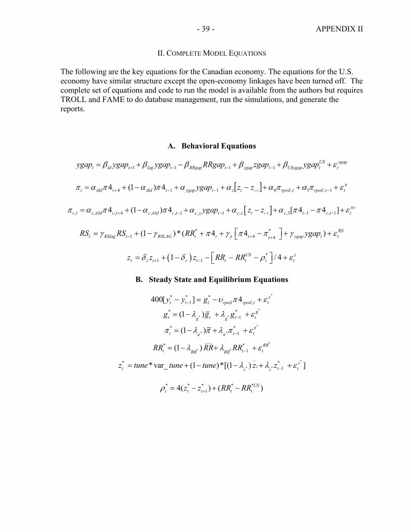
- 39 - APPENDIX II

II. COMPLETE MODEL EQUATIONS The following are the key equations for the Canadian economy. The equations for the U.S. economy have similar structure except the open-economy linkages have been turned off. The complete set of equations and code to run the model is available from the authors but requires TROLL and FAME to do database management, run the simulations, and generate the reports.

A. Behavioral Equations

1 1 1 1US ygap

t ld t lag t RRgap t zgap t USygap t tygap ygap ygap RRgap zgap ygapβ β β β β ε+ − − −= + − + + +

[ ] πππ επαπαααπαπαπ ttrpoiltrpoiltztygaptldtldt tzzygap +++−++−+= −−−+ − 1,1,0114 14)1(4

[ ]1, , , 4 , , 1 , 1 , ,3 1 , 14 (1 ) 4 [ 4 4 ]t

cc t c ld c t c ld c t c y t c z t c t c t tygap z z π

π ππ α π α π α α α π π ε−+ − − − −= + − + + − + − +

* *1 4 4

(1 ) * ( 4 4 ) RSt RSlag t RSLAG t t t ygap t tt

RS RS RR ygapπγ γ π γ π π γ ε− + +⎡ ⎤= + − + + − + +⎣ ⎦

( ) *

1 11 / 4US zt z t z t t t t tz z z RR RRδ δ ρ ε+ − ⎡ ⎤= + − − − − +⎣ ⎦

B. Steady State and Equilibrium Equations

** * *1 ,400[ ] 4 y

t t t rpoil rpoil t ty y g υ π ε−− = − + *

* ** *

1(1 ) gt t t tg g

g g gλ λ ε−= − + + *

* ** *

1(1 )t t tπ

π ππ λ π λ π ε−= − + +

*

* *

___* *

1(1 ) RRt t tRR RR

RR RR RRλ λ ε−= − + + *

* *

_* *

1* var_ (1 )*[(1 ) ]ztt t tz z

z tune tune tune z zλ λ ε−= + − − + +

* * * * *14( ) ( )US

t t t t tz z RR RRρ += − + −

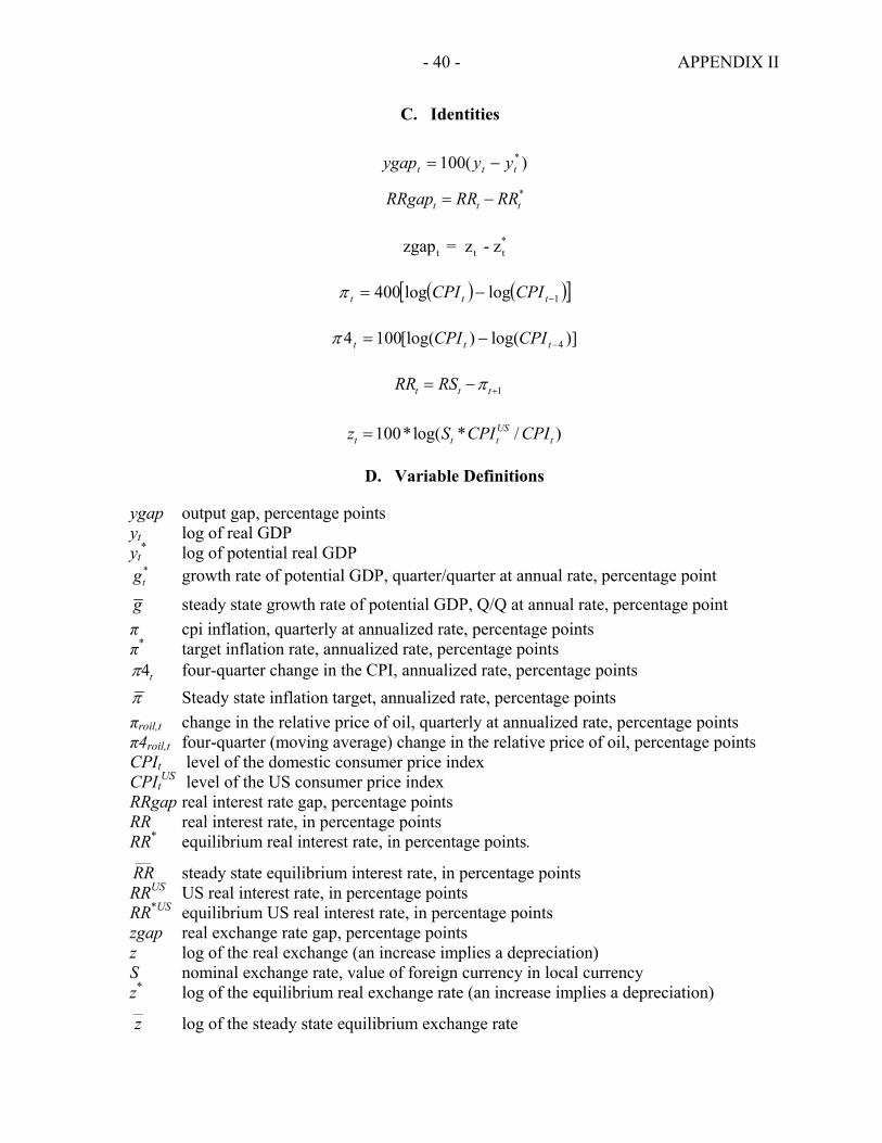
- 40 - APPENDIX II

C. Identities

)(100 *ttt yyygap −=

*t t tRRgap RR RR= −

*

t t tzgap = z - z

( ) ( )[ ]1loglog400 −−= ttt CPICPIπ

)]log()[log(1004 4−−= ttt CPICPIπ

1t t tRR RS π += −

100*log( * / )USt t t tz S CPI CPI=

D. Variable Definitions

ygap output gap, percentage points yt log of real GDP yt

* log of potential real GDP *tg growth rate of potential GDP, quarter/quarter at annual rate, percentage point

g steady state growth rate of potential GDP, Q/Q at annual rate, percentage point π cpi inflation, quarterly at annualized rate, percentage points π* target inflation rate, annualized rate, percentage points

t4π four-quarter change in the CPI, annualized rate, percentage points π Steady state inflation target, annualized rate, percentage points πroil,t change in the relative price of oil, quarterly at annualized rate, percentage points π4roil,t four-quarter (moving average) change in the relative price of oil, percentage points CPIt level of the domestic consumer price index CPIt

US level of the US consumer price index

RRgap real interest rate gap, percentage points RR real interest rate, in percentage points RR* equilibrium real interest rate, in percentage points.

___

RR steady state equilibrium interest rate, in percentage points RRUS US real interest rate, in percentage points RR*US equilibrium US real interest rate, in percentage points zgap real exchange rate gap, percentage points z log of the real exchange (an increase implies a depreciation) S nominal exchange rate, value of foreign currency in local currency z* log of the equilibrium real exchange rate (an increase implies a depreciation) __

z log of the steady state equilibrium exchange rate

- 41 - APPENDIX III

III. ON THE SUPPLY SIDE OF THE MODEL The model in Appendix II has only a rudimentary supply side. Output and the real interest rate appear in all the behavioral equations in gap terms, implying that only deviations from equilibrium levels for output and the real interest rate are modeled. Thus, for example, a shock to real output could be accommodated by an equal and immediate move in aggregate demand, leaving the gaps and hence the rest of the model unaffected. This reflects a choice for simplicity and in particular a recognition that it would require a substantial increase in complexity to usefully model the supply side. The implications of a positive permanent supply shock for the output gap and inflation, for example, are complex. The increase in capacity may reduce the output gap and prices. On the other hand, an investment boom will tend to result until the capital stock has achieved the higher level of productivity.64 As shown in Appendix II there are simple stochastic processes for potential output, the equilibrium interest rate and exchange rate, and the inflation target.

• Potential output is assumed to grow at some steady state growth rate, with potentially serially correlated shocks to both the level and growth rate (thus permanent shocks to the level) of potential output.

• The equilibrium real interest rate and the equilibrium real exchange rate are assumed to follow a stationary process, with temporary but possibly persistent shocks around some steady-state level.

• The equilibrium risk premium is calculated as the value of the risk premium that keeps the real exchange rate on its equilibrium trajectory, given that interest rates are at their equilibrium values. Temporary shocks to the exchange rate are equivalent to and can be interpreted as temporary shocks to the risk premium.

• The inflation target is assumed to follow an integrated process, with only permanent shocks.

These equations serve two purposes. First, the residuals in these equations can be manipulated and the resulting response of the economy examined. As described below, great care must be taken in interpreting these shocks, because of the simplistic nature of the equations. Second, they are necessary when estimating the model using Bayesian techniques. When applying the model to actual data in a forecasting and policy analysis exercise, the equilibrium values for the domestic real interest rate, the U.S. real interest rate, potential output, and the inflation target are all fit from the data using the LRX filter, as described in Appendix IV.65

64Many models have interesting treatments of the supply side and address these issues. The GEM represents one approach.

65Our preliminary work shows the importance of supply side equations, such as these, in applying system estimation techniques.

- 42 - APPENDIX III

The implication of the sparseness of the supply side is that the model does not naturally handle certain sorts of shocks. For example, permanent and temporary shocks to potential output have no effect on the output gap and inflation (of course, they move output itself). The analyst could model richer implications “by hand,” by adding a set of shocks that move potential output, the output gap, and the inflation rate according to her sense of how the underlying supply shock will manifest itself. Similarly, permanent shocks to the equilibrium real interest rate are reflected one-for-one in movements of the actual real interest rate to achieve equilibrium in the IS curve.66 The risk premium will also shift by the same amount in order to achieve equilibrium in the exchange rate equation. There is also no long-run effect on potential output, simply because this is not modeled. The supply side could be enriched with a model in which capital accumulation depends on productivity and the cost of capital, so that potential output would fall in response to an equilibrium real interest rate increase. GEM contains such an extension.

In shocking or forecasting the exchange rate, care must be taken to consider whether to adjust the actual and/or the equilibrium real exchange rate. A depreciation of the actual exchange rate will be expansionary because it opens up a positive exchange rate gap, though the effect is mitigated by the resulting inflation and monetary policy response. A depreciation (increase) of the equilibrium exchange rate will result in a corresponding move of the actual exchange rate. This is because the risk premium adjusts endogenously to movements in the equilibrium exchange rate This makes sense where the movement in the equilibrium exchange rate is associated with an equilibrium risk premium shock (e.g., a "capital account" shock) but perhaps less so in the case of a real shock such as to the terms of trade. The actual exchange rate depreciation will be inflationary through its effects on prices.67 The need to tighten monetary policy to stabilize inflation will be contractionary

66If the central bank smooths interest rates, then there are some transitional dynamics until the nominal rate adjusts to the new equilibrium.

67If the exchange rate gap instead of the exchange rate itself appeared in the Phillips curve, movements in the equilibrium real exchange rate would not affect any variables in the main behavioral equations, as with movements in potential output.

- 43 - APPENDIX IV

IV. CALCULATING THE LONG-RUN EQUILIBRIUM AND THE LRX FILTER The model is expressed in terms of gaps, in other words deviations from long-run equilibrium values. For example, the gap between actual and potential output influences inflation. The dynamic behavior of the model, for example the response to a particular shock, does not depend on the long-run equilibrium values.68 However, to fit the model to actual data or to make a forecast, the equilibrium values of the endogenous variables must be estimated. Here again we propose a simple and eclectic procedure that allows ready incorporation of various views. We detrend each endogenous variable using a flexible filter procedure, dubbed the LRX filter, that, for a given series y, calculates the smoothed or equilibrium series y*. The LRX filter minimizes the deviations of y* from y (with weights w1 in the following equation) while also penalizing, at the operators discretion:

• changes in the rate of change of y* (the usual Hodrick-Prescott filter term, with tightness parameter λ);

• deviations of the growth rate of y* from an assumed (operator supplied) growth rate (DPRIOR), with weights w2; and

• deviations of the level of y* from an assumed (operator supplied) level (PRIOR), with weights w3.69

Thus LRX computes y* by solving the following problem: Given a series yt, find the series y*

t that minimizes the following objective function:

( ) ( ) ( )

( )

22

1 1 21 3

2 21

2 1

min 1

2 3 [ ]

t

T T

t t t t t t ty t t

T T

t t t t t t tt t

w y y y y y y

w y y DPRIOR w y PRIOR

λ∗

∗ ∗ ∗ ∗ ∗− − −

= =

∗ ∗ ∗−

= =

⎡ ⎤− + − − −⎣ ⎦

⎡ ⎤+ − − + −⎣ ⎦

∑ ∑

∑ ∑

The time-varying weights to be attached to each of these factors are at the analyst’s discretion. In the Canada example discussed in this paper and implemented in the associated programs, we found it useful to distinguish between series that are assumed to be stationary and those that are assumed to trend. The real interest rates and the real exchange rate were presumed stationary. It was assumed that the equilibrium values were known for one or more recent quarters. For this quarter(s), a very high weight is placed on the weight parameter w3 and the assumed level of the

68This is a feature specific to linear models of the sort we examine here. In a non linear model such as the IMF Research Department's Global Economic Model (GEM), the dichotomy between the long-run equilibrium and the dynamic behavior of the model disappears.

69In the implementation used and documented in the programs that accompany this paper, there is a fourth term and associated weight that are redundant and need never be used.

- 44 - APPENDIX IV

equilibrium is assigned to PRIOR, forcing the smoothed series to take these assumed values in these quarters. Deviations from those levels are penalized by placing a high (but not prohibitive) weight on the parameter w2 for all time periods. Of course the judgment of the knowledgeable operator is used to add conditions to what is otherwise a purely mechanical filtering approach. Potential output is assumed to trend. An HP filter with tightness constraint of 1600 (or higher) is applied (a conventional method for eliminating high/business cycle frequencies from the series). This is combined with the imposition of a strong view about where the output gap was in a recent quarter. Similarly, for the inflation target, an HP filter is applied with a tightness constraint of 1600, then assumptions about the inflation target at various points are imposed (mostly from public announcements, as is the case in Canada’s IT policy of medium-term announcements of the targets). Filtering methodologies are many and they vary from the simplest univariate (an HP filter) to the multivariate filters used in an estimated system of equations. For instance, the LRX filter, a univariate methodology which allows some weight to be given to priors on the evolution of trend, exploits the data of the series itself to fit the trend. In the case of estimating potential output, for example, better estimates of long-run equilibrium values might result from considering a small system of equations with more data from other variables—an increase in inflation and the degree of excess demand in the labor market (not modeled in our example) might suggest that output is above equilibrium.70

70Typically, it is difficult econometrically to both estimate a dynamic model and estimate the underlying long-run equilibrium—uncertainty about the model parameters translates into uncertainty about the equilibrium values. A Bayesian procedure seems promising, in that the model parameters themselves can be pinned down by narrow priors, and so the analyst can ask: given the model, what is the most sensible long-run equilibrium?

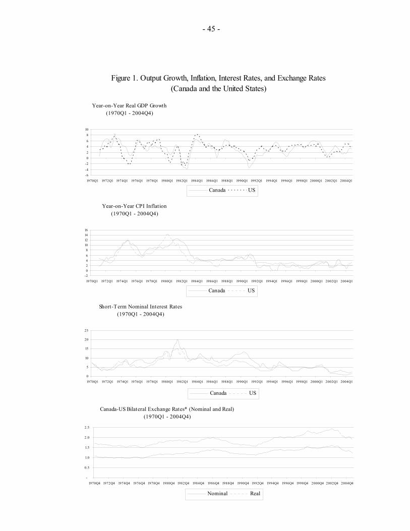
- 45 -

Figure 1. Output Growth, Inflation, Interest Rates, and Exchange Rates(Canada and the United States)

Year-on-Year Real GDP Growth(1970Q1 - 2004Q4)

-6-4

-202

46

810

1970Q1 1972Q1 1974Q1 1976Q1 1978Q1 1980Q1 1982Q1 1984Q1 1986Q1 1988Q1 1990Q1 1992Q1 1994Q1 1996Q1 1998Q1 2000Q1 2002Q1 2004Q1

Canada US

Year-on-Year CPI Inflation (1970Q1 - 2004Q4)

-202468

10121416

1970Q1 1972Q1 1974Q1 1976Q1 1978Q1 1980Q1 1982Q1 1984Q1 1986Q1 1988Q1 1990Q1 1992Q1 1994Q1 1996Q1 1998Q1 2000Q1 2002Q1 2004Q1

Canada US

Short-Term Nominal Interest Rates(1970Q1 - 2004Q4)

0

5

10

15

20

25

1970Q1 1972Q1 1974Q1 1976Q1 1978Q1 1980Q1 1982Q1 1984Q1 1986Q1 1988Q1 1990Q1 1992Q1 1994Q1 1996Q1 1998Q1 2000Q1 2002Q1 2004Q1

Canada US

Canada-US Bilateral Exchange Rates* (Nominal and Real)(1970Q1 - 2004Q4)

-

0.5

1.0

1.5

2.0

2.5

1970Q4 1972Q4 1974Q4 1976Q4 1978Q4 1980Q4 1982Q4 1984Q4 1986Q4 1988Q4 1990Q4 1992Q4 1994Q4 1996Q4 1998Q4 2000Q4 2002Q4 2004Q4

Nominal Real

- 46 -

Figure 2. Inflation in Canada Compared to the Inflation Target PathCanada Year-on-Year CPI Inflation and Targets

(solid=actual, bold=target, dashed=bands)

-2

0

2

4

6

8

10

12

14

1970

Q4

1972

Q4

1974

Q4

1976

Q4

1978

Q4

1980

Q4

1982

Q4

1984

Q4

1986

Q4

1988

Q4

1990

Q4

1992

Q4

1994

Q4

1996

Q4

1998

Q4

2000

Q4

2002

Q4

2004

Q4

- 47 -

Figure 3. Model Variables for Canada (Actual, Trend, and Detrended Series)

* An increase denotes a real depreciation

CANADA log of GDP (solid=actual, dashed=trend)

5.5

6

6.5

7

7.5

1970Q1 1975Q1 1980Q1 1985Q1 1990Q1 1995Q1 2000Q1

CANADAGDP (gap)

-6.0

-5.0

-4.0

-3.0

-2.0

-1.0

0.0

1.0

2.0

3.0

4.0

1970Q1 1975Q1 1980Q1 1985Q1 1990Q1 1995Q1 2000Q1

CANADA Real Interest Rate (solid=actual, dashed=trend)

-8

-6

-4

-2

0

2

4

6

8

10

12

1970Q1 1975Q1 1980Q1 1985Q1 1990Q1 1995Q1 2000Q1

CANADA Real Interest Rate (gap)

-12

-10

-8

-6

-4

-2

0

2

4

6

8

10

1970Q1 1975Q1 1980Q1 1985Q1 1990Q1 1995Q1 2000Q1

CANADA Real Exchange Rate* (solid=actual,

dashed=trend)

0

10

20

30

40

50

60

70

80

90

100

1970Q1 1975Q1 1980Q1 1985Q1 1990Q1 1995Q1 2000Q1

CANADA Real Exchange Rate (gap)

-15.0

-10.0

-5.0

0.0

5.0

10.0

15.0

1970Q1 1975Q1 1980Q1 1985Q1 1990Q1 1995Q1 2000Q1

- 48 -

Figure 4. Model Variables for the United States (Actual, Trend, and Detrended Series)

US log o f GDP (solid=actual, dashed=trend)

8

8.2

8.4

8.6

8.8

9

9.2

9.4

1970Q1 1975Q1 1980Q1 1985Q1 1990Q1 1995Q1 2000Q1

USGDP (gap)

-8 .0

-6 .0

-4 .0

-2 .0

0 .0

2 .0

4 .0

6 .0

1970Q1 1975Q1 1980Q1 1985Q1 1990Q1 1995Q1 2000Q1

US Real Interest Rate (solid=actual, dashed=trend)

-6

-4

-2

0

2

4

6

8

10

1970Q1 1975Q1 1980Q1 1985Q1 1990Q1 1995Q1 2000Q1

US Real Interest Rate (gap)

-8

-6

-4

-2

0

2

4

6

8

1970Q1 1975Q1 1980Q1 1985Q1 1990Q1 1995Q1 2000Q1

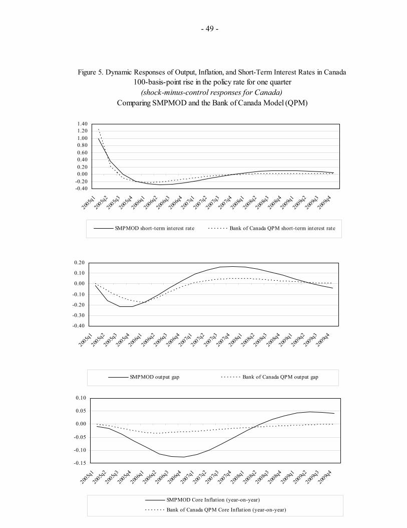
- 49 -

Figure 5. Dynamic Responses of Output, Inflation, and Short-Term Interest Rates in Canada100-basis-point rise in the policy rate for one quarter

(shock-minus-control responses for Canada)Comparing SMPMOD and the Bank of Canada Model (QPM)

-0.15

-0.10

-0.05

0.00

0.05

0.10

2005q

1

2005q

2

2005q

3

2005q

4

2006q

1

2006q

2

2006q

3

2006q

4

2007q

1

2007q

2

2007q

3

2007q

4

2008q

1

2008q

2

2008q

3

2008q

4

2009q

1

2009q

2

2009q

3

2009q

4

SMPMOD Core Inflation (year-on-year)

Bank of Canada QPM Core Inflation (year-on-year)

-0.40

-0.30

-0.20

-0.10

0.00

0.10

0.20

2005q

1

2005q

2

2005q

3

2005q

4

2006q

1

2006q

2

2006q

3

2006q

4

2007q

1

2007q

2

2007q

3

2007q

4

2008q

1

2008q

2

2008q

3

2008q

4

2009q

1

2009q

2

2009q

3

2009q

4

SMPMOD output gap Bank of Canada QPM output gap

-0.40-0.200.000.200.400.600.801.001.201.40

2005q

1

2005q

2

2005q

3

2005q

4

2006q

1

2006q

2

2006q

3

2006q

4

2007q

1

2007q

2

2007q

3

2007q

4

2008q

1

2008q

2

2008q

3

2008q

4

2009q

1

2009q

2

2009q

3

2009q

4

SMPMOD short-term interest rate Bank of Canada QPM short-term interest rate

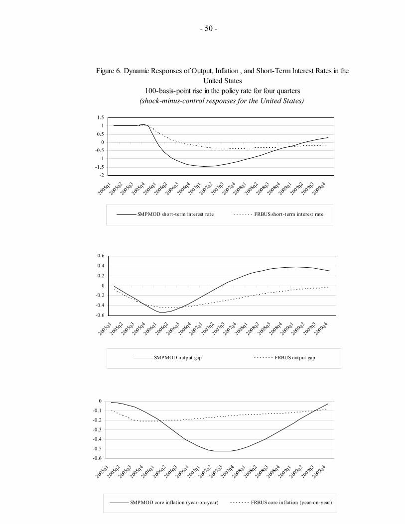
- 50 -

Figure 6. Dynamic Responses of Output, Inflation , and Short-Term Interest Rates in the United States

100-basis-point rise in the policy rate for four quarters(shock-minus-control responses for the United States)

-2-1.5

-1-0.5

00.5

11.5

2005q

1

2005q

2

2005q

3

2005q

4

2006q

1

2006q

2

2006q

3

2006q

4

2007q

1

2007q

2

2007q

3

2007q

4

2008q

1

2008q

2

2008q

3

2008q

4

2009q

1

2009q

2

2009q

3

2009q

4

SMPMOD short-term interest rate FRBUS short-term interest rate

-0.6

-0.4

-0.2

0

0.2

0.4

0.6

2005q

1

2005q

2

2005q

3

2005q

4

2006q

1

2006q

2

2006q

3

2006q

4

2007q

1

2007q

2

2007q

3

2007q

4

2008q

1

2008q

2

2008q

3

2008q

4

2009q

1

2009q

2

2009q

3

2009q

4

SMPMOD output gap FRBUS output gap

-0.6

-0.5

-0.4

-0.3

-0.2

-0.1

0

2005q

1

2005q

2

2005q

3

2005q

4

2006q

1

2006q

2

2006q

3

2006q

4

2007q

1

2007q

2

2007q

3

2007q

4

2008q

1

2008q

2

2008q

3

2008q

4

2009q

1

2009q

2

2009q

3

2009q

4

SMPMOD core inflation (year-on-year) FRBUS core inflation (year-on-year)

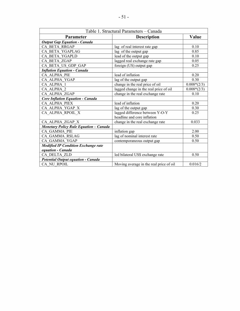
- 51 -

Table 1. Structural Parameters – Canada Parameter Description Value

Output Gap Equation - Canada CA_BETA_RRGAP lag of real interest rate gap 0.10 CA_BETA_YGAPLAG lag of the output gap 0.85 CA_BETA_YGAPLD lead of the output gap 0.10 CA_BETA_ZGAP lagged real exchange rate gap 0.05 CA_BETA_US_GDP_GAP foreign (US) output gap 0.25 Inflation Equation - Canada CA_ALPHA_PIE lead of inflation 0.20 CA_ALPHA_YGAP lag of the output gap 0.30 CA_ALPHA_1 change in the real price of oil 0.008*(2/3) CA_ALPHA_2 lagged change in the real price of oil 0.008*(2/3) CA_ALPHA_ZGAP change in the real exchange rate 0.10 Core Inflation Equation - Canada CA_ALPHA_PIEX lead of inflation 0.20 CA_ALPHA_YGAP_X lag of the output gap 0.30 CA_ALPHA_RPOIL_X lagged difference between Y-O-Y

headline and core inflation 0.25

CA_ALPHA_ZGAP_X change in the real exchange rate 0.033 Monetary Policy Rule Equation – Canada CA_GAMMA_PIE inflation gap 2.00 CA_GAMMA_RSLAG lag of nominal interest rate 0.50 CA_GAMMA_YGAP contemporaneous output gap 0.50 Modified IP Condition Exchange rate equation - Canada

CA_DELTA_ZLD led bilateral US$ exchange rate 0.50 Potential Output equation - Canada CA_NU_RPOIL Moving average in the real price of oil 0.016/2

- 52 -

Table 2. Structural Parameters – United States Parameter Description Value

Output Gap Equation - United States US_BETA_RRGAP lag of real interest rate gap 0.10 US_BETA_YGAPLAG lag of the output gap 0.85 US_BETA_YGAPLD lead of the output gap 0.10 Inflation Equation - United States US_ALPHA_PIE lead of inflation 0.20 US_ALPHA_YGAP lag of the output gap 0.30 US_ALPHA_1 change in the real price of oil 0.009*(2/3) US_ALPHA_2 Lagged change in the real price of oil 0.009*(2/3) Core Inflation Equation - United States US_ALPHA_PIEX lead of inflation 0.20 US_ALPHA_YGAP_X lag of the output gap 0.30 US_ALPHA_RPOIL_X lagged difference between Y-O-Y

headline and core inflation 0.25

Monetary Policy Rule Equation – United States US_GAMMA_PIE inflation gap 2.00 US_GAMMA_RSLAG lag of nominal interest rate 0.50 US_GAMMA_YGAP contemporaneous output gap 0.50 Potential Output equation – United States US_NU_RPOIL Moving average in the real price of oil 0.016 Real Price of Oil equation US_THETA_1 Lagged real oil price gap 0.75

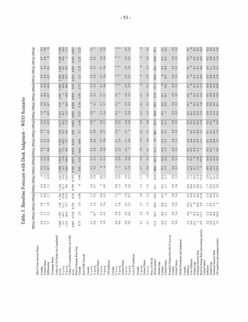
- 53 - Ta

ble

3. B

asel

ine

Fore

cast

with

Des

k Ju

dgm

ent –

WEO

Sce

nario

20

03q1

2003

q220

03q3

2003

q420

04q1

2004

q220

04q3

2004

q420

05q1

2005

q220

05q3

200

5q4

2006

q120

06q2

2006

q320

06q4

2007

q120

07q2

2007

q320

07q4

Shor

t-Ter

m In

tere

st R

ates

Can

ada

2.9

3.2

2.8

2.7

2.2

22.

22.

52.

62.

72.

9 3.

23.

53.

84.

14.

34.

54.

74.

74.

7U

nite

d St

ates

1.

21.

11

0.9

0.9

1.1

1.5

1.8

22.

53

3.5

44.

54.

84.

84.

84.

84.

84.

8D

iffer

entia

l 1.

72.

11.

81.

71.

30.

90.

70.

80.

60.

2-0

.1

-0.3

-0.5

-0.7

-0.7

-0.4

-0.2

-0.1

00

Exch

ange

Rat

es

Val

ue o

f US

Dol

lar (

in C

anad

ian$

)

Leve

l 1.

509

1.39

71.

381.

316

1.31

81.

361.

308

1.21

91.

221

1.22

21.

22

1.21

71.

213

1.21

1.20

71.

205

1.20

31.

201

1.19

81.

194

% y

-o-y

-5

.3-1

0.1

-11.

7-1

5.9

-12.

7-2

.6-5

.3-7

.4-7

.3-1

0.2

-6.7

-0

.2-0

.7-1

-1-0

.9-0

.8-0

.7-0

.8-0

.9%

q-o

-q

-13.

6-2

6.6

-4.7

-17.

40.

613

.6-1

4.6

-24.

60.

80.

3-0

.5

-1.2

-1.2

-0.9

-0.8

-0.8

-0.7

-0.7

-1-1

.2V

alue

of C

anad

ian

Dol

lar (

in U

S$)

le

vel

0.66

30.

716

0.72

50.

760.

759

0.73

50.

765

0.82

10.

819

0.81

90.

82

0.82

20.

825

0.82

60.

828

0.83

0.83

10.

833

0.83

50.

837

Rea

l Exc

hang

e R

ate

Gap

Can

ada

8.72

2.5

2.4

-1.6

80

3.94

0.81

-5.5

3-4

.61

-4.0

5-3

.7

-3.5

4-3

.37

-3.1

4-2

.92

-2.7

1-2

.5-2

.32

-2.2

3-2

.23

Rea

l GD

P G

row

th

Can

ada

%

y-o

-y

3.1

21.

31.

71.

62.

83.

33.

13.

12.

82.

7 2.

92.

93

3.1

3.1

3.2

3.2

3.1

3.1

% q

-o-q

2.

8-0

.71.

43.

32.

73.

93.

22.

52.

82.

82.

9 3

33.

13.

33.

23.

23.

13.

13

Uni

ted

Stat

es

%

y-o

-y

1.9

2.3

3.5

4.4

54.

84

3.7

3.6

3.7

3.6

3.8

3.7

3.7

3.7

3.7

3.7

3.7

3.6

3.6

% q

-o-q

1.

94.

17.

44.

24.

53.

34

3.1

3.8

3.8

3.7

3.7

3.6

3.7

3.7

3.6

3.6

3.6

3.6

3.5

CPI

Infla

tion

Can

ada

%

y-o

-y

4.4

2.8

2.1

1.7

0.8

2.2

22.

32.

52.

12.

4 2.

22.

12.

12.

12

22

22

% q

-o-q

4.

8-1

.61.

82

1.3

3.8

12.

92.

22.

42

2.2

22

22

22

22

Uni

ted

Stat

es

%

y-o

-y

2.9

2.2

2.2

1.9

1.8

2.8

2.7

3.4

3.2

2.7

2.7

2.4

2.3

2.3

2.4

2.5

2.5

2.5

2.5

2.5

% q

-o-q

3.

90.

62.

30.

73.

64.

71.

93.

43

2.4

2 2.

42.

42.

52.

52.

52.

52.

52.

52.

5C

ore

CPI

Infla

tion

Can

ada

%

q-o

-q

3.1

2.2

1.7

1.9

1.3

1.7

1.7

1.6

1.9

1.9

2.1

2.2

2.1

2.1

2.1

22

22

2U

nite

d St

ates

% y

-o-y

2.

11.

81.

51.

51.

31.

92.

83.

14.

13.

83.

1 2.

82.

32.

32.

42.

52.

52.

52.

52.

5Pr

ice

of O

il ($

)

Wor

ld m

arke

t 31

.326

.528

.429

.432

.135

.640

.642

.741

.341

40.3

39

.538

.838

.337

.837

.336

.836

.335

.835

.3O

utpu

t Gap

Can

ada

0.4

-0.4

-0.8

-0.7

-0.7

-0.4

-0.3

-0.4

-0.4

-0.3

-0.3

-0

.3-0

.3-0

.2-0

.10

00.

10.

10.

1U

nite

d St

ates

-3

.3-3

.1-2

.2-2

-1.7

-1.7

-1.5

-1.6

-1.4

-1.3

-1.2

-1

.1-1

-0.9

-0.7

-0.6

-0.5

-0.4

-0.3

-0.2

Pote

ntia

l Out

put G

row

th (%

q-o

-q)

C

anad

a 2.

92.

82.

82.

82.

82.

82.

82.

82.

82.

82.

8 2.

82.

92.

92.

92.

92.

92.

92.

92.

9U

nite

d St

ates

3.

43.

43.

43.

43.

43.

33.

33.

33.

33.

23.

2 3.

23.

23.

23.

23.

23.

23.

23.

23.

2M

odel

Res

idua

ls a

nd Ju

dgm

ent

Can

ada

In

flatio

n 1.

6-4

.6-0

.20.

5-0

.62.

1-1

.21.

50.

20.

20

0.2

0.1

0.1

0.1

0.1

0.1

0.1

0.1

0.1

Cor

e In

flatio

n 0.

4-2

-0.7

0.8

-0.9

1.3

-0.5

0.3

0.5

0.4

0.1

0.2

-0.1

00

00

00

0O

utpu

t Gap

-0

.1-0

.20

0.3

0.3

0.2

0.1

00.

40.

30.

3 0.

30.

30.

30.

30.

30.

30.

30.

20.

2N

omin

al In

tere

st R

ate

-1-0

.7-0

.8-0

.6-0

.8-1

.4-1

.2-1

.0-1

.2-0

.9-0

.8

-0.5

-0.4

-0.2

-0.1

0.1

0.1

0.1

0.1

0.1

Rea

l Exc

hang

e R

ate

(per

cent

age

poin

ts)

6.5

-13.

74.

4-1

1.8

-5.7

13.4

5-1

5.5

-1-1

.5-1

.5

-1.8

-1.9

-1.8

-1.6

-1.3

-0.9

-0.6

-0.4

-0.4

Uni

ted

Stat

es

In

flatio

n 2.

2-1

.21.

3-1

.31.

72.

8-0

.90.

80.

3-0

.1-0

.1

0.2

0.4

0.6

0.5

0.4

0.3

0.3

0.2

0.2

Out

put G

ap

-1.0

-0.3

0.3

-0.2

-0.3

-0.7

-0.2

-0.5

-0.3

-0.2

-0.1

-0

.1-1

.0-0

.00.

00.

00.

00.

.10.

00.

0N

omin

al In

tere

st R

ate

-0.3

-0.8

-1.5

-1.8

-2.2

-2.1

-1.5

-1.5

-1-0

.4-0

.3

00.

30.

50.

40.

20.

20.

20.

10.

1O

il eq

uatio

n (p

erce

ntag

e po

ints

) 12

-16.

62

0.1

5.4

8.2

13.6

8.2

0.6

2.5

1.0

0.3

-0.2

-0.1

-0.5

-0.8

-1.0

-1.3

-1.6

-1.8

- 54 - Ta

ble

4. T

empo

rary

50

Perc

ent I

ncre

ase

in O

il Pr

ice,

200

5–07

2003

q120

03q2

2003

q320

03q4

2004

q120

04q2

2004

q320

04q4

2005

q120

05q2

2005

q3 2

005q

420

06q1

2006

q220

06q3

2006

q420

07q1

2007

q220

07q3

2007

q4Sh

ort-T

erm

Inte

rest

Rat

es

Can

ada

2.9

3.2

2.8

2.7

2.2

2.0

2.2

2.5

3.2

3.6

4.0

4.3

4.4

4.3

4.2

4.1

3.9

3.6

3.4

3.3

Uni

ted

Stat

es

1.2

1.1

10.

90.

91.

11.

51.

82.

63.

54.

1 4.

64.

95

4.9

4.5

4.2

3.9

3.6

3.5

Diff

eren

tial

1.7

2.1

1.8

1.7

1.3

0.9

0.7

0.8

0.6

0.2

-0.1

-0

.3-0

.5-0

.7-0

.7-0

.5-0

.3-0

.2-0

.2-0

.2Ex

chan

ge R

ates

Val

ue o

f US

Dol

lar (

in C

anad

ian$

)

Leve

l 1.

509

1.39

71.

381.

316

1.31

81.

361.

308

1.21

91.

222

1.22

41.

224

1.22

21.

219

1.21

81.

216

1.21

41.

212

1.20

91.

205

1.2

% y

-o-y

-5

.3-1

0.1

-11.

7-1

5.9

-12.

7-2

.6-5

.3-7

.4-7

.3-1

0-6

.4

0.3

-0.2

-0.5

-0.7

-0.6

-0.6

-0.7

-0.9

-1.2

% q

-o-q

-1

3.6

-26.

6-4

.7-1

7.4

0.6

13.6

-14.

6-2

4.6

1.1

0.7

0 -0

.7-0

.8-0

.6-0

.6-0

.6-0

.7-0

.9-1

.4-1

.9V

alue

of C

anad

ian

Dol

lar (

in U

S$)

le

vel

0.66

30.

716

0.72

50.

760.

759

0.73

50.

765

0.82

10.

818

0.81

70.

817

0.81

80.

820.

821

0.82

20.

824

0.82

50.

827

0.83

0.83

4R

eal E

xcha

nge

Rat

e G

ap

C

anad

a 8.

722.

52.

4-1

.68

03.

940.

81-5

.53

-4.5

1-3

.81

-3.3

3 -3

.06

-2.7

8-2

.46

-2.1

8-1

.94

-1.7

3-1

.59

-1.6

-1.7

6R

eal G

DP

Gro

wth

Can

ada

%

y-o

-y

3.1

21.

31.

71.

62.

83.

33.

13

2.8

2.6

2.5

2.5

2.5

2.7

2.8

3.1

3.2

3.3

3.5

% q

-o-q

2.

8-0

.71.

43.

32.

73.

93.

22.

52.

52.

92.

3 2.

42.

32.

83.

13.

13.

33.

43.

53.

6U

nite

d St

ates

% y

-o-y

1.

92.

33.

54.

45

4.8

43.

73.

43.

43.

1 3.

13

33.

23.

53.

84

4.1

4.1

% q

-o-q

1.

94.

17.

44.

24.

53.

34

3.1

3.2

3.4

2.8

2.8

2.8

3.6

3.8

3.9

44.

14.

24.

2C

PI In

flatio

n

Can

ada

%

y-o

-y

4.4

2.8

2.1

1.7

0.8

2.2

22.

32.

72.

73.

1 3

2.8

2.5

2.4

2.2

21.

81.

61.

5%

q-o

-q

4.8

-1.6

1.8

21.

33.

81

2.9

3.3

3.6

2.4

2.7

2.5

2.3

2.1

1.9

1.7

1.6

1.4

1.3

Uni

ted

Stat

es

%

y-o

-y

2.9

2.2

2.2

1.9

1.8

2.8

2.7

3.4

3.5

3.3

3.4

3.3

32.

82.

82.

62.

52.

32.

12

% q

-o-q

3.

90.

62.

30.

73.

64.

71.

93.

44.

13.

72.

5 2.

92.

92.

82.

52.

42.

22

1.9

1.8

Cor

e C

PI In

flatio

n

Can

ada

%

q-o

-q

3.1

2.2

1.7

1.9

1.3

1.7

1.7

1.6

22

2.2

2.4

2.4

2.3

2.3

2.2

2.2

2.1

21.

9U

nite

d St

ates

% y

-o-y

2.

11.

81.

51.

51.

31.

92.

83.

14.

13.

93.

2 3

2.5

2.6

2.7

2.7

2.7

2.6

2.5

2.4

Pric

e of

Oil

($)

W

orld

mar

ket

31.3

26.5

28.4

29.4

32.1

35.6

40.6

42.7

6261

.959

55

.953

50.4

47.8

45.3

42.8

40.4

37.9

35.4

Out

put G

ap

C

anad

a 0.

4-0

.4-0

.8-0

.7-0

.7-0

.4-0

.3-0

.4-0

.3-0

.2-0

.3

-0.3

-0.4

-0.4

-0.4

-0.4

-0.3

-0.3

-0.2

-0.1

Uni

ted

Stat

es

-3.3

-3.1

-2.2

-2-1

.7-1

.7-1

.5-1

.6-1

.4-1

.2-1

.2

-1.1

-1.1

-1.1

-1-0

.9-0

.8-0

.7-0

.5-0

.4Po

tent

ial O

utpu

t Gro

wth

(% q

-o-q

)

Can

ada

2.9

2.8

2.8

2.8

2.8

2.8

2.8

2.8

2.5

2.5

2.5

2.6

2.6

33

3.1

3.1

3.1

3.1

3.1

Uni

ted

Stat

es

3.4

3.4

3.4

3.4

3.4

3.3

3.3

3.3

2.6

2.6

2.6

2.7

2.7

3.4

3.5

3.5

3.5

3.5

3.6

3.6

Mod

el R

esid

uals

and

Judg

men

t

Can

ada

In

flatio

n 1.

6-4

.6-0

.20.

5-0

.62.

1-1

.21.

50.

20.

20

0.2

0.1

0.1

0.1

0.1

0.1

0.1

0.1

0.1

Cor

e In

flatio

n 0.

4-2

-0.7

0.8

-0.9

1.3

-0.5

0.3

0.5

0.4

0.1

0.2

-0.1

00

00

00

0O

utpu

t Gap

-0

.1-0

.20

0.3

0.3

0.2

0.1

00.

40.

30.

3 0.

30.

30.

30.

30.

30.

30.

30.

20.

2N

omin

al In

tere

st R

ate

-1-0

.7-0

.8-0

.6-0

.8-1

.4-1

.2-1

-1.2

-0.9

-0.8

-0

.5-0

.4-0

.2-0

.10.

10.

10.

10.

10.

1R

eal E

xcha

nge

Rat

e (p

erce

ntag

e po

ints

)6.

5-1

3.7

4.4

-11.

8-5

.713

.45

-15.

5-1

-1.5

-1.5

-1

.8-1

.9-1

.8-1

.6-1

.3-0

.9-0

.6-0

.4-0

.4U

nite

d St

ates

Infla

tion

2.2

-1.2

1.3

-1.3

1.7

2.8

-0.9

0.8

0.3

-0.1

-0.1

0.

20.

40.

60.

50.

40.

30.

30.

20.

2O

utpu

t Gap

-1

.0-0

.30.

3-0

.2-0

.3-0

.7-0

.2-0

.5-0

.3-0

.2-0

.1

-0.1

-0.1

-0.0

0.0

0.0

0.0

0.0

0.0

0.0

Nom

inal

Inte

rest

Rat

e -0

.3-0

.8-1

.5-1

.8-2

.2-2

.1-1

.5-1

.5-1

-0.4

-0.3

0

0.3

0.5

0.4

0.2

0.2

0.2

0.1

0.1

Oil

equa

tion

(per

cent

age

poin

ts)

12-1

6.6

20.

15.

48.

213

.68.

20.

62.

51

0.3

-0.2

-0.1

-0.5

-0.8

-1-1

.3-1

.6-1

.8

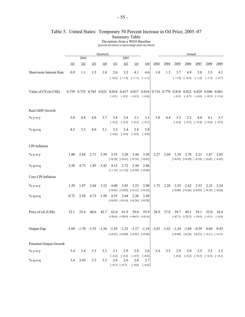
- 55 -

Table 5. United States: Temporary 50 Percent Increase in Oil Price, 2005–07 Summary Table

Deviations from a WEO Baseline (percent deviation) or [percentage point deviation]

Quarterly Annual

2004 2005

Q1 Q2 Q3 Q4 Q1 Q2 Q3 Q4 2003 2004 2005 2006 2007 2008 2009

Short-term Interest Rate 0.9 1.1 1.5 1.8 2.6 3.5 4.1 4.6 1.0 1.3 3.7 4.9 3.8 3.5 4.1 [ +0.6] [ +1.0] [ +1.1] [ +1.1] [ +1.0] [ +0.4] [ -1.0] [ -1.3] [ -0.7]

Value of C$ (in US$) 0.759 0.735 0.765 0.821 0.818 0.817 0.817 0.818 0.716 0.770 0.818 0.822 0.829 0.846 0.861 ( -0.1) ( -0.2) ( -0.3) ( -0.4) ( -0.3) ( -0.7) ( -0.6) ( +0.3) ( +1.6)

Real GDP Growth

% y-o-y 5.0 4.8 4.0 3.7 3.4 3.4 3.1 3.1 3.0 4.4 3.3 3.2 4.0 4.1 3.7 [ -0.2] [ -0.3] [ -0.5] [ -0.7] [ -0.4] [ -0.5] [ +0.4] [ +0.6] [ +0.3]

% q-o-q 4.5 3.3 4.0 3.1 3.2 3.4 2.8 2.8 [ -0.6] [ -0.4] [ -0.9] [ -0.9]

CPI Inflation

% y-o-y 1.80 2.84 2.71 3.39 3.53 3.28 3.44 3.30 2.27 2.69 3.39 2.78 2.21 1.87 2.05 [+0.29] [+0.61] [+0.74] [+0.85] [+0.63] [+0.39] [ -0.29] [ -0.63] [ -0.45]

% q-o-q 3.58 4.73 1.85 3.42 4.15 3.72 2.50 2.86 [+1.15] [+1.32] [+0.50] [+0.46]

Core CPI Inflation % y-o-y 1.29 1.87 2.84 3.12 4.09 3.85 3.23 2.98 1.73 2.28 3.53 2.62 2.53 2.25 2.24 [+0.01] [+0.05] [+0.11] [+0.19] [+0.09] [+0.26] [+0.03] [ -0.25] [ -0.26]

% q-o-q 0.72 3.58 4.73 3.50 4.55 2.64 2.26 2.49 [+0.05] [+0.14] [+0.26] [+0.29]

Price of oil (US$) 32.1 35.6 40.6 42.7 62.0 61.9 59.0 55.9 28.9 37.8 59.7 49.1 39.1 35.0 34.4 (+50.4) (+50.9) (+46.5) (+41.6) (+47.3) (+29.2) ( +8.6) ( +0.1) ( -0.4)

Output Gap -1.69 -1.70 -1.53 -1.56 -1.43 -1.23 -1.17 -1.14 -2.63 -1.62 -1.24 -1.04 -0.59 0.04 0.43 [+0.01] [+0.08] [+0.01] [+0.08] [+0.00] [-0.24] [-0.21] [ +0.11] [ +0.37]

Potential Output Growth

% y-o-y 3.4 3.4 3.3 3.3 3.1 2.9 2.8 2.6 3.4 3.3 2.9 3.0 3.5 3.5 3.3 [ -0.2] [ -0.3] [ -0.5] [ -0.6] [ -0.4] [ -0.2] [ +0.3] [ +0.3] [ +0.1]% q-o-q 3.4 3.43 3.3 3.3 2.6 2.6 2.6 2.7

[ -0.7] [ -0.7] [ -0.6] [ -0.6]

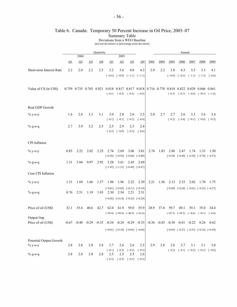
- 56 -

Table 6. Canada: Temporary 50 Percent Increase in Oil Price, 2005–07 Summary Table

Deviations from a WEO Baseline (percent deviation) or [percentage point deviation]

Quarterly Annual

2004 2005

Q1 Q2 Q3 Q4 Q1 Q2 Q3 Q4 2003 2004 2005 2006 2007 2008 2009

Short-term Interest Rate 2.2 2.0 2.2 2.5 3.2 3.6 4.0 4.3 2.9 2.2 3.8 4.3 3.5 3.3 4.1 [ +0.6] [ +0.9] [ +1.1] [ +1.1] [ +0.9] [ +0.3] [ -1.1] [ -1.5] [ -0.6]

Value of C$ (in US$) 0.759 0.735 0.765 0.821 0.818 0.817 0.817 0.818 0.716 0.770 0.818 0.822 0.829 0.846 0.861 ( -0.1) ( -0.2) ( -0.3) ( -0.4) ( -0.3) ( -0.7) ( -0.6) ( +0.3) ( +1.6)

Real GDP Growth

% y-o-y 1.6 2.8 3.3 3.1 3.0 2.8 2.6 2.5 2.0 2.7 2.7 2.6 3.3 3.6 3.4 [ -0.1] [ -0.1] [ -0.2] [ -0.4] [ -0.2] [ -0.4] [ +0.1] [ +0.6] [ +0.5]

% q-o-q 2.7 3.9 3.2 2.5 2.5 2.9 2.3 2.4 [ -0.3] [ +0.0] [ -0.5] [ -0.6]

CPI Inflation

% y-o-y 0.85 2.22 2.02 2.25 2.74 2.69 3.06 3.01 2.74 1.83 2.88 2.47 1.74 1.33 1.50 [+0.26] [+0.56] [+0.68] [+0.80] [+0.58] [+0.40] [ -0.28] [ -0.70] [ -0.53]

% q-o-q 1.31 3.84 0.97 2.92 3.28 3.61 2.45 2.69 [+1.03] [+1.21] [+0.49] [+0.47]

Core CPI Inflation % y-o-y 1.31 1.69 1.66 1.57 1.96 1.96 2.22 2.39 2.21 1.56 2.13 2.33 2.02 1.70 1.75

[+0.01] [+0.05] [+0.11] [+0.19] [+0.09] [+0.26] [ -0.01] [ -0.32] [ -0.27]% q-o-q 0.76 2.51 1.19 1.83 2.30 2.54 2.21 2.51 [+0.05] [+0.14] [+0.25] [+0.29] Price of oil (US$) 32.1 35.6 40.6 42.7 62.0 61.9 59.0 55.9 28.9 37.8 59.7 49.1 39.1 35.0 34.4 (+50.4) (+50.9) (+46.5) (+41.6) (+47.3) (+29.2) ( +8.6) ( +0.1) ( -0.4)

Output Gap Price of oil (US$) -0.67 -0.40 -0.29 -0.35 -0.34 -0.24 -0.29 -0.33 -0.36 -0.43 -0.30 -0.41 -0.22 0.26 0.62

[+0.01] [+0.10] [+0.05] [ -0.04] [+0.03] [ -0.27] [ -0.31] [+0.16] [+0.59]

Potential Output Growth % y-o-y 2.8 2.8 2.8 2.8 2.7 2.6 2.6 2.5 2.9 2.8 2.6 2.7 3.1 3.1 3.0 [ -0.1] [ -0.2] [ -0.2] [ -0.3] [ -0.2] [ -0.1] [ +0.2] [ +0.1] [ +0.0]% q-o-q 2.8 2.8 2.8 2.8 2.5 2.5 2.5 2.6 [ -0.3] [ -0.3] [ -0.3] [ -0.3]

- 57 -

Table 7. Canada: Canadian Interest Rate Shock – One Quarter Increase of 100 b.p. Summary Table

Deviations from a WEO Baseline (percent deviation) or [percentage point deviation]

Quarterly Annual

2004 2005

Q1 Q2 Q3 Q4 Q1 Q2 Q3 Q4 2003 2004 2005 2006 2007 2008 2009

Short-term Interest Rate 2.2 2.0 2.2 2.5 3.6 3.0 2.9 3.0 2.9 2.2 3.1 3.7 4.6 4.8 4.8 [ +1.0] [ +0.4] [ +0.0] [ -0.2] [ +0.3] [ -0.3] [ -0.1] [ +0.1] [ +0.1]

Value of C$ (in US$) 0.759 0.735 0.765 0.821 0.823 0.822 0.821 0.821 0.716 0.770 0.822 0.823 0.832 0.847 0.851 ( +0.5) ( +0.4) ( +0.1) ( -0.2) ( +0.2) ( -0.5) ( -0.2) ( +0.4) ( +0.5)

Real GDP Growth

% y-o-y 1.6 2.8 3.3 3.1 3.1 2.7 2.5 2.7 2.0 2.7 2.7 3.1 3.4 2.9 2.8 [ -0.0] [ -0.2] [ -0.2] [ -0.2] [ -0.2] [ +0.1] [ +0.2] [ -0.0] [ -0.1]

% q-o-q 2.7 3.9 3.2 2.5 2.7 2.2 2.6 3.1 [ -0.1] [ -0.6] [ -0.2] [ +0.0]

CPI Inflation

% y-o-y 0.85 2.22 2.02 2.25 2.47 2.10 2.34 2.15 2.74 1.83 2.27 1.99 1.94 2.00 2.05 [ -0.02] [ -0.03] [ -0.04] [ -0.06] [ -0.03] [ -0.08] [ -0.08] [ -0.02] [+0.02]

% q-o-q 1.31 3.84 0.97 2.92 2.17 2.37 1.90 2.15 [ -0.07] [ -0.03] [ -0.05] [ -0.07]

Core CPI Inflation 1.31 1.69 1.66 1.57 1.93 1.90 2.07 2.14 2.21 1.56 2.01 1.96 1.94 2.03 2.07 % y-o-y [ -0.01] [ -0.02] [ -0.04] [ -0.06] [ -0.03] [ -0.11] [ -0.08] [+0.01] [+0.04] 0.76 2.51 1.19 1.83 2.21 2.37 1.87 2.11 % q-o-q [ -0.03] [ -0.03] [ -0.08] [ -0.11]

Price of oil (US$) 32.1 35.6 40.6 42.7 41.3 41.0 40.3 39.5 28.9 37.8 40.5 38.0 36.0 35.0 34.5 ( -0.0) ( +0.0) ( +0.0) ( +0.0) ( +0.0) ( +0.0) ( +0.0) ( +0.0) ( -0.0)

Output Gap -0.67 -0.40 -0.29 -0.35 -0.37 -0.50 -0.55 -0.50 -0.36 -0.43 -0.48 -0.22 0.23 0.23 0.03 [ -0.02] [ -0.16] [ -0.22] [ -0.21] [ -0.15] [ -0.07] [+0.14] [+0.13] [ -0.00]

Potential Output Growth % y-o-y 2.8 2.8 2.8 2.8 2.8 2.8 2.8 2.8 2.9 2.8 2.8 2.9 2.9 3.0 3.0 [ +0.0] [ +0.0] [ +0.0] [ +0.0] [ +0.0] [ -0.0] [ -0.0] [ +0.0] [ +0.0] % q-o-q 2.8 2.8 2.8 2.8 2.8 2.8 2.8 2.8

[ +0.0] [ +0.0] [ +0.0] [ +0.0]

- 58 -

Table 8. United States: U.S. Interest Rate Shock – One Quarter Increase of 100 b.p. Summary Table

Deviations from a WEO Baseline (percent deviation) or [percentage point deviation]

Quarterly Annual

2004 2005

Q1 Q2 Q3 Q4 Q1 Q2 Q3 Q4 2003 2004 2005 2006 2007 2008 2009

Short-term Interest Rate 0.9 1.1 1.5 1.8 3.0 2.9 3.0 3.3 1.0 1.3 3.0 4.1 4.4 4.6 4.8 [ +1.0] [ +0.4] [ -0.0] [ -0.2] [ +0.3] [ -0.4] [ -0.3] [ -0.1] [ +0.1]

Value of C$ (in US$) 0.759 0.735 0.765 0.821 0.814 0.813 0.815 0.819 0.716 0.770 0.816 0.828 0.835 0.845 0.848 ( -0.6) ( -0.7) ( -0.5) ( -0.3) ( -0.5) ( +0.1) ( +0.2) ( +0.2) ( +0.2) Real GDP Growth

% y-o-y 5.0 4.8 4.0 3.7 3.5 3.6 3.4 3.6 3.0 4.4 3.5 3.7 3.8 3.6 3.3

[ -0.0] [ -0.1] [ -0.2] [ -0.2] [ -0.1] [ +0.0] [ +0.1] [ +0.1] [ -0.0]

% q-o-q 4.5 3.3 4.0 3.1 3.7 3.3 3.6 3.7 [ -0.1] [ -0.5] [ -0.2] [ +0.0] CPI Inflation

% y-o-y 1.80 2.84 2.71 3.39 3.24 2.65 2.67 2.39 2.27 2.69 2.74 2.27 2.36 2.41 2.49 [ -0.00] [ -0.01] [ -0.03] [ -0.06] [ -0.03] [ -0.12] [ -0.14] [ -0.09] [ -0.01]

% q-o-q 3.58 4.73 1.85 3.42 2.98 2.37 1.92 2.29

Core CPI Inflation [ -0.02] [ -0.03] [ -0.08] [ -0.11]

% y-o-y 1.29 1.87 2.84 3.12 4.07 3.79 3.09 2.74 1.73 2.28 3.42 2.24 2.36 2.41 2.49 [ -0.00] [ -0.01] [ -0.03] [ -0.06] [ -0.03] [ -0.12] [ -0.14] [ -0.09] [ -0.01]

% q-o-q 0.72 3.58 4.73 3.50 4.48 2.47 1.92 2.09 [ -0.02] [ -0.03] [ -0.08] [ -0.11] Price of oil (US$) 32.1 35.6 40.6 42.7 41.2 41.0 40.2 39.5 28.9 37.8 40.5 37.9 35.9 34.9 34.4 ( -0.0) ( -0.0) ( -0.0) ( -0.1) ( -0.0) ( -0.1) ( -0.3) ( -0.4) ( -0.4)

Output Gap -1.69 -1.70 -1.53 -1.56 -1.45 -1.43 -1.35 -1.23 -2.63 -1.62 -1.37 -0.89 -0.34 0.03 0.15 [ -0.01] [ -0.13] [ -0.17] [ -0.17] [ -0.12] [ -0.09] [+0.04] [+0.10] [+0.09]

Potential Output Growth % y-o-y 3.4 3.4 3.3 3.3 3.3 3.3 3.3 3.2 3.4 3.3 3.3 3.2 3.2 3.2 3.2 [ +0.0] [ +0.0] [ +0.0] [ +0.0] [ +0.0] [ +0.0] [ +0.0] [ +0.0] [ +0.0]% q-o-q 3.4 3.3 3.3 3.3 3.3 3.2 3.2 3.2 [ +0.0] [ +0.0] [ +0.0] [ +0.0]

- 59 -

Table 9. Canada: Temporary Canadian Dollar Depreciation Shock Summary Table

Deviations from a WEO Baseline (percent deviation) or [percentage point deviation]

Quarterly Annual

2004 2005

Q1 Q2 Q3 Q4 Q1 Q2 Q3 Q4 2003 2004 2005 2006 2007 2008 2009

Short-term Interest Rate 2.2 2.0 2.2 2.5 3.1 3.7 4.3 4.8 2.9 2.2 4.0 5.3 5.1 4.4 4.4 [ +0.5] [ +1.0] [ +1.4] [ +1.6] [ +1.1] [ +1.3] [ +0.4] [ -0.3] [ -0.3]

Value of C$ (in US$) 0.759 0.735 0.765 0.821 0.737 0.762 0.785 0.807 0.716 0.770 0.773 0.836 0.839 0.829 0.828 ( -10.0) ( -7.0) ( -4.2) ( -1.9) ( -5.7) ( +1.1) ( +0.7) ( -1.7) ( -2.2) Real GDP Growth

% y-o-y 1.6 2.8 3.3 3.1 3.1 3.4 3.6 3.8 2.0 2.7 3.5 2.8 2.3 2.9 3.4 [ +0.0] [ +0.6] [ +0.9] [ +0.9] [ +0.6] [ -0.2] [ -0.9] [ -0.0] [ +0.5]

% q-o-q 2.7 3.9 3.2 2.5 3.0 5.1 3.9 3.2 [ +0.2] [ +2.2] [ +1.0] [ +0.1]

CPI Inflation % y-o-y 0.85 2.22 2.02 2.25 2.82 2.50 2.77 2.67 2.74 1.83 2.69 2.37 2.32 2.11 1.93 [+0.33] [+0.37] [+0.39] [+0.46] [+0.39] [+0.30] [+0.30] [+0.08] [ -0.09]

% q-o-q 1.31 3.84 0.97 2.92 3.57 2.54 2.06 2.50 [+1.33] [+0.14] [+0.11] [+0.28] Core CPI Inflation

% y-o-y 1.31 1.69 1.66 1.57 2.05 2.06 2.35 2.58 2.21 1.56 2.26 2.60 2.44 2.06 1.87 [+0.11] [+0.15] [+0.24] [+0.37] [+0.22] [+0.53] [+0.42] [+0.03] [ -0.15]

% q-o-q 0.76 2.51 1.19 1.83 2.68 2.56 2.33 2.75 [+0.44] [+0.15] [+0.38] [+0.53] Price of oil (US$) 32.1 35.6 40.6 42.7 41.3 41.0 40.3 39.5 28.9 37.8 40.5 38.0 36.0 35.0 34.5 ( +0.0) ( +0.0) ( +0.0) ( +0.0) ( +0.0) ( -0.0) ( +0.0) ( +0.0) ( -0.0) Output Gap -0.67 -0.40 -0.29 -0.35 -0.29 0.27 0.53 0.61 -0.36 -0.43 0.28 0.25 -0.39 -0.41 -0.00 [+0.06] [+0.62] [+0.87] [+0.90] [+0.62] [+0.39] [ -0.48] [ -0.51] [ -0.03]

Potential Output Growth % y-o-y 2.8 2.8 2.8 2.8 2.8 2.7 2.8 2.8 2.9 2.8 2.8 2.9 3.0 2.9 2.9 [ -0.0] [ -0.0] [ -0.0] [ -0.0] [ -0.0] [ +0.0] [ +0.0] [ -0.0] [ -0.0] % q-o-q 2.8 2.8 2.8 2.8 2.7 2.7 2.8 2.8 [ -0.1] [ -0.1] [ -0.0] [ -0.0]

- 60 -

Table 10. United States: U.S. Demand Shock – Temporary 0.5 p.p. Increase Summary Table

Deviations from a WEO Baseline (percent deviation) or [percentage point deviation]

Quarterly Annual

2004 2005

Q1 Q2 Q3 Q4 Q1 Q2 Q3 Q4 2003 2004 2005 2006 2007 2008 2009

Short-term Interest Rate 0.9 1.1 1.5 1.8 2.8 4.0 5.2 6.2 1.0 1.3 4.6 7.7 7.2 5.3 3.8 [ +0.0] [ +0.0] [ +0.8] [ +1.5] [ +2.2] [ +2.7] [ +1.8] [ +3.2] [ +2.4] [ +0.5] [ -0.9]

Value of C$ (in US$) 0.759 0.735 0.765 0.821 0.816 0.813 0.813 0.815 0.716 0.770 0.814 0.824 0.830 0.824 0.816 ( +0.0) ( +0.0) ( -0.4) ( -0.7) ( -0.8) ( -0.8) ( -0.7) ( -0.4) ( -0.5) ( -2.3) ( -3.6) Real GDP Growth % y-o-y 5.0 4.8 4.0 3.7 4.2 4.7 4.8 4.9 3.0 4.4 4.6 3.4 2.6 3.0 3.5 [ +0.0] [ +0.0] [ +0.6] [ +1.0] [ +1.1] [ +1.2] [ +1.0] [ -0.2] [ -1.1] [ -0.6] [ +0.2]

% q-o-q 4.5 3.3 4.0 3.1 6.3 5.3 4.3 3.9 [ +0.0] [ +0.0] [ +2.5] [ +1.5] [ +0.6] [ +0.2]

CPI Inflation % y-o-y 1.80 2.84 2.71 3.39 3.28 2.80 2.98 2.92 2.27 2.69 2.99 3.30 3.59 3.10 2.45 [+0.00] [+0.00] [+0.03] [+0.13] [+0.28] [+0.47] [+0.23] [+0.91] [+1.09] [+0.60] [ -0.05]

% q-o-q 3.58 4.73 1.85 3.42 3.14 2.78 2.59 3.18 [+0.00] [+0.00] [+0.14] [+0.38] [+0.59] [+0.78] Core CPI Inflation

% y-o-y 1.29 1.87 2.84 3.12 4.11 3.93 3.40 3.27 1.73 2.28 3.68 3.27 3.59 3.10 2.45 [+0.00] [+0.00] [+0.03] [+0.13] [+0.28] [+0.47] [+0.23] [+0.91] [+1.09] [+0.60] [ -0.05]% q-o-q 0.72 3.58 4.73 3.50 4.64 2.88 2.59 2.98 [+0.00] [+0.00] [+0.14] [+0.38] [+0.59] [+0.78]

Price of oil (US$) 32.1 35.6 40.6 42.7 41.3 41.1 40.4 39.7 28.9 37.8 40.6 38.4 36.8 36.0 35.4 ( +0.0) ( +0.0) ( +0.0) ( +0.1) ( +0.3) ( +0.5) ( +0.2) ( +1.1) ( +2.2) ( +2.8) ( +2.7)

Output Gap -1.69 -1.70 -1.53 -1.56 -0.84 -0.35 -0.09 0.07 -2.63 -1.62 -0.30 -0.09 -0.73 -0.95 -0.65 [+0.00] [+0.00] [+0.59] [+0.95] [+1.09] [+1.13] [+0.94] [+0.71] [ -0.35] [ -0.89] [ -0.71] Potential Output Growth % y-o-y 3.4 3.4 3.3 3.3 3.3 3.3 3.3 3.2 3.4 3.3 3.3 3.2 3.2 3.2 3.2 [ +0.0] [ +0.0] [ +0.0] [ +0.0] [ +0.0] [ +0.0] [ +0.0] [ +0.0] [ +0.0] [ +0.0] [ +0.0] % q-o-q 3.4 3.3 3.3 3.3 3.3 3.2 3.2 3.2 [ +0.0] [ +0.0] [ +0.0] [ +0.0] [ +0.0] [ +0.0]

- 61 -

Table 11. Canada: U.S. Demand Shock – Temporary 0.5 p.p. Increase Summary Table

Deviations from a WEO Baseline (percent deviation) or [percentage point deviation]

Quarterly Annual

2004 2005

Q1 Q2 Q3 Q4 Q1 Q2 Q3 Q4 2003 2004 2005 2006 2007 2008 2009

Short-term Interest Rate 2.2 2.0 2.2 2.5 3.2 3.8 4.6 5.5 2.9 2.2 4.3 7.2 7.6 5.3 3.3 [ +0.6] [ +1.1] [ +1.7] [ +2.3] [ +1.4] [ +3.2] [ +2.9] [ +0.6] [ -1.5]

Value of C$ (in US$) 0.759 0.735 0.765 0.821 0.816 0.813 0.813 0.815 0.716 0.770 0.814 0.824 0.830 0.824 0.759 ( -0.4) ( -0.7) ( -0.8) ( -0.8) ( -0.7) ( -0.4) ( -0.5) ( -2.3) ( -3.6) Real GDP Growth % y-o-y 1.6 2.8 3.3 3.1 3.3 3.3 3.5 3.8 2.0 2.7 3.5 3.4 2.0 1.8 3.0 [ +0.2] [ +0.5] [ +0.7] [ +1.0] [ +0.6] [ +0.4] [ -1.1] [ -1.2] [ +0.2]% q-o-q 2.7 3.9 3.2 2.5 3.6 4.0 3.9 3.9 [ +0.8] [ +1.1] [ +1.1] [ +0.9] CPI Inflation

% y-o-y 0.85 2.22 2.02 2.25 2.52 2.24 2.60 2.57 2.74 1.83 2.48 2.86 3.20 2.82 1.97

[+0.04] [+0.11] [+0.22] [+0.37] [+0.18] [+0.79] [+1.18] [+0.80] [-0.05]% q-o-q 1.31 3.84 0.97 2.92 2.40 2.68 2.39 2.83 [+0.15] [+0.28] [+0.43] [+0.61]

Core CPI Inflation % y-o-y 1.31 1.69 1.66 1.57 1.97 2.00 2.29 2.54 2.21 1.56 2.20 2.84 3.19 2.73 1.86 [+0.03] [+0.09] [+0.19] [+0.33] [+0.16] [+0.77] [+1.17] [+0.71] [-0.16]

% q-o-q 0.76 2.51 1.19 1.83 2.36 2.64 2.35 2.81 [+0.11] [+0.23] [+0.40] [+0.59] Price of oil (US$) 32.1 35.6 40.6 42.7 41.3 41.1 40.4 39.7 28.9 37.8 40.6 38.4 36.8 36.0 35.4 ( +0.0) ( +0.1) ( +0.3) ( +0.5) ( +0.2) ( +1.1) ( +2.2) ( +2.8) ( +2.7) Output Gap -0.67 -0.40 -0.29 -0.35 -0.16 0.12 0.39 0.65 -0.36 -0.43 0.25 0.82 -0.04 -1.16 -1.05

[+0.20] [+0.47] [+0.73] [+0.94] [+0.58] [+0.97] [ -0.13] [ -1.26] [ -1.18]

Potential Output Growth % y-o-y 2.8 2.8 2.8 2.8 2.8 2.8 2.8 2.8 2.9 2.8 2.8 2.9 2.9 2.9 2.9 [ -0.0] [ -0.0] [ -0.0] [ -0.0] [ -0.0] [ -0.0] [ +0.0] [ -0.0] [ -0.0] % q-o-q 2.8 2.8 2.8 2.8 2.8 2.8 2.8 2.8 [ -0.0] [ -0.0] [ -0.0] [ -0.0]

- 62 -

REFERENCES

Armstrong, J., D. Black, D. Laxton, and D. Rose, 1998, "A Robust Method for Simulating Forward-Looking Models," Journal of Economic Dynamics and Control, Vol. 22, pp. 489-501.

Bayoumi, T., D. Laxton and P. Pesenti, 2004, "Benefits and Spillovers of Greater Competition in

Europe: A Macroeconomic Assessment." NBER Working Paper No. 10416 (Cambridge, Massachusetts: National Bureau of Economic Research).

Bayoumi, T., and S. Sgherri, 2004, “Monetary Magic? How the Fed Improved Flexibility of the

Economy,” CEPR Discussion Paper No. 4696 (London: Centre for Economic Policy Research).

Beneš, J., T. Hlédik, D. Vávra, and J. Vlček, 2003, “the Quarterly Projection Model and its

Properties,” in The Czech National Bank’s Forecasting and Policy Analysis System ed. by W. Coats, D. Laxton, and D. Rose (Prague, Czech National Bank).

Bernanke, B., T. Laubach, F. Mishkin, and A. Posen, 1999, Inflation Targeting: Lessons from the

International Experience (Princeton, New Jersey: Princeton University Press). Berg, A., C. Jarvis, M. Stone, and A. Zanello, 2003, "Re-Establishing Credible Nominal Anchors

after a Financial Crisis: A Review of Recent Experience" in Managing Financial Crises: Recent Experience and Lessons for Latin America, ed. by Charles Collyns and Russell Kincaid, IMF Occasional Paper No. 217 (Washington: International Monetary Fund) (Also issued as IMF WP 03/76).

Berg, A., P. Karam, and D. Laxton, 2006, “A Practical Model-Based Approach to Monetary Policy

Analysis—Overview,” IMF Working Paper 06/80 (Washington: International Monetary Fund). Billmeier, A., and L. Bonato, 2002, "Exchange Rate Pass-Through and Monetary Policy in Croatia,"

IMF Working Paper 02/109 (Washington: International Monetary Fund). Blanchard, O., and S. Fischer, 1989, Macroeconomics (Cambridge, Massachusetts: MIT Press). Blejer, M., A. Leone, P. Rabanal, and G. Schwartz, 2002, "Inflation Targeting in the Context of

IMF-Supported Adjustment Programs," in Ten Years of Inflation Targeting: Design, Performance, Challenges, ed. by N. Loayza and R. Soto, (Santiago: Central Bank of Chile).

Bofinger, P., and R. Schmidt, 2004, "Should One Rely on Professional Exchange Rate Forecasts?

An Empirical Analysis of Professional Forecasts for the Euro/US$ Rate," CEPR Discussion Paper No. 4235 (London: Centre for Economic Policy Research).

Botman, D., D. Muir, D. Laxton, and A. Romanov, 2005, “A New-Open-Economy-Macro Model for

Fiscal Policy Evaluation” (unpublished; Washington: International Monetary Fund), draft available from authors.

Brayton and others, 1997, “The Role of Expectations in the FRB/US Macroeconomic Model,” Federal Reserve Bulleting, Vol. 83.

- 63 -

Brayton and Tinsley, 1996, A Guide to FRB/US: A Macroeconomic Model of the United States,

Finance and Economics Discussion Series 1996-42. Washington: Board of Governors of the Federal Reserve System.

Cespedes L., M. Kumhof and E. Parrado, 2003, “Pricing Policies and Inflation Inertia,” IMF

Working Paper 03/87 (Washington: International Monetary Fund). Chacra, Marwan, 2002, “Oil-Price Shocks and Retail Energy Prices in Canada,” Bank of Canada,

Working Paper 2002/38 (Ottawa: Bank of Canada). Chin, M., and G. Meredith, 1998, “Long-Horizon Uncovered Interest Rate Parity,” NBER Working

Paper No. 6797 (November) (Cambridge, Massachusetts: National Bureau of Economic Research).

Choi, W. G., and Y. Jung, 2003, "Optimal Monetary Policy in a Small Open Economy with Habit Formation and Nominal Rigidities," IMF Working Paper 03/5 (Washington: International Monetary Fund).

Choudhri, E., H. Faruqee and D. Hakura, 2002, “Explaining the Exchange Rate Pass-Through in Different Prices,” IMF Working Paper 02/224 (Washington: International Monetary Fund).

Clarida, R., J. Gali, and M. Gertler, 1999, "The Science of Monetary Policy: A New Keynesian

Perspective," Journal of Economic Literature, Vol. 37, No. 4, pp. 1661-1707. Coletti, D., B. Hunt, D. Rose, and R. Tetlow, 1996, "Bank of Canada's New Quarterly Projection

Model. Part 3, The Dynamic Model: QPM," Bank of Canada Technical Report No. 75 (Ottawa: Bank of Canada).

Coats, W., D. Laxton, and D. Rose, 2003, The Czech National Bank’s Forecasting and Policy

Analysis System (Prague: Czech National Bank). Cozier, B., and G. Wilkinson, 1991, “Some Evidence on Hysteresis and the Costs of Disinflation in

Canada,” Bank of Canada, Technical Report No. 55. (Ottawa: Bank of Canada). Debelle, G., 2000, “Inflation Targeting and Output Stabilization in Australia,” in ed. by M. Blejer, A.

Ize, A. Leone, and S. Werlang, Inflation Targeting in Practice, (Washington: International Monetary Fund).

Elekdag, S., and I. Tchakarov, 2004, “Balance Sheet Effects, Exchange Rate Policy and Welfare,”

IMF Working Paper 04/63 (Washington: International Monetary Fund). Erceg, C., and A. Levin, 2001, "Imperfect Credibility and Inflation Persistence," Working Paper,

Board of Governors of the Federal Reserve System (Washington: U.S. Federal Reserve).

- 64 -

Faust, J., E. Swanson, and J. Wright, 2004, “Identifying VARS based on high frequency futures data,” Journal of Monetary Economics, Vol. 51 (September), pp. 1107-1131.

Faust, J., and C. Whiteman, 1997, “General-to-Specific Procedures for Fitting a Data-Admissible,

Theory-Inspired, Congruent, Parsimonious, Encompassing, Weakly-Exogenous, Identified, Structural Model to the DGP: A Translation and Critique,” Carnegie-Rochester Conference Series on Public Policy, Vol. 47 (December), pp. 121–26.

Friedman., B., 2003, "The LM Curve: A Not-So-Fond Farewell," NBER Working Paper No. 10123

(Cambridge: National Bureau of Economic Research). Gali, J., and T. Monacelli, 2002, “Monetary Policy and Exchange Rate Volatility in a Small Open

Economy,” NBER Working Paper No. 8905 (Cambridge, Massachusetts: National Bureau of Economic Research), pp. 1-43.

Garratt, A., K. Lee, H. Pesaran, and Y. Shin, 2003, “A Long Run Structural Macroeconometric

Model of the UK,” The Economic Journal, Vol. 113 (April), pp. 412–27. Gueorguiev, N., 2003, “Exchange Rate Pass-Through in Romania,” IMF Working Paper 03/130

(Washington: International Monetary Fund). Ho, C., and R. McCauley, 2003, “Living with Flexible Exchange Rates: Issues and Recent

Experience in Inflation Targeting Emerging Market Economies,” BIS Working Paper No. 130 (Basel, Switzerland: Bank for International Settlements).

Hunt, B., 2005, “Oil Price Shocks: Can They Account for the Stagflation in the 1970s?” IMF

Working Paper (forthcoming; Washington: International Monetary Fund). Hunt, B., D. Rose, and A. Scott, 2000, "The Core Model of the Reserve Bank of New Zealand's

Forecasting and Policy System," Economic Modelling, Vol. 17, pp. 247-74. Hunt, B., and A. Orr, 1999, Monetary Policy Under Uncertainty, Reserve Bank of New Zealand

Conference Volume (Wellington: Reserve Bank of New Zealand). Hunt, B., P. Isard, and D. Laxton, 2003, “Inflation Targeting and the Role of the Exchange Rate”

(unpublished; Washington: International Monetary Fund), draft available from authors. International Monetary Fund, 2004a, “Policy Formulation, Analytic Frameworks, and Program

Design,” prepared by the Policy Development and Review Department (Washington: International Monetary Fund) http://www.imf.org/external/np/pdr/2004/eng/policy.htm

———, 2004b, “Macroeconomic and Structural Policies in Fund-Supported Programs: Review of

Experience,”, prepared by the Policy Development and Review Department, IMF (Washington: International Monetary Fund) http://www.imf.org/external/np/pdr/2004/eng/design.htm

- 65 -

Isard, P., and B. Hunt, 2003, “Some Implications for Monetary Policy of Uncertain Passthrough,” IMF Working Paper 03/25 (Washington: International Monetary Fund).

Isard, P., and D. Laxton, 1998, “Monetary Policy with NAIRU Uncertainty and Endogenous

Credibility: Perspectives on Policy Rules and the Gains from Experimentation and Transparency,” in Monetary Policy Under Uncertainty, ed. by Benjamin Hunt and Adrain Orr, Reserve Bank of New Zealand Conference Volume, pp. 33-65 (Wellington: Reserve Bank of New Zealand).

———, 2000, “Issues Related to Inflation Targeting,” IMF Staff Country Report No. 00/106

(Washington: International Monetary Fund). Juillard, M., 2004, “DYNARE: A Program for Simulating and Estimating DSGE Models,”

http://www.cepremap.cnrs.fr/dynare/ . ———, D. Laxton, H. Pioro, and P. McAdam, 1998, "An Algorithm Competition: First Order

Iterations Versus Newton-Based Techniques," Journal of Economic Dynamics and Control, Vol. 22, pp. 1291-1318.

Juillard, M., P. Karam, D. Laxton, and P. Pesenti, 2005, “A Simple Welfare-Based Monetary Policy

Rule in an Estimated DSGE Model of the US Economy,” European Central Bank Working Paper (forthcoming; Frankfurt: European Central Bank). Also available at http://www.ny.frb.org/research/economists/pesenti/jukalape.pdf

Khan, M. S., 2003, "Current Issues in the Design and Conduct of Monetary Policy," IMF Working

Paper 03/56 (Washington: International Monetary Fund). Kapetanios, G., A. Pagan, and A. Scott, 2005, “Making a Match: Combining Theory and Evidence

in Policy-Oriented Macroeconomic Modeling,” Centre for Applied Macroeconomic Analysis Working Paper No. 2005-1 (Canberra: Australian National University).

Lane, P., 2001, "The New Open Economy Macroeconomics: A Survey," Journal of International

Economics (August).

Laxton, D., and P. N'Diaye, 2002, "Monetary Policy Credibility and the Unemployment-Inflation Tradeoff: Some Evidence from 17 Industrial Countries," IMF Working Paper 02/220 (Washington: International Monetary Fund).

Laxton, D., and P. Pesenti, 2003,"Monetary Policy Rules for Small, Open, Emerging Economies,"

Journal of Monetary Economics, Vol. 50 (July), pp. 1109–46.

Laxton, D., and A. Scott, 2000, "On Developing a Structured Forecasting and Policy Analysis System Designed to Support Inflation-Forecast Targeting (IFT)," in Inflation Targeting Experiences: England, Finland, Poland, Mexico, Brazil, Chile (Ankara: The Central Bank of the Republic of Turkey), pp. 6-63.

- 66 -

Leeper, E., 2003, "An Inflation Reports Report," Sveriges Riksbank Economic Review, No. 3, pp. 94–118.

———, and J. Roush, 2003, "Putting 'M' Back in Monetary Policy," NBER Working Paper No. 9552 (Cambridge Massachusetts: National Bureau of Economic Research).

Lubik, T., and F. Schorfheide, 2003, “Do Central Banks Respond to Exchange Rate Movements? A

Structural Investigation,” Working Paper, University of Pennsylvania and John Hopkins University, http://www.econ.upenn.edu/~schorf/papers/soe.pdf .

Monacelli, T., 2004, “Into the Mussa Puzzle: Monetary Policy Regimes and the Real Exchange Rate

in a Small Open Economy,” Journal of International Economics, Vol. 62, pp. 191-217. Monetary Authority of Singapore, 2001, “MAS Monetary Policy Statement” (Singapore: MAS). Murchison S., 2001, "NAOMI, A New Quarterly Model. Part II: A Guide to Canadian NAOMI,"

Department of Finance Working Paper No. 2001/25 (Ottawa: Department of Finance). ———, 2004, “Exchange Rate Pass-through and Monetary Policy: How Strong Is the Link?” Bank

of Canada Working Paper (Ottawa: Bank of Canada). Mussa, M., and M. Savastano, 2000, "The IMF Approach to Economic Stabilization" in NBER

Macroeconomics Annual 1999, ed. by B. Bernanke and J. Rotemberg (Cambridge, Massachusetts: MIT Press), pp. 79-122.

Orphanides, A., 2003, "Historical Monetary Policy Analysis and the Taylor Rule," Journal of

Monetary Economics, Vol. 50, pp. 983-1022. Parrado, E., 2004, “Inflation Targeting and Exchange Rate Rules in an Open Economy,” IMF

Working Paper 04/21 (Washington: International Monetary Fund). Reifschneider, D.,R. Tetlow, and J.C. Williams, 1999, “Aggregate Disturbances, Monetary Policy,

and the Macroeconomy: The FRB/US Perspective,” Federal Reserve Bulletin, Vol. 85, pp. 1-19

Romer, D., 2000, "Keynesian Macroeconomics without the Lm Curve," Journal of Economic

Perspectives, Vol. 14, Issue 2 (Spring), pp. 149-69.

Rudebusch, Glenn D., 2002, “Term Structure Evidence on Interest Rate Smoothing and Monetary Policy Inertia,” Journal of Monetary Economics, Vol. 49, pp. 1161–87.

Schmidt-Hebbel, K., and M. Tapia, 2002, “Monetary Policy Implementation and Results in Twenty

Inflation Targeting Countries,” Working Paper No. 166 (Santiago: Central Bank of Chile). Sims, C., 2002, "The Role of Models and Probabilities in the Monetary Policy Process," Brookings

Papers on Economic Activity, 2.

- 67 -

Smets, F., and R. Wouters, 2004, "Comparing Shocks and Frictions in US and Euro Area Business Cycles: A Bayesian DSGE Approach," European Central Bank Working Paper No. 391 (September) (Frankfurt: European Central Bank).

Stiglitz, J., and C. Walsh, 2002, Principles of Macroeconomics (New York: W.W. Norton, 3rd ed.). Stone, M., and A. Bhundia, 2004, “A New Taxonomy of Monetary Regimes,” IMF Working

Paper 04/191 (Washington: International Monetary Fund). Stuber, Gerald, 2001, “The Changing Effects of Energy-Price Shocks on Economic Activity and

Inflation,” Bank of Canada Review (Summer), pp. 3–14. Svensson, L., 1997, “Inflation Forecast Targeting: Implementing and Monitoring Inflation Targets,”

European Economic Review, Vol. 41, pp. 1111-46. _______, 1998, “Inflation Targeting as a Monetary Policy Rule,” NBER Working Paper No. 6790

(Cambridge, Massachussets: National Bureau of Economic Research). _______, 2000, "Open Economy Inflation Targeting," Journal of International Economics, Vol. 50

(February), pp. 155–85. Taylor, J., 1999, Monetary Policy Rules (Chicago: University of Chicago Press).

Truman, E., 2003, Inflation Targeting in the World Economy (Washington: Institute for International

Economics). Woodford, M., 2001, “Imperfect Common Knowledge and the Effects of Monetary Policy,” in P.

Aghion, R. Frydman, J. Stiglitz, and M. Woodford, ed.by Knowledge, Information and Expectations in Modern Macroeconomics: In Honor of Edmund S. Phelps (Princeton, New Jersey: Princeton University Press).

________, 2003a, Interest and Prices: Foundations of a Monetary Theory (Princeton, New Jersey:

Princeton University Press). ________, 2003b, "Optimal Monetary Policy Inertia," Review of Economic Studies, Vol. 70, pp.

861–86. Zettelmeyer, J., 2003, "The Impact of Monetary Policy on the Bilateral Exchange Rate: Chile Versus the United States," IMF Working Paper 03/71 (Washington: International Monetary Fund).