practical path profiling for dynamic optimizers
DESCRIPTION
Practical Path Profiling for Dynamic Optimizers. Michael Bond, UT Austin Kathryn McKinley, UT Austin. Why path profiling?. Processors need long instruction sequences Programs have branches. A. B. C. D. E. Why path profiling?. Compiler identifies hot paths across multiple basic blocks. - PowerPoint PPT PresentationTRANSCRIPT
Practical Path Profilingfor Dynamic Optimizers
Michael Bond, UT AustinKathryn McKinley, UT Austin

Why path profiling?
Processors need long instruction sequences Programs have branches
A
C
E
B
D

Why path profiling?
Compiler identifies hot paths across multiple basic blocks
A
C
E
B
D

Why path profiling?
A
C
E
B
A
C
E
B
D
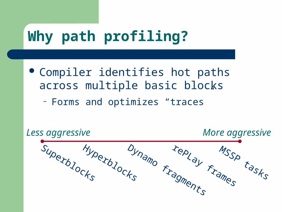
Compiler identifies hot paths across multiple basic blocks– Forms and optimizes “traces”

Why path profiling?
A
C
E
B
A
C
E
B
D
Oops!
Oops!
Compiler identifies hot paths across multiple basic blocks– Forms and optimizes “traces”
Why path profiling?
Superblocks
Dynamo fragments
Hyperblocks
rePLay frames
MSSP tasks
Less aggressive More aggressive
Compiler identifies hot paths across multiple basic blocks– Forms and optimizes “traces”

Ball-Larus path profiling
0
10
20
30
40
70 75 80 85 90 95 100
Accuracy (%)
Ove
rhea
d (
%)
Edge profiling
Ball-Larus path profiling
Targeted path profiling
Practical path profiling
Instrumentation measures execution frequency of each path
Acyclic, intraprocedural paths

Edge profiling
0
10
20
30
40
70 75 80 85 90 95 100
Accuracy (%)
Ove
rhea
d (
%)
Edge profiling
Ball-Larus path profiling
Targeted path profiling
Practical path profiling
Hardware or sampling Estimate hot paths
from edge profile
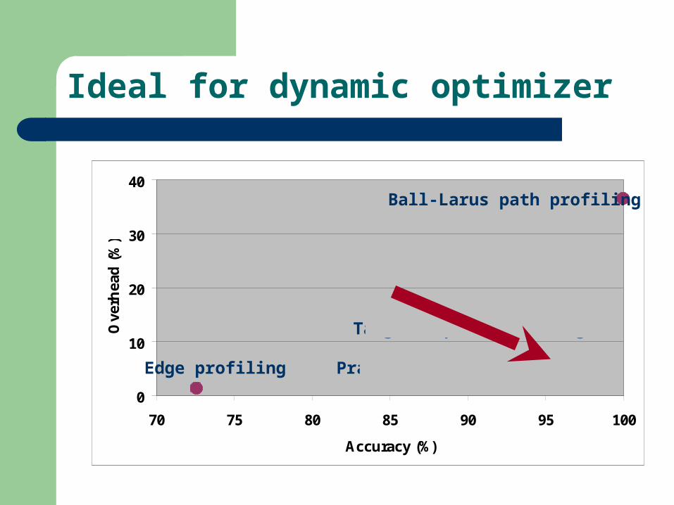
Ideal for dynamic optimizer
0
10
20
30
40
70 75 80 85 90 95 100
Accuracy (%)
Ove
rhea
d (
%)
Edge profiling
Ball-Larus path profiling
Targeted path profiling
Practical path profiling

Targeted path profiling [Joshi et al. ’04]
0
10
20
30
40
70 75 80 85 90 95 100
Accuracy (%)
Ove
rhea
d (
%)
Edge profiling
Ball-Larus path profiling
Targeted path profiling
Practical path profiling
Profile-guided profiling Accuracy good Overhead high for dynamic
optimizer

Practical path profiling
0
10
20
30
40
70 75 80 85 90 95 100
Accuracy (%)
Ove
rhea
d (
%)
Edge profiling
Ball-Larus path profiling
Targeted path profiling
Practical path profiling

Outline
Background– Staged dynamic optimization– Profile-guided profiling– Ball-Larus path profiling
Practical path profiling Methodology
– Edge profile-guided inlining and unrolling– Measuring accuracy with branch-flow metric
Accuracy and overhead

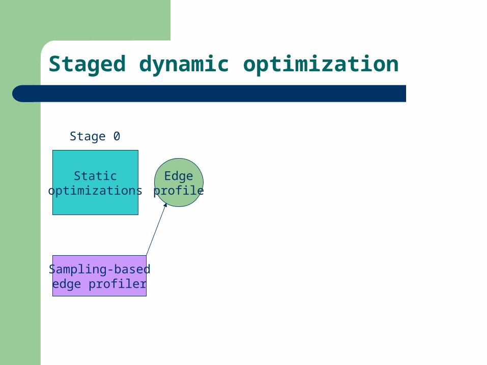
Staged dynamic optimization
Staticoptimizations
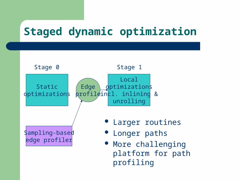
Stage 0
Staged dynamic optimization
Staticoptimizations
Edgeprofile
Stage 0
Sampling-basededge profiler

Staged dynamic optimization
Staticoptimizations
Edgeprofile
Stage 0
Localoptimizationsincl. inlining &
unrolling
Stage 1
Sampling-basededge profiler
Staged dynamic optimization
Staticoptimizations
Edgeprofile
Stage 0
Localoptimizationsincl. inlining &
unrolling
Stage 1
Larger routines Longer paths More challenging platform
for path profiling
Sampling-basededge profiler

Staged dynamic optimization
Staticoptimizations
Edgeprofile
Stage 0
Localoptimizationsincl. inlining &
unrolling
Path profilinginstrumentation
Stage 1
Sampling-basededge profiler

Staged dynamic optimization
Staticoptimizations
Edgeprofile
Stage 0
Localoptimizationsincl. inlining &
unrolling
Path profilinginstrumentation
Stage 1
Pathprofile
Sampling-basededge profiler

Staged dynamic optimization
Staticoptimizations
Edgeprofile
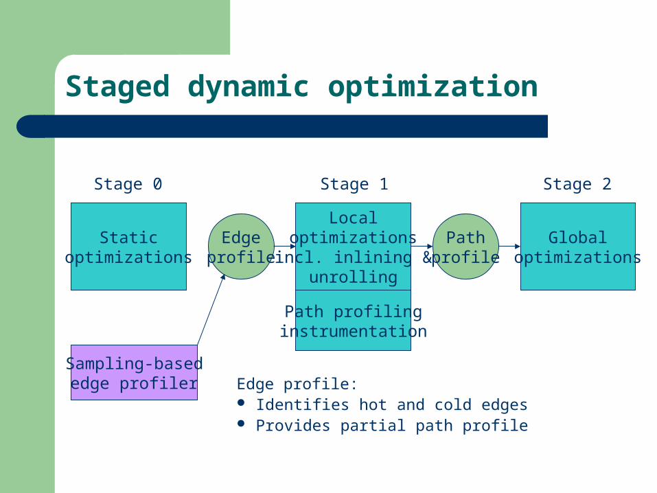
Stage 0
Localoptimizationsincl. inlining &
unrolling
Path profilinginstrumentation
Globaloptimizations
Stage 2 Stage 1
Pathprofile
Sampling-basededge profiler
Staged dynamic optimization
Staticoptimizations
Edgeprofile
Stage 0
Localoptimizationsincl. inlining &
unrolling
Path profilinginstrumentation
Globaloptimizations
Stage 2 Stage 1
Pathprofile
Edge profile: Identifies hot and cold edges Provides partial path profile
Sampling-basededge profiler

Profile-guided profiling
Staticoptimizations
Edgeprofile
Stage 0
Localoptimizationsincl. inlining &
unrolling
Path profilinginstrumentation
Globaloptimizations
Stage 2 Stage 1
Pathprofile
Edge profile: Identifies hot and cold edges Provides partial path profile
Sampling-basededge profiler

Ball-Larus path profiling
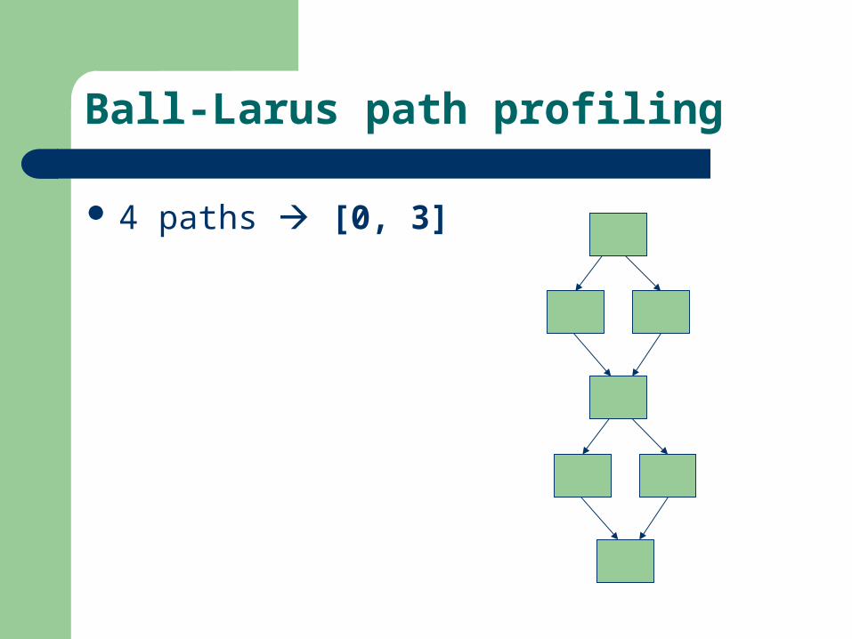
Acyclic, intraprocedural paths– Handles cyclic routines
Instrumentation maintains execution frequency of each path– Each path computes unique integer in [0, N-1]
Ball-Larus path profiling
4 paths [0, 3]

Ball-Larus path profiling
2
1
4 paths [0, 3] Each path sums to
unique integer
0
0

Ball-Larus path profiling
2
4 paths [0, 3] Each path sums to
unique integer
Path 01 0
0

Ball-Larus path profiling
2
4 paths [0, 3] Each path sums to
unique integer
Path 0
Path 11 0
0

Ball-Larus path profiling
2
4 paths [0, 3] Each path sums to
unique integer
Path 0
Path 1
Path 2
1 0
0

Ball-Larus path profiling
2
4 paths [0, 3] Each path sums to
unique integer
Path 0
Path 1
Path 2
Path 3
1 0
0
Ball-Larus path profiling
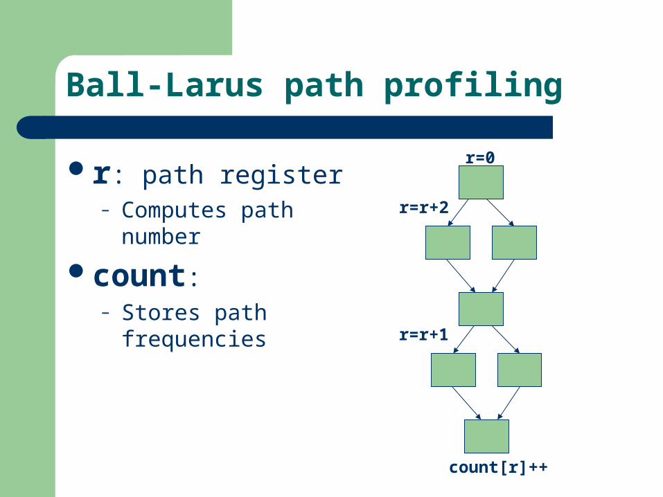
r=r+2
r=0
r=r+1
count[r]++
r: path register– Computes path number
count:– Stores path frequencies

Ball-Larus path profiling
r=r+2
r=0
count[r]++
r: path register– Computes path number
count:– Stores path frequencies– Array by default– Too many paths?
Hash table High overhead
r=r+1

Outline
Background– Ball-Larus path profiling– Staged dynamic optimization– Profile-guided profiling
Practical path profiling Methodology
– Edge profile-guided inlining and unrolling– Measuring accuracy with branch-flow metric
Accuracy and overhead

Practical path profiling
Goal: Reduce instrumentation overhead without hurting accuracy– Use profile-guided profiling
Strategies– Decrease number of possible paths– Avoid instrumenting paths edge profile predicts well– Simplify instrumentation on profiled paths

Practical path profiling
Goal: Reduce instrumentation overhead without hurting accuracy– Use profile-guided profiling
Strategies– Decrease number of possible paths– Avoid instrumenting paths edge profile predicts well– Simplify instrumentation on profiled paths
Techniques from targeted path profiling– Improves techniques– Adds new techniques

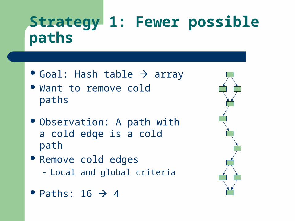
Strategy 1: Fewer possible paths
Goal: Hash table array Want to remove cold paths
4060
397
1000
5050

Strategy 1: Fewer possible paths
Goal: Hash table array Want to remove cold paths
Observation: A path with a cold edge is a cold path
Remove cold edges– Local and global criteria
4060
397
1000
5050New
Strategy 1: Fewer possible paths
Goal: Hash table array Want to remove cold paths
Observation: A path with a cold edge is a cold path
Remove cold edges– Local and global criteria
Paths: 16 4

Remaining paths potentially hot
4 paths [0, 3]
2
1
Strategy 1: Fewer possible paths
0
0

Remaining paths potentially hot
4 paths [0, 3]
Strategy 1: Fewer possible paths
r=r+2
r=0
r=r+1
count[r]++

What if cold edge taken?
Strategy 1: Fewer possible paths
r=r+2
r=0
r=r+1
count[r]++

What if cold edge taken? Cold edges “poison” path
register– Set it to N– Cold paths use [N, 2N-1]
Strategy 1: Fewer possible paths
r=r+2
r=0
r=4
r=4
r=r+1
count[r]++
New

What if cold edge taken? Cold edges “poison” path
register– Set it to N– Cold paths use [N, 2N-1]
What if still too many possible paths?
r=r+2
r=0
r=4
r=4
r=r+1
count[r]++
Strategy 1: Fewer possible paths

What if cold edge taken? Cold edges “poison” path
register– Set it to N– Cold paths use [N, 2N-1]
What if still too many possible paths?
Adjust cold edge threshold until hashing avoided
Strategy 1: Fewer possible paths
r=r+2
r=0
r=4
r=4
r=r+1
count[r]++New
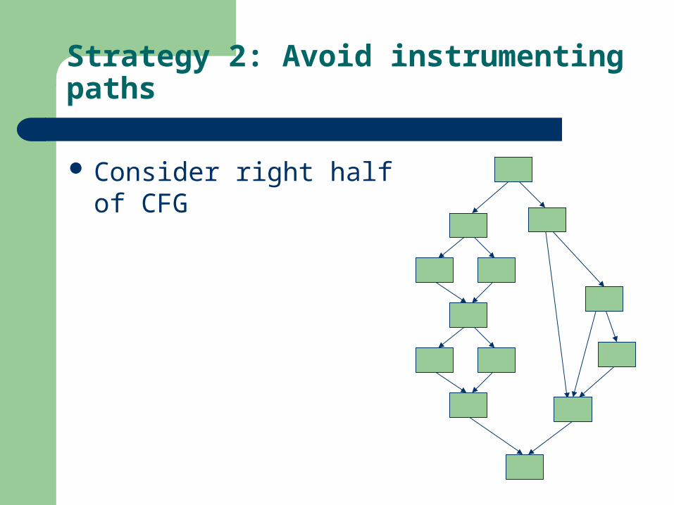
Strategy 2: Avoid instrumenting paths
Consider right half of CFG

Strategy 2: Avoid instrumenting paths
Consider right half of CFG– Obvious paths: Each path
has an edge unique to it– Edge profile provides
perfect path profile

Strategy 2: Avoid instrumenting paths
Consider right half of CFG– Obvious paths: Each path
has an edge unique to it– Edge profile provides
perfect path profile
We don’t instrument the right half of the CFG
r=r+2
r=r+1
r=0
count[r]++

Strategy 2: Avoid instrumenting paths
Synergy: Cold edge removal creates more obvious paths
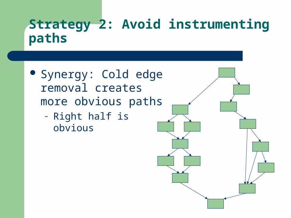
Strategy 2: Avoid instrumenting paths
Synergy: Cold edge removal creates more obvious paths– Right half is obvious

Strategy 2: Avoid instrumenting paths
What if cold edge is part of obvious and non-obvious paths?

Strategy 2: Avoid instrumenting paths
What if cold edge is part of obvious and non-obvious paths?
Right half obvious

Strategy 2: Avoid instrumenting paths
r=r+2
r=r+1
r=0
count[r]++
What if cold edge is part of obvious and non-obvious paths?
Right half obvious– But we haven’t avoided
instrumenting it!
r=4

Strategy 2: Avoid instrumenting paths
What if cold edge is part of obvious and non-obvious paths?
Right half obvious– But we haven’t avoided
instrumenting it!
Aggressive instrumentation pushing
r=r+2
r=r+1
r=0
count[r]++
New

Strategy 2: Avoid instrumenting paths
Overcounts some hot paths
r=r+2
r=r+1
r=0
count[r]++

Strategy 2: Avoid instrumenting paths
Overcounts some hot paths
Example cold path counts hot path number 1
Overcount tends to be small
r=r+2
r=r+1
r=0
count[r]++

Some paths need profiling
Correlation between cascading branches

Strategy 3: Simplify instrumentation
60
60 40
40
Moderately biased branches
New

Strategy 3: Simplify instrumentation
0
0 1
2
Moderately biased branches
Put zeros on hotter edges

Strategy 3: Simplify instrumentation
Moderately biased branches
Put zeros on hotter edges– No instrumentation
on hotter edges
r=r+2
r=0
r=r+1
count[r]++

Outline
Background– Staged dynamic optimization– Profile-guided profiling– Ball-Larus path profiling
Practical path profiling Methodology
– Edge profile-guided inlining and unrolling– Measuring accuracy with branch-flow metric
Accuracy and overhead

Methodology
Path profiling implemented in Scale [McKinley et al.]
– Ahead-of-time compiler deterministic platform
Edge profile-guided inlining and unrolling precede path profiling

Methodology
Path profiling implemented in Scale [McKinley et al.]
– Ahead-of-time compiler deterministic platform
Edge profile-guided inlining and unrolling precede path profiling
Alpha binaries for subset of SPEC2000– C and Fortran 77 only– Scale wouldn’t compile gzip, vortex, gcc
ref inputs for all runs

Measuring accuracy
Compare estimated profile with actual profile– Wall weight matching* or profile overlap
Weight paths by flow: amount of execution– Previous work measures flow with unit-flow metric
Flow(p) = Freq(p)
– We introduce branch-flow metricFlow(p) = Freq(p) x NumBranches(p)

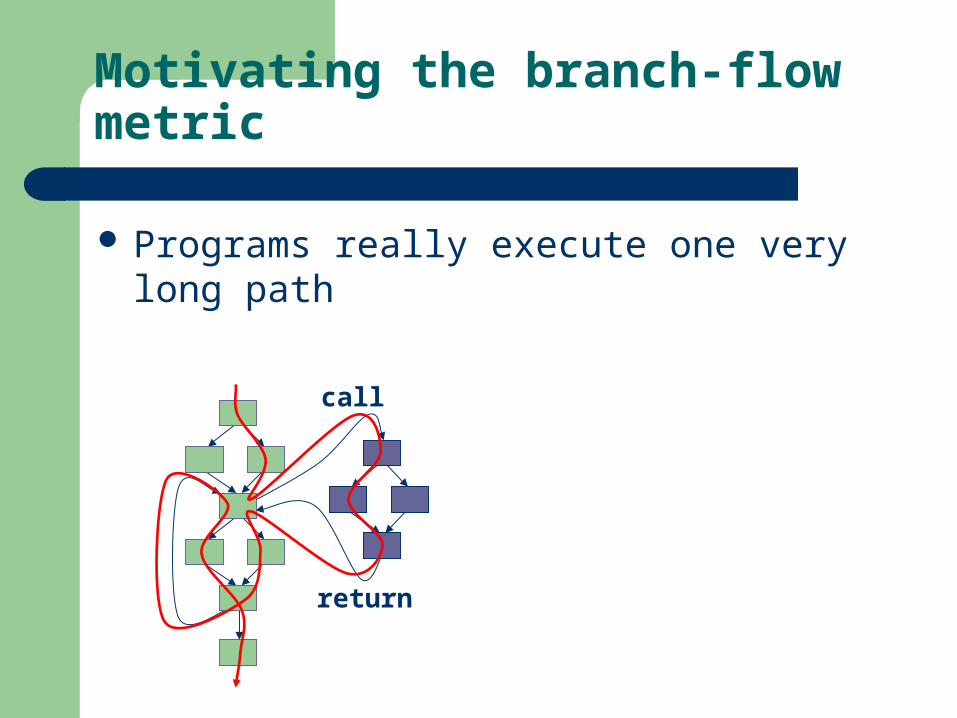
Motivating the branch-flow metric
Programs really execute one very long path
call
return
Motivating the branch-flow metric
Programs really execute one very long path
call
return

Motivating the branch-flow metric
Programs really execute one very long path– Ball-Larus path profiling breaks it into multiple
acyclic, intraprocedural paths
call
return
call
return

Motivating the branch-flow metric
Some paths longer than others– We care more about longer paths– Unit-flow metric unfairly rewards edge profiling
call
return
call
return

Outline
Background– Staged dynamic optimization– Profile-guided profiling– Ball-Larus path profiling
Practical path profiling Methodology
– Edge profile-guided inlining and unrolling– Measuring accuracy with branch-flow metric
Accuracy and overhead

Accuracy
0
10
20
30
40
50
60
70
80
90
100
Ac
cu
rac
y (
%)
Edge profiling Targeted path profiling Practical path profiling

Overhead
0
10
20
30
40
50
60
70
vpr
mcf
craf
ty
parse
r
perlb
mk
gapbzip
2tw
olf
INT A
vg
Overa
ll Avg
Ov
erh
ea
d (
%)
Ball-Larus path profiling Targeted path profiling Practical path profiling

Related work
Dynamo [Bala et al. ’00]
– Successful path-based dynamic optimizer– “Bails out” when no dominant path
Instrumentation sampling & dynamic instrumentation [Arnold & Ryder ’01, Hirzel & Chilimbi ’04, Yasue et al. ’04]
– Lower overhead by extending profiling time– Orthogonal to practical path profiling
Hardware-based path profiling [Vaswani et al. ’05]
– High accuracy when hot path table large enough

Summary
0
10
20
30
40
70 75 80 85 90 95 100
Accuracy (%)
Ove
rhea
d (
%)
Edge profiling
Ball-Larus path profiling
Targeted path profiling
Practical path profiling
Contributions: Inlining and unrolling Branch-flow metric Practical path profiling

Questions?