practicals in r - université de montréalbiol09.biol.umontreal.ca/bio6077/practicals_in_r.pdf ·...
TRANSCRIPT
Practicals using the R statistical language Pierre Legendre August 2005; May, July 2006; Département de sciences biologiques May, July, Nov. 2007; Jan., Feb., April, Aug., Oct. 2008; Université de Montréal February to November 2009, September 2010; January 2011; July, November 2012; April, June, October 2016; January, March, November 2017 0. R packages Install the following R packages. They will be used in these practical exercises. — • Install packages available on CRAN: install.packages(c("ade4", "adegraphics", "adespatial", "ape", "cclust", "cluster", "FD", "geoR", "labdsv", "mapdata", "maps", "rgl", "spdep", "vegan"), dependencies=TRUE) • Install mvpart available on Github. First, install.packages("devtools") if you don’t already have this package installed in your computer. Then: library(devtools) install_github("cran/mvpart", force=TRUE) • Install ‘rdaTest’ from http:/numericalecology.com, following the instructions in section 3 of the document “Introduction_to_R.pdf”.
• Other functions, available on http:/numericalecology.com, will also be used in the course. 1. Compute basic statistics in the R language: Robin data # Import data file ‘Robins.txt’ from your working directory into an object ‘robin’ (class: data frame) # You must first tell R what your working directory is: # Windows: File menu ⇒ Change dir... # Mac OSX: Misc. menu ⇒ Change Working Directory robin <- read.table("Robins.txt") # or: robin = read.table("Robins.txt") # Alternative method: function file.choose() opens a dialogue box to navigate your hard disk robin <- read.table( file.choose() ) # Navigate to find the "Robins.txt" data file # Check that the data have been read correctly robin # or: head(robin) # Copy the wing length values (first column) into an object ‘wing’: wing = robin[,1] wing # Print the contents of object 'wing' class(wing) # Find the class of object 'wing' is.vector(wing) is.matrix(wing) # Transform vector ‘wing’ into an object with class ‘matrix’ in case you need it later: wing.mat = as.matrix(wing) wing.mat is.vector(wing.mat) is.matrix(wing.mat)
Practicals using the R language 2
# Compute the mean wing length: wing.mean = mean(wing) # or: wing.mean = mean(wing.mat) wing.mean # Print the value of the mean # Compute the median wing length: wing.med = median(wing) # or: wing.med = median(wing.mat) wing.med # Print the value of the median # Compute the variance of the wing lengths: wing.var = var(wing) # or: wing.var2 = var(wing.mat) # Print the value of the variance: wing.var # or: wing.var2 is.vector(wing.var) # or: is.vector(wing.var2) is.matrix(wing.var) # or: is.matrix(wing.var2) # Compute the sample size ‘n’: n = length(wing) # Compute the value of ‘n’ ( n = length(wing) ) # Shortcut: compute the value of ‘n’ and print it ( n1 = nrow(wing.mat) ) # or: ( n1 = dim(robin)[1] ) # or: ( n1 = dim(wing.mat)[1] ) # Compute the skewness A3. # # First, compute an unbiased estimate of the moment of order 3, k3: k3 = (n*sum((wing.mat-mean(wing.mat))^3))/((n-1)*(n-2)) k3 # Print the value of k3 # # Then, compute the skewness, A3: A3 = k3/((sqrt(wing.var))^3) A3 # Print the value of A3 # Compute the kurtosis A4. # # First, compute an unbiased estimate of the moment of order 4, k4, and print it: k4 = (n*(n+1)*(sum((wing.mat-mean(wing.mat))^4))-3*(n-1)*((sum((wing.mat-mean(wing.mat) )^2))^2))/((n-1)*(n-2)*(n-3)) k4 # # Then, compute the kurtosis, A4, and print it: A4 = k4/((sqrt(wing.var))^4) A4 # Compute the width of the range of values: wing.range = max(wing)-min(wing) # or: wing.min.max = range(wing) wing.range # wing.min.max # Compute the standard deviation: ( sx = sd(wing) ) # Plot a histogram # The most simple way is to use the function ‘hist’ with all the default values: hist(robin[,1]) # The histogram appears in the graphics window. It can be saved in different formats for future use (menu File: “save as...”)

Practicals using the R language 3
# One can specify the presentation details of the histogram par(mai = c(1.5, 0.75, 0.5, 0.5)) # Modify the margins of the graph. See ?par hist(robin[,1], breaks = "Sturge", freq = TRUE, right =FALSE, main = NULL, xlab = NULL, ylab
= NULL, axes = TRUE) # Look up these specifications in the documentation file of ‘hist’ ?hist # Add axis labels and a title mtext(text="Frequency", side=2, line=3, cex=1, font=1) mtext(text="Wing length (mm)", side=1, line=3, cex=1, font=1) mtext(text="Histogram of Robin wing length", side=1, line=6, cex=1.5, font=1) # ========== # Repeat this exercise for variable Mass(kg), Height(cm) or Length(cm) of file ‘Bears.txt’. Call your file ‘bears’. Be careful when reading the data! — Is that file difficult to read in the R window? Why? # Check that the data have been read correctly! For that, type head(bears) # Check section “Importing a data file to be analysed by R” on pp. 3-4 of “Introduction_to_R.pdf”
# After you have completed the exercise, try the following commands for the ‘bears’ data: summary(bears) plot( bears[, 2:5] ) # ========
Practicals using the R language 4
# How to attribute values to the parameters of an R function # R functions may have several parameters (see for example ?read.table or ?hist) and these parameters often have default values in the function. For example, the following function add3 <- function(a = 0, b = 10, c = -5) a+b+c # has three parameters, a, b and c, which represent numbers. Default values have been given to these parameters: a = 0, b = 10, c = –5. The function adds the three numbers. Example: add3() # gives for result the sum of the three numbers. # Users can replace the default values by other values that they provide. Example of replacement according to the positions of the parameters: add3(2, 4, 6) # The order determines the attribution of values to the parameters. # Same result if values are explicitly given to parameters a, b et c: add3(a=2, b=4, c=6) # Equivalent command: add3(b=4, c=6, a=2) # Can you anticipate the results of the following calls to the function? # 1. Attribution according to positions. What is the value taken by c? What will the sum be? add3(2, 4) # 2. Explicit attribution of a value to b. What are the values taken by a and c? What will the sum be? add3(b=7) ========

Practicals using the R language 5
Examine the output object produced by rda() or cca() of {vegan} # Example: create an output object of function rda() rda.object.name <- rda(a.data.file) # List the first-level elements of the output object, which is rather complex attributes(rda.object.name) # You can then examine the contents of the separate elements as follows. Examples: rda.object.name$call rda.object.name$CA rda.object.name$tot.chi # The structure of rda() and cca() output objects is described in a documentation file: ?cca.object # You can also examine the detailed structure of a given rda or cca output object (a long list): str(rda.object.name) # In the PCA exercise on pp. 7-8, we will use vegan’s summary.cca() function to print the PCA results summary(rda.out, scaling=1) # Note that the function is called by typing summary() and not summary.cca(). The function recognizes the class of the rda.out object, which is "rda" "cca". # If the output says “Total inertia: 0” followed by an error message, that could be due to the fact that the package {ade4} has been loaded after {vegan} and function cca() of {ade4} is masking vegan’s same-name function. If you loaded {adespatial} after {vegan}, {adespatial} has loaded {ade4} and you have the same problem. To solve the issue and make summary.cca() print the PCA or RDA results correctly, you have to completely detach {vegan} and load it again: unloadNamespace("vegan") library("vegan") # Following this operation, the cca() function of {vegan} is masking ade4’s same-name function and summary.cca() should work correctly.

Practicals using the R language 6
2. Simple ordination methods: PCA, CA, PCoA, nMDS # 2.1. Principal component analysis (PCA) # 2.1.1. Principal component analysis (PCA) through matrix algebra # Create the data matrix: Y.mat = matrix(c(2,3,5,7,9,1,4,0,6,2), 5, 2) class(Y.mat) # Check the class attached to object Y.mat # Center matrix Y.mat by columns using function ‘scale’: Y.cent = scale(Y.mat, center=TRUE, scale=FALSE) # Data centered but not standardized # Compute the covariance matrix: Y.cov = cov(Y.cent) # If the data are not standardized (scale=FALSE), the following command is equivalent: Y.cov = cov(Y.mat) # but that is not the case if scale=TRUE. # Compute the eigenvalues and eigenvectors: Y.eig = eigen(Y.cov) # Compare with the result of Ycov.svd = svd(Y.cov) # Compare with the result of Y.svd = svd(Y.cent) # Check the eigenvalues and eigenvectors: Y.eig$values Y.eig$vectors # Transfer the eigenvectors to U. It will be used to represent the variables in scaling type 1 plots: U = Y.eig$vectors # Compute matrix F. It will be used to represent the objects in scaling type 1 plots: F = Y.cent %*% U F # Check the contents of F # Compute matrix U2. It will be used to represent the variables in scaling type 2 plots: U2 = U %*% diag(Y.eig$values^(0.5)) # Compute matrix G. It will be used to represent the objects in scaling type 2 plots: G = F %*% diag(Y.eig$values^(-0.5)) # Scaling type 1 biplot — # Dispersion diagram of the first 2 columns of F produced using the general plot() function: plot(F[,1], F[,2], xlim=c(-4,4), ylim=c(-3,3), asp=1, xlab="Axis 1", ylab="Axis 2") # Notes: (-4,4) = limits of the plot abscissa, (-3,3) = limits of the plot ordinate. # asp=1 : the ratio of the dimensions abscissa/ordinate is fixed to 1 # to obtain a correct representation of the distances among the objects.
Practicals using the R language 7 # Here is another method to obtain the limits of the abscissa and ordinate for the graph. The function "range" provides the min and max values along axes 1 and 2. It can be applied to the columns of F by "apply": F.range = apply(F, 2, range) F.range # Create vectors “xlim” and “ylim” giving the limit values for the plot axes: xlim = c(F.range[1,1], F.range[2,1]) ylim = c(F.range[1,2], F.range[2,2]) plot(F[,1], F[,2], xlim=xlim, ylim=ylim, asp=1, xlab="Axis 1", ylab="Axis 2") # Add to the diagram arrows representing the first two columns of matrix U: arrows(x0=0, y0=0, U[,1]*3, U[,2]*3) # Note: for this example, the coordinates of the variables (from matrix U) are multiplied by 3. # Exercice : plot the diagram for scaling type 2. # This time, use function biplot() of {stat}, designed specifically for PCA, with matrices G and U2 biplot(G, U2) # ======== # 2.1.2. Principal component analysis (PCA) using the ‘vegan’ package # First, load the ‘vegan’ package into your work space: library(vegan) # For this example, the data are found in object Y.mat created at the beginning of section 2.1.1. rda.out = rda(Y.mat) # Default option: scale=FALSE # PCA is calculated by the rda() function. That function can also compute canonical RDA. # The rda() function produces a PCA when a single data file is provided. # With the argument "scale=FALSE", the data are centred by columns but not standardized. # Examine the object produced by function rda(). See the notes entitled “Examine the output object produced by rda() or cca() of {vegan}” on page 5. # Examine the PCA results – eigenvals(rda.out) # Eigenvalues # Scaling = 1: preserves the Euclidean distances among objects # Scaling = 2: preserves the correlations among descriptors # PCA with scaling 1: summary(rda.out, scaling=1) # Species scores, site scores (modified by vegan) biplot(rda.out, scaling=1) # Function biplot.rda() of ‘vegan’ is used # PCA with scaling 2: # This is also the default value of the biplot.rda function summary(rda.out, scaling=2) # Species scores, site scores (modified by vegan) biplot(rda.out, scaling=2) # Function biplot.rda() of ‘vegan’ is used # Note – Vegan’s function summary.cca() transforms the numerical results before printing them. In scaling=1, the species coordinates (U) are multiplied by the “General scaling constant” and the site coordinates (F) are divided by that constant. In scaling=2, the transformations are more complex; see the document “decision-vegan.pdf”. In a nutshell, the species and site coordinates are linear transformations of the coordinates computed in matrices U2 and G of the exercise. # ==========
Practicals using the R language 8
# Exercise: compute a PCA for the file “Spiders_28x12_spe.txt” of Netherland spider assemblages (van der Aart & Smeenk-Enserink 1975. Neth. J. Zool. 25: 1-45). spiders.spe = read.table( file.choose() ) • For species abundance data, one should, in most cases, apply a transformation to the data before computing PCA. The reason is that PCA preserves Euclidean distances among the objects and that distance is inappropriate for community composition data. See section "4. Transformations". spiders.hel = decostand(spiders.spe, "hellinger") # Apply the Hellinger transformation • Compute PCA using vegan’s rda() function; it computes a PCA when a single data file is provided. res <- rda(spiders.hel) • Examine the structure of the output object. See the notes entitled “Examine the output object produced by rda() or cca() of {vegan}” on page 5. # ========== # 2.1.3. Principal component analysis using the ‘PCA.newr’ function # Repeat the spiders exercise using the ‘PCA.newr’ function available among the functions of Numerical ecology with R. The R code in that function is essentially that found in section 2.1.1, plus some added features. You can open file “PCA.newr.R’ using a text editor and examine the code. # First, load the function into your work space: # Windows clients: go to the File menu => Source R Code... # MacOS X clients: go to the Files menu => Source File... pca.out = PCA.newr(spiders.hel) # Default: no standardization of the variables biplot(pca.out) # The default value is scaling type 1 # Compare the results: (a) those of function rda(), i.e. the eigenvalues, eigenvectors and principal components (eigenvals(rda.out), scores(rda.out, scaling=1)), and (b) those of function PCA.newr() (pca.out$eigenvalues, pca.out$U, pca.out$F). Why are there differences? — See the document “decision-vegan.pdf”, p. 4, Table 1, available in the vegan folder.

Practicals using the R language 9
# 2.2. Correspondence analysis (CA) # 2.2.1. Correspondence analysis (CA) through matrix algebra # Read a data table that will be subjected to correspondence analysis. # You may choose 'Table_9.11.txt' (small example from Chapter 9 of manual) # or 'Spiders_28x12_spe.txt' (larger data set, real data). Y = read.table( file.choose() ) # Calculate the basic parameters of Y; save the row and column names n = nrow(Y) p = ncol(Y) n.eigval = min((n-1),(p-1)) site.names = rownames(Y) sp.names = colnames(Y) # Construct the Qbar matrix (contributions to chi-square) fi. = matrix(apply(Y,1,sum),n,1) f.j = matrix(apply(Y,2,sum),1,p) f. = sum(fi.) pi. = as.vector(fi./f.) p.j = as.vector(f.j/f.) E = (fi. %*% f.j)/f. Qbar = (Y - E) * E^(-0.5) / sqrt(f.) # Analyse Qbar by 'svd' svd.res = svd(Qbar) eigenvalues = svd.res$d[1:n.eigval]^2 U = svd.res$v[,1:n.eigval] Uhat = svd.res$u[,1:n.eigval] # Alternative analysis or Qbar by 'eigen' Qbar = as.matrix(Qbar) QprQ.eig = eigen( t(Qbar) %*% Qbar ) eigenvalues = QprQ.eig$values[1:n.eigval] U = QprQ.eig$vectors[,1:n.eigval] Uhat = Qbar %*% U %*% diag(eigenvalues^(-0.5)) # Construct matrices V, Vhat, F, and Fhat for the ordination biplots V = diag(p.j^(-0.5)) %*% U Vhat = diag(pi.^(-0.5)) %*% Uhat F = Vhat %*% diag(eigenvalues^(0.5)) Fhat = V %*% diag(eigenvalues^(0.5)) # Find the limits of the plots V.range = apply(V[,1:2],2,range) Vhat.range = apply(Vhat[,1:2],2,range) F.range = apply(F[,1:2],2,range) Fhat.range = apply(Fhat[,1:2],2,range) par(mfrow=c(1,2)) # Create a drawing window for two graphs # Biplot, scaling type = 1: plot F for sites, V for species # The sites are at the centroids (barycentres) of the species # This projection preserves the chi-square distance among the sites xmin = min(V.range[1,1], F.range[1,1]) - 0.5

Practicals using the R language 10
xmax = max(V.range[2,1], F.range[2,1]) + 0.5 ymin = min(V.range[1,2], F.range[1,2]) - 0.5 ymax = max(V.range[2,2], F.range[2,2]) + 0.5 plot(F[,1:2], asp=1, pch=20, cex=2, xlim=c(xmin,xmax), ylim=c(ymin,ymax), xlab="CA axis 1", ylab="CA axis 2") text(F[,1:2], labels=site.names, pos=4, offset=0.5) points(V[,1:2], pch=22, cex=2) text(V[,1:2], labels=sp.names, pos=4, offset=0.5) title(main = c("CA biplot","scaling type 1"), family="serif") # Biplot, scaling type = 2: plot Vhat for sites, Fhat for species # The species are at the centroids (barycentres) of the sites # This projection preserves the chi-square distance among the species xmin = min(Vhat.range[1,1], Fhat.range[1,1]) - 0.5 xmax = max(Vhat.range[2,1], Fhat.range[2,1]) + 0.5 ymin = min(Vhat.range[1,2], Fhat.range[1,2]) - 0.5 ymax = max(Vhat.range[2,2], Fhat.range[2,2]) + 0.5 plot(Vhat[,1:2], asp=1, pch=20, cex=2, xlim=c(xmin,xmax), ylim=c(ymin,ymax), xlab="CA axis 1", ylab="CA axis 2") text(Vhat[,1:2], labels=site.names, pos=4, offset=0.5) points(Fhat[,1:2], pch=22, cex=2) text(Fhat[,1:2], labels=sp.names, pos=4, offset=0.5) title(main = c("CA biplot","scaling type 2"), family="serif")

Practicals using the R language 11
# 2.2.2 Correspondence analysis (CA) using the ‘vegan’ package # Scaling = 1: preserves the chi-square distances among objects. # Uses matrices F and V, as in Canoco. # Scaling = 2: preserves the chi-square distances among species. # Uses matrices V-hat and F-hat, as in Canoco. # Exemple 1: CA of Aart’s (1973) spider data. Read the data file ‘Spiders_28x12_spe.txt’ library(vegan) spiders=read.table( file.choose() ) spiders.ca=cca(spiders) summary(spiders.ca, scaling=1) plot(spiders.ca, scaling=1) # Note: CA cannot be computed if there are rows or columns that sum to 0 in the data file. This is due to the transformation of Y into matrix Q-bar, which is the first step of CA. # If there are rows or columns that sum to 0, the function ‘c‘ (“combine”) allows users to select the row or column numbers that have sums larger than 0 and use only those in the analysis. # Exemple 2 (if time allows): CA of the cafés of Neuchâtel data. Data file: "Cafes_10x6_spe.txt". The data represent the clientele in 10 restaurants of the town of Neuchâtel in Switzerland. The restaurant names are real; the clientele data were made up by Daniel Borcard to illustrate the properties of CA. cafes.spe=read.table( file.choose() ) cafes.afc=cca(cafes.spe) cafes.afc plot(cafes.afc, scaling=2) summary(cafes.afc, scaling=2, axes=5) # CA can also be computed using function ‘CA.newr’ available on the Web page numericalecology.com. # ==========
Practicals using the R language 12
# 2.3. Principal coordinate analysis (PCoA) # One can use the function cmdscale of the ‘stats’ package to carry out this analysis. “cmds” is the acronym of “classical multidimensional scaling”. # Functions for PCoA are also available in packages ape (function pcoa) and ade4 (function dudi.pco). # PCoA starts with a distance (or dissimilarity) matrix. Distance functions will be studied in Section 3. The Euclidean distance will be used to illustrate how to use PCoA. The Euclidean distance is the default option when using function dist of the ‘stats’ package. # Example: analysis of the file “Spiders_28x12_spe.txt" spiders = read.table( file.choose() ) # Compute the matrix of Euclidean distances spiders.D1 = dist(spiders) # or: spiders.D1 = dist(spiders, method="eucl") # Principal coordinate analysis. Save k=5 axes. Plot a graph of axes 1 and 2. toto4=cmdscale(spiders.D1, 5, eig=TRUE) plot(toto4$points[,1], toto4$points[,2], asp=1, xlab="Axis 1", ylab="Axis 2") # Note: "asp=1" constrains the two axes to the same scale. This ensures that the distances # among objects on the plot are projections of their real distances in multivariate space. ?cmdscale # consult the documentation file of function cmdscale summary(toto4) # to obtain a list of the elements in file toto4 toto4$points # contains the coordinates of the objects along the k=5 requested dimensions toto4$eig # contains the eigenvalues of the principal axes # Repeat the analysis after applying the Hellinger transformation (using function decostand of the vegan package) to the spider abundance data. The transformations are described in Section 4. # Hellinger transformation of species abundances, followed by calculation of Euclidean distances. library(vegan) spiders.hel = decostand(spiders, "hel") # Hellinger transformation spiders.DHell = dist(spiders.hel) # Compute the Hellinger distance # Principal coordinate analysis. res = cmdscale(spiders.DHell, 5, eig=TRUE) limits = apply(res$points, 2, range) xlim = c(limits[1,1], limits[2,1]) + c(-0.2,0) ylim = c(limits[1,2], limits[2,2]) x = res$points[,1] y = res$points[,2] plot(x, y, xlim=xlim, ylim=ylim, asp=1, xlab="Axis 1", ylab="Axis 2") # Fonction text adds the object names to the graph. names = rownames(spiders) text(x, y, labels= names, pos=2, cex=1, offset=1) # PCoA can also be computed using the pcoa() function of the ape package. The biplot.pcoa() function of that package produces nicer ordination plots than those produced above.
Practicals using the R language 13
# 2.4. Non-metric multidimensional scaling (nMDS) # We will first use fonctions nmds and bestnmds of the labdsv package. These functions, written by David W. Roberts, are wrappers for the function isoMDS of Brian D. Ripley’ MASS package. # nMDS starts with a distance matrix. Distance functions will be studied in Section 3. # Example: analyse file "Spiders_28x12_spe.txt" spiders = read.table( file.choose() ) # Hellinger transformation of species abundances, followed by calculation of Euclidean distances. # As a consequence, the "spiders.DHell" matrix will contain Hellinger distances. library(vegan) spiders.hel = decostand(spiders, "hel") spiders.DHell = dist(spiders.hel) # Compute an nMDS solution in k=2 dimensions. If no initial configuration of the points is provided, PCoA is computed. The first two axes of that solution are taken as the initial configuration for nMDS. library(labdsv) toto2 = nmds(spiders.DHell, k=2) plot(toto2) # The bestnmds wrapper provides a list of the successive solutions (paramètre "itr") obtained by using several random configurations as starting points for nMDS. toto2 = bestnmds(spiders.DHell, k=2, itr=20) # The solution with lowest stress is kept in the output object. Plot it. plot(toto2) # ========== # The vegan package contains function metaMDS. This wrapper of isoMDS carries our nMDS following the recommendations of ecologist Peter Minchin. The function automatically looks for a stable solution after several random starting configurations (by default, trymax = 20). # At the end of the analysis, a PCA of the final configuration is computed, so that the variance of the objects is maximum along the first axis. The species are projected in the site ordination graph as weighted averages, in the same way as in correspondence analysis. # The documentation of metaMDS is quite detailed. # The Bray-Curtis distance is the default in metaMDS. Instead, we will use Hellinger distances obtained by computing the Euclidean distance on Hellinger-transformed data. # Compute an nMDS solution in k=2 dimensions (default value). toto3 = metaMDS(spiders.hel, distance="euclidean") plot(toto3, type="t") # type="t" adds species to the graph
Practicals using the R language 14
3. Dissimilarities Dissimilarity (or distance) functions are available in several packages of the R language. 3.1. Package stats, function dist : 6 distances (documentation: ?dist) euclidean: Usual Euclidean distance between the two vectors (2 norm). This is the default value. maximum: Maximum distance between two components of x and y (supremum norm). manhattan: Absolute distance between the two vectors (1 norm). canberra: sum(|x_i - y_i| / |x_i + y_i|). Terms with zero numerator and denominator are omitted
from the sum and treated as if the values were missing. binary: (aka asymmetric binary): The vectors are regarded as binary bits, so non-zero elements are
‘on’ and zero elements are ‘off’. The distance is the proportion of bits in which only one is on amongst those in which at least one is on. ⎯ This coefficient is (1 – Jaccard).
minkowski: The p norm, the pth root of the sum of the pth powers of the differences of the components.
The choice of coefficient is done by typing its name in quotes. Example: dist(data, method="binary") or dist(data, "binary") => In practice, function dist() is mostly used to compute a Euclidean distance matrix. 3.2. Package vegan, function vegdist : 10 distances (documentation: ?vegdist) euclidean d[jk] = sqrt(sum (x[ij]-x[ik])^2) manhattan d[jk] = sum(abs(x[ij] - x[ik])) gower d[jk] = (1/M) sum (abs(x[ij]-x[ik])/(max(x[i])-min(x[i]))); M = number of variables altGower d[jk] = (1/NZ) sum(abs(x[ij] - x[ik])); NZ = n. columns excluding double-zeros canberra d[jk] = (1/NZ) sum ((x[ij]-x[ik])/(x[ij]+x[ik])); exclude double-zeros; NZ as above bray d[jk] = (sum abs(x[ij]-x[ik])/(sum (x[ij]+x[ik])) = Bray & Curtis distance(default) kulczynski d[jk] 1 - 0.5*((sum min(x[ij],x[ik])/(sum x[ij]) + (sum min(x[ij],x[ik])/(sum x[ik])) morisita {d[jk] = 1 - 2*sum(x[ij]*x[ik])/((lambda[j]+lambda[k]) * sum(x[ij])*sum(x[ik])) } where lambda[j] = sum(x[ij]*(x[ij]-1))/sum(x[ij])*sum(x[ij]-1) horn Like morisita, but lambda[j] = sum(x[ij]^2)/(sum(x[ij])^2) binomial d[jk] = sum(x[ij]*log(x[ij]/n[i]) + x[ik]*log(x[ik]/n[i]) - n[i]*log(1/2))/n[i] jaccard
where n[i] = x[ij] + x[ik] d[jk] = 1 - (a / (a+b+c)); binary=TRUE to obtain the Jaccard coeff. for binary data.
"mountford" (Mountford index), "raup" (Raup-Crick probabilistic index), "chao" (Chao index), "cao" and "mahalanobis" can also be obtained. See ?vegdist. The choice of coefficient is done by typing its name in quotes. Example: vegdist(data, method="bray") or vegdist(data, "bray")

Practicals using the R language 15
3.3. Package ade4, function dist.binary : 10 binary distances (documentation: ?dist.binary) => These similarities (S) are converted to distances through the transformation D = sqrt(1 – S) . 1 = Jaccard index (1901) [S3 coefficient of Gower & Legendre] : s1 = a / (a+b+c) 2 = Sokal & Michener index (1958) [S4 coefficient of Gower & Legendre] : s2 = (a+d) / (a+b+c+d) 3 = Sokal & Sneath(1963) [S5 coefficient of Gower & Legendre] : s3 = a / (a + 2(b + c)) 4 = Rogers & Tanimoto (1960) [S6 coefficient of Gower & Legendre] : s4 = (a + d) / (a + 2(b + c) +d) 5 = Czekanowski (1913) or Sørensen (1948) [S7 coefficient of Gower & Legendre] : s5 = 2a / (2a + b + c) 6 = [S9 index of Gower & Legendre (1986)] : s6 = (a - (b + c) + d) / (a + b + c + d) 7 = Ochiai (1957) [S12 coefficient of Gower & Legendre] : s7 = a / sqrt((a + b)(a + c)) 8 = Sokal & Sneath (1963) [S13 coefficient of Gower & Legendre] : s8 = ad / sqrt((a + b)(a + c)(d + b)(d + c)) 9 = Phi of Pearson [S14 coefficient of Gower & Legendre] : s9 = (ad - bc) / sqrt((a + b)(a + c)(d + b)(d + c)) 10 = [S2 coefficient of Gower & Legendre] : s10 = a / (a + b + c + d) # The choice of coefficient is done by typing its number in the list above. Examples: dist.binary(data, method=1) or dist.binary(data, 1) or dist.binary(data, "1") 3.4. Package adespatial, function dist.ldc(): 21 dissimilarity indices (information: ?dist.ldc) # The function allows users to compute 18 quantitative dissimilarity indices:
"hellinger", "chord", "chisquare", "profiles", "percentdiff", "ruzicka", "divergence", "canberra", "whittaker", "wishart", "kulczynski", "ab.jaccard", "ab.sorensen", "ab.ochiai", "ab.simpson", "euclidean", "manhattan", "modmeanchardiff", as well as 3 binary indices: "jaccard", "sorensen", "ochiai".
# These measures are described and analysed in the Legendre & De Cáceres (2013) paper. # Details about the 21 dissimilarity indices are found in the Details of the documentation file. -------- Group 1 – The D matrix is computed by transformation of Y followed by Euclidean distance.
Hellinger D, D[ik] = sqrt(sum((sqrt(y[ij]/y[i+])-sqrt(y[kj]/y[k+]))^2))
chord D, D[ik] = sqrt(sum((y[ij]/sqrt(sum(y[ij]^2))-y[kj]/sqrt(sum(y[kj]^2)))^2))
chi-square D, D[ik] = sqrt(y[++] sum((1/j[+j])(y[ij]/y[i+]-y[kj]/y[k+])^2))
species profiles D, D[ik] = sqrt(sum((y[ij]/y[i+]-y[kj]/y[k+])^2))

Practicals using the R language 16
Group 2 – Other D functions appropriate for the study of beta diversity. In the first two functions, A = sum(min(y[ij],y[kj])), B = y[i+]-A, C = y[k+]-A.
percentage difference D, D[ik] = (sum(abs(y[ij]-y[k,j])))/(y[i+]+y[k+]) or else, D[ik] = (B+C)/(2A+B+C) =
Ružička D, D[ik] = 1-(sum(min(y[ij],y[kj])/sum(max(y[ij],y[kj])) or else, D[ik] = (B+C)/(A+B+C)
coeff. of divergence D, D[ik] = sqrt((1/pp)sum(((y[ij]-y(kj])/(y[ij]+y(kj]))^2))
Canberra metric D, D[ik] = (1/pp)sum(abs(y[ij]-y(kj])/(y[ij]+y(kj]))
Whittaker D, D[ik] = 0.5*sum(abs(y[ij]/y[i+]-y(kj]/y[k+]))
Wishart D, D[ik] = 1-sum(y[ij]y[kj])/(sum(y[ij]^2)+sum(y[kj]^2)-sum(y[ij]y[kj]))
Kulczynski D, D[ik] = 1-0.5((sum(min(y[ij],y[kj])/y[i+]+sum(min(y[ij],y[kj])/y[k+]))
Group 3 – Classical D indices for presence-absence data; these indices are appropriate for beta diversity studies. The D matrices are square-root transformed, as in dist.binary() of {ade4}.
Jaccard D, D[ik] = sqrt((b+c)/(a+b+c))
Sørensen D, D[ik] = sqrt((b+c)/(2a+b+c))
Ochiai D, D[ik] = sqrt(1 - a/sqrt((a+b)(a+c)))
Group 4 – Abundance-based indices of Chao et al. (2006) for quantitative abundance data. These functions correct the index for species that have not been observed due to sampling errors. On output, the D matrices are not square-rooted, contrary to the Jaccard, Sørensen and Ochiai indices in group 3, which are square-root transformed.
abundance-based Jaccard D, D[ik] = 1-(UV/(U+V-UV))
abundance-based Sørensen D, D[ik] = 1-(2UV/(U+V))
abundance-based Ochiai D, D[ik] = 1-sqrt(UV)
abundance-based Simpson D, D[ik] = 1-(UV/(UV+min((U-UV),(V-UV))))
Group 5 – General-purpose dissimilarities that do not have an upper bound (maximum D value). These indices are inappropriate for beta diversity studies.
Euclidean D, D[ik] = sqrt(sum(y[ij]-y[kj])^2)
Manhattan D, D[ik] = sum(abs(y[ij] - y[ik]))

Practicals using the R language 17
modified mean character difference, D[ik] = (1/pp) sum(abs(y[ij] - y[ik]))
-------- # The indices are computed by functions written in C for greater computation speed, especially for large data matrices. These same indices are available in function beta.div() to compute beta diversity and LCBD indices.
3.5. Package cluster, function daisy(): 3 quantitative dissimilarities (documentation: ?daisy) # Dissimilarities among objects can be computed from environmental variables using coefficients in the function ‘daisy’ which correctly handles missing values (NA). The available coefficients are: Euclidean distance, Manhattan distance, and Gower dissimilarity. The choice of coefficient is done by typing its name in quotes. # When computing the Gower coefficient, daisy() recognizes and handles differently variables belonging to different types: quantitative, semi-quantitative (“ordered factor”) and binary variables on the one hand, qualitative multiclass variables (“factors”) on the other. Missing values (NA) are allowed. D = 1 – S. Example: data(dune.env) # available in package ‘vegan’ ?dune # Information about these data # The first variable is quantitative. Variables #2, 4, and 5 are “ordered factors”; they will be treated as if they were quantitative. Variable #3 is a “factor”. mat.gower = daisy(dune.env, "gower") # Method ‘gower’ in vegan’s function vegdist() does not handle missing values nor factors. It only uses quantitative variables. Example: mat.gower.2 = vegdist(dune.env, "gower") # Example of data with missing values, NA (Numerical ecology 2012, p. 280) ex.p260 = matrix(c(2,1,1,2,3,6,NA,3,1,2,1,5,2,2,3,4,2,5,2,2,4,6,5,10),3,8) ex.p260 res.gower = daisy(ex.p260, "gower") # Function vegdist() in ‘vegan’ cannot handle the missing values (NA) in variable #3 res.gower.2 = vegdist(ex.p260, "gower") res.gower.2 = vegdist(ex.p260[,-3], "gower")
3.6. Package FD, function gowdis() : Gower dissimilarity (documentation: ?gowdis) This is the most complete function to compute Gower’s coefficient. It computes the dissimilarity for variables of mixed types, including quantitative, ordered, factor, and binary variables. Variable weights can be specified in that function. Missing values (NA) are allowed. D = 1 – S. Run in gowdis() and daisy() the example data set ‘dummy$trait’ used as example in the gowdis() help file. # ========== # Some tricks of the trade

Practicals using the R language 18
# If a similarity matrix computed by another program is imported into the R console, it can be transformed into a dissimilarity by: mat.D = 1-mat.S # or (better in many cases, to avoid negative eigenvalues in PCoA): mat.D = sqrt(1-mat.S) # That object is a ‘data.frame’. Its type can be changed as follows to the type ‘dist’, required by hclust() , cmdscale() , and the nMDS functions: mat.DD = as.dist(mat.D) # A function in ‘ade4’ tells users whether or not a dissimilarity matrix ‘mat.D’ is Euclidean. If it is not, it will produce negative eigenvalues in principal coordinate analysis (PCoA). See Numerical ecology (2012), pp. 296-298 and 500-506. is.euclid(mat.D) # Examples is.euclid(mat.gower) # Matrix ‘mat.gower’ computed above using daisy() is.euclid(sqrt(mat.gower)) # Matrix ‘mat.gower’ computed above using daisy()
Practicals using the R language 19
4. Transformations # Transform the data. In particular, one may want to transform species presence-absence or abundance data before linear analyses that preserve the Euclidean distance among the objects (PCA, RDA, k-means partitioning), # Load Yari Oksanen’s vegan package. library(vegan) # The vegan function for transformations is decostand. Info : ?decostand # Transformations for species presence-absence or abundance data: • total: divide by margin total (default MARGIN = 1). MARGIN = 1 means “by rows”. • normalize: make margin sum of squares equal to one (default MARGIN = 1). • chi.square: divide by row sums and square root of column sums, and adjust for square root of
matrix total (Legendre & Gallagher 2001). When used with Euclidean distance, the matrix should be similar to the Chi-square distance used in correspondence analysis. However, the results from cmdscale would still differ, since CA is a weighted ordination method (default MARGIN = 1).
• hellinger: square root of method = "total" (Legendre & Gallagher 2001). • log: logarithmic transformation suggested by Anderson et al. (2006). This is not log(y+1). • pa: scale into presence/absence scale (0/1). # Other transformations for physical variables: • max: divide by margin maximum (default MARGIN = 2). MARGIN = 2 means “by columns”. • freq: divide by margin maximum and multiply by number of non-zero items, so that the average
of non-zero entries is one (Oksanen 1983; default MARGIN = 2). • range: standardize values into range 0 ... 1 (default MARGIN = 2). If all values are constant, they
will be transformed to 0. • standardize: scale into zero mean and unit variance (default MARGIN = 2). • pa: scale into presence/absence scale (0/1). # Examples for species abundance data: spiders.transf = decostand(spiders,"total") # transformation to profiles of relative abundances spiders.transf = decostand(spiders,"norm") # chord transformation spiders.transf = decostand(spiders,"chi.sq") # chi-square transformation spiders.transf = decostand(spiders,"hel") # Hellinger transformation spiders.transf = decostand(spiders,"pa") # transformation to presence-absence data # Examples for physical data: data.transf = decostand(data,"range") # range variables to the [0, 1] interval data.transf = decostand(data,"stand") # variable standardization

Practicals using the R language 20
5. Multiple regression # Read file 'Bears.txt' to produce a 'data frame' bears: bears = read.table(file.choose(), header=TRUE, row.names=1) bears # The last column of the table is a factor (sex) represented by characters (letters M, F). # Create a matrix-type file containing only the numerical portion of the 'data frame': bears.mat = as.matrix(bears[,1:4]) # A regression model (function ‘lm’) can be written for the data frame ‘bears’, # with notation ~ to indicate the columns used in the model (response and explanatory variables). # ‘lm’ stands for ‘linear model’ and ~ means ‘function of’. toto = lm(bears[,2] ~ bears[,1] + bears[,3] + bears[,4]) # The regression coefficients are found in the output object 'toto'. toto # The regression coefficients and tests of significance are obtained by the command 'summary': summary(toto) # In the model, one can use directly the names of the variables found in the data frame. # It is useful to have short names for the variables. toto = lm(Mass.kg ~ Estimated.age + Height.cm + Length.cm, data=bears) summary(toto) # One can also write the model using the matrix-type file ‘bears.mat’: toto = lm(bears.mat[,2] ~ bears.mat[,1] + bears.mat[,3] + bears.mat[,4]) summary(toto) # For the matrix-type file ‘bears.mat’, the same command can also be written as: toto = lm(bears.mat[,2] ~ bears.mat[, c(1,3,4)]) summary(toto) # The 5th variable of file bears is a qualitative variable with two classes, M and F. # If that variable is transformed into a factor bears[, 5] = as.factor(bears[, 5]) # it can be used directly in the regression, which becomes an analysis of covariance: toto = lm(bears[,2] ~ bears[,1] + bears[,3] + bears[,4] + bears[,5]) summary(toto) # The fitted values of the regression model are obtained as follows: Fitted = predict(toto) # or else Fitted = fitted.values(toto) Fitted # The residuals of the regression model are obtained as follows: Resid = residuals(toto) Resid # For the analysis of residuals, four graphs are produced in sequence by the command: plot(toto) # These graphs are described in the documentation file ?plot.lm # The two most interesting graphs plot the residuals as a function of the fitted values: plot(toto, which=c(1,3))

Practicals using the R language 21
# In the case of a simple linear regression (with a single explanatory variable), one can produce as follows a graph of the data points showing the regression line: toto = lm(Mass.kg ~ Estimated.age, data = bears) summary(toto) a = summary(toto)$coefficients[1,1] # Intercept b = summary(toto)$coefficients[2,1] # Slope plot(bears[,1], bears[,2], xlab="Age", ylab="Mass") # Plot the data points abline(a, b, col="red") # Plot the regression line # Special tests of significance – A table of additional tests can be obtained by: anova(toto) # Warning: That table is difficult to interpret. The order of the variables in the model is important. The table tests the additional effects of the variables in their order of inclusion in the model. # Nested models can be statistically compared as follows: model1 = lm(bears[,2] ~ bears[,1] + bears[,3] + bears[,4] + bears[,5]) model2 = lm(bears[,2] ~ bears[,1] + bears[,3]) anova(model1, model2) # That function can be used to test the partial effect of a single variable: model1 = lm(bears[,2] ~ bears[,1] + bears[,3] + bears[,4] + bears[,5]) model2 = lm(bears[,2] ~ bears[,1] + bears[,3] + bears[,4]) anova(model1, model2) # Compare this result with that of the test of the partial regression coefficient of variable 5 # computed above. Remember that for a single variable, t = sqrt(F) summary(model1) # ==========
# Function ‘lm’ can be used to carry out regression, single-classification analysis of variance, and analysis of covariance. The function ‘aov’ may, however, provide a more convenient interface for these more complex analyses.
# Function ‘aov’ is a wrapper for function ‘lm’, for fitting linear models to balanced or unbalanced experimental designs, simple or crossed. It can also produce analyses of covariance mixing factors with quantitative variables. The factor(s) must be declared “as.factor”. Details of the analysis of variance or covariance results are given by ‘summary.aov’. # Multivariate analysis of variance is obtained by the function ‘manova’. Manova result details are given by ‘summary.manova’.
Practicals using the R language 22
6. Canonical analyses (RDA and CCA)
# 6.1. Canonical redundancy analysis (RDA) # 6.1.1. Canonical redundancy analysis (RDA) through matrix algebra # Read the data from file "Table_11-3.txt" and transfer them to matrices Table11.3 = read.table( file.choose() ) Table11.3.mat = as.matrix(Table11.3) Y.mat = Table11.3.mat[,1:6] X.mat = Table11.3.mat[,7:10] Y.mat X.mat # Center matrix Y, standardize matrix X. # Note: parameter ‘2’ indicates to apply the function ‘center’ by columns Y = scale(Y.mat, center=TRUE, scale=FALSE) # or: Y = apply(Y.mat,2,scale,center=T,scale=F) X = scale(X.mat, center=TRUE, scale=TRUE) # or: X = apply(X.mat,2,scale,center=T,scale=T) Y X # Note that column #4 is collinear to columns #2 and 3. # Create matrix X3, which only contains the first 3 columns of X: X3 = X[,1:3] ### First part of RDA: multivariate regression # Create X'X and compute inv[X'X]: invX3 = solve( t(X3) %*% X3 ) # Compute the projector matrix: proj(nxn) = X inv[X'X] X' projX3 = X3 %*% invX3 %*% t(X3) # Computed the matrix of regression fitted values, Yhat = projX * Y Yhat3 = projX3 %*% Y Yhat3 # Could we compute Yhat from matrix X (which contains 4 columns) instead of X3? library(MASS) invX = ginv(t(X) %*% X) # Would “invX = solve(t(X) %*% X)” work also? projX = X %*% invX %*% t(X) Yhat = projX %*% Y Yhat # Why is it that ginv() (generalized inverse) works despite the collinearity in matrix X? # Look at the documentation file of function ginv() in package MASS. ### Second part of RDA: PCA of the Yhat matrix of fitted values
Practicals using the R language 23
# Compute the covariance matrix of the fitted values: Yhat3.cov = cov(Yhat3) # Compute the eigenvalues and eigenvectors: Yhat3.eig = eigen(Yhat3.cov) # Examine the eigenvalues and eigenvectors: Yhat3.eig$values Yhat3.eig$vectors # Compute the eigenvalues as fractions of the total variance in matrix Y. # The total variance in Y can be computed in different ways. # One way is to sum the diagonal terms of the covariance matrix, another is to compute the # sum of the squared values of Y, obtained by Hadamard product; Y is already centered. trace = sum(diag(cov(Y))) # or: trace = (sum(Y*Y)) / (n-1) trace # or: trace = (sum(Y^2)) / (n-1) EigvalPercent = Yhat3.eig$values[1:3] / trace EigvalPercent # Scaling type 1: plots will involve matrices F.mat and U, or Z.mat and U. # The equations are described in Numerical ecology (2012), p. 639. # Transfer the first 3 eigenvectors to matrix U (element 'species' in the rda() output list): U = Yhat3.eig$vectors[,1:3] # Compute matrix F.mat: F.mat = Y * U (element 'sites' in the rda() output list): F.mat = Y %*% U F.mat # Compute matrix Z.mat: Z.mat = Yhat * U (element 'constraints' in the rda() output list): Z.mat = Yhat3 %*% U Z.mat
Practicals using the R language 24
# Plot the first two columns of F.mat, with axis 2 reversed; # add the first two columns of matrix U*10 to that diagram: plot(F.mat[,1], -F.mat[,2], xlim=c(-16,16), ylim=c(-10,10), asp=1, xlab="Axis 1", ylab="Axis 2") arrows(x0=0 ,y0=0 ,U[,1]*10 ,-U[,2]*10, code=0) # Biplot using matrices Z.mat (with axis 2 reversed) and U: plot(Z.mat[,1], -Z.mat[,2], xlim=c(-16,16), ylim=c(-10,10), asp=1, xlab="Axis 1", ylab="Axis 2") arrows(x0=0, y0=0, U[,1]*10, -U[,2]*10, code=0) # Notes: the limits set for the abscissa are (-16,16), and (-10,10) for the ordinate. # asp=1 : the ratio of the dimensions abscissa/ordinate is fixed to 1 # Arrows, code=0: arrows without head; code=2: arrows with an arrowhead. # Representation of the explanatory variables in the diagram. # First, compute the matrix containing the correlations between X and Z.mat: corXZ=cor(X, Z.mat) corXZ # Create the diagonal matrix 'D' of weights, sqrt(lambda(k)/trace): D = diag(sqrt(Yhat3.eig$values[1:3]/trace)) # Compute the positions of the explanatory variables in the diagram (element 'biplot' in the rda() # output list). Plot the explanatory variables in the diagram: posX = corXZ %*% D arrows(x0=0, y0=0, posX[,1]*10, -posX[,2]*10, code=2) # Note: for scaling type 1, it would be incorrect to plot the explanatory variables using the values in # the correlation matrix ‘corXZ’: the substrate class variables would not point to the centroids of the # groups of sites containing these substrates. You can verify that by typing: arrows(x0=0, y0=0, corXZ[,1]*10, -corXZ[,2]*10, code=2, col="red") # ========== # Optional exercise: write the equations for scaling type 2 biplots. The equations are described in Numerical ecology (2012), p. 640.

Practicals using the R language 25
# 6.1.2. Canonical redundancy analysis using the vegan package # Data are in a text file called "Table_11-3.txt" # Read the data and transfer them into a matrix called Table11.3.mat, # then into matrices Y.mat (response variables, columns 1 to 6 of Table11.3.mat) and X.mat # (explanatory variables, columns 7 to 10): Table11.3 = read.table( file.choose() ) Y.mat=Table11.3[,1:6] X.mat=Table11.3[,7:10] Y.mat Spec1 Spec2 Spec3 Spec4 Spec5 Spec6 Site1 1 0 0 0 0 0 Site2 0 0 0 0 0 0 Site3 0 1 0 0 0 0 Site4 11 4 0 0 8 1 Site5 11 5 17 7 0 0 Site6 9 6 0 0 6 2 Site7 9 7 13 10 0 0 Site8 7 8 0 0 4 3 Site9 7 9 10 13 0 0 Site10 5 10 0 0 2 4 X.mat Depth Coral Sand Other Site1 1 0 1 0 Site2 2 0 1 0 Site3 3 0 1 0 Site4 4 0 0 1 Site5 5 1 0 0 Site6 6 0 0 1 Site7 7 1 0 0 Site8 8 0 0 1 Site9 9 1 0 0 Site10 10 0 0 1 # Call the ‘vegan’ package library(vegan) # Canonical redundancy analysis (RDA, function ‘rda’) rda.out = rda(Y.mat, X.mat) rda.out Call: rda(X = Y.mat, Y = X.mat) Inertia Rank Total 112.889 Constrained 108.341 3 Unconstrained 4.548 4 Inertia is variance Some constraints were aliased because they were collinear (redundant) # The binary variable “Other”, which was collinear, was eliminated Eigenvalues for constrained axes: RDA1 RDA2 RDA3 74.523 24.942 8.876 Eigenvalues for unconstrained axes: PC1 PC2 PC3 PC4 4.188785 0.313863 0.037037 0.008463

Practicals using the R language 26
# Look at the structure of the output object produced by rda(), where the detailed results of the analysis are found. See the notes entitled “Examine the output object produced by rda() or cca() of {vegan}” on page 5. # Examine the RDA results summary(rda.out, scaling=1) summary(rda.out, scaling=2) # Plot the graph: plot(rda.out, display=c("sp","sites","bp")) # Compute the R2 and adjusted R2 statistics: RsquareAdj(rda.out) # Test of significance of the canonical relationship: anova(rda.out) Permutation test for rda under reduced model Model: rda(X = Y.mat, Y = X.mat) Df Var F N.Perm Pr(>F) Model 3 108.341 47.642 199.000 0.005 ** Residual 6 4.548 --- Signif. codes: 0 `***’ 0.001 `**’ 0.01 `*’ 0.05 `.’ 0.1 ` ‘ 1 # Information on function ‘anova’ for permutation tests: ?anova.cca # Users can impose a predetermined number of permutations. For example, to obtain 9999 random # permutations, the command is written as follows: anova(rda.out, permutations = how(nperm=9999)) # There are another ways to write the RDA model: rda.out = rda(Table11.3[,1:6] ~ Depth + Coral + Sand + Other, data=Table11.3) # or else rda.out = rda(Y.mat ~ . , data=X.mat) # The character ~ means ‘function of’, as in multiple regression models. # The declaration “data=” at the end of the model specification means that the variables that follow the tilde sign (~) are found in that file. That file must have the ‘data.frame’ class. # The period (.) that follows the tilde sign (~) indicates that all variables in file “data” must be included as explanatory variables in the model. # It is necessary to use the functional form of the call to obtain tests of significance by="axis", by="terms" or by="margin" (next page). # ==========
Practicals using the R language 27
# 6.1.3. Tests of individual canonical eigenvalues Table11.3 = read.table( file.choose() ) # Read the data file "Table_11-3.txt" Table.spe = Table11.3[,1:6] Table.env = Table11.3[,7:9] # 1. Automatic test of all individual canonical eigenvalues using vegan’s ‘marginal’ method toto = rda(Table.spe ~ Depth+Coral+Sand, data=Table.env) anova(toto, by="axis") # 2. How does that test work? Manual test of individual canonical eigenvalues using rda() in 'vegan' # First, look at the structure of the output object of function rda() str(toto) # The positions of objects in canonical space are found in matrix ‘toto$CCA$u’ toto$CCA$u # Test the three axes, in succession, in the presence of the previously tested axes (covariables) # This is the ‘forward’ method of Cajo J. F. ter Braak. rda.axe1 = rda(Table.spe, toto$CCA$u[,1]) anova(rda.axe1) rda.axe2 = rda(Table.spe, toto$CCA$u[,2], toto$CCA$u[,1]) anova(rda.axe2) rda.axe3 = rda(Table.spe, toto$CCA$u[,3], toto$CCA$u[,1:2]) anova(rda.axe3) # 6.1.4. Significance tests by="terms" and by="margin" # Test the significance of the additional contribution of each explanatory variable, in a sequential way, following their inclusion order in the model. Compare the following results: toto1 = rda(Table.spe ~ Depth+Coral+Sand, data=Table.env) anova(toto1, by="terms") toto2 = rda(Table.spe ~ Sand+Coral+Depth, data=Table.env) anova(toto2, by="terms") # Test the additional (marginal) contribution of each explanatory variable in the presence of all the other variables in the model. Compare the results of the two following analyses: anova(toto1, by="margin") anova(toto2, by="margin")
Practicals using the R language 28
# 6.2. Partial canonical redundancy analysis # 6.2.1. Example of partial canonical redundancy analysis using matrix algebra # Example: compute the partial, unique contribution of variable ‘Depth’ # to the variation of Y, in the presence of the other variables of matrix X. # Read the data, etc. Table11.3 = read.table( file.choose() ) # Read the data file "Table_11-3.txt" Table11.3.mat = as.matrix(Table11.3) Y.mat=Table11.3.mat[,1:6] X.mat=Table11.3.mat[,7:10] Y = scale(Y.mat, center=TRUE, scale=FALSE) # or: Y = apply(Y.mat,2,scale,center=T,scale=F) X = scale(X.mat, center=TRUE, scale=TRUE) # or: X = apply(X.mat,2,scale,center=T,scale=T) Y X # Create matrix XX containing variable ‘Depth’ as well as the # matrix of covariables W containing the other three variables of X: XX = X[,1] W = X[,2:4] # Regress depth (XX) on the covariables (W); # compute the residuals of that regression: library(MASS) invWprW = ginv(t(W) %*% W) projW = W %*% invWprW %*% t(W) Xres.W = XX - (projW %*% XX) # Compute the canonical analysis (RDA) of Y by XXres: invXprX = ginv(t(Xres.W) %*% Xres.W) projXres.W = Xres.W %*% invXprX %*% t(Xres.W) YhatXX = projXres.W %*% Y YhatXX.cov = cov(YhatXX) YhatXX.eig = eigen(YhatXX.cov) Z.mat = YhatXX %*% YhatXX.eig$vectors[,1] # Examine the single canonical eigenvalue and the positions of the objects along the canonical axis: YhatXX.eig$values[1] Z.mat # Express the canonical eigenvalue as a fraction of the total variance in matrix Y # (eigenvalue = 0.083, P = 0.001): EigvalPercent = YhatXX.eig$values[1] / sum(diag(cov(Y))) EigvalPercent # This standardized eigenvalue gives the partial contribution of ‘Depth’ to the explanation of the # variance of Y in the presence of the other variables of matrix X (semipartial R2). # 6.2.2. Example of partial canonical analysis (here RDA) using ‘vegan’ # # Compute the partial (unique) contribution of variable "Depth" to the explanation of the variance
Practicals using the R language 29
# of Y in the presence of the other variables of matrix X: rda.out = rda(Table11.3[1:6] ~ Depth + Condition(Coral+Sand+Other), data = Table11.3) # or else (same results): rda.out = rda(Y.mat, X.mat[,1], X.mat[,2:4]) anova(rda.out) Permutation test for rda under reduced model Model: rda(X = Y.mat, Y = X.mat[, 1], Z = X.mat[, 2:4]) Df Var F N.Perm Pr(>F) Model 1 9.3407 12.322 999 0.002 ** Residual 6 4.5481 --- Signif. codes: 0 `***' 0.001 `**' 0.01 `*' 0.05 `.' 0.1 ` ' 1 # Compute the semipartial R2; there is no adjusted R-square in partial RDA. RsquareAdj(rda.out) # 6.3. Canonical correspondence analysis (CCA) # Beware: there are cca functions in other R packages, in particular in ade4. # CCA example 1: spider data library(vegan) # Download the two data tables (response and explanatory variables) spiders.spe = read.table( file.choose() ) # Read the data file "Spiders_28x12_spe.txt" spiders.env = read.table( file.choose() ) # Read the data file "Spiders_28x4_env.txt" ( spider.cca = cca(spiders.spe, spiders.env) ) plot(spider.cca, scaling=1) summary(spider.cca, scaling=1, axes=3) anova(spider.cca) # CCA example 2: the cafés of Neuchâtel (D. Borcard) library(vegan) cafes.spe = read.table( file.choose() ) # Read the data file "Cafes_10x6_spe.txt" cafes.env = read.table( file.choose() ) # Read the data file "Cafes_10x3_env.txt" ( cafes.cca = cca(cafes.spe, cafes.env) ) plot(cafes.cca, scaling=1) summary(cafes.cca, scaling=2, axes=3) anova(cafes.cca)
Practicals using the R language 30
7. Two-way Manova by RDA
# Use RDA to carry out a two-way multivariate analysis of variance (Manova). # The two crossed factors (A, B) are represented by Helmert contrasts. Their interaction is represented by variables that are the product of the variables coding for the main factors. Properties: (1) the sum of each variable is zero; (2) all variables are orthogonal (their scalar products are all zero). The group of variables coding for factor A is orthogonal to the group of variables coding for factor B and to the group of variables coding for the interaction A*B. 1. Read the data table (24 rows, 5 columns) table.sp = read.table( file.choose() ) # Read the data file "Table_sp.txt" table.sp # Row labels indicate levels of factors A (3 levels) and B (4 levels), and the replicate number (1, 2) 2. Generate variables representing the two factors # Use ‘gl’ to generate a variable representing factor A with 3 levels and 8 replicates A = gl(3, 8) # Use ‘gl’ to generate a variable representing factor B with 4 levels and 2 replicates repeated 3 times B = gl(4, 2, length=24) # Check that the values so produced correspond to the arrangement of the factors in the data table 3. Create Helmert contrasts for the factors, as well as variables representing the interaction A*B # Examine the documentation files of functions ‘model.matrix’, ‘contrast’, and ‘contr.helmert’ helmert = model.matrix(~ A*B, contrasts=list(A="contr.helmert", B="contr.helmert")) # Examine this table. Which columns represent factor A? Factor B? The interaction? apply(helmert[,2:12], 2, sum) # Check property 1 of Helmert contrasts t(helmert[,2:12]) %*% helmert[,2:12] # Check property 2; or: cor(helmert[,2:12]) 4. Test the interaction using RDA. Factors A and B form the matrix of covariables interaction.rda = rda(table.sp, helmert[,7:12], helmert[,2:6]) anova(interaction.rda, model="direct") # Is the interaction significant? 5. Test main factor A using RDA. Factor B and the interaction form the matrix of covariables. factorA.rda = rda(table.sp, helmert[,2:3], helmert[,4:12]) anova(factorA.rda, model="direct") # Is factor A significant? 6. Test main factor B using RDA. Factor A and the interaction form the matrix of covariables. factorB.rda = rda(table.sp, helmert[,4:6], helmert[,c(2:3, 7:12)]) anova(factorB.rda, model="direct") # Is factor B significant? # Can you calculate the R-square corresponding to the explanation by factors A and B (separately)?
Practicals using the R language 31
8. Selection of explanatory variables in RDA 8.1. Forward selection using forward.sel() of the ‘adespatial’ package # This function uses two files: the response variables and the explanatory variables. library(adespatial) # Examine the documentation file of function forward.sel() ?forward.sel # Download the two data tables (response and explanatory variables) spiders.spe = read.table( file.choose() ) # Read the data file "Spiders_28x12_spe.txt" spiders.env = read.table( file.choose() ) # Read the data file "Spiders_28x15_env.txt" # Function forward.sel() produces a table showing the stepwise inclusion of the explanatory # variables. The user decides from this table which variables will be retained for the RDA # computed using “vegan”. res = forward.sel(spiders.spe, spiders.env) # Quick method to run vegan’s rda() function, using only the selected columns (variables) of file # “spiders.env”. Example where the first three variables were selected: rda(spiders.spe, spiders.env[, res$order[1:3]]) 8.2. Forward, backward or stepwise selection using ordistep() or ordiR2step() # Functions ordistep() and ordiR2step() are available in the vegan package. # Function ordiR2step() produces the same selection as forward.sel() described in section 8.1. # Read the documentation file and run the Examples: ?ordistep # or: ?ordiR2step

Practicals using the R language 32
9. Spatial detrending It is important to remove linear spatial trends that may be present in the response data prior to most forms of spatial analysis. That includes spatial eigenfunction (dbMEM) analysis (section 10). Linear trends represent processes acting at a scale much larger than the study area. These processes cannot be modelled correctly using data acquired in the study area only. # 1. Detrending by regression, function lm() . Univariate case. var1 = c(1:20) var2 = rnorm(20,0,3) var3 = var1 + var2 plot(var1, var3) # Examine variable ‘var3’ produced, as a function of ‘var1’ (abscissa) model.lm = lm(var3 ~ var1) resid = residuals(model.lm) plot(var1, resid) # Examine the residuals, as a function of ‘var1’ (abscissa) ========== # 2. Detrending the response data by multivariate regression, manual eq. 10.16. # Example using the mite data (multivariate) available in {vegan} library(vegan) data(mite) # Species data, 70 x 35 data(mite.xy) # Site coordinates, 70 x 2 Y = mite X = mite.xy # Centre Y and X Y = scale(Y, center=TRUE, scale= FALSE) X = scale(X, center= TRUE, scale= FALSE) # Matrix algebra equation for multivariate regression and calculation of residuals mite.res = Y - (X %*% solve(t(X)%*%X) %*% t(X) %*% Y) ========== # 3. Detrending multivariate response data by regression, function lm() . # Example: multivariate mite data mite.lm = lm(as.matrix(mite) ~ ., mite.xy) mite.resid = residuals(mite.lm) head(mite.resid) # Check the results sum(abs(mite.res - mite.resid)) # The two sets of residuals do not differ diag(cor(mite.res, mite.resid)) # The two sets of residuals have correlations of 1

Practicals using the R language 33
10. dbMEM spatial (or temporal) eigenfunction analysis (formerly called PCNM analysis)1 # Load the packages required for this exercise. # It is important to load the packages in the specified order, loading ade4 before adegraphics. In that way, some functions of ade4 are masked (i.e. they are turned off) by the same-name functions of new package adegraphics. Later, the same-name functions of ade4 will be discarded. library(ade4) library(adegraphics) library(adespatial) # Load the mite data files available in {vegan} library(vegan) data(mite) # Mite species data from "vegan", 70 x 35 data(mite.xy) # Geographic coordinates from "vegan", 70 x 2 # Transform the species data (Practicals p. 16) mite.hel <- decostand(mite, "hellinger") # Read file "mite_env.txt" from the folder of Practicals mite_env = read.table( file.choose() ) # Plot a rough map of the 70 sampling points plot(mite.xy, asp=1) text(mite.xy, labels=rownames(mite.xy), pos=3) # ======== # dbMEM analysis by steps # 1. Detrend the species data (Practicals p. 32) mite.lm = lm(as.matrix(mite.hel) ~ as.matrix(mite.xy)) mite.resid = residuals(mite.lm)
1 The pcnm() function of vegan produces classical PCNM eigenfunctions, for which the eigenvalues do not correspond to the associated Moran’s I indices; the eigenvectors modelling positive spatial correlation are, however, perfectly correlated to the same-rank dbMEM eigenfunctions. They act in the same way when they are used as explanatory variables in a regression or RDA model. Typically, for n sites, PCNMs produce approximately 2n/3 eigenfunctions that have positive eigenvalues. The last third of those have negative Moran’s I, which indicate that they model negative spatial correlation. The pcnm() function of vegan can use weights, and this allows the construction of PCNM variables that remain orthogonal when they are used in canonical correspondence analysis (vegan’s function cca() , section 6.3 in these Practicals).
Practicals using the R language 34
# 2. Construct the dbMEM eigenfunctions using the dbmem() function. See ?dbmem. Note that dbmem() can use the xy coordinates of the sites or a pre-computed geographic distance matrix. # The default option of argument MEM.autocor is to compute only the eigenfunctions modelling positive spatial correlation. However, other options are available for argument MEM.autocor. ?dbmem mite.dbmem = dbmem(mite.xy, silent=FALSE) # Note the truncation value summary(mite.dbmem) # Examine the positive eigenvalues attributes(mite.dbmem)$values # Get the dbMEM eigenvectors modelling positive spatial correlation mite.mem = as.matrix(mite.dbmem) dim(mite.mem) # How many are there? # Plot the spatial weighting matrix of this analysis, showing all edges > truncation value s.label(mite.xy, nb = attr(mite.dbmem, "listw")) # Plot maps of the first 9 dbMEM eigenfunctions using the new s.value() function of adegraphics: s.value(mite.xy, mite.dbmem[,1:9]) # This plot can also be obtained using function s.value() of ade4 (slower); it involves, however, the writing of a for loop: par(mfrow=c(3,3)) for(i in 1:9) { ade4::s.value(mite.xy, mite.mem[ ,i], addaxes=FALSE, include.origin=FALSE, sub=paste("dbMEM #",i), csub=1.5) } # Compute and test the Moran’s I values associated with the dbMEM eigenfunctions # One can check that the eigenvalues are perfectly proportional to Moran’s I ( test <- moran.randtest(mite.dbmem, nrepet = 999) ) plot(test$obs, attr(mite.dbmem, "values"), xlab = "Moran's I", ylab = "Eigenvalues") # Plot the decreasing values of Moran’s I describing the successive dbMEM eigenfunctions. # The red line is the expected value of Moran’s I under H0. plot(test$obs, xlab="MEM rank", ylab="Moran's I") abline(h=-1/(nrow(mite.xy) - 1), col="red") # 3. Compute the R2 and the R2
adjusted for the global model that includes all positive dbMEM RsquareAdj(rda(mite.resid, mite.mem)) # 4. Forward selection (p. 28): identify the significant dbMEM among those that model positive spatial correlation. Use the adjusted R2 above as value for stopping criterion “adjR2thresh”. ( mite.sel = forward.sel(mite.resid, mite.mem, adjR2thresh=0.2455) ) # The selected dbMEM variables are listed in vector "mite.sel$order" (column 2 of output table) ( mite.sel$order )
Practicals using the R language 35
# Obtain an ordered list of the selected variable numbers: ( sel.dbmem = sort(mite.sel$order) ) # Look at the adjusted R-square of the model containing the 8 selected dbMEM (line 8 of table): mite.sel[8,] # 5. Draw maps of the selected eigenfunctions using the new s.value() function of adegraphics: s.value(mite.xy, mite.mem[ ,sel.dbmem]) # This plot can be obtained using function s.value() of ade4 (slower); it involves writing a for loop: par(mfrow=c(3,3)) for(i in 1:length(sel.dbmem)) { ade4::s.value(mite.xy, mite.mem[ ,sel.dbmem[i]], addaxes=FALSE, include.origin=FALSE, sub=paste("dbMEM #", sel.dbmem[i]), csub=1.5) } # 6. Canonical analysis (RDA): compute the dbMEM spatial model mite.rda = rda(mite.resid ~ ., data=as.data.frame(mite.mem[,sel.dbmem])) anova(mite.rda) anova(mite.rda, by="axis") # How many axes of the canonical model are significant at level alpha = 0.05? anova(mite.rda, by="axis", cutoff=0.05) # 7. Draw maps of the three significant canonical axes using function s.value() of ade4 (larger maps) par(mfrow=c(1,3)) for(i in 1:3) { ade4::s.value(mite.xy, mite.rda$CCA$u[,i], addaxes=FALSE, include.origin=FALSE, sub=paste("Canonical axis #",i), csub=1.5) } # These maps could have been produced with the s.value() function of adegraphics. Can you do it? # 8. Other examples of dbMEM analysis are found in the documentation file of the function ?dbmem # ========
Practicals using the R language 36
11. Variation partitioning # Function varpart (from ‘vegan’) partitions the variation of a response table Y with respect to 2, 3, or 4 explanatory tables X1, X2, X3, X4. The underlying method of analysis is canonical redundancy analysis (RDA). It is not necessary to eliminate collinear variables from the explanatory tables before partitioning. The transformations available in decostand (described section 4 above) can be called as options of the varpart function. As usual in R, the help file of varpart is obtained by: library(vegan) ?varpart # The examples provided with the function varpart use Borcard’s soil mite data, available in vegan. data(mite) data(mite.env) data(mite.pcnm) # These are classical PCNM eigenfunctions. See note at bottom of p. 30. # Example for two explanatory tables, "mite.env" and "mite.pcnm". "mite" is the Y (response) # table. "mite.env" contains multistate qualitative variables coded as factors. # There are two ways to write the model: # 1. One can write the file names one after the other, starting with the response table Y, followed by the explanatory data tables. The general format is: result = varpart(Y, X1, X2) # Table ‘mite.env’ contains the nominal variable ‘Substrate’ coded as a factor. We must, first, create a new table in which that variable will be recoded by dummy variables. In this example, the ordinal variable ‘Shrub’ has a mostly linear contribution to the explanation of the mite data. mm = model.matrix(~ SubsDens +WatrCont +Substrate +as.numeric(Shrub) +Topo, mite.env)[,-1] # The function ‘model.matrix’ creates a first column of ‘1’ that is used to compute the intercept in regression. The statement [,-1] at the end of the line removes that column before creating ‘mm’. result2 = varpart(mite, mm, mite.pcnm, transfo="hel") result2 # The parameter transfo="hel" specifies that the Hellinger transformation is to be applied to the response table (‘mite’) before variation partitioning. varpart calls decostand for the transformation. # 2. Researchers who are used to writing regression models with a ‘tilde’ (~), in function lm , can use the same form in varpart . Using this writing, it is not necessary to unpack the variables coded as factors before running varpart . result2 = varpart(mite, ~ SubsDens + WatrCont + Substrate + as.numeric(Shrub) + Topo, mite.pcnm, data=mite.env, transfo="hel") result2 # Same result as above showvarparts(2) # Plot a Venn diagram with the fraction names plot(result2, bg=2:3) # Plot a Venn diagram with the fraction values # This new version of varpart appeared in version 2.3-1 of vegan. It produces coloured Venn diagrams upon request. The choice of colours is specified by parameter ‘bg’ (background colours). # The testable fractions can be tested for significance using vegan’s function rda. # For example, we will test the significance of fraction [a] as follows.

Practicals using the R language 37
# Function rda does not allow one to include a table of covariables residing in a separate file when using the formula with tilde (~). Before calling rda , one must first recode the nominal variable ‘Substrate’ in table ‘mite.env’, if this recoding has not already been done. mm = model.matrix(~ SubsDens +WatrCont +Substrate +as.numeric(Shrub) +Topo, mite.env)[,-1] # The following call to rda contains a call to decostand to apply a Hellinger transformation, specified by "hel", to the mite data prior to the rda . rda.result = rda(decostand(mite, "hel"), mm, mite.pcnm) anova(rda.result) # Example for three explanatory tables. The two following calls to varpart are equivalent. # 1. First, create matrices of dummy variables (design matrices) for the variables coded as factors: mm1 = model.matrix(~ SubsDens + WatrCont, mite.env)[,-1] mm2 = model.matrix(~ Substrate + as.numeric(Shrub) + Topo, mite.env)[, -1] result3 = varpart(mite, mm1, mm2, mite.pcnm, transfo="hellinger") showvarparts(3) # No colours were specified using parameter ‘bg’ plot(result3, bg=2:4) # The numbers determine the colours; try different combinations # Parameters can be added to print negative fractions (they are not printed in the default options), set the number of decimals (parameter ‘digits’), and choose the font size (parameter ‘cex’). Example: plot(result3, cutoff = -Inf, digits=5, cex = 0.7, bg=5:7) # 2. If one prefers to write the model in the functional (~) form: result3 = varpart(mite, ~ SubsDens+WatrCont, ~ Substrate + as.numeric(Shrub) + Topo, mite.pcnm, data=mite.env, transfo="hel") showvarparts(3, bg=2:4) plot(result3, bg=5:7) # For four explanatory tables, the function is called using the general form: result4 = varpart(Y, X1, X2, X3, X4) # Y = response table, X[1 ... 4] = explanatory tables showvarparts(4, bg=4:7) # Hint: varpart can be used to obtain the adjusted R-square for a single explanatory variable: type the explanatory table’s name twice, as in the following example: result1 = varpart(Y, X1, X1)

Practicals using the R language 38
12. Clustering and partitioning methods # 12.1. Partitioning the objects into groups using the K-means method # 1. Prepare the data table. Example: file "Bears.txt" (beware: column 1 has a header) bears = read.table(file.choose(), header=TRUE, row.names=1) # Eliminate column 5, which is a qualitative variable. K-means requires quantitative variables. bears.mat = as.matrix(bears[,1:4]) # The variables must first be standardized because they are not expressed in the same physical units. bears2 = apply(bears.mat, 2, scale, center=TRUE, scale=TRUE) # Note: the parameter ‘2’ indicates to center by columns, not by rows; # ‘center=TRUE’ indicates to center the data on the variables’ means; ‘scale=TRUE’ calls for division of the centered values by the variables’ standard deviations. # Or standardize using the ‘decostand’ function of ‘vegan’: bears2 = decostand(bears.mat, "stand") # 2. Compute partitioning into 5 groups (param. ‘centers’) using ‘cclust’ of the ‘cclust’ package. # This function offers a variety of convex clustering methods; the default method is K-means. # ‘cclust’ is not the best choice for K-means because it does not allow users to automatically repeat # the analysis a large number of times. That function is interesting for other reasons, though. library(cclust) result.cclust.5 = cclust(bears2, centers=5) result.cclust.5 # A brief summary of the results summary(result.cclust.5) # Structure of the output file giving detailed results # Graphs can be obtained where the groups are identified on bivariate plots of the data: plot(bears.mat[,1:2], col=result.cclust.5$cluster) # K-means results on plot of variables 1 and 2 plot(bears.mat[,3:4], col=result.cclust.5$cluster) # K-means results on plot of variables 3 and 4 # Extension to PCA: compute a PCA of ‘bears.mat’, then plot K-means results on ordination: bears.pca = rda(Bear2) # Compute PCA using function ‘rda’ of ‘vegan’ plot(summary(bears.pca)$sites, col=result.cclust.5$cluster) # Compute stopping criteria using the ‘clustIndex’ function of ‘cclust’. These criteria allow one # to choose the best partition among those corresponding to different values of K. # Milligan & Cooper (1985) recommend to maximize the Calinski-Harabasz index (F-statistic). # The maximum of ‘ssi’ is another good indicator of the best partition in the least-squares sense. clustIndex(result.cclust.5, bears2) clustIndex(result.cclust.5, bears2, index=c("calinski","ssi")) # Compute 2 indices only # 3. Compute partitioning in 5 groups (parameter ‘centers’) using ‘kmeans’ of the ‘stats’ package. # This is a more interesting function for K-means because the analysis can be automatically repeated a large number of times (parameter ‘nstart’). The function finds the best solution (smallest value of sum of within-groups sums-of-squares) after repeating the analysis ‘nstart’ times.
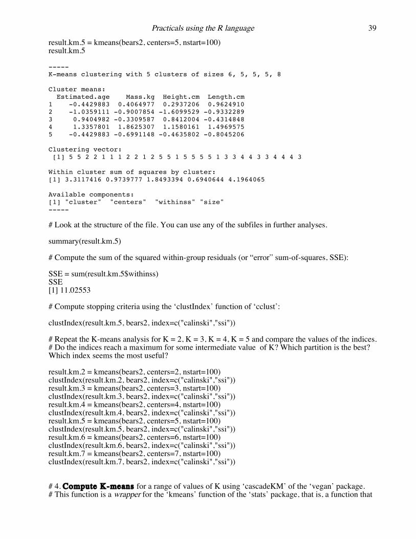
Practicals using the R language 39
result.km.5 = kmeans(bears2, centers=5, nstart=100) result.km.5 ----- K-means clustering with 5 clusters of sizes 6, 5, 5, 5, 8 Cluster means: Estimated.age Mass.kg Height.cm Length.cm 1 -0.4429883 0.4064977 0.2937206 0.9624910 2 -1.0359111 -0.9007854 -1.6099529 -0.9332289 3 0.9404982 -0.3309587 0.8412004 -0.4314848 4 1.3357801 1.8625307 1.1580161 1.4969575 5 -0.4429883 -0.6991148 -0.4635802 -0.8045206 Clustering vector: [1] 5 5 2 2 1 1 1 2 2 1 2 5 5 1 5 5 5 5 1 3 3 4 4 3 3 4 4 4 3 Within cluster sum of squares by cluster: [1] 3.3117416 0.9739777 1.8493394 0.6940644 4.1964065 Available components: [1] "cluster" "centers" "withinss" "size" ----- # Look at the structure of the file. You can use any of the subfiles in further analyses. summary(result.km.5) # Compute the sum of the squared within-group residuals (or “error” sum-of-squares, SSE): SSE = sum(result.km.5$withinss) SSE [1] 11.02553 # Compute stopping criteria using the ‘clustIndex’ function of ‘cclust’: clustIndex(result.km.5, bears2, index=c("calinski","ssi")) # Repeat the K-means analysis for K = 2, K = 3, K = 4, K = 5 and compare the values of the indices. # Do the indices reach a maximum for some intermediate value of K? Which partition is the best? Which index seems the most useful? result.km.2 = kmeans(bears2, centers=2, nstart=100) clustIndex(result.km.2, bears2, index=c("calinski","ssi")) result.km.3 = kmeans(bears2, centers=3, nstart=100) clustIndex(result.km.3, bears2, index=c("calinski","ssi")) result.km.4 = kmeans(bears2, centers=4, nstart=100) clustIndex(result.km.4, bears2, index=c("calinski","ssi")) result.km.5 = kmeans(bears2, centers=5, nstart=100) clustIndex(result.km.5, bears2, index=c("calinski","ssi")) result.km.6 = kmeans(bears2, centers=6, nstart=100) clustIndex(result.km.6, bears2, index=c("calinski","ssi")) result.km.7 = kmeans(bears2, centers=7, nstart=100) clustIndex(result.km.7, bears2, index=c("calinski","ssi")) # 4. Compute K-means for a range of values of K using ‘cascadeKM’ of the ‘vegan’ package. # This function is a wrapper for the ‘kmeans’ function of the ‘stats’ package, that is, a function that
Practicals using the R language 40
# uses a basic function, adding new properties to it. It creates several partitions forming a cascade # from small (parameter ‘inf.gr’) to large values of K (parameter ‘sup.gr’). result.cascadeKM = cascadeKM(bears2, inf.gr=2, sup.gr=10, iter = 100, criterion = 'ssi') # Look at the structure of the results file: summary(result.cascadeKM) # The element ‘partition’ contains a table showing the group attributed to each object: result.cascadeKM$partition # Element ‘results’ gives the SSE statistic as well as the value of the criterion (“calinski” or “ssi”) for each value of K. It is easy to identify the partition for which the criterion is maximum. Element ‘size’ gives the number of objects in each group of every partition. # A plot shows the group attributed to each object for each partition (rows of the graph). The groups are represented by different colours; there are two colours for K = 2, three colours for K = 3, and so on. Another graph shows the values of the chosen stopping criterion for the different values of K: out.bears = plot(result.cascadeKM) # Option ‘sort=TRUE’ reorders the objects in such a way as to put together, insofar as possible, the objects pertaining to each group: out.bears = plot(result.cascadeKM, sortg=TRUE) # The R output object, called ‘out.bears’ in this example, contains a table showing the group attributed to each object, taking into account the new order of the objects.

Practicals using the R language 41
# 12.2. Hierarchical agglomerative clustering # Example: file ‘Bears.txt’ # First, standardize the variables in file bears # before computing the matrix of Euclidean distances (see section 3). bears = read.table(file.choose(), header=TRUE, row.names=1) # Read the file "Bears.txt" bears.mat = as.matrix(bears[,1:4]) bears2 = decostand(bears.mat, "stand") # Standardize the variables bears.D1 = dist(bears2, method="eucl") # Compute Euclidean distance # Methods available in hclust: "ward.D", "ward.D2", "single", "complete", "average" (= UPGMA), "mcquitty" (= WPGMA), "median" (= WPGMC)" and "centroid" (= UPGMC). # Agglomerative clustering, UPGMA method: hclust(D, method = "average", members=NULL) bears.cl = hclust(bears.D1, method="average") plot(bears.cl) # Plot the dendrogram plot(bears.cl, hang=-1) # Examine the following functions: ?identify ?rect.hclust ?cutree ?dendrogram # See in particular option "horiz" # Compute cophenetic correlation # Documentation file: ?cophenetic bears.coph = cophenetic(bears.cl) # Cophenetic distances of the dendrogram cor(bears.D1, bears.coph) # Cophenetic correlation # ========= # Examples of hierarchical agglomerative clustering: Screws and bolts # 1. Hierarchical clustering, using only the binary data in the matrix Screws=read.table( file.choose() ) # Read the file "Screws_and_bolts.txt" Screws.bin=Screws[, 2:9] library(ade4) screws.D1=dist.binary(Screws.bin, method=1) # Compute D = sqrt(1 – Jaccard similarity) screws.cl=hclust(screws.D1, method="average") plot(screws.cl) # 2. Read a square distance matrix (in ASCII) pre-computed by another program screws.S15=read.table( file.choose() ) # Read the file "Screws_D=1-S15.txt" screws.D=as.dist(screws.S15) # Give type “dist” to the distance matrix screws.cl2=hclust(screws.D, method="average") plot(screws.cl2) # ========= # Hierarchical agglomerative clustering: the Ward method Two different algorithms are found in the literature for Ward clustering. In the hclust function of R version >= 3.1.1, the algorithm used by option "ward.D" does not implement Ward's (1963) clustering criterion; this is equivalent to the only option "ward" available in R versions <= 3.0.3. Following Murtagh and Legendre (2013), the hclust function was modified in R version
Practicals using the R language 42
3.1.1; the new option "ward.D2" implements the Ward (1963) criterion. In that algorithm, the dissimilarities are squared before cluster updating. Note that function agnes(*, method="ward") (AGglomerative NESting) of {cluster} also implements Ward's (1963) clustering criterion.
Example –
1. Using function agnes(*, method="ward")
library(cluster) # Documentation file: ?agnes bears.agnes.Ward.D2 <- agnes(bears.D1, diss=TRUE, method="ward") plot(bears.agnes.Ward.D2) bears.agnes.Ward.D2$height # List of fusion levels range(bears.agnes.Ward.D2$height) # Range of the fusion levels 2. Using function hclust(*, method="ward.D2")
bears.hclust.Ward.D2 <- hclust(bears.D1, method="ward.D2") plot(bears.hclust.Ward.D2) bears.hclust.Ward.D2$height # List of fusion levels range(bears.hclust.Ward.D2$height) # Range of the fusion levels 3. Using function hclust(*, method="ward.D") Note: in R versions <= 3.0.3, hclust(*, method="ward") produced the same result
bears.cl <- hclust(bears.D1^2, method="ward.D") # Use squared distances bears.cl$height <- sqrt(bears.cl$height) # Square-root the fusion levels plot(bears.cl, hang=-1) # Draw the dendrogram bears.cl$height # List of fusion levels range(bears.cl$height) # Range of the fusion levels # Are the fusion levels the same in all three methods? Are the fusion levels ranges the same? What is the cause of these differences?
# =========
Practicals using the R language 43
# Agglomerative clustering of the spider data
spiders = read.table( file.choose() ) # Read the file 'Spiders_28x12_spe.txt'
# 1. Compute the percentage difference dissimilarity (alias Bray-Curtis D) using 'vegdist' (vegan package; see section 3.2), followed by agglomerative clustering using hclust() (method="average") and agnes() (method="ward"). Compute the cophenetic correlation for the hclust() result.
# 2. Compute the Hellinger distance: (1) compute a Hellinger transformation of the data (section 4) followed by (2) computation of the Euclidean distance (section 3.1). (3) Then, compute agglomerative clustering using hclust() (method="average") and agnes() (method="ward"). Compute the cophenetic correlation for the hclust() result.
# 3. This exercise will use presence-absence data. Compute the Jaccard distance on the data file using function dist.binary() of ade4; see section 3.3. Users don’t have to pre-transform the data to presence-absence, the dist.binary() function takes care of that transformation. The computed dissimilarities are actually D = sqrt(1 – Jaccard similarity). Finally, compute clustering using hclust() (method= "average") and agnes() (method="ward"). Compute cophenetic correlation for the hclust() result.
# Compare the results, as well as the cophenetic correlations, obtained in #1, 2 et 3. Which dissimilarity measure produces the dendrogram with the highest cophenetic correlation?
# =========

Practicals using the R language 44
13. Correlograms
# Correlograms with tests of significance of individual correlation coefficients are available in: library(spdep) # We will compute correlograms for two variables of the file mite_env.txt, which is available among the data sets of this Short Course. The file mite.env is also available in the vegan package. Variable #1 is Substrate density (‘SubsDens’) and variable #2 is Water content (‘WatrCont’). # Load the mite data files available in {vegan} library(vegan) data(mite.env) # Environmental data, 70 x 5 subs.density <- mite.env[,1] # The geographic coordinates are found in the file mite_xy.txt. Create the file of neighbors. data(mite.xy) # Geographic coordinates, 70 x 2 nb1 <- dnearneigh(as.matrix(mite.xy), 0, 0.7) # Compute the correlogram. mite.correlog <- sp.correlogram(nb1, subs.density, order=14, method="I", zero.policy=TRUE) print(mite.correlog) plot(mite.correlog) # Correct the probabilities for multiple testing using a Bonferroni correction. print(mite.correlog, "bonferroni") plot(mite.correlog) # The correlogram based on the spatial correlation function is obtained as follows: mite.correlog2 <- sp.correlogram(nb1, subs.density, order=14, method="corr", zero.policy=TRUE) print(mite.correlog2) plot(mite.correlog2) # Exercise: compute the correlogram for the variable ‘water.content’. water.content <- mite.env[,2]

Practicals using the R language 45
14. Variogram and interpolated maps by kriging # 1. Basic mapping # World and country maps are available in R. Examples: library(maps) # Basic package to draw maps library(mapdata) # Package with specialized maps, e.g. ‘rivers’ map('world') # or map() # Worls map centered on Europe and Africa map('world2') # World map centered on the Pacific Ocean # Maps by country are also available, for example the map of China. map(region='china') # Map of China without provinces, from the package ‘maps’ map('china') # Map of China with provinces, from the package ‘mapdata’ # Draw capitals of Southeast Asia countries, plus Taipei for perspective capitals = read.table( file.choose() ) # Read the file "SoutheastAsia_capitals.txt" map(region=
c('cambodia','laos','myanmar','thailand','vietnam','brunei','indonesia','malaysia','philippines')) points(capitals[,2], capitals[,1], cex=2, pch=20, col="red") text(capitals [,2], capitals [,1], rownames(capitals), pos=4) # Repeat the exercise using the following map as the base map map(region= c('china',
'cambodia','laos','myanmar','thailand','vietnam','brunei','indonesia','malaysia','philippines')) ========= # 2. Construct an empirical variogram library(geoR) library(vegan) data(mite) # Species data, 70x35 data(mite.env) # Environmental data, 70 x 5 data(mite.xy) # Site coordinates, 70 x 2 water.content <- as.matrix(mite.env[,2]) vario.water <- variog(coords=mite.xy, data=water.content) plot(vario.water) # Fit a variogram model. Save it before quitting the Eyefit window. x11() # For Mac OS X only: open x11 before ‘eyefit’. Operation not necessary in Windows. model.water <- eyefit(vario.water) # Click on “Save” to save the model, then “Quit’. # 3. Conventional kriging for fixed variogram model, variable ‘water.content’ # 3.1. Define a grid for interpolation. The sampled area is a rectangle 2.5m x 10 m. # Beware: The grid spacing must be at least as fine as the precision of the point coordinates # located near the margins of the area to be mapped. pred.grid <- expand.grid(seq(0, 2.5, 0.05), seq(0, 10, 0.05))

Practicals using the R language 46
# 3.2. Interpolate by ordinary kriging (abbreviated "ok"). kc.water <- krige.conv(coords=mite.xy, data=water.content, loc= pred.grid,
krige=krige.control(type.krige="ok", obj.model=model.water)) # 3.3. Map the point estimates and the prediction variance. # Provide space for two graphs side by side in the window. par(mfrow=c(1,2)) # Left portion of the window: draw the interpolated map, using the image.kriging function. image(kc.water, loc = pred.grid, xlab="X", ylab="Y") # 3.4. Add the raw data (standardized) to the map. # Use the s.value function of the ade4 package: # empty squares for values smaller than the mean, full squares for values larger than the mean. library(ade4) s.value(mite.xy, scale(water.content), add.plot=TRUE, csize=0.8, clegend=0) # 3.5. Right portion of the window: draw the map of prediction variance. # Define the axes x <- seq(0, 2.5, 0.05) y <- seq(0, 10, 0.05) # Write the kriging variance information to a matrix krige.water.var <- matrix(kc.water$krige.var, nrow=length(x), ncol=length(y)) # Draw the map of kriging variance, using the image function of the graphics package. image(x=x, y=y, z=krige.water.var, asp=1, col=heat.colors(30)) # Exercise: repeat the mapping operations by kriging for mite species #15, square-root transformed. sp15.sqrt <- sqrt(mite.spe[,15])
Practicals using the R language 47
15. Linear discriminant analysis – Daniel Borcard, 31 mars 2009 # Load required packages library(ade4) library(vegan) # Preparation of the Doubs data (package ade4). See: http://fr.wikipedia.org/wiki/Doubs_(rivière) data(doubs) spe <- doubs$poi # Species abundances env <- doubs$mil # Environmental data spa <- doubs$xy # Geographical coordinates # Remove empty site 8 spe <- spe[-8,] env <- env[-8,] spa <- spa[-8,] # Correct a mistake in env object env[6,1] <- 268 env[7,1] <- 324 # Remove the 'das' variable from the env dataset env = env[,-1] # Transform the species dataset to allow RDA spe.hel = decostand(spe, "hellinger") # Create subset of 3 explanatory variables: altitude, oxygen concentration and # biological oxygen demand env.pars2 <- as.matrix(env[,c(1,9,10)]) # Create four groups of sites based on the clustering dendrogram of the fish abundances gr = cutree(hclust(vegdist(spe.hel,"euc")^2,"ward"),4) ### D^2 ### gr # Verify multivariate homogeneity of within-group variances # using Marti Anderson's betadisper() function {vegan} env.pars2.d1 <- dist(env.pars2) env.MHV <- betadisper(env.pars2.d1,gr) anova(env.MHV) # Parametric test permutest(env.MHV) # Permutational test # Variances are NOT homogeneous. Let us try a log # transformation on variables alt and dbo env.pars3 <- cbind(log(env$alt), env$oxy, log(env$dbo)) colnames(env.pars3) <- c("alt.ln", "oxy", "dbo.ln") row.names(env.pars3) <- row.names(env) env.pars3.d1 <- dist(env.pars3) env.MHV2 <- betadisper(env.pars3.d1,gr) permutest(env.MHV2) # This time the variances are homogeneous! We can proceed.

Practicals using the R language 48
# Test of significance of among-group dispersion: # compute Wilks’ lambda (eq. 11.42) and test its significance (eq. 11.43). # Computation of LDA (discrimination) library(MASS) env.pars3.df <- as.data.frame(env.pars3) spe.lda <- lda(gr ~ alt.ln + oxy + dbo.ln, data=env.pars3.df) spe.lda # The result object contains the information necessary to interpret the LDA summary(spe.lda) # Examine the elements in the output object – # Group means for the 3 variables spe.lda$means # Normalized eigenvectors (matrix C, eq. 11.33) = standardized # discriminant function coefficients C <- spe.lda$scaling # Canonical eigenvalues spe.lda$svd^2 sum.sl <- sum(spe.lda$svd^2) proportion.of.trace <- spe.lda$svd^2/sum.sl # Position of the objects in the space of the canonical variates F <- predict(spe.lda)$x # alternative way: F <- scale(env.pars3.df, center=TRUE, scale=FALSE) %*% C # Classification of the objects spe.class <- predict(spe.lda)$class # Posterior probabilities of objects belonging to the groups spe.post <- predict(spe.lda)$posterior # Table of prior vs predicted spe.table <- table(gr, spe.class)
Practicals using the R language 49
# Percentage of correct classification diag(prop.table(spe.table, 1)) # Plot of objects in the space of the canonical variates # with colors according to their classification plot(F[,1], F[,2], type="n") text(F[,1], F[,2], row.names(env), col=c(as.numeric(spe.class)+1)) abline(v=0, lty="dotted") abline(h=0, lty="dotted") # Draw 95% ellipses around groups library(ellipse) for(i in 1:length(levels(as.factor(gr)))) { cov <- cov(F[gr==i,]) centre <- apply(F[gr==i,], 2, mean) lines(ellipse(cov,centre=centre, level=0.95)) } # Classification of a new object (identification) # A new object is created with ln(alt)=6.8, oxygen=90 and ln(dbo)=3.2 new = c(6.8, 90, 3.2) new = as.data.frame(t(new)) # ‘new’ must be a row table colnames(new) = colnames(env.pars3) predict.new <- predict(spe.lda, newdata=new) predict.new # In which group has the new object has been classified? # Note: group numbers in vector ‘gr’ may differ among computer platforms and versions of R. # This calculation could have been done in the same way for a whole table of new observations. # LDA with jackknife-based classification (i.e., leave-one-out cross-validation) spe.lda.jac <- lda(gr ~ alt.ln + oxy + dbo.ln, data=env.pars3.df, CV=TRUE) summary(spe.lda.jac) # Number and percentages of correct classification spe.jac.class <- spe.lda.jac$class spe.jac.table <- table(gr,spe.jac.class) spe.jac.table # Classification table (see Manuel p. 629) diag(prop.table(spe.jac.table,1))
# The classification success in “spe.jac.table” seems not as good as the result in “spe.table”. Remember, however, that “spe.table” shows an a posteriori classification of the objects that have been used in the computations. It is too optimistic. By comparison, cross-validation results are obtained by computing the ‘lda’ and classification of each object, in turn, with that object taken out of the ‘lda’ calculation. It is more realistic.
Practicals using the R language 50
16. Some common statistical procedures available in R Common statistical tests available in package « stats »
t.test: Student's t-test. Paired t-test: paired=TRUE pairwise.t.test: a posteriori comparisons between groups by t-test var.test: F-test of the ratio of two variances bartlett.test: Bartlett's test of homogeneity of variances friedman.test: Friedman's test (nonparametric analysis of variance without replication) kruskal.test: Kruskal-Wallis test ks.test: Kolmogorov-Smirnov goodness-of-fit test mcnemar.test: McNemar's test power.t.test: power of t-test, one or two samples shapiro.test: Shapiro-Wilk's normality test wilcox.test: Wilcoxon rank sum and signed rank tests. Mann-Whitney U-test: paired=FALSE chisq.test: contingency table analysis, Pearson's chi-square statistic. One gives either two vectors, or a contingency table. One can obtain a permutation test as an option. aov: analysis of variance. The factor(s) must be declared “as.factor”. summary.aov: ‘aov' results manova: multivariate analysis of variance summary.manova: ‘manova' results Confidence intervals
t.test: Student's t-test and confidence intervals, 1 or 2 groups. confint: confidence intervals of the parameters of a model fitted to the data confint.glm (MASS package): confidence intervals of the parameters of a model fitted to the data norm.ci (BOOT package): confidence intervals based on normal approximation boot.ci (BOOT package): bootstrap confidence intervals print.bootci (BOOT package): prints the bootstrap confidence intervals intervals (librairie NLME): confidence intervals of coefficients Multiple regression
lm (package stats) is used to fit linear models. It can be used to carry out regression, single stratum analysis of variance and analysis of covariance (although aov may provide a more convenient interface for these). This function also computes multivariate regressions for multivariate response tables.

Practicals using the R language 51
Linear discriminant analysis
library(MASS) lda (MASS): linear discriminant analysis ldahist: histogram of diagram of group densities pairs.lda: scattergrams for pairs of groups plot.lda: diagrams for objects of class “lda” predict.lda: lda-based classification of multivariate objects library(ade4) discrimin: linear discriminant analysis library(labdsv) spcdisc: a form of discriminant analysis for species data library(sonarX) This library is distributed on the ESA Web page http://esapubs.org/archive/, inside “Ecological Archives A016-047-S1”. ldaTest: linear discriminant analysis Canonical correlation analysis CCorA : function available on the Web page http://www.bio.umontreal.ca/legendre/ Statistical distributions
# Example : FDist for the F distribution – # Ask for information about the F distribution: ?FDist # Applications : pf(F,df1,df2,lower.tail=FALSE) to find probabilities associated to the F distribution qf(prob,df1,df2,lower.tail=FALSE) to find a value of F corresponding to a given probability rf(n,df1,df2) to obtain n random numbers extracted from the specified F distribution df(F,df1,df2) to obtain the density of the F distribution for a given value of F # Ask for information about the other frequently used distributions: ?Normal ?TDist ?Chisquare ?Lognormal ?Binomial ?Multinomial ?NegBinomial ?mvrnorm in package MASS

Practicals using the R language 52
17. Using R as a calculator A simple sum 1+1 [1] 2
Square root of a number sqrt(10) [1] 3.162278
Create a sequence of numbers Information : ?seq seq(0,5,length=6) [1] 0 1 2 3 4 5
Generate a graph Information : ?plot plot(sin(seq(0,2*pi,length=100)))
Create a vector of values x = c(2,3,5,2,7,1) x [1] 2 3 5 2 7 1
Calculate the mean mean(x) [1] 3.333333
Calculate the standard deviation sd(x) [1] 2.250926
Calculate the standard error of the mean sd(x)/sqrt(6) [1] 0.9189366
Sort a vector of values Information : ?sort sort(x) [1] 1 2 2 3 5 7 # or try y=sort(x) y [1] 1 2 2 3 5 7

Practicals using the R language 53
Random normal generator Information : ?rnorm x=rnorm(10,0,1) mean(x) sd(x) x=rnorm(1000,mean=10,sd=5) mean(x) sd(x)
Generate a column vector with zeros Information : ?matrix Vector=matrix(0,10,1) Vector [,1] [1,] 0 [2,] 0 [3,] 0 [4,] 0 [5,] 0 [6,] 0 [7,] 0 [8,] 0 [9,] 0 [10,] 0
Create a sequence of actions: a ‘for’ loop # Use a ‘for’ loop to compute a cumulative mean of random numbers. The cumulative mean should converge to the true mean as the number of values included in the calculation increases. n = 30 # n = sample size vec.means = vector(mode="numeric", length=(n-1)) true.mean = 5 x = rnorm(n, mean=true.mean, sd=1) # Information: ?rnorm for(i in 2:n) { vec.means[i-1] = sum(x[1:i])/i } # Print the vector of mean values vec.means plot(vec.means, ylim=c(true.mean-1, true.mean+1)) abline(h=true.mean, col="red")
=========================