Practices to Optimize Power Meter/Sensor Measurement Speed and Shorten Test Times

Application Note

Abstract Optimizing RF/MW power measurement speed on a power meter and a power sensor is often a subject of concern, especially in a manufacturing environment. This article describes some useful tips on how to effectively minimize test times while obtaining power measurements.

Having a detailed understanding of some of the SCPI commands and settings of the Agilent power meter/sensor is one means of improving measurement speed without compromising measurement accuracy. Selecting the measurement speed settings best-suited to the application need is another method. For example, this application note explains how the Fast measurement setting and buffer size can be best leveraged based on the power level of interest. To increase speed even further, it is important to choose the right format and units in which the results are to be returned. To eliminate as much wasted test time as possible, such as waiting for processes like sensor zeroing and calibration, a basic understanding of the complete operation is required.

2

Introduction Power specifications are often the critical factor in the design, and ultimately the performance, of almost all RF and microwave equipment. Power meters and power sensors are commonly used to capture these power measurements. Understanding the capabilities of the power meter/sensor helps ensure the best power meter/sensor test methodology for capturing power measurement is correctly applied. That knowledge can prevent implementing choices that may cause inaccurate power measurement or needlessly lengthen test time in manufacturing. The following practices explain how to leverage some of the commands, settings, and output selections in order to obtain accurate power measurement and shorten test times.

Introduction .............................................................................................. 2Practice 1: Measurement Query Method ............................................ 3Practice 2: Measurement Averaging .................................................... 4Practice 3: Trigger Mode ........................................................................ 5Practice 4: Power Sensor Measurement Speed ................................ 9Practice 5: Buffer Mode Measurement ............................................. 11Practice 6: Watt Beats dBm in Speed ............................................... 12Practice 7: Real Beats ASCII in Speed ............................................... 13Practice 8: Operation Complete (*OPC) Query ................................. 15Practice 9: External Triggering Measurement .................................. 16Conclusion .............................................................................................. 20Related Agilent Literature ..................................................................... 20Agilent Advantage Services ..................................................Back coverContact Agilent .......................................................................Back cover

Table of Contents

3

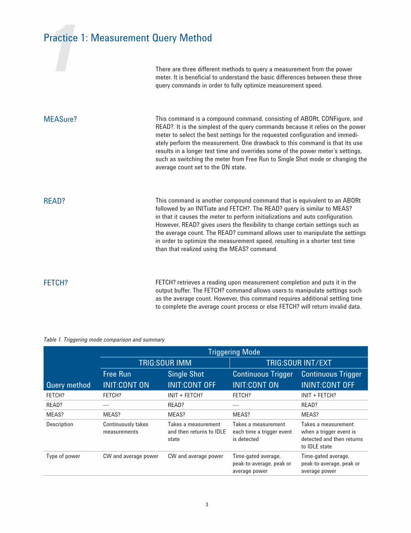
1 There are three different methods to query a measurement from the power meter. It is beneficial to understand the basic differences between these three query commands in order to fully optimize measurement speed.

Practice 1: Measurement Query Method

MEASure?

READ?

FETCH?

This command is a compound command, consisting of ABORt, CONFigure, and READ?. It is the simplest of the query commands because it relies on the power meter to select the best settings for the requested configuration and immedi-ately perform the measurement. One drawback to this command is that its use results in a longer test time and overrides some of the power meter’s settings, such as switching the meter from Free Run to Single Shot mode or changing the average count set to the ON state.

This command is another compound command that is equivalent to an ABORt followed by an INITiate and FETCH?. The READ? query is similar to MEAS? in that it causes the meter to perform initializations and auto configuration. However, READ? gives users the flexibility to change certain settings such as the average count. The READ? command allows user to manipulate the settings in order to optimize the measurement speed, resulting in a shorter test time than that realized using the MEAS? command.

FETCH? retrieves a reading upon measurement completion and puts it in the output buffer. The FETCH? command allows users to manipulate settings such as the average count. However, this command requires additional settling time to complete the average count process or else FETCH? will return invalid data.

Table 1. Triggering mode comparison and summary

Query method

Triggering ModeTRIG:SOUR IMM TRIG:SOUR INT/EXT

Free Run Single Shot Continuous Trigger Continuous TriggerINIT:CONT ON INIT:CONT OFF INIT:CONT ON ININT:CONT OFF

FETCH? FETCH? INIT + FETCH? FETCH? INIT + FETCH?READ? — READ? — READ?MEAS? MEAS? MEAS? MEAS? MEAS?Description Continuously takes

measurementsTakes a measurement and then returns to IDLE state

Takes a measurement each time a trigger event is detected

Takes a measurement when a trigger event is detected and then returns to IDLE state

Type of power CW and average power CW and average power Time-gated average, peak-to-average, peak or average power

Time-gated average, peak-to-average, peak or average power

4

2Practice 2: Measurement Averaging

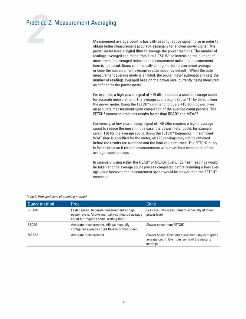
Measurement average count is basically used to reduce signal noise in order to obtain better measurement accuracy, especially for a lower power signal. The power meter uses a digital filter to average the power readings. The number of readings averaged can range from 1 to 1,024. While increasing the number of measurements averaged reduces the measurement noise, the measurement time is increased. Users can manually configure the measurement average or keep the measurement average in auto mode (by default). When the auto measurement average mode is enabled, the power meter automatically sets the number of readings averaged base on the power level currently being measured as defined by the power meter.

For example, a high power signal of +10 dBm requires a smaller average count for accurate measurement. The average count might set to “1” by default from the power meter. Using the FETCH? command to query +10 dBm power gives an accurate measurement upon completion of the average count process. The FETCH? command produces results faster than READ? and MEAS?.

Conversely, at low power, noisy signal of –40 dBm requires a higher average count to reduce the noise. In this case, the power meter could, for example, select 128 for the average count. Using the FETCH? Command, if insufficient WAIT time is specified for the meter, all 128 readings may not be obtained before the results are averaged and the final value returned. The FETCH? query is faster because it returns measurements with or without completion of the average count process.

In summary, using either the READ? or MEAS? query, 128 fresh readings would be taken and the average count process completed before returning a final aver-age value however, the measurement speed would be slower than the FETCH? command.

Table 2. Pros and cons of querying method

Query method Pros ConsFETCH? Faster speed. Accurate measurement at high

power levels. Allows manually-configured average count but requires some settling time.

Less accurate measurement especially at lower power level

READ? Accurate measurement. Allows manually-configured average count thus improved speed.

Slower speed than FETCH?

MEAS? Accurate measurement Slower speed. Does not allow manually-configured average count. Overrides some of the meter’s settings.

5

3Practice 3: Trigger Mode

The power meter has a very flexible triggering system and it can be described as having three modes. It can be setup for a Free Run, Single Shot, or Continuous Trigger cycles using the INITiate:CONTinous command.

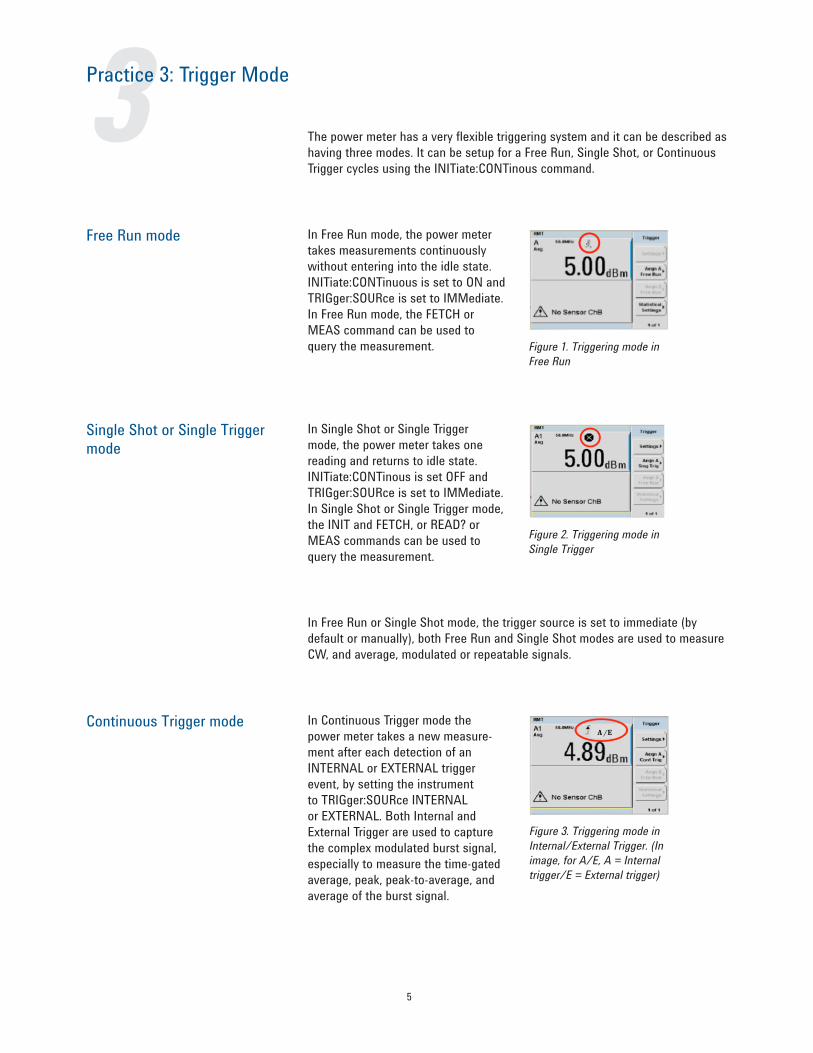
Free Run mode In Free Run mode, the power meter takes measurements continuously without entering into the idle state. INITiate:CONTinuous is set to ON and TRIGger:SOURce is set to IMMediate. In Free Run mode, the FETCH or MEAS command can be used to query the measurement. Figure 1. Triggering mode in

Free Run

Single Shot or Single Trigger mode

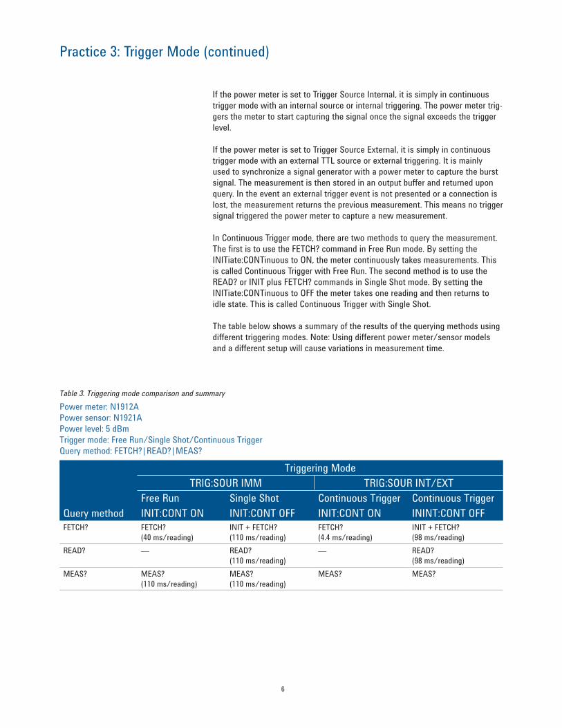
In Single Shot or Single Trigger mode, the power meter takes one reading and returns to idle state. INITiate:CONTinous is set OFF and TRIGger:SOURce is set to IMMediate. In Single Shot or Single Trigger mode, the INIT and FETCH, or READ? or MEAS commands can be used to query the measurement.

Figure 2. Triggering mode in Single Trigger

In Free Run or Single Shot mode, the trigger source is set to immediate (by default or manually), both Free Run and Single Shot modes are used to measure CW, and average, modulated or repeatable signals.

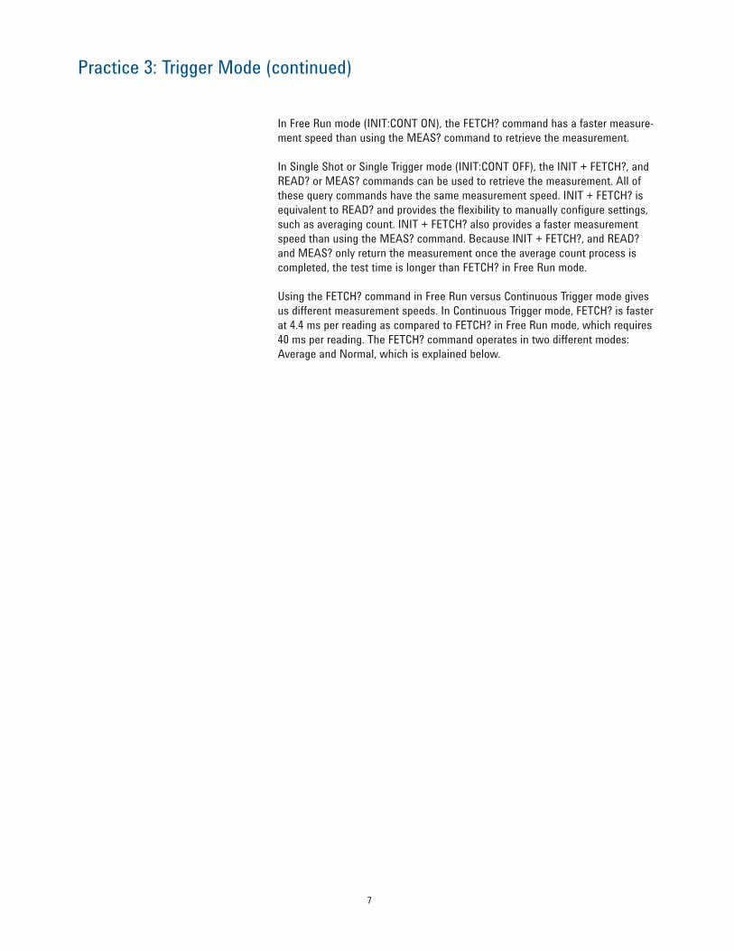
Continuous Trigger mode In Continuous Trigger mode the power meter takes a new measure-ment after each detection of an INTERNAL or EXTERNAL trigger event, by setting the instrument to TRIGger:SOURce INTERNAL or EXTERNAL. Both Internal and External Trigger are used to capture the complex modulated burst signal, especially to measure the time-gated average, peak, peak-to-average, and average of the burst signal.

Figure 3. Triggering mode in Internal/External Trigger. (In image, for A/E, A = Internal trigger/E = External trigger)

6

Practice 3: Trigger Mode (continued)

If the power meter is set to Trigger Source Internal, it is simply in continuous trigger mode with an internal source or internal triggering. The power meter trig-gers the meter to start capturing the signal once the signal exceeds the trigger level.

If the power meter is set to Trigger Source External, it is simply in continuous trigger mode with an external TTL source or external triggering. It is mainly used to synchronize a signal generator with a power meter to capture the burst signal. The measurement is then stored in an output buffer and returned upon query. In the event an external trigger event is not presented or a connection is lost, the measurement returns the previous measurement. This means no trigger signal triggered the power meter to capture a new measurement.

In Continuous Trigger mode, there are two methods to query the measurement. The first is to use the FETCH? command in Free Run mode. By setting the INITiate:CONTinuous to ON, the meter continuously takes measurements. This is called Continuous Trigger with Free Run. The second method is to use the READ? or INIT plus FETCH? commands in Single Shot mode. By setting the INITiate:CONTinuous to OFF the meter takes one reading and then returns to idle state. This is called Continuous Trigger with Single Shot.

The table below shows a summary of the results of the querying methods using different triggering modes. Note: Using different power meter/sensor models and a different setup will cause variations in measurement time.

Table 3. Triggering mode comparison and summaryPower meter: N1912APower sensor: N1921A Power level: 5 dBmTrigger mode: Free Run/Single Shot/Continuous TriggerQuery method: FETCH?|READ?|MEAS?

Query method

Triggering ModeTRIG:SOUR IMM TRIG:SOUR INT/EXT

Free Run Single Shot Continuous Trigger Continuous TriggerINIT:CONT ON INIT:CONT OFF INIT:CONT ON ININT:CONT OFF

FETCH? FETCH?(40 ms/reading)

INIT + FETCH?(110 ms/reading)

FETCH?(4.4 ms/reading)

INIT + FETCH?(98 ms/reading)

READ? — READ?(110 ms/reading)

— READ?(98 ms/reading)

MEAS? MEAS?(110 ms/reading)

MEAS?(110 ms/reading)

MEAS? MEAS?

7

Practice 3: Trigger Mode (continued)

In Free Run mode (INIT:CONT ON), the FETCH? command has a faster measure-ment speed than using the MEAS? command to retrieve the measurement.

In Single Shot or Single Trigger mode (INIT:CONT OFF), the INIT + FETCH?, and READ? or MEAS? commands can be used to retrieve the measurement. All of these query commands have the same measurement speed. INIT + FETCH? is equivalent to READ? and provides the flexibility to manually configure settings, such as averaging count. INIT + FETCH? also provides a faster measurement speed than using the MEAS? command. Because INIT + FETCH?, and READ? and MEAS? only return the measurement once the average count process is completed, the test time is longer than FETCH? in Free Run mode.

Using the FETCH? command in Free Run versus Continuous Trigger mode gives us different measurement speeds. In Continuous Trigger mode, FETCH? is faster at 4.4 ms per reading as compared to FETCH? in Free Run mode, which requires 40 ms per reading. The FETCH? command operates in two different modes: Average and Normal, which is explained below.

8

Practice 3: Trigger Mode (continued)

Average mode versus Normal mode

The power meter/sensor provides two different detector functions: Average mode and Normal mode.

Average mode is used to measure CW, or modulated, repeatable signals. It involves chopping the signals (to reduce 1/f noise) and includes RC filtering, which helps to further reduce the noise of the measured signal. Measurement speed is determined by the measurement mode: Normal, Double, and Fast, which is explained in the next section. In this example, the measurement speed is set to Normal mode by default from the meter to obtain a 40 ms per reading.

Normal mode is used to measure time-gated average, peak, peak-to-average, or average power. In Normal mode, there is no chopper (hence no 1/f noise reduc-tion) and no RC filtering. The reason is that this mode is targeting non-periodic, modulated signals. RC filtering constants are impossible to derive and apply to those signals. Chopping, which generates spikes as a side effect, requires blanking by removing samples around chopping spikes—this would completely destroy the measured modulated signal and any information during that period. To offset those noise disadvantages, Normal mode offers selectivity of the mea-sured interval and its position relative to the trigger events, internal or external event.

In this example, gate length is set to 100 µs by default from the meter and thus it obtains 4.4 ms measurement speed per reading. If the gate time is longer, then the measurement time is longer.

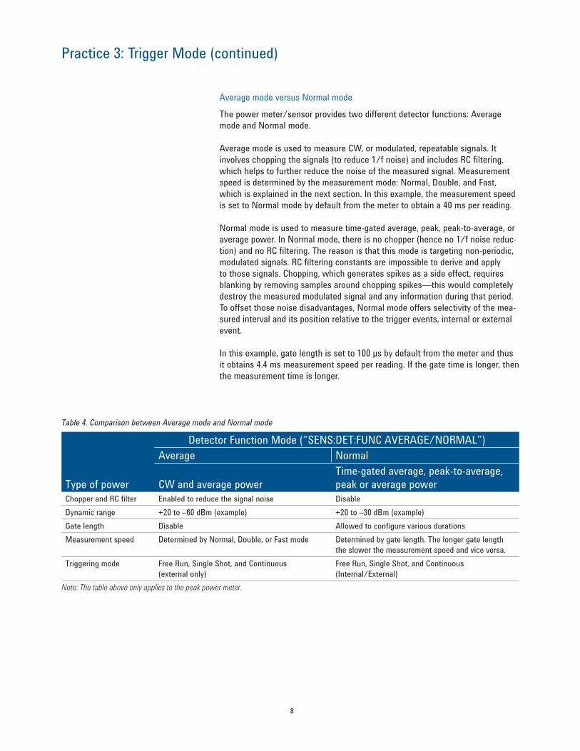
Table 4. Comparison between Average mode and Normal mode

Detector Function Mode (“SENS:DET:FUNC AVERAGE/NORMAL”)Average Normal

Type of power CW and average powerTime-gated average, peak-to-average, peak or average power

Chopper and RC filter Enabled to reduce the signal noise DisableDynamic range +20 to –60 dBm (example) +20 to –30 dBm (example) Gate length Disable Allowed to configure various durations Measurement speed Determined by Normal, Double, or Fast mode Determined by gate length. The longer gate length

the slower the measurement speed and vice versa.Triggering mode Free Run, Single Shot, and Continuous

(external only) Free Run, Single Shot, and Continuous (Internal/External)

Note: The table above only applies to the peak power meter.

9

4Practice 4: Power Sensor Measurement Speed

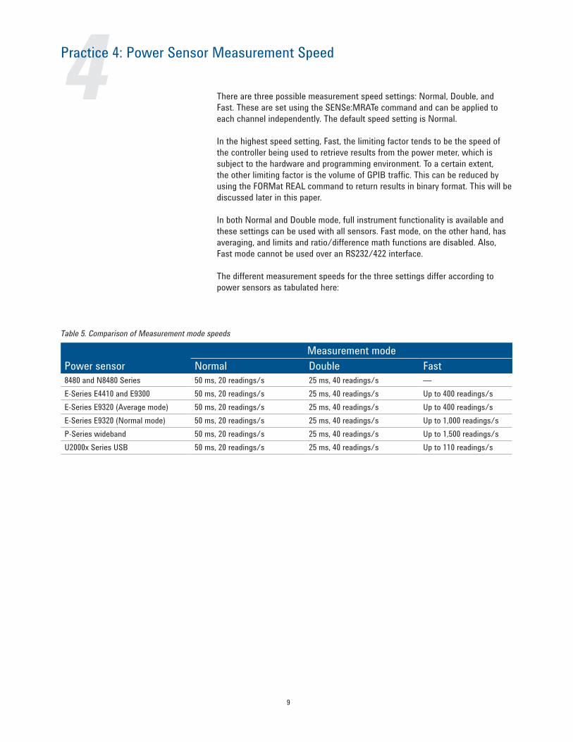
There are three possible measurement speed settings: Normal, Double, and Fast. These are set using the SENSe:MRATe command and can be applied to each channel independently. The default speed setting is Normal. In the highest speed setting, Fast, the limiting factor tends to be the speed of the controller being used to retrieve results from the power meter, which is subject to the hardware and programming environment. To a certain extent, the other limiting factor is the volume of GPIB traffic. This can be reduced by using the FORMat REAL command to return results in binary format. This will be discussed later in this paper. In both Normal and Double mode, full instrument functionality is available and these settings can be used with all sensors. Fast mode, on the other hand, has averaging, and limits and ratio/difference math functions are disabled. Also, Fast mode cannot be used over an RS232/422 interface.

The different measurement speeds for the three settings differ according to power sensors as tabulated here:

Table 5. Comparison of Measurement mode speeds

Power sensorMeasurement mode

Normal Double Fast8480 and N8480 Series 50 ms, 20 readings/s 25 ms, 40 readings/s —E-Series E4410 and E9300 50 ms, 20 readings/s 25 ms, 40 readings/s Up to 400 readings/s E-Series E9320 (Average mode) 50 ms, 20 readings/s 25 ms, 40 readings/s Up to 400 readings/s E-Series E9320 (Normal mode) 50 ms, 20 readings/s 25 ms, 40 readings/s Up to 1,000 readings/s P-Series wideband 50 ms, 20 readings/s 25 ms, 40 readings/s Up to 1,500 readings/s U2000x Series USB 50 ms, 20 readings/s 25 ms, 40 readings/s Up to 110 readings/s

10

Practice 4: Power Sensor Measurement Speed (continued)

The table below shows a summary of the speed improvements using different measurement modes with the following configurations:

Table 6. Pros and cons of various Measurement modesPower meter: N1912APower sensor: N1921A Power level: 5 dBmMeasurement mode: Fast (“SENS:MRATE NORMAL|DOUBLE|FAST”)

Measurement mode Measurement speed Pros ConsNormal (by default) 42.3 ms/reading Accurate measurement. Full

function applied.Slower speed

Double 21.0 ms/reading Accurate measurement. Full function applied. Faster speed.

—

Fast 5.8 ms/reading Fastest speed Less accurate measurement. Some functions are disable (average count, etc.).

The measurement speed in Fast mode is approximately 5.8 ms compared to 42 ms in Normal mode. Fast mode provides the fastest measurement speed by disabling some of the functions such as average count, and it might cause inaccurate measurement, particularly when measuring lower power levels which require some average count to achieve the most accurate measurement. However, users can use programmatic averaging in the software program to improve accuracy.

Double mode is faster than Normal, but slower than Fast mode. But both Normal and Double mode provide accurate measurement and all the functional-ity, such as average count, is still available. Double mode reduces the measure-ment accuracy slightly because of a small increase in noise due to the reduced sampling rate. Measurement speed improvement may vary with different power meters and sensors.

11

5Practice 5: Buffer Mode Measurement

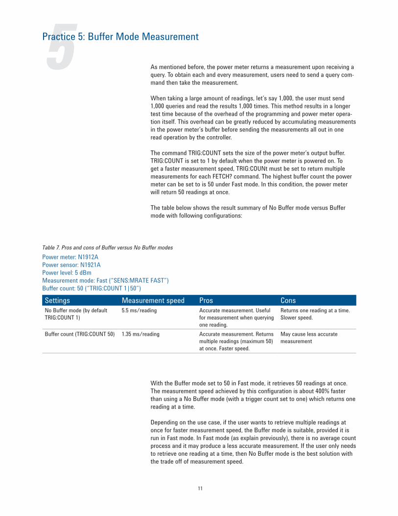
As mentioned before, the power meter returns a measurement upon receiving a query. To obtain each and every measurement, users need to send a query com-mand then take the measurement.

When taking a large amount of readings, let’s say 1,000, the user must send 1,000 queries and read the results 1,000 times. This method results in a longer test time because of the overhead of the programming and power meter opera-tion itself. This overhead can be greatly reduced by accumulating measurements in the power meter’s buffer before sending the measurements all out in one read operation by the controller. The command TRIG:COUNT sets the size of the power meter’s output buffer. TRIG:COUNT is set to 1 by default when the power meter is powered on. To get a faster measurement speed, TRIG:COUNt must be set to return multiple measurements for each FETCH? command. The highest buffer count the power meter can be set to is 50 under Fast mode. In this condition, the power meter will return 50 readings at once. The table below shows the result summary of No Buffer mode versus Buffer mode with following configurations:

Table 7. Pros and cons of Buffer versus No Buffer modesPower meter: N1912APower sensor: N1921A Power level: 5 dBmMeasurement mode: Fast (“SENS:MRATE FAST”)Buffer count: 50 (“TRIG:COUNT 1|50”)

Settings Measurement speed Pros ConsNo Buffer mode (by default TRIG:COUNT 1)

5.5 ms/reading Accurate measurement. Useful for measurement when querying one reading.

Returns one reading at a time. Slower speed.

Buffer count (TRIG:COUNT 50) 1.35 ms/reading Accurate measurement. Returns multiple readings (maximum 50) at once. Faster speed.

May cause less accurate measurement

With the Buffer mode set to 50 in Fast mode, it retrieves 50 readings at once. The measurement speed achieved by this configuration is about 400% faster than using a No Buffer mode (with a trigger count set to one) which returns one reading at a time.

Depending on the use case, if the user wants to retrieve multiple readings at once for faster measurement speed, the Buffer mode is suitable, provided it is run in Fast mode. In Fast mode (as explain previously), there is no average count process and it may produce a less accurate measurement. If the user only needs to retrieve one reading at a time, then No Buffer mode is the best solution with the trade off of measurement speed.

12

6Practice 6: Watt Beats dBm in Speed

Power meters can return measurements in either linear unit in watt, or log unit in dBm. The power meter’s internal circuitry processes and calculates the mea-surement in linear units before converting to other units such as dBm or % for relativity measurement as requested by the user. Therefore optimal performance will be achieved when the output is also in linear units to remove the overhead involved in performing a log function. By default, the meter setting is in dBm units.

Converting watts into dBm:dBm = 10 log (Power/1 mW)

If speed is the priority, acquiring measurements in watt units helps when the application requires taking hundreds or thousands of measurements. However, this speed difference is not significant enough to be noticed in cases where only one or a few measurement points are being taken because it is hidden by the software and hardware latencies.

SCPI: “UNIT:POWER <WATT|DBM>” = To configure the unit to watts or dBm

13

7Practice 7: Real Beats ASCII in Speed

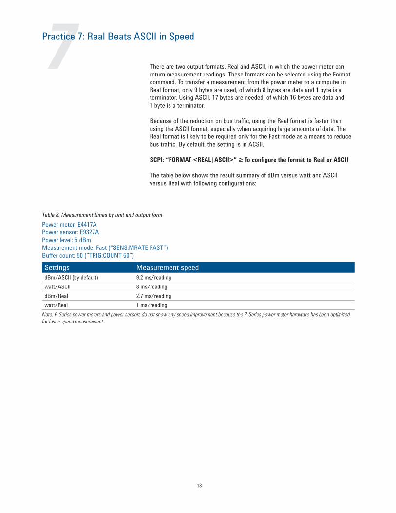
There are two output formats, Real and ASCII, in which the power meter can return measurement readings. These formats can be selected using the Format command. To transfer a measurement from the power meter to a computer in Real format, only 9 bytes are used, of which 8 bytes are data and 1 byte is a terminator. Using ASCII, 17 bytes are needed, of which 16 bytes are data and 1 byte is a terminator. Because of the reduction on bus traffic, using the Real format is faster than using the ASCII format, especially when acquiring large amounts of data. The Real format is likely to be required only for the Fast mode as a means to reduce bus traffic. By default, the setting is in ACSII.

SCPI: “FORMAT <REAL|ASCII>” ≥ To configure the format to Real or ASCII

The table below shows the result summary of dBm versus watt and ASCII versus Real with following configurations:

Table 8. Measurement times by unit and output formPower meter: E4417APower sensor: E9327A Power level: 5 dBmMeasurement mode: Fast (“SENS:MRATE FAST”)Buffer count: 50 (“TRIG:COUNT 50”)

Settings Measurement speeddBm/ASCII (by default) 9.2 ms/readingwatt/ASCII 8 ms/readingdBm/Real 2.7 ms/readingwatt/Real 1 ms/reading

Note: P-Series power meters and power sensors do not show any speed improvement because the P-Series power meter hardware has been optimized for faster speed measurement.

14

Practice 7: Real Beats ASCII in Speed (continued)

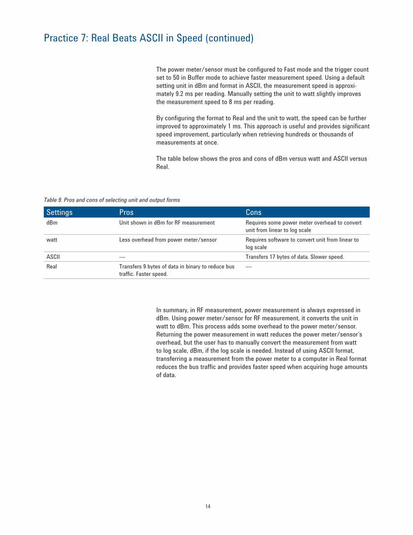
The power meter/sensor must be configured to Fast mode and the trigger count set to 50 in Buffer mode to achieve faster measurement speed. Using a default setting unit in dBm and format in ASCII, the measurement speed is approxi-mately 9.2 ms per reading. Manually setting the unit to watt slightly improves the measurement speed to 8 ms per reading.

By configuring the format to Real and the unit to watt, the speed can be further improved to approximately 1 ms. This approach is useful and provides significant speed improvement, particularly when retrieving hundreds or thousands of measurements at once.

The table below shows the pros and cons of dBm versus watt and ASCII versus Real.

Table 9. Pros and cons of selecting unit and output forms

Settings Pros ConsdBm Unit shown in dBm for RF measurement Requires some power meter overhead to convert

unit from linear to log scale watt Less overhead from power meter/sensor Requires software to convert unit from linear to

log scale ASCII — Transfers 17 bytes of data. Slower speed.Real Transfers 9 bytes of data in binary to reduce bus

traffic. Faster speed.—

In summary, in RF measurement, power measurement is always expressed in dBm. Using power meter/sensor for RF measurement, it converts the unit in watt to dBm. This process adds some overhead to the power meter/sensor. Returning the power measurement in watt reduces the power meter/sensor’s overhead, but the user has to manually convert the measurement from watt to log scale, dBm, if the log scale is needed. Instead of using ASCII format, transferring a measurement from the power meter to a computer in Real format reduces the bus traffic and provides faster speed when acquiring huge amounts of data.

15

8Practice 8: Operation Complete (*OPC) Query

Synchronization often makes it necessary for instruments to communicate that they have finished processing a command and are ready to process the next command. The *OPC? query places an ASCII character 1 into the power meter’s output queue when all pending power meter commands are complete. If the program waits for this response before executing the rest of the program, synchronization between one or more instruments and the computer is ensured.

For example, if the meter is performing a zero and cal, the user must wait for the process to complete before querying for measurements. Querying too early will result in a time out error. On the other hand, setting a fixed wait period that is slightly longer than the longest typical time it takes to zero and calibrate a particular model of power sensor wastes time unnecessarily. Additionally, the typical time taken to zero and calibrate is different for different models of power sensors, is also subject to change with firmware and hardware changes/updates.

The table below shows the pros and cons between *OPC and the Status command:

Table 10. Pros and cons of using Operation Complete query

Settings Pros ConsWithout *OPC — Manually adds fixed wait time. Longer test time.With *OPC Faster test time. Synchronizes computer and

power meter.—

16

9Practice 9: External Triggering Measurement

In many cases, power meters/sensors are used for system calibration in manu-facturing. During system calibration, frequency sweep or power sweep needs to be carried out to compensate for errors or system losses. Sometimes this extends test time, depending on the number of system calibration points used to complete the process.

Frequency sweep mode This mode is used in a frequency response calibration system where the ampli-tude is constant and the frequency of the power source signal is swept. This mode can be used to determine the frequency response of a device under test (DUT).

Power sweep mode Power Sweep mode is used in a power level calibration setup where frequency is constant (CW frequency) and the amplitude of the power source signal is swept. This mode can be used to characterize the flatness, linearity, or gain compression of a DUT.

Conventionally, a signal generator is used as a source and the power meter is connected to the system for system calibration. The signal generator steps thru the frequency/power with constant power/frequency. The power meter is set to the frequency base on the signal generator and captures a measurement. This process continues until the end of the frequency/power step point. Completing one system calibration in manufacturing extends test time. To shorten the test time, a new firmware enhancement allows users to speed up the measurement or calibration using an external triggering capability. This feature performs the frequency/power sweep automatically with signal source and synchronizes through hardware triggering.

17

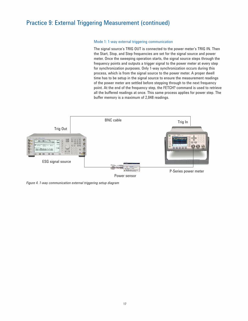
Mode 1: 1-way external triggering communication

The signal source’s TRIG OUT is connected to the power meter’s TRIG IN. Then the Start, Stop, and Step frequencies are set for the signal source and power meter. Once the sweeping operation starts, the signal source steps through the frequency points and outputs a trigger signal to the power meter at every step for synchronization purposes. Only 1-way synchronization occurs during this process, which is from the signal source to the power meter. A proper dwell time has to be setup in the signal source to ensure the measurement readings of the power meter are settled before stepping through to the next frequency point. At the end of the frequency step, the FETCH? command is used to retrieve all the buffered readings at once. This same process applies for power step. The buffer memory is a maximum of 2,048 readings.

Practice 9: External Triggering Measurement (continued)

BNC cable

Trig OutTrig In

ESG signal source

P-Series power meterPower sensor

Figure 4. 1-way communication external triggering setup diagram

18

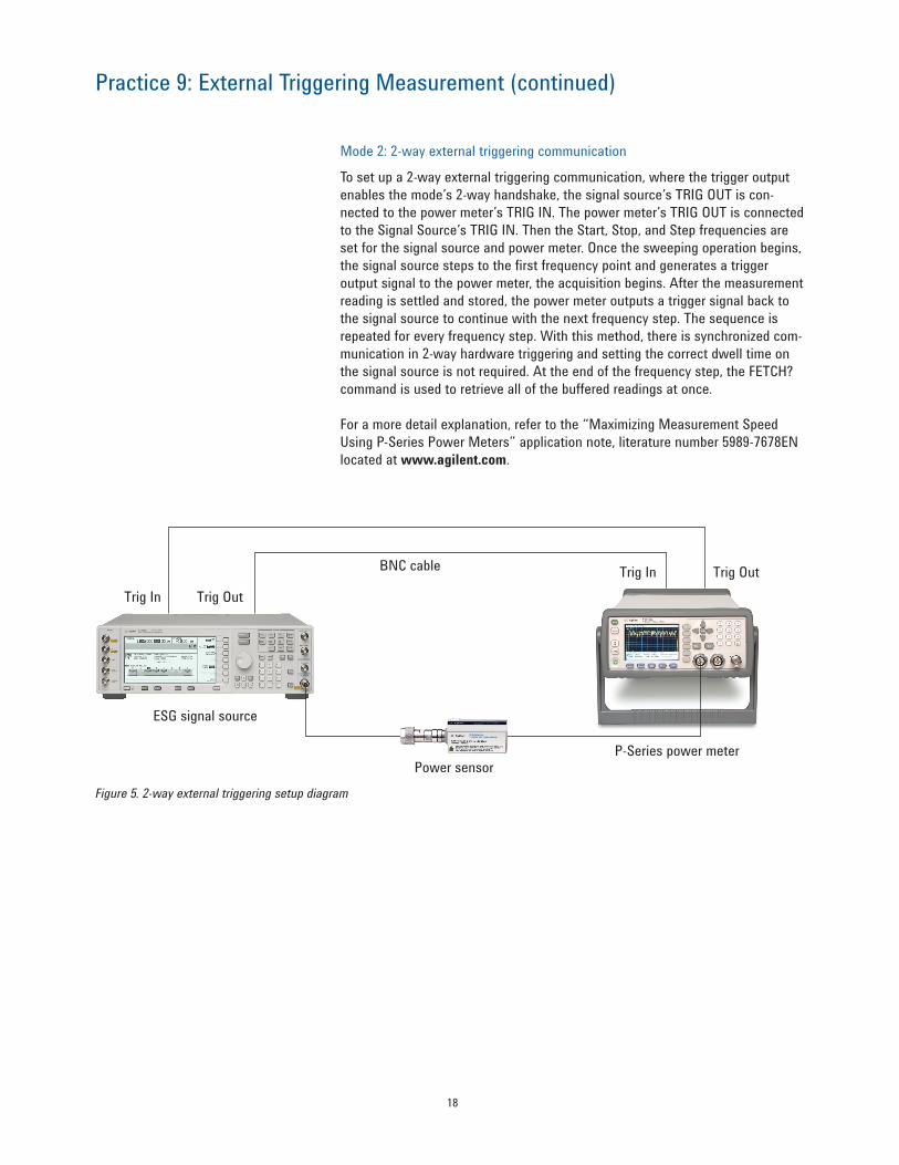
Mode 2: 2-way external triggering communication

To set up a 2-way external triggering communication, where the trigger output enables the mode’s 2-way handshake, the signal source’s TRIG OUT is con-nected to the power meter’s TRIG IN. The power meter’s TRIG OUT is connected to the Signal Source’s TRIG IN. Then the Start, Stop, and Step frequencies are set for the signal source and power meter. Once the sweeping operation begins, the signal source steps to the first frequency point and generates a trigger output signal to the power meter, the acquisition begins. After the measurement reading is settled and stored, the power meter outputs a trigger signal back to the signal source to continue with the next frequency step. The sequence is repeated for every frequency step. With this method, there is synchronized com-munication in 2-way hardware triggering and setting the correct dwell time on the signal source is not required. At the end of the frequency step, the FETCH? command is used to retrieve all of the buffered readings at once.

For a more detail explanation, refer to the “Maximizing Measurement Speed Using P-Series Power Meters” application note, literature number 5989-7678EN located at www.agilent.com.

Practice 9: External Triggering Measurement (continued)

BNC cable

Trig OutTrig In

ESG signal source

P-Series power meterPower sensor

Trig OutTrig In

Figure 5. 2-way external triggering setup diagram

19

Practice 9: External Triggering Measurement (continued)

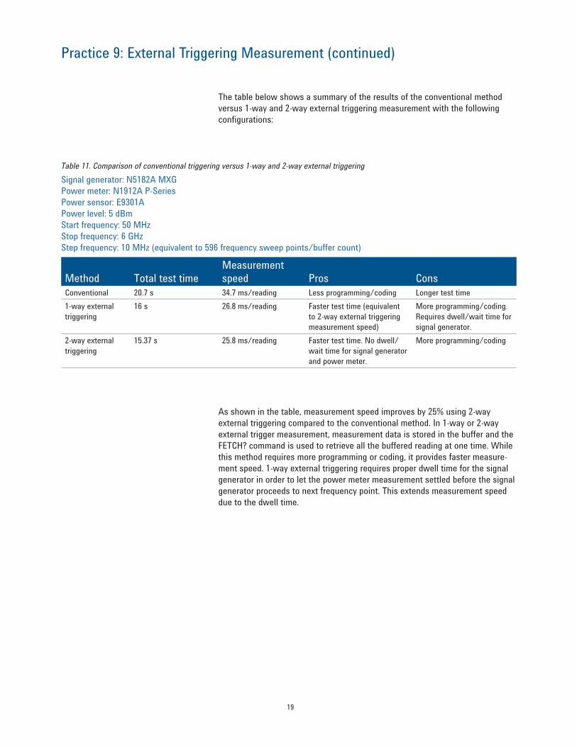
The table below shows a summary of the results of the conventional method versus 1-way and 2-way external triggering measurement with the following configurations:

Table 11. Comparison of conventional triggering versus 1-way and 2-way external triggeringSignal generator: N5182A MXGPower meter: N1912A P-SeriesPower sensor: E9301APower level: 5 dBmStart frequency: 50 MHzStop frequency: 6 GHzStep frequency: 10 MHz (equivalent to 596 frequency sweep points/buffer count)

Method Total test timeMeasurement speed Pros Cons

Conventional 20.7 s 34.7 ms/reading Less programming/coding Longer test time1-way external triggering

16 s 26.8 ms/reading Faster test time (equivalent to 2-way external triggering measurement speed)

More programming/coding. Requires dwell/wait time for signal generator.

2-way external triggering

15.37 s 25.8 ms/reading Faster test time. No dwell/wait time for signal generator and power meter.

More programming/coding

As shown in the table, measurement speed improves by 25% using 2-way external triggering compared to the conventional method. In 1-way or 2-way external trigger measurement, measurement data is stored in the buffer and the FETCH? command is used to retrieve all the buffered reading at one time. While this method requires more programming or coding, it provides faster measure-ment speed. 1-way external triggering requires proper dwell time for the signal generator in order to let the power meter measurement settled before the signal generator proceeds to next frequency point. This extends measurement speed due to the dwell time.

20

Related Agilent Literature

Conclusion

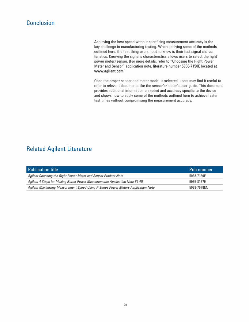
Achieving the best speed without sacrificing measurement accuracy is the key challenge in manufacturing testing. When applying some of the methods outlined here, the first thing users need to know is their test signal charac-teristics. Knowing the signal’s characteristics allows users to select the right power meter/sensor. (For more details, refer to “Choosing the Right Power Meter and Sensor” application note, literature number 5968-7150E located at www.agilent.com.)

Once the proper sensor and meter model is selected, users may find it useful to refer to relevant documents like the sensor’s/meter’s user guide. This document provides additional information on speed and accuracy specific to the device and shows how to apply some of the methods outlined here to achieve faster test times without compromising the measurement accuracy.

Publication title Pub numberAgilent Choosing the Right Power Meter and Sensor Product Note 5968-7150EAgilent 4 Steps for Making Better Power Measurements Application Note 64-4D 5965-8167EAgilent Maximizing Measurement Speed Using P-Series Power Meters Application Note 5989-7678EN

Agilent Email Updates

www.agilent.com/find/emailupdatesGet the latest information on the products and applications you select.

www.lxistandard.orgLAN eXtensions for Instruments puts the power of Ethernet and the Webinside your test systems. Agilent is a founding member of the LXI consortium.

Agilent Channel Partnerswww.agilent.com/find/channelpartnersGet the best of both worlds: Agilent’s measurement expertise and product breadth, combined with channel partner convenience.

For more information on Agilent Technologies’ products, applications or services, please contact your local Agilent office. The complete list is available at:www.agilent.com/find/contactus

AmericasCanada (877) 894 4414 Brazil (11) 4197 3500Mexico 01800 5064 800 United States (800) 829 4444

Asia PacificAustralia 1 800 629 485China 800 810 0189Hong Kong 800 938 693India 1 800 112 929Japan 0120 (421) 345Korea 080 769 0800Malaysia 1 800 888 848Singapore 1 800 375 8100Taiwan 0800 047 866Other AP Countries (65) 375 8100

Europe & Middle EastBelgium 32 (0) 2 404 93 40 Denmark 45 70 13 15 15Finland 358 (0) 10 855 2100France 0825 010 700* *0.125 €/minuteGermany 49 (0) 7031 464 6333 Ireland 1890 924 204Israel 972-3-9288-504/544Italy 39 02 92 60 8484Netherlands 31 (0) 20 547 2111Spain 34 (91) 631 3300Sweden 0200-88 22 55United Kingdom 44 (0) 131 452 0200For other unlisted countries: www.agilent.com/find/contactusRevised: June 8, 2011

Product specifications and descriptions in this document subject to change without notice.

© Agilent Technologies, Inc. 2011Published in USA, July 14, 20115990-8471EN

www.agilent.com

Agilent Advantage Services is committed to your success throughout your equip-ment’s lifetime. To keep you competitive, we continually invest in tools and processes that speed up calibration and repair and reduce your cost of ownership. You can also use Infoline Web Services to manage equipment and services more effectively. By sharing our measurement and service expertise, we help you create the products that change our world.

www.agilent.com/quality

www.agilent.com/find/advantageservices

www.axiestandard.org AdvancedTCA® Extensions for Instrumentation and Test (AXIe) is an open standard that extends the AdvancedTCA for general purpose and semiconductor test. Agilent is a founding member of the AXIe consortium.

www.pxisa.org PCI eXtensions for Instrumentation (PXI) modular instrumentationdelivers a rugged, PC-based high-performance measurement and automation system.