pragmatic approaches for timing analysis - diva portal

Mälardalen University Press DissertationsNo. 128

PRAGMATIC APPROACHES FOR TIMINGANALYSIS OF REAL-TIME EMBEDDED SYSTEMS

Yue Lu

2012

School of Innovation, Design and Engineering



Yue Lu

2012

School of Innovation, Design and Engineering



Yue Lu

Akademisk avhandling

som för avläggande av teknologie doktorsexamen i datavetenskap vidAkademin för innovation, design och teknik kommer att offentligen försvaras

måndagen den 18 juni 2012, 13.15 i Kappa, Mälardalens högskola, Västerås.

Fakultetsopponent: Assistant Professor Enrico Bini, Scuola Superiore Sant'Anna

Akademin för innovation, design och teknik



Yue Lu

Akademisk avhandling

som för avläggande av teknologie doktorsexamen i datavetenskap vidAkademin för innovation, design och teknik kommer att offentligen försvaras

måndagen den 18 juni 2012, 13.15 i Kappa, Mälardalens högskola, Västerås.

Fakultetsopponent: Assistant Professor Enrico Bini, Scuola Superiore Sant'Anna

Akademin för innovation, design och teknik

AbstractMany industrial real-time embedded systems are very large, flexible and highly configurable softwaresystems. Such systems are becoming ever more complex, and we are reaching the stage where evenif existing timing analysis was feasible from a cost and technical perspective, the analysis results areoverly pessimistic, making them less useful to the practitioner. When combined with the fact that mostexisting real-time embedded systems tend to be probabilistic in nature due to high complexity featuredby advanced hardware and more flexible and/or adaptive software applications, this advocates movingtoward pragmatic timing analysis, which are not specifically limited by constrains related to intricatetask execution and temporal dependencies in systems. In this thesis, we address this challenge, and wepresent two pragmatic timing analysis techniques for real-time embedded systems.

The first contribution is a simulation-based analysis using two simple yet novel search algorithms ofmeta-heuristic type, i.e., a form of genetic algorithms and hill-climbing with random restarts, yieldingsubstantially better results, comparing traditional Monte Carlo simulation-based analysis techniques.

As the second contribution, we discuss one major issue when using simulation-based methods for timinganalysis of real-time embedded systems, i.e., model validity, which determines whether a simulationmodel is an accurate representation of the system at the certain level of satisfaction, from a task responsetime and execution time perspective.

The third contribution is a statistical timing analysis which, unlike the traditional timing analysis, doesnot require worst-case execution times of tasks as inputs, and computes a probabilistic task worst-caseresponse time estimate pertaining to a configurable task reliability requirement.

In addition, a number of tools have been implemented and used for the evaluation of our research results.Our evaluations, using dierent simulation models depicting fictive but representative industrial controlapplications, have shown a clear indication that our new timing analysis techniques have the potential tobe both applicable and useful in practice, as well as being complementary to software testing focusing ontiming properties of real-time embedded systems that are used in the domains of industrial automation,aerospace and defense, automotive telematics, etc.

ISBN 978-91-7485-074-1ISSN 1651-4238

Svensk sammanfattning

Många av dagens industriella system innehåller programvara, och de har medtiden kontinuerligt utvecklats och vuxit till stora, komplexa och komplicer-ade mjukvarusystem. For många av dessa industriella system ar korrekt funk-tion beroende av att programvanan utfor ratt saker vid ratt tid. Sakerstallandetav timing hos programvaran kraver att det går att genomfora modellering ochanalys. Denna typ av analys av timing kallas for realtidsanalys, och over desenaste 40 åren har det utvecklats en uppsjo av olika tekniker for modelleringoch analys av realtidssystem.

Trots att dessa analyser ger mojligheter att analysera timing hos industriellasystem så ar analysresultaten ofta for pessimistiska, vilket, såvida inte predik-terbarheten har designats in explicit, gor analysen mindre anvandbar i realis-tiska situationer. Anledningen till att dessa analyser ar mindre anvandbara aratt de ar baserade på enkla modeller vilket kraver pessimistiska forenklingarnar man ska modellera komplexa system samt att analyserna hittar de faktiskavarstafallsresponstiderna gor att de resultat som erhålls ar så osannolika ochforenklade att de ar oanvandbara.

I denna avhandling foreslår vi istallet en ny typav analys av inbyggda re-altidssystem som tar ansats i att introducera en sannolikhet for att en varstafalls-responstid ska intraffa. Givet en sådan analys så kan man filtrera bort analys-varden som ar accepterbart osannolika, och analysen blir darmed anvandbarfor en storre mangd komplexa industriella programvarusystem med krav påtiming.

Avhandlingen innehåller tre vetenskapliga bidrag.Det forsta bidraget ar en kombination av optimeringsalgoritmer och tradi-

tionell simuleringsteknik vilket visar sig ge bra resultat nar det galler att finnarealistisk timing hos komplexa realtidsystem.

Det andra bidraget ar anvandning av statistiska metoder for att gora model-lvaliditetskontroll. Denna validitetskontroll ar avgorande for att sakerstalla att

i

ii

analys gors på modeller som verkligen återspeglar det analyserade systemetstidsbeteende.

Det tredje bidraget ar en statistisk responstidsanalys som inte kraver attvarsta mojliga exekveringstider ar kanda for att erhålla den varsta responstidenhos programvaran, givet en sannolikhet att dar inte finns någon langre respon-stid. Man kan då med statistiska metoder kontrollera hur detaljerad analys somska genomforas for att få tillrackligt tillforlitliga responstidsvarden.

Alla bidrag har utvarderats på modeller av komplexa inbyggda program-varusystem och resultaten ger en tydlig indikation på att de foreslagna metoder-na ar praktiskt anvandbara.

论文概要

迄今为止，很多工业实时嵌入式系统是规模庞大，结构灵活和具有高可配置性的。由

于这些系统越来越复杂，我们所面临的现实是：应用现有的实时分析方法去分析这些

复杂系统在实际中的不可行性。进一步说，当考虑到实时嵌入式系统中的软硬件都具

有极高的复杂性和灵活性，相应地，实时系统的任务时间行为呈现复杂的概率分布。

因此，我们应该着重于开发具有实际应用性的关于实时嵌入式系统的实时分析方法。

针对以上的问题和挑战，此篇论文提出了两种解决方案。

我们的第一个研究贡献是一套应用动态仿真优化的实时分析方法。具体来说，此方法

采用两种不同的元启发式搜索，通过使用遗传学算法和爬山法，来对传统的蒙特卡罗

模拟进行优化。经过对于工业仿真模型的评估，我们发现，和传统的蒙特卡罗模拟方

法相比，我们的方法能够在更短的模拟时间内取得更好的模拟结果。

我们的第二个研究贡献是一套模拟仿真模型的验证方法。通过应用统计学的方法，我

们可以完成对目标系统和模拟系统关于任务响应时间和执行时间的仿真模型验证。

我们的第三个贡献为一套应用统计学的实时分析方法。和传统的实时分析方法不同，

我们的方法既不需要已知最差任务执行时间，也不需要系统仿真模型或是系统源代码，

而是通过对目标系统进行创新式采样，然后基于极限值理论来对采集样本进行统计学

分析，最后计算出一个带有概率的，符合一定任务可靠性标准的任务响应时间。

此外，我们还开发了一系列工具来支持我们的研究理论。通过对数组工业系统模型的

评估，我们发现我们的方法具有很高的准确性和很强的实际应用性。它们能够为那些

在工业自动化，宇宙航天，汽车通讯领域工作的实时嵌入式系统的实时分析提供重要

的理论依据和工具支持。

To my beloved Tianrong, Yingcai and ShaWho gave me birth and is giving me rebirth

Acknowledgments

Before we start this chapter, I would like to mention that comparing the thanks-giving chapter of my Lic. thesis1, there is some resemblance in this newchapter. The main differences between two chapters include some necessarychanges together with some extra “poems” prior to each chapter (except forChapter 1) of this thesis, which is very likely to be the only doctoral thesis inmy short life. Specifically, the “poems” will deliver some extra thanksgivingmessages to some people2. Now, we are ready for going in the thanksgivingchapter, which is the hardest part for me to write, even to start, but might be themost interesting chapter (out of all the chapters in this whole thesis) for peopleto read. So let us drop the less “tasty” main course of the thesis for now, beltup and start this thanksgiving journey!

After sending out countless number of application emails to different uni-versities, I was luckily enough to be accepted by Malardalen Real-Time Re-search Centre (MRTC) at Malardalen University, Oct. 2006. Thank you HansHansson, Christer Norstrom and Bjorn Lisper, for giving me this opportunity!

To me, this thesis is the end of one rewarding journey, along which I havemy pleasure to enjoy the scenery and experience life. Throughout these pastyears, I met different people around the world, with whom I had lots of fun,from whom I knew more about my weaknesses, and whom I would love to par-rot. In the following, I will categorize those people, who have played differentroles in my short life.

Supervisors Without yours encouragement, guidance and patience, I wouldnever ever proceeded to the place where I am now.

1In the Swedish graduate education system, licentiate is a degree between master and doctor,which is the half of a doctor dissertation.

2You know who you are.

v

vi

1. Professor Thomas Nolte, who is officially the main supervisor of my lasttwo-year Ph.D. work (or study or whatever those officers name it). Thankyou for giving me timely help in time of need, constantly encouragingand helping me when I want to give up, teaching me the art of weighingmy written words on a silver scale, being as a nice company at manyconference trips that I really enjoyed, and appreciating me for what myresearch is. Tusen tack!

2. Professor Christer Norstrom, who was the main supervisor of my firstfour-year Ph.D. work since Oct. 2006. Thank you for guiding me, help-ing me and believing in me when I was cracking those “nuts” on myresearch little by little. Though you changed your career to a more chal-lenging position, I do appreciate your timely help and support when Ineeded them desperately. Tusen tack!

3. Dr. Liliana Cucu-Grosjean, thanks for inviting me to visit INRIA Nancy-Grand Est, organizing many unforgettable group activities, and introduc-ing me les fromages et les vins en France. My extra thank you notes willbe expressed by the “poem” prior to Chapter 6. Merci beaucoup et abientot, j’espere.

4. Dr. Iain Bate, who is not officially one of my supervisors, but helped mequite a lot in terms of having countless fruitful discussions, authoring afew papers together, and giving me another chance to know more aboutmy hometown. Many thanks!

5. Dr. Anders Wall, who is my assistant supervisor. Thank you for guidingme and having some useful discussions with me. Tack!

Thesis reviewers Thank you Thomas Nolte and Christer Norstrom for re-viewing my thesis and helping me make the thesis in a better shape. I am alsogoing to thank Enrico Bini, Isabelle Puaut3, Alan Burns and Eduardo Tovarwho accepted to review the thesis as a faculty examiner and examining com-mittee members. In addition, many thanks go to my wife Sha and ThomasNolte, for yours help on the Swedish version of my thesis summary!

Co-authors I would never ever have made the published papers without myco-authors’ professional, persuasive discussions, perseverance, hard workingand competitive nature. Besides my supervisors, I want to thank Johan Kraft,Stefan Bygde, Markus Bohlin, Per Kreuger, Mikael Sjodin, Jukka Maki-Turja

3Madame Isabelle Puaut, a truest mind with a transparent feeling can make the dishes whichgive a home feeling touch. C’est la vie!

vii

and Antonio Cicchetti. Furthermore, I am very grateful to Erik Dahlquist,Diane Pecorari, Linh Thi Xuan Phan, Emma Nehrenheim, Monica Odlare, JanCarlsson, Bjon Lisper and Daniel Sundmark for their constructive commentsand improvement suggestions that we desperately needed, as well as usefulinformation given by their courses. Thank you all!

Friends and colleagues I want to express my heartfelt thanks and immenseappreciation to Insik Shin (who he is wise, disciplined and generous, showingme oriental wisdom, and who gave me the truly comforting words which savedme timely. Thank you very much dear Insik!), Ivica Crnkovic (who showedme his optimism and desire to share his goals with others, hard work and per-severance with a positive attitude. Thank you Ivica!), Aida Causevic4, CristinaSeceleanu, Severine Sentilles, Aneta Vulgarakis, Hongyu Pei-Breivold, StefanBygde5, Nan Guan, Johan Fredriksson, Dag Nystrom, Farhang Nemati, AdnanCausevic, Leo Hatvani, Moris Behnam, Nima Moghaddami, Mikael Åsberg,Juraj Feljan, Fredrik Ekstrand, Huseyin Aysan, Sara Dersten, Andreas Gus-tavsson, Shahina Begum, Mobyen Uddin Ahmed, Svetlana Girs, Eduard Enoiu,Raluca Marinescu, Sara Afshar, Mohammad Ashjaei, Rikard Land, Tiberiu Se-celeanu, Radu Dobrin, Pasqualina Potena, Rui Santos, Ning Xiong, Hang Yin,Jiale Zhou, Kan Yu, Jagadish Suryadevara, Peter Wallin, Andreas Hjertstrom,Abhilash Thekkilakattil, Jorgen Lidholm, Adam Betts, Frank Luders, HelenaJerregård, Marcelo Santos, Nikola Petrovic, Mehrdad Saadatmand, FedericoCiccozzi, Kathrin Dannmann, Batu Akan, Rafia Inam, Saad Mubeen, AnaPetricic, Jospi Maras, Luka Lednicki, and Etienne Borde. Thank you all, and Iam really sorry for this long list.

Next, I would love to thank Åsa Lundkvist, Damir Isovic, Carola Rytters-son, Harriet Ekwall, Kristina Lundqvist, Malin Rosqvist, Malin Swanstrom,Annika Havbrandt, Maria Linden, Hans Hansson, Paul Pettersson, ThomasNolte, Peter Funk, Jan Gustafsson, Lars Asplund6, Rikard Lindell, GunnarWidforss, Mats Bjorkman, Baran Curuklu, Antti Salonen, Mikael Ekstrom andthose who are creating a more comfortable, friendly and international workenvironment at the IDT department. Frankly speaking, I am neither a com-munist, nor a capitalist; I am not a Buddhist, Christian, Jew, Muslim or an

4Dear Aida, thanks for your wakeup calls, many helps and cares about me, which I reallyappreciated, and I am trying to not disappoint dear you. Mmm, so how are you doing today? ;)

5Dear Xiaobai, thanks for your never giving me up when I was screwing up, and your constantlycorrecting me in terms of “beating” me hands down, even when I was not completely wrong. Sorryfor repeating the same words which are in my Lic. thesis, but I mean it.

6A professor who keeps dancing with his robots on his own.

viii

atheist; I have no idea about what happens when we die (but I do know thatwe all die alone physically). Though I have observed many negative effectsof globalization, I am really happy to see that at IDT (Vasterås), we are beingjudged together as a group of lovely people, who are sharing a same goal andkeeping moving forward, but not burying our heads in the sand of past. Sothank you all! BTW, aren’t these many free fruits and bananas, sweet cakesand champagne, more funds and confidence with ourselves, showing karmicpaybacks?!

By the chance, I also want to thank some of my basketball friends in town:Ulf Bryggman (tack for skjutsen och vi ses på nasta vecka!), Berina & IsmirFazlagic (tack for pick and roll, give and go, use backdoor, Alley-oop!), ConnyÅslund and his Aros Basket, as well as ABB basketball.

The important people In the end, if there was something matters more thanothers. I want to thank my mother Tianrong Liu and my father Yingcai Lu,who are there for me many years of grace, for your love, for your bearing mybad temper, for your teaching and showing me the value of knowledge and life,and for your parenting me till today. I love everything you two have done forme to death, without a doubt!7 Last but not least, my thanksgiving messagesare delivered to my dear wife Sha: Without your love, support, perseverance,encouragement, tolerance and patience, endless effort on making me a betterperson (though I am still working on it now), and your sweet accompanyingme for nine years of joy, tears and grace, I would never, ever have come thisfar. So thank you, and I love you all!

The liabilities The work leading up to this thesis was supported by the Swedi-sh Foundation for Strategic Research via the strategic research centre Progress.

The close Finally, it comes to an end, as it has to be. Before I go home, goingto sleep, I would love to say

“Thank you all! Tack ska ni all ha! Merci a vous tous! Xie xie ni men!”

Yue Lu, Vasterås, May 27th, 2012

7Though, sometimes, you might think that I may think you were “nagging me” too much, Iwould love to take the chance to dispel this misconception. As your son, I am happy to be the one,whom you can always turn to, and share something with!

Nothing Rhymed III – ALittle Bit Yellow Life

If life was a word, I don’t understand. Simplest sound, four letters.

If life was a word, do you understand? Though the simplest sound,only four letters.

Life is not fair, when it was not fair at all. I am always washingthe pain by using new pains.

Life is not easy, when it was not easy at all. I am always walkingaway from the color by setting in new colors.

Life is not straightforward, when it was not straightforward at all.I am always removing the fake by adding new fakes.

When there was a time, people started putting you down enough,then what will you start to believe?

When there was always a time, people started painting you in theircolored eyes, then what is the color of you?

The feeling about being a cheap underdog is just so amazing tome, since I believe it is exactly where all of us get started, no mat-ter what is the color of you.

So if life was a word, what is its taste? The simplest combination,

x

the four tastes.

You may know that life is not about how hard it hits you and de-stroy you by its colored hits. It is more about how much you cangain from the hits and keep moving forward, as a person. Moreprecisely, as a better person, no matter what is the color of you.

So if life was a word, I am trying to understand it now. The sim-plest sound and combination, only four “colored” letters.

No matter whatever it was, or whatever it is, or whatever it is go-ing to be, I really do not care, and I will just rise and overcomeit now, in my different purple way, with my courage in patience,which is more important.

Je suis un etre singulier dans une generation desenchantee.

Je vous remercie pour votre gentillesse et votre presence.

La vie en jaune.

C’est la vie.

Bien a vous,Yue Luis Lu

May, 2012

A special and quick thanksgiving note delivering to Mademoi-selle Severine Sentilles, who dear she helped me with my brokenFrancais: Mademoiselle Severine Sentilles, merci beaucoup pourvotre amitie et votre aide.

Vous etes belle, if I have not said this to you before. ;)

Notes for Readers

This thesis deals with the development of pragmatic timing analysis techniquesfor real-time embedded systems. In Chapter 3, we introduce the intended sys-tems featuring intricate task execution and temporal dependencies, resulting insome interesting statistical characteristics of systems’ timing behavior. Chap-ter 4, 5 and 6 position our proposed pragmatic timing analysis techniques, to-gether with the prototype tools implementing our methods, as well as demon-stration of using these tools in the evaluation of our simulation models depict-ing two fictive but representative industrial control applications, respectively.These three chapters present the main research contributions of this thesis.

To get an introduction and a summary of the thesis; the research challengeswe are about to overcome, and the contributions in brief, the reader is referredto Chapter 1. Chapter 2 introduces a formal definition of a real-time embeddedsystem including basic background on real-time scheduling, and defines impor-tant terms in the area of timing and schedulability analysis. Finally, Chapter 7summarizes and concludes the thesis, and discusses some possible future re-search directions in short.

xi

Contents

1 Introduction 31.1 Motive for the Research . . . . . . . . . . . . . . . . . . . . . 3

1.1.1 Non-traditional Expressive Timing Analysis Models . 61.2 Overview of Our Solutions . . . . . . . . . . . . . . . . . . . 6

1.2.1 Simulation Optimization-Based Timing Analysis . . . 71.2.2 Simulation Model Validation Using Statistics . . . . . 71.2.3 Statistical Response-Time Analysis . . . . . . . . . . 8

1.3 Contributions . . . . . . . . . . . . . . . . . . . . . . . . . . 91.4 Thesis Outline . . . . . . . . . . . . . . . . . . . . . . . . . . 10

2 Real-Time Embedded Systems 152.1 Embedded Real-Time Systems . . . . . . . . . . . . . . . . . 152.2 Real-Time Scheduling . . . . . . . . . . . . . . . . . . . . . 17

2.2.1 Task Model . . . . . . . . . . . . . . . . . . . . . . . 172.2.2 Resource Model . . . . . . . . . . . . . . . . . . . . 182.2.3 Scheduling Algorithms . . . . . . . . . . . . . . . . . 192.2.4 Schedulability Analysis . . . . . . . . . . . . . . . . 202.2.5 Utilization-Based Analysis . . . . . . . . . . . . . . . 20

2.3 Response-Time Analysis . . . . . . . . . . . . . . . . . . . . 212.3.1 The Basic RTA . . . . . . . . . . . . . . . . . . . . . 22

2.4 Worst-Case Execution Time Analysis . . . . . . . . . . . . . 232.5 Simulation of Real-Time Embedded Systems . . . . . . . . . 252.6 Summary . . . . . . . . . . . . . . . . . . . . . . . . . . . . 27

3 The Target Real-Time Embedded Systems 313.1 The Target Industrial Control Application . . . . . . . . . . . 31

xiii

xiv Contents

3.2 System Model and Featured Task Execution and Temporal De-pendencies . . . . . . . . . . . . . . . . . . . . . . . . . . . . 33

3.3 Representative Characteristics of Tasks’ Timing Behavior . . . 353.4 Summary . . . . . . . . . . . . . . . . . . . . . . . . . . . . 37

4 Simulation Optimization-Based Timing Analysis 414.1 Introduction . . . . . . . . . . . . . . . . . . . . . . . . . . . 414.2 Related Work on Simulation-Based Analysis . . . . . . . . . . 424.3 Our Proposed Simulation-Based Response-Time Analysis . . . 434.4 Our Solution One – MABERA . . . . . . . . . . . . . . . . . 44

4.4.1 Function SIM . . . . . . . . . . . . . . . . . . . . . . 464.4.2 Function SEL . . . . . . . . . . . . . . . . . . . . . . 474.4.3 Function GEN . . . . . . . . . . . . . . . . . . . . . 49

4.5 Our Solution Two – Hill Climbing with Random Restart (HCRR) 514.5.1 Explicit Representation of System Input . . . . . . . . 514.5.2 The Algorithm Description . . . . . . . . . . . . . . . 52

4.6 Case Studies . . . . . . . . . . . . . . . . . . . . . . . . . . . 544.7 Evaluation Results . . . . . . . . . . . . . . . . . . . . . . . 57

4.7.1 Average Convergence . . . . . . . . . . . . . . . . . 604.8 Summary . . . . . . . . . . . . . . . . . . . . . . . . . . . . 62

5 Simulation Model Validation 675.1 Related Work on Simulation Model Validation . . . . . . . . . 675.2 Our Solution - TTVal . . . . . . . . . . . . . . . . . . . . . . 685.3 The Algorithm . . . . . . . . . . . . . . . . . . . . . . . . . 69

5.3.1 The New Sampling Method . . . . . . . . . . . . . . 695.3.2 Problems with Using Parametric Statistics . . . . . . . 705.3.3 The Two-Sample KS Test . . . . . . . . . . . . . . . 715.3.4 The Non-Traditional Hypothesis Test . . . . . . . . . 725.3.5 The Proposed Method TTVal . . . . . . . . . . . . . . 72

5.4 Evaluation Results . . . . . . . . . . . . . . . . . . . . . . . 735.4.1 The Evaluation Models . . . . . . . . . . . . . . . . . 735.4.2 Change Scenarios and Evaluation Results . . . . . . . 75

5.5 Summary . . . . . . . . . . . . . . . . . . . . . . . . . . . . 76

6 Statistical Response-Time Analysis 816.1 Motive . . . . . . . . . . . . . . . . . . . . . . . . . . . . . . 816.2 Statistical Analysis of Systems . . . . . . . . . . . . . . . . . 82

6.2.1 System Model . . . . . . . . . . . . . . . . . . . . . 82

Contents xv

6.2.2 Background on the EVT Used . . . . . . . . . . . . . 826.2.3 Related Work for the Use of EVT in Real-Time Systems 836.2.4 Overview of Our Approach . . . . . . . . . . . . . . . 84

6.3 RapidRT Analysis Technique . . . . . . . . . . . . . . . . . . 866.3.1 Sampling . . . . . . . . . . . . . . . . . . . . . . . . 866.3.2 Posterior Statistical Correction Process . . . . . . . . 89

6.4 Case Study: An Industrial Robotic Control System . . . . . . 926.4.1 Evaluation Setup . . . . . . . . . . . . . . . . . . . . 926.4.2 Evaluation Models . . . . . . . . . . . . . . . . . . . 946.4.3 Testbed and Toolchain . . . . . . . . . . . . . . . . . 976.4.4 Evaluation Results . . . . . . . . . . . . . . . . . . . 99

6.5 Summary . . . . . . . . . . . . . . . . . . . . . . . . . . . . 102

7 Summary and Future Work 1077.1 Summary . . . . . . . . . . . . . . . . . . . . . . . . . . . . 1077.2 Future Research Directions . . . . . . . . . . . . . . . . . . . 108

A Complete List of Publications 111

Bibliography 121

C’est La Vie

Mathilda: Is life always this hard, or is it just when you are a kid?

Leon: Always like this.

– Leon: The Professional (1994)

Chapter 1

Introduction

Real-time systems are computer systems of which the correctness depends notonly on the logical correctness of the computations performed, but also on thepoint in time the results are provided. Such systems are typically found inembedded applications such as industrial robotic control systems and telecom-munication systems. In this thesis we explore pragmatic timing analysis tech-niques for real-time embedded systems containing intricate task execution andtemporal dependencies. To be specific, we have proposed and developed 1)a simulation optimization-based timing analysis technique (which uses twosimple yet novel search algorithms of metaheuristic type) and, 2) a statisticaltiming analysis technique using different statistical methods and search algo-rithms.

In this chapter, we give an introduction of our research by starting with theoverall research problem, and then introducing research challenges, overviewof our solutions, and contributions. Finally, we conclude this chapter with theoutline of the thesis.

1.1 Motive for the Research

To date, our daily life is getting more and more dependent on embedded sys-tems, as they are becoming more powerful, highly flexible, and less expensive.Typically, embedded systems consist of electronics and software operating toadapt to, or control, its environment. They are different from desktop comput-ers in the sense of interacting with environment via inputs for analog and digital

3

4 Chapter 1. Introduction

sensors, and different types of communication buses and other devices, ratherthan a screen or keyboard. Embedded systems constitute more than 99% of allcomputers in the world [75, 4], and they are commonly used in a wide range ofapplication domains, such as telecommunication, manufacturing, avionics andaerospace, automotive, automation, power control, medical care and so on.

Many industrial embedded systems are very large, flexible, and highly con-figurable software systems, containing event-triggered tasks being triggered byother tasks in complex, nested patterns. Consequently, they have a very compli-cated runtime behavior. Such systems may consist of millions of lines of code,and contain hundreds of tasks, many of which are with real-time constraints.Examples of such systems include the robotic control system IRC 5, developedby ABB1, as well as several telecommunication systems. In such systems,many tasks have intricate dependencies in their temporal behavior, such as 1)asynchronous message-passing and global shared state variables, which maydecide important control-flow conditions with major impact on task executiontime as well as task response time, 2) task offsets, and 3) runtime changeabilityof priorities and periods of tasks.

To maintain, analyze and reuse industrial real-time embedded systems isvery important, difficult and expensive, which, however, offers high businessvalue responding to great concern in industry. In particular, one specific prob-lem in maintenance, i.e., modifying the system after delivery to correct faults,improve performance or other attributes, or to adapt the product to a changedenvironment, is the risk for introducing timing-related errors. For such sys-tems in safety-critical applications, both functional and non-functional correct-ness are often equally important to be ensured. Thus, temporal behavior, e.g.,Worst-Case Response Time (WCRT) of the adhering tasks in systems has tobe known. For instance, a failing industrial robot could halt an entire produc-tion line in a factory for hours, causing a huge financial loss. Software bugsthat lead to slow response time in Anti-lock Brake System (ABS) in cars couldcause loss of human lives, and recall of several hundreds of thousands of ve-hicles to maintenance and bug-fixing. Another fact found by IBM is that 50%of the warranty costs in cars are related to electronics and their embedded soft-ware, and that 30% of those costs are related to timing flaws. The resultingincorrect operation cost industry billions of Euros annually [18].

However, due to high complexity of such systems, the existing relativelywell-developed theories for modeling and analysis of real-time systems arehaving problems which limit their application in the context. For instance,

1www.abb.com, 2012.

1.1 Motive for the Research 5

timing analysis methods such as the basic Response-Time Analysis (RTA) andits variations [32], are often not applicable, as their assumptions of indepen-dent tasks in the analysis do not hold in such systems. The results of theanalysis thereby become overly pessimistic; often too pessimistic to be use-ful. Moreover, the methods like RTA and its variations rely on the existenceof a Worst-Case Execution Time (WCET) of each task. Correspondingly, thequality of the analysis is directly correlated to the quality of WCET estimates.In order to perform a safe analysis covering system worst-case scenarios, staticWCET analysis [79] has to be adopted in the context, of which assumption isthat tasks are isolated in the analysis. Nevertheless, such assumptions makethe option to use static WCET analysis to obtain task-level WCET estimatesnot proper, due to the fact that task intricate temporal dependencies cannot bewell handled. Furthermore, today’s WCET tools cannot analyze the complexhigh-performance CPUs used by many industrial systems, and they require ex-haustive knowledge of all factors including both software and hardware, thatdetermine the execution history of the program under analysis, which is ex-pensive to obtain. On the other hand, intellectual property restrictions and/orincomplete documentation may even make it impossible to construct the cor-responding timing model in analysis.

The state of practice in industry is that many companies developing theirreal-time embedded systems have no means for timing analysis, and are forcedto rely on testing to find timing-related problems. Therefore, measurementsof response time are often performed using an instrumented executable for thetarget system [53]. Nonetheless, for the systems with large size, complex be-havior, and possibly very high response time of tasks under analysis, runningthe actual system may be quite time-consuming and costly. Furthermore, con-sidering that the number of samples often have to be in the order of tens ofthousands or even millions, consequently the total evaluation time can easilybecome prohibitively long. Moreover, all timing errors can in most cases notbe detected in unit testing as they only occur in the integrated system, whenconcurrent activities are interacting or interfering, under a very specific con-dition. Additionally, it is not only extremely difficult and expensive to test allscenarios in the system, but also hard to predict how a product will be used.Enabling RTA of industrial real-time embedded systems is a problem of highindustrial relevance thereof.


1.1.1 Non-traditional Expressive Timing Analysis Models

Using simulation, the evaluation time can be reduced dramatically by analyz-ing a simpler model but still containing detailed behavior of the target system.The most widely applied simulation-based analysis in both academia and in-dustry is Monte Carlo simulation [56], where the simulation model often con-tains execution time data from measurements. Monte Carlo simulation canbe described as keeping the highest result from a set of randomized simula-tions. Examples of tools implementing Monte Carlo simulation include thecommercial tool VirtualTime2 and the academic tool ARTISST [23]. However,the main drawback of Monte Carlo simulation is that of its low state-spacetest coverage, which subsequently decreases the confidence in results of find-ing rare system extreme scenarios, which, nevertheless, are necessary to beexplored. It therefore becomes a challenge for us to improve such coverage,when simulation-based methods are applied.

Additionally, in order to perform pragmatic timing analysis of such sys-tems, a more detailed system model, which depicts the original software pro-gram in the system focusing on the behavior of significance for task schedul-ing, communication and allocation of logical resources, should have to be used.Furthermore, the model should be more expressive comparing the system mod-els used in the basic RTA and its variations. Typically, such models need to beat a certain level of abstraction, in order to avoid that the model becomes ascomplex as the real system.

It is interesting to stress that another alternative approach to the simulation-based methods is to apply formal analysis such as model checking. Modelchecking can be used, for instance, to verify different properties of a softwaresystem, e.g., absence of deadlocks, safety properties, and timeliness proper-ties. Nevertheless, without either using abstraction / deduction techniques, orlimiting its application to the simple real-time embedded systems containingless complex task execution dependencies [50], model checking always suffersfrom the problem state space explosion, which limits its applicability.

1.2 Overview of Our SolutionsIn this thesis, we present two main themes for pragmatic timing analysis ofreal-time embedded systems containing intricate task execution and temporaldependencies. In particular, the first theme deals with simulation optimization-

2www.rapitasystems.com/virtualtime, 2012.

1.2 Overview of Our Solutions 7

based timing analysis to improve the performance of the traditional MonteCarlo simulation. The second theme deals with statistical timing analysis,which, 1) unlike traditional timing analysis, does not require worst-case exe-cution times of tasks as inputs, and 2) computes a probabilistic task worst-caseresponse time estimate.

1.2.1 Simulation Optimization-Based Timing AnalysisIn this thesis we present two simulation optimization-based timing analysismethods, called MABERA and HCRR respectively. Each of them applies ameta-heuristic search algorithm on top of the traditional Monte Carlo simu-lation, yielding substantially better simulation results in finding system rareand extreme scenarios, compared with the Monte Carlo simulation. Thoughthe meta-heuristic search algorithms used in the two methods are different, theprocess that they both share can be briefly divided into the following steps,respectively:

• Population construction: Running the Monte Carlo simulation for acertain number of times.

• Iterative improvements until threshold is reached: Changing sim-ulation input parameters by using either genetic algorithms without theoperator crossover (in MABERA) or hill climbing using random-restarts(in HCRR) iteratively, until e.g., the certain given simulation budgets areconsumed, or the results converge to a certain value without any furtherimprovements.

• Return the best solution: Returning the highest value of the task WCRTestimates found by the algorithm.

Using these two timing analysis methods, we have conducted an evaluationby using different simulation models inspired by two industrial control appli-cations. Moreover, the evaluation results have shown that our methods cansubstantially improve the simulation results in terms of finding much higherWCRT estimates while at the same time requiring a lower number of simula-tions, comparing traditional Monte Carlo simulation.

1.2.2 Simulation Model Validation Using StatisticsA major issue when using simulation-based timing analysis methods is modelvalidity, which is defined as the process of determining whether a simulation


model is an accurate representation of the system, for the particular objectivesof the study [41]. As a model is an abstraction of the target system, some systemdetails may be omitted in the model, for instance when applying execution timemodeling of sub-tasks. Thus, the results from a simulation of such models maynot be identical to the recordings of the system, e.g., wrt. the task response timeand task execution time. In order to convince system experts to use simulation-based methods, the models should reflect the system with a satisfactory level ofsignificance, i.e., as a sufficiently accurate approximation of the actual system.Therefore, an appropriate model validation process should be performed beforeusing the models.

In this thesis, we also introduce our method for simulation model valida-tion by using statistics. Specifically, our method is comprised of a samplingmethod (to achieve qualified analysis samples by removing the adhering de-pendencies which hinder the application of using statistics in the context) anda non-parametric hypothesis test based upon a non-traditional hypothesis test.

1.2.3 Statistical Response-Time Analysis

We call the statistical approach to timing analysis of real-time embedded sys-tems presented in this thesis RapidRT. Unlike the traditional timing analysismethods, RapidRT does not require any results given by the WCET analysis,and it produces a probabilistic WCRT estimate using response time samplesunder a statistical constraint. Our approach can be briefly divided into the fol-lowing five stages, namely:

1. The first stage of the analysis is to capture information from the availablesources concerning the Response Time (RT) of the individual tasks, e.g.,the existing system logs containing recorded task RT data. Specifically,no assumption is made as to whether such sources are collected eithervia simulation, or by monitoring the behavior of the actual target usingsoftware probes as introduced in Chapter 7 in [39].

2. Next, a task RT training data (consisting of a number of task RT sub-training data corresponding to K statistical models to be introduced laterin Section 6.3, Chapter 6) is sampled from the set of available sourcesachieved in Step One. Specifically, each sub-training data is taken sothat an independent and identically distributed (i.i.d.) assumption can bemade, and so that there are sufficient samples that appropriate tuning ofthe final analysis can be performed.

1.3 Contributions 9

3. Then, a posterior statistical correction process is performed to allow theprimary objective of the analysis to be achieved, i.e., to obtain a safe andtight WCRT estimate of tasks. This step decomposes the reliability targetfor the WCRT of tasks, into a number of probabilities to be used in thestatistical analysis. Such probabilities are then associated with differentanalysis context, such as our sampling method, Extreme Value Theory(EVT) and the Goodness-Of-Fit (GOF) hypothesis test (of which moredetails are given in Section 6.3.2, Chapter 6).

4. Given an appropriate task RT sub-training data, the statistical analysis(using EVT, GOF hypothesis test and some search algorithm) is tunedsuch that the maximum of a probability distribution generated with agiven set of parameters is a sufficiently close match, at the required sta-tistical confidence, to the maximum of the actual distribution of the sub-training data. At this step, a calibrated and tight PDF histogram of thetask WCRT consisting of the estimates of the maximum of each task RTsub-training data is obtained.

5. The final stage is to use the achieved task WCRT PDF to obtain the finalWCRT of the task under analysis.

1.3 ContributionsThe specific in-depth technical contributions of the presented research in thisthesis are summarized as follows:

• C1 A New More Expressive Timing Analysis Model for Real-Time Em-bedded Systems that describes intricate task execution and temporal de-pendencies. This model is described by using the modeling language inthe RTSSim simulation framework [38], and we use this new model forthe purpose of evaluation.

• C2 Two Simulation Optimization-Based Approaches to Timing Analy-sis of Real-Time Embedded Systems which can substantially improve theconfidence in finding much higher WCRT estimates while requiring alower number of simulations, comparing traditional Monte Carlo simu-lation, which is the state of art in simulation application in industry. Theproposed approaches are evaluated by using a set of simulation modelsinspired by different industrial control applications.


• C3 A Statistical Model Validation Method which addresses the im-portant issue model validity, by using a non-parametric statistics whenthe simulation-based analysis methods are used. The evaluation usinga number of simulation models describing a fictive but representativeindustrial robotic control system, shows that our proposed method canobtain the correct analysis results.

• C4 A Statistical Timing Analysis of Real-Time Embedded Systems whichconsists of a novel sampling method together with a posterior statisticalcorrection process, to compute a probabilistic task WCRT estimate usinga given task reliability requirement. The proposed method is evaluatedby using simulation models inspired by an industrial control application.

• C5 A Set of Prototyping Tools implementing the ideas from C1-C4. Thecorresponding toolchains include a number of implemented prototypingtools and a few commercial softwares.

1.4 Thesis OutlineThis thesis is written as a monograph, which consists of seven chapters that areorganized as follows:

Chapter 1 introduces the particular research issues that this thesis seeks tosolve. In details, we discuss the motivation, our overall solutions, researchchallenges and the contributions of the thesis: two pragmatic timing analysistechniques for real-time embedded systems containing intricate task executionand temporal dependencies.

Chapter 2 provides a formal definition of a real-time embedded system anddefines important terminology and definitions in the area of timing analysis.This chapter also presents the basic background on real-time scheduling. Inparticular, schedulability analysis, RTA (i.e., the basic RTA and its variations)and the WCET analysis are presented.

Chapter 3 introduces our study system (inspired by an industrial robotic con-trol application) and its relevant system model featured by the adhering taskexecution and temporal dependencies. Additionally, we have also highlightedsome interesting representative descriptive statistics of tasks’ response time

1.4 Thesis Outline 11

and execution time, and the difficulty of performing response-time analysis ofsuch systems, by using the existing analysis methods.

Chapter 4 presents our simulation-based timing analysis of real-time em-bedded systems. Specifically, two simple yet novel search algorithms of meta-heuristic type, i.e., a form of genetic algorithms and hill-climbing with randomrestarts, are used to guide Monte Carlo simulation, yielding much better resultsin terms of finding higher response times of tasks, corresponding to some rareextreme cases. Moreover, two evaluation cases developed by our industrialpartners, and one validation case in the form of simulation models, are used forthe evaluation.

Chapter 5 tackles with an important issue when using simulation-based meth-ods, i.e., simulation model validation. Typically, we address the issue by usingstatistical methods, from a task response time and execution time perspective.Traditionally, such validation work is difficult to be done, due to the compli-cated system’s timing behavior which usually not only makes many of the ex-isting statistical methods fail, but also drives the subjective methods to be in-feasible in such context, due to that the number of scenarios is too large to bepractically considered.

Chapter 6 introduces our statistical timing analysis which provides the func-tionality of deriving a calibrated and tight response time estimate of tasks inreal-time embedded systems containing intricate task execution and temporaldependencies. To be specific, the analysis consists of a novel sampling methodand a posterior statistical correction process using different search algorithmsand statistical techniques.

Chapter 7 summarizes and concludes the thesis, and discusses some possi-ble future research directions.

Glamour SHE

Who is telling the approach by her sinful tempting stiletto heels.Who is wooing the world by her beckoning mean..Who is pushing the fear by her desperate screaming in the bed...

Who is she?

She is deeply hiding in the ocean soul.She is elegantly flaming in the nighty sky..She is extinctly stunning in my legendary league...

She is a superlady, a super lady who she said,

”It’s okay, I just got lost on my laughs.Though I’m a superlady, I did have my cries.I am flying, and I am just fading away...”

Sincerely, after many years of grace, in the fields of gold,

she is just a skinny, not-fidgeting, intriguing den petite blonda,who is watching the world through her glittering blue eyes, andtelling us her simple and interesting stories.


On a lovely, sunny day in March,Vasterås, Sweden

Chapter 2

Real-Time EmbeddedSystems

In this chapter, we will firstly give an introduction to embedded real-time sys-tems, followed by terminology and definitions used throughout this thesis.

2.1 Embedded Real-Time SystemsAn embedded system is defined by IEEE in [72] as a computer system that ispart of a larger system, performing some of the functions of that system. Amore clear definition is given in [43], i.e., embedded systems are computingsystems with tightly coupled hardware and software integration, that are de-signed to perform a dedicated function. So an embedded system is a computercontrolled system used to achieve a specific purpose and the computer is not theend-product itself. Moreover, the role of embedded systems is often to replacea traditional mechanical solution, consequently reducing production costs, in-creasing efficiency and enhancing functionality of the product. For example,by only relying on mechanical solutions, the functions of a modern car likeElectronic Damper Control (EDC) and Adaptive Cruise Control (ACC) wereimpossible to achieve. Furthermore, these systems are characterized by havinga fixed and limited amount of resources, such as memory, I/O and so on.

Systems that rely on time to function correctly are called real-time systems.One common definition is [73]: real-time systems are computer systems inwhich the correctness of the system depends not only on the logical correctness

15

16 Chapter 2. Real-Time Embedded Systems

of the computations performed, but also on which point in time the results areprovided. Moreover, a real-time system is not necessarily required to responsequickly, but should have a temporally predictable response. To exemplify this,consider a classical example: triggering the airbag in a car when an accidenthappens should be neither too early, nor too late. If the airbag is inflating tooearly, it might be partially deflated at the time when the driver or passenger hitsit, leading to fatal results; If it is inflating too late or even not being deployed,the driver or passenger will be posted to a severe situation of being injured,mental fatigue and even dead in the worst case. Such timing, i.e., the timefrom the event occurs until the computer control system produces a response iscalled a response time, for the certain functionality.

There are two key characteristics of real-time systems, i.e., the classifica-tion of the criticality of a failure and the activation of tasks in the system.

According to the first characteristic of the criticality of a system failure,there are two types of real-time systems, i.e., hard real-time systems wherea failure is considered to be a fatal fault, and soft real-time systems whereoccasional failures can be accepted or tolerable.

Hard real-time systems: A real-time system is said to be hard if completionafter its deadline can cause catastrophic consequences [16]. In other words,for hard real-time applications, the system must be able to handle all possiblescenarios, including peak load situations. Consequently, the worst-case sce-nario must be analyzed and considered.

Soft real-time systems: A real-time system is said to be soft if missing adeadline decreases performance of the system, but does not jeopardize its cor-rect behavior [16].

According to the above definitions, most real-time systems are soft, exceptsome safety critical systems, such as airbag, Anti-lock Braking System (ABS)1

in cars. Nonetheless, from the business point of view, if the consequence offailures in soft real-time systems would cause a big financial loss, then suchsystems are sometimes treated as hard real-time systems.

Concerning the second characteristic of the activation of tasks in the sys-tem, there are two types of real-time systems, i.e., time-triggered and event-triggered real-time systems.

Time-triggered real-time systems: Time-triggered systems are systems thatare controlled by the progress of time. The system is often characterized by anenforced periodic activation pattern [37].

1The entire ABS system is considered to be a hard real-time system, while the sub-system thatcontrols the self diagnosis is considered as soft real-time.

2.2 Real-Time Scheduling 17

Event-triggered real-time systems: Event-triggered systems are systemsthat are controlled by the arrival of an event. These systems are characterizedby aperiodic execution, with an unknown, and sometimes unbounded periodtime [37].

In summation, the hard and safety critical parts of real-time systems haveto be guaranteed to meet their timing requirements, and a challenge is thatembedded real-time systems often have very limited resources. In order tomeet this challenge, developers of such systems need proper analysis methodand tool-support.

2.2 Real-Time Scheduling

From the perspective of operating systems, scheduling is the mechanism todecide what task (job) to assign to the CPU at each specific time instant. Real-time scheduling aims at scheduling all tasks while at the same time ensuringthat all tasks in the system will meet their corresponding timing requirements.

2.2.1 Task Model

Real-time software is often divided into so called tasks that represent threads ofcontrol, which execute a piece of software. From a scheduling point of view, atask is an abstraction of functionality and corresponds to a piece of sequentiallyexecutable code. Tasks can be preemptable or non-preemptable. The collectionof tasks that constitute a system is called a task set. A task model consists ofa task set with corresponding attributes, and the constraints and rules underwhich tasks execute. Each task τi is associated with a number of attributesthat describe the temporal requirements and constraints of the correspondingfunctionality. Common examples of task attributes are as follows:

• Period, Ti, specifies the period of a periodic task, i.e., how often task τi

is activated, inversely proportional to the task frequency.

• Worst-Case Execution Time (WCET), Ci, specifies the longest time ittakes to execute the code of task τi if τi could run on the CPU withoutany interruption. There have been many research results covering thetopic of obtaining the WCET of a task. Section 2.4 will introduce themin details.


• Deadline, Di, specifies a constraint on the completion time of task τi.The task must finish its execution no later than Di time units after it hasbeen activated.

• Priority, Pi, is an integer value that represents the relative importancebetween tasks in the system.

In the real-time scheduling community, there are different activation pat-terns commonly considered, which are introduced as follows:

• Periodic tasks are activated at perfect periodicity, i.e., they are activatedat time instants 0, T , ..., nT , where n ∈ N.

• Singular tasks are activated by an event which is generated only once.

• Aperiodic tasks can be activated at any time instant and with any fre-quency. The aperiodic event can be further divided into two types.

– Unbounded represents a stream of aperiodic events for which it isnot possible to establish an upper bound on the number of eventsthat may arrive in a given time interval.

– Bursty represents a stream of aperiodic events that have an upperbound on the number of events that may arrive in a given inter-val. In such an interval, events may arrive with an arbitrarily shortdistance among them (such as a burst of events).

• Sporadic tasks have an uncertainty on when they are activated, but arecharacterized by having a minimum inter-arrival time between two con-secutive activations. From the worst-case scheduling point of view, spo-radic tasks can be considered as periodic tasks, with a period that is equalto its minimum inter-arrival time.

2.2.2 Resource Model

The resource model describes system resources available to applications. Thereare different types of resources: 1) active resources, e.g., a processor that exe-cutes tasks and communication networks delivering messages, and 2) passiveresources that are shared between tasks which may lead to blocking betweentasks, e.g., shared inputs and outputs.

2.2 Real-Time Scheduling 19

2.2.3 Scheduling AlgorithmsA scheduling algorithm aims at satisfying the timing requirements of the entiresystem functionality, i.e., to meet all tasks deadline constraints. There existsa wide variety of scheduling algorithms in the real-time research literature,which can be classified in many ways: priority-based, value-based, rate-based,and server algorithms [16]. One common and coarse grained classification isbased on when the actual scheduling decision, i.e., the decision of what taskto execute at each time point, is made. Scheduling performed before run-timeis denoted as off-line scheduling, and scheduling during run-time is denoted ason-line scheduling.

• Off-line scheduling: Off-line schedules are made off-line, i.e., beforerun-time. During run-time, the dispatcher simply dispatches tasks ac-cording to the predefined schedule. Off-line schedules can resolve com-plex constraints such as execution time, deadline, precedence relation(i.e., a task should always execute before another task) and so on, More-over, it requires very low run-time overhead. In order to find a feasibleschedule using off-line scheduling, the hyper-period (i.e., the least com-mon multiple) of tasks’ period has to be computed at first, and a scheduleis created for this hyper-period. Then during run-time, this hyper-periodis repeated. However, at runtime, off-line schedules have little or noflexibility for different load with respect to e.g., aperiodic tasks (events).

• On-line scheduling: Scheduling decisions are made on-line by a run-time scheduler, according to task priorities. In particular, some task at-tribute, such as deadline, or period, is used by the scheduler to decidewhat task to execute. The priority of tasks can be static in the sense thatthe priorities of tasks cannot be changed at run-time. This type of sched-ules is called Fixed Priority Scheduling (FPS), which is most widespreadboth in research and commercial real-time operating systems. All ma-jor open standards on real-time computing support FPS [69]. Both RateMonotonic (RM) scheduling [12] and Deadline Monotonic (DM) schedu-ling [70] are falling in this category. However, the task priority canalso be dynamic which means that they can change during run-time,and Earliest Deadline First (EDF) [12] is such an example. Drawbacksof on-line scheduling approaches include that the scheduling decisionsare made at run-time, hence a too sophisticated and powerful algorithmwould steal processing power (i.e., CPU time) from tasks, resulting in apenalty in terms of calculation overhead. However, on-line schedulers


can implement more advanced features such as resource reclaiming inthe case that the actual execution time of a task is lower than predictedWCET [11]. The reclaimed resources can be used for executing aperi-odic tasks or to lower processor speed in order to save power. On-lineschedulers are considered to be more flexible.

In this thesis, the target systems are on-line scheduled, priority-based, pre-emptive, real-time embedded systems, which are, however, with intricate taskexecution and temporal dependencies.

2.2.4 Schedulability AnalysisA task set is said to be schedulable if a schedule can be found which guaran-tees that all tasks will meet their timing constraints under all circumstances.Schedulability analysis aims to, before run-time, determine whether a task setis schedulable or not. For most real-time scheduling algorithms, some kind ofschedulability analysis test is available [16]. In static (off-line) scheduling, theschedulability analysis is a result of the construction of the schedule; a so calledproof by construction approach. That is, if a schedule which fulfills all timingrequirements and constraints can be constructed, the systems is, by definition,schedulable.

The two most commonly used schedulability analysis techniques are utiliza-tion-based analysis and response-time based analysis, among several differenttypes of approaches for pre run-time schedulability analysis. In this thesis, oneof our approaches to timing analysis is to use a simulation-based technique,which utilizes the measured response times of tasks in the simulation model,which models the intended system.

2.2.5 Utilization-Based AnalysisIn [44], Liu et al. provided the theoretical foundation for schedulability anal-ysis of FPS, and gives the definition of a critical instant, which, if a task isreleased at the specific time point, will lead to its worst case (longest) responsetime. For a simple task model with independent periodic tasks, such a criti-cal instant is defined as: A critical instant for any task occurs whenever thetask is released simultaneously with the release of all higher priority tasks.Clearly, the critical instant for the entire system will occur when all tasks arereleased simultaneously. They also presented a utilization-based test for de-termining the feasibility of a task set. Utilization-based analysis is a fast but

2.3 Response-Time Analysis 21

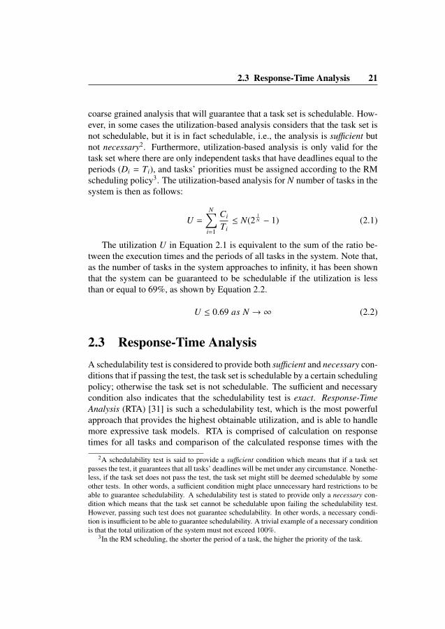
coarse grained analysis that will guarantee that a task set is schedulable. How-ever, in some cases the utilization-based analysis considers that the task set isnot schedulable, but it is in fact schedulable, i.e., the analysis is sufficient butnot necessary2. Furthermore, utilization-based analysis is only valid for thetask set where there are only independent tasks that have deadlines equal to theperiods (Di = Ti), and tasks’ priorities must be assigned according to the RMscheduling policy3. The utilization-based analysis for N number of tasks in thesystem is then as follows:

U =N∑

i=1

Ci

Ti≤ N(2

1N − 1) (2.1)

The utilization U in Equation 2.1 is equivalent to the sum of the ratio be-tween the execution times and the periods of all tasks in the system. Note that,as the number of tasks in the system approaches to infinity, it has been shownthat the system can be guaranteed to be schedulable if the utilization is lessthan or equal to 69%, as shown by Equation 2.2.

U ≤ 0.69 as N → ∞ (2.2)

2.3 Response-Time AnalysisA schedulability test is considered to provide both sufficient and necessary con-ditions that if passing the test, the task set is schedulable by a certain schedulingpolicy; otherwise the task set is not schedulable. The sufficient and necessarycondition also indicates that the schedulability test is exact. Response-TimeAnalysis (RTA) [31] is such a schedulability test, which is the most powerfulapproach that provides the highest obtainable utilization, and is able to handlemore expressive task models. RTA is comprised of calculation on responsetimes for all tasks and comparison of the calculated response times with the

2A schedulability test is said to provide a sufficient condition which means that if a task setpasses the test, it guarantees that all tasks’ deadlines will be met under any circumstance. Nonethe-less, if the task set does not pass the test, the task set might still be deemed schedulable by someother tests. In other words, a sufficient condition might place unnecessary hard restrictions to beable to guarantee schedulability. A schedulability test is stated to provide only a necessary con-dition which means that the task set cannot be schedulable upon failing the schedulability test.However, passing such test does not guarantee schedulability. In other words, a necessary condi-tion is insufficient to be able to guarantee schedulability. A trivial example of a necessary conditionis that the total utilization of the system must not exceed 100%.

3In the RM scheduling, the shorter the period of a task, the higher the priority of the task.


corresponding tasks’ deadlines. Tests that merely provide a sufficient condi-tion are also denoted as approximate tests, since overestimating worst-case re-sponse times will never wrongfully deem a task set as schedulable.

2.3.1 The Basic RTAIn [32], Joseph et al. presented the first basic RTA, where a task τi in the taskmodel is specified by:

• A period, Ti, specifies either the period of a periodic task or the mini-mum inter-arrival time of a sporadic task.

• A worst-case execution time, Ci, specifies the longest time it takes atask to execute the code if it is running on the CPU without any interfer-ences from other tasks.

• A deadline, Di, specifies a constraint on the completion time of the task.The task must finish no later than Di time units after it has been activated.

• A priority, Pi, defines an integer value. As opposed to the RM schedul-ing, priorities can be set arbitrarily.

In addition, the following assumptions must hold for a valid analysis:

• Tasks must be independent, i.e., there can be no synchronization betweentasks.

• Tasks must not suspend themselves.

• Deadlines must be less than or equal to their corresponding task periods,i.e., Di ≤ Ti.

• Tasks must have unique priorities.

The following Equation 2.3 determines the worst case response time Ri oftask τi:

Ri = Ci +∑∀ j∈hp(i)

⌈Ri

T j

⌉×C j (2.3)

where hp(i) is the set of all tasks with priority higher than that of task τi. Theworst-case response time of task τi is the smallest positive value which satisfies

2.4 Worst-Case Execution Time Analysis 23

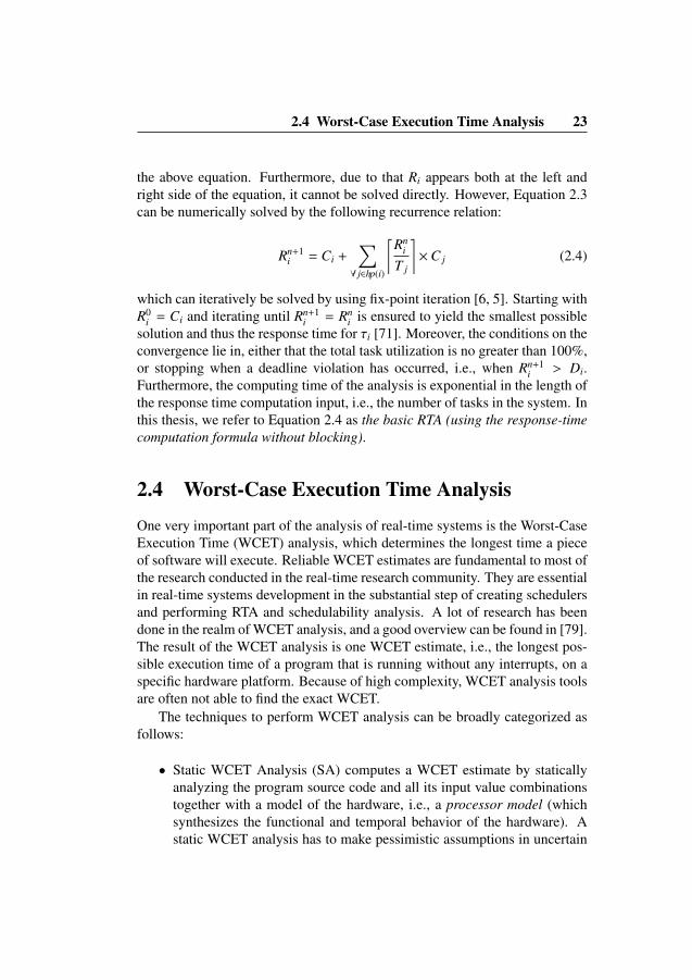
the above equation. Furthermore, due to that Ri appears both at the left andright side of the equation, it cannot be solved directly. However, Equation 2.3can be numerically solved by the following recurrence relation:

Rn+1i = Ci +

∑∀ j∈hp(i)

⌈Rn

i

T j

⌉×C j (2.4)

which can iteratively be solved by using fix-point iteration [6, 5]. Starting withR0

i = Ci and iterating until Rn+1i = Rn

i is ensured to yield the smallest possiblesolution and thus the response time for τi [71]. Moreover, the conditions on theconvergence lie in, either that the total task utilization is no greater than 100%,or stopping when a deadline violation has occurred, i.e., when Rn+1

i > Di.Furthermore, the computing time of the analysis is exponential in the length ofthe response time computation input, i.e., the number of tasks in the system. Inthis thesis, we refer to Equation 2.4 as the basic RTA (using the response-timecomputation formula without blocking).

2.4 Worst-Case Execution Time Analysis

One very important part of the analysis of real-time systems is the Worst-CaseExecution Time (WCET) analysis, which determines the longest time a pieceof software will execute. Reliable WCET estimates are fundamental to most ofthe research conducted in the real-time research community. They are essentialin real-time systems development in the substantial step of creating schedulersand performing RTA and schedulability analysis. A lot of research has beendone in the realm of WCET analysis, and a good overview can be found in [79].The result of the WCET analysis is one WCET estimate, i.e., the longest pos-sible execution time of a program that is running without any interrupts, on aspecific hardware platform. Because of high complexity, WCET analysis toolsare often not able to find the exact WCET.

The techniques to perform WCET analysis can be broadly categorized asfollows:

• Static WCET Analysis (SA) computes a WCET estimate by staticallyanalyzing the program source code and all its input value combinationstogether with a model of the hardware, i.e., a processor model (whichsynthesizes the functional and temporal behavior of the hardware). Astatic WCET analysis has to make pessimistic assumptions in uncertain


cases4, in order to produce a safe upper bound, i.e., a WCET estimatethat is guaranteed to never be smaller than the actual, real WCET, as asafe overestimation.

• Measurement-Based WCET Analysis (MBA) is to perform end-to-endmeasurements of running the target program on the hardware (or simula-tor) for a subset of all input value combinations. The underlying premiseis that the testing regime is representative of real system operation. Fur-ther, with enough testing, the High Water-Mark Time (HWMT) obtainedby measurement-based WCET analysis lies in close proximity to the ac-tual WCET. However, using extensive measurements to ensure enoughtest case coverage or alternatively attempting to enforce the program toexecute its worst case path may be very difficult. Therefore, the selec-tion of test cases to reach the best path coverage (covering the worst casepath) is crucial. Measurement-based WCET analysis may not guaranteeto find the actual WCET in the general case, and may consequently un-derestimate the WCET. To remedy the situation, a safe margin is usuallyto be added to the WCET estimate given by MBA, which for instance isfrom engineering wisdom from previous projects.

• Hybrid Measurement-Based WCET Analysis (HMBA) combines MBAand SA, with the intention of reducing the potential for underestima-tion and overestimation raised by both approaches. To this end, HMBAgleans the execution time of program segments (i.e., instruction blocks)via instrumentation points (ipoints) as the software runs on target. Suchobserved execution times are used in the subsequent stage of WCET cal-culation. However, the key assumption in HMBA is that the WCET ofeach instruction block has been exercised during testing and that mea-surements are sufficient to provide upper loop bounds; otherwise, thesafety of the final estimate is compromised, i.e., it will either underesti-mate or overestimate the actual WCET. There are also some interestingwork in [33, 77, 78] on using Genetic Algorithms (GA) [28] to generatetest vectors to produce a WCET estimate which lies in close proximityto the actual WCET.

• Parametric (or symbolic) WCET analysis expresses the WCET estimateas a formula consisting of parameters of the program, rather than just a

4For example, a loop bound given by flow analysis is larger than the actual value, or low-levelanalysis clarifies a memory access as a cache miss even though it always may result in a cache hit.

2.5 Simulation of Real-Time Embedded Systems 25

Figure 2.1: Relation between execution times and results obtained throughdifferent WCET analysis methods, as shown in [79].

single numerical value. The parameters can be either external, or inter-nal like a symbolic upper bound on a loop. A parametric WCET formulacontains much more information about the program, and it can be usedfor applications like on-line scheduling of tasks where the value of pa-rameters are unknown until runtime, or to find which parts of a codethat has the strongest influence on the WCET. Furthermore, parametricWCET analysis is naturally more complex than classical static WCETanalysis and should not be used on large systems with millions of lines ofcode; rather, the parametric estimation is most efficiently used on smallerprogram parts such as smaller tasks or functions which have input datadependent execution times [17].

Figure 2.1 shows the relationship between the WCET estimates obtainedthrough different WCET analysis methods and the actual WCET, and the Best-Case Execution Time (BCET). The upper and lower timing bounds are safeestimates of WCET and BCET, respectively.

2.5 Simulation of Real-Time Embedded SystemsOur study system (to be introduced in Chapter 3) is described by the modelinglanguage of the RTSSim simulation framework [38], which is quite similar toARTISST [22] and VirtualTime. RTSSim allows for simulating system mod-els containing detailed intricate execution dependencies between tasks (to beintroduced in Section 3.1, Chapter 3), such as asynchronous message-passing,


global shared state variables, and runtime changeability of priority and periodof tasks. In RTSSim, the system consists of a set of tasks, sharing a singleprocessor. RTSSim provides typical RTOS services to the simulation model,such as FPPS, Inter-Process Communication (IPC) via message queues, andsynchronization (semaphores). The tasks in a model are described by using Cfunctions, which are called by the RTSSim framework. The framework pro-vides an isolated “sandbox”, where time is represented in a discrete mannerusing an integer simulation clock, which is only advanced explicitly by thetasks in the simulation model, using a special routine, EXECUTE. Calls to thisroutine models the tasks’ consumption of CPU time.

All time-related operations in RTSSim, such as timeouts and activation oftime-triggered tasks, are driven by the simulation clock, which makes the sim-ulation result independent of process scheduling and performance of the analy-sis PC. The response time and execution time of tasks are measured wheneverthe scheduler is invoked, which happens for example at IPC, task switches,EXECUTE statements, operations on semaphores, task activations and whentasks end. This, together with the simulation clock behavior, guarantees thatthe measured response time and execution time are exact.

In RTSSim, a task may not be released for execution until a certain non-negative time (i.e., the offset) has elapsed after the arrival of the activatingevent. Each task also has a period, a maximum arrival jitter, and a priority.Periods and priorities can be changed at any time by any task in the applica-tion, and offset and jitter can both be larger than the period. Tasks with equalpriorities are served on a first come first served basis. The framework allowsfor three types of selections which are directly controlled by simulator inputdata:

• selection of execution times (for EXECUTE),

• selection of task arrival jitter, and

• selection of task control flow, directly or indirectly based on environ-mental input stimulus.

In addition, the most widely used simulation-based analysis method, i.e.,Monte Carlo simulation, can be realized by providing randomly generated(conforming to a uniform distribution) simulator input data, and gives outputin terms of a set of samples (in terms of timing traces), each of which containsthe measured RT and ET data of each task invocation during simulation.

2.6 Summary 27

2.6 SummaryThis chapter has presented an overview of the basic concepts and terminologyused throughout this thesis for reasoning about embedded real-time systems,timing and schedulability analysis.

Mademoiselle VivianChatterley

I play my basketball since I enjoyed the red passion.

I improvise my dancing since I like the dark blue loneliness.

I design my cuisine since I love the transparent home feeling.

I create my different colorful stories since I am taking a less trav-eled road in a purple wood, comparing others.

Actually, I am just doing many different things like everybody inthis league.

Bonsoir Mademoiselle Vivian Chatterley, may I beg your pardonplease, I just want to date you before my Swedish student visa ex-pires... ;)

Bien a vous,Yue Luis LuMarch, 2012

Chapter 3

The Target Real-TimeEmbedded Systems

In this chapter, we describe the target industrial real-time embedded systemsfeatured by task execution and temporal dependencies, resulting in complicatedtiming behavior of tasks. Specifically, we firstly outline the typically interest-ing task execution and temporal dependencies existing in such systems, whichinvalid the undermining assumptions required by the basic RTA and other tra-ditional timing analysis methods, and then we introduce the relevant represen-tative characteristics of tasks’ timing behavior of response time and executiontime, and the difficulty of using the existing methods to perform timing analysison such systems.

3.1 The Target Industrial Control ApplicationThe system that we study in this work represents a control system for industrialrobotics, developed by our industrial partner. The intended system is quitelarge, containing around three millions of lines of code; while our model is ofmuch smaller scale, but is intentionally designed to include some behavioralmechanisms from the target system, which make it not analyzable by usingexisting timing analysis methods, i.e., the basic RTA and its variations. To bespecific, such behavioral mechanisms include:

• tasks communicate with each other via Inter Process Communication(IPC) through asynchronous message-passing;

31

32 Chapter 3. The Target Real-Time Embedded Systems

• tasks can change the value of global shared state variables which maychange the control flow of other tasks;

• tasks can change scheduling priorities and/or periods dynamically, inresponse to system events.

The system controls a set of electric motors based on periodic sensor read-ings and aperiodic events. The calculations necessary for a real control systemare, however, not included in the model; the model only describes behaviorwith a significant impact on the temporal behavior of the system, such as taskexecution time as well as response time, task interactions and important statechanges. The system contains four periodic application tasks, i.e., the DRIVEtask, the IO task, the CTRL task and the PLAN task. The corresponding taskparameters are shown in Table 3.1, where a lower valued priority is more sig-nificant.

Table 3.1: Task parameters for our study system representing an industrialrobotic control application. The time unit is a simulation time unit (tu).

Task Priority Period Offset Depends onPLAN 5 40 000 0 UICTRL 4 or 2 10 000 or 20 000 0 PLAN, IO, UI, DRIVEIO 3 5 000 500 SensorDRIVE 1 2 000 1 2000 CRTL, UI

The environmental input stimulus in this type of systems is a sequenceof integers from zero to two, denoting the number of external events that aregenerated by a sensor, measured in one period of the IO task. The IO task thensends many messages to the CTRL task. The CTRL task may change priorityand periodicity in response to two specific events in the model. The PLANtask is responsible for planning the movement of the physical object connectedto the motors. The CTRL task calculates control signals for the motors withrespect to coordinates sent from the PLAN task and the IO events providedby the IO task. The DRIVE task actuates the motors based on the CTRL taskoutput, which impacts the execution time of the CTRL task. Moreover, theDRIVE task will change the priority of the CTRL task according to differentconditions.

The study system also describes a user interface (UI) which generates spo-radic events which impacts the system behavior. There are three types of userinterface events: START, STOP and GETSTATUS. The START and STOP

3.2 System Model and Featured Task Execution and TemporalDependencies 33

Figure 3.1: The system architecture of the industrial robotic control applicationwe study in this thesis.

events make the system change between two system modes, IDLE and WORK-ING, with different temporal behaviors. The GETSTATUS event makes thePLAN, CTRL and DRIVE tasks to send a status message to the UI, which in-creases the execution time of those task instances. The task in focus of analysisis the CTRL task, which is with the most complex timing behavior. Further-more, the system architecture is shown in Figure 3.1, and more details aboutour study system and other evaluation models based on it, including their de-tailed pseudo code can be found in [47].

3.2 System Model and Featured Task Executionand Temporal Dependencies

By abstracting information from the description of our study system focusingon timing properties, the system model considered in this thesis is comprised ofa number of periodic tasks. Each periodic task consists of n sub-tasks (wheren ∈ N) and is a tuple τi(Ti, Ji,Oi, Pi,Ci,Di), where Ti is the task period with


maximum jitter Ji, constant offset Oi, a priority Pi, and Ci is the task WCET.Furthermore, the exact knowledge of Ci is not required to be known. In addi-tion, no specific task deadline Di and scheduling approach are assumed. Partic-ularly, the interesting task execution and temporal dependencies which invalidthe undermining assumptions of the basic RTA and its variations are:

• asynchronous message-passing by sending and receiving messages frombuffers, of which one example is shown in lines 1 to 5 in Figure 3.2,where execute statements representing some computation time taken bythe (sub-)task, of which one example is shown in line 4 in Figure 3.2,and such computation time is 198 tu;

• Global Shared State Variables (GSSVs) used in selecting control branchesin tasks, of which one example is shown in lines 7 to 13 in Figure 3.2;

• runtime changeability of task priorities and periods, of which one exam-ple is shown in lines 9 and 13 in Figure 3.2, respectively;

• and constant task offsets, of which one example is shown in Table 3.1 inthe previous section.

In addition, unless program annotation (concerning the number of mes-sages and the specific event triggering tasks to change priority and period) isgiven, the great difficulty of using basic RTA and its variations to analyze suchsystem models mainly matters to obtaining a safe execution time estimate oftasks, which is the inputs of such methods. However, program annotation maybe error-prone and time consuming. To be more specific, considering the fol-lowing example from our study system, where a task first reads all messagesin a message queue and process them, and then the task may change its pri-ority and period depending on different conditions accordingly. For example,the execution time of the code snippet in Figure 3.2 naturally depends on thenumber of received messages: As shown in lines from 1 to 5 in Figure 3.2,apart from the obvious problem of determining the maximum run-time queuelength, other tasks may also preempt the execution of the loop and refill thequeue. When this happens, the number of loop iterations (mattering to the ex-ecution time of the task) is no longer bounded by the maximum queue size.Moreover, the period as well as priority of the task can be changed at runtimedepending on the different conditions pertaining to the value of the GSSV1 asshown in lines from 7 to 13 in the figure. Furthermore, such conditions areoften hard to predict at runtime due to the lack of relevant information.

3.3 Representative Characteristics of Tasks’ Timing Behavior 35

1 msg = recvMessage(MyMessageQueue);

2 while (msg != NO_MESSAGE){

3 process_msg(msg);

4 execute(198);

5 msg = recvMessage(MyMessageQueue);}

6

7 if (GSSV1 == 1){

8 var1 = 10;

9 tcb->period = 20000;}

10 else{

11 var2 = 5;

12 tcb->priority = 4;

13 tcb->period = 10000;}

Figure 3.2: Iteration-loop wrt. message passing, and runtime changeability oftask priorities and periods wrt. global shared state variables.

3.3 Representative Characteristics of Tasks’ Tim-ing Behavior

In this section, we introduce some interesting characteristics of system timingbehavior, by presenting descriptive statistics of response time and executiontime samples of the tasks on focus, taken from our examined industrial controlapplication.

Due to the existence of intricate task execution and temporal dependenciesin systems, an upcoming task Response Time (RT) datum may not be inde-pendent with the RT datum previously recorded in the achieved sample takenfrom the same simulation run. The same problem happens for the task Execu-tion Time (ET) data. More interestingly, outliers existing in such samples ofthe RT and ET data of tasks under analysis cannot be removed, since they arenot caused by system errors or hardware failures. The definition of such out-liers referred in this thesis is introduced as follows: A RT or ET datum beyondan outer fence [62] is considered as (extreme) outlier. Specifically, Table 3.2shows the numerical summary of the center and the spread (or variability) ofthe samples of the RT and ET data of the CTRL task (which has the most com-plicated temporal behavior among all tasks hence is the task under analysis)in the study system, where X, Y, Std. Dev, Q1 and Q3 represents response


Table 3.2: Descriptive statistics of the samples of the RT and ET data of theCTRL task in the study system achieved by the same execution, for a longenough simulation time.

Samples Std. Dev Min Q1 Median Q3 Max LIF UIF LOF UOFXCTRL 199 990 389.98 1 024 1 594 1 919 2 339 6 829 476.5 3 456.5 -641 4 574YCTRL 199 990 276.86 1 024 1 274 1 574 1 724 5 324 599 2 399 -76 3 074

time, execution time, standard deviation, first quartile and third quartile ofthe samples respectively. The presence of strong outliers leads us to considerusing the five-number summary introduced in [57] consisting of Min, Q1, Me-dian, Q3 and Max in Table 3.2. Concerning outliers, by using the definitionsgiven in [62], inner fences and outer fences for the samples of the RT and ETdata of the CTRL task are also shown in Table 3.2, where LIF, UIF, LOF andUOF represent lower inner fence (i.e., Q1 − 1.5 × IQ), upper inner fence (i.e.,Q3 + 1.5 × IQ), lower outer fence (i.e., Q1 − 3 × IQ) and upper outer fence(i.e., Q3 + 3 × IQ) respectively. Note that IQ = Q3 − Q1.

Furthermore, the Probability Density Function (PDF) histograms of thesamples of the RT and ET data of the CTRL task, given a large1 number atsample data, are shown in Figure 3.3 respectively. Note that the outliers inthe picture are not clearly visible, though in fact, they exist in the range of[4 574, 6 829] (for the RT sample) and [3 074, 5 324] (for the ET sample).

In the conventional statistical procedure (parametric test), e.g., t-test, z-test and analysis of variance (ANOVA)2, one important assumption is that theunderlying population is assumed to follow a normal distribution. However,such an assumption cannot be made in our case, since the samples of either theRT data or the ET data of tasks under analysis is often clearly conforming toa multi-modal distribution having several peaks (consider Figure 3.3 as exam-ples). Specifically, because of such distinctive feature of our study system, it isdifficult to bring conventional statistical methods into the context.

1As an example, by running one simulation for the time up to the upper bound of the RTSSimsimulation time, i.e., 231 − 1, we have collected 199 990 samples elements in the sample of the RTand ET data of the CTRL task which is the most complicated task under analysis.

2mathworld.wolfram.com/ANOVA.html, 2012.

3.4 Summary 37

3.4 SummaryThis chapter has introduced our study system (inspired by an industrial roboticcontrol application) and its relevant system model featured by the adhering taskexecution and temporal dependencies. Additionally, we have also highlightedsome interesting representative descriptive statistics of tasks’ response timeand execution time, and the difficulty of performing response-time analysis ofsuch systems, by using conventional timing analysis methods, i.e., the basicRTA and its variations, as well as parametric statistics assuming the normalityof the analysis samples.

Figure 3.3: The Probability Density Function (PDF) histograms of the samplesof the RT data (on the upper part) and ET data (on the lower part) of the CTRLtask (the task under analysis) in our study system model.

Further North

When you said to me, “Honey, our visas are going to expire soon...”,I knew that it is the right time for us to go further north, since thereis a direct flight heading to New York from Winterfell. More im-portantly, we are not creeps, though I know we are from neitherany EU/EEA country nor Switzerland, and we just made a “miser-able” choice. However, there are no worries, my lady, and we aregonna make a change.

Yue Luis LuFebruary, 2012

Chapter 4

SimulationOptimization-Based TimingAnalysis

This chapter introduces our work on simulation-based analysis. In particular,we present two simple yet novel search algorithms of meta-heuristic type thatare used to guide a Monte Carlo simulation. Moreover, the framework is evalu-ated by using industrial relevant models based upon two different control appli-cations, i.e., our study system (introduced in Chapter 3) and the other industrialreal-time control application, showing that our analysis can yield substantiallybetter results, comparing the traditional simulation methods.

4.1 Introduction

When it comes to Response-Time Analysis (RTA) of real-time embedded sys-tems containing intricate task execution and temporal dependencies, it is dif-ficult to make practical use of the traditional analysis techniques such as thebasic RTA [31] and its variations, as such systems invalidate the assumptionsrequired by the analysis methods to be valid. Typically, the disregarded as-sumptions include the facts that tasks can communicate with each other throughasynchronous message-passing, data-dependent task execution times using glo-bal shared state variables, runtime changeability of priorities and periods of

41

42 Chapter 4. Simulation Optimization-Based Timing Analysis

tasks, etc.One solution to the problem outlined above is to use a more detailed sys-

tem model of such systems. Ideally, the models should describe the task exe-cution control flow with respect to resource usage and interaction, e.g., inter-process communication, CPU time and logical resources. Analyzing such de-tailed models by using techniques which are capable of handling such detailedruntime behavior, such as model checking [76] can result in a state-space ex-plosion, which often makes exhaustive analysis infeasible.

Another approach to analyze such a detailed system model, which avoidsthe problems associated with state-space explosion, is to adopt sampling ofthe state space by using simulation-based methods. The downside is a loweraccuracy and confidence of the results; the approach is closer to testing focus-ing on timing properties of the systems, than formal analysis. Some efficientsimulation analysis may however be sufficient in many cases, and it is a farmore efficient method for finding potential timing problems than system-leveltesting, which is the dominating method in industry today.

In this chapter, we present our developed simulation optimization-basedtiming analysis of real-time embedded systems. The analysis uses two simpleyet novel methods, i.e., MABERA ([40]) (based upon genetic algorithms) andhill-climbing algorithm ([66]). Moreover, MABERA considers the system un-der analysis as a blackbox (i.e., no knowledge of the detailed representation ofthe system input is assumed), while HCRR works on a detailed representationof the system-dependent simulation parameters. In addition, we give a thor-ough experimental evaluation of performance, scaling and convergence of theanalysis framework, comparing the results to those obtained from Monte Carlosimulation. Specifically, the evaluation results show that the new analysis issignificantly better than existing approaches in identifying extreme responsetimes using less number of simulations. This is important, since the numberof simulations required directly affects evaluation time, and consequently thepractical feasibility of the approach.

4.2 Related Work on Simulation-Based Analysis

RTA is certainly not something new, and besides the standard approaches suchas the basic RTA [31], formal analysis tools like UPPAAL (presented by [76])can also be used for exhaustive analysis of software systems. However, formodels of industrial systems, without carefully choosing the level of abstrac-tion, the state space of the UPPAAL models can grow too large for them to be

4.3 Our Proposed Simulation-Based Response-Time Analysis 43

practically useful.In regard to simulation-based analysis methods, there are several frame-

works already existing for timing simulation of real-time system models, e.g.,Rapita systems Ltd. developed the commercial tool VirtualTime and Decotignypresented the academic tool ARTISST [23]. Particularly, these solutions rely onMonte Carlo Simulation (MCS), which can be described as keeping the highestresults from a set of randomized simulations. Therefore, MCS is suitable foraverage-case analysis, and can be inefficient in identifying extreme scenariosrelevant to high task response times.

The use of evolutionary algorithms for different types of test case genera-tion has also been studied for quite some time. Alander [1] presents the workabout using Genetic Algorithms (GA) to generate test cases for a software re-lay system used in electrical networks. The purpose of the GA is to provokehigh response times for the software, which is executed in a simulation envi-ronment. Authors of [61] describe various extensions of the traditional GA tobetter suit the type of problems in the real-time domain. More recently, [59]gives a comprehensive comparison of static analysis techniques and evolution-ary algorithms, with regard to schedulability, for several real-time applications.

Samii [67] aim to find extreme response times for distributed systems byoptimizing a set of simulation parameters for models containing temporal at-tributes and communication. They use a type of GA to explore combinations oftask execution times in order to maximize end-to-end response time. Flow ofcontrol within tasks is not considered. Their results depend on the method de-veloped by authors of [64] for identifying situations where decreased executiontimes can lead to increased response times. The stochastic analysis frameworkintroduced by [34] also has a similar basis of temporal task attributes.

4.3 Our Proposed Simulation-Based Response-TimeAnalysis

In the rest of this chapter, we will focus on analyzing the response time of atask by varying the simulation instances used as input for the simulator, eitherfrom a black-box view (adopted by MABERA) using seed schedules, or froma white-box view using a detailed representation of the system input (used byHCRR). Additionally, the analysis of an entire system can be done by perform-ing our analysis several times, once for each task in the system.

We present two methods for simulation optimization which aim at effi-ciently finding extreme scenarios of our study system or other similar ones


with respect to a specific measurable tasks’ response time, by using a combi-nation of a discrete event simulation and meta-heuristic search methods. Thetwo methods, MABERA and its improved version HCRR, both use a simulatoras a deterministic function which returns a value for the runtime property infocus, e.g., the highest recorded response time of tasks, according to a set ofgiven parameters defining the scenarios to explore. Both approaches use thesimulation results in an iterative analysis where the simulation parameters aregradually refined in order to provoke as extreme results as possible. More-over, we performed an evaluation where the two approaches to simulation op-timization are compared with the MCS with respect to computing time and thediscovered response times. The corresponding evaluation results indicate thatboth MABERA and HCRR are significantly more efficient in finding extremeresponse times for a particular task than Monte Carlo simulation. More impor-tantly, HCRR, which uses a variant of the hill climbing approach [66], is vastlymore efficient than MABERA, which uses a kind of GA.

4.4 Our Solution One – MABERAMABERA (Meta-heuristic Approach for Best Effort Response-time Analysis)is using GA, which is the most well-known type of meta-heuristics1, to findhigh task response times pertaining to some extreme cases. The MABERAalgorithm is designed to use an RTSSim simulator executable as a black-boxfunction, which given a set of simulation parameters outputs the highest respon-se-time found during the specified simulation. The objective of the MABERAalgorithm is to find the set of parameters which gives the highest response timeof the task on focus. This is performed by iteratively creating and evaluating aset of independent candidates, a generation, where each candidate is a simula-tion. The specification of a simulation, i.e., the set of parameters to RTSSim,namely a parameter set. The evaluation of a parameter set corresponds torunning an RTSSim simulation, where each simulation produces a simulationresult.

The MABERA algorithm uses an indirect representation of the simulationsto perform, using seed schedules. A seed schedule specifies the seed valuesto use for generation of pseudo-random numbers and thereby the outcomes ofall non-deterministic selections during the simulation. Thus, the combinationof a seed schedule and time instant corresponds to an exact specification of a

1Meta-heuristics are generic solution methods for iterative approximation of search or opti-mization problems.

4.4 Our Solution One – MABERA 45

simulation state. Given a seed schedule and a simulation length, an RTSSimsimulation is thereby a deterministic function. The entire process of MABERAstarts with the first generation of simulations by running Monte Carlo simula-tions. Then, from each generation, a set of promising simulations are selectedas parent simulations and used to create the next generation, where each childsimulation is created by mutation of a single parent. The algorithm iterates inthis manner until a termination condition is reached. The termination thresh-old parameter, tt, decides how many “unsuccessful” generations that are al-lowed before termination, i.e., generations that failed to discover a responsetime higher than the highest response time of the previous generations.

Typically, MABERA can be defined as a function, according to Defini-tion 1, and its detailed presentation in pseudo-code is given by Algorithm 1.Furthermore, the definitions and pseudo-code of the functions used by the al-gorithm are given in the following sections.

Definition 1. r = MABERA(M, T, s, p, tt, l), where r is the highest observedresponse time of the task T in the simulation model M. Parameter s is thepopulation size, p is the number of parents, tt is the termination threshold andl is the simulation length.

Definition 2. A seed schedule is a list of pairs 〈t, s〉, where t and s are integervalues. The t value specifies the point in simulation time when to apply seed s.

Definition 3. A simulation result is a tuple 〈rt, trt, et, tet, pc, tpc, S 〉. The ele-ments rt, et and pc are integer values corresponding to the highest responsetime, execution time and preemption count, respectively, of the task in focus.The elements trt, tet and tpc are integer values specifying the start times of thetask instances corresponding to rt, et and pc. S is the seed schedule used toproduce this simulation result.

Algorithm 1: MABERA(M, T, s, p, tt, l)

Parameters:M: the simulation modelT: the task in focuss: integer value – the population sizep: integer value – number of parents to selecttt: integer value – the termination thresholdl: integer value – the simulation length


Returns:The highest discovered response time of the task T .

Algorithm 1 MABERA(M, T, s, p, tt, l)1: tc← tt2: r ← 03: i← 04: I ← ��5: while i < s do6: Ii ← �0, 0�7: i← i + 18: end while9: while tc > 0 do

10: R← S IM(M, T, I, l)11: if MAX RT (R) > r then12: r ← MAX RT (R)13: tc← tt14: else15: tc← tc − 116: end if17: I ← GEN(S EL(R, p), s)18: end while19: return r

4.4.1 Function SIM

The function SIM represents our RTSSim simulator (introduced in Section 2.5,Chapter 2) that runs a set of simulations of a particular simulation model, asspecified by a list of seed schedules. The result is a list of simulation results,where the i:th simulation result corresponds to the i:th seed schedule.

In RTSSim, a global simulation clock, i.e., an integer variable, is sharedby all tasks. The model may contain probabilistic selection of execution time,inter-arrival time or functional behavior. Such selections are the only source fornon-determinism in the simulation of a model and are decided from pseudo-random numbers, which in turn are decided by the seed schedule. Since thesimulation is deterministic given a specific seed schedule, it is possible torestart a simulation from a specific state, expressed as a seed schedule anda restart time.


To allow for Monte Carlo simulation, the random number generator is re-initialized using a seed that is “randomly” selected, by calculating an integervalue from a high-resolution hardware clock with microsecond resolution. Inour implementation, this is performed when 0 is specified as seed, which isthe case for the last seed change event for each simulation. The selected seedreplaces the 0 in the seed schedule of the simulation result.

4.4.2 Function SEL

The SEL function implements the heuristic selection of parent simulations usedto produce the next generation of simulations. The selection ranks all simula-tion results in the current generation with respect to the three properties rt, etand pc, i.e., the highest response time, execution time and preemption count,respectively, of the task in focus.

The execution time and preemption count properties are included in theselection heuristics due to their potential for making impact on response time,e.g., a task instance with very high execution time but relatively low response-time is also interesting since a different preemption pattern may result in ahigher response time.

The three rank values of each simulation result are multiplied in order toobtain a composite fitness score for the simulation result. The best fitness scoreis 1, which corresponds to a simulation result that holds the record for all threeproperties. The returned set of simulation results contains a specified numberof simulation results with some best (lowest) fitness scores.

The method of combining the three rank values into a total fitness score isnot claimed to be optimal. It gives equal importance to the three indicators,response time, execution time and preemption count. It might be possible toimprove the selection heuristics by adjusting the relative importance of someof these three indicators. Moreover, the ranking hides the absolute differencesin property values between candidates with adjacent ranking. Investigation ofother selection heuristics is part of future work.

Definitions for Function SEL

The pseudo-code defining the SEL function relies on the following definitions:

Definition 4. The ranking of an element in a list of simulation results is thenumber of unique values for the specific property that are equal or larger tothe specified element. The ranking of the simulation result with the highest


property value is 1. Simulation results with equal property values receive thesame ranking.

Definition 5. v = RANK RT (R, i), where v is the ranking of the i:th simulationresult in R, with respect to the response time property of R.

Definition 6. v = RANK ET (R, i), where v is the ranking of the i:th simulationresult in R, with respect to the execution time property of R.

Definition 7. v = RANK PC(R, i), where v is the ranking of the i:th simulationresult in R, with respect to the preemption count property of R.

Definition 8. P = LOW N(R, F, n), where P is a list of n simulation results, asubset of R. The simulation results included in P are the ones with the lowest(i.e., best) corresponding value i the list F. The i:th element in F is the fitnessscore of the i:th simulation result in R.

Pseudo-Code for Function SEL

Parameters:R: a list of simulation resultsp: an integer value – the number of parents to select

Returns:A list of simulation results – the selected parents

Algorithm 2: SEL(R, p)

Algorithm 2 S EL(R, p)1: F ← ��2: i← 03: while i < |R| do4: Fi ← RANK RT (R, i) × RANK ET (R, i) × RANK PC(R, i)5: i← i + 16: end while7: return LOW N(R, F, p)


4.4.3 Function GEN

The GEN function generates a set of child simulations (seed schedules) corre-sponding to a new generation, through mutation of a set of parent simulations(simulation results).

Each resulting seed schedule is based on a single parent simulation, but hasbeen extended with one additional seed change event, at the restart time of theparent. When this seed change event occurs, the simulation leaves the path ofthe parent simulation and follows a randomly selected path. This correspondsto the mutation. The time of this seed change event, the restart time, is in thenormal case randomly selected in a time interval, where the lower bound is therestart time of the parent and the upper bound is the SETI time of the parent.The SETI time is the Start time of the earliest Extreme Task Instance, whereextreme refers to the task instances having the highest value of at least one ofthe following properties: response time, execution time and preemption count.

Definitions for Function GEN

The pseudo-code defining the GEN function relies on the following definitions:

Definition 9. t = RS T (R), where t is the restart time of R, a simulation result,i.e., the t value of the last �s, t� pair in the seed schedule of R.

Definition 10. t = S ET I(R), where t is the S ET I of the simulation result R,i.e., the minimum of the property values trt, tet and tpc of R.

Definition 11. S = S S (R), where S is the seed schedule of the simulationresult R.

Definition 12. r = RAND(a, b), where r is an integer value in the range a ≤r < b, randomly selected according to a uniform probability distribution.

Pseudo-Code for Function GEN

Parameters:P: a list of simulation resultss: an integer value – the population size


Returns:A list of seed schedules – the next generation

Algorithm 3: GEN(P, s)

Algorithm 3 GEN(P, s)1: N ← ��2: i← 03: while i < |P| do4: j← 0

5: while⌊

s|P|⌋

do

6: if S ET I(Pi) < RS T (Pi) then7: t ← RS T (Pi)8: else9: t ← RAND(RS T (Pi), S ET I(Pi))

10: end if11: Ni ← APPEND(S S (Pi), �0, t�)12: i← i + 113: end while14: end while15: return N

It is interesting to point out that MABERA uses no “recombination” or“crossover” operations, which otherwise is common in the GA. This is becausethe meaning of the seeds used during a simulation is not independent, but de-pends on the simulation state when the value is used. They can therefore not beused as independent “chromosomes”, which can be recombined with preservedsemantics. Moreover, MABERA was never intended to be the optimal solution,but was a result of the first investigation of this approach, aiming at assessingthe potential of simulation optimization methods for efficient response-timeanalysis. MABERA was however good enough to motivate a continued effort,which resulted in the significantly more efficient HCRR method, described inthe next section. For more details about MABERA, interested readers can referto the work presented by [40].

4.5 Our Solution Two – Hill Climbing with Random Restart (HCRR)51

4.5 Our Solution Two – Hill Climbing with Ran-dom Restart (HCRR)

In order to address shortcomings of the MABERA approach, we developedHCRR, an improved version of MABERA. Our initial idea was to use a rep-resentation of the input parameters to RTSSim, which more directly corre-sponded to simulation parameters, in a full version of GA using both crossoverand mutation operators. However, initial experiments with the crossover oper-ator, which is the operator most often associated with GA, proved unsuccess-ful and did not show any significant improvement over MABERA. Instead offocusing on the crossover operator, we chose to investigate iterative improve-ment of a single individual as an alternative. It turned out that hill-climbing,augmented with random restarts whenever a local minimum was detected, gavemuch better performance than MABERA.

4.5.1 Explicit Representation of System InputA simulation instance is a set of parameters that exactly determine the outcomeof a simulation. To be specific, a simulation instance is represented using aset of sequences of integers, where each sequence is associated with either anarrival jitter of a task, or an execution time of jobs, or an environmental inputstimulus2. Each value then directly decides a selection of either jitter, executiontime, or state in the task control flow. The advantage of this approach is thatthe direct relationship between representation and model properties makes itpossible to locally refine specific aspects of a given simulation instance. Thisdirect control can be used for guiding the search toward instances with extremeresponse times, as shown in Section 4.5.2.

Let Ji be a sequence of actual jitter values jir experienced by instance rof a task τi. We restrict jir to integer values in the interval [0, ub(Ji)], whereub(Ji) is an upper bound on jitter for task i in units of the smallest measurabletime interval (i.e., clock ticks) for the target system. Furthermore, let Xk be asequence of values for a certain environmental input stimulus or execution timein the simulated program, and X j

k be the jth such input value. We assume that allstimulus and execution times X j

k are of integer type and have upper and lowerbounds, so that lb(Xk) ≤ X j

k ≤ ub(Xk) for all k, j. Execution times are used

2Such environmental input stimulus is represented as various number of events generated byenvironmental task in Model 1 and Validation Model, and various execution time of SoftwareCircuits (SWCs) in Model 2 in Section 4.6.


only for deciding CPU time consumption of execute primitives. Bounds onexecution times can be analyzed using static WCET analysis [79] or estimatedthrough measurements.

A simulation instance S , defining a fully deterministic simulation of themodel, is therefore a set

{J1, J2, ..., Jn, X1, X2, ..., Xm} (4.1)

where n is the number of tasks which have non-zero jitter and m is the num-ber of environmental stimulus and execute statements. Denote by Ni and Mk

the number of values that are used to represent jitter sequence Ji and input se-quence Xk. Ni and Mk can be determined empirically by tracing how manyvalues the simulator uses for each value. In theory, Ni and Mk can be un-bounded, and for some long simulations, Ni and Mk may grow to unacceptablelevels. In such cases, we suggest to set Ni and Mk to be at a fixed acceptablelevel. If there are not enough input values in the sequence, the simulator shouldreport a warning, and start reuse values from the start of the sequence. For theevaluated models in this work, Ni and Mk were long enough to represent allvalues used.

4.5.2 The Algorithm DescriptionThe goal of HCRR is the same as for MABERA, to find as high response timefor a specific task as possible by optimizing the simulator input. The optimiza-tion algorithm of HCRR is based on hill climbing using random-restarts [66].Hill-climbing has the advantage of being one of the simplest meta-heuristicavailable, and is based upon the idea of starting at a random point, and then re-peatedly taking small steps pointing upward (wrt. the objective function, whichin this work is the measured task response time) whenever such search direc-tions exist. If no such steps exist, a local maximum has been reached. Randomrestarts are used to avoid getting stuck in local maxima. Several techniquesfor escaping local minima exist (for example Tabu Search [27] and simulatedannealing [35]), but a set of limited experiments conducted did not show anysignificant performance advantage over hill-climbing with random restarts.

Advantages of HCRR come from the combination of a strictly local im-provement part, which quickly converges to high response times, with diversi-fication mechanisms (jump-back to equal candidates, and full restarts) that areimportant to avoid local maxima. In contrast to MABERA, HCRR does notemploy such a mechanism, and consequently can get stuck in local maxima. Inaddition, the local improvement functionality of MABERA is inefficient due to

4.5 Our Solution Two – Hill Climbing with Random Restart (HCRR)53

a representation of simulation instances as random number sequences. MonteCarlo search, on the other hand, has no means to local improvement, and there-fore exhibits unsatisfactory convergence.

Algorithm 4 HCRR(no f sims,m, k, nB, nR)1: curr ← MONT ECARLO(m, rnd inst())2: best ← curr, no f sims← no f sims − m3: E← {curr}, nonimp← 04: while no f sims > 0 do5: if nonimp > nR then6: curr ← rnd inst(),E← {curr}, nonimp← 07: else8: if (nonimp + 1) mod nB = nB then9: curr ← random element in E

10: end if11: end if12: next ← NBH(curr, �k × len(curr)�)13: S IMULAT E(next), no f sims← no f sims − 114: if R(next) > R(best) then15: best ← next16: end if17: if R(next) > R(curr) then18: curr ← next,E← {next}, nonimp← 019: else20: nonimp← nonimp + 121: if R(next) = R(curr) then22: E← E ∪ {next}23: end if24: end if25: end while26: return best

In brief, HCRR works by iteratively changing a small portion of the modelparameter set, i.e., system explicit input representation, and restarts after a fixednumber of non-improving simulations have been run. Specifically, the imple-mentation of HCRR is given in Algorithm 4. The simulation budget is denotedno f sims, and RT (q) denotes the end time of the task under analysis in the sim-ulation instance q when the task WCRT occurred. The consumption time pointof a simulation input X j

i of any type (jitter, execution time, or environmentalinput) is expressed as T M j

i . q[X ji ] is the current value of X j

i in the simulationinstance q. The function rnd(l, u) returns a random number between l and u if


l < u; otherwise, it returns l. A completely random simulation instance canalso be generated using the call rnd inst().

The HCRR algorithm begins by choosing as starting point the best simu-lation instance from m randomly selected candidates using the MonteCarlomethod. Then, in each iteration, k · len(curr) random values of the current sim-ulation instance curr (which has len(curr) input values) used before TR(curr)are selected and modified using the neighborhood procedure NBH, as shownin Algorithm 5.

Algorithm 5 NBH(inst, n)1: for k = 1→ n do2: X j

i = random element in inst, T M ji < ET (inst)

3: V = {lb(Xi)...ub(Xi)} ÷ {inst[X ji ]}

4: inst[X ji ]← random value in V

5: end for

The response time of the task under analysis is measured by running RTSS-im using the SIMULATE(next) call on a neighbor next. Modifications sug-gested by Nbh that increase response time are accepted, and changes that de-crease response time are rejected. Modifications that have equal response timeare rejected but saved for future reference, as described below.

A pure hill-climbing procedure is susceptible to getting stuck in local max-ima, and can therefore exhibit less than satisfactory performance on manyproblems. In order to avoid convergence to locally maximal areas and to im-prove the probability of finding a true global maximum, two different diversi-fication mechanisms were adopted. First of all, the algorithm jumps back to apreviously encountered, randomly selected simulation instance with an equalresponse time to the current instance after nB non-improving simulations. Thisdistributes focus over a number of equal instances, which can help in avoidingsmall local maxima. The second mechanism performs a full restart of HCRRfrom a random point after nR non-improving simulations. We call nB the jump-back threshold and nR the random-restart threshold.

4.6 Case StudiesThis section describes two industrial cases (including our study system intro-duced in Chapter 3) and one validation case in the form of RTSSim simulationmodels, used for the evaluation. Furthermore, the models have similar archi-

4.6 Case Studies 55

tecture and analysis problems as two industrial real-time applications in use atABB and Arcticus Systems3.

To be specific, Model 1 (M1) represents our study system, i.e., a controlsystem for industrial robots developed by ABB Robotics, which is not possi-ble to analyze using the traditional RTA methods [31]. Model 2 (M2) is con-structed from a test application used by Arcticus Systems, which develops theRubus RTOS used in many vehicular systems. We also use a simplified ver-sion of Model 1 for validation (MV), where the invalid assumptions of RTA inthe system has been removed. The sole purpose of this model is to investigatehow close the response times found by MABERA and HCRR are to the trueWCRTs derived by the exact RTA.

The scheduling policy is FPPS for all models. Model 2 and the validationmodel both use fixed priorities. Model 1 contains one task that changes prioritydynamically.

Model 1: This model is of much smaller scale, comparing the real system,but is designed to include some behavioral mechanisms from the ABB systemwhich the basic RTA and its variations can not take into account:

• tasks with intricate dependencies in temporal behavior due to IPC andglobal shared state variables;

• the use of buffered message queues for IPC, where triggering messagesmay be delayed;

• tasks that change scheduling priority or periods dynamically, in responseto system events.

More detail of the model can be found in Section 3.1, Chapter 3.

Model 2: This model is based on a test application from Arcticus systems,developers of the Rubus RTOS which is used in heavy vehicles. This modeluses a pipe-and-filter architecture, where tasks trigger other tasks through trig-ger ports, forming transactions. The model contains three periodic transactionsand one interrupt-driven task, in total 11 tasks. Except that the interrupt taskhas a small jitter, the other transactions are strictly periodic.

Model 2 is less complex than Model 1 in the sense that there exist no sharedvariables or IPC via message passing which can impact the tasks’ timing and

3www.arcticus-systems.se, 2012.


Figure 4.1: The architecture of Model 2, a test application used in heavy vehi-cles.

functional behavior. Instead, the tasks have large variations in execution times,which makes the state space of this model very large. Furthermore, the evalua-tion focuses on the end-to-end response time of the transaction containing thetasks with the lowest priority. Figure 4.1 shows the architecture of Model 2,and more detail of the model can be found in [13].

Validation Model: Simulation-based methods for RTA have in common thatthe result is not guaranteed to be an exact task response time. We thereforeconstructed a validation model, analyzable using RTA, with the purpose to in-vestigate how close the response times given by HCRR are to the exact WCRTsderived by using RTA. The validation model is based on Model 1 (our studysystem), but simplified in that 1) global shared state variables have been re-moved, 2) task priority and period cannot be changed at runtime hence arestrictly static, and 3) loop bounds have been added manually. As a conse-quence, the validation model has considerably lower complexity, and exhibitsquite different timing properties compared with Model 1.

4.7 Evaluation Results 57

4.7 Evaluation ResultsThe obtained WCRT estimates given by different simulation-based methodsare illustrated by the following labels, which are in Figures 4.2 to 4.5:

• MC: The traditional Monte Carlo approach to generate simulation in-stances using random input data.

• MAB: The MABERA approach, using a population size of 1 250 ofwhich 12 parents are selected for reproduction, unless stated otherwise.The algorithm is modified to run for a limited number of simulations.

• HCRR: The new algorithm based on hill climbing with random restart,as shown in Algorithm 4.

0.2 0.4

MC

0.2 0.4

Rel

ativ

e fr

eque

ncy

MA

B 0.4 0.8

7200 7400 7600 7800 8000 8200 8400 8600H

CR

R

Response time

7400 7600 7800 8000 8200 8400 8600

0 2000 4000 6000 8000 10000Mea

n re

spon

se ti

me

Simulations

MC MAB HCRR

Figure 4.2: Final RT distributions and convergence (mean RT and 95% confi-dence intervals) for Model 1.


Figure 4.2 shows the results obtained for Model 1. The top of the figurecontains the response time distributions of the three algorithms. Results wereobtained by using 200 sample runs for MABERA, 200 runs for MC, and 100runs for HCRR, respectively. For MABERA and MC, each sample requiredon average 81 400 simulations. Each HCRR sample was allowed 10 000 sim-ulations. The bottom of Figure 4.2 shows convergence (mean RT and 95%confidence intervals), using the standard parameters of 10 000 simulations, forthe three algorithms with 100 samples for each algorithm.

The upper part of Figure 4.2 shows that HCRR managed to find the high-est known response time, 8 474, in all 100 sample runs. The highest responsetime found by MABERA was 8 349, and this value was only achieved by onesingle run. The MC approach managed to find a maximum response time of8 390, which is also obtained only once. Note that HCRR was only allowed ap-proximately 12% of the number of simulations used by MC and MABERA. Ifwe compare the number of simulations done when the highest known responsetime was found, HCRR was approximately 1 628 times faster than MABERAand MC. The runtimes for one sample of all algorithms were less than 3 min-utes.

Figure 4.3 shows the obtained results for Model 2 using the standard pa-rameters. In this model, the tasks have large variations in execution times,which makes the state space very large. We can see that HCRR yields a resultapproximately 5% higher than what are obtained from the two other methods.Interestingly, it looks like HCRR was still slowly progressing toward higherresponse times at 10 000 simulations, while both MABERA and MC seems tohave converged quite early to a much lower result. For Model 2, all algorithmsfinished in less than one minute per sample.

In Figure 4.4, we can see the results for the validation model, based onusing the standard parameters. In addition, we show the RTA results. Here,HCRR could find a response time of 4 432 in every sample run, which was alsoconfirmed by the RTA to be the WCRT. For the validation model, MC tookless than 50 seconds, MABERA less than 130 seconds, and HCRR less than90 seconds for one sample run.

Figure 4.5 shows how the different methods scale to larger systems, by il-lustrating the convergence for Model 1 when increasing the model size to 2,3 and 4 subsystems (model instances). As we expected, since the state spaceincreases with the number of subsystems, all three algorithms converge slowerwhen system size is increased. For two subsystems, HCRR is consistentlybetter than both MC and MABERA, with all results reported being higherthan the maximum result found for both MC and MABERA. The results for


0.1 0.2

MC

0.1 0.2

Rel

ativ

e Fr

eque

ncy

MA

B

0.1 0.2

5800 5900 6000 6100 6200 6300 6400

HC

RR

Response time

5900 6000 6100 6200 6300 6400

0 2000 4000 6000 8000 10000Mea

n re

spon

se ti

me

Simulations

MC MAB HCRR

Figure 4.3: Final RT distributions and convergence (mean RT and 95% confi-dence intervals) for Model 2.

3 and 4 subsystems indicate that the difference between the methods decreaseas system size is increased, although HCRR produced on average 4.7 to 11%higher results than both MC and MABERA. For 4 subsystems, none of themethods appears to have converged. However, during the 10 000 simulations,HCRR progressed more quickly to higher response times than both MC andMABERA. Runtimes for a single sample when having 2 subsystems were be-low 4, 7 and 5 minutes for MC, MABERA and HCRR, respectively. Sampleruntimes were below 5, 10 and 6 minutes for 3 subsystems and below 8, 16 and10 minutes for 4 subsystems.

The average end results are summarized in Table 4.1. The last column alsoshows the average number of simulations needed by HCRR to obtain the endresult of the second best method (using 10 000 simulations). As we can see,HCRR reached the second-best result 13 to 112 times faster than the second-


0.2 0.4

MC

0.2 0.4

Rel

ativ

e Fr

eque

ncy

MA

B

0.3 0.6 0.9

4000 4100 4200 4300 4400 4500

HC

RR

Response timeRTA

4000 4100 4200 4300 4400 4500

0 2000 4000 6000 8000 10000Mea

n re

spon

se ti

me

Simulations

MC MAB HCRR RTA

Figure 4.4: Final RT distributions and convergence (mean RT and 95% confi-dence intervals) for the validation model.

best method MABERA did. For all evaluation models, HCRR on average out-performed the other methods in less than 800 simulations, which correspondsto less than 1.5 minutes of computing time on the PC used for the experiments.

4.7.1 Average Convergence

To measure average convergence more exactly, we use the relative differencein average response time results over a time span of d simulations. Specifi-cally, a method has for practical purposes converged (on average) when 1 −R

(k−d)/R

(k) ≤ ε, where R(k)

is the average response time result at the simula-tion k for a set of samples. Additionally, after at least d simulations have beenperformed, convergence will be detected. For our case for the evaluation pre-sented in this work, d obviously needs to be less than the number of simulations


Table 4.1: Average end result and point when HCRR passes the second bestend result.

Model MC MABERA HCRR Passes 2nd bestM1-1 7 682 8 065 8 474 224M1-2 9 693 9 750 10 844 238M1-3 13 555 13 789 14 672 521M1-4 15 235 15 298 16 013 764M2 6 031 6 002 6 299 634MV 4 286 4 288 4 432 89

(10 000) performed in each sample, while using a too low value for d will indi-cate premature convergence. We therefore use d = 1 000 for the convergencecomparison. For the tolerance parameter, we chose a value of ε = 0.001. Inother words, if the average progress in 1 000 simulations is lower than 0.1%,the method is considered as it has converged on average. It is interesting tostress that different parameters will give radically different results on conver-gence, and true convergence is reached and detected only when ε = 0 and d issufficiently large.

Table 4.2: Convergence on iteration k to response time R(k)

for the differentmethods.

MC MABERA HCRRk R

(k)k R

(k)k R

(k)

M1-1 7 632 7 670 7 356 8 062 4 090 8 466M1-2 4 806 9 660 6 518 9 728 7 093 10 830M1-3 3 527 13 502 7801 13 773 5 568 14 578M1-4 3 410 15 175 5 104 15 271 6 948 15 881M2 3 656 5 997 3 552 5 991 9 556 6 295MV – – – – 1 661 4 432

Table 4.2 summarizes the convergence results obtained with the parame-ters above, for Model 1 with 1-4 subsystems (M1-1 to M1-4), Model 2 (M2),and the validation model (MV). In general, we can see that HCRR convergedto significantly higher response times than MABERA and MC. For the val-idation model, the only method to converge within 10 000 simulations wasHCRR. Overall, the results are mostly consistent with what can be seen in Fig-ure 4.2, 4.3 and 4.4, but also classified the slow progress for HCRR on M2 in


Figure 4.3 as convergence. Running the algorithm longer would either yieldslightly higher results or confirm convergence.

For M1-4, convergence of HCRR is also detected in iteration 6 948 after aslow progress between simulation 6 000 and 8 000, but as we can see in Fig-ure 4.5, more average progress is made after simulation 8 000. Sampling morethan 100 runs for M1-4 would most likely even out the slope after simulation6 000. In any case, HCRR has clearly not converged after 10 000 simulations,and running the algorithm longer would likely yield even higher results.

4.8 SummaryThe task execution and temporal dependencies featured by inter-task commu-nication via asynchronous message-passing, global shared state variables, run-time changeability of task’s period and priority, hinder the application of usingthe traditional timing analysis methods [31] to our target systems. However, thesystems containing such task execution and temporal dependencies are widelyexisting in the domain of industrial automation, aerospace and defense, auto-motive telematics, etc. Therefore, to address timing analysis of such systemsis important and with great interests in practice.

In this chapter, we have introduced and evaluated our simulation optimizati-on-based timing analysis of such real-time embedded systems. Specifically,two simple yet novel search algorithms of metaheuristic type, i.e., a form ofgenetic algorithms and hill-climbing with random restarts, are used to guide aMonte Carlo simulation, yielding much better results in terms of finding higherresponse time of tasks, corresponding to some rare extreme cases. Moreover,two industrial cases (including our study system introduced in Section 3.1,Chapter 3) and one validation case in the form of simulation models, are usedfor the evaluation.

9600 9800

10000 10200 10400 10600 10800 11000

0 2000 4000 6000 8000 10000

Mea

n re

spon

se ti

me

Simulations, 2 subsystems

13250 13500 13750 14000 14250 14500 14750

0 2000 4000 6000 8000 10000

Mea

n re

spon

se ti

me


15000 15200 15400 15600 15800 16000 16200

0 2000 4000 6000 8000 10000Mea

n re

spon

se ti

me


MC MAB HCRR

Figure 4.5: Convergence (mean RT and 95% confidence intervals) for model 1using 2-4 subsystems.

The Truest Researchers

Who are the truest researchers? I may propose an answer to thisinteresting question.

The truest researchers are the middle-of-the-road ones who haven’tbeen given anything that they haven’t earned.

They are going to be more valuable to the research communities,since they haven’t been softened by any spoils, accolades, honors,etc.

They are more likely to be leaders, not only because of what theyhave gone through, but also due to the courage, bravery and pa-tience they have, though worries, fears and anxiety are often aroundthem.

Though they have limited skills, they have a foundation, i.e., thedesire and passion to become a better one, every single day in theirshort lives.

They are more confident in what they are doing, as this is grantedby their limitations and failures.

Their excellence is not only in the research, but also in other as-pects of their shining lives, no matter how the others look at it.

Finding such good examples for me to follow is very easy, how-ever, what I treasure at most is to be true to who I am, and whois with the most beautiful flame and the greatest honor when the


purple meteor flies over the night sky.

Yours faithfully,Yue Luis Lu

December, 2010

Chapter 5

Simulation Model Validation

In this chapter, we present our method for simulation model validation by us-ing statistics. Specifically, our method is comprised of a sampling method(to achieve qualified analysis samples by removing the adhering dependen-cies which hinder the application of using statistics in the context) and a non-parametric hypothesis test base upon a non-traditional hypothesis test.

A major issue when using simulation-based timing analysis methods is thatof model validity, which is defined as the process of determining whether a sim-ulation model is an accurate representation of the system, for the particularobjectives of the study [41]. As a model is an abstraction of the system, somesystem details may be omitted in the model, for instance when applying exe-cution time modeling of sub-tasks. Thus, the results from a simulation of suchmodels may not be identical to the recordings of the system, e.g., wrt. the taskresponse time and task execution time. In order to convince system experts touse simulation-based methods, the models should reflect the system with a sat-isfactory level of significance, i.e., as a sufficiently accurate approximation ofthe actual system. Therefore, an appropriate model validation process shouldbe performed before using the models.

5.1 Related Work on Simulation Model Validation

There is a large body of work done in the realm of simulation model validation;these methods are either objective or subjective, and subjective methods are of-ten used for validation of simulation models; examples of subjective methods

67

68 Chapter 5. Simulation Model Validation

are Face Validation and Graphical Comparisons [7], which are highly depen-dent on domain expertise and hence error-prone.

In [2] Andersson presents the notion of model equivalence based on ob-servable property equivalence which is used to compare results of a model andan actual system. Kleijnen [36] presents work about validation on trace-drivensimulation models using bootstrap test on simulation sub-runs. However, itseems that there are no outliers existing in the sampling distributions used intheir analysis. Moreover, the system and simulation models in their work aremuch less complex than the study system in this work (which is introduced inChapter 3), of which the samples used in the analysis are in the form of multi-model distributions, due to the adhering intricate task execution and temporaldependencies. The key innovation that equivalence testing [65] relies upon isthe subjective choice of a region within which differences between test and ref-erence data are considered negligible. For example, a region of indifferencemight be nominated to be 20% of the standard deviation, which introduces ameasure of subjectivity and hence cannot be reasonably applied in our studysystem where there are many outliers in the samples.

5.2 Our Solution - TTVal

As we introduced in Section 3.1, Chapter 3, an upcoming Response Time (RT)datum may not be independent with the RT datum previously recorded at eachsimulation run of our study system, due to the intricate task execution andtemporal dependencies. The same problem happens for Execution Time (ET)data. Moreover, since there are outliers existing in such RT and ET samplesof all tasks, which cannot be simply considered to be caused by system errorsor hardware failures, and hence cannot be removed intentionally. Therefore,to analyze such samples of task RT and ET data by using the conventionalstatistical procedure (i.e., parametric test), e.g., t-test and analysis of variance(ANOVA), is inappropriate, since one important assumption that the under-lying population is assumed to follow a normal distribution cannot be made.Consequently, a new way of achieving the qualified analysis samples of tasks’RT and ET data has to be invented.

In this thesis, we intend to provide a means of evaluating the validity ofsimulation models of real-time embedded systems containing intricate task ex-ecution and temporal dependencies, wrt. timing properties. Specifically, weconsider this particular issue as a statistical problem, which can be solved byusing existing, mature methods from the field of statistics and evaluated by us-

5.3 The Algorithm 69

ing our study system modeled in the RTSSim simulation framework (which isintroduced in Section 2.5, Chapter 2). The problem definition can be outlinedas follows: we are given two RTSSim simulation models S and S

�which rep-

resent the target system and the corresponding simulation model respectively.Furthermore, both the target system and the simulation model contain the sametask set Γ which has a number of tasks, i.e., n, where n ∈ N. Let Xτk , X

�τk

, andYτk , Y

�τk

, denote samples drawn from underlying populations of the RT and ETdata of the same task τk in both S and S

�separately, where 1 ≤ k ≤ n. The goal

of the problem is then to find: whether each paired �Xτk , X�τk�, and �Yτk , Y

�τk�

are significantly different, or if they can be considered statistically equal (i.e.,from the same population), at the certain significance level [58]. More typi-cally, in this work, the significance level of a test is such that the probability ofmistakenly rejecting the null hypothesis is no more than the stated probability,i.e., α = 0.05 which is a typical value and based on preliminary assessmentsproviding appropriate results [74].

5.3 The AlgorithmThis section first shows how to achieve qualified analysis samples (referringto the new samples) of the RT and ET data of tasks in our study system, byusing our proposed sampling method. Next, we show problems with usingconventional parametric statistics in analyzing the new samples of the RT andET data of tasks, the feasibility of applying different non-parametric statisticalhypothesis tests to our case, and the non-traditional hypotheses used in thiswork, respectively. Finally, our proposed algorithm is given.

5.3.1 The New Sampling MethodA key issue of selecting samples from the population of all individuals concern-ing the desired information, is to eliminate bias on the sampling. We thereforepropose to use the technique of Simple Random Samples (SRS) [57], whichgives every possible sample of a given size the same chance to be chosen.In this work, Monte Carlo simulation is used as a way of implementing SRSto collect analysis samples of the RT and ET data of tasks in the simulationmodels. This is done by an embedded random number generator rnd inst()in the RTSSim simulator, which is an improved version of the Pseudo-randomnumber generator used in C. Moreover, empirical results showed that the distri-bution of random numbers given by rnd inst() is conforming to the uniform


distribution, which assures that for each selection in the RTSSim input data, allpossible values in any range are equally likely to be chosen.

In order to remove dependencies between the data in the original samplesof the RT and ET of tasks raised by intricate task execution and temporal de-pendencies, we propose a method by firstly running N Monte Carlo simulationsusing SRS noted as above, each of which simulation contains m recorded sam-ple elements of the RT and ET data of tasks. For each task in the task set Γ,the highest value of m sample elements per each simulation, will be chosen toconstruct a new sample of the RT and ET data of tasks. By doing this, the newconstructed analysis samples of the RT and ET data of tasks can be consideredto satisfy the i.i.d. assumption, since there are no dependencies between anymaximum value of the RT and ET data of tasks between two independent sim-ulations. Refer to Figure 5.1 as an example, which shows the original and newsamples of the RT data of the same task in our study system.

Analogously, the new samples of the RT and ET data of tasks in the realsystem can be collected based on measurements by randomizing inputs to thesystem at first, and then removing outliers from the sampling data if they arecaused by hardware failure or system errors during each system runtime obser-vation, and finally, choosing the highest value of the RT and ET data of tasksin the system. Nevertheless, because such activity is application-specific andout of the main focus of the thesis, we therefore will not discuss it in details.

5.3.2 Problems with Using Parametric Statistics

In order to determine if the conventional statistical procedure (parametric test),e.g., t-test and ANOVA, can be used to infer valid parameters of the tasks’ RTand ET data samples, it first needs to be checked whether the values conformto a normal distribution. In this work, it is done by using a commercial statisticanalysis software EasyFit 1, according to the results given by a Goodness-Of-Fit (GOF) test, i.e., Chi-squared test [19] at α-value of 0.05. The results showthat such new samples do not conform to any of the 65 known distributions inEasyFit, e.g., Normal, Uniform, Student’s t, Lognormal, etc. Since parametrictests cannot be reasonably applied in this work, we thereby consider to usenon-parametric hypothesis tests which make no assumptions on the underlyingpopulation of a sample.

1www.mathwave.com/products/easyfit.html, 2012.

5.3 The Algorithm 71

5.3.3 The Two-Sample KS Test

In non-parametric statistical hypothesis tests, there are a few methods suchas Chi-squared test, Wilcoxon-Mann-Whithney test [80], Kolmogorov-Smirnovtest (the χ2 test, WMW test and KS test respectively, hereafter), which are of-ten used in identifying differences between two samples. The χ2 test, in whichthe expected frequencies of sample elements in the underlying population arecompared with the observed frequencies of the sample elements in the anal-ysis sample. Such expected frequencies are either hypothesized as all equalor on the basis to some priori knowledge or experience. However, in the caseof RTA of our study system containing intricate task execution and temporaldependencies, it is either too subjective to support such a hypothesis, or notaccurate enough due to a limited priori knowledge of the tasks. The χ2 test isnot feasible to be applied thereof. Concerning the WMW test, it disallows tocompare for instance the variability of two samples, as it in fact compares theranks of two samples by computing the ranks of two samples in the groupednew sample. Therefore, the WMW test may fail in the comparing two samplingdistributions taken from two multimodal distributions which are with identicalmean but different variances: the WMW test will draw a conclusion that theyare the same, but actually they are not. So the WMW test cannot be applied toour context neither. The KS test uses the maximum vertical deviation betweenthe two cumulative fraction plot (CFP) curves2 as the statistic D, to which thecorresponding P value will suggest that if there is a significant difference ornot. Hence, the KS test does not have the above issues raised by the χ2 testand the WMW test, and it is also widely used in both academia research andindustrial application. We therefore adopt the KS test at the confidence level95% which is corresponding to the significance level α = 0.05 (i.e., a typicalvalue and based on preliminary assessments providing appropriate results [74])in this work, and the corresponding hypotheses are as follows:

• H0,ks: There is no significant difference between the target system andthe simulation model in the view of either response time or executiontime of the task on focus.

• Ha,ks: There is a significant difference between the target system and thesimulation model in the view of either response time or execution time ofthe task on focus.

2CFP curves are graphical display of how the data (or sample elements) in each sample isdistributed.


5.3.4 The Non-Traditional Hypothesis TestIn [54] and [45], it is recognized that the application of the traditional hypoth-esis tests is not appropriate for model validation. The reason is that traditionalnull hypothesis, i.e., there is no difference between the means, for instance, ofthe populations in perspective of the same interesting property, is tantamountto saying that the model meets the accuracy standard. Correspondingly, theburden of proof rests on the alternative hypothesis, i.e., the model is not ac-ceptable. Moreover, this test strategy is also unsatisfactory because failure toreject the null hypothesis could be due to the model being acceptable, but it canalso be interpreted as the user merely having chosen a test with lower power[65]. Therefore, we will use different hypotheses against the ones in the tradi-tional hypothesis tests, i.e., the traditional null hypothesis should be reversed.The hypotheses used in this work can be formally introduced as follows:

• H0: The simulation model is not a sufficiently accurate approximation ofthe target system at the significance level α = 0.05, from the perspectiveof response time and execution time of adhering tasks.

• Ha: The simulation model is a sufficiently accurate approximation of thetarget system at the significance level α = 0.05, from the perspective ofresponse time and execution time of adhering tasks.

5.3.5 The Proposed Method TTValOur proposed method TTVal is shown in Algorithm 6, which returns the sim-ulation model validation results in terms of the hypotheses introduced in Sec-tion 5.3.4. Furthermore, in this work, since we choose not to perform thevalidation between the real system and the simulation model, we will insteadcompare the simulation model of our study system (as the target system) andwith a set of models S

�(as the relevant simulation models) where a specific

change scenario (as shown in Section 5.4.2) is applied. Hence, in this case,both S and S

�are simulation models being sampled by firstly using Monte

Carlo simulation, which in Algorithm 6 is modeled as a function MTC, withfour parameters: m - the number of samples drawn from each simulation run,τk - the task on focus in the KS test, Property - task response time or executiontime and rnd inst() - a random number generator in the RTSSim simulator.When the reference for comparison is a real system, the samples of the RT andET data of tasks are achieved in the way as introduced in Section 5.3.1, whichin Algorithm 6 is modeled by the function measurement, with four parameters:


m - the number of samples drawn from each execution of the target system,τk - the task on focus in the analysis, Property - task response time or execu-tion time, and rnd testvector() - a random test vector generator. The outline ofTTVal is as follows:

• Achieve the samples of N RT and ET data of all the tasks in both theactual system S and the model S

�by firstly using measurement() and

Monte Carlo simulation MTC(), and then choosing the maximum of therecorded task RT and ET data of each simulation or system executionrespectively (refer to lines 1 to 16 in Algorithm 6).

• Use the KS test to compare if the samples of the RT and ET data of eachtask τk in the task set Γ in both S and S

�are statistically significantly

different iteratively. If the result given by the KS test is Ha,ks, then Al-gorithm 6 draws the conclusion, i.e., the model S

�is not a sufficiently

accurate approximation of the system S from a task response time andexecution time perspective (in other words, we should not reject the nullhypothesis H0 as introduced in Section 5.3.4), and finally, stops the val-idation process. Otherwise, the entire validation process will terminateafter all the samples of the RT and ET data of tasks are evaluated by theKS test (refer to lines 18 to 34 in Algorithm 6). In practice, the KS test isconducted by using a commercial software XLSTAT3, which is a plug-into EXCEL.

5.4 Evaluation ResultsIn this section, we first introduce the evaluation models inspired by our studymodel in brief. Next, we give the description of change scenarios and theexpected results as reference, and finally, we show that our proposed algorithmTTVal can obtain accurate analysis results at the confidence level 95%, whichis equal to the significance level 5%, representing the probability of mistakenlyrejecting the null hypothesis in the two-sample KS test is no more than 5%,when it is true.

5.4.1 The Evaluation ModelsWe examine the idea by using Model 1, i.e., our study system and a set of itsvariations based upon change scenarios (to be introduced in the following sec-

3www.xlstat.com, 2012.


Algorithm 6 TTVal(Γ)1: for all τk such that 1 ≤ k ≤ n in Γ in both S and S

� do2: for all i such that 1 ≤ i ≤ N do3: Xi ← xi,1, ..., xi, j, ..., xi,m ← MTC(m, τk ,RT, rnd inst())4: Xτk ,i ← MAX(Xi)5: Yi ← yi,1, ..., yi, j, ..., yi,m ← MTC(m, τk , ET, rnd inst())6: Yτk ,i ← MAX(Yi)7: X

�i ← x

�i,1, ..., x

�i, j, ..., x

�i,m ← Measurement(m, τk ,RT, rndtestvector())

8: X�τk ,i← MAX(X

�i )

9: Y�i ← y

�i,1, ..., y

�i, j, ..., y

�i,m ← Measurement(m, τk , ET, rndtestvector())

10: Y�τk ,i← MAX(Y

�i )

11: end for12: Xτk ← Xτk ,1, ..., Xτk ,i, ..., Xτk ,N13: Yτk ← Yτk ,1, ..., Yτk ,i, ..., Yτk ,N14: X

�τk← X

�τk ,1, ..., X

�τk ,i, ..., X

�τk ,N

15: Y�τk← Y

�τk ,1, ..., Y

�τk ,i, ..., Y

�τk ,N

16: end for17: ret ← 018: for all τk such that 1 ≤ k ≤ n in Γ in both S and S

� do19: ret ← kstest(Xτk , Xτ�k

, α)

20: if ret = Ha,ks then21: ret ← H022: return ret23: else24: ret ← Ha25: end if26: ret ← kstest(Yτk ,Yτ�k

, α)

27: if ret = Ha,ks then28: ret ← H029: return ret30: else31: ret ← Ha32: end if33: end for34: return ret

tion). The tasks and task parameters in both Model 1 and a set of variationsof Model 1 are presented in Table 5.1, where DUMMY H, PLAN H, CTRL H,CTRL L, DUMMY L, PLAN O and PLAN L represent the DUMMY task withthe priority 1, the PLAN task with the priority 3, the CTRL task with the prior-ity 4, the CTRL task with the priority 6, the DUMMY task with the priority 7,and the PLAN task with the priority 9 respectively. Note that the lower num-bered priority is more significant, i.e., 0 stands for the highest priority. Thetime unit in Table 5.1 is a simulation time unit (tu). Moreover, Row Case inthe table denotes in which case or cases a specific task exists. For example,the DUMMY H task only exists in Case 5 and Case 6. “−” represents the task


Table 5.1: Tasks and task parameters in evaluation models. 0 stands for thehighest priority.

DUMMY H DRIVEPLAN HCTRL H IO CTRL LDUMMY LPLAN OPLAN L

Priority 1 2 3 4 5 6 7 8 9

Period (tu)5 000 or 10 000 2 000 40 000 20 000 5 000 10 000 5 000 40 000 40 000

Offset (tu) 0 12 000 0 0 500 0 0 0 0

Case 5, 6 – 2-2 – – – 4-1, 4-2, 6 – 2-1

appears in all cases.

5.4.2 Change Scenarios and Evaluation Results

Model 1 is considered as the original system S , and a set of variations S�

(asshown in Table 5.2) are considered as simulation models, in which either tasks’execution time, priority and period are changed, or some extra tasks are added.The description of the change scenarios and the corresponding Expected Re-sults (ERs) are introduced as follows. In addition, the ERs are expressed interms of using the hypotheses in our hypothesis test as introduced in Sec-tion 5.3.4, which are opposite to the ones in the traditional hypothesis test.

• Case 1: The execution time of the IO task is doubled, i.e., from 23 to46 tu. Furthermore, due to that the IO task has a higher priority than theCTRL and PLAN task, therefore the RT of not only the CTRL, PLANtask, but also the IO task itself will be changed. Thus H0 is the expectedresult, i.e., there are significant differences between the S and S

�at the

significance level α = 0.05, from the perspective of response time andexecution time of adhering tasks.

• Case 2: When the priority of the PLAN task is lowered comparing itsoriginal priority, the ET and RT of other tasks will not be impacted,since the priority of the PLAN task is the lowest among all tasks in themodel. Consequently, the expected result is Ha.

• Case 3: When the period of the PLAN task which is the lowest prioritytask in the system is increased, the ET and RT of all the tasks are notsupposed to be affected at all, therefore the expected result is Ha.


Table 5.2: Results obtained by using TTVal concerning different models ac-cording to change scenarios, and the Expected Results (ER) as reference.

Cases S�

Changes Description TTVal Confidence Level ER Accuracy

Case 1 IO: C 23→ 46 H0 95% H0 �Case 2 PLAN: Prio 8→ 9 Ha 95% Ha �Case 3 PLAN: T 40 000→ 80 000 Ha 95% Ha �

Case 4-1 DUMMY: Prio = 7, T = 5 000, C = 25 H0 95% H0 �Case 4-2 DUMMY: Prio = 7, T = 5 000, C = 50 H0 95% H0 �Case 5 DUMMY: Prio = 1, T = 5 000, C = 25 H0 95% H0 �

• Case 4: When there is a DUMMY task (refer to as DUMMY L in Ta-ble 5.1) added to Model 1, with different execution times and prioritiesthat are lower than any other tasks, except for the PLAN task in thesystem. Consequently, only the ET or RT of the PLAN task might beaffected after the change. Therefore H0 is expected to be drawn.

• Case 5: When increasing the priority of the DUMMY task to be higherthan all other tasks in the system model, for instance the ET and RT ofthe CTRL and PLAN task are supposed to be changed. Correspondingly,H0 is supposed to be drawn.

In Table 5.2, � means that the analysis result of TTVal at the confidencelevel 95% conforms to the corresponding known expected result; × will begiven otherwise. Furthermore, as shown in Columns TTVal, ER, Accuracyand Confidence Level in Table 5.24, clearly, the results given by our proposedmethod TTVal at the confidence level 95% are in line with the expected results.This also indicates that our proposed method has the potential to be applied asan effective simulation model validation method.

5.5 SummarySimulation model validation is a vital issue when simulation-based methodsare used in analysis. This chapter has presented our work on validation oftemporal simulation models from a task response time and execution time per-spective. Traditionally, such validation work is difficult to be done, due to thecomplicated system’s timing behavior which usually not only makes many of

4In addition, the listing order of such columns is the same as the listing order in Table 5.2.

5.5 Summary 77

the existing statistical methods fail, but also drives the subjective methods to beinfeasible in such context since the number of scenarios is too large to be prac-tically considered. In particular, the evaluation using a number of simulationmodels using our study system describing a fictive but representative industrialrobotic control system, shows that our proposed method can obtain the correctanalysis results. This also indicates that our proposed method has the potentialto be applied as an effective simulation model validation method.

Figure 5.1: The PDF histograms of the original sample (on the upper part) andthe new sample (on the lower part) of the RT data of the CTRL task in ourstudy model.

Time to Say Goodbyes –Nancy, France

Very quietly I take my leave of you as quietly as I approached you.

Very gently I packed my luggage not even a little raindrops ofNancy will I take away.

Saying good-byes always drives me crazy, though it happens allthe time.

One fell in love with Nancy, just because Nancy is Nancy.


November, 2011

A special and quick thanksgiving note delivering to Liliana Cucu-Grosjean and her TRIO team: Madame Liliana Cucu-Grosjean,merci beaucoup de votre aide pour moi a Nancy. Je me suis bienamuse. Salut a tous!

Chapter 6

Statistical Response-TimeAnalysis

In this chapter, we introduce our statistical response-time analysis techniquethat merely relies on samples of task response times from systems, i.e., noknowledge of accurate task WCET estimates is needed.

6.1 MotiveBate [9] and Maki-Turja [51, 52] introduce more detailed RTA methods fordealing with task execution precedence, task offsets and task execution depen-dencies on different modes, however these are comparatively simple modelsand the analysis still relies on accurate WCET values. Another option to the tra-ditional RTA is Real-Time Queueing Theory (RTQT) [8] that provides a way tocompute tasks’ response time distributions using various real-time schedulingalgorithms. Nevertheless, preemption between customers (or tasks) is not per-mitted. In 1991, Atlas et al. [3] proposed a statistical rate monotonic schedulingfor the independent task model, which is a generalization of the classical ratemonotonic scheduling results for periodic tasks with high variable executiontimes and statistical Quality-of-Service (QoS) requirements.

Probabilistic approaches [15, 21, 46, 60] for real-time systems are promis-ing since they can deal with some problems which cannot be addressed by thetraditional RTA. Tasks’ execution times in such analysis methods are usuallymodeled by independent and identically distributed (i.i.d.) discrete random

81

82 Chapter 6. Statistical Response-Time Analysis

variables. However, these assumptions are not always realistic, e.g., due toshared resources such as caches [63].

In this chapter, we introduce the statistical analysis RapidRT, which candeal with a wide range of systems including the systems containing intricatetask execution and temporal dependencies. This is done by using a novel sam-pling method to achieve training data that will be corrected by a posterior pro-cess based on a set of statistical techniques, search algorithms and a certaintask reliability requirement. In particular, we present a new algorithm to obtaina safe and tight upper bound on the WCRT estimate of each task, based upon acalibrated and tight predictive Probability Density Function (PDF) histogramof the task. To be specific, by calibrated we mean that the result given by ourmethod can bound the true task WCRT, i.e., a safe task WCRT estimate. Tight-ness (which is related to pessimism) is about how close the safe result lies to thetrue task WCRT. Clearly, the tighter, the less pessimistic, the better. Moreover,our evaluation has been demonstrated by an extensive set of simulation modelscontaining representative features of real industrial control applications.

6.2 Statistical Analysis of SystemsNext, we will start with the system model in Section 6.2.1 followed by back-ground on the Extreme Value Theory (EVT) used in Section 6.2.2. Next therelated work that has used EVT for analysis of real-time systems is reviewedin Section 6.2.3. Finally an overview of our approach is given in Section 6.2.4.

6.2.1 System ModelThe systems considered in this work are comprised of a number of periodictasks. Each periodic task consists of n sub-tasks (where n ∈ N) and is a tu-ple τi(Ti, Ji,Oi, Pi,Ci,Di). Ti is the task period with maximum jitter Ji, con-stant offset Oi, a priority Pi, and Ci is the task WCET. Furthermore, the exactknowledge of Ci is not required to be known. For the purpose of this thesis, nospecific task deadline and scheduling approach are assumed.

6.2.2 Background on the EVT UsedEVT is a theory of statistics extending the Central Limit Theorem [57] tothe tail of a distribution. More precisely, for a given random variable Y =max{X1, ..., Xn} formed from the maxima of a set of n i.i.d. random variables

6.2 Statistical Analysis of Systems 83

Xi, EVT predicts that the distribution of Y will converge to the GeneralizedExtreme Value (GEV) distribution as n goes to infinity. Therefore EVT is usedto model the risk of the extreme, rare events. Typically, there are two commonapproaches [26]: i.e., Peak Over Threshold (POT) and Block Maxima. Thefirst approach POT only studies the data which exceed over a threshold μ to aGeneralized Pareto Distribution. One disadvantage of POT is that the choiceof the threshold value μ is not evident. Furthermore, POT is known to not be-have well when the data are not sufficient. Therefore, we use the block maximaapproach in this work.

According to EVT, Y converges to one of the three following forms: 1)Gumbel when the underlying distribution has a non-heavy upper tail (e.g.,Normal) and, 2) Frechet when the underlying distribution has a heavy up-per tail (e.g., Pareto) and, 3) Weibull when the underlying distribution has abounded upper tail (e.g., Uniform) and relates to minima (i.e., the smallest ex-treme value). Particularly, a probabilistic estimate can be computed by usingthe best-fit distribution parameters, according to a certain probability of beingexceeded. Since the purpose of our work is to find the higher response timesof tasks concerning rare worst-case scenarios, we therefore use the maximumcase in the Gumbel distribution, referred to as the Gumbel Max distributionin the reminder of the thesis. Equation 6.1 shows an example of using thepercent-point function of the Gumbel Max distribution in EVT, to compute aprobabilistic estimate, which is relevant to this thesis.

est = μ − β × log(−log((1 − Pevt)b)) (6.1)

where μ and β are the two (best-fit) parameters of the Gumbel Max distribution,Pevt is the acceptance probability in EVT, and b is the block size.

6.2.3 Related Work for the Use of EVT in Real-Time Sys-tems

EVT has been applied to the WCET analysis of a program in the recent years,and the featured work includes [25] and [30]. Specifically, in [25], Edgarpresents the way of using EVT for WCET estimation, by firstly fitting the rawmeasured execution time sample to the Gumbel Max distribution based uponan unbiased estimator. A WCET estimate is then calculated using a pertain-ing excess distribution function. However as it is indicated [30], the authorsof [25] fit incorrectly the raw execution time sample to the Gumbel Max dis-tribution, which is intended to model random variables that are the maxima of


a large number of other random variables. Moreover, as pointed out in [29],EVT makes the assumption required by statistics and probability theory, i.e.,the sample elements in the sample have to be i.i.d.. Unfortunately, the execu-tion times of programs usually are not i.i.d., for instance, due to the dependen-cies between different states of the data structure in the program. Hansen [30]presents the work on predicting on how likely a WCET estimate generated byEVT will be exceeded in the future, for a single execution trace of the program.Finally, the search algorithm concerning the best-fit Gumbel Max distributionparameters is done in a simple way, by only doubling the block size. Therefore,there is no guarantee that the best-fit Gumbel Max parameters (correspondingto the possible smallest block size when the Goodness-Of-Fit (GOF) hypothe-sis test is passed) can be obtained and then used in EVT.

6.2.4 Overview of Our Approach

The basic approach followed in this work is summarized by the following fivestages:

1. The first stage of the analysis is to capture information from the availablesources concerning the Response Time (RT) of the individual tasks, e.g.,the existing system logs containing recorded task RT data. Specifically,no assumption is made as to whether such sources are collected eithervia simulation, or by monitoring the behavior of the actual target usingsoftware probes as introduced in Chapter 7 in [39].

2. Next, a task RT training data (consisting of a number of task RT sub-training data corresponding to K statistical models to be introduced inSection 6.3) is sampled from the set of available sources achieved inStage One. Specifically, each sub-training data is taken such that ani.i.d. assumption can be made, and so that there are sufficient samplesallowing for appropriate tuning of the final analysis.

3. Then, a posterior statistical correction process is performed to allow theprimary objective of the analysis to be achieved, i.e., to obtain a safeand tight WCRT estimate of tasks. This step decomposes the reliabilitytarget for the WCRT of tasks into a number of probabilities to be usedin the statistical analysis. Such probabilities are associated with differ-ent analysis context, such as our sampling method, EVT and the GOFhypothesis test (of which more details are given in Section 6.3.2).

6.2 Statistical Analysis of Systems 85

Task RT Training Data(i.e., Timing Traces)

Task Reliability Requirements

Real-TimeEmbedded Systems

A Probabilistic TaskWCRT Estimate

Posterior Statistical Correction Process

Figure 6.1: The work flow about RapidRT.

4. Given an appropriate task RT sub-training data, the statistical analysisin the posterior statistical correction process is tuned such that the max-imum of a probability distribution (in this case the Gumbel Max distri-bution) generated with a given set of parameters is a sufficiently closematch, at the required confidence level, to the maximum of the actualdistribution of the sub-training data. At this step, a calibrated and tightPDF histogram of the task WCRT (consisting of the estimates, each ofwhich is the maximum of a task RT sub-training data) is obtained.

5. The final stage is to use the achieved task WCRT PDF to obtain the finalWCRT of the task under analysis.

The first and fifth of the stages above are effectively the same as Edgar’sapproach, with the obvious difference here response times are analyzed insteadof execution times.

The second stage has been included to overcome the issue that the EVT’sbeing used are intended for data that conform to the i.i.d. assumption. The thirdstage decomposes the system’s objectives into a set of probabilities used by theEVT concerning the Gumbel Max distribution, GOF hypothesis test, differentsearch algorithms, etc. Finally, the parameters of the task RT sub-training dataare tuned to give better results using the percent-point function of the GumbelMax distribution (as shown in Equation 6.1) in the fourth stage. Figure 6.1shows the corresponding work flow.


6.3 RapidRT Analysis Technique

In this section, we introduce the RapidRT analysis in detail by firstly presentingthe description of the proposed sampling method in Section 6.3.1, followed bythe underpinning posterior statistical correction process in Section 6.3.2. Also,in this section the overall algorithm is presented in pseudo-code format.

6.3.1 Sampling

As introduced in Section 6.2.4, the first and second stage in our approach is thesampling method which specifically consists of three steps as follows:

Step One The collection of representative task RT samples: First, the sample whichcould be representative of the underlying task RT population has to becollected in a way without introducing any bias [68]. Furthermore, thisstep concerns with the issues of sampling strategy and sample size. Thesamples achieved in this step will be called Simple Random Sampling(SRS). In this work, we employ the technique of SRS [57], which givesevery possible observation of a given size (i.e., system inputs) the samechance to be chosen (based around the usage of a uniform distribution).The main benefit of SRS is that it guarantees that the chosen sampleis representative of the underlying population [68], without introducingany bias to sampling.

Step Two The collection of the task RT sub-training data rtTk satisfying the i.i.d.

assumption: Based around the SRS task RT samples achieved in theprevious step, we next construct the sub-training data rtT

k which satisfiesthe i.i.d. assumption (and hence can be used by the posterior statisticalcorrection process) and contains the sample with higher response times,compared with the traditional way using Monte Carlo methods.

Step Three The collection of the training data rtT by repeating Step One and Twofor K times and hence comprising K sub-training data rtT

k , which resultsin rtT ← rtT

1 , ..., rtTk , for the K statistical models corresponding to the K

sub-training data.

The main problem in Step One is the determination of the appropriate sam-ple size of an SRS task RT sample, which depends on a number of accuracyfactors that must be considered. In the context of RTA, such factors are desired

6.3 RapidRT Analysis Technique 87

precision of results, confidence level and the degree of variability. We intro-duce their definitions (based on [24] which introduces how to determine thesample size in general) as follows:

1. Desired precision of results: The level of precision is the closeness withwhich the sample predicts where the true values in the population lie.The difference between the sample and the real population is called thesampling error. The commonly assumed sampling error is ±3% and±5%. In addition, the higher level of precision required, the larger sam-ple sizes and the higher cost to achieve those samples will be.

2. Confidence level: The confidence level refers to the percentage of thecollected sample that would have the true population value at the ac-cepted level, at which the sample is within the range of precision. The95% confidence level is more commonly used in practice.

3. Degree of variability: Variability is the degree to which the attributes orconcepts being measured in the questions are distributed throughout thepopulation.

According to statistical evidence [24], the determination of such an SRStask RT sample size can be done by using the above definitions and the tablein Appendix Two in [24]. In this work, the detailed explanation is: since theunderlying task RT population is extremely large due to a very large systemsearch space consisting of task arrival jitter, task execution time and environ-mental input stimulus [14], we therefore use the maximum of all the specifiedpopulation sizes in the table, i.e., 100 000. Since the variability of task RT pop-ulation is too difficult to estimate, it is therefore best to use the conservativefigure of 50% as suggested by [24]. The confidence level is chosen as 95%,which is standard in applied practice. The sampling error is ±3%. Note thatthe reason for choosing the sampling error to be ±3%, other than ±5%, is thatthe larger the sample size is, the higher level of precision is, which is especiallyimportant when we achieve the SRS task RT samples. Consequently, by usingthe information previously given, the sample size of each SRS task RT sampleis determined to be 1 099, when the population size is 100 000, variability is50% and sampling error is ±3%.

Going forward, in Step Two, since there are no dependencies between themaximum of any two independent SRS task RT samples (which are collectedby running two independent executions of the system being analyzed), and weare interested in the prediction of the task WCRT, as a result, such maxima


are taken to achieve the task RT sub-training data rtTk which satisfies the i.i.d.

assumption, and hence can be used by our posterior statistical correction pro-cess. Additionally, when we fit the sample elements in the sub-training datartT

k to the Gumbel Max distribution (in EVT) for the statistical model Mk (i.e.,the i.i.d. task RT sub-training data fitting process hereafter), the correspondingsample size is 191, which is the smallest sample size when the correspondingi.i.d. task RT sub-training data fitting process is successful by using the upper-part binary search [20] to the search space of which the range is [1, 200], basedon our evaluation (as shown in Table 6.1).

In Step Three, by following the same principle of determination of the sam-ple size of an SRS task RT sample using the same table in [24], the sample sizeof the task RT training data rtT (which contains K task RT sub-training datartT

k ) is 398 (as shown in the table in Appendix One in [24]), when the pop-ulation size is 100 000, variability is 50% and sampling error is ±5%. Notethat 398 sub-training data (when the sampling error is ±5%) are sufficientlyenough to construct the task WCRT estimate sample (in Section 6.3.2) accord-ing to our evaluation. The cost of sampling in our algorithm will become ex-pensive otherwise, i.e., 147 146 209 more sample elements than necessary (i.e.,1 099× 191× 1 099− 1 099× 191× 398) without yielding significant improve-ments in the results.

In order to have a better understanding about the sample sizes in differ-ent context of our proposed method, we summarize the above information asfollows:

1. An SRS task RT sample contains a set of measured and representative taskRT data per each system execution by using SRS (without introducingany bias when we achieve those samples), and its sample size is 1 099.

2. A task RT sub-training data rtTk for the model Mk contains a set of max-

ima of SRS task RT samples, and its sample size is 191.

3. A training data rtT for K statistical models (referred as the task WCRTestimate sample in the posterior statistical correction process) is com-prised of a set of sub-training data rtT

k , and its sample size is 398.

The proposed sampling method is illustrated in Figure 6.2, and its imple-mentation is shown in lines from 5 to 8 in Algorithm 7 (to be introduced inSection 6.3.2). The key aspect of this figure is that the multi-modal actualdistribution of response times is transformed into a positive-skewed (i.e., right-skewed or right-tailed) distribution that can summarize the tail of the actual


Figure 6.2: Illustration of our proposed sampling method in RapidRT. Sincewe are only interested in showing the shape of different response time samplesof the same task achieved in different steps, the detailed ranges of task RT dataare not interesting to show clearly in the picture.

distribution. Then, following Step Three we repeat Step One and Two for 398times.

Table 6.1: In the table, × indicates that the i.i.d. task RT sub-training data fittingprocess failed, corresponding to the chosen sample size (which is determinedby the upper-part binary search [20]);

√represents the opposite case otherwise.

100 150 175 188 194 191 190GOF test × × × × √ √ ×

6.3.2 Posterior Statistical Correction Process

The RapidRT analysis takes five input parameters, and returns a probabilisticWCRT estimate of the task τ under analysis. To be specific, the five inputparameters are: τ (the task under analysis), n (the sample size of the task RT


training data rtT ), m (the sample size of a task RT sub-training data rtTk ), l

(the sample size of an SRS task RT sample) and Prr (the given task reliabilityrequirement). Specifically, Prr is the probability of the task τ having a responsetime violation, which is, e.g., no more than 10−9 per hour or 8.784 × 10−6 peryear (i.e., 24 × 366 × 10−9) when Prr is 10−9.

In order to use the given task reliability requirement in the posterior sta-tistical correction process in RapidRT, we have to decompose the algorithmparameter Prr into a set of probabilities according to different kinds of contextas follows:

1. Psampling is the probability of having some sample elements which arenot included in the task RT training data rtT collected by our proposedsampling method. Since the confidence level of the training data rtT

given by our sampling method is 95%, the value of Psampling is 0.05 (i.e.,1 − 0.95).

2. Since the confidence interval for the task WCRT estimate predictive PDFis chosen at the level of 95%, as well as the significance level of the hy-pothesis tests in the posterior statistical correction process is 0.05 (whichare typical values and based on preliminary assessments providing ap-propriate results [74]), the value of the probabilities PREFcl (the signifi-cance level of the task WCRT estimate predictive PDF) and PGOF (thesignificance level of the GOF hypothesis test) is therefore 0.05.

3. Pevt is the acceptance probability in EVT which is used in the Gumbelpercent-point function (as shown in Equation 6.1) to obtain a probabilis-tic WCRT estimate of the task.

In the RapidRT analysis, all the steps outlined above have to be taken oneby one, as a result, Prr is a multiple of Psampling, PREFcl , PGOF and Pevt asexpressed by Equation 6.2.

Prr = Psampling × PREFcl × PGOF × Pevt (6.2)

where Psampling, PREFcl and PGOF are 0.05, and Prr is 10−9.Consequently, the value of Pevt can be calculated by the following equation:

Pevt =Prr

Psampling × PREFcl × PGOF(6.3)

where Psampling, PREFcl and PGOF are 0.05, and Prr is 10−9, and hence Pevt is8 × 10−6 (i.e., 10−9

0.05×0.05×0.05 ).


Next, RapidRT will verify if the task WCRT estimate sample consistingof n probabilistic task WCRT estimates (corresponding to the K task RT sub-training data, where K = n) conforms to a normal distribution or not, basedaround the result given by the non-parametric GOF hypothesis test Kolmogorov-Smirnov test [42] (the KS test hereafter). If it is, then the algorithm will calcu-late the confidence interval (i.e., the CI hereafter) of the task WCRT estimatesample at the confidence level 95%, and choose the upper bound on the CIas the final WCRT of the task. Otherwise, if the task WCRT estimate samplecannot be fitted to a normal distribution, the resampling statistical method boot-strapping will be adopted. Specifically, the way of using the most widely-usedbootstrapping method i.e., bias-corrected and accelerated (BCA) bootstrap toobtain the confidence intervals of a population can be found in [10]. The out-line of the RapidRT analysis is as follows:

1. Compute the task WCRT estimate estk per each sub-training data rtTk

corresponding to the statistical model Mk (which uses the Gumbel Maxdistribution in EVT and a given task reliability requirement). The de-tailed steps are as follows, i.e.,

(a) Set the initial block size b to 1, for each sub-training data rtTk .

(b) If the number of blocks k =⌊m

b

⌋is less than 30, the algorithm stops

since there are not enough samples to generate an estimate [30].

(c) Segment m response times into blocks of size b, and for each of the⌊mb

⌋blocks find its maximum.

(d) Estimate the best-fit Gumbel parameters μ and β to the block max-ima by using the exhaustive search algorithm as shown in lines 16to 23 in Algorithm 7.

(e) Calculate a probabilistic task WCRT estimate based on the best-fitGumbel Max parameters obtained through Step d) (i.e., μ, β) andthe acceptance probability in EVT (i.e., Pevt). In addition, evtgum-belmax in line 19 in Algorithm 7 represents the implementation ofthe Gumbel percent-point function as shown by Equation 6.1 (in-troduced in Section 6.2.2).

2. After verifying if the task WCRT estimate sample

(i.e., ES T ← est1, ..., esti, ..., estn) can successfully be fitted to a normaldistribution by using the KS test, RapidRT will return the result, i.e.,


ES T + 2σES T (the sum of mean value and 2 standard deviation of ES Tat the confidence level 95%).

The precise description of the algorithm using pseudo-code is outlined inAlgorithm 7, in which the lines 8 to 33 show the posterior statistical correctionprocess.Parameters:τ: the task under analysisn: integer value - the sample size of a task WCRT estimate samplem: integer value - the sample size of a task RT sub-training datal: integer value - the sample size of an SRS task RT samplePrr: double value - the given task reliability requirement in terms of a cer-

tain probabilityReturns:

rtest: double value - the WCRT estimate of the task τ

6.4 Case Study: An Industrial Robotic ControlSystem

This section is split into four parts: Section 6.4.1 presents the setup of theevaluations performed in this case study. Section 6.4.2 outlines the evalua-tion models followed by our testbed and toolchain in Section 6.4.3. Finally,Section 6.4.4 disseminates our results and their validity.

6.4.1 Evaluation SetupIn the evaluation of the sampling method of RapidRT, we are interested in im-provements in results given by RapidRT with regard to the obtained higher taskRT data over the traditional sampling method Monte Carlo Experiment [55],the tightness of analysis results given by RapidRT, as well as some brief infor-mation about computing time.

Tightness and Computing Time

One interesting property to investigate in this evaluation is whether the re-sults are calibrated and tight, or not. The tightness of the results obtained byRapidRT is of highest importance from an applicability and usefulness point of

6.4 Case Study: An Industrial Robotic Control System 93

Algorithm 7 RapidRT(τ, n,m, l, Prr)1: Psampling, PREFcl , PGOF ← 0.05, Prr ← 10−9

2: Pevt ← 8 × 10−6 ← Prr

Psampling × PREFcl × PGOF3: n← 398,m← 191, l← 1 0994: for all esti such that 1 ≤ i ≤ n do5: for all rti, j such that 1 ≤ j ≤ m do6: rti, j ← MAX(S RS (τ, l))7: end for8: Xi ← rti,1, ..., rti,m

9: b← 110: k ←

⌊mb

⌋

11: μ, β← 012: success← f alse13: while k ≥ 30 and success = f alse do14: S i ← si,1, ..., si,k ← segment(Xi, b)15: Yi ← yi,1, ..., yi,k ← maxima(S i)16: if passChiS quareTest(Yi,GumbelMax, PGOF) > 0 then17: success← true18: μ, β← ChiS quareTest(Yi, PGOF)19: esti ← evtgumbelmax(μ, β, Pevt, b)20: else21: b← b + 122: k ←

⌊mb

⌋

23: end if24: end while25: end for26: ES T ← est1, ..., esti, ..., estn

27: if passKS (ES T,Normal, PGOF , PREFcl ) then

28: ES T ← 1n×

n∑i=1

esti

29: σES T ←√

1n

n∑i=1

(esti − ES T )2

30: rtest ← ES T + 2σES T

31: else32: rtest ← bootstraptest(ES T )33: end if34: return rtest


view. Specifically, we are not allowed to provide optimistic or too pessimisticresults in terms of response times. If the results would be optimistic, thenthey are invalid, i.e., they are not calibrated. If the results would be a littlebit pessimistic, then they are safe and good to use. If the results would be toopessimistic, then they are not tight and as a result of less use from a practicalpoint of view.

Tightness of the analysis results is difficult to evaluate, unless we have theaccess to the true WCRT of the task under analysis. Hence, in order to assessthe tightness of the results obtained by RapidRT, we need to compare suchanalysis results given by RapidRT to some known best-practice response timevalues. A natural candidate for comparison would be to use the traditional RTA– a technique commonly used to compute the exact WCRT of tasks. However,we cannot compare our results against such the traditional RTA techniques astheir system model assumptions are invalid, due to the intricate task executionand temporal dependencies in the systems targeted by our work.

On the other hand, as a reference for comparison, we can compare theperformance of RapidRT against HCRR (which is introduced in Section 4.5,Chapter 4) – a meta-heuristic search algorithm that guides the traditional MCS,in order to find good and representative response time values that cannot be ob-tained by the traditional MCS. However, HCRR requires an accurate model ofthe system under analysis in order to compute useful results. Under such cir-cumstances, HCRR has shown to perform very well, hence, hinting on a goodperformance also on models that cannot be analyzed by using the traditionalRTA techniques, such as our evaluation models.

It should be noted that RapidRT does not require an accurate model of thesystem under analysis, but merely the training data (in terms of task RT traces)to be used by the analysis. In our experiments, however, we do have accuratemodels of the evaluation systems such that the values given by HCRR could beused to indicate the level of pessimism introduced by RapidRT, as the knownbest-practice WCRT of tasks.

In order to show the possibility of handling some data scaling to the realapplication, we will also evaluate the computing time taken by RapidRT, asanother interesting evaluation property.

6.4.2 Evaluation ModelsIn order to evaluate the performance of RapidRT, we decide to evaluate a largenumber of models of applications. To be specific, our evaluation models arebased around four different base models, which are designed to include some


behavioral mechanisms adopted by an industrial robotic control system, whichis our study system introduced in Section 3.1, Chapter 3. Moreover, we haveapplied system evolution scenarios to these base models to create a total of 32different models used for our evaluation.

Next, we outline the characteristics of our evaluation models, followed bysome details of the base models, as well as the way of designing differentvariations of the base models pertaining to system evolution.

Model Characteristics

The characteristics of the behavioral mechanisms in our evaluation models in-clude intricate task execution and temporal dependencies, e.g., asynchronousmessage-passing by sending and receiving messages from buffers (as shownin lines 1 to 4 in Figure 6.3), execute statements representing some computa-tion time taken by the (sub-)task (as shown in Line 6 in Figure 6.3), GlobalShared State Variables (GSSVs) used in selecting control branches in tasks,runtime changeability of task priorities and periods (as shown in lines 8 to 13in Figure 6.3), and task offsets.

1 msg = recvMessage ( MyMessageQueue ) ;2 w h i l e ( msg != NO MESSAGE ) {3 p r o c e s s m s g ( msg ) ;4 msg = recvMessage ( MyMessageQueue ) ; }56 e x e c u t e ( f o r s o m e t i m e ) ;78 i f (GSSV1 == 1 ) {9 va r1 = 1 0 ;

10 tcb −>p e r i o d = 2 0 0 0 0 ; }11 e l s e {12 va r2 = 5 ;13 tcb −>p e r i o d = 1 0 0 0 0 ; }

Figure 6.3: Iteration-loop wrt. message passing and GSSVs, and runtimechangeability of task priorities and periods in the tasks in the industrial roboticcontrol system evaluated in our work.


Figure 6.4: An industrial robotic control system architecture.

Base Models

As we mentioned previously, our evaluation models are centering around fourdifferent base models, which are designed to have increasing complexity. Thedifferences between these base models are mainly concerning the containedtask execution and temporal dependencies as well as the number of sub-tasks,queues and GSSVs, which are increased from MV1-∗ to MV4-∗, as shown inTable 6.2, making them more complex. The system architecture of the mostcomplicated base model MV4-∗, is shown in Figure 6.4. More details aboutour base models, including their detailed pseudo code can be found in [47].

Model Variations

In order to have a large number of evaluation models, we simply apply sometypical system evolution scenarios to the four base models, each resulting ina set of new system models to analyze. In doing this, we either increase ordecrease the execution time of sub-tasks in tasks in our base models, whichreflects the scenarios of the change on system CPU speed. In practice, suchscenarios can happen e.g., when the system is ported to a new hardware plat-form, which thereby is upgraded or downgraded according to new design re-quirements.

• For the increase in system CPU speed, we limit ourselves to use 2, 5 and10 as relevant factors in the work.


• For the decrease in system CPU speed, we limit ourselves to use 0.9,0.8, 0.7 and 0.6 as relevant factors in the work. It is worth noticingthat a factor of 0.5 will result in the corresponding known best-practicetask WCRT longer than the corresponding task period, i.e., if one wouldassume the deadline of a task to be equal to its corresponding period, ap-plying a factor of 0.5 would violate schedulability of the system. There-fore, the factors that are not bigger than 0.5, are not considered in theevaluation.

Each of the factors highlighted above is marked as a postfix to the modelname, i.e., MV1-2 represents that the CPU speed of the model variation MV1-2 is two times as fast as the CPU speed of the model MV1; In other words, thecorresponding execution time of sub-tasks in MV1-2 is 0.5 times as large asthe corresponding ones in MV1.

To summarize, the task parameters used in these evaluation models areshown in Table 6.3, where the CTRL task is the task under analysis in Sec-tion 6.4.4, which is the task with the most complicated timing behavior.

6.4.3 Testbed and Toolchain

Since we will show the computing time as one of the interesting propertiesof our evaluation, we therefore introduce some brief information about ourtestbed, which is running Microsoft Windows XP Professional, version 2002with Service Pack 3. The computer is equipped with the Intel Core Duo CPUE6550 processor, 2GB RAM and a 4MB L2 Cache. The processor has twocores and one frequency level: 2.33 GHz.

RapidRT is developed to work on samples of timing data, and these sam-ples can be taken either from monitoring of a real system, or from sampling asimulation of a system. For our evaluation purpose, the timing data in the ex-periments presented in this section are taken from the latter, i.e., by simulatingthe system models.

The implementation of RapidRT consists of two parts, and its first part,i.e., our sampling method, is implemented in a relatively straightforward man-ner, which chooses the maximum of the recorded SRS task RT sample corre-sponding to each of a set of independent simulation runs by using Monte CarloSimulation (MCS). Typically, MCS is realized by providing some generatedsimulator input data (conforming to a uniform distribution) in RTSSim (intro-duced in Section 2.5, Chapter 2), which is a simulation framework and allowsfor simulating models describing both the functional and temporal behavior


Table 6.2: Models description and the relevant complexity. The lower num-bered complexity is less complex, i.e., 1 stands for the simplest model.

ModelsSub-tasksQueuesGSSVs Description ComplexityMV-1* 40 7 8 IPC via the bounded

number of messages andGSSVs, and task offsets.

1

MV-2* 42 7 8 IPC via the boundednumber of messages andGSSVs, and runtimechangeability of prior-ities of tasks, and taskoffsets.

2

MV-3* 42 7 8 IPC via the boundednumber of messages andGSSVs, and runtimechangeability of priori-ties and periods of tasks,and task offsets.

3

MV-4* 59 12 10 IPC via the unboundednumber of messages andGSSVs, and runtimechangeability of priori-ties and periods of tasks,and task offsets.

4

of tasks. The interested reader can refer to [38] for a thorough description ofRTSSim.

The other part of RapidRT, i.e., the posterior statistical correction process,is implemented as an executable program with a friendly GUI developed usingMicrosoft’s C# programming language. As shown in Figure 6.5, after loading anumber of timing traces containing task response time training data, RapidRTvisualizes the corresponding timing behavior of the task by presenting somedescriptive statistics, such as minimum, maximum, mean, standard deviation,variance and probability density function. Moreover, RapidRT provides twoways of obtaining a probabilistic task WCRT estimate, by using either somegiven values of parameters (as default) or user defined values. In addition,


Table 6.3: Tasks and task parameters for evaluation models. The lowernumbered priority is more significant, i.e., 0 stands for the highest priority.CTRL H and CTRL L represent the CTRL task with a higher and a lower pri-ority respectively.

Task Period (μs) Offset (μs) Priority ModelsDRIVE 2 000 12 000 2 MV1-*, MV2-*,

MV3-*, MV4-*CTRL H 20 000 0 4 MV2-*, MV3-*,

MV4-*IO 5 000 500 5 MV1-*, MV2-*,

MV3-*, MV4-*CTRL L 10 000 0 6 MV1-*, MV2-*,

MV3-*, MV4-*PLAN 80 000 0 8 MV1-*, MV2-*,

MV3-*, MV4-*

RapidRT supports multiple threads UI, e.g., the software execution processcan be terminated at runtime if users press the button Stop. Figure 6.5 shows anoverview of the tool GUI, which is comprised of four different working views,i.e., SYSTEM TASK TREE view, DESCRIPTIVE STATISTICS OF TASK RTPOPULATION view, PARAMETERS SETTING view and ANALYSIS OUTPUTview.

6.4.4 Evaluation ResultsIn this section we discuss the evaluation results, by firstly presenting the im-provement on the sampling method of RapidRT, which is followed by the cal-ibration and tightness of the task WCRT computed by RapidRT and its com-puting time.

Improvement on the Sampling Method of RapidRT

Here we firstly evaluate the performance of the proposed sampling method, interms of the improvements on results with regard to the collected higher taskRT data, comparing to the traditional sampling method Monte Carlo Experi-ment (MCE). The relevant improvement given by RapidRT is expressed as per-


Figure 6.5: RapidRT Graphical User Interface (GUI).

centages which are calculated in the following way, i.e.,rtRapidRT

sampling−rtMCE

rtMCE× 100%.

As shown in Figure 6.6, our sampling method can find higher task RT data inall the evaluation models with the maximum improvement 23.16%, compar-ing the MCE. More importantly, the samples achieved by our method satisfythe i.i.d. assumption which is required by any statistical correction process,whereas the samples achieved by the traditional sampling method MCE arenot i.i.d., due to the existence of dependencies between tasks.

Tightness

Next, we evaluate the performance of RapidRT in terms of calibration andtightness of the results, comparing the known best-practice task WCRTs. InTable 6.4 and 6.5, the values in Column BP are the known best-practice taskWCRTs for all the models MV1-*, MV2-*, MV3-* and MV4-*, retrieved usingour Best Practice (BP) method HCRR; The inherent pessimism in the resultingWCRT estimates that are provided by RapidRT is expressed as percentages

which are calculated in the following way, i.e., rtRapidRTest −rtBP

rtBP× 100%. As shown

in tables, the results given by RapidRT are at most 14.78% more pessimisticcomparing the known best-practice task WCRTs.

Note that one may argue, after looking at the results, why not use the bestpractice approach as it gives lower response time values, i.e., hinting on less


Figure 6.6: The sampling method of RapidRT can find higher task responsetime data in all evaluation models, when compared with the traditional sam-pling method Monte Carlo Experiment.

pessimism comparing RapidRT. Recall, then that the restriction of the bestpractice approach is that it needs an accurate model of the system under anal-ysis, whereas RapidRT does not have such a requirement. Instead we believeof a broader applicability of RapidRT in complex industrial embedded soft-ware systems, while the evaluation setup in this section is merely designed toinvestigate the properties of calibration and tightness.

Computing Time

Finally, looking at the time it takes to practically use RapidRT on a model of asystem, the computing time of RapidRT is on average a few minutes, of whichthe longest is 4.02 minutes. These indicate that RapidRT has a good potentialof handling real life-scale task systems, which consequently shows its practicalfeasibility.

Experiments summary

Summarizing the above observations, our evaluation results confirm the fol-lowing points:

• Our proposed statistical RTA method (which does not require any knowl-edge about the task execution time), corresponding to different model


complexities, can find calibrated and tight task response time estimates,by bounding the known best-practice task worst-case response times inall our evaluation models. To be specific, such estimates are in the closeproximity to the known best-practice WCRT of tasks, i.e., less than 15%more pessimistic compared with our best practice approach.

• On average the trials RapidRT took only a few minutes to compute. Thisis an important step toward handling real life-scale task systems.

Table 6.4: RapidRT can tightly bound the known best-practice WCRT of tasksin all evaluation models, when CPU speed of systems is increased (or the ETof all sub-tasks in tasks is decreased).

Models BP RapidRT PessimismMV1-1 4 432 4 512.923 1.83%MV1-2 1 842 1 954.082 6.09%MV1-5 740 784.087 5.96%MV1-10 346 374.283 8.17%MV2-1 5 332 5 986.396 12.27%MV2-2 1 892 1 970.612 4.16%MV2-5 760 790.591 4.03%MV2-10 356 394.068 10.69%MV3-1 4 432 5 086.828 14.78%MV3-2 1 842 1 949.110 5.82%MV3-5 740 788.158 6.51%MV3-10 346 375.177 8.43%

M4-1 8 474 8 595.674 1.44%M4-2 3 804 4 058.691 6.70%M4-5 1 342 1 387.387 3.38%

M4-10 668 695.133 4.06%

6.5 SummaryIn this chapter, we have presented our statistical Response-Time Analysis (RTA),which derives a calibrated and tight upper bound on response time estimates

6.5 Summary 103

Table 6.5: RapidRT can more tightly bound the known best-practice WCRT oftasks in all evaluation models, when CPU speed of systems is decreased (or theET of all sub-tasks in tasks is increased).

Models BP RapidRT PessimismMV1-0.9 4 901 5 200.832 6.12%MV1-0.8 6 857 7 606.950 10.94%MV1-0.7 7 823 8 452.365 8.05%MV1-0.6 9 340 10 383.397 11.17%MV2-0.9 6 796 7 010.435 3.16%MV2-0.8 7 419 8 406.046 13.30%MV2-0.7 9 204 9 864.532 7.18%MV2-0.6 11 127 11 718.066 5.13%MV3-0.9 4 901 5 229.438 6.70%MV3-0.8 6 857 7 497.974 9.35%MV3-0.7 7 823 8 891.231 13.66%MV3-0.6 9 340 9 414.106 0.79%M4-0.9 9 312 10 153.057 9.03%M4-0.8 11 089 11 141.422 0.47%M4-0.7 13 108 13 639.713 4.06%M4-0.6 15 167 16 706.451 10.15%

of tasks in real-time embedded systems containing intricate task execution andtemporal dependencies. Specifically, the resulting three contributions are:

1. We have shown how to compute an upper bound on the task worst-caseresponse time estimate based on a given task reliability requirement, aproposed sampling method, together with a posterior statistical correc-tion process by using different statistical methods and search algorithms.

2. The analysis results are calibrated and tight, and the corresponding com-puting time taken by the analysis is a few minutes on average, whichhave shown the potential of handling real life-scale task systems.

3. To the best of our knowledge, this is the first study on statistical RTAwhich does not require any knowledge of the task execution times, ofwhich accurate estimates are difficult to obtain in practice. Instead, our


method uses the measured task response time sample satisfying the inde-pendent and identically distributed assumption, as the qualified trainingdata.

Nothing Rhymed II

An exquisitely captivating academic journey from a start to an end- classical, stylish, and elegant.

Purple clouds gave me an unforgettable magic ride into the azuresky, with the same reason for my arrival and departure.

I am so proud to have been a part of Chou-chou and Lou’s speciallittle world, where the purple dream just has its own way of com-ing true.

When I am going to leave my longing dream and world? I don’tknow exactly, since only time knows what the future is.

Reunion is just a start of another farewell.

The cycle of death of past me and rebirth of future me is just in-evitably about to happen.

The black swan with a fractured wing is the most beautiful saddestin the purple lake.


December, 2011

Chapter 7

Summary and Future Work

In this chapter we first summarize and conclude the thesis, and then we discusssome possible future research directions.

7.1 Summary

This thesis provides a link between the traditional Response-Time Analysis(RTA) and the more complicated domain of real-time embedded systems con-taining intricate task execution and temporal dependencies. We have presentedand discussed some of the difficulties lying in, and proposed several solutionsfor performing pragmatic RTA of such systems by using a collection of differ-ent techniques.

To be specific, we give an introduction to our research by starting with amotive for research, and then giving an overview of our specific analysis tech-niques and contributions. Embedded real-time systems are introduced togetherwith some relevant terminology and definitions. The state of the art of RTA ofreal-time embedded systems is presented, covering real-time scheduling, RTAand Worst-Case Execution Time (WCET) analysis. The research challengesare discussed, and our proposed two pragmatic approaches to timing analysisof real-time embedded systems are presented. Our analysis methods are basedupon simulation optimization using meta-heuristics and statistics. In addition,we have discussed validation of simulation models, which is an important is-sue when simulation-based methods are used. Finally, in the evaluation of ourtechnical contributions, we have used a number of simulation models describ-

107

108 Chapter 7. Summary and Future Work

ing two fictive but representative industrial applications.In the following, we briefly discuss the applicability of our methods sepa-

rately:

• By considering MABERA and HCRR as a simulation-based method,which is widely used in both industry and academia, their usability ishighly dependent on if the simulation models for analysis can be ob-tained. To have such models requires knowledge of the target system,e.g., via the availability of source code or assembly code of the intendedsystem. Moreover, the possibility to address model validity is of utter-most importance.

It is interesting to stress that both MABERA and HCRR can also beused with software testing working on target systems, since both of themcan optimize the system input and use the output to improve the testingresults. The only difference lying here is that MABERA works with ablack box view of the target system (i.e., no knowledge of a detailedsystem input representation is required); while HCRR adopts a whitebox view (i.e., the necessity of a detailed system input representation)for optimization.

• RapidRT is an approach to timing analysis that requires neither sourcecode and/or assembly code of the target system, nor the task WCET es-timates as analysis input, nor simulation models of the target. It adoptsmeasurement and a data analysis process using statistics, to analyze ap-plications in practice. Moreover, all the relevant parameters (i.e., differ-ent sample sizes, a task reliability requirement) in RapidRT can be tuned,rather than being hard coded, to compute an analysis result. Therefore,we are optimistic with the applicability of RapidRT in the context of realindustrial applications.

7.2 Future Research DirectionsIn brief, some interesting future research directions include:

• More evaluations of our developed statistical RTA framework in indus-trial circles.

The RapidRT evaluation has been taken in analyzing the system modelinspired by some industrial robotic control applications, and some case

7.2 Future Research Directions 109

studies in the other domains of automotive telematics, aerospace anddefense, telecommunication, could be interesting to be considered. Ad-ditionally, based upon our current evaluation, the correlation betweenthe tightness of the analysis results of RapidRT and the selected factorsof the change on system CPU speed in our evaluation is not so obviousto observe. We may consider to conduct some relevant investigation onthis issue by using other type of evaluation models, as another part ofour future work.

• The application of using our proposed statistical approach to the WCETanalysis, as a statistical measurement-based WCET analysis method.

Some theoretical foundation and preliminary evaluation have been dis-cussed and studied in [48, 49]. Therefore, some interesting research canbe further conducted in the direction given by the presented approach.

• The exploration of the proposed statistical RTA technique to deal withsoftware systems running on multi cores or multiprocessors.

In general, statistics is widely applied in different domains ranging fromactuarial science, biostatistics, business analytics to environmental statistics,operations research, quality control, statistical finance, etc. Therefore, the ap-plication of RapidRT and its variation can be scouted in some other research,rather than the research in real-time embedded systems.

Appendix A

Complete List of Publications

In this appendix, we give the complete list of publications, to introduce a fullpicture of achievements of my Ph.D. work in the area of real-time systems andsoftware engineering. These publications also include the ones that are notdirectly related to this thesis. Specifically, our publications are divided intothree categories: 1) papers that are fundamental for the thesis contributions,which are referred to as backbone publications and, 2) papers that are relatedto the thesis, but not directly to the thesis main contributions and, 3) papersthat are not related to the thesis. The papers that are not related to the thesis aremainly the results of our research in formal analysis. All the papers are sortedin the chronological order in each category.

With the papers that are fundamental for the thesis contributions, we alsostate my particular contribution in the work, together with how the papers areused in the thesis. Additionally, Table A.1 gives an overview of the relationbetween papers and the chapters in this thesis.

Backbone Publications

1. A Statistical Response-Time Analysis of Real-Time Embedded Sys-tems, Yue Lu, Thomas Nolte, Iain Bate and Liliana Cucu-Grosjean, insubmission to the 33rd IEEE Real-Time Systems Symposium (RTSS’12).

Abstract: Real-time embedded systems are becoming ever more com-plex, and we are reaching the stage where even if static Response-Time

111

112 Chapter A. Complete List of Publications

Table A.1: The relation between our papers and the chapters of the thesis.

Chapter Backbone papers Related papersChapter 1 - -Chapter 2 - -Chapter 3 - 7Chapter 4 5,6 7,14,16,17,23,24Chapter 5 2,3 7,18,19,20Chapter 6 1,4 7,8,12,13,14,15,16,17,21,22Chapter 7 - 9,10,11

Analysis (RTA) was feasible from a cost and technical perspective, theresults of such an analysis are overly pessimistic, making them less use-ful to the practitioner. In fact, system complexity, software flexibilityand adaptiveness, along with advanced hardware features that were orig-inally designed to increase the overall system performance have createda situation where most existing real-time embedded systems tend to beprobabilistic in their runtime behavior. This advocates moving towardstatistical RTA, which instead of calculating worst-case timing proper-ties computes a probabilistic response time estimate pertaining to a giventask reliability requirement. The contribution of this paper is to presentand evaluate such a statistical RTA technique which does not requireworst-case execution times of tasks as inputs and is applicable to realsystems that are complex from a task dependencies perspective.

Thesis contribution: This paper presents our primary contribution tostatistical timing analysis, which defines a rigorous analysis frameworkand also includes the work on the improvement on the sampling method,results accuracy, computing time, comparing our prior work.

My contribution: Yue Lu has been the main driver in this paper, to-gether with other authors who joined the discussion and wrote parts ofthe paper.

2. Assessment of Trace-Differences in Timing Analysis for ComplexReal-Time Embedded Systems, Yue Lu, Thomas Nolte, Iain Bate, Jo-han Kraft and Christer Norstrom, In proceeding of the 6th IEEE Inter-national Symposium on Industrial Embedded Systems (SIES’ 11), pages

113

284–293, June, 2011.

Abstract: In this paper, we look at identifying temporal differencesbetween different versions of Complex Real-Time Embedded Systems(CRTES) by using timing traces representing response times and exe-cution times of tasks. In particular, we are interested in being able toreason about whether a particular change to CRTES will impact on theirtemporal performance, which is difficult to answer due to the compli-cated timing behavior such CRTES have. To be specific, we first pro-pose a sampling mechanism to eliminate dependencies existing in tasks’response time and execution time data in the traces taken from CRTES,which makes any statistical inference in probability theory and statisticsrealistic. Next, we use a mature statistical method, i.e., the nonparamet-ric two-sample Kolmogorov-Smirnov test, to assess the possible tem-poral differences between different versions of CRTES by using timingtraces. Moreover, we introduce a method of reducing the number of sam-ples used in the analysis, while keeping the accuracy of analysis results.This is not trivial, as collecting a large amount of samples in terms ofexecuting real systems is often costly. Our evaluation using simulationmodels describing an industrial robotic control system with complicatedtasks timing behavior, indicates that the proposed method can success-fully identify temporal differences between different versions of CRTES,if there is any. Furthermore, our proposed method outperforms the otherstatistical methods, e.g., bootstrap and permutation tests, that are oftenwidely used in contexts, in terms of bearing on the accuracy of resultswhen other methods have failed.

Thesis contribution: This paper has presented our primary contributionto simulation model validation from a task response time and execu-tion time perspective. The evaluation of our method has shown that ourmethod outperforms the other statistical methods that are often widelyused in practice.

My contribution: Yue Lu has been the main driver in this work, to-gether with other authors who joined the discussion and provided usefulcomments on the paper.

3. A Statistical Approach to Simulation Model Validation in Response-Time Analysis of Complex Real-Time Embedded Systems, Yue Lu,Johan Kraft, Thomas Nolte and Iain Bate, In proceeding of the 26thACM Symposium on Applied Computing (SAC’ 11), pages 711–716,March, 2011.


Abstract: As simulation-based analysis methods make few restrictionson the system design and scale to very large and complex systems, theyare widely used in, e.g., timing analysis of complex real-time embeddedsystems (CRTES) in industrial circles. However, before such methodsare used, the analysis simulation models have to be validated in orderto assess if they represent the actual system or not, which also mattersto the confidence in the simulation results. This paper presents a sta-tistical approach to validation of temporal simulation models extractedfrom CRTES, by introducing existing mature statistical hypothesis teststo the context. Moreover, our evaluation using simulation models depict-ing a fictive but representative industrial robotic control system indicatesthat the proposed method can successfully identify temporal differencesbetween different simulation models, hence it has the potential to be con-sidered as an effective simulation model validation technique.

Thesis contribution: This paper has presented our contribution to sim-ulation model validation from the perspective of the response time oftasks.

My contribution: Yue Lu has been the main driver in this work, to-gether with other authors who joined the discussion and provided usefulcomments on the paper.

4. A Statistical Approach to Response-Time Analysis of Complex Em-bedded Real-Time Systems, Yue Lu, Thomas Nolte, Johan Kraft andChrister Norstrom, In proceeding of the 16th IEEE International Confer-ence on Embedded and Real-Time Computing Systems and Applications(RTCSA’ 10), pages 153–160, August, 2010.

Abstract: This paper presents a novel statistical-based approach to Worst-Case Response-Time (WCRT) analysis of complex real-time system mod-els. These system models have been tailored to capture intricate exe-cution dependencies between tasks, inspired by real industrial controlsystems. The proposed WCRT estimation algorithm is based on Ex-treme Value Theory (EVT) and produces both WCRT estimates togetherwith a probability of being exceeded. By using the tools developed, anevaluation is presented using three different simulation models, and fourother methods as reference: Monte Carlo simulation, MABERA, HCRRand traditional Response-Time Analysis (basic RTA). Empirical resultsdemonstrate that the benefit of the proposed approach, in terms of 1) re-duced pessimism when compared with the basic RTA and 2) validated

115

guarantee of never being less than the actual response time values. Theproposed approach also needs much fewer simulations comparing otherthree simulation-based methods.Thesis contribution: This paper has presented our initial work on usingstatistics with simulation-based analysis methods to perform response-time analysis of real-time embedded systems.My contribution: Yue Lu has been the main driver in this work, col-laborating with other authors who joined the discussion, provided usefulcomments and wrote parts of the paper.

5. Simulation-Based Timing Analysis of Complex Real-Time Systems,Markus Bohlin, Yue Lu, Johan Kraft, Per Kreuger and Thomas Nolte, Inproceeding of the 15th IEEE International Conference on Embedded andReal-Time Computing Systems and Applications (RTCSA’ 09), pages321–328, August, 2009.Abstract: This paper presents an efficient best-effort approach for simula-tion-based timing analysis of complex real-time systems. The methodcan handle in principle any software design which can be simulated, andis based on controlling simulation input using a simple yet novel hill-climbing algorithm. Unlike previous approaches, the new algorithm di-rectly manipulates simulation parameters such as execution times, arrivaljitter and input. An evaluation is presented using six different simulationmodels, and two other simulation methods as reference: Monte Carlosimulation and MABERA. The new method proposed in this paper was4-11% more accurate while at the same time 42 times faster, on average,than the reference methods.Thesis contribution: This paper has presents our simulation optimization-based analysis method, namely Hill Climbing with Random Restarts(HCRR), which is an improved version of our prior work. A thoroughevaluation has shown that HCRR can find more accurate WCRT fasterthan alternative methods, such as MABERA and Monte Carlo simula-tion.My contribution: Yue Lu has been involved in the discussion on thework, designed and implemented an RTSSim evaluation model inspiredby a test application in an Arcticus system, written parts of the paper andreviewed the paper.

6. A Metaheuristic Approach for Best Effort Timing Analysis targetingComplex Legacy Real-Time Systems, Johan Kraft, Yue Lu, Christer


Norstrom and Anders Wall, In proceeding of the 15th IEEE Real-Timeand Embedded Technology and Applications Symposium (RTAS’ 08),pages 258–269, April, 2008.

Abstract: Many companies developing real-time systems today have nomeans for response-time analysis, as their systems violate the assump-tions of traditional analytical methods for response-time analysis and aretoo complex for exhaustive analysis using model checking. This paperpresents a novel approach for best effort response time analysis targetingsuch systems, where probabilistic simulation is guided by a search algo-rithm of meta-heuristic type, similar to genetic algorithms. The best ef-fort approach means that the result is not guaranteed to be the worst-caseresponse time, but also that the method scales to large industrial systems.The proposed method should be regarded as a form of testing, focusingon timing properties. An evaluation is presented which indicates that theproposed approach is significantly more efficient than traditional proba-bilistic simulation in finding extreme task response times. The paper alsopresents a method for finding good parameters for the search algorithm,in order to improve its efficiency.

Thesis contribution: This paper presents one of our two simulationoptimization methods, i.e., MABERA, and we have also evaluated themethod by using a case study in our industrial circles.

My contribution: Yue Lu joined the discussion on the proposed method,implemented the Simopti tool i.e., an implementation of the MABERAsearch algorithm with a Graphic User Interface (GUI), wrote parts of thepaper and reviewed the paper as the second author.

Publications Related to the Thesis

7. An Evaluation Framework for Complex Industrial Real-Time Em-bedded Systems, Yue Lu and Thomas Nolte, Technical Report, MRTC,February, 2012.

8. RapidRT: A Tool For Statistical Response-Time Analysis of Com-plex Industrial Real-Time Embedded Systems, Yue Lu, Thomas Nolte,Liliana Cucu-Grosjean and Iain Bate, Real-Time Systems@Work, OpenDemo Session of the 32nd IEEE Real-Time Systems Symposium (RTSS’11), November, 2011.

117

9. A Trace-Based Statistical Worst-Case Execution Time Analysis ofComponent-Based Real-Time Embedded Systems, Yue Lu, ThomasNolte, Iain Bate and Liliana Cucu-Grosjean, In proceeding of the Work-in-Progress (WiP) session of the 16th IEEE International Conference onEmerging Technology and Factory Automation (ETFA’ 11), pages 1–4,September, 2011.

10. A New Way about using Statistical Analysis of Worst-Case Execu-tion Times, Yue Lu, Thomas Nolte, Iain Bate and Liliana Cucu-Grosjean,ACM SIGBED Review, vol 8, nr 2, ACM, September, 2011.

11. A New Way about using Statistical Analysis of Worst-Case Execu-tion Times, Yue Lu, Thomas Nolte, Iain Bate and Liliana Cucu-Grosjean,In proceeding of the Work-in-Progress (WiP) session of the 23rd EU-ROMICRO Conference on Real-Time Systems (ECRTS’ 11), July, 2011.

12. A Statistical Response-Time Analysis of Complex Real-Time Em-bedded Systems by using Timing Traces, Yue Lu, Thomas Nolte, IainBate and Liliana Cucu-Grosjean, In proceeding of the Work-in-Progress(WiP) session of the 6th IEEE International Symposium on IndustrialEmbedded Systems (SIES’11), pages 43–46, June, 2011.

13. Trace-Based Statistical Timing Analysis of Complex Industrial Real-Time Embedded Systems, Yue Lu, Real-Time in Sweden 2011 (RTiS’11), Editor(s): The Swedish National Real-Time Association (SNART),June, 2011.

14. An Approximate Timing Analysis Framework for Complex Real-Time Embedded Systems, Yue Lu, Thomas Nolte and Johan Kraft, Inproceeding of the 13th IEEE International Conference on ComputationalScience and Engineering (CSE’ 10), pages 102–111, December, 2010.

15. On Using Extreme Value Theory in Response-Time Analysis of Prior-ity-Driven Periodic Real-Time Systems, Yue Lu and Thomas Nolte,In proceeding of the Work-In-Progress (WIP) session of the 31st IEEEReal-Time Systems Symposium (RTSS’ 10), December, 2010.

16. An Approximate Timing Analysis Framework for Complex Real-Time Embedded Systems, Yue Lu, Thomas Nolte, Johan Kraft andChrister Norstrom, The Ph.D. Colloquium at the 43th Winter Simula-tion Conference 2010 (WSC’10), December, 2010.


17. Approximation Techniques for Timing Analysis of Complex Real-Time Embedded Systems, Yue Lu, Licentiate Thesis, Malardalen Uni-versity, October, 2010.

18. On Validation of Simulation Models in Timing Analysis of ComplexReal-Time Embedded Systems, Yue Lu, Johan Kraft, Thomas Nolteand Christer Norstrom, In proceedings of the Work-In-Progress (WIP)session of the 15th IEEE International Conference on Emerging Tech-nologies and Factory Automation (EFTA’ 10), pages 56–59, September,2010.

19. A Statistical Approach to Simulation Model Validation in TimingAnalysis of Complex Real-Time Embedded Systems, Yue Lu, JohanKraft, Thomas Nolte and Christer Norstrom, In proceedings of the 1stInternational Workshop on Analysis Tools and Methodologies for Em-bedded and Real-time Systems (WATERS’ 10) in conjunction with the22nd Euromicro Conference on Real-Time Systems (ECRTS’ 10), pages12–17, July, 2010.

20. A Statistical Approach for Validation of Task Simulation Modelswith Intricate Temporal Execution Dependencies, Yue Lu, Johan Kraft,Thomas Nolte and Christer Norstrom, In proceedings of the Work-In-Progress (WIP) session of the 16th IEEE Real-Time and Embedded Tech-nology and Applications Symposium (RTAS’ 10), pages 5–8, April, 2010.

21. Statistical-based Response-Time Analysis of Systems with ExecutionDependencies between Tasks, Yue Lu, Thomas Nolte, Johan Kraft andChrister Norstrom, In proceeding of the 15th IEEE International Con-ference on Engineering of Complex Computer Systems (ICECCS’ 10),pages 169–179, March, 2010.

22. Statistical-based Response-Time Analysis of Systems with ExecutionDependencies between Tasks, Yue Lu, Thomas Nolte, Johan Kraft andChrister Norstrom, In proceedings of the Work-In-Progress (WIP) ses-sion of the 30th IEEE Real-Time Systems Symposium (RTSS’ 09), pages73–76, December, 2009.

23. Best-Effort Simulation-Based Timing Analysis using Hill-Climbingwith Random Restarts, Markus Bohlin, Yue Lu, Johan Kraft, Per Kreugerand Thomas Nolte. MRTC report ISSN 1404-3041 ISRN MDH-MRTC-236/2009-1-SE, Malardalen Real-Time Research Centre (MRTC), Malar-dalen University, June, 2009.

119

24. Approximate Timing Analysis of Complex Legacy Real-Time Sys-tems using Simulation Optimization, Yue Lu, Markus Bohlin, JohanKraft, Per Kreuger, Thomas Nolte and Christer Norstrom, In Proceed-ings of the Work-In-Progress (WIP) session of the 29th IEEE Real-TimeSystems Symposium (RTSS’ 08), pages 29–32, December, 2008.

Publications Not Included in the Thesis

25. Timing Analyzing for Systems with Task Execution Dependencies,Yue Lu, Thomas Nolte, Iain Bate and Christer Norstrom, In proceedingsof the 34th Annual IEEE Computer Software and Applications Confer-ence (COMPSAC’ 10), pages 515–524, July, 2010.

26. Timing Analyzing for Systems with Execution Dependencies betweenTasks, Yue Lu, Thomas Nolte, Iain Bate and Christer Norstrom, In pro-ceedings of the 25th ACM Symposium on Applied Computing (SAC’10), pages 357–358, March, 2010.

27. Transformational Specification of Complex Legacy Real-Time Sys-tems via Semantic Anchoring, Yue Lu, Antonio Cicchetti, Stefan Bygde,Johan Kraft, Thomas Nolte and Christer Norstrom, In proceedings ofthe 2nd IEEE International Workshop on Component-Based Design ofResource-Constrained Systems (CORCS’ 09) in conjunction with the34th Annual IEEE Computer Software and Applications Conference-(COMPSAC’ 09), pages 510–515, July, 2009.

28. Towards Response-Time Analysis of Complex Real-Time Systemsby using Parametric Worst-Case Execution-Time Estimate on Tasks– A Case Study for Robotic Control System, Yue Lu, Antonio Ci-cchetti, Mikael Sjodin, Jukka Maki-Turja, Stefan Bygde and ChristerNorstrom, In proceedings of the Work-In-Progress (WIP) session of the21st Euromicro Conference on Real-Time Systems (ECRTS’ 09), pages5–8, July, 2009.

Bibliography

[1] J. T. Alander, T. Mantere, G. Moghadampour, and J. Matila. Search-ing protection relay response time extremes using genetic algorithm —software quality by optimization. In Proceedings of the 4th InternationalConference on Advances in Power System Control, Operation and Man-agement (APSCOM’ 97), pages 95–99, 1997.

[2] J. Andersson, A. Wall, and C. Norstrom. Validating Temporal Behav-ior Models of Complex Real-Time Systems. In Proceedings of the 4thConference on Software Engineering Research and Practice in Sweden(SERPS’ 04), September 2004.

[3] A. K. Atlas and A. Bestavros. Statistical rate monotonic scheduling. InProceedings of the 19th IEEE Real-Time Systems Symposium (RTSS’ 98),pages 123–132, 1998.

[4] Audi q7 launch (september 2006).www.carsales.com.au/reviews/2006/large-4x4/audi/q7, 2012.

[5] N. Audsley, A. Burns, M. Richardson, K. Tindell, and A. J. Wellings. Ap-plying New Scheduling Theory to Static Priority Pre-emptive Scheduling.Software Engineering Journal, 8:284–292, 1993.

[6] N. C. Audsley, A. Burns, M. F. Richardson, and A. J. Wellings. HardReal-Time Scheduling: The Deadline-Monotonic Approach. In Proceed-ings of the IEEE Workshop on Real-Time Operating Systems and Soft-ware, pages 133–137, 1991.

[7] O. Balci. How to assess the acceptability and credibility of simulation re-sults. In Proceedings of the 21st conference on Winter simulation (WSC’89), pages 62–71, 1989.

121

122 Bibliography

[8] R. O. Baldwin, N. J. Davis, J. E. Kobza, and S. F. Midkiff. Real-timequeueing theory: A tutorial presentation with an admission control appli-cation. Queueing Systems, 35(1-4):1–21, 2000.

[9] I. Bate and A. Burns. An Integrated Approach to Scheduling in Safety-Critical Embedded Control Systems. Real-Time Syst., 25(1):5–37, 2003.

[10] Resampling Stats Add-in for Excel User’s Guide, Version 4.www.resample.com/content/software/excel/userguide/RSXLHelp.pdf,2012.

[11] G. Bernat, I. Broster, and A. Burns. Rewriting History to Exploit GainTime. In Proceedings of the 25th IEEE International Real-Time SystemsSymposium (RTSS ’04), pages 328–335, 2004.

[12] M. Bertogna, N. Fisher, and S. Baruah. Static-Priority Scheduling andResource Hold Times. Parallel and Distributed Processing Symposium,International, 0:154, 2007.

[13] M. Bohlin, Y. Lu, J. Kraft, P. Kreuger, and T. Nolte. Best-EffortSimulation-Based Timing Analysis using Hill-Climbing with RandomRestarts. Technical Report ISSN 1404-3041 ISRN MDH-MRTC-236/2009-1-SE, Malardalen University, June 2009.

[14] M. Bohlin, Y. Lu, J. Kraft, P. Kreuger, and T. Nolte. Simulation-BasedTiming Analysis of Complex Real-Time Systems. In Proceedings of the15th IEEE International Conference on Embedded and Real-Time Com-puting Systems and Applications (RTCSA’ 09), pages 321–328, August2009.

[15] A. Burns, G. Bernat, and I. Broster. A Probabilistic Framework forSchedulability Analysis. In Proceedings of the 3rd International Con-ference on Embedded Software (EMSOFT’ 03), pages 1–15, 2003.

[16] G. C. Buttazzo. Hard Real-Time Computing Systems: PredictableScheduling Algorithms and Applications. Kluwer Academic Publishers,1997.

[17] S. Bygde. Static WCET Analysis Based on Abstract Interpretation andCounting of Elements. PhD thesis, School of Innovation, Design andEngineering, March 2010.

[18] R. N. Charette. This car runs on code. IEEE Spectrum, 2009.

Bibliography 123

[19] Chi-squared test. www.enviroliteracy.org/pdf/materials/1210.pdf, 2012.

[20] T. Cormen, C. Leiserson, R. Rivest, and C. Stein. Introduction to Algo-rithms. The MIT Press, 2nd revised edition edition, September 2001.

[21] L. Cucu-Grosjean. Probabilistic real-time schedulability analysis: fromuniprocessor to multiprocessor when the execution times are uncertain.Technical report, RR-INRIA, May 2009.

[22] D. Decotigny and I. Puaut. Artisst: An extensible and modular simulationtool for real-time systems. Technical Report 1423, IRISA, 2001.

[23] D. Decotigny and I. Puaut. ARTISST: An Extensible and Modular Simu-lation Tool for Real-Time Systems. In Proceedings of the 5th IEEE Inter-national Symposium on Object-oriented Real-time distributed Computing(ISORC’ 02), pages 365–372, 2002.

[24] How to Determine a Sample Size. exten-sion.psu.edu/evaluation/pdf/TS60.pdf.

[25] S. Edgar and Burns. A. Statistical Analysis of WCET for Scheduling.In Proceedings of the 22nd IEEE Real-Time Systems Symposium (RTSS’01), pages 215–224, 2001.

[26] An Introduction to Extreme Value Thoery. www2.meteo.uni-bonn.de/pfried/Friederichs-Extremes-2010.pdf, 2012.

[27] F. Glover and M. Laguna. Tabu search. In Colin R. Reeves, editor,Modern Heuristic Techniques for Combinatorial Optimization, chapter 3,pages 70–150. McGraw-Hill, 1995.

[28] D. E. Goldberg. Genetic Algorithms in Search, Optimization, and Ma-chine Learning. Addison-Wesley Professional, January 1989.

[29] D. Griffin and A. Burns. Realism in Statistical Analysis of Worst CaseExecution Times. In Proceedings of the 10th International Workshop onWorst-Case Execution Time Analysis (WCET’ 10), pages 49–57, 2010.

[30] J. Hansen, S. Hissam, and G. Moreno. Statistical-Based WCET Estima-tion and Validation. In Proceedings of the 9th International Workshop onWorst-Case Execution Time Analysis (WCET’ 09), pages 123–133, 2009.

[31] I. Lee, J. Y-T. Leung, S. H. Son. Handbook of Real-Time and EmbeddedSystems. Chapman and Hall/CRC (July 23, 2007), 2007.

124 Bibliography

[32] M. Joseph and P. Pandya. Finding Response Times in a Real-Time Sys-tem. The Computer Journal (British Computer Society), 29(5):390–395,October 1986.

[33] U. Khan and I. Bate. WCET Analysis of Modern Processors Using Multi-Criteria Optimisation. In Proceedings of the 1st International Sympo-sium on Search Based Software Engineering (SSBSE’ 09), pages 103–112. IEEE Computer Society, 2009.

[34] K. Kim, J. L. Diaz, L. Lo Bello, J. M. Lopez, C-G Lee, and S. L. Min. AnExact Stochastic Analysis of Priority-Driven Periodic Real-Time Systemsand Its Approximations. IEEE Trans. Comput., 54(11):1460–1466, 2005.

[35] S. Kirkpatrick, C. D. Gelatt, and M. P. Vecchi. Optimization by simulatedannealing. Science, 220:671–680, 1983.

[36] J. P.C. Kleijnen, R. C.H. Cheng, and B. Bettonvil. Validation of trace-driven simulation models: More on bootstrap tests. Winter SimulationConference, 1:882–892, 2000.

[37] H. Kopetz. Event-Triggered Versus Time-Triggered Real-Time Systems.In Proceedings of the International Workshop on Operating Systems ofthe 90s and Beyond, pages 87–101. Springer-Verlag, 1991.

[38] J. Kraft. RTSSim - A Simulation Framework for Complex EmbeddedSystems. Technical Report, Malardalen University, March 2009.

[39] J. Kraft. Enabling Timing Analysis of Complex Embedded Software Sys-tems. PhD thesis, Malardalen University Press, August 2010.

[40] J. Kraft, Y. Lu, C. Norstrom, and A. Wall. A Metaheuristic Approach forBest Effort Timing Analysis targeting Complex Legacy Real-Time Sys-tems. In Proceedings of the 14th IEEE Real-Time and Embedded Tech-nology and Applications Symposium (RTAS’ 08), pages 258–269, 2008.

[41] A. M. Law. How to build valid and credible simulation models. In Pro-ceedings of the 40th Conference on Winter Simulation (WSC’ 08), pages39–47. Winter Simulation Conference, 2008.

[42] A. M. Law and D. M. Kelton. Simulation Modeling and Analysis.McGraw-Hill Higher Education, 1999.

Bibliography 125

[43] Q. Li and C. Yao. Real-Time Concepts for Embedded Systems. CMPBooks, 2003.

[44] C. Liu and J. Layland. Scheduling Algorithms for Multiprogramming ina Hard-Real-Time Environment. Journal of the ACM, 20(1):46–61, 1973.

[45] C. Loehle. A hypothesis testing framework for evaluating ecosystemmodel performance. Ecol. Modeling 97, 20(1):153–165, 1997.

[46] J. M. Lopez, J. L. Dıaz, J. Entrialgo, and D. Garcıa. Stochastic analysisof real-time systems under preemptive priority-driven scheduling. Real-Time Syst., pages 180–207, November 2008.

[47] Y. Lu and T. Nolte. An Evaluation Framework for Complex IndustrialReal-Time Embedded Systems. Technical Report, Malardalen University,February 2012.

[48] Y. Lu, T. Nolte, I. Bate, and L. Cucu-Grosjean. A new way about usingstatistical analysis of worst-case execution times. ACM SIGBED Review,8(2), September 2011.

[49] Y. Lu, T. Nolte, I. Bate, and L. Cucu-Grosjean. A trace-based statisticalworst-case execution time analysis of component-based real-time embed-ded systems. In Proceedings of the 16th IEEE International Conferenceon Emerging Technology and Factory Automation (ETFA’ 11), Work-in-Progress (WiP) session, pages 1–4, September 2011.

[50] Y. Lu, T. Nolte, I. Bate, and C. Norstrom. Timing Analyzing for Systemswith Task Execution Dependencies. In Proceedings of the 34th AnnualIEEE Computer Software and Applications Conference (COMPSAC’ 10),July 2010.

[51] J. Maki-Turja and M. Nolin. Efficient implementation of tight response-times for tasks with offsets. Real-Time Systems Journal, 40(1):77–116,October 2008.

[52] J. Maki-Turja and M. Sjodin. Response-Time Analysis for Transactionswith Execution-Time Dependencies. In Proceedings of the 19th Inter-national Conference on Real-Time and Network Systems (RTNS’ 11),September 2011.

126 Bibliography

[53] M. Marchesotti, R. Podesta, and M. Migliardi. A Measurement-BasedAnalysis of the Responsiveness of the Linux Kernel. In Proceedings ofthe 13th Annual IEEE International Symposium and Workshop on Engi-neering of Computer Based Systems (ECBS’ 06), pages 397–408. IEEEComputer Society, 2006.

[54] D. G. Mayer and D. G. Butler. Statistical validation. Ecol. Modeling 68,20(1):21–32, 1993.

[55] Metropolis, Monte Carlo, and the MANIAC. http://library.lanl.gov/cgi-bin/getfile?00326886.pdf, 2012.

[56] Website of Monte Carlo Simulation.en.wikipedia.org/wiki/Monte Carlo method, 2012.

[57] D. S. Moore, G. P. Mccabe, and B. A. Craig. Introduction to the practiceof statistics. W. H. Freeman and Company, New York, NY 10010, sixthedition, 2009.

[58] David S. Moore, G. P. Mccabe, and B. A. Craig. Introduction to the prac-tice of statistics. W. H. Freeman and Company, New York, NY 10010,sixth edition, 2009.

[59] F. Mueller and J. Wegener. A Comparison of Static Analysis and Evo-lutionary Testing for the Verification of Timing Constraints. Real-TimeSyst., 21(3):241–268, 2001.

[60] N. Navet, L. Cucu, and R. Schott. Probabilistic Estimation of Re-sponse Times Through Large Deviations. In Proceedings of the Work-In-Progress (WIP) session of the 28th IEEE Real-Time Systems Symposium(RTSS’ 07), December 2007.

[61] R. Nossal and T. M. Galla. Solving NP-Complete Problems in Real-Time System Design by Multichromosome Genetic Algorithms. In Pro-ceedings of the SIGPLAN 1997 Workshop on Languages, Compilers, andTools for Real-Time Sys., pages 68–76, 1997.

[62] What are outliers in the data? www.itl.nist.gov/div898/handbook/prc-/section1/prc16.htm, 2012.

[63] E. Quinones, E. Berger, G. Bernat, and F. Cazorla. Using randomizedcaches in probabilistic real-time systems. In Proceedings of the 21st Eu-romicro Conference on Real-Time Systems (ECRTS’ 09), pages 129–138,2009.

Bibliography 127

[64] R. Racu and R. Ernst. Scheduling Anomaly Detection and Optimisationfor Distributed Systems with Preemptive Task-Sets. In Proceedings of the12th IEEE Real-Time and Emeded Technology and Applications Sympo-sium (RTAS’ 06), pages 325–334, 2006.

[65] A. P. Robinson and R. E. Froese. Model validation using equivalencetests. Elsevier, ScienceDirect 2004, 176(1):349–358, 2004.

[66] S. Russell and P. Norvig. Artificial Intelligence: A Modern Approach.Prentice Hall, second edition, 2003.

[67] S. Samii, S. Rafiliu, P. Eles, and Z. Peng. A Simulation Methodologyfor Worst-Case Response Time Estimation of Distributed Real-Time Sys-tems. In Proceedings of the Conference on Design, Automation and Testin Europe (DATE’ 08), volume 10-14, pages 556–561, March 2008.

[68] Website of sampling theory. stattrek.com/Lesson3/SamplingTheory.aspx,2012.

[69] L. Sha, T. Abdelzaher, K. E. årzen, A. Cervin, T. Baker, A. Burns, G. But-tazzo, Marco Caccamo, J. Lehoczky, and A. K. Mok. Real Time Schedul-ing Theory: A Historical Perspective. Real-Time Syst., 28(2-3):101–155,2004.

[70] L Sha, J. P. Lehoczky, and R. Rajkumar. Task scheduling in distributedreal-time systems. In Proceedings of 1987 International Conference onIndustrial Electronics, Control, and Instrumentation (Iecon’ 87), pages909–916, November 1987.

[71] M. Sjodin and H. Hansson. Improved Response-Time Analysis Calcu-lations. In Proceedings of the 19th IEEE Real-Time Systems Symposium(RTSS’ 98), pages 399–409, 1998.

[72] IEEE Computer Science Society. IEEE Standard Glossary of ComputerHardware Terminology. IEEE Std 610.10-1994, page 101, 1995.

[73] J. A. Stankovic and K. Ramamritham, editors. Tutorial: hard real-timesystems. IEEE Computer Society Press, 1989.

[74] S. Stigler. Fisher and the 5% Level. Journal of CHANCE, 21(4):12, 2008.

[75] J. Turley. The two percent solutions. Technical Report articleID 9900861,Malardalen University, December 2002.

128 Bibliography

[76] A tutorial on uppaal. www.it.uu.se/research/group/darts/papers/texts/new-tutorial.pdf, 2012.

[77] J. Wegener and M. Grochtmann. Verifying Timing Constraints of Real-Time Systems by Means of Evolutionary Testing. Real-Time Syst.,15(3):275–298, 1998.

[78] J. Wegener and F. Mueller. A Comparison of Static Analysis and Evo-lutionary Testing for the Verification of Timing Constraints. Real-TimeSyst., 21(3):241–268, 2001.

[79] R. Wilhelm, J. Engblom, A. Ermedahl, N. Holsti, S. Thesing, D. Whal-ley, G. Bernat, C. Ferdinand, R. Heckmann, T. Mitra, F. Mueller, I. Puaut,P. Puschner, J. Staschulat, and P. Stenstrom. The worst-case execution-time problem—overview of methods and survey of tools. Trans. on Em-bedded Computing Sys., 7(3):1–53, 2008.

[80] Wilcoxon-Mann-Whitney test. www.slideshare.net/mhsgeography/mann-whitney-u-test-2880296, 2012.

pragmatic approaches for timing analysis - diva portal

Documents