pragmatic.programming.erlang.jul.2007
TRANSCRIPT

The world is parallel.
If we want to write programs that behave as other objects behave in
the real world, then these programs will have a concurrent structure.
Use a language that was designed for writing concurrent applications,
and development becomes a lot easier.
Erlang programs model how we think and interact.
Joe Armstrong

Programming ErlangSoftware for a Concurrent World
Joe Armstrong
The Pragmatic BookshelfRaleigh, North Carolina Dallas, Texas

Many of the designations used by manufacturers and sellers to distinguish their prod-
ucts are claimed as trademarks. Where those designations appear in this book, and The
Pragmatic Programmers, LLC was aware of a trademark claim, the designations have
been printed in initial capital letters or in all capitals. The Pragmatic Starter Kit, The
Pragmatic Programmer, Pragmatic Programming, Pragmatic Bookshelf and the linking g
device are trademarks of The Pragmatic Programmers, LLC.
Every precaution was taken in the preparation of this book. However, the publisher
assumes no responsibility for errors or omissions, or for damages that may result from
the use of information (including program listings) contained herein.
Our Pragmatic courses, workshops, and other products can help you and your team
create better software and have more fun. For more information, as well as the latest
Pragmatic titles, please visit us at
http://www.pragmaticprogrammer.com
Copyright © 2007 armstrongonsoftware.
All rights reserved.
No part of this publication may be reproduced, stored in a retrieval system, or transmit-
ted, in any form, or by any means, electronic, mechanical, photocopying, recording, or
otherwise, without the prior consent of the publisher.
Printed in the United States of America.
ISBN-10: 1-9343560-0-X
ISBN-13: 978-1-934356-00-5
Printed on acid-free paper with 50% recycled, 15% post-consumer content.
P1.1 printing, July, 2007
Version: 2007-7-17
Contents1 Begin 12
1.1 Road Map . . . . . . . . . . . . . . . . . . . . . . . . . . 13
1.2 Begin Again . . . . . . . . . . . . . . . . . . . . . . . . . 16
1.3 Acknowledgments . . . . . . . . . . . . . . . . . . . . . . 17
2 Getting Started 18
2.1 Overview . . . . . . . . . . . . . . . . . . . . . . . . . . . 18
2.2 Installing Erlang . . . . . . . . . . . . . . . . . . . . . . 21
2.3 The Code in This Book . . . . . . . . . . . . . . . . . . . 23
2.4 Starting the Shell . . . . . . . . . . . . . . . . . . . . . . 24
2.5 Simple Integer Arithmetic . . . . . . . . . . . . . . . . . 25
2.6 Variables . . . . . . . . . . . . . . . . . . . . . . . . . . . 27
2.7 Floating-Point Numbers . . . . . . . . . . . . . . . . . . 32
2.8 Atoms . . . . . . . . . . . . . . . . . . . . . . . . . . . . . 33
2.9 Tuples . . . . . . . . . . . . . . . . . . . . . . . . . . . . 35
2.10 Lists . . . . . . . . . . . . . . . . . . . . . . . . . . . . . 38
2.11 Strings . . . . . . . . . . . . . . . . . . . . . . . . . . . . 40
2.12 Pattern Matching Again . . . . . . . . . . . . . . . . . . 41
3 Sequential Programming 43
3.1 Modules . . . . . . . . . . . . . . . . . . . . . . . . . . . 43
3.2 Back to Shopping . . . . . . . . . . . . . . . . . . . . . . 49
3.3 Functions with the Same Name and Different Arity . . 52
3.4 Funs . . . . . . . . . . . . . . . . . . . . . . . . . . . . . 52
3.5 Simple List Processing . . . . . . . . . . . . . . . . . . . 58
3.6 List Comprehensions . . . . . . . . . . . . . . . . . . . . 61
3.7 Arithmetic Expressions . . . . . . . . . . . . . . . . . . 64
3.8 Guards . . . . . . . . . . . . . . . . . . . . . . . . . . . . 65
3.9 Records . . . . . . . . . . . . . . . . . . . . . . . . . . . . 69
3.10 case and if Expressions . . . . . . . . . . . . . . . . . . 72
3.11 Building Lists in Natural Order . . . . . . . . . . . . . . 73
3.12 Accumulators . . . . . . . . . . . . . . . . . . . . . . . . 74
CONTENTS 6
4 Exceptions 76
4.1 Exceptions . . . . . . . . . . . . . . . . . . . . . . . . . . 76
4.2 Raising an Exception . . . . . . . . . . . . . . . . . . . . 77
4.3 try...catch . . . . . . . . . . . . . . . . . . . . . . . . . . 78
4.4 catch . . . . . . . . . . . . . . . . . . . . . . . . . . . . . 81
4.5 Improving Error Messages . . . . . . . . . . . . . . . . . 82
4.6 Programming Style with try...catch . . . . . . . . . . . . 82
4.7 Catching Every Possible Exception . . . . . . . . . . . . 83
4.8 Old- and New-Style Exception Handling . . . . . . . . . 84
4.9 Stack Traces . . . . . . . . . . . . . . . . . . . . . . . . . 84
5 Advanced Sequential Programming 86
5.1 BIFs . . . . . . . . . . . . . . . . . . . . . . . . . . . . . . 87
5.2 Binaries . . . . . . . . . . . . . . . . . . . . . . . . . . . 87
5.3 The Bit Syntax . . . . . . . . . . . . . . . . . . . . . . . 89
5.4 Miscellaneous Short Topics . . . . . . . . . . . . . . . . 98
6 Compiling and Running Your Program 118
6.1 Starting and Stopping the Erlang Shell . . . . . . . . . 118
6.2 Modifying the Development Environment . . . . . . . . 119
6.3 Different Ways to Run Your Program . . . . . . . . . . . 122
6.4 Automating Compilation with Makefiles . . . . . . . . . 127
6.5 Command Editing in the Erlang Shell . . . . . . . . . . 130
6.6 Getting Out of Trouble . . . . . . . . . . . . . . . . . . . 131
6.7 When Things Go Wrong . . . . . . . . . . . . . . . . . . 131
6.8 Getting Help . . . . . . . . . . . . . . . . . . . . . . . . . 134
6.9 Tweaking the Environment . . . . . . . . . . . . . . . . 135
6.10 The Crash Dump . . . . . . . . . . . . . . . . . . . . . . 136
7 Concurrency 137
8 Concurrent Programming 141
8.1 The Concurrency Primitives . . . . . . . . . . . . . . . . 142
8.2 A Simple Example . . . . . . . . . . . . . . . . . . . . . 143
8.3 Client-Server—An Introduction . . . . . . . . . . . . . . 144
8.4 How Long Does It Take to Create a Process? . . . . . . 148
8.5 Receive with a Timeout . . . . . . . . . . . . . . . . . . 150
8.6 Selective Receive . . . . . . . . . . . . . . . . . . . . . . 153
8.7 Registered Processes . . . . . . . . . . . . . . . . . . . . 154
8.8 How Do We Write a Concurrent Program? . . . . . . . . 156
8.9 A Word About Tail Recursion . . . . . . . . . . . . . . . 156
8.10 Spawning with MFAs . . . . . . . . . . . . . . . . . . . . 157
8.11 Problems . . . . . . . . . . . . . . . . . . . . . . . . . . . 158
CONTENTS 7
9 Errors in Concurrent Programs 159
9.1 Linking Processes . . . . . . . . . . . . . . . . . . . . . . 159
9.2 An on_exit Handler . . . . . . . . . . . . . . . . . . . . . 160
9.3 Remote Handling of Errors . . . . . . . . . . . . . . . . 162
9.4 The Details of Error Handling . . . . . . . . . . . . . . . 162
9.5 Error Handling Primitives . . . . . . . . . . . . . . . . . 170
9.6 Sets of Linked Processes . . . . . . . . . . . . . . . . . . 172
9.7 Monitors . . . . . . . . . . . . . . . . . . . . . . . . . . . 172
9.8 A Keep-Alive Process . . . . . . . . . . . . . . . . . . . . 173
10 Distributed Programming 175
10.1 The Name Server . . . . . . . . . . . . . . . . . . . . . . 177
10.2 The Distribution Primitives . . . . . . . . . . . . . . . . 182
10.3 Libraries for Distributed Programming . . . . . . . . . 185
10.4 The Cookie Protection System . . . . . . . . . . . . . . . 186
10.5 Socket-Based Distribution . . . . . . . . . . . . . . . . . 187
11 IRC Lite 191
11.1 Message Sequence Diagrams . . . . . . . . . . . . . . . 193
11.2 The User Interface . . . . . . . . . . . . . . . . . . . . . 194
11.3 Client-Side Software . . . . . . . . . . . . . . . . . . . . 195
11.4 Server-Side Software . . . . . . . . . . . . . . . . . . . . 199
11.5 Running the Application . . . . . . . . . . . . . . . . . . 203
11.6 The Chat Program Source Code . . . . . . . . . . . . . . 204
11.7 Exercises . . . . . . . . . . . . . . . . . . . . . . . . . . . 211
12 Interfacing Techniques 212
12.1 Ports . . . . . . . . . . . . . . . . . . . . . . . . . . . . . 213
12.2 Interfacing an External C Program . . . . . . . . . . . . 214
12.3 open_port . . . . . . . . . . . . . . . . . . . . . . . . . . 220
12.4 Linked-in Drivers . . . . . . . . . . . . . . . . . . . . . . 221
12.5 Notes . . . . . . . . . . . . . . . . . . . . . . . . . . . . . 225
13 Programming with Files 226
13.1 Organization of the Libraries . . . . . . . . . . . . . . . 226
13.2 The Different Ways of Reading a File . . . . . . . . . . . 227
13.3 The Different Ways of Writing to a File . . . . . . . . . . 235
13.4 Directory Operations . . . . . . . . . . . . . . . . . . . . 239
13.5 Finding Information About a File . . . . . . . . . . . . . 240
13.6 Copying and Deleting Files . . . . . . . . . . . . . . . . 241
13.7 Bits and Pieces . . . . . . . . . . . . . . . . . . . . . . . 241
13.8 A Find Utility . . . . . . . . . . . . . . . . . . . . . . . . 242
CONTENTS 8
14 Programming with Sockets 245
14.1 Using TCP . . . . . . . . . . . . . . . . . . . . . . . . . . 246
14.2 Control Issues . . . . . . . . . . . . . . . . . . . . . . . . 255
14.3 Where Did That Connection Come From? . . . . . . . . 258
14.4 Error Handling with Sockets . . . . . . . . . . . . . . . 259
14.5 UDP . . . . . . . . . . . . . . . . . . . . . . . . . . . . . . 260
14.6 Broadcasting to Multiple Machines . . . . . . . . . . . 263
14.7 A SHOUTcast Server . . . . . . . . . . . . . . . . . . . . 265
14.8 Digging Deeper . . . . . . . . . . . . . . . . . . . . . . . 272
15 ETS and DETS: Large Data Storage Mechanisms 273
15.1 Basic Operations on Tables . . . . . . . . . . . . . . . . 274
15.2 Types of Table . . . . . . . . . . . . . . . . . . . . . . . . 275
15.3 ETS Table Efficiency Considerations . . . . . . . . . . . 276
15.4 Creating an ETS Table . . . . . . . . . . . . . . . . . . . 277
15.5 Example Programs with ETS . . . . . . . . . . . . . . . 279
15.6 DETS . . . . . . . . . . . . . . . . . . . . . . . . . . . . . 284
15.7 What Haven’t We Talked About? . . . . . . . . . . . . . 287
15.8 Code Listings . . . . . . . . . . . . . . . . . . . . . . . . 288
16 OTP Introduction 291
16.1 The Road to the Generic Server . . . . . . . . . . . . . . 292
16.2 Getting Started with gen_server . . . . . . . . . . . . . 301
16.3 The gen_server Callback Structure . . . . . . . . . . . . 305
16.4 Code and Templates . . . . . . . . . . . . . . . . . . . . 309
16.5 Digging Deeper . . . . . . . . . . . . . . . . . . . . . . . 312
17 Mnesia: The Erlang Database 313
17.1 Database Queries . . . . . . . . . . . . . . . . . . . . . . 313
17.2 Adding and Removing Data in the Database . . . . . . 317
17.3 Mnesia Transactions . . . . . . . . . . . . . . . . . . . . 319
17.4 Storing Complex Data in Tables . . . . . . . . . . . . . 323
17.5 Table Types and Location . . . . . . . . . . . . . . . . . 325
17.6 Creating the Initial Database . . . . . . . . . . . . . . . 328
17.7 The Table Viewer . . . . . . . . . . . . . . . . . . . . . . 329
17.8 Digging Deeper . . . . . . . . . . . . . . . . . . . . . . . 329
17.9 Listings . . . . . . . . . . . . . . . . . . . . . . . . . . . . 331
CONTENTS 9
18 Making a System with OTP 335
18.1 Generic Event Handling . . . . . . . . . . . . . . . . . . 336
18.2 The Error Logger . . . . . . . . . . . . . . . . . . . . . . 339
18.3 Alarm Management . . . . . . . . . . . . . . . . . . . . . 346
18.4 The Application Servers . . . . . . . . . . . . . . . . . . 348
18.5 The Supervision Tree . . . . . . . . . . . . . . . . . . . . 351
18.6 Starting the System . . . . . . . . . . . . . . . . . . . . 354
18.7 The Application . . . . . . . . . . . . . . . . . . . . . . . 358
18.8 File System Organization . . . . . . . . . . . . . . . . . 360
18.9 The Application Monitor . . . . . . . . . . . . . . . . . . 361
18.10 Digging Deeper . . . . . . . . . . . . . . . . . . . . . . . 361
18.11 How Did We Make That Prime? . . . . . . . . . . . . . . 363
19 Multicore Prelude 365
20 Programming Multicore CPUs 367
20.1 How to Make Programs Run Efficiently on a Multicore CPU368
20.2 Parallelizing Sequential Code . . . . . . . . . . . . . . . 372
20.3 Small Messages, Big Computations . . . . . . . . . . . 375
20.4 mapreduce and Indexing Our Disk . . . . . . . . . . . . 379
20.5 Growing Into the Future . . . . . . . . . . . . . . . . . . 389
A Documenting Our Program 390
A.1 Erlang Type Notation . . . . . . . . . . . . . . . . . . . . 391
A.2 Tools That Use Types . . . . . . . . . . . . . . . . . . . . 394
B Erlang on Microsoft Windows 396
B.1 Erlang . . . . . . . . . . . . . . . . . . . . . . . . . . . . 396
B.2 Fetch and Install MinGW . . . . . . . . . . . . . . . . . 396
B.3 Fetch and Install MSYS . . . . . . . . . . . . . . . . . . 397
B.4 Install the MSYS Developer Toolkit (Optional) . . . . . 397
B.5 Emacs . . . . . . . . . . . . . . . . . . . . . . . . . . . . 397
C Resources 399
C.1 Online Documentation . . . . . . . . . . . . . . . . . . . 399
C.2 Books and Theses . . . . . . . . . . . . . . . . . . . . . 400
C.3 Link Collections . . . . . . . . . . . . . . . . . . . . . . . 400
C.4 Blogs . . . . . . . . . . . . . . . . . . . . . . . . . . . . . 400
C.5 Forums, Online Communities, and Social Sites . . . . 401
C.6 Conferences . . . . . . . . . . . . . . . . . . . . . . . . . 401
C.7 Projects . . . . . . . . . . . . . . . . . . . . . . . . . . . . 401
C.8 Bibliography . . . . . . . . . . . . . . . . . . . . . . . . . 402
CONTENTS 10
D A Socket Application 403
D.1 An Example . . . . . . . . . . . . . . . . . . . . . . . . . 403
D.2 How lib_chan Works . . . . . . . . . . . . . . . . . . . . 406
D.3 The lib_chan Code . . . . . . . . . . . . . . . . . . . . . 409
E Miscellaneous 419
E.1 Analysis and Profiling Tools . . . . . . . . . . . . . . . . 419
E.2 Debugging . . . . . . . . . . . . . . . . . . . . . . . . . . 422
E.3 Tracing . . . . . . . . . . . . . . . . . . . . . . . . . . . . 431
E.4 Dynamic Code Loading . . . . . . . . . . . . . . . . . . . 435
F Module and Function Reference 439
F.1 Module: application . . . . . . . . . . . . . . . . . . . . . 439
F.2 Module: base64 . . . . . . . . . . . . . . . . . . . . . . . 440
F.3 Module: beam_lib . . . . . . . . . . . . . . . . . . . . . . 441
F.4 Module: c . . . . . . . . . . . . . . . . . . . . . . . . . . 441
F.5 Module: calendar . . . . . . . . . . . . . . . . . . . . . . 443
F.6 Module: code . . . . . . . . . . . . . . . . . . . . . . . . 444
F.7 Module: dets . . . . . . . . . . . . . . . . . . . . . . . . . 445
F.8 Module: dict . . . . . . . . . . . . . . . . . . . . . . . . . 448
F.9 Module: digraph . . . . . . . . . . . . . . . . . . . . . . . 449
F.10 Module: digraph_utils . . . . . . . . . . . . . . . . . . . 450
F.11 Module: disk_log . . . . . . . . . . . . . . . . . . . . . . 451
F.12 Module: epp . . . . . . . . . . . . . . . . . . . . . . . . . 452
F.13 Module: erl_eval . . . . . . . . . . . . . . . . . . . . . . . 453
F.14 Module: erl_parse . . . . . . . . . . . . . . . . . . . . . . 453
F.15 Module: erl_pp . . . . . . . . . . . . . . . . . . . . . . . 454
F.16 Module: erl_scan . . . . . . . . . . . . . . . . . . . . . . 454
F.17 Module: erl_tar . . . . . . . . . . . . . . . . . . . . . . . 454
F.18 Module: erlang . . . . . . . . . . . . . . . . . . . . . . . 455
F.19 Module: error_handler . . . . . . . . . . . . . . . . . . . 464
F.20 Module: error_logger . . . . . . . . . . . . . . . . . . . . 464
F.21 Module: ets . . . . . . . . . . . . . . . . . . . . . . . . . 465
F.22 Module: file . . . . . . . . . . . . . . . . . . . . . . . . . 468
F.23 Module: file_sorter . . . . . . . . . . . . . . . . . . . . . 470
F.24 Module: filelib . . . . . . . . . . . . . . . . . . . . . . . . 471
F.25 Module: filename . . . . . . . . . . . . . . . . . . . . . . 471
F.26 Module: gb_sets . . . . . . . . . . . . . . . . . . . . . . . 472
F.27 Module: gb_trees . . . . . . . . . . . . . . . . . . . . . . 474
F.28 Module: gen_event . . . . . . . . . . . . . . . . . . . . . 475
F.29 Module: gen_fsm . . . . . . . . . . . . . . . . . . . . . . 476

CONTENTS 11
F.30 Module: gen_sctp . . . . . . . . . . . . . . . . . . . . . . 477
F.31 Module: gen_server . . . . . . . . . . . . . . . . . . . . . 478
F.32 Module: gen_tcp . . . . . . . . . . . . . . . . . . . . . . . 478
F.33 Module: gen_udp . . . . . . . . . . . . . . . . . . . . . . 479
F.34 Module: global . . . . . . . . . . . . . . . . . . . . . . . . 479
F.35 Module: inet . . . . . . . . . . . . . . . . . . . . . . . . . 480
F.36 Module: init . . . . . . . . . . . . . . . . . . . . . . . . . 481
F.37 Module: io . . . . . . . . . . . . . . . . . . . . . . . . . . 481
F.38 Module: io_lib . . . . . . . . . . . . . . . . . . . . . . . . 482
F.39 Module: lib . . . . . . . . . . . . . . . . . . . . . . . . . . 483
F.40 Module: lists . . . . . . . . . . . . . . . . . . . . . . . . . 483
F.41 Module: math . . . . . . . . . . . . . . . . . . . . . . . . 487
F.42 Module: ms_transform . . . . . . . . . . . . . . . . . . . 487
F.43 Module: net_adm . . . . . . . . . . . . . . . . . . . . . . 487
F.44 Module: net_kernel . . . . . . . . . . . . . . . . . . . . . 488
F.45 Module: os . . . . . . . . . . . . . . . . . . . . . . . . . . 488
F.46 Module: proc_lib . . . . . . . . . . . . . . . . . . . . . . 489
F.47 Module: qlc . . . . . . . . . . . . . . . . . . . . . . . . . 489
F.48 Module: queue . . . . . . . . . . . . . . . . . . . . . . . 490
F.49 Module: random . . . . . . . . . . . . . . . . . . . . . . 491
F.50 Module: regexp . . . . . . . . . . . . . . . . . . . . . . . 492
F.51 Module: rpc . . . . . . . . . . . . . . . . . . . . . . . . . 492
F.52 Module: seq_trace . . . . . . . . . . . . . . . . . . . . . . 494
F.53 Module: sets . . . . . . . . . . . . . . . . . . . . . . . . . 494
F.54 Module: shell . . . . . . . . . . . . . . . . . . . . . . . . 495
F.55 Module: slave . . . . . . . . . . . . . . . . . . . . . . . . 495
F.56 Module: sofs . . . . . . . . . . . . . . . . . . . . . . . . . 496
F.57 Module: string . . . . . . . . . . . . . . . . . . . . . . . . 500
F.58 Module: supervisor . . . . . . . . . . . . . . . . . . . . . 501
F.59 Module: sys . . . . . . . . . . . . . . . . . . . . . . . . . 501
F.60 Module: timer . . . . . . . . . . . . . . . . . . . . . . . . 502
F.61 Module: win32reg . . . . . . . . . . . . . . . . . . . . . . 503
F.62 Module: zip . . . . . . . . . . . . . . . . . . . . . . . . . 504
F.63 Module: zlib . . . . . . . . . . . . . . . . . . . . . . . . . 504
Index 507

Chapter 1
BeginOh no! Not another programming language! Do I have to learn yet another
one? Aren’t there enough already?
I can understand your reaction. There are loads of programming lan-
guages, so why should you learn another?
Here are five reasons why you should learn Erlang:
• You want to write programs that run faster when you run them on
a multicore computer.
• You want to write fault-tolerant applications that can be modified
without taking them out of service.
• You’ve heard about “functional programming” and you’re wonder-
ing whether the techniques really work.
• You want to use a language that has been battle tested in real
large-scale industrial products that has great libraries and an
active user community.
• You don’t want to wear your fingers out by typing lots of lines of
code.
Can we do these things? In Section 20.3, Running SMP Erlang, on
page 376, we’ll look at some programs that have linear speed-ups when
we run them on a thirty-two-core computer. In Chapter 18, Making a
System with OTP, we’ll look at how to make highly reliable systems that
have been in round-the-clock operation for years. In Section 16.1, The
Road to the Generic Server, on page 292, we’ll talk about techniques for
writing servers where the software can be upgraded without taking the
server out of service.

ROAD MAP 13
In many places we’ll be extolling the virtues of functional programming.
Functional programming forbids code with side effects. Side effects and
concurrency don’t mix. You can have sequential code with side effects,
or you can have code and concurrency that is free from side effects.
You have to choose. There is no middle way.
Erlang is a language where concurrency belongs to the programming
language and not the operating system. Erlang makes parallel program-
ming easy by modeling the world as sets of parallel processes that can
interact only by exchanging messages. In the Erlang world, there are
parallel processes but no locks, no synchronized methods, and no pos-
sibility of shared memory corruption, since there is no shared memory.
Erlang programs can be made from thousands to millions of extremely
lightweight processes that can run on a single processor, can run on a
multicore processor, or can run on a network of processors.
1.1 Road Map
• Chapter 2, Getting Started, on page 18 is a quick “jump in and
swim around” chapter.
• Chapter 3, Sequential Programming, on page 43 is the first of two
chapters on sequential programming. It introduces the ideas of
pattern matching and of nondestructive assignments.
• Chapter 4, Exceptions, on page 76 is about exception handling. No
program is error free. This chapter is about detecting and handling
errors in sequential Erlang programs.
• Chapter 5, Advanced Sequential Programming, on page 86 is the
second chapter on sequential Erlang programming. It takes up
some advanced topics and fills in the remaining details of sequen-
tial programming.
• Chapter 6, Compiling and Running Your Program, on page 118
talks about the different ways of compiling and running your pro-
gram.
• In Chapter 7, Concurrency, on page 137, we change gears. This
is a nontechnical chapter. What are the ideas behind our way of
programming? How do we view the world?
• Chapter 8, Concurrent Programming, on page 141 is about concur-
rency. How do we create parallel processes in Erlang? How do pro-
cesses communicate? How fast can we create parallel processes?

ROAD MAP 14
• Chapter 9, Errors in Concurrent Programs, on page 159 talks about
errors in parallel programs. What happens when a process fails?
How can we detect process failure, and what can we do about it?
• Chapter 10, Distributed Programming, on page 175 takes up dis-
tributed programming. Here we’ll write several small distributed
programs and show how to run them on a cluster of Erlang nodes
or on free-standing hosts using a form of socket-based distribu-
tion.
• Chapter 11, IRC Lite, on page 191 is a pure application chapter.
We tie together the themes of concurrency and socket-based distri-
bution with our first nontrivial application: a mini IRC-like client
and server program.
• Chapter 12, Interfacing Techniques, on page 212 is all about inter-
facing Erlang to foreign-language code.
• Chapter 13, Programming with Files, on page 226 has numerous
examples of programming with files.
• Chapter 14, Programming with Sockets, on page 245 shows you
how to program with sockets. We’ll look at how to build sequential
and parallel servers in Erlang. We finish this chapter with the sec-
ond sizable application: a SHOUTcast server. This is a streaming
media server, which can be used to stream MP3 data using the
SHOUTcast protocol.
• Chapter 15, ETS and DETS: Large Data Storage Mechanisms, on
page 273 describes the low-level modules ets and dets. ets is a
module for very fast, destructive, in-memory hash table opera-
tions, and dets is designed for low-level disk storage.
• Chapter 16, OTP Introduction, on page 291 is an introduction to
OTP. OTP is a set of Erlang libraries and operating procedures
for building industrial-scale applications in Erlang. This chap-
ter introduces the idea of a behavior (a central concept in OTP).
Using behaviors, we can concentrate on the functional behavior
of a component, while allowing the behavior framework to solve
the nonfunctional aspects of the problem. The framework might,
for example, take care of making the application fault tolerant or
scalable, whereas the behavioral callback concentrates on the spe-
cific aspects of the problem. The chapter starts with a general dis-
cussion on how to build your own behaviors and then moves to
describing the gen_server behavior that is part of the Erlang stan-
dard libraries.

ROAD MAP 15
• Chapter 17, Mnesia: The Erlang Database, on page 313 talks about
the Erlang database management system (DBMS) Mnesia. Mnesia
is an integrated DBMS with extremely fast, soft, real-time
response times. It can be configured to replicate its data over sev-
eral physically separated nodes to provide fault-tolerant operation.
• Chapter 18, Making a System with OTP, on page 335 is the second
of the OTP chapters. It deals with the practical aspects of sewing
together an OTP application. Real applications have a lot of small
messy details. They must be started and stopped in a consistent
manner. If they crash or if subcomponents crash, they must be
restarted. We need error logs so that if they do crash, we can figure
out what happened after the event. This chapter has all the nitty-
gritty details of making a fully blown OTP application.
• Chapter 19, Multicore Prelude, on page 365 is a short introduction
to why Erlang is suited for programming multicore computers. We
talk in general terms about shared memory and message passing
concurrency and why we strongly believe that languages with no
mutable state and concurrency are ideally suited to programming
multicore computers.
• Chapter 20, Programming Multicore CPUs, on page 367 is about
programming multicore computers. We talk about the techniques
for ensuring that an Erlang program will run efficiently on multi-
core computers. We introduce a number of abstractions for speed-
ing up sequential programs on multicore computers. Finally we
perform some measurements and develop our third major pro-
gram, a full-text search engine. To write this, we first implement
a function called mapreduce—this is a higher-order function for
parallelizing a computation over a set of processing elements.
• Appendix A, on page 390, describes the type system used to doc-
ument Erlang functions.
• Appendix B, on page 396, describes how to set up Erlang on the
Windows operating system (and how to configure emacs on all
operating systems).
• Appendix C, on page 399, has a catalog of Erlang resources.
• Appendix D, on page 403, describes lib_chan, which is a library for
programming socket-based distribution.
BEGIN AGAIN 16
• Appendix E, on page 419, looks at techniques for analyzing, pro-
filing, debugging, and tracing your code.
• Appendix F, on page 439, has one-line summaries of the most
used modules in the Erlang standard libraries.
1.2 Begin Again
Once upon a time a programmer came across a book describing a funny
programming language. It had an unfamiliar syntax, equal didn’t mean
equals, and variables weren’t allowed to vary. Worse, it wasn’t even
object-oriented. The programs were, well, different....
Not only were the programs different, but the whole approach to pro-
gramming was different. The author kept on and on about concurrency
and distribution and fault tolerance and about a method of programming
called concurrency-oriented programming—whatever that might mean.
But some of the examples looked like fun. That evening the programmer
looked at the example chat program. It was pretty small and easy to
understand, even if the syntax was a bit strange. Surely it couldn’t be
that easy.
The basic program was simple, and with a few more lines of code, file
sharing and encrypted conversations became possible. The programmer
started typing....
What’s This All About?
It’s about concurrency. It’s about distribution. It’s about fault toler-
ance. It’s about functional programming. It’s about programming a dis-
tributed concurrent system without locks and mutexes but using only
pure message passing. It’s about speeding up your programs on multi-
core CPUs. It’s about writing distributed applications that allow people
to interact with each other. It’s about design methods and behaviors
for writing fault-tolerant and distributed systems. It’s about modeling
concurrency and mapping those models onto computer programs, a
process I call concurrency-oriented programming.
I had fun writing this book. I hope you have fun reading it.
Now go read the book, write some code, and have fun.

ACKNOWLEDGMENTS 17
1.3 Acknowledgments
Many people have helped in the preparation of this book, and I’d like to
thank them all here.
First, Dave Thomas, my editor: Dave has been teaching me to write
and subjecting me to a barrage of never-ending questions. Why this?
Why that? When I started the book, Dave said my writing style was like
“standing on a rock preaching.” He said, “I want you to talk to people,
not preach.” The book is better for it. Thanks, Dave.
Next, I’ve had a little committee of language experts at my back. They
helped me decide what to leave out. They also helped me clarify some
of the bits that are difficult to explain. Thanks here (in no particular
order) to Björn Gustavsson, Robert Virding, Kostis Sagonas, Kenneth
Lundin, Richard Carlsson, and Ulf Wiger.
Thanks also to Claes Vikström who provided valuable advice on Mnesia,
to Rickard Green on SMP Erlang, and to Hans Nilsson for the stemming
algorithm used in the text-indexing program.
Sean Hinde and Ulf Wiger helped me understand how to use various
OTP internals, and Serge Aleynikov explained active sockets to me so
that I could understand.
Helen Taylor (my wife) has proofread several chapters and provided
hundreds of cups of tea at appropriate moments. What’s more, she put
up with my rather obsessive behavior for the last seven months. Thanks
also to Thomas and Claire; and thanks to Bach and Handel, Zorro and
Daisy, and Doris, who have helped me stay sane, have purred when
stroked, and have gotten me to the right addresses.
Finally, to all the readers of the beta book who filled in errata requests:
I have cursed you and praised you. When the first beta went out, I was
unprepared for the entire book to be read in two days and for you to
shred every page with your comments. But the process has resulted in
a much better book than I had imagined. When (as happened several
times) dozens of people said, “I don’t understand this page,” then I was
forced to think again and rewrite the material concerned. Thanks for
your help, everybody.
Joe Armstrong
May 2007

Chapter 2
Getting Started2.1 Overview
As with every learning experience, you’ll pass through a number of
stages on your way to Erlang mastery. Let’s look at the stages we cover
in this book and the things you’ll experience along the way.
Stage 1: I’m Not Sure...
As a beginner, you’ll learn how to start the system, run commands in
the shell, compile simple programs, and become familiar with Erlang.
(Erlang is a small language, so this won’t take you long.)
Let’s break this down into smaller chunks. As a beginner, you’ll do the
following:
• Make sure you have a working Erlang system on your computer.
• Learn to start and stop the Erlang shell.
• Discover how to enter expressions into the shell, evaluate them,
and understand the results.
• See how to create and modify programs using your favorite text
editor.
• Experiment with compiling and running your programs in the
shell.
Stage 2: I’m Comfortable with Erlang
By now you’ll have a working knowledge of the language. If you run
into language problems, you’ll have the background to make sense of
Chapter 5, Advanced Sequential Programming, on page 86.

OVERVIEW 19
At this stage you’ll be familiar with Erlang, so we’ll move on to more
interesting topics:
• You’ll pick up more advanced uses of the shell. The shell can do a
lot more than we let on when you were first learning it. (For exam-
ple, you can recall and edit previous expressions. This is covered
in Section 6.5, Command Editing in the Erlang Shell, on page 130.)
• You’ll start learning the libraries (called modules in Erlang). Most
of the programs I write can be written using five modules: lists, io,
file, dict, and gen_tcp; therefore, we’ll be using these modules a lot
throughout the book.
• As your programs get bigger, you’ll need to learn how to automate
compiling and running them. The tool of choice for this is make.
We’ll see how to control the process by writing a makefile. This is
covered in Section 6.4, Automating Compilation with Makefiles, on
page 127.
• The bigger world of Erlang programming uses an extensive library
collection called OTP.1 As you gain experience with Erlang, you’ll
find that knowing OTP will save you lots of time. After all, why
reinvent the wheel if someone has already written the functional-
ity you need? We’ll learn the major OTP behaviors, in particular
gen_server. This is covered in Section 16.2, Getting Started with
gen_server, on page 301.
• One of the main uses of Erlang is writing distributed programs,
so now is the time to start experimenting. You can start with the
examples in Chapter 10, Distributed Programming, on page 175,
and you can extend them in any way you want.
Stage 2.5: I May Learn Some Optional Stuff
You don’t have to read every chapter in this book the first time through.
Unlike most of the languages you have probably met before, Erlang is
a concurrent programming language—this makes it particularly suited
for writing distributed programs and for programming modern multi-
core and SMP2 computers. Most Erlang programs will just run faster
when run on a multicore or SMP machine.
Erlang programming involves using a programming paradigm that I call
concurrency-oriented programming (COP).
1. Open Telecom Platform.2. Symmetric multiprocessing.

OVERVIEW 20
When you use COP, you break down problems and identify the natural
concurrency in their solutions. This is an essential first step in writing
any concurrent program.
Stage 3: I’m an Erlang Master
By now you’ve mastered the language and can write some useful dis-
tributed programs. But to achieve true mastery, you need to learn even
more:
• Mnesia. The Erlang distribution comes complete with a built-in
fast, replicated database called Mnesia. It was originally designed
for telecom applications where performance and fault tolerance
are essential. Today it is used for a wide range of nontelecom appli-
cations.
• Interfacing to code written in other programming languages, and
using linked-in drivers. This is covered in Section 12.4, Linked-in
Drivers, on page 221.
• Full use of the OTP behaviors-building supervision trees, start
scripts, and so on. This is covered in Chapter 18, Making a System
with OTP, on page 335.
• How to run and optimize your programs for a multicore computer.
This is covered in Chapter 20, Programming Multicore CPUs, on
page 367.
The Most Important Lesson
There’s one rule you need to remember throughout this book: program-
ming is fun. And I personally think programming distributed applica-
tions such as chat programs or instant messaging applications is a
lot more fun than programming conventional sequential applications.
What you can do on one computer is limited, but what you can do
with networks of computers becomes unlimited. Erlang provides an
ideal environment for experimenting with networked applications and
for building production-quality systems.
To help you get started with this, I’ve mixed some real-world applica-
tions in among the technical chapters. You should be able to take these
applications as starting points for your own experiments. Take them,
modify them, and deploy them in ways that I hadn’t imagined, and I’ll
be very happy.
INSTALLING ERLANG 21
2.2 Installing Erlang
Before you can do anything, you have to make sure you have a func-
tioning version of Erlang on your system. Go to a command prompt,
and type erl:
$ erl
Erlang (BEAM) emulator version 5.5.2 [source] ... [kernel-poll:false]
Eshell V5.5.2 (abort with ^G)
1>
On a Windows system, the command erl works only if you have installed
Erlang and changed the PATH environment variable to refer to the pro-
gram. Assuming you’ve installed the program in the standard way,
you’ll invoke Erlang through the Start > All Programs > Erlang OTP
menu. In Appendix B, on page 396, I’ll describe how I’ve rigged Erlang
to run with MinGW and MSYS.
Note: I’ll show the banner (the bit that says “Erlang (BEAM) ... (abort
with ∧G)”) only occasionally. This information is useful only if you want
to report a bug. I’m just showing it here so you won’t get worried if you
see it and wonder what it is. I’ll leave it out in most of the examples
unless it’s particularly relevant.
If you see the shell banner, then Erlang is installed on your system.
Exit from it (press Ctrl+G, followed by the letter Q, and then hit Enter
or Return).3 Now you can skip ahead to Section 2.3, The Code in This
Book, on page 23.
If instead you get an error saying erl is an unknown command, you’ll
need to install Erlang on your box. And that means you’ll need to make
a decision—do you want to use a prebuilt binary distribution, use a
packaged distribution (on OS X), build Erlang from the sources, or use
the Comprehensive Erlang Archive Network (CEAN)?
Binary Distributions
Binary distributions of Erlang are available for Windows and for Linux-
based operating systems. The instructions for installing a binary sys-
tem are highly system dependent. So, we’ll go through these system by
system.
3. Or give the command q() in the shell.

INSTALLING ERLANG 22
Windows
You’ll find a list of the releases at http://www.erlang.org/download.html.
Choose the entry for the latest version, and click the link for the Win-
dows binary—this points to a Windows executable. Click the link, and
follow the instructions. This is a standard Windows install, so you
shouldn’t have any problems.
Linux
Binary packages exist for Debian-based systems. On a Debian-based
system, issue the following command:
> apt-get install erlang
Installing on Mac OS X
As a Mac user, you can install a prebuilt version of Erlang using the
MacPorts system, or you can build Erlang from source. Using MacPorts
is marginally easier, and it will handle updates over time. However,
MacPorts can also be somewhat behind the times when it comes to
Erlang releases. During the initial writing up this book, for example,
the MacPorts version of Erlang was two releases behind the then cur-
rent version. For this reason, I recommend you just bite the bullet and
install Erlang from source, as described in the next section. To do this,
you’ll need to make sure you have the developer tools installed (they’re
on the DVD of software that came with your machine).
Building Erlang from Source
The alternative to a binary installation is to build Erlang from the
sources. There is no particular advantage in doing this for Windows
systems since each new release comes complete with Windows binaries
and all the sources. But for Mac and Linux platforms, there can be
some delay between the release of a new Erlang distribution and the
availability of a binary installation package. For any Unix-like OS, the
installation instructions are the same:
1. Fetch the latest Erlang sources.4 The source will be in a file with
a name such as otp_src_R11B-4.tar.gz (this file contains the fourth
maintenance release of version 11 of Erlang).
4. From http://www.erlang.org/download.html.
THE CODE IN THIS BOOK 23
2. Unpack, configure, make, and install as follows:
$ tar -xzf otp_src_R11B-4.tar.gz
$ cd otp_src_R11B-4
$ ./configure
$ make
$ sudo make install
Note: You can use the command ./configure - -help to review the available
configuration options before building the system.
Use CEAN
The Comprehensive Erlang Archive Network (CEAN) is an attempt to
gather all the major Erlang applications in one place with a common
installer. The advantage of using CEAN is that it manages not only
the basic Erlang system but a large number of packages written in
Erlang. This means that as well as being able to keep your basic Erlang
installation up-to-date, you’ll be able to maintain your packages as well.
CEAN has precompiled binaries for a large number of operating systems
and processor architectures. To install a system using CEAN, go to
http://cean.process-one.net/download/, and follow the instructions. (Note
that some readers have reported that CEAN might not install the Erlang
compiler. If this happens to you, then start the Erlang shell and give the
command cean:install(compiler). This will install the compiler.)
2.3 The Code in This Book
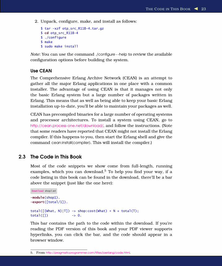
Most of the code snippets we show come from full-length, running
examples, which you can download.5 To help you find your way, if a
code listing in this book can be found in the download, there’ll be a bar
above the snippet (just like the one here):
Download shop1.erl
-module(shop1).
-export([total/1]).
total([{What, N}|T]) -> shop:cost(What) * N + total(T);
total([]) -> 0.
This bar contains the path to the code within the download. If you’re
reading the PDF version of this book and your PDF viewer supports
hyperlinks, you can click the bar, and the code should appear in a
browser window.
5. From http://pragmaticprogrammer.com/titles/jaerlang/code.html.

STARTING THE SHELL 24
2.4 Starting the Shell
Now let’s get started. We can interact with Erlang using an interactive
tool called the shell. Once we’ve started the shell, we can type expres-
sions, and the shell will display their values.
If you’ve installed Erlang on your system (as described in Section 2.2,
Installing Erlang, on page 21), then the Erlang shell, erl, will also be
installed. To run it, open a conventional operating system command
shell (cmd on Windows or a shell such as bash on Unix-based systems).
At the command prompt, start the Erlang shell by typing erl:
Ê $ erl
Erlang (BEAM) emulator version 5.5.1 [source] [async-threads:0] [hipe]
Eshell V5.5.1 (abort with ^G)Ë 1> % I'm going to enter some expressions in the shell ..Ì 1> 20 + 30.Í 50Î 2>
Let’s look at what we just did:
Ê This is the Unix command to start the Erlang shell. The shell
responds with a banner telling you which version of Erlang you
are running.
Ë The shell printed the prompt 1>, and then we typed a comment.
The percent (%) character indicates the start of a comment. All
the text from the percent sign to the end of line is treated as a
comment and is ignored by the shell and the Erlang compiler.
Ì The shell repeated the prompt 1> since we hadn’t entered a com-
plete command. At this point we entered the expression 20 + 30,
followed by a period and a carriage return. (Beginners often for-
get to enter the period. Without it, Erlang won’t know that we’ve
finished our expression, and we won’t see the result displayed.)
Í The shell evaluated the expression and printed the result (50, in
this case).
Î The shell printed out another prompt, this time for command
number 2 (because the command number increases each time a
new command is entered).
Have you tried running the shell on your system? If not, please stop and
try it now. If you just read the text without typing in the commands, you
might think that you understand what is happening, but you will not

SIMPLE INTEGER ARITHMETIC 25
have transferred this knowledge from your brain to your fingertips—
programming is not a spectator sport. Just like any form of athletics,
you have to practice a lot.
Enter the expressions in the examples exactly as they appear in the
text, and then try experimenting with the examples and changing them
a bit. If they don’t work, stop and ask yourself what went wrong. Even
an experienced Erlang programmer will spend a lot of time interacting
with the shell.
As you get more experienced, you’ll learn that the shell is a really pow-
erful tool. Previous shell commands can be recalled (with Ctrl+P and
Ctrl+N) and edited (with emacs-like editing commands). This is covered
in Section 6.5, Command Editing in the Erlang Shell, on page 130. Best
of all, when you start writing distributed programs, you will find that
you can attach a shell to a running Erlang system on a different Erlang
node in a cluster or even make an secure shell (ssh) connection directly
to an Erlang system running on a remote computer. Using this, you can
interact with any program on any node in a system of Erlang nodes.
Warning: You can’t type everything you read in this book into the shell.
In particular, you can’t type the code that’s listed in the Erlang program
files into the shell. The syntactic forms in an .erl file are not expressions
and are not understood by the shell. The shell can evaluate only Erlang
expressions and doesn’t understand anything else. In particular, you
can’t type module annotations into the shell; these are things that start
with a hyphen (such as -module, -export, and so on).
The remainder of this chapter is in the form of a number of short dia-
logues with the Erlang shell. A lot of the time I won’t explain all the
details of what is going on, since this would interrupt the flow of the
text. In Section 5.4, Miscellaneous Short Topics, on page 98, I’ll fill in
the details.
2.5 Simple Integer Arithmetic
Let’s evaluate some arithmetic expressions:
1> 2 + 3 * 4.
14
2> (2 + 3) * 4.
20
Important: You’ll see that this dialogue starts at command number 1
(that is the shell printed, 1>). This means we have started a new Erlang

SIMPLE INTEGER ARITHMETIC 26
Is the Shell Not Responding?
If the shell didn’t respond after you typed a command, thenyou might have forgotten to end the command with a periodfollowed by carriage return (called dot-whitespace).
Another thing that might have gone wrong is that you’vestarted to type something that is quoted (that is, starts with asingle or double quote mark) but have not yet typed a match-ing closing quote mark that should be the same as the openquote mark.
If any of these happen, then the best thing to do is type anextra closing quote, followed by dot-whitespace.
If things go really wrong and the system won’t respond at all,then just press Ctrl+C (on Windows, Ctrl+Break). You’ll see thefollowing output:
BREAK: (a)bort (c)ontinue (p)roc info (i)nfo (l)oaded(v)ersion (k)ill (D)b-tables (d)istribution
Now just press A to abort the current Erlang session.
Advanced: You can start and stop multiple shells. See Sec-tion 6.7, The Shell Isn’t Responding, on page 133 for details.
shell. Every time you see a dialogue that starts with 1>, you’ll have to
start a new shell if you want to exactly reproduce the examples in the
book. When an example starts with a prompt number that is greater
than 1, this means the shell session is continued from the previous
examples so you don’t have to start a new shell.
Note: If you’re going to type these examples into the shell as you read
the text (which is absolutely the best way to learn), then you might
like to take a quick peek at Section 6.5, Command Editing in the Erlang
Shell, on page 130.
You’ll see that Erlang follows the normal rules for arithmetic expres-
sions, so 2 + 3 * 4 means 2 + (3 * 4) and not (2 + 3) * 4.
Erlang uses arbitrary-sized integers for performing integer arithmetic.
In Erlang, integer arithmetic is exact, so you don’t have to worry about
arithmetic overflows or not being able to represent an integer in a cer-
tain word size.
VARIABLES 27
Variable Notation
Often we will want to talk about the values of particular vari-ables. For this I’ll use the notation Var 7→ Value, so, for example,A 7→ 42 means that the variable A has the value 42. When thereare several variables, I’ll write {A 7→ 42, B 7→ true ... }, meaningthat A is 42, B is true, and so on.
Why not try it? You can impress your friends by calculating with very
large numbers:
3> 123456789 * 987654321 * 112233445566778899 * 998877665544332211.
13669560260321809985966198898925761696613427909935341
You can enter integers in a number of ways.6 Here’s an expression that
uses base 16 and base 32 notation:
4> 16#cafe * 32#sugar.
1577682511434
2.6 Variables
How can you store the result of a command so that you can use it later?
That’s what variables are for. Here’s an example:
1> X = 123456789.
123456789
What’s happening here? First, we assign a value to the variable X; then,
the shell prints the value of the variable.
Note: All variable names must start with an uppercase letter.
If you want to see the value of a variable, just enter the variable name:
2> X.
123456789
Now that X has a value, you can use it:
3> X*X*X*X.
232305722798259244150093798251441
6. See Section 5.4, Integers, on page 111.

VARIABLES 28
Single Assignment Is Like Algebra
When I went to school, my math teacher said, “If there’s an Xin several different parts in the same equation, then all the X smean the same thing.” That’s how we can solve equations: ifwe know that X+Y=10 and X-Y=2, then X will be 6 and Y will be4 in both equations.
But when I learned my first programming language, we wereshown stuff like this:
X = X + 1
Everyone protested, saying “you can’t do that!” But theteacher said we were wrong, and we had to unlearn what welearned in math class. X isn’t a math variable: it’s like a pigeonhole/little box....
In Erlang, variables are just like they are in math. When you asso-ciate a value with a variable, you’re making an assertion—astatement of fact. This variable has that value. And that’s that.
However, if you try to assign a different value to the variable X, you’ll
get a somewhat brutal error message:
4> X = 1234.
=ERROR REPORT==== 11-Sep-2006::20:32:49 ===
Error in process <0.31.0> with exit value:
{{badmatch,1234},[{erl_eval,expr,3}]}
** exited: {{badmatch,1234},[{erl_eval,expr,3}]} **
What on Earth is going on here? Well, to explain it, I’m going to have to
shatter two assumptions you have about the simple statement X = 1234:
• First, X is not a variable, at least not in the sense that you’re used
to in languages such as Java and C.
• Second, = is not an assignment operator.
This is probably one of the trickiest areas when you’re new to Erlang,
so let’s spend a couple of pages digging deeper.
Variables That Don’t Vary
Erlang has single assignment variables. As the name suggests, sin-
gle assignment variables can be given a value only once. If you try to
change the value of a variable once it has been set, then you’ll get an

VARIABLES 29
error (in fact, you’ll get the badmatch error we just saw). A variable that
has had a value assigned to it is called a bound variable; otherwise, it
is called an unbound variable. All variables start off unbound.
When Erlang sees a statement such as X = 1234, it binds the variable X
to the value 1234. Before being bound, X could take any value: it’s just
an empty hole waiting to be filled. However, once it gets a value, it holds
on to it forever.
At this point, you’re probably wondering why we use the name variable.
This is for two reasons:
• They are variables, but their value can be changed only once (that
is, they change from being unbound to having a value).
• They look like variables in conventional programming languages,
so when we see a line of code that starts like this:X = ...
then our brains say, “Aha, I know what this is; X is a variable, and
= is an assignment operator.” And our brains are almost right: X is
almost a variable, and = is almost an assignment operator.
Note: The use of ellipses (...) in Erlang code examples just means
“code I’m not showing.”
In fact, = is a pattern matching operator, which behaves like assignment
when X is an unbound variable.
Finally, the scope of a variable is the lexical unit in which it is defined.
So if X is used inside a single function clause, its value does not “escape”
to outside the clause. There are no such things as global or private
variables shared by different clauses in the same function. If X occurs
in many different functions, then all the values of X are different.
Pattern Matching
In most languages, = denotes an assignment statement. In Erlang, how-
ever, = denotes a pattern matching operation. Lhs = Rhs really means this:
evaluate the right side (Rhs), and then match the result against the pat-
tern on the left side (Lhs).
Now a variable, such as X, is a simple form of pattern. As we said ear-
lier, variables can be given a value only once. The first time we say X =
SomeExpression, Erlang says to itself, “What can I do to make this state-
ment true?” Because X doesn’t yet have a value, it can bind X to the
value of SomeExpression, the statement becomes valid, and everyone is
happy.

VARIABLES 30
Then, if at a later stage we say X = AnotherExpression, then this will suc-
ceed only if SomeExpression and AnotherExpression are identical. Here’s an
example of this:
Line 1 1> X = (2+4).- 6- 2> Y = 10.- 105 3> X = 6.- 6- 4> X = Y.- =ERROR REPORT==== 27-Oct-2006::17:25:25 ===- Error in process <0.32.0> with exit value:
10 {{badmatch,10},[{erl_eval,expr,3}]}- 5> Y = 10.- 10- 6> Y = 4.- =ERROR REPORT==== 27-Oct-2006::17:25:46 ===
15 Error in process <0.37.0> with exit value:- {{badmatch,4},[{erl_eval,expr,3}]}- 7> Y = X.- =ERROR REPORT==== 27-Oct-2006::17:25:57 ===- Error in process <0.40.0> with exit value:
20 {{badmatch,6},[{erl_eval,expr,3}]}
Here’s what happened: In line 1 the system evaluated the expression
2+4, and the answer was 6. So after this line, the shell has the following
set of bindings: {X 7→ 6}. After line 3 has been evaluated, we have the
bindings {X 7→ 6, Y 7→ 10}.
Now we come to line 5. Just before we evaluate the expression, we know
that X 7→ 6, so the match X = 6 succeeds.
When we say X = Y in line 7, our bindings are {X 7→ 6, Y 7→ 10}, and
therefore the match fails and an error message is printed.
Expressions 4 to 7 either succeed or fail depending upon the values of
X and Y. Now is a good time to stare hard at these and make sure you
really understand them before going any further.
At this stage it may seem that I am belaboring the point. All the patterns
to the left of the “=” are just variables, either bound or unbound, but
as we’ll see later, we can make arbitrarily complex patterns and match
them with the “=” operator. I’ll be returning to this theme after we have
introduced tuples and lists, which are used for storing compound data
items.

VARIABLES 31
Why Does Single Assignment Make My Programs Better?
In Erlang a variable is just a reference to a value—in the Erlang imple-
mentation, a bound variable is represented by a pointer to an area of
storage that contains the value. This value cannot be changed.
The fact that we cannot change a variable is extremely important and
is unlike the behavior of variables in imperative languages such as C or
Java.
Let’s see what can happen when you’re allowed to change a variable.
Let’s define a variable X as follows:
1> X = 23.
23
Now we can use X in computations:
2> Y = 4 * X + 3.
95
Now suppose we could change the value of X (horrors):
3> X = 19.
Fortunately, Erlang doesn’t allow this. The shell complains like crazy
and says this:
=ERROR REPORT==== 27-Oct-2006::13:36:24 ===
Error in process <0.31.0> with exit value:
{{badmatch,19},[{erl_eval,expr,3}]}
This just means that X cannot be 19 since we’ve already said it was 23.
But just suppose we could do this; then the value of Y would be wrong in
the sense that we can no longer interpret statement 2 as an equation.
Moreover, if X could change its value at many different points in the
program and something goes wrong, it might be difficult saying which
particular value of X had caused the failure and at exactly which point
in the program it had acquired the wrong value.
In Erlang, variable values cannot be changed after they have been set.
This simplifies debugging. To understand why this is true, we must ask
ourselves what an error is and how an error makes itself known.
One rather common way that you discover that your program is incor-
rect is that a variable has an unexpected value. If this is the case, then
you have to discover exactly the point in your program where the vari-
able acquired the incorrect value. If this variable changed values many
FLOATING-POINT NUMBERS 32
Absence of Side Effects Means We Can Parallelize Our Programs
The technical term for memory areas that can be modified ismutable state. Erlang is a functional programming languageand has nonmutable state.
Much later in the book we’ll look at how to program multicoreCPUs. When it comes to programming multicore CPUs, the con-sequences of having nonmutable state are enormous.
If you use a conventional programming language such as Cor Java to program a multicore CPU, then you will have tocontend with the problem of shared memory. In order not tocorrupt shared memory, the memory has to be locked whileit is accessed. Programs that access shared memory must notcrash while they are manipulating the shared memory.
In Erlang, there is no mutable state, there is no shared mem-ory, and there are no locks. This makes it easy to parallelize ourprograms.
times and at many different points in your program, then finding out
exactly which of these changes was incorrect can be extremely difficult.
In Erlang there is no such problem. A variable can be set only once and
thereafter never changed. So once we know which variable is incorrect,
we can immediately infer the place in the program where the variable
became bound, and this must be where the error occurred.
At this point you might be wondering how it’s possible to program with-
out variables. How can you express something like X = X + 1 in Erlang?
The answer is easy. Invent a new variable whose name hasn’t been used
before (say X1), and write X1 = X + 1.
2.7 Floating-Point Numbers
Let’s try doing some arithmetic with floating-point numbers:
1> 5/3.
1.66667
2> 4/2.
2.00000
3> 5 div 3.
1
ATOMS 33
4> 5 rem 3.
2
5> 4 div 2.
2
6> Pi = 3.14159.
3.14159
7> R = 5.
5
8> Pi * R * R.
78.5397
Don’t get confused here. In line 1 the number at the end of the line is
the integer 3. The period signifies the end of the expression and is not
a decimal point. If I had wanted a floating-point number here, I’d have
written 3.0.
“/” always returns a float; thus, 4/2 evaluates to 2.0000 (in the shell). N
div M and N rem M are used for integer division and remainder; thus, 5
div 3 is 1, and 5 rem 3 is 2.
Floating-point numbers must have a decimal point followed by at least
one decimal digit. When you divide two integers with “/”, the result is
automatically converted to a floating-point number.
2.8 Atoms
In Erlang, atoms are used to represent different non-numerical con-
stant values.
If you’re used to enumerated types in C or Java, then you will already
have used something very similar to atoms whether you realize it or
not.
C programmers will be familiar with the convention of using symbolic
constants to make their programs self-documenting. A typical C pro-
gram will define a set of global constants in an include file that consists
of a large number of constant definitions; for example, there might be
a file glob.h containing this:
#define OP_READ 1
#define OP_WRITE 2
#define OP_SEEK 3
...
#define RET_SUCCESS 223
...
ATOMS 34
Typical C code using such symbolic constants might read as follows:
#include "glob.h"
int ret;
ret = file_operation(OP_READ, buff);
if( ret == RET_SUCCESS ) { ... }
In a C program the values of these constants are not interesting; they’re
interesting here only because they are all different and they can be
compared for equality.
The Erlang equivalent of this program might look like this:
Ret = file_operation(op_read, Buff),
if
Ret == ret_success ->
...
In Erlang, atoms are global, and this is achieved without the use of
macro definitions or include files.
Suppose you want to write a program that manipulates days of the
week. How would you represent a day in Erlang? Of course, you’d use
one of the atoms monday, tuesday, . . . .
Atoms start with lowercase letters, followed by a sequence of alphanu-
meric characters or the underscore (_) or at (@) sign.7 For example: red,
december, cat, meters, yards, joe@somehost, and a_long_name.
Atoms can also be quoted with a single quotation mark (’). Using the
quoted form, we can create atoms that start with uppercase letters
(which otherwise would be interpreted as variables) or that contain
nonalphanumeric characters. For example: ’Monday’, ’Tuesday’, ’+’, ’*’,
’an atom with spaces’. You can even quote atoms that don’t need to be
quoted, so ’a’ means exactly the same as a.
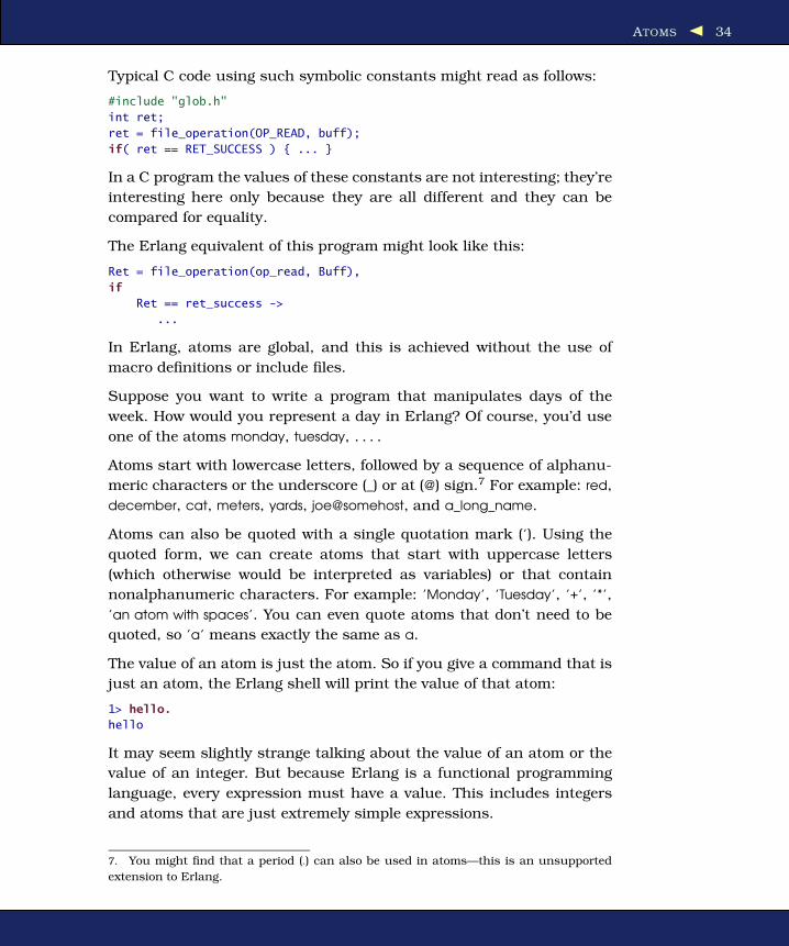
The value of an atom is just the atom. So if you give a command that is
just an atom, the Erlang shell will print the value of that atom:
1> hello.
hello
It may seem slightly strange talking about the value of an atom or the
value of an integer. But because Erlang is a functional programming
language, every expression must have a value. This includes integers
and atoms that are just extremely simple expressions.
7. You might find that a period (.) can also be used in atoms—this is an unsupported
extension to Erlang.
TUPLES 35
2.9 Tuples
Suppose you want to group a fixed number of items into a single entity.
For this you’d use a tuple. You can create a tuple by enclosing the
values you want to represent in curly brackets and separating them
with commas. So, for example, if you want to represent someone’s name
and height, you might use {joe, 1.82}. This is a tuple containing an atom
and a floating-point number.
Tuples are similar to structs in C, with the difference that they are
anonymous. In C a variable P of type point might be declared as follows:
struct point {
int x;
int y;
} P;
You’d access the fields in a C struct using the dot operator. So to set
the x and y values in Point, you might say this:
P.x = 10; P.y = 45;
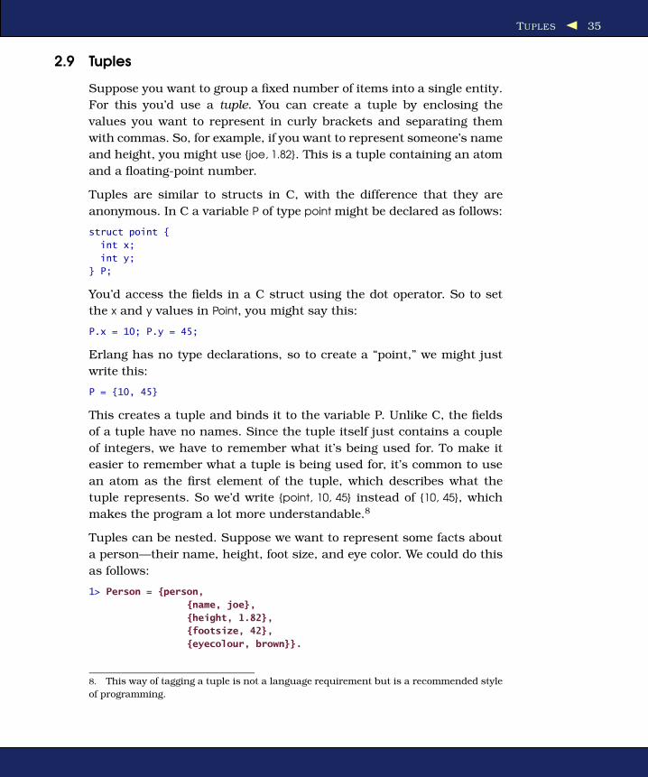
Erlang has no type declarations, so to create a “point,” we might just
write this:
P = {10, 45}
This creates a tuple and binds it to the variable P. Unlike C, the fields
of a tuple have no names. Since the tuple itself just contains a couple
of integers, we have to remember what it’s being used for. To make it
easier to remember what a tuple is being used for, it’s common to use
an atom as the first element of the tuple, which describes what the
tuple represents. So we’d write {point, 10, 45} instead of {10, 45}, which
makes the program a lot more understandable.8
Tuples can be nested. Suppose we want to represent some facts about
a person—their name, height, foot size, and eye color. We could do this
as follows:
1> Person = {person,
{name, joe},
{height, 1.82},
{footsize, 42},
{eyecolour, brown}}.
8. This way of tagging a tuple is not a language requirement but is a recommended style
of programming.

TUPLES 36
Note how we used atoms both to identify the field and (in the case of
name and eyecolour) to give the field a value.
Creating Tuples
Tuples are created automatically when we declare them and are de-
stroyed when they can no longer be used. Erlang uses a garbage col-
lector to reclaim all unused memory, so we don’t have to worry about
memory allocation.
If you use a variable in building a new tuple, then the new tuple will
share the value of the data structure referenced by the variable. Here’s
an example:
2> F = {firstName, joe}.
{firstName,joe}
3> L = {lastName, armstrong}.
{lastName,armstrong}
4> P = {person, F, L}.
{person,{firstName,joe},{lastName,armstrong}}
If you try to create a data structure with an undefined variable, then
you’ll get an error. So in the next line, if we try to use the variable Q
that is undefined, we’ll get an error:
5> {true, Q, 23, Costs}.
** 1: variable 'Q' is unbound **
This just means that the variable Q is undefined.
Extracting Values from Tuples
Earlier, we said that =, which looks like an assignment statement,
was not actually an assignment statement but was really a pattern
matching operator. You might wonder why we were being so pedantic.
Well, it turns out that pattern matching is fundamental to Erlang and
that it’s used for lots of different tasks. It’s used for extracting values
from data structures, and it’s also used for flow of control within func-
tions and for selecting which messages are to be processed in a parallel
program when you send messages to a process.
If we want to extract some values from a tuple, we use the pattern
matching operator =.
Let’s go back to our tuple that represents a point:
1> Point = {point, 10, 45}.
{point, 10, 45}.
TUPLES 37
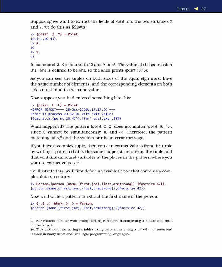
Supposing we want to extract the fields of Point into the two variables X
and Y, we do this as follows:
2> {point, X, Y} = Point.
{point,10,45}
3> X.
10
4> Y.
45
In command 2, X is bound to 10 and Y to 45. The value of the expression
Lhs = Rhs is defined to be Rhs, so the shell prints {point,10,45}.
As you can see, the tuples on both sides of the equal sign must have
the same number of elements, and the corresponding elements on both
sides must bind to the same value.
Now suppose you had entered something like this:
5> {point, C, C} = Point.
=ERROR REPORT==== 28-Oct-2006::17:17:00 ===
Error in process <0.32.0> with exit value:
{{badmatch,{point,10,45}},[{erl_eval,expr,3}]}
What happened? The pattern {point, C, C} does not match {point, 10, 45},
since C cannot be simultaneously 10 and 45. Therefore, the pattern
matching fails,9 and the system prints an error message.
If you have a complex tuple, then you can extract values from the tuple
by writing a pattern that is the same shape (structure) as the tuple and
that contains unbound variables at the places in the pattern where you
want to extract values.10
To illustrate this, we’ll first define a variable Person that contains a com-
plex data structure:
1> Person={person,{name,{first,joe},{last,armstrong}},{footsize,42}}.
{person,{name,{first,joe},{last,armstrong}},{footsize,42}}
Now we’ll write a pattern to extract the first name of the person:
2> {_,{_,{_,Who},_},_} = Person.
{person,{name,{first,joe},{last,armstrong}},{footsize,42}}
9. For readers familiar with Prolog: Erlang considers nonmatching a failure and does
not backtrack.10. This method of extracting variables using pattern matching is called unification and
is used in many functional and logic programming languages.

LISTS 38
And finally we’ll print out the value of Who:
3> Who.
joe
Note that in the previous example we wrote _ as a placeholder for vari-
ables that we’re not interested in. The symbol _ is called an anonymous
variable. Unlike regular variables, several occurrences of _ in the same
pattern don’t have to bind to the same value.
2.10 Lists
We use lists to store variable numbers of things: things you want to
buy at the store, the names of the planets, the results returned by your
prime factors function, and so on.
We create a list by enclosing the list elements in square brackets and
separating them with commas. Here’s how we could create a shopping
list:
1> ThingsToBuy = [{apples,10},{pears,6},{milk,3}].
[{apples,10},{pears,6},{milk,3}]
The individual elements of a list can be of any type, so, for example, we
could write the following:
2> [1+7,hello,2-2,{cost, apple, 30-20},3].
[8,hello,0,{cost,apple,10},3]
Terminology
We call the first element of a list the head of the list. If you imagine
removing the head from the list, what’s left is called the tail of the list.
For example, if we have a list [1,2,3,4,5], then the head of the list is the
integer 1, and the tail is the list [2,3,4,5]. Note that the head of a list can
be anything, but the tail of a list is usually also a list.
Accessing the head of a list is a very efficient operation, so virtually
all list-processing functions start by extracting the head of a list, doing
something to the head of the list, and then processing the tail of the
list.

LISTS 39
Defining Lists
If T is a list, then [H|T] is also a list,11 with head H and tail T. The vertical
bar | separates the head of a list from its tail. [ ] is the empty list.
Whenever we construct a list using a [...|T] constructor, we should make
sure that T is a list. If it is, then the new list will be “properly formed.” If
T is not a list, then the new list is said to be an “improper list.” Most of
the library functions assume that lists are properly formed and won’t
work for improper lists.
We can add more than one element to the beginning of T by writing
[E1,E2,..,En|T]. For example:
3> ThingsToBuy1 = [{oranges,4},{newspaper,1}|ThingsToBuy].
[{oranges,4},{newspaper,1},{apples,10},{pears,6},{milk,3}]
Extracting Elements from a List
As with everything else, we can extract elements from a list with a
pattern matching operation. If we have the nonempty list L, then the
expression [X|Y] = L, where X and Y are unbound variables, will extract
the head of the list into X and the tail of the list into Y.
So, we’re in the shop, and we have our shopping list ThingsToBuy1—the
first thing we do is unpack the list into its head and tail:
4> [Buy1|ThingsToBuy2] = ThingsToBuy1.
[{oranges,4},{newspaper,1},{apples,10},{pears,6},{milk,3}]
This succeeds with bindings
Buy1 7→ {oranges,4}
and
ThingsToBuy2 7→ [{newspaper,1}, {apples,10}, {pears,6}, {milk,3}].
We go and buy the oranges, and then we could extract the next couple
of items:
5> [Buy2,Buy3|ThingsToBuy3] = ThingsToBuy2.
{newspaper,1},{apples,10},{pears,6},{milk,3}]
This succeeds with Buy2 7→ {newspaper,1}, Buy3 7→ {apples,10}, and ThingsTo-
Buy3 7→ [{pears,6},{milk,3}].
11. Note for LISP programmers: [H|T] is a CONS cell with CAR H and CDR T. In a pattern,
this syntax unpacks the CAR and CDR. In an expression, it constructs a CONS cell.

STRINGS 40
2.11 Strings
Strictly speaking, there are no strings in Erlang. Strings are really just
lists of integers. Strings are enclosed in double quotation marks ("), so,
for example, we can write this:
1> Name = "Hello".
"Hello"
Note: In some programming languages, strings can be quoted with
either single or double quotes. In Erlang, you must use double quotes.
"Hello" is just shorthand for the list of integers that represent the indi-
vidual characters in that string.
When the shell prints the value of a list it prints the list as a string, but
only if all the integers in the list represent printable characters:
2> [1,2,3].
[1,2,3]
3> [83,117,114,112,114,105,115,101].
"Surprise"
4> [1,83,117,114,112,114,105,115,101].
[1,83,117,114,112,114,105,115,101].
In expression 2 the list [1,2,3] is printed without any conversion. This is
because 1, 2, and 3 are not printable characters.
In expression 3 all the items in the list are printable characters, so the
list is printed as a string.
Expression 4 is just like expression 3, except that the list starts with a
1, which is not a printable character. Because of this, the list is printed
without conversion.
We don’t need to know which integer represents a particular character.
We can use the “dollar syntax” for this purpose. So, for example, $a is
actually the integer that represents the character a, and so on.
5> I = $s.
115
6> [I-32,$u,$r,$p,$r,$i,$s,$e].
"Surprise"
Character Sets Used in Strings
The characters in a string represent Latin-1 (ISO-8859-1) character
codes. For example, the string containing the Swedish name Håkan will
be encoded as [72,229,107,97,110].

PATTERN MATCHING AGAIN 41
Note: If you enter [72,229,107,97,110] as a shell expression, you might not
get what you expect:
1> [72,229,107,97,110].
"H\345kan"
What has happened to “Håkan”—where did he go? This actually has
nothing to do with Erlang but with the locale and character code set-
tings of your terminal.
As far as Erlang is concerned, a string is a just a list of integers in
some encoding. If they happen to be printable Latin-1 codes, then they
should be displayed correctly (if your terminal settings are correct).
2.12 Pattern Matching Again
To round off this chapter, we’ll go back to pattern matching one more
time.
The following table has some examples of patterns and terms.12 The
third column of the table, marked Result, shows whether the pattern
matched the term and, if so, the variable bindings that were created.
Look through these examples, and make sure you really understand
them:
Pattern Term Result
{X,abc} {123,abc} Succeeds X 7→ 123
{X,Y,Z} {222,def,"cat"} Succeeds X 7→ 222, Y 7→ def,
Z 7→ "cat"
{X,Y} {333,ghi,"cat"} Fails—the tuples have
different shapes
X true Succeeds X 7→ true
{X,Y,X} {{abc,12},42,{abc,12}} Succeeds X 7→ {abc,12}, Y 7→ 42
{X,Y,X} {{abc,12},42,true} Fails—X cannot be both
{abc,12} and true
[H|T] [1,2,3,4,5] Succeeds H 7→ 1, T 7→ [2,3,4,5]
[H|T] "cat" Succeeds H 7→ 99, T 7→ "at"
[A,B,C|T] [a,b,c,d,e,f] Succeeds A 7→ a, B 7→ b,
C 7→ c, T 7→ [d,e,f]
If you’re unsure about any of these, then try entering a Pattern = Term
expression into the shell to see what happens.
12. A term is just an Erlang data structure.

PATTERN MATCHING AGAIN 42
For example:
1> {X, abc} = {123, abc}.
{123,abc}.
2> X.
123
3> f().
ok
4> {X,Y,Z} = {222,def,"cat"}.
{222,def,"cat"}.
5> X.
222
6> Y.
def
...
Note: The command f() tells the shell to forget any bindings it has. After
this command, all variables become unbound, so the X in line 4 has
nothing to do with the X in lines 1 and 2.
Now that we’re comfortable with the basic data types and with the
ideas of single assignment and pattern matching, so we can step up
the tempo and see how to define functions and modules. Let’s see how
in the next chapter.

Chapter 3
Sequential ProgrammingIn this chapter, we’ll see how to write simple sequential Erlang pro-
grams. In the first section, we’ll talk about modules and functions. We’ll
see how the ideas on pattern matching that we learned about in the
previous chapter are used when we define functions.
Immediately after this, we’ll return to the shopping list that we intro-
duced in the previous chapter, and we’ll write some code to work out
the total cost of the items in the shopping list.
As we go along, we’ll make incremental improvements to the programs
we develop. That way you’ll be able to see how the basic ideas evolve,
and not just be presented with some finished program with no explana-
tion as to how we got there. By understanding the steps involved, you’ll
get some ideas that you can apply to your own programs.
Along the way we’ll be talking about higher-order functions (called
funs) and how they can be used to create your own control abstrac-
tions. Finally, we’ll talk about guards, records, case expressions, and if
expressions.
So, let’s get to work....
3.1 Modules
Modules are the basic unit of code in Erlang. All the functions we write
are stored in modules. Modules are stored in files with .erl extensions.

MODULES 44
Modules must be compiled before the code can be run. A compiled
module has the extension .beam.1
Before we write our first module, we’ll remind ourselves about pattern
matching. All we’re going to do is create a couple of data structures
representing a rectangle and a circle. Then we’re going to unpack these
data structures and extract the sides from the rectangle and the radius
from the circle. Here’s how:
1> Rectangle = {rectangle, 10, 5}.
{rectangle, 10, 5}.
2> Circle = {circle, 2.4}.
{circle,2.40000}
3> {rectangle, Width, Ht} = Rectangle.
{rectangle,10,5}
4> Width.
10
5> Ht.
5
6> {circle, R} = Circle.
{circle,2.40000}
7> R.
2.40000
In lines 1 and 2 we created a rectangle and circle. In lines 3 and 6 we
unpacked the fields of the rectangle and circle using pattern matching.
In lines 4, 5, and 7 we printed the variable bindings that were created
by the pattern matching expressions. After line 7 the variable bindings
in the shell are {Width 7→ 10, Ht 7→ 5, R 7→ 2.4}.
Going from pattern matching in the shell to pattern matching in func-
tions is an extremely small step. Let’s start with a function called area
that computes the areas of rectangles and circles. We’ll put this in a
module called geometry and store the module in the file called geome-
try.erl. The entire module looks like this:
Download geometry.erl
-module(geometry).
-export([area/1]).
area({rectangle, Width, Ht}) -> Width * Ht;
area({circle, R}) -> 3.14159 * R * R.
Don’t worry about the -module and -export annotations (we’ll talk about
these later); for now I want you just to stare at the code for the area
function.
1. Beam is short for Bogdan’s Erlang Abstract Machine; Bogumil (Bogdan) Hausman
wrote an Erlang compiler in 1993 and designed a new instruction set for Erlang.

MODULES 45
The function area consists of two clauses. The clauses are separated
by a semicolon, and the final clause is terminated by dot-whitespace.
Each clause has a head and a body; the head consists of a function
name followed by a pattern (in parentheses), and the body consists of a
sequence of expressions,2 which are evaluated if the pattern in the head
is successfully matched against the calling arguments. The patterns are
matched in the order they appear in the function definition.
Note that the patterns such as {rectangle, Width, Ht} have become part of
the area function definition. Each pattern corresponds to exactly one
clause. Let’s look at the first clause of the area function:
area({rectangle, Width, Ht}) -> Width * Ht;
This is a rule for computing the area of a rectangle. When we call geom-
etry:area({rectangle, 10, 5}), the earlier pattern matches with bindings
{Width 7→ 10, Ht 7→ 5}. Following the match, the code following the arrow
-> is evaluated. This is just Width * Ht, which is 10*5, or 50.
Now we’ll compile and run it:
1> c(geometry).
{ok,geometry}
2> geometry:area({rectangle, 10, 5}).
50
3> geometry:area({circle, 1.4}).
6.15752
So what happened here? In line 1 we give the command c(geometry),
which compiles the code in the file geometry.erl. The compiler returns
{ok,geometry}, which means that the compilation succeeded and that
the module geometry has been compiled and loaded. In lines 2 and 3
we call the functions in the geometry module. Note how we need to
include the module name together with the function name in order to
identify exactly which function we want to call.
Extending the Program
Now suppose we want to extend our program by adding a square to our
geometric objects. We could write this:
area({rectangle, Width, Ht}) -> Width * Ht;
area({circle, R}) -> 3.14159 * R * R;
area({square, X}) -> X * X.
2. See Section 5.4, Expressions and Expression Sequences, on page 106.

MODULES 46
or even this:
area({rectangle, Width, Ht}) -> Width * Ht;
area({square, X}) -> X * X;
area({circle, R}) -> 3.14159 * R * R.
In this case, the order of the clauses doesn’t matter; the program means
the same no matter how the clauses are ordered. This is because the
patterns in the clause are mutually exclusive. This makes writing and
extending programs very easy—we just add more patterns. In gen-
eral, though, clause order does matter. When a function is entered,
the clauses are pattern matched against the calling arguments in the
order they are presented in the file.
Before going any further, you should note the following about the way
the area function is written:
• The function area consists of several different clauses. When we
call the function, execution starts in the first clause that matches
the call arguments.
• Our function does not handle the case where none of the patterns
match—our program will fail with a runtime error. This is deliber-
ate.
Many programming languages, such as C, have only one entry point
per function. If we had written this in C, the code might look like this:
enum ShapeType { Rectangle, Circle, Square };
struct Shape {
enum ShapeType kind;
union {
struct { int width, height; } rectangleData;
struct { int radius; } circleData;
struct { int side;} squareData;
} shapeData;
};
double area(struct Shape* s) {
if( s->kind == Rectangle ) {
int width, ht;
width = s->shapeData.rectangleData.width;
ht = s->shapeData.rectangleData.ht;
return width * ht;
} else if ( s->kind == Circle ) {
...
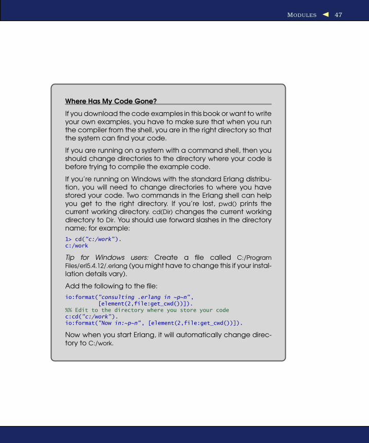
MODULES 47
Where Has My Code Gone?
If you download the code examples in this book or want to writeyour own examples, you have to make sure that when you runthe compiler from the shell, you are in the right directory so thatthe system can find your code.
If you are running on a system with a command shell, then youshould change directories to the directory where your code isbefore trying to compile the example code.
If you’re running on Windows with the standard Erlang distribu-tion, you will need to change directories to where you havestored your code. Two commands in the Erlang shell can helpyou get to the right directory. If you’re lost, pwd() prints thecurrent working directory. cd(Dir) changes the current workingdirectory to Dir. You should use forward slashes in the directoryname; for example:
1> cd("c:/work").c:/work
Tip for Windows users: Create a file called C:/Program
Files/erl5.4.12/.erlang (you might have to change this if your instal-lation details vary).
Add the following to the file:
io:format("consulting .erlang in ~p~n",[element(2,file:get_cwd())]).
%% Edit to the directory where you store your codec:cd("c:/work").io:format("Now in:~p~n", [element(2,file:get_cwd())]).
Now when you start Erlang, it will automatically change direc-tory to C:/work.

MODULES 48
The C code performs what is essentially a pattern matching operation
on the argument to the function; only the programmer has to write the
pattern matching code and make sure that it is correct.
In the Erlang equivalent, we merely write the patterns, and the Erlang
compiler generates optimal pattern matching code, which selects the
correct entry point for the program.
We can see what the equivalent code would look like in Java:3
abstract class Shape {
abstract double area();
}
class Circle extends Shape {
final double radius;
Circle(double radius) { this.radius = radius; }
double area() { return Math.PI * radius*radius; }
}
class Rectangle extends Shape {
final double ht;
final double width;
Rectangle(double width, double height) {
this.ht = height;
this.width = width;
}
double area() { return width * ht; }
}
class Square extends Shape {
final double side;
Square(double side) {
this.side = side;
}
double area() { return side * side; }
}
If you compare the Erlang code with Java code, you’ll see that in the
Java program the code for area is in three different places. In the Erlang
program, all the code for area is in the same place.
3. Adapted from http://java.sun.com/developer/Books/shiftintojava/page1.html.

BACK TO SHOPPING 49
3.2 Back to Shopping
Recall that we had a shopping list that looked like this:
[{oranges,4},{newspaper,1},{apples,10},{pears,6},{milk,3}]
Now suppose that we’d like to know what our shopping costs. To work
this out, we need to know how much each item in the shopping list
costs. Let’s assume that this information is computed in a module
called shop. Start your favorite text editor, and enter the following into
a file called shop.erl.
Download shop.erl
-module(shop).
-export([cost/1]).
cost(oranges) -> 5;
cost(newspaper) -> 8;
cost(apples) -> 2;
cost(pears) -> 9;
cost(milk) -> 7.
The function cost/14 is made up from five clauses. The head of each
clause contains a pattern (in this case a very simple pattern that is
just an atom). When we evaluate shop:cost(X), then the system will try
to match X against each of the patterns in these clauses. If a match is
found, the code to the right of the -> is evaluated.
The cost/1 function must also be exported from the module; this is nec-
essary if we want to call it from outside the module.5
Let’s test this. We’ll compile and run the program in the Erlang shell:
1> c(shop).
{ok,shop}
2> shop:cost(apples).
2
3> shop:cost(oranges).
5
4> shop:cost(socks).
=ERROR REPORT==== 30-Oct-2006::20:45:10 ===
Error in process <0.34.0> with exit value:
{function_clause,[{shop,cost,[socks]},
{erl_eval,do_apply,5},
{shell,exprs,6},
{shell,eval_loop,3}]}
4. The notation Name/N means a function called Name with N arguments; N is called the
arity of the function.5. You can also say -compile(export_all), which exports all the functions in the module.

BACK TO SHOPPING 50
In line 1 we compiled the module in the file shop.erl. In lines 2 and 3,
we asked how much apples and oranges cost (results, 2 and 5 units6).
In line 4 we asked what socks cost, but no clause matched, so we got a
pattern matching error, and the system printed an error message.7
Back to the shopping list. Suppose we have a shopping list like this:
1> Buy = [{oranges,4}, {newspaper,1}, {apples,10}, {pears,6}, {milk,3}].
[{oranges,4},{newspaper,1},{apples,10},{pears,6},{milk,3}]
And say we want to calculate the total value of all the items in the list.
One way we do this might be as follows:
Download shop1.erl
-module(shop1).
-export([total/1]).
total([{What, N}|T]) -> shop:cost(What) * N + total(T);
total([]) -> 0.
Let’s experiment with this:
2> c(shop1).
{ok,shop1}
3> shop1:total([]).
0
Why is this 0? It’s because the second clause of total/1 says that total([ ])
-> 0:
4> shop1:total([{milk,3}]).
21
The function call total([{milk,3}]) matches the clause total([{What,N}|T]} with
T = [ ].8 After the match, the bindings of the variables are {What 7→ milk, N
7→ 3, T 7→ [ ]}. Then the body of the function (shop:cost(What) * N + total(T)) is
entered. All the variables in the body are replaced by the values in the
bindings. So, the value of the body is now the expression shop:cost(milk)
* 3 + total([ ]).
shop:cost(milk) is 7, and total([ ]) is 0; thus, the value of the body is 7*3+0
= 21.
What about a more complex argument?
5> shop1:total([{pears,6},{milk,3}]).
75
6. We’re not really interested in the units here, just that the return values are numbers.7. The “function_clause” part of the error message means that the function call failed
because no clause matched the arguments.8. This is because [X] is just shorthand for [X|[ ]].

BACK TO SHOPPING 51
Where Do I put Those Semicolons?
We use three types of punctuation in Erlang.
Commas (,) separate arguments in function calls, data con-structors, and patterns.
Periods (.) (followed by whitespace) separate entire functionsand expressions in the shell.
Semicolons (;) separate clauses. We find clauses in several con-texts: in kn function definitions and in case, if, try..catch andreceive expressions.
Whenever we see sets of patterns followed by expressions, we’llsee semicolons as separators:
Pattern1 ->Expressions1;
Pattern2 ->Expressions2;
...
This time the first clause of total matches with the bindings {What 7→
pears, N 7→ 6, T 7→ [{milk,3}]}.The result is shop:cost(pears) * 6 + total([{milk,3}]),
which is 9 * 6 + total([{milk,3}]).
But we worked out before that total([{milk,3}]) was 21, so the final result
is 9*6 + 21 = 75.
Finally:
6> shop1:total(Buy).
123
Before we leave this section, we should take a more detailed look at the
function total. total(L) works by a case analysis of the argument L. There
are two possible cases; L is a nonempty list, or L is an empty list. We
write one clause for each possible case, like this:
total([Head|Tail]) ->
some_function_of(Head) + total(Tail);
total([]) ->
0.
In our case, Head was a pattern {What,N}. When the first clause matches
a nonempty list, it picks out the head from the list, does something with
the head, and then calls itself to process the tail of the list. The second
clause matches when the list has been reduced to an empty list ([ ]).

FUNCTIONS WITH THE SAME NAME AND DIFFERENT ARITY 52
The function total/1 actually did two different things. First it looked up
the prices of each of the elements in the list, and then it summed all
the prices. We can rewrite total in a way that separates looking up the
values of the individual items and summing the values. The resulting
code will be clearer and easier to understand. To do this we’ll write two
small list-processing functions called sum and map. But before we talk
about these, we have to introduce the idea of funs. After this, we’ll write
sum and map and then an improved version of total.
3.3 Functions with the Same Name and Different Arity
The arity of a function is the number of arguments that the function
has. In Erlang, two functions with the same name and different arity
in the same module represent entirely different functions. They have
nothing to do with each other apart from a coincidental use of the same
name.
By convention Erlang programmers often use functions with the same
name and different arities as auxiliary functions. Here’s an example:
Download lib_misc.erl
sum(L) -> sum(L, 0).
sum([], N) -> N;
sum([H|T], N) -> sum(T, H+N).
The function sum(L) sums the elements of a list L. It makes use of an
auxiliary routine called sum/2, but this could have been called any-
thing. You could have called the auxilliary routine hedgehog/2, and the
meaning of the program would be the same. sum/2 is a better choice of
name, though, since it gives the reader of your program a clue as to
what’s going on and since you don’t have to invent a new name (which
is always difficult).
3.4 Funs
funs are “anonymous” functions. They are called this because they have
no name. Let’s experiment a bit. First we’ll define a fun and assign it to
the variable Z:
1> Z = fun(X) -> 2*X end.
#Fun<erl_eval.6.56006484>
When we define a fun, the Erlang shell prints #Fun<...> where the ... is
some weird number. Don’t worry about this now.
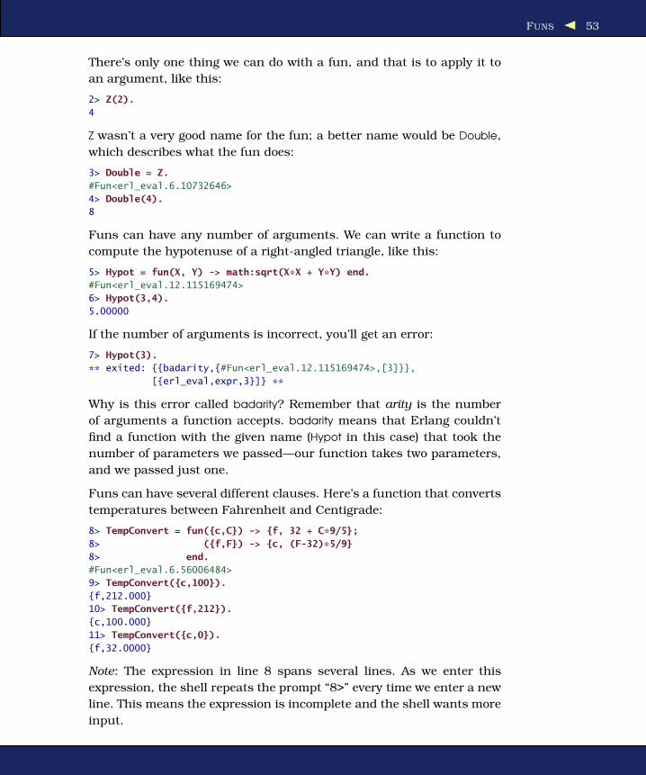
FUNS 53
There’s only one thing we can do with a fun, and that is to apply it to
an argument, like this:
2> Z(2).
4
Z wasn’t a very good name for the fun; a better name would be Double,
which describes what the fun does:
3> Double = Z.
#Fun<erl_eval.6.10732646>
4> Double(4).
8
Funs can have any number of arguments. We can write a function to
compute the hypotenuse of a right-angled triangle, like this:
5> Hypot = fun(X, Y) -> math:sqrt(X*X + Y*Y) end.
#Fun<erl_eval.12.115169474>
6> Hypot(3,4).
5.00000
If the number of arguments is incorrect, you’ll get an error:
7> Hypot(3).
** exited: {{badarity,{#Fun<erl_eval.12.115169474>,[3]}},
[{erl_eval,expr,3}]} **
Why is this error called badarity? Remember that arity is the number
of arguments a function accepts. badarity means that Erlang couldn’t
find a function with the given name (Hypot in this case) that took the
number of parameters we passed—our function takes two parameters,
and we passed just one.
Funs can have several different clauses. Here’s a function that converts
temperatures between Fahrenheit and Centigrade:
8> TempConvert = fun({c,C}) -> {f, 32 + C*9/5};
8> ({f,F}) -> {c, (F-32)*5/9}
8> end.
#Fun<erl_eval.6.56006484>
9> TempConvert({c,100}).
{f,212.000}
10> TempConvert({f,212}).
{c,100.000}
11> TempConvert({c,0}).
{f,32.0000}
Note: The expression in line 8 spans several lines. As we enter this
expression, the shell repeats the prompt “8>” every time we enter a new
line. This means the expression is incomplete and the shell wants more
input.

FUNS 54
Erlang is a functional programming language. Among other things this
means that funs can be used as the arguments to functions and that
functions (or funs) can return funs.
Functions that return funs, or functions that can accept funs as their
arguments, are called higher-order functions. We’ll see a few examples
of these in the next sections.
Now all of this might not sound very exciting since we haven’t seen
what we can do with funs. So far, the code in a fun looks just like
regular function code in a module, but nothing could be further from
the truth. Higher-order functions are the very essence of functional
programming languages—they breathe fire into the belly of the code.
Once you’ve learned to use them, you’ll love them. We’ll see a lot more
of them in the future.
Functions That Have Funs As Their Arguments
The module lists, which is in the standard libraries, exports several
functions whose arguments are funs. The most useful of all these is
lists:map(F, L). This is a function that returns a list made by applying the
fun F to every element in the list L:
12> L = [1,2,3,4].
[1,2,3,4]
13> lists:map(Double, L).
[2,4,6,8].
Another useful function is lists:filter(P, L), which returns a new list of all
the elements E in L such that P(E) is true.
Let’s define a function Even(X) that is true if X is an even number:
14> Even = fun(X) -> (X rem 2) =:= 0 end.
#Fun<erl_eval.6.56006484>
Here X rem 2 computes the remainder after X has been divided by 2, and
=:= is a test for equality. Now we can test Even, and then we can use it
as an argument to map and filter:
15> Even(8).
true
16> Even(7).
false
17> lists:map(Even, [1,2,3,4,5,6,8]).
[false,true,false,true,false,true,true]
18> lists:filter(Even, [1,2,3,4,5,6,8]).
[2,4,6,8]
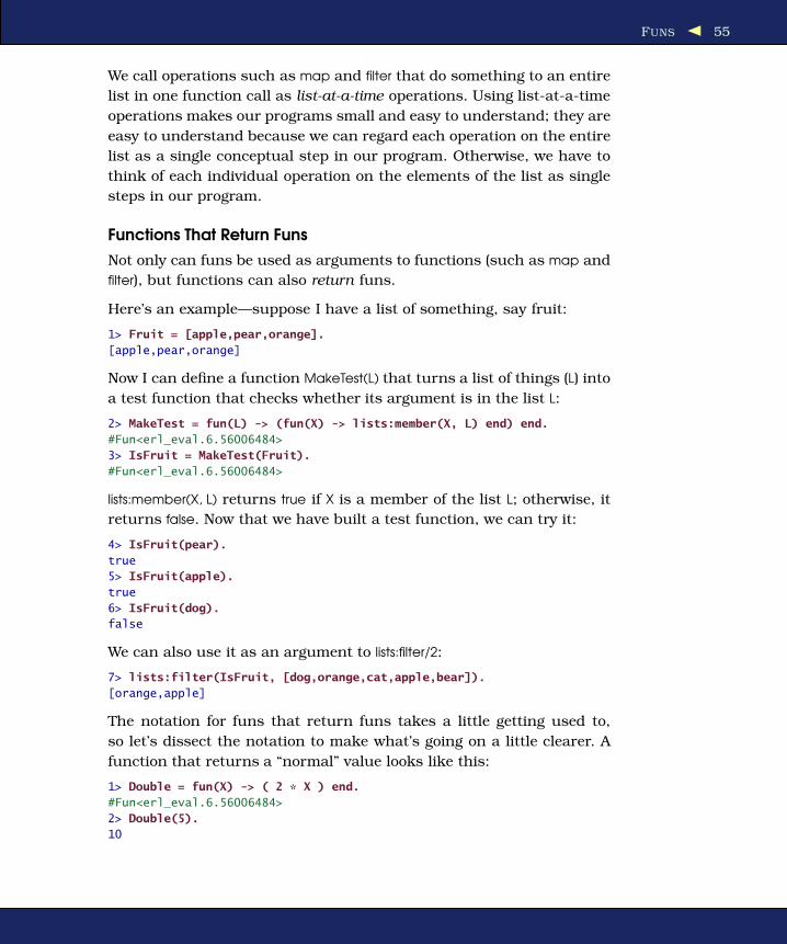
FUNS 55
We call operations such as map and filter that do something to an entire
list in one function call as list-at-a-time operations. Using list-at-a-time
operations makes our programs small and easy to understand; they are
easy to understand because we can regard each operation on the entire
list as a single conceptual step in our program. Otherwise, we have to
think of each individual operation on the elements of the list as single
steps in our program.
Functions That Return Funs
Not only can funs be used as arguments to functions (such as map and
filter), but functions can also return funs.
Here’s an example—suppose I have a list of something, say fruit:
1> Fruit = [apple,pear,orange].
[apple,pear,orange]
Now I can define a function MakeTest(L) that turns a list of things (L) into
a test function that checks whether its argument is in the list L:
2> MakeTest = fun(L) -> (fun(X) -> lists:member(X, L) end) end.
#Fun<erl_eval.6.56006484>
3> IsFruit = MakeTest(Fruit).
#Fun<erl_eval.6.56006484>
lists:member(X, L) returns true if X is a member of the list L; otherwise, it
returns false. Now that we have built a test function, we can try it:
4> IsFruit(pear).
true
5> IsFruit(apple).
true
6> IsFruit(dog).
false
We can also use it as an argument to lists:filter/2:
7> lists:filter(IsFruit, [dog,orange,cat,apple,bear]).
[orange,apple]
The notation for funs that return funs takes a little getting used to,
so let’s dissect the notation to make what’s going on a little clearer. A
function that returns a “normal” value looks like this:
1> Double = fun(X) -> ( 2 * X ) end.
#Fun<erl_eval.6.56006484>
2> Double(5).
10
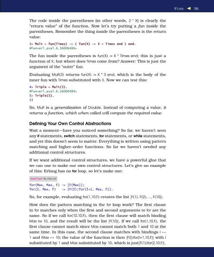
FUNS 56
The code inside the parentheses (in other words, 2 * X) is clearly the
“return value” of the function. Now let’s try putting a fun inside the
parentheses. Remember the thing inside the parentheses is the return
value:
3> Mult = fun(Times) -> ( fun(X) -> X * Times end ) end.
#Fun<erl_eval.6.56006484>
The fun inside the parentheses is fun(X) -> X * Times end; this is just a
function of X, but where does Times come from? Answer: This is just the
argument of the “outer” fun.
Evaluating Mult(3) returns fun(X) -> X * 3 end, which is the body of the
inner fun with Times substituted with 3. Now we can test this:
4> Triple = Mult(3).
#Fun<erl_eval.6.56006484>
5> Triple(5).
15
So, Mult is a generalization of Double. Instead of computing a value, it
returns a function, which when called will compute the required value.
Defining Your Own Control Abstractions
Wait a moment—have you noticed something? So far, we haven’t seen
any if statements, switch statements, for statements, or while statements,
and yet this doesn’t seem to matter. Everything is written using pattern
matching and higher-order functions. So far we haven’t needed any
additional control structures.
If we want additional control structures, we have a powerful glue that
we can use to make our own control structures. Let’s give an example
of this: Erlang has no for loop, so let’s make one:
Download lib_misc.erl
for(Max, Max, F) -> [F(Max)];
for(I, Max, F) -> [F(I)|for(I+1, Max, F)].
So, for example, evaluating for(1,10,F) creates the list [F(1), F(2), ..., F(10)].
How does the pattern matching in the for loop work? The first clause
in for matches only when the first and second arguments to for are the
same. So if we call for(10,10,F), then the first clause will match binding
Max to 10, and the result will be the list [F(10)]. If we call for(1,10,F), the
first clause cannot match since Max cannot match both 1 and 10 at the
same time. In this case, the second clause matches with bindings I 7→
1 and Max 7→ 10; the value of the function is then [F(I)|for(I+1,10,F)] with I
substituted by 1 and Max substituted by 10, which is just[F(1)|for(2,10,F)].

FUNS 57
When Do We Use Higher-Order Functions?
As we have seen, when we use higher-order functions, we cancreate our own new control abstractions, we can pass func-tions as arguments, and we can write functions that return funs.In practice, not all these techniques get used often:
• Virtually all the modules that I write use functions likelists:map/2—this is so common that I almost consider map
to be part of the Erlang language. Calling functions suchas map and filter and partition in the module lists is extremelycommon.
• I sometimes create my own control abstractions. This is farless common than calling the higher-order functions in thestandard library modules. This might happen a few timesin a large module.
• Writing functions that return funs is something I do veryinfrequently. If I were to write a hundred modules, per-haps only one or two modules might use this program-ming technique. Programs with functions that return funscan be difficult to debug; on the other hand, we can usefunctions that return funs to implement things such as lazyevaluation, and we can easily write reentrant parsers andparser combinators that are functions that return parsers.
Now we have a simple for loop.9 We can use it to make a list of the
integers from 1 to 10:
1> lib_misc:for(1,10,fun(I) -> I end).
[1,2,3,4,5,6,7,8,9,10]
Or we can use to compute the squares of the integers from 1 to 10:
2> lib_misc:for(1,10,fun(I) -> I*I end).
[1,4,9,16,25,36,49,64,81,100]
As you become more experienced, you’ll find that being able to create
your own control structures can dramatically decrease the size of your
programs and sometimes make them a lot clearer. This is because you
can create exactly the right control structures that are needed to solve
your problem and because you are not restricted by a small and fixed
set of control structures that came with your programming language.
9. This is not quite the same as a for loop in an imperative language, but it is sufficient
for our purposes.

SIMPLE LIST PROCESSING 58
Common Errors
Some readers have mistakenly typed into the shell fragmentsof code contained in the source code listings. These are notvalid shell commands, and you’ll get some very strange errormessage if you try to do this. So be warned: don’t do this.
If you accidentally choose a module name that collides withone of the system modules, then when you compile your mod-ule, you’ll get a strange message saying that you can’t load amodule that resides in a sticky directory. Just rename the mod-ule, and delete any beam file that you might have made whencompiling your module.
3.5 Simple List Processing
Now that we’ve introduced funs, we can get back to writing sum and
map, which we’ll need for our improved version of total (which I’m sure
you haven’t forgotten about!).
We’ll start with sum, which computes the sum of the elements in a list:
Download mylists.erl
Ê sum([H|T]) -> H + sum(T);Ë sum([]) -> 0.
Note that the order of the two clauses in sum is unimportant. This is
because the first clause matches a nonempty list and the second an
empty list, and these two cases are mutually exclusive. We can test sum
as follows:
1> c(mylists). %% <-- Last time I do this
{ok, mylists}
2> L = [1,3,10].
[1,3,10]
3> mylists:sum(L).
14
Line 1 compiled the module lists. From now on, I’ll often omit the com-
mand to compile the module, and you’ll have to remember to do this
yourself. It’s pretty easy to understand how this works. Let’s trace the
execution:
1. sum([1,3,10])
2. sum([1,3,10]) = 1 + sum([3,10]) (by Ê)
3. = 1 + 3 + sum([10]) (by Ê)
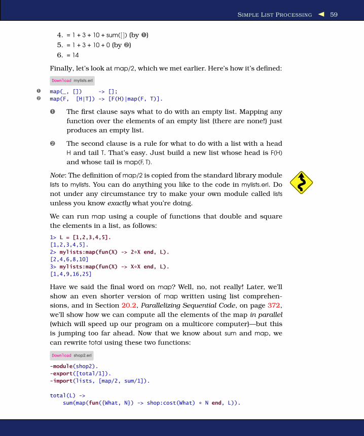
SIMPLE LIST PROCESSING 59
4. = 1 + 3 + 10 + sum([ ]) (by Ê)
5. = 1 + 3 + 10 + 0 (by Ë)
6. = 14
Finally, let’s look at map/2, which we met earlier. Here’s how it’s defined:
Download mylists.erl
Ê map(_, []) -> [];Ë map(F, [H|T]) -> [F(H)|map(F, T)].
Ê The first clause says what to do with an empty list. Mapping any
function over the elements of an empty list (there are none!) just
produces an empty list.
Ë The second clause is a rule for what to do with a list with a head
H and tail T. That’s easy. Just build a new list whose head is F(H)
and whose tail is map(F, T).
Note: The definition of map/2 is copied from the standard library module
lists to mylists. You can do anything you like to the code in mylists.erl. Do
not under any circumstance try to make your own module called lists
unless you know exactly what you’re doing.
We can run map using a couple of functions that double and square
the elements in a list, as follows:
1> L = [1,2,3,4,5].
[1,2,3,4,5].
2> mylists:map(fun(X) -> 2*X end, L).
[2,4,6,8,10]
3> mylists:map(fun(X) -> X*X end, L).
[1,4,9,16,25]
Have we said the final word on map? Well, no, not really! Later, we’ll
show an even shorter version of map written using list comprehen-
sions, and in Section 20.2, Parallelizing Sequential Code, on page 372,
we’ll show how we can compute all the elements of the map in parallel
(which will speed up our program on a multicore computer)—but this
is jumping too far ahead. Now that we know about sum and map, we
can rewrite total using these two functions:
Download shop2.erl
-module(shop2).
-export([total/1]).
-import(lists, [map/2, sum/1]).
total(L) ->
sum(map(fun({What, N}) -> shop:cost(What) * N end, L)).

SIMPLE LIST PROCESSING 60
How I Write Programs
When I’m writing a program, my approach is to “write a bit”and then “test a bit.” I start with a small module with few func-tions, and then I compile it and test it with a few commands inthe shell. Once I’m happy with it, I write a few more functions,compile them, test them, and so on.
Often I haven’t really decided what sort of data structures I’llneed in my program, and as I run small examples, I can seewhether the data structures I have chosen are appropriate.
I tend to “grow” programs rather than think them out com-pletely before writing them. This way I don’t tend to make largemistakes before I discover that things have gone wrong. Aboveall, it’s fun, I get immediate feedback, and I see whether myideas work as soon as I have typed in the program.
Once I’ve figured out how to do something in the shell, I usuallythen go and write a makefile and some code that reproduceswhat I’ve learned in the shell.
We can see how this function works by looking at the steps involved:
1> Buy = [{oranges,4},{newspaper,1},{apples,10},{pears,6},{milk,3}].
[{oranges,4},{newspaper,1},{apples,10},{pears,6},{milk,3}]
2> L1=lists:map(fun({What,N}) -> shop:cost(What) * N end, Buy).
[20,8,20,54,21]
3> lists:sum(L1).
123
Note also the use of the -import and -export declarations in the module:
• The declaration -import(lists, [map/2, sum/1]). means the function
map/2 is imported from the module lists, and so on. This means
we can write map(Fun, ...) instead of lists:map(Fun, ...). cost/1 was not
declared in an import declaration, so we had to use the “fully qual-
ified” name shop:cost.
• The declaration -export([total/1]) means the function total/1 can be
called from outside the module shop2. Only functions that are
exported from a module can be called from outside the module.
By this time you might think that our total function cannot be further
improved, but you’d be wrong. Further improvement is possible. To do
so, we’ll use a list comprehension.

LIST COMPREHENSIONS 61
3.6 List Comprehensions
List comprehensions are expressions that create lists without having to
use funs, maps, or filters. This makes our programs even shorter and
easier to understand.
We’ll start with an example. Suppose we have a list L:
1> L = [1,2,3,4,5].
[1,2,3,4,5]
And suppose we want to double every element in the list. We’ve done
this before, but I’ll remind you:
2> lists:map(fun(X) -> 2*X end, L).
[2,4,6,8,10]
But there’s a much easier way that uses a list comprehension:
4> [2*X || X <- L ].
[2,4,6,8,10]
The notation [ F(X) || X <- L] means “the list of F(X) where X is taken from
the list L.” Thus, [2*X || X <- L ] means “the list of 2*X where X is taken
from the list L.”
To see how to use a list comprehension, we can enter a few expressions
in the shell to see what happens. We start by defining Buy:
1> Buy=[{oranges,4},{newspaper,1},{apples,10},{pears,6},{milk,3}].
[{oranges,4},{newspaper,1},{apples,10},{pears,6},{milk,3}].
Now let’s double the number of every item in the original list:
2> [{Name, 2*Number} || {Name, Number} <- Buy].
[{oranges,8},{newspaper,2},{apples,20},{pears,12},{milk,6}]
Note that the tuple {Name, Number} to the right side of the (||) sign is a
pattern that matches each of the elements in the list Buy. The tuple to
the left side, {Name, 2*Number}, is a constructor.
Suppose we want to compute the total cost of all the elements in the
original list; we could do this as follows. First replace the name of every
item in the list with its price:
3> [{shop:cost(A), B} || {A, B} <- Buy].
[{5,4},{8,1},{2,10},{9,6},{7,3}]
Now multiply the numbers together:
4> [shop:cost(A) * B || {A, B} <- Buy].
[20,8,20,54,21]
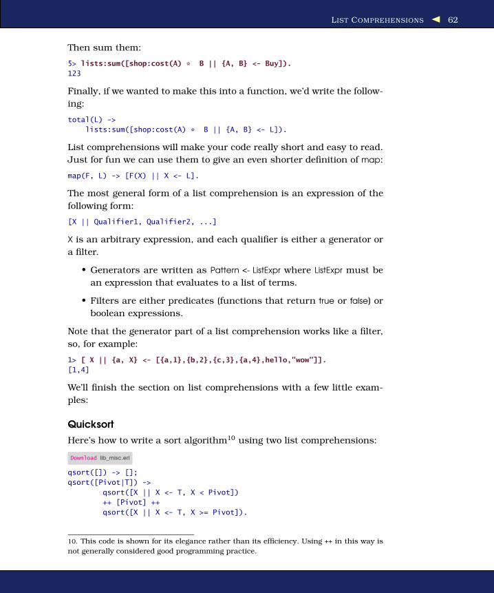
LIST COMPREHENSIONS 62
Then sum them:
5> lists:sum([shop:cost(A) * B || {A, B} <- Buy]).
123
Finally, if we wanted to make this into a function, we’d write the follow-
ing:
total(L) ->
lists:sum([shop:cost(A) * B || {A, B} <- L]).
List comprehensions will make your code really short and easy to read.
Just for fun we can use them to give an even shorter definition of map:
map(F, L) -> [F(X) || X <- L].
The most general form of a list comprehension is an expression of the
following form:
[X || Qualifier1, Qualifier2, ...]
X is an arbitrary expression, and each qualifier is either a generator or
a filter.
• Generators are written as Pattern <- ListExpr where ListExpr must be
an expression that evaluates to a list of terms.
• Filters are either predicates (functions that return true or false) or
boolean expressions.
Note that the generator part of a list comprehension works like a filter,
so, for example:
1> [ X || {a, X} <- [{a,1},{b,2},{c,3},{a,4},hello,"wow"]].
[1,4]
We’ll finish the section on list comprehensions with a few little exam-
ples:
Quicksort
Here’s how to write a sort algorithm10 using two list comprehensions:
Download lib_misc.erl
qsort([]) -> [];
qsort([Pivot|T]) ->
qsort([X || X <- T, X < Pivot])
++ [Pivot] ++
qsort([X || X <- T, X >= Pivot]).
10. This code is shown for its elegance rather than its efficiency. Using ++ in this way is
not generally considered good programming practice.
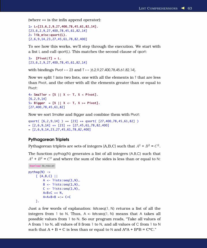
LIST COMPREHENSIONS 63
(where ++ is the infix append operator):
1> L=[23,6,2,9,27,400,78,45,61,82,14].
[23,6,2,9,27,400,78,45,61,82,14]
2> lib_misc:qsort(L).
[2,6,9,14,23,27,45,61,78,82,400]
To see how this works, we’ll step through the execution. We start with
a list L and call qsort(L). This matches the second clause of qsort:
3> [Pivot|T] = L.
[23,6,2,9,27,400,78,45,61,82,14]
with bindings Pivot 7→ 23 and T 7→ [6,2,9,27,400,78,45,61,82,14].
Now we split T into two lists, one with all the elements in T that are less
than Pivot, and the other with all the elements greater than or equal to
Pivot:
4> Smaller = [X || X <- T, X < Pivot].
[6,2,9,14]
5> Bigger = [X || X <- T, X >= Pivot].
[27,400,78,45,61,82]
Now we sort Smaller and Bigger and combine them with Pivot:
qsort( [6,2,9,14] ) ++ [23] ++ qsort( [27,400,78,45,61,82] )
= [2,6,9,14] ++ [23] ++ [27,45,61,78,82,400]
= [2,6,9,14,23,27,45,61,78,82,400]
Pythagorean Triplets
Pythagorean triplets are sets of integers {A,B,C} such that A2 + B2 = C2.
The function pythag(N) generates a list of all integers {A,B,C} such that
A2 + B2 = C2 and where the sum of the sides is less than or equal to N:
Download lib_misc.erl
pythag(N) ->
[ {A,B,C} ||
A <- lists:seq(1,N),
B <- lists:seq(1,N),
C <- lists:seq(1,N),
A+B+C =< N,
A*A+B*B =:= C*C
].
Just a few words of explanation: lists:seq(1, N) returns a list of all the
integers from 1 to N. Thus, A <- lists:seq(1, N) means that A takes all
possible values from 1 to N. So our program reads, “Take all values of
A from 1 to N, all values of B from 1 to N, and all values of C from 1 to N
such that A + B + C is less than or equal to N and A*A + B*B = C*C.”

ARITHMETIC EXPRESSIONS 64
1> lib_misc:pythag(16).
[{3,4,5},{4,3,5}]
2> lib_misc:pythag(30).
[{3,4,5},{4,3,5},{5,12,13},{6,8,10},{8,6,10},{12,5,13}]
Anagrams
If you’re interested in English-style crossword puzzles, you’ll often find
yourself figuring out anagrams. Let’s use Erlang to find all the permu-
tations of a string using the beautiful little function perms where we
have the following:
Download lib_misc.erl
perms([]) -> [[]];
perms(L) -> [[H|T] || H <- L, T <- perms(L--[H])].
1> lib_misc:perms("123").
["123","132","213","231","312","321"]
2> lib_misc:perms("cats").
["cats", "cast", "ctas", "ctsa", "csat", "csta", "acts", "acst",
"atcs", "atsc", "asct", "astc", "tcas", "tcsa", "tacs", "tasc",
"tsca", "tsac", "scat", "scta", "sact", "satc", "stca", "stac"]
X- -Y is the list subtraction operator. It subtracts the elements in Y from
X; there’s a more precise definition in Section 5.4, List Operations ++
and - -, on page 108.
Just for once, I’m not going to explain how perms works, since the expla-
nation would be many times longer than the program, so you can figure
this out for yourself! (But, here’s a hint: To compute all permutations of
X123, compute all permutations of 123 [these are 123 132 213 231 312
321]. Now interleave the X at all possible positions in each permutation,
so adding X to 123 gives X123 1X23 12X3 123X, adding X to 132 gives
X132 1X32 13X2 132X, and so on. Apply these rules recursively.)
3.7 Arithmetic Expressions
All the possible arithmetic expressions are shown in Figure 3.1, on the
following page. Each arithmetic operation has one or two arguments—
these arguments are shown in the table as Integer or Number (Number
means the argument can be an integer or a float).
Associated with each operator is a priority. The order of evaluation of a
complex arithmetic expression depends upon the priority of the opera-
tor: all operations with priority 1 operators are evaluated first, then all
operators with priority 2, and so on.
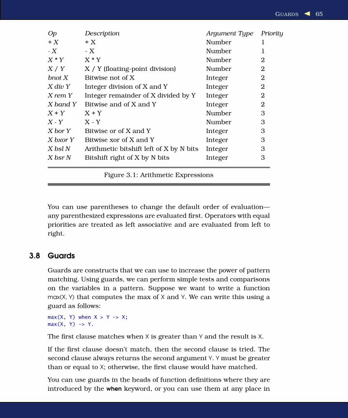
GUARDS 65
Op Description Argument Type Priority
+ X + X Number 1
- X - X Number 1
X * Y X * Y Number 2
X / Y X / Y (floating-point division) Number 2
bnot X Bitwise not of X Integer 2
X div Y Integer division of X and Y Integer 2
X rem Y Integer remainder of X divided by Y Integer 2
X band Y Bitwise and of X and Y Integer 2
X + Y X + Y Number 3
X - Y X - Y Number 3
X bor Y Bitwise or of X and Y Integer 3
X bxor Y Bitwise xor of X and Y Integer 3
X bsl N Arithmetic bitshift left of X by N bits Integer 3
X bsr N Bitshift right of X by N bits Integer 3
Figure 3.1: Arithmetic Expressions
You can use parentheses to change the default order of evaluation—
any parenthesized expressions are evaluated first. Operators with equal
priorities are treated as left associative and are evaluated from left to
right.
3.8 Guards
Guards are constructs that we can use to increase the power of pattern
matching. Using guards, we can perform simple tests and comparisons
on the variables in a pattern. Suppose we want to write a function
max(X, Y) that computes the max of X and Y. We can write this using a
guard as follows:
max(X, Y) when X > Y -> X;
max(X, Y) -> Y.
The first clause matches when X is greater than Y and the result is X.
If the first clause doesn’t match, then the second clause is tried. The
second clause always returns the second argument Y. Y must be greater
than or equal to X; otherwise, the first clause would have matched.
You can use guards in the heads of function definitions where they are
introduced by the when keyword, or you can use them at any place in

GUARDS 66
the language where an expression is allowed. When they are used as
expressions, they evaluate to one of the atoms true or false. If the guard
evaluates to true, we say that the evaluation succeeded; otherwise, it
fails.
Guard Sequences
A guard sequence is either a single guard or a series of guards, sepa-
rated by semicolons (;). The guard sequence G1; G2; ...; Gn is true if at
least one of the guards—G1, G2, ...—evaluates to true.
A guard is a series of guard expressions, separated by commas (,).
The guard GuardExpr1, GuardExpr2, ..., GuardExprN is true if all the guard
expressions—GuardExpr1, GuardExpr2, ...—evaluate to true.
The set of valid guard expressions is a subset of all valid Erlang expres-
sions. The reason for restricting guard expressions to a subset of Erlang
expressions is that we want to guarantee that evaluating a guard ex-
pression is free from side effects. Guards are an extension of pattern
matching, and since pattern matching has no side effects, we don’t
want guard evaluation to have side effects.
In addition, guards cannot be user-defined boolean expressions, since
we want to guarantee that they are side effect free and terminate.
The following syntactic forms are legal in a guard expression:
• The atom true
• Other constants (terms and bound variables); these all evaluate to
false in a guard expression
• Calls to the guard predicates in Figure 3.2, on page 68 and to the
BIFs11 in Figure 3.3, on page 69.
• Term comparisons (Figure 5.3, on page 116)
• Arithmetic expressions (Figure 3.1, on the previous page)
• Booleanexpressions (Section 5.4, Boolean Expressions, on page 103)
• Short-circuit boolean expressions (Section 5.4, Short-Circuit Boo-
lean Expressions, on page 115)
When evaluating a guard expression, the precedence rules described in
Section 5.4, Operator Precedence, on page 112 are used.
11. BIF is short for built-in function See Section 5.1, BIFs, on page 87.

GUARDS 67
Guard Examplesf(X,Y) when is_integer(X), X > Y, Y < 6 -> ...
This means “when X is an integer and X is greater than Y and Y is less
than 6.” The comma, which separates the test in the guard, means
“and.”
is_tuple(T), size(T) =:= 6, abs(element(3, T)) > 5
element(4, X) =:= hd(L)
...
The first line means T is a tuple of six elements, and the absolute value
of the third element of T is greater than 5. The second line means that
element 4 of the tuple X is identical to the head of the list L.
X =:= dog; X =:= cat
is_integer(X), X > Y ; abs(Y) < 23
...
The first guard means X is either a cat or a dog. The second guard
either means that X is an integer and is greater than Y or means that
the absolute value of Y is less than 23.
Here are some examples of guards using short-circuit boolean expres-
sions:
A >= -1.0 andalso A+1 > B
is_atom(L) orelse (is_list(L) andalso length(L) > 2)
Advanced: The reason for allowing boolean expressions in guards is to
make guards syntactically similar to other expressions. The reason for
the orelse and andalso operators is that the boolean operators and/or
were originally defined to evaluate both their arguments. In guards,
there can be differences between (and and andalso) or between (or and
orelse). For example, consider the following two guards:
f(X) when (X == 0) or (1/X > 2) ->
...
g(X) when (X == 0) orelse (1/X > 2) ->
...
The guard in f(X) fails when X is zero but succeeds in g(X).
In practice, few programs use complex guards, and simple (,) guards
suffice for most programs.

GUARDS 68
Predicate Meaning
is_atom(X) X is an atom.
is_binary(X) X is a binary.
is_constant(X) X is a constant.
is_float(X) X is a float.
is_function(X) X is a fun.
is_function(X, N) X is a fun with N arguments.
is_integer(X) X is an integer.
is_list(X) X is a list.
is_number(X) X is an integer or a float.
is_pid(X) X is a process identifier.
is_port(X) X is a port.
is_reference(X) X is a reference.
is_tuple(X) X is a tuple.
is_record(X,Tag) X is a record of type Tag.
is_record(X,Tag,N) X is a record of type Tag and size N.
Figure 3.2: Guard predicates
Use of the True Guard
You might wonder why we need the true guard at all. The reason is
that atom true can be used as a “catchall” guard at the end of an if
expression, like this:
if
Guard -> Expressions;
Guard -> Expressions;
...
true -> Expressions
end
if will be discussed in Section 3.10, if Expressions, on page 73.
Obsolete Guard Functions
If you come across some old Erlang code written a few years ago, the
names of the guard tests were different. Old code used guard tests
called atom(X), constant(X), float(X), integer(X), list(X), number(X), pid(X),
port(X), reference(X), tuple(X), and binary(X). These tests have the same
meaning as the modern tests named is_atom(X)... The use of old names
in modern code is frowned upon.
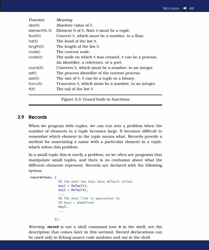
RECORDS 69
Function Meaning
abs(X) Absolute value of X.
element(N, X) Element N of X. Note X must be a tuple.
float(X) Convert X, which must be a number, to a float.
hd(X) The head of the list X.
length(X) The length of the list X.
node() The current node.
node(X) The node on which X was created. X can be a process.
An identifier, a reference, or a port.
round(X) Converts X, which must be a number, to an integer.
self() The process identifier of the current process.
size(X) The size of X. X can be a tuple or a binary.
trunc(X) Truncates X, which must be a number, to an integer.
tl(X) The tail of the list X.
Figure 3.3: Guard built-in functions
3.9 Records
When we program with tuples, we can run into a problem when the
number of elements in a tuple becomes large. It becomes difficult to
remember which element in the tuple means what. Records provide a
method for associating a name with a particular element in a tuple,
which solves this problem.
In a small tuple this is rarely a problem, so we often see programs that
manipulate small tuples, and there is no confusion about what the
different elements represent. Records are declared with the following
syntax:
-record(Name, {
%% the next two keys have default values
key1 = Default1,
key2 = Default2,
...
%% The next line is equivalent to
%% key3 = undefined
key3,
...
}).
Warning: record is not a shell command (use rr in the shell; see the
description that comes later in this section). Record declarations can
be used only in Erlang source code modules and not in the shell.

RECORDS 70
In the previous example, Name is the name of the record. key1, key2,
and so on, are the names of the fields in the record; these must always
be atoms. Each field in a record can have a default value that is used if
no value for this particular field is specified when the record is created.
For example, suppose we want to manipulate a to-do list. We start by
defining a todo record and storing it in a file (record definitions can be
included in Erlang source code files or put in files with the extension
.hrl, which are then included by Erlang source code files12).
Download records.hrl
-record(todo, {status=reminder,who=joe,text}).
Once a record has been defined, instances of the record can be created.
To do this in the shell, we have to read the record definitions into the
shell before we can define a record. We use the shell function rr (short
for read records) to do this:
1> rr("records.hrl").
[todo]
Creating and Updating Records
Now we’re ready to define and manipulate records:
2> X=#todo{}.
#todo{status = reminder,who = joe,text = undefined}
3> X1 = #todo{status=urgent, text="Fix errata in book"}.
#todo{status = urgent,who = joe,text = "Fix errata in book"}
4> X2 = X1#todo{status=done}.
#todo{status = done,who = joe,text = "Fix errata in book"}
In lines 2 and 3 we created new records. The syntax #todo{key1=Val1,
..., keyN=ValN} is used to create a new record of type todo. The keys are
all atoms and must be the same as those used in the record definition.
If a key is omitted, then a default value is assumed for the value that
comes from the value in the record definition.
In line 4 we copied an existing record. The syntax X1#todo{status=done}
means create a copy of the X1 (which must be of type todo), changing
the field value status to done. Remember this is a copy of the original
record; the original record is not changed.
12. This is the only way to ensure that several Erlang modules use the same record
definitions.
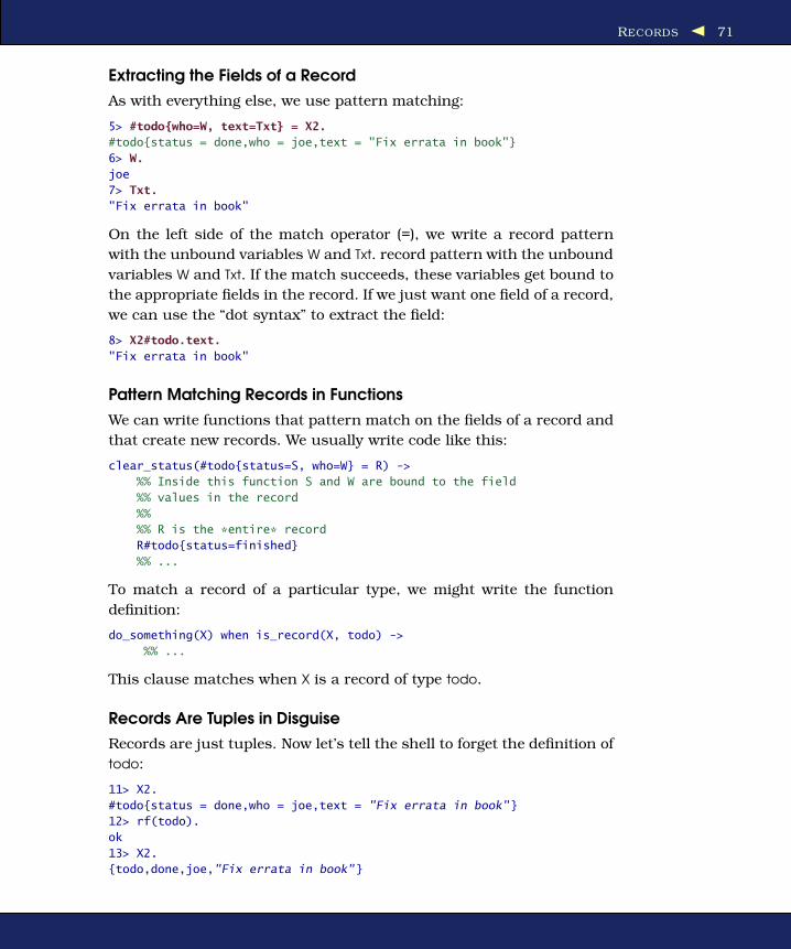
RECORDS 71
Extracting the Fields of a Record
As with everything else, we use pattern matching:
5> #todo{who=W, text=Txt} = X2.
#todo{status = done,who = joe,text = "Fix errata in book"}
6> W.
joe
7> Txt.
"Fix errata in book"
On the left side of the match operator (=), we write a record pattern
with the unbound variables W and Txt. record pattern with the unbound
variables W and Txt. If the match succeeds, these variables get bound to
the appropriate fields in the record. If we just want one field of a record,
we can use the “dot syntax” to extract the field:
8> X2#todo.text.
"Fix errata in book"
Pattern Matching Records in Functions
We can write functions that pattern match on the fields of a record and
that create new records. We usually write code like this:
clear_status(#todo{status=S, who=W} = R) ->
%% Inside this function S and W are bound to the field
%% values in the record
%%
%% R is the *entire* record
R#todo{status=finished}
%% ...
To match a record of a particular type, we might write the function
definition:
do_something(X) when is_record(X, todo) ->
%% ...
This clause matches when X is a record of type todo.
Records Are Tuples in Disguise
Records are just tuples. Now let’s tell the shell to forget the definition of
todo:
11> X2.
#todo{status = done,who = joe,text = "Fix errata in book"}
12> rf(todo).
ok
13> X2.
{todo,done,joe,"Fix errata in book"}
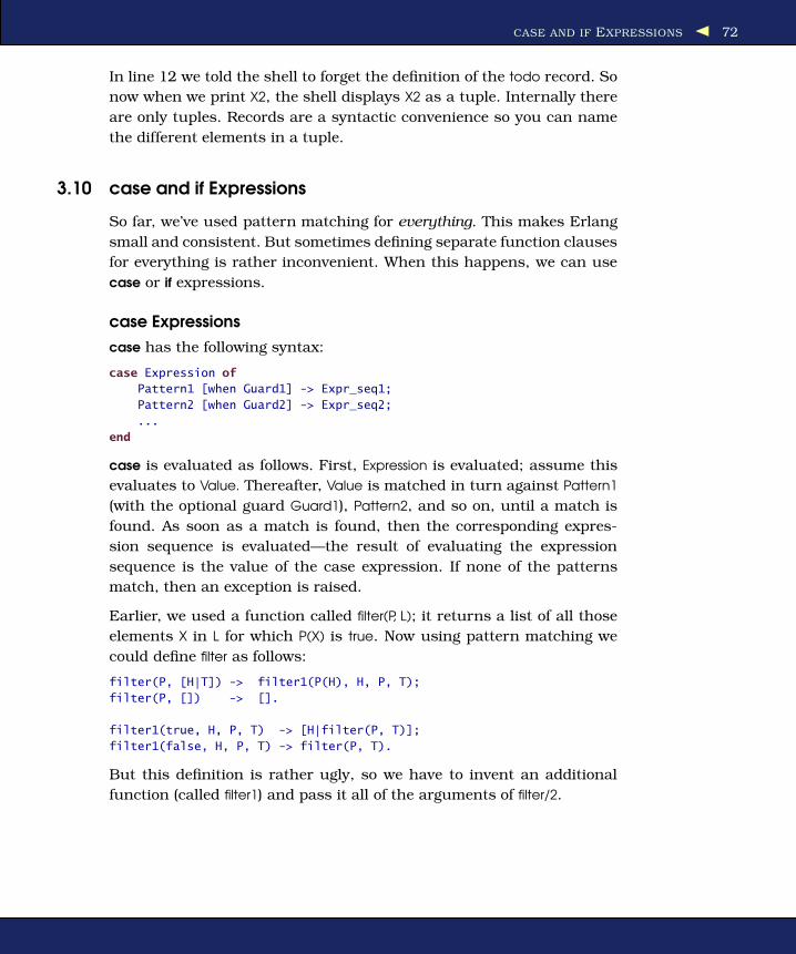
CASE AND IF EXPRESSIONS 72
In line 12 we told the shell to forget the definition of the todo record. So
now when we print X2, the shell displays X2 as a tuple. Internally there
are only tuples. Records are a syntactic convenience so you can name
the different elements in a tuple.
3.10 case and if Expressions
So far, we’ve used pattern matching for everything. This makes Erlang
small and consistent. But sometimes defining separate function clauses
for everything is rather inconvenient. When this happens, we can use
case or if expressions.
case Expressions
case has the following syntax:
case Expression of
Pattern1 [when Guard1] -> Expr_seq1;
Pattern2 [when Guard2] -> Expr_seq2;
...
end
case is evaluated as follows. First, Expression is evaluated; assume this
evaluates to Value. Thereafter, Value is matched in turn against Pattern1
(with the optional guard Guard1), Pattern2, and so on, until a match is
found. As soon as a match is found, then the corresponding expres-
sion sequence is evaluated—the result of evaluating the expression
sequence is the value of the case expression. If none of the patterns
match, then an exception is raised.
Earlier, we used a function called filter(P, L); it returns a list of all those
elements X in L for which P(X) is true. Now using pattern matching we
could define filter as follows:
filter(P, [H|T]) -> filter1(P(H), H, P, T);
filter(P, []) -> [].
filter1(true, H, P, T) -> [H|filter(P, T)];
filter1(false, H, P, T) -> filter(P, T).
But this definition is rather ugly, so we have to invent an additional
function (called filter1) and pass it all of the arguments of filter/2.

BUILDING LISTS IN NATURAL ORDER 73
We can do this in a much clearer manner using the case construct, as
follows:
filter(P, [H|T]) ->
case P(H) of
true -> [H|filter(P, T)];
false -> filter(P, T)
end;
filter(P, []) ->
[].
if Expressions
A second conditional primitive, if, is also provided. Here is the syntax:
if
Guard1 ->
Expr_seq1;
Guard2 ->
Expr_seq2;
...
end
This is evaluated as follows: First Guard1 is evaluated. If this evalu-
ates to true, then the value of if is the value obtained by evaluating the
expression sequence Expr_seq1. If Guard1 does not succeed, Guard2 is
evaluated, and so on, until a guard succeeds. At least one of the guards
in the if expression must evaluate to true; otherwise, an exception will
be raised.
Often the final guard in an if expression is the atom true, which guar-
antees that the last form in the expression will be evaluated if all other
guards have failed.
3.11 Building Lists in Natural Order
The most efficient way to build a list is to add the elements to the head
of an existing list, so we often see code with this kind of pattern:
some_function([H|T], ..., Result, ...) ->
H1 = ... H ...,
some_function(T, ..., [H1|Result], ...);
some_function([], ..., Result, ...) ->
{..., Result, ...}.
This code walks down a list extracting the head of the list H and com-
puting some value based on this function (we can call this H1); it then
adds H1 to the output list Result.
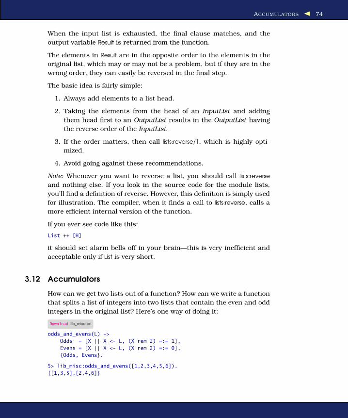
ACCUMULATORS 74
When the input list is exhausted, the final clause matches, and the
output variable Result is returned from the function.
The elements in Result are in the opposite order to the elements in the
original list, which may or may not be a problem, but if they are in the
wrong order, they can easily be reversed in the final step.
The basic idea is fairly simple:
1. Always add elements to a list head.
2. Taking the elements from the head of an InputList and adding
them head first to an OutputList results in the OutputList having
the reverse order of the InputList.
3. If the order matters, then call lists:reverse/1, which is highly opti-
mized.
4. Avoid going against these recommendations.
Note: Whenever you want to reverse a list, you should call lists:reverse
and nothing else. If you look in the source code for the module lists,
you’ll find a definition of reverse. However, this definition is simply used
for illustration. The compiler, when it finds a call to lists:reverse, calls a
more efficient internal version of the function.
If you ever see code like this:
List ++ [H]
it should set alarm bells off in your brain—this is very inefficient and
acceptable only if List is very short.
3.12 Accumulators
How can we get two lists out of a function? How can we write a function
that splits a list of integers into two lists that contain the even and odd
integers in the original list? Here’s one way of doing it:
Download lib_misc.erl
odds_and_evens(L) ->
Odds = [X || X <- L, (X rem 2) =:= 1],
Evens = [X || X <- L, (X rem 2) =:= 0],
{Odds, Evens}.
5> lib_misc:odds_and_evens([1,2,3,4,5,6]).
{[1,3,5],[2,4,6]}
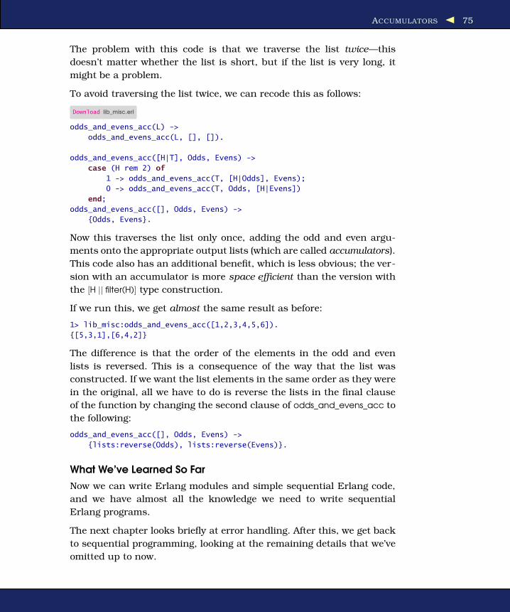
ACCUMULATORS 75
The problem with this code is that we traverse the list twice—this
doesn’t matter whether the list is short, but if the list is very long, it
might be a problem.
To avoid traversing the list twice, we can recode this as follows:
Download lib_misc.erl
odds_and_evens_acc(L) ->
odds_and_evens_acc(L, [], []).
odds_and_evens_acc([H|T], Odds, Evens) ->
case (H rem 2) of
1 -> odds_and_evens_acc(T, [H|Odds], Evens);
0 -> odds_and_evens_acc(T, Odds, [H|Evens])
end;
odds_and_evens_acc([], Odds, Evens) ->
{Odds, Evens}.
Now this traverses the list only once, adding the odd and even argu-
ments onto the appropriate output lists (which are called accumulators).
This code also has an additional benefit, which is less obvious; the ver-
sion with an accumulator is more space efficient than the version with
the [H || filter(H)] type construction.
If we run this, we get almost the same result as before:
1> lib_misc:odds_and_evens_acc([1,2,3,4,5,6]).
{[5,3,1],[6,4,2]}
The difference is that the order of the elements in the odd and even
lists is reversed. This is a consequence of the way that the list was
constructed. If we want the list elements in the same order as they were
in the original, all we have to do is reverse the lists in the final clause
of the function by changing the second clause of odds_and_evens_acc to
the following:
odds_and_evens_acc([], Odds, Evens) ->
{lists:reverse(Odds), lists:reverse(Evens)}.
What We’ve Learned So Far
Now we can write Erlang modules and simple sequential Erlang code,
and we have almost all the knowledge we need to write sequential
Erlang programs.
The next chapter looks briefly at error handling. After this, we get back
to sequential programming, looking at the remaining details that we’ve
omitted up to now.
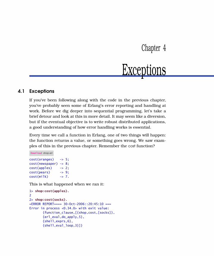
Chapter 4
Exceptions4.1 Exceptions
If you’ve been following along with the code in the previous chapter,
you’ve probably seen some of Erlang’s error reporting and handling at
work. Before we dig deeper into sequential programming, let’s take a
brief detour and look at this in more detail. It may seem like a diversion,
but if the eventual objective is to write robust distributed applications,
a good understanding of how error handling works is essential.
Every time we call a function in Erlang, one of two things will happen:
the function returns a value, or something goes wrong. We saw exam-
ples of this in the previous chapter. Remember the cost function?
Download shop.erl
cost(oranges) -> 5;
cost(newspaper) -> 8;
cost(apples) -> 2;
cost(pears) -> 9;
cost(milk) -> 7.
This is what happened when we ran it:
1> shop:cost(apples).
2
2> shop:cost(socks).
=ERROR REPORT==== 30-Oct-2006::20:45:10 ===
Error in process <0.34.0> with exit value:
{function_clause,[{shop,cost,[socks]},
{erl_eval,do_apply,5},
{shell,exprs,6},
{shell,eval_loop,3}]}

RAISING AN EXCEPTION 77
When we called cost(socks), the function crashed. This happened be-
cause none of the clauses that define the function matched the calling
arguments.
Calling cost(socks) is pure nonsense. There is no sensible value that the
function can return, since the price of socks is undefined. In this case,
instead of returning a value, the system raises an exception—this is the
technical term for “crashing.”
We don’t try to repair the error because this is not possible. We don’t
know what socks cost, so we can’t return a value. It is up to the caller
of cost(socks) to decide what to do if the function crashes.
Exceptions are raised by the system when internal errors are encoun-
tered or explicitly in code by calling throw(Exception), exit(Exception). or
erlang:error(Exception).
Erlang has two methods of catching an exception. One is to enclose
the call to the function, which raised the exception within a try...catch
expression. The other is to enclose the call in a catch expression.
4.2 Raising an Exception
Exceptions are raised automatically when the system encounters an
error. Typical errors are pattern matching errors (no clauses in a func-
tion match) or calling BIFs with incorrectly typed arguments (for exam-
ple, calling atom_to_list with an argument that is an integer).
We can also explicitly generate an error by calling one of the exception
generating BIFs:
exit(Why)
This is used when you really want to terminate the current pro-
cess. If this exception is not caught, the message {’EXIT’,Pid,Why}
will be broadcast to all processes that are linked to the current
process. We’ll say a lot more about this in Section 9.1, Linking
Processes, on page 159, so I won’t dwell on the details here.
throw(Why)
This is used to throw an exception that a caller might want to
catch. In this case we document that our function might throw
this exception. The user of this function has two alternatives: they
can program for the common case and blissfully ignore exceptions,
or they can enclose the call in a try...catch expression and handle
the errors.
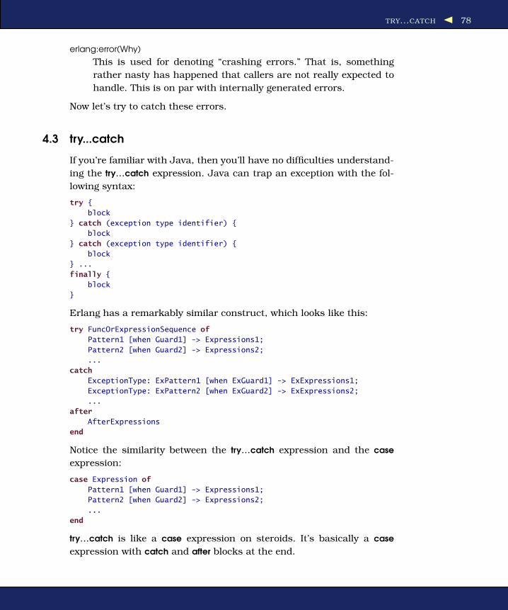
TRY...CATCH 78
erlang:error(Why)
This is used for denoting “crashing errors.” That is, something
rather nasty has happened that callers are not really expected to
handle. This is on par with internally generated errors.
Now let’s try to catch these errors.
4.3 try...catch
If you’re familiar with Java, then you’ll have no difficulties understand-
ing the try...catch expression. Java can trap an exception with the fol-
lowing syntax:
try {
block
} catch (exception type identifier) {
block
} catch (exception type identifier) {
block
} ...
finally {
block
}
Erlang has a remarkably similar construct, which looks like this:
try FuncOrExpressionSequence of
Pattern1 [when Guard1] -> Expressions1;
Pattern2 [when Guard2] -> Expressions2;
...
catch
ExceptionType: ExPattern1 [when ExGuard1] -> ExExpressions1;
ExceptionType: ExPattern2 [when ExGuard2] -> ExExpressions2;
...
after
AfterExpressions
end
Notice the similarity between the try...catch expression and the case
expression:
case Expression of
Pattern1 [when Guard1] -> Expressions1;
Pattern2 [when Guard2] -> Expressions2;
...
end
try...catch is like a case expression on steroids. It’s basically a case
expression with catch and after blocks at the end.

TRY...CATCH 79
try...catch Has a Value
Remember, everything in Erlang is an expression, and all expres-sions have values. This means the expression try...end also has avalue. So, we might write something like this:
f(...) ->...X = try ... end,Y = g(X),...
More often, we don’t need the value of the try...catch expres-sion. So, we just write this:
f(...) ->...try ... end,......
try...catch works as follows: First FuncOrExpessionSeq is evaluated. If this
finishes without raising an exception, then the return value of the func-
tion is pattern matched against the patterns Pattern1 (with optional
guard Guard1), Pattern2, and so on, until a match is found. If a match is
found, then the value of the entire try...catch is found by evaluating the
expression sequence following the matching pattern.
If an exception is raised within FuncOrExpressionSeq, then the catch pat-
terns ExPattern1, and so on, are matched to find which sequence of
expressions should be evaluated. ExceptionType is an atom (one of throw,
exit, or error) that tells us how the exception was generated. If Exception-
Type is omitted, then the value defaults to throw.
Note: Internal errors that are detected by the Erlang runtime system
always have the tag error.
The code following the after keyword is used for cleaning up after FuncOr-
ExpressionSeq. This code is guaranteed to be executed, even if an excep-
tion is raised. The code in the after section is run immediately after
any code in Expressions in the try or catch section of the expression. The
return value of AfterExpressions is lost.
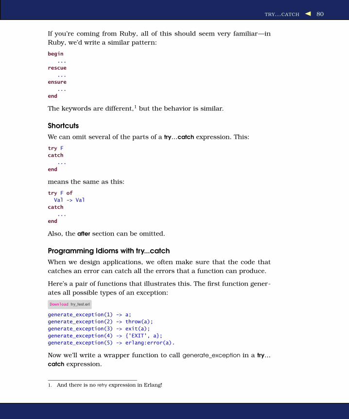
TRY...CATCH 80
If you’re coming from Ruby, all of this should seem very familiar—in
Ruby, we’d write a similar pattern:
begin
...
rescue
...
ensure
...
end
The keywords are different,1 but the behavior is similar.
Shortcuts
We can omit several of the parts of a try...catch expression. This:
try F
catch
...
end
means the same as this:
try F of
Val -> Val
catch
...
end
Also, the after section can be omitted.
Programming Idioms with try...catch
When we design applications, we often make sure that the code that
catches an error can catch all the errors that a function can produce.
Here’s a pair of functions that illustrates this. The first function gener-
ates all possible types of an exception:
Download try_test.erl
generate_exception(1) -> a;
generate_exception(2) -> throw(a);
generate_exception(3) -> exit(a);
generate_exception(4) -> {'EXIT', a};
generate_exception(5) -> erlang:error(a).
Now we’ll write a wrapper function to call generate_exception in a try...
catch expression.
1. And there is no retry expression in Erlang!

CATCH 81
Download try_test.erl
demo1() ->
[catcher(I) || I <- [1,2,3,4,5]].
catcher(N) ->
try generate_exception(N) of
Val -> {N, normal, Val}
catch
throw:X -> {N, caught, thrown, X};
exit:X -> {N, caught, exited, X};
error:X -> {N, caught, error, X}
end.
Running this we obtain the following:
> try_test:demo1().
[{1,normal,a},
{2,caught,thrown,a},
{3,caught,exited,a},
{4,normal,{'EXIT',a}},
{5,caught,error,a}]
This shows that we can trap and distinguish all the forms of exception
that a function can raise.
4.4 catch
The other way to trap an exception is to use the primitive catch. When
you catch an exception, it is converted into a tuple that describes the
error. To demonstrate this, we can call generate_exception within a catch
expression:
Download try_test.erl
demo2() ->
[{I, (catch generate_exception(I))} || I <- [1,2,3,4,5]].
Running this we obtain the following:
2> try_test:demo2().
[{1,a},
{2,a},
{3,{'EXIT',a}},
{4,{'EXIT',a}},
{5,{'EXIT',{a,[{try_test,generate_exception,1},
{try_test,'-demo2/0-fun-0-',1},
{lists,map,2},
{lists,map,2},
{erl_eval,do_apply,5},
{shell,exprs,6},
{shell,eval_loop,3}]}}}]

IMPROVING ERROR MESSAGES 82
If you compare this with the output from the try...catch section, you’ll
see that we lose a lot of precision in analyzing the cause of the problem.
4.5 Improving Error Messages
One use of erlang:error is to improve the quality of error messages. If we
call math:sqrt(X) with a negative argument, we’ll see the following:
1> math:sqrt(-1).
** exited: {badarith,[{math,sqrt,[-1]},
{erl_eval,do_apply,5},
{shell,exprs,6},
{shell,eval_loop,3}]} **
We can write a wrapper for this, which improves the error message:
Download lib_misc.erl
sqrt(X) when X < 0 ->
erlang:error({squareRootNegativeArgument, X});
sqrt(X) ->
math:sqrt(X).
2> lib_misc:sqrt(-1).
** exited: {{squareRootNegativeArgument,-1},
[{lib_misc,sqrt,1},
{erl_eval,do_apply,5},
{shell,exprs,6},
{shell,eval_loop,3}]} **
4.6 Programming Style with try...catch
How do you handle errors in practice? It depends....
Code Where Error Returns Are Common
If your function does not really have a “common case,” you should prob-
ably return something like {ok, Value} or {error, Reason}, but remember
that this forces all callers to do something with the return value. You
then have to choose between two alternatives; you either write this:
...
case f(X) of
{ok, Val} ->
do_some_thing_with(Val);
{error, Why} ->
%% ... do something with the error ...
end,
...
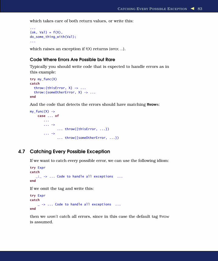
CATCHING EVERY POSSIBLE EXCEPTION 83
which takes care of both return values, or write this:
...
{ok, Val} = f(X),
do_some_thing_with(Val);
...
which raises an exception if f(X) returns {error, ...}.
Code Where Errors Are Possible but Rare
Typically you should write code that is expected to handle errors as in
this example:
try my_func(X)
catch
throw:{thisError, X} -> ...
throw:{someOtherError, X} -> ...
end
And the code that detects the errors should have matching throws:
my_func(X) ->
case ... of
...
... ->
... throw({thisError, ...})
... ->
... throw({someOtherError, ...})
4.7 Catching Every Possible Exception
If we want to catch every possible error, we can use the following idiom:
try Expr
catch
_:_ -> ... Code to handle all exceptions ...
end
If we omit the tag and write this:
try Expr
catch
_ -> ... Code to handle all exceptions ...
end
then we won’t catch all errors, since in this case the default tag throw
is assumed.
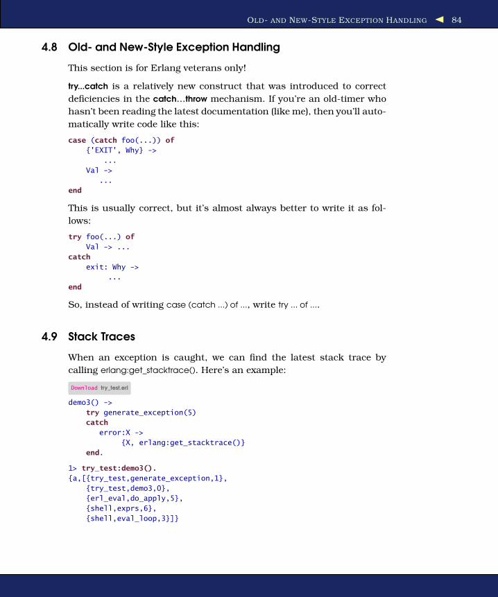
OLD- AND NEW-STYLE EXCEPTION HANDLING 84
4.8 Old- and New-Style Exception Handling
This section is for Erlang veterans only!
try...catch is a relatively new construct that was introduced to correct
deficiencies in the catch...throw mechanism. If you’re an old-timer who
hasn’t been reading the latest documentation (like me), then you’ll auto-
matically write code like this:
case (catch foo(...)) of
{'EXIT', Why} ->
...
Val ->
...
end
This is usually correct, but it’s almost always better to write it as fol-
lows:
try foo(...) of
Val -> ...
catch
exit: Why ->
...
end
So, instead of writing case (catch ...) of ..., write try ... of ....
4.9 Stack Traces
When an exception is caught, we can find the latest stack trace by
calling erlang:get_stacktrace(). Here’s an example:
Download try_test.erl
demo3() ->
try generate_exception(5)
catch
error:X ->
{X, erlang:get_stacktrace()}
end.
1> try_test:demo3().
{a,[{try_test,generate_exception,1},
{try_test,demo3,0},
{erl_eval,do_apply,5},
{shell,exprs,6},
{shell,eval_loop,3}]}

STACK TRACES 85
The stack trace contains a list of the functions on the stack to which
the current function will return if it returns. It’s almost the same as
the sequence of calls that got us to the current function, but any tail-
recursive function calls2 will be missing from the trace.
From the point of view of debugging our program, only the first few lines
of the stack trace are interesting. The earlier stack trace tells us that the
system crashed while evaluating the function generate_exception with
one argument in the module try_test. try_test:generate_exception/1 was
probably called by try_test:demo3() (we can’t be sure about this because
try_test:demo3() might have called some other function that made a tail-
recursive call to try_test:generate_exception/1, in which case the stack
trace won’t have any record of the intermediate function).
2. See Section 8.9, A Word About Tail Recursion, on page 156.

Chapter 5
Advanced SequentialProgramming
By now we’re well on our way to understanding sequential Erlang.
Chapter 3, Sequential Programming, dealt with the basics of writing
functions. This chapter covers the following:
• BIFs: Short for built-in functions, BIFs are functions that are part of
the Erlang language. They look as if they might have been written
in Erlang, but in fact they are implemented as primitive operations
in the Erlang virtual machine.
• Binaries: This is a data type that we use to store raw chunks of
memory in an efficient manner.
• The bit syntax: This is a pattern matching syntax used for packing
and unpacking bit fields from binaries.
• Miscellaneous topics: This deals with a small number of topics
needed to complete our mastery of sequential Erlang.
Once you have mastered this chapter, you’ll know pretty much all there
is to know about sequential Erlang, and you’ll be ready to dive into the
mysteries of concurrent programming.

BIFS 87
5.1 BIFs
BIFs are functions that are built into Erlang. They usually do tasks that
are impossible to program in Erlang. For example, it’s impossible to
turn a list into a tuple or to find the current time and date. To perform
such an operation, we call a BIF.
For example, the BIF tuple_to_list/1 converts a tuple to a list, and time/0
returns the current time of day in hours, minutes, and seconds:
1> tuple_to_list({12,cat,"hello"}).
[12,cat,"hello"]
2> time().
{20,0,3}
All the BIFs behave as if they belong to the module erlang, though the
most common BIFs (such as tuple_to_list) are autoimported, so we can
call it by writing tuple_to_list(...) instead of erlang:tuple_to_list(...).
You’ll find a full list of all BIFs in the erlang manual page in your Erlang
distribution or online at http://www.erlang.org/doc/man/erlang.html.
5.2 Binaries
Use a data structure called a binary to store large quantities of raw
data. Binaries store data in a much more space-efficient manner than
in lists or tuples, and the runtime system is optimized for the efficient
input and output of binaries.
Binaries are written and printed as sequences of integers or strings,
enclosed in double less-than and greater-than brackets. For example:
1> <<5,10,20>>.
<<5,10,20>>
2> <<"hello">>.
<<"hello">>
When you use integers in a binary, each must be in the range 0 to 255.
The binary <<"cat">> is shorthand for <<99,97,116>>; that is, the binary
made up from the ASCII character codes of the characters in the string.
As with strings, if the content of a binary is a printable string, then the
shell will print the binary as a string; otherwise, it will be printed as a
sequence of integers.
We can build a binary and extract the elements of a binary using a
BIF, or we can use the bit syntax (see Section 5.3, The Bit Syntax, on
page 89). In this section, I’ll talk only about the BIFs.

BINARIES 88
@spec func(Arg1,..., Argn) -> Val
What’s all this @spec business?
It’s an example of the Erlang type notation, a docu-mentation convention that the Erlang community uses fordescribing (among other things) the argument and returntypes of a function. It should be fairly self-explanatory, butfor those who want the full details, turn to Appendix A, onpage 390.
BIFs That Manipulate Binaries
The following BIFs manipulate binaries:
@spec list_to_binary(IoList) -> binary()
list_to_binary returns a binary constructed from the integers and
binaries in IoList. Here IoList is a list, whose elements are integers in
0..255, binaries, or IoLists:
1> Bin1 = <<1,2,3>>.
<<1,2,3>>
2> Bin2 = <<4,5>>.
<<4,5>>
3> Bin3 = <<6>>.
<<6>>
4> list_to_binary([Bin1,1,[2,3,Bin2],4|Bin3]).
<<1,2,3,1,2,3,4,5,4,6>>
@spec split_binary(Bin, Pos) -> {Bin1, Bin2}
This splits the binary Bin into two parts at position Pos:
1> split_binary(<<1,2,3,4,5,6,7,8,9,10>>, 3).
{<<1,2,3>>,<<4,5,6,7,8,9,10>>}
@spec term_to_binary(Term) -> Bin
This converts any Erlang term into a binary.
The binary produced by term_to_binary is stored in the so-called
external term format. Terms that have been converted to binaries
by using term_to_binary can be stored in files, sent in messages
over a network, and so on, and the original term from which they
were made can be reconstructed later. This is extremely useful for
storing complex data structures in files or sending complex data
structures to remote machines.
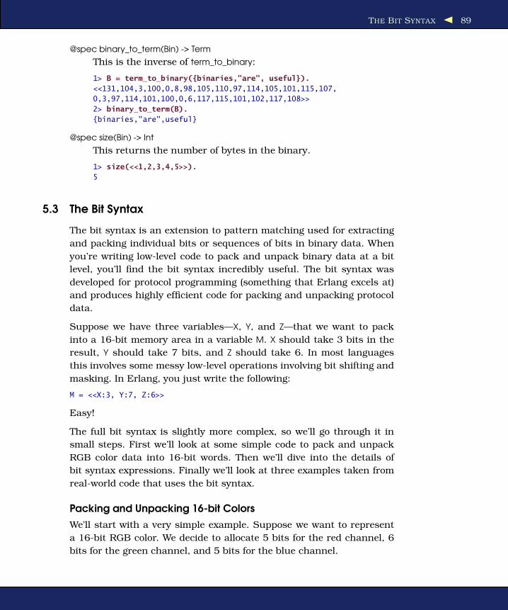
THE BIT SYNTAX 89
@spec binary_to_term(Bin) -> Term
This is the inverse of term_to_binary:
1> B = term_to_binary({binaries,"are", useful}).
<<131,104,3,100,0,8,98,105,110,97,114,105,101,115,107,
0,3,97,114,101,100,0,6,117,115,101,102,117,108>>
2> binary_to_term(B).
{binaries,"are",useful}
@spec size(Bin) -> Int
This returns the number of bytes in the binary.
1> size(<<1,2,3,4,5>>).
5
5.3 The Bit Syntax
The bit syntax is an extension to pattern matching used for extracting
and packing individual bits or sequences of bits in binary data. When
you’re writing low-level code to pack and unpack binary data at a bit
level, you’ll find the bit syntax incredibly useful. The bit syntax was
developed for protocol programming (something that Erlang excels at)
and produces highly efficient code for packing and unpacking protocol
data.
Suppose we have three variables—X, Y, and Z—that we want to pack
into a 16-bit memory area in a variable M. X should take 3 bits in the
result, Y should take 7 bits, and Z should take 6. In most languages
this involves some messy low-level operations involving bit shifting and
masking. In Erlang, you just write the following:
M = <<X:3, Y:7, Z:6>>
Easy!
The full bit syntax is slightly more complex, so we’ll go through it in
small steps. First we’ll look at some simple code to pack and unpack
RGB color data into 16-bit words. Then we’ll dive into the details of
bit syntax expressions. Finally we’ll look at three examples taken from
real-world code that uses the bit syntax.
Packing and Unpacking 16-bit Colors
We’ll start with a very simple example. Suppose we want to represent
a 16-bit RGB color. We decide to allocate 5 bits for the red channel, 6
bits for the green channel, and 5 bits for the blue channel.

THE BIT SYNTAX 90
(We use one more bit for the green channel because the human eye is
more sensitive to green light.)
We can create a 16-bit memory area Mem containing a single RGB
triplet as follows:
1> Red = 2.
2
2> Green = 61.
61
3> Blue = 20.
20
4> Mem = <<Red:5, Green:6, Blue:5>>.
<<23,180>>
Note in line 4 we created a 2-byte binary containing a 16-bit quantity.
The shell prints this as <<23,180>>.
To pack the memory, we just wrote the expression <<Red:5, Green:6,
Blue:5>>.
To unpack the word, we write a pattern:
5> <<R1:5, G1:6, B1:5>> = Mem.
<<23,180>>
6> R1.
2
7> G1.
61
8> B1.
20
Bit Syntax Expressions
Bit syntax expressions are of the following form:
<<>>
<<E1, E2, ..., En>>
Each element Ei specifies a single segment of the binary. Each element
Ei can have one of four possible forms:
Ei = Value |
Value:Size |
Value/TypeSpecifierList |
Value:Size/TypeSpecifierList
Whatever form you use, the total number of bits in the binary must be
evenly divisible by 8. (This is because binaries contain bytes that take
up 8 bits each, so there is no way of representing sequences of bits
whose length is not a multiple of 8.)

THE BIT SYNTAX 91
When you construct a binary, Value must be a bound variable, a literal
string, or an expression that evaluates to an integer, a float, or a binary.
When used in a pattern matching operation, Value can be a bound or
unbound variable, integer, literal string, float, or binary.
Size must be an expression that evaluates to an integer. In pattern
matching, Size must be an integer or a bound variable whose value is
an integer. Size cannot be an unbound variable.
The value of Size specifies the size of the segment in units (we discuss
this later). The default value depends on the type (see below). For an
integer it is 8, for a float it is 64, and for a binary it is the size of the
binary. In pattern matching, this default value is valid only for the very
last element. All other binary elements in the matching must have a
size specification.
TypeSpecifierList is a hyphen-separated list of items of the form End-Sign-
Type-Unit. Any of the previous items can be omitted, and the items can
occur in any order. If an item is omitted, then a default value for the
item is used.
The items in the specifier list can have the following values:
@type End = big | little | native
(@type is also part of the Erlang type notation given in Appendix A).
This specifies the endianess of the machine. native is determined
at runtime, depending upon the CPU of your machine. The default
is big. The only significance of this has to do with packing and
unpacking integers from binaries. When packing and unpacking
integers from binaries on different endian machines, you should
take care to use the correct endianess.
Tip: In the rare case that you really need to understand what’s
going on here, some experimentation may be necessary. To assure
yourself that you are doing the right thing, try the following shell
command:
1> {<<16#12345678:32/big>>,<<16#12345678:32/little>>,
<<16#12345678:32/native>>,<<16#12345678:32>>}.
{<<18,52,86,120>>,<<120,86,52,18>>,
<<120,86,52,18>>,<<18,52,86,120>>}
The output shows you exactly how integers are packed in a binary
using the bit syntax.

THE BIT SYNTAX 92
In case you’re worried, term_to_binary and binary_to_term “do the
right thing” when packing and unpacking integers. So, you can,
for example, create a tuple containing integers on a big-endian
machine. Then use term_to_binary to convert the term to a binary
and send this to a little-endian machine. On the little-endian, you
do binary_to_term, and all the integers in the tuple will have the
correct values.
@type Sign = signed | unsigned
This parameter is used only in pattern matching. The default is
unsigned.
@type Type = integer | float | binary
The default is integer.
@type Unit = 1 | 2 | ... 255
The total size of the segment is Size x Unit bits long. The total seg-
ment size must be greater than or equal to zero and must be a
multiple of 8.
The default value of Unit depends upon Type and is 1 if Type is
integer or float and 8 if Type is a binary.
If you’ve found the bit syntax description a bit daunting, don’t panic.
Getting the bit syntax patterns right is pretty tricky. The best way to
approach this is to experiment in the shell with the patterns you need
until you get it right and then cut and paste the result into your pro-
gram. That’s how I do it.
Advanced Bit Syntax Examples
Learning the bit syntax is difficult, but the benefits are enormous. This
section has three examples from real life. All the code here is cut and
paste from real-world programs. The examples are as follows:
• Finding the synchronization frame in MPEG data
• Unpacking COFF data
• Unpacking the header in an IPv4 datagram
Finding the Synchronization Frame in MPEG Data
Suppose we want to write a program that manipulates MPEG audio
data. We might want to write a streaming media server in Erlang or
extract the data tags that describe the content of an MPEG audio
stream. To do this, we need to identify and synchronize with the data
frames in an MPEG stream.

THE BIT SYNTAX 93
MPEG audio data is made up from a number of frames. Each frame has
its own header followed by audio information—there is no file header,
and in principle, you can cut an MPEG file into pieces and play any
of the pieces. Any software that reads an MPEG stream is supposed to
find the header frames and thereafter synchronize the MPEG data.
An MPEG header starts with an 11-bit frame sync consisting of eleven
consecutive 1 bits followed by information that describes the data that
follows:
AAAAAAAA AAABBCCD EEEEFFGH IIJJKLMM
AAAAAAAAAAA The sync word (11 bits, all ones)
BB 2 bits is the MPEG Audio version ID
CC 2 bits is the layer description
D 1 bit, a protection bit
And so on...
The exact details of these bits need not concern us here. Basically, given
knowledge of the values of A to M, we can compute the total length of
an MPEG frame.
To find the sync point, we first assume that we are correctly positioned
at the start of an MPEG frame. We use the information we find at that
position to compute the length of the frame. We might be pointing at
nonsense, in which case the length of the frame will be totally wrong.
Assuming that we are at the start of a frame and given the length of the
frame, then we can skip to the start of the next frame and see whether
this is another MPEG header frame.
To find the sync point, we first assume that we are correctly positioned
at the start of an MPEG header. We then try to compute the length of
the frame. Then one of the following can happen:
• Our assumption was correct, so when we skip forward by the
length of the frame, we will find another MPEG header.
• Our assumption was incorrect; either we are not positioned at a
sequence of 11 consecutive 1 bits that marks the start of a header
or the format of the word is incorrect so that we cannot compute
the length of the frame.
• Our assumption was incorrect, but we are positioned at a couple of
bytes of music data that happen to look like the start of a header.
In this case, we can compute a frame length, but when we skip
forward by this length, we cannot find a new header.

THE BIT SYNTAX 94
To be really sure, we look for three consecutive headers. The synchro-
nization routine is as follows:
Download mp3_sync.erl
find_sync(Bin, N) ->
case is_header(N, Bin) of
{ok, Len1, _} ->
case is_header(N + Len1, Bin) of
{ok, Len2, _} ->
case is_header(N + Len1 + Len2, Bin) of
{ok, _, _} ->
{ok, N};
error ->
find_sync(Bin, N+1)
end;
error ->
find_sync(Bin, N+1)
end;
error ->
find_sync(Bin, N+1)
end.
find_sync tries to find three consecutive MPEG header frames. If byte N
in Bin is the start of a header frame, then is_header(N, Bin) will return {ok,
Length, Info}. If is_header returns error, then N cannot point to the start of
a correct frame. We can do a quick test in the shell to make sure this
works:
1> {ok, Bin} = file:read_file("/home/joe/music/mymusic.mp3").
{ok,<<73,68,51,3,0,0,0,0,33,22,84,73,84,50,0,0,0,28, ...>>
2> mp3_sync:find_sync(Bin, 1).
{ok,4256}
This uses file:read_file to read the entire file into a binary (see Sec-
tion 13.2, Reading the Entire File into a Binary, on page 231). Now for
is_header:
Download mp3_sync.erl
is_header(N, Bin) ->
unpack_header(get_word(N, Bin)).
get_word(N, Bin) ->
{_,<<C:4/binary,_/binary>>} = split_binary(Bin, N),
C.
unpack_header(X) ->
try decode_header(X)
catch
_:_ -> error
end.
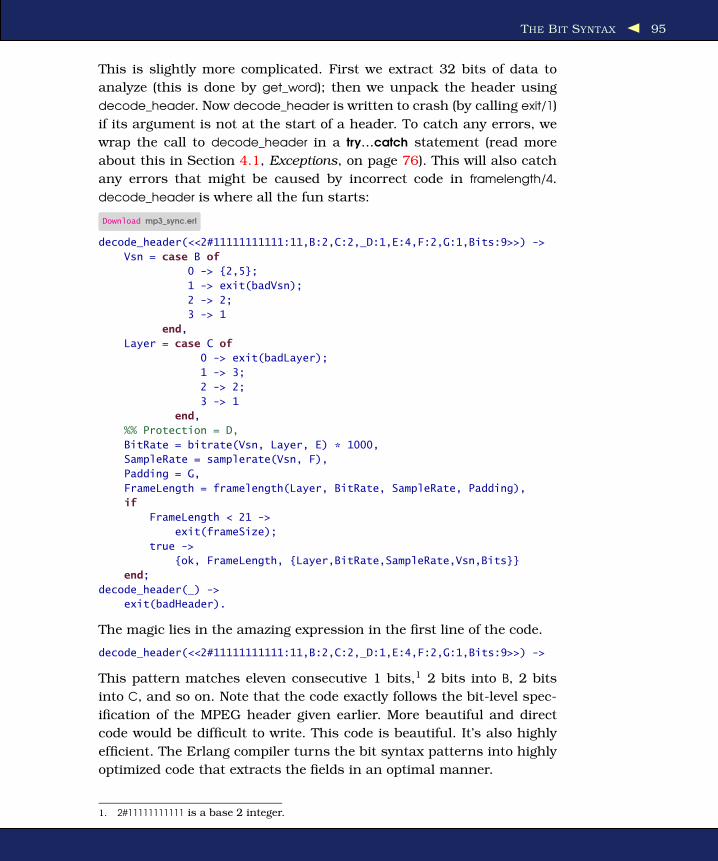
THE BIT SYNTAX 95
This is slightly more complicated. First we extract 32 bits of data to
analyze (this is done by get_word); then we unpack the header using
decode_header. Now decode_header is written to crash (by calling exit/1)
if its argument is not at the start of a header. To catch any errors, we
wrap the call to decode_header in a try...catch statement (read more
about this in Section 4.1, Exceptions, on page 76). This will also catch
any errors that might be caused by incorrect code in framelength/4.
decode_header is where all the fun starts:
Download mp3_sync.erl
decode_header(<<2#11111111111:11,B:2,C:2,_D:1,E:4,F:2,G:1,Bits:9>>) ->
Vsn = case B of
0 -> {2,5};
1 -> exit(badVsn);
2 -> 2;
3 -> 1
end,
Layer = case C of
0 -> exit(badLayer);
1 -> 3;
2 -> 2;
3 -> 1
end,
%% Protection = D,
BitRate = bitrate(Vsn, Layer, E) * 1000,
SampleRate = samplerate(Vsn, F),
Padding = G,
FrameLength = framelength(Layer, BitRate, SampleRate, Padding),
if
FrameLength < 21 ->
exit(frameSize);
true ->
{ok, FrameLength, {Layer,BitRate,SampleRate,Vsn,Bits}}
end;
decode_header(_) ->
exit(badHeader).
The magic lies in the amazing expression in the first line of the code.
decode_header(<<2#11111111111:11,B:2,C:2,_D:1,E:4,F:2,G:1,Bits:9>>) ->
This pattern matches eleven consecutive 1 bits,1 2 bits into B, 2 bits
into C, and so on. Note that the code exactly follows the bit-level spec-
ification of the MPEG header given earlier. More beautiful and direct
code would be difficult to write. This code is beautiful. It’s also highly
efficient. The Erlang compiler turns the bit syntax patterns into highly
optimized code that extracts the fields in an optimal manner.
1. 2#11111111111 is a base 2 integer.

THE BIT SYNTAX 96
Unpacking COFF Data
A few years ago I decided to write a program to make stand-alone Erlang
programs that would run on Windows—I wanted to build a Windows
executable on any machine that could run Erlang. Doing this involved
understanding and manipulating the Microsoft Common Object File
Format (COFF) formatted files. Finding out the details of COFF was
pretty tricky, but various APIs for C++ programs were documented. The
C++ programs used the type declarations DWORD, LONG, WORD, and
BYTE (these type declarations will be familiar to programmers who have
programmed Windows internals).
The data structures involved were documented, but only from a C or
C++ programmer’s point of view. The following is a typical C typedef:
typedef struct _IMAGE_RESOURCE_DIRECTORY {
DWORD Characteristics;
DWORD TimeDateStamp;
WORD MajorVersion;
WORD MinorVersion;
WORD NumberOfNamedEntries;
WORD NumberOfIdEntries;
} IMAGE_RESOURCE_DIRECTORY, *PIMAGE_RESOURCE_DIRECTORY;
To write my Erlang program, I first defined four macros that must be
included in the Erlang source code file:
-define(DWORD, 32/unsigned-little-integer).
-define(LONG, 32/unsigned-little-integer).
-define(WORD, 16/unsigned-little-integer).
-define(BYTE, 8/unsigned-little-integer).
Note: Macros are explained in Section 5.4, Macros, on page 108. To
expand these macros, we use the syntax ?DWORD, ?LONG, and so on.
For example, the macro ?DWORD expands to the literal text 32/unsigned-
little-integer.
These macros deliberately have the same names as their C counter-
parts. Armed with these macros, I could easily write some code to
unpack image resource data into a binary:
unpack_image_resource_directory(Dir) ->
<<Characteristics : ?DWORD,
TimeDateStamp : ?DWORD,
MajorVersion : ?WORD,
MinorVersion : ?WORD,
NumberOfNamedEntries : ?WORD,
NumberOfIdEntries : ?WORD, _/binary>> = Dir,
...

THE BIT SYNTAX 97
If you compare the C and Erlang code, you’ll see that they are pretty
similar. So by taking care with the names of the macros and the layout
of the Erlang code, we can minimize the semantic gap between the C
code and the Erlang code, something that makes our program easier to
understand and less likely to have errors.
The next step was to unpack data in Characteristics, and so on.
Characteristics is a 32-bit word consisting of a collection of flags. Unpack-
ing these using the bit syntax is extremely easy; we just write code like
this:
<<ImageFileRelocsStripped:1, ImageFileExecutableImage:1, ...>> =
<<Characteristics:32>>
The code <<Characteristics:32>> converted Characteristics, which was an
integer, into a binary of size 32 bits. Then the following code unpacked
the required bits into the variables ImageFileRelocsStripped, ImageFileExe-
cutableImage, and so on:
<<ImageFileRelocsStripped:1, ImageFileExecutableImage:1, ...>> = ...
Again, I kept the same names as in the Windows API to keep the seman-
tic gap between the specification and the Erlang program to a mini-
mum.
Using these macros made unpacking data in the COFF format—well,
I can’t really use the word easy—but at least it was possible, and the
code was reasonably understandable.
Unpacking the Header in an IPv4 Datagram
This example illustrates parsing an Internet Protocol version 4 (IPv4)
datagram in a single pattern-matching operation:
-define(IP_VERSION, 4).
-define(IP_MIN_HDR_LEN, 5).
...
DgramSize = size(Dgram),
case Dgram of
<<?IP_VERSION:4, HLen:4, SrvcType:8, TotLen:16,
ID:16, Flgs:3, FragOff:13,
TTL:8, Proto:8, HdrChkSum:16,
SrcIP:32,
DestIP:32, RestDgram/binary>> when HLen >= 5, 4*HLen =< DgramSize ->
OptsLen = 4*(HLen - ?IP_MIN_HDR_LEN),
<<Opts:OptsLen/binary,Data/binary>> = RestDgram,
...

MISCELLANEOUS SHORT TOPICS 98
This code matches an IP datagram in a single pattern-matching expres-
sion. The pattern is complex, spreading over three lines, and illustrates
how data that does not fall on byte boundaries can easily be extracted
(for example, the Flgs and FragOff fields that are 3 and 13 bits long,
respectively). Having pattern matched the IP datagram, the header and
data part of the datagram are extracted in a second pattern matching
operation.
5.4 Miscellaneous Short Topics
We’ve now covered all the major topics in sequential Erlang. What
remains are a number of small odds and ends that you have to know
but that don’t fit into any of the other topics. There’s no particular log-
ical order to these. The topics covered are as follows:
• apply: How to compute the value of a function from its name and
arguments, when the function and module name are computed
dynamically.
• Attributes: The syntax and meaning of the Erlang module attri-
butes.
• Block expressions: Expressions using begin and end.
• Boolean expressions: All the boolean expressions.
• Character set: Which character set does Erlang use?
• Comments: Syntax of comments.
• epp: The Erlang preprocessor.
• Escape sequences: The syntax of the escape sequences used in
strings and atoms.
• Expressions and expression sequences: What exactly is an expres-
sion?
• Function references: How to refer to functions.
• Include files: How to include files at compile time.
• List operations: ++ and - -.
• Macros: The Erlang macro processor.
• Match operator in patterns: How the match operator = can be used
in patterns.
• Numbers: The syntax of numbers.
• Operator precedence: The priority and associativity of all the Erlang
operators.
• The process dictionary: Each Erlang process has a local area of
destructive storage, which can be useful sometimes.

MISCELLANEOUS SHORT TOPICS 99
• References: References are unique symbols.
• Short-circuit boolean expressions: Boolean expressions that are not
fully evaluated.
• Term comparisons: All the term comparison operators and the lex-
ical ordering of terms.
• Underscore variables: Variables that the compiler treats in a spe-
cial way.
apply
The BIF apply(Mod, Func, [Arg1, Arg2, ..., ArgN]) applies the function Func
in the module Mod to the arguments Arg1, Arg2, ... ArgN. It is equivalent
to calling this:
Mod:Func(Arg1, Arg2, ..., ArgN)
apply lets you call a function in a module, passing it arguments. What
makes it different from calling the function directly is that the module
name and/or the function name can be computed dynamically.
All the Erlang BIFs can be called using apply by assuming that they
belong to the module erlang. So, to build a dynamic call to a BIF, we
might write the following:
1> apply(erlang, atom_to_list, [hello]).
"hello"
Warning: The use of apply should be avoided if possible. When the num-
ber of arguments to a function is known in advance, it is much better
to use a call of the form M:F(Arg1, Arg2, ... ArgN) than apply. When calls
to functions are built using apply, many analysis tools cannot work out
what is happening, and certain compiler optimizations cannot be made.
So, use apply sparingly and only when absolutely needed.
Attributes
Module attributes have the syntax -AtomTag(...)2 and are used to define
certain properties of a file. There are two types of module attributes:
predefined and user-defined.
Predefined Module Attributes
The following module attributes have predefined meanings and must
be placed before any function definitions.
2. -record(...) and -include(...) have a similar syntax but are not considered module
attributes.

MISCELLANEOUS SHORT TOPICS 100
-module(modname).
The module declaration. modname must be an atom. This attribute
must be the first attribute in the file. Conventionally the code for
modname should be stored in a file called modname.erl. If you do
not do this, then automatic code loading will not work correctly;
see Section E.4, Dynamic Code Loading, on page 435 for more
details.
-import(Mod, [Name1/Arity1, Name2/Arity2,...]).
Specify that the function Name1 with Arity1 arguments is to be
imported from the module Mod.
Once a function has been imported from a module, then calling
the function can be achieved without specifying the module name.
For example:
-module(abc).
-import(lists, [map/2]).
f(L) ->
L1 = map(fun(X) -> 2*X end, L),
lists:sum(L1)
The call to map needs no qualifying module name, whereas to call
sum we need to include the module name in the function call.
-export([Name1/Arity1, Name2/Arity2, ...]).
Export the functions Name1/Arity1, Name2/Arity2, and so on, from
the current module. Note that only exported functions can be
called from outside a module. For example:
Download abc.erl
-module(abc).
-export([a/2, b/1]).
a(X, Y) -> c(X) + a(Y).
a(X) -> 2 * X.
b(X) -> X * X.
c(X) -> 3 * X.
The export declaration means that only a/2 and b/1 can be called
from outside the module abc. So, for example, calling abc:a(5) will
result in an error because a/1 is not exported from the module.
1> abc:a(1,2).
7
2> abc:b(12).
144
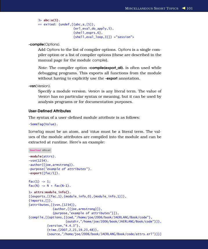
MISCELLANEOUS SHORT TOPICS 101
3> abc:a(5).
** exited: {undef,[{abc,a,[5]},
{erl_eval,do_apply,5},
{shell,exprs,6},
{shell,eval_loop,3}]} ="session">
-compile(Options).
Add Options to the list of compiler options. Options is a single com-
piler option or a list of compiler options (these are described in the
manual page for the module compile).
Note: The compiler option -compile(export_all). is often used while
debugging programs. This exports all functions from the module
without having to explicitly use the -export annotation.
-vsn(Version).
Specify a module version. Version is any literal term. The value of
Version has no particular syntax or meaning, but it can be used by
analysis programs or for documentation purposes.
User-Defined Attributes
The syntax of a user-defined module attribute is as follows:
-SomeTag(Value).
SomeTag must be an atom, and Value must be a literal term. The val-
ues of the module attributes are compiled into the module and can be
extracted at runtime. Here’s an example:
Download attrs.erl
-module(attrs).
-vsn(1234).
-author({joe,armstrong}).
-purpose("example of attributes").
-export([fac/1]).
fac(1) -> 1;
fac(N) -> N * fac(N-1).
1> attrs:module_info().
[{exports,[{fac,1},{module_info,0},{module_info,1}]},
{imports,[]},
{attributes,[{vsn,[1234]},
{author,[{joe,armstrong}]},
{purpose,"example of attributes"}]},
{compile,[{options,[{cwd,"/home/joe/2006/book/JAERLANG/Book/code"},
{outdir,"/home/joe/2006/book/JAERLANG/Book/code"}]},
{version,"4.4.3"},
{time,{2007,2,21,19,23,48}},
{source,"/home/joe/2006/book/JAERLANG/Book/code/attrs.erl"}]}]

MISCELLANEOUS SHORT TOPICS 102
2> attrs:module_info(attributes).
[{vsn,[1234]},{author,[{joe,armstrong}]},{purpose,"example of attributes"}]
3> beam_lib:chunks("attrs.beam",[attributes]).
{ok,{attrs,[{attributes,[{author,[{joe,armstrong}]},
{purpose,"example of attributes"},
{vsn,[1234]}]}]}}
The user-defined attributes contained in the source code file reappear
as a subterm of {attributes, ...}. The tuple {compile, ...} contains informa-
tion that was added by the compiler. The value {version,"4.4.3"} is the ver-
sion of the compiler and should not be confused with the vsn tag defined
in the module attributes. In the previous example, attrs:module_info()
returns a property list of all the metadata associated with a compiled
module. attrs:module_info(attributes)3 returns a list of any attributes asso-
ciated with the file.
Note that the functions module_info/0 and module_info/1 are automati-
cally created every time a module is compiled.
The output of lines 2 and 3 is a bit difficult to read. To make life easier,
we can write a little function that extracts a specific attribute and call
it like this:
4> extract:attribute("attrs.beam", author).
[{joe,armstrong}]
The code to do this is easy:
Download extract.erl
-module(extract).
-export([attribute/2]).
attribute(File, Key) ->
case beam_lib:chunks(File,[attributes]) of
{ok, {_Module, [{attributes,L}]}} ->
case lookup(Key, L) of
{ok, Val} ->
Val;
error ->
exit(badAttribute)
end;
_ ->
exit(badFile)
end.
lookup(Key, [{Key,Val}|_]) -> {ok, Val};
lookup(Key, [_|T]) -> lookup(Key, T);
lookup(_, []) -> error.
3. Other arguments are exports, imports, and compile.
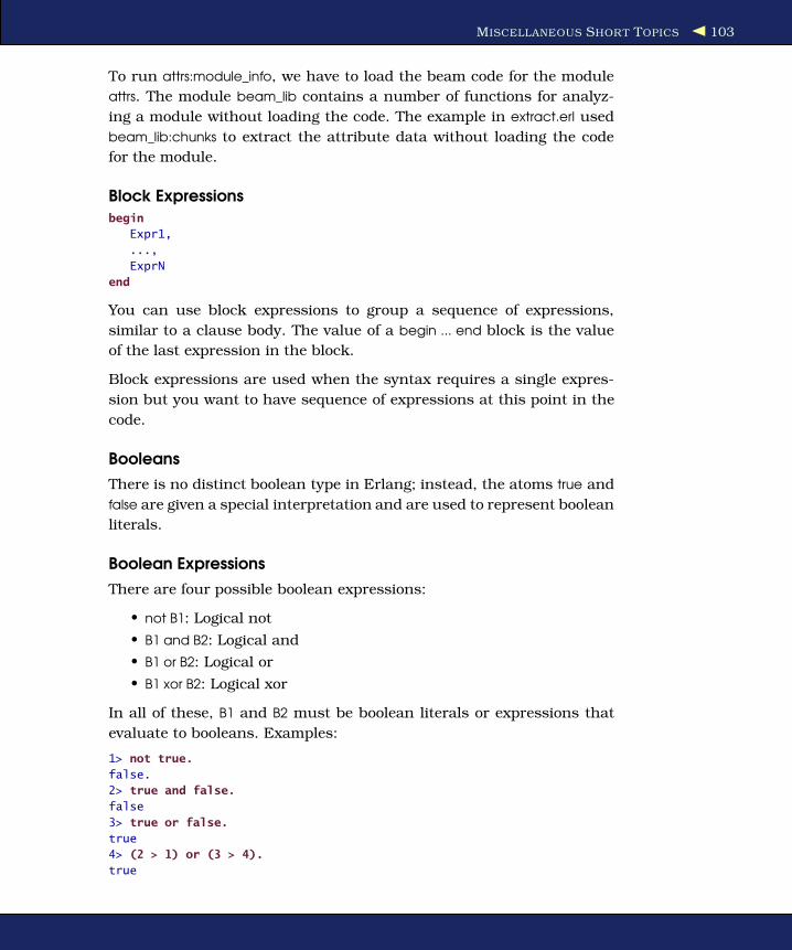
MISCELLANEOUS SHORT TOPICS 103
To run attrs:module_info, we have to load the beam code for the module
attrs. The module beam_lib contains a number of functions for analyz-
ing a module without loading the code. The example in extract.erl used
beam_lib:chunks to extract the attribute data without loading the code
for the module.
Block Expressionsbegin
Expr1,
...,
ExprN
end
You can use block expressions to group a sequence of expressions,
similar to a clause body. The value of a begin ... end block is the value
of the last expression in the block.
Block expressions are used when the syntax requires a single expres-
sion but you want to have sequence of expressions at this point in the
code.
Booleans
There is no distinct boolean type in Erlang; instead, the atoms true and
false are given a special interpretation and are used to represent boolean
literals.
Boolean Expressions
There are four possible boolean expressions:
• not B1: Logical not
• B1 and B2: Logical and
• B1 or B2: Logical or
• B1 xor B2: Logical xor
In all of these, B1 and B2 must be boolean literals or expressions that
evaluate to booleans. Examples:
1> not true.
false.
2> true and false.
false
3> true or false.
true
4> (2 > 1) or (3 > 4).
true
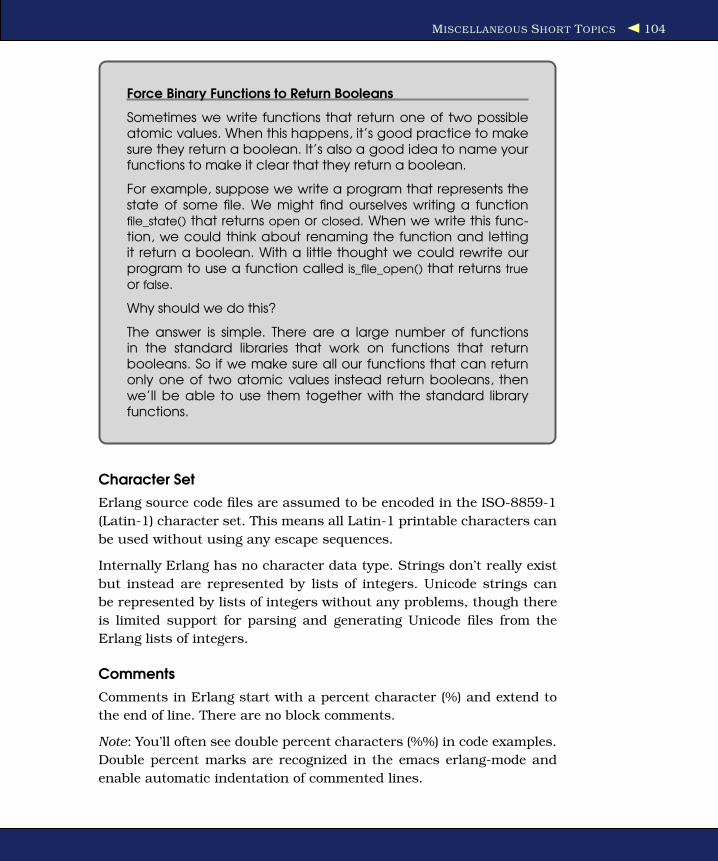
MISCELLANEOUS SHORT TOPICS 104
Force Binary Functions to Return Booleans
Sometimes we write functions that return one of two possibleatomic values. When this happens, it’s good practice to makesure they return a boolean. It’s also a good idea to name yourfunctions to make it clear that they return a boolean.
For example, suppose we write a program that represents thestate of some file. We might find ourselves writing a functionfile_state() that returns open or closed. When we write this func-tion, we could think about renaming the function and lettingit return a boolean. With a little thought we could rewrite ourprogram to use a function called is_file_open() that returns true
or false.
Why should we do this?
The answer is simple. There are a large number of functionsin the standard libraries that work on functions that returnbooleans. So if we make sure all our functions that can returnonly one of two atomic values instead return booleans, thenwe’ll be able to use them together with the standard libraryfunctions.
Character Set
Erlang source code files are assumed to be encoded in the ISO-8859-1
(Latin-1) character set. This means all Latin-1 printable characters can
be used without using any escape sequences.
Internally Erlang has no character data type. Strings don’t really exist
but instead are represented by lists of integers. Unicode strings can
be represented by lists of integers without any problems, though there
is limited support for parsing and generating Unicode files from the
Erlang lists of integers.
Comments
Comments in Erlang start with a percent character (%) and extend to
the end of line. There are no block comments.
Note: You’ll often see double percent characters (%%) in code examples.
Double percent marks are recognized in the emacs erlang-mode and
enable automatic indentation of commented lines.

MISCELLANEOUS SHORT TOPICS 105
% This is a comment
my_function(Arg1, Arg2) ->
case f(Arg1) of
{yes, X} -> % it worked
..
epp
Before an Erlang module is compiled, it is automatically processed by
the Erlang preprocessor epp. The preprocessor expands any macros
that might be in the source file and inserts any necessary include files.
Ordinarily, you won’t need to look at the output of the preprocessor, but
in exceptional circumstances (for example, when debugging a faulty
macro), you might want to save the output of the preprocessor. The
output of the preprocessor can be saved in a file by giving the command
compile:file(M, [’P’]). This compiles any code in the file M.erl and produces
a listing in the file M.P where all macros have been expanded and any
necessary include files have been included.
Escape Sequences
Within strings and quoted atoms, you can use escape sequences to
enter any nonprintable characters. All the possible escape sequences
are shown in Figure 5.1, on the following page.
Let’s give some examples in the shell to show how these conventions
work. (Note: ~w in a format string prints the list without any attempt to
pretty print the result.)
%% Control characters
1> io:format("~w~n", ["\b\d\e\f\n\r\s\t\v"]).
[8,127,27,12,10,13,32,9,11]
ok
%% Octal characters in a string
3> io:format("~w~n", ["\123\12\1"]).
[83,10,1]
ok
%% Quotes and escapes in a string
4> io:format("~w~n", ["\'\"\\"]).
[39,34,92]
ok
%% Character codes
5> io:format("~w~n", ["\a\z\A\Z"]).
[97,122,65,90]
ok
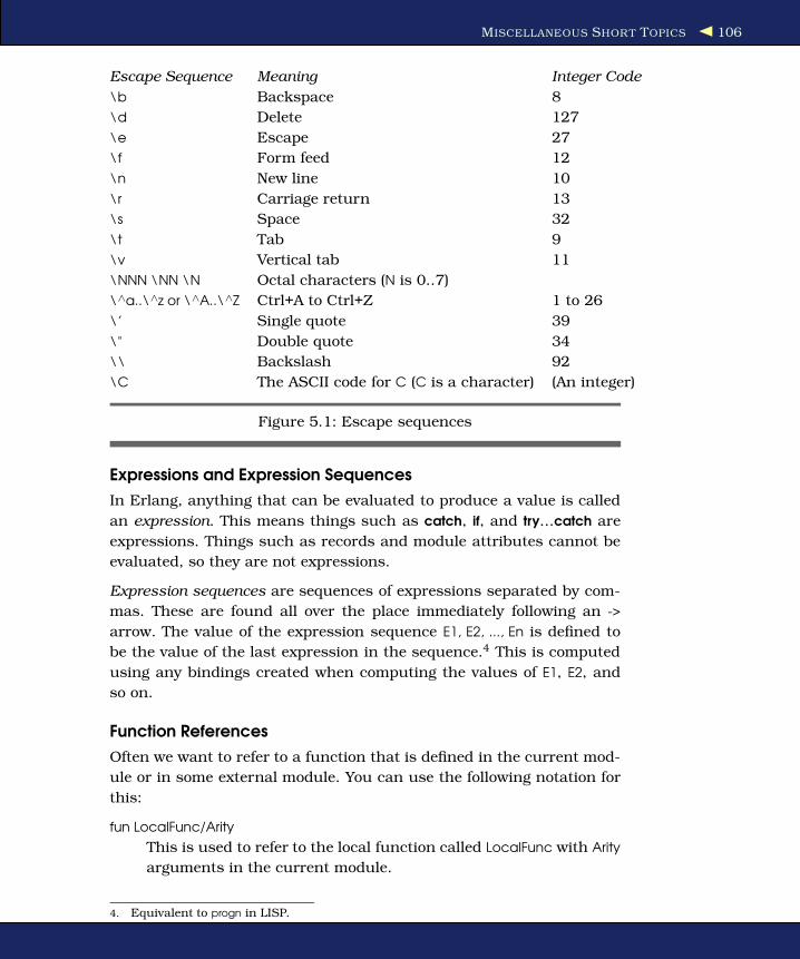
MISCELLANEOUS SHORT TOPICS 106
Escape Sequence Meaning Integer Code
\b Backspace 8
\d Delete 127
\e Escape 27
\f Form feed 12
\n New line 10
\r Carriage return 13
\s Space 32
\t Tab 9
\v Vertical tab 11
\NNN \NN \N Octal characters (N is 0..7)
\∧a..\∧z or \∧A..\∧Z Ctrl+A to Ctrl+Z 1 to 26
\’ Single quote 39
\" Double quote 34
\\ Backslash 92
\C The ASCII code for C (C is a character) (An integer)
Figure 5.1: Escape sequences
Expressions and Expression Sequences
In Erlang, anything that can be evaluated to produce a value is called
an expression. This means things such as catch, if, and try...catch are
expressions. Things such as records and module attributes cannot be
evaluated, so they are not expressions.
Expression sequences are sequences of expressions separated by com-
mas. These are found all over the place immediately following an ->
arrow. The value of the expression sequence E1, E2, ..., En is defined to
be the value of the last expression in the sequence.4 This is computed
using any bindings created when computing the values of E1, E2, and
so on.
Function References
Often we want to refer to a function that is defined in the current mod-
ule or in some external module. You can use the following notation for
this:
fun LocalFunc/Arity
This is used to refer to the local function called LocalFunc with Arity
arguments in the current module.
4. Equivalent to progn in LISP.

MISCELLANEOUS SHORT TOPICS 107
fun Mod:RemoteFunc/Arity
This is used to refer to an external function called RemoteFunc with
Arity arguments in the module Mod.
Here’s an example of a function reference in the current module:
-module(x1).
-export([square/1, ...]).
square(X) -> X * X.
...
double(L) -> lists:map(fun square/1, L).
If we wanted to call a function in a remote module, we could refer to
the function as in the following example:
-module(x2).
...
double(L) -> lists:map(fun x1:square/1, L).
fun x1:square/1 means the function square/1 in the module x1.
Include Files
Files can be included with the following syntax:
-include(Filename).
In Erlang, the convention is that include files have the extension .hrl.
The FileName should contain an absolute or relative path so that the
preprocessor can locate the appropriate file. Library header files can be
included with the following syntax:
-include_lib(Name).
For example:
-include_lib("kernel/include/file.hrl").
In this case, the Erlang compiler will find the appropriate include files.
(kernel, in the previous example, refers to the application that defines
this header file.)
Include files usually contain record definitions. If many modules need
to share common record definitions, then the common record defini-
tions are put into include files that are included by all the modules that
need these definitions.

MISCELLANEOUS SHORT TOPICS 108
List Operations ++ and - -
++ and - - are infix operators for list addition and subtraction.
A ++ B adds (that is, appends) A and B.
A - - B subtracts the list B from the list A. Subtraction means that every
element in B is removed from A. Note that if some symbol X occurs only
K times in B, then only the first K occurrence of X in A will be removed.
Examples:
1> [1,2,3] ++ [4,5,6].
[1,2,3,4,5,6]
2> [a,b,c,1,d,e,1,x,y,1] -- [1].
[a,b,c,d,e,1,x,y,1]
3> [a,b,c,1,d,e,1,x,y,1] -- [1,1].
[a,b,c,d,e,x,y,1]
4> [a,b,c,1,d,e,1,x,y,1] -- [1,1,1].
[a,b,c,d,e,x,y]
5> [a,b,c,1,d,e,1,x,y,1] -- [1,1,1,1].
[a,b,c,d,e,x,y]
++ in Patterns
++ can also be used in patterns. When matching strings, we can write
patterns such as the following:
f("begin" ++ T) -> ...
f("end" ++ T) -> ...
...
The pattern in the first clause is expanded into [$b,$e,$g,$i,$n|T].
Macros
Erlang macros are written as shown here:
-define(Constant, Replacement).
-define(Func(Var1, Var2,.., Var), Replacement).
Macros are expanded by the Erlang preprocessor epp when an expres-
sion of the form ?MacroName is encountered. Variables occurring in the
macro definition match complete forms in the corresponding site of the
macro call.
-define(macro1(X, Y), {a, X, Y}).
foo(A) ->
?macro1(A+10, b)

MISCELLANEOUS SHORT TOPICS 109
That expands into this:
foo(A) ->
{a,A+10,b}.
In addition, a number of predefined macros provide information about
the current module. They are as follows:
• ?FILE expands to the current filename.
• ?MODULE expands to the current module name.
• ?LINE expands to the current line number.
Control Flow in Macros
Inside a macro definition, the following directives are supported. You
can use them to direct the flow of control within a macro:
-undef(Macro).
Undefines the macro; after this you cannot call the macro.
-ifdef(Macro).
Evaluates the following lines only if Macro has been defined.
-ifndef(Macro).
Evaluates the following lines only if Macro is undefined.
-else.
Allowed after a ifdef or ifndef statement. If the condition was false,
the statements following else are evaluated.
-endif.
Marks the end of an ifdef or ifndef statement.
Conditional macros must be properly nested. They are conventionally
grouped as follows:
-ifdef(debug).
-define(...).
-else.
-define(...).
-endif.
We can use these macros to define a TRACE macro. For example:
Download m1.erl
-module(m1).
-export([start/0]).
-ifdef(debug).
-define(TRACE(X), io:format("TRACE ~p:~p ~p~n",[?MODULE, ?LINE, X])).
-else.
-define(TRACE(X), void).
-endif.

MISCELLANEOUS SHORT TOPICS 110
start() -> loop(5).
loop(0) ->
void;
loop(N) ->
?TRACE(N),
loop(N-1).
Note: io:format(String, [Args]) prints the variables in [Args] in the Erlang
shell according to the formatting information in String. The formatting
codes are preceded by a (~) symbol. ~p is short for pretty print, and ~n
produces a newline.5
To compile the code using the trace macro turned on and off, we can
use an additional argument to c/2 as follows:
1> c(m1, {d, debug}).
{ok,m1}
2> m1:start().
TRACE m1:15 5
TRACE m1:15 4
TRACE m1:15 3
TRACE m1:15 2
TRACE m1:15 1
void
c(m1, Options) provides a way of passing options to the compiler. {d,
debug} sets the debug flag to true so that it gets recognized in the -
ifdef(debug) section of the macro definition.
When the macro is turned off, the trace macro just expands to the atom
void. This choice of name has no significance; it’s just a reminder to me
that nobody is interested in the value of the macro.
Match Operator in Patterns
Let’s suppose we have some code like this:
Line 1 func1([{tag1, A, B}|T]) ->- ...- ... f(..., {tag1, A, B}, ...)- ...
In line 1, we pattern match the term {tag1, A, B}, and in line 3 we call
f with an argument that is {tag1, A, B}. When we do this, the system
rebuilds the term {tag1, A, B}. A much more efficient and less error prone
5. io:format understands an extremely large number of formatting options; for more
information, see Section 13.3, Write a List of Terms to a File, on page 235.

MISCELLANEOUS SHORT TOPICS 111
way to do this is to assign the pattern to a temporary variable, Z, and
pass this into f, like this:
func1([{tag1, A, B}=Z|T]) ->
...
... f(... Z, ...)
...
The match operator can be used at any point in the pattern, so if we
have two terms that need rebuilding, such as in this code:
func1([{tag, {one, A}, B}|T]) ->
...
... f(..., {tag, {one,A}, B}, ...),
... g(..., {one, A}), ...)
...
then we could introduce two new variables, Z1 and Z2, and write the
following:
func1([{tag, {one, A}=Z1, B}=Z2|T]) ->
..,.
... f(..., Z2, ...),
... g(..., Z1, ...),
...
Numbers
Numbers in Erlang are either integers or floats.
Integers
Integer arithmetic is exact, and the number of digits that can be repre-
sented in an integer is limited only by available memory.
Integers are written with one of three different syntaxes:
1. Conventional syntax: Here integers are written as you expect. For
example, 12, 12375, and -23427 are all integers.
2. Base K integers: Integers in a number base other than ten are
written with the syntax K#Digits; thus, we can write a number in
binary as 2#00101010 or a number in hexadecimal as 16#af6bfa23.
For bases greater than ten, the characters abc... (or ABC...) repre-
sent the numbers 10, 11, 12, and so on. The highest number base
we can represent in this manner is base 36.

MISCELLANEOUS SHORT TOPICS 112
3. $ syntax: The syntax $C represents the integer code for the ASCII
character C. Thus, $a is short for 97, $1 is short for 49, and so on.
Immediately after the $ we can also use any of the escape sequen-
ces described in Figure 5.1, on page 106. Thus, $\n is 10, $\∧c is
3, and so on.
Here are some examples of integers:
0 -65 2#010001110 -8#377 16#fe34 16#FE34 36#wow
(Their values are 0, -65, 142, -255, 65076, 65076, and 42368, respectively.)
Floats
A floating-point number has five parts: an optional sign, a whole num-
ber part, a decimal point, a fractional part, and an optional exponent
part.
Here are some examples of floats:
1.0 3.14159 -2.3e+6 23.56E-27
After parsing, floating-point numbers are represented internally in
IEEE 754 64-bit format. Real numbers in the range −10323 to 10308 can
be represented by an Erlang float.
Operator Precedence
Figure 5.2 shows all the Erlang operators in order of descending priority
together with their associativity. Operator precedence and associativity
is used to determine the evaluation order in unparenthesized expres-
sions.
Expression with higher priority (higher up in the table) are evaluated
first, and then expressions with lower priority are evaluated. So, for
example, to evaluate 3+4*5+6, we first evaluate the subexpression 4*5,
since (*) is higher up in the table than (+). Now we evaluate 3+20+6. Since
(+) is a left-associative operator, we interpret this as meaning (3+20)+6,
so we evaluate 3+20 first yielding 23; finally we evaluate 23+6.
In its fully parenthesized form, 3+4*5+6 means ((3+(4*5))+6). As with all
programming languages, it is better to use parentheses to denote scope
than to rely upon the precedence rules.

MISCELLANEOUS SHORT TOPICS 113
Operators Associativity
:
#
(unary) +, (unary) -, bnot, not
/, *, div, rem, band, and Left associative
+, -, bor, bxor, bsl, bsr, or, xor Left associative
++, - - Right associative
==, /=, =<, <, >=, >, =:=, =/=
andalso
orelse
Figure 5.2: Operator precedence
The Process Dictionary
Each process in Erlang has its own private data store called the process
dictionary. The process dictionary is an associative array (in other lan-
guages this might be called a map, hashmap, or hash table) composed
of a collection of keys and values. Each key has only one value.
The dictionary can be manipulated using the following BIFs:
@spec put(Key, Value) -> OldValue.
Add a Key, Value association to the process dictionary. The value
of put is OldValue, which is the previous value associated with Key.
If there was no previous value, the atom undefined is returned.
@spec get(Key) -> Value.
Look up the value of Key. If there is an association Key, Value asso-
ciation in the dictionary, return Value; otherwise, return the atom
undefined
@spec get() -> [{Key,Value}].
Return the entire dictionary as a list of {Key,Value} tuples.
@spec get_keys(Value) -> [Key].
Return a list of keys that have the values Value in the dictionary.
@spec erase(Key) -> Value.
Return the value associated with Key or the atom undefined if there
is no value associated with Key. Finally, erase the value associated
with Key.

MISCELLANEOUS SHORT TOPICS 114
@spec erase() -> [{Key,Value}].
Erase the entire process dictionary. The return value is a list of
{Key,Value} tuples representing the state of the dictionary before it
was erased.
For example:
1> erase().
[]
2> put(x, 20).
undefined
3> get(x).
20
4> get(y).
undefined
5> put(y, 40).
undefined
6> get(y).
40
7> get().
[{y,40},{x,20}]
8> erase(x).
20
9> get().
[{y,40}]
As you can see, variables in the process dictionary behave pretty much
like conventional variables in imperative programming languages. If
you use the process dictionary, your code will no longer be side effect
free, and all the benefits of using nondestructive variables that we dis-
cussed in Section 2.6, Variables That Don’t Vary, on page 28 do not
apply. For this reason, you should use the process dictionary sparingly.
Note: I rarely use the process dictionary. Using the process dictionary
can introduce subtle bugs into your program and make it difficult to
debug. One form of usage that I do approve of is to use the processes
dictionary to store “write-once” variables. If a key acquires a value
exactly once and does not change the value, then storing it in the pro-
cess dictionary is sometimes acceptable.
References
References are globally unique Erlang terms. They are created with the
BIF erlang:make_ref(). References are useful for creating unique tags that
can be included in data and then at a later stage compared for equality.
For example, a bug-tracking system might add a reference to each new
bug report in order to give it a unique identity.

MISCELLANEOUS SHORT TOPICS 115
Short-Circuit Boolean Expressions
Short-circuit boolean expressions are boolean expressions whose argu-
ments are evaluated only when necessary.
There are two “short-circuit” boolean expressions:
Expr1 orelse Expr2
This first evaluates Expr1. If Expr1 evaluates to true, Expr2 is not
evaluated. If Expr1 evaluates to false, Expr2 is evaluated.
Expr1 andalso Expr2
This first evaluates Expr1. If Expr1 evaluates to true, Expr2 is evalu-
ated. If Expr1 evaluates to false, Expr2 is not evaluated.
Note: In the corresponding boolean expressions (A or B; A and B), both the
arguments are always evaluated, even if the truth value of the expres-
sion can be determined by evaluating only the first expression.
Term Comparisons
There are eight possible term comparison operations, shown in Fig-
ure 5.3, on the following page.
For the purposes of comparison, a total ordering is defined over all
terms. This is defined so that the following is true:
number < atom < reference < fun < port < pid < tuple < list < binary
What does this mean? This means that, for example, a number (any
number) is defined to be smaller than an atom (any atom), that a tuple
is greater than an atom, and so on. (Note that for the purposes of order-
ing, ports and PIDs are included in this list. We’ll talk about these later.)
Having a total order over all terms means we can sort lists of any type
and build efficient data access routines based on the sort order of the
keys.
All the term comparison operators, with the exception of =:= and =/=,
behave in the following way if their arguments are numbers:
• If one argument is a integer and the other is a float, then the
integer is converted to a float before the comparison is performed.
• If both arguments are integers or if both arguments are floats,
then the arguments are used “as is,” that is, without conversion.
You should also be really careful about using == (especially if you’re a C
or Java programmer). In 99 out of a 100 cases, you should be using =:=.
== is useful only when comparing floats with integers. =:= is for testing

MISCELLANEOUS SHORT TOPICS 116
Operator Meaning
X > Y X is greater than Y.
X < Y X is less than Y.
X =< Y X is equal to or less than Y.
X >= Y X is greater than or equal to Y.
X == Y X is equal to Y.
X /= Y X is not equal to Y.
X =:= Y X is identical to Y.
X =/= Y X is not identical to Y.
Figure 5.3: Term Comparisons
whether two terms are identical.6 If in doubt, use =:=, and be suspicious
if you see ==. Note that a similar comment applies to using /= and =/=,
where /= means “not equal to” and =/= means “not identical.”
Note: In a lot of library and published code, you’ll see == used when the
operator should have been =:=. Fortunately, this kind of error does not
often result in an incorrect program, since if the arguments to == do
not contain any floats, then the behaviors of the two operators are the
same.
You should also be aware that function clause matching always implies
exact pattern matching, so if you define a fun F = fun(12) -> ... end, then
trying to evaluate F(12.0) will fail.
Underscore Variables
There’s one more thing to say about variables. The special syntax _Var-
Name is used for a normal variable, not an anonymous variable. Nor-
mally the compiler will generate a warning if a variable is used only
once in a clause since this is usually the sign of an error. If the variable
is used only once but starts with an underscore, the warning message
will not be generated.
Since _Var is a normal variable, very subtle bugs can be caused by for-
getting this and using it as a “don’t care” pattern. In a complicated pat-
tern match, it can be difficult to spot that, for example, _Int is repeated
when it shouldn’t have been, causing the pattern match to fail.
6. Identical means having the same value (like the Common Lisp EQUAL). Since values
are immutable, this does not imply any notion of pointer identity.

MISCELLANEOUS SHORT TOPICS 117
There are two main uses of underscore variables:
• To name a variable that we don’t intend to use. That is, writing
open(File, _Mode) makes the program more readable than writing
open(File, _).
• For debugging purposes. For example, suppose we write this:
some_func(X) ->
{P, Q} = some_other_func(X),
io:format("Q = ~p~n", [Q]),
P.
This compiles without an error message.
Now comment out the format statement:
some_func(X) ->
{P, Q} = some_other_func(X),
%% io:format("Q = ~p~n", [Q]),
P.
If we compile this, the compiler will issue a warning that the vari-
able Q is not used.
If we rewrite the function like this:
some_func(X) ->
{P, _Q} = some_other_func(X),
io:format("_Q = ~p~n", [_Q]),
P.
then we can comment out the format statement, and the compiler
will not complain.
Now we’re actually through with sequential Erlang. We have not men-
tioned a few small topics, but we’ll return to these as we run into them
in the application chapters.
In the next chapter, we’ll look at how to compile and run your programs
in a variety of ways.

Chapter 6
Compiling and Running YourProgram
In the previous chapters, we didn’t say much about compiling and run-
ning your programs—we just used the Erlang shell. This is fine for small
examples, but as your programs become more complex, you’ll want to
automate the process to make life easier. That’s where makefiles come
in.
There are actually three different ways to run your programs. In this
chapter, we’ll look at all three so you can choose the best method for
any particular occasion.
Sometimes things will go wrong: makefiles will fail, environment vari-
ables will be wrong, and your search paths will be incorrect. We’ll help
you deal with these issues by looking at what to do when things go
wrong.
6.1 Starting and Stopping the Erlang Shell
On a Unix system (including Mac OS X), you start the Erlang shell from
a command prompt:
$ erl
Erlang (BEAM) emulator version 5.5.1 [source] [async-threads:0] [hipe]
Eshell V5.5.1 (abort with ^G)
1>
On a Windows system, click the erl icon.
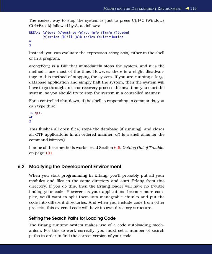
MODIFYING THE DEVELOPMENT ENVIRONMENT 119
The easiest way to stop the system is just to press Ctrl+C (Windows
Ctrl+Break) followed by A, as follows:
BREAK: (a)bort (c)ontinue (p)roc info (i)nfo (l)oaded
(v)ersion (k)ill (D)b-tables (d)istribution
a
$
Instead, you can evaluate the expression erlang:halt() either in the shell
or in a program.
erlang:halt() is a BIF that immediately stops the system, and it is the
method I use most of the time. However, there is a slight disadvan-
tage to this method of stopping the system. If you are running a large
database application and simply halt the system, then the system will
have to go through an error recovery process the next time you start the
system, so you should try to stop the system in a controlled manner.
For a controlled shutdown, if the shell is responding to commands, you
can type this:
1> q().
ok
$
This flushes all open files, stops the database (if running), and closes
all OTP applications in an ordered manner. q() is a shell alias for the
command init:stop().
If none of these methods works, read Section 6.6, Getting Out of Trouble,
on page 131.
6.2 Modifying the Development Environment
When you start programming in Erlang, you’ll probably put all your
modules and files in the same directory and start Erlang from this
directory. If you do this, then the Erlang loader will have no trouble
finding your code. However, as your applications become more com-
plex, you’ll want to split them into manageable chunks and put the
code into different directories. And when you include code from other
projects, this external code will have its own directory structure.
Setting the Search Paths for Loading Code
The Erlang runtime system makes use of a code autoloading mech-
anism. For this to work correctly, you must set a number of search
paths in order to find the correct version of your code.
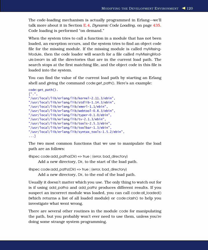
MODIFYING THE DEVELOPMENT ENVIRONMENT 120
The code-loading mechanism is actually programmed in Erlang—we’ll
talk more about it in Section E.4, Dynamic Code Loading, on page 435.
Code loading is performed “on demand.”
When the system tries to call a function in a module that has not been
loaded, an exception occurs, and the system tries to find an object code
file for the missing module. If the missing module is called myMissing-
Module, then the code loader will search for a file called myMissingMod-
ule.beam in all the directories that are in the current load path. The
search stops at the first matching file, and the object code in this file is
loaded into the system.
You can find the value of the current load path by starting an Erlang
shell and giving the command code:get_path(). Here’s an example:
code:get_path().
[".",
"/usr/local/lib/erlang/lib/kernel-2.11.3/ebin",
"/usr/local/lib/erlang/lib/stdlib-1.14.3/ebin",
"/usr/local/lib/erlang/lib/xmerl-1.1/ebin",
"/usr/local/lib/erlang/lib/webtool-0.8.3/ebin",
"/usr/local/lib/erlang/lib/typer-0.1.0/ebin",
"/usr/local/lib/erlang/lib/tv-2.1.3/ebin",
"/usr/local/lib/erlang/lib/tools-2.5.3/ebin",
"/usr/local/lib/erlang/lib/toolbar-1.3/ebin",
"/usr/local/lib/erlang/lib/syntax_tools-1.5.2/ebin",
...]
The two most common functions that we use to manipulate the load
path are as follows:
@spec code:add_patha(Dir) => true | {error, bad_directory}
Add a new directory, Dir, to the start of the load path.
@spec code:add_pathz(Dir) => true | {error, bad_directory}
Add a new directory, Dir, to the end of the load path.
Usually it doesn’t matter which you use. The only thing to watch out for
is if using add_patha and add_pathz produces different results. If you
suspect an incorrect module was loaded, you can call code:all_loaded()
(which returns a list of all loaded module) or code:clash() to help you
investigate what went wrong.
There are several other routines in the module code for manipulating
the path, but you probably won’t ever need to use them, unless you’re
doing some strange system programming.

MODIFYING THE DEVELOPMENT ENVIRONMENT 121
The usual convention is to put these commands in a file called .erlang
in your home directory. Alternatively, you can start Erlang with a com-
mand like this:
> erl -pa Dir1 -pa Dir2 ... -pz DirK1 -pz DirK2
The -pa Dir flag adds Dir to the beginning of the code search path, and
-pz Dir adds the directory to the end of the code path.
Executing a Set of Commands When the System Is Started
We saw how you can set the load path in your .erlang file in your home
directory. In fact, you can put any Erlang code in this file—when you
start Erlang, it first reads and evaluates all the commands in this file.
Suppose my .erlang file is as follows:
io:format("Running Erlang~n").
code:add_patha(".").
code:add_pathz("/home/joe/2005/erl/lib/supported").
code:add_pathz("/home/joe/bin").
Then when I start the system, I’ll see the following output:
$ erl
Erlang (BEAM) emulator version 5.5.1 [source] [async-threads:0] [hipe]
Running Erlang
Eshell V5.5.1 (abort with ^G)
1>
If there is a file called .erlang in the current directory when Erlang is
started, then it will take precedence over the .erlang in your home direc-
tory. This way you can arrange that Erlang will behave in different ways
depending upon where it is started. This can be useful for specialized
applications. In this case, it’s probably a good idea to include some
print statements in the start-up file; otherwise, you might forget about
the local start-up file, which could be very confusing.
Tip: In some systems, it’s not clear where your home directory is, or
it might not be where you think it is. To find out where Erlang thinks
your home directory is, do the following:
1> init:get_argument(home).
{ok,[["/home/joe"]]}
From this we can infer that Erlang thinks that my home directory is
/home/joe.

DIFFERENT WAYS TO RUN YOUR PROGRAM 122
6.3 Different Ways to Run Your Program
Erlang programs are stored in modules. Once you have written your
program, you have to compile it before you can run it. Alternatively,
you can run your program directly without compiling it by running
escript.
The next sections show how to compile and run a couple of programs
in a number of ways. The programs are slightly different, and the ways
in which we start and stop them differ.
The first program, hello.erl, just prints “Hello world.” It’s not responsible
for starting or stopping the system, and it does not need to access any
command-line arguments. By way of contrast, the second program, fac,
needs to access the command-line arguments.
Here’s our basic program. It writes the string containing “Hello world”
followed by a newline (~n is interpreted as newline in the Erlang io and
io_lib modules).
Download hello.erl
-module(hello).
-export([start/0]).
start() ->
io:format("Hello world~n").
Let’s compile and run it three different ways.
Compile and Run in the Erlang Shell$ erl
Erlang (BEAM) emulator version 5.5.1 [source] [async-threads:0] [hipe]
Eshell V5.5.1 (abort with ^G)
1> c(hello).
{ok,hello}
2> hello:start().
Hello world
ok
Compile and Run from the Command Prompt$ erlc hello.erl
$ erl -noshell -s hello start -s init stop
Hello world
$

DIFFERENT WAYS TO RUN YOUR PROGRAM 123
Quick Scripting
Often we want to be able to execute an arbitrary Erlang func-tion from the OS command line. The -eval argument is veryhandy for quick scripting.
Here’s an example:
erl -eval 'io:format("Memory: ~p~n", [erlang:memory(total)]).'\-noshell -s init stop
Windows users: For this to work, you have to either set your PATH
variable to include the directories containing the Erlang executables or
give a fully qualified path (including the quote marks) to erlc and erl.
For example:
"C:\Program Files\erl5.5.3\bin\erlc.exe" hello.erl
..
The first line, erlc hello.erl, compiles the file hello.erl, producing an object
code file called hello.beam. The second command has three options:
-noshell
Start Erlang without an interactive shell (so you don’t get the
Erlang “banner,” which ordinarily greets you when you start the
system).
-s hello start
Run the function hello:start().
Note: When using the -s Mod ... option, the Mod must have been
compiled.
-s init stop
When apply(hello, start, [ ]) has finished, then the system evaluates
the function init:stop().
The command erl -noshell ... can be put in a shell script, so typically we’d
make a shell script to run our program that sets the path (with -pa
Directory) and launches the program.
In our example, we used two -s .. commands. We can have as many func-
tions as we like on the command line. Each -s ... command is evaluated
with an apply statement, and when it has run to completion, the next
command is evaluated.
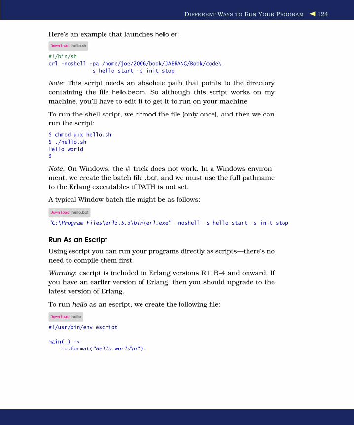
DIFFERENT WAYS TO RUN YOUR PROGRAM 124
Here’s an example that launches hello.erl:
Download hello.sh
#!/bin/sh
erl -noshell -pa /home/joe/2006/book/JAERANG/Book/code\
-s hello start -s init stop
Note: This script needs an absolute path that points to the directory
containing the file hello.beam. So although this script works on my
machine, you’ll have to edit it to get it to run on your machine.
To run the shell script, we chmod the file (only once), and then we can
run the script:
$ chmod u+x hello.sh
$ ./hello.sh
Hello world
$
Note: On Windows, the #! trick does not work. In a Windows environ-
ment, we create the batch file .bat, and we must use the full pathname
to the Erlang executables if PATH is not set.
A typical Window batch file might be as follows:
Download hello.bat
"C:\Program Files\erl5.5.3\bin\erl.exe" -noshell -s hello start -s init stop
Run As an Escript
Using escript you can run your programs directly as scripts—there’s no
need to compile them first.
Warning: escript is included in Erlang versions R11B-4 and onward. If
you have an earlier version of Erlang, then you should upgrade to the
latest version of Erlang.
To run hello as an escript, we create the following file:
Download hello
#!/usr/bin/env escript
main(_) ->
io:format("Hello world\n").
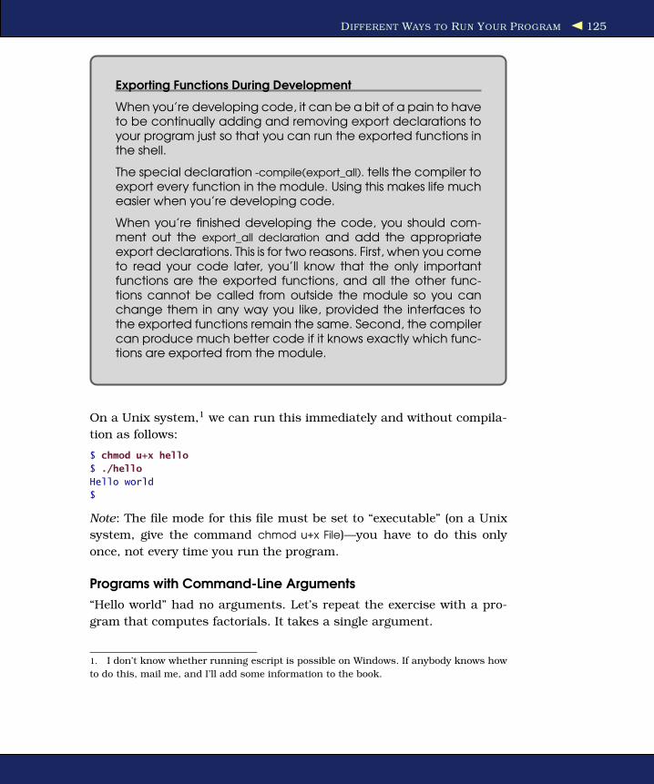
DIFFERENT WAYS TO RUN YOUR PROGRAM 125
Exporting Functions During Development
When you’re developing code, it can be a bit of a pain to haveto be continually adding and removing export declarations toyour program just so that you can run the exported functions inthe shell.
The special declaration -compile(export_all). tells the compiler toexport every function in the module. Using this makes life mucheasier when you’re developing code.
When you’re finished developing the code, you should com-ment out the export_all declaration and add the appropriateexport declarations. This is for two reasons. First, when you cometo read your code later, you’ll know that the only importantfunctions are the exported functions, and all the other func-tions cannot be called from outside the module so you canchange them in any way you like, provided the interfaces tothe exported functions remain the same. Second, the compilercan produce much better code if it knows exactly which func-tions are exported from the module.
On a Unix system,1 we can run this immediately and without compila-
tion as follows:
$ chmod u+x hello
$ ./hello
Hello world
$
Note: The file mode for this file must be set to “executable” (on a Unix
system, give the command chmod u+x File)—you have to do this only
once, not every time you run the program.
Programs with Command-Line Arguments
“Hello world” had no arguments. Let’s repeat the exercise with a pro-
gram that computes factorials. It takes a single argument.
1. I don’t know whether running escript is possible on Windows. If anybody knows how
to do this, mail me, and I’ll add some information to the book.

DIFFERENT WAYS TO RUN YOUR PROGRAM 126
First, here’s the code:
Download fac.erl
-module(fac).
-export([fac/1]).
fac(0) -> 1;
fac(N) -> N*fac(N-1).
We can compile fac.erl and run it in the Erlang shell like this:
$ erl
Erlang (BEAM) emulator version 5.5.1 [source] [async-threads:0] [hipe]
Eshell V5.5.1 (abort with ^G)
1> c(fac).
{ok,fac}
2> fac:fac(25).
15511210043330985984000000
If we want to be able to run this program from the command line, we’ll
need to modify it to take command-line arguments:
Download fac1.erl
-module(fac1).
-export([main/1]).
main([A]) ->
I = list_to_integer(atom_to_list(A)),
F = fac(I),
io:format("factorial ~w = ~w~n",[I, F]),
init:stop().
fac(0) -> 1;
fac(N) -> N*fac(N-1).
We can then compile and run it:
$ erlc fac1.erl
$ erl -noshell -s fac1 main 25
factorial 25 = 15511210043330985984000000
Note: The fact that the function is called main has no significance; it can
be called anything. The important thing is that the function name and
the name on the command line agree.
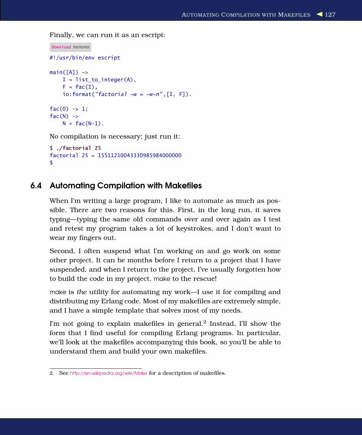
AUTOMATING COMPILATION WITH MAKEFILES 127
Finally, we can run it as an escript:
Download factorial
#!/usr/bin/env escript
main([A]) ->
I = list_to_integer(A),
F = fac(I),
io:format("factorial ~w = ~w~n",[I, F]).
fac(0) -> 1;
fac(N) ->
N * fac(N-1).
No compilation is necessary; just run it:
$ ./factorial 25
factorial 25 = 15511210043330985984000000
$
6.4 Automating Compilation with Makefiles
When I’m writing a large program, I like to automate as much as pos-
sible. There are two reasons for this. First, in the long run, it saves
typing—typing the same old commands over and over again as I test
and retest my program takes a lot of keystrokes, and I don’t want to
wear my fingers out.
Second, I often suspend what I’m working on and go work on some
other project. It can be months before I return to a project that I have
suspended, and when I return to the project, I’ve usually forgotten how
to build the code in my project. make to the rescue!
make is the utility for automating my work—I use it for compiling and
distributing my Erlang code. Most of my makefiles are extremely simple,
and I have a simple template that solves most of my needs.
I’m not going to explain makefiles in general.2 Instead, I’ll show the
form that I find useful for compiling Erlang programs. In particular,
we’ll look at the makefiles accompanying this book, so you’ll be able to
understand them and build your own makefiles.
2. See http://en.wikipedia.org/wiki/Make for a description of makefiles.

AUTOMATING COMPILATION WITH MAKEFILES 128
A Makefile Template
Here’s the template that I base most of my makefiles on:
Download Makefile.template
# leave these lines alone
.SUFFIXES: .erl .beam .yrl
.erl.beam:
erlc -W $<
.yrl.erl:
erlc -W $<
ERL = erl -boot start_clean
# Here's a list of the erlang modules you want compiling
# If the modules don't fit onto one line add a \ character
# to the end of the line and continue on the next line
# Edit the lines below
MODS = module1 module2 \
module3 ... special1 ...\
...
moduleN
# The first target in any makefile is the default target.
# If you just type "make" then "make all" is assumed (because
# "all" is the first target in this makefile)
all: compile
compile: ${MODS:%=%.beam} subdirs
## special compilation requirements are added here
special1.beam: special1.erl
${ERL} -Dflag1 -W0 special1.erl
## run an application from the makefile
application1: compile
${ERL} -pa Dir1 -s application1 start Arg1 Arg2
# the subdirs target compiles any code in
# sub-directories
subdirs:
cd dir1; make
cd dir2; make
...

AUTOMATING COMPILATION WITH MAKEFILES 129
# remove all the code
clean:
rm -rf *.beam erl_crash.dump
cd dir1; make clean
cd dir2; make clean
The makefile starts with some rules to compile Erlang modules and files
with the extension .yrl (these are files containing parser definitions for
the Erlang parser generator program3).
The important part is the line starting like this:
MODS = module1 module2
This is a list of all the Erlang modules that I want to compile.
Any module in the MODS list will be compiled with the Erlang command
erlc Mod.erl. Some modules might need special treatment (for example
the module special1 in the template file), so there is a separate rule to
handle this.
Inside a makefile there are a number of targets. A target is a alphanu-
meric string starting in the first column and terminated by a colon (:).
In the makefile template, all, compile, and special1.beam are all targets.
To run the makefile, you give the shell command:
$ make [Target]
The argument Target is optional. If Target is omitted, then the first target
in the file is assumed. In the previous example, the target all is assumed
if no target is specified on the command line.
If I want to build all my software and run application1, then I’d give the
command make application1. If I wanted this to be the default behavior,
which happens when I just give the command make, then I’d move the
lines defining the target application1 so that they were the first target in
the makefile.
The target clean removes all compiled Erlang object code files and the
file erl_crash.dump. The crash dump contains information that can help
debug an application. See Section 6.10, The Crash Dump, on page 136
for details.
3. The Erlang parser generator is called yecc (an Erlang version of yacc, which
is short for yet another compiler compiler); see the tutorial on the Internet at
http://www.erlang.org/contrib/parser_tutorial-1.0.tgz.

COMMAND EDITING IN THE ERLANG SHELL 130
Specializing the Makefile Template
I’m not a fan of clutter in my software, so what I usually do is start
with the template makefile and remove all the lines that are not rele-
vant to my application. This results in makefiles that are shorter and
easier to read. Alternatively, you could have a common makefile that is
included by all makefiles and that is parameterized by the variables in
the makefiles.
Once I’m through with this process, I’ll end up with a much simplified
makefile, something like the following:
.SUFFIXES: .erl .beam
.erl.beam:
erlc -W $<
ERL = erl -boot start_clean
MODS = module1 module2 module3
all: compile
${ERL} -pa '/home/joe/.../this/dir' -s module1 start
compile: ${MODS:%=%.beam}
clean:
rm -rf *.beam erl_crash.dump
6.5 Command Editing in the Erlang Shell
The Erlang shell contains a built-in line editor. It understands a subset
of the line-editing commands used in the popular emacs editor. Previ-
ous lines can be recalled and edited in a few keystrokes. The available
commands are shown next (note that ∧Key means you should press
Ctrl+Key):
Command Description∧A Beginning of line.∧E End of line.∧F or right arrow Forward character.∧B or left arrow Backward character.∧P or up arrow Previous line.∧N or down arrow Next line.∧T Transpose last two characters.
Tab Try to expand current module or function name.
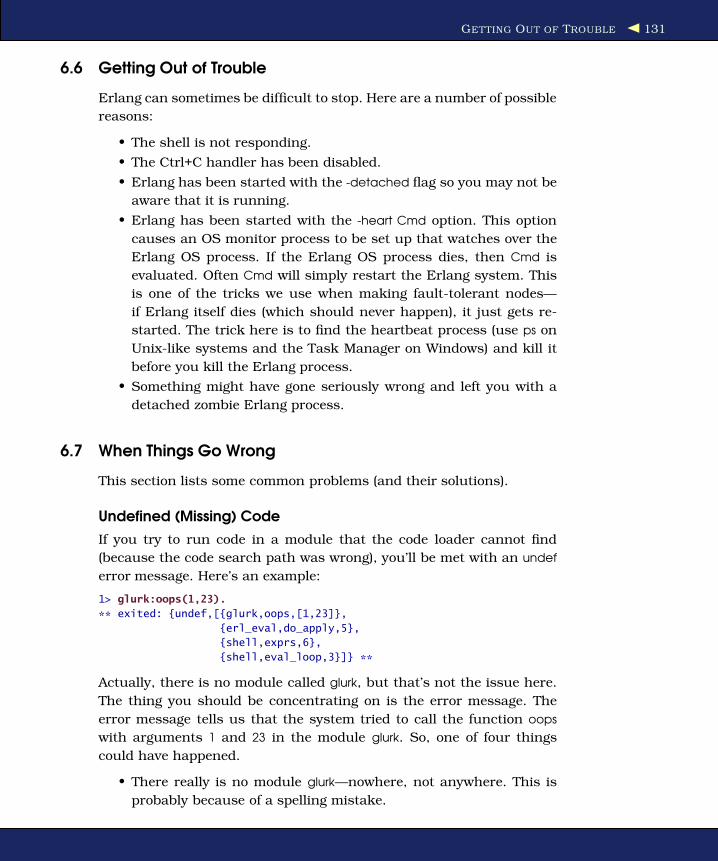
GETTING OUT OF TROUBLE 131
6.6 Getting Out of Trouble
Erlang can sometimes be difficult to stop. Here are a number of possible
reasons:
• The shell is not responding.
• The Ctrl+C handler has been disabled.
• Erlang has been started with the -detached flag so you may not be
aware that it is running.
• Erlang has been started with the -heart Cmd option. This option
causes an OS monitor process to be set up that watches over the
Erlang OS process. If the Erlang OS process dies, then Cmd is
evaluated. Often Cmd will simply restart the Erlang system. This
is one of the tricks we use when making fault-tolerant nodes—
if Erlang itself dies (which should never happen), it just gets re-
started. The trick here is to find the heartbeat process (use ps on
Unix-like systems and the Task Manager on Windows) and kill it
before you kill the Erlang process.
• Something might have gone seriously wrong and left you with a
detached zombie Erlang process.
6.7 When Things Go Wrong
This section lists some common problems (and their solutions).
Undefined (Missing) Code
If you try to run code in a module that the code loader cannot find
(because the code search path was wrong), you’ll be met with an undef
error message. Here’s an example:
1> glurk:oops(1,23).
** exited: {undef,[{glurk,oops,[1,23]},
{erl_eval,do_apply,5},
{shell,exprs,6},
{shell,eval_loop,3}]} **
Actually, there is no module called glurk, but that’s not the issue here.
The thing you should be concentrating on is the error message. The
error message tells us that the system tried to call the function oops
with arguments 1 and 23 in the module glurk. So, one of four things
could have happened.
• There really is no module glurk—nowhere, not anywhere. This is
probably because of a spelling mistake.

WHEN THINGS GO WRONG 132
Has Anybody Seen My Semicolons?
If you forget the semicolons between the clauses in a functionor put periods there instead, you’ll be in trouble—real trouble.
If you’re defining a function foo/2 in line 1234 of the module bar
and put a period instead of a semicolon, the compiler will saythis:
bar.erl:1234 function foo/2 already defined.
Don’t do it. Make sure your clauses are always separated bysemicolons.
• There is a module glurk, but it hasn’t been compiled. The system is
looking for a file called glurk.beam somewhere in the code search
path.
• There is a module glurk and it has been compiled, but the direc-
tory containing glurk.beam is not one of the directories in the code
search path. To fix this, you’ll have to change the search path.
We’ll see how to do this later.
• There are several different versions of glurk in the code load path,
and we’ve chosen the wrong one. This is a rare error, but it can
happen.
If you suspect this has happened, you can run the code:clash()
function, which reports all duplicated modules in the code search
path.
My Makefile Doesn’t Make
What can go wrong with a makefile? Well, lots, actually. But this isn’t
a book about makefiles, so I’ll deal only with the most common errors.
Here are the two most common errors that I get:
• Blanks in the makefile: Makefiles are extremely persnickety. Al-
though you can’t see them, each of the indented lines in the make-
file (with the exception of continuation lines, where the previous
line ends with a (\) character) should begin with a tab character.
If there are any spaces there, make will get confused, and you’ll
start seeing errors.
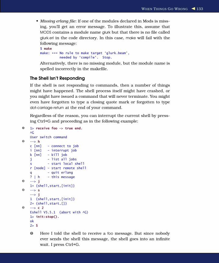
WHEN THINGS GO WRONG 133
• Missing erlang file: If one of the modules declared in Mods is miss-
ing, you’ll get an error message. To illustrate this, assume that
MODS contains a module name glurk but that there is no file called
glurk.erl in the code directory. In this case, make will fail with the
following message:$ make
make: *** No rule to make target ‘glurk.beam',
needed by ‘compile'. Stop.
Alternatively, there is no missing module, but the module name is
spelled incorrectly in the makefile.
The Shell Isn’t Responding
If the shell is not responding to commands, then a number of things
might have happened. The shell process itself might have crashed, or
you might have issued a command that will never terminate. You might
even have forgotten to type a closing quote mark or forgotten to type
dot-carriage-return at the end of your command.
Regardless of the reason, you can interrupt the current shell by press-
ing Ctrl+G and proceeding as in the following example:
Ê 1> receive foo -> true end.
^G
User switch commandË --> h
c [nn] - connect to job
i [nn] - interrupt job
k [nn] - kill job
j - list all jobs
s - start local shell
r [node] - start remote shell
q - quit erlang
? | h - this messageÌ --> j
1* {shell,start,[init]}Í --> s
--> j
1 {shell,start,[init]}
2* {shell,start,[]}Î --> c 2
Eshell V5.5.1 (abort with ^G)
1> init:stop().
ok
2> $
Ê Here I told the shell to receive a foo message. But since nobody
ever sends the shell this message, the shell goes into an infinite
wait. I press Ctrl+G.

GETTING HELP 134
Ë The system enters “shell JCL”4 mode. Here I can never remember
the commands, so I type h for help.
Ì I type j for a listing of all jobs. Job number 1 is marked with a
star, which means it is the default shell. All the commands with
an optional argument [nn] use the default shell unless a specific
argument is supplied.
Í I type s to start a new shell, followed by j again. This time I see
there are two shells marked 1 and 2, and shell 2 has become the
default shell.
Î I type c 2, which connects me to the newly started shell 2, and
then I stop the system.
As you can see, you can have many shells in operation and swap
between them by pressing Ctrl+G and then the appropriate commands.
You can even start a shell on a remote node with the r command.
6.8 Getting Help
On a Unix system, here is the code:
$ erl -man erl
NAME
erl - The Erlang Emulator
DESCRIPTION
The erl program starts the Erlang runtime system.
The exact details (e.g. whether erl is a script
or a program and which other programs it calls) are system-dependent.
...
You can also get help about individual modules as follows:
$ erl -man lists
MODULE
lists - List Processing Functions
DESCRIPTION
This module contains functions for list processing.
The functions are organized in two groups:
...
Note: On a Unix system, the manual pages are not installed by default.
If the command erl -man ... does not work, then you need to install the
4. Job Control Language.

TWEAKING THE ENVIRONMENT 135
manual pages. All the manual pages are in a single compressed archive
at http://www.erlang.org/download.html. The manual pages should be un-
packed in the root of the Erlang installation directory (usually /usr/local/
lib/erlang).
The documentation is also downloadable as a set of HTML files. On
Windows the HTML documentation is installed by default and accessi-
ble through the Erlang section of the Start menu.
6.9 Tweaking the Environment
The Erlang shell has a number of built-in commands. You can see them
all with the shell command help():
1> help().
** shell internal commands **b() -- display all variable bindings
e(N) -- repeat the expression in query <N>
f() -- forget all variable bindings
f(X) -- forget the binding of variable X
h() -- history
...
All these commands are defined in the module shell_default.
If you want to define your own commands, just create a module called
user_default. For example:
Download user_default.erl
-module(user_default).
-compile(export_all).
hello() ->
"Hello Joe how are you?".
away(Time) ->
io:format("Joe is away and will be back in ~w minutes~n",
[Time]).
Once this has been compiled and is placed somewhere in your load
path, then you can call any of the functions in user_default without giv-
ing a module name:
1> hello().
"Hello Joe how are you?"
2> away(10).
Joe is away and will be back in 10 minutes
ok
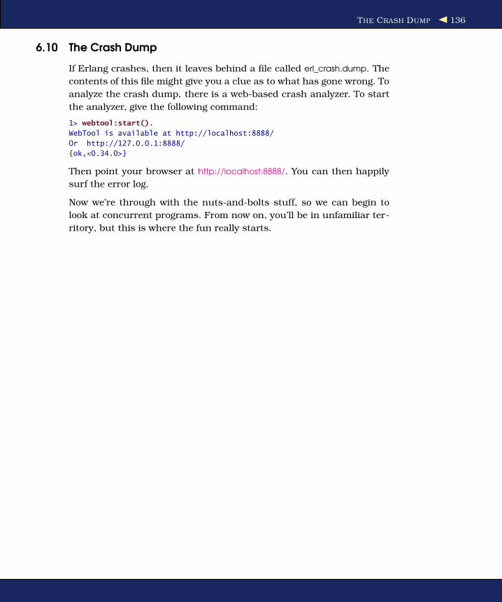
THE CRASH DUMP 136
6.10 The Crash Dump
If Erlang crashes, then it leaves behind a file called erl_crash.dump. The
contents of this file might give you a clue as to what has gone wrong. To
analyze the crash dump, there is a web-based crash analyzer. To start
the analyzer, give the following command:
1> webtool:start().
WebTool is available at http://localhost:8888/
Or http://127.0.0.1:8888/
{ok,<0.34.0>}
Then point your browser at http://localhost:8888/. You can then happily
surf the error log.
Now we’re through with the nuts-and-bolts stuff, so we can begin to
look at concurrent programs. From now on, you’ll be in unfamiliar ter-
ritory, but this is where the fun really starts.

Chapter 7
ConcurrencyWe understand concurrency.
A deep understanding of concurrency is hardwired into our brains.
We react to stimulation extremely quickly, using a part of the brain
called the amygdala. Without this reaction, we would die. Con-
scious thought is just too slow; by the time the thought “hit the
brakes” has formed itself, we have already done it.
While driving on a major road, we mentally track the positions of
dozens, or perhaps hundreds, of cars. This is done without con-
scious thought. If we couldn’t do this, we would probably be dead.
The world is parallel.
If we want to write programs that behave as other objects behave
in the real world, then these programs will have a concurrent
structure.
This is why we should program in a concurrent programming lan-
guage.
And yet most often we program real-world applications in sequen-
tial programming languages. This is unnecessarily difficult.
Use a language that was designed for writing concurrent applica-
tions, and concurrent development becomes a lot easier.
Erlang programs model how we think and interact.
We don’t have shared memory. I have my memory. You have yours.
We have two brains, one each. They are not joined together. To
change your memory, I send you a message: I talk, or I wave my
arms.

CHAPTER 7. CONCURRENCY 138
You listen, you see, and your memory changes; however, without
asking you a question or observing your response, I do not know
that you have received my messages.
This is how it is with Erlang processes. Erlang processes have no
shared memory. Each process has its own memory. To change the
memory of some other process, you must send it a message and
hope that it receives and understands the message.
To confirm that another process has received your message and
changed its memory, you must ask it (by sending it a message).
This is exactly how we interact.
Sue: Hi Bill, my telephone number is 45 67 89 12.
Sue: Did you hear me?
Bill: Sure, your number is 45 67 89 12.
These interaction patterns are well-known to us. From birth on-
ward we learn to interact with the world by observing it and by
sending it messages and observing the responses.
People function as independent entities who communicate bysending messages.
That’s how Erlang processes work, and that’s how we work, so it’s
very easy to understand an Erlang program.
An Erlang program is made up of dozens, thousands, or even hun-
dreds of thousands of small processes. All these processes oper-
ate independently. They communicate with each other by sending
messages. Each process has a private memory. They behave like
a huge room of people all chattering away to each other.
This makes Erlang program inherently easy to manage and scale.
Suppose we have ten people (processes), and they have too much
work to do. What can we do? Get more people. How can we manage
these groups of people? It’s easy—just shout instructions at them
(broadcasting).
Erlang processes don’t share memory, so there is no need to lock
the memory while it is being used. Where there are locks, there
are keys that can get lost. What happens when you lose your keys?
You panic and don’t know what to do. That’s what happens in soft-
ware systems when you lose your keys and your locks go wrong.

CHAPTER 7. CONCURRENCY 139
Distributed software systems with locks and keys always go
wrong.
Erlang has no locks and no keys.
If somebody dies, other people will notice.
If I’m in a room and suddenly keel over and die, somebody will
probably notice (well, at least I hope so). Erlang processes are just
like people—they can on occasions die. Unlike people, when they
die, they shout out in their last breath exactly what they have died
from.
Imagine a room full of people. Suddenly one person keels over and
dies. Just as they die, they say “I’m dying of a heart attack” or “I’m
dying of an exploded gastric wobbledgog.” That’s what Erlang pro-
cesses do. One process might die saying “I’m dying because I was
asked to divide by zero.” Another might say, “I’m dying because I
was asked what the last element in an empty list was.”
Now in our room full of people, we might imagine there are spe-
cially assigned people whose job it is to clear away the bodies. Let’s
imagine two people, Jane and John. If Jane dies, then John will
fix any problems associated with Jane’s death. If John dies, then
Jane will fix the problems. Jane and John are linked together with
an invisible agreement that says that if one of them dies, the other
will fix up any problems caused by the death.
That’s how error detection in Erlang works. Processes can be
linked together. If one of the processes dies, the other process gets
an error message saying why the first process dies.
That’s basically it.
That’s how Erlang programs work.
Here’s what we’ve learned so far:
• Erlang programs are made of lots of processes. These processes
can send messages to each other.
• These messages may or may not be received and understood. If
you want to know whether a message was received and under-
stood, you must send the process a message and wait for a reply.

CHAPTER 7. CONCURRENCY 140
• Pairs of processes can be linked together. If one processes in a
linked pair dies, the other process in the pair will be sent a mes-
sage containing the reason why the first process died.
This simple model of programming is part of a model I call concurrency-
oriented programming.
In the next chapter, we’ll start writing concurrent programs. We need
to learn three new primitives: spawn, send (using the ! operator), and
receive. Then we can write some simple concurrent programs.
When processes die, some other process notices if they are linked to-
gether. This is the subject of Chapter 9, Errors in Concurrent Programs,
on page 159.
As you read the next two chapters, think of people in a room. The peo-
ple are the processes. The people in the room have individual private
memories; this is the state of a process. To change your memory, I talk
to you, and you listen. This is sending and receiving messages. We have
children; this is spawn. We die; this is a process exit.
Chapter 8
Concurrent ProgrammingIn this chapter, we’ll be talking about processes. These are small self-
contained virtual machines that can evaluate Erlang functions.
I’m sure you’ve met processes before, but only in the context of operat-
ing systems.
In Erlang, processes belong to the programming language and NOT the
operating system.
In Erlang:
• Creating and destroying processes is very fast.
• Sending messages between processes is very fast.
• Processes behave the same way on all operating systems.
• We can have very large numbers of processes.
• Processes share no memory and are completely independent.
• The only way for processes to interact is through message passing.
For these reasons Erlang is sometimes called a pure message passing
language.
If you haven’t programmed with processes before, you might have heard
rumors that it is rather difficult. You’ve probably heard horror stories
of memory violations, race conditions, shared-memory corruption, and
the like. In Erlang, programming with processes is easy. It just needs
three new primitives: spawn, send, and receive.

THE CONCURRENCY PRIMITIVES 142
8.1 The Concurrency Primitives
Everything we’ve learned about sequential programming is still true
for concurrent programming. All we have to do is to add the following
primitives:
Pid = spawn(Fun)
Creates a new concurrent process that evaluates Fun. The new
process runs in parallel with the caller. spawn returns a Pid (short
for process identifier). You can use Pid to send messages to the
process.
Pid ! Message
Sends Message to the process with identifier Pid. Message sending
is asynchronous. The sender does not wait but continues with
what it was doing. ! is called the send operator.
Pid ! M is defined to be M—the message sending primitive ! returns
the message itself. Because of this, Pid1 ! Pid2 ! ... ! M means send
the message M to all the processes Pid1, Pid2, and so on.
receive ... end
Receives a message that has been sent to a process. It has the
following syntax:
receive
Pattern1 [when Guard1] ->
Expressions1;
Pattern2 [when Guard2] ->
Expressions2;
...
end
When a message arrives at the process, the system tries to match
it against Pattern1 (with possible guard Guard1); if this succeeds, it
evaluates Expressions1. If the first pattern does not match, it tries
Pattern2, and so on. If none of the patterns matches, the message
is saved for later processing, and the process waits for the next
message. This is described in more detail in Section 8.6, Selective
Receive, on page 153.
The patterns and guards used in a receive statement have exactly
the same syntactic form and meaning as the patterns and guards
that we use when we define a function.

A SIMPLE EXAMPLE 143
8.2 A Simple Example
Remember how we wrote the area/1 function in Section 3.1, Modules,
on page 43? Just to remind you, the code that defined the function
looked like this:
Download geometry.erl
area({rectangle, Width, Ht}) -> Width * Ht;
area({circle, R}) -> 3.14159 * R * R.
Now we’ll rewrite the same function as a process:
Download area_server0.erl
-module(area_server0).
-export([loop/0]).
loop() ->
receive
{rectangle, Width, Ht} ->
io:format("Area of rectangle is ~p~n",[Width * Ht]),
loop();
{circle, R} ->
io:format("Area of circle is ~p~n", [3.14159 * R * R]),
loop();
Other ->
io:format("I don't know what the area of a ~p is ~n",[Other]),
loop()
end.
We can create a process that evaluates loop/0 in the shell:
1> Pid = spawn(fun area_server0:loop/0).
<0.36.0>
2> Pid ! {rectangle, 6, 10}.
Area of rectangle is 60
{rectangle,6,10}
3> Pid ! {circle, 23}.
Area of circle is 1661.90
{circle,23}
4> Pid ! {triangle,2,4,5}.
I don't know what the area of a {triangle,2,4,5} is
{triangle,2,4,5}
What happened here? In line 1 we created a new parallel process.
spawn(Fun) creates a parallel process that evaluates Fun; it returns Pid,
which is printed as <0.36.0>.
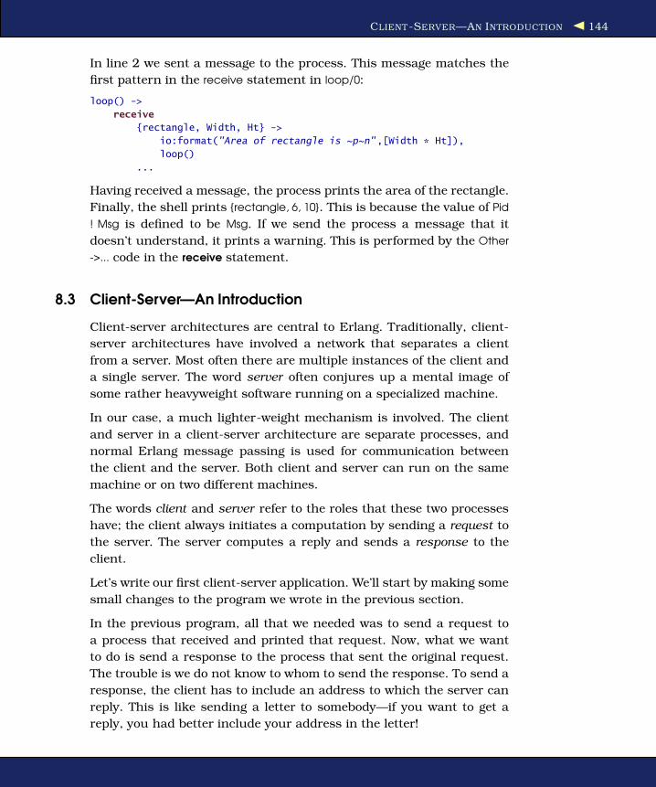
CLIENT -SERVER—AN INTRODUCTION 144
In line 2 we sent a message to the process. This message matches the
first pattern in the receive statement in loop/0:
loop() ->
receive
{rectangle, Width, Ht} ->
io:format("Area of rectangle is ~p~n",[Width * Ht]),
loop()
...
Having received a message, the process prints the area of the rectangle.
Finally, the shell prints {rectangle, 6, 10}. This is because the value of Pid
! Msg is defined to be Msg. If we send the process a message that it
doesn’t understand, it prints a warning. This is performed by the Other
->... code in the receive statement.
8.3 Client-Server—An Introduction
Client-server architectures are central to Erlang. Traditionally, client-
server architectures have involved a network that separates a client
from a server. Most often there are multiple instances of the client and
a single server. The word server often conjures up a mental image of
some rather heavyweight software running on a specialized machine.
In our case, a much lighter-weight mechanism is involved. The client
and server in a client-server architecture are separate processes, and
normal Erlang message passing is used for communication between
the client and the server. Both client and server can run on the same
machine or on two different machines.
The words client and server refer to the roles that these two processes
have; the client always initiates a computation by sending a request to
the server. The server computes a reply and sends a response to the
client.
Let’s write our first client-server application. We’ll start by making some
small changes to the program we wrote in the previous section.
In the previous program, all that we needed was to send a request to
a process that received and printed that request. Now, what we want
to do is send a response to the process that sent the original request.
The trouble is we do not know to whom to send the response. To send a
response, the client has to include an address to which the server can
reply. This is like sending a letter to somebody—if you want to get a
reply, you had better include your address in the letter!
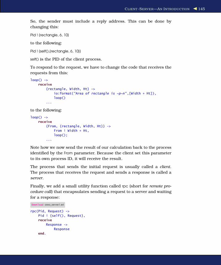
CLIENT -SERVER—AN INTRODUCTION 145
So, the sender must include a reply address. This can be done by
changing this:
Pid ! {rectangle, 6, 10}
to the following:
Pid ! {self(),{rectangle, 6, 10}}
self() is the PID of the client process.
To respond to the request, we have to change the code that receives the
requests from this:
loop() ->
receive
{rectangle, Width, Ht} ->
io:format("Area of rectangle is ~p~n",[Width * Ht]),
loop()
...
to the following:
loop() ->
receive
{From, {rectangle, Width, Ht}} ->
From ! Width * Ht,
loop();
...
Note how we now send the result of our calculation back to the process
identified by the From parameter. Because the client set this parameter
to its own process ID, it will receive the result.
The process that sends the initial request is usually called a client.
The process that receives the request and sends a response is called a
server.
Finally, we add a small utility function called rpc (short for remote pro-
cedure call) that encapsulates sending a request to a server and waiting
for a response:
Download area_server1.erl
rpc(Pid, Request) ->
Pid ! {self(), Request},
receive
Response ->
Response
end.

CLIENT -SERVER—AN INTRODUCTION 146
Putting all of this together, we get the following:
Download area_server1.erl
-module(area_server1).
-export([loop/0, rpc/2]).
rpc(Pid, Request) ->
Pid ! {self(), Request},
receive
Response ->
Response
end.
loop() ->
receive
{From, {rectangle, Width, Ht}} ->
From ! Width * Ht,
loop();
{From, {circle, R}} ->
From ! 3.14159 * R * R,
loop();
{From, Other} ->
From ! {error,Other},
loop()
end.
We can experiment with this in the shell:
1> Pid = spawn(fun area_server1:loop/0).
<0.36.0>
2> area_server1:rpc(Pid, {rectangle,6,8}).
48
3> area_server1:rpc(Pid, {circle,6}).
113.097
4> area_server1:rpc(Pid, socks).
{error,socks}
There’s a slight problem with this code. In the function rpc/2, we send
a request to the server and then wait for a response. But we do not wait
for a response from the server; we wait for any message. If some other
process sends the client a message while it is waiting for a response
from the server, it will misinterpret this message as a response from
the server. We can correct this by changing the form of the receive
statement to this:
loop() ->
receive
{From, ...} ->
From ! {self(), ...}
loop()
...

CLIENT -SERVER—AN INTRODUCTION 147
and by changing rpc to the following:
rpc(Pid, Request) ->
Pid ! {self(), Request},
receive
{Pid, Response} ->
Response
end.
How does this work? When we have entered the rpc function, Pid is
bound to some value, so in the pattern {Pid, Response}, Pid is bound, and
Response is unbound. This pattern will match only a message contain-
ing a two-tuple1 where the first element is Pid. All other messages will
be queued. (receive provides what is called selective receive, which I’ll
describe after this section.)
With this change, we get the following:
Download area_server2.erl
-module(area_server2).
-export([loop/0, rpc/2]).
rpc(Pid, Request) ->
Pid ! {self(), Request},
receive
{Pid, Response} ->
Response
end.
loop() ->
receive
{From, {rectangle, Width, Ht}} ->
From ! {self(), Width * Ht},
loop();
{From, {circle, R}} ->
From ! {self(), 3.14159 * R * R},
loop();
{From, Other} ->
From ! {self(), {error,Other}},
loop()
end.
This works as expected:
1> Pid = spawn(fun area_server2:loop/0).
<0.37.0>
3> area_server2:rpc(Pid, {circle, 5}).
78.5397
1. N-tuple means a tuple of size N, so two-tuple is a tuple of size 2.
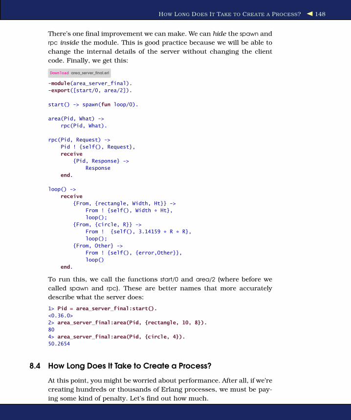
HOW LONG DOES IT TAKE TO CREATE A PROCESS? 148
There’s one final improvement we can make. We can hide the spawn and
rpc inside the module. This is good practice because we will be able to
change the internal details of the server without changing the client
code. Finally, we get this:
Download area_server_final.erl
-module(area_server_final).
-export([start/0, area/2]).
start() -> spawn(fun loop/0).
area(Pid, What) ->
rpc(Pid, What).
rpc(Pid, Request) ->
Pid ! {self(), Request},
receive
{Pid, Response} ->
Response
end.
loop() ->
receive
{From, {rectangle, Width, Ht}} ->
From ! {self(), Width * Ht},
loop();
{From, {circle, R}} ->
From ! {self(), 3.14159 * R * R},
loop();
{From, Other} ->
From ! {self(), {error,Other}},
loop()
end.
To run this, we call the functions start/0 and area/2 (where before we
called spawn and rpc). These are better names that more accurately
describe what the server does:
1> Pid = area_server_final:start().
<0.36.0>
2> area_server_final:area(Pid, {rectangle, 10, 8}).
80
4> area_server_final:area(Pid, {circle, 4}).
50.2654
8.4 How Long Does It Take to Create a Process?
At this point, you might be worried about performance. After all, if we’re
creating hundreds or thousands of Erlang processes, we must be pay-
ing some kind of penalty. Let’s find out how much.

HOW LONG DOES IT TAKE TO CREATE A PROCESS? 149
To investigate this, we’ll time how long it takes to spawn a large number
of processes. Here’s the program:
Download processes.erl
-module(processes).
-export([max/1]).
%% max(N)
%% Create N processes then destroy them
%% See how much time this takes
max(N) ->
Max = erlang:system_info(process_limit),
io:format("Maximum allowed processes:~p~n",[Max]),
statistics(runtime),
statistics(wall_clock),
L = for(1, N, fun() -> spawn(fun() -> wait() end) end),
{_, Time1} = statistics(runtime),
{_, Time2} = statistics(wall_clock),
lists:foreach(fun(Pid) -> Pid ! die end, L),
U1 = Time1 * 1000 / N,
U2 = Time2 * 1000 / N,
io:format("Process spawn time=~p (~p) microseconds~n",
[U1, U2]).
wait() ->
receive
die -> void
end.
for(N, N, F) -> [F()];
for(I, N, F) -> [F()|for(I+1, N, F)].
Here are the results I obtained on the computer I’m using to write this
book, a 2.40GHz Intel Celeron with 512MB of memory running Ubuntu
Linux:
1> processes:max(20000).
Maximum allowed processes:32768
Process spawn time=3.50000 (9.20000) microseconds
ok
2> processes:max(40000).
Maximum allowed processes:32768
=ERROR REPORT==== 26-Nov-2006::14:47:24 ===
Too many processes
...
Spawning 20,000 processes took an average of 3.5 µs/process of CPU
time and 9.2 µs of elapsed (wall-clock) time.

RECEIVE WITH A TIMEOUT 150
Note that I used the BIF erlang:system_info(process_limit) to find the max-
imum allowed number of processes. Note that some of these are re-
served, so your program cannot actually use this number. When we
exceed the system limit, the system crashes with an error report (com-
mand 2).
The system limit is set to 32,767 processes; to exceed this limit, you
have to start the Erlang emulator with the +P flag as follows:
$ erl +P 500000
1> processes:max(50000).
Maximum allowed processes:500000
Process spawn time=4.60000 (10.8200) microseconds
ok
2> processes:max(200000).
Maximum allowed processes:500000
Process spawn time=4.10000 (10.2150) microseconds
3> processes:max(300000).
Maximum allowed processes:500000
Process spawn time=4.13333 (73.6533) microseconds
In the previous example, I set the system limit to half a million pro-
cesses. We can see that the process spawn time is essentially con-
stant between 50,000 to 200,000 processes. At 300,000 processes, the
CPU time per spawn process remains constant, but the elapsed time
increases by a factor of seven. I can also hear my disk chattering away.
This is sure sign that the system is paging and that I don’t have enough
physical memory to handle 300,000 processes.
8.5 Receive with a Timeout
Sometimes a receive statement might wait forever for a message that
never comes. This could be for a number of reasons. For example, there
might be a logical error in our program, or the process that was going
to send us a message might have crashed before it sent the message.
To avoid this problem, we can add a timeout to the receive statement.
This sets a maximum time that the process will wait to receive a mes-
sage. The syntax is as follows:
receive
Pattern1 [when Guard1] ->
Expressions1;
Pattern2 [when Guard2] ->
Expressions2;
...
after Time ->
Expressions
end
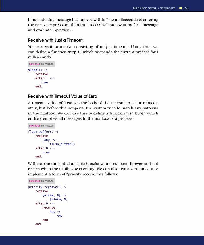
RECEIVE WITH A TIMEOUT 151
If no matching message has arrived within Time milliseconds of entering
the receive expression, then the process will stop waiting for a message
and evaluate Expressions.
Receive with Just a Timeout
You can write a receive consisting of only a timeout. Using this, we
can define a function sleep(T), which suspends the current process for T
milliseconds.
Download lib_misc.erl
sleep(T) ->
receive
after T ->
true
end.
Receive with Timeout Value of Zero
A timeout value of 0 causes the body of the timeout to occur immedi-
ately, but before this happens, the system tries to match any patterns
in the mailbox. We can use this to define a function flush_buffer, which
entirely empties all messages in the mailbox of a process:
Download lib_misc.erl
flush_buffer() ->
receive
_Any ->
flush_buffer()
after 0 ->
true
end.
Without the timeout clause, flush_buffer would suspend forever and not
return when the mailbox was empty. We can also use a zero timeout to
implement a form of “priority receive,” as follows:
Download lib_misc.erl
priority_receive() ->
receive
{alarm, X} ->
{alarm, X}
after 0 ->
receive
Any ->
Any
end
end.

RECEIVE WITH A TIMEOUT 152
If there is not a message matching {alarm, X} in the mailbox, then pri-
ority_receive will receive the first message in the mailbox. If there is no
message at all, it will suspend in the innermost receive and return the
first message it receives. If there is a message matching {alarm, X}, then
this message will be returned immediately. Remember that the after
section is checked only after pattern matching has been performed on
all the entries in the mailbox.
Without the after 0 statement, the alarm message would not be matched
first.
Note: Using large mailboxes with priority receive is rather inefficient, so
if you’re going to use this technique, make sure your mailboxes are not
too large.
receive with Timeout Value of Infinity
If the timeout value in a receive statement is the atom infinity, then the
timeout will never trigger. This might be useful for programs where the
timeout value is calculated outside the receive statement. Sometimes
the calculation might want to return an actual timeout value, and other
times it might want to have the receive wait forever.
Implementing a Timer
We can implement a simple timer using receive timeouts.
The function stimer:start(Time, Fun) will evaluate Fun (a function of zero
arguments) after Time ms. It returns a handle (which is a PID), which
can be used to cancel the timer if required.
Download stimer.erl
-module(stimer).
-export([start/2, cancel/1]).
start(Time, Fun) -> spawn(fun() -> timer(Time, Fun) end).
cancel(Pid) -> Pid ! cancel.
timer(Time, Fun) ->
receive
cancel ->
void
after Time ->
Fun()
end.

SELECTIVE RECEIVE 153
We can test this as follows:
1> Pid = stimer:start(5000, fun() -> io:format("timer event~n") end).
<0.42.0>
timer event
Here I waited more than five seconds so that the timer would trigger.
Now I’ll start a timer and cancel it before the timer period has expired:
2> Pid1 = stimer:start(25000, fun() -> io:format("timer event~n") end).
<0.49.0>
3> stimer:cancel(Pid1).
cancel
8.6 Selective Receive
So far we have glossed over exactly how send and receive work. send
does not actually send a message to a process. Instead, send sends a
message to the mailbox of the process, and receive tries to remove a
message from the mailbox.
Each process in Erlang has an associated mailbox. When you send a
message to the process, the message is put into the mailbox. The only
time the mailbox is examined is when your program evaluates a receive
statement:
receive
Pattern1 [when Guard1] ->
Expressions1;
Pattern2 [when Guard1] ->
Expressions1;
...
after
Time ->
ExpressionTimeout
end
receive works as follows:
1. When we enter a receive statement, we start a timer (but only if an
after section is present in the expression).
2. Take the first message in the mailbox and try to match it against
Pattern1, Pattern2, and so on. If the match succeeds, the message
is removed from the mailbox, and the expressions following the
pattern are evaluated.
3. If none of the patterns in the receive statement matches the first
message in the mailbox, then the first message is removed from
the mailbox and put into a “save queue.” The second message

REGISTERED PROCESSES 154
in the mailbox is then tried. This procedure is repeated until a
matching message is found or until all the messages in the mail-
box have been examined.
4. If none of the messages in the mailbox matches, then the process
is suspended and will be rescheduled for execution the next time a
new message is put in the mailbox. Note that when a new message
arrives, the messages in the save queue are not rematched; only
the new message is matched.
5. As soon as a message has been matched, then all messages that
have been put into the save queue are reentered into the mailbox
in the order in which they arrived at the process. If a timer was
set, it is cleared.
6. If the timer elapses when we are waiting for a message, then evalu-
ate the expressions ExpressionsTimeout and put any saved messages
back into the mailbox in the order in which they arrived at the
process.
8.7 Registered Processes
If we want to send a message to a process, then we need to know its PID.
This is often inconvenient since the PID has to be sent to all processes
in the system that want to communicate with this process. On the other
hand, it is very secure; if you don’t reveal the PID of a process, other
processes cannot interact with it in any way.
Erlang has a method for publishing a process identifier so that any pro-
cess in the system can communicate with this process. Such a process
is called a registered process. There are four BIFs for managing regis-
tered processes:
register(AnAtom, Pid)
Register the process Pid with the name AnAtom. The registration
fails if AnAtom has already been used to register a process.
unregister(AnAtom)
Remove any registrations associated with AnAtom.
Note: If a registered process dies it will be automatically unregis-
tered.
whereis(AnAtom) -> Pid | undefined
Find out whether AnAtom is registered. Return the process iden-
tifier Pid, or return the atom undefined if no process is associated
with AnAtom.

REGISTERED PROCESSES 155
registered() -> [AnAtom::atom()]
Return a list of all registered processes in the system.
Using register, we can revise the example in Section 8.2, A Simple Exam-
ple, on page 143, and we can try to register the name of the process
that we created:
1> Pid = spawn(fun area_server0:loop/0).
<0.51.0>
2> register(area, Pid).
true
Once the name has been registered, we can send it a message like this:
3> area ! {rectangle, 4, 5}.
Area of rectangle is 20
{rectangle,4,5}
A Clock
We can use register to make a registered process that represents a
clock:
Download clock.erl
-module(clock).
-export([start/2, stop/0]).
start(Time, Fun) ->
register(clock, spawn(fun() -> tick(Time, Fun) end)).
stop() -> clock ! stop.
tick(Time, Fun) ->
receive
stop ->
void
after Time ->
Fun(),
tick(Time, Fun)
end.
The clock will happily tick away until you stop it:
3> clock:start(5000, fun() -> io:format("TICK ~p~n",[erlang:now()]) end).
true
TICK {1164,553538,392266}
TICK {1164,553543,393084}
TICK {1164,553548,394083}
TICK {1164,553553,395064}
4> clock:stop().
stop

HOW DO WE WRITE A CONCURRENT PROGRAM? 156
8.8 How Do We Write a Concurrent Program?
When I write a concurrent program, I almost always start with some-
thing like this:
Download ctemplate.erl
-module(ctemplate).
-compile(export_all).
start() ->
spawn(fun() -> loop([]) end).
rpc(Pid, Request) ->
Pid ! {self(), Request},
receive
{Pid, Response} ->
Response
end.
loop(X) ->
receive
Any ->
io:format("Received:~p~n",[Any]),
loop(X)
end.
The receive loop is just any empty loop that receives and prints any
message that I send to it. As I develop the program, I’ll start send-
ing messages to the processes. Because I start with no patterns in the
receive loop that match these messages, I’ll get a printout from the
code at the bottom of the receive statement. When this happens, I add
a matching pattern to the receive loop and rerun the program. This
technique largely determines the order in which I write the program: I
start with a small program and slowly grow it, testing it as I go along.
8.9 A Word About Tail Recursion
Take a look at the receive loop in the area server that we wrote earlier:
Download area_server_final.erl
loop() ->
receive
{From, {rectangle, Width, Ht}} ->
From ! {self(), Width * Ht},
loop();
{From, {circle, R}} ->
From ! {self(), 3.14159 * R * R},
loop();

SPAWNING WITH MFAS 157
{From, Other} ->
From ! {self(), {error,Other}},
loop()
end.
If you look carefully, you’ll see that every time we receive a message,
we process the message and then immediately call loop() again. Such a
procedure is called tail-recursive. A tail-recursive function can be com-
piled so that the last function call in a sequence of statements can be
replaced by a simple jump to the start of the function being called. This
means that a tail-recursive function can loop forever without consum-
ing stack space.
Suppose we wrote the following (incorrect) code:
Line 1 loop() ->- {From, {rectangle, Width, Ht}} ->- From ! {self(), Width * Ht},- loop(),5 someOtherFunc();- {From, {circle, R}} ->- From ! {self(), 3.14159 * R * R},- loop();- ...
10 end
In line 4, we call loop(), but the compiler must reason that “after I’ve
called loop(), I have to return to here, since I have to call someOther-
Func() in line 5.” So, it pushes the address of someOtherFunc onto the
stack and jumps to the start of loop. The problem with this is that
loop() never returns; instead, it just loops forever. So, each time we
pass line 4, another return address gets pushed onto the control stack,
and eventually the system runs out of space.
Avoiding this is easy; if you write a function F that never returns (such
as loop()), make sure that you never call anything after calling F, and
don’t use F in a list or tuple constructor.
8.10 Spawning with MFAs
Most programs we write use spawn(Fun) to create a new process. This
is fine provided we don’t want to dynamically upgrade our code. Some-
times we want to write code that can be upgraded as we run it. If we
want to make sure that our code can be dynamically upgraded, then
we have to use a different form of spawn.
PROBLEMS 158
spawn(Mod, FuncName, Args)
This creates a new process. Args is a list of arguments of the form
[Arg1, Args2, ..., ArgN]. The newly created process starts evaluating
Mod:FuncName(Arg1, Arg2, ..., ArgN).
Spawning a function with an explicit module, function name, and argu-
ment list (called an MFA) is the proper way to ensure that our running
processes will be correctly updated with new versions of the module
code if it is compiled while it is being used. The dynamic code upgrade
mechanism does not work with spawned funs. It works only with explic-
itly named MFAs. For more details, read Section E.4, Dynamic Code
Loading, on page 435.
8.11 Problems
1. Write a function start(AnAtom, Fun) to register AnAtom as spawn(Fun).
Make sure your program works correctly in the case when two
parallel processes simultaneously evaluate start/2. In this case,
you must guarantee that one of these processes succeeds and the
other fails.
2. Write a ring benchmark. Create N processes in a ring. Send a mes-
sage round the ring M times so that a total of N * M messages get
sent. Time how long this takes for different values of N and M.
Write a similar program in some other programming language you
are familiar with. Compare the results. Write a blog, and publish
the results on the Internet!
That’s it—you can now write concurrent programs!
Next we’ll look at error recovery and see how we can write fault-tolerant
concurrent programs using three more concepts: links, signals, and
trapping process exits. That’s in the next chapter.
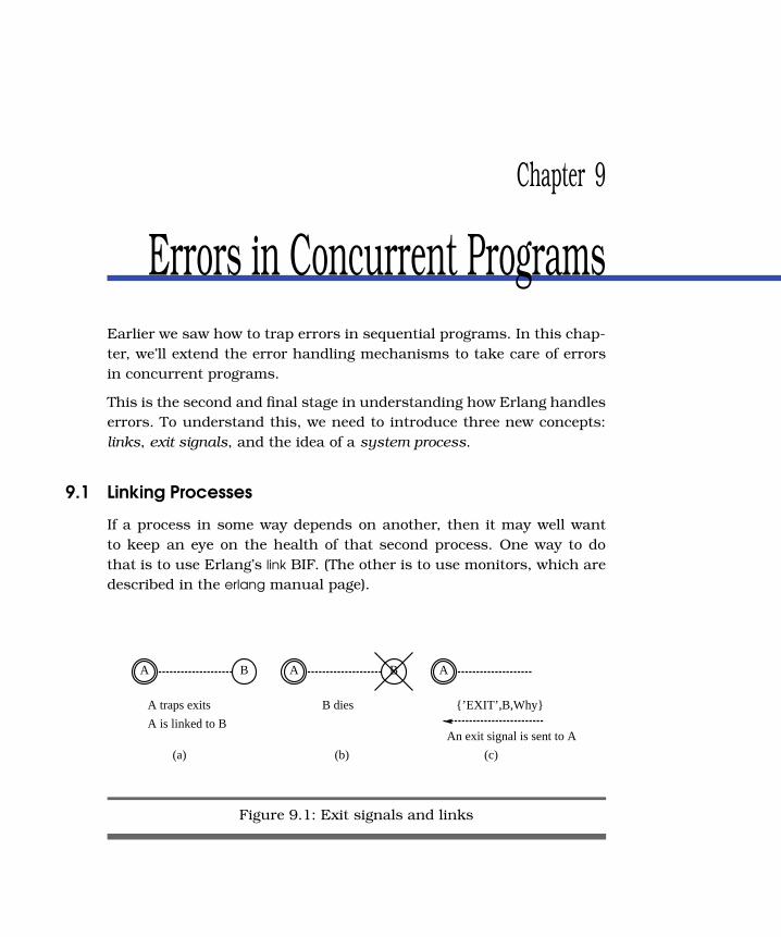
Chapter 9
Errors in Concurrent ProgramsEarlier we saw how to trap errors in sequential programs. In this chap-
ter, we’ll extend the error handling mechanisms to take care of errors
in concurrent programs.
This is the second and final stage in understanding how Erlang handles
errors. To understand this, we need to introduce three new concepts:
links, exit signals, and the idea of a system process.
9.1 Linking Processes
If a process in some way depends on another, then it may well want
to keep an eye on the health of that second process. One way to do
that is to use Erlang’s link BIF. (The other is to use monitors, which are
described in the erlang manual page).
A B
A traps exits
A is linked to B
(a)
A B
B dies
(b)
A
{’EXIT’,B,Why}
An exit signal is sent to A
(c)
Figure 9.1: Exit signals and links

AN ON_EXIT HANDLER 160
Figure 9.1, on the previous page, shows two processes, A and B. They
are linked together (as shown by the dotted line in the diagram). The
link was made when one of the processes called the BIF link(P), with P
being the PID of the other process. Once linked, the two processes will
implicitly monitor each other. If A dies, then B will be sent something
called an exit signal. If B dies, then A receives the signal.
The mechanisms described in this chapter are completely general. They
work on a single node, but they also work on sets of nodes in a dis-
tributed Erlang system. As we’ll see later in Chapter 10, Distributed
Programming, on page 175, we can spawn processes on remote nodes
just as easily as we can spawn processes on the current node. All the
link mechanisms that we talk about in the chapter work equally well in
a distributed system.
What happens when a process receives an exit signal? If the receiver
hasn’t taken any special steps, the exit signal will cause it, too, to exit.
However, a process can ask to trap these exit signals. When a process is
in this state, it is called a system process. If a process linked to a system
process exits for some reason, the system process is not automatically
terminated. Instead, the system process receives an exit signal, which
it can trap and process.
Part (a) of the diagram shows the processes linked together. A is a sys-
tem process (shown by a double circle). In part (b), B dies, and in part
(c), an exit signal is sent to A.
Later in the chapter, we’ll go through all the details of exactly what
happens when an exit signal arrives at a process. But before this, we’ll
start with a short example that shows how to use this mechanism to
write a simple exit handler. The exit handler is a process that evaluates
a particular function, when some other process crashes. The exit han-
dler is in itself a useful building block for constructing more advanced
abstractions.
9.2 An on_exit Handler
We want to perform some action when a process exits. We can write a
function on_exit(Pid, Fun) that creates a link to the process Pid. If Pid dies
with reason, Why and then Fun(Why) is evaluated.

AN ON_EXIT HANDLER 161
Here’s the program:
Download lib_misc.erl
Line 1 on_exit(Pid, Fun) ->- spawn(fun() ->- process_flag(trap_exit, true),- link(Pid),5 receive- {'EXIT', Pid, Why} ->- Fun(Why)- end- end).
In line 3, the statement process_flag(trap_exit, true) turns the spawned
process into a system process. link(Pid) (line 4) links the newly spawned
process to Pid. Finally, when the process dies, an exit signal is received
(line 6) and processed (line 7).
Note: When you read this code, you’ll see we just used a variable Pid
everywhere. This is the process identifier of the linked process. We can’t
use a variable name like LinkedPid to say this, because before we have
evaluated link(Pid), it’s not a linked process. When you see a message
like {’EXIT’, Pid, _}, this should alert you that Pid is a linked process and
that it has just died.
To test this, we’ll define a function F that waits for a single message X
and then computes list_to_atom(X):
1> F = fun() ->
receive
X -> list_to_atom(X)
end
end.
#Fun<erl_eval.20.69967518>
We’ll spawn this:
2> Pid = spawn(F).
<0.61.0>
And we’ll set up an on_exit handler to monitor it:
3> lib_misc:on_exit(Pid,
fun(Why) ->
io:format(" ~p died with:~p~n",[Pid, Why])
end).
<0.63.0>
REMOTE HANDLING OF ERRORS 162
If we send an atom to Pid, the process will die (because it tries to eval-
uate list_to_atom of a nonlist), and the on_exit handler will be called:
4> Pid ! hello.
hello
<0.61.0> died with:{badarg,[{erlang,list_to_atom,[hello]}]}
The function that is invoked when the process dies can, of course, per-
form any computation it likes: it can ignore the error, log the error, or
restart the application. The choice is up to the programmer.
9.3 Remote Handling of Errors
Let’s just stop and think for a moment about the previous example.
It illustrates an extremely important part of the Erlang philosophy,
namely, the remote handling of errors.
Because an Erlang system consists of large numbers of parallel pro-
cesses, we are no longer forced to deal with errors in the process where
the error occurs; we can deal with them in a different process. The
process that deals with the error doesn’t even have to be on the same
machine. In distributed Erlang, described in the next chapter, we’ll see
that this simple mechanism even works across machine boundaries.
This is very important, since if the entire machine has crashed, the
program that fixes the error cannot be on the same machine.
9.4 The Details of Error Handling
Let’s look again at the three concepts that underlie Erlang error han-
dling:
Links
A link is something that defines an error propagation path between
two processes. If two processes are linked together and one of the
processes dies, then an exit signal will be sent to the other process.
The set of processes that are currently linked to a given process is
called the link set of that process.
Exit signals
An exit signal is something generated by a process when the pro-
cess dies. This signal is broadcast to all processes that are in the
link set of the dying process. The exit signal contains an argu-
ment giving the reason why the process died. The reason can be

THE DETAILS OF ERROR HANDLING 163
any Erlang data term. This reason can be set explicitly by call-
ing the primitive exit(Reason), or it is set implicitly when an error
occurs. For example, if a program tries to divide a number by zero,
then the exit reason will be the atom badarith.
When a process has successfully evaluated the function it was
spawned with, it will die with the exit reason normal.
In addition, a process Pid1 can explicitly send an exit signal X to a
process Pid2 by evaluating exit(Pid2, X). The process that sends the
exit signal does not die; it resumes execution after it has sent the
signal. Pid2 will receive a {’EXIT’, Pid1, X} message (if it is trapping
exits), exactly as if the originating process had died. Using this
mechanism, Pid1 can “fake” its own death (this is deliberate).
System processes
When a process receives a non-normal exit signal, it too will die
unless it is special kind of process called a system process. When
a system process receives an exit signal Why from a process Pid,
then the exit signal is converted to the message {’EXIT’, Pid, Why}
and added to the mailbox of the system process.
Calling the BIF process_flag(trap_exit, true) turns a normal process
into a system process that can trap exits.
When an exit signal arrives at a process, then a number of different
things might happen. What happens depends upon the state of the
receiving process and upon the value of the exit signal and is deter-
mined by the following table:
trap_exit Exit Signal Action
true kill Die: Broadcast the exit signal killed to the link set.
true X Add {’EXIT’, Pid, X} to the mailbox.
false normal Continue: Do-nothing signal vanishes.
false kill Die: Broadcast the exit signal killed to the link set.
false X Die: Broadcast the exit signal X to the link set.
If the reason is given as kill, then an untrappable exit signal will be sent.
An untrappable exit signal will always kill the process it is sent to, even
if it is a system process. This is used by the supervisor process in OTP
to kill rogue processes. When a process receives a kill signal, it dies and
broadcasts killed signals to the processes in its link set. This is a safety
measure to avoid accidentally killing more of the system than you had
intended.

THE DETAILS OF ERROR HANDLING 164
The kill signal is intended to kill rogue processes. Think hard before
using it.
Programming Idioms for Trapping Exits
Trapping exits is actually a lot easier than you might suspect from
reading the preceding sections. Although it is possible to use the exit
generation and trapping mechanisms in a number of ingenious ways,
most programs use one of three simple idioms.
Idiom 1: I Don’t Care If a Process I Create Crashes
Here the process that creates a parallel process that just uses spawn:
Pid = spawn(fun() -> ... end)
Nothing else. If the spawned process crashes, the current process con-
tinues.
Idiom 2: I Want to Die If a Process I Create Crashes
To be strict, we should say, “If the process I create crashes with a non-
normal exit.” To achieve this, the process that creates a parallel process
uses spawn_link and must not have previously been set to trap exits. We
just write this:
Pid = spawn_link(fun() -> ... end)
Then if the spawned process crashes with a non-normal exit, the cur-
rent process will also crash.
Idiom 3: I Want to Handle Errors If a Process I Create Crashes
Here we use spawn_link and trap_exits. We code this as follows:
...
process_flag(trap_exit, true),
Pid = spawn_link(fun() -> ... end),
...
loop(...).
loop(State) ->
receive
{'EXIT', SomePid, Reason} ->
%% do something with the error
loop(State1);
...
end

THE DETAILS OF ERROR HANDLING 165
The process evaluating loop now traps exits and does not die if the
processes it is linked to dies. It will see all exit signals (converted to
messages) from dying processes,1 and can take any action it wants
when it detects process failures.
Trapping Exit Signals (Advanced)
You can skip this section on a first reading. Most of what you want to
do will be correctly handled by one of the three idioms shown in the
previous section. If you really want to know, read on. But be warned. It
can be difficult to understand the precise details of these mechanisms.
In most cases, you don’t need to understand the mechanism since if
you use one of the common program idioms (in the previous section) or
the OTP libraries, then the system will “do the right thing” without you
having to worry.
To really understand the details of error handling, we’ll write a little
program to illustrate how error handling and links interact. Our pro-
gram starts as follows:
Download edemo1.erl
-module(edemo1).
-export([start/2]).
start(Bool, M) ->
A = spawn(fun() -> a() end),
B = spawn(fun() -> b(A, Bool) end),
C = spawn(fun() -> c(B, M) end),
sleep(1000),
status(b, B),
status(c, C).
This starts three processes: A, B, and C. The idea is that A will be linked
to B, and B will be linked to C. A will trap exits and watch for exits from
B. B will trap exits if Bool is true, and C will die with exit reason M.
(You might by wondering about the sleep(1000) statement. This is to
allow any messages that come when C dies to be printed before we
check the status of the three processes. It doesn’t change the logic of
the program, but it does alter the printout order.)2
1. Apart from the signal generated by exit(Pid, kill)
2. Using sleep to synchronize processes is unsafe. It’s OK in a short example, but for
production-quality code, explicit synchronization should be performed.

THE DETAILS OF ERROR HANDLING 166
The code for the A, B, and C processes is as follows:
Download edemo1.erl
a() ->
process_flag(trap_exit, true),
wait(a).
b(A, Bool) ->
process_flag(trap_exit, Bool),
link(A),
wait(b).
c(B, M) ->
link(B),
case M of
{die, Reason} ->
exit(Reason);
{divide, N} ->
1/N,
wait(c);
normal ->
true
end.
wait/1 just prints any message that it receives:
Download edemo1.erl
wait(Prog) ->
receive
Any ->
io:format("Process ~p received ~p~n",[Prog, Any]),
wait(Prog)
end.
And the remainder of the program is as follows:
Download edemo1.erl
sleep(T) ->
receive
after T -> true
end.
status(Name, Pid) ->
case erlang:is_process_alive(Pid) of
true ->
io:format("process ~p (~p) is alive~n", [Name, Pid]);
false ->
io:format("process ~p (~p) is dead~n", [Name,Pid])
end.
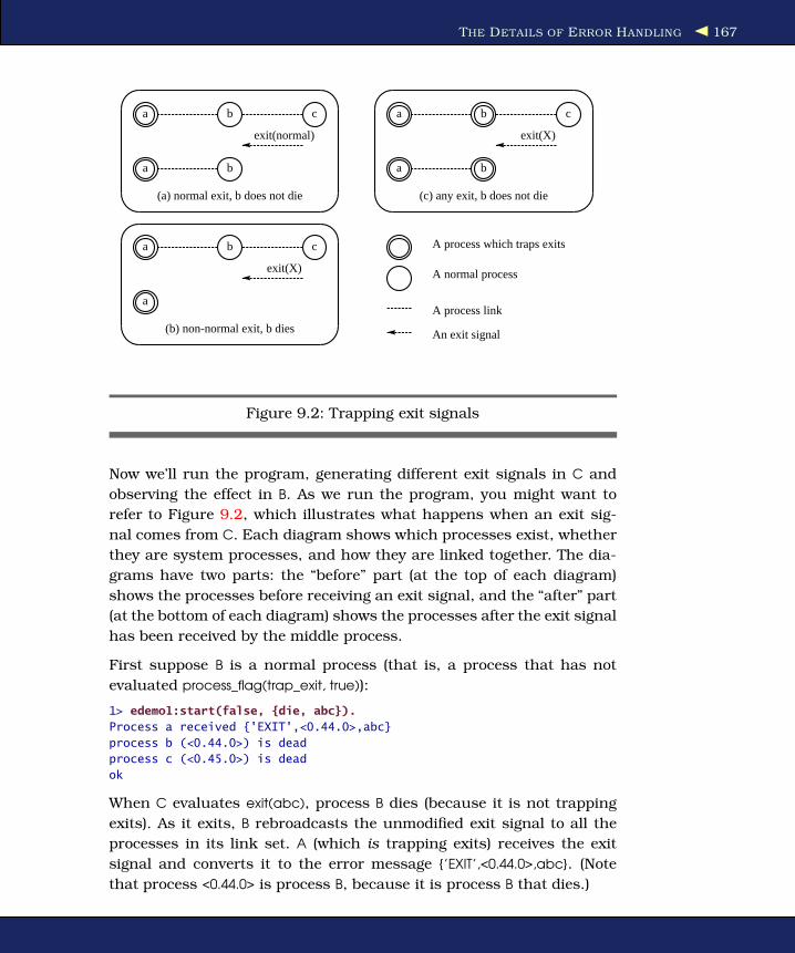
THE DETAILS OF ERROR HANDLING 167
a b c
exit(normal)
a b
(a) normal exit, b does not die
a b c
exit(X)
a
(b) non-normal exit, b dies
a b c
exit(X)
a b
(c) any exit, b does not die
A process which traps exits
A normal process
A process link
An exit signal
Figure 9.2: Trapping exit signals
Now we’ll run the program, generating different exit signals in C and
observing the effect in B. As we run the program, you might want to
refer to Figure 9.2, which illustrates what happens when an exit sig-
nal comes from C. Each diagram shows which processes exist, whether
they are system processes, and how they are linked together. The dia-
grams have two parts: the “before” part (at the top of each diagram)
shows the processes before receiving an exit signal, and the “after” part
(at the bottom of each diagram) shows the processes after the exit signal
has been received by the middle process.
First suppose B is a normal process (that is, a process that has not
evaluated process_flag(trap_exit, true)):
1> edemo1:start(false, {die, abc}).
Process a received {'EXIT',<0.44.0>,abc}
process b (<0.44.0>) is dead
process c (<0.45.0>) is dead
ok
When C evaluates exit(abc), process B dies (because it is not trapping
exits). As it exits, B rebroadcasts the unmodified exit signal to all the
processes in its link set. A (which is trapping exits) receives the exit
signal and converts it to the error message {’EXIT’,<0.44.0>,abc}. (Note
that process <0.44.0> is process B, because it is process B that dies.)

THE DETAILS OF ERROR HANDLING 168
Let’s try another scenario. Here we tell C to die with the reason normal.3
2> edemo1:start(false, {die, normal}).
process b (<0.48.0>) is alive
process c (<0.49.0>) is dead
ok
B does not die, since it received an exit normal signal.
Now let’s make C generate an arithmetic error:
3> edemo1:start(false, {divide,0}).
=ERROR REPORT==== 8-Dec-2006::11:12:47 ===
Error in process <0.53.0> with exit value: {badarith,[{edemo1,c,2}]}
Process a received {'EXIT',<0.52.0>,{badarith,[{edemo1,c,2}]}}
process b (<0.52.0>) is dead
process c (<0.53.0>) is dead
ok
When C tries to divide by zero, an error occurs, and the process dies
with a {badarith, ..} error. B receives this and dies, and the error is prop-
agated to A.
Finally, we’ll have C exit with a Reason of kill:
4> edemo1:start(false, {die,kill}).
Process a received {'EXIT',<0.56.0>,killed} <-- ** changed to killed **process b (<0.56.0>) is dead
process c (<0.57.0>) is dead
ok
The exit reason kill causes B to die, and the error is propagated to the
link set of B with reason killed. The behavior in these cases is illustrated
in Figure 9.2, on the preceding page, boxes (a) and (b).
We can repeat these tests with B trapping exits. This is the situation
depicted in box (c) of Figure 9.2, on the previous page:
5> edemo1:start(true, {die, abc}).
Process b received {'EXIT',<0.61.0>,abc}
process b (<0.60.0>) is alive
process c (<0.61.0>) is dead
ok
6> edemo1:start(true, {die, normal}).
Process b received {'EXIT',<0.65.0>,normal}
process b (<0.64.0>) is alive
process c (<0.65.0>) is dead
ok
3. When a process terminates normally, it has the same effect as if it had evaluated
exit(normal).
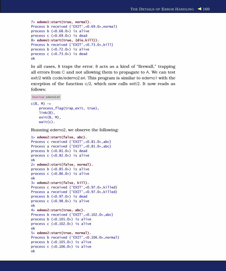
THE DETAILS OF ERROR HANDLING 169
7> edemo1:start(true, normal).
Process b received {'EXIT',<0.69.0>,normal}
process b (<0.68.0>) is alive
process c (<0.69.0>) is dead
8> edemo1:start(true, {die,kill}).
Process b received {'EXIT',<0.73.0>,kill}
process b (<0.72.0>) is alive
process c (<0.73.0>) is dead
ok
In all cases, B traps the error. B acts as a kind of “firewall,” trapping
all errors from C and not allowing them to propagate to A. We can test
exit/2 with code/edemo2.erl. This program is similar to edemo1 with the
exception of the function c/2, which now calls exit/2. It now reads as
follows:
Download edemo2.erl
c(B, M) ->
process_flag(trap_exit, true),
link(B),
exit(B, M),
wait(c).
Running edemo2, we observe the following:
1> edemo2:start(false, abc).
Process c received {'EXIT',<0.81.0>,abc}
Process a received {'EXIT',<0.81.0>,abc}
process b (<0.81.0>) is dead
process c (<0.82.0>) is alive
ok
2> edemo2:start(false, normal).
process b (<0.85.0>) is alive
process c (<0.86.0>) is alive
ok
3> edemo2:start(false, kill).
Process c received {'EXIT',<0.97.0>,killed}
Process a received {'EXIT',<0.97.0>,killed}
process b (<0.97.0>) is dead
process c (<0.98.0>) is alive
ok
4> edemo2:start(true, abc).
Process b received {'EXIT',<0.102.0>,abc}
process b (<0.101.0>) is alive
process c (<0.102.0>) is alive
ok
5> edemo2:start(true, normal).
Process b received {'EXIT',<0.106.0>,normal}
process b (<0.105.0>) is alive
process c (<0.106.0>) is alive
ok

ERROR HANDLING PRIMITIVES 170
6> edemo2:start(true, kill).
Process c received {'EXIT',<0.109.0>,killed}
Process a received {'EXIT',<0.109.0>,killed}
process b (<0.109.0>) is dead
process c (<0.110.0>) is alive
ok
9.5 Error Handling Primitives
Here are the most common primitives for manipulating links and for
trapping and sending exit signals:
@spec spawn_link(Fun) -> Pid
This is exactly like spawn(Fun), but it also creates a link between
the parent and child processes. (spawn_link is an atomic operation,
which is not equivalent to spawn followed by link since the process
might die between the spawn and the link.)
@spec process_flag(trap_exit, true)
This turns the current process into a system process. A system
process is a process that can receive and process error signals.
Note: It is possible to set the trap_exit flag to false, after it has been
set to true. This primitive should be used only to change a regular
process into a system process and not the other way around.
@spec link(Pid) -> true
Create a link to the process Pid if there is not already a link. Links
are symmetric. If a process A evaluates link(B), then it will be linked
to B. The net effect is the same as if B had evaluated link(A).
If the process Pid does not exist, then an exit noproc exception is
raised.
If A is already linked to B and evaluates link(B) (or vice versa), the
call is ignored.
@spec unlink(Pid) -> true
This removes any link between the current process and the pro-
cess Pid.
@spec exit(Why) -> none()
This causes the current process to terminate with reason Why. If
the clause that executes this statement is not within the scope of

ERROR HANDLING PRIMITIVES 171
Joe Asks. . .
How Can We Make a Fault-Tolerant System?
To make something fault tolerant, we need at least two com-puters. One computer does the job, and another computerwatches the first computer and must be ready to take over ata moment’s notice if the first computer fails.
This is exactly how error recovery works in Erlang. One processdoes the job, and another process watches the first processand takes over if things go wrong. That’s why we need to mon-itor processes and to know why things fail. The examples in thischapter show you how to do this.
In distributed Erlang, the process that does the job and theprocesses that monitor the process that does the job can beplaced on physically different machines. Using this technique,we can start designing fault-tolerant software.
This pattern is common. We call it the worker-supervisor model,and an entire section of the OTP libraries is devoted to buildingsupervision trees that use this idea.
The basic language primitive that makes all this possible is thelink primitive.
Once you understand how link works and get yourself accessto two computers, then you’re well on your way to building yourfirst fault-tolerant system.
a catch statement, then the current process will broadcast an exit
signal, with argument Why to all processes to which it is currently
linked.
@spec exit(Pid, Why) -> true
This sends an exit signal with reason Why to the process Pid.
@spec erlang:monitor(process, Item) -> MonitorRef
This sets up a monitor. Item is a PID or a registered name of a
process. For details, see the erlang manual page.

SETS OF LINKED PROCESSES 172
(a) Some linked processes
1 2 3
4
5
6
7 8
9
(b) The linked processes die
1
8 5
9
Figure 9.3: Trapping exit signals
9.6 Sets of Linked Processes
Suppose we have a large set of parallel processes that are involved in
some computation and something goes wrong. How can we identify and
kill all the processes that are involved?
The easiest way to do this is make sure that all the processes that you
want to die as a group are linked together and do not trap exits. If any
of the processes terminates with a non-normal exit reason, then all the
processes in the group will die.
This behavior is illustrated in Figure 9.3. Box (a) represents a set of
nine processes, where processes 2, 3, 4, 6, and 7 are linked together.
If any of these processes dies with a non-normal exit, then the entire
group of processes will die, resulting in box (b).
Sets of linked processes are used to structure software to make fault-
tolerant systems. You can do this yourself in your own design, or you
can use the library functions described in Section 18.5, The Supervision
Tree, on page 351.
9.7 Monitors
Sometimes programming with links is tricky, because links are sym-
metric. If A dies, B will be sent an exit signal, and vice versa. To prevent
a process from dying, we have to make it a system process, but we
might not want to do this. In such occasions we can use a monitor.
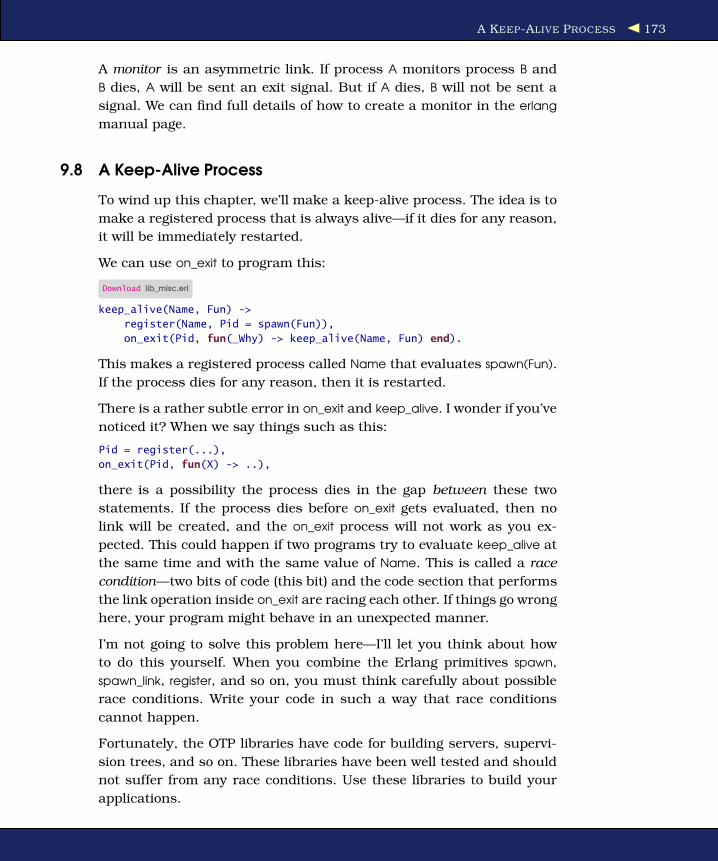
A KEEP-ALIVE PROCESS 173
A monitor is an asymmetric link. If process A monitors process B and
B dies, A will be sent an exit signal. But if A dies, B will not be sent a
signal. We can find full details of how to create a monitor in the erlang
manual page.
9.8 A Keep-Alive Process
To wind up this chapter, we’ll make a keep-alive process. The idea is to
make a registered process that is always alive—if it dies for any reason,
it will be immediately restarted.
We can use on_exit to program this:
Download lib_misc.erl
keep_alive(Name, Fun) ->
register(Name, Pid = spawn(Fun)),
on_exit(Pid, fun(_Why) -> keep_alive(Name, Fun) end).
This makes a registered process called Name that evaluates spawn(Fun).
If the process dies for any reason, then it is restarted.
There is a rather subtle error in on_exit and keep_alive. I wonder if you’ve
noticed it? When we say things such as this:
Pid = register(...),
on_exit(Pid, fun(X) -> ..),
there is a possibility the process dies in the gap between these two
statements. If the process dies before on_exit gets evaluated, then no
link will be created, and the on_exit process will not work as you ex-
pected. This could happen if two programs try to evaluate keep_alive at
the same time and with the same value of Name. This is called a race
condition—two bits of code (this bit) and the code section that performs
the link operation inside on_exit are racing each other. If things go wrong
here, your program might behave in an unexpected manner.
I’m not going to solve this problem here—I’ll let you think about how
to do this yourself. When you combine the Erlang primitives spawn,
spawn_link, register, and so on, you must think carefully about possible
race conditions. Write your code in such a way that race conditions
cannot happen.
Fortunately, the OTP libraries have code for building servers, supervi-
sion trees, and so on. These libraries have been well tested and should
not suffer from any race conditions. Use these libraries to build your
applications.

A KEEP-ALIVE PROCESS 174
We have now covered all the mechanisms for detecting and trapping
errors in an Erlang program. In later chapters we’ll be using these
mechanisms to build reliable software systems that can recover from
faults. Now we’ve finished with programming techniques aimed at
single-processor systems.
The next chapter looks at simple distributed systems.

Chapter 10
Distributed ProgrammingIn this chapter, we’ll introduce the libraries and Erlang primitives that
we’ll use to write distributed Erlang programs.Distributed programs are
programs that are designed to run on networks of computers and that
can coordinate their activities only by message passing.
There are number of reasons why we might want to write distributed
applications. Here are some:
Performance
We can make our programs go faster by arranging that different
parts of the program are run in parallel on different machines.
Reliability
We can make fault-tolerant systems by structuring the system to
run on several machines. If one machine fails, we can continue on
another machine.
Scalability
As we scale up an application, sooner or later we will exhaust
the capabilities of even the most powerful machine. At this stage
we have to add more machines to add capacity. Adding a new
machine should be a simple operation that does not require large
changes to the application architecture.
Intrinsically distributed application
Many applications are inherently distributed. If we write a mul-
tiuser game or chat system, different users will be scattered all
over the globe. If we have a large number of users in a particular
geographic location, we want to place the computation resources
near the users.
CHAPTER 10. DISTRIBUTED PROGRAMMING 176
Fun
Most of the fun programs that I want to write are distributed.
Many of these involve interaction with people and machines all
over the world.
In this book we’ll talk about two main models of distribution:
• Distributed Erlang: Provides a method for programming applica-
tions that run on a set of tightly coupled computers.1 In dis-
tributed Erlang, programs are written to run on Erlang nodes. We
can spawn a process on any node, and all the message passing
and error handling primitives we talked about in previous chap-
ters work as in the single node case.
Distributed Erlang applications run in a trusted environment—
since any node can perform any operation on any other Erlang
node, a high degree of trust is involved. Typically distributed Er-
lang applications will be run on clusters on the same LAN and
behind a firewall, though they can run in an open network.
• Socket-based distribution: Using TCP/IP sockets, we can write dis-
tributed applications that can run in an untrusted environment.
The programming model is less powerful than that used in dis-
tributed Erlang but more secure. In Section 10.5, Socket-Based
Distribution, on page 187, we’ll see how to make applications using
a simple socket-based distribution mechanism.
If you think back to the previous chapters, you’ll recall that the basic
unit that we construct programs from is the process. Writing a dis-
tributed Erlang program is easy; all we have to do is spawn our pro-
cesses on the correct machines, and then everything works as before.
We are all used to writing sequential programs. Writing distributed pro-
grams is usually a lot more difficult. In this chapter, we’ll look at a
number of techniques for writing simple distributed programs. Even
though the programs are simple, they are very useful.
We’ll start with a number of small examples. To do this, we’ll need to
learn only two things; then we can make our first distributed program.
We’ll learn how to start an Erlang node and how to perform a remote
procedure call on a remote Erlang node.
1. For example, machines on the same LAN dedicated to solving a particular problem.

THE NAME SERVER 177
When I develop a distributed application, I always work on the program
in a specific order, which is as follows:
1. I write and test my program in a regular nondistributed Erlang
session. This is what we’ve been doing up to now, so it presents
no new challenges.
2. I test my program on two different Erlang nodes running on the
same computer.
3. I test my program on two different Erlang nodes running on two
physically separated computers either in the same local area net-
work or anywhere on the Internet.
The final step can be problematic. If we run on machines within the
same administrative domain, this is rarely a problem. But when the
nodes involved belong to machines in different domains, we can run
into problems with connectivity, and we have to ensure that our system
firewalls and security settings are correctly configured.
In the next sections, we’ll make a simple name server, going through
these steps in order. Specifically, we will do the following:
• Stage 1: Write and test the name server in a regular undistributed
Erlang system.
• Stage 2: Test the name server on two nodes on the same machine.
• Stage 3: Test the name server on two different nodes on two dif-
ferent machines on the same local area network.
• Stage 4: Test the name server on two different machines belonging
to two different domains in two different countries.
10.1 The Name Server
A name server is a program that, given a name, returns a value asso-
ciated with that name. We can also change the value associated with a
particular name.
Our first name server is extremely simple. It is not fault tolerant, so all
the data it stores will be lost if it crashes. The point of this exercise is not
to make a fault-tolerant name server but to get started with distributed
programming techniques.

THE NAME SERVER 178
Stage 1: A Simple Name Server
Our name server kvs is a simple Key 7→ Value, server. It has the following
interface:
@spec kvs:start() -> true
Start the server; this creates a server with the registered name kvs.
@spec kvs:store(Key, Value) -> true
Associate Key with Value.
@spec kvs:lookup(Key) -> {ok, Value} | undefined
Look up the value of Key, and return {ok, Value} if there is a value
associated with Key; otherwise, return undefined.
The key-value server is implemented using the process dictionary get
and put primitives, as follows:
Download socket_dist/kvs.erl
-module(kvs).
-export([start/0, store/2, lookup/1]).
start() -> register(kvs, spawn(fun() -> loop() end)).
store(Key, Value) -> rpc({store, Key, Value}).
lookup(Key) -> rpc({lookup, Key}).
rpc(Q) ->
kvs ! {self(), Q},
receive
{kvs, Reply} ->
Reply
end.
loop() ->
receive
{From, {store, Key, Value}} ->
put(Key, {ok, Value}),
From ! {kvs, true},
loop();
{From, {lookup, Key}} ->
From ! {kvs, get(Key)},
loop()
end.
We’ll start by testing the server locally to see that it works correctly:
1> kvs:start().
true
2> kvs:store({location, joe}, "Stockholm").
true

THE NAME SERVER 179
3> kvs:store(weather, raining).
true
4> kvs:lookup(weather).
{ok,raining}
5> kvs:lookup({location, joe}).
{ok,"Stockholm"}
6> kvs:lookup({location, jane}).
undefined
So far, we get no unpleasant surprises.
Stage 2: Client on One Node, Server on Second Node but Same
Host
Now we’ll start two Erlang nodes on the same computer. To do this, we
need to open two terminal windows and start two Erlang systems.
First, we fire up a terminal shell,2 and start a distributed Erlang node
in this shell called gandalf; then we start the server:
$ erl -sname gandalf
(gandalf@localhost) 1> kvs:start().
true
Windows note: The Windows name might not be localhost; if it is not
localhost, then you will have to use the name that Windows returned in
place of localhost in all subsequent commands.
The argument -sname gandalf means “start an Erlang node with name
gandalf on the local host.” Note how the Erlang shell prints the name of
the Erlang node3 before the command prompt.
Second, we start a second terminal session and start an Erlang node
called bilbo. Then we can call the functions in kvs using the library
module rpc. (Note that rpc is a standard Erlang library module, which
is not the same as the rpc function we wrote earlier.)
$ erl -sname bilbo
(bilbo@localhost) 1> rpc:call(gandalf@localhost,
kvs,store, [weather, fine]).
true
(bilbo@localhost) 2> rpc:call(gandalf@localhost,
kvs,lookup,[weather]).
{ok,fine}
2. Windows users: Read Appendix B, on page 396. Once you have access to a shell
window, the command erl -name Node should work. Remember to set your paths so you
can find erl.exe (this should have a name something like C:\Program Files\erl5.4.4\bin\erl.exe.3. The node name is of the form Name@Host. Name and Host are both atoms, so they will
have to be quoted if they contain any nonatom characters.
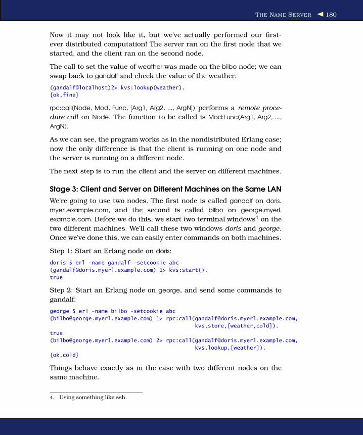
THE NAME SERVER 180
Now it may not look like it, but we’ve actually performed our first-
ever distributed computation! The server ran on the first node that we
started, and the client ran on the second node.
The call to set the value of weather was made on the bilbo node; we can
swap back to gandalf and check the value of the weather:
(gandalf@localhost)2> kvs:lookup(weather).
{ok,fine}
rpc:call(Node, Mod, Func, [Arg1, Arg2, ..., ArgN]) performs a remote proce-
dure call on Node. The function to be called is Mod:Func(Arg1, Arg2, ...,
ArgN).
As we can see, the program works as in the nondistributed Erlang case;
now the only difference is that the client is running on one node and
the server is running on a different node.
The next step is to run the client and the server on different machines.
Stage 3: Client and Server on Different Machines on the Same LAN
We’re going to use two nodes. The first node is called gandalf on doris.
myerl.example.com, and the second is called bilbo on george.myerl.
example.com. Before we do this, we start two terminal windows4 on the
two different machines. We’ll call these two windows doris and george.
Once we’ve done this, we can easily enter commands on both machines.
Step 1: Start an Erlang node on doris:
doris $ erl -name gandalf -setcookie abc
([email protected]) 1> kvs:start().
true
Step 2: Start an Erlang node on george, and send some commands to
gandalf:
george $ erl -name bilbo -setcookie abc
([email protected]) 1> rpc:call([email protected],
kvs,store,[weather,cold]).
true
([email protected]) 2> rpc:call([email protected],
kvs,lookup,[weather]).
{ok,cold}
Things behave exactly as in the case with two different nodes on the
same machine.
4. Using something like ssh.

THE NAME SERVER 181
Now for this to work, things are a slightly more complicated than in the
case where we ran two nodes on the same computer. We have to take
four steps:
1. Start Erlang with the -name parameter. When we have two nodes
on the same machine, we use “short” names (as indicated by the
-sname flag), but if they are on different networks, we use -name.
We can also use -sname on two different machines when they are
on the same subnet. Using -sname is also the only method that will
work if no DNS service is available.
2. Ensure that both nodes have the same cookie. This is why both
nodes were started with the command-line argument -setcookie
abc. (We’ll talk more about cookies later in this chapter.5)
3. Make sure the fully qualified hostnames of the nodes concerned
are resolvable by DNS. In my case, the domain name myerl.
example.com is purely local to my home network and is resolved
locally by adding an entry to /etc/hosts.
4. Make sure that both systems have the same version of the code6
that we want to run. In our case, the same version of the code for
kvs has to be available on both systems. There are several ways of
doing this:
a) In my setup at home, I have two physically separated comput-
ers with no shared file systems; here I physically copy kvs.erl
to both machines and compile it before starting the programs.
b) On my work computer we use workstations with a shared NFS
disk. Here I merely start Erlang in the shared directory from
two different workstations.
c) Configure the code server to do this. I won’t describe how to
do this here. Have a look at the manual page for the module
erl_prim_loader.
d) Use the shell command nl(Mod). This loads the module Mod
on all connected nodes.
5. When we ran two nodes on the same machine, both nodes could access the same
cookie file, $HOME/.erlang.cookie, which is why we didn’t have to add the cookie to the
Erlang command line.6. And the same version of Erlang. If you don’t do this, you’ll get serious and mysterious
errors.

THE DISTRIBUTION PRIMITIVES 182
Note: For this to work, you have to make sure that all the
nodes are connected. Nodes become connected when they
first try to access each other. This happens the first time you
evaluate any expression involving a remote node. The easi-
est way to do this is to evaluate net_adm:ping(Node) (see the
manual page for net_adm for more details).
Stage 4: Client and Server on Different Hosts in the Internet
In principle, this is the same as in stage 3, but now we have to be
much more concerned with security. When we run two nodes on the
same LAN, we probably don’t have to worry too much about security. In
most organizations, the LAN is isolated from the Internet by a firewall.
Behind the firewall we are free to allocate IP addresses in a haphazard
manner and generally misconfigure our machines.
When we connect several machines in an Erlang cluster on the Internet,
we can expect to run into problems with firewalls that do not permit
incoming connections. We will have to correctly configure our firewalls
to accept incoming connections. There is no way to do this in a generic
manner, since every firewall is different.
To prepare your system for distributed Erlang, you will have to take the
following steps:
1. Make sure that port 4369 is open for both TCP and UDP traffic.
This port is used by a program called epmd (short for the Erlang
Port Mapper Daemon).
2. Choose a port or range of ports to be used for distributed Erlang,
and make sure these ports are open. If these ports are Min and
Max (use Min = Max if you want to use only one port), then start
Erlang with the following command:
$ erl -name ... -setcookie ... -kernel inet_dist_listen_min Min \
inet_dist_listen_max Max
10.2 The Distribution Primitives
The central concept in distributed Erlang is the node. A node is a self-
contained Erlang system containing a complete virtual machine with
its own address space and own set of processes.
Access to a single node or set of nodes is secured by a cookie system.
Each node has a single cookie, and this cookie must be the same as

THE DISTRIBUTION PRIMITIVES 183
the cookies of any nodes to which the node talks. To ensure this, all
the nodes in a distributed Erlang system must have been started with
the same magic cookie or have their cookie changed to the same value
by evaluating erlang:set_cookie.
The set of connected nodes having the same cookie defines an Erlang
cluster.
The BIFs that are used for writing distributed programs are as follows:7
@spec spawn(Node, Fun) -> Pid
This works exactly like spawn(Fun), but the new process is spawned
on Node.
@spec spawn(Node, Mod, Func, ArgList) -> Pid
This works exactly like spawn(Mod, Func, ArgList), but the new pro-
cess is spawned on Node. spawn(Mod, Func, Args) creates a new
process that evaluates apply(Mod, Func, Args). It returns the PID of
the new process.
Note: This form of spawn is more robust than spawn(Node, Fun).
spawn(Nod, Fun) can break when the distributed nodes are not run-
ning exactly the same version of a particular module.
@spec spawn_link(Node, Fun) -> Pid
This works exactly like spawn_link(Fun), but the new process is
spawned on Node.
@spec spawn_link(Node, Mod, Func, ArgList) -> Pid
This works like spawn(Node, Mod, Func, ArgList), but the new process
is linked to the current process.
@spec disconnect_node(Node) -> bool() | ignored
This forcibly disconnects a node.
@spec monitor_node(Node, Flag) -> true
If Flag is true, monitoring is turned on; if Flag is false, monitoring
is turned off. If monitoring has been turned on, then the process
that evaluated this BIF will be sent {nodeup, Node} and {nodedown,
Node} messages if Node joins or leaves the set of connected Erlang
nodes.
7. For a fuller description of these BIFs, see the manual page for the erlang module.

THE DISTRIBUTION PRIMITIVES 184
@spec node() -> Node
This returns the name of the local node. nonode@nohost is returned
if the node is not distributed.
@spec node(Arg) -> Node
This returns the node where Arg is located. Arg can be a PID,
a reference, or a port. If the local node is not distributed, non-
ode@nohost is returned.
@spec nodes() -> [Node]
This returns a list of all other nodes in the network to which we
are connected.
@spec is_alive() -> bool()
This returns true if the local node is alive and can be part of a
distributed system. Otherwise, it returns false.
In addition, send can be used to send messages to a locally registered
process in a set of distributed Erlang nodes. The following syntax:
{RegName, Node} ! Msg
sends the message Msg to the registered process RegName on the node
Node.
An Example of Remote Spawning
As a simple example, we can show how to spawn a process on a remote
node. We’ll start with the following program:
Download dist_demo.erl
-module(dist_demo).
-export([rpc/4, start/1]).
start(Node) ->
spawn(Node, fun() -> loop() end).
rpc(Pid, M, F, A) ->
Pid ! {rpc, self(), M, F, A},
receive
{Pid, Response} ->
Response
end.
loop() ->
receive
{rpc, Pid, M, F, A} ->
Pid ! {self(), (catch apply(M, F, A))},
loop()
end.
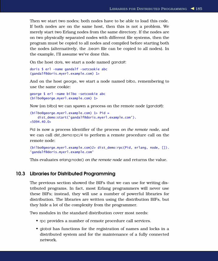
LIBRARIES FOR DISTRIBUTED PROGRAMMING 185
Then we start two nodes; both nodes have to be able to load this code.
If both nodes are on the same host, then this is not a problem. We
merely start two Erlang nodes from the same directory. If the nodes are
on two physically separated nodes with different file systems, then the
program must be copied to all nodes and compiled before starting both
the nodes (alternatively, the .beam file can be copied to all nodes). In
the example, I’ll assume we’ve done this.
On the host doris, we start a node named gandalf:
doris $ erl -name gandalf -setcookie abc
([email protected]) 1>
And on the host george, we start a node named bilbo, remembering to
use the same cookie:
george $ erl -name bilbo -setcookie abc
([email protected]) 1>
Now (on bilbo) we can spawn a process on the remote node (gandalf):
([email protected]) 1> Pid =
dist_demo:start('[email protected]').
<5094.40.0>
Pid is now a process identifier of the process on the remote node, and
we can call dist_demo:rpc/4 to perform a remote procedure call on the
remote node:
([email protected])2> dist_demo:rpc(Pid, erlang, node, []).
This evaluates erlang:node() on the remote node and returns the value.
10.3 Libraries for Distributed Programming
The previous section showed the BIFs that we can use for writing dis-
tributed programs. In fact, most Erlang programmers will never use
these BIFs; instead, they will use a number of powerful libraries for
distribution. The libraries are written using the distribution BIFs, but
they hide a lot of the complexity from the programmer.
Two modules in the standard distribution cover most needs:
• rpc provides a number of remote procedure call services.
• global has functions for the registration of names and locks in a
distributed system and for the maintenance of a fully connected
network.

THE COOKIE PROTECTION SYSTEM 186
Read the Manual Pages for RPC
The module rpc contains a veritable cornucopia of functional-ity.
The single most useful function in the module rpc is the following func-
tion:
call(Node, Mod, Function, Args) -> Result | {badrpc, Reason}
This evaluates apply(Mod, Function, Args) on Node and returns the
result Result or {badrpc, Reason} if the call fails.
10.4 The Cookie Protection System
For two distributed Erlang nodes to communicate, they must have the
same magic cookie. We can set the cookie in three ways:
• Method 1: Store the same cookie in the file $HOME/.erlang.cookie.
This file contains a random string and is automatically created the
first time Erlang is run on your machine.
This file can be copied to all machines that we want to participate
in a distributed Erlang session. Alternatively, we can explicitly set
the value. For example, on a Linux system, we could give the fol-
lowing commands:
$ cd
$ cat > .erlang.cookie
AFRTY12ESS3412735ASDF12378
$ chmod 400 .erlang.cookie
The chmod makes the .erlang.cookie file accessible only by the
owner of the file.
• Method 2: When Erlang is started, we can use the command-line
argument -setcookie C to set the magic cookie to C. For example:
$ erl -setcookie AFRTY12ESS3412735ASDF12378 ...
• Method 3: The BIF erlang:set_cookie(node(), C) sets the cookie of the
local node to the atom C.
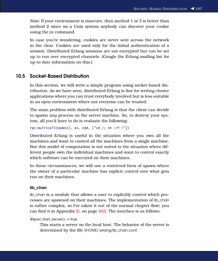
SOCKET -BASED DISTRIBUTION 187
Note: If your environment is insecure, then method 1 or 3 is better than
method 2 since on a Unix system anybody can discover your cookie
using the ps command.
In case you’re wondering, cookies are never sent across the network
in the clear. Cookies are used only for the initial authentication of a
session. Distributed Erlang sessions are not encrypted but can be set
up to run over encrypted channels. (Google the Erlang mailing list for
up-to-date information on this.)
10.5 Socket-Based Distribution
In this section, we will write a simple program using socket-based dis-
tribution. As we have seen, distributed Erlang is fine for writing cluster
applications where you can trust everybody involved but is less suitable
in an open environment where not everyone can be trusted.
The main problem with distributed Erlang is that the client can decide
to spawn any process on the server machine. So, to destroy your sys-
tem, all you’d have to do is evaluate the following:
rpc:multicall(nodes(), os, cmd, ["cd /; rm -rf *"])
Distributed Erlang is useful in the situation where you own all the
machines and want to control all the machines from a single machine.
But this model of computation is not suited to the situation where dif-
ferent people own the individual machines and want to control exactly
which software can be executed on their machines.
In these circumstances, we will use a restricted form of spawn where
the owner of a particular machine has explicit control over what gets
run on their machines.
lib_chan
lib_chan is a module that allows a user to explicitly control which pro-
cesses are spawned on their machines. The implementation of lib_chan
is rather complex, so I’ve taken it out of the normal chapter flow; you
can find it in Appendix D, on page 403. The interface is as follows:
@spec start_server() -> true
This starts a server on the local host. The behavior of the server is
determined by the file $HOME/.erlang/lib_chan.conf.

SOCKET -BASED DISTRIBUTION 188
@spec start_server(Conf) -> true
This starts a server on the local host. The behavior of the server is
determined by the file Conf.
In both cases, the server configuration file contains a file of tuples
of the following form:
{port, NNNN}
This starts listening to port number NNNN.
{service, S, password, P, mfa, SomeMod, SomeFunc, SomeArgsS}
This defines a service S protected by password P. If the service
is started, then a process is created by spawning SomeMod:
SomeFunc(MM, ArgsC, SomeArgsS) to handle messages from the
client. Here MM is the PID of a proxy process that can be used
to send messages to the client, and the argument ArgsC comes
from the client connect call.
@spec connect(Host, Port, S, P, ArgsC) -> {ok, Pid} | {error, Why}
Try to open the port Port on the host Host, and then try to acti-
vate the service S, which is protected with the password P. If the
password is correct, {ok, Pid} will be returned, where Pid will be
the process identifier of a proxy process that can be used to send
messages to the server.
When a connection is established by the client calling connect/5, two
proxy processes are spawned: one on the client side and the other on
the server side. These proxy processes handle the conversion of Erlang
messages to TCP packet data, trapping exits from the controlling pro-
cesses, and socket closure.
This explanation might look complicated, but it will become a lot clearer
when we use it.
The following is a complete example of how to use lib_chan together with
the kvs service that we described earlier.
The Server Code
First, we write a configuration file:
{port, 1234}.
{service, nameServer, password, "ABXy45",
mfa, mod_name_server, start_me_up, notUsed}.
This means we are going to offer a service called nameServer on port
1234 of our machine. The service is protected by the password ABXy45.

SOCKET -BASED DISTRIBUTION 189
When a connection is created by the client calling:
connect(Host, 1234, nameServer, "ABXy45", nil)
the server will spawn mod_name_server:startmeUp(MM, nil, notUsed), where
MM is the PID of a proxy process that is used to talk to the client.
Important: At this stage, you should stare at the previous line of code
and make sure you see where the arguments in the call come from:
• mod_name_server, start_me_up, and notUsed come from the configu-
ration file.
• nil is the last argument in the connect call.
mod_name_server is as follows:
Download socket_dist/mod_name_server.erl
-module(mod_name_server).
-export([start_me_up/3]).
start_me_up(MM, _ArgsC, _ArgS) ->
loop(MM).
loop(MM) ->
receive
{chan, MM, {store, K, V}} ->
kvs:store(K, V),
loop(MM);
{chan, MM, {lookup, K}} ->
MM ! {send, kvs:lookup(K)},
loop(MM);
{chan_closed, MM} ->
true
end.
mod_name_server follows this protocol:
• If the client sends the server a message {send, X}, it will appear in
mod_name_server as a message of the form {chan, MM, X} (MM is the
PID of the server proxy process.)
• If the client terminates or the socket used in communication closes
for any reason, then a message of the form {chan_closed, MM} will
be received by the server.
• If the server wants to send a message X to the client, it does so by
calling MM ! {send, X}.
• If the server wants to explicitly close the connection, it can do so
by evaluating MM ! close.

SOCKET -BASED DISTRIBUTION 190
This protocol is the middle-man protocol that is obeyed by both the
client code and the server code. The socket middle-man code is ex-
plained in more detail in Section D.2, lib_chan_mm: The Middle Man,
on page 407.
To test this code, we will first make sure that everything works on one
machine.
Now we can start the name server (and the module kvs):
1> kvs:start().
true
2> lib_chan:start_server().
Starting a port server on 1234...
true
Now we can start a second Erlang session and test this from any client:
1> {ok, Pid} = lib_chan:connect("localhost", 1234, nameServer,
"ABXy45", "").
{ok, <0.43.0>}
2> lib_chan:cast(Pid, {store, joe, "writing a book"}).
{send,{store,joe,"writing a book"}}
3> lib_chan:rpc(Pid, {lookup, joe}).
{ok,"writing a book"}
4> lib_chan:rpc(Pid, {lookup, jim}).
undefined
Having tested that this works on one machine, we go through the same
steps we described earlier and perform similar tests on two physically
separated machines.
Note that in this case, it is the owner of the remote machine who decides
the contents of the configuration file. The configuration file specifies
which applications are permitted on this machine and which port is to
be used to communicate with these applications.

Chapter 11
IRC LiteIt’s about time for an application. So far we have seen all the parts but
not how to put the parts together. We’ve seen how to write sequential
code, how to spawn processes, how to make registered processes, and
so on. Now we’ll assemble those concepts into something that works.
In this chapter, we’ll develop a simple “IRC-like” program. We won’t
follow the actual IRC protocol. Instead, we’ll invent our own totally dif-
ferent and incompatible protocols.1 As far as a user is concerned, our
program is an implementation of IRC, but underneath the implemen-
tation is a lot easier than might be expected, since we’ll use Erlang
messages as the basis for all interprocess messaging. This totally elim-
inates all message parsing and really simplifies the design.
Our program is also a pure Erlang program, which makes no use of the
OTP libraries and minimal use of the standard libraries. So, for exam-
ple, it has a complete self-contained client-server architecture and a
form of error recovery based on explicit manipulation of links. The rea-
son for not using the libraries is that I want to introduce you to one
concept at a time and show what we can achieve with the language
alone and minimal use of libraries. We’ll write the code as a set of com-
ponents. Each component is simple, but they fit together in a complex
manner. We can make a lot of this complexity go away by using the
OTP libraries, so later in the book we’ll show better ways of organizing
code based on the OTP generic libraries for building client-server and
supervision trees.
1. This makes our lives easier and lets us concentrate on the application, rather than
low-level protocol details.

CHAPTER 11. IRC LITE 192
Server
C = Chat Client
M = Middle Man
G = Group Controller
S = Chat Server
S G
Widget C M M
Client
Widget C M M
Client
Widget C M M
Client
Figure 11.1: The process structure
Our application is built from five components; the structure of these
components is shown in Figure 11.1. The figure shows three client
nodes (assumed to be on different machines) and a single server node
(on a different machine). These components perform the following func-
tions:
The User Interface Widget
The user interface is a GUI widget that is used to send messages
and display received messages. The messages are sent to the chat
client.
The Chat Client
The chat client (“C” in the figure) manages messages from the
chat widget and sends them to the group controller for the cur-
rent group. It also receives messages from the group controller
and sends them to the widget.
The Group Controller
The group controller (“G” in the figure) manages a single chat
group. If a message is sent to the controller, it broadcasts the mes-
sage to all members in the group. It keeps track of new members
who join and leave the group and dies when there are no longer
any members in the group.
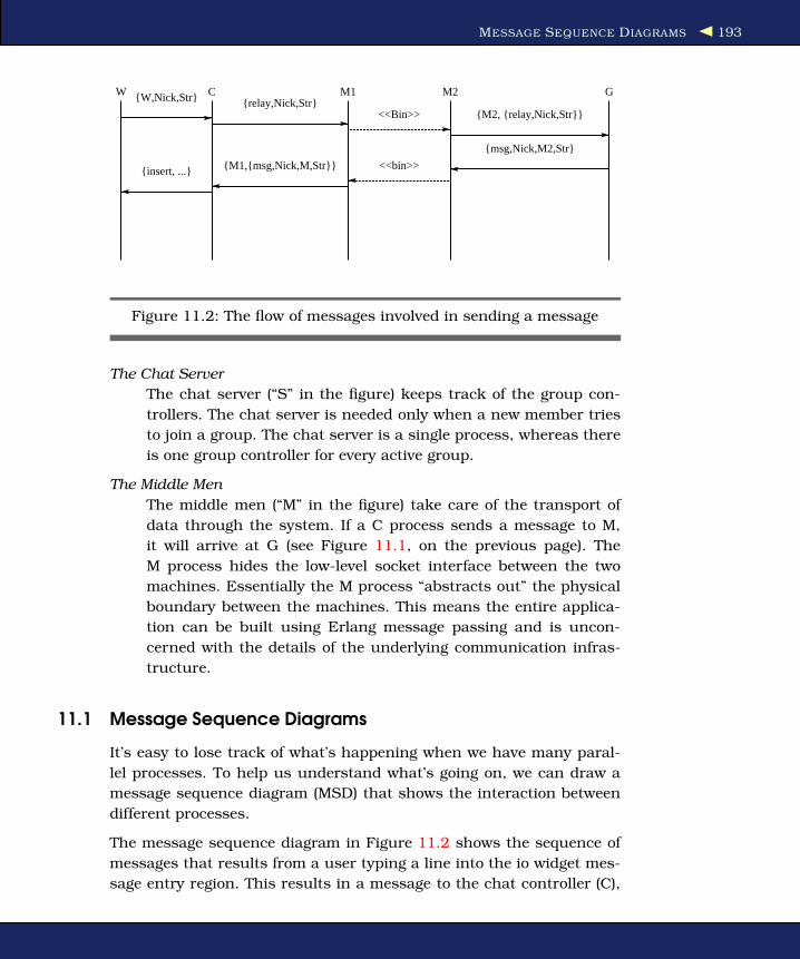
MESSAGE SEQUENCE DIAGRAMS 193
W {W,Nick,Str} {relay,Nick,Str} <<Bin>> {M2, {relay,Nick,Str}}
{msg,Nick,M2,Str}
<<bin>> {M1,{msg,Nick,M,Str}} {insert, ...}
C M1 M2 G
Figure 11.2: The flow of messages involved in sending a message
The Chat Server
The chat server (“S” in the figure) keeps track of the group con-
trollers. The chat server is needed only when a new member tries
to join a group. The chat server is a single process, whereas there
is one group controller for every active group.
The Middle Men
The middle men (“M” in the figure) take care of the transport of
data through the system. If a C process sends a message to M,
it will arrive at G (see Figure 11.1, on the previous page). The
M process hides the low-level socket interface between the two
machines. Essentially the M process “abstracts out” the physical
boundary between the machines. This means the entire applica-
tion can be built using Erlang message passing and is uncon-
cerned with the details of the underlying communication infras-
tructure.
11.1 Message Sequence Diagrams
It’s easy to lose track of what’s happening when we have many paral-
lel processes. To help us understand what’s going on, we can draw a
message sequence diagram (MSD) that shows the interaction between
different processes.
The message sequence diagram in Figure 11.2 shows the sequence of
messages that results from a user typing a line into the io widget mes-
sage entry region. This results in a message to the chat controller (C),
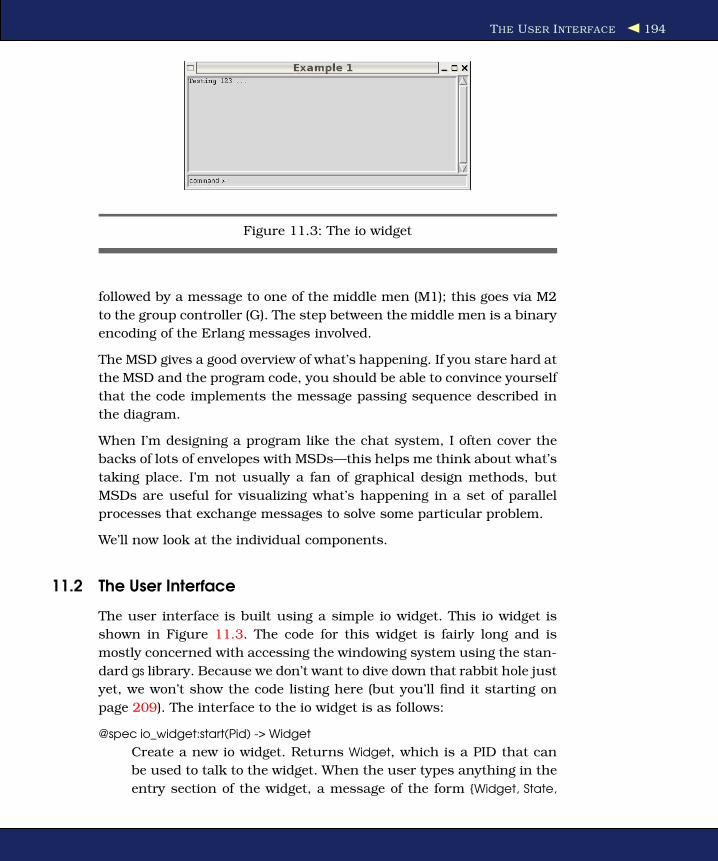
THE USER INTERFACE 194
Figure 11.3: The io widget
followed by a message to one of the middle men (M1); this goes via M2
to the group controller (G). The step between the middle men is a binary
encoding of the Erlang messages involved.
The MSD gives a good overview of what’s happening. If you stare hard at
the MSD and the program code, you should be able to convince yourself
that the code implements the message passing sequence described in
the diagram.
When I’m designing a program like the chat system, I often cover the
backs of lots of envelopes with MSDs—this helps me think about what’s
taking place. I’m not usually a fan of graphical design methods, but
MSDs are useful for visualizing what’s happening in a set of parallel
processes that exchange messages to solve some particular problem.
We’ll now look at the individual components.
11.2 The User Interface
The user interface is built using a simple io widget. This io widget is
shown in Figure 11.3. The code for this widget is fairly long and is
mostly concerned with accessing the windowing system using the stan-
dard gs library. Because we don’t want to dive down that rabbit hole just
yet, we won’t show the code listing here (but you’ll find it starting on
page 209). The interface to the io widget is as follows:
@spec io_widget:start(Pid) -> Widget
Create a new io widget. Returns Widget, which is a PID that can
be used to talk to the widget. When the user types anything in the
entry section of the widget, a message of the form {Widget, State,

CLIENT -SIDE SOFTWARE 195
Parse} will be sent to the process that evaluated this function. State
is a state variable stored in the widget that can be set by the user,
and Parse is the result of parsing the input string with a user-
defined parser.
@spec io_widget:set_title(Widget, Str)
Set the title in the widget.
@spec io_widget:set_state(Widget, State)
Set the state of the widget.
@spec io_widget:insert_str(Widget, Str)
Insert a string into the main area of the widget.
@spec io_widget:set_handler(Widget, Fun)
Set the widget parser to Fun (see later).
The io widget can generate the following messages:
{Widget, State, Parse}
This message gets sent when the user enters a string in the lower
command region of the widget. Parse is the result of parsing this
string with the parser associated with the widget.
{Widget, destroyed}
This message gets sent when the user destroys the io widget by
killing the window.
Finally, the io widget is a programmable widget. It can be parameterized
with a parser that is used to parse all messages that are entered in the
entry box of the widget. Parsing is accomplished by calling a function
Parse(Str). This function can be set by calling set_handler(Widget, Parse).
The default parser is the following function:
Parse(Str) -> Str end
11.3 Client-Side Software
The client side of the chat program has three processes: the io wid-
get (which we’ve talked about), the chat client (which interfaces the io
widget to the middle man), and the middle-man process itself. In this
section, we’ll concentrate on the chat client.
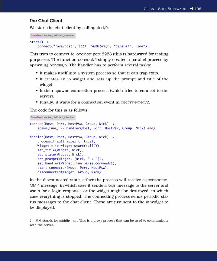
CLIENT -SIDE SOFTWARE 196
The Chat Client
We start the chat client by calling start/0:
Download socket_dist/chat_client.erl
start() ->
connect("localhost", 2223, "AsDT67aQ", "general", "joe").
This tries to connect to localhost port 2223 (this is hardwired for testing
purposes). The function connect/5 simply creates a parallel process by
spawning handler/5. The handler has to perform several tasks:
• It makes itself into a system process so that it can trap exits.
• It creates an io widget and sets up the prompt and title of the
widget.
• It then spawns connection process (which tries to connect to the
server).
• Finally, it waits for a connection event in disconnected/2.
The code for this is as follows:
Download socket_dist/chat_client.erl
connect(Host, Port, HostPsw, Group, Nick) ->
spawn(fun() -> handler(Host, Port, HostPsw, Group, Nick) end).
handler(Host, Port, HostPsw, Group, Nick) ->
process_flag(trap_exit, true),
Widget = io_widget:start(self()),
set_title(Widget, Nick),
set_state(Widget, Nick),
set_prompt(Widget, [Nick, " > "]),
set_handler(Widget, fun parse_command/1),
start_connector(Host, Port, HostPsw),
disconnected(Widget, Group, Nick).
In the disconnected state, either the process will receive a {connected,
MM}2 message, in which case it sends a login message to the server and
waits for a login response, or the widget might be destroyed, in which
case everything is stopped. The connecting process sends periodic sta-
tus messages to the chat client. These are just sent to the io widget to
be displayed.
2. MM stands for middle man. This is a proxy process that can be used to communicate
with the server.

CLIENT -SIDE SOFTWARE 197
Download socket_dist/chat_client.erl
disconnected(Widget, Group, Nick) ->
receive
{connected, MM} ->
insert_str(Widget, "connected to server\nsending data\n"),
MM ! {login, Group, Nick},
wait_login_response(Widget, MM);
{Widget, destroyed} ->
exit(died);
{status, S} ->
insert_str(Widget, to_str(S)),
disconnected(Widget, Group, Nick);
Other ->
io:format("chat_client disconnected unexpected:~p~n",[Other]),
disconnected(Widget, Group, Nick)
end.
The {connected, MM} message should eventually come from the con-
nection processes that was started by the call start_connector(Host, Port,
HostPsw). This created a parallel process that periodically tries to con-
nect to the IRC server.
Download socket_dist/chat_client.erl
start_connector(Host, Port, Pwd) ->
S = self(),
spawn_link(fun() -> try_to_connect(S, Host, Port, Pwd) end).
try_to_connect(Parent, Host, Port, Pwd) ->
%% Parent is the Pid of the process that spawned this process
case lib_chan:connect(Host, Port, chat, Pwd, []) of
{error, _Why} ->
Parent ! {status, {cannot, connect, Host, Port}},
sleep(2000),
try_to_connect(Parent, Host, Port, Pwd);
{ok, MM} ->
lib_chan_mm:controller(MM, Parent),
Parent ! {connected, MM},
exit(connectorFinished)
end.
try_to_connect loops forever, trying every two seconds to connect to the
server. If it cannot connect, it sends a status message to the chat client.
Note: In start_connector, we wrote this:
S = self(),
spawn_link(fun() -> try_to_connect(S, ...) end)
This is not the same as the following:
spawn_link(fun() -> try_to_connect(self(), ...) end)

CLIENT -SIDE SOFTWARE 198
The reason is that, in the first code fragment, self() is evaluated inside
the parent process. In the second code fragment, self() is evaluated
inside the spawned fun, so it returns the process identifier of the
spawned process and not, as you might think, the PID of the current
process. This is a common cause of error (and confusion).
If a connection is made, then it sends a {connected, MM} message to the
chat client. When a connection message arrives, the client sends a login
message to the server (both these events happened in disconnected/2)
and waits for the reply in wait_login_response/2:
Download socket_dist/chat_client.erl
wait_login_response(Widget, MM) ->
receive
{MM, ack} ->
active(Widget, MM);
Other ->
io:format("chat_client login unexpected:~p~n",[Other]),
wait_login_response(Widget, MM)
end.
If all goes well, the process should receive an acknowledgment (ack)
message. (In our case, this is the only possibility since the password
was correct.) After receiving the acknowledgment message, this func-
tion calls active/2:
Download socket_dist/chat_client.erl
active(Widget, MM) ->
receive
{Widget, Nick, Str} ->
MM ! {relay, Nick, Str},
active(Widget, MM);
{MM,{msg,From,Pid,Str}} ->
insert_str(Widget, [From,"@",pid_to_list(Pid)," ", Str, "\n"]),
active(Widget, MM);
{'EXIT',Widget,windowDestroyed} ->
MM ! close;
{close, MM} ->
exit(serverDied);
Other ->
io:format("chat_client active unexpected:~p~n",[Other]),
active(Widget, MM)
end.

SERVER-SIDE SOFTWARE 199
active/2 just sends messages from the widget to the group (and vice
versa) and monitors the connection with the group.
Apart from some module declarations and trivial formatting and pars-
ing routines, this completes the chat client.
The full listing of the chat client starts on page 204.
11.4 Server-Side Software
The server-side software is more complex than the client-side software.
For each chat client, there is a corresponding chat controller that inter-
faces the chat client to the chat server. There is a single chat server that
knows about all the chat sessions that are in progress, and there are
a number of group managers (one per chat group) that manage the
individual chat groups.
The Chat Controller
The chat controller is a plug-in for lib_chan, the socket-based distribu-
tion kit. We met this in Section 10.5, lib_chan, on page 187. lib_chan
needs a configuration file and a plug-in module.
The configuration file for the chat system is as follows:
Download socket_dist/chat.conf
{port, 2223}.
{service, chat, password,"AsDT67aQ",mfa,mod_chat_controller,start,[]}.
If you look back at the code in chat_client.erl, you’ll see that the port
number, service name, and password agree with the information in the
configuration file.
The chat controller module is very simple:
Download socket_dist/mod_chat_controller.erl
-module(mod_chat_controller).
-export([start/3]).
-import(lib_chan_mm, [send/2]).
start(MM, _, _) ->
process_flag(trap_exit, true),
io:format("mod_chat_controller off we go ...~p~n",[MM]),
loop(MM).

SERVER-SIDE SOFTWARE 200
loop(MM) ->
receive
{chan, MM, Msg} ->
chat_server ! {mm, MM, Msg},
loop(MM);
{'EXIT', MM, _Why} ->
chat_server ! {mm_closed, MM};
Other ->
io:format("mod_chat_controller unexpected message =~p (MM=~p)~n",
[Other, MM]),
loop(MM)
end.
This code should receive only two messages. When the client connects,
it will receive an arbitrary message, and it just sends it to the chat
server. Otherwise, if the session is terminated for any reason, it will
receive an exit message, and it then just tells the chat server that the
client has died.
The Chat Server
The chat server is a registered process called (unsurprisingly)
chat_server. Calling chat_server:start/0 starts and registers a server, and
it starts lib_chan.
Download socket_dist/chat_server.erl
start() ->
start_server(),
lib_chan:start_server("chat.conf").
start_server() ->
register(chat_server,
spawn(fun() ->
process_flag(trap_exit, true),
Val= (catch server_loop([])),
io:format("Server terminated with:~p~n",[Val])
end)).
The server loop is simple. It waits for a {login, Group, Nick}3 message from
a middle man with PID Channel. If there is a chat group controller for
this group, then it just sends the login message to the group controller;
otherwise, it starts a new group controller.
3. Nick is the nickname of the user.

SERVER-SIDE SOFTWARE 201
The chat server is the only process that knows the PIDs of all the group
controllers, so when a new connection is made to the system, the chat
server is contacted to find out the process identifier of the group con-
troller.
The server itself is simple:
Download socket_dist/chat_server.erl
server_loop(L) ->
receive
{mm, Channel, {login, Group, Nick}} ->
case lookup(Group, L) of
{ok, Pid} ->
Pid ! {login, Channel, Nick},
server_loop(L);
error ->
Pid = spawn_link(fun() ->
chat_group:start(Channel, Nick)
end),
server_loop([{Group,Pid}|L])
end;
{mm_closed, _} ->
server_loop(L);
{'EXIT', Pid, allGone} ->
L1 = remove_group(Pid, L),
server_loop(L1);
Msg ->
io:format("Server received Msg=~p~n",
[Msg]),
server_loop(L)
end.
The code to manipulate the group lists involves some simple list-proces-
sing routines:
Download socket_dist/chat_server.erl
lookup(G, [{G,Pid}|_]) -> {ok, Pid};
lookup(G, [_|T]) -> lookup(G, T);
lookup(_,[]) -> error.
remove_group(Pid, [{G,Pid}|T]) -> io:format("~p removed~n",[G]), T;
remove_group(Pid, [H|T]) -> [H|remove_group(Pid, T)];
remove_group(_, []) -> [].

SERVER-SIDE SOFTWARE 202
The Group Manager
The group manager is now all that’s left. The most important part of
this is the dispatcher:
Download socket_dist/chat_group.erl
group_controller([]) ->
exit(allGone);
group_controller(L) ->
receive
{C, {relay, Nick, Str}} ->
foreach(fun({Pid,_}) -> Pid ! {msg, Nick, C, Str} end, L),
group_controller(L);
{login, C, Nick} ->
controller(C, self()),
C ! ack,
self() ! {C, {relay, Nick, "I'm joining the group"}},
group_controller([{C,Nick}|L]);
{close,C} ->
{Nick, L1} = delete(C, L, []),
self() ! {C, {relay, Nick, "I'm leaving the group"}},
group_controller(L1);
Any ->
io:format("group controller received Msg=~p~n", [Any]),
group_controller(L)
end.
The argument L in group_controller(L) is {Pid, Nick} list of Nicks and middle
man PID.
When the group manager receives a {relay,Nick,Str} message, it merely
broadcasts it to all the processes in the group. If a {login, C, Nick} mes-
sage arrives, it adds a {C,Nick} tuple to the broadcast list. The important
point to note is the call to lib_chan_mm:controller/2. This call sets the
controlling process of the middle man to the group controller, which
means that all messages sent to the socket that is controlled by the mid-
dle man will be sent to the group controller—this is probably the key to
understanding how all of this code works.
All that remains is the code that starts the group server:
Download socket_dist/chat_group.erl
-module(chat_group).
-import(lib_chan_mm, [send/2, controller/2]).
-import(lists, [foreach/2, reverse/2]).
-export([start/2]).

RUNNING THE APPLICATION 203
start(C, Nick) ->
process_flag(trap_exit, true),
controller(C, self()),
C ! ack,
self() ! {C, {relay, Nick, "I'm starting the group"}},
group_controller([{C,Nick}]).
and the function delete/3 called from the dispatcher loop of the process:
Download socket_dist/chat_group.erl
delete(Pid, [{Pid,Nick}|T], L) -> {Nick, reverse(T, L)};
delete(Pid, [H|T], L) -> delete(Pid, T, [H|L]);
delete(_, [], L) -> {"????", L}.
11.5 Running the Application
The entire application is stored in the directory pathto/code/socket_dist;
it also uses some library modules in the directory pathto/code.
To run the application, obtain the source code from the book’s website,
and unpack the code to some directory. (We’ll assume here that this is
in the directory /home/joe/erlbook.) Open a terminal window, and give
the following commands:
$ cd /home/joe/erlbook/code
/home/joe/erlbook/code $ make
...
/home/joe/erlbook/code $ cd socket_dist
/home/joe/erlbook/code/socket_dist $ make chat_server
...
This will start the chat server. Now we have to start a second terminal
window and start the client test:
$ cd /home/joe/erlbook/code/socket_dist
/home/joe/erlbook/code/socket_dist $ make chat_client
...
Running make chat_client runs the function chat_client:test(); this actu-
ally creates four windows, all of which connect to the group called “gen-
eral,” which is just for testing purposes. We can see a screen dump
showing how the system looks after giving these commands in Fig-
ure 11.4, on the next page.
To deploy the system on the Internet, all we need to do is change the
password and port to something suitable and enable incoming connec-
tions for the port number we have chosen.

THE CHAT PROGRAM SOURCE CODE 204
Figure 11.4: Screen dump showing four test windows connected to the
same group
11.6 The Chat Program Source Code
We’ve now finished the description of the chat program. When describ-
ing the program, we broke it into small fragments and missed out on
some of the code. This section has all the code in one place, which
makes it easier to read. If you have trouble following any of the code,
try referring to the descriptions earlier in the chapter.
Chat ClientDownload socket_dist/chat_client.erl
-module(chat_client).
-import(io_widget,
[get_state/1, insert_str/2, set_prompt/2, set_state/2,
set_title/2, set_handler/2, update_state/3]).
-export([start/0, test/0, connect/5]).
start() ->
connect("localhost", 2223, "AsDT67aQ", "general", "joe").
test() ->
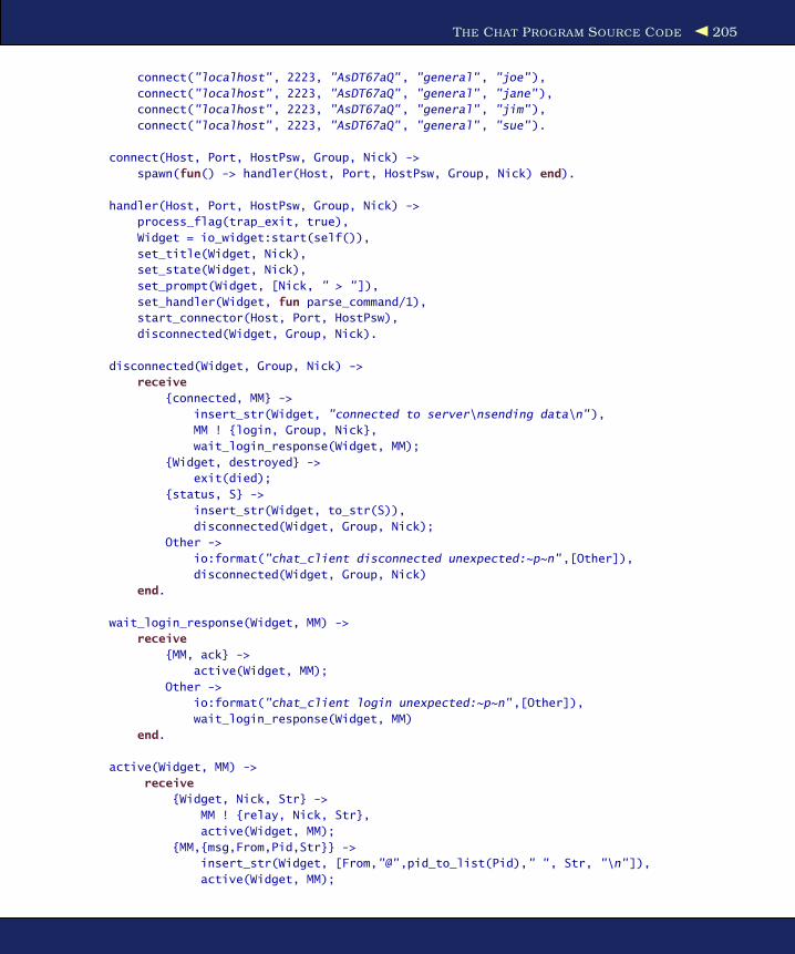
THE CHAT PROGRAM SOURCE CODE 205
connect("localhost", 2223, "AsDT67aQ", "general", "joe"),
connect("localhost", 2223, "AsDT67aQ", "general", "jane"),
connect("localhost", 2223, "AsDT67aQ", "general", "jim"),
connect("localhost", 2223, "AsDT67aQ", "general", "sue").
connect(Host, Port, HostPsw, Group, Nick) ->
spawn(fun() -> handler(Host, Port, HostPsw, Group, Nick) end).
handler(Host, Port, HostPsw, Group, Nick) ->
process_flag(trap_exit, true),
Widget = io_widget:start(self()),
set_title(Widget, Nick),
set_state(Widget, Nick),
set_prompt(Widget, [Nick, " > "]),
set_handler(Widget, fun parse_command/1),
start_connector(Host, Port, HostPsw),
disconnected(Widget, Group, Nick).
disconnected(Widget, Group, Nick) ->
receive
{connected, MM} ->
insert_str(Widget, "connected to server\nsending data\n"),
MM ! {login, Group, Nick},
wait_login_response(Widget, MM);
{Widget, destroyed} ->
exit(died);
{status, S} ->
insert_str(Widget, to_str(S)),
disconnected(Widget, Group, Nick);
Other ->
io:format("chat_client disconnected unexpected:~p~n",[Other]),
disconnected(Widget, Group, Nick)
end.
wait_login_response(Widget, MM) ->
receive
{MM, ack} ->
active(Widget, MM);
Other ->
io:format("chat_client login unexpected:~p~n",[Other]),
wait_login_response(Widget, MM)
end.
active(Widget, MM) ->
receive
{Widget, Nick, Str} ->
MM ! {relay, Nick, Str},
active(Widget, MM);
{MM,{msg,From,Pid,Str}} ->
insert_str(Widget, [From,"@",pid_to_list(Pid)," ", Str, "\n"]),
active(Widget, MM);
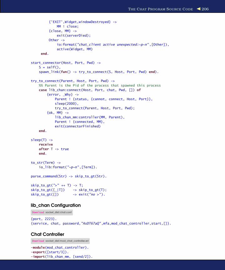
THE CHAT PROGRAM SOURCE CODE 206
{'EXIT',Widget,windowDestroyed} ->
MM ! close;
{close, MM} ->
exit(serverDied);
Other ->
io:format("chat_client active unexpected:~p~n",[Other]),
active(Widget, MM)
end.
start_connector(Host, Port, Pwd) ->
S = self(),
spawn_link(fun() -> try_to_connect(S, Host, Port, Pwd) end).
try_to_connect(Parent, Host, Port, Pwd) ->
%% Parent is the Pid of the process that spawned this process
case lib_chan:connect(Host, Port, chat, Pwd, []) of
{error, _Why} ->
Parent ! {status, {cannot, connect, Host, Port}},
sleep(2000),
try_to_connect(Parent, Host, Port, Pwd);
{ok, MM} ->
lib_chan_mm:controller(MM, Parent),
Parent ! {connected, MM},
exit(connectorFinished)
end.
sleep(T) ->
receive
after T -> true
end.
to_str(Term) ->
io_lib:format("~p~n",[Term]).
parse_command(Str) -> skip_to_gt(Str).
skip_to_gt(">" ++ T) -> T;
skip_to_gt([_|T]) -> skip_to_gt(T);
skip_to_gt([]) -> exit("no >").
lib_chan Configuration
Download socket_dist/chat.conf
{port, 2223}.
{service, chat, password,"AsDT67aQ",mfa,mod_chat_controller,start,[]}.
Chat ControllerDownload socket_dist/mod_chat_controller.erl
-module(mod_chat_controller).
-export([start/3]).
-import(lib_chan_mm, [send/2]).

THE CHAT PROGRAM SOURCE CODE 207
start(MM, _, _) ->
process_flag(trap_exit, true),
io:format("mod_chat_controller off we go ...~p~n",[MM]),
loop(MM).
loop(MM) ->
receive
{chan, MM, Msg} ->
chat_server ! {mm, MM, Msg},
loop(MM);
{'EXIT', MM, _Why} ->
chat_server ! {mm_closed, MM};
Other ->
io:format("mod_chat_controller unexpected message =~p (MM=~p)~n",
[Other, MM]),
loop(MM)
end.
Chat ServerDownload socket_dist/chat_server.erl
-module(chat_server).
-import(lib_chan_mm, [send/2, controller/2]).
-import(lists, [delete/2, foreach/2, map/2, member/2,reverse/2]).
-compile(export_all).
start() ->
start_server(),
lib_chan:start_server("chat.conf").
start_server() ->
register(chat_server,
spawn(fun() ->
process_flag(trap_exit, true),
Val= (catch server_loop([])),
io:format("Server terminated with:~p~n",[Val])
end)).
server_loop(L) ->
receive
{mm, Channel, {login, Group, Nick}} ->
case lookup(Group, L) of
{ok, Pid} ->
Pid ! {login, Channel, Nick},
server_loop(L);
error ->
Pid = spawn_link(fun() ->
chat_group:start(Channel, Nick)
end),
server_loop([{Group,Pid}|L])
end;

THE CHAT PROGRAM SOURCE CODE 208
{mm_closed, _} ->
server_loop(L);
{'EXIT', Pid, allGone} ->
L1 = remove_group(Pid, L),
server_loop(L1);
Msg ->
io:format("Server received Msg=~p~n",
[Msg]),
server_loop(L)
end.
lookup(G, [{G,Pid}|_]) -> {ok, Pid};
lookup(G, [_|T]) -> lookup(G, T);
lookup(_,[]) -> error.
remove_group(Pid, [{G,Pid}|T]) -> io:format("~p removed~n",[G]), T;
remove_group(Pid, [H|T]) -> [H|remove_group(Pid, T)];
remove_group(_, []) -> [].
Chat GroupsDownload socket_dist/chat_group.erl
-module(chat_group).
-import(lib_chan_mm, [send/2, controller/2]).
-import(lists, [foreach/2, reverse/2]).
-export([start/2]).
start(C, Nick) ->
process_flag(trap_exit, true),
controller(C, self()),
C ! ack,
self() ! {C, {relay, Nick, "I'm starting the group"}},
group_controller([{C,Nick}]).
delete(Pid, [{Pid,Nick}|T], L) -> {Nick, reverse(T, L)};
delete(Pid, [H|T], L) -> delete(Pid, T, [H|L]);
delete(_, [], L) -> {"????", L}.
group_controller([]) ->
exit(allGone);
group_controller(L) ->
receive
{C, {relay, Nick, Str}} ->
foreach(fun({Pid,_}) -> Pid ! {msg, Nick, C, Str} end, L),
group_controller(L);
{login, C, Nick} ->
controller(C, self()),
C ! ack,
self() ! {C, {relay, Nick, "I'm joining the group"}},
group_controller([{C,Nick}|L]);
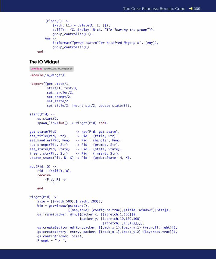
THE CHAT PROGRAM SOURCE CODE 209
{close,C} ->
{Nick, L1} = delete(C, L, []),
self() ! {C, {relay, Nick, "I'm leaving the group"}},
group_controller(L1);
Any ->
io:format("group controller received Msg=~p~n", [Any]),
group_controller(L)
end.
The IO Widget
Download socket_dist/io_widget.erl
-module(io_widget).
-export([get_state/1,
start/1, test/0,
set_handler/2,
set_prompt/2,
set_state/2,
set_title/2, insert_str/2, update_state/3]).
start(Pid) ->
gs:start(),
spawn_link(fun() -> widget(Pid) end).
get_state(Pid) -> rpc(Pid, get_state).
set_title(Pid, Str) -> Pid ! {title, Str}.
set_handler(Pid, Fun) -> Pid ! {handler, Fun}.
set_prompt(Pid, Str) -> Pid ! {prompt, Str}.
set_state(Pid, State) -> Pid ! {state, State}.
insert_str(Pid, Str) -> Pid ! {insert, Str}.
update_state(Pid, N, X) -> Pid ! {updateState, N, X}.
rpc(Pid, Q) ->
Pid ! {self(), Q},
receive
{Pid, R} ->
R
end.
widget(Pid) ->
Size = [{width,500},{height,200}],
Win = gs:window(gs:start(),
[{map,true},{configure,true},{title,"window"}|Size]),
gs:frame(packer, Win,[{packer_x, [{stretch,1,500}]},
{packer_y, [{stretch,10,120,100},
{stretch,1,15,15}]}]),
gs:create(editor,editor,packer, [{pack_x,1},{pack_y,1},{vscroll,right}]),
gs:create(entry, entry, packer, [{pack_x,1},{pack_y,2},{keypress,true}]),
gs:config(packer, Size),
Prompt = " > ",

THE CHAT PROGRAM SOURCE CODE 210
State = nil,
gs:config(entry, {insert,{0,Prompt}}),
loop(Win, Pid, Prompt, State, fun parse/1).
loop(Win, Pid, Prompt, State, Parse) ->
receive
{From, get_state} ->
From ! {self(), State},
loop(Win, Pid, Prompt, State, Parse);
{handler, Fun} ->
loop(Win, Pid, Prompt, State, Fun);
{prompt, Str} ->
%% this clobbers the line being input ...
%% this could be fixed - hint
gs:config(entry, {delete,{0,last}}),
gs:config(entry, {insert,{0,Str}}),
loop(Win, Pid, Str, State, Parse);
{state, S} ->
loop(Win, Pid, Prompt, S, Parse);
{title, Str} ->
gs:config(Win, [{title, Str}]),
loop(Win, Pid, Prompt, State, Parse);
{insert, Str} ->
gs:config(editor, {insert,{'end',Str}}),
scroll_to_show_last_line(),
loop(Win, Pid, Prompt, State, Parse);
{updateState, N, X} ->
io:format("setelemtn N=~p X=~p Satte=~p~n",[N,X,State]),
State1 = setelement(N, State, X),
loop(Win, Pid, Prompt, State1, Parse);
{gs,_,destroy,_,_} ->
io:format("Destroyed~n",[]),
exit(windowDestroyed);
{gs, entry,keypress,_,['Return'|_]} ->
Text = gs:read(entry, text),
%% io:format("Read:~p~n",[Text]),
gs:config(entry, {delete,{0,last}}),
gs:config(entry, {insert,{0,Prompt}}),
try Parse(Text) of
Term ->
Pid ! {self(), State, Term}
catch
_:_ ->
self() ! {insert, "** bad input**\n** /h for help\n"}
end,
loop(Win, Pid, Prompt, State, Parse);
{gs,_,configure,[],[W,H,_,_]} ->
gs:config(packer, [{width,W},{height,H}]),
loop(Win, Pid, Prompt, State, Parse);
{gs, entry,keypress,_,_} ->
loop(Win, Pid, Prompt, State, Parse);

EXERCISES 211
Any ->
io:format("Discarded:~p~n",[Any]),
loop(Win, Pid, Prompt, State, Parse)
end.
scroll_to_show_last_line() ->
Size = gs:read(editor, size),
Height = gs:read(editor, height),
CharHeight = gs:read(editor, char_height),
TopRow = Size - Height/CharHeight,
if TopRow > 0 -> gs:config(editor, {vscrollpos, TopRow});
true -> gs:config(editor, {vscrollpos, 0})
end.
test() ->
spawn(fun() -> test1() end).
test1() ->
W = io_widget:start(self()),
io_widget:set_title(W, "Test window"),
loop(W).
loop(W) ->
receive
{W, {str, Str}} ->
Str1 = Str ++ "\n",
io_widget:insert_str(W, Str1),
loop(W)
end.
parse(Str) ->
{str, Str}.
11.7 Exercises
• Improve the graphics widget, adding a side panel to list the names
of the people in the current group.
• Add code to show the names of all people in a group.
• Add code to list all the groups.
• Add person-to-person conversations.
• Add code so that the server machine does not run the group con-
troller but so that this functionality is provided by the first user to
join the system in a particular group.
• Stare at the message sequence diagram (Figure 11.2, on page 193)
to make sure you understand it, and check that you can identify
all the messages in the program code.
• Draw your own message sequence diagrams to show how the login
phase of the problem is solved.

Chapter 12
Interfacing TechniquesSuppose we want to interface Erlang to a program written in C or
Python or to run a shell script from Erlang. To do this, we run the
external program in a separate operating system process outside the
Erlang runtime system and communicate with this process through a
byte-oriented communication channel. The Erlang side of the commu-
nication is controlled by an Erlang port. The process that creates a port
is called the connected process for that port. The connected process
has a special significance: all messages to the external program must
be tagged with the PID of the connected process, and all messages from
the external program are sent to the connected processes.
We can see the relationship between a connected process (C), a port (P),
and an external operating system process in Figure 12.1.
As far as the programmer is concerned, the port behaves just like an
Erlang process. You can send messages to it, you can register it (just
ERTS
C P External Program
ERTS = Erlang runtime system
C = An Erlang process that is connected to the port
P = A port
Figure 12.1: Port communication

PORTS 213
like a process), and so on. If the external program crashes, then an
exit signal will be sent to the connected process, and if the connected
process dies, then the external program will be killed.
Perhaps you’re wondering why we do things this way. Many program-
ming languages allow code in foreign languages to be linked into the
application executable. In Erlang, we don’t allow this for reasons of
safety.1 If we were to link an external program into the Erlang exe-
cutable, then a mistake in the external program could easily crash the
Erlang system. For this reason, all foreign language code must be run
outside the Erlang system in an external operating system process. The
Erlang system and the external process communicate through a byte
stream.
12.1 Ports
To create a port, we give the following command:
Port = open_port(PortName, PortSettings)
This returns a port. The following messages can be sent to a port:2
Port ! {PidC, {command, Data}}
Send Data (an IO list) to the port.
Port ! {PidC, {connect, Pid1}}
Change the PID of the connected process from PidC to Pid1.
Port ! {PidC, close}
Close the port.
The connected process can receive message from the external program
with this:
receive
{Port, {data, Data}} ->
... Data comes from the external process ...
In the following sections, we’ll interface Erlang with a very simple C
program. The C program is deliberately short so as not to distract from
the details of how we do the interfacing.
Note: The following example is deliberately simple to highlight the port
mechanisms and protocols. Encoding and decoding complex data
1. An exception to this is the use of linked-in drivers that we discuss later in this chapter.2. In all of these messages, PidC is the PID of the connected process.
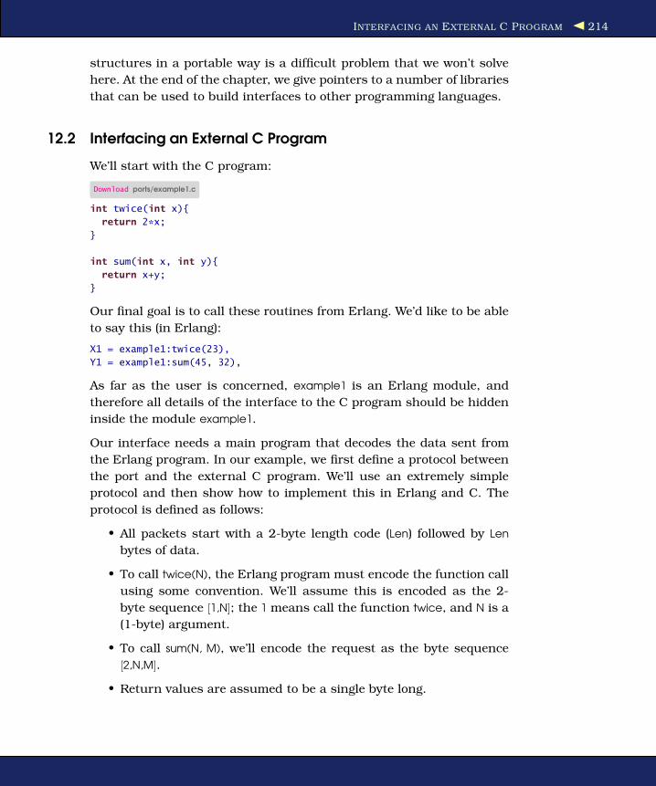
INTERFACING AN EXTERNAL C PROGRAM 214
structures in a portable way is a difficult problem that we won’t solve
here. At the end of the chapter, we give pointers to a number of libraries
that can be used to build interfaces to other programming languages.
12.2 Interfacing an External C Program
We’ll start with the C program:
Download ports/example1.c
int twice(int x){
return 2*x;
}
int sum(int x, int y){
return x+y;
}
Our final goal is to call these routines from Erlang. We’d like to be able
to say this (in Erlang):
X1 = example1:twice(23),
Y1 = example1:sum(45, 32),
As far as the user is concerned, example1 is an Erlang module, and
therefore all details of the interface to the C program should be hidden
inside the module example1.
Our interface needs a main program that decodes the data sent from
the Erlang program. In our example, we first define a protocol between
the port and the external C program. We’ll use an extremely simple
protocol and then show how to implement this in Erlang and C. The
protocol is defined as follows:
• All packets start with a 2-byte length code (Len) followed by Len
bytes of data.
• To call twice(N), the Erlang program must encode the function call
using some convention. We’ll assume this is encoded as the 2-
byte sequence [1,N]; the 1 means call the function twice, and N is a
(1-byte) argument.
• To call sum(N, M), we’ll encode the request as the byte sequence
[2,N,M].
• Return values are assumed to be a single byte long.
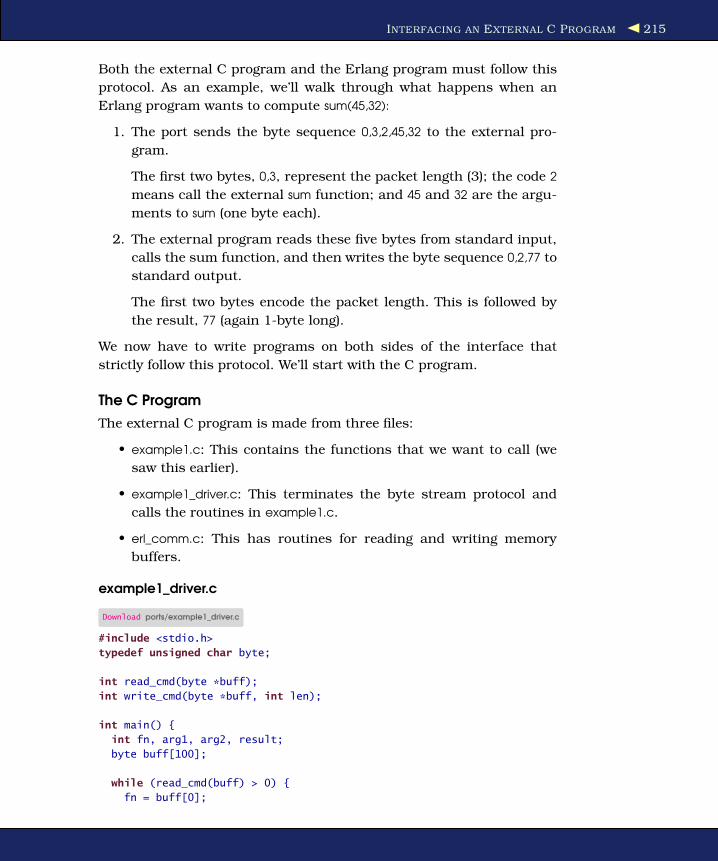
INTERFACING AN EXTERNAL C PROGRAM 215
Both the external C program and the Erlang program must follow this
protocol. As an example, we’ll walk through what happens when an
Erlang program wants to compute sum(45,32):
1. The port sends the byte sequence 0,3,2,45,32 to the external pro-
gram.
The first two bytes, 0,3, represent the packet length (3); the code 2
means call the external sum function; and 45 and 32 are the argu-
ments to sum (one byte each).
2. The external program reads these five bytes from standard input,
calls the sum function, and then writes the byte sequence 0,2,77 to
standard output.
The first two bytes encode the packet length. This is followed by
the result, 77 (again 1-byte long).
We now have to write programs on both sides of the interface that
strictly follow this protocol. We’ll start with the C program.
The C Program
The external C program is made from three files:
• example1.c: This contains the functions that we want to call (we
saw this earlier).
• example1_driver.c: This terminates the byte stream protocol and
calls the routines in example1.c.
• erl_comm.c: This has routines for reading and writing memory
buffers.
example1_driver.c
Download ports/example1_driver.c
#include <stdio.h>
typedef unsigned char byte;
int read_cmd(byte *buff);
int write_cmd(byte *buff, int len);
int main() {
int fn, arg1, arg2, result;
byte buff[100];
while (read_cmd(buff) > 0) {
fn = buff[0];

INTERFACING AN EXTERNAL C PROGRAM 216
if (fn == 1) {
arg1 = buff[1];
result = twice(arg1);
} else if (fn == 2) {
arg1 = buff[1];
arg2 = buff[2];
/* debug -- you can print to stderr to debug
fprintf(stderr,"calling sum %i %i\n",arg1,arg2); */
result = sum(arg1, arg2);
}
buff[0] = result;
write_cmd(buff, 1);
}
}
This code runs an infinite loop reading commands from standard input
calling the application routines and writing the results to standard out-
put.
If you want to debug this program, you can write to stderr. An example
of a debug statement has been commented out from the code.
erl_comm.c
Finally, here’s the code to read and write 2-byte headed packets to and
from standard input and output. The code is written this way to allow
for possible fragmentation of the IO packets.
Download ports/erl_comm.c
/* erl_comm.c */
#include <unistd.h>
typedef unsigned char byte;
int read_cmd(byte *buf);
int write_cmd(byte *buf, int len);
int read_exact(byte *buf, int len);
int write_exact(byte *buf, int len);
int read_cmd(byte *buf)
{
int len;
if (read_exact(buf, 2) != 2)
return(-1);
len = (buf[0] << 8) | buf[1];
return read_exact(buf, len);
}
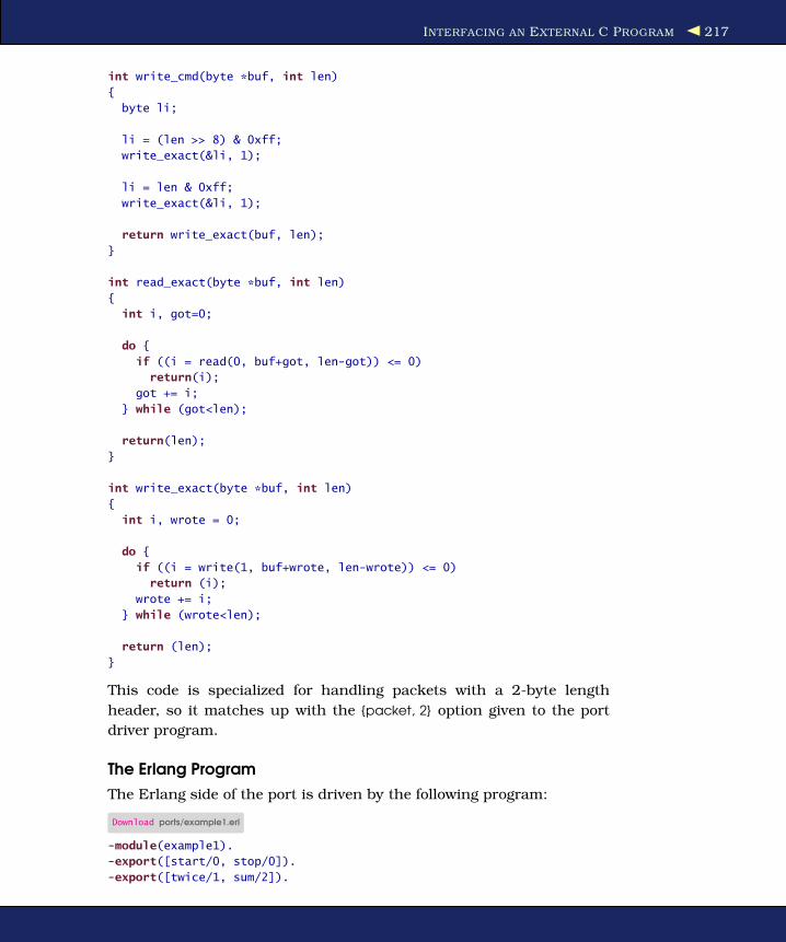
INTERFACING AN EXTERNAL C PROGRAM 217
int write_cmd(byte *buf, int len)
{
byte li;
li = (len >> 8) & 0xff;
write_exact(&li, 1);
li = len & 0xff;
write_exact(&li, 1);
return write_exact(buf, len);
}
int read_exact(byte *buf, int len)
{
int i, got=0;
do {
if ((i = read(0, buf+got, len-got)) <= 0)
return(i);
got += i;
} while (got<len);
return(len);
}
int write_exact(byte *buf, int len)
{
int i, wrote = 0;
do {
if ((i = write(1, buf+wrote, len-wrote)) <= 0)
return (i);
wrote += i;
} while (wrote<len);
return (len);
}
This code is specialized for handling packets with a 2-byte length
header, so it matches up with the {packet, 2} option given to the port
driver program.
The Erlang Program
The Erlang side of the port is driven by the following program:
Download ports/example1.erl
-module(example1).
-export([start/0, stop/0]).
-export([twice/1, sum/2]).

INTERFACING AN EXTERNAL C PROGRAM 218
start() ->
spawn(fun() ->
register(example1, self()),
process_flag(trap_exit, true),
Port = open_port({spawn, "./example1"}, [{packet, 2}]),
loop(Port)
end).
stop() ->
example1 ! stop.
twice(X) -> call_port({twice, X}).
sum(X,Y) -> call_port({sum, X, Y}).
call_port(Msg) ->
example1 ! {call, self(), Msg},
receive
{example1, Result} ->
Result
end.
loop(Port) ->
receive
{call, Caller, Msg} ->
Port ! {self(), {command, encode(Msg)}},
receive
{Port, {data, Data}} ->
Caller ! {example1, decode(Data)}
end,
loop(Port);
stop ->
Port ! {self(), close},
receive
{Port, closed} ->
exit(normal)
end;
{'EXIT', Port, Reason} ->
exit({port_terminated,Reason})
end.
encode({twice, X}) -> [1, X];
encode({sum, X, Y}) -> [2, X, Y].
decode([Int]) -> Int.
The port is opened with this statement:
Port = open_port({spawn, "./example1"}, [{packet, 2}])
The {packet,2} option tells the system to automatically add a 2-byte
packet length header to all packets sent to the external program. So

INTERFACING AN EXTERNAL C PROGRAM 219
if we were to send the message {PidC,{command,[2,45,32]}} to the port, the
port driver would add a 2-byte packet length header and actually send
0,3,2,45,32 to the external program.
On input the port driver will also assume that each incoming packet is
preceded by a 2-byte header and will remove these bytes before sending
the data to the Erlang connected process.
That completes the programs; we use the following makefile to build
the programs. The command make example1 builds the external pro-
gram that is used as an argument in the open_port function. Note that
the makefile also includes code to make the linked-in driver that is
presented later in this chapter.
MakefileDownload ports/Makefile
.SUFFIXES: .erl .beam .yrl
.erl.beam:
erlc -W $<
MODS = example1 example1_lid
all: ${MODS:%=%.beam} example1 example1_drv.so
example1: example1.c erl_comm.c example1_driver.c
gcc -o example1 example1.c erl_comm.c example1_driver.c
example1_drv.so: example1_lid.c example1.c
gcc -o example1_drv.so -fpic -shared example1.c example1_lid.c
clean:
rm example1 example1_drv.so *.beam
Running the Program
Now we can run the program:
1> example1:start().
<0.32.0>
2> example1:sum(45, 32).
77
4> example1:twice(10).
20
...
This now completes our first example.

OPEN_PORT 220
Before passing to the next topic, we should note the following:
• The example program made no attempt to unify Erlang and C’s
idea of what an integer is. We just assumed that an integer in
Erlang and C was a single byte and ignored all problems of pre-
cision and signedness. In a realistic application, we would have
to think rather carefully about the exact types and precisions of
the arguments concerned. This can be difficult, because Erlang
happily manages integers of an arbitrary size, whereas languages
such as C have fixed ideas about the precision of integers and so
on.
• We couldn’t just run the Erlang functions without first having
started the driver that was responsible for the interface (that is,
some program had to evaluate example1:start()before we were able
to run the program). We would like to be able to do this automat-
ically when the system is started. This is perfectly possible but
needs some knowledge of how the system starts and stops. We’ll
deal with this later in Section 18.7, The Application, on page 358.
12.3 open_port
In the previous section we introduced open_port without really saying
what the arguments to this function did. We saw one use of open_port,
with an argument {packet, 2} that added and removed a 2-byte header to
the data sent between Erlang and an external process. open_port takes
a relatively large number of arguments.
Some of the more common arguments are as follows:
@spec open_port(PortName, [Opt]) -> Port
PortName is one of the following:
{spawn, Command}
Start an external program. Command is the name of an exter-
nal program. Command runs outside the Erlang work space
unless a linked-in driver with the name Command is found.
{fd, In, Out}
Allow an Erlang process to access any currently opened file
descriptors used by Erlang. The file descriptor In can be used

LINKED-IN DRIVERS 221
for standard input, and the file descriptor Out can be used for
standard output.3
Opt is one of the following:
{packet, N}
Packets are preceded by an N (1, 2, or 4) byte length count.
stream
Messages are sent without packet lengths. The application
must know how to handle these packets.
{line, Max}
Deliver messages on a one-per line basis. If the line is more
than Max bytes, then it is split at Max bytes.
{cd, Dir}
Valid only for the {spawn, Command} option. The external pro-
gram starts in Dir.
{env, Env}
Valid only for the {spawn, Command} option. The environment
of external program is extended with the environment vari-
ables in the list Env. Env is a list of {VarName, Value} pairs,
where VarName and Value are strings.
This is not a complete list of the arguments to open_port. We can find
the precise details of the arguments in the manual page for the module
erlang.
12.4 Linked-in Drivers
Sometimes we want to run an foreign-language program inside the
Erlang runtime system. In this case, the program is written as a shared
library that is dynamically linked into the Erlang runtime system. The
linked-in driver appears to the programmer as a port program and
obeys exactly the same protocol as for a port program.
Creating a linked-in driver is the most efficient way of interfacing
foreign-language code with Erlang, but it is also the most dangerous.
Any fatal error in the linked-in driver will crash the Erlang system
3. See http://www.erlang.org/examples/examples-2.0.html for an example of connecting to
standard input and output.
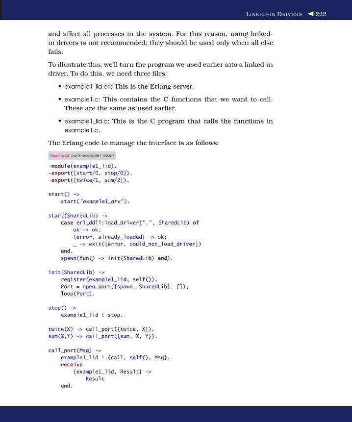
LINKED-IN DRIVERS 222
and affect all processes in the system. For this reason, using linked-
in drivers is not recommended; they should be used only when all else
fails.
To illustrate this, we’ll turn the program we used earlier into a linked-in
driver. To do this, we need three files:
• example1_lid.erl: This is the Erlang server.
• example1.c: This contains the C functions that we want to call.
These are the same as used earlier.
• example1_lid.c: This is the C program that calls the functions in
example1.c.
The Erlang code to manage the interface is as follows:
Download ports/example1_lid.erl
-module(example1_lid).
-export([start/0, stop/0]).
-export([twice/1, sum/2]).
start() ->
start("example1_drv").
start(SharedLib) ->
case erl_ddll:load_driver(".", SharedLib) of
ok -> ok;
{error, already_loaded} -> ok;
_ -> exit({error, could_not_load_driver})
end,
spawn(fun() -> init(SharedLib) end).
init(SharedLib) ->
register(example1_lid, self()),
Port = open_port({spawn, SharedLib}, []),
loop(Port).
stop() ->
example1_lid ! stop.
twice(X) -> call_port({twice, X}).
sum(X,Y) -> call_port({sum, X, Y}).
call_port(Msg) ->
example1_lid ! {call, self(), Msg},
receive
{example1_lid, Result} ->
Result
end.
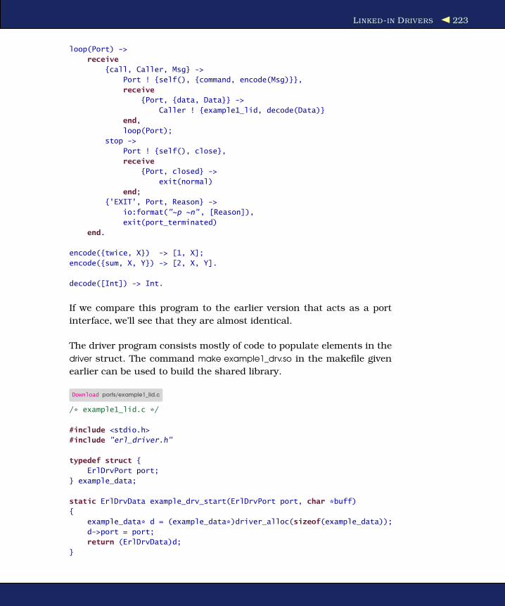
LINKED-IN DRIVERS 223
loop(Port) ->
receive
{call, Caller, Msg} ->
Port ! {self(), {command, encode(Msg)}},
receive
{Port, {data, Data}} ->
Caller ! {example1_lid, decode(Data)}
end,
loop(Port);
stop ->
Port ! {self(), close},
receive
{Port, closed} ->
exit(normal)
end;
{'EXIT', Port, Reason} ->
io:format("~p ~n", [Reason]),
exit(port_terminated)
end.
encode({twice, X}) -> [1, X];
encode({sum, X, Y}) -> [2, X, Y].
decode([Int]) -> Int.
If we compare this program to the earlier version that acts as a port
interface, we’ll see that they are almost identical.
The driver program consists mostly of code to populate elements in the
driver struct. The command make example1_drv.so in the makefile given
earlier can be used to build the shared library.
Download ports/example1_lid.c
/* example1_lid.c */
#include <stdio.h>
#include "erl_driver.h"
typedef struct {
ErlDrvPort port;
} example_data;
static ErlDrvData example_drv_start(ErlDrvPort port, char *buff)
{
example_data* d = (example_data*)driver_alloc(sizeof(example_data));
d->port = port;
return (ErlDrvData)d;
}

LINKED-IN DRIVERS 224
static void example_drv_stop(ErlDrvData handle)
{
driver_free((char*)handle);
}
static void example_drv_output(ErlDrvData handle, char *buff, int bufflen)
{
example_data* d = (example_data*)handle;
char fn = buff[0], arg = buff[1], res;
if (fn == 1) {
res = twice(arg);
} else if (fn == 2) {
res = sum(buff[1], buff[2]);
}
driver_output(d->port, &res, 1);
}
ErlDrvEntry example_driver_entry = {
NULL, /* F_PTR init, N/A */
example_drv_start, /* L_PTR start, called when port is opened */
example_drv_stop, /* F_PTR stop, called when port is closed */
example_drv_output, /* F_PTR output, called when erlang has sent
data to the port */
NULL, /* F_PTR ready_input,
called when input descriptor ready to read*/
NULL, /* F_PTR ready_output,
called when output descriptor ready to write */
"example1_drv", /* char *driver_name, the argument to open_port */
NULL, /* F_PTR finish, called when unloaded */
NULL, /* F_PTR control, port_command callback */
NULL, /* F_PTR timeout, reserved */
NULL /* F_PTR outputv, reserved */
};
DRIVER_INIT(example_drv) /* must match name in driver_entry */
{
return &example_driver_entry;
}
Here’s how we run the program:
1> c(example1_lid).
{ok,example1_lid}
2> example1_lid:start().
<0.41.0>
3> example1_lid:twice(50).
100
4> example1_lid:sum(10, 20).
30

NOTES 225
12.5 Notes
In this chapter, we have looked at the use of ports for interfacing an
external program to Erlang. In addition to the port protocol, we can
use a number of BIFs to manipulate ports. These are described in the
manual page for the erlang module.
At this point you’re probably wondering how to pass complex data
structures between Erlang and an external program. How can you
send strings, tuples, and so on, between Erlang and the outside world?
Unfortunately, there is no simple answer to this question; all that ports
provide is a low-level mechanism for transferring a sequence of bytes
between Erlang and the outside world. This, incidentally, is the same
problem as encountered in socket programming. A socket provides a
stream of bytes between two applications; how these applications inter-
pret these bytes is up to the application.
However, several libraries included in the Erlang distribution simplify
the job of interfacing Erlang to external programs; these include the
following:
http://www.erlang.org/doc/pdf/erl_interface.pdf
Erl interface (ei) is a set of C routines and macros for encoding
and decoding the Erlang external format. On the Erlang side, an
Erlang program uses term_to_binary to serialize an Erlang term,
and on the C side the routines in ei can be used to unpack this
binary. ei can also be used to construct a binary, which the Erlang
side can unpack with binary_to_term.
http://www.erlang.org/doc/pdf/ic.pdf
The Erlang IDL Compiler (ic). The ic application is an Erlang imple-
mentation of an OMG IDL complier.
http://www.erlang.org/doc/pdf/jinterface.pdf
Jinteface is a set of tools for interfacing Java to Erlang. It pro-
vides a full mapping of Erlang types to Java objects, encoding and
decoding Erlang terms, linking to Erlang processes, and so on, as
well as a wide range of additional features.

Chapter 13
Programming with FilesIn this chapter, we’ll look at some of the most commonly used functions
for manipulating files. The standard Erlang release has a large number
of functions for working with files. We’re going to concentrate on the
small fraction of these that I use to write most of my programs. We’ll
also see a few examples of the techniques I use for writing efficient file
handling code. In addition, I’ll briefly mention some of the more rarely
used file operations so you’ll know they exist. If you want more details,
consult the manual pages.
We’ll concentrate on the following areas:
• Organization of the libraries
• Different ways of reading a file
• Different ways of writing to a file
• Directory operations
• Finding information about a file
13.1 Organization of the Libraries
The functions for file manipulation are organized into four modules:
file This has routines for opening, closing, reading, and writing files;
listing directories; and so on. A short summary of some of the
more frequently used functions in file is shown in Figure 13.1,
on page 228. For full details, consult the manual page for the file
module.

THE DIFFERENT WAYS OF READING A FILE 227
filename
This module has routines that manipulate filenames in a platform-
independent manner, so you can run the same code on a number
of different operating systems.
filelib
This module is an extension to file, which contains a number of
utilities for listing files, checking file types, and so on. Most of
these are written using the functions in file.
io This module has routines that work on opened files. It contains
routines for parsing data in a file and writing formatted data to a
file.
13.2 The Different Ways of Reading a File
Let’s look at some options when it comes to reading files. We’ll start
by writing five little programs that open a file and input the data in a
number of different ways.
The contents of a file is just sequence of bytes. Whether they mean
anything depends upon the interpretation of these bytes.
To demonstrate this, we’ll use the same input file for all our examples.
It actually contains a sequence of Erlang terms. Depending upon how
we open and read the file, we can interpret the contents as a sequence
of Erlang terms, as a sequence of text lines, or as raw chunks of binary
data with no particular interpretation.
Here’s the raw data in the file:
Download data1.dat
{person, "joe", "armstrong",
[{occupation, programmer},
{favoriteLanguage, erlang}]}.
{cat, {name, "zorro"},
{owner, "joe"}}.
Now we’ll read parts of this file in a number of ways.

THE DIFFERENT WAYS OF READING A FILE 228
Function Description
change_group Change group of a file.
change_owner Change owner of a file.
change_time Change the modification or last access time of a file.
close Close a file.
consult Read Erlang terms from a file.
copy Copy file contents.
del_dir Delete a directory.
delete Delete a file.
eval Evaluate Erlang expressions in a file.
format_error Return a descriptive string for an error reason.
get_cwd Get the current working directory.
list_dir List files in a directory.
make_dir Make a directory.
make_link Make a hard link to a file.
make_symlink Make a symbolic link to a file or directory.
open Open a file.
position Set position in a file.
pread Read from a file at a certain position.
pwrite Write to a file at a certain position.
read Read from a file.
read_file Read an entire file.
read_file_info Get information about a file.
read_link See what a link is pointing to.
read_link_info Get information about a link or file.
rename Rename a file.
script Evaluate and return the value of Erlang expressions in a file.
set_cwd Set the current working directory.
sync Synchronize the in-memory state of a file with that
on the physical medium.
truncate Truncate a file.
write Write to a file.
write_file Write an entire file.
write_file_info Change information about a file.
Figure 13.1: Summary of file operations (in module file)

THE DIFFERENT WAYS OF READING A FILE 229
Reading All the Terms in the File
data1.dat contains a sequence of Erlang terms; we can read all of these
by calling file:consult as follows:
1> file:consult("data1.dat").
{ok,[{person,"joe",
"armstrong",
[{occupation,programmer},{favoriteLanguage,erlang}]},
{cat,{name,"zorro"},{owner,"joe"}}]}
file:consult(File) assumes that File contains a sequence of Erlang terms. It
returns {ok, [Term]} if it can read all the terms in the file; otherwise, it
returns {error, Reason}.
Reading the Terms in the File One at a Time
If we want to read the terms in a file one at a time, we first open the file
with file:open, then we read the individual terms with io:read until we
reach the end of file, and finally we close the file with file:close.
Here’s a shell session that shows what happens when we read the terms
in a file one at a time:
1> {ok, S} = file:open("data1.dat", read).
{ok,<0.36.0>}
2> io:read(S, '').
{ok,{person,"joe",
"armstrong",
[{occupation,programmer},{favoriteLanguage,erlang}]}}
3> io:read(S, '').
{ok,{cat,{name,"zorro"},{owner,"joe"}}}
4> io:read(S, '').
eof
5> file:close(S)
The functions we’ve used here are as follows:
@spec file:open(File, read) => {ok, IoDevice} | {error, Why}
Tries to open File for reading. It returns {ok, IoDevice} if it can open
the file; otherwise, it returns {error, Reason}. IoDevice is an IO device
that is used to access the file.
@spec io:read(IoDevice, Prompt) => {ok, Term} | {error,Why} | eof
Reads an Erlang term Term from IoDevice. Prompt is ignored if IoDe-
vice represents an opened file. Prompt is used only to provide a
prompt if we use io:read to read from standard input.
@spec file:close(IoDevice) => ok | {error, Why}
Closes IoDevice.

THE DIFFERENT WAYS OF READING A FILE 230
Using these routines we could have implemented file:consult, which we
used in the previous section. Here’s how file:consult might have been
defined:
Download lib_misc.erl
consult(File) ->
case file:open(File, read) of
{ok, S} ->
Val = consult1(S),
file:close(S),
{ok, Val};
{error, Why} ->
{error, Why}
end.
consult1(S) ->
case io:read(S, '') of
{ok, Term} -> [Term|consult1(S)];
eof -> [];
Error -> Error
end.
This is not how file:consult is actually defined. The standard libraries use
an improved version with better error reporting.
Now is a good time to look at the version included in the standard
libraries. If you’ve understood the earlier version, then you should find
it easy to follow the code in the libraries. There’s only one problem. How
can we find the source of the file.erl code? To do this, we use the function
code:which, which can locate the object code for any module that has
been loaded.
1> code:which(file).
"/usr/local/lib/erlang/lib/kernel-2.11.2/ebin/file.beam"
In the standard release, each library has two subdirectories. One, called
src, contains the source code. The other, called ebin, contains compiled
Erlang code. So, the source code for file.erl should be in the following
directory:
/usr/local/lib/erlang/lib/kernel-2.11.2/src/file.erl
When all else fails and the manual pages don’t provide the answers to
all your questions about the code, then a quick peek at the source code
can often reveal the answer. Now I know this shouldn’t happen, but
we’re all human, and sometimes the documentation doesn’t answer all
your questions.

THE DIFFERENT WAYS OF READING A FILE 231
Reading the Lines in a File One at a Time
If we change io:read to io:get_line, we can read the lines in the file one
at a time. io:get_line reads characters until it encounters a line-feed
character or end-of-file. Here’s an example:
1> {ok, S} = file:open("data1.dat", read).
{ok,<0.43.0>}
2> io:get_line(S, '').
"{person, \"joe\", \"armstrong\",\n"
3> io:get_line(S, '').
"\t[{occupation, programmer},\n"
4> io:get_line(S, '').
"\t {favoriteLanguage, erlang}]}.\n"
5> io:get_line(S, '').
"\n"
6> io:get_line(S, '').
"{cat, {name, \"zorro\"},\n"
7> io:get_line(S, '').
" {owner, \"joe\"}}.\n"
8> io:get_line(S, '').
eof
9> file:close(S).
ok
Reading the Entire File into a Binary
You can use file:read_file(File) to read an entire file into a binary using a
single atomic operation:
1> file:read_file("data1.dat").
{ok,<<"{person, \"joe\", \"armstrong\""...>>}
file:read_file(File) returns {ok, Bin} if it succeeds and returns {error, Why}
otherwise.
This is by far the most efficient way of reading files, and it’s a method
that I use a lot. For most operations, I read the entire file into memory
in one operation, manipulate the contents, and store the file in a single
operation (using file:write_file). We’ll give an example of this later.
Reading a File with Random Access
If the file we want to read is very large or if it contains binary data in
some externally defined format, then we can open the file in raw mode
and read any portion of it using file:pread.
Here’s an example:
1> {ok, S} = file:open("data1.dat", [read,binary,raw]).
{ok,{file_descriptor,prim_file,{#Port<0.106>,5}}}

THE DIFFERENT WAYS OF READING A FILE 232
2> file:pread(S, 22, 46).
{ok,<<"rong\",\n\t[{occupation, progr...>>}
3> file:pread(S, 1, 10).
{ok,<<"person, \"j">>}
4> file:pread(S, 2, 10).
{ok,<<"erson, \"jo">>}
5> file:close(S).
file:pread(IoDevice, Start, Len) reads exactly Len bytes from IoDevice start-
ing at byte Start (the bytes in the file are numbered so that the first byte
in the file is at position 1). It returns {ok, Bin} or {error, Why}.
Finally, we’ll use the routines for random file access to write a utility
routine that we’ll need in the next chapter. In Section 14.7, A SHOUT-
cast Server, on page 265, we’ll develop a simple SHOUTcast server (this
is a server for so-called streaming media, in this case for streaming
MP3). Part of this server needs to be able to find the artist and track
names that are embedded in an MP3 file. We’ll do this in the next sec-
tion.
Reading ID3 Tags
MP3 is a binary format used for storing compressed audio data. MP3
files do not themselves contain information about the content of the
file, so, for example, in an MP3 file that contains music, the name of the
artist who recorded the music is not contained in the audio data. This
data (the track name, artist name, and so on) is stored inside the MP3
files in a tagged block format known as ID3. ID3 tags were invented by a
programmer called Eric Kemp to store metadata describing the content
of an audio file. There are actually a number of ID3 formats, but for our
purposes, we’ll write code to access only the two simplest forms of ID3
tag, namely, the ID3v1 and ID3v1.1 tags.
The ID3v1 tag has a simple structure—the last 128 bytes of the file con-
tain a fixed-length tag. The first 3 bytes contain the ASCII characters
TAG, followed by a number of fixed-length fields. The entire 128 bytes is
packed as follows:
Length Contents
3 Header containing the characters TAG
30 Title
30 Artist
30 Album
4 Year
30 Comment
1 Genre
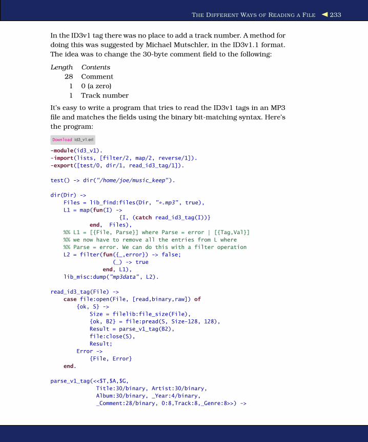
THE DIFFERENT WAYS OF READING A FILE 233
In the ID3v1 tag there was no place to add a track number. A method for
doing this was suggested by Michael Mutschler, in the ID3v1.1 format.
The idea was to change the 30-byte comment field to the following:
Length Contents
28 Comment
1 0 (a zero)
1 Track number
It’s easy to write a program that tries to read the ID3v1 tags in an MP3
file and matches the fields using the binary bit-matching syntax. Here’s
the program:
Download id3_v1.erl
-module(id3_v1).
-import(lists, [filter/2, map/2, reverse/1]).
-export([test/0, dir/1, read_id3_tag/1]).
test() -> dir("/home/joe/music_keep").
dir(Dir) ->
Files = lib_find:files(Dir, "*.mp3", true),
L1 = map(fun(I) ->
{I, (catch read_id3_tag(I))}
end, Files),
%% L1 = [{File, Parse}] where Parse = error | [{Tag,Val}]
%% we now have to remove all the entries from L where
%% Parse = error. We can do this with a filter operation
L2 = filter(fun({_,error}) -> false;
(_) -> true
end, L1),
lib_misc:dump("mp3data", L2).
read_id3_tag(File) ->
case file:open(File, [read,binary,raw]) of
{ok, S} ->
Size = filelib:file_size(File),
{ok, B2} = file:pread(S, Size-128, 128),
Result = parse_v1_tag(B2),
file:close(S),
Result;
Error ->
{File, Error}
end.
parse_v1_tag(<<$T,$A,$G,
Title:30/binary, Artist:30/binary,
Album:30/binary, _Year:4/binary,
_Comment:28/binary, 0:8,Track:8,_Genre:8>>) ->

THE DIFFERENT WAYS OF READING A FILE 234
{"ID3v1.1",
[{track,Track}, {title,trim(Title)},
{artist,trim(Artist)}, {album, trim(Album)}]};
parse_v1_tag(<<$T,$A,$G,
Title:30/binary, Artist:30/binary,
Album:30/binary, _Year:4/binary,
_Comment:30/binary,_Genre:8>>) ->
{"ID3v1",
[{title,trim(Title)},
{artist,trim(Artist)}, {album, trim(Album)}]};
parse_v1_tag(_) ->
error.
trim(Bin) ->
list_to_binary(trim_blanks(binary_to_list(Bin))).
trim_blanks(X) -> reverse(skip_blanks_and_zero(reverse(X))).
skip_blanks_and_zero([$\s|T]) -> skip_blanks_and_zero(T);
skip_blanks_and_zero([0|T]) -> skip_blanks_and_zero(T);
skip_blanks_and_zero(X) -> X.
The main entry point to our program is id3_v1:dir(Dir). The first thing we
do is find all our MP3 files by calling lib_find:find(Dir, "*.mp3", true) (shown
later in Section 13.8, A Find Utility, on page 242), which recursively
scans the directories under Dir looking for MP3 files. Having found the
file, we parse the tags by calling read_id3_tag. Parsing is greatly simpli-
fied because we can merely use the bit-matching syntax to do the pars-
ing for us, and then we can trim the artist and track names by remov-
ing trailing whitespace and zero-padding characters, which delimit the
character strings. Finally, we dump the results in a file for later use
(lib_misc:dump is described in Section E.2, Debugging Techniques, on
page 427).
Most music files are tagged with ID3v1 tags, even if they also have
ID3v2, v3, and v4 tags—the later taggings standards added a differently
formatted tag to the beginning of the file (or more rarely in the middle
of the file). Tagging programs often appear to add both ID3v1 tags and
additional (and more difficult to read) tags at the start of the file. For
our purposes, we’ll be concerned only with files containing valid ID3v1
and ID3v1.1 tags.
Now that we know how to read a file, we can move to the different ways
of writing to a file.

THE DIFFERENT WAYS OF WRITING TO A FILE 235
13.3 The Different Ways of Writing to a File
Writing to a file involves pretty much the same operations as reading a
file. Let’s look at them.
Write a List of Terms to a File
Suppose we want to create a file that we can read with file:consult. The
standard libraries don’t actually contain a function for this, so we’ll
write our own. Let’s call this function unconsult.1
Download lib_misc.erl
unconsult(File, L) ->
{ok, S} = file:open(File, write),
lists:foreach(fun(X) -> io:format(S, "~p.~n",[X]) end, L),
file:close(S).
We can run this in the shell to create a file called test1.dat:
1> lib_misc:unconsult("test1.dat",
[{cats,["zorrow","daisy"]},
{weather,snowing}]).
ok
Let’s check it’s OK:
2> file:consult("test1.dat").
{ok,[{cats,["zorrow","daisy"]},{weather,snowing}]}
To implement unconsult, we opened the file in write mode and then used
io:format(S, "~p.~n", [X]) to write terms to the file.
io:format is the workhorse for creating formatted output. To produce
formatted output, we call the following:
@spec io:format(IoDevice, Format, Args) -> ok
ioDevice is an IO device (which must have been opened in write
mode), Format is a string containing formatting codes, and Args is
a list of items to be output.
For each item in Args, there must be a formatting command in the
format string. Formatting commands begin with a tilde (~) character.
Here are some of the most commonly used formatting commands:
~n Write a line feed. ~n is smart and writes a line feed in a platform-
dependent way. So on a Unix machine, ~n will write ASCII (10)
1. The nice thing about writing a book is I can choose any module or function names I
want and nobody can argue.

THE DIFFERENT WAYS OF WRITING TO A FILE 236
to the output stream, and on a Windows machine it will write
carriage-return line-feed ASCII (13, 10) to the output stream.
~p Pretty-print the argument.
~s The argument is a string.
~w Write data with the standard syntax. This is used to output Erlang
terms.
The format string has about ten quadzillion arguments that nobody in
their right mind can remember. You’ll find a complete list in the man
page for the module io. I remember only ~p, ~s, and ~n. If you start with
these, you won’t have many problems.
Aside
I lied—you’ll probably need more than just ~p, ~s, and ~n. Here are a
few examples:
Format Result
io:format("|~10s|~n", ["abc"]) | abc|
io:format("|~-10s|~n", ["abc"]) |abc |
io:format("|~10.3.+s|~n",["abc"]) |+++++++abc|
io:format("|~10.10.+s|~n",["abc"]) |abc+++++++|
io:format("|~10.7.+s|~n",["abc"]) |+++abc++++|
Writing Lines to a File
This is similar to the previous example—we just use a different format-
ting command:
1> {ok, S} = file:open("test2.dat", write).
{ok,<0.62.0>}
2> io:format(S, "~s~n", ["Hello readers"]).
ok
3> io:format(S, "~w~n", [123]).
ok
4> io:format(S, "~s~n", ["that's it"]).
ok
5> file:close(S).
This created a file called test2.dat with the following contents:
Hello readers
123
that's it

THE DIFFERENT WAYS OF WRITING TO A FILE 237
Writing an Entire File in One Operation
This is the most efficient way of writing to a file. file:write_file(File, IO)
writes the data in IO, which is an IO list to File. (An IO list is a list whose
elements are IO lists, binaries, or integers from 0 to 255. When an IO
list is output, it is automatically “flattened,” which means that all the
list brackets are removed.) This method is extremely efficient and is one
that I often use. The program in the next section illustrates this.
Listing URLs from a File
Let’s write a simple function called urls2htmlFile(L, File) that takes a list
of URLs, L, and creates an HTML file, where the URLs are presented
as clickable links. This lets us play with the technique of creating an
entire file in a single IO operation.
We’ll write our program in the module scavenge_urls. First here’s the
program header:
Download scavenge_urls.erl
-module(scavenge_urls).
-export([urls2htmlFile/2, bin2urls/1]).
-import(lists, [reverse/1, reverse/2, map/2]).
urls2htmlFile(Urls, File) ->
file:write_file(File, urls2html(Urls)).
bin2urls(Bin) -> gather_urls(binary_to_list(Bin), []).
The program has two entry points. urls2htmlFile(Urls, File) takes a list of
URLs and creates an HTML file containing clickable links for each URL,
and bin2urls(Bin) searches through a binary and returns a list of all the
URLs contained in the binary. urls2htmlFile is as follows:
Download scavenge_urls.erl
urls2html(Urls) -> [h1("Urls"),make_list(Urls)].
h1(Title) -> ["<h1>", Title, "</h1>\n"].
make_list(L) ->
["<ul>\n",
map(fun(I) -> ["<li>",I,"</li>\n"] end, L),
"</ul>\n"].
This code returns a deep list of characters. Note we make no attempt to
flatten the list (which would be rather inefficient); we make a deep list
of characters and just throw it at the output routines. When we write a
deep list to a file with file:write_file, the IO system automatically flattens
the list (that is, it outputs only the characters embedded in the lists

THE DIFFERENT WAYS OF WRITING TO A FILE 238
and not the list brackets themselves). Finally, here’s the code to extract
the URLs from a binary:
Download scavenge_urls.erl
gather_urls("<a href" ++ T, L) ->
{Url, T1} = collect_url_body(T, reverse("<a href")),
gather_urls(T1, [Url|L]);
gather_urls([_|T], L) ->
gather_urls(T, L);
gather_urls([], L) ->
L.
collect_url_body("</a>" ++ T, L) -> {reverse(L, "</a>"), T};
collect_url_body([H|T], L) -> collect_url_body(T, [H|L]);
collect_url_body([], _) -> {[],[]}.
To run this, we need to get some data to parse. The input data (a binary)
is the content of an HTML page, so we need an HTML page to scavenge.
For this we’ll use socket_examples:nano_get_url (see Section 14.1, Fetch-
ing Data from a Server, on page 246):
We’ll do this step by step in the shell:
1> B = socket_examples:nano_get_url("www.erlang.org"),
L = scavenge_urls:bin2urls(B),
scavenge_urls:urls2htmlFile(L, "gathered.html").
ok
This produces the file gathered.html:
Download gathered.html
<h1>Urls</h1>
<ul>
<li><a href="old_news.html">Older news.....</a></li>
<li><a href="http://www.erlang-consulting.com/training_fs.html">here</a></li>
<li><a href="project/megaco/">Megaco home</a></li>
<li><a href="EPLICENSE">Erlang Public License (EPL)</a></li>
<li><a href="user.html#smtp_client-1.0">smtp_client-1.0</a></li>
<li><a href="download-stats/">download statistics graphs</a></li>
<li><a href="project/test_server">Erlang/OTP Test
Server</a></li>
<li><a href="http://www.erlang.se/euc/06/">proceedings</a></li>
<li><a href="/doc/doc-5.5.2/doc/highlights.html">
Read more in the release highlights.
</a></li>
<li><a href="index.html"><img src="images/erlang.gif"
border="0" alt="Home"></a></li>
</ul>

DIRECTORY OPERATIONS 239
Writing to a Random-Access File
Writing to a file in random-access mode is similar to reading. First, we
have to open the file in write mode. Next, we use file:pwrite(Position, Bin) to
write to the file.
Here’s an example:
1> {ok, S} = file:open("...", [raw,write,binary])
{ok, ...}
2> file:pwrite(S, 10, <<"new">>)
ok
3> file:close(S)
ok
This writes the characters new starting at an offset of 10 in the file,
overwriting the original content.
13.4 Directory Operations
Three functions in file are used for directory operations. list_dir(Dir) is
used to produce a list of the files in Dir, make_dir(Dir) creates a new direc-
tory, and del_dir(Dir) deletes a directory.
If we run list_dir on the code directory that I’m using to write this book,
we’ll see something like the following:
1> cd("/home/joe/book/erlang/Book/code").
/home/joe/book/erlang/Book/code
ok
2> file:list_dir(".").
{ok,["id3_v1.erl~",
"update_binary_file.beam",
"benchmark_assoc.beam",
"id3_v1.erl",
"scavenge_urls.beam",
"benchmark_mk_assoc.beam",
"benchmark_mk_assoc.erl",
"id3_v1.beam",
"assoc_bench.beam",
"lib_misc.beam",
"benchmark_assoc.erl",
"update_binary_file.erl",
"foo.dets",
"big.tmp",
..
Observe that there is no particular order to the files and no indication
as to whether the files in the directory are files or directories, what the
sizes are, and so on.

FINDING INFORMATION ABOUT A FILE 240
To find out about the individual files in the directory listing, we’ll use
file:read_file_info, which is the subject of the next section.
13.5 Finding Information About a File
To find out about a file F, we call file:read_file_info(F). This returns {ok,
Info} if F is a valid file or directory name. Info is a record of type #file_info,
which is defined as follows:
-record(file_info,
{size, % Size of file in bytes.
type, % Atom: device, directory, regular,
% or other.
access, % Atom: read, write, read_write, or none.
atime, % The local time the file was last read:
% {{Year, Mon, Day}, {Hour, Min, Sec}}.
mtime, % The local time the file was last written.
ctime, % The interpretation of this time field
% is dependent on operating system.
% On Unix it is the last time the file or
% or the inode was changed. On Windows,
% it is the creation time.
mode, % Integer: File permissions. On Windows,
% the owner permissions will be duplicated
% for group and user.
links, % Number of links to the file (1 if the
% filesystem doesn't support links).
major_device, % Integer: Identifies the file system (Unix),
% or the drive number (A: = 0, B: = 1) (Windows).
Note: The mode and access fields overlap. You can use mode to set
several file attributes in a single operation, whereas you can use access
for simpler operations.
To find the size and type of a file, we call read_file_info as in the following
example (note we have to include file.hrl, which contains the definition
of the #file_info record):
Download lib_misc.erl
-include_lib("kernel/include/file.hrl").
file_size_and_type(File) ->
case file:read_file_info(File) of
{ok, Facts} ->
{Facts#file_info.type, Facts#file_info.size};
_ ->
error
end.

COPYING AND DELETING FILES 241
Now we can augment the directory listing returned by list_file by adding
information about the files in the function ls() as follows:
Download lib_misc.erl
ls(Dir) ->
{ok, L} = file:list_dir(Dir),
map(fun(I) -> {I, file_size_and_type(I)} end, sort(L)).
Now when we list the files, they are ordered and contain additional
useful information:
1> lib_misc:ls(".").
[{"Makefile",{regular,1244}},
{"README",{regular,1583}},
{"abc.erl",{regular,105}},
{"alloc_test.erl",{regular,303}},
...
{"socket_dist",{directory,4096}},
...
As a convenience, the module filelib exports a few small routines such as
file_size(File) and is_dir(X). These are merely interfaces to file:read_file_info. If
we just want to the size of a file, it is more convenient to call filelib:file_size
than to call file:read_file_info and unpack the elements of the #file_info
record.
13.6 Copying and Deleting Files
file:copy(Source, Destination) copies the file Source to Destination.
file:delete(File) deletes File.
13.7 Bits and Pieces
So far we’ve mentioned most of the functions that I use on a day-to-day
basis for manipulating files. It’s actually rare that I need to look up the
manual pages to find out more information. So, what have I left out
that you might need to know about? I’ll give you a brief list of the major
omissions. For the details, see the manual pages.
File modes
When we open a file with file:open, we open the file in a particular
mode or a combination of modes. There are actually many more
modes than we might think; for example, it’s possible to read and
write gzip-compressed files with the compressed mode flag, and so
on. The full list is in the manual pages.

A FIND UTILITY 242
Modification times, groups, symlinks
We can set all of these with routines in file.
Error codes
I’ve rather blandly said that all errors are of the form {error, Why};
in fact, Why is an atom (for example, enoent means a file does not
exist, and so on)—there are a large number of error codes, and
they are all described in the manual pages.
filename
The filename module has some useful routines for ripping apart
full filenames in directories and finding the file extensions, and so
on, as well as for rebuilding filenames for the component parts. All
this is done in a platform-independent manner.
filelib
The filelib module has a small number of routines that can save
us some work. For example, filelib:ensure_dir(Name) ensures that all
parent directories for the given file or directory name Name exist,
trying to create them if necessary.
13.8 A Find Utility
As a final example, we’ll use file:list_dir and file:read_file_info to make a
general-purpose “find” utility.
The main entry point to this module is as follows:
lib_find:files(Dir, RegExp, Recursive, Fun, Acc0)
The arguments are as follows:
Dir
The directory name to start the file search in.
RegExp
A regular expression2 to test the files we have found. If the files we
encounter match this regular expression, then Fun(File, Acc) will be
called, where File is the name of the file that matches the regular
expression.
Recursive = true | false
A flag that determines whether search should recurse into the
subdirectories of the current directory in the search path.
2. See the man pages for the module regexp for the syntax of regular expressions.

A FIND UTILITY 243
Fun(File, AccIn) -> AccOut
A function that is applied to the File if regExp matches File. Acc is an
accumulator whose initial value is Acc0. Each time Fun is called,
it must return a new value of the accumulator that is passed into
Fun the next time it is called. The final value of the accumulator is
the return value of lib_find:files/5
We can pass any function we want into lib_find:files/5. For example, we
can build a list of files using the following function, passing it an empty
list initially:
fun(File, Acc) -> [File|Acc] end
The module entry point lib_find:files(Dir, ShellRegExp, Flag) provides a sim-
plified entry point for a more common usage of the program. Here Shell-
RegExp is a simplified form of regular expression that is easier to write
than the full form of regular expression.
As an example of the short form of calling sequence, the following call:
lib_find:files(Dir, "*.erl", true)
recursively finds all Erlang files under Dir. If the last argument had
been false, then only the Erlang files in the directory Dir would have
been found—it would not look in subdirectories.
Finally, here’s the code:
Download lib_find.erl
-module(lib_find).
-export([files/3, files/5]).
-import(lists, [reverse/1]).
-include_lib("kernel/include/file.hrl").
files(Dir, Re, Flag) ->
Re1 = regexp:sh_to_awk(Re),
reverse(files(Dir, Re1, Flag, fun(File, Acc) ->[File|Acc] end, [])).
files(Dir, Reg, Recursive, Fun, Acc) ->
case file:list_dir(Dir) of
{ok, Files} -> find_files(Files, Dir, Reg, Recursive, Fun, Acc);
{error, _} -> Acc
end.

A FIND UTILITY 244
find_files([File|T], Dir, Reg, Recursive, Fun, Acc0) ->
FullName = filename:join([Dir,File]),
case file_type(FullName) of
regular ->
case regexp:match(FullName, Reg) of
{match, _, _} ->
Acc = Fun(FullName, Acc0),
find_files(T, Dir, Reg, Recursive, Fun, Acc);
_ ->
find_files(T, Dir, Reg, Recursive, Fun, Acc0)
end;
directory ->
case Recursive of
true ->
Acc1 = files(FullName, Reg, Recursive, Fun, Acc0),
find_files(T, Dir, Reg, Recursive, Fun, Acc1);
false ->
find_files(T, Dir, Reg, Recursive, Fun, Acc0)
end;
error ->
find_files(T, Dir, Reg, Recursive, Fun, Acc0)
end;
find_files([], _, _, _, _, A) ->
A.
file_type(File) ->
case file:read_file_info(File) of
{ok, Facts} ->
case Facts#file_info.type of
regular -> regular;
directory -> directory;
_ -> error
end;
_ ->
error
end.

Chapter 14
Programming with SocketsMost of the more interesting programs that I write involve sockets one
way or another. A socket is a communication endpoint that allows
machines to communicate over the Internet using the Internet Pro-
tocol (IP). In this chapter, we’ll concentrate on the two core protocols
of the Internet: Transmission Control Protocol (TCP) and User Datagram
Protocol (UDP).
UDP lets applications send short messages (called datagrams) to each
other, but there is no guarantee of delivery for these messages. They
can also arrive out of order. TCP, on the other hand, provides a reliable
stream of bytes that are delivered in order as long as the connection is
established.
Why is programming with sockets fun? Because it allows applications
to interact with other machines on the Internet, which has far more
potential than just performing local operations.
There are two main libraries for programming with sockets: gen_tcp
for programming TCP applications and gen_udp for programming UDP
applications.
In this chapter, we’ll see how to program client and servers using TCP
and UDP sockets. We’ll go through the different forms of servers that
are possible (parallel, sequential, blocking, and nonblocking) and see
how to program traffic-shaping applications that can control the flow of
data to the application.

USING TCP 246
14.1 Using TCP
We’ll start our adventures in socket programming by looking at a simple
TCP program that fetches data from a server. After this, we’ll write a
simple sequential TCP server and show how it can be parallelized to
handle multiple parallel sessions.
Fetching Data from a Server
Let’s start by writing a little function1 that uses a TCP socket to fetch
an HTML page from http://www.google.com:
Download socket_examples.erl
nano_get_url() ->
nano_get_url("www.google.com").
nano_get_url(Host) ->Ê {ok,Socket} = gen_tcp:connect(Host,80,[binary, {packet, 0}]),Ë ok = gen_tcp:send(Socket, "GET / HTTP/1.0\r\n\r\n"),
receive_data(Socket, []).
receive_data(Socket, SoFar) ->
receiveÌ {tcp,Socket,Bin} ->
receive_data(Socket, [Bin|SoFar]);Í {tcp_closed,Socket} ->Î list_to_binary(reverse(SoFar))
end.
How does this work?
Ê We open a TCP socket to port 80 of http://www.google.com by call-
ing gen_tcp:connect. The argument binary in the connect call tells
the system to open the socket in “binary” mode and deliver all
data to the application as binaries. {packet,0} means the TCP data
is delivered directly to the application in an unmodified form.
Ë We call gen_tcp:send and send the message GET / HTTP/1.0\r\n\r\n to
the socket. Then we wait for a reply. The reply doesn’t come all in
one packet but comes fragmented, a bit at a time. These fragments
will be received as a sequence of messages that are sent to the
process that opened (or controls) the socket.
1. The standard library function in the Erlang distribution, http:request(Uri), achieves the
same result, but we want to show how this can be done using the library functions in
gen_tcp.

USING TCP 247
Ì We receive a {tcp,Socket,Bin} message. The third argument in this
tuple is a binary. This is because we opened the socket in binary
mode. This message is one of the data fragments sent to us from
the web server. We add it to the list of fragments we have received
so far and wait for the next fragment.
Í We receive a {tcp_closed, Socket} message. This happens when the
server has finished sending us data.2
Î When all the fragments have come, we’ve stored them in the wrong
order, so we reverse the order and concatenate all the fragments.
Let’s just test that it works:
1> B = socket_examples:nano_get_url().
<<"HTTP/1.0 302 Found\r\nLocation: http://www.google.se/\r\n
Cache-Control: private\r\nSet-Cookie: PREF=ID=b57a2c:TM"...>>
Note: When you run nano_get_url, the result is a binary, so you’ll see is
what a binary looks like when pretty printed in the Erlang shell. When
binaries are pretty printed, all control characters are displayed in an
escaped format. And the binary is truncated, which is indicted by the
three dots (...>>) at the end of the printout. If you want to see all of
the binary, you can print it with io:format or break it into pieces with
string:tokens:
2> io:format("~p~n",[B]).
<<"HTTP/1.0 302 Found\r\nLocation: http://www.google.se/\r\n
Cache-Control: private\r\nSet-Cookie: PREF=ID=b57a2c:TM"
TM=176575171639526:LM=1175441639526:S=gkfTrK6AFkybT3;
expires=Sun, 17-Jan-2038 19:14:07
... several lines omitted ...
>>
3>string:tokens(binary_to_list(B),"\r\n").
["HTTP/1.0 302 Found",
"Location: http://www.google.se/",
"Cache-Control: private",
"Set-Cookie: PREF=ID=ec7f0c7234b852dece4:TM=11713424639526:
LM=1171234639526:S=gsdertTrK6AEybT3;
expires=Sun, 17-Jan-2038 19:14:07 GMT; path=/; domain=.google.com",
"Content-Type: text/html",
"Server: GWS/2.1",
"Content-Length: 218",
"Date: Fri, 16 Feb 2007 15:25:26 GMT",
"Connection: Keep-Alive",
... lines omitted ...
2. This is true only for HTTP/1.0; for more modern versions of HTTP, a different strategy
is used.

USING TCP 248
This is more or less how a web client works (with the emphasis on
less—we would have to do a lot of work to correctly render the resulting
data in a web browser). The previous code is, however, a good starting
point for your own experiments. You might like to try modifying this
code to fetch and store an entire website or automatically go and read
your email. The possibilities are boundless.
Note that the code that reassembled the fragments looked like this:
receive_data(Socket, SoFar) ->
receive
{tcp,Socket,Bin} ->
receive_data(Socket, [Bin|SoFar]);
{tcp_closed,Socket} ->
list_to_binary(reverse(SoFar))
end.
So as the fragments arrive, we just add them to the head of the list
SoFar. When all the fragments have arrived and the socket is closed, we
reverse the list and concatenate all the fragments.
You might think that it would be better to write the code to accumulate
the fragments like this:
receive_data(Socket, SoFar) ->
receive
{tcp,Socket,Bin} ->
receive_data(Socket, list_to_binary([SoFar,Bin]));
{tcp_closed,Socket} ->
SoFar
end.
This code is correct but less efficient than the original version. The
reason is that in the latter version we are continually appending a new
binary to the end of the buffer, which involves a lot of copying of data.
It’s much better to accumulate all the fragments in a list (which will end
up in the wrong order) and then reverse the entire list and concatenate
all the fragments in one operation.
A Simple TCP Server
In the previous section, we wrote a simple client. Now let’s write a
server.
This server opens port 2345 and then waits for a single message. This
message is a binary that contains an Erlang term. The term is an Erlang
string that contains an expression. The server evaluates the expression
and sends the result to the client by writing the result to the socket.

USING TCP 249
How Can We Write a Web Server?
Writing something like a web client or a server is great fun. Sure,other people have already written these things, but if we reallywant to understand how they work, digging under the surfaceand finding out exactly how they work is very instructive. Whoknows—maybe our web server will be better than the best. So,how can we get started?
To build a web server, or for that matter any software that imple-ments a standard Internet protocol, we need to use the righttools and need to know exactly which protocols to implement.
In our example code that fetched a web page, how didwe know that we had to open port 80, and how did weknow that we had to send a GET / HTTP/1.0\r\n\r\n commandto the server? The answer is easy. All the major protocols forInternet services are defined in requests for comments (RFCs).HTTP/1.0 is defined in RFC 1945. The official website for all RFCs ishttp://www.ietf.org (home of the Internet Engineering Task Force).
The other invaluable source of information is a packet snif-fer. With a packet sniffer we can capture and analyze all theIP packets coming from and going to our application. Mostpacket sniffers include software that can decode and ana-lyze the data in the packets and present the data in a mean-ingful manner. One of the most well-known and possibly thebest is Wireshark (previously known as Ethereal), available fromhttp://www.wireshark.org.
Armed with a packet sniffer dump and the appropriate RFCs,we’re ready to write our next killer application.

USING TCP 250
To write this program (and indeed any program that runs over TCP/IP),
we have to answer a few simple questions:
• How is the data organized? How do we know how much data
makes up a single request or response?
• How is the data within a request or the response encoded and
decoded? (Encoding the data is sometimes called marshaling and
decoding the data is sometimes called demarshaling.)
TCP socket data is just an undifferentiated stream of bytes. During
transmission, this data can be broken into arbitrary-sized fragments,
so we need some convention so that we know how much data repre-
sents a single request or response.
In the Erlang case we use the simple convention that every logical
request or response will be preceded by an N (1, 2, or 4) byte length
count. This is the meaning of the {packet, N}3 argument in the
gen_tcp:connect and gen_tcp:listen functions. Note that the arguments
to packet used by the client and the server must agree. If the server
was opened with {packet,2} and the client with {packet,4}, then nothing
would work.
Having opened a socket with the {packet,N} option, we don’t need to
worry about data fragmentation. The Erlang drivers will make sure that
all fragmented data messages are reassembled to the correct lengths
before delivering them to the application.
The next concern is data encoding and decoding. We’ll use the simplest
possible way of encoding and decoding messages using term_to_binary
to encode Erlang terms and using its inverse, binary_to_term, to decode
the data.
Note that the packaging convention and encoding rules needed for the
client to talk to the server is achieved in two lines of code, by using the
{packet,4} option when we open the socket and by using term_to_binary
and its inverse to encode and decode the data.
The ease with which we can package and encode Erlang terms gives
us a significant advantage over text-based methods such as HTTP or
XML. Using the Erlang BIF term_to_binary and its inverse binary_to_term
is typically more than an order of magnitude faster than performing
3. The word packet here refers to the length of an application request or response mes-
sage, not to the physical packet seen on the wire.

USING TCP 251
an equivalent operation using XML terms and involves sending far less
data. Now to the programs. First, here’s a very simple server:
Download socket_examples.erl
start_nano_server() ->Ê {ok, Listen} = gen_tcp:listen(2345, [binary, {packet, 4},
{reuseaddr, true},
{active, true}]),Ë {ok, Socket} = gen_tcp:accept(Listen),Ì gen_tcp:close(Listen),
loop(Socket).
loop(Socket) ->
receive
{tcp, Socket, Bin} ->
io:format("Server received binary = ~p~n",[Bin]),Í Str = binary_to_term(Bin),
io:format("Server (unpacked) ~p~n",[Str]),Î Reply = lib_misc:string2value(Str),
io:format("Server replying = ~p~n",[Reply]),Ï gen_tcp:send(Socket, term_to_binary(Reply)),
loop(Socket);
{tcp_closed, Socket} ->
io:format("Server socket closed~n")
end.
How does this work?
Ê First we call gen_tcp:listen to listen for a connection on port 2345
and set up the message packaging conventions. {packet, 4} means
that each application message will be preceded by a 4-byte length
header.
Then gen_tcp:listen(..) returns {ok, Socket} or {error, Why}, but we’re
interested only in the return case where we were able to open a
socket. Therefore, we write the following code:
{ok, Listen} = gen_tcp:listen(...),
This causes the program to raise a pattern matching exception if
gen_tcp:listen returns {error, ...}. In the successful case, this state-
ment binds Listen to the new listening socket. There’s only one
thing we can do with a listening socket, and that’s to use it as an
argument to gen_tcp:accept.
Ë Now we call gen_tcp:accept(Listen). At this point the program will
suspend and wait for a connection. When we get a connection, this
function returns with the variable Socket bound to a socket that
can be used to talk to the client that performed the connection.

USING TCP 252
Ì When accept returns, we immediately call gen_tcp:close(Listen).
This closes down the listening socket, so the server will not accept
any new connections. This does not affect the existing connection;
it just prevents new connections.
Í We decode the input data (unmarshaling).
Î Then we evaluate the string.
Ï Then we encode the reply data (marshaling) and send it back to
the socket.
Note that this program accepts only a single request; once the program
has run to completion, then no more connections will be accepted.
This is the simplest of servers that illustrates how to package and
encode the application data. It accepts a request, computes a reply,
sends the reply, and terminates.
To test the server, we need a corresponding client:
Download socket_examples.erl
nano_client_eval(Str) ->
{ok, Socket} =
gen_tcp:connect("localhost", 2345,
[binary, {packet, 4}]),
ok = gen_tcp:send(Socket, term_to_binary(Str)),
receive
{tcp,Socket,Bin} ->
io:format("Client received binary = ~p~n",[Bin]),
Val = binary_to_term(Bin),
io:format("Client result = ~p~n",[Val]),
gen_tcp:close(Socket)
end.
To test our code, we’ll run both the client and the server on the same
machine, so the hostname in the gen_tcp:connect function is hardwired
to localhost.
Note how term_to_binary is called in the client to encode the message
and binary_to_term is called in the server to reconstruct the message.
To run this, we need to open two terminal windows and start an Erlang
shell in each of the windows.

USING TCP 253
First we start the server:
1> socket_examples:start_nano_server().
We won’t see any output in the server window, since nothing has hap-
pened yet. Then we move to the client window and give the following
command:
1> socket_examples:nano_client_eval("list_to_tuple([2+3*4,10+20])").
In the server window, we should see the following:
Server received binary = <<131,107,0,28,108,105,115,116,95,116,
111,95,116,117,112,108,101,40,91,50,
43,51,42,52,44,49,48,43,50,48,93,41>>
Server (unpacked) "list_to_tuple([2+3*4,10+20])"
Server replying = {14,30}
In the client window, we’ll see this:
Client received binary = <<131,104,2,97,14,97,30>>
Client result = {14,30}
ok
Finally, in the server window, we’ll see this:
Server socket closed
Improving the Server
In the previous section we made a server that accepted only one con-
nection and then terminated. By changing this code slightly, we can
make two different types of server:
1. A sequential server—one that accepts one connection at a time.
2. A parallel server—one that accepts multiple parallel connections
at the same time.
The original code started like this:
start_nano_server() ->
{ok, Listen} = gen_tcp:listen(...),
{ok, Socket} = gen_tcp:accept(Listen),
loop(Socket).
...
We’ll be changing this to make our two server variants.

USING TCP 254
A Sequential Server
To make a sequential server, we change this code to the following:
start_seq_server() ->
{ok, Listen} = gen_tcp:listen(...),
seq_loop(Listen).
seq_loop(Listen) ->
{ok, Socket} = gen_tcp:accept(Listen),
loop(Socket),
seq_loop(Listen).
loop(..) -> %% as before
This works pretty much as in the previous example, but since we want
to serve more than one request, we leave the listening socket open
and don’t call gen_tcp:close(Listen). The other difference is that after
loop(Socket) has finished, we call seq_loop(Listen) again, which waits for
the next connection.
If a client tries to connect to the server while the server is busy with an
existing connection, then the connection will be queued until the server
has finished with the existing connection. If the number of queued
connections exceeds the listen backlog, then the connection will be
rejected.
We’ve shown only the code that starts the server. Stopping the server is
easy (as is stopping a parallel server); just kill the process that started
the server or servers. gen_tcp links itself to the controlling process, and
if the controlling process dies, it closes the socket.
A Parallel Server
The trick to making a parallel server is to immediately spawn a new
process each time gen_tcp:accept gets a new connection:
start_parallel_server() ->
{ok, Listen} = gen_tcp:listen(...),
spawn(fun() -> par_connect(Listen) end).
par_connect(Listen) ->
{ok, Socket} = gen_tcp:accept(Listen),
spawn(fun() -> par_connect(Listen) end),
loop(Socket).
loop(..) -> %% as before
This code is similar to the sequential server that we saw earlier. The
crucial difference is the addition of a spawn, which makes sure that we

CONTROL ISSUES 255
create a parallel process for each new socket connection. Now is a good
chance to compare the two. You should look at the placement of the
spawn statements and see how these turned a sequential server into a
parallel server.
All three servers call gen_tcp:listen and gen_tcp:accept; the only dif-
ference is whether we call these functions in a parallel program or a
sequential program.
Notes
Be aware of the following:
• The process that creates a socket (by calling gen_tcp:accept or
gen_tcp:connect) is said to be the controlling process for that socket.
All messages from the socket will be sent to the controlling pro-
cess; if the controlling process dies, then the socket will be closed.
The controlling process for a socket can be changed to NewPid by
calling gen_tcp:controlling_process(Socket, NewPid).
• Our parallel server can potentially create many thousands of con-
nections. We might want to limit the maximum number of simul-
taneous connections. This can be done by maintaining a counter
of how many connections are alive at any one time. We increment
this counter every time we get a new connection, and we decre-
ment the counter each time a connection finishes. We can use
this to limit the total number of simultaneous connections in the
system.
• After we have accepted a connection, it’s a good idea to explicitly
set the required socket options, like this:
{ok, Socket} = gen_tcp:accept(Listen),
inet:setopts(Socket, [{packet,4},binary,
{nodelay,true},{active, true}]),
loop(Socket)
• As of Erlang version R11B-3, several Erlang processes are allowed
to call gen_tcp:accept/1 on the same listen socket. This simplifies
making a parallel server, because you can have a pool of pres-
pawned processes, all waiting in gen_tcp:accept/1.
14.2 Control Issues
Erlang sockets can be opened in one of three modes: active, active once,
or passive. This is done by including an option {active, true | false | once}
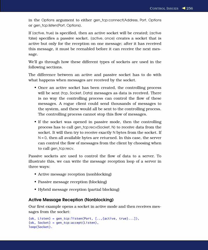
CONTROL ISSUES 256
in the Options argument to either gen_tcp:connect(Address, Port, Options
or gen_tcp:listen(Port, Options).
If {active, true} is specified, then an active socket will be created; {active
false} specifies a passive socket. {active, once} creates a socket that is
active but only for the reception on one message; after it has received
this message, it must be reenabled before it can receive the next mes-
sage.
We’ll go through how these different types of sockets are used in the
following sections.
The difference between an active and passive socket has to do with
what happens when messages are received by the socket.
• Once an active socket has been created, the controlling process
will be sent {tcp, Socket, Data} messages as data is received. There
is no way the controlling process can control the flow of these
messages. A rogue client could send thousands of messages to
the system, and these would all be sent to the controlling process.
The controlling process cannot stop this flow of messages.
• If the socket was opened in passive mode, then the controlling
process has to call gen_tcp:recv(Socket, N) to receive data from the
socket. It will then try to receive exactly N bytes from the socket. If
N = 0, then all available bytes are returned. In this case, the server
can control the flow of messages from the client by choosing when
to call gen_tcp:recv.
Passive sockets are used to control the flow of data to a server. To
illustrate this, we can write the message reception loop of a server in
three ways:
• Active message reception (nonblocking)
• Passive message reception (blocking)
• Hybrid message reception (partial blocking)
Active Message Reception (Nonblocking)
Our first example opens a socket in active mode and then receives mes-
sages from the socket:
{ok, Listen} = gen_tcp:listen(Port, [..,{active, true}...]),
{ok, Socket} = gen_tcp:accept(Listen),
loop(Socket).

CONTROL ISSUES 257
loop(Socket) ->
receive
{tcp, Socket, Data} ->
... do something with the data ...
{tcp_closed, Socket} ->
...
end.
This process cannot control the flow of messages to the server loop. If
the client produces data faster than the server can consume this data,
then the system can be flooded with messages—the message buffers
will fill up, and the system might crash or behave strangely.
This type of server is called a nonblocking server because it cannot block
the client. We should write a nonblocking server only if we can convince
ourselves that it can keep up with the demands of the clients.
Passive Message Reception (Blocking)
In this section, we’ll write a blocking server. The server opens the socket
in passive mode by setting the {active, false} option. This server cannot
be crashed by an overactive client that tries to flood it with too much
data.
The code in the server loop calls gen_tcp:recv every time it wants to
receive data. The client will block until the server has called recv. Note
that the OS does some buffering that allows the client to send a small
amount of data before it blocks even if recv has not been called.
{ok, Listen} = gen_tcp:listen(Port, [..,{active, false}...]),
{ok, Socket} = gen_tcp:accept(Listen),
loop(Socket).
loop(Socket) ->
case gen_tcp:recv(Socket, N) of
{ok, B} ->
... do something with the data ...
loop(Socket);
{error, closed}
...
end.
The Hybrid Approach (Partial Blocking)
You might think that using passive mode for all servers is the correct
approach. Unfortunately, when we’re in passive mode, we can wait for
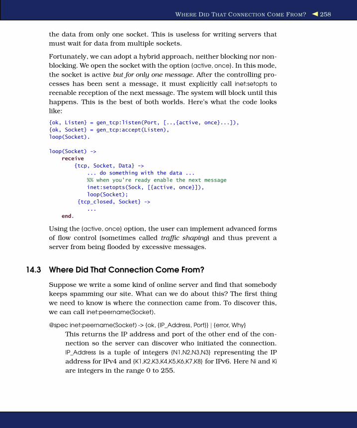
WHERE DID THAT CONNECTION COME FROM? 258
the data from only one socket. This is useless for writing servers that
must wait for data from multiple sockets.
Fortunately, we can adopt a hybrid approach, neither blocking nor non-
blocking. We open the socket with the option {active, once}. In this mode,
the socket is active but for only one message. After the controlling pro-
cesses has been sent a message, it must explicitly call inet:setopts to
reenable reception of the next message. The system will block until this
happens. This is the best of both worlds. Here’s what the code looks
like:
{ok, Listen} = gen_tcp:listen(Port, [..,{active, once}...]),
{ok, Socket} = gen_tcp:accept(Listen),
loop(Socket).
loop(Socket) ->
receive
{tcp, Socket, Data} ->
... do something with the data ...
%% when you're ready enable the next message
inet:setopts(Sock, [{active, once}]),
loop(Socket);
{tcp_closed, Socket} ->
...
end.
Using the {active, once} option, the user can implement advanced forms
of flow control (sometimes called traffic shaping) and thus prevent a
server from being flooded by excessive messages.
14.3 Where Did That Connection Come From?
Suppose we write a some kind of online server and find that somebody
keeps spamming our site. What can we do about this? The first thing
we need to know is where the connection came from. To discover this,
we can call inet:peername(Socket).
@spec inet:peername(Socket) -> {ok, {IP_Address, Port}} | {error, Why}
This returns the IP address and port of the other end of the con-
nection so the server can discover who initiated the connection.
IP_Address is a tuple of integers {N1,N2,N3,N3} representing the IP
address for IPv4 and {K1,K2,K3,K4,K5,K6,K7,K8} for IPv6. Here Ni and Ki
are integers in the range 0 to 255.

ERROR HANDLING WITH SOCKETS 259
14.4 Error Handling with Sockets
Error handling with sockets is extremely easy—basically you don’t have
to do anything. As we said earlier, each socket has a controlling process
(that is, the process that created the socket). If the controlling process
dies, then the socket will be automatically closed.
This means that if we have, for example, a client and a server and
the server dies because of a programming error, the socket owned by
the server will be automatically closed, and the client will be sent a
{tcp_closed, Socket} message.
We can test this mechanism with the following small program:
Download socket_examples.erl
error_test() ->
spawn(fun() -> error_test_server() end),
lib_misc:sleep(2000),
{ok,Socket} = gen_tcp:connect("localhost",4321,[binary, {packet, 2}]),
io:format("connected to:~p~n",[Socket]),
gen_tcp:send(Socket, <<"123">>),
receive
Any ->
io:format("Any=~p~n",[Any])
end.
error_test_server() ->
{ok, Listen} = gen_tcp:listen(4321, [binary,{packet,2}]),
{ok, Socket} = gen_tcp:accept(Listen),
error_test_server_loop(Socket).
error_test_server_loop(Socket) ->
receive
{tcp, Socket, Data} ->
io:format("received:~p~n",[Data]),
atom_to_list(Data),
error_test_server_loop(Socket)
end.
When we run it, we see the following:
1> socket_examples:error_test().
connected to:#Port<0.152>
received:<<"123">>
=ERROR REPORT==== 9-Feb-2007::15:18:15 ===
Error in process <0.77.0> with exit value:
{badarg,[{erlang,atom_to_list,[<<3 bytes>>]},
{socket_examples,error_test_server_loop,1}]}
Any={tcp_closed,#Port<0.152>}
ok

UDP 260
We spawn a server, sleep for two seconds to give it a chance to start, and
then send it a message containing the binary <<"123">>. When this mes-
sage arrives at the server, the server tries to compute atom_to_list(Data)
where Data is a binary and immediately crashes.4 Now that the control-
ling process for the server side of the socket has crashed, the (server-
side) socket is automatically closed. The client is then sent a {tcp_closed,
Socket} message.
14.5 UDP
Now let’s look at the User Datagram Protocol (UDP). Using UDP, ma-
chines on the Internet can send each other short messages called data-
grams. UDP datagrams are unreliable. This means if a client sends
a sequence of UDP datagrams to a server, then the datagrams might
arrive out of order, not at all, or even more than once, but the individ-
ual datagrams, if they arrive, will be undamaged. Large datagrams can
get split into smaller fragments, but the IP protocol will reassemble the
fragments before delivering them to the application.
UDP is a connectionless protocol, which means the client does not have
to establish a connection to the server before sending it a message. This
means that UDP is well suited for applications where large numbers of
clients send small messages to a server.
Writing a UDP client and server in Erlang is much easier than writ-
ing in the TCP case since we don’t have to worry about maintaining
connections to the server.
The Simplest UDP Server and Client
First let’s discuss the server. The general form of a UDP server is as
follows:
server(Port) ->
{ok, Socket} = gen_udp:open(Port, [binary]),
loop(Socket).
loop(Socket) ->
receive
{udp, Socket, Host, Port, Bin} ->
BinReply = ... ,
gen_udp:send(Socket, Host, Port, BinReply),
loop(Socket)
end.
4. The system monitor prints the diagnostic that you can see in the shell.

UDP 261
This is somewhat easier than the TCP case since we don’t need to worry
about our process receiving “socket closed” messages. Note that we
opened the socket in a binary mode, which tells the driver to send all
messages to the controlling process as binary data.
Now the client. Here’s a very simple client. It merely opens a UDP
socket, sends a message to the server, waits for a reply (or timeout), and
then closes the socket and returns the value returned by the server.
client(Request) ->
{ok, Socket} = gen_udp:open(0, [binary]),
ok = gen_udp:send(Socket, "localhost", 4000, Request),
Value = receive
{udp, Socket, _, _, Bin} ->
{ok, Bin}
after 2000 ->
error
end,
gen_udp:close(Socket),
Value
We must have a timeout since UDP is unreliable and we might not
actually get a reply.
A UDP Factorial Server
We can easily build a UDP server that computes the good ol’ factorial
of any number that is sent to it. The code is modeled on that in the
previous section.
Download udp_test.erl
-module(udp_test).
-export([start_server/0, client/1]).
start_server() ->
spawn(fun() -> server(4000) end).
%% The server
server(Port) ->
{ok, Socket} = gen_udp:open(Port, [binary]),
io:format("server opened socket:~p~n",[Socket]),
loop(Socket).
loop(Socket) ->
receive
{udp, Socket, Host, Port, Bin} = Msg ->
io:format("server received:~p~n",[Msg]),
N = binary_to_term(Bin),
Fac = fac(N),
gen_udp:send(Socket, Host, Port, term_to_binary(Fac)),
loop(Socket)
end.

UDP 262
fac(0) -> 1;
fac(N) -> N * fac(N-1).
%% The client
client(N) ->
{ok, Socket} = gen_udp:open(0, [binary]),
io:format("client opened socket=~p~n",[Socket]),
ok = gen_udp:send(Socket, "localhost", 4000,
term_to_binary(N)),
Value = receive
{udp, Socket, _, _, Bin} = Msg ->
io:format("client received:~p~n",[Msg]),
binary_to_term(Bin)
after 2000 ->
0
end,
gen_udp:close(Socket),
Value.
Note that I have added a few print statements so we can see what’s
happening when we run the program. I always add a few print state-
ments when I develop a program and then edit or comment them out
when the program works.
Now let’s run this example. First we start the server:
1> udp_test:start_server().
server opened socket:#Port<0.106>
<0.34.0>
This runs in the background, so we can make a client request:
2> udp_test:client(40).
client opened socket=#Port<0.105>
server received:{udp,#Port<0.106>,{127,0,0,1},32785,<<131,97,40>>}
client received:{udp,#Port<0.105>,
{127,0,0,1}, 4000,
<<131,110,20,0,0,0,0,0,64,37,5,255,
100,222,15,8,126,242,199,132,27,
232,234,142>>}
815915283247897734345611269596115894272000000000
Additional Notes on UDP
We should note that because UDP is a connectionless protocol, the
server has no way to block the client by refusing to read data from
it—the server has no idea who the clients are.
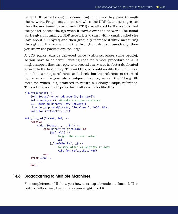
BROADCASTING TO MULTIPLE MACHINES 263
Large UDP packets might become fragmented as they pass through
the network. Fragmentation occurs when the UDP data size is greater
than the maximum transfer unit (MTU) size allowed by the routers that
the packet passes though when it travels over the network. The usual
advice given in tuning a UDP network is to start with a small packet size
(say, about 500 bytes) and then gradually increase it while measuring
throughput. If at some point the throughput drops dramatically, then
you know the packets are too large.
A UDP packet can be delivered twice (which surprises some people),
so you have to be careful writing code for remote procedure calls. It
might happen that the reply to a second query was in fact a duplicated
answer to the first query. To avoid this, we could modify the client code
to include a unique reference and check that this reference is returned
by the server. To generate a unique reference, we call the Erlang BIF
make_ref, which is guaranteed to return a globally unique reference.
The code for a remote procedure call now looks like this:
client(Request) ->
{ok, Socket} = gen_udp:open(0, [binary]),
Ref = make_ref(), %% make a unique reference
B1 = term_to_binary({Ref, Request}),
ok = gen_udp:send(Socket, "localhost", 4000, B1),
wait_for_ref(Socket, Ref).
wait_for_ref(Socket, Ref) ->
receive
{udp, Socket, _, _, Bin} ->
case binary_to_term(Bin) of
{Ref, Val} ->
%% got the correct value
Val;
{_SomeOtherRef, _} ->
%% some other value throw it away
wait_for_ref(Socket, Ref)
end;
after 1000 ->
...
end.
14.6 Broadcasting to Multiple Machines
For completeness, I’ll show you how to set up a broadcast channel. This
code is rather rare, but one day you might need it.

BROADCASTING TO MULTIPLE MACHINES 264
Download broadcast.erl
-module(broadcast).
-compile(export_all).
send(IoList) ->
case inet:ifget("eth0", [broadaddr]) of
{ok, [{broadaddr, Ip}]} ->
{ok, S} = gen_udp:open(5010, [{broadcast, true}]),
gen_udp:send(S, Ip, 6000, IoList),
gen_udp:close(S);
_ ->
io:format("Bad interface name, or\n"
"broadcasting not supported\n")
end.
listen() ->
{ok, S} = gen_udp:open(6000),
loop(S).
loop(S) ->
receive
Any ->
io:format("received:~p~n", [Any]),
loop(S)
end.
Here we need two ports, one to send the broadcast and the other to lis-
ten for answers. We’ve chosen port 5010 to send the broadcast request
and 6000 to listen for broadcasts (these two numbers have no signifi-
cance; I just choose two free ports on my system).
Only the process performing a broadcast opens port 5010, but all
machines in the network call broadcast:listen(), which opens port 6000
and listens for broadcast messages.
broadcast:send(IoList) broadcasts IoList to all machines on the local area
network.
Note: For this to work, the name of the interface must be correct, and
broadcasting must be supported. On my iMac, for example, I use the
name “en0” instead of “eth0.” Note also that if hosts running UDP
listeners are on different network subnets, the UDP broadcasts are
unlikely to reach them, because by default routers drop such UDP
broadcasts.

A SHOUTCAST SERVER 265
14.7 A SHOUTcast Server
To finish off this chapter, we’ll use our newly acquired skills in socket
programming to write a SHOUTcast server. SHOUTcast is a protocol
developed by the folks at Nullsoft for streaming audio data.5 SHOUT-
cast sends MP3- or AAC-encoded audio data using HTTP as the trans-
port protocol.
To see how things work, we’ll first look at the SHOUTcast protocol.
Then we’ll look at the overall structure of the server. We’ll finish with
the code.
The SHOUTcast Protocol
The SHOUTcast protocol is simple:
1. First the client (which can be something like XMMS, Winamp, or
iTunes) sends an HTTP request to the SHOUTcast server. Here’s
the request that XMMS generates when I run my SHOUTcast
server at home:
GET / HTTP/1.1
Host: localhost
User-Agent: xmms/1.2.10
Icy-MetaData:1
2. My SHOUTcast server replies with this:
ICY 200 OK
icy-notice1: <BR>This stream requires
<a href=http://www.winamp.com/>;Winamp</a><BR>
icy-notice2: Erlang Shoutcast server<BR>
icy-name: Erlang mix
icy-genre: Pop Top 40 Dance Rock
icy-url: http://localhost:3000
content-type: audio/mpeg
icy-pub: 1
icy-metaint: 24576
icy-br: 96
... data ...
3. Now the SHOUTcast servers sends a continuous stream of data.
The data has the following structure:
F H F H F H F ...
5. http://www.shoutcast.com/
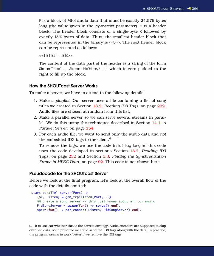
A SHOUTCAST SERVER 266
F is a block of MP3 audio data that must be exactly 24,576 bytes
long (the value given in the icy-metaint parameter). H is a header
block. The header block consists of a single-byte K followed by
exactly 16*K bytes of data. Thus, the smallest header block that
can be represented in the binary is <<0>>. The next header block
can be represented as follows:
<<1,B1,B2, ..., B16>>
The content of the data part of the header is a string of the form
StreamTitle=’ ... ’;StreamUrl=’http:// ...’;, which is zero padded to the
right to fill up the block.
How the SHOUTcast Server Works
To make a server, we have to attend to the following details:
1. Make a playlist. Our server uses a file containing a list of song
titles we created in Section 13.2, Reading ID3 Tags, on page 232.
Audio files are chosen at random from this list.
2. Make a parallel server so we can serve several streams in paral-
lel. We do this using the techniques described in Section 14.1, A
Parallel Server, on page 254.
3. For each audio file, we want to send only the audio data and not
the embedded ID3 tags to the client.6
To remove the tags, we use the code in id3_tag_lengths; this code
uses the code developed in sections Section 13.2, Reading ID3
Tags, on page 232 and Section 5.3, Finding the Synchronization
Frame in MPEG Data, on page 92. This code is not shown here.
Pseudocode for the SHOUTcast Server
Before we look at the final program, let’s look at the overall flow of the
code with the details omitted:
start_parallel_server(Port) ->
{ok, Listen} = gen_tcp:listen(Port, ..),
%% create a song server -- this just knows about all our music
PidSongServer = spawn(fun() -> songs() end),
spawn(fun() -> par_connect(Listen, PidSongServer) end).
6. It is unclear whether this is the correct strategy. Audio encoders are supposed to skip
over bad data, so in principle we could send the ID3 tags along with the data. In practice,
the program seems to work better if we remove the ID3 tags.
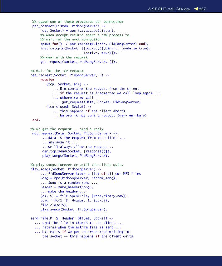
A SHOUTCAST SERVER 267
%% spawn one of these processes per connection
par_connect(Listen, PidSongServer) ->
{ok, Socket} = gen_tcp:accept(Listen),
%% when accept returns spawn a new process to
%% wait for the next connection
spawn(fun() -> par_connect(Listen, PidSongServer) end),
inet:setopts(Socket, [{packet,0},binary, {nodelay,true},
{active, true}]),
%% deal with the request
get_request(Socket, PidSongServer, []).
%% wait for the TCP request
get_request(Socket, PidSongServer, L) ->
receive
{tcp, Socket, Bin} ->
... Bin contains the request from the client
... if the request is fragmented we call loop again ...
... otherwise we call
.... got_request(Data, Socket, PidSongServer)
{tcp_closed, Socket} ->
... this happens if the client aborts
... before it has sent a request (very unlikely)
end.
%% we got the request -- send a reply
got_request(Data, Socket, PidSongServer) ->
.. data is the request from the client ...
.. analayse it ...
.. we'll always allow the request ..
gen_tcp:send(Socket, [response()]),
play_songs(Socket, PidSongServer).
%% play songs forever or until the client quits
play_songs(Socket, PidSongServer) ->
... PidSongServer keeps a list of all our MP3 files
Song = rpc(PidSongServer, random_song),
... Song is a random song ...
Header = make_header(Song),
... make the header ...
{ok, S} = file:open(File, [read,binary,raw]),
send_file(1, S, Header, 1, Socket),
file:close(S),
play_songs(Socket, PidSongServer).
send_file(K, S, Header, OffSet, Socket) ->
... send the file in chunks to the client ...
... returns when the entire file is sent ...
... but exits if we get an error when writing to
the socket -- this happens if the client quits

A SHOUTCAST SERVER 268
If you look at the real code, you’ll see the details differ slightly, but the
principles are the same. Here’s the full listing:
Download shout.erl
-module(shout).
%% In one window > shout:start()
%% in another window xmms http://localhost:3000/stream
-export([start/0]).
-import(lists, [map/2, reverse/1]).
-define(CHUNKSIZE, 24576).
start() ->
spawn(fun() ->
start_parallel_server(3000),
%% now go to sleep - otherwise the
%% listening socket will be closed
lib_misc:sleep(infinity)
end).
start_parallel_server(Port) ->
{ok, Listen} = gen_tcp:listen(Port, [binary, {packet, 0},
{reuseaddr, true},
{active, true}]),
PidSongServer = spawn(fun() -> songs() end),
spawn(fun() -> par_connect(Listen, PidSongServer) end).
par_connect(Listen, PidSongServer) ->
{ok, Socket} = gen_tcp:accept(Listen),
spawn(fun() -> par_connect(Listen, PidSongServer) end),
inet:setopts(Socket, [{packet,0},binary, {nodelay,true},{active, true}]),
get_request(Socket, PidSongServer, []).
get_request(Socket, PidSongServer, L) ->
receive
{tcp, Socket, Bin} ->
L1 = L ++ binary_to_list(Bin),
%% split checks if the header is complete
case split(L1, []) of
more ->
%% the header is incomplete we need more data
get_request(Socket, PidSongServer, L1);
{Request, _Rest} ->
%% header is complete
got_request_from_client(Request, Socket, PidSongServer)
end;
{tcp_closed, Socket} ->
void;
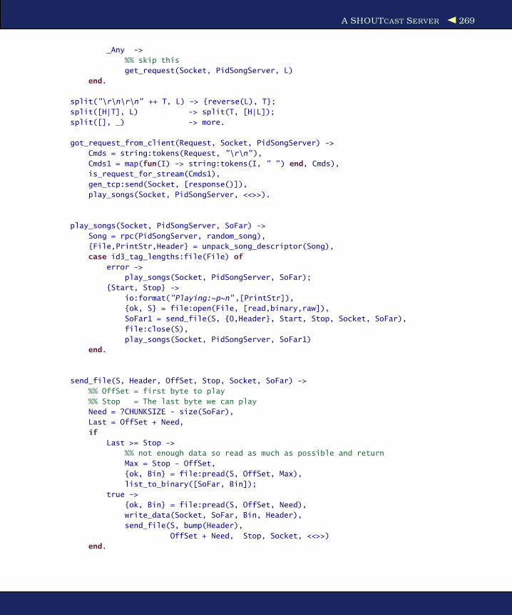
A SHOUTCAST SERVER 269
_Any ->
%% skip this
get_request(Socket, PidSongServer, L)
end.
split("\r\n\r\n" ++ T, L) -> {reverse(L), T};
split([H|T], L) -> split(T, [H|L]);
split([], _) -> more.
got_request_from_client(Request, Socket, PidSongServer) ->
Cmds = string:tokens(Request, "\r\n"),
Cmds1 = map(fun(I) -> string:tokens(I, " ") end, Cmds),
is_request_for_stream(Cmds1),
gen_tcp:send(Socket, [response()]),
play_songs(Socket, PidSongServer, <<>>).
play_songs(Socket, PidSongServer, SoFar) ->
Song = rpc(PidSongServer, random_song),
{File,PrintStr,Header} = unpack_song_descriptor(Song),
case id3_tag_lengths:file(File) of
error ->
play_songs(Socket, PidSongServer, SoFar);
{Start, Stop} ->
io:format("Playing:~p~n",[PrintStr]),
{ok, S} = file:open(File, [read,binary,raw]),
SoFar1 = send_file(S, {0,Header}, Start, Stop, Socket, SoFar),
file:close(S),
play_songs(Socket, PidSongServer, SoFar1)
end.
send_file(S, Header, OffSet, Stop, Socket, SoFar) ->
%% OffSet = first byte to play
%% Stop = The last byte we can play
Need = ?CHUNKSIZE - size(SoFar),
Last = OffSet + Need,
if
Last >= Stop ->
%% not enough data so read as much as possible and return
Max = Stop - OffSet,
{ok, Bin} = file:pread(S, OffSet, Max),
list_to_binary([SoFar, Bin]);
true ->
{ok, Bin} = file:pread(S, OffSet, Need),
write_data(Socket, SoFar, Bin, Header),
send_file(S, bump(Header),
OffSet + Need, Stop, Socket, <<>>)
end.

A SHOUTCAST SERVER 270
write_data(Socket, B0, B1, Header) ->
%% Check that we really have got a block of the right size
%% this is a very useful check that our program logic is
%% correct
case size(B0) + size(B1) of
?CHUNKSIZE ->
case gen_tcp:send(Socket, [B0, B1, the_header(Header)]) of
ok -> true;
{error, closed} ->
%% this happens if the player
%% terminates the connection
exit(playerClosed)
end;
_Other ->
%% don't send the block - report an error
io:format("Block length Error: B0 = ~p b1=~p~n",
[size(B0), size(B1)])
end.
bump({K, H}) -> {K+1, H}.
the_header({K, H}) ->
case K rem 5 of
0 -> H;
_ -> <<0>>
end.
is_request_for_stream(_) -> true.
response() ->
["ICY 200 OK\r\n",
"icy-notice1: <BR>This stream requires",
"<a href=\"http://www.winamp.com/\">Winamp</a><BR>\r\n",
"icy-notice2: Erlang Shoutcast server<BR>\r\n",
"icy-name: Erlang mix\r\n",
"icy-genre: Pop Top 40 Dance Rock\r\n",
"icy-url: http://localhost:3000\r\n",
"content-type: audio/mpeg\r\n",
"icy-pub: 1\r\n",
"icy-metaint: ",integer_to_list(?CHUNKSIZE),"\r\n",
"icy-br: 96\r\n\r\n"].
songs() ->
{ok,[SongList]} = file:consult("mp3data"),
lib_misc:random_seed(),
songs_loop(SongList).
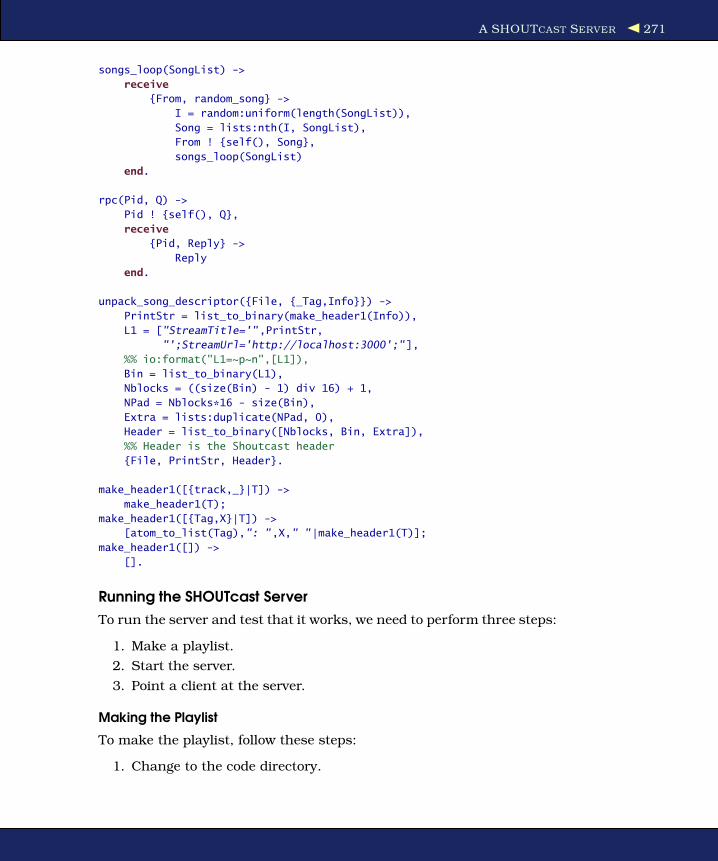
A SHOUTCAST SERVER 271
songs_loop(SongList) ->
receive
{From, random_song} ->
I = random:uniform(length(SongList)),
Song = lists:nth(I, SongList),
From ! {self(), Song},
songs_loop(SongList)
end.
rpc(Pid, Q) ->
Pid ! {self(), Q},
receive
{Pid, Reply} ->
Reply
end.
unpack_song_descriptor({File, {_Tag,Info}}) ->
PrintStr = list_to_binary(make_header1(Info)),
L1 = ["StreamTitle='",PrintStr,
"';StreamUrl='http://localhost:3000';"],
%% io:format("L1=~p~n",[L1]),
Bin = list_to_binary(L1),
Nblocks = ((size(Bin) - 1) div 16) + 1,
NPad = Nblocks*16 - size(Bin),
Extra = lists:duplicate(NPad, 0),
Header = list_to_binary([Nblocks, Bin, Extra]),
%% Header is the Shoutcast header
{File, PrintStr, Header}.
make_header1([{track,_}|T]) ->
make_header1(T);
make_header1([{Tag,X}|T]) ->
[atom_to_list(Tag),": ",X," "|make_header1(T)];
make_header1([]) ->
[].
Running the SHOUTcast Server
To run the server and test that it works, we need to perform three steps:
1. Make a playlist.
2. Start the server.
3. Point a client at the server.
Making the Playlist
To make the playlist, follow these steps:
1. Change to the code directory.

DIGGING DEEPER 272
2. Edit the path in the function start1 in the file mp3_manager.erl to
point to the root of the directories that contain the audio files you
want to serve.
3. Compile mp3_manager, and give the commandmp3_manager:start1().
You should see something like the following:
1> c(mp3_manager).
{ok,mp3_manager}
2> mp3_manager:start1().
Dumping term to mp3data
ok
If you’re interested, you can now look in the file mp3data to see
the results of the analysis.
Starting the SHOUTcast Server
Start the SHOUTcast server with a shell command as follows:
1> shout:start().
...
Testing the Server
1. Go to another window to start an audio player, and point it to the
stream called http://localhost:3000.
On my system I use XMMS and give the following command:
xmms http://localhost:3000
Note: If you want to access the server from another computer,
you’ll have to give the IP address of the machine where the server
is running. So, for example, to access the server from my Windows
machine using Winamp, I use the Play > URL menu in Winamp
and enter the address http://192.168.1.168:3000 in the Open URL dia-
log box.
On my iMac using iTunes I use the Advanced > Open Stream menu
and give the previous URL to access the server.
2. You’ll see some diagnostic output in the window where you started
the server.
3. Enjoy!
14.8 Digging Deeper
In this chapter, we have looked at only the most commonly used func-
tions for manipulating sockets. You can find more information about
the socket APIs in the manual pages for gen_tcp, gen_udp, and inet.

Chapter 15
ETS and DETS: Large DataStorage Mechanisms
ets and dets are two system modules that are used for efficient storage
of large numbers of Erlang terms. ETS is short for Erlang term storage,
and DETS is short for disk ets.
ETS and DETS perform basically the same task: they provide large
key-value lookup tables. ETS is memory resident, while DETS is disk
resident. ETS is highly efficient—using ETS, you can store colossal
amounts of data (if you have enough memory) and perform lookups
in constant (or in some cases logarithmic) time. DETS provides almost
the same interface as ETS but stores the tables on disk. Because DETS
uses disk storage, it is far slower than ETS but will have a much smaller
memory footprint when running. In addition, ETS and DETS tables can
be shared by several processes, making interprocess access to common
data highly efficient.
ETS and DETS tables are data structures for associating keys with
values. The most common operations we will perform on tables are
insertions and lookups. An ETS or DETS table is just a collection of
Erlang tuples.
Data stored in an ETS table is transient and will be deleted when the
ETS table concerned is disposed of. Data stored in DETS tables is per-
sistent and should survive an entire system crash. When a DETS table
is opened, it is checked for consistency. If it is found to be corrupt, then
an attempt is made to repair the table (which can take a long time since
all the data in the table is checked).

BASIC OPERATIONS ON TABLES 274
This should recover all data in the table, though the last entry in the
table might be lost if it was being made at the time of the system crash.
ETS tables are widely used in applications that have to manipulate
large amounts of data in an efficient manner and where it is too costly to
program with nondestructive assignment and “pure” Erlang data struc-
tures.
ETS tables look as if they were implemented in Erlang, but in fact they
are implemented in the underlying runtime system and have differ-
ent performance characteristics than ordinary Erlang objects. In par-
ticular, ETS tables are not garbage collected; this means there are
no garbage collection penalties involved in using extremely large ETS
tables, though slight penalties are incurred when we create or access
ETS objects.
15.1 Basic Operations on Tables
There are four basic operations on ETS and DETS tables:
Create a new table or open an existing table.
This we do with ets:new or dets:open_file.
Insert a tuple or several tuples into a table.
Here we call insert(Tablename, X), where X is a tuple or a list of
tuples. insert has the same arguments and works the same way in
ETS and DETS.
Look up a tuple in a table.
Here we call lookup(TableName, Key). The result is a list of tuples
that match Key. lookup is defined for both ETS and DETS.
(Why is the return value a list of tuples? If the table type is a “bag,”
then several tuples can have the same key. We’ll look at the table
types in the next section.)
If no tuples in the table have the required key, then an empty list
is returned.
Dispose of a table.
When we’ve finished with a table, we can tell the system by calling
dets:close(TableId) or ets:delete(TableId).

TYPES OF TABLE 275
15.2 Types of Table
ETS and DETS tables store tuples. One of the elements in the tuple (by
default, the first) is called the key of the table. We insert tuples into the
table and extract tuples from the table based on the key. What happens
when we insert a tuple into a table depends upon the type of the table
and the value of the key. Some tables, called sets, require that all the
keys in the table are unique. Others, called bags, allow several tuples
to have the same key.
Choosing the correct type of table has important consequences for the
performance of your applications.
Each of the basic set and bag table types has two variants, making for a
total of four types of table: sets, ordered sets, bags, and duplicate bags.
In a set, all the keys in the different tuples in the table must be unique.
In an ordered set, the tuples are sorted. In a bag there can be more
than one tuple with the same key, but no two tuples in the bag can be
identical. In a duplicate bag several tuples can have the same key, and
the same tuple can occur many times in the same table.
We can illustrate how these work with the following little test program:
Download ets_test.erl
-module(ets_test).
-export([start/0]).
start() ->
lists:foreach(fun test_ets/1,
[set, ordered_set, bag, duplicate_bag]).
test_ets(Mode) ->
TableId = ets:new(test, [Mode]),
ets:insert(TableId, {a,1}),
ets:insert(TableId, {b,2}),
ets:insert(TableId, {a,1}),
ets:insert(TableId, {a,3}),
List = ets:tab2list(TableId),
io:format("~-13w => ~p~n", [Mode, List]),
ets:delete(TableId).
This program opens an ETS table in one of four modes and inserts
the tuples {a,1}, {b,2}, {a,1}, and finally {a,3} into the table. Then we call
tab2list, which converts the entire table into a list, and print it.
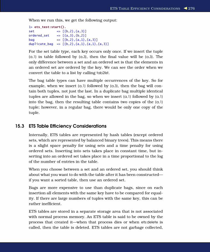
ETS TABLE EFFICIENCY CONSIDERATIONS 276
When we run this, we get the following output:
1> ets_test:start().
set => [{b,2},{a,3}]
ordered_set => [{a,3},{b,2}]
bag => [{b,2},{a,1},{a,3}]
duplicate_bag => [{b,2},{a,1},{a,1},{a,3}]
For the set table type, each key occurs only once. If we insert the tuple
{a,1} in table followed by {a,3}, then the final value will be {a,3}. The
only difference between a set and an ordered set is that the elements in
an ordered set are ordered by the key. We can see the order when we
convert the table to a list by calling tab2list.
The bag table types can have multiple occurrences of the key. So for
example, when we insert {a,1} followed by {a,3}, then the bag will con-
tain both tuples, not just the last. In a duplicate bag multiple identical
tuples are allowed in the bag, so when we insert {a,1} followed by {a,1}
into the bag, then the resulting table contains two copies of the {a,1}
tuple; however, in a regular bag, there would be only one copy of the
tuple.
15.3 ETS Table Efficiency Considerations
Internally, ETS tables are represented by hash tables (except ordered
sets, which are represented by balanced binary trees). This means there
is a slight space penalty for using sets and a time penalty for using
ordered sets. Inserting into sets takes place in constant time, but in-
serting into an ordered set takes place in a time proportional to the log
of the number of entries in the table.
When you choose between a set and an ordered set, you should think
about what you want to do with the table after it has been constructed—
if you want a sorted table, then use an ordered set.
Bags are more expensive to use than duplicate bags, since on each
insertion all elements with the same key have to be compared for equal-
ity. If there are large numbers of tuples with the same key, this can be
rather inefficient.
ETS tables are stored in a separate storage area that is not associated
with normal process memory. An ETS table is said to be owned by the
process that created it—when that process dies or when ets:delete is
called, then the table is deleted. ETS tables are not garbage collected,

CREATING AN ETS TABLE 277
which means that large amounts of data can be stored in the table
without incurring garbage collection penalties.
When a tuple is inserted into an ETS table, all the data structures
representing the tuple are copied from the process stack and heap into
the ETS table. When a lookup operation is performed on a table, the
resultant tuples are copied from the ETS table to the stack and heap of
the process.
This is true for all data structures except large binaries. Large binaries
are stored in their own off-heap storage area. This area can be shared
by several processes and ETS tables, and the individual binaries are
managed with a reference-counting garbage collector that keeps track
of how many different processes and ETS tables use the binary. When
the use count for the number of processes and tables that use a partic-
ular binary goes down to zero, then the storage area for the binary can
be reclaimed.
All of this might sound rather complicated, but the upshot is that send-
ing messages between processes that contain large binaries is very
cheap, and inserting tuples into ETS tables that contain binaries is
also very cheap. A good rule is to use binaries as much as possible for
representing strings and large blocks of untyped memory.
15.4 Creating an ETS Table
ETS tables are created by calling ets:new. The process that creates the
table is called the “owner” of the table. When the table is created, it
has a set of options that cannot be changed. If the owner process dies,
space for the table is automatically deallocated; otherwise, the table
can be deleted by calling ets:delete.
The arguments to ets:new are as follows:
@spec ets:new(Name, [Opt]) -> TableId
Name is an atom. [Opt] is a list of options, taken from the following:
set | ordered_set | bag | duplicate_bag
Create an ETS table of the given type (we talked about these
earlier).
private
Create a private table. Only the owner process can read and
write this table.

CREATING AN ETS TABLE 278
ETS Tables As Blackboards
Protected tables provide a type of “blackboard system.” Youcan think of an protected ETS table as a kind of named black-board. Anybody who knows the name of the blackboard canread the blackboard, but only the owner can write on theblackboard.
Note: An ETS table that has been opened in public mode canbe written and read by any process that knows the table name.In this case, the user must ensure that reads and writes to thetable are performed in a consistent manner.
public
Create a public table. Any process that knows the table iden-
tifier can read and write this table.
protected
Create a protected table. Any process that knows the table
identifier can read this table, but only the owner process can
write to the table.
named_table
If this is present, then Name can be used for subsequent table
operations.
{keypos, K}
Use K as the key position. Normally position 1 is used for the
key. Probably the only time when we would use this option
is if we store an Erlang record (which is actually a disguised
tuple), where the first element of the record contains the
record name.
Note: Opening an ETS table with zero options is the same as opening it
with the options [set,protected,{keypos,1}].
All the code in this chapter uses protected ETS tables. Protected tables
are particularly useful since they allow data sharing at virtually zero
cost. All local processes that know the table identifier can read the
data, but only one process can change the data in the table.
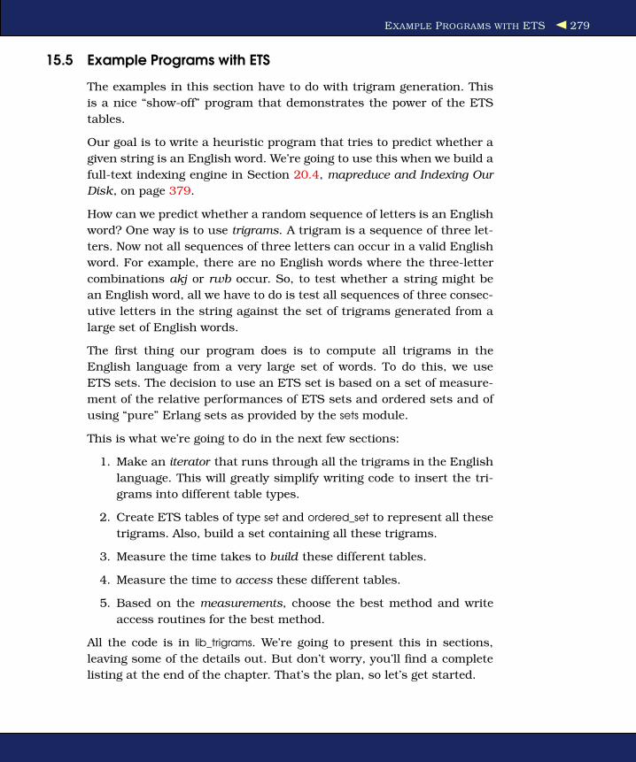
EXAMPLE PROGRAMS WITH ETS 279
15.5 Example Programs with ETS
The examples in this section have to do with trigram generation. This
is a nice “show-off” program that demonstrates the power of the ETS
tables.
Our goal is to write a heuristic program that tries to predict whether a
given string is an English word. We’re going to use this when we build a
full-text indexing engine in Section 20.4, mapreduce and Indexing Our
Disk, on page 379.
How can we predict whether a random sequence of letters is an English
word? One way is to use trigrams. A trigram is a sequence of three let-
ters. Now not all sequences of three letters can occur in a valid English
word. For example, there are no English words where the three-letter
combinations akj or rwb occur. So, to test whether a string might be
an English word, all we have to do is test all sequences of three consec-
utive letters in the string against the set of trigrams generated from a
large set of English words.
The first thing our program does is to compute all trigrams in the
English language from a very large set of words. To do this, we use
ETS sets. The decision to use an ETS set is based on a set of measure-
ment of the relative performances of ETS sets and ordered sets and of
using “pure” Erlang sets as provided by the sets module.
This is what we’re going to do in the next few sections:
1. Make an iterator that runs through all the trigrams in the English
language. This will greatly simplify writing code to insert the tri-
grams into different table types.
2. Create ETS tables of type set and ordered_set to represent all these
trigrams. Also, build a set containing all these trigrams.
3. Measure the time takes to build these different tables.
4. Measure the time to access these different tables.
5. Based on the measurements, choose the best method and write
access routines for the best method.
All the code is in lib_trigrams. We’re going to present this in sections,
leaving some of the details out. But don’t worry, you’ll find a complete
listing at the end of the chapter. That’s the plan, so let’s get started.
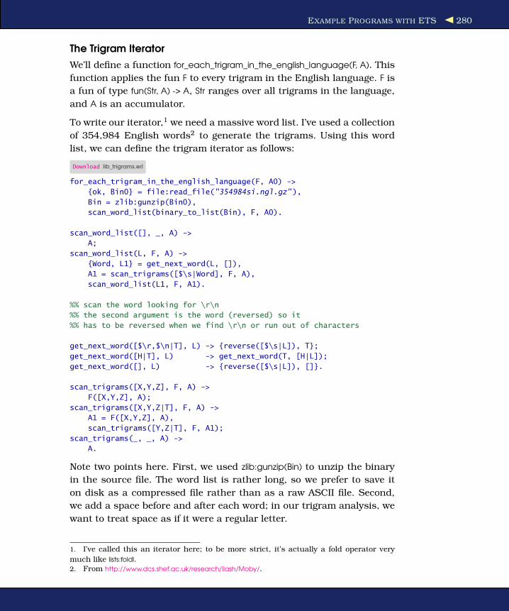
EXAMPLE PROGRAMS WITH ETS 280
The Trigram Iterator
We’ll define a function for_each_trigram_in_the_english_language(F, A). This
function applies the fun F to every trigram in the English language. F is
a fun of type fun(Str, A) -> A, Str ranges over all trigrams in the language,
and A is an accumulator.
To write our iterator,1 we need a massive word list. I’ve used a collection
of 354,984 English words2 to generate the trigrams. Using this word
list, we can define the trigram iterator as follows:
Download lib_trigrams.erl
for_each_trigram_in_the_english_language(F, A0) ->
{ok, Bin0} = file:read_file("354984si.ngl.gz"),
Bin = zlib:gunzip(Bin0),
scan_word_list(binary_to_list(Bin), F, A0).
scan_word_list([], _, A) ->
A;
scan_word_list(L, F, A) ->
{Word, L1} = get_next_word(L, []),
A1 = scan_trigrams([$\s|Word], F, A),
scan_word_list(L1, F, A1).
%% scan the word looking for \r\n
%% the second argument is the word (reversed) so it
%% has to be reversed when we find \r\n or run out of characters
get_next_word([$\r,$\n|T], L) -> {reverse([$\s|L]), T};
get_next_word([H|T], L) -> get_next_word(T, [H|L]);
get_next_word([], L) -> {reverse([$\s|L]), []}.
scan_trigrams([X,Y,Z], F, A) ->
F([X,Y,Z], A);
scan_trigrams([X,Y,Z|T], F, A) ->
A1 = F([X,Y,Z], A),
scan_trigrams([Y,Z|T], F, A1);
scan_trigrams(_, _, A) ->
A.
Note two points here. First, we used zlib:gunzip(Bin) to unzip the binary
in the source file. The word list is rather long, so we prefer to save it
on disk as a compressed file rather than as a raw ASCII file. Second,
we add a space before and after each word; in our trigram analysis, we
want to treat space as if it were a regular letter.
1. I’ve called this an iterator here; to be more strict, it’s actually a fold operator very
much like lists:foldl.2. From http://www.dcs.shef.ac.uk/research/ilash/Moby/.
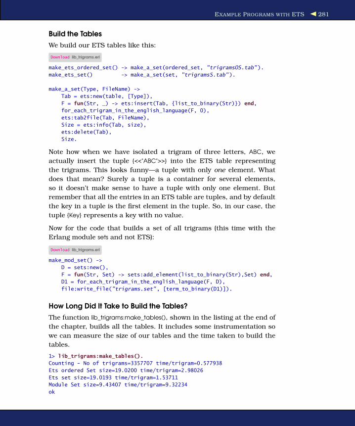
EXAMPLE PROGRAMS WITH ETS 281
Build the Tables
We build our ETS tables like this:
Download lib_trigrams.erl
make_ets_ordered_set() -> make_a_set(ordered_set, "trigramsOS.tab").
make_ets_set() -> make_a_set(set, "trigramsS.tab").
make_a_set(Type, FileName) ->
Tab = ets:new(table, [Type]),
F = fun(Str, _) -> ets:insert(Tab, {list_to_binary(Str)}) end,
for_each_trigram_in_the_english_language(F, 0),
ets:tab2file(Tab, FileName),
Size = ets:info(Tab, size),
ets:delete(Tab),
Size.
Note how when we have isolated a trigram of three letters, ABC, we
actually insert the tuple {<<"ABC">>} into the ETS table representing
the trigrams. This looks funny—a tuple with only one element. What
does that mean? Surely a tuple is a container for several elements,
so it doesn’t make sense to have a tuple with only one element. But
remember that all the entries in an ETS table are tuples, and by default
the key in a tuple is the first element in the tuple. So, in our case, the
tuple {Key} represents a key with no value.
Now for the code that builds a set of all trigrams (this time with the
Erlang module sets and not ETS):
Download lib_trigrams.erl
make_mod_set() ->
D = sets:new(),
F = fun(Str, Set) -> sets:add_element(list_to_binary(Str),Set) end,
D1 = for_each_trigram_in_the_english_language(F, D),
file:write_file("trigrams.set", [term_to_binary(D1)]).
How Long Did It Take to Build the Tables?
The function lib_trigrams:make_tables(), shown in the listing at the end of
the chapter, builds all the tables. It includes some instrumentation so
we can measure the size of our tables and the time taken to build the
tables.
1> lib_trigrams:make_tables().
Counting - No of trigrams=3357707 time/trigram=0.577938
Ets ordered Set size=19.0200 time/trigram=2.98026
Ets set size=19.0193 time/trigram=1.53711
Module Set size=9.43407 time/trigram=9.32234
ok

EXAMPLE PROGRAMS WITH ETS 282
What do these figures tell us? First there are 3.3 million trigrams, and
it took half a microsecond to process each trigram in the word list.
The insertion time per trigram was 2.9 microseconds in an ETS ordered
set, 1.5 microseconds in an ETS set, and 9.3 microseconds in an Erlang
set. As for storage, ETS sets and ordered sets took 19 bytes per trigram,
while the module sets took 9 bytes per trigram.
How Long Does It Take to Access the Tables?
OK, so the tables took some time to build, but in this case it doesn’t
matter. The important question to ask is, How long does it take to access
the tables? To answer this, we have to write some code to measure the
access times. We’ll look up every trigram in our table exactly once and
then take the average time per lookup. Here’s the code that performs
the timings:
Download lib_trigrams.erl
timer_tests() ->
time_lookup_ets_set("Ets ordered Set", "trigramsOS.tab"),
time_lookup_ets_set("Ets set", "trigramsS.tab"),
time_lookup_module_sets().
time_lookup_ets_set(Type, File) ->
{ok, Tab} = ets:file2tab(File),
L = ets:tab2list(Tab),
Size = length(L),
{M, _} = timer:tc(?MODULE, lookup_all_ets, [Tab, L]),
io:format("~s lookup=~p micro seconds~n",[Type, M/Size]),
ets:delete(Tab).
lookup_all_ets(Tab, L) ->
lists:foreach(fun({K}) -> ets:lookup(Tab, K) end, L).
time_lookup_module_sets() ->
{ok, Bin} = file:read_file("trigrams.set"),
Set = binary_to_term(Bin),
Keys = sets:to_list(Set),
Size = length(Keys),
{M, _} = timer:tc(?MODULE, lookup_all_set, [Set, Keys]),
io:format("Module set lookup=~p micro seconds~n",[M/Size]).
lookup_all_set(Set, L) ->
lists:foreach(fun(Key) -> sets:is_element(Key, Set) end, L).
Here we go:
1> lib_trigrams:timer_tests().
Ets ordered Set lookup=1.79964 micro seconds
Ets set lookup=0.719279 micro seconds
Module sets lookup=1.35268 micro seconds
ok

EXAMPLE PROGRAMS WITH ETS 283
These timings are in average microseconds per lookup.
And the Winner Is...
Well, it was a walkover. The ETS set won by a large margin. On my
machine, sets took about half a microsecond per lookup—that’s pretty
good!
Note: Performing tests like the previous one and actually measuring
how long a particular operation takes is considered good programming
practice. We don’t need to take this to extremes and time everything,
only the most time-consuming operations in our program. The non-
time-consuming operations should be programmed in the most beau-
tiful way possible. If we are forced to write nonobvious ugly code for
efficiency reasons, then it should be well documented.
Now we can write the routines that try to predict whether a string is a
proper English word.
To test whether a string might be an English language word, we scan
through all the trigrams in the string and check that each trigram
occurs in the trigram table that we computed earlier. The function
is_word does this.
Download lib_trigrams.erl
is_word(Tab, Str) -> is_word1(Tab, "\s" ++ Str ++ "\s").
is_word1(Tab, [_,_,_]=X) -> is_this_a_trigram(Tab, X);
is_word1(Tab, [A,B,C|D]) ->
case is_this_a_trigram(Tab, [A,B,C]) of
true -> is_word1(Tab, [B,C|D]);
false -> false
end;
is_word1(_, _) ->
false.
is_this_a_trigram(Tab, X) ->
case ets:lookup(Tab, list_to_binary(X)) of
[] -> false;
_ -> true
end.
open() ->
{ok, I} = ets:file2tab(filename:dirname(code:which(?MODULE))
++ "/trigramsS.tab"),
I.
close(Tab) -> ets:delete(Tab).
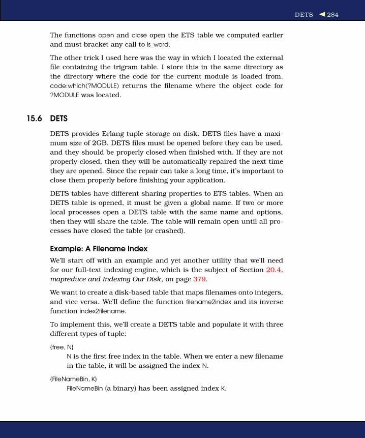
DETS 284
The functions open and close open the ETS table we computed earlier
and must bracket any call to is_word.
The other trick I used here was the way in which I located the external
file containing the trigram table. I store this in the same directory as
the directory where the code for the current module is loaded from.
code:which(?MODULE) returns the filename where the object code for
?MODULE was located.
15.6 DETS
DETS provides Erlang tuple storage on disk. DETS files have a maxi-
mum size of 2GB. DETS files must be opened before they can be used,
and they should be properly closed when finished with. If they are not
properly closed, then they will be automatically repaired the next time
they are opened. Since the repair can take a long time, it’s important to
close them properly before finishing your application.
DETS tables have different sharing properties to ETS tables. When an
DETS table is opened, it must be given a global name. If two or more
local processes open a DETS table with the same name and options,
then they will share the table. The table will remain open until all pro-
cesses have closed the table (or crashed).
Example: A Filename Index
We’ll start off with an example and yet another utility that we’ll need
for our full-text indexing engine, which is the subject of Section 20.4,
mapreduce and Indexing Our Disk, on page 379.
We want to create a disk-based table that maps filenames onto integers,
and vice versa. We’ll define the function filename2index and its inverse
function index2filename.
To implement this, we’ll create a DETS table and populate it with three
different types of tuple:
{free, N}
N is the first free index in the table. When we enter a new filename
in the table, it will be assigned the index N.
{FileNameBin, K}
FileNameBin (a binary) has been assigned index K.

DETS 285
{K, FileNameBin}
K (an integer) represents the file FilenameBin.
Note how the addition of every new file adds two entries to the table: a
File 7→ Index entry and an inverse Index 7→ Filename. This is for efficiency
reasons. When ETS or DETS tables are built, only one item in the tuple
acts as a key. Matching on a tuple element that is not the key can be
done, but it is very inefficient because it involves searching through the
entire table. This is a particularly expensive operation when the entire
table resides on disk.
Now let’s write the program. We’ll start with routines to open and close
the DETS table that will store all our filenames.
Download lib_filenames_dets.erl
-module(lib_filenames_dets).
-export([open/1, close/0, test/0, filename2index/1, index2filename/1]).
open(File) ->
io:format("dets opened:~p~n", [File]),
Bool = filelib:is_file(File),
case dets:open_file(?MODULE, [{file, File}]) of
{ok, ?MODULE} ->
case Bool of
true -> void;
false -> ok = dets:insert(?MODULE, {free,1})
end,
true;
{error,_Reason} ->
io:format("cannot open dets table~n"),
exit(eDetsOpen)
end.
close() -> dets:close(?MODULE).
The code for open automatically initializes the DETS table by inserting
the tuple {free, 1} if a new table is created. filelib:is_file(File) returns true
if File exists; otherwise, it returns false. Note that dets:open_file either
creates a new file or opens an exiting file, which is why we have to
check whether the file exists before calling dets:open_file.
In this code I’ve used the macro ?MODULE a lot of times; ?MODULE
expands to the current module name (which is lib_filenames_dets). Many
of the calls to DETS need a unique atom argument for the table name.
To generate a unique table name, we just use the module name. Since
there can’t be two Erlang modules in the system with the same name,

DETS 286
then if we follow this convention everywhere, we’ll be reasonably sure
that we have a unique name to use for the table name.
I used the macro ?MODULE instead of explicitly writing the module name
every time because I have a habit of changing modules names as I write
my code. Using macros, if I change the module name, the code will still
be correct.
Once we’ve opened the file, injecting a new filename into the table is
easy. This is done as a side effect of calling filename2index. If the filename
is in the table, then its index is returned; otherwise, a new index is
generated, and the table is updated, this time with three tuples:
Download lib_filenames_dets.erl
filename2index(FileName) when is_binary(FileName) ->
case dets:lookup(?MODULE, FileName) of
[] ->
[{_,Free}] = dets:lookup(?MODULE, free),
ok = dets:insert(?MODULE,
[{Free,FileName},{FileName,Free},{free,Free+1}]),
Free;
[{_,N}] ->
N
end.
Note how we store three tuples in the table. The second argument to
dets:insert is either a tuple or a list of tuples. Note also that the filename
is represented by a binary. This is for efficiency reasons. It’s a good idea
to get into the habit of using binaries to represent strings in ETS and
DETS tables.
The observant reader might have noticed that there is a potential race
condition in filename2index. If two parallel processes call
dets:lookup before dets:insert gets called, then filename2index will return
an incorrect value. For this routine to work, we must ensure that it is
only ever called by one process at a time.
Converting an index to a filename is easy:
Download lib_filenames_dets.erl
index2filename(Index) when is_integer(Index) ->
case dets:lookup(?MODULE, Index) of
[] -> error;
[{_,Bin}] -> Bin
end.
There’s a small design decision here. What do we want to happen if
we call index2filename(Index) and there is no filename associated with
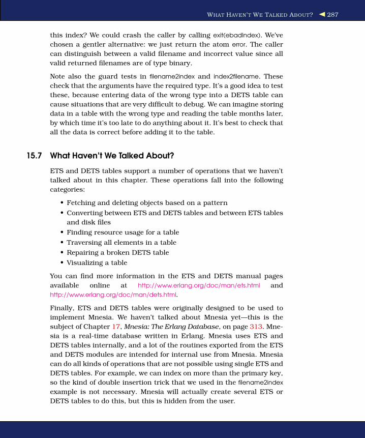
WHAT HAVEN’T WE TALKED ABOUT? 287
this index? We could crash the caller by calling exit(ebadIndex). We’ve
chosen a gentler alternative: we just return the atom error. The caller
can distinguish between a valid filename and incorrect value since all
valid returned filenames are of type binary.
Note also the guard tests in filename2index and index2filename. These
check that the arguments have the required type. It’s a good idea to test
these, because entering data of the wrong type into a DETS table can
cause situations that are very difficult to debug. We can imagine storing
data in a table with the wrong type and reading the table months later,
by which time it’s too late to do anything about it. It’s best to check that
all the data is correct before adding it to the table.
15.7 What Haven’t We Talked About?
ETS and DETS tables support a number of operations that we haven’t
talked about in this chapter. These operations fall into the following
categories:
• Fetching and deleting objects based on a pattern
• Converting between ETS and DETS tables and between ETS tables
and disk files
• Finding resource usage for a table
• Traversing all elements in a table
• Repairing a broken DETS table
• Visualizing a table
You can find more information in the ETS and DETS manual pages
available online at http://www.erlang.org/doc/man/ets.html and
http://www.erlang.org/doc/man/dets.html.
Finally, ETS and DETS tables were originally designed to be used to
implement Mnesia. We haven’t talked about Mnesia yet—this is the
subject of Chapter 17, Mnesia: The Erlang Database, on page 313. Mne-
sia is a real-time database written in Erlang. Mnesia uses ETS and
DETS tables internally, and a lot of the routines exported from the ETS
and DETS modules are intended for internal use from Mnesia. Mnesia
can do all kinds of operations that are not possible using single ETS and
DETS tables. For example, we can index on more than the primary key,
so the kind of double insertion trick that we used in the filename2index
example is not necessary. Mnesia will actually create several ETS or
DETS tables to do this, but this is hidden from the user.

CODE LISTINGS 288
15.8 Code Listings
Download lib_trigrams_complete.erl
-module(lib_trigrams).
-export([for_each_trigram_in_the_english_language/2,
make_tables/0, timer_tests/0,
open/0, close/1, is_word/2,
how_many_trigrams/0,
make_ets_set/0, make_ets_ordered_set/0, make_mod_set/0,
lookup_all_ets/2, lookup_all_set/2
]).
-import(lists, [reverse/1]).
make_tables() ->
{Micro1, N} = timer:tc(?MODULE, how_many_trigrams, []),
io:format("Counting - No of trigrams=~p time/trigram=~p~n",[N,Micro1/N]),
{Micro2, Ntri} = timer:tc(?MODULE, make_ets_ordered_set, []),
FileSize1 = filelib:file_size("trigramsOS.tab"),
io:format("Ets ordered Set size=~p time/trigram=~p~n",[FileSize1/Ntri,
Micro2/N]),
{Micro3, _} = timer:tc(?MODULE, make_ets_set, []),
FileSize2 = filelib:file_size("trigramsS.tab"),
io:format("Ets set size=~p time/trigram=~p~n",[FileSize2/Ntri, Micro3/N]),
{Micro4, _} = timer:tc(?MODULE, make_mod_set, []),
FileSize3 = filelib:file_size("trigrams.set"),
io:format("Module sets size=~p time/trigram=~p~n",[FileSize3/Ntri, Micro4/N]).
make_ets_ordered_set() -> make_a_set(ordered_set, "trigramsOS.tab").
make_ets_set() -> make_a_set(set, "trigramsS.tab").
make_a_set(Type, FileName) ->
Tab = ets:new(table, [Type]),
F = fun(Str, _) -> ets:insert(Tab, {list_to_binary(Str)}) end,
for_each_trigram_in_the_english_language(F, 0),
ets:tab2file(Tab, FileName),
Size = ets:info(Tab, size),
ets:delete(Tab),
Size.
make_mod_set() ->
D = sets:new(),
F = fun(Str, Set) -> sets:add_element(list_to_binary(Str),Set) end,
D1 = for_each_trigram_in_the_english_language(F, D),
file:write_file("trigrams.set", [term_to_binary(D1)]).
timer_tests() ->
time_lookup_ets_set("Ets ordered Set", "trigramsOS.tab"),
time_lookup_ets_set("Ets set", "trigramsS.tab"),
time_lookup_module_sets().
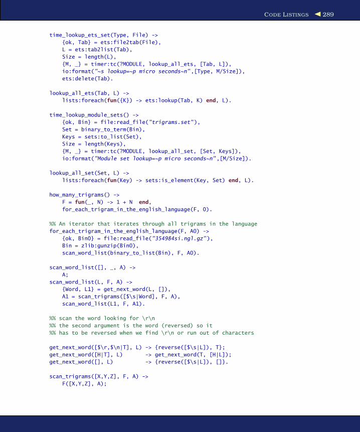
CODE LISTINGS 289
time_lookup_ets_set(Type, File) ->
{ok, Tab} = ets:file2tab(File),
L = ets:tab2list(Tab),
Size = length(L),
{M, _} = timer:tc(?MODULE, lookup_all_ets, [Tab, L]),
io:format("~s lookup=~p micro seconds~n",[Type, M/Size]),
ets:delete(Tab).
lookup_all_ets(Tab, L) ->
lists:foreach(fun({K}) -> ets:lookup(Tab, K) end, L).
time_lookup_module_sets() ->
{ok, Bin} = file:read_file("trigrams.set"),
Set = binary_to_term(Bin),
Keys = sets:to_list(Set),
Size = length(Keys),
{M, _} = timer:tc(?MODULE, lookup_all_set, [Set, Keys]),
io:format("Module set lookup=~p micro seconds~n",[M/Size]).
lookup_all_set(Set, L) ->
lists:foreach(fun(Key) -> sets:is_element(Key, Set) end, L).
how_many_trigrams() ->
F = fun(_, N) -> 1 + N end,
for_each_trigram_in_the_english_language(F, 0).
%% An iterator that iterates through all trigrams in the language
for_each_trigram_in_the_english_language(F, A0) ->
{ok, Bin0} = file:read_file("354984si.ngl.gz"),
Bin = zlib:gunzip(Bin0),
scan_word_list(binary_to_list(Bin), F, A0).
scan_word_list([], _, A) ->
A;
scan_word_list(L, F, A) ->
{Word, L1} = get_next_word(L, []),
A1 = scan_trigrams([$\s|Word], F, A),
scan_word_list(L1, F, A1).
%% scan the word looking for \r\n
%% the second argument is the word (reversed) so it
%% has to be reversed when we find \r\n or run out of characters
get_next_word([$\r,$\n|T], L) -> {reverse([$\s|L]), T};
get_next_word([H|T], L) -> get_next_word(T, [H|L]);
get_next_word([], L) -> {reverse([$\s|L]), []}.
scan_trigrams([X,Y,Z], F, A) ->
F([X,Y,Z], A);

CODE LISTINGS 290
scan_trigrams([X,Y,Z|T], F, A) ->
A1 = F([X,Y,Z], A),
scan_trigrams([Y,Z|T], F, A1);
scan_trigrams(_, _, A) ->
A.
%% access routines
%% open() -> Table
%% close(Table)
%% is_word(Table, String) -> Bool
is_word(Tab, Str) -> is_word1(Tab, "\s" ++ Str ++ "\s").
is_word1(Tab, [_,_,_]=X) -> is_this_a_trigram(Tab, X);
is_word1(Tab, [A,B,C|D]) ->
case is_this_a_trigram(Tab, [A,B,C]) of
true -> is_word1(Tab, [B,C|D]);
false -> false
end;
is_word1(_, _) ->
false.
is_this_a_trigram(Tab, X) ->
case ets:lookup(Tab, list_to_binary(X)) of
[] -> false;
_ -> true
end.
open() ->
{ok, I} = ets:file2tab(filename:dirname(code:which(?MODULE))
++ "/trigramsS.tab"),
I.
close(Tab) -> ets:delete(Tab).

Chapter 16
OTP IntroductionOTP stands for the Open Telecom Platform. The name is actually mis-
leading, because OTP is far more general than you might think. It’s an
application operating system and a set of libraries and procedures used
for building large-scale, fault-tolerant, distributed applications. It was
developed at the Swedish telecom company Ericsson and is used within
Ericsson for building fault-tolerant systems.1
OTP contains a number of powerful tools—such as a complete web
server, an FTP server, a CORBA ORB, and so on—all written in Erlang.
OTP also contains state-of-the-art tools for building telecom applica-
tions with implementations of H248, SNMP, and an ASN.1-to-Erlang
cross-compiler. I’m not going to talk about these here; you can find a
lot more about these subjects by following the links referred to in Sec-
tion C.1, Online Documentation, on page 399.
If you want to program your own applications using OTP, then the
central concept that you will find very useful is the OTP behavior. A
behavior encapsulates common behavioral patterns—think of it as an
application framework that is parameterized by a callback module.
The power of OTP comes from that properties such as fault tolerance,
scalability, dynamic-code upgrade, and so on, can be provided by the
behavior itself. In other words, the writer of the callback does not have
to worry about things such as fault tolerance because this is provided
by the behavior. For the Java-minded, you can think of a behavior as a
J2EE container.
1. Ericsson has released OTP subject to the Erlang Public License (EPL). EPL is a deriva-
tive of the Mozilla Public License (MPL).

THE ROAD TO THE GENERIC SERVER 292
Put simply, the behavior solves the nonfunctional parts of the problem,
while the callback solves the functional parts. The nice part about this
is that the nonfunctional parts of the problem (for example, how to
do live code upgrades) are the same for all applications, whereas the
functional parts (as supplied by the callback) are different for every
problem.
In this chapter, we’ll look at one of these behaviors, the gen_server mod-
ule, in greater detail. But, before we get down to the nitty-gritty details
of how the gen_server works, we’ll first start with a simple server (the
simplest server we can possibly imagine) and then change it in a num-
ber of small steps until we get to the full gen_server module. That way,
you should be in a position to really understand how gen_server works
and be ready to poke around in the gory details.
Here is the plan of this chapter:
1. Write a small client-server program in Erlang.
2. Slowly generalize this program and add a number of features.
3. Move to the real code.
16.1 The Road to the Generic Server
This is the most important section in the entire book, so read it once, read
it twice, read it 100 times—just make sure the message sinks in.
We’re going to write four little servers called server1, server2..., each
slightly different from the last. The goal is to totally separate the non-
functional parts of the problem from the functional parts of the prob-
lem. That last sentence probably didn’t mean much to you now, but
don’t worry—it soon will. Take a deep breath....
Server 1: The Basic Server
Here’s our first attempt. It’s a little server that we can parameterize with
a callback module:
Download server1.erl
-module(server1).
-export([start/2, rpc/2]).
start(Name, Mod) ->
register(Name, spawn(fun() -> loop(Name, Mod, Mod:init()) end)).
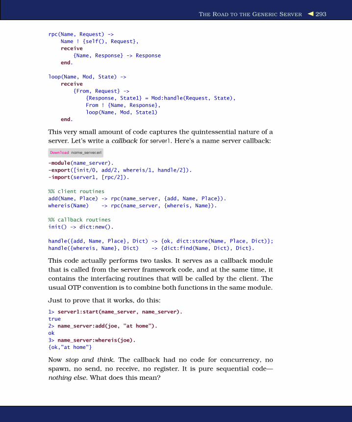
THE ROAD TO THE GENERIC SERVER 293
rpc(Name, Request) ->
Name ! {self(), Request},
receive
{Name, Response} -> Response
end.
loop(Name, Mod, State) ->
receive
{From, Request} ->
{Response, State1} = Mod:handle(Request, State),
From ! {Name, Response},
loop(Name, Mod, State1)
end.
This very small amount of code captures the quintessential nature of a
server. Let’s write a callback for server1. Here’s a name server callback:
Download name_server.erl
-module(name_server).
-export([init/0, add/2, whereis/1, handle/2]).
-import(server1, [rpc/2]).
%% client routines
add(Name, Place) -> rpc(name_server, {add, Name, Place}).
whereis(Name) -> rpc(name_server, {whereis, Name}).
%% callback routines
init() -> dict:new().
handle({add, Name, Place}, Dict) -> {ok, dict:store(Name, Place, Dict)};
handle({whereis, Name}, Dict) -> {dict:find(Name, Dict), Dict}.
This code actually performs two tasks. It serves as a callback module
that is called from the server framework code, and at the same time, it
contains the interfacing routines that will be called by the client. The
usual OTP convention is to combine both functions in the same module.
Just to prove that it works, do this:
1> server1:start(name_server, name_server).
true
2> name_server:add(joe, "at home").
ok
3> name_server:whereis(joe).
{ok,"at home"}
Now stop and think. The callback had no code for concurrency, no
spawn, no send, no receive, no register. It is pure sequential code—
nothing else. What does this mean?

THE ROAD TO THE GENERIC SERVER 294
This means we can write client-server models without understanding
anything about the underlying concurrency models.
This is the basic pattern for all servers. Once you understand the basic
structure, it’s easy to “roll your own.”
Server 2: A Server with Transactions
Here’s a server that crashes the client if the query in the server results
in an exception:
Download server2.erl
-module(server2).
-export([start/2, rpc/2]).
start(Name, Mod) ->
register(Name, spawn(fun() -> loop(Name,Mod,Mod:init()) end)).
rpc(Name, Request) ->
Name ! {self(), Request},
receive
{Name, crash} -> exit(rpc);
{Name, ok, Response} -> Response
end.
loop(Name, Mod, OldState) ->
receive
{From, Request} ->
try Mod:handle(Request, OldState) of
{Response, NewState} ->
From ! {Name, ok, Response},
loop(Name, Mod, NewState)
catch
_:Why ->
log_the_error(Name, Request, Why),
%% send a message to cause the client to crash
From ! {Name, crash},
%% loop with the *original* state
loop(Name, Mod, OldState)
end
end.
log_the_error(Name, Request, Why) ->
io:format("Server ~p request ~p ~n"
"caused exception ~p~n",
[Name, Request, Why]).
This one gives you “transaction semantics” in the server—it loops with
the original value of State if an exception was raised in the handler
function. But if the handler function succeeded, then it loops with the
value of NewState provided by the handler function.

THE ROAD TO THE GENERIC SERVER 295
Why does it retain the original state? When the handler function fails,
the client that sent the message that caused the failure is sent a mes-
sage that causes it to crash. The client cannot proceed, because the
request it sent to the server caused the handler function to crash. But
any other client that wants to use the server will not be affected. More-
over, the state of the server is not changed when an error occurs in the
handler.
Note that the callback module for this server is exactly the same as the
callback module we used for server1. By changing the server and keeping
the callback module constant, we can change the nonfunctional behavior
of the callback module.
Note: The last statement wasn’t strictly true. We have to make a very
small change to the callback module when we go from server1 to server2,
and that is to change the name in the -import declaration from server1
to server2. Otherwise, there are no changes.
Server 3: A Server with Hot Code Swapping
Now we’ll add hot code swapping:
Download server3.erl
-module(server3).
-export([start/2, rpc/2, swap_code/2]).
start(Name, Mod) ->
register(Name,
spawn(fun() -> loop(Name,Mod,Mod:init()) end)).
swap_code(Name, Mod) -> rpc(Name, {swap_code, Mod}).
rpc(Name, Request) ->
Name ! {self(), Request},
receive
{Name, Response} -> Response
end.
loop(Name, Mod, OldState) ->
receive
{From, {swap_code, NewCallBackMod}} ->
From ! {Name, ack},
loop(Name, NewCallBackMod, OldState);
{From, Request} ->
{Response, NewState} = Mod:handle(Request, OldState),
From ! {Name, Response},
loop(Name, Mod, NewState)
end.

THE ROAD TO THE GENERIC SERVER 296
How does this work?
If we send the server a swap code message, then it will change the
callback module to the new module contained in the message.
We can demonstrate this by starting server3 with a callback module
and then dynamically swapping the callback module. We can’t use
name_server as the callback module because we hard-compiled the
name of the server into the module. So, we make a copy of this, calling
it name_server1 where we change the name of the server:
Download name_server1.erl
-module(name_server1).
-export([init/0, add/2, whereis/1, handle/2]).
-import(server3, [rpc/2]).
%% client routines
add(Name, Place) -> rpc(name_server, {add, Name, Place}).
whereis(Name) -> rpc(name_server, {whereis, Name}).
%% callback routines
init() -> dict:new().
handle({add, Name, Place}, Dict) -> {ok, dict:store(Name, Place, Dict)};
handle({whereis, Name}, Dict) -> {dict:find(Name, Dict), Dict}.
First we’ll start server3 with the name_server1 callback module:
1> server3:start(name_server, name_server1).
true
2> name_server:add(joe, "at home").
ok
3> name_server:add(helen, "at work").
ok
Now suppose we want to find all the names that are served by the name
server. There is no function in the API that can do this—the module
name_server has only add and lookup access routines.
With lightning speed, we fire up our text editor and write a new callback
module:
Download new_name_server.erl
-module(new_name_server).
-export([init/0, add/2, all_names/0, delete/1, whereis/1, handle/2]).
-import(server3, [rpc/2]).

THE ROAD TO THE GENERIC SERVER 297
%% interface
all_names() -> rpc(name_server, allNames).
add(Name, Place) -> rpc(name_server, {add, Name, Place}).
delete(Name) -> rpc(name_server, {delete, Name}).
whereis(Name) -> rpc(name_server, {whereis, Name}).
%% callback routines
init() -> dict:new().
handle({add, Name, Place}, Dict) -> {ok, dict:store(Name, Place, Dict)};
handle(allNames, Dict) -> {dict:fetch_keys(Dict), Dict};
handle({delete, Name}, Dict) -> {ok, dict:erase(Name, Dict)};
handle({whereis, Name}, Dict) -> {dict:find(Name, Dict), Dict}.
We compile this and tell the server to swap its callback module:
4> c(new_name_server).
{ok,new_name_server}
5> server3:swap_code(name_server, new_name_server).
ack
Now we can run the new functions in the server:
6> new_name_server:all_names().
[joe,helen]
Here we changed the callback module on the fly—this is dynamic code
upgrade, in action before your eyes, with no black magic.
Now stop and think again. The last two tasks we have done are gener-
ally considered to be pretty difficult, in fact, very difficult. Servers with
“transaction semantics” are difficult to write; servers with dynamic code
upgrade are very difficult to write.
This technique is extremely powerful. Traditionally we think of servers
as programs with state that change state when we send them messages.
The code in the servers is fixed the first time it is called, and if we want
to change the code in the server, we have to stop the server and change
the code, and then we can restart the server. In the examples we have
given, the code in the server can be changed just as easily as we can
change the state of the server.2
2. I use this technique a lot in products that are never taken out of service for software
maintenance upgrades.
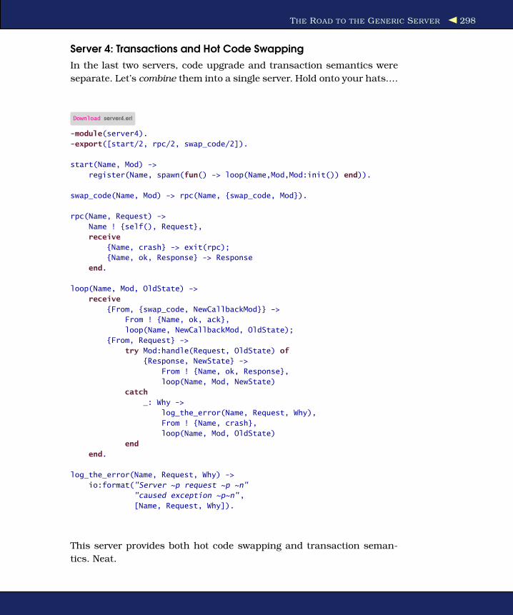
THE ROAD TO THE GENERIC SERVER 298
Server 4: Transactions and Hot Code Swapping
In the last two servers, code upgrade and transaction semantics were
separate. Let’s combine them into a single server. Hold onto your hats....
Download server4.erl
-module(server4).
-export([start/2, rpc/2, swap_code/2]).
start(Name, Mod) ->
register(Name, spawn(fun() -> loop(Name,Mod,Mod:init()) end)).
swap_code(Name, Mod) -> rpc(Name, {swap_code, Mod}).
rpc(Name, Request) ->
Name ! {self(), Request},
receive
{Name, crash} -> exit(rpc);
{Name, ok, Response} -> Response
end.
loop(Name, Mod, OldState) ->
receive
{From, {swap_code, NewCallbackMod}} ->
From ! {Name, ok, ack},
loop(Name, NewCallbackMod, OldState);
{From, Request} ->
try Mod:handle(Request, OldState) of
{Response, NewState} ->
From ! {Name, ok, Response},
loop(Name, Mod, NewState)
catch
_: Why ->
log_the_error(Name, Request, Why),
From ! {Name, crash},
loop(Name, Mod, OldState)
end
end.
log_the_error(Name, Request, Why) ->
io:format("Server ~p request ~p ~n"
"caused exception ~p~n",
[Name, Request, Why]).
This server provides both hot code swapping and transaction seman-
tics. Neat.

THE ROAD TO THE GENERIC SERVER 299
Server 5: Even More Fun
Now that we’ve got the idea of dynamic code change, we can have even
more fun. Here’s a server that does nothing at all until you tell it to
become a particular type of server:
Download server5.erl
-module(server5).
-export([start/0, rpc/2]).
start() -> spawn(fun() -> wait() end).
wait() ->
receive
{become, F} -> F()
end.
rpc(Pid, Q) ->
Pid ! {self(), Q},
receive
{Pid, Reply} -> Reply
end.
If we start this and then send it a {become, F} message, it will become
an F server by evaluating F(). We’ll start it:
1> Pid = server5:start().
<0.57.0>
Our server does nothing and just waits for a become message.
Let’s now define a server function. It’s nothing complicated, just some-
thing to compute factorial:
Download my_fac_server.erl
-module(my_fac_server).
-export([loop/0]).
loop() ->
receive
{From, {fac, N}} ->
From ! {self(), fac(N)},
loop();
{become, Something} ->
Something()
end.
fac(0) -> 1;
fac(N) -> N * fac(N-1).

THE ROAD TO THE GENERIC SERVER 300
Erlang on PlanetLab
A few years ago, when I had my research hat on, I was work-ing with PlanetLab. I had access to the PlanetLab∗ network, so Iinstalled “empty” Erlang servers on all the PlanetLab machines(about 450 of them). I didn’t really know what I would do withthe machines, so I just set up the server infrastructure to dosomething later.
Once I had gotten this layer running, it was an easy job to sendmessages to the empty servers telling them to become realservers.
The usual approach is to start (for example) a web server andthen install web server plug-ins. My approach was to back offone step and install an empty server. Later the plug-in turns theempty server into a web server. When we’re done with the webserver, we might tell it to become something else.
∗. A planet-wide research network (http://www.planet-lab.org)
Just make sure it’s compiled, and then we can tell process <0.57.0> to
become a factorial server:
2> c(my_fac_server).
{ok,my_fac_server}
3> Pid ! {become, fun my_fac_server:loop/0}.
{become,#Fun<my_fac_server.loop.0>}
Now that our process has become a factorial server, we can call it:
4> server5:rpc(Pid, {fac,30}).
265252859812191058636308480000000
Our process will remain a factorial server, until we send it a {become,
Something} message and tell it to do something else.
As you can see from the previous examples, we can make a range of
different types of servers, with different semantics and some quite sur-
prising properties. This technique is almost too powerful. Used to its
full potential, it can yield very small programs of quite surprising power
and beauty. When we make industrial-scale projects with dozens to
hundreds of programmers involved, we might not actually want things
to be too dynamic. We have to try to strike a balance between having
something general and powerful and having something that is useful
for commercial products. Having code that can morph into new ver-

GETTING STARTED WITH GEN_SERVER 301
sions as it runs is beautiful but terrible to debug if something goes
wrong later. If we have made dozens of dynamic changes to our code
and it then crashes, finding out exactly what went wrong is not easy.
The server examples in this section are actually not quite correct. They
are written this way so as to emphasize the ideas involved, but they do
have one or two extremely small and subtle errors. I’m not going to tell
you immediately what they are, but I’ll give you some hints at the end
of the chapter.
The Erlang module gen_server is the kind of logical conclusion of a suc-
cession of successively sophisticated servers (just like the ones we’ve
written so far in this chapter).
It has been in use in industrial products since 1998. Hundreds of
servers can be part of a single product. These servers have been written
by programmers using regular sequential code. All the error handling
and all the nonfunctional behavior is factored out in the generic part of
the server.
So now we’ll take a great leap of imagination and look at the real
gen_server.
16.2 Getting Started with gen_server
I’m going to throw you in at the deep end. Here’s the simple three-point
plan for writing a gen_server callback module:
1. Decide on a callback module name.
2. Write the interface functions.
3. Write the six required callback functions in the callback module.
This is really easy. Don’t think—just follow the plan!
Step 1: Decide on the Callback Module Name
We’re going to make a very simple payment system. We’ll call the mod-
ule my_bank.3
3. In case you’re wondering, there are actually several online financial services written
in Erlang (such as http://kreditor.se/). Now they don’t publish their code, but if they did, it
might look like ours.
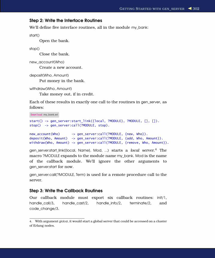
GETTING STARTED WITH GEN_SERVER 302
Step 2: Write the Interface Routines
We’ll define five interface routines, all in the module my_bank:
start()
Open the bank.
stop()
Close the bank.
new_account(Who)
Create a new account.
deposit(Who, Amount)
Put money in the bank.
withdraw(Who, Amount)
Take money out, if in credit.
Each of these results in exactly one call to the routines in gen_server, as
follows:
Download my_bank.erl
start() -> gen_server:start_link({local, ?MODULE}, ?MODULE, [], []).
stop() -> gen_server:call(?MODULE, stop).
new_account(Who) -> gen_server:call(?MODULE, {new, Who}).
deposit(Who, Amount) -> gen_server:call(?MODULE, {add, Who, Amount}).
withdraw(Who, Amount) -> gen_server:call(?MODULE, {remove, Who, Amount}).
gen_server:start_link({local, Name}, Mod, ...) starts a local server.4 The
macro ?MODULE expands to the module name my_bank. Mod is the name
of the callback module. We’ll ignore the other arguments to
gen_server:start for now.
gen_server:call(?MODULE, Term) is used for a remote procedure call to the
server.
Step 3: Write the Callback Routines
Our callback module must export six callback routines: init/1,
handle_call/3, handle_cast/2, handle_info/2, terminate/2, and
code_change/3.
4. With argument global, it would start a global server that could be accessed on a cluster
of Erlang nodes.
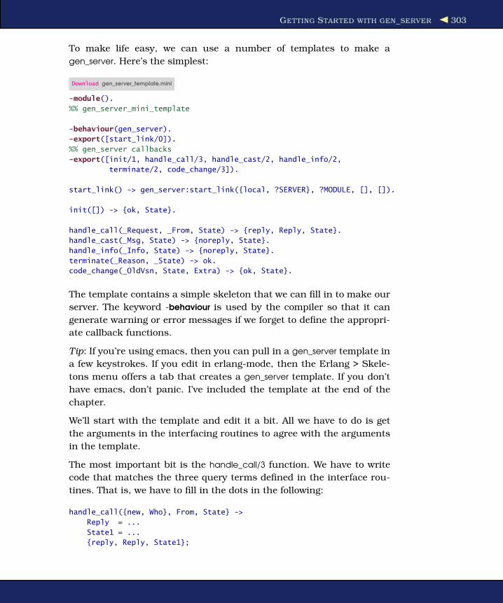
GETTING STARTED WITH GEN_SERVER 303
To make life easy, we can use a number of templates to make a
gen_server. Here’s the simplest:
Download gen_server_template.mini
-module().
%% gen_server_mini_template
-behaviour(gen_server).
-export([start_link/0]).
%% gen_server callbacks
-export([init/1, handle_call/3, handle_cast/2, handle_info/2,
terminate/2, code_change/3]).
start_link() -> gen_server:start_link({local, ?SERVER}, ?MODULE, [], []).
init([]) -> {ok, State}.
handle_call(_Request, _From, State) -> {reply, Reply, State}.
handle_cast(_Msg, State) -> {noreply, State}.
handle_info(_Info, State) -> {noreply, State}.
terminate(_Reason, _State) -> ok.
code_change(_OldVsn, State, Extra) -> {ok, State}.
The template contains a simple skeleton that we can fill in to make our
server. The keyword -behaviour is used by the compiler so that it can
generate warning or error messages if we forget to define the appropri-
ate callback functions.
Tip: If you’re using emacs, then you can pull in a gen_server template in
a few keystrokes. If you edit in erlang-mode, then the Erlang > Skele-
tons menu offers a tab that creates a gen_server template. If you don’t
have emacs, don’t panic. I’ve included the template at the end of the
chapter.
We’ll start with the template and edit it a bit. All we have to do is get
the arguments in the interfacing routines to agree with the arguments
in the template.
The most important bit is the handle_call/3 function. We have to write
code that matches the three query terms defined in the interface rou-
tines. That is, we have to fill in the dots in the following:
handle_call({new, Who}, From, State} ->
Reply = ...
State1 = ...
{reply, Reply, State1};

GETTING STARTED WITH GEN_SERVER 304
handle_call({add, Who, Amount}, From, State} ->
Reply = ...
State1 = ...
{reply, Reply, State1};
handle_call({remove, Who, Amount}, From, State} ->
Reply = ...
State1 = ...
{reply, Reply, State1};
The values of Reply in this code are sent back to the client as the return
values of the remote procedure calls.
State is just a variable representing the global state of the server that
gets passed around in the server. In our bank module, the state never
changes; it’s just an ETS table index that is a constant (although the
content of the table changes).
When we’ve filled in the template and edited it a bit, we end up with the
following code:
Download my_bank.erl
init([]) -> {ok, ets:new(?MODULE,[])}.
handle_call({new,Who}, _From, Tab) ->
Reply = case ets:lookup(Tab, Who) of
[] -> ets:insert(Tab, {Who,0}),
{welcome, Who};
[_] -> {Who, you_already_are_a_customer}
end,
{reply, Reply, Tab};
handle_call({add,Who,X}, _From, Tab) ->
Reply = case ets:lookup(Tab, Who) of
[] -> not_a_customer;
[{Who,Balance}] ->
NewBalance = Balance + X,
ets:insert(Tab, {Who, NewBalance}),
{thanks, Who, your_balance_is, NewBalance}
end,
{reply, Reply, Tab};
handle_call({remove,Who, X}, _From, Tab) ->
Reply = case ets:lookup(Tab, Who) of
[] -> not_a_customer;
[{Who,Balance}] when X =< Balance ->
NewBalance = Balance - X,
ets:insert(Tab, {Who, NewBalance}),
{thanks, Who, your_balance_is, NewBalance};
[{Who,Balance}] ->
{sorry,Who,you_only_have,Balance,in_the_bank}
end,
{reply, Reply, Tab};

THE GEN_SERVER CALLBACK STRUCTURE 305
handle_call(stop, _From, Tab) ->
{stop, normal, stopped, Tab}.
handle_cast(_Msg, State) -> {noreply, State}.
handle_info(_Info, State) -> {noreply, State}.
terminate(_Reason, _State) -> ok.
code_change(_OldVsn, State, Extra) -> {ok, State}.
We start the server by calling gen_server:start_link(Name, CallBackMod, Star-
tArgs, Opts); then the first routine to be called in the callback module is
Mod:init(StartArgs), which must return {ok, State}. The value of State reap-
pears as the third argument in handle_call.
Note how we stop the server. handle_call(Stop, From, Tab) returns {stop, nor-
mal, stopped, Tab} which stops the server. The second argument (normal)
is used as the first argument to my_bank:terminate/2. The third argument
(stopped) becomes the return value of my_bank:stop().
That’s it, we’re done. So let’s go visit the bank:
1> my_bank:start().
{ok,<0.33.0>}
2> my_bank:deposit("joe", 10).
not_a_customer
3> my_bank:new_account("joe").
{welcome,"joe"}
4> my_bank:deposit("joe", 10).
{thanks,"joe",your_balance_is,10}
5> my_bank:deposit("joe", 30).
{thanks,"joe",your_balance_is,40}
6> my_bank:withdraw("joe", 15).
{thanks,"joe",your_balance_is,25}
7> my_bank:withdraw("joe", 45).
{sorry,"joe",you_only_have,25,in_the_bank}
16.3 The gen_server Callback Structure
Now that we’ve got the idea, we’ll take a more detailed look at the
gen_server callback structure.
What Happens When We Start the Server?
The call gen_server:start_link(Name, Mod, InitArgs, Opts) starts everything. It
creates a generic server called Name. The callback module is Mod. Opts
controls the behavior of the generic server. Here we can specify logging
of message, debugging functions, and so on. The generic server starts
by calling Mod:init(InitArgs).

THE GEN_SERVER CALLBACK STRUCTURE 306
The template entry for init is as follows:
%%--------------------------------------------------------------------
%% Function: init(Args) -> {ok, State} |
%% {ok, State, Timeout} |
%% ignore |
%% {stop, Reason}
%% Description: Initiates the server
%%--------------------------------------------------------------------
init([]) ->
{ok, #state{}}.
In normal operation, we just return {ok, State}. For the meaning of the
other arguments, consult the manual page for gen_server.
If {ok, State} is returned, then we have successfully started the server,
and the initial state is State.
What Happens When We Call the Server?
To call the server, the client program calls gen_server:call(Name, Request).
This results in handle_call/3 in the callback module being called.
handle_call/3 has the following template entry:
%%----------------------------------------------------------------------
%% Function:
%% handle_call(Request, From, State) -> {reply, Reply, State} |
%% {reply, Reply, State, Timeout} |
%% {noreply, State} |
%% {noreply, State, Timeout} |
%% {stop, Reason, Reply, State} |
%% {stop, Reason, State}
%% Description: Handling call messages
%%----------------------------------------------------------------------
handle_call(_Request, _From, State) ->
Reply = ok,
{reply, Reply, State}.
Request (the second argument of gen_server:call/2) reappears as the first
argument of handle_call/3. From is the PID of the requesting client pro-
cess, and State is the current state of the client.
Normally we return {reply, Reply, NewState}. When this happens, Reply
goes back to the client, where it becomes the return value of gen_server:
call. NewState is the next state of the server.
The other return values, {noreply, ..} and {stop, ..}, are used relatively
infrequently. no reply causes the server to continue, but the client will
wait for a reply so the server will have to delegate the task of replying

THE GEN_SERVER CALLBACK STRUCTURE 307
to some other process. Calling stop with the appropriate arguments will
stop the server.
Calls and Casts
We’ve seen the interplay between gen_server:call and handle_call. This
is used for implementing remote procedure calls. gen_server:cast(Name,
Name) implements a cast, which is just a call with no return value
(actually just a message, but traditionally it’s called a cast to distin-
guish it from a remote procedure call).
The corresponding callback routine is handle_cast; the template entry is
like this:
%%--------------------------------------------------------------------
%% Function: handle_cast(Msg, State) -> {noreply, NewState} |
%% {noreply, NewState, Timeout} |
%% {stop, Reason, NewState}
%% Description: Handling cast messages
%%--------------------------------------------------------------------
handle_cast(_Msg, State) ->
{noreply, NewState}.
The handler usually just returns {noreply, NewState}, which changes the
state of the server, or {stop, ...}, which stops the server.
Spontaneous Messages to the Server
The callback function handle_info(Info, State) is used for handling spon-
taneous messages to the server. So, what’s a spontaneous message? If
the server is linked to another process and is trapping exits, then it
might suddenly receive a unexpected {’EXIT’, Pid, What} message. Alter-
natively, any process in the system that discovers the PID of the generic
server can just send it a message. Any message like this ends up at the
server as the value of Info.
The template entry for handle_info is as follows:
%%--------------------------------------------------------------------
%% Function: handle_info(Info, State) -> {noreply, State} |
%% {noreply, State, Timeout} |
%% {stop, Reason, State}
%% Description: Handling all non-call/cast messages
%%--------------------------------------------------------------------
handle_info(_Info, State) ->
{noreply, State}.
The return values are the same as for handle_cast.

THE GEN_SERVER CALLBACK STRUCTURE 308
Hasta la Vista, Baby
The server can terminate for many reasons. One of the handle_Something
routines might return a {stop, Reason, NewState}, or the server might
crash with {’EXIT’, reason}. In all of these circumstances, no matter how
they occurred, terminate(Reason, NewState) will be called.
Here’s the template:
%%--------------------------------------------------------------------
%% Function: terminate(Reason, State) -> void()
%% Description: This function is called by a gen_server when it is
%% about to terminate. It should be the opposite of Module:init/1 and
%% do any necessary
%% cleaning up. When it returns, the gen_server terminates with Reason.
%% The return value is ignored.
%%--------------------------------------------------------------------
terminate(_Reason, State) ->
ok.
This code can’t return a new state because we’ve terminated. So, what
can we do with State? Lots of things, it turns out. We could store it on
disk, send it in a message to some other process, or discard it depend-
ing upon the applications. If you want your server to be restarted in the
future, you’ll have to write an “I’ll be back” function that is triggered by
terminate/2.
Code Change
You can dynamically change the state of your server while it is run-
ning. This callback function is called by the release handling subsystem
when the system performs a software upgrade.
This topic is described in detail in the section on release handling in
the OTP design principles documentation.5
%%--------------------------------------------------------------------
%% Func: code_change(OldVsn, State, Extra) -> {ok, NewState} %%
%% Description: Convert process state when code is changed
%%--------------------------------------------------------------------
code_change(_OldVsn, State, _Extra) -> {ok, State}.
5. Availiable from http://www.erlang.org/doc/pdf/design_principles.pdf.

CODE AND TEMPLATES 309
16.4 Code and Templates
This is built into emacs-mode:
gen_server template
Download gen_server_template.full
%%%-------------------------------------------------------------------
%%% File : gen_server_template.full
%%% Author : my name <[email protected]>
%%% Description :
%%%
%%% Created : 2 Mar 2007 by my name <[email protected]>
%%%-------------------------------------------------------------------
-module().
-behaviour(gen_server).
%% API
-export([start_link/0]).
%% gen_server callbacks
-export([init/1, handle_call/3, handle_cast/2, handle_info/2,
terminate/2, code_change/3]).
-record(state, {}).
%%====================================================================
%% API
%%====================================================================
%%--------------------------------------------------------------------
%% Function: start_link() -> {ok,Pid} | ignore | {error,Error}
%% Description: Starts the server
%%--------------------------------------------------------------------
start_link() ->
gen_server:start_link({local, ?SERVER}, ?MODULE, [], []).
%%====================================================================
%% gen_server callbacks
%%====================================================================
%%--------------------------------------------------------------------
%% Function: init(Args) -> {ok, State} |
%% {ok, State, Timeout} |
%% ignore |
%% {stop, Reason}
%% Description: Initiates the server
%%--------------------------------------------------------------------
init([]) ->
{ok, #state{}}.
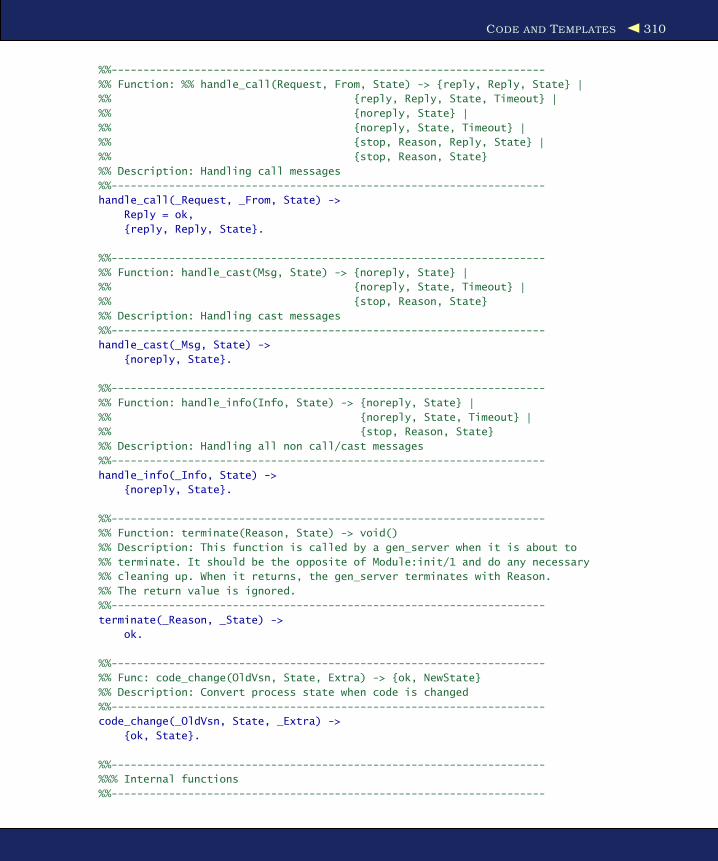
CODE AND TEMPLATES 310
%%--------------------------------------------------------------------
%% Function: %% handle_call(Request, From, State) -> {reply, Reply, State} |
%% {reply, Reply, State, Timeout} |
%% {noreply, State} |
%% {noreply, State, Timeout} |
%% {stop, Reason, Reply, State} |
%% {stop, Reason, State}
%% Description: Handling call messages
%%--------------------------------------------------------------------
handle_call(_Request, _From, State) ->
Reply = ok,
{reply, Reply, State}.
%%--------------------------------------------------------------------
%% Function: handle_cast(Msg, State) -> {noreply, State} |
%% {noreply, State, Timeout} |
%% {stop, Reason, State}
%% Description: Handling cast messages
%%--------------------------------------------------------------------
handle_cast(_Msg, State) ->
{noreply, State}.
%%--------------------------------------------------------------------
%% Function: handle_info(Info, State) -> {noreply, State} |
%% {noreply, State, Timeout} |
%% {stop, Reason, State}
%% Description: Handling all non call/cast messages
%%--------------------------------------------------------------------
handle_info(_Info, State) ->
{noreply, State}.
%%--------------------------------------------------------------------
%% Function: terminate(Reason, State) -> void()
%% Description: This function is called by a gen_server when it is about to
%% terminate. It should be the opposite of Module:init/1 and do any necessary
%% cleaning up. When it returns, the gen_server terminates with Reason.
%% The return value is ignored.
%%--------------------------------------------------------------------
terminate(_Reason, _State) ->
ok.
%%--------------------------------------------------------------------
%% Func: code_change(OldVsn, State, Extra) -> {ok, NewState}
%% Description: Convert process state when code is changed
%%--------------------------------------------------------------------
code_change(_OldVsn, State, _Extra) ->
{ok, State}.
%%--------------------------------------------------------------------
%%% Internal functions
%%--------------------------------------------------------------------
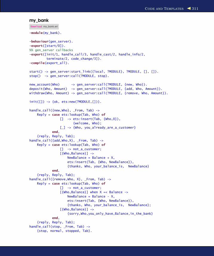
CODE AND TEMPLATES 311
my_bankDownload my_bank.erl
-module(my_bank).
-behaviour(gen_server).
-export([start/0]).
%% gen_server callbacks
-export([init/1, handle_call/3, handle_cast/2, handle_info/2,
terminate/2, code_change/3]).
-compile(export_all).
start() -> gen_server:start_link({local, ?MODULE}, ?MODULE, [], []).
stop() -> gen_server:call(?MODULE, stop).
new_account(Who) -> gen_server:call(?MODULE, {new, Who}).
deposit(Who, Amount) -> gen_server:call(?MODULE, {add, Who, Amount}).
withdraw(Who, Amount) -> gen_server:call(?MODULE, {remove, Who, Amount}).
init([]) -> {ok, ets:new(?MODULE,[])}.
handle_call({new,Who}, _From, Tab) ->
Reply = case ets:lookup(Tab, Who) of
[] -> ets:insert(Tab, {Who,0}),
{welcome, Who};
[_] -> {Who, you_already_are_a_customer}
end,
{reply, Reply, Tab};
handle_call({add,Who,X}, _From, Tab) ->
Reply = case ets:lookup(Tab, Who) of
[] -> not_a_customer;
[{Who,Balance}] ->
NewBalance = Balance + X,
ets:insert(Tab, {Who, NewBalance}),
{thanks, Who, your_balance_is, NewBalance}
end,
{reply, Reply, Tab};
handle_call({remove,Who, X}, _From, Tab) ->
Reply = case ets:lookup(Tab, Who) of
[] -> not_a_customer;
[{Who,Balance}] when X =< Balance ->
NewBalance = Balance - X,
ets:insert(Tab, {Who, NewBalance}),
{thanks, Who, your_balance_is, NewBalance};
[{Who,Balance}] ->
{sorry,Who,you_only_have,Balance,in_the_bank}
end,
{reply, Reply, Tab};
handle_call(stop, _From, Tab) ->
{stop, normal, stopped, Tab}.

DIGGING DEEPER 312
handle_cast(_Msg, State) -> {noreply, State}.
handle_info(_Info, State) -> {noreply, State}.
terminate(_Reason, _State) -> ok.
code_change(_OldVsn, State, Extra) -> {ok, State}.
16.5 Digging Deeper
The gen_server is actually rather simple. We haven’t been through all
the interface functions in gen_server, and we haven’t talked about all
the arguments to all the interface functions. Once you understand
the basic ideas, you can look up the details in the manual page for
gen_server.
In this chapter, we have looked only at the simplest possible way to
use gen_server, but this should be adequate for most purposes. More
complex applications often let gen_server reply with a noreply return
value and delegate the real reply to another process. For information
about this, read the “Design Principles” documentation6 and the man-
ual pages for the modules sys and proc_lib.
6. http://www.erlang.org/doc/pdf/design_principles.pdf

Chapter 17
Mnesia: The Erlang DatabaseSuppose you want to write a multiuser game, make a new website,
or create an online payment system. You’ll probably need a database
management system (DBMS).
Hidden in the thousands of files that appear on our disk when we down-
load Erlang is a complete DBMS called Mnesia. It is extremely fast, and
it can store any type of Erlang data structure.
It’s also highly configurable. Database tables can be stored in RAM (for
speed) or on disk (for persistence), and the tables can be replicated on
different machines to provide fault-tolerant behavior.
Let’s dig deeper.
17.1 Database Queries
Let’s start by looking at Mnesia queries. As we look through this, we
might be surprised to see that Mnesia queries look a lot like both SQL1
and list comprehensions, so there’s actually very little we need to learn
to get started.2
1. A popular language that is used to query relational databases.2. In fact, it really isn’t that surprising that list comprehensions and SQL look a lot alike.
Both are based on mathematical set theory.

DATABASE QUERIES 314
In all our examples, I’ll assume that we have created a database with
two tables called shop and cost. These tables contain the following data.
The shop Table
Item Quantity Cost
apple 20 2.3
orange 100 3.8
pear 200 3.6
banana 420 4.5
potato 2456 1.2
The cost TableName Price
apple 1.5
orange 2.4
pear 2.2
banana 1.5
potato 0.6
To represent these tables in Mnesia, we need record definitions that
define the columns in the tables. These are as follows:
Download test_mnesia.erl
-record(shop, {item, quantity, cost}).
-record(cost, {name, price}).
Now comes a little black magic. I want to show you how queries work,
and I want you to follow along at home. But to do that I have to create
and populate the database for you. So, just for now, trust me. I’ve writ-
ten the initialization code in the file test_mnesia.erl. You can just run it
from within erl.
1> c(test_mnesia).
{ok,test_mnesia}
2> test_mnesia:do_this_once().
=INFO REPORT==== 29-Mar-2007::20:33:12 ===
application: mnesia
exited: stopped
type: temporary
stopped
Now we can move on to our examples.

DATABASE QUERIES 315
Selecting All Data in a Table
Here’s the code to select all the data in the shop table. (For those of you
who know SQL, each code fragment starts with a comment showing the
equivalent SQL to perform the corresponding operation.)
Download test_mnesia.erl
%% SQL equivalent
%% SELECT * FROM shop;
demo(select_shop) ->
do(qlc:q([X || X <- mnesia:table(shop)]));
The heart of the matter is the call to qlc:q, which compiles the query
(its parameter) into an internal form that is used to query the database.
We pass the resulting query to a function called do( ), which is defined
toward the bottom of test_mnesia. It is responsible for running the ques-
tion and returning the result. To make all this easily callable from erl,
we map it to the function demo(select_shop). (The entire listing for mne-
sia_test appears at the end of this chapter.)
We can run it as follows:
1> test_mnesia:start().
ok
2> test_mnesia:reset_tables().
{atomic, ok}
3> test_mnesia:demo(select_shop).
[{shop,orange,100,3.80000},
{shop,pear,200,3.60000},
{shop,banana,420,4.50000},
{shop,potato,2456,1.20000},
{shop,apple,20,2.30000}]
Note: The rows in the table can come out in any order.
The line that sets up the query in this example is as follows:
qlc:q([X || X <- mnesia:table(shop)])
This looks very much like a list comprehension (see Section 3.6, List
Comprehensions, on page 61). In fact, qlc stands for query list compre-
hensions. It is one of the modules we can use to access data in an
Mnesia database.
[X || X <- mnesia:table(shop)] means “the list of X such that X is taken from
the shop Mnesia table.” The values of X are Erlang shop records.

DATABASE QUERIES 316
Note: The argument of qlc:q/1 must be a list comprehension literal and
not something that evaluates to such an expression. So, for example,
the following code is not equivalent to the code in the example:
Var = [X || X <- mnesia:table(shop)],
qlc:q(Var)
Projecting Data from a Table
Here’s a query that selects the item and quantity columns from the shop
table.
Download test_mnesia.erl
%% SQL equivalent
%% SELECT item, quantity FROM shop;
demo(select_some) ->
do(qlc:q([{X#shop.item, X#shop.quantity} || X <- mnesia:table(shop)]));
4> test_mnesia:demo(select_some).
[{orange,100},{pear,200},{banana,420},{potato,2456},{apple,20}]
In the previous query, the values of X are records of type shop. If you
recall the record syntax described in Section 3.9, Records, on page 69,
you’ll remember that X#shop.item refers to the item field of the shop
record. So, the tuple {X#shop.item, X#shop.quantity} is a tuple of the item
and quantity fields of X.
Conditionally Selecting Data from a Table
Here’s a query that lists all items in the shop table where the number
of items in stock is less than 250. Maybe we’ll use this query to decide
which items to reorder.
Download test_mnesia.erl
%% SQL equivalent
%% SELECT shop.item FROM shop
%% WHERE shop.quantity < 250;
demo(reorder) ->
do(qlc:q([X#shop.item || X <- mnesia:table(shop),
X#shop.quantity < 250
]));
5> test_mnesia:demo(reorder).
[orange,pear,apple]
Notice how the condition is described naturally as part of the list com-
prehension.
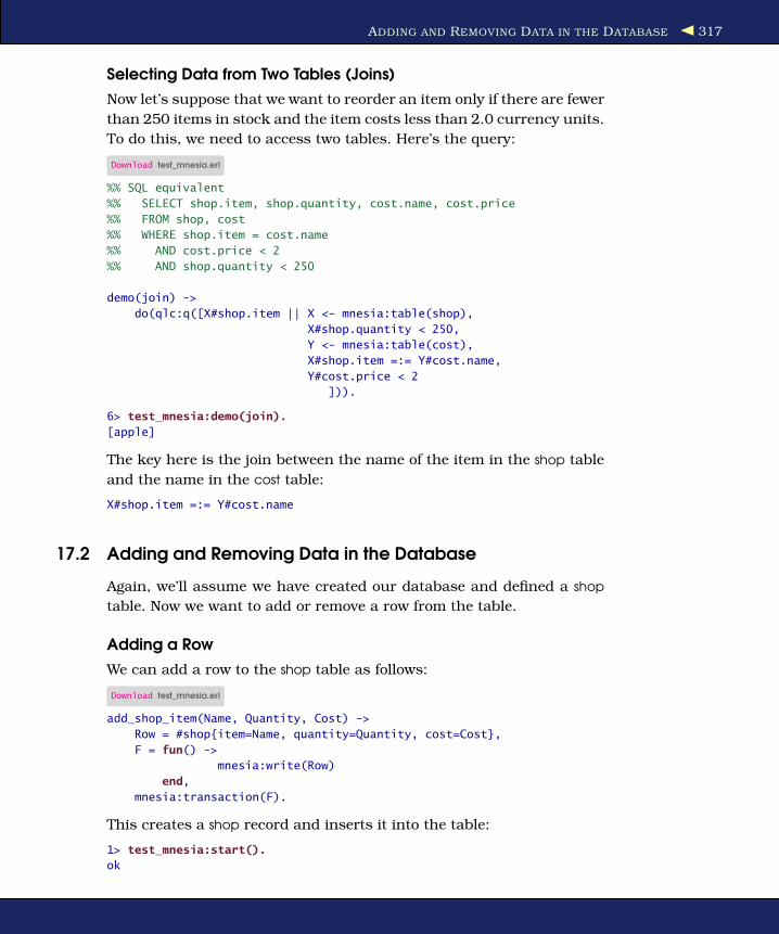
ADDING AND REMOVING DATA IN THE DATABASE 317
Selecting Data from Two Tables (Joins)
Now let’s suppose that we want to reorder an item only if there are fewer
than 250 items in stock and the item costs less than 2.0 currency units.
To do this, we need to access two tables. Here’s the query:
Download test_mnesia.erl
%% SQL equivalent
%% SELECT shop.item, shop.quantity, cost.name, cost.price
%% FROM shop, cost
%% WHERE shop.item = cost.name
%% AND cost.price < 2
%% AND shop.quantity < 250
demo(join) ->
do(qlc:q([X#shop.item || X <- mnesia:table(shop),
X#shop.quantity < 250,
Y <- mnesia:table(cost),
X#shop.item =:= Y#cost.name,
Y#cost.price < 2
])).
6> test_mnesia:demo(join).
[apple]
The key here is the join between the name of the item in the shop table
and the name in the cost table:
X#shop.item =:= Y#cost.name
17.2 Adding and Removing Data in the Database
Again, we’ll assume we have created our database and defined a shop
table. Now we want to add or remove a row from the table.
Adding a Row
We can add a row to the shop table as follows:
Download test_mnesia.erl
add_shop_item(Name, Quantity, Cost) ->
Row = #shop{item=Name, quantity=Quantity, cost=Cost},
F = fun() ->
mnesia:write(Row)
end,
mnesia:transaction(F).
This creates a shop record and inserts it into the table:
1> test_mnesia:start().
ok
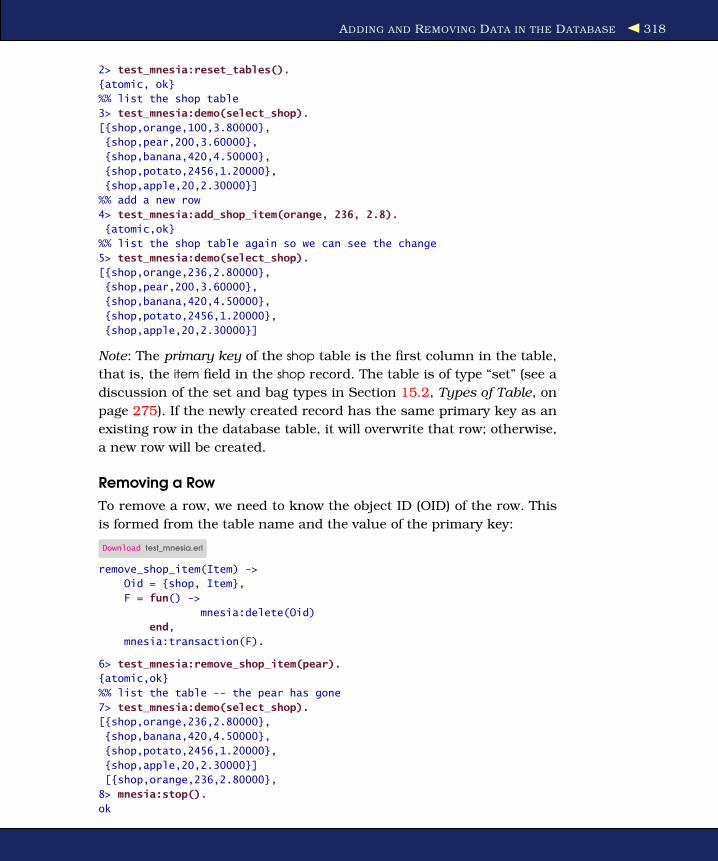
ADDING AND REMOVING DATA IN THE DATABASE 318
2> test_mnesia:reset_tables().
{atomic, ok}
%% list the shop table
3> test_mnesia:demo(select_shop).
[{shop,orange,100,3.80000},
{shop,pear,200,3.60000},
{shop,banana,420,4.50000},
{shop,potato,2456,1.20000},
{shop,apple,20,2.30000}]
%% add a new row
4> test_mnesia:add_shop_item(orange, 236, 2.8).
{atomic,ok}
%% list the shop table again so we can see the change
5> test_mnesia:demo(select_shop).
[{shop,orange,236,2.80000},
{shop,pear,200,3.60000},
{shop,banana,420,4.50000},
{shop,potato,2456,1.20000},
{shop,apple,20,2.30000}]
Note: The primary key of the shop table is the first column in the table,
that is, the item field in the shop record. The table is of type “set” (see a
discussion of the set and bag types in Section 15.2, Types of Table, on
page 275). If the newly created record has the same primary key as an
existing row in the database table, it will overwrite that row; otherwise,
a new row will be created.
Removing a Row
To remove a row, we need to know the object ID (OID) of the row. This
is formed from the table name and the value of the primary key:
Download test_mnesia.erl
remove_shop_item(Item) ->
Oid = {shop, Item},
F = fun() ->
mnesia:delete(Oid)
end,
mnesia:transaction(F).
6> test_mnesia:remove_shop_item(pear).
{atomic,ok}
%% list the table -- the pear has gone
7> test_mnesia:demo(select_shop).
[{shop,orange,236,2.80000},
{shop,banana,420,4.50000},
{shop,potato,2456,1.20000},
{shop,apple,20,2.30000}]
[{shop,orange,236,2.80000},
8> mnesia:stop().
ok

MNESIA TRANSACTIONS 319
17.3 Mnesia Transactions
When we added or removed data from the database or performed a
query, we wrote the code something like this:
do_something(...) ->
F = fun() ->
% ...
mnesia:write(Row)
% ... or ...
mnesia:delete(Oid)
% ... or ...
qlc:e(Q)
end,
mnesia:transaction(F)
F is a fun with zero arguments. Inside F we called some combination of
mnesia:write/1, mnesia:delete/1, or qlc:e(Q) (where Q is a query compiled
with qlc:q/1). Having built the fun, we call mnesia:transaction(F), which
evaluates the expression sequence in the fun.
Why do we do this? What does the transaction mean? To answer this,
suppose we have two processes that try to simultaneously access the
same data. For example, suppose I have $10 in my bank account.
Now suppose two people try to simultaneously withdraw $8 from that
account. What I would like to happen is that one of these transactions
succeeds and the other fails.
This is exactly the guarantee that mnesia:transaction/1 provides. Either
all the reads and writes to the tables in the database within a particular
transaction succeed, or none of them does. If none of them does, the
transaction is said to fail. If the transaction fails, no changes will be
made to the database.
The strategy that Mnesia uses for this is a form of pessimistic locking.
Whenever the Mnesia transaction manager accesses a table, it tries
to lock the record or the entire table depending upon the context. If
it detects that this might lead to deadlock, it immediately aborts the
transaction and undoes any changes it has made.
If the transaction initially fails because some other process is accessing
the data, the system waits for a short time and retries the transaction.
One consequence of this is that the code inside the transaction fun
might be evaluated a large number of times.

MNESIA TRANSACTIONS 320
For this reason, the code inside a transaction fun should not do any-
thing that has any side effects. For example, if we were to write the
following:
F = fun() ->
...
io:format("reading ..."), %% don't do this
...
end,
mnesia:transaction(F),
we might get a lot of output, since the fun might be retried many times.
Note 1: mnesia:write/1 and mnesia:delete/1 should be called only inside a
fun that is processed by mnesia:transaction/1.
Note 2: You should never write code to explicitly catch exceptions in
the Mnesia access functions (mnesia:write/1, mnesia:delete/1, and so on)
since the Mnesia transaction mechanism itself relies upon these func-
tions throwing exceptions on failure. If you catch these exceptions and
try to process them yourself, you will break the transaction mechanism.
Aborting a Transaction
Near to our shop, there’s a farm. And the farmer grows apples. The
farmer loves oranges, and he pays for the oranges with apples. The
going rate is two apples for each orange. So, to buy N oranges, the
farmer pays 2*N apples.
Here’s a function that updates the database when the farmer buys
some oranges:
Download test_mnesia.erl
farmer(Nwant) ->
%% Nwant = Number of oranges the farmer wants to buy
F = fun() ->
%% find the number of apples
[Apple] = mnesia:read({shop,apple}),
Napples = Apple#shop.quantity,
Apple1 = Apple#shop{quantity = Napples + 2*Nwant},
%% update the database
mnesia:write(Apple1),
%% find the number of oranges
[Orange] = mnesia:read({shop,orange}),
NOranges = Orange#shop.quantity,
if
NOranges >= Nwant ->
N1 = NOranges - Nwant,
Orange1 = Orange#shop{quantity=N1},
%% update the database

MNESIA TRANSACTIONS 321
mnesia:write(Orange1);
true ->
%% Oops -- not enough oranges
mnesia:abort(oranges)
end
end,
mnesia:transaction(F).
This code is written in a pretty stupid way because I want to show how
the transaction mechanism works. First, I update the number of apples
in the database. This is done before I check the number of oranges.
The reason I do this is to show that this change gets “undone” if the
transaction fails. Normally, I’d delay writing the orange and apple data
back to the database until I was sure I had enough oranges.
Let’s show this in operation. In the morning, the farmer comes in and
buys 50 oranges:
1> test_mnesia:start().
ok
2> test_mnesia:reset_tables().
{atomic, ok}
%% List the shop table
3> test_mnesia:demo(select_shop).
[{shop,orange,100,3.80000},
{shop,pear,200,3.60000},
{shop,banana,420,4.50000},
{shop,potato,2456,1.20000},
{shop,apple,20,2.30000}]
%% The farmer buys 50 oranges
%% paying with 100 apples
4> test_mnesia:farmer(50).
{atomic,ok}
%% Print the shop table again
5> test_mnesia:demo(select_shop).
[{shop,orange,50,3.80000},
{shop,pear,200,3.60000},
{shop,banana,420,4.50000},
{shop,potato,2456,1.20000},
{shop,apple,120,2.30000}]
In the afternoon the farmer wants to buy 100 more oranges (boy, does
this guy love oranges):
6> test_mnesia:farmer(100).
{aborted,oranges}
7> test_mnesia:demo(select_shop).
[{shop,orange,50,3.80000},
{shop,pear,200,3.60000},
{shop,banana,420,4.50000},
{shop,potato,2456,1.20000},
{shop,apple,120,2.30000}]

MNESIA TRANSACTIONS 322
Why Is the DBMS Called Mnesia?
The original name was Amnesia. One of our bosses didn’t likethe name. He said, “You can’t possibly call it Amnesia—youcan’t have a database that forgets things!” So we droppedthe A, and the name stuck.
When the transaction failed (when we called mnesia:abort(Reason)), the
changes made by mnesia:write were undone. Because of this, the data-
base state was restored to how it was before we entered the transaction.
Loading the Test Data
Now we know how transactions work, so we can look at the code for
loading the test data.
The function test_mnesia:example_tables/0 is used to provide data to ini-
tialize the database tables. The first element of the tuple is the table
name. This is followed by the table data in the order given in the origi-
nal record definitions.
Download test_mnesia.erl
example_tables() ->
[%% The shop table
{shop, apple, 20, 2.3},
{shop, orange, 100, 3.8},
{shop, pear, 200, 3.6},
{shop, banana, 420, 4.5},
{shop, potato, 2456, 1.2},
%% The cost table
{cost, apple, 1.5},
{cost, orange, 2.4},
{cost, pear, 2.2},
{cost, banana, 1.5},
{cost, potato, 0.6}
].
Here’s the code that inserts data into Mnesia from the example tables:
Download test_mnesia.erl
reset_tables() ->
mnesia:clear_table(shop),
mnesia:clear_table(cost),
F = fun() ->
foreach(fun mnesia:write/1, example_tables())
end,
mnesia:transaction(F).

STORING COMPLEX DATA IN TABLES 323
This just calls mnesia:write for each tuple in the list returned by exam-
ple_tables/1.
The do() Function
The do function called by demo/1 is slightly more complex:
Download test_mnesia.erl
do(Q) ->
F = fun() -> qlc:e(Q) end,
{atomic, Val} = mnesia:transaction(F),
Val.
This calls qlc:e(Q) inside an Mnesia transaction. Q is a compiled QLC
query, and qlc:e(Q) evaluates the query and returns all answers to the
query in a list. The return value {atomic, Val} means that the transaction
succeeded with value Val. Val is the value of the transaction function.
17.4 Storing Complex Data in Tables
If you’re a C programmer, how would you store a C struct in a SQL
database? Or if you’re a Java programmer, how would you store an
object in a SQL database? The answer—with great difficulty.
One of the disadvantages of using a conventional DBMS is that there
are a limited number of data types you can store in a table column.
You can store an integer, a string, a float, and so on. But if you want to
store a complex object, then you’re in trouble.
Mnesia is designed to store Erlang data structures. In fact, you can
store any Erlang data structure you want in an Mnesia table.
To illustrate this, we’ll suppose that a number of architects want to
store their designs in an Mnesia database. To start with, we must define
a record to represent their designs:
Download test_mnesia.erl
-record(design, {id, plan}).
Then we can define a function that adds some designs to the database:
Download test_mnesia.erl
add_plans() ->
D1 = #design{id = {joe,1},
plan = {circle,10}},
D2 = #design{id = fred,
plan = {rectangle,10,5}},

STORING COMPLEX DATA IN TABLES 324
D3 = #design{id = {jane,{house,23}},
plan = {house,
[{floor,1,
[{doors,3},
{windows,12},
{rooms,5}]},
{floor,2,
[{doors,2},
{rooms,4},
{windows,15}]}]}},
F = fun() ->
mnesia:write(D1),
mnesia:write(D2),
mnesia:write(D3)
end,
mnesia:transaction(F).
Now we can add some designs to the database:
1> test_mnesia:start().
ok
2> test_mnesia:add_plans().
{atomic,ok}
Now we have some plans in the database. We can extract these with the
following access function:
Download test_mnesia.erl
get_plan(PlanId) ->
F = fun() -> mnesia:read({design, PlanId}) end,
mnesia:transaction(F).
3> test_mnesia:get_plan(fred).
{atomic,[{design,fred,{rectangle,10,5}}]}
4> test_mnesia:get_plan({jane, {house,23}}).
{atomic,[{design,{jane,{house,23}},
{house,[{floor,1,[{doors,3},
{windows,12},
{rooms,5}]},
{floor,2,[{doors,2},
{rooms,4},
{windows,15}]}]}}]}
As you can see, both the database key and the extracted record can be
arbitrary Erlang terms.
In technical terms, we say there is no “impedance mismatch” between
the data structures in the database and the data structures in our
programming language. This means that inserting and deleting complex
data structures into the database is very fast.
TABLE TYPES AND LOCATION 325
Fragmented Tables
Mnesia supports “fragmented tables.” (horizontal partitioningin database terminology). This is designed for implementingextremely large tables. The tables are split into fragments thatare stored on different machines. The fragments are themselvesMnesia tables. The fragments can be replicated, have indexes,and so on, as for any other table.
Refer to the Mnesia User’s Guide for more details.
17.5 Table Types and Location
We can configure Mnesia tables in many different ways. First, tables
can be in RAM or on disk (or both). Second, tables can be located on a
single machine or replicated on several machines.
When we design our tables, we must think about the type of data we
want to store in the tables. Here are the properties of the tables:
RAM tables
These are very fast. The data in them is transient so it will be lost
if the machine crashes or when you stop the DBMS.
Disk tables
Disk tables should survive a crash (provided the disk is not phys-
ically damaged).
When an Mnesia transaction writes to a table and the table is
stored on disk, what actually happens is that the transaction data
is first written to a disk log. This disk log grows continuously, and
at regular intervals the information in the disk log is consolidated
with the other data in the database, and the entry in the disk log
is cleared. If the system crashes, then the next time the system
is restarted, the disk log is checked for consistency, and any out-
standing entries in the log are added to the database before the
database is made available. Once a transaction has succeeded,
the data should have been properly written to the disk log, and if
the system fails after this, then when the system is next restarted,
changes made in the transaction should survive the crash.
If the system crashes during a transaction, then the changes made
to the database should be lost.

TABLE TYPES AND LOCATION 326
Before using a RAM table, you need to perform some experiments to
see whether the entire table will fit into physical memory. If the RAM
tables don’t fit into physical memory, the system will page a lot, which
will be bad for performance.
Since RAM tables are transient, we need to ask ourselves the ques-
tion, Does it matter whether all the data in our RAM table is lost? If
the answer is yes, we will need to replicate the RAM table on disk or
replicate on a second machine (as a RAM or disk table, or both).
Creating Tables
To create a table, we call mnesia:create_table(Name, ArgS), where ArgS is
a list of {Key,Val} tuples. create_table returns {atomic, ok} if the table was
successfully created; otherwise, it returns {aborted, Reason}.
Some of the most common arguments to create_table are as follows:
Name
This is the name of the table (an atom). By convention, it is the
name of an Erlang record—the table rows will be instances of this
record.
{type, Type}
This specifies the type of the table. Type is one of set, ordered_set,
or bag. These types have the same meaning as described in Sec-
tion 15.2, Types of Table, on page 275.
{disc_copies, NodeList}
NodeList is a list of the Erlang nodes where disk copies of the table
will be stored. When we use this option, the system will also create
a RAM copy of the table on the node where we performed this
operation.
It is possible to have a replicated table of type disc_copies on one
node and to have the same table stored as a different table type
on a different node. This is desirable if we want the following:
1. Read operations to be very fast and performed from RAM
2. Write operations to be performed to persistent storage
{ram_copies, NodeList}
NodeList is a list of the Erlang nodes where RAM copies of the table
will be stored.

TABLE TYPES AND LOCATION 327
{disc_only_copies, NodeList}
NodeList is a list of the Erlang nodes where disk-only copies of data
are stored. These tables have no RAM replicas and are slower to
access.
{attributes, AtomList}
This is a list of the column names of the values in a particular
table. Note that to create a table containing the Erlang record xxx,
we can use the syntax {attribute, record_info(fields, xxx)} (alternatively
we can specify an explicit list of record field names).
Note: There are more options to create_table than I have shown here.
Refer to the manual page for mnesia for details of all the options.
Common Combinations of Table Attributes
In all the following, we’ll assume that Attrs is an {attributes,...} tuple.
Here are some common table configuration options that cover the most
common cases:
mnesia:create_table(shop, [Attrs])
• RAM resident on a single node.
• If the node crashes, the table will be lost.
• Fastest of all methods.
• Table must fit in memory.
mnesia:create_table(shop,[Attrs,{disc_copies,[node()]}])
• RAM + disk copy on a single node.
• If the node crashes, the table will be recovered from disk.
• Fast reads, slower writes.
• The table should fit in memory.
mnesia:create_table(shop, [Attrs,{disc_only_copies,[node()]}])
• Disk-only copy on a single node.
• Large tables don’t have to fit in memory.
• Slower than with RAM replicas.
mnesia:create_table(shop,
[Attrs,{ram_copies,[node(),someOtherNode()]})
• RAM resident table on two nodes.
• If both nodes crash, the table will be lost.
• The table must fit into memory.
• The table can be accessed on either node.

CREATING THE INITIAL DATABASE 328
mnesia:create_table(shop,
[Attrs, {disc_copies, [node(),someOtherNode()]}])
• Disk copies on two nodes.
• Can resume on either node.
• Survives double crash.
Table Behavior
When a table is replicated across several Erlang nodes, it is synchro-
nized as far as possible. If one node crashes, the system will still work,
but the number of replicas will be reduced. When the crashed node
comes back online, it will resynchronize with the other nodes where
the replicas are kept.
Note: Mnesia may become overloaded if the nodes running Mnesia stop
functioning. If you are using a laptop that goes to sleep, when it re-
starts, Mnesia might become temporarily overloaded and produce a
number of warning messages. We can ignore these messages.
17.6 Creating the Initial Database
Here is a session that creates an Mnesia database. You need to do this
only once.
$ erl
1> mnesia:create_schema([node()]).
ok
2> init:stop().
ok
$ ls
Mnesia.nonode@nohost
mnesia:create_schema(NodeList) initiates a new Mnesia database on all
the nodes in NodeList (which must be a list of valid Erlang nodes).
In our case, we gave the node list as [node()], that is, the current
node. Mnesia is initialized and creates a directory structure called Mne-
sia.nonode@nohost to store the database. Then we exit from the Erlang
shell and issue the operating system’s ls command to verify this.
If we repeat the exercise with a distributed node called joe, we get the
following:
$ erl -name joe
([email protected]) 1> mnesia:create_schema([node()]).
mnesia:create_schema([node()]).
ok

THE TABLE VIEWER 329
Figure 17.1: Table viewer initial screen
2> init:stop().
ok
$ ls
Or we can point to a specific database when we start Erlang:
$ erl -mnesia dir '"/home/joe/some/path/to/Mnesia.company"'
1> mnesia:create_schema([node()]).
ok
2> init:stop().
ok
/home/joe/some/path/to/Mnesia.company is the name of the directory in
which the database will be stored.
17.7 The Table Viewer
The table viewer is a GUI for viewing Mnesia and ETS tables. The com-
mand tv:start() starts the table viewer. You’ll see the initial display screen
similar to Figure 17.1. To see the tables in Mnesia, you have to select
View > Tab. We can see the table viewer displaying the shop table in
Figure 17.2, on the next page.
17.8 Digging Deeper
I hope I’ve whetted your appetite for Mnesia. Mnesia is a very power-
ful DBMS. It has been in production use in a number of demanding
telecom applications delivered by Ericsson since 1998.
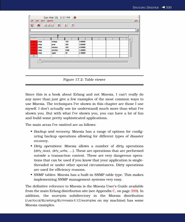
DIGGING DEEPER 330
Figure 17.2: Table viewer
Since this is a book about Erlang and not Mnesia, I can’t really do
any more than just give a few examples of the most common ways to
use Mnesia. The techniques I’ve shown in this chapter are those I use
myself. I don’t actually use (or understand) much more than what I’ve
shown you. But with what I’ve shown you, you can have a lot of fun
and build some pretty sophisticated applications.
The main areas I’ve omitted are as follows:
• Backup and recovery: Mnesia has a range of options for config-
uring backup operations allowing for different types of disaster
recovery.
• Dirty operations: Mnesia allows a number of dirty operations
(dirty_read, dirty_write, ...). These are operations that are performed
outside a transaction context. These are very dangerous opera-
tions that can be used if you know that your application is single-
threaded or under other special circumstances. Dirty operations
are used for efficiency reasons.
• SNMP tables: Mnesia has a built-in SNMP table type. This makes
implementing SNMP management systems very easy.
The definitive reference to Mnesia is the Mnesia User’s Guide available
from the main Erlang distribution site (see Appendix C, on page 399). In
addition, the examples subdirectory in the Mnesia distribution
(/usr/local/lib/erlang/lib/mnesia-X.Y.Z/examples on my machine) has some
Mnesia examples.

LISTINGS 331
17.9 Listings
Download test_mnesia.erl
-module(test_mnesia).
-import(lists, [foreach/2]).
-compile(export_all).
%% IMPORTANT: The next line must be included
%% if we want to call qlc:q(...)
-include_lib("stdlib/include/qlc.hrl").
-record(shop, {item, quantity, cost}).
-record(cost, {name, price}).
-record(design, {id, plan}).
do_this_once() ->
mnesia:create_schema([node()]),
mnesia:start(),
mnesia:create_table(shop, [{attributes, record_info(fields, shop)}]),
mnesia:create_table(cost, [{attributes, record_info(fields, cost)}]),
mnesia:create_table(design, [{attributes, record_info(fields, design)}]),
mnesia:stop().
start() ->
mnesia:start(),
mnesia:wait_for_tables([shop,cost,design], 20000).
%% SQL equivalent
%% SELECT * FROM shop;
demo(select_shop) ->
do(qlc:q([X || X <- mnesia:table(shop)]));
%% SQL equivalent
%% SELECT item, quantity FROM shop;
demo(select_some) ->
do(qlc:q([{X#shop.item, X#shop.quantity} || X <- mnesia:table(shop)]));
%% SQL equivalent
%% SELECT shop.item FROM shop
%% WHERE shop.quantity < 250;
demo(reorder) ->
do(qlc:q([X#shop.item || X <- mnesia:table(shop),
X#shop.quantity < 250
]));
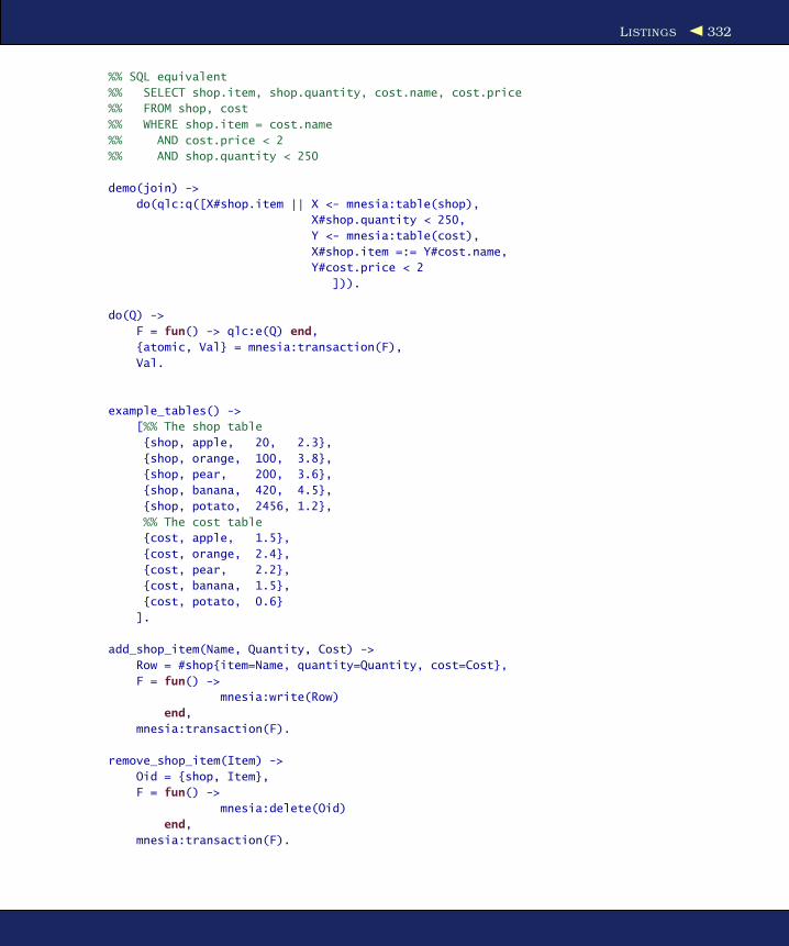
LISTINGS 332
%% SQL equivalent
%% SELECT shop.item, shop.quantity, cost.name, cost.price
%% FROM shop, cost
%% WHERE shop.item = cost.name
%% AND cost.price < 2
%% AND shop.quantity < 250
demo(join) ->
do(qlc:q([X#shop.item || X <- mnesia:table(shop),
X#shop.quantity < 250,
Y <- mnesia:table(cost),
X#shop.item =:= Y#cost.name,
Y#cost.price < 2
])).
do(Q) ->
F = fun() -> qlc:e(Q) end,
{atomic, Val} = mnesia:transaction(F),
Val.
example_tables() ->
[%% The shop table
{shop, apple, 20, 2.3},
{shop, orange, 100, 3.8},
{shop, pear, 200, 3.6},
{shop, banana, 420, 4.5},
{shop, potato, 2456, 1.2},
%% The cost table
{cost, apple, 1.5},
{cost, orange, 2.4},
{cost, pear, 2.2},
{cost, banana, 1.5},
{cost, potato, 0.6}
].
add_shop_item(Name, Quantity, Cost) ->
Row = #shop{item=Name, quantity=Quantity, cost=Cost},
F = fun() ->
mnesia:write(Row)
end,
mnesia:transaction(F).
remove_shop_item(Item) ->
Oid = {shop, Item},
F = fun() ->
mnesia:delete(Oid)
end,
mnesia:transaction(F).
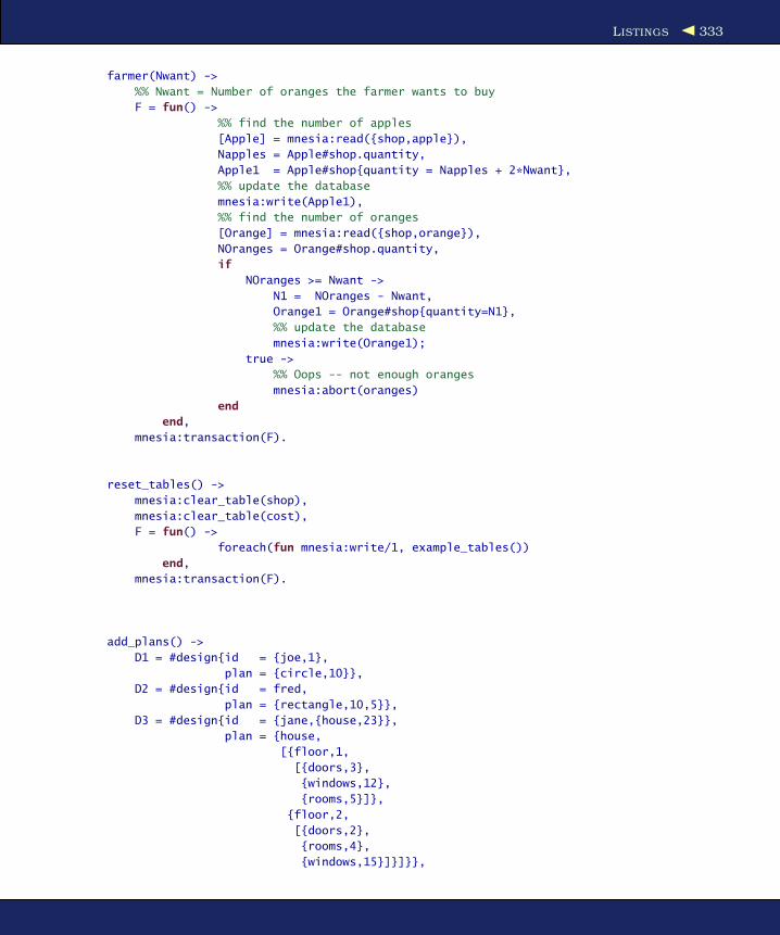
LISTINGS 333
farmer(Nwant) ->
%% Nwant = Number of oranges the farmer wants to buy
F = fun() ->
%% find the number of apples
[Apple] = mnesia:read({shop,apple}),
Napples = Apple#shop.quantity,
Apple1 = Apple#shop{quantity = Napples + 2*Nwant},
%% update the database
mnesia:write(Apple1),
%% find the number of oranges
[Orange] = mnesia:read({shop,orange}),
NOranges = Orange#shop.quantity,
if
NOranges >= Nwant ->
N1 = NOranges - Nwant,
Orange1 = Orange#shop{quantity=N1},
%% update the database
mnesia:write(Orange1);
true ->
%% Oops -- not enough oranges
mnesia:abort(oranges)
end
end,
mnesia:transaction(F).
reset_tables() ->
mnesia:clear_table(shop),
mnesia:clear_table(cost),
F = fun() ->
foreach(fun mnesia:write/1, example_tables())
end,
mnesia:transaction(F).
add_plans() ->
D1 = #design{id = {joe,1},
plan = {circle,10}},
D2 = #design{id = fred,
plan = {rectangle,10,5}},
D3 = #design{id = {jane,{house,23}},
plan = {house,
[{floor,1,
[{doors,3},
{windows,12},
{rooms,5}]},
{floor,2,
[{doors,2},
{rooms,4},
{windows,15}]}]}},

LISTINGS 334
F = fun() ->
mnesia:write(D1),
mnesia:write(D2),
mnesia:write(D3)
end,
mnesia:transaction(F).
get_plan(PlanId) ->
F = fun() -> mnesia:read({design, PlanId}) end,
mnesia:transaction(F).

Chapter 18
Making a System with OTPIn this chapter, we’re going to make a system that could function as
the back end of a web-based company. Our company has two items for
sale: prime numbers and areas. Customers can buy a prime number
from us, or we’ll calculate the area of a geometric object for them. I
think our company has great potential.
We’ll build two servers: one to generate prime numbers and the other
to compute areas. To do this, we’ll use the gen_server framework that
we talked about in Section 16.2, Getting Started with gen_server, on
page 301.
When we build the system, we have to think about errors. Even though
we have thoroughly tested our software, we might not have caught all
the bugs. We’ll assume that one of our servers has a fatal error that
crashes the server. In fact, we’ll introduce a deliberate error into one of
the servers that will cause it to crash.
When the server crashes, we’ll need some mechanism to detect the fact
that it has crashed and to restart it. For this we’ll use the idea of a
supervision tree. We’ll create a supervisor that watches over our servers
and restarts them if they crash.
Of course, if a server does crash, we’ll want to know why it crashed so
that we can fix the problem later. To log all errors, we’ll use the OTP
error logger. We’ll show how to configure the error logger and how to
generate error reports from the error logs.

GENERIC EVENT HANDLING 336
When we’re computing prime numbers and, in particular large prime
numbers, our CPU might overheat. To prevent this, we’ll need to turn
on a powerful fan. To do so, we’ll need to think about alarms. We’ll use
the OTP event handling framework to generate and handle alarms.
All of these topics (creating a server, supervising a server, logging errors,
and detecting alarms) are typical problems that have to be solved in
any production system. So even though our company might have a
rather uncertain future, we can reuse the architecture here in many
systems. In fact, this architecture is used in a number of commercially
successful companies.
Finally, when everything works, we’ll package all our code into an OTP
application. This is a specialized way of grouping everything that has to
do with a particular problem so that it can be started and stopped and
managed by the OTP system itself.
The order in which this material is presented is slightly tricky since
there are many circular dependencies between the different areas.
Error logging is just a special case of event management. Alarms are
just events, the error logger is a supervised process, but the process
supervisor can call the error logger.
I’ll try to impose some order here and present these topics in an order
that makes some kind of sense. We’ll do the following:
1. We’ll look at the ideas used in a generic event handler.
2. We’ll see how the error logger works.
3. We’ll add alarm management.
4. We’ll write two application servers.
5. We’ll make a supervision tree and add the servers to it.
6. We’ll package everything into an application.
18.1 Generic Event Handling
An event is just something that happens—something noteworthy that
the programmer thinks somebody should do something about.
When we’re programming and something noteworthy happens, we just
send an event message to a registered process, like this:
RegProcName ! {event, E}
E is the event (any Erlang term). RegProcName is the name of a regis-
tered process.

GENERIC EVENT HANDLING 337
We don’t know (or care) what happens to the message after we have
sent it. We have done our job and told somebody else that something
has happened.
Now let’s turn our attention to the process that receives the event mes-
sages. This is called an event handler. The simplest possible event han-
dler is a “do nothing” handler. When it receives an {event, X} message, it
does nothing with the event; it just throws it away.
Here’s our first attempt at a generic event handler program:
Download event_handler.erl
-module(event_handler).
-export([make/1, add_handler/2, event/2]).
%% make a new event handler called Name
%% the handler function is noOp -- so we do nothing with the event
make(Name) ->
register(Name, spawn(fun() -> my_handler(fun no_op/1) end)).
add_handler(Name, Fun) -> Name ! {add, Fun}.
%% generate an event
event(Name, X) -> Name ! {event, X}.
my_handler(Fun) ->
receive
{add, Fun1} ->
my_handler(Fun1);
{event, Any} ->
(catch Fun(Any)),
my_handler(Fun)
end.
no_op(_) -> void.
The event handler API is as follows:
event_handler:make(Name)
Make a “do nothing” event handler called Name (an atom). This
provides a place to which to send events.
event_handler:event(Name, X)
Send the event X to the event handler called Name.
event_handler:add_handler(Name, Fun)
Add a handler Fun to the event handler called Name. Now when an
event X occurs, the event handler will evaluate Fun(X).

GENERIC EVENT HANDLING 338
Now we’ll create an event handler and generate an error:
1> event_handler:make(errors).
true
2> event_handler:event(errors, hi).
{event,hi}
Nothing special happens, because we haven’t installed a callback mod-
ule in the event handler.
To get the event handler to do something, we have to write a callback
module and install it in the event handler. Here’s the code for an event
handler callback module:
Download motor_controller.erl
-module(motor_controller).
-export([add_event_handler/0]).
add_event_handler() ->
event_handler:add_handler(errors, fun controller/1).
controller(too_hot) ->
io:format("Turn off the motor~n");
controller(X) ->
io:format("~w ignored event: ~p~n",[?MODULE, X]).
Once this has been compiled, it can be installed:
3> c(motor_controller).
{ok,motor_controller}
4> motor_controller:add_event_handler().
{add,#Fun<motor_controller.0.99476749>}
Now when we send events to the handler, they are processed by the
motor_controller:controller/1 function:
5> event_handler:event(errors, cool).
motor_controller ignored event: cool
{event,cool}
6> event_handler:event(errors, too_hot).
Turn off the motor
{event,too_hot}
What was the point of this exercise? First we provided a name to which
to send events. In this case, it was the registered process called errors.
Then we defined a protocol to send events to this registered process.
But we did not say what would happen to the message when it got
there. In fact, all that happened was that we evaluated noOp(X). Then
at a later stage we installed a custom event handler.

THE ERROR LOGGER 339
Very Late Binding with “Change Your Mind”
Suppose we write a function that hides the event_handler:event
routine from the programmer. For example, say we write thefollowing:
Download lib_misc.erl
too_hot() ->event_handler:event(errors, too_hot).
Then we tell the programmer to call lib_misc:too_hot() in theircode when things go wrong. In most programming languages,the call to the function too_hot will be statically or dynamicallylinked to the code that calls the function. Once it has beenlinked, it will perform a fixed job depending upon the code.If we change our mind later and decide that we want to dosomething else, we have no easy way of changing the behav-ior of the system.
The Erlang way of handling events is completely different. Itallows us to decouple the generation of the event from theprocessing of the event. We can change the processing at anytime we want by just sending a new handler function to theevent handler. Nothing is statically linked, and the event han-dlers can be changed whenever you want.
Using this mechanism, we can build systems that evolve withtime and that never need to be stopped to upgrade the code.
Note: This is not “late binding”—it’s “very late binding, and youcan change your mind later.”
You might be a little puzzled here. Why have we talked about event
handlers? The key point to note is that the event handler provides an
infrastructure where we can install custom handlers.
The error logger infrastructure follows the event handler pattern. We
can install different handlers in the error logger to get it to do different
things. The alarm handling infrastructure also follows this pattern.
18.2 The Error Logger
The OTP system comes packaged with a customizable error logger. We
can look at the error logger from three points of view. The programmer
view concerns the function calls that programmers make in their code
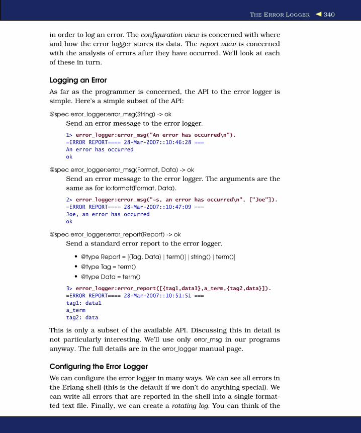
THE ERROR LOGGER 340
in order to log an error. The configuration view is concerned with where
and how the error logger stores its data. The report view is concerned
with the analysis of errors after they have occurred. We’ll look at each
of these in turn.
Logging an Error
As far as the programmer is concerned, the API to the error logger is
simple. Here’s a simple subset of the API:
@spec error_logger:error_msg(String) -> ok
Send an error message to the error logger.
1> error_logger:error_msg("An error has occurred\n").
=ERROR REPORT==== 28-Mar-2007::10:46:28 ===
An error has occurred
ok
@spec error_logger:error_msg(Format, Data) -> ok
Send an error message to the error logger. The arguments are the
same as for io:format(Format, Data).
2> error_logger:error_msg("~s, an error has occurred\n", ["Joe"]).
=ERROR REPORT==== 28-Mar-2007::10:47:09 ===
Joe, an error has occurred
ok
@spec error_logger:error_report(Report) -> ok
Send a standard error report to the error logger.
• @type Report = [{Tag, Data} | term()] | string() | term()]
• @type Tag = term()
• @type Data = term()
3> error_logger:error_report([{tag1,data1},a_term,{tag2,data}]).
=ERROR REPORT==== 28-Mar-2007::10:51:51 ===
tag1: data1
a_term
tag2: data
This is only a subset of the available API. Discussing this in detail is
not particularly interesting. We’ll use only error_msg in our programs
anyway. The full details are in the error_logger manual page.
Configuring the Error Logger
We can configure the error logger in many ways. We can see all errors in
the Erlang shell (this is the default if we don’t do anything special). We
can write all errors that are reported in the shell into a single format-
ted text file. Finally, we can create a rotating log. You can think of the

THE ERROR LOGGER 341
rotating log as a large circular buffer containing messages produced by
the error logger. As new messages come, they are appended to the end
of the log, and when the log is full, the earliest entries in the log are
deleted.
The rotating log is extremely useful. You decide how many files the log
should occupy and how big each individual log file should be, and the
system takes care of deleting old log files and creating new files in a
large circular buffer. You can size the log to keep a record of the last
few days of operations, which is usually sufficient for most purposes.
The Standard Error Loggers
When we start Erlang, we can give the system a boot argument:
$ erl -boot start_clean
This creates an environment suited for program development.
Only a simple form of error logging is provided. (The command
erl with no boot argument is equivalent to erl -boot start_clean.)
$ erl -boot start_sasl
This creates an environment suitable for running a production
system. System Architecture Support Libraries (SASL) takes care
of error logging, overload protection, and so on.
Log file configuration is best done from configuration files, because
nobody can ever remember all the arguments to the logger. In the fol-
lowing sections, we’ll look at how the default system works and then
look at four specific configurations that change how the error logger
works.
SASL with No Configuration
Here’s what happens when we start SASL with no configuration file:
$ erl -boot start_sasl
Erlang (BEAM) emulator version 5.5.3 [async-threads:0] ...
=PROGRESS REPORT==== 27-Mar-2007::11:49:12 ===
supervisor: {local,sasl_safe_sup}
started: [{pid,<0.32.0>},
{name,alarm_handler},
{mfa,{alarm_handler,start_link,[]}},
{restart_type,permanent},
{shutdown,2000},
{child_type,worker}]
... many lines removed ...
Eshell V5.5.3 (abort with ^G)

THE ERROR LOGGER 342
Now we’ll call one of the routines in error_logger to report an error:
1> error_logger:error_msg("This is an error\n").
=ERROR REPORT==== 27-Mar-2007::11:53:08 ===
This is an error
ok
Note the error is reported in the Erlang shell. Where the error is re-
ported depends upon the error logger configuration.
Controlling What Gets Logged
The error logger produces a number of types of report:
Supervisor reports
These are issued whenever an OTP supervisor starts or stops a
supervised process (we’ll talk about supervisors in Section 18.5,
The Supervision Tree, on page 351).
Progress reports
These are issued whenever an OTP supervisor starts or stops.
Crash reports
These are issued when a process started by an OTP behavior ter-
minates with an exit reason other than normal or shutdown.
These three reports are produced automatically without the program-
mer having to do anything.
In addition, we can explicitly call routines in the error_handler module to
produce three types of log report. These let us log errors, warnings, and
informational messages. These three terms have no semantic meaning;
they are merely tags used by the programmer to indicate the nature of
the entry in the error log.
Later, when the error log is analyzed, we can use these tags to help
us decide which log entry to investigate. When we configure the error
logger, we can choose to save only errors and discard all other types of
entry. Now we’ll write the configuration file elog1.config to configure the
error logger:
Download elog1.config
%% no tty
[{sasl, [
{sasl_error_logger, false}
]}].

THE ERROR LOGGER 343
If we start the system with this configuration file, we’ll get only error
reports and not progress reports and so on. All these error reports are
only in the shell.
$ erl -boot start_sasl -config elog1
1> error_logger:error_msg("This is an error\n").
=ERROR REPORT==== 27-Mar-2007::11:53:08 ===
This is an error
ok
Text File and Shell
The next configuration file lists error reports in the shell, and a copy of
everything reported in the shell is also made to a file:
Download elog2.config
%% single text file - minimal tty
[{sasl, [
%% All reports go to this file
{sasl_error_logger, {file, "/home/joe/error_logs/THELOG"}}
]}].
To test this, we start Erlang, generate an error message, and then look
in the log file:
$ erl -boot start_sasl -config elog2
1> error_logger:error_msg("This is an error\n").
=ERROR REPORT==== 27-Mar-2007::11:53:08 ===
This is an error ok
If we now look in /home/joe/error_logs/THELOG, we’ll find it starts like this:
=PROGRESS REPORT==== 28-Mar-2007::11:30:55 ===
supervisor: {local,sasl_safe_sup}
started: [{pid,<0.34.0>},
{name,alarm_handler},
{mfa,{alarm_handler,start_link,[]}},
{restart_type,permanent},
{shutdown,2000},
{child_type,worker}]
...
Rotating Log and Shell
This configuration gives us shell output plus a copy of everything that
was written to the shell in a rotating log file. This is a very useful con-
figuration.

THE ERROR LOGGER 344
Download elog3.config
%% rotating log and minimal tty
[{sasl, [
{sasl_error_logger, false},
%% define the parameters of the rotating log
%% the log file directory
{error_logger_mf_dir,"/home/joe/error_logs"},
%% # bytes per logfile
{error_logger_mf_maxbytes,10485760}, % 10 MB
%% maximum number of logfiles
{error_logger_mf_maxfiles, 10}
]}].
$erl -boot start_sasl -config elog3
1> error_logger:error_msg("This is an error\n").
=ERROR REPORT==== 28-Mar-2007::11:36:19 ===
This is an error
false
When we run the system, all the errors go into a rotating error log. Later
in this chapter we’ll see how to extract this error from the log.
Production Environment
In a production environment, we are really interested only in errors and
not progress or information reports, so we tell the error logger to report
only errors. Without this setting, the system might get swamped with
information and progress reports.
Download elog4.config
%% rotating log and errors
[{sasl, [
%% minimise shell error logging
{sasl_error_logger, false},
%% only report errors
{errlog_type, error},
%% define the parameters of the rotating log
%% the log file directory
{error_logger_mf_dir,"/home/joe/error_logs"},
%% # bytes per logfile
{error_logger_mf_maxbytes,10485760}, % 10 MB
%% maximum number of
{error_logger_mf_maxfiles, 10}
]}].
Running this results in a similar output to the previous example. The
difference is that only errors are reported in the error log.

THE ERROR LOGGER 345
Analyzing the Errors
Reading the error logs is the responsibility of the rb module. It has an
extremely simple interface.
1> rb:help().
Report Browser Tool - usage
===========================
rb:start() - start the rb_server with default options
rb:start(Options) - where Options is a list of:
{start_log, FileName}
- default: standard_io
{max, MaxNoOfReports}
- MaxNoOfReports should be an integer or 'all'
- default: all
...
... many lines omitted ...
...
We start the report browser by telling it how many log entries to read
(in this case the last twenty):
2> rb:start([{max,20}]).
rb: reading report...done.
3> rb:list().
No Type Process Date Time
== ==== ======= ==== ====
11 progress <0.29.0> 2007-03-28 11:34:31
10 progress <0.29.0> 2007-03-28 11:34:31
9 progress <0.29.0> 2007-03-28 11:34:31
8 progress <0.29.0> 2007-03-28 11:34:31
7 progress <0.22.0> 2007-03-28 11:34:31
6 progress <0.29.0> 2007-03-28 11:35:53
5 progress <0.29.0> 2007-03-28 11:35:53
4 progress <0.29.0> 2007-03-28 11:35:53
3 progress <0.29.0> 2007-03-28 11:35:53
2 progress <0.22.0> 2007-03-28 11:35:53
1 error <0.23.0> 2007-03-28 11:36:19
ok
> rb:show(1).
ERROR REPORT <0.40.0> 2007-03-28 11:36:19
===========================================================
This is an error
ok
To isolate a particular error, we can use commands such as rb:
grep(RegExp), which will find all reports matching the regular expres-
sion RegExp. I don’t want to go into all the details of how to analyze
the error log. The best thing is to spend some time interacting with rb

ALARM MANAGEMENT 346
and seeing what it can do. Note that you never need to actually delete
an error report, since the rotation mechanism will eventually delete old
error logs.
If you want to keep all the error logs, you’ll have to poll the error log
at regular intervals and remove the information in which you’re inter-
ested.
18.3 Alarm Management
When we write our application, we need only one alarm—we’ll raise
it when the CPU starts melting because we’re computing a humon-
gous prime (remember, we were making a company that sells prime
numbers). This time we’ll use the real OTP alarm handler (and not the
simple one we saw at the start of this chapter).
The alarm handler is a callback module for the OTP gen_event behavior.
Here’s the code:
Download my_alarm_handler.erl
-module(my_alarm_handler).
-behaviour(gen_event).
%% gen_event callbacks
-export([init/1, handle_event/2, handle_call/2,
handle_info/2, terminate/2]).
%% init(Args) must return {ok, State}
init(Args) ->
io:format("*** my_alarm_handler init:~p~n",[Args]),
{ok, 0}.
handle_event({set_alarm, tooHot}, N) ->
error_logger:error_msg("*** Tell the Engineer to turn on the fan~n"),
{ok, N+1};
handle_event({clear_alarm, tooHot}, N) ->
error_logger:error_msg("*** Danger over. Turn off the fan~n"),
{ok, N};
handle_event(Event, N) ->
io:format("*** unmatched event:~p~n",[Event]),
{ok, N}.
handle_call(_Request, N) -> Reply = N, {ok, N, N}.
handle_info(_Info, N) -> {ok, N}.
terminate(_Reason, _N) -> ok.

ALARM MANAGEMENT 347
This code is pretty similar to the callback code for gen_server, which we
saw earlier in Section 16.3, What Happens When We Call the Server?,
on page 306. The interesting routine is handle_event(Event, State). This
should return {ok, NewState}. Event is a tuple of the form {EventType, Even-
tArg}, where EventType is set_event or clear_event and EventArg is a user-
supplied argument. We’ll see later how these events are generated.
Now we can have some fun. We’ll start the system, generate an alarm,
install an alarm handler, generate a new alarm, and so on:
$ erl -boot start_sasl -config elog3
1> alarm_handler:set_alarm(tooHot).
ok
=INFO REPORT==== 28-Mar-2007::14:20:06 ===
alarm_handler: {set,tooHot}
2> gen_event:swap_handler(alarm_handler,
{alarm_handler, swap},
{my_alarm_handler, xyz}).
*** my_alarm_handler init:{xyz,{alarm_handler,[tooHot]}}
3> alarm_handler:set_alarm(tooHot).
ok
=ERROR REPORT==== 28-Mar-2007::14:22:19 ===
*** Tell the Engineer to turn on the fan
4> alarm_handler:clear_alarm(tooHot).
ok
=ERROR REPORT==== 28-Mar-2007::14:22:39 ===
*** Danger over. Turn off the fan
What happened here?
1. We started Erlang with -boot start_sasl. When we do this, we get
a standard alarm handler. When we set or clear an alarm, noth-
ing happens. This is similar to the “do nothing” event handler we
discussed earlier.
2. When we set an alarm (line 1), we just get an information report.
There is no special handling of the alarm.
3. We install a custom alarm handler (line 2). The argument to
my_alarm_handler (xyz) has no particular significance; the syntax
requires some value here, but since we don’t use the value and we
just used the atom xyz, we can identify the argument when it is
printed.
The ** my_alarm_handler_init: ... printout came from our callback
module.
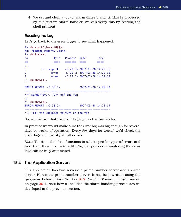
THE APPLICATION SERVERS 348
4. We set and clear a tooHot alarm (lines 3 and 4). This is processed
by our custom alarm handler. We can verify this by reading the
shell printout.
Reading the Log
Let’s go back to the error logger to see what happened:
1> rb:start([{max,20}]).
rb: reading report...done.
2> rb:list().
No Type Process Date Time
== ==== ======= ==== ====
...
3 info_report <0.29.0> 2007-03-28 14:20:06
2 error <0.29.0> 2007-03-28 14:22:19
1 error <0.29.0> 2007-03-28 14:22:39
3> rb:show(1).
ERROR REPORT <0.33.0> 2007-03-28 14:22:39
=====================================================
*** Danger over. Turn off the fan
ok
4> rb:show(2).
ERROR REPORT <0.33.0> 2007-03-28 14:22:19
=====================================================
*** Tell the Engineer to turn on the fan
So, we can see that the error logging mechanism works.
In practice we would make sure the error log was big enough for several
days or weeks of operation. Every few days (or weeks) we’d check the
error logs and investigate all errors.
Note: The rb module has functions to select specific types of errors and
to extract these errors to a file. So, the process of analyzing the error
logs can be fully automated.
18.4 The Application Servers
Our application has two servers: a prime number server and an area
server. Here’s the prime number server. It has been written using the
gen_server behavior (see Section 16.2, Getting Started with gen_server,
on page 301). Note how it includes the alarm handling procedures we
developed in the previous section.
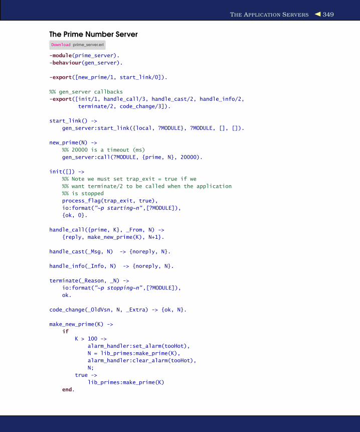
THE APPLICATION SERVERS 349
The Prime Number ServerDownload prime_server.erl
-module(prime_server).
-behaviour(gen_server).
-export([new_prime/1, start_link/0]).
%% gen_server callbacks
-export([init/1, handle_call/3, handle_cast/2, handle_info/2,
terminate/2, code_change/3]).
start_link() ->
gen_server:start_link({local, ?MODULE}, ?MODULE, [], []).
new_prime(N) ->
%% 20000 is a timeout (ms)
gen_server:call(?MODULE, {prime, N}, 20000).
init([]) ->
%% Note we must set trap_exit = true if we
%% want terminate/2 to be called when the application
%% is stopped
process_flag(trap_exit, true),
io:format("~p starting~n",[?MODULE]),
{ok, 0}.
handle_call({prime, K}, _From, N) ->
{reply, make_new_prime(K), N+1}.
handle_cast(_Msg, N) -> {noreply, N}.
handle_info(_Info, N) -> {noreply, N}.
terminate(_Reason, _N) ->
io:format("~p stopping~n",[?MODULE]),
ok.
code_change(_OldVsn, N, _Extra) -> {ok, N}.
make_new_prime(K) ->
if
K > 100 ->
alarm_handler:set_alarm(tooHot),
N = lib_primes:make_prime(K),
alarm_handler:clear_alarm(tooHot),
N;
true ->
lib_primes:make_prime(K)
end.
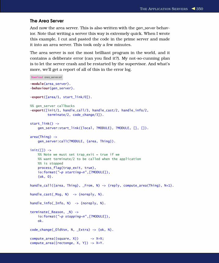
THE APPLICATION SERVERS 350
The Area Server
And now the area server. This is also written with the gen_server behav-
ior. Note that writing a server this way is extremely quick. When I wrote
this example, I cut and pasted the code in the prime server and made
it into an area server. This took only a few minutes.
The area server is not the most brilliant program in the world, and it
contains a deliberate error (can you find it?). My not-so-cunning plan
is to let the server crash and be restarted by the supervisor. And what’s
more, we’ll get a report of all of this in the error log.
Download area_server.erl
-module(area_server).
-behaviour(gen_server).
-export([area/1, start_link/0]).
%% gen_server callbacks
-export([init/1, handle_call/3, handle_cast/2, handle_info/2,
terminate/2, code_change/3]).
start_link() ->
gen_server:start_link({local, ?MODULE}, ?MODULE, [], []).
area(Thing) ->
gen_server:call(?MODULE, {area, Thing}).
init([]) ->
%% Note we must set trap_exit = true if we
%% want terminate/2 to be called when the application
%% is stopped
process_flag(trap_exit, true),
io:format("~p starting~n",[?MODULE]),
{ok, 0}.
handle_call({area, Thing}, _From, N) -> {reply, compute_area(Thing), N+1}.
handle_cast(_Msg, N) -> {noreply, N}.
handle_info(_Info, N) -> {noreply, N}.
terminate(_Reason, _N) ->
io:format("~p stopping~n",[?MODULE]),
ok.
code_change(_OldVsn, N, _Extra) -> {ok, N}.
compute_area({square, X}) -> X*X;
compute_area({rectonge, X, Y}) -> X*Y.

THE SUPERVISION TREE 351
one_for_one supervision
If one process crashes, it is restarted
all_for_one supervision
If one process crashes, all are terminated
and then restarted
Figure 18.1: Two types of supervision tree
18.5 The Supervision Tree
A supervision tree is a tree of processes. The upper processes (supervi-
sors) in the tree monitor the lower processes (workers) in the tree and
restart the lower processes if they fail. There are two types of supervi-
sion tree. You can see them in Figure 18.1.
One-for-one supervision trees
In one-for-one supervision, if a worker fails, it is restarted by the
supervisor.
All-for-one supervision trees
In all-for-one supervision, if any worker dies, then all the worker
processes are killed (by calling the terminate/2 function in the ap-
propriate callback module). Then all the worker processes are re-
started.
Supervisors are created using the OTP supervisor behavior. This behav-
ior is parameterized with a callback module that specifies the supervi-
sor strategy and how to start the individual worker processes in the
supervision tree. The supervisor tree is specified with a function of this
form:
init(...) ->
{ok, {RestartStrategy, MaxRestarts, Time},
[Worker1, Worker2, ...]}.

THE SUPERVISION TREE 352
Here RestartStrategy is one of the atoms one_for_one or all_for_one.
MaxRestarts and Time specify a “restart frequency.” If a supervisor per-
forms more than MaxRestarts in Time seconds, then the supervisor will
terminate all the worker processes and then itself. This is to try to stop
the situation where a process crashes, is restarted, and then crashes
for the same reason, on and on, in an endless loop.
Worker1, Worker2, and so on, are tuples describing how to start each of
the worker processes. We’ll see what these look like in a moment.
Now let’s get back to our company and build a supervision tree.
The first thing we need to do is to choose a name for our company.
Let’s call it sellaprime. The job of the sellaprime supervisor is to make
sure the prime and area servers are always running. To do this, we’ll
write yet another callback module, this time for gen_supervisor. Here’s
the callback module:
Download sellaprime_supervisor.erl
-module(sellaprime_supervisor).
-behaviour(supervisor). % see erl -man supervisor
-export([start/0, start_in_shell_for_testing/0, start_link/1, init/1]).
start() ->
spawn(fun() ->
supervisor:start_link({local,?MODULE}, ?MODULE, _Arg = [])
end).
start_in_shell_for_testing() ->
{ok, Pid} = supervisor:start_link({local,?MODULE}, ?MODULE, _Arg = []),
unlink(Pid).
start_link(Args) ->
supervisor:start_link({local,?MODULE}, ?MODULE, Args).
init([]) ->
%% Install my personal error handler
gen_event:swap_handler(alarm_handler,
{alarm_handler, swap},
{my_alarm_handler, xyz}),
{ok, {{one_for_one, 3, 10},
[{tag1,
{area_server, start_link, []},
permanent,
10000,
worker,
[area_server]},
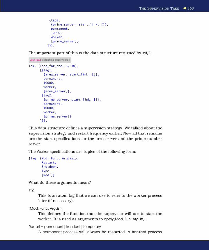
THE SUPERVISION TREE 353
{tag2,
{prime_server, start_link, []},
permanent,
10000,
worker,
[prime_server]}
]}}.
The important part of this is the data structure returned by init/1:
Download sellaprime_supervisor.erl
{ok, {{one_for_one, 3, 10},
[{tag1,
{area_server, start_link, []},
permanent,
10000,
worker,
[area_server]},
{tag2,
{prime_server, start_link, []},
permanent,
10000,
worker,
[prime_server]}
]}}.
This data structure defines a supervision strategy. We talked about the
supervision strategy and restart frequency earlier. Now all that remains
are the start specifications for the area server and the prime number
server.
The Worker specifications are tuples of the following form:
{Tag, {Mod, Func, ArgList},
Restart,
Shutdown,
Type,
[Mod1]}
What do these arguments mean?
Tag
This is an atom tag that we can use to refer to the worker process
later (if necessary).
{Mod, Func, ArgList}
This defines the function that the supervisor will use to start the
worker. It is used as arguments to apply(Mod, Fun, ArgList).
Restart = permanent | transient | temporary
A permanent process will always be restarted. A transient process
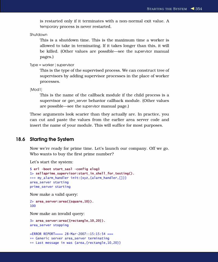
STARTING THE SYSTEM 354
is restarted only if it terminates with a non-normal exit value. A
temporary process is never restarted.
Shutdown
This is a shutdown time. This is the maximum time a worker is
allowed to take in terminating. If it takes longer than this, it will
be killed. (Other values are possible—see the supervisor manual
pages.)
Type = worker | supervisor
This is the type of the supervised process. We can construct tree of
supervisors by adding supervisor processes in the place of worker
processes.
[Mod1]
This is the name of the callback module if the child process is a
supervisor or gen_server behavior callback module. (Other values
are possible—see the supervisor manual page.)
These arguments look scarier than they actually are. In practice, you
can cut and paste the values from the earlier area server code and
insert the name of your module. This will suffice for most purposes.
18.6 Starting the System
Now we’re ready for prime time. Let’s launch our company. Off we go.
Who wants to buy the first prime number?
Let’s start the system:
$ erl -boot start_sasl -config elog3
1> sellaprime_supervisor:start_in_shell_for_testing().
*** my_alarm_handler init:{xyz,{alarm_handler,[]}}
area_server starting
prime_server starting
Now make a valid query:
2> area_server:area({square,10}).
100
Now make an invalid query:
3> area_server:area({rectangle,10,20}).
area_server stopping
=ERROR REPORT==== 28-Mar-2007::15:15:54 ===
** Generic server area_server terminating
** Last message in was {area,{rectangle,10,20}}

STARTING THE SYSTEM 355
Does the Supervision Strategy Work?
Erlang was designed for programming fault-tolerant systems.It was originally developed in the Computer Science Labora-tory at the Swedish Telecom company Ericsson. Since then, theOTP group at Ericsson took over development aided by dozensof internal users. Using gen_server, gen_supervisor, and so on,Erlang has been used to build systems with 99.9999999% reliabil-ity (that’s nine nines). Used correctly, the error handling mech-anisms can help make your program run forever (well, almost).The error logger described here has been run for years in liveproducts.
** When Server state == 1
** Reason for termination ==
** {function_clause,[{area_server,compute_area,[{rectangle,10,20}]},
{area_server,handle_call,3},
{gen_server,handle_msg,6},
{proc_lib,init_p,5}]}
area_server starting
** exited: {{function_clause,
[{area_server,compute_area,[{rectangle,10,20}]},
{area_server,handle_call,3},
{gen_server,handle_msg,6},
{proc_lib,init_p,5}]},
{gen_server,call,
[area_server,{area,{rectangle,10,20}}]}} **
Whoops—what happened here? The area server crashed; we hit the
deliberate error. The crash was detected by the supervisor, and the area
server was restarted by the supervisor. All of this was logged by the
error logger.
After the crash, everything is back to normal, as it should be. Let’s
make a valid request this time:
4> area_server:area({square,25}).
625
We’re up and running again. Now let’s generate a little prime:
5> prime_server:new_prime(20).
Generating a 20 digit prime ........
37864328602551726491
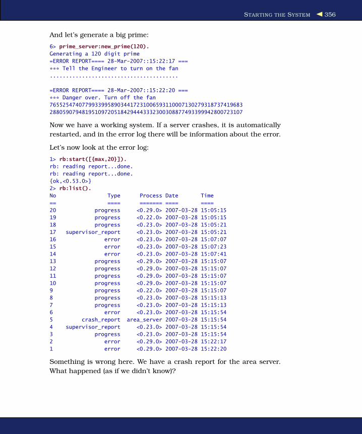
STARTING THE SYSTEM 356
And let’s generate a big prime:
6> prime_server:new_prime(120).
Generating a 120 digit prime
=ERROR REPORT==== 28-Mar-2007::15:22:17 ===
*** Tell the Engineer to turn on the fan
........................................
=ERROR REPORT==== 28-Mar-2007::15:22:20 ===
*** Danger over. Turn off the fan
765525474077993399589034417231006593110007130279318737419683
288059079481951097205184294443332300308877493399942800723107
Now we have a working system. If a server crashes, it is automatically
restarted, and in the error log there will be information about the error.
Let’s now look at the error log:
1> rb:start([{max,20}]).
rb: reading report...done.
rb: reading report...done.
{ok,<0.53.0>}
2> rb:list().
No Type Process Date Time
== ==== ======= ==== ====
20 progress <0.29.0> 2007-03-28 15:05:15
19 progress <0.22.0> 2007-03-28 15:05:15
18 progress <0.23.0> 2007-03-28 15:05:21
17 supervisor_report <0.23.0> 2007-03-28 15:05:21
16 error <0.23.0> 2007-03-28 15:07:07
15 error <0.23.0> 2007-03-28 15:07:23
14 error <0.23.0> 2007-03-28 15:07:41
13 progress <0.29.0> 2007-03-28 15:15:07
12 progress <0.29.0> 2007-03-28 15:15:07
11 progress <0.29.0> 2007-03-28 15:15:07
10 progress <0.29.0> 2007-03-28 15:15:07
9 progress <0.22.0> 2007-03-28 15:15:07
8 progress <0.23.0> 2007-03-28 15:15:13
7 progress <0.23.0> 2007-03-28 15:15:13
6 error <0.23.0> 2007-03-28 15:15:54
5 crash_report area_server 2007-03-28 15:15:54
4 supervisor_report <0.23.0> 2007-03-28 15:15:54
3 progress <0.23.0> 2007-03-28 15:15:54
2 error <0.29.0> 2007-03-28 15:22:17
1 error <0.29.0> 2007-03-28 15:22:20
Something is wrong here. We have a crash report for the area server.
What happened (as if we didn’t know)?

STARTING THE SYSTEM 357
9> rb:show(5).
CRASH REPORT <0.43.0> 2007-03-28 15:15:54
================================================================
Crashing process
pid <0.43.0>
registered_name area_server
error_info
{function_clause,[{area_server,compute_area,[{rectangle,10,20}]},
{area_server,handle_call,3},
{gen_server,handle_msg,6},
{proc_lib,init_p,5}]}
initial_call
{gen,init_it,
[gen_server,
<0.42.0>,
<0.42.0>,
{local,area_server},
area_server,
[],
[]]}
ancestors [sellaprime_supervisor,<0.40.0>]
messages []
links [<0.42.0>]
dictionary []
trap_exit false
status running
heap_size 233
stack_size 21
reductions 199
ok
The printout {function_clause, compute_area, ...} shows us exactly the
point in the program where the server crashed. It should be an easy
job to locate and correct this error. Let’s move on to the next errors:
10> rb:show(2).
ERROR REPORT <0.33.0> 2007-03-28 15:22:17
================================================================
*** Tell the Engineer to turn on the fan
And.
10> rb:show(1).
ERROR REPORT <0.33.0> 2007-03-28 15:22:20
================================================================
*** Danger over. Turn off the fan
These were our fan alarms caused by computing too large primes!

THE APPLICATION 358
18.7 The Application
We’re almost through. All we have to do now is write a file with the
extension .app that contains information about our application:
Download sellaprime.app
%% This is the application resource file (.app file) for the 'base'
%% application.
{application, sellaprime,
[{description, "The Prime Number Shop"},
{vsn, "1.0"},
{modules, [sellaprime_app, sellaprime_supervisor, area_server,
prime_server, lib_primes, my_alarm_handler]},
{registered,[area_server, prime_server, sellaprime_super]},
{applications, [kernel,stdlib]},
{mod, {sellaprime_app,[]}},
{start_phases, []}
]}.
Then we have to write a callback module with the same name as the
mod file in the previous file:
Download sellaprime_app.erl
-module(sellaprime_app).
-behaviour(application).
-export([start/2, stop/1]).
%%--------------------------------------------------------------------
%% Function: start(Type, StartArgs) -> {ok, Pid} |
%% {ok, Pid, State} |
%% {error, Reason}
%% Description: This function is called whenever an application
%% is started using application:start/1,2, and should start the processes
%% of the application. If the application is structured according to the
%% OTP design principles as a supervision tree, this means starting the
%% top supervisor of the tree.
%%--------------------------------------------------------------------
start(_Type, StartArgs) ->
sellaprime_supervisor:start_link(StartArgs).
%%--------------------------------------------------------------------
%% Function: stop(State) -> void()
%% Description: This function is called whenever an application
%% has stopped. It is intended to be the opposite of Module:start/2 and
%% should do any necessary cleaning up. The return value is ignored.
%%--------------------------------------------------------------------
stop(_State) ->
ok.

THE APPLICATION 359
This must export the functions start/2 and stop/1. Once we’ve done all of
this, we can start and stop our application in the shell.
$ erl -boot start_sasl -config elog3
1> application:loaded_applications().
[{kernel,"ERTS CXC 138 10","2.11.3"},
{stdlib,"ERTS CXC 138 10","1.14.3"},
{sasl,"SASL CXC 138 11","2.1.4"}]
2> application:load(sellaprime).
ok
3> application:loaded_applications().
[{sellaprime,"The Prime Number Shop","1.0"},
{kernel,"ERTS CXC 138 10","2.11.3"},
{stdlib,"ERTS CXC 138 10","1.14.3"},
{sasl,"SASL CXC 138 11","2.1.4"}]
4> application:start(sellaprime).
*** my_alarm_handler init:{xyz,{alarm_handler,[]}}
area_server starting
prime_server starting
ok
5> application:stop(sellaprime).
prime_server stopping
area_server stopping
=INFO REPORT==== 2-Apr-2007::19:34:44 ===
application: sellaprime
exited: stopped
type: temporary
ok
6> application:unload(sellaprime).
ok
7> application:loaded_applications().
[{kernel,"ERTS CXC 138 10","2.11.4"},
{stdlib,"ERTS CXC 138 10","1.14.4"},
{sasl,"SASL CXC 138 11","2.1.5"}]
This is now a fully fledged OTP application. In line 2 we loaded the appli-
cation; this loads all the code but does not start the application. Line
4 started the application, and line 5 stopped the application. Note that
we can see from the printout that when the applications were started
and stopped, the appropriate callback functions in the area server and
prime number server were called. In Line 6 we unloaded the applica-
tion. All the module code for the application is removed.
When we build complex systems using OTP, we package them as appli-
cations. This allows us to start, stop, and administer them uniformly.
Note that when we use init:stop() to close down the system, then all
running applications will be closed down in an orderly manner.

FILE SYSTEM ORGANIZATION 360
$ erl -boot start_sasl -config elog3
1> application:start(sellaprime).
*** my_alarm_handler init:{xyz,{alarm_handler,[]}}
area_server starting
prime_server starting
ok
2> init:stop().
ok
prime_server stopping
area_server stopping
$
The two lines following command 2 come from the area and prime num-
ber servers, which shows that the terminator/2 methods in the gen_server
callback modules were called.1
18.8 File System Organization
I haven’t mentioned anything about the file system organization yet.
This is deliberate—my intention is to confuse you with only one thing
at a time.
Well-behaved OTP applications usually have the files belonging to dif-
ferent parts of the application in well-defined places. This is not a
requirement; as long as all the relevant files can be found at runtime,
it doesn’t matter how the files are organized.
In this book I have put most of the demonstration files in the same
directory. This simplifies the examples and avoids problems with search
paths and interactions between the different programs.
The main files used in the sellaprime company are as follows:
File Content
area_server.erl Area server—a gen_server callback
prime_server.erl Prime number server—a gen_server callback
sellaprim_supervisor.erl Supervisor callback
sellaprim_app.erl Application callback
my_alam_handler.erl Event callback for gen_event
sellaprime.app Application specification
elog4.config Error logger configuration file
To see how these files and modules are used, we can look at the se-
quence of events that happens when we start the application:
1. He did come back!
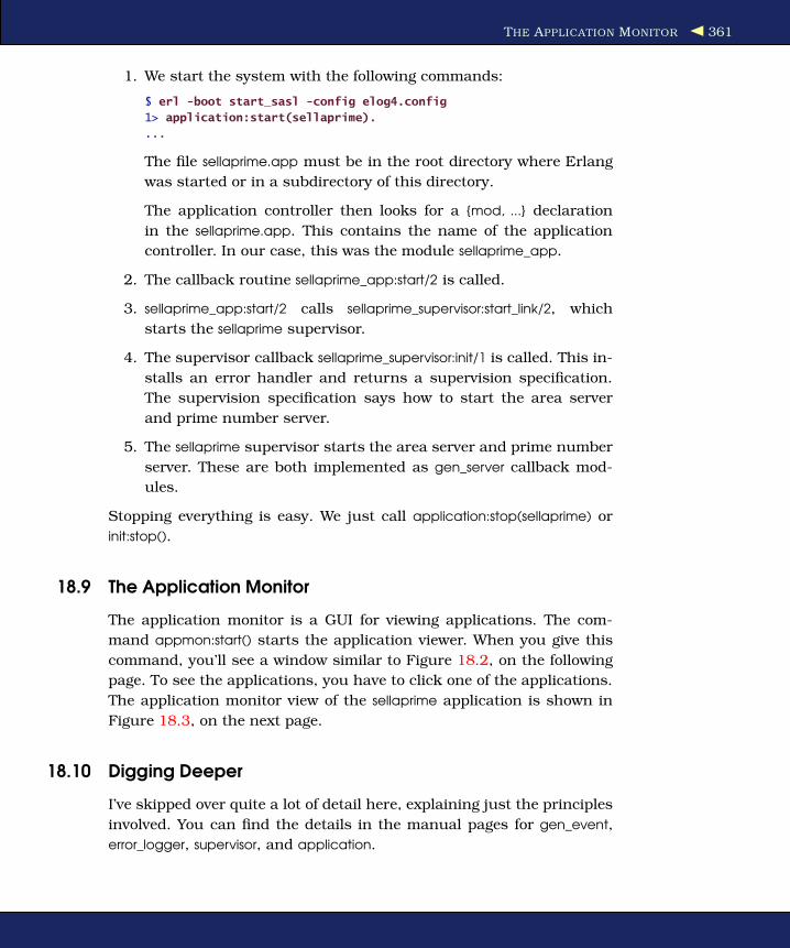
THE APPLICATION MONITOR 361
1. We start the system with the following commands:
$ erl -boot start_sasl -config elog4.config
1> application:start(sellaprime).
...
The file sellaprime.app must be in the root directory where Erlang
was started or in a subdirectory of this directory.
The application controller then looks for a {mod, ...} declaration
in the sellaprime.app. This contains the name of the application
controller. In our case, this was the module sellaprime_app.
2. The callback routine sellaprime_app:start/2 is called.
3. sellaprime_app:start/2 calls sellaprime_supervisor:start_link/2, which
starts the sellaprime supervisor.
4. The supervisor callback sellaprime_supervisor:init/1 is called. This in-
stalls an error handler and returns a supervision specification.
The supervision specification says how to start the area server
and prime number server.
5. The sellaprime supervisor starts the area server and prime number
server. These are both implemented as gen_server callback mod-
ules.
Stopping everything is easy. We just call application:stop(sellaprime) or
init:stop().
18.9 The Application Monitor
The application monitor is a GUI for viewing applications. The com-
mand appmon:start() starts the application viewer. When you give this
command, you’ll see a window similar to Figure 18.2, on the following
page. To see the applications, you have to click one of the applications.
The application monitor view of the sellaprime application is shown in
Figure 18.3, on the next page.
18.10 Digging Deeper
I’ve skipped over quite a lot of detail here, explaining just the principles
involved. You can find the details in the manual pages for gen_event,
error_logger, supervisor, and application.

DIGGING DEEPER 362
Figure 18.2: Application monitor initial window
Figure 18.3: The sellaprime application
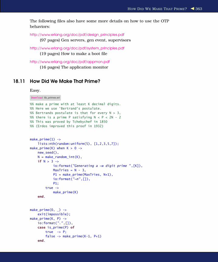
HOW DID WE MAKE THAT PRIME? 363
The following files also have some more details on how to use the OTP
behaviors:
http://www.erlang.org/doc/pdf/design_principles.pdf
(97 pages) Gen servers, gen event, supervisors
http://www.erlang.org/doc/pdf/system_principles.pdf
(19 pages) How to make a boot file
http://www.erlang.org/doc/pdf/appmon.pdf
(16 pages) The application monitor
18.11 How Did We Make That Prime?
Easy.
Download lib_primes.erl
%% make a prime with at least K decimal digits.
%% Here we use 'Bertrand's postulate.
%% Bertrands postulate is that for every N > 3,
%% there is a prime P satisfying N < P < 2N - 2
%% This was proved by Tchebychef in 1850
%% (Erdos improved this proof in 1932)
make_prime(1) ->
lists:nth(random:uniform(5), [1,2,3,5,7]);
make_prime(K) when K > 0 ->
new_seed(),
N = make_random_int(K),
if N > 3 ->
io:format("Generating a ~w digit prime ",[K]),
MaxTries = N - 3,
P1 = make_prime(MaxTries, N+1),
io:format("~n",[]),
P1;
true ->
make_prime(K)
end.
make_prime(0, _) ->
exit(impossible);
make_prime(K, P) ->
io:format(".",[]),
case is_prime(P) of
true -> P;
false -> make_prime(K-1, P+1)
end.
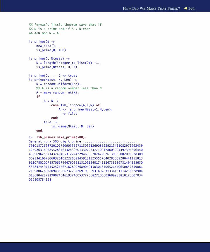
HOW DID WE MAKE THAT PRIME? 364
%% Fermat's little theorem says that if
%% N is a prime and if A < N then
%% A^N mod N = A
is_prime(D) ->
new_seed(),
is_prime(D, 100).
is_prime(D, Ntests) ->
N = length(integer_to_list(D)) -1,
is_prime(Ntests, D, N).
is_prime(0, _, _) -> true;
is_prime(Ntest, N, Len) ->
K = random:uniform(Len),
%% A is a random number less than N
A = make_random_int(K),
if
A < N ->
case lib_lin:pow(A,N,N) of
A -> is_prime(Ntest-1,N,Len);
_ -> false
end;
true ->
is_prime(Ntest, N, Len)
end.
1> lib_primes:make_prime(500).
Generating a 500 digit prime ..............................
7910157269872010279090555971150961269085929213425082972662439
1259263140285528346132439701330792477109478603094497394696440
4399696758714374940531222422946966707622926139385002096578309
0625341667806032610122260234591813255557640283069288441151813
9110780200755706674647603551510515401742126738236731494195650
5578474497545252666718280976890401503018406521440650857349061
2139806789380943526673726726919066931697831336181114236228904
0186804287219807454619374005377766827105603689283818173007034
056505784153

Chapter 19
Multicore PreludeHow can we write programs that run faster on a multicore CPU? It’s all
about mutable state and concurrency.
Back in the old days (twenty-odd years ago), there were two models of
concurrency:
• Shared state concurrency
• Message passing concurrency
The programming world went one way (toward shared state). The Erlang
community went the other way. (Few other languages followed the
“message passing concurrency” road. Others were Oz and Occam.)
In message passing concurrency, there is no shared state. All compu-
tations are done in processes, and the only way to exchange data is
through asynchronous message passing.
Why is this good?
Shared state concurrency involves the idea of “mutable state” (literally
memory that can be changed)—all languages such as C, Java, C++, and
so on, have the notion that there is this stuff called “state” and that we
can change it.
This is fine as long as you have only one process doing the changing.
If you have multiple processes sharing and modifying the same mem-
ory, you have a recipe for disaster—madness lies here.
To protect against the simultaneous modification of shared memory, we
use a locking mechanism. Call this a mutex, a synchronized method,
or what you will, but it’s still a lock.
CHAPTER 19. MULTICORE PRELUDE 366
If programs crash in the critical region (when they hold the lock), disas-
ter results. All the other programs don’t know what to do. If programs
corrupt the memory in the shared state, disaster will also happen. The
other programs won’t know what to do.
How do programmers fix these problems? With great difficulty. On a
unicore processor, their program might just work; but on a multicore—
disaster.
There are various solutions to this (transactional memory is probably
the best), but these are at best kludges. At their worst, they are the
stuff of nightmares.
Erlang has no mutable data structures:1
• No mutable data structures = No locks
• No mutable data structures = Easy to parallelize
How do we do the parallelization? Easy. The programmer breaks up the
solution of the problem into a number of parallel processes.
This style of programming has its own terminology; it’s called concur-
rency-oriented programming.
Now on to the final chapter in the book where we’ll see how our pro-
grams work on a multicore CPU.
1. That’s not quite true, but it’s true enough.

Chapter 20
Programming Multicore CPUsHere’s the good news for Erlang programmers: your Erlang program
might run n times faster on an n core processor—without any changes
to the program.
But you have to follow a simple set of rules.
If you want your application to run faster on a multicore CPU, you’ll
have to make sure that it has lots of processes, that the processes don’t
interfere with each other, and that you have no sequential bottlenecks
in your program.
If instead you’ve written your code in one great monolithic clump of
sequential code and never used spawn to create a parallel process, your
program might not go any faster.
Don’t despair. Even if your program started as a gigantic sequential
program, several simple changes to the program will parallelize it.
In this chapter, we’ll look at the following topics:
• What we have to do to make our programs run efficiently on a
multicore CPU
• How to parallelize a sequential program
• The problem of sequential bottlenecks
• How to avoid side effects
When we’ve done this, we’ll look at the design issues involved in a
more complex problem. We’ll implement a higher-order function called
mapreduce and show how it can be used to program a full-text indexing
engine. mapreduce is an abstraction developed by Google for performing
parallel computations over sets of processing elements.

HOW TO MAKE PROGRAMS RUN EFFICIENTLY ON A MULTICORE CPU 368
Why Should We Care About Multicore CPUs?
You might wonder what all the fuss is about. Do we have tobother parallelizing our program so that it can run on a multi-core? The answer is yes. Today, dual-core CPUs are common-place. In the lab at my workplace, we have some quad coresto play with, and occasionally we get to experiment with athirty-two core machine.
Making a program go twice as fast on a dual-core machine isnot that exciting (but it is a little bit exciting). But let’s not deludeourselves. The clock speeds on dual-core processors are slowerthan on a single-core CPU, so the performance gains can bemarginal.
Intel has a project called Keifer aimed at producing at a thirty-two core processor timed for the market in 2009/2010. Sunalready has an eight-core (with four hardware threads percore) Niagra machine on the market today.
Now although two times doesn’t get me excited, ten timesdoes, and 100 times is really, really exciting. Modern processorsare so fast that a single core can run four hyperthreads, so athirty-two-core CPU might give us an equivalent of 128 threadsto play with. This means that 100 times faster is within strikingdistance.
A factor of 100 does make me excited.
All we have to do is write the code.
20.1 How to Make Programs Run Efficiently on a Multicore CPU
To run efficiently, we have to try to do the following:
1. Use lots of processes.
2. Avoid side effects.
3. Avoid sequential bottlenecks.
4. Write “small messages, big computations” code.
If we do all of these, our Erlang program should run efficiently on a
multicore CPU.

HOW TO MAKE PROGRAMS RUN EFFICIENTLY ON A MULTICORE CPU 369
Use Lots of Processes
This is important—we have to keep the CPUs busy. All the CPUs should
be busy all the time. The easiest way to achieve this is to have lots of
processes.
When I say lots of processes, I mean lots in relation to the number of
CPUs. If we have lots of processes, then we won’t need to worry about
keeping the CPUs busy. This appears to be a purely statistical effect.
If we have a small number of processes, they might accidentally hog
one of the same CPUs; this effect seems to go away if we have a large
number of processes. If we want our programs to be future-proof, we
should think that even though today’s chips might have only a small
number of CPUs, in the future we might have thousands of CPUs per
chip.
Preferably the processes should do similar amounts of work. It’s a bad
idea to write programs where one process does a lot of work and the
others do very little.
In many applications we get lots of processes “for free.” If the applica-
tion is “intrinsically parallel,” then we don’t have to worry about paral-
lelizing our code. For example, if we’re writing a messaging system that
manages some tens of thousands of simultaneous connections, then
we get the concurrency from the tens of thousands of connections; the
code that handles an individual connection will not have to worry about
concurrency.
Avoid Side Effects
Side effects prevent concurrency. Right in the beginning of the book
we talked about “variables that do not vary.” This is the key to under-
standing why Erlang programs can run faster on a multicore CPU than
programs written in languages that can destructively modify memory.
In a language with shared memory and threads, a disaster might hap-
pen if two threads write to common memory at the same time. Systems
with shared memory concurrency prevent this by locking the shared
memory while the memory is being written to. These locks are hidden
from the programmer and appear as mutex or synchronized methods
in their programming languages. The main problem with shared mem-
ory is that one thread can corrupt the memory used by another thread.
So even if my program is correct, another thread can mess up my data
structures and cause my program to crash.
HOW TO MAKE PROGRAMS RUN EFFICIENTLY ON A MULTICORE CPU 370
Erlang does not have shared memory, so this problem does not exist.
Actually, this is not quite true. There are only two ways to share mem-
ory, and the problem can be easily avoided. These two ways of sharing
memory have to do with shared ETS or DETS tables.
Shared ETS or DETS Tables
ETS tables can be shared by several processes. In Section 15.4, Cre-
ating an ETS Table, on page 277, we talked about the different ways
of creating an ETS table. Using one of the options to ets:new, we could
create a public table type. Recall what this did:
Create a public table. Any process that knows the table identifier can
read and write this table.
This can be dangerous. It is safe only if
• we can guarantee that only one process at a time writes to the
table and that all other processes read from the table, and
• the process that writes to the ETS table is correct and does not
write incorrect data into the table.
These properties cannot in general be guaranteed by the system but
instead depend upon the program logic.
Note 1: Individual operations on ETS tables are atomic. What is not
possible is performing a sequence of ETS operations as one atomic unit.
Although we cannot corrupt the data in an ETS table, the tables can
become logically inconsistent if several processes try to simultaneously
update a shared table without coordinating their activities.
Note 2: The ETS table type protected is far safer. Only one process (the
owner) can write to this table, but several processes can read the table.
This property is guaranteed by the system. But remember, even if only
one process can write to an ETS table, if this process corrupts the data
in the table, all processes reading the table will be affected.
If you use the ETS table, type private, and then your programs will
be safe. Similar observations apply to DETS. We can create a shared
DETS table to which several different processes can write. This should
be avoided.
Note: ETS and DETS were created in order to implement Mnesia and
were not originally intended for stand-alone use. The intention is that
application programs should use the Mnesia transaction mechanisms
if they want to simulate shared memory between processes.

HOW TO MAKE PROGRAMS RUN EFFICIENTLY ON A MULTICORE CPU 371
Sequential Bottlenecks
Once we’ve parallelized our program and have made sure we have lots
of processes and no shared memory operations, the next problem to
think about is sequential bottlenecks. Certain things are intrinsically
sequential. If the “sequentialness” lies in the problem, we can’t make it
go away. Certain events happen in a certain sequential order, and no
matter how we try, we can’t change this order. We are born, we live, we
die. We can’t change the order. We can’t do these things in parallel.
A sequential bottleneck is where several concurrent processes need
access to a sequential resource. A typical example is IO. Typically we
have a single disk, and all output to the disk is ultimately sequential.
The disk has one set of heads, not two, and we can’t change that.
Every time we make a registered process, we are creating a potential
sequential bottleneck. So try to avoid the use of registered processes.
If you do create a registered process and use it as a server, make sure
that it responds to all requests as quickly as possible.
Often, the only solution to a sequential bottleneck is to change the
algorithm concerned. There is no cheap and easy fix here. We have to
change the algorithm from a nondistributed algorithm to a distributed
algorithm. This topic (distributed algorithms) has a vast research liter-
ature but has had relatively little take-up in conventional programming
language libraries. The main reason for this is that the need for such
algorithms is not apparent until we try to program networked algo-
rithms or multicore computers.
Programming computers that are permanently connected to the Inter-
net and multicore CPUs will force us to dig into the research literature
and implement some of these amazing algorithms.
A Distributed Ticket-Booking System
Suppose we have a single resource, a set of tickets to the next concert
of the Strolling Bones. To guarantee that when you buy a ticket you
actually get a ticket, we’d conventionally use a single agency that books
all the tickets. But this introduces a sequential bottleneck. How can we
avoid this?
Easy. Imagine you have two ticket agencies. At the start of sales, the
first ticket agency is given all the even-numbered tickets, and the sec-
ond agency is given all the odd-numbered tickets. This way the agencies
are guaranteed not to sell the same ticket twice.

PARALLELIZING SEQUENTIAL CODE 372
If one of the agencies runs out of tickets, then it can request a bundle
of tickets from the other agency.
I’m not saying this is a good method: you might actually want to sit
next to your friends when you go to a concert. But it does remove the
bottleneck, replacing a single ticket office with two.
Replacing the single booking agency by n distributed agencies where n
can vary with time and where the individual agencies can join and leave
the network and crash at any time is an area of active research in dis-
tributed computing. This research goes under the name of distributed
hash tables. If you google this term, you’ll find a vast array of literature
on the subject.
20.2 Parallelizing Sequential Code
Remember the emphasis we made on list-at-a-time operations and in
particular the function lists:map? map is defined like this:
map(_, []) -> [];
map(F, [H|T]) -> [F(H)|map(F, T)].
A simple strategy for speeding up our sequential programs would re-
place all calls to map with a new version of map, which I’ll call pmap,
which evaluates all its arguments in parallel:
Download lib_misc.erl
pmap(F, L) ->
S = self(),
%% make_ref() returns a unique reference
%% we'll match on this later
Ref = erlang:make_ref(),
Pids = map(fun(I) ->
spawn(fun() -> do_f(S, Ref, F, I) end)
end, L),
%% gather the results
gather(Pids, Ref).
do_f(Parent, Ref, F, I) ->
Parent ! {self(), Ref, (catch F(I))}.
gather([Pid|T], Ref) ->
receive
{Pid, Ref, Ret} -> [Ret|gather(T, Ref)]
end;
gather([], _) ->
[].

PARALLELIZING SEQUENTIAL CODE 373
pmap works like map, but when we call pmap(F, L), it creates one parallel
process to evaluate each argument in L. Note that the processes that
evaluate the arguments of L can complete in any order.
The selective receive in the gather function ensures that the order of
the arguments in the return value corresponds to the ordering in the
original list.
There is a slight semantic difference between map and pmap. In pmap,
we use (catch F(H)) when we map the function over the list. In map we
just use F(H). This is because we want to make sure pmap terminates
correctly in the case where the computation of F(H) raises an exception.
In the case where no exceptions are raised, the behavior of the two
functions is identical.
Important: This last statement is not strictly true. map and pmap will
not behave the same way if they have side effects. Suppose F(H) has
some code that modifies the process dictionary. When we call map, the
changes to the process dictionary will be made in the process dictionary
of the process that called map.
When we call pmap, each F(H) is evaluated in its own process, so if we
use the process dictionary, the changes in the dictionary will not affect
the process dictionary in the program that called pmap. So be warned:
Code that has side effects cannot be simply parallelized by replacing a
call to map with pmap.
When Can We Use pmap?
Using pmap instead of map is not a general panacea for speeding up
your programs. The following are some things to think about.
Granularity of Concurrency
Don’t use pmap if the amount of work done in the function is small.
Suppose we say this:
map(fun(I) -> 2*I end, L)
Here the amount of work done inside the fun is minimal. The overhead
of setting up a process and waiting for a reply is greater than the benefit
of using parallel processes to do the job.
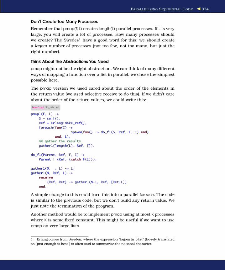
PARALLELIZING SEQUENTIAL CODE 374
Don’t Create Too Many Processes
Remember that pmap(F, L) creates length(L) parallel processes. If L is very
large, you will create a lot of processes. How many processes should
we create? The Swedes1 have a good word for this; we should create
a lagom number of processes (not too few, not too many, but just the
right number).
Think About the Abstractions You Need
pmap might not be the right abstraction. We can think of many different
ways of mapping a function over a list in parallel; we chose the simplest
possible here.
The pmap version we used cared about the order of the elements in
the return value (we used selective receive to do this). If we didn’t care
about the order of the return values, we could write this:
Download lib_misc.erl
pmap1(F, L) ->
S = self(),
Ref = erlang:make_ref(),
foreach(fun(I) ->
spawn(fun() -> do_f1(S, Ref, F, I) end)
end, L),
%% gather the results
gather1(length(L), Ref, []).
do_f1(Parent, Ref, F, I) ->
Parent ! {Ref, (catch F(I))}.
gather1(0, _, L) -> L;
gather1(N, Ref, L) ->
receive
{Ref, Ret} -> gather1(N-1, Ref, [Ret|L])
end.
A simple change to this could turn this into a parallel foreach. The code
is similar to the previous code, but we don’t build any return value. We
just note the termination of the program.
Another method would be to implement pmap using at most K processes
where K is some fixed constant. This might be useful if we want to use
pmap on very large lists.
1. Erlang comes from Sweden, where the expression “lagom är bäst” (loosely translated
as “just enough is best”) is often said to summarize the national character.
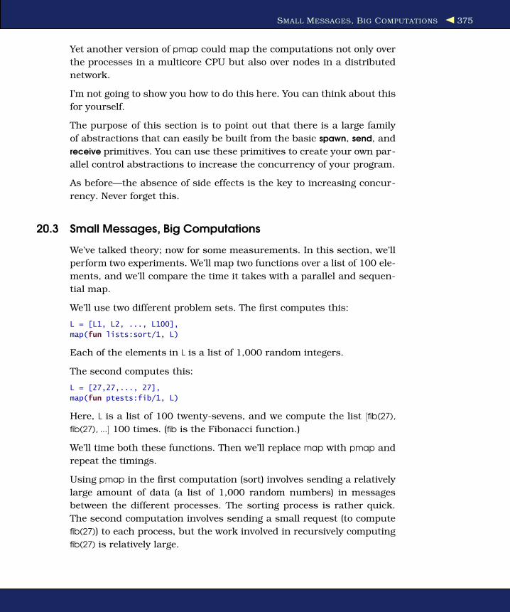
SMALL MESSAGES, BIG COMPUTATIONS 375
Yet another version of pmap could map the computations not only over
the processes in a multicore CPU but also over nodes in a distributed
network.
I’m not going to show you how to do this here. You can think about this
for yourself.
The purpose of this section is to point out that there is a large family
of abstractions that can easily be built from the basic spawn, send, and
receive primitives. You can use these primitives to create your own par-
allel control abstractions to increase the concurrency of your program.
As before—the absence of side effects is the key to increasing concur-
rency. Never forget this.
20.3 Small Messages, Big Computations
We’ve talked theory; now for some measurements. In this section, we’ll
perform two experiments. We’ll map two functions over a list of 100 ele-
ments, and we’ll compare the time it takes with a parallel and sequen-
tial map.
We’ll use two different problem sets. The first computes this:
L = [L1, L2, ..., L100],
map(fun lists:sort/1, L)
Each of the elements in L is a list of 1,000 random integers.
The second computes this:
L = [27,27,..., 27],
map(fun ptests:fib/1, L)
Here, L is a list of 100 twenty-sevens, and we compute the list [fib(27),
fib(27), ...] 100 times. (fib is the Fibonacci function.)
We’ll time both these functions. Then we’ll replace map with pmap and
repeat the timings.
Using pmap in the first computation (sort) involves sending a relatively
large amount of data (a list of 1,000 random numbers) in messages
between the different processes. The sorting process is rather quick.
The second computation involves sending a small request (to compute
fib(27)) to each process, but the work involved in recursively computing
fib(27) is relatively large.
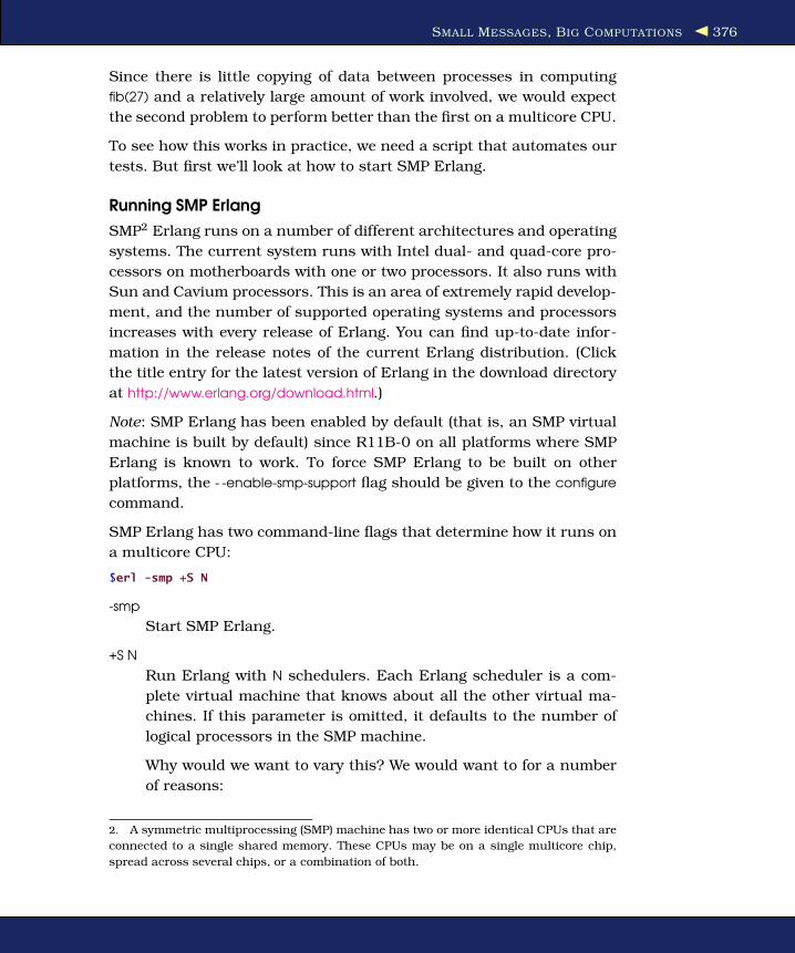
SMALL MESSAGES, BIG COMPUTATIONS 376
Since there is little copying of data between processes in computing
fib(27) and a relatively large amount of work involved, we would expect
the second problem to perform better than the first on a multicore CPU.
To see how this works in practice, we need a script that automates our
tests. But first we’ll look at how to start SMP Erlang.
Running SMP Erlang
SMP2 Erlang runs on a number of different architectures and operating
systems. The current system runs with Intel dual- and quad-core pro-
cessors on motherboards with one or two processors. It also runs with
Sun and Cavium processors. This is an area of extremely rapid develop-
ment, and the number of supported operating systems and processors
increases with every release of Erlang. You can find up-to-date infor-
mation in the release notes of the current Erlang distribution. (Click
the title entry for the latest version of Erlang in the download directory
at http://www.erlang.org/download.html.)
Note: SMP Erlang has been enabled by default (that is, an SMP virtual
machine is built by default) since R11B-0 on all platforms where SMP
Erlang is known to work. To force SMP Erlang to be built on other
platforms, the - -enable-smp-support flag should be given to the configure
command.
SMP Erlang has two command-line flags that determine how it runs on
a multicore CPU:
$erl -smp +S N
-smp
Start SMP Erlang.
+S N
Run Erlang with N schedulers. Each Erlang scheduler is a com-
plete virtual machine that knows about all the other virtual ma-
chines. If this parameter is omitted, it defaults to the number of
logical processors in the SMP machine.
Why would we want to vary this? We would want to for a number
of reasons:
2. A symmetric multiprocessing (SMP) machine has two or more identical CPUs that are
connected to a single shared memory. These CPUs may be on a single multicore chip,
spread across several chips, or a combination of both.
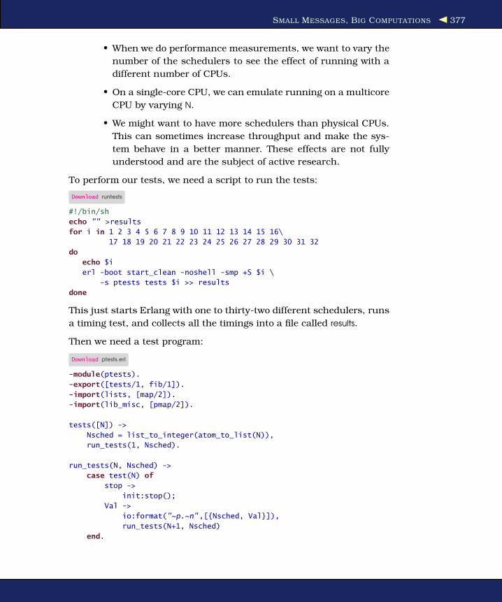
SMALL MESSAGES, BIG COMPUTATIONS 377
• When we do performance measurements, we want to vary the
number of the schedulers to see the effect of running with a
different number of CPUs.
• On a single-core CPU, we can emulate running on a multicore
CPU by varying N.
• We might want to have more schedulers than physical CPUs.
This can sometimes increase throughput and make the sys-
tem behave in a better manner. These effects are not fully
understood and are the subject of active research.
To perform our tests, we need a script to run the tests:
Download runtests
#!/bin/sh
echo "" >results
for i in 1 2 3 4 5 6 7 8 9 10 11 12 13 14 15 16\
17 18 19 20 21 22 23 24 25 26 27 28 29 30 31 32
do
echo $i
erl -boot start_clean -noshell -smp +S $i \
-s ptests tests $i >> results
done
This just starts Erlang with one to thirty-two different schedulers, runs
a timing test, and collects all the timings into a file called results.
Then we need a test program:
Download ptests.erl
-module(ptests).
-export([tests/1, fib/1]).
-import(lists, [map/2]).
-import(lib_misc, [pmap/2]).
tests([N]) ->
Nsched = list_to_integer(atom_to_list(N)),
run_tests(1, Nsched).
run_tests(N, Nsched) ->
case test(N) of
stop ->
init:stop();
Val ->
io:format("~p.~n",[{Nsched, Val}]),
run_tests(N+1, Nsched)
end.

SMALL MESSAGES, BIG COMPUTATIONS 378
test(1) ->
%% Make 100 lists
%% Each list contains 1000 random integers
seed(),
S = lists:seq(1,100),
L = map(fun(_) -> mkList(1000) end, S),
{Time1, S1} = timer:tc(lists, map, [fun lists:sort/1, L]),
{Time2, S2} = timer:tc(lib_misc, pmap, [fun lists:sort/1, L]),
{sort, Time1, Time2, equal(S1, S2)};
test(2) ->
%% L = [27,27,27,..] 100 times
L = lists:duplicate(100, 27),
{Time1, S1} = timer:tc(lists, map, [fun ptests:fib/1, L]),
{Time2, S2} = timer:tc(lib_misc, pmap, [fun ptests:fib/1, L]),
{fib, Time1, Time2, equal(S1, S2)};
test(3) ->
stop.
%% Equal is used to test that map and pmap compute the same thing
equal(S,S) -> true;
equal(S1,S2) -> {differ, S1, S2}.
%% recursive (inefficent) fibonacci
fib(0) -> 1;
fib(1) -> 1;
fib(N) -> fib(N-1) + fib(N-2).
%% Reset the random number generator. This is so we
%% get the same sequence of random numbers each time we run
%% the program
seed() -> random:seed(44,55,66).
%% Make a list of K random numbers
%% Each random number in the range 1..1000000
mkList(K) -> mkList(K, []).
mkList(0, L) -> L;
mkList(N, L) -> mkList(N-1, [random:uniform(1000000)|L]).
This runs map and pmap in the two different test cases. You can see
the results in Figure 20.1, on the next page, where we have plotted the
ratio of times taken by pmap and map. As we can see, CPU-bound com-
putations with little message passing have linear speed-up, whereas
lighter-weight computations with more message passing scale less well.
As a final note, we shouldn’t read too much into these figures. SMP
Erlang is undergoing daily changes, so what is true today may not be
true tomorrow. All we can say is that we are very encouraged by our
results. Ericsson is building commercial products that run almost twice
as fast on dual-core processors, so we are very happy.

MAPREDUCE AND INDEXING OUR DISK 379
0
2
4
6
8
10
12
14
16
0 5 10 15 20 25 30 35
Spe
edup
Number of CPUs
Multicore Performance on a SUN Fire T2000 Server
FibLists
Figure 20.1: Speed-up on multicore CPU
20.4 mapreduce and Indexing Our Disk
Now we’re going to turn theory in practice. First we’ll look at the higher-
order function mapreduce; then we’ll use mapreduce to make a sim-
ple indexing engine. The goal here is not actually to make the world’s
fastest and best indexing engine but to address the design issues that
are involved in constructing such a program.
mapreduce
In Figure 20.2, on the following page, we can see the basic idea of mapre-
duce. We have a number of mapping processes, which produce streams
of {Key, Value} pairs. The mapping processes send these pairs to a reduce
process that merges the pairs, combining pairs with the same key.
Warning: The word map, used in the context of mapreduce, is com-
pletely different from the map function that occurs elsewhere in this
book.
mapreduce is a parallel higher-order function. Proposed by Jeffrey Dean
and Sanjay Ghemawat of Google, it is said to be in daily use on Google
clusters.

MAPREDUCE AND INDEXING OUR DISK 380
{Key, Val}
M
{Key, Val}
M
{Key, Val}
M
{Key, Val} M
{Key, Val}
M
R
M = Map process
R = Reduce process
Figure 20.2: mapreduce
We can implement mapreduce in lots of different ways and with lots of
different semantics—it’s actually more a family of algorithms than one
particular algorithm.
mapreduce is defined as follows:
@spec mapreduce(F1, F2, Acc0, L) -> Acc
F1 = fun(Pid, X) -> void,
F2 = fun(Key, [Value], Acc0) -> Acc
L = [X]
Acc = X = term()
F1(Pid, X) is the mapping function.
The job of F1 is to send a stream of {Key, Value} messages to the
process Pid and then to terminate. mapreduce will spawn a fresh
process for each value of X in the list L.
F2(Key, [Value], Acc0) -> Acc is the reduction function.
When all the mapping processes have terminated, the reduce pro-
cess will have merged all the values for a particular key together.
It then calls F2(Key, [Value], Acc) for each of the {Key, [Value]} pairs it
has collected. Acc is an accumulator whose initial value is Acc0.
F2 returns a new accumulator. (Another way of describing this is
to say that F2 performs a fold over the {Key, [Value]} pairs that it has
collected.)

MAPREDUCE AND INDEXING OUR DISK 381
Acc0 is the initial value of the accumulator, used when calling F2.
L is a list of X values.
F1(Pid, X) will be called for each value of X in L.Pid is a process
identifier of the reduce process; this is created by mapreduce.
mapreduce is defined in the module phofs (short for parallel higher-order
functions):
Download phofs.erl
-module(phofs).
-export([mapreduce/4]).
-import(lists, [foreach/2]).
%% F1(Pid, X) -> sends {Key,Val} messages to Pid
%% F2(Key, [Val], AccIn) -> AccOut
mapreduce(F1, F2, Acc0, L) ->
S = self(),
Pid = spawn(fun() -> reduce(S, F1, F2, Acc0, L) end),
receive
{Pid, Result} ->
Result
end.
reduce(Parent, F1, F2, Acc0, L) ->
process_flag(trap_exit, true),
ReducePid = self(),
%% Create the Map processes
%% One for each element X in L
foreach(fun(X) ->
spawn_link(fun() -> do_job(ReducePid, F1, X) end)
end, L),
N = length(L),
%% make a dictionary to store the Keys
Dict0 = dict:new(),
%% Wait for N Map processes to terminate
Dict1 = collect_replies(N, Dict0),
Acc = dict:fold(F2, Acc0, Dict1),
Parent ! {self(), Acc}.
%% collect_replies(N, Dict)
%% collect and merge {Key, Value} messages from N processes.
%% When N processes have terminated return a dictionary
%% of {Key, [Value]} pairs
collect_replies(0, Dict) ->
Dict;

MAPREDUCE AND INDEXING OUR DISK 382
collect_replies(N, Dict) ->
receive
{Key, Val} ->
case dict:is_key(Key, Dict) of
true ->
Dict1 = dict:append(Key, Val, Dict),
collect_replies(N, Dict1);
false ->
Dict1 = dict:store(Key,[Val], Dict),
collect_replies(N, Dict1)
end;
{'EXIT', _, Why} ->
collect_replies(N-1, Dict)
end.
%% Call F(Pid, X)
%% F must send {Key, Value} messsages to Pid
%% and then terminate
do_job(ReducePid, F, X) ->
F(ReducePid, X).
Before we go any further, we’ll test mapreduce so as to be really clear
about what it does.
We’ll write a little program to count the frequencies of all words in the
code directory that accompanies this book. Here is the program:
Download test_mapreduce.erl
-module(test_mapreduce).
-compile(export_all).
-import(lists, [reverse/1, sort/1]).
test() ->
wc_dir(".").
wc_dir(Dir) ->
F1 = fun generate_words/2,
F2 = fun count_words/3,
Files = lib_find:files(Dir, "*.erl", false),
L1 = phofs:mapreduce(F1, F2, [], Files),
reverse(sort(L1)).
generate_words(Pid, File) ->
F = fun(Word) -> Pid ! {Word, 1} end,
lib_misc:foreachWordInFile(File, F).
count_words(Key, Vals, A) ->
[{length(Vals), Key}|A].

MAPREDUCE AND INDEXING OUR DISK 383
5> test_mapreduce:test().
[{341,"1"},
{330,"end"},
{318,"0"},
{265,"N"},
{235,"X"},
{214,"T"},
{213,"2"},
{205,"start"},
{196,"L"},
{194,"is"},
{185,"file"},
{177,"Pid"},
...
When I ran this, there were 102 Erlang modules in the code directory;
mapreduce created 102 parallel processes, each sending a stream of
pairs to the reduce process. This should run nicely on a 100-core pro-
cessor (if the disk can keep up).
Now that we understand how mapreduce works, we can go back to our
indexing engine.
Full-Text Indexing
When we build an index, one of the things we need to do is find all
the words in a file. This is going to be used in the “map” phase of a
mapreduce operation.
Before we do this, we’ll look at the data structures needed to make a
full-text index.
The Inverted Index
Our full-text index is implemented using an inverted index—in this sec-
tion, we’ll review the idea of an inverted index and see how this is stored
in our system.
To illustrate this, we’ll start with a simple example. Suppose we have
a file system with three files and each file contains a small number of
words.
Our files and their contents might look like this:
Filename Contents
/home/dogs rover jack buster winston
/home/animals/cats zorro daisy jaguar
/home/cars rover jaguar ford
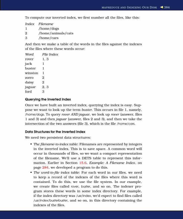
MAPREDUCE AND INDEXING OUR DISK 384
To compute our inverted index, we first number all the files, like this:
Index Filename
1 /home/dogs
2 /home/animals/cats
3 /home/cars
And then we make a table of the words in the files against the indexes
of the files where these words occur:
Word File Index
rover 1, 3
jack 1
buster 1
winston 1
zorro 2
daisy 2
jaguar 2, 3
ford 3
Querying the Inverted Index
Once we have built an inverted index, querying the index is easy. Sup-
pose we want to look up the term buster. This occurs in file 1, namely,
/home/dogs. To query rover AND jaguar, we look up rover (answer, files
1 and 3) and then jaguar (answer, files 2 and 3), and then we take the
intersection of the two answers (file 3), which is the file /home/cars.
Data Structures for the Inverted Index
We need two persistent data structures:
• The filename-to-index table: Filenames are represented by integers
in the inverted index. This is to save space. A common word will
occur in thousands of files, so we want a compact representation
of the filename. We’ll use a DETS table to represent this infor-
mation. Earlier in Section 15.6, Example: A Filename Index, on
page 284, we developed a program to do this.
• The word-to-file index table: For each word in our files, we need
to keep a record of the indexes of the files where this word is
contained. To do this, we use the file system. In our example,
we create files called rover, buster, and so on. The indexer pro-
gram stores these words in some index directory. For example,
if the index directory was /usr/index, we’d expect to find files called
/usr/index/busterbuster, and so on, in this directory containing the
indexes of the files.
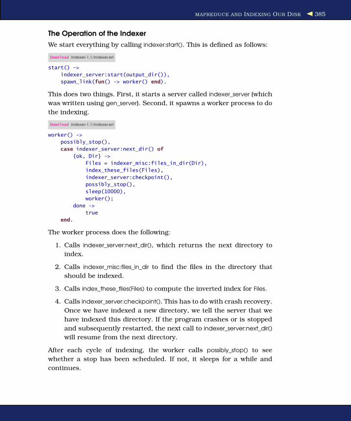
MAPREDUCE AND INDEXING OUR DISK 385
The Operation of the Indexer
We start everything by calling indexer:start(). This is defined as follows:
Download indexer-1.1/indexer.erl
start() ->
indexer_server:start(output_dir()),
spawn_link(fun() -> worker() end).
This does two things. First, it starts a server called indexer_server (which
was written using gen_server). Second, it spawns a worker process to do
the indexing.
Download indexer-1.1/indexer.erl
worker() ->
possibly_stop(),
case indexer_server:next_dir() of
{ok, Dir} ->
Files = indexer_misc:files_in_dir(Dir),
index_these_files(Files),
indexer_server:checkpoint(),
possibly_stop(),
sleep(10000),
worker();
done ->
true
end.
The worker process does the following:
1. Calls indexer_server:next_dir(), which returns the next directory to
index.
2. Calls indexer_misc:files_in_dir to find the files in the directory that
should be indexed.
3. Calls index_these_files(Files) to compute the inverted index for Files.
4. Calls indexer_server:checkpoint(). This has to do with crash recovery.
Once we have indexed a new directory, we tell the server that we
have indexed this directory. If the program crashes or is stopped
and subsequently restarted, the next call to indexer_server:next_dir()
will resume from the next directory.
After each cycle of indexing, the worker calls possibly_stop() to see
whether a stop has been scheduled. If not, it sleeps for a while and
continues.

MAPREDUCE AND INDEXING OUR DISK 386
The actual indexing takes place in index_these_files. This is where we go
parallel and use mapreduce.
Download indexer-1.1/indexer.erl
index_these_files(Files) ->
Ets = indexer_server:ets_table(),
OutDir = filename:join(indexer_server:outdir(), "index"),
F1 = fun(Pid, File) -> indexer_words:words_in_file(Pid, File, Ets) end,
F2 = fun(Key, Val, Acc) -> handle_result(Key, Val, OutDir, Acc) end,
indexer_misc:mapreduce(F1, F2, 0, Files).
handle_result(Key, Vals, OutDir, Acc) ->
add_to_file(OutDir, Key, Vals),
Acc + 1.
add_to_file(OutDir, Word, Is) appends a list of indexes in Is to the file Word
in OutDir.
Download indexer-1.1/indexer.erl
add_to_file(OutDir, Word, Is) ->
L1 = map(fun(I) -> <<I:32>> end, Is),
OutFile = filename:join(OutDir, Word),
case file:open(OutFile, [write,binary,raw,append]) of
{ok, S} ->
file:pwrite(S, 0, L1),
file:close(S);
{error, E} ->
exit({ebadFileOp, OutFile, E})
end.
Running the Indexer1> indexer:cold_start().
2> indexer:start().
...
N> indexer:stop().
Scheduling a stop
ack
Stopping
Comments
This is a complex program (the most complex one in this book), and it
is by no means complete. Even though it is complex, it has a structure
that is simple and understandable.
It has a strategy for starting and stopping the program and recovering
from errors. This is a achieved with indexer_checkpoint. It parallelizes
the search using mapreduce, and it makes a brave attempt at isolating
words from a file.

MAPREDUCE AND INDEXING OUR DISK 387
What would we have to do to turn this toy indexer into a full-featured
indexer? We would have to make a number of improvements:
• Improve the word extraction. This is probably the single area that
needs some major effort. The problem is not particularly difficult,
but the problem has no generic solution. Each file type (Erlang,
PDF, TXT, C, Java, and so on) requires a separate (and different)
analysis technique to extract what might be relevant words. This
has to be repeated for all major natural languages (and spellings).
• mapreduce must be improved to handle extremely large data sets.
The key-value merge steps that I used in mapreduce shown here
ran in memory and without backing disk store. We must give some
careful thought to the problem of how to represent sets of values
where the numbers of elements are extremely large.
• The data structures for the inverted index just used the file system
as a data store and a single DETS table for storing the filename-
to-index map. This technique doesn’t scale well to encompass, for
example, all the filenames of all machines on the planet. For this,
a distributed hash table seems appropriate.
Let’s disregard these problems for a moment and step back to think
about the solution. On the positive side, we have learned a number of
techniques for programming multicore CPUs based on the use of simple
higher-order functions that are free from side effects.
The Indexer Code
All the code for the indexer is in the indexer directory in the code down-
load. It consists of nine files. These files total about 1,200 lines of code,
so we won’t kill trees by including them here.
indexer.erl
The main program. This exports start(), stop(), and cold_start().
These are the only routines that a user of the indexer is supposed
to know about.
indexer_porter.erl
Stemming algorithm. To reduce the number of words in the index,
we try to reduce words to the same base or root form. So, for
example, all the words fishing, fished, and fisher have the same
root (fish). This process is called stemming. The algorithm we use
is the Porter algorithm (because of Martin Porter) and is imple-
mented in the module indexer_porter.
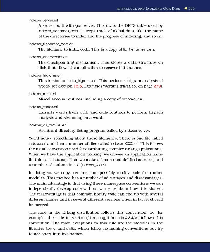
MAPREDUCE AND INDEXING OUR DISK 388
indexer_server.erl
A server built with gen_server. This owns the DETS table used by
indexer_filenames_dets. It keeps track of global data, like the name
of the directories to index and the progress of indexing, and so on.
indexer_filenames_dets.erl
The filename to index code. This is a copy of lib_filenames_dets.
indexer_checkpoint.erl
The checkpointing mechanism. This stores a data structure on
disk that allows the application to recover if it crashes.
indexer_trigrams.erl
This is similar to lib_trigrams.erl. This performs trigram analysis of
words (see Section 15.5, Example Programs with ETS, on page 279).
indexer_misc.erl
Miscellaneous routines, including a copy of mapreduce.
indexer_words.erl
Extracts words from a file and calls routines to perform trigram
analysis and stemming on a word.
indexer_dir_crawler.erl
Reentrant directory listing program called by indexer_server.
You’ll notice something about these filenames. There is one file called
indexer.erl and then a number of files called indexer_XXXX.erl. This follows
the usual convention used for distributing complex Erlang applications.
When we have the application working, we choose an application name
(in this case indexer). Then we make a “main module” (in indexer.erl) and
a number of “submodules” (indexer_XXXX).
In doing so, we copy, rename, and possibly modify code from other
modules. This method has a number of advantages and disadvantages.
The main advantage is that using these namespace conventions we can
independently develop code without worrying about how it is shared.
The disadvantage is that common library code can end up with several
different names and in several different versions when in fact it should
be merged.
The code in the Erlang distribution follows this convention. So, for
example, the code in /usr/local/lib/erlang/lib/mnesia-4.3.4/src follows this
convention. The main exceptions to this rule are the modules in the
libraries kernel and stdlib, which follow no naming conventions but try
to use short intuitive names.

GROWING INTO THE FUTURE 389
20.5 Growing Into the Future
The landscape of computing is changing. Large, monolithic processors
are slowing becoming dinosaurs, eclipsed by the idea that we can put
processing power where we need it. The future has multiple cores, and
the future has distributed processors.
The techniques we grew up with for writing programs are struggling in
this new world. Erlang is a solution for this. In this book, I’ve shown
you how a few basic concepts in Erlang lead to code that is reliable,
maintainable, and that scales well on today’s (and tomorrow’s) archi-
tectures.
Enjoy writing these new style programs.

Appendix A
Documenting Our ProgramErlang has strong ideas about types, but much of what it knows is
implicit. To make it more explicit in documentation, and when talking
about functions, the Erlang community has developed a notation for
talking about types. This notation isn’t part of a program’s source code.
Instead, it’s a documentation device—a way of talking about Erlang
source. Using it, we can specify unambiguously what kinds of parame-
ters a function may accept and what types it returns.
More recently, this same notation has been adopted by a range of tools
that work with Erlang source (which we’ll talk about later).
The type notation is used only for documentation purposes. Type dec-
larations are not Erlang code and cannot be typed into the shell. Type
declarations in Erlang modules are written as part of comments and
are totally ignored by the Erlang compiler. For example, we might write
this:
-module(math).
-export([fac/1]).
%% @spec fac(int()) -> int().
fac(0) -> 1;
fac(N) -> N * fac(N-1).
The type notation is used in the Erlang manual pages and in the API
descriptions that you can find in this book. The notation is informal, in
that we often don’t fully specify the types, but it is formal enough that
we can capture the essence of what a function does.

ERLANG TYPE NOTATION 391
A.1 Erlang Type Notation
We need to define two things: types and function specifications.
Defining a Type
The type named “typeName” is written as typeName(). Types are either
predefined or user-defined. The predefined types are any(), atom(),
binary(), bool(), char(), cons(), deep_string(), float(), function(), integer(),
iolist(), list(), nil(), none(), number(), pid(), port(), reference(), string(), term(),
and tuple().
They have the following meanings:
• any() means “any Erlang data type.” term() is an alias for any().
• atom(), binary(), float(), function(), integer(), pid(), port(), and refer-
ence() are the primitive data types of the Erlang programming
language.
• bool() is one of the atoms true or false.
• char() is a subset of integer() representing a character.
• iolist() is recursively defined as [char() | binary() | iolist()]. A binary
is also allowed as the tail of the list. This is commonly used as
an efficient way of generating character output. See Section 13.3,
Listing URLs from a File, on page 237 for an example of a function
that produces an IO list.
• tuple() is a tuple.
• list(L) is an alias for [L].
• nil() is an alias for the empty list [ ].
• string() is an alias for list(char()).
• deep_string() is recursively defined as [char()|deep_string()].
• none() means “no data type.” This is used for a function that never
returns (an infinite receive loop, for example). Strictly, it’s not a
type but a way of documenting the fact that the function never
returns.
We can construct new types (user-defined types) by writing this:
@type newType() = TypeExpression

ERLANG TYPE NOTATION 392
We’ll give some examples first and then give a more formal definition of
the rules defining a type expression:
@type onOff() = on | off.
@type person() = {person, name(), age()}.
@type people() = [person()].
@type name() = {firstname, string()}.
@type age() = integer().
...
These rules say that, for example, {firstname, "dave"} is of type name(),
[{person, {firstname,"john"}, 35}, {person, {firstname,"mary"}, 26}] is of type peo-
ple(), and so on.
TypeExpression is defined inductively as follows:
• {T1, T2, ..., Tn} is a type expression (called a tuple type) if T1, T2, ... Tn
are type expressions. We say that {X1, X2, ..., Xn} is of type {T1, T2, ...,
Tn} if X1 is of type T1, X2 is of type T2, ... and Xn is of type Tn.
• [T] is a type expression (called a list type) if T is a type expression.
We say that the list [X1, X2, ..., Xn] is of type [T] if all the Xis are of
type T.
• T1 | T2 is a type expression (called the alternation type) if T1 is a type
and T2 is a type. We say that X is of type T1 | T2 if X is of type T1 or
type T2.
• fun(T1, T2, ..., Tn) -> T is a type expression (called the function type) if
all the Tis are type expressions and if T is a type expression. We say
that fun(X1, X2, ..., Xn) -> X is of type fun(T1, T2, ..., Tn) -> T if X1 is of type
T1, X2 is of type T2, ..., and X is of type T.
• A predefined type, a user-defined type, or an instance of a prede-
fined type is a type expression.
Now that we know how to define types, we can move on to function
specifications.
Specifying the Input and Output Types of a Function
Function specifications say what the types of the arguments to a func-
tion are and what the type of the return value of the function is. A
function specification is written like this:
@spec functionName(T1, T2, ..., Tn) -> Tret
Here T1, T2, ..., Tn describe the types of the arguments to a function, and
Tret describes the type of the return value of the function.
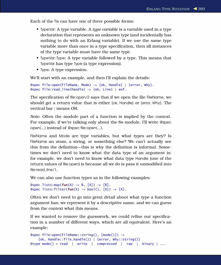
ERLANG TYPE NOTATION 393
Each of the Tis can have one of three possible forms:
• TypeVar: A type variable. A type variable is a variable used in a type
declaration that represents an unknown type (and incidentally has
nothing to do with an Erlang variable). If we use the same type
variable more than once in a type specification, then all instances
of the type variable must have the same type.
• TypeVar::Type: A type variable followed by a type. This means that
TypeVar has type Type (a type expression).
• Type: A type expression.
We’ll start with an example, and then I’ll explain the details:
@spec file:open(FileName, Mode) -> {ok, Handle} | {error, Why}.
@spec file:read_line(Handle) -> {ok, Line} | eof.
The specification of file:open/2 says that if we open the file FileName, we
should get a return value that is either {ok, Handle} or {error, Why}. The
vertical bar | means OR.
Note: Often the module part of a function is implied by the context.
For example, if we’re talking only about the file module, I’ll write @spec
open(...) instead of @spec file:open(...).
FileName and Mode are type variables, but what types are they? Is
FileName an atom, a string, or something else? We can’t actually see
this from the definition—this is why the definition is informal. Some-
times we don’t need to know what the data type of an argument is;
for example, we don’t need to know what data type Handle (one of the
return values of file:open) is because all we do is pass it unmodified into
file:read_line/1.
We can also use function types as in the following examples:
@spec lists:map(fun(A) -> B, [A]) -> [B].
@spec lists:filter(fun(X) -> bool(), [X]) -> [X].
Often we don’t need to go into great detail about what type a function
argument has; we represent it by a descriptive name, and we can guess
from the context what this means.
If we wanted to remove the guesswork, we could refine our specifica-
tion in a number of different ways, which are all equivalent. Here’s an
example:
@spec file:open(FileName::string(), [mode()]) ->
{ok, Handle::file_handle()} | {error, Why::string()}
@type mode() = read | write | compressed | raw | binary | ...

TOOLS THAT USE TYPES 394
Here’s another example:
@spec file:open(string(), Modes) -> {ok, Handle} | {error, string()}
Handle = file_handle(),
Modes = [Mode],
Mode = read | write | compressed | raw | binary | ...
Or here’s even another example:
@spec file:open(string(), [mode()]) -> {ok, file_handle()} | error().
@type error() = {error, string()}.
@type mode() = read | write | compressed | raw | binary | ...
Type Definitions in APIs
When we define APIs in manual pages or in this book, we’ll often use
descriptive lists for function type definitions. In this case we omit the
@spec keyword and write the definition directly. Often we’ll just use type
variables and describe them in the text that follows the description.
Here’s an example, showing part of the file manual page:
file:open(File, [Mode]) -> {ok, Handle} | {error, Why}
Open File (a string) according to Mode. Mode is one of read, write,
and so on. It returns {ok, Handle} if the file could be opened or {error,
Why} where Why is a string describing the error. Once the file has
been successfully opened, it can be accessed through Handle.
file:read_line(Handle) -> {ok, Line} | eof
Read a line from the file opened with Handle. It returns Line (a
string) or eof at end-of-file.
and so on....
A.2 Tools That Use Types
Here are some tools that use types:
EDoc
EDoc is the Erlang program documentation generator. Inspired
by the Javadoc tool for the Java programming language, EDoc is
adapted to the conventions of the Erlang world.
EDoc lets you write the documentation of an Erlang program as
annotations that are embedded in comments in the source code.
These annotations are introduced using tags such as @name,
@doc, @type, @author, and so on.

TOOLS THAT USE TYPES 395
The module edoc exports a large number of functions that can
be used to manipulate Erlang source code files containing Edoc
annotations.
The Dialyzer
The Dialyzer is a static analysis tool that identifies software dis-
crepancies such as type errors, unreachable code, unnecessary
tests, and so on. It works for single Erlang modules or entire (sets
of) applications.
Both these tools are distributed as part of the standard Erlang distri-
bution.

Appendix B
Erlang on Microsoft WindowsI run Erlang on many different platforms, and I like the development
environment to be almost the same on all of them. For Windows I have
found the following setup to be useful. (You might need to change some
of the directory names to match those on your own system.)
Step B.1 is essential for all Windows users. You can follow steps B.2 to
B.4 if you want to have a Unix-like development environment on Win-
dows. You can follow step B.5 if you want to install emacs on Windows
(this is useful since emacs has an advanced mode for editing Erlang
programs).
B.1 Erlang
Go to http://www.erlang.org/download.html, and get the latest Windows
binary (37MB), called otp_win32-R11B-3.exe. When you click the file icon,
Erlang is installed in the default directory. When I did this on my
machine, Erlang was installed in C:\Program Files\erl.5.4.12\.
B.2 Fetch and Install MinGW
MinGW1 stands for Minimalist GNU for Windows.
1. Fetch the MinGW installer. This is a small program (about 130KB)
that talks you through the installation procedure. I used MinGW-
5.0.2.exefrom the download area at http://www.mingw.org/download.shtml.
1. http://www.mingw.org

FETCH AND INSTALL MSYS 397
2. Run the install procedure. Make sure the checkboxes for “MinGW
base tools” and “MinGW make” are selected.
3. Answer Yes to everything. This will install about 44MB of stuff in
the directory C:\MinGW.
B.3 Fetch and Install MSYS
1. Go to http://www.mingw.org/download.shtml, and fetch the latest ver-
sion of MSYS. Look for the current system in the section marked
MSYS, and download the file MSYS-1.0.10.exe (2742KB).
2. Install MSYS-1.0.10.exe by clicking the file icon.
3. Go to the download area of http://sourceforge.net/projects/mingw.
4. Answer the questions. You’ll be asked one question—the location
of MinGW. Reply c:\MinGW.
After this step, you should have a function shell. Selecting Start > Pro-
grams > MinGW > MSYS > msys starts a shell. You should also have a
blue desktop icon that you can click to start the shell.
If you click the icon with a large M on it, you’ll get a shell window where
a lot of your favorite Unix commands will work.
B.4 Install the MSYS Developer Toolkit (Optional)
I do this so I get ssh, and so on. These are “nice to have” but not
essential.
1. Find the file MsysDTK-1.0.1.exe.
2. Use the one-click installer.
B.5 Emacs
1. Go to ftp://ftp.gnu.org/gnu/emacs/windows/, and download the file
emacs-21.3-fullbin-i386.tar.gz.
2. Use WinZip to unpack this into a suitable directory.
3. To complete the installation, navigate to the emacs bin directory,
and click addpm. (This adds a shortcut to emacs in the Start >
Programs tab.) I also make a shortcut to runemacs from my desk-
top.
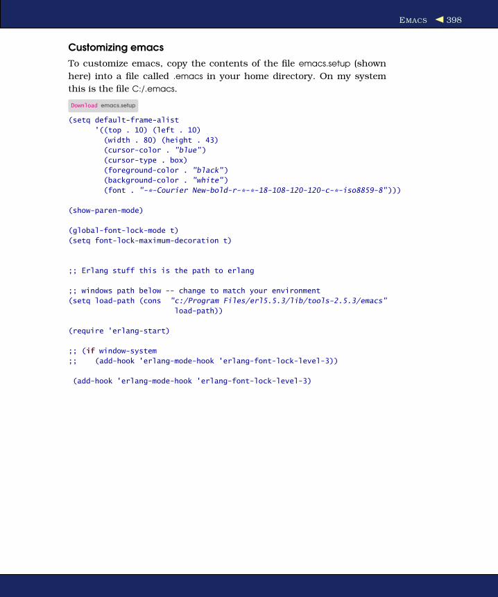
EMACS 398
Customizing emacs
To customize emacs, copy the contents of the file emacs.setup (shown
here) into a file called .emacs in your home directory. On my system
this is the file C:/.emacs.
Download emacs.setup
(setq default-frame-alist
'((top . 10) (left . 10)
(width . 80) (height . 43)
(cursor-color . "blue")
(cursor-type . box)
(foreground-color . "black")
(background-color . "white")
(font . "-*-Courier New-bold-r-*-*-18-108-120-120-c-*-iso8859-8")))
(show-paren-mode)
(global-font-lock-mode t)
(setq font-lock-maximum-decoration t)
;; Erlang stuff this is the path to erlang
;; windows path below -- change to match your environment
(setq load-path (cons "c:/Program Files/erl5.5.3/lib/tools-2.5.3/emacs"
load-path))
(require 'erlang-start)
;; (if window-system
;; (add-hook 'erlang-mode-hook 'erlang-font-lock-level-3))
(add-hook 'erlang-mode-hook 'erlang-font-lock-level-3)
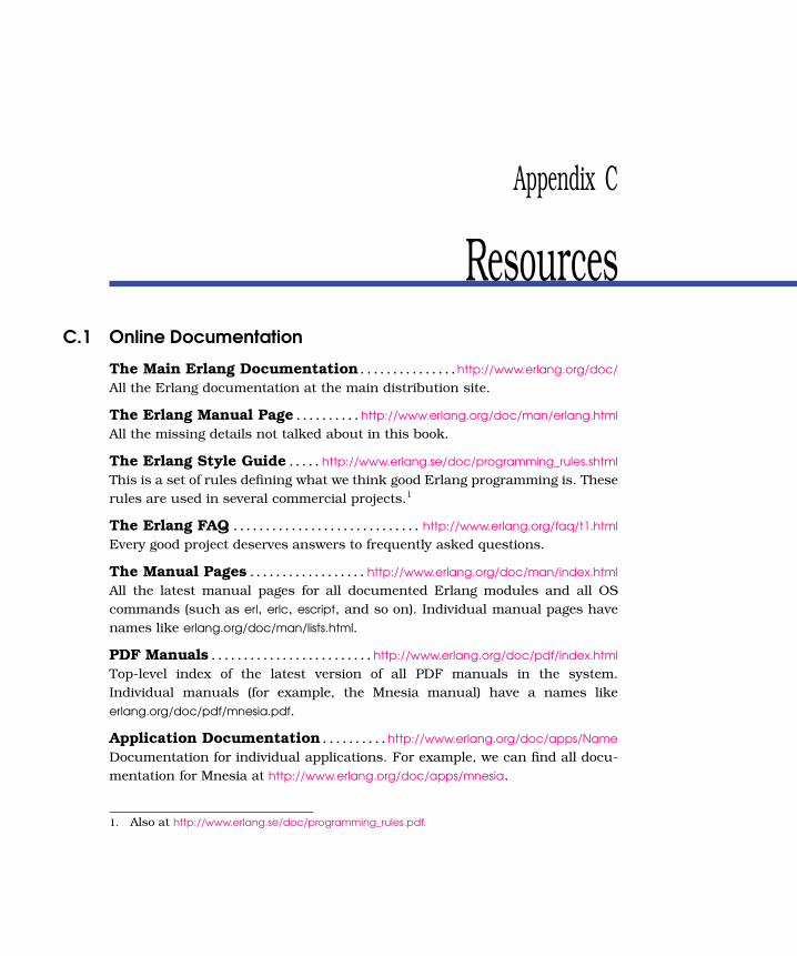
Appendix C
ResourcesC.1 Online Documentation
The Main Erlang Documentation . . . . . . . . . . . . . . .http://www.erlang.org/doc/
All the Erlang documentation at the main distribution site.
The Erlang Manual Page . . . . . . . . . . http://www.erlang.org/doc/man/erlang.html
All the missing details not talked about in this book.
The Erlang Style Guide . . . . . http://www.erlang.se/doc/programming_rules.shtml
This is a set of rules defining what we think good Erlang programming is. These
rules are used in several commercial projects.1
The Erlang FAQ . . . . . . . . . . . . . . . . . . . . . . . . . . . . . http://www.erlang.org/faq/t1.html
Every good project deserves answers to frequently asked questions.
The Manual Pages . . . . . . . . . . . . . . . . . . http://www.erlang.org/doc/man/index.html
All the latest manual pages for all documented Erlang modules and all OS
commands (such as erl, erlc, escript, and so on). Individual manual pages have
names like erlang.org/doc/man/lists.html.
PDF Manuals . . . . . . . . . . . . . . . . . . . . . . . . . http://www.erlang.org/doc/pdf/index.html
Top-level index of the latest version of all PDF manuals in the system.
Individual manuals (for example, the Mnesia manual) have a names like
erlang.org/doc/pdf/mnesia.pdf.
Application Documentation . . . . . . . . . .http://www.erlang.org/doc/apps/Name
Documentation for individual applications. For example, we can find all docu-
mentation for Mnesia at http://www.erlang.org/doc/apps/mnesia.
1. Also at http://www.erlang.se/doc/programming_rules.pdf.
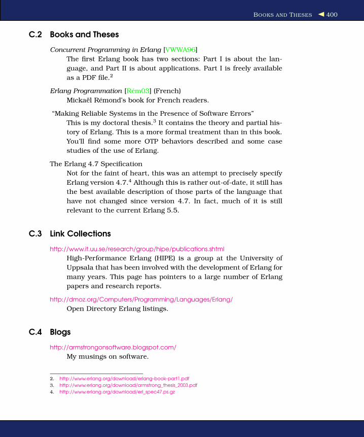
BOOKS AND THESES 400
C.2 Books and Theses
Concurrent Programming in Erlang [VWWA96]
The first Erlang book has two sections: Part I is about the lan-
guage, and Part II is about applications. Part I is freely available
as a PDF file.2
Erlang Programmation [Rém03] (French)
Mickaël Rémond’s book for French readers.
“Making Reliable Systems in the Presence of Software Errors”
This is my doctoral thesis.3 It contains the theory and partial his-
tory of Erlang. This is a more formal treatment than in this book.
You’ll find some more OTP behaviors described and some case
studies of the use of Erlang.
The Erlang 4.7 Specification
Not for the faint of heart, this was an attempt to precisely specify
Erlang version 4.7.4 Although this is rather out-of-date, it still has
the best available description of those parts of the language that
have not changed since version 4.7. In fact, much of it is still
relevant to the current Erlang 5.5.
C.3 Link Collections
http://www.it.uu.se/research/group/hipe/publications.shtml
High-Performance Erlang (HIPE) is a group at the University of
Uppsala that has been involved with the development of Erlang for
many years. This page has pointers to a large number of Erlang
papers and research reports.
http://dmoz.org/Computers/Programming/Languages/Erlang/
Open Directory Erlang listings.
C.4 Blogs
http://armstrongonsoftware.blogspot.com/
My musings on software.
2. http://www.erlang.org/download/erlang-book-part1.pdf
3. http://www.erlang.org/download/armstrong_thesis_2003.pdf
4. http://www.erlang.org/download/erl_spec47.ps.gz

FORUMS, ONLINE COMMUNITIES, AND SOCIAL SITES 401
http://yarivsblog.com/
Yariv Sadan blogs about Erlang and about ErlyWeb, which is a
WEB framework written in Erlang.
http://www.process-one.net/en/blogs/
Blogs by Mickaël Rémond and friends.
C.5 Forums, Online Communities, and Social Sites
http://www.erlang.org/mailman/listinfo
The main Erlang lists. This is mirrored at many sites.
http://www.trapexit.org/
Large Erlang community, including forums, a wiki, and how-tos.
The how-to section5 and the cookbook6 are pretty useful.
Erlounges
Erlounges are held at irregular times and places all over the world.
Erlounges are social events where Erlang users get together (usu-
ally in Pubs or Restaurants) and talk about the joys of program-
ming in Erlang. They are advertised on the Erlang mailing list.
IRC Channels
#erlang on irc.freenode.net.
C.6 Conferences
ACM SIGPLAN Workshop
Annual event. One day.
Erlang User Conference
Annual event.7 Two days.
C.7 Projects
http://jungerl.sourceforge.net/
A large repository of Erlang projects at SourceForge.
5. http://wiki.trapexit.org/index.php/Category:HowTo
6. http://wiki.trapexit.org/index.php/Category:CookBook
7. http://www.erlang.se/euc.

BIBLIOGRAPHY 402
http://cean.process-one.net/
The Comprehensive Erlang Archive Network. An attempt to merge
all ongoing Erlang projects.
http://yaws.hyber.org/
Yet Another Web Server. This is a web server in Erlang that is used
in many commercial products.
http://ejabberd.jabber.ru/
Instant messaging server for the Jabber protocol, written in Erlang.
C.8 Bibliography
[Rém03] Mickaël Rémond. Erlang Programmation. Eyrolles, Paris,
2003.
[VWWA96] Robert Virding, Claes Wikstrom, Mike Williams, and Joe
Armstrong. Concurrent Programming in Erlang. Prentice
Hall, Englewood Cliffs, NJ, second edition, 1996.

Appendix D
A Socket ApplicationThis appendix is devoted to the implementation of the library lib_chan.
We introduced this library in Section 10.5, lib_chan, on page 187, and
we used it Chapter 11, IRC Lite, on page 191.
The code for lib_chan implements an entire layer of networking on top
of TCP/IP, providing both authentication and streams of Erlang terms.
Once we understand the principles used in lib_chan, we should be able
to tailor-make our own communication infrastructure and layer it on
top of TCP/IP.
In its own right, lib_chan is a useful component for building distributed
systems.
To make the appendix self-contained, there is a considerable amount
of overlap with the material in Section 10.5, lib_chan, on page 187.
The code in this appendix is some of the most complex code I’ve intro-
duced so far, so don’t worry if you don’t understand it all on the first
reading. If you just want to use lib_chan and don’t care about how it
works, read the first section and skip the rest.
D.1 An Example
We’ll start with a simple example that shows how to use lib_chan. We’re
going to create a simple server that can compute factorials and Fibo-
nacci numbers. We’ll protect it with a password.
The server will operate on port 2233.
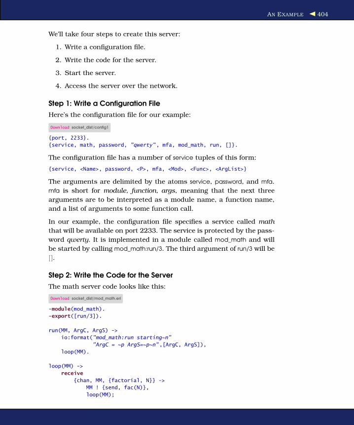
AN EXAMPLE 404
We’ll take four steps to create this server:
1. Write a configuration file.
2. Write the code for the server.
3. Start the server.
4. Access the server over the network.
Step 1: Write a Configuration File
Here’s the configuration file for our example:
Download socket_dist/config1
{port, 2233}.
{service, math, password, "qwerty", mfa, mod_math, run, []}.
The configuration file has a number of service tuples of this form:
{service, <Name>, password, <P>, mfa, <Mod>, <Func>, <ArgList>}
The arguments are delimited by the atoms service, password, and mfa.
mfa is short for module, function, args, meaning that the next three
arguments are to be interpreted as a module name, a function name,
and a list of arguments to some function call.
In our example, the configuration file specifies a service called math
that will be available on port 2233. The service is protected by the pass-
word qwerty. It is implemented in a module called mod_math and will
be started by calling mod_math:run/3. The third argument of run/3 will be
[ ].
Step 2: Write the Code for the Server
The math server code looks like this:
Download socket_dist/mod_math.erl
-module(mod_math).
-export([run/3]).
run(MM, ArgC, ArgS) ->
io:format("mod_math:run starting~n"
"ArgC = ~p ArgS=~p~n",[ArgC, ArgS]),
loop(MM).
loop(MM) ->
receive
{chan, MM, {factorial, N}} ->
MM ! {send, fac(N)},
loop(MM);

AN EXAMPLE 405
{chan, MM, {fibonacci, N}} ->
MM ! {send, fib(N)},
loop(MM);
{chan_closed, MM} ->
io:format("mod_math stopping~n"),
exit(normal)
end.
fac(0) -> 1;
fac(N) -> N*fac(N-1).
fib(1) -> 1;
fib(2) -> 1;
fib(N) -> fib(N-1) + fib(N-2).
When a client connects to port 2233 and requests the service called
math, lib_auth will authenticate the client and, if the password is correct,
spawn a handler process by spawning the function mod_math:run(MM,
ArgC, ArgS). MM is the PID of a middle man. ArgC comes from the client,
and ArgS comes from the configuration file.
When the client sends to a message X to the server, it will arrive as a
{chan, MM, X} message. If the client dies or something goes wrong with
the connection, the server will be sent a {chan_closed, MM} message. To
send a message Y to the client, the server evaluated MM ! {send, Y}, and
to close the communication channel, it evaluated MM ! close.
The math server is simple; it just waits for a {chan, MM, {factorial, N}}
message and then sends the result to the client by evaluating MM !
{send, fac(N)}.
Step 3: Starting the Server
We start the server as follows:
1> lib_chan:start_server("./config1").
lib_chan starting:"./config1"
Terms=[{port,2233},
{service,math,password,"qwerty",
mfa,mod_math,run,[]}]
true
Step 4: Accessing the Server Over the Network
We can test this code on a single machine:
2> {ok, S} = lib_chan:connect("localhost",2233,math,
"qwerty",{yes,go}).
{ok,<0.47.0>}

HOW LIB_CHAN WORKS 406
3> lib_chan:rpc(S, {factorial,20}).
2432902008176640000
4> lib_chan:rpc(S, {fibonacci,15}).
610
4> lib_chan:disconnect(S).
close
mod_math stopping
D.2 How lib_chan Works
lib_chan is built using code in four modules:
• lib_chan acts as a “main module.” The only routines that the pro-
grammer needs to know about are the routines that are exported
from lib_chan. The other three modules (discussed next) are used
internally in the implementation of lib_chan.
• lib_chan_mm encodes and decodes Erlang messages and manages
the socket communication.
• lib_chan_cs sets up the server and manages client connections. One
of its main jobs is to limit the maximum number of simultaneous
client connections.
• lib_chan_auth has code for simple challenge/response authentica-
tion.
lib_chan
lib_chan has the following structure:
-module(lib_chan).
start_server(ConfigFile) ->
%% read configuration file - check syntax
%% call start_port_server(Port, ConfigData)
%% where Port is the required Port and ConfigData
%% contines the configuration data
start_port_server(Port, ConfigData) ->
lib_chan_cs:start_raw_server( ..
fun(Socket) ->
start_port_instance(Socket, ConfigData),
end, ... )
%% lib_chan_cs manages the connection
%% when a new connection comes the fun which is an
%% argument to start_raw_server will be called
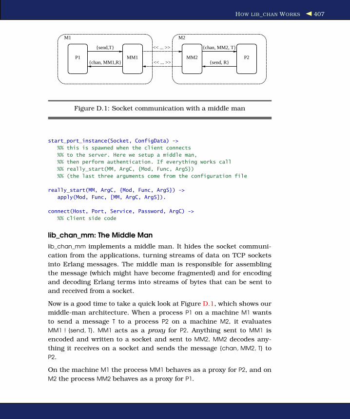
HOW LIB_CHAN WORKS 407
M1
MM1 P1
M2
MM2 P2
{send,T}
{chan, MM1,R}
<< ... >>
<< ... >>
{chan, MM2, T}
{send, R}
Figure D.1: Socket communication with a middle man
start_port_instance(Socket, ConfigData) ->
%% this is spawned when the client connects
%% to the server. Here we setup a middle man,
%% then perform authentication. If everything works call
%% really_start(MM, ArgC, {Mod, Func, ArgS})
%% (the last three arguments come from the configuration file
really_start(MM, ArgC, {Mod, Func, ArgS}) ->
apply(Mod, Func, [MM, ArgC, ArgS]).
connect(Host, Port, Service, Password, ArgC) ->
%% client side code
lib_chan_mm: The Middle Man
lib_chan_mm implements a middle man. It hides the socket communi-
cation from the applications, turning streams of data on TCP sockets
into Erlang messages. The middle man is responsible for assembling
the message (which might have become fragmented) and for encoding
and decoding Erlang terms into streams of bytes that can be sent to
and received from a socket.
Now is a good time to take a quick look at Figure D.1, which shows our
middle-man architecture. When a process P1 on a machine M1 wants
to send a message T to a process P2 on a machine M2, it evaluates
MM1 ! {send, T}. MM1 acts as a proxy for P2. Anything sent to MM1 is
encoded and written to a socket and sent to MM2. MM2 decodes any-
thing it receives on a socket and sends the message {chan, MM2, T} to
P2.
On the machine M1 the process MM1 behaves as a proxy for P2, and on
M2 the process MM2 behaves as a proxy for P1.
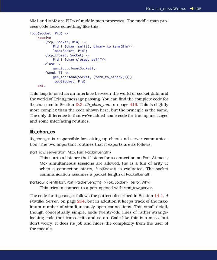
HOW LIB_CHAN WORKS 408
MM1 and MM2 are PIDs of middle-men processes. The middle-man pro-
cess code looks something like this:
loop(Socket, Pid) ->
receive
{tcp, Socket, Bin} ->
Pid ! {chan, self(), binary_to_term(Bin)},
loop(Socket, Pid);
{tcp_closed, Socket} ->
Pid ! {chan_closed, self()};
close ->
gen_tcp:close(Socket);
{send, T} ->
gen_tcp:send(Socket, [term_to_binary(T)]),
loop(Socket, Pid)
end.
This loop is used as an interface between the world of socket data and
the world of Erlang message passing. You can find the complete code for
lib_chan_mm in Section D.3, lib_chan_mm, on page 416. This is slightly
more complex than the code shown here, but the principle is the same.
The only difference is that we’ve added some code for tracing messages
and some interfacing routines.
lib_chan_cs
lib_chan_cs is responsible for setting up client and server communica-
tion. The two important routines that it exports are as follows:
start_raw_server(Port, Max, Fun, PacketLength)
This starts a listener that listens for a connection on Port. At most,
Max simultaneous sessions are allowed. Fun is a fun of arity 1;
when a connection starts, Fun(Socket) is evaluated. The socket
communication assumes a packet length of PacketLength.
start:raw_client(Host, Port, PacketLength) => {ok, Socket} | {error, Why}
This tries to connect to a port opened with start_raw_server.
The code for lib_chan_cs follows the pattern described in Section 14.1, A
Parallel Server, on page 254, but in addition it keeps track of the max-
imum number of simultaneously open connections. This small detail,
though conceptually simple, adds twenty-odd lines of rather strange-
looking code that traps exits and so on. Code like this is a mess, but
don’t worry: it does its job and hides the complexity from the user of
the module.
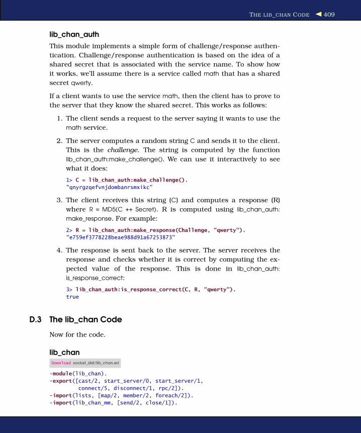
THE LIB_CHAN CODE 409
lib_chan_auth
This module implements a simple form of challenge/response authen-
tication. Challenge/response authentication is based on the idea of a
shared secret that is associated with the service name. To show how
it works, we’ll assume there is a service called math that has a shared
secret qwerty.
If a client wants to use the service math, then the client has to prove to
the server that they know the shared secret. This works as follows:
1. The client sends a request to the server saying it wants to use the
math service.
2. The server computes a random string C and sends it to the client.
This is the challenge. The string is computed by the function
lib_chan_auth:make_challenge(). We can use it interactively to see
what it does:
1> C = lib_chan_auth:make_challenge().
"qnyrgzqefvnjdombanrsmxikc"
3. The client receives this string (C) and computes a response (R)
where R = MD5(C ++ Secret). R is computed using lib_chan_auth:
make_response. For example:
2> R = lib_chan_auth:make_response(Challenge, "qwerty").
"e759ef3778228beae988d91a67253873"
4. The response is sent back to the server. The server receives the
response and checks whether it is correct by computing the ex-
pected value of the response. This is done in lib_chan_auth:
is_response_correct:
3> lib_chan_auth:is_response_correct(C, R, "qwerty").
true
D.3 The lib_chan Code
Now for the code.
lib_chanDownload socket_dist/lib_chan.erl
-module(lib_chan).
-export([cast/2, start_server/0, start_server/1,
connect/5, disconnect/1, rpc/2]).
-import(lists, [map/2, member/2, foreach/2]).
-import(lib_chan_mm, [send/2, close/1]).
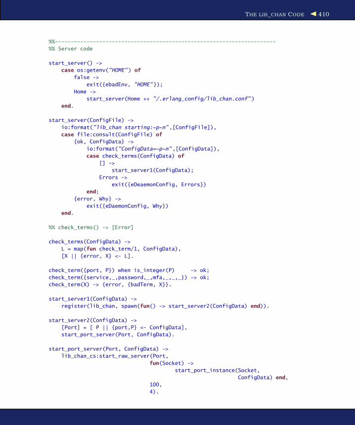
THE LIB_CHAN CODE 410
%%----------------------------------------------------------------------
%% Server code
start_server() ->
case os:getenv("HOME") of
false ->
exit({ebadEnv, "HOME"});
Home ->
start_server(Home ++ "/.erlang_config/lib_chan.conf")
end.
start_server(ConfigFile) ->
io:format("lib_chan starting:~p~n",[ConfigFile]),
case file:consult(ConfigFile) of
{ok, ConfigData} ->
io:format("ConfigData=~p~n",[ConfigData]),
case check_terms(ConfigData) of
[] ->
start_server1(ConfigData);
Errors ->
exit({eDeaemonConfig, Errors})
end;
{error, Why} ->
exit({eDaemonConfig, Why})
end.
%% check_terms() -> [Error]
check_terms(ConfigData) ->
L = map(fun check_term/1, ConfigData),
[X || {error, X} <- L].
check_term({port, P}) when is_integer(P) -> ok;
check_term({service,_,password,_,mfa,_,_,_}) -> ok;
check_term(X) -> {error, {badTerm, X}}.
start_server1(ConfigData) ->
register(lib_chan, spawn(fun() -> start_server2(ConfigData) end)).
start_server2(ConfigData) ->
[Port] = [ P || {port,P} <- ConfigData],
start_port_server(Port, ConfigData).
start_port_server(Port, ConfigData) ->
lib_chan_cs:start_raw_server(Port,
fun(Socket) ->
start_port_instance(Socket,
ConfigData) end,
100,
4).
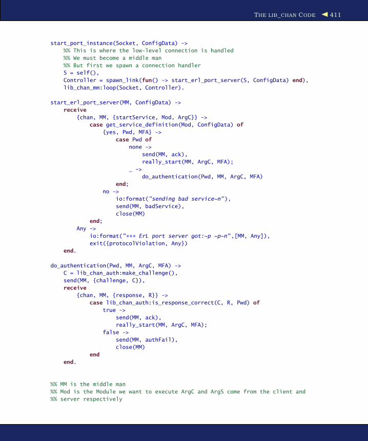
THE LIB_CHAN CODE 411
start_port_instance(Socket, ConfigData) ->
%% This is where the low-level connection is handled
%% We must become a middle man
%% But first we spawn a connection handler
S = self(),
Controller = spawn_link(fun() -> start_erl_port_server(S, ConfigData) end),
lib_chan_mm:loop(Socket, Controller).
start_erl_port_server(MM, ConfigData) ->
receive
{chan, MM, {startService, Mod, ArgC}} ->
case get_service_definition(Mod, ConfigData) of
{yes, Pwd, MFA} ->
case Pwd of
none ->
send(MM, ack),
really_start(MM, ArgC, MFA);
_ ->
do_authentication(Pwd, MM, ArgC, MFA)
end;
no ->
io:format("sending bad service~n"),
send(MM, badService),
close(MM)
end;
Any ->
io:format("*** ErL port server got:~p ~p~n",[MM, Any]),
exit({protocolViolation, Any})
end.
do_authentication(Pwd, MM, ArgC, MFA) ->
C = lib_chan_auth:make_challenge(),
send(MM, {challenge, C}),
receive
{chan, MM, {response, R}} ->
case lib_chan_auth:is_response_correct(C, R, Pwd) of
true ->
send(MM, ack),
really_start(MM, ArgC, MFA);
false ->
send(MM, authFail),
close(MM)
end
end.
%% MM is the middle man
%% Mod is the Module we want to execute ArgC and ArgS come from the client and
%% server respectively

THE LIB_CHAN CODE 412
really_start(MM, ArgC, {Mod, Func, ArgS}) ->
%% authentication worked so now we're off
case (catch apply(Mod,Func,[MM,ArgC,ArgS])) of
{'EXIT', normal} ->
true;
{'EXIT', Why} ->
io:format("server error:~p~n",[Why]);
Why ->
io:format("server error should die with exit(normal) was:~p~n",
[Why])
end.
%% get_service_definition(Name, ConfigData)
get_service_definition(Mod, [{service, Mod, password, Pwd, mfa, M, F, A}|_]) ->
{yes, Pwd, {M, F, A}};
get_service_definition(Name, [_|T]) ->
get_service_definition(Name, T);
get_service_definition(_, []) ->
no.
%%----------------------------------------------------------------------
%% Client connection code
%% connect(...) -> {ok, MM} | Error
connect(Host, Port, Service, Secret, ArgC) ->
S = self(),
MM = spawn(fun() -> connect(S, Host, Port) end),
receive
{MM, ok} ->
case authenticate(MM, Service, Secret, ArgC) of
ok -> {ok, MM};
Error -> Error
end;
{MM, Error} ->
Error
end.
connect(Parent, Host, Port) ->
case lib_chan_cs:start_raw_client(Host, Port, 4) of
{ok, Socket} ->
Parent ! {self(), ok},
lib_chan_mm:loop(Socket, Parent);
Error ->
Parent ! {self(), Error}
end.
authenticate(MM, Service, Secret, ArgC) ->
send(MM, {startService, Service, ArgC}),
%% we should get back a challenge or a ack or closed socket
receive

THE LIB_CHAN CODE 413
{chan, MM, ack} ->
ok;
{chan, MM, {challenge, C}} ->
R = lib_chan_auth:make_response(C, Secret),
send(MM, {response, R}),
receive
{chan, MM, ack} ->
ok;
{chan, MM, authFail} ->
wait_close(MM),
{error, authFail};
Other ->
{error, Other}
end;
{chan, MM, badService} ->
wait_close(MM),
{error, badService};
Other ->
{error, Other}
end.
wait_close(MM) ->
receive
{chan_closed, MM} ->
true
after 5000 ->
io:format("**errror lib_chan~n"),
true
end.
disconnect(MM) -> close(MM).
rpc(MM, Q) ->
send(MM, Q),
receive
{chan, MM, Reply} ->
Reply
end.
cast(MM, Q) ->
send(MM, Q).
lib_chan_csDownload socket_dist/lib_chan_cs.erl
-module(lib_chan_cs).
%% cs stands for client_server
-export([start_raw_server/4, start_raw_client/3]).
-export([stop/1]).
-export([children/1]).

THE LIB_CHAN CODE 414
%% start_raw_server(Port, Fun, Max)
%% This server accepts up to Max connections on Port
%% The *first* time a connection is made to Port
%% Then Fun(Socket) is called.
%% Thereafter messages to the socket result in messages to the handler.
%% tcp_is typically used as follows:
%% To setup a listener
%% start_agent(Port) ->
%% process_flag(trap_exit, true),
%% lib_chan_server:start_raw_server(Port,
%% fun(Socket) -> input_handler(Socket) end,
%% 15,
%% 0).
start_raw_client(Host, Port, PacketLength) ->
gen_tcp:connect(Host, Port,
[binary, {active, true}, {packet, PacketLength}]).
%% Note when start_raw_server returns it should be ready to
%% Immediately accept connections
start_raw_server(Port, Fun, Max, PacketLength) ->
Name = port_name(Port),
case whereis(Name) of
undefined ->
Self = self(),
Pid = spawn_link(fun() ->
cold_start(Self,Port,Fun,Max,PacketLength)
end),
receive
{Pid, ok} ->
register(Name, Pid),
{ok, self()};
{Pid, Error} ->
Error
end;
_Pid ->
{error, already_started}
end.
stop(Port) when integer(Port) ->
Name = port_name(Port),
case whereis(Name) of
undefined ->
not_started;
Pid ->
exit(Pid, kill),
(catch unregister(Name)),
stopped
end.
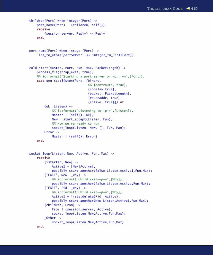
THE LIB_CHAN CODE 415
children(Port) when integer(Port) ->
port_name(Port) ! {children, self()},
receive
{session_server, Reply} -> Reply
end.
port_name(Port) when integer(Port) ->
list_to_atom("portServer" ++ integer_to_list(Port)).
cold_start(Master, Port, Fun, Max, PacketLength) ->
process_flag(trap_exit, true),
%% io:format("Starting a port server on ~p...~n",[Port]),
case gen_tcp:listen(Port, [binary,
%% {dontroute, true},
{nodelay,true},
{packet, PacketLength},
{reuseaddr, true},
{active, true}]) of
{ok, Listen} ->
%% io:format("Listening to:~p~n",[Listen]),
Master ! {self(), ok},
New = start_accept(Listen, Fun),
%% Now we're ready to run
socket_loop(Listen, New, [], Fun, Max);
Error ->
Master ! {self(), Error}
end.
socket_loop(Listen, New, Active, Fun, Max) ->
receive
{istarted, New} ->
Active1 = [New|Active],
possibly_start_another(false,Listen,Active1,Fun,Max);
{'EXIT', New, _Why} ->
%% io:format("Child exit=~p~n",[Why]),
possibly_start_another(false,Listen,Active,Fun,Max);
{'EXIT', Pid, _Why} ->
%% io:format("Child exit=~p~n",[Why]),
Active1 = lists:delete(Pid, Active),
possibly_start_another(New,Listen,Active1,Fun,Max);
{children, From} ->
From ! {session_server, Active},
socket_loop(Listen,New,Active,Fun,Max);
_Other ->
socket_loop(Listen,New,Active,Fun,Max)
end.
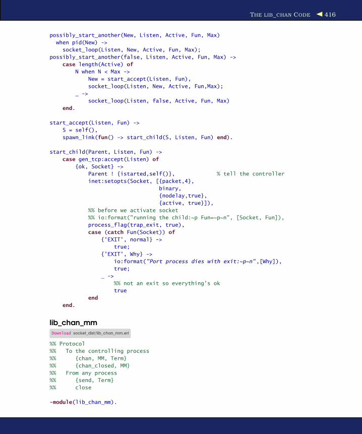
THE LIB_CHAN CODE 416
possibly_start_another(New, Listen, Active, Fun, Max)
when pid(New) ->
socket_loop(Listen, New, Active, Fun, Max);
possibly_start_another(false, Listen, Active, Fun, Max) ->
case length(Active) of
N when N < Max ->
New = start_accept(Listen, Fun),
socket_loop(Listen, New, Active, Fun,Max);
_ ->
socket_loop(Listen, false, Active, Fun, Max)
end.
start_accept(Listen, Fun) ->
S = self(),
spawn_link(fun() -> start_child(S, Listen, Fun) end).
start_child(Parent, Listen, Fun) ->
case gen_tcp:accept(Listen) of
{ok, Socket} ->
Parent ! {istarted,self()}, % tell the controller
inet:setopts(Socket, [{packet,4},
binary,
{nodelay,true},
{active, true}]),
%% before we activate socket
%% io:format("running the child:~p Fun=~p~n", [Socket, Fun]),
process_flag(trap_exit, true),
case (catch Fun(Socket)) of
{'EXIT', normal} ->
true;
{'EXIT', Why} ->
io:format("Port process dies with exit:~p~n",[Why]),
true;
_ ->
%% not an exit so everything's ok
true
end
end.
lib_chan_mmDownload socket_dist/lib_chan_mm.erl
%% Protocol
%% To the controlling process
%% {chan, MM, Term}
%% {chan_closed, MM}
%% From any process
%% {send, Term}
%% close
-module(lib_chan_mm).
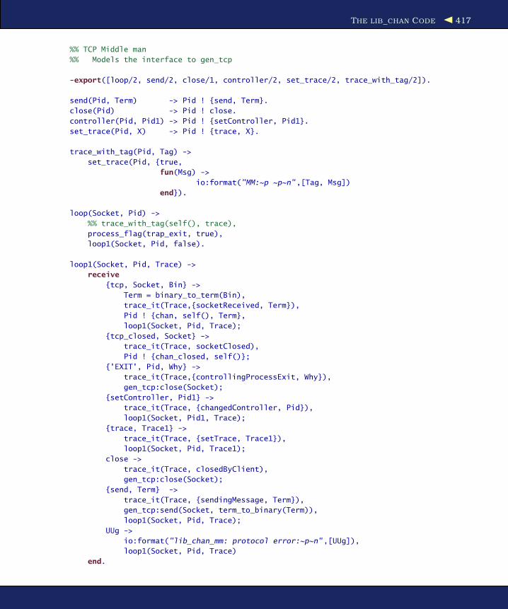
THE LIB_CHAN CODE 417
%% TCP Middle man
%% Models the interface to gen_tcp
-export([loop/2, send/2, close/1, controller/2, set_trace/2, trace_with_tag/2]).
send(Pid, Term) -> Pid ! {send, Term}.
close(Pid) -> Pid ! close.
controller(Pid, Pid1) -> Pid ! {setController, Pid1}.
set_trace(Pid, X) -> Pid ! {trace, X}.
trace_with_tag(Pid, Tag) ->
set_trace(Pid, {true,
fun(Msg) ->
io:format("MM:~p ~p~n",[Tag, Msg])
end}).
loop(Socket, Pid) ->
%% trace_with_tag(self(), trace),
process_flag(trap_exit, true),
loop1(Socket, Pid, false).
loop1(Socket, Pid, Trace) ->
receive
{tcp, Socket, Bin} ->
Term = binary_to_term(Bin),
trace_it(Trace,{socketReceived, Term}),
Pid ! {chan, self(), Term},
loop1(Socket, Pid, Trace);
{tcp_closed, Socket} ->
trace_it(Trace, socketClosed),
Pid ! {chan_closed, self()};
{'EXIT', Pid, Why} ->
trace_it(Trace,{controllingProcessExit, Why}),
gen_tcp:close(Socket);
{setController, Pid1} ->
trace_it(Trace, {changedController, Pid}),
loop1(Socket, Pid1, Trace);
{trace, Trace1} ->
trace_it(Trace, {setTrace, Trace1}),
loop1(Socket, Pid, Trace1);
close ->
trace_it(Trace, closedByClient),
gen_tcp:close(Socket);
{send, Term} ->
trace_it(Trace, {sendingMessage, Term}),
gen_tcp:send(Socket, term_to_binary(Term)),
loop1(Socket, Pid, Trace);
UUg ->
io:format("lib_chan_mm: protocol error:~p~n",[UUg]),
loop1(Socket, Pid, Trace)
end.

THE LIB_CHAN CODE 418
trace_it(false, _) -> void;
trace_it({true, F}, M) -> F(M).
lib_chan_authDownload socket_dist/lib_chan_auth.erl
-module(lib_chan_auth).
-export([make_challenge/0, make_response/2, is_response_correct/3]).
make_challenge() ->
random_string(25).
make_response(Challenge, Secret) ->
lib_md5:string(Challenge ++ Secret).
is_response_correct(Challenge, Response, Secret) ->
case lib_md5:string(Challenge ++ Secret) of
Response -> true;
_ -> false
end.
%% random_string(N) -> a random string with N characters.
random_string(N) -> random_seed(), random_string(N, []).
random_string(0, D) -> D;
random_string(N, D) ->
random_string(N-1, [random:uniform(26)-1+$a|D]).
random_seed() ->
{_,_,X} = erlang:now(),
{H,M,S} = time(),
H1 = H * X rem 32767,
M1 = M * X rem 32767,
S1 = S * X rem 32767,
put(random_seed, {H1,M1,S1}).

Appendix E
MiscellaneousThis appendix presents material about analyzing and debugging code,
and it describes how dynamic code loading works.
E.1 Analysis and Profiling Tools
How can we look into our running program? How can we look for poten-
tial problem code, investigate performance problems, and check for
dead code or the use of deprecated functions? That’s what this section
is all about.
Coverage
When we’re testing our code, it’s often nice to see not only which lines
of code are executed a lot but also which lines are never executed. Lines
of code that are never executed are a potential source of error, so it’s
really good to find out where these are. To do this, we use the program
coverage analyzer.
Here’s an example:
1> cover:start(). %% start the coverage analyser
{ok,<0.34.0>}
2> cover:compile(shout). %% compile shout.erl for coverage
{ok,shout}
3> shout:start(). %% run the program
<0.41.0>
Playing:<<"title: track018 performer: .. ">>
4> %% let the program run for a bit
4> cover:analyse_to_file(shout). %% analyse the results
{ok,"shout.COVER.out"} %% this is the results file

ANALYSIS AND PROFILING TOOLS 420
The Best of All Test Methods?
Performing a coverage analysis of our code answers the ques-tion, Which lines of code are never executed? Once we knowwhich lines of code are never executed, we can design testcases that force these lines of code to be executed.
Doing this is a surefire way to find unexpected and obscurebugs in your program. Every line of code that has never beenexecuted might contain an error. Forcing these lines to be exe-cuted is the best way I know to test a program.
I did this to the original Erlang JAM∗ compiler. I think we gotthree bug reports in two years. After this, there were no reportedbugs.
∗. Joe’s Abstract Machine (the first Erlang compiler)
The results of this are printed to a file:
...
| send_file(S, Header, OffSet, Stop, Socket, SoFar) ->
| %% OffSet = first byte to play
| %% Stop = The last byte we can play
131..| Need = ?CHUNKSIZE - size(SoFar),
131..| Last = OffSet + Need,
131..| if
| Last >= Stop ->
| %% not enough data so read as much as possible and return
0..| Max = Stop - OffSet,
0..| {ok, Bin} = file:pread(S, OffSet, Max),
0..| list_to_binary([SoFar, Bin]);
| true ->
131..| {ok, Bin} = file:pread(S, OffSet, Need),
131..| write_data(Socket, SoFar, Bin, Header),
131..| send_file(S, bump(Header),
| OffSet + Need, Stop, Socket, <<>>)
| end.
...
On the left side of the file, we see the number of times each statement
has been executed. The lines marked with a zero are particularly inter-
esting. Since this code has never been executed, we can’t really say
whether our program is correct.
Designing test cases that cause all the coverage counts to be greater
than zero is a valuable method of systematically finding hidden faults
in our programs.
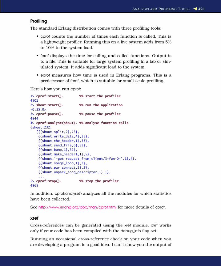
ANALYSIS AND PROFILING TOOLS 421
Profiling
The standard Erlang distribution comes with three profiling tools:
• cprof counts the number of times each function is called. This is
a lightweight profiler. Running this on a live system adds from 5%
to 10% to the system load.
• fprof displays the time for calling and called functions. Output is
to a file. This is suitable for large system profiling in a lab or sim-
ulated system. It adds significant load to the system.
• eprof measures how time is used in Erlang programs. This is a
predecessor of fprof, which is suitable for small-scale profiling.
Here’s how you run cprof:
1> cprof:start(). %% start the profiler
4501
2> shout:start(). %% run the application
<0.35.0>
3> cprof:pause(). %% pause the profiler
4844
4> cprof:analyse(shout). %% analyse function calls
{shout,232,
[{{shout,split,2},73},
{{shout,write_data,4},33},
{{shout,the_header,1},33},
{{shout,send_file,6},33},
{{shout,bump,1},32},
{{shout,make_header1,1},5},
{{shout,'-got_request_from_client/3-fun-0-',1},4},
{{shout,songs_loop,1},2},
{{shout,par_connect,2},2},
{{shout,unpack_song_descriptor,1},1},
...
5> cprof:stop(). %% stop the profiler
4865
In addition, cprof:analyse() analyzes all the modules for which statistics
have been collected.
See http://www.erlang.org/doc/man/cprof.html for more details of cprof.
xref
Cross-references can be generated using the xref module. xref works
only if your code has been compiled with the debug_info flag set.
Running an occasional cross-reference check on your code when you
are developing a program is a good idea. I can’t show you the output of

DEBUGGING 422
xref on the code accompanying this book, because the development is
complete and there aren’t any missing functions. Instead, I’ll show you
what happens when I run a cross-reference check on the code in one of
my hobby projects.
vsg is a simple graphics program that I might release one day. We’ll do
an analysis of the code in the vsg directory where I’m developing the
program:
$ cd /home/joe/2007/vsg-1.6
$ rm *.beam
$ erlc +debug_info *.erl
$ erl
1> xref:d('.')
[{deprecated,[]},
{undefined,[{{new,win1,0},{wish_manager,on_destroy,2}},
{{vsg,alpha_tag,0},{wish_manager,new_index,0}},
{{vsg,call,1},{wish,cmd,1}},
{{vsg,cast,1},{wish,cast,1}},
{{vsg,mkWindow,7},{wish,start,0}},
{{vsg,new_tag,0},{wish_manager,new_index,0}},
{{vsg,new_win_name,0},{wish_manager,new_index,0}},
{{vsg,on_click,2},{wish_manager,bind_event,2}},
{{vsg,on_move,2},{wish_manager,bind_event,2}},
{{vsg,on_move,2},{wish_manager,bind_tag,2}},
{{vsg,on_move,2},{wish_manager,new_index,0}}]},
{unused,[{vsg,new_tag,0},
{vsg_indicator_box,theValue,1},
{vsg_indicator_box,theValue,1}]}]
xref:d(’.’) performs a cross-reference analysis of all the code in the cur-
rent directory that has been compiled with the debug flag. It produces
lists of depreciated, undefined, and unused functions.
Like most tools, xref has a large number of options, so reading the man-
ual is necessary if you want to use the more powerful features that this
program has.
E.2 Debugging
Debugging Erlang is pretty easy. That might surprise you, but this is
a consequence of having single-assignment variables. Since Erlang has
no pointers and no mutable state (with the exception of ETS tables
and process dictionaries), finding out where things have gone wrong is
rarely a problem. Once we have observed that a variable has an incor-
rect value, it’s relatively easy to find out when and where this happened.

DEBUGGING 423
I find a debugger is a very helpful tool when I write C programs, because
I can tell it to watch variables and tell me when their value changes.
This is often important because memory in C can be changed indirectly,
via pointers. It can be hard to know just where a change to some chunk
of memory came from. I don’t feel the same need for a debugger in
Erlang because we can’t modify state through pointers.
In the following sections, we’ll look at Erlang’s compiler diagnostics,
followed by the different ways of debugging a program. They are in
order of difficulty. Debugging using print statements is the easiest way
to debug your program. Tracing a process is the most complex. We have
concentrated on the easiest methods here.
Compiler Diagnostics
When we compile a program, the compiler provides us with helpful error
messages if our source code is syntactically incorrect. Most of these are
self-evident: if we omit a bracket, a comma, or a keyword, the compiler
will give an error message with the filename and line number of the
offending statement. The following are some errors we could see.
Head Mismatch
We’ll get this error if the clauses that make up a function definition do
not have the same name and arity:
Download bad.erl
Line 1 foo(1,2) ->- a;- foo(2,3,a) ->- b.
1> c(bad).
./bad.erl:3: head mismatch
Unbound Variables
Here’s some code containing unbound variables:
Download bad.erl
Line 1 foo(A, B) ->- bar(A, dothis(X), B),- baz(Y, X).
1> c(bad).
./bad.erl:2: variable 'X' is unbound
./bad.erl:3: variable 'Y' is unbound

DEBUGGING 424
This means that in line 2 the variable X has no value. The error isn’t
actually on line 2 but is detected at line 2, which is the first occurrence
of the unbound variable X. (X is also used on line 3, but the compiler
reports only the first line where the error occurs.)
Unterminated String
unterminated string starting with "..."
If we forget a quote mark in a string or atom, we’ll get this error mes-
sage. Sometimes finding the missing quote mark can be pretty tricky.
If you get this message and really can’t see where the missing quote
is, then try placing a quote mark anywhere in your program (or, better,
near to where you think the problem might be). If you recompile the
program, you might get a more precise diagnostic that will help you
pinpoint the error.
Unsafe Variables
If we compile the following code:
Download bad.erl
Line 1 foo() ->- case bar() of- 1 ->- X = 1,5 Y = 2;- 2 ->- X = 3- end,- b(X).
we’ll get a warning:
1> c(bad).
./bad.erl:5: Warning: variable 'Y' is unused
{ok,bad}
This is just a warning, since Y is defined but not used. If we now change
the program to the following:
Download bad.erl
Line 1 foo() ->- case bar() of- 1 ->- X = 1,5 Y = 2;- 2 ->- X = 3- end,- b(X, Y).

DEBUGGING 425
we’ll get an error:
> c(bad).
./bad.erl:9: variable 'Y' unsafe in 'case' (line 2)
{ok,bad}
The compiler reasons that the program might take the second branch
through the case expression (in which event the variable Y will be unde-
fined), so it produces an “unsafe variable” error message.
Shadowed Variables
Download bad.erl
Line 1 foo(X, L) ->- lists:map(fun(X) -> 2*X end, L).
1> c(bad).
./bad.erl:1: Warning: variable 'X' is unused
./bad.erl:2: Warning: variable 'X' shadowed in 'fun'
{ok,bad}
Here, the compiler is worried that we might have made a mistake in
our program. Inside the fun we compute 2*X, but which X are we talk-
ing about: the X that is the argument to the fun or the X that is the
argument to foo?
If this happens, the best thing to do is to rename one of the Xs to make
the warning go away. We could rewrite this as follows:
Download bad.erl
foo(X, L) ->
lists:map(fun(Z) -> 2*Z end, L).
Now there is no problem if we want to use X inside the fun definition.
Runtime Diagnostics
If an Erlang process crashes, we might get an error message. To see the
error message, some other process has to monitor the crashing process
and print an error message when the monitored process dies. If we just
create a process with spawn and the process dies, we won’t get any error
message. The best thing to do if we want to see all the error messages
is always to use spawn_link.
The Stack Trace
Every time a process crashes that is linked to the shell, a stack trace
will be printed.

DEBUGGING 426
To see what’s in the stack trace, we’ll write a simple function with a
deliberate error and call this function from the shell:
Download lib_misc.erl
deliberate_error(A) ->
bad_function(A, 12),
lists:reverse(A).
bad_function(A, _) ->
{ok, Bin} = file:open({abc,123}, A),
binary_to_list(Bin).
1> lib_misc:deliberate_error("file.erl").
** exited: {{badmatch,{error,einval}},
[{lib_misc,bad_function,2},
{lib_misc,deliberate_error,1},
{erl_eval,do_apply,5},
{shell,exprs,6},
{shell,eval_loop,3}]} **
When we called lib_misc:deliberate_error("file.erl"), an error occurred, and
we got a stack trace. Starting at the top of the stack trace, we see the
following line:
{badmatch,{error,einval}}
This comes from the line:
{ok, Bin} = file:open({abc,123}, A),
Calling file:open/2 returned {error, einval}.1 This was because {abc,123} is
not a valid input value to file:open. When we try to match the return
value with {ok, Bin}, we get a badmatch error, and the runtime system
prints {badmatch, {error, einval}}, which is the value that could not be
matched. Following this is a stack trace. The stack trace starts with the
name of the function where the error occurred. This is followed by a list
of the names of the functions that the current function will return to
when it completes. Thus, the error occurred in lib_misc:bad_function/2,
which would have returned to lib_misc:deliberate_error/1, and so on.
Note that it is really only the top entries in the stack trace that are
interesting. If the call sequence to the erroneous function involves a
tail call, then the call won’t be in the stack trace. To see this, we’ll
rename the function deliberate_error and change it the following:
Download lib_misc.erl
deliberate_error1(A) ->
bad_function(A, 12).
1. einval is a POSIX error code short for invalid value.
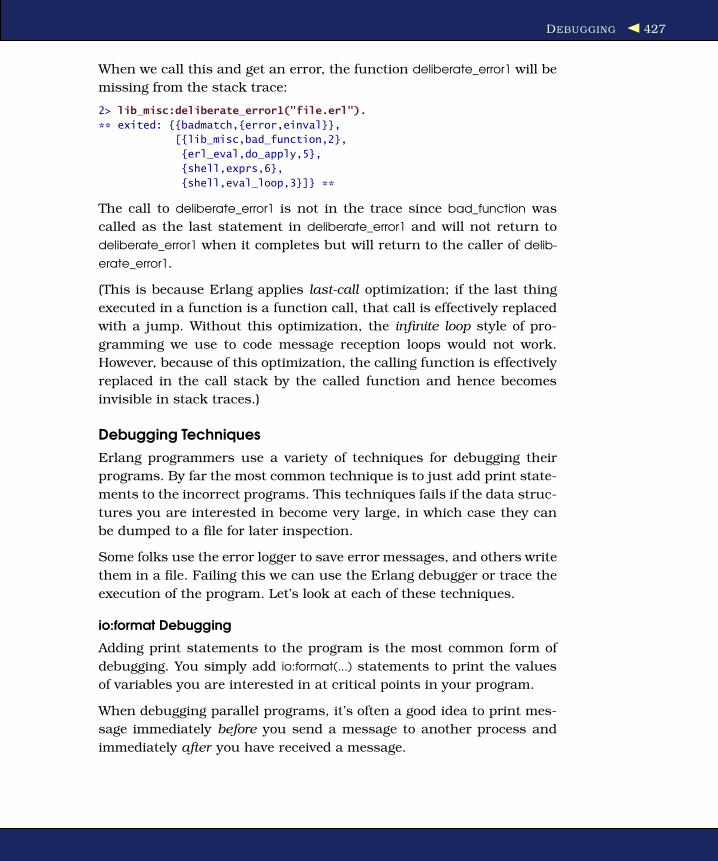
DEBUGGING 427
When we call this and get an error, the function deliberate_error1 will be
missing from the stack trace:
2> lib_misc:deliberate_error1("file.erl").
** exited: {{badmatch,{error,einval}},
[{lib_misc,bad_function,2},
{erl_eval,do_apply,5},
{shell,exprs,6},
{shell,eval_loop,3}]} **
The call to deliberate_error1 is not in the trace since bad_function was
called as the last statement in deliberate_error1 and will not return to
deliberate_error1 when it completes but will return to the caller of delib-
erate_error1.
(This is because Erlang applies last-call optimization; if the last thing
executed in a function is a function call, that call is effectively replaced
with a jump. Without this optimization, the infinite loop style of pro-
gramming we use to code message reception loops would not work.
However, because of this optimization, the calling function is effectively
replaced in the call stack by the called function and hence becomes
invisible in stack traces.)
Debugging Techniques
Erlang programmers use a variety of techniques for debugging their
programs. By far the most common technique is to just add print state-
ments to the incorrect programs. This techniques fails if the data struc-
tures you are interested in become very large, in which case they can
be dumped to a file for later inspection.
Some folks use the error logger to save error messages, and others write
them in a file. Failing this we can use the Erlang debugger or trace the
execution of the program. Let’s look at each of these techniques.
io:format Debugging
Adding print statements to the program is the most common form of
debugging. You simply add io:format(...) statements to print the values
of variables you are interested in at critical points in your program.
When debugging parallel programs, it’s often a good idea to print mes-
sage immediately before you send a message to another process and
immediately after you have received a message.
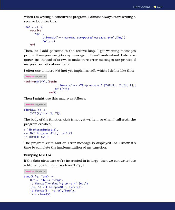
DEBUGGING 428
When I’m writing a concurrent program, I almost always start writing a
receive loop like this:
loop(...) ->
receive
Any ->
io:format("*** warning unexpected message:~p~n",[Any])
loop(...)
end
Then, as I add patterns to the receive loop, I get warning messages
printed if my process gets any message it doesn’t understand. I also use
spawn_link instead of spawn to make sure error messages are printed if
my process exits abnormally.
I often use a macro NYI (not yet implemented), which I define like this:
Download lib_misc.erl
-define(NYI(X),(begin
io:format("*** NYI ~p ~p ~p~n",[?MODULE, ?LINE, X]),
exit(nyi)
end)).
Then I might use this macro as follows:
Download lib_misc.erl
glurk(X, Y) ->
?NYI({glurk, X, Y}).
The body of the function glurk is not yet written, so when I call glurk, the
program crashes:
> lib_misc:glurk(1,2).
*** NYI lib_misc 83 {glurk,1,2}
** exited: nyi *
The program exits and an error message is displayed, so I know it’s
time to complete the implementation of my function.
Dumping to a File
If the data structure we’re interested in is large, then we can write it to
a file using a function such as dump/2:
Download lib_misc.erl
dump(File, Term) ->
Out = File ++ ".tmp",
io:format("** dumping to ~s~n",[Out]),
{ok, S} = file:open(Out, [write]),
io:format(S, "~p.~n",[Term]),
file:close(S).

DEBUGGING 429
This prints a warning message to remind us that we have created a
new file. It then adds a .tmp file extension to the filename (so we can
easily delete all the temporary files later). Then it pretty-prints the term
we are interested in to a file. We can examine the file in a text editor
at a later stage. This technique is simple and particularly useful when
examining large data structures.
Using the Error Logger
We can use the error logger and create a text file with debugging output.
To do so, we create a configuration file such as the following:
Download elog5.config
%% text erorr log
[ {kernel,
[{error_logger,
{file, "/home/joe/error_logs/debug.log"}}]}].
Then we start Erlang with the following command:
erl -config elog5.config
Any error messages created by calling routines in the error_logger mod-
ule, along with any error messages printed in the shell, will end up in
the file specified in the configuration file.
The Debugger
The standard Erlang distribution contains a debugger. I’m not going to
say a lot about it here, other than to tell you how to start it and to give
you pointers to the documentation. Using the debugger once it has been
started is pretty easy. You can inspect variables, single-step the code,
set breakpoints, and so on. Because we’ll often want to debug several
processes, the debugger can also spawn copies of itself, so we can have
several debug windows, one for each process we are debugging.
The only tricky thing is getting the debugger started:
1> %% recompile lib_misc so we can debug it
1> c(lib_misc, [debug_info]).
{ok, lib_misc}
2> im(). %% A window will pop up. Ignore it for now
<0.42.0>
3> ii(lib_misc).
{module,lib_misc}
4> iaa([init]).
true.
5> lib_misc:
...
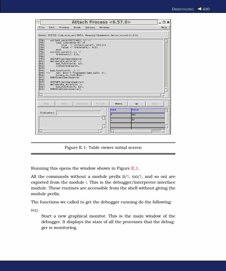
DEBUGGING 430
Figure E.1: Table viewer initial screen
Running this opens the window shown in Figure E.1.
All the commands without a module prefix (ii/1, iaa/1, and so on) are
exported from the module i. This is the debugger/interpreter interface
module. These routines are accessible from the shell without giving the
module prefix.
The functions we called to get the debugger running do the following:
im()
Start a new graphical monitor. This is the main window of the
debugger. It displays the state of all the processes that the debug-
ger is monitoring.

TRACING 431
ii(Mod)
Interpret the code in the module Mod.
iaa([init])
Attach the debugger to any process executing interpreted code
when that process is started.
Digging Deeper
To learn more about debugging, try these resources:
http://www.erlang.org/doc/pdf/debugger.pdf
The debugger reference manual (a 46-page PDF file) is an intro-
duction to the debugger, with screen dumps, API documentation,
and more. It’s a must-read for serious users of the debugger.
http://www.erlang.org/doc/man/i.html
Here you can find the debugger commands that are available in
the shell.
E.3 Tracing
You can always trace a process without having to compile your code
in a special way. Tracing a process (or processes) provides a powerful
way of understanding how your system behaves and can be used to
test complex systems without modifying the code. This is particularly
useful in embedded systems or where you cannot modify the code being
tested.
At a low-level, we can set up a trace by calling a number of Erlang BIFs.
Using these BIFs for setting up complex traces is difficult, so several
libraries are designed to make this task easier.
We’ll start by looking at the low-level Erlang BIFs for tracing and see
how to set up a simple tracer; then we’ll review the libraries that can
provide a higher-level interface to the trace BIFs.
For low-level tracing, two BIFs are particularly important. erlang:trace/3
says, basically, “I want to monitor this process, so please send me a
message if something interesting happens.” erlang:trace_pattern defines
what counts as being “interesting.”

TRACING 432
erlang:trace(PidSpec, How, FlagList)
This starts tracing. PidSpec tells the system what to trace. How is
a boolean that can turn the trace on or off. FlagList governs what
is to be traced (for example, we can trace all function calls, all
messages being sent, when garbage collections occur, and so on).
Once we have called erlang:trace/3, the process that called this
BIF will be sent trace message when trace events occur. The trace
events themselves are determined by calling erlang:trace_pattern/3.
erlang:trace_pattern(MFA, MatchSpec, FlagList)
This is used to set up a trace pattern. If the pattern is matched,
then the actions requested are performed. Here MFA is a {Mod-
ule, Function, Args} tuple that says to which code the trace pattern
applies. MatchSpec is a pattern that is tested every time the func-
tion specified by MFA is entered, and FlagList tells what to do if the
tracing conditions are satisfied.
Writing match specifications for MatchSpec is complicated and doesn’t
really add much to our understanding of tracing. Fortunately, some
libraries2 make this easier.
Using the previous two BIFs, we can write a simple tracer. trace_
module(Mod, Fun) sets up tracing on the module Mod and then evalu-
ates Fun(). We want to trace all function calls and return values in the
module Mod.
Download tracer_test.erl
trace_module(Mod, StartFun) ->
%% We'll spawn a process to do the tracing
spawn(fun() -> trace_module1(Mod, StartFun) end).
trace_module1(Mod, StartFun) ->
%% The next line says: trace all function calls and return
%% values in Mod
erlang:trace_pattern({Mod, '_','_'},
[{'_',[],[{return_trace}]}],
[local]),
%% spawn a function to do the tracing
S = self(),
Pid = spawn(fun() -> do_trace(S, StartFun) end),
%% setup the trace. Tell the system to start tracing
%% the process Pid
erlang:trace(Pid, true, [call,procs]),
2. http://www.erlang.org/doc/man/ms_transform.html
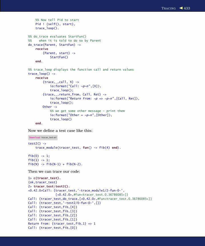
TRACING 433
%% Now tell Pid to start
Pid ! {self(), start},
trace_loop().
%% do_trace evaluates StartFun()
%% when it is told to do so by Parent
do_trace(Parent, StartFun) ->
receive
{Parent, start} ->
StartFun()
end.
%% trace_loop displays the function call and return values
trace_loop() ->
receive
{trace,_,call, X} ->
io:format("Call: ~p~n",[X]),
trace_loop();
{trace,_,return_from, Call, Ret} ->
io:format("Return From: ~p => ~p~n",[Call, Ret]),
trace_loop();
Other ->
%% we get some other message - print them
io:format("Other = ~p~n",[Other]),
trace_loop()
end.
Now we define a test case like this:
Download tracer_test.erl
test2() ->
trace_module(tracer_test, fun() -> fib(4) end).
fib(0) -> 1;
fib(1) -> 1;
fib(N) -> fib(N-1) + fib(N-2).
Then we can trace our code:
1> c(tracer_test).
{ok,tracer_test}
2> tracer_test:test2().
<0.42.0>Call: {tracer_test,'-trace_module1/2-fun-0-',
[<0.42.0>,#Fun<tracer_test.0.36786085>]}
Call: {tracer_test,do_trace,[<0.42.0>,#Fun<tracer_test.0.36786085>]}
Call: {tracer_test,'-test2/0-fun-0-',[]}
Call: {tracer_test,fib,[4]}
Call: {tracer_test,fib,[3]}
Call: {tracer_test,fib,[2]}
Call: {tracer_test,fib,[1]}
Return From: {tracer_test,fib,1} => 1
Call: {tracer_test,fib,[0]}

TRACING 434
Return From: {tracer_test,fib,1} => 1
Return From: {tracer_test,fib,1} => 2
Call: {tracer_test,fib,[1]}
Return From: {tracer_test,fib,1} => 1
Return From: {tracer_test,fib,1} => 3
Call: {tracer_test,fib,[2]}
Call: {tracer_test,fib,[1]}
Return From: {tracer_test,fib,1} => 1
Call: {tracer_test,fib,[0]}
Return From: {tracer_test,fib,1} => 1
Return From: {tracer_test,fib,1} => 2
Return From: {tracer_test,fib,1} => 5
Return From: {tracer_test,'-test2/0-fun-0-',0} => 5
Return From: {tracer_test,do_trace,2} => 5
Return From: {tracer_test,'-trace_module1/2-fun-0-',2} => 5
Other = {trace,<0.43.0>,exit,normal}
Using the Libraries
We can perform the same trace as the previous one using the library
module dbg. This hides all the details of the low-level Erlang BIFs.
Download tracer_test.erl
test1() ->
dbg:tracer(),
dbg:tpl(tracer_test,fib,'_',
dbg:fun2ms(fun(_) -> return_trace() end)),
dbg:p(all,[c]),
tracer_test:fib(4).
Running this, we get the following:
1> tracer_test:test1().
(<0.34.0>) call tracer_test:fib(4)
(<0.34.0>) call tracer_test:fib(3)
(<0.34.0>) call tracer_test:fib(2)
(<0.34.0>) call tracer_test:fib(1)
(<0.34.0>) returned from tracer_test:fib/1 -> 1
(<0.34.0>) call tracer_test:fib(0)
(<0.34.0>) returned from tracer_test:fib/1 -> 1
(<0.34.0>) returned from tracer_test:fib/1 -> 2
(<0.34.0>) call tracer_test:fib(1)
(<0.34.0>) returned from tracer_test:fib/1 -> 1
(<0.34.0>) returned from tracer_test:fib/1 -> 3
(<0.34.0>) call tracer_test:fib(2)
(<0.34.0>) call tracer_test:fib(1)
(<0.34.0>) returned from tracer_test:fib/1 -> 1
(<0.34.0>) call tracer_test:fib(0)
(<0.34.0>) returned from tracer_test:fib/1 -> 1
(<0.34.0>) returned from tracer_test:fib/1 -> 2
(<0.34.0>) returned from tracer_test:fib/1 -> 5

DYNAMIC CODE LOADING 435
Digging Deeper
To learn more about tracing, you need to read three manual pages for
the following modules:
• dbg provides a simplified interface to the Erlang trace BIFs.
• ttb is yet another interface to the trace BIFs. It is higher level than
dbg.
• ms_transform makes match specifications for use in the tracer soft-
ware.
E.4 Dynamic Code Loading
Dynamic code loading is one of the most surprising features built into
the heart of Erlang. The nice part is that it just works without you really
being aware of what’s happening in the background.
The idea is simple: every time we call someModule:someFunction(...), we’ll
always call the latest version of the function in the latest version of the
module, even if we recompile the module while code is running in this
module.
If a calls b in a loop and we recompile b, then a will automatically call
the new version of b the next time b is called.
If many different processes are running and all of them call b, then all
of them will call the new version of b if b is recompiled. To see how this
works, we’ll write two little modules: a and b. b is very simple:
Download b.erl
-module(b).
-export([x/0]).
x() -> 1.
Now we’ll write a:
Download a.erl
-module(a).
-compile(export_all).
start(Tag) ->
spawn(fun() -> loop(Tag) end).
loop(Tag) ->
sleep(),
Val = b:x(),
io:format("Vsn1 (~p) b:x() = ~p~n",[Tag, Val]),
loop(Tag).

DYNAMIC CODE LOADING 436
sleep() ->
receive
after 3000 -> true
end.
Now we can compile a and start a couple of a processes:
1> c(b).
{ok, b}
2> c(a).
{ok, a}
3> a:start(one).
<0.41.0>
Vsn1 (one) b:x() = 1
4> a:start(two).
<0.43.0>
Vsn1 (one) b:x() = 1
Vsn1 (two) b:x() = 1
Vsn1 (one) b:x() = 1
Vsn1 (two) b:x() = 1
The a processes sleep for three seconds, wake up and call b:x(), and
then print the result. Now we’ll go into the editor and change the mod-
ule b to the following:
-module(b).
-export([x/0]).
x() -> 2.
Then we recompile b in the shell. This is what happens:
4> c(b).
{ok,b}
Vsn1 (one) b:x() = 2
Vsn1 (two) b:x() = 2
Vsn1 (one) b:x() = 2
Vsn1 (two) b:x() = 2
...
The two original versions of a are still running, but now they call the
new version of b. So when we call b:x() from within the module a, we
really call “the latest version of b.” We can change and recompile b as
many times as we want, and all the modules that call it will automati-
cally call the new version of b without having to do anything special.
Now we’ve recompiled b, but what happens if we change and recompile
a? We’ll do an experiment and change a to the following:
-module(a).
-compile(export_all).

DYNAMIC CODE LOADING 437
start(Tag) ->
spawn(fun() -> loop(Tag) end).
loop(Tag) ->
sleep(),
Val = b:x(),
io:format("Vsn2 (~p) b:x() = ~p~n",[Tag, Val]),
loop(Tag).
sleep() ->
receive
after 3000 -> true
end.
Now we compile and start a:
5> c(a).
{ok,a}
Vsn1 (one) b:x() = 2
Vsn1 (two) b:x() = 2
...
6> a:start(three).
<0.53.0>
Vsn1 (one) b:x() = 2
Vsn1 (two) b:x() = 2
Vsn2 (three) b:x() = 2
Vsn1 (one) b:x() = 2
Vsn1 (two) b:x() = 2
Vsn2 (three) b:x() = 2
...
Something funny is going on here. When we start the new version of
a, we see that new version running. However, the existing processes
running the first version of a are still running that old version of a
without any problems.
Now we could try changing b yet again:
-module(b).
-export([x/0]).
x() -> 3.
We’ll recompile b in the shell. Watch what happens:
7> c(b).
{ok,b}
Vsn1 (one) b:x() = 3
Vsn1 (two) b:x() = 3
Vsn2 (three) b:x() = 3
...
Now both the old and new versions of a call the latest version of b.
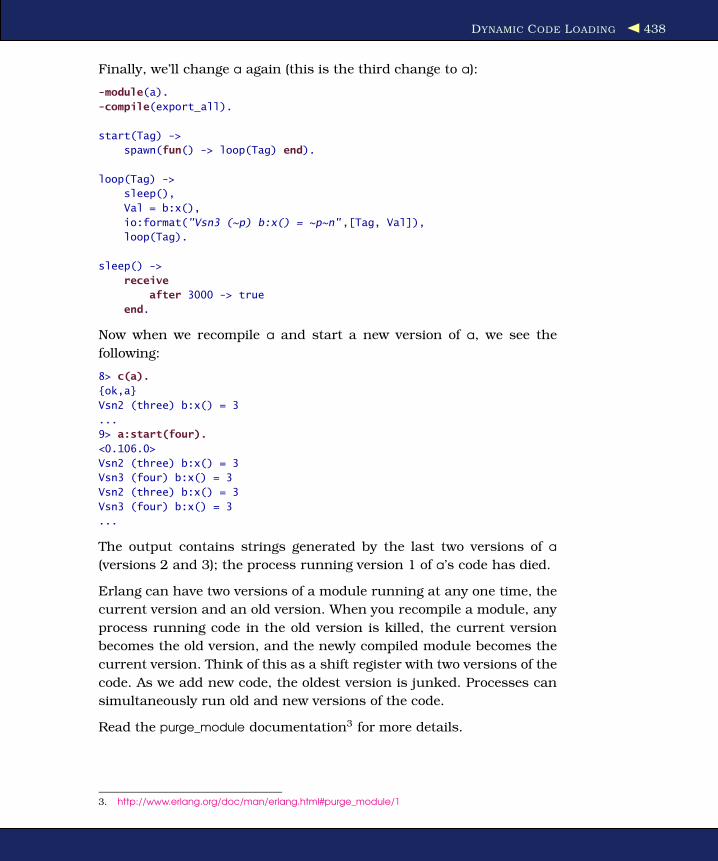
DYNAMIC CODE LOADING 438
Finally, we’ll change a again (this is the third change to a):
-module(a).
-compile(export_all).
start(Tag) ->
spawn(fun() -> loop(Tag) end).
loop(Tag) ->
sleep(),
Val = b:x(),
io:format("Vsn3 (~p) b:x() = ~p~n",[Tag, Val]),
loop(Tag).
sleep() ->
receive
after 3000 -> true
end.
Now when we recompile a and start a new version of a, we see the
following:
8> c(a).
{ok,a}
Vsn2 (three) b:x() = 3
...
9> a:start(four).
<0.106.0>
Vsn2 (three) b:x() = 3
Vsn3 (four) b:x() = 3
Vsn2 (three) b:x() = 3
Vsn3 (four) b:x() = 3
...
The output contains strings generated by the last two versions of a
(versions 2 and 3); the process running version 1 of a’s code has died.
Erlang can have two versions of a module running at any one time, the
current version and an old version. When you recompile a module, any
process running code in the old version is killed, the current version
becomes the old version, and the newly compiled module becomes the
current version. Think of this as a shift register with two versions of the
code. As we add new code, the oldest version is junked. Processes can
simultaneously run old and new versions of the code.
Read the purge_module documentation3 for more details.
3. http://www.erlang.org/doc/man/erlang.html#purge_module/1

Appendix F
Module and Function ReferenceThis appendix contains one-line summaries for most of the modules in
the kernel and stdlib libraries in the standard Erlang distribution. (I’ve
omitted some of the more obscure modules in order to keep the weight
of this book below the point where you’d need mechanical assistance to
pick it up.)
Note: The modules ordsets and orddict are not included in this appendix.
ordsets exports the same functions as sets; the only difference is that an
ordered list is used to represent the elements of the set. orddict exports
the same functions as dict, but a list of pairs is used to represent the
dictionary. The list is ordered by the keys in the dictionary.
F.1 Module: application
Generic OTP application functions.
Module:config_change(Changed, New, Removed) -> ok
Update the configuration parameters for an application.
Module:prep_stop(State) -> NewState
Prepare an application for termination.
Module:start(StartType, StartArgs) -> {ok, Pid} | {ok, Pid, State} | {error, Reason}
Start an application.
Module:start_phase(Phase, StartType, PhaseArgs) -> ok | {error, Reason}
Extended start of an application.
Module:stop(State)
Clean up after termination of an application.
get_all_env(Application) -> Env
Get the configuration parameters for an application.
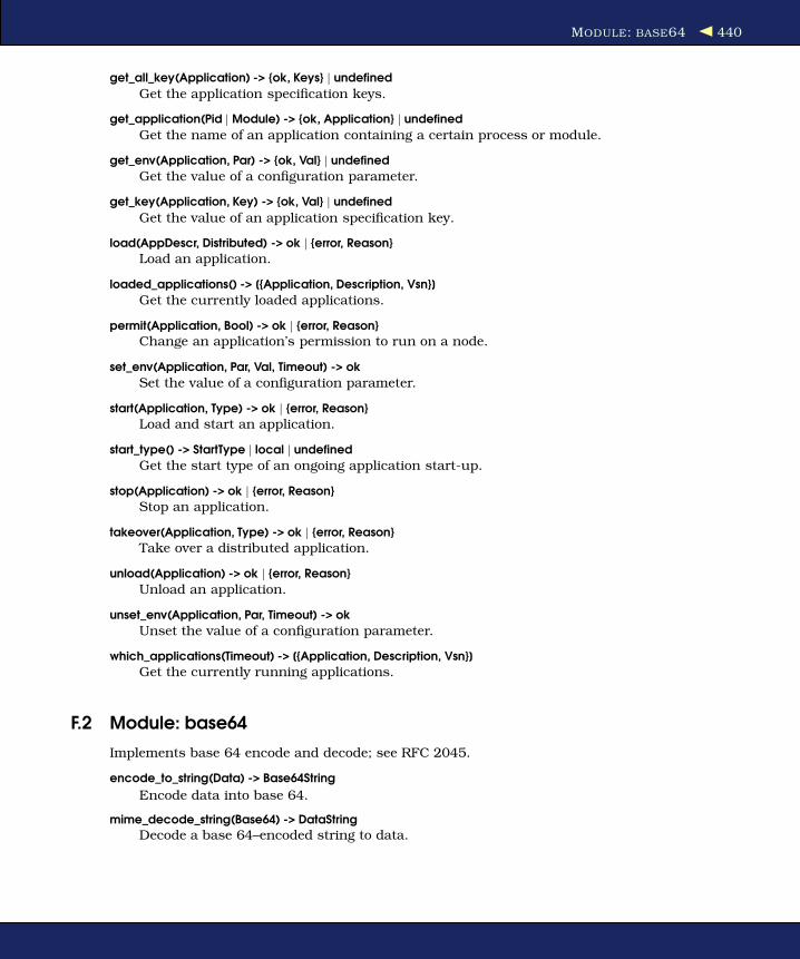
MODULE: BASE64 440
get_all_key(Application) -> {ok, Keys} | undefined
Get the application specification keys.
get_application(Pid | Module) -> {ok, Application} | undefined
Get the name of an application containing a certain process or module.
get_env(Application, Par) -> {ok, Val} | undefined
Get the value of a configuration parameter.
get_key(Application, Key) -> {ok, Val} | undefined
Get the value of an application specification key.
load(AppDescr, Distributed) -> ok | {error, Reason}
Load an application.
loaded_applications() -> [{Application, Description, Vsn}]
Get the currently loaded applications.
permit(Application, Bool) -> ok | {error, Reason}Change an application’s permission to run on a node.
set_env(Application, Par, Val, Timeout) -> ok
Set the value of a configuration parameter.
start(Application, Type) -> ok | {error, Reason}
Load and start an application.
start_type() -> StartType | local | undefined
Get the start type of an ongoing application start-up.
stop(Application) -> ok | {error, Reason}
Stop an application.
takeover(Application, Type) -> ok | {error, Reason}
Take over a distributed application.
unload(Application) -> ok | {error, Reason}
Unload an application.
unset_env(Application, Par, Timeout) -> ok
Unset the value of a configuration parameter.
which_applications(Timeout) -> [{Application, Description, Vsn}]
Get the currently running applications.
F.2 Module: base64
Implements base 64 encode and decode; see RFC 2045.
encode_to_string(Data) -> Base64String
Encode data into base 64.
mime_decode_string(Base64) -> DataStringDecode a base 64–encoded string to data.
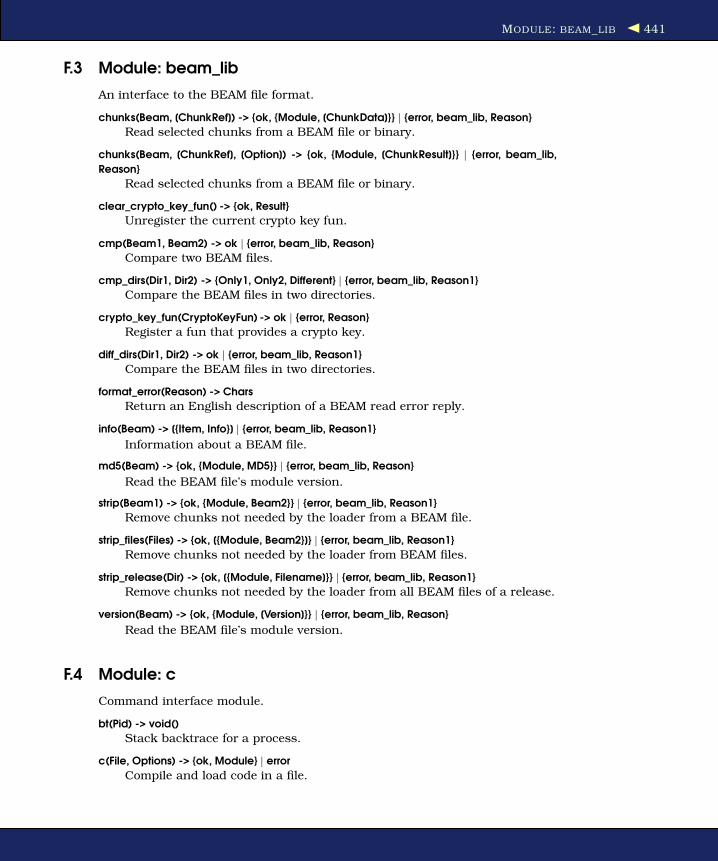
MODULE: BEAM_LIB 441
F.3 Module: beam_lib
An interface to the BEAM file format.
chunks(Beam, [ChunkRef]) -> {ok, {Module, [ChunkData]}} | {error, beam_lib, Reason}
Read selected chunks from a BEAM file or binary.
chunks(Beam, [ChunkRef], [Option]) -> {ok, {Module, [ChunkResult]}} | {error, beam_lib,
Reason}
Read selected chunks from a BEAM file or binary.
clear_crypto_key_fun() -> {ok, Result}
Unregister the current crypto key fun.
cmp(Beam1, Beam2) -> ok | {error, beam_lib, Reason}
Compare two BEAM files.
cmp_dirs(Dir1, Dir2) -> {Only1, Only2, Different} | {error, beam_lib, Reason1}
Compare the BEAM files in two directories.
crypto_key_fun(CryptoKeyFun) -> ok | {error, Reason}
Register a fun that provides a crypto key.
diff_dirs(Dir1, Dir2) -> ok | {error, beam_lib, Reason1}
Compare the BEAM files in two directories.
format_error(Reason) -> Chars
Return an English description of a BEAM read error reply.
info(Beam) -> [{Item, Info}] | {error, beam_lib, Reason1}
Information about a BEAM file.
md5(Beam) -> {ok, {Module, MD5}} | {error, beam_lib, Reason}
Read the BEAM file’s module version.
strip(Beam1) -> {ok, {Module, Beam2}} | {error, beam_lib, Reason1}
Remove chunks not needed by the loader from a BEAM file.
strip_files(Files) -> {ok, [{Module, Beam2}]} | {error, beam_lib, Reason1}
Remove chunks not needed by the loader from BEAM files.
strip_release(Dir) -> {ok, [{Module, Filename]}} | {error, beam_lib, Reason1}
Remove chunks not needed by the loader from all BEAM files of a release.
version(Beam) -> {ok, {Module, [Version]}} | {error, beam_lib, Reason}
Read the BEAM file’s module version.
F.4 Module: c
Command interface module.
bt(Pid) -> void()
Stack backtrace for a process.
c(File, Options) -> {ok, Module} | error
Compile and load code in a file.

MODULE: C 442
cd(Dir) -> void()Change working directory.
flush() -> void()
Flush any messages sent to the shell.
help() -> void()
Help information.
i(X, Y, Z) -> void()
Information about pid <X.Y.Z>.
l(Module) -> void()
Load or reload module.
lc(Files) -> ok
Compile a list of files.
ls() -> void()
List files in the current directory.
ls(Dir) -> void()
List files in a directory.
m() -> void()
Which modules are loaded.
m(Module) -> void()
Information about a module.
memory() -> [{Type, Size}]
Memory allocation information.
memory([Type]) -> [{Type, Size}]
Memory allocation information.
nc(File, Options) -> {ok, Module} | error
Compile and load code in a file on all nodes.
ni() -> void()
Information about the system.
nl(Module) -> void()
Load module on all nodes.
nregs() -> void()
Information about registered processes.
pid(X, Y, Z) -> pid()
Convert X,Y,Z to a PID.
pwd() -> void()Print working directory.
q() -> void()
Quit; shorthand for init:stop().
xm(ModSpec) -> void()
Cross-reference check a module.

MODULE: CALENDAR 443
y(File) -> YeccRet
Generate an LALR-1 parser.
y(File, Options) -> YeccRet
Generate an LALR-1 parser.
F.5 Module: calendar
Local and universal time, day-of-the-week, date and time conversions.
date_to_gregorian_days(Year, Month, Day) -> Days
Compute the number of days from year 0 up to the given date.
datetime_to_gregorian_seconds({Date, Time}) -> Seconds
Compute the number of seconds from year 0 up to the given date and time.
day_of_the_week(Year, Month, Day) -> DayNumber
Compute the day of the week.
gregorian_days_to_date(Days) -> Date
Compute the date given the number of Gregorian days.
gregorian_seconds_to_datetime(Seconds) -> {Date, Time}
Compute the date given the number of Gregorian days.
is_leap_year(Year) -> bool()
Check whether a year is a leap year.
last_day_of_the_month(Year, Month) -> int()
Compute the number of days in a month.
local_time() -> {Date, Time}
Compute local time.
local_time_to_universal_time({Date1, Time1}) -> {Date2, Time2}
Convert from local time to universal time (deprecated).
local_time_to_universal_time_dst({Date1, Time1}) -> [{Date, Time}]
Convert from local time to universal time(s).
now_to_datetime(Now) -> {Date, Time}
Convert now to date and time.
now_to_local_time(Now) -> {Date, Time}
Convert now to local date and time.
seconds_to_daystime(Seconds) -> {Days, Time}
Compute days and time from seconds.
seconds_to_time(Seconds) -> Time
Compute time from seconds.
time_difference(T1, T2) -> {Days, Time}
Compute the difference between two times (deprecated).
time_to_seconds(Time) -> Seconds
Compute the number of seconds since midnight up to the given time.

MODULE: CODE 444
universal_time() -> {Date, Time}
Compute universal time.
universal_time_to_local_time({Date1, Time1}) -> {Date2, Time2}
Convert from universal time to local time.
valid_date(Year, Month, Day) -> bool()
Check whether a date is valid.
F.6 Module: code
Erlang code server.
add_patha(Dir) -> true | {error, What}
Add a directory to the beginning of the code path.
add_pathsa(Dirs) -> ok
Add directories to the beginning of the code path.
add_pathsz(Dirs) -> ok
Add directories to the end of the code path.
add_pathz(Dir) -> true | {error, What}
Add a directory to the end of the code path.
all_loaded() -> [{Module, Loaded}]
Get all loaded modules.
clash() -> ok
Search for modules with identical names.
compiler_dir() -> string()
Library directory for the compiler.
del_path(Name | Dir) -> true | false | {error, What}
Delete a directory from the code path.
delete(Module) -> true | false
Remove current code for a module.
ensure_loaded(Module) -> {module, Module} | {error, What}
Ensure that a module is loaded.
get_object_code(Module) -> {Module, Binary, Filename} | error
Get the object code for a module.
get_path() -> Path
Return the code server search path.
is_loaded(Module) -> {file, Loaded} | false
Check whether a module is loaded.
lib_dir() -> string()
Library directory of Erlang/OTP.
lib_dir(Name) -> string() | {error, bad_name}
Library directory for an application.

MODULE: DETS 445
load_abs(Filename) -> {module, Module} | {error, What}
Load a module, residing in a given file.
load_binary(Module, Filename, Binary) -> {module, Module} | {error, What}
Load object code for a module.
load_file(Module) -> {module, Module} | {error, What}
Load a module.
objfile_extension() -> ".beam"
Object code file extension.
priv_dir(Name) -> string() | {error, bad_name}
Priv directory for an application.
purge(Module) -> true | false
Remove old code for a module.
rehash() -> ok
Rehash or create code path cache.
replace_path(Name, Dir) -> true | {error, What}
Replace a directory with another in the code path.
root_dir() -> string()
Root directory of Erlang/OTP.
set_path(Path) -> true | {error, What}
Set the code server search path.
soft_purge(Module) -> true | false
Remove old code for a module, unless no process uses it.
stick_dir(Dir) -> ok | {error, What}
Mark a directory as sticky.
unstick_dir(Dir) -> ok | {error, What}
Remove a sticky directory mark.
where_is_file(Filename) -> Absname | non_existing
Full name of a file located in the code path.
which(Module) -> Which
The object code file of a module.
F.7 Module: dets
A disk-based term storage.
all() -> [Name]
Return a list of the names of all open DETS tables on this node.
bchunk(Name, Continuation) -> {Continuation2, Data} | ’$end_of_table’ | {error, Reason}
Return a chunk of objects stored in a DETS table.
close(Name) -> ok | {error, Reason}
Close a DETS table.

MODULE: DETS 446
delete(Name, Key) -> ok | {error, Reason}
Delete all objects with a given key from a DETS table.
delete_all_objects(Name) -> ok | {error, Reason}
Delete all objects from a DETS table.
delete_object(Name, Object) -> ok | {error, Reason}
Delete a given object from a DETS table.
first(Name) -> Key | ’$end_of_table’
Return the first key stored in a DETS table.
foldl(Function, Acc0, Name) -> Acc1 | {error, Reason}
Fold a function over a DETS table.
foldr(Function, Acc0, Name) -> Acc1 | {error, Reason}
Fold a function over a DETS table.
from_ets(Name, EtsTab) -> ok | {error, Reason}
Replace the objects of a DETS table with the objects of an ETS table.
info(Name) -> InfoList | undefined
Return information about a DETS table.
info(Name, Item) -> Value | undefined
Return the information associated with a given item for a DETS table.
init_table(Name, InitFun [, Options]) -> ok | {error, Reason}
Replace all objects of a DETS table.
insert(Name, Objects) -> ok | {error, Reason}Insert one or more objects into a DETS table.
insert_new(Name, Objects) -> BoolInsert one or more objects into a DETS table.
is_compatible_bchunk_format(Name, BchunkFormat) -> Bool
Test the compatibility of a table’s chunk data.
is_dets_file(FileName) -> Bool | {error, Reason}
Test for a DETS table.
lookup(Name, Key) -> [Object] | {error, Reason}
Return all objects with a given key stored in a DETS table.
match(Continuation) -> {[Match], Continuation2} | ’$end_of_table’ | {error, Reason}Match a chunk of objects stored in a DETS table, and return a list ofvariable bindings.
match(Name, Pattern) -> [Match] | {error, Reason}Match the objects stored in a DETS table, and return a list of variablebindings.
match(Name, Pattern, N) -> {[Match], Continuation} | ’$end_of_table’ | {error, Reason}Match the first chunk of objects stored in a DETS table, and return a listof variable bindings.
match_delete(Name, Pattern) -> N | {error, Reason}
Delete all objects that match a given pattern from a DETS table.

MODULE: DETS 447
match_object(Continuation) -> {[Object], Continuation2} | ’$end_of_table’ | {error, Reason}Match a chunk of objects stored in a DETS table and return a list ofobjects.
match_object(Name, Pattern) -> [Object] | {error, Reason}
Match the objects stored in a DETS table and return a list of objects.
match_object(Name, Pattern, N) -> {[Object], Continuation} | ’$end_of_table’ | {error, Rea-
son}Match the first chunk of objects stored in a DETS table and return a list ofobjects.
member(Name, Key) -> Bool | {error, Reason}
Test for occurrence of a key in a DETS table.
next(Name, Key1) -> Key2 | ’$end_of_table’
Return the next key in a DETS table.
open_file(Filename) -> {ok, Reference} | {error, Reason}Open an existing DETS table.
open_file(Name, Args) -> {ok, Name} | {error, Reason}
Open a DETS table.
pid2name(Pid) -> {ok, Name} | undefined
Return the name of the DETS table handled by a PID.
repair_continuation(Continuation, MatchSpec) -> Continuation2
Repair a continuation from select/1 or select/3.
safe_fixtable(Name, Fix)
Fix a DETS table for safe traversal.
select(Continuation) -> {Selection, Continuation2} | ’$end_of_table’ | {error, Reason}
Apply a match specification to some objects stored in a DETS table.
select(Name, MatchSpec) -> Selection | {error, Reason}
Apply a match specification to all objects stored in a DETS table.
select(Name, MatchSpec, N) -> {Selection, Continuation} | ’$end_of_table’ | {error, Reason}Apply a match specification to the first chunk of objects stored in a DETStable.
select_delete(Name, MatchSpec) -> N | {error, Reason}
Delete all objects that match a given pattern from a DETS table.
slot(Name, I) -> ’$end_of_table’ | [Object] | {error, Reason}
Return the list of objects associated with a slot of a DETS table.
sync(Name) -> ok | {error, Reason}
Ensure that all updates made to a DETS table are written to disk.
table(Name [, Options]) -> QueryHandle
Return a QLC query handle.
to_ets(Name, EtsTab) -> EtsTab | {error, Reason}
Insert all objects of a DETS table into an ETS table.
traverse(Name, Fun) -> Return | {error, Reason}
Apply a function to all or some objects stored in a DETS table.

MODULE: DICT 448
update_counter(Name, Key, Increment) -> ResultUpdate a counter object stored in a DETS table.
F.8 Module: dict
Key-value dictionary.
append(Key, Value, Dict1) -> Dict2
Append a value to keys in a dictionary.
append_list(Key, ValList, Dict1) -> Dict2
Append new values to keys in a dictionary.
erase(Key, Dict1) -> Dict2
Erase a key from a dictionary.
fetch(Key, Dict) -> Value
Look up values in a dictionary.
fetch_keys(Dict) -> Keys
Return all keys in a dictionary.
filter(Pred, Dict1) -> Dict2
Choose elements which satisfy a predicate.
find(Key, Dict) -> {ok, Value} | error
Search for a key in a dictionary.
fold(Fun, Acc0, Dict) -> Acc1
Fold a function over a dictionary.
from_list(List) -> Dict
Convert a list of pairs to a dictionary.
is_key(Key, Dict) -> bool()
Test whether a key is in a dictionary.
map(Fun, Dict1) -> Dict2
Map a function over a dictionary.
merge(Fun, Dict1, Dict2) -> Dict3Merge two dictionaries.
new() -> dictionary()
Create a dictionary.
store(Key, Value, Dict1) -> Dict2
Store a value in a dictionary.
to_list(Dict) -> List
Convert a dictionary to a list of pairs.
update(Key, Fun, Dict1) -> Dict2
Update a value in a dictionary.
update(Key, Fun, Initial, Dict1) -> Dict2
Update a value in a dictionary.

MODULE: DIGRAPH 449
update_counter(Key, Increment, Dict1) -> Dict2
Increment a value in a dictionary.
F.9 Module: digraph
Directed graphs.
add_edge(G, V1, V2) -> edge() | {error, Reason}Add an edge to a digraph.
add_vertex(G) -> vertex()
Add or modify a vertex of a digraph.
del_edge(G, E) -> true
Delete an edge from a digraph.
del_edges(G, Edges) -> true
Delete edges from a digraph.
del_path(G, V1, V2) -> true
Delete paths from a digraph.
del_vertex(G, V) -> true
Delete a vertex from a digraph.
del_vertices(G, Vertices) -> true
Delete vertices from a digraph.
delete(G) -> trueDelete a digraph.
edge(G, E) -> {E, V1, V2, Label} | false
Return the vertices and the label of an edge of a digraph.
edges(G) -> Edges
Return all edges of a digraph.
edges(G, V) -> Edges
Return the edges emanating from or incident on a vertex of a digraph.
get_cycle(G, V) -> Vertices | falseFind one cycle in a digraph.
get_path(G, V1, V2) -> Vertices | falseFind one path in a digraph.
get_short_cycle(G, V) -> Vertices | falseFind one short cycle in a digraph.
get_short_path(G, V1, V2) -> Vertices | falseFind one short path in a digraph.
in_degree(G, V) -> integer()
Return the in-degree of a vertex of a digraph.
in_edges(G, V) -> Edges
Return all edges incident on a vertex of a digraph.

MODULE: DIGRAPH_UTILS 450
in_neighbours(G, V) -> Vertices
Return all in-neighbors of a vertex of a digraph.
info(G) -> InfoList
Return information about a digraph.
new() -> digraph()Return a protected empty digraph, where cycles are allowed.
new(Type) -> digraph() | {error, Reason}
Create a new empty digraph.
no_edges(G) -> integer() >= 0
Return the number of edges of a digraph.
no_vertices(G) -> integer() >= 0
Return the number of vertices of a digraph.
out_degree(G, V) -> integer()
Return the out-degree of a vertex of a digraph.
out_edges(G, V) -> Edges
Return all edges emanating from a vertex of a digraph.
out_neighbours(G, V) -> Vertices
Return all out-neighbors of a vertex of a digraph.
vertex(G, V) -> {V, Label} | false
Return the label of a vertex of a digraph.
vertices(G) -> Vertices
Return all vertices of a digraph.
F.10 Module: digraph_utils
Algorithms for directed graphs.
components(Digraph) -> [Component]
Return the components of a digraph.
condensation(Digraph) -> CondensedDigraph
Return a condensed graph of a digraph.
cyclic_strong_components(Digraph) -> [StrongComponent]
Return the cyclic strong components of a digraph.
is_acyclic(Digraph) -> bool()Check whether a digraph is acyclic.
loop_vertices(Digraph) -> Vertices
Return the vertices of a digraph included in some loop.
postorder(Digraph) -> Vertices
Return the vertices of a digraph in post-order.
preorder(Digraph) -> Vertices
Return the vertices of a digraph in pre-order.
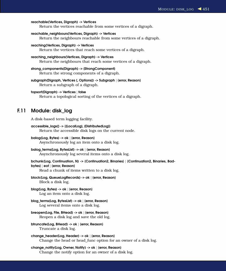
MODULE: DISK_LOG 451
reachable(Vertices, Digraph) -> Vertices
Return the vertices reachable from some vertices of a digraph.
reachable_neighbours(Vertices, Digraph) -> Vertices
Return the neighbours reachable from some vertices of a digraph.
reaching(Vertices, Digraph) -> Vertices
Return the vertices that reach some vertices of a digraph.
reaching_neighbours(Vertices, Digraph) -> Vertices
Return the neighbours that reach some vertices of a digraph.
strong_components(Digraph) -> [StrongComponent]
Return the strong components of a digraph.
subgraph(Digraph, Vertices [, Options]) -> Subgraph | {error, Reason}
Return a subgraph of a digraph.
topsort(Digraph) -> Vertices | false
Return a topological sorting of the vertices of a digraph.
F.11 Module: disk_log
A disk-based term logging facility.
accessible_logs() -> {[LocalLog], [DistributedLog]}
Return the accessible disk logs on the current node.
balog(Log, Bytes) -> ok | {error, Reason}Asynchronously log an item onto a disk log.
balog_terms(Log, BytesList) -> ok | {error, Reason}
Asynchronously log several items onto a disk log.
bchunk(Log, Continuation, N) -> {Continuation2, Binaries} | {Continuation2, Binaries, Bad-
bytes} | eof | {error, Reason}
Read a chunk of items written to a disk log.
block(Log, QueueLogRecords) -> ok | {error, Reason}Block a disk log.
blog(Log, Bytes) -> ok | {error, Reason}Log an item onto a disk log.
blog_terms(Log, BytesList) -> ok | {error, Reason}Log several items onto a disk log.
breopen(Log, File, BHead) -> ok | {error, Reason}Reopen a disk log and save the old log.
btruncate(Log, BHead) -> ok | {error, Reason}
Truncate a disk log.
change_header(Log, Header) -> ok | {error, Reason}
Change the head or head_func option for an owner of a disk log.
change_notify(Log, Owner, Notify) -> ok | {error, Reason}
Change the notify option for an owner of a disk log.

MODULE: EPP 452
change_size(Log, Size) -> ok | {error, Reason}
Change the size of an open disk log.
chunk_info(Continuation) -> InfoList | {error, Reason}
Return information about a chunk continuation of a disk log.
chunk_step(Log, Continuation, Step) -> {ok, Continuation2} | {error, Reason}
Step forward or backward among the wrap log files of a disk log.
close(Log) -> ok | {error, Reason}
Close a disk log.
format_error(Error) -> Chars
Return an English description of a disk log error reply.
inc_wrap_file(Log) -> ok | {error, Reason}
Change to the next wrap log file of a disk log.
info(Log) -> InfoList | {error, no_such_log}
Return information about a disk log.
lclose(Log, Node) -> ok | {error, Reason}Close a disk log on one node.
open(ArgL) -> OpenRet | DistOpenRet
Open a disk log file.
pid2name(Pid) -> {ok, Log} | undefined
Return the name of the disk log handled by a PID.
sync(Log) -> ok | {error, Reason}
Flush the contents of a disk log to the disk.
unblock(Log) -> ok | {error, Reason}Unblock a disk log.
F.12 Module: epp
An Erlang code preprocessor.
close(Epp) -> ok
Close the preprocessing of the file associated withEpp.
open(FileName, IncludePath, PredefMacros) -> {ok,Epp} | {error, ErrorDescriptor}
Open a file for preprocessing.
parse_erl_form(Epp) -> {ok, AbsForm} | {eof, Line} | {error, ErrorInfo}
Return the next Erlang form from the opened Erlang source file.
parse_file(FileName,IncludePath,PredefMacro) -> {ok,[Form]} | {error,OpenError}
Preprocess and parse an Erlang source file.

MODULE: ERL_EVAL 453
F.13 Module: erl_eval
The Erlang meta interpreter.
add_binding(Name, Value, Bindings) -> BindingStructAdd a binding.
binding(Name, BindingStruct) -> Binding
Return bindings.
bindings(BindingStruct) -> BindingsReturn bindings.
del_binding(Name, Bindings) -> BindingStruct
Delete a binding.
expr(Expression, Bindings, LocalFunctionHandler, NonlocalFunctionHandler) -> {value,
Value, NewBindings}
Evaluate the expression.
expr_list(ExpressionList, Bindings, LocalFunctionHandler, NonlocalFunctionHandler) -> {Val-
ueList, NewBindings}
Evaluate a list of expressions.
exprs(Expressions, Bindings, LocalFunctionHandler, NonlocalFunctionHandler) -> {value,
Value, NewBindings}
Evaluate expressions.
new_bindings() -> BindingStructReturn a bindings structure.
F.14 Module: erl_parse
The Erlang parser.
abstract(Data) -> AbsTerm
Convert an Erlang term into an abstract form.
format_error(ErrorDescriptor) -> Chars
Format an error descriptor.
normalise(AbsTerm) -> Data
Convert abstract form to an Erlang term.
parse_exprs(Tokens) -> {ok, Expr_list} | {error, ErrorInfo}Parse Erlang expressions.
parse_form(Tokens) -> {ok, AbsForm} | {error, ErrorInfo}
Parse an Erlang form.
parse_term(Tokens) -> {ok, Term} | {error, ErrorInfo}Parse an Erlang term.
tokens(AbsTerm, MoreTokens) -> Tokens
Generate a list of tokens for an expression.
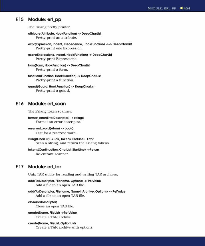
MODULE: ERL_PP 454
F.15 Module: erl_pp
The Erlang pretty printer.
attribute(Attribute, HookFunction) -> DeepCharList
Pretty-print an attribute.
expr(Expression, Indent, Precedence, HookFunction) ->-> DeepCharList
Pretty-print one Expression.
exprs(Expressions, Indent, HookFunction) -> DeepCharList
Pretty-print Expressions.
form(Form, HookFunction) -> DeepCharList
Pretty-print a form.
function(Function, HookFunction) -> DeepCharList
Pretty-print a function.
guard(Guard, HookFunction) -> DeepCharListPretty-print a guard.
F.16 Module: erl_scan
The Erlang token scanner.
format_error(ErrorDescriptor) -> string()
Format an error descriptor.
reserved_word(Atom) -> bool()
Test for a reserved word.
string(CharList) -> {ok, Tokens, EndLine} | ErrorScan a string, and return the Erlang tokens.
tokens(Continuation, CharList, StartLine) ->Return
Re-entrant scanner.
F.17 Module: erl_tar
Unix TAR utility for reading and writing TAR archives.
add(TarDescriptor, Filename, Options) -> RetValue
Add a file to an open TAR file.
add(TarDescriptor, Filename, NameInArchive, Options) -> RetValue
Add a file to an open TAR file.
close(TarDescriptor)
Close an open TAR file.
create(Name, FileList) ->RetValue
Create a TAR archive.
create(Name, FileList, OptionList)
Create a TAR archive with options.

MODULE: ERLANG 455
extract(Name) -> RetValue
Extract all files from a TAR file.
extract(Name, OptionList)
Extract files from a TAR file.
format_error(Reason) -> string()Convert error term to a readable string.
open(Name, OpenModeList) -> RetValue
Open a TAR file.
t(Name)
Print the name of each file in a TAR file.
table(Name) -> RetValue
Retrieve the name of all files in a TAR file.
table(Name, Options)
Retrieve name and information of all files in a TAR file.
tt(Name)
Print name and information for each file in a TAR file.
F.18 Module: erlang
The Erlang BIFs.
abs(Number) -> int() | float()
Arithmetical absolute value.
apply(Fun, Args) -> term() | empty()
Apply a function to an argument list.
apply(Module, Function, Args) -> term() | empty()
Apply a function to an argument list.
atom_to_list(Atom) -> string()
Text representation of an atom.
binary_to_list(Binary) -> [char()]
Convert a binary to a list.
binary_to_list(Binary, Start, Stop) -> [char()]
Convert part of a binary to a list.
binary_to_term(Binary) -> term()
Decode an Erlang external term format binary.
check_process_code(Pid, Module) -> bool()
Check whether a process is executing old code for a module.
concat_binary(ListOfBinaries)
Concatenate a list of binaries (deprecated).
date() -> {Year, Month, Day}
Current date.

MODULE: ERLANG 456
delete_module(Module) -> true | undefined
Make the current code for a module old.
disconnect_node(Node) -> bool() | ignored
Force the disconnection of a node.
element(N, Tuple) -> term()
Get Nth element of a tuple.
erase() -> [{Key, Val}]
Return and delete the process dictionary.
erase(Key) -> Val | undefined
Return and delete a value from the process dictionary.
erlang:append_element(Tuple1, Term) -> Tuple2
Append an extra element to a tuple.
erlang:bump_reductions(Reductions) -> void()
Increment the reduction counter.
erlang:cancel_timer(TimerRef) -> Time | false
Cancel a timer.
erlang:demonitor(MonitorRef) -> trueStop monitoring.
erlang:demonitor(MonitorRef, OptionList) -> trueStop monitoring.
erlang:display(Term) -> true
Print a term on standard output.
erlang:error(Reason)Stop execution with a given reason.
erlang:error(Reason, Args)
Stop execution with a given reason.
erlang:fault(Reason)Stop execution with a given reason.
erlang:fault(Reason, Args)
Stop execution with a given reason.
erlang:fun_info(Fun) -> [{Item, Info}]
Information about a fun.
erlang:fun_info(Fun, Item) -> {Item, Info}
Information about a fun.
erlang:fun_to_list(Fun) -> string()
Text representation of a fun.
erlang:function_exported(Module, Function, Arity) -> bool()
Check whether a function is exported and loaded.
erlang:get_cookie() -> Cookie | nocookie
Get the magic cookie of the local node.

MODULE: ERLANG 457
erlang:get_stacktrace() -> [{Module, Function, Arity | Args}]
Get the call stack backtrace of the last exception.
erlang:hash(Term, Range) -> Hash
Hash function (deprecated).
erlang:hibernate(Module, Function, Args)Hibernate a process until a message is sent to it.
erlang:info(Type) -> Res
Information about the system (deprecated).
erlang:integer_to_list(Integer, Base) -> string()
Text representation of an integer.
erlang:is_builtin(Module, Function, Arity) -> bool()
Check whether a function is a BIF implemented in C.
erlang:list_to_integer(String, Base) -> int()
Convert from text representation to an integer.
erlang:loaded() -> [Module]
List of all loaded modules.
erlang:localtime() -> {Date, Time}
Current local date and time.
erlang:localtime_to_universaltime({Date1, Time1}) -> {Date2, Time2}
Convert from local to Universal Time Coordinated (UTC) date and time.
erlang:localtime_to_universaltime({Date1, Time1}, IsDst) -> {Date2, Time2}
Convert from local to Universal Time Coordinated (UTC) date and time.
erlang:make_tuple(Arity, InitialValue) -> tuple()
Create a new tuple of a given arity.
erlang:md5(Data) -> Digest
Compute an MD5 message digest.
erlang:md5_final(Context) -> DigestFinish the update of an MD5 context, and return the computed MD5 mes-sage digest.
erlang:md5_init() -> Context
Create an MD5 context.
erlang:md5_update(Context, Data) -> NewContext
Update an MD5 context with data, and return a new context.
erlang:memory() -> [{Type, Size}]
Information about dynamically allocated memory.
erlang:memory(Type | [Type]) -> Size | [{Type, Size}]
Information about dynamically allocated memory.
erlang:monitor(Type, Item) -> MonitorRefStart monitoring.
erlang:monitor_node(Node, Flag, Options) -> true
Monitor the status of a node.

MODULE: ERLANG 458
erlang:phash(Term, Range) -> Hash
Portable hash function.
erlang:phash2(Term [, Range]) -> Hash
Portable hash function.
erlang:port_call(Port, Operation, Data) -> term()
Synchronous call to a port with term data.
erlang:port_info(Port) -> [{Item, Info}] | undefined
Information about a port.
erlang:port_info(Port, Item) -> {Item, Info} | undefined | []
Information about a port.
erlang:port_to_list(Port) -> string()
Text representation of a port identifier.
erlang:ports() -> [port()]
All open ports.
erlang:process_display(Pid, Type) -> void()
Write information about a local process on standard error.
erlang:raise(Class, Reason, Stacktrace)Stop execution with an exception of given class, reason, and call stackbacktrace.
erlang:read_timer(TimerRef) -> int() | false
Number of milliseconds remaining for a timer.
erlang:ref_to_list(Ref) -> string()
Text representation of a reference.
erlang:resume_process(Pid) -> true
Resume a suspended process.
erlang:send(Dest, Msg) -> MsgSend a message.
erlang:send(Dest, Msg, [Option]) -> Res
Send a message conditionally.
erlang:send_after(Time, Dest, Msg) -> TimerRef
Start a timer.
erlang:send_nosuspend(Dest, Msg) -> bool()
Try to send a message without ever blocking.
erlang:send_nosuspend(Dest, Msg, Options) -> bool()Try to send a message without ever blocking.
erlang:set_cookie(Node, Cookie) -> true
Set the magic cookie of a node.
erlang:spawn_monitor(Fun) -> {pid(),reference()}
Create and monitor a new process with a fun as entry point.
erlang:spawn_monitor(Module, Function, Args) -> {pid(),reference()}
Create and monitor a new process with a function as entry point.

MODULE: ERLANG 459
erlang:start_timer(Time, Dest, Msg) -> TimerRef
Start a timer.
erlang:suspend_process(Pid) -> true
Suspend a process.
erlang:system_flag(Flag, Value) -> OldValue
Set system flags.
erlang:system_info(Type) -> Res
Information about the system.
erlang:system_monitor() -> MonSettings
Current system performance monitoring settings.
erlang:system_monitor(undefined | {MonitorPid, Options}) -> MonSettings
Set or clear system performance monitoring options.
erlang:system_monitor(MonitorPid, [Option]) -> MonSettings
Set system performance monitoring options.
erlang:trace(PidSpec, How, FlagList) -> int()
Set trace flags for a process or processes.
erlang:trace_delivered(Tracee) -> Ref
Notification when trace has been delivered.
erlang:trace_info(PidOrFunc, Item) -> Res
Trace information about a process or function.
erlang:trace_pattern(MFA, MatchSpec) -> int()
Set trace patterns for global call tracing.
erlang:trace_pattern(MFA, MatchSpec, FlagList) -> int()
Set trace patterns for tracing of function calls.
erlang:universaltime() -> {Date, Time}
Current date and time according to Universal Time Coordinated (UTC).
erlang:universaltime_to_localtime({Date1, Time1}) -> {Date2, Time2}
Convert from Universal Time Coordinated (UTC) to local date and time.
erlang:yield() -> true
Let other processes get a chance to execute.
exit(Reason)Stop execution with a given reason.
exit(Pid, Reason) -> true
Send an exit signal to a process.
float(Number) -> float()
Convert a number to a float.
float_to_list(Float) -> string()
Text representation of a float.
garbage_collect() -> true
Force an immediate garbage collection of the calling process.

MODULE: ERLANG 460
garbage_collect(Pid) -> bool()
Force an immediate garbage collection of a process.
get() -> [{Key, Val}]
Return the process dictionary.
get(Key) -> Val | undefined
Return a value from the process dictionary.
get_keys(Val) -> [Key]
Return a list of keys from the process dictionary.
group_leader() -> GroupLeader
Get the group leader for the calling process.
group_leader(GroupLeader, Pid) -> true
Set the group leader for a process.
halt()Halt the Erlang runtime system, and indicate normal exit to the callingenvironment.
halt(Status)Halt the Erlang runtime system.
hd(List) -> term()
Head of a list.
integer_to_list(Integer) -> string()
Text representation of an integer.
iolist_size(Item) -> int()
Size of an iolist.
iolist_to_binary(IoListOrBinary) -> binary()
Convert an iolist to a binary.
is_alive() -> bool()
Check whether the local node is alive.
is_atom(Term) -> bool()
Check whether a term is an atom.
is_binary(Term) -> bool()
Check whether a term is a binary.
is_boolean(Term) -> bool()
Check whether a term is a boolean.
is_float(Term) -> bool()
Check whether a term is a float.
is_function(Term) -> bool()
Check whether a term is a fun.
is_function(Term, Arity) -> bool()
Check whether a term is a fun with a given arity.
is_integer(Term) -> bool()Check whether a term is an integer.

MODULE: ERLANG 461
is_list(Term) -> bool()
Check whether a term is a list.
is_number(Term) -> bool()
Check whether a term is a number.
is_pid(Term) -> bool()
Check whether a term is a PID.
is_port(Term) -> bool()
Check whether a term is a port.
is_process_alive(Pid) -> bool()
Check whether a process is alive.
is_record(Term, RecordTag) -> bool()
Check whether a term appears to be a record.
is_record(Term, RecordTag, Size) -> bool()
Check whether a term appears to be a record.
is_reference(Term) -> bool()
Check whether a term is a reference.
is_tuple(Term) -> bool()
Check whether a term is a tuple.
length(List) -> int()
Length of a list.
link(Pid) -> true
Create a link to another process (or port).
list_to_atom(String) -> atom()
Convert from a text representation to an atom.
list_to_binary(IoList) -> binary()
Convert a list to a binary.
list_to_existing_atom(String) -> atom()
Convert from a text representation to an atom.
list_to_float(String) -> float()
Convert from a text representation to a float.
list_to_integer(String) -> int()
Convert from a text representation to an integer.
list_to_pid(String) -> pid()
Convert from text representation to a PID.
list_to_tuple(List) -> tuple()
Convert a list to a tuple.
load_module(Module, Binary) -> {module, Module} | {error, Reason}
Load object code for a module.
make_ref() -> ref()
Return an almost unique reference.

MODULE: ERLANG 462
module_loaded(Module) -> bool()
Check whether a module is loaded.
monitor_node(Node, Flag) -> true
Monitor the status of a node.
node() -> Node
Name of the local node.
node(Arg) -> Node
At which node is a PID, port, or reference located.
nodes() -> Nodes
All visible nodes in the system.
nodes(Arg | [Arg]) -> Nodes
All nodes of a certain type in the system.
now() -> {MegaSecs, Secs, MicroSecs}
Elapsed time since 00:00 GMT.
open_port(PortName, PortSettings) -> port()
Open a port.
pid_to_list(Pid) -> string()
Text representation of a PID.
port_close(Port) -> true
Close an open port.
port_command(Port, Data) -> true
Send data to a port.
port_connect(Port, Pid) -> true
Set the owner of a port.
port_control(Port, Operation, Data) -> Res
Perform a synchronous control operation on a port.
pre_loaded() -> [Module]
List of all preloaded modules.
process_flag(Flag, Value) -> OldValue
Set process flags for the calling process.
process_flag(Pid, Flag, Value) -> OldValue
Set process flags for a process.
process_info(Pid) -> [{Item, Info}] | undefined
Information about a process.
process_info(Pid, Item) -> {Item, Info} | undefined | []
Information about a process.
processes() -> [pid()]
All processes.
purge_module(Module) -> void()
Remove old code for a module.

MODULE: ERLANG 463
put(Key, Val) -> OldVal | undefined
Add a new value to the process dictionary.
register(RegName, Pid | Port) -> true
Register a name for a PID (or port).
registered() -> [RegName]All registered names.
round(Number) -> int()
Return an integer by rounding a number.
self() -> pid()
Pid of the calling process.
setelement(Index, Tuple1, Value) -> Tuple2
Set Nth element of a tuple.
size(Item) -> int()
Size of a tuple or binary.
spawn(Fun) -> pid()
Create a new process with a fun as entry point.
spawn(Node, Fun) -> pid()
Create a new process with a fun as entry point on a given node.
spawn(Module, Function, Args) -> pid()
Create a new process with a function as entry point.
spawn(Node, Module, Function, ArgumentList) -> pid()
Create a new process with a function as entry point on a given node.
spawn_link(Fun) -> pid()
Create and link to a new process with a fun as entry point.
spawn_link(Node, Fun) ->Create and link to a new process with a fun as entry point on a specifiednode.
spawn_link(Module, Function, Args) -> pid()
Create and link to a new process with a function as entry point.
spawn_link(Node, Module, Function, Args) -> pid()Create and link to a new process with a function as entry point on a givennode.
spawn_opt(Fun, [Option]) -> pid() | {pid(),reference()}
Create a new process with a fun as entry point.
spawn_opt(Node, Fun, [Option]) -> pid()
Create a new process with a fun as entry point on a given node.
spawn_opt(Module, Function, Args, [Option]) -> pid() | {pid(),reference()}
Create a new process with a function as entry point.
spawn_opt(Node, Module, Function, Args, [Option]) -> pid()
Create a new process with a function as entry point on a given node.

MODULE: ERROR_HANDLER 464
split_binary(Bin, Pos) -> {Bin1, Bin2}
Split a binary into two.
statistics(Type) -> Res
Information about the system.
term_to_binary(Term) -> ext_binary()
Encode a term to an Erlang external term format binary.
term_to_binary(Term, [Option]) -> ext_binary()
Encode a term to en Erlang external term format binary.
throw(Any)
Throw an exception.
time() -> {Hour, Minute, Second}
Current time.
tl(List1) -> List2
Tail of a list.
trunc(Number) -> int()Return an integer by the truncating a number.
tuple_to_list(Tuple) -> [term()]
Convert a tuple to a list.
unlink(Id) -> true
Remove a link, if there is one, to another process or port.
unregister(RegName) -> true
Remove the registered name for a process (or port).
whereis(RegName) -> pid() | port() | undefined
Get the PID (or port) with a given registered name.
F.19 Module: error_handler
Default system error handler.
undefined_function(Module, Function, Args) -> term()
Called when an undefined function is encountered.
undefined_lambda(Module, Fun, Args) -> term()
Called when an undefined lambda (fun) is encountered.
F.20 Module: error_logger
Erlang error logger.
add_report_handler(Handler, Args) -> ResultAdd an event handler to the error logger.
delete_report_handler(Handler) -> Result
Delete an event handler from the error logger.

MODULE: ETS 465
error_report(Report) -> okSend a standard error report event to the error logger.
error_report(Type, Report) -> ok
Send a user defined error report event to the error logger.
format(Format, Data) -> okSend an standard error event to the error logger.
info_msg(Format, Data) -> ok
Send a standard information event to the error logger.
info_report(Report) -> ok
Send a standard information report event to the error logger.
info_report(Type, Report) -> ok
Send a user defined information report event to the error logger.
logfile(Request) -> ok | Filename | {error, What}
Enable or disable error printouts to a file.
tty(Flag) -> ok
Enable or disable printouts to the tty.
warning_map() -> Tag
Return the current mapping for warning events.
warning_msg(Format, Data) -> okSend a standard warning event to the error logger.
warning_report(Report) -> okSend a standard warning report event to the error logger.
warning_report(Type, Report) -> ok
Send a user defined warning report event to the error logger.
F.21 Module: ets
Built-in term storage.
all() -> [Tab]
Return a list of all ETS tables.
delete(Tab) -> true
Delete an entire ETS table.
delete(Tab, Key) -> true
Delete all objects with a given key from an ETS table.
delete_all_objects(Tab) -> trueDelete all objects in an ETS table.
delete_object(Tab,Object) -> true
Delete a specific from an ETS table.
file2tab(Filename) -> {ok,Tab} | {error,Reason}
Read an ETS table from a file.

MODULE: ETS 466
first(Tab) -> Key | ’$end_of_table’
Return the first key in an ETS table.
fixtable(Tab, true|false) -> true | false
Fix an ETS table for safe traversal (obsolete).
foldl(Function, Acc0, Tab) -> Acc1
Fold a function over an ETS table.
foldr(Function, Acc0, Tab) -> Acc1
Fold a function over an ETS table.
from_dets(Tab, DetsTab) -> Tab
Fill an ETS table with objects from a DETS table.
fun2ms(LiteralFun) -> MatchSpec
Pseudofunction that transforms fun syntax to a match_spec.
i() -> void()
Display information about all ETS tables on tty.
i(Tab) -> void()
Browse an ETS table on tty.
info(Tab) -> [{Item, Value}] | undefined
Return information about an ETS table.
info(Tab, Item) -> Value | undefined
Return the information associated with given item for an ETS table.
init_table(Name, InitFun) -> true
Replace all objects of an ETS table.
insert(Tab, ObjectOrObjects) -> trueInsert an object into an ETS table.
insert_new(Tab, ObjectOrObjects) -> bool()
Insert an object into an ETS table if the key is not already present.
is_compiled_ms(Term) -> bool()
Checks whether an Erlang term is the result ofets:match_spec_compile.
last(Tab) -> Key | ’$end_of_table’
Return the last key in an ETS table of typeordered_set.
lookup(Tab, Key) -> [Object]Return all objects with a given key in an ETS table.
lookup_element(Tab, Key, Pos) -> Elem
Return the Pos :th element of all objects with a given key in an ETS table.
match(Continuation) -> {[Match],Continuation} | ’$end_of_table’Continue matching objects in an ETS table.
match(Tab, Pattern) -> [Match]
Match the objects in an ETS table against a pattern.
match(Tab, Pattern, Limit) -> {[Match],Continuation} | ’$end_of_table’Match the objects in an ETS table against a pattern, and return part of theanswers.

MODULE: ETS 467
match_delete(Tab, Pattern) -> true
Delete all objects which match a given pattern from an ETS table.
match_object(Continuation) -> {[Match],Continuation} | ’$end_of_table’
Continue matching objects in an ETS table.
match_object(Tab, Pattern) -> [Object]Match the objects in an ETS table against a pattern.
match_object(Tab, Pattern, Limit) -> {[Match],Continuation} | ’$end_of_table’Match the objects in an ETS table against a pattern, and return part of theanswers.
match_spec_compile(MatchSpec) -> CompiledMatchSpec
Compile a match specification into its internal representation.
match_spec_run(List,CompiledMatchSpec) -> list()
Perform matching, using a compiledmatch_spec, on a list of tuples.
member(Tab, Key) -> true | false
Test for occurrence of a key in an ETS table.
new(Name, Options) -> tid()
Create a new ETS table.
next(Tab, Key1) -> Key2 | ’$end_of_table’
Return the next key in an ETS table.
prev(Tab, Key1) -> Key2 | ’$end_of_table’
Return the previous key in an ETS table of typeordered_set.
rename(Tab, Name) -> Name
Rename a named ETS table.
repair_continuation(Continuation, MatchSpec) -> ContinuationRepair a continuation fromets:select/1orets:select/3that has passed throughexternal representation.
safe_fixtable(Tab, true|false) -> true
Fix an ETS table for safe traversal.
select(Continuation) -> {[Match],Continuation} | ’$end_of_table’Continue matching objects in an ETS table.
select(Tab, MatchSpec) -> [Match]Match the objects in an ETS table against amatch_spec.
select(Tab, MatchSpec, Limit) -> {[Match],Continuation} | ’$end_of_table’Match the objects in an ETS table against amatch_spec, and return part ofthe answers.
select_count(Tab, MatchSpec) -> NumMatchedMatch the objects in an ETS table against amatch_spec, and return thenumber of objects for which thematch_specreturnstrue.
select_delete(Tab, MatchSpec) -> NumDeletedMatch the objects in an ETS table against amatch_spec, and delete objectswhere thematch_specreturnstrue.
slot(Tab, I) -> [Object] | ’$end_of_table’
Return all objects in a given slot of an ETS table.

MODULE: FILE 468
tab2file(Tab, Filename) -> ok | {error,Reason}
Dump an ETS table to a file.
tab2list(Tab) -> [Object]
Return a list of all objects in an ETS table.
table(Tab [, Options]) -> QueryHandle
Return a QLC query handle.
test_ms(Tuple, MatchSpec) -> {ok, Result} | {error, Errors}
Test a match_spec for use in ets:select/2.
to_dets(Tab, DetsTab) -> Tab
Fill a DETS table with objects from an ETS table.
update_counter(Tab, Key, Incr) -> Result
Update a counter object in an ETS table.
F.22 Module: file
File interface module.
change_group(Filename, Gid) -> ok | {error, Reason}
Change group of a file.
change_owner(Filename, Uid) -> ok | {error, Reason}
Change owner of a file.
change_owner(Filename, Uid, Gid) -> ok | {error, Reason}
Change owner and group of a file.
change_time(Filename, Mtime) -> ok | {error, Reason}
Change the modification time of a file.
change_time(Filename, Mtime, Atime) -> ok | {error, Reason}
Change the modification and last access time of a file.
close(IoDevice) -> ok | {error, Reason}
Close a file.
consult(Filename) -> {ok, Terms} | {error, Reason}
Read Erlang terms from a file.
copy(Source, Destination, ByteCount) -> {ok, BytesCopied} | {error, Reason}
Copy file contents.
del_dir(Dir) -> ok | {error, Reason}
Delete a directory.
delete(Filename) -> ok | {error, Reason}
Delete a file.
eval(Filename) -> ok | {error, Reason}
Evaluate Erlang expressions in a file.
eval(Filename, Bindings) -> ok | {error, Reason}
Evaluate Erlang expressions in a file.

MODULE: FILE 469
file_info(Filename) -> {ok, FileInfo} | {error, Reason}
Get information about a file (deprecated).
format_error(Reason) -> Chars
Return a descriptive string for an error reason.
get_cwd() -> {ok, Dir} | {error, Reason}Get the current working directory.
get_cwd(Drive) -> {ok, Dir} | {error, Reason}
Get the current working directory for the drive specified.
list_dir(Dir) -> {ok, Filenames} | {error, Reason}
List files in a directory.
make_dir(Dir) -> ok | {error, Reason}
Make a directory.
make_link(Existing, New) -> ok | {error, Reason}
Make a hard link to a file.
make_symlink(Name1, Name2) -> ok | {error, Reason}
Make a symbolic link to a file or directory.
open(Filename, Modes) -> {ok, IoDevice} | {error, Reason}
Open a file.
path_consult(Path, Filename) -> {ok, Terms, FullName} | {error, Reason}
Read Erlang terms from a file.
path_eval(Path, Filename) -> {ok, FullName} | {error, Reason}
Evaluate Erlang expressions in a file.
path_open(Path, Filename, Modes) -> {ok, IoDevice, FullName} | {error, Reason}
Open a file.
path_script(Path, Filename) -> {ok, Value, FullName} | {error, Reason}
Evaluate and return the value of Erlang expressions in a file.
path_script(Path, Filename, Bindings) -> {ok, Value, FullName} | {error, Reason}
Evaluate and return the value of Erlang expressions in a file.
pid2name(Pid) -> string() | undefined
Return the name of the file handled by a PID.
position(IoDevice, Location) -> {ok, NewPosition} | {error, Reason}
Set a position in a file.
pread(IoDevice, LocNums) -> {ok, DataL} | {error, Reason}
Read from a file at certain positions.
pread(IoDevice, Location, Number) -> {ok, Data} | {error, Reason}
Read from a file at a certain position.
pwrite(IoDevice, LocBytes) -> ok | {error, {N, Reason}}
Write to a file at certain positions.
pwrite(IoDevice, Location, Bytes) -> ok | {error, Reason}
Write to a file at a certain position.

MODULE: FILE_SORTER 470
read(IoDevice, Number) -> {ok, Data} | eof | {error, Reason}
Read from a file.
read_file(Filename) -> {ok, Binary} | {error, Reason}
Read a file.
read_file_info(Filename) -> {ok, FileInfo} | {error, Reason}
Get information about a file.
read_link(Name) -> {ok, Filename} | {error, Reason}
See what a link is pointing to.
read_link_info(Name) -> {ok, FileInfo} | {error, Reason}
Get information about a link or file.
rename(Source, Destination) -> ok | {error, Reason}
Rename a file.
script(Filename) -> {ok, Value} | {error, Reason}
Evaluate and return the value of Erlang expressions in a file.
script(Filename, Bindings) -> {ok, Value} | {error, Reason}
Evaluate and return the value of Erlang expressions in a file.
set_cwd(Dir) -> ok | {error,Reason}Set the current working directory.
sync(IoDevice) -> ok | {error, Reason}Synchronize the in-memory state of a file with that on the physicalmedium.
truncate(IoDevice) -> ok | {error, Reason}
Truncate a file.
write(IoDevice, Bytes) -> ok | {error, Reason}
Write to a file.
write_file(Filename, Binary) -> ok | {error, Reason}
Write a file.
write_file(Filename, Binary, Modes) -> ok | {error, Reason}
Write a file.
write_file_info(Filename, FileInfo) -> ok | {error, Reason}
Change information about a file.
F.23 Module: file_sorter
File sorter.
check(FileNames, Options) -> Reply
Check whether terms on files are sorted.
keycheck(KeyPos, FileNames, Options) -> Reply
Check whether terms on files are sorted by key.
keymerge(KeyPos, FileNames, Output, Options) -> Reply
Merge terms on files by key.

MODULE: FILELIB 471
keysort(KeyPos, Input, Output, Options) -> Reply
Sort terms on files by key.
merge(FileNames, Output, Options) -> Reply
Merge terms on files.
sort(Input, Output, Options) -> Reply
Sort terms on files.
F.24 Module: filelib
File utilities, such as wildcard matching of filenames.
ensure_dir(Name) -> ok | {error, Reason}
Ensure that all parent directories for a file or directory exist.
file_size(Filename) -> integer()
Return the size in bytes of the file.
fold_files(Dir, RegExp, Recursive, Fun, AccIn) -> AccOut
Fold over all files matching a regular expression.
is_dir(Name) -> true | false
Test whetherNamerefers to a directory.
is_file(Name) -> true | false
Test whetherNamerefers to a file or directory.
is_regular(Name) -> true | false
Test whetherNamerefers to a (regular) file.
last_modified(Name) -> {{Year,Month,Day},{Hour,Min,Sec}}
Return the local date and time when a file was last modified.
wildcard(Wildcard) -> list()
Match filenames using Unix-style wildcards.
wildcard(Wildcard, Cwd) -> list()Match filenames using Unix-style wildcards starting at a specified direc-tory.
F.25 Module: filename
Filename manipulation functions.
absname(Filename) -> string()
Convert a filename to an absolute name, relative the working directory.
absname(Filename, Dir) -> string()
Convert a filename to an absolute name, relative a specified directory.
absname_join(Dir, Filename) -> string()
Join an absolute directory with a relative filename.
basename(Filename) -> string()
Return the last component of a filename.

MODULE: GB_SETS 472
basename(Filename, Ext) -> string()Return the last component of a filename, stripped of the specified exten-sion.
dirname(Filename) -> string()
Return the directory part of a path name.
extension(Filename) -> string()
Return the file extension.
find_src(Beam, Rules) -> {SourceFile, Options}
Find the filename and compiler options for a module.
flatten(Filename) -> string()
Convert a filename to a flat string.
join(Components) -> string()
Join a list of filename components with directory separators.
join(Name1, Name2) -> string()
Join two filename components with directory separators.
nativename(Path) -> string()
Return the native form of a file path.
pathtype(Path) -> absolute | relative | volumerelative
Return the type of a path.
rootname(Filename, Ext) -> string()
Remove a filename extension.
split(Filename) -> Components
Split a filename into its path components.
F.26 Module: gb_sets
General balanced trees.
add_element(Element, Set1) -> Set2
Add an (possibly existing) element to agb_set.
balance(Set1) -> Set2
Rebalance tree representation of agb_set.
del_element(Element, Set1) -> Set2
Remove a (possibly nonexisting) element from agb_set.
delete(Element, Set1) -> Set2
Remove an element from agb_set.
filter(Pred, Set1) -> Set2
Filtergb_setelements.
fold(Function, Acc0, Set) -> Acc1
Fold overgb_setelements.
from_list(List) -> Set
Convert a list into agb_set.

MODULE: GB_SETS 473
from_ordset(List) -> Set
Make agb_setfrom an ordset list.
insert(Element, Set1) -> Set2
Add a new element to agb_set.
intersection(SetList) -> Set
Return the intersection of a list ofgb_sets.
intersection(Set1, Set2) -> Set3
Return the intersection of twogb_sets.
is_element(Element, Set) -> bool()
Test for membership of agb_set.
is_empty(Set) -> bool()
Test for emptygb_set.
is_set(Set) -> bool()
Test for agb_set.
is_subset(Set1, Set2) -> bool()
Test for subset.
iterator(Set) -> Iter
Return an iterator for agb_set.
largest(Set) -> term()Return largest element.
new() -> Set
Return an emptygb_set.
next(Iter1) -> {Element, Iter2 | none}
Traverse agb_setwith an iterator.
singleton(Element) -> gb_set()
Return agb_setwith one element.
size(Set) -> int()
Return the number of elements in agb_set.
smallest(Set) -> term()
Return the smallest element.
subtract(Set1, Set2) -> Set3
Return the difference of twogb_sets.
take_largest(Set1) -> {Element, Set2}
Extract the largest element.
take_smallest(Set1) -> {Element, Set2}
Extract the smallest element.
to_list(Set) -> List
Convert agb_setinto a list.
union(SetList) -> Set
Return the union of a list ofgb_sets.

MODULE: GB_TREES 474
union(Set1, Set2) -> Set3
Return the union of twogb_sets.
F.27 Module: gb_trees
General balanced trees.
balance(Tree1) -> Tree2
Rebalance a tree.
delete(Key, Tree1) -> Tree2
Remove a node from a tree.
delete_any(Key, Tree1) -> Tree2
Remove a (possibly nonexisting) node from a tree.
empty() -> Tree
Return an empty tree.
enter(Key, Val, Tree1) -> Tree2
Insert or update key with value in a tree.
from_orddict(List) -> Tree
Make a tree from an orddict.
get(Key, Tree) -> Val
Look up a key in a tree, if present.
insert(Key, Val, Tree1) -> Tree2
Insert a new key and value in a tree.
is_defined(Key, Tree) -> bool()
Test for membership of a tree.
is_empty(Tree) -> bool()
Test for empty tree.
iterator(Tree) -> Iter
Return an iterator for a tree.
keys(Tree) -> [Key]
Return a list of the keys in a tree.
largest(Tree) -> {Key, Val}Return largest key and value.
lookup(Key, Tree) -> {value, Val} | none
Look up a key in a tree.
next(Iter1) -> {Key, Val, Iter2
Traverse a tree with an iterator.
size(Tree) -> int()
Return the number of nodes in a tree.
smallest(Tree) -> {Key, Val}
Return the smallest key and value.
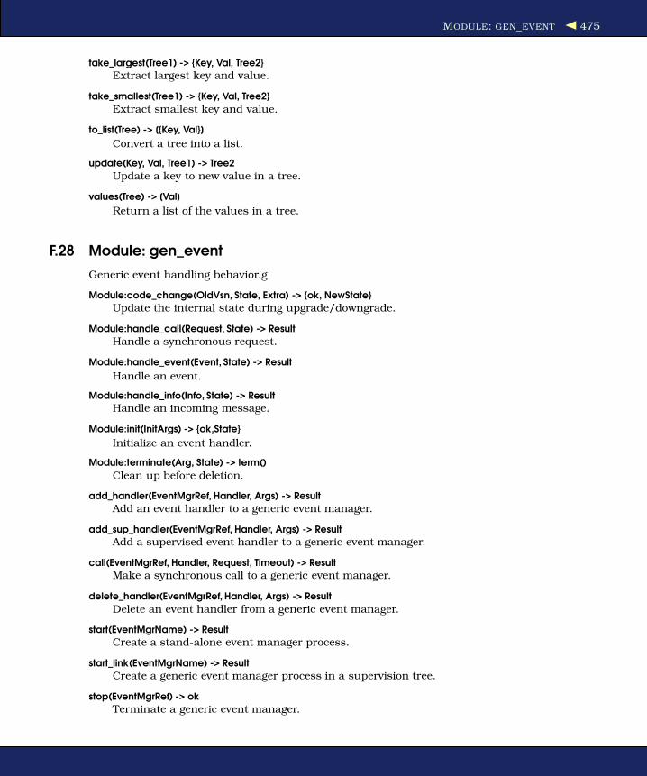
MODULE: GEN_EVENT 475
take_largest(Tree1) -> {Key, Val, Tree2}Extract largest key and value.
take_smallest(Tree1) -> {Key, Val, Tree2}
Extract smallest key and value.
to_list(Tree) -> [{Key, Val}]
Convert a tree into a list.
update(Key, Val, Tree1) -> Tree2
Update a key to new value in a tree.
values(Tree) -> [Val]
Return a list of the values in a tree.
F.28 Module: gen_event
Generic event handling behavior.g
Module:code_change(OldVsn, State, Extra) -> {ok, NewState}
Update the internal state during upgrade/downgrade.
Module:handle_call(Request, State) -> Result
Handle a synchronous request.
Module:handle_event(Event, State) -> Result
Handle an event.
Module:handle_info(Info, State) -> ResultHandle an incoming message.
Module:init(InitArgs) -> {ok,State}
Initialize an event handler.
Module:terminate(Arg, State) -> term()
Clean up before deletion.
add_handler(EventMgrRef, Handler, Args) -> Result
Add an event handler to a generic event manager.
add_sup_handler(EventMgrRef, Handler, Args) -> ResultAdd a supervised event handler to a generic event manager.
call(EventMgrRef, Handler, Request, Timeout) -> ResultMake a synchronous call to a generic event manager.
delete_handler(EventMgrRef, Handler, Args) -> Result
Delete an event handler from a generic event manager.
start(EventMgrName) -> ResultCreate a stand-alone event manager process.
start_link(EventMgrName) -> ResultCreate a generic event manager process in a supervision tree.
stop(EventMgrRef) -> okTerminate a generic event manager.

MODULE: GEN_FSM 476
swap_handler(EventMgrRef, {Handler1,Args1}, {Handler2,Args2}) -> ResultReplace an event handler in a generic event manager.
swap_sup_handler(EventMgrRef, {Handler1,Args1}, {Handler2,Args2}) -> Result
Replace an event handler in a generic event manager.
sync_notify(EventMgrRef, Event) -> ok
Notify an event manager about an event.
which_handlers(EventMgrRef) -> [Handler]
Return all event handlers installed in a generic event manager.
F.29 Module: gen_fsm
Generic finite state machine behavior.
Module:StateName(Event, StateData) -> Result
Handle an asynchronous event.
Module:StateName(Event, From, StateData) -> Result
Handle a synchronous event.
Module:code_change(OldVsn, StateName, StateData, Extra) ->
{ok, NextStateName, NewStateData}
Update the internal state data during upgrade/downgrade.
Module:handle_event(Event, StateName, StateData) -> Result
Handle an asynchronous event.
Module:handle_info(Info, StateName, StateData) -> ResultHandle an incoming message.
Module:handle_sync_event(Event, From, StateName, StateData) -> Result
Handle a synchronous event.
Module:init(Args) -> Result
Initialize process and internal state name and state data.
Module:terminate(Reason, StateName, StateData)
Clean up before termination.
cancel_timer(Ref) -> RemainingTime | falseCancel an internal timer in a generic FSM.
enter_loop(Module, Options, StateName, StateData, FsmName, Timeout)
Enter thegen_fsmreceive loop.
reply(Caller, Reply) -> true
Send a reply to a caller.
send_all_state_event(FsmRef, Event) -> ok
Send an event asynchronously to a generic FSM.
send_event(FsmRef, Event) -> okSend an event asynchronously to a generic FSM.
send_event_after(Time, Event) -> Ref
Send a delayed event internally in a generic FSM.

MODULE: GEN_SCTP 477
start(FsmName, Module, Args, Options) -> Result
Create a stand-alone gen_fsm process.
start_link(FsmName, Module, Args, Options) -> Result
Create a gen_fsm process in a supervision tree.
start_timer(Time, Msg) -> RefSend a timeout event internally in a generic FSM.
sync_send_all_state_event(FsmRef, Event, Timeout) -> Reply
Send an event syncronously to a generic FSM.
sync_send_event(FsmRef, Event, Timeout) -> ReplySend an event synchronously to a generic FSM.
F.30 Module: gen_sctp
The gen_sctp module provides functions for communicating with sockets usingthe SCTP protocol.
abort(sctp_socket(), Assoc) -> ok | {error, posix()}Abnormally terminate the association given byAssoc, without flushing ofunsent data.
close(sctp_socket()) -> ok | {error, posix()}
Completely close the socket and all associations on it.
connect(Socket, IP, Port, Opts) -> {ok,Assoc} | {error, posix()}
Same asconnect(Socket, IP, Port, Opts, infinity).
connect(Socket, IP, Port, [Opt], Timeout) -> {ok, Assoc} | {error, posix()}Establish a new association for the socketSocket, with a peer (SCTP serversocket).
controlling_process(sctp_socket(), pid()) -> ok
Assign a new controlling process PID to the socket.
eof(Socket, Assoc) -> ok | {error, Reason}Gracefully terminate the association given byAssoc, with flushing of allunsent data.
error_string(integer()) -> ok | string() | undefined
Translate an SCTP error number into a string.
listen(Socket, IsServer) -> ok | {error, Reason}
Set up a socket to listen.
open([Opt]) -> {ok, Socket} | {error, posix()}
Create an SCTP socket and bind it to local addresses.
recv(sctp_socket(), timeout()) -> {ok, {FromIP, FromPort, AncData, Data}} | {error, Reason}
Receive a message from a socket.
send(Socket, SndRcvInfo, Data) -> ok | {error, Reason}
Send a message using an#sctp_sndrcvinfo{}record.
send(Socket, Assoc, Stream, Data) -> ok | {error, Reason}Send a message over an existing association and given stream.

MODULE: GEN_SERVER 478
F.31 Module: gen_server
Generic server behavior.
Module:code_change(OldVsn, State, Extra) -> {ok, NewState}Update the internal state during upgrade/downgrade.
Module:handle_call(Request, From, State) -> Result
Handle a synchronous request.
Module:handle_cast(Request, State) -> Result
Handle an asynchronous request.
Module:handle_info(Info, State) -> Result
Handle an incoming message.
Module:init(Args) -> Result
Initialize process and internal state.
Module:terminate(Reason, State)
Clean up before termination.
abcast(Nodes, Name, Request) -> abcastSend an asynchronous request to several generic servers.
call(ServerRef, Request, Timeout) -> ReplyMake a synchronous call to a generic server.
cast(ServerRef, Request) -> ok
Send an asynchronous request to a generic server.
enter_loop(Module, Options, State, ServerName, Timeout)
Enter thegen_serverreceive loop.
multi_call(Nodes, Name, Request, Timeout) -> Result
Make a synchronous call to several generic servers.
reply(Client, Reply) -> true
Send a reply to a client.
start(ServerName, Module, Args, Options) -> Result
Create a stand-alonegen_serverprocess.
start_link(ServerName, Module, Args, Options) -> Result
Create agen_serverprocess in a supervision tree.
F.32 Module: gen_tcp
Interface to TCP/IP sockets.
accept(ListenSocket, Timeout) -> {ok, Socket} | {error, Reason}
Accept an incoming connection request on a listen socket.
close(Socket) -> ok | {error, Reason}
Close a TCP socket.
connect(Address, Port, Options, Timeout) -> {ok, Socket} | {error, Reason}
Connect to a TCP port.

MODULE: GEN_UDP 479
controlling_process(Socket, Pid) -> ok | {error, eperm}
Change controlling process of a socket.
listen(Port, Options) -> {ok, ListenSocket} | {error, Reason}
Set up a socket to listen on a port.
recv(Socket, Length, Timeout) -> {ok, Packet} | {error, Reason}
Receive a packet from a passive socket.
send(Socket, Packet) -> ok | {error, Reason}
Send a packet.
shutdown(Socket, How) -> ok | {error, Reason}
Immediately close a socket.
F.33 Module: gen_udp
Interface to UDP sockets.
close(Socket) -> ok | {error, Reason}
Close a UDP socket.
controlling_process(Socket, Pid) -> ok
Change controlling process of a socket.
open(Port, Options) -> {ok, Socket} | {error, Reason}
Associate a UDP port number with the process calling it.
recv(Socket, Length, Timeout) -> {ok, {Address, Port, Packet}} | {error, Reason}
Receive a packet from a passive socket.
send(Socket, Address, Port, Packet) -> ok | {error, Reason}
Send a packet.
F.34 Module: global
A global name registration facility.
del_lock(Id, Nodes) -> void()
Delete a lock.
notify_all_name(Name, Pid1, Pid2) -> none
Name resolving function that notifies both PIDs.
random_exit_name(Name, Pid1, Pid2) -> Pid1 | Pid2
Name resolving function that kills one PID.
random_notify_name(Name, Pid1, Pid2) -> Pid1 | Pid2
Name resolving function that notifies one PID.
re_register_name(Name, Pid, Resolve) -> void()Atomically reregister a name.
register_name(Name, Pid, Resolve) -> yes | no
Globally register a name for a PID.
MODULE: INET 480
registered_names() -> [Name]All globally registered names.
send(Name, Msg) -> Pid
Send a message to a globally registered PID.
set_lock(Id, Nodes, Retries) -> boolean()
Set a lock on the specified nodes.
sync() -> void()
Synchronize the global name server.
trans(Id, Fun, Nodes, Retries) -> Res | aborted
Micro transaction facility.
unregister_name(Name) -> void()
Remove a globally registered name for a PID.
whereis_name(Name) -> pid() | undefinedGet the PID with a given globally registered name.
F.35 Module: inet
Access to TCP/IP protocols.
close(Socket) -> ok
Close a socket of any type.
format_error(Posix) -> string()
Return a descriptive string for an error reason.
get_rc() -> [{Par, Val}]
Return a list of IP configuration parameters.
getaddr(Host, Family) -> {ok, Address} | {error, posix()}
Return the IP address for a host.
getaddrs(Host, Family) -> {ok, Addresses} | {error, posix()}
Return the IP addresses for a host.
gethostbyaddr(Address) -> {ok, Hostent} | {error, posix()}
Return a hostent record for the host with the given address.
gethostbyname(Name) -> {ok, Hostent} | {error, posix()}
Return a hostent record for the host with the given name.
gethostbyname(Name, Family) -> {ok, Hostent} | {error, posix()}
Return a hostent record for the host with the given name.
gethostname() -> {ok, Hostname} | {error, posix()}
Return the local hostname.
getopts(Socket, Options) -> OptionValues | {error, posix()}
Get one or more options for a socket.
peername(Socket) -> {ok, {Address, Port}} | {error, posix()}
Return the address and port for the other end of a connection.
MODULE: INIT 481
port(Socket) -> {ok, Port}
Return the local port number for a socket.
setopts(Socket, Options) -> ok | {error, posix()}
Set one or more options for a socket.
sockname(Socket) -> {ok, {Address, Port}} | {error, posix()}
Return the local address and port number for a socket.
F.36 Module: init
Coordination of system start-up.
boot(BootArgs) -> void()Start the Erlang runtime system.
get_args() -> [Arg]
Get all nonflag command-line arguments.
get_argument(Flag) -> {ok, Arg} | error
Get the values associated with a command-line user flag.
get_arguments() -> Flags
Get all command-line user flags.
get_plain_arguments() -> [Arg]
Get all nonflag command-line arguments.
get_status() -> {InternalStatus, ProvidedStatus}
Get system status information.
reboot() -> void()
Take down an Erlang node smoothly.
restart() -> void()Restart the running Erlang node.
script_id() -> Id
Get the identity of the used boot script.
stop() -> void()Take down an Erlang node smoothly.
F.37 Module: io
Standard IO server interface functions.
format([IoDevice,] Format, Data) -> ok
Write formatted output.
fread([IoDevice,] Prompt, Format) -> Result
Read formatted input.
get_chars([IoDevice,] Prompt, Count) -> string() | eof
Read a specified number of characters.

MODULE: IO_LIB 482
get_line([IoDevice,] Prompt) -> string() | eof
Read a line.
nl([IoDevice]) -> ok
Write a newline.
parse_erl_exprs([IoDevice,] Prompt, StartLine) -> ResultRead, tokenize and parse Erlang expressions.
parse_erl_form([IoDevice,] Prompt, StartLine) -> Result
Read, tokenize and parse an Erlang form.
put_chars([IoDevice,] IoData) -> ok
Write a list of characters.
read([IoDevice,] Prompt) -> Result
Read a term.
read(IoDevice, Prompt, StartLine) -> Result
Read a term.
scan_erl_exprs([IoDevice,] Prompt, StartLine) -> ResultRead and tokenize Erlang expressions.
scan_erl_form([IoDevice,] Prompt, StartLine) -> Result
Read and tokenize an Erlang form.
setopts([IoDevice,] Opts) -> ok | {error, Reason}
Set options.
write([IoDevice,] Term) -> ok
Write a term.
F.38 Module: io_lib
IO library functions.
char_list(Term) -> bool()
Test for a list of characters.
deep_char_list(Term) -> bool()
Test for a deep list of characters.
format(Format, Data) -> chars()
Write formatted output.
fread(Format, String) -> Result
Read formatted input.
fread(Continuation, String, Format) -> Return
Reentrant formatted reader.
indentation(String, StartIndent) -> int()
Indentation after printing string.
nl() -> chars()
Write a newline.

MODULE: LIB 483
print(Term, Column, LineLength, Depth) -> chars()
Pretty-print a term.
printable_list(Term) -> bool()
Test for a list of printable characters.
write(Term, Depth) -> chars()
Write a term.
write_atom(Atom) -> chars()
Write an atom.
write_char(Integer) -> chars()
Write a character.
write_string(String) -> chars()
Write a string.
F.39 Module: lib
A number of useful library functions.
error_message(Format, Args) -> okPrint error message.
flush_receive() -> void()
Flush messages.
nonl(String1) -> String2
Remove last newline.
progname() -> atom()
Return name of Erlang start script.
send(To, Msg)Send a message.
sendw(To, Msg)
Send a message, and wait for an answer.
F.40 Module: lists
List-processing functions.
all(Pred, List) -> bool()
Return true if all elements in the list satisfyPred.
any(Pred, List) -> bool()
Return true if any of the elements in the list satisfiesPred.
append(ListOfLists) -> List1
Append a list of lists.
append(List1, List2) -> List3
Append two lists.

MODULE: LISTS 484
concat(Things) -> string()
Concatenate a list of atoms.
delete(Elem, List1) -> List2
Delete an element from a list.
dropwhile(Pred, List1) -> List2
Drop elements from a list while a predicate is true.
duplicate(N, Elem) -> List
Make N copies of element.
filter(Pred, List1) -> List2
Choose elements that satisfy a predicate.
flatlength(DeepList) -> int()
Length of flattened deep list.
flatmap(Fun, List1) -> List2
Map and flatten in one pass.
flatten(DeepList) -> List
Flatten a deep list.
flatten(DeepList, Tail) -> List
Flatten a deep list.
foldl(Fun, Acc0, List) -> Acc1
Fold a function over a list.
foldr(Fun, Acc0, List) -> Acc1
Fold a function over a list.
foreach(Fun, List) -> void()
Apply a function to each element of a list.
keydelete(Key, N, TupleList1) -> TupleList2
Delete an element from a list of tuples.
keymap(Fun, N, TupleList1) -> TupleList2
Map a function over a list of tuples.
keymember(Key, N, TupleList) -> bool()
Test for membership of a list of tuples.
keymerge(N, TupleList1, TupleList2) -> TupleList3
Merge two key-sorted lists of tuples.
keyreplace(Key, N, TupleList1, NewTuple) -> TupleList2
Replace an element in a list of tuples.
keysearch(Key, N, TupleList) -> {value, Tuple} | false
Search for an element in a list of tuples.
keysort(N, TupleList1) -> TupleList2
Sort a list of tuples.
last(List) -> Last
Return last element in a list.

MODULE: LISTS 485
map(Fun, List1) -> List2
Map a function over a list.
mapfoldl(Fun, Acc0, List1) -> {List2, Acc1}
Map and fold in one pass.
mapfoldr(Fun, Acc0, List1) -> {List2, Acc1}
Map and fold in one pass.
max(List) -> Max
Return maximum element of a list.
member(Elem, List) -> bool()
Test for membership of a list.
merge(ListOfLists) -> List1
Merge a list of sorted lists.
merge(List1, List2) -> List3Merge two sorted lists.
merge(Fun, List1, List2) -> List3Merge two sorted list.
merge3(List1, List2, List3) -> List4Merge three sorted lists.
min(List) -> Min
Return minimum element of a list.
nth(N, List) -> Elem
Return the Nth element of a list.
nthtail(N, List1) -> Tail
Return the Nth tail of a list.
partition(Pred, List) -> {Satisfying, NonSatisfying}
Partition a list into two lists based on a predicate.
prefix(List1, List2) -> bool()
Test for list prefix.
reverse(List1) -> List2
Reverse a list.
reverse(List1, Tail) -> List2Reverse a list appending a tail.
seq(From, To, Incr) -> Seq
Generate a sequence of integers.
sort(List1) -> List2
Sort a list.
sort(Fun, List1) -> List2
Sort a list.
split(N, List1) -> {List2, List3}
Split a list into two lists.

MODULE: LISTS 486
splitwith(Pred, List) -> {List1, List2}
Split a list into two lists based on a predicate.
sublist(List1, Len) -> List2
Return a sublist of a certain length, starting at the first position.
sublist(List1, Start, Len) -> List2Return a sublist starting at a given position and with a given number ofelements.
subtract(List1, List2) -> List3
Subtract the element in one list from another list.
suffix(List1, List2) -> bool()
Test for list suffix.
sum(List) -> number()
Return sum of elements in a list.
takewhile(Pred, List1) -> List2
Take elements from a list while a predicate is true.
ukeymerge(N, TupleList1, TupleList2) -> TupleList3
Merge two key-sorted lists of tuples, removing duplicates.
ukeysort(N, TupleList1) -> TupleList2
Sort a list of tuples, removing duplicates.
umerge(ListOfLists) -> List1
Merge a list of sorted lists, removing duplicates.
umerge(List1, List2) -> List3
Merge two sorted lists, removing duplicates.
umerge(Fun, List1, List2) -> List3Merge two sorted lists, removing duplicates.
umerge3(List1, List2, List3) -> List4
Merge three sorted lists, removing duplicates.
unzip(List1) -> {List2, List3}
Unzip a list of two tuples into two lists.
unzip3(List1) -> {List2, List3, List4}
Unzip a list of three tuples into three lists.
usort(List1) -> List2Sort a list, removing duplicates.
usort(Fun, List1) -> List2
Sort a list, removing duplicates.
zip(List1, List2) -> List3
Zip two lists into a list of two tuples.
zip3(List1, List2, List3) -> List4
Zip three lists into a list of three tuples.
zipwith(Combine, List1, List2) -> List3
Zip two lists into one list according to a fun.

MODULE: MATH 487
zipwith3(Combine, List1, List2, List3) -> List4
Zip three lists into one list according to a fun.
F.41 Module: math
Mathematical functions.
erf(X) -> float()
Error function.
erfc(X) -> float()
Another error function.
pi() -> float()
A useful number.
sqrt(X)
Diverse math functions.
F.42 Module: ms_transform
Parse_transform that translates fun syntax into match specifications.
format_error(Errcode) -> ErrMessage
Error formatting function as required by theparse_transforminterface.
parse_transform(Forms,_Options) -> FormsTransforms Erlang abstract format containing calls toets/dbg:fun2msinto lit-eral match specifications.
transform_from_shell(Dialect,Clauses,BoundEnvironment) -> term()
Used when transforming fun’s created in the shell intomatch_specifications.
F.43 Module: net_adm
Various Erlang net administration routines.
dns_hostname(Host) -> {ok, Name} | {error, Host}
Official name of a host.
host_file() -> Hosts | {error, Reason}
Read the.hosts.erlangfile.
localhost() -> Name
Name of the local host.
names(Host) -> {ok, [{Name, Port}]} | {error, Reason}
Names of Erlang nodes at a host.
ping(Node) -> pong | pang
Set up a connection to a node.
world(Arg) -> [node()]
Lookup and connect to all nodes at all hosts in.hosts.erlang.
MODULE: NET_KERNEL 488
world_list(Hosts, Arg) -> [node()]
Lookup and connect to all nodes at specified hosts.
F.44 Module: net_kernel
Erlang networking kernel.
allow(Nodes) -> ok | error
Limit access to a specified set of nodes.
connect_node(Node) -> true | false | ignored
Establish a connection to a node.
get_net_ticktime() -> Res
Get net_ticktime.
monitor_nodes(Flag, Options) -> ok | ErrorSubscribe to node status change messages.
set_net_ticktime(NetTicktime, TransitionPeriod) -> Res
Setnet_ticktime.
start([Name, NameType, Ticktime]) -> {ok, pid()} | {error, Reason}Turn an Erlang runtime system into a distributed node.
stop() -> ok | {error, not_allowed | not_found}
Turn a node into a nondistributed Erlang runtime system.
F.45 Module: os
Operating system–specific functions.
cmd(Command) -> string()
Execute a command in a shell of the target OS.
find_executable(Name, Path) -> Filename | false
Absolute filename of a program.
getenv() -> [string()]
List all environment variables.
getenv(VarName) -> Value | false
Get the value of an environment variable.
getpid() -> Value
Return the process identifier of the emulator process.
putenv(VarName, Value) -> true
Set a new value for an environment variable.
type() -> {Osfamily, Osname} | OsfamilyReturn the OS family and, in some cases, the OS name of the currentoperating system.
version() -> {Major, Minor, Release} | VersionStringReturn the operating system version.

MODULE: PROC_LIB 489
F.46 Module: proc_lib
Functions for asynchronous and synchronous start of processes adhering tothe OTP design principles.
format(CrashReport) -> string()
Format a crash report.
hibernate(Module, Function, Args)Hibernate a process until a message is sent to it.
init_ack(Ret) -> void()
Used by a process when it has started.
initial_call(Process) -> {Module,Function,Args} | Fun | false
Extract the initial call of aproc_libspawned process.
spawn(Node, Module, Function, Args) -> pid()
Spawn a new process.
spawn_link(Node, Module, Function, Args) -> pid()
Spawn and link to a new process.
spawn_opt(Node, Module, Func, Args, SpawnOpts) -> pid()Spawn a new process with given options.
start_link(Module, Function, Args, Time, SpawnOpts) -> Ret
Start a new process synchronously.
translate_initial_call(Process) -> {Module,Function,Arity} | Fun
Extract and translate the initial call of a proc_lib spawned process.
F.47 Module: qlc
Query interface to Mnesia, ETS, DETS, and so on.
append(QHL) -> QH
Return a query handle.
append(QH1, QH2) -> QH3
Return a query handle.
cursor(QueryHandleOrList [, Options]) -> QueryCursor
Create a query cursor.
delete_cursor(QueryCursor) -> ok
Delete a query cursor.
e(QueryHandleOrList [, Options]) -> Answers
Return all answers to a query.
fold(Function, Acc0, QueryHandleOrList [, Options]) -> Acc1 | Error
Fold a function over the answers to a query.
format_error(Error) -> Chars
Return an English description of a an error tuple.

MODULE: QUEUE 490
info(QueryHandleOrList [, Options]) -> InfoReturn code describing a query handle.
keysort(KeyPos, QH1 [, SortOptions]) -> QH2
Return a query handle.
next_answers(QueryCursor [, NumberOfAnswers]) -> Answers | Error
Return some or all answers to a query.
q(QueryListComprehension [, Options]) -> QueryHandle
Return a handle for a query list comprehension.
sort(QH1 [, SortOptions]) -> QH2
Return a query handle.
string_to_handle(QueryString [, Options [, Bindings]]) -> QueryHandle | Error
Return a handle for a query list comprehension.
table(TraverseFun, Options) -> QueryHandle
Return a query handle for a table.
F.48 Module: queue
Abstract data type for FIFO queues.
cons(Item, Q1) -> Q2
Insert an item at the head of a queue.
daeh(Q) -> Item
Return the last item of a queue.
from_list(L) -> queue()
Convert a list to a queue.
head(Q) -> Item
Return the item at the head of a queue.
in(Item, Q1) -> Q2
Insert an item at the tail of a queue.
in_r(Item, Q1) -> Q2
Insert an item at the head of a queue.
init(Q1) -> Q2
Remove the last item from a queue.
is_empty(Q) -> true | false
Test whether a queue is empty.
join(Q1, Q2) -> Q3
Join two queues.
lait(Q1) -> Q2
Remove the last item from a queue.
last(Q) -> Item
Return the last item of a queue.
MODULE: RANDOM 491
len(Q) -> N
Get the length of a queue.
new() -> Q
Create a new empty FIFO queue.
out(Q1) -> Result
Remove the head item from a queue.
out_r(Q1) -> Result
Remove the last item from a queue.
reverse(Q1) -> Q2
Reverse a queue.
snoc(Q1, Item) -> Q2
Insert an item at the end of a queue.
split(N, Q1) -> {Q2,Q3}
Split a queue in two.
tail(Q1) -> Q2
Remove the head item from a queue.
to_list(Q) -> list()
Convert a queue to a list.
F.49 Module: random
Pseudorandom number generation.
seed() -> ran()
Seeds random number generation with default values.
seed(A1, A2, A3) -> ran()Seeds random number generator.
seed0() -> ran()
Return default state for random number generation.
uniform()-> float()
Return a random float.
uniform(N) -> int()Return a random integer.
uniform_s(State0) -> {float(), State1}
Return a random float.
uniform_s(N, State0) -> {int(), State1}Return a random integer.

MODULE: REGEXP 492
F.50 Module: regexp
Regular expression functions for strings.
first_match(String, RegExp) -> MatchResMatch a regular expression.
format_error(ErrorDescriptor) -> Chars
Format an error descriptor.
gsub(String, RegExp, New) -> SubRes
Substitute all occurrences of a regular expression.
match(String, RegExp) -> MatchRes
Match a regular expression.
matches(String, RegExp) -> MatchResMatch a regular expression.
parse(RegExp) -> ParseResParse a regular expression.
sh_to_awk(ShRegExp) -> AwkRegExpConvert an sh regular expression into an AWK one.
split(String, RegExp) -> SplitRes
Split a string into fields.
sub(String, RegExp, New) -> SubRes
Substitute the first occurrence of a regular expression.
F.51 Module: rpc
Remote procedure call services.
abcast(Name, Msg) -> void()Broadcast a message asynchronously to a registered process on all nodes.
abcast(Nodes, Name, Msg) -> void()Broadcast a message asynchronously to a registered process on specificnodes.
async_call(Node, Module, Function, Args) -> Key
Evaluate a function call on a node, asynchrous version.
block_call(Node, Module, Function, Args) -> Res | {badrpc, Reason}
Evaluate a function call on a node in the RPC server’s context.
block_call(Node, Module, Function, Args, Timeout) -> Res | {badrpc, Reason}
Evaluate a function call on a node in the RPC server’s context.
call(Node, Module, Function, Args) -> Res | {badrpc, Reason}
Evaluate a function call on a node.
call(Node, Module, Function, Args, Timeout) -> Res | {badrpc, Reason}
Evaluate a function call on a node.
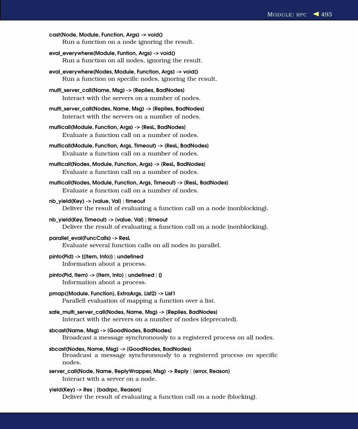
MODULE: RPC 493
cast(Node, Module, Function, Args) -> void()
Run a function on a node ignoring the result.
eval_everywhere(Module, Funtion, Args) -> void()
Run a function on all nodes, ignoring the result.
eval_everywhere(Nodes, Module, Function, Args) -> void()
Run a function on specific nodes, ignoring the result.
multi_server_call(Name, Msg) -> {Replies, BadNodes}
Interact with the servers on a number of nodes.
multi_server_call(Nodes, Name, Msg) -> {Replies, BadNodes}
Interact with the servers on a number of nodes.
multicall(Module, Function, Args) -> {ResL, BadNodes}
Evaluate a function call on a number of nodes.
multicall(Module, Function, Args, Timeout) -> {ResL, BadNodes}
Evaluate a function call on a number of nodes.
multicall(Nodes, Module, Function, Args) -> {ResL, BadNodes}
Evaluate a function call on a number of nodes.
multicall(Nodes, Module, Function, Args, Timeout) -> {ResL, BadNodes}
Evaluate a function call on a number of nodes.
nb_yield(Key) -> {value, Val} | timeout
Deliver the result of evaluating a function call on a node (nonblocking).
nb_yield(Key, Timeout) -> {value, Val} | timeout
Deliver the result of evaluating a function call on a node (nonblocking).
parallel_eval(FuncCalls) -> ResL
Evaluate several function calls on all nodes in parallel.
pinfo(Pid) -> [{Item, Info}] | undefined
Information about a process.
pinfo(Pid, Item) -> {Item, Info} | undefined | []
Information about a process.
pmap({Module, Function}, ExtraArgs, List2) -> List1
Parallell evaluation of mapping a function over a list.
safe_multi_server_call(Nodes, Name, Msg) -> {Replies, BadNodes}
Interact with the servers on a number of nodes (deprecated).
sbcast(Name, Msg) -> {GoodNodes, BadNodes}
Broadcast a message synchronously to a registered process on all nodes.
sbcast(Nodes, Name, Msg) -> {GoodNodes, BadNodes}Broadcast a message synchronously to a registered process on specificnodes.
server_call(Node, Name, ReplyWrapper, Msg) -> Reply | {error, Reason}
Interact with a server on a node.
yield(Key) -> Res | {badrpc, Reason}
Deliver the result of evaluating a function call on a node (blocking).

MODULE: SEQ_TRACE 494
F.52 Module: seq_trace
Sequential tracing of messages.
get_system_tracer() -> Tracer
Return thepid()orport()of the current system tracer.
get_token() -> TraceToken
Return the value of the trace token.
get_token(Component) -> {Component, Val}
Return the value of a trace token component.
print(TraceInfo) -> void()
Put the Erlang termTraceInfointo the sequential trace output.
print(Label, TraceInfo) -> void()Put the Erlang termTraceInfointo the sequential trace output.
reset_trace() -> void()Stop all sequential tracing on the local node.
set_system_tracer(Tracer) -> OldTracer
Set the system tracer.
set_token(Token) -> PreviousToken
Set the trace token.
set_token(Component, Val) -> {Component, OldVal}
Set a component of the trace token.
F.53 Module: sets
Functions for set manipulation.
add_element(Element, Set1) -> Set2
Add an element to aSet.
del_element(Element, Set1) -> Set2
Remove an element from aSet.
filter(Pred, Set1) -> Set2
Filter set elements.
fold(Function, Acc0, Set) -> Acc1
Fold over set elements.
from_list(List) -> Set
Convert a list into aSet.
intersection(SetList) -> Set
Return the intersection of a list ofSets.
intersection(Set1, Set2) -> Set3
Return the intersection of two Sets.
is_element(Element, Set) -> bool()
Test for membership of aSet.

MODULE: SHELL 495
is_set(Set) -> bool()
Test for aSet.
is_subset(Set1, Set2) -> bool()
Test for subset.
new() -> Set
Return an empty set.
size(Set) -> int()
Return the number of elements in a set.
subtract(Set1, Set2) -> Set3
Return the difference of two Sets.
to_list(Set) -> List
Convert aSetinto a list.
union(SetList) -> Set
Return the union of a list of Sets.
union(Set1, Set2) -> Set3
Return the union of two Sets.
F.54 Module: shell
The Erlang shell.
history(N) -> integer()
Sets the number of previous commands to keep.
results(N) -> integer()
Sets the number of previous commands to keep.
start_restricted(Module) -> ok
Exits a normal shell and starts a restricted shell.
stop_restricted() -> ok
Exits a restricted shell and starts a normal shell.
F.55 Module: slave
Functions to starting and controlling slave nodes.
pseudo([Master | ServerList]) -> ok
Start a number of pseudoservers.
pseudo(Master, ServerList) -> ok
Start a number of pseudoservers.
relay(Pid)
Run a pseudoserver.
start(Host, Name, Args) -> {ok, Node} | {error, Reason}
Start a slave node on a host.
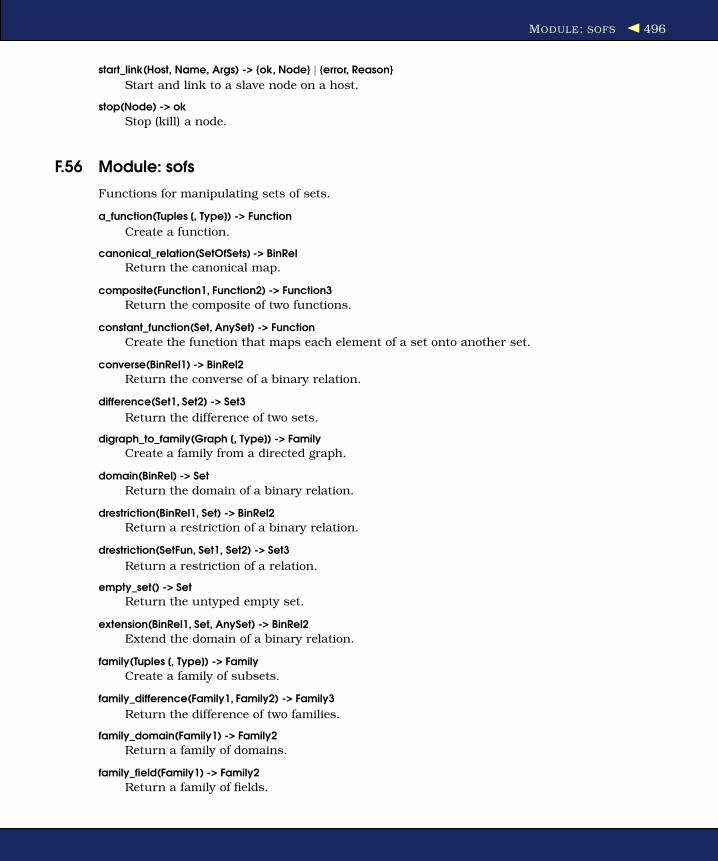
MODULE: SOFS 496
start_link(Host, Name, Args) -> {ok, Node} | {error, Reason}
Start and link to a slave node on a host.
stop(Node) -> ok
Stop (kill) a node.
F.56 Module: sofs
Functions for manipulating sets of sets.
a_function(Tuples [, Type]) -> Function
Create a function.
canonical_relation(SetOfSets) -> BinRel
Return the canonical map.
composite(Function1, Function2) -> Function3
Return the composite of two functions.
constant_function(Set, AnySet) -> Function
Create the function that maps each element of a set onto another set.
converse(BinRel1) -> BinRel2
Return the converse of a binary relation.
difference(Set1, Set2) -> Set3
Return the difference of two sets.
digraph_to_family(Graph [, Type]) -> Family
Create a family from a directed graph.
domain(BinRel) -> Set
Return the domain of a binary relation.
drestriction(BinRel1, Set) -> BinRel2
Return a restriction of a binary relation.
drestriction(SetFun, Set1, Set2) -> Set3
Return a restriction of a relation.
empty_set() -> Set
Return the untyped empty set.
extension(BinRel1, Set, AnySet) -> BinRel2
Extend the domain of a binary relation.
family(Tuples [, Type]) -> Family
Create a family of subsets.
family_difference(Family1, Family2) -> Family3
Return the difference of two families.
family_domain(Family1) -> Family2
Return a family of domains.
family_field(Family1) -> Family2
Return a family of fields.
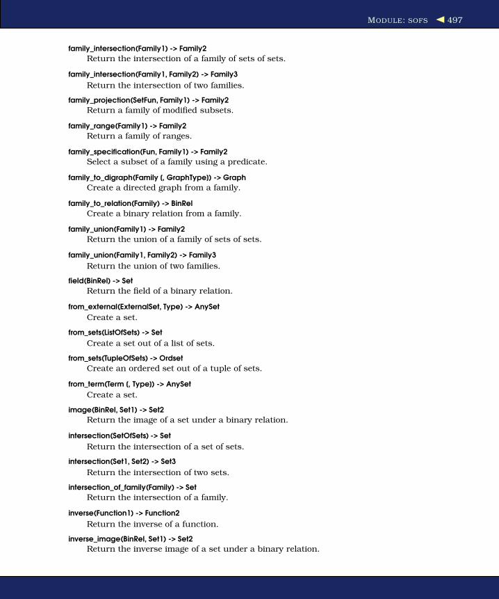
MODULE: SOFS 497
family_intersection(Family1) -> Family2
Return the intersection of a family of sets of sets.
family_intersection(Family1, Family2) -> Family3
Return the intersection of two families.
family_projection(SetFun, Family1) -> Family2
Return a family of modified subsets.
family_range(Family1) -> Family2
Return a family of ranges.
family_specification(Fun, Family1) -> Family2
Select a subset of a family using a predicate.
family_to_digraph(Family [, GraphType]) -> Graph
Create a directed graph from a family.
family_to_relation(Family) -> BinRel
Create a binary relation from a family.
family_union(Family1) -> Family2
Return the union of a family of sets of sets.
family_union(Family1, Family2) -> Family3
Return the union of two families.
field(BinRel) -> Set
Return the field of a binary relation.
from_external(ExternalSet, Type) -> AnySet
Create a set.
from_sets(ListOfSets) -> Set
Create a set out of a list of sets.
from_sets(TupleOfSets) -> Ordset
Create an ordered set out of a tuple of sets.
from_term(Term [, Type]) -> AnySet
Create a set.
image(BinRel, Set1) -> Set2
Return the image of a set under a binary relation.
intersection(SetOfSets) -> Set
Return the intersection of a set of sets.
intersection(Set1, Set2) -> Set3
Return the intersection of two sets.
intersection_of_family(Family) -> Set
Return the intersection of a family.
inverse(Function1) -> Function2
Return the inverse of a function.
inverse_image(BinRel, Set1) -> Set2
Return the inverse image of a set under a binary relation.
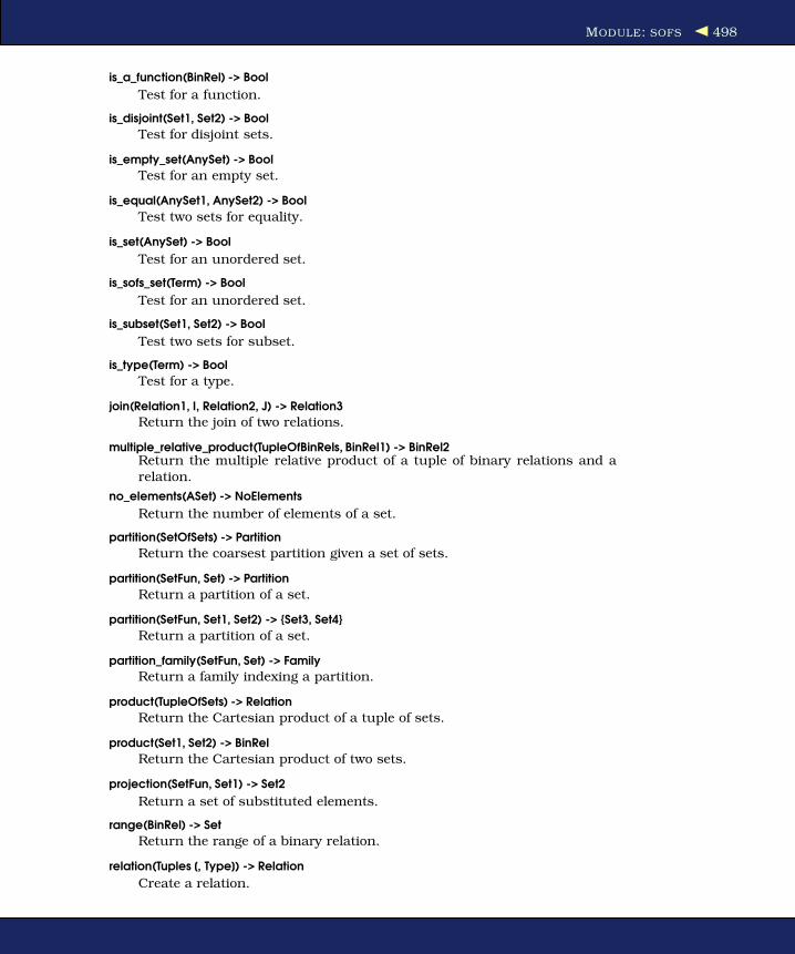
MODULE: SOFS 498
is_a_function(BinRel) -> Bool
Test for a function.
is_disjoint(Set1, Set2) -> Bool
Test for disjoint sets.
is_empty_set(AnySet) -> Bool
Test for an empty set.
is_equal(AnySet1, AnySet2) -> Bool
Test two sets for equality.
is_set(AnySet) -> Bool
Test for an unordered set.
is_sofs_set(Term) -> Bool
Test for an unordered set.
is_subset(Set1, Set2) -> Bool
Test two sets for subset.
is_type(Term) -> Bool
Test for a type.
join(Relation1, I, Relation2, J) -> Relation3
Return the join of two relations.
multiple_relative_product(TupleOfBinRels, BinRel1) -> BinRel2Return the multiple relative product of a tuple of binary relations and arelation.
no_elements(ASet) -> NoElements
Return the number of elements of a set.
partition(SetOfSets) -> Partition
Return the coarsest partition given a set of sets.
partition(SetFun, Set) -> Partition
Return a partition of a set.
partition(SetFun, Set1, Set2) -> {Set3, Set4}
Return a partition of a set.
partition_family(SetFun, Set) -> Family
Return a family indexing a partition.
product(TupleOfSets) -> Relation
Return the Cartesian product of a tuple of sets.
product(Set1, Set2) -> BinRel
Return the Cartesian product of two sets.
projection(SetFun, Set1) -> Set2
Return a set of substituted elements.
range(BinRel) -> Set
Return the range of a binary relation.
relation(Tuples [, Type]) -> Relation
Create a relation.
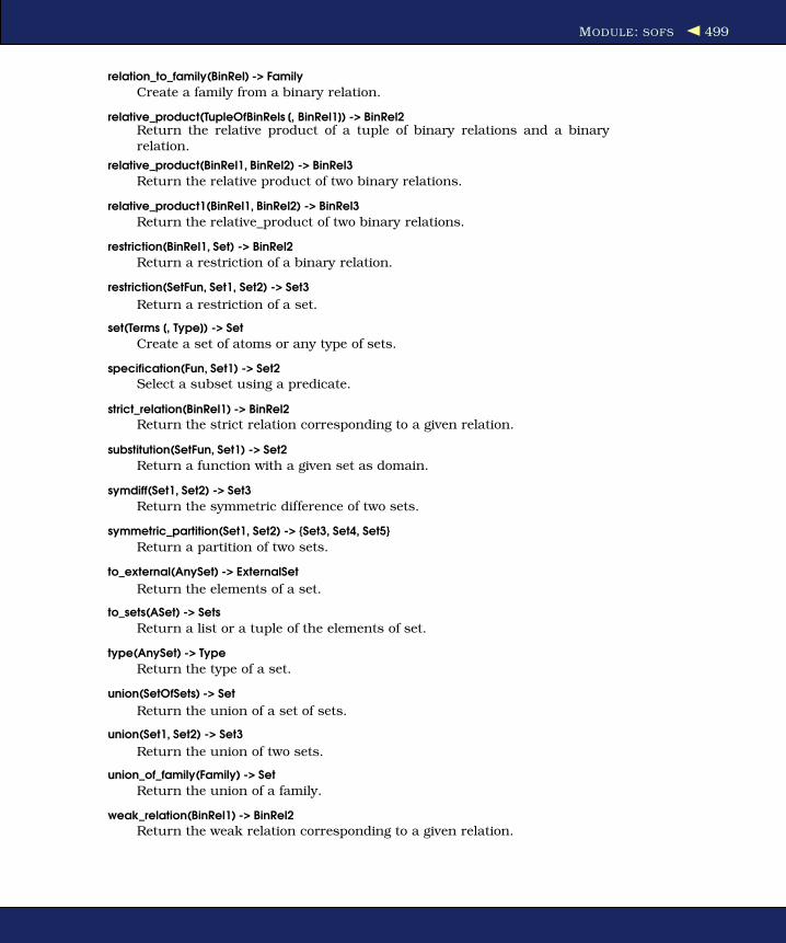
MODULE: SOFS 499
relation_to_family(BinRel) -> Family
Create a family from a binary relation.
relative_product(TupleOfBinRels [, BinRel1]) -> BinRel2Return the relative product of a tuple of binary relations and a binaryrelation.
relative_product(BinRel1, BinRel2) -> BinRel3
Return the relative product of two binary relations.
relative_product1(BinRel1, BinRel2) -> BinRel3
Return the relative_product of two binary relations.
restriction(BinRel1, Set) -> BinRel2
Return a restriction of a binary relation.
restriction(SetFun, Set1, Set2) -> Set3
Return a restriction of a set.
set(Terms [, Type]) -> Set
Create a set of atoms or any type of sets.
specification(Fun, Set1) -> Set2
Select a subset using a predicate.
strict_relation(BinRel1) -> BinRel2Return the strict relation corresponding to a given relation.
substitution(SetFun, Set1) -> Set2
Return a function with a given set as domain.
symdiff(Set1, Set2) -> Set3
Return the symmetric difference of two sets.
symmetric_partition(Set1, Set2) -> {Set3, Set4, Set5}
Return a partition of two sets.
to_external(AnySet) -> ExternalSet
Return the elements of a set.
to_sets(ASet) -> Sets
Return a list or a tuple of the elements of set.
type(AnySet) -> Type
Return the type of a set.
union(SetOfSets) -> Set
Return the union of a set of sets.
union(Set1, Set2) -> Set3
Return the union of two sets.
union_of_family(Family) -> Set
Return the union of a family.
weak_relation(BinRel1) -> BinRel2
Return the weak relation corresponding to a given relation.
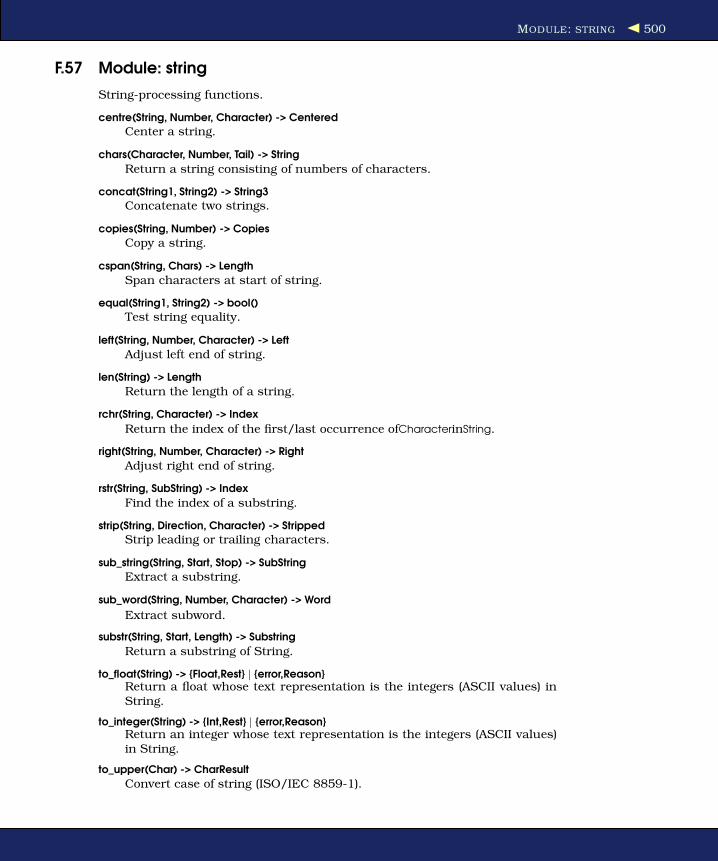
MODULE: STRING 500
F.57 Module: string
String-processing functions.
centre(String, Number, Character) -> CenteredCenter a string.
chars(Character, Number, Tail) -> String
Return a string consisting of numbers of characters.
concat(String1, String2) -> String3Concatenate two strings.
copies(String, Number) -> Copies
Copy a string.
cspan(String, Chars) -> Length
Span characters at start of string.
equal(String1, String2) -> bool()Test string equality.
left(String, Number, Character) -> Left
Adjust left end of string.
len(String) -> Length
Return the length of a string.
rchr(String, Character) -> Index
Return the index of the first/last occurrence ofCharacterinString.
right(String, Number, Character) -> Right
Adjust right end of string.
rstr(String, SubString) -> Index
Find the index of a substring.
strip(String, Direction, Character) -> StrippedStrip leading or trailing characters.
sub_string(String, Start, Stop) -> SubString
Extract a substring.
sub_word(String, Number, Character) -> Word
Extract subword.
substr(String, Start, Length) -> Substring
Return a substring of String.
to_float(String) -> {Float,Rest} | {error,Reason}Return a float whose text representation is the integers (ASCII values) inString.
to_integer(String) -> {Int,Rest} | {error,Reason}Return an integer whose text representation is the integers (ASCII values)in String.
to_upper(Char) -> CharResult
Convert case of string (ISO/IEC 8859-1).

MODULE: SUPERVISOR 501
tokens(String, SeparatorList) -> TokensSplit string into tokens.
words(String, Character) -> Count
Count blank separated words.
F.58 Module: supervisor
Generic supervisor behavior.
Module:init(Args) -> Result
Return a supervisor specification.
check_childspecs([ChildSpec]) -> Result
Check whether child specifications are syntactically correct.
delete_child(SupRef, Id) -> Result
Delete a child specification from a supervisor.
restart_child(SupRef, Id) -> Result
Restart a terminated child process belonging to a supervisor.
start_child(SupRef, ChildSpec) -> Result
Dynamically add a child process to a supervisor.
start_link(SupName, Module, Args) -> Result
Create a supervisor process.
terminate_child(SupRef, Id) -> ResultTerminate a child process belonging to a supervisor.
which_children(SupRef) -> [{Id,Child,Type,Modules}]Return information about all children specifications and child processesbelonging to a supervisor.
F.59 Module: sys
A functional interface to system messages.
Mod:system_code_change(Misc, Module, OldVsn, Extra) -> {ok, NMisc}
Called when the process should perform a code change.
Mod:system_continue(Parent, Debug, Misc)
Called when the process should continue its execution.
Mod:system_terminate(Reason, Parent, Debug, Misc)
Called when the process should terminate.
change_code(Name, Module, OldVsn, Extra, Timeout) -> ok | {error, Reason}
Send the code change system message to the process.
debug_options(Options) -> [dbg_opt()]
Convert a list of options to a debug structure.
get_debug(Item,Debug,Default) -> term()
Get the data associated with a debug option.
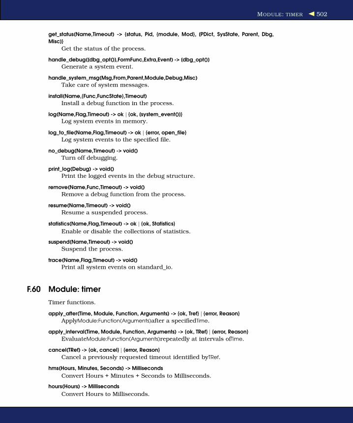
MODULE: TIMER 502
get_status(Name,Timeout) -> {status, Pid, {module, Mod}, [PDict, SysState, Parent, Dbg,
Misc]}
Get the status of the process.
handle_debug([dbg_opt()],FormFunc,Extra,Event) -> [dbg_opt()]
Generate a system event.
handle_system_msg(Msg,From,Parent,Module,Debug,Misc)
Take care of system messages.
install(Name,{Func,FuncState},Timeout)
Install a debug function in the process.
log(Name,Flag,Timeout) -> ok | {ok, [system_event()]}Log system events in memory.
log_to_file(Name,Flag,Timeout) -> ok | {error, open_file}
Log system events to the specified file.
no_debug(Name,Timeout) -> void()
Turn off debugging.
print_log(Debug) -> void()
Print the logged events in the debug structure.
remove(Name,Func,Timeout) -> void()
Remove a debug function from the process.
resume(Name,Timeout) -> void()
Resume a suspended process.
statistics(Name,Flag,Timeout) -> ok | {ok, Statistics}
Enable or disable the collections of statistics.
suspend(Name,Timeout) -> void()
Suspend the process.
trace(Name,Flag,Timeout) -> void()
Print all system events on standard_io.
F.60 Module: timer
Timer functions.
apply_after(Time, Module, Function, Arguments) -> {ok, Tref} | {error, Reason}
ApplyModule:Function(Arguments)after a specifiedTime.
apply_interval(Time, Module, Function, Arguments) -> {ok, TRef} | {error, Reason}
EvaluateModule:Function(Arguments)repeatedly at intervals ofTime.
cancel(TRef) -> {ok, cancel} | {error, Reason}
Cancel a previously requested timeout identified byTRef.
hms(Hours, Minutes, Seconds) -> Milliseconds
Convert Hours + Minutes + Seconds to Milliseconds.
hours(Hours) -> Milliseconds
Convert Hours to Milliseconds.

MODULE: WIN32REG 503
kill_after(Time) -> {ok, TRef} | {error,Reason2}
Send an exit signal with Reason after a specifiedTime.
minutes(Minutes) -> Milliseconds
Converts Minutes to Milliseconds.
now_diff(T2, T1) -> Tdiff
Calculate time difference between now/0 timestamps.
seconds(Seconds) -> Milliseconds
Convert Seconds to Milliseconds.
send_after(Time, Message) -> {ok, TRef} | {error,Reason}
SendMessageto the PID after a specifiedTime.
send_interval(Time, Message) -> {ok, TRef} | {error, Reason}
Send Message repeatedly at intervals ofTime.
sleep(Time) -> ok
Suspend the calling process forTimeamount of milliseconds.
start() -> ok
Start a global timer server (namedtimer_server).
tc(Module, Function, Arguments) -> {Time, Value}
Measure the real time it takes to evaluate apply(Module, Function, Arguments).
F.61 Module: win32reg
Provides access to the registry on Windows.
change_key(RegHandle, Key) -> ReturnValue
Move to a key in the registry.
change_key_create(RegHandle, Key) -> ReturnValue
Move to a key, and create it if it is not there.
close(RegHandle)-> ReturnValue
Close the registry.
current_key(RegHandle) -> ReturnValue
Return the path to the current key.
delete_key(RegHandle) -> ReturnValue
Delete the current key.
delete_value(RegHandle, Name) -> ReturnValue
Delete the named value on the current key.
expand(String) -> ExpandedStringExpand a string with environment variables.
format_error(ErrorId) -> ErrorStringConvert an POSIX error code to a string.
open(OpenModeList)-> ReturnValue
Open the registry for reading or writing.

MODULE: ZIP 504
set_value(RegHandle, Name, Value) -> ReturnValue
Set value at the current registry key with specified name.
sub_keys(RegHandle) -> ReturnValue
Get subkeys to the current key.
value(RegHandle, Name) -> ReturnValue
Get the named value on the current key.
values(RegHandle) -> ReturnValue
Get all values on the current key.
F.62 Module: zip
Utility for reading and creating ZIP archives.
create(Name, FileList, Options) -> RetValue
Create a ZIP archive with options.
extract(Archive, Options) -> RetValue
Extract files from a ZIP archive.
t(Archive)
Print the name of each file in a ZIP archive.
table(Archive, Options)
Retrieve the name of all files in a ZIP archive.
tt(Archive)
Print name and information for each file in a ZIP archive.
zip_close(ZipHandle) -> ok | {error, einval}
Close an open archive.
zip_get(FileName, ZipHandle) -> {ok, Result} | {error, Reason}
Extract files from an open archive.
zip_list_dir(ZipHandle) -> Result | {error, Reason}
Return a table of files in open ZIP archive.
zip_open(Archive, Options) -> {ok, ZipHandle} | {error, Reason}
Open an archive and return a handle to it.
F.63 Module: zlib
Zlib compression interface.
adler32(Z, Binary) -> Checksum
Calculate the adler checksum.
adler32(Z, PrevAdler, Binary) -> Checksum
Calculate the adler checksum.
close(Z) -> ok
Close a stream.

MODULE: ZLIB 505
compress(Binary) -> Compressed
Compress a binary with standard zlib functionality.
crc32(Z) -> CRC
Get current CRC.
crc32(Z, Binary) -> CRC
Calculate CRC.
crc32(Z, PrevCRC, Binary) -> CRC
Calculate CRC.
deflate(Z, Data) -> Compressed
Compress data.
deflate(Z, Data, Flush) ->
Compress data.
deflateEnd(Z) -> ok
End deflate session.
deflateInit(Z) -> ok
Initialize a session for compression.
deflateInit(Z, Level) -> ok
Initialize a session for compression.
deflateInit(Z, Level, Method, WindowBits, MemLevel, Strategy) -> ok
Initialize a session for compression.
deflateParams(Z, Level, Strategy) -> ok
Dynamicly update deflate parameters.
deflateReset(Z) -> ok
Reset the deflate session.
deflateSetDictionary(Z, Dictionary) -> Adler32
Initialize the compression dictionary.
getBufSize(Z) -> Size
Get buffer size.
gunzip(Bin) -> Decompressed
Uncompress a binary with gz header.
gzip(Data) -> CompressedCompress a binary with gz header.
inflate(Z, Data) -> DeCompressed
Decompress data.
inflateEnd(Z) -> ok
End inflate session.
inflateInit(Z) -> ok
Initialize a session for decompression.
inflateInit(Z, WindowBits) -> ok
Initialize a session for decompression.

MODULE: ZLIB 506
inflateReset(Z) -> ok
>Reset the inflate session.
inflateSetDictionary(Z, Dictionary) -> ok
Initialize the decompression dictionary.
open() -> Z
Open a stream and return a stream reference.
setBufSize(Z, Size) -> ok
Set buffer size.
uncompress(Binary) -> Decompressed
Uncompress a binary with standard zlib functionality.
unzip(Binary) -> Decompressed
Uncompress a binary without the zlib headers.
zip(Binary) -> Compressed
Compress a binary without the zlib headers.

IndexSymbols++ operator, 108
– operator, 108
-> arrow, 106
= operator, 29, 36
=:= operators, 115
== operators, 115
$ syntax, 112
% character, 104
%% characters, 104
~ character, 235
AAccumulators, 74–75
Active message reception (nonblocking),
256–257
Active mode, 256
Active once mode, 256
after keyword, 79
Alarm handler (OTP), 346–348
Algebra vs. single assignment variables,
28
Anagrams, 64
Analysis tools, 419–422
Anonymous functions, see Funs
Application monitor (OTP), 361, 362f
apply, 99
appmon:start, 361
area, 44, 46
Area server, 350
Arithmetic expressions
evaluating, 25
every possible, 65f
and guard expressions, 66
sequential programming and, 64
Arity, 52
Atoms
and guard expression, 66
infinity, 152
introduction to, 33–34
and tuples, 35
Attributes, 99–103
arguments for, 102
module, predefined, 99
user-defined, 101
Autocompiling with makefiles, 127–130
BBags, 275, 276
Base K integers, 111
become, 299
begin ... end block, 103
BIFs, 87
apply, 99
for binary manipulation, 88–89
defined, 86
for distributed programs, 183–184
and guard expressions, 66
for process dictionary, 113
for registered processes, 154
and tracing, 431, 435
Binaries, 87–89
and BIF manipulation, 88–89
bits and bytes, 90
defined, 86
punctuation, 87
storage of, 277
truncated, 247
Binary distributions, 21
Binary functions, 104
binary_to_term, 92, 225, 250, 252
Bit syntax, 89–98
16-bit color example, 90
advanced examples, 92–98
defined, 86
expressions, 90–92
finding synchronization frame in
MPEG data, 92–95

BLACKBOARDS 508 CONVENTIONAL SYNTAX
unpacking COFF data, 96–97
and unpacking header in IPv4
datagram, 97
Blackboards, 278
Block expressions, 103
Blogs (Erlang), 401
Bogdan’s Erlang Abstract Machine, see
Beam
Boolean expressions, 66, 103
Booleans, 103, 104
Bottlenecks, sequential, 371
Bound variables, 29
Bugs
catching, 420
reporting, 21
and stack trace, 85
and variables, 31
Built in Function, see BIFs
Ccase, 72–73, 78, 84
catch, 81
Catching exceptions, 77
CEAN, 23
Character set, 104
Chat program, see IRC lite application
chat_server, 200
Clauses and functions, 46
clean, 129
Client, 144
Client-server application, 144–148
Clock example, 155
Code
coverage analysis, 419, 420
locating, 47
missing (undefined), 131
search paths for loading, 119–121
Command prompt, 123
Command-line arguments, 125
Commas, 51
Comments, 104
Compiler diagnostics, 423
Compiling and running programs,
118–136
command editing in Erlang shell,
130
from command prompt, 123
command-line arguments, 125
crash dump, 136
different ways of, 122–127
in Erlang shell, 122
escript, 124
exporting functions, 125
help, 134–135
makefiles, autocompiling, 127–130
modifying development environment,
119–121
problem solving, 131–134
quick scripting, 123
starting/stopping shell, 118–119
stopping shell, 131
Concurrency, 137–140
and dying messages, 139
granularity, 373
importance of, 13
and interactions, 138
and programming, 137
side effects, avoiding, 369
Concurrency-oriented programming
(COP)
defined, 20
and multicore systems, 365–366
Concurrent Programming in Erlang
(Armstrong and Virding), 400
Concurrent programming, 141–158
client server architecture, 144–148
errors, 159–174
details of, 162–169
keep-alive process, 173
linking processes, 159f, 159–160
monitors, 172
on-exit handler, 160–162
primitives, 170–171
remote handling of, 162
sets of linked processes, 172f, 172
example (as process), 143–144
exercises, 158
overview, 141, 158
primitives for, 142
receive with a timeout, 150–153
recursion, 156–157
registered processes, 154–155
selective receive, 153–154
spawning with MFAs, 157–158
time involved in, 148–150
writing (starting), 156
Conferences for Erlang, 401
Connected process, 212
Connectionless protocol, see UDP
Control flow, macros, 109
Ctrl+G, 133, 134
Conventional syntax, 111

COOKIE PROTECTION SYSTEM 509 EBIN DIRECTORY
Cookie protection system, 186–187
Cookies, 181, 183
COP, see Concurrency-oriented
programming
Copying files, 241
cprof, 421
Crash dump, 136
Crash reports, 342
create_table, 326
Cross-references, 421
DDatabase management system (DBMS),
313–330
adding and removing data, 317–318
creating initial database, 328–329
creating Mnesia tables, 326–327
Mnesia table attributes, 327–328
Mnesia table types and location,
325–326
Mnesia transactions, 319–323
do () function, 323
aborting, 320
loading test data, 322
Mnesia’s table viewer, 329, 330f
queries to, 313–317
conditionally selecting table data,
316
joins, 317
projecting data from table, 316
selecting all table data, 315–316
shop and cost tables, 314
storing complex data in tables,
323–324
dbg, 435
Dean, Jeffrey, 379
Debugging, 422–431
and compiler diagnostics, 423
dumping to a file, 428
error logger, 429
and head mismatch, 423
io:format, 427
reference manuals for, 431
and runtime diagnostics, 425
and shadowed variables, 425
stack trace, 426
starting the Erlang debugger, 429
Table viewer initial screen, 430f
and unbound variables, 423
and unsafe variables, 424
and unterminated strings, 424
Decimal points, 33
Decoding, 250, 252
Deleting files, 241
Demarshaling, see Decoding
DETS (disk Erlang term storage)
closing files, 284
code listings for, 287
converting index to filename, 286
efficiency with multicore CPUs, 370
filename index example, 284–287
introduction to, 273–274
and inverted index example, 384
manual for, 287
and Mnesia, 287
operations on tables, 274
sharing properties, 284
support for operations, 287
table types, 275–276
Development environment, modifying,
119–121
Dialyzer, 395
Directory operations, 239
Disk tables, 325
Distributed Erlang, 176
Distributed hash structures, 372
Distributed programming, 175–190
BIFs for, 183–184
cookie protection system, 186–187
libraries for, 185–186
models of, 176
name server application example,
177–182
primitives, 182–185
reasons for, 175
socket based, 187–190
work sequence for, 177
do() function, 323
Documentation, 399
Documenting your program (types),
390–395
definitions in APIs, 394
input/output of a function, 392–394
notation, 390–392
tools for, 394–395
Dollar syntax, 40
Duplicate bags, 275, 276
Dynamic code loading, 435–438
EE messages, 336
ebin directory, 230

EDOC 510 ERRORS
EDoc, 394
edoc module, 395
Efficiency with multicore CPUs,
368–372
distributed computing, 371
processes, 369
sequential bottlenecks, 371
shared ets/dets tables, 370
side effects, avoiding, 369
Emacs installation, 397
Encoding, 250, 252
epmd, 182
epp, 105
eprof, 421
Erl interface (ei), 225
Erlang
application documentation, 399
arithmetic examples, 25–27
atoms, 33–34
benefits of, 12
binary distributions, 21
blogs, 401
bugs, reporting, 21
building from source, 22
and CEAN, 23
character set, 104
and concurrency-oriented
programming, 20
conferences, 401
documentation, 399
examples to download, 23n
FAQs, 399
floating-point numbers, 32–33
forums, 401
4.7 specifications, 400
home directory, 121
installation, 21
link collections, 400
lists, 38–39
literature on, 400
manuals, 135, 399
and mnesia, 20
and networked application, 20
and nonmutable states, 32
parser generator(yecc), 129
pattern matching, 29–30, 41–42
periods in, 24, 26
projects, 401
punctuation, 51
and shared memory, 138
stages of mastery, 18
starting the shell, 24
strengths of, 19
strings, 40–41
style guide, 399
terms, 41
tuples, 35–38
variables, 27–32
where’s my code, 47
Erlang IDL Compiler (ic), 225
Erlang Port Mapper Daemon, 182
Erlang Programmation (Rémond,
Mickaël), 400
erlang:error(Why), 78
erlang:get_stacktrace(), 84
erlang:halt(), 119
Erlounges, 401
Error handling, see Exceptions; Errors
Error logger (OTP), 339–346
API to, 340
configuring, 341–344
log file and shell, 343
production environment, 344
rotating log and shell output, 343
sasl without configuration, 341
standard, 341
what gets logged, 342
error analysis, 345–346
rotating log, 341
Errors
badarity, 53
codes for files, 242
common, 58
concurrent programming, 159–174
details of, 162–169
keep-alive process, 173
linking processes, 159f, 159–160
monitors, 172
on_exit handler, 160–162
primitives, 170–171
remote handing of, 162
sets of linked processes, 172f, 172
and crash dump file, 136
detection of, 139
and the Dialyzer, 395
function_clause, 50n
and linked-in drivers, 222
log (online), 136
missing modules, 133
and pattern matching, 46
shell not responding, 133
and sockets, 259–260

ESCAPE SEQUENCES 511 GEN_SERVER
undef, 131
see also Error logger (OTP)
Escape sequences, 105, 106f
Escript, 124
ETS (Erlang term storage)
as blackboard, 278
building tables, 281
code listings for, 287
creating a table, 277–278
efficiency with multicore CPUs, 370
and garbage collection, 277
introduction to, 273–274
manual for, 287
and Mnesia, 287
operations on tables, 274
overview, 279
properties and efficiency, 276–277
protected tables, 278
support for operations, 287
table types, 275–276
time (speed) involved, 281–284
trigram example programs, 279–284
trigram iterator, 280
ets:delete, 277
ets:new, 277
event messages, 336
Event handler, 337
see also Generic event handling
Exceptions, 76–85
catch, 81
catching, 77
catching all, 83
cost example, 76–77
error messages, improving, 82
new vs. old style of, 84
raising, 77
stack traces, 84–85
try...catch, 78–81
try...catch programming with, 82–83
Exit signals, 165
Exit signals and links, 159f, 160
exit(Why), 77
Exporting functions, 49, 125
Expression sequences, 106
Ff(), 42
FAQs, 399
Fault-tolerant systems, 171, 175
file module, 226
file:read_file(File), 231
filelib module, 227, 241, 242
filename module, 227, 242
Files, including, 107
Files, programming with, 226–243
copying and deleting, 241
and directory operations, 239
error codes, 242
file modes, 241
file operations, 228f
filename module, 242
find utility example, 242–243
finding information about, 240–241
library organization, 226–227
modification times, groups,
symlinks, 242
reading, 227–234
all terms, 229
into a binary, 231
lines, one at a time, 231
with random access, 231–234
terms one at a time, 229–230
writing, 235–239
lines, 236
list of terms, 235–236
in one operation, 237–238
random access, 239
Filters, defined, 62
Find utility, 242–243
Floating-point numbers, 32–33
Floats, 112
flush_buffer, 151
Formatting commands, 235, 236
Forums (Erlang), 401
fprof, 421
Fragmented tables, 325
Function references, 106–107
Functional Programming, 12
Functions
see also Exceptions
Funs, 52–57
as arguments, 54
arguments for, 53
and clauses, 53
defining control abstractions, 56
and higher-order functions, 54, 57
Ggen_event, 346
gen_server, 292, 301–305
callback module name, 301
callback routines, 302
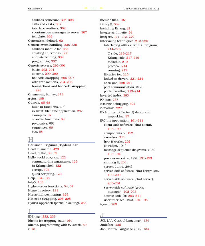
GENERATORS 512 JOB CONTROL LANGUAGE (JCL)
callback structure, 305–308
calls and casts, 307
interface routines, 302
spontaneous messages to server, 307
template, 309
Generators, defined, 62
Generic event handling, 336–339
callback module for, 338
creating an error in, 338
and late binding, 339
program for, 337
Generic servers, 292–301
basic, 292–294
become, 299–300
hot code swapping, 295–297
with transactions, 294–295
transactions and hot code swapping,
298
Ghemewat, Sanjay, 379
global, 185
Guards, 65–68
built-in functions, 69f
in DETS filename application, 287
examples, 67
obsolete functions, 68
predicates, 68f
sequences, 66
true, 68
HHausman, Bogumil (Bogdan), 44n
Head mismatch, 423
Head, of list, 38, 39
Hello world program, 122
command-line arguments, 125
in Erlang shell, 122
escript, 124
quick scripting, 123
Help, 134–135
help(), 135
Higher-order functions, 54, 57
Home directory, 121
Horizontal positioning, 325
Hot code swapping, 295–298
Hybrid approach (partial blocking), 258
IID3 tags, 232, 233
Idioms for trapping exits, 164
Idioms, programming with try...catch, 80
if, 73
Include files, 107
init:stop(), 359
Installing Erlang, 21
Integer arithmetic, 26
Integers, 111–112, 220
Interfacing techniques, 212–225
interfacing with external C program,
214–220
C side, 215–217
Erlang side, 217–219
makefile, 219
protocol, 214
running, 219
libraries for, 225
linked-in drivers, 221–224
open_port, 220–221
port communication, 212f
ports, creating, 213–214
Inverted index, 383
IO lists, 237
io:format debugging, 427
io module, 227
IPv4 (Internet Protocol) datagram,
unpacking, 97
IRC lite application, 191–211
client-side software (chat client),
196–199
components of, 192
exercises, 211
how it works, 202
io widget, 194f
message sequence diagrams, 193f,
193–194
process overview, 192f, 191–193
running it, 203
screen dump, 204f
server-side software (chat controller),
199–200
server-side software (chat server),
200–201
server-side software (group
manager), 202–203
source code for, 203–211
user interface, 194f, 194–195
is_word, 283
JJCL (Job Control Language), 134
Jinteface, 225
Job Control Language (JCL), 134

KEEP-ALIVE PROCESSES 513 MNESIA
KKeep-alive processes, 173
keep_alive, 173
Kemp, Eric, 232
Key, 275
Key-value lookup tables, 273
Key-value server, 178
kill, 163
LLate binding, 339
lib_chan, 199, 200, 403, 406
lib_chan module, 187–188
lib_chan_auth, 409
lib_chan_cs, 408
Libraries
interfacing, 225
linked-in drivers, 221
for MatchSpec, 432n
organization of, 226–227
rpc module, 179
for sockets, programming with, 245
and tracing, 434
trigrams, 279
Libraries (distributed programming),
185–186
Link collections, 400
Linked-in drivers, 20, 221–224
Linking processes, 159f, 159–160
Links, 162
Linux, Erlang installation, 22
List operators, 108
List-at-a-time operations, 55
Lists, 38–39
building in natural order, 73–74
components of, 38
comprehensions, 61–64
defining, 39
empty, 51
extracting elements from, 39
IO, 237
operators, 108
processing of, 58–60
reversing, 74, 75
splitting with accumulators, 74
Load path, manipulating, 120
loop(), 157
MMac OS X
Erlang installation, 22
starting/stopping shell, 118
Macros, 108–110
Magic cookies, 186
Mailboxes, 153
Makefiles
autocompiling, 127–130
problems with, 132
targets, 129
template, 128, 130
“Making Reliable Systems in the
Presence of Software Errors”
(Armstrong), 400
Manuals, 135
map, 58, 59, 62
map/2, 59
mapreduce, 379–388
full-text indexing, 383–384
improvements to make, 387
indexer operation, 385–386
introduced, 367
running indexer, 386
and word map, 379
Marshaling, see Coding
Match operator, 110–111
Message passing concurrency, 365
Message sequence diagrams (MSDs),
193f, 193–194
Middle-man, see IRC lite application
MinGW (Minimalist GNU for Windows),
396
Mnesia, 313–330
adding and removing data, 317–318
backup and recovery, 330
creating initial database, 328–329
creating tables, 326–327
database queries, 313–317
conditionally selecting table data,
316
joins, 317
projecting data from table, 316
selecting all table data, 315–316
shop and cost tables, 314
dirty operations, 330
ETS and DETS and, 287
fragmented tables, 325
history of, 20
listings, 330
manual for, 399
naming of, 322
pessimistic locking, 319
primary keys, 318

MOD_NAME_SERVER 514 OTP (OPEN TELECOM PLATFORM)
records definitions, 314
SNMP tables, 330
storing complex data in tables,
323–324
table attributes, 327–328
table types and location, 325–326
table viewer, 329, 330f
transactions, 319–323
do () function, 323
aborting, 320
loading test data, 322
user’s guide to, 330
mod_name_server, 189
Modules, 44–48
approach to writing, 60
and area function, 44
attributes, 99
compiling, 45
for creating own commands, 135
and epp, 105
exporting from, 49
for file manipulation, 226
five most common, 19
lib_chan, 406
and pattern matching, 44
troubleshooting, 132
Monitors, 172
MP3 ID3 tags, 232, 233
ms_transform, 435
MSDs, see Message sequence diagrams
MSYS, 397
MSYS Developer Toolkit, 397
Multicore CPUs, 367–388
and concurrency-oriented
programming, 365–366
efficiency of programs, 368–372
distributed computing, 371
processes, 369
sequential bottlenecks, 371
shared ets or dets tables, 370
side effects, avoiding, 369
future of, 368
mapreduce and indexing, 379–388
full-text indexing, 383–384
improvements, 387
indexer code, 387–388
indexer operation, 385–386
running indexer, 386
measurements, 375–378, 379f
SMP Erlang, 376–378
parallelizing sequential code,
372–375
abstractions needed for, 374
granularity, 373
pmap, 373
Mutable states, 32, 366
Mutschler, Michael, 233
NName server, 177–182
client-server nodes, 179
different hosts on Internet, 182
role of, 177
running on different machines,
180–182
steps of creating, 177
Naming conventions
for atoms, 34
for commands file, 121
functions and arity, 52
and funs, 52
for -name parameter, 181
system modules, 58
table names in DETS, 286
for variables, 27
nano_get_url, 247
Nodes
connecting, 182
and cookies, 181
cookies for, 183
introduced, 176
and remote spawning, 185
running client and server on
different machines, 180–182
on same computer, 179
none90, 391
Oon_exit, 173
on_exit handler, 160–162
Open Telecom Platform, see OTP
open_port, 220
Operator precedence, 112, 113f
Ordered sets, 275, 276
OTP (open telecom platform), 291–312
code and templates, 309–312
gen_server, 301–305
gen_server callback structure,
305–308
generic servers, 292–301
basic, 292–294
OTP (OPEN TELECOM PLATFORM) SYSTEM 515 Q()
become, 299–300
hot code swapping, 295–297
transactions and, 294–295
transactions and hot code
swapping, 298
OTP (open telecom platform) system,
335–363
alarm handler, 346–348
application, 358–360
application monitor, 361, 362n
application servers, 348–350
code for prime number generation,
363
error logger, 339–346
API to, 340
configuring, 341–344
error analysis, 345–346
file system organization, 360–361
files for behaviors, 363
generic event handling, 336–339
overview of, 335–336
starting the system, 354–357
supervision tree, 351f, 351–354
P+P flag, 150
Packet sniffer, 249
Packets, 250
Parallel server, 253, 254
Parallelizing sequential code, 372–375
Parser generator (yecc), 129
Passive message reception (blocking),
257
Passive mode, 256
Pattern matching, 29–30, 41–42
Erlang vs. C and Java, 48
errors, 37
extracting values from a tuple, 36
guard sequences, 66
and guards, 65–68
match operator, 110–111
record fields, extracting, 71
terms, 41
see also Bit syntax
Performance
and distributed applications, 175
on multicore CPUs, 367
table type, 275, 276
tuple key and, 285
Periods, 24, 26, 51
perms, 64
Persistent data, 274
Pessimistic locking, 319
phofs module, 381
PlanetLab, 300
pmap, 373–375
Port
communication, 212f
Ports
creating, 213–214
interfacing with external C program,
214–220
C side, 215–217
Erlang side, 217–219
makefile, 219
protocol, 214
running, 219
linked-in drivers, 221–224
open_port, 220–221
Primary key, 318
Prime number server, 348
Primitives
for concurrency, 142, 375
distribution, 182–185
error handling, 170–171
Process dictionary, 113–114
Processes
client-server application, 144–148
example of code, 143–144
exceeding maximum number of, 150
keep-alive, 173
linking, 159f, 159–160
mailboxes for, 153
overview, 141
receive with a timeout, 150–153
registered, 154–155
sets of linked, 172f, 172
time involved in creating, 148–150
Profiling tools, 421–422
Progress reports, 342
Punctuation
for binaries, 87
for comments, 104
formatting commands, 235
semicolons, 132
types of, 51
Pure message passing language, 141
pwd(), 47
Pythagorean triplets, 63
Qq(), 119

QUICK SCRIPTING 516 SEQUENTIAL PROGRAMMING
Quick scripting, 123
quicksort, 62
Quote marks
and atoms, 34
and shell, 26
and strings, 40
RRace conditions, 173
Raising an exception, 77
RAM tables, 325
rb module, 345
read_file_info, 240
Reading files, 227–234
all terms in, 229
into a binary, 231
lines, one at a time, 231
with random access, 231–234
terms one at a time, 229–230
receive, 150–154
Receive loop, 156
Receive with a timeout, 150–153
Records, 69–72
creating and updating, 70
extracting fields, 71
in modules vs. shell, 69
pattern matching in functions, 71
as tuples, 71
Recursion, 156–157
References, 114
Registered processes, 154, 371
Remote error handling, 162
Remote spawning, 184–185
Request, 144
Response, 144
RFCs (requests for comments), 249
Rotating log, 341
rpc function, 145
rpc module, 185
Runtime diagnostics, 425
Rémond, Mickaël, 401
SSadan, Yariv, 401
SASL (System Architecture Support
Libraries), 341
Scalability, 175
Scope, 29
Search paths for loading code, 120
Security
and cookies, 187
and running client and server on
Internet, 182
self(), 145, 198
Sellaprime company, see OTP (open
telecom platform) system
Semicolons, 51, 132
send, 153–154
Sequential bottlenecks, 371
Sequential code, parallelizing, 372–375
Sequential programming, 43–75
accumulators, 74–75
apply, 99
arithmetic expressions, 64, 65f, 65
attributes, 99–103
BIFs, 87
binaries, 87–89
bit syntax, 89–98
16-bit color example, 90
advanced examples, 92–98
expressions, 90–92
block expressions, 103
boolean expressions, 103
building lists in natural order, 73–74
case, 72–73
character set, 104
comments, 104
common errors, 58
epp, 105
escape sequences, 105, 106f
expression sequences, 106
function references, 106–107
functions with same name, different
arity, 52
funs, 52–57
guards, 68f, 65–68, 69f
if, 73
include files, 107
list comprehensions, 61–64
list operators (++, –), 108
list processing, 58–60
macros, 108–110
match operator in patterns, 110–111
modules, 44–48
numbers (floats), 112
numbers (integers), 111–112
operator precedence, 112, 113f
process dictionary, 113–114
records, 69–72
references, 114
shopping list example, 49–52
SEQUENTIAL SERVER 517 SUPERVISION TREE
short-circuit boolean expressions,
115
term comparisons, 115–116, 116f
underscore variables, 116–117
Sequential server, 253–254
Server, 144, 292–301
basic, 292–294
become, 299–300
callback, 293
hot code swapping, 295–297
transaction semantics, 297
with transactions, 294–295
transactions and hot code swapping,
298
Sets, 275, 276
sets module, 279
Shadowed variables, 425
Shared memory and mutable states, 32
Shared state concurrency, 365
Shell
arithmetic examples, 25–27
benefits of, 25
built-in commands, 135
command editing in, 130
and command numbers, 24, 26
multiple, starting and stopping, 26
not responding, 26, 133
pattern expressions, 42
starting, 24
starting/stopping, 118–119
stopping, 131
what can’t be typed in, 25
Windows installation, 397
Short-circuit boolean expressions
described, 115
and guard expressions, 66, 67
SHOUTcast server, 265–272
how it works, 266
protocol, 265
pseudo code for, 266–268
running, 271–272
Shutdown, 119
Single assignment variables, 28, 29–31
Size variable, 91
SMP Erlang, 376–378, 379f
Socket-based distribution, 176,
187–190
Sockets, 245–272
broadcasting to multiple machines,
263–264
and connection origins, 258
control issues, 256–258
active message reception, 256–257
hybrid approach (partial blocking),
258
passive message reception, 257
definition of, 245
error handling, 259–260
lib_chan application, 403–409, 409
access server over network, 405
challenge/response
authentication, 409
client server communication, 408
code for server, 404
configuration file, 404
middle man, 407
start server, 405
structure, 406
lib_chan code, 409
lib_chan application
middle-man, 407f
libraries for, 245
listening, 251
modes, 256
and parallel server, 254
and sequential server, 254
SHOUTcast server, 265–272
how it works, 266
protocol, 265
pseudo code for, 266–268
running, 271–272
TCP, 246–255
fetching data from server,
246–248
improving server, 253–255
simple server, 248
writing a web server, 249
and UDP, 260–263
spawn, 148, 164
Spawning, 157–158
remote, 184–185
src directory, 230
Stack traces, 84–85, 426
Stages of mastery, 18
start_connector, 197
Strings, 40–41
character sets for, 40
and dollar syntax, 40
examples of, 40
sum, 58
Supervision tree, 351f, 351–354
all-for-one, 351
SUPERVISOR REPORTS 518 VARIABLES
arguments for, 353
data structure, 353
one-on-one, 351
strategy, 355
worker specs, 353
Supervisor reports, 342
Symbolic constants, see Atoms
Symmetric Multiprocessing, see SMP
System processes, 160, 163
TTables, see Ets (Erlang term storage);
Dets (disk Erlang term storage);
Mnesia
Tail, of list, 38, 39
Tail-recursive, 156–157
Targets, 129
TCP (transmission control protocol),
245
fetching data from server, 246–248
improving server, 253–255
simple server, 248
writing a web server, 249
Term comparisons, 115–116, 116f
and guard expressions, 66
term_to_binary, 88, 92, 225, 250, 252
Terms, 41
Test methods, 420
throw, 83
throw(Why), 77
Timeouts, 150–152
Timers, 152–154
total, 51, 59
Tracing, 431–435
Transaction semantics, 297
Transient data, 274
Trapping exit signals, 167f, 165–169
Trapping exits, 164, 172f
Trigram example programs, 279–284
building tables, 281
defined, 279
iterator, 280
overview, 279
time (speed) involved, 281–284
Troubleshooting, 131–134
true guard, 68
Trusted environment, 176
try vs. case, 84
try...catch, 78–83
programming idioms with, 80
shortcuts, 80
try_to_connect, 197
ttb, 435
Tuples, 35–38
creating, 36
and data storage, 273
in DETS table, 284
extracting values from, 36–38
insert into tables, 274
inserted into tables, 277
and IP addresses, 258
keys, sets and bags, 275
and list comprehensions, 61
lookup in a table, 274
MFA, 432
nesting, 35
and records, 69–72
service, 404
supervisor tree, 352
in tables, 286
Type, 393
TypeExpression, 392
Types, 390–395
definitions in APIs, 394
input/output of a function, 392–394
notation, 390–392
tools for, 394–395
TypeVar, 393
UUDP (user datagram protocol), 245,
260–263
background, 263
factorial server, 261
server and client, 260
Unbound variables, 29, 423
Underscore variables, 116–117
Unix-based systems
and escript, 125
help, 134
shell command, 24
starting/stopping shell, 118
Unsafe variables, 424
Unterminated strings, 424
Untrusted environment, 176
User-defined attributes, 101
VValue variable, 91
Variables
changing value of, 31
introduced, 27–32

WEB SERVER 519 YECC
naming conventions, 27
notation, 27
and pattern matching, 30
scope of, 29
single assignment, 28, 29–31
underscore, 116–117
unexpected values and, 32
WWeb server, writing, 249
Websites
for Armstrong’s doctoral thesis on
Erlang, 400
for CEAN, 23
for connecting to standard
input/output, 221n
for cprof, 421
for Debugger reference manuals, 431
for DETS manual, 287
for emacs installation, 397
for Erlang (Windows download), 22
for Erlang 4.7 specs, 400n
for Erlang application
documentation, 399
for Erlang blogs, 401
for Erlang documentation, 399
for Erlang downloadable examples,
23n
for Erlang error log, 136
for Erlang FAQs, 399
for Erlang forums, 401
for Erlang literature, 400n
for Erlang manuals, 135, 399
for Erlang projects, 401
for Erlang release handling
documentation, 308n
for Erlang sources, 22n
for Erlang style guide, 399
for ETS manual, 287
for Internet Engineering Task Force,
249
libraries for interfacing, 225
for Link collections, 400
for makefile overview, 127n
for MatchSpec libraries, 432n
for MinGW, 396
for MSYS, 397
for online financial services in
Erlang, 301n
for OTP behaviors, 363
for PlanetLab, 300n
for purge_module documentation,
438n
for SHOUTcast, 265n
for SMP Erlang, 376
for Windows binary (Erlang
installation), 396
for wireshark (a packet-sniffer), 249
Windows
batch files, 124
binary distributions, 22
Command prompt, compiling and
running from, 123
and directory navigation, 47
emacs installation, 397
Erlang installation, 21, 396–397
and escript, 125
help documentation, 135
and MinGW, 396
and MSYS, 397
MSYS Developer toolkit, 397
and name server example, 179n
shell command, 24
starting/stopping shell, 118
and unpacking COFF data, 96
wireshark, 249
Word extraction, 387
Worker-supervisor model, 171
Writing to files, 235–239
lines, 236
list of terms, 235–236
in one operation, 237–238
random access, 239
Xxref module, 421
Yyecc, 129