prasanna thesis part 1 - qut · 2010. 6. 9. · prasanna egodawatta b.sc. (civil engineering,...
TRANSCRIPT

TRANSLATION OF SMALL-PLOT SCALE
POLLUTANT BUILD-UP AND WASH-OFF
MEASUREMENTS TO URBAN CATCHMENT SCALE
Prasanna Egodawatta
B.Sc. (Civil Engineering, Honours)
A THESIS SUBMITTED
IN PARTIAL FULFILLMENT OF THE REQUIREMENTS OF
THE DEGREE OF DOCTOR OF PHILOSOPHY
FACULTY OF BUILT ENVIRONMENT AND ENGINEERING
QUEENSLAND UNIVERSITY OF TECHNOLOGY
August -2007


i
KEYWORDS
stormwater quality modelling, pollutant build-up, pollutant wash-off, urban water
quality, rainfall simulation.


iii
ABSTRACT
Accurate and reliable estimations are the most important factors for the development
of efficient stormwater pollutant mitigation strategies. Modelling is the primary tool
used for such estimations. The general architecture of typical modelling approaches is
to replicate pollutant processes along with hydrologic processes on catchment
surfaces. However, due to the lack of understanding of these pollutant processes and
the underlying physical parameters, the estimations are subjected to gross errors.
Furthermore, the essential requirement of model calibration leads to significant data
and resource requirements. This underlines the necessity for simplified and robust
stormwater pollutant estimation procedures.
The research described in this thesis primarily details the extensive knowledge
developed on pollutant build-up and wash-off processes. Knowledge on both build-up
and wash-off were generated by in-depth field investigations conducted on residential
road and roof surfaces. Additionally, the research describes the use of a rainfall
simulator as a tool in urban water quality research. The rainfall simulator was used to
collect runoff samples from small-plot surfaces. The use of a rainfall simulator
reduced the number of variables which are common to pollutant wash-off.
Pollutant build-up on road and roof surfaces was found to be rapid during the initial
time period and the rate reduced when the antecedent dry days increase becoming
asymptote to a constant value. However, build-up on roofs was gradual when
compared to road surfaces where the build-up on the first two days was 66% of the
total build-up. Though the variations were different, it was possible to develop a
common replication equation in the form of a power function for build-up for the two
surface types with a as a multiplication coefficient and b as a power coefficient.
However, the values for the two build-up equation coefficients, a, and b were different
in each case. It was understood that the power coefficient b varies only with the
surface type. The multiplication coefficient varies with a range of parameters
including land-use and traffic volume. Additionally, the build-up observed on road
surfaces was highly dynamic. It was found that pollutant re-distribution occurs with
finer particles being removed from the surface thus allowing coarser particles to build-
iv
up. This process results in changes to the particle size composition of build-up.
However, little evidence was noted of re-distribution of pollutants on roof surfaces.
Furthermore, the particulate pollutants in both road and roof surfaces were high in
adsorption capacity. More than 50% of the road and more than 60% of the roof surface
particulates were finer than 100 µm which increases the capacity to adsorb other
pollutants such as heavy metals and hydrocarbons. In addition, the samples contained
a significant amount of DOC which would enhance the solubility of other pollutants.
The wash-off investigations on road and roof surfaces showed a high concentration of
solid pollutants during the initial part of events. This confirmed the occurrence of the
‘first flush’ phenomenon. The observed wash-off patterns for road and roof surfaces
were able to be mathematically replicated using an exponential equation. The
exponential equation proposed is a modified version of an equation proposed in past
research. The modification was primarily in terms of an additional parameter referred
to as the ‘capacity factor’ (CF). CF defines the rainfall’s ability to mobilise solid
pollutants from a given surface. It was noted that CF varies with rainfall intensity,
particle size distribution and surface characteristics. Additional to the mathematical
replication of wash-off, analysis further focused on understanding the physical
processes governing wash-off. For this, both particle size distribution and physico-
chemical parameters of wash-off pollutants were analysed. It was noted that there is
little variation in the particle size distribution of particulates in wash-off with rainfall
intensity and duration. This suggested that particle size is not an influential parameter
in wash-off. It is hypothesised that the particulate density and adhesion to road
surfaces are the primary criteria that govern wash-off. Additionally, significantly high
pollutant contribution from roof surfaces was noted. This justifies the significance of
roof surfaces as an urban pollutant source particularly in the case of first flush.
This dissertation further describes a procedure to translate the knowledge created on
pollutant build-up and wash-off processes using small-plots to urban catchment scale.
This leads to a simple and robust urban water quality estimation tool. Due to its basic
architecture, the estimation tool is referred to as a ‘translation procedure’. It is
designed to operate without a calibration process which would require a large amount
of data. This is done by using the pollutant nature of the catchment in terms of build-
up and wash-off processes as the basis of measurements. Therefore, the translation

v
procedure is an extension of the current estimation techniques which are typically
complex and resource consuming. The use of a translation procedure is simple and
based on the graphical estimation of parameters and tabular form of calculations. The
translation procedure developed is particularly accurate in estimating water quality in
the initial part of runoff events.


vii
LIST OF PUBLICATIONS
Refereed Journal Papers
• Egodawatta, P., Thomas, E. and Goonetilleke, A. (2006). A mathematical
interpretation of pollutant wash-off from urban road surfaces using simulated
rainfall. Water Research, 41(13), 3025 - 3031.
Refereed International Conference Papers
• Egodawatta, P., and Goonetilleke, A. (2006). Characteristics of pollution build-up
on residential road surfaces. Paper presented at the 7th International conference on
hydroscience and engineering (ICHE 2006), Philadelphia, USA.
• Egodawatta, P., Goonetilleke, A., Thomas, E. and Ayoko, G. A. (2006).
Understanding the interrelationship between stormwater quality and rainfall and
runoff factors in residential catchments. Paper presented at the 7th International
conference on urban drainage modelling and 4th international conference on water
sensitive urban design (7UDM and 4WSUD), Melbourne, Australia.


ix
TABLE OF CONTENTS
Chapter 1 - Introduction 1
1.1 Background 1
1.2 Hypothesis 2
1.3 Aims and Objectives 2
1.4 Justification for the Research 3
1.5 Description of the Research 4
1.6 Scope 5
1.7 Outline of the Thesis 6
Chapter 2 – Urban Hydrology and Water Quality 9
2.1 Background 9
2.2 Hydrologic Impacts 10
2.3 Water Quality Impacts 13
2.3.1 Pollutant Sources 15
2.3.2 Significance of Impervious Surfaces in Stormwater Pollution 18
2.3.3 Pollutant Build-up 20
2.3.4 Pollutant Wash-off 23
2.3.5 First Flush Phenomenon 26
2.4 Primary Stormwater Pollutants 27
2.4.1 Litter 28
2.4.2 Nutrients 28
2.4.3 Heavy Metals 29
2.4.4 Hydrocarbons 29
2.4.5 Organic Carbon 30
2.4.6 Suspended Solids 31
2.5 Hydrologic and Water Quality Modelling Approaches 32
2.5.1 Urban Hydrologic Models 32
2.5.2 Hydrologic Modelling Approaches 34
2.5.3 Urban Water Quality Models 39
2.7 Conclusions 42
x
Chapter 3 - Study Tools 45
3.1 Background 45
3.2 Vacuum Collection System 46
3.2.1 Selection of Vacuum System 47
3.2.2 Sampling Efficiency 48
3.3 Rainfall Simulator 50
3.3.2 Calibration of the Rainfall Simulator 52
3.3.3 Rainfall Intensity and Uniformity of Rainfall 53
3.3.4 Drop Size Distribution and Kinetic Energy of Rainfall 56
3.4 Model Roofs 61
3.4.1 Materials and Dimensions 62
3.5 Statistical and Chemometrics Analytical Tools 63
3.5.1 Mean, Standard Deviation and Coefficient of Variation 64
3.5.2 Method of Least Square 64
3.5.3 Principal Component Analysis 65
3.6 Hydrologic Modelling Software 66
3.7 Conclusions 70
Chapter 4 - Study Area and Sample Collection and Testing 71
4.1 Background 71
4.2 Study Area 71
4.3 Catchment Scale Investigation 74
4.3.1 Catchment Characteristics 74
4.3.2 Catchment Monitoring 77
4.4 Small-plot Scale Investigations 79
4.4.1 Road Surface Investigation 79
4.4.2 Roof Surface Investigation 87
4.5 Treatment and Transport of Samples 90
4.6 Laboratory Testing 91
4.6.1 Particle Size Distribution 91
4.6.2 Other Physio-chemical Parameters 93
4.7 Conclusion 94
xi
Chapter 5 - Analysis of Pollutant Build-up 95
5.1 Background 95
5.2 Data and Pre-processing 95
5.3 Build-up on Road Surfaces 97
5.3.1 Variability of Build-up 97
5.3.2 Mathematical Replication of Build-up 100
5.3.3 Hypothetical Build-up Process 104
5.3.4 Verification of Build-up Equation 105
5.3.5 Particle Size Distribution 107
5.3.6 Analysis of Physio-chemical Parameters 110
5.4 Build-up on Roof Surfaces 114
5.4.1 Mathematical Replication of Build-up 114
5.4.2 Particle Size Distribution 117
5.4.3 Analysis of Physio-chemical Parameters 119
5.5 Conclusions 121
Chapter 6 - Analysis of Pollutant Wash-off 123
6.1 Background 123
6.2 Initially Available Pollutants 124
6.2.1 Road Surfaces 125
6.2.2 Roof Surfaces 127
6.3 Data and Variables 130
6.3.1 Data Pre-processing 130
6.3.2 Selection of Rainfall and Runoff Variables 131
6.4 Analysis of Wash-off from Road Surfaces 131
6.4.1 Variation of Wash-off with Influential Parameters 132
6.4.2 Mathematical Replication of Pollutant Wash-off 135
6.4.3 Estimation of Wash-off Parameters 138
6.4.4 Understanding the Wash-off Process 142
6.4.5 Particle Size Distribution Analysis 143
6.4.6 Physio-chemical Analysis 149
6.5 Analysis of Wash-off from Roof Surfaces 155
6.5.1 Variation of Wash-off with Influential Parameters 156
xii
6.5.2 Mathematical Replication of Pollutant Wash-off 157
6.5.3 Particle Size Distribution Analysis 160
6.5.4 Physio-chemical Analysis 163
6.6 Conclusions 166
Chapter 7 - Catchment Modelling 169
7.1 Introduction 169
7.2 Model Setup 170
7.2.1 Model Architecture 170
7.2.2 Alextown Catchment 172
7.2.3 Gumbeel Catchment 174
7.2.4 Birdlife Park Catchment 175
7.3 Model Calibration 177
7.3.1 Measured Data for Calibration 178
7.3.2 Methods and Parameters 179
7.3.3 Calibration Sequence 182
7.4 Conclusions 184
Chapter 8 - Development of Translation Procedure 185
8.1 Background 185
8.2 Estimation of Pollutant Build-up 186
8.3 Estimation of Fraction Wash-off (FW) 189
8.3.1 Wash-off Model 190
8.3.2 Parameters and Estimation Procedure 192
8.4 Estimation of Stormwater Quality 194
8.4.1 Event Based Water Quality Comparison 196
8.4.2 Comparison of Instantaneous Water Quality 199
8.5 Simplified Wash-off Estimation 206
8.6 Translation Procedure 210
8.6.1 Data for Translation Procedure 212
8.6.2 Estimation of Build-up 212
8.6.3 Estimation of FW 218
8.6.4 Issues on Using the Translation Procedure 221

xiii
8.7 Conclusions 222
Chapter 9 - Conclusions and Recommendations 225
9.1 Conclusions 225
9.1.1 Pollutant Build-up 226
9.1.2 Pollutant Wash-off 228
9.1.3 Translation Procedure 231
9.2 Recommendations for Further Research 232
References 235
Appendix A Calibration of Study Tools 249
Appendix B Study Area 255
Appendix C Pollutant Build-up Data 265
Appendix D Pollutant Wash-off Data 271
Appendix E Catchment Modelling 285
Appendix F Data Analysis 295


xv
LIST OF TABLES
Table 2.1 - Critical source area and contaminant-load percentages 19
Table 3.1 - Measured rainfall intensities for the different control box settings 55
Table 4.1 - Characteristics of Alextown, Gumbeel and Birdlife Park
Catchments 76
Table 4.2 - Characteristics of road sites 81
Table 4.3 - Rainfall intensities and durations simulated during the study 86
Table 4.4 - Percentage recovery of runoff volume comparison with simulated
rain volume 86
Table 4.5 - Characteristics of the possible site for roof surface investigation 88
Table 5.1 - Build-up coefficients for road surfaces 102
Table 5.2- Comparison of observed and predicted build-up pollutants 106
Table 5.3 - Average percentage particle size distribution 108
Table 5.4 - Average percentage particle size distribution – for roof surfaces 117
Table 6.1 - Amounts of initially available pollutants in road sites 125
Table 6.2 - Amount of initially available pollutants in road sites 128
Table 6.3 - Predictive capability of Equation 6.3 137
Table 6.4 - Estimated values for CF and k 140
Table 6.5 - Validity of replication of pollutant wash-off using parameters in
Table 6.4 140
Table 6.6 - Validity of replication of pollutant wash-off equation common
set of parameters 141
Table 6.7 - Percentage wash-off for different intensities and durations 148
Table 6.8 - Average quality parameters and their variation 154
Table 6.9 - Optimum parameters for Equation 6.3 158
Table 6.10 - Performance of Equation 3 with common set of optimum
parameters 159
Table 6.11 - Initially available pollutants prior to rainfall simulations 160
Table 6.12 - Average quality parameters and their variation 165
Table 7.1 - In-build mathematical routines in Mike STORM 170
Table 7.2 - Number of events used for calibration and verification 179
Table 8.1 - Parameters for build-up on road surfaces 187
Table 8.2 - Build-up coefficients for roof surfaces 189

xvi
Table 8.3 - Wash-off parameters for road surfaces 193
Table 8.4 - Parameters used for the fraction wash-off estimations from
roof surfaces 194
Table 8.5 - Estimation of Event Based Suspended Solid Pollutants from
Urban Catchments by Translating Small-plot Pollutant
Processes to Catchment Scale 211
Table 9.1 - Parameters values for build-up replication equation 227
Table 9.2 - Parameter values for wash-off replication equation 229
xvii
LIST OF FIGURES
Figure 2.1 - Changes in runoff hydrograph after urbanisation 10
Figure 2.2 - Pollutant accumulation rate for different land uses 22
Figure 2.3 - Hydrologic representation of surface pollutant load over time 25
Figure 2.4 - Hydrologic processes 33
Figure 2.5 - Time area calculation 39
Figure 3.1 - Water filtration system in Delonghi Aqualand vacuum cleaner 48
Figure 3.2 - a) Section of sample road surface and b) section of road surface
at Gumbeel Court. 49
Figure 3.3 - Comparison of particle size ranges in the original sample
and recovered sample 50
Figure 3.4 - Rainfall Simulator 52
Figure 3.5 - Intensity calibration and uniformity testing of rainfall simulator 54
Figure 3.6 - Spatial variation of the rainfall intensity for control box setting 3–I 55
Figure 3.7 - Experimental setup for drop size test 57
Figure 3.8 - Calibration curve for flour pellets 58
Figure 3.9 - Range of flour pellets developed during pilot experiment 59
Figure 3.10 - Concrete tiled model roof mounted on scissor lifting arrangement 63
Figure 4.1 - Waterways of Gold Coast city 73
Figure 4.2 - Highland Park residential area, demarcation of three
catchments and locations of the gauging instruments 75
Figure 4.3 - Calculation of Fraction Imperviousness 77
Figure 4.4 - Depth gauges and V-notches at the three catchment outlets 78
Figure 4.5 - Interior of automated monitoring stations. 78
Figure 4.6 - Locations of the study sites within Highland Park catchment 80
Figure 4.7 - Dry sample collections from road surface plots 82
Figure 4.8 - Plot Surfaces Boundary and sealing method 85
Figure 4.9 - Rainfall simulator setup at Gumbeel Court 85
Figure 4.10 - Collection of runoff samples to polyethylene containers 86
Figure 4.11 - Rainfall simulation on roof surfaces 90
Figure 4.12 - Malvern Mastersizer model S 92
Figure 5.1 - Pollutant build-up on road surfaces 98
Figure 5.2 - Comparison of different form of equations with solid build-up
xviii
on roads 101
Figure 5.3 - Predictive ability of build-up equation for road surfaces 103
Figure 5.4 - Build-up hypothesis 105
Figure 5.5 - Variation of particle size distribution with antecedent dry days
for road surfaces build-up 108
Figure 5.6 - Physio chemical parameters and antecedent dry days for road
surfaces: Biplot of data against the first two principal components 112
Figure 5.7 - Pollutant build-up on roof surfaces 115
Figure 5.8 - Performances of the replication equations for Build-up on
roof surfaces 116
Figure 5.9 - Variation of particle size distribution with antecedent dry days
for roof surfaces build-up 118
Figure 5.10 - Physio chemical parameters and antecedent dry days for roof
surfaces: Biplot of data against the first two principal components 119
Figure 6.1 - Cumulative particle size distributions of initially available
pollutant samples from road surfaces 126
Figure 6.2 - Cumulative particle size distributions of initially available
pollutant samples 129
Figure 6.3 - Variation of wash-off with rainfall intensity and duration 133
Figure 6.4- Variation of fraction wash-off with rainfall intensity and duration 134
Figure 6.5 - Performance of the replication equation (Equation 6.3) 139
Figure 6.6 - Variation of CF with rainfall intensity 142
Figure 6.7 - Variation of particle size distribution 145
Figure 6.8 - Wash-off particle size distribution for four durations – 20mm/hr
intensity 147
Figure 6.9 - Variations of TS concentrations 151
Figure 6.10 - Quality parameters for wash-off samples from Gumbeel Court
road site: Biplot of data against the first two principal components 152
Figure 6.11 - Observed fraction wash-off (FW) from roof surfaces 157
Figure 6.12 - Performances of the replication equation for roof surface wash-off 159
Figure 6.13 - Averaged particle size distribution for two roof surface types 161
Figure 6.14 - Variation of TS concentration with rainfall intensity and duration 163
Figure 6.15 - Quality parameters for wash-off samples from roof surfaces:
Biplot of data against the first two principal components 164

xix
Figure 7.1 - File structure and simulation sequence in Mike STORM. 171
Figure 7.2 - Drainage network and catchment sub-divisions for Alextown 173
Figure 7.3 - Drainage network and catchment sub-divisions for Gumbeel 174
Figure 7.4 - Drainage network and catchment sub-divisions for Birdlife Park 176
Figure 7.5 - Variation of peak flow ratio with observed peak discharges 183
Figure 7.6 - Variation of Runoff volume ratio with observed runoff volume 183
Figure 8.1 - Simplified Build-up model 188
Figure 8.2 - Conceptual wash-off model 191
Figure 8.3 - Comparison of predicted and observed EMCs 197
Figure 8.4 - Performance of the routing procedure 201
Figure 8.5 - Comparison of continuous water quality estimations with
observed water quality 203
Figure 8.6 - Comparison of observed and predicted instantaneous concentration 205
Figure 8.7 - Method to obtain simplified rainfall event 208
Figure 8.8 - Analysis of estimation accuracy using simplified rainfall events 209
Figure 8.9 - Build-up on road surfaces: residential roads in low population
density residential forms (equivalent to single detached
housing regions) 215
Figure 8.10 - Build-up on road surfaces: residential roads in high population
density residential forms (equivalent to townhouse regions) 216
Figure 8.11 - Build-up on roof surfaces: common residential roofs
(variation developed for corrugated steel and concrete tile roofs
with 200 roofing angle) 217
Figure 8.12 - Wash-off from road surfaces: typical residential roads
(variation developed for roads with 0.66 to 0.92 mm texture
depth and 7.2 to 10.8 % longitudinal slope) 219
Figure 8.13 - Wash-off from roof surfaces: typical residential roofs
(variation developed for roofs with corrugated steel and concrete
tile roofs with 200 roofing angle) 220


xxi
ABBREVIATIONS
AD - Advection Dispersion
ARI - Average Recurrence Interval
AS/NZS - Australian and New Zealand Standards
Cd - Cadmium
COD - Chemical Oxygen Demand
Cr - Chromium
Cu - Copper
CV - Coefficient of Variation
DHI - Danish Hydraulic Institute
DOC - Dissolved Organic Carbon
EC - Electrical Conductivity
EMC - Event Mean Concentration
GCCC - Gold Coast City Council
GIS - Geographical Information System
HEPA - High Efficiency Particulate Air
IC - Inorganic Carbon
IL - Initial Loss
Ni - Nickel
PAH - Polycyclic Aromatic Hydrocarbon
Pb - Lead
PC - Principal Component
PCA - Principal Component Analysis
Rf - Reduction Factor
SD - Standard Deviation
SWMM - Stormwater Management Model
Tc - Time of Concentration
TC - Total Carbon
TDS - Total Dissolved Solids
TN - Total Nitrogen
TOC - Total Organic Carbon
TP - Total Phosphorous
TS - Total Solids

xxii
TSS - Total Suspended Solids
US EPA - United States Environmental Protection Agency
USA - United States of America
Zn - Zinc

xxiii
STATEMENT OF ORIGINAL AUTHORSHIP
The work contained in this thesis has not been previously submitted for a degree or
diploma from any other higher education institution to the best of my knowledge and
belief. The thesis contains no material previously published or written by another
person except where due reference is made.
Prasanna Egodawatta
Date: / /


xxv
ACKNOWLEDGEMENTS
I wish to express my profound gratitude to my principal supervisor A/Prof. Ashantha
Goonetilleke for his guidance, support and professional advice during the research.
Special thanks are also given to my associate supervisors Dr. Godwin Ayoko and
Adjunct Prof. Evan Thomas for their expert advice and guidance during the research. I
would like to acknowledge the Faculty of Built Environmental and Engineering,
Queensland University of Technology for financial support during my candidature.
I would like to express my appreciation to QUT technical staff particularly Mr. Brian
Pelin, Mr. Jim Grandy, Mr. Arthur Powell, Mr. Trevor Laimer, Mr. Terry Beach, Mr.
Ian Tully and Mr. Glen Turner for their assistance in developing the research tools and
for helping in field investigations. My appreciation is further extended to fellow
researchers particularly to Mr. Sandun De Silva, Mr. Hema Illuri, Mr. Yasintha
Bandulaheva, Ms. Thanuja Ranawaka, Mr. S. Jayaragan, Ms. Nandika Miguntanna
and Ms. Donna Steel for their support during field investigations and laboratory
testing.
This research would not have been possible without the support received from a
number of external organisations. The support received from Gold Coast City Council
in providing essential data and permitting me to conduct investigations within council
property, from the Danish Hydraulic Institute for providing a free license for the
modelling software and technical support, and from CSR Roofing for providing
roofing materials is gratefully acknowledged.
Finally, I would like to express my gratitude to all my relatives and friends for the
encouragement I received.


xxvii
DEDICATION
I wish to dedicate this thesis to my father, Ranjith Egodawatta, and mother, Chandra
Walisinghe, for their unlimited support and love and to my two brothers, Chaminda
and Kithsiri, and my sister Samanthi for their support and motivation.

Chapter 1 - Introduction 1
Chapter 1 - Introduction
1.1 Background
Urbanisation leads to an increased percentage of impervious areas on catchment
surfaces. Consequently, this leads to changes in the hydrologic and water quality
characteristics of catchments. Many researchers have reported that increased flood
frequencies and comparatively higher flood peaks are apparent in urban catchments
when compared to rural catchments (ASCE, 1975; Riordan et al., 1978). Urban
stormwater quality is also one of the key environmental concerns at the present time.
Due to increased anthropogenic activities on urban lands, various pollutants
accumulate on catchment surfaces. These pollutants are washed-off during storm
events thereby contributing higher pollutant loads to receiving waters (Bannerman et
al., 1993; Novotny et al., 1985; Sartor et al., 1974).
With the growing awareness of stormwater pollution, many regulatory authorities
strive to implement stormwater management strategies to mitigate the adverse
impacts. Numerous research studies and stormwater quality estimation procedures
have been developed in order to support the decision making processes. Computer
modelling is one such water quality prediction procedure that is widely used. There
are a number of stormwater quality models available, but they are generally based on
similar principles. They first estimate the runoff volume using given rainfall and
geographical parameters. Then, the quality of the runoff is estimated using pollutant
process equations. The pollutant process equations are either a simplified form of
statistical relationships or replications of pollutant processes such as pollutant build-
up and wash-off (Akan and Houghtalen, 2003; Zoppou, 2001).
Stormwater quality computer models which are generally based on a simplified form
of pollutant export relationships using appropriate equations are termed ‘lumped time
base models’. These models estimate the long term pollutant export from catchments
and are widely used for planning and decision making activities. The use of lumped
time base models is limited due to two main issues. Firstly, the representation of
Chapter 1 - Introduction 2
catchment pollutant processes using a simplified pollutant export equation can be
misleading. Pollutant processes on catchment surfaces have complex characteristics
and are influenced by a range of factors such as land use, topography, rainfall and
climatic characteristics. Secondly, these models need an extensive amount of data for
calibration. The acquisition of such data can be difficult and expensive (Akan and
Houghtalen, 2003; Rossman, 2004; XP-AQUALM-User-Manual).
Stormwater quality computer models which use separate mathematical replication
equations for each pollutant process can be termed ‘continuous time base models’.
The primary pollutant processes that are generally replicated in these models are
pollutant build-up and wash-off. These models are capable of simulating water
quality of each storm event in detail. They use replication equations for the two main
pollutant processes: pollutant build-up and wash-off. However, due to limited
knowledge of these pollutant processes, this type of water quality model can lead to
gross errors (Akan and Houghtalen, 2003; Sartor et al., 1974).
1.2 Hypothesis
The knowledge on pollutant build-up and wash-off processes from small-plot urban
impervious surfaces can be translated to an urban catchment scale to enable the
estimation of stormwater quality.
1.3 Aims and Objectives
The primary objective of this research study was to develop a detailed knowledge on
primary pollutant processes of pollutant build-up and wash-off in plot scale and
translate this knowledge to catchment scale leading to a catchment scale water
quality estimating tool.
The major aims of the study were to:
Chapter 1 - Introduction 3
• Develop a detailed understanding of pollutant build-up and its relationship to
antecedent dry days on common urban impervious surfaces such as road and roof
surfaces using small plots.
• Develop a detailed understanding of pollutant wash-off with rainfall intensity and
duration from road and roof surfaces using rainfall simulation on small-plot
surfaces to eliminate the dependency on natural rainfall and its attendant
difficulties.
• Develop an appropriate simplified approach to translate the knowledge on build-
up and wash-off processes to an urban catchment scale in order to estimate
catchment scale stormwater quality.
1.4 Justification for the Research
It is widely accepted that pollutants originating from urban surfaces dramatically
alter receiving water quality. To mitigate the adverse impacts of stormwater
pollution, it is essential to have appropriate management strategies and efficient
treatment designs. However, the effectiveness of such mitigation measures strongly
relies on the accuracy and reliability of stormwater quality estimations.
Modelling is the primary tool used for such estimations. The general architecture of
typical modelling approaches is to replicate pollutant processes along with
hydrologic processes on catchment surfaces. The common pollutant processes
replicated in typical water quality models are pollutant build-up and wash-off.
However, due to the lack of in-depth understanding of these pollutant processes and
the underlying influential parameters, the estimations can be subjected to gross
errors. Furthermore, the essential requirement of model calibration leads to
significant data and resource requirements. Due to the dependency on naturally
occurring rain events, generation of such data is difficult and time consuming. A
further complexity is added due to the non-homogeneous nature of urban catchments.
The above discussion highlights the necessity for in-depth investigations into
pollutant build-up and wash-off. However, in order to eliminate the physical
constrains due to the heterogeneity of urban catchments and the dependency on
Chapter 1 - Introduction 4
naturally occurring rainfall events, special research methodologies were needed for
the investigations. Selection of small-plot surfaces was the approach taken to
eliminate the constraints arising from the heterogeneity of urban surfaces. It was
hypothesised that the characteristics of influential variables are fairly uniform over a
confined area of urban surface. Secondly, the use of artificially simulated rainfall
was the best approach to eliminate the dependency on naturally occurring rainfall.
This approach further provides better control over variables such as intensity and
duration. However, once the in-depth knowledge on pollutant build-up and wash-off
relating to small urban surface plots is created, this knowledge needs to be translated
to catchment scale for practical applications. Hence the extension of the knowledge
is on pollutant build-up and wash-off for the development of the translation
procedure.
1.5 Description of the Research
Special research techniques were used to investigate pollutant build-up and wash-off
on road and roof surfaces. The investigations into build-up and wash-off were
undertaken on small-plot surfaces which were 3 m2 in size. This eliminated the issues
associated with non-homogeneous surface characteristics. The primary variability
considered during pollutant build-up was the antecedent dry period. Variation of
build-up due to other factors such as land-use was accounted for investigating
multiple sites. A rainfall simulator was used for the wash-off investigations. This
helped to overcome constraints associated with the dependency on natural rainfall
events such as their unpredictable occurrence. The investigations were focused on
understanding variability of wash-off due to variations of rainfall intensity and
duration.
The primary data for the validation of the developed translation procedure was
obtained from three urban catchments. All these catchments were residential in land-
use but contained slightly different residential urban forms. The catchments had been
monitored for quantitative and qualitative parameters of runoff. In order to maintain
compatibility of measurements, the investigations into build-up and wash-off were
conducted close to these three catchments. These investigations were conducted on
Chapter 1 - Introduction 5
three road sites and two roof surface types. Variation of build-up with antecedent dry
days and variation of wash-off with rainfall intensity and duration were the primary
focus of investigations.
Samples collected from build-up and wash-off investigations and from the three
urban catchment outlets were tested for a range of physio-chemical parameters.
However, the primary focus was to test parameters related to particulates such as
total suspended solids, total dissolved solids and particle size distribution. This was
due to the consideration of solids as the indicator pollutant for water quality.
A fundamental understanding of build-up and wash-off processes was created by the
analysis of build-up and wash-off data from small-plot surfaces. The analysis
primarily focused on developing mathematical replication equations and
understanding the underlying physical processes. The mathematical replication
equations for each process were simulated for selected storm events so that the water
quality in the three catchments could be estimated. Based on the accuracy of
estimation in comparison to measured water quality, a simplified modelling approach
or translation procedure was developed for estimating catchment scale water quality
using data obtained from small-plots.
1.6 Scope
This research focused on urban stormwater pollutant processes. The research
developed a detailed understanding of pollutant build-up and wash-off processes and
was confined to a specific investigation framework. The important issues in relation
to this work are:
• The research was confined to the Gold Coast area. This limits the research
outcomes in terms of regional and climatic parameters. However, the generic
knowledge developed is applicable outside of the regional and climatic
characteristics of the Gold Coast.
• The field investigations were conducted only for residential land-uses. This limits
the wider applicability of some of the research outcomes where land-use is a

Chapter 1 - Introduction 6
significantly influencing variable. However, once again, the generic knowledge
developed is applicable for other land-uses.
• The research was only confined to two primary pollutant processes, namely
pollutant build-up and wash-off. The transport of pollutants from catchment
surfaces was considered to be only by advection, which can be replicated using
typical runoff routing models.
• The investigation of pollutant processes was confined to road and roof surfaces.
It was considered that these two surface types represent the dominant impervious
fraction and are the most significant contributors to stormwater pollutant load.
• The seasonal variability of pollutant build-up was not considered during the
investigations.
• Three road sites with variable urban-forms formed the study sites. The traffic
volumes in these three sites are typical of residential urban roads. Variable traffic
volumes were not considered for the study.
1.7 Outline of the Thesis
This thesis consists of nine chapters. Chapter 1 is the introduction to the thesis.
Chapter 2 gives the outcomes of the state-of-the-art review of published research
literature. It describes the background information relating to the research and
identified knowledge gaps. Chapter 3 outlines details of the research tools used for
the investigations. The study site selection is discussed in Chapter 4. Chapter 4
further describes the methodology adopted for small-plot pollutant process
investigations and laboratory testing. The primary data analysis is discussed in
Chapter 5 and Chapter 6. Chapter 5 focuses on the analysis of pollutant build-up on
road and roof surfaces whilst Chapter 6 discusses the analysis of pollutant wash-off
on road and roof surfaces. In these two chapters, the objective was to understand the
physical processes governing pollutant build-up and wash-off, to develop
mathematical replications of each process, and to understand the variability of
physio-chemical parameters that influence the adsorption of other pollutants to
particulate pollutants. Chapter 7 discusses the hydrologic modelling of study sites
which was undertaken to obtain the essential hydrologic information for the
development of the translation procedure. The translation procedure developed is

Chapter 1 - Introduction 7
discussed in Chapter 8. Chapter 9 provides the conclusions and recommendations for
further research. Finally, references used throughout the thesis are listed. Appendices
A to F contain information additional to the main text.


Chapter 2 – Urban Hydrology and Water Quality 9
Chapter 2 – Urban Hydrology and Water Quality
2.1 Background
As the concept of sustainable development gains increase recognition around the
world, understanding the adverse impacts of urbanisation on the water environment
is highly important. Water is one of the essential resources for human existence.
Urbanisation and consequent physical changes to catchment surfaces lead to the
deterioration of water quality.
Urbanisation transforms rural lands into residential, commercial and industrial land-
uses. The vegetated catchment surfaces are changed with the introduction of
impervious surfaces such as roofs and road surfaces. Previously natural streams and
waterways are lined and natural flow paths are changed due to the introduction of
artificial drainage systems (Hollis, 1975; Kibler, 1982; Waananen, 1969; Waananen
et al., 1961). Apart from the physical changes to the catchment surfaces,
anthropogenic activities common to urban areas lead to the contribution of
significant amounts of pollutants such as solids, heavy metals and hydrocarbons. The
pollutants found in waterways are greater in load and diversity when compared to
rural areas (ASCE, 1975; Bannerman et al., 1993; House et al., 1993).
Due to the severity of impacts of urbanisation on the water environment, regulatory
authorities have sought to develop mitigation strategies. For mitigation actions to be
efficient and productive, accurate estimation of impacts is critical. Estimations are
primarily based on modelling approaches which replicate hydrologic and water
quality processes (Akan and Houghtalen, 2003; Zoppou, 2001). However, lack of
knowledge of primary processes and the necessity for a large array of data for model
setup and calibration makes modelling inherently difficult.
This chapter focuses on identifying the primary processes and related influential
parameters in urban hydrologic and water quality regimes. The chapter further
discusses the estimation methods for quantitative and qualitative parameters of urban

Chapter 2 – Urban Hydrology and Water Quality 10
runoff. Additionally, the issues relating to qualitative modelling of runoff are
discussed to explore possible knowledge gaps.
2.2 Hydrologic Impacts
The impacts of urbanisation on the hydrologic regime have received significant
research interest. The impacts are apparent not only during storm events, but also in
the long term. The long-term impacts are mainly changes in the natural water
balance. Waananen (1969) noted that urbanisation causes increased long-term water
volumes originating from catchments. The primary reason is the presence of a high
fraction of impervious surfaces which reduces infiltration and increases the runoff
volume. On the other hand, both Hollis (1975) and Waananen (1969) noted that
urban creeks which were previously perennial can become ephemeral for significant
periods of the year. As they suggested, lack of ground water recharge and consequent
reduction of base flow are the primary reasons. This underlines the reasons for large
floods and consequent droughts that urban catchments commonly undergo.
0
20
40
60
80
100
120
140
160
180
200
0 50 100 150 200 250 300 350Time
Dis
char
ge
After Urbanisation Before urbanisation
Figure 2.1 - Changes in runoff hydrograph after urbanisation
(Adapted from Kibler 1982)
Qup
Qnp
tup tnp
Vu
Vn
Qup :- Urban peak discharge
Qnp :- Natural peak discharge
tup :- Urban time to peak discharge tnp :- Natural time to peak discharge Vu :- Urban runoff volume Vn :- Natural runoff volume

Chapter 2 – Urban Hydrology and Water Quality 11
Event based impacts on the hydrologic regime due to urbanisation are the most
serious. As noted by Rao and Delleur (1974) urbanisation causes significant
increases in flood levels which can cause significant property damage. Though the
increase of flood levels is commonly highlighted as a unique feature, it contributes to
a range of changes to the hydrologic regime. As noted by Brater and Sangal (1969)
and Kibler (1982), such changes in hydrologic regime can be better illustrated using
a runoff hydrograph as shown in Figure 2.1.
As seen in Figure 2.1, the primary changes to the runoff hydrograph due to
urbanisation include:
• Reduced time of concentration or catchment lag;
• Increased runoff peak flow;
• Increased runoff volume; and
• Reduced base flow.
Physical changes to catchment surfaces such as increased imperviousness cause such
changes to the hydrograph. However, it is difficult to identify the exact cause of
these changes to the runoff hydrograph. As explained by Hollis (1975), Kibler (1982)
and Waananen (1969), the changes to the runoff hydrograph are caused by a
combination of physical changes to catchment surfaces and the drainage network.
Reduced time of concentration is primarily due to improved hydraulic performance
of catchments. The primary causes for improved hydraulic performances are
introduction of impervious surfaces, uniform slopes and lined channels. The high
fraction of impervious surfaces in urban catchments can decrease the surface
roughness by a significant margin. This reduces the time of travel to the drainage
inlets. The time of travel is further reduced due to regular slopes by limiting
depression storages. The improved performance of the drainage network due to the
introduction of pipes and lined channels conveys the runoff faster. This leads to the
‘flashy’ responses of urban catchments to rainfall events (Kibler, 1982; Mein et al.,
1974; Seaburn, 1969). Such rapid concentration of runoff to the catchment outlet can
further lead to an increase in peak flows, which is one of the most critical impacts of
urbanisation (Rao and Delleur, 1974). Espey et al. (1969) reported a two to four
times increment in peak discharge in the developed catchment that they studied
Chapter 2 – Urban Hydrology and Water Quality 12
compared to a similar undeveloped catchment. They further noted that the increase in
peak flow is a simultaneous feature to the reduction in the time of concentration.
They reported that the reduction in the time of concentration could be up to two-
thirds, depending on the drainage channel improvements. Waananen (1969) also
noted that the time of concentration may be reduced by as much as 70% in an urban
catchment compared to its natural state.
Cech and Assaf (1976) observed that the highest peak runoffs occur in the most
urbanised regions. They studied over 25 years of stream flow records in the coastal
region of the Texas Gulf, USA. They observed that most urbanised and industrialised
areas produce three to five times larger peak flows than the surrounding undeveloped
areas. It was noted however, that these large differences could be attributed to
smaller flood events. For large floods, the effects of urbanisation are partly
overshadowed by the magnitude of the event. Hollis (1975) showed that the effect of
urbanisation is greatest for small floods and as the size of the flood and its recurrence
interval increases, the effect of urbanisation diminishes. This is due to two primary
reasons:
1. Surface roughness significantly affects the stream flow regime for relatively
smaller flow depths. Therefore, change in surface roughness in the catchment
surface and drainage network is significant in altering flow conditions for
relatively smaller storms rather than for larger storms (Boyd et al., 1987; Boyd et
al., 1979).
2. For higher return period storms, rural catchments may become so saturated and
its surfaces would behave similarly to impervious surfaces in an urban
catchment. The magnitude of the higher return period storm events is capable of
overshadowing the limited initial loss of stormwater and relatively small
continuing losses due to saturated land surfaces. Furthermore, as most of the
higher return period storms are preceded by small rainfall bursts there is more of
a possibility of having saturated impervious-like catchment surfaces prior to the
higher return period storms. In such situations, both initial losses and continuing
losses become even less (Hollis, 1975).
It is difficult to draw a general estimate of the relative increase in flood peaks due to
urbanisation as the ‘percentage impervious’ changes from catchment to catchment.

Chapter 2 – Urban Hydrology and Water Quality 13
Furthermore, the simple measurement of ‘percentage impervious’ cannot show the
full extent of the urbanisation impact. Additionally, differences in catchment sizes,
topography, geology and improvements to the drainage network from catchment to
catchment significantly alter the relative increment in peak flow (Hollis, 1975).
Urbanisation leads to an increase in runoff volume on an individual storm basis as
well as annual water yield (ASCE, 1975; Seaburn, 1969; Waananen et al., 1961). A
double mass curve analysis by Waananen et al. (1961) for Santa Clara Valley
showed that outflow is only 76% of the inflow including sewer flows before
development and it increased up to 126% with urban development. Seaburn (1969)
has shown that the direct runoff from urban catchments can increase from 1.1 to 4.6
times greater than the corresponding runoff in the pre-urban period. Cech and Assaf
(1976) noted the significant reduction of infiltration and depression storages as the
main cause of the rise in runoff volume. They have argued that even 100% runoff is
possible for some catchments under certain rainfall conditions. As an example, an
urbanised catchment with saturated pervious surfaces by previous storms may
produce 100% runoff.
Urbanisation leads to a reduction of base flow (Codner et al., 1988). The primary
reason for this is the reduction of infiltration which in turn leads to a reduction of
ground water recharge. Though artificial means of ground water recharge such as
garden irrigation and leakages from water and sewer pipes are common in urban
areas, research suggests that they are not particularly significant (ASCE, 1975;
Kibler, 1982).
2.3 Water Quality Impacts
Urbanisation has a profound impact on the quality of stormwater runoff which
consequently impacts on receiving water bodies. Rainfall and resulting surface runoff
washes air and land surfaces which are a source of a range of materials of physical,
chemical and biological origin. These materials are primarily generated due to
anthropogenic activities common to urban areas. Consequent concentration of these
materials in stormwater will dramatically impact on the receiving water ecosystem.
Chapter 2 – Urban Hydrology and Water Quality 14
This leads to fundamental changes to the natural state of water bodies (House et al.,
1993). The changes in hydrologic regime such as increased runoff velocities and
volumes further compound the qualitative impacts due to enhanced erosion and
dislodgement and entrainment of pollutants built-up on surfaces (Simpson and Stone,
1988).
Pollutants incorporated in stormwater have been recognised as a major contributor to
the receiving water degradation. This is primarily due to the magnitude of the
pollutant load carried and the wide diversity in pollutant types. Sonzogni et al. (1980)
reported 10 to 100 times greater suspended solid and nutrient loads originating from
urban areas compared to similar un-urbanised lands. Line et al. (2002) reported
approximately ten times greater solids loads and more than two times increased
nutrient loads from urbanised catchments compared to rural lands. Lind and Karro
(1995) found that the heavy metal concentration in roadside top soil layer in Sweden
is two to eight times greater when compared to rural lands. Apart from such high
loads, the non-point source origin of stormwater pollutants makes the impact more
critical as it is often difficult to implement appropriate control measures.
The difficulty of implementing control measures is further attributed to complexities
inherent to pollutant processes. The complexities are primarily due to the
involvement of many media, space and time scales in the pollutant generation and
transport processes (Ahyerre et al., 1998). Anon (1981) noted that pollutant loads and
concentrations show significant variation with the land-use. In a study involving 13
catchments in Victoria, Australia, the pollutant export from an industrial catchment
was found to be approximately double compared to the residential catchments.
Furthermore, the residential catchments showed further differences in pollutant
export relative to their age of settlement. Goonetilleke et al. (2005) noted that
variation of land-use is not the only factor that influences pollutant loads and types,
but also the characteristics of pollutants. They noted that the degree of solubility and
the fraction of pollutants associated with the finer particles vary with land-use
characteristics. The authors further noted the inadequate understanding of the
physical processes which govern stormwater pollution processes. This makes the
development of appropriate mitigation strategies more difficult.
Chapter 2 – Urban Hydrology and Water Quality 15
Therefore, in the context of mitigating the impacts of stormwater pollution,
understanding the key elements and its primary characteristics is highly desirable
(Bradford, 1977; Roesner, 1982). As reported in research literature, identification of
the primary sources and understanding the processes that govern pollutant
accumulation on these sources and mobilisation from them are most important steps
(Bannerman et al., 1993; Sartor et al., 1974; Shaheen, 1975; Vaze and Chiew, 2002).
2.3.1 Pollutant Sources
Due to the impact of raindrops and turbulence created by runoff, pollutants are
entrained in stormwater from various urban surfaces (Mackay, 1999). However, rain
water can be polluted before it reaches the ground (Shiba et al., 2002; Vazquez et al.,
2003). The source from which these pollutants originate is one of the most important
factors that influence pollutant composition. The primary pollutant sources identified
in the research literature are:
• Road surfaces;
• Roof surfaces; and
• Gardens and lawns.
(Bannerman et al., 1993)
Even though urban catchment surfaces have become the primary source of
stormwater pollutants, these pollutants could be generated due to various
anthropogenic activities which may take place in other areas. The most common
anthropogenic activities that generate stormwater pollutants are:
• Traffic;
• Industrial processes;
• Construction and demolition activities; and
• Erosion and corrosion in the built environment.
Road surfaces are the most significant source of pollutants in urban stormwater
(Bannerman et al., 1993; Sartor et al., 1974). The main reason for this is the direct
and continuous anthropogenic activities such as vehicular traffic. The highest
proportion of the materials present on road surfaces is traffic related. However,
Chapter 2 – Urban Hydrology and Water Quality 16
atmospheric depositions and eroded materials from adjacent land surfaces are
significant for some land uses. The pollutants present on the road surfaces are mainly
generated from:
• Vehicle exhaust emissions;
• Degradation of vehicle tyres and brake lining;
• Vehicle lubrication system losses;
• Degradation of road surfaces;
• Load losses from vehicles; and
• Atmospheric depositions and soil inputs.
(Bannerman et al., 1993; Shaheen, 1975)
Traffic volume and road surface conditions are the key parameters influencing traffic
related pollutants on road surfaces which will vary from site to site (Novotny et al.,
1985; Sartor et al., 1974). Sartor et al. (1974) carried out a comprehensive survey of
a number of US cities for pollutant build-up on street surfaces. Their research
showed that road surfaces are the most critical pollutant source in urban areas. The
roads selected were subjected to moderately high traffic. According to their research,
the amount and composition of road surface pollutants are influenced by a range of
factors such as land-use, road surface conditions and antecedent dry days. The traffic
volume was not considered as a separate variable and it was represented by land-use.
The following is a summary of their findings:
1. Asphalt paved roads in fair to poor condition were found to have substantially
higher amount of pollutants than good to fair roads and concrete paved roads;
2. The amount of pollutants present on the road surfaces is dependent on the time
elapsed since the last clean either by street sweeping or by rain; and
3. The land-use of the adjacent areas has a significant influence on the pollutants
present on the road surfaces.
Traffic volume is a critical factor that affects the amount of road surface pollutants.
Shaheen (1975) attempted to quantify the amount of traffic related pollutants that
accumulate on road surfaces. According to his estimations, 0.7 g/axle/km of
pollutants is accumulated on road surfaces due to traffic. A high proportion of this
amount is vehicle exhaust and tyre wear. However, the study failed to detect any
Chapter 2 – Urban Hydrology and Water Quality 17
discernable influence on pollutant accumulation on road surfaces due to factors such
as vehicle speed, traffic mix or the composition of the road surface material.
The load and type of pollutants on road surfaces is influenced by a range of traffic
related factors. Novotny et al. (1985) showed that the concentration of abrasion
products such as tyre particles is significantly higher near traffic signal lights and
other traffic bottlenecks such as bridges and bends. Furthermore, traffic volume,
driver behaviour and road geometry influence the accumulation of pollution on road
surfaces (Brinkmann, 1985).
Overall, the pollution concentration of roof surface runoff is not significant when
compared to road surfaces (Bannerman et al., 1993; Van Metre and Mahler, 2003).
However, in general, roof surfaces could represent the highest fraction of impervious
surface, particularly in residential urban catchments. Therefore, for low traffic
density catchments, roof surfaces may be a significant source of pollutants
(Bannerman et al., 1993). At the same time, roof surfaces may be significant for
certain pollutant types. As an example, the heavy metal contribution from roof
surfaces may be significant compared to the other sources for a catchment having an
appreciable percentage of metal roofs (Forster, 1996). Van Metre and Mahler (2003)
showed that the amount of pollutants on roof tops is influenced by factors that are
very site specific. They observed a higher amount of pollutants on roof tops near
highways and industries than those further away.
Depending on the amount of runoff produced, gardens and lawn areas could be
significant contributors to the stormwater pollutant load. For relatively large storms
where gardens and lawn areas produce runoff, they contribute significantly to the
suspended solids load. Furthermore, Bannerman et al. (1993) showed that there is a
significant amount of nutrient loads originating from gardens and lawn areas. The
study showed that 14% of particulate phosphorus in residential areas and 47% of
particulate phosphorus in industrial areas originate from lawns.
Chapter 2 – Urban Hydrology and Water Quality 18
2.3.2 Significance of Impervious Surfaces in Stormwater Pollution
A high proportion of pollutants introduced into urban runoff originates from
catchment surfaces. Bed and bank erosion of the drainage network is relatively low
since most urban channels are well protected. Catchment surfaces can be categorised
into two groups: impervious and pervious. Road surfaces, roofs, parking lots and
driveways are the most common impervious surfaces in urban catchments. Most of
these impervious surfaces are directly connected to the drainage network. Gardens
and lawn areas are the most common examples of pervious surfaces in urban
catchments.
According to Novotny et al. (1985), impervious surfaces produce runoff for most of
the rainfall events since the initial losses are comparatively low. Therefore,
depending on the amount of pollutants accumulated during the dry period and the
pollutant wash-off capacity of rainfall events, the pollutant load originating from
impervious surfaces could be significantly high since runoff occurs more regularly.
According to Sartor et al. (1974), there is a high possibility of accumulating a
significant amount of pollutants within the first two days after a rain event. This
means that impervious surfaces are important pollutant sources (Bannerman et al.,
1993; Forster, 1996; Mackay, 1999; Sartor et al., 1974). Pervious surfaces on the
other hand, produce runoff only for relatively larger rainfall events as infiltration and
other initial losses are comparatively high. Australian Rainfall and Runoff (Pilgrim,
1998) states that the initial loss for Eastern Queensland is 15 to 35 mm. This
indicates that at least 15 mm of rainfall is needed to produce runoff from pervious
surfaces. Consequently, some amount of dissolved pollutants may infiltrate into the
ground and a portion of particulate pollutants may get trapped within the pervious
area due to relatively low runoff velocities. However, for relatively larger and longer
duration storm events, pervious surfaces produce a significant amount of pollutant
load, particularly suspended solids and nutrients, since they have an infinite pool of
such pollutants (Mackay, 1999; Novotny et al., 1985).
It is important to evaluate the relative significance of urban surfaces as pollutant
source areas. The significance varies with the land use, rainfall volume and other
catchment and anthropogenic parameters. The water quality investigations by
Chapter 2 – Urban Hydrology and Water Quality 19
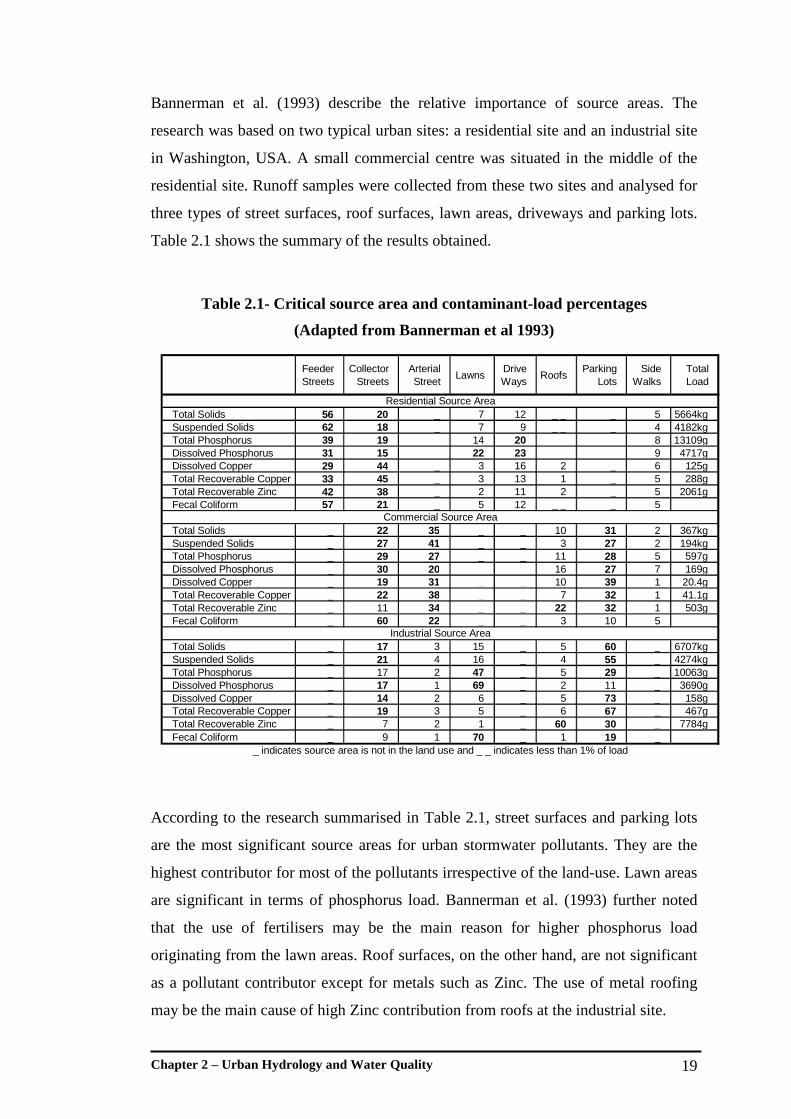
Bannerman et al. (1993) describe the relative importance of source areas. The
research was based on two typical urban sites: a residential site and an industrial site
in Washington, USA. A small commercial centre was situated in the middle of the
residential site. Runoff samples were collected from these two sites and analysed for
three types of street surfaces, roof surfaces, lawn areas, driveways and parking lots.
Table 2.1 shows the summary of the results obtained.
Table 2.1- Critical source area and contaminant-load percentages
(Adapted from Bannerman et al 1993)
Feeder Streets
Collector Streets
Arterial Street
LawnsDrive Ways
RoofsParking
LotsSide
WalksTotal Load
Total Solids 56 20 _ 7 12 _ _ _ 5 5664kgSuspended Solids 62 18 _ 7 9 _ _ _ 4 4182kgTotal Phosphorus 39 19 _ 14 20 _ _ _ 8 13109gDissolved Phosphorus 31 15 _ 22 23 _ _ _ 9 4717gDissolved Copper 29 44 _ 3 16 2 _ 6 125gTotal Recoverable Copper 33 45 _ 3 13 1 _ 5 288gTotal Recoverable Zinc 42 38 _ 2 11 2 _ 5 2061gFecal Coliform 57 21 _ 5 12 _ _ _ 5
Total Solids _ 22 35 _ _ 10 31 2 367kgSuspended Solids _ 27 41 _ _ 3 27 2 194kgTotal Phosphorus _ 29 27 _ _ 11 28 5 597gDissolved Phosphorus _ 30 20 _ _ 16 27 7 169gDissolved Copper _ 19 31 _ _ 10 39 1 20.4gTotal Recoverable Copper _ 22 38 _ _ 7 32 1 41.1gTotal Recoverable Zinc _ 11 34 _ _ 22 32 1 503gFecal Coliform _ 60 22 _ _ 3 10 5
Total Solids _ 17 3 15 _ 5 60 _ 6707kgSuspended Solids _ 21 4 16 _ 4 55 _ 4274kgTotal Phosphorus _ 17 2 47 _ 5 29 _ 10063gDissolved Phosphorus _ 17 1 69 _ 2 11 _ 3690gDissolved Copper _ 14 2 6 _ 5 73 _ 158gTotal Recoverable Copper _ 19 3 5 _ 6 67 _ 467gTotal Recoverable Zinc _ 7 2 1 _ 60 30 _ 7784gFecal Coliform _ 9 1 70 _ 1 19 _
Residential Source Area
Commercial Source Area
Industrial Source Area
_ indicates source area is not in the land use and _ _ indicates less than 1% of load
According to the research summarised in Table 2.1, street surfaces and parking lots
are the most significant source areas for urban stormwater pollutants. They are the
highest contributor for most of the pollutants irrespective of the land-use. Lawn areas
are significant in terms of phosphorus load. Bannerman et al. (1993) further noted
that the use of fertilisers may be the main reason for higher phosphorus load
originating from the lawn areas. Roof surfaces, on the other hand, are not significant
as a pollutant contributor except for metals such as Zinc. The use of metal roofing
may be the main cause of high Zinc contribution from roofs at the industrial site.

Chapter 2 – Urban Hydrology and Water Quality 20
2.3.3 Pollutant Build-up
Understanding the processes involved in pollutant accumulation is an important part
of stormwater quality research. Pollutant accumulation is a complex process since
many variables such as surface type, surface roughness, slope, antecedent dry days
and land-use play an influential role. Numerous research studies have focused on
understanding the variability of pollutant build-up and on developing suitable
models. Such research has sought to understand issues such as:
• Factors that influence pollutant build-up;
• Composition of pollutants in the build-up; and
• Mathematical replication of pollutant build-up.
(Namdeo et al., 1999; Sartor and Boyd, 1972; Shaheen, 1975)
Many researchers have focused on studying pollutant build-up on road surfaces since
roads are an important source area (Sartor et al., 1974; Shaheen, 1975).
Theoretically, one can assume that the pollutant deposition on road surfaces is
uniform, in relation to spatial uniformity of distribution of traffic and dry deposition.
However, due to wind and traffic impacts, pollutants are constantly moved away
from the turbulent areas and deposited in the kerb areas (Namdeo et al., 1999;
Novotny et al., 1985). During this process, there are more possibilities of losing
pollutants from the system by depositing them in pervious areas or being re-entrained
into the atmosphere. Due to the continuous re-distribution process on road surfaces, a
higher proportion of the total solids load is concentrated in the kerb and near kerb
areas (Sartor et al., 1974). This type of pollutant re-distribution is common for roads
where the traffic volume is significantly high.
The primary factors that affect pollutant re-distribution, and hence build-up, are wind
and vehicle induced turbulence. According to Novotny et al. (1985), at least a 20
km/hr wind velocity is required for appreciable pollutant re-distribution.
Furthermore, their research revealed that the mean particle size of the re-suspended
particles is around 15 µm and only 22% of the particles are larger than 30 µm.
However, the general particle size range of the road surface depositions discussed in
other publications is well above the re-entrained particle size range. Sartor et al.
Chapter 2 – Urban Hydrology and Water Quality 21
(1974) noted that only 5.9% of the near kerb depositions are less than 43 µm. Traffic
and traffic-induced turbulence could be the most critical parameter that influences
pollutant re-distribution. Studies by Sartor et al. (1974) and Ball et al. (1998)
revealed that pollutant concentration in near kerb areas is significantly high
compared to the centre of the road. As they have noted, the reason for this is the
movement of pollutants to the less turbulent region due to vehicular induced wind
turbulence. Furthermore, Vaze and Chiew (2002) noted that the pollutant build-up
may vary along the longitudinal direction of the road depending on the slope and the
presence of traffic signals and bottlenecks.
The composition and particle size distribution of accumulated pollutants on road
surfaces are important parameters in water quality research. This is due to the
variation of different particle size ranges in association with other pollutants, method
of transport and the impact on the natural water environment. Sartor et al. (1974)
found that most of the pollutants are adsorbed to particles less than 43 µm. They
reported that 50% of the metals and one-third to one half of nutrients are absorbed to
the finer fraction. The finer fraction (less than 43 µm) was only 5.9% of the total
solids. Bradford (1977) also found that 60% of the heavy metals are associated with
6% of the finer fraction of solids. The concept of the coarser dominant particle
weight and finer dominant pollutant adsorption was further supported by Shaheen
(1975). He reported that the bulk of the accumulated particles are in the range of
500-2000 µm. Ball et al. (1998) noted the influence of regional and catchment
management practices on pollutant build-up and its composition. They observed less
pollutant load in typical suburban roads in Sydney, Australia when compared to
North American roads. However, the particle size distribution of the accumulated
pollutants that was observed was similar to that reported by Sartor et al. (1974).
Contradictory reporting is evident on build-up and its characteristics on road surfaces
where the traffic volume is significantly less. Herngren et al. (2006a) found around
85% of the solids belong to finer particle size groups which was less than 75 µm in
industrial and residential roads. The research was based on roads where the traffic
volume is relatively low and the antecedent dry period was between one to seven
days. However, similar to most other researchers, they observed higher pollution
composition in the finer fraction of solids.
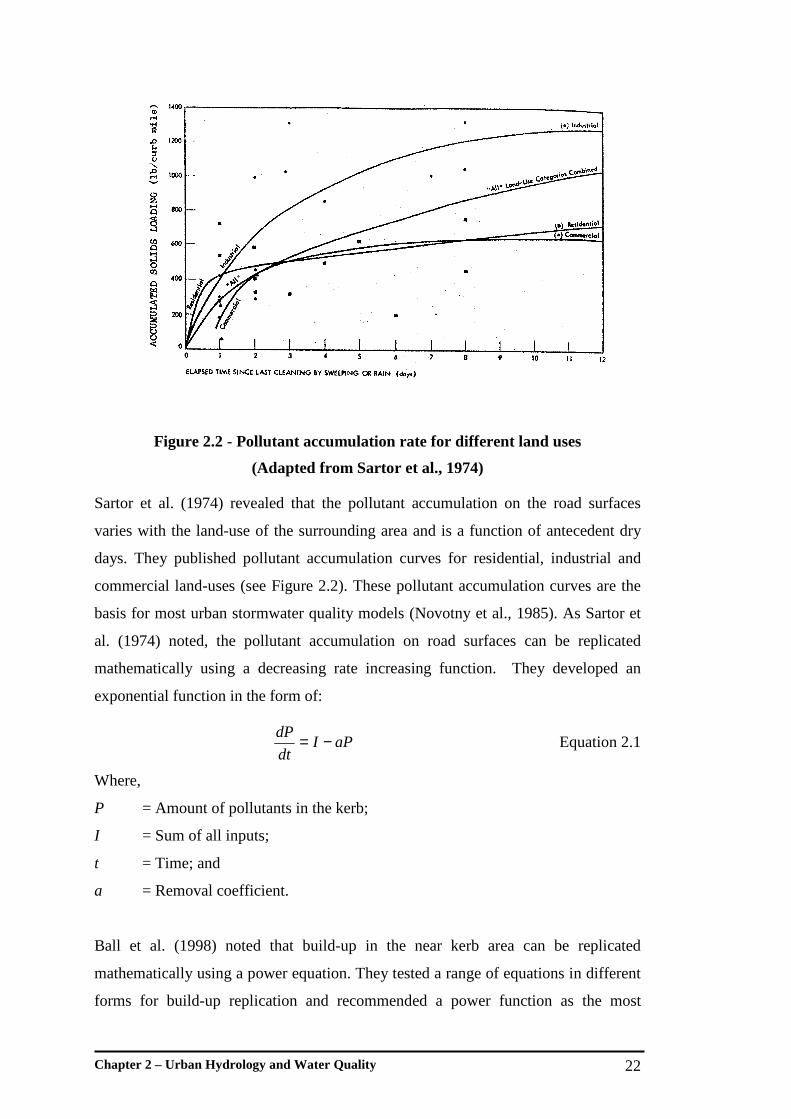
Chapter 2 – Urban Hydrology and Water Quality 22
Figure 2.2 - Pollutant accumulation rate for different land uses
(Adapted from Sartor et al., 1974)
Sartor et al. (1974) revealed that the pollutant accumulation on the road surfaces
varies with the land-use of the surrounding area and is a function of antecedent dry
days. They published pollutant accumulation curves for residential, industrial and
commercial land-uses (see Figure 2.2). These pollutant accumulation curves are the
basis for most urban stormwater quality models (Novotny et al., 1985). As Sartor et
al. (1974) noted, the pollutant accumulation on road surfaces can be replicated
mathematically using a decreasing rate increasing function. They developed an
exponential function in the form of:
aPIdt
dP −= Equation 2.1
Where,
P = Amount of pollutants in the kerb;
I = Sum of all inputs;
t = Time; and
a = Removal coefficient.
Ball et al. (1998) noted that build-up in the near kerb area can be replicated
mathematically using a power equation. They tested a range of equations in different
forms for build-up replication and recommended a power function as the most

Chapter 2 – Urban Hydrology and Water Quality 23
suitable. Their research was based on typical Australian suburban roads with
relatively moderate traffic. As they recovered relatively less pollutants, the results
obtained using the replication equation are significantly different from the equation
proposed by Sartor et al. (1974). However, the phenomenon of decreasing rate
increasing variation of build-up was confirmed. This suggested similar
characteristics of build-up irrespective of land-use, traffic and other factors.
However, due to greater variability of influential parameters such as land-use and
traffic, the amount of build-up could be highly site specific.
2.3.4 Pollutant Wash-off
The pollutants accumulated on urban surfaces are subjected to wash-off during storm
events. During the initial period of rainfall, the catchment surfaces get wet and most
of the soluble pollutants begin to dissolve in a film of water. At the same time, some
of the materials are loosened from the surface and suspended in the water film by the
energy of the falling raindrops. As the water film builds up and begins to flow down
slopes, it also develops an ability to hold pollutants in suspension due to the flow
turbulence. The kinetic energy of the raindrops is comparatively higher than the flow
energy for overland flow situations. However, when the flow is concentrated into
channels and gutters and as the depth increases, the raindrop energy becomes less
important (Mackay, 1999).
The amount of pollutants washed-off from impervious surfaces is primarily
influenced by the amount available on the surface which in turn is related to the
pollutant build-up process (Duncan, 1995). As discussed in Section 2.3.3, build-up is
a dynamic process which primarily varies with the antecedent dry period. This
indicates the influence of antecedent conditions on the amount of pollutant wash-off.
However, as far as the wash-off process is concerned, the influence of the amount of
build-up is limited. The other parameters, primarily rainfall and runoff parameters,
are the most influential in the wash-off process (Novotny et al., 1985; Sartor et al.,
1974).
Chapter 2 – Urban Hydrology and Water Quality 24
Explanation for the processes governing pollutant wash-off varies in the research
literature. However, all hypotheses centre around four influencing rainfall and runoff
variables: rainfall intensity, rainfall volume, runoff rate and runoff volume (Mackay,
1999). These variables correlate with each other: therefore, it is difficult to discern
the degree of influence exerted by them individually on wash-off. Chiew and
McMahon (1999) investigated the relationship between pollutant wash-off and runoff
volume in urban catchments in Australia. They showed that the event mean
concentrations of suspended solids and total phosphorous can be better estimated
using total runoff volume. This implies that the higher runoff volume carries a higher
pollutant load. However, for an urban catchment with well protected pervious
surfaces this may not be true since there should always be an upper limit of pollutant
availability on the catchment surfaces. Chui (1997) showed that event mean
concentration for total suspended solids (TSS) and chemical oxygen demand (COD)
increases with the rainfall intensity rather than with rainfall volume. The rainfall
intensity correlates with the rate of kinetic energy supplied by the raindrops.
Therefore, the pollutant removal capacity of rainfall may increase with intensity.
Herngren et al. (2005a) showed that pollutant wash-off may be influenced by
catchment surface properties such as texture depth. They used simulated rainfall over
several road surface plots to investigate pollutant wash-off behaviour and found that
relatively rough road surfaces are capable of holding a greater fraction of pollutants
within the surface. Furthermore, they showed that pollutant wash-off is influenced by
both rainfall intensity and runoff volume but they were not able to determine the
relative importance of each parameter on pollutant wash-off.
The general understanding of pollutant wash-off implies that rain storms only
remove a fraction of the pollutants from the catchment surface. The experimental
study by Vaze and Chiew (2002) showed that after a significant rainfall event of 39.4
mm, only 35% of the total pollutants were washed-off. The following rainfall event
of 4 mm reduced total pollutant load by 45%. Based on field measurements, Vaze
and Chiew (2002) have proposed two possible pollutant wash-off concepts, as
illustrated in Figure 2.3. These alternative processes are termed as ‘source limiting’
(Figure 2.3a) and transport limiting (Figure 2.3b). According to their research,

Chapter 2 – Urban Hydrology and Water Quality 25
pollutant wash-off from impervious surfaces that are subjected to more frequent
rainfall events is more close to the source limiting process.
Figure 2.3 – Hydrologic representation of surface pollutant load over time
(Adapted from Vaze and Chiew, 2002)
According to Sartor et al. (1974), the rate at which rainfall wash-off removes
particulate pollutants from road surfaces depends on three primary factors: road
surface characteristics, rainfall characteristics, and particle size. However, they have
further suggested that the influence of rainfall intensity is comparatively higher for
pollutant wash-off than for other parameters and the use of rainfall intensity alone in
a pollutant wash-off equation produces acceptable outputs. The pollutant wash-off
equation developed by Sartor et al. (1974) is in exponential form. Rosener (1982)
suggested that the pollutant wash-off equation (Equation 2.2) developed by Sartor et
al. (1974) could be used for all impervious surfaces. However, the equation was
primarily developed based on research data from road surfaces.
)1( kIto eWW −−= Equation 2.2
Where,
Wo = Initial weight of the material of a given particle size;
t = Time of rainfall;
I = Rainfall intensity;
Chapter 2 – Urban Hydrology and Water Quality 26
W = Weight of material of a given particle size removed after time t; and
k = Wash-off coefficient.
The wash-off coefficient ‘k’ varied with the street surface characteristics but was
found to be almost independent of particle size.
2.3.5 First Flush Phenomenon
As noted by numerous researchers, the ‘first flush’ is an important phenomenon
which has strong links to pollutant wash-off and transport. The ‘first flush’ refers to
the higher concentration of pollutants during the initial period of the storm events. It
has been noted that the concentration peak precedes the runoff peak (Deletic, 1998;
Duncan, 1995; Lee et al., 2002).
The first flush phenomenon is the primary justification for most stormwater
treatment design. Most treatment facilities such as retention and detention basins
have been designed so that they treat the initial runoff which in turn contains the
highest concentration. The rest of the runoff is often bypassed without any treatment.
However, the uncertainty of occurrence of ‘first flush’ and the presence of a high
amount of dissolved pollutants which is difficult to treat using such facilities often
leads to failure of treatment (Harrison and Wilson, 1985).
Although the occurrence of first flush has been commonly reported, the observations
are not consistent. Hall and Ellis (1985) and Sonzogni et al. (1980) stated that the
significance of the first flush is overemphasised and only 60% to 80% of the storms
exhibit this phenomenon. Apart from the uncertainty of occurrence, Hoffman et al.
(1984) noted that the timing of the peak concentration for different pollutants could
vary. They noted that the peak of dissolved concentrations often occurs after the peak
of particulate concentrations.
The occurrence and nature of first flush can be influenced by a range of factors.
Harrison and Wilson (1985) noted that the occurrence of first flush is influenced by
the temporal and aerial variation of rainfall events. It is often noted that the highest
Chapter 2 – Urban Hydrology and Water Quality 27
intensity rainfall bursts are in the initial period of rain events. This could cause
higher pollutant wash-off during the initial part of the event which in turn magnifies
the first flush. Furthermore, first flush can be magnified by the presence of a higher
fraction of roof surfaces where most of the pollutant wash-off takes place during the
initial period of runoff. Forster (1996) noted that roofs produce significant
concentrations of pollutants during the initial period of runoff. Catchment
characteristics also have a pronounced influence on the first flush. Lee and Bang
(2000) and Lee et al. (2002) observed high strength first flush occurrence in smaller
and highly impervious catchments compared to larger and less impervious
catchments. However, Bertrand-Krajewski et al. (1998) noted that the influence of
catchment size on first flush is minor.
2.4 Primary Stormwater Pollutants
As stormwater pollution leads to significant deterioration of the quality of receiving
water bodies, identification of specific characteristics and types of urban pollutants is
critically important. Unlike rural catchments, anthropogenic activities in urban
catchments result in a diverse variety of pollutants. Industrial processes, vehicular
traffic, construction and demolition activities and household chemical use are key
anthropogenic activities in urban areas. The common pollutants present in urban
catchments are:
• Litter;
• Nutrients;
• Heavy metals;
• Hydrocarbons;
• Organic carbon; and
• Suspended solids.
2.4.1 Litter
The primary categories of litter are packaging materials such as paper, glass, metals,
plastics and grass and plant leaves. Litter is not a major concern in terms of water
Chapter 2 – Urban Hydrology and Water Quality 28
quality degradation. However, most urban catchments produce a significantly high
volume and mass of litter. Litter contributes to drain blockage and gives an unsightly
appearance to receiving waters. Therefore, the presence of litter in stormwater runoff
is a considerable issue for urban drainage management (Armitage and Rooseboom,
1999; Marais et al., 2001). The research by Allison et al. (1998) in an inner suburban
catchment in Melbourne, Australia, suggested that the nutrient contribution from
litter is an order of magnitude smaller than the nutrients present in typical stormwater
runoff. This implies that the significance of litter is comparatively low purely as a
water pollution agent.
2.4.2 Nutrients
Nutrients are chemicals that are essentially required for plant growth. However, high
contributions of nutrients from urban lands cause excessive growth of plants such as
algae. The excessive growth of algae alters the visual appearance of water bodies.
The visual impact may include colour, turbidity and floating matter. Consequently,
death and decomposition of vegetation will alter water quality parameters such as
dissolved oxygen demand (Brezonik and Stadelmann, 2002; O'Reagain et al., 2004).
Total nitrogen (TN) and total phosphorous (TP) are the most important nutrients that
cause water quality degradation. Many researchers have shown that stormwater
runoff is a significant source of nutrients (for example, Sonzogni et al. (1980).
However, the primary source areas that they refer to are different. According to
Bannerman et al. (1993) and Novotny et al. (1985), significant amounts of nutrients
originate from gardens and lawns in residential catchments which could be the result
of the use of fertiliser. Shaheen (1975) found that road surface runoff contains
significant nitrogen and phosphorous compounds and that a significant fraction of
these pollutants is due to vehicle exhausts. Forster (1996) showed that almost all the
nitrogen compounds originating from roof surfaces are atmospheric depositions.
Significant amounts of nutrients may originate from the degradation of leaf litter.
However, Allison et al. (1998) showed that the nutrient contribution from leaf litter is
two orders of magnitude less than the typical nutrient loads in urban stormwater.

Chapter 2 – Urban Hydrology and Water Quality 29
2.4.3 Heavy Metals
Urban stormwater can contain significant amounts of heavy metals. The research by
Lind and Karro (1995) showed that the top soil of urban roadside green areas contain
two to eight times more heavy metals than top soil in rural areas. These roadside
green areas are designed as stormwater infiltration areas in stormwater management
practice. The common heavy metals found in stormwater runoff are Zinc (Zn), Lead
(Pb), Copper (Cu), Cadmium (Cd), Nickel (Ni) and Chromium (Cr) (Lind and Karro,
1995; Sorme and Lagerkvist, 2002).
The main sources of heavy metals in the urban environment include household and
commercial chemical use, traffic related pollutants, atmospheric depositions and
building materials. Sorme and Lagerkvist (2002) observed that one of the main
sources of Cu is tap water and roof runoff. Their research mainly focused on tracking
heavy metal sources in the urban environment. Furthermore, they identified that one
of the largest sources of Zn was galvanised building materials and car washing
liquids. Sartor et al. (1974) and Zenders (2004) showed that road surfaces contain a
significant amount of heavy metals. According to their research, vehicle exhausts,
tyre and brake lining, and asphalt pavement contributions are the main sources of
heavy metals in a road surface.
2.4.4 Hydrocarbons
Stormwater runoff is a major contributor of hydrocarbon load in an urban
environment (Gray and Becker, 2002). Datry et al. (2003) showed that the bed
sediment of stormwater detention basins contain significant amounts of
hydrocarbons. They tested bed sediment of a stormwater detention basin in France
which had operated for over thirty years. The results showed that 52.9 mg/kg of dry
sediment were present including 15 types of hydrocarbons. According to their
research, most of the hydrocarbons were attached to particulate matter and were
rarely found in the dissolved phase.
Chapter 2 – Urban Hydrology and Water Quality 30
Hydrocarbons can originate both from natural and anthropogenic sources. Natural
sources such as degradation of organic matter and forest fires contribute a minor
fraction of hydrocarbons to the urban environment. Anthropogenic activities are the
major source of hydrocarbon load including Polycyclic Aromatic Hydrocarbons
(PAHs). Van Metre et al. (2000) showed that the increasing trend of PAH in
stormwater runoff is caused by combustion sources. They observed that PAH
concentrations track closely with an increase in automobile use. However, Ngabe et
al. (2000) commented that the chemical composition of PAHs found in stormwater
runoff is more closely related to lubrication oil. Therefore, non-combusted oil losses
could be a major source of hydrocarbons in road surface runoff.
2.4.5 Organic Carbon
Organic carbon is an oxygen demanding material which is commonly found in urban
stormwater runoff. The major impact of organic carbon is the reduction of dissolved
oxygen in water. Excessive loads of oxygen demanding materials can reduce the
amount of dissolved oxygen in receiving water and hence cause significant damage
to aquatic life (Warren et al., 2003).
Gromaire-Mertz et al. (1999) showed that the largest amount of organic carbons
originates from road surfaces in urban environments. The variations of organic
matter on urban surfaces were found to be dependent on a range of parameters such
as antecedent time since the last street cleaning or rainfall event and land use
characteristics. Sartor et al. (1974) showed that organic matter accumulates on road
surfaces much faster than inorganic matter. Roger et al. (1998) showed that in road
surface runoff the organic carbon concentration is significantly high in particles less
than 50 µm.
2.4.6 Suspended Solids
In an urban environment, the pollutants available on paved surfaces such as roads,
roofs, and gardens are mostly in particulate form. During rainfall events some of
Chapter 2 – Urban Hydrology and Water Quality 31
these pollutants dissolve in stormwater, but a significant amount is transported as
particulate pollutants. These particulate pollutants are commonly referred to as
suspended solids. It has been noted that particulate pollutants are kept in suspension
by the raindrop induced turbulence in overland flow (Mackay, 1999).
The size range of the suspended solids varies from very fine solid particles to large
particles depending on the turbulence created by the raindrops. Relatively larger and
dense particles may settle and re-suspend during the flow and the possibility of
settling in the receiving water bodies is high. The physical impact of these settable
solids include smothering of bottom dwelling fauna and flora and changes to the
substrate.
Finer particles remain in suspension for a longer period of time. This is due to the
larger surface area compared to mass and the presence of electrostatic charges (Dong
et al., 1983). Therefore, fine textured particles are most likely to reach receiving
water bodies. Andral et al. (1999) noted that the higher fraction of finer particles
which are less than 100 µm remains in suspension for a longer period of time whilst
a higher fraction of coarser particles which are greater than 100 µm will settle
rapidly. They further noted that treatment for the finer fraction will remove 90% of
the solids which have a high potential to reach receiving waters.
Finer particle ranges are not only actively available in water bodies by being in
suspension but they are also associated with a high fraction of other pollutants such
as hydrocarbons and heavy metals. Herngren et al. (2005a) showed that heavy metal
and hydrocarbon concentrations are strongly correlated with the total suspended
solids load. Sartor et al. (1974) noted a significantly high percentage of nutrients and
organic material in the finer fraction less than 43 µm which was only 5.9% of the
total solids. Since the correlation of suspended solids to other pollutants is strong, the
use of suspended solids as a surrogate to estimate other pollutants is a common
practice. This is the primary reason for the common approach of selecting suspended
solids as an indicator pollutant in stormwater quality research (Akan and Houghtalen,
2003). The capacity for adsorbing other molecules varies with the size, structure and
physio-chemical properties such as electrical conductivity of the particles (Pechacek,
1994; Tai, 1991). As noted by Hamilton et al. (1984) and Warren et al. (2003), the

Chapter 2 – Urban Hydrology and Water Quality 32
other factors influencing pollutant adsorption are organic carbon concentration and
pH.
2.5 Hydrologic and Water Quality Modelling Approaches
With growing awareness of both the hydrologic and water quality impact of
urbanisation, hydrologic modelling and water quality modelling are increasingly
used as estimation tools for understanding the quantity and quality impacts of
stormwater runoff (Zoppou, 2001). Hydrologic models are generally used as a flood
estimation tool for simulating individual storm events or a series of events which has
occurred over a period of time. Unlike hydrologic models, water quality models have
been developed to estimate the long-term pollutant impact on receiving waters.
However, there are a number of models, such as SWMM which have been developed
to estimate pollutant load from an individual storm event (Rossman, 2004). Both
hydrologic and water quality models were first developed for natural or rural
catchments. With the increasing demand for urban hydrologic and pollution models,
both types of models have been modified to handle urban characteristics (Ahyerre et
al., 1998; Zoppou, 2001). In this section, the technical capabilities of hydrologic and
water quality models in an urban context are discussed.
2.5.1 Urban Hydrologic Models
Hydrologic models are usually a combination of mathematical procedures used to
replicate hydrologic processes. This combination ultimately generates quantitative
estimates of stream flow runoff. The main hydrologic processes in a catchment are
illustrated in Figure 2.4.

Chapter 2 – Urban Hydrology and Water Quality 33
Figure 2.4– Hydrologic processes
(Adapted from O’Loughlin and Stack, 2004)
Different mathematical procedures have been developed to estimate each component
of the hydrologic processes (Boyd et al., 2003; Laurenson and Mein, 1995;
O'Loughlin and Stack, 2004). As an example, Horton’s infiltration equation is a
recognised estimation procedure for rainwater infiltration. However, most of the
developed mathematical procedures focus on rural or natural catchments. There are
significant quantitative differences in urban hydrologic processes when compared to
rural hydrologic processes in relation to infiltration and depression storage
(Laurenson, 1962; Waananen et al., 1961). Models that do not account for these
differences may lead to erroneous estimations. In order to overcome these estimation
errors, modifications have been included in rural hydrologic models so that they can
replicate urbanisation effects. In most cases, urban catchment surfaces are considered

Chapter 2 – Urban Hydrology and Water Quality 34
as a combination of three different land cover types: impervious – directly connected,
impervious – supplementary and pervious. Separate mathematical procedures have
been developed to replicate rainfall and runoff processes in these three types of
surfaces (Boyd et al., 2003; O'Loughlin and Stack, 2004).
With the advancement of research knowledge, accurate and complex mathematical
procedures have been developed to replicate each rainfall and runoff process. Use of
these procedures in a hydrologic model increases its complexity. Therefore, model
users often simplify the aspects of urban hydrology to a manageable level of
complexity. However, oversimplification of catchment behaviour may lead to errors.
On the other hand, more complex models need more computational effort and data
resources (Goonetilleke, 1998; Phillips and Yu, 2001; Zoppou, 2001). The simplicity
or complexity of a model depends on the needs. However, a number of primary
features have been recommended to be included in hydrologic models in order to
improve their prediction power (Laurenson, 1964). These are:
• Temporal and spatial variation of rainfall excess;
• Distributed nature of the catchment; and
• Non-linearity of the catchment response.
Hydrologic models which use different mathematical procedures with different
complexity are available. The types of models vary from simple models which are
only capable of estimating peak discharge to complex models that can be used to
estimate the runoff hydrograph. The decision on which model to use depends on the
capabilities of the model and the complexity to which users are accustomed
(O’Loughlin and Stack 2004).
2.5.2 Hydrologic Modelling Approaches
The rational formula is the simplest form of the hydrologic model (Rossmiller,
1980). It is a simple statistical relationship between measurable parameters such as
rainfall intensity, peak discharge and catchment physical properties. The formula is
only capable of estimating peak discharge. The primary advantage of using the
rational formula is its simplicity. It requires comparatively less data and resources to

Chapter 2 – Urban Hydrology and Water Quality 35
perform calculations. Although the formula is widely used in the urban context, care
has to be taken in selecting an appropriate runoff coefficient. Furthermore, due to the
level of simplicity, the estimations could be far from reality. The fundamental
assumptions used are:
• The design storm is uniformly distributed in time and space;
• The storm duration is equal to the time of concentration;
• Peak flow is a fraction of average rainfall rather than the rainfall excess;
• The return period of the peak flow is equal to the return period of storm; and
• Rainfall runoff response is linear.
(Dayaratne, 2000; Goonetilleke, 1998).
With the advent of computers it has become possible to create models that can
handle complex rainfall temporal patterns as inputs and use complex mathematical
replications as hydrologic processes. In this type of complex model, the
mathematical procedures used for estimation can be separated into a loss model and a
routing model.
The loss model represents the rainfall and runoff processes such as interception,
depression storage, infiltration and evaporation. The loss model enables the
estimation of the rainfall excess which is the portion of water available for runoff.
The most common types of loss models are:
• Initial loss – continuing loss model;
• Initial loss – proportional loss model; and
• Infiltration models such as Horton’s infiltration equation.
(Boyd et al., 2003; Laurenson and Mein, 1995; O'Loughlin and Stack, 2004)
For urban catchments, two different loss models are used for impervious and
pervious surfaces. For impervious surfaces, only an initial loss is commonly
subtracted from the rainfall in order to calculate rainfall excess. The general range of
initial loss for impervious surfaces is 0 to 5 mm (Boyd et al., 2003; O'Loughlin and
Stack, 2004). For the pervious area, the initial loss – continuing loss model is the
most widely used and it is the recommended model for most parts of Australia
(Pilgrim, 1998). The common procedure is to subtract complete losses from the

Chapter 2 – Urban Hydrology and Water Quality 36
rainfall prior to routing. However, there are some models which subtract depression
storages first, then calculate the runoff using the routing model and subtract
infiltration losses from the runoff. This latter approach is more realistic since
infiltration may occur continuously during the runoff period (O'Loughlin and Stack,
2004).
The routing model transforms the rainfall excess into a runoff hydrograph using
catchment properties. Routing models incorporate peak attenuation and travel time of
runoff due to the storage action of the catchment and channels. Some of these routing
models are theoretically based and others are conceptual models. The main types of
routing models are:
• Unit hydrograph models;
• Kinematic wave routing models;
• Artificial storage routing models; and
• Time area routing models.
A Unit Hydrograph Models
The unit hydrograph is the catchment response for a unit of excess rainfall. Models
developed based on unit hydrograph methods derive flood hydrographs from the
given rainfall excess hyetograph. To keep computational effort to a minimum, the
catchment parameters are limited to area, length and slope (Espey et al., 1969;
Pilgrim et al., 1981; Sarma et al., 1973).
The basic theoretical contradiction of the unit hydrograph method is its linearity. In
the unit hydrograph method, the rainfall excess and runoff are assumed to be linearly
related (Kitheka et al., 1991). However, it is clearly understood that the rainfall-
runoff relationship for any catchment is nonlinear (Aitken, 1975; Askew, 1970;
Laurenson, 1962). Researchers have attempted to include modifications to the unit
hydrograph method to adapt it to an urban context. In some cases, such as in the
work of Espey et al. (1969), attempts have been made to modify the unit hydrograph
for urban catchments. They have investigated runoff responses from various urban
catchments in order to develop a general urban unit hydrograph. In other cases, the

Chapter 2 – Urban Hydrology and Water Quality 37
parameters of conceptual models based on the unit hydrograph have been modified
in order to replicate urbanisation effects (Sarma et al., 1973). The latter method was
relatively more successful than the former. However, the use of models based on the
unit hydrograph is becoming less popular with the rise of non-linear, more
theoretically-sound, physically-based models.
B Kinematic Wave Models
Mathematical models have been developed to simulate the overland flow of general
irregular surfaces. These models have been used in hydrologic modelling of
catchments. The capability of simulating accurate behaviour and routing of flow in
irregular and complex catchment surfaces using these models is not well known.
However, there are several approximate models commercially available. The use of a
simplified form of kinematic wave equation is one of the most popular forms of
mathematical models. These models are generally referred to as ‘physically-based
models’ (Liu et al., 2004; Sugiyama et al., 1997).
Even though the kinematic wave models are a simplified form, they are relatively
accurate for low flow depths and steep slopes. Although physically-based models
provide similar reliability and accuracy as the storage routing models and time area
routing models (to be discussed later), they need more computational effort.
Therefore, the inclusion of the distributed nature of the catchment into the model by
subdividing it into a number of subcatchments is complex. These are the main
reasons for the relatively low use of kinematic wave models in Australia (Pilgrim et
al., 1981; Zoppou, 2001).
C Storage Routing Models
Storage routing models are among the most popular in urban hydrologic modelling.
The storage routing method is simple and requires less computational effort when
compared to physically-based models. Storage routing models have been developed
for rural catchments and most of them are capable of analysing partially urbanised
catchments with necessary modifications to the model structure. The pioneering
storage routing model was proposed by Laurenson (1964). In his model, the
Chapter 2 – Urban Hydrology and Water Quality 38
catchment was subdivided into sub-areas on the basis of lines of equal travel time or
isochrones. Each sub-area was considered as a reservoir with non-linear outflow
behaviour (Boyd et al., 1979; Boyd et al., 1996; Carroll, 2002; Laurenson, 1962,
1964; Mein et al., 1974).
The basis for most of the storage routing models is very similar to the Laurenson
(1964) model. The main difference in each model is the method of interpreting
physical derivations of sub-areas into a reservoir network and the parameters of the
non-linear equation. RAFTS (Laurenson, 1964), RORB (Laurenson and Mein, 1995)
and WBNM (Boyd et al., 2003) are the most common models developed based on
the storage routing procedure.
D Time Area Routing Models
The time area diagram shows the variation of contributing area to the flow with time
at the outlet for a constant rainfall event. The runoff hydrograph for a given
catchment and given rainfall event can be calculated using a time area diagram as
illustrated in Figure 2.5.
The time area diagram is drawn based on the calculations of the time of
concentration for the various parts of the catchment. For urban catchments, the time
of concentration is the sum of property drainage time, overland flow time and gutter
flow time. Separate calculation procedures are available to calculate each flow time
depending on the physical properties of each drainage item (O'Loughlin and Stack,
2004). The time area diagram could be of concave or convex shape depending on the
shape of the catchment and other factors. However, most of the time area routing
models consider time area diagram as linear. Models such as ILSAX and DRAINS
are the most widely used hydrologic models in Australia that are based on time area
routing (O'Loughlin and Stack, 2004). These two models have been specifically
developed for urban catchments. The models also contain hydraulic procedures to
calculate pipe and channel flow.

Chapter 2 – Urban Hydrology and Water Quality 39
Figure 2.5 – Time area calculation
Adapted from O’Loughlin and Stack (2004)
2.5.3 Urban Water Quality Models
The techniques used for water quality simulation are very similar to hydrologic
simulations (Zoppou, 2001). The primary inputs for water quality models are rainfall
data, geographical data and pollutant load data. The water quality models provide
estimations of pollutant concentrations or loads originating from a catchment. There
are a number of modelling approaches adopted (Zoppou, 2001).
Stormwater quality modelling can be performed on a lumped time base or on a
continuous time base (Akan and Houghtalen, 2003). Lumped time base modelling is

Chapter 2 – Urban Hydrology and Water Quality 40
relatively easier and produce estimates of pollutant load (in kilograms) generated
from a catchment over a relatively long period of time (say a month or year). These
types of models are based on general pollutant export equations for the entire
catchment. Continuous time based models are relatively complex and produce
estimates for pollutant concentration in relatively shorter time steps (a few minutes).
(Akan and Houghtalen, 2003; Zoppou, 2001).
A Continuous Time Based Models
Continuous time based models are based on a combination of mathematical
procedures which are used to replicate stormwater pollutant processes. The common
pollutant processes that these models replicate are pollutant build-up and wash-off.
In most cases, the replication equations are only for suspended solids. Suspended
solids are considered as the indicator pollutant and other pollutant concentrations are
estimated assuming a constant ratio to the suspended solids concentration (Akan and
Houghtalen, 2003).
Different models use different forms of pollutant build-up equations. However, most
of these models use build-up equation in the form of decreasing rate increasing
function. The most common equations in this form are power function or exponential
function. An exponential function in the form of Equation 2.2 is the most common
form of replication equation for pollutant wash-off (Akan and Houghtalen, 2003;
Ball et al., 1998; Novotny et al., 1985; Sartor et al., 1974; Tsihrintzis and Hamid,
1997; Zoppou, 2001).
The replication of pollutant processes alone is not adequate for water quality
modelling. Estimations of hydrologic parameters such as runoff volume are essential
to estimate pollutant concentration. Furthermore, the calculated pollutant
concentration should be routed to the catchment outlet. This highlights the necessity
of parallel simulation of a hydrologic model. A similar procedure to a hydrologic
model is commonly used to route the pollutant concentrations. In this regard, the
pollutant is assumed to be transported only via advection. Advection is the primary
mode of particulate transport in fast flowing water (Akan and Houghtalen, 2003).
Chapter 2 – Urban Hydrology and Water Quality 41
Model calibration, which is the refinement of adjustable model parameters in order to
represent the actual performance of the catchment, is the most important process in
stormwater quality modelling. Measured boundary data, such as pollutograph or
instantaneous water quality data is used to calibrate the water quality model (Gaume
et al., 1998). The calibration parameters are in two sets. Firstly, parameters related to
the build-up equation need to be adjusted until close correlation is achieved between
measured and predicted pollutant load. Secondly, the parameters relating to the
wash-off equation need to be adjusted until close agreement with the measured and
predicted pollutograph is achieved. Though these parameters represent unique
characteristics, separate calibration of them is difficult. Therefore, simultaneous
calibration of parameters is highly recommended (Mike-TRAP, Version 2004).
B Lumped Time Based Models
Continuous time based models provide detailed pollutant load and concentration
estimations. This level of detailed estimations is not required for many engineering
applications, particularly planning level studies (Akan and Houghtalen, 2003). Mean
annual loading rates are often adequate for such applications. Lumped time based
modelling is one such long-term pollutant load estimation procedure (Ahyerre et al.,
1998; Charbeneau and Barrett, 1998; Phillips and Yu, 2001).
The fundamental concept in the lumped time based modelling is very
straightforward. The model estimates the annual pollutant export from a particular
catchment using catchment, land-use or rainfall parameters. There are different types
of models that use different pollutant export equations of varying complexity
(Letcher et al., 1999). For example, the equation developed by the US Environmental
Protection Agency (EPA) to estimate annual pollutant loading is one of the widely
used methods (Akan and Houghtalen, 2003). The equation is:
Ms = α P f s Equation 2.3
Where,
Ms = Weight of pollutant generated per unit land per year;
α = Pollutant loading factor;
P = Annual precipitation;
Chapter 2 – Urban Hydrology and Water Quality 42
f = Population density function; and
s = Street sweeping factor.
(Akan and Houghtalen, 2003)
The information on pollutant loading (the pollutant loading factor α) needs to be
estimated depending on factors such as land-use, population density and traffic
volume (Letcher et al., 1999).
Comprehensive modelling packages have been developed based on the lumped time
based method, including estimation tools for quantitative and qualitative parameters
and management tools. XP-AQUALM is one such model designed for long-term
runoff and pollutant export estimations and costing and policy assessments (XP-
AQUALM-User-Manual, 1996). The non-point source water quality analysis model
of XP-AQUALM consists of a hydrologic model and non-point source pollutant
export model. The hydrologic model is a continuous model, which calculates runoff
on a daily basis. Water quality is estimated using pollutant export equations. These
equations typically consist of a runoff parameter and calibration coefficients. Runoff
parameters are pre-estimates using the hydrologic model whilst calibration
parameters have to be obtained using the calibration procedure (XP-AQUALM-User-
Manual, 1996). Measured event mean concentrations at catchment outlets are often
used as data for calibration exercises (Chiew and McMahon, 1999; Phillips and Yu,
2001).
2.7 Conclusions
The following discussion summarises the important conclusions drawn from the
review of research literature relating to the hydrologic and water quality regime. The
conclusions are mainly focused on the current state of knowledge with respect to
hydrologic and water quality impacts of urbanisation, key pollutant processes and
current modelling approaches and related issues.
Changes to the hydrologic cycle and quantitative impacts of urbanisation are well
documented in literature. Due to the presence of impervious surfaces and lined

Chapter 2 – Urban Hydrology and Water Quality 43
channels in urban catchments, both rainfall loss parameters and runoff parameters
undergo changes. Consequently, this leads to an increase in peak discharge, runoff
volume and reduction of base flow. Furthermore, urban catchments commonly
exhibit a rapid response to rainfall events. There can be a diversity of hydrologic
impacts of urbanisation due to climatic, land-use and topographic changes.
The focus on water quality impacts of urbanisation is of relatively recent origin.
However, there is a significant amount of research that has been done in this field
and fundamental knowledge on water quality is available. It is common knowledge
that anthropogenic activities in urban catchment surfaces produce various pollutants.
These pollutants are washed-off during storm events, creating significant impacts on
receiving waters. In the context of stormwater quality, impervious surfaces are
critically important due to two reasons. Firstly, most of the impervious surfaces such
as roads hold significant amount of pollutants. Secondly, these surfaces are
hydrologically active even for a small rainfall event.
Pollutant sources and pathways are clearly identified in stormwater quality research.
Road surfaces have been recognised as the largest contributor to the pollutant load.
However, the extent of contribution varies from place to place depending on the land
use of the surrounding area, traffic volume and road surface conditions. On the other
hand, other impervious and pervious surfaces are significantly dominant under
certain conditions. The best examples for this are gardens and roof surfaces. Gardens
are a significant source of suspended solids and nutrients for relatively large storm
events. Metal roof surfaces can be a significant source of heavy metals.
Understanding key pollutant processes is critically important in urban water quality
research. Significant research has been carried out on pollution build-up and wash-
off from urban impervious surfaces. However, outcomes of most of this research are
site specific. Due to the significant variation of pollutant processes with rainfall,
topographic and land-use characteristics, it is difficult to explain pollutant processes
in general terms. Furthermore, research in this respect exhibits significant data
scatter. Therefore, the processes that have been developed for pollutant build-up and
wash-off may not be directly applicable for all regions.

Chapter 2 – Urban Hydrology and Water Quality 44
The primary water pollutants identified in literature include suspended solids,
nutrients, hydrocarbons, heavy metals and organic carbon. Suspended solids are the
most common pollutant in stormwater runoff. Most of the other pollutants are
chemically adsorbed to these particulate pollutants. Hence, the chemical impacts of
the suspended solids are of concern. Due to this characteristic, suspended solids are
commonly considered as an indicator pollutant.
Numerous predictive models have been developed for quantity and quality
estimation of stormwater runoff. The estimation of quantity characteristics of
stormwater is a well developed field. There is a wide range of estimation tools
available. Use of these tools for a specific problem depends on the nature of the
problem and acceptance of the tool within the profession. The estimation tools for
quality characteristics of stormwater have been developed recently. Due to the lack
of understanding of underlying pollutant processes and variables, the use of water
quality models can often lead to gross errors. An extensive amount of data is
generally needed to calibrate water quality models. The production of such data is
resource intensive and difficult. Furthermore, due to high costs and inherent
difficulties involved in producing appropriate data, the accuracy of results from the
use of water quality models can be questionable.

Chapter 3 – Study Tools 45
Chapter 3 - Study Tools
3.1 Background
Chapter 2 explained the necessity for an in-depth investigation into pollutant
processes and the underlying parameters in stormwater quality research. Due to the
complex nature of pollutant processes, significant array of data is required to
understand them. As reported in research literature, the techniques used to generate
such data are highly variable. For example, build-up sampling from urban surfaces
has been conducted using vacuum systems. However, the specifications of the
systems used in different research are varied. Vaze and Chiew (2002) used an
industrial vacuuming system to collect street surface depositions. They noted that the
higher power generated by the system increased the sampling efficiency which was
termed as the ratio of collected pollutants to available pollutants. Deletic and Orr
(2005) used a floor and carpet vacuuming system where actions of washing and
vacuuming simultaneously apply. This was due to higher efficiency in retaining finer
particles.
The techniques used to investigate pollutant wash-off show even greater variability.
The variability is primarily in terms of concepts, scale and apparatus used. Sartor et
al. (1974) and Herngren (2006a) used simulated rainfall for wash-off studies.
However, the simulation techniques used and the small-plot area selected for
simulation were significantly different. Vaze and Chiew (2002) used a completely
different technique where they sampled pollutants from road surfaces before and
after natural rain events. The investigation technique used by Roesner (1982) was
further different, and involved the sampling of runoff at catchment outlets in order to
understand the wash-off behaviour.
From the above discussion it is clear that a range of techniques is available to
conduct investigations in water quality research. Each investigation technique has
specific advantages and disadvantages. The best possible technique has often been
selected by rating these advantages and disadvantages according to user preferences
Chapter 3 – Study Tools 46
and to suit specific research requirements. Though the techniques are different, most
of them have earned creditable recognition among the research community, given
that their performances were verified under specific research conditions.
This chapter introduces the sampling apparatus and analytical tools used for this
research. It was intended to use simple approaches for the investigations, so that
these methods can be reproduced in future stages. The apparatus were selected to
ensure the requirement of portability. The analytical tools were selected after close
consideration of the requirements. The selected methods were simple and reliable for
their designated use. The primary study apparatus and analytical tools used for the
research included:
1) Vacuum collection system;
2) Rainfall simulator;
3) Model roof;
4) Statistical and chemometrics analytical tools; and
5) Hydrologic modelling software.
3.2 Vacuum Collection System
Sampling techniques used to collect pollutants from urban surfaces show significant
variability. However, most of these techniques are in the following two categories:
1) Brushing / sweeping; and
2) Vacuuming.
These two methods have specific advantages and disadvantages. Researchers often
used combinations of these methods in order to enhance the collection efficiency
(Deletic and Orr, 2005; Robertson et al., 2003). Brushing or sweeping of road
surfaces are generally efficient in collecting relatively larger particles. Robertson et
al. (2003) noted that brushing and sweeping the road surface can result in biased
outcomes for larger particles. They suggested that this method is more suitable when
finer particles are not important. Bris et al. (1999) suggested that vacuuming is
preferable in order to collect road surface pollutants due to the efficiency that can be
achieved in collecting finer particles. They compared two vacuum collection systems
Chapter 3 – Study Tools 47
and noted that a wet vacuum system was preferable over the conventional dry
vacuum system. This is due to their high level of efficiency in the collection and
retention of finer particles. The wet vacuum system used by Deletic and Orr (2005)
was a modified form of a carpet cleaning system.
3.2.1 Selection of Vacuum System
It is commonly understood that more power is required to enhance the collection
efficiency of particulate pollutants from road surfaces. Many researchers have used
industrial vacuum systems which are relatively powerful (Shaheen, 1975; Vaze et al.,
2000). However, Tai (1991) noted that the collection efficiency should not be the
only criteria to be considered. The efficiency of the conventional domestic vacuum
system he used was 96.4% and this was achieved purely due to the high level of
efficiency in retaining finer particles. As he noted, higher retention efficiency can be
achieved due to the fine and effective filtration system used in domestic vacuum
systems. These findings highlight the necessity to use a vacuum system with a high
powered and efficient filtration system for road surface pollutant sampling. However,
it was difficult to find such a system in the open market. Therefore, additional steps
were taken to include techniques that enhance the sample collection and retention
efficiency.
It was decided to use a simple portable vacuum system for the research as a large
number of sample collections had be carried out. The vacuum system selected was
the Delonghi Aqualand model which consist of a highly compact 1500W motor and
efficient filtration system. The same vacuum system had been used by Herngren
(2005) for his research. In order to enhance the collection efficiency, an attachment
consisting of a small vacuum foot with a brush was used. Use of the brush was
primarily to enhance the collection efficiency by dislodging finer particles. As noted
by Bris et al. (1999), the finer fraction is more strongly bound to the asphalt surface
than the coarser particles. The use of a small foot in the vacuum system concentrates
the air flow into a smaller area so that the power of the system is more effectively
used to collect even the larger particles. Therefore, combined performance of the
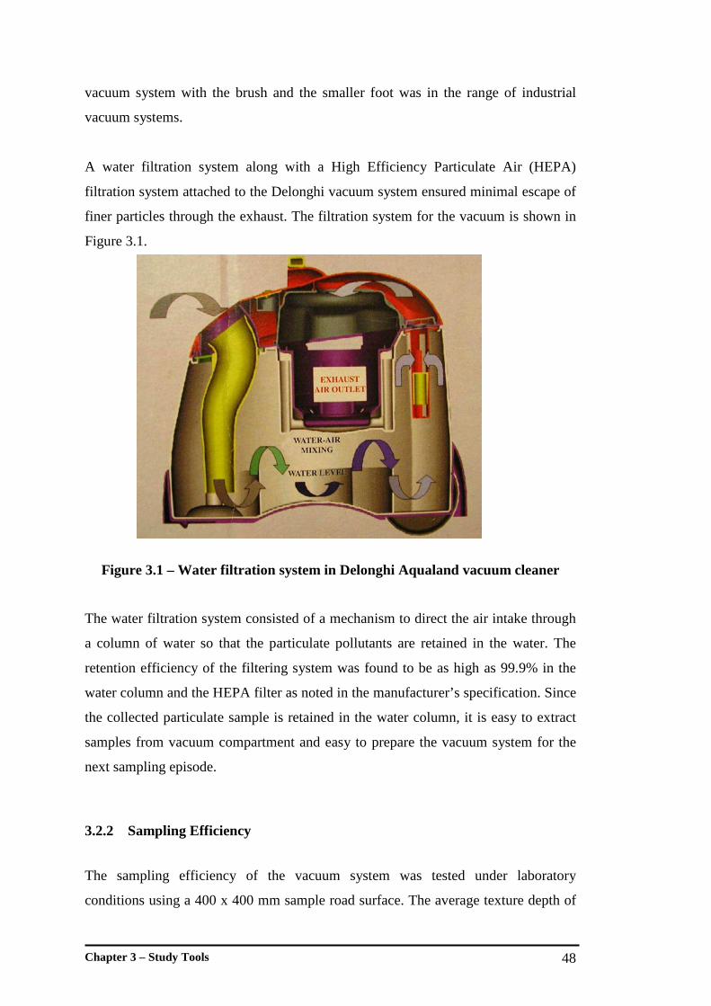
Chapter 3 – Study Tools 48
vacuum system with the brush and the smaller foot was in the range of industrial
vacuum systems.
A water filtration system along with a High Efficiency Particulate Air (HEPA)
filtration system attached to the Delonghi vacuum system ensured minimal escape of
finer particles through the exhaust. The filtration system for the vacuum is shown in
Figure 3.1.
Figure 3.1 – Water filtration system in Delonghi Aqualand vacuum cleaner
The water filtration system consisted of a mechanism to direct the air intake through
a column of water so that the particulate pollutants are retained in the water. The
retention efficiency of the filtering system was found to be as high as 99.9% in the
water column and the HEPA filter as noted in the manufacturer’s specification. Since
the collected particulate sample is retained in the water column, it is easy to extract
samples from vacuum compartment and easy to prepare the vacuum system for the
next sampling episode.
3.2.2 Sampling Efficiency
The sampling efficiency of the vacuum system was tested under laboratory
conditions using a 400 x 400 mm sample road surface. The average texture depth of
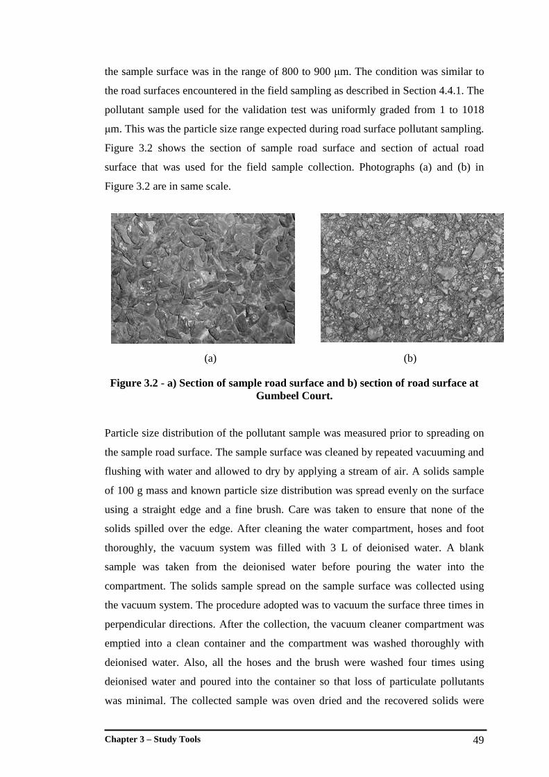
Chapter 3 – Study Tools 49
the sample surface was in the range of 800 to 900 µm. The condition was similar to
the road surfaces encountered in the field sampling as described in Section 4.4.1. The
pollutant sample used for the validation test was uniformly graded from 1 to 1018
µm. This was the particle size range expected during road surface pollutant sampling.
Figure 3.2 shows the section of sample road surface and section of actual road
surface that was used for the field sample collection. Photographs (a) and (b) in
Figure 3.2 are in same scale.
(a) (b)
Figure 3.2 - a) Section of sample road surface and b) section of road surface at Gumbeel Court.
Particle size distribution of the pollutant sample was measured prior to spreading on
the sample road surface. The sample surface was cleaned by repeated vacuuming and
flushing with water and allowed to dry by applying a stream of air. A solids sample
of 100 g mass and known particle size distribution was spread evenly on the surface
using a straight edge and a fine brush. Care was taken to ensure that none of the
solids spilled over the edge. After cleaning the water compartment, hoses and foot
thoroughly, the vacuum system was filled with 3 L of deionised water. A blank
sample was taken from the deionised water before pouring the water into the
compartment. The solids sample spread on the sample surface was collected using
the vacuum system. The procedure adopted was to vacuum the surface three times in
perpendicular directions. After the collection, the vacuum cleaner compartment was
emptied into a clean container and the compartment was washed thoroughly with
deionised water. Also, all the hoses and the brush were washed four times using
deionised water and poured into the container so that loss of particulate pollutants
was minimal. The collected sample was oven dried and the recovered solids were
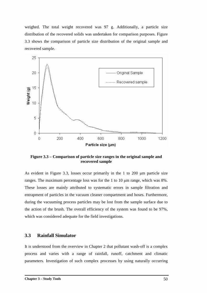
Chapter 3 – Study Tools 50
weighed. The total weight recovered was 97 g. Additionally, a particle size
distribution of the recovered solids was undertaken for comparison purposes. Figure
3.3 shows the comparison of particle size distribution of the original sample and
recovered sample.
Figure 3.3 – Comparison of particle size ranges in the original sample and recovered sample
As evident in Figure 3.3, losses occur primarily in the 1 to 200 µm particle size
ranges. The maximum percentage loss was for the 1 to 10 µm range, which was 8%.
These losses are mainly attributed to systematic errors in sample filtration and
entrapment of particles in the vacuum cleaner compartment and hoses. Furthermore,
during the vacuuming process particles may be lost from the sample surface due to
the action of the brush. The overall efficiency of the system was found to be 97%,
which was considered adequate for the field investigations.
3.3 Rainfall Simulator It is understood from the overview in Chapter 2 that pollutant wash-off is a complex
process and varies with a range of rainfall, runoff, catchment and climatic
parameters. Investigation of such complex processes by using naturally occurring

Chapter 3 – Study Tools 51
rainfall events faces inherent difficulties. This is primarily due to the aerial and
temporal variability of rainfall parameters such as rainfall intensity and kinetic
energy. Furthermore, lack of control over the rainfall parameters and uncertainty of
occurrence makes investigations difficult (Ahyerre et al., 1998; Herngren et al.,
2005b). In such a context, the use of artificially generated rainfall events in urban
water quality research is worthy of consideration. This eliminates a significant
number of constraints that arise due to the random nature and variability of
characteristics of naturally occurring rainfall events. Additionally, the use of rainfall
simulation can produce a large amount of data in a short period of time (Herngren et
al., 2005a; Herngren et al., 2005b).
A rainfall simulator has been designed and fabricated by the Queensland University
of Technology water quality research group so that it can be used in urban
stormwater quality research. Details on the design aspects of the rainfall simulator
can be found in Herngren et al. (2005b) and Herngren (2005).
The rainfall simulator consisted of an A-frame structure with three Veejet 80100
nozzles equally spaced on a swinging nozzle boom (see Figure 3.4). The nozzle
boom is connected to a small motor in order to swing in either direction. The speed
of the swing and delay time is controlled using an electronic control box which in
turn enables the simulator to be calibrated for different rainfall intensities. The water
used for the simulations needs to be specially prepared according to regional
rainwater quality and pumped to the simulator from an externally located tank. The
water pressure at the nozzle boom can be adjusted by a valve so that the simulator
creates the required drop size distribution.
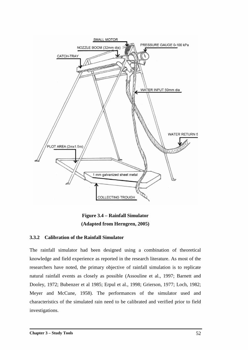
Chapter 3 – Study Tools 52
Figure 3.4 – Rainfall Simulator
(Adapted from Herngren, 2005)
3.3.2 Calibration of the Rainfall Simulator The rainfall simulator had been designed using a combination of theoretical
knowledge and field experience as reported in the research literature. As most of the
researchers have noted, the primary objective of rainfall simulation is to replicate
natural rainfall events as closely as possible (Assouline et al., 1997; Barnett and
Dooley, 1972; Bubenzer et al 1985; Erpul et al., 1998; Grierson, 1977; Loch, 1982;
Meyer and McCune, 1958). The performances of the simulator used and
characteristics of the simulated rain need to be calibrated and verified prior to field
investigations.

Chapter 3 – Study Tools 53
The rainfall simulator used for the field study had previously been calibrated for its
intensities and verified for kinetic energy and drop size distribution in 2003 for the
research published by Herngren (2005). The procedure he adopted was well
documented (Herngren et al., 2005b). However, due to the need to introduce a new
kinetic energy dissipater, the rainfall simulator had to be re-calibrated for this
research study. The kinetic energy dissipater was necessary to reduce the original
kinetic energy of the simulated rainfall to the required level to simulate rainfall
intensities less than 40 mm/hr. The kinetic energy increases with rainfall intensity up
to a threshold value and then remains constant (Rosewell, 1986). Additionally, re-
calibration also helped to adjust the control box settings in order to allow for wear
and tear of the mechanical components in the rainfall simulator.
3.3.3 Rainfall Intensity and Uniformity of Rainfall
Both rainfall intensity measurements and uniformity analysis of rainfall over the plot
area were carried out by placing an array of containers under the simulator in a grid
pattern and measuring the volume of water collected during a known simulated rain
duration. A similar procedure had been used by Herngren (2005) and Loch (1982) to
calibrate their rainfall simulators. In this instance fifteen containers were placed
under the rainfall simulator in three rows (as shown in Figure 3.5) and exposed to 5
min of rainfall simulation. The amount of water collected was measured using a
measuring cylinder and later converted to a depth of rain per unit time (mm/hr). The
experiment was repeated for different settings of the control box. The control box
consists of two control knobs: one to control the speed of oscillation and the other to
control the delay time. The speed control was demarcated 1 to 5. The delay control
was demarcated from A to M. The control box settings for the rainfall intensities
used in this research are shown in Table 3.1. The complete intensity calibration can
be found in Appendix A, Table A.1. The basis for the selected rainfall intensities is
discussed in Section 4.4.1. It was found that the rainfall simulator was capable of
simulating intensities ranging from 20 to 188 mm/hr.
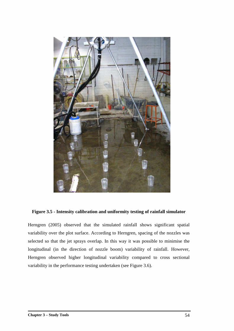
Chapter 3 – Study Tools 54
Figure 3.5 - Intensity calibration and uniformity testing of rainfall simulator
Herngren (2005) observed that the simulated rainfall shows significant spatial
variability over the plot surface. According to Herngren, spacing of the nozzles was
selected so that the jet sprays overlap. In this way it was possible to minimise the
longitudinal (in the direction of nozzle boom) variability of rainfall. However,
Herngren observed higher longitudinal variability compared to cross sectional
variability in the performance testing undertaken (see Figure 3.6).

Chapter 3 – Study Tools 55
Table 3.1 - Measured rainfall intensities for the different control box settings
Figure 3.6 – Spatial variation of the rainfall intensity for control box setting 3–I
(Adapted from Herngren, 2005)
It was not intended to investigate the characteristics of the spatial variability of
simulated rainfall in this research. A realistic measure of the spatial variability; ‘the
uniformity coefficient’ was calculated using the data collected during rainfall
intensity calibration. The same coefficient was used by Christiansen (1942) and
Herngren (2005) in order to describe the uniformity of the simulated rainfall. The
formulation of the uniformity coefficient is as follows:
100]1[ xmxn
XCu ∑−= Equation 3.1
Where,
Rainfall Intensity (mm/hr) Speed Setting Delay Setting
20 1 A
40 1 H
65 2 I
86 3 I
115 3 J
133 3 K

Chapter 3 – Study Tools 56
Cu = Coefficient of uniformity;
X = Deviation of individual observation from mean;
m = Mean value; and
n = Number of observations.
The uniformity coefficient is expressed as a percentage and higher percentages
indicate little spatial variability. The average uniformity coefficient for the complete
range of rainfall intensities tested for the current study was around 85%. This was in
close agreement with the results obtained by Herngren (2005) where the uniformity
coefficient was 80%. More details of the calculation of uniformity coefficient can be
found in Appendix A, Table A.1.
3.3.4 Drop Size Distribution and Kinetic Energy of Rainfall
In simulating rainfall close to natural events, it is important to verify the kinetic
energy and drop size distribution of the simulated rainfall. These two parameters,
along with rainfall intensity, are the primary parameters essential for characterising
rainfall events (Herngren et al., 2005b; Hudson, 1963; Loch, 1982). Considering an
individual raindrop, the kinetic energy is greatly influenced by the size of the drop.
This is due to the variation of both mass and terminal velocity associated with the
drop. However, as far as a rain event is concerned, kinetic energy is influenced by
rainfall intensity. Variation of kinetic energy can be simplified to a reducing rate of
increasing variation from 0 to around 25 J/m2/mm for rainfall intensities of 0 to 40
mm/hr. Beyond that, the kinetic energy is fairly constant at around 25 J/m2/mm
(Herngren et al., 2005b; Rosewell, 1986). The rainfall simulator was originally
designed to simulate kinetic energy in this constant region where rainfall intensities
are greater than 40 mm/hr. For this range, as recommended by Herngren et al.
(2005b), the pressure at the nozzle boom should be adjusted to 41 kPa. During
rainfall simulation, a change of rainfall intensity is achieved by varying the speed of
the nozzle boom movement. Since there is no change to simulator hydraulics, there is
expected to be the same kinetic energy for all the intensities. Therefore, the
verification test was only to check the appropriateness of the pressure at the nozzle
boom to simulate the required drop size and kinetic energy.
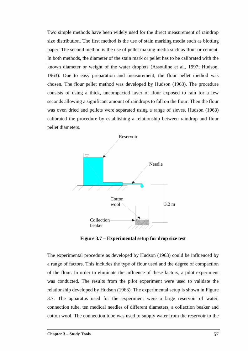
Chapter 3 – Study Tools 57
Two simple methods have been widely used for the direct measurement of raindrop
size distribution. The first method is the use of stain marking media such as blotting
paper. The second method is the use of pellet making media such as flour or cement.
In both methods, the diameter of the stain mark or pellet has to be calibrated with the
known diameter or weight of the water droplets (Assouline et al., 1997; Hudson,
1963). Due to easy preparation and measurement, the flour pellet method was
chosen. The flour pellet method was developed by Hudson (1963). The procedure
consists of using a thick, uncompacted layer of flour exposed to rain for a few
seconds allowing a significant amount of raindrops to fall on the flour. Then the flour
was oven dried and pellets were separated using a range of sieves. Hudson (1963)
calibrated the procedure by establishing a relationship between raindrop and flour
pellet diameters.
3.2 m
Needle
Reservoir
Cotton wool
Collection beaker
Figure 3.7 – Experimental setup for drop size test
The experimental procedure as developed by Hudson (1963) could be influenced by
a range of factors. This includes the type of flour used and the degree of compaction
of the flour. In order to eliminate the influence of these factors, a pilot experiment
was conducted. The results from the pilot experiment were used to validate the
relationship developed by Hudson (1963). The experimental setup is shown in Figure
3.7. The apparatus used for the experiment were a large reservoir of water,
connection tube, ten medical needles of different diameters, a collection beaker and
cotton wool. The connection tube was used to supply water from the reservoir to the
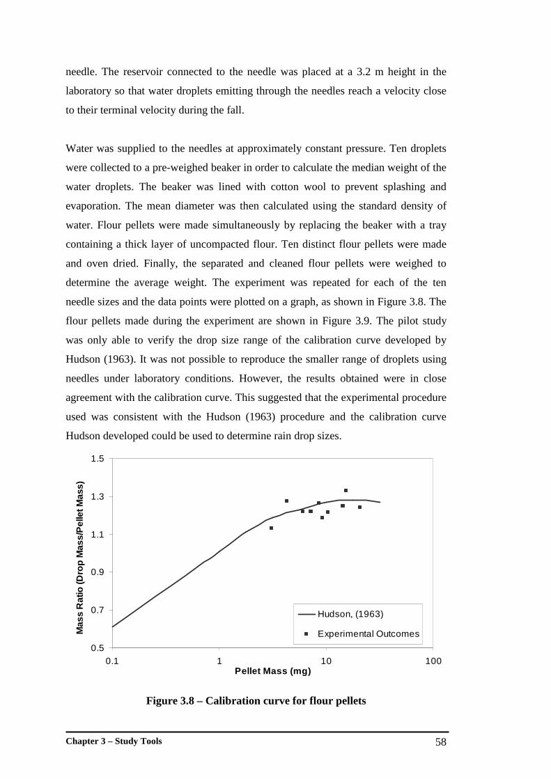
Chapter 3 – Study Tools 58
needle. The reservoir connected to the needle was placed at a 3.2 m height in the
laboratory so that water droplets emitting through the needles reach a velocity close
to their terminal velocity during the fall.
Water was supplied to the needles at approximately constant pressure. Ten droplets
were collected to a pre-weighed beaker in order to calculate the median weight of the
water droplets. The beaker was lined with cotton wool to prevent splashing and
evaporation. The mean diameter was then calculated using the standard density of
water. Flour pellets were made simultaneously by replacing the beaker with a tray
containing a thick layer of uncompacted flour. Ten distinct flour pellets were made
and oven dried. Finally, the separated and cleaned flour pellets were weighed to
determine the average weight. The experiment was repeated for each of the ten
needle sizes and the data points were plotted on a graph, as shown in Figure 3.8. The
flour pellets made during the experiment are shown in Figure 3.9. The pilot study
was only able to verify the drop size range of the calibration curve developed by
Hudson (1963). It was not possible to reproduce the smaller range of droplets using
needles under laboratory conditions. However, the results obtained were in close
agreement with the calibration curve. This suggested that the experimental procedure
used was consistent with the Hudson (1963) procedure and the calibration curve
Hudson developed could be used to determine rain drop sizes.
0.5
0.7
0.9
1.1
1.3
1.5
0.1 1 10 100Pellet Mass (mg)
Mas
s R
atio
(Dro
p M
ass/
Pel
let M
ass)
Hudson, (1963)
Experimental Outcomes
Figure 3.8 – Calibration curve for flour pellets
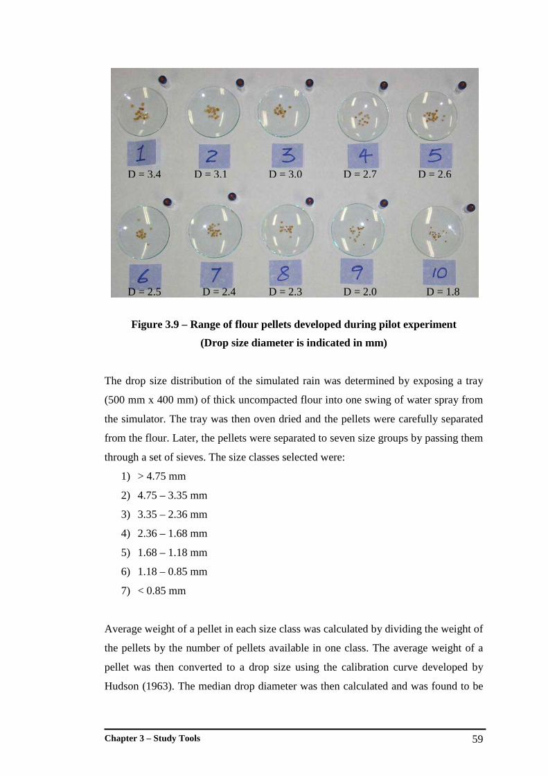
Chapter 3 – Study Tools 59
v
Figure 3.9 – Range of flour pellets developed during pilot experiment
(Drop size diameter is indicated in mm)
The drop size distribution of the simulated rain was determined by exposing a tray
(500 mm x 400 mm) of thick uncompacted flour into one swing of water spray from
the simulator. The tray was then oven dried and the pellets were carefully separated
from the flour. Later, the pellets were separated to seven size groups by passing them
through a set of sieves. The size classes selected were:
1) > 4.75 mm
2) 4.75 – 3.35 mm
3) 3.35 – 2.36 mm
4) 2.36 – 1.68 mm
5) 1.68 – 1.18 mm
6) 1.18 – 0.85 mm
7) < 0.85 mm
Average weight of a pellet in each size class was calculated by dividing the weight of
the pellets by the number of pellets available in one class. The average weight of a
pellet was then converted to a drop size using the calibration curve developed by
Hudson (1963). The median drop diameter was then calculated and was found to be
D = 3.4 D = 3.1 D = 3.0 D = 2.7 D = 2.6
D = 2.5 D = 2.4 D = 2.3 D = 2.0 D = 1.8
Chapter 3 – Study Tools 60
2.05 mm. The median drop size diameter for natural rainfall events is in the range of
2.0 to 2.5 mm (Hudson, 1963). The calculated median drop size was within the range
of the natural drop diameter and therefore the drop size distribution of the simulated
rainfall was considered to be satisfactory for the research study. A complete set of
calculations of drop size distribution is shown in Appendix A, Table A.2.
The terminal velocity for each drop size class was estimated using the tables
provided by Laws (1941). From the average drop size diameter and the
corresponding terminal velocity, the kinetic energy was calculated. It was ensured
that the raindrops produced by the rainfall simulator were reaching the terminal
velocity. As described in Herngren et al. (2005b), the simulator height of 2.5 m is
adequate to reach terminal velocity for any size of droplets with initial velocity
provided by 41 kPa of internal pressure in a Veejet 80100 nozzle. The calculated
kinetic energy was 21.3 J/m2/mm and was close to the natural rainfall kinetic energy
for South-East Queensland where the average as reported by Rosewell (1986), is
around 25 J/m2/mm. Further, Rosewell reported significant variability in rainfall
kinetic energy around the average value.
As explained in Section 4.4.1, it was important to simulate 20 mm/hr rainfall
intensity in order to encompass the rainfall intensity range in the study region. The
typical rainfall kinetic energy for 20 mm/hr intensity is in the range of 16 to 18
J/m2/mm (Rosewell, 1986). The simulator is only capable of simulating constant
rainfall kinetic energy of 21.3 J/m2/mm. Therefore, in order to simulate 20 mm/hr
rainfall intensity, the kinetic energy needed to be reduced. However, physical
changes to the simulator or changes to the hydraulic characteristics of the system
were not options that were considered. This was due to the possibility of degrading
fundamental simulator design concepts such as the longitudinal and cross sectional
rainfall uniformity. Therefore, it was decided to use a system external to the original
rainfall simulator setup in order to reduce the kinetic energy.
The best approach to reduce the kinetic energy was to reduce the average drop size of
the simulated rain. This in turn would help to reduce the mass and terminal velocity
of raindrops which would lead to kinetic energy reduction. The concept was to use a
meshed frame placed just below the nozzles in order to break the large droplets. Two
Chapter 3 – Study Tools 61
mesh materials, shade cloth and fly screen mesh, were tested for this purpose. The
use of fly screen mesh showed satisfactory results as the calculated kinetic energy
reduced to 16 J/m2/mm. Reduction in kinetic energy was mainly due to a reduction in
the drop sizes. The kinetic energy obtained was considered appropriate to simulate
20 mm/hr rainfall intensity. With the new setup, the rainfall simulator was re-
calibrated for 20 mm/hr intensity. The re-calibration confirmed that the original
control box setting for 20 mm/hr as stated in Table 3.1, was satisfactory. However,
the presence of the kinetic energy dissipater reduced the uniformity coefficient to
78%. This was mainly due to the change of direction of the water droplets after
coming into contact with the fly screen mesh. Nevertheless, the use of a fly screen
mesh as an energy dissipater was considered appropriate for the simulation of 20
mm/hr rainfall intensity.
3.4 Model Roofs
For residential catchments with relatively less traffic-generated pollutants on roads,
roof surfaces can be a significant contributor to urban stormwater pollution. This is
primarily due to the presence of a high fraction of impervious surfaces. Though it is
not conclusive, there is evidence to claim that the primary pollutant processes on roof
surfaces are significantly different from the rood surfaces. As noted by Van Metre
and Mahler (2003), build-up on roof surfaces primarily originates from atmospheric
sources which are significantly site specific. Furthermore, the amount of pollutants
and their characteristics were found to be significantly different from the road
surface pollutants. Forster (1996) noted a comparatively high concentration of
pollutants from roof surfaces during the initial period of runoff events. It was further
suspected that the ‘flashy’ contribution from roof surfaces leads to a first flush. This
suggested the possibility of differing wash-off characteristics in roof surfaces. These
factors highlighted the necessity for separate investigations into pollutant build-up
and wash-off on roof surfaces.
Due to the difficulty in coordinating and obtaining permission from residents and
local authorities, residential roofs in the study catchment were not considered.
Additionally, there were technical difficulties in using the rainfall simulator to

Chapter 3 – Study Tools 62
investigate pollutant wash-off on actual roofs. It was decided to fabricate two model
roof surfaces to support the research study.
3.4.1 Materials and Dimensions
The selection of roofing materials and dimensions of the model roofs were done so
that they were representative for the study region and appropriate to be used under
pre-established experimental methodology. As the test area for the rainfall simulator
was 1.5 x 2.0 m, it was a requirement to design roofs to the same dimensions.
Two roofing material types, namely corrugated steel and concrete tiles are
dominantly used within the study region as well as in South-East Queensland. The
design guidelines for these roofing materials have been published by numerous
manufacturers. The appropriate roofing angle is 15 to 300 (Bristile-Roofing, 2004;
Stramit-Manual, 2005). Two model roofs were designed at an angle of 200. The roof
surfaces were intended to be kept at a typical single storied roofing height. The
primary reason for this was to limit the human influence and to reduce the influence
of traffic-induced turbulence close to ground level. O'Hara et al. (2006) noted that a
2.5 m height is appropriate to minimise the influence of turbulence close to the
ground in atmospheric deposition sampling. Consequently, the maximum height of
the model roof surfaces was selected as 2.5 m.
3.4.2 Design and Performance Testing
A scissor lift arrangement was designed so that the roofs could be lifted to the 2.5m
height and when needed, could be lowered to ground level for sample collection. In
this way, the technical difficulties of rainfall simulations on roof surfaces were
overcome.
The scissor arrangement used to mount the roof surfaces consisted of a base frame of
2.1 m x 1.5 m, double scissor arrangement and a top frame. A hydraulic jack
powered by a 2.4 kW hydraulic pump was used to lift the arrangement. Figure 3.10
shows the scissor arrangement. The structural and mechanical design of the scissor
lift was done with reference to 2615, AS/NZS (1995) for hydraulic trolley jacks and
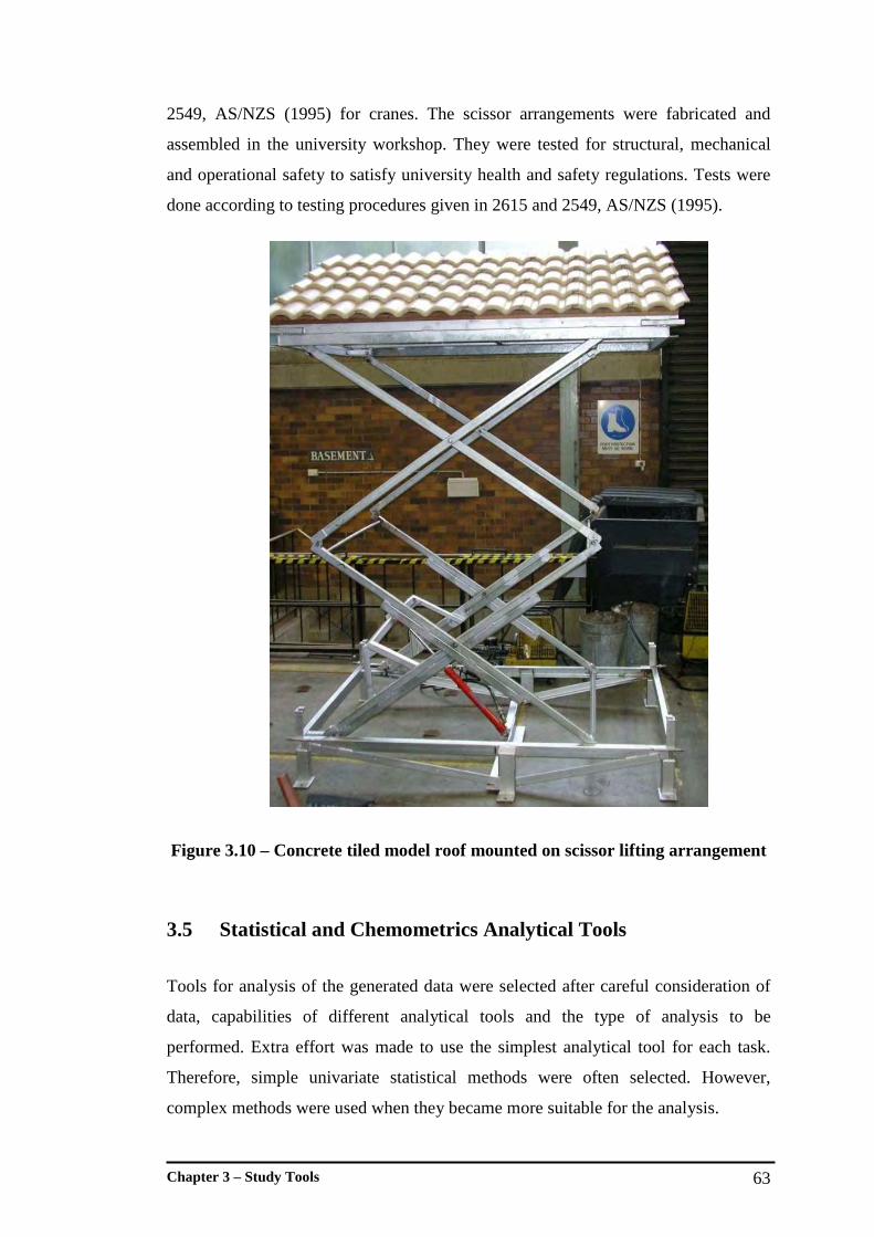
Chapter 3 – Study Tools 63
2549, AS/NZS (1995) for cranes. The scissor arrangements were fabricated and
assembled in the university workshop. They were tested for structural, mechanical
and operational safety to satisfy university health and safety regulations. Tests were
done according to testing procedures given in 2615 and 2549, AS/NZS (1995).
Figure 3.10 – Concrete tiled model roof mounted on scissor lifting arrangement
3.5 Statistical and Chemometrics Analytical Tools
Tools for analysis of the generated data were selected after careful consideration of
data, capabilities of different analytical tools and the type of analysis to be
performed. Extra effort was made to use the simplest analytical tool for each task.
Therefore, simple univariate statistical methods were often selected. However,
complex methods were used when they became more suitable for the analysis.
Chapter 3 – Study Tools 64
The purpose of using the analytical tools was primarily to understand the patterns of
data variability. This was done using plotted graphs supported by simple univariate
statistical measurements such as mean, standard deviation and coefficient of
variation. However, the presence of pollutant processes which have high variability
can limit the use of these simple methods. This problem was overcome by the use of
multivariate analytical approaches. In this regard, analytical suitability of several
multivariate approaches such as principal component analysis, cluster analysis and
discriminate analysis was considered. Ultimately, principal component analysis
(PCA) was selected due to its wide use in water quality research (Alberto et al.,
2001; Bengraine and Marhaba, 2003; Petersen et al., 2001).
3.5.1 Mean, Standard Deviation and Coefficient of Variation
Three statistical measurements: mean, standard deviation (SD) and coefficient of
variation (CV) are commonly used in order to describe the characteristics of a single
variable date set. The mean is primarily the most representative single value that can
be used to describe an entire data set. SD describes the spread or dispersion of data
points with respect to the mean. A smaller SD represents a concentrated data set
whereas a larger SD represents a spread data set (Hamburg, 1994).
SD is also useful in describing how far an individual data point departs from the
mean of the data set. This is primarily done by calculating the ‘standard score’, by
dividing the deviation of the individual data point from the mean by the SD.
However, from an analytical point of view, a measure to describe dispersion of an
entire data set from the mean is the most important. Such a measure is obtained by
expressing standard deviation as a percentage of the mean, which is termed the
coefficient of variation (CV). A data set with CV less than 10% is considered
uniform (Hamburg, 1994).
3.5.2 Method of Least Square
Development of mathematical predictive equations for the observed variations of
pollutant processes is one of the major components of this research. These
Chapter 3 – Study Tools 65
mathematical equations needed to be the ‘best fit’ for the observed data. In this
regard, it was important to establish criteria to define goodness of fit. Among many
methods, the method of least squares was selected as the most appropriate. As noted
by Hamburg (1994) this is the most commonly applied curve fitting technique. The
method of least squares imposes the requirement that the sum of the squares of the
deviations of observed values from the corresponding computed values must be the
minimum. The method can be expressed in mathematical terms as:
∑ − 2....)),(( yxPO is the minimum Equation 3.2
Where,
O = Observed value;
P = Predicted value; and
x, y… = Coefficients influencing predicted value.
Minimisation of the square of deviations is typically done by adjusting coefficients
on a systematic basis. Algorithms for such adjustment of coefficients are embedded
into most analytical software. The algorithm used for this research was the ‘Solver’
in Microsoft XL. The final outcome of the method of least squares is an optimum set
of coefficient values.
3.5.3 Principal Component Analysis
Principal Component Analysis, or PCA, is essentially a pattern recognition technique
which can be used to understand the correlations among different variables and
clusters among objects. It has been used extensively as an analytical tool in water
quality research. For example, Bengraine and Marhaba (2003) used PCA to obtain
the temporal and spatial variation in river water quality and Petersen et al. (2001)
used it to understand the water quality processes in rivers. Regardless of the
widespread use, as noted by Kokot et al. (1998), PCA is more an exploratory tool
rather than one which can be used to obtain the final solution in pattern recognition.
The PCA technique is used to transform the original variables to a new orthogonal
set of Principal Components (PCs) such that the first PC contains most of the data
variance and the second PC contains the second largest variance and so on. The

Chapter 3 – Study Tools 66
orthogonality of PCs enables user to interpret the data variance associated to each of
PCs independently. Furthermore, though PCA produces the same amount of PCs as
the original variables, the first few contain most of the variance. Therefore, the first
few PCs are often selected for interpretation. This consequently reduces the number
of variables without losing useful information in the original data set. The number of
PCs to be used for interpretation is typically selected using the Scree plot method
(Jackson, 1993). The Scree plot is the graphical variation of Eigen values extracted
for each PC. Eigen value interprets the data variation associated with each PC
(Adams, 1995). Detailed descriptions of PCA can be found elsewhere (Adams, 1995;
Kokot et al., 1998).
To perform PCA, the data should be arranged in a matrix with selected variables
arranged in columns and individual measurements or objects arranged in rows.
Standard pre-treatment techniques are often used to eliminate the biased outcomes
due to measurements being in different scales and units. Column standardisation is
the most common pre-treatment method used (Kokot et al., 1991, 1992). This implies
that each cell in a given column is divided by the standard deviation of that particular
column. Hence, each variable is equally weighted with a standard deviation of one.
The application of PCA to a data matrix generates a loading for each variable and a
score for each object on the principal components. Consequently, the data can be
presented diagrammatically by plotting the loading of each variable in the form of a
vector and the score of each object in the form of a data point. This type of plot is
referred to as a ‘Biplot’. The angle between variable vectors is the indicator of degree
of correlation. An acute angle between two variables indicates a strong correlation
whereas an obtuse angle indicates a negative correlation. A right angle between
variables indicates no correlation. Clustered data points in a biplot indicate objects
with similar characteristics.
3.6 Hydrologic Modelling Software
Hydrologic modelling is often used as a support tool in water quality modelling. As
noted by Zoppou (2001), hydrologic modelling tools supply the essential runoff

Chapter 3 – Study Tools 67
information to the water quality modelling tools in order to calculate pollutant
concentrations and hence facilitate estimating pollutant transport to catchment
outlets. For example, water quality model XP-AQUALM operates with a hydrologic
model based on daily water balance.
In this study, calculation of pollutant response at the catchment outlets was to be
determined using a similar procedure to that used in water quality models. This gave
rise to the need for an accurate and reliable hydrologic modelling tool. As noted by
Zoppou (2001), the selected hydrologic model needs to be highly compatible with
the procedure adopted to calculate pollutant mobilisation. Additionally, ASCE
(1985) lists a range of criteria in order to select a suitable hydrologic model.
Considering all these facts, the following selection criteria were used to choose the
hydrologic model:
1) Formulation of the model – The model needed to be based on the time-area
method which is a scientifically based hydrologic analytical procedure
(O'Loughlin and Stack, 2004). This was to ensure the compatibility of the
hydrologic model to pollutant mobilisation calculations.
2) Output – Due to the relatively faster hydrologic and water quality response from
small urban catchments, the ability to simulate fine times steps (1 min) was
important.
3) Data availability – The accuracy and reliability of a model is based on the correct
interpretation of catchment parameters and inputs. This suggested that model
setup and input parameters should be based on an appropriate set of data. Since
different models have different data requirements, the selection of the model
should be in accordance with the available data.
4) Processes – The simulation of hydrologic and hydraulic processes using
scientifically valid procedures is important. The requirement for the time-area
method in hydrologic modelling has already been noted above. Additionally, it
was also a requirement to have a scientifically valid pipe flow routing procedure
to calculate the flow through the urban drainage network.
5) Parameters – Models with different mathematical formulations operate with
different sets of parameters for representing catchment and input conditions. For
successful modelling, these parameters should be able to be derived from the
already available measured data or by calibration processes.

Chapter 3 – Study Tools 68
6) User-friendliness – It was important to select a model that can be easily setup,
calibrated and simulated.
7) Acceptance – It was important to select a model that is widely used and accepted
among the research community.
A number of models which are extensively used in Australia were evaluated against
the selection criteria. The models evaluated were:
• WBNM (Boyd et al., 2003);
• DRAINS (O'Loughlin and Stack, 2004); and
• Mike STORM (Mike STORM, 2004).
Table 3.2 shows the comparison of the models against each selection criteria.

Chapter 3 – Study Tools 69
Table 3.2 – Comparison of model characteristics against selection criteria
Criteria WBNM DRAINS Mike STORM
Hydrologic
representation
Storage routing
method
Time area
method
Three different
methods
including time
area method
Simulation
frequency
Fine time steps
(1 min)
Fine time steps
(1 min)
Fine time steps
(1 min)
Data requirement Can be obtained
by simple
procedures
Can be obtained
by simple
procedures
Can be obtained
by simple
procedures
Pipe and channel
flow routing
Channels are
considered as a
function of
catchment area.
Channel lag
factor is used
Manning’s
equation
Three different
procedures
including
dynamic wave
routing
Nature of parameters Parameters
should be
obtained by
calibration
Parameters
should be
obtained by
experience
Parameters
should be
obtained by
calibration
User-friendliness Easy to setup and
simulate
Easy to setup and
simulate
Easy to setup and
simulate
Acceptance Accepted for both
design and
investigation
Mostly accepted
for design
purposes
Accepted for both
design and
investigation
In consideration of all the above factors, the Mike STORM model was the most
suitable. Mike STORM can simulate a range of hydrologic procedures including the
time-area method. The number of parameters required to setup and simulate Mike
STORM is comparatively small and the parameters are easily obtainable from the
measured data. Furthermore, the pipe flow routing procedure available in the model
is appropriate for the purpose. The model is user-friendly and well recognised among

Chapter 3 – Study Tools 70
the research community. In addition to all the primary features, Mike STORM
consists of an advection – dispersion simulation procedure which can be directly
used to calculate pollutant transport.
3.7 Conclusions
The primary research apparatus used during this research were:
1) Vacuum collection system;
2) Rainfall simulator; and
3) Model roof surfaces.
The vacuum collection system was designed to collect particulate matter from road
surfaces. The system was pre-tested for collection and retention efficiency and was
found to be satisfactory. The rainfall simulator was calibrated to simulate six
different rainfall intensities. A kinetic energy breaker was included in the system so
that smaller rainfall intensities could also be simulated. Performance of the rainfall
simulator was evaluated in terms of drop size distribution and kinetic energy. It was
found that the simulated rainfall is a close replication of natural rainfall. In order to
eliminate the technical difficulties of collecting build-up and wash-off samples from
roof surfaces, two sets of model roofs were developed. These model roofs consisted
of scissor arrangements where the roof can be lifted to the conventional roofing
height for pollutant build-up and lowered to the ground level for build-up and wash-
off sampling.
The analytical tools were selected so that they were best suited for the purpose of the
analysis to be undertaken. The tools were selected on a case by case basis and extra
effort was made to select the simplest tool. PCA was selected to perform analysis
when multiple variables are involved. After evaluation of a number of commonly
used models, Mike STORM was selected according to pre-established selection
criteria. This was to support the pollutant transport calculations.
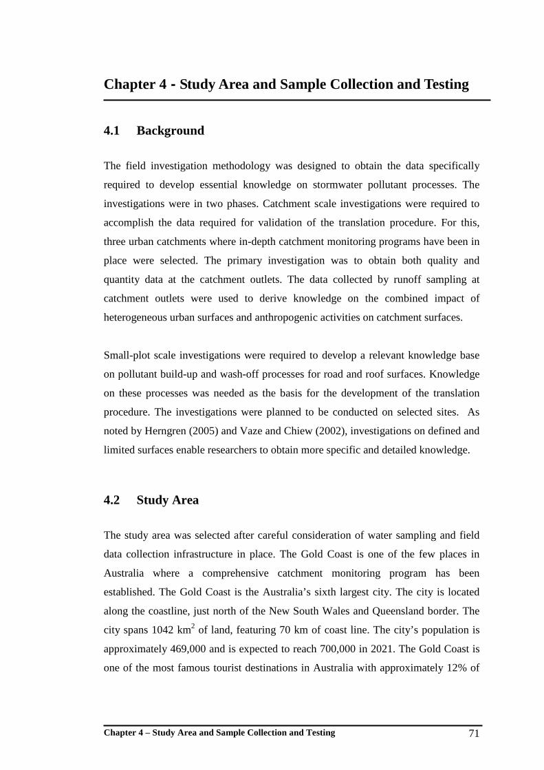
Chapter 4 – Study Area and Sample Collection and Testing 71
Chapter 4 - Study Area and Sample Collection and Testing
4.1 Background
The field investigation methodology was designed to obtain the data specifically
required to develop essential knowledge on stormwater pollutant processes. The
investigations were in two phases. Catchment scale investigations were required to
accomplish the data required for validation of the translation procedure. For this,
three urban catchments where in-depth catchment monitoring programs have been in
place were selected. The primary investigation was to obtain both quality and
quantity data at the catchment outlets. The data collected by runoff sampling at
catchment outlets were used to derive knowledge on the combined impact of
heterogeneous urban surfaces and anthropogenic activities on catchment surfaces.
Small-plot scale investigations were required to develop a relevant knowledge base
on pollutant build-up and wash-off processes for road and roof surfaces. Knowledge
on these processes was needed as the basis for the development of the translation
procedure. The investigations were planned to be conducted on selected sites. As
noted by Herngren (2005) and Vaze and Chiew (2002), investigations on defined and
limited surfaces enable researchers to obtain more specific and detailed knowledge.
4.2 Study Area
The study area was selected after careful consideration of water sampling and field
data collection infrastructure in place. The Gold Coast is one of the few places in
Australia where a comprehensive catchment monitoring program has been
established. The Gold Coast is the Australia’s sixth largest city. The city is located
along the coastline, just north of the New South Wales and Queensland border. The
city spans 1042 km2 of land, featuring 70 km of coast line. The city’s population is
approximately 469,000 and is expected to reach 700,000 in 2021. The Gold Coast is
one of the most famous tourist destinations in Australia with approximately 12% of

Chapter 4 – Study Area and Sample Collection and Testing 72
the population being visitors. The beaches and waterways in particular are the most
important tourist attractions (GCCC-Web, 2006).
The Gold Coast has a subtropical climate with moderate temperatures and summer
dominant precipitation. The summer average temperature ranges from 190 to 290C
and winter temperatures range from 160 to 210C. The city’s stormwater drainage
system features many natural and artificial waterways. These waterways include five
major rivers and numerous creeks, many of which connect to artificial lakes and
canals. The city’s major drainage basins are shown in Figure 4.1. These waterways
flow from the surrounding westward hilly area towards the Pacific Ocean coastline.
Natural vegetation occupies a significant fraction of the regional land particularly
west of the city. High density urban areas are located close to the coastline. Most of
the residential settlements have been developed adjacent to the City’s integrated
waterways promoting luxurious waterside living. However, this extensive urban
development alongside waterways influences key environmental values of the
waterway ecology (GCCC-Web, 2006).

Chapter 4 – Study Area and Sample Collection and Testing 73
Figure 4.1 - Waterways of Gold Coast city
(Adapted from GCCC-Web, 2006)

Chapter 4 – Study Area and Sample Collection and Testing 74
4.3 Catchment Scale Investigation
Among the many catchments monitored by Gold Coast City Council (GCCC), three
small catchments within the Highland Park residential area were selected for further
investigations. This was primarily due to their residential land-use. Highland Park is
within the boundary of the Nerang River catchment. A small tributary, Bunyip Brook is
the study catchment’s primary stormwater drainage. It starts from the westward hilly
area and flows towards the Nerang River. The integrated pipe and channel network
connecting various parts of the area to the tributary further facilitates the stormwater
drainage. Highland Park is totally sewered and consists of several forms of urban
residential developments. The three small catchments were selected to account for these
residential forms (see Figure 4.2). The residential urban forms of these three catchments
are:
1. Alextown, which is a tenement townhouse development of around 60 properties;
2. Gumbeel, which is a duplex housing development with around 20 dual
occupancy residences; and
3. Birdlife Park, which is a high socio-economic area with single detached houses.
4.3.1 Catchment Characteristics
Most of the catchment details were provided by GCCC in the form of maps. These
included:
• Contour map with 5 m height intervals;
• Land use maps;
• Detailed drainage network including creek, pipes, channels and locations of
gully pits (manholes); and
• Aerial photographs.
The provided maps can be found in Appendix B, Figure B.1 to B.4.

Chapter 4 – Study Area and Sample Collection and Testing 75
Figure 4.2 – Highland Park residential area, demarcation of three catchments and locations of the gauging instruments
Alextown
Gumbeel
Birdlife Park
LegendDepth Gauge and water sampling equipment
Rainfall gauge
Bunyip Brook

Chapter 4 – Study Area and Sample Collection and Testing 76
These maps were used to obtain the primary parameters of the study areas. The
parameters obtained included: catchment areas, impervious fractions for various
surface cover types, locations and sizes of pipes and stormwater gullies and the
catchment and drainage line slopes. The parameter values obtained for the catchment
areas and impervious surface fractions are shown in Table 4.1. These parameters
were used in various stages of the research and in particular in the catchment
modelling.
Table 4.1– Characteristics of Alextown, Gumbeel and Birdlife Park catchments
Catchment Area (ha) Impervious Fraction (%)
Alextown 1.9 Road surfaces – 10.5
Roof surfaces – 38.1
Driveways – 8.6
Gumbeel 2.1 Road surfaces – 10.3
Roof surfaces – 19.2
Driveways – 11.2
Birdlife Park 8.6 Road surfaces - 12.4
Roof surfaces - 23.4
Driveways – 11.2
Simple techniques were used to obtain most of the catchment parameters.
Information from contour maps and drainage network maps was used to demarcate
catchment boundaries. Catchment area was measured based on these boundaries
using functions in MapInfo GIS software (MapInfo, 2006). The impervious fraction
of each subcatchment was determined from aerial photographs. By visual inspection
of aerial photographs, it was possible to demarcate different surface covers such as
roads, roofs and driveways. Such demarcations were done for the entire area of each
catchment. These areas were measured separately as catchment area measurement. A
similar technique was used by Charlesworth (2000) to identify the fraction
imperviousness for water quality modelling. Boyd and Milevski (1996) suggested
that the use of aerial photographs is one of the preferred methods to calculate fraction
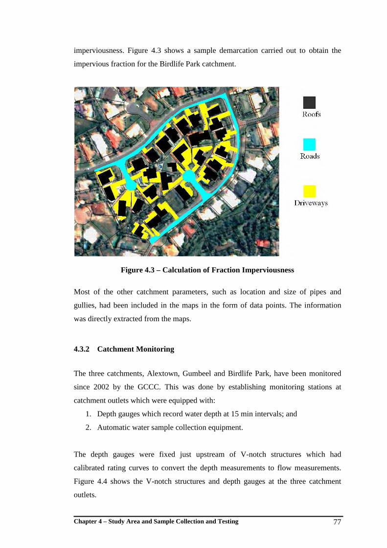
Chapter 4 – Study Area and Sample Collection and Testing 77
imperviousness. Figure 4.3 shows a sample demarcation carried out to obtain the
impervious fraction for the Birdlife Park catchment.
Figure 4.3 – Calculation of Fraction Imperviousness
Most of the other catchment parameters, such as location and size of pipes and
gullies, had been included in the maps in the form of data points. The information
was directly extracted from the maps.
4.3.2 Catchment Monitoring
The three catchments, Alextown, Gumbeel and Birdlife Park, have been monitored
since 2002 by the GCCC. This was done by establishing monitoring stations at
catchment outlets which were equipped with:
1. Depth gauges which record water depth at 15 min intervals; and
2. Automatic water sample collection equipment.
The depth gauges were fixed just upstream of V-notch structures which had
calibrated rating curves to convert the depth measurements to flow measurements.
Figure 4.4 shows the V-notch structures and depth gauges at the three catchment
outlets.
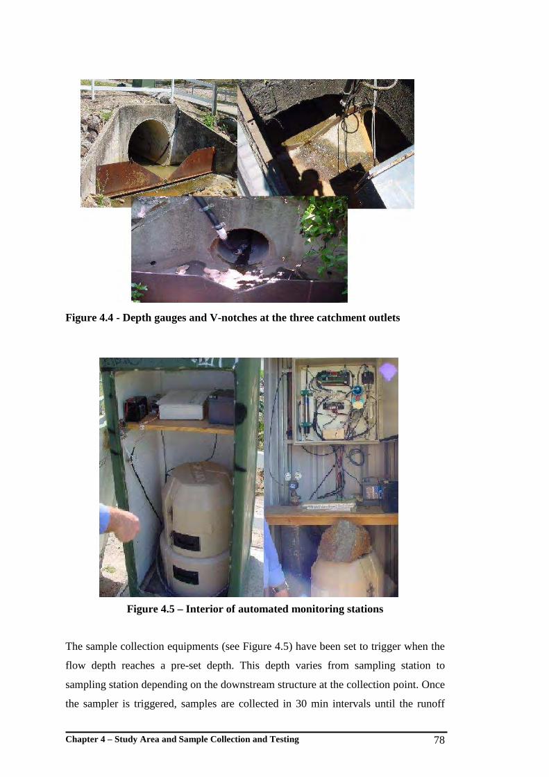
Chapter 4 – Study Area and Sample Collection and Testing 78
Figure 4.4 - Depth gauges and V-notches at the three catchment outlets
Figure 4.5 – Interior of automated monitoring stations
The sample collection equipments (see Figure 4.5) have been set to trigger when the
flow depth reaches a pre-set depth. This depth varies from sampling station to
sampling station depending on the downstream structure at the collection point. Once
the sampler is triggered, samples are collected in 30 min intervals until the runoff
Chapter 4 – Study Area and Sample Collection and Testing 79
depth is above the datum. Each sampler has the capacity to retain 24 samples. The
sampler itself creates a log of the sampling time. More details on the protocol
followed during sample transportation and storage can be found in Section 4.5.
4.4 Small-plot Scale Investigations
As stated in Section 2.3.2, a high fraction of stormwater pollutants originates from
urban impervious surfaces. In particular, road surfaces are the most critical. House et
al.(1993) and Novotny et al.(1985) noted that pollutant impacts associated with road
surface runoff can be significantly higher than secondary treated domestic sewage
effluent. As they further noted, the higher pollutant load from road surfaces often
overshadows the contribution from other sources. However, in general roof surfaces
can represent the highest impervious fraction particularly for residential catchments.
Therefore, the pollutant contribution from roofs could also be significant
(Bannerman et al., 1993). As such, investigations into small-plot pollutant processes
were conducted on both road and roof surfaces.
4.4.1 Road Surface Investigation
A Study Sites
All the small-plot investigations on road surfaces were conducted within the
Highland Park area. This was to obtain representative measurements for the study
catchment. Most of the roads within the catchment are access roads which are
primarily used by local traffic. The roads are in fair to good condition. Except for the
most upstream portion of the catchment where construction activities are ongoing,
most of the pervious areas are well turfed and maintained.
Highland Park is predominantly a residential area. However, there are differences in
residential urban form in different parts. In order to encompass such variability,
study sites were selected within each of the urban forms. However, due to restricted
access into Alextown, the townhouse area, no sites were selected within this

Chapter 4 – Study Area and Sample Collection and Testing 80
catchment. The access roads selected for the study were Lauder Court, Gumbeel
Court and Piccadilly Place (see Figure 4.6).
The exact study locations on these three roads were selected after consideration of
longitudinal slope and alignment, traffic conditions, traffic safety and space for
investigations. A straight road section of about 50 m length with mild slope was
selected for the investigations. Wide road sections were selected so that local traffic
flow was not affected. Furthermore, it was decided to select sites with different
traffic volumes. In this regard, the traffic volume was assumed to be proportional to
the number of surrounding households.
Figure 4.6 – Locations of the study sites within Highland Park catchment
Primary characteristics of the road surfaces were obtained prior to the investigations.
These characteristics included surrounding urban form, number of surrounding
households, longitudinal slope of the road and texture depth of the road surface.
Table 4.2 shows the summary of these characteristics. The texture depth was
measured using the sand patch test as explained in Test Method No E 965 (ASTM,
Gumbeel Court Piccadilly Place
Lauder Court
Highland Park Catchment

Chapter 4 – Study Area and Sample Collection and Testing 81
2006). The procedure was to spread a measured quantity of glass beads in a circular
patch on the cleaned road surface and measure the final diameter. An empirical
equation is available to relate the diameter of the patch to the texture depth of the
surface. The texture depth is considered to be more descriptive in describing the road
surface condition in relation to pollutant build-up and wash-off.
Table 4.2 – Characteristics of road sites
Site Residential urban-form Slope of the road
(%)
Texture depth of the
surface (mm)
Number of households
Lauder Court
Single detached housing area 10 0.66 12
Gumbeel Court
Duplex housing area 7.2 0.92 25
Piccadilly Place
Single detached housing 10.8 0.83 41
Investigations were conducted on one side of the road so that traffic was not
disrupted. The small-plot surfaces for the investigations were selected in the middle
of one traffic lane along the road. There was an implicit assumption that the pollutant
distribution on the road surface was uniform. As noted by Sartor et al. (1974) road
surface pollutants are concentrated in the near kerb area and concentration gradually
reduces towards the centre line of the road. As they have hypothesised, this is caused
by re-distribution of pollutants due to vehicle-induced wind turbulence. Therefore,
selection of the middle strip of one traffic lane for investigation provided an average
concentration of pollutants across the road section.
B Sampling Pollutant Build-up
As stated in Section 2.3.3, pollutant build-up is a dynamic process which varies with
a range of parameters. These parameters include land-use, traffic volume, road
surface characteristics and antecedent dry period. Since the study focused only on
residential catchments, land-use variability was not considered. However, the three
sites selected had slightly different residential urban form. Traffic volumes were
relatively uniform for the catchment. However, a minor variation of traffic was
incorporated by selecting sites with different numbers of surrounding households.
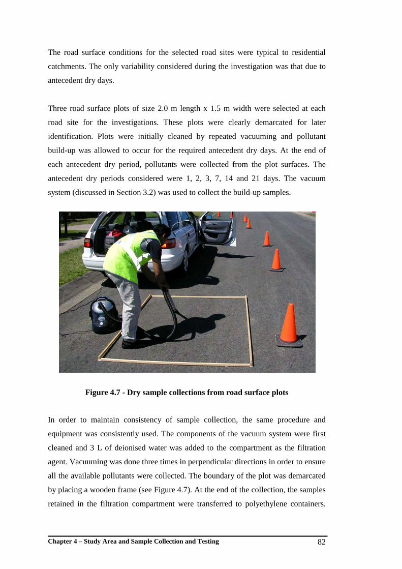
Chapter 4 – Study Area and Sample Collection and Testing 82
The road surface conditions for the selected road sites were typical to residential
catchments. The only variability considered during the investigation was that due to
antecedent dry days.
Three road surface plots of size 2.0 m length x 1.5 m width were selected at each
road site for the investigations. These plots were clearly demarcated for later
identification. Plots were initially cleaned by repeated vacuuming and pollutant
build-up was allowed to occur for the required antecedent dry days. At the end of
each antecedent dry period, pollutants were collected from the plot surfaces. The
antecedent dry periods considered were 1, 2, 3, 7, 14 and 21 days. The vacuum
system (discussed in Section 3.2) was used to collect the build-up samples.
Figure 4.7 - Dry sample collections from road surface plots
In order to maintain consistency of sample collection, the same procedure and
equipment was consistently used. The components of the vacuum system were first
cleaned and 3 L of deionised water was added to the compartment as the filtration
agent. Vacuuming was done three times in perpendicular directions in order to ensure
all the available pollutants were collected. The boundary of the plot was demarcated
by placing a wooden frame (see Figure 4.7). At the end of the collection, the samples
retained in the filtration compartment were transferred to polyethylene containers.

Chapter 4 – Study Area and Sample Collection and Testing 83
The vacuum compartment and all the hoses were thoroughly washed and the water
was added to the container. Sample containers were pre-washed according to
Standard Methods (APHA 1999). The protocol followed in the sample transport and
storage is discussed in Section 4.5.
For uninterrupted investigation, a long dry period was needed. However, there were a
few rain events which affected the continuation of the dry periods. After such
interruptions, the plot surface was cleaned and sampling was undertaken after the
requisite antecedent dry period.
C Sampling Pollutant Wash-off
Pollutant wash-off on a surface is a process which is influenced by a range of
parameters. These parameters include rainfall intensity, duration and road surface
condition. Since the variability of road surface condition is accounted for by
selecting multiple sites, the primary variables considered during the investigations
were rainfall intensity and duration. These were replicated using the rainfall
simulator. Further details on the rainfall simulator are available in Section 3.3.
Wash-off investigations were conducted in the same sites where the build-up
investigations were conducted. However, the other side of the road was used in order
to reduce the influence of wash-off on build-up investigations. Altogether, seven plot
surfaces were selected at each site using the same procedure as described for build-
up sampling. This was to simulate six rainfall intensities and to collect a sample of
the initially available pollutants. The space between plots was such that the
simulation of rain in one plot would not influence the adjacent plots.
It has been noted that wash-off from road surfaces is influenced by the initially
available pollutants on the surface (Duncan, 1995). Hence, it was decided to collect a
representative build-up sample from each road site prior to wash-off investigations. It
was assumed that the pollutant distribution is uniform throughout the road section.
Six rainfall intensities were selected so that they encompassed the common range of
regional rainfall events. This range was determined by undertaking a statistical

Chapter 4 – Study Area and Sample Collection and Testing 84
analysis of rainfall intensities over a five year period from 1999 to 2003. The rainfall
data used for the analysis was obtained from the rain gauge established within the
study catchment, as shown in Figure 4.2. Data obtained was compared with the data
from adjacent rain gauges obtained from Department of Meteorology to verify the
accuracy. For the analysis, the maximum 5 min rainfall intensity from every
significant rain event was extracted. For the analysis, the maximum 5 min rainfall
intensity from every significant rain event was extracted. The extracted intensities
ranged from 5 mm/hr to 150 mm/hr. The analysis revealed that rainfall intensities
were in the range of 15 to 140 mm/hr for more than 99% of the total number of
events. However, the selected six intensities were in the range of 20 to 133 mm/hr. It
was not possible to expand the selected intensity range further due to technical
difficulties in simulating rainfall using the rainfall simulator. Nevertheless, it was
noted that the selected intensity range represents more than 90% of the regional
rainfall events. The rainfall durations were selected based on results published by
Herngren (2005). He observed that there was no significant wash-off of pollutants
beyond a threshold rainfall duration. The selected rainfall intensities and durations
used are given in Table 4.3.
Table 4.3 – Rainfall intensities and durations simulated during the study
A plastic frame with dimensions 1.5 m x 2.0 m was used to demarcate the plot area
during wash-off investigations. This was to prevent water entering or leaving the
demarcated plot so that the total runoff could be collected. A rubber flap was
Rainfall Duration (min) Rainfall Intensity (mm/hr)
Event 1 Event 2 Event 3 Event 4
20 10 20 30 40
40 10 15 25 35
65 10 15 20 30
86 10 15 20 25
115 5 10 15 20
133 5 10 15 20

Chapter 4 – Study Area and Sample Collection and Testing 85
attached to the plastic frame and the inward side of the rubber flap was fixed to the
road surface using waterproof tape. This further ensured watertightness around the
plastic frame. One end of the plastic frame was kept open to fix the catch tray used
for runoff collection. More details of the rainfall simulator can be found in Section
3.3. Figure 4.8 shows the arrangements for plot area demarcation and runoff
collection. Figure 4.9 shows the rainfall simulator set up in the field.
Figure 4.8 – Plot Surfaces Boundary and sealing method
Figure 4.9 – Rainfall simulator setup at Gumbeel Ct.
Gutter tape
Catch tray
Plot boundary
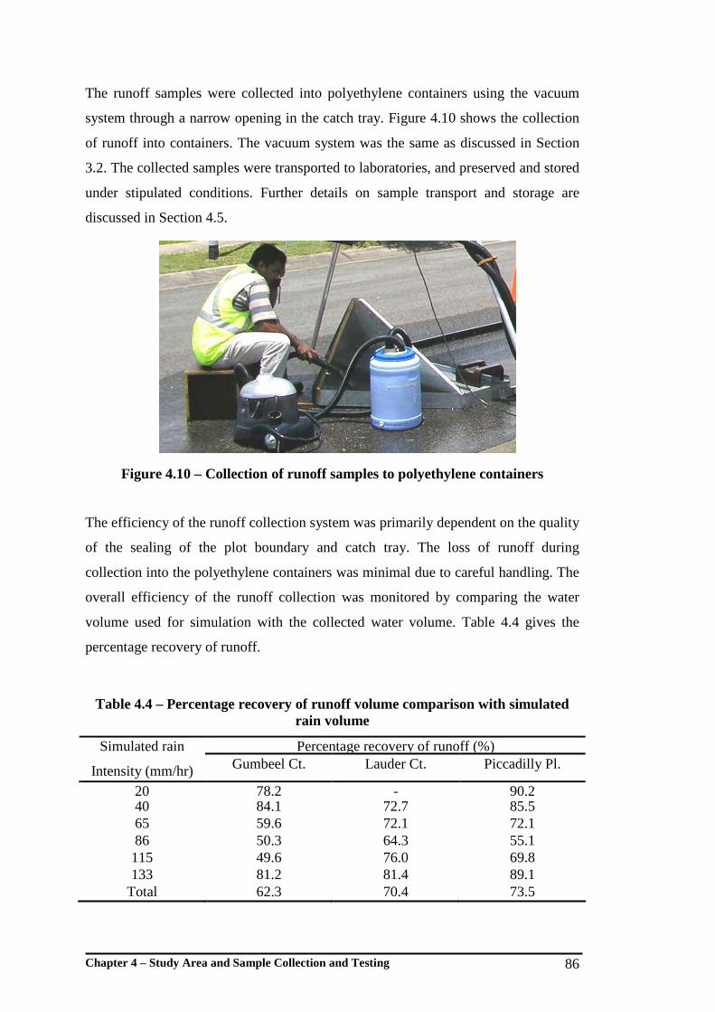
Chapter 4 – Study Area and Sample Collection and Testing 86
The runoff samples were collected into polyethylene containers using the vacuum
system through a narrow opening in the catch tray. Figure 4.10 shows the collection
of runoff into containers. The vacuum system was the same as discussed in Section
3.2. The collected samples were transported to laboratories, and preserved and stored
under stipulated conditions. Further details on sample transport and storage are
discussed in Section 4.5.
Figure 4.10 – Collection of runoff samples to polyethylene containers
The efficiency of the runoff collection system was primarily dependent on the quality
of the sealing of the plot boundary and catch tray. The loss of runoff during
collection into the polyethylene containers was minimal due to careful handling. The
overall efficiency of the runoff collection was monitored by comparing the water
volume used for simulation with the collected water volume. Table 4.4 gives the
percentage recovery of runoff.
Table 4.4 – Percentage recovery of runoff volume comparison with simulated rain volume
Percentage recovery of runoff (%) Simulated rain
Intensity (mm/hr) Gumbeel Ct. Lauder Ct. Piccadilly Pl.
20 78.2 - 90.2 40 84.1 72.7 85.5 65 59.6 72.1 72.1 86 50.3 64.3 55.1 115 49.6 76.0 69.8 133 81.2 81.4 89.1
Total 62.3 70.4 73.5

Chapter 4 – Study Area and Sample Collection and Testing 87
As seen in Table 4.4, the runoff volume can be appreciably less compared to the
simulated rain volume. This could be due to factors such as initial and continuing
losses on road surfaces. During simulations, it took one to three min for runoff to
reach the catch tray, indicating almost complete loss of rainfall during this period.
This is considering the fact that the length of the plot was 2.0 m. A similar range of
rainfall losses was observed by Boyd et al. (2003). They noted that typical rainfall
loss for road surfaces was in the range of 2 to 5 mm. This is equivalent to a 1.5 to 4.5
min delay of runoff for a 65 mm/hr rainfall simulation. Additionally, possible water
leakages through the plastic plot boundary could have led to comparison errors.
Furthermore, the recovery water volume percentage for 86 mm/hr is significantly
lower compared to other intensities. Since this is common to all three sites, error in
simulating rainfall intensities would be the primary reason. However, these errors
were kept to a minimum by careful plot surface sealing, control box settings and
constant monitoring of simulator intensities. Therefore, it was hypothesised that the
volume reduction was primarily due to losses.
4.4.2 Roof Surface Investigation
A Study Site
The roof surface investigations were conducted using the model roof surface
described in Section 3.4. As the model roofs were operated with mechanical lifting
arrangements it was decided to install them in a lock-up space for safety reasons.
There was no suitable place available with lock-up facilities in the Highland Park
catchment. Therefore, it was decided to relocate the roof surface investigation to a
location outside of the original study catchment.
The study site was selected after careful investigation of security, accessibility and
surrounding land use of a number of GCCC-owned properties. Table 4.5 shows the
characteristics of the sites and their suitability for the envisaged investigation.
Considering the above criteria, the Southport Depot was selected as the study site.
This was primarily due to the availability of lock-up space and the presence of
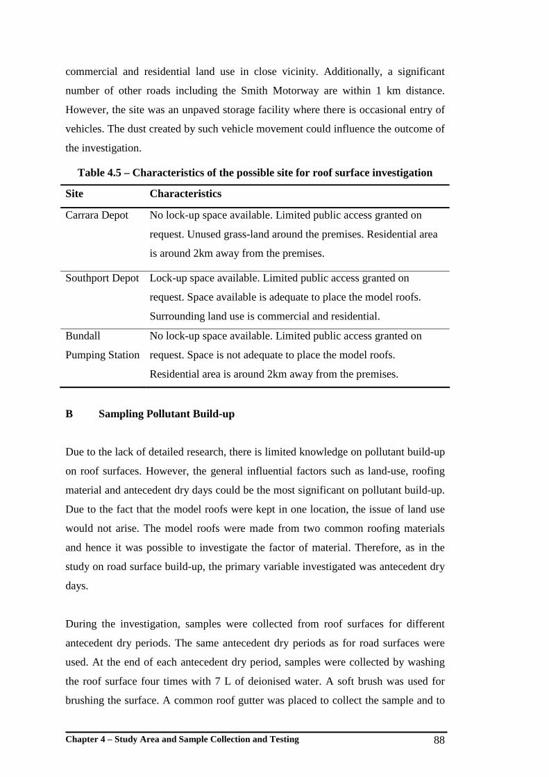
Chapter 4 – Study Area and Sample Collection and Testing 88
commercial and residential land use in close vicinity. Additionally, a significant
number of other roads including the Smith Motorway are within 1 km distance.
However, the site was an unpaved storage facility where there is occasional entry of
vehicles. The dust created by such vehicle movement could influence the outcome of
the investigation.
Table 4.5 – Characteristics of the possible site for roof surface investigation
Site Characteristics
Carrara Depot No lock-up space available. Limited public access granted on
request. Unused grass-land around the premises. Residential area
is around 2km away from the premises.
Southport Depot Lock-up space available. Limited public access granted on
request. Space available is adequate to place the model roofs.
Surrounding land use is commercial and residential.
Bundall
Pumping Station
No lock-up space available. Limited public access granted on
request. Space is not adequate to place the model roofs.
Residential area is around 2km away from the premises.
B Sampling Pollutant Build-up
Due to the lack of detailed research, there is limited knowledge on pollutant build-up
on roof surfaces. However, the general influential factors such as land-use, roofing
material and antecedent dry days could be the most significant on pollutant build-up.
Due to the fact that the model roofs were kept in one location, the issue of land use
would not arise. The model roofs were made from two common roofing materials
and hence it was possible to investigate the factor of material. Therefore, as in the
study on road surface build-up, the primary variable investigated was antecedent dry
days.
During the investigation, samples were collected from roof surfaces for different
antecedent dry periods. The same antecedent dry periods as for road surfaces were
used. At the end of each antecedent dry period, samples were collected by washing
the roof surface four times with 7 L of deionised water. A soft brush was used for
brushing the surface. A common roof gutter was placed to collect the sample and to

Chapter 4 – Study Area and Sample Collection and Testing 89
direct it to a polyethylene container kept underneath the gutter opening. The gutter
was thoroughly washed before and after each sample collection. The model roofs
were lifted to the typical roofing height after each sample collection and prepared for
the next antecedent dry period. The collected samples were transported to
laboratories and stored under prescribed conditions. The protocol followed during
transportation and storage is discussed in Section 4.5.
C Sampling for Pollutant Wash-off
Similar to wash-off investigations for road surfaces, wash-off on roof surfaces was
also conducted using the rainfall simulator. Therefore, the primary variables
considered were rainfall intensity and duration. However, unlike road surface wash-
off investigations, different rainfall intensities were simulated on different days due
to the fact that only one model roof was available for each roofing material. In order
to ensure that an appreciable amount of pollutants was build-up on the roofs, the
interval between simulations was set at seven days. In order to obtain the exact
amount of pollutants available on the model roofs, initially available pollutant
samples were collected from half of each roof surface prior to each rainfall
simulation.
Only four rainfall intensities, 20, 40, 86 and 115 mm/hr, were simulated on roof
surfaces. The 65 mm/hr intensity was not simulated due to similar wash-off
behaviour observed for 40 and 86 mm/hr intensities. The 133 mm/hr intensity was
not simulated due to the rapid wash-off observed. Frequent sampling was not
technically feasible for intensities greater than 115 mm/hr. The durations for these
intensities were selected on site. Frequent samples were collected during the initial
period of each event and simulations were conducted until relatively clean runoff
resulted from the roofs. During simulations, the rainfall simulator was placed exactly
above the lowered model roof (see Figure 4.11). The simulator was raised to
maintain 2.5 m average height from roof to nozzle boom. A common roof gutter was
placed to collect roof surface runoff and to direct it to the polyethylene containers.
Samples were transported to laboratories and stored under prescribed conditions.

Chapter 4 – Study Area and Sample Collection and Testing 90
Figure 4.11 – Rainfall simulation on roof surfaces
4.5 Treatment and Transport of Samples
Two types of treatment procedures were used to handle and transport samples that
were collected in the field. Samples collected during pollution build-up studies and
from catchment outlets were transported to the laboratory immediately after
collection. The average time taken to reach the laboratory from collection was
around one hour. The samples were tested for pH and EC immediately after they
reached the laboratory. A portion of each sample was preserved for further testing by
refrigerating under 40C as specified in Australia / New Zealand Standards for Water
Quality Sampling (AS/NZS, 1998). Deionised water blanks and field water blanks
were included during each sample collection in order to maintain standard quality
control procedure as specified in AS/NZS (1998). Wash-off samples took a longer
time to collect in the field and the average volume of each individual sample was
around 15 L. The samples were transported and a portion preserved similar to the
build-up samples after recording pH and EC.
Chapter 4 – Study Area and Sample Collection and Testing 91
4.6 Laboratory Testing
It is commonly understood that a significant fraction of pollutants are associated with
particulates in stormwater runoff (Pechacek, 1994; Sartor et al., 1974). This is the
primary reason for using suspended solids as the indicator pollutant in stormwater
quality modelling. A common approach used in modelling is to estimate suspended
solids using rainfall and runoff parameters and predict other pollutants by
proportioning (Akan and Houghtalen, 2003). Therefore, in-depth knowledge of
suspended solid characteristics in stormwater runoff is critical.
Laboratory testing was primarily focussed on solids in both build-up and wash-off
samples. Therefore, priority was given to test total suspended solids (TSS), total
dissolved solids (TDS) and particle size distribution. Additionally, the physio-
chemical parameters that influence the adsorption of other pollutants to particulate
pollutants were also tested. As discussed in Section 2.4.6, the primary physio-
chemical parameters that influence the adsorption of other pollutants to solids are
pH, EC, total organic carbon (TOC) and dissolved organic carbon (DOC) (Hamilton
et al., 1984; Pechacek, 1994; Tai, 1991; Warren et al., 2003). Therefore, laboratory
tests were conducted to obtain these parameters. Since direct testing for TOC and
DOC is difficult, total carbon (TC) and inorganic carbon (IC) for original sample and
filtrate were tested. The complete set of parameters tested during the laboratory
analysis was:
1) Particle size distribution;
2) TSS;
3) TDS;
4) pH and EC; and
5) TC and IC for original sample and filtrate.
4.6.1 Particle Size Distribution
Different techniques have been used to investigate the particle size distribution of
suspended solids. Among many methods, wet or dry sieving is the most widely used.
For example, Vaze and Chiew (2002) used 13 sieves, ranging from 38 to 2800 µm, to

Chapter 4 – Study Area and Sample Collection and Testing 92
categorise samples into size classes. However, due to the greater number of samples
to be tested, a faster, accurate and a less labour intensive method was needed.
Therefore, a Malvern Mastersizer S instrument was used in this research.
The Malvern Mastersizer S uses a laser diffraction technique to analyse the particle
size distribution. The laser beam creates a scatter pattern from a flow of particles. It
then uses a Reverse Fourier lens to determine the size of particles from the scatter
pattern. The specific lens used in this research was a Reverse Fourier lens of 300 mm
diameter. As specified, it is capable of analysing particles in the range of 0.05-900
µm. The accuracy of the process is specified as ±2% of the volume median diameter
in this size range (Malvern-Instrument-Ltd, 1997).
Figure 4.12 - Malvern Mastersizer model S
The Malvern Mastersizer S consists of a sample dispersion unit connected by two
flow cells to the optical unit (see Figure 4.12). The results obtained from the optical
unit were converted to percentage particle size distribution using specialised software
supplied by the manufacturer. Two important issues to note in the interpretation of
results from the Malvern Mastesizer are:
1. The particle size distribution is volume based; and
2. The particle size is determined by analysing volume initially and equating
this volume to an equivalent sphere.
(Malvern-Instrument-Ltd, 1997)
Chapter 4 – Study Area and Sample Collection and Testing 93
4.6.2 Other Physio-chemical Parameters
The test methods specified in Standard Methods for Water and Wastewater (APHA,
1999) were used for the laboratory analysis. The analytical procedure followed for
each test parameter is as follows:
A Total Suspended Solids and Total Dissolved Solids
TSS concentration was analysed by measuring the dry weight of solids retained on a
glass fibre filter paper (1 µm pore size). For the filtration, a known volume of sample
was used. The sample volume was chosen so that the increase in dry weight of filter
paper is significant. The sample volumes used were 200 mL for build-up samples
and 500 mL for wash-off samples. The filter papers used were pre-washed and oven
dried before use. TDS was analysed by measuring the dry weight of solids dissolved
in a known volume of water. In this regard, 20 mL of filtrated sample was used. The
Petri dishes used for the analysis were pre-washed and oven dried before use. The
oven temperature used was 1030C to 1050C. The test methods used were 2540C and
2540D (APHA 1999).
B pH and EC
pH and EC were measured immediately after the samples reached the laboratory. A
combined pH /EC meter was used for the measurements and the instrument was pre-
calibrated using standard solutions. The test methods used were 4500H and 2520B
(APHA 1999).
C Organic Carbon
Organic carbon was measured using a Shimadzu TOC-5000A Total Organic Carbon
Analyser. The instrument is capable of measuring inorganic carbon and total carbon
separately. The original sample and filtrate was analysed separately to obtain the
dissolved component of organic carbon.
Chapter 4 – Study Area and Sample Collection and Testing 94
4.7 Conclusions
Two different approaches were adopted to collect the necessary data for the research.
Catchment scale investigations were undertaken to obtain the necessary data for
validation of the translation procedure. For this, water samples collected from three
catchment outlets were tested for a range of water quality parameters. Small-plot
scale investigations were undertaken to obtain primary knowledge on pollutant build-
up and wash-off processes for road and roof surfaces.
The primary variable considered for pollutant build-up was the antecedent dry
period. Build-up samples were collected from road and roof surfaces belonging to a
range of antecedent dry periods. The primary variables considered for wash-off
investigations were rainfall intensity and duration. Wash-off samples were collected
by simulating a range of rainfall intensities for different durations on both road and
roof surfaces.
Samples collected were tested based on prescribed laboratory test procedures. The
primary parameters tested were TSS, TDS, particle size distribution, pH, EC, TC and
IC.

Chapter 5 – Analysis of Pollutant Build-up 95
Chapter 5 - Analysis of Pollutant Build-up
5.1 Background
Among the knowledge requirements for the development of the translation procedure
is detailed understanding of pollutant build-up processes. The field investigations, as
discussed in Section 4.3, generated the primary data on build-up. The main focus of
this chapter is to discuss the analysis of the data to derive relevant knowledge on
build-up processes and for better understanding of the underlying physical processes
of build-up.
Fundamental knowledge on the build-up process which was essential for the
translation procedure was developed by the analysis of solid pollutant loads. In this
regard, the processes were defined in the form of mathematical replication equations.
However, it was necessary to understand the underlying physical processes of build-
up.
5.2 Data and Pre-processing
The data obtained from the laboratory testing was subjected to extensive pre-
processing prior to analysis. The pre-processing methodologies adopted were
different for different test parameters. A complete set of the data used for pre-
processing is shown in Appendix C, Tables C.1 and C.2.
A TSS and TDS
The laboratory test results for TSS and TDS parameters were in the form of
concentrations (mg/L). Since build-up is typically expressed in terms of solid loads,
it was necessary to convert concentration data into loads. For this, each data point
was multiplied by the corresponding sample volume. The addition of loads obtained
for TSS and TDS resulted in the total solids (TS) load for each sample. For
Chapter 5 – Analysis of Pollutant Build-up 96
standardisation, the TS loads were divided by the surface area where the samples
were collected. The final outcome was in the form of (g/m2).
B Particle Size Distribution
The laboratory results for particle size distribution were in the form of volumetric
percentages. Since TS is given as a load, the particle size distribution also needed to
be expressed in load percentages. This was done assuming that there is no variation
in average particle density among different particle size classes. This assumption was
made despite the understanding that particles originating from different sources can
have different densities. For example, wear-off from tyres could be much lighter in
density compared to wear-off from road surfaces. However, the assumption is still
valid if particle size distribution of each density class is the same.
B pH and EC
pH and EC were analysed immediately after samples reached the laboratory.
However, prior to measurements, the sample volume was brought up to 7 L which
was the approximate volume for build-up samples. In this way, the measurements
were standardised and therefore, the outcomes could be comparable with samples
obtained from different sites. It was understood that the pH and EC measurements
would be influenced by the initial pH and EC readings of the deionised water used in
the vacuum system for sample collection. However, it was noted that the variation of
pH and EC in the deionised water was low. The pH ranged from 6.7 to 7.0 for
deionised water used in various stages of build-up sample collection and the
variation of EC was 2 to 10 µS. Therefore, the laboratory test results obtained were
directly used in the data analysis without further pre-processing.
C TC, TOC and DOC
As discussed in Section 4.6, the parameters obtained during laboratory testing were
total carbon (TC) and inorganic carbon (IC) for the original sample and for the
filtrate. From these parameters, values for total organic carbon (TOC) and dissolved

Chapter 5 – Analysis of Pollutant Build-up 97
organic carbon (DOC) were calculated. TOC was defined as the difference between
TC and IC results for the original sample. DOC was considered to be the difference
between the TC and IC results for the filtrate.
5.3 Build-up on Road Surfaces
The pollutant build-up on road surfaces within the study area was investigated based
on three road surfaces. The road sites were Gumbeel Court, Lauder Court and
Piccadilly Place. Details of these road sites are provided in Section 4.3.1. Six to eight
build-up samples were collected from each site representing different antecedent dry
days. The antecedent dry days considered were 1, 2, 3, 7, 14, and 21. The primary
parameters used during build-up data analysis were TS, particle size distribution, pH,
EC, TC, TOC and DOC.
5.3.1 Variability of Build-up
As discussed in Section 2.3.3, pollutant build-up on impervious surfaces is
commonly understood as a decreasing rate increasing function with antecedent dry
days. Although this behaviour is commonly accepted, many researchers have noted
that the build-up rates and loads are site specific (Deletic and Orr, 2005; Herngren et
al., 2006; Vaze and Chiew, 2002). The site specific nature is primarily attributed to
the variability of the influential parameters such as climatic conditions, land-use,
traffic volume and road surface conditions. However, the variability noted during this
investigation was limited. This could be due to the investigation of only residential
land-use. Nevertheless, the pollutant build-up did show appreciable variation, as
shown in Figure 5.1.
As illustrated in Figure 5.1, pollutant build-up during the initial one to two days is
high compared to longer dry periods. The average two day build-up is around 2.3
g/m2/day or about 66% of the total average build-up for 21 days. After the initial two
days, the rate of accumulation is significantly reduced. As the rate reduces, it could
be assumed that the build-up asymptotes to a constant value when the dry days
increase. As explained by Ball et al. (1998), there could be a state of dynamic
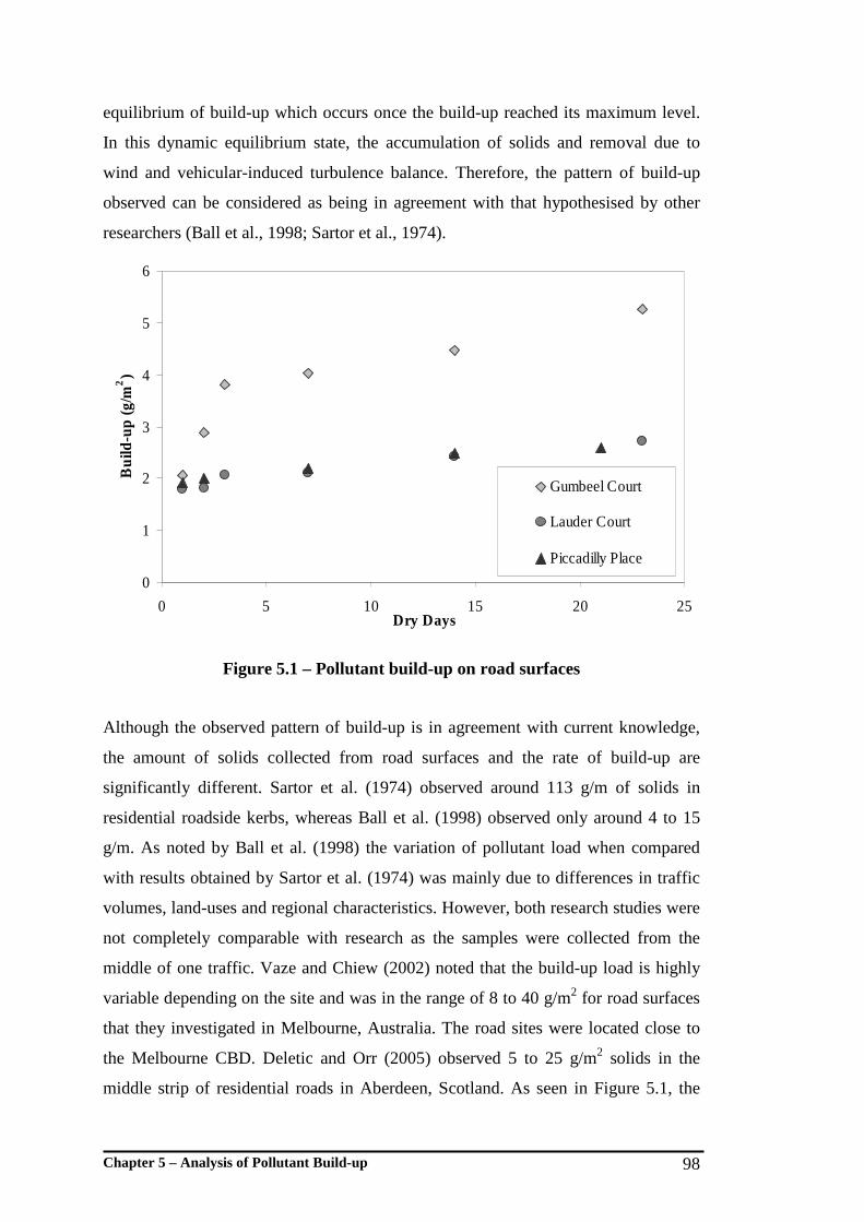
Chapter 5 – Analysis of Pollutant Build-up 98
equilibrium of build-up which occurs once the build-up reached its maximum level.
In this dynamic equilibrium state, the accumulation of solids and removal due to
wind and vehicular-induced turbulence balance. Therefore, the pattern of build-up
observed can be considered as being in agreement with that hypothesised by other
researchers (Ball et al., 1998; Sartor et al., 1974).
0
1
2
3
4
5
6
0 5 10 15 20 25Dry Days
Bui
ld-u
p (g
/m2)
Gumbeel Court
Lauder Court
Piccadilly Place
Figure 5.1 – Pollutant build-up on road surfaces
Although the observed pattern of build-up is in agreement with current knowledge,
the amount of solids collected from road surfaces and the rate of build-up are
significantly different. Sartor et al. (1974) observed around 113 g/m of solids in
residential roadside kerbs, whereas Ball et al. (1998) observed only around 4 to 15
g/m. As noted by Ball et al. (1998) the variation of pollutant load when compared
with results obtained by Sartor et al. (1974) was mainly due to differences in traffic
volumes, land-uses and regional characteristics. However, both research studies were
not completely comparable with research as the samples were collected from the
middle of one traffic. Vaze and Chiew (2002) noted that the build-up load is highly
variable depending on the site and was in the range of 8 to 40 g/m2 for road surfaces
that they investigated in Melbourne, Australia. The road sites were located close to
the Melbourne CBD. Deletic and Orr (2005) observed 5 to 25 g/m2 solids in the
middle strip of residential roads in Aberdeen, Scotland. As seen in Figure 5.1, the

Chapter 5 – Analysis of Pollutant Build-up 99
maximum pollutant load collected from the three study sites varied from 3 to 6 g/m2.
This was significantly less compared to numerous other studies. This could be
mainly due to the general variability associated with build-up arising from factors
such as regional, climatic, land-use, traffic and road surface conditions. However, the
build-up loads and rates observed in this research are representative for low traffic
road surfaces in typical Australian residential land-uses. This can be further
confirmed by the results reported by Herngren et al. (2006), where similar pollutant
loads on road surfaces were observed for sites in the Gold Coast region. They noted
0.8 to 5.3 g/m2 pollutants on low traffic roads in urban residential land-uses.
However, the loads that they observed belonged to different antecedent dry days and
were not in equilibrium conditions.
As evident in Figure 5.1, the build-up varies between the three study sites. The build-
up in the Gumbeel Court site is significantly higher than in the other two sites. The
maximum build-up load observed in Gumbeel Court site was 5.3 g/m2, whereas for
the other two sites it was around 2.7 g/m2. It can be surmised that the variability of
build-up load and rate is due to variation in urban-form, traffic volume and road
surface conditions (see Table 4.2). However, the variation of traffic volume among
the three sites is not significant. As discussed in Section 4.4.1, the variability of
traffic volume is expressed in terms of surrounding households. The influence of
traffic would not be significant since the highest number of households belongs to
Piccadilly Place site where the build-up is comparatively less. Among urban-form
and road surface conditions, urban-form would be the most influential on pollutant
build-up. This is due to the high degree of indirect correlation of urban-form and
consequent variation in population density with the degree of anthropogenic
activities on catchment surfaces.
For the study area, the urban-form primarily describes the population density.
Therefore, the influential variable for the pollutant build-up could be attributed to
population density. There are two primary population density categories within the
study area. Population density equivalent to townhouse areas such as those in the
Gumbeel and Alextown catchments can be termed high population density areas.
Therefore, the build-up in high population density areas can be considered as
represented by the build-up variation observed in Gumbeel Court site. Low
Chapter 5 – Analysis of Pollutant Build-up 100
population density is equivalent to single detached housing areas such as Birdlife
Park catchment. Build-up in such urban-form can be considered as represented by the
build-up variations observed in Lauder Court and Piccadilly Place sites.
5.3.2 Mathematical Replication of Build-up
In the context of stormwater quality modelling, accurate replication of build-up is
important. For this research, it is particularly essential, since mathematical
replication was to be used in the proposed translation procedure. As two different
build-up variations were noted for two population density areas, two different
replications were needed.
As noted in Section 5.3.1, in a generic sense the build-up observed in this research
study is closely comparable to the commonly accepted form. Therefore, it can be
considered that a common replication equation with two different sets of parameters
can be developed for the two build-up variations. In the research literature, a number
of different replication formats have been proposed. It is hypothesised that these
differences could be the result of inconsistency in research techniques and data
interpretations. For example, Sartor et al. (1974) proposed an exponential form of a
build-up equation which provided a reasonable level of accuracy to be used in
stormwater quality models. Modified forms of this exponential equation are used
widely in various stormwater quality models including SWMM (Huber and
Dickinson, 1988). Ball et al. (1998) noted build-up is better replicated by a power
function or a reciprocal function.
In order to identify the most suitable form for replicating pollutant build-up, four
equations were investigated in-depth. These were:
1) Reciprocal format - x
bay += ;
2) Logarithmic format - )ln(xbay += ;
3) Exponential format - bxaey −= ; and
4) Power format - baxy = .

Chapter 5 – Analysis of Pollutant Build-up 101
The equations were tested by developing best fit curves for each equation based on
their ability to replicate the observed pollutant build-up. Since two build-up
variations were noted, it was necessary to standardise these observations prior to
testing. Standardising was done by dividing each data point by the maximum
possible build-up for that site. In this regard, maximum build-up for Lauder Court
and Piccadilly Place sites was considered to be the average of maximum build-up. It
was assumed that the build-up for all three sites has reached equilibrium level at the
end of each investigation period. The standardised parameter was termed the
‘Fraction Build-up’. Figure 5.2 shows the performances of selected equation formats.
0
0.2
0.4
0.6
0.8
1
1.2
0 5 10 15 20 25Dry Days
Fra
ctio
n B
uild
-up
Gumbeel Court Lauder Court
Piccadilly Place Reciprocal
Logarithmic Exponential
Power
Figure 5.2 – Comparison of different form of equations with solid build-up on roads
As evident in Figure 5.2, predictions by both logarithmic and power equations are
visually similar to the observed build-up variation. However, the power equation was
preferred ahead of the logarithmic equation to replicate build-up. This was mainly
due to the recommendation in a previous independent study by Ball et al. (1998).
Hence, the form of the build-up replication equation for road surfaces was taken as:
baDB = Equation 5.1
Where,
B = Build-up load on road surface (g/m2);

Chapter 5 – Analysis of Pollutant Build-up 102
D = Antecedent dry days; and
a and b = Build-up coefficients.
Appropriate values for the build-up coefficients, a and b, needed to be estimated
before the use of the equation. For this research study, a and b were estimated based
on the observed results from the three study areas. Therefore, the parameters would
be most appropriate for the conditions in the study areas. Two sets of parameters
were developed to account for the variability observed for the two population density
areas.
According to the behaviour of the power equation, it was noted that a constant value
for the power coefficient, b, would be appropriate. However, there is a possibility of
variation of b with the surface type. Therefore, the constant value developed is valid
only for similar road surfaces. More details of the surface characteristics can be
found in Table 4.2. The multiplication coefficient, a, denotes the pollutant build-up
rate on the road surface. The coefficient a is the primary parameter that accounts for
the variability of population density areas. Therefore, two values were obtained for a
to represent high and low population density. Although only population density was
considered in this research, a could be influenced by other factors such as land-use,
traffic volume and regional variables.
The two sets of build-up coefficients were developed using the method of least
squares. This method adjusts the parameters such that the cumulative square of error
associated with the prediction of each observed data point is minimal. More details
on the method of least squares can be found in Section 3.5.2. The analysis was done
for low and high population density areas separately. Table 5.1 shows the values
obtained for a and b, and Figure 5.3 shows the predictive accuracy of the equation
with the given parameters. Table 5.1 further shows the statistical significance of
prediction in terms of Mean and CV. It is evident that the accuracy of prediction for
low population density areas is quite good compared to high population density area.
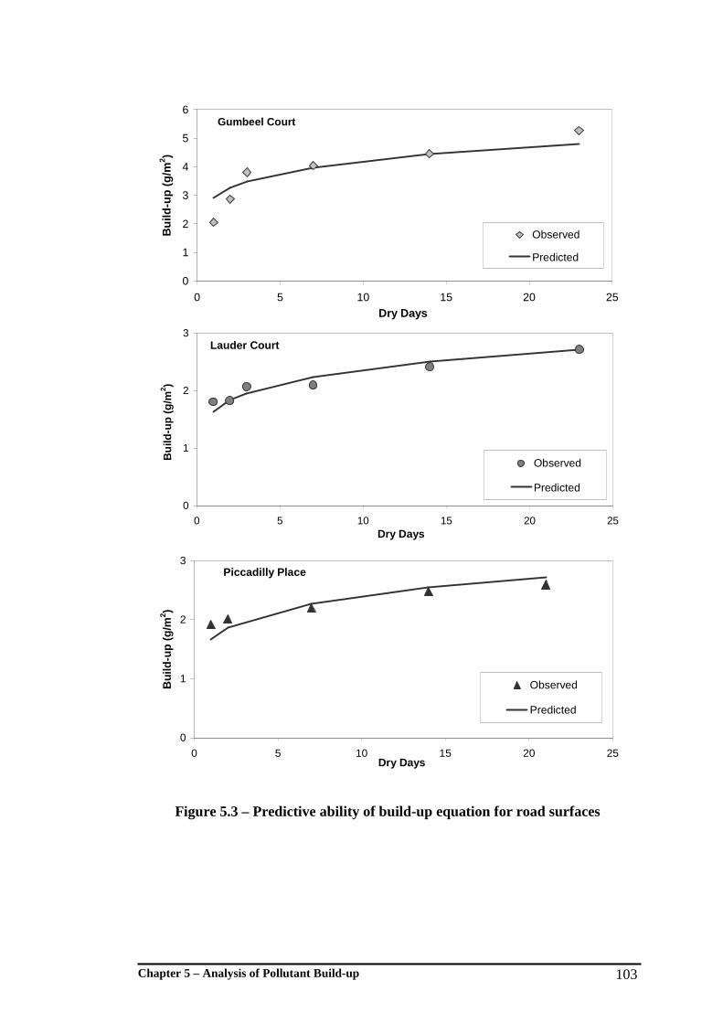
Chapter 5 – Analysis of Pollutant Build-up 103
Gumbeel Court
0
1
2
3
4
5
6
0 5 10 15 20 25Dry Days
Bu
ild-u
p (
g/m
2 )
Observed
Predicted
Lauder Court
0
1
2
3
0 5 10 15 20 25Dry Days
Bu
ild-u
p (
g/m
2 )
Observed
Predicted
Piccadilly Place
0
1
2
3
0 5 10 15 20 25Dry Days
Bu
ild-u
p (
g/m
2 )
Observed
Predicted
Figure 5.3 – Predictive ability of build-up equation for road surfaces

Chapter 5 – Analysis of Pollutant Build-up 104
Table 5.1 – Build-up coefficients for road surfaces
Road Site Characteristics a b Mean CV
Gumbeel Court Townhouse region with high
population density 2.90 0.16 1.05 19%
Lauder Court 1.65 0.16
Piccadilly Place
Single detached housing
regions with low population
density 1.65 0.16
0.98 7%
5.3.3 Hypothetical Build-up Process
As explained in Section 4.4.1, the sampling plots were cleaned and pollutants
allowed to build-up for a specified antecedent dry period. This would mean that the
developed build-up equation relates to the build-up process starting from near zero
initial pollutants. However, it is not reasonable to assume that build-up starts from
near zero under typical conditions in the field. Based on the observations from wash-
off investigations (Chapter 6), an appreciable amount of pollutants remain on an
impervious surface even after a heavy storm event.
The possibility of an appreciable amount of pollutants being initially available on the
road surfaces would mean that Equation 5.1 estimates only the lower limit of build-
up. With the inclusion of initially available pollutants, the total pollutants present on
surfaces would always be higher than the estimated amount given by Equation 5.1.
Many researchers have noted that the simple addition of pre-existing pollutants after
the last storm would not be appropriate to estimate the total build-up (Novotny et al.,
1985; Sartor et al., 1974). Such an approach contradicts the already accepted physical
process of pollutant build-up which was considered to asymptote to a constant value.
An addition would unrealistically increase the estimated pollutant build-up.
The presence of pre-existing pollutants on the road surface would influence the
initial part of the build-up processes, but it should still asymptote to the same
constant value (Alley and Smith, 1981). However, since the time taken to reach the
constant build-up is not known, it is reasonable to assume that the build-up process
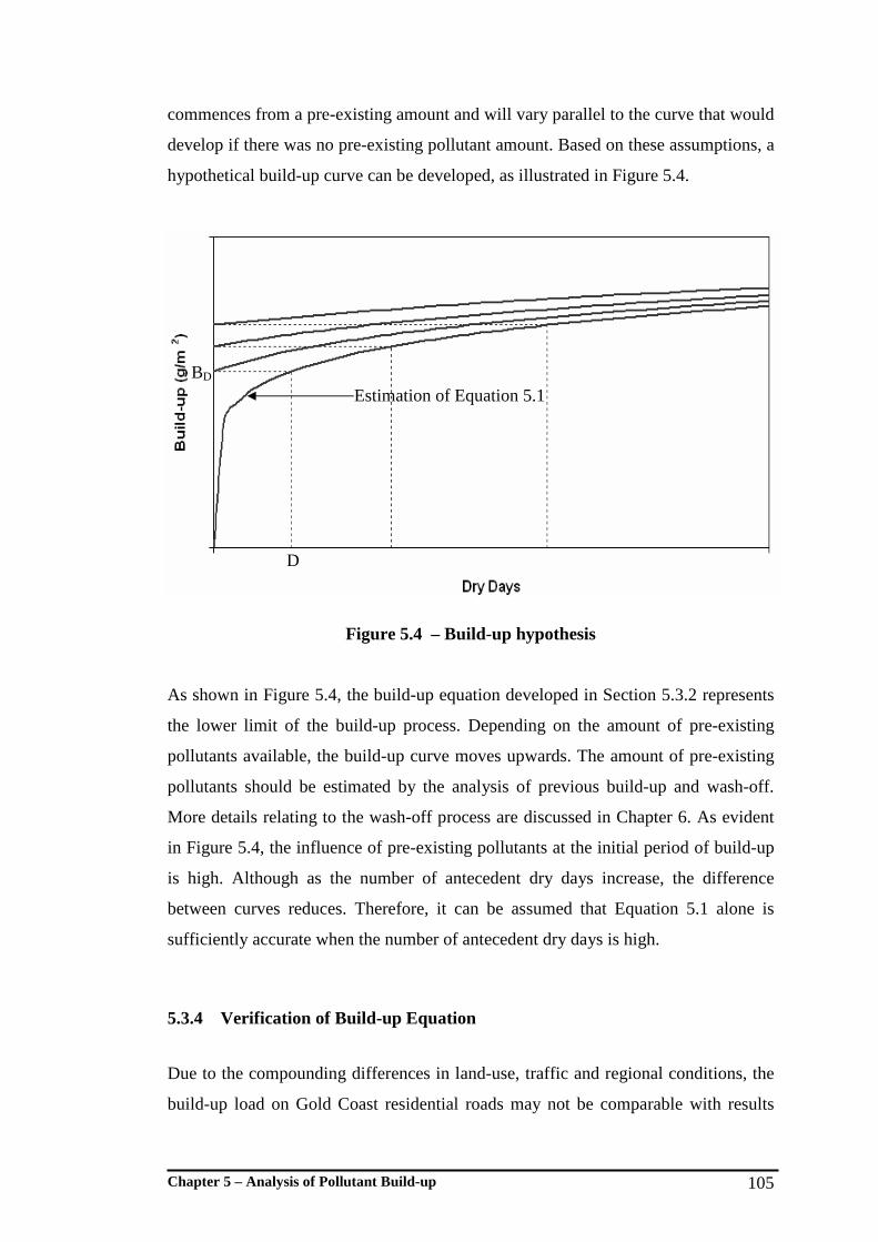
Chapter 5 – Analysis of Pollutant Build-up 105
commences from a pre-existing amount and will vary parallel to the curve that would
develop if there was no pre-existing pollutant amount. Based on these assumptions, a
hypothetical build-up curve can be developed, as illustrated in Figure 5.4.
Figure 5.4 – Build-up hypothesis
As shown in Figure 5.4, the build-up equation developed in Section 5.3.2 represents
the lower limit of the build-up process. Depending on the amount of pre-existing
pollutants available, the build-up curve moves upwards. The amount of pre-existing
pollutants should be estimated by the analysis of previous build-up and wash-off.
More details relating to the wash-off process are discussed in Chapter 6. As evident
in Figure 5.4, the influence of pre-existing pollutants at the initial period of build-up
is high. Although as the number of antecedent dry days increase, the difference
between curves reduces. Therefore, it can be assumed that Equation 5.1 alone is
sufficiently accurate when the number of antecedent dry days is high.
5.3.4 Verification of Build-up Equation
Due to the compounding differences in land-use, traffic and regional conditions, the
build-up load on Gold Coast residential roads may not be comparable with results
Estimation of Equation 5.1
D
BD
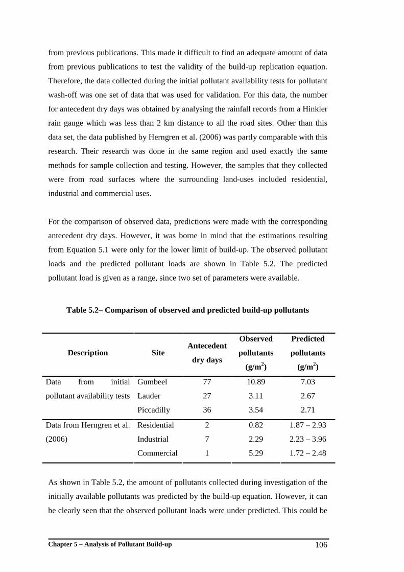
Chapter 5 – Analysis of Pollutant Build-up 106
from previous publications. This made it difficult to find an adequate amount of data
from previous publications to test the validity of the build-up replication equation.
Therefore, the data collected during the initial pollutant availability tests for pollutant
wash-off was one set of data that was used for validation. For this data, the number
for antecedent dry days was obtained by analysing the rainfall records from a Hinkler
rain gauge which was less than 2 km distance to all the road sites. Other than this
data set, the data published by Herngren et al. (2006) was partly comparable with this
research. Their research was done in the same region and used exactly the same
methods for sample collection and testing. However, the samples that they collected
were from road surfaces where the surrounding land-uses included residential,
industrial and commercial uses.
For the comparison of observed data, predictions were made with the corresponding
antecedent dry days. However, it was borne in mind that the estimations resulting
from Equation 5.1 were only for the lower limit of build-up. The observed pollutant
loads and the predicted pollutant loads are shown in Table 5.2. The predicted
pollutant load is given as a range, since two set of parameters were available.
Table 5.2– Comparison of observed and predicted build-up pollutants
Description Site Antecedent
dry days
Observed
pollutants
(g/m2)
Predicted
pollutants
(g/m2)
Gumbeel 77 10.89 7.03
Lauder 27 3.11 2.67
Data from initial
pollutant availability tests
Piccadilly 36 3.54 2.71
Residential 2 0.82 1.87 – 2.93
Industrial 7 2.29 2.23 – 3.96
Data from Herngren et al.
(2006)
Commercial 1 5.29 1.72 – 2.48
As shown in Table 5.2, the amount of pollutants collected during investigation of the
initially available pollutants was predicted by the build-up equation. However, it can
be clearly seen that the observed pollutant loads were under predicted. This could be
Chapter 5 – Analysis of Pollutant Build-up 107
partly due to the presence of pre-existing pollutants. Therefore, Equation 5.1
typically provides an underestimation. Furthermore, the equation was developed
using field data of up to 21 antecedent dry days. However, the three samples
collected during the initial pollutant availability test were well outside the
investigated range. The uncertainty of predictions always increases when an equation
is used for extrapolation.
As seen in Table 5.2, the data from Herngren et al. (2006) shows significant variation
with the predicted build-up ranges. Only the observed build-up for the industrial site
falls within the predicted range whilst the build-up in the residential site is below the
predicted range and in the commercial site it is above the predicted range. The
commercial site was a parking lot which may retain more pollutants due to high
anthropogenic activities and flatness of the surface. Furthermore, pollutant re-
distribution would also be limited due to the reduced speed of vehicles. This
suggested that the predictions made using Equation 5.1 are not suitable to estimate
the pollutant build-up at commercial sites. Both the residential site and industrial
sites were road surfaces which had similar characteristics to the road surfaces
investigated in this research. In fact, the residential site was particularly similar to the
Lauder Court site. Therefore, the differences between observed and estimated values
could be due to errors in the estimation equation. This further highlighted the
uncertainty associated with build-up predictions. However, it is important to bear in
mind that it is pollutant wash-off that is significant rather than pollutant build-up,
even though the former is influenced by the latter.
5.3.5 Particle Size Distribution
Detailed knowledge on the solids composition of pollutants and its variation with a
range of influential parameters is essential for better understanding of the underlying
physical processes of pollutant build-up. For this research study where the solids
were considered the primary pollutant, the composition of build-up was investigated
in terms of particle size distribution. It was well understood that the particle size
distribution can vary with a range of land-use, regional and road surface parameters
(Sartor et al., 1974; Shaheen, 1975).

Chapter 5 – Analysis of Pollutant Build-up 108
The outcomes of particle size distribution measurements were in spectrum format
which can be categorised into any size class according to user preference. More
details on particle size distribution measurements can be found in Section 4.6.1. For
ease of understanding, size spectrums were categorised into six size classes for the
primary analysis. Table 5.3 shows the average volumetric particle size percentages
for six size categories.
Table 5.3 – Average percentage particle size distribution
Solids (Volumetric Percentage)
Size Class (µm) Gumbeel Court Lauder Court Piccadilly Place
<10 3.9 3.3 5.8
10-50 17.8 18.7 23.8
50-100 20.6 25.4 27.7
100-200 22.6 25.7 21.3
200-400 20.5 17.4 13.9
>400 14.5 9.5 7.4
As shown in Table 5.3, the particle size distribution for the three road sites is similar.
This could be primarily attributed to similar traffic volumes in the three sites.
However, the solids composition noted is different to the results reported in other
research studies. On average, for all three sites around 50% and 70% of the solids are
less than 100 µm and 200 µm size respectively. In contrast, Sartor et al.(1974) noted
that only around 43% of the particles were smaller than the 246 µm size for the
samples they collected from roadside kerbs. Furthermore, they found that only 5.9%
of particles were smaller than 43 µm. Ball et al. (1998) noted a 10 to 30% particle
fraction less than 200 µm on suburban road surfaces in Sydney. Deletic and Orr
(2005) noted 50% of the road surface solids were less than 238 µm. They collected
samples from the middle strip of a residential road in Scotland. Therefore, in
comparison to previous research findings, the particulate pollutants observed in this
research are significantly finer. This could be primarily attributed to the residential
nature of the land-use, low traffic volumes on roads and catchment management
practices.

Chapter 5 – Analysis of Pollutant Build-up 109
Apart from the comparison with previous research, detailed analysis of the variation
of particle size distribution with the increase of antecedent dry days was necessary to
understand the primary physical processes of build-up. The outcomes of this analysis
are shown in Figure 5.5.
Figure 5.5 - Variation of particle size distribution with antecedent dry days for road surfaces build-up
Chapter 5 – Analysis of Pollutant Build-up 110
Figure 5.5 shows a significant variation of solids composition with antecedent dry
days. For all three sites, the semi-logarithmic curve for particle size distribution
moves from left to right with the increase in antecedent dry days. This suggested that
the fraction of coarser particles increases with the increase in the dry period. As
noted by Roesner (1982), the particle size distribution of solids depositions can be
assumed to be uniform for any given dry day. Therefore, it is hypothesised that it
would be the re-distributing factors that change the particle size distribution during
build-up by constantly removing finer particles from the surface. As noted by
Namdeo et al. (1999) and Novotny et al. (1985), pollutant re-distribution occurs
depending on the wind and traffic-induced turbulence by re-suspending finer
particles. As they noted, there is a high possibility of these particles to be re-
deposited in nearby pervious areas.
As noted in Section 5.3.2, it could be hypothesised that the pollutant loads asymptote
to a constant value with the increase in dry days. However, the variation of particle
size distribution illustrates the dynamic nature of build-up suggesting the ability to
accumulate newer particles after the removal of older particles so that there is little
variation in pollutant loads as the antecedent dry days increase. This would mean that
the build-up on road surfaces continues as a dynamic process for a long duration
even though the changes to the pollutant load are limited.
5.3.6 Analysis of Physio-chemical Parameters
Since this research focused on suspended solids, the range of chemical impacts
exerted on receiving water due to stormwater pollution is not discussed in detail.
However, as noted in previous research studies, the impacts of chemical pollutants
such as hydrocarbons, heavy metals and nutrients are the most significant (House et
al., 1993). Although the chemical pollutants were not specifically investigated, it was
well understood that most of them are associated with particulate pollutants
(Herngren et al., 2006; Sartor et al., 1974; Shaheen, 1975). Therefore, understanding
the links between suspended solids and other chemical pollutants would improve the
applicability of the research outcomes.
Chapter 5 – Analysis of Pollutant Build-up 111
The amount of other pollutants adsorbed to solids varies with a range of parameters
including factors influencing the availability of chemical pollutants and factors
influencing the adsorption of these pollutants. Understanding the factors influencing
the availability of chemical pollutants on a catchment surface is well beyond the
objectives of this research study. However, understanding the factors influencing the
adsorption of pollutants is important in order to link the outcomes derived from this
research study to the existing knowledge on the estimations of other water quality
pollutants. The fineness of the solids is one of the important properties in relation to
the adsorption of other pollutants. This is discussed in detail in Section 5.2.4. The
other parameters which influence adsorption include pH, EC, TC, TOC and DOC
(Hamilton et al., 1984; Pechacek, 1994; Tai, 1991; Warren et al., 2003). Due to the
availability of multiple variables, principal component analysis (PCA) was used for
data analysis. A description of PCA can be found in Section 3.5.3.
The variables used in the analysis were pH, EC, TC, TOC, DOC and TS divided into
six particle size ranges: <10, 10-50, 50-100, 100-200, 200-400, >400 µm. The
number of samples used for the analysis was 24. A low number of samples used for
the analysis would reduce the confidence in PCA outcomes. However, the number of
samples used was adequate for the development of general understanding. For better
interpretations of PCA outcomes, the original data obtained from laboratory tests was
pre-processed. In this regard, TC, TOC and DOC concentrations were converted to
loads, and solid loads in each size class were converted into fractions. This was to
eliminate the influence of different build-up loads from the three different road sites.
Before the analysis, the data in the matrix was subjected to column standardisation
which is one of the standard pre-processing procedures used in multivariate analysis.
The data matrix used for the analysis is given in Appendix C, Table C.3.
Figure 5.6 shows the PCA biplot which resulted from the analysis.
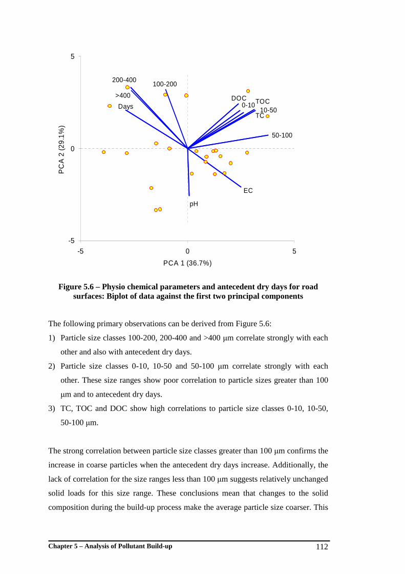
Chapter 5 – Analysis of Pollutant Build-up 112
100-200
50-100
10-50
0-10
DOC
TOC
TC
EC
pH
Days
>400
200-400
-5
0
5
-5 0 5
PCA 1 (36.7%)
PC
A 2
(29.
1%)
Figure 5.6 – Physio chemical parameters and antecedent dry days for road surfaces: Biplot of data against the first two principal components
The following primary observations can be derived from Figure 5.6:
1) Particle size classes 100-200, 200-400 and >400 µm correlate strongly with each
other and also with antecedent dry days.
2) Particle size classes 0-10, 10-50 and 50-100 µm correlate strongly with each
other. These size ranges show poor correlation to particle sizes greater than 100
µm and to antecedent dry days.
3) TC, TOC and DOC show high correlations to particle size classes 0-10, 10-50,
50-100 µm.
The strong correlation between particle size classes greater than 100 µm confirms the
increase in coarse particles when the antecedent dry days increase. Additionally, the
lack of correlation for the size ranges less than 100 µm suggests relatively unchanged
solid loads for this size range. These conclusions mean that changes to the solid
composition during the build-up process make the average particle size coarser. This
Chapter 5 – Analysis of Pollutant Build-up 113
observation further strengthens the description of the physical processes governing
build-up as discussed previously. In Section 5.3.4, the dynamic nature of build-up
was discussed in detail. The outcomes from this analysis confirmed that the threshold
value of particle size that change the re-distribution characteristics is 100 µm. Size
classes below this threshold size range would be subject to a high degree of re-
distribution.
The correlation of chemical parameters with size classes less than 100 µm points to
their high pollutant nature. A threshold value of 100 µm means that, on average, 50%
of the solids have the capacity to adsorb other pollutants. It can be noted in Table 5.3
that, on average, 50% of the solids are less than the 100 µm size range. In contrast,
Sartor et al. (1974) noted that the major fraction of the pollutants is associated with
only 5.9% of particles which were less than 43 µm. The difference could be
attributed to land-use and traffic volume as well as the method of investigation. The
strong correlation of the size ranges less than 100 µm to TOC and DOC suggested
most of these particles are organic. From the data matrix used for the PCA analysis,
it was noted that more than 95% of the carbon compounds are organic and more than
80% of the organic carbon is in soluble form. Higher organic carbon content in build-
up pollutants were also noted by Roger et al.(1998).
The presence of a high fraction of fine solids (less than 100 µm) suggests a high
adsorption capacity in the build-up solids. Since the load of these particle size ranges
is subjected to little variability when the antecedent dry days increase, this capacity
remains fairly unchanged. The possibility of having high DOC was also noted in the
build-up samples. This would lead to enhanced solubility of other pollutants such as
hydrocarbons and heavy metals in stormwater. The solubility could be further
enhanced due to low pH of build-up solids (Hamilton et al., 1984; Pechacek, 1994;
Tai, 1991; Warren et al., 2003).
Chapter 5 – Analysis of Pollutant Build-up 114
5.4 Build-up on Roof Surfaces
Two model roof surfaces, one with corrugated steel and another with concrete tiles,
were used to collect build-up samples. Further details on the model roof surfaces can
be found in Section 3.4. The methodology adopted for sample collection can be
found in Section 4.4.2. Samples collected belonged to 1, 2, 3, 7, 14 and 21
antecedent dry day periods. The primary parameters obtained from the sample testing
were TS, particle size distribution, pH, EC, TC, TOC and DOC.
5.4.1 Mathematical Replication of Build-up
Research studies relating to pollutant build-up on roof surface are extremely limited.
Consequently, the physical processes relating to pollutant build-up on roof surfaces
are not widely understood. In past studies, the primary understanding on roof surface
build-up was gained by investigating roof surface runoff. For example, Van Metre
and Mahler (2003) noted that pollutant concentrations originating from roof surfaces
could vary from around 60 to 500 mg/L depending on the surrounding land-use, roof
setup, and antecedent dry period. Bannerman et al. (1993) also noted the significant
solids concentration that could originate from roof surfaces.
Similar to the data analysis undertaken for road surface build-up, the pollutant loads
collected during field investigations were plotted to understand the variability of
build-up with antecedent days. Figure 5.7 shows the results derived.
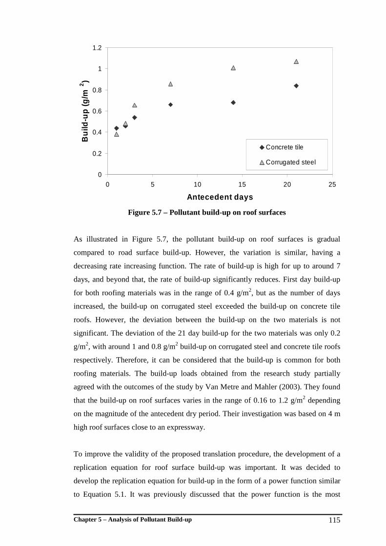
Chapter 5 – Analysis of Pollutant Build-up 115
0
0.2
0.4
0.6
0.8
1
1.2
0 5 10 15 20 25
Antecedent days
Bu
ild-u
p (g
/m2)
Concrete tile
Corrugated steel
Figure 5.7 – Pollutant build-up on roof surfaces
As illustrated in Figure 5.7, the pollutant build-up on roof surfaces is gradual
compared to road surface build-up. However, the variation is similar, having a
decreasing rate increasing function. The rate of build-up is high for up to around 7
days, and beyond that, the rate of build-up significantly reduces. First day build-up
for both roofing materials was in the range of 0.4 g/m2, but as the number of days
increased, the build-up on corrugated steel exceeded the build-up on concrete tile
roofs. However, the deviation between the build-up on the two materials is not
significant. The deviation of the 21 day build-up for the two materials was only 0.2
g/m2, with around 1 and 0.8 g/m2 build-up on corrugated steel and concrete tile roofs
respectively. Therefore, it can be considered that the build-up is common for both
roofing materials. The build-up loads obtained from the research study partially
agreed with the outcomes of the study by Van Metre and Mahler (2003). They found
that the build-up on roof surfaces varies in the range of 0.16 to 1.2 g/m2 depending
on the magnitude of the antecedent dry period. Their investigation was based on 4 m
high roof surfaces close to an expressway.
To improve the validity of the proposed translation procedure, the development of a
replication equation for roof surface build-up was important. It was decided to
develop the replication equation for build-up in the form of a power function similar
to Equation 5.1. It was previously discussed that the power function is the most

Chapter 5 – Analysis of Pollutant Build-up 116
appropriate to replicate build-up. However, the parameters for the power function
needed to be specifically derived to suit the build-up on roof surfaces.
Due to significant similarities in build-up, a common parameter set was developed.
The analytical methodology used for the development of coefficients was similar to
the analytical methodology adopted for the road surface build-up data. The least
squares method was adopted and the most suitable values for a and b were obtained
such that the square of deviation between predicted and observed data points was
minimal. More details on the method of least squares can be found in Section 3.5.2.
The coefficient values obtained were 0.43 and 0.266 for a and b respectively. Figure
5.8 shows the predictive performances of the developed equation irrespective of the
type of roof.
0
0.2
0.4
0.6
0.8
1
1.2
0 5 10 15 20 25
Antecedent days
Bu
ild-u
p (g
/m2)
Concrete tiles Predicted
Corrugated steel
Figure 5.8 – Performances of the replication equations for Build-up on roof surfaces
The build-up replication equation developed for roof surfaces can be used for
predictions. There was no requirement to incorporate a pre-existing pollutant load
from the last storm event. This was due to the high fraction of wash-off from roof
surfaces. Therefore, it can be considered that Equation 5.1 with relevant parameters
would replicate the build-up process with sufficient accuracy.

Chapter 5 – Analysis of Pollutant Build-up 117
Similar to the procedure adopted for the road surfaces, the validity of the build-up
replication equation formulated was tested using the data obtained during the initial
pollutant availability sampling. It was noted that the 7 day average build-up observed
was 2.5 and 3.9 g/m2 for concrete tile and corrugated steel surfaces respectively (see
Table 6.2). The sampling was done three times and the amounts collected show
significant variability. However, the prediction result using Equation 5.1 was 7.1
g/m2 of pollutants, which is a significant overestimation. This illustrates the high
degree of uncertainty associated with roof surface build-up predictions. The
uncertainty would be primarily due to climatic factors such as wind.
5.4.2 Particle Size Distribution
Similar to the particle size distribution analysis for road surfaces, the particle size
distributions for roof surfaces were analysed primarily by categorising into six size
classes. Table 5.4 shows the volumetric percentages for the six classes.
Table 5.4 – Average percentage particle size distribution – for roof surfaces
Solids (Volumetric Percentage)
Size Class (µm) Corrugated steel roof Concrete tile roof
<10 3.34 3.27
10-50 29.72 22.59
50-100 24.79 24.23
100-200 16.16 19.50
200-400 14.23 16.71
>400 10.10 12.97
As shown in Table 5.4, only fractional differences were noted in particle size
distributions between corrugated steel and concrete tile roof surfaces. For both roof
surfaces, a higher fraction of the solids was particles less than 100 µm. Particularly
for the corrugated steel roof, around 60% of the solids were less than 100 µm. This is
comparatively higher than the finer fraction on road surfaces, which was 50%. This
could be attributed to the fineness of atmospheric depositions. Furthermore, due to
the reduced texture depth and greater slope of roof surfaces, larger particles may not

Chapter 5 – Analysis of Pollutant Build-up 118
remain on roof surfaces. Similar to analysis for road surface build-up, particle size
distributions for roof surface build-up samples were analysed in order to understand
the governing processes. Figure 5.9 gives the particle size distributions of build-up
samples for the two roofing materials.
Figure 5.9 - Variation of particle size distribution with antecedent dry days for roof surfaces build-up
As evident in Figure 5.9, it is difficult to identify clear differences in particle size
distribution with antecedent dry days for the two roofing materials. The changes in
particle size distribution were only marginal for different antecedent dry periods and
the differences do not show any clear pattern. This would suggest that only limited
re-distribution occurs on roof surfaces and that initially deposited materials remain
on the surfaces for a relatively longer period of time when compared to road
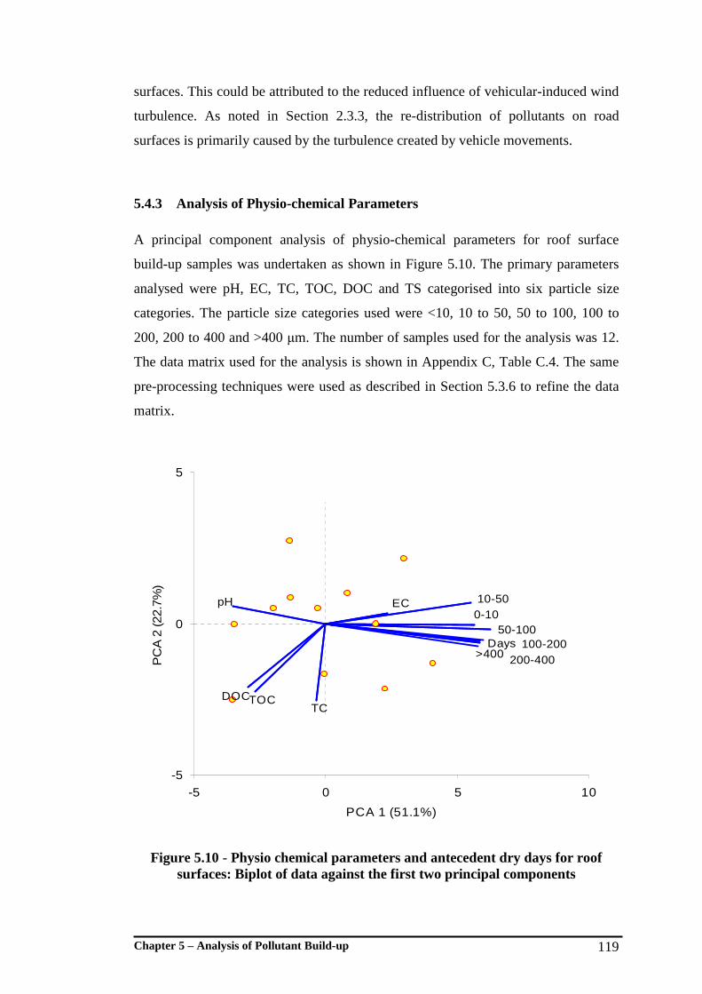
Chapter 5 – Analysis of Pollutant Build-up 119
surfaces. This could be attributed to the reduced influence of vehicular-induced wind
turbulence. As noted in Section 2.3.3, the re-distribution of pollutants on road
surfaces is primarily caused by the turbulence created by vehicle movements.
5.4.3 Analysis of Physio-chemical Parameters A principal component analysis of physio-chemical parameters for roof surface
build-up samples was undertaken as shown in Figure 5.10. The primary parameters
analysed were pH, EC, TC, TOC, DOC and TS categorised into six particle size
categories. The particle size categories used were <10, 10 to 50, 50 to 100, 100 to
200, 200 to 400 and >400 µm. The number of samples used for the analysis was 12.
The data matrix used for the analysis is shown in Appendix C, Table C.4. The same
pre-processing techniques were used as described in Section 5.3.6 to refine the data
matrix.
Days
pH
EC
TC
TOC
DOC
0-10
10-50
50-100
100-200
200-400
>400
-5
0
5
-5 0 5 10
PCA 1 (51.1%)
PC
A 2
(22.
7%)
Figure 5.10 - Physio chemical parameters and antecedent dry days for roof surfaces: Biplot of data against the first two principal components
Chapter 5 – Analysis of Pollutant Build-up 120
The following conclusions can be derived from the resulting biplot:
1) All particle classes strongly correlate with each other and with the antecedent dry
days;
2) EC strongly correlates with all particle size groups whereas pH shows strong
negative correlation with all the particle size classes; and
3) TC shows no correlation with the particle size groups whereas TOC and DOC
show partial negative correlation.
The strong correlation of all the particle size groups to antecedent dry days indicates
the increase in pollutant load with the increase in antecedent dry days. This further
strengthens the conclusions relating to the characteristics of build-up as discussed in
Section 5.4.2. However, in contrast to road surface build-up where particles less than
100 µm were subjected to a high degree of re-distribution, roof surface build-up does
not indicate significant re-distribution of pollutants. This could be primarily due to
the high elevation of roofs where vehicular-induced turbulence is limited.
The strong correlation of EC with particle size groups supports the increase in the
ionic nature of build-up solids. The strong negative correlation of pH shows the
increased of acidic nature of build-up solids. The acidic nature of the atmospheric
depositions was confirmed by Novotny et al. (1985). The non correlation of TC and
the relatively poor negative correlation of TOC and DOC with particle size groups
indicate that there is no variation of these pollutants when the antecedent dry days
increase. This was further confirmed by the relatively similar concentrations of TC,
TOC and DOC for all the antecedent dry days. It was observed that 95% of the TC is
organic and around 80% of the organic carbon is in soluble format. The high fraction
of DOC and the high acidic nature of build-up samples confirm the strong capacity to
enhance the solubility of other pollutants such as heavy metals and hydrocarbons
(Hamilton et al., 1984; Pechacek, 1994; Tai, 1991; Warren et al., 2003).

Chapter 5 – Analysis of Pollutant Build-up 121
5.5 Conclusions The analysis of build-up samples from road and roof surfaces was critical to
understand the processes involved in pollutant build-up and related influential
parameters.
Build-up on road surfaces
• Rate of pollutant build-up is significantly high during the first two days and
reduces as the dry period increases. This is in agreement with the already
understood build-up process.
• It can be hypothesised that build-up load approaches a constant value over time.
• Significant variation in terms of build-up load was detected between the three
road sites. This could be primarily due to the variation in urban-form and the
population density.
• Pollutant build-up on road surfaces can be replicated by a power function in the
form of:
baDB =
Where,
B = Build-up load on road surface (g/m2);
D = Antecedent dry days; and
a and b = Build-up coefficients.
• Though the rate of increase of build-up load reduces after about 21 days, the
dynamic re-distribution of fine particles continues.
• Reduced re-distribution of larger particles and constant accumulation result in
changes to the solids composition of build-up pollutants.
• The fraction of fine particles (<100 µm) dominates on road surfaces. The average
road surface particle size composition demonstrates unique characteristics for
residential catchments.
• The behaviour of fine particle (<100 µm) was completely different to that of
coarse particles in terms of associated organic content. The fine particles were
associated with a greater amount of organic matter compared to coarser particles.
• A reduced fraction of inorganic carbon content was detected on road surfaces
compared to organic carbon. Furthermore, a significantly high fraction of organic
compounds present in road surface pollutants were in soluble form.

Chapter 5 – Analysis of Pollutant Build-up 122
Build-up on roof surfaces
• The rate of build-up is significantly high for up to around seven days and then
reduces after that as the antecedent dry period progresses.
• Similar to build-up on road surfaces, it can be hypothesised that roof surface
build-up approaches a constant value as the antecedent dry period progresses.
• Build-up on roof surfaces can be replicated by a power function similar to that
used for road surfaces. However, a different set of build-up coefficients needs to
be used.
• On average, 60% of the solids deposited on roof surfaces were less than 100 µm
size.
• Only a small variation was detected in the particle size distribution of particulates
belonging to different antecedent dry periods. This suggested that on roof
surfaces there is only limited re-distribution with time.
• A significantly high amount of organic compounds was detected on roof
surfaces. Most of these compounds were in soluble form.

Chapter 6 – Analysis of Pollutant Wash-off 123
Chapter 6 - Analysis of Pollutant Wash-off
6.1 Background
In the context of urban water quality research, an in-depth understanding of the two
main pollutant processes, build-up and wash-off, is important. Due to the site specific
nature and variability with a range of factors, extensive investigations are necessary
to understand these processes. Chapter 5 discussed the outcomes of the in-depth
investigation into pollutant build-up for residential road and roof surfaces. This
chapter presents the outcomes of in-depth investigation into pollutant wash-off from
road and roof surfaces.
Pollutant wash-off is a complex process that varies with a range of rainfall, runoff,
and catchment variables. Vaze and Chiew (2002) and Mackay (1999) noted that
wash-off is influenced by rainfall and runoff variables namely, rainfall intensity,
duration, runoff volume and runoff rate. However, as explained by Chiew and
McMahon (1999), it is difficult to discern the degree of influence of these variables
on wash-off. Inter-correlation of these variables is the primary factor which causes
such difficulty. Therefore, extra effort was made during the data analysis to
understand the role of each variable in wash-off. Other than rainfall and runoff
parameters, wash-off is influenced by the amount and characteristics of pollutants
available on catchment surfaces, which in turn are a function of build-up during the
antecedent dry period (Duncan, 1995). Representative pollutant samples were
collected before the wash-off investigations and tested for physio-chemical
parameters to understand the influence exerted on pollutant wash-off. Furthermore,
Herngren et al. (2005a) noted that wash-off may be influenced by the characteristics
of impervious surfaces. They observed variable characteristics of wash-off for road
surfaces with road surface texture depth and slope. Therefore, the influence of these
two primary road surface characteristic namely, texture depth and slope was also
determined.
The highly variable nature of wash-off with a range of parameters and unpredictable
occurrence of natural events can increase the complexity of the experimental design.

Chapter 6 – Analysis of Pollutant Wash-off 124
This was the main reason for using simulated rainfall for wash-off investigations.
The use of simulated rainfall provided improved control over rainfall and runoff
parameters. Furthermore, it was possible to generate a large amount of data during a
short period of time (Herngren et al., 2005b). Detailed discussion on the use of
simulated rainfall can be found in Section 3.3.
This chapter presents the analytical outcomes of the pollutant wash-off investigations
described in Section 4.3. The investigations were undertaken on three road sites,
namely, Gumbeel Court, Lauder Court and Piccadilly Place, and two roof surface
types, namely, corrugated steel and concrete tile. The wash-off samples collected
during investigations were tested for a range of water quality parameters as discussed
in Section 4.6. Wash-off was separately analysed for road and roof surfaces. During
the analysis, the primary focus was to understand the quantitative wash-off process,
variation of particulate composition of washed-off pollutants and the variation of
quality parameters. Prior to the analysis of wash-off data, analysis was performed to
understand the primary characteristics of initially available pollutants which were
collected before each field test.
6.2 Initially Available Pollutants Duncan (1995) noted that the pollutant load originating from catchments is directly
influenced by the amount of initially available pollutants on catchment surfaces. He
further suggested that the initially available pollutants may be influenced by the
antecedent dry period. This concept was confirmed by Sartor et al. (1974) noting that
wash-off is highly influenced by the characteristics of initially available pollutants
particularly the particle size distribution. They proposed a mathematical equation for
the replication of pollutant wash-off and noted that the validity of the equation is
improved if different sets of parameters were developed for different particle size
ranges.
Initially available pollutant samples were collected prior to wash-off investigations
from both road and roof surfaces. Road surface samples were collected from a 3 m2
plot area at each site using the vacuum system. Roof surface samples were collected
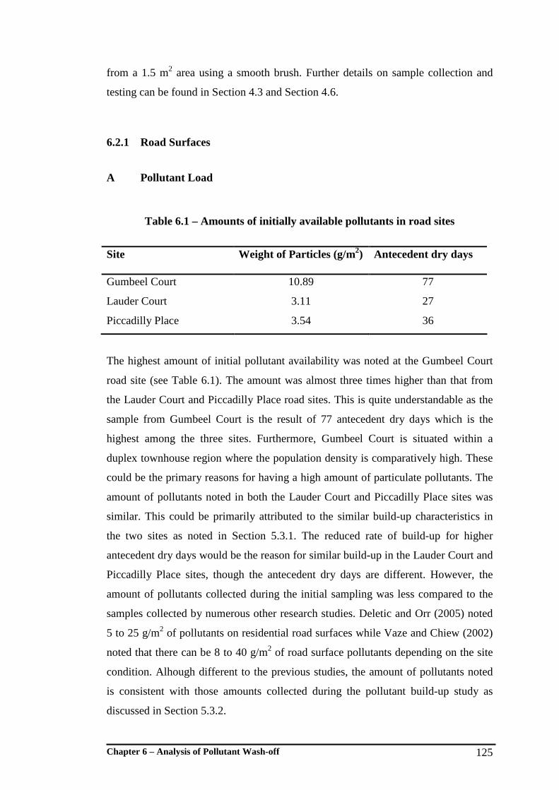
Chapter 6 – Analysis of Pollutant Wash-off 125
from a 1.5 m2 area using a smooth brush. Further details on sample collection and
testing can be found in Section 4.3 and Section 4.6.
6.2.1 Road Surfaces
A Pollutant Load
Table 6.1 – Amounts of initially available pollutants in road sites
Site Weight of Particles (g/m2) Antecedent dry days
Gumbeel Court 10.89 77
Lauder Court 3.11 27
Piccadilly Place 3.54 36
The highest amount of initial pollutant availability was noted at the Gumbeel Court
road site (see Table 6.1). The amount was almost three times higher than that from
the Lauder Court and Piccadilly Place road sites. This is quite understandable as the
sample from Gumbeel Court is the result of 77 antecedent dry days which is the
highest among the three sites. Furthermore, Gumbeel Court is situated within a
duplex townhouse region where the population density is comparatively high. These
could be the primary reasons for having a high amount of particulate pollutants. The
amount of pollutants noted in both the Lauder Court and Piccadilly Place sites was
similar. This could be primarily attributed to the similar build-up characteristics in
the two sites as noted in Section 5.3.1. The reduced rate of build-up for higher
antecedent dry days would be the reason for similar build-up in the Lauder Court and
Piccadilly Place sites, though the antecedent dry days are different. However, the
amount of pollutants collected during the initial sampling was less compared to the
samples collected by numerous other research studies. Deletic and Orr (2005) noted
5 to 25 g/m2 of pollutants on residential road surfaces while Vaze and Chiew (2002)
noted that there can be 8 to 40 g/m2 of road surface pollutants depending on the site
condition. Alhough different to the previous studies, the amount of pollutants noted
is consistent with those amounts collected during the pollutant build-up study as
discussed in Section 5.3.2.
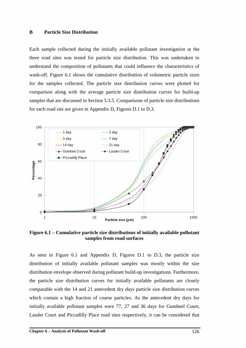
Chapter 6 – Analysis of Pollutant Wash-off 126
B Particle Size Distribution
Each sample collected during the initially available pollutant investigation at the
three road sites was tested for particle size distribution. This was undertaken to
understand the composition of pollutants that could influence the characteristics of
wash-off. Figure 6.1 shows the cumulative distribution of volumetric particle sizes
for the samples collected. The particle size distribution curves were plotted for
comparison along with the average particle size distribution curves for build-up
samples that are discussed in Section 5.3.5. Comparisons of particle size distributions
for each road site are given in Appendix D, Figures D.1 to D.3.
0
20
40
60
80
100
1 10 100 1000Particle size (µm)
Per
cen
tag
e
1 day 2 day
3 day 7 day
14 day 21 day
Gumbee Court Lauder Court
Piccadilly Place
Figure 6.1 – Cumulative particle size distributions of initially available pollutant samples from road surfaces
As seen in Figure 6.1 and Appendix D, Figures D.1 to D.3, the particle size
distribution of initially available pollutant samples was mostly within the size
distribution envelope observed during pollutant build-up investigations. Furthermore,
the particle size distribution curves for initially available pollutants are closely
comparable with the 14 and 21 antecedent dry days particle size distribution curves
which contain a high fraction of coarse particles. As the antecedent dry days for
initially available pollutant samples were 77, 27 and 36 days for Gumbeel Court,
Lauder Court and Piccadilly Place road sites respectively, it can be considered that

Chapter 6 – Analysis of Pollutant Wash-off 127
the particle size composition of particulates is in the expected range. Furthermore, as
seen in Figure 6.1, the distribution curve for the Gumbeel Court site is located to the
right of the curves for Lauder Court and Piccadilly Place road sites, particularly for
the coarser particle size ranges. This indicates a higher fraction of coarser particles in
Gumbeel Court site compared to the other two sites. This further strengthens the
argument developed regarding the change in particle size distribution of build-up
samples when the antecedent dry days increase. As explained in Section 5.3.5, the
composition of pollutants is subjected to continuous change with an increasing
fraction of coarse particles when the antecedent dry days increase.
Figure 6.1 and Appendix D, Figures D.1 to D.3, further show that only around 30%
of the total initially available pollutants were smaller than 100 µm particle size. As
discussed in Section 5.3.6, this is the size range that has the capacity to adsorb other
pollutants such as heavy metals and hydrocarbons. On the other hand, 40% of the
particulate pollutants were larger than 200 µm, where very limited pollutant
adsorption capacity exists. The samples collected during this investigation show
significant deviations from the samples collected by Herngren et al. (2005). They
have noted up to 90% of the solid particles being less than the 150 µm size.
However, the antecedent dry periods for those samples were 1, 2 and 7 days, which
is comparatively low when compared to this investigation.
6.2.2 Roof Surfaces A Pollutant Load
Four samples of initially available pollutants were collected from each roof type
prior to each rainfall simulation. The rainfall simulations were for 20, 40, 86 and 115
mm/hr intensities. Table 6.2 shows the average pollutant loads collected from each
roof type. The collection of samples was generally for a seven day antecedent dry
period apart from the sample collected prior to simulation of the 20 mm/hr intensity
which was a three day period.
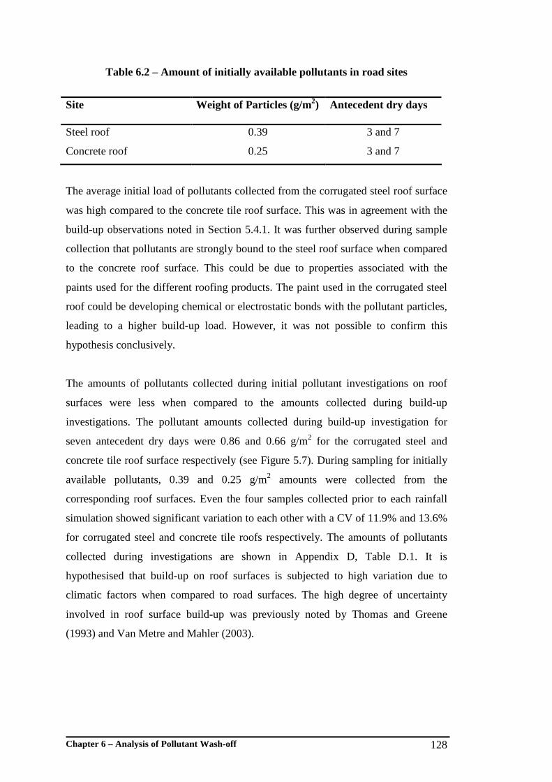
Chapter 6 – Analysis of Pollutant Wash-off 128
Table 6.2 – Amount of initially available pollutants in road sites
Site Weight of Particles (g/m2) Antecedent dry days
Steel roof 0.39 3 and 7
Concrete roof 0.25 3 and 7
The average initial load of pollutants collected from the corrugated steel roof surface
was high compared to the concrete tile roof surface. This was in agreement with the
build-up observations noted in Section 5.4.1. It was further observed during sample
collection that pollutants are strongly bound to the steel roof surface when compared
to the concrete roof surface. This could be due to properties associated with the
paints used for the different roofing products. The paint used in the corrugated steel
roof could be developing chemical or electrostatic bonds with the pollutant particles,
leading to a higher build-up load. However, it was not possible to confirm this
hypothesis conclusively.
The amounts of pollutants collected during initial pollutant investigations on roof
surfaces were less when compared to the amounts collected during build-up
investigations. The pollutant amounts collected during build-up investigation for
seven antecedent dry days were 0.86 and 0.66 g/m2 for the corrugated steel and
concrete tile roof surface respectively (see Figure 5.7). During sampling for initially
available pollutants, 0.39 and 0.25 g/m2 amounts were collected from the
corresponding roof surfaces. Even the four samples collected prior to each rainfall
simulation showed significant variation to each other with a CV of 11.9% and 13.6%
for corrugated steel and concrete tile roofs respectively. The amounts of pollutants
collected during investigations are shown in Appendix D, Table D.1. It is
hypothesised that build-up on roof surfaces is subjected to high variation due to
climatic factors when compared to road surfaces. The high degree of uncertainty
involved in roof surface build-up was previously noted by Thomas and Greene
(1993) and Van Metre and Mahler (2003).

Chapter 6 – Analysis of Pollutant Wash-off 129
B Particle Size Distribution
As samples were collected before each rainfall simulation, four data sets of particle
size distributions were available for analysis. Figure 6.2 shows the particle size
distribution curves for the concrete tile and corrugated steel roofs separately. The
particle size distributions of build-up samples are also shown.
Figure 6.2 – Cumulative particle size distributions of initially available pollutant samples
As evident in Figure 6.2, the particle size distributions for samples collected from
both concrete and steel roof surfaces are similar. For both surfaces, samples show
fairly uniform distribution with dominant finer particles size ranges. On average,
75% of the total solids from the corrugated steel roof and 67% of the total solids

Chapter 6 – Analysis of Pollutant Wash-off 130
from the concrete tile roof are less than 100 µm. However, the observed particle size
distribution is significantly coarser when compared to the results reported by Van
Metre and Mahler (2003). They noted a much smaller fraction of solids from roof
surfaces which were larger than 63 µm. Anthropogenic activities and climatic
conditions in the area adjacent to the study site could be a factor for such deviation in
particle size. However, the fact that the size distributions for all the samples collected
are within the particle size envelope generated during build-up investigations
confirmed the consistency of the investigations.
6.3 Data and Variables
Pollutant wash-off was investigated using simulated rainfall. As noted in Sections
4.4.1 and 4.4.2, six rainfall intensities on road surfaces and four intensities on roof
surfaces were simulated. The resulting runoff totalled 25 samples per road site and
27 samples per roof surface. These samples were tested for a range of water quality
parameters as discussed in Section 4.6. The parameters included TSS, TDS, particle
size distribution, pH, EC, TC, TOC and DOC.
6.3.1 Data Pre-processing
Total solids (TS) concentration was calculated by combining TSS and TDS. The TS
concentration was multiplied by the runoff volume contained in each container in
order to calculate the total weight of solids washed-off during a specific simulation
event. The cumulative wash-off weight was calculated by adding the solids weight to
the corresponding duration components. For example, in the case of the 20mm/hr
intensity and 20 min duration event, TS weight was calculated by adding the weights
belonging to the 0-10 min duration and the 10-20 min duration.
A Malvern Mastersizer was used to determining the particle size distribution of the
suspended solids. The instrument software provided the percentage particle size
distribution curve and it was possible to disaggregate the sample into any given size
class at a later stage. However, the percentages are in volumetric form. For analytical
purposes, it was converted to weight distribution assuming that all particles have the

Chapter 6 – Analysis of Pollutant Wash-off 131
same density. It is understood that there can be particles such as tyre wear having
relatively less density compared to road surface wear. Pre-processing of the other
quality parameters was done in an exactly similar way to the pre-processing of build-
up samples noted in Section 5.2.
6.3.2 Selection of Rainfall and Runoff Variables
The primary rainfall and runoff variables that influence pollutant wash-off are
rainfall intensity, rainfall duration and runoff volume. Contradictory reporting has
been noted on the degree of influence that these variables have on pollutant wash-off
(Chiew and McMahon, 1999; Chui, 1997; Mackay, 1999). As explained by Chiew
and McMahon (1999), these variables correlate with each other and therefore, it is
difficult to discern the degree of influence. From an analytical point of view, it is
difficult to analyse data with a range of correlating variables. It is important to
eliminate variables that provide little information from the analysis.
Selection of appropriate variables was undertaken using a range of plotted graphs of
TS with each variable and combination of variables. It was observed that very little
information can be gained by relating wash-off to runoff volume. Therefore, it was
decided to select rainfall intensity and duration as primary variables. Further analysis
of wash-off was based on these two variables. The same two variables were also used
by Sartor et al. (1974) to describe the wash-off process.
6.4 Analysis of Wash-off from Road Surfaces
The six rainfall intensities simulated on road surfaces were 20, 40, 65, 86, 115 and
133 mm/hr. Five runoff samples from 133 mm/hr rainfall intensity and four samples
from each of the other intensities were collected. The rainfall durations from which
these samples were collected are shown in Table 4.3. Further details on sample
collection and testing were provided in Sections 4.4.1 and 4.6.
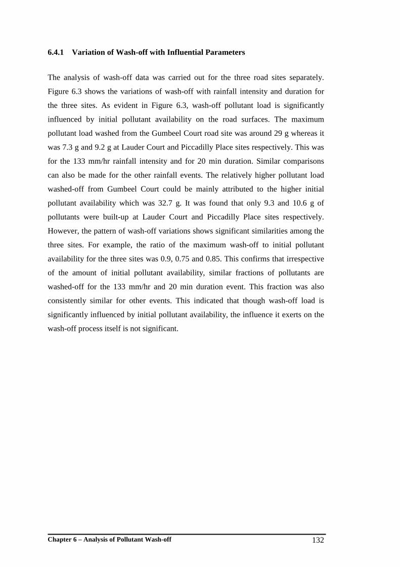
Chapter 6 – Analysis of Pollutant Wash-off 132
6.4.1 Variation of Wash-off with Influential Parameters
The analysis of wash-off data was carried out for the three road sites separately.
Figure 6.3 shows the variations of wash-off with rainfall intensity and duration for
the three sites. As evident in Figure 6.3, wash-off pollutant load is significantly
influenced by initial pollutant availability on the road surfaces. The maximum
pollutant load washed from the Gumbeel Court road site was around 29 g whereas it
was 7.3 g and 9.2 g at Lauder Court and Piccadilly Place sites respectively. This was
for the 133 mm/hr rainfall intensity and for 20 min duration. Similar comparisons
can also be made for the other rainfall events. The relatively higher pollutant load
washed-off from Gumbeel Court could be mainly attributed to the higher initial
pollutant availability which was 32.7 g. It was found that only 9.3 and 10.6 g of
pollutants were built-up at Lauder Court and Piccadilly Place sites respectively.
However, the pattern of wash-off variations shows significant similarities among the
three sites. For example, the ratio of the maximum wash-off to initial pollutant
availability for the three sites was 0.9, 0.75 and 0.85. This confirms that irrespective
of the amount of initial pollutant availability, similar fractions of pollutants are
washed-off for the 133 mm/hr and 20 min duration event. This fraction was also
consistently similar for other events. This indicated that though wash-off load is
significantly influenced by initial pollutant availability, the influence it exerts on the
wash-off process itself is not significant.
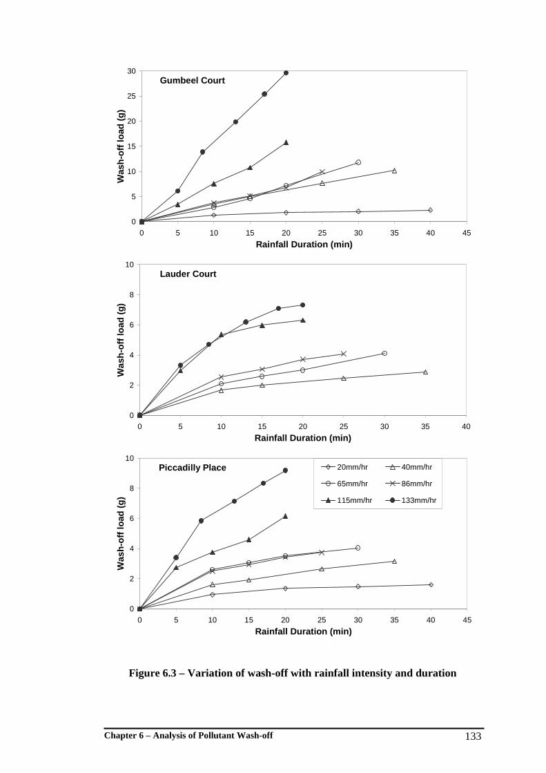
Chapter 6 – Analysis of Pollutant Wash-off 133
Lauder Court
0
2
4
6
8
10
0 5 10 15 20 25 30 35 40
Rainfall Duration (min)
Was
h-o
ff lo
ad (
g)
Gumbeel Court
0
5
10
15
20
25
30
0 5 10 15 20 25 30 35 40 45
Rainfall Duration (min)
Was
h-o
ff lo
ad (
g)
Piccadilly Place
0
2
4
6
8
10
0 5 10 15 20 25 30 35 40 45
Rainfall Duration (min)
Was
h-o
ff lo
ad (
g)
20mm/hr 40mm/hr
65mm/hr 86mm/hr
115mm/hr 133mm/hr
Figure 6.3 – Variation of wash-off with rainfall intensity and duration

Chapter 6 – Analysis of Pollutant Wash-off 134
In order to eliminate the influence of initial pollutant availability on the wash-off
process, a parameter defined as ‘fraction wash-off’ was calculated. Fraction wash-off
for a particular event is the ratio of washed-off pollutant load to the initially available
load. In this way, it was possible to compare the wash-off of pollutants from the three
road sites. Figure 6.4 shows the variation of fraction wash-off with rainfall intensity
and duration for all three sites. Appendix D, Figure D.4 shows the variation of
fraction wash-off with rainfall intensity and duration for the individual sites.
Appendix D, Table D.2 shows the observed data for pollutant loads and calculated
fraction wash-off for each site.
0
0.2
0.4
0.6
0.8
1
0 10 20 30 40
Rainfall Duration (min)
Fra
ctio
n W
ash
-off
Gum 20mm/hr Gum 40mm/hr Gum 65mm/hr
Gum 86mm/hr Gum 115mm/hr Gum 133mm/hr
Lau 40mm/hr Lau 65mm/hr Lau 86mm/hr
Lau 115mm/hr Lau 133mm/hr Pic 20mm/hr
Pic 40mm/hr Pic 65mm/hr Pic 86mm/hr
Pic 115mm/hr Pic 133 mm/hr
Figure 6.4– Variation of fraction wash-off with rainfall intensity and duration
From Figure 6.4 and Appendix D, Figure D.4, two main conclusions can be derived.
Firstly, the largest fraction wash-off is in the range of 0.75 to 0.9 and these values
belong to the 133 mm/hr intensity rainfall simulated for 20 min duration. In
comparison to rain events in South-East Queensland, such an event is in the range of
a ten year ARI event. This means that most of the general storm events are not
capable of washing-off all the pollutants from road surfaces. Similar conclusions
133 mm/hr Cluster

Chapter 6 – Analysis of Pollutant Wash-off 135
were noted by past researchers. Malmquist (1978) repeatedly simulated rain events
on an urban road section. The resulting wash-off load decreased slowly in each
simulation and multiple numbers of events were needed for significant reduction in
wash-off load. Vaze and Chiew (2002) vacuumed road surfaces immediately after
rain events and noted an appreciable fraction of pollutants still remaining on the
surface.
Secondly, the variation of fraction wash-off for different road sites is closely related.
For the 20 mm/hr rainfall intensity, fraction wash-off increases gradually up to
around 0.2 as the duration increases. Similar variation is evident for other intensities.
Furthermore, the gradient of the variation increases when the rainfall intensity
increases. As seen in Figure 6.4, the data points belonging to each rainfall intensity
are clustered into regions suggesting similar behaviour of wash-off for all three sites.
As an example, the cluster for 133 mm/hr intensity is shown in Figure 6.4. Therefore,
it can be concluded that wash-off is a common process and relatively independent
from initial pollutant availability.
6.4.2 Mathematical Replication of Pollutant Wash-off
It is commonly accepted that wash-off from road surfaces can be replicated by an
exponential equation. However, different forms of exponential equations have been
suggested (Chiew et al., 1997; Sartor et al., 1974). The use of different rainfall and
runoff parameters as exponents of the wash-off exponential equation is the most
common difference among various equations that have been proposed. In some
cases, runoff volume is used as the exponent and in some other cases the runoff rate
is used (Chiew et al., 1997). However, it was concluded (see Section 6.3.2) from this
research that wash-off is more closely related to rainfall intensity. Therefore, the
equation proposed by Sartor et al. (1974) was selected as the conceptual basis for the
replication of wash-off. The format of the selected equation is:
)1(0kIteWW −−= Equation 6.1
Where:
W Weight of the material mobilised after time t;
W0 Initial weight of the material on the surface;
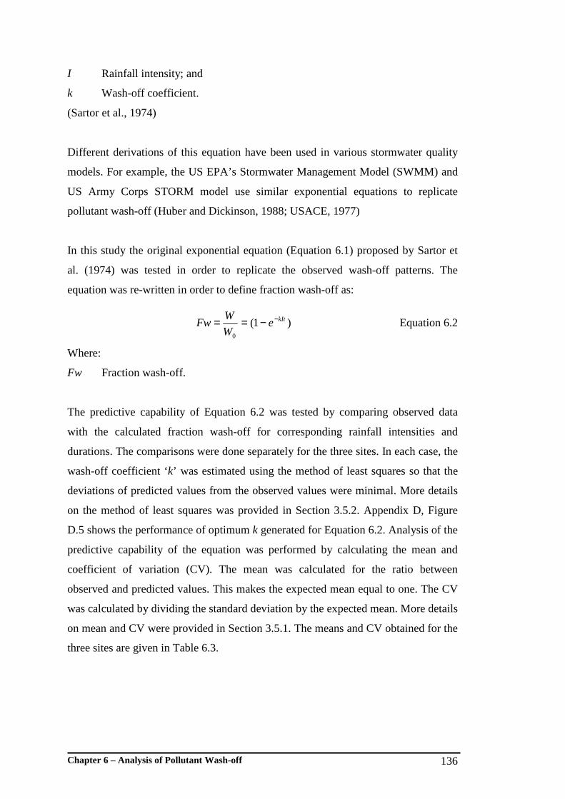
Chapter 6 – Analysis of Pollutant Wash-off 136
I Rainfall intensity; and
k Wash-off coefficient.
(Sartor et al., 1974)
Different derivations of this equation have been used in various stormwater quality
models. For example, the US EPA’s Stormwater Management Model (SWMM) and
US Army Corps STORM model use similar exponential equations to replicate
pollutant wash-off (Huber and Dickinson, 1988; USACE, 1977)
In this study the original exponential equation (Equation 6.1) proposed by Sartor et
al. (1974) was tested in order to replicate the observed wash-off patterns. The
equation was re-written in order to define fraction wash-off as:
)1(0
kIteW
WFw −−== Equation 6.2
Where:
Fw Fraction wash-off.
The predictive capability of Equation 6.2 was tested by comparing observed data
with the calculated fraction wash-off for corresponding rainfall intensities and
durations. The comparisons were done separately for the three sites. In each case, the
wash-off coefficient ‘k’ was estimated using the method of least squares so that the
deviations of predicted values from the observed values were minimal. More details
on the method of least squares was provided in Section 3.5.2. Appendix D, Figure
D.5 shows the performance of optimum k generated for Equation 6.2. Analysis of the
predictive capability of the equation was performed by calculating the mean and
coefficient of variation (CV). The mean was calculated for the ratio between
observed and predicted values. This makes the expected mean equal to one. The CV
was calculated by dividing the standard deviation by the expected mean. More details
on mean and CV were provided in Section 3.5.1. The means and CV obtained for the
three sites are given in Table 6.3.

Chapter 6 – Analysis of Pollutant Wash-off 137
Table 6.3 – Predictive capability of Equation 2
Site Mean Coefficient of Variation (%)
Gumbeel Court 1.41 53.0
Lauder Court 1.04 22.7
Piccadilly Place 1.09 28.4
As evident from Appendix D, Figure D.5, predictions using Equation 6.2 do not
provide adequate accuracy. As shown in Table 6.3, though the mean is close to one,
which is the expected value, higher percentages of CV suggested a scattering of
observed data with respect to predictions using Equation 6.2. Among the three road
sites, the predictions were least accurate for the Gumbeel Court site, where the mean
is 1.41 and CV is 53%.
It is evident from Figure 6.4 and Appendix D, Figure D.4, that the fraction wash-off
approaches a finite value which is lower than one and this value varies with the
rainfall intensity. This phenomenon was observed during the rainfall simulation. The
latter part of most of the less intense rainfall events producesd relatively cleaner
runoff. A similar observation was also reported by Herngren et al. (2005a). This
suggested that a rainfall event has the capacity to mobilise only a fraction of
particulate pollutants on the road surface and once it reaches that capacity relatively
clean runoff results, even though a significant fraction of pollutants is still available
for removal. The equation proposed by Sartor et al. (1974) is based on the
assumption that every storm event has the capacity to remove all the available
pollutants from a surface if it were to continue for an adequate period of time. The
findings from this study confirmed the need to modify the wash-off equation.
The exponential pollutant wash-off equation was modified by introducing the
‘capacity factor’ (CF) and can be written as:
)1(0
kItF eC
W
WFw −−== Equation 6.3
Where:
CF Capacity factor.

Chapter 6 – Analysis of Pollutant Wash-off 138
CF indicates the rainfall event’s capacity to mobilise pollutants. CF will have a value
ranging from 0 to 1 primarily depending on the rainfall intensity. However, other
factors such as road surface condition, characteristics of the available pollutants and
slope of the road may also have an influence on CF.
6.4.3 Estimation of Wash-off Parameters
To use the modified wash-off equation (Equation 6.3), the parameters k and CF must
be estimated. The wash-off coefficient k is an empirical parameter with units (mm-1)
with no physical meaning. Water quality models such as SWMM use a constant
value for k. However, there is evidence to claim that the k is site specific (Millar,
1999). The value k may vary with the pollutant type, rainfall intensity, catchment
area and catchment slope (Alley 1981; Alley and Smith, 1981; Millar, 1999).
However, the use of a constant value for k will reduce the complexity of the wash-off
equation. It has been noted by Huber and Dickinson (1988) that a constant value is
used in the SWMM model and it performs relatively well in estimation.
Estimation of wash-off parameters was done in three steps:
1) The approximate values were first estimated for CF by plotting FW versus rainfall
duration. The curves were drawn freehand in order to obtain the best visual
variation. Appendix D, Figure D.6 shows the plotted variations and estimated CF
values.
2) The best possible values for CF and k were determined using the method of least
squares. In this case, estimates obtained using plots were used as initial values.
3) A single value was determined for k so that the square of difference between
estimated and observed values of FW for one site is a minimum. Figure 6.5
illustrates the performance of the parameters developed for Equation 6.3, and
Table 6.4 gives the CF and k values determined for the different sites.

Chapter 6 – Analysis of Pollutant Wash-off 139
Figure 6.5 – Performance of the replication equation (Equation 6.3)
Chapter 6 – Analysis of Pollutant Wash-off 140
Table 6.4 - Estimated values for CF and k
Capacity Factor CF Site
Wash-off Coefficient k 20
mm/hr 40
mm/hr 65
mm/hr 86
mm/hr 115
mm/hr 133
mm/hr
Gumbeel Court 5.6 x 10⁻⁴ 0.20 0.48 0.50 0.50 0.73 1.00
Lauder Court 8.0 x 10⁻⁴ - 0.48 0.54 0.54 0.80 0.89
Piccadilly Place 8.0 x 10⁻⁴ 0.30 0.45 0.49 0.49 0.66 0.94
The validity of Equation 6.3 with estimated parameters of CF and k was evaluated by
analysing the mean and CV. The combination of mean and CV provides complete
information on the validity of the predicted equation. The mean was calculated for
the resultant of the predicted values divided by the observed value for each data
point. CV was calculated by dividing the standard deviation from the expected return
which was one. The mean and CV for each site are shown in Table 6.5.
Table 6.5 – Validity of replication of pollutant wash-off using parameters in Table 6.4
According to the results shown in Table 6.5, all three mean values are close to one
and therefore, it can be argued that the overall performance of the prediction
equation is satisfactory. However, the CV values indicate that there is a certain
degree of error in estimating each data point. The performance of the wash-off
equation for the Gumbeel Court data is poor whereas the performance of the equation
for Lauder Court and Piccadilly Place are satisfactory. The variation between
observed data and predicted data could be due to reasons such as the build-up data
being non-representative for the site and errors in the calculation of the equation
parameters. The Gumbeel Court site had a relatively high amount of pollutants. As
such there can be a greater possibility of selecting a non-representative sample.
Parameter Gumbeel Court Lauder Court Piccadilly Place
Mean 1.12 0.98 0.98
CV 27% 7% 12%
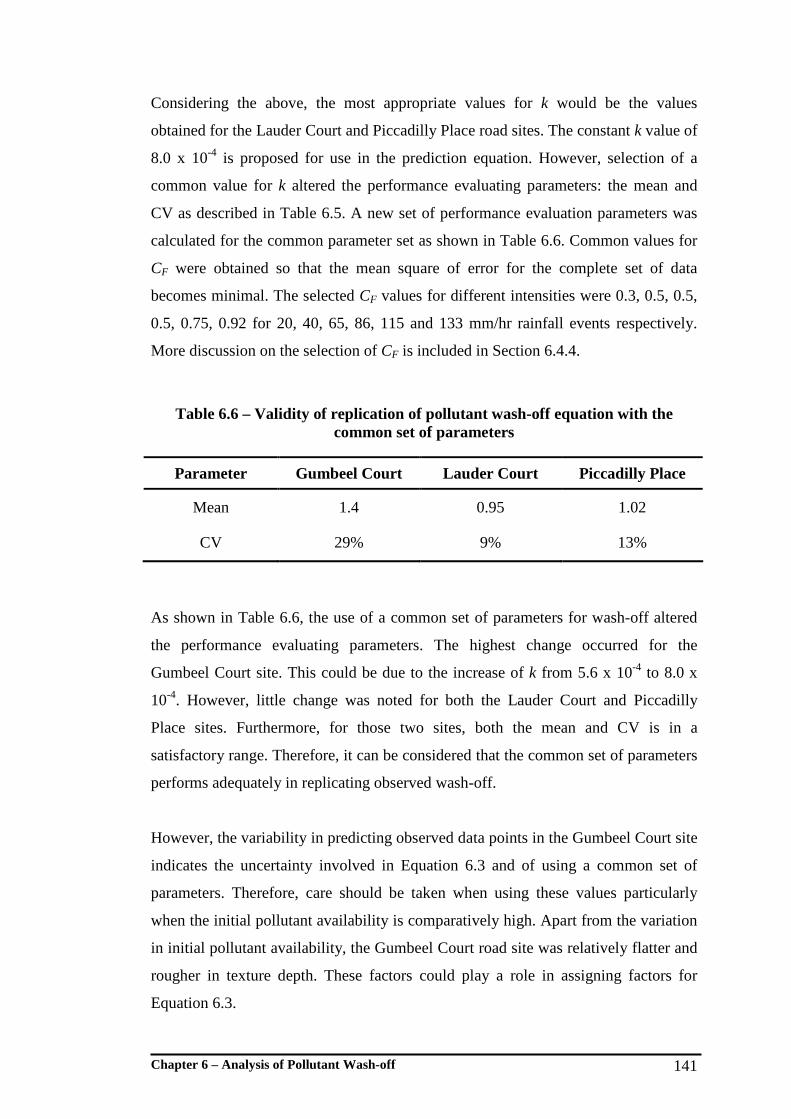
Chapter 6 – Analysis of Pollutant Wash-off 141
Considering the above, the most appropriate values for k would be the values
obtained for the Lauder Court and Piccadilly Place road sites. The constant k value of
8.0 x 10⁻⁴ is proposed for use in the prediction equation. However, selection of a
common value for k altered the performance evaluating parameters: the mean and
CV as described in Table 6.5. A new set of performance evaluation parameters was
calculated for the common parameter set as shown in Table 6.6. Common values for
CF were obtained so that the mean square of error for the complete set of data
becomes minimal. The selected CF values for different intensities were 0.3, 0.5, 0.5,
0.5, 0.75, 0.92 for 20, 40, 65, 86, 115 and 133 mm/hr rainfall events respectively.
More discussion on the selection of CF is included in Section 6.4.4.
Table 6.6 – Validity of replication of pollutant wash-off equation with the common set of parameters
As shown in Table 6.6, the use of a common set of parameters for wash-off altered
the performance evaluating parameters. The highest change occurred for the
Gumbeel Court site. This could be due to the increase of k from 5.6 x 10⁻⁴ to 8.0 x
10-4. However, little change was noted for both the Lauder Court and Piccadilly
Place sites. Furthermore, for those two sites, both the mean and CV is in a
satisfactory range. Therefore, it can be considered that the common set of parameters
performs adequately in replicating observed wash-off.
However, the variability in predicting observed data points in the Gumbeel Court site
indicates the uncertainty involved in Equation 6.3 and of using a common set of
parameters. Therefore, care should be taken when using these values particularly
when the initial pollutant availability is comparatively high. Apart from the variation
in initial pollutant availability, the Gumbeel Court road site was relatively flatter and
rougher in texture depth. These factors could play a role in assigning factors for
Equation 6.3.
Parameter Gumbeel Court Lauder Court Piccadilly Place
Mean 1.4 0.95 1.02
CV 29% 9% 13%
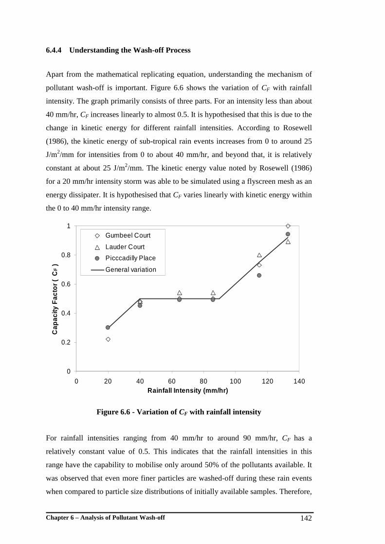
Chapter 6 – Analysis of Pollutant Wash-off 142
6.4.4 Understanding the Wash-off Process
Apart from the mathematical replicating equation, understanding the mechanism of
pollutant wash-off is important. Figure 6.6 shows the variation of CF with rainfall
intensity. The graph primarily consists of three parts. For an intensity less than about
40 mm/hr, CF increases linearly to almost 0.5. It is hypothesised that this is due to the
change in kinetic energy for different rainfall intensities. According to Rosewell
(1986), the kinetic energy of sub-tropical rain events increases from 0 to around 25
J/m2/mm for intensities from 0 to about 40 mm/hr, and beyond that, it is relatively
constant at about 25 J/m2/mm. The kinetic energy value noted by Rosewell (1986)
for a 20 mm/hr intensity storm was able to be simulated using a flyscreen mesh as an
energy dissipater. It is hypothesised that CF varies linearly with kinetic energy within
the 0 to 40 mm/hr intensity range.
0
0.2
0.4
0.6
0.8
1
0 20 40 60 80 100 120 140Rainfall Intensity (mm/hr)
Cap
acity
Fac
tor
(C
F)
Gumbeel Court
Lauder Court
Picccadilly Place
General variation
Figure 6.6 - Variation of CF with rainfall intensity
For rainfall intensities ranging from 40 mm/hr to around 90 mm/hr, CF has a
relatively constant value of 0.5. This indicates that the rainfall intensities in this
range have the capability to mobilise only around 50% of the pollutants available. It
was observed that even more finer particles are washed-off during these rain events
when compared to particle size distributions of initially available samples. Therefore,

Chapter 6 – Analysis of Pollutant Wash-off 143
there is greater possibility of wash-off of most of the finer and lighter particle ranges
during these events. It could be the case that these rainfall intensities are not capable
of creating adequate turbulence to mobilise heavier and larger particles due to sheet
flow on the surface. However, the upper limit of the constant CF (90 mm/hr) could
change with the texture depth of the road and particle size distribution of the
pollutants available. Rainfall events with intensity of more than 90 mm/hr have a
greater capability to mobilise particulate matter. It is hypothesised that this is due to
the high degree of turbulence in the overland flow. The pollutant export study
undertaken in the same urban catchment confirmed the higher mobilisation capacity
of high intensity rainfall events which results in relatively higher pollutant
concentrations and larger average size of the wash-off particles.
6.4.5 Particle Size Distribution Analysis
The factor CF indicates a specific rainfall event’s capacity to mobilise particulate
pollutants from paved surfaces. CF varies with rainfall characteristics and particularly
with rainfall intensity. However, the nature of this relationship is not clearly known.
For example, a 65 mm/hr rainfall event generally removes around 50% of the
pollutants available on the road surface. The reasons for the remainder of the 50% to
remain on the road surface needed to be understood. As noted by Mackay (1999),
raindrop-induced turbulence is the primary factor that keeps the particulate pollutants
in suspension. The kinetic energy in lateral flow is comparatively low compared to
raindrop kinetic energy. However, this is sufficient to move the particles that are
already in suspension.
A Variation of Particle Size Distribution with Rain fall Intensity
In order to better understand the regime governing pollutant wash-off, the particle
size distribution of each sample was analysed. The particle size distribution data was
in volumetric percentages and was converted to weights. More details on the pre-
processing of particle size distribution data can be found in Section 6.3.1. However,
the analysis was first undertaken to understand the variation of particle size
distribution with rainfall intensity. For this, the particle size distribution of the total

Chapter 6 – Analysis of Pollutant Wash-off 144
pollutant sample washed per each intensity was analysed. The weight-based particle
size distribution developed from the analysis is shown in Figure 6.7. Figure 6.7
further shows the particle size distribution of the initially available pollutant sample
so that a detailed comparison is possible.

Chapter 6 – Analysis of Pollutant Wash-off 145
Figure 6.7 – Variation of particle size distribution
Chapter 6 – Analysis of Pollutant Wash-off 146
Figure 6.7 leads to several important observations on the physical process of wash-
off. Firstly, it reveals that the higher fraction of wash-off particles is in the range of 0
to 200 µm. The average weight of washed-off particles less than 200 µm in size was
73%. The coarser range (>200 µm) shows only fractional increments in weight when
the rainfall intensity increases. Therefore, it is not reasonable to argue that the
increment in wash-off load with rainfall intensity is due to the increased capacity of
the rainfall in mobilising coarser particles. It is true that the weight of coarser
particles washed-off has increased with rainfall intensity. However, in comparison,
weight increment of finer particles is most significant. This suggested that there is a
fraction of finer particle size ranges which are not mobilised during less intense rain
events. These particles are subsequently mobilised when the rainfall intensity
increases. It is hypothesised that these finer particle size ranges remain on the road
surface due to their relatively high particle density or adhesion to the road surface
due to either physical or chemical bonding.
Secondly, as evident from Figure 6.7, the pattern of variation of average particle size
distribution for all the intensities is similar. For example, the curve for the 86 mm/hr
intensity is a close replicate of the 20 mm/hr curve with a multiplier. This suggests
that there is a similar particulate composition for all the intensities. This further
strengthens the influence of particle density in relation to wash-off. It would only be
the lower density particles and those only lightly adhering to the surface being
mobilised for smaller rainfall intensities. As the intensity increases, relatively higher
density particles and those more strongly bound to the surface would be mobilised
depending on the turbulence created by the rainfall.
Thirdly, in comparison to particle size distribution of initially available pollutants,
wash-off resulted in a higher amount of finer particles. As seen in Figure 6.7, the
weight of particles smaller than about 150 µm in wash-off samples is greater than
that of the initially available pollutant sample. Furthermore, the weight of particles in
the range of 150 to 600 µm in wash-off samples is significantly less compared to the
initially available pollutant sample. These observations point to the possible break-up
of coarser particles in this size range. This could occur due to the impact energy of
raindrops and turbulence in surface runoff.
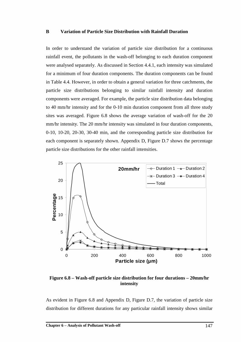
Chapter 6 – Analysis of Pollutant Wash-off 147
B Variation of Particle Size Distribution with Rainfall Duration
In order to understand the variation of particle size distribution for a continuous
rainfall event, the pollutants in the wash-off belonging to each duration component
were analysed separately. As discussed in Section 4.4.1, each intensity was simulated
for a minimum of four duration components. The duration components can be found
in Table 4.4. However, in order to obtain a general variation for three catchments, the
particle size distributions belonging to similar rainfall intensity and duration
components were averaged. For example, the particle size distribution data belonging
to 40 mm/hr intensity and for the 0-10 min duration component from all three study
sites was averaged. Figure 6.8 shows the average variation of wash-off for the 20
mm/hr intensity. The 20 mm/hr intensity was simulated in four duration components,
0-10, 10-20, 20-30, 30-40 min, and the corresponding particle size distribution for
each component is separately shown. Appendix D, Figure D.7 shows the percentage
particle size distributions for the other rainfall intensities.
Figure 6.8 – Wash-off particle size distribution for four durations – 20mm/hr intensity
As evident in Figure 6.8 and Appendix D, Figure D.7, the variation of particle size
distribution for different durations for any particular rainfall intensity shows similar
20mm/hr
0
5
10
15
20
25
0 200 400 600 800 1000Particle size (µm)
Per
cen
tag
e
Duration 1 Duration 2
Duration 3 Duration 4
Total

Chapter 6 – Analysis of Pollutant Wash-off 148
characteristics. For all the durations, the highest weight percentage of particles is in
the 0 to 150 µm range. Therefore, it can be argued that the particulate composition of
wash-off throughout a constant intensity rain event is fairly uniform. This would
mean that the influence of rainfall duration on wash-off particle size distribution is
minimal.
It was further observed that a significant fraction of solids is being washed-off during
the initial period of the rainfall simulations. Table 6.7 gives the weight percentages
of washed-off particulates for different intensities and duration components.
According to Table 6.7, the highest percentage of particulates is removed during the
initial period of the storm for all rainfall intensities. This strengthens the concept of
‘first flush’ where the initial period of a runoff event produces a higher pollutant
concentration and a concentration peak often preceding the runoff peak (Duncan,
1995; Lee et al., 2002).
Table 6.7 – Percentage wash-off for different intensities and durations
Pollutant Load Percentage (%)
Intensity
(mm/hr)
1st
Duration
Component
2nd
Duration
Component
3rd
Duration
Component
4th
Duration
Component
5th
Duration
Component
20 56.6 23.8 9.0 9.1 -
40 42.2 21.2 19.2 16.1 -
65 36.9 19.5 21.9 20.2 -
86 39.8 18.1 21.1 18.6 -
115 37.9 27.1 15.1 18.3 -
133 29.3 25.0 17.5 14.8 12.5
It can be further noted from Table 6.7 that the fraction of pollutant contribution from
the latter part of events increases when the rainfall intensity increases. The particles
mobilised during the latter part could be the high density particles or those more
strongly bound to the road surface. Therefore, it can be postulated that an appreciable
fraction of pollutants in the latter part of high intensity events is high density

Chapter 6 – Analysis of Pollutant Wash-off 149
particles and that the mobilisation of these high density particles along the road
surface is comparatively slow. The slow movement would be due to the random
motion of particles which suspend with raindrop splash and then deposit quickly
when the turbulence reduces.
6.4.6 Physio-chemical Analysis
The quality impacts of stormwater are the most significant (Goonetilleke et al.,
2005). This is primarily due to high concentrations of various pollutants such as
hydrocarbons, heavy metals and nutrients in stormwater. However, this investigation
did not focus on the characteristics of these pollutants. Instead, the parameters that
influence the adsorption of these pollutants to particulate pollutants were
investigated. This would enable the estimation of other pollutants using the
predictive equations developed, with TS being considered as a surrogate parameter.
Many researchers have reported that physio-chemical parameters such as pH, EC,
TC, TOC and DOC influence the adsorption of other pollutants to particulate
pollutants. For example, Pechacek (1994) reported that the adsorption capacity of
solid particles varies with size, structure and physio-chemical properties such as EC.
Tai (1991), Hamilton et al. (1984) and Sansalone et al. (1995) noted that the
desorption of heavy metals is primarily enhanced by lower pH ranges and the
availability of DOC. Warren (2003) noted that the solubility of certain types of
hydrocarbons is influenced by pH and organic carbon content.
The physio-chemical parameters in the form of concentrations were used for the
analysis. This was due to the difficulty of converting parameters such as pH and EC
to loads. Furthermore, the use of concentrations enables easy interpretation of
outcomes. Other than the five physio-chemical parameters, TS was also employed in
the analysis. This was to understand the behaviour of physio-chemical parameters
with TS. In order to maintain the consistency of analysis, TS was also used in the
form of concentration. Furthermore, TS concentrations were separated into six
particle size categories for better understanding of processes and easy interpretations.
Chapter 6 – Analysis of Pollutant Wash-off 150
The analysis was performed using PCA techniques. PCA is one of the common
techniques in water quality research that can be used to analyse multiple variables. A
detailed discussion of PCA was set out in Section 3.5.3. The outcome of PCA
provides an understanding of the degree of correlation between variables. However,
the understanding gained is in relative terms. For example, if X correlates with Y,
when X increases, Y increases. However, the exact behaviour of Y (whether it
increases or decreases) is not known until the exact behaviour of X is known. Due to
the nature of PCA outcomes, it was important to understand the variation of one
variable with rainfall parameters prior to PCA analysis. In this case, TS was selected
as the variable where primary understanding needed to be developed. The knowledge
on variation of TS with rainfall intensity and duration is already known as discussed
in Sections 6.4.1 to 6.4.4. However, this knowledge is based on TS in terms of loads.
The primary understanding on the variation of TS in terms of concentration was
developed by plotting TS concentration with rainfall intensity and duration.
Concentrations resulting from the laboratory testing were directly used in this
analysis. The complete set of data used is available in Appendix D, Table D.3. The
variation of TS concentrations with rainfall intensity and durations is shown in
Figure 6.9.
As illustrated in Figure 6.9, TS concentration shows an exponential decay with the
rainfall durations. The first duration component of the runoff event shows the highest
TS concentration. The concentration reduces exponentially for the second, third and
fourth components. The concentration increases marginally when the rainfall
intensity increases. Such variation is clearly evident for the Lauder Court and
Piccadilly Place sites whereas the Gumbeel Court site shows significant data scatter.
Furthermore, the TS concentrations for the Gumbeel Court site were significantly
high compared to the other two sites. This could be mainly due to the higher amount
of initially available pollutants at the site. In the context of PCA, such data scatter
and high concentration could influence the outcomes, if data from all the catchments
is analysed together. PCA primarily analyses data variance and high concentrations
of TC in Gumbeel Court could produce outcomes biased towards the Gumbeel Court
site data. Therefore, PCA was undertaken for data from the three road sites
separately. Figure 6.10 gives the resulting biplots from the analysis.

Chapter 6 – Analysis of Pollutant Wash-off 151
Figure 6.9 – Variations of TS concentrations

Chapter 6 – Analysis of Pollutant Wash-off 152
Figure 6.10 – Quality parameters for wash-off samples from Gumbeel Court road site: Biplot of data against the first two principal components
Chapter 6 – Analysis of Pollutant Wash-off 153
As evident from Figure 6.10, the biplots belonging to the Lauder Court and
Piccadilly Place road sites show similar correlations whereas the biplot for the
Gumbeel Court road site shows slightly different characteristics. The most significant
deviation is in the degree of correlation shown between particle size groups less than
400 µm and quality parameters TC, TOC and DOC. For both the Lauder Court and
Piccadilly Place sites, these two sets of parameters show good to partial correlation
whereas Gumbeel Court shows no correlation. This could be due to the higher
amount of initially available pollutant load which caused significant data scatter as
observed in Figure 6.9. However, the relative correlation of parameters other than
that between particle sizes less than 400 µm and quality parameters TC, TOC and
DOC is mostly similar for all three biplots. Therefore, the following interpretations
are primarily based on the observations of biplots belonging to the Lauder Court and
Piccadilly Place road sites.
Figure 6.10 leads to the following observations:
1) Particle size classes less than 400 µm strongly correlate with each other,
whereas particle size classes greater than 400 µm negatively correlate with
other size classes.
2) Three water quality parameters: TC, TOC and DOC, strongly correlate with
each other.
3) TC, TOC and DOC show correlations with particle size classes less than 400
µm.
4) Particle sizes greater than 400 µm show negative correlation with TC, TOC
and DOC.
The strong correlation of the particle size classes less than 400 µm with each other
suggested similar variation with rainfall intensity and duration. As these size ranges
represent the highest fraction (around 90%) of the total solids, the concentrations of
these size ranges should marginally increase when the rainfall intensity increases and
reduce when the rainfall duration increases. These are the general understandings
gained by the analysis of Figure 6.9. The negative correlation of particle sizes greater
than 400 µm to other particle size ranges would illustrate the opposite behaviour to
other particle size ranges. Therefore, the consequence would be the increase in
concentration of solids with particle sizes greater than 400 µm as the rainfall duration
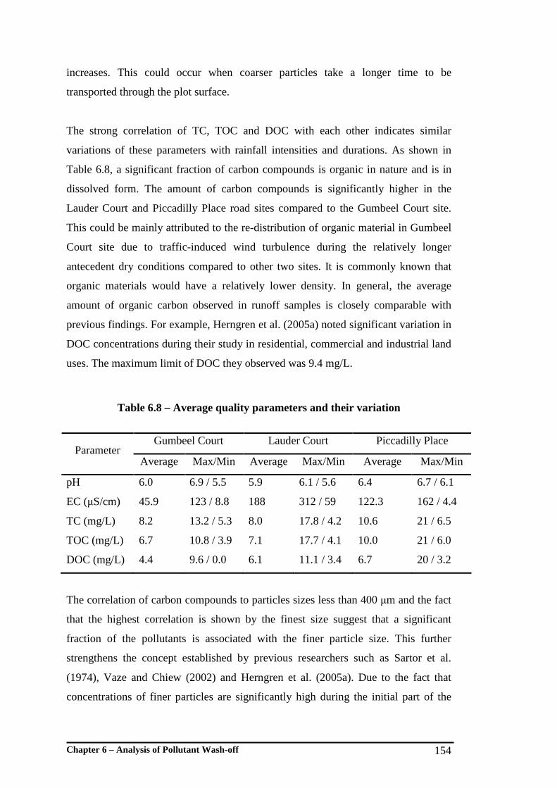
Chapter 6 – Analysis of Pollutant Wash-off 154
increases. This could occur when coarser particles take a longer time to be
transported through the plot surface.
The strong correlation of TC, TOC and DOC with each other indicates similar
variations of these parameters with rainfall intensities and durations. As shown in
Table 6.8, a significant fraction of carbon compounds is organic in nature and is in
dissolved form. The amount of carbon compounds is significantly higher in the
Lauder Court and Piccadilly Place road sites compared to the Gumbeel Court site.
This could be mainly attributed to the re-distribution of organic material in Gumbeel
Court site due to traffic-induced wind turbulence during the relatively longer
antecedent dry conditions compared to other two sites. It is commonly known that
organic materials would have a relatively lower density. In general, the average
amount of organic carbon observed in runoff samples is closely comparable with
previous findings. For example, Herngren et al. (2005a) noted significant variation in
DOC concentrations during their study in residential, commercial and industrial land
uses. The maximum limit of DOC they observed was 9.4 mg/L.
Table 6.8 – Average quality parameters and their variation
Gumbeel Court Lauder Court Piccadilly Place
Parameter Average Max/Min Average Max/Min Average Max/Min
pH 6.0 6.9 / 5.5 5.9 6.1 / 5.6 6.4 6.7 / 6.1
EC (µS/cm) 45.9 123 / 8.8 188 312 / 59 122.3 162 / 4.4
TC (mg/L) 8.2 13.2 / 5.3 8.0 17.8 / 4.2 10.6 21 / 6.5
TOC (mg/L) 6.7 10.8 / 3.9 7.1 17.7 / 4.1 10.0 21 / 6.0
DOC (mg/L) 4.4 9.6 / 0.0 6.1 11.1 / 3.4 6.7 20 / 3.2
The correlation of carbon compounds to particles sizes less than 400 µm and the fact
that the highest correlation is shown by the finest size suggest that a significant
fraction of the pollutants is associated with the finer particle size. This further
strengthens the concept established by previous researchers such as Sartor et al.
(1974), Vaze and Chiew (2002) and Herngren et al. (2005a). Due to the fact that
concentrations of finer particles are significantly high during the initial part of the
Chapter 6 – Analysis of Pollutant Wash-off 155
runoff event, there is a high probability of the washing-off of most of the associated
pollutants during this period. This further confirms the concept of ‘first flush’ which
results in relatively highly polluted runoff during the initial part of runoff events
(Duncan, 1995; Lee et al., 2002). The correlation of carbon compounds to particle
sizes less than 400 µm further confirms a decrease in pollutant concentration when
the rainfall duration increases. The negative correlation of carbon compounds to
particle sizes greater than 400 µm would mean that relatively few pollutants are
associated with particles larger than 400 µm.
The negative correlation of pH with finer particle sizes and other quality parameters
suggest that the runoff becomes less acidic as the rainfall progresses. As evident in
Table 6.8, road surface runoff is acidic. The minimum pH shown in Table 6.8 mostly
belongs to the first duration component suggesting acidic runoff during the initial
period of flow. The lower pH values could be attributed to the higher amount of
initially available pollutants on road surfaces. The lower pH in stormwater further
enhances the solubility of other pollutants.
6.5 Analysis of Wash-off from Roof Surfaces
The characteristics of wash-off from roof surfaces are less well known than for road
surfaces. Forster (1996) investigated runoff from different types of roofs for water
quality parameters. As Forster (1996) noted, metal compounds were the most
significant in roof runoff particularly from metal roofs. He also noted that most of
the roof surface pollutants were removed during the initial period of storm events and
he suggested an exponential equation with negative exponent to replicate the
dissolved component of pollutants whilst little attention was given to understanding
wash-off of particulate pollutants.
The analysis of wash-off data from roof surfaces was done based on the assumption
that it is similar to wash-off from road surfaces. The assumption was strengthened by
the recommendation by Forster (1996) of an exponential equation (in the form of
Equation 6.3). Further, it can be argued that wash-off processes, as discussed in
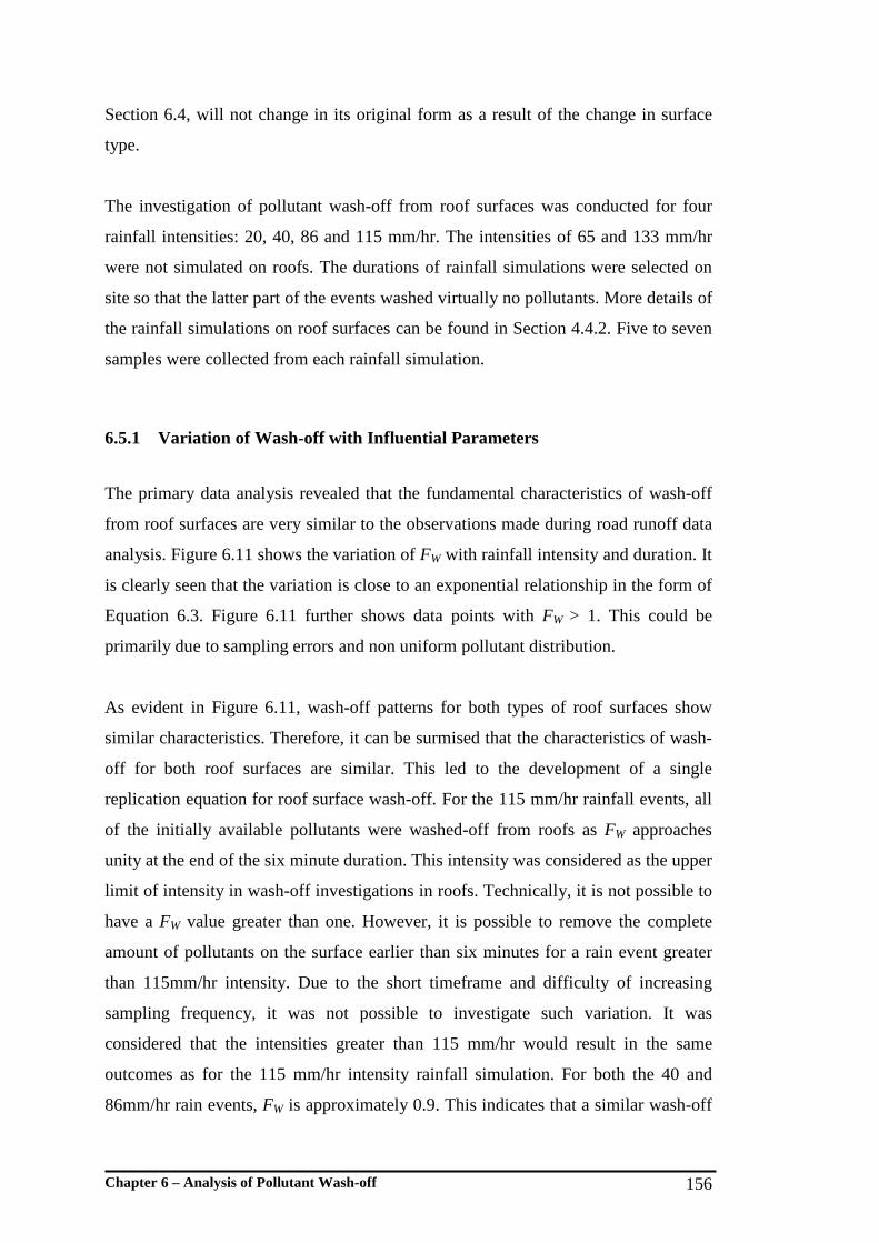
Chapter 6 – Analysis of Pollutant Wash-off 156
Section 6.4, will not change in its original form as a result of the change in surface
type.
The investigation of pollutant wash-off from roof surfaces was conducted for four
rainfall intensities: 20, 40, 86 and 115 mm/hr. The intensities of 65 and 133 mm/hr
were not simulated on roofs. The durations of rainfall simulations were selected on
site so that the latter part of the events washed virtually no pollutants. More details of
the rainfall simulations on roof surfaces can be found in Section 4.4.2. Five to seven
samples were collected from each rainfall simulation.
6.5.1 Variation of Wash-off with Influential Parameters
The primary data analysis revealed that the fundamental characteristics of wash-off
from roof surfaces are very similar to the observations made during road runoff data
analysis. Figure 6.11 shows the variation of FW with rainfall intensity and duration. It
is clearly seen that the variation is close to an exponential relationship in the form of
Equation 6.3. Figure 6.11 further shows data points with FW > 1. This could be
primarily due to sampling errors and non uniform pollutant distribution.
As evident in Figure 6.11, wash-off patterns for both types of roof surfaces show
similar characteristics. Therefore, it can be surmised that the characteristics of wash-
off for both roof surfaces are similar. This led to the development of a single
replication equation for roof surface wash-off. For the 115 mm/hr rainfall events, all
of the initially available pollutants were washed-off from roofs as FW approaches
unity at the end of the six minute duration. This intensity was considered as the upper
limit of intensity in wash-off investigations in roofs. Technically, it is not possible to
have a FW value greater than one. However, it is possible to remove the complete
amount of pollutants on the surface earlier than six minutes for a rain event greater
than 115mm/hr intensity. Due to the short timeframe and difficulty of increasing
sampling frequency, it was not possible to investigate such variation. It was
considered that the intensities greater than 115 mm/hr would result in the same
outcomes as for the 115 mm/hr intensity rainfall simulation. For both the 40 and
86mm/hr rain events, FW is approximately 0.9. This indicates that a similar wash-off
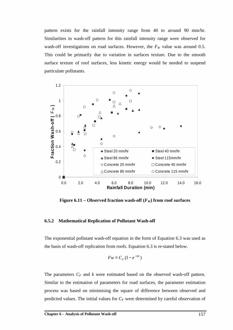
Chapter 6 – Analysis of Pollutant Wash-off 157
pattern exists for the rainfall intensity range from 40 to around 90 mm/hr.
Similarities in wash-off pattern for this rainfall intensity range were observed for
wash-off investigations on road surfaces. However, the FW value was around 0.5.
This could be primarily due to variation in surfaces texture. Due to the smooth
surface texture of roof surfaces, less kinetic energy would be needed to suspend
particulate pollutants.
Figure 6.11 – Observed fraction wash-off (FW) from roof surfaces
6.5.2 Mathematical Replication of Pollutant Wash-off The exponential pollutant wash-off equation in the form of Equation 6.3 was used as
the basis of wash-off replication from roofs. Equation 6.3 is re-stated below.
)1( kItF eCFw −−=
The parameters CF and k were estimated based on the observed wash-off pattern.
Similar to the estimation of parameters for road surfaces, the parameter estimation
process was based on minimising the square of difference between observed and
predicted values. The initial values for CF were determined by careful observation of
0
0.2
0.4
0.6
0.8
1
1.2
0.0 2.0 4.0 6.0 8.0 10.0 12.0 14.0 16.0Rainfall Duration (min)
Fra
ctio
n W
ash
-off
(F
W)
Steel 20 mm/hr Steel 40 mm/hr
Steel 86 mm/hr Steel 115mm/hr
Concrete 20 mm/hr Concrete 40 mm/hr
Concrete 86 mm/hr Concrete 115 mm/hr

Chapter 6 – Analysis of Pollutant Wash-off 158
wash-off variation in Figure 6.11. It was intended to develop a range of CF values
according to rainfall intensity whilst keeping k as a constant. Table 6.9 shows the
values obtained for CF while k is at its optimum value of 9.33 x 10⁻³.
Table 6.9 – Optimum parameters for Equation 6.3
Capacity Factor CF Roof Type
Wash-off Coefficient k 20
mm/hr 40
mm/hr 86
mm/hr 115
mm/hr
Steel 9.33 x 10⁻³ 0.75 0.97 0.87 1.01
Concrete 9.33 x 10⁻³ 0.76 0.99 0.86 1.03
As shown in Table 6.9, the parameter CF obtained for both roof types is similar. This
suggests the possibility of generating a common set of parameters for both roof
types. Further, it is possible to develop a constant CF value for the rainfall intensity
range of 40 to 90 mm/hr. This is due to the similarities of CF for this range as noted
in Table 6.9. Therefore, as for road surface wash-off, it can be assumed that CF varies
linearly from 0.75 to 0.91 for the 20 to 40 mm/hr intensity range, it is constant at
0.91 between 40 to 90 mm/hr intensities and varies linearly from 0.91 to 1 for 90 to
115 mm/hr rainfall intensities. CF was considered to be constant at 1.00 for all the
intensities greater than 115 mm/hr. The values for CF were obtained based on the
method of least squares. The rainfall intensity ranges are exactly the same as the
wash-off process for road surfaces (see Section 6.4.4).
Figure 6.12 shows the performances of the parameters developed for Equation 6.3 in
replicating wash-off from roof surfaces. Performance of the developed parameters
was further verified by obtaining the mean for the ratio between predicted and
observed values and CV ,as given in Table 6.10.

Chapter 6 – Analysis of Pollutant Wash-off 159
Figure 6.12 – Performances of the replication equation for roof surface wash-off
Table 6.10 – Performance of Equation 3 with common set of optimum parameters
As evident from Figure 6.12, the visual performance of the replication equation is
satisfactory. As shown in Table 6.10, the mean for both roof surfaces is close to one
and the CV is around 10%. This confirmed the ability to reproduce with adequate
accuracy the observed wash-off data set using Equation 6.3. Therefore, it can be
considered that the replication equation in the form of Equation 6.3 and the common
set of parameters as described above can be used to replicate pollutant wash-off from
roof surfaces.
It was possible to develop a replicating equation in the form of Equation 6.3 for all
the investigated impervious surface types. The two types of surfaces investigated,
Parameter Corrugated Steel Concrete Tile
Mean 1.01 1.00
CV 10.3% 10.0%
0
0.2
0.4
0.6
0.8
1
1.2
0.0 2.0 4.0 6.0 8.0 10.0 12.0 14.0Rainfall Duration (min)
Fra
ctio
n W
ash
-off
(F
W)
Steel 20 mm/hr Steel 40 mm/hr
Steel 86 mm/hr Steel 115mm/hr
Concrete 20 mm/hr Concrete 40 mm/hr
Concrete 86 mm/hr Concrete 115 mm/hr
Predicted using Equation 3

Chapter 6 – Analysis of Pollutant Wash-off 160
namely, roads and roofs, are vastly different in their primary characteristics
including, surface texture and slope. The ability to use a similar equation for these
surfaces suggested the possibility of using the equation for all the other impervious
surfaces such as driveways.
The wash-off coefficient k also shows significant variation with surface type and
characteristics of pollutants. For wash-off from road surfaces it was 8.0 x 10⁻⁴
whereas for roof surface wash-off it was 9.33 x 10⁻³. The parameter k primarily
defines the shape of the wash-off curve which is more closely related to the surface
type rather than the characteristics of pollutants.
6.5.3 Particle Size Distribution Analysis
The particle size distribution of individual samples was tested in order to understand
the physical processes governing pollutant wash-off and to identify the reasons for
the variation of CF with rainfall intensities. Figure 6.13 shows the average particle
size distribution for both roof surfaces.
As shown in Figure 6.13, the variation in weight for 40 and 86 mm/hr rainfall shows
similarities, whereas the particle size distribution for 115 mm/hr is relatively high
when compared to the other two. The primary cause for this is the variation in
initially available pollutants. Table 6.11 shows the initially available pollutants for
the two roof surfaces.
Table 6.11 – Initially available pollutants prior to rainfall simulations
Pollutant load (g)
Roof Type 20(mm/hr) 40(mm/hr) 86(mm/hr) 115(mm/hr)
Steel 0.264 0.647 0.624 0.810
Concrete tile 0.288 0.386 0.339 0.461
As shown in Table 6.11, initially available pollutants before the 115 mm/hr intensity
simulation is comparatively high when compared to the other three intensities. This

Chapter 6 – Analysis of Pollutant Wash-off 161
could lead to significant variation in wash-off load. Further to this, it is clearly
evident in Table 6.11 that the amount of initially available pollutants on the steel roof
is significantly higher than for the concrete tile roof except prior to the 20 mm/hr
rainfall simulation. This would be the reason for the relatively higher amount of
pollutant wash-off from steel roofs.
Figure 6.13 – Averaged particle size distribution for two roof surface types
Concrete Tile Roof
0
0.1
0.2
0.3
0.4
0.5
0.1 1 10 100 1000Particle Size (µm)
Ave
age
Wei
gh
t (g
)
Corrugated Steel Roof
0
0.1
0.2
0.3
0.4
0.5
0.1 1 10 100 1000Particle Size (µm)
Ave
rag
e W
eig
ht
(g)
40mm/hr
86mm/hr
115mm/hr
Chapter 6 – Analysis of Pollutant Wash-off 162
It was understood that both the 40 and 86 mm/hr rainfall events are not capable of
washing-off all the pollutants from roofs. Since the fraction retained is low, it was
not possible to distinguish which particle size category was retained on the surface.
As evident from Figure 6.13, there are no significant differences in the pattern of
particle size distribution. The majority of the solids are in the range of 1 to 100 µm
with the median around 50 µm for all the samples from the two roofs. It would alter
the wash-off particle size distribution if the additional amount of pollutants washed-
off during the 115 mm/hr rain event belonged to a particular particle size range. As
this was not the case, it can be surmised that the additional amount of pollutant
retained on the roof surface is a well distributed sample.
Due to the fineness of the particles, it is more possible to retain particles on roof
surfaces by chemical bonds rather than gravity. The finer particles are more likely to
be polar and create electrostatic bonds with the roof surfaces. On the other hand,
roofs are angled at 200 and therefore, a significant fraction of the gravity force is in
the direction of the roof slope. Additionally, the low roughness of roofs compared to
road surfaces provides fewer pores within the texture to trap pollutants. This would
mean relatively low resistance against wash-off. Therefore, it can be surmised that
the retention of particles on the surface during low rainfall intensities would be due
to their strong chemical bonds. The less intense rain events would not be able to
supply adequate energy to overcome these bonds thereby allowing the particles to be
retained on the surface.
In comparison to road surface wash-off, particles washed-off from roof surfaces are
significantly fine. This is primarily due to the fineness of the initial pollutants which
are mainly sourced from atmospheric sources. The fineness of the particles on roofs
may create significant differences in terms of gravitational forces and chemical
bonds when compared to road surface pollutants. However, the kinetics of the wash-
off observed from the two surface types were similar. Furthermore, it was possible to
develop a replication equation of similar form for both surface types. Therefore it can
be surmised that rainfall parameters rather than surface type and pollutant
characteristics exert the higher degree of influence on wash-off. The rainfall
parameters are the only unchanged parameters used during the analysis of wash-off
for the two surface types.

Chapter 6 – Analysis of Pollutant Wash-off 163
6.5.4 Physio-chemical Analysis
The analysis of the water quality parameters obtained from the laboratory testing was
undertaken using PCA. Similar to the analysis of water quality data from road
surface runoff, detailed understanding of the variation of TS concentrations was
needed for better interpretation of PCA outcomes. This entailed the analysis of
variation of TS concentrations with rainfall intensity and duration as shown in Figure
6.14.
Figure 6.14 – Variation of TS concentration with rainfall intensity and duration
Corrugated Steel
0
0.1
0.2
0.3
0.4
0.5
0.6
0.0 2.0 4.0 6.0 8.0 10.0 12.0 14.0
Rainfall Duration (min)
Co
nce
ntr
atio
n (
mg
/L)
20 mm/hr
40 mm/hr
86 mm/hr
115 mm/hr
Concrete Tile
0
0.05
0.1
0.15
0.2
0.25
0.3
0.35
0.0 2.0 4.0 6.0 8.0 10.0 12.0 14.0
Rainfall Duration (min)
Co
nce
ntr
atio
n (
mg
/L)
20 mm/hr
40 mm/hr
86 mm/hr
115 mm/hr

Chapter 6 – Analysis of Pollutant Wash-off 164
As illustrated in Figure 6.14, the concentration shows an exponential decay when the
investigated duration components move from the first to the fourth. Furthermore, it
shows an increase in TS concentration particularly for the first duration component
when the intensity increases. This observation is very similar to the variations of TS
concentration in road surface runoff. Therefore, the interpretation of the PCA
outcomes was undertaken using a similar approach.
Figure 6.15 shows the biplot resulting from PCA. Due to the similarities in the
variation of concentrations and comparatively less data scatter, a combined analysis
was done for both roof types.
Figure 6.15 – Quality parameters for wash-off samples from roof surfaces: Biplot of data against the first two principal components

Chapter 6 – Analysis of Pollutant Wash-off 165
Figure 6.15 leads to the following conclusions:
1) All the particle size classes strongly correlate with each other;
2) TC, TOC and DOC strongly correlate with each other; and
3) All the particle size classes show virtually no correlation with TC, TOC and
DOC.
The strong correlation of all the particle size classes with each other would mean
similar variation of all particle sizes during wash-off. As the variation of TS with
rainfall duration was understood as an exponential decay (see Figure 6.14), the
concentration of all the particle size classes should have similar variation with
rainfall parameters.
The strong correlation of TC, TOC and DOC with each other indicates similar
variations of these parameters during rainfall events. However, the higher vectorial
length of TOC and DOC suggested a higher variation compared to TC. As shown in
Table 6.12, both TOC and DOC concentrations are significantly high when
compared to road surfaces. Higher organic carbon content could be due to the
significant fraction of surrounding unpaved land.
Table 6.12 - Average quality parameters and their variation
Steel Roof Concrete Roof
Parameter Value Max/Min Value Max/Min
pH 6.6 7.9 / 4.9 6.6 7.3 / 5.4
EC (µS/cm) 193 371 / 61 160 351 / 61
TC (mg/L) 17.0 38.7 / 4.2 16.5 32.9 / 6.5
TOC (mg/L) 6.3 33.7 / 1.2 7.2 18.9 / 3.2
DOC (mg/L) 5.1 15.2 / 0.9 5.9 11.9 / 2.7
The negative correlation of pH to particle size classes indicates that the acidic nature
of roof surface runoff decreases when the duration of simulations increase. The
average pH for all the initial duration components was 5.67 while it was 6.18, 6.67
and 7.18 respectively for the next consecutive duration components. The lower pH in

Chapter 6 – Analysis of Pollutant Wash-off 166
the initial part of the runoff events and its increase when the duration increases
means that the acidic nature can be primarily attributed to particulate pollutants.
Lower pH and higher fraction of DOC in roof surface runoff increases the likelihood
of having other pollutants in dissolved form (Herngren et al., 2006; Warren et al.,
2003). This can be significant for steel roofs where high concentrations of heavy
metals is a distinct possibility (Bannerman et al., 1993).
6.6 Conclusions
This chapter discussed the analytical outcomes of the extensive investigations into
pollutant wash-off from road and roof surfaces. The analysis primarily focussed on
understanding the characteristics of wash-off of particulate pollutants. This was due
to the fact that particulate pollutants were adopted as the indicator pollutant in the
research study. Additionally, efforts were made to understand the factors that
influence the adsorption of other pollutants to solids.
The outcomes of the analyses are as follows:
1) Wash-off of particulate pollutants can be replicated using an exponential
equation in the form of:
)1( kItF eCFw −−=
Where;
I Rainfall intensity;
k Wash-off coefficient;
Fw Fraction wash-off;
CF Capacity factor; and
t Rainfall duration
CF and k are parameters that need to be estimated in order to use the wash-off
equation. Parameter estimation was undertaken for roads and roofs separately as
these are the primary types of impervious surfaces in urban areas.

Chapter 6 – Analysis of Pollutant Wash-off 167
2) Analysis was undertaken to understand the characteristics of each parameter. CF
was defined as the rainfall capacity to mobilise pollutants. However, it was found
that CF is not purely a property of rainfall characteristics alone. CF shows a
strong relationship to rainfall intensity, particle size distribution of pollutants and
impervious surface type. For simplicity of calculations, CF was estimated for
three rainfall intensity classes. For the 20 to 40 mm/hr intensity range, CF
increased linearly, for the 40 to 90 mm/hr intensity range CF is a constant and for
above the 90 mm/hr intensity it varied linearly to a maximum of one. The values
of CF obtained for these rainfall intensity ranges differ for the two impervious
surface types: roads and roofs. This is due to the differences in the characteristics
of the surfaces and particle size distribution of available pollutants. Wash-off
coefficient k was estimated as a constant for each impervious area type. It was
8.0 x 10⁻⁴ for road surfaces and 9.33 x 10⁻³ for roof surfaces.
3) On average, 73% of road surface wash-off pollutants belong to the 0 – 200 µm
particle size range. Furthermore, it was observed that this particle size range is
dominant for all the rainfall intensities. The average particle size distribution
curves for samples from different rainfall intensities show closely similar
characteristics.
4) Up to 90% of the particles washed-off from roof surfaces belong to the 0 – 100
µm size range. The particle size distribution showed consistent similarities when
both rainfall intensity and duration varied. Only a small fraction of particles were
retained on the roof surface even after the simulation of the lowest rainfall
intensity.
5) For both roof surface types, the highest amount of wash-off occurred during the
initial period of rainfall simulations. This strengthens the first flush concept noted
by many researchers.
6) It was noted that higher fractions of organic carbon are in dissolved form and are
associated with the finer particle size ranges. The amount of organic carbon
reduces when the concentration of particulate pollutants reduces.

Chapter 7 – Catchment Modelling 169
Chapter 7 - Catchment Modelling
7.1 Introduction Chapter 5 and 6 provided extensive information on processes involved in particulate
build-up and wash-off from impervious urban surfaces. The understanding gained
from these investigations enabled the estimation of the amount of particulate
pollutant build-up on different impervious surface types for a given antecedent dry
period and the particulate load removed during a known storm event. In order to
relate the estimated solids load to catchment water quality, detailed knowledge is
needed relating to how discrete plot surfaces are hydrologically connected. The
hydrologic information that is needed is not only the amount of runoff volume that a
particular surface generates, but also the time taken for that particular volume to
transfer to the catchment outlet.
The most feasible approach to generate the requisite hydrologic information that is
needed is to use a calibrated hydrologic model. Hydrologic modelling is commonly
used to estimate runoff from catchments. However, in this case, the use of a
hydrologic model was not for typical use in relation to runoff predictions. The
primary use of a hydrologic model in this research study was to facilitate the
translation of pollutant concentrations from catchment sub-areas to the catchment
outlet.
This chapter discusses in detail the hydrologic modelling used to develop runoff
information. The modelling software used was Mike STORM which was developed
by the Danish Hydraulic Institute (DHI) (Mike STORM, 2004). The chapter first
discusses the basic architecture of Mike STORM and its simulation techniques. Then
the setting up of three catchment models and details of model calibration for a range
of storm events are outlined. The calibrated models were then used for the estimation
of water quality.
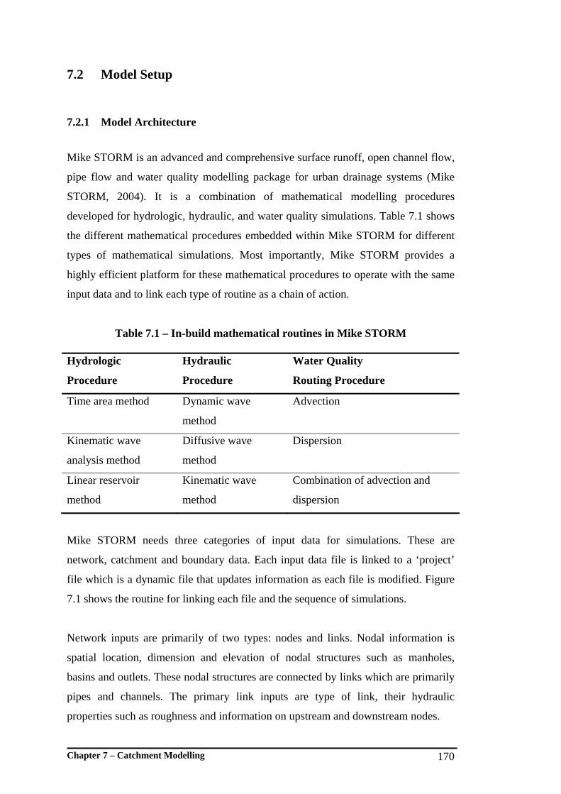
Chapter 7 – Catchment Modelling 170
7.2 Model Setup
7.2.1 Model Architecture
Mike STORM is an advanced and comprehensive surface runoff, open channel flow,
pipe flow and water quality modelling package for urban drainage systems (Mike
STORM, 2004). It is a combination of mathematical modelling procedures
developed for hydrologic, hydraulic, and water quality simulations. Table 7.1 shows
the different mathematical procedures embedded within Mike STORM for different
types of mathematical simulations. Most importantly, Mike STORM provides a
highly efficient platform for these mathematical procedures to operate with the same
input data and to link each type of routine as a chain of action.
Table 7.1 – In-build mathematical routines in Mike STORM Hydrologic
Procedure
Hydraulic
Procedure
Water Quality
Routing Procedure
Time area method Dynamic wave
method
Advection
Kinematic wave
analysis method
Diffusive wave
method
Dispersion
Linear reservoir
method
Kinematic wave
method
Combination of advection and
dispersion
Mike STORM needs three categories of input data for simulations. These are
network, catchment and boundary data. Each input data file is linked to a ‘project’
file which is a dynamic file that updates information as each file is modified. Figure
7.1 shows the routine for linking each file and the sequence of simulations.
Network inputs are primarily of two types: nodes and links. Nodal information is
spatial location, dimension and elevation of nodal structures such as manholes,
basins and outlets. These nodal structures are connected by links which are primarily
pipes and channels. The primary link inputs are type of link, their hydraulic
properties such as roughness and information on upstream and downstream nodes.

Chapter 7 – Catchment Modelling 171
Figure 7.1 – File structure and simulation sequence in Mike STORM.
Catchment inputs primarily consist of catchment area and the node at which the
catchment drains. The catchment should drain to a pre-defined node from nodal
inputs. The same catchment input dialog box is used to define hydrologic parameters.
Separate windows are available to define variables for different hydrologic methods.
Two types of boundary inputs are used in Mike STORM: rainfall boundary and water
level boundary. Details of the rainfall event in the form of intensity time series
should be inserted as a rainfall boundary. There are options to insert several time
series for different rain gauges and to use distributed rainfall patterns for simulations.
The time series of the catchment outlet water level is used as a water level boundary.
This is used to calculate the back-water curve when limited drainage facilities are
available at the catchment outlet.
Inputs Simulations Outputs
Rainfall Records
Catchment Properties Runoff
Hydrographs for each Sub-division
Simulation 1 Hydrologic Simulation
Outlet Water Level
Network Data • Nodes • Links
Runoff Hydrograph at Catchment Outlet
Simulation 2 Hydraulic Simulation

Chapter 7 – Catchment Modelling 172
7.2.2 Alextown Catchment
Alextown is a tenement townhouse development, 1.7 ha in area. The percentages of
impervious surfaces are 10.5%, 38.1% and 8.6% for roads, roofs and driveways
respectively. Further details of the catchment characteristics can be found in Section
4.3.1. The catchment consists of an efficient drainage system with rectangular gully
pits with steel mesh lids placed at the middle of the road to collect road runoff.
Detailed maps of the drainage network including sizes of gully pits and pipe
diameters were provided by the Gold Coast City Council (GCCC). These maps can
be found in Appendix B, Figures B.1 to B.4. Runoff from roofs is directly connected
to the drainage pipe network.
For the modelling, the catchment was divided into 16 sub-areas so that its distributed
nature can be adequately represented. The subdivisions were done after careful
investigation of the catchment contours and drainage network. The sub-areas were
demarcated such that each gully pit accounts for the surrounding drainage area.
Figure 7.2 shows the details of the drainage network and catchment subdivisions.
Appendix E, Figures E.1 to E.3 show the data input to Mike STORM for model
setup. The primary data inputs were location coordinates of gully pits, their surface
and invert elevations, properties of connecting pipes such as diameter and type,
extent of sub-areas and impervious percentages.
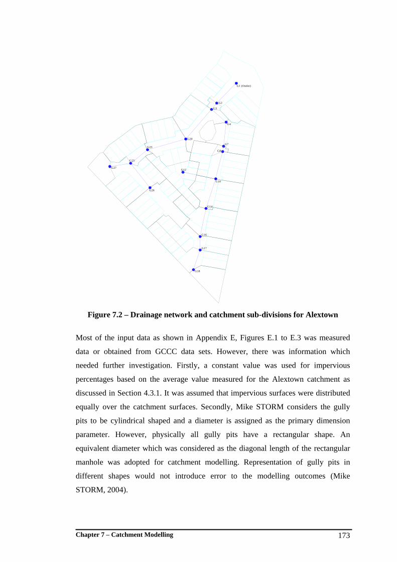
Chapter 7 – Catchment Modelling 173
G1 (Outlet)
G2
G3
G4
G7
G8
G20
G12
G23
G25
G27
G26
G10
G14
G16
G17
G18
Figure 7.2 – Drainage network and catchment sub-divisions for Alextown
Most of the input data as shown in Appendix E, Figures E.1 to E.3 was measured
data or obtained from GCCC data sets. However, there was information which
needed further investigation. Firstly, a constant value was used for impervious
percentages based on the average value measured for the Alextown catchment as
discussed in Section 4.3.1. It was assumed that impervious surfaces were distributed
equally over the catchment surfaces. Secondly, Mike STORM considers the gully
pits to be cylindrical shaped and a diameter is assigned as the primary dimension
parameter. However, physically all gully pits have a rectangular shape. An
equivalent diameter which was considered as the diagonal length of the rectangular
manhole was adopted for catchment modelling. Representation of gully pits in
different shapes would not introduce error to the modelling outcomes (Mike
STORM, 2004).

Chapter 7 – Catchment Modelling 174
7.2.3 Gumbeel Catchment
Gumbeel is a duplex housing development of 2.1 ha. The impervious percentages are
10.3%, 19.2% and 11.2% for roads, roofs and driveways respectively. The catchment
is located in a typical ridge shape area. However, most of the runoff from roads and
roofs is artificially directed to the drainage network. The length of the drainage
network is comparatively short compared to the other study catchments. The total
catchment was divided into two sub-areas and the required parameters were obtained
as for the Alxetown catchment. Figure 7.3 shows the drainage network and
catchment sub-areas and Appendix E, Figures E.4 to E.6 gives the input data for the
Mike STORM model.
Figure 7.3 – Drainage network and catchment sub-divisions for Gumbeel
G1 (Outlet)
G2
G3

Chapter 7 – Catchment Modelling 175
7.2.4 Birdlife Park Catchment
Birdlife Park is a high socio-economic single detached dwelling area of 8.6 ha area.
The catchment is in a valley, with a relatively greater slope when compared to the
other catchments. All the roof runoff in the catchment is directed to road gutters and
then collected by side manholes along with road runoff. Furthermore, any runoff
generated in pervious areas or driveways is accumulated with road runoff. The total
catchment was divided into 54 sub-areas. The parameters for each sub-area were
obtained in the same way as for the Alextown catchment. Figure 7.4 shows the
drainage network and catchment sub-areas and Appendix E, Figures E.7 to E.9 gives
the input data which was used for Mike STORM modelling.
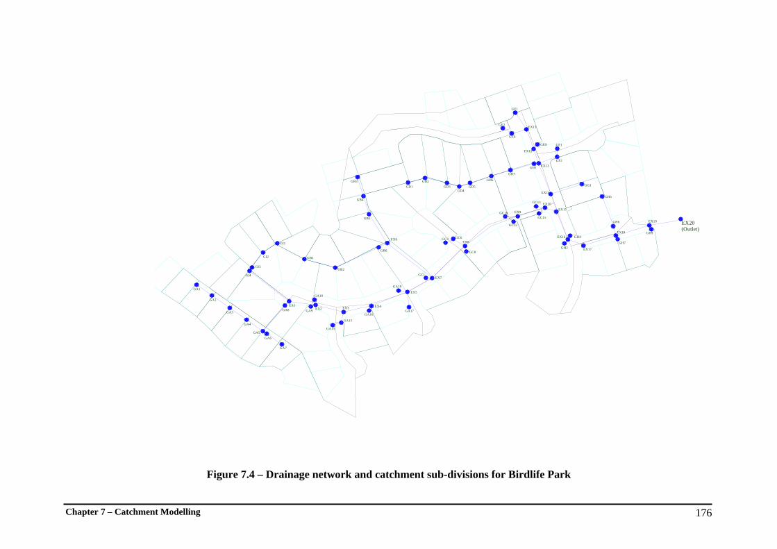
Chapter 7 – Catchment Modelling 176
Figure 7.4 – Drainage network and catchment sub-divisions for Birdlife Park
EX19
GH9
EX17
EX18
GH7
GH6
GH5
EX16 GH4
GH2
EX15
GG1
EX14
EX13GF2
GF1
EX12
GE9
EX11
GE6
GE2
GE1
GH1
GD7
GD6
GD5GD4
GD3GD2
GD1
EX10GC13
GC15
EX9GC10
GC12
EX8
GC8
GC6GC3EX6
GB5
GB4
GB3
GB6
GB2
GB1
EX7GC1
EX5
GA19
GA17EX4
GA16
EX3
GA15
GA13
EX2
GA10
GA9GA8EX1
GI4
GI3
GI2
GI1
GA7
GA6GA5
GA4
GA3
GA2
GA1
EX20 (Outlet)

Chapter 7 – Catchment Modelling 177
7.3 Model Calibration
Model calibration is one of the more important requirements in hydrologic modelling.
Calibration involves the estimation of model parameters which in turn enables the model
to closely match the behaviour of the natural system which it is meant to represent.
There are situations where the model parameters can be estimated using physically-
based measurements. However, in most cases, the model parameters need to be
estimated by trial-and-error processes (Gupta and Sorooshian, 1998).
Even after a model is calibrated to a high level of accuracy, there can be significant
uncertainty involved in its predictions (Pilgrim et al., 1981). However, hydrologic
modelling is the most reliable and accurate method of runoff estimation based on the
current state of knowledge, provided that the model is calibrated and used with care. The
primary uncertainty of hydrologic model prediction is due to the lack of measured data
for calibration. Generally, hydrologic models are calibrated using a number of rain
events that cover only a limited range of possible variations in rainfall characteristics.
Therefore, it is hard to justify the accuracy of prediction, particularly for those rain
events outside the calibrated range.
As noted by Beven and Binley (1992), further uncertainties associated with calibration
of models arise due to structural errors in the model and errors in measurements and
observations. The calibration procedure compensates for such structural, measurement
and observational errors by varying model parameters. Therefore, the parameter set
obtained during calibrations may not be the true set of parameters. It is hard to eliminate
such errors, but they can be minimised by using quality measurements and observations.
As discussed in Section 4.3, measurements were obtained using reliable measuring
systems and equipment. However, the quality of measurements alone does not eliminate
the problems associated with the calibrated model parameters. It is essential to have a
systematic calibration procedure to develop more reliable model parameters (Gupta and
Sorooshian, 1998).
Chapter 7 – Catchment Modelling 178
Various numerical procedures have been developed in order to assist model calibration
(Madsen, 2000; Seibert et al., 2000). These procedures, commonly referred to as
‘automatic calibration’, use different types of optimisation techniques to generate a set
of parameters so that the model output closely matches the measured response.
However, the useability of these techniques is still limited to reduce the parameter space
for manual calibration (Mike STORM, 2004). Mike STORM has an automatic option
that can be used to assist model calibration. However, it is recommended to confirm the
outcome manually. As noted by Beven and Binley (1992), automatic calibration
procedures can often lead to error due to inter-correlation of parameters and an excessive
number of parameters. Therefore, in this study it was decided to use the automatic
calibration procedure only to estimate the initial parameters and the final calibration was
done manually.
7.3.1 Measured Data for Calibration
Data for model calibration was obtained from the procedure explained in Section 4.3.2.
As explained, state-of-the-art technology was used to obtain both rainfall and runoff
data. The rainfall data was obtained from a tipping bucket rain gauge which was situated
within a 2 km proximity to the study catchments. It is acknowledged that the spatially
distributed nature of rainfall events could influence the accuracy of predictions (Shah et
al., 1996). In order to account for such variability, the recommended method is to
include data from surrounding rain gauges. However, the available rain gauges in the
region were further apart from the study catchments. Inclusion of data from these
surrounding gauges, therefore, was not considered to be feasible. It was hypothesised
that an accurate model can be developed using records from the closest rain gauge.
Consequently, the spatial distribution of rainfall was not considered.
The runoff from each catchment outlet has been measured for a range of storm events
since 2002. Measurements have been primarily done for runoff depth and later converted
to runoff rate using rating tables. The runoff data was in 15 min time intervals.

Chapter 7 – Catchment Modelling 179
The model calibration was based on selected rainfall events where measured rainfall,
runoff and water quality data is available. These events were selected by careful
inspection of the available data. The same events were used for the calibration and
verification of hydrologic models. Therefore, the error of calibration due to the selection
of non-representative data was minimal. Table 7.2 shows the number of events selected
for calibration and verification.
Table 7.2 – Number of events used for calibration and verification
Model Name Number of Events for Calibration
Alextown 7
Gumbeel 7
Birdlife Park 13
7.3.2 Methods and Parameters
Mike STORM consists of a range of hydrologic and hydraulic analytical models as
noted in Table 7.1. It is totally at the discretion of the user to decide which combination
of models is suitable for the task. The nature of the research and outcomes required are
decisive factors in such selection. For this study, the model was developed using the
‘time area method’ to simulate catchment hydrologic behaviour. The ‘dynamic wave’
model was used for pipe flow modelling. The hydrologic model based on the time area
method was used since the same procedure was to be used in pollutant translation as a
part of the water quality estimations. The method was first developed by Laurenson
(1962) and is used in a range of models such as ILSAX and DRAINS (O'Loughlin and
Stack, 2004). Further discussion on the time area method and other catchment modelling
approaches can be found in Section 2.5.2(D).
Altogether five parameters are needed for the calibration of the Mike STORM model.
Those parameters are:
1) Time of concentration (Tc);

Chapter 7 – Catchment Modelling 180
2) Reduction factor (Rf);
3) Initial loss (IL);
4) Time area coefficient (a); and
5) Manning’s roughness (n).
Time of concentration (Tc) is one of the most critical parameters which govern the
efficiency of the drainage system. The parameter primarily varies with slope, drainage
length and a range of other factors. However, to maintain simplicity, effort was made to
obtain constant Tc for the sub-areas in each catchment. Variable Tc values were used
when the quality of the calibration became poor. In such cases, Tc was selected based on
the size of the sub-area. Catchment area is one of the primary measures that influences
the time of concentration (Askew, 1970; Boyd et al., 1979). The calibrated constant
values for Tc for Gumbeel and Birdlife Park sub-areas were 20 and 10 min respectively.
For Alextown catchment a range of Tc values were used depending on the extent of the
sub-areas. The values were 2, 8, 20 and 25 min for <100, 100 – 1200, 1200 – 1400 and
greater than 1400 m2 extents respectively.
Reduction factor (Rf) is primarily a measure of the ratio of directly connected
impervious surfaces and the total impervious surfaces. As noted in Section 4.3, the total
impervious surfaces was measured using aerial photographs. However, it was difficult to
identify the directly connected impervious surfaces visually. Boyd and Milevski (1996)
suggested the analysis of volume ratio between runoff and rainfall would be the most
feasible approach to obtain the fraction of directly connected impervious surfaces. The
study they did on 29 catchments revealed that only about 75% of the impervious
surfaces measured from aerial photographs were directly connected. A similar analysis
conducted for the study catchments found that around 90% of the impervious surfaces
were directly connected. Consequently, 0.9 was initially used as Rf for all three
catchments and was subsequently refined during the calibration process. The final values
obtained were 0.95, 0.82 and 0.70 for Alextown, Birdlife Park and Gumbeel catchments
respectively.

Chapter 7 – Catchment Modelling 181
Impervious surface initial loss (IL) was one of the more important parameters that was
decisive in determining runoff volume. IL was determined by calibration and
commenced with the default value of 0.6 mm. As noted by Boyd et al. (1994) and Boyd
and Milevski (1996), the impervious area initial loss can vary from 0 to 5 mm depending
on the surface type and initial moisture content on the surface. IL can vary from event to
event depending on the initial moisture content of the catchment surface. However, for
simplicity of this study, a common value of IL was used for all events per catchment.
After calibration using the selected storm events, the common IL values selected were 3,
0.3, and 5 mm for Alextown, Birdlife Park and Gumbeel catchments. The values
obtained for IL could be influenced by the selected range of storm events for the
calibration. Furthermore, the difference in IL for the three catchments could be due to
factors such as variation of directly connected impervious fraction and variation in road
surface condition.
The time area coefficient (a) primarily represents the shape of the catchment sub-area.
As stated in the Mike STORM user manual (Mike STORM, 2004), the coefficient ‘a’
can vary from 0.5 to 2. Physically, 0.5 and 2 denote convergent and divergent triangular
shapes. The coefficient for a rectangular catchment shape is 1 and it makes the time area
diagram linear. During the demarcation, all effort was made to maintain similar length
width ratio for sub-areas. Additionally, several hydrologic models, for example ILSAX
use a linear time area diagram which means a has a constant value of 1. Therefore, a was
considered to be 1 for all the catchments and for all the events for this study.
Manning’s roughness is the primary parameter used for pipe and channel flow routing.
The drainage networks of all three study catchments were predominantly precast
reinforced concrete pipes. Typical Manning’s roughness coefficients for such pipes are
in the range of 0.012 to 0.015 (Mike STORM, 2004; O'Loughlin and Stack, 2004).
However, the roughness coefficients may vary from the default range due to various
reasons. Firstly, a pipe network consists of joints and gully pots which typically have
high flow resistance when compared to pipes. This makes the overall flow resistance
higher for the drainage network and should be compensated from pipe roughness.

Chapter 7 – Catchment Modelling 182
Secondly, pipe roughness may alter from its original value due to erosion and
depositions. However, due to comparatively shorter drainage networks, the influence of
Manning’s roughness was not clearly visible for the simulated hydrograph. Therefore,
the default value for smooth concrete (0.012) was used for all the models.
7.3.3 Calibration Sequence
As a range of parameters was available for calibration and some of them were correlated
to each other, extra care was needed during calibration. For example, both initial loss
(IL) and reduction factor (Rf) theoretically alter the runoff volume in model response
and it was difficult to decide which parameters were to be adjusted in order to calibrate
runoff volume with the measured response.
To avoid the correlation of adjusted parameters in model response, a definite sequence
of calibration was used. The first step was to adjust Tc so that the peak discharge from
model response and observed runoff coincides. For Alextown catchment, multiple
combinations of Tc were used for calibration since different Tc values were assigned for
different area categories. The second step was to adjust Rf and IL so that the simulated
runoff volume is closely comparable with the measured runoff volume. These two steps
were repeatedly adjusted so that the model response was closely similar to the measured
hydrographs. Default values of a and n were used during the calibration.
During the calibration, optimum parameter sets were first obtained for each calibration
event. After careful investigation of parameter sets, common values were selected to
represent models for each catchment. Using the common values obtained, simulations
were done for each event and the performance was evaluated. Evaluations were done for
both peak discharge and runoff volume. Figure 7.5 shows the variation of ratio between
simulated and observed peak discharges, and Figure 7.6 shows the variation of ratio
between simulated runoff volume and observed runoff volume.

Chapter 7 – Catchment Modelling 183
Figure 7.5 – Variation of peak flow ratio with observed peak discharges
Figure 7.6 – Variation of Runoff volume ratio with observed runoff volume
As seen in Figures 7.5 and 7.6, though significant data scatter is noted, it can be
considered that both simulated peak discharge and runoff volume are closely similar to
the observed peak discharges and runoff volumes. The averages of the peak flow ratio
and runoff volume ratio are 1.13 and 1.0 respectively. The peak flow prediction
Chapter 7 – Catchment Modelling 184
illustrates less consistency with CV being 30%. However, due to the low runoff rates
noted for all the catchments, the accuracy obtained for peak flow predictions was
considered to be in an acceptable range. The CV for volumetric predictions was 14%.
This suggested consistently accurate simulation of correct volumes by calibrated models.
Since the models were only used to facilitate the estimation of water quality by
translating pollutant concentrations from sub-areas to catchment outlets, the predictive
ability for this range was considered adequate.
7.4 Conclusions Three models were developed to simulate hydrologic features of three urban catchments,
Alextown, Gumbeel and Birdlife Park. These three models were calibrated for a range of
storms so that they replicate catchment hydrologic features. The same storm events
which the models were intended to simulate were also used for calibration. In this way,
it was possible to develop the best calibrated models for the intended use.
The parameter set obtained for each model was the optimal for selected storm events.
Therefore, some of the calibrated parameters such as IL were different for the three
catchments. It was considered that this is due to the differences in selected storm events,
differences in the percentage of directly connected impervious surfaces of catchments
and differences in road surface conditions. With optimum parameter sets, notable
differences in prediction were observed for the three catchments. This was in
comparison to the measured peak discharge and runoff volume.
Chapter 8 – Development of Translation Procedure 185
Chapter 8 - Development of Translation Procedure
8.1 Background
Accurate and reliable estimation of stormwater quality is highly valued in urban
planning, catchment management and the design of stormwater treatment measures.
Water quality modelling is the primary tool used for such estimations. Water quality
models are typically based on the understanding gained about key pollutant processes.
The primary understanding of pollutant processes has been gained by detailed
investigations into small-plot surfaces (Letcher et al., 2002). For example, Sartor et al.
(1974) carried out a comprehensive investigation to understand key pollutant processes
on road surfaces. This investigation led to a better understanding of two key pollutant
processes namely, build-up and wash-off, and formed the base for a significant number
of water quality estimation models. Similar investigations for different land-uses and
regions have strengthened the knowledge base on these processes (for example Ball et
al., 1998; Deletic and Orr, 2005; Sartor et al., 1974; Vaze and Chiew, 2002).
Although an in-depth understanding of small-plot pollutant processes is used,
stormwater quality modelling is highly complex. This is primarily attributed to three
factors. Firstly, the understanding gained on small-plot pollutant processes is not totally
adequate to fully account for highly variable urban conditions. It can lead to inaccuracies
in estimations, and mismatches in the pollutant process used. Therefore, further
understanding on pollutant processes and associated physical parameters is needed.
Secondly, the estimation approach used in water quality models based on these
processes is complex. Typical water quality models are replications of both pollutant and
hydrologic processes in sequential order similar to natural occurrence. In order to
achieve higher accuracy, these replications are typically integrated into one platform and
simulated in small time steps. Thirdly, in order to use such complex and highly detailed
models, a large array of data is needed. The data requirement is primarily for the setting
up of the model and for calibration and verification purposes. Due to resource
Chapter 8 – Development of Translation Procedure 186
constraints, such data is difficult to obtain (Grayson et al., 1999; Letcher et al., 2002;
Letcher et al., 1999).
This research is intended to create further knowledge relating to the inherent
complexities that arise in stormwater quality modelling. Chapters 5 and 6 developed a
detailed understanding of the build-up and wash-off processes. This chapter focuses on
the development of a simplified but robust procedure to estimate catchment scale water
quality using the knowledge developed on small-plot pollutant processes. It is
hypothesised that the difficulties highlighted are primarily associated with the complex
approach of using knowledge of small-plot pollutants processes in water quality
modelling. The complexities that arise in modelling do not diminish the validity of the
understanding gained on small-plot pollutant processes. Though the understanding is not
necessarily comprehensive, it provides fundamental scientific explanations on pollutant
processes. This concept strengthens the validity of the use of small-plot pollutant
processes in water quality modelling. However, the approach adopted in the application
of this knowledge in water quality modelling should not be complex and should have
reduced data and resource requirements.
This chapter reports on the development of the approach to translate knowledge on
small-plot pollutant processes to catchment scale, leading to a simplified stormwater
quality estimation procedure. Initially, as part of the development of this procedure, the
degree of validity of small-plot pollutant processes for catchment scale water quality
was investigated. This was done by comparing the predicted water quality at the study
catchment outlets to measured water quality. The predictions were done by
simultaneously replicating pollutant and hydrologic processes which is the typical
approach adopted in simulation procedures in water quality models.
8.2 Estimation of Pollutant Build-up
Pollutant build-up was estimated using the build-up replication equations developed in
Chapter 5. As discussed in Chapter 5, build-up primarily varies with antecedent dry

Chapter 8 – Development of Translation Procedure 187
days, land-use and impervious surface type. Although build-up is subjected to such
variability, it was possible to develop a single replication equation. The variability of
build-up was accounted for by using different sets of coefficients for the build-up
equation.
A Road Surfaces
The pollutant build-up equation as discussed in Chapter 5 is in the form of: baDB =
The corresponding build-up coefficients for the equation are multiplication coefficient a
and power coefficient b. Values for these coefficients were developed for two residential
urban forms, as noted in Section 5.3.2. The coefficient values are as shown in Table 8.1.
Table 8.1 – Parameters for build-up on road surfaces
Urban Form a b
Townhouse regions (high population density) 2.90 0.16
Single detached housing regions (low population density ) 1.65 0.16
However, it was noted in Section 5.3.3 that the estimations obtained from using
Equation 5.1 give only the lower limit of the build-up. The total amount of pollutant
build-up further depends on the pollutant load remaining after a removal event such as a
stormwater runoff event. The most appropriate way to incorporate the pollutant existing
after such an event into the estimation is explained in Section 5.3.3 as a hypothesis.
However, the primary mathematical parameters defining the hypothesis are not well
known. Therefore, a simplified approach to the hypothesised build-up mechanism was
developed as illustrated in Figure 8.1.

Chapter 8 – Development of Translation Procedure 188
0
1
2
3
4
0 5 10 15 20
Antecedent Dry Days
Bui
ld-u
p Lo
ad (g
/m2 )
Lower limit of Build-up - Estimation from Equation 5.1
Linear region - Build-up when pre-existing amount is lessthan two day build-up
Constant regon - Build-up when pre-existing amount isgreater than two day build-up
Figure 8.1 – Simplified Build-up model
A simplified curve of build-up was developed based on two facts. Firstly, as noted in
Section 5.3.3, the influence of the pollutant amount remaining after a wash-off event (or
pre-existing pollutants) is limited when the number of antecedent dry days is high. This
is based on the understanding that the build-up asymptotes to a constant value
irrespective of the amount of pre-existing pollutants. Therefore, the estimation based on
Equation 5.1 is closely accurate when the number of antecedent dry days is high.
Secondly, the high build-up rate is limited to the first two days. This is the region where
the influence of pre-existing pollutants is significant. However, the variation of build-up
for this region when the pre-existing pollutants are available is not directly known. It
was assumed that the variation is linear. A linear variation is acceptable in defining
build-up even when no pre-existing pollutants are available on the surface.
In order to estimate total build-up on roads, the antecedent dry period was first obtained
by investigation of rainfall records. Dry days were counted from the time of the end of
the previous storm. During the count, storms with less than 5 mm rainfall were
disregarded. It was found that the storms with less than 5 mm rainfall produce little
Day 2

Chapter 8 – Development of Translation Procedure 189
runoff and are not capable of creating significant wash-off. Equation 5.1 was directly
applied if the antecedent dry days are greater than 21 days. For antecedent dry days less
than 21 days, the amount of pre-existing pollutants was estimated by analysing the
previous storm and the simplified variation (as shown in Figure 8.1) was used to
estimate build-up. The estimation procedure is further explained in Section 8.6.2.
Appendix F, Table F.1 shows the estimated build-up for sample storm events for the
three study catchments.
B Roof Surfaces
Equation 5.1 with a different set of coefficients was used to estimate the pollutant build-
up on roof surfaces. The coefficient set is given in Table 8.2.
Table 8.2 – Build-up coefficients for roof surfaces Impervious surface type a b
Roof surfaces 0.43 0.266
As observed in wash-off investigations, a high fraction of pollutants are washed-off from
roof surfaces even for relatively small storm events. This means that there are very
limited pollutants remaining on roof surfaces after most frequent storm events.
Therefore, additional approaches to account for pollutants remaining after a wash-off
event would not be required. The estimates derived from Equation 5.1 with appropriate
coefficients were considered adequate for the analysis. Appendix F, Table F.1 gives the
estimated pollution build-up for the three study catchments.
8.3 Estimation of Fraction Wash-off (FW)
As noted in Chapter 6, fraction wash-off can be replicated using an exponential equation
in the form of:
)1( kItF eCFw −−=
Chapter 8 – Development of Translation Procedure 190
The variability accounted for in Equation 6.3 is rainfall intensity and duration. Though
the variability of rainfall intensity and duration was included, the equation was originally
developed for continuous and uniform rainfall events. However, most of the natural
storm events show significant temporal variation. Equation 6.3 was not designed to
account for such temporal variability. Therefore, an appropriate strategy was needed to
account for the temporal variability of rainfall.
8.3.1 Wash-off Model
In order to account for the temporal variability of rainfall events, a conceptual wash-off
model was developed. The wash-off model was primarily a strategy to select an
appropriate wash-off curve depending on rainfall intensity, and an appropriate time of
simulation depending on the fraction washed-off. It was required to change over
between curves to calculate total FW when the rainfall is temporally variable. The basis
for such changeover was to select the starting point of the wash-off curve corresponding
to the given rainfall intensity based on the fraction of pollutants left on the surface after
the previous burst. Figure 8.2 illustrates the graphical interpretation of the wash-off
model. As an example, it explains the wash-off prediction for a hypothetical event with
20, 65 and 40 mm/hr intensities of 25 min duration.

Chapter 8 – Development of Translation Procedure 191
Figure 8.2 – Conceptual wash-off model
Figure 8.2 explains the methodology adopted to calculate total FW for an event when the
intensities are temporally variable. For the initial 5 min duration (20 mm/hr intensity),
FW is estimated using the original wash-off equation. Then, for the second 10 min
duration (65 mm/hr) FW is determined commencing from an initial value equivalent to
the previously determined FW for 20 mm/hr intensity. This is done by drawing a line
parallel to the horizontal axis to intersect the 65 mm/hr intensity curve as shown.
Accordingly, it is possible to account for the continuity of the event and calculate the FW
for the next 10 min duration based on the fraction of pollutants available on the surface.
In simple terms, the wash-off model assumes that the 5 min continuation of 20 mm/hr

Chapter 8 – Development of Translation Procedure 192
intensity is equivalent to approximately 1 min continuation of the 65 mm/hr event. This
is based on the fact that both events result in the same FW. Then the second 10 min
duration starts from the time determined, which is approximately 1 min. The
calculations then continue as illustrated in Figure 8.2. The final value of FW represents
the total fraction of pollutant wash-off for the complete rainfall event. The main features
of the wash-off model are:
1) The method automatically calculates FW based on the remaining fraction of
pollutants on the surface.
2) The model considers rainfall time series as a continuous event and estimates the
overall capacity to mobilise pollutants depending on a range of intensities. This
means that it is possible to generate zero wash-off for a low intensity rainfall time
step preceded by a high intensity rainfall time step. The primary reason for this is
that the capacity of the rainfall event is already reached prior to the low intensity
time step. The capacity of the event is therefore considered as a reflection of all the
previous rainfall time-steps continued up to a particular time step.
3) The model does not necessarily replicate the exact rainfall duration. The starting
point for a rainfall time step is the FW value corresponding to the previous time step.
Calculation of the fraction wash-off based on the above methodology was done using
Visual Basic Macros in Microsoft XL. Appendix F, Figure F.1 shows the sample
calculation undertaken for road surfaces.
8.3.2 Parameters and Estimation Procedure
Other than the rainfall intensity and duration, FW is influenced by parameters such as
surface type, texture depth of the surface, and slope of the surface. Variability of these
parameters is accounted for by specifying different parameter sets for Equation 6.3. As
noted in Chapter 6, two parameter sets were developed for road and roof surfaces.
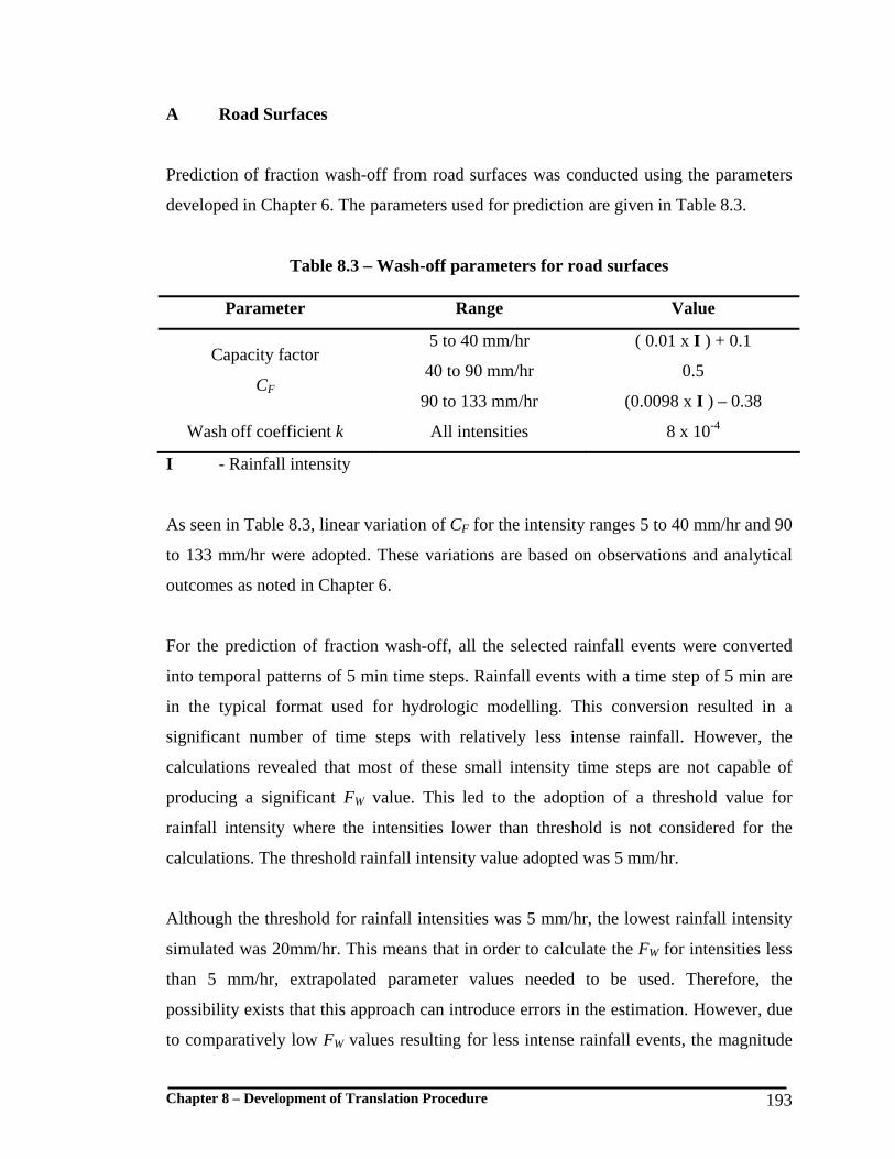
Chapter 8 – Development of Translation Procedure 193
A Road Surfaces
Prediction of fraction wash-off from road surfaces was conducted using the parameters
developed in Chapter 6. The parameters used for prediction are given in Table 8.3.
Table 8.3 – Wash-off parameters for road surfaces
Parameter Range Value
5 to 40 mm/hr ( 0.01 x I ) + 0.1
40 to 90 mm/hr 0.5 Capacity factor
CF 90 to 133 mm/hr (0.0098 x I ) – 0.38
Wash off coefficient k All intensities 8 x 10⁻⁴
I - Rainfall intensity
As seen in Table 8.3, linear variation of CF for the intensity ranges 5 to 40 mm/hr and 90
to 133 mm/hr were adopted. These variations are based on observations and analytical
outcomes as noted in Chapter 6.
For the prediction of fraction wash-off, all the selected rainfall events were converted
into temporal patterns of 5 min time steps. Rainfall events with a time step of 5 min are
in the typical format used for hydrologic modelling. This conversion resulted in a
significant number of time steps with relatively less intense rainfall. However, the
calculations revealed that most of these small intensity time steps are not capable of
producing a significant FW value. This led to the adoption of a threshold value for
rainfall intensity where the intensities lower than threshold is not considered for the
calculations. The threshold rainfall intensity value adopted was 5 mm/hr.
Although the threshold for rainfall intensities was 5 mm/hr, the lowest rainfall intensity
simulated was 20mm/hr. This means that in order to calculate the FW for intensities less
than 5 mm/hr, extrapolated parameter values needed to be used. Therefore, the
possibility exists that this approach can introduce errors in the estimation. However, due
to comparatively low FW values resulting for less intense rainfall events, the magnitude
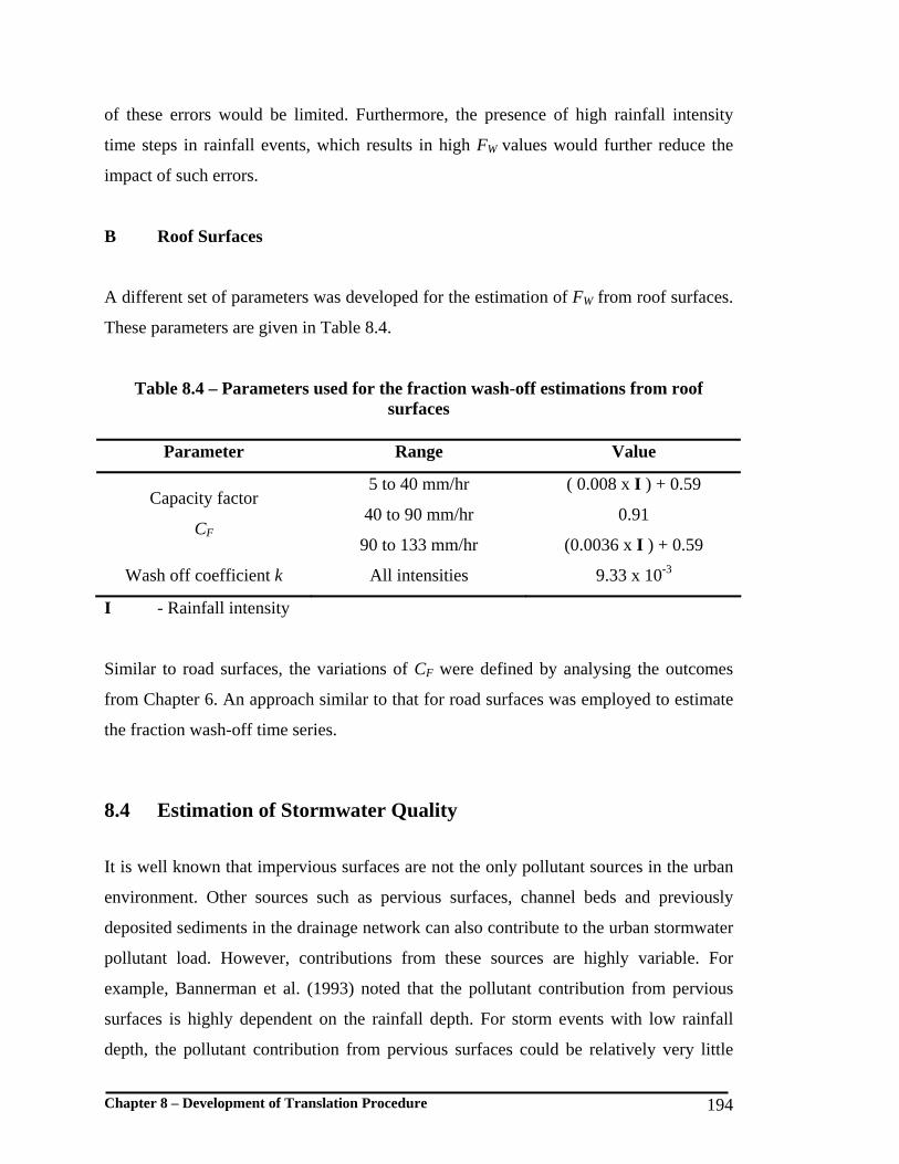
Chapter 8 – Development of Translation Procedure 194
of these errors would be limited. Furthermore, the presence of high rainfall intensity
time steps in rainfall events, which results in high FW values would further reduce the
impact of such errors.
B Roof Surfaces
A different set of parameters was developed for the estimation of FW from roof surfaces.
These parameters are given in Table 8.4.
Table 8.4 – Parameters used for the fraction wash-off estimations from roof surfaces
Parameter Range Value
5 to 40 mm/hr ( 0.008 x I ) + 0.59
40 to 90 mm/hr 0.91 Capacity factor
CF 90 to 133 mm/hr (0.0036 x I ) + 0.59
Wash off coefficient k All intensities 9.33 x 10⁻³
I - Rainfall intensity
Similar to road surfaces, the variations of CF were defined by analysing the outcomes
from Chapter 6. An approach similar to that for road surfaces was employed to estimate
the fraction wash-off time series.
8.4 Estimation of Stormwater Quality
It is well known that impervious surfaces are not the only pollutant sources in the urban
environment. Other sources such as pervious surfaces, channel beds and previously
deposited sediments in the drainage network can also contribute to the urban stormwater
pollutant load. However, contributions from these sources are highly variable. For
example, Bannerman et al. (1993) noted that the pollutant contribution from pervious
surfaces is highly dependent on the rainfall depth. For storm events with low rainfall
depth, the pollutant contribution from pervious surfaces could be relatively very little

Chapter 8 – Development of Translation Procedure 195
due to low runoff, high rate of infiltration and pollutant trapping within rough surfaces.
For storms events with large rainfall depth, pervious surfaces can be a large pool of
pollutants, particularly sediments. However, many researchers have noted that the
pollutant contribution from impervious surfaces is the major component in stormwater
runoff. Most researchers have specifically focused on road surfaces due to their critical
role in contributing stormwater pollutants (Bannerman et al., 1993; Bertrand-Krajewski
et al., 1998; Deletic and Orr, 2005; Sartor et al., 1974; Shaheen, 1975).
These observations suggest that the pollutant contribution from impervious surfaces can
be either major or minor depending on the nature of the storm event, characteristics of
the drainage network and the catchment management practices. This means that for a
given catchment with known catchment and drainage characteristics and for common
regional rainfall characteristics, the relative fraction of pollutants originating from
impervious surfaces could be within a constant range. Based on the above argument, it is
important to understand the relative fraction of pollutant contribution from impervious
surfaces. Furthermore, outcomes of such analysis provide important information as to
how representative small-plot pollutant processes are in catchment scale water quality
predictions.
The pollutant contribution from urban impervious surfaces was estimated based on
pollutant build-up and wash-off processes. The methodology adopted when using these
pollutant processes is discussed in Sections 8.2 and 8.3. Apart from these processes, both
hydrologic and hydraulic processes were also simulated to estimate the runoff. This was
to calculate the pollutant concentrations. The comparison of estimated pollutant
concentration with the observed value was done in two stages. Firstly, the comparison
was ‘event based’, which compared the event mean concentrations (EMCs) of estimated
and observed water quality. Secondly, instantaneous concentrations extracted from the
estimated pollutographs were compared with the corresponding instantaneous
observations.

Chapter 8 – Development of Translation Procedure 196
8.4.1 Event Based Water Quality Comparison
The estimations of pollutant amounts washed-off from road and roof surfaces were done
separately. These were later added together in order to determine the total amount of
pollutants washed-off. Calculation of pollutants washed-off from each impervious
surface type was determined by multiplying the amount of build-up per unit area by the
total area of impervious surface and fraction wash-off. The outcomes of the calculations
are presented in Appendix F, Table F.1. The total area of road and roof surfaces for each
catchment was determined using aerial photographs. Greater details of impervious area
calculations can be found in Section 4.3.1. Mean pollutant concentration for each event
was calculated by dividing the estimated load by runoff volume. The mean concentration
calculated for each rain event was compared with the measured event mean
concentrations for each catchment as shown in Figure 8.3.
It was found that driveways represent a significant fraction of impervious areas in urban
catchments and hence could have an appreciable influence on runoff quality. For the
three study catchments: Alextown, Birdlife Park and Gumbeel, the fraction of driveway
area to total catchment area are 8.6%, 11.2% and 11.2% respectively. For the analysis,
driveways were considered to have similar build-up and wash-off properties to road
surfaces. This assumption is more applicable for build-up estimations since driveways
are subjected to similar traffic-related and atmospheric depositions and pollution re-
distribution. However, due to relatively low texture depth of concrete driveways, the
wash-off could be different to roads. Nevertheless, due to greater variability of primary
surface characteristics such as texture depth, slope and porosity, the wash-off
characteristics of driveways can be significantly different to that of roof surfaces. Hence,
the adoption of wash-off replications of road surfaces for driveways was considered to
lead to less error.
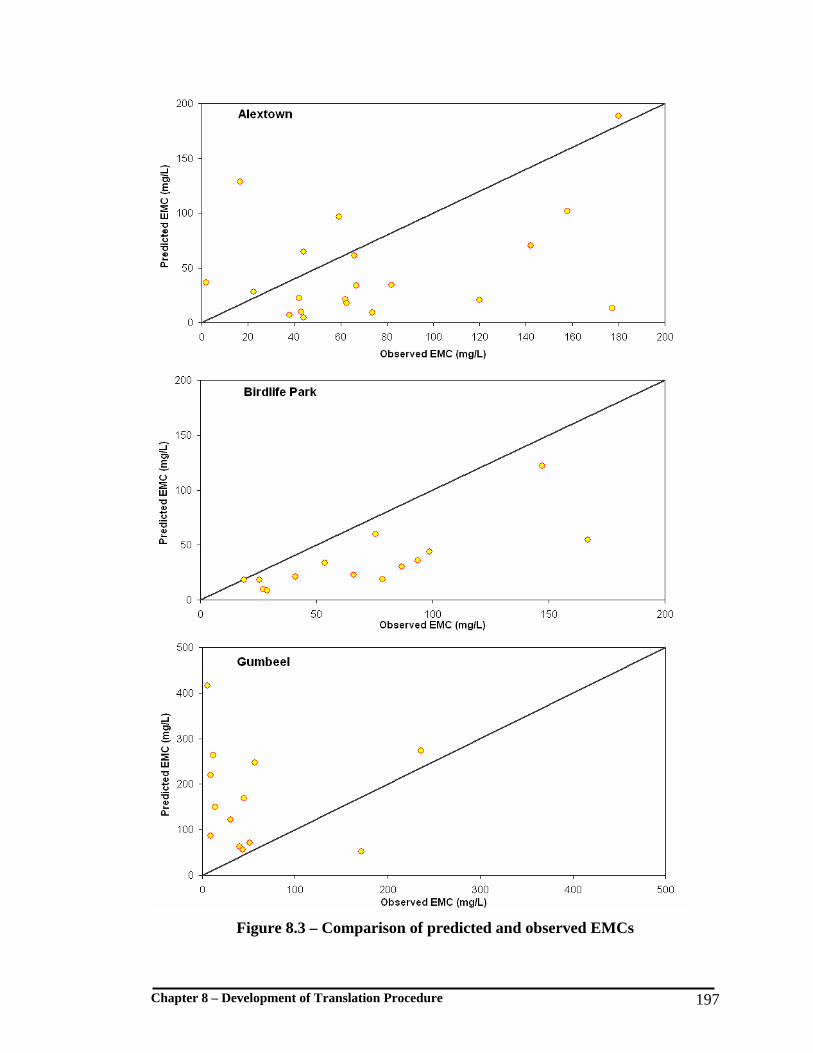
Chapter 8 – Development of Translation Procedure 197
Figure 8.3 – Comparison of predicted and observed EMCs
Chapter 8 – Development of Translation Procedure 198
In the analysis it was noted that a relatively higher amount of pollutants was originating
from roof surfaces. For a significant number of events, the contribution from roof
surfaces is even higher than the contribution from road surfaces (see Appendix F, Table
F.1). This is due to the higher fraction wash-off from roof surfaces which can be
primarily attributed to the relatively smoother surface texture and higher slopes when
compared to road surfaces. This highlights the significance of roof surfaces as an urban
water pollutant source. The significance is particularly important for low intensity storm
events where a higher fraction of pollutants is washed-off from roofs when compared to
roads.
As seen in Figure 8.3, event based estimation of water quality using small-plot pollutant
processes is relatively unsuccessful. The estimated EMCs deviate significantly from the
observed EMCs for most of the storm events. For the Alextown catchment, predictions
are scattered compared to observed EMCs. The estimates relatively under-predict the
water quality at Birdlife Park catchment whereas they over-predict the Gumbeel
catchment water quality. The deviations between predicted and observed EMCs can be
primarily attributed to the following factors:
1) The predicted mean concentrations represent pollutants from impervious surfaces
only. Therefore, for the events where a significant fraction of pollutants originates
from other sources, the observed and predicted water quality would be different.
2) Sampling from storm events was done by pumping from a constant height from the
channel bed, irrespective of the flow depth. This could result in collecting non-
representative samples.
3) EMC samples were prepared from the runoff samples typically collected 30 min
apart. Due to the relatively smaller size of catchments and the ‘flashy’ nature of
storm events, water quality can vary significantly during this time interval. This can
lead to non-representative EMC results for events.
4) The predicted water quality was based on a number of assumptions and conceptual
pollutant processes. This may introduce errors to the predictions.

Chapter 8 – Development of Translation Procedure 199
The unsatisfactory correlation of predicted and observed EMCs suggested that the
replication of small-plot pollutant processes is not satisfactory for predicting the event
based water quality. However, due to the fact that non-correlation could arise from non-
representative EMC measurements, comparison of instantaneous water quality was
undertaken.
8.4.2 Comparison of Instantaneous Water Quality
Estimation of instantaneous water quality was undertaken by simulating pollutant build-
up and wash-off processes along with hydrologic processes. The simulations were done
so that the outcomes of each simulated process were temporally compatible. The
technique used for simulation was similar to the techniques used in typical stormwater
quality estimation models. Instantaneous water quality was then extracted from the
predicted pollutographs and compared with the corresponding observed water quality.
The estimated pollutographs were in 1 min time steps. The detailed procedure used for
simulations and the estimation of pollutographs is discussed below.
A Pollutant wash-off time series
The pollutant load washed-off from a unit area of each surface type was calculated in 5
min time steps. This was done by multiplying the time series of fraction wash-off by
build-up pollutant load. More details on the methodologies adopted to estimate build-up
load and fraction wash-off time series are given in Sections 8.2 and 8.3 respectively. The
resulting values for both road and roof surfaces were multiplied by their corresponding
surface area in the catchment and added together in order to calculate the total amount of
pollutants removed at each time step.
B Translation from Catchment Surfaces to Sub-area Outlet
Translation of estimated wash-off pollutant time series from catchment surfaces to sub-
area outlets was done using a routing procedure. For this, each catchment was

Chapter 8 – Development of Translation Procedure 200
subdivided into sub-areas similar to the catchment subdivisions in Section 7.2. A routing
procedure was developed based on the concept of the time-area method (see Section
2.5.2). When routing, each sub-area was considered to consist of strips with equal area,
having different times of concentration. The pollutants originating from each strip were
considered to arrive at the sub-area outlet at time periods according to their pre-assigned
time of concentration. During the routing, the pollutant load belonging to each strip was
calculated by multiplying each time step of the pollutant wash-off time series by the
ratio between the strip area to total catchment area and impervious fraction. For ease of
calculations, the routing procedure was coded as a Visual Basic Macro in Microsoft XL
interface. Consequently, it was possible to use a Microsoft XL spreadsheet as the
platform for rainfall and catchment data input and to obtain the resulting output.
Appendix F, Figure F.2 gives the Microsoft XL spreadsheet and Figure F.3 gives the
Visual Basic code.
The accuracy of the routing procedure was tested using a series of rainfall events instead
of pollutant loads. This was done due to the similarities of the routing procedure to
hydrologic routing. As the procedure is very similar to the method adopted in Mike
STORM, the outcomes of the routing were compared with simulated runoff using this
model. Furthermore, the primary parameters for the routing procedure were obtained
from the calibrated Mike STORM models as noted in Section 7.3. A sample comparison
is shown in Figure 8.4.
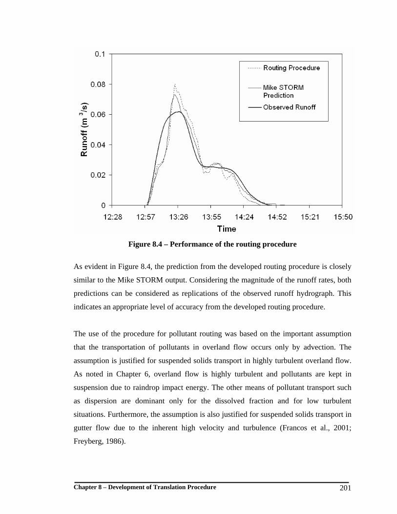
Chapter 8 – Development of Translation Procedure 201
Figure 8.4 – Performance of the routing procedure
As evident in Figure 8.4, the prediction from the developed routing procedure is closely
similar to the Mike STORM output. Considering the magnitude of the runoff rates, both
predictions can be considered as replications of the observed runoff hydrograph. This
indicates an appropriate level of accuracy from the developed routing procedure.
The use of the procedure for pollutant routing was based on the important assumption
that the transportation of pollutants in overland flow occurs only by advection. The
assumption is justified for suspended solids transport in highly turbulent overland flow.
As noted in Chapter 6, overland flow is highly turbulent and pollutants are kept in
suspension due to raindrop impact energy. The other means of pollutant transport such
as dispersion are dominant only for the dissolved fraction and for low turbulent
situations. Furthermore, the assumption is also justified for suspended solids transport in
gutter flow due to the inherent high velocity and turbulence (Francos et al., 2001;
Freyberg, 1986).

Chapter 8 – Development of Translation Procedure 202
C Translation from Sub-area Outlet to Catchment Outlet
In order to obtain the pollutograph at the catchment outlet, the resulting pollutant load
time series for sub-area outlets needed to be translated to the catchment outlet. This was
done using the Mike STORM advection-dispersion (AD) routing model. However, the
AD model is designed only to rout average pollutant concentrations from nodes to the
catchment outlet. Therefore, the average pollutant concentration was calculated for each
event. This was done by dividing the total pollutant load at each time step by the
corresponding runoff volume. The total pollutant load time series was obtained by
adding all the sub-area pollutant load time series together. The use of average
concentration in pollutant translation provides sufficient accuracy.
Apart from the average concentration time series, Mike STORM (AD) also needs both
hydrologic and hydraulic simulation results for each storm event. This was obtained by
simulating calibrated Mike STORM models for each catchment, as explained in Chapter
7. In order to establish the accuracy of estimations, both estimated runoff and water
quality were compared with the observed values. Figure 8.5 shows sample comparisons
for the three study catchments.

Chapter 8 – Development of Translation Procedure 203
Figure 8.5 – Comparison of continuous water quality estimations with observed water quality

Chapter 8 – Development of Translation Procedure 204
D Comparison of Predicted and Observed Water Quality As noted in Section 4.3.2, runoff samples have been collected from the study catchment
outlets and tested for a range of quality parameters. Apart from the quality parameters,
the exact date and time where each sample was collected was also available. These data
are referred to as instantaneous quality observations. From the estimated pollutographs,
the instantaneous water quality records corresponding to the exact collection time of
observed water quality records were extracted. However, prior to extraction, the time
scale of predicted measurements was adjusted so that the predicted hydrograph peaks
and starting points coincide with the peaks and starting points of observed hydrographs.
In this way, it was possible to eliminate the non-synchronised data logging between the
water sampling/flow measuring device and the rain gauge. The extracted data from the
predicted pollutographs and observed instantaneous data was compared to understand
the predictive capability. Figure 8.6 shows the comparison of observed and predicted
instantaneous water quality for all catchments. Appendix F, Figure F.4 gives the
comparisons for individual catchments.
0
100
200
300
400
500
0 100 200 300 400 500
Observed Concentration (mg/L)
Estim
ated
Con
cent
ratio
n (m
g/L)
First Observation per Event
Other Observations
Figure 8.6 – Comparison of observed and predicted instantaneous concentration
Chapter 8 – Development of Translation Procedure 205
As seen in Figures 8.5 and 8.6, the variation of predicted water quality with respect to
observed water quality illustrates a common pattern. However, it is quite clear that the
predictions do not give perfect accuracy. It is commonly accepted that the prediction of
water quality is subjected to a high degree of variability. Consequent to the range of
simplifying assumptions used in predictions, the water quality estimations are subjected
to a high degree of uncertainty (Ahyerre et al., 1998; Huber, 2001). Additionally, non-
representative water sampling can lead to errors in observed water quality which in turn
reduces reliability when used for comparison. Considering these facts, it can be
concluded that the results obtained from the continuous water quality prediction are
within an accuracy range typical of those described in numerous research studies (for
example Ahyerre et al., 1998; Huber, 2001; Im et al., 2003; Leon et al., 2001;
Supriyasilp et al., 2003; Tsihrintzis and Hamid, 1998; Zug et al., 1999).
In the analysis of observed and predicted water quality, the initial water quality
observation of each event and the corresponding extracted quality from the predicted
pollutograph were noted. This was to distinguish the predictive capability for various
stages of the storm event. As seen in Figure 8.6, the accuracy of estimations is high for
the initial observation of each event. In statistical terms, the mean of the ratio between
predicted and observed instantaneous water quality is 1.2 for the initial observation and
15.2 for the others. For highly accurate estimations, the mean should be close to 1.
Furthermore, the initial observations show less data scatter compared to others. The CV
for the initial observation is 60% whereas for others it is 200%. This confirms that the
methodology adopted to estimate water quality is relatively more accurate for the initial
period of storm events.
It was noted during the analysis that estimated pollutant concentration is significantly
high during the initial part of runoff events. This can be particularly noted in Figure 8.5.
This could be primarily attributed to wash-off behaviour from impervious surfaces
where a higher fraction of pollutants is washed-off during the initial part of rainfall
events. Higher fraction wash-off is particularly common for roof surfaces where a
significant number of selected events resulted in 100% wash-off during the initial period

Chapter 8 – Development of Translation Procedure 206
of the rainfall event. The high concentrations of pollutants in the initial part of the runoff
event can also be noted in observed water quality. As noted in Figure 8.6, most of the
initial water quality observations are relatively high compared to others. Such high
concentration of pollutants is termed as ‘first flush’ and has been reported by many
researchers (for example: Duncan, 1995; Lee et al., 2002). This revealed that the initial
part of the runoff is the most critical in terms of deterioration of receiving water quality.
The above discussion leads to two primary conclusions. Firstly, the initial part of the
runoff event is the most critical as a pollutant source to receiving water bodies.
Secondly, the methodology adopted to estimate the stormwater quality is reasonably
accurate in estimating the initial part of the runoff event. These two observations suggest
that pollutant build-up and wash-off measurements used for the estimation procedure are
representative in estimating water quality in the most critical part of the runoff event.
Therefore, the intended translation procedure based on pollutant build-up and wash-off
processes would result in estimations of acceptable accuracy.
8.5 Simplified Wash-off Estimation
Although the estimation procedure described in Section 8.4.2 provides reasonably
accurate results, the method is too complex to be used in simple water quality
estimations. The complexity can be primarily attributed to the procedure for simulating
pollutant wash-off and to the procedure used to translate the wash-off time series to the
catchment outlet. Simulation of wash-off is particularly complex due to the procedure
adopted to account for the temporal variability of rainfall events. In order to eliminate
this complexity, it was felt that a simplified method was needed. However, it was clear
that the use of a simplified method could reduce the accuracy of estimation.
Consequently, every effort was made to obtain the highest possible accuracy using a
simplified method.
The primary approach to simplify the simulations was to obtain an equivalent constant
rainfall intensity that results in a similar fraction wash-off. By this way, it is possible to

Chapter 8 – Development of Translation Procedure 207
eliminate the simulation of rainfall events with high temporal variability. However, it is
noted in Section 6.4.3 that FW is subjected to a higher degree of variability with rainfall
intensity. According to Equation 6.3, the variability is primarily attributed to capacity
factor, CF, which has different values for several ranges of rainfall intensity. This
highlighted the difficulty of obtaining a constant rainfall intensity to represent a
temporally variable rainfall event.
Instead of one constant rainfall intensity, several constant rainfall intensities for different
intensity ranges would be the most appropriate to represent a temporally variable rainfall
event. The rainfall intensity ranges used for defining values for CF would be the most
appropriate. Intensity ranges of 5 to 40 mm/hr, 40 to 90 mm/hr and 90 to 133 mm/hr
were adopted to develop the simplified rainfall event. The average intensity for each
range was calculated by dividing the rainfall depth in each range by the cumulative
rainfall duration for the range. It was assumed that this average intensity continues for
the cumulative duration. The average intensities were arranged in ascending order to
facilitate easy manual estimation of FW. This eliminates the possibility of giving non-
significant wash-off results for smaller average intensities if they were used at the end of
intensity time series. Figure 8.7 shows an illustration of the procedure used to obtain the
simplified rainfall intensity. The detailed calculations for Figure 8.7 are given in
Appendix F, Table F.2.

Chapter 8 – Development of Translation Procedure 208
Figure 8.7 – Method to obtain simplified rainfall event
In order to determine the degree of error involved in using the simplified rainfall events,
the resulting FW was compared to the FW calculated for the original rainfall events. This
was done for road and roof surfaces separately. Figure 8.8 shows the variation of the two
sets of FW values. The events analysed were those selected for the three study
catchments.
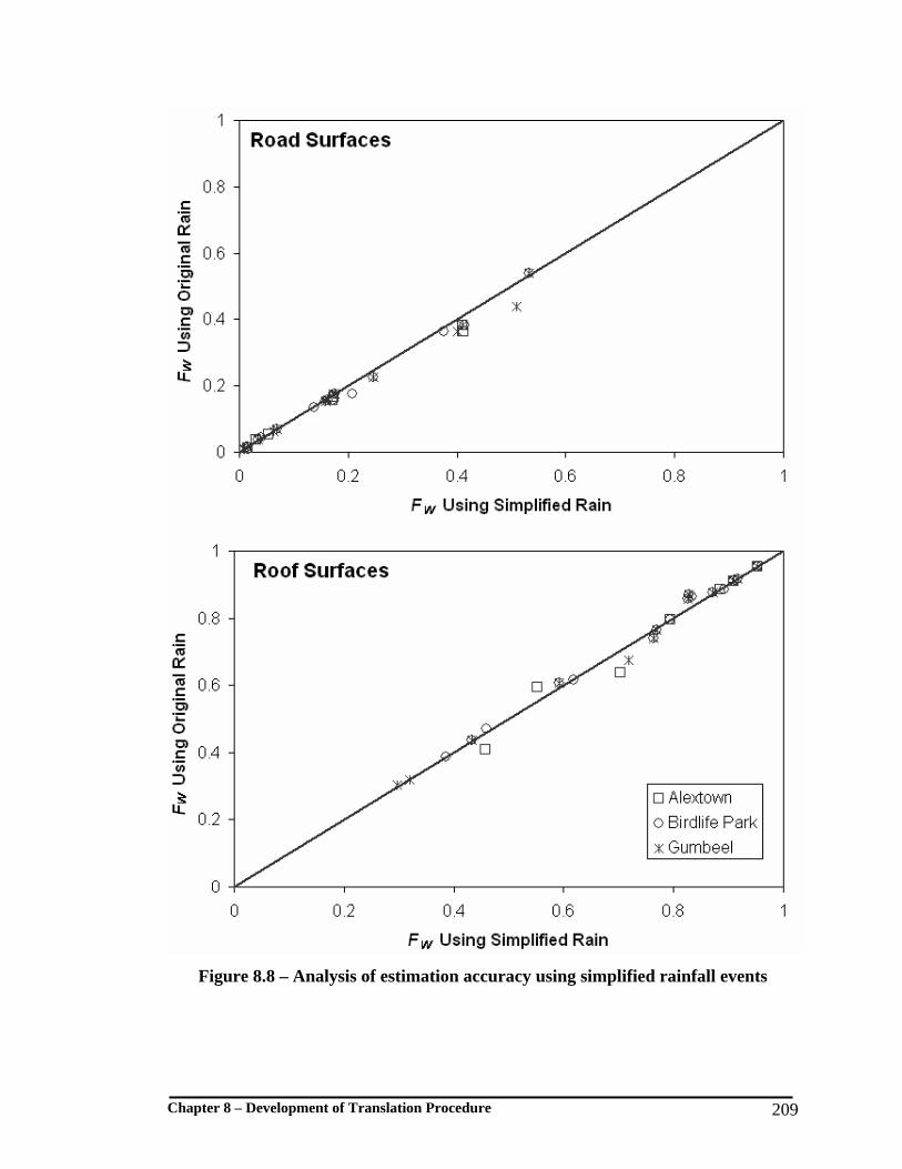
Chapter 8 – Development of Translation Procedure 209
Figure 8.8 – Analysis of estimation accuracy using simplified rainfall events
Chapter 8 – Development of Translation Procedure 210
As seen in Figure 8.7, the difference between the estimation of FW values using original
rainfall events and simplified rainfall events is minimal for both road and roof surfaces.
The mean of the ratio between the two sets of FW values estimated using original and
simplified rainfall events is 0.97 for road surfaces and 1.01 for roof surfaces. The CV for
road and roof surfaces is 9.3% and 3.8% respectively. This suggests that the estimations
resulting from using simplified rainfall events are consistently similar to those obtained
using original rainfall events. Therefore, it can be considered that the use of simplified
rainfall events in FW estimation is accurate enough to be used in water quality
predictions.
8.6 Translation Procedure
A simple tool such as a translation procedure is useful to calculate the amount of
suspended solid pollutants washed-off from urban impervious surfaces. The method can
be based on the knowledge of small-plot pollutant processes, namely, pollutant build-up
and wash-off from road and roof surfaces. The predictions are limited to the amount of
pollutants originating from impervious surfaces. However, as discussed in Section 8.4.2,
urban impervious surfaces are the dominant pollutant source during the initial period of
runoff events. Therefore, the method is valid for prediction for more common storm
events where other sources such as pervious surfaces and erosion are not significant.
For better understanding and simple use, the translation procedure is described in tabular
form below. Table 8.5 shows the estimation procedure. The estimation procedure
requires a typical set of catchment and rainfall data that common water quality
modelling tools often require. This data includes catchment area, impervious percentage,
and temporal distribution of rainfall. The values relating to small-plot pollutant
processes that needed to be obtained from the charts are shown in the following sections.
The methods of using these charts are discussed in Sections 8.2 and 8.3.

Chapter 8 – Development of Translation Procedure 211
Table 8.5 - Estimation of Event Based Suspended Solid Pollutants from Urban Catchments by Translating Small-plot
Pollutant Processes to Catchment Scale
Impervious
Percentage (Im)
(%)
Storm
No.
Catchment
Area (A)
(m2) Roads and
Driveways
Roofs
Build-up on
Roads (B)
(g/m2)
(Figure 8.9& 8.10)
Build-up on
Roofs (B)
(g/m2)
(Figure 8.11)
FW (Ro)
from
Roads
(Figure 8.12)
FW (Rf)
from
Roofs
(Figure 8.13)
Wash-off
from
Roads (g)
(C)
Wash-off
from
Roofs (g)
(D)
Total
Wash-off
Method
See Section 8.6.1
See Section 8.6.2 See Section 8.6.3
A x Im x
B x FW-
(Ro)
A x Im x
B x FW-
(Rf)
C + D
Chapter 8 – Development of Translation Procedure 212
8.6.1 Data for Translation Procedure
The data required for the translation procedure is of two types; catchment data and
rainfall data. The required primary catchment data is catchment area and impervious
surface percentages. The required rainfall data is rainfall temporal pattern for the study
events and dry days prior to the rainfall event. Relevant considerations in relation to
these data requirements are:
1) Catchment demarcation is one of the most important parts of pollutant load
estimation. Since the research was conducted in relatively small urban catchments
with areas of 1.7 to 8.6 ha, it is recommended to demarcate catchments in similar
size. Use of small catchments also mean that pollutants from impervious surfaces
only are washed-off during the initial part of the runoff event.
2) The translation procedure requires percentages of impervious area for two surface
types. Due to similarities of small-plot pollutant processes, roads and driveways
were considered one surface type and roofs were considered a different type. The
percentage of impervious surfaces was measured using aerial photographs. Further
details on the method used are discussed in Section 4.3.1.
3) For the research study, data from the tipping bucket rain gauge situated within a 2
km distance to all sites was used for obtaining the temporal patterns for the rainfall.
However, depending on the aerial variability of rainfall and the accuracy required by
the user, commonly available rainfall data can be used. The same data can be used to
obtain the number of antecedent dry days. During the study, dry days were counted
from the end of the previous storm event to the start of the next storm. Rainfall
events less than 5 mm were disregarded during the count.
8.6.2 Estimation of Build-up
The amounts of pollutant build-up on both road and roof surfaces have to be estimated
separately using the charts provided in Figures 8.9, 8.10 and 8.11. The first two figures

Chapter 8 – Development of Translation Procedure 213
are for two different residential population density categories of low and high. The low
population density is equivalent to typical single detached housing. The high population
density is equivalent to townhouses. Most residential urban land-uses commonly belong
to these two categories. However, for any other conditions where these two land-uses are
not considered suitable, it is possible to develop specific curves by modifying the
relevant parameters. It is recommended to change the multiplication coefficient ‘a’ for
such instances. For mixed residential urban form, selection of an appropriate a is
recommended. Changing the power coefficient ‘b’ is only recommended if the surface
type is different from typical residential road surfaces. A similar approach to obtaining
the necessary parameters for roof surfaces is recommended. The typical build-up
variation for residential catchments is shown in Figure 8.11.
For the simplicity of predictions, charts for road surface build-up were separated into
two regions. The region up to two antecedent dry days is where the build-up is assumed
to vary linearly. For this region, the starting point for the build-up is considered to be
dependent on the pre-existing pollutant amount after the previous rain event. This
pollutant amount needs to be estimated by analysing the previous rain event. A linear
variation is then considered from the pre-existing amount at day zero to typical two day
build-up at day two. In the case where the pre-existing pollutant amount is more than the
two day equivalent build-up, no variation is considered. For the region beyond a two day
antecedent dry period, build-up is considered to be a power function. The estimation
resulting from the power variation is considered to be accurate if the pre-existing
pollutant load is less than the two day equivalent build-up. No variation is considered, if
the pre-existing pollutant load is greater than a two day equivalent build-up.
For the roof surfaces, a pre-existing amount is not considered to be available after a rain
event. This is due to the relatively high wash-off from roof surfaces which leads to near
zero build-up remaining for most rain events. Therefore, only the linear variation up to
two days and the power variation beyond that would be appropriate to estimate the
build-up on roofs.

Chapter 8 – Development of Translation Procedure 214
Line projections can be used to estimate the amount of pollutant build-up using these
charts. However, the first step would be to estimate the pre-existing amount of pollutants
that provides the starting point for using the chart. This can be determined when a series
of consecutive rain events have been analysed.

Chapter 8 – Development of Translation Procedure 215
0
1
2
3
4
0 5 10 15 20
Antecedent Dry Days
Bui
ld-u
p Lo
ad (g
/m2 )
Figure 8.9 - Build-up on road surfaces: residential roads in low population density residential forms (equivalent to single
detached housing regions)
Linear Region
Starting point depends on the load remaining after the previous storm
Power Variation B = aDb a = 1.65 and b = 0.16
If the pollutant load remaining after the previous storm event is greater than 2 day equivalent build-up, use horizontal line as the build-up variation

Chapter 8 – Development of Translation Procedure 216
0
1
2
3
4
5
6
0 5 10 15 20Antecedent Dry Days
Bui
ld-u
p Lo
ad (g
/m2 )
Figure 8.10 - Build-up on road surfaces: residential roads in high population density residential forms (equivalent to
townhouse regions)
Linear Region
Starting point depends on the un-washed load from the previous storm
Power Variation B = aDb a = 2.9 and b = 0.16If the pollutant load remaining after the previous storm event is greater than 2 day equivalent build-up, use horizontal line as the build-up variation

Chapter 8 – Development of Translation Procedure 217
0
0.2
0.4
0.6
0.8
1
1.2
0 5 10 15 20Antecedent Dry Days
Bui
ld-u
p Lo
ad (g
/m2 )
Figure 8.11 - Build-up on roof surfaces: common residential roofs (variation developed for corrugated steel and concrete tile
roofs with 200 roofing angle)
Linear Region
No un-washed pollutant amount considered
Power Variation B = aDb a = 0.43 and b = 0.266
No separate variation is needed to account for the pollutant load remaining after the previous storm event
Chapter 8 – Development of Translation Procedure 218
8.6.3 Estimation of FW
FW for both road and roof surfaces has to be determined using Figures 8.12 and 8.13
respectively. Figure 8.12, which represents the wash-off from road surfaces was
developed for roads with 0.66 to 0.92 mm texture depth and 7.2 to 10.8% longitudinal
slopes. However, the variation of FW as noted in Figures 8.12 and 8.13 would be
applicable to most of the common residential road surfaces. As similar pavement
methods are commonly used in road construction, the variation of texture depth would
not deviate significantly from the investigated range. Furthermore, no significant
variation of wash-off characteristics is expected due to changes in the longitudinal slope.
Figure 8.13, which represents wash-off from roof surfaces was developed for corrugated
steel and concrete tile roofs with 200 roofing angle. However, the outcomes are
considered to be satisfactory for most of the common roofing types and for different
roofing angles.
For the estimation of FW, it is recommended to use simplified rainfall events. It was
noted in Section 8.5 that simplified rainfall events are capable of providing estimations
close to those obtained using the original rain events. The procedure to be adopted to
obtain a simplified rainfall event is given in Section 8.5 and illustrated in Appendix F,
Table F.2. The original rainfall events used in the analysis should be obtained from
measured data as explained in Section 8.6.1.
The variation of FW for intensities other than those illustrated in the charts should be
interpolated and plotted. The interpolations would be valid only for the intensities
greater than 5 mm/hr and less than 133 mm/hr. Intensities less than 5 mm/hr can be
disregarded from the analyses due to relatively low FW. It is recommended that the curve
for 133 mm/hr (as shown in Figure 8.12) should be used for any greater rainfall
intensity. The upper limit of intensity for Figure 8.13 is 115 mm/hr. The procedure for
the estimation of FW for other intensities can be carried out in a way similar to that for
the wash-off model discussed in Section 8.3.1 and illustrated in Figure 8.2.

Chapter 8 – Development of Translation Procedure 219
20 mm/hr
40 mm/hr
90 mm/hr
115 mm/hr
133 mm/hr
0
0.2
0.4
0.6
0.8
1
0 10 20 30 40
Rainfall Duration (min)
F W
Figure 8.12 - Wash-off from road surfaces: typical residential roads (variation developed for roads with 0.66 to 0.92 mm
texture depth and 7.2 to 10.8 % longitudinal slope)
)1(0
kItF eC
WWFw −−==
See Section 8.6.3 for CF and k
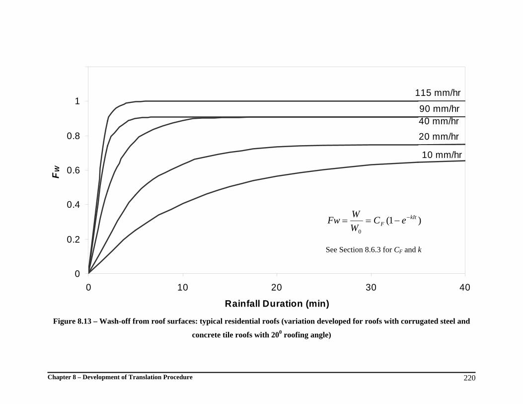
Chapter 8 – Development of Translation Procedure 220
10 mm/hr
20 mm/hr40 mm/hr90 mm/hr
115 mm/hr
0
0.2
0.4
0.6
0.8
1
1.2
0 10 20 30 40
Rainfall Duration (min)
F W
Figure 8.13 – Wash-off from roof surfaces: typical residential roofs (variation developed for roofs with corrugated steel and
concrete tile roofs with 200 roofing angle)
)1(0
kItF eC
WWFw −−==
See Section 8.6.3 for CF and k
Chapter 8 – Development of Translation Procedure 221
8.6.4 Issues in Using the Translation Procedure
A Validity of the Translation Procedure to Other Geographical Regions
The translation procedure is a simplified approach to estimate the amount of pollutants
washed-off from urban catchments. With the use of appropriate build-up and wash-off
data to best suit the characteristics of a given catchment, the procedure would be as
accurate as a typical stormwater quality modelling tool.
As discussed in Chapter 6, the variation of build-up on both road and roof surfaces is
parameterised by the multiplication coefficient ‘a’ and power coefficient ‘b’. It was
understood that b varies with the surface type, where two values were obtained for road
and roof surfaces. The values obtained for b would be appropriate for any common road
and roof surface types. However, investigations are needed if a high fraction of other
surfaces such as parking lots is present within the catchment.
The coefficient a defines the pollutant accumulation potential of the catchment surfaces
which would vary with population density, land-use, traffic volume and other regional
factors. Two coefficient values for road surfaces, specifically for high and low
population density residential urban form, and one coefficient value for common
residential roof surfaces have been derived. For catchments with characteristics other
than these urban forms, values for a can be obtained based on the amount of pollutant
availability on road surfaces. However, this would require experience and judgement.
Furthermore, a field investigation to justify the assumed values would be advisable.
As discussed in Chapter 6, the primary characteristics that influence pollutant wash-off
other than rainfall parameters are surface type and condition. The parameter values
defining wash-off from most common road and roof surfaces have already been
developed. Therefore, the curves shown in Figures 8.12 and 8.13 are applicable for most
of the road and roof surfaces in urban catchments with common land-uses. Furthermore,
it can be considered that driveways are equivalent to road surfaces. However, these

Chapter 8 – Development of Translation Procedure 222
values would not be appropriate for surfaces such as brick pavements and further
investigations are recommended.
B Interpretation of Outcomes
Since the translation procedure is based on pollutant build-up and wash-off, the
outcomes only reflect the pollutant amount originating from catchment impervious
surfaces. However, impervious surfaces are not the only pollutant sources in the urban
environment. Depending on the requirement, other methods can be used to estimate the
amount of pollutants originating from other sources such as pervious surfaces. Though
not comprehensive, the translation procedure estimates the most critical fraction of
pollutants which causes the most significant impact on receiving waters.
8.7 Conclusions
Prior to the development of the translation procedure the validity of small-plot pollutant
processes being representative of catchment impervious surfaces was evaluated. This
was done by replicating pollutant build-up and wash-off processes for a range of
selected rainfall events for the three study catchments where water quality observations
were available. Predicted and measured water qualities were compared using two
approaches.
Comparison of event EMCs of predicted and observed water quality showed limited
correlation. Therefore, it was considered that the validity of estimating event based
water quality using small-plot pollutant processes is not appropriate. It is hypothesised
that this is primarily due to pollutant contributions from pervious surfaces, non-
representative EMC observations and errors in water quality estimations.
The comparison of instantaneous water quality observations with quality data from
predicted pollutographs resulted in close correlations. The error associated with such
comparisons was considered to be in the acceptable range for water quality predictions

Chapter 8 – Development of Translation Procedure 223
which are generally highly variable. Therefore, small-plot pollutant processes can be
representative of catchment scale water quality particularly for the initial part of runoff
events. The translation procedure developed is limited to pollutants originating from
impervious surfaces which are the predominant source during the initial period of runoff
events.
The translation procedure is a simplified tool that can be used to estimate suspended
solid loads washed-off by a particular rainfall event. The method uses knowledge build-
up and wash-off processes developed for road and roof surfaces. However, the
knowledge developed relating to small-plot processes is limited to the specific land-uses
and surface types.


Chapter 9 – Conclusions and Recommendations 225
Chapter 9 - Conclusions and Recommendations
9.1 Conclusions
The research project primarily developed a simplified procedure to estimate urban
stormwater quality by developing an in-depth understanding of pollutant build-up and
wash-off processes in small plots. The procedure was based on the hypothesis that the
translation of pollutant build-up and wash-off knowledge from small plots using rainfall
simulator can be used for predicting catchment scale water quality. However, build-up
and wash-off data is not readily available for various land-uses and climatic conditions.
This led to the development of fundamental knowledge on these processes as part of the
research study.
The data needed for the development of fundamental knowledge on pollutant build-up
and wash-off and the data for validation of the model were generated from in-depth
investigations undertaken on selected residential road and roof surfaces. Altogether,
three road sites and two roof surface types were investigated. Investigations were based
on small-plot areas. This was to eliminate difficulties inherent in the use of non-
homogeneous areas. Wash-off investigations were undertaken using simulated rainfall
events. This was to eliminate constraints inherent in the dependency of natural rainfall
events and their unpredictable nature. Data for the validation of the model was generated
by collecting runoff samples from three urban catchment outlets, namely, Alextown,
Gumbeel and Birdlife Park. Samples from a significant number of storm events have
been collected from these catchment outlets. Samples generated from all field
investigations were tested for a range of standard water quality parameters.
Data analysis was undertaken to develop mathematical replication equations and to
develop understanding on the underlying physical processes of build-up and wash-off.
The analysis further extended to an estimation of water quality of the three catchments
for a selected number of storm events. The accuracy of the estimations was tested by

Chapter 9 – Conclusions and Recommendations 226
comparison with the measured water quality at the catchment outlets. Based on the
accuracy of prediction, the simplified water quality estimation procedure was developed.
9.1.1 Pollutant Build-up
Analysis of build-up data revealed rapid build-up during the initial period after site
cleaning. However, the build-up observed on roof surfaces was gradual compared to
road surfaces where the rate was 2.3 g/m2/day for first two days and account for around
66% of the total build-up. Rapid variation in build-up during the initial period was
considered to be due to the higher impact of anthropogenic activities on road surfaces
such as traffic. The rapid reduction in the rate of build-up with the equilibrium condition
attained for the latter period was considered to be due to the influence of pollutant re-
distribution. This concept is justified by the gradual build-up pattern observed on roof
surfaces. Roof surface pollutants are mostly from atmospheric sources and re-
distribution would be relatively limited.
Although the pattern of pollutant build-up is common, the build-up loads observed for
the three road surfaces were different. The build-up load on the Gumbeel Court site was
significantly high compared to the Lauder Court and Piccadilly Place sites. The build-up
loads observed at the Lauder Court and Piccadilly Place sites were similar. The
differences in urban form and population density were considered as the primary cause
for such variation. Notable variation of build-up load was also evident on two roof
surface types. It was hypothesised that this is due to differences in the properties of
coatings used on the roofing products. However, this difference in build-up load was not
considered significant in water quality modelling.
It was possible to develop mathematical replication equations for build-up on roads and
roofs in a common format. A power equation was the most suitable. The variation of
build-up on roads due to urban form and population density was accounted for by using
two sets of parameters. A separate set of parameters was also developed for roof
surfaces. The proposed build-up equation is in the form of:
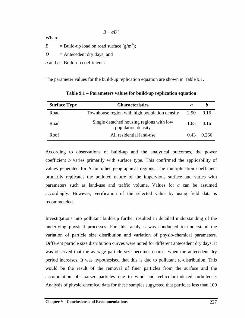
Chapter 9 – Conclusions and Recommendations 227
baDB = Where,
B = Build-up load on road surface (g/m2);
D = Antecedent dry days; and
a and b = Build-up coefficients.
The parameter values for the build-up replication equation are shown in Table 9.1.
Table 9.1 – Parameters values for build-up replication equation
Surface Type Characteristics a b
Road Townhouse region with high population density 2.90 0.16
Road Single detached housing regions with low population density
1.65 0.16
Roof All residential land-use 0.43 0.266
According to observations of build-up and the analytical outcomes, the power
coefficient b varies primarily with surface type. This confirmed the applicability of
values generated for b for other geographical regions. The multiplication coefficient
primarily replicates the polluted nature of the impervious surface and varies with
parameters such as land-use and traffic volume. Values for a can be assumed
accordingly. However, verification of the selected value by using field data is
recommended.
Investigations into pollutant build-up further resulted in detailed understanding of the
underlying physical processes. For this, analysis was conducted to understand the
variation of particle size distribution and variation of physio-chemical parameters.
Different particle size distribution curves were noted for different antecedent dry days. It
was observed that the average particle size becomes coarser when the antecedent dry
period increases. It was hypothesised that this is due to pollutant re-distribution. This
would be the result of the removal of finer particles from the surface and the
accumulation of coarser particles due to wind and vehicular-induced turbulence.
Analysis of physio-chemical data for these samples suggested that particles less than 100

Chapter 9 – Conclusions and Recommendations 228
μm are highly susceptible to re-distribution. The analysis noted relatively limited change
in sample load for this range, whilst particles coarser than this range progressively
accumulate. However, the high degree of pollutant re-distribution was not evident on
roof surfaces. This would be due to the lack of influence of vehicle-induced wind
turbulence in the vicinity of roof surfaces.
The pollutants observed on both road and roof surfaces were significantly finer
compared to results reported in previous research. On average, 50% of the road surface
solid pollutants and 60% of the roof surface solid pollutants were finer than the 100 μm
size range. The fineness of the road surface pollutants could be due to the low traffic
volumes in residential roads which formed the study sites. It was observed that a high
amount of soluble organic carbon is associated with the finer fraction of solids from both
road and roof surfaces. Hence, there is significant potential of having a relatively high
amount of other pollutants such as heavy metals and hydrocarbons being adsorbed to the
finer particles or in dissolved form when there is a wash-off event.
9.1.2 Pollutant Wash-off
Investigations into pollutant wash-off were conducted to understand the behaviour for a
range of influential factors and to measure the specific wash-off rates from impervious
surfaces. It was found that wash-off load is influenced by the initially available pollutant
amount on the surface. However, the wash-off process was found to be independent of
initial pollutant availability. This conclusion was based on the consistently similar
variation patterns of ‘fraction wash-off’ for the three road sites despite differences in
pollutant availability. Although a range of rainfall and runoff variables can be related, it
was found that the wash-off process is most adequately defined by two rainfall variables:
intensity and duration. These two variables were used in the mathematical replication of
wash-off.
The mathematical replication equation developed is a modified version of the original
exponential equation proposed by Sartor et al. (1974). The modification is primarily in

Chapter 9 – Conclusions and Recommendations 229
terms of an additional parameter referred to as the ‘capacity factor’, CF. The study
results showed that a storm event has the capacity to wash-off only a fraction of
pollutants available and this fraction varies primarily with rainfall intensity, kinetic
energy of raindrops and particle size distribution of the pollutants. The CF is defined to
incorporate this capacity in the replication equation. The modified wash-off equation is
in the form of:
)1( kItF eCFw −−=
Where,
I Rainfall intensity;
k Wash-off coefficient;
Fw Fraction wash-off;
CF Capacity factor; and
t Rainfall duration.
The modification made to the common pollutant wash-off equation is an improvement to
the current usage. The parameters developed are shown in Table 9.2.
Table 9.2 – Parameter values for wash-off replication equation
Parameter Range Value
For Road Surfaces
5 to 40 mm/hr ( 0.01 x I ) + 0.1
40 to 90 mm/hr 0.5 Capacity factor
CF 90 to 133 mm/hr (0.0098 x I ) – 0.38
Wash off coefficient k All intensities 8 x 10⁻⁴
For Roof Surfaces
5 to 40 mm/hr ( 0.008 x I ) + 0.59
40 to 90 mm/hr 0.91
Capacity factor
CF
90 to 133 mm/hr (0.0036 x I ) + 0.59
Wash off coefficient k All intensities 9.33 x 10⁻³
I - Rainfall intensity

Chapter 9 – Conclusions and Recommendations 230
The particle size distribution of washed-off pollutants from both road and roof surfaces
was significantly finer. From road and roof surfaces around 90% of the pollutants were
less than 200 μm and less than 100 μm respectively. It was further noted that there is
mismatch of these wash-off size range with the particle size distribution of initially
available pollutants. This could be the result of the fragmentation of larger particles due
to raindrop-induced turbulence.
The study further noted little variation in particle size distribution of suspended solids
with the variation in rainfall parameters such as rainfall intensity and duration. This
would mean that there is no variation of the underlying physical processes that govern
pollutant wash-off. These findings would help to enhance the current conceptual
understanding into wash-off processes.
The analysis of wash-off showed that the inherent processes led to relatively higher
concentrations of pollutants during the initial part of runoff events. This implies that
there should be a significant focus on the initial part of the runoff events for the design
of treatment systems.
Very limited research has been undertaken in the past on roof surface wash-off. This
research has contributed to the fundamental understanding of roof surface wash-off and
also developed a mathematical replication equation. It was found that the wash-off
behaviour is not different to road surfaces though the surface characteristics and particle
size distribution of the particulates are different. This confirmed that a common form of
wash-off behaviour could be assumed for most urban impervious surfaces. A high
fraction wash-off was observed during the initial part of rain events even when the
intensity was low. This could significantly increase the first flush effect. Furthermore,
this indicates that roof runoff is cleaner for most of the latter part of storm events.
In the data analysis, it was noted that a relatively high amount of pollutants was
originating from roof surfaces. Particularly for low intensity rainfall events, the load
originating from roofs exceeded the load from roads. These findings question the general
Chapter 9 – Conclusions and Recommendations 231
understanding of the role of road surfaces as the primary pollutant contributor to
stormwater runoff. The higher contribution from roof surfaces is primarily attributed to
the large surface area and low surface texture that causes most of the pollutants to wash-
off even in low intensity rain. Therefore, the significance of roof surfaces arises in the
case of low intensity rain events where road surface contribution could be significantly
less. Also, low intensity rainfall events are the most frequent and therefore it is possible
that a relatively significant amount of pollutants would be generated from roof surfaces
when compared to roads.
9.1.3 Translation Procedure
Translation of small-plot pollutant processes to catchment scale is based on the
hypothesis that measured parameters can be used for direct estimation of catchment
scale water quality. Therefore, the translation procedure is a unique estimation tool that
shows significant conceptual differences to the common water quality modelling tools.
Water quality models replicate commonly known pollutant processes to predict water
quality. The translation procedure was based on the measured pollutant processes for
representative catchment surfaces. Therefore, the calculation is a direct estimation of the
water quality and there is no requirement for calibration. Hence, this reduces the
complexities commonly associated with urban stormwater quality modelling. The
translation procedure is simple to use and straightforward in calculations. Furthermore,
the procedure is reliable when compared to the empirical methods used in lumped
estimations.
The translation procedure was developed for residential land-uses in the Gold Coast
region. However, the procedure is applicable for other land-used in other regions with
appropriate coefficients for build-up and wash-off replications. Most of the coefficients
are applicable to other geographical regions with little modification needed. However,
the estimation of the multiplication coefficient ‘a’ in the build-up replication equation
requires attention. Apart from the appropriate coefficients, data on catchment
characteristics such as surface area, percentage impervious and rainfall records is needed

Chapter 9 – Conclusions and Recommendations 232
as input data. These data requirements are typical for most water quality models. The
translation procedure estimates the amount of the pollutants washed from catchment
impervious surfaces which are the most critical in receiving water quality degradation.
Furthermore, the estimation represents the pollutant load generated during the initial part
of the storm event.
9.2 Recommendations for Further Research
The outcomes of this research have contributed to the current knowledge base in relation
to pollutant build-up and wash-off from road and roof surfaces. Furthermore, this
research developed a stormwater quality estimation tool based on an innovative
conceptual approach. Apart from these research outcomes, several areas were identified
where further detailed investigations are warranted as discussed below.
• During the research study, the high variability of pollutant build-up was noted. This
was primarily in terms of pollutant load, rate and composition variation mainly with
antecedent dry period, land-use, urban form and traffic related parameters. A
significant amount of past research has focused on identifying the variability induced
by these parameters. However, further research is still needed particularly in order to
identify the variability of pollutant composition with the increase of antecedent dry
days.
• The understanding gained on pollutant build-up by this research is limited to
residential roads and roofs. Further investigations are needed to understand the
build-up on other surfaces types, such as driveways and parking lots where such
areas are significant.
• Further investigation into pollutant wash-off is essential in order to strengthen the
existing knowledge base. The understanding gained from this research is limited to
typical residential roads and roofs. There are other impervious surface types
Chapter 9 – Conclusions and Recommendations 233
common to urban areas such as concrete pavements, driveways and parking lots
where characteristics of wash-off were not investigated.
• Pollutant contribution from urban pervious surfaces and its characteristics are not
adequately understood. It is accepted that pervious surfaces can contribute
significantly depending on the storm characteristics. However, further investigations
are needed to understand the contribution and to develop appropriate mathematical
replications.
• Impacts of stormwater pollution are due to a range of pollutant types. This research
specifically focussed on suspended solids as it is an indicator pollutant. However,
further research is needed to understand the adsorption of other common pollutants
in urban stormwater. Such understanding provides valid platform to translate the
knowledge gained and estimation techniques developed, for other pollutants.


235
References Adams, M.J. (1995). Chemometrics in analytical spectroscopy. Cambridge [England]: Royal Society of Chemistry. Ahyerre, M., Chebbo, G., Tassin, B. and Gaume, E. (1998). Storm water quality modelling, an ambitious objective? Water Science and Technology, Vol 37(1), 205-213. Aitken, A.P. (1975). Hydrologic Investigation and Design of Urban Stormwater Drainage System, Australian Water Resources Council, Technical paper No. 10, Canberra. Akan, A.O. and Houghtalen, R.J. (2003). Urban Hydrology, Hydraulics and Stormwater Quality - Engineering Applications and Computer Modelling. New Jersey: John Willey and sons. Alberto, W.D., Maria del Pilar, D., Maria Valeria, A., Fabiana, P.S., Cecilia, H.A. and Maria de los Angeles, B. (2001). Pattern recognition techniques for the evaluation of spatial and temporal variations in water quality. A Case Study: Suquia River Basin (Cordoba-Argentina). Water Research, 35(12), 2881-2894. Alley, W. M. (1981). Estimation of impervious area wash-off parameters. Water Resource Research, Vol 17(4), 1161-1166. Alley, W.M. and Smith, P.E. (1981). Estimation of accumulation parameters for urban runoff quality modelling. Water Resources Research, Vol 17 (6), 1657-1664. Allison, R.A., Chiew, F.H.S. and McMahon, T.A. (1998). Nutrient contribution of leaf litter in urban stormwater. Journal of Environmental Management, Vol 54(4), 269-272. Andral, M.C., Roger, S., Montrejaud-Vignoles, M. and Herremans, L. (1999). Particle size distribution and hydrodynamic characteristics of solid matter carried by runoff from motorways. Water Environment Research, Vol 71(4), 398 – 407. Anon. (1981). Characterisation of pollution in urban stormwater runoff: Australian Water Resources Council Technical Paper No. 60. APHA. (1999). Standard methods for the examination of water and waste water. Washington, D.C: American Public Health Association. Armitage, N.P. and Rooseboom, A. (1999). The removal of litter from stormwater conduits in the developing world. Water Science and Technology, Vol 39(9), 277-284. AS/NZS. (1995). 2549 - Australian New Zealand Standards, Cranes (including hoists and winches).

236
AS/NZS. (1995). 2615 - Australian New Zealand Standards, Hydraulic trolley jacks. AS/NZS. (1998). 5667.1 - Australian New Zealand Standards, Water quality - Sampling. Unpublished manuscript. ASCE. (1975). Aspects of hydrological effects of urbanisation. Journal of Hydraulics Division (ASCE), HY5, 449-468. ASCE. (1985). Evaluation of hydrologic models used to quantify major land-use change effects. Journal of Irrigation and Drainage Engineering, ASCE, Vol 111(1), 1-17. Askew, A.J. (1970). Variation in Lag time for Natural Catchments. Journal of Hydraulics Division (ASCE), HY2, 317-329. ASTM. (2006). Standard test method for measuring pavement macrotexture depth using a volumetric technique. Method E965-96. Askew, A. J. (1970). Variation in lag time for natural catchments. Journal of the Hydraulic Division - Proceedings of the American Society of Civil Engineers, HY 2, 317-329. Assouline, S., El Idrissi, A. and Persoons, E. (1997). Modelling the physical characteristics of simulated rainfall: A comparison with natural rainfall. Journal of Hydrology, Vol 196, 336-347. Ball, J.E., Jenks, R. and Aubourg, D. (1998). An assessment of the availability of pollutant concentrations on road surfaces. The Science of the Total Environment, Vol, 209, 243-254. Bannerman, R.T., Owens, D.W., Dodds, R.B. and Hornewer, N.J. (1993). Sources of pollutants in Wisconsin stormwater. Water Science and Technology, Vol 28 (3-5), 241-259. Barnett, A.P. and Dooley, A.E. (1972). Erosion potential of natural and simulated rainfall compared. Transactions of the Asae, 1112-1114. Bengraine, K. and Marhaba, T.F. (2003). Using principal component analysis to monitor spatial and temporal changes in water quality. Journal of Hazardous Materials, Vol 100(1-3), 179-195. Bertrand-Krajewski, J.L., Chebbo, G. and Saget, A. (1998). Distribution of pollutant mass vs volume in stormwater discharges and the first flush phenomenon. Water Research, Vol 32(8), 2341-2356. Beven, K. and Binley, A. (1992). The future of distributed models: Model calibration and uncertainty prediction. Hydrological Processes, Vol 6, 279-298.
237
Boyd, M.J., Bates, B.C., Pilgrim, D.H. and Cordery, I. (1987). General runoff routing model, Computer programs and ser guide, Report No 170: Water Research Laboratory, The University of New South Wales. Boyd, M.J., Bufill, M.C. and Knee, R.M. (1994). Predicting pervious and impervious storm runoff from urban drainage basins. Hydrological Sciences Journal, Vol 39(4), 321-332. Boyd, M.J. and Milevski, P. (1996). Modelling runoff from pervious and impervious surfaces in urban catchments. Paper presented at the 7th International Conference on Urban Storm Drainage, Hannover, Germany. Boyd, M.J., Pilgrim, D.H. and Cordery, I. (1979). An improved runoff routing model based on geomorphological relations. Paper presented at the proceedings of the Hydrology and Water Resources Symposium. Boyd, M.J., Rigby, E.H. and Van Drie, R. (2003). WBNM 2003, User Guide. Boyd, M. J., Rigby, T. and VanDrie, R. (1996). A comprehensive flood model for natural and urban catchments. Paper presented at the 7th International Conference on Urban Storm Drainage, Hannover, Germany. Bradford, W.L. (1977). Urban stormwater pollutant loadings: A statistical summary through 1972. Journal Water Pollution Control Federation, Vol. 49, 613-657. Brater, E.F. and Sangal, S. (1969). Effects of urbanisation on peak flows. Proceedings of the Second Water Resources Symposium: Effects of Watershed Changes on Streamflow, Austin, 201-214. Brezonik, P.L. and Stadelmann, T.H. (2002). Analysis and predictive models of stormwater runoff volumes, loads and pollutant concentrations from watersheds in the Twin Cities Metropolitan area, Minnesota, USA. Water Research, Vol 36(7), 1743-1757. Brinkmann, W.L.F. (1985). Urban Storm Water Pollutants: Sources and Loadings. GeoJournal, Vol. 11(No. 3), 277-283. Bris, F.J., Garnaud, S., Apperry, N., Gonzalez, A., Mouchel, J.M., Chebbo, G. and Thevenot, D. R. (1999). A street deposit sampling method for metal and hydrocarbon contamination assessment. The Science of the Total Environment, Vol 235(1-3), 211-220. Bristile-Roofing. (2004). Installation and Specification Manual. Bubenzer, G.D., Molnau, M. and McCool, D.K. (1985). Low intensity rainfall with a rotating disk simulator. Transactions of the ASAE, Vol. 28(4), 1230-1232.
238
Carroll, D.G. (2002). URBS A catchment management & flood forecasting rainfall runoff routing model -User manual. Cech, I. and Assaf, K. (1976). Quantative assessment of changes in urban runoff. Journal of Irrigation and Drainage Division, ASCE, Vol. 102, 119-125. Charbeneau, R.J. and Barrett, M.E. (1998). Evaluation of methods for estimating stormwater pollutant loads. Water Environment Research, 70(7), 1295-1302. Charlesworth, A.T. (2000). Modelling stormwater pollution within urban catchments. PhD Thesis, Queensland University of Technology, Brisbane. Chiew, F.H.S., Duncan, H.P. and Smith, W. (1997). Modelling pollutant build-up and washoff: Keep it simple. Paper presented at the 24th Hydrology and Water Resources Symposium Proceedings, Auckland. Chiew, F.H.S. and McMahon, T.A. (1999). Modelling runoff and diffuse pollution loads in urban areas. Water Science and Technology, Vol 39(12), 241-248. Christiansen, J.P. (1942). Irrigation by sprinkling (Bulletin No. 670): University of California, Agricultural Experiment Station. Chui, P.C. (1997). Characteristics of stormwater quality from two urban catchments in Singapore. Environmental Monitoring and Assessment, Vol 44, 173-181. Codner, G.P., Laurenson, E.M. and Mein, R.G. (1988). Hydrologic effects of urbanisation: A Case Study. Proceedings of the Hydrology and Water Resources Symposium, 201-205. Datry, T., Malard, F., Vitry, L., Hervant, F. and Gibert, J. (2003). Solute dynamics in the bed sediments of a stormwater infiltration basin. Journal of Hydrology, Vol 273(1-4), 217-233. Dayaratne, S.T. (2000). Modelling of urban storm water drainage system using ILSAX (Thesis). Victoria University of Technology. Deletic, A. (1998). The first flush load of urban surface runoff. Water Research, Vol 32(8), 2462-2470. Deletic, A. and Orr, D.W. (2005). Pollution build-up on road surfaces. Journal of Environmental Engineering, Vol 131(1), 49-59. Dong, A., Simsiman, G.V. and Chesters, G. (1983). Particle-size distribution and phosphorus levels in soil, sediment, and urban dust and dirt samples from the Menomonee River Watershed, Wisconsin, U.S.A. Water Research, Vol 17(5), 569-577.

239
Duncan, H.P. (1995). A review of urban stormwater quality processes (Report No 95/9): Cooperative research centre for catchment hydrology. Erpul, G., Gabriels, D. and Janssens, D. (1998). Assessing the drop size distribution of simulated rainfall on a wind tunnel. Soil and Tillage Research, Vol 45, 455-463. Espey, W.H., Winslow, D.E. and Morgan, C.W. (1969). Urban effects on the unit hydrograph. Proceedings of the Second Water Resources Symposium, 215-228. Forster, J. (1996). Patterns of roof runoff contamination and their potential implications on practice and regulation of treatment and local infiltration. Water Science and Technology, Vol 33, 39-48. Francos, A., Bidoglio, G., Galbiatl, L., Bouraoul, R., Elosa, F.J., Rekolainen, S., Manni, K. and Granlund, K. (2001). Hydrological and water quality modelling in a medium-sized coastal basin, Physics and Chemistry of the Earth, Vol 26(1), 47-52. Freyberg, D.L. (1986). Natural gradient experiment on solute transport in a sand aquifer: Spatial moments and the advection and dispersion of nonreactive tracers. Water Resource Research, Vol 22(13). Gaume, E., Villeneuve, J.P. and Desbordes, M. (1998). Uncertainty assessment and analysis of the calibrated parameter values of an urban storm water quality model. Journal of Hydrology, Vol 210(1-4), 38-50. GCCC-Web. (2006). Gold Coast City Council's web page-www.goldcoast.qld.gov.au (2006 – 12 – 10) Goonetilleke, S.A. (1998). Use of geographical information systems for hydrological evaluation and urban planning. PhD Thesis, Queensland University of Technology, Brisbane. Goonetilleke, S.A., Thomas, E., Ginn, S. and Gilbert, D. (2005). Understanding the role of land use in urban stormwater quality management. Journal of Environmental Management, Vol 74(1), 31-42. Gray, S.R. and Becker, N.S.C. (2002). Contaminant flows in urban residential water systems. Urban Water, Vol 4(4), 331-346. Grayson, R., Argent, R. and Western, A. (1999). Scoping study for implementation of water quality management frameworks: Final report. (CEAH Report No: 2/99). Melbourne, Victoria, Australia: University of Melbourne. Grierson, I.T. a. O.J.M. (1977). A rainfall simulator for field studies of run-off and soil erosion. Journal of Agriculture Engineering research, Vol 22, 37-44.

240
Gromaire-Mertz, M.C., Garnaud, S., Gonzalez, A. and Chebbo, G. (1999). Characterisation of Urban Runoff Pollution in Paris. Water Science and Technology, Vol 39(2), 1-8. Gupta, H.V. and Sorooshian, S. (1998). Toward improved calibration of hydrologic models: Multiple and non-commensurable measures of information. Water Resource Research, Vol 34(4), 751-763. Hall, M.J. and Ellis, J.B. (1985). Water quality problem in urban areas. GeoJournal, Vol 11(3), 265 - 275. Hamburg, M. (1994). Statistical analysis for decision making (6th edition ed.). Philadelphia: The Dryden Press, Harcourt Brace College Publishers. Hamilton, R.S., Revitt, D.M. and Warren, R.S. (1984). Levels and physio-chemical associations of Cd, Cu, Pb and Zn in road sediments. The Science of the Total Environment, Vol 33, 59-74. Harrison, R.M. and Wilson, S.J. (1985). The chemical composition of high- way drainage waters. The Science of the Total Environment, Vol 43, 63-77. Herngren, L. (2005). Build-up and wash-off process kinetics of PAHs and heavy metals on paved surfaces using simulated rainfall. Queensland University of Technology - Thesis, Brisbane, Australia. Herngren, L., Goonetilleke, A. and Ayoko, G. A. (2005a). Understanding heavy metal and suspended solids relationships in urban stormwater using simulated rainfall. Journal of Environmental Management, Vol 76, 149-158. Herngren, L., Goonetilleke, S.A. and Ayoko, G.A. (2006). Analysis of heavy metals of in road-deposited sediments. Analytica Chimica Acta, Vol 571, 270-278. Herngren, L., Goonetilleke, A., Sukpum, R. and De Silva, D. Y. (2005b). Rainfall simulation as a tool for urban water quality research. Environmental Engineering Science, Vol 22(3), 378-383. Hoffman, E.J., Mills, G.L., Latimer, J.S. and Quinn, J.G. (1984). Urban runoff as a source of polycyclic aromatic hydrocarbons to coastal waters. Environmental Science & Technology, Vol 18(8), 580 - 587. Hollis, G.E. (1975). The effects of urbanisation on floods of difference recurrence interval. Water Resource Research, Vol 11(No. 3), 431-435. House, M.A., Ellis, J.B., Herricks, E.E., Hvitved-Jacobsen, T., Seager, J., Lijklema, L., Aalderink, H. and Clifforde, I.T. (1993). Urban drainage impact on receiving water quality. Water Science and Technology, Vol 27(12), 117-158.
241
Hoy, R.D. (1972). The Measurement and analysis of raindrop size distribution: Bureau of Meteorology, Department of Interior. Huber, W.C. (2001). New options for overland flow routing in SWMM. Urban Drainage Modeling, 23-29. Huber, W.C. and Dickinson, R.E. (1988). Stormwater management model (SWMM), version 4, User's manual (No. EPA/600/3-88/001a). Athens, Ga: US Environmental Protection Agency. Hudson, N.W. (1963). Raindrop size distribution in high intensity storms. Agricultural Research, Vol1, 6-11. Im, S.J., Brannan, K.M. and Mostaghimi, S. (2003). Simulating hydrologic and water quality impacts in an urbanizing watershed. Journal of the American Water Resources Association, Vol 39(6), 1465-1479. Jackson, D. A. (1993). Stopping rune in principal component analysis: A comparison of heuristical and statistical approach. Ecology, Vol 74((8)), 2204 - 2214. Kibler, D. F. (1982). Urban hydrology and the stormwater problem. Washington, DC.: American Geophysical Union. Kitheka, S., Sander, G.C., Rose, C.W. and Parlange, J.Y. (1991). Comparison of instantaneous unit hydrograph theory with solutions of the kinematic overland flow equation. Challenges for Sustainable Development; National Conference Publication - Institution of Engineers, Australia, 1(91, Part 22), 214-218. Kokot, S., Grigg, M., Panayiotou, H. and Phuong, T.D. (1998). Data interpretation by some common chemometrics methods. Electroanalysis, Vol 10(16), 1-8. Kokot, S., King, G., Keller, H.R. and Massart, D.L. (1991). Microwave digestion: An analytical procedure. Analytica Chimica Acta, Vol 259, 267-279. Kokot, S., King, G., Keller, H.R. and Massart, D.L. (1992). Application of chemometrics for the selection of microwave digestion procedure. Analytica Chimica Acta, Vol 268, 81-94. Laurenson, E.M. (1962). Hydrograph synthesis by runoff routing. University of New South Wales, New South Wales. Laurenson, E.M. (1964). A catchment storage model for runoff routing. Journal of Hydrology, Vol 2(2), 141-163. Laurenson, E.M. and Mein, R.G. (1995). RORB - Version 4: Runoff Routing Program, User Manual: Department of Civil Engineering, Monash University, Victoria.

242
Laws, J.O. (1941). Measurements of the fall velocity of water drops and raindrops. Transactions, American Geophysical Union, 709-721. Lee, J.G. and Bang, K.W. (2000). Characterization of urban stormwater runoff. Water Research, Vol 34(6), 1773-1780. Lee, J.G., Bang, K.W., Ketchum, L.H., Choe, J.S. and Yu, M.J. (2002). First flush analysis of urban storm runoff. The Science of the Total Environment, Vol 293, 163-175. Leon, L.F., Soulis, E.D., Kouwen, N. and Farquher, G.J. (2001). Non-point source pollution: A distributed water quality modelling approach. Water Research, Vol 35(4), 997-1007. Letcher, R.A., Jakeman, A.J., Calfas, M., Linforth, S., Baginska, B. and Lawrence, I. (2002). A comparison of catchment water quality models and direct estimation techniques. Environmental Modelling & Software, Vol 17(1), 77-85. Letcher, R.A., Jakeman, A.J., McKee, L.J., Merritt, W.S., B.D.E. and Baginska, B. (1999). Review of techniques to estimate catchment exports. Sydney,Australia.: NSW EPA. Lind, B.B. and Karro, E. (1995). Stormwater infiltration and accumulation of heavy metals in roadside green areas in Goteborg, Sweden. Ecological Engineering, Vol 5(4), 533-539. Line, D.E., White, N.M., Osmond, D.L., Jennings, G.D. and Mojonnier, C.B. (2002). Pollutant export from various land uses in the Upper Neuse river basin. Water Environment Research, Vol 74(1), 100-108. Liu, Q.Q., Chen, L., Li, J.C. and Singh, V.P. (2004). Two-dimensional kinematic wave model of overland-flow. Journal of Hydrology, Vol 291(1-2), 28-41. Loch, R.J. (1982). Rainfall simulator methodology: Concepts for realistic research: Soil Conservationist, Department of Primary Industries. Mackay, S. (1999). Sediment, nutrient and heavy metal characteristics of urban stormwater runoff, Report No. 139 - Urban Water Research Association of Australia. Madsen, H. (2000). Automatic calibration of a conceptual rainfall-runoff model using multiple objectives. Journal of Hydrology, Vol 235(3-4), 276-288. Malmquist, P. (1978). Atmospheric fallout and street cleaning - effects of urban stormwater and snow. Progress in Water Technology, Vol 10, 495-505. Malvern Instrument Ltd. (1997). Sample dispersion and refractive index guide. MAN 0079, U.K.

243
MapInfo. (2006). MapInfo professional, Version 8.5 - User Guide. Marais, M., Armitage, N. and Pithey, S. (2001). A study of the litter loadings in urban drainage systems--methodology and objectives. Water Science and Technology: a Journal of the International Association on Water Pollution Research, Vol 44(6), 99-108. Mein, R.G., Laurenson, E.M. and McMahon, T.A. (1974). Simple nonlinear model for flood estimation. Journal of Hydraulics Division (ASCE), Vol 100(HY 11), 1507-1518. Meyer, L.D. and McCune, D.L. (1958). Rainfall simulator for runoff plots. Agricultural Engineering, 644-648. MikeSTORM. (2004). User Guide: Danish Hydraulic Institute - Water and Environment. MikeTRAP. (Version 2004). User Guide: Danish Hydraulic Institute - Water and Environment. Millar, R.G. (1999). Analytical determination of pollutant wash-off parameters. Journal of Environmental Engineering, Vol 125(10), 989-992. Namdeo, A.K., Colls, J.J. and Baker, C.J. (1999). Dispersion and re-suspension of fine and coarse particulates in an urban street Canyon. The Science of the Total Environment, Vol 235(1-3), 3-13. Ngabe, B., Bidleman, T.F. and Scott, G.I. (2000). Polycyclic aromatic hydrocarbons in storm runoff from urban and coastal South Carolina. The Science of the Total Environment, Vol 255(1-3), 1-9. Novotny, V., Sung, H.M., Bannerman, R. and Baum, K. (1985). Estimating nonpoint pollution from small urban watersheds. Journal Water Pollution Control Federation, Vol. 57, 744-748. O'Hara, S.L., Clarke, M.L. and Elatrash, M.S. (2006). Field measurements of desert dust deposition in Libya. Atmospheric Environment, In Press, Corrected Proof. O'Loughlin, G. and Stack, B. (2004). DRAINS User Manual. Sydney. O'Reagain, P.J., Brodie, J., Fraser, G., Bushell, J.J., a, C.H.H., Faithful, J.W. and Haynes, D. (2004). Nutrient loss and water quality under extensive grazing in the upper Burdekin river catchment, North Queensland. Marine Pollution Bulletin. Pechacek, L.D. (1994). Urban runoff based on land use and particle size. Proceedings of National Conference on Hydraulic Engineering, 1243-1246.

244
Petersen, W., Bertino, L., Callies, U. and Zorita, E. (2001). Process identification by principal component analysis of river water-quality data. Ecological Modelling, Vol 138(1-3), 193-213. Phillips, B.C. and Yu, S. (2001). Catchment based water quality modelling in urbanising catchments in Australia. Urban Drainage Modelling, 238-249. Pilgrim, D.H. (Ed.). (1998). Australian rainfall and runoff - A Guide to Flood Estimation, Vol 1. Barton, ACT: The Institute of Engineers, Australia. Pilgrim, D.H., Cordery, I. and Boyd, M.J. (1981). Australian development in flood hydrograph modelling. Paper presented at the rainfall runoff relationship, Proceedings of the International Symposium on Rainfall Runoff Modelling, Mississippi State University, Mississippi, USA. Rao, R.A. and Delleur, J.W. (1974). Instantaneous unit hydrograph, peak discharge and time lags in urban basins. Hydrological Science Bulletin, Vol 19,185-98. Riordan, E.J., Grigg, N.S. and Hiller, R.L. (1978). Measuring the effects of urbanisation on the hydrologic regime. Paper presented at the Urban Storm Drainage, Proceedings of the International Conference, University of Southampton. Robertson, D.J., Taylor, K.G. and Hoon, S.R. (2003). Geochemical and mineral magnetic characterisation of urban sediment particulates, Manchester, UK. Applied Geochemistry, Vol 18(2), 269-282. Roesner, L.A. (1982). Quality of urban runoff. Urban Stormwater Hydrology, American Geophysical Union. Washington, DC. 161-188 Roger, S., Montrejaud-Vignoles, M., Andral, M.C., Herremans, L. and Fortune, J.P. (1998). Mineral, physical and chemical analysis of the solid matter carried by motorway runoff water. Water Research, Vol 32(4), 1119-1125. Rosewell, C.J. (1986). Rainfall kinetic energy in Eastern Australia. Journal of Applied Meteorology, Vol 25(11), 1695-1701. Rossman, L.A. (2004). Stormwater Management Model - User's Manual (Version 5): United States Environmental Protection Agency. Rossmiller, R.L. (1980). The rational method revisited. Paper presented at the International Symposium on Urban Runoff, University of Kentucky, Lexington, Kentucky, 1-12. Sansalone, J.J., Buchberger, S.G. and Koechling, M.T. (1995). Correlations between heavy metals and suspended solids in highway runoff: Implications for control strategies. Transportation Research Record, 112-119.
245
Sarma, P.B.S., Delleur, J.W. and Rao, A.R. (1973). Comparison of rainfall-runoff models for urban areas. Journal of Hydrology, Vol 18(3-4), 329-347. Sartor, J.D., Boyd, G.B. and Agardy, F.J. (1974). Water pollution aspects of street surface contaminants (No. EPA-R2-72/081). US Environmental Protection Agency, Washington, DC, USA. Seaburn, G.E. (1969). Effect of urban development on direct runoff to East Meadow Brook, Nassau Country, Long Island, New York. US Geological Survey Professional Paper 627-B, B1-14. Seibert, J., Uhlenbrook, S., Leibundgut, C. and Halldin, S. (2000). Multiscale calibration and validation of a conceptual rainfall-runoff model. Physics and Chemistry of the Earth, Part B: Hydrology, Oceans and Atmosphere, Vol 25(1), 59-64. Shah, S.M.S., O'Connell, P.E. and Hosking, J.R.M. (1996). Modelling the effects of spatial variability in rainfall on catchment response: Experiments with distributed and lumped models. Journal of Hydrology, Vol 175(1-4), 89-111. Shaheen, D.G. (1975). Contribution of urban roadway usage to water pollution (No. EPA-600/2-75-004). US Environmental Protection Agency, Washington, DC, USA. Shiba, S., Hirata, Y. and Yagi, S. (2002). Variation of rainwater quality due to interactive mass transfer between raindrops and atmosphere. Development and Application of Computer Techniques to Environmental Studies; Environmental Studies, Vol 7, 139-148. Simpson, D.E. and Stone, V.C. (1988). Case study of urban runoff pollution: Data collection, runoff quality, and loads. Water SA, Vol 14(4), 229-237. Sonzogni, W.C., Chesters, G., Coote, D.R., Jeffs, D.N., Konrad, J.C., Ostry, R.C. and Robinson, J.B. (1980). Pollution from land runoff. Environmental Science & Technology, Vol. 14(2), 58-72. Sorme, L. and Lagerkvist, R. (2002). Sources of heavy metals in urban wastewater in Stockholm. The Science of the Total Environment, Vol 298(1-3), 131-145. Stramit-Manual. (2005). Queensland Roofing, Walling, Rainwater and Structural Products. Sugiyama, H., Kadoya, M., Nagai, A. and Lansey, K. (1997). Evaluation of the storage function model parameter characteristics. Journal of Hydrology, Vol 191(1-4), 332-348. Supriyasilp, T., Graettinger, A.J. and Durrans, R. (2003). Quantitatively directed sampling for main channel and hypothetic water-quality modelling. Advances in Water Resources, Vol. 26, 1029-1037.

246
Tai, Y.-L. (1991). Physical and chemical characteristics of street dust and dirt from urban areas. Master of Science thesis, The Graduate School, Department of Civil Engineering, The Pennsylvania State University. Thomas, P.R. and Greene, G.R. (1993). Rainwater quality from different roof catchments. Water Science and Technology, Vol. 28, 291-299. Tsihrintzis, V.A. and Hamid, R. (1997). Modeling and management of urban stormwater runoff quality: A review. Water Resources Management, Vol 11(2), 137-164. Tsihrintzis, V.A. and Hamid, R. (1998). Runoff quality prediction from small urban catchments using SWMM. Hydrological Processes, Vol 12(2), 311-329. USACE, U.S.A.C.E. (1977). Storage, treatment, overflow, runoff model (STORM): user's manual (Report No. NTIS AD-A955-817): Hydrologic Engineers Centre, Davis, Calif. Van Metre, P.C. and Mahler, B.J. (2003). The contribution of particles washed from rooftops to contaminant loading to urban streams. Chemosphere, Vol 52(10), 1727-1741. Van Metre, P.C., Mahler, B.J. and Furlong, E.T. (2000). Urban Sprawl Leaves Its PAH Signature. Environmental Science & Technology, Vol 34(19), 4064-4070. Vaze, J. and Chiew, F.H.S. (1997). A field study to investigate the effect of raindrop impact energy and overland flow shear stress on pollutant wash-off. Melbourne, Australia: Department of Civil and Environmental Engineering, University of Melbourne. Vaze, J. and Chiew, F.H.S. (2002). Experimental study on pollutant accumulation on an urban road surface. Urban Water, Vol. 4, 379-389. Vaze, J., Chiew, F.H.S., Suryadi, L. and Khanal, K. (2000). Pollutant accumulation on an urban road surface. Melbourne: University of Melbourne, Australia. Vazquez, A., Costoya, M., Pena, R.M., Garcia, S. and Herrero, C. (2003). A rainwater quality monitoring network: a preliminary study of the composition of rainwater in Galicia (NW Spain). Chemosphere, Vol 51(5), 375-386. Waananen, A.O. (1969). Urban effects of water yield. Paper presented at the Proceedings of the second water resources symposium, Effects of watershed changes on streamflow, Austin. Waananen, A.O. (1961). Hydrologic effects of urban growth - some characteristics of urban runoff. US Geological Survey Professional Paper 424-C, C353-356.
247
Warren, N., Allan, I.J., Carter, J.E., House, W.A. and Parker, A. (2003). Pesticides and other micro-organic contaminants in freshwater sedimentary environments--a review. Applied Geochemistry, Vol 18(2), 159-194. XP-AQUALM-User-Manual. Version 2.2. Zanders, J.M. (2004). Road sediment: characterization and implications for the performance of vegetated strips for treating road run-off. Science of the Total Environment, In Press, Corrected Proof. Zoppou, C. (2001). Review of urban storm water models. Environmental Modelling & Software, Vol 16(3), 195-231. Zug, M., Phan, L., Bellefleur, D. and Scrivener, O. (1999). Pollution wash-off modelling on impervious surfaces: Calibration, validation, transposition. Water Science and Technology, Vol 39(2), 17-24.


249
APPENDIX A
CALIBRATION OF STUDY TOOLS

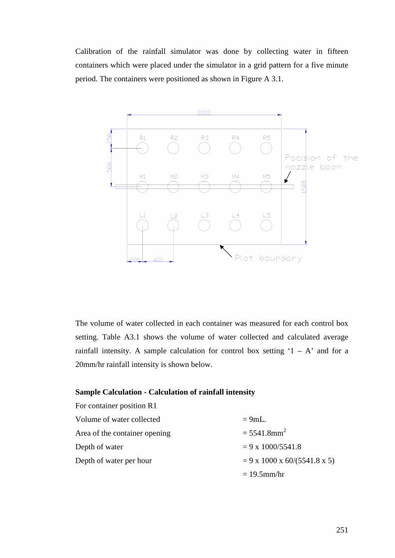
251
Calibration of the rainfall simulator was done by collecting water in fifteen
containers which were placed under the simulator in a grid pattern for a five minute
period. The containers were positioned as shown in Figure A 3.1.
The volume of water collected in each container was measured for each control box
setting. Table A3.1 shows the volume of water collected and calculated average
rainfall intensity. A sample calculation for control box setting ‘1 – A’ and for a
20mm/hr rainfall intensity is shown below.
Sample Calculation - Calculation of rainfall intensity
For container position R1
Volume of water collected = 9mL.
Area of the container opening = 5541.8mm2
Depth of water = 9 x 1000/5541.8
Depth of water per hour = 9 x 1000 x 60/(5541.8 x 5)
= 19.5mm/hr
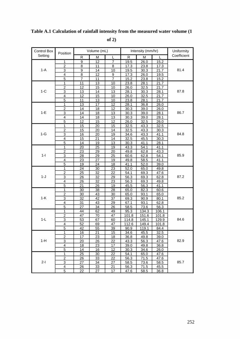
252
Table A.1 Calculation of rainfall intensity from the measured water volume (1
of 2)
R M L R M L1 9 12 7 19.5 26.0 15.22 8 11 8 17.3 23.8 17.33 9 14 10 19.5 30.3 21.74 8 12 9 17.3 26.0 19.55 7 11 7 15.2 23.8 15.21 11 13 10 23.8 28.1 21.72 12 15 10 26.0 32.5 21.73 13 14 13 28.1 30.3 28.14 12 15 10 26.0 32.5 21.75 11 13 10 23.8 28.1 21.71 13 17 12 28.1 36.8 26.02 14 18 12 30.3 39.0 26.03 14 18 13 30.3 39.0 28.14 14 18 13 30.3 39.0 28.15 12 15 12 26.0 32.5 26.01 15 20 15 32.5 43.3 32.52 15 20 14 32.5 43.3 30.33 16 20 19 34.6 43.3 41.14 15 21 14 32.5 45.5 30.35 14 19 13 30.3 41.1 28.11 20 25 19 43.3 54.1 41.12 23 29 20 49.8 62.8 43.33 28 29 25 60.6 62.8 54.14 23 27 19 49.8 58.5 41.15 19 24 18 41.1 52.0 39.01 24 30 23 52.0 65.0 49.82 25 32 22 54.1 69.3 47.63 26 32 29 56.3 69.3 62.84 26 32 23 56.3 69.3 49.85 21 26 19 45.5 56.3 41.11 30 38 28 65.0 82.3 60.62 30 43 30 65.0 93.1 65.03 32 42 37 69.3 90.9 80.14 31 43 29 67.1 93.1 62.85 27 34 26 58.5 73.6 56.31 44 62 49 95.3 134.3 106.12 47 70 47 101.8 151.6 101.83 53 67 60 114.8 145.1 129.94 52 69 47 112.6 149.4 101.85 42 55 39 90.9 119.1 84.41 16 21 15 34.6 45.5 32.52 17 23 18 36.8 49.8 39.03 20 26 22 43.3 56.3 47.64 18 23 17 39.0 49.8 36.85 14 16 12 30.3 34.6 26.01 25 30 22 54.1 65.0 47.62 26 33 22 56.3 71.5 47.63 27 34 27 58.5 73.6 58.54 26 33 21 56.3 71.5 45.55 22 27 17 47.6 58.5 36.8
85.2
87.2
85.9
84.8
85.7
82.9
84.61-L
1-H
2-I
1-G
1-I
1-J
1-K
Uniformity Coefficient
1-A
1-C
1-E 86.7
87.8
81.4
Volume (mL) Intensity (mm/hr)Position
Control Box Setting

253
Table A.1 Calculation of rainfall intensity from the measured water volume (2
of 2)
R M L R M L1 33 41 28 71.5 88.8 60.62 33.5 43 28 72.5 93.1 60.63 34.5 42.5 35.5 74.7 92.0 76.94 34 44 27 73.6 95.3 58.55 33 33 23 71.5 71.5 49.81 42.5 52 37 92.0 112.6 80.12 44.5 55 35.5 96.4 119.1 76.93 45 53.5 45 97.4 115.8 97.44 45 58 35 97.4 125.6 75.85 31.5 42 30 68.2 90.9 65.01 62 77 55 134.3 166.7 119.12 65 83 53 140.7 179.7 114.83 66 82 71 142.9 177.6 153.74 67 86.5 54 145.1 187.3 116.95 55 67 42.5 119.1 145.1 92.01 41 57.5 40 148.0 207.5 144.42 44.5 60.5 37 160.6 218.3 133.53 47 60 50.5 169.6 216.5 182.34 46 60.5 36.5 166.0 218.3 131.75 38 49 31 137.1 176.8 111.91 45.5 59 43.5 164.2 212.9 157.02 49 64 40 176.8 231.0 144.43 48 62 52 173.2 223.8 187.74 50 65 40 180.4 234.6 144.45 41 52 33.5 148.0 187.7 120.91 39.5 49 36 142.6 176.8 129.92 40 52.5 35 144.4 189.5 126.33 43 52.5 44.5 155.2 189.5 160.64 43 54.5 32.5 155.2 196.7 117.35 33.5 42 27 120.9 151.6 97.41 35 40.5 30 75.8 87.7 65.02 38.5 48 34 83.4 103.9 73.63 46 55 45 99.6 119.1 97.44 40 50 32 86.6 108.3 69.35 34 39 30 73.6 84.4 65.01 42 52 49 90.9 112.6 106.12 50 58 52 108.3 125.6 112.63 57 70 63 123.4 151.6 136.44 56 56 54 121.3 121.3 116.95 40 52 48 86.6 112.6 103.91 54 64 52 116.9 138.6 112.62 58 74 56 125.6 160.2 121.33 64 75 64 138.6 162.4 138.64 58 74 57 125.6 160.2 123.45 53 62 53 114.8 134.3 114.8
Control Box Setting
PositionVolume (mL) Intensity (mm/hr) Uniformity
Coefficient
86.2
84.8
83.2
85.1
84.5
89.4
89.7
84.6
84.63-L
3-I
3-J
3-K
2-K
2-L
1-M
2-M
2-J
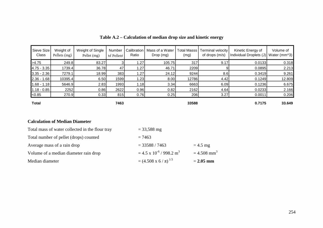
254
Table A.2 – Calculation of median drop size and kinetic energy
Sieve Size Class
Weight of pallets (mg)
Weight of Single Pallet (mg)
Number of pallets
Calibration Ratio
Mass of a Water Drop (mg)
Total Masss (mg)
Terminal velocity of drops (m/s)
Kinetic Energy of Individual Droplets (J)
Volume of Water (mm^3)
>4.75 249.8 83.27 3 1.27 105.75 317 9.17 0.0133 0.318
4.75 - 3.35 1739.4 36.78 47 1.27 46.71 2209 9 0.0895 2.213
3.35 - 2.36 7279.1 18.99 383 1.27 24.12 9244 8.6 0.3419 9.261
2.36 - 1.68 10395.4 6.50 1599 1.23 8.00 12786 4.42 0.1249 12.809
1.68 - 1.18 5646.9 2.83 1993 1.18 3.34 6663 6.09 0.1236 6.675
1.18 - 0.85 2252 0.86 2622 0.96 0.82 2162 4.64 0.0233 2.166<0.85 270.9 0.33 815 0.76 0.25 206 3.27 0.0011 0.206
7463 33588 0.7175 33.649Total
Calculation of Median Diameter
Total mass of water collected in the flour tray = 33,588 mg
Total number of pellet (drops) counted = 7463
Average mass of a rain drop = 33588 / 7463 = 4.5 mg
Volume of a median diameter rain drop = 4.5 x 10⁻⁶ / 998.2 m3 = 4.508 mm3
Median diameter = (4.508 x 6 / π) 1/3 = 2.05 mm
Pellets (mg)
Pellet (mg) of Pellets

255
APPENDIX B
STUDY AREA


257
Figure B.1 – Contour map for Highland Park residential area – contours are 5 m intervals


259
Figure B.2 – Land-use map for Highland Park residential area

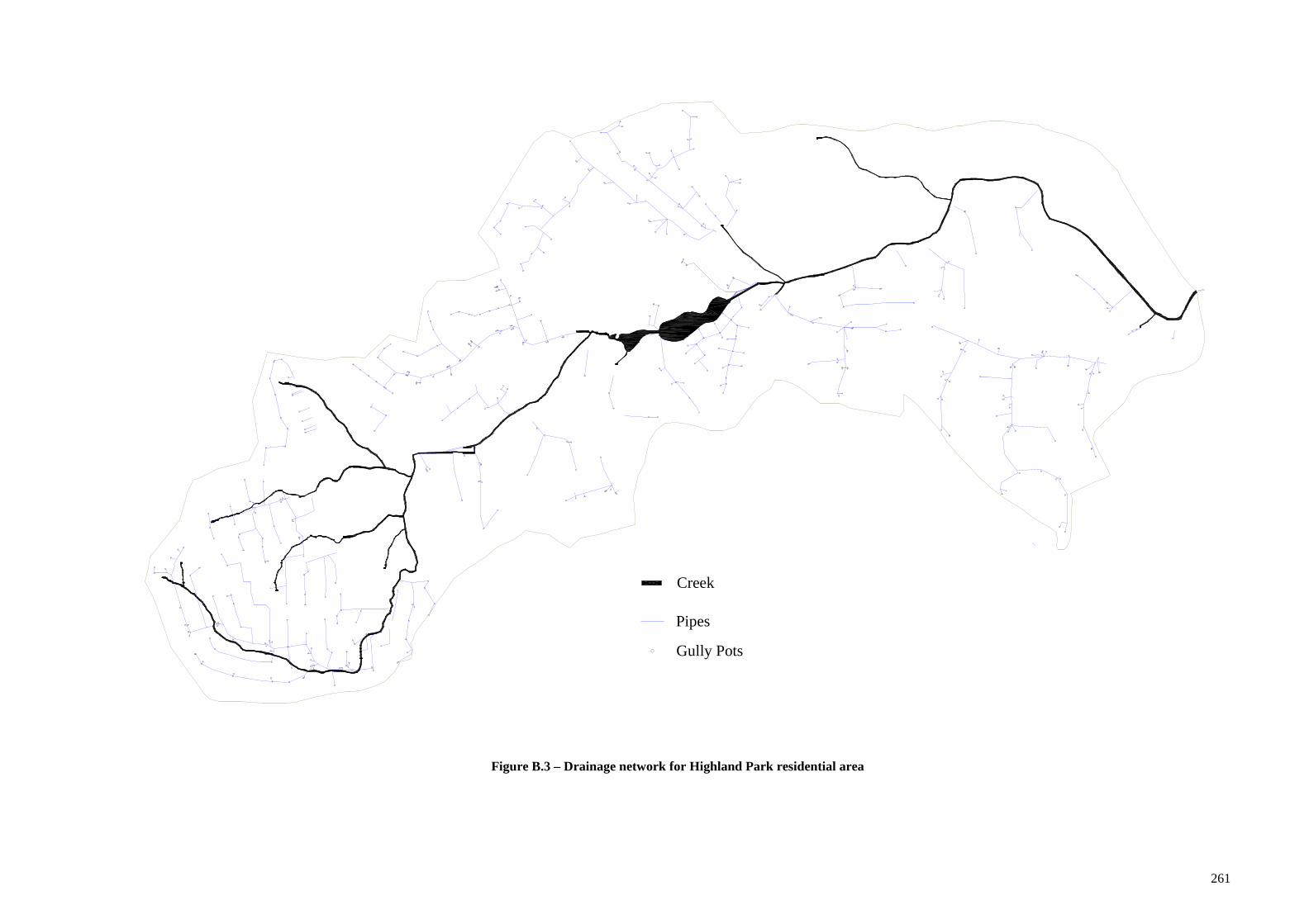
261
Gully Pots
Creek
Pipes
Figure B.3 – Drainage network for Highland Park residential area

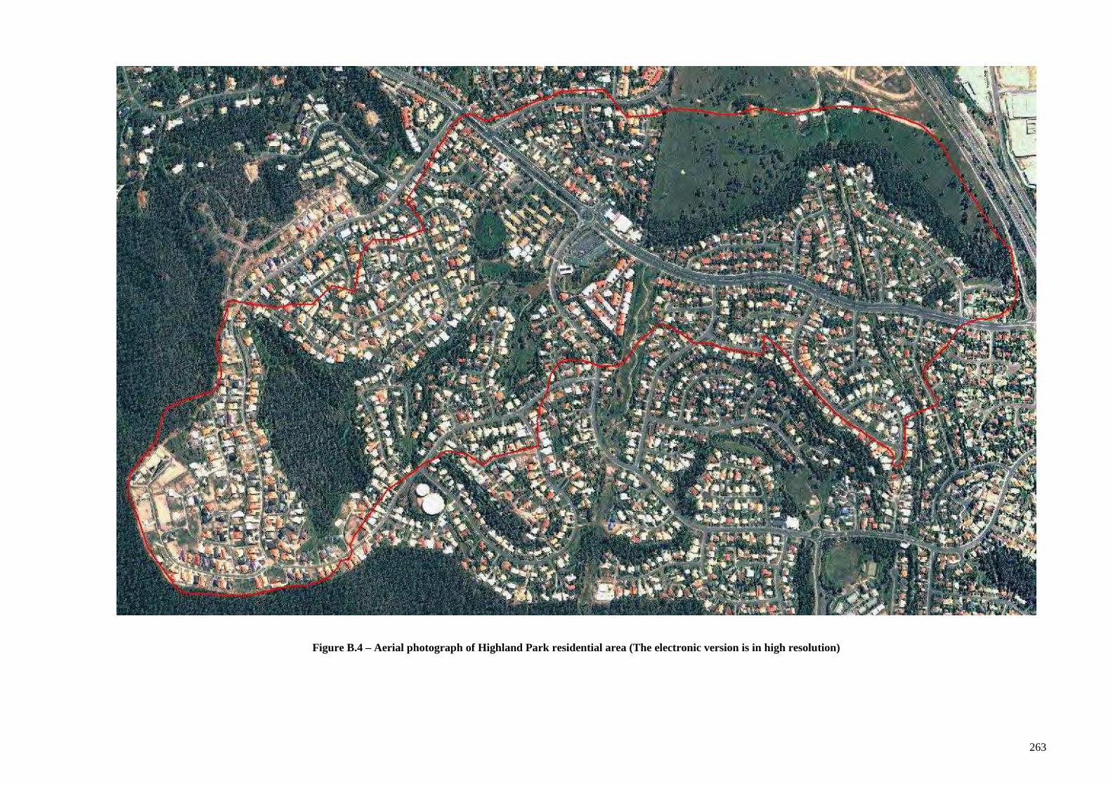
263
Figure B.4 – Aerial photograph of Highland Park residential area (The electronic version is in high resolution)


265
APPENDIX C
POLLUTANT BUILD-UP DATA


267
Table C.1 – Unprocessed data matrix for road surface build-up
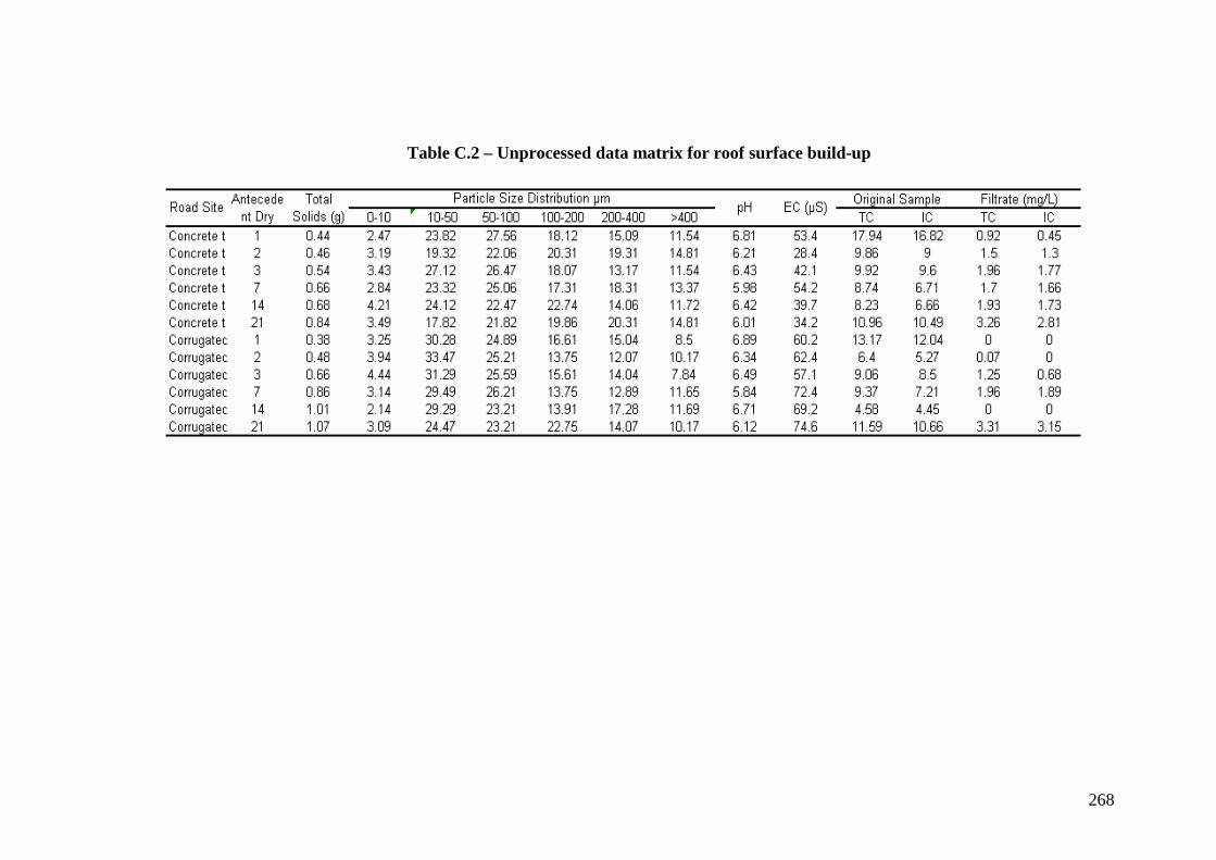
268
Table C.2 – Unprocessed data matrix for roof surface build-up
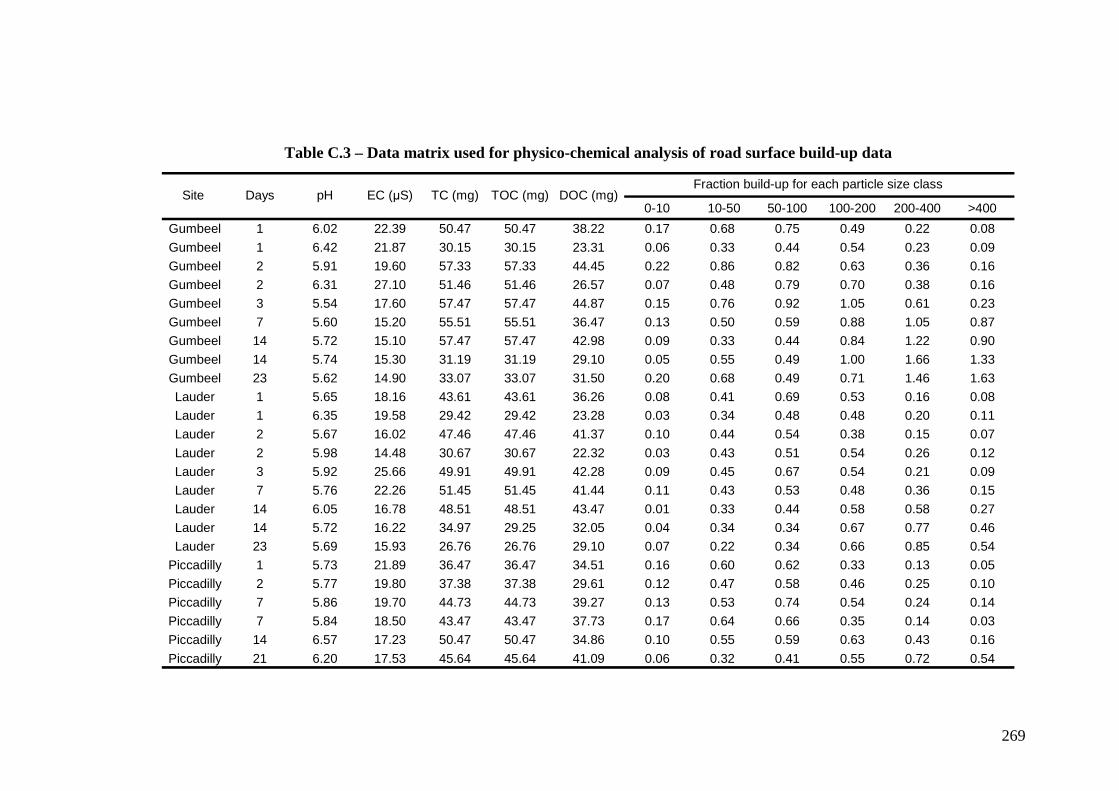
269
Table C.3 – Data matrix used for physico-chemical analysis of road surface build-up data
0-10 10-50 50-100 100-200 200-400 >400
Gumbeel 1 6.02 22.39 50.47 50.47 38.22 0.17 0.68 0.75 0.49 0.22 0.08
Gumbeel 1 6.42 21.87 30.15 30.15 23.31 0.06 0.33 0.44 0.54 0.23 0.09
Gumbeel 2 5.91 19.60 57.33 57.33 44.45 0.22 0.86 0.82 0.63 0.36 0.16
Gumbeel 2 6.31 27.10 51.46 51.46 26.57 0.07 0.48 0.79 0.70 0.38 0.16
Gumbeel 3 5.54 17.60 57.47 57.47 44.87 0.15 0.76 0.92 1.05 0.61 0.23
Gumbeel 7 5.60 15.20 55.51 55.51 36.47 0.13 0.50 0.59 0.88 1.05 0.87
Gumbeel 14 5.72 15.10 57.47 57.47 42.98 0.09 0.33 0.44 0.84 1.22 0.90
Gumbeel 14 5.74 15.30 31.19 31.19 29.10 0.05 0.55 0.49 1.00 1.66 1.33
Gumbeel 23 5.62 14.90 33.07 33.07 31.50 0.20 0.68 0.49 0.71 1.46 1.63
Lauder 1 5.65 18.16 43.61 43.61 36.26 0.08 0.41 0.69 0.53 0.16 0.08
Lauder 1 6.35 19.58 29.42 29.42 23.28 0.03 0.34 0.48 0.48 0.20 0.11
Lauder 2 5.67 16.02 47.46 47.46 41.37 0.10 0.44 0.54 0.38 0.15 0.07
Lauder 2 5.98 14.48 30.67 30.67 22.32 0.03 0.43 0.51 0.54 0.26 0.12
Lauder 3 5.92 25.66 49.91 49.91 42.28 0.09 0.45 0.67 0.54 0.21 0.09
Lauder 7 5.76 22.26 51.45 51.45 41.44 0.11 0.43 0.53 0.48 0.36 0.15
Lauder 14 6.05 16.78 48.51 48.51 43.47 0.01 0.33 0.44 0.58 0.58 0.27
Lauder 14 5.72 16.22 34.97 29.25 32.05 0.04 0.34 0.34 0.67 0.77 0.46
Lauder 23 5.69 15.93 26.76 26.76 29.10 0.07 0.22 0.34 0.66 0.85 0.54
Piccadilly 1 5.73 21.89 36.47 36.47 34.51 0.16 0.60 0.62 0.33 0.13 0.05
Piccadilly 2 5.77 19.80 37.38 37.38 29.61 0.12 0.47 0.58 0.46 0.25 0.10
Piccadilly 7 5.86 19.70 44.73 44.73 39.27 0.13 0.53 0.74 0.54 0.24 0.14
Piccadilly 7 5.84 18.50 43.47 43.47 37.73 0.17 0.64 0.66 0.35 0.14 0.03
Piccadilly 14 6.57 17.23 50.47 50.47 34.86 0.10 0.55 0.59 0.63 0.43 0.16
Piccadilly 21 6.20 17.53 45.64 45.64 41.09 0.06 0.32 0.41 0.55 0.72 0.54
Fraction build-up for each particle size class Site Days pH EC (µS) TC (mg) TOC (mg) DOC (mg)
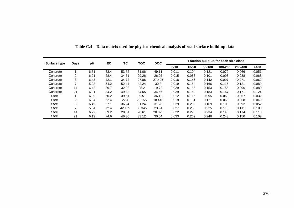
270
Table C.4 – Data matrix used for physico-chemical analysis of road surface build-up data
0-10 10-50 50-100 100-200 200-400 >400Concrete 1 6.81 53.4 53.82 51.06 49.11 0.011 0.104 0.121 0.079 0.066 0.051Concrete 2 6.21 28.4 34.51 29.26 26.95 0.015 0.088 0.101 0.093 0.088 0.068Concrete 3 6.43 42.1 34.72 27.86 27.405 0.018 0.146 0.142 0.097 0.071 0.062Concrete 7 5.98 54.2 52.44 42.24 30.3 0.019 0.154 0.166 0.115 0.121 0.089Concrete 14 6.42 39.7 32.92 25.2 19.72 0.029 0.165 0.153 0.155 0.096 0.080Concrete 21 6.01 34.2 49.32 34.65 34.56 0.029 0.150 0.183 0.167 0.171 0.124
Steel 1 6.89 60.2 39.51 39.51 36.12 0.012 0.115 0.095 0.063 0.057 0.032Steel 2 6.34 62.4 22.4 22.155 18.445 0.019 0.161 0.121 0.066 0.058 0.049Steel 3 6.49 57.1 36.24 31.24 31.28 0.029 0.206 0.169 0.103 0.092 0.052Steel 7 5.84 72.4 42.165 33.345 23.94 0.027 0.253 0.225 0.118 0.111 0.100Steel 14 6.72 69.2 20.61 20.61 20.025 0.022 0.295 0.234 0.140 0.174 0.118Steel 21 6.12 74.6 46.36 33.12 30.04 0.033 0.262 0.248 0.243 0.150 0.109
TC TOC DOCFraction build-up for each size class
Surface type Days pH EC

271
APPENDIX D
POLLUTANT WASH-OFF DATA

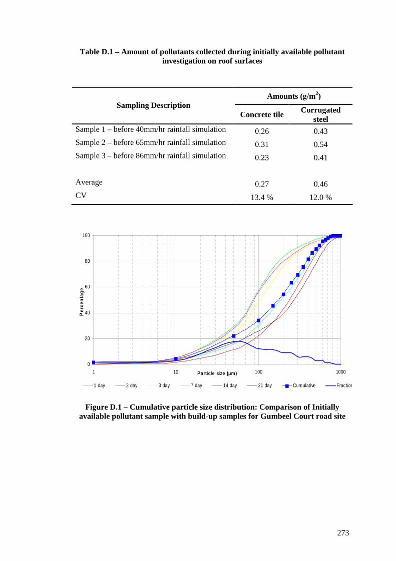
273
Table D.1 – Amount of pollutants collected during initially available pollutant investigation on roof surfaces
Amounts (g/m2) Sampling Description
Concrete tile Corrugated steel
Sample 1 – before 40mm/hr rainfall simulation 0.26 0.43
Sample 2 – before 65mm/hr rainfall simulation 0.31 0.54
Sample 3 – before 86mm/hr rainfall simulation 0.23 0.41
Average 0.27 0.46
CV 13.4 % 12.0 %
0
20
40
60
80
100
1 10 100 1000Particle size (µm)
Per
cen
tag
e
1 day 2 day 3 day 7 day 14 day 21 day Cumulative Fractions
Figure D.1 – Cumulative particle size distribution: Comparison of Initially
available pollutant sample with build-up samples for Gumbeel Court road site

274
0
20
40
60
80
100
1 10 100 1000Particle size (µm)
Per
cen
tag
e
1 day 2 day 3 day 7 day 14 day 21 day Cumulative Fractions
Figure D.2 – Cumulative particle size distribution: Comparison of Initially
available pollutant sample with build-up samples for Lauder Court road site
0
20
40
60
80
100
1 10 100 1000Particle size (µm)
Per
cen
tag
e
1 day 2 day 3 day 7 day 14 day 21 day Cumulative Fractions
Figure D.3 – Cumulative particle size distribution: Comparison of Initially
available pollutant sample with build-up samples for Piccadilly Place road site

275
Figure D.4 – Variation of fraction wash-off with rainfall intensity and duration for three road sites

276
Table D.2 – Observed wash-off data and calculation of fraction wash-off
Site / Sampling Intensity (mm/hr)
Duration (min)
TSS Concentration
(mg/L)
Wash-off Pollutant Load
(mg)
Cumultive Wash-off
Load (mg)
Fraction Wash-off
Gumbeel - wash-off 20 10 189.8 1267.9 1267.9 0.04
Gumbeel - wash-off 20 20 62.4 507.9 1775.8 0.06
Gumbeel - wash-off 20 30 31.2 237.1 2012.9 0.06
Gumbeel - wash-off 20 40 28.8 255.2 2268.1 0.07
Gumbeel - wash-off 40 10 224.8 3484.4 3484.4 0.11
Gumbeel - wash-off 40 15 175.2 1531.2 5015.6 0.16
Gumbeel - wash-off 40 25 155.2 2421.1 7436.8 0.23
Gumbeel - wash-off 40 35 129 2458.7 9895.5 0.31
Gumbeel - wash-off 65 10 213.6 2806.7 2806.7 0.09
Gumbeel - wash-off 65 15 162.8 1756.6 4563.3 0.14
Gumbeel - wash-off 65 20 233.6 2560.3 7123.6 0.22
Gumbeel - wash-off 65 30 197.2 4582.9 11706.5 0.36
Gumbeel - wash-off 86 10 205 3735.1 3735.1 0.12
Gumbeel - wash-off 86 15 119.6 1356.3 5091.4 0.16
Gumbeel - wash-off 86 20 128.8 1566.2 6657.6 0.21
Gumbeel - wash-off 86 27 193.6 3221.5 9879.1 0.31
Gumbeel - wash-off 115 5 273.4 3390.2 3390.2 0.11
Gumbeel - wash-off 115 10 236.2 4006.0 7396.1 0.23
Gumbeel - wash-off 115 15 211.8 3177.0 10573.1 0.33
Gumbeel - wash-off 115 22 267.4 4925.5 15498.6 0.48
Gumbeel - wash-off 133 5 336.4 5987.9 5987.9 0.19
Gumbeel - wash-off 133 9 326 7595.8 13583.7 0.42
Gumbeel - wash-off 133 13 253.6 5908.9 19492.6 0.61
Gumbeel - wash-off 133 17 233.6 5456.9 24949.5 0.77
Gumbeel - wash-off 133 20.5 178.2 4095.0 29044.5 0.90 Gumbeel - Initial
pollutant load 5209.4 32694.1
Lauder - wash-off 40 10 117.6 1665.2 1665.2 0.18
Lauder - wash-off 40 15 42.8 335.6 2000.8 0.21
Lauder - wash-off 40 25 28.8 459.6 2460.4 0.26
Lauder - wash-off 40 35 32.4 419.3 2879.7 0.31
Lauder - wash-off 65 10 100.2 2104.2 2104.2 0.23
Lauder - wash-off 65 15 39 474.2 2578.4 0.28
Lauder - wash-off 65 20 33.6 408.6 2987.0 0.32
Lauder - wash-off 65 30 42.2 1053.3 4040.3 0.43
Lauder - wash-off 86 10 115.4 2538.8 2538.8 0.27
Lauder - wash-off 86 15 30.6 508.0 3046.8 0.33
Lauder - wash-off 86 20 40.2 668.1 3714.9 0.40
Lauder - wash-off 86 25 26.2 365.2 4080.1 0.44
Lauder - wash-off 115 5 165.8 2961.2 2961.2 0.32
Lauder - wash-off 115 10 100 2308.0 5269.2 0.56
Lauder - wash-off 115 15 26.6 611.3 5880.5 0.63
Lauder - wash-off 115 20 14.2 333.7 6214.2 0.67
Lauder - wash-off 133 5 135.8 3305.4 3305.4 0.35
Lauder - wash-off 133 10 54.6 1381.4 4686.8 0.50
Lauder - wash-off 133 14.4 52 1322.9 6009.6 0.64
Lauder - wash-off 133 18.5 34.8 827.5 6837.2 0.73
Lauder - wash-off 133 20 21.8 204.0 7041.2 0.75
Lauder - Initial pollutant load 1340.8 9332.0
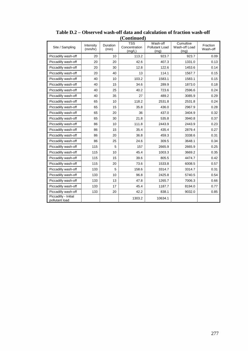
277
Table D.2 – Observed wash-off data and calculation of fraction wash-off (Continued)
Site / Sampling Intensity (mm/hr)
Duration (min)
TSS Concentration
(mg/L)
Wash-off Pollutant Load
(mg)
Cumultive Wash-off Load
(mg)
Fraction Wash-off
Piccadilly wash-off 20 10 113.2 923.7 923.7 0.09
Piccadilly wash-off 20 20 42.6 407.3 1331.0 0.13
Piccadilly wash-off 20 30 12.8 122.6 1453.6 0.14
Piccadilly wash-off 20 40 13 114.1 1567.7 0.15
Piccadilly wash-off 40 10 103.2 1583.1 1583.1 0.15
Piccadilly wash-off 40 15 34.6 289.9 1873.0 0.18
Piccadilly wash-off 40 25 40.2 723.6 2596.6 0.24
Piccadilly wash-off 40 35 27 489.2 3085.9 0.29
Piccadilly wash-off 65 10 118.2 2531.8 2531.8 0.24
Piccadilly wash-off 65 15 35.8 436.0 2967.9 0.28
Piccadilly wash-off 65 20 36 437.0 3404.9 0.32
Piccadilly wash-off 65 30 21.8 535.8 3940.8 0.37
Piccadilly wash-off 86 10 111.8 2443.9 2443.9 0.23
Piccadilly wash-off 86 15 35.4 435.4 2879.4 0.27
Piccadilly wash-off 86 20 36.8 459.3 3338.6 0.31
Piccadilly wash-off 86 25 24.6 309.5 3648.1 0.34
Piccadilly wash-off 115 5 157 2665.9 2665.9 0.25
Piccadilly wash-off 115 10 45.4 1003.3 3669.2 0.35
Piccadilly wash-off 115 15 39.6 805.5 4474.7 0.42
Piccadilly wash-off 115 20 73.6 1533.8 6008.5 0.57
Piccadilly wash-off 133 5 158.6 3314.7 3314.7 0.31
Piccadilly wash-off 133 10 96.8 2425.8 5740.5 0.54
Piccadilly wash-off 133 13 47.8 1265.7 7006.3 0.66
Piccadilly wash-off 133 17 45.4 1187.7 8194.0 0.77
Piccadilly wash-off 133 20 42.2 838.1 9032.0 0.85 Piccadilly - Initial pollutant load
1303.2 10634.1

278
Figure D.5 – Comparison of observed data with predicted using Equation2
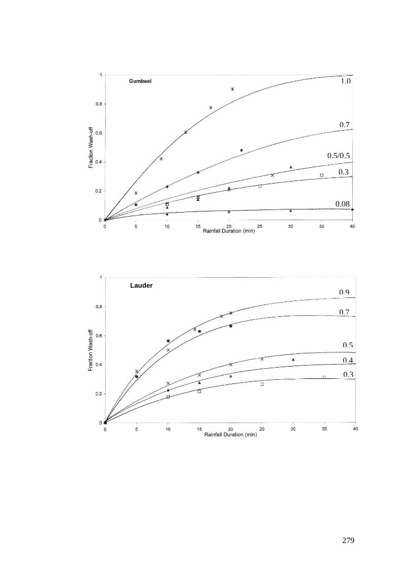
279
1.0
0.7
0.08
0.5/0.5
0.3
0.9
0.5
0.7
0.4
0.3
Lauder

280
Figure D.6 – Initial estimates for CF using freehand sketches
0.9
0.7
0.1
0.4/0.4
0.3

281
Figure D.7 – Variation of wash-off particle size distribution with rainfall duration
40mm/hr
0
5
10
15
20
25
0 200 400 600 800 1000
Particle size (µm)
Per
cen
tag
e
65mm/hr
0
5
10
15
20
25
0 200 400 600 800 1000
Particle size (µm)
Per
cen
tag
e
86mm/hr
0
5
10
15
20
25
30
0 200 400 600 800 1000
Particle size (µm)
Per
cen
tag
e
Duration 1 Duration 2
Duration 3 Duration 4
Total

282
Figure D.7 – Variation of wash-off particle size distribution with rainfall duration - Continued
115mm/hr
0
5
10
15
20
25
0 200 400 600 800 1000Particle size (µm)
Per
cen
tag
e
133mm/hr
0
5
10
15
20
25
0 200 400 600 800 1000
Particle size (µm)
Per
cen
tag
e
Duration 1 Duration 2
Duration 3 Duration 4
Duration 5 Total

283
Table D.3 – Data matrix used for analysis of quality parameters resulted from road surface investigations
<10 µm 10 - 50 µm 50 - 100 µm 100 - 200 µm 200 - 400 µm >400 µm
G11 6.3 54.9 13.2 10.8 9.6 6.2 36.0 47.9 44.0 36.1 19.8
G12 6.1 22.3 9.8 9.6 8.2 2.0 9.7 13.4 15.1 13.4 8.9
G13 6.1 19.7 6.4 5.3 4.7 1.6 6.1 6.9 7.4 6.1 3.0
G14 6.2 15.3 8.3 6.5 3.9 0.9 5.0 6.4 6.8 6.2 3.6
G21 5.6 26.2 9.6 8.4 5.8 9.3 40.1 52.1 57.8 43.7 22.1
G22 5.8 28.6 9.5 7.1 -0.1 7.8 33.2 40.1 46.4 36.9 10.8
G23 5.8 28.7 5.3 5.3 5.1 5.2 23.7 29.7 29.4 33.0 46.7
G24 5.7 64.7 6.3 4.7 3.2 3.5 17.0 20.6 17.7 22.2 49.0
G31 5.8 77.0 10.7 8.5 6.6 10.4 45.8 48.0 48.7 39.4 21.6
G32 5.7 123.0 8.9 6.8 4.1 5.5 26.1 32.9 35.5 36.4 26.7
G33 6.9 75.5 9.4 6.5 2.8 8.5 52.8 67.9 62.7 32.8 9.0
G34 6.1 46.5 8.0 6.0 3.2 3.9 21.0 27.4 34.0 55.3 56.4
G41 5.6 53.5 9.4 7.7 4.9 9.4 43.1 49.0 43.9 32.0 25.9
G42 6.1 63.5 8.3 8.1 5.5 4.2 24.9 32.0 34.2 21.3 3.1
G43 6.3 62.0 8.5 6.1 3.0 3.0 25.3 33.8 33.9 23.5 9.3
G44 6.3 80.0 8.8 6.1 2.9 5.7 38.9 45.6 45.9 40.9 16.6
G51 5.8 66.0 9.8 8.1 7.2 27.9 86.7 57.8 47.3 40.0 13.6
G52 5.7 66.1 8.1 7.0 4.6 11.4 53.1 50.0 44.4 43.3 34.4
G53 6.2 37.4 5.5 5.5 5.0 11.8 56.0 51.8 44.2 29.5 18.7
G54 6.2 38.2 8.2 6.6 3.2 12.2 61.9 62.5 54.8 45.2 31.1
G61 5.7 36.7 8.6 7.7 5.2 39.6 105.1 71.2 54.5 43.0 23.3
G62 6.1 22.8 5.6 4.8 3.8 19.1 98.1 93.2 59.8 36.2 20.0
G63 6.2 18.5 7.7 5.9 2.8 7.8 50.3 54.7 48.6 42.9 50.3
G64 6.2 10.5 5.7 4.0 2.7 6.3 39.0 47.3 40.2 36.9 65.8
G65 6.2 8.8 5.5 3.9 2.7 9.3 43.6 49.9 44.9 27.6 4.0
L21 5.8 219.0 14.2 13.9 11.1 6.5 25.8 30.0 25.0 18.3 12.1
L22 5.6 182.0 17.9 17.7 8.2 2.9 9.5 9.9 6.7 5.8 8.1
L23 5.9 174.3 8.5 7.9 7.6 1.8 6.5 4.5 3.0 4.5 8.6
L24 6.0 171.8 6.7 4.1 6.5 1.7 7.0 5.9 4.7 6.0 7.3
L31 5.8 114.8 9.3 8.8 7.6 7.0 32.6 24.1 16.8 11.8 8.1
L32 6.0 92.3 6.4 4.5 6.2 1.3 7.9 11.2 4.6 3.2 11.1
L33 6.1 90.6 6.0 5.5 4.9 2.1 10.0 7.4 5.7 4.7 3.8
L34 6.1 75.9 7.1 6.2 4.3 0.9 4.9 9.4 3.7 2.1 23.5
L41 5.7 66.4 12.6 10.1 8.2 7.0 33.6 28.2 23.3 14.4 8.9
L42 6.0 50.8 6.4 4.4 6.1 1.1 7.7 8.5 5.5 3.5 4.3
L43 6.0 113.4 7.2 5.9 4.9 2.2 9.9 8.6 6.0 5.0 8.3
L44 6.0 149.6 11.1 9.0 5.4 1.4 6.7 7.7 4.7 3.7 2.0
L51 5.8 226.0 8.9 6.2 8.5 13.0 52.5 36.7 30.9 20.0 12.8
L52 5.9 229.6 7.0 7.0 6.4 2.7 14.8 22.8 11.5 9.0 43.2
L53 6.0 249.1 6.3 6.3 5.3 9.4 4.1 1.6 2.3 5.6 3.7
L54 6.1 254.0 5.3 5.3 4.0 0.3 1.7 3.2 2.2 2.3 4.6
L61 5.7 296.0 7.5 5.4 5.9 2.5 19.8 33.0 28.1 26.9 27.4
L62 5.7 311.0 7.1 7.1 5.2 1.2 8.4 13.4 7.8 8.7 15.3
L63 5.7 312.0 4.9 4.9 4.8 0.8 4.1 12.6 13.0 7.3 20.8
L64 5.9 312.0 4.2 4.2 3.8 0.4 3.2 7.8 6.1 4.2 16.3
L65 5.9 252.2 4.4 4.4 3.8 0.4 2.3 4.2 3.1 2.3 10.7
P11 6.3 107.3 21.0 21.0 19.5 8.3 38.0 33.0 22.8 9.5 1.6
P12 6.7 81.2 13.6 13.2 9.5 2.6 8.1 8.9 10.0 9.5 3.5
P13 6.4 79.2 11.1 10.8 7.6 0.4 3.0 4.5 1.7 1.4 1.8
P14 6.3 74.4 10.8 9.9 5.6 0.6 2.8 2.7 2.4 2.7 1.8
P21 6.7 81.2 16.0 15.9 13.1 8.5 41.5 26.2 13.7 7.8 5.7
P22 6.5 96.2 11.5 11.1 8.5 1.8 9.2 7.7 5.6 5.7 4.7
P23 6.3 100.4 9.9 9.7 6.9 1.7 9.5 9.4 8.0 6.4 5.2
P24 6.3 105.1 9.8 9.0 4.7 0.9 4.4 6.5 3.8 2.9 8.7
P31 6.4 137.4 11.8 11.5 9.8 14.6 38.1 31.1 23.7 11.0 1.0
P32 6.3 124.8 9.7 8.9 4.4 1.9 7.7 8.2 7.2 7.2 3.7
P33 6.4 125.8 6.5 6.4 5.7 1.9 7.8 7.6 6.7 6.2 5.9
P34 6.3 125.4 6.6 6.0 4.0 0.6 3.2 6.3 4.8 3.2 3.7
P41 6.3 151.4 12.6 12.6 11.7 11.8 40.1 30.0 17.2 7.7 5.0
P42 6.3 139.5 10.7 10.3 5.2 1.8 10.0 10.5 6.6 3.7 2.9
P43 6.3 137.6 10.1 10.0 4.7 1.6 10.3 12.3 5.7 1.8 5.6
P44 6.4 135.1 7.8 7.6 4.6 0.3 3.4 14.9 2.3 1.9 1.5
P51 6.2 162.3 13.4 11.5 8.9 19.3 50.2 35.9 26.5 18.7 6.5
P52 6.4 131.5 9.7 9.0 4.9 1.2 6.5 17.2 10.9 4.2 5.5
P53 6.5 136.3 9.4 8.6 3.8 0.7 5.3 11.8 6.3 3.7 12.8
P54 6.4 127.9 10.3 9.2 4.9 3.2 18.4 18.8 15.6 11.2 6.4
P61 6.1 154.5 11.5 10.7 5.2 16.3 37.1 34.7 37.5 25.0 8.0
P62 6.4 139.4 8.9 7.4 3.8 4.6 21.1 31.9 25.4 6.4 7.7
P63 6.5 134.5 8.5 7.3 3.2 1.2 8.4 13.4 13.4 7.9 3.6
P64 6.4 133.5 6.5 6.0 4.3 1.1 8.3 10.3 11.2 10.6 3.9P65 6.5 135.3 6.6 6.1 3.7 0.3 2.4 4.4 3.2 7.8 24.6
Particulate Concentrations (mg/L)ID pH EC TC TOC DOC


285
APPENDIX E
CATCHMENT MODELLING

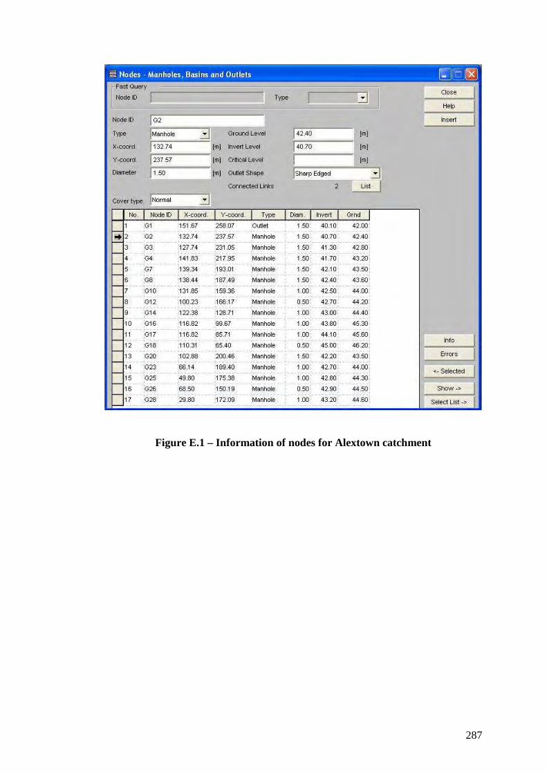
287
Figure E.1 – Information of nodes for Alextown catchment

288
Figure E.2 – Information of links for Alextown catchment

289
Figure E.3 – Information of sub-areas for Alextown catchment
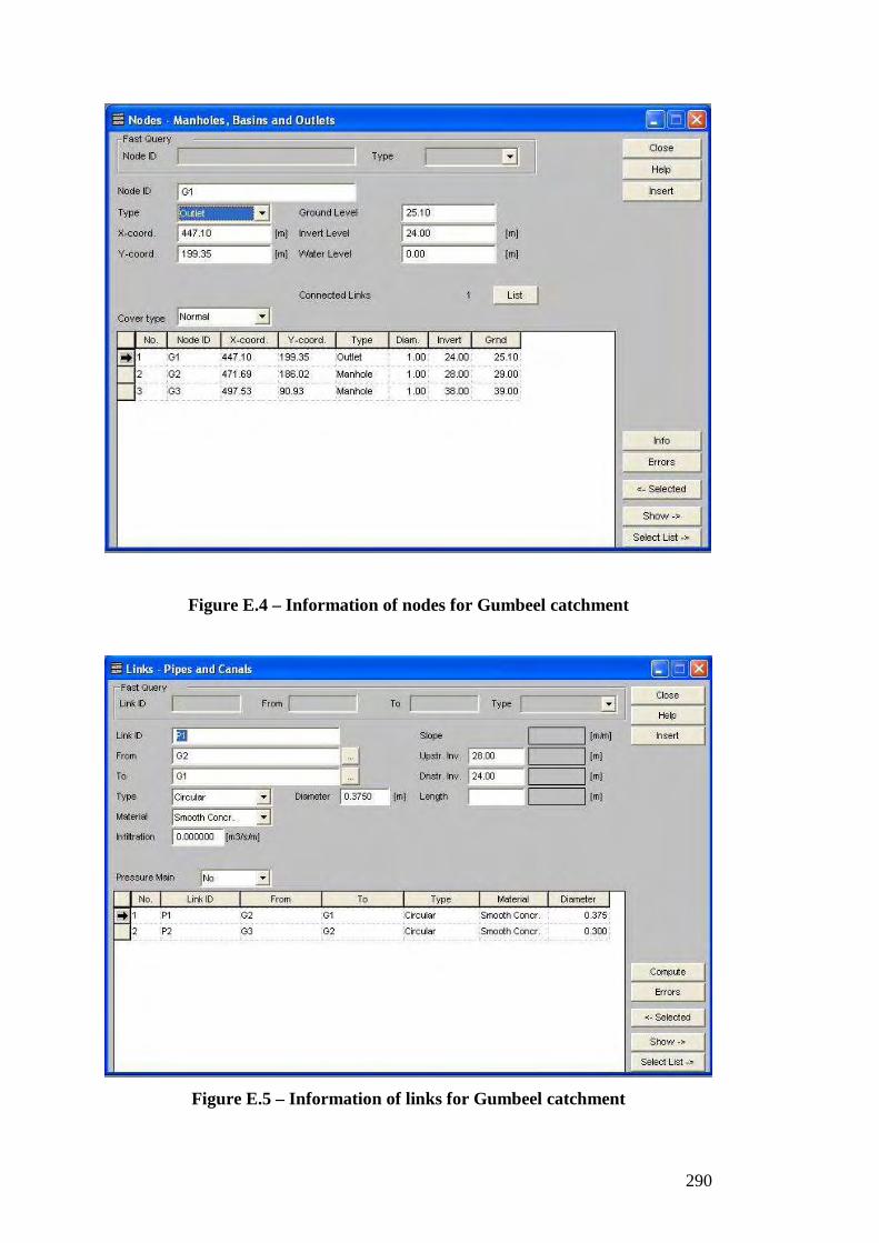
290
Figure E.4 – Information of nodes for Gumbeel catchment
Figure E.5 – Information of links for Gumbeel catchment
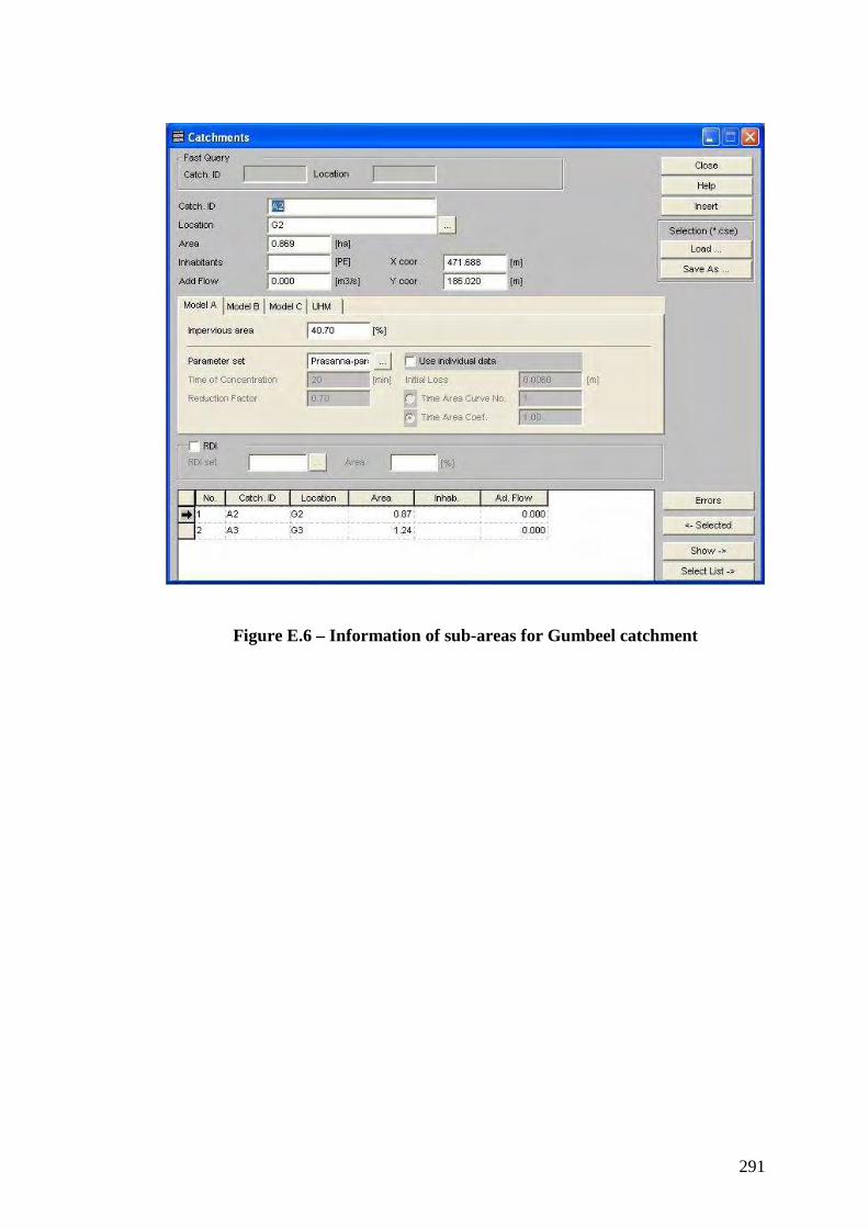
291
Figure E.6 – Information of sub-areas for Gumbeel catchment

292
Figure E.7 – Information of nodes for Birdlife Park catchment
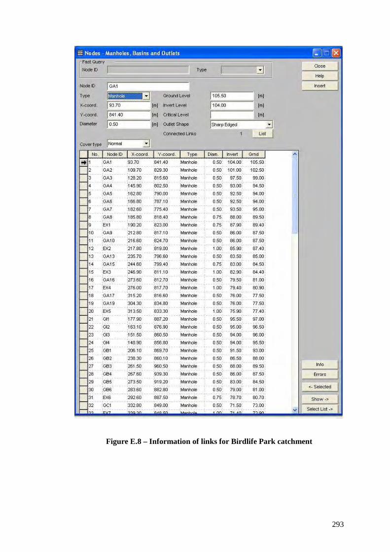
293
Figure E.8 – Information of links for Birdlife Park catchment

294
Figure E.9 – Information of sub-areas for Birdlife Park catchment

295
APPENDIX F
DATA ANALYSIS

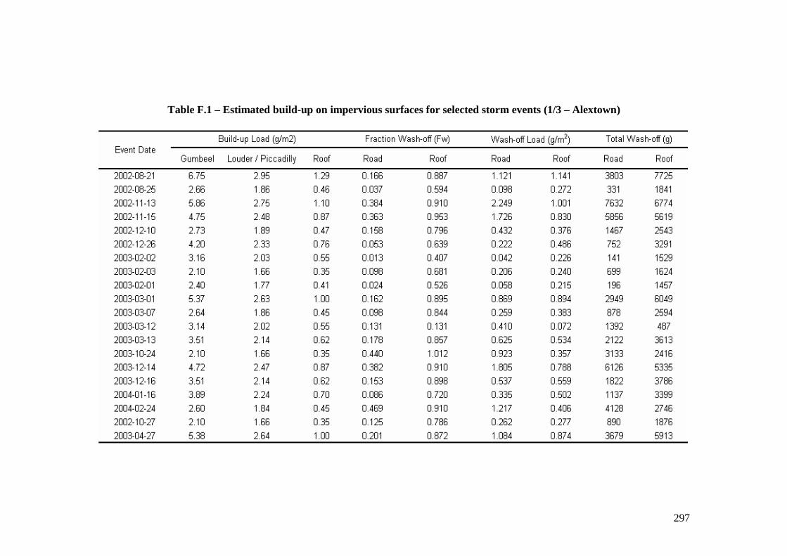
297
Table F.1 – Estimated build-up on impervious surfaces for selected storm events (1/3 – Alextown)
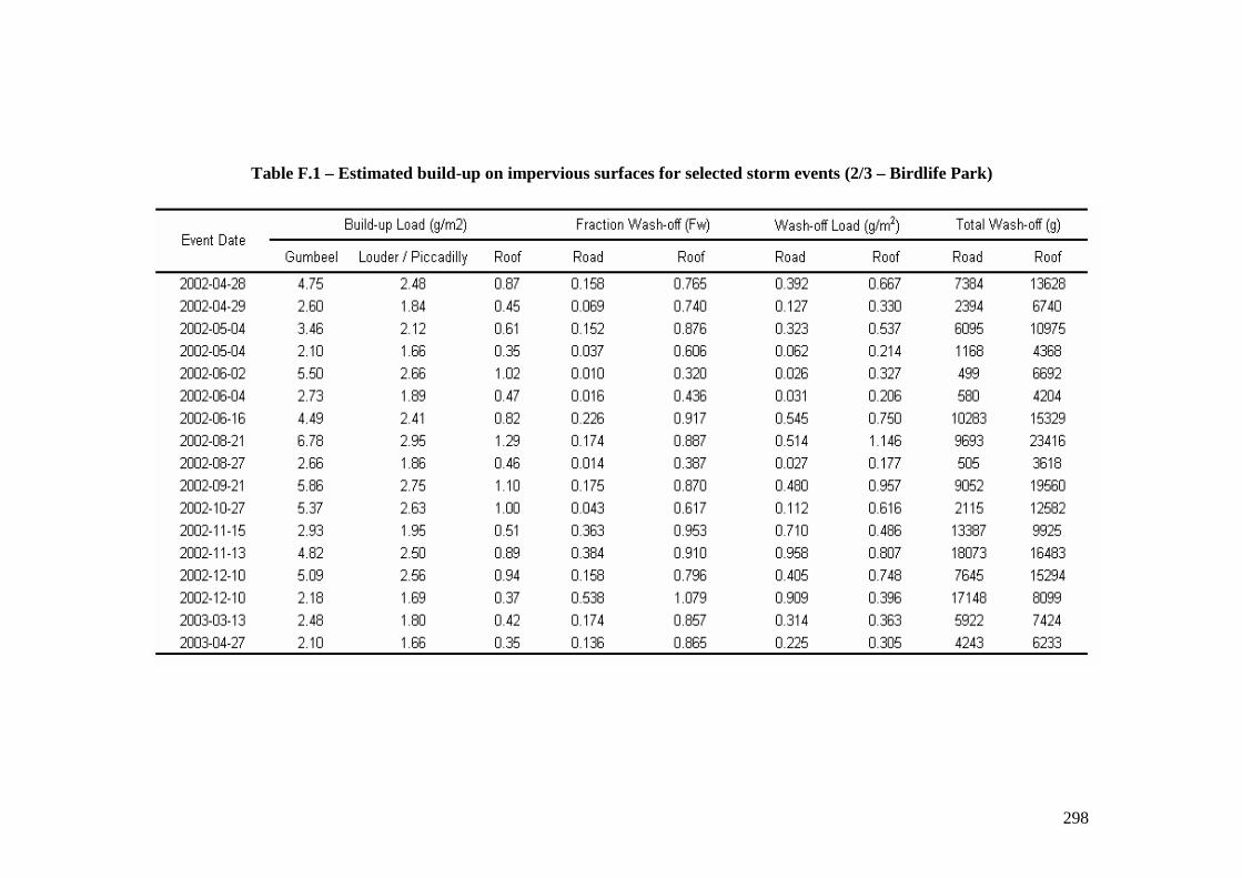
298
Table F.1 – Estimated build-up on impervious surfaces for selected storm events (2/3 – Birdlife Park)
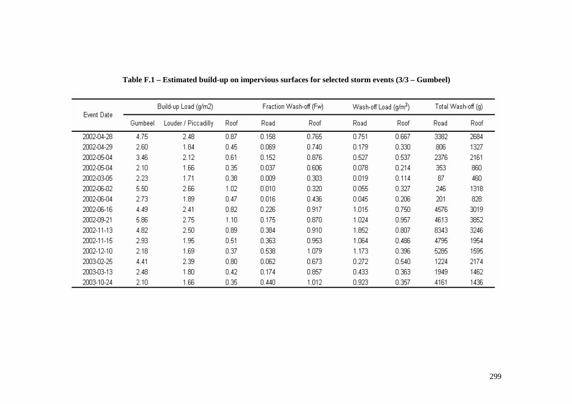
299
Table F.1 – Estimated build-up on impervious surfaces for selected storm events (3/3 – Gumbeel)

300
Figure F.1 – Conceptual Wash-off model: Sample calculation and Visual Basic coding

301
Figure F.2 – Rainfall and pollutant routing model: Inputs, catchment characteristics and outputs
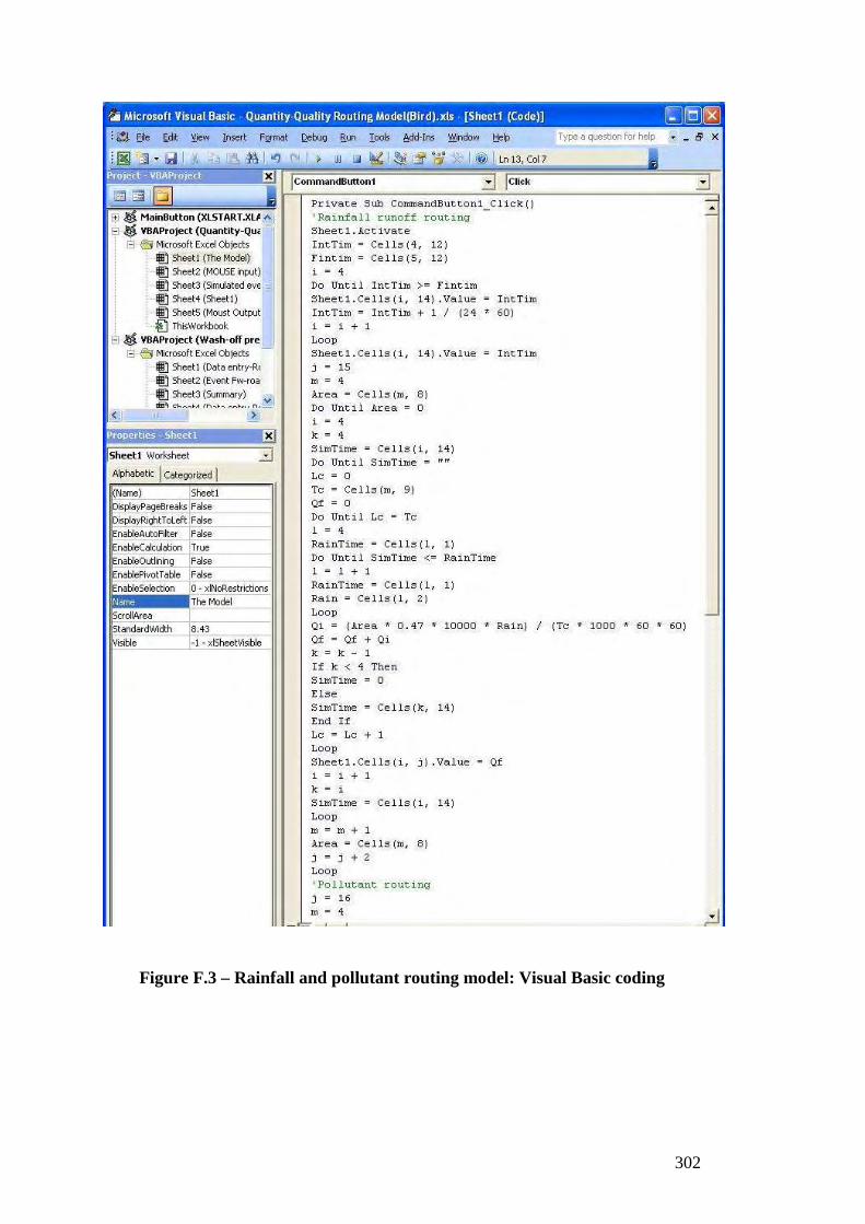
302
Figure F.3 – Rainfall and pollutant routing model: Visual Basic coding

303
Figure F.4 - Comparison of observed and predicted instantaneous
concentrations: Individual catchment basis
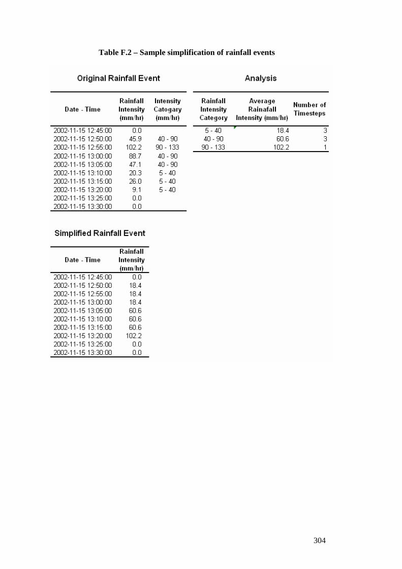
304
Table F.2 – Sample simplification of rainfall events