pratibha - ijssbtijssbt.org/downloads/ijssbt vol 1 no 1 march 2012.pdfpratibha: international...
TRANSCRIPT


PRATIBHA: INTERNATIONAL JOURNAL OF
SCIENCE, SPIRITUALITY, BUSINESS AND
TECHNOLOGY
(IJSSBT)
Vol.1, No.1, March 2012
ISSN (Print) : 2277-7261
www.ijssbt.org
EDITOR(s)-IN-CHIEF:
Prof. Dr. Kishor S. Wani
Prof. Dr. Shailendra Kumar Mittal
IJSSBT

PRATIBHA: INTERNATIONAL JOURNAL OF SCIENCE,
SPIRITUALITY, BUSINESS AND TECHNOLOGY (IJSSBT)
PRATIBHA: INTERNATIONAL JOURNAL OF SCIENCE, SPIRITUALITY,
BUSINESS AND TECHNOLOGY (IJSSBT) is a research journal published by Shram
Sadhana Bombay Trust‘s COLLEGE of ENGINEERING & TECHNOLOGY, Bambhori, Jalgaon (MAHARASHTRA, INDIA). College was founded by
PRESIDENT, GOVT. of INDIA, Honorable Excellency Sau. PRATIBHA DEVI
SINGH PATIL.
College is awarded as Best Engineering College of Maharashtra State by Engineering Education Foundation Pune in year 2008-09.
The College has ten full-fledged departments. The Under Graduate programs in 7 courses are accredited by National Board of Accreditation, All India Council for Technical Education, New Delhi for 5 years with effect from 19/07/2008 vide letter number NBA/ACCR-414/2004. QMS of the College conforms to ISO 9001:2008 and is certified by JAAZ under the certificate number: 1017-QMS-0117.The college has been included in the list of colleges prepared under Section 2(f) of the UGC Act, 1956 vide letter number F 8-40/2008 (CPP-I) dated May, 2008 and 12(B) vide letter number F. No. 8-40/2008(CPP-I/C) dated September 2010. UG courses permanently affiliated to North Maharashtra University are: Civil Engineering, Chemical Engineering, Computer Engineering, Electronics and Telecommunication Engineering, Electrical Engineering, Mechanical Engineering, Information Technology. Two years Post Graduate courses are Mechanical Engineering in specialization with Machine Design, Civil Engineering in specialization with Environmental Engineering, Computer Engineering in specialization with Computer Science and Engineering, Electronics and Telecommunication in specialization with Digital Electronics. Civil Engineering Department and Mechanical Engineering Department labs are
registered for Ph.D. Programs. Spread over 25 Acres, the campus of the college is
beautifully located on the bank of River Girna.
The International Journal of Science, Spirituality, Business and Technology
(IJSSBT) is an excellent, intellectual, peer reviewed journal that takes scholarly approach
in creating, developing, integrating, sharing and applying knowledge about all the fields
of study in Engineering, Spirituality, Management and Science for the benefit of
humanity and the profession.
The audience includes researchers, managers, engineers, curriculum designers
administrators as well as developers.

AIM AND SCOPE
Our philosophy is to map new frontiers in emerging and developing technology areas in research, industry and governance, and to link with centers of excellence worldwide to provide
authoritative coverage and references in focused and specialist fields. The journal presents its
readers with broad coverage across all branches of Engineering, Management Spirituality and
Science of the latest development and applications.
All technical or research papers and research results submitted to IJSSBT should be original
in nature. Contributions should be written for one of the following categories:
1. Original research
2. Research Review / Systematic Literature Review
3. Short Articles on ongoing research 4. Preliminary Findings
5. Technical Reports / Notes
IJSSBT publishes on the following topics but NOT LIMITED TO:
SCIENCES
Computational and industrial
mathematics and statistics, and other
related areas of mathematical sciences Approximation theory
Computation
Systems control Differential equations and dynamical
systems
Financial math Fluid mechanics and solid mechanics
Functional calculus and applications
Linear and nonlinear waves
Numerical algorithms Numerical analysis
Operations research
Optimization Probability and stochastic processes
Simulation
Statistics Wavelets and wavelet transforms
Inverse problems
Artificial intelligence
Neural processing
Nuclear and particle physics Geophysics
Physics in medicine and biology
Plasma physics Semiconductor science and
technology
Wireless and optical communications Materials science
Energy and fuels
Environmental science and
technology Combinatorial chemistry
Natural products
Molecular therapeutics Geochemistry
Cement and concrete research,
Metallurgy Crystallography and
Computer-aided materials design
COMPUTER ENGINEERING AND INFORMATION TECHNOLOGY
Information Systems e-Commerce Intelligent Systems
Information Technology
e-Government
Language and Search Engine Design Data Mining and Web Mining
Cloud Computing
Distributed Computing
Telecommunication Systems Artificial Intelligence
Virtual Business and Enterprise
Computer Systems
Computer Networks Database Systems and Theory
Knowledge Management

Computational Intelligence
Simulation and Modeling Scientific Computing and HPC
Embedded Systems
Control Systems
ELECTRONICS AND TELECOMMUNICATION ENGINEERING
3D Vision
3D TV
Biometrics Graph-based Methods
Image and video indexing and
database retrieval Image and video processing
Image-based modeling
Kernel methods
Model-based vision approaches Motion Analysis
Non-photorealistic animation and
modeling Object recognition
Performance evaluation
Segmentation and grouping Shape representation and analysis
Structural pattern recognition
Computer Graphics Systems and
Hardware Rendering Techniques and Global
Illumination
Real-Time Rendering Fast Algorithms
Fast Fourier Transforms
Digital Signal Processing
Wavelet Transforms Mobile Signal Processing
Statistical Signal Processing
Optical Signal Processing Data Mining Techniques
Motion Detection
Content-based Image retrieval Video Signal Processing
Watermarking
Signal Identification
Detection and Estimation of Signal Parameters
Nonlinear Signals and Systems
Signal Reconstruction
Time-Frequency Signal Analysis Filter Design and Structures
Spectral Analysis
Adaptive and Clustering Algorithms Fast Fourier Transforms
Virtual, Augmented and Mixed
Reality
Geometric Computing and Solid Modeling
Game Design and Engine
Development 3D Reconstruction
GPU Programming
Graphics and Multimedia Image Processing
Interactive Environments
Software and Web accessibility
Graphics & Perception Computational Photography
Pattern recognition and analysis
Medical image processing Visualization
Image coding and compression
Face Recognition
Image segmentation Face recognition
Radar Image Processing
Sonar Image Processing Signal Identification
Super-resolution imaging
Signal Reconstruction Filter Design
Adaptive Filters
Multi-channel Filtering
Noise Control Control theory and practice
CIVIL ENGINEERING
Geotechnical Structures
Transportation
Environmental Engineering Earthquakes
Water Resources
Hydraulic and Hydraulic Structures
Construction Management, and Material
Structural mechanics
Soil mechanics and Foundation Engineering
Coastal engineering and River
engineering

Ocean Engineering
Fluid-solid-structure interactions, offshore engineering and marine
structures
Constructional management and other
civil engineering relevant areas Surveying
Transportation Engineering
CHEMICAL ENGINEERING
Organic Chemistry Inorganic Chemistry
Physical Chemistry
Analytical Chemistry Biological Chemistry
Industrial Chemistry
Agricultural & Soil Chemistry Petroleum Chemistry
Polymers Chemistry
Nanotechnology
Green Chemistry Forensic
Photochemistry
Computational Chemical Physics
Chemical Engineering
Wastewater treatment and engineering Biosorption
Chemisorptions
Heavy metal remediation
Phytoremediation Novel treatment processes for
wastewaters
Land reclamation methods Solid waste treatment
Anaerobic digestion
Gasification Landfill issues
Leachate treatment and gasification
Water and Wastewater Minimization
Mass integration Emission Targeting
Pollution Control
Safety and Loss Prevention Conceptual Design
Mathematical Approach
Pinch Technology Energy Audit
Production Technical Knowledge
ELECTRICAL ENGINEERING
Power Engineering
Electrical Machines
Instrumentation and control Electric Power Generation
Transmission and Distribution
Power Electronics
Power Quality & Economic Renewable Energy
Electric Traction, Electromagnetic
Compatibility and Electrical
Engineering Materials High Voltage Insulation Technologies
High Voltage Apparatuses
Lightning Detection and Protection
Power System Analysis, SCADA and Electrical Measurements
MECHANICAL ENGINEERING
Fluid mechanics Heat transfer
Solid mechanics
Refrigeration and air conditioning Renewable energy technology
Materials engineering
Composite materials
Marine engineering Petroleum and mineral resources
engineering
Textile engineering Leather technology
Industrial engineering
Operational research Manufacturing processes
Machine design
Quality control
Mechanical maintenance Tribology

MANAGEMENT
Accounting and Finance
Marketing
Operations Management Human resource management
Management Strategy
Information technology
Business Economics
Public Sector management Organizational behavior
Research methods
SPIRITUALITY
Relevance of Science & Spirituality in
decision & Policy making
Rigors in Scientific Research &
Insights from Spiritual wisdom Dividends from Scientific research &
Spiritual Temper
Spiritual Wisdom in disaster
management
Techno-Spiritual aspects of
development
BIO-TECHNOLOGY
Molecular biology and the chemistry
of biological process to aquatic and
earth environmental aspects as well as computational applications
Policy and ethical issues directly
related to Biotechnology
Molecular biology Genetic engineering
Microbial biotechnology
Plant biotechnology
Animal biotechnology
Marine biotechnology Environmental biotechnology
Biological processes
Industrial applications
Bioinformatics Biochemistry of the living cell
Bioenergetics
IJSSBT prides itself in ensuring the high quality and professional standards.
All submitted papers are to be peer-reviewed for ensuring their qualities.
Frequency : Two issues per year
Page charges : There are no page charges to individuals or institutions.
ISSN : 2277-7261 (Print version)
Subject Category : Science, Engineering, Business and Spirituality
Published by : Shram Sadhana Bombay trust’s College of Engineering and
Technology, Bambhori, Jalgaon
REQUIREMENTS FOR MANUSCRIPT PREPARATION
The following information provides guidance in preparing manuscript for IJSSBT.
Papers are accepted only in English.
Papers of original research, research review/systematic literature review, short articles on ongoing research, preliminary findings, and technical reports/notes should not exceed 15
typeset, printed pages.
Abstracts of 150-200 words are required for all papers submitted. Each paper should have three to six keywords. Section headings should be concise and
numbered sequentially as per the following format.
All the authors (maximum three authors) of a paper should include their full names, affiliations, postal address, telephone and fax numbers and email address on the cover
page of the manuscript as per following format. One author should be identified as the
Corresponding Author.

Biographical notes on contributors are not required for this journal.
For all manuscripts non-discriminatory language is mandatory. Sexist or racist terms should not be used.
Authors must adhere to SI units . Units are not italicized.
The title of the paper should be concise and definitive (with key words appropriate for
retrieval purposes).
Manuscript Format
Document : The Manuscript should be prepared in English language by using MS Word (.doc format). An IJSSBT paper should not exceed 15 typeset,
printed pages including references, figures and abstract etc.
Paper : Use A4 type paper page (8.27″x 11.69″).
Paper format: two columns with equal width and spacing of
0.25″.
Margins : Leave margins of article 1.3" at the left and for top, bottom, and right sides 1″.
Font Size & Style: 10 Point Times new roman, and typed in single space, Justified.
Title Page :
Title of the paper should be in bold face, Title case: font size 16, Times New Roman,
centered.
Name of the authors in normal face, Title case: font size 11 italic, Times New Roman.
Addresses and affiliations of all authors: normal face, title case font size 10, Times New
Roman.
Email address: normal face, lower case font size 10, Times New Roman.
Abstract (Font size 10, bold face) Abstract should be in brief and structured. The abstract should tell the context, basic procedure, main findings and principal conclusions. It should emphasize new aspect of study or research.
Avoid abbreviation, diagram and references in abstract. It should be single spaced and should not
exceed more than 200 words.
Keywords: (Font size 10, bold face, italic)
I. INTRODUCTION (Font size 10, bold face)
Provide background, nature of the problem and its significance. The research objective is often
more sharply focused when stated as a question. Both the main and secondary objectives should be clear. It should not include data or conclusions from the work being reported.
All Main Heading with Roman numbers (Font size 10, bold face)
With Subheading of (Font size 10, bold face, Title Case with A, B, C…..Numbering)
Picture / Figure : Pictures and figures should be appropriately included in the

main text, e.g. Fig No. 1 (Font size 9).
Table format : Font: Times New Roman, font size: 10
e.g. Table No. 1 (Font size 9)
References (font size 8, Times New Roman)
References should be arranged alphabetically with numbering. References must be complete and
properly formatted. Authors should prepare the references according to the following guidelines.
For a book:
References must consist of last name and initials of author(s), year of publication, title of book (italicized), publisher‘s name, and total pages.
[1] Name and initial of the Author, ―Topic Name‖, title of the book, Publisher name, Page
numbers, Year of publication.
For a chapter in a book:
References must consist of last name and initials of author(s), year of publication, title of chapter, title of book (italicized), publisher‘s name, and inclusive pages for the chapter.
[1] Name and initial of Author, ―Title of chapter‖, title of the book, Publisher name, total pages of chapter, year of publication.
For a Journal article: Journals must consist of last name and initials of author(s), year of publication of journal, title of paper, title of journal (italicized),volume of journal, page numbers (beginning of article - end of
article).
[1] Name and initial of the Author, ―topic name‖, title of journal, volume & issue of the journal;
Page numbers of article, year of publication.
Conference Proceedings: References must consist of last name and initials of author(s), year of publication, title of paper,
indication of the publication as proceedings, or extended abstracts volume; name of the
conference (italicized or underlined), city and state and Country where conference was held, conference sponsor‘s name, and pages of the paper.
[1] Name and initial of the Author, title of the paper, Proceedings, name of the conference, City, State, country, page numbers of the paper, Year of publication.
The title of the journal is italicized and font size 8, Times New Roman.
Final Submission:
Each final full text paper (.doc, .pdf) along with corresponding signed copyright transfer form
should be submitted by email [email protected],
Website: www.ijssbt.org/com

S.S.B.T.’S COLLEGE OF ENGINEERING & TECHNOLOGY, BAMBHORI,
JALGAON
GOVERNING BODY
Dr. D. R. Shekhawat Chairman
Shri Rajendrasingh D. Shekhawat Managing Trustee & Member
Shri V. R. Phadnis Member
Shri Jayesh Rathore Member
Mrs. Jyoti Rathore Member
Dr. R. H. Gupta Member
Arch. Shashikant R. Kulkarni Member
Dr. K.S. Wani Principal & Ex-Officio Member Secretary
Shri S. P. Shekhawat Asstt. Prof. & Member
Shri Shantanu Vasishtha Asstt. Prof. & Member
LOCAL MANAGEMENT COMMITTEE
Dr. D. R. Shekhawat Chairman
Shri Rajendrasingh D. Shekhawat Managing Trustee & Member
Shri V. R. Phadnis Member
Dr. R. H. Gupta Member
Arch. Shashikant R. Kulkarni Member
Dr. K.S. Wani Principal & Ex-Officio Member Secretary
Shri S. P. Shekhawat
(Representative of Teaching Staff)
Asstt. Prof. & Member
Shri Shantanu Vasishtha
(Representative of Teaching Staff)
Asstt. Prof. & Member
Shri S. R. Girase
(Representative of Non-Teaching Staff)
Member

EDITOR(s)-IN-CHIEF
Prof. (Dr.) K. S. WANI,
M. Tech. (Chem. Tech.), D.B.M., Ph. D.
LMISTE, LMAFST, MOTAI, LMBRSI
Principal,
S.S.B.T.‘s College of Engineering and Technology,
P.B. 94, Bambhori,
Jalgaon-425001 Maharashtra, India
Mobile No. +919422787643
Phone No. (0257) 2258393,
Fax No. (0257) 2258392,
Email id: [email protected]
Dr. SHAILENDRA KUMAR MITTAL
Ph.D. (Electrical Engineering)
Professor
Member IEEE, Senior Member IACSIT, LMISTE
Director - Research and Development
S.S.B.T.‘s College of Engineering and Technology,
P.B. 94, Bambhori,
Jalgaon-425001 Maharashtra, India
Mobile No. +91 9422788382
Phone No. (0257) 2258393,
Fax No. (0257) 2258392.
Email id : [email protected]
Web Address : www.ijssbt.org/com
EDITORIAL BOARD
Prof. SUBRAMANIAM GANESAN
Director, Real Time & DSP Lab.,
Electrical and Computer Engineering Department,
Oakland University, Rochester, MI 48309, USA.
IEEE Distinguished Visiting Speaker (2005-2009) and Coordinator.
IEEE SEM CS chapter Chair, Region 4 and CS Society Board member
SAE, ASEE, ACM member
Prof. ALOK VERMA
Old Dominion University
Norfolk
Virginia, USA
Prof. EVANGELINE GUTIERREZ Programme Manager, Global Science and Technology Forum Pvt. Ltd
10 Anson Road, Singapore

Dr. G.P. PATIL
Distinguish Professor of Mathematics Statistics
Director, Center for Statistical Ecology and Environmental Statistics
Editor-in-Chief, Environmental and Ecological Statistics
Department of Statistics
The Pennsylvania State University, USA
Dr. ABAD A. SHAH Professor, Department of Computer Science & Engineering
University of Engineering and Technology
G. T. Road Lahore, Pakistan
Dr. ANSHUMAN TRIPATHI
Ph. D.
Principal Engineer VESTAF, SINGAPORE
Dr. MUHAMMAD MASROOR ALI
Professor, Department of Computer Science and Engineering
Bangladesh University of Engineering and Technology
Dhaka-1000, Bangladesh [email protected]
Dr. RAMESH CHANDRA GOEL
Former Director General
Deharadun Institute of Technology
Deharadun, Uttarakhad, India
Dr. DINESH CHANDRA
Ph. D.
Professor
Department of Electrical Engineering
Motilal Nehru National Institute of Technology
Allahabad-U.P., India
Dr. BHARTI DWIVEDI
Ph. D.
Professor
Department of Electrical Engineering
Government Institute of Engineering & Technology
Luknow, India
Dr. L. A. Patil
Ph. D.
Professor & Head
Dept of Physics
Pratap College Amalner
Jalgaon, India

Dr. M. QASIM RAFIQ
Ph. D. (Computer Engineering)
Professor
Senior Member IEEE (USA)
FIETE, FIE, LMCSI
Department of Computer Engineering
Z.H. College of Engineering & Technology
Aligarh Muslim University (A.M.U.)Aligarh, India
Dr. RAZAULLHA KHAN
Ph. D. (Civil Engineering)
Professor
Department of Civil Engineering
Z.H. College of Engineering & Technology
Aligarh Muslim University (A.M.U.)
Aligarh, India
Dr. K. HANS RAJ
Professor
Department of Mechanical Engineering
Faculty of Engineering
Dayalbagh Educational Institute, Dayalbagh
AGRA-India
Dr. DURGESH KUMAR MISHRA Professor and Head (CSE), Dean (R&D)
Acropolis Institute of Technology and Research, Indore, MP, India
Chairman, IEEE Computer Society, Bombay Chapter
Chairman IEEE MP Subsection
Chairman CSI Indore Chapter
Dr. SUDHIR CHINCHOLKAR
Ph.D. Microbiology
Professor & Head (Microbiology)
N.M.U. University, Jalgaon, India
Dr. M. A. LOKHANDE
Ph. D.
Professor and Head
Department of Commerce
Member Indian Commerce Association
Dr. Babasaheb Ambedkar Marathwada University, Aurangabad, India
Dr. K. K. SHUKLA
Ph.D.
Professor
Department of Civil Engineering
Motilal Nehru National Institute of Technology
Allahabad- U.P., India

Dr. RAHUL CAPRIHAN
Ph.D.
Professor
Department of Mechanical Engineering
Faculty of Engineering
Dayalbagh Educational Institute
Dayalbagh, Agra, India
Dr. SATISH KUMAR Ph. D.
Professor
Department of Electrical Engineering
Faculty of Engineering
Dayalbagh Educational Institute
Dayalbagh, Agra, India
Dr. VED VYAS J. DWIVEDI Professor (Electronics and Communication Engineering)
Director
Noble Group of Institutions, Junagadh, Gujarat, India
*Editor-in-Chief*
*International Journal on Science and Technology*
Dr. RAM PAL SINGH
Ph.D.
Professor
Department of Civil Engineering
Motilal Nehru National Institute of Technology
Allahabad- India
Dr. ANURAG TRIPATHI
Ph.D.
Professor
Department of Electrical Engineering
Government Institute of Engineering & Technology
Luknow, India
Dr. (Mrs.) ARUNIMA DE
Ph.D.
Professor
Department of Electrical Engineering
Government Institute of Engineering & Technology
Luknow, India
Dr. A.P. DONGRE Ph. D.
Department of Management Studies
North Maharashtra University, Jalgaon India

Dr. V. VENKATACHALAM
Principal, The Kavery Engineering College,
Mecheri. Salem District.
Dr. T. RAVICHANDRAN Research Supervisor,
Professor & Principal
Hindustan Institute of Technology
Coimbatore, Tamil Nadu, India
Dr. BHUSHAN TRIVEDI
Professor & Director, GLS-MCA, Ahmedabad.
Dr. NEERAJ BHARGAVA
HoD, Department of Computer Science,
MDS University, Ajmer.
Dr. CRISTINA NITA-ROTARU
Purdue University
Dr. RUPA HIREMATH
Director, IIPM, Pune
Dr. A. R. PATEL
HoD, Department of Computer Science,
H. North Gujarat University, Patan. Gujarat
Dr. PRIYANKA SHARMA
Professor, ISTAR, VV Nagar,
Gujarat.
Dr. V.P.ARUNACHALAM
Principal
SNS College of Technology
Sathy Main Road,
Coimbatore - 35.
Dr. B. S. AGRAWAL
Gujarat
Dr. SATYEN PARIKH
Professor, Dept of Comp Sci.
Ganpat University, Mehsana. Gujarat.
Dr. P. V. VIRAPARIA
VV Nagar, Gujarat.

Dr. ARUMUGANATHAN Professor, Department of Mathematics and Computer Applications
PSG College of Technology, Coimbatore-641 004
Tamilnadu, INDIA.
Dr. H. B. BHADKA
Director (I/c)
C. U. Shah College of Master of Computer Application
Campus of C. U. Shah College of Engineering & Technology
Surendranagar-Ahmedabad
Dr. MOHAMMED MUSSADIQ
Ph. D.
Professor & Head, Department of Microbiology,
Shri Shivaji College of Arts, Commerce & Science, Akola.
Dr. ZIA-UL HASAN KHAN
Ph. D.
Professor & Head, Department of Biochemistry,
Shri Shivaji College of Arts, Commerce & Science, Akola.

PUBLICATION SECRETARY
SUHAS M. SHEMBEKAR
Assistant Professor
Electrical Engineering Department
S. S. B. T.‘s College of Engineering and Technology, Bambhori, Jalgaon (M.S.)
DHANESH S. PATIL
Assistant Professor
Electrical Engineering Department
S. S. B. T.‘s College of Engineering and Technology, Bambhori, Jalgaon (M.S.)
LOCAL REVIEW COMMITTEE
Dr. K. S. Wani
Principal
S.S.B.T.‘s College of Engineering &
Technology,
Bambhori, Jalgaon
Dr. M. Husain
Professor & Head
Department of Civil Engineering
Dr. I.D. Patil
Professor & Head
Department of Bio-Technology
Dr. S.L. Patil
Associate Professor & Head
Department of Applied Science
Dr. M. N. Panigrahi
Professor
Department of Applied Science
Dr. V.R. Diware
Assistant Professor
Department of Chemical Engineering
S. R. Suralkar
Associate Professor & Head
Department of Electronics &
Telecommunication Engineering
J. R. Chaudhary
Associate Professor & Head
Department of Mechanical Engineering
K. P. Adhiya
Associate Professor & Head
Department of Computer Engineering
D. U. Adokar
Associate Professor & Head
Department of Electrical Engineering
S. S. Gharde
Assistant Professor & Head
Department of Information Technology
V. S. Rana
Assistant Professor & Head
Department of Business Administration

PRATIBHA: INTERNATIONAL JOURNAL OF SCIENCE,
SPIRITUALITY, BUSINESS AND TECHNOLOGY
(IJSSBT) Table of Contents
Volume 1, No.1, March, 2012
Luus Jaakola Algorithm Based Order Reduction of Discrete Interval Systems…...01 Vinay Pratap Singh, Dinesh Chandra, Robin Rastogi
Continuous Wavelet Transform for Discrimination between Inrush and Fault
Current Transients in Transformer…………………………………….……………....…09
S. R. Paraskar, M. A. Beg, G. M. Dhole
Anti-Microbial Susceptibility Patterns of Enterobacteriaceae Isolated from Tertiary
Care Unites in Akola City……………………………………………….……...…………...15
M. Musaddiq, and Snehal Nemade
A New U-Shaped Heuristic for Disassembly Line Balancing Problems...…………..21
Shwetank Avikal, and P. K. Mishra
Modified Cadmium Stannate Nanostructured Thin Films Prepared by Spraying
Technique for the Detection of Chemical Warfares ……………………………….…...28
L. A. Patil, V. V. Deo, and M. P. Kaushik
Discrimination of Capacitor Switching Transients Using Wavelet ………………….34
M.A.Beg, Dr.M.K.Khedkar, Dr.G.M.Dhole
Study of Profitability and Break-Even Analysis For Glycolytic Depolymerization Of
Poly (Ethylene Terephthalate) (PET) Waste During Chemical Recycling Of Value
Added Monomeric Products ……………………………………………………………….38
Dr. V.R. Diware, A. S. Goje, Dr. S. Mishra
Effect of Dot (Direct Observation Treatment) Therapy on Hepatic Enzymes and
Calcium Level in Serum of T.B. Patients ……………………………………………….43
S. S. Warke, G V Puranik and Z. H. Khan
Multimedia Data Mining: A Survey ……………………………………..……………....49
Sarla More, and Durgesh Kumar Mishra
A dimensionless approach for rate of re-aeration in river Gange…………………....56
R. P. Singh
Short Term Load Prediction Considering the Effect of Temperature as a Weather
Parameter Using a Combinatorial Model of Wavelet and Recurrent Neural
Networks……………………………………………………………………………………….62 Anand B. Deshmukh, Dineshkumar U. Adokar
Human Power: An Earliest Source of Energy and It’s Efficient Use……………......67 K. S. Zakiuddin, H. V. Sondawale, and
J. P. Modak

Signal Processing based Wavelet Approach for Fault Detection of Induction
Motor………………………………………………………………………..……………….....70
A.U.Jawadekar, Dr G.M.Dhole, S.R.Paraskar
Feature Extraction of Magnetizing Inrush Currents in Transformers by Discrete
Wavelet Transform …………….……………………………………………………………76
Patil Bhushan Prataprao, M. Mujtahid Ansari, and S. R. Parasakar
Pollution Control: A Techno-Spiritual Perspective …………………………………....82
Dr M Husain, Dr K S Wani, and S P Pawar
A new method of speed control of a three-phase induction motor incorporating the
overmodulation region in SVPWM VSI…………………………………………….….....86 S. K. Bhartari, Vandana Verma, Anurag Tripathi
Study of Dynamic Performance of Restructured Power System with Asynchronous
Tie-Lines Using Conventional PI Controllers……………………………………….…..92 S. K. Pandey, V. P. Singh, P. Chaubey
Performance Analysis of Various Image Compression Techniques……….…….….97 Dipeeka O. Kukreja, S.R. Suralkar
, A.H. Karode
Discrimination between Atrial Fibrillation (AF) & Normal Sinus Rhythm (NSR)
Using Linear Parameters……………………………………………………………….…108 Mayuri J. Patil, Bharati K. Khadse, S. R. Suralkar

PRATIBHA: INTERNATIONAL JOURNAL OF SCIENCE, SPIRITUALITY,
BUSINESS AND TECHNOLOGY (IJSSBT), Vol. 1, No.1, March 2012
ISSN (Print) 2277—7261
1
Luus Jaakola Algorithm Based Order Reduction of Discrete
Interval Systems
Vinay Pratap Singh1, Dinesh Chandra
2, Robin Rastogi
3
1,3EED, M. N. National Institute of Technology, Allahabad-211004, India 2Professor, EED, M. N. National Institute of Technology, Allahabad-211004, India
Emails: [email protected], [email protected], [email protected]
Abstract: This paper presents a method for
order reduction of discrete interval systems in
which the denominator of the model is obtained
by pole-clustering while the numerator is
derived by retaining first m time
moments/Markov parameters of high-order
discrete interval system as well as minimizing
errors between subsequent n time
moments/Markov parameters of high-order
discrete interval system and model, such that m
+ n = r, where r is the order of model. The
inverse distance measure criterion is used for
pole clustering. The algorithm due to Luus
Jaakola is used for minimization of objective
function which is weighted squared sum of
errors between n time moments/Markov
parameters of high-order discrete interval
system and those of the model. The proposed
method is validated by a worked example.
Keywords: Interval system, Kharitonov
Polynomials, Order reduction, Padé
approximants, Pole-clustering method.
I. INTRODUCTION
Various methods have been proposed for order reduction of continuous-time and discrete-time
systems. Out of these methods, the methods based
on power series expansion [1]-[10] of the system
transfer function have received considerable
attention of researchers. One of these methods,
which is known as Padé approximation [1] has
been found to very useful in theoretical physical
research [11]-[12] due to its simplicity. But the
model obtained using Padé approximation often
leads to be unstable even though the high-order
system is stable. To overcome this problem, Routh
approximant [4] was introduced. However, this
method tends to approximate only low frequency
behavior of high-order system [13]. Therefore,
Routh approximant does not always lead to good
model. Various attempts [5]-[9] have been made to
improve the Routh approximant method.
Some of the above methods have been applied
for order reduction of high-order interval systems
[14]-[20]. Bandypadhyay et al. [14] presented
Routh-Padé approximation for order reduction of
high-order continuous interval systems in which
the denominator is obtained by direct truncation of the Routh-table and the numerator is obtained by
matching the time moments of the high-order
interval system and model. In [20], a method is
presented for obtaining the model of high-order
discrete interval system (HODIS) in which the
denominator of model is determined by retaining
dominant poles of the HODIS and the numerator is
obtained by matching first r time moments of the
HODIS and model. However, in this method only
time moments are considered for obtaining the
model. For good overall response, Markov
parameters should also be considered in addition to time moments as the transient state and steady
state matching depend on Markov parameters and
time moments, respectively.
In this paper, a method for order reduction of
HODIS in which the denominator of the model is
determined [21]-[23] by pole-clustering and the
numerator is derived by retaining first m time
moments/Markov parameters of HODIS as well as
minimizing errors between subsequent n time
moments/Markov parameters of HODIS and model, such that m + n = r. The Luus Jaakola
algorithm is used for minimization of objective
function which is weighted squared sum of errors
between n time moments/Markov parameters of
HODIS and those of the model. The IDM criterion
is used for pole clustering. The brief outline of this
paper is organized as follows: section-II covers
problem formulation, section-III contains Luus
Jaakola algorithm, a worked numerical example is
included in section-IV to illustrate the method and
finally, paper is concluded in section-V.
II. PROBLEM FORMULATION
Consider a HODIS given by the transfer
function 1
0 0 1 1 1 1
0 0 1 1
[ , ] [ , ] [ , ]( )
[ , ] [ , ] [ , ]
( )
( )
n
n n
n n
n n
b b b b z b b zG z
a a a a z a a z
N z
D z
(1)
where [ , ]i ia a for 0,1, ,i n are denominator

PRATIBHA: INTERNATIONAL JOURNAL OF SCIENCE, SPIRITUALITY,
BUSINESS AND TECHNOLOGY (IJSSBT), Vol. 1, No.1, March 2012
ISSN (Print) 2277—7261
2
coefficients of ( )nG z with ia and
ia as lower
and upper bounds of interval [ , ]i ia a ,
respectively, and [ , ]i ib b for 0,1, , 1i n are
numerator coefficients of ( )nG z with ib and
ib
as lower and upper bounds of interval [ , ]i ib b ,
respectively.
The transfer function ( )nG z can also be expanded
in its power series expansion around 1z and
z as:
0 0 1 1( ) [ , ] [ , ]( 1)
[ , ]( 1)
n
n
n n
G z z
z
(2)
(expansion around 1z )
1 2
1 1 2 2( ) [ , ] [ , ]
[ , ]
n
n
n n
G z M M z M M z
M M z
(3)
(expansion around z )
where [ , ]i i for 0,1,i are proportional to
the time moments of HODIS, and [ , ]i iM M for
1,2,i are Markov parameters of HODIS.
Assuming [ , ]i i ib b b for 0,1, , 1i n ,
[ , ]i i ia a a for 0,1, ,i n , [ , ]i i i for
0,1,i and [ , ]i i iM M M for 1,2,i , (1),
(2) and (3) are identified to be, respectively, (4),
(5) and (6).
1
0 1 1
0 1
( )n
n
n n
n
z zG z
z z
b b b
a a a (4)
0 1( 1) ( 1)n
nz z (5) 1 2
1 2
n
nz z z M M M (6)
Suppose, it is desired to obtain a thr -order (
r n ) model given by the transfer function
1
0 0 1 1 1 1
0 0 1 1
ˆ ˆ ˆ ˆ ˆ ˆ[ , ] [ , ] [ , ]( )
ˆ ˆ ˆ ˆ ˆ ˆ[ , ] [ , ] [ , ]
ˆ ( )
ˆ ( )
r
r r
r r
r r
r
r
b b b b z b b zG z
a a a a z a a z
N z
D z
(7)
where ˆ ˆ[ , ]i ia a for 0,1, ,i r and ˆ ˆ[ , ]i ib b for
0,1, , 1i r are, respectively, denominator and
numerator coefficients of ( )rG z .
The transfer function ( )rG z can also be expanded
in its power series expansion around 1z and
z as:
0 0 1 1ˆ ˆ ˆ ˆ( ) [ , ] [ , ]( 1)
ˆ ˆ[ , ]( 1)
r
r
r r
G z z
z
(8)
(expansion around 1z )
1 2
1 1 2 2ˆ ˆ ˆ ˆ( ) [ , ] [ , ]
ˆ ˆ[ , ]
r
r
r r
G z M M z M M z
M M z
(9)
(expansion around z )
where ˆ ˆ[ , ]i i for 0,1,i are proportional to
the time moments of model, and ˆ ˆ[ , ]i iM M for
1,2,i are Markov parameters of model.
Assuming ˆ ˆ ˆ[ , ]i i ib b b for 0,1, , 1i r ,
ˆˆ ˆ[ , ]i i ia a a for 0,1, ,i r , ˆ ˆ ˆ[ , ]i i i for
0,1,i and ˆ ˆ ˆ[ , ]i i iM M M for 1,2,i , (7),
(8) and (9) are identified to be, respectively, (10),
(11) and (12).
1
0 1 1
0 1
ˆ ˆ ˆ( )
ˆ ˆ ˆ
r
r
r r
r
z zG z
z z
b b b
a a a (10)
0 1ˆ ˆ ˆ( 1) ( 1)r
rz z (11)
1 2
1 2ˆ ˆ ˆ r
rz z z M M M (12)
A. Calculation of Poles of HODIS
Consider interval polynomial ( )E z given by
1
0 0 1 1 1 1
1
0 1 1
( ) [ , ] [ , ] [ , ] n n
n n
n n
n
E z e e e e z e e z z
z z z
e e e(13)
The poles [20] of discrete interval polynomial
( )E z are calculated as:
Let F be the interval matrix given as
0 1 2 1
0 1 0 0
0 0 1 0
0 0 0 1
n
F
e e e e
(14)
The matrix F can be written as
,c cF F F F F (15)
where
PRATIBHA: INTERNATIONAL JOURNAL OF SCIENCE, SPIRITUALITY,
BUSINESS AND TECHNOLOGY (IJSSBT), Vol. 1, No.1, March 2012
ISSN (Print) 2277—7261
3
1
2, 1,2, ,
1
2
c i j i j i j
c i j i j i j
f f f
i j n
f f f
(16)
and i jf , i jf are the lower and upper bounds of
thij element of F .
The real part i
and imaginary part i
of the thi
eigenvalue H
i of F are given as
( ) ,
( ) ,
1,2, ,
i i
i i c i c
i i
i i c i c
F F F S F F S
F F F T F F T
i n
(17)
where denotes component wise multiplication
and elements of matrices iS and iT are given by
,
,
sgn
sgn
i i i i i
k j k j k j
i i i i i
k j k j k j
S t s t s
T t s t s (18)
where s and t are, respectively, the thi
eigenvector and reciprocal eigenvector of cF , with
and denoting the real and imaginary parts,
respectively.
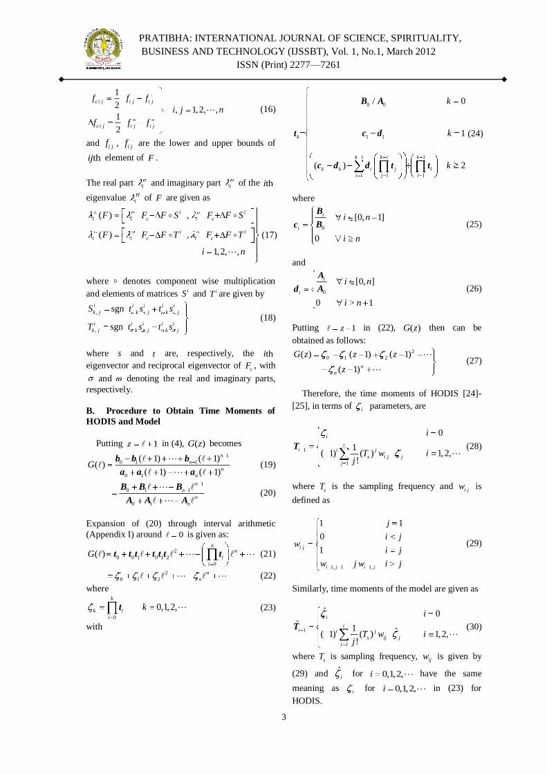
B. Procedure to Obtain Time Moments of
HODIS and Model
Putting 1z in (4), ( )G z becomes
1
0 1 1
0 1
( 1) ( 1)( )
( 1) ( 1)
n
n
n
n
G
b b b
a a a (19)
1
0 1 1
0 1
n
n
n
n
B B B
A A A (20)
Expansion of (20) through interval arithmetic
(Appendix I) around 0 is given as:
2
0 0 1 0 1 2
0
( )n
n
i
i
G t t t t t t t (21)
2
0 1 2
n
n (22)
where
0
0,1,2,k
k i
i
k t (23)
with
0 0
1 1
11
1 1 1
/ 0
1
( ) 2
k
k i kk
k k i j l
i j l
k
k
k
B A
t c d
c d d t t
(24)
where
0
[0, 1]
0
i
i
i n
i n
B
Bc (25)
and
0
[0, ]
0 1
i
i
i n
i n
A
Ad (26)
Putting 1z in (22), ( )G z then can be
obtained as follows: 2
0 1 2( ) ( 1) ( 1)
( 1)n
n
G z z z
z
(27)
Therefore, the time moments of HODIS [24]-
[25], in terms of i
parameters, are
1
1
0
1( 1) ( ) 1,2,
!
i
ii i j
s i j j
j
i
T w ij
T (28)
where sT is the sampling frequency and i jw is
defined as
1, 1 1,
1 1
0
1i j
i j i j
j
i jw
i j
w j w i j
(29)
Similarly, time moments of the model are given as
1
1
ˆ 0ˆ 1 ˆ( 1) ( ) 1,2,
!
i
ii i j
s ij j
j
i
T w ij
T (30)
where sT is sampling frequency, ijw is given by
(29) and ˆi for 0,1,2,i have the same
meaning as i for 0,1,2,i in (23) for
HODIS.

PRATIBHA: INTERNATIONAL JOURNAL OF SCIENCE, SPIRITUALITY,
BUSINESS AND TECHNOLOGY (IJSSBT), Vol. 1, No.1, March 2012
ISSN (Print) 2277—7261
4
C. Procedure to Obtain Markov Parameters of
HOIS and Model
Expansion of (4) through interval arithmetic
(Appendix I) around z is given as: 1 2 3
1 1 2 1 2 3
1
( )
nn
i
i
G z z z z
z
(31)
1 2 3
1 2 3
n
n
z z z
z
M M M
M (32)
where
0 0
1 1
/ 0
1
/ 2
k
k
k
P Q k
B A
t c d (33)
with
1
1 1
( )k ik
k k i j
i j
P c d d t
1
1
k
l
l
Q t
1
[0, 1]
0
i
ni
i n
i n
b
bC (34)
and
[0, ]
0 1
i
ni
i n
i n
a
aD (35)
Hence, the Markov parameters of HODIS are
1
1,2,k
k i
i
k (36)
Similarly, Markov parameters of the model are
given as
1
ˆ ˆ 1,2,k
k i
i
k (37)
where ˆi for 1,2,i have the same meaning as
i for 1,2,i in (33) for HODIS.
D. Procedure to Obtain Denominator
Polynomial of Model
The cluster center using pole clustering
technique [21]-[23] is obtained by grouping the
poles of HODIS. In this process, separate cluster
partitions should be made for real poles and
complex conjugate poles and then cluster centers
for these cluster partitions are obtained. Each real
cluster center or pair of complex conjugate cluster
centers are, respectively, replaced by real pole or pair of complex conjugate poles of model,
respectively. The inverse distance measure (IDM)
criterion is used for clustering the poles of HODIS.
For obtaining thr order model, r cluster
centers should be obtained from r cluster
partitions. The steps for IDM criterion follow as:
Step 1: Arrange the poles of HODIS in r cluster
partitions collecting the real and complex
conjugate poles in separate cluster partitions.
Step 2: Obtain the cluster centers:
The cluster center for real poles is obtained as 1
1
1k
i i
c k (38)
where c is cluster center of cluster partition
containing k real poles 1 2( , , , )k of
HODIS.
The pair of cluster centers for complex conjugate
poles in the form of R Ij is obtained as
1
1
1
1
1
1
lR
Ri i
lI
Ii i
l
l
(39)
where R and I are, respectively, real and
imaginary parts of cluster pair R Ij in which
l pairs of complex conjugate poles
1 1 2 2, , ,R I R I R I
l lj j j are
grouped.
Step 3: Obtain the denominator of model:
The denominator polynomial ˆ ( )rD z of thr -order
model is given as
Case 1: If all obtained cluster centers are real
1
ˆ ( )r
r i
cD z z (40)
Case 2: If one pair of cluster centers is complex
conjugate and ( 2)r cluster centers are real
2
1 1 1 1
1
ˆ ( ) ( ) ( ) ( )r
R I R I C
r i
i
D z z j z j z
(41)
Case 3: If all obtained cluster centers are complex
conjugates

PRATIBHA: INTERNATIONAL JOURNAL OF SCIENCE, SPIRITUALITY,
BUSINESS AND TECHNOLOGY (IJSSBT), Vol. 1, No.1, March 2012
ISSN (Print) 2277—7261
5
/2
1
ˆ ( ) ( ) ( )r
R I R I
r i i i i
i
D z z j z j (42)
The denominator polynomial of the model is
obtained by (40), (41) or (42) depending upon the
nature of cluster centers.
E. Procedure to Obtain Numerator Polynomial
of Model:
Once the denominator polynomial of model is
obtained, the numerator polynomial is determined
by retaining first m time moments/Markov
parameters of HODIS as well as minimizing errors
between subsequent n time moments/Markov
parameters of HODIS and model such that
m n r . The time moments of the HODIS and
model are obtained by (28) and (30), respectively,
and the Markov parameters of the HODIS and
model are given by (36) and (37), respectively.
The numerator parameters of model are obtained
by matching first m time moments/Markov
parameters of HODIS to those of model, given as
ˆ 0 1,2, ,
ˆ 0 1,2, ,
i i
j j
i p
j q
p q m
T T
M M (43)
and minimizing a weighted squared sum of the
errors, between subsequent n time
moments/Markov parameters of HODIS and those
of model, given as
' ' '
1 1
ˆ ˆ( ) ( )u v
C i j j ji ii p j q
J T T M M (44)
where '
i and '
j are non-negative numbers, and
u v r .
The objective function (44) is normalized as
follows:
1 1
ˆˆ1 1
u vji
C i j
i p j q ji
JMT
T M (45)
However, in (45), it is assumed that 0i
T and
0j
M .
III. LUUS JAAKOLA ALGORITHM The algorithm due to Luus and Jaakola [26] is
used for finding the minimum value of objective
function (45) obtained in last section. In Luus
Jaakola algorithm, initial values for all variables
and corresponding search intervals are chosen at
random and then in every next iteration, search
intervals are contracted by a constant contraction
factor. This algorithm has been applied in many
problems in optimal control [8],[27].
IV. NUMERICAL SECTION
Let the transfer function [20] of a third-order
interval system be given as 2
2 3
[8,10] [3,4] [1,2]( )
[0.8,0.85] [4.9,5] [9,9.5] [6,6]
( )
( )
z zG z
z z z
N z
D z
(46)
Suppose, it is desired to obtain a second-order
( 2)r model given by the transfer function
0 0 1 1
2 2
0 0 1 1 2 2
0 1 2
2
0 1 2 2
ˆ ˆ ˆ ˆ[ , ] [ , ]( )
ˆ ˆ ˆ ˆ ˆ ˆ[ , ] [ , ] [ , ]
ˆ ˆ ( )
ˆˆ ˆ ˆ ( )
P b b b b zG z
a a a a z a a z
z N z
z z D z
b b
a + a a
(47)
The poles, calculated using (17), of the HODIS (46) are
1
2
3
[ 0.5340, 0.2680]
[ 0.7125, 0.5361]
[ 0.8534, 0.7203]
H
H
H
(48)
Since poles (48) are real, thus, using (38), the
cluster centers obtained by grouping 1
H in one
cluster partition and 2
H and 3
H in other cluster
partition are
1 [ 0.5340, 0.2680]C ,
2 [ 0.7766, 0.6147]C (49)
and the denominator obtained using (40) is
2 1 2
2
2
0 0 1 1 2 2
ˆ ( ) ( )( )
( [ 0.5340, 0.2680])( [ 0.7766, 0.6147])
[0.1647,0.4147] [0.8827,1.3106] [1,1]
ˆ ˆ ˆ ˆ ˆ ˆ[ , ] [ , ] [ , ]
C CD z z z
z z
z z
a a a a z a a z
(50)
First time moment and Markov parameter, as
given by (28) and (36), respectively, of the HODIS are
1
1
[0.5621,0.7729]
[0.1667,0.3333]
T
M (51)
and the first time moment and Markov parameter,
as given by (30) and (37), respectively, of the
model are
0 1
1
0 1 2
11
2
ˆ ˆˆ
ˆ ˆ ˆ
ˆˆ
ˆ
b bT
a a a
bM
a
(52)
Using (43), numerator parameters are obtained
as
1 1 0 1ˆ ˆˆ [1.1508,2.1064]T T b b (53)
The objective function (45) for this problem is
given as:

PRATIBHA: INTERNATIONAL JOURNAL OF SCIENCE, SPIRITUALITY,
BUSINESS AND TECHNOLOGY (IJSSBT), Vol. 1, No.1, March 2012
ISSN (Print) 2277—7261
6
11 2
1
ˆ ˆ/1
[0.1667,0.3333]C j
j
Jb a
(54)
Starting with various initial conditions and ranges,
the Luss-Jaakola algorithm converges to following
optimal solution
1ˆ [0.1508,1.1064]b (55)
Using (53) and (55), the second-order model
obtained is
2 2
[0.0107,0.1054] [1.1401,2.0010]( )
[0.1647,0.4147] [0.8827,1.3106]
P zG z
z z (56)
and the second-order model proposed in [20] is
2 2
[0.8845,0.9] [0.5921,0.6055]( )
[0.1437,0.3805] [0.8041,1.2465]
O zG z
z z (57)
The step and impulse responses of one of the
rational systems constructed with the help of
Kharitonov polynomials (Appendix II) of numerator and denominator of (46), (56) and (57)
are shown in Fig. 1 and 2, respectively.
Fig No. 1 Step Responses of HODIS and models.
Fig No. 2 Impulse Responses of HODIS and models.
The best-case ISEs (Appendix III) of impulse
responses for (56) and (57) are given in Table 1.
Table 1
Best-case ISE for impulse response
Model Best-case ISE
(56) 4.1521
(57) 8.0926
It is clear from Fig. 1-2 that the responses of
proposed model (56) when compared to (46) is
better than that of (57) and also, the best-case ISE
of (56) is lower than that of (57). This confirms the
applicability of proposed method for order
reduction of HODIS.
V. CONCLUSION A method for obtaining model of given HODIS
is proposed in which the denominator is obtained
by pole clustering and the numerator is determined
by minimizing errors between time
moments/Markov parameters of HODIS and model
in addition to retaining some initial time
moments/Markov parameters of HODIS. The
objective function which is weighted squared sum
of errors between time moments/Markov
parameters of HODIS and those of model is
minimized using Luus Jaakola algorithm. The
proposed method is validated by a numerical example.
APPENDIX I
Interval Arithmetic
The rules of interval arithmetic [17] are defined
as follows:
Suppose, [ ],c cc and [ ],d dd are two
intervals.
Addition:
[ , ] [ , ] [ , ]c c d d c d c dc d
Subtraction:
[ , ] [ , ] [ ],c c d d c d c dc d
Multiplication:
[ , ][ , ]
[min( , , , ),
max( , , , )]
c c d d
c d c d c d c d
c d c d c d c d
c d
Division:
/ [ , ] / [ , ] [ , ] / [1/ ,1/ ];
/ [ , ] / [ , ] 1
c c d d c c d d
d d d d
c d
d d
APPENDIX II
Kharitonov Polynomials
Consider a family of real interval polynomials
[28]: 1
0 1 1
0 0 1 1
( )
[ , ] [ , ] [ , ]
n n
n n
n
n n
D z z z z
z z
The four Kharitonov polynomials associated with
( )D z are given as:
0 5 10 15 20 25-0.5
0
0.5
1
1.5
Time (sec)
Am
pli
tud
e
Step Response
(46)
(56)
(57)
0 5 10 15 20 25
-2
-1
0
1
2
Time (sec)
Am
pli
tud
e
Impulse Response
(46)
(56)
(57)

PRATIBHA: INTERNATIONAL JOURNAL OF SCIENCE, SPIRITUALITY,
BUSINESS AND TECHNOLOGY (IJSSBT), Vol. 1, No.1, March 2012
ISSN (Print) 2277—7261
7
2 3 4
1 0 1 2 3 4( )D z z z z z
2 3 4
2 0 1 2 3 4( )D z z z z z
2 3 4
3 0 1 2 3 4( )D z z z z z
2 3 4
4 0 1 2 3 4( )D z z z z z
APPENDIX III
ISE of Impulse Response
The integral-squared-error (ISE) for impulse
responses between ( )nG z and ( )rG z is obtained as
11 1( ) ( )
2J E z E z dz
i z
where
( ) ( ) ( )n rE z G z G z
( ), 1,2, ,4.
( )
p
q
B zp q
A z
Each of ( )pB z and ( )qA z represents four
Kharitonov polynomials (Appendix II).
The ISE can recursively [29],[13] be obtained as 2
00 0
( )1jnj
n jj
BJ
A A
where n is the order of error signal ( )E z and 0
nA ,
j
jB , and 0
jA are defined in [29].
The best-case ISE [30] is obtained as
, 1, ,4min ( , )best case p q
p qISE J B A
REFERENCES [1] Y. Shamash, ―Stable reduced order models using Padé
type approximation,‖ IEEE Trans. Auto. Cont., vol. 19,
pp. 615-616, 1974.
[2] M. Aoki, ―Control of large-scale dynamic systems by
aggregation,‖ IEEE Trans. Auto. Cont., vol. 13, pp. 246-
253, 1968.
[3] N. K. Sinha, and B. Kuszta, ―Modeling and identification
of dynamic systems,‖ New York: Van Nostand Reinhold,
pp. 133-163, 1983.
[4] M. F. Hutton, and B. Friedland, ―Routh approximations
for reducing the order of linear time-invariant systems,‖
IEEE Trans. Autom. Control, vol 20, pp. 329-337, 1975.
[5] Y. Shamash, ―Model reduction using the Routh stability
criterion and the Padé approximation technique,‖ Int. Jr.
Control, vol. 21, pp. 475-484, 1975.
[6] S. Rao, S. S. Lamba, and S. V. Rao, ―Routh-approximant
time-domain reduced-order modelling for single-input
single-output systems,‖ IEE Proc., Control Theory Appl.,
vol. 125, pp. 1059-1063, 1978.
[7] Singh, D. Chandra, and H. Kar, ―Improved Routh-Padé
approximants: a computer-aided approach,‖ IEEE Trans.
on Automatic Control, vol. 49, no. 2, pp. 292-296, 2004.
[8] V. Singh, D. Chandra, and H. Kar, ―Optimal Routh
approximants through integral squared error minimisation:
computer-aided approach,‖ IEE Proceedings-Control
Theory and Applications, vol. 151, no. 1, pp. 53-58, 2004.
[9] S. K. Mittal, and D. Chandra, ―Stable optimal model
reduction of linear discrete time systems via integral
squared error minimization: computer-aided approach,‖
Jr. of Advanced Modeling and Optimization, vol. 11, no.
4, pp. 531-547, 2009.
[10] S. K. Mittal, D. Chandra, and B. Dwivedi ―Improved
Routh-Pade approximants using vector evaluated genetic
algorithm to controller design,‖ Jr. of Advanced Modeling
and Optimization, vol. 11, no. 4, pp. 579-588, 2009.
[11] G. A. Baker, ―Essenstials of Padé approximants,‖ New
York: Academic, 1975.
[12] G. A. Baker, and P. R. Graves-Morris, ―Padé
approximants, Part-II: Extensions and Applications,‖
London: Addison-Wesley, 1981.
[13] Y. Choo, ―Suboptimal bilinear Routh approximant for
discrete systems,‖ ASME Jr. of Dynamic systems,
measurement, and control, vol. 128, pp. 742-745, 2006.
[14] B. Bandyopadhyay, O. Ismail, and R. Gorez, ―Routh-Padé
approximation for interval systems,‖ IEEE Trans. Auto.
Cont., vol. 39, no. 12, pp. 2454-2456, 1994.
[15] Y. Dolgin, and E. Zeheb, ―On Routh-Padé model
reduction of interval systems,‖ IEEE Trans. on Auto.
Control, vol. 48, no. 9, pp. 1610-1612, 2003.
[16] B. Bandyopadhyay, A. Upadhye, and O. Ismail, ―
Routh approximation for interval systems,‖ IEEE Trans.
on Automatic Control, vol. 42, no. 8, pp. 1127-1130,
1997.
[17] G. V. K. R. Sastry, G. Raja, and P M. Rao, ―Large scale
interval system modeling using Routh approximants,‖ IET
Journal, vol. 36, no. 8, pp. 768-769, 2000.
[18] O. Ismail, and B. Bandyopadhyay, ―Model reduction of
linear interval systems using Padé approximation,‖ IEEE
International Symposium on Circuits and Systems
(ISCAS), vol.2, pp. 1400 – 1403, 1995.
[19] V. P. Singh, and D. Chandra, ―Routh approximation based
model reduction using series expansion of interval
systems,‖ IEEE Inter. Conf. on Power, Control &
Embedded Systems (ICPCES), pp. 1-4, 2010.
[20] O. Ismail, B. Bandyopadhyay, and R. Gorez, ―Discrete
interval system reduction using Padé approximation to
allow retention of dominant poles,‖ IEEE Trans. on
Circuits and Systems_I: Fundamental theory and
applications, vol. 44, no. 11, pp.1075-1078, 1997.
[21] K. Sinha, and J. Pal, ―Simulation based reduced order
modeling using a clustering technique,‖ Comput. Elect.
Eng., vol. 16, no. 3, pp. 159-169, 1990.
[22] B. Vishwakarma, and R. Prasad, ―Clustering method for
reducing order of linear system using Pade
approximation,‖ IETE Journal of Research, vol. 54, no. 5,
pp. 326-330, 2008.
[23] W. T. Beyene, ―Pole-clustering and rational-interpolation
techniques for simplifying distributed systems,‖ IEEE
Trans. on Circuits and Systems-I: Fundamental Theory
and Applications, vol. 46, no. 12, pp.1468-1472, 1999.
[24] C. Hwang, and Y. P. Shih, ―On the time moments of
discrete systems,‖ Int. J. Contr., vol. 34, pp. 1227-1228,
1981.
[25] Y. Shamash, ―Continued fraction methods for the
reduction of discrete-time dynamic systems,‖ Int. J.
Contr., vol. 20, pp. 267-275, 1974.
[26] R. Luus and T. H. I. Jaakola, ―Direct search and
systematic reduction of size of search region,‖ AIChE J.,
vol. 19, pp. 760-766, 1973.
[27] V. Singh, ―Obtaining Routh-Pade approximants using the
Luus-Jaakola algorithm,‖ IEE Proceedings - Control
Theory and Applications, vol. 152, no. 2, pp. 129-132,
2005.
[28] V. L. Kharitonov, ―Asymptotic stability of an equilibrium
position of a family of system of linear differential
equation,‖ Differential‘Nye Uravenia, vol. 14, pp. 1483-
1485, 1978.
[29] K. J. Astrom, E. I. Jury, and R. G. Agniel, ―A numerical
method for evaluation of complex integrals,‖ IEEE Trans.
on Auto. Contr., vol. 15, pp. 468-471, 1970.
[30] C.-C. Hsu, and C.-H. Yu, ―Design of optimal controller
for interval plant from signal energy point of view via
evolutionary approaches,‖ IEEE Trans. On Systems,
Manand Cybernetics-Part B: Cybernetics, vol. 34, no. 3,
pp.1609-1617, 2004.

PRATIBHA: INTERNATIONAL JOURNAL OF SCIENCE, SPIRITUALITY,
BUSINESS AND TECHNOLOGY (IJSSBT), Vol. 1, No.1, March 2012
ISSN (Print) 2277—7261
8

PRATIBHA: INTERNATIONAL JOURNAL OF SCIENCE, SPIRITUALITY,
BUSINESS AND TECHNOLOGY (IJSSBT), Vol. 1, No.1, March 2012
ISSN (Print) 2277—7261
9
Continuous Wavelet Transform for Discrimination between
Inrush and Fault Current Transients in Transformer
S. R. Paraskar1, M. A. Beg
2, G. M. Dhole
3
1,2,3Department of Electrical Engineering, S.S.G.M. College of Engineering Shegaon. (M.S.), 44203, India. 1srparaskar@ gmail.com, [email protected], [email protected]
Abstract: This paper presents the
characterization of fault transient in
transformer using Continuous wavelet
transform (CWT). This characterization will
add the diagnostic of internal fault in
transformer. The detection method can provide
information of internal turns to turns fault in
winding. CWT analysis provides discrimination
of inrush current and fault from terminal
parameter. This will add advance concept of on
line monitoring of transformer from terminal
quantity.
Keywords: Continuous wavelet transform (CWT),
inrush, turns to turns fault, transformer.
I. INTRODUCTION
The trends towards a deregulated global
electricity market has put the electric utility under
severe stress to reduce operating costs, enhance the
availability of generation, transmission and
distribution equipment, and improve supply of
power and service to customers. Using efficient methods of detection and classification of
transients will help the utilities to accomplish these
objectives.
Transformers are essential and important
elements of power systems and whose unexpected
outage can cause the total disruption of electrical
supply and subsequent major economic loss.
Hence, detection and classification of faults
through certain intelligent procedure can provide
early warning of electrical failure and could
prevent catastrophic losses. Fault detection in transformer has been
conducted in several manners. The existing
methods can be classified in following major
groups like Electrical Based Technique and Oil
Based Technique. The electric based methods
decide the condition of transformer by means of
differential relaying techniques, and oil based
technique is mainly represented by Dissolved gas
Analysis (DGA). The fault diagnosis with this
procedure requires complex and, expensive sensors
capable of detecting the different gases dissolved
in transformer oil as a consequence of failure.
Several industrial methods exits for online and
offline fault diagnosis of transformer, but all of
them are expensive, complex and time consuming.
To take the diagnostic decisions, transformer fault must be characterized by analyzing quantities of
data, which could be generated through computer
simulation or field experiments.
The power transformer protection is one of the
critical issues in power system. Since minimization
of frequency and duration of unwanted outages, is
very desirable, this high demand imposed on
power transformer protective relays; this includes
the requirement of dependability associated with
no false tripping and operating speed associated
with short fault clearing time.
One of the main concerns in protecting this particular component of power system lies in the
accurate and rapid discrimination of magnetizing
inrush current from other different faults. This is
because the magnetizing inrush current, which
occurs during the energizing the transformers,
generally results in several times full, load current
and therefore can cause mal operation of relay.
Such mal operation of a differential relays can
affect both reliability and stability of the whole
power system.
Traditionally transformer protection methods that use its internal behavior are based on differential
protection and the studies for improvement of
transformer protection have focused on
discrimination between internal short circuit faults
and inrush currents in transformer, [4], [5].
But incipient faults in equipment containing
insulation material are also very important.
Detection of these types of faults can provide
information to predict failure ahead of time. The
major cause of incipient faults is the deterioration
of insulation in the electrical equipment. When the
condition of system equipment degrades because of electrical, thermal or chemical effects,
intermittent incipient fault begin to persist in the
system, leading to more frequent outages degraded
the quality of service and eventually longer
outages. Until finally a catastrophic failure occurs
and service cannot be restored until the source of
failure is repaired [6].
The basic philosophy of protective device
is different for incipient faults than for short
circuits. The classical short circuit methods can not
detect incipient faults by using the terminal

PRATIBHA: INTERNATIONAL JOURNAL OF SCIENCE, SPIRITUALITY,
BUSINESS AND TECHNOLOGY (IJSSBT), Vol. 1, No.1, March 2012
ISSN (Print) 2277—7261
10
behavior of transformer unless a major arcing fault
occur that will be detected by protective device
such as fuse and relay protection.
Since incipient faults develop slowly
there is a time for careful observation and testing.
Conventional protective device cannot detect these
faults. Supplementary protective system and
methods, which may not be based on terminal behavior of transformers, are needed for power
system transformer [5].
Over the years various incipient fault
detection techniques, such as dissolved gas
analysis and partial discharge analysis [15] have
been successfully applied to large power
transformer fault diagnosis. On line condition
monitoring of transformers can give early warning
of electrical failure and could prevent catastrophic
losses. Hence a powerful method based on signal
analysis should be used in monitoring. This
method should discriminate between normal and abnormal operating cases that occur in distribution
system related to the transformers such as external
faults, internal faults, magnetizing inrush, load
changes, aging, arcing, etc.
There have been several methods based
on time domain and frequency domain techniques.
In previous study researchers have used Fourier
Transform or Windowed Fourier Transform. Since
FT gives only frequency information of signal,
time information is lost. In Windowed FT or short
time FT has the limitation of a fixed window width, so it does not provide good resolution in
both time and frequency. A wide window, for
example gives good frequency resolution but poor
time resolution, where as a narrow window gives
good time resolution but poor frequency
resolution. Wavelets on the other hand provide
greater resolution in time for high frequency
components of a signal and greater resolution in
frequency components of signal. In a sense
Wavelet have a window that automatically adjusts
to give the appropriate resolutions. Therefore in recent studies Wavelet transform based methods
have been used for analysis of characteristics of
terminal current and voltages, [4], [8].
Traditional Fourier analysis, which deals
with periodic signals and has been the main
frequency domain analysis tool in many
applications, fails to describe the eruptions
commonly existing in transient processes such as
magnetic in rush and incipient faults.
The Wavelet transform (WT) on the other hand
can be useful in analyzing the transient
phenomenon associated with the transformer faults.
II. METHODOLOGY/METHODS IN
DETAILS
A case study on custom built transformer
will be presented in this paper. The laboratory
experimental works will focuses mainly on the
inter turn short circuits in the transformer and
inrush currents. The acquired data will be analyzed as per the fundamentals of signal processing. The
probable and possible methods are briefly
discussed below.
A. Fourier Transform
It is well known from Fourier theory that
a signal can be expressed as the sum of a, possibly
infinite, series of sines and cosines. This sum is
also referred to as a Fourier expansion. The main
disadvantage of a Fourier expansion is that it has
only frequency resolution and no time resolution.
This means that although we might be able to determine all the frequencies present in a signal,
we do not know when they are present. To
overcome this problem in the past decades several
solutions have been developed which are more or
less able to represent a signal in the time and
frequency domain at the same time.
The idea behind these time-frequency
joint representations is to cut the signal of interest
into several parts and then analyze the parts
separately. It is clear that analyzing a signal this
way will give more information about the when and where of different frequency components, but
it leads to a fundamental problem as well: how to
cut the signal? Suppose that we want to know
exactly all the frequency components present at a
certain moment in time. We cut out only this very
short time window using a Dirac pulse [2],
transform it to the frequency domain and ...
something is very wrong. The problem here is that
cutting the signal corresponds to a convolution
between the signal and the cutting window. Since
convolution in the time domain is identical to multiplication in the frequency domain and since
the Fourier transform of a Dirac pulse contains all
possible frequencies the frequency components of
the signal will be smeared out all over the
frequency axis. (Please note that we are talking
about a two-dimensional time-frequency transform
and not a one-dimensional transform.) In fact this
situation is the opposite of the standard Fourier
transform since we now have time resolution but
no frequency resolution whatsoever. The
underlying principle of the phenomena just
described is due to Heisenberg's uncertainty principle, which, in signal processing terms, states
that it is impossible to know the exact frequency
and the exact time of occurrence of this frequency
in a signal. In other words, a signal can simply not

PRATIBHA: INTERNATIONAL JOURNAL OF SCIENCE, SPIRITUALITY,
BUSINESS AND TECHNOLOGY (IJSSBT), Vol. 1, No.1, March 2012
ISSN (Print) 2277—7261
11
be represented as a point in the time-frequency
space. The uncertainty principle shows that it is
very important how one cuts the signal. The
wavelet transform or wavelet analysis is probably
the most recent solution to overcome the
shortcomings of the Fourier transform. In wavelet
analysis the use of a fully scalable modulated
window solves the signal-cutting problem. The window is shifted along the signal and for every
position the spectrum is calculated. Then this
process is repeated many times with a slightly
shorter (or longer) window for every new cycle. In
the end the result will be a collection of time-
frequency representations of the signal, all with
different resolutions. Because of this collection of
representations we can speak of a multiresolution
analysis.
In the case of wavelets we normally do not
speak about time-frequency representations but
about time-scale representations, scale being in a way the opposite of frequency, because the term
frequency is reserved for the Fourier transform.
Since from literature it is not always clear what is
meant by small and large scales, I will define it
here as follows: the large scale is the big picture,
while the small scales show the details. Thus,
going from large scale to small scale is in this
context equal to zooming in.
Following sections presents the wavelet
transform and develop a scheme that will allow us
to implement the wavelet transform in an efficient way on a digital computer.
B. The continuous Wavelet Transform
The continuous wavelet transform was developed
as an alternative approach to the short time
Fourier transforms to overcome the resolution
problem. The wavelet analysis described in the
introduction is known as the continuous wavelet
transform or CWT. More formally it is written as:
--(1)
Where * denotes complex conjugation. This
equation shows how a function f(t) is decomposed
into a set of basis functions , called the wavelets.
The variables s and, scale and translation, are the
new dimensions after the wavelet transform. For
completeness sake (2) gives the inverse wavelet
transform.
------------- (2)
The wavelets are generated from a single basic
wavelet ψ (t), the so-called mother wavelet, by
scaling and translation:
------ (3)
In (3) s is the scale factor, τ is the translation
factor and the factor s-1/2 is for energy normalization across the different scales. It is
important to note that in (1), (2) and (3) the
wavelet basis functions are not specified. This is a
difference between the wavelet transform and the
Fourier transform, or other transforms. The theory
of wavelet transforms deals with the general
properties of the wavelets and wavelet transforms
only. It defines a framework within one can design
wavelets to taste and wishes.
C. Wavelet Properties The most important properties of wavelets are
the admissibility and the regularity conditions and
these are the properties which gave wavelets their
name.
Functions ψ (t) satisfying the admissibility
condition
----- (4)
can be used to first analyze and then reconstruct a
signal without loss of information. In (4) ψ (ω
) stands for the Fourier transform of ψ(t). The
admissibility condition implies that the Fourier
transform of ψ(t) vanishes at the zero frequency,
i.e.
---------------- (5)
This means that wavelets must have a band-pass
like spectrum. This is a very important
observation, which we will use later on to build an
efficient wavelet transform.
A zero at the zero frequency also means that the
average value of the wavelet in the time domain
must be zero,
----------------- (6)
and therefore it must be oscillatory. In other words,
ψ(t) must be a wave.

PRATIBHA: INTERNATIONAL JOURNAL OF SCIENCE, SPIRITUALITY,
BUSINESS AND TECHNOLOGY (IJSSBT), Vol. 1, No.1, March 2012
ISSN (Print) 2277—7261
12
As can be seen from (1) the wavelet transform
of a one-dimensional function is two-dimensional;
the wavelet transform of a two-dimensional
function is four-dimensional. The time-bandwidth
product of the wavelet transform is the square of
the input signal and for most practical applications
this is not a desirable property. Therefore one
imposes some additional conditions on the wavelet functions in order to make the wavelet transform
decrease quickly with decreasing scale s. These are
the regularity Conditions and they state that the
wavelet function should have some smoothness
and concentration in both time and frequency
domains. Regularity is a quite complex concept
and we will try to explain it a little using the
concept of vanishing moments. If we expand the
wavelet transform (1) into the Taylor series at t = 0
until order n (let γ = 0 for simplicity) we get :
------------- (7)
Here f (p) stands for the pth derivative of f and O(n+1) means the rest of the expansion. Now, if
we define the moments of the wavelet by Mp,
----------- (8)
then we can rewrite (7) into the finite development
---------- (9)
From the admissibility condition we already have
that the 0th moment M0 = 0 so that the first term in
the right-hand side of (9) is zero. If we now
manage to make the other moments up to Mn zero
as well, then the wavelet transform coefficients (s,
) will decay as fast as sn+2 for a smooth signal f(t).
This is known in literature as the vanishing
moments[4] or approximation order. If a wavelet
has N vanishing moments, then the approximation
order of the wavelet transform is also N. The
moments do not have to be exactly zero, a small
value is often good enough. In fact, experimental research suggests that the number of vanishing
moments required depends heavily on the
application . Summarizing, the admissibility
condition gave us the wave, regularity and
vanishing moments gave us the fast decay or the
let, and put together they give us the wavelet.
III. EXPERIMENT SETUP
The main component of the experiment setup is
230V/230V, 50Hz 2KVA single phase
transformer. The transformer is having 5 tap on
primary winding, first four tap after each 10turns and on secondary having total 27 tap, each of
10turns. The taps are especially provided for turns
to turns fault application. The primary winding
was connected across rated voltage at rated
frequency. The transformer was loaded at 50% of
its full load. The application of fault on primary,
secondary and both winding was done with the
help of external contactor.
A portable data acquisition system was used to
collect the instant of faulted samples. The primary
and secondary current and voltage were measured with help of current transformer (CT) and Potential
transformer (PT), suitable for data acquisition
system. The current and voltage signal were
recorded at sampling rate of 10000 sample/s. The
experimental circuit and labortory set up is as
shown in Fig. 2(a) and Fig. 2(b).
Fig No. 2(a) Experimental Circuit
Fig No. 2(b) Laboratory Setup

PRATIBHA: INTERNATIONAL JOURNAL OF SCIENCE, SPIRITUALITY,
BUSINESS AND TECHNOLOGY (IJSSBT), Vol. 1, No.1, March 2012
ISSN (Print) 2277—7261
13
IV. RESULTS AND DISCUSSION
A. Inrush Transients
When a transformer is de-energized, a
permanent magnetization of the core remains due
to hysteresis of the magnetic material. This
―residual flux‖ is influenced by the transformer
core material .When a transformer is energized the instantaneous magnitude of core flux at the instant
of energization is the residual flux. The amount of
offset of the sinusoidal flux generated by the
applied voltage depends upon the point of voltage
wave where the transformer is energized. The core
flux can therefore reach a value double the normal
flux plus residual flux. The most severe case where
energization at voltage zero, the peak transient
core is more than two time higher than the peak
normal core flux. Experimental readings for inrush
current are taken accordingly. Fig.3. Shows CWT
of Inrush current.
Fig No. 3 CWT of Inrush current.
B. Internal Short Circuit Transient Internal fault are the fault that occurs within
protective zone and protective scheme suppose to
sense the fault and take action on it. Internal fault
is generally turns to turns short circuit fault.
Fig.4. shows the CWT result from turns to turns
fault on primary side. The fault was created with
help of external contactor. The turns to turns fault
was done between 10 to 20 turns of primary
winding on rated voltage and loaded condition.
Fig. No. 4 CWT for Interturn fault
V. CONCLUSION
This paper presents a new approach for
discrimination between inrush current and internal
faults in power transformer by pattern recognition
technique using CWT. The CWT gives the
contours for inrush current and internal fault very
distinctly. The obtained results clearly show that the scheme can provide accurate discrimination
between Inrush and fault condition in transformer.
The online implementation of this technique needs
to be explored using suitable artificial intelligence
method.
REFERENCES [1] Karen L Butter-pury & Mustafa bagriyanik,
―Characterization of transients in Xmer using DWT‖
IEEE Transactions on power system, Vol.18 No.2 may
2003.
[2] Jawed Faiz, ―A Novel Wavelet-based algorithm of
internal faults‖ from magnetizing inrush currents in power
transformers.‖ IEEE Transactions on power delivery,
Vol.21 No.4 Oct 2006.
[3] Karen L Butter-pury, ―Identifying Transformer Incipient
Events fir maintaining Distribution system reliability‖
Proceedings of the 36th Hawai International Conference
on system sciences 2003.
[4] M.A.Rahman and B Jeyarurya ―A state of art reviews of
transformer protection algorithm, ―IEEE Transactions on
power delivery, Vol.3 PP 534-544 Apr-1988.
[5] P.M.Anderson, Power system protection. Piscataway NJ:
IEEE press 1999.
[6] H.Wang and K.L.Butter ―Modelling transformers with
internal incipient faults.‖ IEEE Transactions on power
delivery, Vol.17 PP 500-509 Apr-2002.
[7] P.L.Mao and R.K Agrawal, ―A wavelet transform base
decision making logical method for dissemination
between internal faults and inrush currents in power
transformers,‖ Electrical Power and Energy system,‖
Vol.22 PP 389 – 395, 2000.
[8] P.L.Mao and R.K.Agrawal ―A novel approach to the
classification of the transient phenomena‘s in power
transformers using combine wavelet transform and neural
network, ―IEEE Transactions on power delivery, Vol.16
No.4 PP 654-660 Oct 2001.
[9] Y.Y.Hong & C.W.Wang, ―Switching
detection/classification using discrete wavelet transform
and self organizing mapping network―IEEE Transactions
power delivery, Vol.20 No.2PP1662– 1668 APR – 2005.

PRATIBHA: INTERNATIONAL JOURNAL OF SCIENCE, SPIRITUALITY,
BUSINESS AND TECHNOLOGY (IJSSBT), Vol. 1, No.1, March 2012
ISSN (Print) 2277—7261
14
[10] S.A.Saleh and M.A.Rahman , ―Modelling and protection
of three phase power transformer using wavelet packet
transform‖ IEEE Transactions on power delivery, Vol.20
No.2pt II PP 1273 – 1282 APR – 2005.
[11] O.A.S.Yousef, ―A wavelet based technique for
discrimination between faults and magnetizing inrush
currents in transformer‖ IEEE Transactions on power
delivery, Vol.18 No.1 PP 170 – 176 Jan – 2003.
[12] C.K.Chui, ed: Wavelets: - A tutorial in theory and
application academic Press. Inc. 1992.
[13] G.Kaiser, A Friendly guide to wavelets, Birk base 1994.
[14] S Mallat, ―A theory for multi resolution signal
decomposition: the wavelet representation,‖ IEEE
Transactions on power Anal and much Intel, Vol.111 PP
674 – 693 Jul 1989.
[15] C.E.Lin, J.M. Ling and C.L.Haury ―Expert system for
new fault diagnoses using dissolved gas analysis, ―IEEE
Transactions on power delivering , Vol.08 PP 231 – 236
Jan l 1993.

PRATIBHA: INTERNATIONAL JOURNAL OF SCIENCE, SPIRITUALITY,
BUSINESS AND TECHNOLOGY (IJSSBT), Vol. 1, No.1, March 2012
ISSN (Print) 2277—7261
15
Anti-Microbial Susceptibility Patterns of Enterobacteriaceae
Isolated from Tertiary Care Unites in Akola City
M. Musaddiq1, and Snehal Nemade
2
1,2P.G. Department of Microbiology, Shri Shivaji College, Akola 444001, (M.S.) India.
Emails: [email protected], [email protected]
Abstract: The development of antibiotic
resistance can be viewed as global problem in
microbial genetic ecology. Bacterial infection is
the most common cause for hospital visits. Most
of members of the Enterobacteriaceae family
are a leading cause of infectious diseases in both
the community and acute care settings.
Monitoring antibiotic susceptibility patterns of
uropathogens at a local level yields important
information regarding emerging problems of
antibiotic resistance and provides assistance in
managing empirical therapy. The existence of
large concern over the increasing resistance to
antibiotics for clinically important pathogens
which cause varied number of diseases has led
to monitor the prevailing resistance pattern
microbes in a study which was carried out in
the city of Akola. In the present study, different
one four nine clinical samples were collected
from government hospitals and different
pathological laboratories. Isolation and
identification of isolates belonging to family
Enterobacteriaceae was done based on their
morphologic, cultural and biochemical
characteristics .The prominent isolates then
evaluated for antimicrobial resistance by Disc
Diffusion Method. The samples 51% were
positive and 48.99% were negative to the
infection. The highest causative organism was
E.coli followed by Klebsiella. Antibiotic
resistance profile obtained revealed high
resistance of isolates to Ampicillin , Amoxicillin,
Nalidixic Acid, Ciprofloxacin .In contrast
organisms showed susceptibility to
Chloramphenicol and then to Colistin. These
findings indicate that continued surveillance at
a local level is essential to maintaining the
efficacy and safety of empirical therapy.
Keywords: Antibiotics, Enterobacteriaceae, multi
drug resistance.
I. INTRODUCTION
Enterobacteriaceae belong to the normal
enteric flora in humans and may cause infections.
E.coli is the leading urinary tract pathogens with
septicaemia potential, whereas Klebsiella
pneumonia causes opportunistic infections and often outbreaks in hospital settings. Beta lactam
are the first choice for treatment of infections
caused by the Enterobacteriaceae and might be
destroyed by extended spectrum of β-lactamases. ESBL producing Enterobacteriaceae are a
challenge to clinical microbiology laboratory and
infection control teams.
Multi drug resistance has significantly
increased in recent years. The existence of
enzymes of extended spectrum β-lactamases
producing organism that are resistant to virtually
all β-lactam antibiotics have been reported
(Philippon et al.,1989).ESBLs are plasmid
mediated class A enzymes commonly found in the
family Enterobacteriaceae mainly Klebsiella pneumonia and E.coli. Infections caused by
ESBLs- producing bacteria often involve
immunocompromise patients, making it difficult to
eradicate the organisms in high risk wards, such as
intensive care units.(Bonnet et al.,2000).The
emergence and spread of resistance in
Enterobacteriaceae are complicating the treatment
of serious nosocomial infections and threatening to
create species resistant to all currently available
agents. The present increase in resistance to second
and third generation cephalosporin observed in
medical institutions as a result of the acquisition and expression of extended spectrum β-lactam
enzymes among Enterobacteriaceae has posed a
serious public health problem. The clinical
implications are extremely serious and lack of
sensitive diagnostic method needed to guide
therapy, monitor resistance developments and
implementing intervention strategies have
complicating the problem( Brad ford;2001;
Stureburg and Merck,2003). The ESBL producing
bacteria are increasingly causing urinary tract
infections both in hospitalized and outpatients. The increase of drug resistance among these organisms
has made therapy difficult and has led greater use
of expensive broad spectrum antibiotics such as
third generation of cephalosporin. The vast
majority of Entaerbacteriaceae , including ESBL
producers, remains susceptible to carbapenems and
these agents are considered preferred empiric
therapy for serious Enterobacteriaceae infections,
carbapenem resistance, although rare, appears to
be increasingly.
Better antibiotic stewardship and
infection control are needed to prevent further spread of ESBLs and other forms of resistance in
Enterobacteriaceae throughout the world. Area

PRATIBHA: INTERNATIONAL JOURNAL OF SCIENCE, SPIRITUALITY,
BUSINESS AND TECHNOLOGY (IJSSBT), Vol. 1, No.1, March 2012
ISSN (Print) 2277—7261
16
specific monitoring studies aimed to gain
knowledge about the type of pathogens responsible
for specific infections and their resistance patterns
may help the clinicians to choose the correct
empirical treatment. Hence, this study was
undertaken to fine out the antibiotic susceptibility
pattern of the isolated pathogenic
Enterobacteriaceae from various specimens from hospital acquired infections.
II. MATERIALS AND METHODS
Clinical samples (viz urine, skin swabs,
blood etc) were collected in sterilized tryptone
soya broth and exposed to further analysis. Prior
incubation loopfull of each enriched culture was
streaked on MacConkey Agar and Blood Agar
plates. All plates were incubated at 37oC for
24hrs.Colonies with different morphological
characters, nature of haemolysis, and Gram
characters were selected and inoculated on respective selective or differential media viz. Endo
Agar, C.L.E.D Agar, Hekton Enteric Agar etc. All
plates were incubated at 37oC for 24hours.
Antibiogram in presence of usually
recommended antibiotics was studied by Kirby-
Bauer Disc Diffusion Method (1966). Isolates were
categorized as susceptible, moderately susceptible
and resistant based upon interpretative criteria
developed by the clinical and laboratory standards
institute (CLSI) and results were recorded as per zone of inhibition. The antibiotic used were-
Nalidixic acid (30 mcg ), Amoxicilin (10 mcg),
Ampicillin (30mcg ), Ciprofloxacin (
30mcg),Norfloxacin(30 mcg) , Chloramphenicol
(50 mcg) ,Tetracyclin (30 mcg),Colistin(10mcg ).
III. RESULTS
Out of 149 samples were recorded which
showed 51% positive for the presence of infection
caused by organisms and 48.99% showed negative
which is the absence of organisms. In the present study highest causative organism
isolated was E.coli(52.63%), followed by
K.pneumonia (17.10%), Enterobacter sps.
(10.52%) , Morganella sps.(1.31%), Proteus
sps.(14.47%), and Citrobacter sps. (1.31%),
Salmonella sps. Figure.1
Frequency of isolation of pathogenic
organisms from various specimens is depicted in
Table –I . It can be observed that with urine as the
specimen source, highest infective organism
isolated was E.coli(51.06%) followed by K.pneumonia(17.02%), Enterobacter sps.
(12.75%), Proteus sps. (17.07%) and Citrobacter
sps. (2.12%).
In burn swabs highest infective organism isolated
was E.coli(55%) followed by K.pneumonie (20%),
Enterobacter sps.(10%), Proteus sps.(15%).
In pus only three organisms, E.coli (66.66%)
followed by K.pneumonae(16.66%) and
Morganella(16.66%). E.coli and Salmonella was
the only organism isolated from blood and serum respectively.
The positive culture reports showed varied
responses to different antibiotics by the organisms
in the biological samples. Since, Urinary tract
infections are the most common among the
infections, frequent and primary testing of urine
samples is advised by the practitioners. Thus, the
study concentrates on the antibiotic susceptibility
of obtained predominant isolates. The resistance
percentage for the antibiotics was highest than the
sensitive percentage from the results it was revealed that all the isolates analyzed were
sensitive to Chloramphenicol followed by colistin.
Tetracyclin was also found to have considerable
inhibition against all obtained isolates except
E.coli and K. pneumoniae(83.84%).
Ciprofloxacin inhibited (90%) considerably all the
isolates of Morganella, Citrobacter sps.
,Salmonella sps.and all Proteus species while few
isolates of E.coli (87.5%), K. pneumonia
(38.46%),Enterobacter sps. (37.5%), were found
resistant to it.
Ampicillin and Nalidixic acid resistance
was revealed by all the obtained isolates with
variable percentage viz. E.coli(100%)isolates were
resistant to Ampicillin while 95% isolates
exhibited resistance towards Nalidixic acid, few
strains of K.pneumoniae (61.53%), Enterobacter
sps(87.5%),Morganella(100%),Proteus sps.
(36.36%), Citrobacter sps and Salmonella sps.
(100%), were found resistance to Nalidixic acid.
E.coli was found to show high resistance to Norfloxacin followed by
K.pneumoniae(46.15%),Enterobacter sps.(75%),
Morganella sps. (100%), Proteus sps.(27.27%)
,Citrobacter sps.(100%),Salmonella sps.(100%)
resistance pattern in response to it and least
inhibition was recorded in presence of amoxicillin.
All bacterial isolates exhibited variable percentage
of resistance towards it.

PRATIBHA: INTERNATIONAL JOURNAL OF SCIENCE, SPIRITUALITY,
BUSINESS AND TECHNOLOGY (IJSSBT), Vol. 1, No.1, March 2012
ISSN (Print) 2277—7261
17
Table No. 1 Frequency distribution of isolated predominant pathogenic organisms
Isolates Percentage Occurrence
E.coli 52.63
K.pneumoniae 17.10
Enterobacter sps 10.52
Morganella sps 1.31
Proteus sps 14.47
Citrobacter sps 1.31
Salmonella sps. 2.73
E.coli53%
K.pneumoniae17%
Enterobacter sps11%
Morganella sps1%
Proteus sps14%
Citrobacter sps1%
Salmonella sps.3%
Figure 1 : Rrequency Distribution of Isolated Prominant Pathogens

PRATIBHA: INTERNATIONAL JOURNAL OF SCIENCE, SPIRITUALITY,
BUSINESS AND TECHNOLOGY (IJSSBT), Vol. 1, No.1, March 2012
ISSN (Print) 2277—7261
18
Table No. 2: Antibacterial resistance pattern (%) exhibited by obtained isolates.
Name of
Antibiotics
Name of organism
E.coli K.
pneumoniae
Enterobacter
sps
Morganella
sps
Proteus
sps
Citrobacter
sps
Salmonella
sps.
Nalidixic acid 95 61.53 87.5 100 36.36 100 100
Amoxicillin 97.5 92.3 62.5 100 45.45 100 100
Ampicillin 100 92.3 75 100 63.63 100 100
Ciprofloxacin 87.5 38.46 37.5 0 27.27 0 0
Norfloxacin 82.5 46.15 75 100 27.27 0 0
Chloramphenicol 62.5 61.52 25 0 36.36 0 0
Tetracyclin 85 83.84 37.5 0 18.18 0 0
Colistin 70 23.7 0 0 0 0 100
0
20
40
60
80
100
120
Percen
tage (
%)
Antibiotics
Antibacterial resistance pattern (%) exhibited by obtained isolates
E.coli
K.pneumoniae
Enterobacter sps
Morganella sps
Proteus sps
Citrobacter sps
Salmonella sps.

PRATIBHA: INTERNATIONAL JOURNAL OF SCIENCE, SPIRITUALITY,
BUSINESS AND TECHNOLOGY (IJSSBT), Vol. 1, No.1, March 2012
ISSN (Print) 2277—7261
19
Out of 76 cultures positive specimens isolates,
61.84% (47 specimens) were urine samples
indicating that urinary tract infection (UTI) is the
most common hospital acquired infection. A high
isolation rate of pathogens from urine samples of
clinically suspected UTI show a good correlation
between clinical findings and microbiological
methods. UTI is one of the most important causes of morbidity in general population and is the
second most common cause of hospital visits.
Gram negative organisms were the commonest
organisms present in specimens, amongst which
E.coli , Klebsiella sps. , Enterobacter sps. ,
Proteus sps., Morganella sps. Salmonella sps.
Were confirmed by standard conventional tests. In
the present study E.coli 40(52.63%) and Klebsiella
13(17.10%) are the most prominent organisms
isolated from different samples of infected patients
(Fig: 1) Similar study was conducted among 1020
pathogen from 11308 urine sample, revealed that 620 strains(60.78%) of E. coli and 115
strains(11.27%) of K. Pneumoniae (Ava Behrooozi
et al.,2010) were isolated from urine specimens of
patients correlates our present study. The study
was formulated for an outlay of the clinical sources
at specified areas. Various studies on antibiotic
resistance are emerging with an intention to bring
into lime light about the resistance that is
developing among the microorganisms towards the
antibiotics. Organisms showing different responses
towards antibiotics .However reasons for the cause of this resistant activity can be framed out as either
more frequent and unnecessary usage of antibiotics
or prescribing newer antibiotics with newer
antibiotics with newer combination for faster
recovery of infections. In the present study, the top
resistance percentage was observed by ampicillin
(100%), Amoxicillin (97.5), Nalidixic acid (95%),
Ciprofloxacin(87.5%), Tetracycline (85%).
Penicillin group of antibiotics are drugs of choice
for a wide variety of infectious diseases.
Unfortunately these drugs are readily hydrolyzed by broad spectrum β-lactamases that are found
with increasing frequency in clinical isolates of
these gram negative bacteria. Many reports in the
literature suggest an increased resistance to
ampicillin (80-100%). A study from western Nepal
reported high prevalence of resistance to
ampicillin, nalidixic acid and norfloxacin (Das et
al.,2006). Studies conducted in Eastern Jorden was
similar to the present study in organism profile in
urine sample and resistance pattern was high to
Co-trimoxazole (59.5%), Gentamycin (43.2%),
Nalidixic acid (29.3%) and least to Norfloxacin (11%) and Ciprofloxacin (3.8%) (Younis et
al.,2009). A retrospective study in a tertiary care
setting in Bangalore had high resistance to Co-
trimoxazole, Amicillin, Amoxicillin and
fluroquinolones by E. coli (Priya et al.,2002). It is
worth to note that maximum organisms exhibited
multiple drug resistance specially E.coli and
Klebsiella. These pathogens have been reported as
major cause of nosocomial infection. A
nosocomial infection surveillance system may be
introduce to reduce the rate nosocomial infections
and for better therapeutic options. From present investigation, we can say that there are increasing
instances where the resistance to antimicrobials
acquired by previously susceptible organisms is
the cause of treatment failure or requires
administration of larger doses and toxic agents.
Irrational and inappropriate use of antibiotics has
been a major cause in development of drug
resistance. Therapeutic decisions in infections
involve consideration of susceptibility resistance
patterns.Prophylactic/combined antibiotic therapy
and adverse reaction of drug etc.
REFERENCES [1] Ava Behrooozi, Mohammad Rahbar, and Jalil Vand
Yousefi, 2010. Frequency of Extended Spectrum Beta-
Lactamase (ESBLs) producing Escherichia coli and
Klebseilla pneumonia isolated from urine in an Iranian
1000-bed tertiary care hospital. African Journal of
Microbiology Research,4:881-884.
[2] Abu Shaqra Q. Occurrence and antibiotic sensitivity of
Enterobacteriaceae isolated from a group of Jordanian
patients with community acquired urinary tract infections.
Cytobios 2000;101:15-21. (s)
[3] Bonnet, R., Sampaio, J.L.M. and Chana,L. C. 2000. A
novel class A extended-spectrum β- lactamase (BES-1) in
Serratia marcescens isolated in Brazil. Antimicrobial
Agents and Chemotherapy, 44:3061–3068.
[4] Bradford, P.A. 2001. Extended – spectrum beta –
lactamases in the 21st century: characterization,
epidemiology, and detection of this important resistance
threat. Clin.Microbiol. Rev., 14: 933 - 51. Sturenburg, E.
and Mack, D. 2003. Extended Spectrum b- lactamases:
implications for the clinical microbiology laboratory. J.
Infection., 47: 273 - 95.
[5] Chitnis SV, Chitnis V, Sharma N, Chitnis DS. Current
status of drug resistance among gram negative bacilli
isolated from admitted cases in a tertiary care centre. JAPI
2003;51:28-32. (s)
[6] Das RN, Chandrashekhar TS, Joshi HS, Gurung M,
Shrestha N, Shivananda PG. Frequency and Susceptibility
profile of pathogens causing urinary tract infections at a
tertiary care hospital in western Nepal. Singapore Med J
2006;47:281-5. (s)
[7] Jones RN, Kugler KC, Pfaller MA, Winokur PL.
Characteristics of pathogens causing urinary tract
infections in hospitals in North America: results from the
SENTRY Antimicrobial Surveillance Program 1997.
Diagn Microbiol Infect Dis 1999;35:55-63. (s)
[8] Kamini W. (2006) Emerging Problem of Antimicrobial
Resistance in Developing Countries: Interwining Socio
economic Issues. Regional Health Forum WHO South-
East Asia Region, 7( 1), 2006.
[9] National Committee for Clinical Laboratory Standards.
Performance standards for antimicrobial disk
susceptibility tests. Approved standard M2 A7 NCCLS,
Villanova, PA. 1995; 15. (s)
[10] Navaneeth BV, Belwadi S, Suganthi N. Urinary
pathogens resistance to common antibiotics: a
retrospective analysis. Trop Doct 2002;32:20-2. (s)

PRATIBHA: INTERNATIONAL JOURNAL OF SCIENCE, SPIRITUALITY,
BUSINESS AND TECHNOLOGY (IJSSBT), Vol. 1, No.1, March 2012
ISSN (Print) 2277—7261
20
[11] Philippon, A., Labia, R. and Jacoby, G. 1989. Extended
spectrum beta lactamases. Antimicrob. Agents
Chemother., 33 :1131-1136.
[12] Priya P., Khurana R. and George J. (2002) Indian J.
Pharma., 34; 278-280
[13] Shrinivasa H, Parija SC, Bhattacharya S, Sehgal R.
Incidence of ciprofloxacin resistance in urinary isolates
Eastern Nepal. J comm Dis 1999;31:45-7. (s)
[14] Tambekar DH, Dhanorkar DV, Gulhane SR, Khandelwal
VK, Dudhane MN. Antibacterial susceptibility of some
urinary tract pathogens to commonly use antibiotics.
African J Biotech 2006; 5 (17): 1562-5. (s)
[15] Younis N., Quol K., Momani T, Awaisheh F.A. and
Kayed D.A. (2009) J. Nepal Med. Assoc., 48(173): 14-19.
PRATIBHA: INTERNATIONAL JOURNAL OF SCIENCE, SPIRITUALITY,
BUSINESS AND TECHNOLOGY (IJSSBT), Vol. 1, No.1, March 2012
ISSN (Print) 2277—7261
21
A New U-Shaped Heuristic for Disassembly Line Balancing
Problems
Shwetank Avikal1, and P. K. Mishra
2
1,2MED, M. N. National Institute of Technology, Allahabad, India Emails: [email protected], [email protected]
Abstract: The product recovery operations are
fully based on disassembly line balancing. The
disassembly line is a best chaise of automated
disassembly or returned product. It is very
difficult to find the optimal balance of a
disassembly line because of its N-P hard nature.
In this paper a new U-shaped heuristic is
proposed to assign the parts to the disassembly
work stations under precedence constraints and
we compared the proposed heuristically
obtained solutions with the other heuristically
solutions to see that this is performing well or
not. The heuristic tries to minimize the
minimum number of workstations while
addressing the hazardous, high demand and low
disassembly cost components. Examples are
considers to illustrate the methodology of the
proposed heuristics. For the problem tested, we
observe that the heuristic described in this
paper generated significantly better result.
Keywords: Disassembly, Heuristic, Line
balancing, U-shape assembly line.
I. INTRODUCTION
Now a day‘s more and more manufacturers
are beginning to recycle and remanufacturer their
post-consumed products due to insertion of new
product, more rigid environment legislation,
increased public awareness and extended
manufacturer responsibility. In addition, the
economic attractiveness of reusing product, subassemblies or parts instead of disposing of them
has further fueled this effort. Recycling is a
process performed to retrieve the material contents
of used and non-functioning products.
Remanufacturing, on the other hand, is
also an industrial process in which warm-out
products are restored to like-new product‘s
conditions. Thus, remanufacturing provides the
quality standards of new product with used parts
[18].
In order to minimize the amount of waste sent to landfills, product recovery seeks to obtain
materials and component from old or outdated
products through recycling and remanufacturing –
this includes the reuse of components and
products. There are many attributes of a product
that enhance product recovery; examples include:
ease of disassembly, modularity, type and
compatibility of materials used, material
identification markings, and efficient cross-
industrial reuse of common parts/materials. The
first crucial step of product recovery is
disassembly [14].
End-of life processing of complex
products such as electronic product is becoming increasingly important, because they contain a
large variety of hazardous, useful as well as
valuable components and materials. Disassembly
is often used to separate such components and
materials. A disassembly precedence graph (DPG)
is frequently used to describe a disassembly
process. Box in this graph refer to operations,
typically the detachments of components. Arcs
represent the precedence relationships. Both yield
and costs are associated with every operation [19].
Disassembly is defined as the methodical extraction of valuable parts/subassemblies and
materials from discarded products through a series
of operations. After disassembly, reusable
parts/subassemblies are cleaned, refurbished,
tested and directed to inventory for
remanufacturing operations. The recyclable
materials can be sold to raw-material suppliers,
while the residuals are sent to landfills [14].
Recently, disassembly has gained a great
deal of attention in the literature due to its role in
product recovery. A disassembly system faces many unique challenges; for example, it has
significant inventory problems because of the
disparity between the demands for certain parts or
subassemblies and their yield from disassembly.
The flow process is also different. As opposed to
the normal ―convergent‖ flow in regular assembly
environment, in disassembly the flow process is
―divergent‖ (a single product is broken down into
many subassemblies and parts). There is also a
high degree of uncertainty in the structure and the
quality of the returned product. The conditions of
the products received are usually unknown and the reliability of the components is suspects. Some
parts of the product may cause pollution or may be
hazardous. These parts tend to have a higher
chance of being damaged and hence may require

PRATIBHA: INTERNATIONAL JOURNAL OF SCIENCE, SPIRITUALITY,
BUSINESS AND TECHNOLOGY (IJSSBT), Vol. 1, No.1, March 2012
ISSN (Print) 2277—7261
22
special handling, which can also influence the
utilization of the disassembly workstations. For
example, an automobile slated for disassembly
contents a variety of parts that are dangerous to
remove and/or present a hazard to the environment
such as the battery, airbags, fuel and oil. Various
demanded sources may also lead to complications
in disassembly line balancing. The reusability of parts creates a demand for these parts, however,
the demands and availability of the reusable parts
is significantly less predictable than what is found
in the assembly process. Finally, disassembly line
balancing is critical in minimizing the use of
valuable recourses (such as time and money)
invested in disassembly and maximizing the level
of automation of the disassembly and the quality of
the parts (or material) removed [18].
In this paper an analysis of U-shaped
disassembly line has been carried out using proposed heuristic. In section II, the relevant
literature has reviewed, while section III depicts
precise description of the U-shaped and traditional
straight-line layout. In section IV, disassembly line
balancing problems has been described and in
section V, the proposed heuristic has been
described and in section VI a practical example
and computational results have been shown while
the conclusion in section VII.
II. LITERATURE REVIEW
Product recovery involves a number of
steps [1]. The first crucial step is disassembly.
Disassembly is a methodical extraction of valuable
parts/subassemblies and materials from post-used
products through a series of operations [2] [3].
After disassembly, re-usable parts/subassemblies
are cleaned, refurbished, tested and directed to the
part/subassembly inventory for remanufacturing
operations. The recyclable materials can be sold to
raw-material suppliers and the residuals are disposed of [14].
The basic disassembly line balancing
problem (DLBP) can be stated as the assignment
of disassembly tasks to workstations such that all
the disassembly precedence relations are satisfied
and some measure of effectiveness is optimized.
Gungor and Gupta presented the first introduction
to the disassembly line-balancing problem [4-6]
and developed an algorithm for solving the DLBP
in the presence of failures with the goal of
assigning tasks to workstations in a way that probabilistically minimizes the cost of defective
parts [7]. Tang et al. developed an algorithm to
facilitate disassembly line design and optimization
[10]. McGovern et al. first applied combinatorial
optimization techniques to the DLBP [9], [14].
Gungor and Gupta [11, 12] described the DLBP
and developed a heuristic algorithm for solving the
DLBP with the goal of minimizing the cost of
defective parts [20]. McGovern & Gupta [18]
presented a disassembly solution and that was
found first by greedy modal then improving the solution with the help of 2-opt heuristic. Gupta and
Lambert [3] provide a heuristically solution for the
disassembly line balancing problems that
incorporating sequencing dependent part removal
costs. McGovern et al. [13] first proposed applying
combinatorial optimization techniques to the
DLBP. Later, various combinatorial optimization
techniques to solve DLBP were compared by
McGovern and Gupta [14]. The fact that even a
simple disassembly line balancing problem is NP-
complete was proven in literature [15], and a
genetic algorithm was presented for obtaining optimal solutions for DLBP. Ranky et. al. [16]
proposed a dynamic disassembly line balancing
algorithm that aims at smoothing the load of the
shop floor. In order to solve the profit-oriented
DLBP, Altekin et. al. [17] developed the first
mixed integer programming algorithm for the
DLBP [20]. Ding et.al. [20] Proposed a multi
objective disassembly line balancing problem and
then solve this by an ant colony algorithm.
The benefits of the U-line as compared to a straight
line include reduction in the wasted movement of operator, work-in-process inventory, and improved
productivity, easier implementation of zero-defects
comparing, higher flexibility in workforce
planning in the face of changing demand, and
improvement in material handling. Several authors
have provided an explanation of U-shaped
production lines and the way they operate, as well
as the benefits realized by their implementation
[15].
So a lot of research on U-shaped
assembly line balancing has been done but no research is available on U-shaped disassembly line
balancing.
III. U-SHAPED AND TRADITIONAL
STRAIGHT-LINE LAYOUT
The traditional straight line layout allows to
organize the tasks sequentially in one direction to
form stations. A U-line, however, permits tasks
located on both side of the line to form stations.
Fig. 1 (a, b) illustrate the fundamental difference
between the straight line and U-line layouts. When
using a straight line layout, operator performs one or more tasks on a continuous portion of the line.
When using a U-shaped layout, operators are
allowed to work across both legs of the line, while
partially assembled units follow the U-shaped

PRATIBHA: INTERNATIONAL JOURNAL OF SCIENCE, SPIRITUALITY,
BUSINESS AND TECHNOLOGY (IJSSBT), Vol. 1, No.1, March 2012
ISSN (Print) 2277—7261
23
configuration. By allowing operators to work
across both legs of the line, the U-shaped layout in
fig. 1 requires fewer workstations then the
comparable straight line layout [24].
The U-line balancing problem is to assign tasks to
stations arranged in a U-shaped production line
[13]. The U-shaped assembly line balancing
problem may be define as: assigning all the tasks on the U-line to form a minimal number of work
stations while the work contents in each station
should not be greater than the given cycle time.
Fig 1.a. Traditional straight assembly line layout
Fig 1.b. U-shaped assembly line layout
Notations:
J = 1,2,3,4
NWS = Number of Workstations
CT = Cycle Time
WS = Work Load
Z = Total Idle Time
K = 1,2,3,
n = Number of Parts to Remove
PRT = Total Part Removal Time
minNWS = Minimum No of Workstations
maxNWS = Maximum No of Workstations
h = Part‘s Hazardous or not (0, 1)
H = Part Hazardousness
kPS = Position of Part in Removal Sequence
kD = Demand of Part K
D = Demand of Total Parts
kC = Part Removal Cost
kT = Part Removal Times
IV. DISASSEMBLY LINE BALANCING
PROBLEM DESCRIPTION
Problem assumptions include the following:
1. Part removal times are deterministic,
2. Part removal times are constant,
3. Each product undergoes complete
disassembly,
4. All products contain all parts with no
additions, deletions, or modifications,
5. All the parts are assigned,
6. Each part is assigned to one and only one
workstation,
7. The sum of the part removal times of all the
parts those are assigned to a workstation
must not exceed CT.
8. The precedence relationships among the
parts must not be violated.
9. Any part can be assign to any workstation. The main objective of the work is to Minimizing
the sum of the workstation idle times, which will
also minimize the total number of workstations.
This objective is represented as:
Minimize 2
1
NWS
jjZ CT WS
The perfect line balance, 0Z
Line balancing seeks to achieve Perfect
Balance (all idle times equal to zero). When this is
not achievable, either line Efficiency (IE) or the
Smoothness Index (SI) is used as a performance
evaluation tool for disassembly line balancing, Elsayed and Boucher [3].
In addition, we find:
The maximum number of workstations can be
calculated as:
maxNWS n
The minimum number of workstations can be
calculated as:
1
min
n
kkPRT
NWSCT
A hazardous measure has developed to
quantify each solution sequence performance, with
a lower calculated value being more desirable.
This measure is based upon binary variables that indicates whether the part is considered to contain
hazardous material (the binary variable is equal to
one if hazardous, otherwise zero) and its position is
the sequence. A given solution sequence hazard
measure is define as the sum of hazard binary
variables multiplied by their position in the
sequence, thereby rewarding the removal of
hazardous part early in the part removal sequence
[18]. The position in sequence is calculated as the
number of predecessors of the component or the
number of components which are necessary to
remove earlier to the hazardous component. This measure is represented as:
1*
n
k kkH h PS
1,
0,k
hazardoush
otherwise
If individual hazardous measure of a component is
required then it can be calculated as
*k kH h PS
A demand measure has developed to quantify each
solution sequence performance, with a lower

PRATIBHA: INTERNATIONAL JOURNAL OF SCIENCE, SPIRITUALITY,
BUSINESS AND TECHNOLOGY (IJSSBT), Vol. 1, No.1, March 2012
ISSN (Print) 2277—7261
24
calculated value being more desirable. This
measure is based upon positive integer values that
indicate the quantity required of this part after it is
removed (or zero if not desired) and its position in
the sequence. Any given solution sequence
demand measure is defined as the sum of the
demand value multiplied by their component‘s
position in the sequence. Position in sequence is calculated as the number of predecessors of the
component or the number of components which
are necessary to remove earlier to refer component,
rewarding the removal of high demand parts early
in the part removal sequence [18].
1*
n
k kkD d PS
If individual demand measure of a component is
required then it can be calculated as
*k kD d PS
V. PROPOSED HEURISTIC
The heuristic is developed to achieve following
objectives:
1. Minimize the total minimum number of
disassembly work stations to decrease total
idle time, 2. Balance the disassembly line,
3. Remove hazardous parts/components early
in the disassembly sequence,
4. Remove high demand components before
low demand components ,
5. Remove low disassembly cost components
before high disassembly cost components,
6. Remove the parts which have large part
removal time before the parts which have
small part removal time and
7. Assign same type of parts at same
workstations (e.g. hazardous component at same work stations, high demand
component at same workstations).
The proposed heuristic is a U-shaped
heuristic where the parts are assigned to the
workstations which are arranged in U-shaped. The
product comes from one direction to disassemble
and the parts are removed at each workstation.
The proposed heuristic is based on some simple
priority rules that are based on knowledge. The
first priority rule assign the parts which are hazardous, then second rule assign the part to the
workstation, that have highest demand and then in
decreasing order, then third rule is based on pert
removal cost, and it assign the part from minimum
part removal cost to high part removal cost or in
increasing order of part removal cost and in the last
the forth rule assign the part to the workstation in
order of decreasing part removal time.
The priority rules on which the proposed heuristic
is based are as follows:
1. Maximum part hazardous
2. High part demand
3. Low disassembly cost
4. Maximum part removal time
The heuristic ranking procedure is as follows:
1. Find the hazardous parts and rank them
according to their decreasing order of hazardousness,
2. Find the parts that have demand and list
them in decreasing demand order,
3. List the parts in order of their increasing
part removal cost order, and
4. List the parts in order of their decreasing
part removal time
Then assign a rank to all the parts, based on
above priority rules. Assign the first rank to that
part that is hazardous and have high demand, low
part removal cost and have highest part removal time in case of tie. It means if two parts have
property of same hazardous then it is a case of tie,
so now check for their demand, if one of them
have more demand than other one, assign it at first
rank but if the demands of both parts are same then
check for their part removal cost, if one of them
have lower cost than other one , assign it at first
rank and if the part removal cost is again same and
it is again case of tie, so check for their part
removal time and assign them rank in order of their
part removal time.
After assigning rank to all parts, start the
assignment of parts to the workstations in order of
decreasing their rank and their precedence
constraints. If a task has first rank but it cannot be
assigned to workstations because of precedence
constraints, then check for next part in the rank list
and again check for assignment. If task is eligible
for assignment but the time available at the current
workstation is not enough then check next
assignable task and no if part can be assign on current workstations, start a new workstation with
full of cycle time and repeat the same till all parts
get assigned to workstations.
VI. COMPUTATIONAL EXAMPLE
The developed algorithm has been investigated on
a variety of test cases to confirm its performance
and to optimize parameters. The proposed U-
shaped heuristic has been used to provide a
solution to the disassembly line balancing problem
based on the disassembly sequencing problem
presented by Kongar and Gupta [25] where the objective is to completely disassemble a given
product (see Figure 1) consisting of n = 10
components and several precedence relationships
(e.g., parts 5 and 6 need to be removed prior to part

PRATIBHA: INTERNATIONAL JOURNAL OF SCIENCE, SPIRITUALITY,
BUSINESS AND TECHNOLOGY (IJSSBT), Vol. 1, No.1, March 2012
ISSN (Print) 2277—7261
25
7). The problem and its data were modified with a
disassembly line operating at a speed which allows
CT = 40 seconds for each workstation to perform
its required disassembly tasks. This provided an
application to a previously explored disassembly
problem. This practical and relevant example
consists of the data for the disassembly of a
product as shown in Table 1. It consists of ten
subassemblies with part removal times of kT = {14,
10, 12, 18, 23, 16, 20, 36, 14, 10}, hazardousness
as kh = {0, 0, 0, 0, 0, 0, 1, 0, 0, 0}, part demand
kd
= {0, 500, 0, 0, 0, 750, 295, 0, 360, 0}, and part
removal cost as kC = {27, 63, 48, 62, 24,18, 83,77,
93, 10}, The disassembly line is operated at a
speed that allows 40 seconds for each workstation
[18].
Fig. 2: example of product precedence relationships
Table 1: Knowledge based of the example from literature
Part Time Hazardous Demand Cost
1 14 0 0 27
2 10 0 500 63
3 12 0 0 48
4 18 0 0 62
5 23 0 0 24
6 16 0 485 18
7 20 1 295 83
8 36 0 0 77
9 14 0 360 93
10 10 0 0 10
After applying proposed heuristic a ranking is
provide to all the tasks and then assign them
according to their rank from higher to lower order
and according to their precedence constraints.
The final ranking of the parts removal is as
follows: Table 2. Ranking of tasks
Tank
s No. 1 2 3 4 5 6 7 8 9 10
Rank 7 3 8 9 6 2 1 10 4 5
In this list the part number 7 is ranked first because
it has hazardous property and it also have some
demand, after this part number 6 is assigned at rank 2 cause of it has no hazardous property but it
have maximum demand over demand of all the
parts. Then part number 2 is assigned at rank 3 and
part number 9 at rank 4, because of part number 2
have much more demand and it require minimum 8
removed parts to remove it and part number 9 do
not require any removed part to remove it. Part
number 10 and 5 are also assigned at rank 5 and 6,
these tasks do not have hazardous property and
demand also, so here, there part removal cost is
consider as decision variable and according to their part removal cost they are assigned ranking. This
process is also repeated for the part number 1,3,4,8
and they got assign their respective rank.
After assigning rank to all the parts to
remove, the assignment of part to the workstations
is started. Start first workstation with the cycle
time as CT=40, and check the rank list for the
assignment of parts to the workstations that are
arranged in U-shaped. Task number 7 hast first
rank in the list but it cannot be assign to the
workstation because of its precedence constraints, so move to next one and the next part i.e. part
number 6, and it can be assign to the work station.
After this, again check the list from starting and
the part number 7 is again not assignable, so move
to next one. The next part is part number 2 and it
can be assign to same workstation, and the next
part that is part number 9, can also be assign to the
same workstation. Now first workstation has been
completed because it has no idle time so no more
parts can be assign on this workstation, so start a
new workstation with CT=40, and start the
assignment procedure again. For this new workstation, check the rank list from start, and task
number 7 is again not assignable, so again move to
next part and assign part number 5, and again
check the rank list because of same part number 7
cannot be assign so assign the part number 1 at
second workstation. The idle time left on second
workstation is 3 seconds and no task can be assign
in this workstations, so again start a new
workstation with CT=40, and repeat the procedure
of parts assignments. Now at this third
workstation, part number 7 is assigned which was not earlier assigned because of its precedence
relations, and then check for the next not assigned

PRATIBHA: INTERNATIONAL JOURNAL OF SCIENCE, SPIRITUALITY,
BUSINESS AND TECHNOLOGY (IJSSBT), Vol. 1, No.1, March 2012
ISSN (Print) 2277—7261
26
parts in the rank list, and assigned the part number
10 at the same workstation. Now the idle time of
third workstation is 10 seconds and no part in the
list can be assigned on this workstation, start a new
forth workstation with CT=40 sec, and again check
for assignment and assign the part number 4 & 3 at
this workstation and idle time left at forth
workstation is 10 sec, here no task can be assign on forth workstation, so start a new one with CT=40,
and assign the last part i.e. part number 8 at fifth
workstation and the remaining idle time on this
workstation is 4 sec and there is no more task
available in the rank list to be assign, so the
procedure of assignment of parts on the
workstations is now completed and the assignment
of parts to the work station has shown in Fig. 3.
Fig. 3: Assignment of parts on the workstations
Table 3: Solution by Proposed Heuristic
W/S No. Part assigned Part removal
time
Idle
time
1. 6
2
9
16
10
14
24
14
00
2. 5
1
23
14
17
3
3. 7
10
20
10
20
10
4. 3
4
12
18
28
10
5. 8 36 4
The problem solved by proposed heuristic is also
solved by 2-opt heuristic by Mc.Govern & Gupta.
The comparison of results of this problem, with
result of Mc.Govern & Gupta is given as: Table 4: Comparison of Solutions
S.
No. Bases
Mc.Govern &
Gupta Proposed
1.
Number of
Workstation
s
Five Five
2. Cycle Time 40 Seconds 40seconds
3. Line
Efficiency 73% 73%
4. Workstation
s Efficiency
1. 97.5%
2. 85%
3. 80%
4. 90%
5. 80%
1. 100%
2. 92.5%
3. 75%
4. 75%
5. 90%
5. Heuristic
Based on
1. Hazardous
Part
2. Part
Demand
3. Part
Removal
1. Hazardous Part
2. Part Demand
3. Part Removal
Cost
4. Part Removal
Time
Time
6. Objectives
1. Minimize
The No. of
Workstation
s
2. Balance
The Line
1. 3.Remove
Hazardous
Part First
3. Remove
High
Demand
Parts Before
Low
Demand
Parts
1. Minimize The
No. of
Workstations
2. Balance The
Line
3. 3.Remove
Hazardous Part
First
4. Remove High
Demand Parts
Before Low
Demand Parts
5. Remove Same
Parts At Same
Workstation
(Hazardous
Part At Same,
High Demand
Parts At Same
Workstation)
7. Line Type Straight Line U-Shaped Line
VII. CONCLUSION
An efficient, near optimal, multi objective
heuristic is presented for U-shaped deterministic
disassembly line balancing. The proposed heuristic
is able to achieve all of the objectives and provide
an efficient solution with minimum number of
workstations. It disassemble all high demands parts
at the same workstation then try to remove
hazardous part at the same workstations then
assign the part to the workstations with respect to
their minimum part disassembly costs and then
according to their part removal time. The comparisons shows that the proposed heuristic
performs better then the heuristic provided by M.
McGovern and Gupta while achieving one more
objective i.e. assign the same parts at same
workstations (high demanded parts at same and
hazardous parts at same workstations). It is
because of its U-shape and arrangement of its
priority rules. The U-shape of the line allows the
assignment of parts on both sides of the line. If we
compare this U-shaped line to straight line then, in
U-shaped, parts are assigned from both directions and it can be seen that task no 8 that is assigned at
fifth workstation cannot be possible at straight line
because of precedence resections and it can only
possible in U-shaped line. So because of U-shaped
and arrangement of priority rules the proposed
heuristic performs better and provides optimal/near
optimal significant solutions. This proposed
heuristic provides an additional advantage i.e. the
workers are allowed to move to any workstations,
so that they can work freely.
REFERENCES [1] A. Gungor, and S. M. Gupta, ―Issues in
Environmentally Conscious Manufacturing and
Product Recovery: A Survey‖, Computers and
Industrial Engineering, Vol. 36, No. 4, pp. 811-853,
1999.

PRATIBHA: INTERNATIONAL JOURNAL OF SCIENCE, SPIRITUALITY,
BUSINESS AND TECHNOLOGY (IJSSBT), Vol. 1, No.1, March 2012
ISSN (Print) 2277—7261
27
[2] L. Brennan, S. M. Gupta, and K. N. Taleb,
―Operations Planning Issues In An
Assembly/Disassembly Environment‖, International
Journal of Operations and Production Planning, Vol.
14, No. 9, pp. 57-67, 1994.
[3] S. M. Gupta, and K. N. Taleb, ―Scheduling
Disassembly‖, International Journal of Production
Research, Vol. 32, pp. 1857-1866, 1994.
[4] A. Gungor, and S. M. Gupta, ―Disassembly Line
Balancing‖, Proceedings of the 1999 Annual Meeting
of the Northeast Decision Sciences Institute, Newport,
Rhode Island, March 24-26, pp. 193-195, 1999.
[5] A. Gungor, and S. M. Gupta, ―A Systematic Solution
Approach to the Disassembly Line Balancing
Problem‖, Proceedings of the 25th International
Conference on Computers and Industrial
Engineering, New Orleans, Louisiana, March 29-
April 1, pp. 70-73, 1999.
[6] A. Gungor, and S. M. Gupta, ―Disassembly Line In
Product Recovery‖, International Journal of
Production Research, Vol. 40, No. 11, pp. 2569-2589,
2002. 9.
[7] S. M. Gupta, and K. N. Taleb, ―Scheduling
disassembly‖, International Journal of Production
Research, Vol. 32, pp. 1857-1866, 1994.
[8] A. Gungor, and S. M. Gupta, ―A Solution Approach
to The Disassembly Line Problem In The Presence Of
Task Failures‖, International Journal of Production
Research, Vol. 39, No. 7, pp. 1427-1467, 2001.
[9] S. M. McGovern, et.al., ―Solving Disassembly
Sequence Planning Problems Using Combinatorial
Optimization‖, Proceedings of the 2003 Annual
Meeting of the Northeast Decision Sciences Institute,
Providence, Rhode Island, pp. 178-180, March 2003.
[10] Y. Tang, M, et.al., ―A Systematic Approach to
Disassembly Line Design‖, Proceedings of the 2001
IEEE International Symposium on Electronics and the
Environment, Denver, Colorado, May 7-9, pp. 173-
178, 2001.
[11] Gungor A & Gupta SM, ―A Solution Approach To
The Disassembly Line Problem In The Presence Of
Task Failures‖, International Journal of Production
Research, Vol. 39, No.7, pp. 1427–1467, 2001.
[12] Gungor A, Gupta SM, ―Disassembly Line in Product
Recovery‖, International Journal of Production
Research, Vol. 40, No.11, pp. 2569–2589, 2002.
[13] McGovern SM et.al., ―Solving Disassembly Sequence
Planning Problems Using Combinatorial
Optimization‖, Proceedings of the 2003 Annual
Meeting of Northeast Decision Sciences Institute,
Providence, Rhode Island, pp 178–180, 2003.
[14] McGovern SM, Gupta SM, ―Combinatorial
Optimization Methods For Disassembly Line
Balancing‖, Proceedings of the 2004 SPIE
International Conference on Environmentally
Conscious Manufacturing, Philadelphia,
Pennsylvania, pp 53–66, 2004.
[15] McGovern SM, Gupta SM, ―A Balancing Method
And Genetic Algorithm For Disassembly Line
Balancing‖, European journal of Operation Research,
Vol. 179, pp.692–708, 2007.
[16] Ranky RJ et.al. (2003), ―Dynamic Scheduling And
Line Balancing Methods, And Softwaretools For
Lean And Reconfigurable Disassembly Cells And
Lines‖, Proceedings of the IEEE International
Symposium on Electronics and Environment, Boston,
Massachusetts, pp 234–239
[17] Altekin FT et. al., ―Profit-Oriented Disassembly-Line
Balancing‖, International Journal of Production
Research, vol. 46, pp.2675–2693, 2008.
[18] Seamus M.McGovern & Surendra M.Gupta, ―2-Opt
Heuristic For The Disassembly Line Balancing
Problem‖, Iris, Northeastern University, Boston,
USA, January 1, 2003.
[19] Surendra M.Gupta & A.J.D.lambert, ―A Heuristic
Solution for Disassembly Line Balancing Problem
Incorporating Sequence Dependent Costs‖, Iris,
Northeastern University, Boston, USA, January 1,
2005.
[20] Ding et.al., ―A New Multi-Objective Ant Colony
Algorithm For Solving The Disassembly Line
Balancing Problems‖, International Journal of
Advance Manufacturing Technology, Vol. 48, pp.
761-771, 2010.
[21] Chiang & Urban, ―The Stochastic U-Shaped
Balancing Problem: A Heuristic Procedure‖,
European Journal of Operational Research, vol. 175,
pp. 1767-1781, 2005.
[22] Hadi et.al., ―A Shortest Route Formulation Of Simple
U-Type Assembly Line Balancing Problem‖, Applied
Mathematical Modeling, vol. 29, pp. 373-380, 2005.
[23] Toksari et.al., ―Simple And U-Type Assembly Line
Balancing Problems With A Learning Effect‖,
Applied Mathematical Modeling, vol. 32, pp. 2954-
2961, 2008.
[24] Aase et.al., ―U-Shaped Assembly Line Layout and
Their Impact on Labor Productivity: An Experimental
Study‖. European Journal of Operation Research.
Vol. 156, pp. 698-711, 2004.
[25] Kongar, E. & Gupta. S. M., ―A genetic algorithm for
disassembly process planning‖, proceedings of the
2001 SPIE International Conference on
Environmentally Concious Manufacturing II, Newton,
Massachusetts, October 28-29, pp. 54-62, 2001

PRATIBHA: INTERNATIONAL JOURNAL OF SCIENCE, SPIRITUALITY,
BUSINESS AND TECHNOLOGY (IJSSBT), Vol. 1, No.1, March 2012
ISSN (Print) 2277—7261
28
Modified Cadmium Stannate Nanostructured Thin Films
Prepared by Spraying Technique for the Detection of
Chemical Warfares
L. A. Patil1, V. V. Deo
2, and M. P. Kaushik
3
1 Nanomaterials Research Lab., Department of Physics, Pratap College, Amalner, 425 401, India. 2 Defence Research and Development Establishment, Gwalior 474 002, India.
Emails: [email protected]
Abstract: In present study spray pyrolysis
technique was employed to prepare pure and
doped CdSnO3 thin films. The spray pyrolyzed
thin films were observed to be nanostructured
in nature with particle size less than 10 nm and
characterized to investigate its structural,
microstructural and chemical properties by
means of XRD, SEM/EDS, TEM and surface
profilometry. Pure and Zn doped CdSnO3
nanostructured thin films were tested against
THE simulants of chemical warfare agents
(CWA). The Zn doped nanostructured thin
films showed good sensing performance
towards the simulants as compared to the pure
thin films. The effect of nanocrystalline nature
on simulant-sensing properties of pure CdSnO3
and Zn-doped CdSnO3 thin films was discussed
and interpreted.
Keywords: Spray pyrolysis technique,
Nanostructured CdSnO3 thin films, Zn doping,
CWA simulant, simulant response, speed of
response and recovery.
I. INTRODUCTION
Nanostructured metal oxide-based gas
sensors have been a major area of extensive
research because of their use in detecting several
toxic, inflammable, odorless gases and deadly Chemical warfare agents (CWA) and it‘s simulants
over the past decades [1-11]. Chemical warfare
agents can be defined as , a chemical which is
intended for use in military or civilized area
operations to kill, seriously injure, or incapacitate
humans or animals through its toxicological
effects[12,13]. As a result of high toxicity of
chemical warfare agents (CWAs), fast and correct
detection of CWAs is a great urge to protect living
beings. Due to high toxicity of CWA, structural
analogs i.e. simulants are generally used for
research purpose. The gas sensing properties are totally
dependent upon the reaction between
semiconducting metal oxides and target gas.
Mechanism of gas-sensing involves the redox
reaction at the metal oxide surface, leading to the
change in the depletion layer of the grains that
ultimately change the electrical resistance of the
metal oxide. For the change in electrical resistance
of the metal oxide, there are many possible
reactions; the most commonly accepted reaction
that leads to changes in electrical resistance is the adsorption of gases on the metal oxide surface.
Adsorption is nothing but a surface effect and
nanostuctured metal oxides possess high surface to
volume ratio, which enhances this effect [14-16].
Metal oxide gas sensors improve their
sensitivity and response/recovery time due to
nanocrystalline nature of the material associated,
which is the most attractive quality of
nanomaterials. Basically the improvements are
because of the high surface area to volume ratio
and smaller crystallite size compared to conventional microcrystalline materials [17].
Despite of binary semiconducting metal oxide e.g.
ZnO, SnO2, TiO2 etc, perovskites (ABO3) with
good thermal stability are also interesting materials
for gas sensing. The flexibility for introduction of
variety of dopant for the enhancement of sensing
properties is only due to the cations size difference
between A and B. These interesting characteristics
of perovskites also make them promising candidate
for catalytic applications [18]. Cadmium Stannate
(CdSnO3) based gas sensors are efficient for
detection of reducing gases such as Cl2, C2H5OH gas and ammonia [19-21] etc. Various techniques
such as thermal decomposition, ball milled, co-
precipitation method, low-temperature ion
exchange, solid-state reaction, CVD, Sputter
deposition, Electron Beam Technique [22-28] etc.
have been employed to prepare CdSnO3 thin films.
In the present investigation, spray pyrolysis
technique was employed to prepare pure and zinc
doped CdSnO3 thin films because the technique is
simple and involves low cost equipments and raw
materials. The technique involves a simple technology in which an ionic solution (containing
the constituent elements of a compound in the

PRATIBHA: INTERNATIONAL JOURNAL OF SCIENCE, SPIRITUALITY,
BUSINESS AND TECHNOLOGY (IJSSBT), Vol. 1, No.1, March 2012
ISSN (Print) 2277—7261
29
form of soluble salts) is sprayed over heated
substrates [29]. By this method, dopants can be
easily introduced into the matrix of the film by
using appropriate precursors [30]. Additives or
dopants enhance the properties of the sensors, such
as sensitivity, selectivity, lowering the operating
temperature, response and recovery time etc [31-
33]. The morphology and microstructure of the films were investigated by x-ray diffraction (XRD)
, energy dispersive x-ray (EDX) analyzer,
transmission electron microscopy (TEM) and
surface profilometry. In this work we tested
sensors to sense dimethyl methylphosphonate
(DMMP), a simulant -Sarin gas (Nerve agent), 2-
chloroethyl ethyl sulfide (2-CEES) and chloroethyl
phenyl sulfide (CEPS) - simulants of - Mustard gas
(blister agent) namly, [34]. The electrical and gas
sensing tests were carried out by indigeneous gas
sensing system [35]. Measurements were carried
out at different operating temperatures, ranging from 250 to 400 0C. The operating temperature of
the sensors was adjusted by a regulated dc power
supply to the heater.
II. EXPERIMENTAL
Figure1. Spray pyrolysis setup.
Figure 1 shows the schamatic diagram of spray
pyrolysis system. Samples were prepared by
simlpe and versatile spray pyrolsis technique. In
this technique, the precursor solution was sprayed
onto a heated substrate using air as carrier gas. The
setup consists of spray nozzle, heater, air compresssor, flow meter, power supply,
temperature indicator and thermocople. The
CdSnO3 thin films were prepared by spraying the
solution mixure of aqueous solutions of: cadmium
tertranitrate (Cd(NO3)2·4H2O - 0.1 M) and tin
pentachloride (SnCl4·5H2O - 0.1 M) with 1:1
proportions. Few drops of HCl were added to get
the transparent solution. The stock solution was
delivered to nozzle with the help of compressed
air. The aerosol produced by nozzle was sprayed
onto the heated glass substrate (300 0C). The
spraying time was kept as 5 min and the thin film was referred to as S1.
To obtain the three types of zinc doped
films, 1, 2.5 and 5 vol.% solutions of Zn
(NO3)2.3H2O were added into the equal proportion
of solution mixture of: cadmium tertranitrate
(Cd(NO3)2·4H2O - 0.1 M) and tin pentachloride
(SnCl4·5H2O - 0.1 M) . Each solution was sprayed
for 5 minutes and the films so obtained were
referred to as Z1, Z2 and Z3 respectively. The
undoped and doped films were fired at 500 0C for
1h, prior to characterization and gas sensing studies. CEES/DMMP/CEPS (4 ppm) in gaseous
form was used to test sensing performance of the
pure and Zn-CdSnO3 based sensors.
The gas response of the sensor to
reducing gases is defined as S = Ig/Ia which Ia and
Ig are the current in air and in test gas,
respectively. The response time is defined as the
times needed for the sensor-current to change by
90% of the difference from the maximum value to
the minimum after the test gas injection. The
recovery time is the times required for the sensor
current to change by 90% of the difference from the minimum value to the maximum after exposure
of gas [36].
III. RESULTS AND DISCUSSION
A. Structural Analysis
Figure2. XRD of sample S1.
Figure 2 shows the X-ray diffraction of sample S1.
Several peaks in graph for S1 were observed to be nearly matching with to perovskite type CdSnO3
(JCPDS file No. 34-0758 and 34-0885). The
symbols, sphere and square corresponds to
hexagonal and orthorhombic phase of CdSnO3 in
figure 2. Hexagonal phase is the most dominant,
whilst the orthorhombic phase is present to a lesser
extent. The diffractogram (figure2) indicates that
the prepared CdSnO3 thin films are amporphus in
nature. The Zn doped X-ray diffraction doesnot
show any peak corresponding to the zinc. The
reason may be the very low content of zinc in CdSnO3 .
B. Quantitative elemental analysis

PRATIBHA: INTERNATIONAL JOURNAL OF SCIENCE, SPIRITUALITY,
BUSINESS AND TECHNOLOGY (IJSSBT), Vol. 1, No.1, March 2012
ISSN (Print) 2277—7261
30
Table1. Elemental composition data of sample S1 and Z1. --- ------------------------------------------------------------------------
at %
Sample --------------------------------------------------------
Cd Sn O Zn
-----------------------------------------------------------------------------
S1 19.53 33.88 46.5 ---
Z1 09.97 21.83 67.90 0.31
-----------------------------------------------------------------------------
The table 1 shows the Elemental composition of
pure and doped samples. The films were observed
to be nonstoichiometric in nature.
C. Thickess Measurement
Thickess of the samples were measured using surface profiler. Table 2 shows the thickness and
roughness of samples as follows:
Table2. Thickness and roughness of samples.
----------------------------------------------------
Sample Thickness Roughness
(nm) (nm)
----------------------------------------------------
S1 454 110.1
Z1 417.8 73.2
------------------------------------------------------
It is clear from the table that the Zinc doping has
lowered the thickness and surface roughness as compared to the undoped samples.
D. Microstructural Study:
Figure3(a). Transmission electron microscopic image of sample S1
Figure3(b). Transmission electron microscopic image of
sample Z1.
Figure 3 (a) and (b) shows the transmission
electron microscopic images of sample S1 and Z1
respectively. Average particle size for sample S1
and Z1 were calculated from TEM images are 3.55
and 4.33 nm respectively. It is clear from the
image 3 (b) that the zinc doping in CdSnO3
transforms the particle shapes into specific
morphology- like hexagonal and square .
IV. ELECTRICAL PROPERTIES OF THE
SENSORS
A. I-V Characteristics:
Figure4. I-V curves of sample S1 and Z1.
The working temperature was varied
within the range of 250 oC - 450 oC. Figure 4
depicts I-V curves of S1 and Z1 samples. Linear nature of I-V curve of sensor
shows good ohmic contact. The ohmic contact is
very important to the gas sensing properties, b
ecause the sensitivity of the gas sensor is affec
ted by contact resistance [37].

PRATIBHA: INTERNATIONAL JOURNAL OF SCIENCE, SPIRITUALITY,
BUSINESS AND TECHNOLOGY (IJSSBT), Vol. 1, No.1, March 2012
ISSN (Print) 2277—7261
31
B. Sensing responses of modified and
unmodified samples:
Figure5(a). Response of S1and Z1 to 2-CEES,
Figure 5(b). Response of Z1 to 2-CEES, DMMP and CEPS
Figure 5(a) shows the responses of the S1
(undoped) and Z1(Zn doped) sensors upon
exposure to 4 ppm DMMP, 2-CEES and CEPS.
The response to 2-CEES in case of S1 (S = 6) and
Z1 (S = 15.56) were higher than the response to
DMMP and CEPS. Also, Zn doping in CdSnO3
enhances the simulant response. Sample Z1
observed to be more sensitive and selective to 2-
CEES than the other two simulants as shown in
figure 5(b).
C. Selectivity and speed of response of modified
and unmodified sensors
Figure 6(a). Selectivity profile of Z1
Figure 6(b). Response and recovery profile of Z1.
Figure 6 (a) shows the selectivity profile of sample
Z1 for 2-CEES (4 ppm) at 350 oC. The dynamic
response transients are shown in figure 6 (b). The
response time of Z1 to 2-CEES was observed to be
4 sec. While the recovery time to of Z1 to 2-CEES
was recorded as 100 sec.
V. DISCUSSION
The sensing mechanism is based on the effect of surface reactions of gas species on electron/hole
concentration on the conduction band of the
sensing material and creating a space charge layer,
depending on whether it is an n- or p-type
semiconductor. Such a depletion layer modifies the
electrical conduction barrier at the grain
boundaries. The bulk conductivity of the sensing
material is the average of resistivity of bulk
particles and grain boundaries. In microcrystalline
materials the depth of the space charge layer is
negligible compared to the grain diameter. In nanocrystalline materials, however, the depth of
the space charge layer could be comparable to the

PRATIBHA: INTERNATIONAL JOURNAL OF SCIENCE, SPIRITUALITY,
BUSINESS AND TECHNOLOGY (IJSSBT), Vol. 1, No.1, March 2012
ISSN (Print) 2277—7261
32
grain radius and the whole grain could be
considered as a depleted layer. The electrical
conduction is therefore controlled by the whole
grain conductivity and the material becomes
sensitive for very small gas concentrations in the
surrounding atmosphere. This sensing mechanism
relies on the fact that the electrical characteristics
of materials depend on the amount of chemisorbed molecules. In air, the surface of a semiconducting
material is covered with adsorbed oxygen layer.
The process involves as shown in equations (1)
and (2), physisorption of oxygen molecules in air,
which then capture electrons from the near-surface
region of the semiconductor[38]:
1/2 O2(g) O(ads) (1)
O(ads) + 2e O2-(ads) (2)
The well accepted sensing mechanism for n-type semiconductor sensors involves three-step process
i.e. an adsorption-oxidation-desorption process.
An ion radius of Zn2+ (0.073 nm) has
similar to that of Sn4+ (0.071 nm) and smaller than
Cd2+ (0.095 nm), so that it can be incorporated into
the CdSnO3 lattice easily by substituting for Sn4+
or Cd2+. Zn as dopant results in surface
modification and the formation of more oxygen
vacancies, which can facilitate the enhancement of
gas-sensing properties. It may be due to an ability
of Zn ion to substitute Sn/Cd ions easily.It may be because of smaller ionic radius of Zn2+ (0.073 nm)
than Cd2+ (0.095 nm) and close to Sn4+ (0.071 nm)
[39-41].
The resistance of the film is very high
when oxygen ions are adsorbed on heated Zn
doped CdSnO3 (sample Z1) surface at higher
temperatures above 300 0C due to abstraction of
surface electrons. The exposed 2-
ClCH2CH2SCH2CH3 (2-CEES), would be first
divided into the •SCH2CH3 and ClCH2CH2•
radicals as eq. (3). Through both chorine and sulfur moieties (which have unpaired electrons), these
radicals would try to adsorb onto the film onto
Lewis acid sites (i.e. metal ions). The radicals
would act as a Lewis base (electron donors) and
could interact with Lewis acid sites (i.e. metal ion)
in the process of adsorption. Due to oxidation, the
byproducts like CO2, Cl2, H2O, and SO2 would be
released and electron would return back to metal
oxide surface shown in eq (4) and (5). The process
may be represented in scheme [42].
Decomposition of 2-chloroethyl ethyl sulphide (2-
CEES)
2- CEES ClCH2CH2• •SCH2CH3 (3)
Oxidation of chloroethylene and return of electrons
back to the film
2 CH2 CH2 Cl + 8 O- 2CO2 + Cl2 + 4 H2
O + 8 e- (4)
Oxidation of ethylsulphide and return of electrons
back to the film
2 CH3 CH2 S + 13 O- 2 SO2 + 5 H2 O +
2 CO2 + 13 e- (5)
Thus, in whole process of adsorption, dissociation and oxidation, electrons are returned back to
material and film resistance is increased. This
process is therefore for detection of exposed
CEES.
VI. CONCLUSIONS
Pure and Zn doped CdsnO3 thin films, prepared
using a simple spray pyrolysis technique, were
observed to be nanostructured in nature. The
particle size of the films was observed to be below
10 nm. Due to nanocrystillinity and Zn doping, the CdSnO3 sensor showed good response to 2-CEES
at an operating temperature 350 oC as compared to
pure CdSnO3 sensor. The sensor responded rapidly
to 4 ppm of 2-CEES (response time 4 sec). The
recovery time was 100 sec. The Zn doped
nanostructured CdSnO3 thin films prepared by
using spray pyrolysis technique is a promising
sensor candidate for the detection of CWA
simulants.
ACKNOWLEDGEMENTS
The authors are thankful to the Defence Research
& Development Establishment (DRDE), Gwalior,
Defence Research Development Organization
(DRDO), Government of India, New Delhi for
providing financial support. The authors are also
thankful to the Head, Department of Physics and
Principal, Pratap College, Amalner for providing
laboratory facilities for this work.
REFERENCES
[1] Park J and Lee J 2009 Sens Actuators B 136 151.
[2] Kapse V, Ghosh S, Chaudhari G, Raghuwanshi F and
Gulwade D 2009 Vacuum 83 346.
[3] Sarala Devi G, Manorama S and Rao VJ 1995 Sens
Actuators B 28 31.
[4] Jimenez I, Arbiol J, Dezanneau G, Cornet A and Morante
JR 2003 Sens Actuators B 93 475.
[5] Zhua BL, Xie CS, Wu J, Zeng DW, Wang AH and Zhao
XZ 2006 Mater Chem Phys 96 459.
[6] Chaudhari GN, Bende AM, Bodade AB, Patil SS and
Sapkal VS 2006 Sens Actuators B 115 297.
[7] Kugishima M, Shimanoe K and Yamazoe N 2006 Sens
Actuators B 118 171.
[8] Berger F, Brunol E, Planade R, Chambaudet A 2003 Thin
Solid Films 436 1.
[9] Tomchenko A, Harmer G and Marquis B 2005 Sens
Actuators B 108 41.
[10] Brunol E, Berger F, Fromm M and Planade R 2006 Sens
Actuators B 120 35.

PRATIBHA: INTERNATIONAL JOURNAL OF SCIENCE, SPIRITUALITY,
BUSINESS AND TECHNOLOGY (IJSSBT), Vol. 1, No.1, March 2012
ISSN (Print) 2277—7261
33
[11] Kanu A, Haigh P and Hill H 2005 Analytica Chimica Acta
553 148.
[12] Kim D, Gweon B, Moon S and Choe W 2009 Curr App
Phys 9 1093.
[13] Wang Y, Zhou Z, Yang Z, Chen X, Xu D and Zhang Y
2009 Nanotechnology 20 345502.
[14] Wilson DM, Dunman K, Roppel T and Kalim R 2000
Sens Actuators B 62 199.
[15] Gaidi M, Chenevier B and Labeau M. 2000 Sens
Actuators B 62 43.
[16] Wada K and Egashira M 2000 Sens Actuators B 62 211.
[17] Cadena G, Riu J and Rius F 2007Analyst 132 1083.
[18] Ghasdi M and Alamdari H 2010 Sens Actuators B 148
478.
[19] Shannon R, Gillson J and Bouchard R 1977 J. Phys.
Chem. Solids 38 877.
[20] Cardile C, Meinhold R, MacKenzie K 1987 J. Phys.
Chem. Solids 48 881.
[21] Chu X and Cheng Z 2004 Sens. Actuators B 98 215 .
[22] Sharma Y, Sharma N, Subba Rao G and Chowdari B 2009
J Power Source 192 627.
[23] Natu G and Wu Y 2010 J Phys Chem C 114 6802.
[24] X Jia, Fan H, Lou X and Xu 2009 J Appl Phys A 94 837.
[25] Tang Y, Jiang Y, Jia Z, Li B, Luo L and Xu L 2006 Inorg
Chem 45 10774.
[26] Zhang T, Shen Y, Zhang R and Liu X 1996 Mater Lett 27
161.
[27] Haacke G, Mealmaker W and Siegel L 1978 Thin Solid
Films 55 67.
[28] Ali H, Mohamedy H, Wakkad M, and Hasaneen M 2009
Jap J App Phy 48 041101.
[29] Prajapati C, Pandey S and SahayP 2011 Physica B 406
2684.
[30] Mardare D, Iacomi F, Cornei N, Girtan M and Luca D
2010 Thin Solid Films 518 4586.
[31] Bai S, Tong Z, Li D, Huang X, Luo R and Chen A 2007
Sci in China Series E: Tech Sci 50 18.
[32] Korotcenkov G, Boris I , Cornet A , Rodriguez J , Cirera
A , Golovanov V, Lychkovsky Y and Karkotsky G 2007
Sens Actuators B 120 657.
[33] Tan R, Guo Y, Zhao J, L, Xu T and Song W 2011 Trans.
Nonferrous Met. Soc. China 21 1568.
[34] Bartelt-Hunt S, Knappe D and Barlaz M 2008 Criti Rev
Environ Sci Techno 38 112.
[35] Patil L A, Shinde M D, Bari A R, Deo V V, Patil D M
and Kaushik M P 2011 Sens Actuators B 155 174.
[36] Wang D, Hu P, Xu J and Dong X and Pan Q 2009 Sens
Actuators B 140 383.
[37] Faglia G, Comini E, Sberveglieri G, Rella R, Siciliano P
and Vasanelli L 1998 Sens Actuators B 53 69.
[38] Gaskov M and Rumyantseva M 2000 Inorg Mater 36 293.
[39] Zhang G and Liu M 2000 Sens Actuators B 69 144.
[40] Neri G, Bonavita, Galvagno S, Li X, Galatsis K and
Wlodarski W 2003 IEEE SENS J 3 195.
[41] Tian S, Gao Y, Zeng D and Xie C 2012 J Am Ceram Soc
95 436.
[42] Martyanov and Klabunde K 2003 Environ. Sci.
Technol 37 3448.

PRATIBHA: INTERNATIONAL JOURNAL OF SCIENCE, SPIRITUALITY,
BUSINESS AND TECHNOLOGY (IJSSBT), Vol. 1, No.1, March 2012
ISSN (Print) 2277—7261
34
Discrimination of Capacitor Switching Transients Using
Wavelet
M.A.Beg1, Dr.M.K.Khedkar
2, Dr.G.M.Dhole
3
1,3 Shri Sant Gajanan Maharaj College of Engineering, Shegaon 2Vice Chancellor, Sant Gadege Baba Amravati University.
Abstract: Switchable shunt capacitor banks are
in extensive use to improve loading of the lines
as well as to support system voltages. As these
capacitor banks are frequently switched in and
out of duty, energization and de-energization
transients are produced and raise concern.
These are the most common transient events
present in power systems. This paper presents
a method to distinguish between transients
arising out of isolated capacitor switching and
back-to-back capacitor switching. The DWT
(Discrete Wavelet Transform) of modal voltage
signal is used to extract distinguishing features
from the voltage waveform of these events.
Keywords: Transients, Discrete Wavelet
Transform (DWT), Multi Resolution Analysis
(MRA), power quality (PQ).
I. INTRODUCTION
Due to their widespread applications,
capacitor switching transients are the most
common transient events on the power system,
second only to voltage sag disturbances. Capacitor switching operations are frequently correlated with
problems such as nuisance tripping of adjustable
speed drives, process controls, and any load that
cannot tolerate subcycle overvoltage transients.
Unfortunately, most utilities have very limited
resources to identify these problems and correlate
them with the capacitor switching operations.
Switching of transmission capacitor banks
may cause high phase to phase voltages on
transformers and the magnification of transient at consumer end distribution capacitor. Problems are
common in plants with capacitor and dc drive
systems. The advent of pulse width –modulated
(PWM) inverters created a whole new concern for
capacitor switching
The application of shunt capacitors can lead to
following additional side effects:
1) Bring about severe harmonic distortion, and
resonance with load –generated harmonics;
2) Increase in the transient inrush current of
power transformer in the system, create overvoltage, and prolong its decay rate;
3) Capacitor themselves can be stressed due to
switching transient;
4) Increase the duty on switching devices , which
may be stressed beyond the specified ratings
in American National Standards Institute
(ANSI)/IEEE standards;
5) Discharge into an external fault , and produce
damaging over voltages across current
transformer (CT) secondary terminals; and
6) Impact sensitive loads, i.e. drive system, and
bring about the shut down. The wavelet transform (WT) can be used to
detect PQ problems and identify their occurrences
in terms of time, generating data in both time and
frequency domains, via the multi resolution
analysis (MRA). These data will also be crucial to
the classification of these events, as unique
features of the various types of disturbance can be
identified in the data emerging from the different
levels of resolution, available in the MRA. The
results obtained may be dealt with by a variety of
techniques, including artificial neural networks
(ANNs) in order to classify them. Parsons [1] investigated the disturbance
energy flow during the transient period and the
polarity of the initial peak of the disturbance power
to find out the relative but not the exact location of
the switched capacitor bank. Sochuliakova [2]
presented an analytical expression of the position
of a switched capacitor as a function of transient
frequency. Kim [3] applied a backward Kalman
filter to find the location of a switched capacitor
bank by estimating the voltage rise of capacitor
bank. Unfortunately, this solution is also impractical to implement because it is based on the
assumption that an exact power system dynamic
model exists.
T. E Grebe presents power quality issues
arising out of application of utility capacitor banks,
such as capacitor switching transients and power
system harmonics in,[4]. Makram et al in [5]
described a frequency domain based approach for
the analysis of shunt capacitor switching transients
in the presence of harmonic sources, unbalanced
feeder configuration, and combinations of single-
and three-phase loads. Chang et al analyzed the effect of transients arising due to utility capacitor
switching, on mass rapid transit(MRT),using

PRATIBHA: INTERNATIONAL JOURNAL OF SCIENCE, SPIRITUALITY,
BUSINESS AND TECHNOLOGY (IJSSBT), Vol. 1, No.1, March 2012
ISSN (Print) 2277—7261
35
EMTP simulations considering ,size ,location, and
switching instant, in [6].In this paper a single
modal voltage signal is generated by combining all
the three phase voltages. This modal signal is than
decomposed using DWT up to five detail levels.
The spectral energy density of the fifth detail level
coefficients is used to discriminate between
isolated and back to back capacitor switching events. This paper is organized as follows. Wavelet
transform is briefly discussed in section I. Features
for discrimination is presented in section II. Finally
the conclusion is presented in section III.
II. WAVELET TRANSFORM AND MULTI
RESOLUTION ANALYSIS
A wavelet is a short-term duration wave.
These functions have been proposed in connection
with the analysis of signals - primarily transients -
in a wide range of applications. The basic concept
of wavelet analysis is the use of a wavelet as a kernel function in integral transforms and in series
expansions much like the sinusoid is used in
Fourier analysis or the Walsh functions in Walsh
analysis. Unlike Fourier analysis which uses one
basis function, wavelet analysis relies on wavelets
of a rather wide functional form. The basis wavelet
is termed a mother wavelet. An informal statement
of conditions for a function to be a wavelet are that
the function:
Must be oscillatory.
Must decay quickly to zero (can only be non-zero for a short period of the wavelet
function).
must integrate to zero (i.e., the dc
frequency component is zero)
In most cases, a band pass type signal
(limited in time and frequency) is admissible.
These conditions allow the wavelet transform to
translate a time-domain function into a
representation that is localized in both time (space)
and frequency (scale). The term time-frequency is
used to describe this type of multi resolution analysis.
Wavelet transform expands a signal in terms of a
wavelet, generated using translation and dilation of
a fixed wavelet function called the ‗‗mother
wavelet‖. A mother wavelet is defined as
-j/2 -j
j,kΨ (t) = 2 Ψ(2 t-k) (1)
Wavelets analyze any signal by using an approach
called the multi resolution analysis (MRA), i.e., it analyzes the signal at different frequencies with
different resolutions. MRA is designed to give
good time resolution and poor frequency resolution
at high frequencies and good frequency resolution
and poor time resolution at low frequencies.
Discrete wavelet transform (DWT) can be
implemented using a tree-structured filter bank. An
input signal x[n] is decomposed as
[ ] [ ] [2 ]high
n
y k x n g k n (2)
[ ] [ ] [2 ]low
n
y k x n h k n (3)
Where, [ ]highy k
and [ ]lowy k
are the
outputs of the high pass and low pass filter at a
given level, after sub-sampling by 2. Here, g[n] is
a high pass filter; h[n]is a low pass filter.
The selection of the mother wavelet
depends on the application.
In this paper Daubeschies, with four filter
coefficients (db4) has been used.db4 is very well
suited to analyze power system transients.
III. FEATURE FOR DISCRIMINATION
An existing 132 kv transmission network of
state transmission company has been simulated in
PSCAD-EMTDC and analysis is done using
wavelet tool box in MATLAB.
A modal voltage signal-
m= M Eabc (4)
Where Eabc = [ Ea Eb Ec ]T
Em is modal voltage signal ,Ea, Eb, Ec are three
phase voltages and M a column vector of modal
coefficient having 1x3 dimensions, has been used
in this method.
MRA of wavelet transform of modal signal
provides the following information –
1 2, , ,.., ,.., { }n i n mA d d d d DWT E (5)
Where, An is the set of approximate wavelet
coefficients at level n.
d1, d2… dn is the set of detailed coefficients
of wavelet transform at first, second…nth
decomposition level. Fig.1 and 2 shows the MRA
wavelet decomposition of modal voltage signal of
(4) for isolated and back to back capacitor
switching. The top figure is the modal voltage
signal,a5 represent the approximate coefficients of
the fifth level and d1 to d5 are the detail coefficients. Horizontal axis is time in seconds.
Close examination of these provides no
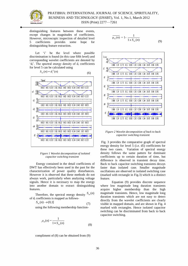
PRATIBHA: INTERNATIONAL JOURNAL OF SCIENCE, SPIRITUALITY,
BUSINESS AND TECHNOLOGY (IJSSBT), Vol. 1, No.1, March 2012
ISSN (Print) 2277—7261
36
distinguishing features between these events,
except changes in magnitudes of coefficients.
However, microscopic inspection of detailed level
5 coefficients provides some hope for
distinguishing feature extraction.
Let ‗i‘ be the level where possible
discrimination is found (in this case fifth level) and corresponding wavelet coefficients are denoted by
‗di‘. The spectral energy density of di coefficients
for level 5 can be calculated using 2( ) ( )xx iS n d n
(6)
Figure 1 Wavelet decomposition of isolated capacitor switching transient
Energy contained in the detail coefficients of
DWT has effectively been used in the past for the
characterization of power quality disturbances.
However it is observed that these methods do not
always work, particularly when analyzing voltage
signals. Hence it is necessary to map the energy
into another domain to extract distinguishing features.
Therefore, the spectral energy density ( )xxS n
of di coefficients is mapped as follows-
( ) (0,1]xxS n (7)
using the following membership function-
1( )
1 ( )A
xx
nS n
(8)
compliment of (8) can be obtained from (9)
A
1μ ( ) = 1-
1 ( )xx
nS n
(9)
Figure 2 Wavelet decomposition of back to back capacitor switching transient
Fig. 3 provides the comparative graph of spectral
energy density for level 5 (i.e. d5) coefficients for
these two cases. Variation of spectral energy
density follows the same pattern for dominant
coefficients up to certain duration of time, but
difference is observed in transient decay time.
Back to back capacitor switching transients decays
faster than isolated case. Smaller magnitude
oscillations are observed in isolated switching case
(marked with rectangle in Fig.3) which is a distinct
feature. Equation (9) provides discrete sequence
where low magnitude long duration transients
acquire higher membership than the high
magnitude transients. Hence, low magnitude long
duration transients which are not easy to detect
directly from the wavelet coefficients are clearly
visible in mapped domain, and are shown in Fig. 4
marked with rectangles. Hence isolated capacitor
switching can be discriminated from back to back
capacitor switching.

PRATIBHA: INTERNATIONAL JOURNAL OF SCIENCE, SPIRITUALITY,
BUSINESS AND TECHNOLOGY (IJSSBT), Vol. 1, No.1, March 2012
ISSN (Print) 2277—7261
37
Figure 3 Spectral energy density plot for isolated and back to back capacitor switching
Figure 4 Feature extraction
IV. Conclusion
Distinguishing feature for identification
of isolated capacitor switching and back to back
capacitor switching is extracted in this paper using
wavelet analysis. Wavelet is capable of extracting low frequency as well high frequency components
from the power system transients and hence it is
superior to Fourier analysis.
REFERENCES: 1. C. Parsons, W. M. Grady, E. J. Powers, and J. C. Soward,
―A direction finder for power quality disturbances based
upon disturbance power and energy,‖ IEEE Trans. Power
Del., vol. 15, no. 3, pp. 1081–1085, Jul. 2000.
2. D. Sochuliakova, D. Niebur, C. Nwankpa, R. Fischl, and
D. Richardson, ―Identification of capacitor position in a
radial system,‖IEEE Trans. Power Del., vol. 14, no. 4, pp.
1368–1373, Oct. 1999.
3. J. S. Kim, W. M. Grady, A. Arapostathis, J. C. Soward,
and S. C. Bhatt, ―A time domain procedure for locating
switched capacitors in power distribution systems,‖ IEEE
Trans. Power Del., vol. 17, no. 4,pp. 1044–1049, Oct.
2002 }.
4. T.E. Grebe, ―Application of Distribution system capacitor
banks and their impacts on power quality‖, IEEE
transactions on industry applications,vol..32, No.3,
pp.714-719 May/June1996.
5. E.B.Makram, et al. ―Transient analysis of capacitor
switching in unbalanced distribution system with
harmonic distortion‖, Electric power components and
systems, vol...17, issue 2, pp.75-92,1989.
6. C.S.Chang, et al. ―Determination of worst case capacitor
switching overvoltage of MRT system using genetic
algorithm‖, Electric power components and systems,
vol.27, issue 11, pp. 1161-1170, Oct 1999}.

PRATIBHA: INTERNATIONAL JOURNAL OF SCIENCE, SPIRITUALITY,
BUSINESS AND TECHNOLOGY (IJSSBT), Vol. 1, No.1, March 2012
ISSN (Print) 2277—7261
38
Study of Profitability and Break-Even Analysis For Glycolytic
Depolymerization Of Poly (Ethylene Terephthalate) (PET)
Waste During Chemical Recycling Of Value Added
Monomeric Products
Dr. V.R. Diware1, A. S. Goje
2, Dr. S. Mishra
3
1SSBT‘s College of Engineering and Technology, Bambhori, Jalgaon, M.S., (INDIA).
2G.H.Raisoni College of engineering and Management, Ahmednagar, M. S., India. 3 Department of Chemical Technology, North Maharashtra University, Jalgaon, M.S., India.
E-mail: [email protected], [email protected], [email protected]
ABSTRACT: Cost estimation, profitability and
break-even analysis for glycol tic
depolymerization of poly (ethylene
terephthalate) (pet) waste was carried out using
a batch reactor. different costs were
determined. obtained data was used to decide
the feasibility of the process technology for its
commercialization. the break-even point was
estimated for the process that showed much
more adequate return on the investment, which
has an industrial significance.
Key words: poly (ethylene terephthalate)
depolymerisation, material balance, cost, profit,
return, break-even point
I. INTRODUCTION
The growing interest in pet waste recycling is due
to the widespread use for various domestic and
engineering applications. Ecological and
economical considerations advocate the
introduction of wide-scale recycling. Market is
increasing rapidly and will further be boosted by
current developments of pet grades, and produces
high waste pet materials after use or during pet synthesis. Hence, among different methods of pet
waste recycling, chemical recycling has recently
been paid much more attention. [1–2] various
researchers [3–12] has studied depolymerization of
pet. application of these methods depends on end
use of recovered products. appreciable amounts of
monomeric products were recovered during
chemical recycling of pet. [3–8] results of their
studies did not report the feasibility of the method
of recovery of monomers for commercialization.
[1–12] hence, there were no required data
available about cost estimation and profitability analysis that are essential for process selection
during plant design for a new product. In absence
of a reliable and sufficient necessary data of
profitability and break-even analysis, reaction and
mass transport engineers are forced to scale-up the
established reactors and or separating equipments
in economically undesirable small steps.
Additionally, the available reaction and or mass
transport data are insufficient for designing new reactor and or separation equipment concepts with
justifiable expenditure. for process selection as
well as process development for optimal plant
design, the knowledge of cost estimation,
profitability and break-even analysis is required.
hence, this study is undertaken to fulfill the
industrial requirements for commercialization.
however, literature does not show these types of
study for glycol tic depolymerization of pet at
optimal conditions. in this work cost estimation,
profitability and the break-even analysis are
studied for glycolytic depolymerization of pet waste at various optimal reaction conditions.
A. Theory
Although the technical parameters are influencing
the selection and design of a given type of process
may be unique, cost is usually only parameter
relevant to all processes. Cost is often the
parameter used to select the optimum process from
the alternatives available. Economical information
plays an important role in setting many states of
the process. However, cost analysis is used to determine the minimum economic way of
achieving the desired goal. An understanding of
the economics involved in the process is important
in making decision at both the engineering and
management levels. Every engineer should be able
to execute an economical evaluation of a proposed
project. If the project is not profitable, it should
obviously not be pursued and the earlier such a
project can be identified, the fever is the resources
that will be wasted. Before the cost of a process
can be evaluated, the factors contributing to the
cost must be recognized. [13] An acceptable plant design must present a process that is capable of
operating under conditions that will yield a

PRATIBHA: INTERNATIONAL JOURNAL OF SCIENCE, SPIRITUALITY,
BUSINESS AND TECHNOLOGY (IJSSBT), Vol. 1, No.1, March 2012
ISSN (Print) 2277—7261
39
significant profit. Since net profit equals total
income minus all expenses, it is essential that the
chemical process engineer be aware of the
different types of costs involved in manufacturing
processes. Capital must be allocated for direct
plant expenses, such as those for raw materials,
labour, and equipment. Besides direct expenses,
many other indirect expenses are incurred, and these must be included if a complete analysis of
the total cost is to be obtained. Some examples of
these indirect expenses are administrative salaries;
product distribution costs, and costs for interplant
communications.[13– 15] The selection of process
using cost analysis is normally based on capital
and operating cost. All equipment costs were
reported [13] to be accurate to within 20 %.
Variations in the total cost can be attributed to a
number of variable factors such as cost of auxiliary
equipment, new installation, local labour cost,
engineering overhead, location and accessibility of plant site, and type of industry (installation work).
[13]
A capital investment is required for any
industrial process, and determination of the
necessary investment is an important part of a
plant design project. The total investment for any
process consists of fixed capital investment for
physical equipment and facilities in the plant
alongwith working capital that must be available to
pay salaries, keep raw materials and products on
hand, and handle other special items requiring a direct cash outlay. Moreover, in an analysis of
costs in industrial processes, capital investment
costs, manufacturing costs, and general expenses
including income taxes must be taken into
consideration. [13, 14] The flow chart for the
glycolytic depolymerization of PET using ethylene
glycol (EG) was developed for complete recovery
of monomers (Figure 9) [8] at various optimal
process conditions. Based on the various
information of glycolytic depolymerization process
of PET, [8]
the material balances were evaluated for raw materials as well as products.
In present study, costing of fixed capital
investment was under taken by calculating initially
the total equipment costs for the depolymerization
process. Then using the percentage of purchased
equipment costs the fixed capital investment was
evaluated. Then total product cost and hence total
expenses were calculated. Total annual income,
gross profit, and net profit were computed.
Finally, payback period, rate of return and break-
even point analysis were computed.
II. EXPERIMENTAL
A. Material, Chemicals And Reagents
PET used was procured from Garaware Polyesters,
Aurangabad, M.S., (INDIA). Here waste just mean
materials left over after some products were made
from raw material that was free from any additives
/ plasticizers. The other materials used were
neutral water, methanol, HCl, CaO, sodium sulfate,
ethylene glycol, zinc acetate, urea, etc., obtained from s. d. Fine Chemicals (INDIA). These
chemicals were used as received without further
purification.
B. Glycolysis of PET
Glycolysis reactions [8] were carried out in a 1 L
four-necked batch reactor at various temperatures
ranging from 100-220 O C at the interval of 10 OC
and 1 atm pressure. Reactor was equipped with a
thermometer and two reflux condensers. A stirrer
was put in reactor to ensure proper mixing.
Reaction was carried out by taking 10 g PET in 40
mL of ethylene glycol (EG) using glycolysis catalyst (i.e., 0.002 mol of zinc acetate) with 4
pieces of porcelain for different periods of time
ranging from 30 to 150 min. Different particle
sizes ranging from 50 to 512.5 µm of PET were
taken for this reaction (separately). After
completion of glycolysis reaction of PET, the
batch reactor was removed from heating mantel
and 50 mL of boiling neutral water was slowly
introduced into reaction mixture. Whole reaction
mixture was quickly filtered.
Unreacted PET was collected, washed with neutral water, dried in controlled oven at 95 OC until its
constant weight that was recorded.
Remaining filtrate was methanolized (second step
required in process) with additional catalyst (i.e.,
0.002 mol of urea) for 30 min at 190 OC and 1 atm
pressure. Reaction mixture was cooled in an ice-
bath. White crystalline flakes of DMT were
formed. It was filtered and washed with 50 mL of
cooled neutral water in order to remove catalysts,
and dried in a controlled oven at 95 OC until its
constant weight, which was recorded. From remaining liquid phase, EG was separated
using salting-out method [2, 8] by introduction of
sodium sulfate. Both monomeric products (DMT
and EG) were analyzed qualitatively and
quantitatively. Percent depolymerization of PET,
yield of DMT and yield of EG were determined by
gravimetry and defined in following ways.
A. Depolymerization of PET (%)
= {(WPET,i - WPET,R) / WPET,i} x 100 (1).
Yield of DMT (%) = {mDMT,O / mPET,i } x 100 (2).
Yield of EG (%)
= (mEG,O/ mPET,i ) x 100 (3).

PRATIBHA: INTERNATIONAL JOURNAL OF SCIENCE, SPIRITUALITY,
BUSINESS AND TECHNOLOGY (IJSSBT), Vol. 1, No.1, March 2012
ISSN (Print) 2277—7261
40
Where WPET,i is initial weight of PET, WPET,R is
weight of unreacted PET, mDMT,O is number of
moles of DMT, mEG,O is number of moles of EG,
and mPET,i, is initial number of moles of PET
monomeric units.
Process Reaction For Glycolysis Of PET
O O
||
(-C - -C – O – CH2CH2 – O–) n– + n
(PET)
Catalysts
HOCH2CH2OH n H 3COOC- ( EG) Methanol
-COOCH3 + n HOCH2CH2OH (DMT) (EG)
Analyses Of Depolymerized Products (EG And
DMT) Of PET
Liquid and solid products obtained from
depolymerization of PET were analyzed [8] by
determining their various physical properties (like
melting point, boiling point, molecular weight,
acid value, etc.) to confirm them.
Material Balance For Glycolytic
Depolymerization Of PET:
Maximum PET Weight % loss = 98.78 %.
Molecular Weight of PET = 16703 g mol -1.
Mol.Wt. of Dimethyl Terephthalate (DMT) = 194
g mol -1.
Mol.Wt. of Ethylene Glycol (EG) = 62 g mol -1.
Mol.Wt. of DMT + EG = 194 + 62 = 256 g mol -1.
Mol.Wt. of DMT + EG – H2O = 194 + 62 –18 =
256 – 18 = 238 g mol -1.
From 238 = 1 Water molecule was liberated.
From 16703 = 70.2 Water molecule will liberate.
100 % Material = 10 g PET. 98.78 % Conversion of Material = 9.878 g PET.
16703 give 70.2 Water molecules.
9.878 g give 0.042 g Water molecules.
Total weight of products (DMT + EG) = 9.878 +
0.042 = 9.92 g.
In 256 g, EG is 62 g (Theoretical).
In 9.92 g, EG is 2.4025 g (Theoretical).
Wt. of DMT = 9.92- 2.4025 = 7.5175 g
(Theoretical).
Wt. of EG = 2.3722 g (Experimental).
Wt. of DMT = 7.4213 g (Experimental).
Basis of calculation: Plant Production capacity of
76800 Kg DMT per Annum.
Raw materials required to produce 76800 Kg
DMT:
PET = 103486 Kg.
EG = 413944 L.
CaO = 35000 Kg.
Neutral Water = 537600 L.
HCl = 19200 L. Na2SO4 = 76800 Kg.
Z. A. (Zinc Acetate, Catalyst for glycolysis) =
5175 Kg.
Urea, Catalyst for methanolysis (second step
required in process) = 1243 Kg.
Methanol = 206972 L.
Monomeric Products Produced That Were
Recovered:
DMT = 76800 Kg.
EG = 24549 L.
Costs Estimation:
Total Equipment Costs:
Sr.
No. Equipment No. Cost per
equipment
(Rs)
Cost
(Rs)
1 Reactor 1 82000 82000
2 Evaporator 1 78000 78000
3 Filter 2 51000 10200
4 Dryer 1 72000 72000
5 Centrifugal
Pump
3 25000 75000
6 Vacuum
Pump
1 42000 42000
7 Rectangular
Tank
10 22000 220000
Total Equipment Costs (TEC): 671000
Capital Investment:
Fixed Capital Investment:
Direct Costs:
Sr.
No. Item % TEC Cost
(Rs)
1 Purchased
Equipment
100 671000
2 Purchased
Equipment
Installation
39 261690
3 Instrumentation
& Controls
(Installed)
13 87230
4 Piping
(Installed)
31 208010
5 Electrical
(Installed)
10 67100
6 Building
(Including
Services)
29 194590

PRATIBHA: INTERNATIONAL JOURNAL OF SCIENCE, SPIRITUALITY,
BUSINESS AND TECHNOLOGY (IJSSBT), Vol. 1, No.1, March 2012
ISSN (Print) 2277—7261
41
7 Yard
Improvements
10 67100
8 Service
Facilities
(Installed)
55 369050
9 Land 6 40260
Total Direct Cost (TDC) Rs
1966030
Indirect Costs:
Sr.
No. Item % TEC Cost (Rs)
1 Engineering
And
Supervision
32 214720
2 Construction Expenses
34 228140
3
Total Indirect Cost: T I D C:
Rs 442860
Total Direct Costs And Indirect Costs:
Rs 2408890
Other Charges:
Sr.
No. Item %
TD&IDC
Cost (Rs)
1 Contractors
Fees
5 120445
2 Contingency 10 240889
Fixed Capital Investment = Rs 2770224.
Working Capital Investment = 74 % TEC = Rs
496540.
Total Capital Investment = Rs 3266764.
Total Product Cost:
Manufacturing Cost: Direct Production Costs: Raw Materials Cost:
Sr.
No.
Raw
Material
Raw
Material
(Kg /
Yr)
Cost
(Rs /
Kg)
Cost
(Rs / Yr)
1 PET 103486 22 2276692
2 EG 413944 200 82788800
3 CaO 35000 70 2450000
4 Neutral
Water
537600 5 2688000
5 HCl 19200 40 768000
6 Na2SO4 76800 54 4147200
7 Zinc Acetate
5175 200 1035000
8 Urea 1243 60 74580
9 Methanol 206972 55 41383460
Total Raw Materials Costs = Rs 107611732.
Operating Labour Costs:
S
r.
N
o.
Post 1) N
o.of
Posts
Pay
(Rs/
Mont
h)
Pay
(Rs
/yr)
1 II. M
A
N
A
G
I
N
G
D
I
R
E
C
T
O
R
1 12000 144
000 2 Plant Manager 1 6000 720
00
3 Shift Engineer 3 4000 144
000
4 Shift Supervisor 3 3000 108
000
5 Operator 15 2500 450
000
6 Skilled Labour 10 2000 240
000
7 Unskilled Labour 30 1500 540
000
Total Operating Labour Costs = Rs 1698000. Office Materials And Clerical Expenses = 10 %
TOLC = Rs 169800.
Utilities = 75 % TOLC = Rs 1273500.
Maintenance And Repairs = 2 % FCI = Rs 55405.
Operating Supplies = 10 % M & R = Rs 5541.
Laboratory Charges = 10 % TOLC = Rs 169800.
Patents And Royalties = 10 % TOLC = Rs 169800.
Fixed Charges:
Depreciation = 10 % FCI + 2 % Building Value =
277023 + 3892 = 280915.
Local Taxes = 1 % FCI = Rs 27703.
Insurance = 0.4 % FCI = Rs 11080. Plant Overhead = 50 % TOLC = Rs 849000.
General Expenses:
Administrative Costs = 15 % TOLC = Rs 849000.
Distribution And Selling Costs = 15 % TOLC = Rs
254700.
Research And Development Costs = 15 % TOLC =
Rs 254700.
Financing (Interest) Costs = 10 % FCI = Rs
277023.
Total Product Costs = Manufacturing Costs +
General Expenses. Total Product Costs = Rs 113957699.
Total Expenses = Total Capital Investment + Total
Product Costs
Total Expenses = 3266764 + 113957699 = Rs
117224463.
Profitability Analysis:
Total Product Annual Income:
Sr.
No. 1) Prod-
2) ucts
Production
(Kg/Yr)
Cost
(Rs/Kg)
Income
(Rs/Yr)
1 3) DMT 76800 1500 115200000
2 EG 24549 200 4909800
Total Product Annual Income = Rs 120109800.
B. Gross Profit = TPAI – Total Expenses =
120109800 – 117224463
= Rs 2885337.
C. Net Profit = Gross Profit – Income Tax. =
Gross Profit – 40 % Gross Profit
= 60 % Gross Profit = Rs 1731202.
PRATIBHA: INTERNATIONAL JOURNAL OF SCIENCE, SPIRITUALITY,
BUSINESS AND TECHNOLOGY (IJSSBT), Vol. 1, No.1, March 2012
ISSN (Print) 2277—7261
42
Payback Period = (FCI / NP) = (2770224 /
1731202) = 1.6 Yrs = 19.2 Months.
Rate of Return = (NP / FCI) x 100 = (1731202 /
2770224) x 100 = 62.5 %.
Break Even Analysis:
Break Even Point (Units) = [FCI / (Selling Price
per Unit - Variable Cost per Unit)].
= [2770224 / (1500 – 1350)] = 18468.16 Kg. Break Even Point (as a % capacity) = [BEP (units)
/ Total capacity of Product] x 100.
= (18468.16 / 76800) x 100. = 24 %.
Conclusion
Cost estimation, profitability and break-even
analysis for glycolytic depolymerization of poly
(ethylene terephthalate) (PET) waste was revealed
that the rate of return on investment and payback
period is pretty good that has an industrial
significance. Various cost analysis data is used to
decide the feasibility of the process for industrial application. The break-even point (as a %
capacity), payback period and rate of return were
estimated that were recorded as 24 %, 1.6 years
and 62.5 % respectively for the process. Payback
period, rate of return and break-even point values
indicates that the much more excellent viability of
the process of glycolytic depolymerization of PET
at various optimal conditions.
References [1] Paszun, D.; Spychaj, T.; Nowaczek, N. Chemical
recycling of Poly (Ethylene Terephthalate) -PET.
Ekoplast. 1, 259, 1993 (in Polish).
[2] Paszun, D.; Spychaj, T. Chemical recycling of Poly
(Ethylene Terephthalate). Ind. Eng. Chem. Res. 36, 1373, 1997.
[3] Mishra, S.; Goje, A. S.; Zope, V. S. Proceedings:
International Conference On Plastic Waste Mangt and
Environment., 163, New Delhi, March 2001
[4] S. Mishra, V.S.Zope, A.S.Goje. Kinetic and
Thermodynamic studies of Depolymerization of Poly
(Ethylene Terephthalate) Waste By Saponification Reactions.
Polymer International.51 (12), 1310, 2002.
[5] S. Mishra, A.S.Goje. Kinetics of Glycolysis of Poly
(Ethylene Terephthalate) Waste Powder At Moderate Pressure
And Temperature. J. Appl. Polym. Sci. 87 (10), 1569, 2003.
[6] S. Mishra, A. S.Goje. Kinetic and Thermodynamic study of
Methanolysis of Poly (Ethylene Terephthalate) Waste Powder.
Polymer International. 52 (3), 337, 2003.
[7] S. Mishra, A.S.Goje, and V.S.Zope. Chemical Recycling,
Kinetics and Thermodynamics of Poly (Ethylene Terephthalate
(PET) Waste Powder by Nitric Acid Hydrolysis. Polymer
Reaction Engg. 11 (1), 79, 2003.
[8] A.S.Goje, S. Mishra. Chemical Kinetics, Simulation and
Thermodynamics of Glycolytic Depolymerization of Poly
(Ethylene Terephthalate) Waste with Catalyst Optimization for
Recycling of Value added Monomeric Products.
Macromolecular Materials and Engg. 288 (4), 326-336, 2003.
[9] Chen, J. Y.; Ou, C. F.; Hu, Y. C.; Lin, C.C.
Depolymerization of PET Resin Under Pressure. J. Appl.
Polym. Sci. 42, 1501, 1991.
[10] Yoshioka, T.; Sato, T.; Okuwaki, A. J. Hydrolysis of
Waste PET by NaOH at 150 o
C for a Chemical Recycling. J.
Appl. Polym. Sci.52, 1353, 1994.
[11] Ben-Zu, Wan., Chih-Yu, Kao., and Wu-Hsun, Cheng.;
Kinetics of Depolymerization of PET in a Potassium Hydroxide
Solution. Ind. Eng. Chem. Res. 40, 509, 2001.
[12] Oku, A.; Hu, L. C.; Yamade, E. Alkali Decomposition of
PET with Sodium Hydroxide in Non-aqueous Ethylene Glycol:
A Study on Recycling of TPA and EG. J. Appl. Polym. Sci. 63,
595, 1997.
[13] Maycock, J. C.; McKenna, J.D.; Theodore, L. Hand book
of Air Pollution Control Engg. And Technology. Lewis
Publishers, New York,p-277, 1995.
[14] Peter; M. S.; Timmerhaus, K.D. Plant Design and
Economics for Chemical Engineers. McGraw-Hill Publication,
Singapore, p 183, edn 1991.
[15] Vilbrandt, F, C.; Dryden, C, E. Chemical Engineering
Plant Design. McGraw Hill, Kogakusa, Ltd, 4Th
edn, p – 84,
1959.

PRATIBHA: INTERNATIONAL JOURNAL OF SCIENCE, SPIRITUALITY,
BUSINESS AND TECHNOLOGY (IJSSBT), Vol. 1, No.1, March 2012
ISSN (Print) 2277—7261
43
Effect of Dot (Direct Observation Treatment) Therapy on
Hepatic Enzymes and Calcium Level in Serum of T.B. Patients
S. S. Warke1, G V Puranik
2, and Z. H. Khan
3
1,2Department of Pathology, B.Y.L. Nair Ch. Hospital & T.N.Medical College, Mumbai-8 (India) 3Department of Biochemistry Shri Shivaji College, Akola-444001 (India.)
Emails: [email protected], [email protected], [email protected]
Abstract: In the present study, the Biochemical
manifestations of liver toxicity caused by co-
administration of anti-tuberculosis drugs,
rifampicin (RIF), isoniazid (I NH),
pyrazinamide (PZA) and Ethembutol (ETH) in
TB patients were investigated. Significant
alterations were observed in serum glutamate
oxaloacetat transaminase (SGOT), Serum
glutamate pyruvate transaminase (SGPT),
Serum Alkaline phosphatase (ALP), Serum
Acidic Phosphatase (ACP) its prostatic factor
(APF) and serum calcium on 15th
day of
treatment. However all the checked parameters
came to normal level (equal to control) on 6th
months of treatment except SGOT and SGPT.
Key words: Anti-tuberculosis drug, liver toxiocity,
Hepatic Enzymes, DOT therapy.
I. INTRODUCTION
In developing countries Tuberculosis is
still a major public health problem both in children
as well as in adults [1]
In 1956 there were about 15 lakhs patients
in India having tuberculosis infection. But now it
is estimated that there are about 14 million T. B. patients in our country of whom about 3.5 million
are infectious (sputum positive). About 2.2
million T. B. patients are added every year out of
which 1 million are sputum positive. Five lakh
people in India die due to tuberculosis every year.
i.e. one patient with tuberculosis die every minute
more than 1000 people every day [2].
There were about 28 thousand T.B.
patient in Mumbai in 2008 survey [3].
To combat against such an increasing infectious disease in the country it is imperative
that further intensive research is to be undertaken.
Hence the present study is proposed to see the
effect on Hepatic enzymes levels in T.B. patients
undergoing treatment with antituberculosis drug
like Rifampacin, Isoniazid, Pyrozinamide and
Ethambutol.Most reported cases of hepatic
dysfunction due to anti-TB drugs are reported to
occur within the first 3 months of starting the
treatment [4].Now a days T.B. Patients are
subjected to DOTS (Direct Observation Treatment
System) therapy thrice a week. It may have effect
on liver as it is a main site of drug metabolism, Mc Neill L. et.al. [5], reported that In a community
setting, we found a threefold increase in the risk of
hepatotoxicity among patients receiving
pyrazinamide/rifampin (13%) as compared to
isoniazid (4%). The risk of severe hepatotoxcity
requiring hospitalization was 5% (2 of 43 patients)
in the pyrazinamide/rifampin group prior to the
more intensive monitoring.
Kristic Buric et.al. [6], has also studied
levels of serum transaminases in DOT therapy.
Deck K.A. et.al. [7], have been reported side effects of rifampicin in tuberculosis patients.
According to Schare L. Smith J.P. [8], a number of
patients receiving antituberculous chemotherapy
develop serum transaminase elevations
unaccompanied by symptoms. However, the
finding that these enzymes rises may be induced
by INH alone has not been previously emphasized.
Moreover, serum transaminase elevations and
histologic evidence of hepatic damage has not been
previously reported in asymptomatic subjects
receiving isoniazid for chemoprophylaxis.
One set of the asymptomatic reaction in
all cases occurred within 2 months of initiating
INH. In general, the rise in enzymes appeared
sooner in hospitalized patients, who had more
frequent blood studies, than in the outpatient
group, although early detection does not appear to
account for all differences. Indications for
interruption of INH based on SGOT and SGPT
limits were not established while early experience
was being accumulated on the tuberculosis in
patients service. As a result, individual physician or patient concern generated by the chemical
abnormalities prompted temporary interruption of
INH in seven of the eight hospitalized reactors. In
one of these cases SGOT was 600 and SGPT, 900
units before the drug was interrupted; whether or
not these values represent the potential maximum
severity of the reaction is unknown.

PRATIBHA: INTERNATIONAL JOURNAL OF SCIENCE, SPIRITUALITY,
BUSINESS AND TECHNOLOGY (IJSSBT), Vol. 1, No.1, March 2012
ISSN (Print) 2277—7261
44
It has been found that such studies i.e.
levels of liver enzymes with respect to duration
have not been yet done. Hence the present study is
proposed to see the effect on Hepatic enzymes
levels in T.B. Patients undergoing treatment with
antituberculosis drugs (INH, Isonizid, Rifanpacin
and Ethembutal combinely).
II. MATERIALS AND METHODS
The study was conducted on out-door patients in
one of the corporation Hospital, Nair Hospital and
T. M. Medical College, Mumbai – 8.
100 Patients were examined in respiratory
Medicine Unit. Patients of either sex between age
group 15 to 60 year with pulmonary tuberculosis
were studies for serum SGOT, SGPT, Alkaline
Phosphatase and Acid Phosphatase with respect to
duration of treatment.Diagnosis of Tuberculosis
(TB) was based on detection of Acid Fast Bacilli (AFB) and direct smear examination by Ziehi
Nelson staining and also on culture for AFB [9].
All above diagnostic examination were carried out
in Department of Microbiology, Nair Hospital and
T. N. Medical College along with chest X-ray in
Radiology Department of the Hospital Diagnosis
was confirmed clinically in OPD of the Hospital
by senior physicians.
Patients were treated with antituberculosis
drugs. All the drugs were given thrice a week through out for 6 months under the direct
supervision of clinical staff. Patients treated with
the following drugs :
1. Cap. Rifanpacin (RIF) on empty stomach 1
Cap. (450 mg).
2. Tab. Isonazid (INH) 2 Tab. (300 mg).
3. Tab. Ethanbutol (ETH) 2 Tab. (600 mg).
4. Tab. Pyrazinamide (PZA) 2 Tab. (750
mg).
All drugs were given for two months.
After two months tablets ethanbutal and Tablet
Pyrazinamide were ceased but treatment continued
with Cap. Rifampacin and Tab. Isoniazid for a
period of further four months.Blood samples of all
patients were collected on zero day (before start of
treatment), 15 days, 1 month, 2 month, 3 month, 4
month and 6 month of treatment period.Approval
from Institutional Ethics committees for research
work was obtained.
A. Sample Collection :
Various blood samples were collected in plain
bulb and serum was separated.Serum AST (SGOT)
and serum ALT (SGPT) enzymes were estimated
by modified IFCC by kinetic method (10, 11, 12)
by using Olympus AU 400 Auto Analyzer in
Chemical Pathology Lab of Nair
Hospital.Enzymatic Diethalamine Kinetic Method
(13) was followed for ALP estimation by using
same instrument.Acid Phosphatase was estimated
by IFCC method modified from Kind and King Method (14).Serum calcium levels were estimated
by cresolphthalein comilexone method (15) by
using Auto Analyzer Olympus AU 400
III. PATIENTS SELECTION CRITERIA
A. Inclusion Criteria
1. Patients of either sex in the age group 18-60
years. 2. New cases of Pulmonary T.B. as diagnosed by
using Revised National Tuberculosis Control
Programme (RNTCP) diagnostic algorithum.
B. Exclusion Criteria
1. Retreatment cases of Pulmonary T.B. relapse,
failure, treatment after defaulter with Cagetory
II.
2. Sputum smear negative for pulmonary T.B. 3. Patients suffering from active liver disease.
4. Patients suffering from severe renal cardiac
disease admitted in ICU of the Hospital.
5. Patients suffering from other associated
pulmonary diseases.
6. Pregnant and lactating female.
7. Patients suffering from HIV
C. Selection of Control
1. Healthy 10 male / female volunteers in the age
group of 15-60 years.
2. On the basis of following Lab investigations
within the normal range;
a) Hb / CBC, ES
b) LFT and AST, ALT. S. Bilirubin
c) BUN and Serum creatinin

PRATIBHA: INTERNATIONAL JOURNAL OF SCIENCE, SPIRITUALITY,
BUSINESS AND TECHNOLOGY (IJSSBT), Vol. 1, No.1, March 2012
ISSN (Print) 2277—7261
45
IV. RESULT AND DISCUSSION
Table No. 1 Effect of Antituberculosis Drugs* on SGOT and SGPT in IU/Lit. in Serum of Patients with Respect to
Duration of Treatment.
Duration of
Treatment
SGOT Percentage
changes
SGPT Percentage Changes
Control 20.66 0.88 1 -- 19.17 0.94 --
Zero Days 34.80 2.46 P <
0.001
+ 68.44 25.76 3.40 Z = 1.88
P > 0.05
+ 34.37
15 Days 42.22 4.93 P < 0.001
+ 104.35 27.91 3.45 P < 0.01
+ 45.58
1 Month 29.95 3.27 P < 0.001
+ 44.96 23.86 2.89 1.57, P < 0.001
+ 24.46
2 Months 27.76 2.45 P < 0.01
+ 34.36 28.43 3.62 2.47, P < 0.05
+ 48.30
3 Months 31.53 3.13 P < 0.001
+ 52.61 24.95 2.51 2.15, P < 0.05
+ 30.15
4 Months 26.30 2.01 P < 0.01
+ 27.29 25.02 2.56 2.13, P < 0.05
+ 30.51
6 Months 29.64 3.14 P < 0.001
+ 43.46 30.17 5.02 Z = 2.2, P < 0.05
+ 57.38
Values are Mean SE (N = 100) * (1) Cap. Rifanpacin (RIF) on empty stomach 1 Cap. (450 mg). (2) Tab. Isonazid (INH) 2 Tab. (300 mg).
(3) Tab. Ethanbutol (ETH) 2 Tab. (600 mg). (4) Tab. Pyrazinamide (PZA) 2 Tab. (750 mg). For 2 Months
Durgs 3 + 4 continued upto 6 months. P < 0.001 Highly Significant, P < 0.01 More Significant,
P < 0.05 Significant, P > 0.05 Not Significant.
Table No. 2 Effect of Antituberculosis Drugs* on Alkaline phosphatase, Acid Phosphatase and Prostetic acid
Phosphatase IU/Lit. In patients with Respect to Duration of Treatment.
Duration
of
Treatme
nt
Alkaline
Phosphatase
%
change
Acid
Phosphatase
% change Protatic Acid
Phosphatase
% change
Control 156.5 3.06 -- 1.806 0.06 -- 0.92 0.04 --
Zero Days
279.14 22.83 P < 0.001
+78.36 3.23 0.25 P < 0.001
+78.8 1.28 0.07 P < 0.001
+39.13
15 Days 285.63 24.17 P < 0.001
+82.51 2.78 0.24 P < 0.001
+53.9 1.71 0.08 P < 0.001
+85.86
1 Month 240.16 21.00 P < 0.001
+53.45 2.71 0.17 P < 0.001
+50.0 1.04 0.05 P < 0.05
+13.04
2 Months 232.50 18.65 P < 0.001
+48.56 2.46 0.15 P < 0.001
+36.2 0.92 0.05 P > 0.05
0
3 Months 223.32 17.92 P < 0.001
+42.69 2.39 0.13 P < 0.001
+32.2 0.96 0.05 P > 0.05
+4.34
4 Months 192.52 16.56 P < 0.05
+23.01 2.11 0.07 P < 0.001
+16.8 0.99 0.04 P > 0.05
+7.60
6 Months 186.15 19.35 P > 0.05
+18.94 1.80 0.06 P > 0.05
-1.0 0.92 0.04 P > 0.05
0
Values are Mean SE (N = 100) * (1) Cap. Rifanpacin (RIF) on empty stomach 1 Cap. (450 mg). (2) Tab. Isonazid (INH) 2 Tab. (300 mg).
(3) Tab. Ethanbutol (ETH) 2 Tab. (600 mg). (4) Tab. Pyrazinamide (PZA) 2 Tab. (750 mg). For 2 Months
Durgs 3 + 4 continued upto 6 months.

PRATIBHA: INTERNATIONAL JOURNAL OF SCIENCE, SPIRITUALITY,
BUSINESS AND TECHNOLOGY (IJSSBT), Vol. 1, No.1, March 2012
ISSN (Print) 2277—7261
46
P < 0.001 Highly Significant, P < 0.01 More Significant,
P < 0.05 Significant, P > 0.05 Not Significant.
Table No. 3 Effect of antituberculosis drugs* on serum calcium in mg/dl in serum of patient with respect to duration of
treatment.
Duration of Treatment Serum calcium Percentage change
Control 9.66 0.10
Zero Days 8.60 0.10 P < 0.001 - 11
15 Days 8.71 0.10 P < 0.001 - 10
1 Month 8.66 0.10 P < 0.001 - 11
2 Months 8.49 0.09 P < 0.001 - 13
3 Months \8.39 0.10 P < 0.001 - 14
4 Months 8.64 0.14 P < 0.001 - 18
6 Months 8.49 0.12 P < 0.001 - 13
Values are Mean SE (N = 100) * (1) Cap. Rifanpacin (RIF) on empty stomach 1 Cap. (450 mg). (2) Tab. Isonazid (INH) 2 Tab. (300 mg).
(3) Tab. Ethanbutol (ETH) 2 Tab. (600 mg). (4) Tab. Pyrazinamide (PZA) 2 Tab. (750 mg). For 2 Months
Durgs 3 + 4 continued upto 6 months.
P < 0.001 Highly Significant, P < 0.01 More Significant,
P < 0.05 Significant, P > 0.05 Not Significant.
Figure 1 :- Treatment of antituberculosis drugs on serum
calcium levels
80%
85%
90%
95%
100%
105%
Control 0 days 15 days 1 months 2 months 3 months 4 months 6 months
Period
Pe
rce
nta
ge

PRATIBHA: INTERNATIONAL JOURNAL OF SCIENCE, SPIRITUALITY,
BUSINESS AND TECHNOLOGY (IJSSBT), Vol. 1, No.1, March 2012
ISSN (Print) 2277—7261
47
V. RESULTS
Table I shows the effect of anti-
tuberculosis drugs on serum transferases i.e. SGOT
and SGPT which are marker of liver function.
In control group of patients SGOT level
was found to be 20.66 + 0.88 IU/L which
significantly increased in pretreated T.B. patients to 34.80 + 2.46 which was 68.45% higher. The
value further increases on treatment with T.B.
drugs and it reaches to 42.22 + 4.93 on 15th day.
The magnitude of increase being 104% higher as
compared to control.
Afterward the SGOT level remains some
what constant from 1 month post treatment to 2
months, 3 months, 4 month and upto 6 months. On
6th month value was 29.64 which was still
significantly high (43.46%) with respect to control.
Similar pattern have been observed in
SGPT also. In control group the SGPT level was
19/17 + 0.94 IU/L which increased to 25.76 + 3.4
IU/L in T.B. Patients prior to start of treatment.
The rise being 34.37%. A significant rise was
observed on 15 days post-treatment period by
45.59%. The value remain almost increased in all
post-treatment groups i.e. 1 month, 2 month, 3
month, 4 month and 6 month post treatment. On
6th month the value was 30.16 + 5.02 IU/L which
in 57.38% higher than control group.
Table II indicates the effects of anti-T.B
drugs on serum Alkaline phsophatase, Acid
Phosphatasea and Prostatic factor of Acid
phsophatase in T.B. patients. The healthy subjects
of control group showed 156.5 + 3.06. 1.806 +
0.06, 0.92 + 0.04 IU/L values of Alkaline
phosphatase, Acid Phosphatase and prostatic factor
of acid phosphatase respectively. Significant
increase was found in all three parameters in
pretreated T.B. patients. The value being 279.14 + 22.83, 3.23 + 0.25 and 1.28 + 0.07 respectively in
Alkaline Acid and Prostatic acid phosphatase
respectively.
The percent increase was 78.36%, 78.8%
and 39.13% respectively in Acid, Alkaline and
Prostatic acid Phosphatases.
All parameters reaches to highest value
on 15th day post treatment. The Alkaline
phosphatase was reached to 285.63 + 24.17 IU/L
which was 82.5% higher than control. The Acid phsophatase increased to 2.78 + 0.24 IU/I which
was 53.9 % higher and Prostatic factor of acid
phsophatase reached to 1.71 + 0.08 IU/L which
was 85.86% higher than control.
After one month treatment of T.B. drugs
till 6 months through 2, 3, 4 month the gradual
decrease in all three parameters observed, which
reached to normal level on 6th month post-
treatment.
Table III represents the serum calcium
level in T.B. patiets on treatment with DOT therapy. The healthy group of subjects showed
9.66 + 0.10 mg/dl serum calcium. As compared to
it the T.B. patients group prior to treatment shows
significant decreased of 11%, the magnitude being
8.60 + 0.10 mg/dl. The decrease in level was
persistent till period of investigation. It was -10%.
–11%, -13%, -14%, -11% and -13% on 15 days
post-treatment, 1, 2, 3, 4 and 6th month post
treatment period of T.B. drug.
VI. DISCUSSION
The results showed that biomarkers of toxicity in serum of Tuberculosis patients were
stimulated significantly after administration of
anti-T.B. drug.
In normal i.e. control group serum SGOT
and SGPT levels were found 20.5 IU/Lit and 19.1
IU/Lit respectively. The normal levels of ALP was
156.7 IU/L, whereas serum calcium content was
9.71 mg%. The acid phosphatase level and
prostatic acid phosphatase levels in control groups
were 1.80 and 0.92 IU/L respectively. In tuberculosis patients on zero day i.e. prior to
treatment all values were significantly high. All
the parameters reached to highest level on 15th day
of treatment but start to decline till 6th month post-
treatment (through 1, 2, 3, 4 months post treatment
values).
The present study revealed that the
hepatic injury by anti-TB drugs (in combination)
is due to membrane damage as indicated by
increase serum markers (13). However decline in
levels of serum marker after 1 month till 6 months, through 2nd, 3rd, 4th month of treatment may be due
to aquantance in development of detoxifying
mechanism in hepatic cells for Sr. Acid and
Alkaline phosphatase. However SGOT and SGPT
levels remains almost constant from 1 month to 6
month through 2nd, 3rd and 4th month of treatment.
The reason is that the theraphy was continued till 6
months. SGOT and SGPT might have been came
to normal after end of therapy. Further research is
in progress regarding aspect.
In conclusion a temporary rise in ALP, ACP, APF and Sr. Calcium have been observed till
15 days post treatment which come to normal at
one month onwards. However SGOT and SGPT
remained high significantly till end of experiment.

PRATIBHA: INTERNATIONAL JOURNAL OF SCIENCE, SPIRITUALITY,
BUSINESS AND TECHNOLOGY (IJSSBT), Vol. 1, No.1, March 2012
ISSN (Print) 2277—7261
48
The out come of hepatic adverse effect is often
made more severe by continued administration of
the offending drugs after the onset of the first
manifestation of liver damage. Therefore, both
physician and patients should be educated about
the possibility of hepatiotoxicity during
antitubercular treatment and about the necessity of
monitoring liver status (14).
ACKNOWLEDGEMENT
The authors are thankful to Dr. Sanjay N.
Oak, The Director, BMC, Medical Education and
Major Hospital for providing collected Blood
samples from T.B. patients of attending DOTS
medicine, Nair Hospital and to Dr. Jaya
Deshpande, Ex. Head of Department of Pathology,
for Providing the laboratory facility to carry out
the work.
Thanks are also due to Providing
chemical facilities by Nana Parkar Smriti Samiti, Parel and Rupchand Bansari and also Lab Incharge
Miss Ajita Kulkarni, Sr. Biochemist and V. D.
Rane, Lab. Tech, Gurunath Shinde, Umesh Shinde
and Laxman Chougule and Dhodke, Kuwar and all
lab technician for their co-operation and for
invaluable help and important suggestion.
REFERENCES [1] Udani P. M. (1961): Incidence of tuberculosis in children.
Indian J. Child Helath, : 10 : 566 – 575.
[2] M. M. Puri (2003) : Stop TB-use dots. Employment
News Weekly 29 March – 4 April/ XXVII No. 52. 1.
[3] Health Department Survey (2008) : Maharashtra Times
24 – 9 – 2008.
[4] Davies D. M. Editor (1999) : Text book of adverse drug
reactions. London Oxford Medical Publications.
[5] Mc Neill L. et al., (2003) : Pyraznamide and Rifampicin
vs Isoniazid for the treatment of Lattent tuberculosis.
Chest, 123 (1) – 102 – 06.
[6] Krastic Buric et al., (1980) : The activity of Transminase
(GOT) and (GPT), Alkaline phosphatase. Plucne bolesti
Tuberk : 92 (3), 132 – 8.
[7] Deck K. A. et al., (1976) : Frequency Diagnosis and
course of Kepatoxic efforts of Rifampicin. Med. Klln., 71
(4) : 1836 – 41.
[8] Seharer L., Smith J. P. (1969) : Serum transminase
elevation and other hepatic abnormalities in patients
receiving Isoniazid. Ann. Intern. Med., 71 (6) : 1113 –
20.
[9] Warke S. S. and Khan Z. H. (2004) :Effect of anti
tuberculosis drug on serum electrolytes levels osmolarity,
Blood pH and PCO2 levels in tuberculosis patients. Asian
Jr. of Microbiol Env. Sc. Vol. 5, No.(1): 89 – 91.
[10] Bergmete H. U., Horder M, Rej R.(1986) : Approved
Recommendation (1985) on IFCC Method for the
measurement of catalytic concentration of enzymes part 3.
IFCC Method for L/ Aspartate aminstransferase. J. Clin.
Chem. Clin biochem.; 24, 497 – 510.
[11] Penttila, I. M. et al., (1975) : Scand. J. Clin. Lab. Invest,
36, 2751.
[12] Hafkensheild, J. C. M et al., (1979): J. Clin. Chem. Clin
biochem.; 17, 219.
[13] Klin Lab (1992) : Age-dependent reference Limits of
Several enzymes in Plsama at different measuring
termeratures/ 38, 555-61.
[14] Seiler, D., Nagel. Tritschler W. and Lsoser S. (1983) : J.
Clin. Chem. Clin. Biochem., 21 : 519.
[15] Young S.D., Pestaner L.C., and Gibbeman V. (1975) :
Clin. Chem.Vol 21, No. 5.
[16] Sheikh A., Tasduq Kaiser Peerzada,. Supriya Kaul, Rinku
Bhat, Rakesh K. Johri (2005) : Biochemical
Manifestations of antituberculosis drugs induced
hepatotoxicity and the effect of silymarin. Hepatology
research, 31 132 – 135.
[17] Francois Durand, gilles Jebrak Dominique Pesseyre et al.,
(1996) : Hepatotoxicity of antitubercular treatments.
Drug safety Des. 15 (6) : 394 – 405.

PRATIBHA: INTERNATIONAL JOURNAL OF SCIENCE, SPIRITUALITY,
BUSINESS AND TECHNOLOGY (IJSSBT), Vol. 1, No.1, March 2012
ISSN (Print) 2277—7261
49
Multimedia Data Mining: A Survey
Sarla More1, and Durgesh Kumar Mishra
2
1Assistant Professor, Truba Institute of Engineering and information Technology, Bhopal 2Professor and Head (CSE), Sri Aurobindo Institute of Technology, Indore
Emails: [email protected], [email protected]
Abstract: Multimedia data mining (MDM) can
be defined as the process of finding interesting
patterns from media data such as audio, video,
image and text that are not ordinarily accessible
by basic queries and associated results. MDM is
the mining of knowledge and high level
multimedia information from large multimedia
database system. MDM refers to pattern
discovery, rule extraction and knowledge
acquisition from multimedia database. To
extract knowledge from multimedia database
multimedia techniques are used. We compare
MDM techniques with the state of the art data
mining techniques involving clustering,
classification, sequence pattern mining,
association rule mining and visualization. This
paper is a survey on the problems and solution
of MDM it elaborates basic concepts,
application at various areas, techniques ,
approaches and other useful areas which need
to be work for MDM. Analyzing this huge
amount of multimedia data to discover useful
knowledge is a challenging problem which has
opened the opportunity for research in MDM.
Keywords: Multimedia Data Mining, Feature
Extraction, Knowledge acquisition, visualization.
I. INTRODUCTION
Multimedia data mining can be better
understood by its purpose and scope. According to
MPEG-7 Standard the kinds of data belong to the
multimedia data [1] are of four types audio data,
which includes sounds, speech, and music; image
data ,video data, which include time-aligned sequences of images; and electronic or digital ink,
which is sequences of time aligned 2D or 3D
coordinates of a stylus, a light pen, data glove
sensors, graphical, temporal, relational and
categorical data or a similar device are stored in a
multimedia database and used to develop a
multimedia system [2]. The meaning of term
MDM means several data sources of different
modalities are processing at the same time. The
MDM‘s primary purpose is to process media data
alone or in a combination with other data for
finding patterns useful for business. Definition1. ―MDM is the exploration and
analysis, by automatic or semi-automatic means, of
large quantities of data in order to discover meaningful patterns and rules‖
Definition2. ―Multimedia data mining is a
subfield of data mining that deals with an
extraction of implicit knowledge, multimedia data
relationship or other patterns not explicitly stored
in multimedia database‖.
The goals of MDM are to discover useful
information from large disordered data and to
obtain knowledge from the information. There are mainly six tasks for MDM: summarization,
association, classification, clustering, trend
analysis and deviation analysis. The working of
MDM system is similarity search in multimedia
data, Description based retrieval system, build
indices and perform object retrieval based on
image description such as keywords, caption, size
and time of creation, content based retrieval
system, support retrieval based on the image
content, such as color, histogram, texture, shape,
object and wavelet transform. The multimedia
mining involves two basic steps:
• Extraction of appropriate features from the data.
• Selection of data mining methods to identify the
desired information.
For multimedia information system and
retrieval of content based image/audio/video
Multimedia database is used and provides search
and efficient storage organization. Data mining
tool operate on structured data so that powerful
tools are required for the unstructured or semi-structured data and dynamic audio-visual features
available in multimedia database. Mining of
multimedia data requires two or more data types
such as text and video or text video and audio.
Multimedia mining reaches much higher
complexity from huge volume of data such as
diversity of sensor, time or condition of
acquisition. Mining in multimedia is referred to
automatic annotation or annotation mining.

PRATIBHA: INTERNATIONAL JOURNAL OF SCIENCE, SPIRITUALITY,
BUSINESS AND TECHNOLOGY (IJSSBT), Vol. 1, No.1, March 2012
ISSN (Print) 2277—7261
50
Fig No. 1 Multimedia data mining
Multimedia and data mining are two very
interdisciplinary and multidisciplinary areas with
independently and simultaneously rapid
developments in recent years, for many decision-
making applications the need for tools to extract
hidden useful knowledge embedded within multimedia collections has become central point
for research.
II. RELATED WORK
A. Background of multimedia data mining:
Since 1960 the research in the field of
multimedia has begun for combining different
media data into one application where text and
images were combined in a document. During the
research and development process, the
synchronization of audio, video, and animation
were done using a timeline which specify when they should be played. The problems of
multimedia data capture, storage, transmission, and
presentation have been investigated in the middle
of 1960 where the multimedia standards MPEG-4,
X3D, MPEG-7, and MX have continued to grow.
Which are adapted and can transparently handle
sound, images, videos, and 3-D objects that
combined with events, synchronization, and
scripting languages and can describe the content of
any multimedia object. For multimedia distribution
and database applications different algorithms need to be used. Such a database can be queried, for
example, with the SQL multimedia and application
packages called SQL/MM. The MDM covers the
following areas:
Media compression and storage.
Delivering streaming media over
networks with required quality of service.
Media restoration, transformation, and
editing.
Media indexing, summarization, search,
and retrieval.
Creating interactive multimedia systems
for learning/training and creative art
production.
Creating multimodal user interfaces.
B. Multimedia Mining
1. Processing Text:
The Unstructured text documents can be
represented as ―bag-of-words‖ such as huge
feature vectors, where each feature encodes the
presence or absence of a word from the dictionary common to all documents. a naive Bayesian
classifier is used for such vectors to be analyzed to
classify documents into
By predefined groups, or by self
organizing maps
A type of neural networks to cluster
documents according to topics
Trees: we consider the structure of
documents expressed using HTML
tags
Multi-valued attributes, which corresponds to some parts of the
document instead of single term. for
filtering e-mails this approach was
used.
2. Processing Graphs:
In the machine learning community processing
graphs or trees such as organic molecules or web
sites and HTML documents has become an
important part of research. Between the classic
attribute-value and multi-relational representation of training data graph structures are there. Graph is
more expressive than a flat representation this is
the motivation for using graph representation in the
area of machine learning, and directly learning
from graphs is potentially more efficient than
multirelational learning.
3. Processing Images:
In the field of pattern recognition a number of
approaches to image processing can be used for
feature extraction. Texture analysis, line detection,
edge detection, segmentation and region of interest processing are some of the tasks solved in image
processing. Fourier transformation, smoothing,
color histograms, contour representations are tools
that are used to solve these tasks. The images
decomposed into segments or regions can then be
represented in relational form and machine
learning algorithms can be applied.
4. Processing Audio:
In multimedia applications audio data plays an
important role. Band energy, zero crossing rate, frequency centroid, Band-width and pitch period
are most frequently used features for audio
processing. Audio signals can also be decomposed
using wavelet transformation.
Multimedia
Data Mining
Text
Combination
of data types
Audio
Video
Image

PRATIBHA: INTERNATIONAL JOURNAL OF SCIENCE, SPIRITUALITY,
BUSINESS AND TECHNOLOGY (IJSSBT), Vol. 1, No.1, March 2012
ISSN (Print) 2277—7261
51
5. Processing Video:
The tasks of digital video processing are
automatic segmentation, indexing, content-based
retrieval and classification. High-level information
from video includes detecting trigger events.
C. Multimedia data mining goals and
methods: Dissecting a set of objects, uncovering rules,
decision trees, pattern recognition, trend
prediction, and dimensionality reduction are some
goals in MDM [3].
1. Dissecting a Set of objects
The most popular goal in data mining is
dissecting a set of objects which is described by
high-dimensional data into small comprehensive
units, classes, substructures, or parts. These
substructures give better understanding and
control, and based on suitable information can
assign a new situation to one of these classes, which can be classified as supervised or
unsupervised. Each object originates from one of
the predefined classes and is described by a data
vector. But it is unknown to which class the object
belongs, and this class must be reconstructed from
the data vector. In unsupervised classification
(clustering), according to the object content
without a priori knowledge a new object is
classified into a cluster of objects. It used in MDM
early processes.
2. Uncovering rules:
An association rule method is used If goal of
MDM is to be expressed as uncovering interesting
rules [3]. An association rule takes a form of an
implication X→Y, where X and Y denote
antecedent and consequent of the rules
respectively. X and Y belong to set of objects I, X
∩ Y = Φ, and D denotes a set of cases. We
describe support s and confidence c as two
parameters. The rule X→Y has support s in D,
where s% of the data cases in D contains both X and Y and the rule holds confidence c in D, where
c% of the data cases in D that support X also
support Y. Association rule mining selects rules
which have support greater than user-specified
minimum support threshold. Confidence of the rule
is at least from 0 to 1 confidence threshold. An
association rule mining algorithm works in two
steps:
Finds all large item sets that meet the
minimum support constraint
It generates rules from all large item sets
that satisfy the minimum confidence constraints.
III. DATA MINING VERSUS
MULTIMEDIA DATA MINING
Current data mining tools operate on structured
data, resides in large relational databases whereas
data in multimedia databases are semi structured or
unstructured. Compared with data mining,
multimedia mining reaches much higher
complexity resulting from:
The huge volume of data,
The variability and heterogeneity of the
multimedia data such as diversity of
sensors, time or conditions of acquisition
The content meaning of multimedia is
subjective.
Unstructured data: It is simply a bit stream. For
example pixel level representation of images,
video, and audio, and character level
representation for text. To extract semantics from
this data substantial processing and interpretation are required. It is difficult to interpret the database
as this kind of data is not broken down into smaller
logical structures.
IV. ARCHITECTURE OF
MULTIMEDIA DATA MINING
To design and develop a MDM system some
architecture are available. The first architecture
includes Extracting data or metadata from the
unstructured database in figure 2 which Store the
extracted data in a structured database and apply
data mining tools on the structured database.
Structured
Data
Unstructured Data
Fig No. 2 Converting unstructured data to structured
data for Mining
In Figure 3 architecture as a starting point data
collection is considered to be a learning system.
The overall achievable performance determines by the quality of raw data. The goal of data pre-
processing is to discover important features from
raw data. Data cleaning, normalization,
transformation, and feature selection comes under
data pre-processing. At pre-processing stage if
informative features be identified Learning can be
straightforward. Detailed procedure depends
highly on the nature of raw data and problem‘s
domain. In some cases, prior knowledge can be
extremely valuable [4].
Data Mining Tool

PRATIBHA: INTERNATIONAL JOURNAL OF SCIENCE, SPIRITUALITY,
BUSINESS AND TECHNOLOGY (IJSSBT), Vol. 1, No.1, March 2012
ISSN (Print) 2277—7261
52
Fig No. 3 Multimedia mining process
For many systems, Domain experts
conduct these stages. Training set is the product of
data pre-processing. A learning model has to be
chosen to learn from training set. The steps of
multimedia mining are iterative. In order to
improve the results the analyst jump back and forth
between major tasks .
Figure 4 present architecture of applying MDM in different multimedia types [2]. The main
stages of data mining process are:
A. Domain Understanding: It requires learning
how the results of data-mining will be used so
as to gather all relevant prior knowledge
before mining.
B. Data selection: This stage requires the user to
target a database or select a subset of fields or
data records to be used for data mining.
C. Learning and Pre-processing: Integrating data
from different sources and making choices
about representing or coding certain data
fields is the task of this stage. It serves as
input to the pattern discovery stage. Because
certain fields may contain data at levels of
details which are not considered suitable for
the pattern discovery stage representation
choices are needed. In MDM the
preprocessing stage is of considerable
importance given the unstructured nature of multimedia data.
D. Discovering Patterns: The pattern discovery
stage is the heart of the entire data mining
process. The hidden patterns and trends in the
data are actually uncovered in this stage.
Several approaches of pattern discovery stage
includes association, classification, clustering,
regression, time-series analysis and
visualization.
E. Interpretations: To evaluate the quality of
discovery and its value to determine whether
previous stage should be revisited or not this
stage of data mining process is used.
F. Reporting and using discovered knowledge:
This final stage reporting and putting to use
the discovered knowledge to generate new
actions or products and services or marketing
strategies as the case may be.
Fig No. 4 Architecture of Multimedia data mining
The above mentioned stages of data mining
process such as Data preprocessing, cleaning and
transformation, Discovering patterns,
Interpretation, and Reporting and using discovered
knowledge contains the highest importance and
novelty from the MDM perspective. Thus, we can
organize Multimedia Data Mining State of the Art
review. The proposed scheme achieves the following goals [5].
Discussion of the existing preprocessing
techniques for multimedia data in MDM
literature.
Identifying specific problems encountered
during data mining of multimedia data
from feature extraction, transformation,
representation and data mining techniques
perspective.
Discuss the current approaches to solve
the identified problems and their limitations.
Identification of open issues in the MDM
area.
Model
Data Collection
Machine Learning
Data Preprocessing
- Data cleaning
- Feature Selection
-Feature Extraction
Raw Data
Training set

PRATIBHA: INTERNATIONAL JOURNAL OF SCIENCE, SPIRITUALITY,
BUSINESS AND TECHNOLOGY (IJSSBT), Vol. 1, No.1, March 2012
ISSN (Print) 2277—7261
53
V. ISSUES IN MULTIMEDIA DATA
MINING
Before MDM develops into a conventional,
mature and trusted discipline some issues have to
be addressed. These issues pertain to be the MDM
approaches and their limitations. Major Issues in
MDM includes content based retrieval and similarity search which are integrated with mining
methods, generalization and multidimensional
analysis, classification and prediction analysis, and
mining associations in multimedia data [6].
Content based retrieval in multimedia is a
challenging problem [7]. To gain insight into the
meaning contained in databases is objective of
multi-dimensional analysis. The multi-dimensional
approach makes navigating the database easier,
screening for a particular subset of data, or asking
for data in a particular way, and being able to
define analytical calculations. The speed of these operations is much quicker and more consistent
than in other database structures as the data is
physically stored in a multi-dimensional structure
[8].
Feature Fusion:
With features extracted from multimedia data an
important issue is how features should be
integrated for mining and other applications. On
each modality most of the multimedia analysis is
performed separately, and to arrive at the final decision about input data results are brought
together at a later stage. This approach is called
late fusion or decision-level fusion. This is a
simple approach, we lose valuable information
about the multimedia events or objects present in
the data.
VI. APPROACHES TO MDM
The integration of storage and search techniques
with standard data mining methods is required for multimedia database mining. Promising
approaches [4] includes Construction of
multimedia data cubes, the extraction of multiple
features from multimedia data, and similarity
based pattern searching.
A. Multimedia data cube: Primarily on the basis
of visual content this facilitates multiple
dimensional analyses of multimedia data.
Multimedia Miner as a MDM system
prototype has been designed and developed
which includes the construction of a multimedia data cube that facilitates multiple
dimensional analysis of multimedia data. The
mining of multiple kinds of knowledge
includes characterization (summarization),
discrimination (comparison), classification,
association and clustering, in image and video
databases.
B. Feature extraction: To extract patterns and
derive knowledge from large collections of
images, audio and video it takes the
information contained in multimedia data. Some features that are used include short-time
energy, pause rate, zero-crossing rate,
normalized harmonicity, fundamental
frequency, frequency spectrum, bandwidth,
spectral centroid, spectral roll-off frequency
and band energy ratio [9].
C. Similarity based pattern searching: In
multimedia retrieval and data mining
Similarity search is a crucial task. It can be
defined as searching for a set of similar
objects to a given query object.
D. Database approach: This approach views
multimedia data as structured. Manually or
semi-automatically features are extracted. The
features or attributes on unstructured data,
entail a high level of abstraction. In the
features the higher the level of abstraction, the
lower the scope for ad-hoc queries.
VII. TECHNIQUES OF MDM
A. MDM Process Using Classification Rules:
In this approach, main focus is on discovering
the semantic structures. We use the classification
rule approaches to perform data mining process
because this approach only induce absolutely
accurate rules. Examples of this work are:
1. The Hidden Markov Model
2. Detection of soccer goal shots using
decision tree
B. MDM Process Using Clustering:
Clustering is a process of organizing objects
into groups whose members are similar in some
way. It is one of the unsupervised learning data
mining technique. In unsupervised classification,
the problem is to group a given collection of
unlabeled multimedia files into meaningful clusters
according to the multimedia content without
Apriori knowledge. Recent works in this area are:
1. Unsupervised neural nets & staff
organizing maps
2. Incremental clustering at various resolutions, using Haar Wavelet
transforms and K- means
C. MDM Process Using Association Rules:
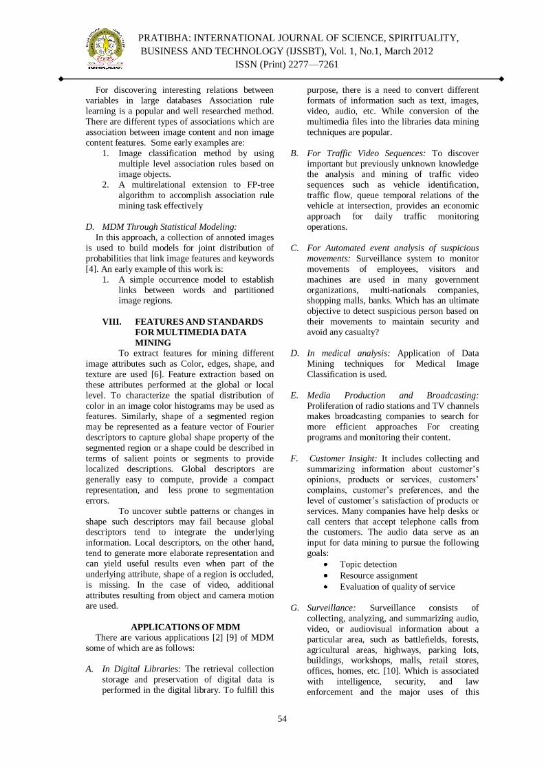
PRATIBHA: INTERNATIONAL JOURNAL OF SCIENCE, SPIRITUALITY,
BUSINESS AND TECHNOLOGY (IJSSBT), Vol. 1, No.1, March 2012
ISSN (Print) 2277—7261
54
For discovering interesting relations between
variables in large databases Association rule
learning is a popular and well researched method.
There are different types of associations which are
association between image content and non image
content features. Some early examples are:
1. Image classification method by using
multiple level association rules based on image objects.
2. A multirelational extension to FP-tree
algorithm to accomplish association rule
mining task effectively
D. MDM Through Statistical Modeling:
In this approach, a collection of annoted images
is used to build models for joint distribution of
probabilities that link image features and keywords
[4]. An early example of this work is:
1. A simple occurrence model to establish
links between words and partitioned image regions.
VIII. FEATURES AND STANDARDS
FOR MULTIMEDIA DATA
MINING
To extract features for mining different
image attributes such as Color, edges, shape, and
texture are used [6]. Feature extraction based on
these attributes performed at the global or local
level. To characterize the spatial distribution of
color in an image color histograms may be used as features. Similarly, shape of a segmented region
may be represented as a feature vector of Fourier
descriptors to capture global shape property of the
segmented region or a shape could be described in
terms of salient points or segments to provide
localized descriptions. Global descriptors are
generally easy to compute, provide a compact
representation, and less prone to segmentation
errors.
To uncover subtle patterns or changes in
shape such descriptors may fail because global descriptors tend to integrate the underlying
information. Local descriptors, on the other hand,
tend to generate more elaborate representation and
can yield useful results even when part of the
underlying attribute, shape of a region is occluded,
is missing. In the case of video, additional
attributes resulting from object and camera motion
are used.
APPLICATIONS OF MDM
There are various applications [2] [9] of MDM
some of which are as follows:
A. In Digital Libraries: The retrieval collection
storage and preservation of digital data is
performed in the digital library. To fulfill this
purpose, there is a need to convert different
formats of information such as text, images,
video, audio, etc. While conversion of the
multimedia files into the libraries data mining
techniques are popular.
B. For Traffic Video Sequences: To discover
important but previously unknown knowledge the analysis and mining of traffic video
sequences such as vehicle identification,
traffic flow, queue temporal relations of the
vehicle at intersection, provides an economic
approach for daily traffic monitoring
operations.
C. For Automated event analysis of suspicious
movements: Surveillance system to monitor
movements of employees, visitors and
machines are used in many government
organizations, multi-nationals companies, shopping malls, banks. Which has an ultimate
objective to detect suspicious person based on
their movements to maintain security and
avoid any casualty?
D. In medical analysis: Application of Data
Mining techniques for Medical Image
Classification is used.
E. Media Production and Broadcasting:
Proliferation of radio stations and TV channels makes broadcasting companies to search for
more efficient approaches For creating
programs and monitoring their content.
F. Customer Insight: It includes collecting and
summarizing information about customer‘s
opinions, products or services, customers‘
complains, customer‘s preferences, and the
level of customer‘s satisfaction of products or
services. Many companies have help desks or
call centers that accept telephone calls from the customers. The audio data serve as an
input for data mining to pursue the following
goals:
Topic detection
Resource assignment
Evaluation of quality of service
G. Surveillance: Surveillance consists of
collecting, analyzing, and summarizing audio,
video, or audiovisual information about a
particular area, such as battlefields, forests,
agricultural areas, highways, parking lots, buildings, workshops, malls, retail stores,
offices, homes, etc. [10]. Which is associated
with intelligence, security, and law
enforcement and the major uses of this

PRATIBHA: INTERNATIONAL JOURNAL OF SCIENCE, SPIRITUALITY,
BUSINESS AND TECHNOLOGY (IJSSBT), Vol. 1, No.1, March 2012
ISSN (Print) 2277—7261
55
technology are military, police, and private
companies that provide security services.
There are several goals of surveillance data
mining:
1. Objector event detection/recognition
2. Summarization 3. Monitoring
H. Intelligent Content Service: The Intelligent
Content Service (ICS) is ―a semantically smart
content-centric set of software services that
enhance the relationship between information
workers and computing systems by making
sense of content, recognizing context, and
understanding the end user‘s requests for
information‖ The MDM techniques can help
to achieve the following goals:
Indexing Web media and using advanced media search
Advanced Web-based services
I. Knowledge Management: Many companies
consider their archives of documents as a
valuable asset. They spend a lot of money to
maintain and provide access to their archives
to employees. Besides text documents, these
archives can contain drawings of designs,
photos and other images, audio and video
recording of meetings and multimedia data for training.
XI. CONCLUSION
This paper proposes a survey of
multimedia data mining. The key idea is to provide
review of MDM, which is an active and growing
area of research. While the majority of the work
has been devoted to the development of data
mining methodologies to deal with the specific
issues of multimedia data, Several applications of
multimedia data mining have been investigated. Many of the recent MDM applications are focused
on traffic monitoring and video surveillance,
possibly due to increased attention to homeland
security. In the coming years, we expect the MDM
applications to grow especially in areas of
entertainment and medicine. Almost all of the
MDM efforts to date have been with the
centralized data mining algorithms; however, this
is expected to change as more and more
multimedia content is searched and accessed
through peers. The MDM is an active and growing
area of research.
FUTURE WORK
Our review provides analysis of MDM, methods
for MDM and compares the result of them. In
future we explore the effect of Multimedia
techniques on multimedia database to mine the multimedia components and improve the
multimedia database environment. Researchers in
multimedia information systems, in the search of
techniques for improving the indexing and
retrieval of multimedia information, are looking
for new methods for discovering indexing
information.
REFERENCES [1] Manjunath BS, Salembier Ph, Sikora T, ―Introduction to
MPEG-7 Multimedia Content Description Interface‖
Wiley, New York, 2002.
[2] Manjunath T.N, Ravindra S Hegadi, Ravikumar G .K, ―A
survey on multimedia data mining and its relevance
today‖, IJCSNS International Journal of Computer
Science and Network Security, VOL.10 No.11, November
2010.
[3] Janusz Swierzowicz Rzeszow, ―Multimedia Data Mining
Trends and Challenges‖ University of Technology, Poland
2009.
[4] S. Kotsiantis, D. Kanellopoulos, P. Pintelas, ―Multimedia
Mining, WSEAS Transactions on Systems‖, Issue 10,
Volume 3, December 2004, pp. 3263-3268.
[5] Chidansh Amitkumar Bhatt · Mohan S. Kankanhalli,
―Multimedia data mining: state of the art and challenges‖,
Multimed Tools and Applications (2011) 51:35–76.
[6] Sanjeev kumar R. Jadhav, and Praveenkumar
Kumbargoudar, ―Multimedia Data Mining in Digital
Libraries: Standards and Features‖, ACVIT- 07, Dr.
Babasaheb Ambedkar MarathWada University,
Aurangabad, MS-India.
[7] Mittal, Ankush, ―An overview of multimedia content-
based retrieval strategies‖, Publication: Informatica,
October 1 2006.
[8] You, J. Liu, L. Li, and K.H. Cheung, ―on data mining and
warehousing for multimedia information retrieval‖, From
Proceeding (365) Artificial and Computational
Intelligence – 2002.
[9] Valery A. Petrushin and Latifur Khan, ―Multimedia Data
Mining and Knowledge Discovery‖, Springer, 2007 pp. 3-
17.
[10] Valery A. Petrushin and Latifur Khan ―Multimedia Data
Mining and Knowledge Discovery‖, Springer 2007.

PRATIBHA: INTERNATIONAL JOURNAL OF SCIENCE, SPIRITUALITY,
BUSINESS AND TECHNOLOGY (IJSSBT), Vol. 1, No.1, March 2012
ISSN (Print) 2277—7261
56
A dimensionless approach for rate of re-aeration in river
Ganges
R. P. Singh
Professor, Department of Civil Engineering, MNNIT, Allahabad-211004, U.P., INDIA
Abstract: This communication presents a
methodology to evaluate the re-aeration rate
term in basic dissolved oxygen (DO) deficit
models by incorporating some important
parameters like turbulence, width, depth and
length of streams, which are necessary for fast
biochemical oxygen demand (BOD) assimilation
in streams. A mathematical model based on
dimensional approach for rate of re-aeration as
well as DO deficits, using basic philosophy of
Bhargava (1986) model, is presented. The
simulation of data on river Ganges in India,
indicate that the predictions of DO deficits are
in close agreement with the experimentally
observed values. The methodology presented in
accounts for all the important factors affecting
re-aeration in streams and thus, may offer an
alternative to traditionally used approaches for
representing re-aeration rate.
Keywords: Dissolved oxygen; BOD assimilation;
DO deficit; River Ganges; Pollution reduction
I. INTRODUCTION
Dissolved Oxygen in river is one of the most
important indices for assessing the river‘s health and is a prime consideration in streams
assimilation capacity. Many factors affect the
dissolved oxygen concentration in river water and
can be broadly classified into three main
categories, namely 1) Geophysical factors, 2) Bio-
chemical factors and 3) Physical factors. Geo-
physical factors include river flow, temperature of
water body, climatic conditions, surface expanse,
turbulence, type and amount of organic matter and
depth of the water body. Bio-chemical & physical
forces include dilution and dispersion, mass-transfer phenomena, photosynthetic activities, bio-
oxidation and reduction and all the natural and
man-made sources and sinks of dissolved oxygen.
Polluted streams are usually characterized by a
decline in DO level, followed by a recovery in the
dissolved oxygen level along the length of stream.
The initial decrease in DO level occurs due to
greater rate of oxygen removal by biological
oxidation than that recouped by re-aeration. The
rate of biological oxidation is directly proportional
to the quantity of organic material present and
consequently decreases with time. The minimum DO deficit will occur at a point where the rate of
supply of oxygen by re-aeration equals the rate of
its consumption by biological oxidation.
Thereafter, the re-aeration process dominates and
the dissolved oxygen deficit is gradually reduced.
A number of mathematical models for
DO deficit [(Streeter and Phelps 1925), (Fair 1939), (Bhatia and Mc. Bean 1986) and (Bhargava
1986)] have been developed to assess the DO
behaviour in streams. Little or no attention has
been paid towards the modification of re-aeration
rate term, which depends upon the number of
variables. Also, the river Ganges in India is famous
for fast BOD assimilation capacity (Bhargava
1983). Therefore, there is a need to incorporate the
important variables affecting the re-aeration
phenomenon so that the condition of river can be
described in a better way.
In the present paper, the original DO deficit model developed by Bhargava (1986),
which was originally derived from Streeter and
Phelps (1925) DO model, has been modified by
replacing the re-aeration rate term by a new term.
In Bhargava (1986) model, the BOD assimilation
term was divided into two fractions, i.e. settleable
and non-settleable fractions. But, no attention was
paid by earlier investigators to modify/replace the
rate of re-aeration term (rR), which is of great
significance in fast self purification of streams.
From the literature, it is evident that the term ‗rR‘ is largely influenced by the river‘s characteristics
such as width, depth, turbulence and velocity, and
length along the course of river, time of travel as
well as initial and saturation DO levels of stream.
Keeping these factors in view, a dimensional
analysis is performed to derive a dimensionless
expression for the re-aeration rate term and the
same was used in Bhargava (1986) model, for
further prediction of DO deficits in streams. The
reported data from the study of Bhargava (1986)
on river Ganges in India has been used in
predictions and also compared with the observed values. It is believed that the methodology
presented in this paper will prove better to
represent comprehensively the re-aeration rate
rather than representing ‗rR‘ by a single parameter
‗kR‘, the re-aeration coefficient, as used by many
previous researchers.
II. THEORETICAL BACKGROUND
When an organic effluent is discharged into a
stream, it exerts a biochemical oxygen demand
(BOD) with the processes of BOD assimilation and

PRATIBHA: INTERNATIONAL JOURNAL OF SCIENCE, SPIRITUALITY,
BUSINESS AND TECHNOLOGY (IJSSBT), Vol. 1, No.1, March 2012
ISSN (Print) 2277—7261
57
atmospheric re-aeration proceeding
simultaneously. In many situations the oxygen
demand will initially exceed the re-aeration rate, so
the DO concentration will fall rapidly. If the rate of
consumption lowers the oxygen concentration, the
oxygen mass transfer rate will increase. At some
point downstream of point of discharge the rate of
re-aeration and the rate of consumption becomes equal and the oxygen concentration stops
declining. This is the critical point of the curve,
where the oxygen deficit is maximum and the
dissolved oxygen concentration is lowest, called as
critical DO deficit (Dc) and the corresponding time
is called as critical time (tc). Thereafter, re-aeration
phenomenon predominates and the dissolved
oxygen concentration rises to approach saturation
DO level. As the rate of mass transfer is
proportional to the oxygen concentration, the rate
of re-aeration slows down near the asymptotic
point. As per Streeter and Phelps (1925), the
rate dissolved oxygen (DO) deficit can be
expressed as a function of BOD assimilation and
re-aeration rates, which is the algebraic sum of rate
of de-oxygenation (rD) and the rate of re-aeration
(rR) and is given by the expression:
RDrr
dt
dD (1)
where, both rD and
rR follow first order kinetics with respect to BOD
of waste and DO deficit ‗D‘ respectively and are expressed as:
kSdt
dDr
D (2)
DkrRR
(3)
where, dt
dD = the rate of change of DO deficit, k =
de-oxygenation rate constant (d-1), kR = re-aeration
rate constant, (d-1), and S = BOD remained after
time t, mg/L. Therefore, Eq. (1) becomes
DkkSdt
dDR
(4)
As per Bhargava (1986), the DO Deficit in the
river due to discharge of wastewater is affected by
the settling of settleable organic particles. If the
settleable portion of the initial BOD concentration is S0-x, which would be completely removed within
a transition time ‗T =v
d (days)‟ where d= depth
of river, m, v = settling velocity of bio-flocculated particles (m/s) and S0-y is the non-settleable organic
fraction (mg/l), then, the total initial BOD, ‗S0‘
will be given by
S0 = S0-x+ S0-y (5)
The settled fraction of settleable portion of initial
BOD concentration (So-x), at time„t‟ is given by
td
vS
xo. Therefore, the non-settleable fraction
(S1) of settleable portion of initial BOD
concentration (So-x), at time „t‟, is given by
td
vSSS
xxo 01 (6)
The non-settleable portion (S2) of total initial BOD
concentration (S0), at time t is given by, kt
yeSS
02 (7)
Hence, BOD remaining at time ‗t‘ will be
kt
yxeSt
d
vSSSS
00211 (8)
Bhargava (1986) pointed out that non-settleable
organic matter exerts the oxygen demand at a
maximum rate equal to the rate of BOD exertion
(k). But, the settleable organic matter would exert a
part of its oxygen demand before it reaches the
bottom of the streams and this rate constant is denoted as (m). It is to be noted that this rate
constant of oxygen demand (m) may be even more
than kR, such that the maximum value of (m) would
equal to kR. Thus, k for the first term of the right
hand side of the Eq. (8) should be (m), and for the
second term of right hand side of the equation (8)
would be (k). From Eqs. (4) and (8), we have,
DkekStd
vmS
dt
dDR
kt
yx 001 (9)
The exact solution of Eq. (9), for t< T (Transition
time), t = T =d/v and t >T can be given
respectively by Eqs. (10), (11) and (12).
tktkkt
y
R
RR
tk
x
R
RR
R
eDeeSkk
k
kt
d
v
d
v
keS
k
mD
00
0
1111
(10)
v
dRk
v
dRk
v
dRk
y
RR
v
dRk
x
R
TeDeeS
kk
k
d
v
keS
k
mD
0001
111
(11)
v
dtRk
T
tRkv
dkRk
kt
y
R
eDeeSkk
kD
0
(12)
where DT is the DO deficit at T = d/v, d = depth of
river and v = settling velocity of bio-flocculated
particles. Other model equations developed are
available else where (Bhargava 1986).
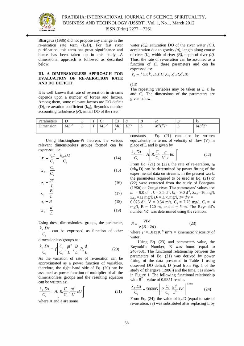
PRATIBHA: INTERNATIONAL JOURNAL OF SCIENCE, SPIRITUALITY,
BUSINESS AND TECHNOLOGY (IJSSBT), Vol. 1, No.1, March 2012
ISSN (Print) 2277—7261
58
Bhargava (1986) did not propose any change in the
re-aeration rate term (kRD). For fast river
purification, this term has great significance and
hence has been taken up in this study. A
dimensional approach is followed as described
below.
III. A DIMENSIONLESS APPROACH FOR
EVALUATION OF RE-AERATION RATE
AND DO DEFICIT
It is well known that rate of re-aeration in streams
depends upon a number of forces and factors.
Among them, some relevant factors are DO deficit
(D), re-aeration coefficient (kR), Reynolds number
accounting turbulence (R), initial DO of the river
water (Ci), saturation DO of the river water (Cs),
acceleration due to gravity (g), length along course
of river (L), width of river (B), depth of river (d).
Thus, the rate of re-aeration can be assumed as a
function of all these parameters and can be
expressed as:
),,,,,,,,,( BdRgCCtLkDfrsiRR
(13)
The repeating variables may be taken as L, t, kR
and Cs. The dimensions of the parameters are
given below.
Parameters D L T Ci Cs g B R D kR
Dimension ML-3
L T ML-3
ML-
3
LT-2
L M0L
0T
0 L ML
3T
-1
Using Buckingham-Pi theorem, the various relevant dimensionless groups formed can be
expressed as:
s
R
s
R
C
tDk
C
tr ...1
(14)
s
i
C
C2
(15)
L
gt 2
3 (16)
L
B4
(17)
R5
(18)
L
d6
(19)
Using these dimensionless groups, the parameter,
s
R
C
tDk ..can be expressed as function of other
dimensionless groups as:
L
dR
L
B
L
gt
C
Cf
C
tDk
s
i
s
R ,,,,.. 2
(20)
As the variation of rate of re-aeration can be
approximated as a power function of variables,
therefore, the right hand side of Eq. (20) can be
assumed as power function of multiplier of all the dimensionless groups and the resulting equation
can be written as: a
s
i
s
R BdL
gt
C
CRA
C
tDk3
2
.....
(21)
where A and a are some
constants. Eq. (21) can also be written
equivalently in terms of velocity of flow (V) in place of L and is given by
a
s
i
s
R BdtV
g
C
CRA
C
tDk
....
..3
(22)
From Eq. (21) or (22), the rate of re-aeration, rR
(=kR.D) can be determined by power fitting of the experimental data on streams. In the present work,
the parameters required to be used in Eq. (21) or
(22) were extracted from the study of Bhargava
(1986) on Ganga river. The parameters‘ values are:
m = 9.0 d-1 , k = 3.5 d-1, kR = 9.0 d-1, S0-x =16 mg/l,
S0-y =12 mg/l, D0 = 3.75mg/l, T= d/v =
0.025 d-1, V = 0.54 m/s, Cs = 7.75 mg/l, Ci = 4
mg/l, B = 120 m, and d = 5 m. The Reynold‘s
number ‗R‘ was determined using the relation:
)2.( dB
VBdR (23)
where =1.01x10⁻⁶ m2/s = kinematic viscosity of
water.
Using Eq. (23) and parameters value, the
Reynold‘s Number, R was found equal to
2467631. The functional relationship between the
parameters of Eq. (21) was derived by power fitting of the data presented in Table 1 using
observed DO deficit, D (read from Fig. 1 of the
study of Bhargava (1986)) and the time, t as shown
in Figure 1. The following functional relationship
with R2 – value of 0.9851 results. 8882.0
3
2
...506005..
BdL
gt
C
CR
C
tDk
s
i
s
R (24)
From Eq. (24), the value of kR.D (equal to rate of
re-aeration, rR) was substituted after replacing L by

PRATIBHA: INTERNATIONAL JOURNAL OF SCIENCE, SPIRITUALITY,
BUSINESS AND TECHNOLOGY (IJSSBT), Vol. 1, No.1, March 2012
ISSN (Print) 2277—7261
59
V.t in Eq. (9) and the modified equation is expressed as:
1118.0
8882.0
3
8882.1
00.....5060051 tBd
V
gCRCekSt
d
vmS
dt
dDis
kt
yx (25)
The exact solution of Eq. (25), for t< T (Transition time), t = T =d/v and t >T can be given respectively by Eqs. (26), (27) and (28) and expressed as:
yis
kt
yxxSDtBd
V
gCRCeS
d
tvmStmSD
00
8882.0
8882.0
3
8882.1
0
2
00.....569697
2
. (26)
yis
v
dk
yxxSD
v
dBd
V
gCRCeS
v
dmS
v
dmSD
00
8882.08882.0
3
8882.1
000.....569697
2 . (27)
8882.08882.0
3
8882.1
0
8882.0
8882.0
3
8882.1
0
.....569697
.....569697
v
dBd
V
gCRC
eSDtBdV
gCRCeSD
is
v
dk
yTis
kt
y
(28)
The critical time, tc for tc ≤ T and tc > T can be respectively modified to following equations:
1118.0
8882.0
3
8882.1
00.....5060051
cis
ckt
ycxtBd
V
gCRCekSt
d
vmS (29)
1118.0
8882.0
3
8882.1
0.....506005
cis
ckt
ytBd
V
gCRCekS (30)
The critical DO deficit, Dc for tc ≤ T and tc > T can be determined by first determining tc from Eqns. (29)
and (30) respectively by trial and error and using t = tc and D = Dc in Eqs. (26) and (28).
IV. RESULTS AND DISCUSSION
The input parameters and the data for prediction of
DO deficits were taken from the study of Bhargava
(1986) and are presented in the text above and
Table 1. The predicted DO deficits were computed
using Eqs. (10), (11) and (12) respectively for t< T
(Transition time), t = T =v
dd/v and t >T for
Bhargava (1986) model and Eqs. (26), (27) and
(28) for modified model. Predicted DO deficits for
both the models are computed only against the
known experimental values and are given in Table
1. The predicted DO deficits along with the
observed DO deficits are also plotted in Figure 2.
It can be seen that the predictions are comparable
and somewhat better by use of the modified
equation than those predicted using Bhargava (1986) model. Thus, the modification proposed in
the re-aeration rate term has practical utility in
modelling DO in rivers like Ganges having fast
purification capacity.
The present work demonstrates that a
dimensionless approach can be used to replace the
rate of re-aeration term in DO deficit modelling. Traditionally, re-aeration coefficient has been the
subject of dimensionless analysis. Errors may
creep in the representation of re-aeration
coefficient and this coupled with D term to
represent re-aeration rate may adversely affect the
DO deficit computations. Thus, instead of
following this line of attack, it was preferred to
look into the possibility of representing re-aeration
rate term itself. Results from Figs. 1 and 2 clearly
indicate that this approach can also work. Due to
lack of data on other rivers, the approach has not been tested for other conditions and it is expected
that the concept presented in this paper will
simulate further interest and applications in DO
modelling in streams.

PRATIBHA: INTERNATIONAL JOURNAL OF SCIENCE, SPIRITUALITY,
BUSINESS AND TECHNOLOGY (IJSSBT), Vol. 1, No.1, March 2012
ISSN (Print) 2277—7261
60
V. CONCLUSIONS
The present study is basically aimed to develop a
functional relationship for re-aeration rate using
dimensionless approach, which is tested to be
applicable to the rivers having fast BOD
assimilation capability like river Ganges in India.
The concept developed gives satisfactory results in prediction of DO deficits in river Ganges.
However, the validity of the approach needs
further investigation on other rivers.
ACKNOWLEDGEMENTS
The author is grateful to the Ministry of Human
Resources Development (MHRD), Government of
India, New Delhi for providing help and assistance
in completion of this work. Authors are also
thankful to Director, MNNIT, Allahabad, U.P.,
India, for providing the facilities needed for the
work.
Notation
The following symbols are used in this paper:
A , = constant;
a = constant;
B = width of river;
BOD = biochemical oxygen demand;
Ci = initial dissolved oxygen;
Cs = saturation dissolved oxygen;
DO = dissolved oxygen;
D = dissolved oxygen deficit; Dc = critical dissolved oxygen deficit;
DT = dissolved oxygen deficit at transition
time, T;
D0 = initial dissolved oxygen deficit;
d = depth of river;
k = biochemical oxygen demand rate
constant for settleable organic matter;
kR = re-aeration rate constant;
L = length of river course;
m = biochemical oxygen demand rate
constant for non-settleable organic matter;
R = Reynold‘s number;
rD = rate of de-oxygenation;
rR = rate of re-aeration;
S = biochemical oxygen demand remained
after time t;
S1 = non-settleable fraction of settleable
portion of initial BOD concentration at time t;
S1 = settleable fraction of settleable portion
of initial BOD concentration at time t;
S0 = total biochemical oxygen demand at
time t = 0;
S0-x =settleable biochemical oxygen demand
at time t = 0;
S0-y =non-settleable biochemical oxygen demand at time t = 0;
T = transition time;
t = time
tc = critical time;
v = settling velocity of bioflocculated
particles;
V = velocity of flow;
ν = kinematic viscosity.
Table 1: Observed and Predicted DO deficits
Time,
days
Distance from
point of
dischargea , m
Observed DO
deficitb, D , mg/l
Predicted DO deficitc , D,
mg/l
Predicted DO deficitd ,
D, mg/l
0.000 0.00 3.75 3.750 3.750000
0.010 466.56 6.83 4.920 4.726915 0.020 933.12 5.08 5.418 5.201299
0.025 1166.40 4.80 5.445 5.228913
0.050 2332.80 4.60 5.170 5.021416
0.065 3032.64 4.15 5.000 4.892359
0.075 3499.20 4.55 4.880 4.801045
0.100 4665.60 4.35 4.590 4.549683
0.110 5132.16 4.30 4.520 4.439106
0.125 5832.00 4.95 4.210 4.262094
0.150 6998.40 4.80 4.014 3.937328 acomputed by multiplying time with velocity of flow.
b extracted from study of Bhargava (1986) c using Bhargava (1986) model
d using present model

PRATIBHA: INTERNATIONAL JOURNAL OF SCIENCE, SPIRITUALITY,
BUSINESS AND TECHNOLOGY (IJSSBT), Vol. 1, No.1, March 2012
ISSN (Print) 2277—7261
61
Fig. 1.Variation of dimensionless parameters
Fig. 2. Variation of dissolved oxygen deficit with time. kR.D.t / Cs with R.Ci.g.t2.B.d / (Cs.L3).
REFERENCES
[1] Bhargava, D. S. (1986). ―DO Sag Model for
Extremely Fast River Purification.‖ J. Environ.
Engrg, ASCE, 112(3), 573-585.
[2] Bhargava, D. S. (1983). ―Most Rapid BOD
Assimilation in Ganga and Yamuna Rivers.‖ J.
Environ. Engrg., ASCE, 109(1), 174-188.
[3] Bhatia, K. K. S. and McBean, E. A. (1986). ―Steady
State Modelling of Dissolved Oxygen in River
Speed (Canada).‖ J. IAH, 9(4), 11-24.
[4] Fair, G. M. (1939). ―The Dissolved Oxygen Sag –
An Analysis.‖ J. Sewage Works, 11(3), 445.
[5] Streeter, M. W. and Phelps, E. E. (1925). ―A Study
of the Pollution and Natural Purification of the Ohio
Rivers.‖ U.S. Public Health Bulletin No. 146.
0
1
2
3
4
5
6
7
8
0 0.02 0.04 0.06 0.08 0.1 0.12 0.14 0.16
Time, days
Disso
lved
O
xyg
en
D
eficit, D
, m
g/l
DO Deficit, mg/l (Experimental values)
DO Deficit, mg/l (Bhargava (1986) model)
DO Deficit, mg/l (Modified model)
y = 506005x-0.8882
R2 = 0.9851
0
0.1
0.2
0.3
0.4
0.5
0.6
0.7
0.8
0.9
0.00E+00 1.00E+07 2.00E+07 3.00E+07 4.00E+07 5.00E+07 6.00E+07
Dimensionless parameter, R.Ci.g.t2.B.d / (Cs.L
3)
Dim
en
sio
nle
ss p
aram
eter,
kR.D
.t/C
s

PRATIBHA: INTERNATIONAL JOURNAL OF SCIENCE, SPIRITUALITY,
BUSINESS AND TECHNOLOGY (IJSSBT), Vol. 1, No.1, March 2012
ISSN (Print) 2277—7261
62
Short Term Load Prediction Considering the Effect of
Temperature as a Weather Parameter Using a Combinatorial
Model of Wavelet and Recurrent Neural Networks
Anand B. Deshmukh1, Dineshkumar U.Adokar
2
S.S.P.M‘s College of Engineering & Technology, Amravati (MS), India
S.S.B.T‘s College of Engineering & Technology Bambhori, Jalgaon (MS), India
Email:[email protected], [email protected]
Abstract:-In this paper, a novel combinatorial
model of Wavelet and RNNs is developed for
one-day-ahead electrical power load prediction.
For this purpose three RNN predictors are
modeled on different frequency components
such as approximation component and several
other detailed components of wavelet
transformed load data for one-day-ahead
prediction. The best predictor is chosen on each
frequency component on the grounds of
validation performance with respect to the
performance measures on training and testing
dataset. The final prediction is achieved by
adding the forecast of best predictor on each
component in the different seasons. The results
offered by the proposed technique are
outperformed the traditional statistical
technique.
Keywords- short-term load prediction, recurrent
neural networks, Daubechies, statistical methods,
weather information
. I. INTRODUCTION
Short-term load prediction relies on
historical load, weather condition, and industrial
demand, daily and seasonal patterns. Short-term
prediction is indeed a complex problem.
Conventional methods have been used to predict the hourly load such as autoregressive moving
average, linear regression, stochastic time series,
and general exponential smoothing [1]. Such
methods cannot properly represent the complex
nonlinear relationships between the load and a
series of stochastic factors such as daily and
weekly time rhythms special events and correlation
properties of weather conditions which can cause
high unpredictable variations in power demand.
ANNs are able to give better performance in dealing with the nonlinear relationships among
their input variables [2]-[4]. ANNs could extract
implicit nonlinear relationships among the input
variables by learning from training data.
Combining the wavelet transform with other
techniques such as autoregressive modeling, and
neural networks for predicting electrical load
demand has been studied [5]-[8]. Wavelet analysis
provides time and frequency representation
simultaneously. The wavelet transform is applied
to decompose the original time domain signal into
several other scales with different levels of
resolution in what is called as multiresolution
decomposition [9],[10].
By analyzing the electric load we find that
the load curve shows certain periodicities of year, month and day and the periodicities nested in each
other. Therefore, the load series can be considered
as a linear combination of sub-series characterized
by different frequencies. Each sub-series
corresponds to a range of frequencies and show
much more regularities so they are predicted more
precisely than the original load series.
In this research work Db4 has been
confirmed as a best mother wavelet. To obtain
better results and ensure that the adopted model
results in convergence, this paper investigate factors that influence the overall performance of
the recurrent neural networks (RNNs) such as the
determination of the right network topology, good
selection of data patterns and the selection of
appropriate and efficient training algorithm and a
number of possible combinations of inputs load
and various weather variables. Next, a
performance analysis is carried out on the basis of
performance measures such as mean square error
(MSE), correlation coefficient (r) and daily mean
absolute percentage error (DMAPE) for different
seasonal load series of the year 2009.
II. METHODOLOGY USED
Available electric load time series and
weather data is retrieved from the authentic data
repositories. The electric load time series
pertaining to these data sets reflect the
demography, culture, environment that are specific
and exclusive for a Vidarbha region of
Maharashtra state. The data is conditioned using
wavelet transform technique in order to extract
prominent features and important statistical parameters of the data sets.

PRATIBHA: INTERNATIONAL JOURNAL OF SCIENCE, SPIRITUALITY,
BUSINESS AND TECHNOLOGY (IJSSBT), Vol. 1, No.1, March 2012
ISSN (Print) 2277—7261
63
Optimal Recurrent Neural Network model is
designed with a view to minimize prediction error,
mean square error (MSE), normalized MSE and
mean absolute percentage error (MAPE).The
neural network model is trained on the training
dataset at least five times with different random
initialization of connection weights which is
usually chosen as very small arbitrary real numbers .The trained network is assessed on different
datasets, such as training and testing data sets.
The proposed Recurrent Neural Network
architectures that are used for predicting given load
time series include-
1. Elman RNN
2. Jordon RNN
3. Fully Recurrent Neural Network
based on gamma memory filter
For computer simulation and design of
aforementioned RNNs, Matlab 7.0 and
Neurosolutions 5.06 are used. The parameters
which are set include number of hidden layers, number of neurons in each hidden layer, activation
function of neurons in output layer. Appropriate
learning algorithms such as standard back
propagation with momentum term, conjugate
gradient algorithm, quick propagation algorithm
and delta bar delta algorithm. Further an
exhaustive experimentation has been undertaken in
order to set the optimal values of momentum term
and step size in hidden as well as in output layer.
In addition, the value of gamma parameter and
number of taps for FRNN based on gamma
memory filter is optimally configured.
III. WAVELET-TRANSFORM BASED
LOAD TIME SERIES
The main idea of the wavelet multi-
resolution analysis (MRA) is that any function f (t)
can be approximated step by step, and the
approximation of each step is just to smooth f (t) by a low-pass function Φ (t) which will also
expand or contract according to step. Therefore, f
(t) was approximated in different precision in
different steps. In this paper, the Mallat algorithm
is adopted to decompose the load signal.
Figure 1 show one week load curve in rainy
season. It is seen that, reconstructed sub-series
show much more regularities. The approximation
A2 (t) varies with the period of a day and the value
is relatively big, which is the basic load of the
system. D2(t) appears to be small value and strong regularities. for the sub-series A2(t), D2(t) and
D1(t), three D1(t) is the random component in the
the load, whose value is fairly trivial in the entire
load. In this paper, aforementioned RNNs are
optimally designed and developed simultaneously
on each frequency component to predict them.
After getting the prediction result of each sub-
series by different optimally designed RNNs, the
best RNN is chosen on each component on the
basis of their validation performance such as MSE, r and MAPE on the prediction test data set.
Finally, prediction of best RNN of each sub-series
is added in order to achieve final prediction in all
seasons.
Figure 1 : Wavelet-transformed load time series of one
week load data (July 1 to July 7, 2009)
Selection of optimal parameters:
In order to achieve optimally configured
RNN, the various optimal parameters of the
proposed best RNN predictors are decided for
different frequency bands such as approximation
component and several other detail components in various seasons, as depicted in Table 1.
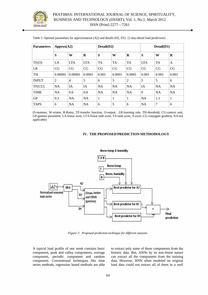
PRATIBHA: INTERNATIONAL JOURNAL OF SCIENCE, SPIRITUALITY,
BUSINESS AND TECHNOLOGY (IJSSBT), Vol. 1, No.1, March 2012
ISSN (Print) 2277—7261
64
Table 1: Optimal parameters for approximation (A2) and details (D2, D1) {1-day-ahead load prediction}
Parameters Approx(A2) Detail(D2) Detail(D1)
S W R S W R S W R
TF(O) LA LTA LTA TA TA TA LTA TA A
LR CG CG CG CG CG CG CG CG CG
TH 0.00001 0.00001 0.0001 0.001 0.0001 0.0001 0.001 0.001 0.001
INPUT 2 4 5 6 3 2 5 5 6
TF(CU) NA IA IA NA NA NA IA NA NA
TIME NA 0.6 0.8 NA NA NA 0 NA NA
GP 0.3 NA NA 1 1 1 NA 1.1 1
TAPS 6 NA NA 6 5 6 NA 7 6
(S-summer, W-winter, R-Rainy, TF-transfer function, O-output, LR-learning rule, TH-threshold, CU-context unit, GP-gamma parameter, LA-linear axon, LTA-linear tanh axon, TA-tanh axon, A-axon ,CG-conjugate gradient, NA-not applicable)
IV. THE PROPOSED PREDICTION METHODOLOGY
Figure 2: Proposed prediction technique for different seasons.
A typical load profile of one week contains basic
component, peak and valley components, average
component, periodic component and random
component. Conventional techniques like time
series methods, regression based methods are able
to extract only some of these components from the
historic data. But, ANNs by its non-linear nature
can extract all the components from the training
data. However, RNN when modeled on original
load data could not extract all of them in a well

PRATIBHA: INTERNATIONAL JOURNAL OF SCIENCE, SPIRITUALITY,
BUSINESS AND TECHNOLOGY (IJSSBT), Vol. 1, No.1, March 2012
ISSN (Print) 2277—7261
65
defined manner. A certain regularity of the data is
an important precondition for the successful
application of neural networks (NNs).
Hence, a novel technique of
combinatorial model of wavelet and RNNs is
proposed for the prediction of one-day-ahead load
prediction for different seasons.
Figure 2 shows block diagram of
proposed prediction methodology. Here, idea is to
decompose the different seasonal load series using
Daubechies 4 with decomposition of levels two
and to model it via individual fitting of each level
of resolution (frequency bands).The suggested
RNNs are modeled on each frequency component
and the final prediction is obtained by adding the
forecast of best predictor on each frequency band.
The best RNN for A2 in the different seasonal load
series is chosen on the basis of their validation performance with respect to the performance
measures like MSE, r and MAPE. It is observed
that, the approximation A2 and all two levels of
detail components are taken into account to
―reconstruct‖ the load series.
V. SIMULATION RESULTS AND THE
EFFECT OF TEMPERATURE AS A
WEATHER PARAMETER
The proposed architecture of best predictor is trained on approximation component
for different seasons with and without considering
the weather information such as temperature as one
of the input variables. The effect of weather
parameter on STLP for a typical day in winter
season (Friday, October 16, 2009) is investigated
without considering temperature as a weather
information and considering temperature are
shown in figure 3 & figure 4 respectively. The
daily mean absolute percentage error (DMAPE)
and maximum absolute percentage error (maximum APE) of typical weekdays in a winter
season (16 to 22 October 2009) are shown in Table
2.The weather information such as temperature is
considered as an input variable only for
approximate component .However, temperature as
a weather information have not been considered
for detail component as it is least significant on
detail components.
The results depicted in table 2 show that,
on 17/10/09, 19/10/09, 20/10/09 and 22/10/09 the
prediction accuracy is improved when lone temperature as one of the input weather variable is
considered. Hence from the results it is confirmed
that temperature as a weather variable plays
significant role in improving the prediction
accuracy and the suggested combinatorial model of
wavelet and RNNs performs better when
temperature as a weather parameter is introduced
as an additional input variable. It is worthwhile to
notice that the prediction accuracy is degraded
significantly on all days when no weather
information is given to the adopted models.
Table 2: Effect of temperature as a weather parameter on
the performance of best chosen load predictor
Date Performa-
nce metrics
Effect of temperature on
prediction error
Without
considering
temperature
With
temper-
ature
16/10/09 Max(APE) 9.71 10.92
MAPE (%) 3.67 3.64
17/10/09 Max(APE) 7.86 5.96
MAPE (%) 2.98 2.60
18/10/09 Max(APE) 7.24 7.61
MAPE (%) 2.40 2.19
19/10/09 Max(APE) 6.77 5.51
MAPE (%) 2.55 2.38
20/10/09 Max(APE) 15.68 13.39
MAPE (%) 4.13 3.98
21/10/09 Max(APE) 12.26 13.11
MAPE (%) 4.16 4.24
22/10/09 Max(APE) 16.01 15.75
MAPE (%) 4.271 4.04
Fig.3:Comparison of the actual load and the predicted
load for Friday (16-Oct. 2009) without considering weather variables.

PRATIBHA: INTERNATIONAL JOURNAL OF SCIENCE, SPIRITUALITY,
BUSINESS AND TECHNOLOGY (IJSSBT), Vol. 1, No.1, March 2012
ISSN (Print) 2277—7261
66
Fig.4: Comparison of the actual load and the predicted
load for Friday (16-Oct. 2009) considering with temperature.
From the figures (3 & 4), it is observed that,
prediction accuracy is improved when temperature as an additional input variable is considered
.However; prediction performance is degraded
reasonably when no weather information is given
to the RNNs.
VI. CONCLUSION
The major contribution of this research is
the increase in the one-day-ahead prediction
accuracy in all seasons by employing the proposed
combinatorial model of wavelet and RNNs. The
exhaustive experimentation is made to explore the
best RNN on different frequency component
according to the characteristics of each component
and finally, prediction is achieved by adding the
predictions of best RNNs on different frequency
components. The proposed technique offers
reliable and encouraging results.
The adopted models in the proposed
technique are evaluated with different weather
information in order to judge the effect of a
particular weather parameter on accurate load
prediction. It has been observed from Table 2 that
the DMAPE and maximum APE are less when
lone predicted weather parameter such as
temperature was introduced as one of the input
variable.
Finally we could conclude that the
proposed novel combination of wavelet and RNN
for STLP considering the effect of weather
parameters with systematic design procedure of
optimal neural network for addressing, one-day-
ahead load prediction provides more accuracy than
the existing methodologies .
REFERENCES:
[1] I. Moghram and S. Rahman, ―Analysis and evaluation of
shortterm load forecasting techniques , ― IEEE Trans.
Power Syst. , vol. 4, no. 4.1484-1491. Nov. 1989.
[2] E. Sanchez-Sinencio and C. Lau. Artificial neural
networks. Paradigms, Applications and Hardware
Implementations. Piscataway,NJ:IEEE Press, 1992.
[3] B.S. Kermanshahi, C. H. poskar, G. Swift, P. McLaren
,W. Pedrycz, W. Buhr and A. Silik, ―Artificial neural
networks for forecasting daily loads of a Canadian
electricity utility‖in Proc IEEE 2nd
Int. Forum
Applications of Neural Networks to Power Systems ,
1993, pp. 302-307.
[4] T. W. S. Chow and C. T. Leung, ― Neural Networks
based short term load forecasting using weather
compensation‖ IEEE Trans Power Syst., Vol. 11, No. 4,
pp. 1736-1742, Nov. 1996.
[5] A. K. Saha, S. Chowdhury, S. P. Chowdhury, Y. H.
Song, and G.A. Taylor,‖ Application of Wavelets in
Power System Load Forecasting‖, in Proc. IEEE Power
Eng. Soc. General Meeting, 2006.
[6] Y. Bi. J. Zhao and D. Zhang, ―Power load forecasting
algorithm based on wavelet packet analysis‖ in Proc.
IEEE Int. Conf. Power system technology, 2004, pp.
987-990.
[7] D. Tao, W. Xiuli, and W. Xifan, ―a combined model of
wavelet and neural network for short term load
forecasting,‖ in Proc. IEEE Int. Conf. Power system
technology, 2002, pp. 2331-2335.
[8] A. J. R. Reis and A.P.A. da Silva, ―Fearure extraction
via multi resolution analysis for short term load
forecasting, ‖ IEEE Trans Power Syst., Vol. 20, No. 1,
pp. 189-198, Feb. 2005.
[9] C.K.Chui,An introduction to wavelets .New York:
Academic,1992,pp 6-18.
[10] S.Mallat,‖ A theory for multiresolution signal
decomposition –the wavelet representation,‖IEEE
trans.Pattern Anal.Mach.Intell,vol.11,no.7,pp.674-
693,Jul.1989.

PRATIBHA: INTERNATIONAL JOURNAL OF SCIENCE, SPIRITUALITY,
BUSINESS AND TECHNOLOGY (IJSSBT), Vol. 1, No.1, March 2012
ISSN (Print) 2277—7261
67
Human Power: An Earliest Source of Energy and It’s Efficient
Use
K. S. Zakiuddin1
, H. V. Sondawale2, J. P. Modak
3
1Dean (Academics), Priyadarshini College of Engineering, Nagpur-440001, India 2MED, Smt. Rajshree Mulak College of Engineering for Women, Nagpur-440009, India
3Dean (Research and Development), Priyadarshini College of Engineering, Nagpur-440001, India
Emails: [email protected], [email protected], [email protected]
Abstract: This paper discusses the importance
of human power from the earliest times to the
present and its future scope. As the use of
natural fuel is incresed due to industrial
development, it’s storage going to end. We need
to come with alternate source of energy, i.e non
conventional energy. Human power credits its
importance in search of an alternative source of
energy as it fulfills the requirement of
renewable source of energy. More effective use
of human power can do by using mechanisms.
The technology used to transmit human power
to the working unit is termed as human
powered machine. The appropriate and most
effective technology to use human power
efficiently is bicycle technology. In bicycle
technology the operator uses the pedal to
operate the machine and transmits power
through crank, chain and freewheels to the
working unit. This machine widely can be used
to generate electric power, to operate various
home appliances, to drive water pump,
harvesting activities in agriculture and for
physical fitness.
Keywords: Human Power machine, Bicycle
Technology, Dinapod, Flywheel.
I. INTRODUCTION
Manual work involves the natural movements of
a human with regards to direction, speed and
frequency. A man exerts his physical strength
directly by walking, pushing, pulling, pressing,
lifting, carrying and throwing activities [1]. When
there is a restricted use of natural movements, it
causes more fatigue. Also the repetitive
movements without an implement results in
laborious and tedious task. It recommends the use of tools and equipments to reduce fatigue and to
improve human efficiency.
II. NECESSITY OF HUMAN POWERED
MACHINES
Growing demands for energy, coupled with
expiable natural resources, has resulted in a
demand for the development of renewable energy
sources. A renewable energy is the energy
available in natural form can be replaced by
another form by the natural or artificial processes.
In natural form it is not in usable form, so some devices are required to transform the energy in
usable form. There are so many sources which are
qualified as renewable energy sources e.g. solar,
water, tides, geothermal, biomass, wind etc. and
having endless existence.
Some limitations are noted down to use
these energy sources. It requires favorable local
geographical and climatic conditions to use
efficiently. Also the energy sources required costly
equipments to transform the energy in usable form.
The equipments like water turbines, windmills,
solar energy collectors etc. and also storage media are out of the coverage of general people. The
property of endless existence make the renewable
energy sources important, but the high initial
andmaintenance cost of the equipments is the great
obstacle to use these sources.
It‘s a present need to find out an
alternative to these renewable energy sources
which will be suitable to use any time and at any
place and which is reachable to general user.
Human power is one such form of renewable
energy that has been used historically to varying degrees. Direct application of human power is
III. HUMAN POWERED MACHINES
These are the human power magnification units
driven manually, the units may be driven by hand
or foot. Thus, the human powered machines can be
categorized as
1. Hand Operated Human Powered Machines:
These machines are operated by hand and are
available in the following forms
i. Hand Crank with Gear Transmission
Unit: Rotary motion of crank is transmitted through gear train. Gear
train may be used to rise speed and/or
torque, e.g. Sugarcane Juice
extractor.
ii. Hand Crank with Chain Drive:
Rotary motion of crank is transmitted
through crank and chain drive as in
bicycle, e.g. Tri-cycle for
orthopedically handicapped person.

PRATIBHA: INTERNATIONAL JOURNAL OF SCIENCE, SPIRITUALITY,
BUSINESS AND TECHNOLOGY (IJSSBT), Vol. 1, No.1, March 2012
ISSN (Print) 2277—7261
68
2. Foot Operated Human Powered Machines:
These machines are operated by foot and
following Two basic forms of foot operated
human powered machines are available i. Treadle Powered Unit: To drive
treadle powered unit operator uses
one foot to pedal the machine. These
machines are available with
following mechanical arrangements,
Treadle Powered Unit with
Crank, Connecting Rod: The
oscillating motion of pedal is
converted in to rotary motion
through crank and connecting
rod and then is transmitted to
processing unit. Chain and crank or belt and pulley may be used
for further transmission, e.g.
Sewing Machine
ii. Bicycle Technology: The rotary
motion of foot pedal is transmitted
through crank, chain and sprocket to
the processing unit.
IV. THE DYNOPOD [2] Bicycles can sometimes be adapted to
drive the devices mentioned above, but the result is often inefficient. It is frequently cheaper in initial
and maintenance costs to use a properly designed
and constructed dynapod. A dynapod is a portable
pedaling device that consists of a stand, saddle,
handlebar, pedals, and sprocket wheel. The name
comes from the Greek words for "power" and
"foot." Dynapod power varies according to the size
and fitness of the operator and the length of time
spent pedaling.
There are three kinds of dynapods: 1) A one-person dynapod that utilizes belt drive.
It can be built either with or without chain drive.
2) A two-person dynapod that can be pedaled
either by one person at a time, or by two people
together. It is also possible to fit a special adaptor
so that a direct shaft drive leads off the unit and
powers a flour mill or other machine. (When this is
done, only one person can pedal at a time.)
3) A one-person dynapod that has belt drive, chain
drive, and direct drive. It is very similar to the
two-person dynapod.
The two-person dynapod illustrated below (Figure 5) has been attached to a grain mill, but the unit
can be adapted to a wide variety of uses. The
dynapod frame can be made of wood or welded
steel, depending on cost and availability of
materials. Heavily weighted flywheel provides
extra power and smoothes out the pedal stroke,
reducing operator fatigue.
Fig No. 1: Two Person Dynapod with Chaindrive
operating a Grain Mill.
V. HUMAN POWER FLYWHEEL
MOTOR CONCEPT [3, 4]
The evolved machine system comprised
of three subsystems namely (i) Energy Unit :
Comprising of a suitable peddling mechanism,
speed rise gear pair and Flywheel conceptualized
as Human Powered Flywheel Motor (HPFM) (ii)
Suitable torsionally flexible clutch and torque amplification gear pair and (iii) a process unit. The
suggested machine system uses human energy
achieved by peddling and stores this energy in a
flywheel at an energy-input rate convenient to the
peddler. After storing the maximum possible
energy in the flywheel (peddling time could be 1-2
minutes) the same can be made available for the
actuation of any process unit by making available
the energy stored in the flywheel through a suitable
clutch and torque-amplification if needed. Thus the
flywheel will decelerate depending on the actual resisting torque offered by the process. It implies
that the peddler does not pedal while the flywheel
is supplying energy to the process-unit.
Fig No. 2: Human Powered Flywheel Motor Concept

PRATIBHA: INTERNATIONAL JOURNAL OF SCIENCE, SPIRITUALITY,
BUSINESS AND TECHNOLOGY (IJSSBT), Vol. 1, No.1, March 2012
ISSN (Print) 2277—7261
69
VI. APPLICATIONS OF HUMAN
POWERED MACHINES
1. Domestic Use:
A bicycle-powered soap-
making machine,Pedal-powered and hand-cranked grain mills, Coffee mills or Coffee
pulpers, Food mills, Strainers and Juicers,
Ice cream makers , Washing Machine, Sewing
Machine, Water Pump, etc.
2. Commercial and Industrial Use:
Hand-Cranked tool Sharpeners, Pedal Power
Grinders and Tool Sharpeners, Foot Powered
Scroll Saws, A Stationary Bicycle and Dual
Wheel Bench Grinders, A Treadle Powered
Lathe, Potter‘s Wheel, Tire Pumps, etc.
3. Agricultural Use:
Pedal Operated Chaff Cutters, Hand Operated
Threshers, Pedal Operated Threshers, Treadle
Powered Threshers, Hand Operated
Winnowers, Pedal Operated Winnowers,
Pedal Operated Irrigation Pumps, Cultivators,
Seeders, etc.
4. Transportation:
Bicycle, Bicycle Trailers, Cycle Rickshaw,
Hand Cranked Tri-cycle, etc.
5. Electrical Generator: A Pedal Operated
AC/DC Electrical Generator Unit.
6. Physical Fitness: A Bicycle Unit for Physical
Fitness.
VII. CONCLUSION
From above discussion it can be concluded as
1. Human power is easy to use and no need of special training.
2. As no combustion of fuel takes place so no air
pollution.
3. Human powered machines can be
manufactured locally.
4. Low initial and maintainance cost.
5. Self dependent source of energy.
6. Best alternative source of energy.
REFERENCES
[1] H. J. Hopfen (1969): Farm Implements for Arid and
Tropical Regions Published by Food and Agriculture
Organization of the United Nations, Via delle Terme di
Caracalla 00100 Rome, Italy. Published in AT
Microfiche Reference Library, pp.150
[2] David Gordon Wilson (1986): Understanding Pedal
Power, A Technical Paper-51, Published in Volunteers in
Technical Assistance, ISBN: 0-86619-268-9, Published by
VITA, 1600 Wilson Boulevard, Suite 500, Arlington,
Verginia-22209 USA.
[3] J. P. Modak (1982): Manufacture of Lime-Flyash-Sand
Bricks using Manually Driven Brick Making Machine,
Project Report, Project sponsored by MHADA, Mumbai,
Emeritus Professor of Mechanical Engineering and Dean
(R&D) Priyadarshini College of Engineering, Near
Central Reserve Police Force Campus, Hingna Road,
MIDC, NAGPUR 440019 (INDIA), pp 1-50.
[4] Zakiuddin Sayed Kazi, J.P. Modak (2010): Design and
Development of Human Energized Chaff Cutter, New
York Science Journal, PP. 104-108.
[5] www.ferrari-tractors.com: A treadle powered machine FT
370, Gridley, CA 95948

PRATIBHA: INTERNATIONAL JOURNAL OF SCIENCE, SPIRITUALITY,
BUSINESS AND TECHNOLOGY (IJSSBT), Vol. 1, No.1, March 2012
ISSN (Print) 2277—7261
70
Signal Processing based Wavelet Approach for Fault Detection
of Induction Motor
A.U.Jawadekar1, Dr G.M.Dhole
2, S.R.Paraskar
3
Department of Electrical Engineering, S.S.G.M. College of Engineering Shegaon. (M.S.),44203, India.
Email:anjali.jawadekar@ gmail.com1,[email protected], ,[email protected]
Abstract: Condition monitoring and fault
detection of induction motor have been
challenging task for engineers and researchers
mainly in industries as faults and failures of
induction motor can lead to excessive
downtimes and generate large losses in terms of
maintenance and lost revenue. This motivates
motor monitoring, incipient fault detection and
diagnosis. Online monitoring of induction
motor can lead to diagnosis of electrical and
mechanical faults. Most recurrent faults in
induction motor are turn to turn short circuit,
bearing deterioration, and cracked rotor bar.
This paper presents a signal processing based
frequency domain approach using wavelet
transform and Artificial neural network based
algorithm for multiple fault detection in
induction motor .Motor line currents are
captured under various fault conditions .DWT
is used for data processing and this data is then
used for testing and training of ANN. Three
different types of wavelets are used for signal
processing to demonstrate the superiority of
Db4 wavelet over other standard wavelets for
accurate fault classification of induction motor.
Experimentation results obtained proves the
suitability of proposed algorithm.
Keywords : Induction Motor, Discrete wavelet
transform, Multiple fault detection.
I. INTRODUCTION
Induction motor possesses advanced
features such as simple construction, small volume and light weight, which leads to their wide use in
engineering applications. In spite of their
robustness and reliability they occasionally fail and
hence require constant attention. It is well known
that faults on induction motor causes interruption
of manufacturing process which induces a
significant loss for the firm. Major faults in
induction motor includes stator winding faults,
bearings faults, rotor faults and external faults such
as voltage unbalance ,phase failure, single phasing.
Bearing faults are responsible for approximately
one fifth of all faults .Interturn short circuit in
stator winding stands for nearly one third of
reported faults. Broken rotor bar and end ring
faults represent around 10 percent of induction
motor faults. Early fault detection allows
preventive maintenance to be scheduled for
machines during scheduled downtimes and prevent an extended period of downtime caused by
extensive motor failure, improving the reliability
of motor driven system. With proper system
monitoring and fault detection schemes, cost of
maintaining the motors can be greatly reduced,
while the availability of these machines can be
significantly improved. Many Engineers and
Researchers have focused their attention on
incipient fault detection and preventive
maintenance in recent years. Different
methodologies based on current and vibration spectral analysis have been proposed using FFT
and DWT for induction motor preventive
monitoring of specific faults. FFT analysis has
been utilized by Habetler et .al[1-2] for detecting
thermal overload and bearing faults, analyzing the
motor current signals. In [3] detection of broken
rotor bar is done by applying Fourier transform, to
improve the diagnosis and to permit the detection
of incipient rotor bar , analysis is completed by
Hilbert transform. Stator currents are analyzed via
wavelet packet decomposition to detect bearing
defects in [4]. A fault indicator, so called swing angle for broken rotor bar and interturn fault is
investigated in [5]. This fault indicator is based on
rotating magnetic field pendulous oscillations
concept in faulty squirrel cage induction motor.
FFT vibration analysis is used for detecting
cracked rotor bar and inner race and outer race
bearing defects. [6,7]. Time frequency domain
techniques have been used for fault diagnosis of
induction motor, which includes STFT,FFT, high
resolution spectral analysis[8-12].Online induction
motor diagnosis system using MCSA with signal and data processing algorithm is used to diagnose
induction motor faults such as breakage of rotor
bars, bearing defects and air gap eccentricity. [13].
Detection of broken rotor bars and interturn short
circuit in stator windings based on analysis of three
phase current envelopes of induction motor using
reconstructed phase space transform is proposed in

PRATIBHA: INTERNATIONAL JOURNAL OF SCIENCE, SPIRITUALITY,
BUSINESS AND TECHNOLOGY (IJSSBT), Vol. 1, No.1, March 2012
ISSN (Print) 2277—7261
71
[14]. Artificial Intelligence play a dominant role in
field of conditioning monitoring and different
techniques such as neural network, fuzzy inference
systems, expert system, adoptive neural fuzzy inference system and genetic algorithm are being
widely used for feature extraction and
classification purpose [16 12]. It can be
summarized that there are countless techniques for
diagnosis and prognosis of specific induction
motor faults, most of these techniques are applied
offline, which demands a generalized technique
that allows online multiple fault detection.
This paper presents an application of DWT and
ANN to diagnose different faults in induction
motor such as bearing and inter turn faults based
on the analysis of three phase stator currents in both healthy and faulty condition. Since choice of
particular wavelet plays a vital role for extracting
features of generated harmonics, therefore an
attempt is made to investigate threee different
types of wavelets to establish the superiority of
Db4 wavelet over other standard wavelets namely
Daubechies(Db2 and Db6). Experimentation
results demonstrate the suitability of proposed
algorithm for multiple fault detection in induction
motor namely inner and outer race bearing defects,
stator Interturn short circuit, with 100 % classification accuracy.
II. WAVELET TRANSFORM
Wavelet analysis is about analyzing the
signal with short duration finite energy functions
which transform the considered signal into another
useful form. This transformation is called Wavelet
Transform (WT). Let us consider a signal f(t),
which can be expressed as-
lt
llatf )()( (1)
Where, l is an integer index for the finite or
infinite sum. Symbol al are the real valued expansion coefficients, while υl(t) are the
expansion set.
If the expansion (1) is unique, the set is called a
basis for the class of functions that can be so
expressed. The basis is orthogonal if-
(2)
Then coefficients can be calculated by the inner
product as-
dttk
tftk
tf )()()(),( (3)
If the basis set is not orthogonal, then a dual
basis set υk(t) exists such that using (3) with the
dual basis gives the desired coefficients. For
wavelet expansion, equation (1) becomes-
k jt
kjkjatf )(
,,)( (4)
In (4) j and k are both integer indices and
υjk (t) are the wavelet expansion function that
usually form an orthogonal basis. The set of expansion coefficients ajk are called Discrete
Wavelet Transform (DWT).
There are varieties of wavelet expansion
functions (or also called as a Mother Wavelet)
available for useful analysis of signals. Choice of
particular wavelet depends upon the type of
applications. If the wavelet matches the shape of
signal well at specific scale and location, then large
transform value is obtained, vice versa happens if
they do not correlate. This ability to modify the frequency resolution can make it possible to detect
signal features which may be useful in
characterizing the source of transient or state of
post disturbance system. In particular, capability of
wavelets to spotlight on short time intervals for
high frequency components improves the analysis
of signals with localized impulses and oscillations
particularly in the presence of fundamental and
low order harmonics of transient signals. Hence,
Wavelet is a powerful time frequency method to
analyze a signal within different frequency ranges
by means of dilating and translating of a single function called Mother wavelet.
The DWT is implemented using a
multiresolution signal decomposition algorithm to
decompose a given signal into scales with different
time and frequency resolution. In this sense, a
recorder-digitized function a0(n), which is a
sampled signal of ƒ(t), is decomposed into its
smoothed version a1(n) (containing low-frequency
components), and detailed version d1(n)
(containing higher-frequency components), using filters h(n) and g(n), respectively. This is first-scale
decomposition. The next higher scale
decomposition is now based on signal a1(n) and so
on, as demonstrated in Figure.1

PRATIBHA: INTERNATIONAL JOURNAL OF SCIENCE, SPIRITUALITY,
BUSINESS AND TECHNOLOGY (IJSSBT), Vol. 1, No.1, March 2012
ISSN (Print) 2277—7261
72
Figure:1
The analysis filter bank divides the spectrum
into octave bands. The cut-off frequency for a given level j is found by –
fc = fs ∕ 2 j+1 (5)
where fs is the sampling frequency. The sampling
frequency in this paper is taken to be 10 kHz.
III. EXPERIMENT SETUP
For experimentation and data generation
a 2 H.P, 3 phase, 4 pole, 415 volts, 50 Hz squirrel
cage induction motor is used for staging different
faults on the motor. Experimental set up is shown
in Figure 2
Figure. 2:Experimental Set-up
Motor used for experiment has 24 coils and 36 slots. Each phase comprising of 8 coils has 300
turns. Each phase is tapped where tapping is made
after 10 turns, starting from star point (neutral).
Tapings are drawn from coils where each group
comprises of approximately 70 to 80 turns. Spring
and belt arrangement is used for mechanical
loading of motor. With 10 Khz sampling frequency
200 samples per cycle are recorded for different
load conditions and at different mains supply
conditions for following cases.
1. Healthy: 2 H.P motor is fed from three phase
balanced supply. Load on the motor is varied from
75 % of full load to full load with spring and belt
arrangement .Stator current signals and phase
voltages are captured for no load, 75 % of full load
up to full load conditions.
2: Bearing Defects (Inner and Outer Race): Motor
under test comprises of two bearings number 6204
and 6205. Bearings having natural defects caused
by regular operation of motor are used in
experimental study. Motor is fitted with different combinations of bearings having inner race or
outer race defects. Stator currents and voltages for
each combination of bearing are captured to
compare it with healthy bearing condition.
Different experiments are conducted with different
combinations of rear side and load side bearings to
assess the effect of bearings on performance of
motor.
3: Stator Interturn Short Circuit
For this case study, stator windings of induction motor are modified to have several accessible
tappings that can be used to introduce inter turn
short circuits. For this experimentation phase A is
tapped, where each tapping is made after 10 turns.
Different experimentations are conducted with 10
turns, 20 turns and 30 turns short circuited in phase
A of motor and for different loading conditions,
phase voltage and stator current signals are
recorded.
IV. FEATURE EXTRACTION USING DWT.
Current signals obtained for abnormal conditions
of motor are similar to normal motor signals. Data
acquired does not directly reveal any information
usable for fault detection. For feature extraction
Db4 is used as a mother wavelet since it has good
performance results for fault analysis. To
demonstrate the effectiveness of Db4 for accurate
fault classification four different wavelets are used.
Based on sampling rate of 10 KHz, current signals
are decomposed into five levels using different wavelet transforms to obtain MRA coefficients.
Table I gives range of frequency band for detail
coefficient up to five levels.

PRATIBHA: INTERNATIONAL JOURNAL OF SCIENCE, SPIRITUALITY,
BUSINESS AND TECHNOLOGY (IJSSBT), Vol. 1, No.1, March 2012
ISSN (Print) 2277—7261
73
Table I: Frequency levels of Wavelet Functions Coefficients
Level
number
Wavelet
component
Component
type
Frequency band
(Hz)
1 d1 Detail 5000:2500
2 d2 Detail 2500:1250
3 d3 Detail 1250:625
4 d4 Detail 625:312.5
5 d5 Detail 312.5:156.25
5 a5 Approximation 156.25:78.125
Figure 3 shows the decomposition of stator current up to
five level for healthy and for different fault conditions.
Figure 3.a Wavelet decomposition of stator current for healthy state of motor
Figure 3.b Wavelet decomposition of stator current
for the motor under bearing fault
Figure 3.c Wavelet decomposition of stator current for
the motor under stator interturn fault
These wavelet coefficients extracted from raw
transient signal contains large amount of
information. Though this information is useful, it is
difficult for ANN to train that large data, another
alternative is to input the energy content in the
detailed coefficient according to Parseval‘s theorem. Parseval‘s theorem relates the energy of
current signal to the wavelet coefficient. Norm of
energy of signal can be partitioned in terms of
expansion coefficients. The energy of signal is
partitioned at different resolution levels in different
ways depending on the signals to be analyzed.
Amongst different decomposition level levels 3-5
in MRA are seen to be the most dominant band
hence feature extraction from level 3-5 could be effectively realized using MRA analysis technique.
Energies of level d3-d5 are computed and used as
input to neural network. Neural network is trained
and further used for induction motor fault
classification.
V. RESULTS AND DISCUSSION
An ANN with its excellent pattern recognition capabilities can be effectively
employed for the fault classification of three phase
induction motor. In this paper 3 layers fully
connected FFANN is used and trained with
supervised learning algorithm called back

PRATIBHA: INTERNATIONAL JOURNAL OF SCIENCE, SPIRITUALITY,
BUSINESS AND TECHNOLOGY (IJSSBT), Vol. 1, No.1, March 2012
ISSN (Print) 2277—7261
74
propagation. FFANN consist of one input layer,
one hidden layer, and one output layer. With
respect to hidden layer it is customary that number
of neurons in hidden layer is done by trial and error. Same approach is used in proposed
algorithm. Randomized data is fed to neural
network and number of processing elements in
hidden layer is varied.
TanhAxon transfer function and
Momentum learning rule is used for training the
network and average minimum square error MSE
on training and testing data is obtained.
Momentum=0.7, data used for training purpose is
60 %, for testing is 40 %, step size in hidden layer
and output layer=0.1. Energies of level d3-d5 of stator currents are
computed, and fed as input to neural network.
Output layer consists of five neurons representing
healthy, bearing fault, and stator Interturn short
circuit condition. With these assumptions variation
of percentage accuracy of classification for
induction motor under healthy, bearing fault,
Interturn fault condition with respect to number of
processing elements in hidden layer is obtained. In
order to demonstrate the superiority of Db4
wavelet, detail analysis of fault classification is done using different wavelets. Results tabulated in
table II validate the efficacy of Db4 for fault
classification.
Table II: Fault Classification Percentage Accuracy
for Db4 Wavelet
Number of
Processing
Elements
Percentage Accuracy of
Classification
Healthy Bearing
Fault
Interturn
Fault
1 20 100 100
2 33 100 100
3 100 75 100
4 100 100 100
Figure 4 shows variation of percentage accuracy of
classification with number of processing elements
in hidden layer for the same
Figure 4: Percentage Accuracy with respect to number
of processing elements
Table III-and IV shows the result obtained using
other wavelets. From the results tabulated in table
II to IV it is apparent that with four number of
processing elements in hidden layer 100 percent
classification accuracy is obtained with
Db4,whereas other wavelets for the same number
of processing elements fails to give 100 percent
classification accuracy.
Table III: Fault Classification Percentage Accuracy
for Db2 Wavelet
NO of
Proces
sing
Eleme
nts
Percentage Accuracy of Classification
Healthy
Bearin
g
Fault
Intertu
rn
Fault
Rotor
bar
crack
Volta
ge
Unbal
ance
1 10 10 100 100 10
2 100 30 100 75 100
3 20 100 100 100 80
4 66 75 100 100 100
5 50 80 100 100 80
6 50 100 100 50 100
7 100 83 100 100 100
8 100 75 100 100 90
9 100 100 100 100 90
0
10
20
30
40
50
60
70
80
90
100
1 2 3 4
%
A
C
C
U
R
A
C
Y
Number of Processing Elements
Percentage Accuracy for Db4 Wavelet
Healthy
Bearing Fault
Interturn Fault

PRATIBHA: INTERNATIONAL JOURNAL OF SCIENCE, SPIRITUALITY,
BUSINESS AND TECHNOLOGY (IJSSBT), Vol. 1, No.1, March 2012
ISSN (Print) 2277—7261
75
Table IV: Fault Classification Percentage Accuracy for
Db6 Wavelet
NO of
Process
ing
Elemen
ts
Percentage Accuracy of Classification
Health
y
Bearin
g
Fault
Intertu
rn
Fault
Roto
r
bar
crac
k
Voltage
Unbala
nce
1 10 100 55 100 10
2 33 50 100 100 100
3 100 100 83 100 66
4 100 80 100 90 100
5 100 83 100 100 80
6 50 100 100 100 100
7 100 75 100 100 100
8 100 75 100 100 100
9 100 100 100 100 75
VI. CONCLUSION
This paper proposes new approach to fault detection and classification of three phase
induction motor, validating its effectiveness
through different cases of study that considered the
motor under diverse fault conditions like faulty
bearings and stator interturn fault. Line current
signals recorded under healthy and faulty
conditions are passed through series of signal
processing procedures .Subsequently DWT is
utilized to extract the features which derive rich
information about the fault from stator current
signals. Since selection of particular wavelet plays an important role for extracting dynamic features
of generated harmonics, therefore an investigation
is carried out using three different wavelets to
establish the efficacy of Db4 over other wavelets.
Thus feature extraction using Db4, Feed Forward
Artificial Neural Network with Momentum
learning rule and TanhAxon transfer function and
with four processing elements in hidden layer is
the best network to classify multiple faults in
induction motor.
REFERENCES
[1] T.G Habetter ,R.G.Hartley, R.M.Tallan, R.Sang
Bin,L.Obaid &T.Stack,‖Complete . Current based
Induction motor condition monitoring , stator ,rotor,
bearings, and load in Technical proceedings CIEP
2002 IEEE 2002, pp-3-8
[2] M.E.H. Benbouzid H. Nejjari R.Beguenane
,M.Vieira,‖Induction motor asymmetrical fault
detection using advanced signal processing
Techniques‖, Transaction on Energy conversion IEEE
volume 14,1999,pp147-152.
[3] G.Didier,E.Ternisien,O.Caspary,and H.Razik ,‖A
New Approach to Detect Broke n Rotors Bars in
Induction Machines by Current Spectrum Analysis‖,
Mechanical Systems and Signal Processing 21,2
(2007) pp1127-1142
[4] Levetnt Eren and Michael J Dvaney ,‖Bearing
damage detection via Wavelet packet decomposition
of stator current‖ , IEEE Transaction on
Instrumentation and measurement vol 533 N0-2 PP
431-436 April 2004
[5] Behrooz Mirafzal ,Nabeel A.O. Demerdash, ―An
Innovative Methods of Induction Motor Interturn
and Broken bar Fault diagnostics IEEE Transactions
on Industry Application , vol 42, No2 ,pp 405-410
March April 2006
[6] H.Oeak ,K.A.Loparo, ―Estimation of running speed
and bearing defect frequencies of an induction motor
from vibration data.‖, Mechanical systems and signal
processing Elsevier vol 18 2004 pp514-533
[7] J.J.Rangel Magdaleno,R.J.Romero Troncoso ,L.M.
Contreras Medina and A.Garcia Perez ,‖FPGA
implementation of a novel algorithm for on line bar
breakage detection on induction motor in proceedings
of IMTC 2008 ,IEEE 2008,pp-720-725.
[8] Aderiano M.da Silva,Richard J.Povinelli and Nabeel
A.O Demerdash,‖Induction Machine broken bar and
stator short fault diagnostic based on three phase
stator current envelope‖ IEEE Transaction Ind
Electronics , vol 55 no 3, pp 1310-1318 March 2008.
[9] H.Douglas,P Pillay ,A.K.Ziarani, ― A new algorithm
for transient motor current signature analysis using
wavelet‖ IEEE transaction Industrial Application
volume 40, no 5 ,pp1361-1368 september/October
2004
[10] M.E.H.Benbouzid et al, Induction motor‘s detection
and localization using stator current advancd signal
processing technique, ―IEEE transaction on Power
Electron vol 14, no1 ,pp 14-22 January 1999
[11] T.W.S.Chow & S.Hai , Induction Machine fault
diagnostic analysis with wavelet technique, IEEE
transaction Ind Electron vol 51,no 3 pp558-565 June
2004
[12] W.Thomson & M Fenger ,‖ Current Sigature analysis
to detect imduction motor faults IEEE Industrial
Application Mag-vol 7, no 4 pp26-34 July//August
2001.
[13] Jee Hoon Jung,Jong –Jae Lee ,Bong Hwan Kwan,
Member IEEE ,‖Online diagnosis of induction motor
using MCSA‖, IEEE Transaction on Industrial
Electroncs vol 53, No-6 pp 1842-1852 Dec 2006
[14] A.M.Daselva ,R.J. Poveneli ,N.A. Odemer Dash
―,Induction Machine Broken bar and stator current
short circuit fault diagnosis based on three phase
stator current envelope ― IEEE transaction on
Industrial Electronics ,2008 pp1310-1318.].
[15] Tian Han ,Bosuk,,Yang ,Won –Ho-Choi and Jae
Sikkim ,‖Fault diagnosis system of Induction Motor
based on Neural Network and Genetic Algorithm
using Stator Current signals , Hindavi publishing
Corporation International Journal of Rotating
Machinery vol 2006 Article I.D. 61690 pp 1-13.
[16] Paya.P.A Esal I. ―Artificial Neural Network based
fault diagnostics of rotating machinery using Wavelet
Transforms as preprocessor ―, Mechanical Systems
and Signal Processing 1997 No 11, pp 751-765
[17] F.Zidani M.E.H. Benbouzid D.Dialllo ,M.S. Nailsaed
,‖ Induction Motor Stator fault diagnosis by current
Concordia Pattern based Fuzzy decision system IEEE
Transaction on Energy Conversion 2003 pp 469-475.

PRATIBHA: INTERNATIONAL JOURNAL OF SCIENCE, SPIRITUALITY,
BUSINESS AND TECHNOLOGY (IJSSBT), Vol. 1, No.1, March 2012
ISSN (Print) 2277—7261
76
Feature Extraction of Magnetizing Inrush Currents in
Transformers by Discrete Wavelet Transform
Patil Bhushan Prataprao1, M. Mujtahid Ansari
2, and S. R. Parasakar
3
1Dept of Electrical Engg., R.C.P.I.T. Shirpur (MS) India 2Dept. of Electrical Engg. SSBT‘s C.O.E.T, Jalgaon (MS) India
3Dept. of Electrical Engg., S. S. G.M.C.E, Sheagaon. (MS ) India
Emails: [email protected], [email protected], [email protected]
Abstract: Transformers are essential and
important elements of electric power system
and their protection is critical. Traditional
protection gives only terminal condition on the
basis of protection of transformer.
Discrimination between an internal fault and a
magnetizing inrush current has long been
recognized as a challenge for power
transformer protection. In this paper a new
method based on the Wavelet Transform
techniques for discrimination of internal fault
from magnetizing inrush current by considering
different behavior of the differential current
under fault and inrush current conditions is
described. Wavelet analysis is about analyzing
the signal with short duration finite energy
functions. They transform the considered signal
into another useful form. Wavelet
decomposition is ideal for studying transient
signals and obtaining a much better current
characterization and a more reliable
discrimination. This algorithm has been
developed by considering different behaviors of
the differential currents under fault and inrush
current conditions obtained from test on custom
built single phase transformer is presented. A
discriminating function and feature extraction
is defined in terms of difference of two-peak
amplitude of wavelet coefficients in a specific
band. This discrimination will aid in
development of an automatic detection method
and shall give information to predict the failure
ahead of time so that the necessary corrective
actions are taken to prevent outages and reduce
down time. Tests are performed on 2KVA,
230/230Volt custom built single phase
transformer. Discrete Wavelet Transform
concept is used for feature extraction.
Index Terms: Inrush current, internal fault,
second harmonic component power transformer,
wavelet transform.
I. INTRODUCTION
Today‘s world of technology, the power transformer is one of the important links in a
power system. Without it, the present power
utilities would not at all be feasible [5], [16].
Differential relays are prone to maloperation in the
presence of transformer inrush currents. Inrush
currents result from transients in transformer
magnetic flux .The conventional approach uses the
second harmonic component of differential
currents to restrain operation of differential relay to
avoid tripping during magnetizing inrush
conditions [4]. Harmonic restraint methods may not be adequate to prevent differential element
operation for unique cases with very low harmonic
content in the operating current. Modern methods
for differentiating inrush current from fault current,
may be required to ensure security without
sacrificing fast and dependable operations when
energizing a faulted transformer. In the modern
power system, high performance relays are
required, especially in terms of operating speed.
Magnetizing inrush also exhibit a characteristic of
peaked wave, which is caused by asymmetric
saturation of transformer core. Identifying magnetizing inrush by these characteristics opens a
new avenue of research for improving the
operating speed of relays [15].
The presence of second harmonic
component in the magnetizing inrush current can
no longer be used as a means to discriminate
between magnetizing inrush current and internal
fault, since the second harmonic component may
also be introduced during internal fault due to
variety of other factors such as current transformer saturation or presence of a shunt capacitor etc
[4],[13].
Transformer protection includes
transformer inductance during saturation, flux
calculated from the integral of voltage, and the

PRATIBHA: INTERNATIONAL JOURNAL OF SCIENCE, SPIRITUALITY,
BUSINESS AND TECHNOLOGY (IJSSBT), Vol. 1, No.1, March 2012
ISSN (Print) 2277—7261
77
differential current. New methods have been
adopted which include ANN, and fuzzy logic.
Also, some techniques have been adopted to
identify the magnetizing inrush and internal faults [16], [12]. A wavelet-based signal processing
technique is an effective tool for power system
transient‘s analysis and feature extraction [4].
Wavelet-based method can use to identify inrush
current and internal faults. The second harmonic
component is used as a characteristics component
of the asymmetrical magnetization peculiar to the
inrush. At first, the wavelet transform concept is
used. The property of multi resolution in time and
frequency provided by wavelets is described,
which allows accurate time location of transient
components while simultaneously retaining information about fundamental frequency and its
lower order harmonics, which facilitates the
detection of transformer inrush currents. The
technique detects the inrush currents by extracting
the wavelet components contained in the line
currents using data window less than half power
frequency cycle. The results prove that the
proposed technique is able to offer the desired
responses and could be used as a fast, reliable
method to discriminate between inrush
magnetizing and power frequency faults [8].In this paper a wavelet-based scheme is developed to
identify inrush current and to distinguish it from
internal faults. A custom-built single-phase
transformer was used to collect the data from
controlled experiments. In the experiments
different faults were done on both primary and
secondary windings of transformer. Method is
independent of setting any threshold for
discrimination amongst these. A discriminating
function and feature extraction is defined in terms
of difference of two-peak amplitude of wavelet
coefficients in a specific band.
II. WAVELET TRANSFORM
The wavelet transforms associated with fast
electromagnetic transients are typically no periodic
signals, which contain both high-frequency
oscillations and localized impulses superimposed
on the power frequency and its harmonics. If
signals are altered in a localized time instant, the
entire frequency spectrum can be affected. To
reduce the effect of non-periodic signals on the DFT, the short-time Fourier transform (STFT) is
used. It assumes local periodicity within a
continuously translated time window.Fig.1
illustrates the implementation procedure of a
Discrete WT (DWT), in which S is the original
signal; LPF and HPF are the low-pass and high
pass filters respectively. At the first stage an
original signal is divided in to two halves of the
frequency bandwidth, and sent to both LPF and
HPF. Then the output of LPF is further cut in half
of the frequency bandwidth and then sent to the
second stage, this procedure is repeated until the signal is decomposed to a pre-defined certain level.
If the original signal were being sampled at Fs Hz,
the highest frequency that the signal could contain,
from Nyquist‘s theorem, would be Fs/2 Hz. This
frequency would be seen at the output of the high
pass filter, which is the first detail 1; similarly, the
band of frequencies between Fs/4 and Fs/8 would
be captured in detail 2, and so on. The sampling
frequency in this paper is taken to be 10 kHz and
Table I shows the frequency levels of the wavelet
function coefficients.
Decomposition Level Frequency
Components, Hz
D1 5000-2500
D2 2500-1250
D3 1250-625
D4 625-312.5
D5 312.5-156.25
A5 0-156.25
Table No.1 Frequency levels of wavelet functions
coefficients
Fig No. 1 Implementation of DWT
II. PROPOSED METHOD
In figure 2, it is quite clear that slope of inrush
differential waveform is lower at initial than its
slope increases as time passes. The slop of fault
differential waveform is higher than its slop
decreases as time passes. A high value of slope indicates the presence of high frequency
components. These features are independent of the
connected power system and depend on the
different nature of current and parameters of
transformer.

PRATIBHA: INTERNATIONAL JOURNAL OF SCIENCE, SPIRITUALITY,
BUSINESS AND TECHNOLOGY (IJSSBT), Vol. 1, No.1, March 2012
ISSN (Print) 2277—7261
78
Fig No. 2: Different behavior of fault and inrush current
This significant marked difference between the
initial slope of the differential current due to fault
and that due to magnetizing inrush current has
been used to discriminate between inter-urn fault
and magnetizing inrush current. As per the
proposed method for internal fault (in one case an inter-turn short circuit) the amplitude of high
frequency is large initially and then it decreases.
Hence high frequency components are captured in
first two levels i.e. D1 and D2, as shown in
Fig.3.1.Where as, in case of inrush current the
amplitude of high frequency component initially is
less and then increases. Therefore, in the first two
levels that is D1, D2 nothing is seen where as in
D3 high amplitude is observed in Fig.3.2.
Fig No. 3.1 Illustration of Wavelet decomposition of
fault Current
Fig No. 3.2 Illustration of Wavelet decomposition of inrush Current
A simplified flowchart of the proposed
algorithm has been shown in Fig 3.3,block (1)
implements the calculation of the differential
current; the restraining currents are only used at
the stage of blocks (1) and (2) to prevent false
tripping due to, current-transformer (CT)
mismatch, CT error between LV and HV sides and
error caused by tap-changer. Block (2) signifies
that the relay is activated if any one of three-phase
differential currents is over a setting of the differential protection. If the output of block 2 is
―Yes‖, there is an internal fault or inrush current
which must be discriminated.
The proposed algorithm commences from block
(3) and its aim is to discriminate internal fault from
inrush current. Block (3) implements the WT to the
differential currents. Block (4) estimates A, B,
which are the amplitudes of the two first peak of
differential current following the disturbance. The
peaks are considered as A and B i.e. the absolute value of differential current. Finally the decision is
made by block (5) to discriminate internal faults
from inrush currents where in the case of inrush
current A<B and in case of internal fault A>B. If
an internal fault is detected, the relay will issue a
tripping signal; otherwise, the relay will be
restrained and does not operate.

PRATIBHA: INTERNATIONAL JOURNAL OF SCIENCE, SPIRITUALITY,
BUSINESS AND TECHNOLOGY (IJSSBT), Vol. 1, No.1, March 2012
ISSN (Print) 2277—7261
79
Fig No. 3.3 Flow chart of proposed algorithm
III. EXPERIMENTAL SETUP
The main components of the experiment
setup are 230V/230V, 50Hz, 2KVA single phase
transformer. The transformer is having 5 tap on
primary winding, first four tap after each 10 turns
and on secondary having total 27 tap, each of 10
turns. The taps are especially provided for turn to turn fault application. The application of fault on
primary, secondary and both winding was done
with the help of external contactor. A portable data
acquisition system was used to collect the instant
of faulted samples.
The Tektronix DSO, TPS 2014 B, with
100 MHz bandwidth and adjustable sampling rate
of 1GHz is used to capture the currents. The
Tektronix current probes of rating 100 mV/A,
input range of 0 to 70 Amps AC RMS, 100A peak
and frequency range DC to 100KHz are used. The current and voltage signal were recorded at
appropriate sampling rate of 10Kz sample/s.
Different cases of inter turn short circuit are
staged, considering the effect of number of turns
shorted on primary and secondary and load
condition. The following experiments were
conducted on the custom built transformer.
1. Primary current without load was acquired for healthy condition.
2. Four percentage (10 turns) of primary turns were
kept short circuited on load and then the
transformer was energized and differential current
acquired.
3. The same procedure was also repeated for only
secondary winding short-circuited.
The proposed algorithm was tested on the custom-
built transformer .The experimental set up is as
shown in Fig. 4.
Fig No. 4 Experimental Setup
V. RESULTS AND DISCUSSIONS
Different cases of inrush current and inter
turn short circuit were staged on the custom built transformer by varying the parameters, which
significantly affects the characteristics of these
currents. These parameters are the residual core
flux, the voltage angle at the time of switching.
Different cases of inter turn short circuit are
staged, considering the effect of number of turns
shorted on primary and secondary and load
condition.
The following experiments were
conducted on the custom built transformer.
1. Primary current was acquired without load for
healthy condition. 2. Differential current was captured with load and
four percent (10 turns) of primary turns were short
circuited through contractor .
3. The same procedure was repeated for secondary
winding.
Total 180 sets of signals were captured
for different cases i.e. inrush and inter turn faults at
different mains supply conditions. This captured
data was then analyzed for the faults using
discrete wavelet transform for classification of

PRATIBHA: INTERNATIONAL JOURNAL OF SCIENCE, SPIRITUALITY,
BUSINESS AND TECHNOLOGY (IJSSBT), Vol. 1, No.1, March 2012
ISSN (Print) 2277—7261
80
Inrush and faults. Figure 5.1 shows the differential
current (represented as ‗Signal‘) due to inter-turn
short circuit of 4% winding near to neutral in
primary winding, with their detailed coefficients from Wavelet Transform up to D5 level. Here, the
daub- 4-mother wavelet is used to obtain the
desired wavelet coefficients. In figure 5.1, the
respective signal and its |d5| is shown in the next
consecutive figures. These figures illustrates
usefulness and accuracy of proposed algorithms in
classifying the inter turn fault and inrush currents
of a transformer. At the bottom of this figure
absolute value of d5 is given. The detailed
description and interpretation of fig. 5.1 is given
below-
a) Original Differential current signal is captured with data acquisition system discussed
previously, and represented as ‗Signal‘ in the
figure 5.1. The fault is initiated at sample
number 557 (Approx.) and it is marked as ‗x‘
in figure.
b) In the fig. 5.1, the absolute value of |d5| as
shown in figure, the first two consecutive peak
values after the fault instant are the good
approximations for the initial slope changes in
the fault and inrush current.
c) The absolute value of the coefficients of d5 waveform is shown at the bottom of this
figure. In this, A and B are the amplitudes of
first two peaks following the disturbance. The
fig. 5.1, It is seen that for inter-turn fault A>B.
In the event of A>B trip command can be
issued in quarter cycle.
d) The features used for diagnosis normally are
seen in the high frequency range and not in
lower frequency.
e) In the fig. 5.1,it is obvious that the amplitudes
of wavelet coefficients in D5 are larger than
that of D1-D4. Many wavelets were tried as an analyzing wavelet, but finally Daubochies 4
(Db4) gave encouraging and distinguishing
features, magnitude of two consecutive peaks
A and B, follows the same relation i.e. A>B.
f) In the fig. 5.2, Inrush current exhibits different
behavior or feature than the fault current,
though their amplitudes are comparable.
Inrush current starts with low slope and
increase rapidly afterwards.
g) The acquired inrush current signal is
decomposed into five levels. No peaking was observed at the starting instant in d1-d2 level,
as appeared in inter-turn fault. But high
frequency oscillations can be noted in these
levels, as high slope follows the low slope in
inrush current.
h) In the fig. 5.2, the d5 and |d5|, the consecutive
peaks A and B can be obtained and compared.
For inrush, it can noted that A<B.
(a)
(b)
Fig No. 5.1 DWT decomposition of differential fault current (a) Fault current signal (b) |d5| coefficients
(a)
(b)
Fig No. 5.2: DWT decomposition of Inrush current (a)
Inrush current signal (b) |d5| coefficients
Following the previous discussion, proposed technique does not require any threshold value for
discrimination amongst the magnetizing inrush and
inter-turn faults in the transformer. The algorithm
for the discrimination is presented below-
1. Capture the differential current with
appropriate sampling frequency under the
previously said conditions.
2. Apply MRA technique to obtain the discrete
wavelet transform up to 5th decomposition
level.
3. Obtain |d5| 4. Find the first two peak values A and B of |d5|
5. Calculate M=A-B
6. If M<0 then it is Inrush Current.
7. If M>0 then it is Fault and provide trip signal or alarm

PRATIBHA: INTERNATIONAL JOURNAL OF SCIENCE, SPIRITUALITY,
BUSINESS AND TECHNOLOGY (IJSSBT), Vol. 1, No.1, March 2012
ISSN (Print) 2277—7261
81
VI. CONCLUSIONS
The second harmonic component is commonly
used for blocking differential relay in power
transformers, to avoid the needless trip by
magnetizing inrush current. The major drawback
of the differential protection of power transformer
is the possibility for false tripping caused by the
magnetizing inrush current during transformer
energization. In this situation, the second harmonic
component present in the inrush current is used as a discrimination factor between fault and inrush
currents. In this paper, a new algorithm is
presented which discriminate between the inter-
turn fault and magnetizing inrush current. The
algorithm used wavelet coefficients as a
discriminating function. Two peak values
corresponding to the |d5| level following the fault
instant are used to discriminate the cases studied.
As criterion compare the two peak values, hence
no threshold settings are necessary in this
algorithm. Proposed technique is discussed in depth and validated through the practical results
obtained on custom-built transformer.
REFERENCES
[1] Benteng He,Xuesong Zhang,and Zhiqian Q.Bo ―A New
Method to Identify InrushCurrent Based on Error
Estimation‖. IEEE Transactions on power delivery, Vol
.21,No. 3 JULY 2006.
[2] C.K.Chui, ed: Wavelets “A tutorial in theory and
application academic” Press. Inc. 1992.
[3] H.Wang and K.L.Butter ―Modelling transformers with
internal incipient faults.‖ IEE E Transactions on power
delivery”, Vol.17 PP 500-509 Apr-2002.
[4] Jawed Faiz, ―A Novel Wavelet-based algorithm of internal
faults from magnetizing inrush currents in power
transformers.‖ IEEE Transactions on power delivery,
Vol.21 No.4 Oct 2006.
[5] Karen L Butter-pury & Mustafa Bagriyanik,
―Characterization of transients in transformer using
DWT‖ IEEE Transactions on power system, Vol.18 No.2
may 2003.
[6] Karen L Butter-pury, ―Identifying Transformer Incipient
Events fir maintaining Distribution system reliability‖
Proceedings of the 36th Hawai International Conference
on System Sciences 2003.
[7] M.A.Rahman and B Jeyarurya ―A state of art reviews of
transformer protection Algorithm‖,IEEE Transactions on
power delivery, Vol.3 PP 534-544 Apr-1988.
[8] O.A.S.Yousef, ―A wavelet based technique for
discrimination between faults and magnetizing inrush
currents in transformer‖ IEEE Transactions on power
delivery Vol.18 No.1 PP 170 – 176 Jan – 2003.
[ 9 ] P.M.Anderson, Power system protection. Piscataway NJ:
IEEE press 1999.
[10] H.Wang and K.L.Butter ―Modelling transformers with
internal incipient faults.‖ IEEE Transactions on power
delivery, Vol.17 PP 500-509 Apr-2002.
[11] P.L.Mao and R.K Agrawal, ―A wavelet transform based
logic method for discrimination between internal faults
and inrush currents in power transformers,” Electrical
Power and Energy system, Vol.22 PP 389 – 395, 2000.
[12] P.L.Mao and R.K.Agrawal ―A novel approach to the
classification of the transient phenomena‘s in power
transformers using combine wavelet transform and neural
network, ―IEEE Transactions on power delivery, Vol.16
No.4 PP 654-660 Oct 2001.
[13] S.A.Saleh and M.A.Rahman , ―Modelling and protection
of three phase power Transformer using wavelet packet
transform‖ IEEE Transactions on power delivery,
Vol.20 No.2pt II PP 1273 – 1282 APR – 2005.
[14] S Mallat, ―A theory for multi resolution signal
decomposition: the wavelet Representation,‖ IEEE
Transactions on power Anal and much Intel, Vol.111 PP
674 – 693 Jul 1989.
[15] Y.Y.Hong and C.W.Wang, ―Switching detection /
classification using discrete wavelet transform and self
organizing mapping network” IEEE Transactions on
power delivery, Vol.20 No.2pt II PP 1662 – 1668 APR –
2005.
[16] Y Kukaki ― Power differential method for discrimination
between fault and magnetizing inrush current in
transformer‖ IEEE Transactions on power delivery, Vol
.12,pp1109-115, JULY 1197.

PRATIBHA: INTERNATIONAL JOURNAL OF SCIENCE, SPIRITUALITY,
BUSINESS AND TECHNOLOGY (IJSSBT), Vol. 1, No.1, March 2012
ISSN (Print) 2277—7261
82
Pollution Control: A Techno-Spiritual Perspective
Dr M Husain1, Dr K S Wani
2, and S P Pawar
3
1SSBT‘s College of Engineering and Technology, Bambhori, Jalgaon, MS, India. (Corresponding author) 2SSBT‘s College of Engineering and Technology, Bambhori, Jalgaon, MS, India.
3SSVP‘s B S Deore Polytechnic College, Dhule, MS.
Email: [email protected]
Abstract: The previous century has seen a
tremendous growth in Science and technology.
This is followed by incredible industrial growth,
population rise and radical transformation of
life style making it more luxurious. At the same
time, environmental degradation has appeared
as a darker side of development. On one side
the living standard is rising up but on the other
side the quality of life is degrading. This has
induced scientists all over the world to think
over development without destruction. Indian
mythology gives lot emphasis on environment
friendly life style and sustainability. Ancient
Indian peers have contemplated adequately on
the issue of development without destruction.
This paper highlights the spiritual guidelines
given in the Indian mythology for
environmental protection. The equivalence
between modern environmental protection
concepts and traditional Indian ideology is
logically discussed here. The relevance of
ancient mythological directives and wisdom in
modern environmental problem solving is
described. Thus this paper is an endeavor to
look back to move ahead towards a world of no
pollution.
Key words: Environmental protection, Pollution
control, Sustainability, Spirituality, and
Mythology.
I. INTRODUCTION
In the modern society environment and pollution
are perhaps the most important, most relevant and
most discussed issues. The present paper is also
concerned with the environment and pollution. Lets first have and insight into the words
environment and pollution:
The word environment is quite comprehensive and
inclusive. Referring to the dictionary, the word
environment simply means, whatever we see all
around [1]. However this simple meaning is quite
vast and contended. If we see all around, it
includes- land, water, air, sky, vegetations,
animals, human beings, microorganisms, property,
time and space, electromagnetic flux and so on
including ourselves. This includes everything of
lithosphere to biosphere, living to non-living
world. This infinite list can be replaced by a single word that is ENERGY. What we see all around is
nothing but different forms of energy. So the word
environment can be defined as energy in time and
space. All our materialistic knowledge is based
upon the concept that the energy cannot be created
it cannot be destroyed. Similarly the basis of
Indian spirituality is given in following couplet of
Gita [2]:
Na enam chindanti shastrani, na enam dahti
pawakah, Na ch enam cledyanti api, na enam shoshyati marutah.
The soul is eternal, weapons cannot damage it, fire
cannot burn it, water cannot wet it and air cannot
dry it.
So, what we see all around (environment) is
energy in time and space. But this definition is
incomplete. In fact what we see all around includes
one more important phenomenon that is the cycles
going on in nature. The cycles like C cycle, N
cycle, P cycle, and so on. The list can be again
infinite. In fact it is a very important feature of the environment that everything is inter-related with
cycles. The cycles are also interwoven and quite
complex. The Einstein‘s basic equation E= mc2 in
fact refers to this basic philosophy that the energy
is subjected to cycles. Various elements of
environment are in fact various forms of energy
and are interrelated with cycles. Similarly, Gita [2]
pronounces:
Vasansi Jirnani yatha vhay, annayni sanyati
navani dehi, tatha sharinani vihay jirnani annayni snayati navani dehi.
As we change the old clothes, the eternal soul
changes the body. Body is the physical
manifestation of soul.
Thus the word environment can be more
comprehensively defined as energy cycles in time
and space. The universal energy subjected to
cycles of creations and destructions.
Yet the definition is incomplete. There is one more
important aspect of the environment that we see is
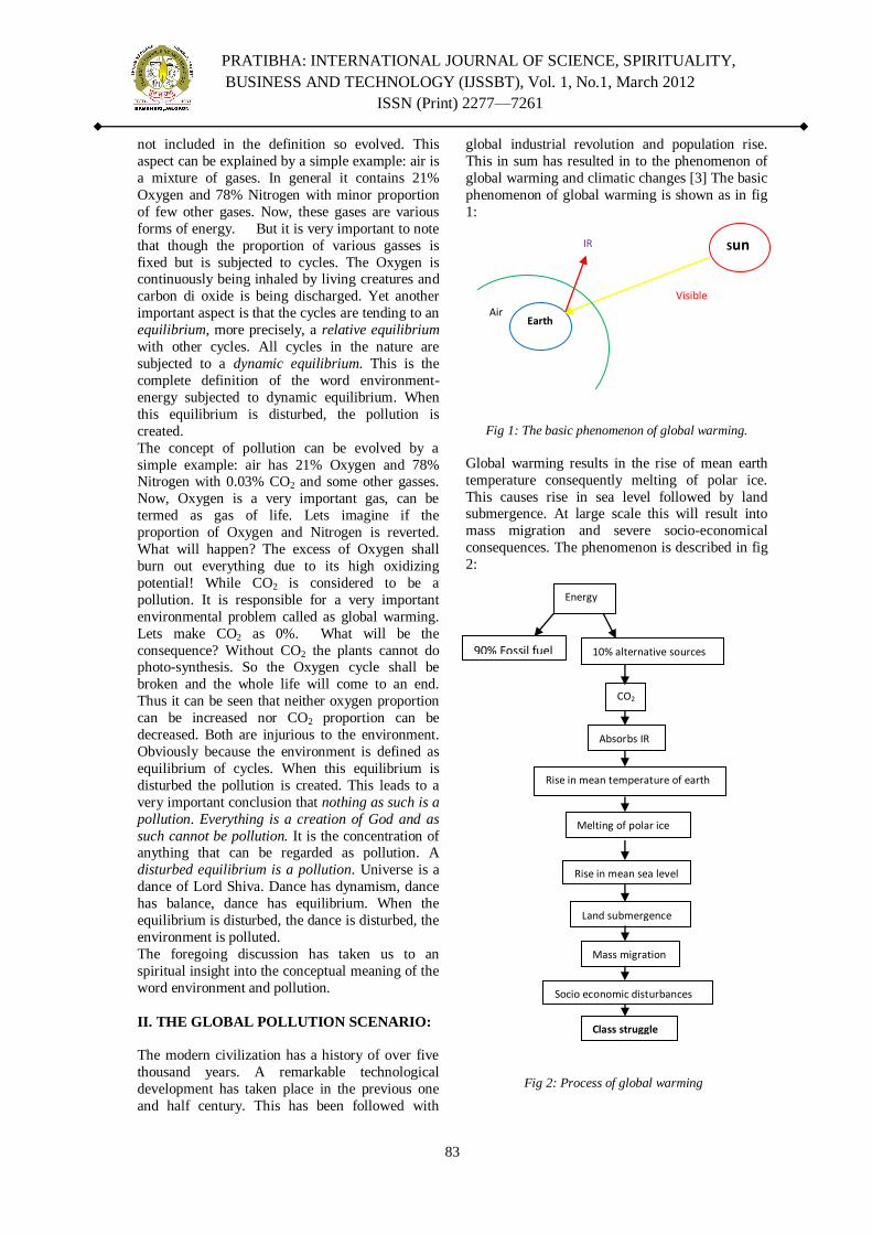
PRATIBHA: INTERNATIONAL JOURNAL OF SCIENCE, SPIRITUALITY,
BUSINESS AND TECHNOLOGY (IJSSBT), Vol. 1, No.1, March 2012
ISSN (Print) 2277—7261
83
not included in the definition so evolved. This
aspect can be explained by a simple example: air is
a mixture of gases. In general it contains 21%
Oxygen and 78% Nitrogen with minor proportion
of few other gases. Now, these gases are various
forms of energy. But it is very important to note
that though the proportion of various gasses is
fixed but is subjected to cycles. The Oxygen is continuously being inhaled by living creatures and
carbon di oxide is being discharged. Yet another
important aspect is that the cycles are tending to an
equilibrium, more precisely, a relative equilibrium
with other cycles. All cycles in the nature are
subjected to a dynamic equilibrium. This is the
complete definition of the word environment-
energy subjected to dynamic equilibrium. When
this equilibrium is disturbed, the pollution is
created.
The concept of pollution can be evolved by a
simple example: air has 21% Oxygen and 78% Nitrogen with 0.03% CO2 and some other gasses.
Now, Oxygen is a very important gas, can be
termed as gas of life. Lets imagine if the
proportion of Oxygen and Nitrogen is reverted.
What will happen? The excess of Oxygen shall
burn out everything due to its high oxidizing
potential! While CO2 is considered to be a
pollution. It is responsible for a very important
environmental problem called as global warming.
Lets make CO2 as 0%. What will be the
consequence? Without CO2 the plants cannot do photo-synthesis. So the Oxygen cycle shall be
broken and the whole life will come to an end.
Thus it can be seen that neither oxygen proportion
can be increased nor CO2 proportion can be
decreased. Both are injurious to the environment.
Obviously because the environment is defined as
equilibrium of cycles. When this equilibrium is
disturbed the pollution is created. This leads to a
very important conclusion that nothing as such is a
pollution. Everything is a creation of God and as
such cannot be pollution. It is the concentration of anything that can be regarded as pollution. A
disturbed equilibrium is a pollution. Universe is a
dance of Lord Shiva. Dance has dynamism, dance
has balance, dance has equilibrium. When the
equilibrium is disturbed, the dance is disturbed, the
environment is polluted.
The foregoing discussion has taken us to an
spiritual insight into the conceptual meaning of the
word environment and pollution.
II. THE GLOBAL POLLUTION SCENARIO:
The modern civilization has a history of over five
thousand years. A remarkable technological
development has taken place in the previous one
and half century. This has been followed with
global industrial revolution and population rise.
This in sum has resulted in to the phenomenon of
global warming and climatic changes [3] The basic
phenomenon of global warming is shown as in fig
1:
Fig 1: The basic phenomenon of global warming.
Global warming results in the rise of mean earth
temperature consequently melting of polar ice.
This causes rise in sea level followed by land submergence. At large scale this will result into
mass migration and severe socio-economical
consequences. The phenomenon is described in fig
2:
CO2
Fig 2: Process of global warming
Visible Air
IR
Earth
Sun
Class struggle
Mass migration
Socio economic disturbances
90% Fossil fuel 10% alternative sources
CO2
Absorbs IR
Rise in mean temperature of earth
Melting of polar ice
Rise in mean sea level
Land submergence
Energy
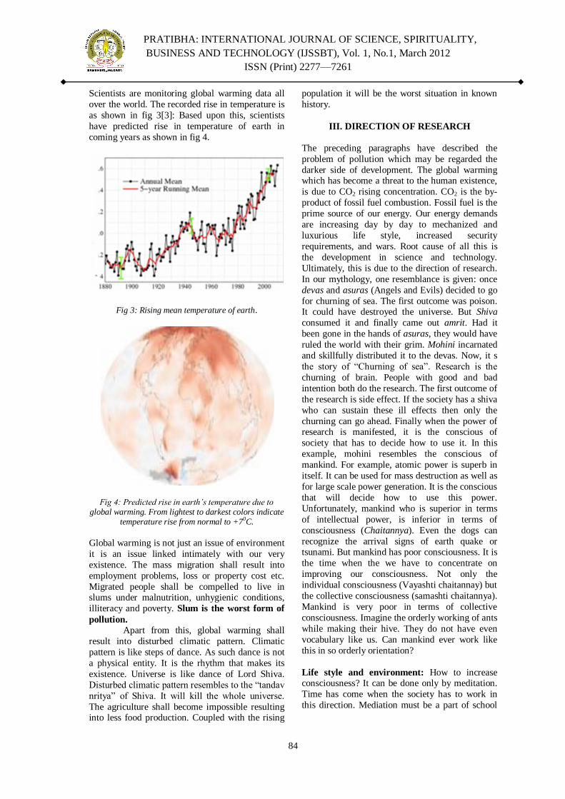
PRATIBHA: INTERNATIONAL JOURNAL OF SCIENCE, SPIRITUALITY,
BUSINESS AND TECHNOLOGY (IJSSBT), Vol. 1, No.1, March 2012
ISSN (Print) 2277—7261
84
Scientists are monitoring global warming data all
over the world. The recorded rise in temperature is
as shown in fig 3[3]: Based upon this, scientists
have predicted rise in temperature of earth in
coming years as shown in fig 4.
Fig 3: Rising mean temperature of earth.
Fig 4: Predicted rise in earth‟s temperature due to global warming. From lightest to darkest colors indicate
temperature rise from normal to +70C.
Global warming is not just an issue of environment
it is an issue linked intimately with our very
existence. The mass migration shall result into
employment problems, loss or property cost etc.
Migrated people shall be compelled to live in slums under malnutrition, unhygienic conditions,
illiteracy and poverty. Slum is the worst form of
pollution. Apart from this, global warming shall
result into disturbed climatic pattern. Climatic
pattern is like steps of dance. As such dance is not
a physical entity. It is the rhythm that makes its
existence. Universe is like dance of Lord Shiva.
Disturbed climatic pattern resembles to the ―tandav
nritya‖ of Shiva. It will kill the whole universe.
The agriculture shall become impossible resulting into less food production. Coupled with the rising
population it will be the worst situation in known
history.
III. DIRECTION OF RESEARCH
The preceding paragraphs have described the
problem of pollution which may be regarded the
darker side of development. The global warming which has become a threat to the human existence,
is due to CO2 rising concentration. CO2 is the by-
product of fossil fuel combustion. Fossil fuel is the
prime source of our energy. Our energy demands
are increasing day by day to mechanized and
luxurious life style, increased security
requirements, and wars. Root cause of all this is
the development in science and technology.
Ultimately, this is due to the direction of research.
In our mythology, one resemblance is given: once
devas and asuras (Angels and Evils) decided to go
for churning of sea. The first outcome was poison. It could have destroyed the universe. But Shiva
consumed it and finally came out amrit. Had it
been gone in the hands of asuras, they would have
ruled the world with their grim. Mohini incarnated
and skillfully distributed it to the devas. Now, it s
the story of ―Churning of sea‖. Research is the
churning of brain. People with good and bad
intention both do the research. The first outcome of
the research is side effect. If the society has a shiva
who can sustain these ill effects then only the
churning can go ahead. Finally when the power of research is manifested, it is the conscious of
society that has to decide how to use it. In this
example, mohini resembles the conscious of
mankind. For example, atomic power is superb in
itself. It can be used for mass destruction as well as
for large scale power generation. It is the conscious
that will decide how to use this power.
Unfortunately, mankind who is superior in terms
of intellectual power, is inferior in terms of
consciousness (Chaitannya). Even the dogs can
recognize the arrival signs of earth quake or tsunami. But mankind has poor consciousness. It is
the time when the we have to concentrate on
improving our consciousness. Not only the
individual consciousness (Vayashti chaitannay) but
the collective consciousness (samashti chaitannya).
Mankind is very poor in terms of collective
consciousness. Imagine the orderly working of ants
while making their hive. They do not have even
vocabulary like us. Can mankind ever work like
this in so orderly orientation?
Life style and environment: How to increase consciousness? It can be done only by meditation.
Time has come when the society has to work in
this direction. Mediation must be a part of school

PRATIBHA: INTERNATIONAL JOURNAL OF SCIENCE, SPIRITUALITY,
BUSINESS AND TECHNOLOGY (IJSSBT), Vol. 1, No.1, March 2012
ISSN (Print) 2277—7261
85
curriculum. It must be a part of office working. It
must be a compulsory practice in each house.
We have also seen that it is the rising energy
demand that has resulted into global warming [4].
Our energy demand has increased because of three
reasons: luxurious life style, wars, security
requirement. Again, mediation only can make us
strong enough and keep us from laziness so that we may not need luxury. And we may get rid of war-
mentality.
Consciousness directs intellect: Our laziness and luxurious life style has made au
more dependent upon machines. This has increased
the use of machines and consequently the
consumption of energy. 75% of world‘s energy is
used by the 25% population of developed world.
Rest of the 75% population uses only 25% of the
energy [5]. The higher consumption of energy has
tremendously raised the living standard. Yet it has not necessarily enhanced the quality of life too. In
fact it has posed the modern society with new kind
of problems. Several new kinds of diseases and
disorders have appeared. Most of them including
diabetes are due to lack of physical work. The
excessively mechanized lifestyle and rush for has
increased hypertension problems. Pollution has
caused early aging and several diseases. People
have comfortable beds in sophisticated bedrooms
but they depend upon medicines to sleep. People
have mobile phones but yet facing communication gap problems in near relations. Sum total of all this
has indeed degraded the modern life quality which
earlier people used to have as a natural gift.
Regular practicing of meditation and yoga can
have combating effect of diseases and mental
disorders. It can radically reorient the mass
psychology. Development does not always mean
mechanization. For instance ―Mayan civilization‖
of American continent had developed mathematics
and astronomy to a great extent. But they had not
invented the wheel. It is even important they had not prohibited the invention of wheel, rather their
collective consciousness was adequately developed
so that their researcher did not get poised with the
invention of wheel. It is the consciousness which is
supreme. Consciousness supersedes intellect [6-7].
Consciousness directs intellect; for individual as
well as for society.
IV. SUSTAINABLE DEVELOPMENT
Time has come when we have to learn sustainable
development and environmental friendly life style [8].
What is exactly meant by sustainability? One has
a right to harness the nature but not to exploit the
nature. A simple well known example explains it:
milking a cow harnessing, cutting the cow is
exploiting. It is the basic philosophy applicable to
all development projects. Rig Ved has pronounced
in one of its hymn: thy bosom mountains, sky is
your girdle, oceans sing your glory, O‘ mother
earth forgive me as I touch you with my feet. If we
recognize that nature is our mother, it care us like a
mother, by none of our act we will pollute it. All our actions will be so humble, so gentle so soft that
they will never hurt the nature.
REFERENCES [1] Oxford English Dictionary: The definitive recording of the
English Language, Oxford University Press, UK.
[2] Mythological literature including GEETA published by
Geeta Press Gorakhpur, UP.
[3] Wikipedia of global warming.
[4] Pachauri R K and Sridharan P V (2008) Looking back to
think ahead, TERI Publication Delhi.
[5] Wikipedia of Energy.
[6] Peter Russel (2006) From science to God: the mystery of
consciousness and the meaning of life, New World Library,
Navota.
[7] Peter Russel (2006) The evolution of consciousness, New
World Library, Navota.
[8] Joann Loviglio (2007) Scientists bridging the spirituality
gap, Associated Press, Philadelphia.

PRATIBHA: INTERNATIONAL JOURNAL OF SCIENCE, SPIRITUALITY,
BUSINESS AND TECHNOLOGY (IJSSBT), Vol. 1, No.1, March 2012
ISSN (Print) 2277—7261
86
A NEW METHOD OF SPEED CONTROL OF A THREE-PHASE
INDUCTION MOTOR INCORPORATING THE OVERMODULATION
REGION IN SVPWM VSI
S. K. Bhartari1, Vandana Verma
2, Anurag Tripathi
3*
1,2Author is with PSIT Engineering College, Kanpur 3Author is with Institute of Engineering. & Technology, Lucknow
Abstract: This paper proposes the matlab based
model of a new scheme of speed control of the
three phase induction motor under which the
speed command is compared with the actual
speed and the error is processed to generate the
gating patterns for the space vector modulated
voltage source inverter. The space vector
modulation technique ensures linearity till an
output of 90.7% of the installed inverter
capacity. Beyond this value, if higher inverter
output is desired, the operation is termed as
overmodulation. The speed control scheme
incorporates the two reported regions of
overmodulation i.e. I & II and ensures a smooth
transition of the motor till 100% of its rated
speed and also beyond that in the field
weakening region. Overmodulation is a non-
linear process, and it involves two modes of
operation depending on modulation index (MI).
Mode I provides compensation of the voltage
vector to be applied while mode II uses the
concept of continuous application of a
particular voltage vector in order to achieve the
desired average voltage vector and hence
angular velocity. In this paper, the range of
mode I operation of overmodulation is extended
beyond usual modulation index thus far
reported (0.9535) in the literature, thus
stretching the arrival of Mode II further
towards six step. This delay in the arrival of
overmodulation Mode II reduces the non-
linearity effect as the lower order harmonics are
minimized, thereby enhancing the
controllability of the motor angular velocity.
This helps in mitigating the current and torque
ripples in the motor. The satisfactory operation
of the extended range of mode I and the smooth
transition into mode II and six step is verified
using simulation results.
Keywords: Overmodulation, SVPWM, Volt–
Second compensation.
I. INTRODUCTION
The basic advantage of SVPWM is that it increases
the linear range of operation till a modulation
index of 90.7% unlike the conventional sine PWM
method having linear range till a modulation index
of 78.5%. The concept of operation of linear or
non-linear region is based on modulation index
that indirectly provides information about the
inverter utilization capability. . This feature of
SVPWM puts on edge over other PWM
techniques. Till M I ≤ 0.907 SVPWM inverter operates in the linear region meaning whereby that
the modulation index is directly proportional to the
fundamental component of the line side voltage.
Beyond M I = 0.907 SVPWM inverter stands
operating in the non-linear or in other words
overmodulation region. This overmodulation
region is further divided into two zones. Zone 1
lies between 0.907 < M I ≤ 0.9535 and zone II lies
between 0.9535 < M I ≤ 1.0.
The main aim of any PWM technique is to utilize
the inverter to its full capacity that is achieved only
with six-step operation but at the cost of loss of controllability. In SVPWM, the operation from
under modulation to overmodulation finally leads
to the six-step operation.
The normal and six-step operating regions
of a modulator can be easily programmed, but to
maintain continuity between these two regions,
overmodulation is required. Besides this,
overmodulation helps in exploiting the voltage
capability of the inverter and therefore is necessary
to improve the dynamic response of the drive. To
this end, several methods of achieving overmodulation are suggested.
In [1], the overmodulation range is divided into
two sub-regions and the inverter switching is
defined based upon the unique characteristics

PRATIBHA: INTERNATIONAL JOURNAL OF SCIENCE, SPIRITUALITY,
BUSINESS AND TECHNOLOGY (IJSSBT), Vol. 1, No.1, March 2012
ISSN (Print) 2277—7261
87
of the two regions. In the first sub-region, a pre-
processor modifies the magnitude of the reference
voltage vector before the conventional space vector modulator processes it. In the second sub-
region, the pre-processor modifies both the angle
and magnitude of the reference voltage vector. To
avoid the solution of nonlinear equations, two look
up tables are used and continuous control of
voltage is obtained until six-step region. While the
fundamental voltage cannot be obtained in every
sampling period, [1] gets it in a fundamental cycle.
The other overmodulation schemes like [2],[3],[4],
[5] use the basic geometrical understanding
provided in [1]. However, these methods differ from each other in the manner they implement the
overmodulation switching strategy. In terms of
minimum processing time, the method given in [4]
is the fastest. However, due to large harmonic
content in the voltage waveform, it results into
distorted current and flux waveforms. The method
described in [2] uses computationally intensive
classification algorithms to achieve
overmodulation. Instead of pre-processing the
voltage vector as in [1], references [3] and [5] use
approximated piecewise linearized equations to
achieve overmodulation switching. All these methods have effectively extended the DC-bus
utilization of the inverter until the six-step mode
and are tested for the open loop V/f drives. During
overmodulation, lower order harmonics are added
to improve the fundamental cycle voltage gain of
the modulator. However, when used in a closed
loop torque and flux vector control scheme like
FOC, these harmonics interfere with the working
of linear current controllers, [6]. In reference [6], a
method of compensation is proposed that uses an inverse model to estimate the harmonic component
of the current vector during overmodulation. This
harmonic content is then discarded from the inputs
to the linear controllers. During dynamics at high
angular velocities, the method developed by
Mochikawa et al. selects the voltage vector that is
vectorially closest to the reference [7]. This is
achieved by projecting the reference voltage vector
tip point on the closest inverter hexagon side.
Another method implemented by Seidl et al. [8],
uses neural networks for implementation, [7]. This approach however fails to utilize the voltage
capability and requires a computationally intensive
control algorithm. In the reference [9] an attempt is
made to overcome the adverse effect of the
nonlinear gain on the linear current controllers by
utilizing the nonlinear inverter gain function
model. This method appears to give a performance
that is similar to a much simpler approach using
look-up tables that are proposed in [1].
Besides the SVM based overmodulation
methods discussed in the above paragraphs, a class
of discontinuous PWM methods [10] have been described that extend the linear range of operation
using the sine-triangle PWM scheme. In this
category, the popular methods tested for V/f
induction motor drives are the one by Ogasawara
[11]. A hybrid method that combines the
advantages of these methods is developed in [10].
However, the steady state FOC drive performance
Figure 1: The complete SVM scheme applied to a three phase Induction motor

PRATIBHA: INTERNATIONAL JOURNAL OF SCIENCE, SPIRITUALITY,
BUSINESS AND TECHNOLOGY (IJSSBT), Vol. 1, No.1, March 2012
ISSN (Print) 2277—7261
88
using these methods in the overmodulation range is
shown to be oscillatory.
II. CONTRIBUTION AND ORGANIZATION
OF THE PAPER:
The proposed strategy of extending the range of
overmodulation zone I and further achieving a smooth transition to overmodulation II and six
step, considers the instantaneous value of stator
voltage vector. The gating pattern is generated by
the sampled error between the reference voltage
vector and the estimated or actual voltage vector.
Consideration of stator voltage vector error as the
commanded value helps to achieve zero flux vector
error in a fundamental cycle for all operating
angular velocities. Figure 1 shows the complete
scheme for the speed control of the three phase
Induction motor.The achievement of the increased
MI for zone I overmodulation, carried out right from the fundamental principle of calculating the
switching times and selection of switching states is
discussed in this paper. The mathematical
equations developed are simulated through
MATLAB / SIMULINK and the results of
simulations are then validated through
experimental results.
III. SPACE VECTOR MODULATION
TECHNIQUE:
The figure 2 shows the three modes of operation of
SVPWM. The operation within the inscribed circle
of the regular hexagon is the linear region while
operation outside the inscribed circle till the
circumscribed circle around the hexagon depicts
overmodulation region.
overmodulation
01
2
3
4
5
100
110010
001 101
Locus of Undermodulation
(Linear Region)
Overmodulation (Zone I & II)
V*Desired Ref Voltage
Figure 2: Showing the various regions of modulation
At the end of the liner modulation i.e. at a MI
>0.907, the reference voltage vector tip traces a
circle whose radius becomes greater than that of
the inscribed circle of the hexagon representing the
voltage vectors which can be applied in the six
sectors.
IV. OVERMODULATION (ZONE I)
As can be seen from the figure 3, the whole situation in the OVMI stage can be divided into two regions. In region A, the value of the (desired) reference voltage
vector *( )sV k i.e. OD, is more than the actual available
voltage vector ( )sV k i.e. OC, which in region B is the
other way round.
A
B
II
I
D
o
C
*( )sV k
*( ) ( )s sV k V k
*( ) ( )s sV k V k
Figure 3: Overmodulation compensation
In region A, the maximum available reference
voltage vector is max0.866 ( )sV k . So,
Max loss (of volt-sec) in region A =
*max( ) 0.866 ( )s sV k V k
(1)
Among the switching times τau_a, τau_b,
and τau_0, τau_0 becomes negative in region A,
which is not possible practically, so τau_0 is taken
to be equal to zero and the switching is obtained by
applying active states for τau_a and τau_b period
only. The voltage vector in this region thus moves
along the hexagon till the boundary of the region B
starts.
In the region B, there is an ample
available voltage vector ( )sV k magnitude to
accommodate tau_0 so all the three switching
times are applied albeit in a modified manner. The loss of angular velocity in the region A is
compensated in the region B. This compensation
results in the modification of the switching times.
Max.compensation=*
max( ) ( )c s sk V k V k
(2)
Where ck is a compensation factor which decides
what percentage of the maximum voltage vector
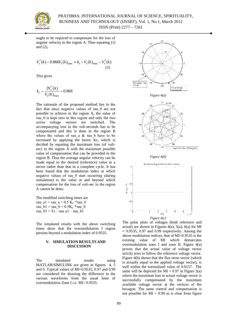
PRATIBHA: INTERNATIONAL JOURNAL OF SCIENCE, SPIRITUALITY,
BUSINESS AND TECHNOLOGY (IJSSBT), Vol. 1, No.1, March 2012
ISSN (Print) 2277—7261
89
ought to be required to compensate for the loss of
angular velocity in the region A. Thus equating (1)
and (2),
* *
max max( ) 0.866 ( ) ( ) ( )s s c s sV k V k k V k V k
(3)
This gives
*
max
2 ( )0.866
( )
sc
s
V kk
V k
The rationale of the proposed method lies in the
fact that since negative values of τau_0 are not
possible to achieve in the region A, the value of
τau_0 is kept zero in this region and only the two
active voltage vectors are switched. The
accompanying loss in the volt-seconds has to be compensated and this is done in the region B
where the values of τau_a & τau_b have to be
increased by applying the factor Kc, which is
decided by equating the maximum loss (of volt-
sec) in the region A with the maximum possible
value of compensation that can be provided in the
region B. Thus the average angular velocity can be
made equal to the desired (reference) value in a
sector rather than that in a complete cycle. It has
been found that the modulation index at which
negative values of τau_0 start occurring (during simulation) is the value at and beyond which
compensation for the loss of volt-sec in the region
A cannot be done.
The modified switching times are
τau_a1 = τau_a + 0.5 KC *τau_0
τau_b1 = τau_b + 0.5KC *τau_0
τau_01 = Ts – τau_a1 – τau_b1
The simulated results with the above switching
times show that the overmodulation I region
persists beyond a modulation index of 0.9535.
V. SIMULATION RESULTS AND
DISCUSSION
The simulated results using
MATLAB/SIMULINK are given in figures 4, 5
and 6. Typical values of MI=0.9535, 0.97 and 0.99
are considered for showing the difference in the
various waveforms from the usual limit of
overmodulation Zone I i.e. MI= 0.9535.
Figure 4(a)
Figure 4(b)
Figure 4(c)
The polar plots of voltages (both reference and
actual) are shown in Figures 4(a), 5(a), 6(a) for MI
= 0.9535, 0.97 and 0.99 respectively. Among the
above modulation indices, that of MI=0.9535 is the
existing value of MI which demarcates
overmodulation zone I and zone II. Figure 4(a)
proves that the actual value of voltage vector
strictly tries to follow the reference voltage vector.
Figure 4(b) shows that the flux error vector (which
is actually equal to the applied voltage vector), is
well within the normalized value of 0.0157. The same will be depicted for MI = 0.97 in Figure 5(a)
where the maximum loss in actual voltage vector is
successfully compensated by the maximum
available voltage vector at the vertices of the
hexagon. The same control and compensation is
not possible for MI = 0.99 as is clear from figure
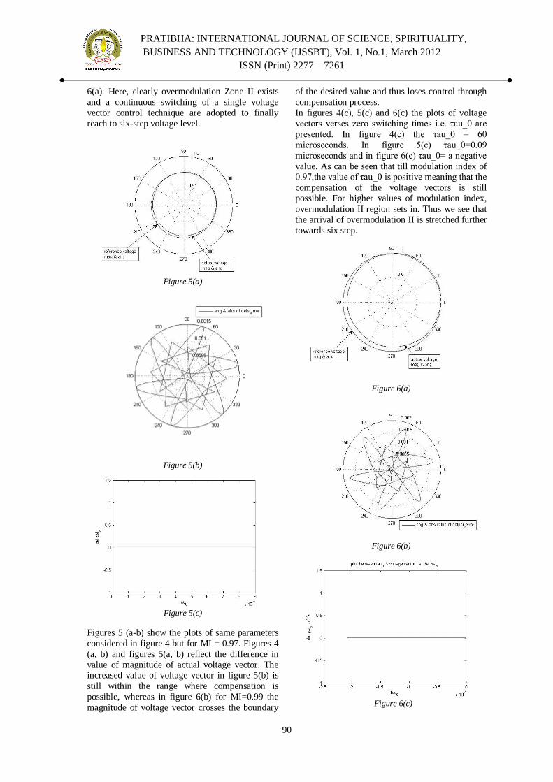
PRATIBHA: INTERNATIONAL JOURNAL OF SCIENCE, SPIRITUALITY,
BUSINESS AND TECHNOLOGY (IJSSBT), Vol. 1, No.1, March 2012
ISSN (Print) 2277—7261
90
6(a). Here, clearly overmodulation Zone II exists
and a continuous switching of a single voltage
vector control technique are adopted to finally
reach to six-step voltage level.
Figure 5(a)
Figure 5(b)
Figure 5(c)
Figures 5 (a-b) show the plots of same parameters
considered in figure 4 but for MI = 0.97. Figures 4
(a, b) and figures 5(a, b) reflect the difference in
value of magnitude of actual voltage vector. The increased value of voltage vector in figure 5(b) is
still within the range where compensation is
possible, whereas in figure 6(b) for MI=0.99 the
magnitude of voltage vector crosses the boundary
of the desired value and thus loses control through
compensation process.
In figures 4(c), 5(c) and 6(c) the plots of voltage
vectors verses zero switching times i.e. τau_0 are
presented. In figure 4(c) the τau_0 = 60
microseconds. In figure 5(c) τau_0=0.09
microseconds and in figure 6(c) τau_0= a negative
value. As can be seen that till modulation index of 0.97,the value of τau_0 is positive meaning that the
compensation of the voltage vectors is still
possible. For higher values of modulation index,
overmodulation II region sets in. Thus we see that
the arrival of overmodulation II is stretched further
towards six step.
Figure 6(a)
Figure 6(b)
Figure 6(c)

PRATIBHA: INTERNATIONAL JOURNAL OF SCIENCE, SPIRITUALITY,
BUSINESS AND TECHNOLOGY (IJSSBT), Vol. 1, No.1, March 2012
ISSN (Print) 2277—7261
91
The negative values of τau_0 directly reflect the
zone of operation in overmodulation II region in
SVPWM inverter. Since τau_0 cannot be negative
so is kept zero and the control is achieved through
active state vectors. Thus, the overmodulation zone
II operation starts. The simulated results in figures
4(c), 5(c) and 6(c) define and conclude the
extended range of operation of Zone I in overmodulation region.
The smooth control of torque and speed of three-
phase induction motor is easily possible now with
extended range of overmodulation Zone I. This
gives greater flexibility in obtaining the required
input voltage of the motor from the SVPWM
inverter by generating the gating signals
accordingly. It also helps in better and smooth
transition from overmodulation to six-step
operation. Moreover, extended range of Zone I
improve the transient response of the torque and
speed of the induction motor by reducing the pulsations in the torque in the dynamic condition.
VI. CONCLUSION
The novel approach towards the achievement
of extended range of Zone I overmodulation
presented in this paper when realized through
simulations show the improved transient response
of the induction motor with less effect of non
linearity faced during overmodulation operation in
SVPWM inverter. Since the Zone I range is
stretched beyond the existing value of MI=0.9535, in turn, automatically reduces the range of
operation in Zone II i.e. now zone II region starts
at a much later value of MI. Hence, the control and
transition to six step operation of the required
voltage vector is much easy and even. The
proposed approach removes the problem arising
out of the extreme non linearity starting with the
advent of overmodulation zone II by increasing the
range of operation of zone I
REFERENCES [1] J. Holtz, W. Lotzkat, and A. M. Khambadkone, ―On
continuous control of pwm inverters in overmodulation range
including six-step,‖ IEEE Transaction on Power Electronics,
vol. 8, pp. 546–553, 1993.
[2] A. R. Bakhshai, G´eza, Jo´os, P. K.Jain, and H. Jin,
―Incorporating the overmodulation range in space vector pattern
generators using a classification algorithm,‖
IEEE Trans. on Power Electronics, vol. 15, pp. 83 – 91, January
2000.
[3] D.-C. Lee and G.-M. Lee, ―A novel overmodulation
technique for space-vector pwm inverters,‖ IEEE Trans. on
Power Electronics, vol. 13, no. 6, pp. 1144–1151, 1998.
[4] S. Bolognani and M.Zigliotto, ―Novel digital continuous
control of svm inverters in the overmodulation range,‖ IEEE
Trans. on Industrial Applications, vol. 33, no. 2, pp. 525–530,
1997.
[5] G. Narayanan and V. T. Ranganathan, ―Overmodulation
algorithm for space vector modulated inverters and its
application to low switching frequency pwm techniques,‖ in
Electric Power Applications, IEE Proceedings, vol. 148,
November 2001.
[6] A. M. Khambadkone and J. Holtz, ―Current control in
overmodulation range for space vector modulation based vector
controlled induction motor drives,‖
(Nagoya, Japan), pp. 1334–1339, October 2000.
[7] H. Mochikawa, T. Hirose, and T. Umemoto,
―Overmodulation of voltage source pwm inverter,‖ in JIEE-Ind
Society conference records, 1991.
[8] D. R. Seidl, D. A. Kaiser, and R. D. Lorenz, ―One-step
optimal space vector pwm current regulation using a neural
network,‖ in IEEE-Industrial Application Soc. Conf. Rec.,
1994.
[9] R. J. Kerkman, T. M. Rowan, D. Leggate, and B. J. Seibel,
―Control of pwm voltage inverters in pulse dropping range,‖
IEEE Industry Application Magazine, vol. 2, pp. 24–31, Sept-
Oct 1996.
[10] A. M. Hava, R. J. Kerkman, and T. A. Lipo., ―Carrier-
based PWM-VSI overmodulation strategies: analysis,
comparison, and design,‖ IEEE Transactions on Power
Electronics, vol. 13, pp. 674–689, July 1998.
[11] S. Ogasawara, H. Akagi, and A. Nabae, ―A novel PWM
scheme of voltage source inverter based upon space vector
theory,‖ in European Power Electronics Conference records,
1989.

PRATIBHA: INTERNATIONAL JOURNAL OF SCIENCE, SPIRITUALITY,
BUSINESS AND TECHNOLOGY (IJSSBT), Vol. 1, No.1, March 2012
ISSN (Print) 2277—7261
92
STUDY OF DYNAMIC PERFORMANCE OF
RESTRUCTURED POWER SYSTEM WITH
ASYNCHRONOUS TIE-LINES USING CONVENTIONAL
PI CONTROLLERS
S. K. Pandey1, V. P. Singh
2 , P. Chaubey
3
1,2,3Electrical Engineering Department, MNNIT, Allahabad – 211004, India
Emails: [email protected],
1Corresponding Author Abstract: This paper presents a comprehensive
study on dynamic performance of a two-area
restructured power system interconnected via
parallel ac/dc transmission links with
conventional PI controllers. It has been
observed that the dynamic performance i.e.
frequency deviation and deviation in power tie-
line improved with dc link in parallel with ac
tie-line in terms of overshoot and settling time.
The dynamic responses for small perturbation
have been observed with PI controller with and
without dc links and result of both have been
compared.
Key words: Asynchronous tie-lines; Restructured
power system; HVDC transmission links; Load
frequency control.
I. INTRODUCTION
For large scale electrical power systems that
normally consist of interconnected control areas
representing coherent groups of generators, load
frequency control is very important in power
system operation and control for supplying
sufficient and reliable electric power with good
quality [1-3]. In case of area load changes and
abnormal conditions, such as outages of generation and varying system parameters, mismatches in
frequency and scheduled tie-line power flows
between areas can be caused. These mismatches
are corrected by controlling, which is defined as
the regulation of the power output of generators
within a prescribed area. The main objective of the
LFC is to satisfy the requirements such as zero
steady state errors in tie-line exchanges and
frequency deviations, optimal transient behaviors
and in steady state, the power generation levels
should satisfy the optimal dispatch conditions. A little attention has been paid to use of HVDC
transmission link as system interconnection. A
favorable effect on system dynamic performance
has been achieved considering such system
interconnection [4-5].
Under restructured or open market system
(deregulation) the power system structure changed
in such a way that would allow the evolving of
more specialized industries for generation (Genco),
transmission (Transco) and distribution (Disco). In the restructured power system, DISCOs in each
area can contract with GENCOs in its or other
areas[3-5]. As there are several Gencos and Discos
in the restructured power system, a Disco has the
freedom to have a contract with any Genco for
transaction of power. A Disco may have a contract
with a Genco in another control area. Such
transactions are called ―bilateral transactions.‖ All
the transactions have to be cleared through an
impartial entity called an independent system
operator (ISO). The ISO has to control a number of so-called ―ancillary services‖ one of which is load
frequency control.
II. RESTRUCTURED POWER SYSTEM
The traditional power system industry has a
―vertically integrated utility‖ (VIU) structure. In
the restructured or open market system
(deregulated), vertically integrated utilities no
longer exist. In the restructured power system,
GENCOs sell power to various DISCOs at
competitive prices. Thus, DISCOs have the freedom to choose the GENCOs for contracts.
They may or may not have contracts with the
GENCOs in their own area. There can be various
combinations of contracts between DISCOs and
GENCOs which can be conveniently visualized by
the concept of a ‗DISCO participation matrix‘
(DPM). The rows of a DPM correspond to
GENCOs and columns to DISCOs which contract
power. Each entry in this matrix can be thought as
a fraction of a total load contracted by a DISCO
(column) towards a GENCO (row). The sum of all the entries in a column in this matrix is unity.
Consider a two-area power system in which each
area has two GENCOs and two DISCOs in it. Let
GENCO1, GENCO2, DISCO1, and DISCO2 be in
area1 and GENCO3, GENCO4, DISCO3, and
DISCO4 be in area 2 as shown in Fig.1 [3-5].

PRATIBHA: INTERNATIONAL JOURNAL OF SCIENCE, SPIRITUALITY,
BUSINESS AND TECHNOLOGY (IJSSBT), Vol. 1, No.1, March 2012
ISSN (Print) 2277—7261
93
Fig.1. Block Diagram of two area restructured power
system.
The corresponding DPM for a two-area power
system will have the structure that follows:
11 12 13 14
21 22 23 24
31 32 33 34
41 42 43 44
cpf cpf cpf cpf
cpf cpf cpf cpf
cpf cpf cpf cpf
cpf cpf cpf cpf
where jdcpf is contract participation factor of -thj
GENCO in the load following of -thd DISCO.
DPM shows the participation of a DISCO in a
contract with any GENCO, hence the name Disco
Participation Matrix. The diagonal elements of
DPM corresponding to the local demands and off
diagonal elements corresponding to the demands
of the DISCOs in one area to the GENCOs in
another area.
III. TWO AREA POWER SYSTEM MODEL
The two area power system model used in this
paper is as follows:
It is a two-area restructured or open system
(deregulated) interconnected system consisting of
identical thermal power plants. The two-areas are
interconnected via AC tie-line in parallel with
HVDC link. The single line diagram of power system model
under consideration is shown in Fig.2 [3-5]. The
transmission links are considered as long
transmission lines specifically of length greater
than break even distance length of AC and HVDC
transmission lines. The distance normally used as
break even distance is about 600km.
The mathematical model of the two-area
thermal systems under restructured or open market
(deregulated) is shown in Fig.3.
Fig.2. Two area power system with parallel AC/HVDC
links.
Fig.3 (A): Simulink model of Two-area restructured Asynchronous power system.
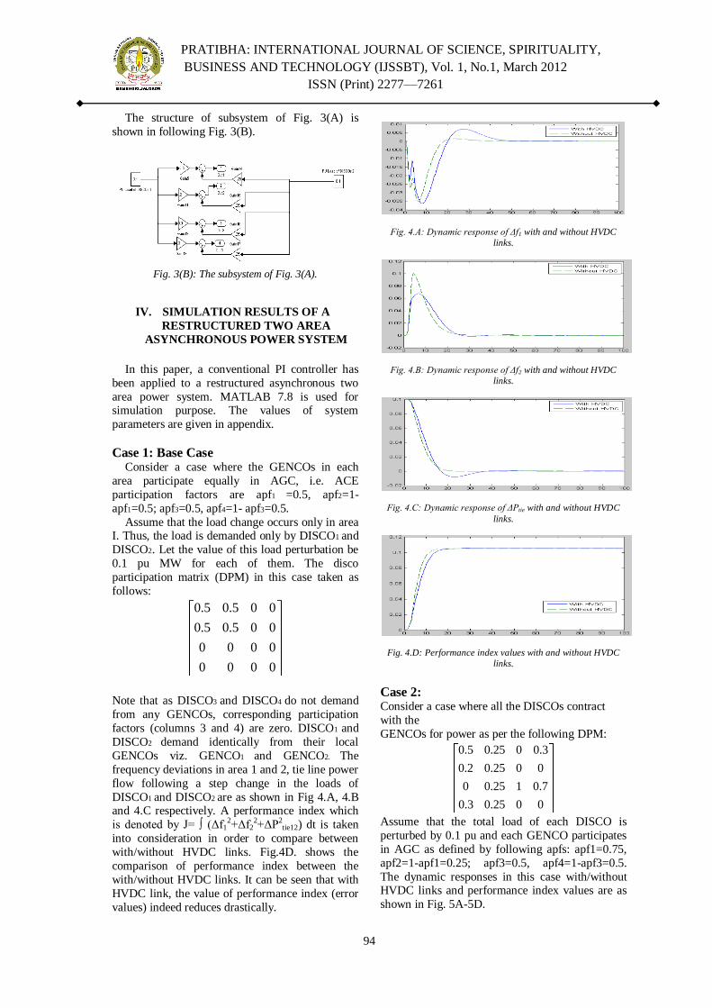
PRATIBHA: INTERNATIONAL JOURNAL OF SCIENCE, SPIRITUALITY,
BUSINESS AND TECHNOLOGY (IJSSBT), Vol. 1, No.1, March 2012
ISSN (Print) 2277—7261
94
The structure of subsystem of Fig. 3(A) is
shown in following Fig. 3(B).
Fig. 3(B): The subsystem of Fig. 3(A).
IV. SIMULATION RESULTS OF A
RESTRUCTURED TWO AREA
ASYNCHRONOUS POWER SYSTEM
In this paper, a conventional PI controller has
been applied to a restructured asynchronous two
area power system. MATLAB 7.8 is used for simulation purpose. The values of system
parameters are given in appendix.
Case 1: Base Case Consider a case where the GENCOs in each
area participate equally in AGC, i.e. ACE
participation factors are apf1 =0.5, apf2=1-
apf1=0.5; apf3=0.5, apf4=1- apf3=0.5.
Assume that the load change occurs only in area I. Thus, the load is demanded only by DISCO1 and
DISCO2. Let the value of this load perturbation be
0.1 pu MW for each of them. The disco
participation matrix (DPM) in this case taken as
follows:
0.5 0.5 0 0
0.5 0.5 0 0
0 0 0 0
0 0 0 0
Note that as DISCO3 and DISCO4 do not demand
from any GENCOs, corresponding participation
factors (columns 3 and 4) are zero. DISCO1 and
DISCO2 demand identically from their local
GENCOs viz. GENCO1 and GENCO2. The
frequency deviations in area 1 and 2, tie line power
flow following a step change in the loads of
DISCO1 and DISCO2 are as shown in Fig 4.A, 4.B and 4.C respectively. A performance index which
is denoted by J= ∫ (Δf12+Δf2
2+ΔP2tie12) dt is taken
into consideration in order to compare between
with/without HVDC links. Fig.4D. shows the
comparison of performance index between the
with/without HVDC links. It can be seen that with
HVDC link, the value of performance index (error
values) indeed reduces drastically.
Fig. 4.A: Dynamic response of Δf1 with and without HVDC
links.
Fig. 4.B: Dynamic response of Δf2 with and without HVDC
links.
Fig. 4.C: Dynamic response of ΔPtie with and without HVDC
links.
Fig. 4.D: Performance index values with and without HVDC
links.
Case 2: Consider a case where all the DISCOs contract
with the
GENCOs for power as per the following DPM:
0.5 0.25 0 0.3
0.2 0.25 0 0
0 0.25 1 0.7
0.3 0.25 0 0
Assume that the total load of each DISCO is
perturbed by 0.1 pu and each GENCO participates
in AGC as defined by following apfs: apf1=0.75,
apf2=1-apf1=0.25; apf3=0.5, apf4=1-apf3=0.5.
The dynamic responses in this case with/without HVDC links and performance index values are as
shown in Fig. 5A-5D.

PRATIBHA: INTERNATIONAL JOURNAL OF SCIENCE, SPIRITUALITY,
BUSINESS AND TECHNOLOGY (IJSSBT), Vol. 1, No.1, March 2012
ISSN (Print) 2277—7261
95
Fig. 5.A: Dynamic response of Δf1 with and without HVDC links.
Fig. 5.B: Dynamic response of Δf2 with and without HVDC links.
Fig. 5.C: Dynamic response of ΔPtie with and without HVDC links.
Fig. 5.D: Performance index values with and without
HVDC links.
Case 3: Contract Violation
Consider case 2 again except that DISCO1
demands an additional 0.1 pu MW which is not
contracted out to any GENCO. The uncontracted load of DISCO1 reflects in the generations of
GENCO1 and GENCO2. Thus, this excess load is
taken up by the GENCOs in the same area as that
of the DISCO making the uncontracted demand.
The dynamic responses in this case are as shown in
Fig. 6A-6D.
Fig. 6.A: Dynamic response of Δf1 with and without HVDC links.
Fig. 6.B: Dynamic response of Δf2 with and without HVDC links.
Fig. 6.C: Dynamic response of ΔPtie with and without HVDC links.
Fig. 6.D: Performance index values with and without HVDC links.
V. CONCLUSION
In this paper, power system model with identical
thermal units under restructured scenario with and without HVDC links are considered for the study.
By incorporating the HVDC links, the oscillations,
peak overshoot and settling time are improved.
The degradation in system dynamic performance
of a restructured two area can be compensated
effectively by incorporating HVDC links parallel
with AC tie-line as area interconnection between
two power system areas. It may be therefore
concluded that, dynamic performance of the
restructured two area power system enhanced with
HVDC links.

PRATIBHA: INTERNATIONAL JOURNAL OF SCIENCE, SPIRITUALITY,
BUSINESS AND TECHNOLOGY (IJSSBT), Vol. 1, No.1, March 2012
ISSN (Print) 2277—7261
96
REFERENCES
[1] N. Jaleel, D. N.Ewart and L. H. Fink, ―Understanding
automatic generation control‖, IEEE Trans.on Power
Systems, vol.7, no.3, pp. 1106-1122, 1992.
[2] O. I. Elgerd and C. Fosha, ―Optimum megawatt-frequency
control of multiarea electric energy systems‖, IEEE trans.
Power Apparatus & system, vol. 89, no. 4, pp. 556-563,
1970.
[3] V. Donde, M. A. Pai and I. A. Hiskens, ―Simulation and
optimization in an AGC system after deregulation‖, IEEE
Ttrans. power systems, vol. 16, no. 3, 2001.
[4] C. S. Rao, Z. Naghizadeh and S. Mahadavi,
―Improvement of dynamic performance of hydrothermal
system under open market scenario using asynchronous
tie-lines‖, World J. of modeling and Simulation, vol. 4, no.
2, pp 153-160, 2008.
[5] H. D. Mathur and H. V. Manjunath, ―Study of dynamic
performance of thermal units with asynchronous tie-liens
using Fussy based controller, J. Electrical systems, vol. 3,
no. 3, pp. 124-130, 2007.
APPENDIX
All the notations carry the usual meanings.
System Data:
1 2r rP P = Rated area capacities = 1200 Mw
1 2g gT T = Governor time constants = 0.08s
1 2g gK K = Governor Gain constant= 1.0
1 2t tT T =Turbine time constant= 0.3s
1 2t tK K =Turbine gain constant=1.0
1 2p pT T = Power system time constants = 20s
1 2p pK K =System Gains = 120 Hz/p.u.Mw
1 2R R =Regulation parameter= 2.4Hz/p.u. Mw
1 2B B = Bias constants = 0.425p.u. Mw/Hz
12T = Synchronizing coefficient= 0.0868s
Data for ac and dc Links:
dcK =Gain associated with dc link= 1.0
dcT = Time constant of dc link= 0.2s
Controller Gains:
1.0, 0.4, 0.0p I DK K K

PRATIBHA: INTERNATIONAL JOURNAL OF SCIENCE, SPIRITUALITY,
BUSINESS AND TECHNOLOGY (IJSSBT), Vol. 1, No.1, March 2012
ISSN (Print) 2277—7261
97
Performance Analysis of Various Image Compression
Techniques
Dipeeka O. Kukreja1, S.R. Suralkar
2, A.H. Karode
3
S.S.B.T‘s College of Engineering And Technology, Bambhori, Jalgaon Email: [email protected], [email protected], [email protected]
Abstract: Digital image compression has
numerous practical applications to effectively
utilize storage capacities & shorten
transmission time. This paper aims at the
analysis of various lossless and lossy image
compression techniques. For lossless
compression Huffman coding method and for
lossy compression Discrete Cosine Transform
(DCT), Discrete Wavelet Transform (DWT)
using Embedded Zerotree Wavelet (EZW) and
Block Truncation Coding (BTC) methods are
described. These image compression strategies
are examined for their relative effectiveness.
Finally a performance comparison is made
between these techniques based on different
parameters like Peak Signal to Noise
Ratio(PSNR), Compression Ratio (CR), Root
Mean Square Error(RMSE) , Structural
Similarity (SSIM) etc.
Keywords - Huffman coding, DCT, DWT, EZW
coding, CR, SSIM.
I. INTRODUCTION
With the continual expansion of multimedia and
Internet applications, the needs and requirements
of the technologies used, grew and evolved. To
address these needs and requirements in the specific area of still image compression, many
efficient techniques with considerably different
features have recently been developed for image
compression. A common characteristic of most
images is that the neighboring pixels are highly
correlated and therefore contain highly redundant
information. The basic objective of image
compression is to find an image representation in
which pixels are de-correlated.
The image compression may be lossless
or lossy. In lossless compression, no loss of data is
accepted & reconstructed image is identical to the original image while in lossy compression, some
image information is lost & reconstructed image is
similar but not identical to the original image.
Huffman method is one of the most
commonly used lossless image compression
technique .When coding the symbols of an
information source individually, Huffman coding
yields the smallest possible number of code
symbols per source symbol. It provides the better
quality of the reconstructed image but the value of
CR is very small. The Lossless compression is
mainly preferred for medical images where minor
loss of data is not accepted. To obtain the high
value of CR of the reconstructed image with some loss of data accepted, lossy image compression
methods are used.
A Discrete Cosine Transformation
(DCT) is similar to the Discrete Fourier Transform
(DFT) [1] [3], but using only real numbers &
widely used in signal processing. Joint
Photographic Experts Group (JPEG) is a
commonly used standard technique of compression
for photographic images which utilizes DCT. DCT
separates images into parts of different frequencies
(i.e. dc & ac components) where less important
frequencies are discarded through quantization and important frequencies are used to retrieve the
image during decompression. But the disadvantage
of DCT scheme is the ―blocking artifacts‖ in
reconstructed image at high compression ratio
which degrades quality of reconstructed image.
Hence In recent time, much of the research
activities in image coding have been focused on
the Discrete Wavelet Transform (DWT). It
provides better image quality than DCT, especially
at higher compression ratio [6]. JPEG 2000 image
compression standard makes use of DWT. The discrete wavelet transform maps an image into a
set of coefficients that constitute a multiscale
representation of the image. Discrete Wavelet
Transform (DWT) of a signal is computed by
passing it through a series of filters giving
approximation & detailed coefficients.
Approximation coefficients are used to retrieve the
image during decompression [1].
Also in DCT, edges of the reconstructed image are
blurred but smooth. Hence to improve the
sharpness of the edges in the reconstructed image BTC technique is used. It produces sharp edges;
however, these edges do have a tendency to be
ragged. This technique uses a one bit
nonparametric quantizer to quantize pixels in an
image while preserving the first two or three
statistical moments.
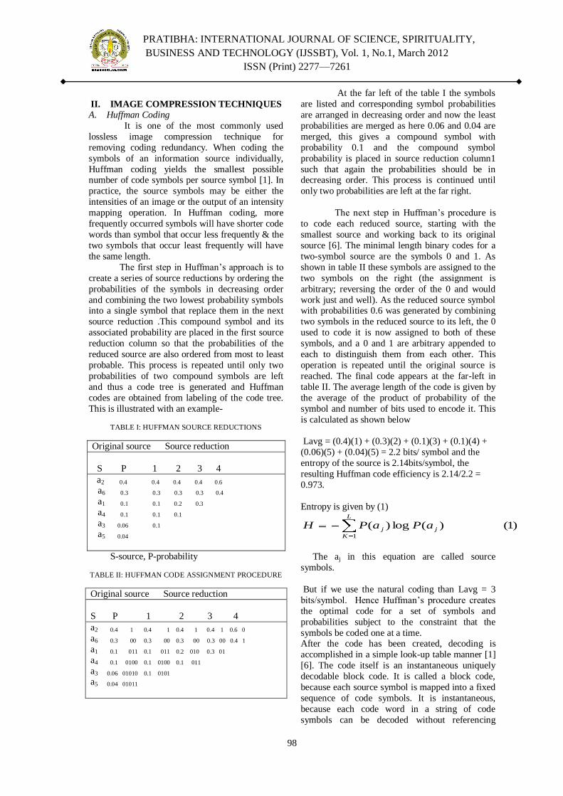
PRATIBHA: INTERNATIONAL JOURNAL OF SCIENCE, SPIRITUALITY,
BUSINESS AND TECHNOLOGY (IJSSBT), Vol. 1, No.1, March 2012
ISSN (Print) 2277—7261
98
II. IMAGE COMPRESSION TECHNIQUES
A. Huffman Coding
It is one of the most commonly used
lossless image compression technique for
removing coding redundancy. When coding the
symbols of an information source individually,
Huffman coding yields the smallest possible number of code symbols per source symbol [1]. In
practice, the source symbols may be either the
intensities of an image or the output of an intensity
mapping operation. In Huffman coding, more
frequently occurred symbols will have shorter code
words than symbol that occur less frequently & the
two symbols that occur least frequently will have
the same length.
The first step in Huffman‘s approach is to
create a series of source reductions by ordering the
probabilities of the symbols in decreasing order
and combining the two lowest probability symbols into a single symbol that replace them in the next
source reduction .This compound symbol and its
associated probability are placed in the first source
reduction column so that the probabilities of the
reduced source are also ordered from most to least
probable. This process is repeated until only two
probabilities of two compound symbols are left
and thus a code tree is generated and Huffman
codes are obtained from labeling of the code tree.
This is illustrated with an example-
TABLE I: HUFFMAN SOURCE REDUCTIONS
Original source Source reduction
S P 1 2 3 4
a2 0.4 0.4 0.4 0.4 0.6 a6 0.3 0.3 0.3 0.3 0.4
a1 0.1 0.1 0.2 0.3
a4 0.1 0.1 0.1
a3 0.06 0.1
a5 0.04
S-source, P-probability
TABLE II: HUFFMAN CODE ASSIGNMENT PROCEDURE
Original source Source reduction
S P 1 2 3 4
a2 0.4 1 0.4 1 0.4 1 0.4 1 0.6 0
a6 0.3 00 0.3 00 0.3 00 0.3 00 0.4 1
a1 0.1 011 0.1 011 0.2 010 0.3 01
a4 0.1 0100 0.1 0100 0.1 011
a3 0.06 01010 0.1 0101
a5 0.04 01011
At the far left of the table I the symbols
are listed and corresponding symbol probabilities
are arranged in decreasing order and now the least
probabilities are merged as here 0.06 and 0.04 are
merged, this gives a compound symbol with
probability 0.1 and the compound symbol
probability is placed in source reduction column1
such that again the probabilities should be in decreasing order. This process is continued until
only two probabilities are left at the far right.
The next step in Huffman‘s procedure is
to code each reduced source, starting with the
smallest source and working back to its original
source [6]. The minimal length binary codes for a
two-symbol source are the symbols 0 and 1. As
shown in table II these symbols are assigned to the
two symbols on the right (the assignment is
arbitrary; reversing the order of the 0 and would
work just and well). As the reduced source symbol with probabilities 0.6 was generated by combining
two symbols in the reduced source to its left, the 0
used to code it is now assigned to both of these
symbols, and a 0 and 1 are arbitrary appended to
each to distinguish them from each other. This
operation is repeated until the original source is
reached. The final code appears at the far-left in
table II. The average length of the code is given by
the average of the product of probability of the
symbol and number of bits used to encode it. This
is calculated as shown below
Lavg = (0.4)(1) + (0.3)(2) + (0.1)(3) + (0.1)(4) +
(0.06)(5) + (0.04)(5) = 2.2 bits/ symbol and the
entropy of the source is 2.14bits/symbol, the
resulting Huffman code efficiency is 2.14/2.2 =
0.973.
Entropy is given by (1)
)1()(log)(1
L
K
jj aPaPH
The aj in this equation are called source
symbols.
But if we use the natural coding than Lavg = 3
bits/symbol. Hence Huffman‘s procedure creates
the optimal code for a set of symbols and
probabilities subject to the constraint that the
symbols be coded one at a time. After the code has been created, decoding is
accomplished in a simple look-up table manner [1]
[6]. The code itself is an instantaneous uniquely
decodable block code. It is called a block code,
because each source symbol is mapped into a fixed
sequence of code symbols. It is instantaneous,
because each code word in a string of code
symbols can be decoded without referencing

PRATIBHA: INTERNATIONAL JOURNAL OF SCIENCE, SPIRITUALITY,
BUSINESS AND TECHNOLOGY (IJSSBT), Vol. 1, No.1, March 2012
ISSN (Print) 2277—7261
99
succeeding symbols. It is uniquely decodable,
because any string of code symbols can be
decoded in only one way. Thus, any string of
Huffman encoded symbols can be decoded by
examining the individual symbols of the string in a
left to right manner. For the binary code of table II,
a left-to-right scans of the encoded string
010100111100 reveals that the first valid code word is 01010, which is the code for symbol a3.
The next valid code is 011, which corresponds to
symbol a1. Valid code for the symbol a2 is 1, valid
code for the symbols a6 is 00. Continuing in this
manner reveals the completely decoded message a3
a1 a2a2 a6, so in this manner the original image or
data can be decompressed using Huffman
decoding.
1) Proposed Algorithm
The proposed algorithm is as mentioned.
1. Read the input image. 2. Convert the given color image into grey level
image.
3. Find the symbols (i.e. pixel value which is non-
repeated).
4. Calculate the probability of each symbol.
5. Probability of symbols are arranged in
decreasing order and lower probabilities are
merged and this step is continued until only two
probabilities are left and codes are assigned
according to rule that the highest probable symbol
will have a shorter length code. 6. Further Huffman encoding is performed i.e.
mapping of the code words to the corresponding
symbols will result in a compressed data.
7. The original image is reconstructed i.e.
decompression is done by using Huffman
decoding.
B. Discrete Cosine Transformation (DCT)
Currently the standard Discrete Cosine
Transformation (DCT) based algorithm of the
JPEG is the most widely used and accepted for image compression. It has excellent compaction
for highly correlated data. DCT separates images
into parts of different frequencies where less
important frequencies are discarded through
quantization and important frequencies are used to
retrieve the image during decompression [3].
Compared to other input dependent transforms,
DCT has many advantages: (1) It has been
implemented in single integrated circuit; (2) It has
the ability to pack most information in fewest
coefficients.
In DCT the quality of the processed
image is controlled by utilizing variable
quantization matrix. The quantization matrix level
varies from the range 1 to 100, where 1 gives the
poorest image quality and highest compression,
while 100 gives the best quality and lowest
compression. As a result quality to compression
ratio can be selected to meet different needs. JPEG committee suggests matrix with quality level 50 as
standard matrix. For obtaining quantization
matrices with other quality levels, scalar
multiplications of standard quantization matrix are
used. For a quality level greater than 50, the
standard quantization matrix is multiply by (100-
quality level)/50 & for a quality level less than 50,
the standard quantization matrix is multiply by
50/quality level [9]. Values of the scaled
quantization matrix are then rounded off & clipped
to have the positive integer values between 1
to255.
1) Proposed Algorithm
The proposed algorithm is as mentioned.
1. Read the input image.
2. The algorithm can be tested for gray and color
images.
3. The image is Level- shifted by subtracting 128
from each entry.
4. Check the dimensions of the input image as a
multiple of blocksize. If not padding is done .
5. The given image is divided into blocks of 8Х8.
6. Calculate DCT matrix.
7. DCT is applied to each block by multiplying the
each block with DCT matrix on the left and
transpose of DCT matrix on its right.
8. Each block is then compressed through
quantization.
Depending upon quality level, quantization
matrix is selected.
9. Encode the quantize coefficients in zigzag
sequences. 10. The array of compression blocks that constitute
the image is stored in a drastically reduced amount
of space.
11. The image is reconstructed through
decompression using Inverse-DCT.
12. Restore image to normal by Level-shift the
image back by adding 128 from ach entry & Clip
off padded rows and columns.
13 .Finally determine Image quality assessment
parameters.

PRATIBHA: INTERNATIONAL JOURNAL OF SCIENCE, SPIRITUALITY,
BUSINESS AND TECHNOLOGY (IJSSBT), Vol. 1, No.1, March 2012
ISSN (Print) 2277—7261
100
The 2-D DCT (2) shown computes the i, jth entry of the DCT of an image.
)2(2
)12(cos
2
)12(cos),()()(
2
1
),(
1
0
1
0 N
iy
N
ixyxpjCiC
N
jiD
N
y
N
x
Where
01
02
1
)(
uif
uifuC
For the standard 8 X 8 block that JPEG compression uses, N equals 8 and x and y range from 0 to 7.
Hence D (i, j) would be as shown in (3)
)3(16
)12(cos
16
)12(cos),()()(
4
1
),(
1
0
1
0
iyixyxpjCiC
jiD
N
y
N
x
Since the DCT utilizes cosine functions , the resulting matrix depends on the horizontal, diagonal,
and vertical frequencies. Hence, an image block with a lot of change in frequency has a very random
looking resulting matrix, while an image matrix of just one color has a resulting matrix of a large value for
the first element and zeros for the other elements. To get the matrix form of (2), one must use the following equation shown in (4)
)4(
02
)12(cos
2
01
iifN
ij
N
iifN
T ji
The first row (i = 1) of the matrix has all the entries equals to 1/√8 as expected from above
equation.
The next step is to apply DCT to 8X8
block. The pixel values of 8×8 images range
from 0 to 255, where 0 is for pure black and pure
white is represented by 255. Thus, it can be seen
how a photo illustration and so on can be
accurately represented by these 256 shades of gray.
Now, let‘s start with DCT of a block
image-pixel values. This particular block was
chosen from the very upper left hand corner of an
image. Since an image comprises hundreds or even thousands of 8×8 blocks of pixels, the
following description for one 8×8 block is a part of
the JPEG process. As DCT is designed to work on
pixel values ranging from -128 to 127, the original
block is leveled off by subtracting 128 from every
entry & also checks the dimensions of the input
image as a multiple of block size. If dimensions of
the input image are not a multiple of block size,
padding is done .This results in the generation of
matrix ‗M‘ given by (5).
)5('TMTD
Here matrix ‗M‘ is first multiplied by the DCT
matrix ‗T‘ on the left, this transforms the rows.
The columns are then transformed by multiplying
by the transpose of the DCT matrix on the right.
This yields the matrix ‗D‘. This block matrix now
consists of 64-DCT co-efficient, Cij, where i and j
range from 0 to 7. The top-left co-efficient, C00,
correlates to the low frequencies of the original
image block which contain the important image information. As one moves away from C00 in all
the directions, the DCT correlate to higher and
higher frequencies of the image block, where C77
corresponds to the highest frequency. These high-
frequency coefficients contain the less-important
image information. It is significant to note that the
human eye is most sensitive to low frequencies,
and results from the quantization step will reflect
the said fact.
After the transformation, quantization is carried
out by dividing transformed image matrix by the

PRATIBHA: INTERNATIONAL JOURNAL OF SCIENCE, SPIRITUALITY,
BUSINESS AND TECHNOLOGY (IJSSBT), Vol. 1, No.1, March 2012
ISSN (Print) 2277—7261
101
quantization matrix & rounding to the nearest
integer value. Mathematically it is given by (6).
)6(),(
),(),(
jiQ
jiDroundjiC
It allows varying levels of image
compression and quality through selection of
specific quantization matrices. JPEG committee
suggests matrix with quantization level 50 as
standard matrix [8].
99 103 100 112 98 95 92 72
101 120 121 103 87 78 64 49
92 113 104 81 64 55 35 24
77 103 109 68 56 37 22 18
62 80 87 51 29 22 17 14
56 69 57 40 24 16 13 14
55 60 58 26 19 14 12 12
61 51 40 24 16 10 11 16
50Q
After quantization, only the few low frequency
coefficients have significant values while most of
the high frequency coefficients have zero values.
In addition, the zeros representing the less
important higher frequencies that have been
discarded, giving rise to the lossy part of
compression & only the remaining non-zero co-
efficient will be used to reconstruct the image.
Fig 1: Zigzag Sequence
If we use different quantization matrices than
use of Q10 would gives C significantly more zeros,
while Q90 would result in very few zeros. After
quantization most of the coefficients have zero
values. JPEG takes advantage of this by encoding
quantized coefficients in zigzag sequence as shown
in figure 1.This zigzag process helps entropy
coding by placing low-frequency coefficients
(usually larger values) before the high-frequency
coefficients (usually close to zero).
The original image is reconstructed using
decompression technique. For that initially element
of C is multiply by the corresponding element of quantization matrix using (7) shown below.
R (i, j) = Q (i, j) X C (i, j) (7)
The IDCT is next applied to matrix R, which is
rounded to the nearest integer. Also 128 is added
to each element of that result.
N=round (T‘RT) + 128 (8)
Finally Clip off padded rows and columns if
padding is done, giving the decompressed version of original 8 Х 8 image block M.
C. Discrete Wavelet Transform (DWT)
Wavelet Transform has become an
important method for image compression. Wavelet
based coding provides substantial improvement in
picture quality at high compression ratios mainly
due to better energy compaction property of
wavelet transforms. In previous section, DCT
transform the original pixels into a few large numbers and many small numbers. In contrast, the
wavelet transforms of this section decompose an
image into bands (regions or subbands) that
correspond to different pixel frequencies.
Fig 2: 1 level decomposition
Discrete wavelet transform (DWT ) maps an image into a set of coefficients that constitute a
multiscale representation of the image [1]. Discrete
Wavelet Transform (DWT) of a signal is computed
by passing it through a series of filters and down
samplers. This wavelet filters are designed so that
the coefficients in each subband are almost
uncorrelated from the coefficients in other
subbands. In DWT First the samples are passed
through a low pass filter with impulse response
g(n) giving approximation or average coefficients.
The signal is decomposed simultaneously using a

PRATIBHA: INTERNATIONAL JOURNAL OF SCIENCE, SPIRITUALITY,
BUSINESS AND TECHNOLOGY (IJSSBT), Vol. 1, No.1, March 2012
ISSN (Print) 2277—7261
102
high pass filter h(n), giving the detailed
coefficients. Approximation is high scale, low
frequency components of the signal. The details
are low scale, high frequency components of the
signal. Since half the frequencies of the signal are
removed, the filter outputs are down sampled by 2.
This constitutes 1 level of decomposition as shown
in above figure 2.
Like the one dimensional discrete wavelet
transform, the two-dimensional DWT can be
implemented using digital filter and down
samplers. Initially each row is filtered and then
down sampled to obtain two subbands images.
Then each column is filtered and down sampled to
obtain four subbands images. The four subbands
created are named as LL, LH, HL and HH, where
the first letter corresponds to the filter applied to
the rows, and the second letter corresponds to the
filter applied to the columns. Here in the two-dimensional case, LL represents approximation
coefficients while LH, HL and HH represent
horizontal, vertical and diagonal detail coefficients.
After first level of decomposition, the
Approximation subband LL is then decomposed
into four subbands at level two as shown in figure
4 and the process can be continued in the same
manner for further levels. Reconstruction can be
obtained from the approximation subband LL only.
Thus the wavelet structure has potential for the
image compression which is extensively used in JPEG 2000 standard [2][10].
The DWT scheme decomposed image
into approximate & detail coefficients. After
decomposition aside from quantizing away small
coefficient, the next step is how to code the
wavelet coefficients. The Embedded Zerotree
Wavelet algorithm popularly known as EZW is an
efficient coding scheme developed by Shapiro
[3].It is an efficient coding scheme based on the
multi-resolution nature of wavelet transforms. The resulting algorithm gave a better performance at
higher compression ratio than the existing
schemes. This scheme efficiently exploits the
parent-child relationship of the DWT coefficients
to code and compress them efficiently.
LL1
HL1
LH1
HH1
Fig 3: First stage of Discrete wavelet transform
LL2
HL2
HL1
LH2 HH2
LH1
HH1
Fig 4: A two-scale wavelet decomposition
The two important features of the EZW coding are
significance map coding and successive
approximation quantization. The coding of the
significance map is achieved using a new data
structure known as zerotree. Figure 5 shows
pictorial representation of the zerotree on 3-stage
wavelet decomposition.
Fig5: Zerotree scanning for encoding significance map
The coefficient at coarse scale is called the parent
while all corresponding coefficients at next finer
scale of same spatial location and similar
orientation are called children. For a given parent,
the set of all coefficients at all finer scale are called
descendants. Similarly for a given child, the set of
all coefficients at all coarser scale are called ascentors. The scanning of the coefficients is
performed in such a way that no child is scanned
before its parent [3] [4].
In EZW initially a threshold level is
selected. Depending upon a threshold level,
significance map of symbols will be generated to
indicate the significance of the coefficients.
Usually, a 4-symbol alphabet (ZTR, IZ, POS, and
NEG) is used to represent the significance map.
The four symbols are:
1) zerotree (ZTR),which means the coefficient and all its descendants are insignificant;
2) isolated zero (IZ), which means that the
coefficient is insignificant but has some significant
descendants;
3) positive significant(POS), which means a
positive significant coefficient;

PRATIBHA: INTERNATIONAL JOURNAL OF SCIENCE, SPIRITUALITY,
BUSINESS AND TECHNOLOGY (IJSSBT), Vol. 1, No.1, March 2012
ISSN (Print) 2277—7261
103
4) negative significant(NEG), which means a
negative significant coefficient.
After significance mapping, Embedded
coding is achieved using successive approximation
quantization (SAQ) method. The SAQ method
sequentially applies a sequence of thresholds T0,
……, TN-1 to determine the significance of each coefficient . The threshold are chosen such that Ti=
Ti-1/2. The initial threshold are chosen such that |xj|
< 2T0 [3].A dominant list and a subordinate list are
maintained during encoding and decoding process.
During a dominant pass, coefficients having their
coordinates on the dominant list are compared to
threshold Ti to determine their significance. If a
coefficient is found to be significant, its magnitude
is appended to the subordinate list and the
coefficient in the wavelet transform array is set to
zero to enable the possibility of zerotree occurring
on future dominant passes at smaller thresholds. The resulting significance map is zerotree-coded.
The dominant pass is followed by
subordinate pass .All coefficients on the
subordinate list are scanned and their magnitude is
refined. Effectively, the width of the uncertainty
interval for the true magnitude of the coefficients
is cut in half. For each magnitude on the
subordinate list, the refinement can be encoded
using a binary value with a 1 indicating that the
true value falls in the upper half of the uncertainty
interval and 0 indicating that it falls in the lower half. After the subordinate pass, the magnitudes of
the subordinate list are sorted in decreasing order
to the extent that decoder can perform the same
sort. The process continues to alternate between
the two passes, with the threshold halved before
each dominant pass. The encoding stops when
some target stopping criterion has been met.
1) Proposed Algorithm
The proposed algorithm is as follows:-
1. Read the input image. 2. Define the wavelet decomposition level and also
type of wavelet (either Haar or biorthogonal
wavelet) used.
3. Computes four filters associated with the
selected wavelet.
4. Decomposes the input image into subbands
using DWT at different level .
5. At each level of decomposition, determine it‘s
approximate & detail (horizontal, vertical and
diagonal ) coefficients.
6. Define the initial threshold level & encode the
Wavelet coefficients using EZW. 7. EZW decoding is than done to reconstruct the
original input coefficients .
8. The image is reconstructed through
decompression using Inverse- DWT.
9. Finally Determine Image quality assessment
parameters.
D. Block Truncation Coding
Quantization is an important technique for
image compression. Any quantization method should be based on a principle that determines
what data items to quantize and by how much[5].
This technique uses a one bit nonparametric
quantizer. The principle used by the block
truncation coding (BTC) method and its variants
is to quantize pixels in an image while preserving
the first two statistical moments. In the basic BTC
method, the image is divided into blocks (normally
4×4 or 8×8pixels each) .After dividing the picture
into blocks, the blocks are coded individually, each
into a two level signal[11]. The levels for each block are chosen such that the first two sample
moments are preserved. Assuming that a block
contains n pixels with intensities p1 through pn, the
first two moments are the mean and variance is
given by (9) & (11) shown below:
)9(1
1
n
i
ipn
p
And
101
1
22n
i
ipn
p
respectively. The standard deviation of the block is
1122 pp
The principle of the quantization is to select
three values, a threshold pthr, a high value p+, and a
low value p−. Each pixel is replaced by either p+
or p−, such that the first two moments of the new
pixels (i.e., their mean and variance) will be
identical to the original moments of the pixel
block. The rule of quantization is that a pixel pi is quantized to p+ if it is greater than the threshold,
and is quantized to p− if it is less than the
threshold. Thus,
thri
thri
i
ppifp
ppifpp
Intuitively, it is clear that the mean p is a good
choice for the threshold[5][11]. The high and low
values can be determined by writing equations that preserve the first two moments and solving them.
We denote by n+ the number of pixels in the

PRATIBHA: INTERNATIONAL JOURNAL OF SCIENCE, SPIRITUALITY,
BUSINESS AND TECHNOLOGY (IJSSBT), Vol. 1, No.1, March 2012
ISSN (Print) 2277—7261
104
current block that are greater than or equal to the
threshold. Similarly, n− stands for the number of
pixels that are smaller than the threshold. The sum
n+ + n− equals to the number of pixels n in the
block. Once the mean p has been computed, both
n+ and n− are easy to calculate. Preserving the first
two moments is expressed by (12) & (13).
12pnpnpn
13222 pnpnpn
Solving for p+ and p−:
n
npp
n
npp
Each block is then described by the values of p , σ
and bit plane consisting of 1's and 0's indicating
whether pixels are above or below pthr [11]. These
solutions are generally real numbers, but they have
to be rounded to the nearest integer, which implies
that the mean and variance of the quantized block
may be somewhat different from those of the
original block. In this type of coding techniques
the block boundaries are not visible in the reconstructed pictures.
The basic BTC method is simple and fast.
Its main drawback is the way it loses image
information, which is based on pixel intensities in
each block, and not on any properties of the human
visual system. This led many researchers to
develop enhanced and extended versions of the
basic BTC. The original BTC is based on the
principle of preserving the first two statistical
moments of a pixel block. The variant described
here changes this principle to preserving the first two absolute moments. The first absolute moment
is given by (14)
141
1
n
i
ia ppn
p
The high & low values can also be written as
)15(1
pp
i
i
pn
p
)16(1
pp
i
i
pn
p
The advantage of using a nonparametric
quantizer is that the quantizer formulation is
available in closed form; this greatly simplifies the
computational load. But One especially annoying
feature of the basic BTC is that straight edges in
the original image become jagged in the
reconstructed image.
1) Proposed Algorithm
The proposed algorithm is as mentioned.
1. Read the input image.
2. Define the block size. 3. The given image is divided in small no
overlapping blocks of size as mentioned above.
4. Determine mean value of each block & assign
threshold value is equal to the mean value.
5. Determine no. of pixels in the current block
having pi greater than pthr & also determine p+
value.
6. Determine no. of pixels in the current block
having pi less than pthr & also p- value.
7. A bit plane is constructed such that each pixel
location is coded as a ―1‖ or a ―0‖ depending on
whether that pixel is greater than pthr . 8. The bit plane and mean value are sent to the
receiver.
9. The picture block is reconstructed such that
mean value is preserved. That is, pixels in the bit
plane that are ―1‖ are set to ―p+‖ and the ―0‖ are
set to ―p-‖.
10. Finally Determine Image quality assessment
parameters.
III. SIMULATION RESULTS
The different image compression
schemes discussed and elaborated here are
simulated on MATLAB platform [2]. For
performance analysis purpose we looked at 3-
Standard Test Images. For lossless compression,
Huffman method provides CR of 1.2, 1.1 & 1.14
for the images named lena, cameraman & mandril
respectively. The result of huffman coding method
for cameraman is shown in figure 6.
For lossy compression DCT, DWT&
BTC methods are discussed & compared. The compression efficiency is measured using the CR.
The quality of the image is analyzed by measuring
PSNR and RMSE. SSIM index is a method for
measuring the similarity between two images [12].
The variable quantization DCT technique when
applied to the images will generate variable PSNR
with compression. For instance, DCT application
to lena image produces the PSNR of 27.25, 31.98,
39.06 and CR of 11.33, 6.42, 6.09 corresponding
to Q10, Q50 and Q90 respectively. Fig. 7 shows
the application of DCT algorithm to image, which
in turn consists of original input image with reconstructed images using three different
quantization levels Q10, Q50 and Q90. Table III
represents performance summary of DCT
algorithm to the images, and Table IV represents

PRATIBHA: INTERNATIONAL JOURNAL OF SCIENCE, SPIRITUALITY,
BUSINESS AND TECHNOLOGY (IJSSBT), Vol. 1, No.1, March 2012
ISSN (Print) 2277—7261
105
performance summary of DWT algorithm. If we
consider only PSNR values we can observe that
DWT algorithm provides better image quality than
DCT algorithm and if we consider CR, it provide
the high compression than DCT. The DWT
algorithm results better quality of reconstructed
image than the DCT at high compression ratio
because of the artifacts resulting from the block
based DCT scheme as shown in figure 8. From fig
9 we observed that the edges of the reconstructed
image are blurred but smooth in DCT while edges
are sharp but ragged in BTC. Hence in BTC we get
the artifacts but it is different from artifacts in
DCT.
Original Image Reconstructed Image
CR = 1.14 Fig 6: Image Compression results of Huffman Technique
Original image Reconstructed Image (Q10)
CR =11.33, PSNR =27.25
Reconstructed Image (Q50) Reconstructed Image (Q90)
CR =6.42, PSNR =31.98 CR =6.09, PSNR =39.06
Fig 7: Application of Discrete Cosine Transformation to image with Q10, Q50 and Q90

PRATIBHA: INTERNATIONAL JOURNAL OF SCIENCE, SPIRITUALITY,
BUSINESS AND TECHNOLOGY (IJSSBT), Vol. 1, No.1, March 2012
ISSN (Print) 2277—7261
106
Original image Reconstructed image - DCT Reconstructed image - DWT
Fig 8: Image Compression results of Discrete Cosine Transformation and Discrete Wavelet Transform
Original image Reconstructed image - DCT Reconstructed image - BTC
Fi
Fig9: Image Compression results of Discrete Cosine Transformation and Block Truncation Coding
TABLE III: PERFORMANCE SUMMARY OF DCT ALGORITHM
Image CR PSNR RMSE MSSIM
lena (256x256)
6.09 39.46 2.71 0.94
7.43 38.13 3.15 0.91
11.35 35.83 4.12 0.88
Cameraman (512x512)
7.33 48.70 0.93 0.98
13.66 43.32 1.74 0.96
21.3 40.00 2.54 0.94
Mandril (512x512)
4.99 41.61 2.11 0.97
8.41 35.88 4.09 0.91
14.96 32.82 5.82 0.82

PRATIBHA: INTERNATIONAL JOURNAL OF SCIENCE, SPIRITUALITY,
BUSINESS AND TECHNOLOGY (IJSSBT), Vol. 1, No.1, March 2012
ISSN (Print) 2277—7261
107
TABLE IV: PERFORMANCE SUMMARY OF DCT ALGORITHM
IV. CONCLUSION
The various image compression techniques
compared and contrasted here reveals that images can be substantially compressed as application
demands. Lossless method of image compression
is mostly used to compress medical images where
loss of data result in mislead in the diagnosis while
lossy method is mostly used to compress photo
graphics images . In an image as the redundant
information gets added as more number of co-
efficients considered. This in turn increases the
computational time along with storage space
requirements.
In image compression technique we expect the
high compression ratio (CR) and also better quality of the reconstructed image. From the above results
we conclude that as CR increases, value of PSNR
decreases and RMSE increases. In DCT at high
compression ratio quality of image degrades due to
blocking artifacts. Hence at high compression
ratio DWT technique is used which gives the better
quality of the reconstructed image as compared to
DCT. Also in DCT reconstructed image have the
blurred but smooth edges .To get sharp edges BTC
technique is used which result in reconstructed
image having artifacts quite different from those produced by other techniques.
REFERENCES [1] R.C Gonzalez, R.E Woods, ―Digital Image Processing‖
(Third Edition), Pearson Education.
[2] R.C Gonzalez, R.E Woods, Steven L Eddins, ―Digital
Image Processing Using MATLAB‖, Pearson Education.
[3] Ze-Nian Li, Mark S. Drew, ―Fundamentals of
Multimedia‖, PHI Education.
[4] David Salomon, ―A Concise Introduction to Data
Compression‖, Springer_Verlag , 2008.
[5] David Salomon, ―Data Compression‖ (Fourth Edition),
Springer-Verlag London Limited, 2007.
[6] J. H.Pujar, L.M.Kadlaskar, ― A New Lossless Method of
Image Compression & Decompression using Huffman
Coding Techniques‖ Journal of Theoretical and
Applied Information Technology, Page No.1-nsformation,
Haar Transformation, Simultaneous Encryption and
Compression Techniques.‖ IEEE International
Conference on Digital Image Processing , Page No.1-6,
Nov 2009
[7] Mahendra M. Dixit1, Prof. Priyatamkumar, ―Comparative
Analysis of Variable Quantization DCT and Variable
Rank Matrix SVD Algorithms for Image Compression
Applications‖, IEEE International Conference, Page No.1-
5, 2010.
[8] Ken Cabeen & Peter Gent, ―Image Compression and the
Discrete Cosine Transform‖, Page No.1-11.
[9] Andrew B. Watson, ―Image Compression using the
Discrete Cosine Transform‖, NASA Research Center,
Page No.1-8.
[10] J. M. Shapiro, "Embedded image coding using zerotree of
wavelet coefficients‖, IEEE Transactions on Signal
Processing, Vol. 41, Page No.1 -18, Dec 1993.
[11] E.J. Delp & 0. Robert Mitchell, ―Image Compression
Using Block Truncation Coding IEEE Transactions on‖
Communication, Vol. 27,Page no 1 - 8 , September 1979.
[12] Zhou Wang , ―Image Quality Assessment: From Error
Visibility to Structural Similarity‖, IEEE Transactions on
Image Processing, Vol. 13, Page No.4, April 2004.
Image
Q
level CR PSNR RMSE MSSIM
lena (256x256)
90 6.09 39.06 2.83 0.96
50 6.42 31.98 6.41 0.9
10 11.33 27.25 11.06 0.78
Cameraman (512x512)
90 7.34 46.41 1.21 0.99
50 7.94 38.88 2.89 0.96
10 13.65 31.23 6.99 0.87
Mandril (512x512)
90 4.90 42.35 1.95 0.99
50 4.94 34.21 4.96 0.95
10 8.35 26.78 11.67 0.79

PRATIBHA: INTERNATIONAL JOURNAL OF SCIENCE, SPIRITUALITY,
BUSINESS AND TECHNOLOGY (IJSSBT), Vol. 1, No.1, March 2012
ISSN (Print) 2277—7261
108
Discrimination Between Atrial Fibrillation (AF) & Normal
Sinus Rhythm (NSR) Using Linear Parameters
Mayuri J. Patil1, Bharati K. Khadse
2, S. R. Suralkar
3
1,2,3Electronics and Telecommunication Dept. SSBT‘s COET Bambhori, Dist:Jalgaon. Emails: [email protected], [email protected], [email protected]
Abstract: Heart rate analysis method can be
used for discern between atrial fibrillation (AF)
and Normal Synus Rhythm (NSR). Atrial
fibrillation is one of the common sustained
cardiac arrhythmia diagnose by
electrocardiogram (ECG). The Heart rate
variability (HRV) and standard measurements
techniques are used to detect QRS Complexes
from ECG. All R peaks are detected for RR
intervals. Various parameters can be measured
using linear indexes of HRV like SDNN,
SDANN, RMSSD, PNN50, LF, HF, VLF etc. It
classifies NSR and AF patients using spectral
parameter LF/HF ratio.
Keywords: Heart rate, ECG, QRS complex, RR
interval, R peak
I. INTRODUCTION
One of the most common cardiac arrhythmias
is atrial fibrillation. In Europe alone, about 4.5
million people are affected [2]. The probable
prevalence is about 1% in the general population,
increasing with age. Above the age of 50, the
probability of developing atrial fibrillation doubles
with every decade of life [1].Because of
demographic expansion, the number of patients
with atrial fibrillation will increase in the future.
Atrial fibrillation has become a widespread disease
in industrialized countries. This supraventricular tachyarrhythmia is characterized by ungraceful
atrial commencement with the substantial decline
of atrial mechanical function and hemodynamic
devastation. Atrial fibrillation is not life aggressive
but the most dreaded impediment is embolism, and
strokes in particular. The rate of ischemic stroke
among patients with atrial fibrillation is two to
seven times higher than for people who don‘t
suffer from atrial fibrillation [2]. One out of six
ischemic strokes is caused by atrial fibrillation [1].
Unfortunately, AF remains under diagnosed, as it
is often asymptomatic: up to 30% of all patients with AF are unaware of their diagnosis [3]. Thus,
there are high risk patients, unaware of the disease.
Atrial fibrillation is typically diagnosed by
electrocardiogram (ECG). It is characterized by the
substitution of reliable P waves by express
oscillations or fibrillatory waves, associated with
an irregular and often too rapid ventricular
response when atrioventricular conduction is
intact. As atrial fibrillation is often intermittent, it
may not be detected on standard 12-lead ECG or
even on a 24-hour ECG recording (Holter). But it
is essential to identify these patients so that they
can be medicated. Ischemic strokes can then be prevented.
II. QRS DETECTION METHODOLOGY
QRS detectors can be divided in to two stages: a
filtering stage and a decision stage. The filtering
stage is used to emphasize the QRS complex and
to reduce noise and the influence of the other
waves in the ECG signal (P and T waves).
Typically first a bandpass filter is applied to the
signal to reduce noise and to suppress P and T waves and then put through a non-linear stage to
enhance the QRS complex. Then the QRS
enhanced signal is thresholded and some decision
logic is used for the final stage of detection.
Wavelet transformation has proven to be a very
efficient tool in the analysis of ECG signals. Its
ability to automatically remove noise and to cancel
out undesired fenomena such as baseline drift are a
benefit over other techniques. When an arrhythmia
appears, such a monitor can be programmed to
immediately store an interval of the abnormal ECG for subsequent conduction to a central station
where a physician can interpret it. Such a device
requires a very accurate QRS recognition
capability. False detection results in unnecessary
transmission of data to the central station or
requires an excessively large memory to store any
ECG segments that are unnecessarily captured.
Thus, an accurate QRS detector is an important part
of many ECG instruments. QRS detection is
difficult, not only because of the physiological
variability of the QRS complexes, but also because
of the various types of noise that can be present in the ECG signal.

PRATIBHA: INTERNATIONAL JOURNAL OF SCIENCE, SPIRITUALITY,
BUSINESS AND TECHNOLOGY (IJSSBT), Vol. 1, No.1, March 2012
ISSN (Print) 2277—7261
109
Figure.1 Block diagram of QRS detector algorithm
Noise sources include muscle noise,
artifacts due to electrode motion, power-line
involvement, baseline wander, and T waves with
high-frequency characteristics similar to QRS
complexes. In given approach, digital filters reduce
the influence of these noise sources, and thereby
improve the signal-to-noise ratio. Of the many
QRS detectors proposed in the literature, few give
serious enough concentration to noise reduction.
Software QRS detectors typically include
one or more of three different types of processing
steps: linear digital filtering, nonlinear
transformation, and decision rule algorithms [2].
Linear processes include a band pass filter, a
derivative, and a moving window integrator. The
nonlinear transformation that is used is signal
amplitude squaring. Applying thresholds provide
part of the decision rule algorithm.
Figure 2.A Output of QRS Detection Algorithm for NSR a) Original signal b) Filter output c) derivative output d)
squaring output e) averaging f) QRS detection
Figure 2.B Output of QRS Detection Algorithm for AF
a) Original signal b) Filter output c) derivative output d) squaring output e) averaging f) QRS detection
Fig. 2.A and Fig.2.B shows signals at
various steps in digital signal processing of Normal
Sinus Rhythm and Atrial fibrillation. A real-time
QRS detection algorithm was developed by Pan
and Tompkins [2].First, in order to ease noise, the
signal passes through a digital band pass filter
composed of cascaded high-pass and low-pass filters. Fig. 2.A.(b) shows the output of this filter.
The next process after filtering is differentiation
[Fig. 2.A.(c)], followed by squaring [Fig.2.A. (d)],
and then moving window integration [Fig.
2.A.(e)]. Information about the slope of the QRS is
obtained in the derivative stage. The squaring
process intensifies the slope of the frequency
response curve of the derivative and helps restrict
false positives caused by T waves with higher than
usual spectral energies. The moving window
integrator produces a signal that includes
information about both the slope and the width of the QRS complex. Fig. 2.A.(f) shows the final
output stream of pulses marking the locations of
the QRS complexes after application of the
adaptive thresholds.
Figure 3.RR interval time series for 10 min duration and
HRV signal
0 0.5 1 -500
0
500
a)original signal 0 0.5 1
-500
0
500
b) Filtered output
0 100 200 300 -200
0
200
c) Differentiate output 0 100 200 300
0
1
2 x 10 4
d)squaring output
0 0.5 1 0
5000
10000
e)averaging op 0 1 2 3
-1000
0
1000
f)QRS DETECTION
0 1 2 3 -500
0
500
a)original signal 0 1 2 3 -1000
0
1000
b)filtered output
0 100 200 300 -500
0
500
c)differentiate
0 100 200 300 0
1
2 x 10 5
d)squaring output
0 1 2 3 0
2 4 x 10 4
e)averaging op 0 2
4 6 -1000
0
1000
f)QRS DETECTION

PRATIBHA: INTERNATIONAL JOURNAL OF SCIENCE, SPIRITUALITY,
BUSINESS AND TECHNOLOGY (IJSSBT), Vol. 1, No.1, March 2012
ISSN (Print) 2277—7261
110
III. HEART RATE VARIABILITY
The distance between adjacent QRS
complexes is termed as the normal to normal (NN)
or the R to R (RR) intervals. Heart rate variability
(HRV) refers to the beat-to-beat alterations in heart
rate. Under inactive conditions, the ECG of healthy individuals exhibits periodic variation in R-R
intervals. The HRV measurements are captured
noninvasively from the ECG signal. The results
from this HRV data are capable of portraying
physiological condition of the patient and are an
important indicator of cardiac disease. Variability
in heart rate is clinically linked to lethal
arrhythmias, hypertension, coronary artery disease,
congestive heart failure, organ transplant,
tachycardia, neuropathy, and diabetes.There are
two methods in linear analysis time domain and
frequency domain analysis.
A. Time Domain Analysis
The easiest inference of HRV is portrayed
by the time domain measures. Originally, HRV
was measured manually from the mean R-R
interval in time domain and its standard deviation
measured on short-term 5 minute ECG segment.
With these methods either the heart rate or each
QRS complex or the RR intervals between
successive normal complexes are determined.
Simple time–domain variables include the mean RR interval, the mean heart rate, the difference
between maximum and minimum heart rate, etc.
Table I shows in detail the various time domain
HRV parameters [3].Recordings for a longer
period of 24 hours allow complex statistical time-
domain analysis. These statistical parameters may
be derived from direct measurements of the RR
intervals or from the differences between RR
intervals. The simplest variable to calculate is
square root of variance i.e. the standard deviation
of the NN interval (SDNN). Since variance is mathematically equal to total power under the
curve, SDNN covers complete variability in the
ECG recording.
;50501
1 countmsRRRRNNN
i
ii
;%100.50
50N
NNpNN
msmsmsRRRRN
SDNNN
i
i ,,;1
1
N
i
i
N msmsRRNN
RRRRRRR
1
1 ,;1.....2
N
i
ii msmsmsRRRRN
SDANN1
2
,,;1
1
1
2
1 ,,;1
1 N
i
ii msmsmsRRRRN
RMSSD
TABLE I. TIME DOMAIN HRV PARAMETERS
Variables Unit Description
Statistical measures
SDNN ms Standard deviation of all NN intervals
SDANN ms Standard deviation of averages of NN
intervals in all 5 min. segments of the
entire reading.
RMSSD ms The square root of mean of the sum of
the square of differences between
adjacent NN intervals
NN50
count
Number of pairs of adjacent NN
intervals differing by more than 50ms
in the entire recording
pNN50 % NN50 count divided by the total
number of all NN intervals
B. Frequency Domain Analysis:
In distinction to the time domain
measures of HRV mentioned above, recent
developments in microprocessor technology has
enabled the calculation of frequency measures on
the same ECG data. Frequency measures involve
the spectral analysis of HRV. The RR interval time
series is an irregularly time-sampled signal. This is
not an issue in time domain, but in the frequency-domain it has to be taken into account. If the
spectrum estimate is calculated from this
irregularly time-sampled signal, additional
harmonic components appear in the spectrum.
Therefore, the RR interval signal is usually
interpolated before the spectra analysis to recover
an evenly sampled signal from the irregularly
sampled event series. The HRV spectrum contains
the high frequency (0.18 to 0.4 Hz) component,
which is due to respiration and the low frequency
(0.04 to 0.15 Hz) component that appears due to
both the vagus and cardiac sympathetic nerves [3]. Ratio of the low-to-high frequency spectra is used
as an index of parasympathetic sympathetic
balance. Frequency domain HRV variables are
detailed in Table II [3]. In the frequency-domain
analysis power spectral density (PSD) of the RR
series is calculated. Methods for calculating the
PSD may be divided into Fast Fourier transform
(FFT) based and autoregressive (AR) model based
methods. The PSD is analyzed by calculating
powers and peak frequencies for different
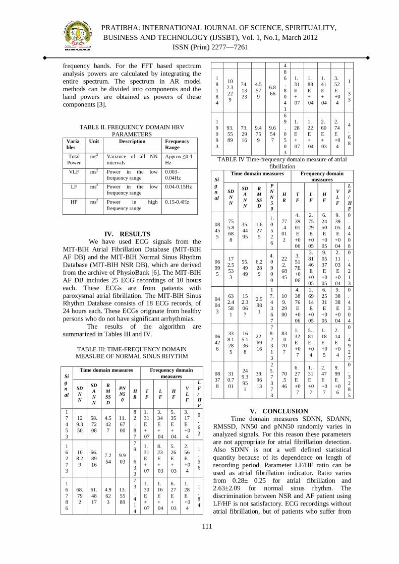
PRATIBHA: INTERNATIONAL JOURNAL OF SCIENCE, SPIRITUALITY,
BUSINESS AND TECHNOLOGY (IJSSBT), Vol. 1, No.1, March 2012
ISSN (Print) 2277—7261
111
frequency bands. For the FFT based spectrum
analysis powers are calculated by integrating the
entire spectrum. The spectrum in AR model
methods can be divided into components and the
band powers are obtained as powers of these
components [3].
TABLE II. FREQUENCY DOMAIN HRV
PARAMETERS Varia
bles
Unit Description Frequency
Range
Total
Power
ms2
Variance of all NN
intervals
Approx.≤0.4
Hz
VLF ms2 Power in the low
frequency range
0.003-
0.04Hz
LF ms2 Power in the low
frequency range
0.04-0.15Hz
HF ms2 Power in high
frequency range
0.15-0.4Hz
IV. RESULTS
We have used ECG signals from the
MIT-BIH Atrial Fibrillation Database (MIT-BIH
AF DB) and the MIT-BIH Normal Sinus Rhythm
Database (MIT-BIH NSR DB), which are derived
from the archive of PhysioBank [6]. The MIT-BIH
AF DB includes 25 ECG recordings of 10 hours
each. These ECGs are from patients with
paroxysmal atrial fibrillation. The MIT-BIH Sinus Rhythm Database consists of 18 ECG records, of
24 hours each. These ECGs originate from healthy
persons who do not have significant arrhythmias. The results of the algorithm are
summarized in Tables III and IV.
TABLE III: TIME-FREQUENCY DOMAIN MEASURE OF NORMAL SINUS RHYTHM
Si
g
n
al
Time domain measures Frequency domain
measures
SD
N
N
SD
A
N
N
R
M
SS
D
PN
N5
0
H
R
T
F
L
F
H
F
V
L
F
L
F
/
H
F
1
7
4
5
3
12
9.3
50
58.
72
08
4.5
42
7
11.
67
00
8
2
.
8
7
1.
31
E
+
07
3.
34
E
+
04
5.
35
E
+
04
3.
17
E
+0
4
0
.
6
2
1
6
2
7
3
10
8.2
9
66.
89
16
7.2
54
9.9
03
7
9
.
6
3
3
1.
31
E
+
07
8.
23
E
+
03
5.
26
E
+
03
2.
56
E
+0
4
1
.
5
6
1
6
7
8
6
68.
79
2
61.
48
17
4.9
62
3
13.
55
89
7
3
.
4
1
4
1.
30
E
+
07
1.
16
E
+
04
6.
27
E
+
03
1.
28
E
+0
4
1
.
8
4
4
1
8
1
8
4
10
2.3
22
9
74.
13
23
4.5
57
9
6.8
66
8
6
.
8
0
4
1
1.
31
E
+
07
1.
88
E
+
04
1.
41
E
+
04
3.
52
E
+0
4
1
.
3
3
1
9
0
9
3
93.
55
89
73.
29
16
9.4
75
9
9.6
54
7
6
9
.
0
5
0
3
1.
28
E
+
07
1.
22
E
+
04
2.
60
E
+
03
2.
74
E
+0
4
4
.
6
8
TABLE IV Time-frequency domain measure of atrial
fibrillation
Si
g
n
al
Time domain measures Frequency domain
measures
SD
N
N
SD
A
N
N
R
M
SS
D
P
N
N
5
0
H
R
T
F
L
F
H
F
V
L
F
L
F
/
H
F
08
45
5
75
5.8
68
8
35.
44
95
1.6
27
5
1.
0
5
2
6
77
.4
01
2
4.
39
01
E
+0
06
2.
75
29
E
+0
05
6.
24
50
E
+0
05
9.
39
05
E
+0
04
0
.
4
4
0
8
06
99
5
17
2.5
53
3
55.
49
49
6.2
28
9
4.
0
9
0
0
22
2.
68
45
3.
51
7E
+0
06
3.
81
46
E
+0
05
9.
05
37
E
+0
05
2.
11
03
E
+0
04
0
.
4
2
1
3
04
04
3
63
2.4
58
1
15
2.3
06
7
2.5
98
1
1
7.
4
3
6
7
10
9.
29
00
4.
38
76
E
+0
06
2.
69
14
E
+0
05
6.
25
31
E
+0
05
9.
38
38
E
+0
04
0
.
4
3
0
4
06
42
6
33
8.1
28
5
16
5.1
36
8
22.
69
16
7
8.
2
3
1
3
83
.0
70
7
1.
32
E
+0
7
5.
81
E
+0
4
1.
18
E
+0
5
2.
14
E
+0
4
0
.
4
9
2
7
08
37
8
31
0.7
01
24
9.3
95
1
39.
96
13
2
5.
7
3
7
3
70
.5
46
6.
27
E
+0
7
1.
31
E
+0
7
2.
47
E
+0
7
9.
99
E
+0
6
0
.
3
2
8
5
V. CONCLUSION
Time domain measures SDNN, SDANN,
RMSSD, NN50 and pNN50 randomly varies in
analyzed signals. For this reason these parameters
are not appropriate for atrial fibrillation detection.
Also SDNN is not a well defined statistical
quantity because of its dependence on length of
recording period. Parameter LF/HF ratio can be
used as atrial fibrillation indicator. Ratio varies
from 0.28± 0.25 for atrial fibrillation and 2.63±2.09 for normal sinus rhythm. The
discrimination between NSR and AF patient using
LF/HF is not satisfactory. ECG recordings without
atrial fibrillation, but of patients who suffer from

PRATIBHA: INTERNATIONAL JOURNAL OF SCIENCE, SPIRITUALITY,
BUSINESS AND TECHNOLOGY (IJSSBT), Vol. 1, No.1, March 2012
ISSN (Print) 2277—7261
112
atrial fibrillation, will be analyzed in more detail to
improve the algorithm. When the ECG recording
time is extended, the detection rate increases. But
this procedure is time-consuming for patients, as
well as for physicians, and even then, not all
patients will be identified . This algorithm allows
patients suffering from atrial fibrillation to be
identified in an easier and more convenient way.
REFERENCES [1] Patrick S. Hamilton and Willis J. Tompkins, ―Quantitative
investigation of QRS detection rules using the MIT-BIH
arrhythmia database‖ IEEE Trans. Biomed. Eng., vol.
BME-33, no. 12, pp. 1157-1165, 1986.
[2] J. Pan and W. J. Tompkins, "A real-time QRS detection
algorithm,"IEEE Trans. Biomed. Eng., vol. BME-32, no.
3, pp. 230-236, 1985.
[3] Dipali bansal,Munna khan,A.K.Salhan, ―A Review of
measurement and analysis of Heart Rate
variability‖Internation conference on computer and
automation Engineering.
[4] Task force of the European society of cardiology and the
North American society of spacing and electrophysiology.
―Heart rate variability: standards of measurement,
physiological interpretation and clinical
use”.Circulation,vol93,no.5,1043-1065,1996.
[5] European Heart Journal(1996) 17,354-381
[6] Database:- MIT-BIH Normal Sinus Rhythm & MIT-BIH
Atrial Fibrillation from www.physionet.org
[7] Fe smith, Ej bowers Langley, j Allen, A Murray medical
physics, Freeman hospital, Newcastle upon Tyne,UK
‗Heart rate variability characteristics required for
simulation of interval sequence‟.
[8] Gari D.Clifford St.Cross College ―Signal Processing
Methods For Heart Rate Variability‖.
[9] Rangaraj M. Rangayan ―Biomedical Signal Analysis, A
case-study approach‖.
[10] W.J.Tompkins, Ed.,‖Biomedical Digital Signal
processing‖.
[11] Nicole Kikillus, Gerd Hammer, Steven Wieland and
Armin Bolz,‖ Algorithm for Identifying Patients with
Paroxysmal Atrial Fibrillation without Appearance on the
ECG ‖Proceedings of the 29th Annual International
Conference of the IEEE EMBS Cité Internationale, Lyon,
France August 23-26, 2007.
[12] M. Brennan, M. Palaniswami*, and P. Kamen‖
Communications‖, IEEE Transactions On Biomedical
Engineering, Vol. 48, No. 11, November 2001.
