Pre-release Forecasting via Functional Shape Analysis

Of An Online Virtual Stock Market

Natasha Foutz and Wolfgang Jank ∗

* The authors are, respectively, Assistant Professor of Marketing (Email: nfoutz@rhsmith.umd.edu; Phone: 301.405.7229; Fax: 301.405.0146) and Associate Professor of Decision, Operations and Information Technology (Email: wjank@rhsmith.umd.edu; Phone: 301.405.1118; Fax: 301.405.8655), both at the Robert H. Smith School of Business, University of Maryland, College Park, MD 20742. The authors contributed equally to the paper and are listed in an alphabetical order. The authors thank Hollywood Stock Exchange, TNS Media Intelligence, and Nielsen EDI for generously providing managerial insights and the data used in this study. The authors also thank Anocha Aribarg, Chris Dellarocas, Michel Wedel, and participants at the 2007 DC Colloquium, DIT-Marketing Joint Luncheon, and 2007 ACM EC Prediction Market Workshop for their helpful comments.

Pre-release Forecasting via Functional Shape Analysis

Of An Online Virtual Stock Market

Abstract

Pre-release forecasting of demand for new products is crucial for allocating limited marketing

resources and is one of the most challenging tasks facing decision makers. To address this long-standing

challenge, many innovative approaches have been proposed in the past. Recently, the emergence of online

virtual stock markets (VSMs) has presented new opportunities for making dynamic and possibly more

accurate forecasts. In this study, we present a novel approach for analyzing VSMs, via functional shape

analysis (FSA). In essence, this novel approach characterizes important features of heterogeneous VSM price

histories using only a small number of distinguishing shapes (e.g. trending up or down; last-moment velocity

spurt). These shapes carry information about demand and provide accurate pre-release forecasts.

We illustrate our approach in the context of pre-release forecasting of release-weekend revenues of

motion pictures, and assess its performance using movie-by-movie cross validations. The results show that

while some of the methods traditionally used in movie forecasting can result in errors as high as 90.87%, the

proposed approach has an error of only 5.28%. It also improves over alternate methods (e.g. volume-

weighted-averages) for characterizing trading histories. These improvements persist, and magnify, when FSA

is applied to derive early forecasts, long before the product release. We also discuss interpretations of these

shapes and link them to existing Marketing theories, which may help decision makers identify indicators of

a potentially successful new product.

FSA of VSM introduces a novel and powerful pre-release forecasting tool to the Marketing literature.

It can be readily applied to forecasting demand for a variety of new products. This research also attempts

to demonstrate the increasing importance of virtual market data as a tool for Marketing research and

decision making, and functional data analysis as a novel technique useful for investigating a wide array of

Marketing questions.

Key words and phrases: Pre-release Forecasting; Innovation; Marketing Research; Entertainment Marketing; Motion Picture; Online Virtual Stock Market; Prediction Market; Trading Dynamics; Nonparametric Statistical Methods; Functional Shape Analysis; Functional Data Analysis; Smoothing; Functional Principal Component Analysis; Data Mining; E-commerce.

1

1. INTRODUCTION

Today’s businesses view innovations as the prime engine of growth. However, introductions of

innovative, and often short-lifecycle, products (e.g. motion pictures, music, video games) are confronted with

enormous financial stakes, highly uncertain demand, and alarming failure rates. To increase ROI, managers

need to make important marketing decisions (e.g. release timing, advertising, distribution) long before

releases, and subsequently adapt decisions given dynamic competitive and demand situations. Therefore,

there is great interest in deriving early, dynamic, and accurate pre-release demand forecasts to guide decision-

making. Such forecasts are particularly crucial for short-lifecycle products since their initial demand

comprises a large proportion of the overall demand.

Marketing researchers have long acknowledged the importance, and the difficulty, of pre-release forecasting

(Bass et al. 2001). To address this long-standing challenge, past studies have applied linear (Sawhney and

Eliashberg 1996) and non-linear (Ainslie, Drèze, and Zufryden 2005; Roberts and Urban 1988; Urban, Hauser,

and Roberts 1990) statistical methods to analyze, for example, historical demand of comparable new products and

cross-sectional product features (Bayus 1993; Sawhney and Eliashberg 1996; Bass et al. 2001; Lee, Boatwright,

and Kamakura 2003; Shugan and Mitra 2006), characteristics of innovative concepts or developers (Shugan and

Mitra 2006; Eliashberg, Hui, and Zhang 2007), demand for the same new product in other distribution channels

or geographical markets (Neelamegham and Chintagunta 1999; Bronnenberg and Sismeiro 2002), advance

purchase orders (Moe and Fader 2002), and consumer surveys and clinics (Bass et al. 2001; Eliashberg et al.

2000; Shugan and Swait 2000).

In recent years, marketers have become increasingly interested in harnessing the power of online

virtual games, or more generally, virtual communities (e.g. MySpace, Second Life) in marketing research and

decision-making (2006 – 2008 MSI Research Priorities). In particular, numerous online virtual stock markets

(VSMs) have been established to aggregate the wisdom of crowds (Surowiecki 2005) and forecast demand for a

large variety of new products. These include, but are not limited to, VSMs of motion pictures (HSX; IEM),

books (Media Predict; Simon & Schuster), software (Inkling); DVDs (Intrade), music albums (HSX), TV

shows (Inkling), video games and game consoles (SimExchange; Yahoo! Tech Buzz Game), disc drives

(StorageMarkets), MP3s, PDAs, and cell phones (Inkling). A rapidly increasing number of major corporations

(e.g. HP, Intel, Microsoft, Google, Yahoo, GE, Corning, Eli Lilly, and Goldman Sachs) are also establishing

internal or employee-only VSMs to forecast, for example, new product release timing and sales (e.g. Plott and

Chen 2002).

These online VSMs present new opportunities for deriving dynamic and possibly more accurate

forecasts. In this study, we present a novel approach for analyzing VSMs, via functional shape analysis

2

(FSA). In essence, this approach characterizes important features of heterogeneous VSM price histories using

only a small number of distinguishing shapes (e.g. trending up or down; last-moment velocity spurt). These

shapes carry information about demand and provide accurate pre-release forecasts.

We illustrate the approach in the context of forecasting of release-weekend revenues of motion

picture, and assess its performance using movie-by-movie cross validations. The results show that while some

of the methods traditionally used in movie forecasting can result in errors as high as 90.87%, the proposed

approach has an error of only 5.28%. It also improves over alternate methods (e.g. volume-weighted-

averages) for characterize trading histories. These improvements persist, and magnify, when FSA is applied to

derive early forecasts, long before the product release. We also discuss interpretations of the trading shapes

and link them to existing Marketing theories which can help decision makers identify indicators of a

potentially successful new product.

FSA of VSM introduces a novel and powerful pre-release forecasting tool to the Marketing literature.

It can be readily applied to forecasting demand for a variety of new products. This research also attempts

to demonstrate the increasing importance of virtual market data as a tool for Marketing research and

decision making, and functional data analysis as a novel technique useful for investigating a wide array of

Marketing questions (e.g. auction, click stream, WOM, and diffusion).

The rest of the paper unfolds as follows. In Section 2, we introduce key features and prior applications of

VSMs; and motivate our use of trading price histories in demand forecasting. In Section 3, we describe how FSA

of VSM can be used in pre-release forecasting. We apply our method to movie forecasting in Section 4 and

describe empirical findings and links with existing marketing theories. We conclude in Section 5.

2. ONLINE VIRTUAL STOCK MARKETS

Online VSMs (also known as prediction markets, betting exchanges, or idea futures) are increasingly

used to aggregate information from online communities and to forecast a wide range of events, e.g. presidential

elections, sports wins/losses, and more recently, demand for new products. For example, a stock is IPO-ed

when a new product development is publicized. The trading price at any time (e.g., $70 per share) reflects the

traders’ current, collective expectation of the initial demand for the product (e.g., $70m revenues). Similar to

real-life stock markets, new information about the product emerges over time and influences traders’ beliefs:

those who believe a higher demand (e.g., $80m), compared to the current trading price, tend to buy, with real or

endowed play money1, and those who believe otherwise sell or short. Traders may buy, sell, or short at any time; 1 Examples of online VSMs that use real money include the IEM, TradeSports, Intrade, Betfair, Foresight Exchange, HedgeStreet, etc. And examples of those using play money include HSX, NewsFutures, ProTrade Sports, Inkling, Yahoo! Tech Buzz Game, etc.

3

and the winning (if bought low and sold high) and losing amount (if otherwise) is recorded in their personal

account with the online VSM. Trading often terminates when the new product is released. The liquidation price

of the stock equals the realized initial demand for the product.

Online VSMs have several features that make them desirable for forecasting purposes. For example,

they are dynamic in nature, as opposed to static when using, e.g., only characteristics of a product. The trading prices

continuously reflect the most updated forecast (Hanson 1999). They also circumvent the need to aggregate

individuals’ forecasts, since trading prices have aggregated all traders’ forecasts through the embedded trading

mechanism (Jeppesen and Molin 2003; Füller et al. 2006). Therefore, using VSMs alleviates sampling and

aggregation biases (Churchill and Iacobucci 2001) present in, e.g., surveys. Furthermore, they provide

monetary or nominal (e.g., self-pride) incentives to reward participants for active information discovery and

truthful information revelation, and as a result, produce high-quality forecasts. They also motivate participation

by providing an enjoyable and entertaining experience (Dahan et al. 2007). Finally, they can be readily

established2, and have instantaneous access to online participants worldwide. They are economic to implement

and maintain, as compared to repeated consumer clinics, and have almost zero marginal cost when including

additional players.

The most straightforward approach, when analyzing VSMs for forecasting purposes, is to use the

latest prices prior to new product releases. A number of studies3 report that these latest prices provide reliable

forecasts, regardless of whether real or play money is used, or any other specific design features of the VSMs

(e.g., Pennock et al. 2001; Gruca, Berg, and Cipriano 2003; Spann and Skiera 2003). While simple to

implement, these latest prices are not available when early marketing decisions (e.g. release timing) need to be

made. Furthermore, it is possible that price histories embed additional information that can improve forecast

accuracy. Cases in point are past behavioral research in both Marketing and Finance (e.g., Kahneman and

Tversky 1979; Camerer, Loewenstein, and Rabin 2003; Barberis and Thaler 2003) who have documented

human behavioral anomalies in a wide array of domains, e.g., stock trading (Johnson, Tellis, and Macinnis

2005) and product choices (Huang and Chen 2006). Several features of online VSMs and the experiential

nature of many short-lifecycle new products, invite one to postulate that VSMs are not efficient. That is, the

latest prices may not fully reflect all the relevant information about new products, and therefore price histories

may indeed contain valuable information to improve forecast accuracy.

2 A number of free software (e.g. FreeMarket, ideafutures, Zocalo) and commercial software (e.g. Prediction Trader by NewsFutures, Foresight Server by Consensus Point, and Virtual Specialist by HSX) are available for implementing and maintaining online VSMs. 3 Several studies (Rhode and Strumpf 2007; Hanson, Oprea, and Porter 2006) also provide evidence that online VSMs cannot be systematically manipulated beyond a short time period.

4

For example, the current (or latest) price may not immediately or fully incorporate all the available

information, due to the delay in information flow from a few industry insiders who are knowledgeable about

the new product, to a large number of novices or less knowledgeable traders. Information cascade may also

lead to herd behavior (Hanson and Putler 1996; Dholakia and Soltysinski 2001; Huang and Chen 2006), as

individuals inevitably learn from others about the potential demand for the (often experiential) new product.

Even if information immediately diffuses to every individual, individuals may not act (e.g., trade)

immediately upon the information, or may not interpret the information properly and act accordingly. Since it

is difficult to evaluate new products (e.g. movies, books, music, TV shows) prior to releases due to their

experiential nature, individuals may either over- or under- react to pre-release information about the product

(De Bondt and Thaler 1985). Past research (e.g., Johnson and Tellis 2005; Johnson, Tellis, and Macinnis

2005) has also documented that traders tend to dump past losers and buy past winners, thus leading to hyped-

up prices of winning stocks. Lastly, the maximum shares a trader may buy/sell often imposed by a VSM, also

leads to lower liquidity and lack of efficiency in these VSMs (Lamont and Thaler 2003; Ho and Chen 2007).

As we will demonstrate later, VSM trading prices (at least those of HSX) do not follow a random

walk (Malkiel 1973). And thus information embedded in the trading price histories may provide improved

forecasting accuracy of demand for new products. For example, a new product whose trading prices increase

very sharply towards the time of its release may generate more demand than one whose prices increase at a much

lower rate. The shape of that trading history (i.e., sharp increase) could be indicative of a last-moment hype

that may stimulate a much higher demand than what would have been predicted by the latest price alone. In

the next section, we will show how FSA discovers the most indicative shapes from the data.

3. FUNCTIONAL SHAPE ANALYSIS

FSA is housed within a more general framework of functional data analysis (FDA). In contrast to classical

statistics where the focus is on a sample of data points or vectors, FDA focuses on a sample of functional

observations (e.g., Ramsay and Silverman 2005), e.g., curves, images, or objects. While the methodological

efforts in this emerging field are rather strong (e.g. James and Sugar 2003 on functional clustering; James 2002 on

functional generalized linear models), little work has been done using FDA for forecasting. Interestingly, a growing

number of studies have successfully implemented FDA to address issues of interest to marketers, e.g. online

auctions (Jank and Shmueli 2006; Reddy and Dass 2006; Wang, Jank, and Shmueli 2007), advertising (Elpers,

Wedel, and Pieters 2003), open source development (Stewart, Darcy, and Daniel 2006), and penetration curves

(Sood, James, and Tellis 2007). Our research of using FDA to analyze VSMs contributes to the functional

forecasting area, and introduces FDA as a solution for another important topic in Marketing: pre-release

5

demand forecasting of new products.

In the following, we describe the three main steps of our approach. More details can be found in the

Appendices4. We first smooth the observed trading price histories using penalized smoothing splines (Ruppert,

Wand, and Carroll. 2003; see Appendix A for computational details and the Online Appendix for robustness to

different smoothing parameters). Smoothing eliminates noise from the raw data that might result from

recording-errors, system-errors, or simply random fluctuations over time. Furthermore, a smooth trading path

allows derivation of trading dynamics, captured by its first derivatives (i.e., trading velocities) and second

derivative (i.e., trading accelerations). As we will demonstrate in Section 4, trading dynamics are an important

element of our forecasting model.

Next, we employ Functional Principal Component Analysis (FPCA) to characterize heterogeneous price

histories across new product stocks with a small number of shapes. FPCA is a functional generalization of

ordinary principal component analysis (PCA) (Ramsay and Silverman 2005). While PCA operates on a set of

discrete data vectors, FPCA operates on continuous functional objects (e.g., trading paths). The goal of FPCA

(as of PCA) is to project the original data onto a new space of reduced, orthogonal dimensions. As a result, the

reduced dimensions (i.e., shapes in our context) characterize the most important patterns in the original

data, while preserving the majority of the data variation.

We outline the fundamentals of FPCA below and defer more details to Appendix B. To make the

discussion more concrete, let us assume for the moment that we have measurements of each trading path at

p discrete time points. Let 1( ,..., )s s snY y y= denote the [ n × p ] matrix consisting of n smooth trading

paths. Further decompose the [ p × p ] correlation matrix obtained from sY , : ( )sR Corr Y= , into TP PΛ ,

where Λ is a matrix of eigenvalues and 1 2[ , ,... ]TpP e e e= is the corresponding matrix of eigenvectors. In this

simplified example, each ie is a [1× p ] vector, but in reality ie is a continuous function in time, i.e.,

( )i ie e t= . We can think of each eigenvector ie as shape-defining characteristics. For instance, an

eigenvector may bring out the differences between the beginning and end trading prices. Alternatively, an

eigenvector may bring out the change in price (gradual/steep, convex/concave) between adjacent trading

4 Two related methods in the forecasting context are time series analysis and technical analysis. While time series analysis is typically concerned with the forecasting of a single univariate (or multivariate) sequence, our goal is to learn from shapes common across many sequences of heterogeneous trading price histories. Technical Analysis (TA) is a method of evaluating securities by analyzing statistics (e.g. past trading volume) generated by market activities. While both FSA and TA are built upon the premise that there is value in the trading history, they have quite different goals. TA intends to “beat the market” in the sense of determining the future market value or trend. In contrast, our method uses shapes of the trading path to predict an outside-market event (i.e. demand for a new product). Our method also differs from TA in that it provides an automated, data-driven approach for forecasting, while TA requires strong user input (e.g., in the form of which technical chart to use for analysis). Furthermore, while TA is typically applied to the entire trading history, and thus suffers the common criticism of being “too late”, we use FSA for early forecasting based on only partial history, as we will demonstrate in Section 4.4. Lastly, FSA can be applied to much broader non-financial contexts (e.g. auction; advertising).

6

periods. Each eigenvector ie captures iλ × 100% of the variability in sY , where iλ is the i th eigenvalue or the

i th diagonal element in Λ . The eigenvector corresponding to the largest eigenvalue is denoted as the first

principal component (PC). Similarly, the second PC is the eigenvector that corresponds to the second highest

eigenvalue, and so on. The common practice is to choose only those eigenvectors that correspond to the largest

eigenvalues (i.e., the most important shapes) that explain the highest percentage of variations in sY . By

discarding those eigenvectors that explain no or only a very small proportion of the variations, we capture the

most important characteristics of the observed data patterns without much loss of information.

Finally, we identify the key shapes using variable selection techniques (including correlation analysis

and step-wise regression) and forecast demand in a parametric model using only these key shapes.

One major appeal of our method is that it discovers the most relevant set of shapes in an automated, data-

driven fashion, and thus readily generalizes to a wide variety of different forecasting contexts and applications (e.g.

auctions; advertising; as discussed earlier). For example, as compared to past studies that characterize VSM price

histories using summary statistics, e.g. averages, volume weighted averages, or medians (Dahan et al. 2007;

Dahan, Soukhoroukova, and Spann 2007), FSA does not require heavy, subjective user input, e.g., about which

statistics to investigate, which may vary from one application to the next. Principal components are also not

limited to a particular class of shapes (e.g. linear, polynomial) and, as such, result in a very flexible set of shapes.

Another advantage of our method is that it relies on a minimal number of assumptions. Its main

assumption is that the underlying functional object is observed on a grid fine enough to reliably re-construct

the functional object. Our weekly trading prices spanning over a nearly one-year horizon are well-suited for

forecasting release week revenues of new products.

A third advantage of this method is that it automatically produces estimates of the trading dynamics,

e.g., the speed at which the trading price is changing. Dynamics, unlike summary statistics used in past

studies, are a novel concept in the context of forecasting models. They are important since they capture instant

changes in information dissemination (e.g., changes in the buzz or hype for a new product) that are typically

not entirely reflected by contemporaneous prices. We will later show how the inclusion of dynamics improves

forecast accuracy and leads to new insight about product success.

4. EMPIRICAL STUDY

4.1 Data Analysis

We illustrate our approach in the empirical context of pre-release forecasting of movie release-weekend

revenues. The $34 billion motion picture industry (Digital Entertainment Group 2006) has long identified pre-

release demand forecasting as one of the most crucial, yet challenging, tasks (Sawhney and Eliashberg 1996;

7

Eliashberg et al. 2000). To reap the costly investment of each film5, studios carefully select their marketing

actions (e.g. release timing, media buying, and distribution planning) during the pre-release period (Figure 1)

based on their forecast of demand, particularly demand from the release weekend. Release-weekend revenues

are crucial as they often account for nearly half of a movie’s overall theatrical revenues and provide a strong

signal, to studios, distributors, and audience, of a films’ revenue potential in subsequent channels, e.g., videos

and international releases.

----- Insert Figure 1 Here -----

Hollywood Stock Exchange (HSX) is the best-known motion picture VSM. Established in 1996, it has

attracted nearly 2 million users. Each user is initially endowed with two million Hollywood Dollars (H$2m),

and can increase personal net worth by strategically selecting and trading movie stocks (buying low and

selling high). Traders are further motivated by the opportunities to exchange virtual money for merchandise and

the honor to appear on the Leader Board, to actively search for information about the upcoming movies and

participate in HSX trading activities. The trading price (e.g., $70) at any time reflects traders’ collective

expectation of a movie’s first-four-weekend revenues (e.g., $70m). Trading is halted on the day (typically Friday)

of the movie’s wide release (to at least 650 domestic theaters). The price is adjusted Sunday midnight as the

release-weekend revenues times 2.86 and then trading is resumed. The stock is de-listed after the movie is

exhibited in theaters for four weekends. And the liquidation price equals the realized first-four-weekend

revenues.

Since most movies are released on Fridays, and trading on Fridays is considered as the most active and

representative, we obtain from HSX each Friday’s daily-high and daily-low prices for each movie, and use the

average of the two as a measure of the movie’s trading price for the week. After merging HSX data with

Nielsen EDI box office data and removing movies with less than 52 weeks of pre-release HSX trading, our final

sample consists of the last 52 weeks7 of pre-release trading prices of 262 movies released between December

5 Hollywood studios spent on average $65.8 million to produce, and $34.5 million to market, a film (U.S. Theatrical Market Statistics 2006); yet on average accrues only $32.7 million in box office revenues (US Entertainment Industry Market Statistics 2006). 6 2.8 is used since a movie’s first-four-weekend revenues are on average 2.8 times its release-weekend revenues. Please also see hsx.com for uses of other possible multipliers. 7 A balanced sample is a pre-requisite for FSA. We acknowledge this as a limitation of the method. We are hopeful, though, that as solutions for missing data evolve, our method will also become better applicable to unbalanced samples. Moreover, we use 52 weeks in order to allow for early forecasts of almost one year prior to release. Other lengths of pre-release trading periods are also admissible, depending on the specific contexts at hand. Finally, left-censoring the price histories (or using shorter trading histories) makes our result a more conservative representation of the predictive power of the VSM.

8

2003 and July 2005. We perform the Dickey-Fuller test8 (Dickey and Fuller 1979) and reject the null

hypothesis that trading prices follow a random walk (critical values = 2.51 without a drift and 1.55 with a

drift; both significant at .01 level). This result can be attributable to a number of reasons (see our earlier

discussion in Section 2). It also suggests that using trading price histories of this not-so-efficient market might

provide improved forecasting accuracy.

After smoothing the trading price histories (as the first step of our approach), we obtain smooth

trading paths. The shapes of these trading paths are considerably heterogeneous across movies (see Figure 2

for a few sample paths). For example, while prices increase towards the release week (i.e., week 0) for some

movies like AMITTYVILLE HORROR and MAN ON FIRE, they decrease for others like INTERMISSION and

THE MUDGE BOY. Trading histories for some, like ALEXANDER, display an overall concave shape, while for

others, like TORQUE, they display an overall convex shape. Also, the speed at which prices increase or decrease

differs greatly: particularly early on (WIN A DATE vs. PAYCHECK) or close to release (WIN A DATE vs.

ELEKTRA). For some movies, prices increase only gradually over time, e.g. AMITTYVILLE HORROR, but very

sharply for others, e.g. WHITE NOISE. As discussed in Section 2, these different trading shapes plausibly contain

important information about the potential demand, e.g. a last-moment hype surrounding a new product. Thus our

goal is to extract the most indicative shapes via FSA, and then use them for forecasting.

----- Insert Figure 2 Here -----

Figure 3 shows the percentage of data variability captured by the first few PCs of the trading paths,

velocities, and accelerations. We observe that the first PC of the trading path explains nearly 75% of the

variations; the second and third PCs also carry considerable information; and the higher-order PCs are

negligible. For the trading velocities and accelerations, the first five PCs capture most of the variability.

Therefore, we initially retain the first 3 PCs of the paths, the first 5 PCs of the velocities, and the first 5 PCs of

the accelerations.

----- Insert Figure 3 Here -----

To avoid visual cluttering, we display the first 3 PCs of the paths and velocities in Figure 4. To

provide better interpretations to these PCs, we introduce the concept of principal component scores (PCSs),

computed from the corresponding PCs. Recall that PCs rotate the original data onto a space where all data-

dimensions are orthogonal to one another. Therefore, each PC can be used as a weighting factor of the original

data. That is, if a component value is high (low), then the corresponding data point (i.e., trading price) receives

8 While a large number of prior studies, mainly from Finance, have focused on testing whether the Efficient Market Hypothesis (EMH; Fama 1970) holds, or whether the stock prices follow a random walk (Lo and Mackinlay 2002), our focus is on how to improve pre-release forecast accuracy via analyzing VSM prices, if they do not follow a random walk.

9

a large (small) weight. Similarly, principal component values with opposite signs (positive / negative) exhibit

weightings in opposite directions. To be more specific, the j th PCS for movie i , ijS , is the inner product of

movie i ’s trading path (or trading dynamics) 1( ,..., )s s si i ipy y y= (evaluated on a finite grid, see Appendix B) and

the jth PC, 1( ,..., )j j jpe e e= (evaluated on the same grid). For example, the first PCS for the first movie in our

data is defined as 11 11 11 1 1... .s sp pS y e y e= + + Note that while the PCs are common across all movies, the PCSs are

movie-specific and input into our forecasting model.

----- Insert Figures 4 and 5 Here -----

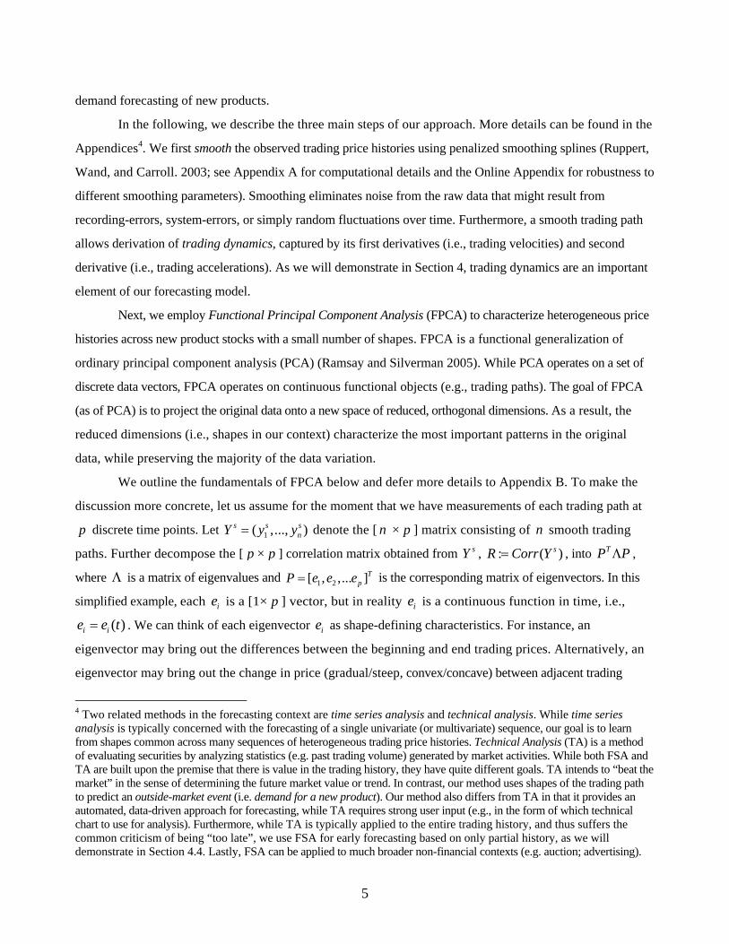
To better illustrate what these PCs (or shapes) in Figure 4 represent, we discuss three exemplary

movies in Figure 5. Notice that the first PC of the trading paths (the solid black line in the top panel of Figure

5), P.PC1, remains almost constant (and negative) over the entire trading period, and thus places almost equal

(and negative) weights on each data point (i.e., trading price) along the trading path. That is, P.PC1 captures

the difference in the 52-week-averages across movies: a movie with a relatively high (low) 52-week average has

a negative (positive) P.PCS1. For example, the 52-week-average is H$32 across all movies, H$27 for 13

GOING ON 30, H$84 for ALEXANDER, and H$47 for AMITYVILLE HORROR. Correspondingly, Figure 5

confirms that P.PCS1 (the black circle in the bottom left panel) is positive for 13 GOING ON 30, but negative

for AMITYVILLE HORROR, and most negative for ALEXANDER.

P.PC2 is negative in the first half (i.e., puts negative weights on early prices) and positive in the

second half (i.e., puts positive weights on late prices) of the trading period. It therefore captures the difference

between early and late prices: a movie with an upward (downward) trend results in a positive (negative)

P.PCS2. Similarly, P.PC3 captures the difference between the mid-term and early-late-average (ELA) prices: a

movie with a higher (lower) mid-term than ELA has a positive (negative) P.PCS3. An example of a higher

mid-term than ELA trading is a concave shape. Figure 5 confirms the difference in shapes for the three movies.

. Using similar rationale, V.PC1 emphasizes last-moment velocity spurts. It is essentially zero until the

end where it turns negative: thus a movie with a positive (negative) last-moment velocity spurt has a negative

(positive) V.PC2. Similarly, V.PC2 points to early velocity spurts: a movie with positive (negative) early

velocity spurts has a negative (positive) V.PC2. As we will show in the next section, these five PCs capture the

most significant variations in the trading price histories. We also provide discussion on how these shapes are

related to potential demand for new products in Section 4.3.

As the final step in our model, we employ variable selection techniques to retain, from the initial 13

candidate shapes, a smaller number of key shapes for prediction. Both correlation analysis and step-wise

regression choose to retain the same 5 shapes: P.PC1 (average), P.PC2 (early.late), P.PC3 (mid.ELA), V.PC1

(last-moment velocity spurt) and V.PC2 (early velocity spurt). We then use linear regression to link release-

10

weekend revenues to these 5 key shapes, or more precisely, their corresponding movie-specific PCSs9. We

evaluate the predictive performance using movie-by-movie, full cross-validations. That is, we hold out one

movie at a time, estimate the model on the remaining 261 movies, and then use the estimated parameters to

forecast the held-out movie’s release-weekend revenues10. Table 1 presents the Mean Absolutely Percentage

Error (MAPEs) of the proposed Model C1 and a set of alternate models. We will describe in Section 4.4 the

application of our method to early, partial price histories in deriving early and dynamic forecasts.

4.2 Model Comparison

Model A1 in Table 1 is based on the cross-sectional product features (i.e., movie characteristics) available

prior to release and traditionally used in pre-release forecasting (Sawhney and Eliashberg 1996). They include

genres (e.g., drama), sequel (yes/no), production budgets, MPAA ratings (e.g., PG-13), run time (or length of the

movie in minutes), and studios (e.g., Universal)11. Model A2 includes both product features and pre-release ad

spending12 (17 media, e.g. newspaper and TV, combined) during the last 10 pre-release weeks.

The second set of models use only the latest prices (B1), latest prices augmented with product features

(B2), and latest prices augmented with both product features and pre-release ads (B3). To unveil the contribution

of the trading dynamics, the proposed 5-shape model (C1) is compared with a model (C2) using only the 3 path

shapes (i.e., ignoring the dynamic information of the trading velocities V.PC1 and V.PC2). Model C1 is further

compared with a model using all 13 shapes (C3). To examine whether the proposed model can be further

9 Other models, e.g. log-log (Elberse and Eliashberg 2003), exponential (Krider and Weinberg 1998), or Poisson (Neelamegham and Chintagunta 1999) models were used to forecast weekly revenue decays. When forecasting release-weekend revenues, we also explored a log-linear model whose fit and prediction are worse than the linear model. 10 We also perform the same analysis forecasting the first-four-weekend revenues and report all relevant results in our Online Appendix. 11 Other movie characteristics (e.g. star salary) are not included as they are often correlated with e.g. production budget. We also estimate a number of additional models augmenting movie characteristics by distribution (number of screens), professional evaluations (critics ratings; Oscars), and audience evaluations (i.e. user ratings as reasonable proxies for pre-test audience response). The results (displayed in the Online Appendix) show that the forecast accuracy of these models improves over Models A1 and A2, nonetheless not sufficient to outperform the proposed Model C1 using only the 5 key shapes. In addition, given that U.S. movies are generally released to domestic theaters before any other channels (e.g. videos) or geographical markets (e.g. European countries), and that movie tickets are generally not purchased in advance, we will not compare our model with a model based on demand of the same product in other distribution channels or geographical markets (Neelamegham and Chintagunta 1999; Bronnenberg and Sismeiro 2002), or a model based on advance purchase orders (Moe and Fader 2002). Moreover, while we do not have access to consumer surveys and clinics data (Eliashberg et al. 2000), we believe the proposed approach can be advantageous and more economic when repeated and dynamic pre-release forecasts are needed for decision making. 12 Advertising for a movie often starts three to four months prior to its theatrical release, peaks at release, and rapidly diminishes after release. Across the 262 movies in our sample, 72.14% of the theatrical ad dollars were spent prior to releases. And the ads during the last 10 pre-release weeks, which are used in our model, account for 98.69% of the total pre-release ads. The Hausman specification test (Hausman 1978) rejects the hypothesis of endogeneity in the weekly pre-release advertising in our data.

11

improved, we augment the 5-shape model with product features (C4), pre-release ads (C5), both product features

and pre-release ads (C6), and the latest prices (C7).

To examine whether trading price histories can be captured equally well with summary statistics used in

prior studies (Dahan et al. 2007), or simple measures of trends (as opposed to the output from FSA), we estimate a

series of models using averages (D1), volume weighted averages (D2), medians (D3), averages and linear trend

(D4), and averages, linear trend, and nonlinear trend13 (D5). Yet another way to investigate the power of FSA is to

try and replicate the 5 key shapes from model C1 using simpler tools. To that end, we compute the 52-week

averages (avg.), the latest-minus-earliest prices (end.early), the week –25 price minus the latest-earliest-averages

(mid.ELA), the late spurt (as the slope of the linear trend over the demeaned prices from week –9 to week 0) and the

early spurt (as the slope of the linear trend over the demeaned prices from week –51 to week –42). This results in

model E1.

To provide further credibility to the variable selection approach and the linearity assumption of our model,

we estimate a CART (Classification And Regression Tree) and a GAM14 (Generalized Additive Model) on all 13

shapes, respectively (E2 and E3), and on the 5 shapes used in the proposed model (E4 and E5), respectively.

Table 1 displays the results15.

----- Insert Table 1 Here -----

The results show that Models A1 and A2 yield the highest forecast errors. Also, augmenting the latest

price with movie characteristics and ads does not reduce errors, which suggests that information contained in

movie characteristics and ads have been fully incorporated in the Latest Price16. The proposed Model C1

produces the lowest forecast errors (MAPE = 5.28) and reduces the error over the Model B1 using the latest

prices alone (MAPE = 10.35) by nearly 50%. As we will show in Section 4.4, when early forecasts are

13 The linear trend is the slope obtained by fitting a zero-intercept linear model on the 52 weekly demeaned trading prices. Similarly, the nonlinear trend is obtained by fitting a quadratic model after removing the means and linear trends from the 52 weekly trading prices. 14 CART models are often used in place of variable selection methods since they have built-in mechanisms to choose the most important predictors. Specifically, CART recursively partitions the data and builds separate models within each data-partition in a tree-like fashion. GAMs do not assume a strict functional relationship between the response and the predictors and therefore replace the restrictive linearity assumptions (as in the proposed Model C1) with a more flexible non-parametric form. 15 We also allow for movie-specific coefficients and then use Bayesian methods to estimate all the models from Table 1 that do not take advantage of cross-sectional information (i.e., through extracted key shapes). Overall, the results (displayed in the Online Appendix) show that shrinkage-based methods improve upon their frequentist counterparts; nonetheless, they do not outperform the proposed Model C1. It is also important to note that, from a practical point of view, Bayesian estimation takes a significantly longer amount of time to complete. Thus, if interest lies in real-time forecasts for dynamic, on-demand decisions, then our least-squares approach has a sizable edge. 16 To validate this, we also estimate Models B1 ~ B3 using all 262 movies. The coefficients for movie characteristics and ads are all insignificant. F-tests (F=1.45 and p-value = 0.07 for Model B2; F=1.19 and p-value = 0.22 for Model B3) cannot reject the null hypotheses that the coefficients for movie characteristics (for Model B2) and for movie characteristics and ads (for Model B3) are jointly zero.

12

required, the advantage of the proposed model over one using the latest prices is further magnified. In

light of the costly investment and low ROI of each movie, such improvement in forecast accuracy is sizeable

and managerially important for Hollywood studios in pre-release marketing planning (e.g. media purchasing,

theater booking, or contracting of movie-related merchandise like toys).

When removing the trading dynamics (i.e., V.PC1 and V.PC2) from the proposed Model C1, the

forecast accuracy is reduced considerably (Model C2). This suggests that the trading dynamics are an

important factor. We will take a closer look at this in the next section. We also notice that the proposed 5-

shape model outperforms the full 13-shape model, which points to the successful performance of our

variable selection technique. When augmenting the 5 shapes with movie characteristics, pre-release ads,

or the latest prices, the forecast errors increase, which is likely a result of model over-fitting (i.e., movie

characteristics, pre-release ads, or the latest prices do not capture any additional patterns in the data and,

as a consequence, fit noise).

Models D1 ~ D5 yield higher forecast errors than the proposed 5-shape model. This shows that

summary statistics (particularly without capturing any dynamics in the data) have limitations. Moreover,

as discussed earlier in Section 3, FSA automates the discovery of the most important patterns in the data,

and therefore not only eases the danger of leaving out important statistics, but also facilitates the ready

applications to alternate contexts. The results also show that while the measures used in Model E1 do not

perfectly replicate our 5-shape model, its forecast performance provides evidence that there is value in the

5 key shapes, even if constructed in a much simpler form. Finally, the proposed model outperforms all

CART models. One common criticism of CART is that it frequently over-fits data. The result also suggests that

our variable selection procedure is quite effective in identifying important predictors and rendering a

parsimonious, yet powerful, forecasting model. While Model C1 also outperforms the 13-shape GAM model

(E3), its performance is identical to the 5-shape GAM model (E5). We view this as evidence that the

relationships among the data are well-captured by our linear model.

To summarize, the proposed model using five key trading shapes identified via FSA provides better

pre-release forecasting than several alternate models that rely on conventional pre-release information, e.g., cross-

sectional product characteristics or pre-release ads. This model also accounts for information embedded in the

trading histories and thus outperforms a model that relies solely on the latest prices. As we will show later in

Section 4.4, the advantage of the proposed model over alternate models persists, and magnifies, when early

and dynamic forecasts are derived using early, partial trading price histories.

4.3 Parameter Estimates

13

Interpreting the coefficients in our forecasting model (Table 2) requires extra care since each PCS is a

linear combination of the information across the entire trading history. Recall from Section 4.1 that the larger

P.PCS1, P.PCS2, P.PCS3, V.PCS1, and V.PCS2, is, respectively, the lower the 52-week average, the steeper

the upward trend, the more concave the shape, and the smaller the last-moment velocity spurt, or the early

velocity spurt, is, respectively. Therefore, the significant coefficients of these predictors (Table 2) show that

higher 52-averages, steeper upward trends, and more rapid (and positive) last-moment and early price speeds

all are associated with higher release-weekend revenues. These indicators can be collectively used as

managers’ decision rules of thumb.

----- Insert Table 2 Here -----

To provide better understanding of how these key shapes are linked to demand for new products in

general (and not just movies), we provide some plausible theoretical interpretations below. The first shape

(P.PC1) reflects an overall appeal of a new product, relative to a myriad of many other available new

products. The average trading price of each new product stock accounts for information about, for example,

(i) individual traders’ preferences toward the new product (in terms of product characteristics, product-

consumer-fit, etc.), and their collective beliefs of other potential adopters’ preferences; (ii) the firm’s

marketing activities, e.g. distribution and advertising; and (iii) potential competition. Consider KINGDOM

OF HEAVEN and EULOGY (Figure 2) as an example. The former is traded at $H87.56 on average, whereas

the latter is traded at H$10.60. The large difference could result from the fans’ overwhelming affection

towards Orlando Bloom who stars in KINGDOM OF HEAVEN. It may also be attributable to much stronger

pre-release ad support ($31 million for KINGDOM OF HEAVEN vs. $0.2 million for EULOGY) that could

inform and persuade the public to view the movie. The same set of information (e.g. product features, adopter

preference, marketing effort, and competitive intensity) that influences the overall trading price (or demand

expectation) of a new product also influences the actual demand of the product at the time of its release

(Henard and Szymanski 2001). Also interestingly, notice that while P.PC1 appears almost constant over time,

its magnitude in fact slightly increases. This suggests that P.PC1 weighs recent information about the product

slightly higher than earlier information, consistent with the “recency effect” widely studied in the Behavioral

Marketing literature (e.g. Haugtvedt and Wegener 1994).

The second important shape (P.PC2) pertains to the inter-temporal sentiment toward this new

product. A positive (or upward), as opposed to a negative (or downward), sentiment contributes to new

product success, as plausibly explained by the well-known Prospect Theory (Kahneman and Tversky 1979).

According to this theory, a higher demand expectation early on and a lower one later, possibly as a result of

more negative information about the new product over time (e.g. insufficient supply; product flaws), leads to

14

“over-expectation” among traders and potential adopters in general. Therefore, “loss aversion” will possibly

dissuade more adopters from purchasing the product at the time of its release. This is also consistent with our

observation (Figure 4) that early on a relatively high trading price (or demand expectation) is weighted more

negatively, by P.PC2, than a relatively low price (or demand expectation). This is consistent with why many

firms are greatly interested in strategically managing pre-release expectations for their new products (Kopalle

and Lehmann 2004).

V.PC1 is related to the last-moment hype about the new product. “Marketing hype” is “a set of pre-

launch activities that lead to the creation of an environment conducive to the acceptance of new products”

(Wind and Mahajan 1987), including distribution, media, and opinion leaders. While marketing scholars have

long advocated for incorporation of marketing hype in new product forecasting models (Mahajan and Wind

1988), few have examined this issue. Our study shows that the speed of change in the trading price (or

demand expectations) in the last few weeks towards a new product’s release is a strong indicator of the

product’s early demand. A rapid change in the last-moment demand expectation is possibly indicative that (i)

the last-moment information about the new product (e.g., available through advertising or critics’ reviews)

rapidly disseminates across potential adopters; and (ii) the strength of preferences over, and beliefs of success

about, the new product, is high. Ultimately, these factors translate to faster adoption at the time of release. The

influence of such last-moment hype may also rationalize why firms from many industries of short-lifecycle

products often dramatically ramp up their ad spending towards the release time (Elberse and Anand 2007).

The last important shape, V.PC2, reflects the influence of early pre-announcement hype toward the

new product (or more precisely, new product concept). A stream of marketing research has demonstrated that

new product pre-announcements may cannibalize demand for existing products (Moorthy and Png 1992),

create pent-up demand and network externalities (Dranove and Gandal 2003), generate word-of-mouth

(Eliashberg and Robertson 1988), promote brand preference and perceptions of the new products (Lilly and

Walters 2000; Nagard-Assayag and Manceau 2001), and deter releases of rival products (Bayus, Jain, and

Rao 2001; Foutz and Kadiyali 2005). A rapid change in the demand expectations early on may indicate that

(i) information about the new product concept, or initial development, rapidly diffuses across potential

adopters; and (ii) the preference, or confidence, over this new product concept, or initial development, is

strong. Thus, we anticipate that V.PC2 could be correlated with, for example, (a) whether a movie is a sequel

(or more generally, an extension, or new generation, of a previously successful new product), and (b)

production budgets (which may lead to higher probability of NPD success). Indeed, the average V.PCS2 for

sequel movies is –2.89 (recall that a strong early velocity spurt is associated with a more negative V.PCS2)

15

and .37 for non-sequels. We also detect a fairly strong correlation of –.43 between V.PCS2 and production

budgets.

Besides our study, several other studies report similar shapes across a wide variety of domains. For

instance, Subramaniam, Varadhan and Crainiceanu (2006) discovered shapes similar to P.PC1 ~ P.PC3 in the

evolution of traffic across large corporate networks. Sood, James and Tellis (2007) identified a similar set of

shapes in the market penetration curves of 21 categories of new products across 70 countries. Therefore, it is

possible that these shapes can be generalized to other non-movie (or more broadly, non- new product) contexts.

Still, we encourage future research to validate these empirical findings and theoretical explanations in demand

forecasting of other new products (e.g. music, books, software, and MP3s). We believe such effort is also made

possible and catalyzed by the rapid emergence of many new product VSMs, and the increasing prominence of

virtual market data as an important marketing research tool.

4.4 Early and Dynamic Pre-release Forecasting

The results so far suggest that our model using the 5 key shapes is capable of yielding accurate

predictions. While this result is curious, it is not of most practical use since the proposed model (and others in

Table 1) utilizes information until the Friday prior to the product release (i.e., week 0). In reality, early (i.e.,

prior to week 0) and dynamic (i.e., incorporating newly arriving information on the fly) pre-release forecasts

are most valuable to managers since many marketing decisions for new products (Figure 1 as an example) need

to be made long before the actual release and need to be adaptive to changing competitive environments and

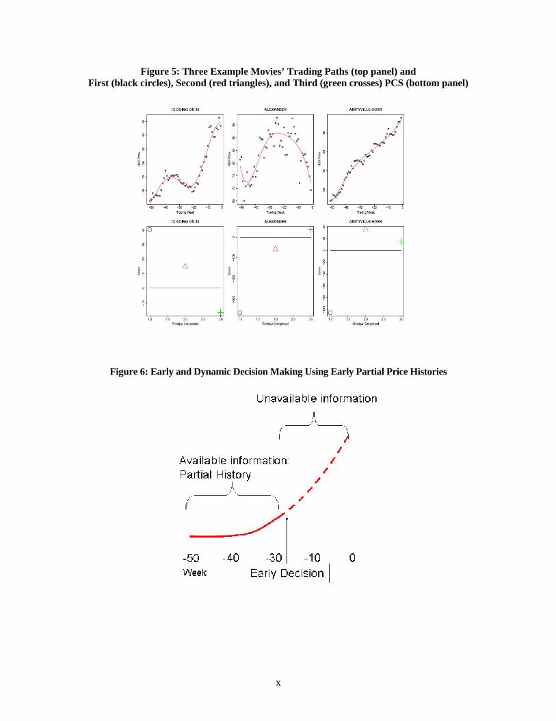
demand situations. One main advantage of our model is that it can be applied, readily and repeatedly, to early,

partial price histories. These early, partial price histories contain information available from early on (e.g. t =

week –51) until a desired decision time t (see Figure 6), which often occurs many weeks prior to the release

(e.g. t = week –40, or t = week –30).

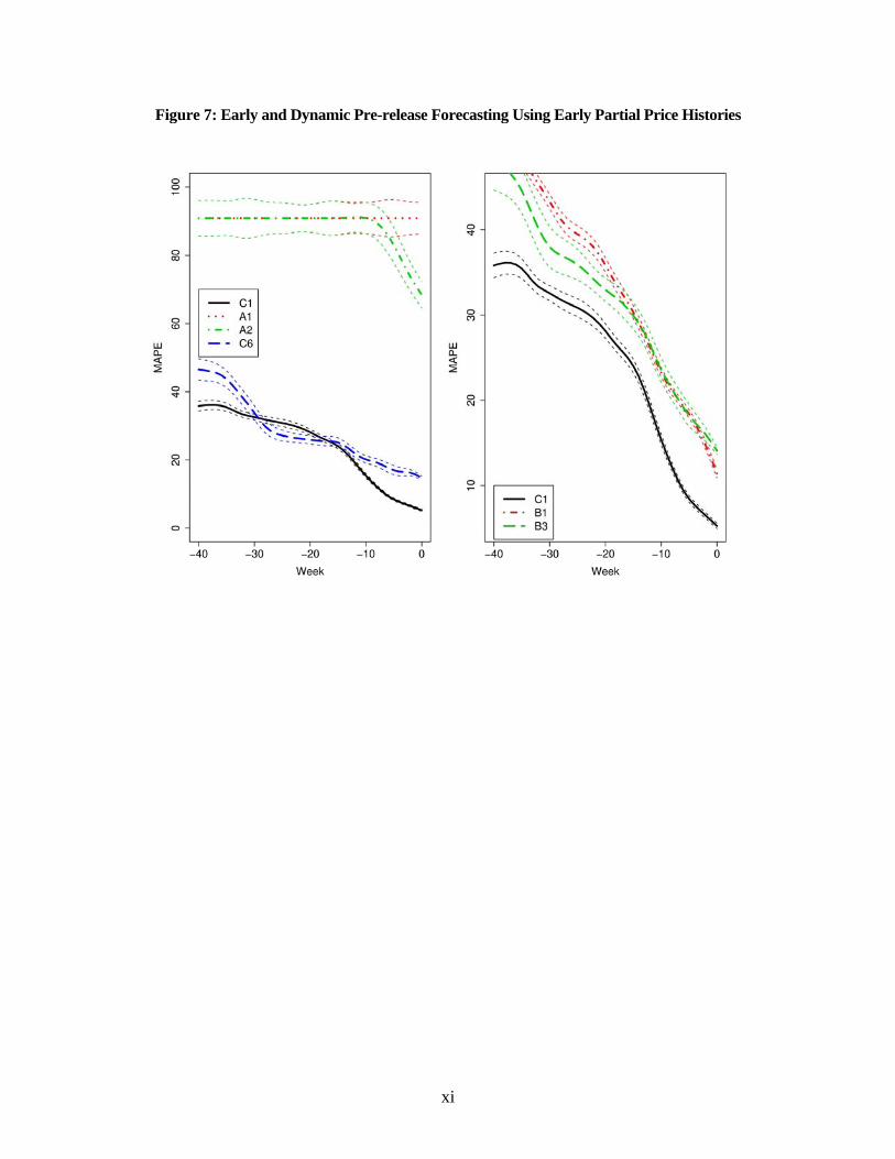
We analyze the partial price histories, producing early and dynamic forecasts at different decision

times, ranging from very early (t = –40) to very late (t = 0) using all models displayed in Table 1. To

avoid visual cluttering, we only show, in Figure 7, the resulting prediction accuracy (together with 95%

confidence bands) for the proposed model (C1) and those using product features and pre-release ads

(Models A1, A2, C6; left panel of Figure 7) and those using the latest price at any time t (Models B1 and

B3; right panel of Figure 7).

----- Insert Figures 6 and 7 Here -----

Overall, we see that, not surprisingly, managers can derive increasingly accurate forecasts (i.e.,

with reducing MAPEs) as more information becomes available over time (i.e., closer to week 0). The

16

forecast accuracy of the proposed model (C1) increases only gradually early on (e.g. week –40 to –15), but

rather rapidly thereafter. This indicates that the amount of information about new products increases at a

non-constant speed, especially when pre-release ads for the new products commence (also see Figure 1).

The left panel shows that Model A2, using both product characteristics and pre-release ads,

produces better forecast after ads commence, compared to the (static) Model A1 with only product

characteristics. Model C6, using product characteristics, pre-release ads, and 5 key shapes, significantly

improves Models A1 and A2 across all time periods. For a short period, it also provides slightly better

forecast than Model C1, but the improvement is only marginally significant. This suggests that much

information about the products is already reflected in the trading shapes, and thus adding such information

likely leads to model overfitting.

The right panel of Figure 7 shows that the proposed model (C1) significantly outperforms Model

B1 using only the latest prices. The discrepancy is particularly large early on (see also Table 3 for a

numerical comparison). It is also interesting to see that Model B3, which augments the latest prices with

product characteristics and pre-release ads, initially improves Model B1 using the latest prices alone. This

is in contrast to the left panel where Model C6 does not improve over C1. This provides more evidence

that while trading shapes account for most product-related information already early on, the latest prices

do not. Only as time progresses, does relevant information eventually get absorbed into the latest prices.

----- Insert Table 3 Here -----

Overall, the results show that the proposed model can provide early and dynamic forecasts

accurately. Similar forecasts cannot be accomplished, at least not as easily, using conventional methods, e.g.,

product characteristics (which are generally time invariant and therefore do not capture change in the

perception of the product), sales in other channels or markets (which are generally not available early on), or

consumer surveys/clinics (which are expensive to administer repeatedly).

5. CONCLUSION

Pre-release forecasting of demand for new products is one of the most crucial, yet challenging, tasks

facing marketers. The recent, rapid emergence of new product-oriented VSMs provides creative solutions to

this long-standing challenge. In this study, we demonstrate that functional shape analysis of VSM price

histories is capable of improving over traditionally used methods, e.g. product characteristics, and alternate methods

that may be used to analyze VSMs, e.g. the volume-weighted-averages. These improvements persist, and

magnify, when FSA is applied to early, partial trading histories to derive early and dynamic forecasts.

In an application of pre-release forecasting of release-weekend revenues of motion pictures, our

17

method identifies four shapes that may assist decision makers to identify a potentially successful new product.

For example, we find that a high average trading price, a strong upward trend, and a rapid price increase

towards the time of release and early on, are all strong indicators of potential success. We further provide

plausible interpretations of these shapes as characterizing the overall appeal of the new product, inter-temporal

sentiment towards the product, last-moment hype, and early pre-announcement hype, each contributing to the initial

demand for the short-lifecycle new product.

This research introduces a novel and powerful pre-release forecasting method to the Marketing

literature. One advantage of FSA is that it is data-driven and automatically discovers the most relevant shapes

that characterize the longitudinal data at hand. As a result, it can be readily applied, as a decision support

system, to forecasting demand for a large variety of new products (e.g. books, games, and MP3s). These

applications are further catalyzed by the increasing availability of data from virtual markets and virtual games

(e.g., Second Life) as important tools for Marketing research and corporate decision-making.

We acknowledge that this study is only the first step in demonstrating the potential usefulness of VSMs

to marketers and unveiling functional data analysis to address a wide range of issues of interest to marketers. It

would be informative to see whether similar shapes can be identified when forecasting demand for a variety of

new product prior to release, and thus shed light on possible theoretical generalizations that identify, and more

importantly, help create success factors prior to release. Even more broadly, shapes embedded in rich marketing

longitudinal data, e.g. pricing, advertising, click stream to social networking websites, and online WOM, may

convey important information about preferences or competitive actions. The recent increase in the number of

studies that successfully use functional data analysis to address interesting marketing questions, e.g. auctions

(Jank, Shmueli, and Wang 2006; Reddy and Dass 2006), advertising (Elpers, Wedel, and Pieters 2003), and

diffusion (Sood, James, and Tellis 2007), testifies to the potential of this approach. Finally, we want to

point out that an increasing number of marketing scholars are discovering the potential of online VSMs and other

virtual markets in measuring preferences (e.g., Dahan et al. 2007), generating new product ideas (Soukhoroukova,,

Spann, and Skiera. 2007), and assessing the effectiveness of marketing mix (e.g. Elberse and Anand 2007).

These also represent fruitful directions for future research.

i

References

Ainslie, A., X. Drèze, F. Zufryden. 2005. Modeling movie life cycles and market share. Marketing Science 24(3) 508–517.

Barberis, N., R. Thaler. A Survey of Behavioral Finance. 2003. Bass, F. M., K. Gordon, T. L. Ferguson, M. L. Gith. 2001. DirecTV: Forecasting diffusion of a new

technology prior to product launch. Interfaces 31(3) S82–S93. Bayus, B. 1993. High-definition television: Assessing demand forecasts for a next generation consumer

durable. Management Science 39(11) 1319–1333. Bayus, B., S. Jain, A. G. Rao. 2001. Truth or consequences: an analysis of vaporware and new product

preannouncements. Journal of Marketing Research 38(February) 3–13. Bronnenberg, B. J., C. Sismeiro. 2002. Using multi-market data to predict brand performance in markets for

which no or poor data exist. Journal of Marketing Research 39 1–17. Camerer, C. F., G. Loewenstein, M. Rabin. eds. 2003. Advances in Behavioral Economics. Princeton

University Press, Princeton, NJ. Churchill, G. A., D. Iacobucci. 2001. Marketing Research: Methodological Foundations, 8th ed. Harcourt

Publishing, New York. Dahan E., A. W. Lo, T. Poggio, N. Chan, A. Kim. 2007. Securities trading of concepts (STOC). Working

paper, UCLA. Dahan, E., A. Soukhoroukova, M. Spann. 2007. Organizing securities markets for opinion surveys with

infinite scalability. Proceedings of the 2007 Product Development and Management Association (PDMA) Conference, Orlando, Florida.

De Bondt, W. F. M., R. H. Thaler. 1985. Does the stock market overreact? Journal of Finance 40(July) 793–

805. Dholakia, U. M., K. Soltysinski. 2001. Coveted or overlooked? The psychology of bidding for comparable

listings in digital auctions. Marketing Letters 12(3). 225–237. Dickey, D. A., W. A. Fuller. 1979. Distribution of the estimators for autoregressive time series with a unit root.

Journal of the American Statistical Association 74, 427–431. Dranove, D., N. Gandal. 2003. The DVD vs. DIVX standard war: Empirical evidence of network effect and

preannouncement effects. Journal of Economics and Management Strategy 12 363–386. Elberse, A., B. N. Anand. 2007. The effectiveness of pre-release advertising for motion pictures: An empirical

investigation using a simulated market. Information Economics and Policy 19(3–4) 319–343. Elberse, A., J. Eliashberg. 2003. Dynamic behavior of consumers and retailers regarding sequentially released

products in international markets: The case of motion pictures. Marketing Science 22(3) 329–354. Eliashberg, J., S. K. Hui, Z. J. Zhang. 2007. From storyline to box office: A new approach for green-lighting

ii

movie scripts. Management Science. 53(6) 881–893. Eliashberg, J., J.- J. Jonker, M. Sawhney, B. Wierenga. 2000. MOVIEMOD: An implementable decision support

system for pre-release market evaluation of motion pictures. Marketing Science 19( 3) 226–243. Eliashberg, J., T. S. Robertson. 1988. New product pre-announcing behavior: A market signaling study.

Journal of Marketing Research 25(August) 282–292. Elpers, J. L., M. Wedel, R. Pieters. 2003. Why do consumers stop viewing television commercials? Two

experiments on the influence of moment-to-moment entertainment and information value. Journal of Marketing Research XL. (November) 437–453.

Fama, E. F. 1970. Efficient capital markets: A review of theory and empirical work. Journal of Finance, 25

383–417. Foutz, N. Z., V. Kadiyali. 2005. Evolution of preannouncements and their impact on new product release timing:

Evidence from the U.S. motion picture industry. Marketing Dynamics Conference, Davis, CA, 2005. Füller, J., M. Bartl, H. Ernst, H. Mhlbacher. 2006. Community-based innovation: How to integrate members

of virtual communities into new product development. Electronic Commerce Research 6(1) 57–73. Gruca, T. S., J. E. Berg, M. Cipriano. 2003. The effect of electronic markets on forecasts of new product

success. Information Systems Frontiers 5(1) 95–105. Hanson, R. 1999. Decision markets. IEEE Intelligent Systems 14(3) 16–19. Hanson, R., R. Oprea, D. Porter. 2006. Information aggregation and manipulation in an experimental market.

Journal of Economic Behavior & Organization 60 449–459. Hanson, W. A., D. S. Putler. 1996. Hits and misses: Herd behavior and online product popularity. Marketing

Letters 7 297–305. Haugtvedt, C. P., D. T. Wegener. 1994. Message order effects in persuasion: An attitude strength perspective.

Journal of Consumer Research 21(1) 205–218. Hausman, J. 1978. Specification tests in econometrics. Econometrica 46(6) 1251–1271. Henard, D. H., D. M. Szymanski. 2001. Why some new products are more successful than others. Journal of

Marketing Research 38(3) 362–375. Ho, T.-H., K.-Y. Chen. 2007. New product blockbusters: The magic and science of prediction markets.

California Management Review 50(1) 144–158. Huang, J,-H., Y.-F. Chen. 2006. Herding in online product choice. Psychology and Marketing 23(5) 413–428. James, G. M. 2002. Generalized linear models with functional predictors. Journal of the Royal Statistical

Society B 64(3) 411–432. James, G. M., C. A. Sugar. 2003. Clustering sparsely sampled functional data. Journal of the American

Statistical Association 98 397–408.

iii

Jank, W., G. Shmueli. 2006. Functional data analysis in electronic commerce research. Statistical Science 21 155–166.

Jeppesen, L. B., M. J. Molin. 2003. Consumers as co-developers: Learning and innovation outside the firm.

Technology Analysis and Strategic Management 15(3) 363–383. Johnson, J., G. J. Tellis. 2005. Blowing bubbles: Heuristics and biases in the run-up of stock prices. Journal of the

Academy of Marketing Science 33(4) 486–503. Johnson, J., G. J. Tellis., D. J. Macinnis. 2005. Losers, winners, and biased trades. Journal of Consumer Research

32(September) 324 – 329. Kahneman, D., A. Tversky. 1979. Prospect theory: An analysis of decision under risk. Econometrica 47(2)

263–292. Kopalle, P. K., D. R. Lehmann. 2004. Setting quality expectations when entering a market: What should the

promise be? Marketing Science 25(1) 8–24. Krider, R. E., C. B. Weinberg. 1998. Competitive dynamics and the introduction of new products: The

motion picture timing game. Journal of Marketing Research 35(1) 1–15. Lamont, O.A., R. H. Thaler. 2003. Can the market add and subtract? Mispricing in tech stock carve-outs.

Journal of Political Economy 111(2) 227–268. Lee, J., P. Boatwright, W. A. Kamakura. 2003. A bayesian model for pre-launch sales forecasting of

recorded music. Management Science 49(2) 179–196. Lilly, B., R. G. Walters. 2000. An exploratory examination of retaliatory pre-announcing. Journal of

Marketing Theory and Practice 8(4) 1–9. Lo, A. W., A. C. Mackinlay. 2002. A Non-Random Walk Down Wall Street, 5th ed. Princeton: Princeton

University Press, Princeton, NJ, 4–47. Mahajan, V., Y. Wind. 1988. New product forecasting models: direction for research and implementation.

International Journal of Forecasting 4(3) 341–358. Malkiel, B. G. 1973. A Random Walk Down Wall Street, 6th ed. W. W. Norton & Company, Inc., New York,

NY. Moe, W., P. S. Fader. 2002. Using advance purchase orders to forecast new product sales. Marketing Science

21(3) 347–364. Moorthy, S., I. P. L. Png. 1992. Market segmentation, cannibalization, and the timing of product

introductions. Management Science 38(3) 345–359. Nagard-Assayag, E. L., D. Manceau. 2001. Modeling the impact of product preannouncements in the context

of indirect network externalities. International Journal of Research in Marketing 18 203–219. Neelamegham, R., P. K. Chintagunta. 1999. A bayesian model to forecast new product performance in

domestic and international markets. Marketing Science 18(2) 115–136.

iv

Pennock, D. M., S. Lawrence, C. L. Giles, F. A. Nielsen. 2001. The real power of artificial markets. Science 291(5506) 987–988.

Plott, C. R., K.-Y Chen. 2002. Information aggregation mechanisms: Concept, design and implementation for

a sales forecasting problem. California Institute of Technology and HP Labs. Ramsay, J. O. 1998. Estimating smooth monotone functions. Journal of the Royal Statistical Society B 60(2)

365–375. Ramsay, J. O., B. W. Silverman. 2005. Functional Data Analysis, 2nd ed. Springer-Verlag, New York. Reddy, S. K., M. Dass. 2006. Modeling on-line art auction dynamics using functional data analysis. Statistical

Science 21(2) 179–193. Rhode, P. W., K. S. Strumpf. 2007. Manipulating political stock markets: A field experiment and a century of

observational data. Working paper, UNC. Roberts, J. H., G. L. Urban. 1988. Modeling multi-attribute utility, risk, and relief dynamic for new consumer

durable brand choice. Management Science 34(2) 167–185. Ruppert, D., M. P. Wand, R. J. Carroll. 2003. Semi-parametric Regression. Cambridge University Press,

Cambridge. Sawhney, M. S., J. Eliashberg. 1996. A parsimonious model for forecasting gross box-office revenues of motion

pictures. Marketing Science 15(2) 113–131. Shugan, S. M., D. Mitra. 2006. People metrics and new product forecasting. Marketing Science Conference,

Singapore, June 2006. Shugan, S. M., J. Swait. 2000. Enabling movie design and cumulative box office predictions using historical

data and consumer intent-to-view. ARF Entertainment Conference, Nov. 1–2, Beverly Hills. Sood, A., G. M. James, G. J. Tellis. 2007. Functional regression: A new model and approach for predicting

market penetration of new products. Marketing Science. Conditionally accepted. Soukhoroukova, A., M. Spann, B. Skiera. 2007. Creating new product ideas with idea markets. Marketing

Science Conference, Singapore, June 2006. Spann, M., B. Skiera. 2003. Internet-based virtual stock markets for business forecasting. Management Science

49(10) 1310–1326. Stewart, K. J., D. P. Darcy, S. Daniel. 2006. Opportunities and challenges applying functional data analysis

to the study of open source software. Statistical Science 21(2) 167–178. Subramaniam, G., R. Varadhan, C. Crainiceanu. 2006. Developing Feature Extraction Rules for Screening

Large Number of Time Series, Interdisciplinary Statistics and Bioinformatics, July, 2006. Surowiecki, J. 2005. The Wisdom of Crowds. Random House, Inc., New York, NY. Urban, G. L., J. R. Hauser, J. H. Roberts. 1990. Pre-launch forecasting of new automobiles. Management Science

36(4) 401–420.

v

Wang, S., W. Jank, G. Shmueli. 2007. Explaining and forecasting online auction prices and their dynamics

using functional data analysis. Journal of Business and Economic Statistics. In press. Wind, J., V. Mahajan. 1987. Marketing hype: A new perspective for new product research and introduction.

The Journal of Product Innovation Management 4(1) 43–49.

vi

Table 1: Model Comparison: Forecasting Release-weekend Revenues

Model Model Description MAPE (%) A1 Movie Charact. 90.87 A2 Movie Charact. + Ad 69.37 B1 Latest Price 10.35 B2 Latest Price + Movie Charact. 11.64 B3 Latest Price + Movie Charact. + Ad 12.54 C1 5 Shapes 5.28 C2 3 Path Shapes (i.e., No Dynamics Shapes) 19.26 C3 All 13 Shapes 8.87 C4 5 Shapes + Movie Charact. 11.07 C5 5 Shapes + Ad 6.23 C6 5 Shapes + Movie Charact. + Ad 12.79 C7 5 Shape + Latest Price 8.65 D1 Avg. 18.60 D2 Volume Weighted Avg. 7.39 D3 Median 25.25 D4 Avg.+ Linear 10.72 D5 Avg. + Linear + Nonlinear 18.56 E1 Avg. + End.Early + Mid.ELA + Late Spurt + Early Spurt 11.06 E2 CART on All 13 Shapes 21.42 E3 GAM on All 13 Shapes 8.87 E4 CART on 5 Shapes 21.19 E5 GAM on 5 Shapes 5.28

Table 2: Forecasting Release-weekend Revenues Using 5 Shapes

Estimate Std. Err. P-Value Intercept 14605721.69 416562.60 0.00 P.PC1: Average –52905.94 1994.66 0.00 P.PC2: Early vs. Late 79175.23 12121.40 0.00 P.PC3: Mid vs. ELA –27755.01 20363.75 0.17 V.PC1: Last-moment Velocity Spurts –1227986.42 97196.90 0.00 V.PC2: Early Velocity Spurts –412539.62 163888.87 0.01

vii

Table 3: Improvement of Model C1 over Alternate Models in Figure 7: MAPE(%) of Alternate Models minus MAPE (%) of Model C1

Model Model Description Week -40 Week -30 Week -20 Week -10 Week 0 A1. Movie Charact. 55.61 57.82 61.98 76.25 85.59 A2. Movie Charact. + Ad 55.61 57.82 61.98 76.25 63.79 C6. 5 Shapes + Movie Charact. + Ad 10.77 1.14 –2.78 4.72 6.97 B1. Latest Price 14.36 10.98 7.7.1 7.95 5.07 B3. Latest Price + Movie Charact. + Ad 12.29 4.03 3.61 8.00 8.04

viii

Figure 1: Hollywood Decisions in the Weeks Leading to Release Weekend

Figure 2: Examples of HSX Trading Price Histories

ix

Figure 3: Percentages of Variances of Trading Paths, Velocities, and Accelerations, Respectively, Explained by Their First 9 PCs

Figure 4: The First 3 PCs of Trading Paths (top panel) and First 3 PCs of Trading Velocities (bottom panel)

x

Figure 5: Three Example Movies’ Trading Paths (top panel) and First (black circles), Second (red triangles), and Third (green crosses) PCS (bottom panel)

Figure 6: Early and Dynamic Decision Making Using Early Partial Price Histories

xi

Figure 7: Early and Dynamic Pre-release Forecasting Using Early Partial Price Histories

xii

Appendix

Appendix A. Deriving Smooth Trading Paths

Functional data analysis operates on a set of continuous functional objects, e.g., a set of continuous curves describing the daily temperature changes (Ramsay and Silverman 2005), the prices in an online auction (Jank and Shmueli 2006), or the trading prices of an online VSM. Despite their continuous nature, limitations in human perception and measurement capability allow us to record only discrete, e.g., weekly, observations of these curves. Thus, the first step is to recover, from the observed data, the underlying continuous functional objects using smoothing techniques. There are a variety of different data smoothers. We use a very flexible and computationally efficient technique called the penalized smoothing spline (Ruppert, Wand, and Carroll 2003).

Let 1,..., Lτ τ be a set of knots. Then, a polynomial spline of order p is given by 2

0 1 21

( ) ... ( ) ,L

p pp pl l

lf t t t t tβ β β β β τ +

=

= + + + + + −∑

where [ 0]uu uI+ ≥= denotes the positive part of the function u . Define the roughness penalty 2( ) { ( )} ,m

mPEN t D f t dt= ∫

where , 1,2,3,...,mD f m = denotes the thm derivative of the function f . The penalized smoothing spline f minimizes the penalized squared error

2, { ( ) ( )} ( ),m mPENSS y t f t dt PEN tλ λ= − +∫

where ( )y t denotes the observed data at time t , and the smoothing parameter λ controls the trade-off between data-fit and smoothness of the function f . Using 2m = leads to the commonly encountered cubic smoothing spline. Other possible smoothers include the use of B-splines or radial basis functions (Ruppert, Wand, and Carroll 2003).

Estimation of the smoothing splines is done is a way very similar to ordinary least squares. Define the 1L p+ + vector of spline basis functions

21( ) (1, , ,..., ,[( ) ] ,...,[( ) ] )p p p

Lx t t t t t tτ τ+ += − − . Then we can write ( ) ( )f t x t β= , where 0 1 1( , ,..., , ,..., ) 'p p pLβ β β β β β= is the 1L p+ + parameter vector. The roughness penalty can now be written as

' ,mP Dβ β= where the symmetric positive semi-definite penalty matrix D is defined as { ( )}'{ ( )} .m mD D x t D x t dt= ∫

We can rewrite the penalized residual sum of squares as

' 2,

1{ ( ) } .

n

m i ii

Q D y x tλ λβ β β=

= + −∑

Let '1( ,..., )ny y y= denote the vector of the observed HSX trading values and define the matrix of spline basis

functions 1

2

( )( )

...( )n

x tx t

X

x t

⎛ ⎞⎜ ⎟⎜ ⎟=⎜ ⎟⎜ ⎟⎜ ⎟⎝ ⎠

.

We can now write ' '

, ( ) ( ).mQ D y X y Xλ λβ β β β= + − − Setting the gradient equal to zero and rearranging terms yields the estimating equations ' '( ) .X X D X yλ β+ =

xiii

Solving for β gives the penalized spline estimator

' 1 '( ) .ps X X D X yβ λ∧

−= +

We note that the Hessian matrix equals '2( ).X X Dλ+ Since the matrix 'X X is positive definite and Dλ is

positive semi-definite, the Hessian matrix is positive definite and, hence, psβ∧

indeed minimizes the penalized residual sum of squares.

In this study, we use smoothing splines of order 4p = , a smoothing parameter of 50λ = , and we place a knot at every week of the trading period. Since we consider 52 trading weeks for each movie, this results in a total of 52 knots per trading path. While the choice of the smoothing parameters can appear arbitrary, our specific selection is guided by the goal of obtaining smooth functional objects that (visually) represent the original data well. Moreover, we also conducted a robustness study and found that the results do not vary much for different choices of the smoothing parameters (see Online Appendix A at the Marketing Science website).

xiv

Appendix B. Functional Principal Component Analysis (FPCA)

FPCA is a functional generalization of PCA. Ordinary PCA operates on a set of data vectors, say, 1,..., nx x , where each observation is a p-dimensional data vector 1( ,..., )T

i i ipx x x= . The goal of ordinary PCA is to find a projection of 1,..., nx x into a new space which maximizes the variance along each component of the new space and at the same time renders the individual components of the new space orthogonal to one another. In other words, the goal of ordinary PCA is to find a PC vector 1 11 1( ,..., )T

pe e e= for which the PCS

1 1 1T

i j ij ij

S e x e x= =∑

maximize 21ii

S∑ subject to 22

1 1 1.jj

e e= =∑

This yields the first PC 1e . In the next step, we compute the second PC 2 21 2( ,..., )Tpe e e= for which, similar to

the above, the principal component scores 2 2

Ti iS e x= maximize 2

2iiS∑ subject to 2

2 1e = and the additional

constraint

2 1 2 1 0.T

j jj

e e e e= =∑

This second constraint assures that that the resulting principal components are orthogonal. This process is repeated for the remaining PC 3,..., .pe e . The functional version of PCA is similar in nature, except for that we now operate on a set of continuous curves rather than discrete vectors. As a consequence, summation is replaced by integration. More specifically, assume that we now have a set of curves 1( ),..., ( )nx s x s , each measured on a continuous scale indexed by s . The goal is now to find a corresponding set of PC curves ( )ie s that, as previously, maximize the variance along each component and are orthogonal to one another. In other words, we first find the PC function 1( )e s whose PCS

1 1( ) ( )i iS e s x s ds= ∫

maximize 21ii

S∑ subject to 22

1 1 1.e ds e= =∫

Similar to the discrete case, the next step involves finding 2e for which the PCS 2 2 ( ) ( )i iS e s x s ds= ∫ maximize 22ii

S∑ subject to 22 1e = and the additional constraint

2 1( ) ( ) 0.e s e s ds =∫

In practice, the above integrals are overcome either by operating on a fine grid or, alternatively, by finding a lower dimensional expression for the PC functions ( )ie s with the help of basis expansions. For instance, let 1( ) ( ),..., ( )Ks s sφ φ φ= be a suitable basis expansion (Ramsay 1998), then we can write

1( ) ( ) ( ) ,

KT

i ik k ik

e s b s s bφ φ=

= =∑

for a set of basis coefficients 1 ,..., .i iKb b b= In that fashion, the integral in e.g. (18) becomes

2 1 1 2( ) ( ) ,Te s e s ds b Wb=∫

where ( ) ( ) .TW s s dsφ φ= ∫ For more details, see Ramsay and Silverman (2005).