precautionary saving from different sources of income
TRANSCRIPT

POLICY RESEARCH WORKING PAPER 2761
Precautionary Saving from Much of past cerfature hasassumed that households in
Different Sources of Income developingcountriessaveat
the same ir,argir-ial rate from
Evidence from Rural Pakistan all sources of income. But inrural Pakistan households
save at very different marginal
Richard H. Adams Jr. rates from dliferenr souces of
income. The marginal
propensity to save from those
sources of income that are
more variable and
uncertain-like external
remittances-ts much higher
than from those sources of
income that are more
predictable-like rental
income.
The World BankPoverty Reduction and Economic Management NetworkPoverty Reduction Group HJanuary 2002
Pub
lic D
iscl
osur
e A
utho
rized
Pub
lic D
iscl
osur
e A
utho
rized
Pub
lic D
iscl
osur
e A
utho
rized
Pub
lic D
iscl
osur
e A
utho
rized
Pub
lic D
iscl
osur
e A
utho
rized
Pub
lic D
iscl
osur
e A
utho
rized
Pub
lic D
iscl
osur
e A
utho
rized
Pub
lic D
iscl
osur
e A
utho
rized
I POLICY RESEARCH WORKING PAPER 2761
Summary findingsFew studies have tried to measure how households in a external remittances (0.711) is much higher than that fordeveloping country save from each of the different rental income (0.08S). As the precautionary model ofincome sources at their disposal. To help fill that gap, saving suggests, the reasons for this relate to uncertainty:Adams uses five-year panel data to examine how income that is more variable tends to be saved at a higherhouseholds in rural Pakistan save from each of seven marginal rate. Faced with incomplete capital and creditseparate sources of income. markets, households in rural Pakistan save "for a rainy
Adams finds that households save from different day" by putting away mainly those sources of incomesources of income at significantly different marginal that are more variable and uncertain.rates. For example, the marginal propensity to save from
This paper-a product of the Poverty Reduction Group, Poverty Reduction and Economic Management Network-is partof a larger effort in the network to understand how households use savings for investment and development in developingcountries. Copies of the paper are available free from the World Bank, 1818 H Street NW, Washington, DC 20433. Pleasecontact Nelly Obias, room MC4-834, telephone 202-473-1986, fax 202-522-3283, email address [email protected] Research Working Papers are also posted on the Web at http://econ.worldbank.org. The author may be contactedat [email protected]. January 2002. (31 pages)
The Policy Research Working Paper Series disseminates the findings of work in progress to encourage the exchange of ideas about
development issues. An objective of the series is to get the findings out quickly, even if the presentations are less than fully polished. Thepapers carry the names of the authors and should be cited accordingly. The findings, interpretations, and conclusions expressed in this
paper are entirely those of the authors. They do not necessarily represent the view of the World Bank, its Executive Directors, or thecountries they represent.
Produced by the Policy Research Dissemination Center
Precautionary Saving from Different Sources of Income:
Evidence from Rural Pakistan
Richard H. Adams, Jr.
PRMPR
MSN MC4-415
World Bank
I 818 H Street, NW
Washington, DC 20433
Phone: 202-473-9037
E-Mail: [email protected]
Draft: For Comments Only


The propensity to save from different sources of income has received considerable
attention in the literature on economic development [Bhalla, 1978, 1979.1980; Mus rove,
1979; Wolpin. 1982; Gersovitz. 1988; Deaton. 1990, 1992; Morduch. 1990; Paxson,
1992; Alderman, 19961. However, none of these studies attempt to measure how rural
households in a developing country save from each of the full complement of income
sources at their disposal.' At least four reasons exist for this neglect. First, from a
theoretical standpoint, many analysts simply assume that the marginal propensity to save
(MPS) from one source of income is the same as that for income from any other source.
In other words, a dollar is a dollar and households do not base their saving behavior on
the particular source of income. Second, some analysts argue that while the MPS may
differ between sources of income, the reasons for this relate more to the variability of
income rather than to the special characteristics of any particular income source. For
example, the precautionary saving model suggests that marginal rates of saving are
positively correlated with the variability or uncertainty of income. That is, at the
household level sources of income which are more variable and less certain will be saved
at a higher marginal rate, all other things being equal. Third, from a more practical
standpoint, the whole topic of how households save from different sources of income is
not easy to analyze. The intertemporal nature of saving means that panel data on the

-3-
behavior of households over time is needed, if the lifetime behavior of households is not
to be inferred from the behavior of contemporaneous cohorts of different ages. And,
unfortunately, there is a dearth of panel data sets -- in both developed and developing
counties -- which provide good information either on saving or on saving by type of
income. Fourth, even when panel data on savings exist, saving itself has proved to be a
notoriously difficult variable to measure [Deaton. 19901. For example, at the household
level saving is often measured as the residual between observed income and observed
expenditures. If it is true that household surveys tend to under report income, then saving
would be underestimated. Also, measuring saving as the difference between observed
income and observed expenditures has the potential of introducing a correlation between
the dependent and independent variables when saving is studied with regression analysis.
The resulting marginal propensities to save may thus be biased.
The purpose of this article is to analyze how households save from each of the full
complement of income sources at their disposal by making use of a unique, 5-year panel
data set from rural Pakistan. The article seeks to make three contributions. First, the
panel data from Pakistan are used to estimate saving functions in which the marginal
propensities to save from seven different sources of income - non-farm, agricultural,
livestock, rental, external remittances, internal remittances and other - are allowed to
differ. This exercise shows that incomes from different sources of income are, in fact,
saved at different marginal rates. Second, the paper shows that the reasons for this saving
behavior are related to uncertainty. As suggested by the precautionary saving model,
sources of income which are more variable and less certain tend to be saved at higher
marginal rates. Third, in this study the availability of observed estimates of saving makes

4it possible to overcome the correlation of errors problem in estimating income and saving
which bedevils other empirical studies. This allows a more precise means of analyzing
saving behavior from different sources of income.
The balance of this study is organized as follows. Section 1 presents a model of
household saving. Section 2 presents the data set and discusses the construction of
different measures of saving. Section 3 operationalizes the saving model and Section 4
presents empirical results which show that incomes from separate sources are, in fact,
saved at different marginal rates. These findings lead in Section 5 to a discussion of how
these results conform to a precautionary model of saving and how income variability and
uncertainty affect savings. Section 6 concludes.
1. A Model of Household Saving
A simple, two-period consumption-saving model can be written as:
max U(ci) + 8EU(c 2) (1)
where the household maximizes utility (U) based upon its consumption (c) in time period
1, and its expected utility (EU) based upon its consumption in time period 2.
With multiple sources of income (yn; n = 1, . . .N), if incomes are certain in both
periods, the budget constraint in the second period becomes:
C2=O + r)(EYnl -CO+ ZYn2=(1 +r)(YI-C)+Y2 (2)n n
where r equals the real rate of interest, and Y is total income.
From equation (2) it follows that consumption, or saving, should depend on total
income irrespective of source. This implication would hold regardless of how many time
periods are under consideration, whether or not individuals can borrow, and whether or

5not the real rate of interest is known.
However, equation (2) is not very realistic because in most situations, incomes are
uncertain in the second period, and different sources of income may be more or less
predictable. This uncertainty about incomes can be modeled in several ways, one
possibility being (vector) auto-regressive:
Yn, t+l =an C anjYjt + Unt (3)
where unt is the variance of income source n in time t.
From equation (3) the consumer-saver's problem now becomes:
max U(Y1 - s) + SEU(s(l +r) + Y2) Iynl;n=l,...N (4)
The expression E yn refers to the conditional expectation of future income given current
income. In equation (4) Ynt affects st in two ways: first, it affects current income in a
symmetrical manner across income sources; and second, it influences the expectation of
future income in a manner that is asymmetric as long as ann differs across n.
Equation (4) isolates several points that will be pursued in this paper. If, for
example, "risk" is measured not by income variance, but rather by income predictability,
then the variance of untbecomes crucial. In other words, some sources of income may be
more predictable than others (e.g., a,,, close to 1), and thus one might expect a lower
marginal propensity to save from these more predictable income sources. In more
concrete terms, the variance of rental income may be high in the cross-section of
households, but relatively stable and predictable over time for the household. If rental
income is high in the first period, then the household will predict that it will also be high
in the second period, and this means that it has to save less out of rental income in the

6present to finance consumption in the future.
Equations (3) and (4) thus set out the bare bones of a model with parameters --
a,1j,b, 6 and c* -- which can be estimated and tested as a joint null hypothesis. This model
will be operationalized and estimated in Sections 3 and 4.
2. Data
a. The Data Set
Data were collected in a series of 14 interviews with 469 households over a five-
year time period (1986-87 to 1990-91) in rural Pakistan. In these interviews data were
collected on a wide range of topics, including income, expenditures, saving, education
and household assets.2
While intensive in nature, this survey was not designed to be a representative
study of saving in rural Pakistan as a whole. Rather the survey was quite focused, that is,
it was designed to analyze the determinants of poverty in rural Pakistan. To these ends,
the "poorest" district in each of three Pakistan provinces was selected for surveying, with
poverty being defined on the basis of a production and infrastructure index elaborated by
Pasha and Hasanr 1982]. The selected districts included Attock (Punjab province), Badin
(Sind province) and Dir (Northwest Frontier province). Since rural poverty also exists in
more prosperous areas, a fourth district Faisalabad (Punjab province) was also added to
the sarnple.3
Table I presents summary data for consumption expenditure and income in the
survey. All figures in the table are expressed in real per capita terms by deflating to a
base year (1986-87) using district-specific consumer price indices, consisting of food and

7nonfood price indices weighted by their respective average budget shares. These price
indices were constructed from survey data; they suggest that inflation during the study
4period averaged 21.7 percent per year.
As shown in Table 1, the seven sources of income in the survey include:
(1) Non-fann - Includes wage earnings from non-farm labor, government and
private sector employment plus profits from non-farm enterprises;
(2) Agricultural - Includes net income from all crop production including
imputed values from home production and crop by-products plus wage earnings from
agricultural labor;
(3) Livestock - Includes net returns from traded livestock (cattle, poultry) plus
imputed values of home-consumed livestock plus bullock traction power;
(4) Rental - Includes rents received from ownership of assets such as land,
machinery and water;
(5) External remittances - Includes income (money and goods) received from an
international migrant;
(6) Internal remittances - Includes income (money and goods) received from an
internal migrant in Pakistan;
(7) Other - Includes pensions (government), cash and zakat (alms payments to
the poor).
All income figures in Table 1 are in net terms. This means that the remittance
figures are calculated net of any household-to-migrant flows and direct migration costs.
b. Alternative Saving Measures

8Using these data, there are at least two ways to measure saving. Each of these
saving measures has its own type of measurement problems.
The first measure, SAVE 1, is defined as the difference between observed income
and observed consumption expenditure. SAVE1 is a traditional measure of saving and
roughly corresponds to the concept of saving used in the national accounts. However,
SAVEI is subject to at least two kinds of measurement error. First, SAVE1 may
overestimate saving because it includes all expenditures on durable goods. While some
durable goods (like vehicles) may be considered a type of investment since they yield a
flow of services over a number of years, other durable goods (such as household goods)
represent a more problematic type of investment. Second, SAVEI is not measured
directly but is rather measured as the residual between two variables (income and
expenditures), each of which is likely to be measured with error. As discussed above,
such measurement error may have the effect of biasing estimates of the marginal
propensities to save for the various sources of income upward toward 1.
The second saving measure, SAVE2, is defined as net real and financial saving,
that is, (expenditures on land purchase, land improvement, animal purchase, education,
building and financial savings) minus (income from land sales, animal sales and other
sales). SAVE2 has the distinct advantage of being an observed variable, and thus it is
uncorrelated with errors in estimating income. Moreover, SAVE2 also explicitly includes
education expenses, which is an important, but often-neglected, type of human capital
investment. However, SAVE2 may suffer from its own type of measurement problems,
since net loans are not included. In all likelihood, SAVE2 also underestimates gold and
jewelry holdings, but these forms of saving are seldom accurately captured in any

9household survey.
Finally, it should be noted that both SAVE I and SAVE2 variables are measured
on the basis of flows, and thus, do not take into account depreciation of real assets. This
decision can be justified on the grounds that many rural assets (like housing) are very
difficult to price, and thus any depreciation rate is essentially arbitrary.
Table 2 presents summary data for SAVE1 and SAVE2 ranked by income
quintile group. Unlike other household surveys in developing countries, which often
(and somewhat implausibly) find that the bottom 50 to 80 percent of the income
distribution is dissaving [D)eaton. 1992: 139], average saving rates are relatively high. In
Table 2 SAVE1 (income minus consumption expenditure) is negative only for the two
lowest income groups; for the top quintile, the average rate of saving is a very high 47.0
percent. The reason for this high figure is probably measurement error: since SAVE1
includes all expenditures on durables, it tends to overestimate the rate of saving for all
groups, and especially for the rich. By comparison, SAVE2 (net real and financial
savings) does not show negative saving for any group and generally records less variation
in saving rates across income quintiles. For the top quintile group, SAVE2 suggests a
more reasonable average rate of saving of 21.3 percent.
3. Operationalizing the Saving Model
Following the notation of section (1), a standard saving model can be written as:
S = an+ bi(y inl + Yin2 + .. . + Yint) + errorint (5)
where S is saving and yint represents the income of household i from any of n sources in
year t.

10
Equation (5) is rather sparse. Work by other analysts, such as Deaton [1990
19921 and Paxson [19921, has suggested that saving may be affected by other factors,
such as life-cycle variables and education. On this basis, equation (5) can be rewritten as:
S = an + bl(vin, + Yin2 +. . . + Yint) + b2AHAGE + b3AMEDUC
+ errOrint (6)
where AHAGE is a vector of household age variables and AMEDUC is a vector of
education variables for household males.
In equation (6) parameter bi is the short-run marginal propensity to save (MPS).
Parameter b2 measures a vector of household-age variables that capture the number of
household members in different age categories. In general, life-cycle models suggest that
households with greater numbers of young children and older people can be expected to
save less, since the current labor income of these household members is less than the
annuity value of their lifetime wealth. Finally, parameter b3 measures a vector of male
education variables. 5 Although theoretically ambiguous, it is of empirical interest to find
out whether more educated households -- that is, those with more educated males -- save
more.
Equation (6) assumes that the MPS does not differ by source of income. However,
if incomes from more variable sources are saved at higher marginal rates, then equation
(6) is inappropriate. In such a case:
bi = f(VARi. 1 + VARi. 2 +... + VARint) (7)
where VAR represents the variability of the income of household i from any of n sources
in time t.
If equation (7) is true, then a system of saving functions is needed which allows for
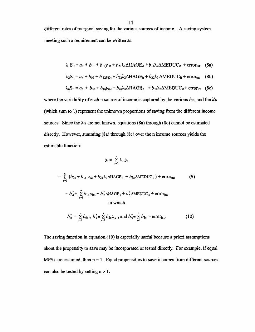
11
different rates of marginal saving for the various sources of income. A saving system
meeting such a requirement can be written as:
XISjt = a. + bol + bilyilt + b2jkXAHAGEjt + b3 lX2AMEDUC1 t + error1nt (8a)
k2Sit = a. + bo2 + b IZYi2t + b22X2AHAGEIt + b32X3 AMEDUCit + error1 nq (8b)
Sit = an + bo. + bivit + b2.4AHAGEit + b3.X.AMEDUCit+ errorint (8c)
where the variability of each n source of income is captured by the various b's, and the X's
(which sum to 1) represent the unknown proportions of saving from the different income
sources. Since the X's are not known, equations (8a) through (8c) cannot be estimated
directly. However, summing (8a) through (8c) over the n income sources yields the
estimable fuiction:
n
Si sSits=1
n
=E (bos + bjlsy;st + b2s %,AHAGEi, + b3,AMEDUCi,) + errorint (9)s=l
= bO+ bis yist + b 2 AHAGEi, + b3 AMEDUCi, + errorints=l
in which
n n~~~bo = E bos, b= 2 b25 . , and b3= E b3s + errorint. (10)
The saving function in equation (10) is especially useful because a priori assumptions
about the propensity to save may be incorporated or tested directly. For example, if equal
MPSs are assumed, then n = 1. Equal propensities to save incomes from different sources
can also be tested by setting n > 1.

124. Estimation Results
The saving functions in equations (6) and (9) were estimated using the data
described above. Dependent and independent variables were measured in real per capita
household terms.
Initially, equation (6) was estimated under the assumption that incomes from
different sources have a common MPS:
SAVE1, SAVE2 = bo +blYToTit + b2AHAGEit + b3AMEDUCit + errorsng (11)
The variables are defined in Table 3. The model was then estimated following
equation (9) which allows the MPSs to differ by income source:
SAVEI, SAVE2 = b 0 + bi i YNF,it + bI2 YAG,it + bl3 YLv,it
+ b14 YRNjt + b15 YExT,t + b16 YINTit
+ b17 YOTH,t + b2AHAGEit + b;AMEDUCit
+ errorint (12)
Equations (11) and (12) were estimated using ordinary least squares (OLS) on
pooled, 5-year data. Estimates for the two different definitions of savings (SAVE1 and
SAVE2) are presented in Tables 4 and 5. In both tables all of the income coefficients
(except those for livestock and internal remittances) are statistically significant at the 5
percent level. In the tables some of the household age variables (HAGE) are statistically
significant, but in only one case is the male education variable (MEDUC) significant.
Since it is likely that each household will have a different dispersion of saving,

13White's general test for heteroskedUticity was performed., Results suggested that
heteroskedasticity is present at the 5 percent level of significance in the "combined
income" equations in both tables. Re-estimating these equations using weighted least
squares failed to remove this heteroskedastictity; moreover, using weighted least squares
produced regressions with insignificant F-statistics. The decision was thus made to use
the OLS results. Fortunately, heteroskedasticity was not present in the OLS results for
the "7 income components" equations in either table.
In Table 4 the F-statistic for the "7 income components" model suggests that the
coefficients for the various sources of income are not statistically equal to one another.
Further tests also reject the null hypothesis of equal coefficients for the income
components in this equation at the 1 percent level of significance.
In Table 5 both the F-statistic for the "seven income components" model and
further diagnostics produce identical results. In this table the coefficients for the various
income components are also statistically different from one another at the 1 percent level.
To summarize, results for both the SAVE 1 and SAVE2 models suggest that
separate sources of income are saved at significantly different marginal rates. For
example, in the SAVEI model the MPS out of external remittances (0.907) is much
higher than that (0.589) out of internal remittances. Likewise, in the SAVE2 model the
MPS out of other income (1.025) is twelve times higher than the MPS for rental income
(0.085).
In general, the MPSs for the separate sources of income are much higher for
SAVE1 than SAVE2. The reasons for this have been broached above. Not only does
SAVE1 include expenditures on all durable goods, but this saving variable is measured as

14the residual between observed income and observed expenditures, each of which is
measured with error. These measurement errors have the effect of biasing all of the
MPSs in the SAVE1 model towards 1.
It should also be noted that the results here do not support the hypothesis that the
MPS for total income is a weighted average of the MPSs from the separate sources of
income.6 Based on the average weights of the different sources of income reported in
Table 1, the weighted MPS for total income in the SAVE 1 model is 0.817, while that for
total income in the SAVE2 model is 0.179. Both of these estimated MPS for total
income are statistically different from the MPSs for total income reported in Tables 4 and
5 for SAVEI (0.851) and SAVE2 (0.243).
Finally, it should be noted that the results of Tables 4 and 5 do not conform to
those predicted by the life-cycle models. These models generally predict a hump-shaped
pattern of saving, with the young and old dissaving and the adults saving. However, with
the exception of the variable for household members over 65 (HAGE65) for the SAVE 1
model in Table 4, none of the results conform to this pattern. These results are similar to
those of Paxson [19921 and Deaton and Paxson [19921, who suggest that in developing
countries old-age support comes more from transfers among generations than from any
reduction in the marginal rate of saving.
5. Precautionary Saving and the Uncertainty of Income
Since incomes from separate sources are indeed saved at different marginal rates,
the question arises: What are the economic reasons for this?

15In the literature it is commonly suggested that the reasons for this phenomenon
have to do with income variability and uncertainty: all other things being equal, sources
of income which are more variable and less certain will tend to be saved at a higher
marginal rate. While this may be true, different models of saving treat the effects of
variability and uncertainty differently. In the permanent income hypothesis, put forth by
Friedman [19571. the marginal utility of consumption is linear, the expectation of
marginal utility is the marginal utility of the expectation, and so increases in future
uncertainty do not by themselves affect saving. However, newer models of saving treat
uncertainty differently. The precautionary model, for example, assumes that the marginal
utility of consumption is convex, so that increases in the uncertainty of income lead to a
reduction in current consumption and an increase in saving. In the precautionary model,
increases in uncertainty raise the valuation of future consumption, because of the
inclusion of more possible states when the valuation of consumption is very high: and this
increases the marginal incentive to save in the present. Following Deaton [1992: 641. the
precautionary model of saving can be written as:
El Al nc,+, 1 p-'(E,r,+, - 8) + (13)2 t
where o2 i S the time t variance
co = var, (A1 nc+, -p-'r,+,) (14)
According to equations (13) and (14), the expected utility of a change in consumption (c)
in time period t +1 depends on the household's risk aversion (p) to expected changes in
the real rate of interest (r) and consumption growth, where consumption growth is greater

16the larger is risk aversion (p) and the larger is uncertainty as measured by (ot'. The last
term in equation (14) is the contribution of the precautionary model, postponing
consumption in the face of (income) uncertainty.
Precautionary saving models, like those in (13) and (14), are difficult to
operationalize and solve. However, equation (13) reveals an important insight due to
Carroll [19911. Any variable that helps predict the future variability of consumption, for
example, current income, will have a role in predicting the growth rate of consumption
(and also saving).
For the purposes of this paper, it is possible to hypothesize that households look
to the future when they decide to save, and that they choose to save based on how much
they expect their current income to vary. More specifically, it can be hypothesized that
households will save more of their income from those sources of income that are variable
and uncertain at present. In this case, income uncertainty is somewhat similar to
Campbell's "saving for a rainy day" [19871 except that here the focus is on saving based
upon uncertainty about the level of a specific source of income.
To measure income variability or uncertainty at the household level, two
measures have been posed in the literature [Carrroll and Samwick. 19981. The first
measure is the variance of income. As noted above, it has usually been assumed that
utility has a constant-absolute-risk-aversion (CARA) form, and that the shock to income
is additive and distributed normally with a variance of a2. These assumptions have been
motivated not so much by plausibility but by the permanent income hypothesis that
implies an exact linear relationship between consumption and uncertainty. The second
measure of uncertainty used in previous work is the variance of the log of income. While

17Carroll and Samwick [1998: 4121 note that there is no formal theoretical justification for
using this measure, it has the twin advantage of being relatively easy to calculate and of
being perhaps the most familiar measure of variability.
Using these two measures of uncertainty, the following method was used to
estimate the effect of uncertainty on savings. Using the results from equation (12),
marginal propensities to save were estimated for each household i from each of the n
separate sources of income. The resulting values were then regressed on either: (a) the
variance of the lagged value of each n source of income; or (b) the variance of the log of
the lagged value of each n source of income. Dropping the household i subscripts, the
basic specification used was:
X(MPS)(ynt) = bo + bi(VAR)(ynt-1) + p. (15)
or
X(MPS)(ynt) = bo + bi(VARLY)(ynt-1) + p. (16)
where VAR is the variance of n source of income and VARLY is the variance of the log
of n source of income in year t.
Equations (15) and (16) were estimated by OLS on the pooled, 5-year data using
the two different definitions of savings: SAVE 1 and SAVE2. The results are presented
in Table 6. In the table, for each definition of savings, the seven sources of income are
listed from high to low on the basis of their overall marginal propensities to save (as
reported in Tables 4 and 5).
For the SAVE1 model in Table 6, greater variability or uncertainty in lagged
income does not explain differences in the propensity to save from income because there
is no positive relationship between the two variables. The reason for this may be

18measurement error. Since SAVE1 is measured as the residual between two observed
variables (income and expenditures), each of which is measured with error, all of the
MPSs in the SAVE1 model are biased. It is likely that such biases conceal the effects of
income uncertainty on savings rates from the different sources of income.
However, for the SAVE2 model in Table 6 the findings are quite different. Here
variability or uncertainty in lagged income does seem to explain the differences in
marginal savings rates between separate sources of income. In the SAVE2 model those
sources of income which are most variable are also those with the highest marginal
propensity to save, and as the value of income uncertainty falls so does the marginal
propensity to save. This is exactly what the precautionary model of saving predicts, and
unless some alternative explanation can be found, suggests that households in rural
Pakistan do indeed save more at the margin from those sources of income which are more
variable and uncertain.
6. Conclusion
Three key findings emerge from this study which has used five-year panel data to
examine how rural households in a developing country save from each of the full
complement of income sources at their disposal.
First, contrary to much work which assumes that the marginal propensity to save
(MPS) is the same for all sources of income, this paper shows that separate sources of
income are saved at significantly different marginal rates. For example, the MPS out of
other income (1.025) is twelve times higher than the MPS for rental income (0.085).
Moreover, this finding is robust over different definitions of savings. No matter how

19saving is defined, there are large and statistically significant differences in the marginal
rates at which income is saved from separate sources of income.
Second, in investigating the economic reasons for this phenomenon, this paper
points to the importance of income variability and uncertainty. Just as predicted by the
precautionary model of savings, those sources of income which are more variable and less
certain will be saved at a higher marginal rate, all other things being equal. Confronted
with incomplete capital and credit markets, residents of rural Pakistan seem to save "for a
rainy day" by putting away at the margin more of those sources of income which vary
more now (and presumably also in the future).
Third, this paper shows the importance of having observed estimates of saving in
order to overcome measurement problems in estimating saving. For example, there is no
particular relationship between income variability and marginal saving rates when saving
is estimated as the residual between two variables (income and expenditures), each of
which is measured with error, and together which may be correlated with saving.
However, when saving is measured more accurately and without bias - using observed
values -- sources of income which are more variable are saved at a higher marginal rate.
From a methodological standpoint, in order to accurately estimate marginal propensities
to save using regression analysis, it is important to remove the bias caused by the
correlation of errors between the dependent and independent variables.

20
Notes
1. While none of these studies analyze how households save from each of
the full complement of income sources at their disposal, two studies examine
how households save from several different income sources. Bhalla [19781
uses three-year panel data from rural India to analyze the MPS for two
sources of income: agricultural and non-agricultural. Using a shorter, three-
year version of the panel data set from rural Pakistan used in this paper,
Alderman [19961 examines marginal rates of saving for three income
sources: domestic remittances, international remittances and pensions.
2. These data were collected by the International Food Policy Research
Institute (IFPRI) working in collaboration with Pakistani research institutes:
Applied Economic Research Centre (University of Karachi), Punjab Economic
Research Institute (Lahore), the University of Baluchistan (Quetta), and the
Center for Applied Economic Studies (University of Peshawar). For more
details, see Adams and He [19951.
3. The 469 households were distributed as follows: 84 from Attock District
(Punjab province), 166 from Badin District (Sind province), 127 from Dir
District (Northwest Frontier Province), and 92 from Faisalabad District
(Punjab province).

21
4. In her study using household data from rural Thailand, Paxson [1992]
shows the importance of adjusting income and savings data for inflation.
5. The level of female education in rural Pakistan is very low. See, for
example, Adams [19981.
6. For example, in their analysis of the marginal propensity to consume
(MPC) separate types of income, Holbrook and Stafford [1971: 191 suggest
that the MPC for total income is "merely a weighted average of common
propensities to consume different types of income, with the weights being
the fraction of the total income represented by each type of income."

22
References
Adams, R., 1998, 'Remittances, Investment and Rural Asset Accumulation in Pakistan',
Economic Development and Cultural Change Vol. 47, No. 1, pp. 155-173.
Adams, R. and J. He, 1995, Sources of Income Inequality and Poverty in Rural Pakistan,
Research Report 102, Washington, DC: International Food Policy Research
Institute.
Alderman, H., 1996, 'Saving and Economic Shocks in Rural Pakistan', Journal of
Development Economics Vol. 51, No. 2, pp. 343-366.
Bhalla, S., 1978, 'The Role of Sources of Income and Investment Opportunities in Rural
Savings', Journal of Development Economics Vol. 5, No. 3, pp. 259-281.
Bhalla, S., 1979, 'Measurement Errors and the Permanent Income Hypothesis: Evidence
From Rural India', American Economic Review Vol. 69, No. 3, pp. 295-307.
Bhalla, S., 1980, 'The Measurement of Permanent Income and Its Application to Savings
Behavior', Journal of Political Economy Vol. 88, No. 3, pp. 722-744.
Campbell, J., 1987, 'Does Saving Anticipate Declining Labor Income? An Alternative
Test of the Permanent Income Hypothesis', Econometrica Vol. 55, No. 6, pp. 1249-
1273.
Carroll, C., 1991, 'Buffer Stock Saving and the Permanent Income Hypothesis', draft
Manuscript, Board of Governors of the Federal Reserve System.
Carroll, C. and A. Samwick, 1998, 'How Important is Precautionary Saving?',
Review of Economics and Statistics Vol. 80, No. 3, pp. 410-419.
Deaton, A., 1990, 'Saving in Developing Countries: Theory and Review', Proceedings

23
Of the World Bank Annual Conference on Development Economics. 1989.
Washington, DC: World Bank.
Deaton, A., 1992, Understanding Consumption, Oxford: Clarendon Press.
Deaton, A. and C. Paxson, 1992, 'Patterns of Aging in Thailand and Cote d'Ivoire' in
D. Wise (ed.), Issues in the Economics of Aging. Chicago, n1: University of
Chicago Press.
Friedman, M., 1957, A Theory of the Consumption Function, Princeton, NJ:
National Bureau of Economic Research.
Gersovitz, M., 1988, 'Saving and Development', in H. Chenery and T. Srinivasan (eds.),
Handbook of Development Economics. Vol. 1, New York, NY: North Holland.
Holbrook, R. and F. Stafford, 1971, 'The Propensity to Consume Separate Types of
Income: A Generalized Permanent Income Hypothesis', Econometrica, Vol. 39,
No. 1, pp. 1-21.
Morduch, J., 1990, 'Risk, Production and Saving: Theory and Evidence from Indian
Households', draft manuscript, Harvard University, Cambridge, MA.
Musgrove, P., 1979, 'Permanent Household Income and Consumption in Urban South
America', American Economic Review. Vol. 69, No. 3, pp. 355-368.
Pasha, H. and T. Hasan, 1982, 'Development Ranking of Districts of Pakistan',
Pakistan Journal of Applied Economics. Vol. 1, pp. 157-192.
Paxson, C., 1992, 'Using Weather Variability to Estimate the Response of Savings to
Transitory Income in Thailand', American Economic Review, Vol. 82, No. 1,
pp. 15-33.
Wolpin, K., 1982, 'A New Test of the Permanent Income Hypothesis: The Impact of
Weather on the Income and Consumption of Farm Households in India',
International Economic Review. Vol. 23, No. 3, pp. 583-594.

Table 1-Summary of mean annual per capita household income and consumption expenditure data from rural Pakistan, 1986-87 to 1990-91
Year Consumption _ Income
expenditurea' External InternalNon-farm Agricultural Livestock Rental Remittances Remittances Otherbl
1986-87 2,170.09 937.64 661.26 465.73 465.01 247.22 276.89 -15.44(1,280.76) (1,090.32) (1,559.87) (578.69) (1,829.74) (951.95) (551.53) (256.58)
1987-88 2,154.50 1,117.16 807.46 416.98 299.26 269.74 139.23 99.22(1,236.33) (1,257.51) (2,072.42) (688.41) (2,229.84) (1,262.82) (380.17) (507.32)
1988-89 1,907.15 906.26 699.00 417.53 315.75 127.53 59.39 106.72(1,194.00) (1,043.21) (1,611.23) (533.98) (1,903.84) (674.55) (189.88) (365.78)
1989-90 1,901.53 955.79 436.25 330.93 176.65 178.89 54.13 23.70(1,648.86) (1,053.29) (738.12) (409.73) (654.41) (772.28) (223.18) (101.14)
1990-91 2,358.16 922.26 597.62 256.25 282.42 293.74 129.01 28.76(1,951.35) (1,026.50) (1,221.20) (482.75) (1,042.25) (1,576.49) (450.45) (125.93)
Average 2,098.28 967.82 640.32 377.48 307.82 223.42 131.73 48.59(1,500.21) (1,009.14) (1,511.04) (551.39) (1,641.89) (1,099.66) (392.08) (314.11)
Notes: N = 469 households. Standard deviations are given in parenthesis. All data in constant 1986 rupees;in 1986, 1 Pakistan rupee = US $0.062
a/ Consumption expenditure includes expenditures on food and drink, clothing, ceremonies, cinema and medical.b/ Other income includes government pensions, cash and zakat (payments to the poor).
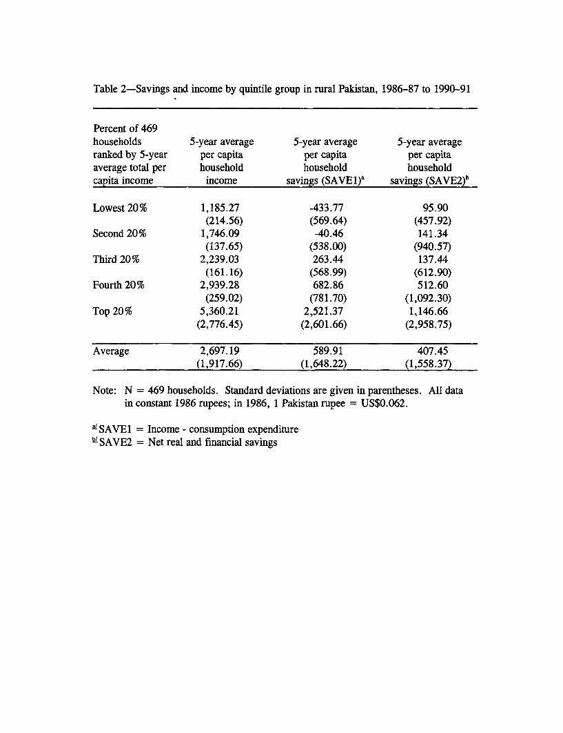
Table 2-Savings and income by quintile group in rural Pakistan, 1986-87 to 1990-91
Percent of 469households 5-year average 5-year average 5-year averageranked by 5-year per capita per capita per capitaaverage total per household household householdcapita income income savings (SAVEl)' savings (SAVE2)b
Lowest 20% 1,185.27 -433.77 95.90(214.56) (569.64) (457.92)
Second 20% 1,746.09 -40.46 141.34(137.65) (538.00) (940.57)
Third 20% 2,239.03 263.44 137.44(161.16) (568.99) (612.90)
Fourth 20% 2,939.28 682.86 512.60(259.02) (781.70) (1,092.30)
Top 20% 5,360.21 2,521.37 1,146.66(2,776.45) (2,601.66) (2,958.75)
Average 2,697.19 589.91 407.45(1,917.66) (1,648.22) (1,558.37)
Note: N = 469 households. Standard deviations are given in parentheses. All datain constant 1986 rupees; in 1986, 1 Pakistan rupee = US$0.062.
a'SAVE 1 = Income - consumption expenditureb SAVE2 = Net real and financial savings
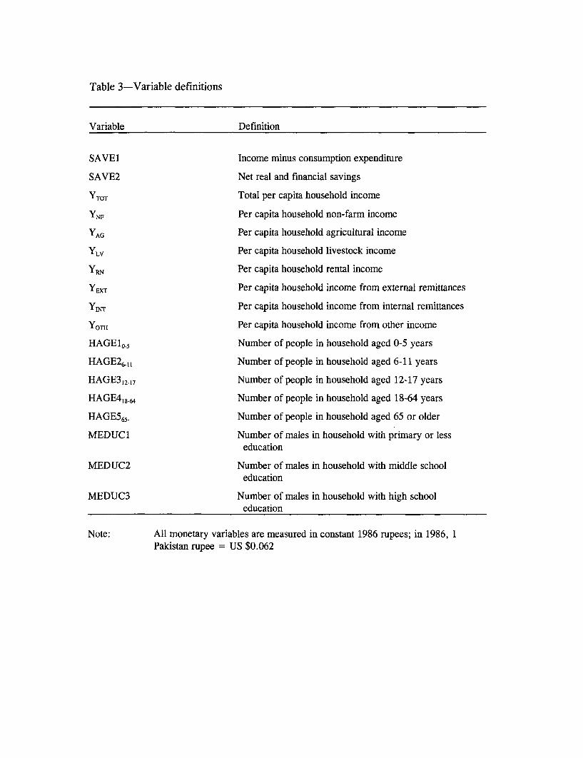
Table 3-Variable definitions
Variable Definition
SAVE1 Income minus consumption expenditure
SAVE2 Net real and financial savings
YTOT Total per capita household income
YNF Per capita household non-farm income
YAG Per capita household agricultural income
YLV Per capita household livestock income
YRN Per capita household rental income
YEXT Per capita household income from external remittances
YINT Per capita household income from internal remittances
YOTH Per capita household income from other income
HAGE10-5 Number of people in household aged 0-5 years
HAGE26-1 Number of people in household aged 6-11 years
HAGE3 12-17 Number of people in household aged 12-17 years
HAGE4 18_64 Number of people in household aged 18-64 years
HAGE565- Number of people in household aged 65 or older
MEDUC1 Number of males in household with primary or lesseducation
MEDUC2 Number of males in household with middle schooleducation
MEDUC3 Number of males in household with high schooleducation
Note: All monetary variables are measured in constant 1986 rupees; in 1986, 1Pakistan rupee = US $0.062

Table 4- Savings function for SAVE1 (Income - consumption expenditure) using OLS
Combined 7 incomeVariable income components
YTOT 0.851(68.387)**
YNF 0.829(30.264)**
YAG 0.859(42.120)**
YLV 0.710(13.255)**
YRN 0.852(45.605)**
YEXT 0.907(33.708)**
YINT 0.589(7.665)**
YOTH 0.799(8.472)**
HAGE105 125.832 116.155(6.836)** (6.275)**
HAGE26-1 81.219 67.788(3.859)** (3.195)**
HAGE31217 84.891 81.302(3.071)** (2.925)**
HAGE41s64 -2.636 0.289(-0.192) (0.021)
HAGE565 -96.346 -100.499(-2.019)* (-2.105)
MEDUCI -78.244 -78.737(-2.560)* (-2.549)*
MEDUC2 -90.504 -90.459(-1.933) (-1.938)
MEDUC3 -4.041 18.401(-0.052) (0.235)
Constant -2,087.047 -1,995.523(-26.031)** (-22.121)**
Adj. R2 0.671 0.673
F-Stata 531.621 323.014
Notes: Data are pooled over 5 years.N =469 households/2,345 observations. Numbers in parentheses are t-statistics (two-tailed).
' The reported F-statistic is a joint test of the null hypothesis that the coefficients on the separate incomesource variables are equal to one another. The null hypothesis of equal coefficients is rejected.
* Significant at the 0.05 level.

Table 4 - Savings function for SAVE1 (contd)
** Significant at the 0.01 level.

Table 5-Savings function for SAVE2 (Net real and financial savings) using OLS
Combined 7 incomeVariable income components
YTOT 0.243(9.756)**
YNF 0.210(3.913)**
YAG 0.116(2.904)**
YLV -0.175(-1.675)
RN 0.085(2.322)*
YMT 0.711(13.509)**
YINT 0.291(1.941)
YOTH 1.025(5.559)**
HAGE10 -5 30.206 35.745(0.818) (0.988)
HAGE26-1 , -54.556 -71.970(-1.291) (-1.736)
HAGE3, 2, 7 7.458 26.323(0.134) (0.485)
HAGE4,844 23.634 15.842(0.856) (0.584)
HAGE56 5- 38.641 79.230(0.403) (0.849)
MEDUC1 75.637 2.036(1.233) (0.034)
MEDUC2 173.952 158.422(1.851) (1.737)
MEDUC3 174.851 235.659(1.113) (1.539)
Constant -533.657 -251.167(-3.316)** (-1.454)
Adj. R2 0.055 0.110
F-Stata 16.104 20.411
Notes: Data are pooled over 5 years.N =469 households/2,345 observations. Numbers in parentheses are t-statistics (two-tailed).
a The reported F-statistic is a joint test of the null hypothesis that the coefficients on the separate incomesource variables are equal to one another. The null hypothesis of equal coefficients is rejected.
* Significant at the 0.05 level.

Table 5-Savings function for SAVE2 (contd)
** Significant at the 0.01 level.

Table 6. Regressions of marginal propensity to save on uncertainty measures
(a) SAVEI (Income minus consumption expenditure)
Variance of Variance of logSource of income MPS1 income (Yt 1) of income (Yt,1) Constant Adj R'
External remittance, 0.907 1.212 1.702 312.2 0.301(2.812)** (2.53)
Agricultural income 0.859 0.713 0.812 278.3 0.336(2.164)** (3.01)
Rental income 0.852 0.605 0.791 164.1 0.402(3.104)** (1.97)*
Non-farm income 0.829 0.971 0.952 343.2 0.41(2.987)* (2.07)*
Other income2 0.799 1.103 0.962 237.1 0.401(2.92)* (3.07)*
Livestock income 0.71 0.452 0.501 142.2 0.254(1.96)* (2.01)*
Internal remittances 0.589 0.607 0.619 115.1 0.381(1.98)* (2.11)*
(b) SAVE2 (Net real and financial savings)
Variance of Variance of logSource of income MPS' income (Yt1,) of income (Yt-1) Constant Adj R'
Other income2 1.025 1.402 1.315 328.3 0.451(3.020)** (3.171)**
External remittance, 0.711 1.017 0.945 261.2 0.501(3.780)** (4.012)**
Internal remittance 0.291 0.962 0.874 478.2 0.418(3.811)** (4.50)**
Non-farm income 0.21 0.621 0.599 189.6 0.58(3.010)** (2.187)**
Agricultural income 0.116 0.581 0.572 310.5 0.455(5.101)** (5.02)**
Rental income 0.085 0.472 0.512 210.6 0.414(2.151)* (1.971)*
Livestock income -0.175 -0.217 -0.243 497.1 0.406(-1.10) (-0.981)
Notes: Data are pooled over 5 years. N=469 households/2,345 observations. Numbers inparentheses are t-statistics (two-tailed).
1Marginal propensity to save (MPS) calculated from equation (12) and listed in Tables 4 and 5.
21Other income includes government pensions, cash and zakat (payments to the poor).
*Significant at the 0.05 level.**Significant at the 0.01 level.

Policy Research Working Paper Series
ContactTitle Author Date for paper
WPS2741 Female Wage Inequality in Latin Luz A. Saavedra December 2001 S. NyairoAmerican Labor Markets 34635
WPS2742 Sectoral Allocation by Gender of Wendy V. Cunningham December 2001 S. NyairoLatin American Workers over the 34635Liberalization Period of the 1960s
WPS2743 Breadwinner or Caregiver? How Wendy V. Cunningham December 2001 S. NyairoHousehold Role Affects Labor 34635Choices in Mexico
WPS2744 Gender and the Allocation of Nadeem llahi December 2001 S. NyairoAdult Time: Evidence from the Peru 34635LSMS Panel Data
WPS2745 Children's Work and Schooling: Nadeem llahi December 2001 S. NyairoDoes Gender Matter? Evidence 34635from the Peru LSMS Panel Data
WPS2746 Complementarity between Multilateral Dilip Ratha December 2001 S. CrowLending and Private Flows to Developing 30763Countries: Some Empirical Results
WPS2747 Are Public Sector Workers Underpaid? Sarah Bales December 2001 H. SladovichAppropriate Comparators in a Martin Rama 37698Developing Country
WPS2748 Deposit Dollarization and the Financial Patrick Honohan December 2001 A. YaptencoSector in Emerging Economies Anqing Shi 38526
WPS2749 Loan Loss Provisioning and Economic Luc Laeven December 2001 R. VoSlowdowns: Too Much, Too Late? Giovanni Mainoni 33722
WPS2750 The Political Economy of Commodity Masanori Kondo December 2001 D. Umali-DeiningerExport Policy: A Case Study of India 30419
WPS2751 Contractual Savings Institutions Gregorio Impavido December 2001 P. Braxtonand Banks' Stability and Efficiency Alberto R. Musalem 32720
Thierry Tressel
WPS2752 Investment and Income Effects of Klaus Deininger January 2002 M. FernandezLand Regularization: The Case of Juan Sebastian Chamorro 44766Nicaragua
WPS2753 Unemployment, Skills, and Incentives: Carolina Sanchez-Paramo January 2002 C. Sanchez-ParamoAn Overview of the Safety Net System 32583in the Slovak Republic
Policy Research Working Paper Series
ContactTitle Author Date for paper
WPS2754 Revealed Preference and Abigail Barr January 2002 T. PackardSelf-Insurance: Can We Learn from Truman Packard 89078the Self-Employed in Chile?
WPS2755 A Framework for Regulating Joselito Gallardo January 2002 T. IshibeMicrofinance Institutions: The 38968Experience in Ghana and the Philippines
WPS2756 Incomeplete Enforcement of Pollution Hua Wang January 2002 H. WangRegulation: Bargaining Power of Nlandu Mamingi 33255Chinese Factories Benoit Laplante
Susmita Dasgupta
WPS2757 Strengthening the Global Trade Bernard Hoekman January 2002 P. FlewittArchitecture for Development 32724
WPS2758 Inequality, the Price of Nontradables, Hong-Ghi Min January 2002 E. Hernandezand the Real Exchange Rate: Theory 33721and Cross-Country Evidence
WPS2759 Product Quality, Productive Aart Kraay January 2002 R. BonfieldEfficiency, and International Isidro Soloaga 31248Technology Diffusion: Evidence from James TyboutPlant-Level Panel Data
WPS2760 Bank Lending to Small Businesses George R. G. Clarke January 2002 P. Sintim-Aboagyein Latin America: Does Bank Origin Robert Cull 37644Matter? Maria Soledad Martinez Peria
Susana M. Sanchez