predictable stock returns in the united states and japan

Predictable Stock Returns in theUnited States and Japan: A Study of

Long-Term Capital Market IntegrationThe Harvard community has made this

article openly available. Please share howthis access benefits you. Your story matters

Citation Campbell, John Y., and Yasushi Hamao. 1992. Predictable stockreturns in the United States and Japan: A study of long-term capitalmarket integration. Journal of Finance 47, no. 1: 43-69.

Published Version http://dx.doi.org/10.2307/2329090

Citable link http://nrs.harvard.edu/urn-3:HUL.InstRepos:3207694

Terms of Use This article was downloaded from Harvard University’s DASHrepository, and is made available under the terms and conditionsapplicable to Other Posted Material, as set forth at http://nrs.harvard.edu/urn-3:HUL.InstRepos:dash.current.terms-of-use#LAA

http://osc.hul.harvard.edu/dash/open-access-feedback?handle=&title=Predictable%20Stock%20Returns%20in%20the%20United%20States%20and%20Japan:%20A%20Study%20of%20Long-Term%20Capital%20Market%20Integration&community=1/1&collection=1/2&owningCollection1/2&harvardAuthors=4afad70af18188b8d02dc80e32382e5b&departmentEconomics

http://nrs.harvard.edu/urn-3:HUL.InstRepos:3207694

http://nrs.harvard.edu/urn-3:HUL.InstRepos:dash.current.terms-of-use#LAA



NBER WORKING PAPER SERIES

PREDICTABLE STOCK RETURNS IN THE UNITED STATES AND JAPAN:

A STUDY OF LONG-TERN CAPITAL MARKET INTEGRATION

John Y. Campbell

Yasushi Hamao

Working Paper No. 3191

NATIONAL BUREAU OF ECONOMIC RESEARCH1050 Massachusetts Avenue

Cambridge, MA 02138December 1989

This research has been supported by the National Science Foundation and theJohn N. Olin Fellowship at the NEER (Campbell), and the Dean Witter Foundation(Hamao). We are grateful to the Financial Markets Group at the London Schoolof Economics for its hospitality, to Daniel Hardy for able research assistance,to Daiwa Securities for providing some of he data, and to Rene Stulz and ananonymous referee for helpful comments on an earlier draft of the paper. Thispaper is part of NBER's research program in Financial Markets and MonetaryEconomics. Any opinions expressed are those of the authors not those of the

National Bureau of Economic Research.

NBER Working Paper #3191December 1989

PREDICTABLE STOCK RETURNS IN THE UNITED STATES AND JAPAN:A STUDY OF LONG-TERM CAPITAL MARKET INTEGRATION

ABSTRACT

This paper studies the predictability of monthly excess returns on equityportfolios over the domestic short-term interest rate in the U.S. and Japanduring the period 1971:1-1989:3. The paper finds that similar variables,including the dividend-price ratio and interest rate variables, help toforecsst excess returns in each country. In addition, in the 1980's U.S.variables help to forecast excess Japanese stock returns. There is evidence ofcommon movement in expected excess returns across the two countries, which is

suggestive of integration of long-term capital markets.

John Y. Campbell Yasushi HamaoWoodrow Wilson School Graduate School of InternationalRobertson Hall Relations and Pacific Studies

Princeton University Q-062, UC San DiegoPrinceton, NJ 08544 La Jolla, CA 92093

1. Introduction

There is by now a large literature documenting the fact that in the

United States, excess stock returns move through time in a predictable

fashion. For example, excess returns on broad equity portfolios over

Treasury bills are forecast by the dividend-price ratio on stock, by the

level of interest rates, by the long-term yield spread, and by the month

of the year (the so-called January effect'))

Much less research has been done on stock markets in the rest of the

world. In the case of Japan there has been some work which documents the

existence of a January effect, and some work on stock returns in relation

to inflation, but to our knowledge there is no published study of the

overall predictability of excess stock returns in Japan.2

In this paper we study U.S. and Japanese stock market data

simultaneously. We ask whether similar domestic variables forecast

excess returns in the two countries, and then whether international

variables improve the forecasts obtainable from domestic variables. We

study the extent to which predictable movements in excess returns in

Japan are correlated with those in the U.S. We estimate and test a

highly restricted model in which expected excess returns in Japan and the

1 See Campbell (1987), Campbell and Shiller (1988), Fama and French(1988), Fama and Schwert (1977), Keim and Stambaugh (1986), among others.

2 One unpublied paper which does present forecasts of Japanesestock returns is Sentana and Wadhwani (1989). See Gultekin and Gultekin(1983), Jaffe and Westerfield (1985), and Kato and Schallheim (1984) forthe January effect in Japan. See Gultekin (1983) and Solnik (1983) forinternational evidence on inflation (measured directly or using short-term interest rates) in relation to stock returns. Jaffe and Westerfield(1985) also look at day-of-the-week effects in Japan, as do Condoyanni,O'Hanlon and Ward (1988). Finally, Cumby (1987) tries to explain thepredictability of stock returns in several countries using a consumptioncapital asset pricing model.

1

U.S. are driven by a common unobserved variable, so that they are

perfectly correlated. The model generates estimates of the component of

expected exceas returns which is common to both countries.

Our work has value as simple data description. But we are also

interested in the extent to which U.S. and Japanese stock markets (and

international long-term capital markets more generally) can be described

as "integrated". If capital markets are integrated, then assets which

are traded in different markets, but which have identical risk

characteristics, will have an identical expected return. The difficulty

in testing this is of course that one needs a particular asset pricing

model in order to measure risk characteristics. A finding of imperfect

integration can always be attributed to misspecification of one's model

of risk.

Most comparative work on international stock markets has used cross-

sectional information on the unconditional mean returns of securities

traded in different markets. A static asset pricing model (such as the

CAPM or the APT with constant parameters) is estimated and used to test

the null hypothesis that market risk prices are the same across

countries, against the alternative that they differ.3

Our strategy is rather different. Instead of looking at the cross-

sectional pattern of mean returns on stock portfolios, we try to exploit

the time-variation in expected stock returns in the U.S. and Japan. We

will argue that common movement in expected excess returns in the two

See Cho, Eun and Senbet (1986), Cultekin, Gultekin and Penati(1989), Jorion and Schwartz (1986), and Stehle (1977). There is alsosome work on dynamic international asset pricing models, for example

Cumby (1988) and Korajczyk (1985).

2

countries is indirect evidence of integration. In particular, we would

find perfectly correlated expected excess returns if capital markets are

integrated and assets have constant betas on a single source of risk

whose market price moves through time.4

Of course, our approach is subject to the general difficulty with all

tests of integration. For example, if Japanese and U.S. firms are

exposed to different sources of risk, and if the prices of these risks

move independently, then expected excess returns will move independently

even if prices are set in a single world capital market.

Nevertheless we believe that a finding of common movement is

suggestive of integration. Common movement in expected returns means

that some force is affecting the equilibrium return in the U.S. and

Japanese stock markets in the same way. We are agnostic about what this

force might be. The possibilities include changes in volatility or some

broader measure of "business cycle risk" (Fama and French 1989), changes

in the risk aversion of a representative agent as aggregate wealth rises

and falls (Marcus 1989), and exogenous shifts in the demand for stock of

"noise traders" which must be accommodated by utility-maximizing traders

(Campbell and Kyle 1988). But if market-clearing takes place in the U.S.

and Japanese stock markets independently, then equilibrium returns would

move together only by coincidence.5

For direct evidence that a single "world factor" affected cx poststock market returns in many countries at the time of the crash of 1987,and that stock markets' responses to the crash were consistent withtheir historical betas on this factor, see Roll (1988).

Our argument can be seen as analogous to that of Feldstein andHorioka (1980). They argue that if international capital markets wereperfectly integrated, then there would be no reason to expect savings andinvestment in a particular country to be correlated with one another.

3

Our approach also differs from much of the existing literature in that

we measure the excess returns on long-term assets in each country

relative to a short-term interest rate denominated in the same currency.

Thus exchange rate movements do not directly affect the excess returns

studied in this paper. We could of course extend our approach to include

the excess return on a short-term Japanese investment over a short-term

U.S. investment; this excess return could be used to convert our own-

currency excess returns into common-currency excess returns. However

this type of excess return, across short-term investments in different

currencies, has already been extensively studied in the literature.6

The organization of our paper is as follows. In section 2 we describe

the asset pricing framework which motivates our empirical work. In

section 3 we describe our data set. In section 4 we present preliminary

regressions which document the existence of predictable excess stock

returns. In section 5 we try to use the results from section 4 to

characterize the extent to which U.S. and Japanese stock markets are

integrated. We estimate a single-latent-variable model which restricts

expected excess stock returns in the U.S. and Japan to move together.

Section 6 extends the analysis to include returns on size-ranked

portfolios of stocks, and section 7 concludes.

Evidence that these variables are correlated is suggestive that

international capital markets are imperfectly integrated. Similarly, weargue that if international capital markets were entirely segmented, thenthere would be no reason to expect equilibrium returns in differentcountries to be correlated with one another. Evidence that expectedreturns are correlated is suggestive that international capital marketsare integrated at least to some degree.

6 For a survey, see Obstfeld (1986).

4

2. The Asset Pricina Framework

The most general asset pricing model we consider is a K-factor model

of the following form:

(1) rit+l — Et(it÷l] +k_lkt+l + 6it+l

Here . is the excess return on asset i held from time t to time t÷l,1, t+i

the difference between the random real return on asset i and the riskfree

real rate of interest. The excess return on asset i equals the expected

excess return, plus the sum of K factor realizations k t÷l times their

betas or factor loadings ik' plus an idiosyncratic error The

asset pricing model is dynamic in the sense that the expected excess

return can vary through time, but static in that the beta coefficients

are assumed to be constant through time.

The expected excess return is restricted by the model as follows:

(2) — k_lktwhere Akt is the "market price of risk" for the k'th factor at time t.

This type of restriction can be generated by any of a number of

intertemporal asset pricing models.

Now suppose thnt the information set, at time t consists of a vector of

N forecasting variables Xt n—l. . .N (where is a constant), and that

conditional expectations are linear in these variables. Then the k'th

risk price can be written

5

N(3) A — SO X

kt knntn—i

and equation (2) becomes

K N N

(4) E(ij÷i] — 5ilc OknXnt — Sk—i n—i n—i

Equation (4) aays that the IN coefficients 0in obtained by regressing I

excess returns on N forecasting variabies tan be written in terms of 1K

beta coefficients and KN coefficients which define market prices of risk.

There are two main ways in whith this system can be used in empiricai

work. Either one can assume that certain factors are observabie; or one

tan assume that factors are unobservabie, but the number of factors is

smaii reiative to the number of assets and forecasting variabies.

Observabie factors

Suppose that we observe a portfoiio whose return has a beta of one on

the first factor, and zero on the other factors. Suppose further that

the return on this portfoiio has zero idiosyncratic risk. Caii the

return on this portfoiio Then we have

K N K

(5) r÷i — fiir,+i + ik OknXnt + ikk,t+i +k—2 n—i k—2

- N* -— flri+1 + S ainXnt + u+i.n—i

6

In a regression of excess return i on excess return I and the information

variables X the inclusion of excess return I "soaks up" the timent

variation in the risk price for factor 1. The coefficients on X ,nt in

now reflect only the time variation in the risk prices for factors 2

through K. If these risk prices are zero, then all coefficients ci willbe zero; if these risk prices are constant, then the intercept a11 will

be nonzero but the other coefficients a* for n—2.. .N will be zero.in

This approach can be applied in the international context as follows.

Suppose we think that the Japanese stock market obeys a multi-factor

model, where the first factor is an international factor and the other

factors are domestic Japanese factors. Suppose that the international

factor is well proxied by the U.S. stock market return. Then we can

regress the Japanese market return on the U.S. market return and a set of

forecasting variables. The variance of Ea* X , relative to the varianceinnt

of ajX (the fitted value when the Japanese market is regressed only

on X), is a measure of the variation in risk prices of domestic factors

relative to the variation in the risk prices of all factors. In the

extreme case where only the international factor is priced, the

coefficients a will all be zero. In the case where only the risk price

for the international factor varies through time, the coefficients

will be zero apart from the intercept.

Unobservable factors

One objection to the above procedure is that it assumes that the U.S.

stock market is an adequate proxy for the international factor in the

asset pricing model. This gives the U.S. market a special role which may

not be appropriate.

7

An alternative approach is to assume that there is a single priced

international factor which is unobservable, and no priced domestic

factors in either the U.S. or Japan. If we work with two stock returns,

one from each country, and N forecasting variables, then equation (4)

imposes that — where the k subscript has been dropped since

there is only one factor. The underlying parameters and 9n are only

identified up to a normalization; if we normalize l — 1, the restricted

system can be written as

(6)l,t÷l l 2 9N X].tz + "l,t+lr2+1 fl21 fl292 . . 29N v21

The first row of the coefficient matrix in (6) identifies the 9

coefficients, the first column identifies the coefficient and the

remaining N-I coefficients are restricted. These restrictions enforce a

perfect correlation between the expected excess return in the U.S.

market, and the expected excess return in the Japanese market. The

restricted specification is sometimes called a single-latent-variable

model.7 It can be estimated and tested using Hansen's (1982) Generalized

Method of Moments, which allows for conditional heteroskedasticity in the

variance-covariance matrix of returns.

The model (6) can be generalized to allow for unobserved domestic

factors whose risk prices are constant or depend only on a subset of the

X. When such factors are present, the restrictions in (6) apply only

For more details on this model, see Hansen and Hodrick (1983),Gibbons and Ferson (1985), Campbell (1987), and Campbell and Clarida

(1987).

8

to those elements of the X which do not affect the risk prices of thent

domestic factors. Unfortunately, we Cannot allow for arbitrary domestic

factors because the model then becomes unidentified.

Even if the overidentifying restrictions of equation (6) are rejected,

the estimated coefficients may still be of interest. The fitted values

from (6) are the best possible forecasts of stock returns in the two

Countries subject to the restriction that the forecasts be perfectly

correlated with one another; thus they can be interpreted as estimates of

a common international component in expected stock returns. Below we

will compare these estimates with unrestricted regression forecasts of

stock returns in the two countries.

How we measure returns

Our discussion so far has proceeded under the assumption that we are

measuring each asset return in real terms, relative to a common riskfree

real return. In our application, we might pick the return on 1-month

U.S. Treasury bills deflated by the U.S. consumer price index as the

riskfree real return, and measure all other returns relative to this.

This way of measuring excess returns can be simplified if we are

willing to approximate the real return on an asset by the nominal return

less the inflation rate of the appropriate price index. (The

approximation holds exactly for continuously compounded returns.) Then

the inflation rate cancels out of the expression for the excess return

and we can avoid the need to measure the price index. We use this

approach below.

We can also work with linear combinations of excess returns. For

example, if we use the same kind of approximation for exchange rates as

9

for inflation rates, then the excess yen return on the Japanese stock

market relative to the Japanese short-term interest rate is approximately

equal to the excess dollar return on the Japanese stock market relative

to the dollar return on a short-term Japanese investment.8 This in turn

is equal to the excess dollar return on the Japanese stock market

relative to the U.S. short-term interest rate, less the excess dollar

return on a short-term Japanese investment relative to the U.S. short-

term interest rate. If both the component excess returns obey the

restrictions of equation (5) or equation (6), then the difference between

them will also obey these restrictions.9 Thus we can test our models

using excess stock returns in each country measured relative to that

country's own short-term interest rate. We use this procedure below)°

Omitted information variables

In our empirical work we use forecasting variables Xnt which are known

to the market at time t. Generally, we do not wish to assume that we

have included all the relevant variables. Fortunately, the methods

8 Foran alternative analysis, which does not rely on the

approximation above, see Stulz (1981). Stulz presents a continuous-timemodel in which the covariance between stock returns and exchange ratemovements (which creates approximation error in our approach) appearsexplicitly. In Stulz's model the covariance is assumed to be constant,which means that it will not affect empirical work based on time-variation in expected returns.

A special case would be uncovered interest parity. In this casethe expected excess dollar return on a short-term Japanese investmentrelative to the U.S. short-term interest rate is zero, so it triviallyobeys the restrictions of equation (6). Eut uncovered interest parity isnot required for our procedure to be valid. This is fortunate, sincethere is considerable evidence against uncovered yen/dollar interest parity.

10 Weobtained very similar results when we ran regressions for

excess returns measured in dollars relative to the U.S. short-terminterest rate.

10

described above are robust to omitted information. y taking conditional

expectations of equations (5) and (6), it is straightforward to show that

the various restrictions hold in the same form when a subset of the

*relevant information is used. Thus if the coefficients a in equationin

(5) are zero for the true information vector used by the market, they

will also be zero if a subset of this vector is included in (5).

Similarly, if the market's forecasts of excess returns in the two

countries are perfectly correlated, then forecasts using a subset of the

market's information must also be perfectly correlated.

11

3. Data and Saniole Period

The comparative approach of this paper requires that the data be

comparable across the two countries to the greatest extent possible. The

last month for which we are able to obtain complete data in both

countries is March 1989.

U.S. data

For the U.S. , we use standard publicly available data. Stock prices

and dividends are taken from the Center for Research on Security Prices

(CRSP) monthly stock tape. We study a value-weighted index of New York

Stock Exchange stocks, and also a set of equally-weighted portfolios,

organized by firm size.11 We use a 1-month Treasury bill yield as our

short-term interest rate, and a long-term (approximately 20-year)

government bond yield to compute the long-short yield spread. These

series are from Ibbotson Associates (1989).

.Jaoanese data

The most commonly used and readily available Japanese stock price

indexes are the Nikkei 225 and the Tokyo Stock Exchange Price Index

(TOPIX). These indexes, however, are not comparable with the CRSP value-

weighted New York Stock Exchange index. The Nikkei index is a price-

weighted index of only 225 stocks out of more than 1500 stocks listed

currently on the Tokyo Stock Exchange, representing about 50% of total

capitalization. The TOPIX is a value-weighted index constructed from all

11 The size portfolios are rebalanced monthly according tocapitalization at the end of the previous month. For the last 15 monthsof the sample, 1988:1-1989:3, we were obliged to use the dividend yieldon the S&P 500 index in place of the dividend yield on the CRSP value-weighted portfolio. In earlier years these two series move very closelytogether, so this substitution is unlikely to have any noticeable effecton our empirical results.

12

the stocks traded on the first section of the Tokyo Stock Exchange with

97% of the total (first and second section) capitalization, but neither

TOPIX nor Nikkei properly account for dividend payments.

We therefore constructed our value-weighted index from individual

stock returns including and excluding dividends.12 The universe of stock

used is the Tokyo Stock Exchange, first and second sections; foreign

firms listed on the TSE are excluded from the sample.13 Our database is

an extension of the one presented in detail in Hamao (1988, 1989) and

Hamao and Ibbotson (1989), and it starts in January 1970. Since we need

one year's lag in order to construct a 1-year moving average dividend-

price ratio, our sample period starts in January 1971.

Japanese bond markets did not develop until the 1970's, and data are

therefore not available before 1970. There is no equivalent of Treasury

bills in Japan; thus the short-term interest rate used here is a combined

series of the call money rate (1971:1-1977:11) and the Gensaki rate

(1977:12-1988:12). The Gensaki rate, an interest rate applied to bond

repurchase agreements, is less subject to regulation than the call money

rate, but it became available only after 1977. The call money rate is

the "unconditional" rate, which is applied to transactions maturing in

less than one month, and the Gensaki rate we use has one month maturity.

The long-term Japanese government yield we use is for bonds with 9 to 10

years to maturity, which is the longest consistently available maturity.

12Our Japanese individual stock returns data were compiled from the

raw data on prices kept by Daiwa Securities and adjusted for dividendpayments, stock splits, etc. This database is comparable to the CRSPfiles.

13 Our U.S. sample does include a few Japanese firms in the form ofAmerican Depositary Receipts, but overall there is minimal cross-listing.

13

Samule oeriod

Limitations on the availability of Japanese data, discussed above,

confine us to the sample period 1971:1-1989:3. Within this period,

financial markets in both countries have undergone some institutional

changes. The system of financial regulation in the U.S. has changed

gradually through the period we study, but Japanese capital markets have

experienced a more radical deregulation)' Before 1970, there was

virtually no free short-term interest rate. Although the Gensaki market

grew substantially in the 1970's, it was not until 1978 that the

authorities completely lifted restrictions in the short-term market.

After the first issue of government bonds in 1966, financial

institutions, which were the major bondholders, were not allowed to sell

government bonds in a secondary market until 1977.

More recently a major deregulation occurred with the revision of the

Foreign Exchange Law in December 1980. The old Foreign Exchange Law

prohibited all transactions with foreign countries in principle, whereas

under the new law controls over many types of capital flow have been

removed. For example, it is now possible for a foreigner to invest in up

to 10% of the equity of a Japanese company without the permission of the

Ministry of Finance. With this deregulation, along with the development

of the secondary bond market in the 1980's, it is natural to divide the

whole period 1971:1-1989:3 (219 observations) into two subsamples,

1971:1-1980:12 (120 observations) and 1981:1-1989:3 (99 observations).

14See Pigott (1983), Japanese Ministry of Finance (1987) and Suzuki

(1987) for a description of Japanese financial deregulation.

14

4. Forecasting Excess Returns on Value-Wejzhted Stock Indexes in the

United States and Japan

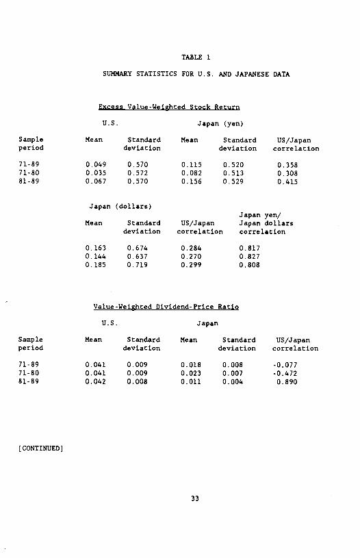
Table 1 reports basic statistics which summarize the behavior of some

of the most important variables we study. For each variable we report

the mean and standard deviation of the U.S. and Japanese series, and the

correlation between the U.S. and Japanese series, over the full sample

and both subsamples.

At the top of the table we give statistics for the excess returns on

the U.S. and Japanese value-weighted indexes over each country's domestic

short-term interest rate. Monthly returns are measured at an annual

rate. Japanese stocks have a higher mean return than U.S. stocks in both

the 1970's and the 1980's, but the gap widens in the 1980's with the

sustained rise in the Japanese market. The correlation between U.S. and

Japanese stock returns is fairly stable in the range 0.3 to about 0.4.

For comparison, we also summarize the behavior of the excess dollar

return on Japanese stocks over the U.S. short-term interest rate. The

mean of this series is somewhat higher, reflecting yen appreciation over

the period; the standard deviation is higher and the correlation with

excess returns on U.S. stocks is lower. The two Japanese excess return

series have a correlation of about 0.8.

Next we look at the behavior of dividend-price ratios on the two stock

indexes (where the dividend is the average over the previous year, and

the price is the current price). Dividend-price ratios have been found

to predict excess returns in the U.S. , and they will be important

explanatory variables in our regression analysis. We find that the

Japanese dividend-price ratio has a lower mean than the U.S. dividend-

15

price ratio (in fact, it has been lower than the U.S. in every month

since the mid-1970's). The Japanese dividend-price ratio has been

falling over time, again reflecting the rise in Japanese stock prices

during the 1980's15 The U.S. and Japanese series are negatively

correlated in the 1970's, but highly positively correlated in the 1980's.

Figure 1 plots the two countries' dividend-price ratios, and these

characteristics of the data can be clearly seen.

We repeat the exercise for levels of and changes in the U.S. bill rate

and the Japanese short rate, again measured at an annual rate. These

interest rates will also be used as forecasting variables for excess

returns. U.S. interest rates tend to rise slightly over the full sample,

period, while Japanese rates fall; however the medium-run movements of

the two interest rates are positively correlated. For this reason the

rates have higher correlations over the subsamples than over the whole

sample period. In the short run, month-by-month changes in the two

interest rates are only very weakly correlated and are more variable in

the U.S. than in Japan.

Finally, we report summary statistics for the long-short yield spread

in the two countries. The U.S. and Japanese yield spreads are weakly

positively correlated, with a higher mean in the U.S. Figures 2 and 3

show the history of short- and long-term interest rates in the U.S. and

Japan, respectively.

15 For a more detailed analysis of Japanese dividend yields and thelevel of the Japanese market, see French and Poterba (1989).

16

Forecastinr excess stock returns with domestic variables

In Table 2 we regress excess returns in the U.S. and Japan on a

variety of forecasting variables. U.S. results appear on the left hand

side of the table, and Japanese results on the right hand side. For each

country we use forecasting variables which are specific to that country.

We report coefficients, with heteroskedasticity-consistent standard

16errors in parentheses, for the whole sample and each subsample. For

each regression, we also report the adjusted statistic, the joint

significance of the coefficients (excluding a constant term and January

dummy), and the significance level for a test of stability of the

coefficients across subsamples.

We begin Table 2 by testing the significance of the January effect.

In the U.S., a regression of the excess stock return on a January dummy

yields positive but insignificant coefficients, with a decline from the

1970's to the 1980's. In Japan, on the other hand, the January dummy is

significant at the 2 or 3% level in the full sample and each subsample.

We include the January dummy in all our subsequent regressions but do not

report its estimated value.

Next we regress the excess stock return on the domestic dividend-price

ratio. We find weak evidence that this variable has forecasting power.

In the U.S. , the estimated coefficient is positive in the full sample and

each subsample; it is significant at almost the 5% level in the 1970's,

but insignificant in the 1980's. In Japan, the coefficient is positive

and highly significant in the 1970's, but negative and insignificant in

16 The heteroskedasticity-consistent standard errors are generallyquite similar to the ordinary standard errors in these regressions.

17

the 1980's. This of course reflects the fact that the Japanese market

continued to perform well in the 1980's even when Japanese dividend

yields fell below their historical range.

The next regression forecssts the stock return using the short-term

interest rate. This variable too has some explanatory power. In each

country and sample period the estimated coefficient is negative, but its

statistical significance varies greatly. The interest rate effect is

strongest in the U.S. in the 1980's, and in Japan in the 1970's.

When we combine the dividend-price ratio and the short-term interest

rate, we obtain a forecasting model which is very successful in the U.S.

data. The dividend-price ratio has a consistently positive sign, while

the short-term interest rate is consistently negative. The adjusted

is about 0.1, and the variables are jointly significant at the 1% level,

over the full sample and each subsample. There is no evidence that the

estimated coefficients change from the 1970's to the 1980's. In Japan,

the estimates are very similar to the U.S. in the 1970's, with an even

higher of almost 13%. However the forecasting model breaks down

completely in the 1980's.

One possible objection to the results presented so far is that the

short-term interest rate may be nonstationary, as suggested by Campbell

and Shiller (1987) among others. If the short rate is nonstationary,

then test statistics from a regression of stock returns on the short rate

will not have the standard asymptotic distribution. Even if the short

rate is stationary but highly serially correlated, there can be finite-

sample difficulties as pointed out by Mankiw and Shapiro (1986) and

18

Stambaugh (1986)17

Accordingly, in the rest of Table 2 we experiment with other variables

which can be combined with the short rate to produce a stationary time

series. We first replace the level of the 1-month interest rate with the

change in the interest rate. This variable has forecasting power in the

1970's, but not in the 1980's.

Next we take the difference between the long-term government bond

yield and the level of the short rate. As Campbell and Shiller (1987)

point out, this long-short yield spread will be stationary if term premia

and changes in short rates are stationary. The yield spread is a

successful forecasting variable (with a positive coefficient) in every

sample period in the U.S. , and in the 1970's in Japan.

Finally, when we estimate a system including the dividend-price ratio,

the lagged change in the short rate, and the long-term yield spread, we

obtain strong joint significance levels in the 1970's but much weaker

ones in the 1980's. The deterioration in forecast power is less serious

in the U.S. (where the yield spread remains individually significant)

than in Japan.

In summary, Table 2 provides considerable evidence that U.S. and

Japanese stock returns can be forecast using similar types of domestic

variables. The major qualification to this statement is that the

predictability of Japanese returns seems to disappear in 1981-89.

17 A similar objection could be made to the use of the dividend-priceratio in our regressions. The Japanese dividend-price ratio, inparticular, is characterized by low-frequency movement in the 1980's.

19

Forecasting excess stock returns with international variables

In Table 3 we push the investigation one stage further. We regress

U.S. and Japanese excess returns on a common international set of

forecasting variables. This enables us to see whether foreign-country

variables have any ability to predict excess returns when they are added

to domestic variables. We first use a relatively small set of

international forecasting variables (aJanuary dummy, and U.S. and

Japanese dividend-price ratios and short rates), and then a larger Set

which excludes the level of the short rate (a January dummy, and U.S. and

Japanese dividend-price ratios, changes in short rates, and long-short

yield spreads). We will call the first specification the "short rate

level' specification, and the second the "yield spread" specification.

In Table 3 we find no evidence that Japanese variables help to

forecast U.S. stock returns. None of the Japanese variables are

individually or jointly significant. We also find no evidence that U.S.

variables help to forecast Japanese stock returns in the 1970's.

In the 1980's, however, when Japanese variables fail to predict

Japanese returns, we find that U.S. variables do come in. The adjusted

R2 statistics rise from 0.01 to 0.11 when the U.S. variables are added to

the short rate level specification, and from 0.03 to 0.09 when the U.S.

variables are added to the yield spread specification.18 Both countries'

data are needed for successful forecasting; a regression of Japanese

stock returns on U.S. variables alone has an adjusted R2 of less than

18 This finding seems to be consistent with the results of Hamao,Masulis, and Ng (1989) for high-frequency data. They find that theJapanese stock market is more sensitive to foreign shocks than are theAmerican or British stock markets.

20

0.02 in either specification. As one would expect, there is strong

evidence of instability between the 1970's and the 1980's in the

coefficients of the international forecasting equations for Japanese

stock returns.

Both of the international specifications for Japanese stock returns

include the U.S. and Japanese dividend-price ratios. These variables

enter with extremely large coefficients of opposite sign: in the short

rate level specification, for example, the forecast of the Japanese stock

return is 80 times the Japanese dividend-price ratio minus 41 times the

U.S. dividend-price ratio. This result can be better understood if one

recalls that the U.S. and Japanese dividend-price ratios have a very high

correlation of 0.89 in the 1980's (see Table 1). The U.S. dividend-price

ratio has more than double the standard deviation of the Japanese

dividend-price ratio. Thus the regression seems to be forecasting

Japanese stock returns using the difference between the two countries'

dividend-price ratios, weighted inversely by their standard deviations.19

This variable is positively correlated with each country's dividend-price

ratio, even though it is formed as a difference, because of the strong

positive correlation of the two components. It peaks in 1982; the

corresponding peak in the fitted value of the regression is shown in

Figure 5b below.

19 We also tried replacing the levels of the two dividend-priceratios with their logs. We obtained a regression equation with a similarforecasting power, and coefficients on the U.S. and Japanese logdividend-price ratios which were opposite in sign. The coefficient onthe Japanese log dividend-price ratio was somewhat larger in magnitude.These results are consistent with those in Table 3.

21

5. Some Evidence on Capital Market Inte2ration

We have found evidence that similar types of variables help to predict

stock returns in the U.S. and Japan. In the 1970's, the parallel

behavior of the two markets is particularly clear. In the 1980's, there

is little or no predictability of Japanese returns using Japanese

variables alone. But in this period there is an interesting cross-

country effect: when U.S. variables are added to the forecasting

equation, it becomes possible to predict Japanese stock returns with an

R2 of about 10%. The next question we consider is whether these facts

are consistent with any of the simple models of an integrated world

capital market that we presented in section 2.

An observable factor model

In Table 4 we estimate a regression in the form of equation (5). We

add the excess U.S. stock return to the regression of the excess Japanese

return on forecasting variables. If the predictability of Japanese

returns is due merely to the changing risk price of an international

factor, which is adequately proxied by the U.S. market, then the

inclusion of the U.S. stock return in the regression should destroy the

significance of the forecasting variables.

In fact the presence of the U.S. stock return has very little effect

on the other coefficients in the regression. The U.S. return gets a

coefficient between 0.25 and 0.45 (this is the "beta" of the Japanese

index on the U.S. index), but the other variables remain just as

significant as they were before.2°

20 Given the instability of the Japanese regression coefficients wepresent only subsample results. Full sample results are similar.

22

An unobservable factor model

We next ask whether predictable excess stock returns in the U.S. and

Japan move together through time. As discussed in section 2, if

international capital markets are integrated and predictable excess

returns are due to changes in the price of risk of a single world factor,

then one would expect to find common movement in expected excess returns

in the U.S. and Japan.

It is important to note that common movement of fitted values can

occur even in the absence of the cross-country effect discussed above.

It is possible that the U.S. and Japanese domestic forecasting variables

are correlated in such a way that the domestic forecasts of excess

returns are highly correlated. In fact Table 5 shows that the sample

correlations of fitted values from the short rate specification in Table

3 are 0.44 in the 1970's and 0.24 in the 1980's. These correlations are

somewhat increased by the presence of the January effect; if one looks at

deseasonalized fitted values, the correlations fall to 0.32 and 0.08.

Thus in the 1970's, when there are no significant cross-country effects,

the U.S. and Japanese fitted values are moderately correlated; in the

1980's, when international variables are essential for forecasting

Japanese stock returns, the fitted values are much less correlated.

One problem with the discussion so far is that it does not take into

account the sampling error in the coefficients of Table 3. Without

further analysis, we cannot be sure that the correlations of the fitted

values are significantly different from zero or one. In fact, we shall

now show that a model with perfectly correlated expected returns fits the

data about as well in the 1980's as in the 1970's.

23

In Table 5 we estimate a single-latent-variable model of the form (6).

This model imposes the testable restriction that expected excess stock

returns are perfectly correlated across countries. We work with demeaned

stock returns at the left of the table, and with demeaned and

deseasonalized returns (the residuals from a regression of returns on a

constant and January dummy) at the right of the table. The forecasting

variables are the same ones used in the short rate and yield spread

specifications of Table 3. Given the instability of the Japanese

coefficients, we estimate the system separately for the 1970's and the

1980's.

The first excess return in the system is the U.S. excess stock return,

therefore we normalize the for the U.S. to equal one. The free

coefficients of the model are then the 0 , n—l.. .N, and the fi coefficientn

for the Japanese excess return. In Table 5 we report the Japanese with

an asymptotic standard error in parentheses. (To save space, the 9

coefficients are not reported.) The system is estimated, and the

overidentifying restrictions are tested, over the full sample period and

each of the subsamples.

Table 5 shows that there is some evidence against a model with a

single unobservable factor, but it is much weaker than the evidence for

predictable stock returns in each country. In the short rate

specification, the model (6) is rejected at the 8% level when the January

dummy is restricted, and at the 4% level when the dummy is left

unrestricted. Presumably this is due to the fact that the January dummy

obeys the model restrictions; leaving it unrestricted saves on degrees of

freedom without reducing the value of the test statistic. It is

24

important to note that the significance levels at which the model is

rejected do not change much from the 1970's to the 1980's, even though

the unrestricted correlations of regression fitted values are lower in

the 1980's.

Another way to evaluate the performance of the model with a single

unobservable factor is to compare the variance of the restricted forecast

with the variance of the unrestricted forecast from Table 3. If the

restricted variance is much smaller than the unrestricted variance, then

the restrictions are causing a serious deterioration in forecast power.

In Table S we report the ratio of the two variances for the U.S. and

Japanese markets. In the short rate specification the ratio is above 0.8

for Japan and between 0.3 and 0.5 for the U.S., indicating that the

restricted model is fitting Japanese returns at some cost to the quality

of its U.S. forecasts. Once again there is little change in these

numbers between the 1970's and the 1980's.

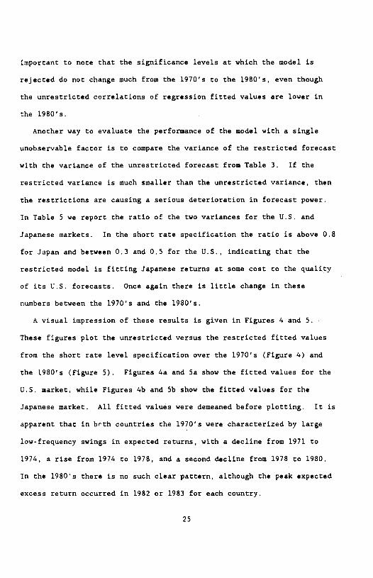
A visual impression of these results is given in Figures 4 and 5.

These figures plot the unrestricted versus the restricted fitted values

from the short rate level specification over the 1970's (Figure 4) and

the 1980's (Figure 5). Figures 4a and 5a show the fitted values for the

U.S. market, while Figures 4b and Sb show the fitted values for the

Japanese market. All fitted values were demeaned before plotting. It is

apparent that in bcth countries the 1970's were characterized by large

low-frequency swings in expected returns, with a decline from 1971 to

1974, a rise from 1974 to 1978, and a second decline from 1978 to 1980.

In the 1980's there is no such clear pattern, although the peak expected

excess return occurred in 1982 or 1983 for each country.

25

6. Forecasting Excess Returns on Size-Ranked Stock Portfolios in the

United States and Jauan

It is well known that small stock returns in the U.S. display some

anomalous behavior, particularly a strong January effect. As a final

empirical exercise, we look at size-ranked portfolios of U.S. and

Japanese stocks. We examine a portfolio of stocks formed by equally

weighting the firms in the first quintile of market value (the smallest

one fifth of the market), an equally-weighted portfolio of stocks in the

third quintile, and an equally-weighted portfolio of stocks in the fifth

quintile (the largest one fifth of the market). These portfolios are

rebalanced every month.

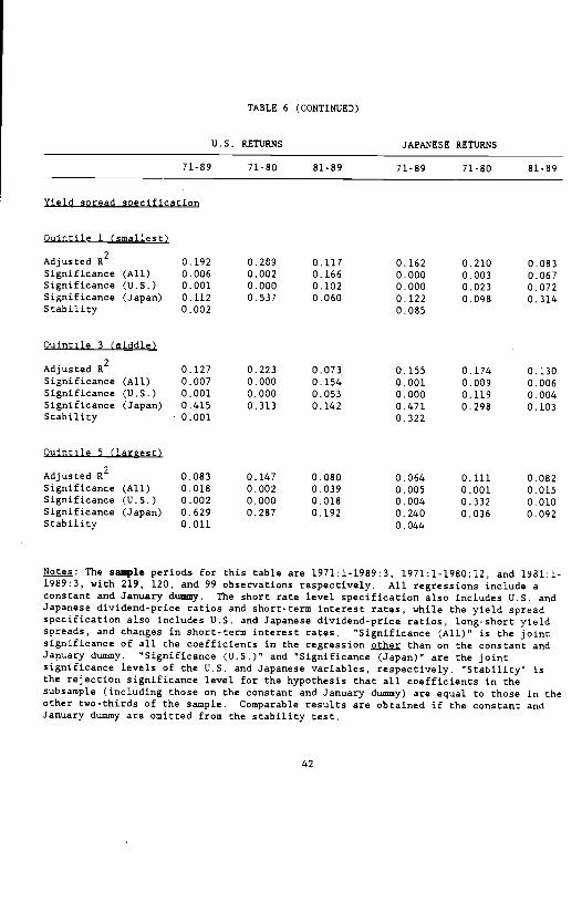
Table 6 summarizes the results of regressing these portfolio returns

on the international variables which were used in Table 3. To save space

we report only the adjusted R2 statistics and significance levels, not

the full set of coefficients.

The general pattern in Table 6 is that small stock returns are more

predictable than large stock returns. This is partly due to the strong

January effect in small stock returns, but the significance levels for

the other forecasting variables also tend to be stronger in the small

stock regressions. The exception to this pattern is that returns on

large Japanese stocks in the 1980's are more predictable than returns on

small Japanese stocks.

In Table 7 we estimate single-latent-variable models for matched pairs

of U.S. and Japanese size portfolios. The table reports the significance

levels at which the model restrictions are rejected. In the 1970's the

latent variable specification is always rejected at the 10% level, but

26

not always at the 5% level. The rejections are stronger for small

stocks. It is tempting to interpret this finding as reflecting the fact

that the expected returns on large firms are primarily determined by the

changing price of a common international source of risk, whereas small

firms are exposed to domestic sources of risk. But the stronger

rejections for small stocks could also result simply from the fact that

small stock returns have greater predictable variation. In the 1980s,

the test results for the single-latent-variable model are more erratic

and dependent on the particular specification used.

27

7. Conclusion

In this paper we have compared the predictable components of excess

stock returns in the U.S. and Japan. Our main results are as follows:

1. In both countries it is generally possible to forecast excess stock

returns over the domestic short-term interest rate using similar sets of

domestic variables. The domestic dividend-price ratio and long-short

yield spread have a generally positive effect on excess stock returns,

while the short rate and the change in the short rate have a negative

effect. These effects are fairly stable in the U.S. between the 1970's

and the 1980's, but in Japan they are much weaker in the 1980's.

2. Japanese variables do not help to forecast U.S. excess stock

returns, but U.S. variables do help to forecast Japanese excess stock

returns in the 1980's. In particular, the level of the Japanese

dividend-price ratio relative to the U.S. dividend-price ratio is a

powerful forecasting variable.

3. Expected excess stock returns in the U.S. and Japan are positively

correlated, particularly in the 1970's. There is some evidence against

the hypothesis that expected excess stock returns in the two countries

are perfectly correlated, but the evidence is not overwhelming. In both

the 1970's and the 1980's, estimates of the common component of expected

returns explain 30 or 40% of the variance of expected returns in the

U.S., and 80% of the variance of expected returns in Japan.

4. The predictability of excess stock returns is generally stronger

for small stocks. In the 1970's, small stocks also provide the strongest

evidence against the hypothesis that expected excess stock returns are

perfectly correlated across countries.

28

These results are consistent with the view that expected stock returns

are determined largely by the changing price of risk of a single common

factor in a world capital market. In this sense our results suggest that

U.S. and Japanese stock markets are substantially integrated. We find

the degree of integration to be fairly constant from the 1970's to the

1980's. More generally, our results should help to guide research on the

causes of changing expected stock returns in the United States. Whatever

these causes are, they cannot be entirely local but must have the

potential to move expected stock returns in other countries as well.

29

Bibliograohy

Campbell, John Y "Stock Returns and the Term Structure" Journal ofFinancial Economics 18:373-399, June 1987.

Campbell, John Y. and Richard H. Clarida, "The Term Structure ofEuromarket Interest Rates: An Empirical Investigation", Journal ofMonetary Economics 19:25-44, January 1987.

Campbell, John Y. and Albert S. Kyle, "Smart Money, Noise Trading, andStock Price Behavior", National Bureau of Economic Research Technical

Working Paper No. 71, October 1988.

Campbell, John Y. and Robert J. Shiller, "Cointegration and Tests ofPresent Value Models", Journal of Political Economy 95:1062-1088, October1987.

Campbell, John Y. and Robert J. Shiller, "Stock Prices, Earnings andExpected Dividends", Journal of Finance 43:661-676, July 1988.

Cho, D. Chinhyung, Cheol S. Eun and Lemma W. Senbet, "International

Arbitrage Pricing Theory: An Empirical Investigation", Journal of Finance41:313-330, June 1986.

Condoyanni, L., J. O'Hanlon and C.W.R. Ward, "Weekend Effects in StockMarket Returns: International Evidence", in Elroy Dimson ed. Stock MarketAnomalies 52-63, Cambridge University Press 1988.

Cwnby, Robert E .,"Consumption Risk and International Asset Returns:Some Empirical Evidence", National Bureau of Economic Research Working

Paper No. 2383, September 1987.

Cumby, Robert E "Is It Risk? Explaining Deviations from UncoveredInterest Parity", Journal of Monetary Economics 22:279-299, September1988.

Fama, Eugene F. and Kenneth R. French, "Dividend Yields and ExpectedStock Returns", Journal of Financial Economics 22:3-25, October 1988.

Fama, Eugene F. and Kenneth R. French, "Business Conditions andExpected Returns on Stocks and Bonds", forthcoming Journal of FinancialEconomics, 1989.

Fama, Eugene F. and C. William Schwert, "Asset Returns and Inflation",Journal of Financial Economics 5:115-146, 1977.

Feldstein, Martin and Charles Horioka, "Domestic Saving andInternational Capital Flows", Economic Journal 90:314-329, 1980.

French, Kenneth R. and James M. Poterba, "Are Japanese Stock Prices

Too High?", unpublished paper, August 1989.

30

Gibbons, Michael R. and Wayne Ferson, "Testing Asset Pricing Modelswith Changing Expectations and an Unobservable Market Portfolio", Journalof Financial Economics 14:217-236, 1985.

Gultekin, N. Bulent, "Stock Market Returns and Inflation: Evidencefrom Other Countries", Journal of Finance 38:49-65, March 1983.

Gultekin, N. Bulent and Mustafa N. Gultekin, "Stock MarketSeasonality: International Evidence", Journal of Financial Economics12:469-481, 1983.

Gultekin, N. Bulent, Mustafa N. Gultekin and Alessandro Penati,"Capital Controls and International Capital Market Segmentation: TheEvidence from the Japanese and American Stock Markets", Journal ofFinance 44:849-869, September 1989.

Hamao, Yasushi, "An Empirical Examination of the Arbitrage PricingTheory: Using Japanese Data", Jaoan and the World Economy 1:45-61, 1988.

Hamao, Yasushi, "Japanese Stocks, Bonds, Bills, and Inflation",Journal of ?ortfolio Manazement 15:20-26, 1988.

Hamao, Yasushi, in collaboration with Roger Ibbotson, Stocks. Bonds.and Inflation - Japan. 1989 Yearbook, Chicago, IL: Ibbotson Associates,1989.

Hamao, Yasushi, Ronald Masulis, and Victor Ng, "Correlations in PriceChanges and Volatility Across International Stock Markets", forthcomingReview of Financial Studies, 1989.

Hansen, Lars Peter, "Large Sample Properties of Generalized Method ofMoments Estimators", Ecpnometrica 50:1029-1054, July 1982.

Hansen, Lars Peter and Robert J. Hodrick, "Risk Averse Speculation inthe Forward Foreign Exchange Market: An Econometric Analysis of LinearModels", in Jacob A. Frenkel ed. Exchanae Rates and International

Macroeconomics, Chicago: University of Chicago Pess, 1983.

Ibbotson Associates, Stocks. Bonds. Bills. andInflation - 1989Yearbook, Chicago, IL: Ibbotson Associates, l989

Jaffe, Jeffrey and Randolph Westerfield, "Patterns in Japanese CommonStock Returns: Day of the Week and Turn of the Year Effects", Journal ofFinancial and Quantitative Analysis 20:261-271, June 1985.

Japanese Ministry of Finance, Okura-Sho Kokusai Kinvuu Kyoku Nenoo(Annual Reoort of the International Finance Division), Tokyo: Kinyuu

Zaisei Jijo Kenkyuu Kai, 1987.

Jorion, Philippe and Eduardo Schwartz, "Integration vs. Segmentationin the Canadian Stock Market", Journal of Finance 41:603-613, July 1986.

31

Kato, Kiyoshi and James S. Schaliheim, "Seasonal and Size Anomalies inthe Japanese Stock Market", Journal of Financial and quantitativeAnalysis 20:243-259, June 1985.

Keim, Donald 8. and Robert F. Stambaugh, "Predicting Returns in theStock and Bond Markets", Journal of Financial Economics 17:357-390,December 1986.

Korajczyk, Robert A.," The Pricing of Forward Contracts for ForeignExchange", Journal of Political Economy 93:346-368, 1985.

Mankiw, N. Gregory and Matthew D. Shapiro, "Do We Reject Too Often?Small Sample Properties of Tests of Rational Expectations Models",Economics Letters 20:139-145.

Marcus, Alan J .,"An Equilibrium Theory of Excess Volatility and MeanReversion in Stock Market Prices", National Bureau of Economic Research

Working Paper No. 3106, September 1989.

Obstfeld, Maurice, "How Integrated are World Capital Markets: Some NewTests", NBER Working Paper No. 2075, November 1986.

Pigott, Charles, "Financial Reform in Japan", Economic Review, FederalReserve Bank of San Francisco, 1:25-46, 1983.

Roll, Richard, "The International Crash of October 1987", in RobertKamphuis et al. eds. Black Monday and the Future of Financial Markets,

Homewood, IL: Irwin, 1988.

Sentana, Enrique and Sushil Wadhwani, "Semi-Parametric Estimation andthe Predictability of Stock Market Returns: Some Lessons from Japan",unpublished paper, London School of Economics, April 1989.

Solnik, Bruno, "The Relation between Stock Prices and InflationaryExpectations: The International Evidence", Journal of Finance 38:35-48,March 1983.

Stainbauglt, Robert F. , "Bias in Regressions with Lagged Stochastic

Regressors", unpublished paper, Graduate School of Business, Universityof Chicago, 1986.

Stehie, Richard, "An Empirical Test of the Alternative Hypotheses ofNational and International Pricing of Risky Assets", Journal of Finance

32:493-502, May 1977.

Stulz, Rene M., "A Model of International Asset Pricing", Journal ofFinancial Economics 9:383-406, 1981.

Suzuki, Yoshio ed. , The Japanese Financial System, Oxford: ClarendonPress, 1987.

32

TAZLE 1

SUMMARY STATISTICS FOR U.S. AND JAPANESE DATA

Excess Value-Wei2hted Stock Return

U.S. Japan (yen)

Sample Mean Standard Mean Standard US/Japanperiod deviation deviation correlation

71-89 0.049 0.570 0.115 0.520 0.35871-80 0.035 0.572 0.082 0.513 0.30881-89 0.067 0.570 0.156 0.529 0.415

Japan (dollars)Japan yen!

Mean Standard US/Japan Japan dollarsdeviation correlation correlation

0.163 0.674 0.284 0.8170.144 0.637 0.270 0.8270.185 0.719 0.299 0.808

Value-We jzhted Dividend-Price Ratio

U.S. Japan

Sample Mean Standard Mean Standard US/Japanperiod deviation deviation correlation

71-89 0.041 0.009 0.018 0.008 -0.07771-80 0.041 0.009 0.023 0.007 -0.47281-89 0.042 0.008 0.011 0.004 0.890

[CONTINUED]

33

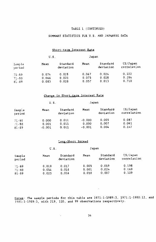
TABLE I (CONTINIJED)

SUNNARY STATISTICS FOR U.S. AND JAPANESE DATA

Short-term Interest Rate

U.S. Japan

Sample Mean Standard Mean Standard US/Japan

period deviation deviation correlation

71-89 0.074 0.028 0.067 0.024 0.222

71-80 0.066 0.025 0.075 0.028 0.284

81-89 0.083 0.028 0.057 0.013 0.710

Chane in Short-term Interest Rate

U.S. Japan



71-89 0.000 0.011 -0.000 0.005 0.087

71-80 0.001 0.011 0.000 0.007 0.061

81-89 -0.001 0.011 -0.001 0.004 0.147

LonE-Short Svread

U.S. Japan



71-89 0.019 0.017 0.005 0.019 0.198

71-80 0.014 0.016 0.001 0.024 0.169

81-89 0.025 0.016 0.010 0.007 0.109

jQ: The aample periods for this table are 1971:1-1989:3, 1971:1-1980:12, and1981:1-1989:3, with 219, 120, and 99 observations respectively.

34

TABLE 2

FORECASTING EXCESS STOCK RETURNSWITH DOMESTIC VARIABLES

U.S. STOCK RETURNS JAPANESE STOCK RETURNS

71-89 71-80 81-89 71-89 71-80 81-89

Januarydummy

0.282

(0.163)

0.312

(0.239)

0.247

(0.218)

0.329

(0.107)

0.294

(0.107)

0.364

(0.190)

Adjusted R2

Stability

0.0150.898

0.015 0.005 0.0270.536

0,017 0.030

Dividend-

price ratio8.113

(4.810)11.020(5.723)

3.321(8.936)

2.960(5.083)

19,590

(7.320)

-4.872

(10.523)

Adjusted R2

SignificanceStability

0.0260.0930.940

0.0380.056

0.0180.711

0.0250.5610.019

0.0730.008

0.0210.644

Short rate -2.703

(1.254)

-2,148

(2.237)

-4.166

(1.781)

-3.897

(1.494)

-4.292

(1.682)

-1.718

(3.982)

Adjusted R2SignificanceStability

0.0280.0320.601

0.0160.339

0.0390.021

0.0560.0100.886

0.0650.012

0.0210,667

Dividend- 23.589 23.169 28.333 9.282 20.691 -2.920price ratio (6.429) (7.368) (12.523) (5.190) (7.392) (21.158)Short rate -7.421 -7.232 -9.909 -5.208 -4.568 .0.784

(1.804) (2.824) (2.953) (1.562) (1.650) (8.100)

Adjusted R2 0.100 0.096 4.109 0.070 0.129 0.011Significance 0.000 0.007 0.004 0.004 0.001 0.898

Stability 0.423 0.167

CONTINUED]

35

TABLE 2 (CONTINUED)

U.S. STOCK RETURNS JAPANESE STOCK RETURNS

71-89 71-80 81-89 71-89 71-80 81-89

Change inshort rate

-10.789

(4.539)

-17.799

(5.263)

-1.875

(7.113)

-8.947

(4.658)

-11.703

(4.975)

5.091

(12.282)

Adjusted R2


0.0550.0180.352

0.1310.001

-0.0040.793

0.0320.0560.476

0.0320.020

0.0210.679

Long-shortspread

6.916

(2.278)

8.035

(3.351)

6.869

(2.980)

3.933

(1.912)

4.718

(1.959)

-12.982

(9.431)

Adjusted R2


0.0530.0030.888

0.0560.018

0.0350.023

0.0430.0410.294

0.0590.018

0.0460.172

Dividend- 9.257 13.230 5.782 4.644 21.324 0.258

price ratio (4.486) (5.305) (8.423) (5.072) (7.431) (11.297)

Change in -7.347 -14.388 1.257 -6.490 -5.557 4.600

short rate (4.562) (5.223) (6.754) (4.342) (4.439) (12.479)

Long-Short 6.219 6.362 7.473 4.060 5.249 -12.981

spread (2.392) (3.227) (3.160) (1.919) (1.937) (10.157)

Adjusted R2 0.089 0.171 0.021 0.045 0.131 0.026

Significance 0.002 0.000 0.129 0.048 0.002 0.529


j.g: The sample periods for this table are 1971:1-1989:3, 1971:1-1980:12, and1981:1-1989:3, with 219, 120, and 99 observations respectively. All regressionsinclude a constant and January dummy. Heteroskedasticity-consistent standard errorsare reported in parentheses. "Significance" is the joint significance of all thecoefficients in the regression gj than on the constant and January dummy."Stability" is the rejection significance level for the hypothesis that allcoefficients in the subsample (including those on the constant and January dummy) areequal to those in the other two-thirds of the sample. Comparable results areobtained if the constant and January dummy are omitted from the stability test.

36

TABLE 3

FORECASTING EXCESS STOCK RETURNSWITN INTERNATIONAL VARIABLES

U.S. STOCK

71-89 71-80 81-89 71-89 71-80 81-89

Short rate level specification

25.573 26.538 -4.443 1.717

(7.070)

-41231(11.911)

U S 24526dividend-price ratio (6.356) (7.764) (16.534) (5.137)

-1.128 -2.115 -3.482U S -7.467 -6.014

(2.124) (2.138)short rate (1.867) (2.946) (3.065) (1.549)

6.778 17.758 79.951Japanese -1.582 10.909 -1.950

(9.555) (26.378)dividend-price ratio (4.746) (7.626) (28.365) (5.508)-4.129 -4.101 -2.309

Japanese -1.261 -1.170(1.608) (1.679) (7.921)

short rate (2.032) (2.122) (9.073)

Adjusted R2 0.096 0.092 0.092 0.0740.003

0.1200.001

0.1050.001

Significance (All) 0.001 0.018 0.0200.139 0.563 0.000

Significance (U.S.) 0.000 0.0050.038 0.022 0.001

Significance (Japan) 0.691 0.3070.001

Stability 0.388

Yield spread specification

U.S. 9.509 16.942 18.685 -9.154 -0.390 -44.816

dividend-price ratio (4.612) (6.122) (16.383) (4.049) (6.109) (10.686)

U.S. -7.018 -14.431 4.033 0,264 3.591 -2.111

change in short rate (4.389) (4.903) (6.218) (2.850) (3.856) (6.253)

U.S. 6.214 4.536 9.396 2.307 4.198 0.683

long-short spread (2.323) (3.195) (3.384) (1.886) (2.585) (2.613)

Japanese 3.409 10.952 12.673 4.682 19.404 67.892

dividend-price ratio (4.321) (7.350) (24.208) (4.904) (9.242) (18.105)

Japanese -7.644 -5.178 -19.358 -5.768 -3.637 13 663

change in short rate (6.403) (6.878) (13.178) (4.398) (4.755) (11.491)

Japanese 0.191 2.427 -19.968 3.566 4.735 -8.624

long-short spread (2.306) (2.214) (12.987) (1.846) (1.795) (10334)

Adjusted R2 0.084 0.173 0.047 0.065 0.123 0.090

Significance (All) 0.011 0.000 0.092 0.006 0.001 0.005

Significance (U.S.) 0.002 0.000 0.047 0.012 0.345 0.001

Significance (Japan) 0.563 0.277 0.273 0.096 0.020 0.003


[NOTES ON NEXT PAGE]

37

N9s&s: The sample periods for this tsble sre 1971:1-1989:3, 1971:1-1980:12, and 1981:1-1989:3, with 219, 120, and 99 observations respectively. All regressions include aconstant and January dummy. Heterosicedasticity-consistent standard errors are reportedin parentheses. "Significance (All)" is the joint significance of all the coefficientsin the regression gg than on the constant and January dummy. "Significance (U.S.)"and "Significance (Japan)" are the joint significance levels of the U.S. and Japanesevariables, respectively. "Stability" is the rejection significance level for thehypothesis that all coefficients in the subsample (including those on the constant andJanuary dummy) are equal to those in the other two-thirds of the sample. Comparableresults are obtained if the constant and January dummy are omitted from the stabilitytest.

38

TABLE 4

AN OBSERVABLE FACTOR MODEL FORTHE EXCESS JAPANESE STOCK RETURN

JAPANESE STOCK RETURN

71-80 81-89


0.253 0.410U.S.

excess stock return (0.103) (0.076)

Adjusted R2 0.185 0.275

Significance (All) 0.001 0.001Significance (U.S.) 0.502 0.000

Significance (Japan) 0.031 0.001

Yield soread specification

U.S. 0.283 0.429excess stock return (0.096) (0.071)

Adjusted R2 0.198 0.286

Significance (All) 0.002 0.000

Significance (U.S.) 0.119 0.000

Significance (Japan) 0.042 0.000

The sample periods for this table are 1971:1.1989:3, 1971:1-1980:12, and 19811989:3, with 219, 120, and 99 observations respectively. All regressions include aconstant, January dummy, and U.S. excess stock return, as well as the variables listin Table 3 for the short rate level and yield spread specifications.Heteroskedasticity-consistent standard errors are reported in parentheses."Significance (All)" is the joint significance of all the coefficients in the

regression than on the constant, the U.S. excess return and the January dummy.

"Significance (U.S.)" and "Significance (Japan)" are the joint significance levels othe U.S. and Japanese variables (other than the constant. U.S. excess return and

January dummy) respectively.

39

TABLE 5

AN UNOBSERVABLE FACTOR MODELOF EXCESS U.S. AND JAPANESE STOCK RETURNS

DEMEANED DEMEANED AND DESEASONALIZED

71-80 81-89 71-80 81-89

Short rate level soecificstion

1.342

(0.443)

1.681

(0.819)

1.411

(0.571)Japanese 1.594beta (0.687)

Model restrictions 0.079 0.085 0.040 0.042

R2 ratio (U.S.) 0.339 0.445 0.308 0.320

ratio (Japan) 0.889 0.853 0.882 0.817

Unrestricted 0.435correlation

0.235 0.320 0.078

Yield soread soecification

Japanese 0.862 -1.738 0.745 -1.654beta (0.250) (1.127) (0.250) (1.081)

Model restrictions 0.089 0.151 0.046 0.185

R2 ratio (U.S.) 0.649 0.264 0.639 0.325

R2 ratio (Japan) 0.761 0.692 0.586 0.895

Unrestricted 0.314 0.043 0.219 -0.178correlation

)jQ.tE.a: The sample periods for this table are 1971:1-1989:3, 1971:1-1980:12, and 1981:1-1989:3, with 219, 120, and 99 observations respectively. The table reports the resultsof estimating a single-latent-variable model, equation (6) in the text, on demeaneddata, and demeaned and deseasonalized data (the residuals from a first-stage regressionof returns on a constant and January dummy). The instruments used in the short ratelevel and yield spread specifications are listed in Table 3. "Japanese beta" is theestimated loading of the excess Japanese stock return on the single unobserved factor(the U.S. loading is normalized to one), with an aaymptotic standard error inparentheses. "Model restrictions" is the significance level for a test of theoveridentifying restrictions of the single-latent-variable model. "R2 ratio" is theratio of the variance of the restricted model forecast to the variance of theunrestricted regression forecast of the stock return. "Unrestricted correlation" isthe correlation of the unrestricted regression forecasts of stock returns in the twocountries.

40

TAM.E 6

FORECASTING EXCESS RETURNS ON SIZE PORTFOLIOSWITH INTERNATIONAL VARIABLES

U.S. RETURNS

71-89 71-80 81-89 71-89 71-80 81-89

Short rate level soecificatiop

Ouintile 1 (smallest)

Adjusted R2 0.212 0.277 0.159 0.167 0.209 0.083


Significance (U.S.) 0.000 0.002 0.004 0.007 0.040 0.053



puintile 3 (middle)

Adjusted R2 0.150 0.187 0.109 0.157 0.173 0.127


Significance (U.S.) 0.000 0.001 0.004 0.012 0.223 0.005



Ouintile 5 (largest)

Adjusted R2 0.099 0.085 0.113 0.076 0.108 0.097


Significance (U.S.) 0.000 0.008 0.003 0.053 0.587 0.002



[CONTINUED

41

TANLE 6 (CONTINTJED)

U.S. RETURNS JAPANESE RETURNS

71-89 71-80 81-89 71-89 71-80 81-89

Yield soread soecifjcption

Quintile 1 (smallest)

Adjusted R2 0192 0.289 0.117 0.162 0.210 0.083Significance (All) 0.006 0.002 0.166 0.000 0,003 0.067Significance (U.S.) 0.001 0.000 0.102 0.000 0.023 0.072Significance (Japan) 0.112 0.537 0.060 0.122 0.098 0.314Stability 0.002 0.085

Quintile 3 (middle)

Adjusted R2 0.127 0.223 0.073 0.155 0.174 0.130Significance (All) 0.007 0.000 0.154 0.001 0.009 0.006Significance (U.S.) 0.001 0.000 0.053 0.000 0.119 0,004Significance (Japan) 0.415 0.313 0.142 0.471 0.298 0.103Stability 0.001 0.322

Quintile 5 (larmest)

Adjusted R2 0.083 0.147 0.080 0.064 0.111 0.082Significance (All) 0.018 0.002 0.039 0.005 0.001 0.015Significance (U.S.) 0.002 0.000 0.018 0.004 0.332 0.010Significance (Japan) 0.629 0.287 0.192 0.240 0.036 0.092Stability 0.011 0.044

.g: The sanpie periods for this table are 1971:1-1989:3, 1971:1-1980:12, and 1981:1-1989:3, with 219, 120, and 99 observations respectively. All regressions include aconstant and January dumuiy. The short rate level specification also includes U.S. andJapanese dividend-price ratios and short-term interest rates, while the yield spreadspecification also includes U.S. and Japanese dividend-price ratios, long-short yieldspreads, and changes in short-term interest rates. 'Significance (All)" is the jointsignificance of all the coefficients in the regression than on the constant andJanuary dummy. "Significance (U.S.)" and "Significance (Japan)" are the jointsignificance levels of the U.S. and Japanese variables, respectively. "Stability" isthe rejection significance level for the hypothesis that all coefficients in thesubsample (including those on the constant and January dummy) are equal to those in theother two-thirds of the sample. Comparable results are obtained if the constant andJanuary dummy are omitted from the stability test.

42

TAELE 7

AN UNO8SERVABLE FACTOR MODELOF U.S. AND JAPANESE SIZE PORTFOLIO RETURNS

71-80 81-89 71-80 81-89


0.083 0.013 0.055Qujntjle 1 (smallest) 0.034

Quintile 3 (middle) 0.036 0.220 0.020 0.045

Quintile 5 (largest) 0.088 0.101 0.049 0.049

Yield spread specification

Quintile 1 (smallest) 0.033 0.209 0.030 0.101

Quintile 3 (middle) 0.055 0.373 0.037 0.157

Quincile 5 (largest) 0.082 0.020 0.041 0.037

Notes: The sample periods for this table are 1971:1-1989:3, 1971:1-1980:12, and 1981:1-1989:3, with 219, 120, and 99 observations respectively. The table reports the resultsof estimating single-latent-variable models on demeaned data, and demeaned anddeseasonalized data (the residuals from a first-stage regression of returns on aConstant and January dummy). The instruments used in the short rate level and yieldspread specifications are listed in Table 3. The numbers given are significance levelsfor tests of the overidentifying restrictions of the single-latent-variablespecification.

43

Annualized rate0.040,02 0,06a Ga

-4

-4

-J-4

008

ai.,.. 0

c1

FIGURE 1

U.S. AND JAPANESE DIVIDEND-PRICE RATIOS

(Solid line is U.S., dotted line is Japan)

• U.S. LONG- AND

(Solid line is short

FIGURE 2

SHORT-TERM INTEREST RATES

rate, dotted line is long race)

CI)

0

Go

0

O . DO—A

Annualized rQte0,10 0.15

U

-4

0.1-

Annualized rate0.08

FIGURE 3

JAPANESE LONG- AND SHORT-TERM INTEREST RATES

(Solid line is short rate, dotted line is long rate)

C

-4'

CD

-CD-I-C-

0

FIGURE 4a

U.S. FITTED RETURNS, 1971-1980

(Solid line is unrestricted, dotted line is international component)

Annualized rate0.00—0.80

-4

-4U,

-4-4

Annualized rate-0.80 —0,40 0,00 0.40 0.80-J

-4cM

-4(J1

a

-4-4

FIGURE 4b

JAPANESE FITTED RETURNS, 1971-1980


Annualized rate—0,80 —0.40 0.00 0.40 0.80

1

C

FIGURE Sa

U.S. FITTED RETURNS, 1981-1989


Annualized rake0.00

FIGURE 5b

JAPANESE FITTED RETURNS, 1981-1989


predictable stock returns in the united states and japan

Documents