predicted and measured arrival rates of meteors over
TRANSCRIPT

Predicted and Measured Arrival Rates of Meteors over Forward
Scatter Links
Robert Stanley Mawrey March 1991
Submitted in partial fulfilment of the requirements for the degree of Doctor of Philosophy in the Department of Electronic
Engineering, U ni versity of Natal.
or

Abstract
•
Investigations into currently accepted methods of modelling variations in the
arrival rate of meteors over forward-scatter meteor links have revealed some
shortcomings. In these investigations, particular emphasis is placed on the work
of Rudie due to its current acceptance in the literature. The non-uniform radiant
distribution of meteors measured by Davies and modelled by Rudie, is critically
examined and predictions using these models are compared with measured results
taken over two forward-scatter links in the Southern Hemisphere. A new, alter
native method of including the effect of non-uniform radiant distributions on the
predicted arrival rate of meteors is given. The method used by Rudie to model
Davies' measured radiant distribution is shown to be unnecessarily complicated
and a simpler alternative is given. Furthermore, Rudie's distribution is shown not
to be derived from a particular set of Davies' results as implied by Rudie.
Other non-uniform distributions of meteors are also investigated. Comparisons
between monthly-averaged daily cycles of measured and predicted arrival rates
of meteors for a midpath and an endpath meteor link are used to reveal the validity
and limitations of the published distributions. A new graphical method is used to
aid in determining the validity and limitations of the non-uniform distributions.
Discrepancies in the published predicted and measured annual variations in the
arrival rate of meteors are investigated. Contrary to recently published informa
tion, predicted annual variations in the arrival rate of meteors for meteor radiants
close to the ecliptic are shown to be comparable to measured results.
ii

Preface
The author was born in Durban on 30 April, 1964. The author's involvement in
meteor-scatter communications began in 1985 as a final year B.Sc. Eng. student
in the Department of Electronic Engineering at the University of Natal, Durban.
In 1986 he registered as a M.Sc. Eng. student at the university of Natal and joined
the Meteor-Scatter Research team to investigate meteor-scatter receiver design.
This investigation resulted in a greater and greater involvement in the measure
ment of meteor-scatter reflections and the author submitted a thesis in June 1988
entitled "A Meteor Scatter Measurement System". The M.Sc. Eng. degree was
awarded with distinction in August 1988.
The research work described in this thesis was performed in the Department of
Electronic Engineering, University of Natal, Durban, under the supervision of
Professor Anthony D. Broadhurst. These studies represent original work by the
author and have not been submitted in any form to another university. Where use
has been made of the work of others, it has been duly acknowledged in the text.
iii

Acknowledgements
I would like to take this opportunity to thank a few of the many people that I have
had the pleasure of working with during this thesis project:
Paul Rodman for his invaluable assistance with software support and advice
without whom any modifications to the Meteor Prediction Model would
have been impossible;
Peter Handley for his extremely professional management of the Meteor
Scatter programme;
David Fraser for his moral support and friendship throughout this project;
Stuart Mel ville for cooperation and assistance in the papers we co-au thored;
Professor A. D. Broadhurst for his assistance with the completion of this
thesis;
James Larsen for his permission to continue development of the Meteor
Prediction Model and for his suggestion of this topic of investigation;
Rod Radford for his tireless running of the measurement system and for
always being willing to go the extra mile;
Gernot Larsen for his generous offer of office space for two years and for
bearing all the inconvenience that his offer entailed.
I would like to thank the Foundation for Research and Development, Salbu (Pty)
Ltd) and the University of Natal for their support. In particular, I would like to
thank Mr Dave Larsen of Salbu (Pty) Ltd for supporting the Meteor-Scatter
Research Project.
iv

Last, but not least, I would like to thank my family for all their support and
especially my wife, Alison, for all her understanding during the difficult times of
thesis preparation.
v

Table of Contents
1 Introduction 1
1.1 Meteor-burst communications .............. 1
1.2 Modelling meteor-burst communications ........ . ..... 2
1.3 Problem Statement ............................ 3
1.4 Thesis summary and claims ...................... 4
2 Radiant distributions and modelling the arrival rate of meteors 6
2.1 Measured non-uniform density distributions of sporadic meteors .......... . .... . ............... 6
2.1.1 Hawkins' data .. .. .... .... . .. .... .. . ........ 8 2.1.2 Davies'data .· ·· .. .. . ... ....... .. .......... 1 0 2.1.3 McCrosky and Posen 's data ............ .. .... ... 13 2.1.4 Harvard data ... ... .. . . ... ... ... . ...... .. .. 14 2.1.5 Pupyshev's data . . .... .. ..... . .. .. . . . . . . .... 16
2.2 Ecllptlcal orbital distribution simulated by Rudie ........ 23
2.3 Velocity distribution of sporadic meteors ............ 26
2.4 Predicting the arrival rate of meteors over forward-scatter links ................................ 27
2.4.1 Development of meteor prediction models . .. .. . . . .. . .. 28 2.4.2 Comparisons between predicted and measured variations
in the arrival rate of meteors .. . .. . . .. . ... .. ... 30 2.4.3 Published annual variations in the arrival rate of meteors ... . 34 2.4.4 Published year-to -year variations in the arrival rate of
meteors ..... ... .. . . .... .. .... . . .... ... 38
2.5 Problems and uncertainties ..... . ................ 40
3 Calculation of the arrival rate of meteors 41
3.1 The physical properties of meteors ................. 41 3.1 .1 Mass distribution of meteors . ...... .. .. . ..... . . . .41 3.1.2 Ionization ......... . .. .... .. . .. . .. . ...... .42
vi

3.2 RadIo reflection properties . . .................... 44
3.3 ReceIved power .... . . . ...................... 48 3.3.1 Underdense model ......... .. .. . . . ..... . . . .. . 48 3.3.2 Overdens.e model ....... . . . .... .. .... .. . 50
3.4 Antenna gaIn and polarization ........... 50
3.5 Observable meteor trails ........................ 51 3.5.1 Average duty cycle . . . . . . . . . . . . . . . . . . . . . . . . .54
3.6 IncludIng the effect of the non-unIform radiant distribution of meteors . . . . . . . . . . . . . . . . . . . . . . . . . . . 54
3.7 Meteor Showers 59
3.8 NoIse sources 62
3.9 Computer-based prediction model ....... . ......... 63 3.9.1 Implementation of the arrival rate calculations .63
4 Rudie's orbital distribution and Davies' data 65
4.1 Rudie's orbital distribution . ..... . 4.1 .1 Orbital parameters of meteor orbits
65 . .. . . . 66
4.2 Transformation from orbital parameters to an eclIptlcal orbital distribution .................... 68
4.2.1 Extraction of an approximate heliocentric distribution from Davies ' distributions of orbital parameters . ...... .. . 71
4.3 Heliocentric to geocentric transformation ............. 76 4.3.1 Rudie's technique .... ... . . .. . . .. .. ... ... . .79 4.3.2 Corrections due to the gravitational effect of the earth .82 4.3.3 Other corrections . . . . . . . . . . . . . . . . . . . . . . . .. 83
4.4 Numerical simulation of the heliocentrIc to geocentric radIant density transformation ........... 83
4.5 Approximation of Davies' observed radiant distribution 85
4.6 Rudie's simulated distribution In geocentric coordinates 87
4.7 ExtrapolatIon of Davies' observed distributIon .. 90
4.8 Summary of findings . . . . . . . . . . . . . . . . . 91

5 Comparisons between predicted and measured arrival rates of meteors 93
5.1 Measured results ... . ....................... 93 5.1.1 System description .. . ... .. ...... . . . .. .. ..... . 93 5.1 .2 Data capture , recording and processing ............ . . 96
5.2 Graphical technique of determining the relative contributions of regions In the celestial sphere to the arrival rate of meteors .. . .... . ................... 99
5.3 Comparison between measured and predicted arrival rates of meteors . . . . . . . . . . . . . . . . . . . . . . . . . . .109
5.4 Comparisons between measured and predicted results .110 5.4.1 Annualvariation .... . .............. . .. . .. .. 123
5.5 Conclusions ..... . ................ 125
6 Conclusions 127
Appendix A - Area on the surface of a sphere .............. 130
References .......... ... ....................... 132
viii

List of Figures
2-1 Meteor radiant given in eclipticallongitude, A, and latitude, ~, relative to the apex of the earth's way. ............ . .... . .. .7
2-2 Apparent change in direction of a meteor radiant as seen by an observer on the earth. . . . . . . . . . . . . . . . . . . . . . . . . . . . . . . . .7
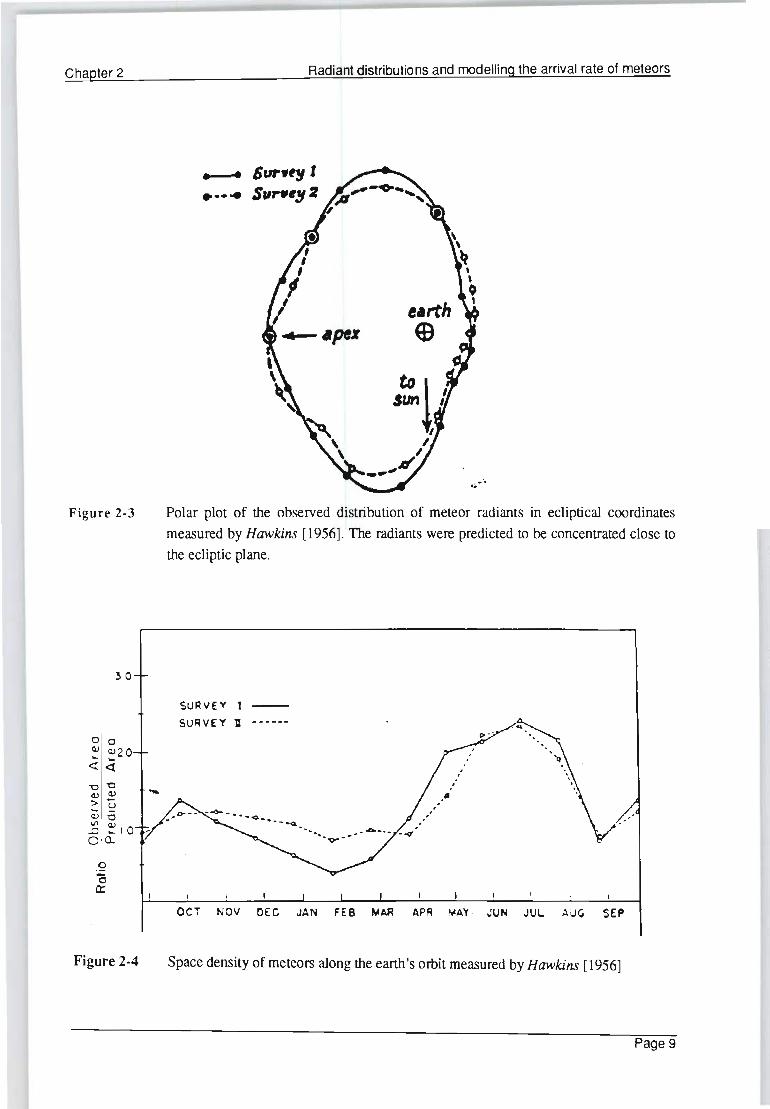
2-3 Polar plot of the observed distribution of meteor radiants in ecliptical coordinates measured by Hawkins [1956]. The radiants were predicted to be concentrated close to the ecliptic plane. . . . . .9
2-4 Space density of meteors along the earth's orbit measured by Hawkins [1956]. ..... . ......... . . . ....... . ........ .9
2-5 Polar plot of sporadic meteor radiants in ecliptical coordinates, corrected for observational selection: - - - - radiants within 20° of the ecliptic; _. _. radiants within 40° of the ecliptic;-- all radiants, Davies [1957]. ... . . . . . . . . . . . . . . . . . . . . . . .. 11
2-6 Distribution of 1 fa for sporadic meteors, weighted for observational selection. Ordinates: Weighted number of meteors, Davies [1957]. . . ........... . ................. . . . .. 12
2-7 Distribution of inclination of orbits with aphelion distances greater than 3 AU. Orbits with aphelion distances greater than 10 AU shown shaded, Davies [1957]. ....................... . . 12
2-8 Distribution of inclination of orbits with aphelion distances less than 3 AU, Davies [1957] . . . . . . . . . . . . . . . . . . . . . . . . . . . . .12
2-9 Photographic observed distribution of meteors extracted from McCrosky and Posen [1961]. .. . .. ............ . . . ..... . .13
2-10 Observed radiant density of meteors measured as part of the Harvard meteor project, Southworth fJnd Sekanina [1975]. ... . . . . .15
2-11 Contour map of the relative density of meteor radiants for January in geocentric ecliptical coordinates measured by Pupyshev et al. [1980]. .. . .......................... . ... . ... 17
2-12 Contour map of the relative density of meteor radiants for February in geocentric ecliptical coordinates measured by Pupyshev et al. [1980]. . .. .... . ............ . ........... .. .... 17
2-13 Contour map of the relative density of meteor radiants for March in geocentric ecliptical coordinates measured by Pupyshev et al. [1980]. . ....... . .. . ........ . ..... . ... . ....... 18
2-14 Contour map of the relative density of meteor radiants for April in geocentric ecliptical coordinates measured by Pupyshev et al. [1980] ................................... . ... 18
2-15 Contour map of the relative density of meteor radiants for May in geocentric ecliptical coordinates measured by Pupyshev et aI. [1980] ............... . ............ . ....... . .. 19
2-16 Contour map of the relative density of meteor radiants for June in geocentric ecliptical coordinates measured by Pupyshev et al. [1980]. . .......... . .......................... 19
ix
2-17 Contour map of the relative density of meteor radiants for July in geocentric ecliptical coordinates measured by Pupyshev et ai. [1980] . . .. ..... . ..... . .. .. ... . . .. . .. . . . .. .... 20
2-18 Contour map of the relative density of meteor radiants for August in geocentric ecliptical coordinates measured by Pupyshev et ai . [1980]. .. . . . ... . .. . ... . . . . .. . .. . . . .. . .. . . .. 20
2-19 Contour map of the relative density of meteor radiants for September in geocentric ecliptical coordinates measured by Pupyshev et al. [1980]. . . . ... ........ . . . . .. . .... ... . . . .. . . . 21
2-20 Contour map of the relative density of meteor radiants for October in geocentric ecliptical coordinates measured by Pupyshev et ai. [1980]. .. ..... . ..... . .... ...... . . .. . . . . . . .. 21
2-21 Contour map of the relative density of meteor radiants for November in geocentric ecliptical coordinates measured by Pupyshev et ai. [1980] . . . . ... . . . . . ...... . . . .. . .... ..... . . .. .. 22
2-22 Contour map of the relative density of meteor radiants for December in geocentric ecliptical coordinates measured by Pupyshev et ai . [1980]. . .. .... ... . .. ... ... .. . . . ....... ... . ... 22
2-23 Contour map of the yearly-averaged relative density of meteor radiants in geocentric ecliptical coordinates measured by Pupyshev et ai . [1980]. .. . . .. . .... . ... ...... .. . .. . 23
2-24 Contour map of Rudie's orbital simulation of meteors. . . . . . . . . . . .24
2-25 Observed distribution of meteors given by Rudie [1967]. ..... .. . .25
2-26 Contour map of the relative density distribution of geocentric velocity versus geocentric elongation angle extracted from data given in McCrosky and Posen [1961] . . . . . . . . . . . . . . . . . . . . . . . .. 27
2-27 Arrival rate of meteors (meteors/min) for a 960 km mid-latitude link (solid lines) and predicted results for March and September (broken lines). Weitzen [1986]. . . . . . . . . . . . . . . . . . . . . .. 31
2-28 Arrival rate of meteors (meteors/min) for a 1260 km high-latitude link (solid lines) and predicted results for February and July (broken lines). Weitzen [1986] ... . ........ ........ . . . ....... 31
2-29 Monthly meteor arrival rate prediction with (broken line) and without (solid line) the effect of shower meteors considered according to Weitzen [1986]. ... . . ... .. .. . .. . ... . . ....... . .. 32
2-30 Comparison between predicted and measured annual variation in the monthly-averaged hourly arrival rate of meteors for a forward-scatter link in the Southern Hemisphere given by Mawrey [1990]. . . ... ... . . . . . . . . . . . . . . . . .. . . ... 33
2-31 Annual cycles of meteors given by McKiniey [1961]. Curve A, naked-eye visual observations. (Murakami [1955].) Curve B, telescopic visual observations. (Kresakova and Kresak [1955].) Curve C, forward-scatter radio observations. Multiply ordinate scale by 20. (Vogan and Campbell [1957].) Curve D, back-scatter radio observations. Multiply ordinate scale by 2. (Weiss [1957] .). . . . . . . . . . . . . . . . . . . . . . . . . . 34
2-32 The annual variation in the arrival rate of meteors recorded at mid-northern latitudes presented by Keay [1963] . . 35
x

2-33 Some normalised annual variations in the arrival rate of meteors measured over forward-scatter links . . . .. . ... . . .. . 36
2-34 The annual variation of meteor arrival rates in both the Northern and Southern hemisphere presented by Keay [1963]. . . . . .. . . . . . 37
2-35 The annual variation in the arrival rate of meteors intercepting the earth based on comparisons between predicted and measured results for the Northern and Southern hemisphere presented by Keay [1963]. . . .. . .. .. . .... . . . . .. . ... . .. . . . . .. .37
2-36 Annual variation in average hourly meteor rate between 1 February 1963 and 31 August 1965 presented by Keay and Ellyett [1968]. . 38
2-37 Annual variation in the diurnal ratio of maximum to minimum meteor rates presented by Keay and Ellyett [1968] . ... . ..... ... . 39
3-1 Diagram to illustrate the geometry of forward-scatter. . 45
3-2 Diagram to illustrate the principal Fresnel region. . . . . 47
4-1 Elliptical orbit of a meteor travelling around the sun ... .. . .. . . .... .. 66
4-2
4-3
4-4
4-5
4-6
4-7
4-8
4-9
Ec1iptical coordinate system.
Range of possible orbital parameters of meteors 1 fa and e that intercept the earth (shaded region). . .... . .. . .. . .. . . . .
Velocity components of a meteor .. . . ..... . ... . .... .
Regions on the 1 fa versus e plane corresponding to the orbital distributions given by Davies. . .. . . . .. .. . ..... . . . . .
Example of the transformation from a region in orbital space to a region in heliocentric space . . ... ... . . . . ... ... . .... . . .
Contour plot of the approximated relative radiant density of meteors in heliocentric ecliptical coordinates . . . .. . . . . .... .
Diagram to illustrate the transformation from a heliocentric to a geocentric radiant density distribution. . .... . . . . .
Zenith attraction. . . .. .... ... .. ........ .. .... 4-10 Diagram to illustrate the numerical method of simulating the
. 67
. 68
. 69
. 72
.74
.75
.78
.82
heliocentric to geocentric radiant density transformation. . 84
4-11 Observed radiant distribution of meteors obtained using an extrapolation of Davies' orbital parameters. Davies' observed radiant distribution was not used. . . . . .. .. .. . ... .. ..... . 86
4-12 Polar plots of the approximated observed radiant distribution.
Symmetry about the line of longitude through Ag = 18d' should be assumed. . . ....... ... . ... .. . . ......... . . .. 86
4-13 Contour map of the geocentric density distribution of meteors derived using Rudie's orbital simulation and transformation. An average heliocentric velocity of 35 kilometres per second was used. . .. 88
4-14 Comparison between Davies' polar plot of all sporadic meteors radiants versus the actual results obtained using Rudie's extrapolation. (Compare with Figure 2-25.) .... . . .. .. . .. .... .... .. . . 88
xi

4-15 Contour map of the geocentric density distribution of meteors derived using the numerical transformation. An average heliocentric velocity of 35 kilometres per second was used. ... .. . . . . 89
4-16 Contour map of the geocentric density distribution of meteors extrapolated directly from Davies ' polar plots (Figure 2-5). . .. . . . 91
5-1 Contour plot of the combined predicted antenna illumination pattern of the meteor region for the mid path system. Tx and Rx are the transmitter and receiver locations respectively. . . ... . .... . .. . 95
5-2 Contour plot of the combined predicted antenna illumination pattern of the meteor region for the end path system. Rx is the receiver location. . . . . .. ... ...... .. . . . . .. .. . ....... . 95
5-3 Days and hours during which data has been captured using the end path system during 1989 and 1990. .. . .. . . . . .......... . . 97
5-4 Days and hours during which data has been captured using the midpath system during 1988,1989 and 1990 (for 1990 see next page).. . 98
5-5 Contour map of the relative contribution of parts of the meteor region for the midpath system at 06hOO on 23 September using Rudie's radiant distribution of meteors . .. . ... . ... . .. . . .... 100
5-6 Relative contributions of parts of the celestial sphere to the arrival rate of meteors for the midpath system on 23 September at 06hOO. . 101
5-7 Relative contributions of parts of the celestial sphere to the arrival rate of meteors for the endpath system on 23 September at 06hOO. 101
5-8 Relative contribution of meteors on the celestial sphere to the arrival rate of meteors for the midpath system on 23 September at 06hOO local time. Rudie 's radiant distribution was used. . .. . 103
5-9 Relative contribution of meteors on the celestial sphere to the arrival rate of meteors for the endpath system on 23 September at 06hOO local time. Rudie 's radiant distribution was used. . .. . 103
5-10 Contour plots of the midpath relative contributions on the celestial sphere for a uniform geocentric radiant distribution (Uniform) and for Rudie's radiant distribution (Rudie) for 23 September at OOhOO, 06hOO, 12hOO and 18hOO local time. . . ...... . .. . . 104
5-11 Contour plots of the endpath relative contributions on the celestial sphere for a uniform geocentric radiant distribution (Uniform) and for Rudie 's radiant distribution (Rudie) for 23 September at OOhOO, 06hOO, 12hOO and 18hOO local time . . . ......... . . 105
5-12 Contour plots of the midpath relative contributions on the celestial sphere for a uniform geocentric radiant distribution (Uniform) and for Rudie's radiant distribution (Rudie) for 21 March, 21 June, 23 September and 22 December at 06hOO. . ... . .... . .. 107
5-13 Contour plots of the endpath relative contributions on the celestial sphere for a uniform geocentric radiant distribution (Uniform) and for Rudie's radiant distribution (Rudie) for 21 March, 21 June, 23 September and 22 December at 06hOO. . .. ..... .. . . 108
xii
5-14 Comparison between measured (solid diamond) and predicted (square) monthly-averaged daily cycles of meteors for the midpath system using Rudie's distribution. (Trails per hour versus local time) .. ... .. ........ .. .. . ... .... . .. . ... 112
5-15 Comparison between measured (solid diamond) and predicted (square) monthly-averaged daily cycles of meteors for the midpath system using Davies' ex.trapolated distribution. (Trails per hour versus local time) .. ........ .... ...... .... . ...... 113
5-16 Comparison between measured (solid diamond) and predicted (square) monthly-averaged daily cycles of meteors for the midpath system using Pupyshev's yearly-averaged distribution. (Trails per hour versus local time) ..................... . . . 114
5-17 Comparison between measured (solid diamond) and predicted (square) monthly-averaged daily cycles of meteors for the midpath system using Pupyshev's monthly-averaged distribution. (Trails per hour versus local time) ......................... 115
5-18 Comparison between measured (solid diamond) and predicted (square) monthly-averaged daily cycles of meteors for the endpath system using Rudie's distribution. (Trails per hour versus local time) . ......... ... .............. ..... .... .. 116
5-19 Comparison between measured (solid diamond) and predicted (square) monthly-averaged daily cycles of meteors for the endpath system using Davies' ex.trapolated distribution. (Trails per hour versus local time) ... ....... ........... .. .... .... 117
5-20 Comparison between measured (solid diamond) and predicted (square) monthly-averaged daily cycles of meteors for the endpath system using Pupyshev's yearly-averaged distribution. (Trails per hour versus local time) ...... .... ....... .. .. . .. 118
5-21 Comparison between measured (solid diamond) and predicted (square) monthly-averaged daily cycles of meteors for the endpath system using Pupyshev's monthly-averaged distribution. (Trails per hour versus local time) ..................... . . . 119
5-22 Contour plots of the endpath radiant contributions on the celestial sphere for a uniform geocentric radiant distribution (Uniform) and for Rudie's radiant distribution (Rudie) for March at 08hOO, lOhOO, 12hOO and 14hOO local time. . . . . . . . . . . . . . . . . . 120
5-23 Regions of relative contribution of meteor radiants on the celestial sphere for the end path system on 21 March at 04hOO local time. 122
5-24 Normalised measured (solid diamond) and predicted (square) monthly-averaged annual variation in the arrival rate of meteors for the midpath system versus month of year. . ............. 124
5-25 Normalised measured (solid diamond) and predicted (square) monthly-averaged annual variation in the arrival rate of meteors for the end path system versus month of year. .......... " 124
5-26 Apparant annual variation in the monthly-averaged space density of meteors estimated using the midpath (square) and the endpath (solid diamond) system. (Normalised variation versus month of year) ..... . ..... . ......... . .......... . .. . .. 125
xiii

List of Tables
2-1
3-1
3-2
Rudie's simulation of the orbital distribution of meteors, Rudie [1967]
Measured values of k.
Values of k~j. . ....
. 24.
.42
.44
3-3 Values of A and B. . . . . . . . . . . . . . . . . . . 49
3-4 The major meteor showers, McKinley [1961]. . .................. 60
4-1 Assumed distribution of Va versus e used to extrapolate Davies' orbital data. Uniform distribution with respect to e was assumed. . ... 73
5-1 Midpath and endpath system parameters. ..... .94
5-2 Midpath and end path antenna configuration. .. . . 94
xiv

Chapter 1 Introduction
Chapter 1
Introduction
1.1 Meteor-burst communications
The use of naturally occurring ionization trails left by meteors 1 burning up in the
earth's upper atmosphere to communicate cheaply and reliably over long dis
tances is now an established communication technique. Every day billions of
meteoroidsl, in orbit around the sun, collide with the earth's atmosphere. The
meteors bum up at heights ranging between 80 and 120 kilometres above the
earth's surface forming trails of ionization tens of kilometres long with an initial
diameter of approximately one metre. The meteor ionization trails or meteor trails
may be used to reflect radio waves between two points on the earth's surface.
The curvature of the earth's surface limits the separation between the two points
to a maximum of approximately 2000 kilometres. Very high frequency radio
waves, rather than high frequency radio waves, are typically used for communi
cation purposes to avoid interference caused by ionospheric reflections. The
duration of the reflected signal is limited by diffusion of the ionized trail, but is
sufficiently long to support burst-mode data communication.
The birth of the concept of the reflection of radio waves off meteor trails or
meteor-scatter can be traced back to the late 1920's and early 1930's. Although
The term meteor is a general term used to describe the whole phenomenon associated with the entry into the earth's atmosphere of a particle from space. A meteoroid is an object moving in interplanetary space which, on entering the earth' s atmosphere, produces the phenomenon of a meteor. For simplicity, the term meteor in this thesis includes the term meteoroid.
Page 1

Chapter 1 Introduction
most of the basic theory of meteor-scatter propagation was developed during the
1950's, the development of practical communication systems was limited by the
available technology. One of the earliest data communications systems was the
JANET test system developed by the Defense Research Board of Ottawa during
the 1950's. (See Forsyth et al. [1957].) The improvement in electronic technology
enabled the data processing and data storage limitations of the early test systems
to be overcome and one of the fIrst commercial systems to be implemented was
the Snopak telemetry (SNOTEL) system described by Barton and Burke [1977] .
Since the late 1970's there has been considerable renewed interest in meteor-burst
communications when it became apparent that it offered a reliable and cheap
method of communication that, in particular circumstances, offered advantages
over other communications techniques such as satellites. Applications of some
of the more recent systems include remote data gathering, teletype, facsimile,
vehicle tracking and back -up for military early warning radar systems. For further
reading, one of the most recent summaries of meteor-burst communications has
been given by favus [1990].
1.2 Modelling meteor-burst communications
Modelling any type of communications technique is essential to understand and
optimise its performance. To aid in the design, implementation and understanding
of meteor-burst communications and propagation, theoretical models have been
developed and implemented since the 1950's by James and Meeks [1956], Hines
[1956] and Rudie [1967]. As mentioned by Weitzen [1986] and Mawrey [1990],
the complexity of the meteor-burst communications channel requires the im
plementation of sophisticated computer-based meteor prediction models. A de
scription of the development of computer-based prediction models is presented
in Chapter 2. One of the most important parameters affecting communications
performance is the arrival rate of meteor trails useful for communication over a
forward-scatter link. (The termforward-scatter is used here to describe reflection
Page 2

Chapter 1 I ntroductio n
via meteor trails between two separated points on the earth's surface, as opposed
to back-scatter where the transmission and reception points are coincident.) In
order to predict the arrival rate of meteors the most sophisticated meteor predic
tion models include the effect of the following parameters:
• Path location, orientation and geometry
• Transmitter power, receiver sensitivity, and operating frequency
• Antenna polar patterns and antenna polarization
• Galactic and local noise sources
• Physical characteristics of meteor trails
• Meteor showers
• Non-uniform distribution of meteors intercepting the earth
The axial rotation of the earth, the orbital rotation of the earth around the sun,
and a non-uniform distribution of meteors intercepting the earth, are the three
primary factors resulting in variations in the arrival rate of meteor trails. In order
to model these effects accurately, it is necessary to have a model of the distribution
of meteors intercepting the earth and to incorporate the effects of this distribution
of meteors on the arrival rate of meteor trails useful for communication over
forward-scatter links.
1.3 Problem Statement
Investigations into currently accepted methods of predicting the arrival rate of
meteors over forward-scatter links have revealed the following problems:
• There appears to be a lack of information regarding the validity of the
currently available measured distributions of meteors intercepting the
earth.
• Discrepancies exist regarding the accepted annual variation in the arrival
rate of meteors intercepting the earth and therefore also over a forward
scatter link.
Page 3

Chapter 1
•
Introduction
Limitations exist with the method used by Rudie [1967] to model the
distribution of meteors in space and also to incorporate the effects of the
distribution on the arrival rate of meteors over a forward-scatter link.
Limitations with Rudie's techniques are significant since Rudie's tech
nique has received recent acceptance by Weitzen [1986], Larsen and
Rodman [1988], and Desourdis etal. [1988].
1.4 Thesis summary and claims
Currently available measured radiant distributions of meteors are presented in
Chapter 2. A summary of existing methods of predicting the arrival rate of
meteors over forward-scatter links is given, as well as some comparisons between
published predicted and measured variations in the arrival rate of meteors.
Discrepancies between published, measured and predicted annual variations in
the annual arrival rate of meteors are also presented.
A summary of the technique used in this thesis to calculate the arrival rate of
meteor trails useful for communication over a forward-scatter link is given in
Chapter 3. A new, alternative method of incorporating the effect of a non-uniform
distribution of meteors on the arrival rate of meteors is proposed.
An investigation into the distribution of meteors presented by Rudie [1967],
which were based on the measurements performed by Davies [1957], is presented
in Chapter 4. The limitations of the apparent method used by Rudie to generate
a distribution based on Davies' results are given. A new, alternative, and far
simpler method of using Davies' results is proposed.
In order to verify the validity of the radiant distributions of meteors presented in
Chapter 2, comparisons between measured and predicted arrival rates of meteors
over a forward-scatter link in the Southern Hemisphere are given in Chapter 5.
A new graphical method of determining which region of a particular radiant
Page 4

Chapter 1 Introduction
distribution contributes to the arrival rate of meteors over the forward-scatter
link, for a particular system, time of day, and time of year is proposed. This is
useful to determine the validity of parts of the various distributions. The annual
variation in the arrival rate of meteors intercepting the earth is also estimated
using the measured and predicted annual variations in the arrival rate of meteors
over the forward-scatter link for the two different systems. The estimated annual
variation obtained using the two systems is compared with the published results
presented in Chapter 2 and conclusions are drawn regarding the actual annual
variation of meteors intercepting the earth. Finally, an overall conclusion is given
in Chapter 6.
PageS

Chapter 2 Radiant distributions and modelling the arrival rate of meteors
Chapter 2
Radiant distributions and modelling the arrival rate of
meteors
The current state and development of modelling variations in the arrival rate of
meteors over forward-scatter links is described in this chapter. Due to the
dependence of variations in the arrival rate of meteors over forward-scatter links
on non-uniform distributions, published non-uniform radiant distributions are
described in some detail. Problems and limitations with the current state of
modelling variations in the arrival rate of meteors are also mentioned.
2.1 Measured non-uniform density distributions of sporadic meteors The distribution of meteor radiants intercepting the earth may be described in
terms of an ecliptical coordinate system illustrated in Figure 2-1. The ecliptical
coordinate system may be defined as a right handed cartesian system with its
origin at the centre of the earth and its axis pointing in the direction of the earth's
motion (apex), the direction of the sun and the direction perpendicular to the
ecliptic plane (plane of the earth's motion around the sun). The direction of
meteor radiants in eclipticallongitude, A, and latitude, ~, relative to the apex is
shown in Figure 2-1. The effect of the earth's motion on the apparent direction
of a meteor radiant is illustrated in Figure 2-2. As a result of the vector addition
of the earth's orbital velocity, Ve, and a meteor's velocity, V h' relative to the sun,
a meteor will appear to come from direction, R g' with velocity, Vg, relative to the
Page 6

Chapter 2
Figure 2-1
Figure 2-2
Antisun
Earth
Apex
Radiant distributions and modelling the arrival rate of meteors
"
Antapex
"-
Meteor radiant
"- I Y To sun
"-. ;:f "- I Pr ' . f th di . _ . . _ ~ OJectIon 0 e meteor ra ant A. '-l onto the ecliptic plane
Meteor radiant given in eclipticallongitude, A., and latitude, ~, relative to the apex of the
earth's way.
___ Celestial Sphere
Observer's Horizon
Apparent change in direction of a meteor radiant as seen by an observer on the earth
Page 7

Chapter 2 Radiant distributions and modelling the arrival rate of meteors
observer on the earth at O. The effect of the earth's gravitational attraction and
the earth's rotation have been ignored. Rg andRh respectively, are the geocentric
and heliocentric meteor radiants.
Measurements of meteor velocities and radiants have shown that most meteors
intercepting the earth travel in the same direction as the earth travels around the
sun Hawkins [1956], Davies [1957], Southworth and Sekanina [1975]. The
vector addition of the earth's orbital velocity and a meteor's velocity results in
most meteors entering the earth's atmosphere on the apex hemisphere of the earth.
In heliocentric coordinates, therefore, most meteor radiants are clustered around
the antapex, whilst in geocentric coordinates most meteor radiants appear to be
concentrated around the apex hemisphere.
2.1.1 Hawkins' data
Between October 1949 and September 1951, approximately 240 000 sporadic
meteor reflections were measured using radar at 10drell Bank, England,
2° 18' W,53° 14' N. (See Lovell [1954] and Hawkins [1956].) The distribution
of sporadic meteor radiants was determined on a statistical basis by analysing the
relative number of meteor reflections measured using two narrow-beam aerials.
The results of the analysis of these measurements are shown in Figures 2-3 and
2-4. Figure 2-3 gives polar plots of the yearly-averaged distribution of meteor
radiants in geocentric eclipticallongitude. "Survey 1" and "Survey 2" are the
measurements between, October 1949 and September 1950, and, October 1950
and September 1951, respectively. The results showed a concentration of meteor
radiants close to the ecliptic plane in the direction of the apex and at ecliptical
longitudes of Ag = 65° and Ag = 295° known, respectively, as the sun and
antisun regions. The nature of the measurements did not enable the distribution
of radiants with respect to eclipticallatitude to be determined. The close corre-
Page 8
Chapter 2
Figure 2-3
30
-0'0 4J 4J > -u ~-o ~ ~ I O Dc..
.2 Ci a::
Figure 2-4
-
Radiant distributions and modelling the arrival rate of meteors
.-.. Sury'y I
..... S""'~!J2
t • • '",
Polar plot of the observed distribution of meteor radiants in ecliptical coordinates
measured by Hawkins [1956] . The radiants were predicted to be concentrated close to
the ecliptic plane.
SUR .... Ey I SURVEY 11
. ....... .-_ .. _ . • -q"
.".. -. . .. -.
, ,
OCT NOV OEC JAN FEB MAR APR MAY JUN JUL .liJ~ SEP
Space density of meteors along the earth's orbit measured by Hawkins [1956]
Page 9
Chapter 2 Radiant distributions and modelling the arrival rate of meteors
lation between the two surveys indicated that there was little year-to-year
variation in the distribution of radiants averaged over this duration.
Comparisons of measured monthly variations with predicted results based on the
yearly-averaged space density of meteors shown in Figure 2-3 indicated that the
space density of meteors along the earth's orbit was not constant and varied as
shown in Figure 2-4, Hawkins [1956] . Although not explicitly mentioned by
Hawkins, the latitude at which the measurements were taken enabled few radiants
south of the ecliptic to be measured, and therefore, the results presented by
Hawkins consisted primarily of radiants north of the ecliptic.
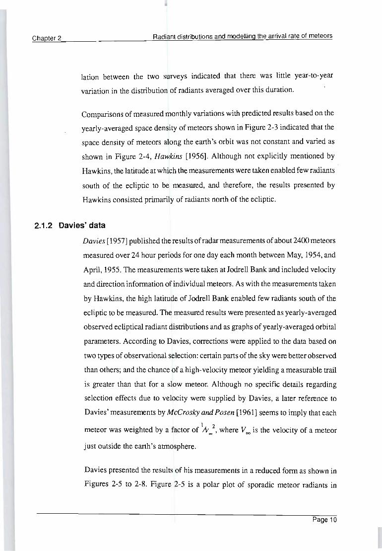
2.1.2 Davies' data
Davies [1957] published the results of radar measurements of about 2400 meteors
measured over 24 hour periods for one day each month between May, 1954, and
April, 1955. The measurements were taken at Jodrell Bank and included velocity
and direction information of individual meteors. As with the measurements taken
by Hawkins, the high latitude of Jodrell Bank enabled few radiants south of the
ecliptic to be measured. The measured results were presented as yearly-averaged
observed ecliptical radiant distributions and as graphs of yearly-averaged orbital
parameters. According to Davies, corrections were applied to the data based on
two types of observational selection: certain parts of the sky were better observed
than others; and the chance of a high-velocity meteor yielding a measurable trail
is greater than that for a slow meteor. Although no specific details regarding
selection effects due to velocity were supplied by Davies, a later reference to
Davies' measurements by McCrosky and Posen [1961] seems to imply that each
meteor was weighted by a factor of ~ 00
2, where V 00 is the velocity of a meteor
just outside the earth's atmosphere.
Davies presented the results of his measurements in a reduced form as shown in
Figures 2-5 to 2-8. Figure 2-5 is a polar plot of sporadic meteor radiants in
Page 10

Chapter 2
Figure 2-5
Radiant distributions and modelling the arrival rate of meteors
eclipticallongitude. The results were presented as the sum of various ranges of
geocentric eclipticallatitude, ~g' versus eclipticallongitude, Ag, as shown in the
figure.
Similar to Hawkins' results, Davies' results showed concentrations of meteor
radiants at the apex, sun and antisun regions. Davies' results, however, were far
less uniform than Hawkins' results and gave more information regarding the
distribution of meteor radiants with respect to ecliptical latitude. Davies also
presented the results of his measurements as distributions of orbital parameters
of meteors as shown in Figures 2-6 to 2-8. Unfortunately, however, the original
data used to generate these, graphs was not published.
27d'
T An'i I0I0,
poin'
~------~--~----~-----U~--I~ ~Ape.
Sun
! 90·
Polar plot of sporadic meteor radiants in ecliptical coordinates, corrected for observa
tional selection: - - - - radiants within 20° of the ecliptic; - , - . radiants within 40° of the ecliptic;- all radiants, Davies [1957].
Page 11

Chapter 2
Figure 2-6
Figure 2-7
Figure 2-8
Radiant distributions and modelling the arrival rate of meteors
200
100
1 o 0.5 1.0 1.5 2.0 a
Distribution of 1/ a for sporadic meteors, weighted for observational selection. Ordinates:
Weighted num ber of meteors, Davies [1957].
30
20
%
10
o 60 120 .0
IBO l
Distribution of inclination of orbits with aphelion distances greater than 3 AU. Orbits
with aphelion distances greater than 10 AU shown shaded, Davies [1957].
% e < OJ .0
o
0.3 < e < 0.7
% e > 0.7
Distribution of inclination of orbits with aphelion distances less than 3 AU, Davies [1957].
Page 12

Chapter 2 Radiant distributions and modelling the arrival rate of meteors
2.1.3 McCrosky and Posen's data
M cCrosky and Posen [1961] presented, amongst other parameters, the geocentric
velocity and radiants of 2529 meteors, of which approximately 400 were shower
meteors. The meteors were photographed from New Mexico between February,
1952, and July, 1954, as part of the Harvard Meteor Project. McCrosky and
Posen's data has been converted to an observed radiant distribution which is given
as a contour plot of meteor radiants in geocentric ecliptical coordinates in Figure
2-9. The absence of radiants in the direction of the sun is due to the photographic
nature of the measurements. The meteor radiants appear concentrated north of
the ecliptic due to observational selection. As with the previous distributions ,
meteor radiants are concentrated at the antisun and apex regions. McCrosky and
Posen's data also provides infonnation regarding the velocity distribution of
meteors, which is given in Section 2.3.
90.-------------------------~~--_=~----~ MinitoUHI: o 100 . 0 . :
70 , '" .. , . , '
so ,,', ,'" ., ' :" ' . ' :".,. ';.' " ' :' " · . . . · . . . · . . .
30 "' , ' .". , ., ",. , ;. " , ,
· . . . 10 " " . .. , . " :' . "':"" " ',."" ,
, , , , .. . .
-10 · . . . ', ' .... ',' .... :. . . . . . : ..... : . .... . :. · , , , , .
-30 · , .. . ... ' .......... :- .... -: . . . .. : .. . . . . : . . .. . · '" · '" · '" -so · . . . .:. . . . . ~ . . . . . :. . . . . .: . . . . .. ' . . . . .: . . . . . : . . . . .:. . . . . · . " · . . . · . ..
, ,
: ..... -: ..... : ...... : . .. . . , ,
· . . .. ; .. . . . ': . .. . . : ..... . : ... . -70 , ,
MaxitoUHI:
100 . 0
90 . 91
81 . 82
72 . 73
63 . S ....
5 .... . 55
.045 . 45
36.36
27.27
18.18
9 . 091
o
Figure 2·9 Photographic observed distribution of meteors extracted from McCrosky and Posen [1961].
Page 13
Chapter 2 Radiant distributions and modelling the arrival rate of meteors
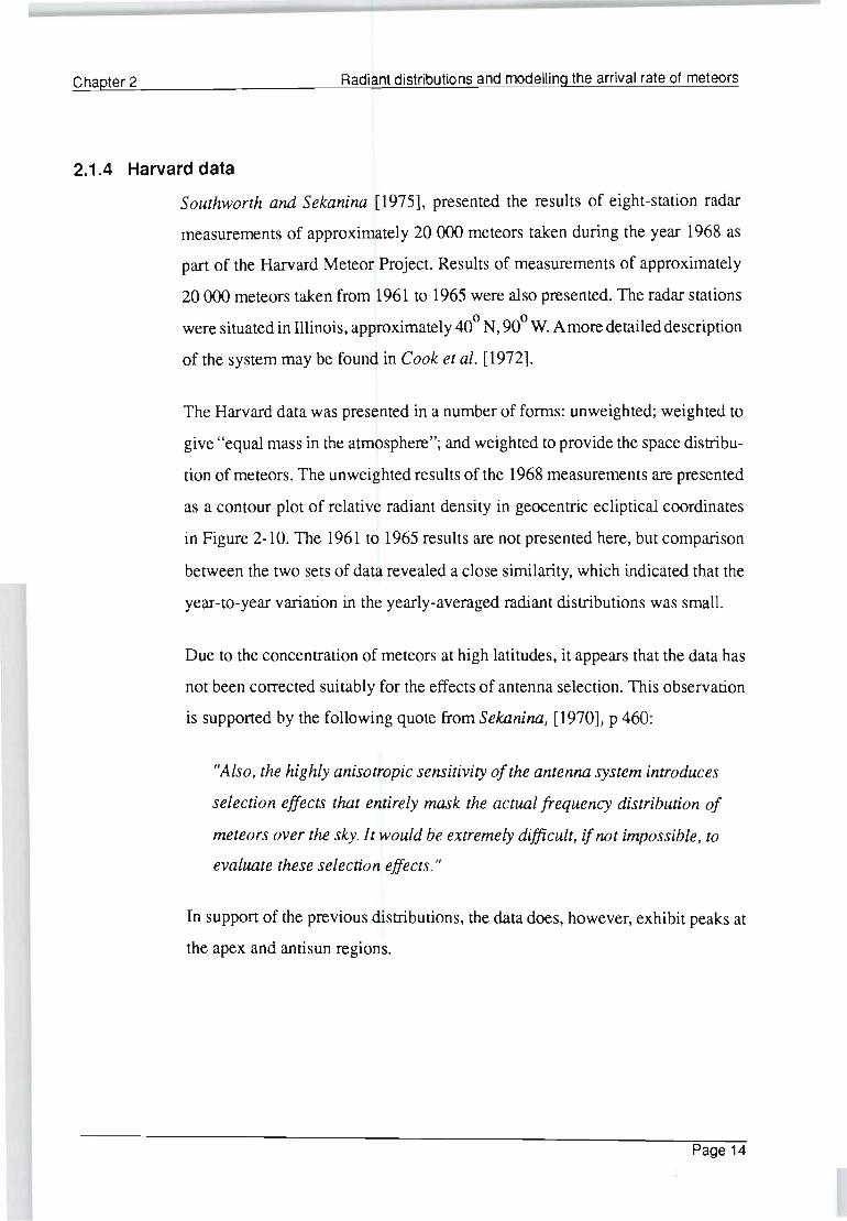
2.1.4 Harvard data
Southworth and Sekanina [1975], presented the results of eight-station radar
measurements of approximately 20 000 meteors taken during the year 1968 as
part of the Harvard Meteor Project. Results of measurements of approximately
20000 meteors taken from 1961 to 1965 were also presented. The radar stations
were situated in lllinois, approximately 40° N, 90° W. A more detailed description
of the system may be found in Cook et al. [1972].
The Harvard data was presented in a number of forms: unweighted; weighted to
give "equal mass in the atmosphere"; and weighted to provide the space distribu
tion of meteors. The unweighted results of the 1968 measurements are presented
as a contour plot of relative radiant density in geocentric ecliptical coordinates
in Figure 2-10. The 1961 to 1965 results are not presented here, but comparison
between the two sets of data revealed a close similarity, which indicated that the
year-to-year variation in the yearly-averaged radiant distributions was small.
Due to the concentration of meteors at high latitudes, it appears that the data has
not been corrected suitably for the effects of antenna selection. This observation
is supported by the following quote from Sekanina, [1970], p 460:
"Also, the highly anisotropic sensitivity of the antenna system introduces
selection effects that entirely mask the actual frequency distribution of
meteors over the sky. It would be extremely difficult, if not impossible, to
evaluate these selection effects."
In support of the previous distributions, the data does, however, exhibit peaks at
the apex and antisun regions.
Page 14
Chapter 2
90
BO
70
60
50
40
~g 30
20
10
11: 54 17/9/90
90
BO
70
60
50
40
~g 30
20
10
11:29 17/9/90
Radiant distributions and modelling the arrival rate of meteors
· . · .. .. : . ... . . : . .. . . :' ... . . : ... . .
· . . .. : . . . ... : . . . .. :. . . . . . : .. . . . · . . . · .. · .... : . . . . . -: ..... :- . ..
· . . .. : . . . . . . : . . ... : . . . . . . : . . .. . . . .
· . . : .... " . . ... ;. ... · .
A. - 90° g
A. - 90° g
. . .. ',' .. ..
..... : . . . . .
t1ini",u", : t1axi",u",:
o 23.00
23 . 00
20.70
18.40
16 . 10
13 . BO
11.50
9 . 200
6 . 900
4.600
2.300
o
Ul . 3 . 1 23 Aug 90
t1ini",u", : 3.000 t1axi",u",: 94.00
94.00
84.90
75 . 80
66 . 70
57 . 60
"'8 . 50
39 .... 0
30.30
21.20
12 . 10
3 . 000
U1.3.1 23 Aug 90
Figure 2-10 Observed radiant density of meteors measured as part of the Harvard meteor project, Southworth and Sekanina [1975] .
Page 15

Chapter 2 Radiant distributions and modelling the arrival rate of meteors
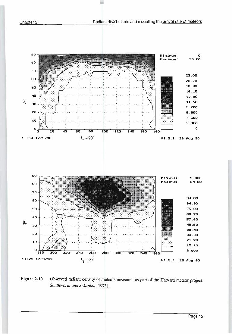
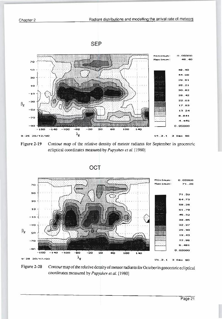
2.1.5 Pupyshev's data
Tabulated monthly distributions of meteors in geocentric coordinates presented
in Pupyshev et ai. [1980], have been made available to the author by personal
correspondence. Unfortunately, however, the original document is apparently
classified and is not available to the author. Based on the title of Pupyshev's
reference, the method of measurement is assumed to be radar and the data has
been assumed to be in the form of a radiant density of meteors. Pupyshev's data
represents the only measured distribution of meteors radiants known to the author
that includes a relatively equal distribution of radiants north and south of the
ecliptic. Although no reference is available to the author, personal discussion
arising from the Milcom 90 Conference indicated that the results were based on
measurements taken at Mogadishu, Somalia, Africa, and possibly also in the
USSR. A reference to measurements taken at Mogadishu from December, 1968,
to May, 1970, is given by Svetashkova, [1987].
The data have been reproduced as contour maps for each month of the year in
Figures 2-11 to 2-22. The data contoured in Figures 2-11 to 2-22 were divided
into cells 7.5° square, and the density of each cell was smoothed by averaging
with the adjacent cells. Even after smoothing the data, it is clear that the
distributions are rough. It is not known how many meteors were used to generate
each distribution. Since the original monthly-averaged data appeared to be rough,
a yearly-averaged distribution has been generated from the monthly-averaged
data. The yearly-averaged distribution of meteors is presented in Figure 2-23.
Consistent with previous distributions, the yearly-averaged distribution of me
teors shows similar concentrations at the antisun and apex regions. High concen
trations of meteor radiants, however, are also found at the north and particularly
the south ecliptic poles.
Page 16

Chapter 2 Radiant distributions and modelling the arrival rate of meteors
JAN
H in i.,·",,,,,,,,: 0
70 H~Ni"u": 82 . 70
SO 82 . 70
75.~0 30
S7.SS
'10 SO.~5
52.S3 -~o
15. ~~
37.59
30.07 Pg
-30
-50 22.55
-70 ~5 . 0""
7.S~8
0 -~80 - ...... 0 -'loa - so -20 20 so .. 00 ...... 0
O : SS 20/'12/90 U'I . 3 . '1 3 De., 90
Figure 2-11
70
so
30
'10
-~o
-30
Pg -so
-70
-90
-'180
Contour map of the relative density of meteor radiants for January in geocentric ecliptical coordinates measured by Pupyshev et al. [1980]
FEB
HiniMUM: 0
t1~Ni"u" : 37 . 20
37 . 20
33.82
30 . ......
27.05
23.67
20 . 29
'1S . S"
"3 . 53
'10."S
. . , ' , ' , , , , I· ' , , ', ' , 6.76"
3.382 , .' •••• • I • ••• ,' ••
- ...... 0 -"00 -so -20 20 so .. 00 ...... 0 a
9 : 08 20/'12/90
Figure 2-12
U'I.3.'1 3 De., SO
Contour map of the relative density of meteor radiants for February in geocentric ecliptical coordinates measured by Pupyshev etal. [1980]
Page 17

Chapter 2 Radiant distributions and modelling the arrival rate of meteors
MAR
f1iniI"lUM : 0
70 "'.aMi ......... : B3 . 60
SO 83 . BO
76 . 00 30
6B . ~0
~o 60 . BO
53 . 20 -~o
~5 . 60
~g - 30 3B . 00
30 . ~0
- so 22 . 00
- 70 ~5 . 20
7 . 600
0 - ~BO -~~O -~OO - 60 - 20 20 80 ~OO ~~O
9 : ~0 20/~2/90 U~ . 3. ~ 3 D.", SO
Figure 2-13 Contour map of the relative density of meteor radiants for March in geocentric ecliptical coordinates measured by Pupyshev et al. [1980]
APR
H iniru .• I"I : 0
70 MaMi. ... u ... : 27 . 20
so 27 . to
30 .' 2"' . B~
22 . ~7
~o ~9.7~
-~O ' . ~7 . 25
2~ . 7B
- 30 22.32
~g - so o S . B55
7 . 39~
- 70 ~ . 927
2 . ~B~
-~80 - ~~o -~OO -80 -20 20 0
80 tOO t~o
9:~2 20/~2/90 U~.3.~ 3 D.", 90
Figure 2-14 Contour map of the relative density of meteor radiants for April in geocentric ecliptical coordinates measured by Pupyshev et al. [1980]
Page 18

Chapter 2
70
so
30
~o
-30
- so
- 70
9 : ~'" 20/~2/90
Radiant distributions and modelling the arrival rate of meteors
MAY
- 20 20 60
· . .. .. . . . ,
· . .. . . . . ...
~oo
ttIn i"'u .... ;
".aMi""u .. :
U~ . 3 . ~
0
~ ... ~.O
~ ... ~ . o
~29 . 2
~15 . ...
~02 . 5
99 . 73
76 . 9~
6 ... . 09
5~ . 27
39 . .... 5
25 . 8-4
~2 . 82
0
3 D.<> 90
Figure 2-15 Contour map of the relative density of meteor radiants for May in geocentric ecliptical coordinates measured by Pupyshev et al. [1980]
so
30
~o
-30
-so
- 70
. . . . . .. . . . .
. . .. . .. . .....
9:~9 20/~2/90
JUN
-20 20 60
· . ',' .. . ' ,'
~oo
Hini""u",,: 0
"aMI ... "" ... : "'8 . 910
-46 . 90
-42 . 8-4
38.37
3-4. t~
29 . 85
25 . 59
2~ . 32
~7 . 05
~2.79
9 . 527
... . 26 ...
0
U~ . 3 . t 3 D.<> 90
Figure 2-16 Contour map of the relative density of meteor radiants for June in geocentric ecliptical coordinates measured by Pupyshev et al. [1980]
Page 19

Chapter 2 Radiant distributions and modelling the arrival rate of meteors
JUL
Hini ... u .... ; 0
70 ".aMi"" ....... : 59 . 00
so 59 . 00
53 . S-4 30
-4B . 27
1.0 -42.91.
37 . 55 -1.0
32.1B
-30 2S . 02
21 . -45
-so lS . 0S
-70 1.0 . 73
5 . 3S-4
-so 0 -20 20 ao 100 1-40
9 : 21. 20/1.2/S0 U1..3.1. 3 D.", 90
Figure 2-17 Contour map of the relative density of meteor radiants for July in geocentric ecliptical coordinates measured by Pupyshev et al. [1980]
AUG
Hini .... """' : 0 . 1.0000
70 .. . .. ".aMi ... "" ... : -49 . 00
so -49.00
30 -44.55
-40 . 11
1.0 35 . aa
-1.0 31 . 22
28 . 77
-30 22.33
~g -so 1.7 . BB
1.3.-4-4
- 70 . ". " . ".' ... '." S . SS1.
-4 . 5-45 -so
0 . 1.0000 -20 20 ao 100
9 : 23 20/1.2/90 U1..3.1.
Figure 2-18
3 D.", 90
Contour map of the relative density of meteor radiants for August in geocentric ecliptical coordinates measured by Pupyshev et al. [1980]
Page 20
Chapter 2 Radiant distributions and modelling the arrival rate of meteors
SEP
tti.ni~u,",; 0 . 05000
70 I1.aMiMU" : 4B.40
50 4B.-40
......... 00 30
39 . 61.
1.0 35 . 21.
30.B2 -1.0
26 . .... 2
~g -30 22.03
1.7 . 63 -so
1.3 . 24
-70 B.B41.
.... . .... 45
-90 0 . 05000 -1.BO -140 -100 -60 -20 20 60 100 140
9:25 20/1.2/90 U1..3.1. 3 D_c: 90
Figure 2-19 Contour map of the relative density of meteor radiants for September in geocentric ecliptical coordinates measured by Pupyshev et al. [1980]
OCT
Hlnl"",u .... = 0.02000
70 ... .aMi .. u"": 71. . 20
50 71. . 20
30 64 . 73
5B . 26
10 51 . 79
-1.0 45 . 32
3B . aS
-30 32 . 37
~g - so 25 . 90
1.9.-43
-70 1.2.96
6 ..... 91. -90
-1.BO -1 .... 0 -100 -60 -20 20 BO 100 1--40 0 . 02000
9 : 2B 20/1.2/90 Ul. . 3.1. 3 D_c: 90
Figure 2-20 Contour map of the relative density of meteor radiants for October in geocentric ecliptical coordinates measured by Pupyshev et al. [1980]
Page 21

Chapter 2 Radiant distributions and modelling the arrival rate of meteors
NOV
... In i,·'''.''''''': O . O~OOOOO
70 t1~Mi"u ... : 55 . BO
50 55 . BO
50 . 92 30
.... 5 . 7 ....
~O .... 0 . 66
35 . 58 -~O
30.50
~g -30 25 ..... ~
20 . 33 -50
~5.25
-70 ~o . ~7
5 . 09~
-BO O.OtOOOOO -20 20 so ~oo
B : 30 20/~2/BO Ul.3 . 1 3 D_c 90
Figure 2-21
70
50
30
~O
-~O
-30
~g -SO
-70
-90
-~SO
Contour map of the relative density of meteor radiants for November in geocentric
ecliptical coordinates measured by Pupyshev et al. [1980]
DEC
H in I.""" ... ",,: 0 . . .. '.' . "" . . . "aNiMU": ~02 . 0
102.0
92 . 73
03 . .... 5
7 ..... 18
S ..... 9~
55.6 ....
.... S . 3S
37.09
27 . 92
19 . 55
9 . 273
0 -1 .... 0 -100 -SO -20 20 SO ~OO t .... O
9 : 32 20/12/90 Ag
Figure 2-22
Ul . 3.1 :3 D_c 90
Contour map of the relative density of meteor radiants for December in geocentric ecliptical coordinates measured by Pupyshev et al. [1980]
Page 22

Chapter 2 Radiant distributions and modelling the arrival rate of meteors
Yearly-averaged
t11"1,",'-I11: O.~SSsO
l1 .. uc l ... u ... : ~OO . O
70
50 ~OO . O
SO . SS 30
O~ . s~
~o 72 . 80
S3 . 82
-~o S~ . 77
~S.73
36.60 ~g -30
-50 27 . G~
~8 . 59 -70
S.S~5
-so 0.~S950
-~oo -~~o -~OO -so -20 20 60 ~oo ~~O
~3:53 20/~2/90 U~.3.~ 3 0 ... gO
Figure 2-23 Contour map of the yearly-averaged relative density of meteor radiants in geocentric ecliptical coordinates measured by Pupyshev et al. [1980]
2.2 Ecliptical orbital distribution simulated by Rudie
An ecliptical orbital density distribution of meteors was simulated by Rudie using
the results presented by Davies. The orbital distribution was simulated as closed
fonn equations that are reproduced in Table 2-1. A contour plot of Rudie's
simulation based on the equations in Table 2-1 is given in Figure 2-24. No
derivation of these equations was given by Rudie. The only infonnation regarding
the origin of these equations was the following quote from Rudie's thesis, Rudie
[1967] p 68:
"The orbital distribution described by Figures 3-6 through 3-8 can be
simulated. A simulation is given in Table I, where Nh ( A', W) is the
relative polar density of sporadic meteor orbits in ecliptic coordinates."
Rudie's Figures 3-6 to 3-8 correspond to Figures 2-6 to 2-8 and Rudie's Table I
corresponds to Table 2-1.
Page 23

Chapter 2 Radiant distributions and modelling the arrival rate of meteors
Table 2-1 Rudie's simulation of the orbital distribution of meteors, Rudie [1967] .
Nh(4.~h)
-0.56 CNB + [( 0.56 CNB)2 + 2.24 CNA 1 Y2
2CNA
-0.944 CNB + [{ 0.944 CNB}2 + 2.828 CNA 1 Y2
2CNA
-1.25 CNB + [{ 1.25 CNB)2 + 2.5 CNA 1 Y2
2CNA
0
0.5
2 '.-2 -0.3 cos ~iI + [ ( 0.3 cos ~iI) + 4 sin2~11 1
2 sin2~iI
-0.22 cos ~iI + [ (0.22 cos ~iI)2 + 4 sin2~iI 1 Y2
2 sin2~11 2 '.-2
-0.9 cos ~iI + 9 [ (0.3 cos ~iI) + 4 sin2~" 1 4 sin
26i1
CNA = 1 - 2 sin ~iI cos ~iI
2
60
o
-30
-60 lillffif -so LSllililiJ ....
Ail
Oo~ 4< 40°
3200 ~ Ail < 360°
400 ~ All < 60°
3()(f < All < 320°
600 ~ All < 80°
2800 < Ail < 300°
80° ~ 4< 100°
260° < Ail < 280°
80° ~ Nt < 1000
260° < Ail < 280°
100° ~ Ail < 11 0°
1100 ~ Ail < 210°
210° ~ Ail < 260°
CNB = 0.707 (sin~II + cos ~iI )
. . . . . . . . . . . . . "" " " " "
~20 ~BO 200 2~O 200 320 360
Figure 2-24 Contour map of Rudie's orbital simulation of meteors.
~iI
I ~iI I ~ 90°
I ~II I ~ 90°
I ~II I ~ 90°
I ~II I ~ 12°
12° < I ~iI I ~ 90°
I ~II I ~ 90°
I ~II I ~ 90°
I ~II I ~ 90°
Hini ..... u ..... :
H_Mi .............. : o
""" . asa
""".asa
""" . OO?
3 . 562
2 . 67"-
2 . 22&
"- . ?a,,-
"- . 336
o
U"-.3."- 3 D_c: so
Page 24

Chapter 2 Radiant distributions and modelling the arrival rate of meteors
L meteors within 20 o
Apex o M meteors within 40
of the ecliptic
of the ecliptic ~-.:::': ---- -~ -;,:: .
," H all meteors
Figure 2-25 Observed distribution of meteors given by Rudie [1967].
In support of his simulated orbital distribution, Rudie compared results obtained
from his so called "orbit-radiant" transformation with Davies' measured results
of Figure 2-5. Rudie's results are reproduced in Figure 2-25. As mentioned by
Rudie, there are only two minor deviations between the results when compared
as polar plots as shown in Figures 2-5 and 2-25. The widths of the regions of
intense radiant activity near the sun and antisun in Figure 2-25 are narrower than
those in Figure 2-5, and the locations of those regions differ by about ten degrees.
As will be shown later, the similarity between the results does not, however,
necessarily imply that the Rudie's orbital distribution is an accurate repre
sentation of the actual orbital distribution, but simply serves to show that
combination of Rudie's orbital simulation and transformation produces a result
that is similar to the actual observed result.
Page 25

Chapter 2 Radiant distributions and modelling the arrival rate of meteors
2.3 Velocity distribution of sporadic meteors
As will be shown in the following chapter, the velocity distribution of meteors
is an important parameter in determining the arrival rate of meteors over a
forward-scatter link. Unfortunately, however, very little published information
on this parameter is available.
Radar measurements of meteor velocities have shown that the majority of
meteors travel in elliptical orbits around the sun with an average heliocentric
velocity of approximately 35 kilometres per second, Davies [1957], McKinley
[1961]. The only presentation of the velocity distribution of meteors versus
position on the celestial sphere known to the author was by Andrianov and
Pupyshev [1972]. Based on the measurements taken by McCrosky and Posen and
by radar measurements of 2200 meteors taken from April to May, 1965, and
October, 1966, at Kazan, USSR, Andrianov and Pupyshev presented distributions
of geocentric velocities for sixteen regions on the celestial sphere. Although
statistically a small sample set, analysis of the radar measurements and McCrosky
and Posen's data revealed no clear seasonal or latitudinal dependence of geocen-
tric velocity on the elongation angle, ego Differences between the radar and
photographic measurements were found, as might be expected, due to the
different selection effects inherent in the two types of measurement. Unfortunate
ly the reproduction of the graphical data presented by Andrianov and Pupyshev
available to the author is of very poor quality and is therefore not reproduced
here. McCrosky and Posen's original data is however available and has been
analysed by the author. A contour map of the relative density distribution of
geocentric velocity versus geocentric elongation angle extracted from McCrosky
and Posen [1961] is presented in Figure 2-26.
McCrosky and Posen's measurements conflrm the expected maximum and
minimum geocentric velocities of approximately 11 and 72 kilometres per second
limited by the escape velocities of the earth and sun respectively. The regions of
Page 26

Chapter 2 Radiant distributions and modelling the arrival rate of meteors
72~------------~----~--~----~--~----~--1 Hlnl .. " ....... : o ~OO.O "aMi ......... :
. ... ' . ' . . .. " , .. .. . : . ... . . : .. .
56
. . . . . . ' . .... ': . .... : ... . . : . .... ~OO.O
90 . 9~
... 9 .. ... :- ..... : .. . .. : . . . . . . : .. .. .
as . &2
. . . . " . . . ~.. . . .
. ' .. . ... " .. . . .. ..... ', · . . ... 0 72.73
· . . · . . B3 . S'" · . · . . . . '. ' . . . . ~ . . ... ' . ' .... , . ... ' , ' . . . . · . . 32 5 .... . 55 · .
" ...5 ..... 5 ... 24 . ~
~ .: . . . . . . : .. . .
36 . 3B
~ ~6 27 . 27
~9. sa 9
9 . 09~
o 0
0 20 .... 0 60 60 ~oo ~20 ~ .... O ~60 ~90
Elon1iJati~
~ .... : .... ~ 2~'/~2./90 U~ . 3 . ~ 3 D.c 90
Figure 2-26 Contour map of the relative density distribution of geocentric velocity versus geocentric elongation angle extracted from data given in McCrosky and Posen [1961]
high contribution also correlate well with the expected mean heliocentric velocity
of 35 kilometres per second.
2.4 Predicting the arrival rate of meteors over forward-scatter links As mentioned by Mawrey [1990], the modelling of meteor-scatter links to predict
communication performance has received renewed interest during the last de
cade. One of the most important parameters affecting communication perfor
mance is the arrival rate of meteors over a forward-scatter link. The theory and
measurements published since the late 1940's have been combined in the form
of advanced computer-based prediction models. The recent computer-based
prediction models may be divided into two broad categories. The fIrst category,
which includes the models by Haakinson [1983], Sachs [1984] and Felber et al.
[1985], is based on the assumption that the arrival rate of meteors for any arbitrary
link can be predicted by scaling data from known reference links. The second
Page 27

Chapter 2 Radiant distributions and modelling the arrival rate of meteors
category includes the models by Brown [1985], Weitzen [1986], Larsen and
Rodman [1988] and Desourdis et al. [1988] that use the theory of the physical
properties of meteors, as well as the effects of a non-uniform distribution of
meteors intercepting the earth.
2.4.1 Development of meteor prediction models
U sing the geometrical tangential requirements of forward··scattering from under
dense meteor trails, the characteristics of the power received from an underdense
trail, and the assumption that a meteor trail only acts as a useful radiator when at
least half its principal Fresnel zone is ionized, Eshleman and Manning [1954]
calculated the relative contribution of parts of the meteor region to forward-scat
ter communication. Based on the assumption of a uniform geocentric distribution
of meteors intercepting the earth, Eshleman and Manning's results showed that,
primarily due to geometrical requirements, regions of high contribution occurred
either side of the path between the transmitter and receiver with a null along the
path midpoint between the regions of high contribution. Due to the assumption
of a uniform distribution of meteors, Eshleman and Manning's method was
unable to predict any variations in the arrival rate of meteors.
The first predictions of variations due to the effect non-uniform radiant distribu
tions on the arrival rate of meteors over forward-scatter links were presented by
Hines [1956] and James and Meeks [1956]. Using an alternative method of
predicting the relative contribution of various sky regions, Hines [1955], Hines
and Pugh [1956], Hines [1956] published predicted daily variations in forward
scattered meteor signals based on the assumption that sporadic meteor radiants
could be modelled as a diffuse concentration of radiants centered on the apex of
the earth's way. Details of the distribution used by Hines were not given. By
improving the method of calculating the relative contribution of parts of the
meteor region developed by. Eshleman and Manning, and by developing an
approximate technique of including Hawkins' non-uniform radiant distribution,
Page 28

Chapter 2 Radiant distributions and modelling the arrival rate of meteors
James and Meeks [1956] presented comparisons between predicted and
measured daily cycles of meteors. The poor correlation between the predicted
and measured daily cycles obtained by James and Meeks was subsequently
improved by James [1958] who modelled Hawkins' radiant distribution as a
three-point concentration of radiants along the ecliptic at the apex, sun and
antisun peaks as measured by Hawkins [1956] and Lovell [1954].
Rudie [1967] improved on the previous method of modelling the arrival rate of
meteors by generating a distribution of meteors that approximated Davies '
measured distribution. Besides incorporating the effect of a non-uniform distribu
tion of meteors, Rudie also used an alternative method of calculating the relative
contribution of parts of the meteor region. Rudie's model was the fIrst published
model to include a non-uniform distribution with potential contributions across
the entire celestial sphere. Investigations by the author have revealed some
problems with Rudie's technique that are discussed in greater detail in Chapter
4.
The importance of investigating Rudie's method in greater detail is illustrated by
the fact that three out of the four recently developed advanced prediction models,
namely, the models by Weitzen [1986], Larsen and Rodman [1988], and Deso
urdis et al. [1988], are based on Rudie's method of calculating the effect of
Davies' non-uniform radiant distribution on the arrival rate of meteors. Brown's
model uses an approximation of Hawkins' distribution.
Although the effect of non-uniform distributions is of primary importance in this
thesis it is important to note that the recent computer based prediction models
offer signifIcant improvement over the previous models. One of the primary
reasons for this is the incorporation of more of the underlying physical parameters
and theory into an integrated prediction tool. Detailed descriptions of the recent
prediction models are given in the literature.
Page 29

Chapter 2 Radiant distributions and modelling the arrival rate of meteors
As part of the investigation into predicted and measured arrival rates of meteors,
the meteor prediction model developed by Larsen and Rodman has been further
developed by the author.
2.4.2 Comparisons between predicted and measured variations in the arrival rate of meteors
The non-uniform distribution of meteor radiants intercepting the earth results in
predicted variations in the arrival rate of meteors over a particular meteor-scatter
link. In the case of the yearly-averaged non-uniform distributions of meteors in
geocentric ecliptical coordinates given in the previous section, predicted daily
and seasonal variations may be seen to be due to changes in position of the
particular link relative to the geocentric ecliptical coordinate system. The daily
rotation of the earth about its axis and an anisotropic distribution of meteors in
geocentric ecliptical coordinates results in a daily cycle of meteors, whilst the tilt
of the earth's axis relative to the ecliptic plane similarly results in a seasonal or
annual variation in meteor arrival rates.
Few published comparisons between measured and predicted variations in the
arrival rate of meteors exist. Jame~ [1958] presented comparisons between
predicted results based on a three-point approximation to Hawkins' radiant
distribution and measured daily variations in the arrival rate of meteors for three
different meteor links. Although a reasonable agreement between the measured
and predicted results was obtained, the approximate nature of the radiant distribu
tion used by James limited the accuracy of the predicted results. Rudie [1967]
demonstrated the feasibility of his prediction technique by demonstrating the
effect of his non-uniform distribution on relative meteor activity on the meteor
region. Rudie did not, however, integrate over the sky region to compare
measured and predicted variations in the arrival rate of meteors directly. Using
Rudie's technique Weitzen [1986] compared measured and predicted monthly
averaged daily variations in the arrival rate of meteors for two different links.
Page 30

Chapter 2
w
~ ... ~
~ A. .. C a ... t. :r::
Figure 2-27
.... J ."
3 . •
2.'
2 .•
..S
... • . 5
Radiant distributions and modelling the arrival rate of meteors
.... / , SE~EHBER , ,
MARl'II
, . '
\
• .• '--_"'--_.....-_____ -""'_ ........ __ ~_"__ _ _'__~ _ _l
• • a • •• .- •• •• 2.
TI~ or 0., <LOCAL TI~[)
Arrival rate of meteors (meteors/min) for a 960 kIn mid-latitude link. (solid lines) and
predicted results for March and September (broken lines). Weitzen [1986]
.. , ... i 1:
ti I . • 60 .. C 0 ... ~
•••
Figure 2-28 Arrival rate of meteors (meteors/min) for a 1260 kIn high-latitude link (solid lines) and
predicted results for February and July (broken lines). Weitzen [1986]
Page 31

Chapter 2
'" ~ c
"' ... :> i II: C
• . 1
3.'
2.8
"8 " "
Radiant distributions and modelling the arrival rate of meteors
I
I I
I
I
I
I
" I
I
- -\
\ \
\
..... .....
" "
•. aL-~--~--~~~~--~--~--~~--~--~---. 8 2 1 • , • 7 • , ,. ·11 I ..
Figure 2-29 Monthly meteor arrival rate prediction with (broken line) and without (solid line) the
effect of shower meteors considered according to Weitzen [1986]
Weitzen's comparisons are reproduced in Figure 2-27 and 2-28. The correlation
between Weitzen's measured and predicted results is good, although, from
Weitzen [1986], it appears that the predicted results have been scaled according
to an expected seasonal variation in meteor arrival rates. According to Weitzen
[1986] seasonal variations in the number of meteors predicted by considering
only sporadic meteors do not correspond to observed data and additional factors
are required. Variations in monthly meteor arrival rate with and without the effect
of meteor showers predicted by Weitzen are reproduced in Figure 2-29. The
source of these predictions was not given by Weitzen, although it appears that
the solid line is based on a prediction using Rudie's distribution whilst the dotted
line appears very similar to the annual variation measured by Hawkins [1956].
As mentioned by Mawrey [1990] and described in greater detail later, the
inclusion of an annual scaling factor can only be approximate, since the effect of
showers and the variation in the radiant distribution will vary from link to link
Page 32

Chapter 2 Radiant distributions and modelling the arrival rate of meteors
J8
~ ~ .... " .. . ~ ......... . ; •. .. ...... , ......... , ... - ... . ; ...... .. ~ .. ···;·· ··· ·,········ ! ·· ····1
18 .......... , .......... , .......... , ........... ,.
... 58
<II
J8
18
= ) ' ~ ~ ,
..' ...
_ PJoM ittM -_ ..... aw"'tt& _ rz..,.I lct" . .. . .... au.reot
, !. .. ...... , .......... :---.... i
- - - .1 " ..
.' "-, ~ - --\ , .; - .-. ~ . ,
; t .... '&n ,.11 ...... ",,. "..y Jun Ju 1 ...... ... Oct Nov Dec ~on re. ..... ftpr "". Jun Jul Au, So. 0. -_ P're41ct" - _ .... av..t'K _PN4 ict.. -_ .... ~
Figure 2-30 Comparison between predicted and measured annual variation in the monthly-averaged hourly arrival rate of meteors for a forward-scatter link: in the Southern Hemisphere given by Mawrey [1990].
depending on factors such as geographical location and other link parameters.
Hawkins' measured yearly variation of the relative number of meteors intercept
ing the earth was also initially adopted by Brown [1985] but was subsequently
found to be inappropriate by StefJancin and Brown [1986]. The only direct
comparison between predicted and measured annual cycles of meteors over a
forward-scatter link known to the author was given by Mawrey [1990]. The
predicted results using Rudie's radiant distribution and measured results taken in
the Southern Hemisphere are reproduced in Figure 2-30. These results will be
analysed in greater detail later but it is important to note at this stage that, contrary
to some predictions, there was no large annual variation in the measured arrival
rate of meteors.
Page 33

Chapter 2 Radiant distributions and modelling the arrival rate of meteors
2.4.3 Published annual variations in the arrival rate of meteors
~ ..,
9
8
7
'06 ... ... C> .. ~5 >
-.::: ~4
2
Summaries of published annual variations in the arrival rate of meteors have been
presented by McKinley [1961] and Keay [1963]. McKinley [1961] presented
mean annual variation of meteor rates measured by naked-eye visual observa
tions, telescopic visual observations, forward-scatter radio observations and
back-scatter radio observations. The annual cycle of meteors presented by
McKinley is shown in Figure 2-31. Including the results presented by McKinley
[1961], Keay [1963] presented further annual variations in the arrival rate of
meteors recorded at mid-northern latitudes. The annual variations of meteors
were scaled for easy comparison and are reproduced in Figure 2-32.
Forward-scatter cycles have been extracted from papers by Vogan and Campbell
[1957], Sinno [1979] and Srirama Rao et al. [1983]. The cycle extracted from
?- ---a.... ,.. .... ,/ "-, .....
p' ~ I '
I " I ~
~ I ,
~/ "-
/ /
/
~ I
o Jon April May June July AUQ Now Dec
Lonqitude of sun o· I 90· 180"
Figure 2-31 Annual cycles of meteors given by McKinley [1961]. Curve A, naked-eye visual obselVations. (Murakami [1955].) CulVe B, telescopic visual obselVations. (Kresakowi
and Kresak [1955].) Curve C, forward-scatter radio obselVations. Multiply ordinate scale by 20. (Vogan and Campbell [1957].) Curve D, back-scatter radio observations. Multiply ordinate scale by 2. (Weiss [1957].)
Page 34
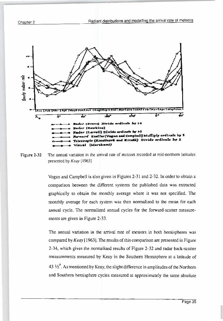
Chapter 2 Radiant distributions and modelling the arrival rate of meteors
_-.. • ..... ,. C~., DiY"'" ..... lift. ~ 1-. __ -0--0 ~.lfar (_kin_) _-... R.cI •• (Lov.Ul J)iYi ___ t-a. _ ..., • • .........""" scat t.,.(V .. _'" 0. .... bcl I) Multlpl7 ordJnatc b,r S a 10 • TeJcscople (ltJ'C~ end KredJl) D ... id .. enllnar. h7 2 • • • V~II" (M .. rakaml}
Figure 2-32 The annual variation in the arrival rate of meteors recorded at mid-northern latitudes presented by Keay [1963]
Vogan and Campbell is also given in Figures 2-31 and 2-32. In order to obtain a
comparison between the different systems the published data was extracted
graphically to obtain the monthly average where it was not specified. The
monthly average for each system was then normalized to the mean for each
annual cycle. The normalized annual cycles for the forward-scatter measure
ments are given in Figure 2-33.
The annual variation in the arrival rate of meteors in both hemispheres was
compared by Keay [1963]. The results of this comparison are presented in Figure
2-34, which gives the normalized results of Figure 2-32 and radar back-scatter
measurements measured by Keay in the Southern Hemisphere at a latitude of
43 Y2°. As mentioned by Keay, the slight difference in amplitudes of the Northern
and Southern hemisphere cycles measured at approximately the same absolute
Page 35

Chapter 2 Radiant distributions and modelling the arrival rate of meteors
2 .. .................................. .. .... .. ... . .
1.5 .................... . . . . .. .......... ..... ... .
o +---~---+--~----~--~--~---+--~~--+---~--~ Jan Feb Mar Apr May Jun Jul Aug Sep Oct Nov Dec
+ Rao75 * Sinno 57 *" Sinno 58 -tr Vogan 55 ~ Vogan 56
Figure 2-33 Some nonnalised annual variations in the arrival rate of meteors measured over forward
scatter links.
latitude indicated that there was also a slight annual variation in the density of
meteors intercepting the earth. Comparisons between predictions of the annual
variation of meteors using a three-point radiant distribution, similar to the
distribution presented by James [1958], and measured annual variations of
meteors indicated the annual variation in the density of meteors intercepting the
earth had the form given in Figure 2-35, Keay [1963].
As mentioned by Keay [1963] the results presented in Figure 2-35 vary signifi
cantly from the annual variation in the number of meteors intercepting the earth
presented by Hawkins [1956] that is reproduced in Figure 2-4. Based on the
apparent current acceptance of Hawkins' results by Weitzen [1986] this discrep
ancy will be further investigated in Chapter 5.
Page 36

Chapter 2 Radiant distributions and modelling the arrival rate of meteors
• • .. Jrorthcr. 1I..,laphcrc tA~.,. fr.-lit n •. l)
o 0 0 SautitCt'R Bemiephu. .....r. W.lfiPbr ardinalt ,.u)
Figure 2-34 The annual variation of meteor arrival rates in both the Northern and Southern hemi
sphere presented by Keay [1963].
.,
~ I.~~----------------~~--~------------~--------~~------~-I ~ I!-
. .,
Figure 2-35
.--.--. 1fot1hcrIIlrlmliIphcn DlacaPC, .. r_"~.""NtJL>'n __ ·• ~"'" X'rsall.""~) D 0 0 :a.an..rn •• al ..... R...r-. ClarlahoJo..reh. ~ ....
.. - ..... n... ___ ~ ...... ~ •. u e• ''''in.~,
The annual variation in the arrival rate of meteors intercepting the earth based on
comparisons between predicted and measured results for the Northern and Southern hemisphere presented by Keay [1963].
Page 37

Chapter 2 Radiant distributions and modelling the arrival rate of meteors
2.4.4 Published year-to-year variations in the arrival rate of meteors
200
o
Published year-to-year variations in the arrival rate of meteors have been pre
sented or may be extracted from the data given by Hawkins [1956], Ellyett and
Keay [1963], Millman and McIntosh [1964 & 1966] and Southworth and Sekan
ina [1975]. One of the most detailed investigations intotheyear-to-yearvariation
in arrival rates was performed by Keay and Ellyett [1968]. Annual variations in
the average hourly meteor rate from February 1963 to August 1965 presented by
Ellyett and Keay are reproduced in Figure 2-36. As mentioned by Ellyett and
Keay, apart from an inexplicable fluctuation in March 1964, the form of the
annual variation is similar for each year. The overall level of activity varies from
year to year as shown in Figure 2-36 although an even greater variation was found
between data measured during 1960/61 (not shown here) and during 1963 to
1965, Ellyett and Keay [1964] and Millman and McIntosh [1964]. Subsequent
investigation, Linblad [1967], Ellyett [1977], Ellyett and Kennewell [1980]
1883 -..-._
1884' • • • 11165· •••
F N A M ..J
t--.~ , ;
A' ,
A • , .. ' -. . " . ,,( . . . \: , A ,
! ~
..J A SON 0
Figure 2-36 Annual variation in average hourly meteor rate between 1 February 1963 and 31 August 1965 presented by Keay and Ellyett [1968].
Page 38

Chapter 2
10 2
S loW ~
~ z ~
5 aC
~ ~ c z u: ;:)
C
o
Radiant distributions and modelling the arrival rate of meteors
• o
~ ,./V-"0 o. ~~ • •
o F M A M J A
. - 0
.'1J6O • 1961
• UI63 o 19.4
• '96S
o • . ~ .- I-.......~
., 0",,-
SON o
• .....
Figure 2·37 Annual variation in the diurnal ratio of maximum to minimum meteor rates presented
by Keay and Ellyett [1968]
indicates that there may be an inverse correlation between apparent meteor arrival
rates and the solar cycle due to the sun-controlled variations of atmospheric
density in the meteor region.
As mentioned by Ellyett and Keay, although there is considerable variation in
the extreme rates from year to year, the relative variation in rates from year to
year is far smaller. This is illustrated by the ratio of minimum to maximum diurnal
rates presented by Keay and Ellyett [1968] that is reproduced in Figure 2-37. The
correlation in the year-to-year variations in the arrival rate of meteors appears to
indicate that the radiant distribution of meteors remains relatively constant from
year to year.
Page 39

Chapter 2 Radiant distributions and modelling the arrival rate of meteors
2.5 Problems and uncertainties Of the distributions presented at the beginning of this chapter, only the distribu
tions given by Hawkins and indirectly by Davies have been used in published
models. Rudie's interpretation of Davies' distribution appears to have received
the widest acceptance but no detailed analysis of the applicability or limitations
of the use of this model have been published. An investigation of the validity of
Pupyshev's distributions is important for a number of reasons. Firstly, no pub
lished account of the use of the distributions presented by Pupyshev for the
prediction of forward-scatter variations are known to the author. Secondly,
Pupyshev's distributions are the only known distributions that consist of a large
proportion of radiants south of the ecliptic, and thirdly, Pupyshev's distributions
are the only distributions known to the author that provide monthly-averaged
rather than yearly-averaged distributions.
Besides the need for a more detailed analysis of the presently used radiant
distributions based on comparisons between measured and predicted data, the
contradiction between large predicted variations in the annual arrival rate of
meteor based on Hawkins ' results that appears to have some acceptance in the
literature, and the relatively small variation in some of the measured results
requires further examination.
As already mentioned, the general acceptance of Rudie's method of applying
Davies' results also requires further attention.
Page 40

Chapter 3 Calculation of the arrival rate of meteors
Chapter 3
Calculation of the arrival rate of meteors
The technique used to calculate the arrival rate of meteors over a meteor scatter
link is described in this chapter. Theory used to calculate the arrival rate of
observable underdense meteors over a forward-scatter link are presented and a
simple technique of including the effect of non-uniform distributions of meteors
on the arrival rate of meteors is described.
The method of implementation of the theory described in this chapter as part of
an advanced computer-based prediction model is also described.
3.1 The physical properties of meteors
3.1.1 Mass distribution of meteors
Based on observational data of meteors the relationship between the mass of
meteors, m, and the average arrival rate of meteors, N, entering the earth's
atmosphere at a particular radiant and at a particular time has been shown to be:
McKinley [1961]
dN = K' m-s dm m (3-1)
where K'm and s are constants determined by measurement.
The integrated form of the above expression is often used, namely
Page 41

Chapter 3 Calculation of the arrival rate of meteors
l-s K -k N(m) - Kmm ... mm (3-2)
where N{m) is the anival rate of meteors, N, greater than mass, m, entering the
earth's atmosphere for a particular radiant and time of day and year, Km is a
constant, and k - s - 1.
The above expressions are only strictly true over a limited range of mass, but are
normally assumed to be accurate over the range of masses typically used for
communication purposes. Some measured values of k are given in Table 3-1.
Table 3-1 Measured values of k.
k Reference
1.3:t 0.3 McIntosh and Simek n9691
1.1 Babadzhanov et al. fl9851
Particular values of k may also be associated with different meteor showers and
particular meteor trail families. A value of k = 1.25 has been used in this thesis.
3.1.2 Ionization
As a meteoroid enters the earth's atmosphere, collisions between the meteoroid
and individual air particles in the atmosphere result in the kinetic energy of the
meteoroid being transformed into heat, light and ionization, McKinley [1961].
The ionization is produced in the form of an electrically neutral tube of positive
ions and electrons with an initially small radial component. The radius of the tube
of ionization increases with time due to radial diffusion of the meteor trail. The
amount of ionization produced is usually described as the number of electrons
per unit length along the axis of the meteors path, since the radial component
remains approximately constant for the duration of the trail. The electron com
ponent of the ionization is considered, since the presence of free electrons results
in the radio reflective properties of meteor trails. It has been shown by McKinley
Page 42

Chapter 3 Calculation of the arrival rate of meteors
[1961] that the electron line density is directly proportional to the mass of the
meteor and the density of the atmosphere. The relationship between electron line
density, q, and height, h, above the earth's surface has been shown by Kaiser
[1953], to be approximately
where
qrnax is the maximum electron line density (ionization) in electrons per
metre,
hqrnax is the height of maximum ionization above the earth's surface in
kilometres, and
H is a scale height in kilometres. (H = 7 km.)
Kaiser [1953], has shown that the maximum ionization of a meteor is
(3-4)
where
Kqrnax is a constant,
m is the mass of the meteor in kilograms,
~i is the probability that a single atom will produce a free electron,
~ is the zenith angle [ radians], and
Y is a constant typically assumed to be equal to one.
McKinley [1961], has shown that the ionization probability has the form
Page 43

Chapter 3 Calculation of the arrival rate of meteors
(3-5)
where k~i is a constant and V 00 is the velocity of the meteor in metres per second.
Various values of k~ . have been published, some of which are given in Table 3-2. I
Table 3-2 Values of ktli.
kll j Reference
3:1 Davies et al fl9591
5 McKinley fl9611 4 Verniani fl9651
The height of maximum ionization in kilometres has been shown to be a function
of meteor velocity and maximum ionization, McKinley [1961], and is given as
(3-6)
/
3.2 Radio reflection properties
The forward-scatter radio reflection properties of meteor trails have been derived
by Eshleman [1955] and Hines and Forsyth [1957]. Trails with electron line
densities of less than approximately 1014
electrons per metre may be modelled
as a line of individual electrons and are called underdense trails. Trails with an
electron line density of greater than approximately 1014
electrons per metre have
been modelled as a metallic cylinder and are called overdense trails. In order to
describe the radio refection properties of these trails, the geometrical require
ments for reflection via a meteor trail between two points on the earth's surface
will first be described.
Page 44

Chapter 3 Calculation of the arrival rate of meteors
Meteor trail (direction n
TRP- plane
t
/ /~~...\
h - plane
z Rr ~ to Y
Jt 0 tx
D -;/- D -/ Tangent plane to the earth's surface through T and R (XY-plane)
Figure 3-1 Diagram to illustrate the geometry of forward-scatter.
The geometry of forward-scatter reflection is illustrated in Figure 3-1. T and R
are points on the surface of the earth, corresponding to the transmitter and receiver
respectively. A plane through T and R is shown. A right-handed cartesian system
is defined at the midpoint between T and R with its centre at 0, and with its X
and Y axis in the plane of the tangential plane through T and R. The -2 axis passes
through the centre of the earth and the point 0 is actually beneath the earth's
surface. The h-plane is a tangential plane to the earth's surface at a height, h,
above the earth's surface at point P. Forreflection to occur between points T and
R on the earth's surface it may be shown that a meteor trail must lie in the plane
of the tangent to the spheroid
1 (3-7)
Page 45

Chapter 3 Calculation of the arrival rate of meteors
where Xo and Zo are the intercepts of the spheroid with the X and Z axis
respectively. The Y axis' intercept is also zo' Rudie [1967]. This plane is shown
as the meteor-plane or m-plane in Figure 3-1. For a particular meteor, reflection
between points T and R is shown in the figure to occur at point P(xp' yp' zp) at
the intersection of the m-plane, h-plane and TRP plane. (The TRP-plane is the
plane through points T, R and P.) Point P is the centre of the region of the meteor
trail contributing constructively to the amplitude of the reflected signal.
James and Meeks [1956], have shown that the normal to the spheroid at point
P = (xp' Yp' zp) is
(3-8)
where
1 nx = 2 cos <l> [ xp (GR + GT) + D (GR - GT) ]
1 nz = 2 cos <l> [ zp (GR + GT) ] ' and
where
1 1 GR = R = _I 2 2 2' and
R 'J (D + xp) + Yp + zp
A right-handed cartesian coordinate system with unit vectors t, :', ~, and origin
P, may be defined with f and:' in the m-plane, and with fin the direction of the
Page 46
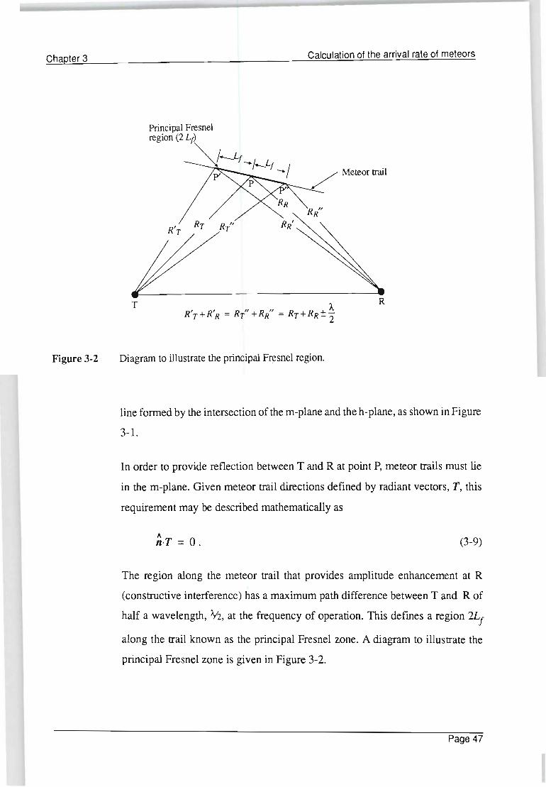
Chapter 3
Figure 3-2
Calculation of the arrival rate of meteors
~," _____ / Meteor trail
RT RT"
T R , R' R" R" R R + A. R T+ R = T + R = T+ R - 2.
Diagram to illustrate the principal Fresnel region.
line formed by the intersection of the m-plane and the h-plane, as shown in Figure
3-1.
In order to provide reflection between T and R at point P, meteor trails must lie
in the m-plane. Given meteor trail directions defined by radiant vectors, T, this
requirement may be described mathematically as
1\ n·T = O. (3-9)
The region along the meteor trail that provides amplitude enhancement at R
(constructive interference) has a maximum path difference between T and R of
half a wavelength, 112, at the frequency of operation. This defines a region 2Lf
along the trail known as the principal Fresnel zone. A diagram to illustrate the
principal Fresnel zone is given in Figure 3-2.
Page 47

Chapter 3 Calculation of the arrival rate of meteors
3.3 Received power
3.3.1 Underdense model
The received signal power available at a matched receiver from an underdense
trail at R is, Sugar [1964]
(3-10)
where
1: ..
2 2 2d 2 2 A; sec <p t. -32 3t to -8 3t YO , ... ---2~' andri =- 2 2'
32 3t2 d' ')...2 sec cp ')... sec cp
Pr is the transmitter power [watts],
Gr and GR are the transmitting and receiving antenna gains respectively,
')... is the operating wavelength [metres],
q is th~ electron line density [ electrons/metre],
re- is the radius of an electron s:::I 2.8 x 1O-15metres,
s2 is the antenna polarization factor which has been described by Rudie
[1967] and Larsen and Rodman [1988] (See Section 3-4.),
~ is the angle between the intersection of the propagation plane and the
meteor plane, and the meteor trail, as shown in Figure 3.1 [radians],
2cp is the angle between Rr and RR as shown in Figure 3.1 [radians],
d is the radial diffusion constant of the meteor trail described in Section 2 3.1.2 [m Is],
2to is the time in seconds taken to form the principal Fresnel zone, 2Lf, and
Page 48
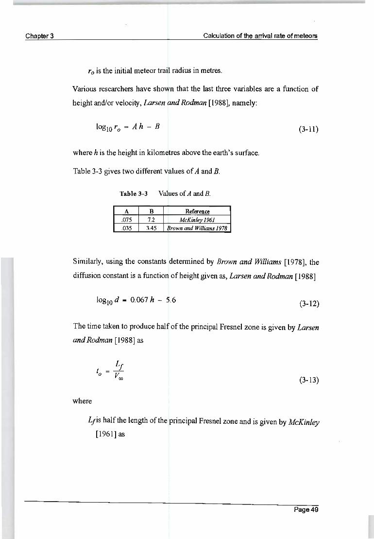
Chapter 3 Calculation of the arrival rate of meteors
ro is the initial meteor trail radius in metres.
Various researchers have shown that the last three variables are a function of
height and/or velocity, Larsen and Rodman [1988], namely:
(3-11)
where h is the height in kilometres above the earth's surface.
Table 3-3 gives two different values of A and B.
Table 3-3 Values of A and B.
A B Reference .075 7.2 McKinlev 1961 .035 3.45 Brown and William3 1978
Similarly, using the constants determined by Brown and Williams [1978], the
diffusion constant is a function of height given as, Larsen and Rodman [1988]
10glO d = 0.067 h - 5.6 (3-12)
The time taken to produce half of the principal Fresnel zone is given by Larsen
and Rodman [1988] as
(3-13)
where
Ljis half the length of the principal Fresnel zone and is given by McKinley
[1961] as
Page 49

Chapter 3 Calculation of the arrival rate of meteors
(3-14)
3.3.2 Overdense model
It is generally accepted that the analytical approximation of the power received
from an overdense trail is, in practice, not accurate. (See McKinley [1961]. Rudie
[1967], Weitzen [1983] and Larsen et al. [1990].) However, the approximate
expression for the power received from an overdense trail as developed by Hines
and Forsyth [1957] is
where
3.4 Antenna gain and polarization
The antenna gain and polarization factors Gr, GR, and S may be calculated using
the theory described by Rudie [1967], p 97-104, combined with the Numerical
Electromagnetic Code (NEC) - Method of Moments software described by Burke
and Pogio [1981]. No detail regarding this method will be given, suffice to say
that the results obtained by NEC enable the antenna gains and polarization to be
accurately calculated in three dimensional space, which enable the gain and
polarization factors to be calculated at any point in the meteor region. This theory
has been implemented by Larsen and Rodman [1988].
Page 50
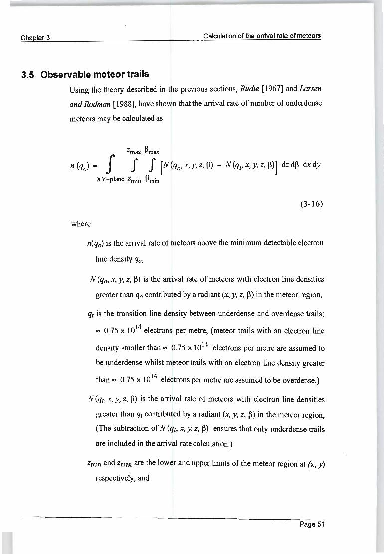
Chapter 3 Calculation of the arrival rate of meteors
3.5 Observable meteor trails
Using the theory described in the previous sections, Rudie [1967] and Larsen
and Rodman [1988], have shown that the arrival rate of number of underdense
meteors may be calculated as
Zmax ~max
n (qo) = f J J [N(qo'x,y,z, ~) - N(qpx,y,z, ~)l dzd~ dxdy
XY -plane zmin ~min
(3-16)
where
n(%) is the arrival rate of meteors above the minimum detectable electron
line density qo,
N (qo, x, y, Z, ~) is the arrival rate of meteors with electron line densities
greater than qo contributed by a radiant (x, y, Z, ~) in the meteor region,
qt is the transition line density between underdense and overdense trails;
r;;:$ 0.75 x 10¹⁴
electrons per metre, (meteor trails with an electron line
density smaller than r;;:$ 0.75 x 10¹⁴ electrons per metre are assumed to
be underdense whilst meteor trails with an electron line density greater
14 than r;;:$ 0.75 x 10 electrons per metre are assumed to be overdense.)
N (qt, x, y, Z, ~) is the arrival rate of meteors with electron line densities
greater than qt contributed by a radiant (x, y, Z, ~) in the meteor region,
(The subtraction of N (qt, x, y, z,~) ensures that only underdense trails
are included in the arrival rate calculation.)
Zmin and Zmax are the lower and upper limits of the meteor region at (x, y)
respectively, and
Page 51

Chapter 3 Calculation of the arrival rate of meteors
~min and ~max are the minimum and maximum angles that a meteor may
have to satisfy the tangential requirements at (x, y, z).
By algebraic manipulation of Equations 3-1 to 3-15, Larsen and Rodman [1988],
have shown that
where
[
COS y~ V ~~ij{h)] k N(q) = K COS ~ -~---
q
9 ( hqrnax - h ) [ 1 ( hqrnax - h )] 2 f(h) = 4"exp H 1 - 3exp H , and
(3-17)
K is a constant dependant on radiant position, time of day and time of year.
K may be derived from a" particular radiant distribution of meteors as
shown in Section 3.6.
From Equation 3-9, the minimum detectable line density is
(3-18)
where
PRmin is the minimum received power [watts].
N(qo) andN(qt) may thus be found by substituting, qo from Equation 3-18, and
qt respectively into Equation 3-17.
The previous equations may be expressed in tenns of x, y, z and ~ using the
following equations developed by James and Meeks [1956]:
Page 52

Chapter 3 Calculation of the arrival rate of meteors
(3-19)
\II ' -l[ T m = SIn
(3-20)
where
'I'm is the angle between the z-axis and the m-plane (See Figure 3-1.), and
(3-21)
Em is the angle between the intersection of the h-plane and the m-plane, and the
intersection of the TRP-plane and the m-plane (See Figure 3-1), and
'l -1 [-..J z2 + i ] 'f 1\.1 = cos Rr I x> 0
or
Furthermore
(3-22)
where
Page 53
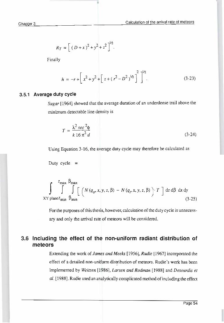
Chapter 3 Calculation of the arrival rate of meteors
Finally
2 1;2
[ 2 2 [ 2 2 1I2J J h = -r + x + y + z + (r - D ) . (3-23)
3.5.1 Average duty cycle
Sugar [1964] showed that the average duration of an underdense trail above the
minimum detectable line density is
T _ /...2 sec 2$ - k 161t2 d (3-24)
U sing Equation 3-16, the average duty cycle may therefore be calculated as
Duty cycle =
For the purposes of this thesis, however, calculation of the duty cycle is unnecess
ary and only the arrival rate of meteors will be considered.
3.6 Including the effect of the non-uniform radiant distribution of meteors
Extending the work of James and Meeks [1956], Rudie [1967] incorporated the
effect of a detailed non-uniform distribution of meteors. Rudie's work has been
implemented by Weitzen [1986], Larsen and Rodman [1988] and Desourdis et
al. [1988]. Rudie used an analytically complicated method of including the effect
Page 54

Chapter 3 Calculation of ttie arrival rate of meteors
of a non-uniform distribution of meteors based on the simulated orbital distribu
tion of meteors described in Chapter 2. As shown in Chapter 2 and later in Chapter
4, the non-uniform distribution of meteors may be completely described by using
a geocentric (observed) radiant distribution in ecliptical coordinates. This section
proposes a new and simpler method of including the effect of the non-uniform
radiant distribution for a given link. The effect of geographic position, orienta
tion, and time of day or year is included by referencing a meteor radiant in the
link coordinates to the geocentric eclipticallongitude and latitude.
With reference to Equation 3-16 and Figure 3-1, the effect of the non-uniform
radiant density on the relative number of meteors, N, seen at a particular (x, y, z,
~) may be included by assuming that K = C Og in Equation 3-17 where Og is the
non-uniform radiant density and C is a scaling constant. The relationship
between a meteor radiant in terms of (x, y, z, ~) and eclipticallongitude Ag and
latitude ~g may be found as follows.
The equation defining the surface with a constant height, h, above the earth's
surface, in terms of the f. 1. t coordinate system in Figure 3-1, is
-'./ 2 2 2 -'./2 2 z = f(x, y) = (h + r) - x -y - r - D (3-26)
where
r is the radius of the earth, and
D is half the distance between the transmitter and receiver as illustrated in
Figure 3-1.
The normal to the surface, Z = fix, y) , at point, P = (xp' yp' zp)' is
(3-27)
Page 55

Chapter 3 Calculation of the arrival rate of meteors
where
A vector defining the intersection of the h-plane and the m-plane is
I_A
= nhn x n
f J ~ = -Ix -iy 1
nx ny nz
The unit vector, t. is thus
where
A right-handed coordinate system may be defined as
(3-28)
(3-29)
Page 56

Chapter 3 Calculation of the arrival rate of meteors
(3-30)
As shown in Figure 3-1, the radiant of a meteor may be defined in terms of the
t, ;" ~ coordinate system, and hence the 1, J, i, coordinate system. Let T be the
trail radiant where
(3-31)
and 8m = Em + ~ is the angle between the intersection of the m-plane and the
h-plane, and the meteor radiant.
The transformation matrix relating the 1, J, i, coordinate system to the geocentric
ecliptical coordinate system ~,Jg, ig,where ~g,~, and ig are the right-handed
unit vectors in the direction of the apex, sun and perpendicular to the ecliptic
plane defining the eclipticaI coordinate system on the 23 September is given as,
James [1958]
A=
sin '" sin 60 + sin locos 60 cos '"
sin a cos 10 cos 60
- cos 60
cos '" sin 60
+ cos a sin 10 cos 60
sin 1/'
sinacos",sin60
+ cos a cos 10 cos 60
- sin a sin locos 60 sin '"
sin 10 sin 60 cos '" - sin", cos 60
- cos'" cos 10
cos a cos '" cos 60
+ sin a cos 10 sin 60
+cosa.~.~~", ~a~~-cosa.",cos~
cos a cos 10 sin 60
- sinacos1/'cos60
-.a.~.~~", cosa.~+.a.",cos~
PageS7

Chapter 3 Calculation of the arrival rate of meteors
(3-32)
where
l)a is the azimuth angle measured from north clockwise to the X-axis so that
la is the latitude of the midpoint between T and R. (In the northern
hemisphere fa > 0 and in the southern hemisphere la < 0.),
a is 23°27', the angle between the earth's axis and the ecliptic normal, and
'tV is the nutation angle which is equal to ood td where td is the elapsed time
in solar days since noon of September 23 and Wd is the rotation of the
earth per solar day; OOd is 360.9856 degrees per day.
Including the motion of the earth around the sun, the radiant of the meteor in
terms of the geocentric ecliptical coordinate system given in Figure 2.1 is thus
cos<JlR Sln<JlR 0
Tg = A T -sin<JlR cos<JlR 0 001
where 'I'R is equal to [ 3~62" + ; 1 radians.
(3-33)
Page 58

Chapter 3 Calculation of the arrival rate of meteors
The geocentric ecliptical latitude and longitude corresponding to a particular
meteor radiant T is thus
[ - T 1 -1 gx
A.g "" tan Tgy
' and (3-34)
(3-35)
3.7 Meteor showers
As mentioned by Weitzen [1986] and Mawrey [1990], shower meteors can have
a major effect on the arrival rate of meteors during the duration of a particular
shower. As mentioned by Mawrey [1990], the distinction between sporadic and
shower meteors is difficult to determine and the majority of sporadic meteor
distributions are bound to include a small shower component. A quantitative
method of distinguishing between shower and sporadic meteors was given by
Southworth and Hawkins [1963], but for the purposes of this thesis, shower
meteors will be limited to the well known major meteor showers listed in Table
3-4.
As is the case in Table 3-4 meteor shower radiants are often described in terms
of right ascension, a, and declination, l). The duration of the showers in Table
3-4 is the time during which the activity of the shower is greater than one-quarter
the peak value. As mentioned by McKinley [1961], there are large variations in
Page 59
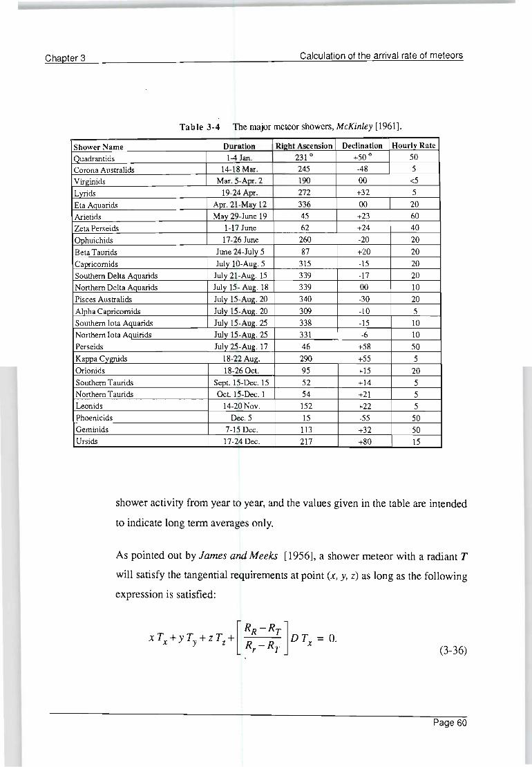
Chapter 3 Calculation of the arrival rate of meteors
Table 3-4 The major meteor showers, McKinley [1961].
Shower Name Duration Ri2ht Ascension Declination Hourly Rate
I Quadrantids 1-4 Jan. 231 0 +50 0 50
Corona Australids 14-18 Mar. 245 -48 5
Virginids Mar. 5-Apr. 2 190 00 <5
Lyrids 19-24 Apr. 272 +32 5
Eta Aquarids Apr. 21-May 12 336 00 20
Arietids May 29-June 19 45 +23 60
Zeta Perseids 1-17 June 62 +24 40
I Ophuichids 17-26 June 260 -20 20
Beta Taurids June 24-July 5 87 +20 20
Capricomids July 10-Aug. 5 315 -15 20
Southern Delta Aquarids July 21-Aug. 15 339 -17 20
Northern Delta Aquarids July 15- Aug. 18 339 00 10
Pisces Australids July 15-Aug. 20 340 -30 20
Alpha Capricomids July 15-Aug. 20 309 -10 5
Southern Iota Aquarids July 15-Aug. 25 338 -15 10
Northern Iota Aquirids July 15-Aug. 25 331 -6 10
Perseids July 25-Aug. 17 46 +58 50
Kappa Cygnids 18-22 Aug. 290 +55 5
Orionids 18-26 Oct. 95 +15 20
Southern Taurids Sept. 15-Dec. 15 52 +14 5 Northern Taurids Oct. 15-Dec. 1 54 +21 5
Leonids 14-20 Nov. 152 +22 5 Phoenicids Dec. 5 15 -55 50 Geminids 7-15 Dec. 113 +32 50 Ursids 17-24 Dec. 217 +80 15
shower activity from year to year, and the values given in the table are intended
to indicate long tenn averages only.
As pointed out by James and Meeks [1956], a shower meteor with a radiant T
will satisfy the tangential requirements at point (x, y, z) as long as the following
expression is satisfied:
(3-36)
Page 60

Chapter 3 Calculation of the arrival rate of meteors
A method of converting from right ascension and declination to T is James
[1958]:
(3-37)
(3-38)
(3-39)
where
A is the azimuth angle of the meteor radiant measured from north to east.
The azimuth angle and zenith of the meteor radiant may be found as follows:
where
sin 8 - sin fa cos· ~ cos A = --------~--
cos fa sin ~
cos ~ = sin fa sin 8 + cos fa cos H cos 8
8 is the right ascension of the radiant, and
H is the hour angle.
(3-40)
(3-41)
The relationship between right ascension, a., and hour angle is approximately:
H = 99.40° +.1 + 0.9856 d + 15.041 n - a. (3-42)
where
d is the number of days since January 1,
n is the number of hours since midnight, and
Page 61
Chapter 3 Calculation of the arrival rate of meteors
~ is the number of degrees that the path midpoint is east of the standard time
meridian.
The above equations enable the effect of individual meteor showers to be
included in the calculation of the total arrival rate of meteors. For the purposes
of this thesis, however, meteor shower contributions will not be included. As
described later in Chapter 5, in general, this does not cause a significant error if
monthly-averaged meteor rates are calculated.
3.8 Noise sources
The effect of man-made and galactic noise sources may included by modelling
the effect of external noise sources on the receiver's noise floor, Mawrey [1988],
p 132. The effect of environmental noise on the received signal-to-noise ratio is:
Sj PR -
Nj BnkbCTj+Te) (3-43)
where
Sj is the receiver's input signal power [W],
Nj is the receiver's input noise power [W],
Tj is the environmental noise temperature received by the antenna [K],
Te is the effective input noise temperature of the receiver [K],
Bn is the receiver's noise bandwidth [Hz], and
kb is Boltzmann's constant (1.381 x 10⁻²³ JIK).
The environmental noise temperature at the frequencies used in forward scatter
communication is primarily a combination of man-made, atmospheric and ga
lactic noise, Mawrey [1988]. The contribution due to galactic noise is computed
Page 62
Chapter 3 Calculation of the arrival rate of meteors
by integrating the receiver polar pattern over the region of the galactic noise map
generated by NASA Taylor [1973]. It may be seen from Equation 3-43 that the
minimum received power of Equation 3-18 is affected by the received signal-to
noise ratio requirement.
3.9 Computer-based prediction model The equations described in the previous sections have been implemented as part
of an advanced meteor-scatter prediction model. Modifications to the prediction
model have been specified by the author as part of the investigation into variations
in the arrival rate of meteors over forward-scatter links. These specifications
include the simpler method of incorporating the effect of non-uniform radiant
distributions described in Section 3-6, as well as the incorporation of the radiant
distributions described in Chapter 2. Other involvement by the author in the
development of the meteor prediction model was the specification of methods of
predicting the effects of shower meteors as well as the effects of galactic noise
contributions. A detailed description of the capabilities of the meteor prediction
model may be found in Larsen and Rodman [1988] and Rodman [1989].
3.9.1 Implementation of the arrival rate calculations
For the purposes of this thesis only a subset of the capabilities of the meteor
prediction model is required, namely, the calculation of the arrival rate of
underdense meteors over a forward-scatter link as well as the measured database
facilities described in Chapter 5.
The calculation of the arrival rate of underdense meteors is performed by software
implementation of the equations described in the previous sections. This calcu
lation essentially consists of numerical integration of Equation 3-16. The total
arrival-rate of meteors is calculated by summing over the contribution of points
in the meteor region. The position of the points in the meteor region are typically
Page 63

Chapter 3 Calculation of the arrival rate of meteors
chosen to be ten kilometres apart. The contribution at each point in the meteor
region is calculated as described by the inner two integrals of Equation 3-16. This
integration is also performed numerically. The effect of a non-uniform distribu
tion of meteors may be included using the the technique described in Section 3-6.
In order to concentrate on the effect of non-uniform distributions of meteors on
the arrival rate of meteors, the effect of as many variables and constants whose
values are presently uncertain, and whose effect on the relative variation in the
arrival rate of meteors was found to be minimal, were not included. This resulted
in the time taken to form the first Fresnel zone, 2to' and the initial trail radius,
r 0' of Equation 3-10 being assumed equal to zero. In order to be directly compared
with measured data, the effect of galactic noise contributions on the predicted
arrival rate of meteors was also not included, since the method of data processing
described in Chapter 5 effectively removes the effects of noise on the measured
arri val rate of meteors.
Page 64

Chapter 4 Rudie's orbital distribution and Davies' data
Chapter 4
Rudie's orbital distribution and Davies' data
This chapter investigates the widely accepted distribution of meteor radiants
presented by Rudie [1967] . Investigations into Rudie's method of modelling the
distribution of meteor radiants reveals the limitations of this technique. A new,
alternative method of extrapolating Davies' data is proposed.
4.1 Rudie's orbital distribution
As mentioned in Chapter 2, an investigation into Rudie's method of deriving an
orbital distribution based on Davies ' results has revealed some limitations. Rudie
claimed that the orbital distribution described by Davies' Figures 2-6 to 2-8 could
be simulated, and that if the simulation was realistic, then a radiant distribution
derived from it should compare favourably with Davies' radiant distribution
shown in Figure 2-5. As no derivation of the simulation given by Rudie is
available, a more detailed investigation into Rudie's technique is perfonned. The
results of this investigation show that the orbital parameters given by Davies were
not sufficient to derive the simulation given by Rudie and that Rudie's orbital
simulation could, therefore, only have been derived from Davies' radiant dis
tribution.
The following subsection briefly describes the orbital parameters of meteor orbits
in order to develop the necessary background for describing the transfonnation
Page 65
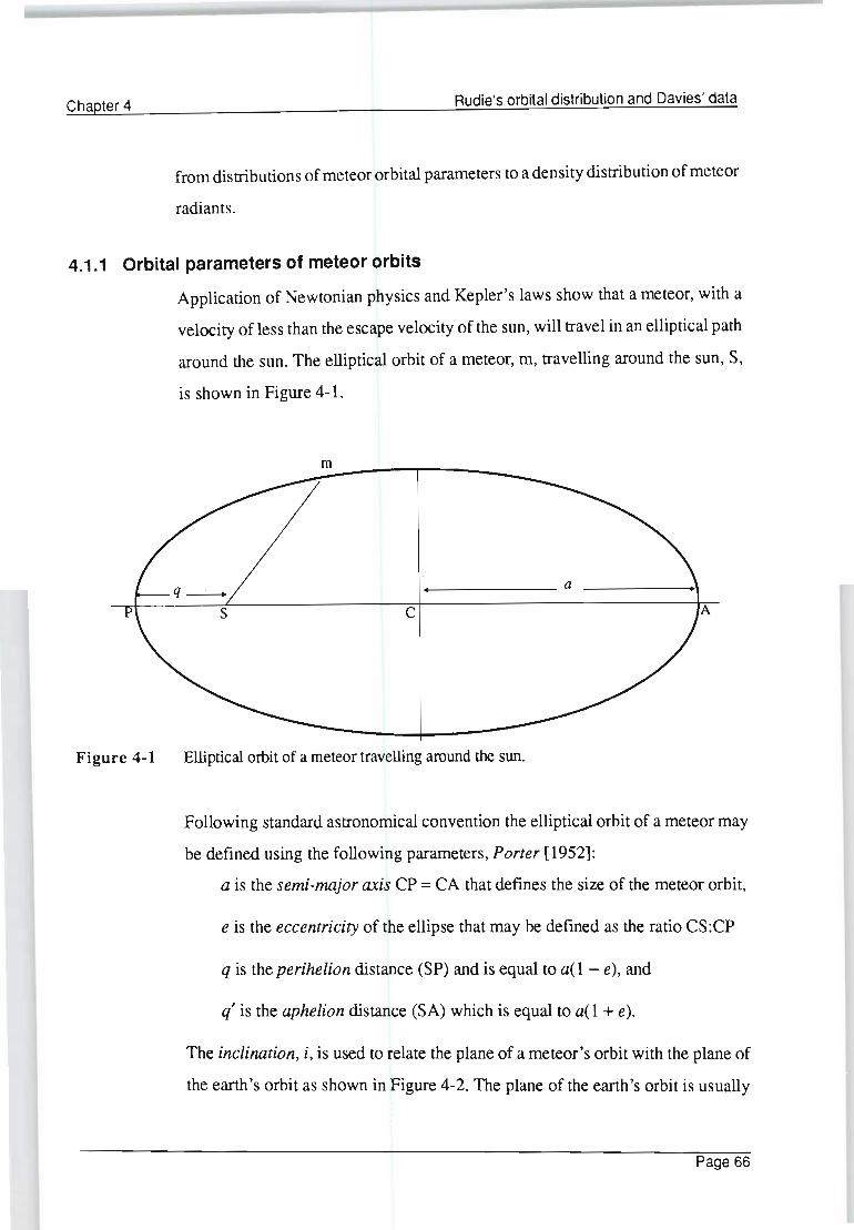
Chapter 4 Rudie's orbital distribution and Davies' data
from distributions of meteor orbital parameters to a density distribution of meteor
radiants.
4.1.1 Orbital parameters of meteor orbits
Application of Newtonian physics and Kepler's laws show that a meteor, with a
velocity of less than the escape velocity of the sun, will travel in an elliptical path
around the sun. The elliptical orbit of a meteor, m, travelling around the sun, S,
is shown in Figure 4-1.
m
c
Figure 4-1 Elliptical orbit of a meteor travelling around the sun.
Following standard astronomical convention the elliptical orbit of a meteor may
be defined using the following parameters, Porter [1952]:
a is the semi-major axis CP = CA that defines the size of the meteor orbit,
e is the eccentricity of the ellipse that may be defmed as the ratio CS:CP
q is the perihelion distance (SP) and is equal to a( 1 - e), and
q' is the aphelion distance (SA) which is equal to aCl + e).
The inclination, i, is used to relate the plane of a meteor's orbit with the plane of
the earth's orbit as shown in Figure 4-2. The plane of the earth's orbit is usually
Page 66

Chapter 4
Figure 4-2
Meteor plane
Ecliptical coordinate system.
Rudie's orbital distribution and Davies' data
known as the ecliptic plane. 0), the argument of the perihelion, is the angle
between the ecliptic plane and the axis SP. Figure 4-2 illustrates an eclipticai
coordinate system with the ~, J and ~, axis pointing in the direction of the
tangential direction of the earth's motion, the sun and perpendicular to the ecliptic
plane, respectively.
In order to intercept the earth, a meteor must satisfy certain combinations of
meteor orbital parameters, a, and, e. By inspection of Figure 4-1, and because
the earth follows a close approximation to a circular orbit, it may be seen that
meteors with a perihelion distance greater than the distance from the sun to the
earth, or meteors with an aphelion distance less than the distance from the sun to
the earth, cannot intercept the earth. Thus for a meteor to intercept the earth:
q = aC1 - e) :::; 1 AU, and
q' = aC1 + e) ~ 1 AU, (4-1)
where one AU (Astronomical earth unit.) is the earth's distance from the sun.
This may be rearranged as:
Page 67
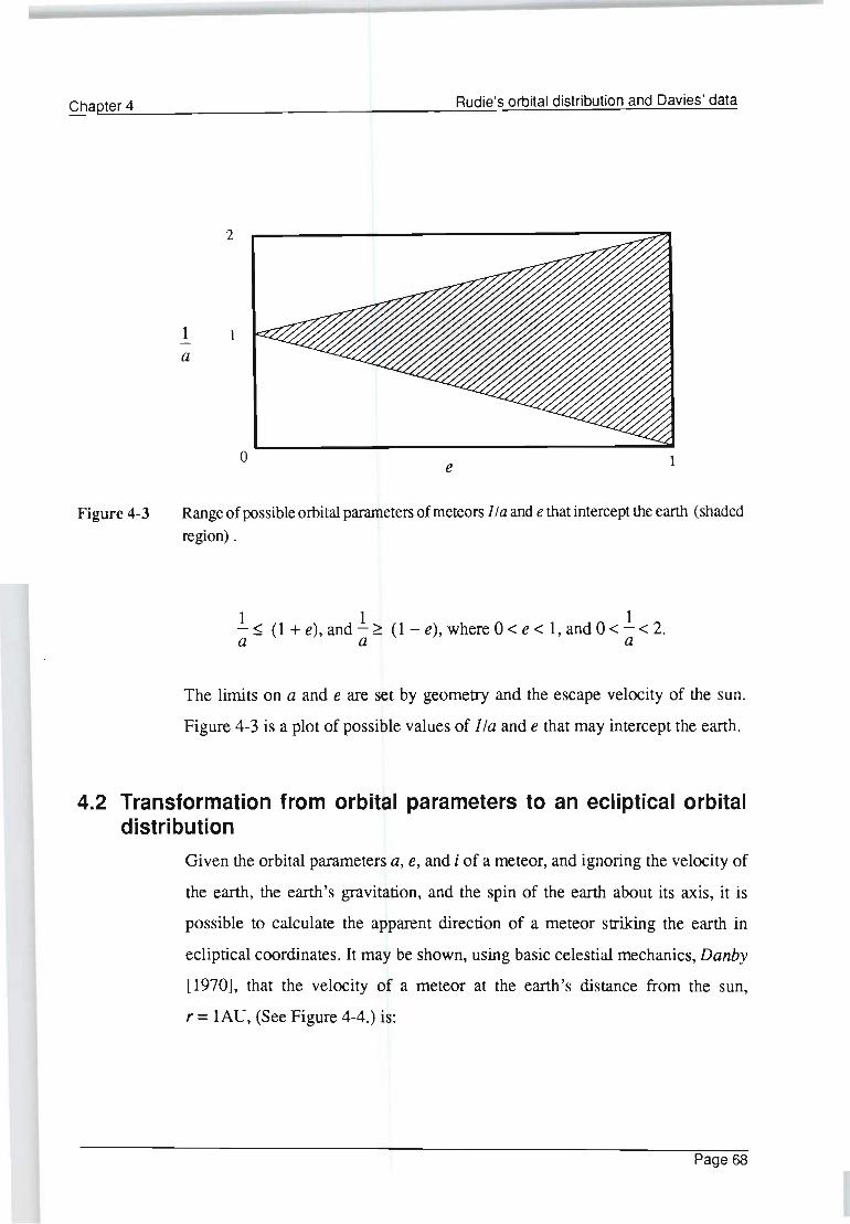
Chapter 4
Figure 4-3
2
1 1
a
e
Rudie's orbital distribution and Davies' data
1
Range of possible orbital parameters of meteors 1/ a and e that intercept the earth (shaded region) .
111 - ~ (1 + e), and - ~ (1 - e), where 0 < e < 1, and 0 < - < 2. a a a
The limits on a and e are set by geometry and the escape velocity of the sun.
Figure 4-3 is a plot of possible values of 1 fa and e that may intercept the earth.
4.2 Transformation from orbital parameters to an ecliptical orbital distribution
Given the orbital parameters a, e, and i of a meteor, and ignoring the velocity of
the earth, the earth's gravitation, and the spin of the earth about its axis, it is
possible to calculate the apparent direction of a meteor striking the earth in
ecliptical coordinates. It may be shown, using basic celestial mechanics, Danby
[1970], that the velocity of a meteor at the earth's distance from the sun,
r = lAU, (See Figure 4-4.) is:
Page 68

Chapter 4
Figure 4-4
Rudie's orbital distribution and Davies' data
v
Velocity components of a meteor.
dr dv ~ dr ~ dt = r dt I + dt j (4-2)
dr ...fa GM . E -= e sm dt r
dv where -dt
[1- !...]
E = ± cos -1 ~ ,G is the gravitational constant, and M is the mass of the
sun.
The rotation of the meteor plane onto the ecliptic plane through the inclination,
i, is thus:
[ 0 10] ~~ ~~I\. . " (l,j,~) = (I ,j ,k) c?S~ 0 -sm., SIn, 0 cos, (4-3)
Page 69
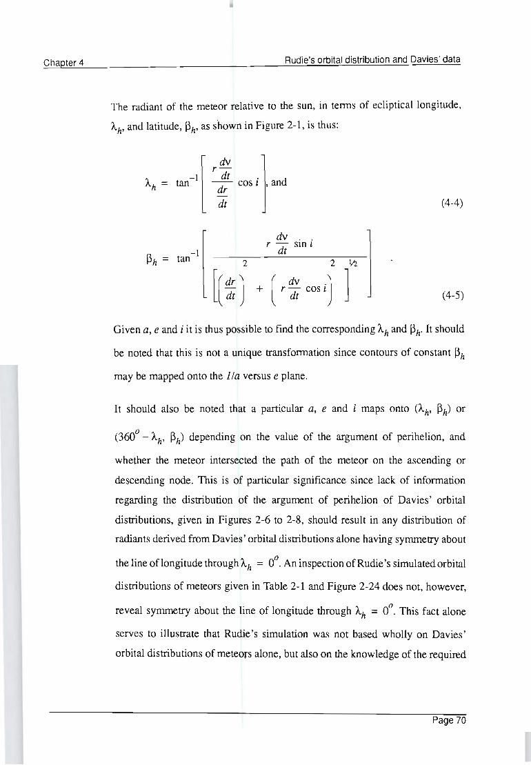
Chapter 4 Rudie's orbital distribution and Davies' data
The radiant of the meteor relative to the sun, in terms of ec1iptica110ngitude,
Ah' and latitude, ~h' as shown in Figure 2-1, is thus:
'I -1 fl.h = tan
r:l -1 fJh = tan
dv r-dt . d dr cos 1 , an
dt
dv . . r dt sm 1
2 2 III
[( :) + (r ~ cos i) ]
(4-4)
(4-5)
Given a, e and i it is thus possible to find the corresponding Ah and ~h. It should
be noted that this is not a unique transformation since contours of constant ~h
may be mapped onto the 1 fa versus e plane.
It should also be noted that a particular a, e and i maps onto (Ah, ~h) or
(360° - Ah' ~h) depending on the value of the argument of perihelion, and
whether the meteor intersected the path of the meteor on the ascending or
descending node. This is of particular significance since lack of information
regarding the distribution of the argument of perihelion of Davies' orbital
distributions, given in Figures 2-6 to 2-8, should result in any distribution of
radiants derived from Davies' orbital distributions alone having symmetry about
the line of longitude through Ah = 0°. An inspection of Rudie's simulated orbital
distributions of meteors given in Table 2-1 and Figure 2-24 does not, however,
reveal symmetry about the line of longitude through Ah = 0°. This fact alone
serves to illustrate that Rudie 's simulation was not based wholly on Davies'
orbital distributions of meteors alone, but also on the knowledge of the required
Page 70

Chapter 4 Rudie's orbital distribution and Davies' data
geocentric distribution of Figure 2-5, which exhibits asymmetry about the line
of longitude through Ag = 0°.
Although it is clear that Rudie 's orbital simulation was not based solely on
Davies' orbital distributions of meteors, the derivation of the actual equations
used to simulate the orbital distribution is unknown. Amore detailed investigation
into the information given by Davies' distributions of orbital parameters has led
the author to believe that Rudie's simulation was based primarily on a knowledge
of the required geocentric distribution, and that the equations of Table 2-1 were
generated to provide the required geocentric polar plot of Figure 2-5, after
transformation to geocentric coordinates. Rudie's transformation from a he
liocentric to a geocentric radiant distribution of meteors is discussed later.
4.2.1 Extraction of an approximate heliocentric distribution from Davies' distributions of orbital parameters
In order to further illustrate the fact that the distributions of orbital parameters
given by Davies' provides only limited information regarding the heliocentric
distributions of meteors and that they were therefore inadequate to generate the
distribution simulated by Rudie, an approximate heliocentric distribution of
meteors will be derived from Davies ' distributions of orbital parameters alone.
The reduced form of the data presented by Davies makes it necessary to
extrapolate the data into a distribution that may be used to transform from the
distribution in orbital parameters of meteors to the ecliptical orbital distribution.
The extrapolation of this data can only be an approximation.
In order to perform the required transformation, Davies' results have been
extrapolated into a distribution of 1 fa verses e versus i. This extrapolation has
been performed by noting that the graphs of distribution of inclinations map onto
Page 71
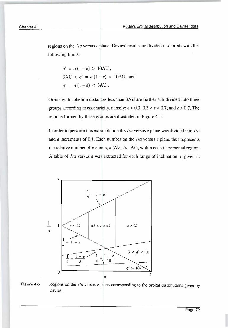
Chapter 4
Figure 4-5
Rudie's orbital distribution and Davies' data
regions on the 1 fa versus e plane. Davies' results are divided into orbits with the
following limits:
q' = a (1 - e) > 10AU,
3AU < q' = a (1- e) < 10AU, and
q' = a (1 - e) < 3AU.
Orbits with aphelion distances less than 3AU are further sub-divided into three
groups according to eccentricity, namely: e < 0.3; 0.3 < e < 0.7; and e > 0.7. The
regions fonned by these groups are illustrated in Figure 4-5.
In order to perfonn this extrapolation the 1 fa versus e plane was divided into 1 fa
and e increments of 0.1. Each number on the lIa versus e plane thus represents
the relative number of meteors, n (~Va. ~e, ill ), within each incremental region.
A table of 1 fa versus e was extracted for each range of inclination, i, given in
2 ~------------------------------~
1 - = 1 + e a
1 1 0.3 < e < 0.7 e> 0.7
a
1 + e/.!_~ 3<q'<10
- = -3- a -\ 10
o~------------------~--~--~ 1 e
Regions on the 1 fa versus e plane corresponding to the orbital distributions given by Davies.
Page 72
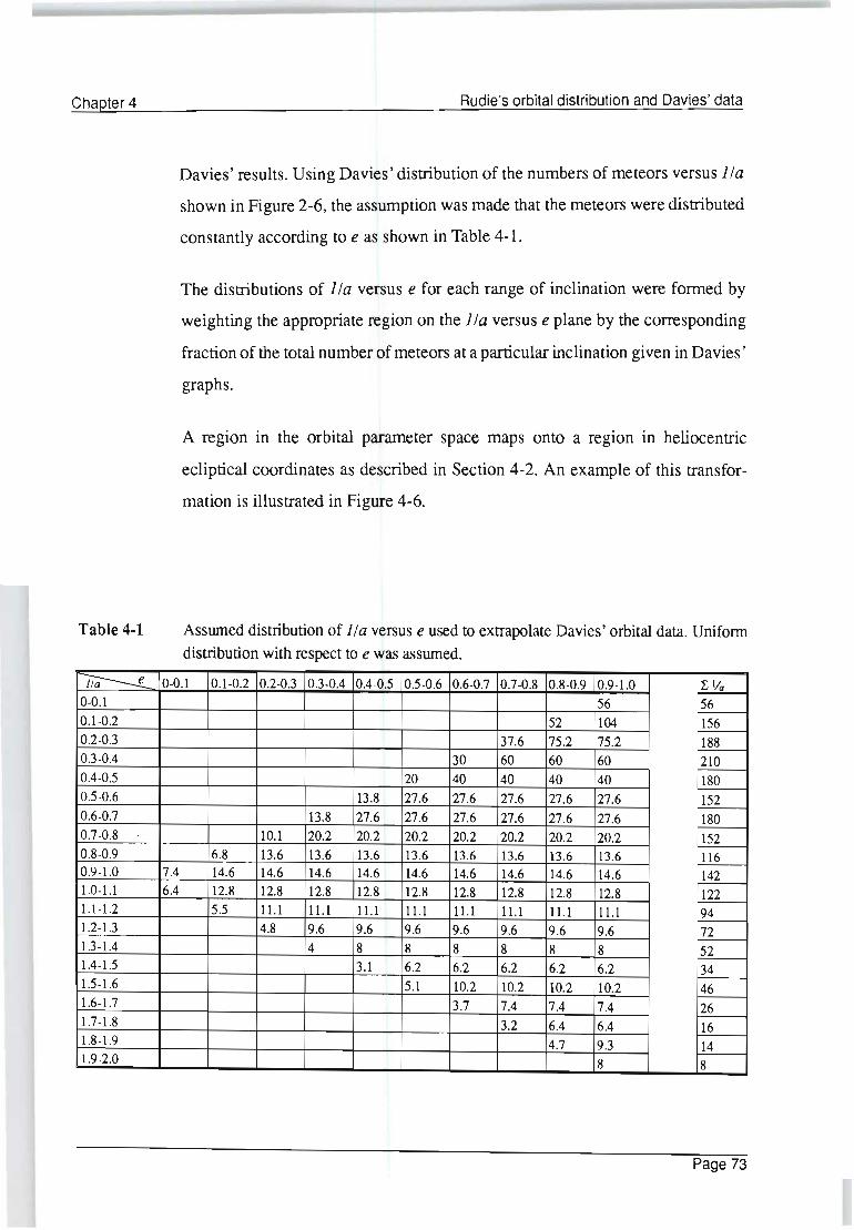
Chapter 4
Table 4-1
lia--..! 0-0.1
0.1-0.2
0.2-0.3
0.3-0.4
0.4-0.5
0.5-0.6
0.6-0.7
0.7-0.8
0.8-0.9 0.9-1.0
1.0-1.1
1.1 -1.2
1.2-1.3
1.3-1.4
1.4-1.5
1.5-1.6
1.6-1.7
1.7-1.8
1.8-1.9
1.9-2.0
Rudie's orbital distribution and Davies' data
Davies' results. Using Davies' distribution of the numbers of meteors versus 1 fa
shown in Figure 2-6, the assumption was made that the meteors were distributed
constantly according to e as shown in Table 4-1.
The distributions of 1 fa versus e for each range of inclination were formed by
weighting the appropriate region on the 1 fa versus e plane by the corresponding
fraction of the total number of meteors at a particular inclination given in Davies'
graphs.
A region in the orbital parameter space maps onto a region in heliocentric
ecliptical coordinates as described in Section 4-2. An example of this transfor
mation is illustrated in Figure 4-6.
Assumed distribution of lIa versus e used to extrapolate Davies' orbital data. Uniform distribution with respect to e was assumed.
0-0.1 0.1-0.2 0.2-0.3 0.3-0.4 0.4-0.5 0.5-0.6 0.6-0.7 0.7-0.8 0.8-0.9 0.9-1.0 L Va 56 56
52 104 156
37.6 75.2 75.2 188
30 60 60 60 210
20 40 40 40 40 180
13.8 27.6 27.6 27.6 27.6 27.6 152
13.8 27.6 27.6 27.6 27.6 27.6 27.6 180
10.1 20.2 20.2 20.2 20.2 20.2 20.2 20.2 152 6.8 13.6 13.6 13.6 13.6 13.6 13.6 13.6 13.6 116
7.4 14.6 14.6 14.6 14.6 14.6 14.6 14.6 14.6 14.6 142 6.4 12.8 12.8 12.8 12.8 12.8 12.8 12.8 12.8 12.8 122
5.5 ILl ILl ILl ILl ILl ILl ILl ILl 94 4.8 9.6 9.6 9.6 9.6 9.6 9.6 9.6 72
4 8 8 8 8 8 8 52 3.1 6.2 6.2 6.2 6.2 6.2 34
5.1 10.2 10.2 10.2 10.2 46
3.7 7.4 7.4 7.4 26 3.2 6.4 6.4 16
4.7 9.3 14
8 8
Page 73

Chapter 4
Figure 4·6
Rudie's orbital distribution and Davies' data
90
t--- 0.9 < Va < 1.0 0.4 < e < 0.5
I--- o 0 40 < i < SO
""~ ~ ~
o 90 A.h 180
Example of the transfonnation from a region in orbital space to a region in heliocentric space.
A program was written to transfonn from orbital parameters to the ecliptical
heliocentric distribution. The transformation was performed by digitizing the
heliocentric celestial sphere into 5° increments of Ah and ~h' The region on the
heliocentric celestial sphere corresponding to each cell of (~1ja. ~e, ru) was
calculated using the equations described in Section 4-2. The number of meteors,
n ( ~1ja. ~e, ~i), in each cell, (~1ja. ~e, ru), were distributed so that an even
density distribution was obtained in each of the incremental regions, (Mh
, ~~h)'
The relative contribution for each increment, (~Ah' ~~h)' was obtained for each
transfonnation using the following expression:
(4·6)
Page 74
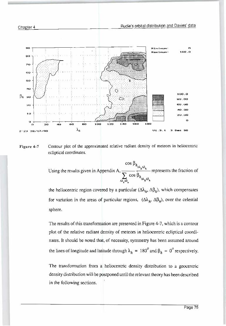
Chapter 4 Rudie's orbital distribution and Davies' data
90 Hini~u ... :
M.aMi .. u .. :
90
70
so
so
""'0
~h 30
1.00.0 .. -: . .... : ..... 90 . 00
20 .' .' ', ' ...... , ...... . .. ' . ' . .... ' ... . so . OO
""'0.00
1.0 20.00
o 0
0 20 ""'0 so 90 1.00 1.20 1.""'0 1.BO 1.80
2 : 23 29/1.2/90 U 1. . 3 . 1. 3 D_<> 90
Figure 4-7 Contour plot of the approximated relative radiant density of meteors in heliocentric
ecliptical coordinates.
cos ~h dA.~
Using the results given in Appendix A, II II represents the fraction of L cos ~h
M d~ Mlld~1I h h
the heliocentric region covered by a particular (~h' ~~h)' which compensates
for variation in the areas of particular regions, (~h' ~~h)' over the celestial
sphere.
The results of this transformation are presented in Figure 4-7, which is a contour
plot of the relative radiant density of meteors in heliocentric ecliptical coordi
nates. It should be noted that, of necessity, symmetry has been assumed around
the lines of longitude and latitude through Ah = 1800
and ~h = 00 respectively.
The transformation from a heliocentric density distribution to a geocentric
density distribution will be postponed until the relevant theory has been described
in the following sections.
Page 75

Chapter 4 Rudie's orbital distribution and Davies' data
4.3 Heliocentric to geocentric transformation
Using an involved method, Rudie developed a technique of transforming from a
heliocentric to a geocentric radiant distribution. In order to put the method
developed by Rudie into perspective, a more accurate and analytically simpler
technique will fIrst be described.
The transformation in meteor direction between the heliocentric and geocentric
distributions may be simply derived with reference to Figure 2-2, Lovell [1954] .
The relationship between the elongations of Rg and Rh is simply
[V] . -1 e . = cg + SIn V
h s~ Eg
(4-7)
The relationship between elongation, C, ecliptical longitude, A, and ecliptical
latitude, ~, relative to the apex is
cos C = cos A cos ~ .
The geocentric direction numbers of a meteor are
19 = cos Ag cos ~g
mg = sin t..g cos ~g
ng = sin ~g
(4-8)
(4-9)
Using simple vector addition, the heliocentric direction numbers are thus
lh = Vg 19 - Ve
mh = Vgmg
nh = Vg ng (4-10)
Page 76

Chapter 4 Rudie's orbital distribution and Davies' data
where from Figure 2-2 it may be seen that
(4-11)
[ ( V ]~ . -1 e. cos Eh = cos Eg + sm V h sm Eg
(4-12)
U sing the heliocentric direction numbers, the heliocentric eclipticallongitude, Ah'
and eclipticallatitude, ~h' are thus
(4-13)
Equations 4-7 to 4-13 consist of a transformation in direction between a geocen
trically referenced meteor radiant, Ag, and, ~g' and a heliocentrically referenced
meteor radiant, Ah, and, ~h'
The transformation between geocentric and heliocentric distributions results in
a radiant density transformation th.at may be described in terms of an area
transformation. Figure 4-8 illustrates this change in area. Due to the effect of the
direction transformation on each meteor, the same meteors seen emanating from
an incremental surface on the celestial sphere, dS h' in heliocentric coordinates,
will appear to emanate from an incremental surface, dSg, in geocentric coordi-
nates.
By defining the incremental surfaces as being bounded by lines of constant
elongation and by lines of longitude relative to the apex, as shown in Figure 4-8,
it is possible to find the ratio between dS g and dS h' Using the theory shown in
Appendix A, the ratio of these areas is:
Page 77
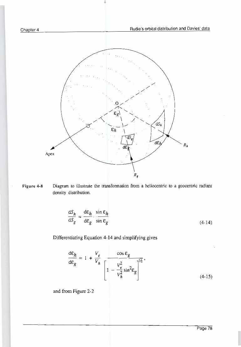
Chapter 4
Figure 4·8
Rudie 's orbital distribution and Davies' data
Apex
Diagram to illustrate the transfonnation from a heliocentric to a geocentric radiant density distribution.
(4-14)
Differentiating Equation 4-14 and simplifying gives
(4-15)
and from Figure 2-2
Page 78
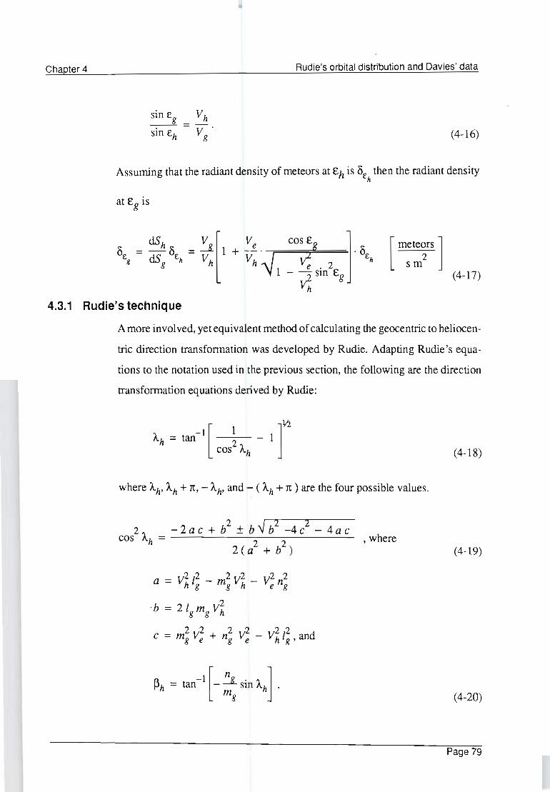
Chapter 4 Rudie's orbital distribution and Davies' data
(4-16)
Assuming that the radiant density of meteors at ch is Be then the radiant density h
at cg is
(4-17)
4.3.1 Rudie's technique
A more involved, yet equivalent method of calculating the geocentric to heliocen
tric direction transformation was developed by Rudie. Adapting Rudie's equa
tions to the notation used in the previous section, the following are the direction
transformation equations derived by Rudie:
where I...h' I...h + 1t, -I...h' and - ( I...h + 1t ) are the four possible values.
2,\ _-2ac+b2±b~b2-4c2-4ac cos II.h - 2 2 ' where
2(a + b )
2 2 2 2 2 2 a = V h I g - mg V h - Ve n g
2 'b=2Ig mg Vh
2 2 2 2 2 2 c = mg Ve + ng Ve - Vh 19 , and
(4-18)
(4-19)
(4-20)
Page 79
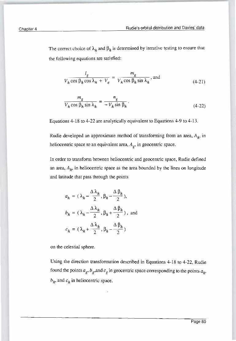
Chapter 4 Rudie's orbital distribution and Davies' data
The correct choice of Ah and f3h is detennined by iterative testing to ensure that
the following equations are satisfied:
= V A' 'I ' and h cos tJh sm II.h (4-21)
(4-22)
Equations 4-18 to 4-22 are analytically equivalent to Equations 4-9 to 4-13.
Rudie developed an approximate method of transfonning from an area, A h' in
heliocentric space to an equivalent area, Ag, in geocentric space.
In order to transfonn between heliocentric and geocentric space, Rudie defined
an area, Ah, in heliocentric space as the area bounded by the lines on longitude
and latitude that pass through the points
!1 Ah !1 f3h ah = (Ah--2-' f3h--2
-),
!1 Ah !1 ~h bh = (I."h - -2- , ~h + -2-)' and
!1 Ah !1 ~h ch = (Ah +-2-' ~h--2-)
on the celestial sphere.
U sing the direction transfonnation described in Equations 4-18 to 4-22, Rudie
found the points ag, bg,and cg in geocentric space corresponding to the points ah'
b h' and chin heliocentric space.
Page 80

Chapter 4 Rudie's orbital distribution and Davies' data
The angles, 0a b' and 0a c between points ag and bg and points ag and cg g g g g
respectively on the celestial sphere were found using Equations 4-21,4-22, the
vector dot product and the relationship
1;2
tan e = ± [-+ -1] , as cos e
1 2
Ilg a Ilg b + V g a V g b ) g g g g
-1 Da c = tan
g g [
( Ag a Ag c + ~g a ~g c + V g a V g c )2
g g g g g g
(4-23)
(4-24)
(4-25)
where Ag*, Ilg*, and V g* correspond to the geocentric direction cosines associated
with * = ag, bg, or cg.
Rudie then made the assumption that
(4-26)
This assumption is, however, only approximate, since, even as an approximation
for small angles, the vectors, aig and agcg, formed by the points ag, bg and cg
are not necessarily mutually perpendicular.
A more accurate approximation of A g for.1 ::::: 0 is
(4-27)
Since an analytically more accurate technique has already been derived, the
expansion of the above expression will not be performed.
Page 81

Chapter 4 Rudie's orbital distribution and Davies' data
4.3.2 Corrections due to the gravitational effect of the earth
The effect of the earth's gravitation on the path of a meteor may be descrioed
with reference to Figure 4-9, Porter [1952]. A meteor travelling in a straight line
Me will be forced into a hyperbolic orbit, MOM', due to the gravitational
attraction of the earth. This effect results in the zenith angle of the radiant
changing from ~' to ~ relative to an observer at O. Since the meteor is always
displaced towards the observer's zenith, this effect is known as zenith attraction.
Porter has shown that the relationship between ~ and ~' is :
tan ( ~ - ;') 2 (4-28)
where V 00 = ~V; + 124.9 [lcJrVs], is the actual speed with which the meteor
enters the earth's atmosphere due to the gravitational attraction of the earth. As
mentioned by Porter, the correction for zenith attraction is a maximum for when
Zenith : /
Original path of . /
the meteor----. / . / . /
- ____ c ___ _ /
c/ "-Earth 's surface
Tangent to MOM' at 0
Figure 4-9 Zenith attraction.
Page 82

Chapter 4 Rudie's orbital distribution and Davies' data
the radiant lies near the horizon, and is near the antapex. The maximum correction
under these circumstances will approach 17°.
As shown by Rudie [1967] it is important to note that the effect of zenith attraction
cannot be taken into account in the prediction of the influence of radiant
distributions on the arrival rate of meteors due to the lack of information
regarding the geocentric velocity of the incident meteors.
4.3.3 Other corrections
As mentioned by Porter [1952], and Rudie [1967], the effect of the earth 's spin
on the radiant of a meteor is negligible and may therefore be neglected. The
deceleration of a meteor due to the earth's atmosphere results in a decrease in
V 00 of between 0.5 to 1 kilometres per second in the meteor region. The effect
of atmospheric deceleration may similarly be neglected.
4.4 Numerical simulation of the heliocentric to geocentric radiant density transformation
As shown by Rudie [1967] the transformation from heliocentric to a geocentric
radiant distribution may be approximated using the transformation described in
Section 4.3.1. Using the methods of Sections 4.3, the radiant density of any point
in geocentric coordinates may be calculated by transforming to the corresponding
radiant in heliocentric coordinates and calculating the density transformation of
radiants at that point. This method thus involves "looking-up" the geocentric
density distribution of meteors based on the known heliocentric distribution. The
disadvantage of this technique is that multiple counting or omission of meteors
from the heliocentric distribution will occur to a lesser or greater degree depend
ing on the position of the radiants chosen to "look-up" in geocentric coordinates.
The following numerical technique was developed to avoid multiple counting
Page 83

Chapter 4 Rudie's orbital distribution and Davies' data
and omission of meteors as well as to provide a potentially accurate density
transformation:
The numerical simulation of the heliocentric to geocentric radiant density trans
formation is illustrated in Figure 4-10. The numerical transformation is per
formed by transforming the number of meteors in small regions over the entire
heliocentric sphere to their appropriate region on the geocentric sphere. The
heliocentric and geocentric spheres are projected in rectangular coordinates in
Figure 4-10. As shown in Figure 4-10, the heliocentric and geocentric spheres
are divided into small regions defined by incremental lines of longitude and
latitude, !1'A. and !1~. The corresponding (on transformation) incremental region
in geocentric coordinates is calculated for all the incremental regions in heliocen
tric coordinates, and the number of meteors in each of the incremental regions in
heliocentric coordinates is added to the corresponding region in geocentric
coordinates. As long as the incremental regions in heliocentric coordinates are
far smaller that the regions in geocentric coordinates, the radiant density in each
Transformation --------- .......... // ..... ...... ,
...... , ...... "
900 r---:---:-~/'-/----::-:oo...-.:-::..;;;..-------____,-- - - ~ -r:::::'~--:-__:___:__:_-------__, : / - ..... ~ . :/ .".'''- .....
o . Ah IIh -90 ~----~~--------------~ o Ag 3&·/
Geocentric ecliptical coordinates
.. J ~h f
-:-~~-_900~-~~~~-------~
00
Ala 36(/
Heliocentric ecliptical coordinates
Figure 4-10 Diagram to illustrate the numerical method of simulating the heliocentric to geocentric radiant density transformation.
Page 84
Chapter 4 Rudie's orbital distribution and Davies' data
of the incremental regions in geocentric coordinates will be defmed by the
number of meteors divided by the area of the incremental region. Following this
technique, the number of meteors , N"-g ~g (LUg, ~~g) ' in each incremental region
in geocentric coordinates, (LUg, ~~g)' is thus:
and the relative radiant density, Ogl.. ~ , at geocentric radiant, Ag, ~g is g g
NAg ~g (LUg, ~~g) =
cos ~g
(4-29)
(4-30)
4.5 Approximation of Davies' observed radiant distribution
To complete the extraction of an observed radiant distribution based on Davies '
orbital parameters alone, the heliocentric distribution approximated in Section
4.2.1 is transformed to a geocentric distribution. An estimation of the validity of
the final results is then determined by a comparison with Davies' actual observed
distribution. It should be remembered, however, that the heliocentric distribution
derived in Section 4.2.1 was based on an extrapolation of Davies' orbital
parameters and therefore the derived geocentric distribution will similarly only
be an approximation. This exercise is undertaken to demonstrate the results of a
more rigorous technique of deriving the geocentric distribution using Davies'
orbital parameters exclusively.
Using the theory described ·in Section 4.3 and 4.4, the heliocentric radiant
distribution shown in Figure 4-7 was transformed to a geocentric distribution.
The results of this transform~tion are shown in Figure 4-11. As mentioned in
Section 4.2, the lack of information about the argument of the perihelion results
Page 85

Chapter 4
90
80
70
60
SO
40
~g 30
20
10
Rudie's orbital distribution and Davies' data
Hini ... u ... : Haxi ... u ... :
o 100 . 0
100 . 0
90.00
80 . 00
70.00
60 . 00
50 . 00
40 . 00
30 . 00
20 . 00
10.00
o
10 : 13 3/9/90 Ag U1 . 3 . 1 23 Aug 90
Figure 4-11
Figure 4-12
Observed radiant distribution of meteors obtained using an extrapolation of Davies '
orbital parameters. Davies' observed radiant distribution was not used.
Meteors within 20 o
of the ecliptic
Apex
Polar plots of the approximated observed radiant distribution. Symmetry about the line
of longitude through Ag = 1800 should be assumed.
Page 86

Chapter 4 Rudie's orbital distribution and Davies' data
in forced symmetry about A. = 180°. In order to compare these results with the g .
geocentric distribution observed by Davies in Figure 2-5, the transformed results
are displayed in a form similar to that given by Davies in Figure 4-12. It is clear
from a comparison between the two polar plots that the transformed results differ
significantly from the actual results given in Figure 2-5 .. It is clear therefore that
an extraction of a geocentric radiant distribution, using Davies' orbital parameters
alone, can only generate a rough approximation. The loss of information caused
by the original assumptions described in Section 4.2.1, results in an inaccurate
geocentric radiant distribution. The inaccuracy of this result serves to emphasize
the fact that Rudie's orbital simulations were not based on the orbital parameters
alone.
4.6 Rudie's simulated distribution in geocentric coordinates In order to facilitate comparison between Rudie's orbital distribution of meteors
and other geocentric distributions of meteors, Rudie's simulated orbital distribu
tion has been transformed to geocentric ecliptical coordinates using the theory
described by Rudie in Section 4.3 and is reproduced as a contour map of the
geocentric density distribution of meteors in Figure 4-13. For the purposes of the
transformation, an average heliocentric velocity of 35 kilometres per second was
used.
The results obtained in Figure 4-13 are also presented as a polar plot of all
sporadic meteor radiants versus ecliptical longitude in Figure 4-14. Davies'
results for all sporadic meteor radiants from Figure 2-5 are also presented in
Figure 4-14. It is interesting to note that the results of Rudie's transformation
differ significantly from the results given by Rudie in Figure 2-25 (plot H). The
comparison between Rudie's simulated and Davies measured results in Figure
4-13 actually show a far better correspondence than illustrated by Figure 2-25.
Page 87

Chapter 4 Rudie's orbital distribution and Davies' data
Hini ..... u .... : 0
70 M ... Ml,..u ... : etOO.O
50 etOO . O
90.9et 30 .. . . .. .
0'- .02
etO 72.73
~g 63 . 64 -etO
54 . 55
-30 45 ..... 5
36 . 36 -50
27.27
-70 etO . '-O
S . OSet
0 -etOO -'- .... 0 -etOO -so -20 20 so '-00 '- .... 0
0 : 29 3/et/9et
Figure 4-13
Davies
Rudie
Uet.3.et 3 D_c 90
Contour map of the geocentric density distribution of meteors derived using Rudie's
orbital simulation and transformation. An average heliocentric velocity of 35 kilometres per second was used.
Figure 4-14 Comparison between Davies' polar plot of all sporadic meteors radiants versus the actual
results obtained using Rudie's extrapolation (Compare with Figure 2-25.).
Page 88

Chapter 4
70
50
30
Rudie's orbital distribution and Davies' data
This seems to indicate that Rudie's plots reproduced in Figure 2-25 were only a
rough representation of his actual results.
To test the validity of the approximations associated with Rudie's heliocentric to
geocentric transformation, the orbital simulation given by Rudie has been trans
formed to geocentric coordinates using the more accurate numerical technique
described in Section 4.4. Increments of Ah and ~h of 0.25 degrees were used for
the incremental regions on the heliocentric sphere and increments of Ag and ~g
of 5 degrees were used for the incremental regions on the geocentric sphere.
Figure 4-15 is a contour map of the relative radiant density of meteors in
geocentric coordinates obtained using the numerical transformation. Comparison
between Figures 4-13 and 4-15 reveals some differences, which confmns that
the transformation used by Rudie is only approximate. Since the original he
liocentric distribution is only an approximation, however, the adoption of the
Ht.ni. .... u ..... :
"_Mi'""u .... :
o ,,"00 . 0
,,"00 . 0
SO.9,,"
a,," .82
""0 . . .... . 72.73
63.6~
5~.55
-30 ~5 . ~5
36.36 -50
27 . 27
-70 .. .. ............ .. 'SB . 1.&
. . S.09,,"
. . .. '. -90 ..... '. " ',.', ' , ' ..... o
-,,"aD -,,"~O -,,"~O -60 -20 20 60 ""00 ""~o
Figure 4-15 Contour map of the geocentric density distribution of meteors derived using the numeri
cal transformation. An average heliocentric velocity of 35 kilometres per second was used.
Page 89

Chapter 4 Rudie's orbital distribution and Davies' data
geocentric distribution obtained using the slightly improved numerical transfor
mation would probably be meaningless.
4.7 Extrapolation of Davies' observed distribution
It is possible to obtain an approximation of the observed radiant distribution in
ecliptical coordinates by directly extrapolating Davies' results reproduced in
Figure 2-5. A direct extrapolation of Davies' results provides a far simpler and
possibly more accurate method of obtaining the observed distribution, and avoids
the unnecessary complication of simulating a suitable heliocentric distribution
that transfonns to Davies' measured geocentric distribution.
As shown in Figure 2-5, the observed distribution of sporadic meteors is given
as three polar plots: radiants within 20° of the ecliptic; radiants within 40° of the
ecliptic; and all radiants. Due to the latitude at which the measurements were
taken, radiants less than approximately _20° were not observable. It is therefore
possible to divide the data into three regions: -20° < ~g < 20°; 20° < ~g < 40°;
and 40° < ~g < 90°. Due to the lack of data south of ~g = -20°, it is necessary to
assume symmetry about the ecliptic. Taking into account the respective areas of
the three regions on the celestial hemisphere, it is thus possible to calculate the
average radiant density in each region. An additional item of infonnation for
40° < ~g < 90° is that, assuming a gradual change in density, the radiant density
around the ecliptic poles should be similar. As a simple approximation a linear
decrease in density may be assumed for 40° < ~g < 90° as ~g increases. Due to
the poor resolution about the antapex an approximately unifonn radiant density,
based on the overall density, may be assumed as a fIrst order approximation.
Figure 4-16 is a contour plot of the extrapolated results. Davies' polar plots were
was graphically extracted in 5° increments of Ag. It is clear from Figure 4-16 that
Page 90

Chapter 4 Rudie's orbital distribution and Davies' data
1'1 in i,",u", : 0 . -,",SSS7
t1aKi,",u",: 1.00 . 0 70
so 1.00 . 0
90.95
30 81. . S1.
1.0 72.96
63.92
5-,", . 77 ~g -1.0
-'"'5.73 -30
36.S8
- 50 27 . 63
1.8 . 59 -70
9 . 5-'"'2
-90 0.-'"'9597
-1.ao -1.-'"'0 -1.00 -60 -20 20 60
9 : 1.1. 3/1./91. U1. . 3.1. :3 D_c: 90
Figure 4-16 Contour map of the geocentric density distribution of meteors extrapolated directly from
Davies' polar plots (Figure 2-5).
the extrapolated results show the expected concentrations at the apex, Ag = 65°,
and Ag = 295° . Since Figure 4-16 is extrapolated directly from Figure 2-5, a polar
plot of Figure 4-16 would be identical to Figure 2-5.
4.8 Summary of findings
Analysis of Davies ' data has shown that Rudie's simulation was not based on the
distributions of orbital parameters given by Davies. Although the technique used
by Rudie to simulate a suitable orbital distribution is not completely clear, it is
probable that Rudie's heliocentric distribution was derived from a transformation
of Davies' geocentric distribution to heliocentric coordinates. Whether this was
performed as an iterative process by selecting a suitable set of equations to
simulate the heliocentric distribution that provided, on transformation, the correct
geocentric distribution, or, whether this was performed by transforming some
Page 91

Chapter 4 Rudie's orbital distribution and Davies' data
form of the geocentric distribution directly to heliocentric coordinates and
approximating the results as a set of equations, or whether this was performed as
a combination of the two techniques, is unknown. Rudie obtained what was
probably a reasonable approximation to Davies' measured results as a compari
son between the results presented as polar plots and a comparison between
directly extrapolated distributions and Rudie's geocentric distributions has
shown.
The use of Rudie's simulation by Weitzen [1986], Larsen and Rodman [1988]
and Desourdis et al. [1988] is indicative of the acceptance of Rudie's method of
the simulation of Davies' results. The following quote by Weitzen [1986], pages
1012-1013, further demonstrates the acceptance of Rudie's technique:
"Next the empirical distribution of meteor orbits in ecliptic latitude and
longitude, determined by Davies and approximated by Rudie as a series
of closedform equations, is transformed to a distribution of meteor trail
radiants observed at the earth. This transformation represents Rudie's
significant contribution to meteor modeling and takes into consideration
the effect of the Earth's orbital velocity on the direction and velocity of a
meteor as the trail is formed."
Since it has been shown that Rudie's simulation was simply an involved extra
polation of Davies ' observed distribution and since Davies' observed distribution
may be obtained by extrapolating Davies' results directly, it is doubtful that this
was in fact Rudie's significant contribution to meteor modelling. It should also
be remembered that Davies' measurements were based on a sample set of only
2400 radiants measured at high northern latitudes that implies that the resolution
of the original measured distribution was probably not very detailed. It is
therefore clear that a large number of existing meteor prediction models are
probably based on an involved approximation of originally meagre data.
Page 92

Chapter 5 Comparisons between predicted and measured arrival rates of meteors
ChapterS
Comparisons between predicted and measured arrival
rates of meteors
In order to verify the validity of the radiant distributions presented in Chapter 2
and Chapter 4, comparisons between predicted and measured arrival rates of
meteors for a forward-scatter link between Pretoria and Durban, South Africa are
given in this chapter. The comparisons performed in this chapter represent the
most detailed evaluation of the known radiant distributions of meteors presented
to date, and answer some of the questions regarding the validity of the various
distributions. Measured annual variations in the arrival rate of meteors are also
presented and contrasted with previous measured and predicted results.
5.1 Measured results
A brief description of the measurement systems, the method of data capture, and
data processing techniques used to extract the required data, is given here.
5.1.1 System description
Meteor trail reflection envelopes have been measured and recorded using two
systems over a link between Pretoria and Durban, South Africa. Table 5-1
summarizes some of the important parameters of the two systems. Apart from
the antenna configurations, the system parameters for the two systems are
identical. One of the systems is designed to illuminate the meteor region between
Page 93

Chapter 5 Comparisons between predicted and measured arrival rates of meteors
Table 5-1 Midpath and endpath system parameters.
Transmitter Location Irene, Pretoria, South Africa,
Latitude -250 43" 58',
Longitude 280 12" 00'
Receiving Site Camperdown, Durban, South Africa
Latitude -290 49" 01 ,
Longitude 31 0 00" ,
57
Path Length 532km
Transmitter Power 350W
Transmitter Frequency 50.050 MHz midpath 50.055 MHz endpath
Receiving System Noise Bandwidth 2kHz
Receiving System Noise Figure 6dB
Table 5-2 Midpath and endpath antenna configuration.
Antenna Midpath Endpath
11 element log periodic 11 element log periodic Transmitting Horizontally polarized Horizontally polarized
3 metres high 8.5 metres high Maximum gain 15 dBi Maximum gain 15 dBi
5 element yagi 3 element yagi Receiving Horizontall y polarized Vertically mounted
3 metres high 112 metre high (reflector) Maximum gain 13.5 dBi Maximum gain 8 dBi
Page 94

Chapter 5
so
\em
-75
-200 - 300
~S : 39 7 ..... 2 ..... 9""
Figure 5-1
o
\em
- "'so
-300 -200
Comparisons between predicted and measured arrival rates of meteors
Hini"u",: -2~ . 37
MaMiMu",, : 27.48
~ Hart:h
27 . -40
24 . -4&
2~ . -40
Gain ~9 . -4&
,,"5 . -4&
dBi ~2 . -4&
9.-460
6 . -460
3 . -460
0 . -4&000
- 2 . 5-40
-2~ . 37
-~SO o
\em U~ . 3 . ~ 3 Oec 90
Contour plot of the combined predicted antenna illumination pattern of the meteor region for the midpath system. Tx and Rx are the transmitter and receiver locations respectively.
Hini"u" : -63 . -42
MaM i"'UM : 24 . 26
~ Harth
2-4 . 20
2~.2&
~o . :z&
~S . 20
~:z . :z&
9.260
B.200
3 . 260
0.26000
-2.7-40
-5 . 7-40
-B3 . -42
-25 ~SO
""5:55 7 ..... 2 ..... 9~ km
U~ . 3 . ~ 3 Dec 90
Figure 5-2 Contour plot of the combined predicted antenna illumination pattern of the meteorregion for the end path system. Rx is the receiver location.
Page 95

Chapter 5 Comparisons between predicted and measured arrival rates of meteors
the transmitter and receiver sites and is called the midpath system, whilst the
other system is designed to illuminate the meteor region above the receiving site
and is called the endpath system. Details of the midpath and endpath systems'
antennas are given in Table 5-2. A contour plot of the combined predicted antenna
illumination pattern of the meteor region for the midpath and endpath systems
calculated using the technique used by Larsen and Rodman [1988] (See Sec
tion 3.4) is given in Figures 5-1 and 5-2 respectively.
5.1.2 Data capture, recording and processing
The received signal strength of meteor reflections is continuously recorded by
the receiving systems. A continuous, unmodulated carrier signal is transmitted
and each receiving system has the ability to discriminate between valid signals
and unwanted noise bursts. Each receiving system is calibrated in one decibel
steps from -140 to -,80 dBm. Both the received signal and noise is converted to
audio frequency, detected using a square-law device, logged and converted to dc
for analogue-to-digital conversion. A detailed description of the analogue receiv
ing system has been given by Mawrey [1988]. During the presence of a received
trail reflection, the converted signal and noise voltages are sampled every five
milliseconds and stored on magnetic disk for further analysis.
The digitized trail envelopes are further analysed and categorized according to
the shape of the trail envelope (typed) using the trail classification scheme
developed by Melville et al. [1989]. Summary information is then extracted from
the classified trail envelopes. Using the summary information it is possible, for
example, to extract the number of underdense trails received above a chosen
signal level at a particular time.
Midpath and endpath data relevant to this thesis have been captured using the
midpath system from October 1988 to November 1990. The endpath system has
been operational from August 1989 to November 1990. Calendars of the days
Page 96

Chapter 5 Comparisons between predicted and measured arrival rates of meteors
All Non-e .... pty Fi I .. ,. $y,.t .... : F V ..... r: ~990
24
20
~6 ~ :::I ~2 0
:l: B
4
~
24
20
~ ~6
~ ~2 B
4 ~
Figure 5-3
D ... y
JAn F.b HAr Apr HAY Jun
. I : I .. 320 360
'1 . I I
II . I ~ I I . - .
Jul Aug s.P Oct Nov D.c
Days and hours during which data has been captured using the end path system during 1989 and 1990.
Page 97

Chapter 5 Comparisons between predicted and measured arrival rates of meteors
All Non-et"\pty FII .. 5 $Y5t: ..... : E V .... r: t9B 9
2 4
20
t6 I-:J t2 0 l:
B
4 t
24
20
16 I-
~ t2
B
4 1
Figure 5-4
.lull .. " O .. y
Feb t1.r Apr t1~ .lun
.lui
Days and hours during which data has been captured using the midpath system during
1988, 1989 and 1990 (for 1990 see next page).
Page 98

Chapter 5 Comparisons between predicted and measured arrival rates of meteors
Figure 1-2 continued
and hours during which data have been captured using the midpath and endpath
systems are given in Figures 5-3 and 5-4 respectively. The large gaps in the
captured data throughout the year were caused by other tests being run that
interfered with the midpath and endpath measurements.
5.2 Graphical technique of determining the relative contributions of regions in the celestial sphere to the arrival rate of meteors
The interaction between a particular radiant distribution of meteors and the arrival
rate of meteors is typically illustrated as the relative contribution of parts of the
meteor region to the arrival rate of meteors for a particular meteor-scatter link.
An example of this is given in Figure 5-5. Figure 5-5 is a contour map of the
contribution relative parts of the meteor region for the midpath system at 06hOO
Page 99

Chapter 5
km 50
-75
- 200
-300
Comparisons between predicted and measured arrival rates of meteors
Rx ':-::-::::;:;;~~~;,.,;: - - - - -.
--~~~~~ :
o
km
I I
. . . . . . · 4 , .
MiniMuM: a "_xlMU" : O . 00208S~
~ Harth
Relative arrival rate of meteors
[ Meteors ]
unit area2.unit time
0_0020a5~
o_oo~ssa~
0 _ 00~25~~
0 . 00093-'10
0 _ 000"'~70
o
~ ~ : 3~ 25/ _. __
Figure 5-5 Contour map of the relative contribution of parts of the meteor region for the midpath system at 06hOO on 23 September using Rudie's radiant distribution of meteors
on 23 September using Rudie's radiant distribution of meteors . This method of
illustrating the interaction between radiant distributions and the arrival rate of
meteors, is ideally suited to displaying the relative contribution of parts of the
meteor region to the arrival rate of meteors, when using a particular radiant
distribution. Since the points of contribution of a particular radiant fonn a line
when plotted on Figure 5-5, the interaction between the particular radiant
distribution and the particular forward-scatter system is obscured.
Since every point of the meteor region is associated with a number of possible
meteor radiants that may contribute to the arrival rate of meteors at that point, it
is possible to calculate the regions of contribution of meteor radiants on the
celestial sphere to the overall arrival rate of meteors for a particular meteor-scatter
system. The contributions of parts of the celestial sphere to the arrival rate of
Page 100

Chapter 5
70
SO
30
~o
~g -~o
-30
-so
-70
-90
Comparisons between predicted and measured arrival rates of meteors
• • • •••• • 0 •• • • . .
• • ••••• "0 • •• •• ' •• •• . .
Hlnit'u ....... :
".aMi"" ....... :
o ~OO.O
Relative contribution rate
[ meteors 1
radians2
.unit time
~OO.O
eo.oo
60 . 00
"0 . 00
20 . 00
o -~eo -~4D -~OO -GO -20 20 GO ~OO ~"O
9 : 27 25/~/9~
Figure 5-6
70
so
30
~o
~g -~o
-30
-so
-70
-90
Relative contributions of parts of the. celestial sphere to the arrival rate of meteors for the mid path system on 23 September at 06hOO.
Hini ............ :
"'.aMi"" .... ",, :
o ""00 . 0
Relative contribution rate
[ meteors 1
radians 2
.unit time
""00 . 0
eo.oo
GO.OO
"0.00
20 . 00
-~eo -~4D -~oo -GO -20 20 GO ~OO ~"O o
~G:"G 2"/~/9,,"
Figure 5-7 Relative contributions of parts of the celestial sphere to the arrival rate of meteors for the endpath system on 23 September at 06hOO.
Page 101

Chapter 5 Comparisons between predicted and measured arrival rates of meteors
meteors for the midpath system on 23 September at 06hOO is contoured in Figure
5-6 in geocentric ecliptical coordinates. A uniform geocentric radiant density
distribution of meteor radiants with an average heliocentric velocity of 35
kilometres per second was used to generate Figure 5-6. The geometrical require
ments of forward-scatter, and the illumination pattern of the transmitter and
receiver antennas, are the primary factors that determine the shape of the regions
of contribution. For example, the illumination of the midpath between the
transmitter and receiver and the geometrical tangential requirements of forward
scatter, which result in regions of high contribution at either side of the line
between the transmitter and receiver as shown in Figure 5-5, also results in two
"arms" of contribution in Figure 5-6. The effect of changing the antenna illumi
nation pattern, as is the case with the endpath system, is illustrated in Figure 5-7.
Figure 5-7 shows the relative contribution of radiants for the endpath system at
the same time and date as the midpath system. As shown in Figure 5-7, the
illumination of the meteor region above the receiver results in a different
concentration of meteor radiants contributing to the arrival rate of meteors.
Since Figures 5-6 and 5-7 were generated using a uniform geocentric radiant
distribution of meteors, the interaction between a particular radiant distribution
of meteors and the arrival rate of meteors may be graphically illustrated by
superimposing the contributions shown in Figures 5-6 and 5-7 with a particular
non-uniform radiant distribution. For the purposes of this description Rudie's
radiant distribution shown in Figure 4-13 may be used. Superposition of Figures
5-6 and 5-7 with Figure 4-13 illustrates the interaction between Rudie's radiant
distribution and the arrival rate of meteors. The normalized midpath and endpath
contributions of meteors on the celestial sphere using Rudie's distribution is given
in Figures 5-8 and 5-9. Figures 5-8 and 5-9 are formed, in effect, by multiplication
of the radiant contributions of Figures 5-6 and 5-7 with Rudie's distribution.
Page 102
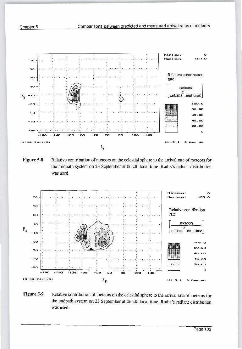
Chapter 5
70
SO
30
1.0
~g - 1.0
-30
- so
-70
-so
Comparisons between predicted and measured arrival rates of meteors
· . '.' ••• • I •
.. .. : .. . . . : .. .
o ... . ..... : . .. . . : ..
· . . . ', .. . . . ' . .. ...... .. ', . ... , . . . . ,', . . . . , .. . . · . . '.
Ht.nt.""u"", :
ttaMl ... u .. :
o 1.00 . 0
Relative contribution rate
[ meteors 1
radians2
.unit time
1.00 . 0
80 . 00
60 . 00
.... 0 . 00
20.00
o -1.80 -1.40 -1.00 -60 -20 20 60 1.00 1. .... 0
l3 : 58 2 .... /1./S1.
Figure 5-8
70
so
30
1.0
~g -1.0
-30
- so
-70 '.
-so
U 1. .3 . 1. 3 0 • ., so
Relative contribution of meteors on the celestial sphere to the arrival rate of meteors for the midpath system on 23 September at 06hOO local time. Rudie's radiant distribution was used.
. . . · .... .. -. ' .... '.'
· . : .... . : . .... -: . . . .
· . : .. . . . : . . ... -:.
.' . ... . ', ... . . ' ..... . .. . . . ' . . ..... . .. . ' ... . . . ' .. . . . . . . . . .
. . • • I • • • • '.' • • • •
Hini,.u ...... :
,.. ... Mi ... u ... : o
1.00 . 0
Relative contribution rate
[ meteors 1
radians 2
.unit time
'1.00 . 0
80.00
80.00
.... 0.00
20 . 00
-1.80 -1.40 - 1.00 -so - 20 20 80 1.00 1. .... 0 o
1.6 : .... 8 2 .... /1./S1.
Figure 5-9
U1. . 3.1. 3 0 • ., so
Relative contribution of meteors on the celestial sphere to the arrival rate of meteors for the endpath system on 23 September at 06hOO local time. Rudie's radiant distribution was used.
Page 103

Chapter 5 Comparisons between predicted and measured arrival rates of meteors
. ~ .
v~. c>
o 70
' 00 . 0
OOhOO Uniform
06hOO Uniform
~~~ _ ' 110 _ t,«J _ '00 -eo _ 210 :ro eo t OO '40
12hOO Uniform
18hOO Uniform
o
OOhOO Rudie
06hOO Rudie
o ,0)0 . 0
12hOO Rudie
~ .. ~. 'O ~---:-=---, ~ _ • .., - t40 - tOO -eo - 20 20 .0 t OO ......
18hOO Rudie
o t oo . O
Figure 5-10 Contour plots of the midpath relative contributions on the celestial sphere for a uniform geocentric radiant distribution (Uniform) and for Rudie's radiant distribution (Rudie) for 23 September at OOhOO, 06hOO, 12hOO and 18hOO local time.
Page 104

Chapter 5 Comparisons between predicted and measured arrival rates of meteors
o "_.'''''t'''" ' .00 . 0
06hOO Uniform
o 1 00 . 0
OOhOO Rudie
06hOO Rudie ~ ....
~ ... ~~ _ teo _ • ..., _ tOO ....., eo 100 • ...,
\It . 3 . \ :a _., t. : ~ 2 ...... ' ... . '
12hOO Uniform
18hOO Uniform
o '00 . 0 .. ~
12hOO Rudie i
~.. . ~~ - --=--:-::'-'._.- ~
18hOO Rudie
o .'- . 0
o 100 . 0
o 1 00 . 0
Figure 5-11 Contour plots of the endpath relative contributions on the celestial sphere for a unifonn geocentric radiant distribution (tJnifonn) and for Rudie's radiant distribution (Rudie) for 23 September at OOhOO, 06hOO, 12hOO and 18hOO local time.
Page 105

Chapter 5 Comparisons between predicted and measured arrival rates of meteors
The daily variation in the arrival rate of meteors, caused by the interaction
between a non-uniform radiant distribution of meteors and the axial rotation of
the earth, may be clearly illustrated using the graphical technique described in
this section. Figures 5-10 and 5-11 , respectively, are contour plots of the midpath
and endpath contributions for 23 September at OOhOO, 06hOO, 12hOO and 18hOO
local time. Contributions assuming a uniform geocentric radiant distribution as
well as the superposition using Rudie's distribution are shown. It should be noted
that the contributions have been normalized for each contour plot and relative
contributions between plots are not shown. Since most meteor radiants are
concentrated about the apex hemisphere, the daily cycle in the arrival rate of
meteors may clearly be illustrated by the interaction between the regions of
meteor contribution on the celestial sphere and the non-uniform radiant distribu
tion of meteors.
The annual variation in the arrival rate of meteors, caused by the axial tilt of the
earth and the rotation of the earth about the sun, may also be illustrated. The
longitudinal precession of regions of high contribution on the celestial sphere is
illustrated in Figures 5-12 and 5-13. Figures 5-12 and 5-13, respectively, are the
midpath and endpath contributions on the celestial sphere for 21 March, 21 June,
23 September and 22 December at 06hOO local time. As may be expected, the
movement of regions of high contribution on the celestial sphere, caused by the
earth's axial tilt and the earth's rotation about the sun, is far smaller than
movement on the celestial sphere caused by the axial rotation of the earth.
One of the significant uses of this graphical technique is as an aid to the
verification of radiant distributions. As will be shown in the following section,
this graphical technique may be used in the comparison between predicted and
measured arrival rates of meteors in order to determine the validity of various
radiant distributions.
Page 106

Chapter 5 Comparisons between predicted and measured arrival rates of meteors
_.eo - '40 _ Ie.. __ - 30 20 ... t.DO
D
,00 . D
March Unifonn
D t.oo . D
June Unifonn
Sept. Unifonn
Dec. Unifonn
D
loo . D
. ... .. .. : . . ~. .. .
. fij ... ~
····I·~ . . . . ~
" :
(J
o
March Rudie
June Rudie
Sept Rudie
Dec. Rudie
Figure 5-12 Contour plots of the midpath relative contributions on the celestial sphere for a uniform
geocentric radiant distribution (Uniform) and for Rudie's radiant distribution (Rudie)
for 21 March, 21 June, 23 September and 22 December at 06hOO.
Page 107

Chapter 5
.•. :::: ... . ::::. ... ,.. if. ·
. .; ,' . .
- lao - 1«11 - tOO -.u - 210 20 eo
Comparisons between predicted and measured arrival rates of meteors
. .
March Unifonn
June Unifonn
Sept. Unifonn
Dec. Unifonn
o '00 . 0
o "'.0 . 0
o "00 . 0
.. , . .
March Rudie
June Rudie
Sept.
~.~ .•• !I .• --,:::---:... ~ idre
- .eo - l<C - tDO -eo - 30 20 eo 100 • ..,
Dec. Rudie
o ' 00 , 0
o .~ 0
o '00 . 0
o .00 . 0
Figure 5-13 Contour plots of the end path relative contributions on the celestial sphere for a uniform
geocentric radiant distribution (Uniform) and for Rudie's radiant distribution (Rudie) for 21 March, 21 June, 23 September and 22 December at 06hOO.
Page 108
Chapter 5 Comparisons between predicted and measured arrival rates of meteors
5.3 Comparison between measured and predicted arrival rates of meteors
In order to evaluate the validity of the various radiant distributions of meteors it
was decided to compare variations in the predicted arrival rate of underdense
meteors using a particular radiant distribution with the measured arrival rate of
underdense meteors. The arrival rate of meteors was chosen rather than the
duration because the arrival rate of meteors can be predicted more accuratel y than
the duration of meteors. Furthermore, the arrival rate of meteors is more directly
related to the density distribution of meteor radiants.
It was decided to compare the arrival rate of underdense meteors rather than
overdense meteors, or even all meteor types, for three basic reasons. Firstly, the
prediction of underdense meteor rates is better defined than the prediction of
overdense meteors due to the fact that the underdense received power model is
better defined than the overdense model. Secondly, owing to the well defined
theoretical shape of the underdense trail envelope, the classification of measured
underdense trails is also thought to be better defined than the overdense type
classifications. Thirdly, the selection of only underdense trail types has the effect
of eliminating other types of propagation such as sporadic E from the measured
data.
In order to eliminate the effect of a varying noise threshold on the measured
arrival rate of meteors, the measured results were extracted as underdense trails
above a fixed signal level of -110 dBm, which was well above the measured
background noise level. The predicted results were similarly generated assuming
a constant background noise threshold.
Since the short term variation in the measured data can be large, and since the
predicted results are inherently based on monthly- or yearly-averaged data,
presentation of the results as monthly-averaged daily cycles of meteors was
Page 109

Chapter 5 Comparisons between predicted and measured arrival rates of meteors
chosen. Standard deviation error bars have been produced for the measured data
to give an indication of the variation of the data Owing to the large number and
time intensive nature of the predictions, the results for only alternate months of
the year, namely, January 1990, March 1990, May 1990, July 1990, September
1990 and December 1989, have been given. The omission of every alternate
month is possibly only significant in the case of the predictions based on the
monthly-averaged distributions, but, as will be shown later, since the yearly-av
eraged data seems more reliable and the difference in predictions from month to
month using yearly-averaged distributions is not significant, the presentation of
results for every alternate month was found to be adequate.
Monthly-averaged daily cycles of underdense meteors have been predicted for
the midpath and the endpath system. Simulations have been performed using the
following radiant distributions: Rudie's; Davies' extrapolated; Pupyshev's
monthly-averaged; and Pupyshev' s yearly-averaged. As may have been expected
based on the form of the distributions shown in Chapter 2, simulations using
Hawkins', McCrosky and Posen's, and the Harvard distributions confirmed that
these distributions are a very poor representation of the real distribution of
meteors in space. Predicted cycles for these distributions are therefore not
presented here.
The simulated cycles have been compared with measured results by plotting
measured and predicted results for each month. Since only relative rates are
required, the measured and predicted results have been scaled so that the
yearly-average for the measured and predicted results are the same. This enables
any differences in the predicted and measured annual cycle of meteors to be seen.
5.4 Comparisons between measured and predicted results
Measured and predicted results for the midpath and endpath system using
Rudie's, Davies' extrapolated, Pupyshev's yearly-averaged, and Pupyshev's
Page 110

Chapter 5 Comparisons between predicted and measured arrival rates of meteors
monthly-averaged radiant distributions are presented in Figures 5-14 to 5-17 and
Figures 5-19 to 5-21 respectively. The vertical lines in the measured results
represent the monthly-averaged standard deviation for the measured data.
The predicted results using Rudie's and Davies' extrapolated distributions
are very similar. Although, as shown in Chapter 4, there appear to be
significant differences between the two distributions, the averaging effect of
a large area of contributing radiants tends to minimize the differences be
tween the distributions. The similarity of the results from the two distribu
tions, however, stands to reason since they are both based on Davies' data.
Comparison between the measured and predicted midpath cycles using
Rudie's or Davies' extrapolated distributions shows that there is a reasonable
correlation between the results. Apart from the discrepancy during the July
evening hours caused by showers, the only major error appears to occur from
approximately 08hOO to 14hOO local time where the predicted results are
almost consistently higher than the measured results. The regions of radiant
contribution on the celestial sphere for the midpath system at 08hOO, 10hOO,
12hOO and 14hOO shown in Figure 5-22 illustrate the area on the celestial
sphere where the distribution may be in error. Unfortunately, however, owing
to the large region of contribution, it is not possible to localize the regions
on the celestial sphere where the distributions may be in error in any more
detail.
Midpath measured and predicted comparisons using Pupyshev's yearly- and
monthly-averaged distributions show a far poorer correlation than Rudie's or
Davies' extrapolated distribution. The shape and maximum-to-minimum vari
ation for the yearly-averaged Pupyshev distribution differs significantly from the
measured results and the monthly-averaged Pupyshev distributions provide even
poorer results. Based on these results it is possible to conclude that the monthly
averaged distributions are probably poor and that Pupyshev's yearly-averaged
Page 111

Chapter 5 Comparisons between predicted and measured arrival rates of meteors
70 JAN 1990
60
Rudie's Midpath 70
60
MAR 1990
1 2 3 4 5 6 7 8 9 10 11 12 13 14 15 16 17 18 19 20 21 22 23 24 70 I 2 3 4 5 6 7 8 9 10 11 12 13 14 15 16 17 18 IV 20 21 22 23 24 70
60 JULI990 MAY 1990 60
30
20
10
70 I 2 3 4 5 6 7 8 9 10 II 12 13 14 15 16 17 18 IV 20 21 22 23 24 70 I· 2 3 4 5 6 7 8 9 10 11 12 13 " 15 16 17 18 19 20 21 22 23 24
SEP 1990 60
NOV 1989 60
ro ro
o o~~~~~~~~~~~~~~~
I 2 3 4 5 6 7 8 9 10 11 12 13 14 15 16 17 18 19 20 21 22 23 24 I 2 3 4 5 6 7 8 9 10 II 12 13 " 15 16 17 18 19 20 21 22 23 24
Figure 5-14 Comparison between measured (solid diamond) and predicted (square) monthly-aver
aged daily cycles of meteors for the midpath system using Rudie's distribution. (Trails
per hour versus local time)
Page 112

Chapter 5 Comparisons between predicted and measured arrival rates of meteors
70 JAN 1990
60
50
30
10
Davies' extrapolated Midpath 70
60
50
40
10
MAR 1990
O~~~~~~~~~~~~~~
I 2 3 4 5 6 7 8 9 10 II 12 13 1. 15 16 17 18 19 20 21 22 23 U 70 1 2 3 • 5 6 7 8 9 10 11 12 13 1. 15 16 17 18 19 20 21 22 23 U 70
60 MAY 1990 60 JULI990
50 50
40 40
30 30
20 20
10 10
70 1 2 3 4 5 6 7 8 9 10 II 12 13 1. 15 16 17 18 19 20 21 22 23 U 70 1 2 3 • 5 6 7 8 9 10 11 12 13 1. 15 16 17 18 19 20 21 22 23 U
SEP 1990 60 NOV 1989
60
50 50
40 40
30 30
o O~~~~~rT~~~~~~~rT~
1 2 3 4 5 6 7 8 9 10 11 12 13 1. 15 16 17 18 19 20 21 22 23 U 1 2 3 • 5 6 7 8 9 10 II 12 13 1. 15 16 17 18 IV 20 21 22 23 U
Figure 5-15 Comparison between measured (solid diamond) and predicted (square) monthly-averaged daily cycles of meteors for the midpath system using Davies' extrapolated distribution. (Trails per hour versus local time)
Page 113

Chapter 5 Comparisons between predicted and measured arrival rates of meteors
70
so
50
\
Pupyshev's Yearly-averaged Midpath 70
JAN 1990 MAR 1990
so
50
I 2 3 4 5 6 7 8 9 10 \I 12 13 14 15 16 17 18 19 2Q 21 22 23 24 70 I 2 3 4 5 6 7 8 9 10 \I 12 13 14 15 16 17 18 19 2Q 21 22 23 24 70
so MAY 1990 so JULI990
50 50
\ 40 40
30 30
20 20
10 10
70 I 2 3 4 5 6 7 8 9 10 \I 12 13 14 15 16 17 18 19 2Q 21 22 23 24 70 I 2 3 4 5 6 7 8 9 10 \I 12 13 14 15 16 17 18 19 2Q 21 22 23 24
so
50
40
30
20
10
SEP 1990 so NOV 1989
50
j t 40
30
20
10
O~~~~~rT~~~~rT~~~~
I 2 3 4 5 6 7 8 9 ID \I 12 13 14 15 16 17 18 19 2Q 21 22 23 24 I 2 3 4 5 6 7 8 9 ID \I 12 13 14 15 16 17 18 19 2Q 21 22 23 24
Figure 5-16 Comparison between measured (solid diamond) and predicted (square) monthly-averaged daily cycles of meteors for the midpath system using Pupyshev's yearly-averaged distribution. (Trails per hour versus local time)
Page 114

Chapter 5 Comparisons between predicted and measured arrival rates of meteors
Pupyshev's Monthly-averaged Midpath 70 70
JAN 1990 MAR 1990
60 60
50 50
t 10 10
o O~~~~~~~~~TY~Fr~~~
70 1 2 3 4 5 6 7 8 9 10 11 12 13 14 15 16 17 18 19 20 21 22 23 24 70 1 2 3 4 5 6 7 8 9 10 11 12 13 14 15 16 17 18 19 20 21 22 23 24
60 MAY 1990 60 JUL1990
50 50
10 10
t \ t t t ! + + + + ! \
o o~~~~~~~~~~~~~~~
70 1 2 3 4 5 6 7 8 9 10 11 12 13 14 15 16 17 18 19 20 21 22 23 24 70 1 2 3 4 5 6 7 8 9 10 11 12 13 14 15 16 17 18 19 20 21 22 23 24
60 SEP 1990 60 NOV 1989
50 50
10
o O~~~~~~~~~~~~~~~
1 2 3 4 5 6 7 8 9 10 11 12 13 14 15 1& 17 18 19 20 21 22 23 24 1 2 3 4 5 & 7 8 9 10 11 12 13 14 15 1& 17 18 19 20 21 22 23 24
Figure 5-17 Comparison between measured (solid diamond) and predicted (square) monthly-averaged daily cycles of meteors for the midpath system using Pupyshev 's monthly-averaged distribution. (Trails per hour versus local time)
Page 115
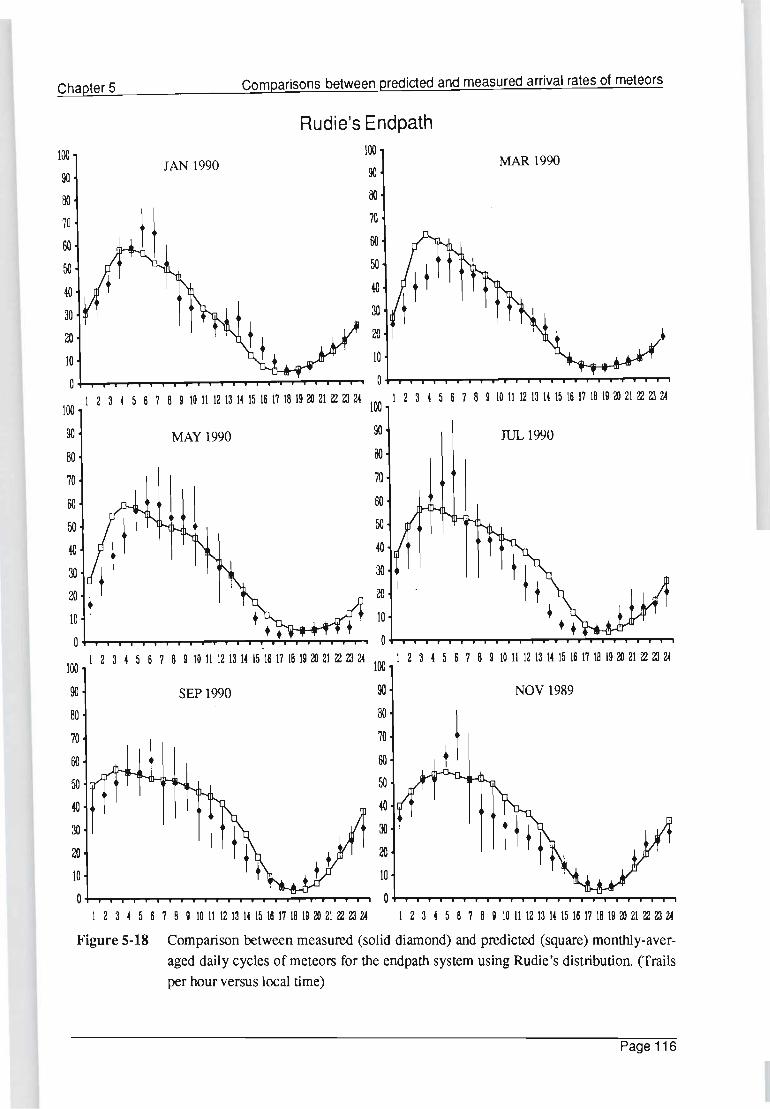
Chapter 5 Comparisons between predicted and measured arrival rates of meteors
100
90
80
70
60
50
40
30
20
JAN 1990
Rudie's Endpath 100
90
80
70
60
50
40
30
20
rn rn
MAR 1990
+
o o~~~~~~~~~~~~~~~
1 2 3 4 5 6 7 8 9 10 II 12 13 14 15 16 17 18 19 ~ 21 22 23 24 I 2 3 4 5 6 7 8 9 10 II 12 13 14 15 16 17 18 19 ~ 21 22 23 24 ~ ~
90 MAY 1990 90 JUL 1990
80
70
60
50
40
30
20
10
80
70
60
50
40
30
20
10
t j I + • + .......... ,,",-,'r
o~~~~~~~~~~~~~~~
100 1 2 3 4 5 6 7 8 9 10 II 12 13 14 15 16 17 18 19 ~ 21 22 23 24 100 I 2 3 4 5 6 7 8 9 10 II 12 13 14 15 16 17 18 19 ~ 21 22 23 24
90 SEP 1990 90 NOV 1989
80
70
60
80
70
60
50 50
40 40
30 30
20 20
rn rn
o O~~~~~~~~~~~~~~~
I 2 3 4 5 6 7 8 9 10 II 12 13 14 15 16 17 18 19 ~ 21 22 23 24 1 2 3 4 5 & 7 8 9 10 II 12 13 14 15 16 17 18 19 ~ 21 22 23 24
Figure 5-18 Comparison between measured (solid diamond) and predicted (square) monthly-aver
aged daily cycles of meteors for the endpath system using Rudie's distribution. (Trails
per hour versus local time)
Page 116

Chapter 5
100
90
80
70
60
50
40
30
20
10
0
JAN 1990
Comparisons between predicted and measured arrival rates of meteors
Davies' extrapolated Endpath 100
90
BO
70
60
50
40
30
20
10
MAR 1990
o~~~~~~~~~~~~~~~
100 1 2 3 4 5 6 7 8 Q 10 \I 12 13 14 15 16 17 18 19 ~ 21 22 Zl 24 100 1 2 3 4 5 6 7 8 Q 10 \I 12 13 14 15 16 17 18 19 ~ 21 22 Zl 24
90
BO
70
60
50
40
30
20
10
0
MAY 1990 90
BO
70
60
50
40
30
20
JULI990
~ J 10
T~' o~~~~~~~~~~~~~~ 100 1 2 3 4 5 6 7 8 9 10 \I 12 13 14 15 16 17 18 19 ~ 21 22 Zl 24 100 1· 2 3 4 5 6 7 8 Q 10 \I 12 13 14 15 16 17 18 19 ~ 21 22 Zl 24
90
BO
70
60
50
40
30
20
10
SEP 1990 90
00
70
60
50
40
30
20
10
NOV 1989
o~~~~~~~~~~~~~~~
1 2 3 4 5 S 7 8 Q 10 \I 12 13 14 15 16 17 18 19 ~ 21 22 Zl 24
Figure 5·19 Comparison between measured (solid diamond) and predicted (square) monthly-averaged daily cycles of meteors for the end path system using Davies' extrapolated distribution. (Trails per hour versus local time)
Page 117
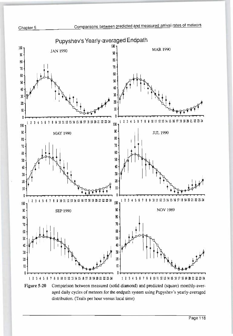
Chapter 5 Comparisons between predicted and measured arrival rates of meteors
100
90
BO
70
60
50
40
30
20
10
Pupyshev's Yearly-averaged Endpath 100
JAN 1990 90
BO
70
60
50
40
30
20
10
MAR 1990
O~~~~~~~~~~~rT~~ O~~~~rT~~~~~~~~~
100 1 2 3 4 5 6 7 8 9 10 11 12 13 14 15 16 17 18 19 ~ 21 22 Z! 24 100 1 2 3 4 5 6 7 8 9 10 11 12 13 14 15 16 17 18 19 ~ 21 22 Z! 24
90
BO
70
60
50
40
30
20 f 10
MAY 1990 90
BO
70
60
50
40
30
20
10
JULl990
O~~~~~rT~~~~~~~~~ o~~~~~~~~~~~~~~~
100 1 2 3 4 5 6 7 8 9 10 11 12 13 14 15 16 17 18 19 31 21 22 Z! 24 100 I 2 3 4 5 6 7 8 9 10 11 12 13 14 15 16 17 18 19 31 21 22 Z! 24
90
BO
70
60
SEP 1990 90
BO
70
60
50 50
40 40
30 30
20 20
m m
NOV 1989
o 0 +---~~r""T"~""T"""~"'I"""T"""'I"""T'"~~'-""T""T""'1 1 2 3 4 5 6 7 8 9 10 11 12 13 14 15 16 17 18 19 ~ 21 22 Z! 24 I 2 3 4 5 6 7 8 9 10 11 12 13 14 15 16 17 18 19 ~ 21 22 Z! 24
Figure 5-20 Comparison between measured (solid diamond) and predicted (square) monthly-averaged daily cycles of meteors for the endpath system using Pupyshev's yearly-averaged distribution. (Trails per hour versus local time)
Page 118

Chapter 5
100
90
eo
: t \ l\ : t t \ 20
10
Comparisons between predicted and measured arrival rates of meteors
Pupyshev's Monthly-averaged Endpath 100
JAN 1990 90
eo
70
MAR 1990
O~~~~~~~~~rT~~~~~
100 1 2 3 4 5 6 7 8 9 10 II 12 13 14 15 16 17 18 19 al 21 ~ 23 24 100 1 2 3 4 5 6 7 8 9 10 II 12 13 14 15 16 17 18 19 al 21 ~ 23 24
90
SO
70
60
50
40
30
20
10
MAY 1990
t
O~~~~~~~~~~~~~~~
90
eo
70
60
50
40
30
20
10
JULI990
O~~~~~~~~~~~~~~
100 1 2 3 4 5 6 7 8 9 10 II 12 13 14 15 16 17 18 19 al 21 ~ 23 24 100 1 2 3 4 5 6 7 8 9 10 II 12 13 14 15 16 17 18 19 al 21 ~ 23 24
90
eo
70
60
50
40
30
20
10
90
~ Ij t t : t t 20
10
NOV 1989
o O~~~~~~~~~~~~~~
1 234 5 6 7 8 9 W II ~ ~ U ffi ~ n ~ ~ al D ~ 23 24 1 234 5 6 7 8 9 W II ~ ~ U ffi ~ n ~ ~ al D ~ 23 24
Figure 5-21 Comparison between measured (solid diamond) and predicted (square) monthly-averaged daily cycles of meteors for the endpath system using Pupyshev 's monthly-averaged distribution. (Trails per hour versus local time)
Page 119
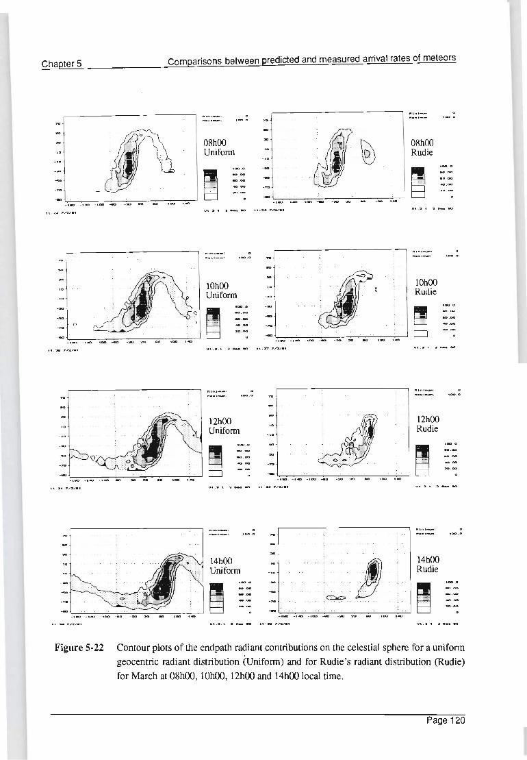
Chapter 5
-- .
Comparisons between predicted and measured arrival rates of meteors
08hOO Unifonn
10hOO Unifonn
. tGO . D 7U
.
08hOO Rudie
~~~ _,., -t"" _ tOO __ - :10 2CI eo tOO • ...,
10hOO Rudie
1 00 . 0 1'U
12hOO Unifonn
14hOO Unifonn
. tDO . •
12hOO Rudie
. ,gO . D
Figure 5-22 Contour plots of the endpath radiant contributions on the celestial sphere for a unifonn geocentric radiant distribution (Unifonn) and for Rudie's radiant distribution (Rudie) for March at 08hOO, IOhOO, 12hOO and 14hOO local time.
Page 120

Chapter 5 Comparisons between predicted and measured arrival rates of meteors
distribution produces poorer results than Rudie's or Davies' extrapolated distribu
tion.
An examination of the endpath measured and predicted cycles, however, shows
that predictions using Pupyshev's yearly-averaged distribution correlate better
than the endpath predictions using Rudie's or Davies' extrapolated distribution,
which appears to contradict the findings for the midpath predictions. An inspec
tion of the regions of contribution on the celestial sphere for the midpath and
endpath systems shown in Figures 5-10 to 5-13, along with an inspection of the
radiant distributions, appears to offer a possible reason for this discrepancy. As
shown in Section 5.2, the radiant contribution on the celestial sphere for the
midpath system includes a greater concentration of radiants at higher latitudes
than the endpath system. An inspection of Pupyshev 's yearly-averaged distribu
tion shows a greater contribution' of radiants at high latitudes around the north
and south ecliptic poles than Rudie's or Davies' extrapolated distribution. The
contribution of the high latitude radiants on Pupushev's yearly-averaged midpath
prediction results in higher predicted counts around 18hOO local time and
therefore also distorts the shape of the midpath predicted cycle. Owing to the
endpath radiant contributions occurring around the ecliptic and the good corre
lation obtained for the measured and predicted results using Pupyshev's yearly
averaged distribution, Pupyshev's distribution seems to be accurate about the
ecliptic plane. Care should be taken, however, in the evaluation of the radiant
distributions in this way, since it is clear that predictions using Rudie's, Davies'
extrapolated, and Pupyshev's yearly-averaged distributions, all produced good
correlation with the measured results and yet are different distributions. It is clear
that the large area of the radiants on the celestial sphere that contribute to meteor
count reduces the effect of differences between the distributions.
One notable observation from the comparison between the measured and pre
dicted endpath cycles using Rudie's or Davies' extrapolated distribution is that a
Page 121

Chapter 5
70
so
30
Comparisons between predicted and measured arrival rates of meteors
•• •• ' , • • • • I ••••• ' •••••• ' •••• · .
.' .
l1ini ... u ... : o 1.00 . 0
Relative contribution rate
[ meteors ]
radianl.unit time .... ' .' ..... . ... ' ... . . . .. ... . . . 1.0 .. . . . . .... .
~g -1.0 . : . ... . : . .... : . .... : .... . . : . . . .
· . . . - 30
........ . .. .. ..... ... .. ........ - ... . 1.00 . 0
BO . OO -so . . . . . : .. . . . :- . . . . -: .. . .. : . .... : ... . . : ..... : . ..... : . .. .
60 . 00
- 70 · .
. ,' •.• • • ' ..... ," .. • • , •.. .• '0 •...•... -40 . 00
20.00 . . · . . .
- 90 • • ', ' • •• ' ,' •••• ' , ' • •• • I •••• ',' • •• • I ••• • ',' •• •• ' ••••• o -1.80 -1.40 -1.00 -so -20 20 60 100 1-40
9 : 2-4 6/2/91
Figure 5-23 Regions of relative contribution of meteor radiants on the celestial sphere for the end path
system on 21 March at 04hOO local time
peak in meteor count is predicted earlier than the measured peak that typically
occurs at 06hOO local time. The contribution of radiants on the celestial sphere
for the predicted endpath March peak at 04hOO is shown in Figure 5-23, which
shows that the peak is caused primarily by the anti-sun contribution. This seems
to indicate that the position and/or amplitude of the anti-sun contribution relative
to the apex contribution for Rudie 's or Davies' extrapolated distribution may be
incorrect. The low resolution of this technique of verifying the radiant distribu
tions makes it difficult to determine the actual problem, but comparison between
Rudie's or Davies ' extrapolated and Pupyshev's yearly-averaged distribution
seems to indicate that the relative amplitude of the radiant contributions about
the apex for Rudie's or Davies ' extrapolated distribution may be too low.
Finally, as was the case with the midpath system, an inspection of the measured
and predicted results for the endpath system using Pupyshev's monthly-averaged
Page 122
Chapter 5 Comparisons between predicted and measured arrival rates of meteors
distributions show poor correlation. Although only half the monthly-averaged
distributions have been presented here, the results are sufficient to show that
Pupyshev's monthly-averaged data is poor. This result, and the fact that the
yearly-averaged distributions give better results than the monthly-averaged
distributions, confmns the observation that the monthly-averaged data appeared
to have little resolution.
5.4.1 Annual variation
The measured results for both the midpath and the endpath system show that
there is very little annual variation in the measured monthly-averaged arrival rate
of meteors. As shown in Chapter 2, owing to the discrepancy between the various
measured results, there is a high degree of uncertainty regarding the expected
annual variation in the arrival rate of meteors. The results shown here contrast
sharply with the large annual variation in the arrival rate of meteors adopted by
Weitzen for example, based, apparently, on Hawkins' results. The variation in
the space density of meteors with solar longitude has been estimated using similar
techniques to those used by Hawkins [1956] and Keay [1963]. The space density
of meteors with solar longitude has been estimated by comparing the measured
and predicted results, using Rudie's or Davies' distribution, for the midpath and
endpath system. Figures 5-24 and 5-25 are graphs of the normalized predicted
and measured monthly-averaged annual variation in the arrival rate of meteors
for the midpath and endpath system respectively. The annual variation in the
space density of meteors has been estimated by finding the ratio of the measured
to predicted results for the midpath and endpath systems as shown in Figure 5-26.
The annual variation predicted using the midpath system is very similar to the
variation predicted by Keay [1963] that is reproduced in Figure 2-35. The
difference between the midpath and endpath results may possibly be due to their
being a greater variation in the space density of meteors at higher ecliptical
latitudes that would affect the midpath measurements more than the endpath
Page 123
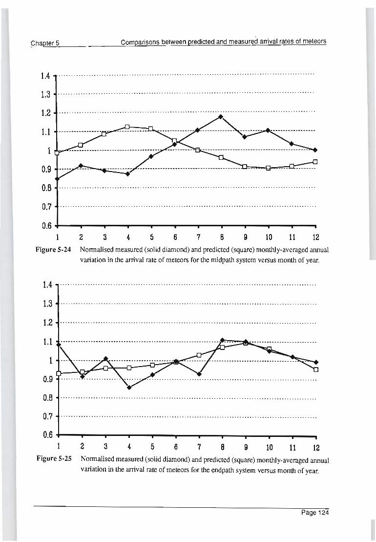
Chapter 5 Comparisons between predicted and measured arrival rates of meteors
14 ...................................................................................................... . .
1.3 .... ..... ..... .. ........... ....... ... ............................... .... .. ........... .. ........ .. ... . .
12 ...... .................................................................................................... . .
1.1
1
0.9
O B ...................................................................................................... . .
07 ...... .. ............................................................................................... . . 0.6 +--__ .--...... - ..... --....--r--........ -~-.,.....-r----,
1 2 3 5 6 7 B 9 10 11 12
Figure 5-24 Nonnalised measured (solid diamond) and predicted (square) monthly-averaged annual variation in the arrival rate of meteors for the midpath system versus month of year.
14 ........... ........ ................................................................................. ...... . ·
13 ............. .... ... ..... ......... .......... ............................. .... ................ ..... ......... . ·
12 ....... ....... ....... .... ..... .. ... ... ..................................... ............ .... ....................... . ·
1.1 .z=.~,;;,;.:,' . -.... _ .................. .
1
0.9
O B .............................................................................................................. . ·
O 7 ....................................................................................................... . · 0.6 +--~-~-....... .....,.-----.r---....... - ........ - ..... -_-_-_
1 2 3 5 6 7 B 9 10 11 12 Figure 5-25 Nonnalised measured (solid diamond) and predicted (square) monthly-averaged annual
variation in the arrival rate of meteors for the endpath system versus month of year.
Page 124

Chapter 5 Comparisons between predicted and measured arrival rates of meteors
14 .......... .............. .... ................. ...... .. ... .... ......... ..... ... ....... . · ...... .... ... ... ..... ... .
1.3 ..... .......... .. ..... .... ........... .... .... .. .. .. .. ....... .. ..... .. ......... .... .. ... ....... .....
12 .. .. .... .. ....... .... .. . ·
1.1
1
0.9
O 8 .. ..... ................ .... ......... .... ............... .... ... .. .. .. .......... . ·
0.7 .... .. .... .... .... ... ... .. .... .. .... ... ........ ....... ............... ........... ...... ... .... .... .. .. .
0.6 "--....... ---,....----.---r-....... -...,....-~--r--~-r----. 1 2 3 5 6 7 B 9 10 11 12
Figure 5-26 Apparant annual variation in the monthly-averaged space density of meteors estimated
using the midpath (square) and the endpath (solid diamond) system. (Normalised
variation versus month of year)
measurements. This would also account for the good correlation obtained with
Keay's results, which were based on measurements taken at mid latitudes. The
results presented here and by Keay conflrm the probable error of Hawkins' space
density variation. Since the space density variation of meteors does not appear
to vary uniformly across the celestial sphere, the scaling of a yearly-averaged
density distribution of meteors, in order to take into account the variation in space
density of meteors, would not produce accurate predicted results.
5.5 Conclusions
Comparisons between measured and predicted annual variations of meteor
counts shows that the predicted results are very close to the measured results,
which indicates that a large variation in the space density of meteors with solar
longitude does not occur. This result is in sharp contrast to the large variations
Page 125
Chapter 5 Comparisons between predicted and measured arrival rates of meteors
predicted by Hawkins, and indicates that the variation is even lower than the
variation presented by Keay [1963] .
Comparisons between predicted and measured results for both the midpath and
endpath systems seem to indicate that Rudie's or Davies' extrapolated distribu
tions provide the most accurate results overall. The good performance of Pu
pyshev's yearly-averaged distribution for the endpath system seems to indicate,
however, that Pupyshev's yearly-averaged distribution is more accurate than
Rudie's or Davies' extrapolated distribution around the ecliptic. The performance
of Pupyshev's monthly-averaged distribution was poor, which indicates that the
monthly-averaged distributions are not reliable.
Although the most reasonable results overall were obtained using Rudie's or
Davies' distributions, the results obtained were by no means ideal. This is to be
expected, since the measurements on which they are based are by no means
comprehensive. It should also be remembered that the effect of integrating
contributions of meteors over the meteor region tends to hide the fact that the
actual relative distribution of meteors in the meteor region may not be accurate
for a particular radiant distribution, although the integrated value may be. This
has serious implications for the design of communication systems where the
distribution of meteors across the meteor region needs to be known in order to
optimize system parameters such as antenna polar patterns. Although the results
of this chapter have shown that Rudie's or Davies' distributions produce reason
able results there is, therefore, still a need for a far more comprehensive set of
radar measurements to determine the density, velocity and mass distributions of
meteors intercepting the earth throughout the year.
Page 126
Chapter 6 Conclusion
Chapter 6
Conclusions
Questions regarding the origin of the heliocentric distribution presented by Rudie
[1967] have been discussed in Chapter 4. A detailed investigation into the origin
of the heliocentric distribution presented by Rudie has shown that Rudie 's
heliocentric distribution is simply an unnecessarily complicated extrapolation or
approximation of a particular set ofresults presented by Davies [1957]. Further
more it has been shown that distributions of orbital parameters of meteors
presented by Davies could not have been used by Rudie to generate his heliocen
tric distribution of meteors directly. An alternative, far simpler extrapolation of
Davies' results has been given in the form of a geocentric radiant distribution of
meteors. A method of converting from a heliocentric to geocentric radiant
distribution, which is slightly more accurate than the method given by Rudie,
was also given in Chapter 4. Using either technique it was shown that very similar
results were obtained for the transformation of Rudie's heliocentric distribution
to geocentric coordinates. For the purposes of modelling the effect of radiant
distributions on the arrival rate of meteors, theory developed in Chapter 3 has
shown that the incorporation of radiant distributions presented in geocentric
coordinates is analytically far simpler than the method used by Rudie of including
the effect of a radiant distribution given in heliocentric coordinates.
Comparisons between measured and predicted monthly-averaged daily cycles of
meteors have answered some of the questions surrounding the validity of the
various radiant distributions presented in Chapters 2 and 4. Comparisons between
Page 127

Chapter 6 Conclusion
measured and predicted cycles have shown that, for the purposes of predicting
arrival rates of meteors, Rudie's distribution and Davies' extrapolated distribu
tion are very similar. Comparisons between predicted and measured midpath and
endpath cycles have shown that Pupyshev's yearly-averaged distribution appears
most accurate for radiants close to the ecliptic plane. The apparent approximate
nature of Pupyshev's monthly-averaged distributions has also been confIrmed,
with the predicted cycles based on the monthly-averaged distributions producing
poor results. Although the predicted endpath results using Pupyshev's yearly
averaged distributions produced the best correlation overall, on average, Rudie 's
distribution or Davies' extrapolated distributions produced the best results for
both the midpath and endpath predictions.
Some of the confusion regarding the expected annual variation in the arrival rate
of meteors has been resolved. Comparisons between measured and predicted
annual variations in the arrival rate of meteors have shown that the apparent
annual variation in the space density of meteors is small. The results presented
in this thesis tend to agree with results presented by McKinley [1961] and Keay
[1963] and are in sharp contrast to recent predictions by Weitzen [1986].
Since it is clear that Rudie's distribution or Davies' extrapolated distribution are
the best available distributions at present and a comprehensive, new set of radar
measurements is probably required to more adequately characterize the distribu
tion of meteors intercepting the earth, modem computer-based meteor prediction
models are limited by Davies' original measurements. The signifIcance of this
limitation to the modelling of communication systems depends, naturally, on the
application. Comparisons between predicted and measured arrival rates of me
teors in Chapter 5 have shown that reasonable results can be obtained. However,
the limitations of the radiant distributions become apparent when more detailed
resolution is required from the distributions. In situations where knowledge of
the relative contribution of parts of the meteor region is required, for example,
Page 128

Chapter 6 Conclusion
as in the design of optimum antenna illumination patterns, the reliability of the
predictions is still uncertain. Bearing in mind the limitations of particular regions
of the radiant distributions described in this thesis can, however, aid in reducing
this uncertainty.
Page 129

Appendix A Area of the surface of a sphere
Appendix A .
Area on the surface of a sphere
Given a unit sphere in polar coordinates
r = cos ~ cos A. f + cos ~ sin A. J + sin ~ J
The area on the surface bounded by the lines of longitude and latitude that pass
.. tiA. tiA. ~ ~ . through the pomts. A. - 2' A. + 2' ~ - 2 ,and ~ + 2 1S
13+¥ A+1!.2A
A=J J dA.d~
= 2 ti A. sin ti ~ cos ~
Page 130

Appendix A Area of the surface of a sphere
For ~ ~ z 0, sin ~ ~ = ~ ~
Hence
Page 131

References
References
Andrianov, N. S. and Pupyshev, Yu. A, 1972 "The Distribution of the Geocentric Velocities of Sporadic Meteors over the Celestial Sphere", Translation of "Meteornoye Rasprostraneniye Radiomln (Meteoric Propagation of Radio Waws), No.7, Kazan' University Press, Kazan', 1970", NTIS N72-26720, pp 1-18.
Babadzhanov, P. B., Bibarsov, R Sh., Getman, V. S., and Kolmakov, V. M., 1985, "The Incident Flux Density of Meteors According to Observations in Dunshanbe", Solar System Res., Vol. 19, No.4, pp 217-222.
Barton, M. and Burke, M., 1977, "SNOTEL: An Operational Data Acquisition System using Meteor Burst Technology", Western Snow Conference, April 18-21, 1977, Albuquerque, New Mexico, pp 1-10.
Brown, D. W. and Williams, H. P., 1978, "The perfonnance of Meteor-Burst Communications at Different Frequencies", AGARD Conference Proceedings, Vol. 244.
Brown, D. W., 1985, "A Physical Meteor-Burst Propagation Model and Some Significant Results for Communication System Design", IEEE Journal on Selected Areas in Communications, Vol. SAC-3, No.5, pp. 745-755.
Burke, 0. 1. and Pogio, A 1., 1981, "Numerical Electromagnetic Code (NEC) - Method of Moments", Lawrence Liwrmore Laboratory, NOSC, Technical Document 116.
Cook, A. F., Flannery, M. R, Levy, H. II, McCrosky, R E., Sekanina, Z., Shao, C. _Y, Southworth, R. B., and Williams, J. T., 1972, "Meteor Research Program", Smithsonian Astrophysical Observatory, NASA CR-2109.
Danby, 1. M. A, 1970, "Fundamentals of Celestial Mechanics", The MacMillian Company, 866 Third Avenue, New York, New York, Third Printing 1970.
Davies, 1. 0., 1957, "Radio Observations of Meteors", Admnces in Electronics and Electron PhYSics, Vol. 9, pp. 95-128.
Davies,1. 0., Greenhow, 1. S., and Hall, 1. E., 1959, "The Effect of Attachment on Radio Echo-Observations of Meteors", Proc Roy Soc A, Vol. 253, pp 130.
Page 132

References
Desourdis, R. I. Jr., Merrill, S. C., Wojtaszek, 1. R and Hernandez, K, 1988, "Meteor Burst Link Performance Sensitivity to Antenna Pattern, Power Margin and Range", IEEE MILCOM 88, pp 257-263.
EUyett, C. D., 1977, "Solar Influence on Meteor Rates and Atmospheric Density Variations at Meteor Heights", Journal of Geophysical Research, Vol. 82, pp 1455-1462.
EUyett, C. D. and Keay, C. S. L., 1961, "Southern Hemisphere Meteor Rates", Monthly Notices of the Royal Astronomical Society, Vol. 125, pp. 325-346.
EUyett, C. D. and Keay, C. S. L., 1964, "Meteors: An Unexpected Increase in 1963", Science, Vol. 146, p 1458.
Ellyett, C. D. and Kennewell, 1. A, 1980, "Radar Meteor Rates and Atmospheric Density Changes", Nature, Vol. 287, No. 5782, pp. 521-522.
Eshleman, Von R. and Manning, L. A, 1954, "Radio Communication by Scattering From Meteoric Ionization", Proceedings of the IRE, Vol. 42, pp. 530-536.
Eshleman, Von R., 1955, "Theory of Radio Reflections from Electron-Ion Clouds", IRE Transactions on Antennas and Propagation, pp 32-39.
Felber, E, Davis, H., Stahl, R., Wheeler, R. and Wright, D., 1985, "Concepts for Near Continuous Reception of VHF (yery High Frequency) Signals Using Meteor Burst Propagation", JAYCOR, San Diego, CA, Report No. JAYCOR-J200-85-875/2393.
Forsyth, P. A, Vogan, E. L., Hansen, D. R. and Hines, C. 0.,1957, "The Principles of JANET - A Meteor-Burst Communication System", Proceedings of the IRE, Vol. 45, pp 1642-1657.
Haakinson, E. 1., 1983, "Meteor Burst Communications Model", NTIA Report 83-116, US Department of Commerce, Springfield, VA22161.
Hawkins, G. S., 1956, "Radio Echo Survey of Sporadic Meteor Radiants", Monthly Notices of the Royal Astronomical SOCiety, Vol. 116, No. 1, pp 92-104.
Hines, C. 0., 1955, "Diurnal Variations in the Number of Shower Meteors Detected by the Forward-Scattering of Radio Waves. Part I. Theory.", Canadian Journal of Physics, Vol. 33, No. 9, pp. 493-503.
Hines, C. 0 ., 1956, "Diurnal Variations in Forward-Scattered Meteor Signals", Journal of Atmospheric and Terrestrial PhYSics, Vol. 9, No.4, pp. 229-232.
Page 133

References
Hines, C. O.and Pugh, R. E., 1956, "The Spatial Distribution of Signal Sources in Meteoric Forward-Scattering", Canadian Journal 0/ Physics, Vol. 35, pp. 703-71 1.
Hines, C. O. and Forsyth, P. A., 1957, "The Forward-Scattering of Radio Waves from Overdense Meteor Trails", Canadian Journal o/Physics, Vol. 35, pp 1033-1041.
James, J. C. and Meeks, M. L., 1956, "On the Relative Contributions of Various Sky Reqions to Meteor-Trail Communications", Georgia Institute 0/ Technology, Atlanta, Georgia, Engineering Experiment Station, Naval Research Contract No. NOnr-991(02), Technical Report No. 1.
James, J. C., 1958, "The Influence of Meteor Radiant Distributions on Radio Echo Rates", Georgia Institute o/Technology, Atlanta, Georgia, Engineering Experiment Station, Naval Research Contract No. NOnr-991 (02), Technical ReportNo. 3, pp 1-105.
Kaiser, T. R., 1953, "Radio Echo Studies of Meteor Ionisation", Phil. Mag., Vol. 2, pp 495-544.
Keay, C. S. L., 1963, "The Distribution of Meteors around the Earth's Orbit", Monthly Notices o/the Royal Astronomical SOCiety, Vol. 126, pp 165-176.
Keay, C. S. L. and Ellyett, C. D., 1968, "Southern Hemisphere Meteor Rates Final Report", NASA-CR-105828, NTIS N69-37252, 94p.
Kresakova, M. and Kresak, L., "On the Activity of Telescopic Meteors and Some Related Problems", Contr. Astron. Obs. Skalnate Pleso, Vol. 1, pp 40-77.
Larsen, J. D. and Rodman, P. J., 1988, "Study into Meteor Scatter Communication Systems", Salbu (Pty) Ltd., POBox 109, Irene, South Africa, Project N, Part II, Vol. 2.
Larsen, J. D., Melville, S. W. and Mawrey, R. S., 1990, "Adaptive Data Rate Capacity of Meteor-Burst Communications", 1990 IEEE Military Communications Conference, Monterey California, Vol. 2, pp 863-867.
Linblad, B. A., 1967, "Solar Cycle Variations in Atmospheric Density as Deduced from Meteor Observations", Space Research VII (North Holland Publ. Co., Amsterdam), pp. 1029-1043.
Lovell, A. C. B., 1954, "Meteor Astronomy", The International Series o/Monographs on Physics, Oxford University Press, London.
Page 134
•

References
Mawrey, R S., 1988, "A Meteor Scatter Measurement System", MSc. Eng. Thesis, University of Natal, Durban, South Africa
Mawrey, R S., 1990, "A Comparison between Predicted and Measured Annual Cycles of Meteors", The Third South African IEEE Conference on Theoretical and Practical Work in Communications and Signal Processing (COMSIG 90), Johannesburg, IEEE Catalog No. 90TH0314-5, pp 32-37.
McCrosky, R E. and Posen, A, 1961, "Orbital Elements of Photographic Meteors", Smithsonian Contributions to Astrophysics, Vol. 4, No.2, pp 15-84.
McIntosh, B. A and Simek, M., 1969, "Mass Distributions of Meteoroids Detennined by Radar Observations of Underdense Meteor Trails", Canadian Journal of Physics, Vol. 47, No.1, pp. 7-22.
McKinley, D. W. R, 1961, "Meteor Science and Engineering", McGraw-Hill, New York.
Melville, S. W., Larsen, 1. D., Letschert, R Y, and Goddard, W D., 1989, "The Classification of Meteor Trail Reflections by a Rule-Based System", Transactions of the South African Institute of Electrical Engineers, Vol. 80, No. 1, pp 104-116.
Millman,P. M. andMcIntosh,B. A, 1964, "Meteor Radar Statistics 1", Canadian Journal of Physics, No. 42, pp. 1730-1742.
Millman, P. M. and McIntosh, B. A, 1966, "Meteor Radar Statistics II", Canadian Journal of Physics, No. 44, pp. 1593-1602.
Murakami, T., 1955, "On the Annual Variation of Sporadic Meteors. I and II", Publ. Astron. Soc. Japan, Vol. 7, pp 49-64.
Porter, F. G., 1952, "Comets and Meteor Streams", The International Astrophysical Series, Vol. 2, Chapman & Hall Ltd., London.
Pupyshev, Yu. A, Filimonova, T. K, and Kazakova, T. v., 1980, "Charts of the Distribution over the Entire Sky of the Visible Density of Radiants of Sporadic Meteors", taken from the book Meteornoye Rasprostraneniye Radio win, Kazan', Kazan' University Press, 112 pp.
Rodman, P. 1., 1989, "A Microcomputer-based Meteor Burst Communications Prediction Modelling System", User Manual IBM PC Version 1.3, Salbu (Ply) Ltd, P o Box 109, Irene, South Africa.
Page 135
References
Rudie, N. H., 1967, "The Relative Distribution of Observable Meteor Trails in ForwardScatter Meteor Communications ", PhD. Thesis, Montana State University.
Sachs, D., 1984, "Improvement of VHF (MB) Model", Science Applications International Corporation, La Jolle, CA., Report No. SAIC-84/1634.
Sekanina, Z., 1970 "Statistical Model of Meteor Streams 1. Analysis of the Model", Icarus 13, pp 459-474.
Sinno, K, 1979, "A Role for Metallic Ions of Meteor Origin in VHF Ionospheric Forward-Scattering and Further Contribution to the Formation of Sporadic-E", Journal of The Radio Research Laboratories, Vol. 26, No. 120/121, pp. 101-116.
Southworth, R B. and Hawkins, G. S., 1963, "Statistics of Mete or Streams", Smithsonian Contributions to Astrophysics, Vol. 7.
Southworth, R B. and Sekanina, Z., 1975, "Physical and Dynamical Studies of Meteors' " Smithsonian Institution, Cambridge, Mass. 02138, NASACR-2615.
Srirama Rao, M., Ratnam, S. R, Krishna Rao, D. A. V. and Bhagiratha Rao, E., 1983, "Survey of Meteor Signal Rates Observed over a VHF Forward-Scatter Link Between Waltair & Dehra Dun", Indian Journal of Radio and Space Physics, Vol. 12, No. 2, pp. 50-52.
Steffancin, W. and Brown, D., 1986, "CSC (Computer Sciences Corporation) Meteor Burst Model Enhancement Test Report", Computer Sciences Corp., Falls Church, VA., Contract No. DCAI00-84-C-0030, pp 1-51.
Sugar, G. R, 1964, "Radio Propagation by Reflection from Meteor Trails", Proceedings of the IEEE, Vol. 52, pp 116-136.
Svetashkova, N. T., 1987, "Density Variations of Meteor Flux along the Earth's Orbit", MiddleAtmosphereProgram. Handbookfor Map, Vol. 25, NTIS N88-14545, pp 311-315.
Taylor, R E., 1973, "136-MHzl400-MHz Radio-Sky Maps", Proceedings of the IEEE (Letters), April, pp 469-472.
Vemiani, F., 1965, Smithsonian Contributions to Astrophysics, Vol. 8, pp 141 .
Vogan, E. L. and Cambell, L. L., 1957, "Meteor Signal Rates Observed in Forward-Scatter", Canadian Journal of PhYSics, Vol. 35, pp. 1176-1189.
Page 136

References
Weiss, A A, 1957, "Meteor Activity in the Southern Hemisphere", Australian Journal o/Physics, Vol. 10, No.2.
Weitzen,1. A, 1983, "Feasibility of High Speed Digital Communications on the Meteor Scatter Channel", PhD. Thesis, The University of Wisconsin - Madison.
Weitzen, 1. A, 1986, "Predicting the Arrival Rate of Meteors Useful for Meteor Burst Communication", Radio Science, Vol. 21, No. 6, pp 1009-1020.
Yavus, D. Y, 1990, "Meteor Burst Communications",IEEE Communications Magazine, September, pp 40-48.
Page 137