predicting brain mechanics during closed head impact ... · predicting brain mechanics during...
TRANSCRIPT

Predicting brain mechanics during closed head impact :numerical and constitutive aspectsBrands, D.W.A.
DOI:10.6100/IR552152
Published: 01/01/2002
Document VersionPublisher’s PDF, also known as Version of Record (includes final page, issue and volume numbers)
Please check the document version of this publication:
• A submitted manuscript is the author's version of the article upon submission and before peer-review. There can be important differencesbetween the submitted version and the official published version of record. People interested in the research are advised to contact theauthor for the final version of the publication, or visit the DOI to the publisher's website.• The final author version and the galley proof are versions of the publication after peer review.• The final published version features the final layout of the paper including the volume, issue and page numbers.
Link to publication
General rightsCopyright and moral rights for the publications made accessible in the public portal are retained by the authors and/or other copyright ownersand it is a condition of accessing publications that users recognise and abide by the legal requirements associated with these rights.
• Users may download and print one copy of any publication from the public portal for the purpose of private study or research. • You may not further distribute the material or use it for any profit-making activity or commercial gain • You may freely distribute the URL identifying the publication in the public portal ?
Take down policyIf you believe that this document breaches copyright please contact us providing details, and we will remove access to the work immediatelyand investigate your claim.
Download date: 13. Jul. 2018

Predicting brain mechanics duringclosed head impact
- numerical and constitutive aspects -

CIP-DATA LIBRARY TECHNISCHE UNIVERSITEIT EINDHOVEN
Brands, Davy W.A.
Predicting brain mechanics during closed head impact : numerical and constitutiveaspects / by Davy W.A. Brands. - Eindhoven : Technische Universiteit Eindhoven,2002.Proefschrift. - ISBN 90-386-2713-0NUGI 834Trefwoorden: hoofd; letselbiomechanica / hersenweefsel; constitutieve modellering/ hersenweefsel; materiaalkarakterisering / letselbiomechanica;eindige-elementenmethode / hersenweefsel; golfvoortplanting; numerieke aspectenSubject headings: head; injury biomechanics / brain tissue; constitutive modelling /brain tissue; material characterization / impact biomechanics; finite elementmodelling / brain tissue; wave propagation; numerical aspects
Printed by the University Press Facilities, Eindhoven, The Netherlands
This research was financially supported by TNO Prins Maurits Laboratory, TheNetherlands and the University Research Program of Ford Motor company.

Predicting brain mechanics duringclosed head impact
- numerical and constitutive aspects -
PROEFSCHRIFT
ter verkrijging van de graad van doctoraan de Technische Universiteit Eindhoven,
op gezag van de Rector Magnificus, prof.dr. R.A. van Santen,voor een commissie aangewezen door het College voor Promoties
in het openbaar te verdedigen opdonderdag 14 maart 2002 om 16.00 uur
door
Davy Wilhelmus Anna Brands
geboren te Maastricht

Dit proefschrift is goedgekeurd door de promotoren:
prof.dr.ir. D.H. van Campenenprof.dr.ir. J.S.H.M. Wismans
Copromotor:dr.ir. P.H.M. Bovendeerd

voor Bianca
voor mijn ouders

vi

Contents
Summary xi
1 General introduction 11.1 Introduction to head injury biomechanics . . . . . . . . . . . . . . . . 2
1.1.1 Epidemiology of head injury . . . . . . . . . . . . . . . . . . . . 21.1.2 Basic anatomy of the head . . . . . . . . . . . . . . . . . . . . . 21.1.3 Load-injury scheme . . . . . . . . . . . . . . . . . . . . . . . . . 31.1.4 Head injury criteria . . . . . . . . . . . . . . . . . . . . . . . . . 41.1.5 Head models . . . . . . . . . . . . . . . . . . . . . . . . . . . . 6
1.2 Finite Element modelling of head impact . . . . . . . . . . . . . . . . . 91.2.1 Mathematical model . . . . . . . . . . . . . . . . . . . . . . . . 91.2.2 Numerical solution method . . . . . . . . . . . . . . . . . . . . 101.2.3 Model validation . . . . . . . . . . . . . . . . . . . . . . . . . . 111.2.4 Conclusion . . . . . . . . . . . . . . . . . . . . . . . . . . . . . 12
1.3 Scope of study . . . . . . . . . . . . . . . . . . . . . . . . . . . . . . . 121.3.1 Objectives . . . . . . . . . . . . . . . . . . . . . . . . . . . . . . 121.3.2 Strategy . . . . . . . . . . . . . . . . . . . . . . . . . . . . . . . 131.3.3 Outline of the thesis . . . . . . . . . . . . . . . . . . . . . . . . 13
2 Numerical accuracy: analysis of wave propagation in blunt head impact 152.1 Introduction . . . . . . . . . . . . . . . . . . . . . . . . . . . . . . . . . 162.2 Elementary theory on wave propagation . . . . . . . . . . . . . . . . . 16
2.2.1 Elastic wave equation . . . . . . . . . . . . . . . . . . . . . . . 162.2.2 Solution for 1-D elastic wave equation . . . . . . . . . . . . . . 182.2.3 Viscoelastic theory . . . . . . . . . . . . . . . . . . . . . . . . . 19
2.3 Importance of wave phenomena in the human head . . . . . . . . . . . 202.3.1 Lower bound of frequency range . . . . . . . . . . . . . . . . . 202.3.2 Upper bound of frequency range . . . . . . . . . . . . . . . . . 212.3.3 Reflection: mode conversion . . . . . . . . . . . . . . . . . . . 22
2.4 Simulation of wave propagation:theoretical considerations . . . . . . . . . . . . . . . . . . . . . . . . . 232.4.1 Numerical stability . . . . . . . . . . . . . . . . . . . . . . . . . 232.4.2 Numerical accuracy . . . . . . . . . . . . . . . . . . . . . . . . 23
vii

viii Contents
2.5 Simulation of wave propagation: numerical results . . . . . . . . . . . 262.5.1 Analytical solution . . . . . . . . . . . . . . . . . . . . . . . . . 262.5.2 The numerical model . . . . . . . . . . . . . . . . . . . . . . . . 272.5.3 Results . . . . . . . . . . . . . . . . . . . . . . . . . . . . . . . . 28
2.6 Discussion . . . . . . . . . . . . . . . . . . . . . . . . . . . . . . . . . . 302.6.1 Wave propagation during head impact . . . . . . . . . . . . . . 302.6.2 Numerical accuracy . . . . . . . . . . . . . . . . . . . . . . . . 312.6.3 Implications for existing head models . . . . . . . . . . . . . . . 322.6.4 Methods of improvement . . . . . . . . . . . . . . . . . . . . . 33
2.7 Conclusions . . . . . . . . . . . . . . . . . . . . . . . . . . . . . . . . . 34
3 Comparison of the dynamic behaviour of brain tissue and two modelmaterials 353.1 Introduction . . . . . . . . . . . . . . . . . . . . . . . . . . . . . . . . . 363.2 Materials and methods . . . . . . . . . . . . . . . . . . . . . . . . . . . 363.3 Results . . . . . . . . . . . . . . . . . . . . . . . . . . . . . . . . . . . . 403.4 Discussion . . . . . . . . . . . . . . . . . . . . . . . . . . . . . . . . . . 423.5 Conclusions . . . . . . . . . . . . . . . . . . . . . . . . . . . . . . . . . 453.6 Acknowledgments . . . . . . . . . . . . . . . . . . . . . . . . . . . . . 45
4 Large shear strain dynamic behaviour of brain tissue and silicone gelmodel material 474.1 Introduction . . . . . . . . . . . . . . . . . . . . . . . . . . . . . . . . . 484.2 Materials and methods . . . . . . . . . . . . . . . . . . . . . . . . . . . 484.3 Results . . . . . . . . . . . . . . . . . . . . . . . . . . . . . . . . . . . . 544.4 Discussion . . . . . . . . . . . . . . . . . . . . . . . . . . . . . . . . . . 594.5 Conclusions . . . . . . . . . . . . . . . . . . . . . . . . . . . . . . . . . 644.6 Acknowledgments . . . . . . . . . . . . . . . . . . . . . . . . . . . . . 64
5 A non-linear viscoelastic material model for brain tissue 655.1 Introduction . . . . . . . . . . . . . . . . . . . . . . . . . . . . . . . . . 665.2 General formulation of the model . . . . . . . . . . . . . . . . . . . . . 66
5.2.1 Multiplicative strain decomposition . . . . . . . . . . . . . . . . 665.2.2 Constitutive assumptions . . . . . . . . . . . . . . . . . . . . . 685.2.3 Multi-mode description . . . . . . . . . . . . . . . . . . . . . . 70
5.3 Determination of brain tissue material parameters . . . . . . . . . . . 705.3.1 Small strain experiments: Multi-mode Maxwell model . . . . . 715.3.2 Large strain stress relaxation experiments . . . . . . . . . . . . 725.3.3 Bulk behaviour: Ultrasonic experiments . . . . . . . . . . . . . 74
5.4 Numerical implementation . . . . . . . . . . . . . . . . . . . . . . . . . 755.4.1 Time integration in MADYMO . . . . . . . . . . . . . . . . . . . 755.4.2 Stress computation . . . . . . . . . . . . . . . . . . . . . . . . . 765.4.3 Accuracy of the time integration scheme . . . . . . . . . . . . . 77
5.5 Simulation of stress relaxation experiments . . . . . . . . . . . . . . . 795.5.1 Model description . . . . . . . . . . . . . . . . . . . . . . . . . 79

Contents ix
5.5.2 Results . . . . . . . . . . . . . . . . . . . . . . . . . . . . . . . . 795.5.3 Discussion and conclusions . . . . . . . . . . . . . . . . . . . . 80
5.6 Conclusion . . . . . . . . . . . . . . . . . . . . . . . . . . . . . . . . . 81
6 FE modelling of transient rotation of a simple physical head model 836.1 Introduction . . . . . . . . . . . . . . . . . . . . . . . . . . . . . . . . . 846.2 Experimental model . . . . . . . . . . . . . . . . . . . . . . . . . . . . 85
6.2.1 Experimental setup . . . . . . . . . . . . . . . . . . . . . . . . . 856.2.2 Experimental results . . . . . . . . . . . . . . . . . . . . . . . . 886.2.3 Discussion on experiment . . . . . . . . . . . . . . . . . . . . . 89
6.3 Numerical model . . . . . . . . . . . . . . . . . . . . . . . . . . . . . . 916.3.1 Methods . . . . . . . . . . . . . . . . . . . . . . . . . . . . . . . 916.3.2 Numerical results: REF material model . . . . . . . . . . . . . . 936.3.3 Numerical results: CPL material model . . . . . . . . . . . . . . 95
6.4 Discussion . . . . . . . . . . . . . . . . . . . . . . . . . . . . . . . . . . 966.5 Conclusions . . . . . . . . . . . . . . . . . . . . . . . . . . . . . . . . . 98
7 Effects of constitutive modelling on brain response in a 3-D FE head model 997.1 Introduction . . . . . . . . . . . . . . . . . . . . . . . . . . . . . . . . . 1007.2 Numerical model . . . . . . . . . . . . . . . . . . . . . . . . . . . . . . 1007.3 Results . . . . . . . . . . . . . . . . . . . . . . . . . . . . . . . . . . . . 104
7.3.1 Reference model: REF . . . . . . . . . . . . . . . . . . . . . . . 1057.3.2 Model variants: cpl and sof . . . . . . . . . . . . . . . . . . . . 107
7.4 Discussion . . . . . . . . . . . . . . . . . . . . . . . . . . . . . . . . . . 1107.4.1 Numerical model accuracy . . . . . . . . . . . . . . . . . . . . . 1107.4.2 Reference model response . . . . . . . . . . . . . . . . . . . . . 1107.4.3 Variation of material models . . . . . . . . . . . . . . . . . . . . 112
7.5 Conclusions . . . . . . . . . . . . . . . . . . . . . . . . . . . . . . . . . 113
8 Discussion, Conclusions and Recommendations 1158.1 Introduction . . . . . . . . . . . . . . . . . . . . . . . . . . . . . . . . . 1168.2 Discussion . . . . . . . . . . . . . . . . . . . . . . . . . . . . . . . . . . 116
8.2.1 Requirements for the numerical accuracy of FE head models . . 1168.2.2 Brain tissue constitutive behaviour: experiments and model . . 1178.2.3 Application in a three-dimensional head model . . . . . . . . . 1188.2.4 Consequences for head modelling . . . . . . . . . . . . . . . . 119
8.3 Conclusions . . . . . . . . . . . . . . . . . . . . . . . . . . . . . . . . . 1208.4 Recommendations . . . . . . . . . . . . . . . . . . . . . . . . . . . . . 121
8.4.1 Numerical quality, validation of head models . . . . . . . . . . 1218.4.2 Constitutive modelling of brain tissue . . . . . . . . . . . . . . 1218.4.3 Geometry and interface description in head models . . . . . . 122
References 123
A Test of numerical implementation 133A.1 Introduction . . . . . . . . . . . . . . . . . . . . . . . . . . . . . . . . . 134
x Contents
A.2 Simple shear stress relaxation . . . . . . . . . . . . . . . . . . . . . . . 134A.3 Objectivity: uni-axial deformation . . . . . . . . . . . . . . . . . . . . . 137A.4 Hydrostatic compression . . . . . . . . . . . . . . . . . . . . . . . . . . 138A.5 Combined shear and extension: cyclic loading and unloading . . . . . 139A.6 Conclusions . . . . . . . . . . . . . . . . . . . . . . . . . . . . . . . . . 141
B Modification of non-linear viscoelastic material model 143B.1 Modification of the model . . . . . . . . . . . . . . . . . . . . . . . . . 144B.2 Requirements for positive stiffness . . . . . . . . . . . . . . . . . . . . 144B.3 Determination of brain tissue material parameters . . . . . . . . . . . 145B.4 Implications for material behaviour . . . . . . . . . . . . . . . . . . . . 146B.5 Discussion and conclusions . . . . . . . . . . . . . . . . . . . . . . . . 147
Samenvatting 149
Dankwoord 153
Curriculum Vitae 155

Summary
Annually, motor vehicle crashes world wide cause over a million fatalities and over ahundred million injuries. Of all body parts, the head is identified as the body regionmost frequently involved in life-threatening injury. To understand how the braingets injured during an accident, the mechanical response of the contents of the headduring impact has to be known. Since this response cannot be determined during anin-vivo experiment, numerical Finite Element (FE) modelling is often used to predictthis response. Current FE head models contain a detailed geometrical description ofanatomical components inside the head but lack accurate descriptions of the brainmaterial behaviour and contact between e.g. skull and brain. Also, the numericalsolution method used in current models (explicit Finite Element Method) does notprovide accurate predictions of transient phenomena, such as wave propagation, inthe nearly incompressible brain material.The aim of this study is to contribute to the improvement of FE head models used topredict the mechanical response of the brain during a closed head impact. The topicsof research are the accuracy requirements of explicit FEM for modelling the dynamicbehaviour of brain tissue, and the development of a constitutive model for describingthe nearly incompressible, non-linear viscoelastic behaviour of brain tissue in a FEmodel.The accuracy requirements of the numerical method used depend on the type ofmechanical response of the brain, wave propagation or a structural dynamics typeof response. The impact conditions for which strain waves will propagate insidethe brain have been estimated analytically using linear viscoelastic theory. It wasfound that shear waves (S-waves) can be expected during a traffic related impact,(frequencies between 25 and 300 Hz), while compressive waves (P-waves) areexpected during short duration, high velocity, ballistic impacts (frequencies between10 kHz and 3 MHz). For this reason FE head models should be capable of accuratelyreplicating the wave front during wave propagation, which poses high numericalrequirements.An accuracy analysis, valid for one-dimensional linear viscoelastic material behaviourand small strains, revealed that modelling wave propagation phenomena with explicitFEM introduces two types of errors: numerical dispersion and spurious reflection.These errors are introduced by the spatial and temporal discretisation and causethe predicted wave propagation velocity to be lower than in reality. As a result,strain and strain rate levels will deviate from reality. Since both strain and strain
xi

xii Summary
rate are associated with the occurrence of brain injury they should be predictedcorrectly. However, given the element size in current state of the art 3-D humanhead models, accurate modelling of wave propagation is impossible. For accuratemodelling of S-waves the typical element size in head models (5 mm) should bedecreased by a factor of ten which can be accomplished by mesh refinement. Foraccurate modelling of P-waves the typical element size should be decreased by afactor of hundred. For this reason mesh refinement is not feasible anymore anddevelopments on spatial and temporal discretisation methods used in the FiniteElement Method are recommended. As these developments are beyond the scopeof this research, shear behaviour is emphasised in the remainder of the study.The mechanical behaviour of brain tissue has been characterised using simple shearexperiments. The small strain behaviour of brain tissue is investigated using anoscillatory strain (amplitude 1%). Frequencies relevant for impact (1-1000 Hz) couldbe obtained using the Time/Temperature Superposition principle. Strains associatedwith the occurrence of injury (20% simple shear) were applied in stress relaxationexperiments. It was found that brain tissue behaves as a non-linear viscoelasticmaterial. Shear softening (i.e. decrease in stiffness) appeared for strains above 1%(approximately 35% softening for shear strains up to 20%) while the time relaxationbehaviour was nearly strain independent.A constitutive description capable of capturing the material behaviour observed inthe material experiments was developed. The model is a non-linear extension ofa linear multi-mode Maxwell model. It utilises a multiplicative decomposition ofthe deformation gradient tensor into an elastic and an inelastic part. The inelastic,time dependent behaviour is modelled using a simple Newtonian law acting on thedeviatoric part of the stress only. The elastic, strain dependent behaviour is modelledby a hyper-elastic, second order Mooney-Rivlin material formulation. Althoughisotropy was assumed in this study, the model formulation is such that implementinganisotropy, present in certain regions of the brain, is possible. Brain tissue materialparameters were obtained from small strain oscillatory experiments and the constantstrain part from the stress relaxation experiments.The constitutive model was implemented in an existing explicit FE code (MADYMO).In view of the nearly incompressible behaviour of brain tissue, Heun’s (predictor-corrector) integration method was applied for obtaining sufficient numerical accuracyof the model at time steps common for head impact simulations. As a first test, theinitial part of the stress relaxation experiments, which was not used for fitting thematerial parameters, was simulated and could be reproduced successfully.To test both the numerical accuracy of explicit FEM and the constitutive modelformulation at conditions resembling a traffic related impact a physical (i.e.laboratory) head model has been developed. A silicone gel (Dow Corning Sylgard527 A&B) was used to mimic the dynamical behaviour of brain tissue. The gelwas mechanically characterized in the same manner as brain tissue. It was foundthat silicone gel behaves as a linear viscoelastic solid for all strains tested (up to50%). Its material parameters are in the same range as the small strain parametersof brain tissue, but viscous damping at high frequencies is more pronounced. It wasconcluded that for trend studies and benchmarking of numerical models the gel is

Summary xiii
a good model material. The gel was put in a cylindrical cup that was subjected toa transient rotational acceleration. Gel deformation was recorded using high speedvideo marker tracking. The gel was modelled using the new constitutive law and thephysical model experiments were simulated. Good agreement was obtained withexperimental results indicating the model to be suitable for modelling the nearlyincompressible silicone gel. It was shown that correct decoupling of hydrostatic anddeviatoric deformation in the stress formulation is necessary for correct prediction ofthe response of the nearly incompressible material.Finally, the constitutive model was applied in an existing 3-D FE model of the humanhead to asses the effect of non-linear brain tissue material behaviour on the response.The external mechanical load on the 3-D FE head model (an eccentric rotation) waschosen such as to obtain strains within the validity range of the material experiments(20% shear strain). This resulted in external loading levels values below the onesassociated with injury in literature. A possible explanation for this is the fact thatshear stiffness values, commonly used in head models in literature, are too highin comparison with material data found in recent literature and own experiments.Also the estimated injury threshold of 20% strain, indicated by studies on isolatedaxons, might be to conservative. Another possible explanation may be that a certaindegree of coupling between hydrostatic and deviatoric parts of the deformation in thestress formulation might exist in reality which is not modelled in current constitutiveformulation.Application of the non-linear behaviour in the model influences the level of stresses(decrease by 11%) and strains (increase by 21%) in the brain but not the temporaland spatial distribution. However, it should be noted that these effects on stresses andstrains hold for one specific loading condition in one specific model only. For a moregeneral conclusion on the effects of non-linear modelling in brain tissue, applicationin different models is recommended.

xiv Summary

Chapter 1
General introduction
A general introduction in the field of injury biomechanics is provided. First epidemiology and theimportance of head injury biomechanics is presented. To facilitate a discussion on the developmentof head injuries during impact basic anatomy of the head is presented. Furthermore, the eventsduring an impact are classified as a mechanical part which leads to an internal mechanicalresponse of the brain inside the head and a subsequent part which involves the development ofinjury, the injury mechanism. This classification is used to point out the limitations of existing headinjury criteria and to discuss the various types of head models used for improving insight in therelation between a load on the head and the resulting injury. The present study focuses on gaininginsight in the internal mechanical response. Finite Element (FE) models are found to be a powerfultool to investigate the mechanical response of the head. When used in combination with biologicalor physical models they can provide insight into which mechanical quantities are responsible for theoccurrence of injury. If this knowledge is established they even can predict the occurrence of injury.The status of FE head modelling is reviewed in a separate section paying attention to geometry,constitutive behaviour, interface conditions between various structures inside the head, numericalsolution methods and experimental validation. The scope of the present research, presented in thefinal section, is on the improvement of FE models, in particular on constitutive modelling of braintissue and on numerical artefacts present in the predictions of current FE head models.
1

2 Chapter 1
1.1 Introduction to head injury biomechanics
1.1.1 Epidemiology of head injury
Annually, motor vehicle crashes worldwide cause over a million fatalities and over ahundred million injuries. In 1998, traffic accidents were the leading cause of death forthe age groups of 1 to 34 years in the United States [163]. Focusing on the EuropeanUnion (EU) countries only, there were about 45000 reported fatalities and 1.5 millioncasualties in 1995 [47]. The socio-economic costs (the pure economic costs plus thevalue of lost human lives and seriously injured persons) of traffic accidents in the EUfor 1999 were estimated to exceed 160 billion Euro [48].Of all body parts, the head is identified as the body region most frequently involved inlife-threatening injury in crash situations [46]. In the United States, 2 million casesof traumatic brain injury (TBI) were recorded in 1990, 51600 of which resulted infatal outcome [160]. Despite development of injury protection measures (belts, airbags, helmets), and increase of governmental regulations, traffic accidents were stillresponsible for about 40% of all TBI cases in the United Kingdom in 1997 [157].Furthermore, about one third of the hospitalized victims suffered from permanentdisability [31; 158]. As a result, TBI due to crash impacts provide a high contributionto societal costs [32; 166]. For prevention of head injuries, the mechanism how animpact on the head leads to injury has to be understood. This is the subject of studyin the field of head injury biomechanics.
1.1.2 Basic anatomy of the head
To ease the discussion on the mechanics of head injuries, the relevant aspects of theanatomy of the head are presented here. The head consists of a facial area and thecranial skull surrounded by the scalp. The face is not of interest in this study and willnot be discussed. The outer surface of the head is covered by the scalp, which is asoft tissue layer with a thickness of about 5 to 7 mm. Underneath, the cranial skull,or neuro cranium, is present. It is the part of the skull that covers the brain. Further
Dura materSkull
Subdural spaceArachnoid
BrainPia materSubarachnoid space
CerebellumSpinal cord
oblongataMedulaPonsMidbrain
Cerebrum
Brainstem
Falx cerebrum
TentoriumForamen Magnum
Figure 1.1: Overview of important anatomical components of the head. based on [121]. Left:Coronal section of the meninges of the brain. Right: Principal parts of the brain insagittal section.
General introduction 3
inwards, three membranes are present that surround the brain: the meninges. Fromoutside to the inside these are: the dura mater, the arachnoid and the pia mater(refer to Figure 1.1). These meninges are separated from each other by subduraland subarachnoidal spaces respectively. These spaces contain water-like liquid, thecerebrospinal fluid (CSF). It is believed that this fluid plays an important role in theshock absorbing capacities of the head. Blood vessels called bridging veins, crossthe meninges. The brain itself, consists largely of a network of nerve cells, neuronsand supportive cells, glia. These are functionally arranged into areas that are grayor white in color. Gray matter is composed primarily of nerve cell bodies (neurons)while white matter is composed of myelinated nerve cell processes (axons). Alsoblood vessels are present inside the brain tissue. The brain is structurally separatedin several parts. The most important ones are, the cerebrum, the cerebellum, and thebrain stem which consists of midbrain, pons and medulla oblongata. It connects thebrain to the spinal cord via an opening in the skull called foramen magnum (see Figure1.1). The cerebrum and cerebellum are divided in left and right hemispheres by falxcerebri and the falx cerebelli respectively. These are invaginations of the dura mater.A similar invagination, the tentorium, separates cerebrum and cerebellum. Also CSFfilled cavities are present in various parts of the brain, the ventricles.
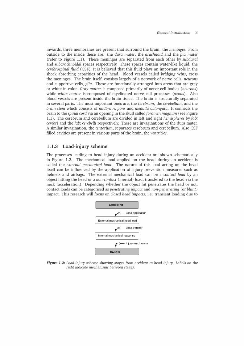
1.1.3 Load-injury scheme
The processes leading to head injury during an accident are shown schematicallyin Figure 1.2. The mechanical load applied on the head during an accident iscalled the external mechanical load. The nature of this load acting on the headitself can be influenced by the application of injury prevention measures such ashelmets and airbags. The external mechanical load can be a contact load by anobject hitting the head or a non-contact (inertial) load, transfered to the head via theneck (acceleration). Depending whether the object hit penetrates the head or not,contact loads can be categorised as penetrating impact and non-penetrating (or blunt)impact. This research will focus on closed head impacts, i.e. transient loading due to
External mechanical head load
Internal mechanical response
Injury mechanism
Load transfer
Load application
ACCIDENT
INJURY
Figure 1.2: Load-injury scheme showing stages from accident to head injury. Labels on theright indicate mechanisms between stages.

4 Chapter 1
non-penetrating impacts or inertial loading. The external mechanical load causes aninternal mechanical response of the various anatomical components of the head whichcan be expressed in local quantities such as stresses and strains. When the internalmechanical response exceeds an injury tolerance level of an anatomical component,injury to this component occurs via an injury mechanism (i.e. the sequence ofphysiological changes leading to injury due to a mechanical stimulus). Different partsof the head may be injured through a variety of different injury mechanisms.This research will focus on traumatic brain injury (TBI). The internal mechanicalresponse of the brain is a key quantity for understanding the transformation of theexternal mechanical load to injury. It originates from the external mechanical loadthat is transfered from the scalp to the brain tissue via the skull and an interfaceconsisting of meninges and CSF. The internal mechanical response is influenced bymagnitude and time duration of the external mechanical load. The magnitude ofthe external mechanical load has to be such that stresses and/or strains associatedwith injury do occur inside the brain tissue. This means that certain tolerance levelshave to be exceeded. The duration of an impact determines the nature of the strainfield in the brain. Short duration impacts are defined here as impacts in which thecharacteristic loading time is on the order of the characteristic time period of thehead system (determined by the eigenfrequencies). They occur when a projectilewith low mass (e.g. a bullet) hits (the protected) head at high velocity. These willalso be called ballistic impacts. The internal mechanical response of the brain thenis dominated by wave propagation. This means that a wave front that consists of alarge stress or strain gradient propagates in the brain tissue. The behaviour of thestrain or stress field at the wave front is important. The propagation of stress wavesinside brain tissue has, since long, been hypothesised to be of importance in theinternal mechanical response [54; 59; 62; 114; 115] but, to this authors knowledge,it has never clearly been pointed out under which circumstances wave propagation islikely to be present in the internal mechanical response. When the head hits a heavyobject with lower velocity, a longer duration impact occurs. The internal mechanicalresponse then is called of structural dynamics type. Wave fronts propagating as suchcannot be distinguished anymore, instead the response will be more of a low gradienttype. At even slower loading conditions a quasi-static response will occur in whichinertia effects can be neglected. However, this type of response is not relevant forimpact conditions.
1.1.4 Head injury criteria
To assess the risk of sustaining a head injury, and to assess the effectiveness ofpotential protection measures, an injury criterion is needed (i.e. a physical parameterwhich correlates well with injury severity of the body part in question [115]). Thefirst extensive quantification of head tolerance to impact is the Wayne State ToleranceCurve (WSTC) [66; 67; 85]. The WSTC shows that, in linear acceleration loading,the risk of brain damage due to non-penetrating impacts is determined by boththe magnitude and the duration of the acceleration pulse. Short duration, highacceleration impacts (2 ms and 400 g respectively) lead to similar injury risk as

General introduction 5
long duration, low acceleration impacts (30 ms and 80 g respectively). The curveis developed using a combination of linear skull fracture data in (embalmed) cadaverheads (short duration impacts), brain concussion data in animal heads (mediumduration impacts) and, non injury producing, low acceleration, volunteer data. Thelater is considered as asymptotic value of the curve for long impact durations. Thevalidity of the curve was confirmed through a series of experiments on subhumanprimates by Ono et al. [116]. The WSTC served as the basis for the injury criterioncurrently used in automotive impact regulations, the Head Injury Criterion (HIC), It isdefined as [155],
HIC =
((t2 � t1)
�1
t2 � t1
Z t2
t1
a(t)dt
�2:5)
max(1.1)
in which a(t) is the resultant translational head acceleration and t1 and t2 the,varying, initial and final times of the interval during which HIC attains a maximumvalue. For regulations the maximum interval t2 � t1 is set to 15 or 36 ms [42]. Forcadaver data in frontal impact, HIC has been shown to be a reasonable discriminatorbetween severe and less severe injury [140]. It also correlates with the risk for cranialfracture in cadavers after impact [124]. However, for impacts in various directions,bad correlation between HIC and injury severity has been found [107]. An importantdrawback of HIC is that head rotation is not taken into account although rotation isdebated to be the primary cause for various types of traumatic brain injury [2; 60; 70].Head injury criteria including head rotation also were proposed but never extensivelyvalidated (e.g. GAMBIT in [108] and HIP in [109]).The injury criteria presented so far predict injury risk from the external mechanicalload on the head, which can be measured directly from a crash dummy head, butdo not take into account the internal mechanical response. Furthermore, they donot discriminate between various types of traumatic brain injury, such as such assubdural hematoma (SDH, disruption of the bridging veins between skull and brain),blood brain barrier breakdown, (BBB, (temporary) breakdown of blood vessels withinthe brain) or diffuse axonal injury (DAI, neural damage involving prolonged loss ofconsciousness).Recent research focuses on so called next-generation injury assessment tools that usecomputational head models. A more detailed injury prediction is obtained using acomputed internal mechanical response resulting from dummy-measured externalmechanical loading [15]. An example of such injury assessment tool is SIMon, asimulated injury monitor, recently proposed by Bandak et al. [15]. It includes a simpleFinite Element model of the head originally developed in [12; 40]. It addresses boththe load transfer from external mechanical load on the head to internal mechanicalresponse and prediction of the risk of injury using tissue level injury tolerances.However, these tolerance levels and the underlying injury mechanisms are not yetwell established and need additional research. The various types of head modelsused in head injury research will be discussed in more detail in next section.

6 Chapter 1
1.1.5 Head models
Head models are often used in approval tests for cars and helmets. Moreoverthey can be used for research on the internal mechanical response and injurymechanisms. In the subsequent section head models used in research will beemphasised. These can be divided in three categories: biological models, physicalmodels and numerical models. For each model category advantages and disadvantagesin terms of mechanical accessibility (to what extent can the internal mechanicalresponse be measured), injury information (does the model provide information onhow injury occurs), and biofidelity (how realistic is the model for modelling thehuman head) will be discussed.
Biological models For the purpose of this study the following four types ofbiological models are distinguished: in-vivo human models, animal models, humancadavers and tissue level models. The first three types of models, the so called wholehead biological models in Figure 1.2, in principle allow the investigation of the internalmechanical response after impact. However, capturing this response is complicateddue to the inaccessibility of the brain in the cranial cavity. The experiments neededto exercise biological models are complicated by precautions needed when workingwith in-vivo models or for keeping in-vitro models fresh. Furthermore, ethical aspectshave to be considered when using a biological model.
In-vivo human models provide maximum biofidelity. However their use is severelylimited since external head loading has to be applied below the injury range [161].Victims in accidents can constitute as a source of in-vivo human data within theinjury range however the external mechanical loading history during such accidentis not available. For this reason the external mechanical load on the head of thevictim is reconstructed using data found on the site of the accident. Subsequently,the internal mechanical response of the head is reconstructed using Finite Elementmodelling. Finally, this response is correlated to the physical injury sustained,visualised using MRI scanning or CT scanning, or to functional injuries, determinedusing cognitive investigation methods. A disadvantage of this method is that theaccuracy of the reconstruction method is low due to many uncertainties encounteredin the reconstruction process of the mechanical response [154].
Animal models enable extension of the external mechanical load into the injuryrange. They are subjected to a well prescribed external mechanical load after whichthe resulting injury is investigated [60; 98; 99; 100; 131]. In this manner arelation between external mechanical load and injury sustained can be obtained. Inearly studies, a qualitative idea of the internal mechanical response was obtainedusing invasive methods such as the cranial window [64; 65; 133]. More recently,the use of the non-invasive MRI tagging method is investigated [43]. Also FiniteElement modelling of the animal head is used to reconstruct the internal response[99; 131; 152]. Exact translation of external mechanical loading from animal data
General introduction 7
to human values is generally impossible due to geometry differences in combinationwith viscoelastic material behaviour of the brain tissue.
Human cadaver models also allow experiments within the injury range. Detailedinformation on the topology of the resulting injuries can be gained from dissectionafter the impact experiments. Some information on the internal mechanicalresponse has been obtained using intracranial pressure measurements [104; 150],intracranial miniature accelerometers [68; 150] or by high speed x-ray markertracking techniques [3]. However, these methods are always invasive. Furthermore itis unknown how postmortem changes influence the mechanical response measured.
Tissue level biological models are living tissue specimens on which mechanicalexperiments are performed [10; 56; 141]. A load is applied on for example anisolated axon and physiological changes in terms of resting potential (depolarization)are determined [56]. Since these models are not exercised in situ (i.e. not inside thehead), they are not suited for prediction of internal mechanical response. However,tissue level injury tolerance levels can be obtained. Apart from potential differencesbetween animal and human tissue characteristics the biofidelity is good.
Physical head models are widely used in the evaluation of protective measures.Most well known are the rigid crash dummy heads and head impactors, used inapproval tests for cars and helmets. The resultant acceleration history of the headis measured and HIC is determined. Head models that include some anatomicalstructures such as the brain, can provide insight into the internal mechanical responseof the head at impact loading. The most simplified method is to model the contentsof the head as lumped masses connected by a damped spring system [162]. Othermodels include deformable brain tissue mimicking materials such as water [73], oil[69] or silicone gel [24; 71; 90; 157]. A more complete overview of physical modelscan be found in Bradshaw et al. [24].It is relatively easy to perform experiments with physical models. Furthermore,models with deformable brain tissue materials can provide validation data fornumerical head models since model properties are well defined. However, differencesbetween the models and the real head prevent quantitative derivation of tissuelevel tolerance levels. Furthermore, it is unknown to which extend the mechanicalbehaviour of the model materials used resembles the real head material behaviour.
Numerical head models commonly used for gaining insight in the internalmechanical response of the head in terms of field parameters such as stresses andstrains, are Finite Element Models (FEM) [11; 36; 37; 40; 72; 94; 126; 127;136; 150; 151; 167; 168; 169]. Numerical models, in principle, can offer a goodbiofidelity when thoroughly validated. However validation of such model is nottrivial and has been a topic of research for many years. When a validated model isestablished it is easy to exercise it in different impact situations. Furthermore thesemodels can also serve as a tool for development of injury prevention measures.

8 Chapter 1
It can be concluded that biological models can provide data on injury sustained dueto some external mechanical load, but provide only minor information on internalmechanical response. This is due to mechanical inaccessibility. FE models andphysical models can be used for obtaining information on the internal mechanicalresponse of brain tissue during an impact but do not allow for prediction of injurywithout prior assumptions about tissue level injury tolerance levels. This means thatfor obtaining insight in the complete pathway between external mechanical load onthe head and TBI a combination of head models and research methods has to beused. An example of this is to use a biological model (animal or cadaver) to providedata on external mechanical load and injury sustained, while the internal responseis reconstructed using numerical or physical models. By comparing the internalresponse obtained from numerical or physical models with histological data on injurylocations in the head of a biological model, insight can be gained in tissue tolerancelevels in terms of stress and strain quantities.Table 1.1 provides an overview of the various research techniques for assessment oftissue tolerance levels, as well as potential stress and strain candidates for predictionof injury. It can be seen that tissue tolerance levels are formulated in virtually allstrain and stress measures. Von Mises stress (VMS) and maximum principal strains(MPS) showed statistical correlation with the occurrence of DAI. MPS also could beassociated with BBB. Pressure has been proposed as an injury criterion especially inrelation with cavitation in the CSF layer due to negative pressures at the contre-coupsite of an impact, but research on the validity of this theory is ongoing [112].Bandak and co-workers developed a cumulative damage strain measure (CDSM). Itis based on the assumption that DAI can be associated with the cumulative volumeof the brain matter experiencing tensile strains over a critical level sometime duringimpact [11]. This tensile strain is represented by the maximum principal strain inthe criterion. A similar measure based on negative pressure, the dilatation damagemeasure (DDM) was proposed in [13]. The application of these criteria implies theuse of a FE model to predict the internal mechanical response.
Table 1.1: Overview of stress/strain quantities associated with injury by various authors. NUM:Numerical study only, no direct correlation, PHY: Physical model study only, TLB:Tissue level biological models, NCA: Animal models combined with numericalmodel, PCA: Physical model combined with animal experiments.
Method Max shear Max. Principal Von Mises Pressurestrain strain stress
NUM [35; 70; 150; 167] [11] [14; 33; 165; 167]PHY [157] [14; 63; 111; 157]TLB [9; 10]�,[141]�
NCA [152] [99]�,[131]+ [99]�,[131; 152]PCA [90; 92]
� Statistical correlation with Diffuse Axonal Injury.+ Statistical correlation with Blood Brain Barrier damage.
General introduction 9
1.2 Finite Element modelling of head impact
In the previous section two stages were distinguished in the pathway from externalmechanical load on the head to brain injury during an accident: the developmentof the internal mechanical response and the development of TBI when this internalmechanical response exceeds tissue level tolerance levels. For this reason it isexpected that insight in the internal mechanical response of the head will lead toimproved understanding of the subsequent injury mechanisms causing certain typesof injury. In this study Finite Element (FE) head modelling will be used for obtaininginsight in the internal mechanical brain response.The use of FE techniques for modelling the head started in the early seventies ofthe last century. FE head models that have been developed from 1971 until 1998are reviewed in literature in [74; 130; 154]. A FE head model basically consistof a set differential equations, the mathematical model, that is solved numericallyusing the Finite Element Method. To create the mathematical model, assumptionsfor the geometry, material behaviour and interface conditions between of the varioussubstructures of the head have to be made. These assumptions present in current FEhead models are reviewed in section 1.2.1. When solving the resulting equations,numerical artefacts are introduced by the FE method used. For this reason thenumerical solution method typically used for these models will be discussed next.Finally the methodology used for validating these complex models is discussed insection 1.2.3.
1.2.1 Mathematical model
Geometry modelling In the first FE models, the skull-brain system was usuallyapproximated by a two or three-dimensional spherical or elliptical fluid filled shell[74]. With the advancement of imaging techniques such as for example ComputedTomography scanning (CT) and Magnetic Resonance Imaging (MRI) an increasingamount of geometrical data has become available in digital format. With theadditional increase of CPU power, this resulted in an increase in geometric complexityin FE models, leading to three-dimensional models with many anatomical details (e.g.[36; 37; 40; 72; 94; 126; 127; 167; 168; 169]). Also, two-dimensional models witheven higher geometrical detail (including temporal lobes and sulci (folds) at brainsurface) have been presented recently [99; 100; 110].
Interface modelling Interfaces exist between the various structures within thecranial cavity. Experiments show that relative motion occurs between the variousbrain parts during impact [3; 132]. This is especially true for the skull andbrain separated by meninges and CSF. Until now, modeling each of these structuresindividually has been infeasible, amongst others because of the problems associatedwith the combination of solid and fluid behaviour in one model. Instead, interfacemechanical behaviour is modelled with a certain degree of suppression of therelative tangential and normal motion of skull and brain. For the tangential motion,descriptions range from no slip via different friction levels to frictionless motion

10 Chapter 1
[37; 99]. Some models use a failure criterion, above which skull and brain canseparate [40; 41]. Other models approximate the interface by a layer of soft, easilydeformable elements [72; 99; 167].
Modelling of brain tissue material behaviour It has been shown experimentallythat brain tissue exhibits non-linear, time dependent material behaviour [4; 44; 120].Regional differences in material behaviour are present [5; 123]. Furthermore, fibrousparts of the brain show anisotropy (brainstem [8], corpus callosum [123]). Thebulkmodulus of brain tissue is about 106 times higher than the shear modulus,indicating nearly incompressible material behaviour [45; 61; 83; 84].Most FE head models to date assume isotropic linear viscoelastic material behaviourfor brain tissue. Regional differences in brain material behaviour have beenincorporated in some models in that grey and white matter were modelled usingdifferent material parameters [3; 99; 167; 168]. Physical model simulationresults show that deformations occurring in the brain exceed the validity rangeof infinitesimal strain theory [24; 141]. Also the nearly incompressible materialbehaviour puts special demands on the constitutive formulations used. It is notobvious whether correct large strain formulations have been used in every FE headmodel reported [113].Application of non-linear material models for modelling impact in 3-D human headFE models has not been found in literature. Application in a 2-D animal FE model wasfound but no comparison with linear models was presented [99; 100]. Low velocityindenter animal experiments have been simulated using a 3-D animal FE model in[98]. The material models used in these studies all were based on hyperelasticStrain Energy Density functions (SED) expressed in strain invariants (Green elasticmaterials). First- [95; 118] and second-order [96; 97] versions of the Mooney-RivlinSED (original by Mooney [101]) are used as well as a first-order Ogden, or Seth[137] SED. Viscoelastic behaviour is modelled by making the constants in the SEDtime dependent using a Prony series, akin to the definition of the stress relaxationfunction in linear viscoelastic theory (quasi-linear theory [53]). As such, the timedependent behaviour is independent of the strain applied.The material parameters for the Ogden variant have been fitted to large deformationshear tests and have been checked for unconfined compression behaviour andreasonable agreement has been found [123]. The Mooney-Rivlin based models arefitted on results of unconfined compression experiments found in [44; 57; 96]. Nocheck on the simple shear behaviour has been reported.
1.2.2 Numerical solution method
The accuracy of the numerical solution depends on spatial and temporal discretisationused by the Finite Element Method. The requirements for the discretisation used aredetermined by the type of internal mechanical response to be expected at certain typesof impact. When a wave propagation response is expected, numerical requirementsto accurately replicate the wave front are higher than when a structural dynamic typeof response is expected. The numerical accuracy is almost never treated in references

General introduction 11
found on head modelling. However, they have been shown to have a significant effecton simulation results in a FE code commonly used for head modelling [113].
1.2.3 Model validation
To assess the quality of FE head models, usually the computed brain response iscompared with experimental results obtained from cadaver experiments. In doing so,two problems are encountered. Firstly the suitability of the data set used for completemodel validation. Apart from post-mortem effects, the suitability of the experimentalresults is influenced by limited spatial resolution and invasive techniques used toobtain quantitative data. This will be illustrated with some examples. Most commonlyused for model validation (e.g. in [37; 72; 128; 168]) are pressure historiesmeasured at four points in the CSF-layer of a cadaver subjected to frontal impactby Nahum et al. [104]. Apart from effects discussed before an other drawback isthat shear effects inside the brain are not represented in the experimental pressuredata used. Al-Bsharat et al. [3] simulated low speed occipital impact and comparedrelative skull-brain displacements with three-dimensional x-ray marker trajectoriesdetermined in a cadaver. Although the primary objective of this study was to gaininsight in the skull-brain interface, this data set also can be used for providing insightin the shear behaviour. Turquier et al. [151] used intra-cranial acceleration as wellas epi-dural and ventricular pressure signals obtained from cadaver experiments in[150]. They found qualitative agreement with experimental data but also foundoscillations in their response which they attributed to numerical artefacts. Thisraises a second limitation of this type of validation methods. Even if these datasetswould contain sufficient information to completely validate a FE model, there is stilla methodological problem in that the identification of the origin of discrepanciesbetween model and experimental results is difficult since errors can be introduced bythe experimental method, mathematical model assumptions or the numerical solutionprocedure.Physical models which include a deformable brain structure can be used as a tool toassess the quality of the numerical solution method separately. Such experimentalmodel can be designed to minimise the number of mathematical modellingassumptions while maximising mechanical accessibility. This can be achieved byusing a known, simplified geometry, materials with known material properties, usingtransparent components for optical measurement techniques, etc. When confidencein the numerical method is gained in this manner, the recommendations obtainedfrom this method can be applied in a complete head model, thus reducing effects ofnumerical artefacts in the solution method. However, references found in literaturewhich compare numerical model results with physical model results, only focus ondetermining the effects of interface modelling at the skull-brain interface and not onnumerical accuracy [34; 55; 149].

12 Chapter 1
1.2.4 Conclusion
It can be concluded that current state of the art head FE models contain detailedgeometrical description of anatomical components inside the head but lack accuratedescriptions of non-linear brain material behaviour and interfaces inside the head.Furthermore it is not obvious to which extent numerical artefacts influence theresponses obtained especially when a wave propagation response is expected. Currentmodel validation methods involve complete biological head models. Although thisprovides maximum biofidelity, the method lacks the capability of distinguishingbetween sources of discrepancies between model and experiment results, e.gexperimental errors, mathematical model assumptions and the numerical solutionprocedure artefacts. Physical models can be a valuable tool to obtain more insight inthe presence of numerical artefacts as they can be designed such as to minimise thenumber of modelling assumptions and maximising mechanical accessibility.
1.3 Scope of study
It has been shown that the development of TBI during an impact on the head consistsof two stages. In the first stage the external mechanical load on the head is transferedinto the head and causes the internal mechanical response of the brain inside thehead. The second stage consists of the development of traumatic brain injury via aninjury mechanism. The present research focuses on the first stage: the determinationof the internal mechanical response of brain tissue. This will be done using FiniteElement models. Important aspects of these models are: geometry, constitutivemodels, interface conditions between of the various intracranial substructures andnumerical accuracy. The focus in this study will be on constitutive modelling of braintissue and on the accuracy of the solution method.
1.3.1 Objectives
The aim of this study is to contribute to the improvement of FE head models usedto predict the mechanical response of the brain during a closed head impact. Morespecifically the objectives are:
� to investigate the accuracy of numerical methods commonly used for predictingbrain response (explicit FEM) in crash impact, especially in relation to wavepropagation
� to develop a constitutive model for describing the nearly incompressible, non-linear viscoelastic behaviour of brain tissue in a Finite Element model,
� to asses the effects of non-linear material behaviour on the internal mechanicalresponse by applying the constitutive model in a 3-D Finite Element model, and
� to discuss the consequences of this research for current state of the art headmodelling.

General introduction 13
It has to be noted that developments on spatial and temporal discretisation methodsused in the Finite Element Method are not a topic of this research.
1.3.2 Strategy
Numerical accuracy As the numerical requirements for predicting a wavepropagation response are higher than for a structural dynamics response, it will beestimated when wave propagation inside brain tissue is likely to occur. This will bedone using small strain linear viscoelastic theory. The accuracy of current explicitFinite Element Models then will be treated in terms of a wave propagation problem.It will be shown that if wave propagation is predicted correctly, lower frequency(structural dynamic) response is also predicted correctly. Accuracy requirementswill be developed using a simple one dimensional wave propagation problem. Thecapability of current head models to predict a wave propagation response accuratelywill be estimated. Recommendations are given on required temporal and spatialdiscretisation needed for accurate modelling of wave propagation.The validity of these recommendations at large strains cannot be tested usinganalytical solutions anymore. For this reason, a simple physical head model isdeveloped that mimics the brain behaviour during a traffic related impact. In thismodel geometry and boundary conditions are known. The material behaviour ofthe brain tissue mimicking material is mechanically characterised. In this manner,uncertainties in the mathematical model are eliminated as much as possible, leavingdifferences between numerical model and experimental results to be caused bynumerical artefacts.
Constitutive modelling The constitutive behaviour of brain tissue is characterisedusing shear experiments in a strain and frequency range representative for trafficrelated impacts. This provides data on the non-linear viscoelastic behaviour of braintissue. This data is used for the development of a constitutive model suitable for largedeformations and rotations. The constitutive model is implemented in an existingexplicit Finite Element code commonly used for crash impact simulations [148]. Theaccuracy of the model in predicting the large strain response of nearly incompressiblematerials such as brain tissue is tested using the simple physical model.
Application The non-linear viscoelastic material model is applied in an existing 3-DFE model of the human head in order to asses the effect of non-linear brain tissuematerial behaviour on the computed response. The quality of the response calculatedwill be discussed using the knowledge on numerical accuracy obtained before.
1.3.3 Outline of the thesis
Chapter 2 contains the investigation on the presence and accurate modelling ofwave propagation inside brain tissue. Chapters 3 and 4 deal with the mechanicalcharacterisation of brain tissue as well as the material for mimicking the brain

14 Chapter 1
tissue in the physical model. First a comparison for small strains (1%) but realisticfrequencies (1-1000 Hz) is presented in Chapter 3. Then the comparison is extendedto large strains (up to 20% and 50% for brain tissue and model material respectively)in Chapter 4. In Chapter 5 a non-linear viscoelastic material model will be developedand brain tissue material parameters will be fitted to the experimental data. Chapter6 contains the experimental and numerical results of the physical model experimentswhich serve for the investigation to numerical artefacts at large strains as well asfor testing the newly developed material model. The material model with non-linearbrain tissue material parameters will be applied in a three-dimensional Finite ElementModel of the head in Chapter 7. Finally the result of this study will be discussed inChapter 8.

Chapter 2
Numerical accuracy: analysis ofwave propagation in blunt head
impact
The numerical accuracy of the explicit finite element method (explicit FEM), commonly used formodelling the internal mechanical response of the human head during impact, is treated in termsof a wave propagation problem. First the conditions for strain waves to propagate inside the headhave been estimated. It was found that, due to the nearly incompressible, viscoelastic nature ofbrain tissue, dilatational (P) waves and distortional (S) waves exist at different frequency ranges.S-waves can be expected during a traffic related impact, with frequencies between 25 and 300 Hz,while P-waves are expected during ballistic impacts with frequency between 10 kHz and 3 MHz.Therefore, wave propagation inside brain tissue should be considered a real possibility and FE headmodels should provide an accurate replication of it. When modelling wave propagation phenomenawith explicit FEM, two types of errors occur: numerical dispersion and spurious reflection. Thefirst error is influenced by the mesh density applied while the latter error is influenced by meshinhomogeneities. An analysis with P-waves yielded the rule of thumb that for modelling wavepropagation correctly, at least 24 elements per maximum wavelength should be used (error instrain rate less than 2.5%). Theory indicates that this rule also holds for S-waves. Considering themesh density used in current state of the art 3-D human FE head models, accurate modelling ofwave propagation is impossible. For modelling S-waves mesh refinement in current explicit FEM isan option. For modelling P-waves changes in spatial discretisation are recommended.
15

16 Chapter 2
2.1 Introduction
As explained in Chapter 1, FE models are an important tool for assessment of theinternal mechanical response. A FE head model basically consist of a set differentialequations, the mathematical model, that is solved numerically using the FiniteElement Method. In this Chapter, numerical artefacts, introduced by the FE methodduring solving of the mathematical model equations, are investigated. Only FEmethods commonly used for head impact modelling (so called explicit FEM) will beconsidered in this Chapter.The internal mechanical response of the head may be either of wave propagationnature or of structural dynamics nature, depending on the type of impact subjectedto the head. The modelling requirements for wave phenomena are higher thanfor modelling a structural dynamics response. For this reason a wave propagationproblem will be used to estimate the accuracy of the explicit FEM.The outline of this Chapter is as follows. First, elementary theory on wavepropagation is presented. It is used to investigate the impact conditions for whichwave propagation inside brain tissue is likely to occur in section 2.3. Section 2.4contains an analytical investigation of numerical errors introduced by the explicitFEM. This theory is checked numerically by simulation of wave propagation in a1-D beam in section 2.5. Section 2.6 contains a discussion on: the likelihood ofwave propagation inside the brain due to impact type, implications for the modellingaccuracy in existing head models and potential improvements. Conclusions are shownin section 2.7.
2.2 Elementary theory on wave propagation
Biological tissues, including brain tissue, behave like viscoelastic solids. It will beassumed that elementary wave theory in semi-infinite, isotropic, linear viscoelasticmedia can be used for the analysis in this Chapter. The theory presented is based on[19].
2.2.1 Elastic wave equation
In absence of body forces the three-dimensional equations of motion in a continuumare given by,
~r � � = �@2~u
@t2(2.1)
where � is the mass density of the material, ~r � � the divergence of the symmetricCauchy stress tensor, t the time, and ~u the displacement vector. The linear strain, ",is defined as,
" =1
2
��~r~u�c
+�~r~u��
(2.2)

Numerical accuracy: analysis of wave propagation in blunt head impact 17
in which superscript c denotes the conjugate of a tensor. Linear elastic materialbehaviour is described by Hooke’s law,
� = �Ltrace(")I + 2�L" (2.3)
in which �L and �L are the Lame parameters for the material. Substitution of Hooke’slaw into equation (2.1) gives the Navier equations for the medium,
(�L + �L) ~r�~r � ~u
�+ �Lr2~u = �
@2~u
@t2(2.4)
in which r2 � ~r � ~r. By applying the vector identity,
r2~u = ~r�~r � ~u
�� ~r�
�~r� ~u
�(2.5)
and introducing both dilatation 4 = ~r � ~u, which represents the change in volume ofthe material, and rotation ~! = 1
2
�~r� ~u
�[76], equation (2.4) can be rewritten as,
(�L + 2�L) ~r4� 2�L~r� ~! = �@2~u
@t2(2.6)
Equation (2.6) is the three-dimensional wave equation for unbounded linear elasticmedia. It describes the propagation of two types of waves through the medium:waves of distortion or S-waves, in which particle motion occurs perpendicular tothe direction of propagation of the wave, and waves of dilatation or P-waves, whichcorrespond with the change of volume.The dilatational wave equation is derived by taking the divergence of equation (2.6),
r24 =1
c2p
@4@t2
(2.7)
with cp =q
�L+2�L� the propagation velocity of the P-wave.
The distortional wave equation is obtained by taking the cross-product of the gradientoperator and equation (2.6),
r2~! =1
c2s
@~!
@t2(2.8)
in which cs =q
�� represents the propagation velocity of the S-wave.
Often, linear elastic material parameters are provided in terms of Young’s modulus Eand Poisson’s ratio �. They are related to the Lame parameters �L and �L by,
�L =�E
(1 + �) (1� 2�)and �L =
E
2 (1 + �)(2.9)
Alternatively, bulk modulus K and shear modulus G can be used.
K = �L +2
3�L and G = �L (2.10)
With these parameters, the expressions for the wave propagation velocities become,
cp =
sK + 4
3G
�and cs =
sG
�(2.11)

18 Chapter 2
2.2.2 Solution for 1-D elastic wave equation
A general solution of the 1-D wave equation for P-waves will be derived usingelementary theory to serve as analytical solution for comparison with the numericalsolution in section 2.5. This theory supposes that the motion due to the wave isprimarily one-dimensional. In a linear elastic material this can be accomplishedby setting Poisson’s ratio � to zero. The Lame parameters then become �L = 0and �L = E
2 . Substituting this in the three-dimensional wave equation (2.6) andaccounting for one-dimensional motion by ~u = u, gives the one-dimensional waveequation,
@2u
@x2� 1
c2@2u
@t2= 0 (2.12)
were c =q
E� is the phase velocity of the one-dimensional wave. Taking the partial
derivative of one-dimensional wave equation (2.12) with respect to x,
@2
@t2
�@u
@x
�= c2
@2
@x2
�@u
@x
�(2.13)
shows that the strain, " = @u=@x, is governed by the same one-dimensional waveequation that governs the displacement. A general solution of this equation was givenby d’Alembert as,
" = f1 (k (x� ct)) + f2 (k (x+ ct)) (2.14)
where f1 and f2 are arbitrary, twice-differentiable functions. k represents the wavenumber, defined as,
k =2�
�=
!
c(2.15)
with �, the wavelength and !, the angular frequency. It can be seen that f1 describesa wave propagating in positive x direction and f2 one propagating in negative xdirection. The boundary conditions applied determine which solution occurs in thereal material. Since we are dealing with a linear relation between stress and strain,the general d’Alembert solution, equation (2.14), can be written as a series of time-harmonic waves,
" = Re
0@Xj
j"j j ei(kjx�!t))1A ; j = 1 to1 (2.16)
in which i denotes the imaginary number and Re(a) the real part of number a.
Wave propagation in a slender elastic beam of infinite length will be used in thischapter for determination of the numerical quality of Finite Element Models. It isassumed that the beam consists of the domain x � 0. It is loaded with a prescribedforce history, F (x = 0; t) at its edge, x = 0. Since there is only one-dimensional

Numerical accuracy: analysis of wave propagation in blunt head impact 19
motion, the cross-area of the beam remains constant (A = A0), so the resulting strainat the beams edge can be written as,
"(x = 0; t) =F (x = 0; t)
EA0(2.17)
Since x � 0 and since the boundary condition is applied at x = 0, the only physicalrealistic wave will be a forward propagating one. The general solution for the strainwave propagating the beam therefore will be of the form,
"(x; t) = f (k (x� ct)) (2.18)
Applying boundary condition (2.17) the analytical solution for the strain historyinside the slender beam becomes,
"(x; t) =F (k (x� ct))
EA0(2.19)
2.2.3 Viscoelastic theory
Linear viscoelastic material behaviour can be included in the linear elastic theory bysimply writing both bulk modulus and shear modulus as complex quantities (denotedwith superscript *), as,
G�(!) = G0(!) + iG00(!) and K�(!) = K 0(!) + iK 00(!) (2.20)
in which G0(!) and K 0(!) are called elastic or storage moduli and, G00(!) and K 00(!)are loss moduli and i =
p�1 the imaginary number. Note that all properties dependon the angular frequency, !. The complex moduli reduce to the real linear elasticmoduli, defined by equation (2.10), when the loss moduli are zero and the storagemoduli are independent of frequency.The complex moduli are used in equation (2.11) to obtain complex phase velocitiesfor P-waves,
c�p(!) =
sK�(!) + 4
3G�(!)
�(2.21)
and for S-waves,
c�s(!) =
sG�(!)
�(2.22)
or more generally,
c�(!) = kc�(!)k ei' (2.23)
in which kc�(!)k is the 2 norm and '(!) the phase angle of the complex phasevelocity. The general solution for a forward propagating time-harmonic displacementwave in a viscoelastic material can be written in complex notation as,
~u = A~dei(k�(!)~x�~p�!t) (2.24)

20 Chapter 2
in which , k�(!) is the complex wave number, ~x the position vector, and ~p and ~d unitvectors in the directions of wave propagation and particle displacement respectively.k�(!) can be obtained by substituting the complex phase velocity, c�(!) in equation(2.15) while assuming that the angular velocity, !, is a real number,
k�(!) =!
kc�(!)k (cos'(!)� isin'(!)) = kre(!) + ikim(!) (2.25)
In this equation, index re and im denote the real and imaginary parts of a complexquantity respectively. Substitution in equation (2.24) yields,
~u = A~de�kim~x�~peikre(~x�~p�kc�k2
cret) (2.26)
Attenuation Equation (2.26) shows that the amplitude of the wave decreases asfunction of the imaginary part of the wave number, kim(!), and the distance traveled~x � ~p. This is called wave attenuation. For this reason, kim(!), is often denoted inliterature as attenuation coefficient, �(!).
Dispersion The effective phase velocity, which we define here as the phase velocityby which a wave with certain frequency actually travels in the material, is given inequation (2.26) by,
ceff (!) =kc�(!)k2cre(!)
(2.27)
Note that ceff (!) is frequency dependent, i.e. components with different frequencieswill travel at different phase velocities. This is called dispersion. For linear elasticmaterial behaviour, ceff reduces to the real, frequency independent, elastic wavevelocity according to equation (2.11).
2.3 Importance of wave phenomena in the humanhead
The extent to which wave phenomena are present in the human head during animpact is estimated using elementary wave theory. Lower and upper frequencybounds for which wave propagation occurs will be estimated using boundaryconditions, posed by geometry, and viscoelastic material damping. Furthermore,waves, traveling inside the head, will reflect at boundaries between the varioussubstructures within the head. As a result P-waves can convert to S-waves and viceversa. This mode conversion can act as a different source for the presence of a certainwave type.
2.3.1 Lower bound of frequency range
As explained in Chapter 1, the dynamic response of the contents of the head is saidto be dominated by wave propagation when the characteristic loading time is on the

Numerical accuracy: analysis of wave propagation in blunt head impact 21
order of the time constants of the system, reflected in the system eigenfrequencies. Alower bound for the frequency range at which waves exist can be found by observingthe largest wavelength, �max, that fits within the head diameter, L, i.e.
�max =c
fmin= L (2.28)
Assuming a head diameter of 0.2 m and applying a typical shear wave velocity of5 m=s [102] provides a typical lower frequency bound of 25 Hz for S-waves. ForP-waves the propagation velocity equals 1550 m=s [45; 83], providing a minimumfrequency of 7750 Hz.
2.3.2 Upper bound of frequency range
Since brain tissue behaves like a viscoelastic solid, waves traveling in the tissue willdisplay frequency dependent attenuation. An upper bound of the frequency range forwave propagation in the head is defined as the frequency at which an incident wavewill be attenuated by 99% after having propagated 0.2 m through the head, i.e. fromone side to the other.
S-waves Values for storage and loss shear modulus do depend significantly onfrequency (see for example [120]). Also there is a large spread between valuesreported by various authors. Values at upper and lower end of the measuredfrequency spectrum found in literature, are used to obtain an impression of theextreme situations of material damping (see Table 2.1). Application in the viscoelasticsolution, equation (2.26), provides the amplitude of the wave as a function offrequency f and distance traveled ~x � ~p. The normalised amplitude of S-waves asfunction of frequency and distance traveled, is shown in Figure 2.1. The attenuationwhen using the Peters et al. data is larger than in the Shuck et al. data. For thisreason, the upper bound for the relevant frequency range for S-waves in the head hasbeen estimated to be 300 Hz using the Shuck et al. data.
P-waves Etoh et al. [45] determined the attenuation coefficient, �, of brain tissuefor frequencies between 0.35 and 5 MHz using ultra sound. Their data was foundto be in range of older data by Goldman and Hueter [61], and could be fitted by thefollowing function,
� = af2 +b
2�f (2.29)
Table 2.1: Material parameters used for estimating the viscous behaviour of brain tissue.
Reference G0 [Pa] G
00 [Pa] Frequency [Hz]Peters et al. [120] 600 150 16
Shuck et al. [134] 1:5 � 105 8:0 � 104 400

22 Chapter 2
The values of the fit parameters a and b were not mentioned in their paper but weredetermined graphically from fit results presented instead; a = �1:7 � 10�12 s2=m andb = 7:1 � 10�5 s=m. This function fits the experimental data well for frequenciesup to 3 MHz approximately. Figure 2.2 shows the normalised amplitude of a P-wave obtained using the fitted attenuation coefficients as function of frequency andpropagation distance. The attenuation at 0.2 m equals 53% at 350 kHz and increasesto 98% at 3 MHz. When assuming equation (2.29) to be valid for frequencies below350 kHz also, it can be seen that the attenuation at 0.2 m is less than 10% forfrequencies up to 50 kHz.
2.3.3 Reflection: mode conversion
In general, two phenomena can be observed when a wave hits a boundary of twomedia with different material properties. First, part of the incident wave will bereflected and another part will be diffracted into the other medium. Second, modeconversion can occur, i.e. a P-wave transforms into an S-wave and vice versa (referto e.g. [1] for more information on mode conversion). In the head however, modeconversion is expected to be irrelevant. This is due to the different frequency rangesat which P- and S-waves can propagate inside a head. When a P-wave would be
0.2
0.4
0.6
0.8
1
0 0.1 0.20
100
200
300
400
Distance traveled [m]
Fre
quen
cy [H
z]
Peters et al. 1997
0.2
0.4
0.6
0.8
1
0 0.1 0.20
100
200
300
400
Distance traveled [m]
Fre
quen
cy [H
z]
Shuck et al. 1970
Figure 2.1: Normalised amplitude of S-waves in brain tissue as a function of frequency andpropagation distance, based on linear viscoelastic theory. Shear moduli taken fromTable 2.1.
0.2
0.4
0.6
0.8
1
0 0.1 0.20
1
2
3
Propagation dist. [m]
Fre
quen
cy [M
Hz]
Figure 2.2: Attenuation behaviour of P-waves according to fitted data by [45]. Normalisedamplitude as function of frequency and propagation distance.

Numerical accuracy: analysis of wave propagation in blunt head impact 23
converted in to an S-wave, its frequency would be that high that the S-wave wouldbe attenuated in very short distance, thus disabling effective propagation. Whena S-wave will be converted in a P-wave, the frequency will be that low that theresulting pressure will more be of a structural dynamical response instead of a wavepropagation response.
2.4 Simulation of wave propagation:theoretical considerations
When simulating elastic wave propagation using the explicit Finite Element Method,both accuracy and numerical stability are important. These phenomena areinfluenced by both the spatial and temporal discretisation used.
2.4.1 Numerical stability
In typical FE codes used for impact modelling, time discretisation is performed usingexplicit time integration methods such as the Central Difference Method (e.g. LS-DYNA3D [86], PAM-CRASH [117], MADYMO [148]). In such explicit time integrationmethod, quantities for the next time increment are predicted from known quantitiesat current and previous moments in time. No iteration is performed during one timeincrement, providing low computational effort per time step. However, small timesteps have to be used because explicit integration methods are only conditionallystable. For the Central Difference Method, the maximum time step �tmax to be usedfor stability is determined by the the Courant number [38], C,
C =c ��tmax
�x� 1 (2.30)
This requirement means that, during one time step, the distance traveled by thefastest wave in the model (c � �tmax) should be smaller than the smallest typicalelement size in the mesh (�x). The stability requirement gives an upper bound forthe time step to be used. If a smaller the time step is taken the time integrationprocedure becomes more accurate.
2.4.2 Numerical accuracy
Two error sources appear when wave propagation is modelled using FEM: numericaldispersion and spurious reflections. Both error sources depend mainly on thespatial discretisation used (element formulation and mesh density). In explicit FEcodes, spatial discretisation is usually achieved by constant strain elements withlinear displacement functions and lumped mass matrices. A three-dimensionalbrick element contains eight integration points when full integration is applied.Computational costs can be reduced by using a reduced integration technique inwhich only one integration point per element is used. Both methods will beconsidered.

24 Chapter 2
Numerical dispersion is the phenomenon that waves of different wavelength travelat different phase velocities due to numerical artefacts. For constant strain elementswith lumped mass matrices, it can be shown analytically that, in a one-dimensionalsituation, the phase velocity in the discrete mesh cFEM is related to the theoreticalphase velocity c via [20],
cFEMc
=sin��x
���x�
(2.31)
This means that the phase velocity in the discrete mesh is dependent on thewavelength � and element size �x. Also it can be seen that there cannot be anywave propagation when �x = �. Since wavelength � is related to its frequency fby the phase velocity c, an upper bound on the frequency in the mesh for which nowaves will be propagated can be found as [17; 20],
fcutoff =c
�x(2.32)
Mullen and Belytschko [103] extended this analysis to two-dimensional FiniteElement semi-discretisations. They considered the two dimensional wave equationwhich is valid for both P-waves and S-waves. Figure 2.3 shows the dispersion cFEM
cin square elements, as a function of the angle between the elements and wavepropagation direction. �. It can be seen that the dispersion increases when �increases from 0 to 45Æ. Moreover, numerical dispersion depends on the elementintegration scheme used, full versus reduced integration. For � = 0, no differencesbetween fully and reduced integrated elements exist and dispersion is governed byequation (2.31). However, when a wave arrives at a certain angle � 6= 0, thedispersive errors in the reduced integrated elements increase stronger than in thefully integrated ones.
Θy
x
0 0.1 0.2 0.3 0.40.2
0.4
0.6
0.8
1
∆x/λ [−]
Cfe
m/C
Full integration
0 0.1 0.2 0.3 0.40.2
0.4
0.6
0.8
1
∆x/λ [−]
Cfe
m/C
Reduced integration
θ = 0θ = 45 o
θ = 0θ = 45 o
Figure 2.3: Numerical dispersion in bilinear quadrilateral elements with lumped mass matrix,as a function of relative mesh density �x
�for various directions � (extreme values
shown) (Figure according to theory in [103]).

Numerical accuracy: analysis of wave propagation in blunt head impact 25
It can be concluded that for constant strain elements with lumped mass matrix,commonly used in explicit FE codes, 18 elements per wavelength should be usedto reduce the dispersion error to less than 1%, independent of incident angle.
Spurious reflection due to mesh non-uniformity In a uniform Finite Elementmesh, elastic waves propagate without reflection. However, due to non-uniformityin the mesh distribution, spurious reflections can occur in the computed solution.Bazant et al. [17] analyzed a compressive wave traveling in a rectangular meshconsisting of two uniform parts with different element sizes (�x1 and �x2 in Figure2.4). Amplitudes of the waves diffracted and reflected at the transition plane betweenthe mesh parts were derived analytically. Influences of element size ratio �x2
�x1, and
number of elements per wavelength of the second mesh part, ��x2
, were determinedand shown in Figure 2.5. In the ideal case there would be no reflection, so theamplitude of the, normalised, diffracted wave would be equal to one. Figure 2.5shows that spurious reflection occurs when a wave passes between two elements ofdifferent sizes. For increasing element size difference this reflection increases. It canalso be seen that this effect is more prominent when wavelength � covers only a few
1
transition plane
∆ x1 2
x∆
Figure 2.4: Rectangular Finite Element Mesh used by Bazant et al. [17]
x∆ 1/x∆ 2 x∆ 1/x∆ 2
x∆ 2 x∆ 2λ/ =2/5 λ/ =2/51.5
1.4
1.3
1.1
0.9
1.0
1.2
1 2 3 50.7 10
0.0
0.1
0.2
0.3
0.4
0.5
1053210.7
Diff
ract
ed a
mpl
itude
Ref
lect
ed a
mpl
itude
1/4
1/3
1/61/10
1/3
1/4
1/6
1/10
Figure 2.5: Amplitude of diffracted wave and reflected wave normalised to the amplitude ofthe incident wave, as function of mesh size ratio �x2
�x1and relative mesh size �
�x2.
(Data taken from [17])

26 Chapter 2
Finite Element sizes �x2. If � > 10�x2 the normalised amplitude of the reflectedwave will be less than 2.5% for all mesh size ratios shown.
2.5 Simulation of wave propagation: numericalresults
The theory presented in previous section is valid for single frequency waves onlyand does not take into account effects of the temporal discretisation. In a realisticloading history, multiple frequencies are present. The resulting wave form thereforewill be a wave envelope consisting of components with various wavelengths. Inthis section, suitable discretisation requirements for realistic input conditions areinvestigated. This has been done by modelling the propagation of one-dimensional P-waves in a slender linear elastic beam in an explicit Finite Element Code (MADYMO),thus taking in to account both temporal and spatial discretisation. The reason formodelling P-waves is to obtain a true one-dimensional problem which is impossiblewhile modelling S-waves.
2.5.1 Analytical solution
For slender beams in which the wavelength is much longer than the beam diameter,one-dimensional elementary wave theory can be used. The beam is loaded at oneedge by a prescribed force history, F (t), resembling a pulse obtained obtained byimpacting a head of a seated cadaver [104]. This pulse is often used for benchmarkinghead models (e.g. [37; 72]). For reasons of simplicity the pulse is approximated by,
F (t) = Fmax sin4(2�f0t)
�Fmax = 6900N 0 � t � 1
2f0
Fmax = 0N t > 12f0
(2.33)
with f0 = 62:5Hz (see Figure 2.6). The analytical solution for the strain wave is
0 2 4 6 80
2
4
6
8
10
Time [ms]
For
ce [k
N]
ApproximationNahum
102
104
10−2
100
Frequency [Hz]
Nor
mal
ised
PS
D
Figure 2.6: Input force history fitted on Nahum pulse [104] (left) and power spectral densitynormalised to maximum frequency contribution (right).

Numerical accuracy: analysis of wave propagation in blunt head impact 27
obtained by substituting F (t) into equation (2.19),
" (x; t) =Fmax
EA0sin4
�2�f0c
(x� ct)
�(2.34)
2.5.2 The numerical model
A slender linear elastic beam has been modelled in MADYMO. The length of the beamwas chosen as 30 m and its square cross-sectional area, A0, was set to 9 � 10�4m2.The material properties of the beam are such that the wave propagation velocity c0approximates the speed of sound in brain tissue (1500 m
s [45; 83]). To obtain a trueone-dimensional wave propagation response, Poisson’s ratio, �, is set to zero. Thematerial parameters are shown in Table 2.2.
Spatial discretisation The beam has been modelled using cubic elements, with oneelement over the cross-section of the beam. As shown in section 2.4, choices of bothspatial and temporal discretisation depend on the wavelength expected in the mesh.In Figure 2.6, the Power Spectral Density of the input force pulse normalised to itsmaximum value is shown. It can be seen that frequencies which contribute with morethan 1 percent to the total power cover a wide frequency range (normalised PSD> 0.01 for 0 � f � 830 Hz). In the absence of a distinct characteristic frequency,the discretisation will be arbitrarily related to the longest wavelength present. It isdetermined by the duration of the force applied and equals, �max = c0
2f0= 12m. Mesh
densities ranging from 12 to 100 elements per maximum wavelength have been used.When changing the mesh density, the initial shape of all elements was kept cubic byadapting the area of the beam edge, A0.
Boundary conditions The impact on the beam has been modelled by a prescribednodal force at the beam edge at x = 0 according to equation (2.33). In order toenable comparison of the strain results, the prescribed load has been scaled to thebeam area, A0, such that the applied stress remains the same for all mesh densities.
Temporal discretisation The maximum time step required for stability isdetermined by the Courant number in equation (2.30). The Courant number iskept at constant value when applying different mesh densities. In the reference
Table 2.2: linear elastic material parameters used for modelling one-dimensional P-wavepropagation in a linear elastic slender beam with MADYMO.
Material parameter ValueE 2.25 GPa
� 0.0 [-]� 1000 kg=m3
c =q
E�
1500 m=s

28 Chapter 2
simulations, a Courant number of 12 was used. Also a Courant number of 0.8475
(the maximum Courant number MADYMO allows) has been used to study the effectof the time discretisation on the accuracy of the solution. The simulation time hasbeen set to 20 ms, which is the theoretical time for the wave to reach to end of thebeam. In this manner no reflection at the end of the beam should occur during thesimulation.
2.5.3 Results
Strain histories obtained with 12 elements per longest wavelength are comparedto the theoretical results at various positions in the beam in Figure 2.7. In theorythe pulse propagates through the beam without any dispersion, i.e its shape remainsthe same. In the numerical solution three types of error arise: the amplitude isoverestimated, the amplitude reduces during propagation, and the shape of the waveenvelope changes. This latter error is characterised by decrease and increase of thestrain gradients at the front and rear of the wave envelope respectively. Furthermoreadditional waves trailing the actual wave envelope occur.The errors will be analysed more quantitatively in terms of maximum absolute strain,strain rate and wave envelope propagation velocity.
Strain and strain rate Figure 2.8 shows the relative error, Erel, in the strainamplitude and maximum strain rate at various points in the beam as function ofmesh density used. The relative error is defined as,
Erel =jSnum:max � Sth;maxj
jSth;maxj (2.35)
in which Snum;max and Sth;max represent maximum values of numerical andtheoretical solutions respectively.The left plot in Figure 2.8 shows the error in the strain amplitude. This error seemsto decrease while the wave travels through the beam. However, this is caused by thefact that the maximum strain is overestimated in the numerical solution. As the wavetravels further the maximum amplitude will become less than the theoretical one and
0 5 10 15 20−4
−3
−2
−1
0
Time [ms]
Str
ain
X 1
000
[−]
5 m 10 m 15 m 20 m
NumericalTheory
Figure 2.7: Numerical time-strain history determined at various positions in the beam.Numerical solution (12 elements/�max, C = 0:5) versus theory.

Numerical accuracy: analysis of wave propagation in blunt head impact 29
the error will increase again. To reduce the relative error in the strain amplitude toless than 1%, mesh densities of approximately 24 elements per maximum wavelengthhave to be used. For coarser meshes the error increases strongly.The relative error in the strain rate (Figure 2.8, right plot) increases while the wavepropagates through the beam. For decreasing element sizes the error decreases.When 50 elements per maximum wavelength are used, the error decreases to lessthan 1%.
Wave propagation velocity Due to numerical dispersion, the shape of the waveenvelope changes, making the determination of a single wave propagation velocityimpossible. For this reason phase velocities are determined at five strain levels,1000�"=-1, -1.5, -2, -2.5, -3, during increasing and decreasing phase of the strain.The mean, maximum and minimum phase velocities in the wave envelope obtainedwith two time step sizes, are shown in Figure 2.9 for increasing mesh density. It canbe seen that increasing the element size provides lower wave propagation velocities,as expected theoretically. For the reference simulation (C = 0:5), the mean dispersionerror becomes larger than 1% when less than 16 elements per maximum wavelength
0 50 1000
1
2
3
4
elements/λmax
[m−1]
|E(ε
)|m
ax [%
]
max.5 m 10 m15 m20 m
0 50 1000
5
10
15
20
elements/λmax
[m−1]
|E(d
ε/dt
)|m
ax [%
]
max.5 m 10 m15 m20 m
Figure 2.8: Relative errors in strain amplitude (left) and maximum strain rate (right) atvarious propagation distances (shown in legend) as function of mesh density used(C = 0:5).
0 50 1000.97
0.98
0.99
1
1.01
Elements/λmax
c FE
M/c
Courant = 0.5
minimummean maximum
0 50 1000.97
0.98
0.99
1
1.01
Elements/λmax
c FE
M/c
Courant = 0.8475
Figure 2.9: Effect of mesh density (in elements per maximum wavelength) and time step usedon dispersion behaviour. Left: reference simulations, C = 0:5, right: maximumtime step, C = 0:8475.

30 Chapter 2
are used. The phase velocity values determined at the wave front, are smaller thanthe ones at the rear of the wave (indicated by the maximum and minimum values inthe plots). This effect is larger for coarser meshes.Comparing the left and right plots in Figure 2.9 shows that the errors obtained at thesmallest time step (C = 0:5) are larger than the ones obtained at the larger time step.So, decreasing the time step size leads to an increasing dispersion error.
2.6 Discussion
Finite Element head models are used to assess the dynamical behaviour of the head.Most 3-D FE head models found in literature are developed using the explicit FiniteElement Method. Linear (visco)elastic material behaviour for the brain tissue isassumed in all cases. For this reason the theory of the previous section can beused to assess if current headmodels are capable of describing wave phenomenacorrectly. First it will be estimated during which type of impacts the presence ofwave propagation in brain tissue is likely. Then numerical requirements for accuratemodelling will be summarised from previous sections. Implications of these findingsfor current state of the art headmodels will be provided next. Finally, some methodsfor improvement will be provided.
2.6.1 Wave propagation during head impact
The conditions for strain waves to propagate inside the head have been estimatedusing linear viscoelastic theory for isotropic material behaviour. A lower bound of therelevant frequency range is obtained by defining that waves can propagate only whenthe wavelength fits inside a typical head measure (0.2 m). The upper bound of therelevant frequency range is defined as the frequency at which an incident wave will beattenuated by 99% after having propagated 0.2 m. It was concluded that dilatational,or P-waves exist in a frequency range between 8 kHz and 3 Mhz. This is consistentwith findings of Young and Morphey [165], who numerically analysed a fluid filledsphere and concluded that impact durations less than 0.1 ms were needed to obtaina wave propagation response instead of a structural dynamic one. Distortional orS-waves exist at frequencies between 25 Hz and 300 Hz. The contribution of modeconversion at reflection at the boundaries of brain substructures is considered to be ofno importance, since the relevant frequency ranges for P- and S-waves are distinctlydifferent.The presence of wave propagation in the head also depends on impact loadingapplied. The analysis of the Power Spectral Density in section 2.5 showed that theupper bound for the frequency in typical. low velocity, traffic related impacts is onthe order of 1 kHz. For this reason P-waves will not be present in such impact butS-waves will. During a non-penetrating ballistic impact, first a direct impact with aduration of approximately 2 to 100 �s [18; 23] will occur. After this, inertia willcause the head to rotate with a typical duration on the order of ms [22]. This meansthat P-waves can be present at the start and S-waves might develop later on. For this
Numerical accuracy: analysis of wave propagation in blunt head impact 31
reason it can be concluded that, from a mechanics point of view, wave propagationinside the head should be considered a real possibility for both low velocity, highmass, traffic related impacts as well as high velocity, low mass, ballistic impacts.
2.6.2 Numerical accuracy
When modelling wave propagation with explicit FEM two types of errors can appear:numerical dispersion and spurious reflection due to mesh inhomogeneities. Althoughonly P-waves were considered in the accuracy analysis, the theory presented in section2.4 is valid for both P- and S-waves. For this reason we assume that for modellingS-waves the same accuracy requirements hold.
Numerical dispersion The wave velocity calculated will always be lower thanthe analytical one due to numerical dispersion. For single frequency waves thiscould be investigated analytically. Taking less elements per wave length increasesnumerical dispersion. When the element size equals the wave length waves arenot propagated anymore (see equation (2.32)). When modelling a realistic input,multiple frequencies are present. Waves with long wavelengths travel faster in themesh than short ones (see Figure 2.3). As a result the strain gradient at the frontof a wave envelope decreases in time while the gradient at the rear of the envelopeincreases. These effects have been quantified numerically using errors in maximumstrain, strain rate and average propagation velocity of a wave envelope propagating ina beam. It was found that the strain rate requirement is the most stringent. When 24elements per maximum wavelength are used, the strain rate error equals 2.5% aftera wave has traveled 1.66 times its maximum wavelength (the length of the beam).The dispersion error (average propagation velocity) and maximum strain error thenare less than 1%. Further increase of the mesh density leads to small improvementsof the accuracy only. For this reason, 24 elements per maximum wavelength will beused as a guideline for accurate modelling of wave propagation.However, some remarks have to be made. First, this value should be seen as alower bound since it is determined for 1-D wave propagation only. The analyticalresults in Figure 2.3 on page 24 show that in the two-dimensional case, where wavesdo not necessarily propagate along the mesh direction, the number of elementsper wavelength should be increased by 40%. Although not investigated here, it isexpected that this effect will be stronger in a three dimensional mesh. However,this effect can be partially made ineffective by accounting for the effect of temporaldiscretisation. The error introduced by the Central Difference time integration schemeused by MADYMO proved to be compensatory with the dispersion error caused bythe spatial discretisation. It can be derived theoretically, that for a Courant numberC = 1 no dispersion will occur when elements with linear displacement interpolationfunctions are used [20]. Since all results presented are valid for C = 0:5, numericaldispersion can be reduced by taking the time step close to the critical time stepdetermined by the Courant number. However, in a realistic mesh, multiple elementsizes are present. This means that the Courant number varies per element. As aresult, the gain in accuracy will vary per element also. Also, choosing the Courant

32 Chapter 2
number close to one may result in instabilities when severe deformations occur. Asolution of this problem it to update the time step during the simulation using theCourant criterion based on the deformed mesh. Finally, it has to be noted that theexact number of elements per maximum wavelength depends on the actual pulseshape used. For this reason the mesh density proposed should be used at reasonablesmooth input signals only.
Spurious reflection due to mesh size inhomogeneities is expected to play a minorrole when the mesh requirements for numerical dispersion are met. A numericalinvestigation in a simple one-dimensional layout showed that the dispersionrequirements are indeed stronger than the ones on mesh homogeneity [26]. Howeverit has to be reminded that only cubic elements were used in that study. The effect ofstrongly deformed or even degenerated elements was not investigated.
2.6.3 Implications for existing head models
As wave propagation in the brain is a real possibility, FE head models should becapable of accurate description of wave propagation. With given constraints suchas temporal and spatial integration techniques currently present in explicit FiniteElement codes, this accuracy is mainly determined by the element size used. Itwas seen that a wave can propagate in a one dimensional FE mesh with reducedintegrated, lumped mass, constant strain elements, when the frequency is lower thanthe cut-off frequency provided in equation (2.32) on Page 24. For obtaining anaccurate solution in a typical traffic related impact, at least 24 elements per maximumwavelength are needed. These facts will be used for estimating the performance ofcurrent FE head models.The element size used in 3-D FE head models ranges from approximately 5 mm to 18mm [36; 37; 40; 72; 77; 128; 167]. Assuming an element size of 5 mm and knowingthat P-waves travel in brain tissue at approximately 1550 m
s [45], provides a cut-offfrequency of 310 kHz while an accurate solution is provided for frequencies up to13 kHz only. S-waves travel at approximately 5 m
s (1-10ms [102]) yielding a cut-
off frequency of 1000 Hz and a maximum frequency for accuracy of 42 Hz. Thesevalues are plotted in Figure 2.10 for comparison with the frequency ranges expectedduring traffic related and ballistic impact. Also, the frequency range for which S- andP-waves are expected inside the head are plotted. These numbers indicate that onlythe lower end of the relevant frequency spectrum can be modelled accurately. This isespecially true since the frequency limits best case values based on one-dimensionaltheory and smallest element size reported. Given current estimations, it can be seenthat the modelling demands for correct modelling of P-waves in a high velocity impactare most stringent. A coarse estimation is that for modelling S-waves, the frequencythat limits the accuracy has to be increased by a factor of 10 while for P-waves this isa factor of 100.

Numerical accuracy: analysis of wave propagation in blunt head impact 33
2.6.4 Methods of improvement
The results presented here hold for explicit FEM which use constant strain elementswith a lumped mass matrix and the Central Difference time integration scheme.A method to prevent spurious wave reflection as well as wave dispersion fromovershadowing the true dynamic response in explicit FE packages is to eliminateall wavelengths which are smaller than the critical wavelength determined using theaccuracy requirement in equation (2.31) or Figure 2.3. This can be done by expandingthe applied load in a Fourier series and delete all frequency terms corresponding towavelengths smaller than the critical one [17]. An other possibility is to adjust themesh size such that the greatest part of the frequency contents of the applied loadcan be modelled correctly.Although it is beyond the scope of this thesis to make alterations to element type andtime integration scheme used, some comments on how to improve the prediction ofwave propagation by using different spatial discretisation methods will be provided.Elements with lumped mass matrices are known to be computationally effective, butunderestimate the wave propagation velocity. Elements with consistent mass matrixtend to overestimate wave velocities. The least dispersion was obtained when ageneralised mass matrix M = 1
2Mconsistent +12Mlumped was used [20]. Elements
with quadratic interpolation functions were found to display negligible numericaldispersion. However, these elements can introduce a significant amount of additionalnoise into the solutions due to the existence of two solutions at each wavelength(refer to [20] for background information).
101
102
103
104
105
106
Impact
Presence
Traffic
S−Waves
Ballistic
P−Waves
Frequency [Hz]
FEM accuracy limit FEM cut−off frequency
Figure 2.10: Capability of modelling wave propagation by current state of the art FE headmodels. Impact: Frequencies expected during various impact types. Presence:Frequencies at which waves can occur inside the head. FEM accuracy limit:maximum frequencies for accurate wave propagation modelling. FEM cut-offfrequency: maximum frequency that can propagate in mesh (equation (2.32)).

34 Chapter 2
2.7 Conclusions
The following conclusions can be drawn from previous discussion.
� Wave propagation inside brain tissue should be considered a real possibility forboth low velocity, high mass, traffic related impacts as well as high velocity, lowmass, ballistic impacts.
� Typically 24 elements per wave length are needed for accurate modelling.
� When decreasing the number of elements per wave length, the predicted wavepropagation velocity decreases. As a result, computed maximum strain valuesand strain rate values will be incorrect
� In current state of the art 3-D human head models the smallest element sizeequals 5 mm, making accurate modelling of wave propagation impossible.
� For modelling S-waves the frequency that limits the accuracy of the modelshould be increased by a factor of 10. Reducing the mesh size of 0.5 mm isa possible solution, especially with the advances in computer hardware.
� For modelling P-waves current explicit FEM the frequency that limits theaccuracy of the model should be increased by a factor of 100. Reducing themesh size is not a realistic option anymore. Instead alternative methods shouldbe pursued such as the use of elements with quadratic displacement functionsor generalised mass matrix.
As developments on spatial and temporal discretisation methods are not a topic ofthis research, it is decided to emphasise shear phenomena in brain tissue for theremainder of this research.

Chapter 3
Comparison of the dynamicbehaviour of brain tissue and
two model materials
This section has been published in the Stapp Car Crash Conference proceedings1. It contains thesmall strain characterisation of porcine brain tissue as well as that of two potential model materialsfor use in the physical head model. Brain measurement data are evaluated against literature data,and a model material has been chosen for use in the physical model in Chapter 6.
1Brands, D.W.A., Bovendeerd, P.H.M., Peters, G.W.M., Paas, M., Bree ,van J. and J.S.H.M. Wismans(1999): “Comparison of the dynamic behaviour of brain tissue and two model materials”, Proceedings ofthe 43th Stapp Car Crash Conference, Paper no. 99sc21, pp. 57-64.
35

36 Chapter 3
Abstract
Linear viscoelastic material parameters of porcine brain tissue and two brainsubstitute materials for use in mechanical head models (edible bone gelatinand dielectric silicone gel) were determined in small deformation, oscillatoryshear experiments. Frequencies to 1000 Hertz could be obtained using theTime/Temperature Superposition principle. Brain tissue material parameters (i.e.dynamic modulus (phase angle) of 500 (10Æ) and 1250 Pa (27Æ) at 0.1 and 260 Hzrespectively) are within the range of data reported in literature. The gelatin behavesmuch stiffer (modulus on the order of 100 kPa) and does not show viscous behaviour.Silicone gel resembles brain tissue at low frequencies but becomes more stiffer andmore viscous at higher frequencies (dynamic modulus (phase angle) 245 Pa (7Æ)and 5100 Pa (56Æ) at 0.1 and 260 Hz respectively). Furthermore, the silicone gelbehaves linearly for strains up to at least 10%, whereas brain tissue exhibits non-linear behaviour for strains larger than 1%.
3.1 Introduction
Mechanical head models are used for head injury assessment and research. Most wellknown are crash dummy heads and head impactors used in approval tests for carsand helmets. Head models that include some anatomical structures such as the brain,can provide insight into the response mechanisms within the head at impact loading,thereby avoiding the technical and ethical problems related to in vivo and in vitroexperiments on animals and humans. Moreover, they can provide validation data fornumerical head models. An important component of such a detailed mechanical headmodel is the model material, mimicking the behaviour of real brain tissue.In this study, linear viscoelastic material parameters of two brain substitute materialswill be presented and compared with those of porcine brain tissue. The substitutematerials are a gelatin mixture used by the North Atlantic Treaty Organisation (NATO)as a tissue mimicking material [105] and transparent silicone gel from Dow Corning(Sylgard 527 A&B dielectric silicone gel), a brain model material used previously inmechanical head models by Viano et al. [157] and Meaney et al. [92]. Both modelmaterials and the porcine brain tissue were subjected to oscillatory shear experimentsup to 16 Hz, on the same apparatus, making one on one comparison possible. Byapplying the Time/Temperature Superposition Principle for both brain tissue andmodel materials, the frequency range could be extended up to 1000 Hz [51].
3.2 Materials and methods
Experimental Setup
Experiments are performed on two rotational viscometers, Rheometrics FluidsSpectrometer II (RFS) and Rheometrics ARES (ARES) [125], using a plate-plate

Comparison of the dynamic behaviour of brain tissue and two model materials 37
configuration. These viscometers are basically the same. The temperature control onthe ARES is more accurate, while the torque transducer of the RFS is more sensitive.Samples are centered between 50-mm diameter flat parallel disks. A prescribedoscillatory strain is applied on the one plate, while the torque is measured on the otherplate that is fixed. The frequency range of the measuring devices is limited by inertialeffects (0.1 to 16 Hz). The strain applied is defined as the plate displacement at theedge of the sample divided by the sample height. This sample height is determinedby adjusting the distance between the plates such that the normal force measuredreaches 0.1 mN . The plate distance then is measured with an accuracy of 1 �m usingthe build-in distance measurement device of the viscometers. When necessary a moistchamber is used to prevent dehydration of the sample.For the oscillatory experiments a sinusoidal strain is imposed on the sample,
(t) = 0 sin(!t) (3.1)
When steady state is reached and strain amplitude 0 is sufficiently small, the shearstress � will also be sinusoidal, but with a phase shift Æ due to the viscous behaviour.
�(t) = Gd 0 sin(!t+ Æ) (3.2)
Both viscoelastic characteristics, phase shift Æ(!; T ) and dynamic modulus Gd(! T ),are functions of the angular frequency ! and temperature T . In principle we areinterested in these parameters at one temperature (e.g., 38ÆC for brain tissue) for afrequency range up to several kHz. However, the frequency range of the viscometeris limited to 16 Hz. To obtain information on the material behaviour at higherfrequencies the Time/Temperature Superposition principle (TTS) can be employed[120]. A set of isothermal characteristics, such as the phase angle, Æ, and dynamicmodulus, Gd, are determined within the measurable frequency range at differenttemperatures. Next, these characteristics are shifted along the logarithmic frequencyaxis to an arbitrarily chosen reference characteristic of this set, to form one smoothcurve: the master curve. This whole curve, then, is valid for the temperature at whichthe reference characteristic is measured (i.e., the reference temperature Tref ). In thismanner, frequencies higher than the maximum allowed test frequency can be assessedby lowering the temperature below the reference temperature. The frequency rangethat can be obtained in this manner thus depends on the temperature range thatis used and on the temperature sensitivity of the material parameters. The TTSprinciple can be applied for linear viscoelastic material behaviour only. Its applicationis valid when indeed a smooth master curve can be obtained from the isothermalcharacteristics2
Materials
Brain tissue Porcine brain tissue was harvested from six-months-old pigs obtainedfrom a local slaughterhouse, immediately following sacrifice by electrical shock.During transportation and preparation, the brain material was wetted with a
2For more details on the applicability of the TTS principle the reader is referred to Ferry (1980) [51].

38 Chapter 3
physiological saline solution to prevent dehydration. Samples were cut using a corkbore. The time span between sacrifice and testing was approximately four hours.The limited sensitivity of the torque transducers requires a certain minimum diameterof the sample. Cylindrical samples of 12-mm diameter were needed to providemeasurement results within the measuring range. Since it proved to be impossibleto obtain a sample of this diameter, consisting purely of white or grey matter, asample was prepared from tissue out of the thalamus of porcine brain. This tissueis located near the center of the brain. Visual inspection showed that this tissueconsists of a homogeneous mixture of grey and white matter. To eliminate scatteringof measurement data by anisotropy, all samples were cut in the same direction withtheir cylinder axis perpendicular to the sagittal plane. The sample heights variedbetween 1 and 2 mm.
Gelatin model material Edible bone gelatin, used within NATO as a tissuemimicking material, was prepared by dissolving gelatin powder in water at 50ÆC.This liquid mixture was cooled down to room temperature to become a solid thatcould be tested. In this paper gelatin was tested in two mass ratios, a 20% solution(1 part gelatin and 4 parts water), as prescribed by the NATO regulation [105] and a4% solution.The 20% gelatin was shaped to cylindrical 10-mm diameter samples of thickness 1 to2 mm. The 4% gelatin proved to be difficult in handling and could not be shaped.For this reason the warm, liquid, gelatin mixture was poured directly between theplates of the viscometer and cooled down in-situ. After cooling down the sampleheight was determined as previously described under EXPERIMENTAL SETUP. Bythis method, 50-mm-diameter samples with a height between 1.5 and 2 mm wereobtained. An advantage of this method is that the maximum plate diameter can beused for measuring, providing better reproducibility of measurements due to absenceof centering inaccuracy.
Silicone gel Silicone dielectric gel from Dow Corning (Sylgard( Dielectric Gel 527A&B) is a brain substitute material previously used in physical head models by Vianoet al. [157] and Meaney et al. [92]. This gel consists of two components thatwere mixed together in a one-to-one ratio. The gel was cured between the platesof the viscometer for four hours at a temperature of 65 ÆC. After cooling it downto room temperature (25ÆC) the height was re-adjusted as to account for possibleshrinkage during curing (see EXPERIMENTAL SETUP). The diameter of the samplesthus became 50 mm and the height was on the order of 0.35 mm.
Experimental protocol
Linear strain regime As explained before, linear viscoelastic theory can be appliedonly for sufficiently small shear strains. The boundaries of this linear regime wereexamined by carrying out oscillatory shear experiments with constant frequency(1.6 Hz) but increasing strain amplitude (0.1 to 10%). The linear range was

Comparison of the dynamic behaviour of brain tissue and two model materials 39
determined using the criterion that the material behaves linearly if the measuredmaterial parameters Gd and Æ are independent of the applied strain amplitude .Different reference temperatures were used for different materials. The propertiesof the brain tissue were determined at 38ÆC, thus resembling the animal’s bodytemperature. The material properties of the gelatin were determined at 10ÆC, whichis its recommended temperature for use [105]. The silicone gel was measured at25ÆC, resembling the laboratory environmental temperature at which it can be usedin a mechanical head model.
Frequency sweep After the determination of the linear regime, experiments werecarried out at increasing frequencies (0.1-16 Hz) with a chosen, constant strainamplitude in the linear range (frequency sweep). In this it was assumed that thischosen strain amplitude lies in linear range for the complete measuring frequencyrange. The experimental results of porcine brain tissue, gelatin and silicone gel arecompared with each other.
Time/Temperature superposition Frequency sweeps at different, constant,temperatures were performed to expand the frequency range using TTS. The mastercurves for the brain tissue were composed of 7 isothermal characteristics determinedat temperatures between 4 and 40ÆC. This temperature range is bounded by thephase transition of water at 0ÆC and the permanent brain damage that can resultdue to, for example, the solidifying of proteins at 41ÆC [58]. The master curve forsilicone gel was composed of 9 isothermal characteristics. Temperatures between -50ÆC and 25ÆC were used. The wide temperature range necessary for the silicone gelcould not be met by the RFS. For this reason, the ARES was used for both materials.Differences in measurement results of both viscometers under the same conditionswere within the experimental spread of one viscometer. For gelatin no master curveswere determined, for reasons that will be explained further on.Finally, it was checked whether the measurements at different temperatures hadinfluenced the material properties of the sample by repeating a test at roomtemperature. Table 3.1 provides an overview of the experimental conditions.
Table 3.1: Overview of experimental conditions. n: number of samples, 4T: temperaturerange, MC: Moist chamber (yes/no), d: sample diameter.
Material n 4T [ÆC] Tref [ÆC] MC d [mm] DevicePorcine brain 4� 4, 40 38 y 12 RFS-ARESGelatine 4% 7 10, 15 10 y 50 RFSGelatine 20% 4 10, 15 10 y 10 RFSSilicone gel 2 -50, 25 25 n 50 RFS-ARES�Each sample taken from a different animal.

40 Chapter 3
3.3 Results
Linear strain regime
The results of the four brain tissue samples are shown in Figure 3.1. For strainamplitudes larger than 1%, the brain tissue was considered to behave non-linearly.All model materials were found to show linear viscoelastic behaviour within the strainrange tested (i.e., up to 10% strain). For this reason, it was decided to use a strainamplitude of 1% for both frequency sweep as well as TTS.
Frequency sweep
In Figure 3.2, the results of the frequency sweep are shown. The dynamic modulusof the porcine brain tissue increases with frequency. It can be seen that the resultsof three samples spread within 30% range of their average, while the result of thefourth sample is significantly higher. Averaged over all samples, the dynamic modulusincreases from 500 Pa at 0.1 Hz to 665 Pa at 10 Hz. The phase angle of brain tissue
10−1
100
101
100
200
300
400
500
Strain [%]
Gd [P
a]
10−1
100
101
0
10
20
30
40
Strain [%]
Pha
se a
ngle
[o ]
Figure 3.1: Dynamic modulus Gd (left) and phase angle Æ (right) of four brain samples,versus strain amplitude at constant frequency f =1.6 Hz, and temperatureTbrain =38ÆC. Results of different samples denoted with different symbols.
10−1
100
101
102
104
106
Frequency [Hz]
Gd [P
a]
10−1
100
101
0
20
40
60
Frequency [Hz]
Pha
se a
ngle
[o ]
Gelatin Silicone gelBrain tissue
Figure 3.2: Dynamic modulus Gd (left) and phase angle Æ (right) versus frequency f atconstant strain amplitude 1%, Tbrain =38ÆC, Tsilicone =25ÆC.
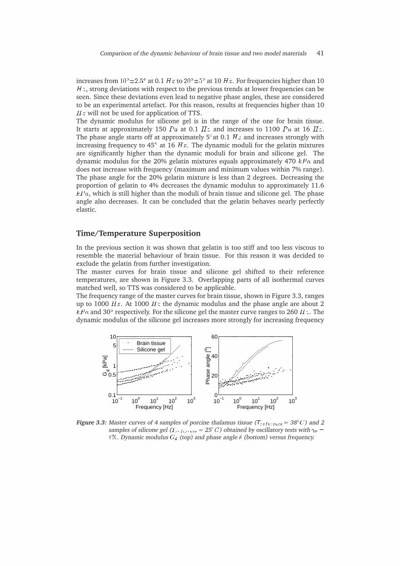
Comparison of the dynamic behaviour of brain tissue and two model materials 41
increases from 10Æ�2:5Æ at 0.1Hz to 20Æ�5Æ at 10 Hz. For frequencies higher than 10Hz, strong deviations with respect to the previous trends at lower frequencies can beseen. Since these deviations even lead to negative phase angles, these are consideredto be an experimental artefact. For this reason, results at frequencies higher than 10Hz will not be used for application of TTS.The dynamic modulus for silicone gel is in the range of the one for brain tissue.It starts at approximately 150 Pa at 0.1 Hz and increases to 1100 Pa at 16 Hz.The phase angle starts off at approximately 5Æat 0.1 Hz and increases strongly withincreasing frequency to 45Æ at 16 Hz. The dynamic moduli for the gelatin mixturesare significantly higher than the dynamic moduli for brain and silicone gel. Thedynamic modulus for the 20% gelatin mixtures equals approximately 470 kPa anddoes not increase with frequency (maximum and minimum values within 7% range).The phase angle for the 20% gelatin mixture is less than 2 degrees. Decreasing theproportion of gelatin to 4% decreases the dynamic modulus to approximately 11.6kPa, which is still higher than the moduli of brain tissue and silicone gel. The phaseangle also decreases. It can be concluded that the gelatin behaves nearly perfectlyelastic.
Time/Temperature Superposition
In the previous section it was shown that gelatin is too stiff and too less viscous toresemble the material behaviour of brain tissue. For this reason it was decided toexclude the gelatin from further investigation.The master curves for brain tissue and silicone gel shifted to their referencetemperatures, are shown in Figure 3.3. Overlapping parts of all isothermal curvesmatched well, so TTS was considered to be applicable.The frequency range of the master curves for brain tissue, shown in Figure 3.3, rangesup to 1000 Hz. At 1000 Hz the dynamic modulus and the phase angle are about 2kPa and 30Æ respectively. For the silicone gel the master curve ranges to 260 Hz. Thedynamic modulus of the silicone gel increases more strongly for increasing frequency
10−1
100
101
102
103
0.1
0.5
1
5
10
Frequency [Hz]
Gd [k
Pa]
Brain tissueSilicone gel
10−1
100
101
102
103
0
20
40
60
Frequency [Hz]
Pha
se a
ngle
[o ]
Figure 3.3: Master curves of 4 samples of porcine thalamus tissue (Treference= 38ÆC) and 2samples of silicone gel (Treference= 25ÆC) obtained by oscillatory tests with 0 =1%. Dynamic modulus Gd (top) and phase angle Æ (bottom) versus frequency.

42 Chapter 3
than the one of brain tissue. At 260 Hz it reaches 5100 Pa whereas the averagedynamic modulus for brain tissue equals 1250 Pa. The phase angle for the siliconegel also increases more progressively. At 260 Hz for example, the phase angle for thesilicone gel reaches 56Æ whereas the one for brain tissue equals approximately 27Æ.The re-tests of silicone gel and brain tissue at their reference temperatures showedthat the temperature changes did not permanently alter the material properties.
3.4 Discussion
Mechanical head models that include some anatomical structures, such as the brain,can be used for head injury assessment, for gaining insight into the responsemechanisms within the head at impact loading or for validation purposes fornumerical head models. An important component of such a model is the materialthat mimics the dynamical behaviour of brain tissue.In this study, two brain mimicking materials and porcine brain tissue were subjectedto small strain, oscillatory shear experiments. It was shown that both model materialsbehave linear viscoelastic for strains up to at least 10% while brain tissue behaveslinearly to only 1%. In the linear strain range, the Time/Temperature Superpositionprinciple could be applied for capturing the high frequency behaviour of the materials.
Brain Tissue
Master curves that span a frequency range to 1000 Hz could be obtained. Peterset al., who investigated the validity of the TTS principle on white matter tissue ofcalf brains, obtained a frequency range to 1 MHz, by measuring between 6 and38ÆC [120]. Apart from different animal origin, no explanation for the differentfrequency range can be provided. These findings on the applicability of the principleare in contrast to findings of Arbogast et al. [14] who could not find any temperaturedependency of the material behaviour of brain tissue within the temperature rangementioned above.For the brain tissue both the dynamic modulus and the phase angle show anincreasing tendency for increasing frequencies. Our results are within the range ofthe data reported in literature, shown in Figure 3.4. These are presented in termsof elastic (or storage) modulus G
0
and viscous (or loss) modulus G00
. They can beobtained from the dynamic modulus Gd and phase angle Æ using [51],
G0
= Gd cos(Æ) (3.3)
and
G00
= Gd sin(Æ) (3.4)
For reasons of clarity, data by Shuck and co-workers, who performed materialcharacterisation on human cerebral brain tissue [135; 134], are not included in Figure3.4. In a frequency range of 5 to 350 Hz, they found a storage modulus rangingfrom 7.6 kPa to 33.9 kPa and a loss modulus ranging from 2.8 kPa to 81.4 kPa

Comparison of the dynamic behaviour of brain tissue and two model materials 43
( 0=1.3%). These values are significantly higher than the ones shown in Figure 3.4.The reason for this is unknown, but differences that are expected to influence thematerial parameters, might exist in post-mortem time, amplitude of applied strainand different donors.
Model Materials
The applicability of the model materials in a mechanical head model is predominantlydetermined by the mimicking qualities of the model materials, but also by theirexperimental manageability. The latter includes factors such as aging, temperaturesensitivity and ease of preparation, which are important in every day laboratorypractice. Both considerations will be discussed.For the Sylgard 527 A&B silicone gel a frequency range up to 260 Hz could beobtained by applying TTS in the chosen temperature range of 25 to -50ÆC. It isbelieved that the frequency range can be expanded to higher frequencies, withoutany problems, by measuring at temperatures below -50ÆC.Our results correspond well with the findings of Arbogast et al. [6]. They presentedthe dynamic shear modulus of the same silicone gel for testing their high frequencyshear device. Unfortunately they did not report the phase angle so this could not becompared with our data.The dynamic modulus of silicone gel equals that of brain tissue in a range up to10 Hz. For higher frequencies, up to 260 Hz, the silicone gel becomes stiffer thanbrain tissue. Thus, when applied in a head model at room temperature, strains in thesilicone gel are expected to be lower than in real brain tissue, for those frequencies.Moreover, these high frequency strains will be damped stronger in the silicone gelthan in brain tissue, since the phase angle and hence the loss modulus, of the gel ishigher than that of brain tissue.The experimental manageability of the silicone gel proved to be good. The effect of
10−1
100
101
102
103
102
103
104
12
3 4
5
6
Frequency [Hz]
G’ [
Pa]
Literature dataBrain tissue Silicone gel
10−1
100
101
102
103
101
102
103
104
1,2 34
5
6
Frequency [Hz]
G’’
[Pa]
Figure 3.4: Storage modulus G0
(left) and loss modulus G00
(right) of measured results (braintissue (n=4) and silicone gel (n=2)), and literature data (numbered): 1. humanwhite matter [50], 2. human cerebrum [91], 3. porcine brainstem ( 0=2.5%)[5], 4. porcine cerebrum ( 0=2.5%) [142], 5. calf cerebrum ( 0=1.0%) [120], 6.porcine cerebrum ( 0=2.5%) [143].

44 Chapter 3
material aging is tested by repeating a frequency sweep test, at room temperature,after the material had been in the measuring device for three days at 25ÆC. Thedynamic modulus showed an increase of approximately 10% over the completefrequency range. The phase angle showed a decrease of 2.5 degrees. Repeating theexperiment one day after this, did not reveal additional differences. For this reason itcan be concluded that the influence of material aging is low.The dynamic modulus of the gelatin model material was decades higher than themodulus of brain tissue (a factor of 50 for the 4% gelatin solution and a factor of 2000for the 20% solution). The phase angle remained almost zero (0-2Æ). Both quantitiesdid not depend on frequency. This indicates that, within the frequency range tested(0.1-16 Hz), the gelatin behaves as a nearly perfect elastic solid that is too stifffor mimicking brain tissue. In theory, the stiffness of the gelatin can be loweredby using lower percentage mixtures than the 4% mixture. However, in practice thisis not possible because of the high damage sensitivity of the material, causing it tobreak up at very low strains. Furthermore, the material behaviour of the gelatinwas very sensitive to aging (parameters change with in hours after preparation) andmechanical failure. For these reasons it can be concluded that gelatin is not suitableas a model material for brain tissue.
Accuracy analysisThe accuracy of the measurement is determined by the accuracy with which the shearcan be applied on the oscillating plate, and the measuring accuracy of torque on thefixed plate. The rotation of the plates can be applied with discrete steps of 5 � 10�6rad [125]. With the diameters and thickness’ used, the relative discretisation error inthe applied shear becomes 4% of the shear strain amplitude for the silicone gel. Forbrain tissue this is 0.15%. The torque can be measured with a relative error of 0.16%[125]. In translating the measured torque into the dynamic modulus, this relativeerror has to be increased with relative errors in the sample height, the applied strainand four times the relative error in the sample diameter [164]. In this manner thetotal relative error in the dynamic modulus was estimated to be 20% for the braintissue and 5% for the silicone gel measurements.In the experiments, the assumed pure shear deformation requires that the sample isin an stress-free state before loading. Indeed the samples are stress-free, immediatelyafter they are mounted in between the plates (neglecting earth gravity). However,since they stick to the plates, depending on possible shrinkage during cooling downand/or curing, the stress-free state might be lost. By adjusting the plate distancebefore each measurement such that the normal force on the (cured) sample is closeto zero, we tried to restore the stress-free state as much as possible. Finally, duringcuring of the gels, and by adhesion to the plates, the molecular structure, and thusthe mechanical behaviour, of the gel near the plates might differ from that in thebulk material. As a consequence the measured material parameters would depend onsample thickness. A test using silicone gel with a sample thickness of 0.9 mm revealedthat the difference with the 0.35-mm results presented in Figure 3.2, is smaller thanthe spread between the 0.35-mm results themselves. Thus the measured propertiesare believed to be bulk properties.

Comparison of the dynamic behaviour of brain tissue and two model materials 45
Limitations of current work
For determining the material behaviour of a model material to be used in amechanical head model under real impact conditions, the material has to beinvestigated at finite strains and high frequencies. Typical frequencies are on the orderof 1000 Hz, whereas studies on isolated axons indicate strains of about 15% to beresponsible for injury [141]. In this paper the small strain behaviour was determinedin the complete relevant frequency range using the Time/Temperature superpositiontheory. For determination of the large strain behaviour the TTS theory is not valid.Even if linear viscoelastic parameters, such as Gd and Æ, are obtained from oscillatorystrain measurements outside the linear range, they have no meaning, since the basicassumption of these experiments, that a sinusoidal strain input leads to a sinusoidalstress output, has been violated. For this reason, material properties in the 1% rangecannot be extended into the 15% range, relevant for injury. Characterisation of thematerials at large strains requires additional test methods such as stress or strainrelaxation experiments. This will be subject of future work (Chapter 4).Finally, this study is limited in that reasonable large brain samples had to be usedwhich did not exist of white or grey matter only. For this reason, the reported materialproperties are to be considered as average properties of grey and white matter. Alsoeffects of anisotropy, resulting from fibre structure, were averaged in this way.
3.5 Conclusions
It can be concluded that 4% and 20% edible bone gelatin mixtures are not suitablefor application as a brain tissue model material in a mechanical head model. Thedynamic modulus of Dow Corning Sylgard 527 A&B silicone dielectric gel is similar tothat of porcine thalamus tissue for strains up to 1% at frequencies up to approximately10 Hz. For higher strains brain tissue behaves non-linear while the silicone gelbehaves linear for strains up to at least 10%. Above 10 Hz the dynamic modulus ofthe silicone gel increases much stronger with frequency than the one of brain tissue.At 1% strain, the phase angle of silicone gel is similar to that of brain tissue only upto 1 Hz. Above 1 Hz it increases more with frequency than that of brain tissue. Thus,silicone gel may be used in mechanical head models to obtain a qualitative impressionof the behaviour of the brain tissue during accident conditions but strain levels in thegel will differ from those in the real brain.
3.6 Acknowledgments
The authors would like to acknowledge TNO Prins Maurits Laboratory and Ford MotorCompany for their financial support of this research, N. Plasmans and R. Bours forconducting part of the experiments and B. de Wit of slaughterhouse ’de Wit GeldropBV’, for providing the porcine brain tissue.

46 Chapter 3

Chapter 4
Large shear strain dynamicbehaviour of brain tissue and
silicone gel model material
This chapter contains a paper presented at the Stapp Car Crash Conference in Atlanta, GA, USA.November 20001 It is a continuation the material experiments presented in Chapter 3 in that themechanical characterisation of brain tissue as well as the silicone gel material model for largeshear strains is concerned. These results will be used for determination of a material model andmaterial parameters in the following chapters.
1Brands, D.W.A., Bovendeerd, P.H.M., Peters, G.W.M and J.S.H.M. Wismans (2000): “The large straindynamic behaviour of in-vitro porcine brain tissue and a silicone gel model material”, The Stapp Journal,44, pp. 249-260.
47

48 Chapter 4
Abstract
The large strain dynamic behaviour of brain tissue and silicone gel, a brain substitutematerial used in mechanical head models, was compared. The non-linear shear strainbehaviour was characterised using stress relaxation experiments. Brain tissue showedsignificant shear softening for strains above 1% (approximately 30% softening forshear strains up to 20%) while the time relaxation behaviour was nearly strainindependent. Silicone gel behaved as a linear viscoelastic solid for all strains tested(up to 50%) and frequencies up to 461 Hz. As a result, the large strain timedependent behaviour of both materials could be derived for frequencies up to 1000Hz from small strain oscillatory experiments and application of Time TemperatureSuperpositioning. It was concluded that silicone gel material parameters are in thesame range as those of brain tissue. Nevertheless the brain tissue response will notbe captured exactly due to increased viscous damping at high frequencies and theabsence of shear softening in the silicone gel. For trend studies and benchmarking ofnumerical models the gel can be a good model material.
4.1 Introduction
Mechanical head models that include anatomical structures such as the brain, canprovide insight into the response mechanisms within the head at impact loading.Moreover, they can provide validation data for numerical head models. An importantcomponent of such detailed mechanical head model is the model material, mimickingthe behaviour of real brain tissue in the relevant mechanical range. This rangecomprises strains up to 20%, the strain level associated with injury [141], andfrequencies up to 1000 Hz, a frequency typical for traffic related impacts.A model material previously used for mimicking the behaviour of brain tissuein physical head models is Dow Corning Sylgard 527 A&B dielectric silicone gel[71; 92; 157]. In a previous study we compared the small strain dynamic behaviourof the model material with that of porcine brain tissue [27] and with the small strainbrain tissue results by other authors [5; 50; 91; 120; 142; 143]. It was concludedthat for strains up to 1%, the dynamic behaviour of silicone gel resembles that ofbrain tissue for frequencies up to 260 Hz.In this study, oscillatory shear experiments and stress relaxation experiments havebeen performed at finite strain levels on both silicone gel and porcine brain tissue,completing the material characterisation in the full relevant dynamic range.
4.2 Materials and methods
Experimental setup
Simple shear experiments have been performed on a rotational viscometer(Rheometrics ARES [125]). Samples were placed between 25-mm diameter flatparallel disks. A prescribed rotation was applied on the one plate, while the torque, T,

Large shear strain dynamic behaviour of brain tissue and silicone gel model material 49
was measured on the other plate that was fixed. For determining the sample height,the distance between the plates was lowered until the normal force measured reached0.1mN . The plate distance was then measured with an accuracy of 1 �m using abuild-in measurement device of the viscometer. Correct temperature conditions wereobtained by controlled air temperature. Dehydration of the brain tissue samples wasprevented by controlling humidity using a custom build moist chamber. To preventslip between the brain tissue samples and the plates two methods of sample fixationwere investigated. First a cyanoacrylate adhesive (Sicomet 85, Henkel, Germany) hasbeen used to fixate the samples to the plates and second the coefficient of friction ofthe plates has been increased by fixing waterproof sandpaper (P220) to the platesusing two-sided adhesive tape.
Data acquisition
If we assume that there is no material displacement perpendicular to the platesurfaces, the strain in the sample can be written as a function of time t and radius ras,
(r; t) =�(t)r
H=
R(t)r
R; 0 < r < R (4.1)
were � represents plate rotation, H the sample height, R(t) the strain at the sampleedge and R the sample radius. The total transient torque can be written as a functionof the strain at the sample edge as,
T (t; R) = 2�
Z R
0
�(r; t)r2dr (4.2)
For linear strain independent material behaviour, the integral can be solved exactly.By introduction of the shear modulus G(t) = �(r; t)= (r; t), the modulus, Ga(t), candetermined as a function of total transient torque and the strain at the plates edge,
Ga(t) =2T (t; R(t))
�R3 R(t)(4.3)
This modulus, which is obtained directly from the viscometer, represents the truematerial parameter, G(t), for strains within the linear regime of the material only. Forstrains outside the linear range, Ga(t) denotes an apparent modulus that representssome average modulus over the strain range present in the material.All moduli and strains, presented in this paper, are apparent moduli, defined byequation (4.3), and strains at the sample edge unless stated otherwise.
Sample preparation
Brain Tissue Porcine brain tissue was harvested from six-months-old pigs obtainedfrom a local slaughterhouse, immediately following sacrifice by electrical shock.During transportation, complete hemispheres were submerged in a physiological

50 Chapter 4
saline solution to prevent dehydration. Sagittal slices were cut using a standardrotating-disk meat slicer (Bizerba GmbH & Co., Balingen, Germany). From theseslices, 24-mm diameter cylindrical samples were cut using a cork bore. Samples wereprepared from tissue located near the centre of the brain (thalamus region). Visualinspection showed that this tissue consists of a mixture of grey and white matterparts. To eliminate scattering of measurement data by anisotropy, all samples werecut in the same direction with their cylinder axis perpendicular to the sagittal plane.The sample heights varied between 2.3 and 3.6 mm. The time span between sacrificeand end of testing was approximately four hours. All samples were kept refrigeratedat 4ÆC and submerged in a physiological saline solution until the actual experimentstarted.
Silicone gel Silicone dielectric gel from Dow Corning (Sylgard Dielectric Gel 527A&B) is a brain substitute material previously used in physical head models [71; 92;157]. This gel consists of two components that were mixed together in a one-to-oneratio. The gel was cured between the plates of the viscometer for four hours at atemperature of 65ÆC. After cooling it down to room temperature (25ÆC) the heightwas re-adjusted as to account for possible shrinkage during curing (see section 4.2).The diameter of the samples thus became 25 mm and the height was on the order of1.3 mm.
Loading conditions
Two types of loading conditions have been used: oscillatory strain for characterisingthe linear behaviour of the materials and step strain with subsequent stress relaxationfor the non-linear behaviour.
Oscillatory strain During the oscillatory experiments a sinusoidal strain is imposedon the sample,
(t) = 0 sin(!t) (4.4)
When steady state is reached and strain amplitude 0 is sufficiently small, the shearstress � will also be sinusoidal, but with a phase shift Æ due to the viscous behaviour,
�(t) = Gd 0 sin(!t+ Æ) (4.5)
Both viscoelastic characteristics, phase shift, Æ(!; t), and dynamic modulus, Gd(!; T ),are functions of the angular frequency, !, and temperature, T . To obtain informationon the material behaviour at higher frequencies than the maximum frequency ofthe viscometer, 16 Hz, the Time/Temperature Superposition principle (TTS) can beemployed [27; 120]. A set of isothermal characteristics, such as the phase angle Æand dynamic modulus Gd, was determined within the, viscometer-limited, frequencyrange at different temperatures, !T . Next, the phase angle characteristic was shiftedalong the logarithmic frequency axis to an arbitrarily chosen reference characteristic
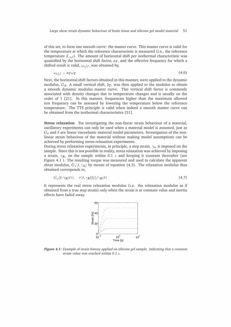
Large shear strain dynamic behaviour of brain tissue and silicone gel model material 51
of this set, to form one smooth curve: the master curve. This master curve is valid forthe temperature at which the reference characteristic is measured (i.e., the referencetemperature Tref ). The amount of horizontal shift per isothermal characteristic wasquantified by the horizontal shift factor, aT , and the effective frequency for which ashifted result is valid, !eff , was obtained by,
!eff = aT!T (4.6)
Next, the horizontal shift factors obtained in this manner, were applied to the dynamicmodulus, Gd. A small vertical shift, bT , was then applied to the modulus to obtaina smooth dynamic modulus master curve. This vertical shift factor is commonlyassociated with density changes due to temperature changes and is usually on theorder of 1 [21]. In this manner, frequencies higher than the maximum allowedtest frequency can be assessed by lowering the temperature below the referencetemperature. The TTS principle is valid when indeed a smooth master curve canbe obtained from the isothermal characteristics [51].
Stress relaxation For investigating the non-linear strain behaviour of a material,oscillatory experiments can only be used when a material model is assumed, just asGd and Æ are linear viscoelastic material model parameters. Investigation of the non-linear strain behaviour of the material without making model assumptions can beachieved by performing stress-relaxation experiments.During stress relaxation experiments, in principle, a step strain, 0, is imposed on thesample. Since this is not possible in reality, stress relaxation was achieved by imposinga strain, R, on the sample within 0.1 s and keeping it constant thereafter (seeFigure 4.1 ). The resulting torque was measured and used to calculate the apparentshear modulus, Ga(t; R) by means of equation (4.3). The relaxation modulus thusobtained corresponds to,
Ga(t; R(t)) = �(t; R(t))= R(t) (4.7)
It represents the real stress relaxation modulus (i.e. the relaxation modulus as ifobtained from a true step strain) only when the strain is at constant value and inertiaeffects have faded away.
10−2
100
102
0
20
40
60
Time [s]
Str
ain
[%]
Figure 4.1: Example of strain history applied on silicone gel sample. indicating that a constantstrain value was reached within 0.1 s.

52 Chapter 4
During the brain tissue experiments it was observed that the relaxation curves fordifferent strain values have a tendency to be parallel. This suggests that, the stressrelaxation modulus can be separated into a strain and a time dependent part,
Ga(t; R) = ha( R)G(t) (4.8)
In this equation the time dependent behaviour, which is represented by G(t), equalsthe linear viscoelastic modulus (which does not depend on strain). ha( R) equals thedamping function determined from the apparent modulus, Ga [87]. The dampingfunction thus quantifies the effect of the strain applied on the shear modulus.When time strain factorisation can be carried out, the material characterisation willbe simplified considerably, since the time dependent behaviour can be obtained forhigh frequencies using the linear oscillatory experimental results. The validity of thistime strain factorisation for brain tissue has been investigated by applying equation(4.8) on the experimental data. For each sample, a scaling function, H(t; R;
refR ),
was defined as,
H(t; R; refR ) =
Ga(t; R)
Ga(t; refR )
(4.9)
If factorisation is valid, the scaling function H(t; R; refR ) will be independent of time
and correspond to the damping function ha( R) when refR is chosen in the linearrange of the material. The scaling function, H(t; R;
refR ), was time-averaged to
�H( R; refR ), and the large strain relaxation moduli, Ga(t; R) then were normalised
to refR using,
Gnorm(t; refR ) =Ga(t; R)
�H( R; refR )
(4.10)
Experimental protocol
Linear strain regime: Oscillatory strain Silicone gel has been shown to behavelinear for strains up to at least 10% at 16 Hz [27]. In this paper the behaviourof the silicone gel has been investigated up to 50% strain and higher frequencies.First, isothermal measurements at constant strain amplitudes of 1% and 20% butincreasing frequencies (0.1 Hz to 32 Hz) were performed at temperatures rangingfrom 25 to -60ÆC (Dynamic Frequency Sweeps, DFS). Master curves were createdfrom the isothermal DFS results using Time Temperature Superpositioning and shift-factors were determined. Next, oscillatory experiments with constant frequency, 16Hz, but increasing strain amplitudes, up to 50% (Dynamic Strain Sweeps, DSS) wereperformed at 24, -40, -50 and -60ÆC. At each temperature, the linear range of thematerial was determined by checking for which strain values the material parameterswere strain independent. Possible permanent effects of these low temperatures on thematerial properties were checked by repeating a measurement at 24ÆC after the lowtemperature measurements were completed. Effective frequencies for the DSS results

Large shear strain dynamic behaviour of brain tissue and silicone gel model material 53
were obtained by using the horizontal shift-factors obtained from the TTS results, andf=16 Hz in equation (4.6).Oscillatory strain experiments on brain tissue were performed to study the effects ofthe different adhesion methods on brain tissue by comparing the results obtained withadhesion methods with those obtained without adhesive methods in our previousstudy [27]. For brain tissue it has been shown that the linear range is on the order of1% strain [27]. For this reason all master curves were constructed from isothermalcharacteristics at 1% strain and frequencies up to 16 Hz. Temperatures between 4ÆCand 38ÆC have been used. Low temperature measurements have been performed firstto minimise the effect of sample ageing due to autolytic processes in the brain tissue.
Non-linear strain regime: Stress-relaxation Strain values ranging from 5% to20% were applied on 4 samples of brain tissue and the apparent modulus wasmeasured during 100 s. The temperature used equals 38ÆC. Two samples of siliconegel were tested at 24ÆC and at 10, 30 and 50% strain values to provide resultsfor comparison with those of brain tissue. By testing two samples an indication ofreproducibility of the measurement could be obtained. Given the ramp shape of theprescribed strain in Figure 4.1, it has been assumed that the measured shear modulusequals the stress relaxation modulus due to a step response for t > 0.1 s. An overviewof all experimental conditions is provided in Table 4.1.
Time-strain factorisation To compare the relaxation behaviour of the varioussamples more quantitatively, time dependent and strain depend behaviour wereobserved separately. First, scaling function, H(t; R;
refR ), was determined from the
stress relaxation results using equation (4.9), and choosing refR = 5% (n=3) and6% (n=1). The value of H was evaluated for t = 0.1 to 9.6 s with time intervalsof 0.5 s. Then these values were time averaged, as to obtain damping functionvalues, �H( R;
refR ), from which the normalised relaxation moduli, Gnorm(t), were
determined using equation (4.10).
Table 4.1: Overview of experimental conditions. n: number of samples, �T temperaturerange, MC: Moist camber (yes/no), d sample diameter, � : strain range
Material Measurement n �T Tref MC d �
type [-] [ÆC] [ÆC] [mm] [%]Silicone gel DSS 1 -60;24 24 n 25 1;50
DFS+TTS 3 -60;24 24 n 25 1;50SR 2 24 24 n 25 10&50
Brain tissue DFS+TTS 5* 4,38 38 y 24 1SR 4* 38 38 y 24 5;20
DSS = Dynamic Strain Sweep, DFS+TTS = Dynamic Frequency Sweep and application ofTime Temperature Superpositioning, SR = Stress Relaxation* 2 adhesive fixed samples, 2 sandpaper fixed samples

54 Chapter 4
4.3 Results
Oscillatory strain experimentsSilicone gel Figure 4.2 shows master curves of silicone gel obtained from dynamicfrequency sweeps at 1 and 20% strain (three samples used), together with thehorizontal shift factors aT .The dynamic modulus ranges from 258 Pa to 15.2 kPa at 0.16 and 1150 Hzrespectively, while the average phase angle values vary from 9.4Æ to 57Æ at 0.16 and417 Hz. Maximum differences with respect to the mean value, due to differentsamples, were 21% for the dynamic modulus and 15% for the phase angle, both atf=0.16 Hz. For dynamic modulus and phase angle respectively, these differencesdecrease to 7.2% and 2.8% at 50Hz and 0.4 and 0.26% at 260 Hz. Horizontal shiftfactors up to 28 were obtained at -60ÆC. Between the three samples, the horizontalshift factors coincided within 2%.The results of the 16 Hz, Dynamic Strain Sweeps on silicone gel, performed at 24,-40, -50 and -60ÆC, are shown in Figure 4.3 . The change in dynamic modulus overa strain range from 1 to 50% equals less than 1.6% for all temperatures except at-60ÆC. At this temperature the dynamic modulus increases 8.3% with respect to itsminimum value. For strains up to 36% the difference remains within 5%. Whenincreasing the strain from 1 to 50%, the change in phase angle is less than 2.3%for all temperatures. Repeating the 24ÆC measurement after the low temperaturemeasurements gave maximum differences in dynamic modulus and phase angle of1.35% and 0.58% respectively. The effective frequencies at which the results are validwere determined using the average shift factors, aT;mean, from the master curves.They are shown in Table 4.2.
Brain tissue To estimate the effect of the fixation methods (adhesive andsandpaper) on small strain oscillatory results, master curves have been constructedand compared with those obtained without fixation in Figure 4.4 . It can be seen
10−1
100
101
102
103
102
103
104
Frequency [Hz]
Dyn
amic
mod
ulus
[Pa]
γ0 =1%*
γ0 =1%*
γ0 =20%
10−1
100
101
102
103
0
10
20
30
40
50
60
Frequency [Hz]
Pha
se a
ngle
[o ]
−60 −40 −20 0 2010
0
101
102
Temperature [oC]
Hor
izon
tal s
hiftf
acto
r aT
Figure 4.2: Master curves for Dow Corning Sylgard 527 A&B silicone gel (T = 24ÆC and25ÆC [27]) at strain amplitudes from [27]. Dynamic modulus (left), phase angle(middle), horizontal shift factor, aT (right).

Large shear strain dynamic behaviour of brain tissue and silicone gel model material 55
that the dynamic moduli of the fixed samples lie between the non fixed ones forfrequencies above 0.7 Hz. Fixed values tend to be in the lower regions of the nonfixed range. The phase angle values of the fixed samples lie between the resultsobtained without fixation except for one sandpaper fixed sample.
100
101
102
0
2000
4000
6000
8000
T=24oC, T=24oC (2)
T=−40oC
T=−50oC
T=−60oC
Strain amplitude [%]
Dyn
amic
mod
ulus
[Pa]
100
101
102
45
50
55
60
T=24oC T=24oC (2)
T=−40oC
T=−50oC T=−60oC
Strain amplitude [%]
Pha
se a
ngle
[o ]Figure 4.3: Determination of the linear strain range of silicone gel at several temperatures.
Dynamic Strain Sweeps performed at 16 Hz and at 24ÆC, -40ÆC, -50ÆC and -60ÆC and repeated thereafter on 24ÆC (2). Dynamic modulus (left) and phaseangle (right) versus strain amplitude.
Table 4.2: Shift factors aT;mean�range from Dynamic Frequency Sweep tests, at temperaturesused in Dynamic Strain Sweep Experiments. Effective frequency, feff , calculatedusing average shift factor aT;mean and the DSS frequency of 16 Hz.
T [ÆC] n [-] aT � range [-] feff [Hz]24 3 1�0 16-40 2 9.3�0.1 149-50 2 16.4�0.2 262-60 1 28.8 461
10−1
100
101
102
103
0.1
1
5
10
Frequency [Hz]
Dyn
amic
mod
ulus
[kP
a] no fix*no fix glue sand
10−1
100
101
102
103
0
20
40
60
Frequency [Hz]
Pha
se a
ngle
[o ]
Figure 4.4: Master curves of porcine brain tissue to show the effect of fixation method(adhesive (glue), n=2 and sand paper (sand), n=2, no adhesion method (no fix),n=1) on small strain response ( R = 1%, Tref = 38ÆC). Results presented in[27] (n=4), obtained without adhesion method, printed as reference (no fix*).Dynamic modulus (left) and phase angle (right) versus frequency.

56 Chapter 4
Stress relaxation experiments
Silicone gel In Figure 4.5 the shear moduli of the silicone gel were determinedfrom the strain history depicted in Figure 4.1 and application of equation (4.3). Notethat the strain is not at constant value for times less than 0.1 s. Although also shearmoduli were determined for times less than 0.1 s, only moduli obtained after 0.1 swere considered to be pure relaxation moduli. The average relaxation modulus ofsample 1 obtained from measurements at three strain values (shown in Figure 4.5,upper plot), equals 357�12.8 Pa and 216�10.6 Pa at 0.1 and 100 s respectively(mean values standard deviation). When the strain is increased from 10% to 50% thetime-averaged increase of the modulus of sample 1 equals 12.6% (t=0.1s to 100s).The shear modulus of sample 2 increases by 4.1% at the same strain range. Thestrain-averaged relaxation moduli of both samples differ by 3.8% with respect to theirmutual average (Figure 4.5, right plot). With respect to time dependent behaviour itcan be observed that both relaxation moduli reach a plateau value. Between 27 and100 s the average modulus changes by 1 percent only.
Brain Tissue Stress-relaxation experiments were performed on four brain tissuesamples. Strain values applied vary between 5 and 20%. In Figure 4.6 stressrelaxation moduli of brain samples are shown. Results obtained with the siliconegel at R = 10% were included for comparison. All brain tissue samples show shearstrain softening for strains up to 20%, i.e. the relaxation modulus decreases as afunction of strain applied. While shear strain softening seems consistent per sample,the associated change of relaxation modulus (approximately 35%) is less than thespread between relaxation moduli of different samples (approximately 90%). Alsoit can be observed that the relaxation modulus does not reach a plateau value after100 s.
10−2
100
102
102
103
Time [s]
Rel
axat
ion
mod
ulus
[Pa]
Sample 1Sample 2
10−2
100
102
102
103
Time [s]
Rel
axat
ion
mod
ulus
[Pa]
γ=10%γ=30%γ=50%
Figure 4.5: Stress relaxation results for one sample of silicone gel at three strain levels,indicating presence/absence of strain dependency (left) (T = 24:3ÆC, R =10,30 and 50%). Average shear moduli per sample, (n=2) obtained at 3 strain levels,indicating reproducibility (right). Moduli represent relaxation moduli for t > 0:1 s.

Large shear strain dynamic behaviour of brain tissue and silicone gel model material 57
Time-strain factorisation The scaling function, H(t; R; refR ), was determined by
choosing refR = 5% (samples G1, G2 and S1) and 6% (sample S2). The values of H ,evaluated for t = 0.1 to 9.6 s with time intervals of 0.5 s, are shown in figure 4.7 .The scaling functions of sample G1 do not seem to depend on time (maximum changein time less than 3.4% with respect to the time-averaged value). Also the 10% result ofthe G2 sample, and the 20% result of sample S1 do not show a clear trend (maximumchanges 4.1% and 12% respectively). The 20% result of sample G2 and the 16% and20% results of the S2 sample show a decreasing trend in time (maximum changes16% for G2 ( R=20%) and 26% for S2 ( R=20%), respectively). This trend ispredominately present during the first 0.6 s. This means that if time-strain separationis applied according to equation (4.10), the maximum error in the time-dependentnormalised relaxation modulus, Gnorm(t;
refR ), equals 26%. If we neglect the 0.1s
value of H, the largest error decreases to 13.8%. The effect of leaving out the 0.1sresults on the time averaged damping function values, �H , equals 1.1% at maximum.Time averaged damping function values, �H( R;
refR ), as well as normalised
relaxation moduli, Gnorm(t; refR ), are shown in Figure 4.8 .The results for sample G1 deviate from those of G2, S1 and S2. For the latter threesamples the average shear softening at 20% strain is 30% 6.8% (mean standarddeviation). The mean relaxation modulus varies from 367 130 Pa at 0.1 s to 173
10−2
100
102
102
103
Time [s]
Rel
axat
ion
mod
ulus
[Pa]
Sample: G1
γ=5% γ=10%γ=15%gel
10−2
100
102
102
103
Time [s]
Rel
axat
ion
mod
ulus
[Pa]
Sample: G2
γ=5% γ=10% γ=20% silicone gel
10−2
100
102
102
103
Time [s]
Rel
axat
ion
mod
ulus
[Pa]
Sample: S1
γ=5% γ=20% silicone gel
10−2
100
102
102
103
Time [s]
Rel
axat
ion
mod
ulus
[Pa]
Sample: S2
γ=6% γ=16% γ=20% silicone gel
Figure 4.6: Stress relaxation results of porcine brain tissue (n = 4, T = 38ÆC) compared withSylgard 527 A&B silicone gel response (sample 1, = 10%, T = 24ÆC). Eachfigure shows a result of a single brain sample. G1 and G2: glued samples, S1 andS2: sand paper fixed samples. Moduli represent relaxation moduli for t > 0:1 s.

58 Chapter 4
47.2 Pa at 10 s for these samples. The coefficient of variation (standard deviationnormalised with mean value) remains within 35% for all times to 50 s.
2 4 6 8 10
0.6
0.8
1
1.2
Time [s]
H(γ
,γre
f ,t)
Sample G1
γref = 5%
γ =10 %
γ =15%
2 4 6 8 10
0.6
0.8
1
1.2
Time [s]
H(γ
,γre
f ,t)
Sample G2
γref = 5%
γ =10 %
γ =20%
2 4 6 8 10
0.6
0.8
1
1.2
Time [s]
H(γ
,γre
f ,t)
Sample S1
γref = 5%
γ = 5%(2)
γ =20%
2 4 6 8 10
0.6
0.8
1
1.2
Time [s]
H(γ
,γre
f ,t)
Sample S2
γref = 6%
γ =16 %
γ =16(2) %
γ =20%
Figure 4.7: Time dependency of scaling function H(t; r; ). Results of four samples shown inseparate figures. Measurements marked (2) indicate repeated measurements.
5 10 15 20 250.5
0.6
0.7
0.8
0.9
1.0
γ [%]
Dam
ping
func
tion
G1G2S1S2
10−1
100
101
102
101
102
103
104
Time [s]
Gno
rm [P
a]
Figure 4.8: Overview relaxation moduli normalised to 5% (samples G1, G2 and S1) and 6%(sample S2) results (right) and damping functions of the four brain tissue samplestested, time averaged from 0.1 to 10 s (left). Double damping function values ofS1 at 16% and S2 at 5%, indicate repeated measurements.

Large shear strain dynamic behaviour of brain tissue and silicone gel model material 59
4.4 Discussion
The mechanical behaviour of brain tissue and silicone gel, a brain substitute materialused previously in mechanical head models were compared in a strain and frequencyrange representing impact conditions. Oscillatory shear experiments were usedto characterise the material within the linear range, the non-linear behaviour ischaracterised using shear stress relaxation experiments.
Silicone gel results
The results of the stress relaxation experiments at room temperature, show a 4.9%variation of shear modulus when strains varying from 10 to 50% were applied.To obtain an idea on the high frequency large strain behaviour of the silicone gelDynamic Strain Sweeps were carried out at low temperatures. It was observed thatincreasing the strain from 1 to 50% leads a maximum variations of 8.1% and 2.3%for isothermal dynamic modulus and phase angle respectively. To asses the effectivefrequencies at which these low temperature results were valid, horizontal shift factorswere determined from master curves that were obtained by applying TTS in the sametemperature range as the DSS experiments. If we assume an increase of modulus by8.3% due to a strain increase by 500% (from 1 to 50% strain) to be negligible, itcan be concluded that Dow Corning Sylgard 527 A&B behaves as a linear viscoelasticsolid for strains up to 50% and frequencies up to 461 Hz.
Repeatability/Reproducibility It has been shown that the room temperaturematerial behaviour of the silicone gel was repeatable after low temperature, highstrain, experiments (a maximum difference 1.4%).The reproducibility of the stress relaxation experiments is checked by comparing theresults obtained with two different samples, cured from two different batches. It wasobserved that differences were within 3.8%. Reproducing the TTS experiments withthree different samples obtained from three different batches provided differences inhorizontal shift factor values of less than 2%. Differences in dynamic modulus rangedfrom 20% to 0.2% for increasing frequencies. Differences in phase angle ranged from15% to 0.2%. From these results it can be concluded that the reproducibility of theexperiments was within 20%.
Comparison with literature Ivarsson et al. [71] performed a Dynamic FrequencySweep on Dow Corning Sylgard 527 A&B silicone gel in a frequency range from1 to 20 Hz ( R =0.65%, T =30ÆC, thickness, 3 mm). They found dynamicmodulus values that were approximately 50% higher than ours. The phase anglewas approximately 25% lower. A possible explanation for these differences might bedifferent curing circumstances of the gel (temperature, time duration). Unfortunatelyno information was provided on the curing circumstances of the gel tested.
60 Chapter 4
Brain Tissue results
Sample fixation When large strains were applied to the brain tissue, sample slipoccurred when the standard smooth metal plates were used. The presence of sampleslip could be observed best in stress relaxation experiments. When no slip precautionwas taken, the measured time relaxation behaviour seemed to be dependent on thestrain applied, i.e. strain-time factorisation was not valid anymore. It is believedthat this effect is caused by sample slip since it was absent when either sandpaperor glue were used to fix the sample to the plate. It could be seen that the smallstrain results were in range of the results without slip precautions. This finding issupported by Arbogast et al. [4] who also did not find differences when a cyano-acrylate gel was applied in a dynamic frequency sweep experiment on porcine braintissue. The large strain stress relaxation results did not reveal consistent differencesbetween the fixation methods results. Both time relaxation behaviour as well as strainsoftening showed same tendencies. A drawback of using the adhesive, is the unknownadhesive thickness which could not be accounted for in the results. When sandpaperwas used the thickness of paper and tape can easily be accounted for by zeroing theplate height with paper and tape attached to them. A drawback of sandpaper is thatsample slipping might still be possible, but as indicated before it was believed thatthis was not the case in the results presented.
Adhesive fixed samples When comparing the damping functions and normalisedmoduli of the four brain tissue samples, the results of the G1 sample were foundto deviate from the results of the other samples. This deviation might have beencaused by a relatively thick glue layer present at G1, that could not be accounted forin the data processing. Since the glue behaves as a rigid solid when compared tothe very compliant brain tissue, the real brain sample thickness will be lower thanthe measured plate distance. As a result the reported shear strain, R, will be lowerthan the real strain at the samples edge (see equation (4.1)). For this reason thedamping function values of sample G1, are valid at higher strains than shown inFigure 4.7. Furthermore the reported shear modulus will also be higher than in reality(see equation (4.3)) [164]. This is apparent in Figure 4.7. For this reason the resultsof sample G1 will not be considered in the further discussion.
Sandpaper For the sandpaper fixed samples, S1 and S2, measurement repeatabilitywas investigated. When the 5% measurement of sample S1, was repeated, a 1.8%difference of the damping function was found. For sample S2 the 16% measurementwas repeated after the 20% strain measurement and a 5.0% difference in dampingfunction was found. Further more the damping function value of the repeatedmeasurement were higher than the value at 20% strain, indicating that the shearsoftening observed cannot be caused by structural sample damage due to the highstrains applied.
Time-strain factorisation In the constant strain part (i.e. after t=0.1 s) of thelog-log relaxation plots, the curves for different strain values have a tendency to be

Large shear strain dynamic behaviour of brain tissue and silicone gel model material 61
parallel. This suggests that the stress relaxation modulus can be separated into astrain and a time dependent part. It was estimated that the maximum error madeby assuming time-strain factorisation to be valid is on the order of 26% and 13% ifthe 0.1s result is omitted. However, no final conclusions on the applicability of straintime factorisation could be drawn yet, since the number of samples is too low toillustrate statistical significance. Our findings are supported by findings of Prange etal. [122], who concluded that time-strain factorisation could be performed on theirmeasurement results.With respect to the stress dependent behaviour it was noted that all brain tissuesample tested exhibit shear softening when strains up to 20% were applied. Theaverage shear softening equals 30% (n=3). The spread between samples given bythe coefficient of variation equals 23%. The presence of shear softening was alsofound by Prange et al. [122]. Arbogast et al. [7] presented shear moduli at t=60s for grey and white matter. These data corresponded to an average shear softeningof approximately 30% when 5% strain was taken as reference strain, as done in thispaper.The spread of the normalised relaxation moduli, characterising the time dependentbehaviour, equals 35% (coefficient of variation, n=3). It was also observed that therelaxation modulus does not reach a plateau value after 100 s. This is not uncommonfor biological tissues; Fung for instance investigated the creep behaviour of muscletissue under tension (i.e. he applied a constant stress and measured the resultingstrain) and did not find a plateau value even after one day [53].
Comparison brain tissue and silicone gel
Stress-relaxation The large strain behaviour of both materials is compared in thestress relaxation results depicted in Figure 4.6. The relaxation modulus of the siliconegel lies within the spread of the brain sample results. Nevertheless two differencescan be seen. First, strain dependent shear softening, found in brain tissue, is absentin the silicone gel results. Second, the time dependent relaxation behaviour differs.The modulus of silicone gel shows a plateau value whereas the brain tissue does not.Also the silicone gel relaxation modulus decreases faster than the one of brain tissue.
High frequency behaviour For assessing the large strain, high frequency behaviourof the brain tissue, use can be made of the fact that time-strain factorisation seemsto be valid. This implicates that the large strain viscous behaviour can be derivedcompletely from small strain oscillatory experiments. This is also true for silicone gel,since the material behaviour of the silicone gel proved to be independent of strain forstrain values of at least 50%. For obtaining insight in the high frequency behaviourof brain tissue and silicone gel in the linear strain range, it has been shown beforethat Time Temperature Superpositioning can be applied [27][120]. A summary ofthe small strain results is provided in Figure 4.9 which contains all silicone gel data,brain tissue data and data obtained from [27].It can be concluded that, at 0.1 Hz, the phase angle of silicone gel lies at the lowerboundary of the brain tissue samples range. It stays within range for frequencies

62 Chapter 4
between 0.1 and 1 Hz. For frequencies exceeding 1 Hz, the phase angle becomeshigher than the one of brain tissue. For the reasons mentioned above, it can beconcluded that also at finite strains, more viscous damping will be present in thesilicone gel response.The small strain dynamic modulus of the silicone gel is higher than the modulusof brain tissue for frequencies above 25 Hz. Due to the shear softening behaviourof the brain tissue, it can be expected that for large strains the modulus will beoverestimated even more by the silicone gel. Furthermore the non-linear strainbehaviour of brain tissue, in principle, might lead to multiple dynamic states duringa certain excitation, while this will not be the case in the linear silicone gel (see e.g.[106]).
Methods
Strain field the large strain experiments were conducted on a rotational viscometer.As a result a non-homogeneous strain field will be present between the plates. Theshear strain increases linearly from zero at the centre of the plate, to a maximumvalue at the plate edge. As long as the material behaves linearly elastic, as for thesilicone gel, the computed relaxation modulus represents the true material property.For the large strain relaxation experiments on the brain tissue, the computed modulusrepresents some average over the strain range imposed on the material. Correctionfor non-homogeneous strain fields during stress-relaxation experiments is possiblewithout assuming a specific type of constitutive equation [138]. However theapplication of this correction requires measurements at smaller strain intervals thanpresented here.
Inertia effects In deriving material behaviour from the experimental data it isassumed that inertia effects are absent in the samples. For the Dynamic Frequencyexperiments, this was checked using theory found in [21]. The torque measured,which involves inertia to some extent, will be called Ti. The torque to be expectedfrom quasi-static theory, i.e. without inertia effects, will be called Tqs. It can be shown
10−1
100
101
102
103
102
103
104
Frequency [Hz]
Dyn
amic
mod
ulus
[Pa] Brain Tissue
Silicone gel
10−1
100
101
102
103
0
20
40
60
Frequency [Hz]
Pha
se a
ngle
[o ]
Figure 4.9: Comparison of small strain ( =1%) master curves for porcine brain tissue (n=9)and silicone gel (n=3). Dynamic modulus (left) and phase angle (right).

Large shear strain dynamic behaviour of brain tissue and silicone gel model material 63
that,
Ti =h�
sin(h�)Tqs where � =
s!2�
Gd(4.11)
and ! is the angular frequency, � the mass density, Gd the dynamic modulus and hthe sample height. Checking in Figure 4.4 at the most suspicious result, i.e. when theactual frequency used in the experiment is at maximum and the dynamic modulusis at minimum (i.e. at !=100 rad/s, f = 16 Hz), reveals moduli varying between400 and 1200 Pa (approximately). Applying a mass density of 1000 kg/m (estimate)and thickness varying from 2.3 mm to 3.6 mm, provides errors ranging from 2.2% to5.4% in the torque measured. For the stress relaxation experiments the inertia effectsat 0.1 s are estimated by assuming a frequency of 10 Hz in equation (4.11). Themaximum overestimation of the torque then equals 2.9%.
Limitations of current research
In-vitro versus in-vivo The main limitation of this kind of research is the factthat in-vitro brain tissue was used. Changes between living tissue and post-mortemtissue will occur due to absence of e.g. pressurization of the vascular networkinside the brain tissue. With current test methodology it is impossible to asses theeffect of these changes on the mechanical behaviour. Furthermore, the mechanicalproperties of brain tissue will change after death due to autolytic processes. Althoughinevitable, this effect can be reduced by proper sample handling. In this researchwe minimised these effects by minimising time between sacrifice and end of theexperiments. Furthermore the samples were stored refrigerated, submerged in aphysiological solution. And finally, in the TTS measurements the low temperaturemeasurements were performed first. Peters et al. [120] showed that repeating a DFSat R=1%, 110 minutes after the start of the TTS experiments, provided differencesless than 10% in both dynamic modulus and phase angle.
Statistical significance The results presented, are obtained using a very limitedamount of samples. This is especially true for the brain tissue samples were a largespread in measurement results could be observed. For this reason it has been chosento present the results as is, i.e. without performing statistical post processing onthe data. The results should therefore be interpreted in terms of trends rather thanabsolute values.
Measurement accuracy In determining the damping functions of brain tissue, astrain value of 5% was chosen as reference strain. To obtain the true dampingfunction, h( ), refR should be chosen in the linear range of the material. For braintissue this means below 1% strain [27]. Unfortunately, in our relaxation experiments,the torque signal displayed too much measurement noise for strains below 5%,attributed to the fact that the signal was close to the lower measurement limit ofthe viscometer.

64 Chapter 4
When large shear strains are applied upon a body, the resulting stress will not be ashear stress only, but a normal force will be present also. However, since a constantplate distance was used the experiment is still a simple shear test (with a shear straindepending on the radius). It proved to be impossible to determine the normal forceduring the large strain experiments. Since the normal force level was within the noiselevel of our normal force transducer in our viscometer (0.1 mN). For this reason theuse of a more accurate rheometer is recommended for future research.
4.5 Conclusions
In this study, the large strain behaviour of Dow Corning Sylgard 527 A&B siliconegel was compared with the one of porcine brain tissue. The non-linear behaviourwas characterised using stress relaxation experiments. It was shown that siliconegel behaves as a linear viscoelastic solid for strains up to 50% and frequencies up to461Hz (less than 8% strain stiffening). Brain tissue exhibits shear softening (30%at 20% strain) and it seems that the time dependent behaviour of brain tissue doesnot depend on the strain level. This implicates that the large strain time dependentbehaviour of both materials can be derived completely from small strain oscillatoryexperiments and application of the Time Temperature Superpositioning Theory. Fromthese it has been shown that, for frequencies above 1 Hz, the phase angle of siliconegel increases stronger with frequency than the phase angle of brain tissue. For thisreason it is believed that silicone gel will not predict the response of brain tissueexactly in a physical head model. This is due to increased viscous material damping athigh frequencies and absence of shear softening in the silicone gel. However, for trendstudies and benchmarking of numerical models the gel can be a good alternative.
4.6 Acknowledgments
The authors would like to thank TNO Prins Maurits Laboratory and Ford Motorcompany for their financial support to this research and B. de Wit of abattoir deWit Geldrop BV, for providing the porcine brain tissue.

Chapter 5
A non-linear viscoelasticmaterial model for brain tissue
A non-linear viscoelastic material model for describing the dynamical behaviour of brain tissue ispresented. The model is based on a generalised Maxwell model. A multiplicative decompositionof the deformation gradient tensor into an elastic and an inelastic part has been applied. Theinelastic, time dependent behavior is described with a simple Newtonian law that acts on thedeviatoric stress contribution only. The elastic part is modelled by a, non-linear, second-orderMooney-Rivlin model1. In both inelastic and elastic parts deviatoric and volumetric stresscontributions are separated. A rotation invariant strain update law for the inelastic right Cauchy-Green deformation tensor is derived using kinematics only. For time integration, the improvedEuler method (Heun’s method) is used in order to obtain adequate accuracy at time steps commonlyused in explicit impact simulations. Finally, the biofidelity of the model has been tested bysimulation of the stress relaxation experiments presented in Chapter 4.
1Parts on strain dependent behaviour are also presented in: Brands, D.W.A, Bovendeerd, P.H.M., andG.W.M. Peters (2000): “Finite shear behaviour of brain tissue under impact loading”, ASME-WAM, Conf. onCrashworthiness, Occupant Protection and Biomechanics in Transportation Systems, AMD-Vol. 246/BED- 49,pp.175-188.
65

66 Chapter 5
5.1 Introduction
In the two previous chapters the mechanical behaviour of brain tissue under shearstrain loading has been determined experimentally for frequencies up to 1000 Hzand strains up to 20%. It has been shown that for small strains the material behaveslike a linear viscoelastic solid. In stress relaxation experiments, it was observed thatthe material exhibits shear softening. i.e. decreasing shear stiffness as a function ofstrain applied. Furthermore, the time dependent behaviour seems to be independentof the strain applied. In this chapter, a non-linear viscoelastic material model ispresented that can describe the phenomena observed experimentally. First a rathergeneral formulation of the model is given after which constitutive choices are made.Relevant material parameters are identified and fitted to experimental data. Next,the numerical solution of the equations in the time domain will be treated. Finallythe model will be tested by simulating the stress relaxation experiments presented inprevious section.
5.2 General formulation of the model
The basic idea behind the constitutive modeling is a generalised multi-mode Maxwellmodel for a solid, in which the Cauchy stress is additively composed in an elasticpart, �0, and one or more viscoelastic parts, �i (Figure 5.1). First, theory valid fora single mode will be presented. Then, the extension to a multi-mode model will bepresented.
5.2.1 Multiplicative strain decomposition
For an arbitrary material element in a loaded configuration, Ct, the local actualdeformation with respect to a predefined reference state, C0, is determined by thedeformation gradient tensor F (see Figure 5.2). The supposition is made that the
s dn n
nσ
0
1
0
s
s
d1
1σ
σ
Figure 5.1: A spring-dashpot model as a mechanical analog of the constitutive model. S0 toSn are (non-linear) springs, d1 to dn are (linear) dashpots.

A non-linear viscoelastic material model for brain tissue 67
deformation gradient tensor can be split multiplicatively into an elastic part, Fe, andan inelastic part, Fp (as is done in e.g. [81]),
F = Fe � Fp (5.1)
The inelastic contribution refers to the deformation (with respect to the referencestate), of the relaxed stress-free configuration, Cp, which is determined as a fictitiousstate that would be recovered instantaneously when all loads were removed fromthe material element considered. The velocity gradient tensor, L = _F � F�1, can bedecomposed additively into an elastic part, Le and an inelastic part, Lp,
L = Le + Lp (5.2)
in which,
Le = _Fe � Fe�1 and Lp = Fe � _Fp � F�1p � F�1
e (5.3)
Both parts of the velocity gradient tensor can be decomposed additively as,
L =D + (5.4)
in which D = 12 (L + Lc) represents the symmetric rate of deformation tensor (Ac
denotes the conjugate of tensor A) and = 12 (L � Lc), the skew-symmetric spin
tensor. Application of this decomposition to the elastic part, Le, yields,
De =1
2(Le +Le
c) and e =1
2(Le �Le
c) (5.5)
The inelastic part of the velocity gradient tensor, Lp, can be decomposed likewiseinto Dp and p. However, this decomposition does not provide a unique fictitiousstress free state, Cp, since rigid-body rotation can be assigned to F p as well as to F e.Uniqueness is achieved by requiring that the inelastic deformation occurs spin free[81], i.e.
p = 0 (5.6)
C0Ct
CP
F
Fp Fe
Figure 5.2: Graphical representation of the multiplicative decomposition of the deformationgradient tensor F . A inelastic part Fp transforms the reference state C0 to the,fictitious, stress free state Cp while the elastic part Fe transforms the stress freestate, Cp, to the deformed state Ct.
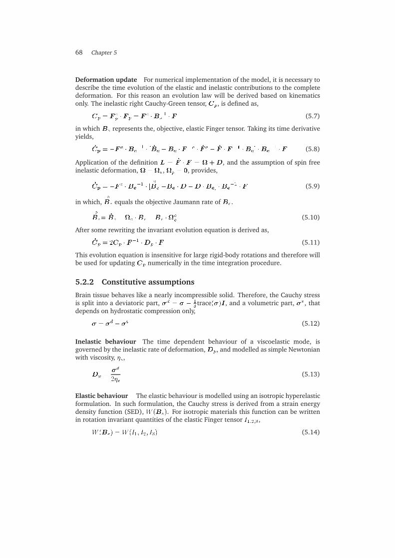
68 Chapter 5
Deformation update For numerical implementation of the model, it is necessary todescribe the time evolution of the elastic and inelastic contributions to the completedeformation. For this reason an evolution law will be derived based on kinematicsonly. The inelastic right Cauchy-Green tensor, Cp, is defined as,
Cp = Fcp � F p = F
c �B�1e � F (5.7)
in which Be represents the, objective, elastic Finger tensor. Taking its time derivativeyields,
_Cp = �F c �Be
�1 � [ _Be �Be � F�c � _F c � _F � F�1 �Be] �Be
�1 � F (5.8)
Application of the definition L = _F � F = +D, and the assumption of spin freeinelastic deformation, = e, p = 0, provides,
_Cp = �F c �Be
�1 � [Æ
Be �Be �D �D �Be] �Be
�1 � F (5.9)
in which,ÆBe equals the objective Jaumann rate of Be.
Æ
Be= _Be �e �Be �Be �ce (5.10)
After some rewriting the invariant evolution equation is derived as,
_Cp = 2Cp � F�1 �Dp � F (5.11)
This evolution equation is insensitive for large rigid-body rotations and therefore willbe used for updating Cp numerically in the time integration procedure.
5.2.2 Constitutive assumptions
Brain tissue behaves like a nearly incompressible solid. Therefore, the Cauchy stressis split into a deviatoric part, �d = � � 1
3 trace(�)I , and a volumetric part, �v, thatdepends on hydrostatic compression only,
� = �d + �v (5.12)
Inelastic behaviour The time dependent behaviour of a viscoelastic mode, isgoverned by the inelastic rate of deformation,Dp, and modelled as simple Newtonianwith viscosity, �s,
Dp =�d
2�s(5.13)
Elastic behaviour The elastic behaviour is modelled using an isotropic hyperelasticformulation. In such formulation, the Cauchy stress is derived from a strain energydensity function (SED), W (Be). For isotropic materials this function can be writtenin rotation invariant quantities of the elastic Finger tensor I1;2;3,
W (Be) =W (I1; I2; I3) (5.14)

A non-linear viscoelastic material model for brain tissue 69
with,
I1 = trace(Be)
I2 = 12
�trace(Be)
2 � trace(B2e)�
I3 = det(Be)(5.15)
For obtaining a consistent separation of deviatoric and volumetric parts in the Cauchystress tensor, the SED is formulated in a separated isochoric part, �W and a volumetricpart,Wv,
W = W (I1; I2) +Wv(I3) (5.16)
In this equation, I1;2 = I1;2(Be) with Be, the isochoric elastic Finger tensor,
Be = J�2=3e Be (5.17)
in which, Je = det(F e), represents the normalised volume of the elastic part of thedeformation. The resulting Cauchy stress can be written as,
� =2pI3
�@W
@I1B
d
e �@W
@I2
�B�1
e
�d�+ 2
pI3@Wv
@I3I (5.18)
in whichBd
e equals the deviatoric part of the isochoric elastic Finger tensor. Note thatthe first part of the stress, in the square brackets, is completely deviatoric whereas thesecond part occurs by the hydrostatic deformation only.SED equation (5.16) can be rewritten as a general series approximation,
W =NX
i+j=1
Cij(t)(�I1 � 3)i(�I2 � 3)j +MXk=1
Ck(t)(I3 � 1)k (5.19)
The parameters N and M determine the general character of the material behaviour.For simple shear, it has been shown in Chapter 4 that brain tissue exhibits shearsoftening. For this reason it is required that N > 1. The simplest choice thenbecomes N = 2, thus obtaining a second-order Mooney-Rivlin SED. Miller et al. [96]successfully fitted results of unconfined compression experiments with brain tissuewith of N = 2 and i 6= j. In [29], we did show that shear softening during simpleshear could be predicted well using negative second-order constants. The isochoricpart of the SED then becomes,
W = C10(I1 � 3) + C01(I2 � 3) + C20(I1 � 3)2 + C02(I2 � 3)2 (5.20)
This yields the deviatoric part of the Cauchy stress tensor,
�d = 2
Je
�C10 + 2C20
�I1 � 3
�B
de
� 2Je
�C01 + 2C02
�I2 � 3
� �B�1e
�d (5.21)
Only few literature data on linear viscoelastic hydrostatic behaviour of brain tissueis present. Furthermore it is shown in Chapter 2 that significant damping due

70 Chapter 5
to hydrostatic deformation occurs as high frequencies only. For this reason, thevolumetric part of the stress is modelled as simple as possible as,
�v = K(Je � 1)I (5.22)
with K being the bulk modulus.Note that, as the Cauchy stress is expressed in terms of (invariants of) the elasticFinger tensor, conservation of objectivity is guaranteed when indeed the spin isattributed to the elastic deformation, as done here. Furthermore, since a true hyperelastic material law is used for the Cauchy stress, the elastic part of the deformationwill cause no energy dissipation at repeated loading and unloading of the elastic partof the deformation. So the inelastic part completely controls energy dissipation, asrequired.
5.2.3 Multi-mode description
The theory presented is extended to a multi-mode model by applying the straindecomposition in each mode i separately. For each mode, the modal straindecomposition will be applied in constitutive equations (5.21) and (5.22) to providethe viscoelastic modal stress contribution �i. The elastic contribution, �0 isdetermined by substituting the total Finger tensor, B, for Be in equations (5.21)and (5.22). Finally the complete Cauchy stress can be obtained by simply adding allmodal stress contributions,
� = �0 +
nXi=1
�i (5.23)
5.3 Determination of brain tissue material parameters
The experimentally found time-strain separability of the shear stress behaviourwill be used to determine the material parameters for brain tissue. The timedependent behaviour is determined using small strain oscillatory experiment datawhile the strain dependent behaviour is obtained from large strain stress relaxationexperiments.The material data shows a large spread caused by measurement noise as well asbiological variation of the various samples used. However trends observed werepresent for all samples. To eliminate the spread by biological variation, materialparameters will only be fitted on experimental data of the single sample that hasbeen used in both small strain oscillatory experiments as well as large strain stressrelaxation experiments (sample G2 in Chapter 4). The bulk behaviour was notdetermined in current experiments and will be determined from literature data onultrasound experiments [45; 61; 83].

A non-linear viscoelastic material model for brain tissue 71
5.3.1 Small strain experiments: Multi-mode Maxwell model
For small shear strains, the non-linear viscoelastic constitutive equations used reduceto a multimode Maxwell model. The Maxwell model can be presented in terms ofstorage modulus, G
0
and loss modulus, G00
,
G0
= G0 +
nXi=1
Gi�2i!
2
1 + �2i!2
(5.24)
G00
=
nXi=1
Gi�i!
1 + �2i!2
in which i indicates the contribution of the separate modes, while n is the numberof modes used. For a given number of modes, the optimal sets of relaxation times,�i and shear moduli Gi are determined from linear viscoelastic data obtained fromsmall strain oscillatory tests, using a Levenbergh-Marquardt fit algorithm [170]. Theequilibrium mode, G0, cannot be obtained from the oscillatory data since the lowestfrequency used is too large, as can be seen by the absence of a plateau value for G
0
on the lower frequency range in Figure 5.3. For this reason, G0 was determined fromthe stress relaxation experiments (refer to page 73).The experimental data as well a the fit obtained with a four mode Maxwell model areshown in Figure 5.3. The figure shows that the material behaviour is not fitted well atlow frequencies in that G
0
is underestimated. A possible explanation will be providedin the discussion in section 5.5.3.
Relation with non-linear model
The relation between the linear Maxwell relaxation moduli Gi and the non-linearmodel parameters C10;i and C01;i can be found by linearising constitutive equation(5.21) for simple shear. This results in,
(C10;i + C01;i) = 0:5Gi (5.25)
100
102
104
102
103
104
Frequency [Hz]
G’ [P
a]
ExpFit
100
102
104
102
103
104
Frequency [Hz]
G’’ [P
a]
Figure 5.3: Storage and loss modulus G0
and G00
from sample G2 in Chapter 4 together with4 mode Maxwell fit. During fits, G0 set to value obtained from Stress Relaxationexperiments.

72 Chapter 5
With respect to the inelastic behaviour it is assumed that the inelastic part of thedeformation is governed by linear Newtonian behaviour. Viscosity, �s;i now can befound using,
�s;i = Gi�i (5.26)
5.3.2 Large strain stress relaxation experiments
The large strain shear behaviour of porcine brain tissue was characterised usinga rotational plate-plate viscometer. The strain field present between the plates isnon-homogeneous. As a result, apparent material parameters were measured, i.e.parameters valid for some average strain present between the plates. A correctionmethod by Soskey and Winter [138] will be used to obtain the true materialparameter, G(t; R). The approach is valid for stress relaxation experiments in arotational plate-plate viscometer.
Method
Based on kinematics only, the true relaxation modulus, G(t; R), can be obtained fromthe experimentally determined apparent modulus, Ga(t; R), via,
G(t; R) = Ga(t; R)
�1 +
@ lnGa(t; R)
4@ ln R
�(5.27)
In Chapter 4 the relaxation modulus was successfully factorised into a time dependentpart, the linear relaxation modulus, G(t), and a strain dependent part, h( ), the so-called damping function. Applying this to equation (5.27) leads to,
G(t; R) = ha( R)
�1 +
@ lnha( R)
4@ ln R
�G(t) (5.28)
with ha( R), the apparent damping function that is obtained directly from the stressrelaxation data. Thus, when time strain separation is valid, only the apparentdamping function needs to be corrected to obtain the real relaxation modulus.
Damping function
For simple shear the damping function of a hyper elastic material can be written as,
h( ) =
�( )
lim 0!0
�( 0) 0
=2�@W ( )@I1
+ @W ( )@I2
�lim 0!0 2
�@W ( 0)@I1
+ @W ( 0)@I2
� (5.29)
with, the shear strain, �( ) the shear stress, I1 and I2 the first and second invariantof the Finger tensor B, and W ( ) the hyper-elastic strain energy density function forsimple shear. Substituting SED equation (5.20) into equation (5.29) while applyingFinger tensor B for simple shear, and I1 = I2 = 2 + 3, gives,
h( ) = 1 + 2 2fnls and fnls =C02 + C20
C01 + C10(5.30)

A non-linear viscoelastic material model for brain tissue 73
in which fnls will be referred to as non-linear shear parameter. This function is fittedto the experimentally found damping functions, H( R;
refR ), obtained in Chapter
4, using a Nelder-Mead simplex (direct search) method [89]. This fit is used tocorrect the data using equation (5.27) and equation (5.30) has been fitted again tothe corrected data to obtain the true non-linear shear parameter, fnls. The quality ofthe fitted data is quantified by the average error of the fit at each experimental datapoint and the standard deviation of the error.
Fit results
To obtain realistic fits for the damping function, (i.e.lim !0 h( ) = 1), the damping
function value at 5% strain is assumed to be valid at 1% strain also. The left plotin Figure 5.4 shows the damping function, fitted on the experimental data of sampleG2. The non-linear shear parameter, fnls, equals -2.99. The mean fit error� standarddeviation equals 3:0 �10�3�8:0 �10�3. The corrected experimental results in the rightplot in Figure 5.4, show that the shear softening of sample G2 equals 37.1% at 20.3%strain. Fitting the second-order Mooney-Rivlin model to the corrected data providesfnls= -4.49. The mean error equals 3:0 � 10�3 � 8:6 � 10�3, i.e approximately 1% ofthe experimental values.
Determination equilibrium mode
As mentioned in section 5.3.1, the small strain equilibrium mode, G0, is determinedfrom the stress relaxation results. It will be defined as the small strain relaxationmodulus at t= 0.5 s, since the behaviour of brain tissue at later moments in timeis not of interest in impact situations. Since the smallest strain used in the stressrelaxation experiments, 5%, is outside the linear range of the material behaviour(refer to Chapter 3) the small strain modulus is obtained by rewriting equation (4.8)
0 5 10 15 200.4
0.6
0.8
1
γ [%]
h(γ)
ExperimentFit data
0 5 10 15 200.4
0.6
0.8
1
γ [%]
h(γ)
Raw data Corrected dataCorrected fit
Figure 5.4: Correction for non-homogeneous strain field using second-order Mooney-Rivlin onresults of sample G2 in [28]. Left: Fit results on uncorrected experimental data(filled diamond denotes copied 5% result). Right: Corrected data using 2nd orderMooney-Rivlin model.
74 Chapter 5
as,
G(t) =Ga(t; = 5%)
ha( = 5%)(5.31)
with ha( = 5%) obtained from equation (5.30) and fnls = -2.99. This results in G0
= 255 Pa.
Relation with non-linear model
It is assumed that the experimentally determined non-linear shear parameter, fnls,can be applied on the elastic part of every mode, i.e.,
C20;i + C02;i
C10;i + C01;i= fnls for i = 1 ton (5.32)
Note that applying this constant ratio for each mode, reduces the number of materialparameters, but introduces a difference with the description of the stress in theexperimental results. The value of the experimentally determined damping functionis determined by the complete shear strain whereas the non-linear behaviour in thematerial model, is governed by the elastic part of the deformation. So time-strainseparability is not guaranteed in the model.To ultimately determine the material parameters C10;i, C01;i, C20;i and C02;i, theratios f1;i =
C10;i
C01;iand f2;i =
C20;i
C02;ihave to be known. It is not possible to determine
these from results of shear experiments. Miller and Chinzei [96] fitted a second-orderMooney-Rivlin model to results of low velocity, unconfined compression experimentson porcine brain tissue using f1 = f2 = 1. In the present study it is assumed thatf1;i = f2;i = 1 for all modes i = 0 to n.
5.3.3 Bulk behaviour: Ultrasonic experiments
The hydrostatic behaviour was chosen to be purely elastic. As a consequence, thehydrostatic pressure will be attributed to the elastic stress part �v0 only,
K0 = K and Ki = 0; i = 1 ton (5.33)
From ultrasonic experiments, the velocity of dilatational waves in brain tissue, cp, isknown to be approximately 1550 m=s [45; 61; 83]. Using linear elastic theory, andknowing that the material is nearly incompressible (i.e. K >> Gi), the bulk modulusis determined as,
K = c2p � (5.34)
in which mass density, �, equals approximately 1040 kg=m3 for brain tissue. Thisprovides a bulk modulus of 2.5 GPa.Table 5.1 provides an overview of all material parameters fitted.

A non-linear viscoelastic material model for brain tissue 75
5.4 Numerical implementation
The material model is implemented in a Finite Element Code (MADYMO). First it isexplained how time integration is performed in the existing code. Then the stressupdate routine utilising a predictor-corrector scheme, will be presented. Finally theaccuracy of the model is investigated.
5.4.1 Time integration in MADYMO
The general outline of the MADYMO FEM integration scheme is presented in Figure 5.5[147]. Nodal displacements at the next time step, u(t+�t) are predicted starting fromthe displacements at the current moment in time, u(t). The integration cycle consistsof four steps. In the first step deformation gradient tensors, F (t), at the elementintegration point are computed from the nodal displacements, u(t). The second stepdeals with the computation of the stresses at the element integration points, �(t).From these stresses, the internal nodal forces at the current time, fint(t), are obtainedin the third step. Finally nodal accelerations at time, t are calculated by applying themomentum equilibrium equations. From these accelerations the nodal displacements
Table 5.1: Material parameters obtained from fitting the non-linear material model on braintissue shear data (sample G2 in Chapter 4)
Mode Maxwell parameters Non-linear parameters Bulk modulusi Gi [Pa] �i [ms] fnls [-] f1 [-] f2 [-] K [GPa]0 255.3* 1 -4.49 1+ 1+ 2.51 269.08 70.1 -4.49 1+ 1+ 02 322.63 7.62 -4.49 1+ 1+ 03 426.96 1.42 -4.49 1+ 1+ 04 3299.4 0.122 -4.49 1+ 1+ 0
* G0 obtained from stress relaxation data using equation (5.31)+ Constants chosen arbitrarily, could not be determined from shear experiments
f int
F (t)
σ(t)
σ(t)
int
u(t)
extMu(t) = f - f
t=t+ t∆σ ∆(t- t)
Figure 5.5: General layout MADYMO FEM time integration scheme, conform [147].

76 Chapter 5
on the next moment in time, u(t + �t), are determined using an (explicit) CentralDifference integration scheme. Then the complete sequence can start again for thenext time increment.
5.4.2 Stress computation
The stress computation scheme needed for calculation of the Cauchy stress at presenttime, �(t), (step two in Figure 5.5), is provided in Figure 5.6. The following quantitiesshould be known at the start of the current time, t: F (t��t),Cp;i(t��t), and �di (t��t), stored in the previous time step and F (t), computed from the displacements,u(t), computed from the momentum equilibrium equations at previous time step.This is generally true. However, the deformation and stress state at the start of thesimulation should be specified. It is assumed that there is no initial deformation, i.e.F (0) = F e;i(0) = Cp;i(0) = I , and no initial stress, �(0) = 0.The next steps in Figure 5.6 are straightforward, except for step 4. To determineCp;i(t), an explicit time integration scheme, the so-called improved Euler method orHeun’s method, is used. Explicit time integration is chosen because modelling thetransient material behaviour during impacts requires many small time steps.
1. Get data from previous time step F (t ��t), Cp;i(t ��t), �di (t ��t) and F (t) for each modei=1 to n.
2. Reconstruct inelastic deformation rate for mode i,
Dp;i(t��t) =�di (t ��t)
2�s;i
3. Determine time derivative of inelastic right Cauchy-Green strain tensor for mode i, using equation(5.11),
_Cp;i(t��t) = 2Cp;i(t��t) � F�1(t ��t) �Dp;i(t ��t) � F (t ��t)
4. Determine Cp;i(t) using Cp;i(t��t) and _Cp;i(t��t) in improved Euler time integration scheme.
5. Calculate Be;i(t) = F (t) �C�1p;i(t) � F (t)c.
6. Apply Be;i(t) in hyper elastic law (equation (5.21)) to determine �di (t).
7. Repeat steps 2 to 6 for every mode i=1 to n.
8. Determine elastic stress contribution �0(t) = �d0(t) + �v0(t), using B(t) in equations (5.21) and
(5.22).
9. Add modal stress contributions and elastic part via equation (5.23).
10. Store Cp;i(t), F (t) and �di (t) for use in next time step.
Figure 5.6: Stress computation scheme for determining the Cauchy stress at the currentmoment in time, �(t), using the non-linear viscoelastic material model (the secondbox in the general time integration scheme in Figure 5.5. n denotes the number ofviscoelastic modes.

A non-linear viscoelastic material model for brain tissue 77
First an estimation of the inelastic right Cauchy-Green strain, eCp;i(t), is made byusing the Euler forward method,eCp;i(t) = Cp;i(t��t) + _Cp;i(t��t)�t (5.35)
in which _Cp;i(t � �t) was obtained in step 3 using evolution equation (5.11). Thepredicted tensor, eCp;i(t), is used in steps 5, 6, 2 and 3 in Figure 5.6 to determine a
prediction of the deformation rate e_Cp;i(t) . The predicted eCp;i(t) then is corrected byapplying the trapezoidal rule,
Cp;i(t) = Cp;i(t��t) +1
2
�_Cp;i(t��t) +
e_Cp;i(t)��t (5.36)
5.4.3 Accuracy of the time integration schemeIn this section it is investigated whether the accuracy of the improved Euler method issufficient for modelling nearly incompressible materials, such as brain tissue, at timesteps commonly used in impact simulations (�t = O(10�6) s). To do so, the stressupdate scheme of Figure 5.6 is implemented in MATLAB 5.3 [89]. Simple shear ( 0 =20%) is applied step wise at t = 0.5 s and kept constant thereafter. A single modemodel is used with shear modulus G1 = 2(C10 + C01) = 1000 Pa, C20 = C02 =0,bulk modulus, K1 = 1 GPa and time constant �1 = 1 s. In this section only resultsinteresting for the accuracy analysis are shown. A complete overview of numericaland analytical results can be found in Appendix A.The upper left plot in Figure 5.7 shows the computed shear stress versus time. Theinitial stress equals approximately 200 Pa and decreases in time. The slope of thesemi-logarithmic plot equals -1 corresponding with the time constant applied. Twotypes of error appear in the stress results. The first type of error acts on the relaxationbehaviour of the shear stress. The time history of the relative error in the shear stress,�Erel(t), is defined as,
�Erel(t) =j�num(t)� �th(t)j
�th(t)(5.37)
in which �num(t) and �th(t) represent the numerical and theoretical obtained shearstress histories respectively. The upper right plot in Figure 5.7 shows that the relativeerror, �Erel decreases to approximately 1% when a time step of 0.01 s or less is used.The second error appears in the volumetric stress. Since simple shear is an isochoricdeformation, the volumetric stress should be zero. It decreases quadratically withdecreasing time step, as shown in the lower plot in Figure 5.7.
Discussion
The error in the volumetric stress is determined by the limited accuracy of theintegration method used. For brain tissue, this error becomes relevant since the bulkmodulus is approximately 106 times higher than the shear modulus. The residualvolumetric stress at �t = 10�6 s, typical in automotive impact simulations, isdetermined by extrapolating the results in the lower plot Figure 5.7 and equals 10�5

78 Chapter 5
Pa. This error is on the order of 10�7 times the initial shear stress and is consideredto be sufficiently small.The error during stress relaxation is determined by ratio time step over time constantused. In the present simulation the time constant, �, was set to 1 s. Taking a timestep of 0.01 s yielded an error of 1%. This implies that the time step has to be chosensuch that �t=� < 0:01 for accurate shear stress results. The smallest relaxation timefor brain tissue equals 1:2 � 10�4 s (refer to Table 5.1 on page 75). This means thataccurate solutions are indeed obtained when a time step of 10�6 s , common in impactsimulations, is used.An issue not discussed on is the objectivity of the stress formulation. Although thisshould be trivial, Nusholtz and Shi (1998) showed that in a commercially availableexplicit FE package, objectivity of the stress results during large rotations was notguaranteed to that date [113]. When undeformed solid elements were rotated by 4revolutions, an artificial normal stress on the order of 9 GPa appeared (linear elasticmaterial behaviour, E = 200 GPa and � = 0:3). Applying this rotation provided amaximum error on the order of 10�7 Pa for the model presented in this section. Thisindicates correct objective behaviour. Different loading types such as cyclic loadingand unloading, did not lead to different error causes than the ones discussed for thesimple shear simulation in this section. For more information on these simulationsthe reader is refereed to appendix A.
5 10 15 2010
−10
10−5
100
105
Time [s]
σ xy [P
a]
5 10 15 2010
−6
10−4
10−2
100
Time [s]
∆Ere
l [−]
∆t=100 ms∆t=10 ms ∆t=1 ms ∆t=0.1 ms
101
102
103
104
100
105
1/∆t [s−1]
σv [Pa]
Figure 5.7: Results of simple shear stress relaxation simulation. Top left: Shear stress versustime. Top right: Relative error histories (�Erel in equation (5.37)) in shear stressfor various time steps. Bottom: Residual volumetric stress versus reciprocal timestep.

A non-linear viscoelastic material model for brain tissue 79
5.5 Simulation of stress relaxation experiments
The time dependent behaviour of the material model is obtained from small strainexperiments only, while all information on strain dependent behaviour comes fromthe constant strain phase of large strain stress relaxation experiments. In thissection it is investigated whether the model predicts the stress relaxation experiments,presented in Chapter 4, including the transient phase.
5.5.1 Model description
A three-dimensional FE model of the rheometer experiments has been developed.Brain tissue constitutive behaviour is modelled using the material parameters in Table5.1. The geometry of the brain sample is modelled by a quarter cylinder only withdiameter 25 mm and thickness 2 mm, to reduce CPU time. Symmetry boundaryconditions are applied on the cross-sectional planes. The lower plane is rotatedaccording to the experimental obtained rotation history obtaining the strain histories,reprinted in Figure 5.8, which are valid at the sample edge. The upper-plane is rigidlysupported and the resulting torque along the axis of rotation is determined. Theapparent stress is calculated from the resulting torque in the same manner as in theexperimental results (refer to equation 4.3) for comparison.Spatial discretisation is obtained using cubic elements with linear interpolationfunctions. To prevent mesh locking, likely to occur due to the nearly incompressiblematerial behaviour, reduced spatial integration is used. Seven element layers areused in thickness direction whereas approximately twelve elements are used in radialdirection. The time step used is determined via the Courant criterion (refer toequation 2.30) and equals 1:66 �10�7 s. This is approximately 10�3 times the smallesttime constant and should provide accurate solutions.
5.5.2 Results
In Figure 5.8 the apparent shear stresses, experimentally obtained at 5, 10 and 20%maximum edge strain, are plotted together with the numerical results. The modelpeak stress values are over estimated by 12 to 23% during the transient part of theloading (t < 0:1 s) ( �Epeak in Table 5.2). Then, during the subsequent relaxationphase, the stress decay is faster than in reality. The numerical results even drop
Table 5.2: Overview of the maximum relative differences between numerical results andexperimental results. �Epeak: difference between peak values during transientloading part , �Erelax: maximum negative difference during relaxation, �Et=0:5s:difference at t = 5 s.Max. strain 0 [-] �Epeak [%] �Erelax [%] �Et=0:5s [%]
0.05 19.5 0.4 3.80.1 22.8 0.9 6.50.2 12.2 2.3 5.1

80 Chapter 5
below the experimental results providing a maximum difference of 2.3% at 5% strain(�Erelax in Table 5.2) . At the end of the simulation, at t = 0:5 s, no relaxation ispresent any more in the numerical stresses which are higher than the experimentalresults at that time by 4% at 10% strain (�Et=0:5s in Table 5.2).
5.5.3 Discussion and conclusions
Stress relaxation experiments have been simulated including the transient loadingpart at times less than approximately 0.1 s. It could be observed that the modelcorrectly predicts the overall behaviour of the brain tissue, i.e. the presence of shearsoftening and the stress relaxation. Nevertheless differences between experimentaldata and numerical results are present.
Relaxation behaviour During the transient phase of the loading, the model predictshigher stresses than found experimentally. Then, during subsequent relaxation,the stresses are described within 6% accuracy. However, after 0.1 s the predictedstresses decay faster and tends to reach a plateau value which is not present in theexperimental results. Two causes can be found for this. Firstly, the equilibrium modewas fitted to the 0.5 s value. As a result there will be no relaxation from that momentof time on. Secondly, when the modal contributions to the relaxation behaviour arestudied, it can be seen that the behaviour from 0.2 to 0.5 s is governed by a singlemode only. This can be improved by using more modes in the model.
Peak values The differences in peak values during transient loading might becaused by the fact that the linear material parameters and non-linear parameters arederived from separate sets of experiments. The linear parameters were determinedfrom a master curve constructed from several dynamic frequency sweep experimentsat various temperatures (DFS). Subsequently, stress relaxation experiments (SR) werecarried out from which the non-linear behaviour was taken as well as the small strain
0 0.1 0.2 0.3 0.40
10
20
30
Time [s]
Str
ain
[%]
0 0.1 0.2 0.3 0.40
20
40
60
80
Time [s]
Str
ess
[Pa]
γ0=0.05
γ0=0.1
γ0=0.2
NumExp
Figure 5.8: Simulation results of stress relaxation experiment at three strain levels versusexperimental results (apparent stresses sample G2 in Chapter 4). Left: sampleedge shear strain histories, Right: apparent shear stresses, Num = MADYMO result,Exp = Experiment.

A non-linear viscoelastic material model for brain tissue 81
equilibrium mode. In the process of performing these experiments, experimentaldata will be influenced by factors as material ageing and differences in humidityconditions, which always exist between separate experiments. A clue for the presenceof such differences can be found by observing the trends of the errors while predictingDFS and SR experiments. The trends in the errors in the SR experiments are strainindependent, i.e. overestimated initial stress followed by better prediction of longterm behaviour. For this reason trends in the error in the DFS experiment shouldresemble those of the SR experiments, i.e. overestimated moduli at high frequenciesand about correct ones at low frequencies. The opposite however is true, lowfrequency values of the elastic modulus are underestimated while high frequencyvalues are approximately correct (refer to Figure 5.3). This indicates that the generalstiffness of the brain tissue was higher during the DFS experiments than in the SRexperiments.Finally it should be mentioned that the time-strain separability, assumed in thederivation of the material parameters, has never been validated for times less than0.1 s (i.e. frequencies above 10 Hz). Darvish and Crandall recently presentedexperimental results that indicate that for frequencies above 27 Hz, also timedependent non-linearities might be present in brain tissue [39].
5.6 Conclusion
In this chapter a non-linear viscoelastic material model for the large strain shearbehavior of brain tissue in impact conditions has been presented. The inelastic,time dependent behavior is described with a simple Newtonian law that acts on thedeviatoric stress contribution only. Based on the experimental data in Chapters 3and 4, the deviatoric elastic part is modelled by a non-linear, second-order Mooney-Rivlin model. Since this experimental data did not provide information on potentialanisotropic behaviour present in brain tissue [8; 123] isotropic material behaviour isassumed. However, anisotropic behaviour can be included in strain energy densityequation (5.20). The hydrostatic part is assumed to be linear elastic. The modelhas been implemented in an explicit Finite Element code. Care has been takenthat the numerical accuracy of the model suffices for predicting the behaviour of anearly incompressible material such as brain tissue at large strains and large rotationsexpected during impact by using the improved Euler integration scheme for timeintegration of the inelastic deformation.Material parameters have been determined from simple shear experiments presentedin Chapters 3 and 4. In elaborating these parameters, time-strain separability wasassumed to be valid. Linear parameters were determined from small strain oscillatoryexperiments, whereas the strain dependent non-linearity was determined from stressrelaxation experiments. It was found that the strain dependent behaviour could befitted well when negative second-order parameters, C20 and C02 were used. As aresult negative stiffness can occur at strains exceeding the strain range for which themodel has been fitted on. When the model is used during a transient simulation, thishas to be kept in mind.

82 Chapter 5
The ratios C10
C01
and C20
C02
could not be determined from the experimental data. Thisis a result of the fact that the first and second invariant of the elastic Finger tensorare equal to each other in simple shear. In principle, these ratios can be determinedfrom unconfined compression experiments, available from literature [96]. However, alarge spread exists between the experimental results obtained from different samplesand also between various literature sources (refer to Figure 3.4 in Chapter 3). For thisreason no efforts have been made in fitting the material parameters of our sample tothe literature data. Instead the ratios C10
C01
and C20
C02
were set to 1 as done in [96].The material model has been tested by simulation of brain tissue stress relaxationexperiments including the transient part of the shear strain. It was found that duringthis transient part, the model over-predicts the stress values. In the constant strainphase, the strain dependent behaviour of brain tissue is described quite well althoughdifferences were present in relaxation behaviour. It is expected that these results canbe improved by putting more effort in fitting material parameters.It can be concluded that the present model and it’s current parameters, capture themost important features of the material behaviour, i.e. shear softening for strains upto 20% and viscoelastic material behaviour.

Chapter 6
FE modelling of transientrotation of a simple physical
head model
The objective of this chapter is to investigate errors related to material modelling and spatialdiscretisation in an explicit Finite Element code during traffic related impacts. A silicone gelfilled cylindrical cup was subjected to a transient rotational acceleration. Two variants of themodel exist, an open cup, allowing large strains at modest impact conditions, and a closed cup,mimicking the closed geometry of a real head. In both geometries gel response was measured usingoptical markers. The open cup experiments could be simulated very well using the material modeldeveloped in Chapter 5 in which hydrostatic and deviatoric parts of the strain were separated inthe stress formulation. The error in angular marker displacements was less than 22%. The closedcup trajectories were overestimated by 62% but the time history looks realistic. Increasing themesh density from 28 to 56 elements per cup diameter yields changes of displacements of 4% only.This supports the rule of thumb derived in Chapter 2, that 24 elements per maximum wave lengthare needed for accurate modelling. Without decoupling the hydrostatic and deviatoric parts of thestress, the stiffness at finite shear strain was overestimated severely, especially in the closed cupsimulation. This illustrates the dangers of extrapolating small strain theory to finite deformations,especially with nearly incompressible material behaviour.
83
84 Chapter 6
6.1 Introduction
Physical, i.e. mechanical, head models, that contain deformable representations ofsubstructures of the head can be used for gaining insight in strain levels occurring inthe dynamic response of the head during impact [71; 90; 93; 141]. However, physicalmodels can also be used for investigating the accuracy of Finite Element Models usedin impact simulations.Finite Element models of the head, potentially suffer from two kinds of errors. Thefirst kind of errors, mathematical modelling errors, arise by assumptions made intranslating the reality to a mathematical description of that reality in terms of a setof differential equations. These errors are caused by assumptions about materialbehaviour, boundary conditions, geometry etc. The second kind of errors, numericalerrors, are introduced by the numerical method used for solving the mathematicaldifferential equations; in this case the Finite Element Method. Numerical errorsare caused by the spatial and temporal discretisation needed to translate themathematical model to a numerical model. Examples of numerical errors arenumerical dispersion and spurious reflections investigated in Chapter 2 for smallstrains.In this chapter, the capability of an explicit Finite Element code to predict transientbrain response during a traffic related impact will be investigated. Emphasis will begiven to numerical errors introduced by the spatial discretisation, and mathematicalerrors caused by material modelling assumptions, in particular the effect of separatingthe deviatoric and volumetric deformation in the stress formulation presented inChapter 5.During impacts at which brain injury occurs, strain levels of approximately 20% canbe expected (refer to Chapters 3 and 4). At such deformation levels, validation ofnumerical models using analytical solutions is impossible. For this reason a physicalmodel is developed with emphasis on straightforward translation to a mathematicalmodel rather than for prediction of a real head impact response. This has beenachieved by using a simple geometry, well characterised brain tissue model materialand known boundary conditions. The model was subjected to a known, transientrotational acceleration and the mechanical response of the brain model material wasmeasured. In this manner, errors that arise from translating the physical model to amathematical model are eliminated as much as possible. The experiments have beensimulated with a Finite Element model that includes that material model developedin previous chapter. The influence of mesh density on the response is investigated byvarying the mesh density. The effect of decoupling the deviatoric and volumetricparts of the deformation in the stress formulation was investigated by repeatingthe simulations with a linear viscoelastic material model that does not use suchdecoupling.
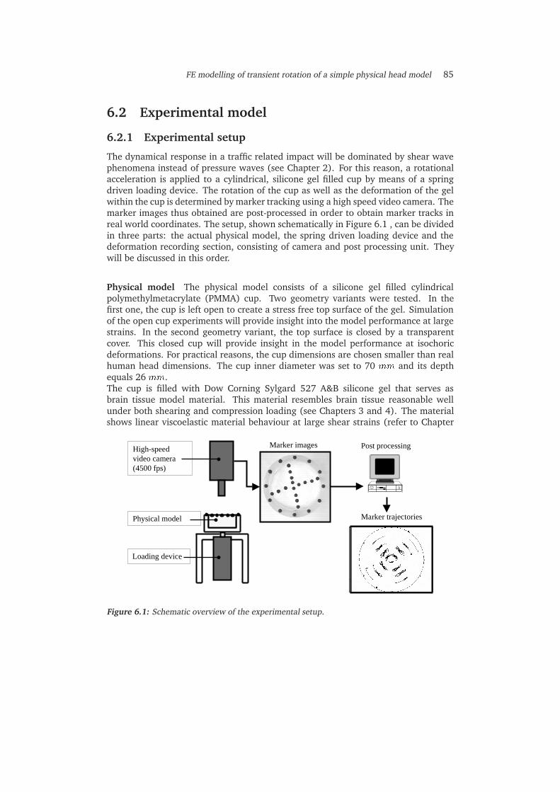
FE modelling of transient rotation of a simple physical head model 85
6.2 Experimental model
6.2.1 Experimental setup
The dynamical response in a traffic related impact will be dominated by shear wavephenomena instead of pressure waves (see Chapter 2). For this reason, a rotationalacceleration is applied to a cylindrical, silicone gel filled cup by means of a springdriven loading device. The rotation of the cup as well as the deformation of the gelwithin the cup is determined by marker tracking using a high speed video camera. Themarker images thus obtained are post-processed in order to obtain marker tracks inreal world coordinates. The setup, shown schematically in Figure 6.1 , can be dividedin three parts: the actual physical model, the spring driven loading device and thedeformation recording section, consisting of camera and post processing unit. Theywill be discussed in this order.
Physical model The physical model consists of a silicone gel filled cylindricalpolymethylmetacrylate (PMMA) cup. Two geometry variants were tested. In thefirst one, the cup is left open to create a stress free top surface of the gel. Simulationof the open cup experiments will provide insight into the model performance at largestrains. In the second geometry variant, the top surface is closed by a transparentcover. This closed cup will provide insight in the model performance at isochoricdeformations. For practical reasons, the cup dimensions are chosen smaller than realhuman head dimensions. The cup inner diameter was set to 70 mm and its depthequals 26 mm.The cup is filled with Dow Corning Sylgard 527 A&B silicone gel that serves asbrain tissue model material. This material resembles brain tissue reasonable wellunder both shearing and compression loading (see Chapters 3 and 4). The materialshows linear viscoelastic material behaviour at large shear strains (refer to Chapter
High-speedvideo camera(4500 fps)
Physical model
Loading device
Post processing
Marker trajectories
Marker images
Figure 6.1: Schematic overview of the experimental setup.

86 Chapter 6
4). Ultrasonic experiments on the silicone gel indicate that the P-wave propagationvelocity in silicone gel equals 1048 � 43m=s [139] compared to 1550m=s in braintissue [45; 83]. From this it can be derived that the bulk modulus of the gel equalsapproximately 1 GPa, which is about half the bulk modulus of brain tissue. Anadditional advantage of this gel is that it sticks to the PMMA walls (and cover) of the(closed) cup, thus providing a well defined, no-slip, boundary condition. The A andB components of the gel were mixed in a one-to-one mass ratio and left hardening inthe cup for at least two weeks before experiments commenced.
Loading device The cup is rotated along its axis of symmetry by a spring, connectedto the cup via a ratchet wheel. The maximum rotation angle over which the cup isaccelerated is set to 2.2 rad. When the cup reaches its end of motion range it hitsthe support frame and is stopped abruptly. The design of the spring driven loadingdevice is such that strain and strain rate levels associated with injury can be reached.Strain levels ranging from 15% to 21% have been associated with the occurrence ofaxonal injury [10; 141] whereas 19% natural strain (i.e. 21% stretch) has beenassociated with the breakdown of the blood brain barrier [131]. The strain rateassociated with injury is unknown but is estimated as follows. Animal data revealedthat, at a change of angular velocity, �! = 150 rad=s, an angular acceleration, _!, of1:5�104 rad=s2 could be associated with the occurrence of Diffuse Axonal Injury [141].From these experiments, a typical time duration for the impact can be estimatedusing, Timpact =
�!_! = 10ms. If it is assumed that indeed strain values of 15 to 21%
occurred during these impacts and that a constant strain rate was present, a lowerbound estimate of the typical strain rate becomes, _ = max
Timpact= 15 to 21 s�1.
Deformation recording Histories of both gel deformation and cup rotation weredetermined using marker tracking. 4-mm diameter markers were perforated out of aslide of black plastic material and placed in the gel (gel markers) and on the cup edge(cup markers) (refer to Figure 6.2) . The mass density of the markers is less than thatof the gel. For the open cup the gel markers were placed on top of the silicone gelwhile for the closed cup, the gel markers were placed at half cup height in a planeparallel to the top plane. During the experiment all marker positions were recorded
Open cup: side top Closed cup: side top
Figure 6.2: Side and top view of the cylindrical model. Left two pictures: open cup. Right twopictures: closed cup. Note that cup markers are placed on top of cup edge whereasgel markers are placed on top (open cup) or in the center plane (closed cup).

FE modelling of transient rotation of a simple physical head model 87
at 4500 frames per second by a high-speed video camera (Kodak Ektrapro ES MotionAnalyser) at a resolution of 256X256, 8-bit gray-scale pixels. The optical axis of thecamera was positioned as to approximately coincide with the axis of rotation of thecup (refer to Figure 6.1). Special lighting equipment utilizing infrared filters hasbeen used to reduce object heating and reflections have been eliminated by the useof diffuse lighting.The markers were tracked using the MATLAB Image Processing Toolbox [89]. Markerpositions in pixels were computed from contour plots of the images using a circlefit method based on a least square approximation. The image coordinates wereconverted to real world coordinates using a linear transformation according to,
x˜mm = T � x
˜pix(6.1)
in which x˜mm denotes real world marker coordinates in mm, x
˜pixthe image
coordinates in pixels and T a 2 � 2 transformation matrix. To determine thetransformation matrix, the positions of the cup markers were determined beforehandusing an X-Y measuring device. The initial coordinates of the cup markers inpixels were determined from the first recorded frame. The components of thetransformation matrix were determined using a least square approximation usingMATLAB [89]. The Cartesian coordinates thus obtained were converted to polarcoordinates. To do this, the rotation point was determined using the fact thatthe trajectories of the cup markers should be a (part of a) circle. First, theinitial and end position of every cup marker was determined. Then, the bisectorsperpendicular to the lines connecting initial and end position of each cup markerwere determined. These perpendicular bisectors should cross in the rotational point.
t = 20 ms t = 26.6 ms t = 33.2 ms
t=39.8 ms t=46.4 ms t=53 ms
Figure 6.3: Sequence of frames starting at t = 20ms (upper left) to 53 ms (lower right). Cuprotation is clock wise.

88 Chapter 6
In this manner, the rotation point has been determined for each couple of cup markerswith approximately perpendicular bisectors. The average value has been taken as thebest estimate of the real rotation point.
6.2.2 Experimental results
Open cup Figure 6.3 shows a sequence of frames of the open cup during theacceleration part of the loading. In these pictures, the markers can clearly bedistinguished. From the positions of the cup markers, rotation and angular velocityfor the cup have been determined as a function of time. They are shown in the upperleft plots in Figure 6.4. The angular velocity of the cup increases during the first 53ms to a value of 90 rad=s approximately. At 53 ms, the cup is stopped at its end ofmotion range at 2.2 rad. The deformation of the gel will be studied until that momentin time only since this part of the loading was designed to reproduce a typical impactload. The upper right plot of Figure 6.4 shows marker trajectories of three selectedmarkers in the gel as well as the trajectories of the markers on the cup. It can be seenthat the rotation of the cup is axisymmetric, as expected. In the lower left plot therotation of the gel markers, relative to a cup-fixed co-rotating coordinate system, isshown. It can be seen that the markers lag behind in motion with respect to the cup.Also it can be seen that the relative marker rotation increases for increasing radial
0 20 40 60
−2
−1
0
ω [r
ad]
0 20 40 60−100
−50
0
Time [ms]
dω/d
t [ra
d/s]
−40 −20 0 20 40
−20
0
20
123
x [mm]
y [m
m]
0 20 40 60−0.2
0
0.2
0.4
0.6
0.8
Time [ms]
Rel
. rot
atio
n [r
ad] 1
23
0 20 40 60−1
0
1
2
3
Time [ms]
Rad
. dis
pl. [
mm
] 123
Figure 6.4: Results of open cup experiment. Top left: cup rotation and angular velocity. Topright: Marker trajectories: initial positions of gel markers numbered 1 to 3, initialpositions of cup markers labeled *. Bottom left: Circumferential displacementsof gel markers relative to cup circumferential displacement. Bottom right: Radialdisplacements of gel markers.

FE modelling of transient rotation of a simple physical head model 89
distance from the edge of the cup. This is expected since there is decreasing influenceof edge boundary conditions towards the centre. Peak relative rotation occurs firstat about 40 ms at marker 1 close to the cylinder edge and occurs a few ms laterin marker displacements 2 and 3. The lower right plot of Figure 6.4 shows thatmaximal radial gel marker displacements are on the order of 2 mm. The accuracyof the radial measurements is determined by observing the radial displacements ofthe cup markers. For the open cup it was observed that the radial position of the cupmarkers is constant within 0.3 mm. For this reason it can be concluded that the radialgel marker displacements are significant. They are related to the three-dimensionaldeformation present during this experiment as shown in Figure 6.5.
Closed cup Figure 6.6 shows the experimental results of the closed cup. It canbe seen that the applied load is similar to the one applied on the open cup. Themaximum relative rotations equal 0.12 and 0.24 rad for markers 1 and 2. Theradial displacements of the markers are on the order of 0.1 mm while the radialdisplacements of the cup markers are on the order of 0.5 mm. For this reason noconclusions can be drawn on the exact radial displacements of the gel markers.
6.2.3 Discussion on experiment
Accuracy of the experiment The accuracy of the experiment is determined by twofactors. The first factor is the accuracy of the measurement system used. This isdetermined by the resolution used in combination with marker size. Since the cupimage fills the complete field of view, 256 pixels cover approximately 80 mm. Thus,the typical pixel size equals 256=80 = 0:3mm. As a result, a marker diameter will becovered by 12 pixels. The accuracy by which marker positions are obtained is roughlyestimated as pixel size over number of pixels per marker and equals 0.03 mm. Thiscorresponds with the noise level seen in the lower right plot of Figure 6.6.A second factor determining the accuracy are errors induced by performing theexperiment itself. In this case, the loading spring is released manually. As a result,a small translational motion of the cup with respect to the camera can be present.Furthermore the optical axis of the camera is not positioned exactly perpendicularto the marker plane. The magnitude of these inaccuracies has been estimated byobserving the change in radial position of the cup markers which was on the order of0.3 and 0.5 mm for the open and closed cup experiment respectively.
Figure 6.5: Side view of open cup experiment showing the three-dimensional deformationfield present. Time history from left to right.

90 Chapter 6
Impact loading conditions The gel response during the experiment, in terms ofstrain and strain rate, should be representative for impact conditions. For estimatingthe strain levels in the experiment, it is assumed that the marker motion is two-dimensional in the image plane recorded by the high-speed camera. A lower boundfor the shear strain, (t), occurring in this plane can be found using,
(t) =(R0 +�R) sin��(t)
Rcup � (R0 +�R) cos��(t)(6.2)
in which R0, Rcup, and �R represent the initial radial position of the marker, thecup radius and the change of marker radial position respectively while ��(t) is theangular marker displacement relative to the cup (refer to Figure 6.7). This strainrepresents a shear strain that would occur at the edge of the cup. When simple shearis assumed the maximum principal strain, �(t), can be determined as,
�(t) =
"1 +
(t)2
2+ (t)
r1 +
(t)2
4
# 1
2
� 1 (6.3)
The principal strain histories thus obtained are shown in Figure 6.7. For the opencup the maximum principal strain values range from 10% to 49% while for the closedcup experiments strain values of 9% and 15% were found. The maximum strainrate values were determined using numerical differentiation and equal 45 s�1 for the
0 10 20 30 40
−2
−1
0
ω [r
ad]
0 10 20 30 40−100
−50
0
Time [ms]
dω/d
t [ra
d/s]
−40 −20 0 20 40
−20
0
20
1
2
x [mm]
y [m
m]
0 10 20 30 40−0.2
−0.1
0
0.1
0.2
0.3
Time [ms]
Rel
. rot
atio
n [r
ad]
12
0 10 20 30 40−0.2
−0.1
0
0.1
Time [ms]
Rad
. dis
pl. [
mm
] 12
Figure 6.6: Experimental results of closed cup experiment. Top left: cup rotation andangular velocity. Top right: Marker trajectories: initial positions of gel markersnumbered 1 and 2, initial positions of cup markers labeled *. Bottom left: Relativecircumferential displacements of gel markers. Bottom right: Radial displacementsof gel markers.

FE modelling of transient rotation of a simple physical head model 91
open cup and 20 s�1 for the closed cup. Although these values are rough estimates,it is concluded that both maximum strain values as well as strain rate values in thephysical model are within the impact range estimated in section 6.2.1 (i.e. strainvalues of 15% to 21% and strain rate values of 15 s�1 to 21 s�1).
6.3 Numerical model
The experiments, described in previous section, have been simulated in MADYMO. Thematerial model presented in Chapter 5 was used to describe the material behaviourof the silicone gel.
6.3.1 Methods
Mathematical model In the mathematical model it is assumed that no slip occursbetween the gel and the cup and that the cup and its cover behave rigidly. For thisreason the cylindrical geometry of the gel is modelled only. For the closed cup, radialand axial motion of all outer surfaces are suppressed while circumferential motionis prescribed according to the experimentally obtained rotation history in Figure 6.6.For the open cup, the same boundary conditions hold except for the upper surface,which is considered stress free while the other outer surfaces are subjected to therotation history in Figure 6.4.The silicone gel used behaves like a linear viscoelastic solid for strains up to 50%and frequencies up to 461 Hz (refer to Chapters 3 and 4). For this reason, a linearfour-mode Maxwell model has been fitted to the experimental data using the methodalready presented in Chapter 5. The fitted relaxation times, �i, and shear moduli,Gi, are shown in Table 6.1. Figure 6.8 shows that the model fits the experimentaldata well. The bulk modulus applied has been determined from ultrasonic data, asK = c2p� where cp = 1048m=s [139] and mass density � = 970 kg=m3 (refer to thetheory in Section 2.2, Chapter 2).These material parameters have been applied in the material model presented inChapter 5 in which the non-linear material behaviour was disabled (fnls = 0) and
cupR
R + R0 ∆∆φ
Cup edge
Marker
atan(γ)
0 20 40
0
0.2
0.4
0.6
Time [ms]
Str
ain
[−]
123
0 10 20 30 400
0.05
0.1
0.15
0.2
Time [ms]
Str
ain
[−]
12
Figure 6.7: Left: Graphical representation of strain computation. Middle and Right: Estimatedmaximum principal strain histories. Middle: Open cup, Right: Closed cup.

92 Chapter 6
again it was assumed that c10;i = c01;i =12Gi. The model will be referred to as REF
material model in this Chapter.To investigate the influence of the degree of coupling between hydrostatic anddeviatoric stress, the simulations of open and closed cup were also performed usingthe linear viscoelastic material model already present in MADYMO (LINVIS) [148].In this model, which will be referred to as the CPL material model from now on,correct large deformation behaviour has been achieved by linearly coupling theGreen-Lagrange strain, E = 1
2 (Fc � F � I), to the Second Piola-Kirchoff stress tensor,
S, according to,
S = Ktrace(E)I + 2
Z t
�1
G(t� �) _Edd� (6.4)
in which, for small deformations, K resembles the bulk modulus and G(t) a timedependent relaxation modulus. The Cauchy stress then is obtained using,
� =1
det(F )F � S � F c (6.5)
Numerical implementation Spatial discretisation of the mathematical model hasbeen achieved using brick elements with linear interpolation functions and reduced
Table 6.1: Four-mode Maxwell parameters for Sylgard 527 A&B silicone gel fitted to oscillatorydata presented in Chapter 4.
Mode Maxwell parameters Bulk modulusi Gi [Pa] �i [ms] K [GPa]0 216.41 1 1.0651 122.32 309.8 -2 378.79 24.71 -3 1717.2 2.156 -4 27599 9:743 � 10�2 -
100
102
103
104
Frequency [Hz]
G’ [P
a]
ExperimentFit result
100
102
102
103
104
Frequency [Hz]
G’’ [P
a]
Figure 6.8: Storage and loss modulus G0
and G00
of Sylgard 527 A%B silicone gel togetherwith 4 mode Maxwell fit. Fitted material parameters are shown in Table 6.1.

FE modelling of transient rotation of a simple physical head model 93
integration. The element size is based on the error analysis in Chapter 2.Approximately 24 elements per maximum wave length in the model have to be usedto reduce errors due to numerical dispersion to less than 1%. If we assume thatthe maximum wavelength present equals the diameter of the cup, the lower boundfor the mesh density equals at least 24 elements over the diameter. In this case 28elements over the diameter have been used. To keep the initial element shape closeto cubic, twelve element layers have been used over the cup height. To investigatethe effect of spatial discretisation on the numerical results, the simulation of the opencup experiments has been repeated with both a more coarse and a more refined mesh.The coarse mesh has been created by merging eight elements of the reference meshinto a single, larger element. Mesh refinement has been achieved by splitting everyelement in the reference mesh into eight new elements. To reduce computationaltime using this finest mesh, a quarter cylinder was modelled only while symmetryconditions were applied on the cutting planes. The meshes are shown in Figure 6.9.
Post processing Nodes have been selected with radial distances as close aspossible to the distances determined experimentally. Trajectories in the x-y planewere determined and are presented in polar coordinates for comparison with theexperimental results.
6.3.2 Numerical results: REF material model
Reference mesh open model Figure 6.10 shows the time histories of nodaldisplacements in polar coordinates corresponding to the marker displacements ofmarkers 1, 2 and 3 in the open cup (see Figure 6.4). The experimental resultsare plotted in the figure for comparison. It can be seen that the model predicts
Coarse mesh Reference mesh Refined mesh
Figure 6.9: Meshes used for modelling open and closed cup. Refined mesh consists of quartermesh only with symmetry boundary conditions applied on cutting planes.

94 Chapter 6
the marker trajectories quite well. The general shape of the curves is the same forboth experiment and simulation. The numerical model however, overestimates therelative rotation of the markers by 17%, 14% and 24% for markers 1, 2 and 3,respectively. The time history of the radial displacement shows that the numericalresults are within range of the experimental ones. The radial displacements remainapproximately zero until 30 ms. After this, they increase to 2 mm approximately.
Reference mesh closed model The experimental closed cup results are comparedwith the numerical reference mesh results in Figure 6.11. The numerical model over-predicts the amplitude of the angular rotation by 62% and 46% for marker 1 and 2,respectively. The predicted radial displacements are on the order of 0.1 mm and are inthe same of order of magnitude as the experimental results. However, the reliabilityof the radial displacements from the experiment was low (refer to page 89).
Mesh density variation The simulations of the open cup have been repeated withtwo different mesh densities. The results in Figure 6.12 show that the trends in allresults remain the same. The average maximum value of the angular displacements
0 20 40−0.2
0
0.2
0.4
0.6
0.8
Time [ms]
Rel
. rot
atio
n [r
ad]
0 20 40−1
0
1
2
3
Time [ms]
Rad
. dis
pl. [
mm
] 1 2 3 Exp
Figure 6.10: Marker trajectories obtained with reference mesh and REF material model versusexperimental results open cup (dotted line). Left: Angular displacements relativeto cup. Right: Radial displacements.
0 10 20 30 40−0.2
0
0.2
0.4
Time [ms]
Rel
. rot
atio
n [r
ad]
0 10 20 30 40
−0.2
−0.1
0
0.1
0.2
Time [ms]
Rad
. dis
pl. [
mm
]
1 2 Exp
Figure 6.11: Marker trajectories obtained with reference mesh and REF material model versusexperimental results closed cup (dotted line). Left: Angular displacementsrelative to cup. Right: Radial displacements.
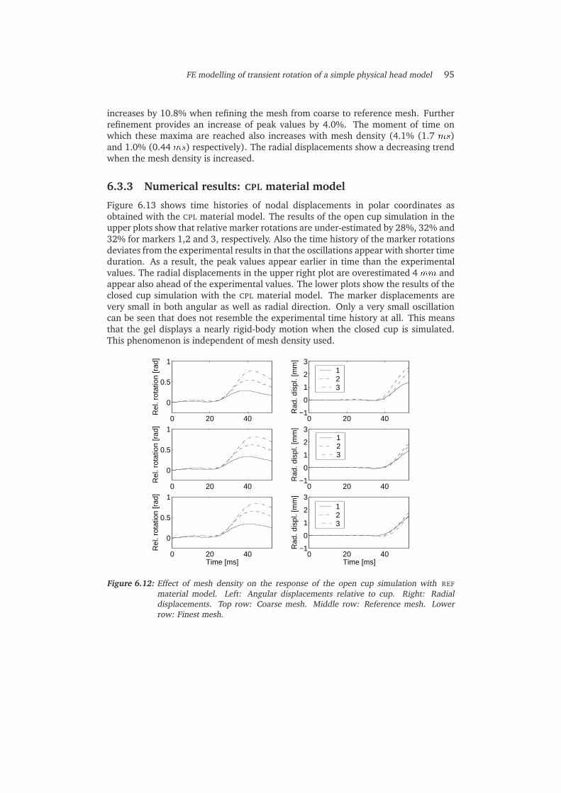
FE modelling of transient rotation of a simple physical head model 95
increases by 10.8% when refining the mesh from coarse to reference mesh. Furtherrefinement provides an increase of peak values by 4.0%. The moment of time onwhich these maxima are reached also increases with mesh density (4.1% (1.7 ms)and 1.0% (0.44 ms) respectively). The radial displacements show a decreasing trendwhen the mesh density is increased.
6.3.3 Numerical results: CPL material model
Figure 6.13 shows time histories of nodal displacements in polar coordinates asobtained with the CPL material model. The results of the open cup simulation in theupper plots show that relative marker rotations are under-estimated by 28%, 32% and32% for markers 1,2 and 3, respectively. Also the time history of the marker rotationsdeviates from the experimental results in that the oscillations appear with shorter timeduration. As a result, the peak values appear earlier in time than the experimentalvalues. The radial displacements in the upper right plot are overestimated 4 mm andappear also ahead of the experimental values. The lower plots show the results of theclosed cup simulation with the CPL material model. The marker displacements arevery small in both angular as well as radial direction. Only a very small oscillationcan be seen that does not resemble the experimental time history at all. This meansthat the gel displays a nearly rigid-body motion when the closed cup is simulated.This phenomenon is independent of mesh density used.
0 20 40
0
0.5
1
Rel
. rot
atio
n [r
ad]
0 20 40−1
0
1
2
3
Rad
. dis
pl. [
mm
]
123
0 20 40
0
0.5
1
Rel
. rot
atio
n [r
ad]
0 20 40−1
0
1
2
3
Rad
. dis
pl. [
mm
]
123
0 20 40
0
0.5
1
Time [ms]
Rel
. rot
atio
n [r
ad]
0 20 40−1
0
1
2
3
Time [ms]
Rad
. dis
pl. [
mm
]
123
Figure 6.12: Effect of mesh density on the response of the open cup simulation with REF
material model. Left: Angular displacements relative to cup. Right: Radialdisplacements. Top row: Coarse mesh. Middle row: Reference mesh. Lowerrow: Finest mesh.

96 Chapter 6
6.4 Discussion
The open cup experiments could be simulated quite well with the REF materialmodel. The time history of the marker angular displacements could be reproducedwith 22% accuracy. This difference may be caused by errors in the choice of thematerial parameter values. The values used were determined on a different gelspecimen than the one used in this experiment. The experimental data of threedifferent samples in Chapter 4 differed by approximately 0.2 to 20% depending onthe frequency used. The effect of this spread has been investigated by performingan additional simulation with material parameters increased by 10%. The resultsobtained with the reference mesh are shown in Figure 6.14. It can be observed thatthe model with increased parameters provides good predictions of the experimentallydetermined marker displacements. Maximum numerical errors in angular rotationequal 8.9%, 0.23% and 2.5% for marker 1,2 and 3 respectively.
The closed cup simulation results with REF material model also show overestimatedexperimental angular displacements but correct trends in time history. A possibleexplanation for this overestimation is again the uncertainty in the materialparameters. However, the fact that the overestimation in this isochoric deformationstate is more pronounced than in the open cup simulations suggests a secondhypothesis.In the REF material model, the hydrostatic behaviour is decoupled from the deviatoric
0 10 20 30 40−0.2
0
0.2
0.4
Time [ms]
Rel
. rot
atio
n [r
ad]
0 10 20 30 40
−0.2
−0.1
0
0.1
0.2
Time [ms]
Rad
. dis
pl. [
mm
]
1 2 Exp
0 20 40−0.2
0
0.2
0.4
0.6
0.8
Time [ms]
Rel
. rot
atio
n [r
ad]
0 20 40−1
0
1
2
3
4
5
Time [ms]
Rad
. dis
pl. [
mm
] 1 2 3 Exp
Figure 6.13: Marker trajectories obtained with reference mesh and CPL material model versusexperimental results (dotted line). Top: Open cup results. Bottom: Closed cupresults. Left: Angular displacements relative to cup. Right: Radial displacements.

FE modelling of transient rotation of a simple physical head model 97
part of the Cauchy stress (refer to equations (5.21) and (5.22) in Chapter 5).Furthermore the deviatoric stress depends on the deviatoric part of the isochoricdeformation only. As a result, the shear behaviour of the model is independent of thehydrostatic deformation. If, in reality, some coupling between shear and hydrostaticdeformation is present, implementation of this coupling in the material model willlead to reduced displacements in the simulation results. This will be more pronouncedin the closed cup simulation than in the open cup simulation. However, the presenceof this partial coupling could not be validated in the present material experimentsand remains to be investigated. This can be done by determining the normal forcehistory during a simple shear experiment or by applying a different deformation, forexample an unconfined compression.
Mesh density Increasing the mesh density using the REF material model, revealeddifferences in amplitude of the marker displacements on the order of 4%. The timehistory behaviour, i.e. the ’shape’ of the time history, did not change. This indicatesthat the results of the reference mesh can be used to indicate where and when peakstrain or stress values occur. Although it is unclear whether the results of the finestmesh used were not mesh-size independent yet, no further mesh refinement has beenperformed since this would yield excessive computational times.
Effect of decoupled hydrostatic and deviatoric stress The importance ofdecoupling the hydrostatic strain from the deviatoric stress was clearly illustratedby the results with the CPL material model. The open cup simulation showedunderestimation of the strain response, whereas in the closed cup simulation virtuallyno strains were present at all. The reason for this behaviour will be illustrated usingan example.In absence of time dependent behaviour (G(t) = G), the constitutive equation (6.4)reduces to,
S = (K � 2
3G)trace(E)I + 2GE (6.6)
0 20 40−0.2
0
0.2
0.4
0.6
0.8
Time [ms]
Rel
. rot
atio
n [r
ad]
0 20 40−1
0
1
2
3
Time [ms]
Rad
. dis
pl. [
mm
] 1 2 3 Exp
Figure 6.14: Marker trajectories obtained with reference mesh, REF material model and 10%increased material parameters, versus experimental results (dotted line). Left:Angular displacements relative to cup. Right: Radial displacements.

98 Chapter 6
which in fact represents Hooke’s law for linear elastic materials in which theinfinitesimal strain measure " is replaced by the Green-Lagrange strain E. Let usassume that the deformation patterns in the closed cup resemble that of isochoricsimple shear. The resulting shear stress component of the Cauchy stress ,� , thendepends on both shear modulus, G, and bulk modulus, K,
� = G
� +
2
3 3�+
1
2K 3 (6.7)
Due to the nearly incompressible material behaviour (G = 1000 Pa and K = 109 Paapproximately, refer to Table 6.1), the last term in equation (6.7), related to the bulkmodulus, will dominate the shear behaviour already for very small strains: for = 1%this term will be a factor of 50 larger than the first term, related to the shear modulus.This behaviour does not correspond with the behaviour observed experimentally.
6.5 Conclusions
A simple physical model was used to create a response in silicone gel model materialresembling that of brain tissue in a traffic related impact. Two variants were used, anopen cup and a closed cup. In both geometries gel responses resembling brain tissueimpact response could be obtained. Maximum principal strain values of 49% and15% occurred during open and closed cup experiments, respectively. These are in theorder of the 20% strain threshold above which tissue damage was induced in animalexperiments. The strain rates obtained in the experiments (45 s�1 and 20 s�1 foropen and closed experiment, respectively) are also of correct magnitude compared tothe 20 s�1 value estimated to be present in a real head during impact.The open cup experiments could be simulated very well using the material modeldeveloped in Chapter 5. Maximum errors in angular marker displacements whereless than 22% and reduced to 8.9% when the material properties were increasedwithin the experimental range shown in Chapter 4 (10% increase). The closedcup trajectories were overestimated by 62% but time history looked realistic. Apossible explanation might be the assumed decoupling between shear and hydrostaticdeformation in the constitutive formulation (refer to section 6.4). Increasing the meshdensity from 28 to 56 elements per cup diameter yielded changes of displacementsof 4% only but did not alter the nature of the time history. This supports the rule ofthumb derived in Chapter 2, that 24 elements per maximum wave length are neededfor accurate modelling.The closed cup simulations showed that without decoupling the hydrostatic anddeviatoric parts of the stress, the stiffness at finite shear strain was severelyoverestimated. This effect was largest for the closed cup simulation. Thisillustrates the importance of correct constitutive modelling when dealing with nearlyincompressible behaviour, especially when applying such material model in a headmodel which also consists of a more or less closed geometry. The presence of thiseffect in a real head model will therefore be studied in the next chapter.

Chapter 7
Effects of constitutivemodelling on brain response in
a 3-D FE head model
It is investigated how the choice of brain constitutive model affects the dynamic response of braintissue in a three-dimensional head model. Three brain models are used: the model presentedin Chapter 5 with and without shear softening included, and the standard linear multi-modeviscoelastic material model present in MADYMO 5.4.1. In the latter model, the deviatoric andhydrostatic response is not decoupled, in contrast to the first two model variants. The headmodel is subjected to a transient eccentric rotation in the sagittal plane and the brain response isinvestigated in quantities, commonly associated with injury. It was found that large strains occurat modest impact conditions. This is most likely caused by the values for the shear moduli appliedin the model. These are at least a factor of ten lower than the ones used in head models in literaturebut comparable to material data in recent literature and own experiments. Shear softeninginfluences the strain and stress levels but not the spatial distribution. The pressure responsewas of quasi-static nature and did not depend on non-linear material behaviour. Decoupling ofdeviatoric and hydrostatic deformation in the constitutive model was found to be necessary forcorrect prediction of brain response in head modelling.
99

100 Chapter 7
7.1 Introduction
In previous chapters a non-linear viscoelastic material model capable of describingthe material behaviour of brain tissue under simple shear conditions was presented.The model is capable of describing the shear softening observed for strains up to20%. Physical model simulations in the previous chapter pointed out that the modelis capable of accurately predicting the dynamical response of a nearly incompressiblelinear viscoelastic material under impact conditions. It was found that decouplingof the deviatoric and volumetric deformation in the stress tensor was crucial for thegood performance under isochoric deformations.In the present chapter, the constitutive model is applied in a three-dimensional headmodel, subjected to rotational acceleration history in posterior-anterior direction.To investigate the effect of shear softening as well as decoupling of volumetric anddeviatoric deformation, brain tissue’s constitutive description is changed accordingly.The effect of the various modelling approaches will be analysed by comparingpredicted local brain responses, expressed in quantities associated with injury inliterature.
7.2 Numerical model
The head model used was originally developed in the implicit Finite Element CodeMARC [88] by Claessens [36] and has been evaluated using intracranial pressureresponses obtained from a cadaver experiment by Nahum [37; 104]. This model wastransfered to the explicit Finite Element Code LS-DYNA3D [86] for use in an accidentreconstruction study [154]. In that study improvements with respect to element sizeand shape were carried out. Furthermore, the anatomical detail of the model wasincreased by including a more realistic geometry near the skull base and falx cerebriand by including an element layer between cerebri and skull to model the dura mater.In the present study, the model is transformed to MADYMO 5.4.1 format[146]. Allmaterial descriptions were retained except for the constitutive model and modelparameters of the brain tissue. In the next sections the model will be presentedbriefly. More detailed information about the model can be found in the work ofClaessens [36; 37] and Verhoeve [154].
Geometry The geometry of the model is based on the Visible Human data set[153] which consists of MRI (Magnetic Resonance Imaging) and CT (ComputedTomography) transversal images of a male person. Head length (195 mm), width(155 mm) and height (225 mm) have been scaled to 50th percentile measuresaccording to Pheasant [119]. The anatomical structures, included in the model,are shown in Figure 7.1. They are grouped in three components; the cranium, themeningeal layers and CSF, and the brain tissue. Table 7.1 provides information oneach component and constitutive models used. All substructures in the head modelare assumed to be rigidly connected to each other. The brain is tied to the skull viaa layer of compliant elements and the motion of brain tissue through the foramen

Effects of constitutive modelling on brain response in a 3-D FE head model 101
magnum is suppressed. The head is meshed in one continuous mesh consisting of8-node brick elements. Spatial integration is achieved using one integration point perelement only (reduced integration). Hourglass control is used to suppress the zeroenergy deformation modes that exist for reduced integrated brick elements [148].
Constitutive assumptions In this study we will not model a direct contact impact.For this reason the cranium is assumed to be rigid. The meningeal layers weremodelled as in the original model by Claessens [36; 37], i.e. linear elastic materialmodel with material parameters taken from Ruan et al. [126] (refer to Table 7.2).The brain tissue is modelled using a four mode viscoelastic material model. Threemodelling variants have been investigated:
1. REF: In the reference simulation, the brain tissue is modelled using the newlydeveloped material model with linear material parameters, i.e. shear softeningis not included.
2. SOF: Like REF but with shear softening added.
Cerebellum
Cerebrum
Falx Cerebelli
Falx cerebri
Brainstem
Dura mater
Neurocranium
Viscerocranium
Tentorium cerebelli
Figure 7.1: Overview of the head model [154]. The right half of the head model is shown withthe brain, the meningeal layers (dura mater with falx and tentorium) and the skullseparated. In the model, these structures are connected to each other, resulting ina continuous Finite Element mesh.

102 Chapter 7
3. CPL: The linear viscoelastic material model as present in MADYMO version 5.4.1has been used (LINVIS). This model linearly couples the second Piola-Kirchoffstress tensor to the Green-Lagrange strain and includes viscous behaviour usingan integral form. As a result deviatoric and hydrostatic part of the deformationare not decoupled. (Refer to the Discussion section of Chapter 6 for moredetails).
Comparing the REF and SOF results provides insight into the effect of shear softeningon the dynamic response of brain tissue. Comparing the REF and CPL results showsthe importance of decoupling the deviatoric and hydrostatic parts of the deformationin the stress formulation in a realistic head geometry.The decoupled non-linear viscoelastic material model used in the SOF simulation, is aslightly adapted version of the model presented in Chapter 5. The latter model, wascapable of predicting the shear softening observed within the experimental strainrange (up to 20% shear strain). However, for strain levels outside the experimentalstrain range, negative shear stiffness can occur. To prevent numerical problemsassociated with negative stiffness, an extra deviatoric stress was added to thedeviatoric stress part of the original model. The stress formulation was chosen suchthat its effect on the response is minimal within the experimental strain range whilenegative stiffness is prevented for shear strains beyond that range. However, this extrastress will cause shear stiffening to occur for strains beyond the experimental range.For this reason extra care has to be taken in interpreting results at strains outside theexperimental range. The complete theory on the model adaptation is presented inAppendix B.
Table 7.1: Configuration of the head model used; presentation of the structures included, thenumber and type of elements used, and constitutive models used.Anatomical structure No. of elements Constitutive modelCranium (skull) 3212 Rigidviscerocranium (facial bones) 188neurocranium 3024Meningeal layers & CSF 3188 Linear elasticDura mater 2536- falx cerebri 448- falx cerebelli 18- tentorium cerebelli 186Brain tissue 7692 Viscoelastic*cerebrum/corpus callosum 6758cerebellum 732brainstem 202* Three variants are used:REF: decoupled-linear viscoelastic: no shear softeningSOF: decoupled non-linear viscoelastic: shear softening.CPL: linear viscoelastic, coupled deviatoric / hydrostatic behaviour

Effects of constitutive modelling on brain response in a 3-D FE head model 103
Brain tissue material parameters are taken from Chapter 5. Except for the non-linearparameter, fnls which has been fitted again to eliminate the small effect within theexperimental range caused by the model adaptation (refer to Appendix B). They areshown in Table 7.2.
Loading conditions An eccentric rotation in posterior-anterior direction has beenapplied to the model using a time history obtained from [11]. The axis of rotationis positioned at 155 mm below the anatomical origin of the model which is locatedin the ear hole projected to the sagittal plane. The eccentricity resembles a typicalneck length [49; 144]. The rotational acceleration time history consists of two sinefunctions shown in Figure 7.2, where the initial acceleration portion equals twice theamplitude and half the duration of the subsequent deceleration portion. The totalrotational pulse duration was set to 30 ms whereas the maximum angular velocitywas set to 5 s�1 as to obtain strain values inside the brain tissue within the rangeof the material characterization experiments in Chapter 4, i.e. 20% shear strain
Table 7.2: Material properties used for the anatomical components in the three-dimensionalhead model.
Structure Shear modulus Time constants Bulk Non linear MassGi i = 0� n �i, i = 0� n modulus K par. fnls density
[Pa] [ms] [GPa] [�] [ kgm3 ]
Cranium(skull)
1 - 1 - 2070
Meninges& CSF
1:086 � 106 - 0:105 - 1130
Brain tissueREF, CPL 255, 269, 323 1,70.1, 7.63 2.5 0 1040
427, 3299 1.41, 0.12SOF 255, 269, 323 1,70.1, 7.63 2.5 -5.5553 1040
427, 3299 1.41, 0.12
0 10 20 30−500
0
500
1000
Time [ms]
Rot
atio
nal a
cc. [
s−2 ]
0 10 20 300
1
2
3
4
5
Time [ms]
Rot
atio
nal v
el. [
s−1 ]
��������
Figure 7.2: Angular rotation history used according to [11]. Left: Angular acceleration andschematic indicating direction of acceleration. Right: Angular velocity. Timeduration set to 30 ms and maximum angular velocity to 5 s�1.

104 Chapter 7
corresponding to a Von Mises strain of approximately 0.22. This results in a maximumhead rotation angle of 0.075 rad.
Time discretisation The MADYMO Finite Element module uses the conditionallystable Central Difference Method for time integration, as is common in explicit FiniteElement codes. The maximum time step for obtaining a stable solution is determinedby the Courant criterion which depends on mesh size and wave propagation velocity.In Chapter 2 is shown that application of the maximum time step provides the mostaccurate solution. In the present simulations this maximum time step is multipliedby 0.85 and kept constant during the complete simulation. This yields a time step of4 �10�4 ms, which results in 75000 time increments to simulate the full 30 ms impact.
Post processing The effect of the various brain tissue modelling approaches onthe dynamical brain response will be investigated in terms of parameters associatedwith injury. In Chapter 1 (Table 1.1) it has been shown that shear strain, maximumprincipal strain, Von Mises stress and pressure have been identified by various authorsas potential causes for brain injury. These parameters can be described by thefollowing three quantities,
� Von Mises, or effective, strain, EVM =q
32 trace(Ed �Ed): This rotation
invariant strain measure depends on the deviatoric Green-Lagrange strain,Ed, only and is a measure of distortional deformation. As such, it provides
information on shear deformation present in the brain tissue. Furthermore,this measure closely resembles the maximum principal strain due to the nearlyincompressible nature of the brain tissue.
� Von Mises stress, �VM =q
32 trace(�d � �d): As viscoelastic material behaviour
is assumed, the stress measure depends both on strain and strain rate quantities.Differences between Von Mises stress and Von Mises strain distributionstherefore reflect the contribution of strain rate effects.
� Pressure, p = � 13 trace(�): Apart from being a potential injury cause, this
quantity has been used in many studies [37; 72; 128; 129; 168], for evaluatinghead models against cadaver experiments by Nahum [104].
For each element in the brain mesh, maximum values appearing during the impacttime history are determined and shown in contour plots of various para-sagittal cross-sections. Areas of interest will be determined and the time history of the quantities inthese areas will be plotted.
7.3 Results
All simulations are performed on a Silicone Graphics Origin computer, with a 180MHz, IP 27, R10.000 processor. The computational time equals approximately 10hours and 30 minutes for all model variants.

Effects of constitutive modelling on brain response in a 3-D FE head model 105
7.3.1 Reference model: REF
Figure 7.3 shows contour plots of the maximum Von Mises strain and stress valuesduring the impact in various para-sagittal cross-sections in the brain. The Von Misesstrain ranges up to about 0.3 while the Von Mises stress ranges up to approximately400 Pa. Both stresses and strains show similar, concentric, contour patterns withminimum values concentrated in the center of the cerebri. Maximum values appear atthe upper part of the cerebral cortex (cross-sections 2 and 3 in Figure 7.3), in the mid-brain section (cross-section 1) and superior to the tentorium cerebelli (cross-sections3 and 4). Another concentration of maximum values is found in the concave regionnear the temporal lobes. These will not be taken into account in the next discussionsince it is believed that this maximum is severely influenced by bad element qualityin that region.The Von Mises stress and Von Mises strain histories in two elements, located in thesuperior cerebral cortex region (C) and in the mid-brain (M) are plotted in Figure7.4. Both Von Mises strain and Von Mises stress time histories show the sametendencies. The mid-brain time histories of both stresses and strains lag behind thetime histories in the cortical region. In turn, the cortical time histories lag behindthe input rotational acceleration pulse in Figure 7.2. In both regions the strain timehistory lags behind the stress time history. Finally, superior cortex stress and strainvalues approach to zero at about 20 to 25 ms, while midbrain stress and strain levels
Stress [Pa]70 3502802101400.0
0.25 Strain [-]0.05 0.10 0.15 0.200.0 1234
1 2 21
3 4
Maximum Von Mises stressesMaximum Von Mises strains
43
Figure 7.3: Para-sagittal cross-sections (1 to 4) showing Von Mises strains (left) and stresses(right) in the brain section of the three-dimensional head model in referencesimulation ( REF). Maximum values appearing during complete impact time historyare shown.

106 Chapter 7
remain relatively high.The pressure response of the REF model is shown in Figure 7.5. The upper contourplot, in the left part of Figure 7.5, shows the pressure distribution at t = 5ms, whichis at maximum positive angular acceleration. Positive pressures arise in the posteriorregion while negative pressures are present in anterior region. The lower plot is takenduring maximum deceleration of the head, at t = 20ms. It can be seen that pressuresin anterior and posterior region changed sign while absolute values are lower thanduring acceleration. In both plots the spatial pressure gradient in A-P direction isnearly a constant. This is also true for other moments in time not shown in Figure7.5.To study the pressure time history, two elements were selected located on posterior(P) and anterior (A) regions (see left plot of Figure 7.5). The pressure time historiesin both P and A element are plotted in the right part of the figure. As seen in thecontour plots, the pressures differ in sign. Their time behaviour follows the rotationalacceleration input history of Figure 7.2. The largest pressure difference between Pand A element occurs at 5.0 ms and equals 27.8 kPa.
0 10 20 300
100
200
300
400
Time [ms]
σ VM
[Pa]
MC
0 10 20 300
0.1
0.2
0.3
0.4
Time [ms]
EV
M [−
]
M
C
Figure 7.4: Time histories of Von Mises stress (left) and Von Mises strain (right) in twoelements located in Mid-brain region (M) and superior cerebral Cortex region (C).
0 10 20 30−20
−10
0
10
20
Time [ms]
p [k
Pa]
PA
-7.5 -2.5 2.5 7.5 12.5
[kPa]3.01.2-0.6t=20 ms
-2.4-4.2
[kPa]t=5 ms
t= 5 msP
A
t= 20 ms
Figure 7.5: Pressure response of the brain in reference simulation ( REF). Right: Time historyof pressure in two elements at posterior (P) and anterior (A) region. Center:Pressure contour plots with different scaling at t = 5 ms and t = 20 ms.

Effects of constitutive modelling on brain response in a 3-D FE head model 107
7.3.2 Model variants: cpl and sof
Figures 7.6 and 7.7 show contour plots of maximum values of Von Mises strains andstresses for all model variants. The SOF variant provides approximately the samespatial distribution of maximum Von Mises stresses and strains than the REF model.However, maximum strain values increase by approximately 21% whereas maximumVon Mises stresses tend to decrease by 11%.The CPL variant clearly provides completely different stress and strain patterns thanthe REF model. Strain levels are lower by a factor of 10 and the concentric patternspresent in REF and SOF are less evident. The Von Mises stresses are higher by
0.250.100.050.0 0.200.15
SOF
REF
21
21
21 3
3
3 4
4
4
CPL: Strains X 10
Von Mises strain values [-]
2
43
1
Figure 7.6: Para-sagittal cross-sections (1 to 4) showing maximum values of the Von Misesstrains in the brain section of the three-dimensional head model. Top row, SOF:shear softening. Middle row, REF: reference simulation. Lower row, CPL: coupledhydrostatic part (strains � 10).

108 Chapter 7
approximately a factor of five but the concentric pattern remains present.The Von Mises stress and Von Mises strain time histories for the element locatedin the mid-brain region selected previously (M) are shown in Figure 7.8. The leftplot shows that the maximum strain level increases in the SOF simulation whereas itoccurs later in time. The stress history in the right plot, shows that shear softeningleads to decreasing maximum stresses which again appear later in time than in theREF simulation.The results of the CPL variant differ strongly from the reference results. The VonMises strain values remain close to zero during the complete simulation while the
SOF
REF
21
21
21 3
3
3 4
4
4
2
43
1
CPL: Stresses X 0.2
Von Mises stress values [-]
0.0 35028021014070
Figure 7.7: Para-sagittal cross-sections (1 to 4) showing maximum values of the Von Misesstresses in the brain section of the three-dimensional head model. Top row, SOF:shear softening. Middle row, REF: reference simulation. Lower row, CPL: coupledhydrostatic part (stress � 0.2).

Effects of constitutive modelling on brain response in a 3-D FE head model 109
stress shows high peaks. Furthermore higher frequencies seem to be present in bothstress and strain histories.The spatial pressure response shows constant gradients for all model variants and istherefore not plotted. The pressure time history of elements located in anterior (pA)and posterior region (pP ) is shown in Figure 7.9 as well as the pressure difference,�p = pP � pA. Since the spatial pressure gradient is a constant in posterior-anterior direction, the pressure difference over head length provides a measure forthe pressure gradient. The effect of shear softening on the pressure response isnegligible (maximum difference 0.3 Pa). The element pressure histories of the CPL
model variant differ completely from the reference model; the time history doesnot follow the input angular acceleration any more. Instead the pressure showsan oscillatory history that remains mainly negative for both posterior and anteriorelement. However, the A-P pressure difference in the CPL model equals the oneobtained with REF variant within 2 kPa.
0 10 20 300
0.1
0.2
0.3
0.4
Time [ms]
EV
M [−
]
0 10 20 300
0.2
0.4
0.6
Time [ms]
σ VM
[kP
a]
REF SOF CPL × 0.2
M
Figure 7.8: Effect of brain tissue modelling variants, Von Mises strain (left)and Von Mises stress(right) histories of element in mid-brain region (M). Note: �VM �0:2 at CPL result.
0 10 20 30−60
−40
−20
0
20
Time [ms]
p [k
Pa]
P
0 10 20 30−60
−40
−20
0
20
Time [ms]
A
0 10 20 30−20
−10
0
10
20
30
Time [ms]
∆p [k
Pa]
REFSOFCPL
AP
Figure 7.9: Pressure time histories of elements located in posterior (P) (left) and anterior (A)region (center) as well as pressure difference: �p = pP � pA (right) to illustratethe effect of brain tissue modelling variants.

110 Chapter 7
7.4 Discussion
In this chapter three modelling variants of the constitutive behaviour of brain tissueare applied in an existing Finite Element head model. The effects on the responsecaused by shear softening and by the decoupling of hydrostatic and deviatoricdeformation in the brain tissue material model have been investigated. Other modelassumptions such as geometry and constitutive behaviour of different parts of thehead were left unaltered. As such the conclusions presented hold within the currenthead model. Extrapolation to reality depends on the quality of the other modelassumptions which were not subject of research in this chapter.
7.4.1 Numerical model accuracy
The accuracy of the Finite Element procedure used, is determined by time-step andthe mesh density. In Chapter 2 it is shown that maximum accuracy is reached whenthe time step is chosen close to the required step for stability. For this reason themaximum allowable time step in MADYMO was used. The mesh density will becharacterized by the number of elements over the head diameter. For the brainsection in the model 20, 22 and 22 elements are used in anterior-posterior, superior-inferior and lateral direction respectively. In Chapter 6 it was concluded that typically28 elements over the diameter are needed for accurate prediction of the dynamicalresponse of a physical model. As a result, the computed solutions will not be atmaximum accuracy. This is especially true since the required mesh density wasobtained in a homogeneous model, without substructures of different stiffness andmass density as is the case in the head model. However, for practical reasons the useof a higher mesh density has been omitted. Furthermore, it was shown in Chapter6 that a coarse mesh (11 elements per diameter) did not alter the nature of theresponse. For this reason it is believed that the response predicted by the model willreflect trends due to different material modelling correctly.In the head model, linear (constant strain) elements with reduced integration andlumped mass matrixes are used. Although computational effective, these elementsallow zero energy modes or hourglass modes to be present which can be suppressedby adding a small stiffness capable of stopping the formation of the anomalous modesbut having negligible effect on the stable global modes. No details on the hourglasssuppression method in MADYMO were found, but examples of suppression methodscan be found in [52] and [78]. During the simulations in this chapter, the hourglasssuppression routine contributed less than 4.5% to the total internal energy of themodel.
7.4.2 Reference model response
The level of the angular velocity used, is chosen as to obtain strains within the rangefor which the material properties measured are valid (20% maximum engineeringshear strain). The resulting maximum acceleration equals 750 rad=s2 and theangular velocity equals 5 rad=s. This is lower than typically used in other model

Effects of constitutive modelling on brain response in a 3-D FE head model 111
studies. Bandak & Eppinger (1995) applied the same time history with maximumrotational velocity set to 35 rad=s and found principal strains on the order of 0.1[11]. Application of this loading history on the present REF model leads to maximumprincipal strains and Von Mises strains exceeding 1.0. Zhang et al (2001) modelleda direct impact and found maximum shear strains on the order of 0.06 [167].Unfortunately no acceleration histories were provided.To explain the discrepancy between present findings and those in literature, the levelsof shear moduli used will be investigated. The material parameters used in presentmodel were obtained from the brain material data in Chapter 4. This data was withinrange of that found in recent literature. However, older literature data suggests thatthe shear modulus of brain tissue is much higher. The shear moduli used in headmodels in literature are often based on this older data and are at least a factor of tenhigher than those used here [11; 37; 72; 99; 167; 169].To illustrate the effect of higher shear moduli in present model, a simulation wasperformed using a single mode linear variant of the new material model. Materialparameters for brain tissue as used by Zhang et al. [167] were taken: G0 = 7:1 kPa,G1 = 30:4 kPa, �1 = 1:43 ms and K = 2:19 GPa. The time duration and maximumangular velocity were set to the average values used by Bandak & Eppinger [11]; 20ms and 25 rad=s respectively. This results in a maximum angular acceleration of 6000rad=s2. The maximum Von Mises strains equal approximately 0.15, which is withinthe expected range especially since the moduli used here were on the lower bound ofthose found in literature. For this reason it can be concluded that the discrepancy instrain levels between the present model and those in literature, most likely originatesfrom the shear moduli used.
Pressure response In Chapter 2 it was analytically estimated that the frequenciespresent in traffic related impacts are too low for pressure waves to exist inside braintissue. This has been verified using the simulation results in this chapter. The contourplots show that the pressure distribution over the brain displays a nearly constantgradient. The posterior-anterior pressure difference qualitatively follows the linearacceleration time history of the head. This indicates a quasi-static pressure response.In that case, the pressure difference at a certain moment in time, �p(t), can beestimated from the balance of momentum as,
�p(t) = ��x(t)l (7.1)
in which �x(t) equals the linear acceleration, � the mass density and l a typical lengthmeasure. The linear acceleration can be estimated from the product of the angularacceleration and the neck length (155 mm), while the head length (195 mm) servesas typical length measure, l. Inserting the maximum angular acceleration 750 s�2, att = 5 ms, provides an estimated �p of 24 kPa which agrees qualitatively with themaximum value in Figure 7.9, �p = 28 kPa.The pressure difference is independent of the material behaviour assumed in bothnumerical results and quasi-static theory. Furthermore, it was shown in Chapter 2that the pressure distribution poses the least demands on numerical accuracy due toits high wave propagation velocity. For these reasons it can be concluded that pressure

112 Chapter 7
difference is not a critical measure for testing the quality of both material model andnumerical model during traffic related impacts.
7.4.3 Variation of material models
Shear softening The contour plots in Figures 7.6 and 7.7 reveal that the shearsoftening does not alter the overall pattern of the stress and strain field present in thehead, however the level of stress and strain quantities is changed. The histograms inFigure 7.10 show the distribution of maximum Von Mises stress and strain values forall elements inside the brain. The left plot shows that, due to shear softening, higherVon Mises strains occur in favor of strains in the region of 0.12 to 0.2. The Von Misesstress distribution, shown in the right plot, shifts to lower values despite the largerstrains. Also the time history of stresses and strains shown in Figure 7.9 changesin level but not in shape. The pressure response was not significantly changed byapplication of the shear softening. This is as expected since shear softening acts onthe deviatoric part of the stress only.
Coupling deviatoric and hydrostatic parts The decoupling of deviatoric andhydrostatic parts of the stress has large influence on spatial and temporal stressand strain distribution. As seen in Figure 7.10, the coupled LINVIS model presentin MADYMO 5.4.1 provided low strains with high stresses. This trend agrees withthe results of the physical model simulations in Chapter 6. In that chapter itwas concluded that stresses were over predicted when an isochoric deformationwas enforced. It can be concluded that, even when surrounded by a relativelycompressible modelled skull-brain interface, coupling of deviatoric and hydrostaticdeformation parts in the stress formulation leads to severe overestimation of the stresswhile the strain is underestimated.The pressures in posterior and anterior brain region showed large differences with
2 6 10 14 18 22 26 300
5
10
15
20
25
30
35
EVM × 100 [−]
Ele
men
ts [%
]
CPLSOFREF
50 150 250 350 450 550 650 >7500
20
40
60
80
σVM [Pa]
Ele
men
ts [%
]
100%
Figure 7.10: Histograms showing the distribution of maximum Von Mises strain, EVM (left)and maximum Von Mises stress, �VM (right) over the elements in the brain.Results of all modelling variants shown.
Effects of constitutive modelling on brain response in a 3-D FE head model 113
respect to the reference simulation. The pressure response did not follow the inputangular acceleration anymore. However, posterior-anterior pressure differences weresimilar to the reference simulation, indicating that conservation of momentum hasbeen satisfied.
7.5 Conclusions
In this chapter, it is investigated how the choice of brain constitutive model affects thedynamic response of brain tissue in a three-dimensional head model. Effects of shearsoftening and decoupling of deviatoric and hydrostatic behaviour on the responsehave been investigated leading to the following conclusions:
� Shear softening mainly influences the levels of deviatoric strain and stress butnot their spatial and temporal distributions.
� The decoupling of deviatoric and hydrostatic parts of the deformation in thestress formulation has large influence on both spatial and temporal distributionof stress and strain. Using a fully coupled model (linearly coupling second-orderPiola-Kirchoff stress to Green-Lagrange strain) causes severe overestimation ofmaterial stiffness for nearly incompressible materials such as brain tissue.
� With the fully decoupled model large strains at modest impact conditions werefound. This is probably caused by the shear stiffness used which were a factor10 lower than those used in head models in literature but comparable to recentmaterial measurement data on brain tissue.
� The pressure history, and especially the pressure gradient history is a poormeasure for determining the quality of a head model, as often done in literature.During the load applied in present study, which is typical for traffic relatedimpacts, the pressure gradient is completely determined by the equilibrium ofmomentum, and thus independent of the choice of the brain material model.

114 Chapter 7

Chapter 8
Discussion, Conclusions andRecommendations
In this Chapter, an integral discussion of the results of the previous chapters will be provided.Conclusions will be drawn and recommendations for further study will be provided.
115

116 Chapter 8
8.1 Introduction
The head is identified as the body region most frequently involved in life-threateninginjury in crash situations [46]. For a better understanding of the way in which anexternal mechanical load applied on the head during an impact leads to brain injury,the internal mechanical response of the brain tissue has to be known. Finite Elementhead models are an important tool for assessment of the internal mechanical responsein various research strategies. This research aims to contribute to the improvementof these FE models. The objectives of this research were formulated in Chapter 1 as:
� to investigate the accuracy of numerical methods commonly used for predictingbrain response (explicit FEM) in crash impact, especially in relation to wavepropagation,
� to develop a constitutive model for describing the nearly incompressible, non-linear viscoelastic behaviour of brain tissue in a Finite Element model,
� to asses the effects of non-linear material behaviour on the internal mechanicalresponse by applying the constitutive model in a 3-D Finite Element model, and
� to discuss the consequences of this research for current state of the art headmodelling.
Developments on spatial and temporal discretisation methods used in the FiniteElement Method were not a topic of this research. In section 8.2 the way in whichthese objectives were met are discussed. Then conclusions will be drawn in section8.3. Finally, recommendations for future research will be provided.
8.2 Discussion
8.2.1 Requirements for the numerical accuracy of FE head models
The internal mechanical response of the head may be either of wave propagationnature or of structural dynamics nature, depending on the type of impact on the head.The modelling requirements for wave phenomena are higher than for modelling astructural dynamics response since higher strain gradients are present over smallervolumes of material. The relevance of wave propagation in the internal mechanicalresponse was investigated on the basis of a small strain analysis in Chapter 2. It wasfound that shear waves (S-waves) can be expected during a traffic related impact,(frequencies between 25 and 300 Hz), while compressive waves (P-waves) areexpected during short duration, high velocity, ballistic impacts (frequencies between10 kHz and 3 MHz). For this reason FE head modes should be capable of accuratereplication of strain wave propagation inside brain tissue.When modelling wave propagation using the explicit Finite Element Method withreduced integrated elements and lumped mass matrices (common in crash researchFE modelling) two types of error appear in the solution: numerical dispersion and
Discussion, Conclusions and Recommendations 117
spurious reflection due to mesh inhomogeneities. These errors cause the predictedwave propagation velocity to be too low and strain and strain rate levels will deviatefrom reality. These errors can be reduced by choosing spatial discretisation sufficientlysmall. From one-dimensional simulation results in Chapter 2 it was estimated thatat least 24 elements per maximum wave length are required for reducing the errorin wave propagation velocity to less than 1%. The errors in strain and strain rate,which increase with distance traveled, then equal 1% and 2.5% respectively aftera wave has traveled 1.66 its maximum wavelength. The physical model simulationresults in Chapter 6 indicate that this mesh density requirement is also valid for athree-dimensional deformation situation. The error made by applying the CentralDifference time integration scheme proved to be compensatory for the error by thespatial discretisation. For this reason the time step was kept as large as possible, butwithin the range for obtaining a stable solution (Courant number close to 1).
8.2.2 Brain tissue constitutive behaviour: experiments and model
In Chapter 3, the small strain behaviour of porcine brain tissue was determined usingoscillatory shear experiments on a rotational plate-plate viscometer. Frequencies to1000 Hz could be obtained using the Time/Temperature Superposition principle. Thelarge shear strain behaviour was investigated in Chapter 4, at strain levels associatedwith the occurrence of injury (20% shear strain [141]). Stress relaxation experimentswere performed since these allow interpretation of the experimental results atconstant strain without making constitutive choices beforehand. Brain tissue showedshear softening (i.e. decrease in stiffness) for strains above 1% (approximately 35%softening for shear strains up to 20%) while the time relaxation behaviour was nearlystrain independent. The validity of the time-strain factorization is valid still needsto be investigated for frequencies above 10 Hz, especially since recent experimentaldata suggests that time-dependent non-linearities might be present in brain tissue athigher frequencies [39].A non-linear viscoelastic material model for the large strain behaviour of brain tissuein impact conditions has been presented in Chapter 5. Hydrostatic and deviatoricparts of the strain are separated in the stress formulation. The hydrostatic partis assumed to be linear elastic and depends on volumetric deformation only. Theinelastic, time dependent behavior is described with a simple Newtonian law thatacts on the deviatoric stress contribution only. The shear softening observed isdescribed by the deviatoric elastic part which is modelled by a non-linear second-order Mooney-Rivlin model, based on isochoric deformation only. The constitutivebehaviour is formulated in differential form, in which the Cauchy stress is calculatedin a total Lagrangian formulation. This allows easy alterations to both elastic andviscous behaviour when needed. Furthermore, in contrast to an incremental UpdatedLagrangian approach commonly used, no time-step dependent approximation errorsare introduced when large rotations are present. To this authors knowledge this isthe first time that a non-linear viscoelastic model is implemented in this mannerin an explicit Finite Element code. Brain tissue material parameters were obtainedfrom small strain oscillatory experiments and the constant strain part from the stress

118 Chapter 8
relaxation experiments.The deviatoric part of the model has been tested by 3-D simulations of the rotationalviscometer stress relaxation experiments including the transient loading part. It wasfound that the model captures the mechanical phenomena observed experimentally,shear softening and viscous behaviour, for strains within the experimental region i.e.shear strains up to 20%. For strains outside this region the model is not validated.In fact, for simple shear exceeding 20% shear strain the model predicts a negativetangential stiffness. To prevent this from happening, the constitutive model wasextended with third order terms. For shear strains over 40% the extended modelpredicts shear stiffening behaviour instead of shear softening which is probably notrealistic for brain tissue (refer to Appendix B). Furthermore it is unknown whether themethod used for preventing negative tangential stiffness is valid for every arbitrarydeformation.The importance of correct separation of deviatoric and volumetric parts of thedeformation in the stress formulation was illustrated in simulations of physical modelexperiments (Chapter 6). In these experiments, a cylindrical cup filled with siliconegel, mimicking the brain material, was subjected to a transient rotation. It wasshown that the model could predict measured gel displacement within 20% errorrange. Application of a material model without correct decoupling of isochoric andvolumetric strain parts in the formulation, clearly showed that the response in aclosed geometry was severely underestimated resulting in a nearly rigid body likemotion of the gel.
8.2.3 Application in a three-dimensional head model
The non-linear material model was applied in a three-dimensional head model inChapter 7. The external mechanical load on the 3-D FE head model (an eccentricrotation) was chosen such as to obtain strains within the validity range of the materialmodel (i.e. up to to the tissue level tolerance level of 20% shear strain). It wasobserved that, in the head model, the tissue tolerance level was reached at externalloading values below the ones associated with injury in literature (e.g. in [109]).This discrepancy may be partly explained by the fact that shear stiffness in the modelis low compared to that in other models presented in literature. However, the stiffnessvalues used are considered to be realistic since they fit the experimental data well (seeChapter 5), while the experimental data is in range of material data found in recentliterature (see Chapter 3).Another possible explanation may be that hydrostatic and deviatoric parts of thedeformation are completely decoupled in the stress formulation, which has not beenverified experimentally. An indication for the presence of some degree of couplingis provided by the simulation results of the physical model in Chapter 6. The gelresponse in the open cup was less overestimated than in the closed cup. This indicatesthat, at least for the silicone gel used, volumetric behaviour (open versus closed cup)influences deviatoric behaviour (shear strain levels) in the physical model.Finally the reason for limiting the validity of the material model to 20% shear straincan be discussed. This range was based on two observations: first, obtaining reliable

Discussion, Conclusions and Recommendations 119
experimental data at strains outside this range was not possible with current testsetup, second, a 20% strain threshold for axonal injury was found in literature [141].For this reason it was assumed that 20% strain represents an upper boundary forstrains present in brain tissue during impact of the head. However, in a recent studythere was no evidence of mechanical damage during brain tissue stress relaxationexperiments up to 50% [123]. This implies that strain values exceeding 20% shearstrain might be present during head impact.The effect of shear softening on the brain response was investigated by applying thematerial model with and without shear softening in the head model. The resultsshowed that maximum Von Mises strain values increased by approximately 21%whereas maximum Von Mises stress values decreased by approximately 11% whenshear softening was applied. When interpreting these differences it should be notedthat maximum strain levels were concentrated in relatively small areas inside themodel. As a result, only a small fraction of the brain material experiences strainslarge enough to be influenced by shear softening. Furthermore, it should be notedthat these differences hold for one specific loading condition in one specific modelonly.
8.2.4 Consequences for head modelling
In Chapter 2 is is concluded that wave propagation is likely to occur during impactson the head. For this reason, head models should be capable of accurate predictionof wave propagation. When using explicit FEM, this accuracy depends on elementsize used. In current state of the art 3-D human head models the element size equalstypically 5 mm. This means that S-waves can be modelled accurately for frequenciesup to 42 Hz, about one tenth of the upper relevant frequency for S-waves to bepresent in the head. P-waves can be modelled for frequencies up to 13 kHz, aboutone hundredth of the upper relevant frequency for P-waves to exist. This means thatnone of these models will accurately predict wave propagation. As a result, computedmaximum strain values and strain rate values will be incorrect. Both quantities areassociated with the occurrence of brain injury (refer to Table 1.1 in Chapter 1) andshould be predicted correctly.Despite the limited accuracy of current head models, reported validation resultssuggest good performance of these models. The reason for this is that current 3-Dhead models are almost exclusively tested against pressure data obtained by Nahumet al. [104] from human cadavers subjected to frontal impact. The duration of thisimpact is typical for traffic related impacts and equals approximately 8 ms. This istoo long to introduce P-waves. As a result, a constant spatial pressure gradient willoccur which is completely determined by the equilibrium of momentum, and thusindependent of the choice of the brain material model. This has been confirmed bythe invariance of the pressure (gradient) response on the material model used in thenumerical model results in Chapter 7. Correct simulation of this pressure response,does not imply correct simulation of shear wave response.In current 3-D head models, brain tissue is modelled as a linear viscoelastic solid.The simulation results with the non-linear material model in Chapter 7 indicate

120 Chapter 8
that the reported strain values, obtained with linear models, are under estimatedwhile stress values are overestimated. However, the validity of these conclusionsin different models and loading conditions is not straight forward due to manydifferences between models such as different skull-brain interface models, different(linear) material parameters, etc.
8.3 Conclusions
� Wave propagation is likely to be present during impacts on the head.Dilatational (P) waves will propagate during ballistic impacts whereasdistortional (S) waves will propagate during traffic related impacts.
� For correct numerical modelling of propagation of both P-waves and S-waves,in explicit FE models, typically 24 elements per wavelength should be used.Furthermore the time step should be chosen as large as possible, i.e. the Courantnumber should be close to 1.
� Spatial discretisation in current 3-D Finite Element head models is too coarseto model wave propagation accurately. As a result, predicted maximum strainlevels and strain rate values will deviate from the real solution.
� Pressure history, measured in traffic related impact experiments is often usedto assess FE head model quality. Since pressure history during traffic relatedimpacts is completely determined by static equilibrium of momentum, it is nota critical measure for testing.
� For simple shear, brain tissue behaves as a non-linear viscoelastic solid. Itdisplays shear softening (i.e. decrease in stiffness) for strains above 1%.
� The time relaxation behaviour of brain tissue is nearly strain independent.However, for frequencies above 10 Hz this remains to be investigated.
� A three-dimensional non-linear viscoelastic material model that describes theshear softening observed in brain tissue under simple shear has been developedand implemented in the explicit MADYMO FE code. It has been shown thatthe model is capable of predicting realistic deformations by simulating physicalmodel experiments and material experiments.
� The material model has been applied in a three-dimensional head model for asingle loading case. It was found that shear softening influences mainly strainand stress levels but not their temporal and spatial distribution. Differences inpressure history were negligible.

Discussion, Conclusions and Recommendations 121
8.4 Recommendations
8.4.1 Numerical quality, validation of head models
Head models in explicit FEM can be made suitable for modelling S-waves by reducingthe mesh size to 0.5 mm. This seems feasible considering the rapid advances incomputer hardware. However, for P-waves, reducing the mesh size to 0.05 mm is nota realistic option. Instead alternative spatial discretisation methods should be pursuedsuch as the use of elements with quadratic displacement functions or generalisedmass matrix. Another method for increasing mesh density while maintaining realisticcomputational costs it the use of two-dimensional head models. A trend can beseen towards the development of two-dimensional head models that represent across sectional area of the head with very detailed geometry [100; 110]. However,additional assumptions on stress and strain boundary conditions are needed (plainstress / plain strain). Furthermore, out of plane phenomena cannot be studied in thistype of models.Validation methods for head models for traffic related impacts should focus on thedeviatoric strain response. A potential method to gain data on the deviatoric strainresponse in biological models is the MRI tagging method [43]. In principle thismethod enables non-invasive quantification of the strain field inside the brain inanimal experiments with high spatial resolution. However, application in the highfrequency range is not trivial and requires further investigation. A different source ofdata from ongoing research are human cadaver experiments in which high speedx-ray marker tracking techniques are used [3]. Drawbacks of this method arethe invasiveness (application of physical markers is required) and the low spatialresolution that can be reached. However, it main advantage is the high temporalresolution, sufficient for impact recording. Finally, the present research showed thatphysical models can be used to obtain more insight in the presence of numericalartefacts when they are designed to minimise the number of modelling assumptionsand to maximise mechanical accessibility. For this reason the use of physical modelsin this manner should be encouraged.
8.4.2 Constitutive modelling of brain tissue
The high-strain, high-frequency behaviour of brain tissue has to be determined.Inertial effects will have to be taken into account during analysis of the high frequencyexperimental data. This makes the analytical correction of the inhomogeneousstrain field applied in the rotational viscometer impossible. For this reason itis recommended to use a translating shear device that better approximates thehomogeneous simple shear conditions (see e.g. [39; 123]). Furthermore such deviceallows the investigation of anisotropic material behaviour inside brain tissue. Alsothe validity range of the material model has to be increased up to at least 50% [123].The interaction between hydrostatic compression and deviatoric response in braintissue has to be investigated. For this reason material experiments in future studiesshould aim at acquiring three-dimensional stress data by for instance recording the

122 Chapter 8
normal force during stress relaxation experiments.The simple shear deformation, applied in the material experiments, is insufficientto reveal the complete constitutive behaviour of brain tissue. Using a differentdeformation mode, such as unconfined compression, allows determination of theremaining material parameters.Finally, the non-linear viscoelastic material model has to be applied in a three-dimensional head model under different impact conditions. This will provide moreinsight in the effect of the non-linear constitutive model on stresses and strains in thebrain.
8.4.3 Geometry and interface description in head models
The work in this thesis focused on numerical quality of head models and constitutivemodelling of brain tissue. The strain field inside the head (and so the effect of shearsoftening) is also influenced by geometry and the interfaces present between thevarious parts of the brain (e.g. meninges and CSF, tentorium, falx).Insight in the effect of geometrical detail on the internal response can be gained usingphysical models [24; 71; 157]. It has been shown that, for example, the presence ofthe CSF filled ventricles in the brain can reduce strain levels inside brain tissue by40% [71].FE simulations of physical model experiments indicate that introducing relativemotion between skull and brain leads to strain reduction at smooth parts of thebrain whereas strain increases at relatively sharp invaginations such as the falx[34; 55; 149]. In the FE head model used in Chapter 7, the sliding effect in theskull-brain interface is modelled by using a single layer of elements with low shearmodulus tied to the brain tissue as done previously by various authors [72; 99; 167].It has been shown that this method does not suffice to predict the relative motionsobserved experimentally [3].For this reason a more realistic manner of modelling the skull-brain interface shouldbe investigated. However, detailed insight in the mechanics of the skull-braininterface is still lacking. A problem in this is that the effect of this interface depends onthe pressure in the CSF which depends on blood pressure. For this reason experimentson in-vivo biological models should be aimed for. The internal response then shouldbe measured by preferably a non-invasive method such as MR tagging [43].

References
[1] Achenbach, J.D. (1973): Wave Propagation in elastic solids, North-Hollandpublishing company, London, Amsterdam, Elsevier publishing company, inc,New-York.
[2] Adams, J.H., Graham, D.I., and T.A. Gennarelli (1983): “Head injury in man andexperimental animals: neuropathology”, Acta Neuro chir., 32, pp.15-30.
[3] Al-Bsharat, A.S., Hardy, W.N., Yang, K.H., Khalil, T.B., Tashman, S. and A.I. King(1999):“Brain Skull Relative Displacement Magnitude Due to Blunt Head Impact:New experimental Data and Model”, Proceedings of the 43th Stapp Car CrashConference, Paper no. 99sc22, pp. 321-332.
[4] Arbogast K.B, Meaney, D.F. and L.E. Thibault (1995):“BiomechanicalCharacterization of the Constitutive Relationship for the Brainstem”, Proceedingsof the 39th Stapp Car Crash Conference, SAE Paper 952716, pp.153-159.
[5] Arbogast, K.B. and S.S. Margulies (1997): ”Regional Differences in MechanicalProperties of the Porcine Central Nervous System”, Proceedings of the 41st StappCar Crash Conference, SAE Paper 973336, pp. 293-300.
[6] Arbogast, K.B., Thibault, K.L., Pinheiro, B.S., Winey, K.I. and S.S. Margulies(1997): ”A high frequency shear device for testing soft biological tissues”, Journalof Biomechanics, 7, pp. 757-759.
[7] Arbogast, K.B., Prange, M.T, Meaney, D.F. and S.S. Margulies (1997): “Propertiesof Cerebral Gray and White Matter Undergoing Large deformation”, Proceedingsof the Seventh Injury Prevention through Biomechanics Symposium, Centers forDisease Control, Wayne State University, USA.
[8] Arbogast, K.B. and S.S. Margulies (1998): “Material characterization of thebrainstem from oscillatory shear tests”, Journal of Biomechanics, 31, pp. 801-807.
[9] Bain, A.C. and D.F. Meaney (1999): “Thresholds for Mechanical Injury to the InVivo White Matter”, Proceedings of the 43th Stapp Car Crash Conference, Paper99SC19, pp. 295-302.
[10] Bain, A.C. and D.F. Meaney (2000):“Tissue-Level Thresholds for Axonal Damagein an Experimental Model of Central Nervous System White Matter Injury”,Journal of Biomechanical Engineering, ASME, 122, pp. 615-622.
[11] Bandak, F.A. and R.H. Eppinger (1994)” A three-dimensional finite elementsanalysis of the human brain under combined rotational and translationalaccelerations”, Proceedings of the 38th Stapp Car Crash Conference, SAE Paper942215, pp. 148-163.
[12] Bandak, F.A. (1995): “On the mechanics of impact neurotrauma: A Review andcritical synthesis”, Journal of Neurotrauma, 12(4), pp. 635-649.
[13] Bandak, F.A. (1997): “Impact traumatic brain injuries: a mechanicalperspective” in Neurotraumatology: Biomechanic aspects, Cytologic and MolecularMechanisms, eds. M. Oehmichen and H.G. Konig, Schmid-Romhild, pp. 58-83.
123

124 References
[14] Bandak, F.A., Chan, P.C., Yu, J. and J. Stuhmiller (1999): “Influence of thesubarachnoidal cerebrospinal fluid layer on the dynamic response of the brain:an experimental and computational study”, in Injury Biomechanics Research:Prooceedings of teh 27th human subjects biomechanics workshop, San Diego,U.S.A., pp. 115-139.
[15] Bandak, F.A., Zhang, A.X., Tannous, R.E., DiMasi, F., Masiello, P. and R.Eppinger (2001): “SIMon: a simulated injury monitor: appliction to head injuryassessment”, Proceedings of the 17th Int. technical conference on the EnhancedSafety of Vehicles, Amsterdam, The Netherlands.
[16] Bathe, K.J. (1996): Finite element procedures, Englewood Cliffs : Prentice Hall,.[17] Bazant, Z.P. (1978):“Spurious reflection of elastic waves in nonuniform finite
element grids”, Computer Methods in Applied Mechanics and Engineering, 16, pp.91-100.
[18] Bax, P.T.M. (2001): Pressure wave propagation in tissue model material afterballistic impact, numerical and experimental analysis, Technical Report, Dynamicsand Controll Technology, D&C 2001.03.
[19] Bedford, A. and D.S. Drumheller (1994): Introduction to elastic wavepropagation, Wiley Publishers, Chichester, N-Y, Brisbane, Toronto, Singapore.
[20] Belytschko, T. and R. Mullen (1977):“On Dispersive Properties of Finite ElementSolutions”, in Modern Problems in Elastic Wave Propagation, Int. Union ofTheoretical and Applied Mechanics, ed by. J. Miklowitz and J.D. Achenbach, WileyPublishers, New York, Chichester, Brisbane, Toronto, pp. 67-82.
[21] Bird, R.B., Armstrong, R.C., and O. Hassager (1987): Dynamics of PolymerLiquids: Vol. 1: Fluid Mechanics, John Wiley and Sons, N.Y., U.S.A.
[22] Bolduc, M. and S. Tylko (1998):“Hybrid III head response to undefeated combathelmet in a ballistic environment”, presented at the 2nd meeting of the NATOTask Group: Behind Armour Blunt Trauma, Colchester, UK.
[23] Booij, S.M. (1998): “Optische weergave en kwantificatie van drukgolvenin gelatine bij inslag van een projectiel”, Trainee report, Delft University ofTechnology, in Dutch.
[24] Bradshaw, D.R.S., Ivarsson, J., Morfey, C.L. and D.C. Viano (2001): “Simulationof acute subdural hematoma and diffuse axonal injury in coronal head impact”,Journal of Biomechanics, 34 , pp. 85-94.
[25] Brands, D.W.A. (1998): “Constitutive modelling of brain tissue (literaturereview)”, Technical report, WFW 98.020, Eindhoven University of Technology,Eindhoven, The Netherlands.
[26] Brands, D.W.A. (1999): “Wave propagation in head impact response: Assesmentof physical possibility and numerical artifacts”, Technical report, WFW 99.005,Eindhoven University of Technology, Eindhoven, The Netherlands.
[27] Brands, D.W.A., Bovendeerd, P.H.M., Peters, G.W.M., Paas, M., Bree ,van J. andJ.S.H.M. Wismans (1999): “Comparison of the dynamic behaviour of brain tissueand two model materials”, Proceedings of the 43th Stapp Car Crash Conference,Paper no. 99sc21, pp. 57-64.
[28] Brands, D.W.A., Bovendeerd, P.H.M., Peters, G.W.M and J.S.H.M. Wismans(2000): “The large strain dynamic behaviour of in-vitro porcine brain tissue anda silicone gel model material”, The Stapp Journal, 44, pp. 249-260.
[29] Brands, D.W.A, Bovendeerd, P.H.M., and G.W.M. Peters (2000): “Finiteshear behaviour of brain tissue under impact loading”, ASME-WAM, Conf. onCrashworthiness, Occupant Protection and Biomechanics in Transportation Systems,AMD-Vol. 246/BED- 49, pp.175-188.

References 125
[30] Bree, J. (1999): “Impact duration of soft rubber bullet”, personalcommunication.
[31] Brooks, C.A., Gabella B, Hoffman R, Sosin D, and G. Whiteneck (1997):“Traumatic brain injury: designing and implementing a population-based follow-up system.”, Arch Phys Med Rehabil, 78(8) : S26-S3.
[32] Carsten, O. and J. Day (1988): “Injury Priority Analysis, Task A.”, in TechnicalReport DOT HS 807 224, U.S. Dept. of Transportation National Highway TrafficSafety Administration (NHTSA), Washington D.C., USA.
[33] Chan, R. K.-C., Maseillo, P.J., and G.S. Srikantiah (1986): “PORTOS-A computercode for solving general three dimensional time-dependent two-fluid equations”,ASME 86-WA/NE-3 Winter Annual Meeting, Anaheim, CA., USA.
[34] Cheng, L.Y., Rifai, S., Khatua, T. and R.L. Piziali (1990): “Finite ElementAnalysis of Diffuse Axonal Injury”, Proceedings of the 34th Stapp Car CrashConference, SAE Paper 900547, pp. 141-154.
[35] Chu, C-S., Lin, M-S, Huang, H-M. and M-C Lee (1994):“Finite element analysisof cerebral contusion”, Journal of Biomechanics, 27(2), pp. 187-194.
[36] Claessens (1997): Finite Element Modelling of the Human Head under ImpactConditions, Ph.D. dissertation, Eindhoven University of Technology, Eindhoven,The Netherlands.
[37] Claessens, M., Sauren, F. and J. Wismans (1997):“Modelling of the Human Headunder Impact Conditions: A Parametric Study”, Proceedings of the 41th Stapp CarCrash Conference, SAE 973338, pp. 315-328.
[38] Courant, R., Friedrichs, K. and H. Lewy (1928):“On the Partial DifferenceEquations of Mathematical Physics”, Math. Ann, 100, pp. 32-74.
[39] Darvish, K.K. and J. R. Crandall (2000): “Comparison between quasilinear and anonlinear viscoelastic model for brain tissue”, ASME-WAM Proceedings, Orlando,Florida, USA.
[40] DiMasi, F., Marcus, J. and R. Eppinger (1991): “3D anatomic brain model forrelating cortical strains to automobile crash loading”, Proceedings of the 13thTechnical Conference on the Safety of Experimental Safety Vehicles, Paper no. 91-S8-0-11, Paris, France.
[41] DiMasi, F., Eppinger, R. and F.A. Bandak (1995): “Computational analysis ofhead impact response under car crash loadings”, SAE Paper 952718.
[42] NHTSA (2000): “Federal Motor Vehicle Safety Standards: Standard No. 208;Occupant crash protection”, in Technical Report 49 CFR 571.208, U.S. Departmentof Transportation, National Highway Traffic Safety Administration.
[43] Dougherty, L., Ross, K., Afshar, P. and S.S. Margulies (1999): “Measurementsof intracranial tissue distortion during rapid angular motions”, CDC-Proceedings:Injury Prevention through biomechanics, M.J. Grimm ed., Novi, Michigan, U.S.A,pp.85 - 94.
[44] Estes, M.S. and J.H. McElhaney (1970): “Response of brain Tissue toCompressive Loading”, ASME Paper, 70-BHF-13.
[45] Etoh A., Mitaku, S., Yamamoto, J. and K. Okano (1994): “Ultrasonic AbsorptionAnomaly of Brain Tissue”, Japanese Journal of Applied Physics, 33, pp. 2874-2879.
[46] European Transport Safety Council (1993): Report in Motorcycle Safety,European Experimental Vehicles Committee Ad-Hoc Group.
[47] European Transport Safety Council (1997): A strategic Road Safety Plan for theEuropean Union, Brussels, Belgium.
[48] European Transport Safety Council (1999): Exposure Data for Travel RiskAssessment.

126 References
[49] Ewing, C.L. and D.J. Thomas (1972):“Human head and neck response to impactacceleration”, Monograph 21, USAARL 73-1, Naval Aerospace and RegionalMedical Centre, Pensacola, USA.
[50] Fallenstein, G.T., Hulce, V.D. and J.W. Melvin (1969) ”Dynamic Properties ofHuman Brain Tissue”, Journal of Biomechanics, 2, pp 217-226.
[51] Ferry, J. (1980): Viscoelastic properties of polymers. John Wiley & Sons, NewYork, NY, USA.
[52] Flanagan, D.P. and T. Belytschko (1981):“A uniform strain hexahedron andquadrilateral and orthogonal hourglass control”, International Journal Meths.Engineering, 17, pp. 679-706.
[53] Fung, Y.C. (1970):“Stress strain history relations of soft tissues in simpleelongation”, in Biomechanics, its Foundations and Objectives, Prentice Hall,Englewood Cliffs, NJ.
[54] Fung, Y.C. (1990): Biomechanics: motion, flow, stress and growth, Springer-Velag, Berlin, Germany.
[55] Galbraith, C.G. and P. Tong (1988): “Boundary Conditions in Head InjuryFinite Element Modelling”, Int. Workshop on Human Subjects for BiomechanicalResearch, pp. 179-193.
[56] Galbraith, J.A., Thibault, L.E. and D.R. Matteson (1993): “Mechanical andElectrical Responses of the Squit Giant Axon to Simple Elongation”, Journal ofBiomechanical Engineering, 115, pp. 13-22.
[57] Galford, J.E. and J.H. McElhaney (1970): “A viscoelastic Study of Scalp Brainand Dura”, Journal of Biomechanics, Vol. 3, pp.211-221.
[58] Ganong, W. (1981): Review of Medical Physiology. Lange medical Publications,Los Altos, CA, USA.
[59] Gennarelli, T.A. (1981): “Mechanistic Approach to the Head Injuries: Clinicaland Experimental Studies of the Important Types of Injury”, Head Injury Criteria -A Consensus Workshop, U.S. Government Printing Office, Washington D.C., USA,pp. 20-25.
[60] Gennarelli, T.A., Thibault, L.E., Tomei, G., Wiser, R., Graham, D. and J Adams(1987):“Directional dependence of axonal brain injury due to centroidal and non-centroidal acceleration”, Proceedings of the 31st Stapp Car Crash Conference, SAEPaper 872197, pp.49-53.
[61] Goldman, D.E. and T.F. Hueter (1956): Journal of the Acoustical Society ofAmerica, 28, p.35.
[62] Goldsmith, W. (1966): “The physical processes producing head injury”,Proceedings of the Head Injury Conference, Lippincott, pp 350-382.
[63] Goldsmith, W. and P. Lubock (1980):“Experimental Cavitation Studies in aModel Head-Neck System”, Journal of Biomechanics, 12, pp. 211-222.
[64] Gosh, H.H., Gooding, E. and R.C. Schneider (1969): “Distortion anddisplacement of the brain in experimental head injuries”, Surgical Forum, 20-425-6.
[65] Gosh, H.H., Gooding, E. and R.C. Schneider (1970): “The lexan calvarium forthe study of cerebral responses to acute trauma”, Journal of Trauma, 10, pp.370-376.
[66] Gurdjian, E.S., Webster, J.E. and H.R. Lissner (1955): “Observations on theMechanics of Brain Concussion, Contusion and Laceration”, Surg. Gynecology andObstetrics, 101, pp. 680-690.

References 127
[67] Gurdjian, E.S., Lissner, H.R. and L.M. Patrick (1962): “Protection of the headand neck in sports”, Journal of the American Medical Association, 182, pp. 509-512.
[68] Hardy, W.N., Foster, C.D., King, A.I., and S. Tashman (1998): “Update on thestudy of headinjury kinematics”, Symposium proceedings, Centers for DiseaseControl, pp. 177-184.
[69] Hodgson, V. R., Mason, M. W. and L.M. Thomas (1972): “Head model forimpact”, Proceedings of the 16th Stapp Car Crash Conference. , SAE report 720969,SAE, New York, pp. 1-13.
[70] Holbourn, A.H.S. (1945):“The mechanics of brain injuries”, Br. Med. Bull., 3, pp.147-149.
[71] Ivarsson, J., Viano, D.C., and Lvsund, P. and B. Aldman (2000):“Strain relieffrom the cerebral ventricles during head impact: experimental studies on naturalprotection of the brain”, Journal of Biomechanics, 33, pp. 181-189.
[72] Kang, H-S., Willinger, R., Diaw, B.M. and B. Chinn (1997):“Validation of a 3DAnatomic Human Head Model and Replication of Head Impact in MotorcycleAccident by Finite Element Modelling”, Proceedings of the 41th Stapp Car CrashConference, SAE 973339, pp.329-338.
[73] Kenner, V.H. and W. Goldsmith (1973): “Impact on a simple physical model ofthe head”, Journal of Biomechanics, 6, pp. 1-11.
[74] Khalil, T.B. and D.C. Viano (1982): “Critical issues in finite element modelingof head impact”, Proceedings of the 26th Stapp Car Crash Conference, SAE, pp.87-102.
[75] Kinsler, L.E., Frey, A.R., Coppens, A.B. and J.V. Sanders (1982): Fundamentalsof Acoustics, Third Edition, John Wiley & Sons, New-York, p 462.
[76] Kolsky, H. (1963): Stress waves in solids, Dover Publications Inc. New York,U.S.A.
[77] Krabbel, G. (1998): Ein recherisches Schadel-Hirn-Modell zur Unterzuchungdynamischer Belastingen des Kopfes, Ph.D. dissertation, Technische UniversitatBerlin, ISBN 3-7983-1767-4, in German.
[78] Kosloff, D. and G.A. Frazier (1974):“Treatment of hourglass patterns in loworder finite element codes”, Int. Journal Anal. Meth. Geomech., 2, pp.57-72.
[79] Kreyszig, E. (1993): Advanced Engineering Mathematics, 7th edition, Wiley, NewYork
[80] Lakes, R.S. (1999): Viscoelastic Solids, Chapter 2, CRC Press LLC, London, UK.[81] Leonov, A. (1976): “Non equilibrium thermodynamics and rheology of
viscoelastic polymer media”, Rheologica Acta, 15, pp. 85-98.[82] Lighthall, J.W. (1988): “Controlled corticaliImpact: A new experimental brain
injury model”, Journal of Neurotrauma, 5, pp. 1-15.[83] Lin, S-C, Shieh, S-J and M.J. Grimm (1997): “Ultrasonic measurements of brain
tissue properties”, Proceedings of the Symposium of the Centers for Disease Controland Prevention, pp. 27-31.
[84] Lin, S-C and M.J. Grimm (1998): “Characterization of the mechanical propertiesof brain tissue using ultrasound”, Proceedings of the Symposium of the Centers forDisease Control and Prevention, pp. 59-64.
[85] Lissner, H.R., Lebow, M. and F.G. Evans (1960): “Experimental studies on therelation between acceleration and itracranial pressure changes in man”, Surg.Gynecology and Obstetrics, 111, pp. 320-338.

128 References
[86] LSTC (1996): LS-Dyna User Manual, version 940, Livermore SoftwareTechnology Corporation.
[87] Macosko C.M. (1993): Rheology: principles, measurements and applications,VCH Publishers, USA, Germany and UK.
[88] MARC Analysis Research Corporation (1994), MARC K6.1.[89] MathWorks, Inc. (1999): Matlab 5.3 User’s Guide, South Natick, MA, USA.[90] Margulies, S.S., Thibault, L.E. and T.A. Genneralli (1990):“Physical Model
Simulations of brain Injury in the Primate”, Journal of Biomechanics, 23, 8, pp.823-836.
[91] McElhaney, J.H., Melvin, J.W., Roberts, V.L. and H.D. Portnoy (1972):”Dynamiccharacteristics of tissue of the head”, Symposium Perspectives in BiomedicalEngineering, pp. 1-8
[92] Meaney, D.F., Ross, D.T., Winkelstein, B.A., Brasko, J., Goldstein, D., Bilston,L.B., Thibault, L.E. and T.A. Gennarelli (1994): ”Modification of the corticalimpact model to produce axonal injury in the rat cerebral cortex”, Journal ofNeurotrauma, 11 (5), pp. 599-612.
[93] Meaney, D.F., Smith, D.H., Shreiber, D.I. Bain A.C. Miller R.T. Ross, D.T. andT.A. Genneralli (1995):“Biomechanical Analysis of Experimental Diffuse AxonalInjury”, Traumatic Brain Injury: Bioscience and Mechanics, Mary Ann Liebert, Inc.pp.167-172.
[94] Mendis, K.K. (1992): Finite element modeling of the brain to establish diffuseaxonal injury criteria, Ph. D. dissertation, Ohio State University, USA.
[95] Mendis, K.K., Stalnaker, R.L. and S.H. Advani (1995):“A constitutive relationship for large deformation Finite Element Modelling of Brain tissue”, Journal ofBiomechanical Engineering: Transactions of the ASME, 117, pp. 279-285.
[96] Miller, K. and K. Chinzei (1997): “Constitutive modelling of brain tissue:Experiment and Theory:, Journal of Biomechanics, 30 (11/12), pp. 1115-1121.
[97] Miller, K. (1999): “Constitutive model of brain tissue suitable for finite elementanalysis of surgical procedures”,Technical note in Journal of Biomechanics, 32,pp. 531-537.
[98] Miller, K., Chinzei, K., Orssengo, G. and P. Bernarz (2000): “Mechanicalproperties of brain tissue in-vivo: experiment and computer simulation”, Journalof Biomechanics, 33, pp. 1369-1376.
[99] Miller, R.T., Margulies, S.S., Leoni, M., Nonaka, M., Chen, X., Smith, D.H. andD.F. Meaney (1998):“Finite element modelling approaches for predicting injuryin an experimental model of severe diffuse axonal injury”, Proceedings of the 42ndStapp Car Crash Conference, Paper no. SAE 983154, pp. 155-167.
[100] Miller, R.T., Smith, D.H., Chen, X., Xu, B-N., Leoni, M. Nonaka, M. and D.F.Meaney (1999): “Comparing Experimental Data to Traumatic Brain Injury FiniteElement Models”, Proceedings of the 43rd Stapp Car Crash Conference, Paper no.99sc20, pp. 303-312.
[101] Mooney (1940): “A theory of large elastic deformation”, Journal of appliedphysics, 11, pp. 582-592.
[102] Moore, P. (1997):“A Very Smart Dummy”, New Scientist, 2089, pp. 38-42.[103] Mullen R. and T. Belytschko (1982):“Dispersion analysis of finite element
semidiscretizations of the two-dimensional wave equation”, Int. Journal fornumerical methods in engineering, 18, pp. 11-29.
[104] Nahum, A.M. Smith, R.W. and C.C. Ward (1977):“Intracranial pressuredynamics during head impact”, Proceedings 21st Stapp Car Crash Conference, SAEPaper 770922, pp. 339-366.

References 129
[105] NATO (1981): Evaluation Procedures for future NATO Small Arms WeaponSystems, Report AC/225 (Pane-III) D/14 (redraft 1980).
[106] Nayfeh, A.H., and B. Balachandran (1995): Applied Non Linear Dynamics:Analytical, Computational and Experimental Methods, John Wiley & Sons, NewYork, USA.
[107] Newman, J.A. (1980): “Head Injury Criteria in Automotive Crash Testing”,Proceedings of the 27th Stapp Car Crash Conference, SAE Paper 801317, pp. 701-747.
[108] Newman, J.A. (1986): “A Generalized Acceleration Model for Brain InjuryThreshold (GAMBIT)”, Proceedings of the 1986 International IRCOBI Conference,Bron, France.
[109] Newman J., Barr, C., Beusenberg, M., Fournier, E., Shewchenko, N.,Welbourne, E., and C. Withnall (2000): ”A New Biomechanical Assessment ofMild Traumatic Brain Injury Part 2: Results and Conclusions”; Proceedings of the2000 IRCOBI Conference on the Biomechanics of Impact, Montpellier, France, pp.223-233.
[110] Nishimoto, T. and S. Murakami (2000): “Direct impact simulations of diffuseaxonal injury by axial head model”, JSAE Review, 21, pp. 117-123.
[111] Nusholtz, G., Glascoe, L.G. and E.B. Wylie (1996):“Modelling Cavitationduring Head Impact”, Proceedings of NATO/AGARD Head Impact Conference, Paper6.
[112] Nusholtz, G.S., Glascoe, L.G. and E.B. Wylie (1997): “Cavitation During HeadImpact”, Proceedings 41st Stapp Car Crash Conference, SAE Paper 970390, pp.151-162.
[113] Nusholtz, G.S. and Y. Shi (1998): “Physical reality in FE head models: rotationand strain”, Proc. Mech. of Protection, SP-1355, Paper no. SAE 980355, pp.37-54.
[114] Ommaya A.K. (1988): “Mechanisms and Preventive Management of HeadInjuries, a Paradigm for Injury Control”, Proceedings 32nd AAAM conference.
[115] Ommaya, A.K., Thibault L., and F.A. Bandak (1994): “Mechanisms of ImpactHead Injury”, International Journal of Impact Engineering, 15(4), pp. 535-560.
[116] Ono, K., Kikuchi, A., Nakamura, M., Kobayashi, H. and N. Nakamura (1980):“Human head tolerance to sagittal impact: reliable estimation deduced fromsubhuman primates and human cadaver skuls”, Proceedings 24th Stapp Car CrashConference, SAE Paper 801303, pp. 101-160.
[117] PAM-CRASH, PAM Systems International, ESI group.[118] Pamidi M.R. and S.H. Advani (1978): “Nonlinear Constitutive Equations for
Human Brain Tissue”, transactions of the ASME, 100, pp. 44-48.[119] Pheasent, S. (1986): Bodyspace: anthropometry, ergonomics and design, Taylor
& Francis, London.[120] Peters, G., Meulman, H and A. Sauren (1997):“Application of the Time
Temperature Superposition Theory on Brain Tissue”, Biorheology, 34, pp. 127-138.
[121] Pike, J.A. (1990): Automotive safety - Anatomy, Injury, Testing and Regulation,Society of Automotive Engineering, Inc. 400 Commonwealth Drive, Warrendale,PA. 15069-0001, USA.
[122] Prange M.T. and S.S. Margulies (1999): “Anisotropy and Inhomogeneity of theMechanical Properties of Brain Tissue at Large Deformation”, Symp. Proc. Centersof Disease Control and Prevention, Wayne State University, pp. 95-100.

130 References
[123] Prange, M.T., Meaney, D.F. and S.S. Margulies (2000): “Defining BrainMechanical Properties: Effects of Region, Direction and Species”, The StappJournal, 44, pp. 205-214.
[124] Ran, A., Koch, M. and H. Mellander (1984): “Fitting Injury versus ExposureData into a Risk Function”, Proceedings of the International IRCOBI Conference onthe Biomechanics of Impact held at Delft, The Netherlands, Bron, France, 1984.
[125] Rheometric Scientific (1993): Advanced Rheometric Expansion System, ARES,with 2K FRTN1 force transducer and liquid Nitrogen air temperature control,Instrument manual, 902-30004, Piscataway, New Jersey, USA.
[126] Ruan, J.S., Khalil, T. and A.I. King (1991): “Human Head Dynamic Response toSide Impact by Finite Element Modeling”, Journal of Biomechanical Engineering,113, pp. 276-283
[127] Ruan, J.S., Khalil, T. and A.I. King (1992): “Finite element analysis of thehuman head to impact”, Advances in Bioengineering, ASME-BED 22, pp. 249-252.
[128] Ruan, J.S., Khalil, T. and A.I. King (1993): “Finite Element Modeling of DirectHead Impact”, Proceedings 37th Stapp Car Crash Conference, SAE Paper 933114,pp. 69-81.
[129] Ruan, J.S., Khalil, T.B and A.I. King (1997):“Impact Head Injury Analysis usingan Explicit Finite Element Human Head Model”, Journal of Traffic Medicine, 25(1/2).
[130] Sauren, A.A.H.J. and M.H.A. Claessens (1993): “Finite element modelling ofhead impact: The second decade”, Proceedings of the 1993 International IRCOBIConference, pp. 241-254.
[131] Schreiber D.I., Bain, A.C. and D.F. Meaney (1997):“In Vivo Thresholds forMechanical Injury to the Blood-Brain Barrier”, Proceedings of the 41th Stapp CarCrash Conference, SAE Paper 973335, pp. 277-291.
[132] Shatsky, S., Alter III, W., Evans, D. Armbrustmacher, V., Earle, K. and G. Clark(1974):“Traumatic distortions of the primate head and chest: Correlation ofbiomechanical, radiological and pathological data”, Proceedings of the 18th StappCar Crash Conference, SAE Paper 741186, pp. 351-381.
[133] Sheldon, C.H., Pudenz, R. Restarski, J.S. and W.M. Craig (1944): “The luciteclavarium - a method for direct observation of the brain”, Journal of Neurosurgery,1, pp. 67-75.
[134] Shuck, L. Haynes, R. and J. Fogle (1970):“Determination of ViscoelasticProperties of Human Brain Tissue”, ASME Paper, No. 70-BHF-12.
[135] Shuck, L.Z. and S.H. Advani (1972): ”Rheological Response of Brain Tissue inShear”, ASME Journal of Basic Engineering, pp. 905-911
[136] Shugar, T.A. and M.G. Kalona (1975):“Development of finite element headinjury model”, Journal of the engineering mechanics division: ASCE, 101, EM3,pp. 223-239.
[137] Seth B.R in Reiner M. and D. Abir, Eds. (1964): Second-Order Effects inElasticity, Plasticity and Fluid Mechanics, Pergamon, Oxford, pp. 162-
[138] Soskey P.R., and H.H. Winter (1984): “Large Step Shear Strain Experimentswith Parallel-Disk Rotational Rheometers”, Journal of Rheology, 28(5), pp. 625-645.
[139] Stelwagen, U. and E. Boer (2000): Ultrageluidsmetingen aan siliconengel, TNO-Report HAI-RPT-000020, TNO-TPD, Delft, The Netherlands, In Dutch.
[140] Tarriere, C. (1981): Head and Neck Injury Criteria - A Concensus Workshop, pp.218-228, A.K. Ommaya ed., U.S. Dept. of Transport, NHTSA, Washington D.C.,USA.

References 131
[141] Thibault, L.E., Gennarelli, T.A., Margulies, S.S., Marcus, J., and Eppinger,R. (1990): ”The strain dependent pathophysiological consequences of inertialloading on central nervous system tissue”, Proceedings IRCOBI conference onbiomechanics of impact, Lyon, France, pp. 191-202.
[142] Thibault, K.L. and S.S. Margulies (1996): ”Material Properties of theDeveloping Porcine Brain”, Proceedings IRCOBI conference on biomechanics ofimpact, Dublin, pp. 75-85.
[143] Thibault, K.L. and S.S. Margulies (1998): ”Age-dependent material propertiesof the porcine cerebrum: effect on pediatric inertial head injury criteria”, Journalof Biomechanics, 31, pp. 1119-1126.
[144] Thunnissen, J.G.M. Wismans, J.S.H.M., Ewing C.L. and D.J. Thomas(1995):“Human Volunteer Head-neck Response in Frontal Flexion: A NewAnalysis”, Proceedings 39th Stapp Car Crash Conference, Paper no SAE 952721,pp. 439-460.
[145] TNO (1997): MADYMO Theory manual, Version 5.3, TNO-Road VehiclesResearch Institute, Delft, The Netherlands.
[146] TNO (1999): MADYMO User’s manual 3D, Version 5.4, TNO-Automotive, Delft,The Netherlands.
[147] TNO (1999): MADYMO Programmer’s manual 3D, Version 5.4, TNO-Automotive, Delft, The Netherlands.
[148] TNO (2001): MADYMO Theory manual, Version 6.0, TNO-Automotive, Delft,The Netherlands.
[149] Tong, DiMasi, Carr, Eppinger, Marcus and Galbraith (1989): “Finite ElementModeling of Head Injury Caused by Inertial Loading”, 12th InternationalConference on Experimental Safety Vehicles, Goteborg, pp. 617-627.
[150] Trosseille, X., Tarriere, C., Lavaste, F., Guillon, F. and A. Domont(1992):“Development of a F.E.M. of the human head according to a specific testprotocol”, Proceedings 35th Stapp Car Crash Conference, SAE Paper 922527, pp.235-252.
[151] Turquier, F., Kang, H.S., Trosseille, X., Willinger, R., Lavaste, F., Tarriere, C.and A. Domont (1996): “Validation Study of a 3D Finite Element Head ModelAgainst Experimental Data”, Proceedings of the 40th Stapp Car Crash Conference,SAE Paper 962431, pp. 283-294.
[152] Ueno, K. Melvin, J.W., Li, L. and J.W. Lighthall (1995): “Development of tissuelevel brain injury criteria by finite element analysis”, Journal of Neurotrauma,12(4), pp.695-706.
[153] U.S. National Library of Medicine (1996): The Visible Human Project, WorldWide Web page: http://www.nlm.nih.gov/research/visible/visible human.html.
[154] Verhoeve, R.S.J.M. (1998): Computer Model of the Human Head to AssessMechanical Brain Loading in Car Collisions, ISBN 90-5282-941-1, Stan AckermansInstitute, Eindhoven, The Netherlands.
[155] Versace, J. (1971): “ A review of the severity index”, Proceedings of the 15thStapp Car Crash Conference, SAE Paper 710881.
[156] Viano, D., Holst, H. von, and E. Gordon: Serious brain injury from traffic relatedcauses: Priorities for primairy prevention.
[157] Viano, D., Aldman, B., Pape, K., van Hoof, J. and H. von Holst (1997): ”BrainKinematics in physical model tests with translational and rotational acceleration”,Int. Journal of Crashworthiness, 2 (2), pp.191-205.

132 References
[158] Viano, D., Holst, H. von, and E. Gordon (1997): “Serious brain injury fromtraffic related causes: Priorities for primairy prevention”, Accident Analysis &Prevention, 29(6), pp. 811-816.
[159] Vosbeek, P.H.J. (1994): A Micromechanical Approach to Deformation andFailure of Discrete Media, Ph.D. Dissertation, Eindhoven University of Technology,Eindhoven, The Netherlands.
[160] Waxweiler, R.J., Thurman, D., Sniezek, J., Sosin, D. and J. O’Niell (1995):“Monitoring the impact of traumatic brain injury: A review and update”, Journalof Neurotrauma, 12(4), pp. 509-516.
[161] Willinger, R. and D. Cesari (1990): “Determination of Cerebral Motion atImpact through Mechanical Impedance Measurement”, Proceedings of the 1990International IRCOBI Conference, pp. 203-213.
[162] Willinger, R., Baumgartner, D., Chinn, B. and E. Schuller (2001): “New dummyhead prototype: development, validation and injury criteria”, Int. Journal ofCrashworthiness, 6(3), pp. 281-293.
[163] WISQARS (2001): “Leading Causes of Death Report, 1998”, inWeb-based Injury Statistics Query and Reporting System (WISQARS),Centers for Disease Control and Prevention, Word Wide Web Page:http://webapp.cdc.gov/sasweb/ncipc/leadcaus.html.
[164] Whorlow, R. (ed.) (1992): Rheological techniques. Ellis Horwood, Chichester,West Sussex, Great Britain.
[165] Young, P.G. and C.L. Morphey (1998):“Intracranial Pressure Transients causedby head impacts”, Proceedings IRCOBI conference on biomechanics of impact,G”oteborg, pp. 391-403.
[166] Zeidler, F. Pletchen, B., Mattern, R., Alt, B., Miksch, T., Eichendorf, W.and S. Reiss (1989): “Development of a New Injury Cost Scale”, 33rd annualproceedings, Association for the Advancement of Automotive Medicine.
[167] Zhang, L., Yang, K. H. and A.I. King (2001):“Comparison of brain responsesbetween frontal and lateral impacts by finite element modeling”, Journal ofNeurotrauma, 18(1), pp. 21-30.
[168] Zhou, C., Khalil, T.B. and A.I. King (1995):“A New Model Comparing ImpactResponses of the Homogeneous and Inhomogeneous Human Brain”, Proceedingsof the 39th Stapp Car Crash Conference, SAE Paper 952714.
[169] Zhou, C. Khalil, T.B. and A.I. King (1996):“Viscoelastic response of the humanbrain to sagittal and lateral rotational acceleration by finite element analysis”,Proceedings of the International IRCOBI Conference on the Biomechanics of Impact,pp.35-48.
[170] Zoetelief, W. (1992): On the numerical simulation of the multilayer injectionmoulding process, Technical Report WFW 92.100, Eindhoven Universiy ofTechnology, Eindhoven, The Netherlands

Appendix A
Test of numericalimplementation
A series of benchmark tests are performed for determining which integration method has tobe used for obtaining sufficient accuracy at time steps commonly used in impact simulations(�t = O(10�6) s). It will be shown why the Euler Improved method was chosen instead of aless computationally expensive Euler Forward method. Both methods are compared in the simpleshear experiment discussed in Chapter 5. Furthermore different deformation histories have beenapplied to check the accuracy of the Euler Improved integration method with respect to objectivityand correct decoupling of hydrostatic and deviatoric parts.
133

134 Appendix A
A.1 Introduction
As explained in Chapter 5, a time integration scheme is needed to update the inelasticright Cauchy-Green strain tensor Cp using the evolution equation (5.11). In section5.4 it is shown that the Euler Improved integration scheme is accurate for a simpleshear stress relaxation experiment. In this chapter, different loading conditionsfor testing the numerical accuracy of the material model are applied. It will beshown why the Euler Improved method was chosen instead of a less computationallyexpensive Euler Forward method. Also analytical solutions are provided which arenot shown in the main text. The loading conditions and their motivation are listedbelow,
1. Simple shear stress relaxation: For comparison of Euler Forward and EulerImproved integration schemes
2. Uni-axial deformation followed by rotation: For testing the objectivity of theformulation
3. Hydrostatic compression: For testing whether the hydrostatic part is purelyelastic
4. Combined shear and extension: Checking for residual stresses after cyclicloading and unloading
To perform the simulations, the stress update scheme of Figure 5.6 and both timeintegration schemes, were implemented in MATLAB 5.3 [89]. Single mode, brain-likematerial properties were applied according to Table A.1.
A.2 Simple shear stress relaxation
In this section, it will be investigated if the Euler Improved method, which iscomputational expensive per time step, is really needed for numerical accuracy. Thecomputation time is important when performing crash impact simulations since manydegrees of freedom and small time steps are used. A simple shear stress relaxationexperiment has been simulated using both Euler Improved and the less computationalexpensive Euler Forward method (equation (5.35)) and results have been compared.
Material parameter Value in load case Equation number1 2 3 4
C10 = C01 [Pa] 250 250 250 250 ( 5.21,5.25)C20 = C02 [Pa] 0 0 0 0 (5.21)
K [Pa] 1�109 2000 1�109 1�109 (5.22)� [s] 1 1�109 1 1 (5.13,5.26)
Table A.1: Material parameters typical for brain like tissue used in the simple one-mode testproblems performed in MATLAB. Load case numbers correspond with summary intext.

Test of numerical implementation 135
The following deformation gradient tensor history is used,
F (t) =
24 1 (t) 00 1 00 0 1
35 with�
(t) = 0 0 � t < 0:5��t (t) = 0 0:5 < t � 20
(A.1)
in which �t represents the time step used. The maximum shear strain, 0, was set to0.2, a strain value commonly associated with brain injury.For single mode linear viscoelastic material behaviour the analytical solution for thestress history can be obtained (see e.g. [80]) in matrix form,
�(t) =
24 23 (t)(2C10 + C01) 2(C10 + C01) 0
2(C10 + C01) � 23 (t)(C10 + 2C01) 0
0 0 0
35M(t) (A.2)
in which,8<:M(t) = 0 t < 0:5��tM(t) = _ 0�(1� e�(t�0:5+�t)=�) 0:5��t � t � 0:5
M(t) = _ 0�(1� e��t=�)e�(t�0:5)=� t > 0:5(A.3)
Note that the stress consists of a deviatoric part only, so there will be no volumetriccontribution, i.e. �v = 0.
Results
Stress data of a run with the Euler Improved scheme and a time step of 10�4 sis shown in the left column of Figure A.1. As expected, �zz , �yz and �zx remainzero. The other stress components show a relaxation behaviour, which is presentin the deviatoric stress part only (compare middle and right plots). Furthermore,the right plot shows a straight line indicating indeed a single time constant to bepresent. However, when observing the volumetric normal stresses in the middle partof the figure, it can be seen that these do not remain zero. This error is causedby numerical inaccuracy in combination with the high bulk modulus, K, used. Itdecreases with decreasing time step, as shown in Figure A.2. The Euler Improvedscheme shows a quadratic convergence whereas the Euler Forward scheme provideslinear convergence. The residual stresses were plotted against CPU time in the samefigure. It can be concluded that the Euler Improved method provides the best resultfor a certain, fixed, CPU time.To investigate the error during stress relaxation in shear stress component, �xy, thetime histories of the relative error at various time steps used have been plotted inFigure A.3. It can be seen that for both methods the relative error decreases toapproximately 1% when sufficient small time steps are used. However for the EulerImproved method a time step of 0.01 s suffices to achieve this accuracy whereas�t = 10�4 s is required for the Euler Forward scheme.It can be concluded that the Euler Improved method is computationally morebeneficial compared to a simple Euler Forward integration rule, which takes less CPU

136 Appendix A
effort per time step but requires smaller time steps for given accuracy. For this reasonthe Euler Improved method is chosen in the numerical model formulation in Chapter5.
0 10 20−20
−10
0
10
20
30
σ [P
a]
σxx
σyy
σzz
0 10 200
50
100
150
200
Time [s]
σ [P
a]
σxy
σyz
σzx
0 10 200
0.02
0.04
0.06
0.08
0.1
0.12
σxxv
σyyv
σzzv
0 10 20−1
−0.5
0
0.5
1
Time [s]
σxyv
σyzv
σzxv
0 10 2010
−15
10−10
10−5
100
105
σxxd
−σyyd
σzzd
0 10 2010
−10
10−5
100
105
Time [s]
σxyd
σyzd
σzxd
Figure A.1: Simulation results of step response using Euler Improved time integration . �t =10�4 s, 0 = 0:2. Left: Stress components versus time. Middle: volumetric part�v. Right: deviatoric part �d.
101
102
103
104
100
105
1/dt [s−1]
Res
idua
l σv [P
a]
EFEI
100
101
102
103
100
105
CPU time [s]
Res
idua
l σv [P
a]
Figure A.2: Convergence study of two integration methods, Euler Forward (EF) and EulerImproved (EI). Left: Residual volumetric stress versus time step. Right: residualvolumetric stress versus CPU time of MATLAB simulation.

Test of numerical implementation 137
A.3 Objectivity: uni-axial deformation
For testing the objectivity of the material model, the following deformation historyhas been applied to a material body,
F = R �Uwith,
R =
24 cos�(t) sin�(t) 0� sin�(t) cos�(t) 0
0 0 1
35 and U =
24 �(t) 0 00 1 00 0 1
35 (A.4)
the rotation and the elongation tensors,R andU , in matrix notation respectively. Thetime histories for �(t) and �(t) are shown in Figure A.4. First an uni-axial compressionis applied. Then the compressed material is rotated twice. After this the compressionis released and a uni-axial stretch is applied. The compressed material is rotatedtwice again. After this the material deformation is released again. Elastic materialbehaviour is obtained by setting the time constant of the damper to 109 s. Thisprevents stress relaxation of the deviatoric stress for better observing the objectivityof the stress. Furthermore the bulk modulus, K, has been lowered to 2000 Pa, sinceotherwise the hydrostatic part of the stress will overshadow the deviatoric part.The accuracy of the solution has been determined via the analytical solution for theprincipal stresses. Since U is a diagonal matrix, the principal stresses, �11; �22 and �33,can be calculated by substituting U for F in constitutive equations (5.21) and (5.22).Written in terms of stretch, �(t), this yields,
�11 =43C10
��1=3 � ��5=3
�� 43C01
���7=3 � ��1=3
�+K (�� 1)
�22 =23C10
���5=3 � �1=3
�� 23C01
���1=3 � ��7=3
�+K (�� 1)
�33 =23C10
���5=3 � �1=3
�� 23C01
���1=3 � ��7=3
�+K (�� 1)
(A.5)
The principal stresses of the numerical solution have been determined as theeigenvalues of the Cauchy stress matrix using the EIG command in MATLAB [89].
5 10 15 2010
−6
10−4
10−2
100
EF
Time [s]
Rel
. err
or σ
xy [−
]
∆t=100 ms∆t=10 ms ∆t=1 ms ∆t=0.1 ms
5 10 15 2010
−6
10−4
10−2
100
EI
Time [s]
Rel
. err
or σ
xy [−
]
Figure A.3: Relative error histories for shear stress as a function of time step and integrationmethod used (relative error definition in equation (5.37)). Left: Euler Forwardresults (EF), Right: Euler Improved results (EI).

138 Appendix A
Results
The resulting Cauchy stresses are shown in Figure A.4 in both fixed coordinates (lowerleft graph) as well as in principal directions (lower right graph). The relative errorin the principal stresses is on the order of 5 � 10�9 when �t = 0.01 s. Increasing thebulkmodulus to 2 GPa provides relative errors on the order of 10�13 while K = 0provides maximum relative errors of 6 � 10�9.
A.4 Hydrostatic compression
A hydrostatic compression is applied as to asses whether the deviatoric part iscompletely decoupled from the hydrostatic part in the numerical implementation.Since viscous behaviour acts on the deviatoric part only, no viscous effects areexpected during hydrostatic compression. The following deformation tensor isapplied,
F = �(t)I (A.6)
From this it follows that B = �2(t)I and Bd= 0. As a result the Cauchy stress will
be purely volumetric and elastic,
�(t) = �v(t) = �3(t)K1I
0 5 100
0.5
1
1.5
Time [s]
Str
ain/
Rot
atio
n [−
]
λ(t)φ(t)/10
0 5 10−600
−400
−200
0
200
400
600
Time [s]
Cau
chy
stre
ss [P
a]
σxx
σyy
σzz
0 5 10−150
−100
−50
0
50
100
150
Time [s]
She
ar s
tres
s [P
a]
σxy
σyz
σzx
0 5 10−600
−400
−200
0
200
400
600
Time [s]
Prin
cipa
l str
ess
[Pa]
σ11
σ22
σ33
Figure A.4: In and output data from combined uni-axial extension and compression with �t =0:01 s. Upper left: Prescribed elongation �(t), and rigid body rotation angle �(t).Upper right, lower left: Cauchy stress components, Lower right: Principal stresses,sorted �11 > �22 > �33.

Test of numerical implementation 139
The elongation factor �(t)= 0.8 for 0.5 < t < 5 s and �(t) = 1.2 for 10 < t < 15s. At other moments in time between 0 and 20 s , �(t) = 1. Viscoelastic materialparameters according to Table A.1 are used.
Results
The results of a simulation using �t = 0:1 s are shown in Figure A.5 . It can be seenthat the deviatoric stress remains indeed close to zero (10�14), whereas relaxationis absent in the volumetric stress. The relative error found when comparing thevolumetric stress values during the with analytical ones was on the order of 10�32.
A.5 Combined shear and extension: cyclic loading andunloading
A cycle of applying simple shear, stretching the sheared volume in one direction withelongation factor �(t), releasing the shear strain and releasing the stretch has beensimulated. The objective of this exercise is to investigate the residual stresses afterthis cyclic loading.
0 5 10 15 20−1
0
1
2x 10
9 Normal stresses
σ ii [Pa]
σxx
σyy
σzz
0 5 10 15 20−1
−0.5
0
0.5
1Shear stresses
σ ij [Pa]
σxy
σyz
σzx
0 5 10 15 20−1
0
1
2x 10
9 Volumetric part
σ ii [Pa]
σxx,v
σyy,v
σzz,v
0 5 10 15 20−1
−0.5
0
0.5
1Volumetric part
σ ij [Pa]
σxy,v
σyz,v
σzx,v
0 5 10 15 200
1
2
3
4x 10
−14 Deviatoric part
Time [s]
σ ii [Pa]
σxx,d
σyy,d
σzz,d
0 5 10 15 20−1
−0.5
0
0.5
1Deviatoric part
Time [s]
σ ij [Pa]
σxy,d
σyz,d
σzx,d
Figure A.5: Stress history for hydrostatic compression experiment. Upper: Total Cauchy stress.Middle: Volumetric part. Lower: deviatoric part.

140 Appendix A
The deformation gradient tensor can be written as,
F (t) =
24 1 (t) 00 �(t) 00 0 1
35 (A.7)
in which �(t) and (t) are chosen as shown in Figure A.6. The residual volumetricnormal stresses and normal deviatoric stresses at the end of the simulation for bothintegration methods are compared with each other.
Results
It is shown in Figure A.7 that the residual normal volumetric stresses converge to zerowhen a sufficiently small time step is used. This convergence is quadratic when theEuler Improved scheme is used. Extrapolating this result to a time-step �t = 10�6 sprovides a volumetric stress on the order of 10�5 Pa as was the case in the simpleshear experiment. The residual deviatoric stresses converge to a constant value whichcorresponds with the relaxed stress present at that time.
0 5 10 15 200
0.05
0.1
0.15
0.2
Time [s]
Str
ain
[−]
γ(t) λ(t)−1
Figure A.6: Deformation history of combined shear and extension case.
102
104
10−5
100
105
1010
1/∆ t
Res
idua
l vol
umet
ric s
tres
s
EIEF
102
104
10−1
100
1/∆ t
Res
idua
l nor
mal
dev
iato
ric s
tres
s
Figure A.7: Residual normal stresses. Left: Erroneous volumetric stresses, Right: Deviatoricstresses. EI: Euler Improved, EF: Euler Forward.

Test of numerical implementation 141
A.6 Conclusions
� Application of the Euler Improved integration method is needed for reducingerrors to acceptable values when time steps on the order of 10�6 s, typical inautomotive impact simulations are used.
� The numerical implementation of the Cauchy stress formulation meets theobjectivity requirement.
� Hydrostatic deformation is completely decoupled from the deviatoricdeformation.
� Cyclic loading and unloading, another potential cause of errors did not lead todifferent error causes than the ones discussed for the simple shear simulation inChapter 5.

142 Appendix A

Appendix B
Modification of non-linearviscoelastic material model
The non-linear material model presented in Chapter 5 describes the behaviour of brain tissue forsimple shear strains up to 20%. However, for strains outside this strain region, negative stiffnesscan occur due to the negative second order Mooney-Rivlin parameters applied. To prevent thisfrom happening, the model is modified as to ensure that the influence of this correction within thevalidated range of 0 to 20% shear strain is as small as possible. To retain maximum biofidelity,the model is fitted to the experimental results again. As with the original model, the predictedresponse outside the experimental strain range does not resemble brain tissue behaviour, in factstrain stiffening behaviour will be predicted whereas brain tissue is expected to show shear softening(recall that shear softening only means a decrease in stiffness, not negative stiffness). The solutionpresented in this appendix should be seen as a method for preventing numerical problems in caseswhen localised high strains in a model a unavoidable.
143
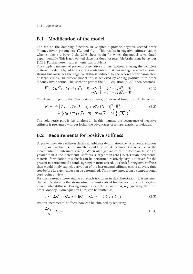
144 Appendix B
B.1 Modification of the model
The fits on the damping functions in Chapter 5 provide negative second orderMooney-Rivlin parameters, C02 and C20. This results in negative stiffness valueswhen strains are beyond the 20% shear strain for which the model is validatedexperimentally. This is not wanted since this does not resemble brain tissue behaviour[123]. Furthermore it causes numerical problems.The simplest manner of preventing negative stiffness without altering the completematerial model is by adding a stress contribution that has negligible effect at smallstrains but overrules the negative stiffness induced by the second order parametersat large strains. In present model this is achieved by adding positive third orderMooney-Rivlin terms. The isochoric part of the SED, equation (5.20), then becomes,
W = C10(I1 � 3) + C01(I2 � 3) +C20(I1 � 3)2 + C02(I2 � 3)2
+C30(I1 � 3)3 + C03(I2 � 3)3(B.1)
The deviatoric part of the Cauchy stress tensor, �d, derived from this SED, becomes,
�d = 2
Je
nC10 + 2C20
�I1 � 3
�+ 3C30
�I1 � 3
�2oB
d
e
� 2Je
nC01 + 2C02
�I2 � 3
�+ 3C30
�I1 � 3
�2o�B�1
e
�d (B.2)
The volumetric part is left unaltered. In this manner, the occurrence of negativestiffness is prevented without losing the advantages of a hyperelastic formulation.
B.2 Requirements for positive stiffness
To prevent negative stiffness during an arbitrary deformation the incremental stiffnesstensor, or Jacobian J = @�=@" should be be determined (in which " is theincremental, infinitesimal strain). When all eigenvalues of the Jacobian tensor aregreater than 0, the incremental stiffness is larger than zero [159]. For an incrementalmaterial formulation this check can be performed relatively easy. However, for thepresent material model a total Lagrangian form is used. To check for negative stiffnessthen would imply explicit derivation of the incremental stiffness matrix at every timestep before its eigenvalues can be determined. This is unwanted from a computationalcosts point of view.For this reason, a more simple approach is chosen in this dissertation. It is assumedthat simple shear is the strain situation most critical for the occurrence of negativeincremental stiffness. During simple shear, the shear stress, �ij , given by the thirdorder Mooney-Rivlin equation (B.2) can be written as,
�ij = 2(C10 + C01) + 4(C20 + C02) 3 + 6(C30 + C03)
5 (B.3)
Positive incremental stiffness now can be obtained by requiring,
@�ij@
= Gmin (B.4)
Modification of non-linear viscoelastic material model 145
for every shear strain, . Stiffness, Gmin, is an arbitrarily chosen minimum, positive,stiffness that is allowed in the simple shear solution. By writing Gmin as a fraction,�, of the small strain shear stiffness,
Gmin = 2�(C10 + C01) (B.5)
the sum of the third order terms can be solved from equation (B.4),
C30 + C03 =3f2nls5� 5�
(C10 + C01) (B.6)
in which fnls = C20+C02
C10+C01
, the non-linear shear parameter. By posing the additionalassumption that C30 = C03, as done for the first and second order parameters, thethird order parameters are defined.
B.3 Determination of brain tissue material parameters
As the modification acts on the strain dependent behaviour only, the only parameterinfluenced by this modification is the non-linear shear parameter, fnls. This parameterhas been fitted again to the experiment data. The damping function used for fittingis already corrected for inhomogeneous strain field with the original model (refer toChapter 5)).For simple shear, the damping function of the third order Mooney-Rivlin formulationcan be written as,
h( ) = 1 + 2 2C02 + C20
C01 + C10+ 3 4
C03 + C30
C01 + C10(B.7)
By eliminating C03 + C30 from equation (B.7) using equation (B.6), the dampingfunction becomes,
h( ) = 1 + 2 2fnls +9
5 4
f2nls1� �
(B.8)
This function, with � = 0 is fitted to the damping function.
Fit results
Fitting the damping function of equation (B.7) to the corrected data of Chapter 5provides fnls= -5.5553. Figure B.1 shows the fits of the damping functions within theexperimental range. It can be seen that the modified model (MR3) fit differs slightlyfrom the original fit presented in Chapter 5. This is confirmed by the mean error andstandard deviation of the error at each experimental data point. This error equals4:5 � 10�3 � 8:8 � 10�3 and is higher than the original fit (error: 3:0 � 10�3 � 8:6 � 10�3)but still acceptable. The damping functions for strains beyond the experimental rangeare shown in the right graph in Figure B.1. The original fit decreases below zero whilethe modified fit starts to increase again after a certain strain. Table B.1 provides anoverview of all material parameters fitted with the modified material model.

146 Appendix B
B.4 Implications for material behaviour
The implications of the modification for the elastic stress behaviour are illustratedusing simple shear results using the elastic mode of Table B.1 only. The left graph inFigure B.2 shows that differences between modified and original model are indeed
0 5 10 15 200.6
0.7
0.8
0.9
1
γ [%]
dam
ping
func
tion
h(γ)
ExpMR2MR3
0 20 40−1
0
1
2
γ [%]
dam
ping
func
tion
h(γ)
Figure B.1: Effect of modification on dampingfunction. Fits of original (MR2) and modified(MR3) model versus corrected experimental data from G2 sample (Exp) (refer toChapter 4). Left: Experimental strain range. Right: Larger strain range.
Table B.1: Material parameters obtained from fitting the modified non-linear material modelon brain tissue shear data (sample G2 in Chapter 4)
Mode Maxwell parameters Non-linear parameters Bulk modulusi Gi = 2(C10 + C01) [Pa] �i [ms] fnls [-] f1 [-] f2 [-] K [GPa]0 255.26* 1 -5.5553 1+ 1+ 2.51 269.08 70.1 -5.5553 1+ 1+ 02 322.63 7.63 -5.5553 1+ 1+ 03 426.96 1.41 -5.5553 1+ 1+ 04 3299.4 0.123 -5.5553 1+ 1+ 0
* G0 obtained from stress relaxation data using equation (5.31)+ Constants chosen arbitrarily, could not be determined from shear experiments
0 5 10 15 200
10
20
30
40
50
γ [%]
She
ar s
tres
s [P
a]
MR2MR3
0 10 20 30 40 50−20
0
20
40
60
80
100
γ [%]
She
ar s
tres
s [P
a]
Figure B.2: Shear stress versus strain. Elastic material behaviour assumed by modelling onlythe elastic mode in Table B.1. Fits of original (MR2) and modified (MR3) modelused. Left: Experimental strain range. Right: Larger strain range.

Modification of non-linear viscoelastic material model 147
small for strains up to 20%. The right graph shows that the original model alreadypredicted negative incremental stiffness for strains exceeding approximately 19%.For larger strains the stress decreases until negative values occur at 32% strainapproximately. The modified model shows a monotonically increasing stiffness. Forstrains over 34% the stiffness exceeds the initial small strain stiffness, whereas forstrain above 42% the model predicts higher stresses than a linear material modelwould have done.
B.5 Discussion and conclusions
The non-linear viscoelastic material model presented in Chapter 5 has been modifiedto prevent negative stiffness at strains beyond the validity range of the original modelby adding a third order Mooney-Rivlin term to the original second order formulation.In this manner advantages of a hyper elastic formulation (no energy absorption,objectivity) are maintained.As the stress dependent behaviour of the material has been altered, the non-linearshear parameter is fitted to the experimental determined dampingfunction again.Simple shear simulations showed that negative strains are indeed prevented by themodification, but for strains over 34%, the incremental stiffness exceeds the initialsmall strain stiffness. The model then actually does not predict shear softeninganymore but shear stiffening. Furthermore, this may lead to instability of the,conditionally stable, explicit Central Difference Time integration scheme used (referto section dealing with the Courant number in Chapter 2 for details).It can be concluded that the model still describes the shear behaviour of brain tissuewhen strains do not exceed 20%. For larger strains, biofidelity is not guaranteedbut numerical problems due to negative stiffness are prevented. However, it isrecommended to prevent these strains from being present in the model.

148 Appendix B

Samenvatting
Jaarlijks overlijden er meer dan een miljoen mensen aan verkeersongevallen terwijler meer dan honderdmiljoen gevallen met letsel voorkomen. Bij een ongevalssituatieis het hoofd een van de meest kwetsbare delen van het menselijk lichaam. Omte begrijpen hoe een inslag op het hoofd tot hersenletsel leidt, is het belangrijkde mechanische responsie van het hoofd te kennen. Het is niet mogelijk omdeze responsie met behulp van in-vivo experimenten (experimenten met levendewezens) te bepalen. Daarom worden vaak numerieke eindige-elementenmodellen(E.E.M.) gebruikt. De huidige E.E.M. van het hoofd bevatten een zeer gedetailleerdeweergave van de anatomie maar zijn sterk vereenvoudigd m.b.t. de beschrijvingvan het materiaalgedrag van het hersenweefsel en de contact interacties tussen deverschillende anatomische delen van het hoofd. Ook treden er fouten op door degebruikte numerieke benaderingsmethode, de expliciete eindige-elementenmethode.De doelstelling van deze studie is het verbeteren van eindige-elementenhoofdmodellen, met name de volgende twee aspecten: de nauwkeurigheid van denumerieke methode en de beschrijving van het materiaalgedrag van de hersenen.Om de nauwkeurigheid van de numerieke methode te bepalen dienen we eerstte weten welk type mechanische responsie te verwachten valt. Met namegolfverschijnselen zijn hierbij van belang daar deze hoge eisen stellen aan denumerieke methoden. Een analytische studie naar de inslagomstandigheden waarbijgolffenomenen in de hersenen kunnen voorkomen gaf aan dat het waarschijnlijkis dat ze aanwezig zijn. Afschuifgolven (S-golven) worden verwacht tijdensverkeersongevallen (frequenties tussen 25 Hz en 300 Hz). Druk golven (P-golven)kunnen ontstaan bij hoge-snelheidsinslagen (bijvoorbeeld kogel inslagen op hetbeschermde hoofd) bij frequenties tussen de 10 kHz en 3 MHz.Uit het voorafgaande volgt dat de numerieke methode voor het modelleren vaneen hoofd gedurende een inslag geschikt moet zijn om golffenomenen nauwkeurigte kunnen beschrijven. Daarom is een analytische nauwkeurigheidsanalyse vanbestaande hoofdmodellen uitgevoerd. Deze analyse is geldig voor kleine rekkenen laat zien dat er twee typen fouten ontstaan in eindige-elementensimulatiesvan golffenomenen: numerieke dispersie en numerieke reflecties. Deze foutenworden beınvloed door de discretisatie in ruimte en tijd. Bijgevolg zullen devoorspelde rekken en reksnelheden incorrect zijn. Daar deze grootheden geassocieerdworden met het ontstaan van letsels is correcte voorspelling noodzakelijk. Metde elementgrootte typisch voor huidige hoofdmodellen (meer dan 5 mm) kunnen
149
150 Samenvatting
golffenomenen niet nauwkeurig gemodelleerd worden. Voor het modelleren vanafschuifgolven moet de elementgrootte met een factor tien verkleind worden. Voorhet modelleren van drukgolven zou de elementgrootte met een factor honderdverkleind moeten worden. Dit geeft echter onrealistisch grote modellen. Daarom zaler voor dit type golven gezocht dienen te worden naar andere discretisatie methodenin ruimte en tijd. Daar dit geen doelstelling was van dit onderzoek wordt in hetvervolg alleen nog maar afschuifgedrag beschouwd.Het mechanische gedrag van hersenweefsel is onderzocht met behulp vanafschuifexperimenten. Voor kleine rekken werden experimenten met een harmonischgeexciteerde rek (amplitude 1%) gebruikt. Door toepassing van het zogeheten TijdTemperatuur Superpositie beginsel konden materiaal gegevens verkregen wordenbij frequenties die relevant zijn bij verkeersongevallen (maximaal 1000 Hz).Afschuifrekken die verantwoordelijk geacht worden voor het ontstaan van vanletsel (20% afschuifrek) werden toegepast in spanningsrelaxatie experimenten.Hersenweefsel blijkt zich als een niet-lineair viscoelastisch materiaal te gedragen bijrekken boven 1%. De afschuifstijfheid neemt af bij toenemende rekken terwijl hettijdsafhankelijke gedrag bijna onafhankelijk is van de opgelegde rek.Gebaseerd op de experimentele bevindingen is een materiaalmodel ontwikkeld.Het model is een niet-lineaire uitbreiding van het multi-mode Maxwell model.De rektensor wordt gesplitst in een elastisch en een inelastisch deel viaeen multiplicatieve decompositie. Het inelastische, tijdsafhankelijke gedrag isgemodelleerd als een eenvoudige Newtonse vloeistof. Het rekafhankelijke, elastischedeel is gemodelleerd met een hyperelastische formulering (2de orde Mooney-Rivlin). De modelformulering is geschikt om anisotroop gedrag (zoals aangetoondaanwezig in sommige delen van de hersenen) te implementeren maar voor dezestudie is vooralsnog isotroop materiaalgedrag aangenomen. Materiaalparametersvoor hersenweefsel werden bepaald uit de kleine-rekexperimenten en het constanterekdeel van de spanningsrelaxatie experimenten.Het materiaalmodel is geımplementeerd in het expliciete eindige-elementenpakketMADYMO. Om bij modelleren van het bijna incompressibele hersenweefsel, metgangbare tijdstappen, nauwkeurige oplossingen te krijgen is een predictie-correctieintegratie methode toegepast. De spanningsrelaxatie-experimenten, inclusief hettransiente deel van de rekgeschiedenis dat niet voor parameterfitten gebruikt is, zijnmet succes gesimuleerd.Om zowel de bevindingen over numerieke nauwkeurigheid en de constitutieveformulering te testen is een laboratorium hoofdmodel ontwikkeld. Het dynamischegedrag van de hersenen is nagebootst met Dow Corning Sylgard 527 A&Bsiliconengel. De mechanische eigenschappen van deze gel zijn op de zelfde manierbepaald als die van hersenweefsel. De gel gedraagt zich lineair viscoelastisch voor degeteste rekniveaus tot 50% afschuiving. De materiaalparameters van de siliconengelliggen dicht bij die van hersenweefsel al is er meer materiaaldemping bij hogefrequenties. Er is geconcludeerd dat deze siliconengel gebruikt kan worden in eenlaboratorium hoofdmodel voor trend studies en testen van numerieke modellen.Een cilindervormig bakje, gevuld met siliconengel, is belast met een transıentehoekversnelling zoals die bij een verkeersongeval kan voorkomen. De vervorming

Samenvatting 151
van de gel is geregistreerd met behulp van marker detectie in high-speed video-opnamen. De gel is gemodelleerd met het nieuwe constitutieve model en delaboratorium hoofdmodel experimenten zijn gesimuleerd. De experimentele ennumerieke resultaten vertoonden grote overeenkomsten. Dit geeft aan dat hetmateriaalmodel inderdaad een realistische responsie kan beschrijven. Ook het belangvan een correcte splitsing van volumetrische en deviatorische deformatie in despanningsformulering bij het modelleren van bijna niet-samendrukbare materialenis aangetoond.Tenslotte is het materiaalmodel toegepast in een bestaand 3-dimensionaal model vanhet menselijke hoofd. De belasting op het hoofd (een excentrische rotatie) was zogekozen dat de rekniveaus in de experimentele range lagen. Resultaten met en zondertoepassing van niet-lineair materiaalgedrag werden vergeleken. Het niet-lineairemateriaalgedrag zorgde ervoor dat de rekniveaus met 21% toenamen terwijl despanningsniveaus met 11% daalden. De ruimtelijke verdeling en de tijdsgeschiedenisveranderden echter nauwelijks. Het effect van het niet-lineaire materiaalgedrag isechter maar voor een belasting conditie onderzocht. Ook de manier waarop anderestructuren in het hoofd gemodelleerd zijn zullen de responsie, en dus het effectvan niet-lineair materiaalmodel beınvloeden. Verder onderzoek hierna wordt sterkaanbevolen.Verder was het opvallend dat rekken in het model bereikt werden die geassocieerdworden met het ontstaan van letsel (20%) bij een belasting op het hoofd die veel lagerwas dan belastingen die in de literatuur met letsel in verband gebracht worden. Eenmogelijke oorzaak hiervoor is dat de stijfheid van het hersenweefsel in hoofdmodellenuit de literatuur te hoog is in vergelijking met materiaalgegevens uit de recenteliteratuur en uit eigen experimenten. Een andere mogelijke verklaring kan zijn dat erwellicht toch een (zwakke) koppeling tussen deviatorisch en volumetrisch deel vande rek in het materiaalmodel aanwezig dient te zijn.

152 Samenvatting

Dankwoord
Graag wil ik iedereen bedanken die op welke manier dan ook heeft meegeholpen aanhet tot stand komen van mijn proefschrift en aan het aangenaam maken van mijnperiode als promovendus bij de Technische Universiteit Eindhoven.Allereerst wil ik mijn copromotor Peter Bovendeerd bedanken. Peter, jouw didactischevaardigheden en vermogen om elk probleem terug te brengen naar fundamenteletheorie waren erg verhelderend. Verder was het altijd fijn een bakkie koffie tescoren/tanken. Jammer dat jij dit vakgebied gaat verlaten. Peter, veel succes met jetroetelkindje, de hartmechanica. Ook Gerit Peters, bedankt voor jouw inbreng m.b.t.materiaalkarakterisering en je welgemeende interesse in dit vakgebied.Er was een grote toestroom van studenten die middels stages en afstudeer opdrachteneen grote bijdrage leverden aan dit onderzoek. Dit onder andere door de PR vanPeter tijdens een studiereis in Amerika. Daarom wil ik jullie, Niels Plasmans, MichielRoersma, Maarten van der Burght, Ronald Faassen, Erik Folgering, Roy Bours, JiskaKotte, Patricia Bax, Olaf Bressers en Marijn Theulings bedanken voor jullie inzet.Rob van de Berg, bedankt voor het bouwen van het laboratorium hoofdmodel. Nietalleen jouw vaardigheden op het gebied van draaien, frezen, schroeven, enz. maarvooral ook voor jouw vermogen om van een simpele schets een bruikbare opstellingte maken.Ook de mensen bij de afdeling MADYMO bij TNO-Automotive in Delft wil ikbedanken voor de door hun verleende faciliteiten bij het implementatie van hetmateriaalmodel. Met name Pier Nauta, bedankt voor jouw inzet, meedenken en hulpbij het implementeren.Uiteraard wil ik Jan van Bree van TNO-PML in Rijswijk niet vergeten. Jij was initiatorvan dit onderzoek en hebt voor de financiele ondersteuning vanuit TNO-Prins MauritsLaboratorium zorggedragen. Wat ik erg gewaardeerd heb aan onze samenwerking isde vrijheid die ik gekregen heb om dit onderzoek naar eigen inzicht in te kunnenvullen.Verder wil ik mijn collega’s bedanken die ervoor zorgen dat de werksfeer hier erg goedis. Mijn mede-bestuursleden 1998-1999 van het AiO genootschap Hora Est zijndeEric van den Bosch, Liesbeth Geerts, Alex Serrarens en Henri Brouwers. Met namehet survival weekend en de excursie naar het pathologisch museum in Nijmegen ende daarop volgende gebeurtenissen waren voor mij onvergetelijke ervaringen.Ook mijn kamergenoten wil ik niet vergeten. Frans Duinhouwer jij was het die het on-line Doomen (na werktijd) introduceerde in de vakgroep. Marielle Bosboom, als er
153

154 Dankwoord
ook maar iets was dat geregeld moest worden was jij het die als echte regelneef ervoorzorgde dat we niets te kort kwamen op onze kamer. En last but zeker not least, Ericvan den Bosch, mede-biker en vraagbaak voor menig MATLAB of LATEX probleem. Demanier waarop wij elkaar aanvoelden op het gebied van zinnige en onzinnige zakengrensde aan telepathie. Eric, bedankt voor jouw motivatie door jouw optimistischekijk op zaken (wederzijdse motivatie technieken) en veel succes in jouw toekomst.Verder wil ik mijn ouders bedanken voor hun stimulans om aan deze studie tebeginnen. Tenslotte jou, lieve Bianca, jij was er altijd als ik je nodig had en ik was ervaak genoeg niet voor jou. Nu kan ik er wat meer voor jou zijn.

Curriculum Vitae
Dave Brands was born on February 8, 1972 in Maastricht, The Netherlands.He studied Mechanical Engineering at Eindhoven University of Technology, TheNetherlands. He received his Master’s degree in November 1996 on Finite ElementModelling of a motor cycle helmet during impact. This research was conducted at TheNetherlands Research Organisation, TNO, Road Vehicles in Delft, The Netherlands.During this study he got interested in impact biomechanics research. He decidedto continue in this field and started this Ph.D. study in February 1997 at EindhovenUniversity of Technology, within the section Dynamics and Biomechanics of Prof.dr.ir.Dick van Campen and Prof.dr.ir. Jac Wismans. This work was supported by thePrins Maurits Laboratory of The Netherlands Research Organisation, TNO in Rijswijk,The Netherlands. During this research he received the Stapp Car Crash ConferenceStudent Award in 1999. As of July 15, 2001 Dave is employed at the MaterialsTechnology group in the section mechanical engineering at Eindhoven University ofTechnology.
155

156 Curriculum Vitae