predicting freakish sea state with an operational third ... · decades ago. the mysterious sea is...

Nat. Hazards Earth Syst. Sci., 14, 945–957, 2014www.nat-hazards-earth-syst-sci.net/14/945/2014/doi:10.5194/nhess-14-945-2014© Author(s) 2014. CC Attribution 3.0 License.

Natural Hazards and Earth System

SciencesO

pen Access

Predicting freakish sea state with an operational third-generationwave model

T. Waseda1, K. In 1,*, K. Kiyomatsu1, H. Tamura2, Y. Miyazawa2, and K. Iyama1,**

1Graduate School of Frontier Sciences, University of Tokyo, Kashiwa, Japan2Japan Marine and Earth, Science and Technology, Yokohama, Kanagawa ,Japan* now at: Automobile R&D Center, Honda Automobile, Tochigi, Japan** now at: R&D Center, JR East Group, Saitama, Japan

Correspondence to:T. Waseda ([email protected])

Received: 24 August 2013 – Published in Nat. Hazards Earth Syst. Sci. Discuss.: 6 November 2013Revised: 2 October 2013 – Accepted: 2 March 2014 – Published: 22 April 2014

Abstract. The understanding of freak wave generationmechanisms has advanced and the community has reacheda consensus that spectral geometry plays an important role.Numerous marine accident cases were studied and revealedthat the narrowing of the directional spectrum is a good in-dicator of dangerous sea. However, the estimation of the di-rectional spectrum depends on the performance of the third-generation wave model. In this work, a well-studied marineaccident case in Japan in 1980 (Onomichi-Maruincident) isrevisited and the sea states are hindcasted using both the DIA(discrete interaction approximation) and SRIAM (SimplifiedResearch Institute of Applied Mechanics) nonlinear sourceterms. The result indicates that the temporal evolution of thebasic parameters (directional spreading and frequency band-width) agree reasonably well between the two schemes andtherefore the most commonly used DIA method is qualita-tively sufficient to predict freakish sea state. The analysesrevealed that in the case ofOnomichi-Maru, a moving galesystem caused the spectrum to grow in energy with limiteddownshifting at the accident’s site. This conclusion contra-dicts the marine inquiry report speculating that the two swellsystems crossed at the accident’s site. The unimodal wavesystem grew under strong influence of local wind with apeculiar energy transfer.

1 Introduction

A number of ship accidents in the northwestern PacificOcean, especially in the sea east of Japan, were reporteddecades ago. The mysterious sea is coined “the Dragon’sTriangle” mimicking the famous “Bermuda Triangle” in theAtlantic Ocean (Berlitz, 1989). During World War II, Ad-miral Halsey and his fleet sailed into the heart of TyphoonCobra in the North Pacific, and lost three destroyers (Druryand Clavin, 2007). Recently Atsukawa (1999) analysed themeteorological conditions during this incident and suggestedthat the vessel might have encountered a wave of over 30 min height (Fig. 1). Although this description is rather specula-tive, Atsukawa did make numerous interesting observations:the ship had encountered waves over 30 m, which were fol-lowed by 28 m waves; the Kuroshio Current is present; andthe bow of the ship had surfaced. These observations are re-lated to the formation of a wave group, wave–current inter-action and a slamming load. Undoubtedly, Atsukawa’s obser-vation is influenced by the well-known and well-studied ma-rine accident near Japan, theOnomichi-Maruincident (Ya-mamoto et al., 1983). The incident is memorable because ofthe famous picture of the ship without the bow (Fig. 2). Be-cause of lack of knowledge about freak/rogue waves at thattime, the cause of the incident was mistakenly attributed toa high wave called theSankaku-namiin Japanese or triangu-lar wave, which suggests a crossing of large swells. We willshow in this study that this was not the case and the direc-tional spectrum was unimodal at the time of the incident.

Published by Copernicus Publications on behalf of the European Geosciences Union.

946 T. Waseda et al.: Predicting freakish sea state

Historical incidents of the freak wave or the rogue waveare well documented in the text book by Kharif, Pelinovskyand Sulnyev (2010). The large waves that appear in the oceanunexpectedly are named differently, each representing oneof the characters of the freak wave: giant wave, mad-dogwave, wall of water, holes in the sea, three sisters, pyrami-dal waves, etc. Scientists and engineers define them as wavesthat are “higher than twice the significant wave height” andare “isolated”. For linear- and narrow-banded random waves,the distribution of wave height is approximately Rayleighlike (Longuett-Higgins and Cart-Wright, 1953) and thereforethe appearance of waves over twice the significant waveheight is about once every 3000 waves. Inevitably, the en-counter of ships with freak and giant waves is rare, but Kharifand Pelinovsky (2003) report that during the period 1969–1994 22 super-carrier ships and 525 lives in total may havebeen lost due to freak waves in the Atlantic and the Pacificoceans. Nine of the accidents occurred in the Dragon’s Tri-angle, including the two large, Japanese carrier ships: theBolivar −Maru and theOnomichi-Maru. More recent inci-dents of fishing boats, ferry boats and theOnomichi-Maruaredocumented in Waseda et al. (2012). Out of seven incidents,five occurred when the directional spectrum narrowed. Noneof the incidents had direct evidence of the ship encounteringthe freak wave, but the freakish-sea index which maps thedimension of the directional spectrum indicated a dangeroussea state for those cases.

The freakish-sea index maps the trajectory of the direc-tional spreading (σθ ) and frequency bandwidth (Qp) and wassuccessfully used in the study of theSuwa-Maruincident byTamura et al. (2009) and of theOnomichi-Maruincident byIn et al. (2009). What the freakish-sea index indicates is thetemporal change of the geometry of the directional spectrum.In most of the incidents studied by Waseda et al. (2012),the freakish-sea index was changing rapidly in time. Further-more, in some cases, the incidents occur exactly when thefreakish-sea index indicated the narrowest directional spec-trum.

Numerous “freak wave indices” are suggested. Attributingthe modulational instability of the long-crested waves for theformation of large-amplitude waves, Onorato et al. (2001)and Janssen (2003) independently introduced a parameterthat compares the relative magnitude of nonlinearity and dis-persion. Those parameters were called the Ursell number andthe Benjamin–Feir index respectively. The latter terminol-ogy is used more often in recent literatures. These studieswere experimentally extended to include the effect of direc-tional spreading of the wave spectrum by Waseda (2006).However, earlier works already indicated evidences that forrealistic directional spreading, the occurrence probability offreak waves is small (Onorato et al., 2002; Soquet-Juglard etal., 2005). In turn, the freak wave occurrence becomes highwhen the bandwidth of the wave spectrum is narrow (Toffoliet al., 2008; Onorato et al., 2009a, b; Waseda et al., 2009;Mori et al., 2011; Xiao et al., 2013). The conclusion de-

duced from these experimental works were validated by ob-servations indicating that under certain meteorological con-ditions the probability of freak wave occurrence will increase(Waseda et al. 2011).

In this paper, the wave field during the time of the acci-dent of theOnomichi-Maruwill be hindcasted with an op-erational wave model (WAVEWATCH III). The comparisonof the model results with the sea states described in the of-ficial report of the marine accident inquiry were presentedearlier by In et al. (2009). A brief overview of theOnomichi-Maru incident and the hindcast simulation will be providedin Sect. 2. The comparison of the spectral evolution andthe deduced freakish-sea index will be compared betweenthe DIA (discrete interaction approximation) simulation andSRIAM (Simplified Research Institute of Applied Mechan-ics) simulation in Sects. 3 and 4. The possible cause of thefreakish sea state under moving gale conditions will be dis-cussed in Sect. 5.; and the Conclusion follows.

2 Hindcast simulation of theOnomichi-Maru accident

The Japanese bulk-carrierOnomichi-Maruwas built in 1965(200 m, 60 000 t). On 30 December 1980, during a voyagecarrying a full load of coal from the United States to Japan,she encountered an extremely high wave and as a result of theslamming impact lost her bow. The fact that a super-carriership over 200 m was split into two bodies by the force ofa wave’s impact came to a shock for the Japanese Ministryof Transportation. A committee was organized to investigatethe cause of the accident, concurrently with the marine ac-cident inquiry. The committee concluded that the impact ofthe slam was too strong for her body to remain intact andthe Onomichi-Maruwas broken into two (Yamamoto et al.,1983). The estimated height of the wave was about 20 m. Thecommittee reported that at the time of the accident, steadyswell came from the west with 8–9 m significant wave heightand 12 s wave period, and another relatively unsteady swellcame from the west-northwest with 3.8–6.2 m significantwave height and 12 s wave period. The committee concludedthat the former steady swell caused the pitching motion of theship, and an unlucky superposition of the second swell madean extreme wave which caused severe slamming. However,our simulation result shows that this was not the case.

We conducted a three-tiered nested-wave hindcast sim-ulation covering the period from 1 December 1980 to10 January 1981 by an operational third-generation wavemodel WAVEWATCH III (Tolman 2002). The first level(nest1) covers the whole Pacific Ocean at 1◦ resolution(95◦ E–70◦ W, −75◦ S–75◦ N), the second level (nest2) cov-ers the northwestern Pacific Ocean with 0.25◦ resolution(135◦–180◦ E, 22◦–47◦ N), and the last level (nest3) cov-ers an area around the accident’s site with 0.125◦ resolu-tion (150◦–160◦ E, 26◦–36◦ N). The topography of each areawas specified by ETOPO2 (NOAA). As the wind data, weused the JRA-25 (Japanese Re-Analysis 25 years) data of the

Nat. Hazards Earth Syst. Sci., 14, 945–957, 2014 www.nat-hazards-earth-syst-sci.net/14/945/2014/

T. Waseda et al.: Predicting freakish sea state 947

Table 1. Summary of conditions of theOnomichi-Maruaccidentfrom the marine accident inquiry report (JST Japan standard time).

The details of the accident

Date 1980-12-30-14:30 (JST)Locale 156◦11′ E, 31◦0′ N

The particulars ofOnomichi-Maru

Length 216.40 mBreadth 31.7 mDraft 17.3 m

The sea state

Height Period Length Dir.(from)

Swell 1 8–9 m 12 s 150–180 m WSwell 2 4–6 m 12 s 225–284 m WNWWind wave 4 m 8 s no data WSW

Wind Lv.8 Beaufort rank=> 17.2− −20.7 m s−1 WSW

Japan Meteorological Agency, which is 1.25◦ resolution at3 h intervals covering most areas of the globe. The model set-ting is detailed in In et al. (2009) and will be briefly summa-rized here: the number of directions was set to 24 (spaced by15◦) for SRIAM and 36 (spaced by 10◦) for DIA; the num-ber of frequencies was set to 25 levels, with the incrementalfactor of 1.1 in the frequency range 0.0412–0.4056 Hz, or1.08 in the range of 0.0412–0.2611 Hz. The source terms ofthe WAVEWATCH III (Tolman–Chalikov source terms) wereselected by benchmarking the model setting against the fetchlaw with an ideal wind condition (Iyama 2007).

The nonlinear wave–wave interaction term (Snl) is cal-culated by both the DIA method (Hasselmann et al., 1985)and the SRIAM method (Komatsu and Masuda, 1996). TheSRIAM method approximates the Hasselman’s collision in-tegral (Hasselmann, 1963) with 20 optimized combinationsof resonant quartets instead of one in DIA. The SRIAMmethod was implemented in realistic simulations for the firsttime by Tamura et al. (2008, 2009 and 2010), demonstratingthat the directional spectrum under rapidly changing windconditions and the spectral tail are better resolved by theSRIAM method. In Tamura et al. (2009), spectral evolutionof swell and wind–wave interaction was hindcasted for theSuwa-MaruNo. 58 incident (June 2008) using SRIAM Snl.In this study, we have made hindcast simulation with bothDIA and SRIAM Snl and compared the spectral evolutions.These model results were validated by Iyama (2007) andIn (2009) with observational data of NOWPHAS (Nation-wide Ocean Wave information network for Ports and HAr-bors; Port and Airport Research Institute in Japan) and thedrifting GPS buoy.

The sea state during the accident and the particulars ofOnomichi-Marufrom the marine inquiry report are summa-rized in Table 1. Swells 1 and 2 were suggested to be themain cause of the accident. The committee report states that

Fig. 1. A schematic of theP ittsburgh encountering giant wave of30 m (reproduced from Atsukawa, 1999).

swell 1 from the west caused the pitching motion of the ship,and an unlucky superposition of the swell 2 from the west-northwest made an extreme wave of 20 m which caused asevere slamming impact. However, from the wave field mapof Otsubo (1983), the main locations of these swells seem faraway from the actual accident’s site (Fig. 3 left). This histori-cal hand-drawn wave-field map is likely based on the secondgeneration wave model, which was the most reliable at thattime (Tomita, 2009). The swell 1 is indicated by a horizontalarrow and the swell 2 by an oblique arrow in the south. Theaccident’s location is marked by the cross.

These swell systems are indeed well resolved in our sim-ulation (Fig. 3). In the north of the accident’s site (solidsquare), the wave (12–12.5 s) which might correspond toswell 1 is propagating from the west, and in the southwest ofthe accident’s site, the wave (11.5–12 s) which might corre-spond to swell 2 is propagating from the west-northwest. Atthe accident’s location, a wave (12.41 s, 8.22 m) was propa-gating eastward, slightly oriented towards the south (rotated5.36◦ to the south, Fig. 3). In an area south of 35◦ N, thedirections of wind and wave (swell 1) are almost the same(Fig. 4). Along the latitude of the accident’s site (31◦ N), thewave directions are nearly constant (eastward) and the peakperiod becomes longer as the waves propagate to the east.The westerly winds were sustained for about 5 days beforethe time of the accident.

The significant wave height and the three parameters rel-evant for freak wave prediction are mapped in Fig. 5. A re-gion with high nonlinearity (steepness), narrow directionalspreading and reduced dispersion (narrow frequency band-width) is found in a large area stretching from east to west inwhich the accident’s site is located at the centre1. The area

1Wave steepness (ak): ak =π√2

×HsLm

Frequency peakedness (Qp) (Goda, 1970) :

Qp = 2m−20

∫∞

0 dσσ[∫ 2π

0 F (σ,θ)dθ]2

wherem0 =∫ 2π0

∫∞

0 F (σ,θ)dσdθ

Directional spreading (σθ ) (Kuik et al., 1988):

σθ =

2

1−

(a2

+b2

m20

) 12

1

2

wherea =

∫ 2π0

∫∞

0 cos(θ)F (σ,θ)dσdθ,b =∫ 2π0

∫∞

0 sin(θ)F (σ,θ)dσdθ

www.nat-hazards-earth-syst-sci.net/14/945/2014/ Nat. Hazards Earth Syst. Sci., 14, 945–957, 2014


Fig. 2.An image of theOnomichi-Maruwithout a bow.

represents where the probability of freak wave occurrenceis high. The temporal evolution of the wind speed, signifi-cant wave height, spectral peak period, steepness, frequencybandwidthQp and directional spreadingσθ , are plotted inFig. 6. A gale of over 14 m s−1 started on 27 December andreached its maximum when the accident occurred on 30 De-cember. TheQp increased within a day before the accident,and σθ decreased continuously during the gale condition.Despiteak remained relatively unchanged, the directionalspectrum narrowed and became narrowest when the accidentoccurred. Therefore, theOnomichi-Marumay have sailedthrough the centre of a dangerous sea where freak wave oc-currence was high. Furthermore, the evolution of the direc-tional spectrum reveals that the coexistence of the two swellsystems, as suggested by the inquiry committee, is highly un-likely at the accident’s location (Sect. 3).

3 Spectral evolution

The spectral evolution at the test site will be investigatedbased on the third-generation wave model outputs. Evolutionof the directional spectrum will be described for both DIAand SRIAM computations (Sect. 3.1). In Sect. 3.2, the sourceterms will be studied in detail comparing the two schemes.

3.1 Directional spectrum

The wave-energy density at the time of the accident is uni-modal and is unequivocally reproduced by both DIA andSRIAM hindcast simulations (Figs. 7 and 8, lower left). Thetwo swell systems as indicated by the incident report are notpresent in these simulation results. The projection of the di-rectional spectrum to the frequency and directional domain

are calculated as follows:

F (σ) =

2π∫0

F (σ,θ)dθ, (1)

F (θ) =

∞∫0

F (σ,θ)dσ . (2)

The F (σ,θ), F (σ) andF (θ) from six different times be-fore the accident (72, 48, 24, 12, and 6 h) and at the timeof the accident are shown for both DIA and SRIAM com-putations (Figs. 7, 8). Both the frequency and the directionalwave spectra are unimodal and narrow, and do not indicatea multiple-wave system or a mixed-sea condition. The peakof the energy spectrum occurs at 0.0803 Hz (the wave periodabout 12.54 s or 240 m in wavelength). The energy rapidlygrew within 72 h before the accident with a slight down-shifting, and veered from west-southwest to west-northwest(Fig. 7, DIA). The directional shifting, however, is not asswift in the directional spectrum from the SRIAM calcula-tion (Fig. 8) which shows small peaks at both−10◦ (west-northwest) and 20◦ (west-southwest). Although these peaksmight appear to correspond to the two swell systems (Ta-ble 1), they are not swells as they both grew rapidly in timeand are strongly affected by local wind.

The evolution of the directional spectrum, however, isatypical of a wind sea. In typical wind seas, the energy in-crease is associated with spectral downshifting, i.e. followsthe fetch law. It appears that the peak of the frequency spec-trum downshifts only slightly while the energy increasesrapidly. From 29 to 30 December, the significant wave heightincreased more than 20 % (Fig. 6). For wind seas in localequilibrium, the wave period should then increase followingthe Toba’s law (Toba, 1973) but the actual increase seemsto saturate (see Appendix A for further analysis). Thus, itseems that in the last 24 h before the accident, the evolu-tion of the wave field was unusual. This tendency is evidentin both DIA and SRIAM computations, and the frequencyspectrum is even narrower with SRIAM. Comparing the fre-quency spectra 48 h before and after the accident, the rapidnarrowing of spectral bandwidth in just a few days is ratherremarkable.

Overall, we can conclude that there was only one wavesystem at the accident’s site and it is strongly influenced bythe local wind. Because the value of the directional spreadingσθ , was minimum at the accident’s time (Fig. 6), the sea con-dition was likely not a crossing sea as conjectured in the ac-cident report. With a relatively narrow directionality and fre-quency bandwidth, the possibility of freak wave occurrencemight have increased, and caused the accident.

3.2 The source functions

As the wind sea grows under constant wind forcing, the en-ergy is transferred from the waves in the frequency range



Fig. 3. The historical wave-field map (contours are significant wave height, arrows indicate direction of waves, and cross the marks theaccident’s location) reproduced from Otsubo (1983) (left), and the peak period and direction from this simulation (right; colour shading isthe peak period, and the arrows show the wave propagation direction).

Fig. 4. (Left) The field data of significant wave height (Hs, contour) and wind speed vector when the accident occurred. White square is theaccident’s site. The data is from the second-level field (nest2). Wind vectors are subsampled at every 5 grids. (Right) The field data of peakperiod (contour) and peak direction (arrows) when the accident occurred. White square is the accident’s site.

higher than the peak of the spectrum to the frequency rangelower than the peak and to the spectral tail (Hasselman et al.,1985). As a result, the spectral peak downshifts. The trans-fers of energy among spectral components occur due to fourwave-resonant interactions and the shape of the transfer func-tion depends on the spectral geometry. The growth of fetch-limited or duration-limited wind seas under constant windforcing is thus characterized by this typical nonlinear trans-fer function Snl and the associated self-similar spectrum.

However, under changing wind conditions, the directionalspectrum deviates from the standard self-similar spectralshape and likewise the Snl. Rapid narrowing of the fre-quency spectrum with limited spectral peak downshiftingis a remarkable feature during theOnomichi-Maruaccident(Figs. 7, 8). Thus a peculiar shape of Snl is expected. Thetemporal evolution of Snl in frequency domain is depicted

in Fig. 9. From 72 to 48 h before the accident, the peak ofthe spectrum gradually downshifts (Figs. 7, 8) and so is thepeak of the Snl. However, from 24 h before the accident, theenergy level of the peak builds up while the peak of the Snlis more or less fixed in frequency. Another notable featureof the Snl is the large negative value in the range of around0.075–0.18 Hz (1–2.5 times the spectral peak frequency) andthe large positive value in the range of around 0.18–0.3 Hz(2.5–4 times the spectral peak frequency). Thus, a large partof the spectral energy is transferred to both the peak of thespectrum and to the tail of the spectrum as a result of nonlin-ear wave–wave interaction.

However, the spectral shape at frequencies higher thantwice the peak (−0.15 Hz) remains more or less unchanged.Tamura et al. (2010) has shown that in the operational wavemodel, the nonlinear source term annuls the imbalance of the



Fig. 5. Significant wave height (top left), wave steepness (top right), directional spreading (bottom left) and frequency peakedness (bottomright) at the time of theOnomichi-Maruaccident (30 December 1980). The crosses denote the accident’s location.

Fig. 6. Time series of sea state parameters from 25 December to31 December in 1980 at the accident’s site (156.1◦ E, 31.0◦ N) ;wind speed, significant wave height (Hs), wave steepness (ak), peakperiod (peakp), frequency peakedness (Qp), and directional spread-ing (σθ ). The red dot marks the accident’s time.

energy input and dissipation and therefore the equilibriumspectral tail remains unchanged. Therefore, the large Snl val-ues at frequency ranges higher than twice the spectral peakare not an indication of spectral change. Indeed a large partof the wind input energy is redistributed elsewhere by non-linear transfer (Fig. 10). Most likely, the energy is transferredto the frequency range of the spectral peak, but at obliqueangles. The tendency to broaden the spectrum at the peakis more prominent with the SRIAM computation (compareFigs. 7 and 8). The spectrum is quite narrow in frequencybut relatively broad in direction. This broadening is a conse-quence of active energy transfer among spectral components.Therefore it is apparent that the wave system is not a simplelinear superposition of the two swell systems. A few daysbefore the accident, the wave field was more or less bimodal(note the two wave systems are different from swell 1 and 2).As the gale system developed, the unimodal directional spec-trum developed around 0.1 Hz and gradually downshifted toaround 0.07 Hz where the spectral energy developed rapidly.The spectral geometry will be characterized by two parame-ters, directional spreading and frequency bandwidth, i.e. thefreakish-sea index, in the next section.



Fig. 7.Directional spectrum at the time of the accident (lower left) and the spectrum enlarged around the peak (upper right). The evolution intime of the spectrum projected on the frequency domain (upper left) and on the directional domain (lower right) is shown from 3 days beforethe accident to the time of the accident. The simulation was made using DIA.

4 Freakish-sea index

In the case of theOnomichi-Maruaccident, the directionalspectrum rapidly narrowed in frequency and direction in24 h. A number of marine accidents occur in similar situ-ations in which the sea states rapidly changed. Those inci-dents are described in Waseda et al. (2012) and Tamura etal. (2009). None of these marine accidents have solid evi-dence of freak wave occurrence but these case studies sug-gest that an operational wave model is useful in providing awarning criterion for ships navigating in open ocean. A visu-alized risk index of freak waves will be useful and we pro-posed to use the joint-probability-density function (JPDF) ofthe directional spreadingQp and the frequency peakednessσθ as an indicator of the likelihood of freak waves (In et al.,2009; Tamura et al., 2009). The idea of the freakish-sea indexis to visualize the development of its spectrum in theQp andσθ domain. In the case ofSuwa −maru incident, Tamura etal., (2009) showed nicely that the spectrum narrowed rapidlyin less than 6 h as a result of interaction of background swell

and wind sea. The spectrum thus developed from a bimodalstate to unimodal state. In the case ofOnomichi-Maru, therapid change ofQp was associated with local developmentof the wave system.

These spectral developments might be affected by the set-ting of the operational model. In the case ofOnomichi-Maruincident, both the DIA and SRIAM nonlinear source termswere used. As illustrated in Sect. 3, the use of the SRIAMmethod slightly broadened the spectrum in direction but nar-rowed the spectrum in frequency. Let us now compare theperformance of DIA and SRIAM simulations in expressingthe freakish-sea index (Fig. 11). Apparently, the timing ofthe accident is unequivocally represented at the turning pointof theQp andσθ trajectories; i.e. both simulations commonlyindicate that the accident occurred when the directional spec-trum was narrowest within the 4 days. The values of bothQpand σθ are about the same despite the subtle difference inthe directional distribution at the peak frequency (Figs. 7, 8).At other times, the SRIAM simulation tends to show slightlybroader spectrum in direction but the frequency bandwidth



Fig. 8.Same as Fig. 7 but for the simulation made using SRIAM.

Fig. 9.The nonlinear transfer function corresponding to the SRIAMsimulation result shown in Fig. 8. The results shown are for 72, 48,24, 12, and 6 h before the accident and at the time of the accident.

seem to agree. Qualitatively, the two diagrams convey thesame message that the accident occurred at the turning pointof theQp andσθ trajectory. For operational use, DIA is 20times faster than SRIAM. Our comparison suggests that theDIA simulation is sufficient to provide qualitatively correctinformation useful for the warning criterion.

5 Wind-sea development under changing wind field

The change of the wave spectrum in time observed at a fixedlocation is determined by not only the source functions butalso the propagation term. Classical fetch laws are obtainedonly for those cases where either the tendency term can beneglected (fetch-limited) or the propagation term can be ne-glected (duration-limited). In realistic cases, wind fields arechanging in both time and space so that both the tendencyand the propagation terms are important. It is therefore notsurprising if the overall change in the spectral shape devi-ates from ideal cases of fetch- or duration-limited wind sea.Nevertheless, it is of interest to find out how the wind fieldchanged in theOnomichi-Maruaccident case.



Fig. 10.The wind input source function (left) and the nonlinear transfer function of the SRIAM simulation (right) at the time of the accident.

Fig. 11.2-D scatter plot of frequency peakedness and directional spreading by 1 h interval for 48 h before and after the accident (left DIA,right SRIAM). Red cross and red point indicate the accident’s time.

The wind speed and wind vectors of 29 December 12:00and 30 December 00:00 UTC (Universal Time Coordinated)are presented in Fig. 12. A strong gale system with maxi-mum velocity close to 20 m s−1 covered a large area east ofJapan (3000 km by 1000 km) and moved 1000 km to the eastin 12 h. The gale system itself strengthening and the changeof wind speed observed at the accident’s location can be at-tributed to its eastward movement. Therefore, initially thewind speed is decaying to the east along the 31◦ N latitude(28 December 06:00 UTC) but as the gale system moves to-wards the east, the wind speed is increasing to the east along31◦ N (12/29 18:00 UTC); Fig. 13. When the accident oc-curred (30 December 06:00 UTC), the peak of the gale sys-tem reached the accident’s location and the highest windspeed was recorded. Evolution of the wave spectrum undersuch conditions is not straightforward and it is likely that the

wind speed, the propagation speed and the spatial scale of thegale system coincidentally matched to enhance the freakishsea state at the accident’s location.

6 Conclusions

The direct cause of a marine accident often remains unex-plained. However, marine accidents do occur under certainsea states (e.g. Toffoli et al., 2005). As demonstrated in pre-vious studies, a number of marine accidents were associatedwith narrowing of the directional spectrum (Tamura et al.,2009; In et al., 2009; Waseda et al., 2012). The narrowing ofthe spectrum can be visualized in a diagram of the directionalspreadingσθ and frequency peakednessQp. Marine acci-dents tended to occur in the turning point of the trajectory in



Fig. 12.Wind field evolution: 12 h before the accident (left) and at the time of the accident (right). The contour shading is the wind speedand the arrows indicate wind direction.

Fig. 13.Wind speed sections along 31◦ N from 135◦–180◦ E from28 December 06:00 UTC to 30 December 06:00 UTC.

this domain. We called theQp andσθ diagram the freakish-sea index. In this study, we have shown that the dangerous seastate can be well predicted with both DIA and SRIAM simu-lations. The response of the directional spectrum to changingwind condition is sensitive to the accuracy of the nonlinearinteraction source term (Tamura et al., 2008). However, foroperational use, the DIA is most commonly used. Therefore,the finding that the freakish-sea index is equally well pre-dicted with DIA and SRIAM is good news for operationalpurposes. Of course, both are model results and ought tobe validated by observations. However, the observations inthis region are rather limited. The hindcast simulations of thePacific Ocean with SRIAM and DIA were validated againstavailable buoy observations by Tamura et al. (2010); it was

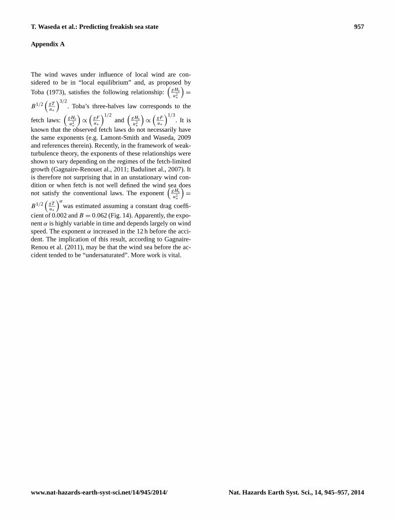
Fig. 14.Evolution of the exponentα (black line) and the wind speed(green line) 24 h before and after the accident. The horizontal axisis time in UTC and the vertical axes are the exponentα (rangingfrom around 1.5 to 1.525) and the wind speed (ranging from 12.5 to19 m s−1).

shown that the energy is reproduced equally well while thepeak period was better reproduced by SRIAM. Apart fromsuch difference between models, a common shortcoming ofthe models is that the directional spectrum tends to be muchbroader than observations (Babanin et al., 2010). Therefore,the numerous freak-wave indices are quantitatively inaccu-rate when estimated from the wave model. What theQp andσθ diagram indicates is a much larger change of the spec-tral geometry as a result of meteorological forcing. On thephysical aspect, the case study of theOnomichi-Maruinci-dent revealed that a moving gale system is associated with



the development of the freakish sea. While the spectral peakperiod remained relatively unchanged, the energy increased.As a result, the spectrum narrowed. The dynamics of suchspectral development is yet to be understood and left for fu-ture study.

Acknowledgements.The authors are grateful for the three anony-mous reviewers and the editors of the NHESS special editionfor their constructive comments. The analysis presented in theAppendix developed from the suggestion of one of the reviewers.The first author thanks Takeshi Kinoshita and Hiroshi Tomita fortheir encouragement and criticism during the course of research.The work was partially supported by Grants-in-Aid for ScientificResearch of the Japan Society for the Promotion of Science.

Edited by: E. Bitner-GregersenReviewed by: five anonymous referees

References

Atsukawa, M.: Showa no kamikaze, Haruzee Kantai ga sogushitataifuni tsuite, Ichikawa Gakuen Chigakuka Kishoshitsu, 1999 (inJapanese).

Babanin, A. V., Tsagareli, K. N., Young, I. R., and Walker, D. J.,Numerical investigation of spectral evolution of wind waves, PartII: Dissipation term and evolution tests, J. Phys. Oceanogr., 40,667–683, 2010.

Badulin, S. I., Babanin, A. V., Zakharov, V. E., and Resio, D.:Weakly turbulent laws of wind-wave growth, J. Fluid Mechan.,591, 339–378, 2007.

Berlitz, C.: The Dragon’s Triangle, Wynwood Press, 1989.Drury, B. and Clavin, T.: Halsey’s Typhoon: The True Story of a

Fighting Admiral, an Epic Storm, and an Untold Rescue, GrovePress, 2007.

Gagnaire-Renou, E., Benoit, M., and Badulin, S. I.: On weakly tur-bulent scaling of wind sea in simulations of fetch-limited growth,J. Fluid Mechan., 669, 178–213. 2011.

Goda Y.: Numerical experiments on wave statistics with spectralsimulation, Report of National Institute for Land and Infrastruc-ture Management, 9, 3–57, 1970.

Hasselmann, K.: On the non-linear energy transfer in a gravity-wavespectrum, J. Fluid Mech, 12, 481–500, 1962.

Hasselman, S., Hasselman, K., Allender, J. H., and Barnett, T. P.:Computations and Parameterizations of the Nonlinear EnergyTransfer in a Gravity-Wave Spectrum, Part II: Parameterizationsof the Nonlinear Energy Transfer for Application in Wave Mod-els, J. Phys. Oceanogr., 15, 1378–1390, 1985.

In, K.: Research on high accuracy wave forecasting to ensure safetyof the ship navigation, 2009, Master’s thesis the Department ofEnvironmental and Ocean Engineering, School of Engineering,the University of Tokyo, 2009.

In, K., Waseda, T., Kiyomatsu, K., Tamura, H., Miyazawa, Y., andIyama, K.: Analysis of a marine accident and freak wave predic-tion with an operational wave model, Pros., 19th Int, Offshoreand Polar Engineering Conf., ISOPE, Osaka, Japan, 3, 877–883,2009.

Iyama, K.: Development of a wave forecasting system to predictfreak wave occurrence, Master’s thesis, the Department of En-

vironmental and Ocean Engineering, School of Engineering, theUniversity of Tokyo, 2007.

Janssen, P. A. E. M.: Nonlinear Four-Wave Interactions and FreakWaves, J. Phys. Oceanogr., 33, 863–884, 2003.

Kharif, C. and E. Pelinovsky: Physical mechanisms of the roguewave phenomenon, Europ. J. Mech. B/Fluids, 22, 603–634,2003.

Komatsu, K. and Masuda, A.: A New Scheme of Nonlinear EnergyTransfer among Wind Waves: RIAM Method –Algorithm andPerformance-, J. Phys. Oceanogr., 52, 509–537, 1996.

Kuik, A. J., Van Vledder, G. Ph., and Holthuijsen, L.: Amethod forthe routine analysis of pitch-and-roll buoy wave data, J. Phys.Oceanogr., 18, 1020–1034, 1988.

Lamont-Smith, T. and Waseda, T.: Wind wave growth at short fetch,J. Phys. Oceanogr., 38, 1597–1606, 2008.

Mori, N. and Janssen, P. A. E. M.: Dependence of freak wave oc-currence on kurtosis, Rogue Wave 2004 IFREMER, Brest, 2004.

Mori, N. and Janssen, P. A. E. M.: On kurtosis and occurrence prob-ability of freak waves, J. Phys. Oceanogr., 36, 1471–1483, 2006.

Mori, N., Onorato, M., and Janssen, P. A.: On the estimation of thekurtosis in directional sea states for freak wave forecasting, J.Phys. Oceanogr., 41, 1484–1497, 2011.

Otsubo, H.: Wreckage offshore the Nozima Peninsula, Symposiumon destruction of ships and marine structures, 1983 (in Japanese).

Onorato, M., A. R. Osborne, Serio, M., and Bertone, S.: FreakWaves in Random Oceanic Sea States, Phys. Rev. Lett., 86,5831–5834, 2001.

Onorato, M., Osborne, A. R., and Serio, M.: Extreme wave events indirectional, random oceanic sea states, Phys. Fluids, 14, 25–28,2002.

Onorato, M., Osborne, A. R., Serio, M., Cavaleri, L., Bran-dini, C., and Stansberg, C. T.: Observation of stronglly non-Gaussian statistics for random sea surface gravity wavesin wave flume experiments, Phys. Rev. E, 70, 067302,doi:10.1103/PhysRevE.70.067302, 2004.

Onorato, M., Waseda, T., Toffoli, A., Cavaleri, L., Gramstad,O., Janssen, P. A. E. M., Kinoshita, T., Monbaliu, J., Mori,N., Osborne, A. R., Serio, M., Stansberg, C. T., Tamura, H.,and Trulsen, K.: On the statistical properties of directionalocean waves: the role of the modulational instability in theformation of extreme events, Phys. Rev. Lett., 102, 114502,doi:10.1103/PhysRevLett.102.114502, 2009.

Soquet-Juglard, H., Dysthe, K., Trulsen, K., Krogstat, H. E., andLiu, J.: Probability distribution of surface gravity waves duringspectral changes, J. Fluid Mech., 116, 207–225, 2005.

Tamura, H., Waseda, T., Miyazawa, Y., Komatsu, K.. Current-Induced Modulation of the Ocean Wave Spectrum and the Roleof Nonlinear Energy Transfer, J. Phys. Oceanogr., 38, 2662–2684, 2008.

Tamura, H., Waseda, T., and Miyazawa, Y., Freakish seastate and swell-windsea coupling: Numerical study of theSuwa-Maru incident, Geophys. Res. Lett., 36, L01607,doi:10.1029/2008GL036280, 2009.

Tamura, H., Waseda, T., and Miyazawa, Y.: Impact of non-linear energy transfer on the wave field in Pacific hindcastexperiments, J. Geophys. Res. Oc., (1978–2012) 115.C12.,doi:10.1029/2009JC006014, 2010.

Toba, Y.: Local balance in the air-sea boundary processes, J.Oceanogr. Soc. Japan, 29, 209–220, 1973.


http://dx.doi.org/10.1103/PhysRevE.70.067302

http://dx.doi.org/10.1103/PhysRevLett.102.114502

http://dx.doi.org/10.1029/2008GL036280

http://dx.doi.org/10.1029/2009JC006014


Toffoli, A., Lefevre, J. M., Bitner-Gregersen, E., and Monbaliu, J.,Towards the identification of warning criteria: Analysis of a shipaccident database, Appl. Oc. Res., 27, 281–291, 2005.

Toffoli, A., Bitner-Gregersen, E., Onorato, M., and Babanin, A. V.:Wave crest and trough distributions in a broad-banded directionalwave field, Oc. Engin., 35, 1784–1792, 2008.

Tolman, H. L.: User manual and system documentation of WAVE-WATCH III version 2.22, NOAA/NWS/NCEP/MMAB Techni-cal Note, 222, 133 pp., 2002.

Tomita, H.: ISSC 2009 I.1 Environment, Official Discusser, in:Proc. 17th International Ship and Offshore Structures Congress(ISSC), 3, Seoul, Korea, 2009.

Waseda, T.: Impact of directionality on the extreme wave occur-rence in a discrete random wave system,” 9th International Work-shop on Wave Hindcasting and Forecasting, 2006.

Waseda, T., Kinoshita, T., and Tamura, H., Evolution of a RandomDirectional Wave and Freak Wave Occurrence, J. Phy. Oceanogr.,38, doi:10.1175/2008JPO4031.1, 2009.

Waseda, T., Hallerstig, M., Ozaki, K., and Tomita, H. En-hanced freak wave occurrence with narrow directional spec-trum in the North Sea, Geophys. Res. Lett., 38, L13605,doi:10.1029/2011GL047779, 2011.

Waseda, T., Tamura, H., and Kinoshita, T.: Freakish sea index andsea states during ship accidents, J. Mar. Sci. Technol., 17, 305–314, 2012.

Xiao, W., Liu, Y., Wu, G., and Yue, D. K.: Rogue wave occurrenceand dynamics by direct simulations of nonlinear wave-field evo-lution, J. Fluid Mechan., 720, 357–392, 2013.

Yamamoto, Y., Otsubo, H., Iwai, Y., Watanabe, I., Kumano, A., Fu-jino, M., Fukasawa, T., Aoki, M., Ikeda, H., and Kuroiwa, T.:Disastrous Damage of a Bulk Carrier due to Slamming, The lec-ture of The Society of Naval Architects of Japan in 1983, 1983.


http://dx.doi.org/10.1175/2008JPO4031.1

http://dx.doi.org/10.1029/2011GL047779


Appendix A

The wind waves under influence of local wind are con-sidered to be in “local equilibrium” and, as proposed by

Toba (1973), satisfies the following relationship:(

gHsu2

∗

)=

B1/2(

gTu∗

)3/2. Toba’s three-halves law corresponds to the

fetch laws:(

gHsu2

∗

)∝

(gFu∗

)1/2and

(gHsu2

∗

)∝

(gFu∗

)1/3. It is

known that the observed fetch laws do not necessarily havethe same exponents (e.g. Lamont-Smith and Waseda, 2009and references therein). Recently, in the framework of weak-turbulence theory, the exponents of these relationships wereshown to vary depending on the regimes of the fetch-limitedgrowth (Gagnaire-Renouet al., 2011; Badulinet al., 2007). Itis therefore not surprising that in an unstationary wind con-dition or when fetch is not well defined the wind sea doesnot satisfy the conventional laws. The exponent

(gHsu2

∗

)=

B1/2(

gTu∗

)α

was estimated assuming a constant drag coeffi-

cient of 0.002 andB = 0.062 (Fig. 14). Apparently, the expo-nentα is highly variable in time and depends largely on windspeed. The exponentα increased in the 12 h before the acci-dent. The implication of this result, according to Gagnaire-Renou et al. (2011), may be that the wind sea before the ac-cident tended to be “undersaturated”. More work is vital.


predicting freakish sea state with an operational third ... · decades ago. the mysterious sea is...

Documents