Predicting power conversion efficiency of organic photovoltaics: models and data analysis

Preprint Cambridge Centre for Computational Chemical Engineering ISSN 1473 – 4273

Predicting power conversion efficiency of organicphotovoltaics: models and data analysis

Andreas Eibeck4, Daniel Nurkowski1, Angiras Menon2, Jiaru Bai2,

Jinkui Wu3, Li Zhou3, Sebastian Mosbach1,2, Jethro Akroyd1,2, Markus

Kraft2,4,5

released: February 23, 2021

1 CMCL InnovationsSheraton HouseCastle ParkCambridge CB30AXUK

2 Department of Chemical Engineeringand BiotechnologyUniversity of CambridgePhilippa Fawcett DriveCambridge, CB3 0ASUnited Kingdom

3 School of Chemical EngineeringSichuan UniversitySichuanChina

4 CARESCambridge Centre for AdvancedResearch and Education in Singapore1 Create WayCREATE Tower, #05-05Singapore, 138602

5 School of Chemicaland Biomedical EngineeringNanyang Technological University62 Nanyang DriveSingapore, 637459

Preprint No. 268

Keywords: organic photovoltaics, PCE, machine learning, neural networks, baseline models

Edited by

CoMoGROUP

Computational Modelling GroupDepartment of Chemical Engineering and BiotechnologyUniversity of CambridgePhilippa Fawcett DriveCambridge, CB3 0ASUnited Kingdom

E-Mail: mk306@cam.ac.ukWorld Wide Web: https://como.ceb.cam.ac.uk/

Abstract

In this paper, the ability of three selected machine learning neural and baseline mod-els in predicting the power conversion efficiency (PCE) of organic photovoltaics(OPVs) using molecular structure information as an input is assessed. The bi-directionallong short-term memory (gFSI/BiLSTM), attentive fingerprints (Attentive FP), andsimple graph (Simple GNN) neural networks as well as baseline support vector re-gression (SVR), random forests (RF), and high dimensional model representation(HDMR) methods are trained to both the large and computational Harvard clean en-ergy project database (CEPDB) and the much smaller experimental Harvard organicphotovoltaic 15 dataset (HOPV15). It was found that the neural-based models gen-erally performed better on the computational dataset with the Attentive FP modelreaching a state of the art performance with the test set mean squared error of 0.071.The experimental dataset proved much harder to fit, with all the models exhibiting arather poor performance. Contrary to the computational dataset, the baseline modelswere found to perform better than the neural models. To improve the ability of ma-chine learning models to predict PCEs for OPVs, either better computational resultsthat correlate well with experiments or more experimental data at well-controlledconditions are likely required.

BHJ Organic Solar Cell

Anode

Cathode

+-Acceptor

Donor

Light

SMILES c1coc(c1)-c1cc2[nH]ccc2[nH]1

C, aromatic single

H

N

OH

HHH

H

H H

N

FeatureGeneration

H

N

O

H

HHH

H

H H

N

Circular Iteration

PC

E

Readout

Highlights• Neural and baseline models assessed for predicting PCE of organic photo-

voltaics.

• Computational (CEPDB) and experimental (HOPV15) literature datasets con-sidered.

• The CEPDB fitted well by all models, but predicted PCEs disagree with exper-iments.

• The HOPV15 fitted poorly, with the baseline models being better than the neu-ral models.

1

Contents

1 Introduction 3

2 Data 5

2.1 Harvard clean energy project dataset . . . . . . . . . . . . . . . . . . . . 5

2.2 Harvard organic photovoltaic dataset . . . . . . . . . . . . . . . . . . . . 6

3 Methodology 9

3.1 Models and descriptors . . . . . . . . . . . . . . . . . . . . . . . . . . . 9

3.1.1 Bi-directional long short-term memory network . . . . . . . . . . 10

3.1.2 Simple graph neural network . . . . . . . . . . . . . . . . . . . . 11

3.1.3 Attentive fingerprint . . . . . . . . . . . . . . . . . . . . . . . . 12

3.1.4 Baseline models . . . . . . . . . . . . . . . . . . . . . . . . . . 13

3.2 Training and hyperparameter optimisation . . . . . . . . . . . . . . . . . 15

3.3 Software and tools . . . . . . . . . . . . . . . . . . . . . . . . . . . . . 18

4 Results and discussion 18

4.1 Harvard clean energy project dataset results . . . . . . . . . . . . . . . . 18

4.2 Harvard organic photovoltaic dataset results . . . . . . . . . . . . . . . . 20

5 Conclusions 23

A Appendix 25

References 29

2

1 Introduction

With a strong global push towards clean energy generation, more resources are beinginvested in researching and developing photovoltaic devices. Whilst silicon-based solarcells remain the most prominent in the solar cell market, other materials have also beenrapidly gaining interest, such as perovskite-based solar cells [11, 40] that have been seen toachieve promising power conversion efficiencies (PCEs)[15]. However, perovskite basedcells are known to have environmental stability and processing issues [43]. As a conse-quence, organic solar cells (OSCs) have been gaining interest, due to their low weight,flexibility, environment stabilities, and ease of manufacture [3, 38, 48]. Although OSCsoften have substantially lower PCEs [13, 38], recent synthesis efforts and theoretical pre-dictions have suggested that OSCs could achieve conversion efficiencies that make themcompetitive with silicon and perovskite-based materials [33, 37, 51] with potential PCEsreaching as high as 20% [37], or even 30% [51] in some cases.

As conducting experiments can prove to be challenging both time and resource-wise,computational methods are often employed to enable rapid screening of candidate ma-terials for organic solar cells based on PCE. Frequently, computational estimates of thePCE employ the widely used Scharber equation [38], which predicts the PCE of a givenorganic solar cell architecture from only a few key parameters, all of which can be de-termined by application of quantum chemical methods such as density functional theory(DFT). However, DFT calculations require substantial computational time that is not con-ducive to fast screening. Therefore, machine learning (ML) methods are often used toderive quantitative structure property relationships (QSPR) between the performance ofthe organic photovoltaic and the underlying properties of the materials, as they can makeuse of existing computational and experimental data and make predictions at a fraction ofthe cost.

A wide variety of machine learning algorithms have been applied to predict the perfor-mance of organic photovoltaics by using different target data sets. The Harvard CleanEnergy Project Database (CEPDB) [13], is one such target data set for ML models thatcontains computationally determined PCE values for 2.3 million organic photovoltaic can-didates. An example of ML methods being applied to the CEPDB is the artificial neuralnetwork (ANN) trained by Pyzer-Knapp et al. [29], who achieved good prediction accu-racy for PCE and other molecular properties. Various deep learning models have alsobeen applied, including the convolutional neural network of Sun et al. [41], who classi-fied organic photovoltaic candidates into low performance (<5% PCE) and high perfor-mance (5-10%PCE) materials, as well as various graph neural network (GNN) approachesthat directly predict PCE [9], [52], [34]. Recent approaches have integrated the attentionmechanism, originally introduced for recurrent neural networks for machine translation[5], in order to improve performance by focusing on local substructures that are rele-vant for the prediction task. For example, Wu et al. [49] used attention to couple a Bi-Directional Long Short-Term Memory (LSTM, [14]) and multilayer perceptron (MLP)to predict PCE based on sequentialized molecular structure and fragment types. The au-thors achieved a very high degree of prediction accuracy on the CEPDB and identifiedfunctional groups that contribute towards a molecule having higher PCE.

However, it has been noted that computational predictions of PCE of OSCs often do not

3

agree well with experimental measurements, and that machine learning approaches likeGaussian process regression are necessary to improve agreement [13, 23, 30]. As a con-sequence, experimental OPV datasets, such as the Harvard Organic PhotoVoltaic dataset(HOPV15) [22], are often used to train ML methods instead. Examples include the k-Nearest Neighbours (k-NN) and Kernel Ridge Regression (KRR) models used for directPCE prediction by Padula et al. [27], the ANN and RF methods used for classification byNagasawa et al. [26], and the five ML models (MLP, Deep Neural network (DNN), Con-volutional Neural Network, RF, and Support Vector Machine (SVM)) trained by Sun et al.[42]. In general, ML models perform worse on experimental data than the CEPDB, withbetter performing models reaching Pearson correlation coefficients r of 0.7. Given this,studies have also tried to include additional DFT-computed molecular descriptors in theML models to improve performance on experimental datasets. This includes the trainingof RF, ANN, and gradient boosting regression trees by Sahu and Ma [35], Sahu et al. [36]in conjunction with 13 DFT derived molecular descriptors and 300 experimental PCEs, aswell as the work by Zhao et al. [54], who trained SVM, k-NN, and KRR models with a va-riety of different DFT derived descriptors and 566 experimental PCEs. The performanceof these ML models was similar, achieving correlations of r = 0.7−0.8, and suggests thatincluding DFT descriptors achieves only a modest improvement, possibly due to manydescriptors being implicitly linked to structure.

Ultimately, the goals of these works is to train an ML model that can accurately andquickly screen candidate OPV materials to identify potential high performance candi-dates for further characterization. Whilst it appears that several different ML approachescan achieve similar levels of performance, a crucial aspect is the choice of training data.Training to computationally determined PCEs has the advantage of large and standardizeddatasets with controllable and known degrees of freedom [24], but these PCEs correlatepoorly to experimental measurements which can undermine their utility. However, train-ing to experimentally characterized PCEs is harder due to the wide variety of experimentalconditions, expected experimental errors, larger number of degrees of freedom and usu-ally smaller amount of available data.

In light of these considerations, the aim of this paper is to critically test the ability of ma-chine learning models to predict the PCE of organic photovoltaics based on the SMILES-derived molecular structure information, as well as assess the impact and implications ofthe choice of training data. To do this, three neural machine learning models are trained:the BiLSTM model used by Wu et al. [49], the Attentive Fingerprints (FP) used by Xionget al. [52] and a simple Graph Neural Network (Simple GNN) that serves as an intermedi-ate between these two models in terms of featurization included. Three baseline models:Random Forests (RF), Support Vector Regression (SVR), and High Dimensional ModelRepresentation (HDMR) are also trained for comparative purposes. These six modelsare trained to predict PCE based on descriptions of molecular structure generated fromSMILES strings and finger print analysis. In order to test the impact of training data, thesix models are trained to both the large, entirely computational CEPDB, and the small,experimental HOPV15 dataset. Finally, the impact of the training data and choice ofML model on predicting PCEs that are ultimately useful for guiding organic photovoltaicdesign is critically assessed based on the training results.

4

2 Data

2.1 Harvard clean energy project dataset

The first major dataset used in this work is the Harvard CEPDB, developed originallyby Hachmann et al. [13]. As mentioned previously, the CEPDB only contains computa-tional results for approximately 2.3 million organic solar cell acceptor candidate materials.Whilst the original servers and websites for the CEPDB are no longer in use, the data canbe accessed from the following website: https://www.matter.toronto.edu/basic-content-page/data-download. The CEPDB provides substantial data for training machine learningalgorithms. The molecular structures in the CEPDB are generated from 26 different build-ing blocks, as detailed in Hachmann et al. [13]. Each species in the CEPDB is assigned anID, with the stoichiometry and SMILES string also provided to give the basic molecularstructural information for the organic solar cell acceptor species. For each species, thePCE, the short circuit current density Jsc, the open circuit voltage Voc, the HOMO energy,the LUMO energy, and the HOMO-LUMO gap are reported as computed by the DFTmethods described by Hachmann et al. [13]. The PCE values reported in the CEPDB arecomputed using the Scharber equation:

PCE =FF Voc Jsc

Pin, (1)

where FF is the fill factor and Pin is the input power. Scharber et al. [38] also developedmodels for the various parameters in the Scharber equation, which are used to derive theCEPDB data. The fill factor, FF is assumed to be 0.65, and the open circuit voltage givenby the following expression, derived by Scharber et al. [38]

Voc =1e

(|EDonorHOMO|− |EAcceptorLUMO|

)−0.3, (2)

with e as the electron charge, EDonorHOMO being the energy of the highest occupiedmolecular orbital (HOMO) of the donor material in the cell, EAcceptorLUMO similarlybeing the energy of the lowest unoccupied molecular orbital (LUMO) of the acceptor ma-terial in the cell, and 0.3 being an empirical correction. In the CEPDB, the acceptor isassumed to be PCBM, a class of fullerenic derivatives commonly used as electron ac-ceptors in both hybrid perovskite and organic photovoltaic materials. The magnitude ofEAcceptorLUMO is assumed to be 4.3 eV, in accordance with experimental measurements[53].

The two remaining parameters in the Scharber equation, Jsc, and Pin, are both derivedfrom the incident solar photon flux density, which essentially amounts to integrating theAir Mass 1.5 (AM1.5) spectra [12]. For this spectra, integrating the spectra across thewavelength gives a Pin of approximately 1000 W/m2. The short circuit current density isgiven by:

Jsc = EQE× e∫

∞

Eg

φph(E)dE, (3)

5

with the external quantum efficiency EQE set to 0.65 in the Scharber model, Eg as theband gap of the donor material, and φph being the incident solar photo flux density as afunction of the energy E.

The Scharber Model shows that computing PCE, Voc, and Jsc only requires determiningthe HOMO and LUMO levels of the donor material in the OSC, which is readily derivedfrom the quantum chemical calculations performed by Hachmann et al. [13].

Before implementing and training the various machine learning algorithms to the data inthe CEPDB, the data is first pre-processed to understand the characteristics of the speciesin the CEPDB. First, all of the provided SMILES strings are checked to see if they arevalid, in that they successfully encode a sensible molecular structure that can be identifiedby RDKit. In total 9821 invalid SMILES were identified and thus these species were re-moved from consideration for training purposes. Next, the maximum length of the validSMILES, the maximum number of atoms in a single molecule in the data set, and thedifferent atom types are identified, as these define the bounds of the structures that themachine learning methods will need to model. For the CEPDB, the maximum length ofSMILES and maximum number of atoms in a single molecule are 83 and 53 respectively.There are seven different atoms in the CEPDB, namely C, H, O, N, Si, and Se. However,several atoms can be either aromatic or non-aromatic. This can significantly impact theunderlying chemistry and molecular behaviour, which is another factor to be taken intoaccount. A final layer of pre-processing is related to the reported PCE values, in whichmolecules with a PCE value smaller than the defined threshold value of 0.0001 are alsoremoved from consideration, as such species are not going to be useful for OSC appli-cations. This resulted in another 109425 species being removed from the CEPDB set,resulting in 2203603 remaining species to be used as potential training data.

After the CEPDB is pre-processed, stratified sampling is then applied to derive a set of25000 candidate OSC donors for training and testing the machine learning models, asutilizing the full pre-processed CEPDB is computationally prohibitive. A set size of 25000species is both computationally affordable and large enough for the training of machinelearning models to be tractable, and is in line with previous literature works [49]. Inthis case, the maximum PCE value in the pre-processed CEPDB is 11.13%. As such,the pre-processed data are first assigned to 56 bins of equal widths of 0.2%, with thefirst bin including species with PCE [0,0.2) and the last bin including species with PCE[11.0,11.2). Once the pre-processed data is divided into the 56 bins, stratified samplingwithout replacement is then performed with respect to these bins. This is done so that thePCE profile of the selected 25000 species is close to the PCE profile for the entire pre-processed dataset. Once the 25000 species are selected, this is then divided into a set of15000 species for training the machine learning method, a validation set of 5000 speciesused to evaluate the ML model fit while tuning hyperparameters, and a test set of 5000species used to give the final evaluation of the ML model fit.

2.2 Harvard organic photovoltaic dataset

The second major dataset used in this work is the HOPV15 dataset, which consists of 350different experimentally characterized organic solar cell donor structures that have been

6

collated from various works in the literature by Lopez et al. [22]. The HOPV15 data isaccessible as a single file from the original publication [22]. For each of the 350 species,the HOPV15 data set contains the SMILES and InChI strings that define the molecularstructure, as well as the DOI for the original work that experimentally characterized thespecies in question. The experimental data in HOPV15 also includes the constructiontype of the donor species, the architecture of the solar cell, the complement used (i.e. theacceptor material), and any measured photovoltaic characteristics of the organic solar cell.These photovoltaic characteristics include the HOMO and LUMO energies of the donor,the electrochemical and optical gaps of the donor, as well as the PCE, Jsc, Voc, and FillFactor, but not all of these properties are measured for all 350 species in HOPV15.

The HOPV15 dataset contains experimental results from a variety of different experimen-tal conditions, which can be seen in the breakdown of the solar cell characteristics. Thereare 127 solar cells that made use of molecular constructions for the donor, whilst 220used polymeric constructions for the donor species. In terms of the architecture, 270 ex-periments involved bulk heterojunction solar cells, 13 made use of bilayer solar cells formeasurements, and 64 used Dye-Sensitized-Solar-Cells (DSSCs). The acceptor materialused also varies, unlike in CEPDB. In this case 139 experiments made use of PC61BMas an acceptor, 133 used PC71BM, 9 used C60, 64 used TiO2, 1 used ICBA, and 1 usedPDI. For three species in the HOPV15, no experimental information was provided at all.

Given the variety of experiments used to generate the data in HOPV15, pre-processingand sampling are again applied to the data before any training and testing of machinelearning algorithms is performed. As with CEPDB, the SMILES strings are first checkedfor validity. In this case, all 350 SMILES strings are able to be processed by RDKit.The second pre-processing step removes species that do not have experimental PCEs,which excludes 7 species. This leaves 343 species to be sampled from. It is worth notingthat for these species, there is an extra atom type compared to CEPDB, namely that offluorine, meaning 8 different atoms are possible. Additionally, whilst the smallest speciesin HOPV15 contains just 12 atoms, the largest contains 142 atoms, and the average size ofspecies is roughly 71 atoms, meaning that in general the donor candidates here are muchlarger than the species in CEPDB. This, in addition with the extra atom type mean thatHOPV15 contains substantially different structures for the ML methods to model whencompared to CEPDB.

Although it is very affordable to train to the entirety of the HOPV15 data, as this involvesjust 343 PCE values and SMILES strings to be processed, there is the additional issue ofthe variability of experiments and solar cell set ups used to measure these PCEs. As aconsequence, not all of the measured PCEs in HOPV15 are directly comparable as theyare in the CEPDB, due to the differences in experimental methodology. Therefore, onlyPCEs measured using similar experimental conditions were selected to try and get a con-sistent dataset. Specifically, since the CEPDB PCE values assume a PCBM type materialfor the acceptor, PCEs measured with a solar cell that did not use PCBM or similar ma-terials as the acceptor were excluded, namely those that used TiO2. Similarly, only PCEsmeasured for solar cells using a bulk heterojunction architecture were chosen, to removethis variable from the dataset. This sampling meant that 267 PCEs were selected from theHOPV15 dataset to provide a more consistent set of experimental values to train the MLmethods to.

7

It is worth noting that the HOPV15 data set also contains substantial computational datafor each of the 350 organic solar cell donor candidates. This includes optimized geome-tries for up to 20 conformers for each species which are within 5 kcal/mol of the minimumenergy structure at the BP86/def2-SVP level of theory [22]. Additionally, for each con-former, the HOMO, LUMO, HOMO-LUMO gap, Jsc, Voc, and Scharber equation PCE arereported having been computed using the def2-SVP basis set and four DFT functionals,namely BP86, B3LYP, PBE0, and M06-2X. This does provide DFT data that could be in-corporated as descriptors in the machine learning model. However, a sample comparisonbetween the HOMO-LUMO gap, LUMO energy, and PCE predicted using B3LYP/def2-SVP and the corresponding experimentally measured values for these properties suggestpoor agreement between computation and experiment. This is seen in Figure 1.

1 2 3 4 5Experimental Gap [eV]

1.0

1.5

2.0

2.5

3.0

3.5

4.0

4.5

5.0

B3LY

P H

OM

O-L

UM

O G

ap [e

V]

4.0 3.5 3.0 2.5Experimental LUMO [eV]

4.0

3.5

3.0

2.5

2.0

1.5

1.0

0.5

B3LY

P LU

MO

[eV]

0 5 10Experimental PCE [%]

0

2

4

6

8

10

B3LY

P Sc

harb

er P

CE

[%]

Figure 1: Comparison between Donor Gap, Donor LUMO energy, and Scharber PCEpredicted computationally by DFT and by various experiments in HOPV15.

The agreement is also poor for the other three functionals used. This does suggest thatPCEs purely predicted by the Scharber equation are insufficient to predict the actual per-formance of the material, in agreement with Padula et al. [27]. Furthermore, the plots alsosuggest that these popular DFT methods struggle when predicting the HOMO-LUMOgap and LUMO energy of the donor, two popular descriptors used for machine learningmodels of PCE. This may also explain why inclusion of properties computed by DFTin the previous work of Zhao et al. [54] resulted in only a modest improvement of theML model performance, in that these properties are not well described by DFT and thusmay not correlate well to experimental PCE results. Given this, it was decided that noadditional descriptors predicted by DFT would be included in subsequent machine learn-ing models, and that the models would only be trained to relate PCE to the underlyingmolecular structure of the donor as described by the SMILES strings.

8

3 Methodology

3.1 Models and descriptors

While the neural networks and ML methods utilized in this paper differ in many respects,they also have some general methodological steps in common. The steps common to all ofthe ML methods are introduced first, with details specific to each ML method introducedin the subsequent subsections. An overview of the structure of the ML methods utilizedin this work is presented in Figure 2.

Figure 2: Overview of neural networks and baselines used in this paper and alignmentof their building blocks to three general steps: feature generation, circulariteration, and readout.

The left-hand side of Figure 2 shows an example of a SMILES string and its correspondingstructure for one of the smaller molecules in the CEPDB. This example structure containsonly 21 atoms, including hydrogens, which are treated explicitly throughout this work.Figure 2 also illustrates three general methodological steps in the ML methods: featuregeneration, circular iteration, and readout. These are each discussed in turn below.

Feature generation. Feature generation is where a SMILES string is converted into amolecular graph. This graph represents the moleculuar structure, with node features in-cluding properties such as the atom type and aromaticity and edge features including prop-erties like the bond type. These node and edge features are determined by RDKit [19].

Circular iteration. For a given node, circular iteration transforms and joins the featuresof this node with the features of its neighbour nodes and of the edges that connect themin a circular and iterative manner. An example is illustrated in Figure 2, for the carbonatom marked by a dark green dot. This carbon atom has three direct neighbour nodes with

9

atom types O, C and C which are connected by two aromatic bonds and one single bond.The green circle indicates the merge of the bond and neighbour features for the markedcarbon atom in the first iteration. In parallel, the merge is performed analogously for eachfurther node in the molecular graph and its direct neighbours. Afterwards, all node statesare updated with the merged result. All ML methods perform these transformations andmerging, but they do differ in the way of how they transform and merge the information.

Once one iteration is complete, the entire procedure may be repeated once again for theupdated node states. After the second iteration, the updated node states now not onlyinclude information about the directly neighbouring nodes and connections, but also in-formation about the direct neighbours’ neighbours. For the carbon atom in Figure 2, thisis indicated by the light green oval covering all nodes with a distance of one or two edges.As a consequence, as more merge and update iterations are performed, each node statewill contain information on an increasingly large environment within the molecular graph.

Readout. First, all node states resulting from the previous circular iterations are aggre-gated to a single state on the graph level (i.e. on the molecule level). Next the aggregatedstate is used to predict the target value, e.g. by feeding it into a multilayer perceptron. Theexecution of these two steps comprises readout.

Note that some models in Figure 2 contain additional building blocks or steps that do notalign perfectly with these three overarching steps. For instance, the BiLSTM is a centralblock in the g-FSI/BiLSTM model and is placed between the steps “Circular Iteration”and “Readout”. Detailed descriptions of the steps that are specific to each ML method areprovided in the following sections.

3.1.1 Bi-directional long short-term memory network

A sequential and deep-learning model using a bi-directional long short-term memory net-work with an attention mechanism and multilayer perceptron has been implemented. Thisarchitecture has been proven to be very successful for organic photovoltaics PCE predic-tion [49], thus it was decided to use it in this work as one of the neural models. Only thekey model aspects are provided here. Readers are directed to [18, 49] for a more detaileddescription.

Feature generation. This step follows the common procedure as described previously.Atom types and their aromaticity are used to encode the node features whereas bond types(single, double, triple and aromatic bonds) are used to encode the edge features.

Circular iteration. The Weisfeiler-Lehman algorithm [47] is used to circulate aroundthe nodes of molecular graphs generated in the previous step. The algorithm consists oftwo stages: (i) an initial assignment stage, in which each node and edge are assignedthe unique integer identifiers that represent their starting features set, and (ii) an iterativeupdating stage, in which each node identifier is updated to reflect the identifiers of itsneighbours and each edge identifier is updated to reflect the identifiers of nodes it con-nects. Once all nodes and edges have generated their new identifiers, the algorithm cycleis repeated until the requested number of iterations is reached. At the end, the final nodeidentifiers are assembled into the final molecular fingerprint vector. Since the node and

10

edge features only include atom and bond types information, one can also think about thismolecular fingerprint vector as a unique list of sub-molecular fragments building the par-ent molecule, hence the name graph fragments sequence identifiers (g-FSI) in the originalpublication [49]. In this paper only a single iteration of the Weisfeiler-Lehman algorithmhas been performed by setting its radius parameter to one. To avoid the confusion withordinary BiLSTM networks, the model will be referred to as g-FSI/BiLSTM for the re-mainder of the paper.

The g-FSI vector encodes two important structural aspects: fragment (fingerprint) typesand their order in the molecule. Note that mapping discovered fragment types to uniqueinteger identifiers proceeds on a first-found first-served basis with no hashing. There-fore, it is dependent on the order in which the data is processed. In order to eliminatethis dependency, prior to using the model, the selected datasets are processed first to cre-ate the fragment-identifiers look-up dictionaries. This step also finds the molecules withthe largest number of fragments which are in turn used to define the maximum sequencelength for the BiLSTM network. Furthermore, it is important to highlight that the orderof fragments in the g-FSI vector depends on the order in which the molecular graph nodesare processed. To keep the fragments that are spatially close to each other together (e.gtwo fragments that are part of the same aromatic ring), the molecular graph has been iter-ated in the breadth first search (BFS) order.

Node type embedding and BiLSTM. This step starts from passing the g-FSI vectorsthrough a trainable embedding layer, which for a single molecule, results in creatinga sequence of real-valued fragments embedding vectors (one for each fragment integeridentifier). Secondly, the embedding vectors are processed by the forward and backwardBiLSTM cells resulting in a sequence of hidden forward and backward state vectors.

Readout. In order to obtain the final PCE value, the two BiLSTM hidden states are con-catenated and weighted-summed in the attention layer. This is followed by propagatingthe attention layer output through a multilayer perceptron.

3.1.2 Simple graph neural network

The neural network presented in this section is simple in three respects: (1) It belongs tothe class of graph convolutional networks but is implemented in a straight-forward man-ner. Compared to [9] and [17] it simplifies the iteration update by applying the empiricalmean. (2) Moreover, compared to g-FSI/BiLSTM model and Attentive FP, it does notmake use of any attention mechanism. That means it treats all neighbours of all nodesin the same way. (3) It uses only a small number of node types as features and no edgefeatures.

Feature generation. All distinguishable tuples of the form (atom type, atom aromatic-ity) are identified in the datasets leading to 8 and 12 different node types for CEPDB andHOPV15. This approach is equivalent to the Weisfeiler-Lehman algorithm for radius zero.Then, each different node type is mapped to its own vector in the space RED where ED de-notes the embedding dimension and the vector elements are trainable weights. While the

11

node types for Simple GNN are different from the fragment types for the g-FSI/BiLSTMmodel, their embedding into a continuous space is analogous.

Circular iteration. For each node v in the molecular graph, the embedding vector ischosen corresponding to its node type and used as initial node state h0(v) ∈ RED. Thegraph layers of simple GNN are indexed with l ranging from 1 to the overall layer count,CL. Each layer can be described in terms of the message passing neural network (MPNN)framework introduced in [10]: First, messages with transformed states are received fromv’s direct neighbour nodes N(v) and aggregated,

ml(v) =1

#N(v) ∑u∈N(v)

W lhl−1(u) (4)

where W l ∈ RED×ED denotes a matrix of trainable weights and #N(v) is the number ofneighbour nodes. Finally, the state of node v at layer l is updated by

hl(v) = relu(hl−1(v)+ml(v)) (5)

where the rectified linear activation function, relu, is applied component-wise. For sim-plicity, W l is a square matrix such that all node states have the same dimension, ED,throughout all graph layers. Here, the layer count, CL, plays the same role as for Atten-tive FP (section 3.1.3), as the radius in the Weisfeiler-Lehman algorithm (section 3.1.1),and as the radius for generating Morgan fingerprints (see section 3.1.4): it corresponds tothe maximum distance of (direct and indirect) neighbour nodes that may contribute to thefinal state of node v.

Readout. The state of the graph G is set to the empirical mean over all node states atlayer l = CL, i.e.

h(G) =1

#N(G) ∑u∈N(G)

hCL(u) (6)

where N(G) is the set of all nodes in G. Finally, the graph state h(G) ∈ RED is fed intoa multilayer perceptron with one output neuron for PCE prediction analogously to theg-FSI/BiLSTM model from section 3.1.1.

3.1.3 Attentive fingerprint

Attentive FP (fingerprint) is a graph neural network that was introduced by Xiong et al.[52] and achieves state-of-the-art performance on several data sets that are widely usedin ML research according to a comprehensive assessment of several neural networks andML methods by Wu et al. [50]. Attentive FP makes use both of Gated Recurrent Units(GRU, [7]) and attention and thus resumes ideas of Gated Graph Neural Networks [21]and Graph Attention Networks [45]. It applies the attention mechanism both on the atomicnode level and on the molecular graph level to focus on substructures that are relevant for

12

predicting target variables.

Feature generation. Nine node features (including atom types and atom aromaticity)and four edge features (including bond type) are used as input features, with most of thembeing one-hot encoded. A detailed list of the input features can be found in Xiong et al.[52].

Circular iteration. For each target node v in the molecular graph, its node features arefed into a fully connected layer with FS units where FS denotes the Fingerprint Size. Theoutput is used as initial node state h0(v) ∈ RFS. Edge features are handled explicitly onlyat the beginning of the first iteration: the node features of each direct neighbour u ∈ N(v)and the features of the edge between u and v are concatenated and fed into another fullyconnected layer having the same number FS of units. From here, all states have the samesize FS and the actual circular iteration can be formulated in terms of the MPNN frame-work [10] - analogously to the simple GNN from the previous section. Roughly speaking,all summands in Equation 4 are multiplied with their corresponding attention weights cal-culated between the states of v and u and replacing the uniform weights 1

#N(v) . Then, theirsum is fed as input vector into a GRU which replaces the simple update function in Equa-tion 5. This means the state of v is updated to the resulting hidden state of the GRU at theend of each iteration and is used as the starting point for the next iteration.

Readout. A virtual super node is added to the molecular graph and connected to allof its atom nodes. Its state represents the state of the entire graph and is initialized withthe sum of all atom node states updated at the end of the last iteration. The super nodestate itself is updated throughout several iterations using its own GRU. In each iteration,the attention weight between the super node and an atom node is calculated in the sameway as between two atom nodes. Finally, the super node state is fed into a fully connectedlayer which has one output neuron in the case of PCE as target variable.

The GRU can be regarded as a less complex version of an LSTM. The g-FSI/BiLSTMmodel uses breadth first search for ordering the fragments of a molecule and applies twoLSTMs in a bidirectional manner to find patterns within the “horizontal” sequence of or-dered fragments. In contrast, the GRU in Attentive FP conveys information for each targetnode in the molecular graph “vertically”, i.e. from layer to layer, and in each layer, thelocal environment from its direct neighbours is merged with its own information fromprevious layers (i.e. from previous time steps). Moreover, the information flows for allnodes layer-wise and in parallel and the nodes share the same GRU and correspondingtrainable weights.

3.1.4 Baseline models

In this paper, we use Morgan fingerprints as input features for all baseline methods. Themain idea behind Morgan fingerprints stems from the Morgan algorithm [25] which aimsto provide a unique numbering scheme of chemical structures. The Morgan algorithm isspecific to molecular graphs and tries to solve the isomorphism problem between them,while the Weisfeiler-Lehman algorithm shares the same goal for graphs in general.

13

RDKit implements Morgan fingerprints along the Extended Connectivity Fingerprint al-gorithm, a modified Morgan algorithm described in [32]. The generation of Morgan fin-gerprints requires two integer-valued parameters - the fingerprint radius, FR, and the fin-gerprint size, FS, - and involves several steps as illustrated in Figure 2. This includesapplying the three general steps of feature generation, circular iteration, and readout asfollows:

Feature Generation. RDKit converts SMILES into molecular graphs with atom andbond features and uses these features to generate the corresponding Morgan fingerprints.

Circular iteration. For each atom in the molecular graph, an identifier is initialized as abit vector derived from the atom features. In a predefined order, each identifier is concate-nated with the identifiers attached to its direct neighbour atoms and with the bit-encodedtypes of bonds in between. Then, a suitable hash function is applied to the concatenatedbit vector to obtain a vector that has a fixed length (usually, 32 or 64 bits) and differs fromother generated bit vectors with high probability. Finally, all atom identifiers are updatedwith the hashed vectors and the entire procedure is repeated until the maximum numberof iterations - given by the radius FR - is reached.

Duplicate Structure Removal. All atom identifiers during initialization and all iterationsare gathered. In this additional removal step, identifiers referring to the same substructureare removed.

Readout. A fingerprint vector with FS bits is initialized with zeros. Each remainingidentifier is converted to an integer i and the bit at position (i mod FS) in the fingerprintvector is set to one.

The resulting bit vector is called a Morgan fingerprint. If the hash function is chosenproperly and FS is large enough, collisions are unlikely and consequently, different sub-structures tend to be represented by different bits. While Figure 2 emphasizes the iterativebehaviour that the fingerprint algorithm has in common with the Weisfeiler-Lehmann al-gorithm and graph neural networks, Morgan fingerprints are usually regarded as part ofthe feature generation. Next, we will shortly describe the baseline methods and how theymake use of Morgan fingerprints as input features.

Support Vector Regression (SVR)

The support vector regression model uses the support vector machines for function esti-mation [39]. Two important hyperparameters are the regularization parameter C and theparameter ε , which specifies that the loss between the predicted value and the target valuevanishes if their distance is smaller than ε . As in [54], we use the RBF kernel and replacethe metric term between two points in the Euclidean space by a distance term betweentwo Morgan fingerprints. The resulting function is:

exp(GK(1−T (x,x′))2) (7)

where the kernel coefficient GK is a hyperparameter, x and x′ are two bit vectors of sizeFS and T denotes the Tanimoto similarity index given by

14

T (x,x′) =∑1≤i≤FS(xi∧ x′i)∑1≤i≤FS(xi∨ x′i)

∈ [0,1] (8)

Random forests (RF)

Random forests (RF) is an ensemble method that can be used for classification and re-gression. The method constructs a number of decision trees by randomly subsamplingfrom the dataset and by randomly selecting subsets of features [6]. The method makesa prediction by averaging the outcome of the decision trees. Important hyperparametersare the number of trees, the maximum number of samples and the maximum number offeatures. A full list of the RF hyperparameters and their ranges is provided in Table A2in the Appendix. In the case of Morgan fingerprints, the fingerprint size corresponds tothe number of overall features from which a maximum number of bits is selected for con-structing an individual decision tree.

High Dimensional Model Representation (HDMR)

The High Dimensional Model Representation is the final chosen baseline model. Themethod works by approximating an unknown multivariable function, f , using its finiteexpansion [31]. In this case, f represents a mapping between a molecular fingerprintvector bit values, xi and the final power conversion efficiency of an organic heterojunc-tion solar cell, y, with the molecular fingerprint vector generated from the structure ofthe donor candidate molecule. Under the HDMR representation, the function, f can beapproximated using the following expression:

y≈ f (x) = f0 +Nx

∑i=1

fi(xi)+Nx

∑i=1

Nx

∑j=1

fi j(xi,x j), (9)

where Nx is the dimension of the input space, for this application it is equal to the fin-gerprint size, FS, and f0 represents the mean value of f (x). The above approximationis sufficient in many situations in practice since terms containing functions of more thantwo input parameters can often be ignored due to their negligible contributions comparedto the lower-order terms [20]. The terms in Equation (9) are evaluated by approximatingthe functions fi(xi) and fi j(xi,x j) with orthonormal basis functions, φk(xi). In this work,the basis functions have been constructed from ordinary polynomials [20]. The HDMRparameters are listed in Table A2.

3.2 Training and hyperparameter optimisation

Given the complexity and the number of different machine learning models consideredin this work, performing manual hyperparameter fine-tuning for all of the models wouldpresent a substantial challenge. Furthermore, if each model has manual fine-tuning ofits hyperparameters, it becomes difficult to create a fair comparison between models, asone may have just had its hyperparameters tuned more carefully than another. Instead,two different automated strategies have been used to try and keep a level of consistencyin how the different models have their hyperparameters tuned. These strategies are ex-plained below.

15

Strategy I. This strategy is depicted in Figure 3 and has been used for hyperparame-ter optimisation when training each ML method on the CEPDB dataset. The dataset issplit into three sets: training, validation and test sets with a ratio of 0.6/0.2/0.2. Then aBayesian optimisation based hyperparameter tuning is performed where the models aretrained on the training set with different configurations (trials) sampled within the searchspace. In case of the neural models (g-FSI/BiLSTM, Simple GNN and Attentive FP) thetraining process is performed for 400 epochs using the Adam optimiser [16]. The val-idation set is used to monitor the training process using the mean squared error as theperformance metric. For the neural models, this metric was employed for early stoppingto prevent over-fitting, as well as assessing the performance of suggested parameter con-figurations. For all models aside from HDMR, 10 trials are first randomly sampled for thehyperparameter optimiser to estimate a statistical model for the objective function. Theremaining 90 trials are suggested by an acquisition function that is continuously updatedover the performance of the sampled combination of hyperparameters. The whole processis handled by the Tree-structured Parzen Estimator algorithm implemented in the Optunaframework.

Test set

Validation set

Training setOptimiserValidation

scoreTrial

Trainer Model

Model re-training

Hyper-parameter optimisation loop

Best Trial

Config file

START

Training + validation set

Trainer Model

END

Test score

Figure 3: Strategy I: hyperparameter optimisation and model re-training.

In case of the HDMR model, since the only considered hyperparameters are 6 differentfingerprints bit numbers and 4 different radii (as shown in Table A2), it was possible to doa full manual grid-search approach, resulting in 24 trials performed. Subsequently, the hy-perparameters of the best trial are used in the final model-retraining step. The training andvalidation sets are combined and re-shuffled with a different seed for the new split. Eachmodel was again trained with early stopping monitored. The final model performance ischecked on the test set, which is withheld from the machine learning method throughout

16

the hyperparameter optimisation process.

Strategy II. This strategy is depicted in Figure 4 and has been used to fine-tune the MLmodels on the HOPV15 dataset. It can be seen that strategy II differs from strategy Ionly by the additional use of nested cross-validation. In this approach, the hyperparame-ter optimisation and the model generalisation error estimation are performed m times byseparating m different test and training sets from the whole dataset. This is also called theouter loop. Then, for each m-fold dataset split, the training set is further split into k dif-ferent training and validation sets, which constitutes an inner loop. Subsequently, for thesame set of hyperparameters suggested by the optimiser, k different models are trained,each using a different k-fold split of the total training data. Then, the mean squared valida-tion error across all the trained models is used to assess the final trial performance. In theend, m best trials are found and tested in the model re-training step. The final model testscore is taken as the mean squared test error across all m folds. Given that the HOPV15dataset size is not too prohibitive, the total number of outer and inner folds, (m,k), was setto 5 for all of the models. The remaining details of the model training and trial samplingprocedures are the same as in the strategy I.

Test set

Validation set

Training setOptimiserMean validation

scoreTrial

Cross-validation

Trainer Model m

Model re-training

Hyper-parameter optimisation loop

Best Trial

Config file

START

Training + validation set

Trainer Model 1

k = 1

Trainer Model 5

k = 5

m = 1

m = 5

Test scorem = 1

Test scorem = 5

END

Mean testscore

Figure 4: Strategy II: hyperparameter optimisation and model re-training.

Further information regarding the choice of hyperparameters set for each model and theirsampling ranges can be found in the Appendix A.

17

3.3 Software and tools

All of the machine learning models considered in this work, except the HDMR, were im-plemented in Python. The g-FSI/BiLSTM model was re-implemented using the PyTorchframework and by following the original description of the model in Wu et al. [49]. ThePyTorch backend of the Deep Graph Library (DGL) [46], was used to build the SimpleGNN model. For Attentive FP, the code was obtained from a publicly available repository[1]. The RF and SVR baseline models were built in Python using the Scikit learn library[28], whereas all the HDMR simulations were performed using a commercial software,Model Development Suite (MoDS) [8]. The conversion of SMILES strings to moleculargraphs as well as molecular fingerpint generation were done using the RDKit library [2].Finally, the hyperparameter optimisations were performed with Optuna [4] for all modelsaside from HDMR.

4 Results and discussion

4.1 Harvard clean energy project dataset results

This section presents the results obtained by optimising and training the selected MLmodels on the CEPDB dataset using strategy I. The final models performance metrics forpredicting power conversion efficiencies of organic solar cells, in terms of mean squarederror (MSE), mean absolute error (MAE), coefficient of determination (R2) and Pearsoncorrelation coefficient (r), are collated in Table 1.

Table 1: Performance of the models trained on CEPDB data in predicting the PCE valuesof organic photovoltaics.

Model / Dataset CEPDB

set MSE MAE R2 r

g-FSI/BiLSTMtrain 0.038 0.151 0.993 0.997val 0.207 0.322 0.964 0.982test 0.225 0.329 0.961 0.981

Simple GNNtrain 0.036 0.145 0.994 0.997val 0.085 0.208 0.985 0.993test 0.091 0.209 0.984 0.992

Attentive FPtrain 0.024 0.118 0.996 0.998val 0.062 0.176 0.989 0.995test 0.071 0.180 0.988 0.994

SVR train 0.008 0.009 0.999 0.999test 0.297 0.383 0.949 0.974

RF train 0.008 0.060 0.999 0.999

18

Table 1: (Continued)

test 0.569 0.534 0.902 0.950

HDMR train 0.413 0.475 0.929 0.964test 0.530 0.536 0.909 0.953

The results in Table 1 suggest that all models can achieve a reasonably good fit for theCEPDB data, with the largest test set MSE being 0.569 for random forests. However,there are still some differences between the performance of the ML methods, and so eachmethod is discussed in turn.

g-FSI/BiLSTM. Although this model still performs rather well with a quite low test setMSE of 0.225, it performs relatively poorly when compared to the other neural models.By comparing the training and validation sets errors, it can be inferred that there is somedegree of over-fitting. As mentioned in section 3.1.1, this ML architecture has been ap-plied previously to the CEPDB dataset by Wu et al. [49] who managed to obtain the testset MSE of 0.12. Although this is lower than the current results, it is important to under-stand that the sampled CEPDB data points used in this and Wu et al. [49] studies were notthe same, hence difference in performance.

Attentive FP. This model performs the best out of all the ML methods, with the MSEas low as 0.071 on the test set. This is, to the best of our knowledge, the best result ob-tained so far on the CEPDB dataset. The next best result is from our Simple GNN model(explained in the next paragraph), whereas the next best literature result of 0.12 MSE isfrom Wu et al. [49] as explained previously. Figure 5 visualises the predicted vs measuredPCEs for the training and test sets, where only a little scatter is observed. Xiong et al.[52] evaluated their Attentive FP on several data sets ranging from quantum chemistry tophysiology and achieved state-of-the-art predictive performance. They also trained theirmodel on a CEPDB subset and reported a mean MSE of 0.82 ± 0.07 which was calculatedfrom three runs for different seeds using optimized hyperparameter values. As describedin section 2.1, species with a PCE value smaller than 0.0001 were removed from CEPDBduring pre-processing. Without the removal of these species, the implementation for At-tentive FP used in this work yields an error of the same order, suggesting the results areconsistent with Xiong et al. [52].

Simple GNN. The model has been found to have the second best performance with thetest set MSE of 0.091. This is somewhat surprising, given the simplicity of the methodand the fact that it uses only two atom features. This demonstrates the power of graphneural networks, and how they are a rather natural machine learning approach to mod-elling molecules.

The optimal hyperparameters derived for each neural method are collated in Table A3in the Appendix. It can be seen that the g-FSI/BiLSTM and Simple GNN methods havethe same optimal embedding dimension and number of MLP hidden layers. The optimalnumber of neurons in the hidden layer is also nearly the same for these two methods.

Baseline models. The three selected baseline models have shown to offer a robust alterna-

19

(a) Training set (b) Test set

Figure 5: Attentive FP regression plot showing the predicted vs measured PCEs for thetraining (a) and test (b) sets. The marginal distribution of the measured andpredicted PCE values are plotted at the side and on the top.

tive to their neural models counterparts. Support vector regression is the best performingbaseline model with a test set MSE of 0.297. Figure 6 shows the predicted vs measuredPCEs for the training and test sets. It can be seen that these plots have a bit more scatterin them when compared to the same plots for Attentive FP.

It can also be noticed from Table 1 that HDMR and random forests have comparableperformance with their test set MSEs of 0.530 and 0.569 respectively. This is rather sur-prising for HDMR, as the model is not naturally suited to deal with integer-valued inputs,making this particular application a rather challenging one.

Table A4 in the Appendix lists the most optimal hyperparameters for all of the base-line models. Noticeably, the optimal fingerprint size and radius is same across all threemodels. This does mean that there is some generality as to which parameters are suitablefor the CEPDB dataset for both the neural and baseline ML methods.

4.2 Harvard organic photovoltaic dataset results

This section presents the results obtained by optimising and training the selected MLmodels on the HOPV15 dataset using strategy II. Table 2 collates the mean performancemetrics for all the models across all 5 outer loop cross-validation folds. The error barestimates are also provided and are given as one population standard deviation, which fora normal distribution would correspond to a 68% confidence interval.

20

(a) Training set (b) Test set

Figure 6: Support vector regression plot showing predicted vs measured PCEs for thetraining (a) and test (b) sets. The marginal distribution of the measured andpredicted PCE values are plotted at the side and on the top.

Table 2: Performance of the models trained on HOPV15 data in predicting the PCE val-ues of organic photovoltaics.a

Model / Dataset HOPV15

set MSE MAE R2 r

g-FSI/BiLSTMtrain 1.072±0.675 0.780±0.271 0.776±0.149 0.900±0.079val 3.273±0.447 1.425±0.141 0.363±0.067 0.625±0.052test 3.486±0.647 1.480±0.169 0.299±0.090 0.580±0.064

Simple GNNtrain 1.494±0.712 0.918±0.300 0.711±0.128 0.866±0.065val 2.641±0.695 1.293±0.166 0.426±0.073 0.680±0.063test 3.295±0.279 1.454±0.092 0.330±0.053 0.598±0.047

Attentive FPtrain 2.936±1.101 1.377±0.377 0.420±0.211 0.648±0.138val 3.020±0.964 1.397±0.227 0.355±0.081 0.597±0.070test 4.417±1.503 1.672±0.223 0.127±0.193 0.455±0.113

SVR train 0.276±0.479 0.196±0.306 0.946±0.093 0.973±0.046test 2.687±0.487 1.319±0.095 0.453±0.109 0.684±0.083

RF train 0.703±0.610 0.579±0.343 0.859±0.123 0.934±0.059test 2.876±0.415 1.318±0.065 0.414±0.089 0.657±0.061

HDMR train 0.724±0.171 0.673±0.070 0.855±0.035 0.927±0.019

21

Table 2: (Continued)

test 3.185±0.540 1.411±0.080 0.350±0.135 0.623±0.078a Provided model accuracy metrics are given as a mean across all m-folds and the error bars are given

as σ , which for a normal distribution would correspond to a confidence level of 68%

g-FSI/BiLSTM. The model mean test MSE is second lowest of the neural models. Nev-ertheless, the model performance is much worse compared with the CEPDB dataset. Theobtained mean test MAE of 1.480 is a bit higher than the value reported by Wu et al. [49],where it was about 1.25 (without cross-validation).

Attentive FP. This model now has the worst performance across all the tried modelswith a mean test MSE of 4.417. The model also has the largest variation across the outercross-validation folds, meaning it is very sensitive to the partition of the training set. Thisis in complete contrast to its performance on the CEPDB dataset, when it was found tobe the best performer. A potential explanation for these “surprising” findings could bethat among all of the ML models, Attentive FP is the most sophisticated one. Therefore,the small and varied amount of data in the HOPV15 dataset might make it difficult to train.

Simple GNN. Although the model has the best test MSE and MAE among all the triedneural models and one of the lowest variations across outer cross-validation folds, its per-formance on HOPV15 is still much worse compared to CEPDB.

Baseline models. In case of the HOPV15 dataset, the three baseline models performmuch better than their neural counterparts. This time, SVR is not only the best perform-ing baseline model with respect to the test MSE, as it was on the CEPDB dataset, but itis also the best performing overall model. The second best performing model is RF withthe test set MSE of 2.876 followed by the HDMR model with 3.185 MSE. However, themean test errors for SVR, RF and HDMR only slighty differ, in particular when consid-ering their relatively large empirical variance. Nevertheless, the baseline model resultsconfirm the known fact that when training to smaller datasets with larger variability, it canbe advantageous to have fewer degrees of freedom in the models.

As the models generally performed poorly on the HOPV15 dataset, the potential of trans-fer learning to improve model performance was also assessed. Transfer learning wasimplemented for all three neural network models by taking the best model identified dur-ing the hyperparameter optimisation on CEPDB dataset and continually training on theHOPV15 dataset in an end-to-end fashion. The rationale is that the neural network modelsare believed to be able to generalise the fragments and sub-structures of a molecule thatare important to PCE when trained on the CEPDB, thus accelerating the learning processwhen the model is applied to a smaller but somewhat different dataset like HOPV15. Themodel performance when utilizing transfer learning was compared to the model perfor-mance when the weights are randomly initialized and trained on the HOPV15 dataset.However, the transfer learning did not result in any statistically significant improvementin performance.

22

Analysing the results it can be seen that for HOPV15 dataset the selected machine learn-ing models are all unable to present a clear correlation between the molecular structuresfrom SMILES and the target PCE which was not the case for the CEPDB dataset. It isthen important to discuss potential causes of such a poor models behaviour on HOPV15.One, rather obvious, reason is that the HOPV15 data are inhomogeneous, meaning thatthey were collated across different labs, so it is very unlikely that the data points are fromthe same experimental setups. As a consequence, the PCEs are much more difficult tocompare, as they are not all determined using the same method like is done computa-tionally with the CEPDB. Different experiments also have different associated errors withthem, which have not been included or taken into consideration here. Furthermore, thereis an extra atom type included in the HOPV15 that is not in the CEPDB, which is fluorine.The number of fragment types in HOPV15 is also much larger in comparison to CEPDB,with HOPV15 having 156 fragments in comparison to just 56 in CEPDB. This means thatthe chemical complexity of HOPV15 is higher than CEPDB, which poses a challenge asthe dataset is much smaller to begin with. Additionally, the number of variables influ-encing PCE in the real-world OPV materials is likely larger compared to the number ofvariables in the simple Scharber model (CEPDB dataset). While some of these variablesmay correlate with structural information encoded in SMILES strings, it is plausible thatthere are other non-accounted for factors. For example, this includes bulk properties ofOPV materials such as the structure of the layer and OPV itself, the microstructure ofany polymers used in the OPV conjunction, and the contact area between the donor andacceptor in the OPV to name a few [44]. These factors likely make the HOPV15 datasetmore challenging for machine learning purposes.

5 Conclusions

In this paper, the ability of five machine learning models and HDMR to predict the PCE oforganic photovoltaics based on molecular structure information is assessed, including theimpact and implications of the choice of training data. Three neural (gFSI/BiLSTM, Sim-ple GNN and Attentive FP) and three baseline (SVR, RF, HDMR) models are trained onthe larger, computational Harvard CEPDB dataset and on the much smaller, experimentalHOPV15 dataset.

The contrasting datasets result in contrasting performance of the machine learning mod-els. In the case of the CEPDB, the Simple GNN and Attentive FP neural models work verywell, and the Attentive FP in particular achieves very low test MSE. The g-FSI/BiLSTMperforms noticeably worse. The baseline models perform worse on average than the neu-ral models, although SVR does reasonably well. In general, all the machine learningmodels are able to derive high correlation coefficients between the learned PCE valuesand the actual PCE values in the CEPDB, suggesting that the CEPDB PCE values corre-late well to the SMILES string of the donor molecules.

In the case of the HOPV15, the performance of all machine learning models is muchworse. Attentive FP now performs the worst, with Simple GNN and g-FSI/BiLSTM also

23

presenting very large errors. Contrary to the CEPDB, the baseline models now outperformthe neural methods, which could due to the fact that the neural methods need to train theweights and have insufficient data to do so. Still, the performance of all machine learningmodels is not very good. This is likely due to the nature of the HOPV15 dataset, whichis smaller and also much less homogeneous than CEPDB due to expected differences inexperimental set ups, larger chemical complexity of the species in the dataset, and possiblya larger number of variables influencing real-world organic solar cell PCEs that may notbe strongly correlated with the structural information of the donor molecules encoded inthe SMILES strings, such as bulk solar cell properties. Transfer learning was also tried forthe neural models by first training on CEPDB and then training on the HOPV15 dataset.The transfer learning did not result in any statistically significant changes in performance,which is possibly due to the aforementioned differences between the two datasets.

Ultimately, whilst a variety of machine learning methods can accurately model PCEspredicted by the Scharber Model and DFT, they struggle with modelling experimentallydetermined PCEs. This is an issue as the computed PCEs do not match well with exper-imentally determined PCEs. Going forward, to improve the performance of ML modelsin predicting PCEs that agree with experimental methods, more experimental measure-ments at a consistent set of experimental conditions would be useful. Alternatively, try-ing to improve the computational results so that they are more in line with experimentalmeasurements, either by making use of more accurate quantum chemical calculations, orbetter methods for estimating the PCE, may also help, as these are much easier to stan-dardize and a large amount of starting data that can be improved upon already exists. Thiswill hopefully improve the potential of fast, computational screening of candidate organicphotovoltaic donors for clean energy generation in the future.

Acknowledgements

This research is supported by the National Research Foundation, Prime Minister’s Of-fice, Singapore under its Campus for Research Excellence and Technological Enterprise(CREATE) programme. J. Bai acknowledges financial support provided by CSC Cam-bridge International Scholarship from Cambridge Trust and China Scholarship Council.MK gratefully acknowledges the support of the Alexander von Humboldt foundation.

24

A Appendix

Table A1: Neural models hyperparameters.

Parameter name Parameter value Parameter sampling

g-FSI/BiLSTMMax sequence length (SEQ) 60, 160 fixed valuea

No. of attention neurons (NA) SEQ fixed valueEmbedding dimension (ED) 8, 16, 32, 64, 128, 256 categorical

No. of neurons in MLP input layer (NI) 2×ED fixed valueNo. of hidden MLP layers (NL) 1 – 4 integer

No. of hidden MLP neurons (HN) 8 – 256 custom-integerb

Dropout rate (DR) 0.0−0.3 uniformLearning rate (LR) 10−5−10−2 log-uniform

Weight decay rate (WD) 10−5−10−2 log-uniform

Simple graph neural networkEmbedding dimension (ED) 8, 16, 32, 64, 128, 256 categorical

No. of convolutional layers (CL) 1 – 6 integerNo. of hidden MLP layers (NL) 1 – 4 integer

No. of hidden MLP neurons (HN) 8 – 256 custom-integerb

Dropout rate (DR) 0.0−0.3 uniformLearning rate (LR) 10−5−10−2 log-uniform

Weight decay rate (WD) 10−5−10−2 log-uniform

Attentive fingerprintFingerprint size (FS) 8 – 256 integer

No. of atom node layers (AL) 1 – 6 integerNo. of super node layers (SL) 1 – 4 integer

Dropout rate (DR) 0.0−0.3 uniformLearning rate (LR) 10−5−10−2 log-uniform

Weight decay rate (WD) 10−5−10−2 log-uniforma first value - CEPDB, second value - HOPV15b the number of neurons in the first hidden layer is fixed and equal to the size of the embedding

dimension: HN1 = ED; the number of neurons in the subsequent layers is sampled from theprovided range in decreasing direction (is equal to or smaller than the number of neurons in theprevious layer): HNi ≤ HNi−1 i = 2,3,4

25

Table A2: Baseline models hyperparameters.

Parameter name Parameter value Parameter sampling

Fingerprint parameters (all baseline models)Fingerprint size (FS) 128, 256, 512, 1024, 2048, 4096 categorical

Fingerprint radius (FR) 2, 3, 4, 5 categoricalFingerprint chirality (FC) True fixed value

Fingerprint bond types (FB) True fixed value

Support vector regression parametersSVR kernel (SK) custom-rbf -

Gamma kernel coefficient (GK) 10−3 – 20.0 loguniformRegularization parameter (CP) 10−1 – 20.0 loguniform

Epsilon parameter (EP) 10−4 – 1.0 loguniform

Random forests parametersNo. of trees (NT) 16 – 256 integer

Max tree depth (MD) 10 – 100 integerMin samples split (MSS) 2 – 5 integerMin samples leaf (MSL) 1 – 5 integer

Max features (MF) 0.05, 0.1, 0.5, 1.0 categoricalBootstrap (BS) True, False categorical

Max samples (MS) 5 – 50 integer

High dimensional model representation parametersPolynomial order (PO) 6 fixed value

HDMR order (HO) 2 fixed value

26

Table A3: Neural models optimal hyperparameters for CEPDB dataset after 100 trials.

Parameter name Optimal parameter value

g-FSI/BiLSTMMax sequence length (SEQ)a 60, 160

No. of attention neurons (NA) SEQEmbedding dimension (ED) 256

No. of neurons in MLP input layer (NI) 2×EDNo. of hidden MLP layers (NL) 1

No. of hidden MLP neurons (HN) 145Dropout rate (DR) 1.7050×10−2

Learning rate (LR) 1.8521×10−3

Weight decay rate (WD) 1.9480×10−5

Simple graph neural networkEmbedding dimension (ED) 256

No. of convolutional layers (CL) 6No. of hidden MLP layers (NL) 1

No. of hidden MLP neurons (HN) 144Dropout rate (DR) 5.9461×10−2

Learning rate (LR) 8.6572×10−4

Weight decay rate (WD) 1.4280×10−5

Attentive fingerprintFingerprint size (FS) 195

No. of atom node layers (AL) 5No. of super node layers (SL) 2

Dropout rate (DR) 1.237×10−1

Learning rate (LR) 5.4619×10−4

Weight decay rate (WD) 1.9332×10−5

a first value - CEPDB, second value - HOPV15

27

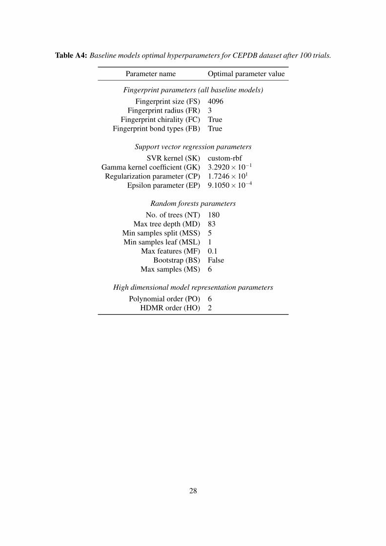
Table A4: Baseline models optimal hyperparameters for CEPDB dataset after 100 trials.

Parameter name Optimal parameter value

Fingerprint parameters (all baseline models)Fingerprint size (FS) 4096

Fingerprint radius (FR) 3Fingerprint chirality (FC) True

Fingerprint bond types (FB) True

Support vector regression parametersSVR kernel (SK) custom-rbf

Gamma kernel coefficient (GK) 3.2920×10−1

Regularization parameter (CP) 1.7246×101

Epsilon parameter (EP) 9.1050×10−4

Random forests parametersNo. of trees (NT) 180

Max tree depth (MD) 83Min samples split (MSS) 5Min samples leaf (MSL) 1

Max features (MF) 0.1Bootstrap (BS) False

Max samples (MS) 6

High dimensional model representation parametersPolynomial order (PO) 6

HDMR order (HO) 2

28

References[1] Dgl-LifeSci, last accessed 2020-12-16. https://github.com/awslabs/dgl-

lifesci.

[2] RDKit: Open-source cheminformatics, last accessed 2020-12-16. https://www.rdkit.org.

[3] O. A. Abdulrazzaq, V. Saini, S. Bourdo, E. Dervishi, and A. S. Biris. Organicsolar cells: a review of materials, limitations, and possibilities for improvement.Particulate Science and Technology, 31(5):427–442, 2013.

[4] T. Akiba, S. Sano, T. Yanase, T. Ohta, and M. Koyama. Optuna: A next-generationhyperparameter optimization framework. In Proceedings of the 25rd ACM SIGKDDInternational Conference on Knowledge Discovery and Data Mining, 2019.

[5] D. Bahdanau, K. Cho, and Y. Bengio. Neural machine translation by jointly learningto align and translate. arXiv preprint arXiv:1409.0473, 2014.

[6] L. Breiman. Random forests. Machine Learning, 45(1):5–32, 2001.

[7] K. Cho, B. Van Merriënboer, C. Gulcehre, D. Bahdanau, F. Bougares, H. Schwenk,and Y. Bengio. Learning phrase representations using RNN encoder-decoder forstatistical machine translation. arXiv preprint arXiv:1406.1078, 2014.

[8] CMCL Innovations. MoDS (Model Development Suite), version 2020.2.2, 2020.https://cmclinnovations.com/products/mods/.

[9] D. K. Duvenaud, D. Maclaurin, J. Iparraguirre, R. Bombarell, T. Hirzel, A. Aspuru-Guzik, and R. P. Adams. Convolutional networks on graphs for learning molecularfingerprints. Advances in Neural Information Processing Systems, 28:2224–2232,2015.

[10] J. Gilmer, S. S. Schoenholz, P. F. Riley, O. Vinyals, and G. E. Dahl. Neural messagepassing for quantum chemistry. arXiv preprint arXiv:1704.01212, 2017.

[11] M. A. Green, A. Ho-Baillie, and H. J. Snaith. The emergence of perovskite solarcells. Nature Photonics, 8(7):506–514, 2014.

[12] C. A. Gueymard, D. Myers, and K. Emery. Proposed reference irradiance spectrafor solar energy systems testing. Solar Energy, 73(6):443–467, 2002.

[13] J. Hachmann, R. Olivares-Amaya, S. Atahan-Evrenk, C. Amador-Bedolla, R. S.Sánchez-Carrera, A. Gold-Parker, L. Vogt, A. M. Brockway, and A. Aspuru-Guzik.The Harvard clean energy project: large-scale computational screening and designof organic photovoltaics on the world community grid. The Journal of PhysicalChemistry Letters, 2(17):2241–2251, 2011.

[14] S. Hochreiter and J. Schmidhuber. Long short-term memory. Neural Computation,9(8):1735–1780, 1997.

29

[15] M. Jeong, I. W. Choi, E. M. Go, Y. Cho, M. Kim, B. Lee, S. Jeong, Y. Jo, H. W.Choi, J. Lee, et al. Stable perovskite solar cells with efficiency exceeding 24.8% and0.3-v voltage loss. Science, 369(6511):1615–1620, 2020.

[16] D. P. Kingma and J. Ba. Adam: A method for stochastic optimization, 2017. URLhttps://arxiv.org/abs/1412.6980.

[17] T. N. Kipf and M. Welling. Semi-supervised classification with graph convolutionalnetworks. arXiv preprint arXiv:1609.02907, 2016.

[18] G. Lambard and E. Gracheva. SMILES-x: autonomous molecular compounds char-acterization for small datasets without descriptors. Machine Learning: Science andTechnology, 1(2):1–11, 2020. doi:10.1088/2632-2153/ab57f3.

[19] G. Landrum. Rdkit: A software suite for cheminformatics, computational chemistry,and predictive modeling, 2013.

[20] G. Li, S.-W. Wang, and H. Rabitz. Practical approaches to construct RS-HDMRcomponent functions. The Journal of Physical Chemistry A, 106(37):8721–8733,2002. doi:10.1021/jp014567t.

[21] Y. Li, D. Tarlow, M. Brockschmidt, and R. Zemel. Gated graph sequence neuralnetworks. arXiv preprint arXiv:1511.05493, 2015.

[22] S. A. Lopez, E. O. Pyzer-Knapp, G. N. Simm, T. Lutzow, K. Li, L. R. Seress,J. Hachmann, and A. Aspuru-Guzik. The Harvard organic photovoltaic dataset. Sci-entific Data, 3(1):1–7, 2016.

[23] S. A. Lopez, B. Sanchez-Lengeling, J. de Goes Soares, and A. Aspuru-Guzik. De-sign principles and top non-fullerene acceptor candidates for organic photovoltaics.Joule, 1(4):857–870, 2017.

[24] N. Meftahi, M. Klymenko, A. J. Christofferson, U. Bach, D. A. Winkler, and S. P.Russo. Machine learning property prediction for organic photovoltaic devices. npjComputational Materials, 6(1):1–8, 2020.

[25] H. L. Morgan. The generation of a unique machine description for chemicalstructures-a technique developed at chemical abstracts service. Journal of Chem-ical Documentation, 5(2):107–113, 1965.

[26] S. Nagasawa, E. Al-Naamani, and A. Saeki. Computer-aided screening of conju-gated polymers for organic solar cell: classification by random forest. The Journalof Physical Chemistry Letters, 9(10):2639–2646, 2018.

[27] D. Padula, J. D. Simpson, and A. Troisi. Combining electronic and structural fea-tures in machine learning models to predict organic solar cells properties. MaterialsHorizons, 6(2):343–349, 2019.

[28] F. Pedregosa, G. Varoquaux, A. Gramfort, V. Michel, B. Thirion, O. Grisel, M. Blon-del, P. Prettenhofer, R. Weiss, V. Dubourg, J. Vanderplas, A. Passos, D. Cournapeau,M. Brucher, M. Perrot, and E. Duchesnay. Scikit-learn: Machine learning in Python.Journal of Machine Learning Research, 12:2825–2830, 2011.

30

[29] E. O. Pyzer-Knapp, K. Li, and A. Aspuru-Guzik. Learning from the Harvard cleanenergy project: The use of neural networks to accelerate materials discovery. Ad-vanced Functional Materials, 25(41):6495–6502, 2015.

[30] E. O. Pyzer-Knapp, G. N. Simm, and A. A. Guzik. A Bayesian approach to calibrat-ing high-throughput virtual screening results and application to organic photovoltaicmaterials. Materials Horizons, 3(3):226–233, 2016.

[31] H. Rabitz and Ö. F. Alis. General foundations of high-dimensional modelrepresentations. Journal of Mathematical Chemistry, 25(2-3):197–233, 1999.doi:10.1023/A:1019188517934.

[32] D. Rogers and M. Hahn. Extended-connectivity fingerprints. Journal of ChemicalInformation and Modeling, 50(5):742–754, 2010.

[33] S. Rühle. Tabulated values of the Shockley–Queisser limit for single junction solarcells. Solar Energy, 130:139–147, 2016.

[34] S. Ryu, J. Lim, S. H. Hong, and W. Y. Kim. Deeply learning molecular structure-property relationships using attention-and gate-augmented graph convolutional net-work. arXiv preprint arXiv:1805.10988, 2018.

[35] H. Sahu and H. Ma. Unraveling correlations between molecular properties and de-vice parameters of organic solar cells using machine learning. The Journal of Phys-ical Chemistry Letters, 10(22):7277–7284, 2019.

[36] H. Sahu, F. Yang, X. Ye, J. Ma, W. Fang, and H. Ma. Designing promising moleculesfor organic solar cells via machine learning assisted virtual screening. Journal ofMaterials Chemistry A, 7(29):17480–17488, 2019.

[37] M. C. Scharber and N. S. Sariciftci. Efficiency of bulk-heterojunction organic solarcells. Progress in Polymer Science, 38(12):1929–1940, 2013.

[38] M. C. Scharber, D. Mühlbacher, M. Koppe, P. Denk, C. Waldauf, A. J. Heeger, andC. J. Brabec. Design rules for donors in bulk-heterojunction solar cells—towards10% energy-conversion efficiency. Advanced Materials, 18(6):789–794, 2006.

[39] A. J. Smola and B. Schölkopf. A tutorial on support vector regression. Statistics andComputing, 14(3):199–222, 2004.

[40] H. J. Snaith. Perovskites: the emergence of a new era for low-cost, high-efficiencysolar cells. The journal of Physical Chemistry Letters, 4(21):3623–3630, 2013.

[41] W. Sun, M. Li, Y. Li, Z. Wu, Y. Sun, S. Lu, Z. Xiao, B. Zhao, and K. Sun. The useof deep learning to fast evaluate organic photovoltaic materials. Advanced Theoryand Simulations, 2(1):1800116, 2019.

[42] W. Sun, Y. Zheng, K. Yang, Q. Zhang, A. A. Shah, Z. Wu, Y. Sun, L. Feng, D. Chen,Z. Xiao, et al. Machine learning–assisted molecular design and efficiency predictionfor high-performance organic photovoltaic materials. Science Advances, 5(11):1–8,2019. doi:10.1126/sciadv.aay4275.

31

[43] A. Urbina. The balance between efficiency, stability and environmental impactsin perovskite solar cells: a review. Journal of Physics: Energy, 2(2):1–25, 2020.doi:10.1088/2515-7655/ab5eee.

[44] K. Vandewal, S. Himmelberger, and A. Salleo. Structural factors that affect theperformance of organic bulk heterojunction solar cells. Macromolecules, 46(16):6379–6387, 2013.

[45] P. Velickovic, G. Cucurull, A. Casanova, A. Romero, P. Lio, and Y. Bengio. Graphattention networks. arXiv preprint arXiv:1710.10903, 2017.

[46] M. Wang, D. Zheng, Z. Ye, Q. Gan, M. Li, X. Song, J. Zhou, C. Ma, L. Yu,Y. Gai, T. Xiao, T. He, G. Karypis, J. Li, and Z. Zhang. Deep graph library: Agraph-centric, highly-performant package for graph neural networks. arXiv preprintarXiv:1909.01315, 2019.

[47] B. Weisfeiler and A. Lehmann. A reduction of a graph to a canonical form and analgebra arising during this reduction. Nauchno-Technicheskaya Informatsia, 2(9):12–16, 1968.

[48] D. Wöhrle and D. Meissner. Organic solar cells. Advanced Materials, 3(3):129–138,1991.

[49] J. Wu, S. Wang, L. Zhou, X. Ji, Y. Dai, Y. Dang, and M. Kraft. Deep-learningarchitecture in QSPR modeling for the prediction of energy conversion efficiency ofsolar cells. Industrial & Engineering Chemistry Research, 2020.

[50] Z. Wu, B. Ramsundar, E. N. Feinberg, J. Gomes, C. Geniesse, A. S. Pappu,K. Leswing, and V. Pande. MoleculeNet: a benchmark for molecular machine learn-ing. Chemical Science, 9(2):513–530, 2018.

[51] Y. Xie, W. Wang, W. Huang, F. Lin, T. Li, S. Liu, X. Zhan, Y. Liang, C. Gao, H. Wu,et al. Assessing the energy offset at the electron donor/acceptor interface in organicsolar cells through radiative efficiency measurements. Energy & Environmental Sci-ence, 12(12):3556–3566, 2019.

[52] Z. Xiong, D. Wang, X. Liu, F. Zhong, X. Wan, X. Li, Z. Li, X. Luo, K. Chen,H. Jiang, et al. Pushing the boundaries of molecular representation for drug discov-ery with the graph attention mechanism. Journal of Medicinal Chemistry, 2019.

[53] Z. Xu, L.-M. Chen, M.-H. Chen, G. Li, and Y. Yang. Energy level alignment of poly(3-hexylthiophene):[6, 6]-phenyl c 61 butyric acid methyl ester bulk heterojunction.Applied Physics Letters, 95(1):178, 2009.

[54] Z.-W. Zhao, M. del Cueto, Y. Geng, and A. Troisi. Effect of increasing the descrip-tor set on machine learning prediction of small molecule-based organic solar cells.Chemistry of Materials, 32(18):7777–7787, 2020.

32