predicting the aftermath of vortex breakup in rotating ow
TRANSCRIPT

J. Fluid Mech. (2011), vol. 669, pp. 90–119. c© Cambridge University Press 2011
doi:10.1017/S0022112010004945
Predicting the aftermath of vortex breakupin rotating flow
G. F. CARNEVALE1†, R. C. KLOOSTERZIEL2, P. ORLANDI3AND D. D. J. A. van SOMMEREN4‡
1Scripps Institution of Oceanography, University of California, San Diego, La Jolla, CA 92093, USA2School of Ocean and Earth Science and Technology, University of Hawaii,
Honolulu, HI 96822, USA3Dipartimento di Meccanica e Aeronautica, University of Rome, ‘La Sapienza’,
via Eudossiana 18, 00184 Roma, Italy4Eindhoven University of Technology, PO Box 513, 5600 MB Eindhoven, the Netherlands
(Received 20 May 2010; revised 17 September 2010; accepted 17 September 2010;
first published online 11 January 2011)
A method for predicting the outcome of vortex breakup in a rotating flow isintroduced. The vortices dealt with here are subject to both centrifugal and barotropicinstabilities. The prediction of the aftermath of the breakup relies on knowinghow both centrifugal and barotropic instabilities would equilibrate separately. Atheoretical model for non-linear equilibration in centrifugal instability is weddedto two-dimensional simulation of barotropic instability to predict the final vorticesthat emerge from the debris of the original vortex. This prediction method is testedagainst three-dimensional Navier–Stokes simulations. For vortices in which a rapidcentrifugal instability triggers a slower barotropic instability, the method is successfulboth qualitatively and quantitatively. The skill of the prediction method decreases asthe time scales of the two instabilities become comparable.
Key words: geophysical and geological flows, turbulent flows, vortex flows
1. IntroductionVortex breakup is a complicated process that often involves multiple instabilities.
Nevertheless, in a rotating flow, the result of breakup and re-equilibration is usuallya combination of simple vortex structures. Vortex monopoles, dipoles and tripoles,with their axes aligned along the ambient rotation axis, emerge out of the debris ofthe original vortex. Here, we consider the possibility of predicting the aftermath ofvortex breakup based on our knowledge of the tendencies of the different instabilitiesinvolved.
Van Heijst & Kloosterziel (1989) and Kloosterziel & van Heijst (1991) investigatedvortex breakup and re-equilibration in rotating tank experiments. The tank was filledwith water with uniform density and then placed in rotation about a vertical axis.The fluid was allowed to reach a state of solid-body rotation. Then, an open-endedthin-walled hollow cylinder was placed vertically in the fluid. A vortex was created
† Email address for correspondence: [email protected]‡ Present address: BP Institute and Department of Applied Mathematics and Theoretical Physics,
University of Cambridge, Cambridge CB3 0EZ, UK.
Aftermath of vortex breakup in rotating flow 91
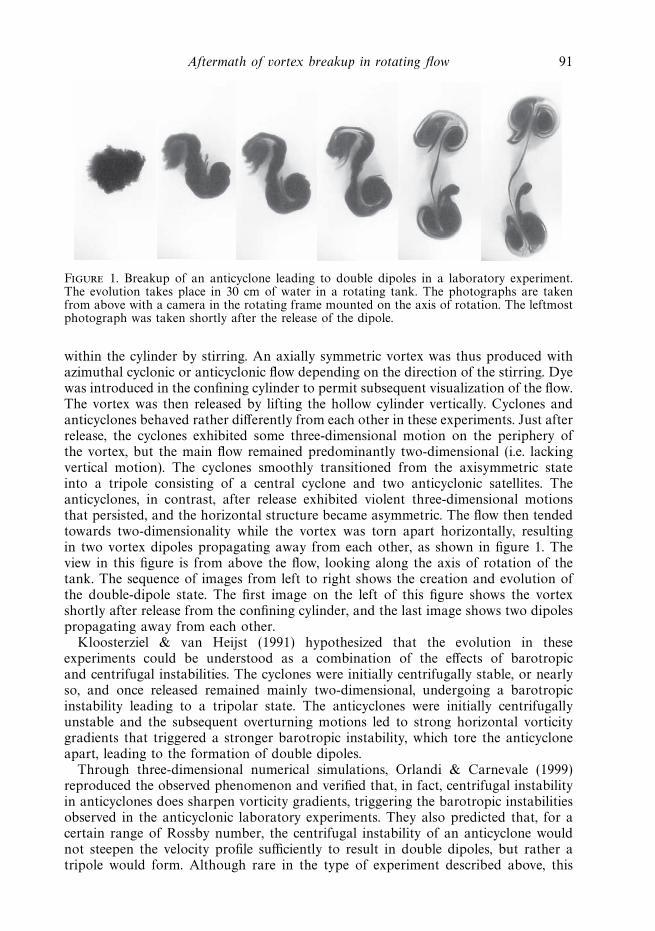
Figure 1. Breakup of an anticyclone leading to double dipoles in a laboratory experiment.The evolution takes place in 30 cm of water in a rotating tank. The photographs are takenfrom above with a camera in the rotating frame mounted on the axis of rotation. The leftmostphotograph was taken shortly after the release of the dipole.
within the cylinder by stirring. An axially symmetric vortex was thus produced withazimuthal cyclonic or anticyclonic flow depending on the direction of the stirring. Dyewas introduced in the confining cylinder to permit subsequent visualization of the flow.The vortex was then released by lifting the hollow cylinder vertically. Cyclones andanticyclones behaved rather differently from each other in these experiments. Just afterrelease, the cyclones exhibited some three-dimensional motion on the periphery ofthe vortex, but the main flow remained predominantly two-dimensional (i.e. lackingvertical motion). The cyclones smoothly transitioned from the axisymmetric stateinto a tripole consisting of a central cyclone and two anticyclonic satellites. Theanticyclones, in contrast, after release exhibited violent three-dimensional motionsthat persisted, and the horizontal structure became asymmetric. The flow then tendedtowards two-dimensionality while the vortex was torn apart horizontally, resultingin two vortex dipoles propagating away from each other, as shown in figure 1. Theview in this figure is from above the flow, looking along the axis of rotation of thetank. The sequence of images from left to right shows the creation and evolution ofthe double-dipole state. The first image on the left of this figure shows the vortexshortly after release from the confining cylinder, and the last image shows two dipolespropagating away from each other.
Kloosterziel & van Heijst (1991) hypothesized that the evolution in theseexperiments could be understood as a combination of the effects of barotropicand centrifugal instabilities. The cyclones were initially centrifugally stable, or nearlyso, and once released remained mainly two-dimensional, undergoing a barotropicinstability leading to a tripolar state. The anticyclones were initially centrifugallyunstable and the subsequent overturning motions led to strong horizontal vorticitygradients that triggered a stronger barotropic instability, which tore the anticycloneapart, leading to the formation of double dipoles.
Through three-dimensional numerical simulations, Orlandi & Carnevale (1999)reproduced the observed phenomenon and verified that, in fact, centrifugal instabilityin anticyclones does sharpen vorticity gradients, triggering the barotropic instabilitiesobserved in the anticyclonic laboratory experiments. They also predicted that, for acertain range of Rossby number, the centrifugal instability of an anticyclone wouldnot steepen the velocity profile sufficiently to result in double dipoles, but rather atripole would form. Although rare in the type of experiment described above, this

92 G. F. Carnevale, R. C. Kloosterziel, P. Orlandi and D. D. J. A. van Sommeren
Figure 2. Breakup of an anticyclone leading to a tripole in a laboratory experiment. Theevolution takes place in 30 cm of water in a rotating tank. The photographs are taken fromabove with a camera in the rotating frame mounted on the axis of rotation.
prediction was later verified in the laboratory. An example of tripole formation froman anticyclone is shown in figure 2.
Early in the development of this subject, there was a good theoretical understandingof barotropic instability and the end states that resulted due to nonlinear effects (cf.Dritschel 1986; Flierl 1988; Carton & McWilliams 1989; Carton, Fierl & Polvani1989; Kloosterziel & Carnevale 1992; Carnevale & Kloosterziel 1994). Until recently,however, a comparable understanding of the nonlinear saturation of the centrifugalinstability in unconfined vortices was lacking, even though there had been severaldetailed studies (e.g. Carnevale et al. 1997; Smyth & McWilliams 1998). Thus, notheoretical prediction could be made of the final result of the combined effectof the two instabilities. The missing piece of the puzzle has now been providedby Kloosterziel, Carnevale & Orlandi (2007a), who deduce a rule for the infinite-Reynolds-number equilibration of centrifugal instability. We will show how this rulecan be combined with what is known of barotropic instability to make predictionsabout the combined effects of centrifugal and barotropic instabilities without resortingto costly three-dimensional simulations.
This work is motivated in part by the many oceanic examples of anticyclonesthat are marginally stable to centrifugal instability. These strong anticyclones arethought to be generated by frictional torques on strong currents passing coasts andislands (D’Asaro 1988). Some specific examples of these anticyclones are found inthe wake of the island of Hawaii (Flament et al. 2001), in the wake of the Canaryislands (Aristegui et al. 1994), and in the Beaufort Sea, where they have been createdby flow through Barrow Canyon (D’Asaro 1988). All these vortices were probablycentrifugally unstable when they were formed and then went through an adjustmentthat brought them to marginal stability. The work presented here is a contributiontowards understanding that adjustment process. Our results could be the basis forparametrizing the effects of centrifugal instability in general circulation models withresolution too coarse to permit centrifugal instability.
The method of prediction developed here may be generalizable to systems otherthan vortices. A straightforward extension of this work would be to the predictionof the outcome of inertial instability in parallel shear flows. In the atmosphere, suchinstability is believed to cause phenomena like clear air turbulence (Knox 1997), rainbands or squall lines (Bennetts & Hoskins 1979), the banded structure of Jupiter’satmosphere (Stone 1967) and the vertically stacked temperature extrema near theequatorial stratopause (Hayashi, Shiotani & Gille 1998). In the equatorial pacificocean, it may cause the observed ‘interleaving’ of alternately saltier and fresher layers

Aftermath of vortex breakup in rotating flow 93
eθer
ez
z
r
w
u
f
Unstableregion
Unstableregion
v
(a) (b)
θ
Figure 3. (a) Schematic diagram showing the cylindrical coordinate system. (b) A schematicrepresentation of ‘rib’ vortices. The signs refer to the sign of the azimuthal vorticity ωθ . Thelinear instability creates a stack of rings of azimuthal vorticity of alternating sign (rib vortices)centred on the axis of the primary vortex (r = 0). Note that f = 2Ω is the Coriolis parameterand Ω is the angular rotation rate of the ambient flow into which the vortex is introduced.
(Richards & Edwards 2003). We have already taken the first step towards developinga method for predicting the outcome of inertial instability on parallel shear flow inKloosterziel, Orlandi & Carnevale (2007b), and further development analogous tothat for vortices presented here will be the subject of future work.
The plan of this paper is as follows. In § 2, we briefly review the new theory ofnonlinear equilibration of centrifugal instability and then outline relevant aspects ofwhat is known about the nonlinear equilibration of barotropic instability. Then, in§ 3 a scheme for combining the two theories of equilibration to make predictions ofthe outcome of the combined instabilities is given. In § 4, we test this theory in themost favourable situation, in which the centrifugal instability is much faster thanthe barotropic instability. To test the limits of this kind of prediction, in § 5 a lessfavourable case is explored for which the time scales of the two instabilities aresimilar. Conclusions are presented in § 6.
2. The basic instabilitiesBoth centrifugal and barotropic instabilities in their ideal form are not fully
three-dimensional. Centrifugal instability is ideally an axisymmetric instability, whilebarotropic instability can be treated as a pure two-dimensional flow problem. In thissection we will discuss basic characteristics of these two instabilities, focusing on hownonlinearities saturate these instabilities and lead to characteristic final stable states.We will begin with centrifugal instability and place special emphasis on the recentadvances that allow the prediction of the equilibrated state in the high-Reynolds-number limit. The discussion of the barotropic instability will be a review of earlierwork with emphasis on points relevant to this paper.
2.1. Nonlinear equilibration in axisymmetric centrifugal instability
In the breakup of anticyclones described in the Introduction, there is a vigorous three-dimensional instability during the early evolution. This three-dimensional phase is theresult of centrifugal instability. To describe the evolution of the vortex, it is convenientto use a cylindrical coordinate system (r, θ, z) where the z-axis corresponds to thevertical direction (see figure 3a). The velocities (u, v, w) correspond to the radial,

94 G. F. Carnevale, R. C. Kloosterziel, P. Orlandi and D. D. J. A. van Sommeren
azimuthal and vertical directions. The components of vorticity in this coordinatesystem are given by
ωr = r−1∂θw − ∂zv, ωθ = ∂zu − ∂rw, ωz = r−1(∂r (rv) − ∂θu). (2.1)
An axisymmetric barotropic vortex with its axis coincident with the vertical axis isdefined by the azimuthal velocity field V (r). In the initially null field of azimuthalvorticity ωθ , centrifugal instability creates a stack of vortex rings similar to thewell-known toroidal Taylor–Couette vortices in the flow between concentric rotatingcylinders. This perturbation appears and grows in an annular region of instability (seefigure 3b) that can be defined through the Rayleigh criterion for centrifugal instability(Rayleigh 1916; Drazin & Reid 1981). The original version of this criterion was derivedfor axisymmetric flow in an inertial frame of reference. Subsequently, the criterionwas generalized for vortices in a rotating frame (see Sawyer 1947; Kloosterziel & vanHeijst 1991). Inviscid linear stability is determined by the distribution of the absoluteangular momentum defined by L ≡ r(V + Ωr), where V is the azimuthal velocity ofthe flow, Ω is the ambient angular rotation rate and r is the radial distance from theaxis of the vortex. The flow is unstable in an annulus where the magnitude of theabsolute angular momentum decreases, in other words where dL2/dr < 0.
We will base our discussion here on a family of vortices parametrized by a ‘steepnessparameter’ α which controls the strength of the vorticity gradients outside the vortexcore. The advantages of using this family are the following: namely all the vorticeshave zero circulation (hence finite energy); it can be used to match velocity profilesfound in laboratory experiments reasonably well; its parameter α controls, to a greatextent, the character of the instability; and it has been the subject of many previoustheoretical and numerical investigations (e.g. Carton & McWilliams 1989; Carton et al.1989; Orlandi & van Heijst 1992; Carton & Legras 1994; Carnevale & Kloosterziel1994; Kloosterziel & Carnevale 1999; Orlandi & Carnevale 1999; Gallaire & Chomaz2003). The velocity profile for this family is given by
V (r) = ± r
2exp(−rα), (2.2)
where we have non-dimensionalized the velocity by a characteristic velocity U andradius by a length scale L. The ± sign determines whether the vortex is a cycloneor anticyclone. The factor of 1/2 normalization of the velocity is chosen to fix thenon-dimensional vorticity at r =0 to be +1 for cyclones and −1 for anticyclones. Thevorticity derived from this velocity profile is aligned along the vertical direction. Itsamplitude is given by
ωz(r) = ±(1 − α
2rα
)exp(−rα). (2.3)
From the velocity and length scales U and L, we define the Rossby and Reynoldsnumbers for this flow as
Ro = ±U/f L and Re = UL/ν, (2.4)
respectively, where f = 2Ω is the Coriolis parameter. The Rossby number is defined sothat the positive/negative sign corresponds to cyclones/anticyclones. In what follows,we have non-dimensionalized all spatial quantities using the length scale L and timewith the advective time scale L/U.
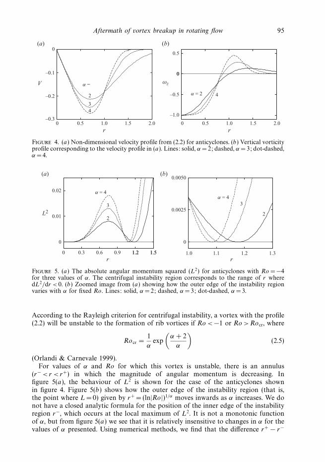
For the anticyclonic case, figure 4 shows how the velocity V and vorticity ωz profileschange with α. Note how vorticity gradients increase with increasing α. The graphs inthe cyclonic case would be the same as these save for a sign change for the amplitude.
Aftermath of vortex breakup in rotating flow 95
0 0.5 1.0 1.5 2.0
43
2
α = V
r r 0 0.5 1.0 1.5 2.0
–0.3
–0.2
–0.1
–1.0
–0.5
0.5 0
(a) (b)
0
4
ωz
0
α = 2
Figure 4. (a) Non-dimensional velocity profile from (2.2) for anticyclones. (b) Vertical vorticityprofile corresponding to the velocity profile in (a). Lines: solid, α= 2; dashed, α= 3; dot-dashed,α= 4.
0
0.01
0.02
(a) (b)
0 0.3 0.6 0.9 1.2 1.5
3
2
α = 4
L2
r r 1.2 1.5
0
0.0025
0.0050
1.0 1.1 1.2 1.3
3
2
α = 4
Figure 5. (a) The absolute angular momentum squared (L2) for anticyclones with Ro = −4for three values of α. The centrifugal instability region corresponds to the range of r wheredL2/dr < 0. (b) Zoomed image from (a) showing how the outer edge of the instability regionvaries with α for fixed Ro. Lines: solid, α= 2; dashed, α= 3; dot-dashed, α= 3.
According to the Rayleigh criterion for centrifugal instability, a vortex with the profile(2.2) will be unstable to the formation of rib vortices if Ro < −1 or Ro >Rocr, where
Rocr =1
αexp
(α + 2
α
)(2.5)
(Orlandi & Carnevale 1999).For values of α and Ro for which this vortex is unstable, there is an annulus
(r− < r < r+) in which the magnitude of angular momentum is decreasing. Infigure 5(a), the behaviour of L2 is shown for the case of the anticyclones shownin figure 4. Figure 5(b) shows how the outer edge of the instability region (that is,the point where L =0) given by r+ = (ln|Ro|)1/α moves inwards as α increases. We donot have a closed analytic formula for the position of the inner edge of the instabilityregion r−, which occurs at the local maximum of L2. It is not a monotonic functionof α, but from figure 5(a) we see that it is relatively insensitive to changes in α for thevalues of α presented. Using numerical methods, we find that the difference r+ − r−

96 G. F. Carnevale, R. C. Kloosterziel, P. Orlandi and D. D. J. A. van Sommeren
r– r+ r– r+ r– r+
r r r
z
0.3 1.3 0.3 1.3 0.3 1.30
1(a) (b) (c)
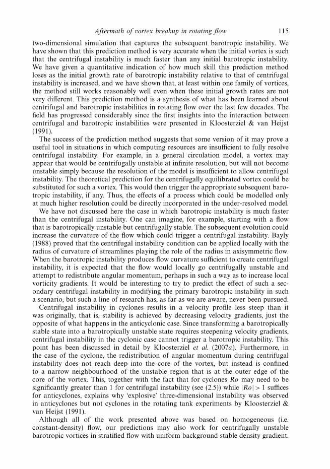
0
1
0
1
Figure 6. Overturning motions induced by centrifugal instability visualized by plots ofazimuthal vorticity in an axisymmetric flow simulation. (a) (t = 28) The linear phase ofthe instability from random small-scale perturbations creates a stack of rings of azimuthalvorticity of alternating sign (rib vortices) centred on the axis (r = 0) of the primary vortex.(b) (t = 56) Nonlinear interactions of the rib vortices cause the formation of dipolar structuresthat propagate outside the initial unstable region. (c) (t = 64) Extensive mixing of angularmomentum that extends well beyond the initial instability region results from the propagationof the perturbations. These are results for velocity profile (2.2) with Ro = −4 and α= 3. Theflow is bounded above (at z = 1) and below (at z = 0) by free-slip surfaces. The computationalflow domain extends from r =0 to r = 6. The boundary at r =6 is also free-slip. The Reynoldsnumber for this run was 6 × 10⁴. Positive/negative contours of ωθ are black/grey. The contourinterval is 0.003. The range of the initial unstable region, r− <r < r+, is indicated by thevertical dashed lines.
is a monotonically decreasing function of α for α> 2. In other words, for fixed Ro,the instability region becomes narrower as α increases.
Starting from small-scale random initial perturbations, the instability begins withinthe annulus of instability. The perturbation grows into a stack of ‘rib vortices’ asillustrated in the schematic diagram in figure 3(b), where we plot the azimuthalvorticity in an r–z (radial–vertical) cross-section. In inviscid theory, the most unstablerib vortices would be those of infinitesimal vertical dimension (Stone 1966; Dunkerton1981; Bayly 1988; Smyth & McWilliams 1998; Gallaire & Chomaz 2003). However,the damping effect of viscosity on small scales results in a balance that selects a fastest-growing mode of finite scale that emerges from the linear phase of the instability. Forincreasing Re, the preferred vertical scale of the motions was found by Kloosterzielet al. (2007a) to decrease as Re−1/3.
Kloosterziel et al. (2007a) studied the axisymmetric unfolding of centrifugalinstability well beyond the initial linear phase. Their goal was to understand theultimate tendency of the centrifugal instability acting alone. By using axisymmetricsimulations, for which the barotropic instability is suppressed, they were able to followthe evolution of the pure (that is, axisymmetric) centrifugal instability all the waythrough to nonlinear equilibration. The numerical method will be discussed in § 4.The typical early phases of this axisymmetric evolution are illustrated in figure 6taken from a numerical simulation at high Re. Figure 6(a) shows the rib vortices inthe ωθ field that grow out of the small-scale random perturbations during the lineardynamics phase of the instability growth. Note that these rib vortices are initiallyconfined to the region of instability defined by the Rayleigh criterion. The limits ofthis region, r− < r < r+, are indicated by the dashed vertical lines in each figure. Asthe axisymmetric evolution continues past the linear-instability phase, the rib vortices
Aftermath of vortex breakup in rotating flow 97
0
0.5(a) (b)
0 1 2
L
r– r+
r
rc
–0.25
0
0 1 2
V
r
rc
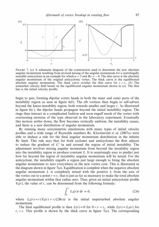
Figure 7. (a) A schematic diagram of the construction used to determine the new absoluteangular momentum resulting from inviscid mixing of the angular momentum for a centrifugallyunstable anticyclone in an example for which α= 3 and Ro = −4. The thin curve is the absoluteangular momentum of the original anticyclonic vortex. The thick curve is the equilibratedabsolute angular momentum. The thick curve overlies the thin curve for r > rc . (b) Theazimuthal velocity field based on the equilibrated angular momentum shown in (a). The thinline is the initial velocity profile.
begin to pair, forming dipolar vortex heads in both the inner and outer parts of theinstability region as seen in figure 6(b). The rib vortices then begin to self-advectbeyond the linear-instability region, both towards smaller and larger r . As illustratedin figure 6(c), the dipolar heads propagate beyond the initial instability region. Therings then interact in a complicated fashion and soon engulf much of the vortex withoverturning motions of the type observed in the laboratory experiment. Eventuallythis motion settles down, the flow becomes vertically uniform, the instability ceases,and there is a new distribution of angular momentum.
By running many axisymmetric simulations with many types of initial velocityprofiles and a wide range of Reynolds numbers Re, Kloosterziel et al. (2007a) wereable to deduce a rule for the final angular momentum distribution in the infiniteRe limit. This rule says that for both cyclones and anticyclones the flow adjuststo reduce the gradient of L2 in and around the region of initial instability. Theadjustment involves mixing angular momentum from beyond the instability regioninto the instability region to produce constant L. It is surprisingly easy to predict justhow far beyond the region of instability angular momentum will be mixed. For theanticyclone, the instability engulfs a region just large enough to bring the absoluteangular momentum to zero everywhere in the new vortex core. This is illustrated inthe diagram shown in figure 7(a). Equilibration is complete when the negative absoluteangular momentum L is completely mixed with the positive L from the axis ofthe vortex out to a point r = rc that is just as far as necessary to make the total absoluteangular momentum within that radius zero. Thus, given an initial anticyclonic profileV0(r), the value of rc can be determined from the following formula:
∫ rc
0
L0(r)r dr = 0, (2.6)
where L0(r) = r (V0(r) + r/(2Ro)) is the initial unperturbed absolute angularmomentum.
The final equilibrated profile is then L(r) = 0 for 0 <r < rc, while L(r) = L0(r) forrc < r . This profile is shown by the thick curve in figure 7(a). The corresponding
98 G. F. Carnevale, R. C. Kloosterziel, P. Orlandi and D. D. J. A. van Sommeren
prediction for the equilibrated velocity field is
V (r) =
− r
2Ro, 0 ! r ! rc,
V0(r), rc < r.(2.7)
Within the new core (i.e. where r ! rc), the predicted flow is given in dimensionalform as V (r) = −Ωr , which is just solid-body rotation with the angular velocity −Ω ,that is, the negative of the angular velocity of the tank. This means that the predictedflow in the core is stationary in the laboratory frame of reference. The profile for theequilibrated V is shown by the thick solid line in figure 7(b). This singular velocityprofile is approached ever more closely in numerical axisymmetric experiments as theReynolds number is increased (Kloosterziel et al. 2007a , figure 13a).
Cyclones can also be centrifugally unstable as noted above. However, centrifugalinstability in barotropically stable cyclones cannot trigger barotropic instability. Thedifference between cyclones and anticyclones is discussed further in § 6.
2.2. Nonlinear equilibration in 2-D Barotropic Instability
The initial axisymmetric flow in an anticyclone has anticyclonic vorticity in the coresurrounded by an annulus of cyclonic vorticity. In the later stages of the instability, thisdistribution is rearranged, in some cases rather dramatically. In the examples shown inthe Introduction, a tripole and a pair of dipoles emerged out of the debris of the vortexbreakup. More exotic structures such as quadrupoles (an anticyclone surrounded bythree cyclonic satellites) have also been observed as temporary structures whichthen break up, leaving monopoles, dipoles or tripoles as stable byproducts of thebreakup; see Morel & Carton (1994) and Carnevale & Kloosterziel (1994) for a fullerdescription of these possibilities.
The horizontal segregation of the vertical vorticity resulting in these structuresis the result of barotropic instability. This is an instability of horizontal shear thatcan be understood completely within the context of two-dimensional flow. Since theinstability is two-dimensional, it makes no difference if the initial flow is cyclonicor anticyclonic except for an overall sign change in the vorticity distribution. The(necessary) criterion for this instability is given by the inflection point theorem ofRayleigh (1880). Originally for planar shear, a generalized form of the criterion alsoapplies to initially axisymmetric flow (see Drazin & Reid 1981). There is no knowngeneral sufficient criterion for the instability. Linear theory can be applied to piecewiseuniform axisymmetric vorticity profiles to predict analytically the growth rates forvarious azimuthal modes, that is, modes that vary as eimθ . This was done by Stern(1987) and Flierl (1988) by normal modes analysis and by Kloosterziel & Carnevale(1992) through an energy method. For more general profiles, as would be appropriatefor laboratory flows, numerical analysis can be used to predict the growth rates ofindividual azimuthal modes. The barotropic instability of velocity profile (2.2) hasbeen studied as a model for laboratory flows as well as for geophysical flows. For thisprofile, figure 8 shows how the growth rates of the first three unstable modes vary withthe steepness parameter (cf. Carton & McWilliams 1989; Carnevale & Kloosterziel1994; Gallaire & Chomaz 2003). These are measured exponential amplification ratesof the perturbations that follow exp(γ t) with t the non-dimensionalized time. Thereare no growing modes for α " 1.85. As α is increased above this critical value,mode m =2 is the first to become unstable. The growth of this mode is responsiblefor tripole formation. As α is increased further, higher modes also become unstable.The double-dipole formation seen in the Introduction results from the growth of a

Aftermath of vortex breakup in rotating flow 99
0
0.1
0.2
0.3
1 2 3 4 5 6 7 8
m = 2 3 4
γ
α
m = 2
m = 3
m = 4
(a) (b)
Figure 8. (a) Non-dimensional exponential growth rate γ of the barotropic instability forazimuthal modes m= 2, 3, 4 (data from Kloosterziel & Carnevale 1999). (b) Products ofnonlinear evolution when the initial perturbation is purely mode m= 2 (tripole), 3 (quadrupole)or 4 (pentapole). Blue/red represents positive/negative vorticity.
combination of mode m =2 and higher modes, and so can occur only for α # 3.Carnevale & Kloosterziel (1994) showed that mode m =3 may grow into a stablequadrupole, but its stability was rather fragile, and small disturbances of a few percent of its maximum vorticity led to its destruction. Because of its fragile stability, thequadrupole is not ordinarily seen as an end state of the kind of anticyclone breakupdescribed above; however, Beckers & van Heijst (1998) have shown that it is possibleto routinely generate quadrupoles in the laboratory by strongly stimulating modem = 3 initially, in agreement with the numerical study by Carton (1992). The modem = 4 growth can result in creating a pentapole (as in figure 8). This ‘square vortex’becomes unstable when fluctuations bring two of the outer satellites close together.The satellites then coalesce in pairs, forming a transient tripole that then usuallybreaks up into a pair of dipoles. Higher-order structures, resulting from the growth ofhigher-order azimuthal modes, also become unstable when the outer satellites comeclose together and coalesce, resulting in some combination of monopoles, dipoles andtripoles.
The long-term outcome of the barotropic instability will depend on the valueof α as well as the distribution of initial perturbation energy among the possibleunstable modes for that value of α. For α " 1.85, the flow is not unstable andremains a monopole. A tripole results for 1.85 " α " 3 (Kloosterziel & Carnevale1999). For higher values, the vortex can go through a remarkable array of forms,depending on how many azimuthal modes are unstable and the precise form of theinitial perturbation. Very complicated flows can result, especially when the initialperturbation has significant energy in spatial scales on the order of that characteristicof the unperturbed vortex. The flow can evolve through a series of intermediate statesincluding, for example, hexapoles, pentapoles and quadrupoles. Except for small-scaledebris in the form of thin vorticity filaments and the small vortices that may becreated by the roll-up of filaments, the final result is some combination of monopoles,dipoles, tripoles and quadrupoles, although the quadrupole is a less likely componentas discussed above. If the initial disturbance is made of only small-scale small-amplitude randomly distributed velocity fluctuations, we find that the end product iseither a monopole, a tripole or a pair of dipoles.

100 G. F. Carnevale, R. C. Kloosterziel, P. Orlandi and D. D. J. A. van Sommeren
3. Full 3-D simulation versus predictionOur goal is to determine how well the outcome of the breakup of an anticyclonic
vortex can be predicted by using what we know of the nonlinear equilibration ofthe axisymmetric centrifugal instability and the 2-D barotropic instability. In thelaboratory experiments discussed above, it appears that an early rapid centrifugalinstability sets up conditions for a barotropic instability that then follows. For inviscidflow, we can predict the outcome of pure centrifugal instability by using (2.7). Here wewill use this formula to give us an approximation of the effects of centrifugal instabilityin the early part of the actual 3-D flow. Then, lacking a general theory to predict theequilibration of barotropic instability, we use 2-D simulation of the Navier–Stokesequations to predict the outcome of the barotropic instability. The initial conditionfor this 2-D simulation is taken as the theoretical equilibrium of the centrifugalinstability and random grid-scale noise. The 3-D viscous flow will never actuallyachieve the velocity discontinuity contained in (2.7). Therefore, perhaps one shouldconsider using an artificially smoothed version of this profile for an initial conditionof the 2-D simulation. The singular profile could be smoothed by estimating thediffusive effect of viscosity acting over some period of time or perhaps, more simply,the discontinuity could be arbitrarily smoothed over the scale of a few gridpoints.Either choice would be artificial and arbitrary, so for the time being we have usedformula (2.7) as is, simply rendering it on the finite 2-D grid used in the next phase ofthe prediction. The Reynolds number used for the 2-D simulation is that of the 3-Dsimulation to which the prediction will be compared. The grid for the 2-D simulationis the same as the horizontal grid used in the 3-D simulation.
In summary, this prediction scheme replaces the centrifugal instability phase ofthe evolution by jumping to the velocity field given by (2.7). Then the barotropicinstability phase of the flow is replaced by a two-dimensional simulation. This schemehas the best chance of succeeding when the initial flow is centrifugally unstablebut barotropically stable. In that case, in the full 3-D simulation, the flow mustbecome centrifugally unstable before any barotropic instability can take place. Thus,we take as our first case an initial profile with steepness parameter α= 1.8, which isbarotropically stable as discussed in § 2.2 above. On the other hand, the predictionscheme should be expected to have less skill if the initial instability rates for the twoinstabilities are comparable. How well the scheme does under these circumstanceswill be tested using an example with α= 3. In both cases, we have explored a rangeof Re and Ro as will be discussed below.
4. Centrifugal instability faster than barotropic instability (α = 1.8)As explained above, the velocity profile (2.2) is barotropically stable for α " 1.85.
If we take as an initial condition the velocity profile (2.2) with α= 1.8, there willbe no barotropic instability initially. There will, however, be centrifugal instability ifthe Rossby number is sufficiently negative. The inviscid criterion tells us that we willhave centrifugal instability if and only if Ro < −1; however, since we cannot reproduceinfinite Re flow numerically, we must consider the effects of finite Re.
The numerical method used is a finite-difference staggered-mesh scheme that solvesthe incompressible Navier–Stokes equations in a cylindrical coordinate system (r, θ, z)with the z-axis coincident with the axis of the initial vortex, which is parallel to the axisof rotation of the background as sketched in figure 3. The details of the method, whichis energy conserving in the absence of viscosity in the limit of infinitesimal time steps,are described in detail in Verzicco & Orlandi (1996) and Orlandi (2000). We impose

Aftermath of vortex breakup in rotating flow 101
free-slip boundary conditions on the top and bottom of the computational domain andon the cylindrical wall. To allow sufficient room for the unfolding of the barotropicinstability, we have taken the radial range as 0< r < 6. The coordinate system isstretched in the radial direction to allow for a uniform maximal radial resolution upto r = 2 and gradually diminishing resolution for larger r . Changing the stretching tobegin beyond r = 2.25 showed no significant effect on the results when applied in testcases. In the vertical direction, sufficient space is needed to represent the rib vorticesdiscussed above. This is more of a concern at low Re than at high Re because the ribvortices are thinner in the vertical direction the higher the value of Re. For high Re,the concern is to have sufficient resolution in the vertical direction to resolve the ribvortices. Our previous experience with axisymmetric simulations (Kloosterziel et al.2007a) and 3-D simulations (Orlandi & Carnevale 1999) of centrifugal instabilitysuggested that the vertical range 0 <z < 1 would be adequate for present purposes.Each 3-D simulation was initiated with the ideal velocity profile (2.2) and a randomperturbation of amplitude 1 % of V (r) was applied to the azimuthal velocity atevery point in the domain. Perturbations of much lower amplitude were found tobe too weak to initiate instability before the vertical vorticity diffused significantly,especially at low values of Re. Thus, this 1 % perturbation level was used in allsimulations.
Simulations were performed from Re =5000 (i.e. 5k) to Re = 30k. Problems withinsufficient resolution become marked at Re = 20k and were unacceptable at Re =30k.The adequacy of the resolution was tested both by examining how quickly energyfalls off in spectral space during the most turbulent phase of the breakup (see theAppendix for more details) and by grid refinement. The grid-refinement tests involvedcomparing the end results of key simulations using grids with N grid points in eachof the three coordinate directions with N varied from 97 to 129 to 193. It wasfound that the simulations with N = 129 were well resolved up to and includingRe =15k. The results reported throughout the paper are based on simulations withN = 129.
Through 3-D simulation, we find that for α= 1.8 at Re = 15k, the centrifugalinstability is insufficient to induce barotropic instability from Ro = − 1 down toRo ≈ −2.05, while tripoles form for −2.05 # Ro # −2.45 and double dipoles for−2.45 # Ro. We will now examine two examples in some detail.
4.1. Example: tripole formation: α= 1.8, Ro = −2.35
We begin with a case of evolution that leads to a tripole. Before looking at thefinal outcome of the instability, it is interesting to examine the effects of the initialinstability, which in this case must be centrifugal. A centrifugally unstable vortexevolving three-dimensionally will suffer a much more complicated initial developmentthan that possible in axisymmetric flow due to the potential for unstable modes withnon-zero azimuthal wavenumber. The evolution of the azimuthal component of thevorticity is a useful diagnostic, at least for the early flow, because initially there isno ωθ associated with the basic profile (2.2). The growth of the rib vortices discussedin the Introduction is well captured by growth in ωθ . To help analyse the complexevolution, we decompose the azimuthal vorticity perturbation field ωθ (r, θ, z, t) intoazimuthal ‘m’ and vertical ‘k-modes’ according to
ωθ (r, m, k, t) =
∫ 2π
θ=0
∫ 1
z=0
ωθ (r, θ, z, t) sin(2πkz)e−imθ dz dθ . (4.1)
102 G. F. Carnevale, R. C. Kloosterziel, P. Orlandi and D. D. J. A. van Sommeren
100(a) (b)
10–1
10–2
10–3
10–4
10–5
100
10–1
10–2
10–3
10–4
10–5
0 50 100 150 200
Υ
t t
m = 0
k = 0.5k = 1.0k = 1.5k = 2.0k = 2.5k = 3.0
0 50 100 150 200
m = 1
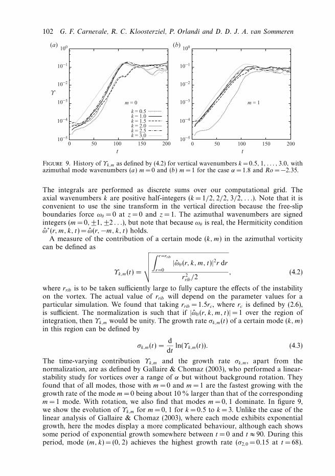
Figure 9. History of Υk,m as defined by (4.2) for vertical wavenumbers k =0.5, 1, . . . , 3.0, withazimuthal mode wavenumbers (a) m= 0 and (b) m= 1 for the case α= 1.8 and Ro = −2.35.
The integrals are performed as discrete sums over our computational grid. Theaxial wavenumbers k are positive half-integers (k = 1/2, 2/2, 3/2, . . .). Note that it isconvenient to use the sine transform in the vertical direction because the free-slipboundaries force ωθ = 0 at z =0 and z = 1. The azimuthal wavenumbers are signedintegers (m =0, ±1, ±2 . . .), but note that because ωθ is real, the Hermiticity conditionω∗(r, m, k, t) = ω(r, −m, k, t) holds.
A measure of the contribution of a certain mode (k, m) in the azimuthal vorticitycan be defined as
Υk,m(t) =
√√√√√
∫ r=rrib
r=0
|ωθ (r, k, m, t)|2r dr
r2rib/2
, (4.2)
where rrib is to be taken sufficiently large to fully capture the effects of the instabilityon the vortex. The actual value of rrib will depend on the parameter values for aparticular simulation. We found that taking rrib =1.5rc, where rc is defined by (2.6),is sufficient. The normalization is such that if |ωθ (r, k, m, t)| =1 over the region ofintegration, then Υk,m would be unity. The growth rate σk,m(t) of a certain mode (k, m)in this region can be defined by
σk,m(t) =d
dtln(Υk,m(t)). (4.3)
The time-varying contribution Υk,m and the growth rate σk,m, apart from thenormalization, are as defined by Gallaire & Chomaz (2003), who performed a linear-stability study for vortices over a range of α but without background rotation. Theyfound that of all modes, those with m =0 and m =1 are the fastest growing with thegrowth rate of the mode m =0 being about 10 % larger than that of the correspondingm =1 mode. With rotation, we also find that modes m =0, 1 dominate. In figure 9,we show the evolution of Υk,m for m =0, 1 for k = 0.5 to k =3. Unlike the case of thelinear analysis of Gallaire & Chomaz (2003), where each mode exhibits exponentialgrowth, here the modes display a more complicated behaviour, although each showssome period of exponential growth somewhere between t =0 and t ≈ 90. During thisperiod, mode (m, k) = (0, 2) achieves the highest growth rate (σ2,0 = 0.15 at t = 68).
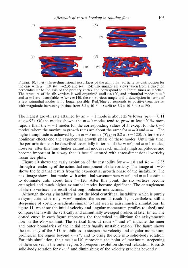
Aftermath of vortex breakup in rotating flow 103
90 120
140 190
(a) (b)
(c) (d)
Figure 10. (a–d ) Three-dimensional isosurfaces of the azimuthal vorticity ωθ distribution forthe case with α= 1.8, Ro = −2.35 and Re = 15k. The images are views taken from a directionperpendicular to the axis of the primary vortex and correspond to different times as labelled.The structure of the rib vortices is well organized until t ≈ 120, and azimuthal modes m= 0and m= 1 are identifiable. After t ≈ 140, the rib vortices tangle and a description in terms ofa few azimuthal modes is no longer possible. Red/blue corresponds to positive/negative ωθ
with magnitude increasing in time from 3.2 × 10⁻³ at t = 90 to 3.3 × 10⁻¹ at t =190.
The highest growth rate attained by an m =1 mode is about 25 % lower (σ0.5,1 = 0.11at t = 92). Of the modes shown, the m =0 modes tend to grow at least 20 % morerapidly than the m =1 modes for the corresponding values of k, except for the k =6modes, where the maximum growth rates are about the same for m =0 and m =1. Thehighest amplitude is achieved by an m =0 mode (Υ2.5,0 ≈ 0.2 at t = 120). After t ≈ 90,nonlinear effects end the exponential growth phase of these modes. Until this time,the perturbation can be described essentially in terms of the m =0 and m = 1 modes;however, after this time, higher azimuthal modes reach similarly high amplitudes andbecome important in a way that is best illustrated with three-dimensional vorticityisosurface plots.
Figure 10 shows the early evolution of the instability for α= 1.8 and Ro = −2.35through a rendering of the azimuthal component of the vorticity. The image at t =90shows the field that results from the exponential growth phase of the instability. Thenext image shows that modes with azimuthal wavenumbers m = 0 and m = 1 continueto dominate until about time t = 120. After this point, the rib vortices becomeentangled and much higher azimuthal modes become significant. The entanglementof the rib vortices is a result of strong nonlinear interactions.
Although the early instability is not the ideal centrifugal instability, which is purelyaxisymmetric with only m = 0 modes, the essential result is, nevertheless, still asteepening of vorticity gradients similar to that seen in axisymmetric simulations. Infigure 11, we show the initial velocity and angular momentum profiles (dashed) andcompare them with the vertically and azimuthally averaged profiles at later times. Thedotted curve in each figure represents the theoretical equilibrium for axisymmetricflow in the Re = ∞ limit. The vertical lines at radii r− and r+ indicate the innerand outer boundaries of the initial centrifugally unstable region. The figure showsthe tendency of the 3-D instabilities to steepen the velocity and angular momentumprofiles, in the region beyond r = r+, and to bring the core into solid-body rotation.For this simulation, the time t = 140 represents the point of maximum steepeningof these curves in the outer region. Subsequent evolution showed relaxation towardssolid-body rotation for r < r+ and diminishing of the velocity gradient beyond r+.

104 G. F. Carnevale, R. C. Kloosterziel, P. Orlandi and D. D. J. A. van Sommeren
0 0.2 0.4 0.6 0.8 1.0 1.2
0
−0.1
−0.2
−0.3
r0 0.2 0.4 0.6 0.8 1.0 1.2
r
V L
r− r+
−0.05
0
0.05
0.10
0.15
r− r+
Figure 11. The radial profile of the vertically averaged azimuthal velocity and angularmomentum of the vortex from the 3-D simulation with α= 1.8, Ro = −2.35 and Re = 15k.The curves correspond to times t = 0, 90, 140 and 190. The initial t =0 profile is shown by ablack dashed line ( ) and the later times by solid lines with shading from black to lightgrey of decreasing intensity with increasing time. The theoretical profile of the vortex afterstabilization by the axisymmetric centrifugal instability at infinite Reynolds number is shownby a dotted line ( ). The inner and outer radii (r−, r+) of the initial centrifugally unstableregion are denoted by the dash-dotted ( ) vertical lines.
t = 220 t = 360
0
t = 550
min max
(a) (b) (c)
Figure 12. (a–c) Evolution of ωz averaged over z for the case α=1.8, Ro = −2.35 andRe = 15k. The corresponding figure showing the evolution of azimuthal power is 13(a). Thelimits on the grey-scale vary between minimum and maximum values that change with time:t = 220 (min = −2,max = 1), t = 360 (−1.2, 0.6) and t = 550 (−1.2, 0.4). The full horizontalextent of the computational domain out to r = 6 is shown.
Of course, at any finite Re, the steepening of the gradients can never reach thepredicted infinite slope. The change of the averaged velocity profile with Re isdiscussed in detail by Kloosterziel et al. (2007a). Although the steepening of thegradient is incomplete, it is sufficient, as we will see, to trigger barotropic instabilityin accord with the hypothesis of Kloosterziel & van Heijst (1991) and in agreementwith Orlandi & Carnevale (1999).
As the centrifugal instability steepens the velocity gradient, various barotropicallyunstable modes begin to grow. The effect on the vortex can be seen in the verticallyaveraged vertical component of the vorticity field ωz(r, θ, t) shown in figure 12. Byt = 220, a large-scale distortion away from axisymmetry is just becoming noticeable.By t = 360, a tripole has formed, but at this point it is difficult to know whether this

Aftermath of vortex breakup in rotating flow 105
0
0.1
0.2
0.3
0.4
100 200 300 400 500 600 700
α = 1.8Ro = −2.35
2
41
3
t t
p
pθT
0
0.2
0.4
0.6
0.8
1.0
100 200 300 400
α = 1.8Ro = −3
2
41 3
pθT
(a) (b)
Figure 13. Evolution of the power pz,m in azimuthal modes of ωz. The thick labelled curvesshow the evolution of power in azimuthal modes 1–4 (dashed black line, m= 1; solid blackline, m= 2; dashed grey line, m= 3; solid grey line, m= 4). The thin solid line is the total powerin ωθ . All curves are normalized by the instantaneous power of the axisymmetric component(i.e. |ωz,0(t)|2). For (a, b) α= 1.8 and Re = 15k. (a) The case Ro = −2.35 is an example forwhich a tripole results. (b) The case Ro = −3 is one for which a pair of dipoles results.
vortex will remain a tripole or split into a pair of dipoles. However, the subsequentevolution is simply continued rotation and viscous diffusion of the tripole.
To analyse this behaviour in detail, we can compare the ‘power’, that is variance,in the various azimuthal modes of ωz(r, θ, t) with that in the axisymmetric (m = 0)mode. We define the modal amplitude as
ωz,m(t) ≡∫ 2π
θ = 0
∫ rmax
r=0
∫ 1
z=0
ωz(r, θ, z, t)e−imθr dr dθ dz, (4.4)
where the integration is over the entire computational domain. For the simulationsreported here, rmax = 6. The Fourier transform in θ is performed using a fast Fouriertransform and the integrals in r and z are computed as sums on the discretecomputational grid. The ratio of the contribution of modes m and −m relativeto the axisymmetric part of the flow is
pz,m(t) ≡ |ωz,m|2 + |ωz,−m|2|ωz,0|2 = 2
|ωz,m|2|ωz,0|2 , (4.5)
where we have used the Hermiticity constraint to simplify. In addition, it is usefulto consider the total power in the ωθ -field relative to that in the axisymmetric partof ωz. This will give us a measure of the importance of centrifugal instability, whichgenerates ωθ . Thus, we define the total power in ωθ relative to that in the axisymmetricpart of ωz:
pTθ (t) ≡ 1
|ωz,0|2∫ 2π
θ=0
∫ rmax
r=0
∫ 1
z=0
ω2θ (r, θ, z, t)r dr dθ dz. (4.6)
In figure 13(a), the evolution of the power in the most highly excited azimuthal modesof the vertically averaged vertical vorticity ωz is plotted along with pT
θ . We first notethat rapid growth in pT
θ precedes growth in the azimuthal modes of ωz. Departure ofthe vortex from axisymmetry is measured by the power pz,m(t) in modes m (= 0. Aftert = 100, there is some significant growth in modes |m| = 1, 2, 3 and 4 that all remainat about the same level until around t = 220; however, they each have less than 5 %of the power compared with the axisymmetric mode. The combined effect of theseazimuthal modes does not yet cause a very strong distortion of the vortex away from

106 G. F. Carnevale, R. C. Kloosterziel, P. Orlandi and D. D. J. A. van Sommeren
axisymmetry, as we see remains the case in figure 12 at t = 220. Then, around t = 220,pz,2(t) begins to grow rapidly. When this reaches about 10 %, a tripole is seen to beginto emerge, and by t = 360, we have the well-formed tripole shown in figure 12 at thattime. Note that pz,4(t) grows to about the 5 % level around t = 360. This is relatedto a thinning of the central anticyclonic vortex. As pz,4(t) subsequently decreases, thecentral vortex becomes more circular. Even though pz,2(t) decreases to about the 10 %level after it has peaked at t = 360, it remains the dominant mode, and the vorticityconfiguration remains that of a tripole as shown in figure 12 at t = 550. At timet = 550, pz,1(t) is near its peak value and seems to rival pz,2(t); however, this seems tohave little effect on the form of the tripole. As an aside, we note that modes m = ± 1are interesting in that they are never unstable in the pure barotropic problem (seefigure 8). Their growth is made possible only with the freedom of variation in z andthey play an important role in the 3-D centrifugal instability, as discussed above. Inthe barotropic problem, they can be related to the propagation of the vortex structuresince they correspond to a dipolar perturbation, and a dipolar distribution of ωz
would exhibit self-induced motion. In the centrifugal instability, on the other hand,these modes change the axisymmetric ring modes of the pure centrifugal instabilityinto helical modes.
4.2. Double-dipole formation: α=1.8, Ro = −3
For sufficiently negative Rossby numbers (Ro " −2.45 with Re = 15k), the evolutionof the vortex becomes more complicated and more interesting. Figure 13(b) showsthe histories of the power in the first four perturbation azimuthal modes of ωz alongwith the total power in ωθ for a simulation with Ro = −3. With α= 1.8, there is stillno initial barotropic instability, and as in the previous case, we see that rapid growthin pT
θ (t) precedes growth in the azimuthal modes of ωz. Also as in the previous case,eventually there is significant growth and sustained amplitude in pz,2(t). The mostsignificant difference between figures 13(a) and 13(b) is that in figure 13(b) we see anappreciable sustained growth in pz,4(t). To see how this affects the evolution of thevortex, we will now compare the evolution of the ωz vorticity distribution shown infigure 14 with the modal power histories in figure 13.
In figure 14, we see that around t = 210 the distribution of ωz has formed a triangularcore of anticyclonic vorticity surrounded by three cyclonic satellites, a quadrupole.This is related to the growth of pz,3(t), which peaks at about 8 % and is around 6 % att = 210 (see figure 13b). Such a triangular structure has been the subject of previoustheoretical study, numerical simulations and laboratory experiments (Carnevale &Kloosterziel 1994; Beckers & van Heijst 1998). This configuration with three cyclonicsatellites can persist indefinitely if the initial perturbation is carefully prepared anddominated by mode m = 3; however, for random initial conditions as used here, this isusually just a transient phase of the evolution. As discussed by Morel & Carton (1994)and Carnevale & Kloosterziel (1994), the quadrupole becomes unstable when two ofits satellites come close to each other and merge, as is about to happen at t = 210. Thesubsequent merger seen in figure 14 around t =225 results in a configuration in whichpz,2(t) dominates, that is a tripole. Unlike the previous case, with Ro = −2.35, wherethe central vortex eventually becomes more circular, here the central vortex, beingstrongly sheared by the outer satellites, becomes more elongated. It eventually rolls upinto two anticyclones that pair with the two cyclonic satellites, as seen in figure 14(e,f ). The resulting pair of dipoles has a significant mode m =4 component along withmode m =2. The growth of pz,4(t) in figure 13(b) corresponds to this formation of the

Aftermath of vortex breakup in rotating flow 107
t = 255
t = 160 t = 210(a) (b) (c)
(d) (e) ( f )
t = 225
t = 320 t = 370
0
min max
Figure 14. (a–f ) Evolution of ωz averaged over z for the case α=1.8, Ro = −3 and Re =15k.The corresponding figure showing the evolution of azimuthal power is 13(b). The limits onthe grey-scale vary between minimum and maximum values that change with time: t = 160(−4, 2), t = 210 (−2.5, 1.5), t = 225 (−2, 1), t = 255 (−1.5, 1.0), t = 320 (−1.2, 0.8) and t = 370(−1.2, 0.8).
double-dipole structure. After about t = 400, the propagating dipoles begin to interactwith the walls of the domain. For simulations with more negative Ro at the same α,the behaviour is similar to that shown in figure 14, except that the early formation ofa quadrupole may be preceded by the formation of structures of higher order, thatis, structures with even more satellites. As with the quadrupole, these too becomeunstable with the merger of the outer satellites. Eventually, the merger process resultsin the formation of double dipoles, as shown in the late stages in figure 14.
4.3. Testing the prediction: α= 1.8
Next, we test whether the combined effect of centrifugal and barotropic instabilitiescan be predicted based solely on our inviscid prescription for centrifugal instabilityand two-dimensional simulations of barotropic instability, as explained in § 3. Infigure 15(a), we show the contour plot of the vertical vorticity at mid-depth for a fully3-D simulation of the evolution. The flow at this stage is nearly uniform in the verticaldirection. We show the mid-depth field here rather than a vertically averaged fieldto allow some of the small-scale features to be evident. Furthermore, we have usedcontour plots rather than grey-scale to allow a somewhat more detailed comparisonbetween the 3-D simulation and the prediction.

108 G. F. Carnevale, R. C. Kloosterziel, P. Orlandi and D. D. J. A. van Sommeren
x
y
−2 0 2 4−4
−2
0
2
4(a)
x−2 0 2 4−4
−2
0
2
4(b)
Figure 15. Comparison of the results of the three-dimensional simulation with the prediction.(a) Vorticity field at mid-depth at time t = 380 in the fully three-dimensional simulation.(b) Predicted vorticity field at time τ = 330 from the two-dimensional simulationof the barotropic part of the prediction. The isolevels increase from −0.5 to 0.3with increments of 0.04. Black/grey contours represent negative/positive isolevels. α= 1.8,Ro = −2.35 and Re =15k.
At this point in the evolution of the flow, the centrifugal instability has run itscourse, and the barotropic instability has been triggered and finally equilibrated,resulting in a tripole. For comparison, the vorticity distribution from our predictionis given in figure 15(b). The time scales are different in the two cases. Figure 15(a)corresponds to the 3-D simulation at time t = 380 after the initial condition, whilethe time τ = 330 in figure 15(b) is the time since the initiation of the 2-D simulationstarting from the theoretical centrifugal equilibrium state. The 3-D result and theprediction are remarkably similar. Note that the overall orientation of the fields is notsignificant since it only depends on the particular orientation of the field of randomperturbations used to initiate the flow.
Next, we consider the Ro = −3 case, which, as seen above, results in double dipoles.Since this is still a case with α=1.8, the initial profile is again barotropically stableand it is the centrifugal instability that drives the flow towards barotropic instability.The result of a full 3-D simulation is illustrated by the vertical vorticity at mid-depthin figure 16(a). This can be compared with the prediction in figure 16(b), based againon our inviscid prescription for centrifugal instability equilibration followed by the2-D simulation. Even though the vorticity minima in the anticyclones are somewhatmore diffuse in the prediction than in the 3-D simulation, overall the results matchvery well.
4.4. Regime diagram: α=1.8
Another measure of the skill of our prediction scheme is how well it can predict theboundaries between the regimes in which the final result of evolution from small-scale random initial perturbations is a monopole, a tripole or double dipoles. Theresults depend on the Reynolds number. Our predictions are based on the inviscidextrapolation for centrifugal instability and should thus improve as Re increases. Onthe other hand, for a given resolution, the numerical simulations will degrade inquality as Re is increased and small scales are not properly represented, thus limitingthe accessible range of Re.

Aftermath of vortex breakup in rotating flow 109
x
y
−4 −2 0 2 4 6−6
−4
−2
0
2
4
6(a)
x−4 −2 0 2 4 6−6
−4
−2
0
2
4
6(b)
Figure 16. Comparison of the results of the three-dimensional simulation with the prediction.(a) Vorticity field at the mid-depth at time t = 360 in the fully three-dimensional simulation.(b) Predicted vorticity field at time τ = 240 from the two-dimensional simulation of thebarotropic part of the prediction. The isolevels increase from −0.4 to 0.2 with incrementsof 0.03. Black/grey contours represent negative/positive isolevels. α= 1.8,Ro = −3.0 andRe = 15k.
We have performed a series of 3-D simulations designed to map out the boundarybetween the regimes in which small-scale random perturbations of our basic profilewill lead to a final monopole, a tripole or double-dipole configuration. The 3-Dsimulations were compared with our prediction scheme described above using 2-Dsimulation. The resolution of both the 3-D and 2-D simulations was 129 points ineach coordinate direction.
Determining the border between the tripole regime and the double-dipole regimewas very straightforward. For simulations near this border, the flow reaches a pointat which a tripole forms with an elongated elliptical anticyclone in the centre and twocyclonic satellites. The flow is then at a critical point in the evolution. One of two verydifferent scenarios follows. In one scenario, the anticyclone continues to elongate andthen rolls up into two anticyclones. Each of these ‘daughter’ anticyclones then partnerswith one of the cyclonic satellites to create one of the dipoles in the resulting double-dipole configuration. In the other scenario, the elongation of the central anticycloneceases and is followed by ‘axisymmetrization’ (Melander, McWilliams & Zabusky1987) of the central vortex. In the latter scenario, the resulting configuration remainsa tripole with a nearly circular central vortex during the long viscous decay phasethat follows.
The double-dipole states are generally not as symmetric as that shown in figure 14at t = 370. In some cases, one of the dipoles is composed of a very strong vortexand a very weak vortex. For a given Ro and Re that produce a double-dipole state,the degree of symmetry of the dipoles is sensitive to the choice of the seed for therandom generation of the initial small-scale perturbation. When one of the vorticesin a dipole is very weak, it may become sheared out around the stronger companionvortex, and the resulting final state of the system may look more like a dipole and aseparate monopole than two dipoles. We have not tried to create a separate categoryfor these states but just consider them as examples of the limiting case of asymmetryin the double-dipole state.

110 G. F. Carnevale, R. C. Kloosterziel, P. Orlandi and D. D. J. A. van Sommeren
–3.8
–3.4
–3.0
–2.6
–2.2
–1.8
5 7 9 11 13 15
Monopole
Tripole
Double dipoles
Re
Ro
α = 1.8
Figure 17. Regime diagram for the case with α= 1.8, in which the centrifugal instability isinitially faster than the barotropic instability. The solid black curve is the boundary betweentripoles and double dipoles resulting from 3-D simulations. The dashed black curve is theprediction for this boundary. The solid grey curve is the boundary between monopoles andtripoles resulting from 3-D simulations. The dashed grey curve is the prediction for thisboundary. The sampling error is indicated by the error bars. Re is given in units of 1000.
Determining the border between the monopole and the tripole regimes provedless straightforward than for the tripole to double-dipole transition. The problemhere is that some mode m =2 growth may be observed without the formation ofwell-defined cyclonic satellites. One needs to somewhat arbitrarily decide how muchmode m =2 distortion of the monopole is necessary to classify it as a tripole ratherthan a monopole. Barba & Leonard (2007) confronted this issue in a study of theemergence of tripoles from vortices with net circulation. In their definition of atripole, they required that the zero-vorticity contour pinches off, isolating the twosatellite vortices from each other. We considered using this criterion, but found thatin our case of zero net circulation, the zero contour line was rather more complicated,and we found it difficult to precisely state whether it closed around each of thesatellites or not. For example, sometimes it would close around one satellite but notaround the other, or just nearly close, with the formation of many thin filaments thatmade the contour difficult to follow. A detailed discussion of this filamentation andits dynamic implications is found in Carton & Legras (1994). We considered usingother contour levels. At levels below 0.05 (which is 5 % of the unperturbed |ωz| atr = 0), we found that some ambiguity remained in some cases. At level 0.05, therewas no ambiguity in deciding when the contours pinched off or not for any of thesimulations near the transition boundary. The states in which this contour pinchedoff seemed reasonably described as tripoles. Testing with a contour level 0.06 andabove, we found some states in which the contour did pinch off unambiguously, butfor a vorticity distribution that looked very much like a monopole with only a weakmode-2 perturbation. Thus, 0.05 seemed a reasonable choice, and we decided to deemthe structure a tripole when this contour pinched off.
The regime diagram resulting from the 3-D simulations is shown in figure 17 alongwith our predictions. The solid curves with solid symbols are deduced from the3-D simulations. The regime boundary predictions are shown by dashed curves. The
Aftermath of vortex breakup in rotating flow 111
curves are drawn by plotting the average of Ro of the two simulations that define thetransition from one behaviour to the other at a given Re. For example at Re = 15k, atripole was found for Ro = −2.5 and double dipoles at Ro = −2.6. Thus, the regimeboundary was marked at the midpoint Ro = −2.55. One could thus assign an errorto this point as +Ro = ±0.05, which is just the sampling error. The sampling error isindicated by the error bars on each data point.
The curves in figure 17 imply that the smaller Re the larger Ro needs to be toobtain a transition from the monopole state. This seems reasonable since a Laplacianviscosity will damp the azimuthal modes more than the axisymmetric mode (thehigher m the more efficient the damping). There is a trade-off between high viscosity(damping) at low Re and the large amount of available energy that can be releasedat large Ro, making transitions possible at small Re if Ro is sufficiently large. Forfixed Ro " −2.6, the graphs of the 3-D results show that as Re increases, onegoes from monopoles to tripoles to double dipoles. This reflects the fact that asRe increases, the damping on mode m =2, the mode necessary to create a tripole,becomes insufficient to prevent its growth to significant levels, while mode m =4 is stillsuppressed, and thus a tripole results. Then for even higher Re, mode m =4 is able togrow and double dipoles result. Although mode m =3 is also barotropically unstable,and its growth would also be expected, it typically leads to a transient configurationas explained in § 2.2. Similarly, modes with m > 4 also become important as Reis increased, but they too lead to structures that are unstable and transient. Thetendency of the curves in the high-Re limit is not entirely clear. We do not havedata beyond Re = 15k that is sufficiently well resolved to say whether the regimeboundaries asymptote to two distinct values in the Re → ∞ limit or if perhaps theyboth converge towards Ro = −1, in which case we would always find double dipolesafter centrifugal instability at Re = ∞.
Figure 17 reveals that for fixed Re, the gap in Ro where tripoles result is relativelynarrow compared with the ranges in which double dipoles or monopoles result, bothof which extend beyond the limits of the figure. This may account for the fact thatin early experimentation with anticyclones produced by stirring in a rotating tank(Kloosterziel & van Heijst 1991), only monopoles or double dipoles were observed asfinal states.
In terms of the validity of our predictions, we should expect that at low Re thedifference between 3-D simulations and our prediction, which is based in part oninviscid projections for the centrifugal instability, is relatively large but improveswith increasing Re. We see that this is the case, for example, for the monopole totripole boundary. At low Re, viscous effects diminish the ability of the centrifugalinstability to steepen the velocity profile. Thus, it is more difficult to produce thehigher azimuthal modes needed to produce tripoles than in the inviscid case, and sotripole production requires a higher Ro than predicted. As Re increases, the effects ofviscosity become less important and the gap between prediction and 3-D simulationsdiminishes, plateauing for Re $ 10k, before shrinking to the size of the samplingerror at Re =15k. A similar trend is found for the tripole to double-dipole transitionboundary. For that boundary, the gap between prediction and 3-D simulationsbecomes about the sampling error for Re $ 8k. For both boundaries, the predictionsystematically underestimates the magnitude of Ro needed to achieve transition fora given Re because finite Re does not permit the full steepening of the vorticitygradients that the prediction assumes. Nevertheless, the success is remarkable, and wewould expect that the gap between prediction and 3-D simulations would decreasefurther with increasing Re, given sufficient numerical resolution.
112 G. F. Carnevale, R. C. Kloosterziel, P. Orlandi and D. D. J. A. van Sommeren
5. Barotropic instability faster than centrifugal instability (α= 3)For α higher than 1.85, the growth rate of the barotropic instability will be non-
zero from the initial moment. In that case, centrifugal instability and barotropicinstability will be in competition from the beginning. One can imagine that as longas the centrifugal instability is substantially faster than the barotropic instability, ourprediction scheme should continue to exhibit skill in predicting the outcome of thecombined instability. However, the prediction scheme should lose skill as the growthrate of the initial barotropic instability increases to and exceeds that of the centrifugalinstability. Here we test how well the scheme does in the situation when the growthrate of barotropic instability is initially somewhat larger than that of centrifugalinstability.
The barotropic instability growth rate for mode m = 2 (the mode responsible fortripole production) acting alone is approximately 0.077, as shown in figure 8(a).Note that since the Coriolis parameter does not enter into the 2-D flow equations,the growth rate for the barotropic instability has no dependence on the Rossbynumber. The growth rate of the centrifugal instability, however, does depend on theRossby number of the flow. The growth rate for the pure centrifugal instability maybe obtained by performing axisymmetric simulations. For α= 3 and Re =15k, wefind that as Ro is decreased from Ro = −1.0 to Ro = −2.2, the growth rate of thecentrifugal instability increases from 0.0 to 0.073. Thus, in this range of Ro, thecentrifugal instability is slower than the barotropic instability.
As we shall see, the transition from the tripole regime to the double-dipole regimeoccurs at Ro ≈ −1.45, which falls in this range of Ro. Furthermore, for α= 3, thebarotropic instability is sufficiently strong that tripoles form for all Ro from Ro = −1(the inviscid centrifugal instability boundary) down to the tripole to double-dipoletransition boundary. Thus, there is no monopole to tripole regime transition boundaryin this case.
Examining the evolution of the azimuthal modes provides some insight into thedynamics, as in the α= 1.8 case. First, we consider a case that results in a tripole.We take Ro = −1.3 as an example. In figure 18(a), we see the evolution of pz,m(t)(defined by (4.5)) for m =1–4 as well as pT
θ (t). Since in this case all of the powerlevels are very small except for pz,2(t), we plot the graphs on a logarithmic scale tofacilitate comparison between them. The first thing to note is that the barotropicinstability is evident early on with pz,2(t) growing much more rapidly than pT
θ . Thestrong growth of mode m =2 results in the formation of a tripole. Note that pT
θ neverbecomes more than a tenth of a per cent (10−3). The flow begins to take the form of atripole as pz,2(t) reaches 10 % at around t = 130. It is a well-defined tripole at t = 170,when pz,2(t) is at its maximum, and remains a well-defined, although slowly decaying,tripole after that. Mode 4 grows rapidly until about t = 150; however, pz,4(t) remainssmall (less than 3%) and so the structure is dominated by mode m =2 and the flowremains a tripole.
Next, we look at the azimuthal modal growth in a case which results in doubledipoles. We take Ro = −1.46 as an example. In contrast with the previous case, herewe do see early growth in pT
θ that competes with the growth in mode m =2 andreaches over 10 % before decaying, suggesting that centrifugal instability plays asignificant role. A tripole forms around t = 145, when pz,2(t) has reached 10 %. Aspz,4(t) reaches 10 % at t =220, the central anticyclonic vortex becomes elongated, andby t = 233, with pz,4(t) reaching 15 %, the elongated anticyclone rolls up, forming twoanticyclones that go into creating the final pair of dipoles, similar to those shown infigures 14 and 16. Although at α= 3, mode m =2 can grow even in the absence of

Aftermath of vortex breakup in rotating flow 113
–9
–8
–7
–6
–5
–4
–3
–2
–1
0
0 100 200 300 400 500 600 700
α = 3
Ro = −1.3
2
4
13
t
p pθT
α = 3
Ro = −1.46
2
1
3
4
pθT
(a)
–8
–7
–6
–5
–4
–3
–2
–1
0
0 50 100 150 200 250 300t
(b)
Figure 18. Evolution of the power pz,m in azimuthal modes of ωz. The thick labelled curvesshow the evolution of power in azimuthal modes m= 1–4 (dashed black line, m= 1; solidblack line, m= 2; dashed grey line, m= 3; solid grey line, m= 4). The thin solid line is the totalpower in ωθ . All curves are normalized by the instantaneous power |ωz,0(t)|2. For each panel,α= 3 and Re = 15k. (a) The case Ro = −1.3 is an example in which a tripole is produced. (b)The case Ro = −1.46 is one for which double dipoles result. The p-axis is logarithmic.
–2.0
–1.8
–1.6
–1.4
–1.2
5 7 9 11 13 15
α = 3
Ro
Re
Tripole Tripole
Double dipoles
(a) (b)
–2.6
–2.4
–2.2
–2.0
–1.8
–1.6
–1.4
–1.2
1.8 2.0 2.2 2.4 2.6 2.8 3.0α
Re = 15k
Double dipoles
Figure 19. (a) The regime diagram for the case with α= 3 in which the barotropic instabilityis initially faster than the centrifugal instability. The thick solid curve results from 3-Dsimulations. The thin dashed curve is the prediction. Error bars are not included because thesampling error is +Ro = ±0.005 or less and the error bars would be obscured by the symbolson the lines. Re is given in units of 1000. (b) Variation of the regime boundary with α. Thethick solid curve results from 3-D simulations. The thin dashed curve is the prediction.
centrifugal instability, while mode m =4 cannot (see figure 8). Thus, it is the effectof the centrifugal instability that allows growth in mode m = 4, and this growth willonly happen if the centrifugal instability (here measured by pT
θ ) is sufficiently strong.
5.1. Regime diagram: α= 3
In figure 19(a), we compare the predicted boundary for the transition from the tripoleregime to the double-dipole regime with that found with 3-D simulation. Although

114 G. F. Carnevale, R. C. Kloosterziel, P. Orlandi and D. D. J. A. van Sommeren
the curves have similar tendencies, the predicted curve systematically underestimatesthe magnitude of Ro. The sampling error on these curves is +Ro = ±0.005, much lessthan in the case α= 1.8 and much less than the separation of the curves. The 3-Dα= 3 simulations proved less costly in computer time than the α=1.8 simulation,because the velocities involved for runs near the regime boundaries are lower (because|Ro| is lower in this case), and this allowed more simulations to be run for this caseand, hence, higher precision in determining the regime boundary.
As for the case with α= 1.8, the gap between prediction and 3-D simulationdecreases with increasing Re, here going from +Ro = 0.370 to 0.1875 as Re goesfrom 5k to 15k. In other words, the prediction improves with increasing Re. Thegap at Re =15k is, however, larger than that for the case of the α= 1.8 tripole todouble-dipole transition border which is 0.075. This is perhaps what we should expectgiven the competing roles here of centrifugal and barotropic instabilities from t =0,as discussed above.
Overall, it is remarkable that even though in this case the barotropic instabilityis somewhat faster than the centrifugal instability, the prediction at least capturesthe form of the regime boundary. Attempts to match the shape of the curves infigure 19(a), as well as those in figure 17, to simple power laws in Re did not provefruitful. Additional experiments reaching to Re = 30k show that the gap betweenprediction and simulation continues to narrow as Re increases; however, the issueof grid resolution with Re > 15k is as in the case of the α=1.8 simulations, andwe feel that those simulations are not sufficiently resolved to be presented here. Thesystematic underestimation of Ro by the prediction in figure 19(a) is not surprising,for two reasons. First, as we have discussed for the case of α= 1.8, the predictionis based on an infinite Re centrifugally equilibrated V that is discontinuous. Such adiscontinuous profile will have higher growth rates for m = 2 and higher modes thanthe smoothed profiles that would actually result from a finite-Re simulation. Second,for α= 3, the centrifugal instability will not have time to steepen vorticity gradientsas much as it would if the barotropic instability were slower.
5.2. Regime boundary as a function of α
To quantify how the dependence of the difference between prediction and 3-Dsimulation grows with increasing α at fixed Re, we present, in figure 19(b), the tripoleto double-dipole transition Ro as a function of α for both our prediction and our3-D simulation results. The graph shows that for Re = 15k and increasing α, the gapbetween prediction and 3-D simulation opens up from +Ro =0.075 at α= 1.8 to+Ro =0.1875 at α=3. This trend can be expected to continue since with increasingα the barotropic instability will become ever faster. The best results are for lowα where the centrifugal instability is much more rapid than barotropic instability.However, this graph suggests that for sufficiently high Re, there is a wide range of αfor which the prediction scheme is fairly skilful.
6. ConclusionWe have presented a new method for predicting the final vortices that emerge
from the breakup of a centrifugally unstable vortex in a rotating flow. This methodconsists of first theoretically predicting the velocity profile towards which centrifugalinstability acting alone in an axisymmetric inviscid flow would drive the vortex.This theoretical prediction uses a simple construction based on angular momentumconservation. The resulting velocity profile is then used as the initial state of a
Aftermath of vortex breakup in rotating flow 115
two-dimensional simulation that captures the subsequent barotropic instability. Wehave shown that this prediction method is very accurate when the initial vortex is suchthat the centrifugal instability is much faster than any initial barotropic instability.We have given a quantitative indication of how much skill this prediction methodloses as the initial growth rate of barotropic instability relative to that of centrifugalinstability is increased, and we have shown that, at least within one family of vortices,the method still works reasonably well even when these initial growth rates are notvery different. This prediction method is a synthesis of what has been learned aboutcentrifugal and barotropic instabilities in rotating flow over the last few decades. Thefield has progressed considerably since the first insights into the interaction betweencentrifugal and barotropic instabilities were presented in Kloosterziel & van Heijst(1991).
The success of the prediction method suggests that some version of it may prove auseful tool in situations in which computing resources are insufficient to fully resolvecentrifugal instability. For example, in a general circulation model, a vortex mayappear that would be centrifugally unstable at infinite resolution, but will not becomeunstable simply because the resolution of the model is insufficient to allow centrifugalinstability. The theoretical prediction for the centrifugally equilibrated vortex could besubstituted for such a vortex. This would then trigger the appropriate subsequent baro-tropic instability, if any. Thus, the effects of a process which could be modelled onlyat much higher resolution could be directly incorporated in the under-resolved model.
We have not discussed here the case in which barotropic instability is much fasterthan the centrifugal instability. One can imagine, for example, starting with a flowthat is barotropically unstable but centrifugally stable. The subsequent evolution couldincrease the curvature of the flow which could trigger a centrifugal instability. Bayly(1988) proved that the centrifugal instability condition can be applied locally with theradius of curvature of streamlines playing the role of the radius in axisymmetric flow.When the barotropic instability produces flow curvature sufficient to create centrifugalinstability, it is expected that the flow would locally go centrifugally unstable andattempt to redistribute angular momentum, perhaps in such a way as to increase localvorticity gradients. It would be interesting to try to predict the effect of such a sec-ondary centrifugal instability in modifying the primary barotropic instability in sucha scenario, but such a line of research has, as far as we are aware, never been pursued.
Centrifugal instability in cyclones results in a velocity profile less steep than itwas originally, that is, stability is achieved by decreasing velocity gradients, just theopposite of what happens in the anticyclonic case. Since transforming a barotropicallystable state into a barotropically unstable state requires steepening velocity gradients,centrifugal instability in the cyclonic case cannot trigger a barotropic instability. Thispoint has been discussed in detail by Kloosterziel et al. (2007a). Furthermore, inthe case of the cyclone, the redistribution of angular momentum during centrifugalinstability does not reach deep into the core of the vortex, but instead is confinedto a narrow neighbourhood of the unstable region that is at the outer edge of thecore of the vortex. This, together with the fact that for cyclones Ro may need to besignificantly greater than 1 for centrifugal instability (see (2.5)) while |Ro| > 1 sufficesfor anticyclones, explains why ‘explosive’ three-dimensional instability was observedin anticyclones but not cyclones in the rotating tank experiments by Kloosterziel &van Heijst (1991).
Although all of the work presented above was based on homogeneous (i.e.constant-density) flow, our predictions may also work for centrifugally unstablebarotropic vortices in stratified flow with uniform background stable density gradient.
116 G. F. Carnevale, R. C. Kloosterziel, P. Orlandi and D. D. J. A. van Sommeren
Kloosterziel et al. (2007a) have shown that the results of axisymmetric centrifugalinstability with or without background stratification are the same as long as theReynolds number is sufficiently high. Stratification changes the form of the rib vortices(flatter rib vortices for higher stratification) and the time scale of centrifugal instability,but at high Reynolds numbers, the instability results in the same redistribution ofangular momentum as found in the unstratified case. However, possible decouplingbetween layers in the vertical direction may lead to some difference in the evolution inthe barotropic instability part of the evolution. How well the unstratified predictionswork in the stratified case would be worth testing in future work. Consideringbaroclinic vortices (i.e. vortices with vertical shear) in stratified flow would introduceanother level of complication. We are currently developing a prediction scheme forthe outcome of centrifugal instability for baroclinic vortices. This is much moredifficult than in the barotropic vortex case in stratified flow, where the unperturbedisopycnals are flat. In the baroclinic case, mixing of angular momentum takes placealong isopycnals that are not horizontal and the mixing results in changing the shapeof the isopycnals. Further progress must be made on this problem before predictionssimilar to those given above can be made.
Finally, we note that Kloosterziel et al. (2007b) give a prescription for predictingthe effect of centrifugal instability on rotating planar shear flows. As mentionedin the Introduction, it may be possible to use this prediction in a scheme to predictthe outcome of a fully 3-D flow starting with a planar shear flow. The prediction ofKloosterziel et al. (2007b) could be used to replace the centrifugal instability phaseof the flow and then 2-D simulations based on the predicted profile may capture thesubsequent evolution to some extent.
G.F.C. and R.C.K. acknowledge support from the National Science Foundationgrants OCE 07-26482 and OCE 07-26866, respectively. D.D.J.A.v.S. acknowledgessupport from Dr Hendrik Muller’s Vaderlandsch Fonds and TU/e FSB.
Appendix. Resolution testIn the test of the adequacy of the grid resolution at high Re, we take the Fourier
sine transform of the vertical velocity w at a radius inside the instability region. Wedefine an azimuthally averaged amplitude at r = 1 as
wk(t) =1
2π
∫ 2π
θ=0
∫ 1
z=0
w(r = 1, θ, z, t) sin(2πkz) dz dθ . (A 1)
The axial wavenumbers k are positive half-integers (k = 1/2, 2/2, 3/2, . . .). The Fouriersine transform in z is performed using a fast Fourier transform on our discretecomputational grid, and the integral in θ is calculated by discretization on the grid.The resulting power spectrum w2
k is plotted in figure 20 for different values of Reand different computational resolutions at Ro = −2.5 and α=1.8. At these values ofRo and α, vortex breakdown results in a tripole, but for slightly more negative Rotwo dipoles form instead. In figure 20(a), we see that the spectra for resolutions 973,1293 and 1933 at Re = 15k approximately coincide with their respective maximumwavenumber. Since each simulation has different random initial conditions, we donot expect the spectra to coincide point by point, yet the overlap is very good. Eachspectrum corresponds to the time t =175, when centrifugal overturning is most active(i.e. when pT
θ is near its maximum). At resolution 1933, the spectrum shows a steeppower law, perhaps as steep as k−6, from about k =3 to about k = 25, followed by a

Aftermath of vortex breakup in rotating flow 117
10–22
(a)
10–20
10–18
10–16
10–14
10–12
10–10
10–8
10–6
10–4
1 10 100
k
10–22
(b)
10–20
10–18
10–16
10–14
10–12
10–10
10–8
10–6
10–4
1 10 100
k
w– 2k
k–6
1933
1293
973
k–6
Re = 30kRe = 15k
Figure 20. Fourier sine power spectrum of the vertical velocity w at r = 1 averaged over θfor simulations with α= 1.8 and Ro = −2.5 taken at t = 175. (a) This plot shows how thespectrum changes for fixed Re =15k with increasing resolution: 973 (thick black line), 1293
(thick grey line) and 1933 (thin dashed line). The curve k−6 is shown for comparison. (b) Thisplot shows how the spectrum changes for fixed resolution 1293 with increasing Re: grey line,Re = 15k; black line, Re = 30k.
rapid dissipation-range fall-off, into a relatively flat ‘noise’ range for k greater thanabout 55. Reaching the noise level in the spectrum is an indication of good resolutionat 1933. The k−6 power-law fall-off in this spectrum of the rib vortices recalls thespectrum of the Lamb dipole, which falls off similarly (Orlandi 2009). That thespectrum with resolution 1293 matches the spectrum with resolution 1933 up to aboutthe noise range suggests that we have adequate resolution at Re = 15k with 1293
points. At resolution 973, the spectrum ends in the dissipation range, which perhapssuggests adequate resolution, but, to be safe, 1293 resolution was used to explorethe regime boundaries. For fixed resolution 1293, as Re is increased beyond 15k, thehigh k spectral fall-off becomes less steep, filling in the spectrum with power-law-like behaviour out to the spectral cutoff. Figure 20(b) illustrates this by comparingthe spectra for Re = 15k and Re = 30k at Ro = −2.5. The lack of a rapid spectralfall-off for Re beyond 15k suggested that this is the limit of the parameter range thatwe can explore with resolution 1293.
REFERENCES
Aristegui, J., Sangra, P., Hernandez-Leon, S., Canton, M., Hernandez-Guerra, A. & Kerling,J. L. 1994 Island-induced eddies in the Canary Islands. Deep Sea Res. 41, 1509–1525.
Barba, L. A. & Leonard, A. 2007 Emergence and evolution of tripole vortices from net circulationinitial conditions. Phys. Fluids 19, 017101.
Bayly, B. J. 1988 Three-dimensional centrifugal-type instabilities in inviscid two-dimensional flows.Phys. Fluids 31, 56–64.
Beckers, M. & van Heijst, G. J. F. 1998 The observation of a triangular vortex in a rotating fluid.Fluid Dyn. Res. 22, 265–279.
Bennetts, D. A. & Hoskins, B. J. 1979 Conditional symmetric instability: a possible explanationfor frontal rainbands. Q. J. R. Meteorol. Soc. 105, 945–962.
Carnevale, G. F., Briscolini, M., Kloosterziel, R. C. & Vallis, G. K. 1997 Three-dimensionallyperturbed vortex tubes in a rotating flow. J. Fluid Mech. 341, 127–163.
Carnevale, G. F. & Kloosterziel, R. C. 1994 Emergence and evolution of triangular vortices.J. Fluid Mech. 259, 305–331.
Carton, X. J. 1992 The merger of homostrophic shielded vortices. Europhys. Lett. 18, 697–703.

118 G. F. Carnevale, R. C. Kloosterziel, P. Orlandi and D. D. J. A. van Sommeren
Carton, X. J., Fierl, G. R. & Polvani, L. M. 1989 The generation of tripoles from unstableaxisymmetric isolated vortex structures. Europhys. Lett. 9, 339–344.
Carton, X. J. & Legras, B. 1994 The life-cycle of tripoles in two-dimensional incompressible flows.J. Fluid Mech. 267, 53–82.
Carton, X. & McWilliams, J. C. 1989 Barotropic and baroclinic instabilities of axisymmetricvortices in a quasi-geostrophic model. In Mesoscale/Synotopic Coherent Structures inGeophysical Turbulence (ed. J. C. J. Nihoul & B. M. Jamart), pp. 225–244. Elsevier.
D’Asaro, E. A. 1988 Generation of submesoscale vortices: a new mechanism. J. Geophys. Res. 93,6685–6693.
Drazin, P. G. & Reid, W. H. 1981 Hydrodynamic Stability . Cambridge University Press.
Dritschel, D. G. 1986 The nonlinear evolution of rotating configurations of uniform vorticity.J. Fluid Mech. 172, 157–182.
Dunkerton, T. J. 1981 On the inertial instability of the equatorial middle atmosphere. J. Atmos.Sci. 38, 2354–2365.
Flament, P., Lumpkin, R., Tournadre, J. & Armi, L. 2001 Vortex pairing in an unstable anticyclonicshear flow: discrete subharmonics of one pendulum day. J. Fluid Mech. 440, 401–409.
Flierl, G. R. 1988 On the instability of geostrophic vortices. J. Fluid Mech. 197, 349–388.
Gallaire, F. & Chomaz, J. M. 2003 Three-dimensional instability of isolated vortices. Phys. Fluids15 (8), 2113–2126.
Hayashi, H., Shiotani, M. & Gille, J. C. 1998 Vertically stacked temperature disturbances near theequatorial stratopause as seen in cryogenic limb array etalon spectrometer data. J. Geophys.Res. 103, 19469–19483.
van Heijst, G. J. F. & Kloosterziel, R. C. 1989 Tripolar vortices in a rotating fluid. Nature 338,569–571.
Kloosterziel, R. C. & Carnevale, G. F. 1992 Formal stability of circular vortices. J. Fluid Mech.242, 249–278.
Kloosterziel, R. C. & Carnevale, G. F. 1999 On the evolution and saturation of instabilities oftwo-dimensional isolated circular vortices. J. Fluid Mech. 388, 217–257.
Kloosterziel, R. C., Carnevale, G. F. & Orlandi, P. 2007a Inertial instability in rotating andstratified fluids: barotropic vortices. J. Fluid Mech. 583, 379–412.
Kloosterziel, R. C. & van Heijst, G. J. F. 1991 An experimental study of unstable barotropicvortices in a rotating fluid. J. Fluid Mech. 223, 1–24.
Kloosterziel, R. C., Orlandi, P. & Carnevale, G. F. 2007b Saturation of inertial instability inrotating planar shear flows. J. Fluid Mech. 583, 413–422.
Knox, J. A. 1997 Possible mechanisms for clear-air turbulence in strongly anticyclonic flows.J. Atmos. Sci. 125, 1251–1259.
Melander, M. V., McWilliams, J. C. & Zabusky, N. J. 1987 The axisymmetrization and vorticity-gradient intensification of an isolated two-dimensional vortex through filamentation. J. FluidMech. 178, 137–159.
Morel, Y. G. & Carton, X. J. 1994 Multipolar vortices in two-dimensional incompressible flows.J. Fluid Mech. 267, 23–51.
Orlandi, P. 2000 Fluid Flow Phenomena: A Numerical Toolkit . Kluwer.
Orlandi, P. 2009 Energy spectra power laws and structures. J. Fluid Mech. 623, 353–374.
Orlandi, P. & Carnevale, G. F. 1999 Evolution of isolated vortices in a rotating fluid of finitedepth. J. Fluid Mech. 381, 239–269.
Orlandi, P. & van Heijst, G. J. F. 1992 Numerical simulation of tripolar vortices in 2D flow. FluidDyn. Res. 9, 179–206.
Rayleigh, Lord 1880 On the stability, or instability, of certain fluid motions. Proc. Lond. Math.Soc. 11, 57–70.
Rayleigh, Lord 1916 On the dynamics of revolving fluids. Proc. R. Soc. Lond. A 93, 148–154.
Richards, K. J. & Edwards, N. R. 2003 Lateral mixing in the equatorial pacific: the importanceof inertial instability. Geophys. Res. Lett. 30, 1–4.
Sawyer, S. J. 1947 Notes on the theory of tropical cyclones. Q. J. R. Meteorol. Soc. 73, 101–126.
Smyth, W. D. & McWilliams, J. C. 1998 Instability of an axisymmetric vortex in a stably stratified,rotating environment. Theor. Comput. Fluid Dyn. 11, 305–322.

Aftermath of vortex breakup in rotating flow 119
Stern, M. E. 1987 Horizontal entrainment and detrainment in large-scale eddies. J. Phys. Oceanogr.17, 1688–1695.
Stone, P. H. 1966 On non-geostrophic stability. J. Atmos. Sci. 23, 390–400.Stone, P. H. 1967 An application of baroclinic stability theory to the dynamics of the Jovian
atmosphere. J. Atmos. Sci. 24, 642–652.Verzicco, R. & Orlandi, P. 1996 A finite-difference scheme for three-dimensional incompressible
flows in cylindrical coordinates. J. Comput. Phys. 123, 402–414.