predicting the seismic behavior of the dywidag ductile connector
TRANSCRIPT

Predicting the Seismic Behavior of the Dywidag Ductile
Connector (DDC) Precast Concrete System
A Master’s Project
Presented to
the Faculty of California Polytechnic State University
San Luis Obispo, California
In partial fulfillment
of the Requirements for the Degree
Master of Science in Architecture with a Specialization in Architectural Engineering
by
Elizabeth M. Kenyon
July 2008

ii
© 2008
Elizabeth Mary Kenyon
ALL RIGHTS RESERVED

iii
COMMITTEE MEMBERSHIP
TITLE: Predicting the Seismic Behavior of the Dywidag Ductile
Connector (DDC) Precast Concrete System
AUTHOR: Elizabeth Mary Kenyon
DATE SUBMITTED: July 2008
COMMITTEE CHAIR: Cole McDaniel, Ph.D., P.E.
COMMITTEE MEMBER: Pamalee Brady, Ph.D., P.E.
COMMITTEE MEMBER: Ansgar Neuenhofer, Ph.D., P.E.
COMMITTEE MEMBER: Kevin Dong, M.E., S.E.

iv
ABSTRACT
Predicting the Seismic Behavior of the Dywidag Ductile Connector (DDC) Precast
Concrete System
Elizabeth Mary Kenyon
Structural engineering is heavily dependent on the use of computers. When
creating a building model using structural analysis software, it is required that the
designer have an understanding of the system behavior and the modeling program
capabilities.
Some engineers in the Southern California region are taking steps towards
incorporating the Dywidag ductile connector (DDC) and super hybrid systems into
building practice due to the advantages found in these systems’ construction methods and
seismic performance.
As the DDC and super hybrid systems reach industry, the design engineer will
need to model these systems using structural analysis programs. This report describes
two DDC specimens that were each modeled two ways: (1) using elastic members in
conjunction with nonlinear rotational hinges (lumped plasticity model), and (2) using
finite elements (fiber model). The experimental pushover curve for each test specimen
was compared to the corresponding analytical backbone curves.
The fiber modeling focuses on providing a means to study the joint behavior as
the parameters of the system change. The lumped plasticity model provides the design
engineer with a means for modeling a three-dimensional DDC building in order to get
acceptable global demand values. This project offers modeling suggestions for both the
fiber models and the lumped plasticity models used to predict the seismic behavior of the
DDC precast concrete system.
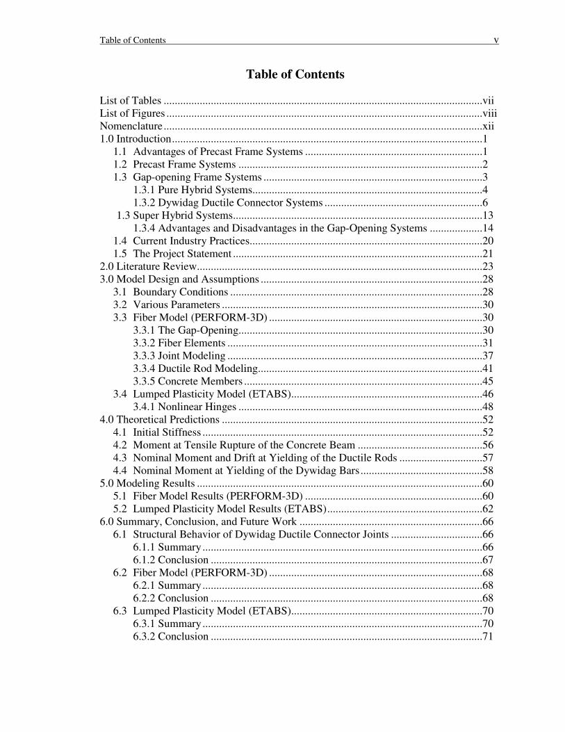
Table of Contents v
Table of Contents
List of Tables ...................................................................................................................vii
List of Figures ..................................................................................................................viii
Nomenclature...................................................................................................................xii
1.0 Introduction................................................................................................................1
1.1 Advantages of Precast Frame Systems ................................................................1
1.2 Precast Frame Systems ........................................................................................2
1.3 Gap-opening Frame Systems ...............................................................................3
1.3.1 Pure Hybrid Systems...................................................................................4
1.3.2 Dywidag Ductile Connector Systems .........................................................6
1.3 Super Hybrid Systems..........................................................................................13
1.3.4 Advantages and Disadvantages in the Gap-Opening Systems ...................14
1.4 Current Industry Practices....................................................................................20
1.5 The Project Statement ..........................................................................................21
2.0 Literature Review.......................................................................................................23
3.0 Model Design and Assumptions ................................................................................28
3.1 Boundary Conditions ...........................................................................................28
3.2 Various Parameters ..............................................................................................30
3.3 Fiber Model (PERFORM-3D) .............................................................................30
3.3.1 The Gap-Opening........................................................................................30
3.3.2 Fiber Elements ............................................................................................31
3.3.3 Joint Modeling ............................................................................................37
3.3.4 Ductile Rod Modeling.................................................................................41
3.3.5 Concrete Members ......................................................................................45
3.4 Lumped Plasticity Model (ETABS).....................................................................46
3.4.1 Nonlinear Hinges ........................................................................................48
4.0 Theoretical Predictions ..............................................................................................52
4.1 Initial Stiffness .....................................................................................................52
4.2 Moment at Tensile Rupture of the Concrete Beam .............................................56
4.3 Nominal Moment and Drift at Yielding of the Ductile Rods ..............................57
4.4 Nominal Moment at Yielding of the Dywidag Bars............................................58
5.0 Modeling Results .......................................................................................................60
5.1 Fiber Model Results (PERFORM-3D) ................................................................60
5.2 Lumped Plasticity Model Results (ETABS)........................................................62
6.0 Summary, Conclusion, and Future Work ..................................................................66
6.1 Structural Behavior of Dywidag Ductile Connector Joints .................................66
6.1.1 Summary.....................................................................................................66
6.1.2 Conclusion ..................................................................................................67
6.2 Fiber Model (PERFORM-3D) .............................................................................68
6.2.1 Summary.....................................................................................................68
6.2.2 Conclusion ..................................................................................................68
6.3 Lumped Plasticity Model (ETABS).....................................................................70
6.3.1 Summary.....................................................................................................70
6.3.2 Conclusion ..................................................................................................71

Table of Contents vi
6.4 Future Work .........................................................................................................72
6.4.1 Dywidag Ductile Connector System...........................................................72
6.4.2 Super Hybrid System ..................................................................................72
References ........................................................................................................................78
Cited References .........................................................................................................78
Additional References.................................................................................................80
Appendices.......................................................................................................................82
Appendix A .................................................................................................................82
DDC #1 Initial Stiffness.......................................................................................82
DDC #1 Column Shear at the Tension Rupture of the Concrete.........................83
DDC #1 Column Shear at Yielding of the Ductile Rods.....................................84
DDC #1 Predicted Displacement at Yield ...........................................................85
DDC #1 Column Shear at Yielding of the Dywidag Bars ...................................85
DDC #1 Determining Rigid Link Length ............................................................86
DDC #1 ETABS Nonlinear Hinge Properties .....................................................87
Appendix B .................................................................................................................88
DDC #2 Initial Stiffness.......................................................................................88
DDC #2 Column Shear at the Tension Rupture of the Concrete.........................89
DDC #2 Column Shear at Yielding of the Ductile Rods.....................................90
DDC #2 Predicted Displacement at Yield ...........................................................91
DDC #2 Column Shear at Yielding of the Dywidag Bars ...................................91
DDC #2 Determining Rigid Link Length ............................................................92
DDC #2 ETABS Nonlinear Hinge Properties .....................................................93
Appendix C .................................................................................................................94
Super Hybrid Initial Stiffness ..............................................................................94
Super Hybrid Column Shear at the Tension Rupture of the Concrete.................95
Super Hybrid Column Shear at Yielding of the Ductile Rods.............................96
Super Hybrid Predicted Displacement at Yield ...................................................97
Super Hybrid Column Shear at Yielding of the Dywidag Bars...........................97
Super Hybrid Determining Rigid Link Length....................................................98
Appendix D..................................................................................................................99
DDC #1 XTRACT Input Properties ....................................................................99
DDC #1 PERFORM-3D Approximations ...........................................................102
Appendix E .................................................................................................................104
DDC #2 XTRACT Input Properties ....................................................................104
DDC #2 PERFORM-3D Approximations ...........................................................106
Appendix F..................................................................................................................108
Super Hybrid XTRACT Input Properties ............................................................108
Super Hybrid PERFORM-3D Approximations...................................................110
Appendix G .................................................................................................................113
Appendix H .................................................................................................................118
Appendix I...................................................................................................................122

List of Tables vii
List of Tables
Table 1: The observed behavior in the Pankow #4 DDC system subassemblage (Chang,
Hutchinson, and Englekirk 2007) ..................................................................... 9
Table 2: Cantilevered fiber beam study results at a load factor of one............................. 36
Table 3: Effective stiffness valued recommended, (Table 6-5) in (ASCE 2000)............. 48
Table 4: Theoretical predictions for the DDC subassemblage test specimens ................. 59
Table 5: PT Steel Properties ............................................................................................. 75
Table 6: DDC #1 XTRACT input beam properties .......................................................... 99
Table 7: DDC #1 XTRACT input column properties..................................................... 101
Table 8: DDC #2 XTRACT input beam properties ........................................................ 104
Table 9: DDC #2 XTRACT input column properties..................................................... 105
Table 10: Super hybrid XRACT input column properties.............................................. 108
Table 11: Super hybrid XRACT input beam properties ................................................. 109
Table 12: DDC #1 day of testing properties (Chang, Hutchinson, and Englekirk 2007)113
Table 13: DDC #1 material test data (Chang, Hutchinson, and Englekirk 2007) .......... 113
Table 14: DDC #2 material test results (SEQAD 1993)................................................. 118
Table 15: Super hybrid day of testing properties (Chang, Hutchinson, and Englekirk
2007) ............................................................................................................. 122
Table 16: Super hybrid material test data (Chang, Hutchinson, and Englekirk 2007) ... 122

List of Figures viii
List of Figures
Figure 1: Classification of precast ductile frames (Englekirk 2003) .................................. 3
Figure 2: Gap-opening behavior ......................................................................................... 4
Figure 3: Pure hybrid system (a) seismic elements (b) construction elements................... 5
Figure 4: (a) Deformed shape of beams after testing, (b) Unit #1, pure hybrid system,
at 2.8% drift (MacRae and Priestley 1994)....................................................... 6
Figure 5: Isometric view of DDC system (Englekirk 2003)............................................... 7
Figure 6: DDC connection – shear transfer mechanism (Englekirk 2003)......................... 8
Figure 7: Joint elevation of Pankow #4 at 0.67% drift (Chang, Hutchinson, and
Englekirk 2007) .............................................................................................. 10
Figure 8: Partial joint elevation of Pankow #4 at 5.35% drift (Chang, Hutchinson, and
Englekirk 2007) .............................................................................................. 11
Figure 9 : Joint elevation of Pankow #4 at 7.07% drift (Chang, Hutchinson, and
Englekirk 2007) .............................................................................................. 12
Figure 10: Isometric view of the super hybrid joint (Englekirk 2003) ............................. 13
Figure 11: Force-displacement hysteretic loop approximations at 2% (Chang,
Hutchinson, and Englekirk 2007) and (Stanton, Day, and MacRae 1999)..... 15
Figure 12: Force-displacement hysteretic loop approximations at 3-3.5% (Chang,
Hutchinson, and Englekirk 2007) and (Stanton, Day, and MacRae 1999)..... 16
Figure 13: Force-displacement hysteretic loop approximations at 5% (Chang
Hutchinson, and Englekirk 2007) and (Stanton, Day, and MacRae 1999)..... 17
Figure 14: Pure hybrid force-displacement hysteretic loop approximations at 2%, 3%,
and 5% drift (Stanton, Day, and MacRae 1999)]............................................ 17
Figure 15: DDC force-displacement hysteretic loop approximations at 2%, 3%, and
5% drift (Chang, Hutchinson, and Englekirk 2007)]...................................... 18
Figure 16: Super hybrid force-displacement hysteretic loop approximations at 2%,
3.5%, and 5% drift (Chang, Hutchinson, and Englekirk 2007) ...................... 19
Figure 17: Interior unbonded post-tensioned beam-column sub-assemblage fiber
model (El Sheikh et al.1997) .......................................................................... 23
Figure 18: Confined and unconfined concrete stress-strain curves from (Mander et al.
1988) ............................................................................................................... 24
Figure 19: Schematic elevation of the DDC #1 test specimen (Chang Hutchinson, and
Englekirk 2007) .............................................................................................. 25
Figure 20: Force-displacement hysteretic loop approximations for DDC #1................... 26
Figure 21: Schematic elevation of the DDC #2 test specimen (SEQAD 1993) ............... 26
Figure 22: Force-displacement hysteretic loop approximations for DDC #2................... 27
Figure 23: Schematic elevation of a five-story moment frame building .......................... 28
Figure 24: Test configuration and boundary conditions ................................................... 29
Figure 25: Model configuration and boundary conditions for DDC #1 and DDC #2 ...... 30
Figure 26: Typical fiber element cross section ................................................................. 32
Figure 27: Cantilevered beam moment diagram with various fiber segments ................. 34
Figure 28: Cantilevered beam end displacement verses load scale factor........................ 35
Figure 29: Subassemblage fiber configuration ................................................................. 37
Figure 30: Rigid end zones for beam-column joint modeling (Elwood et al. 2007) ........ 38
List of Figures ix
Figure 31: Fiber model joint configuration....................................................................... 39
Figure 32: Force-displacement backbone curves for the DDC #1 fiber model with
varying rigidity of the joint ............................................................................. 40
Figure 33: Force-displacement backbone curves for the DDC #2 fiber model with
varying the rigidity of the joint ....................................................................... 41
Figure 34: Modeling aspects of the ductile rod ................................................................ 42
Figure 35: Force-displacement backbone curves for the fiber model DDC #1 with
varying ductile rod lengths.............................................................................. 43
Figure 36: Force-displacement backbone curves for the fiber model DDC #2 with
varying ductile rod lengths.............................................................................. 43
Figure 37: Force-displacement backbone curves for the fiber model DDC #2 with
various numbers of fiber elements along the length of the ductile rod........... 45
Figure 38: Lumped Plasticity subassemblage configuration ............................................ 47
Figure 39: Force-displacement backbone curve for the lumped plasticity model DDC
#2 with varying the nonlinear hinge properties .............................................. 50
Figure 40: Force-displacement backbone curve for the lumped plasticity model DDC
#2 with varying the nonlinear hinge location ................................................. 51
Figure 41: Subassemblage nomenclature and geometry................................................... 53
Figure 42: DDC ductile rod geometry and stress.............................................................. 54
Figure 43: Force-displacement backbone curve for the DDC #1 fiber model relative to
test data and theoretical predictions................................................................ 60
Figure 44: Force-displacement backbone curve for the DDC #2 fiber model relative to
test data and theoretical predictions................................................................ 61
Figure 45: Force-displacement backbone curve for the DDC #1 lumped plasticity
model to test data and theoretical predictions................................................. 63
Figure 46: Force-displacement backbone curve for the DDC #2 lumped plasticity
model relative to test data and theoretical predictions.................................... 64
Figure 47: Force-displacement backbone curve for the lumped plasticity DDC #1
model relative to test data and theoretical predictions.................................... 65
Figure 48: Force-displacement backbone curve for the ETABS model of DDC #2
relative to test results and theoretical predictions ........................................... 65
Figure 49: Schematic elevation of the Pankow #2 super hybrid test specimen (Chang
Hutchinson, and Englekirk 2007) ................................................................... 73
Figure 50: Super Hybrid force-displacement hysteretic loop approximations ................. 74
Figure 51: Constitutive relationship of post-tensioned steel strand.................................. 75
Figure 52: Force-displacement backbone curve for the fiber model of the super hybrid
relative to the test results and theoretical predictions ..................................... 76
Figure 53: Interaction diagram from XTRACT of the super hybrid column ................... 98
Figure 54: DDC #1 approximate confined concrete beam constitutive properties......... 102
Figure 55: DDC #1 approximate unconfined concrete beam properties ........................ 102
Figure 56: DDC #1 approximate confined concrete column properties ......................... 102
Figure 57: DDC #1 approximate unconfined concrete column properties ..................... 103
Figure 58: DDC #1 approximate Dywidag properties.................................................... 103
Figure 59: DDC #1 approximate ductile rod properties ................................................. 103
Figure 60: DDC #2 approximate confined concrete beam constitutive properties......... 106

List of Figures x
Figure 61: DDC #2 approximate confined concrete column constitutive properties ..... 106
Figure 62: DDC #2 approximate unconfined concrete beams and column properties ... 106
Figure 63: DDC #2 approximate Dywidag properties.................................................... 107
Figure 64: DDC #2 approximate longitudinal column steel reinforcement properties .. 107
Figure 65: DDC #2 approximate ductile rod properties ................................................. 107
Figure 66: Super hybrid approximate confined concrete beam properties ..................... 110
Figure 67: Super hybrid approximate confined concrete column properties.................. 110
Figure 68: Super hybrid approximate unconfined concrete beam properties ................. 110
Figure 69: Super hybrid approximate unconfined concrete column properties.............. 111
Figure 70: Super hybrid approximate unconfined concrete slab properties ................... 111
Figure 71: Super hybrid approximate longitudinal column reinforcement properties ... 111
Figure 72: Super hybrid approximate Dywidag properties............................................. 112
Figure 73: Super hybrid approximate ductile rod properties .......................................... 112
Figure 74: DDC #1 beam elevation (Chang, Hutchinson, and Englekirk 2007) ............ 113
Figure 75: DDC #1 section cut 1/SK-5 through the beam (Chang, Hutchinson, and
Englekirk 2007) ............................................................................................ 114
Figure 76: DDC #1 section cut 2/SK-5 through the beam (Chang, Hutchinson, and
Englekirk 2007) ............................................................................................ 114
Figure 77: DDC #1 column elevation (Chang, Hutchinson, and Englekirk 2007)......... 115
Figure 78: DDC #1 section cut 1/SK-4 through the column (Chang, Hutchinson, and
Englekirk 2007) ............................................................................................ 116
Figure 79: DDC #1 section cut 2/SK-4 through the column (Chang, Hutchinson, and
Englekirk 2007) ............................................................................................ 116
Figure 80: Prototype of forged ductile rod (Englekirk 2003) ......................................... 117
Figure 81: DDC #1 test data (Chang, Hutchinson, and Englekirk 2007) ....................... 117
Figure 82: Isometric view of a DDC joint similar to DDC #2 (Englekirk 2003) ........... 119
Figure 83: DDC #2 ductile rod geometry (Englekirk 2003)........................................... 119
Figure 84: Relationship between stress and strain for the ductile rod in Figure 83........ 120
Figure 85: DDC #2 force-displacement hysteretic data (SEQAD 1993)........................ 120
Figure 86: DDC #2 joint elevation (Englekirk 1995) ..................................................... 121
Figure 87: DDC #2 plan view of the column at the ductile rod elevation in the joint
(Englekirk 1995) ........................................................................................... 121
Figure 88: Super hybrid column elevation (Chang, Hutchinson, and Englekirk 2007) . 123
Figure 89: Super hybrid section cut 1/SK-5 through the column (Chang, Hutchinson,
and Englekirk 2007)...................................................................................... 124
Figure 90: Super hybrid section cut 2/SK-5 through the column (Chang, Hutchinson,
and Englekirk 2007)...................................................................................... 124
Figure 91: Super hybrid section cut 1/SK-4 through the column (Chang, Hutchinson,
and Englekirk 2007)...................................................................................... 125
Figure 92: Super hybrid south beam elevation (Chang, Hutchinson, and Englekirk
2007) ............................................................................................................. 125
Figure 93: Super hybrid section cut 1/SK-9 through the south beam (Chang,
Hutchinson, and Englekirk 2007) ................................................................. 126
Figure 94: Super hybrid section cut 2/SK-9 through the south beam (Chang,
Hutchinson, and Englekirk 2007) ................................................................. 126
List of Figures xi
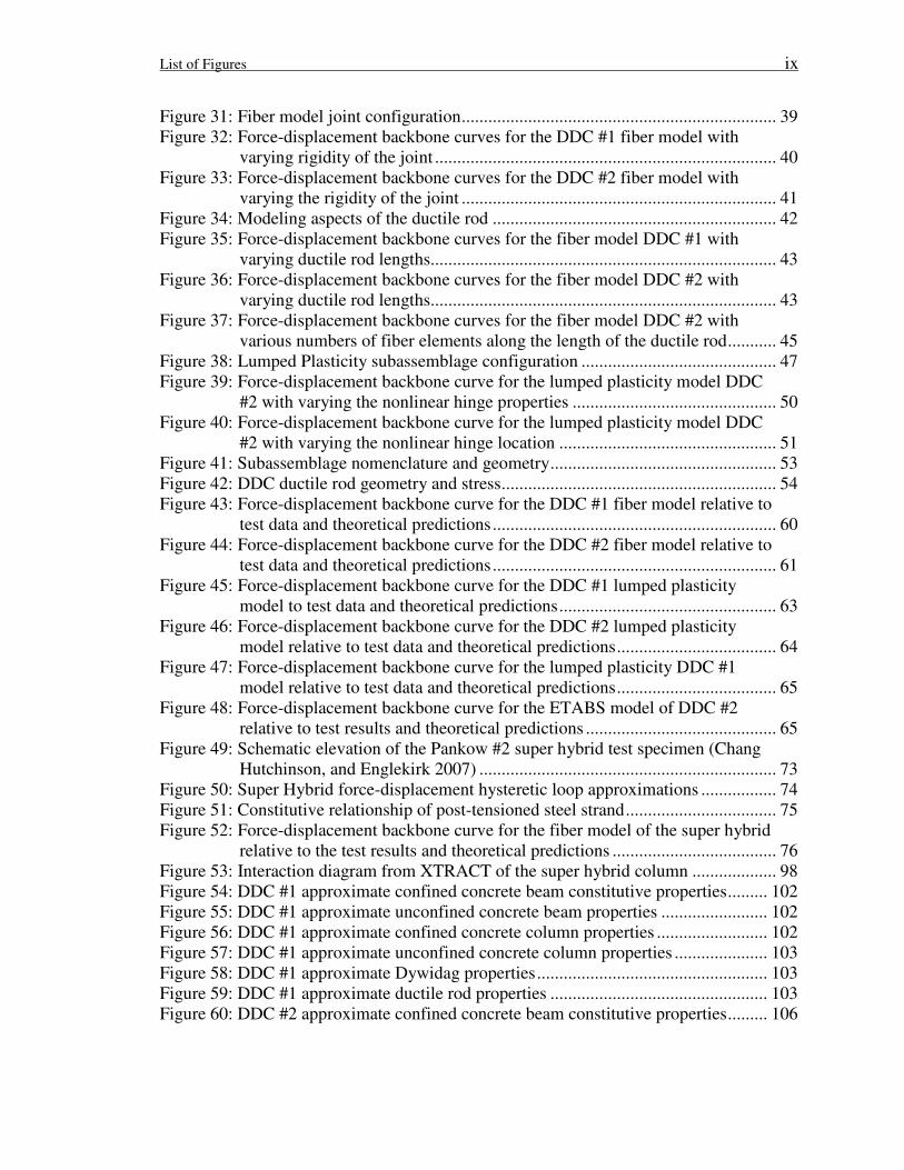
Figure 95: Super hybrid plan of the north beam at the pinned end connection (Chang,
Hutchinson, and Englekirk 2007) ................................................................. 127
Figure 96: Super hybrid north beam elevation (Chang, Hutchinson, and Englekirk
2007) ............................................................................................................. 127
Figure 97: Super hybrid section cut 1/SK-6 through the north beam (Chang,
Hutchinson, and Englekirk 2007) ................................................................. 128
Figure 98: Super hybrid section cut 2/SK-6 through the north beam (Chang,
Hutchinson, and Englekirk 2007) ................................................................. 128
Figure 99: Super hybrid section cut 2/SK-7 through the north beam (Chang,
Hutchinson, and Englekirk 2007) ................................................................. 129
Figure 100: Super hybrid force-displacement hysteretic data (Chang, Hutchinson, and
Englekirk 2007) ............................................................................................ 129
Figure 101: Super hybrid material tests (Chang, Hutchinson, and Englekirk 2007)...... 130

List of Figures xii
Nomenclature
ACI American Concrete Institute
AISI American Iron and Steel Institute
ASCE American Society of Civil Engineers
ASTM American Society for Testing and Material
CBC California Building Code
C1 Half of the length of the column within the joint, in.
C2 Half of the length of the beam within the joint, in.
DB Dywidag bars
DDC Dywidag ductile connector
DOT Day of Test
DR Ductile rod
fc’ Compressive strength of concrete, ksi
FEMA Federal Emergency Management Agency
fu Ultimate strength, ksi
fy Yield strength, ksi
hb Height of the beam, in.
IBC International Building Code
Ieff Effective moment of inertia, in4
Ig Gross moment of inertia, in4
KINITIAL Initial stiffness, kips/in.
Lb Length of the beam, in.
Lcr Plastic hinge length, in.
LP Lumped plasticity
Mcr Moment at tensile rupture of the concrete, kip-in.
Mn Nominal moment capacity at yielding of the ductile rods, kip-in.
Mn-DB Nominal moment capacity at yielding of the Dywidag reinforcement bars,
kip-in.
PT Post Tensioned
UBC Uniform Building Code
γ Drift ratio, %
γcr Drift at tensile rupture of the concrete, %
γy Drift at yielding of the ductile rods, %
∆ Displacement, in.
εy Yield strain, in./in.
θ Rotation, rad/in.
Φ Curvature, radian

1.0 Introduction 1
1.0 INTRODUCTION
Over the past fifty years, structural engineering has experienced significant
technological advancement. During the mid-twentieth century, structural engineering
involved procedures such as hand calculations of moment distribution and drafting with a
T-square. Today, a large portion of structural engineering is accomplished on the
computer with the help of structural analysis programs. With this new medium for
making design decisions comes a need to understand how structural systems should be
modeled on the computer. In particular, this report focuses on the computer modeling of
the Dywidag ductile connector (DDC) frame, a type of precast system.
1.1 Advantages of Precast Frame Systems
Research on precast systems has been motivated by the immense advantages
found in these systems relative to their monolithic, cast-in-place counter parts (Priestley
1991). Precast systems require less formwork than monolithic systems. In addition,
some precast manufactures are able to apply architectural finishes to the precast structural
elements, therein eliminating additional cladding costs for the building owner. Less in-
situ pouring, formwork construction, and additional facade construction can lead to a
quicker erection time, reduced material cost, and better quality control. Another reason
precast frames are more desirable than monolithic concrete frames is due to their
structural performance. Precast moment frames can be designed to respond similar to or
more favorably than a monolithic concrete ductile moment frame (Cheok and Stone
1993).
1.0 Introduction 2
With these construction and structural performance advantages, why aren’t there
more precast systems in the seismic regions of the United States? According to Nigel
Priestley (1991), organizer of the Precast Seismic Structural Systems (PRESS) Research
Program,
To a considerable extent, the reason for the lack of advancement of precast
structural systems in the United States can be attributed to uncertainty about their
seismic performance…The codes require confirmation of the suitability of new
designs by satisfaction of performance criteria provided by expensive and time-
consuming structural testing. This requirement inhibits innovation and has forced
research and design practice into a narrow focus of reinforced [monolithic]
concrete emulation instead of expanding the scope to take advantage of the
strengths and differences of precast construction.
1.2 Precast Frame Systems
Precast frame systems can be divided into four categories according to the
connection location of the precast elements and the plastic hinge region. These four
categories are shown in Figure 1. Category (a), (c), and (d) are precast frames that are
designed to behave like monolithic moment frames with plastic hinges occurring in the
beam. Each of these three categories differs according to the shape of the precast
elements used. Category (a) consists of precast elements that come in a cruciform shape.
Category (c) consists of multi-story column elements and single-span beam elements.
Category (d) consists of single-story column elements and multi-span beam elements.

1.0 Introduction 3
Figure 1: Classification of precast ductile frames (Englekirk 2003)
Category (b) consists of the same types of precast elements as category (c); however,
category (b) is designed to have plastic hinges occur at the beam-column interface, where
the precast elements meet. Category (b) is more commonly known as a gap-opening
system, and it is under this category that the DDC system is classified.
1.3 Gap-opening Frame Systems
The joint behavior of a gap-opening system is shown graphically in Figure 2.
(a) (b)
(c) (d) Strong, nonyielding connection joining precast members.
Ductile, energy-dissipating connection joining precast members.
“Hinged”, free but guided connection joining precast members or
points of inflection.
Plastic hinge location (first yield).

1.0 Introduction 4
Figure 2: Gap-opening behavior
The gap-opening system is characterized by the opening of the beam-column interface
which permits drift in the system with minimal damage to the main structural elements.
This system has been studied in the United States since the early 1990’s. The first gap-
opening system to evolve was the pure hybrid system. In the mid 1990’s the Dywidag
Ductile Connector (DDC) System was developed, and almost a decade later came the
development of the super hybrid system in the early twenty-first century. The sections to
follow describe the configuration, construction methods, and behavioral characteristics of
the three gap-opening frame systems.
1.3.1 Pure Hybrid Systems
The pure hybrid frame is one type of gap-opening system that gets its name from
its combined use of mild steel and post-tensioning (PT) strands. Throughout a seismic
response, the PT strands are designed to remain elastic; the mild steel is designed to yield
and act as the energy dissipating element. The PT strands provide a restoring force which
tends to move the system back towards its original position after the frame has been
displaced by lateral forces (El-Sheikh, et al. 1997). Also, due to the compression forces
Gap opening
∆

1.0 Introduction 5
imposed on the joint by the PT strands, shear transfer occurs in the concrete through
friction at the beam-column interface. The typical configuration of a pure hybrid joint is
shown in Figure 3(a).
Figure 3: Pure hybrid system (a) seismic elements (b) construction elements
(Hawileh, Tabatabai, and Rahman 2006) (Cheok and Stone 1993)
The pure hybrid system is constructed on site by first erecting the precast columns. Then,
the beams are shored in place while the mild steel is fed through the columns and beams
via the trough access areas, shown in Figure 3(b). The mild steel is either fully or
partially grouted. The beam-column interface is grouted with fiber-reinforced grout.
After adequate curing, the PT strands are fed through the PT duct, see Figure 3(b), and
post tensioned.
(a) (b)
Trough
PT
Duct
Reinforcing bar
debonded locally
Fiber-reinforcing
grout
Post-tensioning
Tendon
(unbonded)
Mild reinforcing
bar (grouted in
trough)

1.0 Introduction 6
Figure 4: (a) Deformed shape of beams after testing, (b) Unit #1, pure hybrid system, at
2.8% drift (MacRae and Priestley 1994)
The observed behavior of the pure hybrid system is crushing of the toe of the concrete
beam as the drift demand increases; this behavior is shown in Figure 4(a) and (b). Failure
is due to 25% strength degradation of the system.
1.3.2 Dywidag Ductile Connector Systems
The DDC system is a type of gap-opening frame that uses a Dywidag ductile
connector as the main energy dissipating element, as opposed to typical reinforcing bars
used by the pure hybrid system. An isometric view of the DDC joint is shown in Figure
5.
(b) (a)
Toe of
the Beam
Heel of
the Beam

1.0 Introduction 7
Figure 5: Isometric view of DDC system (Englekirk 2003)
The DDC system is constructed by first erecting the columns. Then, the beams
are erected and the bolts, labeled in Figure 5, are tightened to the ductile rods (DR) by
threading them through the steel block, also known as the Dywidag ductile connector.
Structural grouting is not required since the steel blocks are designed to transfer all of the
shear force across the beam-column interface. The ductile rods use a combination of
bond strength and bearing area to distribute lateral forces through the joint. This load
path is shown in Figure 6.
Ductile Rod (DR)
Dywidag Ductile
Connector (DDC)
Dywidag Bar
(DB)
Bolt used to
connect the
beam to the
column

1.0 Introduction 8
Figure 6: DDC connection – shear transfer mechanism (Englekirk 2003)
The development of the [DDC] assemblage… was motivated by a desire to
improve the postyield behavior of concrete ductile frames…The adaptation of the
ductile connection concept to precast concrete is logical, because it allows
postyield deformations to be accommodated where members are joined…The
Achilles heel of a properly conceived ductile frame beam has always been the toe
(no pun intended) of the frame beam where large compressive and shear stresses
combine (Englekirk 2003).
The elongated reinforcing bars within the beam tend to buckle due to the cyclic tensile
overstraining caused by lateral loading. Therefore, the DDC system solves these
problems with the following alterations:
(1) Relocating the yielding element to within the joint as to provide it with
nondeteriorating lateral support, (2) allowing for the strain in the toe region of the
beam to be controlled, and (3) transferring shear in the joint by means of friction
between the steel block and steel washer (Englekirk 2003).
1.0 Introduction 9
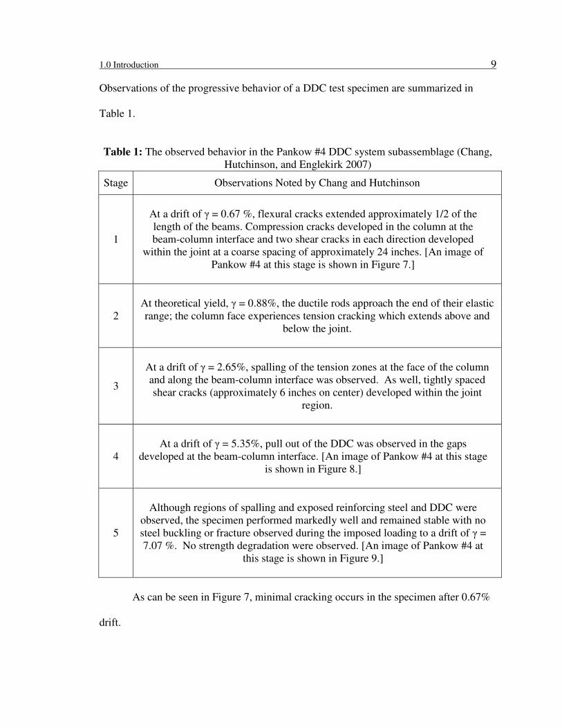
Observations of the progressive behavior of a DDC test specimen are summarized in
Table 1.
Table 1: The observed behavior in the Pankow #4 DDC system subassemblage (Chang,
Hutchinson, and Englekirk 2007)
Stage Observations Noted by Chang and Hutchinson
1
At a drift of γ = 0.67 %, flexural cracks extended approximately 1/2 of the
length of the beams. Compression cracks developed in the column at the
beam-column interface and two shear cracks in each direction developed
within the joint at a coarse spacing of approximately 24 inches. [An image of
Pankow #4 at this stage is shown in Figure 7.]
2
At theoretical yield, γ = 0.88%, the ductile rods approach the end of their elastic
range; the column face experiences tension cracking which extends above and
below the joint.
3
At a drift of γ = 2.65%, spalling of the tension zones at the face of the column
and along the beam-column interface was observed. As well, tightly spaced
shear cracks (approximately 6 inches on center) developed within the joint
region.
4
At a drift of γ = 5.35%, pull out of the DDC was observed in the gaps
developed at the beam-column interface. [An image of Pankow #4 at this stage
is shown in Figure 8.]
5
Although regions of spalling and exposed reinforcing steel and DDC were
observed, the specimen performed markedly well and remained stable with no
steel buckling or fracture observed during the imposed loading to a drift of γ =
7.07 %. No strength degradation were observed. [An image of Pankow #4 at
this stage is shown in Figure 9.]
As can be seen in Figure 7, minimal cracking occurs in the specimen after 0.67%
drift.

1.0 Introduction 10
Figure 7: Joint elevation of Pankow #4 at 0.67% drift (Chang, Hutchinson, and Englekirk
2007)
Figure 7 shows the pre-yield condition of the specimen. Figure 8 shows the
condition of the specimen after it was subjected to a drift of 5.35%. At this point, the
specimen had already yielded the ductile rods and the Dywidag reinforcement in the
beam.

1.0 Introduction 11
Figure 8: Partial joint elevation of Pankow #4 at 5.35% drift (Chang, Hutchinson, and
Englekirk 2007)
In contrast to Figure 8, Figure 9 shows the condition of the specimen after the
cracking and spalling has eliminated continuous lateral support along the Dywidag bars
and therefore the bars have buckled. The DDC system does not completely eliminate
buckling of the beam reinforcement, but it does increase the subassemblage drift levels
associated with buckling of these bars.

1.0 Introduction 12
Figure 9 : Joint elevation of Pankow #4 at 7.07% drift (Chang, Hutchinson, and
Englekirk 2007)
The buckling of the beam reinforcement near the beam-column interface is
slightly visible, from the Figure 9 elevation, through the small flare out of the ends of the
concrete beams.
A more recent evolutionary turn for the family of precast gap-opening frames was the
development of the super hybrid system which incorporates aspects of both the DDC and
pure hybrid systems.

1.0 Introduction 13
1.3.3 Super Hybrid Systems
The super hybrid system refers to the gap-opening frame that uses a DDC as the
main energy dissipating element, and PT strands as the restoring force within the system.
The super hybrid frame eliminates the extensive grouting required to construct the pure
hybrid system, as well as reduces member sizes required of the DDC system when
designed under monolithic moment frame code provisions. The configuration of a super
hybrid joint is shown in Figure 10.
Figure 10: Isometric view of the super hybrid joint (Englekirk 2003)
Dywidag Ductile
Connector (DDC)
Dywidag Bar
(DB)
Ductile Rod (DR)
Post Tensioning
Strands (PT)

1.0 Introduction 14
The super hybrid erection process is analogous to that of the DDC system except
for the additional feeding and tensioning of the PT. The progressive behavior of the
super hybrid system is similar to the DDC. The only super hybrid test conducted thus far
showed failure of the joint via buckling of the Dywidag bar portion of the DDC, at
around 7% drift.
Each of these gap-opening frame systems has unique physical traits though they
all share the same gap-opening behavior. Taking a closer look at the hysteretic test
results of these systems helps shed light on the behavioral differences between them.
1.3.4 Advantages and Disadvantages in the Gap-Opening Systems
The advantages and disadvantages of each gap-opening system depend on the
system’s seismic performance and constructability. As mentioned in the previous
section, the pure hybrid system requires shoring, which makes it a less desirable gap-
opening system from a construction stand point. This section will focus on the
performance-based advantages and disadvantages.
Figure 11 shows the approximate normalized hysteretic loops of the DDC, pure
hybrid, and super hybrid systems at 2% drift. Around 2% drift the pure hybrid specimen
shows desirable results. The energy dissipation is present and comparable in all
specimens. The pure hybrid specimen has a greater pinching effect than the other
specimens, and therefore, it experiences less residual drift.

1.0 Introduction 15
-1.5
-1
-0.5
0
0.5
1
1.5
-2.5 -2 -1.5 -1 -0.5 0 0.5 1 1.5 2 2.5
Drift (%)
F/F
y
DDC 2007
Super Hybrid 2007
Pure Hybrid 1999
Figure 11: Force-displacement hysteretic loop approximations at 2% (Chang,
Hutchinson, and Englekirk 2007) and (Stanton, Day, and MacRae 1999)
Figure 12 shows the approximate hysteretic loops of each system at 3-3.5% drift. At this
drift ratio, the residual drift has roughly doubled, relative to the 2% loops, for the DDC
and super hybrid specimens. The energy dissipation in the DDC and super hybrid
specimens is greater than that of the pure hybrid specimen.

1.0 Introduction 16
-1.5
-1
-0.5
0
0.5
1
1.5
-4 -3 -2 -1 0 1 2 3 4
Drift (%)
F/F
y
DDC 2007
Super Hybrid 2007
Pure Hybrid 1999
Figure 12: Force-displacement hysteretic loop approximations at 3-3.5% (Chang,
Hutchinson, and Englekirk 2007) and (Stanton, Day, and MacRae 1999)
Figure 13 shows the approximate hysteretic loops of each specimen at 5% drift. At this
level of drift, the relative energy dissipation is distinctly different in the DDC and super
hybrid specimens relative to the pure hybrid specimen. At 5% drift the pure hybrid
subassemblage decreases in strength to about 75% of its capacity, and thus has reached
failure.

1.0 Introduction 17
-1.5
-1
-0.5
0
0.5
1
1.5
2
-6 -4 -2 0 2 4 6
Drift (%)
F/F
y
DDC 2007
Super Hybrid 2007
Pure Hybrid 1999
Figure 13: Force-displacement hysteretic loop approximations at 5% (Chang,
Hutchinson, and Englekirk 2007) and (Stanton, Day, and MacRae 1999)
The degradation in strength of the pure hybrid system is more visually apparent in Figure
14 which only shows the various hysteretic loops of the pure hybrid system.
-1.5
-1
-0.5
0
0.5
1
1.5
-6 -4 -2 0 2 4 6
Drift (%)
F/F
y
Pure Hybrid at 5%
Pure Hybrid at 3%
Pure Hybrid at 2%
Figure 14: Pure hybrid force-displacement hysteretic loop approximations at 2%, 3%,
and 5% drift (Stanton, Day, and MacRae 1999)]
25% (F/Fy)MAX (F/Fy)MAX

1.0 Introduction 18
In contrast to the pure hybrid specimen, degradation in strength from 2% to 5% drift is
not present in the DDC system and the super hybrid system. Both systems’ test results
are shown in Figure 15 and Figure 16 respectively.
-1.5
-1
-0.5
0
0.5
1
1.5
-6 -4 -2 0 2 4 6
Drift (%)
F/F
yDDC #1 at 5%
DDC #1 at 3.5%
DDC #1 at 2%
Figure 15: DDC force-displacement hysteretic loop approximations at 2%, 3%, and 5%
drift (Chang, Hutchinson, and Englekirk 2007)]
A disadvantage of the DDC and super hybrid systems is the greater levels of residual drift
compared to the pure hybrid system.
Though the behavior of the DDC specimen and super hybrid specimen appear to
be very similar, they differ in their subassemblage composition, besides just the presence
or absence of PT.

1.0 Introduction 19
-1.5
-1
-0.5
0
0.5
1
1.5
2
-6 -4 -2 0 2 4 6
Drift (%)
F/F
y
Super Hybrid at 5%
Super Hybrid at 3.5%
Super Hybrid at 2%
Figure 16: Super hybrid force-displacement hysteretic loop approximations at 2%, 3.5%,
and 5% drift (Chang, Hutchinson, and Englekirk 2007)
The super hybrid specimen, results shown in Figure 16, had a total of 8 ductile rods
within the joint compared to 12 ductile rods within the joint of the DDC specimen. With
four less ductile rods, less steel is used in the joint and in adjacent members.
As previously mentioned, when looking at the gap-opening systems from a
constructability stand point, the DDC and super hybrid systems require less erection time
than the pure hybrid system, but still maintain the same advantages over a monolithic
frame as the pure hybrid system. As well, the DDC and super hybrid systems show
minimal signs of strength degradation at drift levels over 4%.
The Northridge earthquake caused a significant amount of damage in steel frame
buildings and subsequent research suggests that it will be difficult to attain post-
yield story drifts of 3 percent in steel ductile frames. Story drifts of 3.5 percent in
concrete frames produce considerable distress and this is also the case in

1.0 Introduction 20
structural steel subassemblies. The ductile connector [DDC] is not only easily
capable of exceeding these levels of story drift but does so without damaging the
system (Englekirk 1995).
With the above mentioned level of potential demand on structural systems in Southern
California, as well as the advantages of the DDC and super hybrid systems, some
engineers in the region have tried to incorporate these systems into building practice.
1.4 Current Industry Practices
Design codes in the United States such as the Uniform Building Code (UBC),
International Building Code (IBC), and the American Concrete Institute Code (ACI)
permit the design of precast structures in high seismic zones via three routes.
The first route requires the design of precast structures to emulate the behavior of
a comparable monolithic concrete structure in terms of strength and toughness. For
example, the Hollywood Highlands building uses the DDC as the primary lateral system;
however, the design procedures followed chapter 16, chapter 19, and chapter 21 of the
2001 California Building Code (CBC) under the category of special moment resisting
frame. The general seismic demand and capacity design for the DDC is the same as
designing a monolithic moment frame. Taking this design approach results in larger
member sizes than are necessary (Chen 2007).
The second route for design permits a new type of lateral system, but requires
experimental and analytical evidence verifying satisfactory behavior of the precast
systems under simulated seismic loading (Celik and Sritharan, 2004). This route requires
1.0 Introduction 21
a substantial amount of time, effort, and money, and, for these reasons, is typically not
the approach taken.
The third route requires the design of a hybrid system that fits within the
parameters set by the Standard ACI T1.2-03, which is titled Special Hybrid Moment
Frames Composed of Discretely Jointed Precast and Post-Tensioned Concrete Members.
The T1.2-03 provides detailed guidelines for the mechanism requirements for the pure
hybrid frame. “This limits the type of hybrid frame acceptable by this specific code, to
those frames whose design characteristics do not exceed the bounds of the properties of
the pure hybrid specimens used in the validation tests for code ACI T1.2-03” (Hawkins
and Ghosh 2004). Due to such limitations, design engineers have been denied permission
to use the ACI T1.2-03 code for the design of a super hybrid system.
Due to the lack of testing on super hybrid and DDC frames, and the relatively new
nature of the systems, attempts to use these systems outside the monolithic code sections
have failed (Chen 2007). With the recent testing and research done at UCSD on the DDC
and super hybrid systems, the implementation of these systems into practice is becoming
more plausible via the second route previously mentioned.
1.5 The Project Statement
As the Dywidag ductile connector and super hybrid systems reach industry, the
design engineer will need to model these systems using structural analysis software. This
report provides two examples of tested DDC specimens that were each modeled in
PERFORM-3D and ETABS. The experimental backbone curve for each test specimen

1.0 Introduction 22
was compared to the corresponding analytical pushover curves. Preceding these results is
a discussion on the parameters to consider when creating a lumped plasticity model
(ETABS) and a fiber model (PERFORM-3D).
The fiber modeling focuses on providing a means to study the joint behavior as
the parameters of the system are changed. This fiber modeling uses finite element
analysis on beam elements containing multiple fibers to determine the internal forces of
the system. Each fiber is analyzed individually at its mid-span and mid-height. The
results produce a piecewise approximation of the internal forces along each member
within the system. This approach is a valuable method for researching the DDC system,
as it is more cost effective than testing numerous system configurations. As well, fiber
modeling is a tool which can greatly effect design decisions by helping the engineer
better understand the effects of varying parameters of the system.
The lumped plasticity modeling provides the design engineer with a means for
modeling a three-dimensional building with a DDC system. The lumped plasticity model
uses elastic members in conjunction with nonlinear moment-rotation hinges. With such a
model, the engineer has the tools to get acceptable global demand forces within a
reasonable time frame.
This project provides modeling suggestions for both the fiber models and the
lumped plasticity models used to predict the seismic behavior of the DDC precast
concrete system.
2.0 Literature Review 23
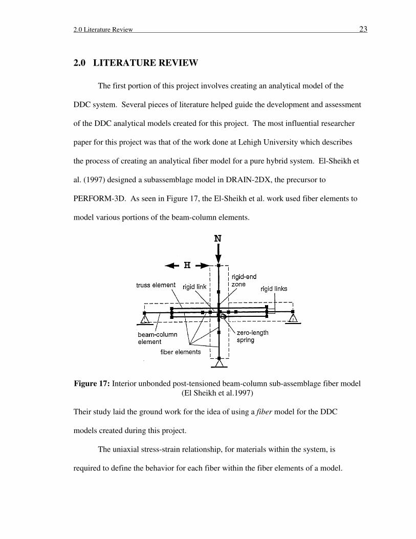
2.0 LITERATURE REVIEW
The first portion of this project involves creating an analytical model of the
DDC system. Several pieces of literature helped guide the development and assessment
of the DDC analytical models created for this project. The most influential researcher
paper for this project was that of the work done at Lehigh University which describes
the process of creating an analytical fiber model for a pure hybrid system. El-Sheikh et
al. (1997) designed a subassemblage model in DRAIN-2DX, the precursor to
PERFORM-3D. As seen in Figure 17, the El-Sheikh et al. work used fiber elements to
model various portions of the beam-column elements.
Figure 17: Interior unbonded post-tensioned beam-column sub-assemblage fiber model
(El Sheikh et al.1997)
Their study laid the ground work for the idea of using a fiber model for the DDC
models created during this project.
The uniaxial stress-strain relationship, for materials within the system, is
required to define the behavior for each fiber within the fiber elements of a model.

2.0 Literature Review 24
Various models have been used in the past to mimic the stress-strain properties of
structural materials. For this project, the stress-strain model developed by Mander et al.
(1988) was used to define the constitutive properties necessary for modeling the
concrete members. Figure 18 labels some of the characteristics of Mander’s Model.
Figure 18: Confined and unconfined concrete stress-strain curves from (Mander
et al. 1988)
The above mentioned Mander’s stress-strain models were used in the DDC fiber model
to define the confined and unconfined concrete properties within the beams and
columns.
After the fiber models were created, they were blindly tested against their
corresponding sets of experimental data. The two DDC test specimens modeled are
Pankow #4 and SEQAD #1. Figure 19 shows an elevation of the Pankow #4 specimen,
which is referred to as DDC #1.
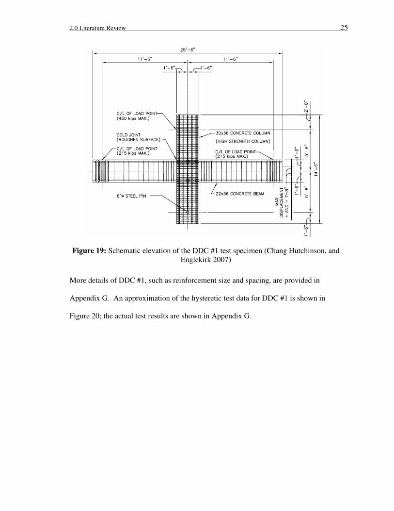
2.0 Literature Review 25
Figure 19: Schematic elevation of the DDC #1 test specimen (Chang Hutchinson, and
Englekirk 2007)
More details of DDC #1, such as reinforcement size and spacing, are provided in
Appendix G. An approximation of the hysteretic test data for DDC #1 is shown in
Figure 20; the actual test results are shown in Appendix G.
2.0 Literature Review 26
-200
-150
-100
-50
0
50
100
150
200
-6 -4 -2 0 2 4 6
Drift (%)
Forc
e (k
ips)
DDC #1 at 5%
DDC #1 at 3.5%
DDC #1 at 2%
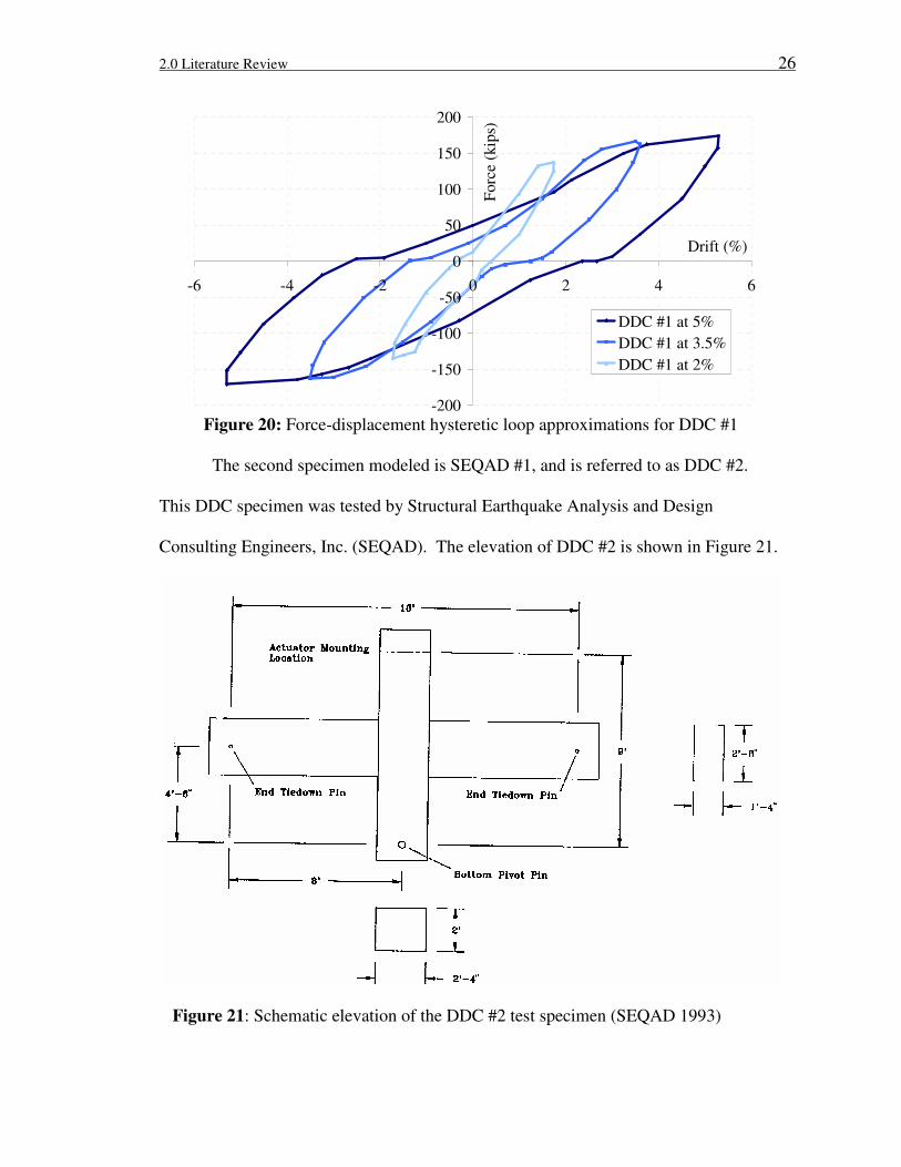
Figure 20: Force-displacement hysteretic loop approximations for DDC #1
The second specimen modeled is SEQAD #1, and is referred to as DDC #2.
This DDC specimen was tested by Structural Earthquake Analysis and Design
Consulting Engineers, Inc. (SEQAD). The elevation of DDC #2 is shown in Figure 21.
Figure 21: Schematic elevation of the DDC #2 test specimen (SEQAD 1993)

2.0 Literature Review 27
An approximation of the hysteretic test data for DDC #2 is shown in Figure 22. The
actual test results, as well as specimen details such as reinforcement layout, are
provided in Appendix H.
-250
-200
-150
-100
-50
0
50
100
150
200
250
-6 -4 -2 0 2 4 6
Drift (%)
Fo
rce
(kip
s)
DDC #2 at 1.5%
DDC #2 at 3%
DDC #2 at 4.5%
Figure 22: Force-displacement hysteretic loop approximations for DDC #2.
More of the El-Sheikh et al. paper as well as a study conducted by Elwood et al. (2007)
are mentioned in Section 3.0 as their content is discussed in greater detail and parallels
some of the studies conducted for this project.

3.0 Model Design and Assumptions 28
3.0 MODEL DESIGN AND ASSUMPTIONS
In the process of modeling DDC #1 and DDC #2 many assumptions were made.
Some assumptions are standard practice, where as others are recently developed
techniques. Along with modeling the DDC specimens, some small parametric studies
were conducted.
3.1 Boundary Conditions
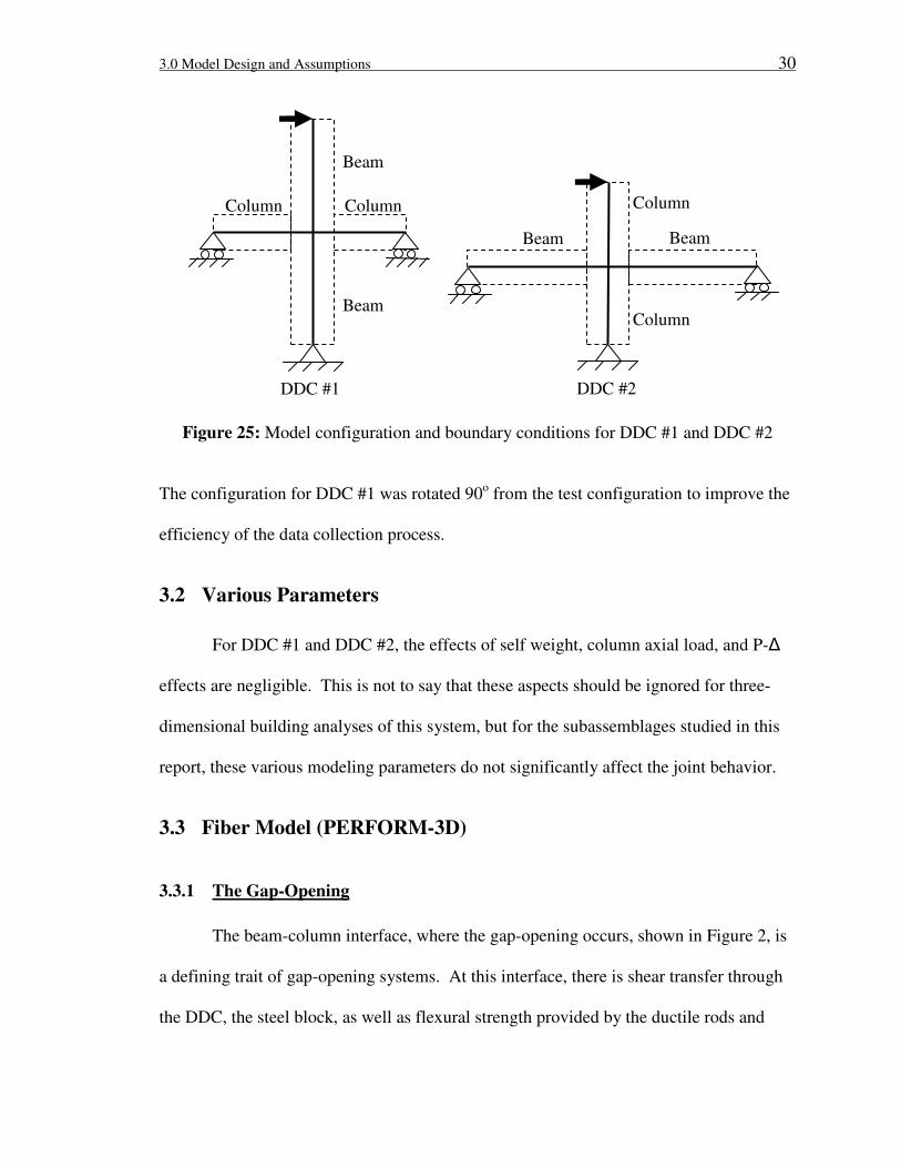
The specimens studied are typical interior frame elements as shown in Figure 23.
Figure 23: Schematic elevation of a five-story moment frame building
The subassemblage is a cruciform shape which spans from the mid-point of the beams
and has a height extending from the mid-point of each column; the subassemblage
terminates at the theoretical inflection points of the frame.
Subassemblage
Story 5
Story 4
Story 3
Story 2
Story 1 Subassemblage
½ LB ½ LB
½ LC
½ LC
LB LB
LC
LC

3.0 Model Design and Assumptions 29
In the case of the global geometry of the subassemblages, DDC #1 and DDC #2
were tested and restrained in different ways. Figure 24 shows the loading locations and
boundary conditions for both test specimens.
Figure 24: Test configuration and boundary conditions
The force-displacement output from each test varies. For DDC #1 the test data collected
at UCSD is a graph of the beam shear verses the drift between the beam ends. For DDC
#2 the test data collected by SEQAD is a graph of the column shear verses the drift
between the column ends. Figure 25 shows the boundary conditions and applied loading
location for the computer models.
Column
Column
Beam Beam
DDC #2
Beam
Column
Column
Beam
DDC #1
3.0 Model Design and Assumptions 30
Figure 25: Model configuration and boundary conditions for DDC #1 and DDC #2
The configuration for DDC #1 was rotated 90o from the test configuration to improve the
efficiency of the data collection process.
3.2 Various Parameters
For DDC #1 and DDC #2, the effects of self weight, column axial load, and P-∆
effects are negligible. This is not to say that these aspects should be ignored for three-
dimensional building analyses of this system, but for the subassemblages studied in this
report, these various modeling parameters do not significantly affect the joint behavior.
3.3 Fiber Model (PERFORM-3D)
3.3.1 The Gap-Opening
The beam-column interface, where the gap-opening occurs, shown in Figure 2, is
a defining trait of gap-opening systems. At this interface, there is shear transfer through
the DDC, the steel block, as well as flexural strength provided by the ductile rods and
Column
Column
Beam Beam
DDC #2
Column Column
Beam
Beam
DDC #1
3.0 Model Design and Assumptions 31
compressive concrete. Since the steel block is designed to remain elastic, the main
modeling concern at this interface is the lack of deformation compatibility due to the gap-
opening. The process of gap opening and closing under the action of flexural loading is
captured in the fiber elements by having an increase in the number of fibers subjected to
tension as the loading increases, and a decrease in the number of fibers subjected to
tension as the loading decreases.
The important aspect of this gap-opening behavior in PERFORM-3D is the
ultimate tensile strain in the material properties. The ultimate tensile strain value should
be relatively large in order to allow the analysis of the system to continue well past the
point in which a fiber has lost all its strength. For example, Figure 54 shows the confined
concrete beam properties for DDC #1. At 0.012 strain the fiber with this assigned
material characteristics would have no more strength; however, it is still permitted to
increase in strain up to 0.5 in./in. in order to allow for large deformations, an essential
characteristic for the gap-opening interface.
3.3.2 Fiber Elements
Fiber elements were decided upon as a means to model not just the gap-opening,
but also the inelastic regions of the beams and columns. A typical cross section for a
fiber element is shown in Figure 26.

3.0 Model Design and Assumptions 32
Figure 26: Typical fiber element cross section
A study by El-Sheikh et al. (1997) concluded the following about fiber element cross
sections:
1. The number of fibers has a negligible effect on the moment capacity of the beam.
2. An increase in the number of fibers reduces the ultimate rotation capacity due to
the crushing of the confined concrete, up to a certain limit where the ultimate
rotation becomes almost constant. It is adequate to assume ∆h
/H = 0.02 to achieve
good accuracy. [Refer to Figure 26.]
3. Dividing the unconfined cover concrete at the top and bottom edges of the cross-
section into more than one fiber does not affect the accuracy of the analysis.
Steel Fiber
Confined
Concrete
Fiber
Unconfined
Concrete
Fiber
H
∆h
Bottom
Top
*Each
rectangle
and circle
represents
one fiber in
the cross
section of a
fiber
element
Fiber element
cross section

3.0 Model Design and Assumptions 33
4. A coarse distribution of fibers may be used for concrete types other than spiral
confined concrete.
DDC #1 and DDC #2 have no spirally confined concrete, and even though the El-
Sheikh et al. results say coarser fiber spacing is acceptable for other forms of confined
concrete, the height of the confined fibers was decided upon using the ∆h
/H ratio.
Therefore, the confined concrete fiber heights should be 0.64in. and 0.72in; a height of
0.5in. was chosen for ease of construction.
The fiber element length is an aspect of fiber modeling equally important to the
analysis as sizing the fibers within the fiber element. Each fiber element has constant
behavior across its length which is determined according to the demands at mid-span of
the fiber element. Therefore, a beam composed of several fiber elements will have a
cross-sectional moment of inertia, curvature and so on that varies in a stepwise fashion
across the length of the beam. The fiber segment, where the moment is at its maximum,
is an important fiber element in determining the moment capacity of the beam. When
comparing the two cantilever beams in Figure 27, the maximum moment, MMAX, is better
approximated by the 8-segment fiber beam rather than the 4-segment fiber beam due to
the location, along the moment diagram, that M1 is defined.
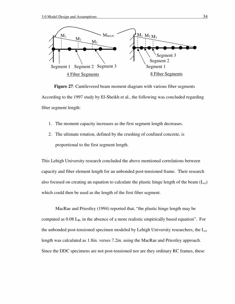
3.0 Model Design and Assumptions 34
Figure 27: Cantilevered beam moment diagram with various fiber segments
According to the 1997 study by El-Sheikh et al., the following was concluded regarding
fiber segment length:
1. The moment capacity increases as the first segment length decreases.
2. The ultimate rotation, defined by the crushing of confined concrete, is
proportional to the first segment length.
This Lehigh University research concluded the above mentioned correlations between
capacity and fiber element length for an unbonded post-tensioned frame. Their research
also focused on creating an equation to calculate the plastic hinge length of the beam (Lcr)
which could then be used as the length of the first fiber segment.
MacRae and Priestley (1994) reported that, “the plastic hinge length may be
computed as 0.08 LB, in the absence of a more realistic empirically based equation”. For
the unbonded post-tensioned specimen modeled by Lehigh University researchers, the Lcr
length was calculated as 1.8in. verses 7.2in. using the MacRae and Priestley approach.
Since the DDC specimens are not post-tensioned nor are they ordinary RC frames, these
Segment 1 Segment 2 Segment 3
M3 M2
M1
4 Fiber Segments
Segment 3
Segment 2
Segment 1
M1 M2 M3
8 Fiber Segments
MMAX

3.0 Model Design and Assumptions 35
results act only as guidelines in determining the first segment length within the DDC
model.
A small study was conducted on a 138in. cantilevered beam with load applied at
its free end. The beam had similar properties and geometry to the DDC #1 beam. There
were five fiber models of this beam created using 2, 4, 8, 16, 32, and 64 fiber elements
per beam with uniform fiber element length. As the applied load was increased from zero
to 150 kips, the displacement over the loading history was recorded as can be seen in
Figure 28.
-0.5
-0.45
-0.4
-0.35
-0.3
-0.25
-0.2
-0.15
-0.1
-0.05
0
0 0.2 0.4 0.6 0.8 1
Load Scale Factor
En
d D
isp
lace
men
t (i
n.)
Model with 2 FibersModel with 4 FibersModel with 8 FibersModel with 16 FibersModel with 32 FibersModel with 64 Fibers
Figure 28: Cantilevered beam end displacement verses load scale factor
All of the cantilevered beam models show the same response up to about 20 kips which is
expected since the demand load is still within the elastic range of the beams. As the load
increases, the beam behaviors go nonlinear and the difference in beam response becomes
Displacement
values shown
in Table 2
3.0 Model Design and Assumptions 36
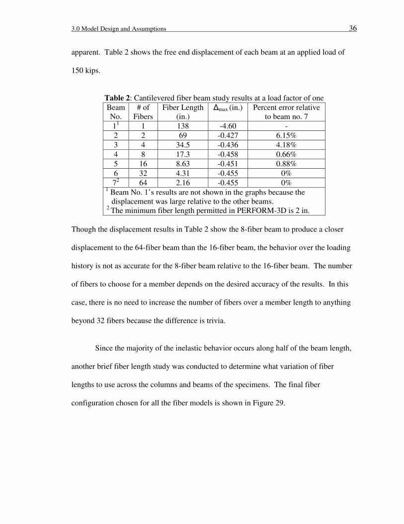
apparent. Table 2 shows the free end displacement of each beam at an applied load of
150 kips.
Table 2: Cantilevered fiber beam study results at a load factor of one
Beam
No.
# of
Fibers
Fiber Length
(in.)
∆max (in.) Percent error relative
to beam no. 7
11 1 138 -4.60 -
2 2 69 -0.427 6.15%
3 4 34.5 -0.436 4.18%
4 8 17.3 -0.458 0.66%
5 16 8.63 -0.451 0.88%
6 32 4.31 -0.455 0%
72 64 2.16 -0.455 0%
1 Beam No. 1’s results are not shown in the graphs because the
displacement was large relative to the other beams. 2
The minimum fiber length permitted in PERFORM-3D is 2 in.
Though the displacement results in Table 2 show the 8-fiber beam to produce a closer
displacement to the 64-fiber beam than the 16-fiber beam, the behavior over the loading
history is not as accurate for the 8-fiber beam relative to the 16-fiber beam. The number
of fibers to choose for a member depends on the desired accuracy of the results. In this
case, there is no need to increase the number of fibers over a member length to anything
beyond 32 fibers because the difference is trivia.
Since the majority of the inelastic behavior occurs along half of the beam length,
another brief fiber length study was conducted to determine what variation of fiber
lengths to use across the columns and beams of the specimens. The final fiber
configuration chosen for all the fiber models is shown in Figure 29.
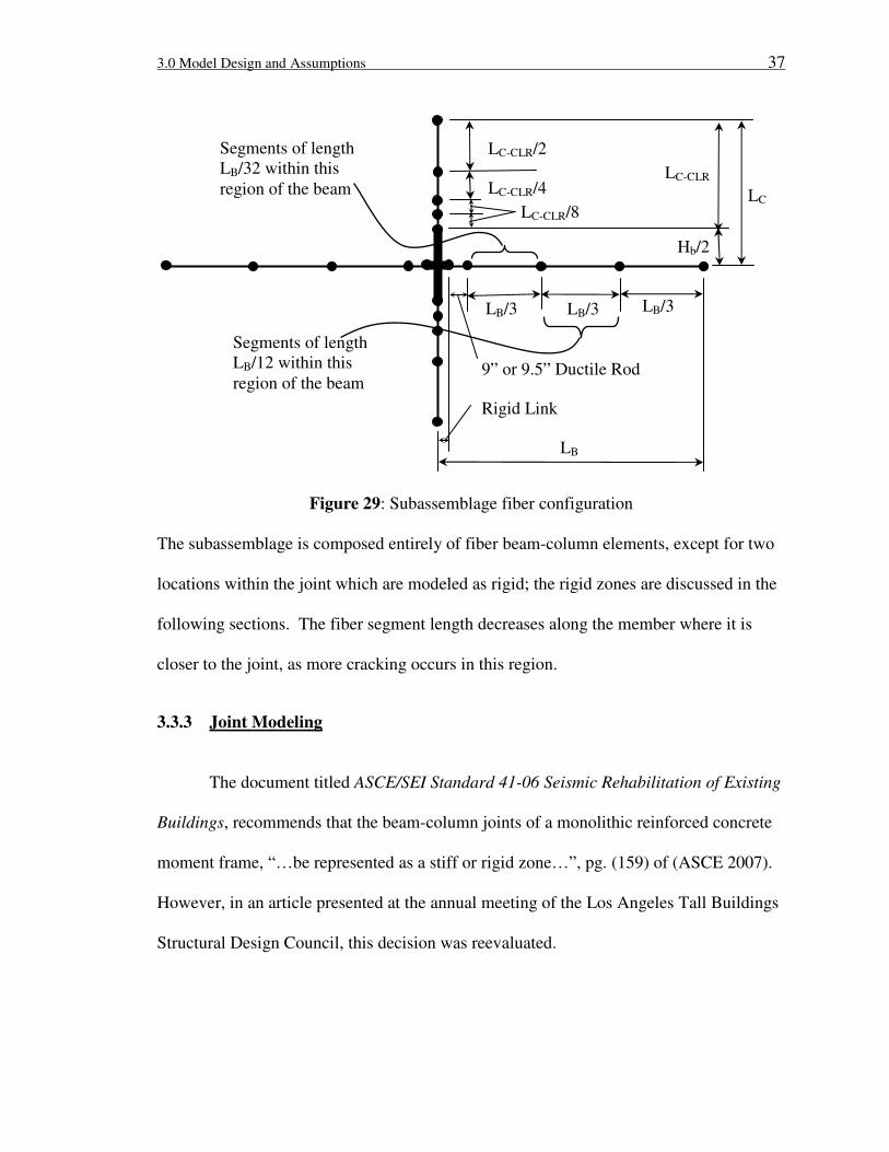
3.0 Model Design and Assumptions 37
Figure 29: Subassemblage fiber configuration
The subassemblage is composed entirely of fiber beam-column elements, except for two
locations within the joint which are modeled as rigid; the rigid zones are discussed in the
following sections. The fiber segment length decreases along the member where it is
closer to the joint, as more cracking occurs in this region.
3.3.3 Joint Modeling
The document titled ASCE/SEI Standard 41-06 Seismic Rehabilitation of Existing
Buildings, recommends that the beam-column joints of a monolithic reinforced concrete
moment frame, “…be represented as a stiff or rigid zone…”, pg. (159) of (ASCE 2007).
However, in an article presented at the annual meeting of the Los Angeles Tall Buildings
Structural Design Council, this decision was reevaluated.
LB/3 LB/3
LC-CLR/2
LC-CLR/4 LC-CLR
Hb/2
LB
LB/3
9” or 9.5” Ductile Rod
LC-CLR/8
Rigid Link
LC
Segments of length
LB/12 within this
region of the beam
Segments of length
LB/32 within this
region of the beam
3.0 Model Design and Assumptions 38
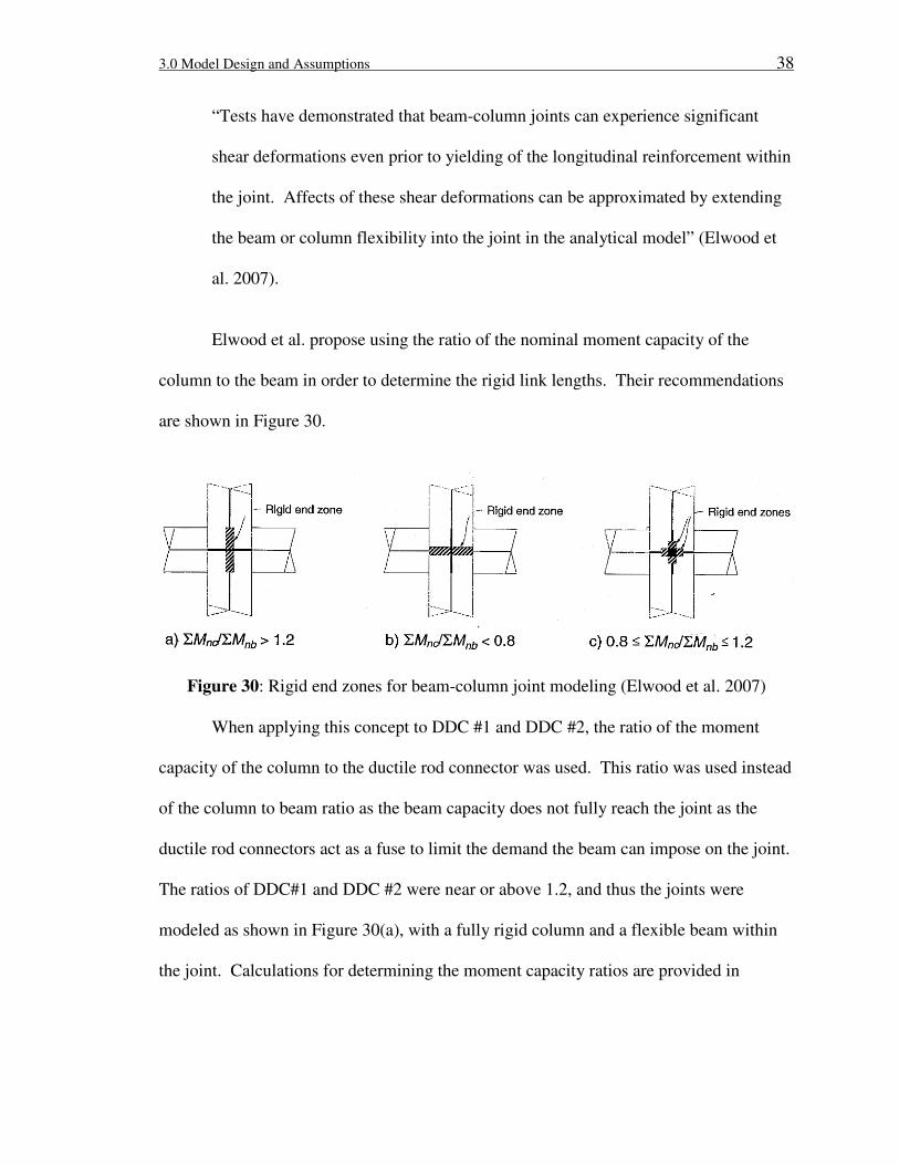
“Tests have demonstrated that beam-column joints can experience significant
shear deformations even prior to yielding of the longitudinal reinforcement within
the joint. Affects of these shear deformations can be approximated by extending
the beam or column flexibility into the joint in the analytical model” (Elwood et
al. 2007).
Elwood et al. propose using the ratio of the nominal moment capacity of the
column to the beam in order to determine the rigid link lengths. Their recommendations
are shown in Figure 30.
Figure 30: Rigid end zones for beam-column joint modeling (Elwood et al. 2007)
When applying this concept to DDC #1 and DDC #2, the ratio of the moment
capacity of the column to the ductile rod connector was used. This ratio was used instead
of the column to beam ratio as the beam capacity does not fully reach the joint as the
ductile rod connectors act as a fuse to limit the demand the beam can impose on the joint.
The ratios of DDC#1 and DDC #2 were near or above 1.2, and thus the joints were
modeled as shown in Figure 30(a), with a fully rigid column and a flexible beam within
the joint. Calculations for determining the moment capacity ratios are provided in
3.0 Model Design and Assumptions 39
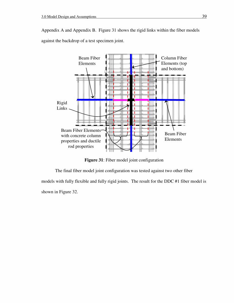
Appendix A and Appendix B. Figure 31 shows the rigid links within the fiber models
against the backdrop of a test specimen joint.
Figure 31: Fiber model joint configuration
The final fiber model joint configuration was tested against two other fiber
models with fully flexible and fully rigid joints. The result for the DDC #1 fiber model is
shown in Figure 32.
Column Fiber
Elements (top
and bottom)
Beam Fiber
Elements
Beam Fiber
Elements
Rigid
Links
Beam Fiber Elements
with concrete column
properties and ductile
rod properties

3.0 Model Design and Assumptions 40
0
20
40
60
80
100
120
140
160
180
0 1 2 3 4 5
Drift (%)
Fo
rce
(kip
s)
DDC #1 test data at 5%
DDC #1 test data at 3.5%
DDC #1 test data at 2%
DDC #1 test data backbonecurve
Fiber model with rigid columnand flexible beam within thejoint
Fiber model with rigid elementswithin the joint, no DR
Fiber model with no rigidelements in the joint, with DR
Figure 32: Force-displacement backbone curves for the DDC #1 fiber model with
varying rigidity of the joint
By making the beam and column lengths within the joint fully rigid, the initial stiffness
and the capacity of the system increased. There is a small difference in the results
between the fully-flexible-joint fiber model and the rigid-column-joint fiber model.
These results graphically demonstrate the small contribution the portion of the column
within the joint has on the subassemblage stiffness. This same test was performed on
DDC #2 and the fiber model result is shown in Figure 33.

3.0 Model Design and Assumptions 41
0
50
100
150
200
250
300
350
0 1 2 3 4
Drift (%)
Fo
rce
(kip
s)
DDC #2 test data at 1.5%
DDC #2 test data at 3%
DDC #2 test data at 4.5%
DDC #2 test data backbonecurve
Fiber model with a fully rigidjoint, no DR
Fiber model with a rigidcolumn and a flexible beamwithin the joint
Fiber model with no rigidelements within the joint, andwith a DR
Figure 33: Force-displacement backbone curves for the DDC #2 fiber model with
varying the rigidity of the joint
Both results from DDC #1 and DDC #2 validate the applicability of this rigid joint
calculation to the DDC systems.
3.3.4 Ductile Rod Modeling
The ductile rod is the region of the DDC designed to yield in response to lateral
loading. Thus, the constitutive and geometric properties of the ductile rod play a
substantial role in the behavior of this system. The ductile rod stress-strain and geometric
properties for each test specimen are provided in Appendix G and Appendix H. As well,
the PERFORM-3D approximations of the stress-strain properties can be found in
Appendix D and Appendix E.
The ductile rods are modeled as fibers within the specific fiber elements shown as
the pink segments in Figure 31. Taking a closer look at the ductile rod in Figure 34, the

3.0 Model Design and Assumptions 42
only portion of the ductile rod being modeled is the slender shank portion of the
hardware. The head portion of the ductile rod is modeled as rigid; refer to the horizontal
black segment at the center of the joint in Figure 31. The threaded connection portion of
the ductile rod is ignored. In place of this segment of column is a beam fiber segment
which contains concrete beam fibers and Dywidag fibers. Thus, this segment is modeled
as a continuation of the beam. Modeling this segment with beam properties as opposed
to column properties has shown to have a minimal effect on the analysis results.
Figure 34: Modeling aspects of the ductile rod
Another aspect of the ductile rod that appears to have a substantial effect on the behavior
of the DDC system is the modeled length of the ductile rod. A study was conducted on
DDC #1 and DDC #2 where the respective fiber models were assigned ductile rod shank
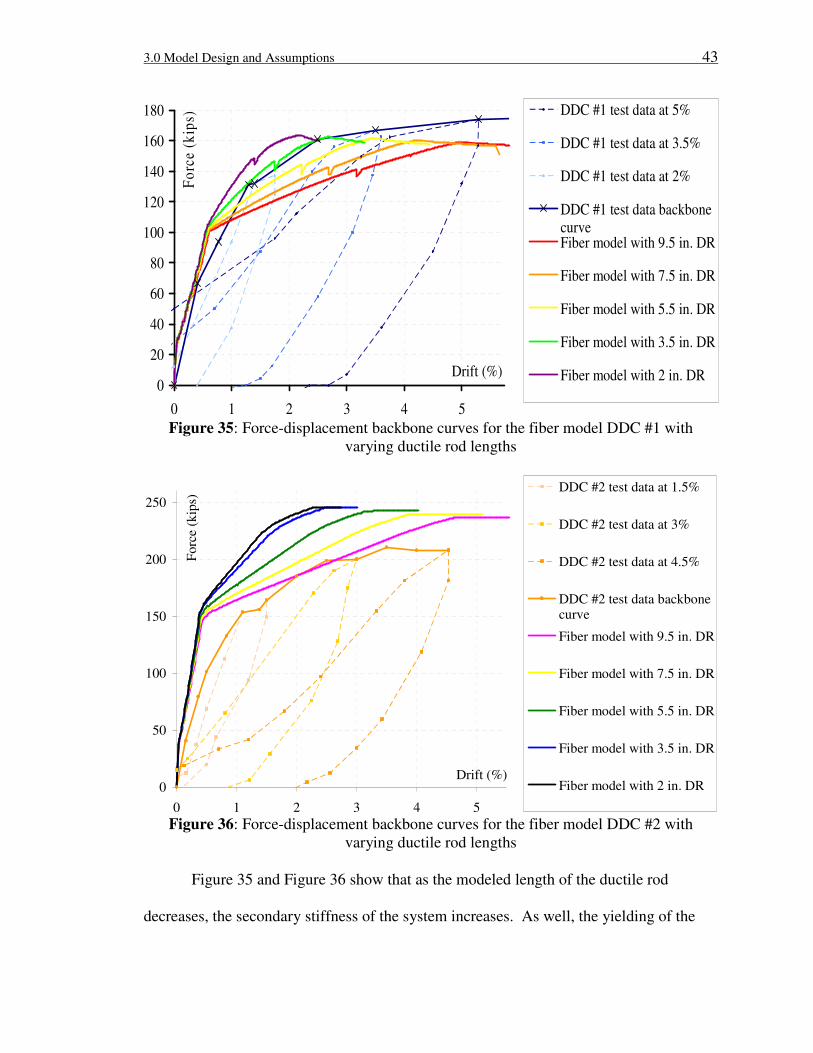
lengths of 2in., 3.5in., 5.5in., 7.5in., and 9.5in. The results from this study are shown in
Figure 35 and Figure 36.
Ductile Rod Segment
Modeled, the Shank Modeled as rigid,
the Head
Modeled as a
portion of the
beam with
Dywidag
Reinforcement,
the threaded
connection
3.0 Model Design and Assumptions 43
0
20
40
60
80
100
120
140
160
180
0 1 2 3 4 5
Drift (%)
Fo
rce
(kip
s) DDC #1 test data at 5%
DDC #1 test data at 3.5%
DDC #1 test data at 2%
DDC #1 test data backbonecurveFiber model with 9.5 in. DR
Fiber model with 7.5 in. DR
Fiber model with 5.5 in. DR
Fiber model with 3.5 in. DR
Fiber model with 2 in. DR
Figure 35: Force-displacement backbone curves for the fiber model DDC #1 with
varying ductile rod lengths
0
50
100
150
200
250
0 1 2 3 4 5
Drift (%)
Forc
e (k
ips)
DDC #2 test data at 1.5%
DDC #2 test data at 3%
DDC #2 test data at 4.5%
DDC #2 test data backbonecurve
Fiber model with 9.5 in. DR
Fiber model with 7.5 in. DR
Fiber model with 5.5 in. DR
Fiber model with 3.5 in. DR
Fiber model with 2 in. DR
Figure 36: Force-displacement backbone curves for the fiber model DDC #2 with
varying ductile rod lengths
Figure 35 and Figure 36 show that as the modeled length of the ductile rod
decreases, the secondary stiffness of the system increases. As well, the yielding of the

3.0 Model Design and Assumptions 44
Dywidag threaded bars shift to an earlier point in the pushover analysis from about 4.5%
to 2.2% drift. From Figure 35 it appears as if modeling the ductile rod as having a length
of 3.5in. to 5.5in. produces more approximate results. Since this is an uncalibrated
analysis, the shorter ductile rod lengths are not used in the creation of the blind prediction
fiber model results. What is hypothesized from these results is that perhaps the ductile
rod only becomes debonded from the concrete column for a portion of its length, and thus
has a smaller effective shank length than the geometric length. From this report, nothing
regarding the debond length of the ductile rod can be concluded; however, it is
recommended that this topic be explored further.
The last study associated with the ductile rod relates to the number of fiber
elements used to represent the ductile rod. In this study the ductile rod was modeled
using the following variations: (1) 9.5in. fiber element, (2) 4.75in. fiber elements, (3)
3.16in. fiber elements, and (4) 2.375in. fiber elements. This brief study was only
conducted on DDC #2. The results from this study are shown in Figure 37.

3.0 Model Design and Assumptions 45
0
50
100
150
200
250
0 1 2 3 4 5 6
Drift (%)
Forc
e (k
ips)
DDC #2 test data at1.5%
DDC #2 test data at3%
DDC #2 test data at4.5%
DDC #2 test databackbone curve
Fiber model with 1DR fiber element
Fiber model with 2DR fiber elements
Fiber model with 3DR fiber elements
Fiber model with 4DR fiber elements
Figure 37: Force-displacement backbone curves for the fiber model DDC #2 with
various numbers of fiber elements along the length of the ductile rod
As Figure 37 shows, when the number of ductile rod fiber elements increase over the DR
shank length, the ultimate curvature of the system decreases. For the blind prediction
fiber model of each system, only one fiber was used across the entire length of the ductile
rod shank, as there is no reason to substantiate doing otherwise.
Overall, the ductile rod plays perhaps the most significant role in the behavior of
the DDC system and more research into the number of fibers and/or the lengths of fibers
used in modeling the ductile rod is recommended.
3.3.5 Concrete Members
As mentioned earlier, the concrete members are modeled using several fiber
elements. All fiber elements have the same cross section along a member though they
3.0 Model Design and Assumptions 46
vary in length. This means the fiber models ignore the increase in transverse
reinforcement around the beam ends; this aspect of modeling was not within the scope of
modeling research for this project.
The concrete member properties for each specimen can be found in Appendix G
and Appendix H. Mander’s model, shown in Figure 18, was used to determine the
concrete material properties (Mander et al. 1988). The material approximations are
shown in Appendix D and Appendix E. The major discrepancy with using Mander’s
model is that it is not applicable to high strength concrete, which is found in some
members of the specimens. Since this discrepancy exists with the column and due to the
minimal contribution the column has on the flexibility of the subassemblage, this
approach was considered acceptable for this project.
3.4 Lumped Plasticity Model (ETABS)
The structural analysis software, ETABS, is considered by many to be a more
commonly used program than PERFORM-3D in the structural engineering industry.
However, ETABS analysis capabilities are more limited than PERFORM-3D. For
example, fiber elements are not incorporated into the ETABS interface. There are two
many reasons for exploring modeling capabilities of the DDC system in ETABS: (1) to
determine an acceptable method for modeling the DDC system in an office environment
where the design engineer only has access to ETABS, and (2) to determine an acceptable
method for modeling a DDC building in order to get global design forces. The ETABS
subassemblage configuration is shown in Figure 38. Similar to the fiber models, the
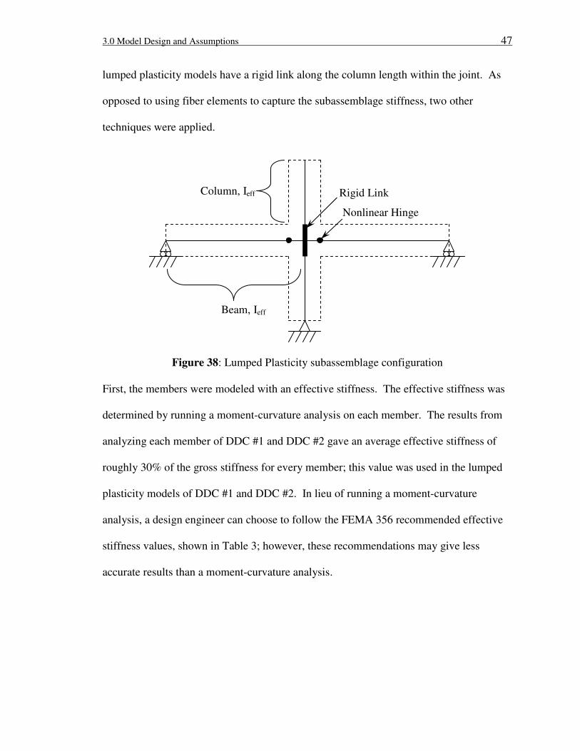
3.0 Model Design and Assumptions 47
lumped plasticity models have a rigid link along the column length within the joint. As
opposed to using fiber elements to capture the subassemblage stiffness, two other
techniques were applied.
Figure 38: Lumped Plasticity subassemblage configuration
First, the members were modeled with an effective stiffness. The effective stiffness was
determined by running a moment-curvature analysis on each member. The results from
analyzing each member of DDC #1 and DDC #2 gave an average effective stiffness of
roughly 30% of the gross stiffness for every member; this value was used in the lumped
plasticity models of DDC #1 and DDC #2. In lieu of running a moment-curvature
analysis, a design engineer can choose to follow the FEMA 356 recommended effective
stiffness values, shown in Table 3; however, these recommendations may give less
accurate results than a moment-curvature analysis.
Beam, Ieff
Column, Ieff Rigid Link
Nonlinear Hinge

3.0 Model Design and Assumptions 48
Table 3: Effective stiffness valued recommended, (Table 6-5) in (ASCE 2000)
Component Flexural
Rigidity
Shear
Rigidity
Axial
Rigidity
Beams-nonprestressed 0.5EcIg 0.4EcAw -
Beams-prestressed EcIg 0.4 EcAw -
Columns with compression due
to design gravity loads >
0.5Agf’c
0.7 EcIg 0.4 EcAw EcAg
Columns with compression due
to design gravity loads < 0.3
Agf’c or with tension
0.5 EcIg 0.4 EcAw EsAs
Note: It shall be permitted to take Ig for T-beams as twice the value of Ig
of the web along. Otherwise, Ig shall be based on the effective
width as defined in Section 6.4.1.3 [in reference (ASCE 2000)].
For columns with axial compression falling between the limits
provided, linear interpolation shall be permitted. Alternatively, the
more conservative effective stiffness shall be used.
The second technique applied to the lumped plasticity model, to help it
approximate the nonlinear behavior of a DDC system, is to assign a nonlinear hinge at the
beam-column interface, the hinges are shown in Figure 38.
3.4.1 Nonlinear Hinges
This technique of applying an effective stiffness to the members and a lumped
nonlinear hinge to mimic the plastic hinge region is similar to the approach often used for
monolithic concrete frames. However, what sets the DDC system apart is that it has tri-
linear hinge properties as opposed to bilinear hinge properties because there are two main
yield points within the system. The first yield point represents the yielding of the ductile
rod; the second yield point represents the yielding of the Dywidag bars. The yield
moment and yield rotation calculations are shown in Appendix A and Appendix B. The
curvatures for both the Dywidag and the ductile rod were calculated using, Equation 1.

3.0 Model Design and Assumptions 49
Equation 1: Concrete T-beam curvature, Eqn. (4.57d) in (Priestley 2007)
b
y
h
εφ
7.1=
The rotation of one beam was calculated using Equation 2.
Equation 2: Concrete beam rotation, Eqn. (4.52) in (Priestley 2007)
6
bL×=
φθ
The ultimate rotation of the nonlinear hinge was taken from test data. Both Equation 1
and Equation 2 were used to determine the rotation of the beam at yielding of the ductile
rod and yielding of the Dywidag bars. Figure 39 shows the difference in using Equation
2 to calculate the Dywidag rotation verses using the test data to determine the rotation of
the subassemblage at yielding of the Dywidag bars.
Figure 39 graphically demonstrates how Equation 2 does not account for the
plastic rotation in the ductile rod when calculating the rotation of the beam at yielding of
the Dywidag bars. The curve labeled “Blind model with Ieff and a Bilinear Curve
(partially based on test data)” uses the hysteretic test data to determine the rotation of the
subassemblage at yielding of the Dywidag bars; yielding of the ductile rod was
determined theoretically using Equation 2. Using the test results, to determine the yield
rotation of the specimen, produces a better approximation of system behavior, as can be
seen in Figure 39, but it is not a realistic route for the typical design engineer as it
involves experimental testing. One aspect of future research may involve creating an
equation to determine the rotation of the DDC system at yielding of the Dywidag bars
with simultaneous plastic hinging of the ductile rods and gap-opening.

3.0 Model Design and Assumptions 50
0
50
100
150
200
0 1 2 3 4
Drift (%)
Fo
rce
(kip
s)
DDC #2 TEST Data at 1.5%
DDC #2 TEST Data at 3%
DDC #2 TEST Data at 4.5%
DDC #2 TEST Data Backbone
Curve
Theoretical Tension Capacity of
the Concrete in the Beam
Theoretical Yield of the Ductile
Rods
Theoretical Yield of the Dywidag
Bars
Theoretical Initial Stiffness
Blind model with Ieff and a
Bilinear Hinge
Blind model with Ieff and a
Bilinear Curve (partially based on
test data)
Figure 39: Force-displacement backbone curve for the lumped plasticity model DDC #2
with varying the nonlinear hinge properties
The ETABS nonlinear hinge lumps two separate inelastic events, which occur
over various lengths, into one zero-length hinge location. In actuality, the ductile rod
yields slightly closer to the center of the joint than the yielding of the Dywidag bars.
Each yield event can be idealized as an elastic perfectly-plastic (EPP) curve. When
combining both EPP curves into one, the new curve is trilinear with zero stiffness after
the second yield event has occurred. A small study was conducted to determine if
lumping the yielding events makes a difference in the ETABS approximation. Figure 40
shows the results of moving the location of the nonlinear hinge from the center of the
joint to the beam-column interface.

3.0 Model Design and Assumptions 51
0
50
100
150
200
250
0 1 2 3 4
Drift (%)
Fo
rce
(kip
s)
DDC #2 TEST Data at 1.5%
DDC #2 TEST Data at 3%
DDC #2 TEST Data at 4.5%
DDC #2 TEST Data BackboneCurve
Theoretical Tension Capacity ofthe Concrete in the Beam
Theoretical Yield of the DuctileRods
Theoretical Yield of the DywidagBars
Theoretical Initial Stiffness
Model with hinge location 4.8 in.from the center of the joint
Model with hinge location 16 in.from the center of the joint
Model with hinge location 1in.from the center of the joint
Figure 40: Force-displacement backbone curve for the lumped plasticity model DDC #2
with varying the nonlinear hinge location
The results show that varying the location of the nonlinear hinge from the center of the
joint to the face of the joint does not have a substantial effect on the results. Therefore,
consolidating both nonlinear events into one hinge is an acceptable approach for
approximating the inelastic properties of the DDC joint.
4.0 Theoretical Predictions 52
4.0 THEORETICAL PREDICTIONS
Along with creating a fiber model and lumped plasticity model of each test
specimen, theoretical predictions of specimen behavior were calculated. The following
values were predicted:
• Initial stiffness, KINITIAL.
• Moment in the beam at the tensile rupture of the concrete beam, Mcr, and
the associated drift, γcr.
• Nominal moment capacity of the ductile rods, Mn., and the associated drift,
γy.
• Nominal moment capacity of the beam with Dywidag reinforcement bars,
Mn-DB.
All hand calculations mentioned above, for DDC #1 and DDC #2, can be found in
Appendix A and Appendix B respectively.
4.1 Initial Stiffness
The initial stiffness was determined by means of virtual work. First, standard
nomenclature for the subassemblage was established and is shown in Figure 41.
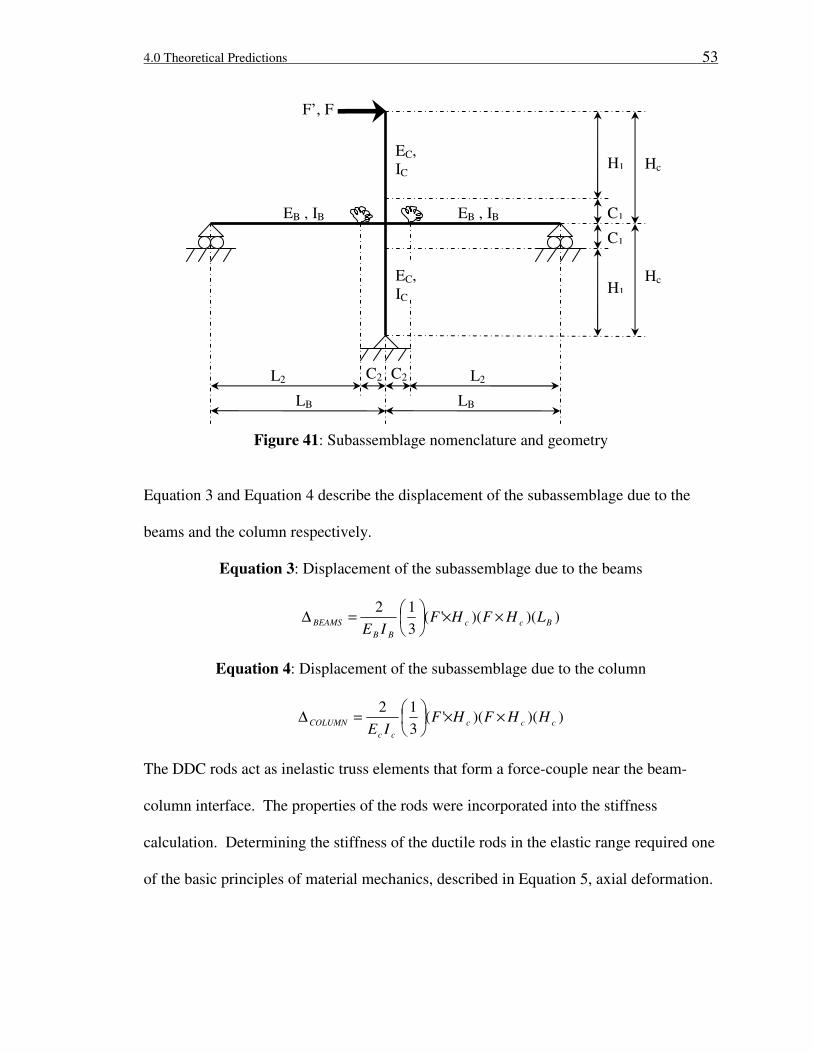
4.0 Theoretical Predictions 53
Figure 41: Subassemblage nomenclature and geometry
Equation 3 and Equation 4 describe the displacement of the subassemblage due to the
beams and the column respectively.
Equation 3: Displacement of the subassemblage due to the beams
))()('(3
12Bcc
BB
BEAMS LHFHFIE
××
=∆
Equation 4: Displacement of the subassemblage due to the column
))()('(3
12ccc
cc
COLUMN HHFHFIE
××
=∆
The DDC rods act as inelastic truss elements that form a force-couple near the beam-
column interface. The properties of the rods were incorporated into the stiffness
calculation. Determining the stiffness of the ductile rods in the elastic range required one
of the basic principles of material mechanics, described in Equation 5, axial deformation.
H1
C1
C1
Hc
Hc H1
L2 L2
LB LB
C2 C2
EB , IB
EB , IB
EC,
IC
EC,
IC
F’, F
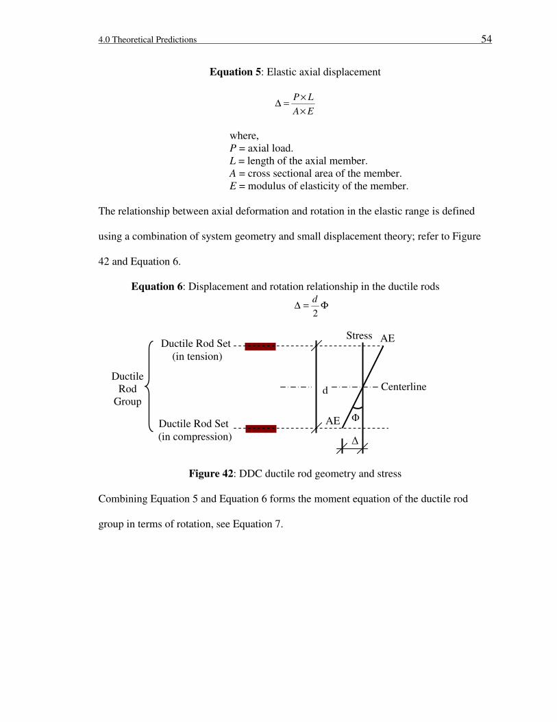
4.0 Theoretical Predictions 54
Equation 5: Elastic axial displacement
EA
LP
×
×=∆
where,
P = axial load.
L = length of the axial member.
A = cross sectional area of the member.
E = modulus of elasticity of the member.
The relationship between axial deformation and rotation in the elastic range is defined
using a combination of system geometry and small displacement theory; refer to Figure
42 and Equation 6.
Equation 6: Displacement and rotation relationship in the ductile rods
Φ=∆2
d
Figure 42: DDC ductile rod geometry and stress
Combining Equation 5 and Equation 6 forms the moment equation of the ductile rod
group in terms of rotation, see Equation 7.
d Centerline
AE
AE
Φ
∆
Stress Ductile Rod Set
(in tension)
Ductile Rod Set
(in compression)
Ductile
Rod
Group
4.0 Theoretical Predictions 55
Equation 7: Moment-rotation relationship in the ductile rods
Θ×
×
×
××=×= 2
2d
L
EANdFM
KSPRING
where,
A = cross-sectional area of one ductile rod.
N = number of ductile rods.
E = modulus of elasticity of the ductile rods.
L = length of the shank portion of the ductile rod.
d = distance between the compression and tension sets of
ductile rods.
The contribution of the ductile rods to the global stiffness is analogous to adding a
rotational spring at each beam-to-column interface as is shown in Figure 41. The portion
of the global displacement due to the spring is described in Equation 8, where KSPRING is
defined in Equation 7.
Equation 8: Ductile rod rotational spring stiffness
SPRING
SPRINGROTATIONALK
MM '_
×=∆
where,
M = actual moment seen by the spring.
M’ = virtual moment seen by the spring.
The summation of Equation 3, Equation 4, and Equation 8 result in the subassemblage
stiffness of a DDC system, refer to Equation 9.
Equation 9: DDC subassemblage stiffness
SPRINGROTATIONALCOLUMNBEAMSDDC _∆+∆+∆=∆
The spring permits much more drift within the system and thus greatly reduces the
subassemblage stiffness relative to an equivalent monolithic system. The shear
deformation within the system was not included as its effects on the system are
insignificant relative to the ductile rod’s rotational spring.

4.0 Theoretical Predictions 56
4.2 Moment at Tensile Rupture of the Concrete Beam
The moment in the beam that is associated with the tensile rupture of the concrete is
determined using Equation 10.
Equation 10: Cracking moment
t
gr
cry
IfM = , Eqn. (9-9) in (ACI 2005)
where,
fr = cf '5.7 , modulus of rupture of the concrete,
Eqn. (9-10) in (ACI 2005).
f’c = compressive strength of the concrete.
Ig = gross moment of inertia of the beam cross-section.
yt = distance from the centroidal axis of the gross cross
section, neglecting reinforcement, to the tension face.
The subassemblage displacement at the cracking moment was calculated for DDC #1
using Equation 11.
Equation 11: Cracking displacement for DDC #1
INITIAL
bcr
K
V=∆
where,
Vb = CLRb
crM
−l
, beam shear.
KINITIAL = initial stiffness of the subassemblage.
lb-CLR = clear distance from the pinned support of the beam
to the face of the joint.
DDC #1 test results provide the beam shear verses beam drift where as DDC #2 test
results provide the column shear verses the column drift. For this reason, there are two
different equations to describe the cracking displacement for DDC #1 and DDC #2. The

4.0 Theoretical Predictions 57
subassemblage displacement at the cracking moment for DDC #2 was calculated using
Equation 12.
Equation 12: Cracking displacement for DDC #2
INITIALcCLRb
bcrcr
K
M
××
×=∆
− ll
l
where,
lb = distance from the pinned support of the beam to the
center of the joint.
lb-CLR = clear distance from the pinned support of the beam
to the face of the joint.
lc = distance from the pinned support of the column to the
center of the joint.
KINITIAL = initial stiffness of the subassemblage.
4.3 Nominal Moment and Drift at Yielding of the Ductile Rods
The nominal moment capacity of the ductile rod was calculated using Equation 13.
Equation 13: Nominal moment capacity of the ductile rod connectors
)'( ddNTM yn −= , Eqn. (2.1.73) in (Englekirk 2003)
where,
N = number of ductile rods.
Ty = yFA × , the axial force which causes yielding of the
ductile rod.
A = cross-sectional area of one ductile rod.
Fy = yield stress of the ductile rod.
d = distance from the centroid of the tensile ductile rod
group to the extreme compression fibers.
d’ = distance from the centroid of the compressive ductile
rod group to the extreme compression fibers.
The subassemblage displacement was calculated using the yield rotation, refer to
Equation 14.
4.0 Theoretical Predictions 58
Equation 14: Yield rotation of a concrete frame subassemblage
b
by
yh
Lεθ
5.0= , Eqn. (4.58a) in (Priestley et al. 2007)
where,
εy = Fy/E, yield strain of the ductile rod.
Fy = yield stress of the ductile rod.
E = modulus of elasticity of the ductile rod.
Lb = full horizontal length of the subassemblage from one
beam end to the other.
hb= cross-sectional height of the beam.
The yield displacement was then calculated using Equation 15.
Equation 15: Displacement of the subassemblage
Hy ×=∆ θ
where,
θy = yield rotation.
H = total height of the subassemblage from the top of the
column to the column base.
*Note: DDC #1 test results provide the beam shear vs.
beam drift where as DDC #2 test results provide the
column shear vs. the column drift. For this reason, the
H value in Equation 15 may vary.
4.4 Nominal Moment at Yielding of the Dywidag Bars
The nominal moment capacity of the Dywidag bars within the beam was calculated using
Equation 16.
Equation 16: Nominal moment capacity of the beam with Dywidag bars
)2
( adFAM ysn −=
where,
As = total area of all tensile Dywidag bars.
Fy = yield stress of the ductile rod.
d = distance from the centroid of the tensile ductile rod
group to the extreme compression fibers.

4.0 Theoretical Predictions 59
a = bf
FA
c
ys
'85.0, depth of the concrete compression block
according to the Whitney stress block theory.
f’c = compressive strength of the concrete.
b = width of the beam cross-section.
All of the hand calculated results for both the DDC #1 and DDC #2 are shown in Table 4.
Table 4: Theoretical predictions for the DDC subassemblage test specimens
DDC
System
KINITIAL
(kips/in)
Mcr, Moment
at Tensile
Rupture of the
Concrete
Beam (kip*in)
γcr,
Tensile
Rupture
Drift (%)
Mn,
Nominal
Moment
(kip*in)
γy,
Yield
Drift
(%)
Mn-DB,
Nominal
Moment for
the Dywidag
Bars (kip*in)
#1 180.3 2642 0.0525% 12,772 0.794% 18,930
#2 156 1,101 0.142% 7,217 0.621% 9,710
The values shown in Table 4 were used to determine the forces in the beams and column
at each yielding event. It is the member forces, drifts, and initial stiffness which are
plotted in the results section for each specimen.

5.0 Modeling Results 60
5.0 MODELING RESULTS
A static push-over analysis was run for each test specimen using a fiber model
and a lumped plasticity model to determine the approximate backbone curve of the DDC
systems. In the analyses, a monotonic, steadily-increasing lateral load was applied to the
structure, until a predetermined limit state was reached. All modeling results were
plotted up until a 25%, or greater, reduction in ultimate strength occurred in the modeling
results.
5.1 Fiber Model Results (PERFORM-3D)
Figure 43 shows the results from the fiber model of DDC #1 as it compares to the
theoretical predictions, see Table 4, and test data.
0
20
40
60
80
100
120
140
160
180
0 1 2 3 4 5 6
Drift (%)
Fo
rce
(kip
s)
DDC #1 test data at 5%
DDC #1 test data at 3.5%
DDC #1 test data at 2%
DDC #1 test data backbonecurve
Theoretical tensile ruptureof the concrete in the beam
Theoretical yield of theductile rods
Theoretical yield of thedywidag bars
Theoretical initial stiffness
Blind prediction fibermodel
Calibrated fiber model
Figure 43: Force-displacement backbone curve for the DDC #1 fiber model relative to
test data and theoretical predictions
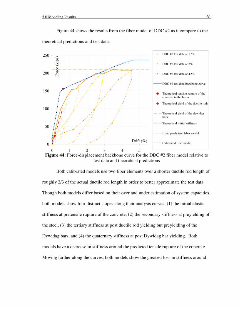
5.0 Modeling Results 61
Figure 44 shows the results from the fiber model of DDC #2 as it compare to the
theoretical predictions and test data.
0
50
100
150
200
250
0 1 2 3 4 5
Drift (%)
Fo
rce
(kip
s) DDC #2 test data at 1.5%
DDC #2 test data at 3%
DDC #2 test data at 4.5%
DDC #2 test data backbone curve
Theoretical tension rupture of the
concrete in the beam
Theoretical yield of the ductile rods
Theoretical yield of the dywidag
bars
Theoretical initial stiffness
Blind prediction fiber model
Calibrated fiber model
Figure 44: Force-displacement backbone curve for the DDC #2 fiber model relative to
test data and theoretical predictions
Both calibrated models use two fiber elements over a shorter ductile rod length of
roughly 2/3 of the actual ductile rod length in order to better approximate the test data.
Though both models differ based on their over and under estimation of system capacities,
both models show four distinct slopes along their analysis curves: (1) the initial elastic
stiffness at pretensile rupture of the concrete, (2) the secondary stiffness at preyielding of
the steel, (3) the tertiary stiffness at post ductile rod yielding but preyielding of the
Dywidag bars, and (4) the quaternary stiffness at post Dywidag bar yielding. Both
models have a decrease in stiffness around the predicted tensile rupture of the concrete.
Moving farther along the curves, both models show the greatest loss in stiffness around
5.0 Modeling Results 62
the predicted yield of the ductile rods. In addition, both model’s system strength
continues to increase to, at least, yielding of the Dywidag bars.
Some discrepancies in the models relative to their corresponding test specimens
can be seen. The DDC #2 blind fiber model reaches ultimate strength over 20 kips higher
than its calculated shear force capacity in the column, 211 kips, associated with yielding
of the Dywidag bars. On the other hand, DDC #1 under estimates the test specimen’s
ultimate shear force strength of 174 kips by 30 kips. As well, the DDC #1 blind fiber
model has an initial stiffness closer to the theoretical prediction; where as DDC #2 does
not.
5.2 Lumped Plasticity Model Results (ETABS)
Figure 45 shows the results from the lumped plasticity model of DDC #1 as it
compares to theoretical predictions and test data.

5.0 Modeling Results 63
0
20
40
60
80
100
120
140
160
180
0 1 2 3 4 5
Drift (%)
Fo
rce
(kip
s) DDC #1 test data at 5%
DDC #1test data at 3.5%
DDC #1 test data at 2%
DDC #1 test data Backbone
Theoretical tensile rupture of the
concrete in the beam
Theoretical yield of the ductile
rods
Theoretical yield of the dywidag
bars
Theoretical initial stiffness
Blind lumped plasticity model
using a bilinear hinge
Blind lumped plasticity model
using a trilinear hinge
Figure 45: Force-displacement backbone curve for the DDC #1 lumped plasticity model
to test data and theoretical predictions
Figure 46 shows the results from the lumped plasticity model of DDC #2 as it
compares to theoretical predictions and test data.

5.0 Modeling Results 64
0
50
100
150
200
0 1 2 3 4
Drift (%)
Fo
rce
(kip
s)
DDC #2 test data at 1.5%
DDC #2 test data at 3%
DDC #2 test data at 4.5%
DDC #2 test data backbone curve
Theoretical tensile rupture of theconcrete in the beam
Theoretical yield of the ductile
rods
Theoretical yield of the dywidag
bars
Theoretical initial stiffness
Blind lumped plasticity model
using a trilinear hinge
Blind lumped plasticity model
using a bilinear hinge
Figure 46: Force-displacement backbone curve for the DDC #2 lumped plasticity model
relative to test data and theoretical predictions
An all encompassing results graph of the trilinear lumped plasticity model approximation,
the fiber model approximation, the theoretical predictions, and the specimen test data are
shown for DDC #1 and DDC #2 in Figure 47 and Figure 48 respectively.
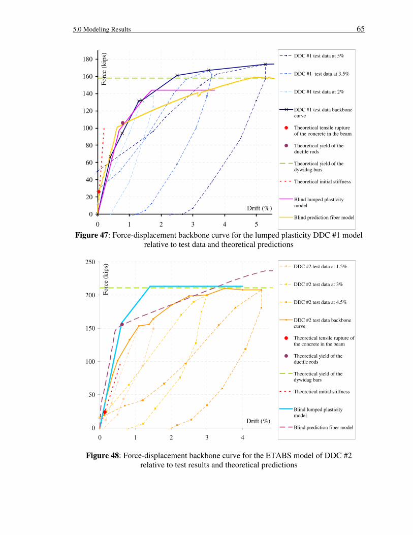
5.0 Modeling Results 65
0
20
40
60
80
100
120
140
160
180
0 1 2 3 4 5
Drift (%)
Forc
e (k
ips)
DDC #1 test data at 5%
DDC #1 test data at 3.5%
DDC #1 test data at 2%
DDC #1 test data backbone
curve
Theoretical tensile rupture
of the concrete in the beam
Theoretical yield of the
ductile rods
Theoretical yield of the
dywidag bars
Theoretical initial stiffness
Blind lumped plasticity
model
Blind prediction fiber model
Figure 47: Force-displacement backbone curve for the lumped plasticity DDC #1 model
relative to test data and theoretical predictions
0
50
100
150
200
250
0 1 2 3 4
Drift (%)
Fo
rce
(kip
s)
DDC #2 test data at 1.5%
DDC #2 test data at 3%
DDC #2 test data at 4.5%
DDC #2 test data backbone
curve
Theoretical tensile rupture of
the concrete in the beam
Theoretical yield of the
ductile rods
Theoretical yield of the
dywidag bars
Theoretical initial stiffness
Blind lumped plasticity
model
Blind prediction fiber model
Figure 48: Force-displacement backbone curve for the ETABS model of DDC #2
relative to test results and theoretical predictions

6.0 Summary, Conclusion, and Future Work 66
6.0 SUMMARY, CONCLUSION, AND FUTURE WORK
This report describes the results of research on the modeling of the Dywidag
ductile connector (DDC) system. The research areas covered by this report include the
analytical modeling and behavior of beam-column subassemblages under lateral load,
theoretical means for predicting the system behavior, the use of fiber elements to model
the system’s characterize and study the system behavior, and the development of a
lumped plasticity model which can be used in DDC building models to determine global
frame behavior. This section summarizes the results, presents the conclusions from the
previous sections, and mentions potential areas of future research.
6.1 Structural Behavior of Dywidag Ductile Connector Joints
6.1.1 Summary
A summary of the structural behavior of the Dywidag ductile connector system,
which was determined by (Chang, Hutchinson, and Englekirk 2007) is as follows:
1. Failure of the specimen occurs at the point of buckling of the Dywidag bars
within the beam after cracking and spalling around the beam toe and heel has
occurred.
2. The main modes of deformation in the DDC joint are gap-opening and shear
cracking.

6.0 Summary, Conclusion, and Future Work 67
3. There are two yielding points within the system. This first being the ductile rods,
located within the joint, and the second being the Dywidag bars, which act as the
longitudinal reinforcement within the beam.
4. The specimen may experience pull-out of the DDC at large drifts. This is
mitigated by increasing the transverse volumetric ratio of reinforcement within
the joint.
5. The specimens tested have shown no signs of strength degradation up to 4.5%
drift.
6.1.2 Conclusion
The main conclusions regarding the structural system behavior of DDC joints are:
1. Gap-opening under flexure is the desired mode of deformation and allows for the
strain in the toe region of the beam to be controlled.
2. The ductile rod moves the location of the yielding from the beam to within the
joint where it has nondeteriorating lateral supported (Englekirk 2003).
3. Shear forces are transferred by friction from steel to steel across the beam-column
interface. The load path travels from the face of the ductile rod to the beam
transfer block via a set of shim plates. The pretensioning of the bolt activated this
frictional load transfer (Englekirk 2003).

6.0 Summary, Conclusion, and Future Work 68
6.2 Fiber Model (PERFORM-3D)
6.2.1 Summary
The fiber model, described in Section 3.3 was used to model the Dywidag ductile
connector specimens. PERFORM-3D fiber beam-column elements were used to
represent both the gap-opening under flexure, and the nonlinear inelastic behavior of the
concrete in the members and joint. The beam-column joint is not modeled as fully rigid
to account for some of the shear deformation that occurs in the joint. Only a fiber
element of a length equivalent to that of the ductile rod shank is modeled with ductile rod
fibers; other fibers within this fiber element have the confined concrete column
constitutive properties. The inelastic behavior in the test specimen is concentrated at the
end of the beam near the gap opening at the beam-column interface; this plastic hinge
length is unknown. Shorter fiber lengths were required along the member where high
demands existed. The portion of the column within the joint was modeled as fully rigid,
with minimal change to the system behavior. The DDC #1 and DDC #2 fiber models
seemed to under estimate the yield drift of the system. As well, the fiber models are not
consistent in approximating the shear force in the members at ultimate force demand.
The fiber model provides a reasonable estimate of the force-displacement backbone curve
for the DDC system, but more time and research could produce better results.
6.2.2 Conclusion
Studies of the fiber model and its modeling parameters lead to the following conclusions:

6.0 Summary, Conclusion, and Future Work 69
1. The confined concrete fibers, with the maximum strain, should be modeled with a
height of approximately 2% of the beam height (El-Sheikh et al.1997).
2. The unconfined concrete fibers may be more coarsely distributed over the cross
section as shown in Figure 26 (El-Sheikh et al. 1997).
3. The number of fiber segments used to model the beams and column should
decrease in length as the member gets closer to the joint, as demand values and
curvature variation increases. The recommended fiber segment configuration is
shown in Figure 31, but a more in-depth study is recommended.
4. The joint rigidity should be modeled according to the recommendations by
(Elwood et al. 2007). Rather than use a capacity ratio of column-to-beam, as
Elwood recommends for monolithic frames, the capacity ratio of column to
ductile-rod set should be used; the ductile rod set is the fuse which limits the
applied moment the beam can crank into the joint. Thus far, this approach has led
to a rigid column and flexible beam arrangement within the joint.
5. The ductile rods are modeled as fibers within a fiber element of which is the
length of the ductile rod shank. Concrete properties within this fiber segment are
based on the confined concrete column region. The head of the ductile rod is
modeled as rigid, where as the rest of the joint and ductile rod is modeled using
fiber elements with the properties of the beam.
6. Dividing the ductile rod fiber element into multiple fiber segments reduces the
ultimate rotation of the system without altering the stiffness characteristics.
7. Shortening the ductile rod fiber segment decreases the ultimate rotation while also
increasing the post-yield stiffness of the system.
6.0 Summary, Conclusion, and Future Work 70
6.3 Lumped Plasticity Model (ETABS)
6.3.1 Summary
The lumped plasticity (LP) model, described in Section 3.4 is used to model the
Dywidag ductile connector system for global structural system analysis. Elastic concrete
members with effective stiffness values are used to represent the nonlinear inelastic
behavior of the concrete members. The nonlinear hinge, located at the beam-column
interface, is used to represent yielding of the ductile rod and yielding of the Dywidag
bars. Similar to the fiber model, the lumped plasticity model’s beam-column joint is not
modeled as fully rigid as to account for some of the shear deformation that occurs in the
joint. The nonlinear hinge properties are assigned according to nominal moment
capacities of the ductile rods and Dywidag bars. The rotations are determined via
monolithic frame curvature and rotation calculations. The lumped plasticity model can be
used to perform a nonlinear pushover analysis. The DDC #1 and DDC #2 lumped
plasticity models seemed to under estimate the yield drift of the system. Similar to the
fiber model, the lumped plasticity model does not show consistency in approximating the
shear force in the members at ultimate force demands. Similar to the their corresponding
fiber models, the LP simplified model of DDC #1 under estimated the ultimate strength
of the system and the LP model of DDC #2 over estimated the ultimate strength of the
system. The LP model provides an acceptable estimate of the force-displacement
backbone curve for the DDC system.

6.0 Summary, Conclusion, and Future Work 71
6.3.2 Conclusion
Studies of the lumped plasticity (LP) model and its modeling parameters have led to the
following conclusions:
1. The moment-rotation behavior of the joint is essentially an inelastic trilinear curve
with discontinuities at the point of ductile rod yielding and Dywidag bar yielding.
2. The nonlinear hinge can be defined using yield rotation calculations for
conventional monolithic concrete moment frames; though, this is where the
majority of the model inaccuracies occur. The difficulty lies in predicting the
yield rotation, since Equation 2 does not account for gap-opening and plastic
rotation in the system. These inadequacies led to a large underestimation of yield
rotation.
3. The same procedures were used for the fiber model and the LP model in
determining the joint rigidity.
4. The LP models under estimate the ductile rod yield rotation for both DDC #1 and
DDC #2. The LP model underestimates the strength of DDC #1 while over
estimating the strength of DDC #2.

6.0 Summary, Conclusion, and Future Work 72
6.4 Future Work
6.4.1 Dywidag Ductile Connector System
Throughout this report the need for more research in various aspects of the DDC
system became apparent. The following is a list of suggested future research topics to
explore:
1. Determine the debond length of the ductile rod in a test specimen when cyclically
loaded within the system.
2. A more in-depth study on defining the various fiber lengths across a member.
3. Define the plastic hinge length in the DDC system.
4. Create a simplified methodology to characterize the rotation of the system due to
gap-opening.
5. Create an equation to approximate the rotation of the system at yielding of the
Dywidag bars that would incorporate rotation due to gap-opening and plastic
hinging of the ductile rods.
6. Determine why the simplified model underestimated the strength of DDC #1
while it over estimated the strength of DDC #2.
7. Study the effects of the reinforcement ratio on the over or under estimation of the
fiber model.
6.4.2 Super Hybrid System
The super hybrid system is a relatively new type of lateral system, which has
several benefits. In order to incorporate this system into practice, more needs to be

6.0 Summary, Conclusion, and Future Work 73
understood about the system behavior. For this reason, it is highly recommended that
future research involve the analytical modeling of the super hybrid system using the fiber
and the lumped plasticity modeling approaches previously mentioned in this report.
A fiber model of the super hybrid system, shown in Figure 49, was modeled.
Figure 49: Schematic elevation of the Pankow #2 super hybrid test specimen (Chang
Hutchinson, and Englekirk 2007)
More details of the specimen are provided in Appendix I. An approximation of
the super hybrid hysteretic test data is shown in Figure 50. The actual test results are
shown in Appendix I.

6.0 Summary, Conclusion, and Future Work 74
-200
-150
-100
-50
0
50
100
150
200
-6 -4 -2 0 2 4 6
Drift (%)
Fo
rce
(kip
s)
Super Hybrid at 5%
Super Hybrid at 3.5%
Super Hybrid at 2%
Figure 50: Super Hybrid force-displacement hysteretic loop approximations
Only a fiber model was created of this super hybrid specimen. The system used the
same modeling techniques as the DDC systems.
The major differences in the super hybrid specimen versus the DDC specimen are
the beam cross sections, the number of ductile rods, and the presence of post tensioned
(PT) strands. However, only major modeling difference between the super hybrid
specimen and the DDC specimens is the presence of the PT.
The PT was modeled as a truss element connected to the specimen at both beam
ends. A compressive loading strain was applied to the truss in order to mimic the
compressive PT forces. The truss element was assigned the idealized constitutive
properties of the PT steel (grade 270), refer to Figure 51.

6.0 Summary, Conclusion, and Future Work 75
0
50
100
150
200
250
300
0 0.01 0.02 0.03 0.04 0.05
Strain (in/in)
Str
ess
(k
si)
(εpl, fpl)
(εpu, fpu)
αEp
Ep
Figure 51: Constitutive relationship of post-tensioned steel strand
Table 5 provides the values associated with the variables in Figure 51.
Table 5: PT Steel Properties
PT Properties for grade 270 strand
Ep = 28,000 ksi
εpu = 0.05
fpu = 270 ksi
fpl = 0.8fpu
The strain load applied to the truss bar was determined using Equation 17 since the initial
PT force was within the elastic range of the PT strands.
Equation 17: Elastic axial strain
EA
P
×=ε
where,
P = axial load, 450 kips.
A = cross sectional area of the member, 3.11 in2.
E = modulus of elasticity of the member.
Therefore, the loading strain applied to the bar was -0.00517 in./in. This technique for
modeling PT using a truss element and strain loading is similar to the method used in the

6.0 Summary, Conclusion, and Future Work 76
report by (El Sheikh et al. 1997). The constitutive properties and approximations for the
super hybrid specimen can be found in Appendix I and Appendix F respectively. The
theoretical results, shown in Figure 52, are calculated in Appendix C. The pushover
analysis results of the super hybrid fiber model are shown in Figure 52.
0
50
100
150
200
0 1 2 3 4 5
Drift (%)
Fo
rce
(kip
s) Super hybrid test data at 5%
Super hybrid test data at 3.5%
Super hybrid test data at 2%
Super hybrid test data
backbone curve
Blind prediction fiber model
Fiber model without strength
degradation
Fiber model without strengthdegradation and without the
PT forceTheoretical rupture of the
tensile concrete in the beam
Theoretical initial stiffness
Theoretical yield of
thenductile rods
Theoretical yield of theDywidag bars
Figure 52: Force-displacement backbone curve for the fiber model of the super hybrid
relative to the test results and theoretical predictions
The theoretical stiffness was calculated for the super hybrid as if it were a monolithic
system. This theoretical stiffness matches the super hybrid fiber model results but not the
test data. As well, the force associated with theoretical yielding of the Dywidag bars is
1.3 times the force associated with the strength capacity of the test specimen.
The blind prediction fiber model of the super hybrid failed at 1% drift as the fiber
model experiences a decrease in system strength of over 25%. When the super hybrid

6.0 Summary, Conclusion, and Future Work 77
fiber model was run such that no fibers experienced strength degradation, the fiber model
behavior did not reach failure until after a drift of 5%, refer to Figure 52. When the super
hybrid model was run once more with no strength degradation and no PT force applied,
the results were closest to the test data’s backbone curve.
References 78
REFERENCES
Cited References
ACI Committee 318. 2005. Building Code Requirements for Structural Concrete (ACI
318-05) and Commentary (ACI 318R-05). Farmington Hills, MI: ACI.
ASCE. Prestandard and Commentary for the Seismic Rehabilitation of Buildings. (FEMA
356) and Commentary (FEMA 356-C). Washington, D.C., 2000.
ASCE. Seismic Rehabilitation of Existing Buildings (ASCE/SEI 41-06). Structural
Engineering Institute. American Society of Civil Engineers. Reston, VA, 2007.
Celik, O.; and Sritharan, S., An Evaluation of Seismic Design Guidelines Proposed for
Precast Concrete Hybrid Frame Systems. ISU-ERI-Ames Report ERI-04425,
Iowa State University, Ames, IA, January, 2004.
Chadwell, C., “XTRACT User Guidelines,” Version 3.0.8. TRC. www.imbsen.com.
2007.
Chang, B.; Hutchinson, T.; and Englekirk, R., “Charles Pankow Foundation Sponsored
Beam/Column Subassembly Testing Program”. Interim Report. October 30,
2007.
Chang, B.; Hutchinson, T.; and Englekirk, R., “Charles Pankow Foundation Sponsored
Beam/Column Subassembly Testing Program”. Interim Report #2. December 19,
2007.
Chen, Richard. Interview with author, December 17, 2007.
Cheok, G.; and Stone, W., "Performance of 1/3-Scale Model Precast Concrete Beam-
Column Connections Subjected to Cyclic Inelastic Loads - Report No. 3," NISTIR
5246, National Institute of Standards and Technology, Gaithersburg, MD, August,
1993.
Elwood, K.; Matamoros, A,; Wallace, J.; Lehman, D.; et al, “Update to ASCE/SEI 41
Concrete Provisions,” 2007Annual Meeting of the Los Angeles Tall Buildings
Structural Design Council, Los Angeles, California, May 2007.
El-Sheikh, M,; Pessiki, S.; Sause, R.; Lu, L.-W.; and Kurama, Y., “Seismic Analysis,
Behavior, and Design of Unbonded Post-Tensioned Precast Concrete
Frame,”Earthquake Engineering Research Report, Report No. EQ-97-02, Lehigh
University, Bethlehem, Nov. 1997.
References 79
Englekirk, R., “The Development and Testing of a Ductile Connector for Assembling
Precast Concrete Beams and Columns,” PCI Journal, Vol. 40, No. 2, March-April
1995, pp. 36-51.
Englekirk, R., Seismic Design of Reinforced and Precast Concrete Buildings. John Wiley
and Sons, Inc. Hoboken, New Jersey, 2003.
Englekirk, R., “Design and Behavior of the Super Hybrid System,” 2007
Precast/Prestressed Concrete Institute 53rd Annual Convention, Phoenix, Arizona,
October 2007.
Hawkins, N.; and Ghosh, S., “Requirements for the use of PRESSS Moment Resisting
Frames,” PCI Journal, Vol. 49, No. 2, Mar.-April 2004, pp. 98-103.
Hawileh, R.; Tabatabai, H.; Rahman, A.; and Amro, A., “Non-dimensional Design
Procedures for Precast, Prestressed Concrete Hybrid Frames,” PCI Journal, Vol.
51, No. 5, Sept.-Oct. 2006, pp. 110-130.
MacRae, G. and Priestley, M.J.N., “Precast Post-Tensioned Ungrouted Concrete Beam-
Column Subassemblage Tests,” Report No. SSRP 94/10, Department of Applied
Mechanics and Engineering Science, University of California San Diego, CA
March 1994.
Mander, J.; Priestley, M.; and Park, R, “Theorical Stress-Strain Model for Confined
Concrete,” Journal of Structural Engineering, American Society of Civil
Engineers, Vol. 114, No. 8, Aug 1988a, pp. 1804-1826.
Nakaki, S.; Englekirk, R.; and Plaehn, J., “Ductile Connectors for a Precast Concrete
Frame,” PCI Journal, Vol. 39, No. 5, Sept.-Oct. 1994, pp. 46-59.
Priestley, M.J.N., “Overview of PRESSS Research Program,” PCI Journal, Vol. 36, No.
4, July-Aug. 1991, pp.50-57.
Priestley, M.J.N.; Tao, J.R., “Seismic Response of Precast Prestressed Concrete Frames
with Partially Debonded Tendons,” PCI Journal, Vol.38, No. 1, Jan.-Feb. 1993,
pp. 58-66.
Priestley, M.J.N.; Calvi, G.M.; Kowalsky, M.J., Displacement-Based Seismic Design of
Structures. Istituto Universitario di Studi Superiori di Pavia (IUSS) Press. Pavia,
Italy, 2007.
SEQAD Consulting Engineers, “Precast Ductile Connector Beam-Column Test,” Report
No. 93-02, Solana Beach, CA March 1993.

References 80
Stanton, J.; Day, S.; and MacRae, G., "Testing of Hybrid Frame Interior, Exterior, and
Corner Beam-Column Specimens,” Report No.98195-2700, Department of Civil
and Environmental Engineering, University of Washington, WA 1999.
Additional References
Adachi, Masato; and Nishiyama, Minehiro, “Hysteretic Behavior of Precast Post-
Tensioned Beam-Column Joint Assemblage”. Transactions of the Japan Concrete
Institute, Vol. 19, 1997, pp.211-218.
Cheok, G.; and Lew, H.S., "Performance of 1/3-Scale Model Precast Concrete Beam-
Column Connections Subjected to Cyclic Inelastic Loads," NISTIR 4433, National
Institute of Standards and Technology, Gaithersburg, MD, Oct., 1990.
Cheok, G.; and Lew, H. S., "Performance of 1/3-Scale Model Precast Concrete Beam-
Column Connections Subjected to Cyclic Inelastic Loads - Report No. 2," NISTIR
4589, National Institute of Standards and Technology, Gaithersburg, MD, June,
1991.
Cheok, G.; and Stone, W., "Performance of 1/3-Scale Model Precast Concrete Beam-
Column Connections Subjected to Cyclic Inelastic Loads - Report No. 4," NISTIR
94045, National Institute of Standards and Technology, Gaithersburg, MD, June,
1994.
Cheok, G.; Stone, W.; and Nakaki, S., “Simplified Design Procedure for Hybrid Precast
Concrete Connections,” NISTIR 5765, National Institute of Standards and
Technology, Gaithersburg, MD, February, 1996.
Englekirk, R., “An Innovative Design Solution for Precast Prestressed Concrete
Buildings in High Seismic Zones,” PCI Journal, Vol. 41, No. 4, July-Aug. 1996,
pp. 44-53.
Englekirk, R., “Design-Construction of The Paramount – A 39-Story Precast Prestressed
Concrete Apartment Building,” PCI Journal, Vol. 47, No. 5, July-Aug. 2002, pp.
56-72.
“Northridge Earthquake January 17, 1994 Preliminary Reconnaissance Report,”
Earthquake Engineering Research Institute, pp. 40.
Iverson, J.K., and Hawkins, N.M., “Performance of Precast/Prestressed Concrete
Building Structures During Northridge Earthquake,” PCI Journal, Vol. 39, No. 2,
Mar.-Apr. 1994, pp. 38-55.
References 81
Park, R., “A Perspective on the Seismic Design of Precast Concrete Structures in New
Zealand,” PCI Journal, May-June 1995, pp. 40-60.
PERFORM 3-D Nonlinear Analysis and Performance Assessment for 3D Structures User
Guide, Version 4, Computers and Structures Inc., Aug. 2006.
Popovics, S., “A Numerical Approach to Complete Stress-Strain Curves for Concrete,”
Cement and Concrete Research, Vol. 3, No. 5, Sept. 1973, pp. 583-599.
Raynor, D.; Lehman, D.; and Stanton, J., “Bond-Slip of Reinforcing Bars Grouted in
Ducted,” ACI Journal, Vol. No. , Sept-Oct. 2002, pp. 568-576.

Appendix 82
APPENDICES
Appendix A
DDC #1 Initial Stiffness

Appendix 83
MATLAB OUTPUT Kspring_system = 14.1 (kips/in.), spring stiffness
Dmnv = 0.483 (in.), Displacement of the monolithic system using
Ieff = 0.3Ig for both members
Kmnv = 207 (kips/in.), Stiffness of the monolithic system using
Ieff = 0.3Ig for both members
DmnvDDC = 0.555 (in.), Displacement of the DDC system
KmnvDDC = 180.3 (kips/in.), Stiffness of the DDC system
DDC #1 Column Shear at the Tension Rupture of the Concrete

Appendix 84
DDC #1 Column Shear at Yielding of the Ductile Rods
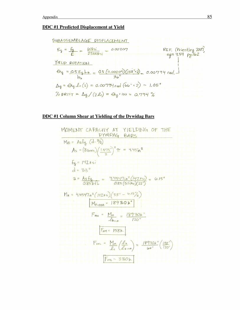
Appendix 85
DDC #1 Predicted Displacement at Yield
DDC #1 Column Shear at Yielding of the Dywidag Bars

Appendix 86
DDC #1 Determining Rigid Link Length
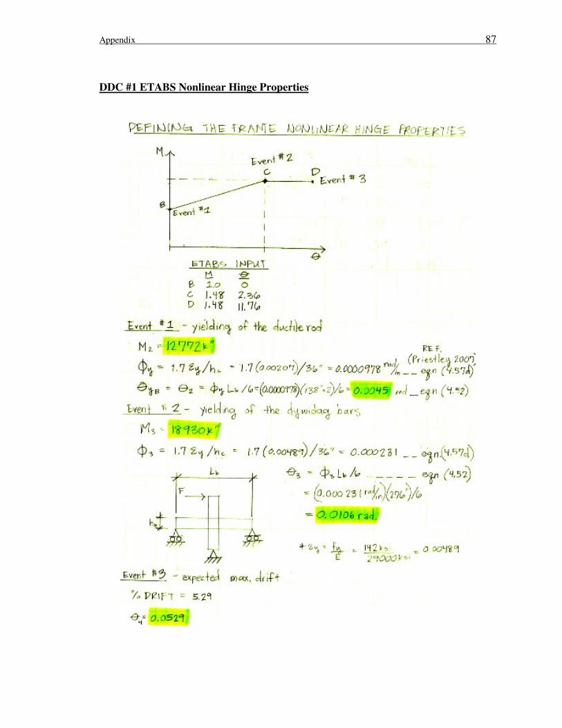
Appendix 87
DDC #1 ETABS Nonlinear Hinge Properties

Appendix 88
Appendix B
DDC #2 Initial Stiffness
OUTPUT
Kspring_system = 17.0 (kips/in.), spring stiffness
Dmnv = 0.581 (in.), Displacement of the monolithic system using
Ieff = 0.3Ig for both members
Kmnv =172 (kips/in.), Stiffness of the monolithic system using
Ieff = 0.3Ig for both members
DmnvDDC = 0.640 (in.), Displacement of the DDC system
KmnvDDC = 156 (kips/in.), Stiffness of the DDC system
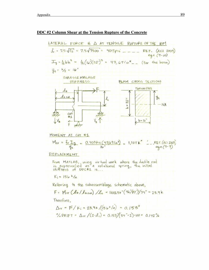
Appendix 89
DDC #2 Column Shear at the Tension Rupture of the Concrete
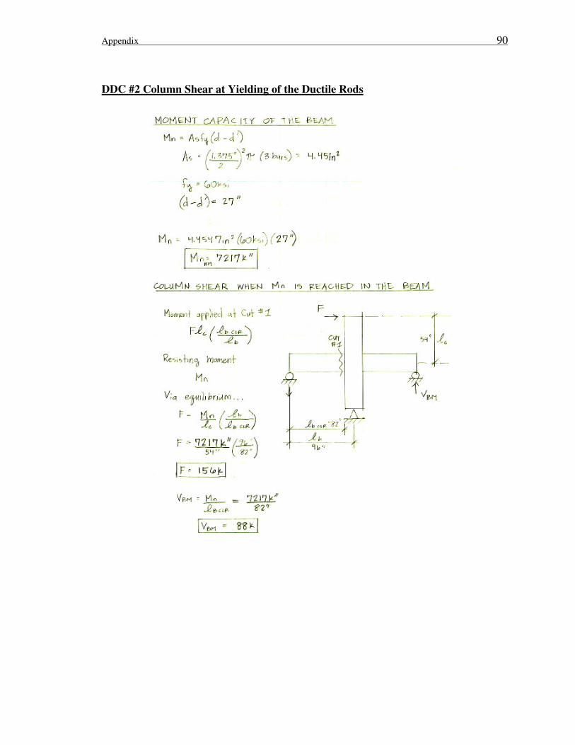
Appendix 90
DDC #2 Column Shear at Yielding of the Ductile Rods

Appendix 91
DDC #2 Predicted Displacement at Yield
DDC #2 Column Shear at Yielding of the Dywidag Bars

Appendix 92
DDC #2 Determining Rigid Link Length

Appendix 93
DDC #2 ETABS Nonlinear Hinge Properties

Appendix 94
Appendix C
Super Hybrid Initial Stiffness
OUTPUT Kspring_system = 15.2 (kips/in.), spring stiffness
Dmnv = 0.458 (in.), Displacement of the monolithic system using
Ieff = 0.3Ig for both members
Kmnv = 219 (kips/in.), Stiffness of the monolithic system using
Ieff = 0.3Ig for both members
DmnvDDC = 0.524 (in.), Displacement of the DDC system
KmnvDDC = 191 (kips/in.), Stiffness of the DDC system
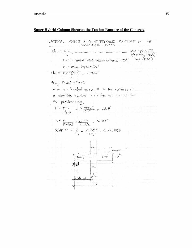
Appendix 95
Super Hybrid Column Shear at the Tension Rupture of the Concrete
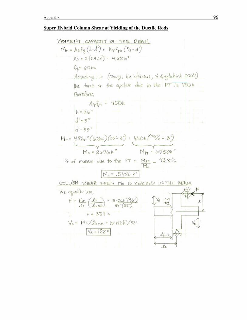
Appendix 96
Super Hybrid Column Shear at Yielding of the Ductile Rods
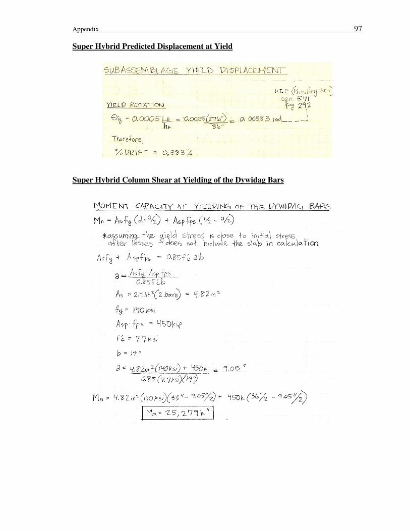
Appendix 97
Super Hybrid Predicted Displacement at Yield
Super Hybrid Column Shear at Yielding of the Dywidag Bars
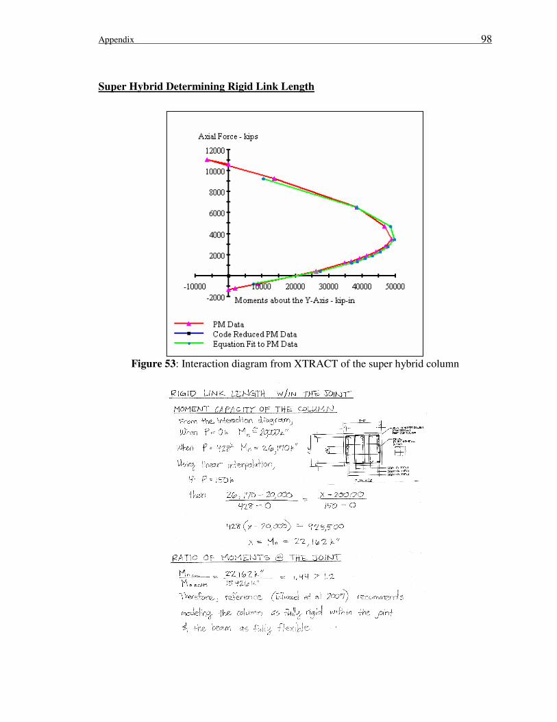
Appendix 98
Super Hybrid Determining Rigid Link Length
Figure 53: Interaction diagram from XTRACT of the super hybrid column

Appendix 99
Appendix D
DDC #1 XTRACT Input Properties
Table 6: DDC #1 XTRACT input beam properties
Details DDC #1 (Pankow #4)
Confined Concrete Strength Calculation
Type of transverse reinforcing Rectangular hoops
Transverse reinforcing bar yield stress (ksi) 60
X transverse reinforcing steel ratio 1 0.0034
Y transverse reinforcing steel ratio 1 0.00139
Average distance between tied longitudinal bars (in) 2 17.3
Number of longitudinal bars around core 6
Confined core area (in2) 627
(varying) Tie spacing along member (in)
8” o.c.
28-Day compressive concrete strength (ksi) 5.5
Confined concrete strength (ksi) 3 6.049
Crushing Strain Calculation
Transverse reinforcing steel strain at fracture (in/in) 0.12
Transverse (volumetric) reinforcing steel ratio 4 0.0048
Crushing strain, εcu 3, 6
0.012
Mander’s Confined Concrete Curve Calculation
Tension Strength (ksi) -0.556
Yield Strain, εcy 5 0.002029
Concrete Elastic Modulus (ksi) 7 4246
Unconfined Concrete Curve Calculation
Yield Strain 5 0.0014 (default)
Crushing Strain 6 0.004 (default)
Spalling Strain 8 0.006 (default)
Post Crushing Strength 9 0 (default)
Failure Strain 10
1
1. X Transverse Steel Reinforcing Ratio (ρx):
The transverse reinforcing ratio in one of the two principal directions. This
ratio can be calculated by taking a ‘cut’ across the section in the ‘X direction’. The
ratio may be calculated as follows:
rx = (the total area of all transverse steel the cut passed through within a depth
of one transverse reinforcement spacing) / [(the section dimension in the X
direction)*(transverse reinforcement spacing)].
2. Average Distance Between Tied Longitudinal Bars:

Appendix 100
Previous Table (cont’.): DDC #1 XTRACT Input Beam Properties
This is the (perimeter of the core section) / (number of perimeter longitudinal
bars).
3. Calculated by XTRACT using Mander’s model
4. Transverse (volumetric) reinforcing steel ratio:
ρ = ρx + ρy
5. Yield Strain (εcy)
Concrete compression yield strain is typically never used in design; however,
because the limit state of the ‘Yield Moment’ is controlled by the first yield of any
material, XTRACT requires this parameter. A reasonable value (the default) is 70% of
the strain at peak stress (f`cc)- for this project, XTRACT uses the default value.
Because the strain at peak stress for unconfined concrete is typically .002, the default
for this parameter becomes 0.0014.
6. Crushing strain, εcu
Crushing strain is associated with the concrete strain that occurs at the same
time as hoop or transverse reinforcing fracture. If the section satisfies ACI 318-95
Chapter 21 design requirements, crushing strain may be assumed at .015. If a more
detailed calculation is required, this may be used. To calculate the confined crushing
strain, the user may use the Crushing Strain Calculator or may enter the values directly.
For unconfined crushing strain, the default is assumed to be 0.004. This correlates well
for bending failures with some inherent conservatism. The ACI value and lower bound
is typically taken as .003.
7. Concrete Elastic Modulus:
E = 57000√f’c , where f’c is in units of psi
8. Spalling Strain (εsp):
Strain at completion of material spalling. Default is 0.006.
9. Post Crushing Strength (fcp):
Strength of unconfined concrete after spalling. The default value of 0 is used
in this project.
10. Failure Strain:
“Because in analyzing a confined concrete section (section with significant
transverse reinforcement) for its nonlinear behavior, the confined core will typically
have a compression strain capacity that far exceeds that of the cover (or unconfined)
concrete this value can be different than the crushing strain. For unconfined concrete on
a confined concrete section, the strain to end computation (the ultimate limit state) will
be different than the crushing strain.
This is the input value that terminates the Moment Curvature analysis: i.e. If
the user was performing a moment curvature analysis of an unconfined section, this
value should be set to .004. If the section is confined and cover spalling is not the
desired quantity to terminate the analysis (the ultimate limit state), then this value
should be set to 1.0 (or a high number so as to not control failure). Default is 0.0 so as
to remind the user of the importance of this parameter.”(Chadwell 2007). For this
project the failure strain is set to 1.0. 11
Information provided by reference (SEQAD Consulting Engineers 1993) 12
Calculated using the following equation: f’t = 7.5√f’c (ACI 2005): equation (9-10). 13
In the case of these variables, information was not provided and engineering judgment
in conjunction with other references was used to determine these values 14
Values were used here from the Dywidag material tests conducted in conjunction with
the 2007 Pankow series testing conducted at UCSD, research done separately from the
SEQAD research * For all other footnotes see DDC #1 Appendices

Appendix 101
Table 7: DDC #1 XTRACT input column properties
Details DDC #1 (Pankow #4)
Confined Concrete Strength Calculation
Type of transverse reinforcing Rectangular hoops
Transverse reinforcing bar yield stress (ksi) 75
X transverse reinforcing steel ratio 1 0.00646
Y transverse reinforcing steel ratio 1 0.00517
Average distance between tied longitudinal bars (in) 2 6.66
Number of longitudinal bars around core 18
Confined core area (in2) 891
(varying) Tie spacing along member (in)
6” o.c.
28-Day compressive concrete strength (ksi) 9.58
Confined concrete strength (ksi) 3 11.7
Crushing Strain Calculation
Transverse reinforcing steel strain at fracture (in/in) 0.12
Transverse (volumetric) reinforcing steel ratio 4 0.01163
Crushing strain, εcu 3, 6
0.01652
Mander’s Confined Concrete Curve Calculation
Tension Strength (ksi) 12
-0.958
Yield Strain, εcy 5 0.002869 (default)
Concrete Elastic Modulus (ksi) 7 5579
Unconfined Concrete Curve Calculation
Yield Strain 5 0.0014 (default)
Crushing Strain 6 0.004 (default)
Spalling Strain 8 0.006 (default)
Post Crushing Strength 9 0 (default)
Failure Strain 10
1
* For all other footnotes see DDC #1 Beam Properties table

Appendix 102
DDC #1 PERFORM-3D Approximations
DDC #1 Confined Concrete Beam Properties
-2
-1
0
1
2
3
4
5
6
7
-0.002 0 0.002 0.004 0.006 0.008 0.01 0.012 0.014Strain
Co
nc
rete
Str
en
gth
(ks
i)XTRACT: Mander's Model PERFORM 3D Approximation
Figure 54: DDC #1 approximate confined concrete beam constitutive properties
DDC #1 Unconfined Concrete Beam Properties
-2
-1
0
1
2
3
4
5
6
-0.001 0 0.001 0.002 0.003 0.004 0.005 0.006 0.007
Strain
Co
nc
rete
Str
en
gth
(k
si)
XTRACT: Mander's Model PERFORM 3D Approximation
Figure 55: DDC #1 approximate unconfined concrete beam properties
DDC #1 Confined Concrete Column Properties
-4
-2
0
2
4
6
8
10
12
14
-0.005 0 0.005 0.01 0.015 0.02Strain
Co
nc
rete
Str
en
gth
(k
si)
XTRACT: Mander's Model PERFORM 3D Approximation
Figure 56: DDC #1 approximate confined concrete column properties
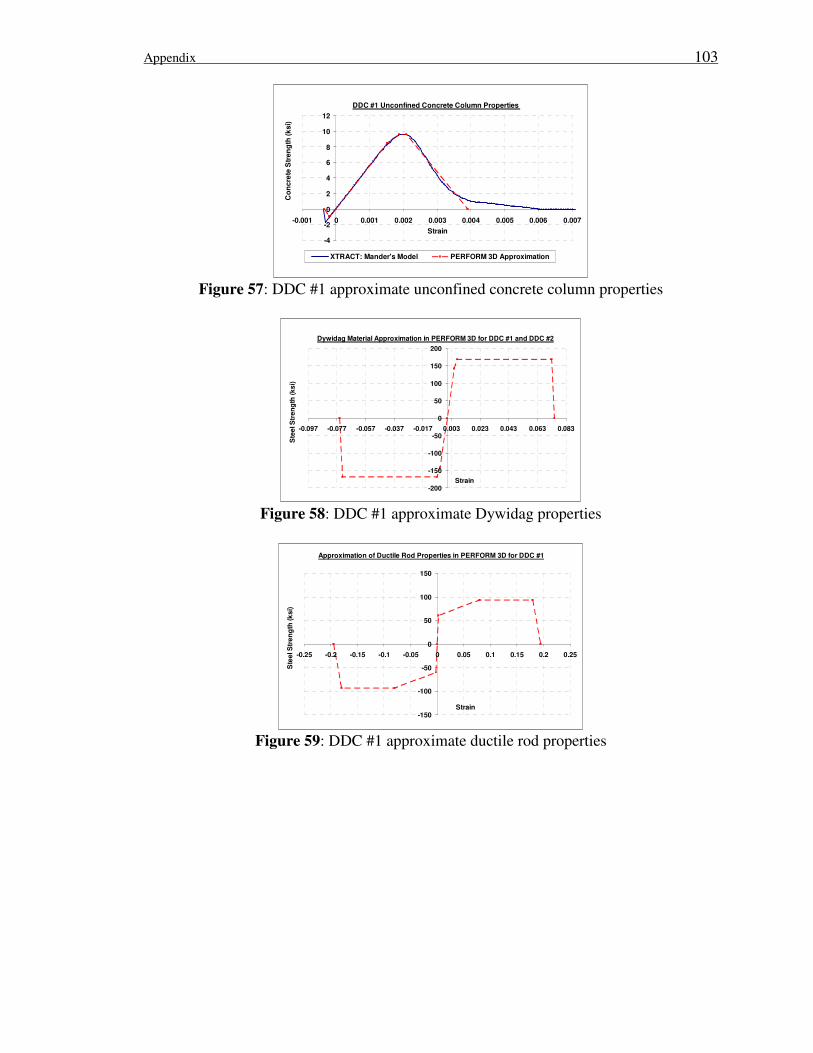
Appendix 103
DDC #1 Unconfined Concrete Column Properties
-4
-2
0
2
4
6
8
10
12
-0.001 0 0.001 0.002 0.003 0.004 0.005 0.006 0.007
Strain
Co
nc
rete
Str
en
gth
(k
si)
XTRACT: Mander's Model PERFORM 3D Approximation
Figure 57: DDC #1 approximate unconfined concrete column properties
Dywidag Material Approximation in PERFORM 3D for DDC #1 and DDC #2
-200
-150
-100
-50
0
50
100
150
200
-0.097 -0.077 -0.057 -0.037 -0.017 0.003 0.023 0.043 0.063 0.083
Strain
Ste
el S
tre
ng
th (
ks
i)
Figure 58: DDC #1 approximate Dywidag properties
Approximation of Ductile Rod Properties in PERFORM 3D for DDC #1
-150
-100
-50
0
50
100
150
-0.25 -0.2 -0.15 -0.1 -0.05 0 0.05 0.1 0.15 0.2 0.25
Strain
Ste
el S
tre
ng
th (k
si)
Figure 59: DDC #1 approximate ductile rod properties

Appendix 104
Appendix E
DDC #2 XTRACT Input Properties
Table 8: DDC #2 XTRACT input beam properties
Details DDC #2 (SEQAD #1)
Confined Concrete Strength Calculation
Type of transverse reinforcing Rectangular hoops
Transverse reinforcing bar yield stress (ksi) 11
66
X transverse reinforcing steel ratio 1 0.00208
Y transverse reinforcing steel ratio 1 0.00104
Average distance between tied longitudinal bars (in) 2 21
Number of longitudinal bars around core 4
Confined core area (in2) 377
(varying) Tie spacing along member (in) 11
12” o.c.
28-Day compressive concrete strength (ksi) 11
4.5
Confined concrete strength (ksi) 3 4.627
Crushing Strain Calculation
Transverse reinforcing steel strain at fracture (in/in) 13
0.18
Transverse (volumetric) reinforcing steel ratio 4 0.00312
Crushing strain, εcu 3, 6
0.01522
Mander’s Confined Concrete Curve Calculation
Tension Strength (ksi) 12
-0.402
Yield Strain, εcy 5 0.001598
Concrete Elastic Modulus (ksi) 7 3824
Unconfined Concrete Curve Calculation
Yield Strain 5 0.0014 (default)
Crushing Strain 6 0.004 (default)
Spalling Strain 8 0.006 (default)
Post Crushing Strength 9 0 (default)
Failure Strain 10
1 11
Information provided by reference (SEQAD Consulting Engineers 1993) 12
Calculated using the following equation: f’t = 7.5√f’c (ACI 2005): equation (9-10). 13
In the case of these variables, information was not provided and engineering judgment in
conjunction with other references was used to determine these values 14
Values were used here from the Dywidag material tests conducted in conjunction with the 2007
Pankow series testing conducted at UCSD, research done separately from the SEQAD research * For all other footnotes see DDC #1 Beam Properties table
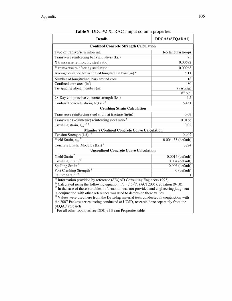
Appendix 105
Table 9: DDC #2 XTRACT input column properties
Details DDC #2 (SEQAD #1)
Confined Concrete Strength Calculation
Type of transverse reinforcing Rectangular hoops
Transverse reinforcing bar yield stress (ksi) 75
X transverse reinforcing steel ratio 1 0.00692
Y transverse reinforcing steel ratio 1 0.00968
Average distance between tied longitudinal bars (in) 2 5.11
Number of longitudinal bars around core 18
Confined core area (in2) 480
(varying) Tie spacing along member (in)
8” o.c.
28-Day compressive concrete strength (ksi) 4.5
Confined concrete strength (ksi) 3 6.451
Crushing Strain Calculation
Transverse reinforcing steel strain at fracture (in/in) 0.09
Transverse (volumetric) reinforcing steel ratio 4 0.0166
Crushing strain, εcu 3, 6
0.02
Mander’s Confined Concrete Curve Calculation
Tension Strength (ksi) 12
-0.402
Yield Strain, εcy 5 0.004435 (default)
Concrete Elastic Modulus (ksi) 7 3824
Unconfined Concrete Curve Calculation
Yield Strain 5 0.0014 (default)
Crushing Strain 6 0.004 (default)
Spalling Strain 8 0.006 (default)
Post Crushing Strength 9 0 (default)
Failure Strain 10
1 11
Information provided by reference (SEQAD Consulting Engineers 1993) 12
Calculated using the following equation: f’t = 7.5√f’c (ACI 2005): equation (9-10). 13
In the case of these variables, information was not provided and engineering judgment
in conjunction with other references was used to determine these values 14
Values were used here from the Dywidag material tests conducted in conjunction with
the 2007 Pankow series testing conducted at UCSD, research done separately from the
SEQAD research * For all other footnotes see DDC #1 Beam Properties table
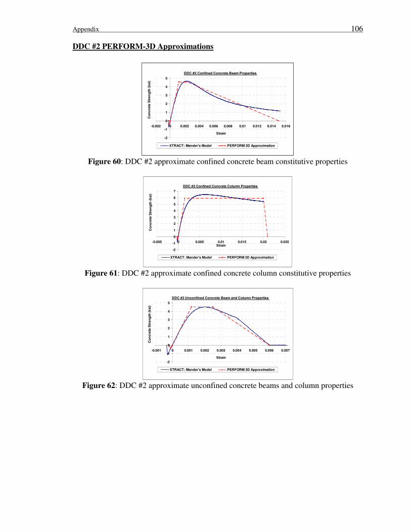
Appendix 106
DDC #2 PERFORM-3D Approximations
DDC #2 Confined Concrete Beam Properties
-2
-1
0
1
2
3
4
5
-0.002 0 0.002 0.004 0.006 0.008 0.01 0.012 0.014 0.016
Strain
Co
nc
rete
Str
en
gth
(k
si)
XTRACT: Mander's Model PERFORM 3D Approximation
Figure 60: DDC #2 approximate confined concrete beam constitutive properties
DDC #2 Confined Concrete Column Properties
-2
-1
0
1
2
3
4
5
6
7
-0.005 0 0.005 0.01 0.015 0.02 0.025Strain
Co
ncre
te S
tre
ng
th (k
si)
XTRACT: Mander's Model PERFORM 3D Approximation
Figure 61: DDC #2 approximate confined concrete column constitutive properties
DDC #2 Unconfined Concrete Beam and Column Properties
-2
-1
0
1
2
3
4
5
-0.001 0 0.001 0.002 0.003 0.004 0.005 0.006 0.007
Strain
Co
ncre
te S
tre
ng
th (
ksi)
XTRACT: Mander's Model PERFORM 3D Approximation
Figure 62: DDC #2 approximate unconfined concrete beams and column properties

Appendix 107
Dywidag Material Approximation in PERFORM 3D for DDC #2
-200
-150
-100
-50
0
50
100
150
200
-0.1 -0.08 -0.06 -0.04 -0.02 0 0.02 0.04 0.06 0.08 0.1
Strain
Ste
el S
tre
ng
th (
ks
i)
Figure 63: DDC #2 approximate Dywidag properties
Approximation of Longitudinal Column Reinforcement Properties in
PERFORM 3D for DDC #2
-150
-100
-50
0
50
100
150
-0.06 -0.04 -0.02 0 0.02 0.04 0.06
Strain
Ste
el S
tre
ng
th (
ks
i)
Figure 64: DDC #2 approximate longitudinal column steel reinforcement properties
Approximation of Ductile Rod Properties in PERFORM 3D for DDC #2
-150
-100
-50
0
50
100
150
-0.25 -0.2 -0.15 -0.1 -0.05 0 0.05 0.1 0.15 0.2 0.25
Strain
Ste
el S
tre
ng
th (
ks
i)
Figure 65: DDC #2 approximate ductile rod properties

Appendix 108
Appendix F
Super Hybrid XTRACT Input Properties
Table 10: Super hybrid XRACT input column properties
Details Super Hybrid
(Pankow #2)
Confined Concrete Strength Calculation
Type of transverse reinforcing Rectangular hoops
Transverse reinforcing bar yield stress (ksi) 11
77
X transverse reinforcing steel ratio 1 0.00717
Y transverse reinforcing steel ratio 1 0.00689
Average distance between tied longitudinal bars (in) 2 7.7
Number of longitudinal bars around core 18
Confined core area (in2) 720
(varying) Tie spacing along member (in) 11
6” o.c.
28-Day compressive concrete strength (ksi) 11
10.25
Confined concrete strength (ksi) 3 12.53
Crushing Strain Calculation
Transverse reinforcing steel strain at fracture (in/in) 13
0.12
Transverse (volumetric) reinforcing steel ratio 4 0.01406
Crushing strain, εcu 3, 6
0.01852
Mander’s Confined Concrete Curve Calculation
Tension Strength (ksi) 12
0.759
Yield Strain, εcy 5 0.00296
Concrete Elastic Modulus (ksi) 7 5771
Unconfined Concrete Curve Calculation
Yield Strain 5 0.0014 (default)
Crushing Strain 6 0.004 (default)
Spalling Strain 8 0.006 (default)
Post Crushing Strength 9 0 (default)
Failure Strain 10
1
11 Information provided by reference (SEQAD Consulting Engineers 1993)
12 Calculated using the following equation: f’t = 7.5√f’c (ACI 2005): equation (9-10).
13 In the case of these variables, information was not provided and engineering
judgment in conjunction with other references was used to determine these values 14
Values were used here from the Dywidag material tests conducted in conjunction
with the 2007 Pankow series testing conducted at UCSD, research done separately
from the SEQAD research * For all other footnotes see DDC #1 Beam Properties table
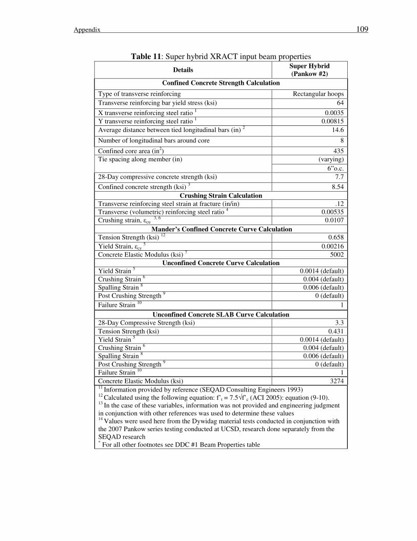
Appendix 109
Table 11: Super hybrid XRACT input beam properties
Details Super Hybrid
(Pankow #2)
Confined Concrete Strength Calculation
Type of transverse reinforcing Rectangular hoops
Transverse reinforcing bar yield stress (ksi) 64
X transverse reinforcing steel ratio 1 0.0035
Y transverse reinforcing steel ratio 1 0.00815
Average distance between tied longitudinal bars (in) 2 14.6
Number of longitudinal bars around core 8
Confined core area (in2) 435
(varying) Tie spacing along member (in)
6”o.c.
28-Day compressive concrete strength (ksi) 7.7
Confined concrete strength (ksi) 3 8.54
Crushing Strain Calculation
Transverse reinforcing steel strain at fracture (in/in) .12
Transverse (volumetric) reinforcing steel ratio 4 0.00535
Crushing strain, εcu 3, 6
0.0107
Mander’s Confined Concrete Curve Calculation
Tension Strength (ksi) 12
0.658
Yield Strain, εcy 5 0.00216
Concrete Elastic Modulus (ksi) 7 5002
Unconfined Concrete Curve Calculation
Yield Strain 5 0.0014 (default)
Crushing Strain 6 0.004 (default)
Spalling Strain 8 0.006 (default)
Post Crushing Strength 9 0 (default)
Failure Strain 10
1
Unconfined Concrete SLAB Curve Calculation
28-Day Compressive Strength (ksi) 3.3
Tension Strength (ksi) 0.431
Yield Strain 5 0.0014 (default)
Crushing Strain 6 0.004 (default)
Spalling Strain 8 0.006 (default)
Post Crushing Strength 9 0 (default)
Failure Strain 10
1
Concrete Elastic Modulus (ksi) 3274 11
Information provided by reference (SEQAD Consulting Engineers 1993) 12
Calculated using the following equation: f’t = 7.5√f’c (ACI 2005): equation (9-10). 13
In the case of these variables, information was not provided and engineering judgment
in conjunction with other references was used to determine these values 14
Values were used here from the Dywidag material tests conducted in conjunction with
the 2007 Pankow series testing conducted at UCSD, research done separately from the
SEQAD research * For all other footnotes see DDC #1 Beam Properties table

Appendix 110
Super Hybrid PERFORM-3D Approximations
Super Hybrid Confined Concrete Beam Properties
-2
0
2
4
6
8
10
-0.002 0 0.002 0.004 0.006 0.008 0.01 0.012
Strain
Co
nc
rete
Str
en
gth
(ks
i)
XTRACT: Mander's Model PERFORM 3D Approximation
Figure 66: Super hybrid approximate confined concrete beam properties
Super Hybrid Confined Concrete Column Properties
-4
-2
0
2
4
6
8
10
12
14
-0.005 0 0.005 0.01 0.015 0.02
Strain
Co
ncre
te S
tren
gth
(ksi)
XTRACT: Mander's Model PERFORM 3D Approximation
Figure 67: Super hybrid approximate confined concrete column properties
Super Hybrid Unconfined Concrete Beam Properties
-2
-1
0
1
2
3
4
5
6
7
8
9
-0.001 0 0.001 0.002 0.003 0.004 0.005 0.006
Strain
Co
nc
rete
Str
en
gth
(k
si)
XTRACT: Mander's Model PERFORM 3D Approximation
Figure 68: Super hybrid approximate unconfined concrete beam properties
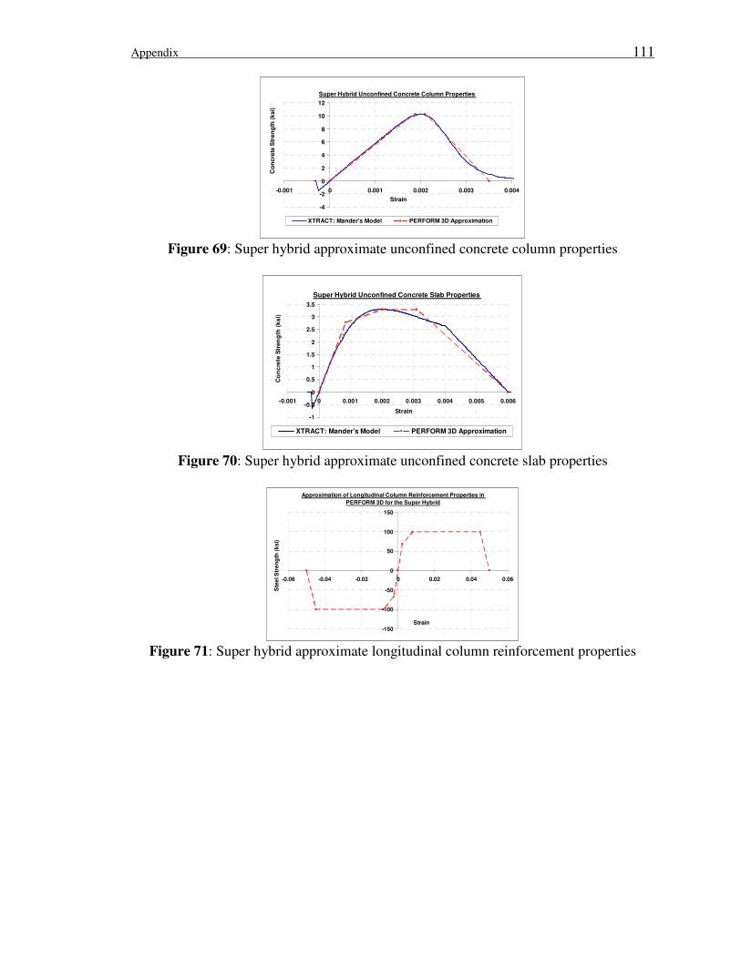
Appendix 111
Super Hybrid Unconfined Concrete Column Properties
-4
-2
0
2
4
6
8
10
12
-0.001 0 0.001 0.002 0.003 0.004
Strain
Co
ncre
te S
tren
gth
(ksi)
XTRACT: Mander's Model PERFORM 3D Approximation
Figure 69: Super hybrid approximate unconfined concrete column properties
Super Hybrid Unconfined Concrete Slab Properties
-1
-0.5
0
0.5
1
1.5
2
2.5
3
3.5
-0.001 0 0.001 0.002 0.003 0.004 0.005 0.006
Strain
Co
nc
rete
Str
en
gth
(k
si)
XTRACT: Mander's Model PERFORM 3D Approximation
Figure 70: Super hybrid approximate unconfined concrete slab properties
Approximation of Longitudinal Column Reinforcement Properties in
PERFORM 3D for the Super Hybrid
-150
-100
-50
0
50
100
150
-0.06 -0.04 -0.02 0 0.02 0.04 0.06
Strain
Ste
el S
tre
ng
th (
ks
i)
Figure 71: Super hybrid approximate longitudinal column reinforcement properties
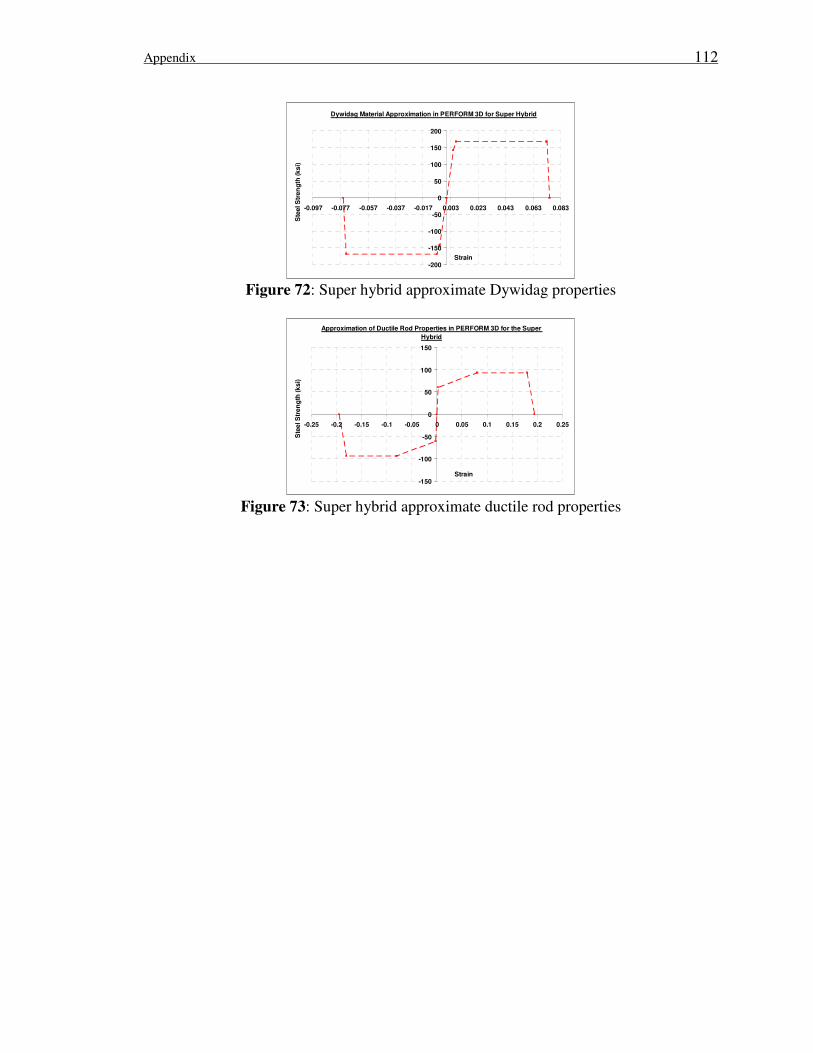
Appendix 112
Dywidag Material Approximation in PERFORM 3D for Super Hybrid
-200
-150
-100
-50
0
50
100
150
200
-0.097 -0.077 -0.057 -0.037 -0.017 0.003 0.023 0.043 0.063 0.083
Strain
Ste
el S
tre
ng
th (
ks
i)
Figure 72: Super hybrid approximate Dywidag properties
Approximation of Ductile Rod Properties in PERFORM 3D for the Super
Hybrid
-150
-100
-50
0
50
100
150
-0.25 -0.2 -0.15 -0.1 -0.05 0 0.05 0.1 0.15 0.2 0.25
Strain
Ste
el S
tre
ng
th (
ks
i)
Figure 73: Super hybrid approximate ductile rod properties
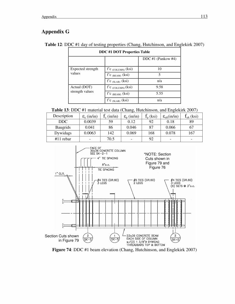
Appendix 113
Appendix G
Table 12: DDC #1 day of testing properties (Chang, Hutchinson, and Englekirk 2007)
DDC #1 DOT Properties Table
DDC #1 (Pankow #4)
f’c (COLUMN) (ksi) 10
f’c (BEAM) (ksi) 5
Expected strength
values
f’c (SLAB) (ksi) n/a
f’c (COLUMN) (ksi) 9.58
f’c (BEAM) (ksi) 5.55
Actual (DOT)
strength values
f’c (SLAB) (ksi) n/a
Table 13: DDC #1 material test data (Chang, Hutchinson, and Englekirk 2007)
Description εy (in/in) fy (in/in) εp (in/in) fp (ksi) εult(in/in) fult (ksi)
DDC 0.0039 59 0.12 92 0.18 89
Baugrids 0.041 86 0.046 87 0.066 67
Dywidags 0.0063 142 0.069 168 0.078 167
#11 rebar - 70.5 - 92 - -
Figure 74: DDC #1 beam elevation (Chang, Hutchinson, and Englekirk 2007)
Section Cuts shown in Figure 79
*NOTE: Section Cuts shown in Figure 79 and
Figure 76
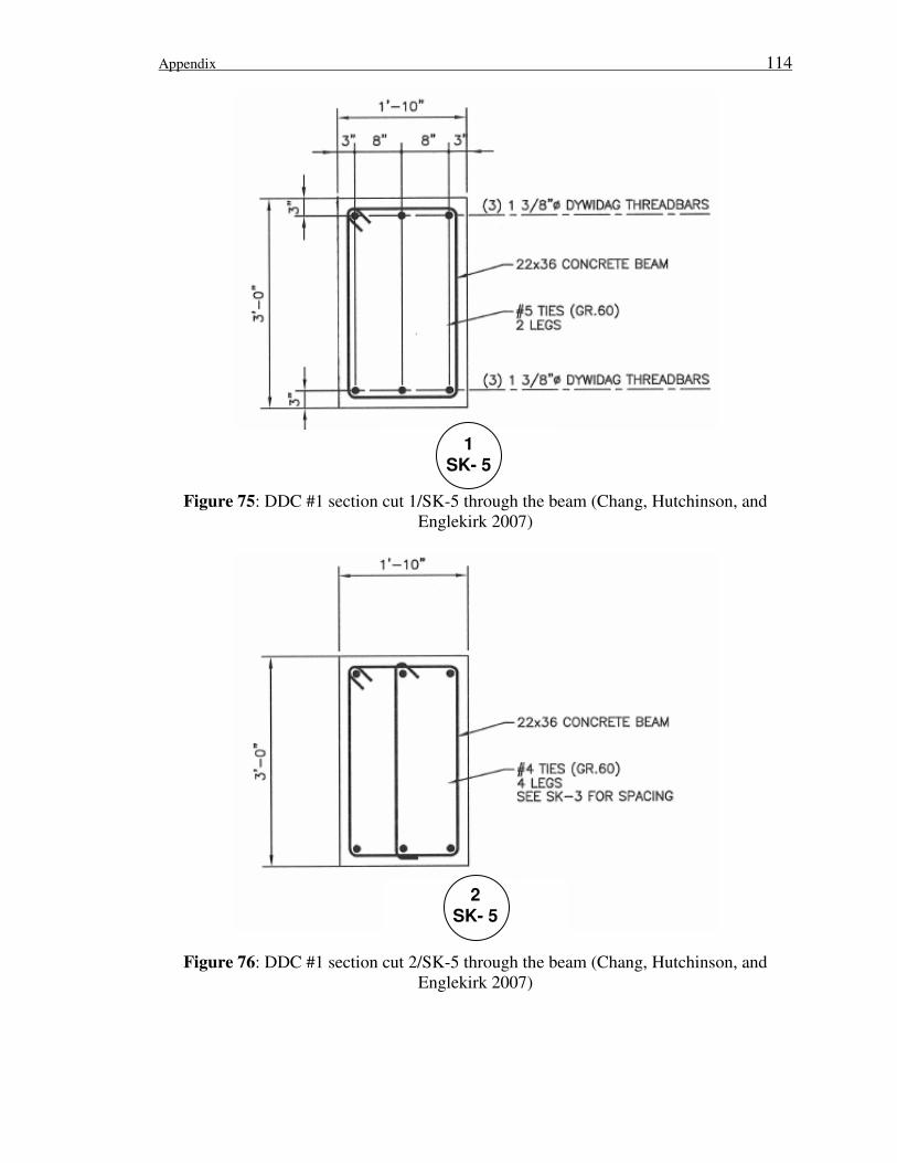
Appendix 114
Figure 75: DDC #1 section cut 1/SK-5 through the beam (Chang, Hutchinson, and
Englekirk 2007)
Figure 76: DDC #1 section cut 2/SK-5 through the beam (Chang, Hutchinson, and
Englekirk 2007)
1 SK- 5
2 SK- 5

Appendix 115
Figure 77: DDC #1 column elevation (Chang, Hutchinson, and Englekirk 2007)
*NOTE: Section Cuts shown in Figure 78 and
Figure 79
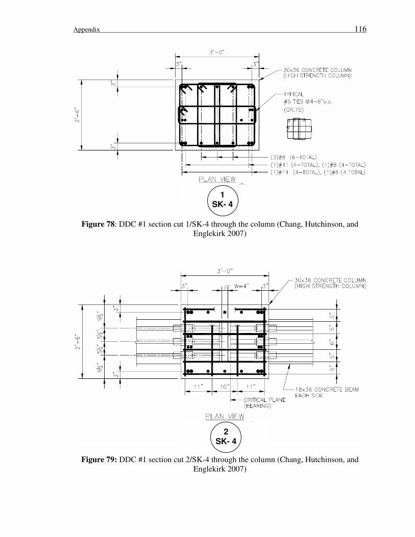
Appendix 116
Figure 78: DDC #1 section cut 1/SK-4 through the column (Chang, Hutchinson, and
Englekirk 2007)
Figure 79: DDC #1 section cut 2/SK-4 through the column (Chang, Hutchinson, and
Englekirk 2007)
1 SK- 4
2 SK- 4
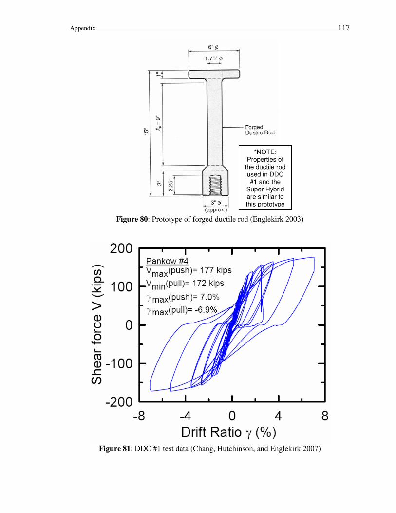
Appendix 117
Figure 80: Prototype of forged ductile rod (Englekirk 2003)
Figure 81: DDC #1 test data (Chang, Hutchinson, and Englekirk 2007)
*NOTE: Properties of
the ductile rod used in DDC #1 and the
Super Hybrid are similar to this prototype
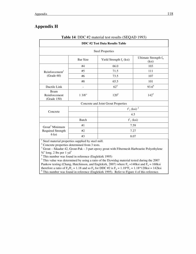
Appendix 118
Appendix H
Table 14: DDC #2 material test results (SEQAD 1993)
DDC #2 Test Data Results Table
Steel Properties
Bar Size Yield Strength fy (ksi) Ultimate Strength fu
(ksi)
#4 66.0 103
#5 71.5 111
#6 73.5 107
Reinforcement1
(Grade 60)
#8 65.5 101
Ductile Link - 624 93.6
6
Beam
Reinforcement
(Grade 150)
1 3/8” 1204 142
5
Concrete and Joint Grout Properties
f’c (ksi) 2
Concrete 4.5
Batch f’c (ksi)
#1 7.59
#2 7.27
Grout3 Minimum
Required Strength
6 ksi #3 8.07
1 Steel material properties supplied by steel mill.
2 Concrete properties determined from 3 tests.
3 Grout – Sikadur 42, Grout-Pak – 3 part epoxy grout with Fibermesh Harbourite Polyethylene
¾” long, 2 lbs per 1 yd3
4 This number was found in reference (Englekirk 1995)
5 This value was determined by using a ratio of the Dywidag material tested during the 2007
Pankow testing (Chang, Hutchinson, and Englekirk, 2007) where Fy =140ksi and Fu = 168ksi
therefore a ratio of Fu/Fy = 1.18 and so Fu for DDC #2 is Fu = 1.18*Fy = 1.18*120ksi = 142ksi 6 This number was found in reference (Englekirk 1995). Refer to Figure 4 of this reference.
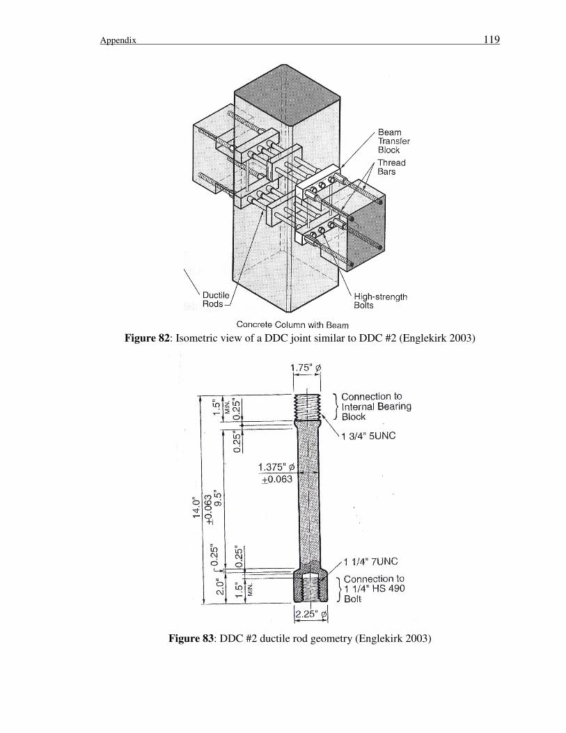
Appendix 119
Figure 82: Isometric view of a DDC joint similar to DDC #2 (Englekirk 2003)
Figure 83: DDC #2 ductile rod geometry (Englekirk 2003)

Appendix 120
Figure 84: Relationship between stress and strain for the ductile rod in Figure 83
Figure 85: DDC #2 force-displacement hysteretic data (SEQAD 1993)

Appendix 121
Figure 86: DDC #2 joint elevation (Englekirk 1995)
Figure 87: DDC #2 plan view of the column at the ductile rod elevation in the joint
(Englekirk 1995)

Appendix 122
Appendix I.
Table 15: Super hybrid day of testing properties (Chang, Hutchinson, and Englekirk
2007)
Super Hybrid DOT Properties Table
Super Hybrid
(Pankow #2)
f’c (COLUMN) (ksi) 10
f’c (BEAM) (ksi) 5
Expected strength
values
f’c (SLAB) (ksi) 3
f’c (COLUMN) (ksi) 10.25
f’c (BEAM) (ksi) 7.7
Actual (DOT)
strength values
f’c (SLAB) (ksi) 3.39
Table 16: Super hybrid material test data (Chang, Hutchinson, and Englekirk 2007)
Description εy (in/in) fy (in/in) εp (in/in) fp (ksi) εult(in/in) fult (ksi)
DDC 0.0040 60 0.124 91 0.195 82
Dywidags 0.0054 144 0.074 169 0.11 165
#4 rebar 0.0041 64 0.11 92 0.20 88
#5 rebar 0.0046 77 0.079 98 0.14 94
#6 rebar 0.0044 67 0.10 111 0.16 105
#11 rebar - 69.5 - - - -

Appendix 123
Figure 88: Super hybrid column elevation (Chang, Hutchinson, and Englekirk 2007)
*NOTE: Section Cuts are shown in
Figure 89, Figure 90, and Figure 91
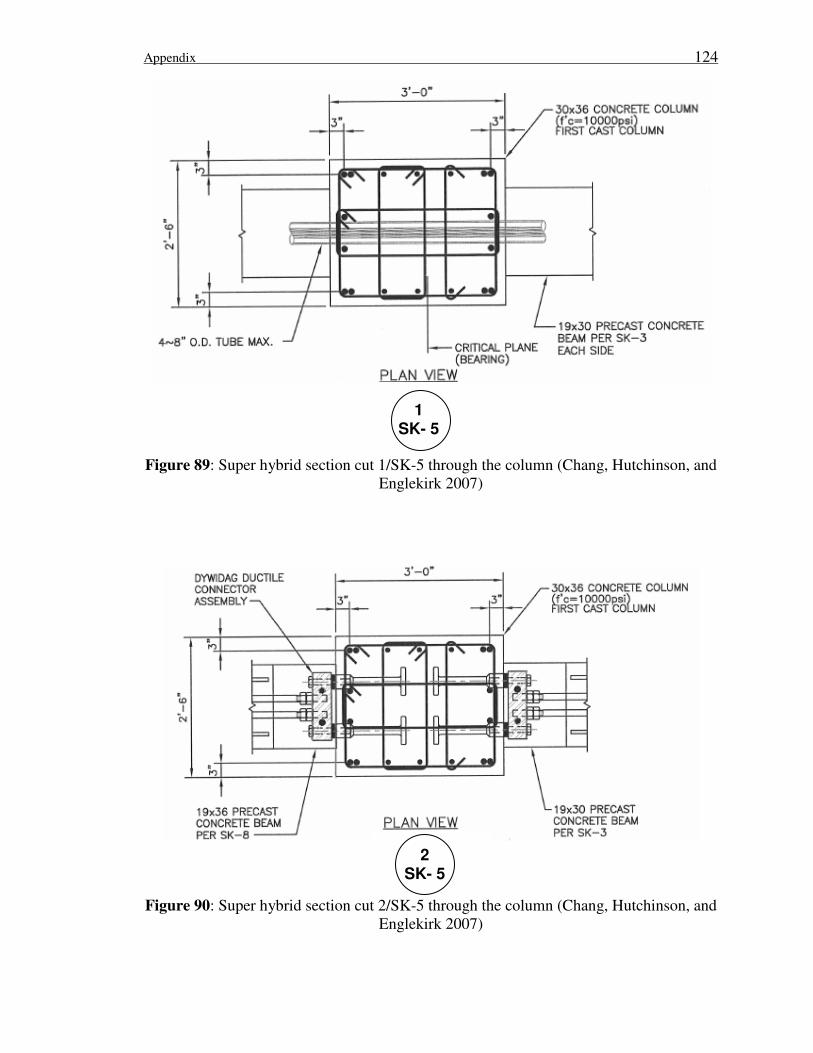
Appendix 124
Figure 89: Super hybrid section cut 1/SK-5 through the column (Chang, Hutchinson, and
Englekirk 2007)
Figure 90: Super hybrid section cut 2/SK-5 through the column (Chang, Hutchinson, and
Englekirk 2007)
1 SK- 5
2 SK- 5

Appendix 125
Figure 91: Super hybrid section cut 1/SK-4 through the column (Chang, Hutchinson, and
Englekirk 2007)
Figure 92: Super hybrid south beam elevation (Chang, Hutchinson, and Englekirk 2007)
1 SK- 4
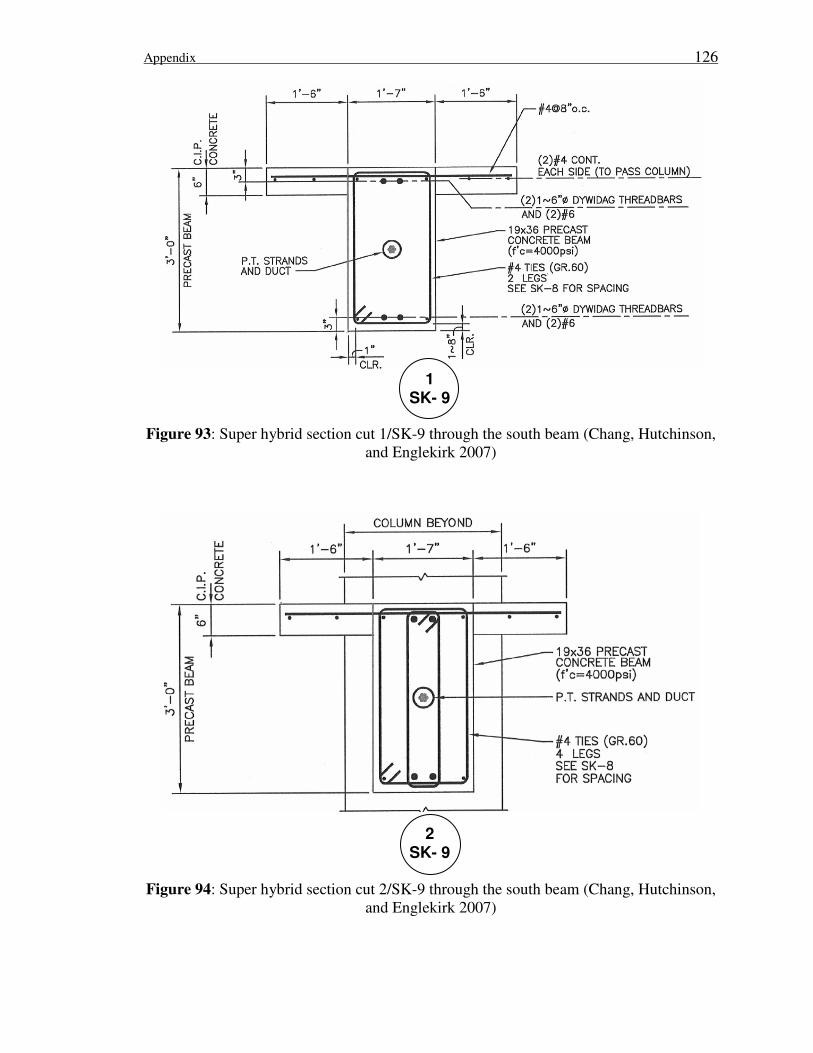
Appendix 126
Figure 93: Super hybrid section cut 1/SK-9 through the south beam (Chang, Hutchinson,
and Englekirk 2007)
Figure 94: Super hybrid section cut 2/SK-9 through the south beam (Chang, Hutchinson,
and Englekirk 2007)
2 SK- 9
1 SK- 9

Appendix 127
Figure 95: Super hybrid plan of the north beam at the pinned end connection (Chang,
Hutchinson, and Englekirk 2007)
Figure 96: Super hybrid north beam elevation (Chang, Hutchinson, and Englekirk 2007)

Appendix 128
Figure 97: Super hybrid section cut 1/SK-6 through the north beam (Chang, Hutchinson,
and Englekirk 2007)
Figure 98: Super hybrid section cut 2/SK-6 through the north beam (Chang, Hutchinson,
and Englekirk 2007)
1 SK- 6
2 SK- 6
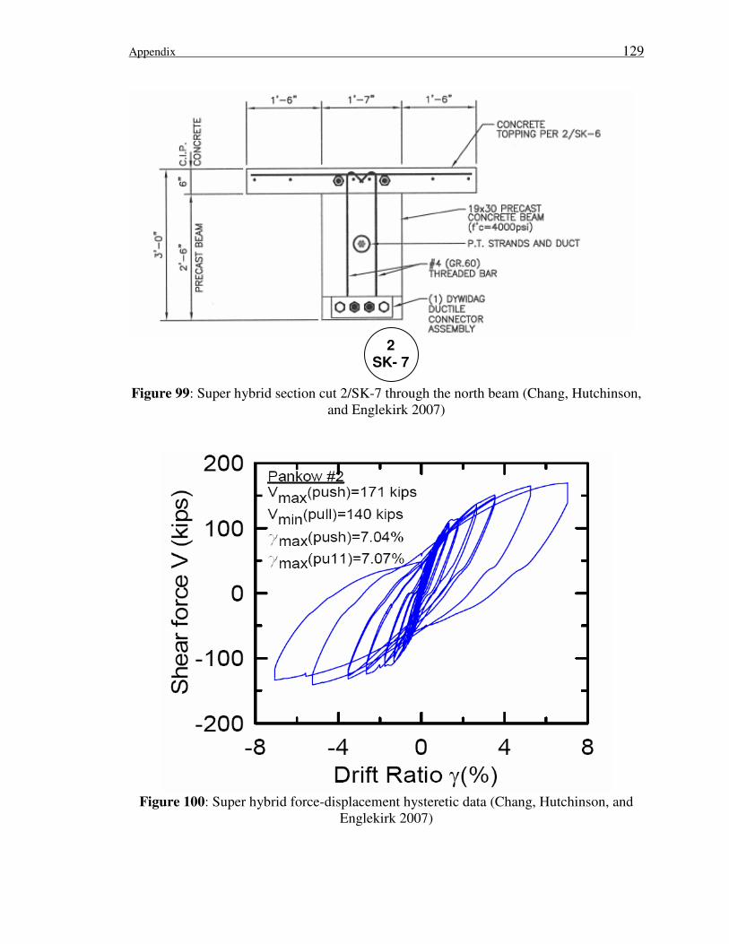
Appendix 129
Figure 99: Super hybrid section cut 2/SK-7 through the north beam (Chang, Hutchinson,
and Englekirk 2007)
Figure 100: Super hybrid force-displacement hysteretic data (Chang, Hutchinson, and
Englekirk 2007)
2 SK- 7
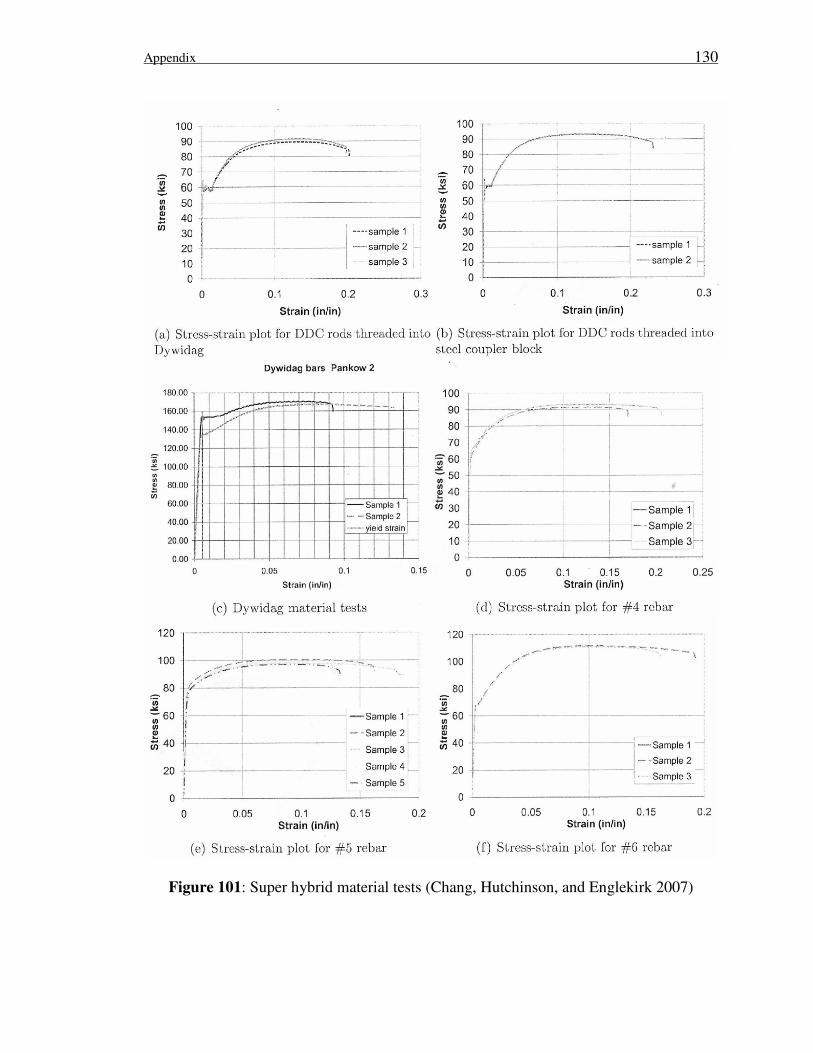
Appendix 130
Figure 101: Super hybrid material tests (Chang, Hutchinson, and Englekirk 2007)