prediction and compensation of magnetic beam deflection in

Helmholtz-Zentrum Dresden-Rossendorf (HZDR)

Prediction and compensation of magnetic beam deflection in MR-integrated proton therapy: A method optimized regarding accuracy,

versatility and speed

Schellhammer, S. M.; Hoffmann, A. L.;

Originally published:

January 2017

Physics in Medicine and Biology 62(2017)4, 1548-1564

DOI: https://doi.org/10.1088/1361-6560/62/4/1548

Perma-Link to Publication Repository of HZDR:

https://www.hzdr.de/publications/Publ-23534

Release of the secondary publication based on the publisher's specified embargo time.

https://www.hzdr.de

https://www.hzdr.de

https://doi.org/10.1088/1361-6560/62/4/1548

https://www.hzdr.de/publications/Publ-23534

Prediction and compensation of magnetic beamdeflection in MR-integrated proton therapy: Amethod optimized regarding accuracy, versatilityand speed

Sonja M. Schellhammer1 and Aswin L. Hoffmann1,2

1 Helmholtz-Zentrum Dresden-Rossendorf, Institute of Radiooncology,Handelallee 26, 01309 Dresden, Germany2 Department of Radiotherapy and Radiooncology, University Hospital CarlGustav Carus at the Technische Universitat Dresden, Dresden, Germany

E-mail: [email protected]

Abstract. The integration of magnetic resonance imaging (MRI) and protontherapy for on-line image-guidance is expected to reduce dose deliveryuncertainties during treatment. Yet, the proton beam experiences a Lorentzforce induced deflection inside the magnetic field of the MRI scanner, and severalmethods have been proposed to quantify this effect. We analyze their structuraldifferences and compare results of both analytical and Monte Carlo models. Wefind that existing analytical models are limited in accuracy and applicability due tocritical approximations, especially including the assumption of a uniform magneticfield. As Monte Carlo simulations are too time-consuming for routine treatmentplanning and on-line plan adaption, we introduce a new method to quantify andcorrect for the beam deflection, which is optimized regarding accuracy, versatilityand speed. We use it to predict the trajectory of a mono-energetic protonbeam of energy E0 traversing a water phantom behind an air gap within anomnipresent uniform transverse magnetic flux density B0. The magnetic fieldinduced dislocation of the Bragg peak is calculated as function of E0 and B0 andcompared to results obtained with existing analytical and Monte Carlo methods.The deviation from the Bragg peak position predicted by Monte Carlo simulationsis smaller for the new model than for the analytical models by up to 2 cm. Themodel is faster than Monte Carlo methods, less assumptive than the analyticalmodels and applicable to realistic magnetic fields. To compensate for the predictedBragg peak dislocation, a numerical optimization strategy is introduced andevaluated. It includes an adjustment of both the proton beam entrance angleand energy of up to 25 ◦ and 5 MeV, depending on E0 and B0. This strategy isshown to effectively reposition the BP to its intended location in the presence ofa magnetic field.

Submitted to: Phys. Med. Biol.

Keywords: proton therapy, image-guided radiotherapy, IGPT, magnetic resonanceimaging, MR guidance, beam trajectory prediction

Modelling magnetic beam deflection in MR-integrated proton therapy 2

1. Introduction

Proton therapy is a type of external beam radiation treatment that uses high-energy protons to treat cancer. As compared to photon-based radiotherapy, its mainadvantage lies in the pronounced dose maximum, the Bragg peak, which is energy-dependent in depth and bordered by steep dose gradients, especially at the distal edge(Jakel 2009). However, the gradients also make the dose distribution very sensitiveto inter- and intrafractional uncertainties resulting from setup errors and anatomicalvariations (i.e., organ motion and deformation), which gives rise to considerable rangeuncertainties (Lomax 2008).

The aim of real-time image-guided radiotherapy is to reduce these uncertainties byimaging essential parts of the patient anatomy in treatment position during irradiation.Thus, tissue motions and deformations can be tracked and dynamic beam delivery withenhanced dose conformality and reduced safety margins is rendered possible. Magneticresonance imaging (MRI) has been suggested to be a promising candidate for this task,offering a fast real-time imaging modality with excellent soft tissue contrast withoutusing ionising radiation for image formation (Raaymakers et al. 2008). The conceptfeasibility to integrate MRI with photon-based radiotherapy into a hybrid system hasbeen shown by several research groups in the Netherlands (Lagendijk et al. 2014a),Canada (Fallone 2014) and Australia (Keall et al. 2014). Because of the increasedgeometrical sensitivity of proton therapy, this technique is expected to profit evenmore from an integration with MRI.

So far, MR-integrated proton therapy (MRiPT) has only been described asa hypothetical modality in simulation studies (Raaymakers et al. 2008, Wolf &Bortfeld 2012, Moteabbed et al. 2014, Oborn et al. 2015, Li 2015, Hartmanet al. 2015, Moser 2015). Likewise challenging as in MR-integrated photon therapy,there are specific technological and physical problems that need to be solved whenfacing MRiPT. For example, there will be mutual interactions between the magneticfield of the MRI scanner and that of the beam transport magnets and the beam steeringand monitoring system (Schippers & Lomax 2011). Probably more problematicis the fact that, being charged particles, the therapeutic protons will be deflectedby the magnetic field of the MRI scanner (Oborn et al. 2016). Different studieshave focussed on quantifying the beam deflection effect for dosimetric and treatmentplanning purposes using particle tracking with Monte Carlo simulations (Raaymakerset al. 2008, Moteabbed et al. 2014, Oborn et al. 2015, Li 2015, Moser 2015) or analyticalmodels (Wolf & Bortfeld 2012, Hartman et al. 2015).

As pointed out by Oborn et al. (2015), the general consensus from these worksis that the proton beam deflection within a patient or water phantom is predictableand so essentially correctable during treatment planning stages. However, differentapproaches have been introduced to assess this effect, and neither their structuraldifferences nor their degree of accordance have been analyzed. Differences can beexpected, since all approaches are subject to their respective shortcomings. Forinstance, previously published analytical models imply critical assumptions, and areonly applicable to the simplified case of a uniform (i.e. unrealistic) magnetic field.Monte Carlo simulations are potentially more accurate, but very time-consuming,which inhibits their use for routine treatment plan optimization and real-timetreatment plan adaption. Thus, a method is required to quantify and correct forthe deflection, which is optimized towards accuracy, versatility and calculation time.

The aim of the current work therefore is three-fold. Firstly, we analyze and


compare results published so far in terms of dosimetric accuracy and discuss thelimitations of the different methods. Secondly, we present a new model to estimatethe trajectory of a mono-energetic proton beam traversing a water/air phantom insidea uniform transverse magnetic field and evaluate its performance against results ofthe previous models. Thirdly, we use the new model to introduce a fast and accuratebeam correction strategy for repositioning the Bragg peak to its intended location inthe presence of the magnetic field. To help understand the limitations of previouslypublished analytical models, a condensed review and analysis thereof is given in section2. On this basis, a new model to estimate and compensate for the magnetic fieldinduced proton beam deflection is presented in section 3. The setup for the subsequentevaluation and comparison of this model in relation to existing approaches is detailedin section 4. Obtained results are given in section 5. In section 6, the main findingsand most important implications are discussed. A short conclusion and outlook tofurther investigations are provided in section 7.

2. Analysis of existing analytical models

For a better understanding of the following chapters, previously published analyticalmodels are shortly reviewed in this section. Being first order approaches, the methodsmodel a mono-energetic proton beam traversing a simple water/air phantom inside auniform transverse magnetic field.

2.1. General considerations

Consider a uniform magnetic field in vacuum of flux density ~B = B0 · ~ez which isaligned parallel to the z-axis and translation invariant. Let a monoenergetic protonpencil beam of kinetic energy E0 with an initial velocity ~v0 = v0 · ~ex perpendicular to

~B traverse the field (see figure 1a). The entrance velocity v0 = c ·√

E0(E0+2m0c2)(E0+m0c2)2

is

connected to E0 through the proton rest mass m0 and the speed of light c. Carryingthe elementary electric charge q, the proton’s equation of motion is governed by theLorentz force

~F =d~p

dt= γm0

d~v

dt+m0~v

dγ

dt= q(~v × ~B) (1)

with the relativistic momentum ~p = γm0~v and the Lorentz factor γ = 1√1−( v0

c )2. As

v0 is constant, which yields dγdt = 0, this differential equation has a simple analytical

solution

vx = v0 cos(qB0

γm0t), vy = v0 sin(

qB0

γm0t), vz = 0 (2)

for the velocity components vx, vy and vz in x-, y- and z-direction, respectively. The

protons thus move in a circular course with an angular frequency ω0 = qB0

γm0. The

radius of this course, the gyroradius, is given by

r =v0ω0

=γm0v0qB0

. (3)

Now consider a setup geometry with a water phantom placed inside a virtualgantry-based MRiPT system. The distance between the proton beam nozzle and thewater phantom’s surface is denoted by dair. As opposed to the vacuum situation,protons deposit energy when traversing media until stopping at a finite range R0.


(a) (b)

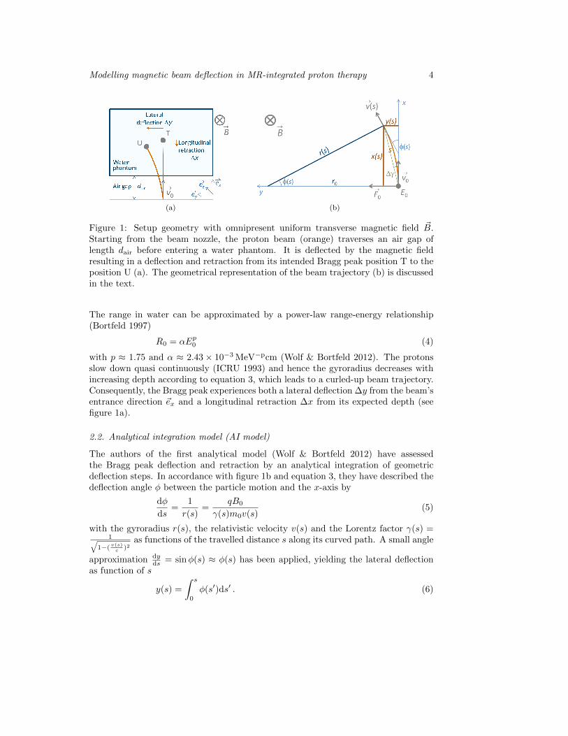
Figure 1: Setup geometry with omnipresent uniform transverse magnetic field ~B.Starting from the beam nozzle, the proton beam (orange) traverses an air gap oflength dair before entering a water phantom. It is deflected by the magnetic fieldresulting in a deflection and retraction from its intended Bragg peak position T to theposition U (a). The geometrical representation of the beam trajectory (b) is discussedin the text.

The range in water can be approximated by a power-law range-energy relationship(Bortfeld 1997)

R0 = αEp0 (4)

with p ≈ 1.75 and α ≈ 2.43× 10−3 MeV−pcm (Wolf & Bortfeld 2012). The protonsslow down quasi continuously (ICRU 1993) and hence the gyroradius decreases withincreasing depth according to equation 3, which leads to a curled-up beam trajectory.Consequently, the Bragg peak experiences both a lateral deflection ∆y from the beam’sentrance direction ~ex and a longitudinal retraction ∆x from its expected depth (seefigure 1a).

2.2. Analytical integration model (AI model)

The authors of the first analytical model (Wolf & Bortfeld 2012) have assessedthe Bragg peak deflection and retraction by an analytical integration of geometricdeflection steps. In accordance with figure 1b and equation 3, they have described thedeflection angle φ between the particle motion and the x-axis by

dφ

ds=

1

r(s)=

qB0

γ(s)m0v(s)(5)

with the gyroradius r(s), the relativistic velocity v(s) and the Lorentz factor γ(s) =1√

1−( v(s)c )2

as functions of the travelled distance s along its curved path. A small angle

approximation dyds = sinφ(s) ≈ φ(s) has been applied, yielding the lateral deflection

as function of s

y(s) =

∫ s

0

φ(s′)ds′ . (6)


The deflection at the end of the trajectory in a water phantom without air gap(i.e. dair = 0) has thus been obtained by analytical integration as

∆y = y(s = R0) (7)

=7

30

qB0α2

√2m0

(2m0c2)3

[√1 +

E0

2m0c2

(3

(E0

2m0c2

)2

− 4

(E0

2m0c2

)+ 8

)− 8

].

In an analogous manner, the longitudinal position x(s) has been obtained by assumingdxds = cosφ(s) ≈ 1− φ(s)2

2 which yields

x(s) = s− 1

2

∫ s

0

φ2(s′)ds′ . (8)

This term has been treated non-relativistically (i.e. γ = 1 and v(s) =√

2E(s)m0

) and

thus the overall retraction length was quantified by

∆x = R0 − x(R0) =q2B2

0α3E3p−1

0

2m0

2p2

(4p− 1)(3p− 1). (9)

The model was stated to be applicable to slab phantom geometries of arbitrarymaterial thickness and composition by addition of the deflections obtained in eachlayer. For air gaps, energy loss has been assumed to be negligible, yielding

dair = xair(s) = s− q2B20s

3

12m0E0and yair(s) =

qB0s2

2√

2m0E0

. (10)

An advantage of the AI model is that the whole curved beam trajectory can becalculated from x(s) and y(s), which is important for treatment planning anddosimetric verification. However, the model cannot be easily adapted to realistic,inhomogeneous magnetic fields mainly because of the pathlength parametrization,but also due to the need for an analytical description of the magnetic flux densitydistribution.

2.3. Trigonometric model (TG model)

In the work of Wolf and Bortfeld (2012), no concrete compensation strategy for thebeam deflection has been proposed. This problem has been adressed by a more recentpaper (Hartman et al. 2015). Here, a simplified analytical model has been introducedin order to propose a beam deflection correction strategy. Several assumptionshave been made to enable a direct trigonometric quantification of the proton beamdeflection without the use of more complex methods such as integration. Firstly, thechange of the gyroradius due to energy loss in matter has been neglected, i.e. r(s) = r0.Secondly, longitudinal beam retraction was not taken into account, i.e. ∆x = 0 andx(s = R0) = R0. Following these approximations and figure 1b, the lateral deflectionin the water phantom (with dair = 0) has been expressed as

∆y = r0

(1− cos

[arcsin

(R0

r0

)]), (11)

which can be simplified to

∆y = r0 −√r20 −R2

0 . (12)


As a third approximation, the proton motion was assumed to be non-relativistic (γ = 1

and v(s) =√

2E(s)m ), which yields a (constant) gyroradius of

r0 =

√2mE0

qB0≈ 14.4

√E0

B0T cm (MeV)−

12 . (13)

The airgap of thickness dair in front of the water phantom has been accounted for byreplacing R0 with (R0 + dair), assuming that energy loss in air is negligible.

A correction strategy for the deflection has been proposed by applying an anglecorrection to the entrance direction ~v0 of the beam. According to figure 1b, it wasobtained by

∆γ = arctan

(y(R0)

x(R0)

)= arctan

(∆y

R0

). (14)

The authors stated that this angle correction could be implemented either by pencilbeam scanning magnets or by an isocentric gantry rotation around the phantom.

2.4. Summary

Although both the AI and the TG model offer a reasonable first approach to theproblem of magnetic proton beam deflection in a transverse uniform magnetic field,they have their respective shortcomings. The AI model relies on a small angleapproximation which is problematic for large deflection angles, treats retractionnon-relativistically and does not offer a compensation strategy for the Bragg peakdeflection. The TG model neglects relativistic effects, beam retraction and thedecreasing gyroradius as a function of penetration depth. Neither the AI nor theTG model seems applicable to a realistic, i.e. non-uniform, magnetic field and patientanatomy. Aiming to provide a solution which is more accurate and versatile thanthese two models, but faster than Monte Carlo approaches, we therefore present andverify an alternative model in the following sections.

3. New model formulation

The model we propose is an iterative analytical method to reconstruct the trajectoryof a monoenergetic proton beam based on first physics principles and geometricalconsiderations. It contains less critical approximations than currently availableanalytical models and offers a correction strategy for the predicted beam deflectionand retraction.

3.1. Incremental reconstruction of the proton beam trajectory

Consider the geometry presented in section 2 and figure 2 and let the proton beam’sentry position to the magnetic field be ~x0 = (x0, y0, z0). The initial gyroradius causedby the magnetic field is (cf. equation 3)

r0 =γm0v0qB0

=

√2m0E0(1 + E0

2m0c2)

qB0. (15)

The first relevant point of the trajectory is the entrance position of the proton beamat the surface of the water phantom ~x1. Energy loss inside the airgap is considered tobe negligible, therefore ~x1 is obtained by

~x1 = R(∆φ0) · ~x0 , (16)


(a) (b)

Figure 2: Geometrical representation of the proposed model. The proton beamdeflection in air is calculated trigonometrically assuming no energy loss (a), whereasa changing gyroradius due to energy loss is taken into account in water (b). Symbolsare explained in the text.

with the rotation matrix R(∆φ0) rotating the point ~x0 counterclockwise through an

angle ∆φ0 about the center of rotation ~O0 = (x0, y0 + r0, z0) (see figure 2a). ∆φ0satisfies

∆φ0 = arcsin(dairr0

) . (17)

Inside the water phantom, energy loss is modeled by the continuous slowing downapproximation (ICRU 1993) and discretized into small steps of constant energy andhence constant gyroradius (see figure 2b). The energy step size ε is chosen forevery simulation such that the studied parameters, i.e. ∆y, ∆x and the correctionparameters, are independent of ε within the decimal precision they are given in.Following equation 4, for each energy step i (i = 1, ..., n with n = bE0

ε c) the travelledpath length in water, si, can be calculated from (see eq. 4)

si = R0 − αEpi , (18)

which results in an incremental deflection angle of

∆φi =si+1 − si

ri=

∆siri

(19)

with the energy-dependent gyroradius ri =

√2m0Ei(1+

Ei2m0c2

)

qB0(in analogy to equation

15). The next particle position ~xi+1 is obtained by applying the rotational matrix of

angle ∆φi to ~xi, i.e. ~xi+1 = R(∆φi) ·~xi. Here, the center of rotation ~Oi is determinedby (cf. figure 2a)

~Oi =ri

| ~Oi−1 − ~xi|( ~Oi−1 − ~xi) . (20)

Thus, the proton trajectory is fully reconstructed until reaching the Bragg peak atstep i = n. The overall deflection ∆y and retraction ∆x are then obtained as theprojections of the difference between the Bragg peak positions ~xn with and withoutmagnetic field. It was verified that the total traveled pathlength is equal to the protonrange within 0.1 mm accuracy, i.e. sn −R0 < 0.1 mm.

The algorithm has been realized in MATLAB (Release 2015b, The MathWorks,Inc., Natick, Massachusetts, United States).


Figure 3: The proposed correction algorithm includes a correction of the proton energy∆E0 and entrance angle ∆γ such that the actual Bragg peak location U coincides withthe intended position T.

3.2. Correction strategy

As an advancement to the TG model, we propose a correction strategy thatsimultaneously adjusts the proton beam entrance angle and energy (see figure 3).The angle correction ∆γ compensates for the lateral deflection of the Bragg peak andcan only be applied by pencil beam scanning magnets. The energy correction ∆E0

accounts for the retraction caused by the path curvature and has not been consideredbefore. Both correction parameters are optimized such that the distance to agreement(DTA) between the corrected Bragg peak position ~xn,corr = ~xn( ~B, γ0 +∆γ,E0 +∆E0)and the intended position ~xn,0 = ~xn(0 T, γ0, E0)

DTA = |~xn,corr − ~xn,0| (21)

is minimized. This bi-parameter optimization is performed numerically using theMATLAB Optimization Toolbox function fminsearch, which implements the simplexsearch method (Lagarias et al. 1998).

As an alternative to the angle correction, a patient shift has been suggestedby Moteabbed et al. (2014). However, the deflection of a single Bragg peak stronglydepends on the beam energy, entrance angle and the irradiated geometry, and thereforecannot completely be compensated for by a constant shift. For the same reason, weagree with Oborn et al. (2015) that MRiPT can only be realized using a pencil beamscanning technique.


4. Setup and parameter choice

The new method described in section 3 has been used to predict the trajectories ofmonoenergetic proton pencil beams of energies E0 between 60 MeV and 250 MeV ina uniform transversal magnetic field of magnetic flux density B0. Selected examplesfor B0 were 0.5 T as a commonly used flux density in open MRI systems, 1.5 T astypical value for diagnostic images, and 3 T because of its allowance for very fastsequences, which are important for on-line image-guidance (Lagendijk et al. 2014b).The trajectories were studied in two different geometries: one with a water phantomalone, and one with an air gap between the phantom and the beam nozzle of thicknessdair. The parameter dair = 25 cm was chosen by way of example as a typical distancebetween the beam nozzle and the patient.

The lateral deflection ∆y and longitudinal retraction ∆x were calculated asfunctions of E0 and B0 with both the new model and the two analytical models (AI andTG, as discussed in section 2). Currently being the most accurate method for protontrajectory prediction, published values obtained by Monte Carlo particle tracking(Raaymakers et al. 2008, Moteabbed et al. 2014, Li 2015, Moser 2015) were comparedto the results gained with the three models. Correction parameters ∆γ and ∆E0 werecalculated and compared to the TG method, and beam trajectories obtained withboth correction methods were reconstructed in order to evaluate whether a distanceremains to the intended Bragg peak position.

The required decimal precision of results was chosen to be 0.1 mm for ∆x and∆y, 0.1 ◦ for ∆γ, and 0.1 MeV for ∆E0. Accordingly, the energy step size ε wasreduced until these parameters were constant on the first decimal place, yielding arequired step size of ε = 0.1 MeV. This corresponds to a steplength in water ∆s (seeeq. 18 and 19) of up to 0.3 mm for high proton energies (Ei = 250 MeV) and down to4× 10−4 mm for low energies (Ei = 0.1 MeV).

Calculations were carried out on a PC workstation with 8 GB RAM and a 64 BitIntel Core i3-3220 dual core processor running at 3.3 GHz. The calculation for oneexperiment (defined by E0, B0 and dair) took less than 0.07 s for ∆x and ∆y, and lessthan 28 s for ∆γ and ∆E0 for all studied energies and magnetic flux densities.


5. Results

5.1. Bragg peak deflection and retraction

We first compare results obtained with our model to those of the two analytical modelsdiscussed in section 2. A discussion of differences and an interpretation of results followin section 6.

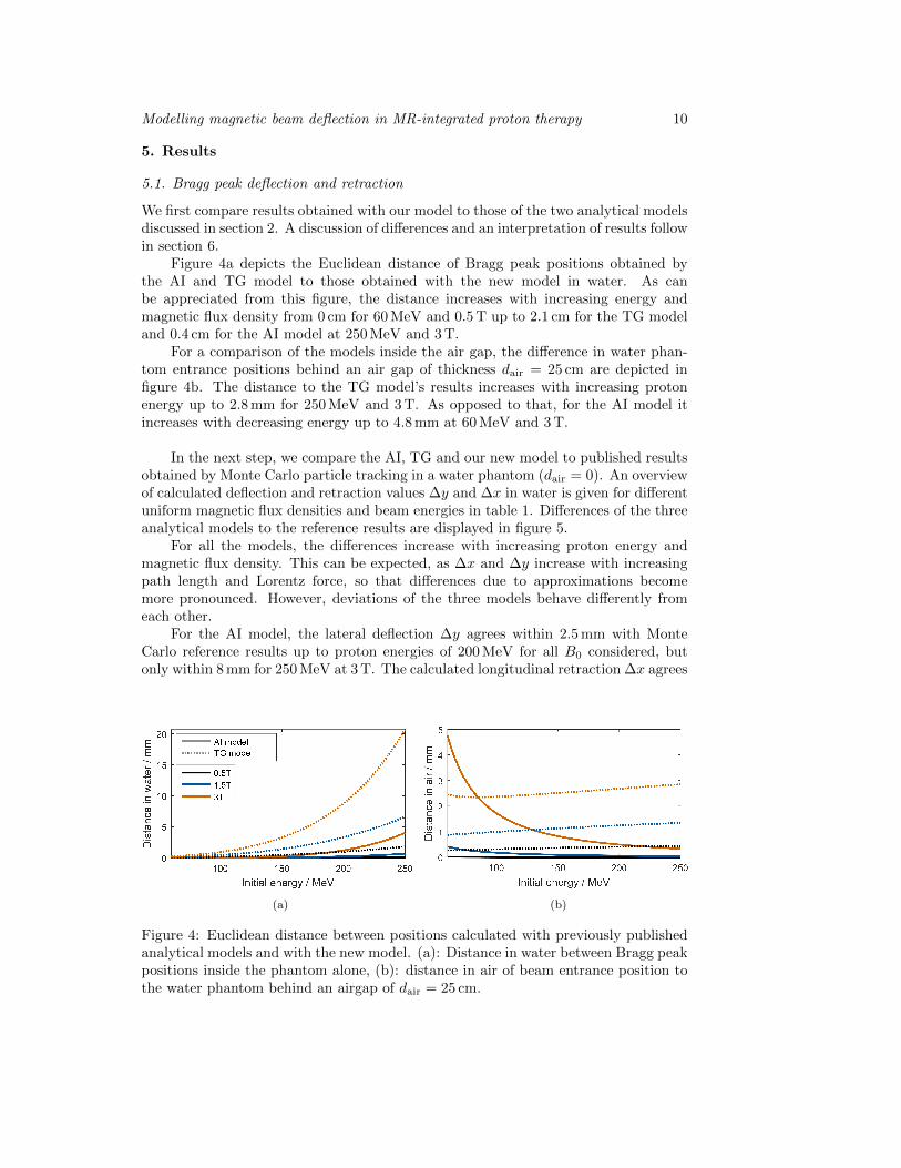
Figure 4a depicts the Euclidean distance of Bragg peak positions obtained bythe AI and TG model to those obtained with the new model in water. As canbe appreciated from this figure, the distance increases with increasing energy andmagnetic flux density from 0 cm for 60 MeV and 0.5 T up to 2.1 cm for the TG modeland 0.4 cm for the AI model at 250 MeV and 3 T.

For a comparison of the models inside the air gap, the difference in water phan-tom entrance positions behind an air gap of thickness dair = 25 cm are depicted infigure 4b. The distance to the TG model’s results increases with increasing protonenergy up to 2.8 mm for 250 MeV and 3 T. As opposed to that, for the AI model itincreases with decreasing energy up to 4.8 mm at 60 MeV and 3 T.

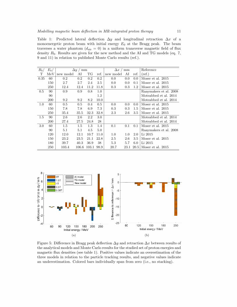
In the next step, we compare the AI, TG and our new model to published resultsobtained by Monte Carlo particle tracking in a water phantom (dair = 0). An overviewof calculated deflection and retraction values ∆y and ∆x in water is given for differentuniform magnetic flux densities and beam energies in table 1. Differences of the threeanalytical models to the reference results are displayed in figure 5.

For all the models, the differences increase with increasing proton energy andmagnetic flux density. This can be expected, as ∆x and ∆y increase with increasingpath length and Lorentz force, so that differences due to approximations becomemore pronounced. However, deviations of the three models behave differently fromeach other.

For the AI model, the lateral deflection ∆y agrees within 2.5 mm with MonteCarlo reference results up to proton energies of 200 MeV for all B0 considered, butonly within 8 mm for 250 MeV at 3 T. The calculated longitudinal retraction ∆x agrees

(a) (b)

Figure 4: Euclidean distance between positions calculated with previously publishedanalytical models and with the new model. (a): Distance in water between Bragg peakpositions inside the phantom alone, (b): distance in air of beam entrance position tothe water phantom behind an airgap of dair = 25 cm.


Table 1: Predicted lateral deflection ∆y and longitudinal retraction ∆x of amonoenergetic proton beam with initial energy E0 at the Bragg peak. The beamtraverses a water phantom (dair = 0) in a uniform transverse magnetic field of fluxdensity B0. Results are given for the new method and the AI and TG models (eq. 7,9 and 11) in relation to published Monte Carlo results (ref.).

B0/ E0/ ∆y / mm ∆x / mm ReferenceT MeV new model AI TG ref. new model AI ref. (ref.)

0.35 60 0.2 0.2 0.2 0.2 0.0 0.0 0.0 Moser et al. 2015150 2.7 2.7 2.4 2.5 0.0 0.0 0.1 Moser et al. 2015250 12.4 12.4 11.2 11.8 0.3 0.3 1.2 Moser et al. 2015

0.5 90 0.9 0.9 0.8 1.0 Raaymakers et al. 200890 1.2 Moteabbed et al. 2014200 9.2 9.2 8.2 10.0 Moteabbed et al. 2014

1.0 60 0.5 0.5 0.4 0.5 0.0 0.0 0.0 Moser et al. 2015150 7.8 7.8 6.9 7.3 0.3 0.3 1.5 Moser et al. 2015250 35.4 35.5 32.3 32.8 2.3 2.6 3.5 Moser et al. 2015

1.5 90 2.6 2.6 2.2 3.0 Moteabbed et al. 2014200 27.4 27.5 24.8 28 Moteabbed et al. 2014

3.0 60 1.5 1.5 1.3 1.4 0.1 0.1 0.1 Moser et al. 201590 5.1 5.1 4.5 5.0 Raaymakers et al. 2008120 12.0 12.1 10.7 11.0 1.0 1.0 2.0 Li 2015150 23.2 23.5 21.1 22.8 2.5 2.6 3.5 Moser et al. 2015180 39.7 40.3 36.9 38 5.3 5.7 6.0 Li 2015250 103.4 106.6 103.1 98.9 20.7 23.1 20.5 Moser et al. 2015

4

6

8

-4

-2

0

2

60 90 120 180150 200 250Initial energy / MeV

(a)

5

0

-5

-10

-15

-20

-25120 150 180 250

(b)

Figure 5: Difference in Bragg peak deflection ∆y and retraction ∆x between results ofthe analytical models and Monte Carlo results for the studied set of proton energies andmagnetic flux densities (see table 1). Positive values indicate an overestimation of thethree models in relation to the particle tracking results, and negative values indicatean underestimation. Colored bars individually span from zero (i.e., no stacking).


within 1.5 mm with the reference for all studied setups, except for 250 MeV and 3 T(3 mm). Here, the lateral deflection tends to be overestimated, whereas retraction bytrend seems to be underestimated.

For the TG model, the deflection ∆y agrees with Monte Carlo results within 2 mmfor all setups except for 200 MeV and 1.5 T, and 250 MeV and 3 T, where the deviationsamount to 3.2 mm and 4.2 mm, respectively. The TG model tends to underestimate∆y. The full neglection of the longitudinal retraction of the Bragg peak leads todifferences in ∆x of up to 2.1 cm for 250 MeV and 3 T.

Results obtained with our new model show an agreement with the reference re-sults in ∆y within 2 mm for all studies setups, except for 250 MeV at 1.5 T (2.6 mm)and 3 T (4.6 mm). The retraction ∆x agrees within 1.5 mm for all studied energiesand magnetic flux densities. The new model shows a trend of overestimating lateraldeflection and underestimating longitudinal retraction.

A statistical comparison of the accuracy of the three models in relation to theMonte Carlo results is displayed in figure 6. Regarding the lateral deflection ∆y,the three models show only small differences in both median and average deviation,which amount to 0.5 mm and 1 mm, respectively. However, the upper percentiles (i.e.75 % and 91 %) deviate stronger from zero for the TG model than for the other twomodels, and the AI model shows a strong outlier of 8 mm at 250 MeV and 3 T. Forthe longitudinal retraction ∆x, the median and average deviation of the new modeland the AI model are comparably low (below 1 mm), but only the new model shows asmaller 91 %-percentile and no outlier. As retraction is neglected in the TG model, allstudied statistical measures are highly increased as compared to the two other models.The sample size for this inter-model comparison has been limited to 11 and 16 datapoints for retraction and deflection, respectively.

Figure 6: Boxplots of absolute differences in Bragg peak deflection ∆y and retraction∆x between the different models and Monte Carlo reference results (see table 1).


5.2. Beam correction parameters

To compensate for the deflection of the Bragg peak, calculated correction parameters∆γ and ∆E0 are presented for different proton energies E0 and magnetic flux densitiesB0 in table 2. The beam energy correction calculated with our model ranges from∆E0 = 0.1 MeV (0.2 %) for 60 MeV and 0.5 T up to ∆E0 = 4.7 MeV (2 %) for 250 MeVand 3 T. The angle correction ranges from ∆γ = 3.6 ◦ for 60 MeV and 0.5 T up to∆γ = 24.4 ◦ for 250 MeV and 3 T. The difference to the correction angle from the TGmodel is smaller than 0.5 ◦ for magnetic flux densities up to 1.5 T, but exceeds to 3.8 ◦

(16 %) at 250 MeV and 3 T.

Table 2: Beam energy and angle correction parameters for different initial energies andmagnetic flux densities for a distance between the phantom surface and the entranceposition of the beam to the magnetic field of dair = 25 cm.

B0/ E0 / New correction parameters TG modelT MeV ∆E0 / MeV ∆γ/◦ ∆γ/◦

0.5 60 0.1 3.6 3.3100 0.1 3.2 3.3150 0.1 3.3 3.3200 0.1 3.6 3.6250 0.1 4.0 4.0

1.5 60 0.5 10.7 11.1100 0.5 9.6 10.0150 0.6 9.8 10.1200 0.8 10.7 11.0250 1.1 12.0 12.3

3 60 2.0 21.5 24.6100 2.1 19.3 21.5150 2.5 19.7 21.9200 3.3 21.6 24.3250 4.7 24.4 28.2

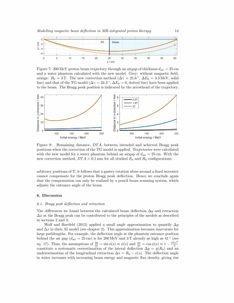
As an example, proton trajectories modelled with the new model for bothcorrection parameter sets are depicted for E0 = 200 MeV and B0 = 3 T in figure 7.As the correction method of the TG model does not include an energy correction,the Bragg peak retraction is not compensated for. Additionally, the lateral deflection∆y is overcompensated by a too large correction angle. Therefore, the DTA betweenthe intended Bragg peak position without a magnetic field and its corrected positioninside the field (see equation 21 and figure 8) is non-zero. It ranges from 0.3 mmfor 60 MeV and 0.5 T up to 4.3 cm for 250 MeV and 3 T. With the new correctionmethod presented here, the calculated DTA is below 0.1 mm for all studied E0 andB0 configurations.

In addition to these differences, we dispute that the beam angle correction can beimplemented by a gantry rotation, as stated by Hartman et al. (2015). To see this,assume for example the intended Bragg peak position (indicated by ”T” in figure 1a)to coincide with the gantry’s isocenter of rotation. A gantry rotation will then resultin a concentric displacement of the actual Bragg peak position U around T, but it willnot compensate for the deflection, i.e. render U = T. Transferring this consideration to


Figure 7: 200 MeV proton beam trajectory through an airgap of thickness dair = 25 cmand a water phantom calculated with the new model. Grey: without magnetic field,orange: B0 = 3 T. The new correction method (∆γ = 21.6 ◦, ∆E0 = 3.3 MeV, solidline) and that of the TG model (∆γ = 24.3 ◦, ∆E0 = 0, dotted line) have been appliedto the beam. The Bragg peak position is indicated by the arrowhead of the trajectory.

Figure 8: Remaining distance, DTA, between intended and achieved Bragg peakpositions when the correction of the TG model is applied. Trajectories were calculatedwith the new model for a water phantom behind an airgap of dair = 25 cm. With thenew correction method, DTA < 0.1 mm for all studied E0 and B0 configurations.

arbitrary positions of T, it follows that a gantry rotation alone around a fixed isocentercannot compensate for the proton Bragg peak deflection. Hence we conclude againthat the compensation can only be realized by a pencil beam scanning system, whichadjusts the entrance angle of the beam.

6. Discussion

6.1. Bragg peak deflection and retraction

The differences we found between the calculated beam deflection ∆y and retraction∆x at the Bragg peak can be contributed to the principles of the models as describedin sections 2 and 3.

Wolf and Bortfeld (2012) applied a small angle approximation to quantify ∆yand ∆x in their AI model (see chapter 2). This approximation becomes inaccurate forlarge pathlengths. For example, the deflection angle at the phantom entrance positionbehind the air gap (dair = 25 cm) is for 200 MeV and 3 T already as high as 41 ◦ (see

eq. 17). Thus, the assumptions of dyds = sinφ(s) ≈ φ(s) and dx

ds = cosφ(s) ≈ 1− φ(s)2

2constitute a systematic overestimation of the lateral deflection ∆y = y(R0) and anunderestimation of the longitudinal retraction ∆x = R0 − x(s). The deflection anglein water increases with increasing beam energy and magnetic flux density, giving rise


to increasing discrepancies relative to the reference data. In addition, the neglectionof relativistic effects for the calculation of ∆x contributes to an increasing uncertaintywith increasing energy. These trends can be clearly observed in figures 4a and 5a. Inair, the effect of a decreasing gyroradius with decreasing energy dominates, thereforethe travelled pathlength and deflection angle increase with decreasing energy. Asthe accuracy of the model decreases with increasing deflection angle, this leads to anopposite trend as compared to the lateral deflection, as is appreciated from figures 4band 5a.

Similarly, we can observe how the approximations brought forward by Hartmanet al. (2015) affect the accuracy of the TG model’s predictions. The model neglectsretraction, the changing gyroradius due to energy loss and relativistic effects. Theaccuracy of these approximations decreases with increasing magnetic flux density andproton energy, as is depicted in figure 4. Note that differences in figure 4b are solelydue to the neglection of relativistic effects, which leads to an underestimation of thegyroradius. The trend to underestimate the deflection in water, as depicted in figure5a, can be ascribed to the overestimation of the gyroradius by assuming r(s) = r0.In addition, it was shown that the assumption of a negligible longitudinal Bragg peakretraction exceeds an accuracy of 2 mm already at intermediate energies (see figure 5a).

The new model presented in the current work does not rely on these assumptionsand shows an equally good or better agreement to Monte Carlo results over thewhole energy range from 60 MeV to 250 MeV. The remaining differences can beattributed to the approximations of the model, i.e. neglecting scattering, energy-lossfluctuations, range straggling, generation of secondary particles and energy loss in air.Those simplifications were applied to reduce calculation time, but can in principle beincluded due to the structure of the model being a simplified particle tracking method.The tendency of overestimating lateral deflection and underestimating longitudinalretraction might result from the spectral dispersion of the proton beam due to themagnetic field (Moser 2015), which is not included in the model. Another factor ofuncertainty is the proton range R0, which has been approximated by equation 4 andused as an estimate for the position of the Bragg peak. R0 deviates from measuredBragg peak positions (Paul 2013, Schardt et al. 2008) by less than 0.4 mm up to protonenergies of 200 MeV.

On the other hand, results obtained by Monte Carlo particle tracking were usedin this publication as reference data. However, this approach is theoretical in natureand its accuracy strongly depends on the choice of input parameters and physicsmodels. Consequently, dosimetric measurements have to be carried out for a reliableevaluation of the different models. While this study primarily aimed to introduce thenew method, this will be subject to future studies.

In the presented model, the particle’s equation of motion (eq. 1) has been solvedanalytically (eq. 2). As an alternative, a full numerical solution by means of a Runge-Kutta method has been proposed recently (Moser 2015). However, as the protonvelocity is considered to be constant in each calculation step, the analytical solutionapplies not only in vacuum but also in media. We therefore consider the Runge-Kuttamethod to be superfluous in this case, as it will compromise the calculation accuracyand workload.


6.2. Beam correction

The proposed strategy for a compensation of the Bragg peak deflection includes anadjustment of the initial proton beam energy and entrance angle. It was shown thatthis method effectively repositions the Bragg peak to the intended spot for all studiedbeam energies and magnetic flux densities. The range difference corresponding to∆E0 ranges between 0.01 cm (0.3 %) for 60 MeV and 0.5 T and 1.27 cm (3.3 %) for250 MeV and 3 T (see table 2 and eq. 4). The main factor of uncertainty for theproton range in a well-defined geometry is statistical pathlength straggling, and thestandard deviation of the range due to this effect ranges between 1.2 % for 60 MeV and1.1 % for 250 MeV (Janni 1982, Paganetti et al. 2012). Being comparably high, theenergy correction should therefore not be neglected in MRiPT, especially for higherproton energies and magnetic flux densities.

The reason for the remaining discrepancy of the Bragg peak position correctedby the TG model is seen in the approximations mentioned above. The neglection ofretraction constitutes an overestimation of the total path length, and the neglectionof relativistic effects leads to an underestimation of the gyroradius and thus an overes-timation of the beam deflection. Both approximations result in an overcompensationof the beam deflection.

The calculation time of the new model is strongly decreased as compared to MonteCarlo models. It can be further reduced by using a higher-performant computer andby reducing the required accuracy, which was chosen conservatively in this study.

7. Conclusion and Outlook

Although previous work has indicated that there is general consensus that the protonbeam trajectory in a water/air phanom setting inside a transverse magnetic field ispredictable, our quantitative comparison of the different methods has shown thatpredictions of different models only agree for certain proton beam energies andmagnetic flux densities. Therefore, shortcomings of previously published analyticalmethods have been analyzed and quantified. The inclusion of critical assumptionsand the lack of applicability to realistic, i.e. non-uniform, magnetic flux densitiesand patient anatomies have been identified as main problems. To overcome thesedeficiencies, a new model has been developed and shown to be both less assumptiveand more versatile than existing analytical approaches, and faster than Monte Carlomodels.

Thus, the new model is useful to get a fast and accurate estimate for thebeam deflection and retraction which is to be expected in MRiPT, and for thecorrection parameters needed for a compensation thereof. It can help in the planningof experimental setups for dosimetric feasibility studies of MRiPT, and its simplestructure helps to understand underlying physical mechanisms. Furthermore, it canbe used as reference solution when setting up a Monte Carlo model or an experimentalstudy. As pointed out by Hartman et al. (2015), intensity-modulated MRiPT planningcan be realized by two Monte Carlo calculation steps - one for selection of beamletswhose deflected Bragg peaks lie inside the target, and one for dose calculation. Thus,another possible application of the model is to replace the first Monte Carlo step inorder to reduce the overall calculation time.

We have presented the new model in a simplicistic form for a first approach


to the problem of magnetic deflection of the proton beam. However, the structureof the model allows for an easy extension to more realistic cases, especially includingrange straggling and non-uniform magnetic fields and material compositions. Magneticflux density vectors of arbitrary distribution and phantom/patient geometries can beincluded due to the full reconstruction of the trajectory, which provides knowlegdeof the proton position at every iteration step. In addition to its reduced amount ofapproximations, the presented model thus offers a critically enhanced applicabilitycompared to existing analytical models. Future studies will involve a comprehensivebenchmarking of the new model with both Monte Carlo simulations and experimentalmeasurements.

Acknowledgments

The authors would like to thank Wolfgang Enghardt (OncoRay, Dresden, Germany)for useful comments on the manuscript. We furthermore express our gratitude toMarco Schippers (PSI, Villigen, Switzerland) for discussing the initial ideas of thenew model.

References

Bortfeld T 1997 An analytical approximation of the Bragg curve for therapeutic proton beams Med.Phys. 24(12), 2024–2033.

Fallone B G 2014 The Rotating Biplanar Linac-Magnetic Resonance Imaging System Semin. Radiat.Oncol. 24, 200–202.

Hartman J, Kontaxis C, Bol G H, Frank S J, Lagendijk J J W, van Vulpen M & Raaymakers B W2015 Dosimetric feasibility of intensity modulated proton therapy in a transverse magneticfield of 1.5 T Phys. Med. Biol. 60, 5955–5969.

ICRU 1993 Stopping Powers and Ranges for Protons and Alpha Particles ICRU Report 49 .Jakel O 2009 Medical physics aspects of particle therapy Radiat. Prot. Dosimetry 137(1-2), 56–166.Janni J F 1982 Proton range-energy tables, 1 keV - 10 GeV Atomic Data and Nuclear Tables 27, 147–

339.Keall P J, Barton M & Crozier S 2014 The Australian Magnetic Resonance Imaging-Linac Program

Semin. Radiat. Oncol. 24, 203–206.Lagarias J C, Reeds J A, Wright M H & Wright P E 1998 Convergence Properties of the Nelder-Mead

Simplex Method in Low Dimensions SIAM J. Optimiz. 9(1), 112–147.Lagendijk J J, Raaymakers B W & van Vulpen M 2014a The magnetic resonance imaging-linac system

Semin. Radiat. Oncol. 24(3), 207–9.Lagendijk J J W, Raaymakers B W, den Berg C A T V, Moerland M A, Philippens M E & van

Vulpen M 2014b MR guidance in radiotherapy Phys. Med. Biol. 59, R349–R369.Li J S 2015 Investigation of MRI guided proton therapy Med. Phys. 42, 3311.Lomax A J 2008 Intensity modulated proton therapy and its sensitivity to treatment uncertainties 2:

the potential effects of inter-fraction and inter-field motions Phys. Med. Biol. 53, 1043–1056.Moser P 2015 Effects on particle beams in the presence of a magnetic field during radiation therapy

Master’s thesis Technische Universiat Wien.Moteabbed M, Schuemann J & Paganetti H 2014 Dosimetric feasibility of real-time MRI-guided

proton therapy Med. Phys. 41(11), 111713 1–11.Oborn B M, Dowdell S, Metcalfe P E, Crozier S, Guatelli S, Rosenfeld A B, Mohan R & Keall P J

2016 MRI Guided Proton Therapy: Pencil beam scanning in an MRI fringe field ICTR-PHEGeneva, February 15-19.

Oborn B M, Dowdell S, Metcalfe P E, Crozier S, Mohan R & Keall P J 2015 Proton beam deflectionin MRI fields: Implications for MRI-guided proton therapy Med. Phys. 42, 2113–2124.

Paganetti H, Gottschalk B, Schippers M, Lu H M, Flanz J, Slopsema R, Flanz J, Palmans H, Li Z,Flampouri S, Yeung D K, Engelsman M, Lomax A, Clasie B, Kooy H M, Palta J R, BertC, Trofimov A V, Unkelbach J H, Craft D, Parodi K, Ipe N E & van Luijk P 2012 ProtonTherapy Physics CRC Press, Taylor & Francis Group.


Paul H 2013 in D Belkic, ed., ‘Theory of Heavy Ion Collision Physics in Hadron Therapy’ Vol. 65 ofAdvances in Quantum Chemistry Academic Press.

Raaymakers B, Raaijmakers A J E & Lagendijk J J 2008 Feasibility of MRI guided proton therapy:magnetic field dose effects Phys. Med. Biol. 53, 5615–5622.

Schardt D, Steidl P, Kramer M, Weber U, Parodi K & Brons S 2008 Precision Bragg-CurveMeasurements for Light-Ion Beams in Water GSI Scientific Report 2007, 373.

Schippers J M & Lomax A J 2011 Emerging technologies in proton therapy Acta Oncol. 50(6), 838–850.

Wolf R & Bortfeld T 2012 An analytical solution to proton Bragg peak deflection in a magnetic fieldPhys. Med. Biol. 57, N329–N337.

prediction and compensation of magnetic beam deflection in

Documents